Plasma Turbulence

Bogdan A. Hnat Centre for Fusion, Space and Astrophysics

University of Warwick

1.  Introduction to turbulence (general) –  Definitions, examples from astrophysics

2.  Key concepts from fluid turbulence (homogeneous, isotropic and incompressible)

–  Navier-Stokes equation, symmetries, scaling transformation, role of pressure, vorticity, nonlinear energy transfer, correlation tensor, closure, nonlinear energy transfer

3.  Phenomenological models of fluid turbulence –  Kolmogorv’s K41 model, energy spectrum, energy cascade in 3D and 2D

4.  Statistical methods in turbulence, Structure Functions –  Kolmogorv’s hypothesis, scale-by-scale fluctuation definition, SF

5.  MHD plasma turbulence –  Similarity with HT, Elsasser variables, IK and GS phenomenological

models of MHD turbulence

Plan for this lecture:

There is no single definition of turbulence, but often the following features are attributed to turbulence: •  Apparently chaotic motion of fluid / plasma parcels which

forms structures on many scales •  Large fluctuations in macroscopic parameters, such as

pressure, flow speed and density •  Nonlinear energy transfer between different spatial scales •  Dynamical system in which the probability of large events

is higher than that given by a Gaussian distribution

What is plasma turbulence ?

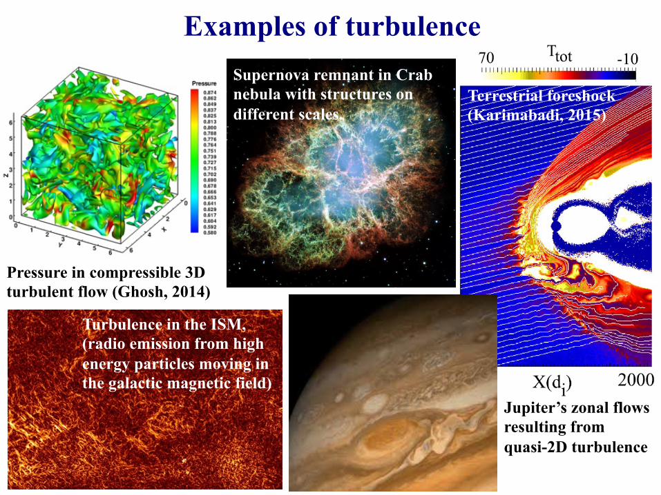
Examples of turbulence

Pressure in compressible 3D turbulent flow (Ghosh, 2014)

Supernova remnant in Crab nebula with structures on different scales.

Turbulence in the ISM, (radio emission from high energy particles moving in the galactic magnetic field)

Terrestrial foreshock (Karimabadi, 2015)

Jupiter’s zonal flows resulting from quasi-2D turbulence

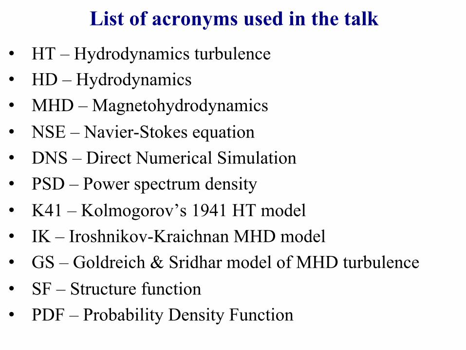
•  HT – Hydrodynamics turbulence •  HD – Hydrodynamics •  MHD – Magnetohydrodynamics •  NSE – Navier-Stokes equation •  DNS – Direct Numerical Simulation •  PSD – Power spectrum density •  K41 – Kolmogorov’s 1941 HT model •  IK – Iroshnikov-Kraichnan MHD model •  GS – Goldreich & Sridhar model of MHD turbulence •  SF – Structure function •  PDF – Probability Density Function

List of acronyms used in the talk

Part I: Main concepts of hydrodynamic turbulence

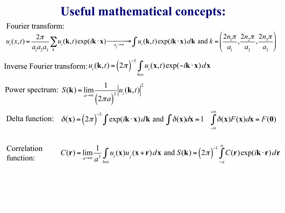
Useful mathematical concepts: Fourier transform:

ui (x,t) =2πa1a2a3

ui (k,t)exp(ik ⋅x) ai→∞$ →$$ ui (k,t)exp(ik ⋅x)dk∫

k∑ and k = 2n1π

a1,2n2πa2

,2n3πa3

'

())

*

+,,

Inverse Fourier transform: ui (k,t) = 2π( )−3

ui (x,t)exp(−ik ⋅x)dxbox∫

Delta function: δ(x) = 2π( )−3

exp(ik ⋅x)dk∫ and δ(x)∫ dx =1 δ(x)−∞

+∞

∫ F (x)dx = F (0)

Correlation function:

C(r) = lima→∞

1a3

ui (x)u j (x+ r)dxbox∫ and S(k) = 2π( )

−1C(r)exp(ik ⋅r)dr

−a

a

∫

Power spectrum: S(k) = lima→∞

1

2πa( )3ui (k,t)

2

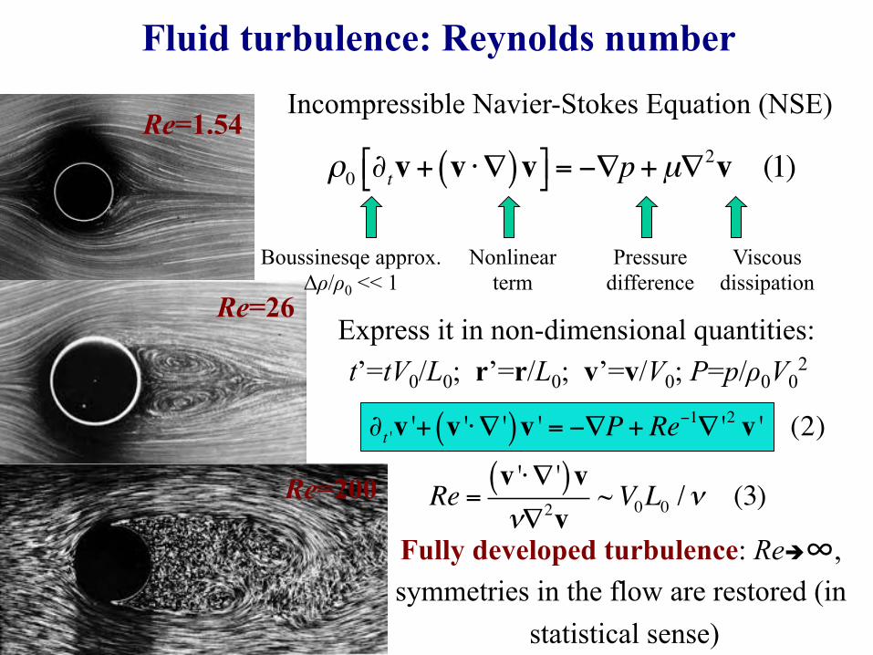
∂t 'v '+ v '⋅∇ '( )v ' = −∇P + Re−1∇ '2 v ' (2)

Re =v '⋅∇ '( )vν∇2v

~V0L0 /ν (3)

Fluid turbulence: Reynolds number

ρ0 ∂tv+ v ⋅∇( )v$% &'= −∇p+µ∇2v (1)

Incompressible Navier-Stokes Equation (NSE)

Express it in non-dimensional quantities: t’=tV0/L0; r’=r/L0; v’=v/V0; P=p/ρ0V0

2

Re=1.54

Re=26

Re=200

Boussinesqe approx. Δρ/ρ0 << 1

Nonlinear term

Pressure difference

Viscous dissipation

Fully developed turbulence: Reè∞, symmetries in the flow are restored (in

statistical sense)

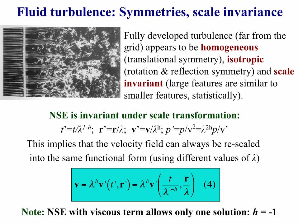
Fully developed turbulence (far from the grid) appears to be homogeneous (translational symmetry), isotropic (rotation & reflection symmetry) and scale invariant (large features are similar to smaller features, statistically).

Fluid turbulence: Symmetries, scale invariance

NSE is invariant under scale transformation: t’=t/λ1-h; r’=r/λ; v’=v/λh; p’=p/v2=λ2hp/v’

This implies that the velocity field can always be re-scaled into the same functional form (using different values of λ)

v = λ hv ' t ',r '( ) = λ hv ' tλ1−h

, rλ

"

#$

%

&' (4)

Note: NSE with viscous term allows only one solution: h = -1

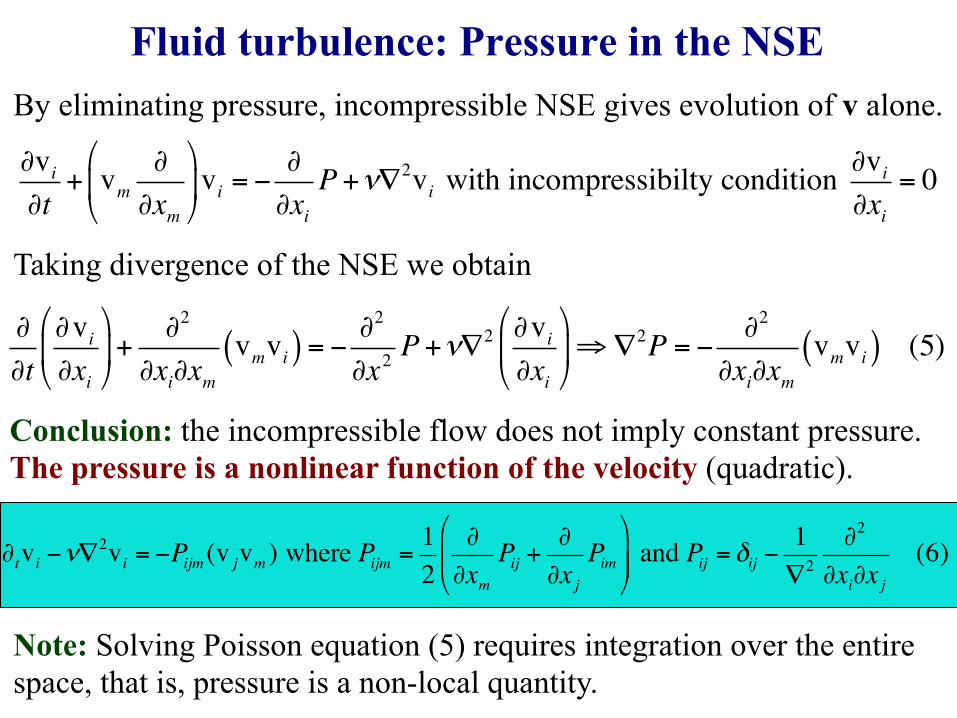
Fluid turbulence: Pressure in the NSE By eliminating pressure, incompressible NSE gives evolution of v alone.

Taking divergence of the NSE we obtain

∂vi

∂t+ vm

∂∂xm

"

#$

%

&'vi = −

∂∂xi

P +ν∇2vi with incompressibilty condition ∂vi

∂xi= 0

∂∂t

∂vi∂xi

"

#$

%

&'+

∂2

∂xi∂xmvmvi( ) = − ∂2

∂x2P +ν∇2 ∂vi

∂xi

"

#$

%

&'⇒ ∇2P = − ∂2

∂xi∂xmvmvi( ) (5)

Conclusion: the incompressible flow does not imply constant pressure. The pressure is a nonlinear function of the velocity (quadratic).

∂tvi −ν∇2vi = −Pijm (v jvm ) where Pijm =

12

∂∂xm

Pij +∂∂x j

Pim$

%&&

'

()) and Pij = δij −

1∇2

∂2

∂xi∂x j(6)

Note: Solving Poisson equation (5) requires integration over the entire space, that is, pressure is a non-local quantity.

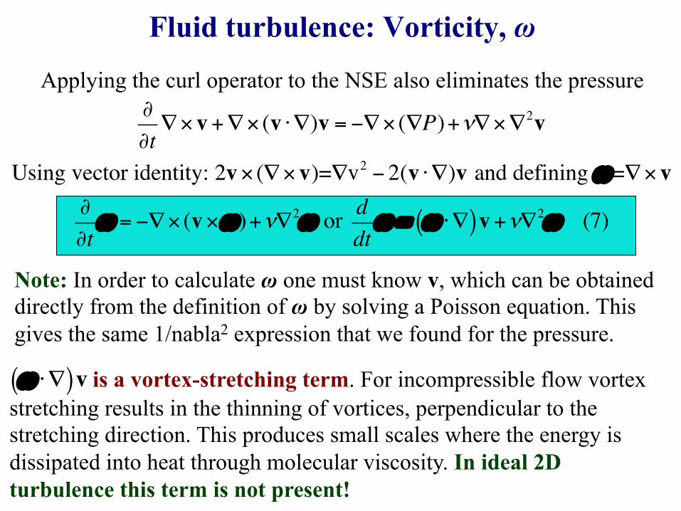
∂∂t∇× v+∇× (v ⋅∇)v = −∇× (∇P)+ν∇×∇2v

Using vector identity: 2v× (∇× v)=∇v2 − 2(v ⋅∇)v and defining ω=∇× v∂∂tω = −∇× (v×ω )+ν∇2ω or d

dtω = ω ⋅∇( )v+ν∇2ω (7)

Fluid turbulence: Vorticity, ω

Applying the curl operator to the NSE also eliminates the pressure

Note: In order to calculate ω one must know v, which can be obtained directly from the definition of ω by solving a Poisson equation. This gives the same 1/nabla2 expression that we found for the pressure.

is a vortex-stretching term. For incompressible flow vortex ω ⋅∇( )vstretching results in the thinning of vortices, perpendicular to the stretching direction. This produces small scales where the energy is dissipated into heat through molecular viscosity. In ideal 2D turbulence this term is not present!

•  Dynamical description of turbulence is nearly impossible, but experiments show that some statistical features are robustly reproducible. For example, power-law spectra are commonly observed in turbulent flows

•  Statistical averages are normally performed over the spatial volume of the flow of interest.

•  Sometimes statistical ensemble average is used , that is, we average over many realisations of the flow under the same conditions

•  Statistical features should be independent of the initial conditions and the form of a driver, as long as there is a significant scale separation between the driver and dissipation

•  Ergodicity becomes an important issue: when are averages over time the same as the averages over realisations

Fluid turbulence: why look at statistics?

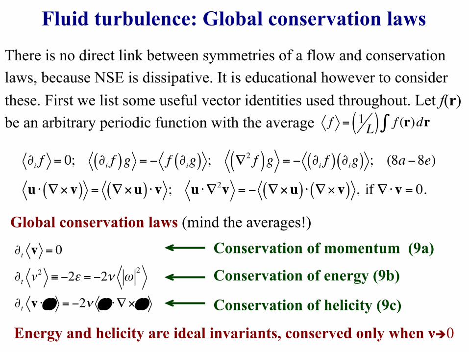
Fluid turbulence: Global conservation laws

There is no direct link between symmetries of a flow and conservation laws, because NSE is dissipative. It is educational however to consider these. First we list some useful vector identities used throughout. Let f(r) be an arbitrary periodic function with the average f = 1

L( ) f (r)dr∫

Global conservation laws (mind the averages!)

∂i f = 0; ∂i f( )g = − f ∂ig( ) ; ∇2 f( )g = − ∂i f( ) ∂ig( ) ; (8a−8e)

u ⋅ ∇× v( ) = ∇×u( ) ⋅v ; u ⋅∇2v = − ∇×u( ) ⋅ ∇× v( ) , if ∇⋅v = 0.

∂t v = 0

∂t v2 ≡ −2ε = −2ν ω

2

∂t v ⋅ω = −2ν ω ⋅∇×ω

Conservation of momentum (9a)

Conservation of energy (9b)

Conservation of helicity (9c)

Energy and helicity are ideal invariants, conserved only when νè0

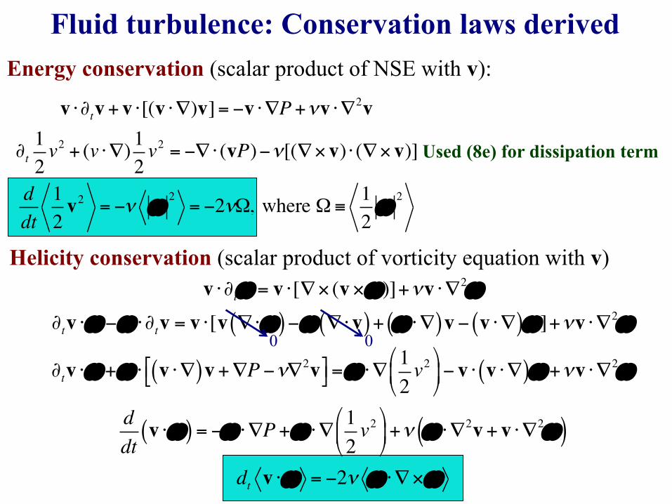
v ⋅∂tv+ v ⋅[(v ⋅∇)v]= −v ⋅∇P +νv ⋅∇2v

∂t12v2 + (v ⋅∇) 1

2v2 = −∇⋅ (vP)−ν[(∇× v) ⋅ (∇× v)]

ddt

12v2 = −ν ω

2= −2νΩ, where Ω≡

12ω

2

Fluid turbulence: Conservation laws derived Energy conservation (scalar product of NSE with v):

Helicity conservation (scalar product of vorticity equation with v)

Used (8e) for dissipation term

v ⋅∂tω = v ⋅[∇× (v×ω )]+νv ⋅∇2ω

∂tv ⋅ω −ω ⋅∂tv = v ⋅[v ∇⋅ω( )−ω ∇⋅v( )+ ω ⋅∇( )v− v ⋅∇( )ω ]+νv ⋅∇2ω

∂tv ⋅ω +ω ⋅ v ⋅∇( )v+∇P −ν∇2v&' ()=ω ⋅∇12v2

*

+,

-

./− v ⋅ v ⋅∇( )ω +νv ⋅∇2ω

ddtv ⋅ω( ) = −ω ⋅∇P +ω ⋅∇ 1

2v2

*

+,

-

./+ν ω ⋅∇2v+ v ⋅∇2ω( )

dt v ⋅ω = −2ν ω ⋅∇×ω

0 0

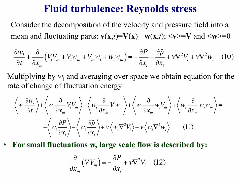
Fluid turbulence: Reynolds stress Consider the decomposition of the velocity and pressure field into a mean and fluctuating parts: v(x,t)=V(x)+ w(x,t); <v>=V and <w>=0

Multiplying by wi and averaging over space we obtain equation for the rate of change of fluctuation energy

•  For small fluctuations w, large scale flow is described by:

∂wi

∂t+

∂∂xm

ViVm +Viwm +Vmwi +wiwm( ) = − ∂P∂xi

−∂p∂xi

+ν∇2Vi +ν∇2wi (10)

wi∂wi

∂t+ wi

∂∂xm

ViVm + wi∂∂xm

Viwm + wi∂∂xm

wiVm + wi∂∂xm

wiwm =

− wi∂P∂xi

− wi∂p∂xi

+ν wi∇2Vi +ν wi∇

2wi (11)

∂∂xm

ViVm( ) = − ∂P∂xi

+ν∇2Vi (12)

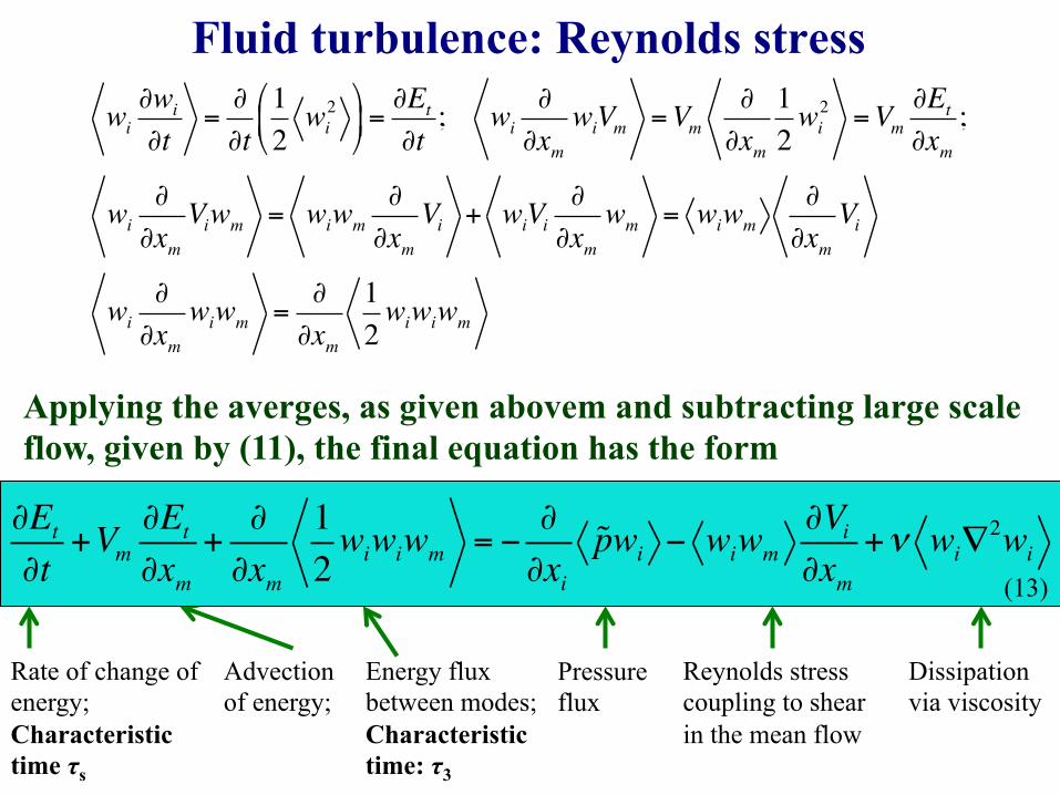
Fluid turbulence: Reynolds stress

Applying the averges, as given abovem and subtracting large scale flow, given by (11), the final equation has the form

wi∂wi

∂t=∂∂t

12wi2"

#$

%

&'=

∂Et

∂t; wi

∂∂xm

wiVm =Vm∂∂xm

12wi2 =Vm

∂Et

∂xm;

wi∂∂xm

Viwm = wiwm∂∂xm

Vi + wiVi∂∂xm

wm = wiwm∂∂xm

Vi

wi∂∂xm

wiwm =∂∂xm

12wiwiwm

Rate of change of energy; Characteristic time τs

Advection of energy;

Energy flux between modes; Characteristic time: τ3

Pressure flux

Reynolds stress coupling to shear in the mean flow

Dissipation via viscosity

∂Et

∂t+Vm

∂Et

∂xm+

∂∂xm

12wiwiwm = −

∂∂xipwi − wiwm

∂Vi∂xm

+ν wi∇2wi

(13)

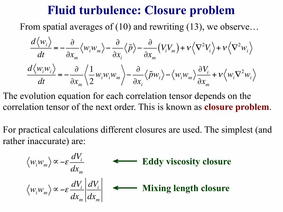
Fluid turbulence: Closure problem

d wi

dt= −

∂∂xm

wiwm −∂∂xip −

∂∂xm

ViVm( )+ν ∇2Vi +ν ∇2wi

d wiwi

dt= −

∂∂xm

12wiwiwm −

∂∂xipwi − wiwm

∂Vi∂xm

+ν wi∇2wi

The evolution equation for each correlation tensor depends on the correlation tensor of the next order. This is known as closure problem. For practical calculations different closures are used. The simplest (and rather inaccurate) are:

wiwm ∝−εdVidxm

wiwm ∝−εdVidxm

dVidxm

Eddy viscosity closure

Mixing length closure

From spatial averages of (10) and rewriting (13), we observe…

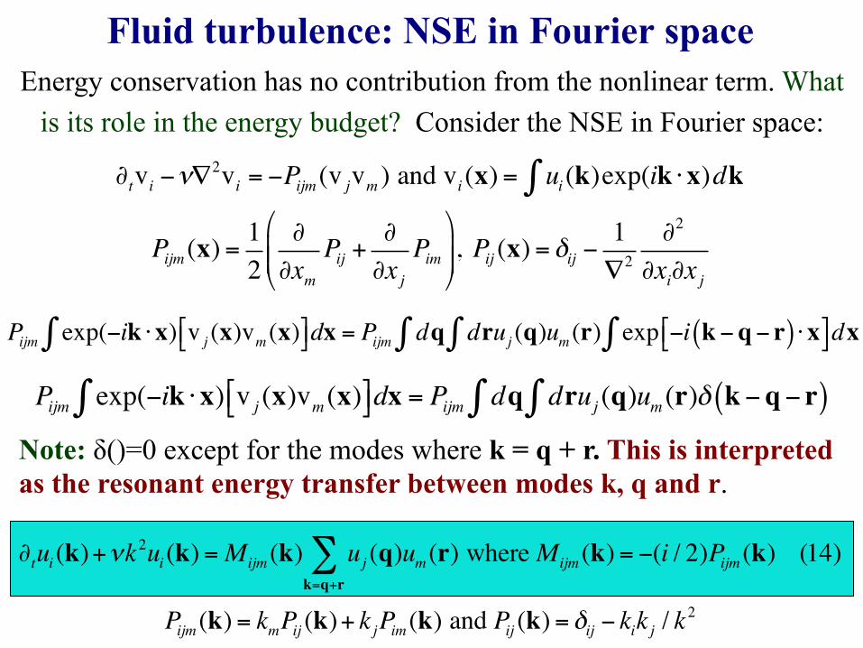
Fluid turbulence: NSE in Fourier space Energy conservation has no contribution from the nonlinear term. What

is its role in the energy budget? Consider the NSE in Fourier space:

Pijm exp(−ik ⋅x)∫ v j (x)vm (x)$% &'dx = Pijm dq druj (q)um (r) exp −i k−q− r( ) ⋅x$% &'dx∫∫∫

Note: δ()=0 except for the modes where k = q + r. This is interpreted as the resonant energy transfer between modes k, q and r.

∂tvi −ν∇2vi = −Pijm (v jvm ) and vi (x) = ui (k)exp(ik ⋅x)dk∫

Pijm (x) = 12

∂∂xm

Pij +∂∂x j

Pim&

'((

)

*++, Pij (x) = δij −

1∇2

∂2

∂xi∂x j

Pijm exp(−ik ⋅x)∫ v j (x)vm (x)$% &'dx = Pijm dq druj (q)um (r)δ k−q− r( )∫∫

∂tui (k)+νk2ui (k) =Mijm (k) uj (q)k=q+r∑ um (r) where Mijm (k) = −(i / 2)Pijm (k) (14)

Pijm (k) = kmPij (k)+ kjPim (k) and Pij (k) = δij − kik j / k2

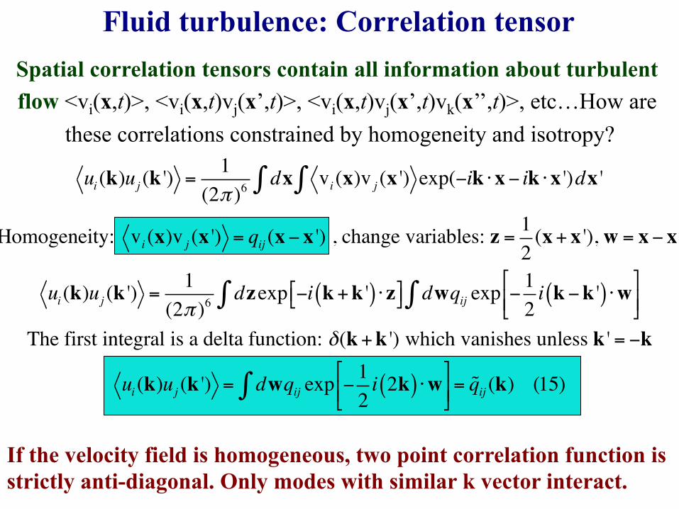
ui (k)uj (k ') =1

(2π )6 dx vi (x)v j (x ')∫ exp(−ik ⋅x− ik ⋅x ')dx '∫

Homogeneity: vi (x)v j (x ') = qij (x− x ') , change variables: z = 12

(x+ x '), w = x− x '

ui (k)uj (k ') =1

(2π )6 dzexp −i k+k '( ) ⋅ z$% &' dwqij∫ exp −12i k−k '( ) ⋅w

$

%(&

')∫The first integral is a delta function: δ(k+k ') which vanishes unless k ' = −k

ui (k)uj (k ') = dwqij exp −12i 2k( ) ⋅w

$

%(&

')∫ = qij (k) (15)

Fluid turbulence: Correlation tensor Spatial correlation tensors contain all information about turbulent flow <vi(x,t)>, <vi(x,t)vj(x’,t)>, <vi(x,t)vj(x’,t)vk(x’’,t)>, etc…How are

these correlations constrained by homogeneity and isotropy?

If the velocity field is homogeneous, two point correlation function is strictly anti-diagonal. Only modes with similar k vector interact.

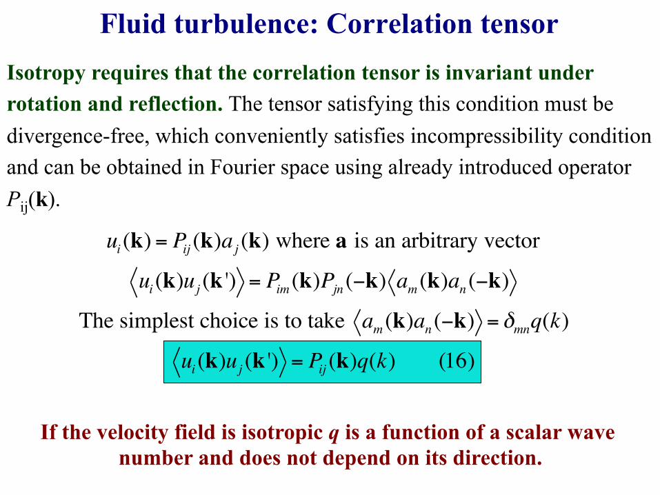
Fluid turbulence: Correlation tensor Isotropy requires that the correlation tensor is invariant under rotation and reflection. The tensor satisfying this condition must be divergence-free, which conveniently satisfies incompressibility condition and can be obtained in Fourier space using already introduced operator Pij(k).

If the velocity field is isotropic q is a function of a scalar wave number and does not depend on its direction.

ui (k) = Pij (k)aj (k) where a is an arbitrary vector

ui (k)uj (k ') = Pim (k)Pjn (−k) am (k)an (−k)

The simplest choice is to take am (k)an (−k) = δmnq(k)

ui (k)uj (k ') = Pij (k)q(k) (16)

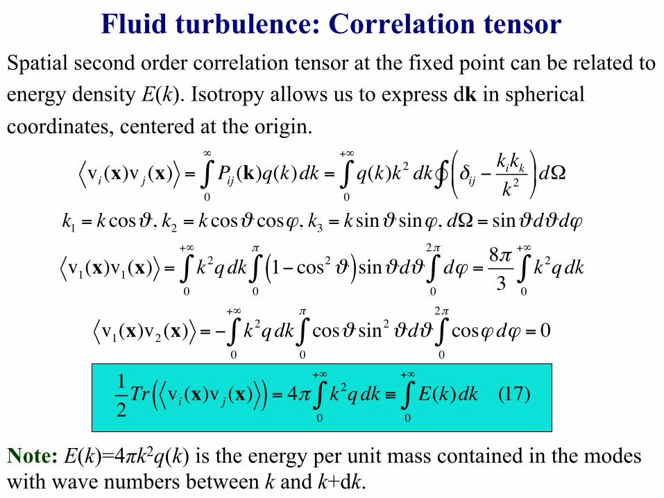
Fluid turbulence: Correlation tensor Spatial second order correlation tensor at the fixed point can be related to energy density E(k). Isotropy allows us to express dk in spherical coordinates, centered at the origin.

Note: E(k)=4πk2q(k) is the energy per unit mass contained in the modes with wave numbers between k and k+dk.

vi (x)v j (x) = Pij (k)q(k)dk0

∞

∫ = q(k)k2 dk δij −kikkk2

$

%&

'

()dΩ∫

0

+∞

∫k1 = k cosϑ , k2 = k cosϑ cosϕ, k3 = k sinϑ sinϕ, dΩ = sinϑdϑdϕ

v1(x)v1(x) = k2qdk0

+∞

∫ 1− cos2ϑ( )0

π

∫ sinϑdϑ dϕ0

2π

∫ =8π3

k2qdk0

+∞

∫

v1(x)v2(x) = − k2qdk0

+∞

∫ cosϑ0

π

∫ sin2ϑdϑ cosϕ dϕ0

2π

∫ = 0

12Tr vi (x)v j (x)( ) = 4π k2qdk

0

+∞

∫ ≡ E(k)dk0

+∞

∫ (17)

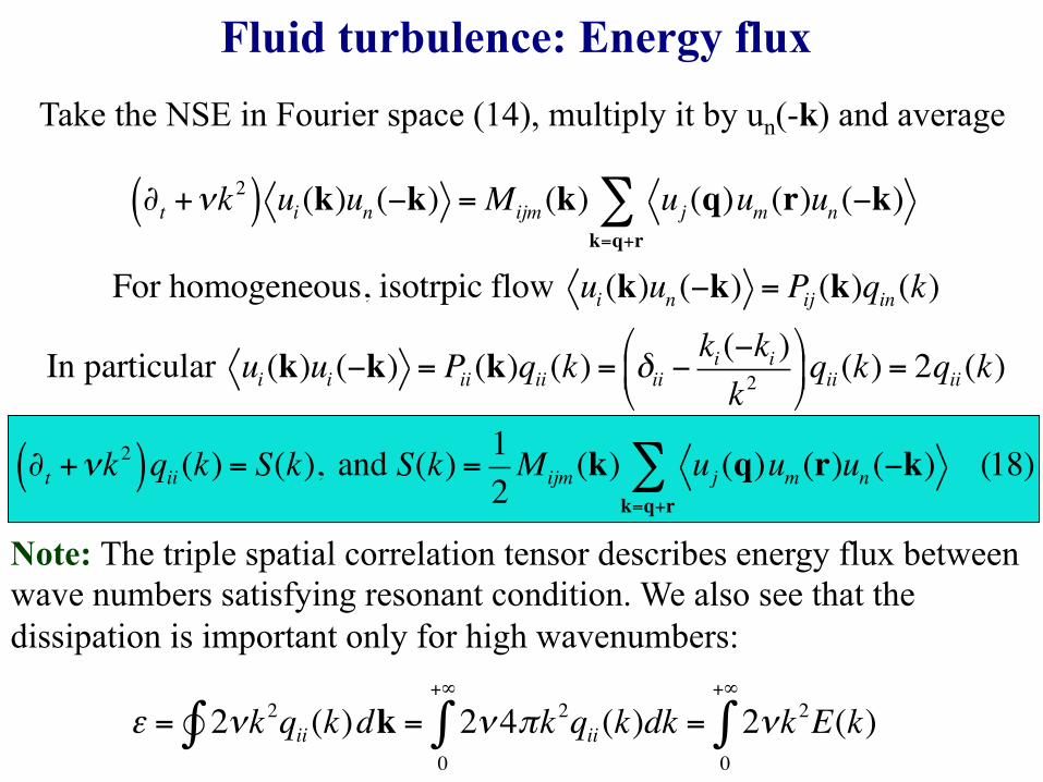
Fluid turbulence: Energy flux Take the NSE in Fourier space (14), multiply it by un(-k) and average

Note: The triple spatial correlation tensor describes energy flux between wave numbers satisfying resonant condition. We also see that the dissipation is important only for high wavenumbers:

ε = 2νk2qii (k)dk∫ = 2ν4π0

+∞

∫ k2qii (k)dk = 2νk20

+∞

∫ E(k)

∂t +νk2( ) ui (k)un (−k) =Mijm (k) uj (q)um (r)un (−k)

k=q+r∑

For homogeneous, isotrpic flow ui (k)un (−k) = Pij (k)qin (k)

In particular ui (k)ui (−k) = Pii (k)qii (k) = δii −ki (−ki )k2

$

%&

'

()qii (k) = 2qii (k)

∂t +νk2( )qii (k) = S(k), and S(k) = 1

2Mijm (k) uj (q)um (r)un (−k)

k=q+r∑ (18)

Part II: Phenomenological approaches to hydrodynamic

turbulence. Kolmogorov’s 1941 theory of turbulence.

Fluid turbulence phenomenology: cheat sheet

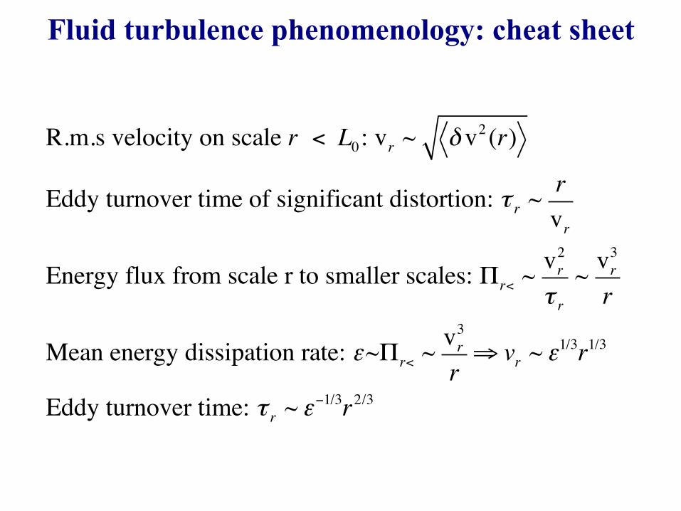
R.m.s velocity on scale r < L0: vr ~ δ v2 (r)

Eddy turnover time of significant distortion: τ r ~ rvr

Energy flux from scale r to smaller scales: Πr< ~ vr2

τ r~ vr

3

r

Mean energy dissipation rate: ε~Πr< ~ vr3

r⇒ vr ~ ε1/3r1/3

Eddy turnover time: τ r ~ ε−1/3r2/3

Fluid turbulence phenomenology: K41

Kolmogorov used two “hypothesis of similarity” which led to the derivation of the functional form of the power-law spectrum. •  SH1: At high Re values, all small scale statistical properties of

turbulence are uniquely and universally determined by the scale r, the mean energy dissipation ε(k) and the viscosity ν.

•  SH2: In the limit Reè∞ all small scale statistical properties of

turbulence are uniquely and universally determined by the scale r, the mean energy dissipation ε(k).

10ï1 100 101 10210ï4

10ï2

100

log10(k)

log 10(PSD)

Driving

Dissipation

~k-5/3

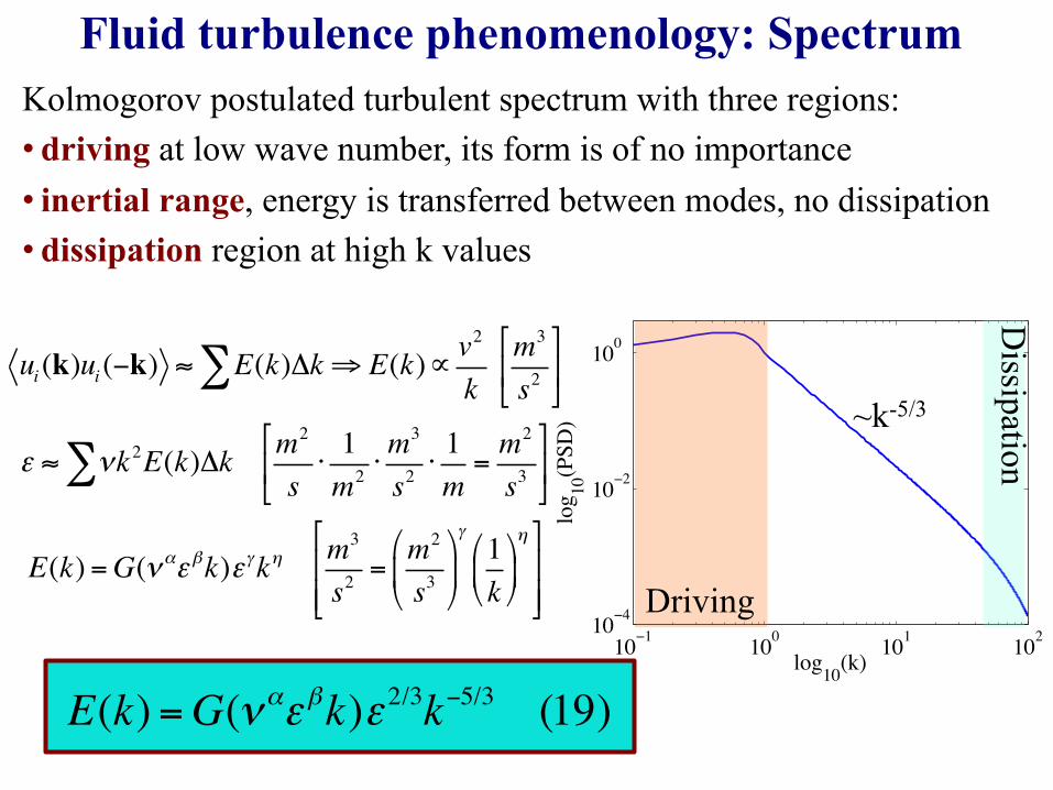
Fluid turbulence phenomenology: Spectrum Kolmogorov postulated turbulent spectrum with three regions: • driving at low wave number, its form is of no importance • inertial range, energy is transferred between modes, no dissipation • dissipation region at high k values

ui (k)ui (−k) ≈ E(k)Δk⇒ E(k)∝ v2

k∑ m3

s2

'

()

*

+,

ε ≈ νk2E(k)Δk m2

s⋅

1m2 ⋅

m3

s2 ⋅1m=m2

s3

'

()

*

+,∑

E(k) =G(ναεβk)εγkη m3

s2 =m2

s3

.

/0

1

23

γ1k.

/01

23η'

())

*

+,,

E(k) =G(ναεβk)ε 2/3k−5/3 (19)

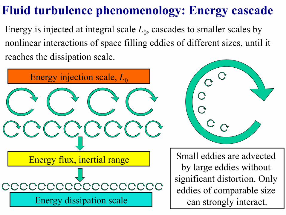
Fluid turbulence phenomenology: Energy cascade Energy is injected at integral scale L0, cascades to smaller scales by nonlinear interactions of space filling eddies of different sizes, until it reaches the dissipation scale.

Energy injection scale, L0

Energy flux, inertial range

Energy dissipation scale

Small eddies are advected by large eddies without

significant distortion. Only eddies of comparable size

can strongly interact.

WARNING 1: It is often incorrectly assumed that the power-law power spectrum with index close to -5/3 is indicative of turbulent process. This is not true: there are other systems that can produce the same spectra, but are not dynamically equivalent to turbulence. In order to identify turbulence in the physical system, one has to identify the energy cascade, that is, a region in wavenumber space where energy is transferred from mode to mode without dissipation (nonlinear term).

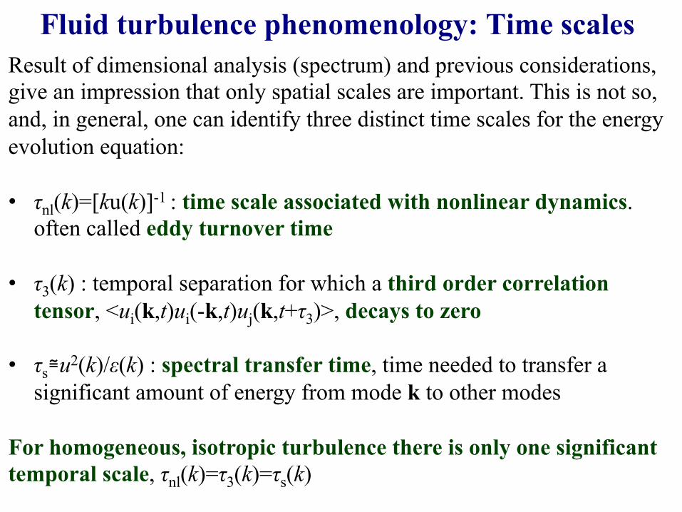
Fluid turbulence phenomenology: Time scales Result of dimensional analysis (spectrum) and previous considerations, give an impression that only spatial scales are important. This is not so, and, in general, one can identify three distinct time scales for the energy evolution equation: •  τnl(k)=[ku(k)]-1 : time scale associated with nonlinear dynamics.

often called eddy turnover time •  τ3(k) : temporal separation for which a third order correlation

tensor, <ui(k,t)ui(-k,t)uj(k,t+τ3)>, decays to zero •  τs≅u2(k)/ε(k) : spectral transfer time, time needed to transfer a

significant amount of energy from mode k to other modes

For homogeneous, isotropic turbulence there is only one significant temporal scale, τnl(k)=τ3(k)=τs(k)

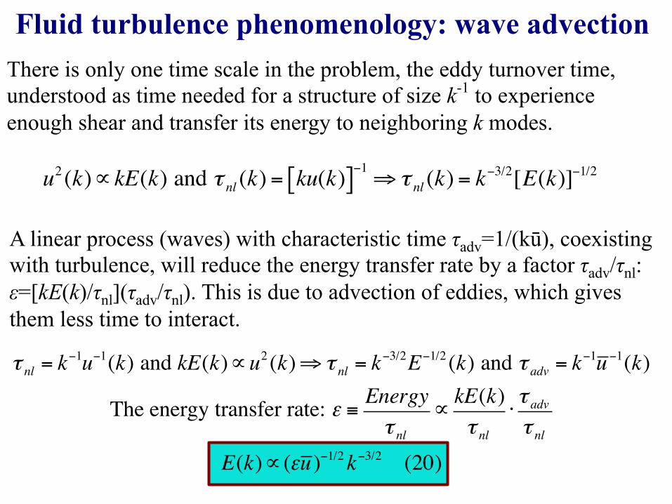
Fluid turbulence phenomenology: wave advection

u2 (k)∝ kE(k) and τ nl (k) = ku(k)[ ]−1⇒ τ nl (k) = k−3/2[E(k)]−1/2

There is only one time scale in the problem, the eddy turnover time, understood as time needed for a structure of size k-1 to experience enough shear and transfer its energy to neighboring k modes.

τ nl = k−1u−1(k) and kE(k)∝u2 (k)⇒ τ nl = k

−3/2E−1/2 (k) and τ adv = k−1u −1(k)

The energy transfer rate: ε ≡ Energyτ nl

∝kE(k)τ nl

⋅τ advτ nl

E(k)∝ (εu)−1/2k−3/2 (20)

A linear process (waves) with characteristic time τadv=1/(kū), coexisting with turbulence, will reduce the energy transfer rate by a factor τadv/τnl: ε=[kE(k)/τnl](τadv/τnl). This is due to advection of eddies, which gives them less time to interact.

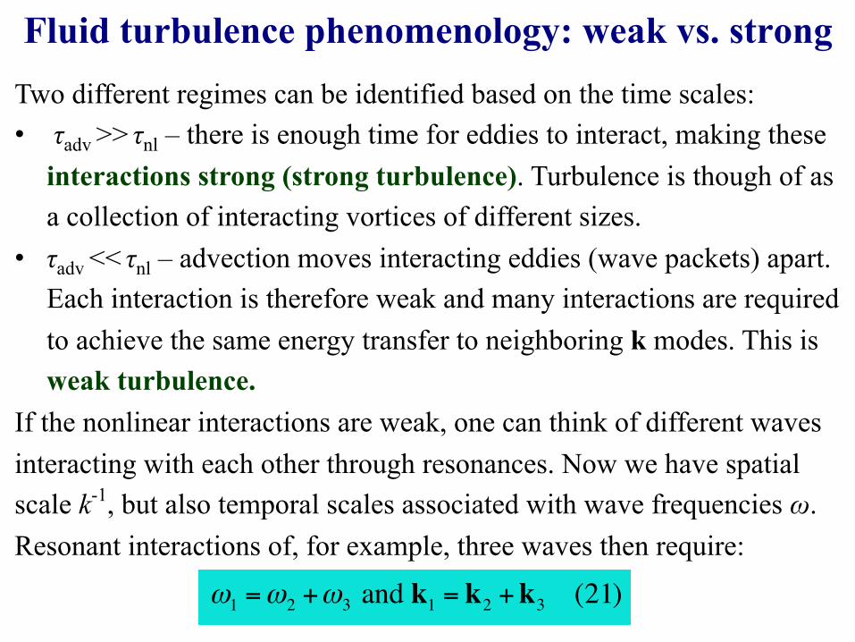
Fluid turbulence phenomenology: weak vs. strong Two different regimes can be identified based on the time scales: •  τadv >> τnl – there is enough time for eddies to interact, making these

interactions strong (strong turbulence). Turbulence is though of as a collection of interacting vortices of different sizes.

•  τadv << τnl – advection moves interacting eddies (wave packets) apart. Each interaction is therefore weak and many interactions are required to achieve the same energy transfer to neighboring k modes. This is weak turbulence.

If the nonlinear interactions are weak, one can think of different waves interacting with each other through resonances. Now we have spatial scale k-1, but also temporal scales associated with wave frequencies ω. Resonant interactions of, for example, three waves then require:

ω1 =ω2 +ω3 and k1 = k2 +k3 (21)

WARNING 2: Nonlinear interactions are sometimes labeled as “local” or “non-local” in k-space. Energy cascade is “local” because only similar wave number modes can interact. For wave turbulence very different triads may satisfy resonant conditions. However, the distinction should be made between nonlinear interaction and energy transfer: take two modes with k1=1.00 and k2=-1.01. If these can interact the energy will be transferred to the mode k3=k1+k2=0.01. The interaction is “local” but the energy transfer is “non-local”.

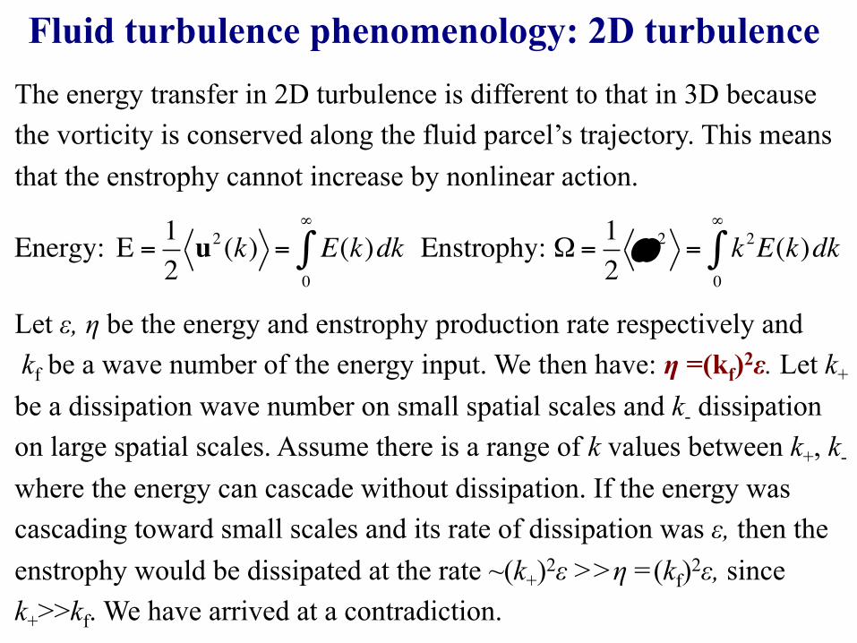
Fluid turbulence phenomenology: 2D turbulence The energy transfer in 2D turbulence is different to that in 3D because the vorticity is conserved along the fluid parcel’s trajectory. This means that the enstrophy cannot increase by nonlinear action.

Energy: E =12u2 (k) = E(k)dk

0

∞

∫ Enstrophy: Ω =12ω 2 = k2E(k)dk

0

∞

∫

Let ε, η be the energy and enstrophy production rate respectively and kf be a wave number of the energy input. We then have: η =(kf)2ε. Let k+ be a dissipation wave number on small spatial scales and k- dissipation on large spatial scales. Assume there is a range of k values between k+, k- where the energy can cascade without dissipation. If the energy was cascading toward small scales and its rate of dissipation was ε, then the enstrophy would be dissipated at the rate ~(k+)2ε >>η =(kf)2ε, since k+>>kf. We have arrived at a contradiction.

10ï1 100 101 10210ï6

10ï4

10ï2

100

log10(k)

log 10(PSD) D

riving

Dissipation

~k-5/3

~k-3

Ω E

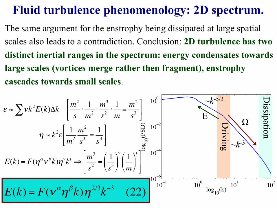
Fluid turbulence phenomenology: 2D spectrum. The same argument for the enstrophy being dissipated at large spatial scales also leads to a contradiction. Conclusion: 2D turbulence has two distinct inertial ranges in the spectrum: energy condensates towards large scales (vortices merge rather then fragment), enstrophy cascades towards small scales.

ε ≈ νk2E(k)Δk m2

s⋅1m2 ⋅

m3

s2⋅1m=m2

s3$

%&

'

()∑

η ~ k2ε 1m2

m2

s3=1s3

$

%&

'

()

E(k) = F(ηαν βk)ηγkι ⇒ m3

s2=1s3,

-.

/

01γ 1m,

-.

/

01ι$

%&&

'

())

E(k) = F(ναηβk)η2/3k−3 (22)

Part III: Statistical description of hydrodynamic turbulence.

Structure functions.

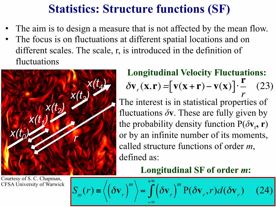
•  The aim is to design a measure that is not affected by the mean flow. •  The focus is on fluctuations at different spatial locations and on

different scales. The scale, r, is introduced in the definition of fluctuations

Statistics: Structure functions (SF)

r

x(t3) x(t4)

x(t2) x(t1)

x(t0)

δvr (x,r)= v(x+ r)− v(x)[ ] ⋅ rr(23)

Longitudinal Velocity Fluctuations:

Sm(r) ≡ δvr( )m= δvr( )

m

−∞

+∞

∫ P(δvr ,r)d(δvr ) (24)

The interest is in statistical properties of fluctuations δv. These are fully given by the probability density function P(δvr, r) or by an infinite number of its moments, called structure functions of order m, defined as:

Longitudinal SF of order m: Courtesy of S. C. Chapman, CFSA University of Warwick

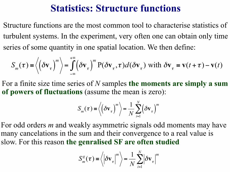
Statistics: Structure functions Structure functions are the most common tool to characterise statistics of turbulent systems. In the experiment, very often one can obtain only time series of some quantity in one spatial location. We then define:

For a finite size time series of N samples the moments are simply a sum of powers of fluctuations (assume the mean is zero):

Sm(τ ) ≡ δvτ( )m= δvτ( )

m

−∞

+∞

∫ P(δvτ ,τ )d(δvτ ) with δvτ ≡ v(t +τ )− v(t)

Sm(τ ) ≡ δvτ( )m=1N

δvτ( )m

i=1

N

∑

For odd orders m and weakly asymmetric signals odd moments may have many cancelations in the sum and their convergence to a real value is slow. For this reason the genralised SF are often studied

Smg (τ ) ≡ δvτ

m=1N

δvτm

i=1

N

∑

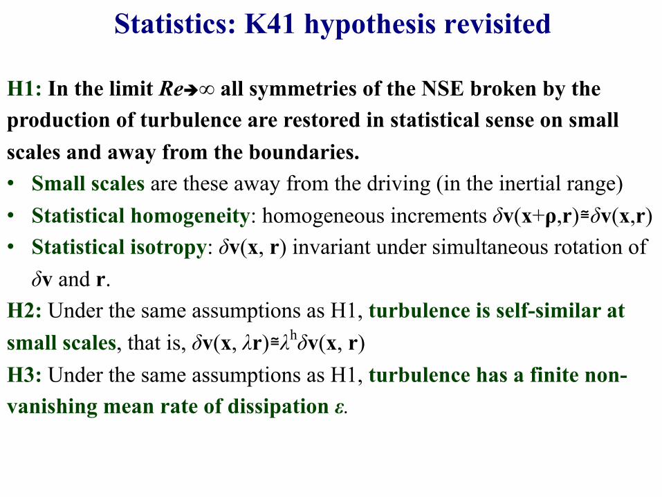
Statistics: K41 hypothesis revisited

H1: In the limit Reè∞ all symmetries of the NSE broken by the production of turbulence are restored in statistical sense on small scales and away from the boundaries. •  Small scales are these away from the driving (in the inertial range) •  Statistical homogeneity: homogeneous increments δv(x+ρ,r)≅δv(x,r) •  Statistical isotropy: δv(x, r) invariant under simultaneous rotation of δv and r.

H2: Under the same assumptions as H1, turbulence is self-similar at small scales, that is, δv(x, λr)≅λhδv(x, r) H3: Under the same assumptions as H1, turbulence has a finite non-vanishing mean rate of dissipation ε.

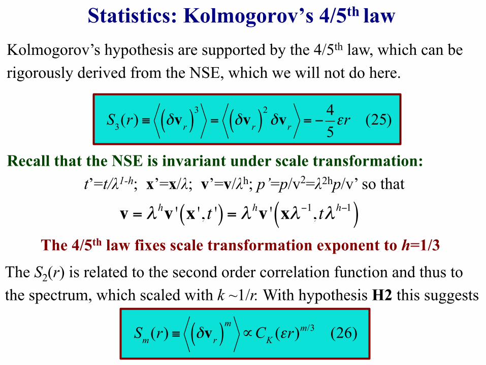
Statistics: Kolmogorov’s 4/5th law Kolmogorov’s hypothesis are supported by the 4/5th law, which can be rigorously derived from the NSE, which we will not do here.

S3(r) ≡ δvr( )3= δvr( )

2δvr = −

45εr (25)

Recall that the NSE is invariant under scale transformation: t’=t/λ1-h; x’=x/λ; v’=v/λh; p’=p/v2=λ2hp/v’ so that

v = λ hv ' x ', t '( ) = λ hv ' xλ−1, tλ h−1( )The 4/5th law fixes scale transformation exponent to h=1/3

The S2(r) is related to the second order correlation function and thus to the spectrum, which scaled with k ~1/r. With hypothesis H2 this suggests

Sm(r) ≡ δvr( )m∝CK (εr)

m/3 (26)

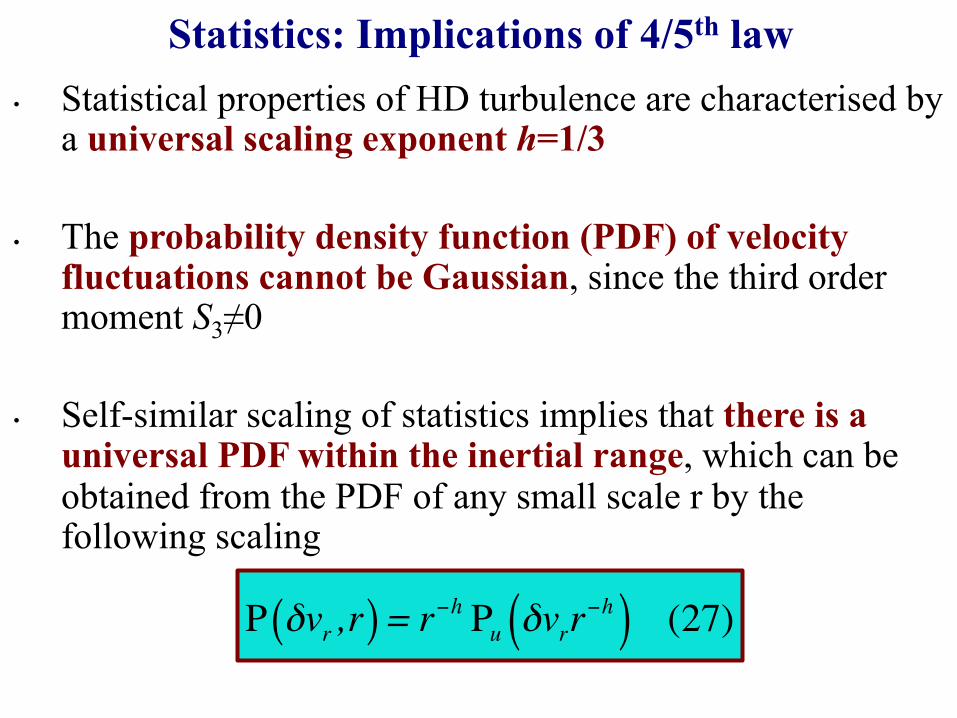
Statistics: Implications of 4/5th law

P δvr ,r( )= r−h Pu δvrr−h( ) (27)

•  Statistical properties of HD turbulence are characterised by a universal scaling exponent h=1/3

•  The probability density function (PDF) of velocity fluctuations cannot be Gaussian, since the third order moment S3≠0

•  Self-similar scaling of statistics implies that there is a universal PDF within the inertial range, which can be obtained from the PDF of any small scale r by the following scaling

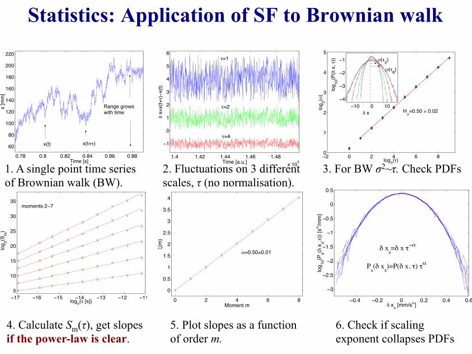
Statistics: Application of SF to Brownian walk

0.78 0.8 0.82 0.84 0.86 0.88

60

80

100

120

140

160

180

200

220

Time [s]

x [m

m]

Range growswith time

x(t) x(t+o)

1.4 1.42 1.44 1.46 1.48x 104

−1

0

1

2

3

4

5

6

Time [a.u.]b

x=x(

t+o)−x

(t)

o=1

o=2

o=4

−2 0 2 4 6 80

1

2

3

4

5

log 2(m

)

log2(o)

−10 0 10−4

−3

−2

−1

b x

log 10

(P(b

x, o

))

Hm=0.50 ± 0.02

m(o2)

m(o8)

−17 −16 −15 −14 −13 −12 −115

10

15

20

25

30

35

log2(o [s])

log 2(S

m)

moments 2−7

0 2 4 6 8

0

0.5

1

1.5

2

2.5

3

3.5

4

Moment m

c(m

)

_=0.50±0.01

−0.4 −0.2 0 0.2 0.4 0.6

−3

−2.5

−2

−1.5

−1

−0.5

0

0.5

b xs [mm/s_]

log 10

(Ps(b

xs,o)

) [s_

/mm

]

b xs=b x oï_

Ps(b xs)=P(b x, o) o_

1. A single point time series of Brownian walk (BW).

2. Fluctuations on 3 different scales, τ (no normalisation).

3. For BW σ2~τ. Check PDFs

4. Calculate Sm(τ), get slopes if the power-law is clear.

5. Plot slopes as a function of order m.

6. Check if scaling exponent collapses PDFs

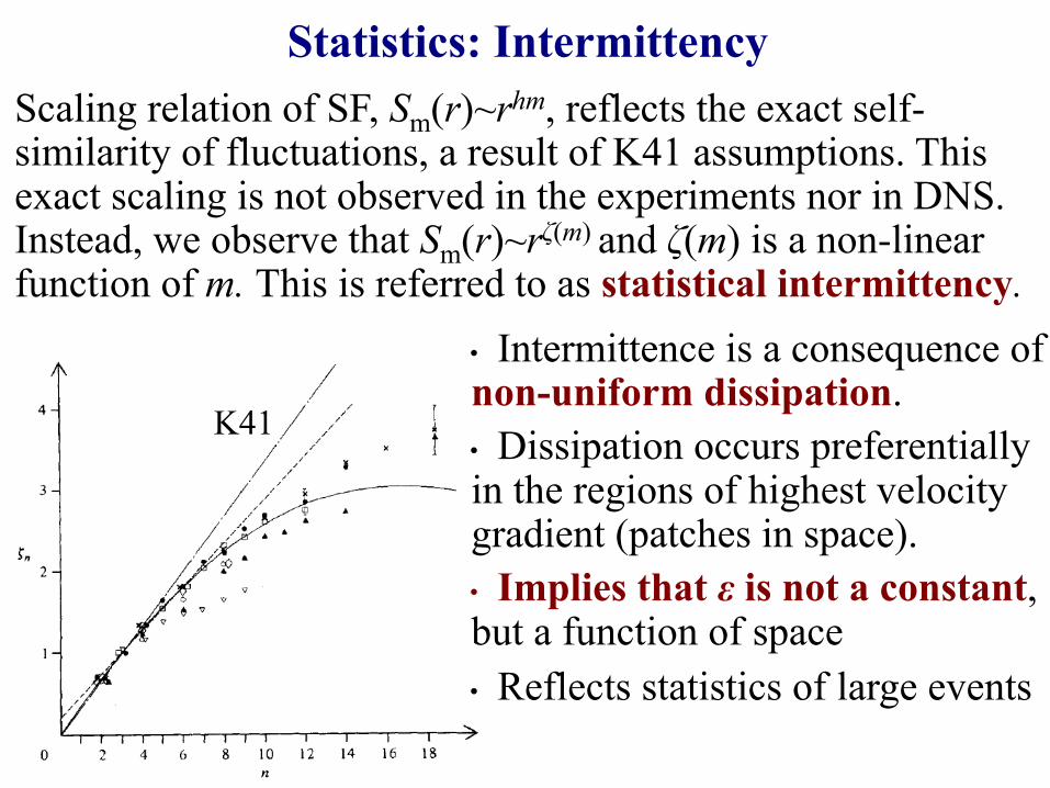
Statistics: Intermittency Scaling relation of SF, Sm(r)~rhm, reflects the exact self-similarity of fluctuations, a result of K41 assumptions. This exact scaling is not observed in the experiments nor in DNS. Instead, we observe that Sm(r)~rζ(m) and ζ(m) is a non-linear function of m. This is referred to as statistical intermittency.

K41

•  Intermittence is a consequence of non-uniform dissipation. •  Dissipation occurs preferentially in the regions of highest velocity gradient (patches in space). •  Implies that ε is not a constant, but a function of space •  Reflects statistics of large events

WARNING 3: It is often incorrectly stated that the statistical intermittency of turbulence is measured by the departure of moments or PDF from the values given by the Gaussian process. We have already noted that, even for K41 theory, the third order moment of velocity fluctuations does not vanish, that is, the statistics of these fluctuations is not Gaussian! Scaling exponent of structure functions for Gaussian process is h=1/2, while for K41 turbulence it is h=1/3.

Part IV: Plasma turbulence on MHD scales. Theory and solar

wind observations.

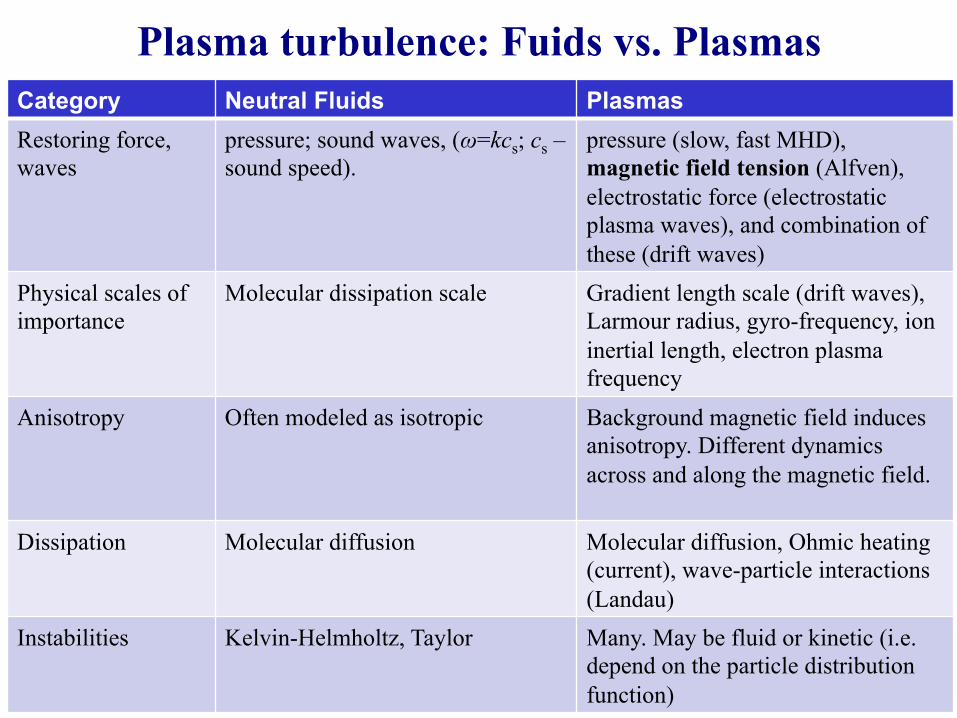
Plasma turbulence: Fuids vs. Plasmas Category Neutral Fluids Plasmas Restoring force, waves

pressure; sound waves, (ω=kcs; cs – sound speed).

pressure (slow, fast MHD), magnetic field tension (Alfven), electrostatic force (electrostatic plasma waves), and combination of these (drift waves)

Physical scales of importance

Molecular dissipation scale Gradient length scale (drift waves), Larmour radius, gyro-frequency, ion inertial length, electron plasma frequency

Anisotropy Often modeled as isotropic Background magnetic field induces anisotropy. Different dynamics across and along the magnetic field.

Dissipation Molecular diffusion Molecular diffusion, Ohmic heating (current), wave-particle interactions (Landau)

Instabilities Kelvin-Helmholtz, Taylor Many. May be fluid or kinetic (i.e. depend on the particle distribution function)

There are few plasma systems that serve as an archetypes of turbulence: •  Solar interior, dynamo process requires complex flow •  Supersonic and Super-Alfvénic collisionless solar wind •  Magnetically confined space and laboratory plasmas such as

terrestrial magnetosphere and fusion plasma in tokamaks

There are significant differences in the physics operating in these systems, for example •  MHD may be appropriate for the solar wind large scale turbulence,

but in confined plasmas with large gradients in plasma parameters a multi-fluid model may be needed

•  Solar wind is nearly unbound, but in the solar interior a good representation of the boundary conditions is fundamental

For the rest of this lecture we focus only on MHD turbulence.

Examples of turbulent plasma systems

Examples of turbulent plasma: solar wind

•  Stream of supersonic and super-Alfvénic particles •  Velocity ~500 km/s, density ~5 cm-3, IMF ~5 nT •  Consists of electrons, protons (96%), ions (4%) •  Exhibits slow and fast components, reflecting different

points of origin •  Includes other “components”: solar flares, coronal mass

ejections, etc… •  Plasma β≈1, but density fluctuations much lower in

amplitude compared with magnetic field and velocity •  Natural laboratory for unbound plasma turbulence,

diagnosed by a number of spacecraft instruments with temporal resolutions that covers MHD and sub ion-gyro scales.

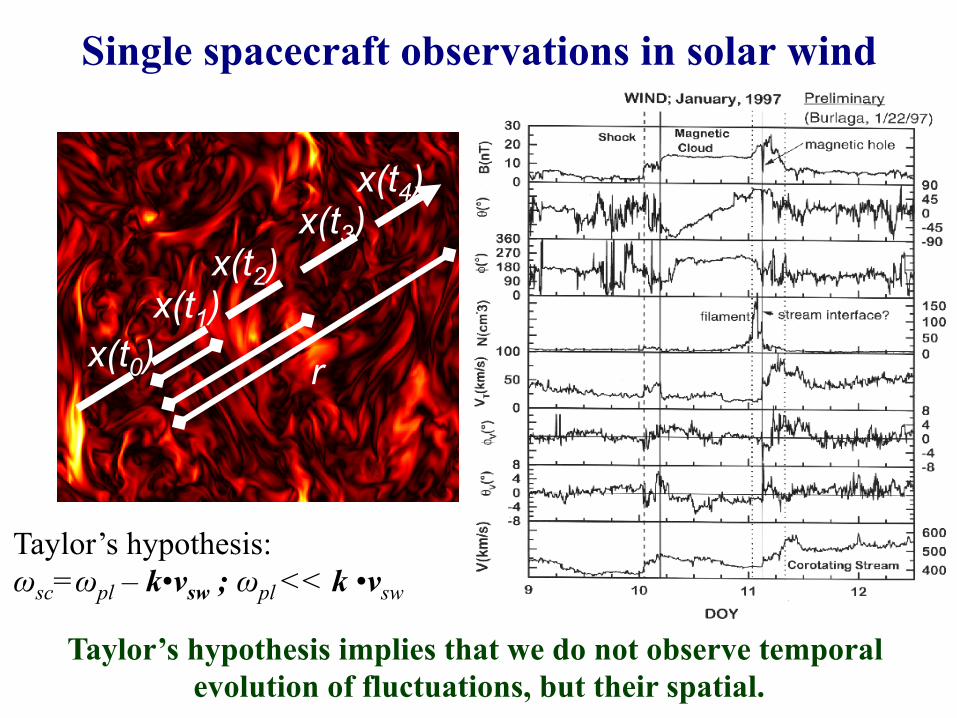
Single spacecraft observations in solar wind

r

x(t3) x(t4)

x(t2) x(t1)

x(t0)

Taylor’s hypothesis: ωsc=ωpl – k•vsw ; ωpl << k •vsw

Taylor’s hypothesis implies that we do not observe temporal evolution of fluctuations, but their spatial.

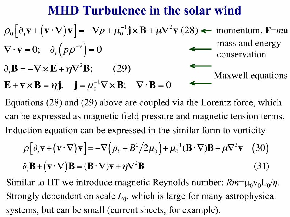
MHD Turbulence in the solar wind ρ0 ∂tv+ v ⋅∇( )v$% &'= −∇p+µ0

−1j×B+µ∇2v (28)

∇⋅v = 0; ∂t pρ−γ( ) = 0

∂tB = −∇×E+η∇2B; (29)

E+ v×B =η j; j= µ0−1∇×B; ∇⋅B = 0

momentum, F=ma mass and energy conservation

Maxwell equations

Equations (28) and (29) above are coupled via the Lorentz force, which can be expressed as magnetic field pressure and magnetic tension terms. Induction equation can be expressed in the similar form to vorticity

ρ ∂tv+ v ⋅∇( )v$% &'= −∇ pk +B2 2µ0( )+µ0−1(B ⋅∇)B+µ∇2v 30( )

∂tB+ v ⋅∇( )B = (B ⋅∇)v+η∇2B (31)

Similar to HT we introduce magnetic Reynolds number: Rm=µ0v0L0/η. Strongly dependent on scale L0, which is large for many astrophysical systems, but can be small (current sheets, for example).

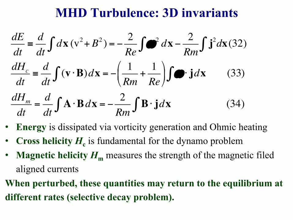
MHD Turbulence: 3D invariants

dEdt

≡ddt

dx∫ (v2+B2 ) = − 2Re

ω 2 dx− 2Rm∫ j2∫ dx (32)

dHc

dt≡ddt

(v ⋅B)dx = − 1Rm

+1Re

%

&'

(

)* ω ⋅ jdx∫∫ (33)

dHm

dt=ddt

A ⋅Bdx = − 2Rm

B ⋅ jdx∫∫ (34)

•  Energy is dissipated via vorticity generation and Ohmic heating •  Cross helicity Hc is fundamental for the dynamo problem •  Magnetic helicity Hm measures the strength of the magnetic filed

aligned currents When perturbed, these quantities may return to the equilibrium at different rates (selective decay problem).

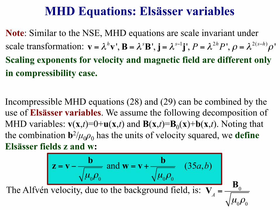
MHD Equations: Elsässer variables

Note: Similar to the NSE, MHD equations are scale invariant under scale transformation: Scaling exponents for velocity and magnetic field are different only in compressibility case.

v = λ hv ',B = λ sB ', j= λ s−1j', P = λ 2hP ', ρ = λ 2(s−h)ρ '

Incompressible MHD equations (28) and (29) can be combined by the use of Elsässer variables. We assume the following decomposition of MHD variables: v(x,t)=0+u(x,t) and B(x,t)=B0(x)+b(x,t). Noting that the combination b2/µ0ρ0 has the units of velocity squared, we define Elsässer fields z and w:

z = v− bµ0ρ0

and w = v+ bµ0ρ0

(35a,b)

The Alfvén velocity, due to the background field, is: VA =B0µ0ρ0

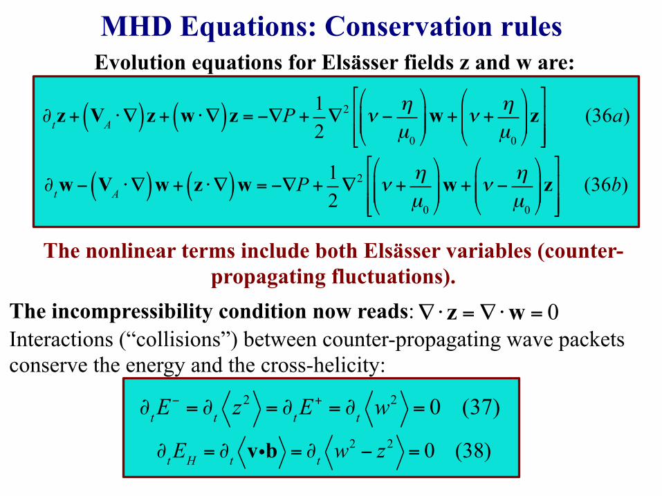
MHD Equations: Conservation rules

∂tz+ VA ⋅∇( )z+ w ⋅∇( )z = −∇P + 12∇2 ν −

ηµ0

!

"##

$

%&&w+ ν +

ηµ0

!

"##

$

%&&z

!

"##

$

%&&

(36a)

∂tw− VA ⋅∇( )w+ z ⋅∇( )w = −∇P + 12∇2 ν +

ηµ0

!

"##

$

%&&w+ ν −

ηµ0

!

"##

$

%&&z

!

"##

$

%&&(36b)

Evolution equations for Elsässer fields z and w are:

Interactions (“collisions”) between counter-propagating wave packets conserve the energy and the cross-helicity:

∂tEH = ∂t vib = ∂t w2 − z2 = 0 (38)

∂tE− = ∂t z

2 = ∂tE+ = ∂t w

2 = 0 (37)

The nonlinear terms include both Elsässer variables (counter-propagating fluctuations).

The incompressibility condition now reads: ∇⋅ z =∇⋅w = 0

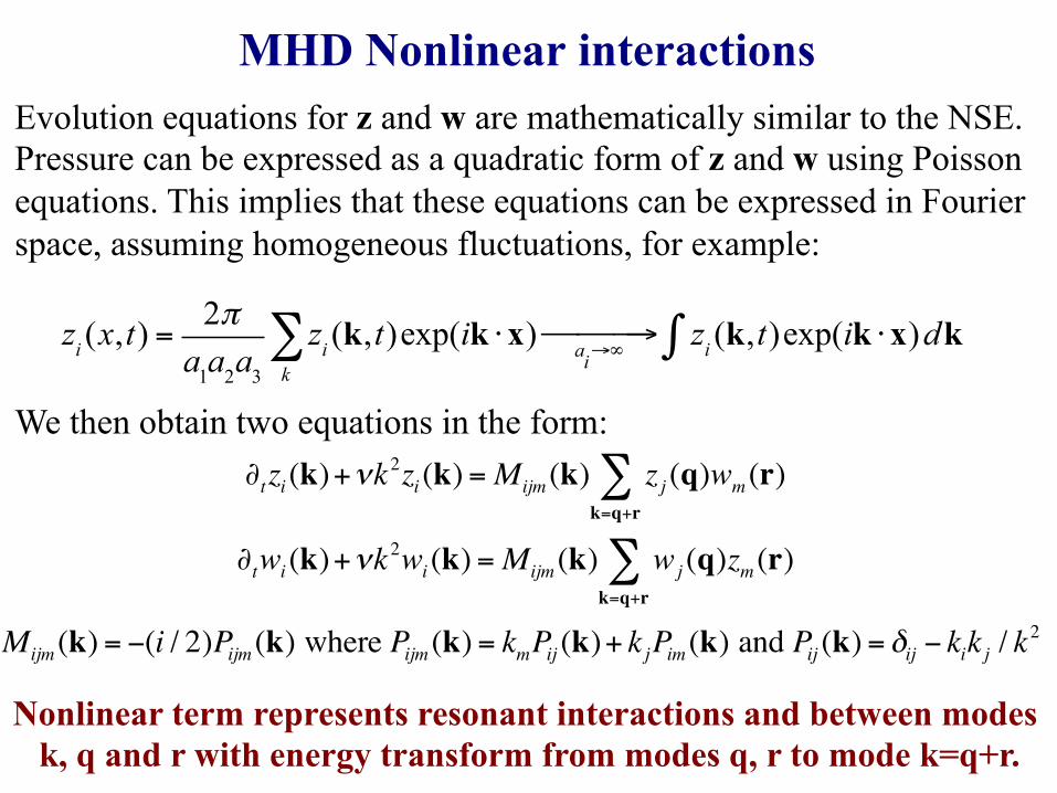
MHD Nonlinear interactions Evolution equations for z and w are mathematically similar to the NSE. Pressure can be expressed as a quadratic form of z and w using Poisson equations. This implies that these equations can be expressed in Fourier space, assuming homogeneous fluctuations, for example:

zi (x,t) =2πa1a2a3

zi (k,t)exp(ik ⋅x) ai→∞$ →$$ zi (k,t)exp(ik ⋅x)dk∫

k∑

∂t zi (k)+νk2zi (k) =Mijm (k) zj (q)k=q+r∑ wm (r)

∂twi (k)+νk2wi (k) =Mijm (k) wj (q)k=q+r∑ zm (r)

Mijm (k) = −(i / 2)Pijm (k) where Pijm (k) = kmPij (k)+ kjPim (k) and Pij (k) = δij − kik j / k2

We then obtain two equations in the form:

Nonlinear term represents resonant interactions and between modes k, q and r with energy transform from modes q, r to mode k=q+r.

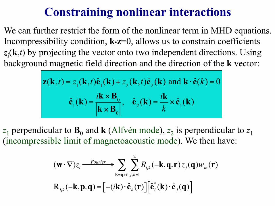
Constraining nonlinear interactions We can further restrict the form of the nonlinear term in MHD equations. Incompressibility condition, k�z=0, allows us to constrain coefficients zi(k,t) by projecting the vector onto two independent directions. Using background magnetic field direction and the direction of the k vector:

z(k,t) = z1(k,t)e1(k)+ z2 (k,t)e2 (k) and k ⋅ e(k) = 0

e1(k) =ik ×B0

k ×B0

, e2 (k) = ikk× e1(k)

z1 perpendicular to B0 and k (Alfvén mode), z2 is perpendicular to z1 (incompressible limit of magnetoacoustic mode). We then have:

(w ⋅∇)ziFourier# →## Rijk (−k,q,r)

j,k=1

2

∑ zj (q)k=q+r∑ wm (r)

Rijk (−k,p,q) = −(ik) ⋅ ek (r)[ ] ei*(k) ⋅ e j (q)'( )*

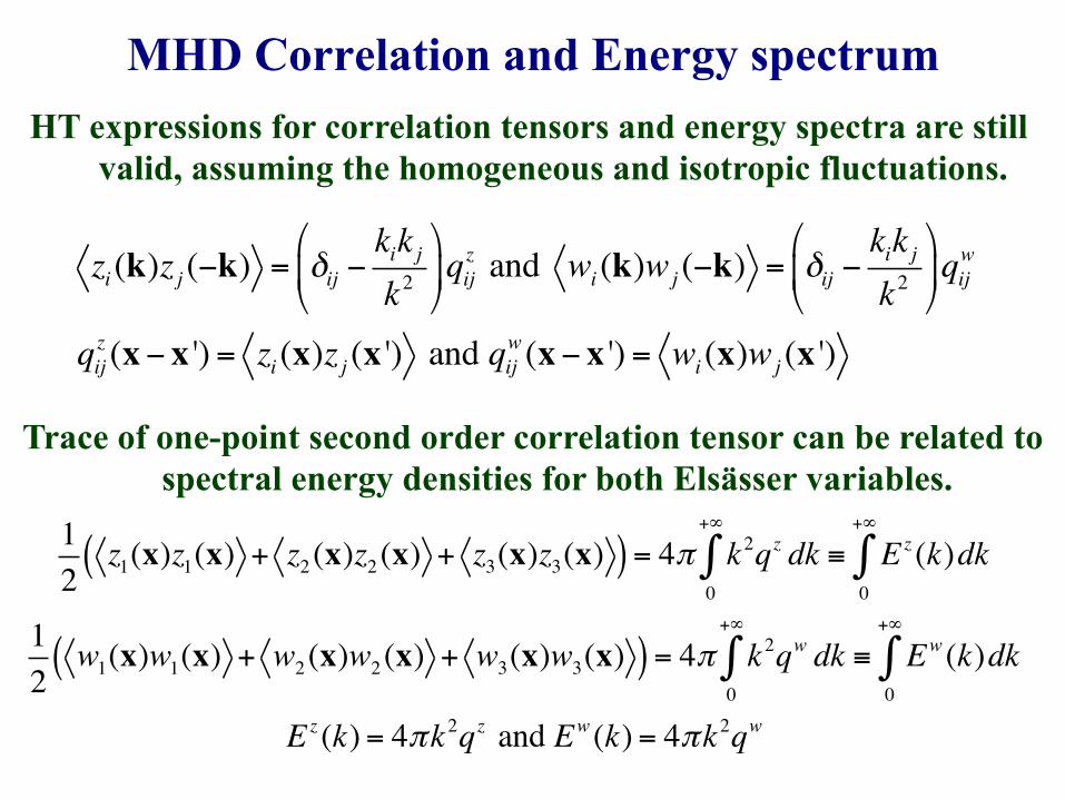
MHD Correlation and Energy spectrum HT expressions for correlation tensors and energy spectra are still

valid, assuming the homogeneous and isotropic fluctuations.

zi (k)zj (−k) = δij −kik jk2

"

#$

%

&'qij

z and wi (k)wj (−k) = δij −kik jk2

"

#$

%

&'qij

w

qijz (x− x ') = zi (x)zj (x ') and qij

w (x− x ') = wi (x)wj (x ')

12

z1(x)z1(x) + z2 (x)z2 (x) + z3(x)z3(x)( ) = 4π k2qz dk0

+∞

∫ ≡ Ez (k)dk0

+∞

∫

12

w1(x)w1(x) + w2 (x)w2 (x) + w3(x)w3(x)( ) = 4π k2qw dk0

+∞

∫ ≡ Ew (k)dk0

+∞

∫

Ez (k) = 4πk2qz and Ew (k) = 4πk2qw

Trace of one-point second order correlation tensor can be related to spectral energy densities for both Elsässer variables.

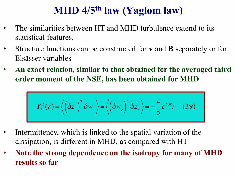
MHD 4/5th law (Yaglom law) •  The similarities between HT and MHD turbulence extend to its

statistical features. •  Structure functions can be constructed for v and B separately or for

Elsässer variables •  An exact relation, similar to that obtained for the averaged third

order moment of the NSE, has been obtained for MHD

Y3z (r) ≡ δzr( )

2δwr = δwr( )

2δzr = −

45ε z ,wr (39)

•  Intermittency, which is linked to the spatial variation of the dissipation, is different in MHD, as compared with HT

•  Note the strong dependence on the isotropy for many of MHD results so far

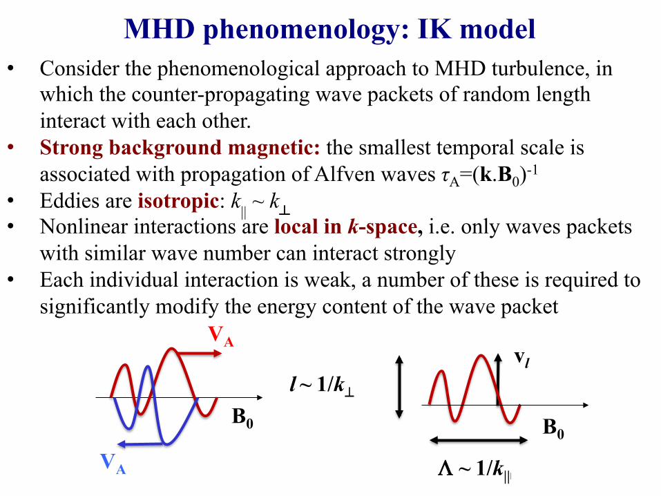
MHD phenomenology: IK model

B0

Λ ~ 1/k|||

l ~ 1/k⊥ vl

VA

VA B0

•  Consider the phenomenological approach to MHD turbulence, in which the counter-propagating wave packets of random length interact with each other.

•  Strong background magnetic: the smallest temporal scale is associated with propagation of Alfven waves τA=(k.B0)-1

•  Eddies are isotropic: k|| ~ k┴

•  Nonlinear interactions are local in k-space, i.e. only waves packets with similar wave number can interact strongly

•  Each individual interaction is weak, a number of these is required to significantly modify the energy content of the wave packet

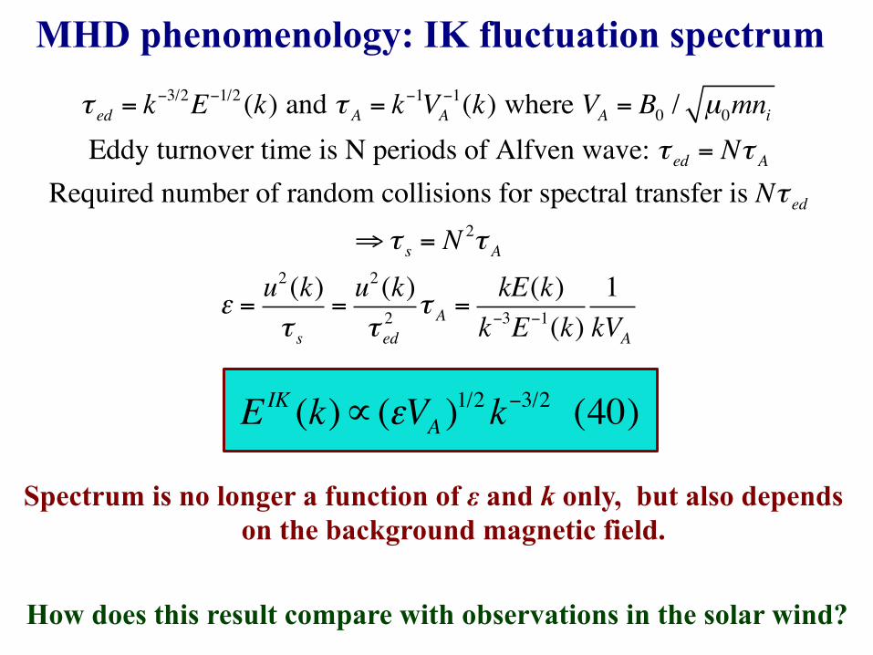
MHD phenomenology: IK fluctuation spectrum

Spectrum is no longer a function of ε and k only, but also depends on the background magnetic field.

How does this result compare with observations in the solar wind?

τ ed = k−3/2E−1/2 (k) and τ A = k

−1VA−1(k) where VA = B0 / µ0mni

Eddy turnover time is N periods of Alfven wave: τ ed = Nτ ARequired number of random collisions for spectral transfer is Nτ ed

⇒ τ s = N2τ A

ε =u2 (k)τ s

=u2 (k)τ ed

2 τ A =kE(k)

k−3E−1(k)1kVA

EIK (k)∝ (εVA )1/2k−3/2 (40)

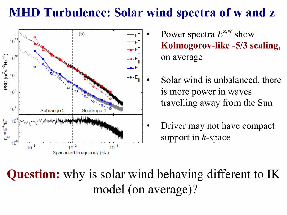
MHD Turbulence: Solar wind spectra of w and z •  Power spectra Ez,w show

Kolmogorov-like -5/3 scaling, on average

•  Solar wind is unbalanced, there is more power in waves travelling away from the Sun

•  Driver may not have compact

support in k-space

Question: why is solar wind behaving different to IK model (on average)?

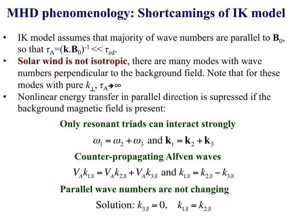
MHD phenomenology: Shortcamings of IK model

•  IK model assumes that majority of wave numbers are parallel to B0, so that τA=(k.B0)-1 << τed.

•  Solar wind is not isotropic, there are many modes with wave numbers perpendicular to the background field. Note that for these modes with pure k

┴, τAè∞

•  Nonlinear energy transfer in parallel direction is supressed if the background magnetic field is present:

ω1 =ω2 +ω3 and k1 = k2 +k3

VAk1,|| =VAk2,|| +VAk3,|| and k1,|| = k2,|| − k3,||

Solution: k3,|| = 0, k1,|| = k2,||

Parallel wave numbers are not changing

Only resonant triads can interact strongly

Counter-propagating Alfven waves

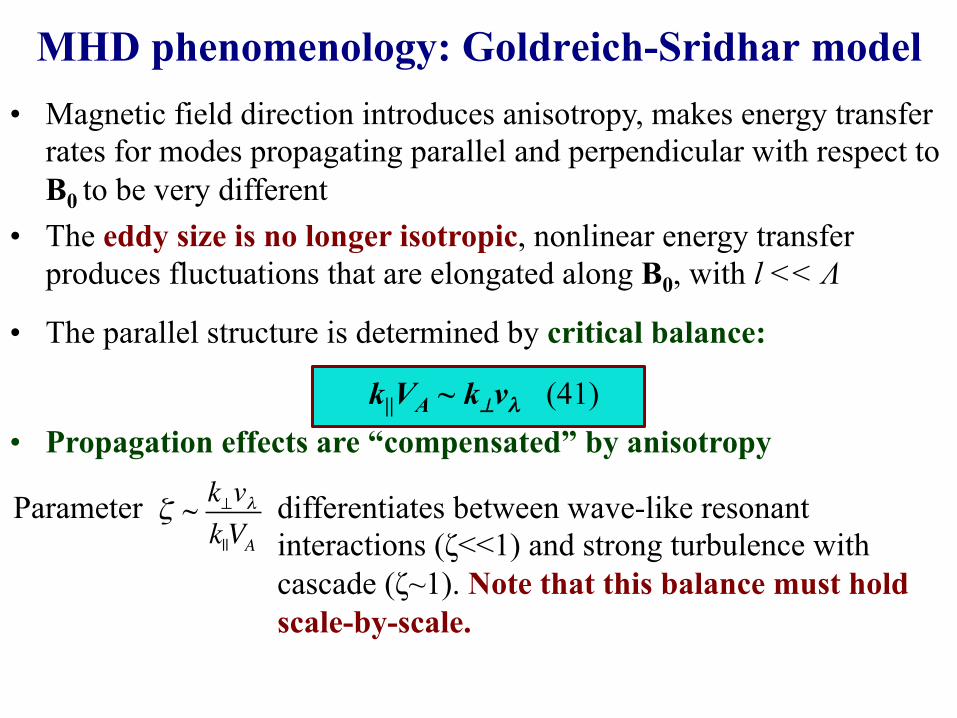
•  Magnetic field direction introduces anisotropy, makes energy transfer rates for modes propagating parallel and perpendicular with respect to B0 to be very different

•  The eddy size is no longer isotropic, nonlinear energy transfer produces fluctuations that are elongated along B0, with l << Λ

•  The parallel structure is determined by critical balance:

k||VA ~ k⊥vλ (41) •  Propagation effects are “compensated” by anisotropy

MHD phenomenology: Goldreich-Sridhar model

ζ ~ k⊥vλk||VA

Parameter differentiates between wave-like resonant interactions (ζ<<1) and strong turbulence with cascade (ζ~1). Note that this balance must hold scale-by-scale.

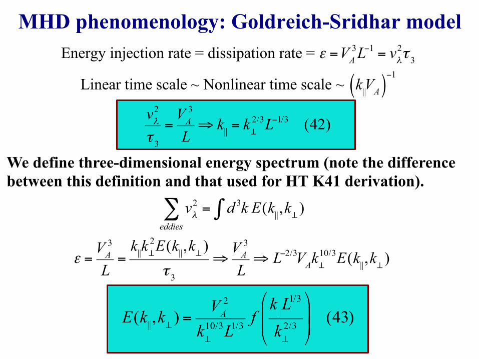
Energy injection rate = dissipation rate = ε =VA3L−1 = vλ

2τ 3

Linear time scale ~ Nonlinear time scale ~ k||VA( )−1

vλ2

τ 3

=VA

3

L⇒ k|| = k⊥

2/3L−1/3 (42)

MHD phenomenology: Goldreich-Sridhar model

We define three-dimensional energy spectrum (note the difference between this definition and that used for HT K41 derivation).

vλ2

eddies∑ = d 3k E(k|| ,k⊥ )∫

ε =VA3

L=k||k⊥

2E(k|| ,k⊥ )τ 3

⇒VA3

L⇒ L−2/3VAk⊥

10/3E(k|| ,k⊥ )

E(k|| ,k⊥ ) =VA2

k⊥10/3L1/3

fk||L

1/3

k⊥2/3

"

#$$

%

&'' (43)

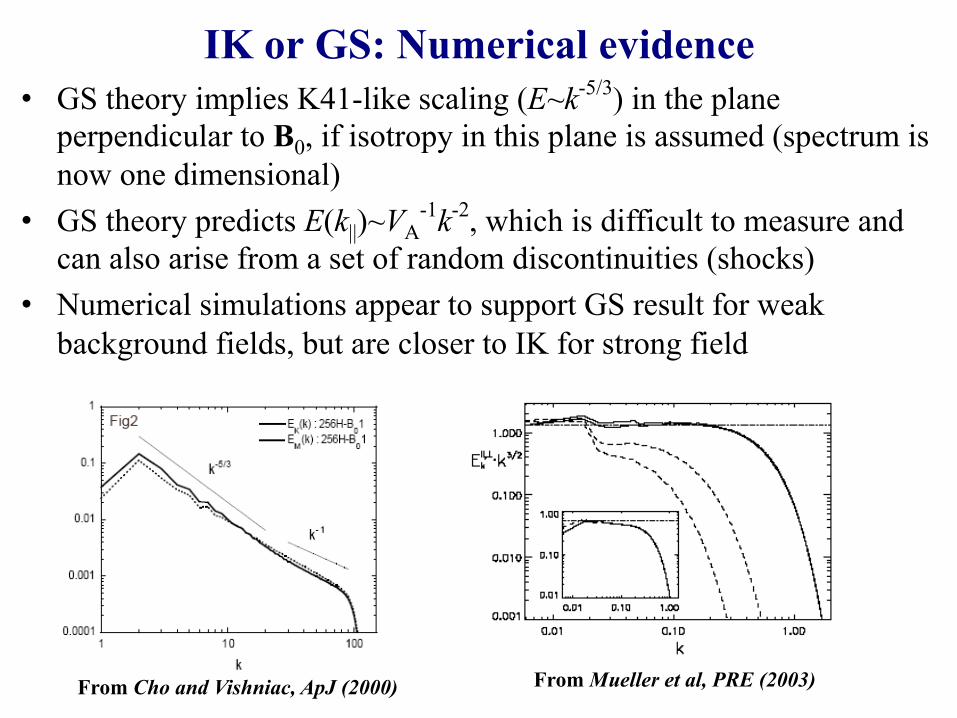
IK or GS: Numerical evidence

From Mueller et al, PRE (2003)

•  GS theory implies K41-like scaling (E~k-5/3) in the plane perpendicular to B0, if isotropy in this plane is assumed (spectrum is now one dimensional)

•  GS theory predicts E(k||)~VA-1k-2, which is difficult to measure and

can also arise from a set of random discontinuities (shocks) •  Numerical simulations appear to support GS result for weak

background fields, but are closer to IK for strong field

From Cho and Vishniac, ApJ (2000)