Planning of Power Distribution Systems with High ... · Penetration of Renewable Energy Sources Using Stochastic Optimization Sérgio da Fonseca Santos ... Planning of Power Distribution

UNIVERSIDADE DA BEIRA INTERIOR Engenharia

Planning of Power Distribution Systems with High

Penetration of Renewable Energy Sources Using Stochastic Optimization

Sérgio da Fonseca Santos

Tese para obtenção do Grau de Doutor em

Engenharia Electrotécnica e de Computadores (3º ciclo de estudos)

Orientador: Prof. Doutor João Paulo da Silva Catalão Co-orientador: Prof. Doutor Carlos Manuel Pereira Cabrita

Co-orientador: Doutor Desta Zahlay Fitiwi

Covilhã, julho de 2017

ii

UNIVERSITY OF BEIRA INTERIOR Engineering

Planning of Power Distribution Systems with High

Penetration of Renewable Energy Sources Using Stochastic Optimization

Sérgio da Fonseca Santos

Thesis submitted in fulfillment of the requirements for the degree of Doctor of Philosophy in

Electrical and Computer Engineering (3rd cycle of studies)

Supervisor: Prof. Dr. João Paulo da Silva Catalão (University of Porto)

Co-supervisors: Prof. Dr. Carlos Manuel Pereira Cabrita (University of Beira Interior)

Dr. Desta Zahlay Fitiwi (Comillas Pontifical University)

Covilhã, July 2017

iii

This work was supported by FEDER funds through COMPETE 2020 and by Portuguese

funds through FCT, under Projects FCOMP-01-0124-FEDER-020282 (Ref.

PTDC/EEA-EEL/118519/2010), POCI-01-0145-FEDER-016434, POCI-01-0145-FEDER-006961,

UID/EEA/50014/2013, UID/CEC/50021/2013, and UID/EMS/00151/2013. Also, the research

leading to these results has received funding from the EU Seventh Framework Programme

FP7/2007-2013 under grant agreement no. 309048. Moreover, Sérgio F. Santos gratefully

acknowledges UBI / Santander Totta for the doctoral incentive grant in the Engineering

Faculty.

iv

Acknowledgments

Firstly, I would like to express my sincere gratitude to my Ph.D. advisors Prof. João Paulo da

Silva Catalão and Prof. Carlos Manuel Pereira Cabrita for the continuous support of my Ph.D.

study and related research, for their patience, motivation and immense knowledge. Their

guidance helped me at all times during the research and writing of this thesis.

Besides my advisors, I would like to address a special thanks to Dr. Desta Zahlay Fitiwi, my

co-advisor and friend, for his trust, support and especially for his insightful comments

throughout my studies.

I thank all the co-authors of my works and especially to my closest collaborators, Dr. Miadreza

Shafie-khah, Dr. Bizuayehu Abebe Worke, Dr. Nikolaos Paterakis and Dr. Ozan Erdinç. I thank

my fellow colleagues in the “Sustainable Energy Systems Lab” for the stimulating discussions

and for all their help in the past years.

I also want to thank Eng. Filipe Mendonça, from EDA, S.A. - Eletricidade dos Açores, for his

demonstrated availability, for the real data used in the case studies in this thesis, and

especially for patiently addressing my urgent requests, always responding so promptly.

I would like to thank the European Project FP7 SiNGULAR (Smart and Sustainable Electricity

Grids under Large-Scale Renewable Integration) and the Santander Research Grant from the

Engineering Faculty of UBI, which provided me with economic means to fulfill this Ph.D.

Thesis.

Last but not least, I would like to thank my family, especially my parents, and all my friends

who have been beside me in the last two years.

v

Resumo

Atualmente há um esforço global para integrar mais recursos energéticos distribuídos nas

redes elétricas, impulsionado por fatores técnico-económicos e ambientais, particularmente

ao nível da rede de distribuição. Estes recursos incluem tipicamente tecnologias facilitadoras

das redes elétricas inteligentes, tais como geração distribuída, sistemas de armazenamento

de energia, e gestão ativa da procura.

A integração de fontes de geração distribuída (energias renováveis, principalmente) está a

aumentar progressivamente em muitas redes de distribuição, e é provável que esta tendência

continue nos próximos anos devido ao avanço de soluções emergentes, esperando-se assim

que as limitações técnicas existentes sejam ultrapassadas e que facilitem a integração

progressiva das fontes de geração distribuída. Espera-se também que os acordos feitos pelos

países para limitar as emissões de gases de efeito de estufa e para mitigar as alterações

climáticas acelerem a integração de fontes de energia renováveis.

No entanto, a natureza intermitente e volátil da maioria das fontes de energia renováveis (em

particular, eólica e solar) faz com que a sua integração nas redes de distribuição seja uma

tarefa complexa. Isto porque tais recursos introduzem variabilidade operacional e incerteza

no sistema. Assim, é essencial o desenvolvimento de novas metodologias e ferramentas

computacionais inovadoras para beneficiar uma integração óptima da geração distribuída

renovável e minimizar os possíveis efeitos colaterais.

Nesta tese são desenvolvidas novas metodologias e ferramentas computacionais inovadoras

que consideram a variabilidade operacional e a incerteza associadas à geração a partir de

fontes de energia renováveis, juntamente com a integração de tecnologias facilitadoras das

redes elétricas inteligentes. As metodologias e ferramentas computacionais desenvolvidas são

testadas em casos de estudo reais, bem como em casos de estudo clássicos, demonstrando a

sua proficiência computacional comparativamente ao atual estado-da-arte. Devido à inerente

incerteza e variabilidade das fontes de energia renováveis, nesta tese utiliza-se programação

estocástica. Ainda, para assegurar a convergência para soluções ótimas, o problema é

formulado utilizando programação linear inteira-mista.

Palavras Chave

Fontes de energia renováveis; Geração distribuída; Planeamento de investimentos;

Programação linear inteira-mista estocástica; Redes elétricas inteligentes; Reforço da rede;

Sistemas de armazenamento de energia; Variabilidade e incerteza.

vi

Abstract

Driven by techno-economic and environmental factors, there is a global drive to integrate

more distributed energy resources in power systems, particularly at the distribution level.

These typically include smart-grid enabling technologies, such as distributed generation (DG),

energy storage systems and demand-side management.

Especially, the scale of DG sources (mainly renewables) integrated in many distribution

networks is steadily increasing. This trend is more likely to continue in the years to come due

to the advent of emerging solutions, which are expected to alleviate existing technical

limitations and facilitate smooth integration of DGs. The favorable agreements of countries to

limit greenhouse gas (GHG) emissions and mitigate climate change are also expected to

accelerate the integration of renewable energy sources (RESs).

However, the intermittent and volatile nature of most of these RESs (particularly, wind and

solar) makes their integration in distribution networks a more challenging task. This is

because such resources introduce significant operational variability and uncertainty to the

system. Hence, the development of novel methodologies and innovative computational tools

is crucial to realize an optimal and cost-efficient integration of such DGs, minimizing also

their side effects.

Novel methodologies and innovative computational tools are developed in this thesis that

take into account the operational variability and uncertainty associated with the RES power

generation, along with the integration of smart-grid enabling technologies. The developed

methodologies and computational tools are tested in real-life power systems, as well as in

standard test systems, demonstrating their computational proficiency when compared with

the current state-of-the-art. Due to the inherent uncertainty and variability of RESs,

stochastic programming is used in this thesis. Moreover, to ensure convergence and to use

efficient off-the-shelf solvers, the problems addressed in this thesis are formulated using a

mixed integer linear programming (MILP) approach.

Keywords

Distributed Generation (DG); Energy Storage Systems (ESSs); Investment planning; Network

reinforcement; Renewable Energy Sources (RES); Smart grids; Stochastic mixed integer linear

programming; Variability and uncertainty.

vii

Contents

Acknowledgments ............................................................................................. iv

Resumo .......................................................................................................... v

Abstract......................................................................................................... vi

Contents ....................................................................................................... vii

List of Figures ............................................................................................... xiii

List of Tables ................................................................................................. xv

List of Symbols .............................................................................................. xvii

Relevant Acronyms ......................................................................................... xxv

Chapter 1 ........................................................................................................ 1

Introduction ..................................................................................................... 1

1.1 Background ........................................................................................... 1

1.2 Research Motivation and Problem Definition ................................................... 5

1.3 Research Questions, Objectives and Contributions of the Thesis .......................... 6

1.4 Methodology .......................................................................................... 9

1.5 Notation............................................................................................... 9

1.6 Organization of the Thesis ......................................................................... 9

Chapter 2 ...................................................................................................... 12

Renewable Energy Systems: An Overview ............................................................... 12

2.1 Introduction ........................................................................................ 12

2.2 Clime Change ...................................................................................... 14

2.3 Renewable Energy Trend ........................................................................ 15

2.4 Green Energy Production Options .............................................................. 16

2.4.1 Wind Energy ............................................................................... 17

2.4.2 Solar Energy ............................................................................... 19

2.4.2.1. Solar PV ......................................................................... 19

2.4.2.2. Solar CSP ........................................................................ 20

2.4.3 Geothermal Energy ....................................................................... 22

2.4.4 Hydro Energy .............................................................................. 24

2.4.5 Bioenergy ................................................................................... 25

2.4.6 Ocean Energy .............................................................................. 26

viii

2.5 Economic Aspect of Renewable Energy Systems ............................................. 27

2.5.1 Driving Factors ............................................................................ 28

2.5.2 Life-Cycle Costs ........................................................................... 29

2.5.3 Economic Trend of Renewable Energy Systems ..................................... 29

2.6 Benefits and Barriers of RESs ................................................................... 31

2.6.1 RES Integration Opportunities .......................................................... 31

2.6.2 RES Integration Challenges and Barriers .............................................. 32

2.6.3 Alleviating the Challenges and Barriers ............................................... 34

2.7 Current Trend and Future Prospects........................................................... 35

2.8 Chapter Conclusions .............................................................................. 36

Chapter 3 ...................................................................................................... 37

Impact of Operational Variability and Uncertainty on Distributed Generation Investment

Planning: A Comprehensive Sensitivity Analysis ........................................................ 37

3.1 Introduction ........................................................................................ 37

3.2 Uncertainty and Variability in DGIP ............................................................ 40

3.2.1 Terminology ............................................................................... 40

3.2.2 Sources of Uncertainty and Variability in DGIP ...................................... 41

3.3 Mathematical Model .............................................................................. 43

3.3.1 Brief Description of the problem ....................................................... 43

3.3.2 Objective Function ....................................................................... 43

3.3.3 Constraints ................................................................................. 47

3.3.3.1 Load Balance Constraints ..................................................... 47

3.3.3.2 Investment Limits .............................................................. 47

3.3.3.3 Generation Capacity Limits .................................................. 47

3.3.3.4 Unserved Power Limit ......................................................... 48

3.3.3.5 DG Penetration Level Limit .................................................. 48

3.3.3.6 Logical Constraints ............................................................. 48

3.3.3.7 Network Model Constraints ................................................... 48

3.3.3.8 Radiality Constraints .......................................................... 49

3.4 Case Studies ........................................................................................ 49

3.4.1 System Data ................................................................................ 49

ix

3.4.2 Scenario Definition ....................................................................... 51

3.4.3 Impact of Network Inclusion/Exclusion on DGIP Solution ......................... 51

3.4.4 Results and Discussion ................................................................... 52

3.4.4.1 Demand Growth and CO2 Price ............................................... 52

3.4.4.2 Interest Rate .................................................................... 53

3.4.4.3 DG Penetration Level Factor ................................................. 53

3.4.4.4 Fuel Prices and Electricity Tariffs ........................................... 55

3.4.4.5 Wind and Solar Power Output Uncertainty ................................ 56

3.4.4.6 Demand and RES Power Output Uncertainty .............................. 57

3.4.4.7 Generator Availability ......................................................... 58


Chapter 4 ...................................................................................................... 60

Multi-Stage Stochastic DG Investment Planning with Recourse...................................... 60

4.1 Introduction ........................................................................................ 60

4.2 Modeling Uncertainty and Variability in DGIP ................................................ 61


4.3.1 Overview and Modeling Assumptions .................................................. 62

4.3.2 Brief Description of the Problem ....................................................... 63


4.3.4 Constraints ................................................................................. 68

4.3.4.1 Load Balance Constraints ..................................................... 68

4.3.4.2 Linear Constraints of Generation Cost ..................................... 68

4.3.4.3 Investment Limits .............................................................. 69

4.3.4.4 Generation Capacity Limits .................................................. 69

4.3.4.5 Unserved Power Limit ......................................................... 70

4.3.4.6 DG Penetration Limit .......................................................... 70


4.3.4.8 Network Model Constraints ................................................... 71


4.4 Case Studies ........................................................................................ 73

4.4.1 System Data and Assumptions .......................................................... 73

x

4.4.2 Scenario Definition ....................................................................... 74


4.4.3.1 Deciding the number of representative clusters ......................... 77

4.4.3.2 DGIP results ..................................................................... 78

4.4.3.3 The significance of the proposed models .................................. 79


Chapter 5 ...................................................................................................... 82

Impacts of Optimal Energy Storage Deployment and Network Reconfiguration on Renewable

Integration Level in Distribution System ................................................................. 82

5.1 Introduction ........................................................................................ 82



5.2.2 Constraints ................................................................................. 87

5.2.2.1 Kirchhoff’s Current Law (Active Power Balances)........................ 87

5.2.2.2 Energy Storage Model Constraints .......................................... 88

5.2.2.3 Active Power Limits of DGs ................................................... 89

5.2.2.4 Active Power Limits of Power Purchased .................................. 89



5.3 Case Studies ........................................................................................ 91

5.3.1 System Data and Assumptions .......................................................... 91



Chapter 6 ..................................................................................................... 100

New Multi-stage and Stochastic Mathematical Model for Maximizing RES Hosting Capacity .. 100

6.1 Introduction ....................................................................................... 100

6.2 Uncertainty and Variability Management .................................................... 104

6.3 Mathematical Model ............................................................................. 106

6.3.1 Brief Description of the Problem ...................................................... 106

6.3.2 Objective Function ...................................................................... 107

6.3.3 Constraints ................................................................................ 112

xi

6.3.3.1 Kirchhoff’s Voltage Law ...................................................... 112

6.3.3.2 Flow Limits ..................................................................... 114

6.3.3.3 Line Losses ...................................................................... 116

5.3.3.4 Kirchhoff’s Current Law (Active and Reactive Load Balances) ....... 116

6.3.3.5 Bulk Energy Storage Model Constraints ................................... 117

6.3.3.6 Active and Reactive Power Limits of DGs ................................. 119

6.3.3.7 Reactive Power Limit of Capacitor Bank .................................. 120

6.3.3.8 Active and Reactive Power Limits of Power Purchased ................ 120

6.3.3.9 Logical Constraints ............................................................ 121

6.3.3.10 Radiality Constraints ........................................................ 121

6.4 Case Studies ....................................................................................... 123

6.4.1 System Data and Assumptions ......................................................... 123

6.4.2 A Strategy for Reducing Combinatorial Solution Search Space .................. 125

6.4.3 Results and Discussion .................................................................. 128

6.4.3.1 Considering DGs Without Reactive Power Support ...................... 129

6.4.3.2 Considering DGs With Reactive Power Support .......................... 138

6.4.3.3 Impact of Wind Turbine and Solar PV Selections on the Results ..... 141

6.5 Chapter Conclusions ............................................................................. 142

Chapter 7 ..................................................................................................... 143

Conclusions, Directions for Future Work and Contributions ......................................... 143

7.1 Main Conclusions ................................................................................. 143

7.2 Directions for Future Works .................................................................... 150

7.3 Contributions of the Thesis ..................................................................... 150

7.3.1 Book Chapters ............................................................................ 150

7.3.2 Publications in Peer-Reviewed Journals ............................................. 151

7.3.3 Publications in International Conference Proceedings ............................ 152

Appendices ................................................................................................... 154

Appendix A ................................................................................................... 155

Appendix B ................................................................................................... 156

Appendix C ................................................................................................... 157

Appendix D ................................................................................................... 159

xii

Appendix E ................................................................................................... 161

Bibliography .................................................................................................. 165

xiii

List of Figures

FIGURE 1.1 GLOBAL NEW INVESTMENT IN RENEWABLE ENERGY [1]……………………………………………… 2

FIGURE 1.2 GLOBAL INVESTMENTS IN RENEWABLE ENERGY BY REGION [1]…………………………………… 3

FIGURE 1.3 NEW INVESTMENTS IN RENEWABLES ENERGY BY SECTOR (IN BILLIONS OF US DOLLARS) [5] ………………………………………………………………………………………………………………………

4

FIGURE 1.4 RENEWABLE POWER GENERATION CAPACITY AS A SHARE OF GLOBAL POWER [1]…………… 4

FIGURE 2.1 SUSTAINABILITY IN THE ELECTRICITY SECTOR [17]…………………………………………………… 13

FIGURE 2.2 a) AVERAGE ANNUAL GROWTH RATES OF RENEWABLES (2008 – 2013); b) GLOBAL ELECRICITY PRODUCTION (2013) [20]……………………………………………………………………

17

FIGURE 2.3 WIND POWER TOTAL WORLD CAPACITY (2000-2013) [26]……………………………………… 18

FIGURE 2.4 FINAL ENERGY CONSUPTION FOR BIOENERGY IN EU [30]…………………………………………… 26

FIGURE 2.5 DEVELOPMENT AND FUTURE TREND OF GENERATION CAPACITY, DEMAND AND WHOLESALE

ELECTRICITY MARKET PRICE IN CENTRAL EUROPE FROM 2010 [49]……………………………. 32

FIGURE 2.6 MAIN REASONS IN THE EU 27 FOR ISSUE “LACK OF COMMUNICATIONS” [50]……………… 33

FIGURE 2.7 SOURCES OF OPERATIONAL FLEXIBILITY IN POWER SYSTEMS, ADAPTED FROM [54]………… 35

FIGURE 3.1 ILLUSTRATION OF VARIABILITY AND UNCERTAINTY IN WIND POWER OUTPUT………………… 40

FIGURE 3.2 A SCHEMATIC REPRESENTATION OF (a) POSSIBLE FUTURE SCENARIO’S TRAJECTORIES WITH MULTIPLE SCENARIO SPOTS ALONG THE PLANNING HORIZON, (b) A DECISION STRUCTURE AT EACH STAGE [89]…………………………………………………………………………

42

FIGURE 3.3 ILLUSTRATION OF COST COMPONENTS WITHIN AND OUTSIDE THE PLANNING HORIZON…… 44

FIGURE 3.4 IMPACT OF INTEREST RATE ON DG INVESTMENTS AND ENERGY PRODUCTION FROM WIND AND SOLAR SOURCES……………………………………………………………………………………………

53

FIGURE 3.5 VARIATIONS OF EMISSIONS, INVESTMENT AND EXPECTED SYSTEM COSTS WITH DG PENETRATION LEVEL FACTOR…………………………………………………………………………………

54

FIGURE 3.6 VARIATION OF DG INVESTMENTS WITH PENETRATION LEVEL AND THEIR EFFECT ON TOTAL

CO2 EMISSIONS…………………………………………………………………………………………………… 55

FIGURE 4.1 A GRPHICAL ILLUSTRATION OF SCENARIO GENERATION……………………………………..……. 62

FIGURE 4.2 A SCHEMATIC REPRESENTATION OF (a) POSSIBLE FUTURE SCENARIO TRAJECTORIES AND (b) A DECISION STRUCTURE [88]………………………………………………………………………….

64

FIGURE 4.3 A SAMPLE DEMAND PROFILE FOR DAY 11 IN THE SECOND STAGE (i.e. τ = 2) OF THE FIRST PERIOD, REFLECTING DEMAND GROWTH UNCERTAINTY………………………………………

75

FIGURE 4.4 WIND AND SOLAR PV POWER OUTPUT UNCERTAINTY CHARACTERIZATION EXAMPLE………. 75

FIGURE 4.5 EFFECT OF SNAPSHOT REDUCTION ON THE INVESTMENT COST……………………………………. 77

FIGURE 4.6 EVOLUTION OF EMISSIONS OVER THE PLANNING STAGES……………………………………………. 79

xiv

FIGURE 4.7 COST OF IGNORING UNCERTAINTY…………………………………………………………………………. 80

FIGURE 5.1 SINGLE LINE DIAGRAM OF THE TEST SYSTEM IN BASE CASE………………………………………… 92

FIGURE 5.2 OLTIMAL PLACEMENT AND SIZE OF DGS AND ESSS FOR DIFFERENT CASES (* ONLY IN

CASES E AND F)………………………………………………………………………………………………… 96

FIGURE 5.3 AVERAGE VOLTAGE PROFILES IN THE SYSTEM FOR DIFFERENT CASES…………………….….… 97

FIGURE 5.4 CUMULATIVE DISTRIBUTION FUNCTION OF AVERAGE VOLTAGES IN THE SYSTEM FOR

DIFFERENT CASES…………………………………………….………………………………………………… 97

FIGURE 5.5 TOTAL SYSTEM LOSSES PROFILE……………………………………………………………………………. 98

FIGURE 6.1 SINGLE-LINE DIAGRAM OF THE IEEE 41- BUS DISTRIBUTION NETWORK SYSTEM……………. 123

FIGURE 6.2 CUMULATIVE DISTRIBUTION FUNCTION (CDF) OF VOLTAGES IN THE BASE CASE………….… 124

FIGURE 6.3 DECISION VARIABLE FOR ESS AT EACH NODE (LAST STAGE)……………………………………… 126

FIGURE 6.4 INVESTMENT SOLUTION FOR CAPACITOR BANKS AT EACH NODE (LAST STAGE)………………. 126

FIGURE 6.5 INVESTMENT SOLUTION FOR DGs AT EACH NODE (LAST STAGE)…………………………………. 127

FIGURE 6.6 PROFILES OF VOLTAGE DEVIATIONS WITHOUT SYSTEM EXPANSION IN THE FIRST STAGE…… 132

FIGURE 6.7 PROFILES OF VOLTAGE DEVIATIONS AT EACH NODE AFTER EXPANSION IN THE FIRST STAGE 132

FIGURE 6.8 VARIANCE OF VOLTAGE DEVIATIONS AT EACH NODE AS A RESULT OF VARIATIONS IN SYSTEM

OPERATIONAL STATES…………………………………………………………………………………………. 133

FIGURE 6.9 NETWORK LOSSES WITH AND WITHOUT SYSTEM EXPANSION (FIRST STAGE)…………………. 134

FIGURE 6.10 EVOLUTION OF SOLAR AND WIND ENERGY PRODUCTION SHARE WITH VARYING POWER FACTOR…………………………………………………………………………………………………………….

135

FIGURE 6.11 EVOLUTION OF SOLAR PV ENERGY PRODUCTION SHARE WITH VARYING POWER FACTOR.. 135

FIGURE 6.12 VOLTAGE DEVIATION AT EACH NODE DURING PEAK DEMAND HOUR FOR DIFFERENT POWER

FACTOR VALUES………………………………………..………………………………………………………. 136

FIGURE 6.13 VOLTAGE DEVIATION AT EACH NODE DURING VALLEY HOUR FOR DIFFERENT POWER

FACTOR VALUES………………………….……………………………………………………………………… 137

FIGURE 6.14 AVERAGE VOLTAGE DEVIATIONS AT EACH NODE FOR DIFFERENT POWER FACTOR VALUES… 137

FIGURE 6.15 EVOLUTION OF WIND AND SOLAR PV ENERGY PRODUCTION SHARE WITH VARYING POWER

FACTOR…………………………………………………………………………………………………………... 138

FIGURE 6.16 EVOLUTION OF TOTAL ENERGY AND EMISSION COSTS WITH VARYING POWER FACTOR…… 139

FIGURE 6.17 AVERAGE VOLTAGE DEVIATIONS AT EACH NODE FOR DIFFERENT POWER FACTOR VALUES. 140

FIGURE 6.18 VOLTAGE DEVIATIONS AT EACH NODE DURING VALLEY HOUR FOR DIFFERENT POWER

FACTOR VALUES…………………………………………………………………………………………………. 140

FIGURE 6.19 AVERAGE VOLTAGE DEVIATIONS AT EACH NODE FOR DIFFERENT DG SIZES……….…… 142

xv

List of Tables

TABLE 2.1 RENEWABLE ELECTRIC POWER CAPACITY (TOP REGIONS/COUNTRIES IN 2013) [20]… 17

TABLE 2.2 WIND POWER GLOBAL CAPACITY AND ADDITIONS [20]………………………………………. 18

TABLE 2.3 WIND POWER GENERATION TECHNOLOGIES [20]………………………………………………… 19

TABLE 2.4 SOLAR PV GLOBAL CAPACITY AND ADDITIONS [20]……………………………………………. 21

TABLE 2.5 SOLAR ENERGY TECHNOLOGIES [20]…………….…………………………………………………. 21

TABLE 2.6 CONCENTRATING SOLAR THERMAL POWER (CSP) [20]………………………………………… 21

TABLE 2.7 SOLAR (CSP) ENERGY TECHNOLOGIES [20]………………………………………………………. 22

TABLE 2.8 GEOTHERMAL POWER GLOBAL CAPACITY AND ADDITIONS [20]……………………………… 23

TABLE 2.9 GEOTHERMAL POWER ECHNOLOGIES [20]………………………………………………….……… 23

TABLE 2.10 HYDRO POWER GLOBAL CAPACITY AND ADDITIONS [20]……………………………………… 24

TABLE 2.11 HYDRO POWER TECHNOLOGIES [20]………………………………………………………………… 25

TABLE 2.12 OCEAN POWER TECHNOLOGIES [20]…………………………………………………………………. 27

TABLE 3.1 DATA FOR EXISTING GENERATORS……………………………………………………………………. 50

TABLE 3.2 DATA FOR CANDIDATE GENERATORS…………………………………………………………………. 50

TABLE 3.3 DEMAND GROW AND CO2 PRICE SCENARIOS………………………………………………………. 51

TABLE 3.4 IMPACT OF DEMAND GROWTH AND CO2 PRICE UNCERTAINTY ON DG INVESTMENTS…… 52

TABLE 3.5 VARIATION OF OBJECTIVE FUNCTION VALUE WITH DEMAND GROWTH AND CO2 PRICE

SCENARIOS……………………………………………………………………………………………………

53

TABLE 3.6 IMPACT OF PRICE AND DG TARIFFS ON DG INVESTMENT DECISIONS……………………….. 56

TABLE 3.7 IMPACT OF WIND AND SOLAR PV OUTPUT UNCERTAINTY ON DG INVESTMENT

DECISIONS…………………………………………………………………………………………………….

56

TABLE 3.8 IMPACT OF SNAPSHOT AGGREGATION ON DG INVESTMENT DECISIONS……………………… 57

TABLE 4.1 EXPRESSION OF COST COMPONENTS IN THE OBJECTIVE FUNCTION…………………………… 65

TABLE 4.2 DATA FOR EXISTING GENERATORS……………………………………………………………………. 73

TABLE 4.3 DATA FOR CANDIDATE GENERATORS…………………………………………………………………. 74

TABLE 4.4 DEMAND GROWTH AND EMISSIONS SCENARIOS……………………………………………………. 76

xvi

TABLE 4.5 IMPACT OF SNAPSHOT REDUCTION ON SYSTEM VARIABLES……………………………………… 77

TABLE 4.6 DG INVESTMENTS IN EACH STAGE………………………………………………………………….…. 78

TABLE 5.1 DISTINGUISHING THE DIFFERENT CASES……………………………………………………………… 93

TABLE 5.2 RESULTS OF RELEVANT VARIABLES FOR DIFFERENT CASES……………………………………. 94

TABLE 5.3 OPTIMAL SIZES AND LOCATIONS OF DGS AND ESSS FOR DIFFERENT CASES……………… 95

TABLE 5.4 TOTAL DGS AND ESSS FOR DIFFERENT CASES…………………………………………………… 96

TABLE 5.5 OPTIMAL RECONFIGURATION OUTCOME FOR DIFFERENT CASES (LIST OF SWITCHES TO

BE OPENED)……………….…………………………………………………………………………………

98

TABLE 6.1 COMPUTATIONAL SIZE OF THE OPTIMIZATION PROBLEM………………………………………… 128

TABLE 6.2 OPTIMAL INVESTMENT SOLUTION OF CAPACITOR BANKS AT THE END OF THE

PLANNING HORIZONT…………………………………………………….……………………………….

129

TABLE 6.3 OPTIMAL INVESTMENT SOLUTIONS OF DGs AT THE END OF THE PLANNING HORIZONT 130

TABLE 6.4 OPTIMAL INVESTMENT SOLUTION OF ESS AT THE END OF THE PLANNING HORIZONT…. 130

TABLE 6.5 VALUES OF SYSTEM VARIABLES WITH VARYING POWER FACTOR OF RES-BASED DGs…. 134

TABLE 6.6 VALUES OF SYSTEM VARIABLES WITH VARYING POWER FACTOR OF RES-BASED DGs…. 139

TABLE 6.7 VALUES OF SYSTEM VARIABLES WITH DIFFERENT SIZES OF RES-BASED DGs……………… 141

xvii

List of Symbols

The main notations used in Chapters 3, 4 and 5 are listed below. Other symbols are defined

where they first appear.

Chapter3

Sets and Indices

𝑘/Ω𝑘 Index/Set of DG alternatives of the same type

𝑚, 𝑛/Ω𝑛 Indices/Set of nodes

𝑝/Ω𝑝 Index/Set of DG types

𝑠/Ω𝑠,𝑤/Ω𝑤 Indices/Sets of scenarios and snapshots, respectively

𝑠𝑠/Ω𝑠𝑠 Index/Set of substations

𝑡/𝛺𝑡 Index/Set of planning stages (t = 1, 2… T)

E Index for existing DGs

N Index for new DGs

SS Substation

T Planning horizon

Parameters

𝑏𝑛𝑚 Susceptance of line 𝑛 −𝑚 (p.u.)

𝑑𝑛,𝑠,𝑤,𝑡 Electricity demand at each node (MW)

𝐸𝑅𝑝,𝑘𝑁 , 𝐸𝑅𝑝,𝑘

𝐸 Emission rate of a new or existing generator (tons of CO2/MWh)

𝑓𝑛𝑚𝑚𝑎𝑥 Flow limit of line 𝑛 −𝑚 (MW)

𝑔𝑛𝑚 Conductance of line 𝑛 −𝑚 (p.u.)

𝑖 Interest rate

𝐼𝐶𝑝,𝑘𝑁 Installation cost of DG (€)

𝐼𝑛𝑣𝐿𝑖𝑚𝑡 Available annual budget for investment (€)

𝑀𝐶𝑝,𝑘𝑁 , 𝑀𝐶𝑝,𝑘

𝐸 Maintenance cost of new and existing DGs (€), respectively

𝑀𝑛𝑚 Big-M parameter corresponding to line 𝑛 − 𝑚

𝑁𝑛 Number of nodes

𝑁𝑆𝑆 Number of substations

𝑂𝐶𝑝,𝑘𝑁 , 𝑂𝐶𝑝,𝑘

𝐸 Operation cost of new and existing DGs (€/MWh), respectively

𝑉𝑛𝑜𝑚𝑖𝑛𝑎𝑙 Nominal voltage of the system (V)

휂𝑝,𝑘 Lifetime of DGs (years)

𝜆𝑠,𝑤,𝑡𝐸𝑀𝐼 Emission price (€/tons)

𝜆𝑠,𝑤,𝑡 Average cost of electricity (€/MWh)

𝜋𝑤 Weight associated to representative snapshot w (hours)

𝜌𝑠 Probability of scenario s

𝜎𝑠𝑠,𝑠,𝑤,𝑡 Price of purchased electricity (€/MWh)

xviii

𝜐𝑠,𝑤,𝑡 Penalty for unserved energy (€/MWh)

𝜑 DG penetration limit factor (%)

Variables and Functions

𝑓𝑛𝑚,𝑠,𝑤,𝑡 Power flow through feeder 𝑛 − 𝑚

𝑔𝑝,𝑘,𝑛,𝑠,𝑤,𝑡𝐸 ,𝑔𝑝,𝑘,𝑛,𝑠,𝑤,𝑡

𝑁 Power generated by existing and new DG

𝑔𝑠𝑠,𝑠,𝑤,𝑡𝑆𝑆 Power purchased from upstream (grid)

𝑢𝑝,𝑘,𝑛,𝑡𝐸 Utilization indicator variable (1 if an existing generator is utilized; 0

otherwise)

𝑥𝑝,𝑘,𝑛,𝑡𝑁 Binary investment variable for DG

𝑧𝑛𝑚 Binary variable associated to line 𝑛 − 𝑚 (1 if the line is connected; 0

otherwise)

𝐸𝐶𝑡𝐸 , 𝐸𝐶𝑡

𝑁 Expected cost of energy generated by existing and new DGs (€)

𝐸𝐶𝑡𝑆𝑆 Expected cost of purchased energy (€)

𝐸𝑀𝐶𝑡𝐸, 𝐸𝑀𝐶𝑡

𝑁 Expected cost of emissions for existing and new DGs (€)

𝐸𝑁𝑆𝐶𝑡 Expected cost of unserved energy (€)

𝐼𝑛𝑣𝐶𝑡𝑁 Amortized NPV investment cost of DG (€)

𝑀𝑛𝑡𝐶𝑡𝑁, 𝑀𝑛𝑡𝐶𝑡

𝐸 Annual maintenance cost of new and existing DGs, respectively (€)

𝛿𝑛,𝑠,𝑤,𝑡 Unserved power (MW)

∆𝑉𝑛,𝑠,𝑤,𝑡 Voltage deviation at each node (kV)

휃𝑛𝑚,𝑠,𝑤,𝑡 Voltage angle difference between nodes 𝑛 −𝑚 (radians)

Chapter 4

Sets and Indices

𝑘/𝛺𝑘 Index/Set for DG alternatives of the same type

𝑙/𝛺𝑙 Index/set for generation cost linearization

𝑛/𝛺𝑛 Index/set of nodes

𝑝/𝛺𝑝 Index/set for DG types

𝑠/𝛺𝑠 Index/set for scenarios

𝑠𝑠/𝛺𝑠𝑠 Index/set for substations

𝑡/𝛺𝑡 Index/set for planning stages (t = 1, 2… T)

𝑤/𝛺𝑤 Index/set for snapshots

N1 DG investment pool in the first period

N2 DG investment pool in the second period

𝛺𝑐 Set of all network corridors

𝜏/𝛺𝑃1; 휁/𝛺𝑃2 Indices/Sets of planning stages in periods P1 and P2, respectively

Parameters

𝑏𝑛𝑚 Susceptance of line 𝑛 −𝑚 (S)

xix

𝑑𝑛,𝑠,𝑤,𝑡 Electricity demand at each node (MW)

𝑓𝑛𝑚𝑚𝑎𝑥 Flow limit of line 𝑛 − 𝑚 (MW)

𝑔𝑛𝑚 Conductance of line 𝑛 − 𝑚 (S)

𝑖 Discount rate (%)

𝐸𝑅𝑝,𝑘𝑁 , 𝐸𝑅𝑝,𝑘

𝐸 Emission rate of new or existing generator (tons/MWh)

𝐸𝑅𝑠𝑠𝑆𝑆 Emission rate at substation 𝑠𝑠

𝐷𝑠,𝑤,𝑡 Total demand in the system for each scenario, snapshot and year (MW)

𝐺𝑚𝑎𝑥𝑝,𝑘,𝑠,𝑤𝐷𝐺 Maximum generation limits of existing or new DGs (MW), where

𝐷𝐺 ∈ 𝐸, 𝑁

𝐺𝑚𝑖𝑛𝑝,𝑘,𝑠,𝑤𝐷𝐺 Minimum generation limits of existing or new DG (MW), where 𝐷𝐺 ∈

𝐸, 𝑁

𝐼𝐶𝑝,𝑘𝑁 Investment cost of DG (€)

𝐼𝑛𝑣𝐿𝑖𝑚𝑡 Maximum available budget for investment (€)

𝐿 Number of piecewise linear segments

𝑀𝑛𝑚 Big-M parameter corresponding to line 𝑛 − 𝑚

𝑁𝑛 Number of nodes

𝑁𝑆𝑆 Number of substations

𝑀𝐶𝑝,𝑘𝑁 , 𝑀𝐶𝑝,𝑘

𝐸 Annual maintenance cost of new or existing DGs (€)

𝑇 Length of the planning horizon

𝑇1 Length of the first investment period

𝑇2 Length of the second investment period

𝑉𝑛𝑜𝑚𝑖𝑛𝑎𝑙 Nominal voltage of the system (kV)

𝛼, 𝛽, 𝛾, 𝜉 Relevance factors of the cost terms

휂𝑝,𝑘 Life-time of DG (years)

𝜇𝑠,𝑤,𝑡𝐸𝑀𝐼 Emission price (€/tons)

𝜋𝑤 Weight associated to snapshot w (in hours)

𝜌𝑠 Probability of scenario s

𝜎𝑠𝑠,𝑠,𝑤,𝑡 Price of purchased electricity (€/MWh)

𝜑 DG penetration limit (%)

𝜐𝑠,𝑤,𝑡 Penalty for unserved energy (€/MWh)

𝜅𝑠,𝑤,𝑡 Cost of losses (€/MWh)

Variables and Functions

𝑓𝑛𝑚,𝑠,𝑤,𝑡 Power flow through feeder 𝑛 − 𝑚

𝑔𝑠𝑠,𝑠,𝑤,𝑡𝑆𝑆 Power purchased from upstream (grid)

𝑔𝑝,𝑘,𝑛,𝑠,𝑤,𝑡𝐸 ,𝑔𝑝,𝑘,𝑛,𝑠,𝑤,𝑡

𝑁 Power generated by existing or new generator

𝐸𝐶𝑡𝑆𝑆 Expected NPV cost of purchased energy (€)

𝐸𝐶𝑡𝑁 , 𝐸𝐶𝑡

𝐸 Expected NPV cost of energy production using new and existing DGs (€)

𝐸𝑀𝐶𝑡𝐸, 𝐸𝑀𝐶𝑡

𝑁 Expected NPV emission cost of existing or new DGs (€)

xx

𝐸𝑁𝑆𝐶𝑡 Expected NPV cost of unserved power (€)

𝐼𝑛𝑣𝐶𝑡𝑁 NPV investment cost of DGs (€)

𝐿𝑜𝑠𝑠𝑡 Expected cost of network losses (€)

𝑀𝑛𝑡𝐶𝑡𝑁, 𝑀𝑛𝑡𝐶𝑡

𝐸 Expected NPV annual maintenance cost of new and existing DGs,

respectively (€)

𝑂𝐶𝑝,𝑘,𝑠,𝑛𝑤,𝑡𝑁 , 𝑂𝐶𝑝,𝑘,𝑠,𝑛,𝑤,𝑡

𝐸 Cost of production using new or existing DGs (€/MWh)

𝑢1𝑝,𝑘,𝑛,𝜏𝐸 Binary variable for indicating the utilization of an existing generator in

the 1st period

𝑢2𝑝,𝑘,𝑛,𝑠,𝜁𝐸 Binary variable for indicating the utilization of an existing generator in

the 2nd period

𝑥𝑝,𝑘,𝑛,𝑡𝑁1 “Here and now” investment variable of DG (in the 1st period), 0 if not

installed; otherwise, non-zero

𝑥𝑥𝑝,𝑘,𝑛,𝑠,𝑡𝑁1 “Wait and see” (Recourse) investment variable of DG (in the 2nd

period), 0 if not installed; otherwise, non-zero

𝑦𝑝,𝑘,𝑛,𝑠,𝑡𝑁2 Investment variable of DG in the 2nd period, 0 if not installed;

otherwise, non-zero

𝑧𝑛𝑚 Binary utilization variable associated to line 𝑛 − 𝑚

𝛿𝑛,𝑠,𝑤,𝑡 Unserved power (MW)

𝜆𝑝,𝑘,𝑛,𝑠,𝑤,𝑡,𝑙𝐸 SOS2 variable in generation cost curve linearization of existing DGs

𝜆𝑝,𝑘,𝑛,𝑠,𝑤,𝑡,𝑙𝑁1 SOS2 variable for piecewise linearization of generation cost curve of

new DGs in the first pool

𝜆𝑝,𝑘,𝑛,𝑠,𝑤,𝜁,𝑙𝑁2 SOS2 variable for piecewise linearization of generation cost curve of

new DGs in the second pool

∆𝑉𝑛,𝑠,𝑤,𝑡 Voltage deviation at each node (kV)

휃𝑛𝑚,𝑠,𝑤,𝑡 Voltage angle difference between nodes 𝑛 − 𝑚 (radians)

Chapter 5

Sets/Indices

𝑔/𝛺𝑔/ 𝛺𝐷𝐺 Index/set of generators/DGs

𝑘/𝛺𝑘 Index/set of branches

𝑠/𝛺𝑠 Index/set of scenarios

𝑡/𝛺𝑡 Index/set of time stages

𝑤/𝛺𝑤 Index/set of snapshots

𝜍/𝛺𝜍 Index/set of substations

Parameters

𝐸𝑅𝑔𝐸 , 𝐸𝑅𝑔

𝑁 , 𝐸𝑅𝜍𝑆𝑆 Emission rates of existing and new DGs, and energy purchased,

respectively (tCO2e/MWh)

xxi

𝐼𝐶𝑔,𝑖, 𝐼𝐶𝑘, 𝐼𝐶𝑡𝑟 , 𝐼𝐶𝑒𝑠,𝑖 Investment cost of DG, line, transformer and energy storage, respectively

(M€)

𝐿𝑇𝑒𝑠 , 𝐿𝑇𝑔 , 𝐿𝑇𝑘 , 𝐿𝑇𝑡𝑟 Lifetimes of energy storage, DG, distribution line, and transformer

system, respectively (years)

𝑀𝐶𝑒𝑠𝐸 , 𝑀𝐶𝑒𝑠

𝑁 Maintenance cost of existing / new storage per year (M€)

𝑀𝐶𝑔𝐸 , 𝑀𝐶𝑔

𝑁 Maintenance costs of existing and new DGs (M€/yr)

𝑀𝐶𝑘𝑁, 𝑀𝐶𝑘

𝐸 Maintenance cost of new and existing line (M€/yr)

𝑀𝐶𝑡𝑟𝑁 , 𝑀𝐶𝑡𝑟

𝐸 Maintenance cost of new/existing transformer per year (M€)

𝑂𝐶𝑔,𝑖,𝑠,𝑤,𝑡𝐸 , 𝑂𝐶𝑔,𝑖,𝑠,𝑤,𝑡

𝑁 Operation cost of unit energy production by existing and new DGs

(€/MWh)

휂𝑐ℎ,𝑒𝑠, 휂𝑑𝑐ℎ,𝑒𝑠 Charging/discharging efficiency

𝜆𝑠,𝑤,𝑡𝐶𝑂2𝑒 Price of emissions (€/tons of CO2 equivalent)

𝜆𝑠,𝑤,𝑡𝑒𝑠 Variable cost of energy storage (€/MWh)

𝜆𝑠,𝑤,𝑡𝜍

Price of electricity purchased (€/MWh)

𝜇𝑒𝑠 Scaling factor

𝜌𝑠, 𝜋𝑤 Probability of scenario s and weight (in hours) of snapshot group w

𝜐𝑠,𝑤,𝑡 Penalty for unserved power (€/MW)

Variables

𝐷𝑠,𝑤,𝑡𝑖 Active power demand at node i (MW)

𝐸𝑒𝑠,𝑖,𝑠,𝑤,𝑡 Reservoir level of ESS (MWh)

𝐼𝑒𝑠,𝑖,𝑠,𝑤,𝑡𝑐ℎ , 𝐼𝑒𝑠,𝑖,𝑠,𝑤,𝑡

𝑑𝑐ℎ Charging/discharging indicator variables

𝑃𝑒𝑠,𝑖,𝑠,𝑤,𝑡𝑐ℎ , 𝑃𝑒𝑠,𝑖,𝑠,𝑤,𝑡

𝑑𝑐ℎ Charged/discharged power (MW)

𝑃𝑔,𝑖,𝑠,𝑤,𝑡𝐸 , 𝑃𝑔,𝑖,𝑠,𝑤,𝑡

𝑁 Active power produced by existing and new DGs (MW)

𝑃𝑘,𝑠,𝑤,𝑡 Power flow through branch k (MW)

𝑃𝜍,𝑠,𝑤,𝑡𝑆𝑆 Active power imported from grid (MW)

𝑢𝑔,𝑖,𝑡, 𝑢𝑘,𝑡 Utilization variables of existing DG and lines

𝑥𝑔,𝑖,𝑡 , 𝑥𝑒𝑠,𝑖,𝑡 , 𝑥𝑘,𝑡 , 𝑥𝑡𝑟,𝑠𝑠,𝑡 Investment variables for DG, storage systems, transformer and

distribution lines, respectively

𝛿𝑖,𝑠,𝑤,𝑡 Unserved power at node i (MW)

𝜑𝑘,𝑠,𝑤,𝑡 Losses associated to each feeder (MW)

Functions

𝐸𝐶𝑡𝐷𝐺 Expected cost of energy from DGs (M€)

𝐸𝐶𝑡𝐸𝑆 Expected cost of energy from energy storage (M€)

𝐸𝐶𝑡𝑆𝑆 Expected cost of energy purchased from upstream (M€)

𝐸𝑚𝑖𝐶𝑡𝐷𝐺 Expected emission cost of DG power production (M€)

xxii

𝐸𝑚𝑖𝐶𝑡𝑁 , 𝐸𝑚𝑖𝐶𝑡

𝐸 Expected emission cost of power production using new and existing DGs,

respectively (M€)

𝐸𝑚𝑖𝐶𝑡𝑆𝑆 Expected emission cost of purchased power (M€)

𝐸𝑁𝑆𝐶𝑡 Expected cost of unserved power (M€)

𝐼𝑛𝑣𝐶𝑡𝐷𝑁𝑆, 𝑀𝑛𝑡𝐶𝑡

𝐷𝑁𝑆 NPV investment/maintenance cost of DNS components (M€)

Chapter 6

Sets/Indices

𝑐/Ω𝑐 Index/set of capacitor banks

𝑒𝑠/Ω𝑒𝑠 Index/set of energy storages

𝑖/Ω𝑖 Index/set of buses

𝑔/Ω𝑔/ Ω𝐷𝐺 Index/set of DGs

𝑘/Ω𝑘 Index/set of branches

𝑠/Ω𝑠 Index/set of scenarios

𝑡/Ω𝑡 Index/set of time stages

𝑤/Ω𝑤 Index/set of snapshots

𝜍/Ω𝜍 Index/set of substations

Parameters

𝐶𝑖𝑗 Cost of branch i-j (€)

𝐸𝑒𝑠,𝑖𝑚𝑖𝑛 , 𝐸𝑒𝑠,𝑖

𝑚𝑎𝑥 Energy storage limits (MWh)

𝐸𝑅𝑔𝑁 , 𝐸𝑅𝑔

𝐸 , 𝐸𝑅𝜍𝑆𝑆 Emission rates of new and existing DGs, and energy purchased at sub-

stations, respectively (tons of CO2 equivalent—tCO2e/MWh)

𝑔𝑘, 𝑏𝑘, 𝑆𝑘𝑚𝑎𝑥 Conductance, susceptance and flow limit of branch k (Ω, Ω, MVA)

𝐼𝐶𝑔,𝑖, 𝐼𝐶𝑘, 𝐼𝐶𝑒𝑠,𝑖 , 𝐼𝐶𝑐,𝑖 Investment cost of DG, line, energy storage system and capacitor banks,

respectively (€)

𝐿 Total number of linear segments (€)

𝐿𝑇𝑔, 𝐿𝑇𝑘 , 𝐿𝑇𝑒𝑠,𝐿𝑇𝑐 Lifetimes of DG, line, energy storage system and capacitor banks,

respectively (years)

𝑀𝐶𝑐, 𝑀𝐶𝑒𝑠 Maintenance cost of capacitor bank and energy storage system per year

(€)

𝑀𝐶𝑔𝑁, 𝑀𝐶𝑔

𝐸 Maintenance costs of new and existing DGs per year (€)

𝑀𝐶𝑘𝑁, 𝑀𝐶𝑘

𝐸 Maintenance costs of new and existing branch k per year (€)

𝑀𝑃𝑘 , 𝑀𝑄𝑘 Big-M parameters associated to active and reactive power flows through

branch k, respectively (€)

𝑁𝑖 , 𝑁𝜍 Number of buses and substations, respectively

𝑂𝐶𝑔,𝑖,𝑠,𝑤,𝑡𝑁 , 𝑂𝐶𝑔,𝑖,𝑠,𝑤,𝑡

𝐸 Operation cost of unit energy production by new and existing DGs

(€/MWh)

𝑃𝑒𝑠,𝑖𝑐ℎ,𝑚𝑎𝑥 , 𝑃𝑒𝑠,𝑖

𝑑𝑐ℎ,𝑚𝑎𝑥 Charging and discharging power limits of a storage system (MW)

xxiii

𝑃𝑠𝑜𝑙,ℎ Hourly solar PV output (MW)

𝑃𝑟 Rated power of a DG unit (MW)

𝑃𝑤𝑛𝑑,ℎ Hourly wind power output (MW)

𝑄𝑐0 Rating of minimum capacitor bank

𝑅𝑐 A certain radiation point (often taken to be 150 W/m2)

𝑅ℎ Hourly solar radiation (W/m2)

𝑟𝑘, 𝑥𝑘 Resistance and reactance of branch k, respectively

𝑅𝑠𝑡𝑑 Solar radiation in standard condition (usually set to 1000 W/m2)

𝑣𝑐𝑖 Cut-in wind speed (m/s)

𝑣𝑐𝑜 Cut-out wind speed (m/s)

𝑣ℎ Observed/sampled hourly wind speed (m/s)

𝑉𝑛𝑜𝑚 Nominal voltage (kV)

𝑣𝑟 Rated wind speed (m/s)

𝑍𝑖𝑗 Impedance of branch i-j (Ω)

𝛼𝑙 , 𝛽𝑙 Slopes of linear segments

휂𝑒𝑠𝑐ℎ , 휂𝑒𝑠

𝑑𝑐ℎ Charging and discharging efficiencies of a storage system (%)

𝜆𝑠,𝑤,𝑡𝐶𝑂2𝑒 Price of emissions (€/tCO2e)

𝜆𝑒𝑠,𝑖,𝑠,𝑤,𝑡𝑑𝑐ℎ Cost of energy discharged from storage system (€/MWh)

𝜆𝑠,𝑤,𝑡𝜍

Price of electricity purchased from upstream (€/MWh)

𝜌𝑠, 𝜋𝑤 Probability of scenario s and weight (in hours) of snapshot group w

𝜐𝑠,𝑤,𝑡 Penalty for unserved power (€/MWh)

Variables

𝐷𝑠,𝑤,𝑡𝑖 , 𝑄𝑠,𝑤,𝑡

𝑖 Active and reactive power demand at node i (MW, MVAr)

𝐸𝑒𝑠,𝑖,𝑠,𝑤,𝑡 Stored energy (MWh)

𝐼𝑒𝑠,𝑖,𝑠,𝑤,𝑡𝑐ℎ , 𝐼𝑒𝑠,𝑖,𝑠,𝑤,𝑡

𝑑𝑐ℎ Charge-discharge indicator variables

𝑃𝑔,𝑖,𝑠,𝑤,𝑡𝑁 , 𝑃𝑔,𝑖,𝑠,𝑤,𝑡

𝐸 Active power produced by new and existing DGs (MW)

𝑃𝜍,𝑠,𝑤,𝑡𝑆𝑆 , 𝑄𝜍,𝑠,𝑤,𝑡

𝑆𝑆 Active and reactive power imported from grid (MW)

𝑃𝑘 , 𝑄𝑘 , 휃𝑘 Active and reactive power flows, and voltage angle difference of link k,

respectively (MW, MVAr, radians)

𝑝𝑘,𝑠,𝑤,𝑡,𝑙, 𝑞𝑘,𝑠,𝑤,𝑡,𝑙 Step variables used in linearization of quadratic flows (MW, MVAr)

𝑃𝐿𝑘, 𝑄𝐿𝑘 Active and reactive power losses, respectively (MW, MVAr)

𝑃𝐿𝜍,𝑠,𝑤,𝑡 , 𝑄𝐿𝜍,𝑠,𝑤,𝑡 Active and reactive losses at substation 𝜍 (MW, MVAr)

𝑃𝑒𝑠,𝑖,𝑠,𝑤,𝑡𝑐ℎ , 𝑃𝑒𝑠,𝑖,𝑠,𝑤,𝑡

𝑑𝑐ℎ Power charged to and discharged from storage system (MW)

𝑄𝑖,𝑠,𝑤,𝑡𝑐 Reactive power injected by capacitor bank at node i (MVAr)

𝑄𝑔,𝑖,𝑠,𝑤,𝑡𝑁 , 𝑄𝑔,𝑖,𝑠,𝑤,𝑡

𝐸 Reactive power consumed/produced by new and existing DGs (MVAr)

𝑢𝑔,𝑖,𝑡, 𝑢𝑘,𝑡 Utilization (status) variables of DG and line (1 if it is connected; 0,

otherwise)

xxiv

𝑉𝑖 , 𝑉𝑗 Voltage magnitudes at nodes i and j (kV)

𝑥𝑔,𝑖,𝑡 , 𝑥𝑒𝑠,𝑖,𝑡 , 𝑥𝑐,𝑖,𝑡 , 𝑥𝑘,𝑡 Investment variables for DG, energy storage system, capacitor banks and

distribution lines

𝛿𝑖,𝑠,𝑤,𝑡 Unserved power at node i (MW)

휃𝑖, 휃𝑗 Voltage angles at nodes i and j (radians)

Functions

𝐸𝐶𝑡𝑆𝑆 Expected cost of energy purchased from upstream (€)

𝐸𝑁𝑆𝐶𝑡 Expected cost of unserved power (€)

𝐸𝑚𝑖𝐶𝑡𝐷𝐺 Expected emission cost of power production using DG (€)

𝐸𝑚𝑖𝐶𝑡𝑁 , 𝐸𝑚𝑖𝐶𝑡

𝐸 Expected emission cost of power production using new and existing DGs,

respectively (€)

𝐸𝑚𝑖𝐶𝑡𝑆𝑆 Expected emission cost of purchased power (€)

𝐼𝑛𝑣𝐶𝑡𝐶𝐴𝑃 , 𝑀𝑛𝑡𝐶𝑡

𝐶𝑎𝑝 NPV investment/maintenance cost of capacitor banks (€)

𝐼𝑛𝑣𝐶𝑡𝐷𝐺 , 𝑀𝑛𝑡𝐶𝑡

𝐷𝐺 , 𝐸𝐶𝑡𝐷𝐺 NPV investment/maintenance/expected energy cost of DGs, respectively

(€)

𝐼𝑛𝑣𝐶𝑡𝐸𝑆, 𝑀𝑛𝑡𝐶𝑡

𝐸𝑆, 𝐸𝐶𝑡𝐸𝑆 NPV investment/ maintenance/ expected energy cost of an energy

storage system, respectively (€)

𝐼𝑛𝑣𝐶𝑡𝐿𝑁 , 𝑀𝑛𝑡𝐶𝑡

𝐿𝑁 NPV investment/ maintenance cost of a distribution line (€)

xxv

Relevant Acronyms

AC Alternating Current

BRICS Brazil, Russia, India, China, South Africa

CIU Cost of Ignoring Uncertainty

CO2 Carbon Dioxide

COE Cost of Energy

CSP Concentrated Solar Power

DC Direct Current

DERs Distributed Energy Resources

DG Distributed Generation

DGIP Distributed Generation Investment Planning

DNSs Distribution Network Systems

DSO Distribution System Operator

ECIU Expected Cost of Ignoring Uncertainty

EU European Union

EVPI Expected value of perfect information

GAMS General Algebraic Modelling System

GHG Greenhouse Gas

IEA International Energy Agency

IREN International Renewable Energy Agency

LCOE Levelized Costs of Electricity

MILP Mixed Integer Linear Programming

NOx Nitrogen Oxide

NPV Net Present Value

OMR Operation, Maintenance and Reliability

OM&ENS Operation, Maintenance and Energy Not Served

PDFs Probability Distribution Functions

PV Solar Photovoltaic Power

RESs Renewable Energy Sources

S-MILP Stochastic Mixed Integer Linear Programming

SOS2 Special Ordered Sets of type 2

SOx Sulphur Oxide

TEMC Total Emissions Cost

TIC Total Investment Cost

TLC Total Losses Cost

TOMRC Total Operation, Maintenance and Reliability Cost

TOMUEC Total Operation, Maintenance and Unserved Energy Cost

TSOs Transmission System Operators

UN United Nations

xxvi

US United States

WD Wind

1

Chapter 1

Introduction

1.1 Background

Electrical energy is one of the most important factors in today's modern societies, specifically

the relationship with a complex energy system that eases transportation, allows the

manufacture of consumer products and facilitates the dissemination of information and

knowledge through the media. The energy in modern societies provides comfort, well-being,

security and leisure to the society.

The vast majority of the energy consumed today in the societies comes from non-sustainable

energy sources, also called conventional energy sources. Conventional energy sources

constitute fossil fuels such as coal, natural gas and refined petroleum products and nuclear

power. Only a small part of the energy produced in the world comes from renewables, often

called unconventional energy sources.

Renewable energy sources (RESs) include solar, hydro, wind, biomass, geothermal power or

tidal energy. The fact that most of the energy used nowadays comes from conventional

sources raises several concerns, especially in relation to energy dependence, security,

affordability and sustainability. Such concerns are leading to the current perspective of

large-scale RES integration, which is one of the most important trends in the electrical

systems around the world.

RESs have enormous potential because, in principle, they can meet several times the world’s

energy demand [1]. They can provide sustainable energy services because of the vast

availability of such resources, wide-spread across the globe. Thus, it is now widely recognized

that the integration of RESs brings a lot of benefits to all electric system stakeholders from

economic, environmental, social and/or technical perspectives.

RES integration can increase the electricity markets diversification, contributing to the

realization of a long-term sustainable energy strategy, and the much needed reduction of

GHG emissions locally and globally by reducing the carbon footprint of power generation using

conventional means.

Generally, there is a global consensus on climate change mitigation and limiting GHG

emissions that along with energy dependence, security and other structural issues are forcing

states to create new market policies and introduce new energy policies (policies related to

RES, in particular) that support the development and utilization of RESs.

2

The integration of RESs in electrical systems (particularly, at distribution levels) is expected

to accelerate as a result of the agreements of several countries [2] to limit the emissions and

mitigate climate change. The level of distributed generation (DG) introduced in distribution

systems follows an upward trend, and it is generally acknowledged that DGs will contribute

immensely to the effort of resolving most of the aforementioned concerns both globally and

locally, including the realization of RES integration goals set forth by different entities [3].

The availability of several mature DG technologies and their decreasing trend of costs, along

with the complicated nature of building new transmission lines, the increasing demand for

greater reliability of supply, among others, has encouraged significant investment in DGs

(particularly in the renewable type, such as wind and solar).

As already mentioned, the integration of RESs in power systems has been growing since 2005

in a gradual and sustainable manner [4]. So far, the renewable energy investment targets,

including climate change policies and improved cost-competitiveness, have been sufficient to

allow the steady growth of global electricity production share of RESs at the expense of

polluting power sources. A very high renewable investment was recorded in 2011 buoyed by

the different initiatives such as "green stimulus" in Germany and Italians’ solar roofs [3].

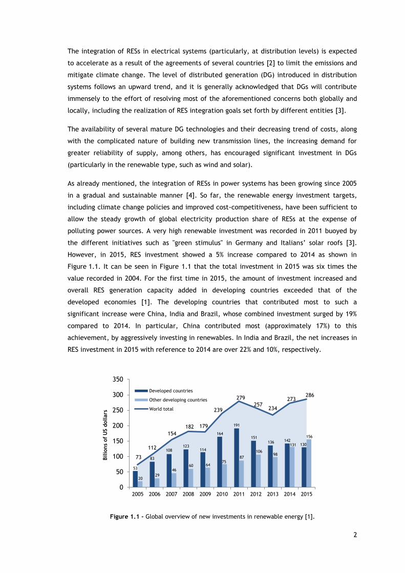
However, in 2015, RES investment showed a 5% increase compared to 2014 as shown in

Figure 1.1. It can be seen in Figure 1.1 that the total investment in 2015 was six times the

value recorded in 2004. For the first time in 2015, the amount of investment increased and

overall RES generation capacity added in developing countries exceeded that of the

developed economies [1]. The developing countries that contributed most to such a

significant increase were China, India and Brazil, whose combined investment surged by 19%

compared to 2014. In particular, China contributed most (approximately 17%) to this

achievement, by aggressively investing in renewables. In India and Brazil, the net increases in

RES investment in 2015 with reference to 2014 are over 22% and 10%, respectively.

Figure 1.1 - Global overview of new investments in renewable energy [1].

53

83

108 123

114

164

191

151 136 142

130

20 29

46 60 64

75 87

106 98

131

156

73

112

154

182 179

239

279

257 234

273 286

0

50

100

150

200

250

300

350

2005 2006 2007 2008 2009 2010 2011 2012 2013 2014 2015

Bilio

ns

of

US d

ollars

World total

Developed countries

Other developing countries

World total

3

The developing countries that contributed most to such a significant increase were China,

India and Brazil, whose combined investment surged by 19% compared to 2014. In particular,

China contributed most (approximately 17%) to this achievement, by aggressively investing in

renewables. In India and Brazil, the net increases in RES investment in 2015 with reference to

2014 are over 22% and 10%, respectively. Other countries that also made significant

investments in 2015 were South Africa (329% compared to 2014) as well as Mexico and Chile

whose investments in 2015 increased by 105% and 151% compared to 2014, respectively.

All together, they are the top 10 countries that have invested more in renewable energy in

2015 along with Morocco, Uruguay, the Philippines, Pakistan and Honduras. Investments can

be clearly seen in Figure 1.2, which shows the renewable investment trajectories by country

and/or region. In comparison, RES investments in Europe fell by 21%, despite the wind energy

financing record of 17 billion US dollars, an increase of 11%. In the United States, investments

increased by 19%, two thirds of which were in solar energy.

Among the several renewable energy types, the one that saw significant growth was the

large-scale hydro. However, excluding this one, it can be seen that from all renewable energy

sources, wind and solar were the ones that attracted the highest investments in 2015

(constituting 62 and 56 GW of new installed capacity, respectively), well above the 2014

values. In Figure 1.3, one can see the new investments in renewable energy by sector, and it

appears that, for the first time, investment in solar energy was higher than that of any other

renewable type (excluding large-scale hydro).

In 2015, although there was a new record, the generation capacity (Figure 1.4) added is far

from what would be desired to address the current global challenges, mentioned earlier.

The United Nations conference in Paris on climate change, known as COP21, generated an

unprecedented agreement among 195 countries to achieve zero emissions in the second half

of the century [2]. Thus, the large-scale integration of renewable energy sources (especially,

in distribution systems) will require significant investments in infrastructures.

Figure 1.2 – Global overview of investments in renewables by region [1].

4

Figure 1.3 – New investments in renewable energy by sector (in billions of US dollars) [5].

Figure 1.4 – Renewable power generation capacity as a share of global power [1].

However, large-scale integration of RES-based DGs often poses a number of technical

challenges in the system from the stability, reliability and power quality perspectives. This is

because integrating RESs introduces significant operational variability and uncertainty to the

distribution system, making operation, planning and control rather complicated.

Solar 2,4

Biofuels 0,5

Wind;0,4

Geothermal 0,01

Small Hydro 0,03 Biomass 0,07

Marine 0,03

19,5%

27,3%

41,7%

31,6%

39,8%

48,6%

40,2%

49,0% 53,6%

7,5% 8,2% 9,2% 10,2% 11,4% 12,7% 13,8%

15,2% 16,2%

5,2% 5,3% 5,9% 6,1% 6,9% 7,8% 8,5% 9,1% 10,3%

0,0%

10,0%

20,0%

30,0%

40,0%

50,0%

60,0%

2007 2008 2009 2010 2011 2012 2013 2014 2015

Renewable capacitychange as a % ofglobalcapacitychange (net)

Renewable power asa % of global powercapacity

renewable power asa % of global powergeneration

5

Hence, such a high-level integration effort is likely to be supported by certain smart-grid

technologies and concepts that have the capability to enhance the flexibility of the entire

distribution systems. Energy Storage Systems (ESSs) can play a vital role in integrating

variable energy sources. In addition, a dynamic Reconfiguration of Distribution Systems (RDS)

can be very important because it can considerably enhance the flexibility of the system and

voltage profiles, thereby increasing chances of accommodating large-scale RES power.

1.2 Research Motivation and Problem Definition

As demonstrated in the background, RESs make a crucial part of the solution for

environmental sustainability; hence, they will play an important role in power systems. The

integration of RESs should, in principle, reduce the risk of fuel price volatility and geopolitical

pressures and ensure that these do not pose a significant impact on the overall public

welfare. However, large-scale penetration of RESs will necessarily involve a process of

adapting and changing the existing infrastructure because of their intrinsic characteristics,

such as intermittency and variability.

The growing need for intermittent RESs, in conjunction with the electrical mix changes in the

long-term, will probably affect the distribution and transmission systems. In this context, a

change in power generation options, resulting from a high contribution of RESs, may require

network grid updates. Regulatory agencies are heavily committed to increasing RES

integration, not only due to environmental but also technical and economic reasons, as

explained in the previous section.

The main challenge with most RESs is their inherent variability and uncertainty, making

operation, control and planning very complicated. DG penetration increases the variation of

voltage and current in the network. Hence, increasing DG penetration may have a negative or

a positive impact depending on various factors such as the size of the system and the loads

type, requiring comprehensive modeling and simulations to assess its impact. If not properly

planned, this may lead to an uncertain increase in the feeders’ power flows, resulting in

network congestion and increased losses in the network. It is in this context that the first two

problems, addressed in this thesis, appear.

The integration of smart-grid enabling technologies has the capability to alleviate the

negative consequences of large-scale integration of DGs. In other words, in order to facilitate

(speed up) the much-needed transformation of conventional (passive) Distribution Network

Systems (DNSs) and support large-scale RES integration, different smart-grid enabling

technologies such as reactive power sources, advanced switching and storage devices are

expected to be massively deployed in the short-term.

6

The integration of Energy Storage Systems (ESSs) along with RESs has become one of the most

viable solutions to facilitate the increased penetration of DG resources. Energy storage

systems “level” the mismatch between renewable power generation and demand. This is

because these devices store energy during periods of low electricity demand (price) or high

RES power production, and then release it during periods of peak demand and low RES

production. Therefore, in addition to their technical support to the system, ESSs bring

substantial benefits for end-users and DG owners through reliability and power quality

improvement as well as cost reduction. Besides, ESSs are being developed and applied in

power grids to cope with a number of issues such as smoothing the energy output from RESs

and improving the stability of the electrical system. ESSs also increase savings during peak

hours and minimize the impact of intermittent generation sources, leading to a more efficient

management of the integrated system. Despite the high capital costs of many ESS

technologies, their deployment in distribution systems is in the upward trend. Cost-cutting

and the strong need of integrating RES-based DGs is expected to push the demand for the

simultaneous deployment of ESSs in distribution network systems. In other words, distributed

ESSs will increase dramatically in the years to come. Hence, proper planning of such systems

is crucial for a healthy operation of the system as a whole.

Electrical distribution systems are interconnected by switches but predominantly operated

radially. These switches are often used for emergency purposes such as to evade load

curtailment during fault cases. However, the system can be reconfigured to find the best

topology that minimizes power losses in the system and improve operational performance.

This in turn improves the flexibility in the system, which may help to accommodate (absorb)

more variable power. Investigating the capability of network switching and/or expansion

along with ESS deployment in RES integration level is another problem addressed in this

thesis. Generally, this thesis develops strategies, methods and tools that are very crucial to

guide such a complex decision-making process, i.e. maximizing the penetration level of RESs

in DNSs without jeopardizing the power quality, system stability and integrity.

1.3 Research Questions, Objectives and Contributions of the Thesis

This thesis presents a comprehensive analysis of DG investment planning decisions

(renewables in particular). New analysis tools and methods are developed in this thesis that

take into account the operational variability and uncertainty associated with the RES power

generation along with the integration of smart-grid enabling technologies. The ultimate aim

of all this is to enable existing systems to accommodate large-scale variable energy sources

(wind and solar type DGs in particular) while maintaining the power quality and system

stability at the required/standard levels at a minimum possible cost.

7

In particular, the following research questions are addressed:

What is the current status of RES penetration across the world (with a special focus

at distribution levels)? What are the main impeding factors for RES integration?

How can the potential benefits of RESs be reaped without significant negative

consequences?

What are the parameters of uncertainty and/or variability that most influence the

decision-making process in terms of investment solutions in DGs (especially,

renewables)?

How should different sources of uncertainty be modeled in the complex decision-

making problem concerning DG investment planning?

From a quantitative and qualitative point of view, what are the impacts of network

switching and/or reinforcement, as well as deployment of ESSs on the level of

renewable power integrated in the system?

How can the penetration of renewable energy sources in the power distribution

system be maximized with currently available technologies?

o What is the effect of reactive power support capability on the RES-based DG

integration level?

o What are the implications of integrating smart-grid enabling technologies in

the distribution systems with respect to maximizing RES integration,

reducing energy losses, costs and improving voltage profiles?

The main objectives of this thesis are:

To carry out a state-of-the-art review on the current status of RES penetration across

the world (with a particular focus at distribution levels), their economic aspects,

current integration challenges and future prospects, and other related issues.

To develop appropriate optimization models and methods for planning distribution

systems under uncertainty and large-scale penetration of variable energy sources.

To perform a comprehensive analysis with the aim of identifying the stochastic

parameters that most influence the decision-making process in terms of investment

solutions in DGs (especially, renewables).

To develop methods for handling the most significant sources of uncertainty in the

complex decision-making problem concerning DG investment planning.

8

To investigate the impacts of network switching and/or reinforcement, as well as

deployment of ESSs on the level of renewable power integrated in the system.

To develop mechanisms for maximizing the penetration level of variable energy

sources in the power distribution systems with the help of currently available

technologies.

To optimally deploy smart-grid enabling technologies in the distribution systems, and

investigate the implications in terms of RES-based integration level and overall

system performance.

The contributions of this thesis (all already published in prestigious venues) are summarized

as follows:

An overview on RESs and the underlying issues related to the RES theme such as

climate change and its mitigation, RES characteristics and technological aspects, the

most important economic aspects as well as the challenges and opportunities of

integrating RESs in power systems. This contribution is published in the form of a

Book Chapter in ELSEVIER [6].

The development of an improved multi-stage and multi-scenario DG investment

planning mathematical formulation that investigates the effect of uncertainty and

operational variability on DG investment solutions. This contribution is published in

the IEEE Transactions on Sustainable Energy [7].

The development of a two-period planning framework that combines both robust

short-term and strategic medium to long-term decisions in dynamic and stochastic DG

investment problems. This contribution is published in the IEEE Transactions on

Sustainable Energy [8].

The development of a multi-stage and stochastic model, which considers

simultaneous integration of ESSs and RES-based DGs as well as network

reconfiguration/reinforcement. This contribution is published in Applied Energy –

ELSEVIER [9].

The presentation of a novel approach which simultaneously considers the optimal

sizing, time and placement integration of smart-grid enabling technologies to support

a large-scale RES-based DG integration. A comprehensive analysis of considering RES

based DGs with and without reactive power support capabilities is also included.

This contribution is published in the IEEE Transactions on Sustainable Energy,

Part I [10] and Part II [11].

9

1.4 Methodology

The mathematical models developed in this thesis are based on well-established methods,

namely, mixed-integer linear programming (MILP), multi-objective optimization and

two-period stochastic programming. In order to achieve the main research objective, beyond

simulation models, this thesis develops methods and solution strategies to analyze the

expansion planning of DNSs under uncertainty, and a dramatically changing power generation

scheme over time.

The proposed optimization models and the solutions strategies are implemented in GAMS©

and solved in most cases using the CPLEX™ algorithm, mostly by invoking default parameters.

The clustering methodology is implemented in the MATLAB© programming environment, and

Visual Basic™ with Excel© used as an interface for this purpose.

1.5 Notation

The present thesis uses the notation commonly used in the scientific literature, harmonizing

the common aspects in all sections, wherever possible. However, whenever necessary, in

each section, a suitable notation may be used. The mathematical formulas will be identified

with reference to the subsection in which they appear and not in a sequential manner

throughout the thesis, restarting them whenever a new section or subsection is created.

Moreover, figures and tables will be identified with reference to the section in which they are

inserted and not in a sequential manner throughout the thesis.

Mathematical formulas are identified by parentheses (x.x.x) and called “Equation (x.x.x)” and

references are identified by square brackets [xx]. The acronyms used in this thesis are

structured under synthesis of names and technical information coming from both the

Portuguese or English languages, as accepted in the technical and scientific community.

1.6 Organization of the Thesis

The thesis comprises seven chapters which are organized as follows:

Chapter 1 is the introductory chapter of the thesis. First, the background of the thesis is

presented. Then, the research motivations and the problem definition are provided.

Subsequently, the research questions and contributions of this thesis are presented. Then, the

methodology used throughout the thesis is introduced, followed by the adopted notations.

Finally, the chapter concludes by outlining the structure of the thesis.

10

In Chapter 2, a comprehensive overview of RES is presented. First, RESs are framed in the

climate change perspective, followed by a renewable energy trend. Then, the green energy

production options are presented and the individual characterization in recent years of each

one is made jointly with the respective technologies. Subsequently, the most important

economic aspects on RESs to be considered when investing in this type of technology are

presented. Finally, the benefits and RES integration barriers as well the present/future

perspectives are discussed.

In Chapter 3, a DG investment planning model is formulated as a novel multi-stage and

multi-scenario optimization problem, in order to perform a comprehensive sensitivity analysis

and identify the uncertain parameters which significantly influence the decision-making in

distributed generation investments and quantify their degree of influence. A real–world

distribution network system is used to carry out the analysis.

Taking the findings of the analysis in Chapter 3 as input, a detailed model is developed to

guide the complex decisions-making process of DG investment planning in distribution system

in the face of uncertainty. This is presented in Chapter 4. The problem is formulated from a

coordinated system planning viewpoint, in which the net present value of costs rated to

losses, emission, operation and maintenance, as well as the cost of unserved energy are

simultaneously minimized. The formulation is anchored on a two-period planning horizon,

each having multiple stages. The operational variability and uncertainty introduced by

intermittent generation sources, electricity demand, emission prices, demand growth and

others are accounted for via probabilistic and stochastic methods, respectively. Metrics such

as cost of ignoring uncertainty and value of perfect information are used to clearly

demonstrate the benefits of the proposed stochastic model.

Chapter 5 presents a novel mechanism to quantify the impacts of network switching and/or

reinforcement as well as deployment of ESSs on the level of renewable power integrated in

the system. To carry out this analysis, a dynamic and multi-objective stochastic mixed integer

linear programming (S-MILP) model is developed, which jointly takes the optimal deployment

of RES-based DGs and ESSs into account in coordination with distribution network

reinforcement and/or reconfiguration.

A new multi-stage and stochastic mathematical model, developed to support the decision-

making process of planning distribution network systems (DNSs) for integrating large-scale

“clean” energy sources is presented in Chapter 6. Another aim of this chapter is to examine

the theoretical aspects and mathematical formulation in a comprehensive manner.

The proposed model is formulated from the system operator’s viewpoint, and determines the

optimal sizing, timing and placement of distributed energy technologies (particularly,

renewables) in coordination with some enabling technologies. Moreover, heuristic strategies

for reducing the combinatorial solution search space in relation to the optimal placement of

DGs, ESSs and reactive power sources are investigated.

11

Chapter 7 presents the main conclusions of this work. Guidelines for future works in these

fields of research are provided. Moreover, this chapter reports the scientific contributions

that resulted from this research work and that have been published in journals with high

impact factor (first quartile), as book chapters or in conference proceedings of high standard

(IEEE).

12

Chapter 2

Renewable Energy Systems: An Overview

This chapter aspires to provide an overview of RESs and the underlying issues related to the

RESs theme such as climate change and its mitigation. The types of RESs are also briefly

discussed focusing on their characteristics and technological aspects. This is followed by the

most important economic aspects as well as the challenges and opportunities of integrating

RESs in power systems. All this leads to an efficient exploitation of their wide-range benefits

while sufficiently minimizing their negative impacts. Finally, the chapter is summarized with

some concluding remarks.

2.1 Introduction

All societies need energy services to satisfy their needs (such as cooking, lighting, heating,

communications, etc.) and to support productive services. In order to secure sustainable

development, the delivery of energy services needs to be safe and cause low environmental

impacts [12]–[14].

Social sustainability and economic development require security and easy access to energy

resources, which are indispensable to promote sustainable energy and essential services.

This means applying different strategies at different levels to revamp economic development.

To be environmentally benign, energy services should provoke low environmental impacts,

including greenhouse gas (GHG) emissions.

According to the study in [3], fossil fuels are still the main primary energy sources. A major

revolution is required in how energy is produced and used in order to preserve a sustainable

economy capable of providing the required public services (both in developed and developing

countries), and laying effective support mechanisms to climate change mitigation and

adaptation efforts [15].

A major concern in both developed and developing countries, including emerging economies,

is that without having abundant and accessible energy sources, it is not possible to maintain

the current paradigm in the medium and long term, from an economic point of view.

In accordance with the International Energy Agency (IEA) reference scenario, the primary

global energy consumption will grow between 40% and 50% until 2030, at an annual average

rate of 1.6%. Without a major paradigm shift in energy policies throughout the world, fossil

fuels are still expected to cover about 83% of the increase in demand [3].

13

The reasons for this strong growth are essentially two: the continuous increase in world

population and the economic convergence between developed and developing countries,

especially with emerging economies such as India and China that are leading the economic

recovery from the recent global economic crisis, and becoming the major consumers of

non-renewable energy sources. This change must be answered with structural measures, such

as by putting a real monetary value to energy. Some of the promising solutions are

accelerating renewable energy integration, promoting energy efficiency and supporting

transport systems modernization. This can be achieved by promoting more transparent

markets to flourish and creating an enabling environment for competition in all sectors of the

economy and energy production [16].

The sustainability of energy systems is now an important factor for socio-economic

development. Sustainability depends on three major components (as schematically

demonstrated in Figure 2.1): i) the security of access to energy, ii) the accessibility of

services and iii) environmental compatibility. Changing the energy scenario presents itself as

a huge challenge whose solution ultimately depends on the political will of governing bodies

to make the necessary investments on a global scale. In the medium and long term horizon,

investment decisions will affect the cost and the environmental impacts of infrastructures.

Most likely, the energy supply will be the main factor of possible models for future

development at global, regional and national levels.

Figure 2.1 - Sustainability in the electricity sector [17].

14

2.2 Clime Change

GHG emissions associated with energy services are the major causes of climate change.

The report in [3] indicates that “most of the observed increase in global average temperature

since the mid-20th century is very likely due to the observed increase in anthropogenic

greenhouse gas concentrations”.

The carbon dioxide (CO2) concentrations have grown continuously to about 390 ppm of CO2 in

2010, a 39% increase since pre-industrial levels [18]. The global average temperature

increased by 0.76 ºC (from 0.57 °C to 0.95 °C) between 1850 and 1899. And, between 2001

and 2015, the warming trend has increased significantly. Note that forest abatement, fires,

and the release of non-CO2 gases from industry, trade and agriculture also contribute to

global warming [18]. Moreover, all indicators show that there will be a significant increase in

demand for primary energy during the twenty-first century [18].

The emission rates are also expected to substantially exceed the natural removal rates,

causing a continuous increase in GHG concentrations in the atmosphere, and consequently the

rise in average global temperature. The Cancun agreement [19] appeals to reduce GHG

emissions and limit the global average temperature rise below 2°C, taking the pre-industrial

value as a reference. It has recently been agreed on to a target level of 1.5°C in the average

temperature rise.

Historically, developed countries are the main contributors to global GHG emissions, and

continue to have the highest total history of per capita emissions [20]. In recent years, GHG

emissions in most developing countries have been increasing, currently covering more than

half of the total emissions. For instance, the total annual emissions in China surpassed that of

the USA in recent years [20].

However, the latest climate conference, COP-21 (UN climate conference) in Paris [21], brings

hope for the fight against climate change where, for the first time, representatives of almost

every country in the world convened together in an effort to reduce emissions and counter

the effects of global warming.

The Paris Agreement, which will take effect after 2020, underscores the fact that the

participation of all nations – not just rich countries – is crucial to combat climate change.

On the whole, 195 member countries of the UN Climate Convention and the European Union

have ratified the document [21].

The long-term goal of the agreement is to keep global warming "well below 2°C." This is the

point in which scientists argue that the planet is doomed to a future of no return, leading to

devastating effects such as rising sea levels, extreme weather events (droughts, storms and

floods), and lack of water and food.

15

2.3 Renewable Energy Trend

An increase in an overall world trend in the awareness of climate change and the need for

mitigation efforts is bringing forth huge increase in the deployment of renewable energy in

comparison to fossil fuel energy sources. The landmark that signals the dawning of this

renewable age goes hand in hand with the degree of advancement in technologies and a

higher degree of RES penetration, which is being achieved around the world. Furthermore,

there are several driving factors for these remarkable growths among which are favorable

government support policy and increasing competitiveness in costs. After several decades of

efforts in research and continuous development in RES, the yearly growth in the capacity of

these plants is becoming greater than the total investment capacity added in power plants

based on coal, natural gas and oil all combined together [22]. Nowadays, RESs have reached a

significant level of share in energy supply options, becoming one of the prominent global

alternative power supply sources. This trend will continue increasing at faster rates as long as

the world’s desire for industrial scale clean energy sources is on the higher side [3].

The latest global trends in renewable energy investment status reports indicate that,

renewables represented a 58.5% of net additions to global power capacity in 2014, with

significant growth in all regions, which represents an estimated 27.7% of the world’s power

generating capacity, enough to supply an estimated 22.8% of global electricity. Wind, solar

and biomass power generations reached an estimated 9.1% of the world’s electricity in 2014,

up from 8.5% in 2013. According to renewables status report [23], the overall cost-cutting

achieved to date helped to ensure such a strong momentum in 2014, reaching an investment

boom up to 29% in solar, and 11% in wind technologies, and geothermal managing to raise

23%. Further cuts in the cost of generation for both solar and wind look to be on the cards in

2015 [23]. The report on global renewable energy 2015 [23] also indicates the continued

growth of RES participation in parallel proportion with the energy consumption and the falling

oil prices. In addition, issues related to the untapped RES potentials indicate that it still

requires a growing effort in pursuing innovative approaches to increase its participation in

order to guarantee a clean energy future. Concerning the regional expansion of RES

utilization, such growth scheme is not limited to the industrialized regions, but also an

increasing number of developing countries are even becoming important manufacturers and

installers of this fashionable energy source.

Another essential growth trend currently being observed, which is worth mentioning here, is

the diversity of applications of the renewable sources. The use of renewables is no more

limited to the power generation only, but its use is expanding in heat related and

transpiration applications. In this regard, several supporting technologies like heat supply and

storage systems are helping flourish the deployment of these important energy resources

across many countries. Also, a significant contribution to the world transport sector is being

promoted with an increased share in the use of Ethanol and Biodiesel in combination with

fossil fuels.

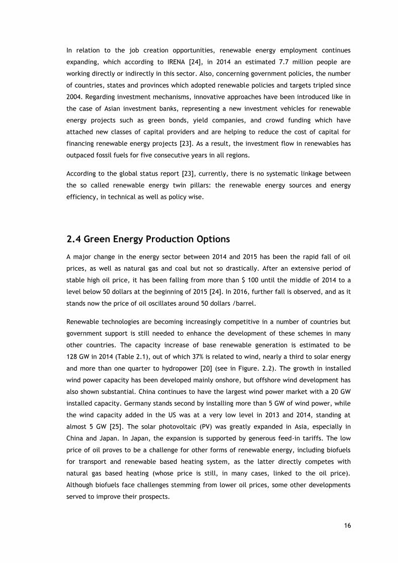
16

In relation to the job creation opportunities, renewable energy employment continues

expanding, which according to IRENA [24], in 2014 an estimated 7.7 million people are

working directly or indirectly in this sector. Also, concerning government policies, the number

of countries, states and provinces which adopted renewable policies and targets tripled since

2004. Regarding investment mechanisms, innovative approaches have been introduced like in

the case of Asian investment banks, representing a new investment vehicles for renewable

energy projects such as green bonds, yield companies, and crowd funding which have

attached new classes of capital providers and are helping to reduce the cost of capital for

financing renewable energy projects [23]. As a result, the investment flow in renewables has

outpaced fossil fuels for five consecutive years in all regions.

According to the global status report [23], currently, there is no systematic linkage between

the so called renewable energy twin pillars: the renewable energy sources and energy

efficiency, in technical as well as policy wise.

2.4 Green Energy Production Options

A major change in the energy sector between 2014 and 2015 has been the rapid fall of oil

prices, as well as natural gas and coal but not so drastically. After an extensive period of

stable high oil price, it has been falling from more than $ 100 until the middle of 2014 to a

level below 50 dollars at the beginning of 2015 [24]. In 2016, further fall is observed, and as it

stands now the price of oil oscillates around 50 dollars /barrel.

Renewable technologies are becoming increasingly competitive in a number of countries but

government support is still needed to enhance the development of these schemes in many

other countries. The capacity increase of base renewable generation is estimated to be

128 GW in 2014 (Table 2.1), out of which 37% is related to wind, nearly a third to solar energy

and more than one quarter to hydropower [20] (see in Figure. 2.2). The growth in installed

wind power capacity has been developed mainly onshore, but offshore wind development has

also shown substantial. China continues to have the largest wind power market with a 20 GW

installed capacity. Germany stands second by installing more than 5 GW of wind power, while

the wind capacity added in the US was at a very low level in 2013 and 2014, standing at

almost 5 GW [25]. The solar photovoltaic (PV) was greatly expanded in Asia, especially in

China and Japan. In Japan, the expansion is supported by generous feed-in tariffs. The low

price of oil proves to be a challenge for other forms of renewable energy, including biofuels

for transport and renewable based heating system, as the latter directly competes with

natural gas based heating (whose price is still, in many cases, linked to the oil price).

Although biofuels face challenges stemming from lower oil prices, some other developments

served to improve their prospects.

17

Table 2.1 - Renewable Electric Power Capacity (Top Regions/Countries in 2013) [20]

TECHNOLOGY WORLD

EU-28

BRICS CHINA UNITED STATES

GERMANY SPAIN ITALY INDIA

(GW) Wind Power 318 117 115 91 61 34 23 8.6 20

Solar Energy PV 139 80 21 19.9 12.1 36 5.6 17.6 2.2

Solar Energy CSP 3.4 2.3 0.1 ~0 0.9 ~0 2.3 ~0 0.1

Geothermal 12 1 0.1 ~0 3.4 ~0 0 0.9 0

Hydropower 1,000 124 437 260 78 5.6 17.1 18.3 44

Bioenergy 88 35 24 6.2 15.8 8.1 1 4 4.4

Ocean Power 0.5 0.2 ~0 ~0 ~0 0 ~0 0 0

Total Renewable

Power Capacity 560 235 162 118 93 78 32 31 27

a) b)

Figure 2.2 - a) Average Annual Growth Rates of Renewables (2008 – 2013); b) Global Electricity

Production (2013) [20].

For instance, to overcome the current dark prospects of biofuels in Brazil, the government

increased the ethanol rate of mixture from 25% to 27% and from 5% in biodiesel to 7%, and

increased gasoline taxes, while Argentina and Indonesia have increased their biofuels

mandates [20]. A long period of low oil prices could result in neglecting the promotion of

energy efficiency and instead returning to wasteful consumption. However, there is no

evidence to date that this has occurred [22].

2.4.1 Wind Energy

Wind power has been used for thousands of years in a variety of applications. Wind energy

can be transformed into mechanical energy or electricity. But wind power remained in the

background in detriment of other fuels for various technical, social and economic reasons. It

was the oil crisis in the 1970s, which led to a renewed interest in wind power technology

especially for electricity generation connected to the grid, to pump water and to provide

power in remote areas.

18

The technical potential of wind power to serve the energy needs is immense. Although wind

resource varies around the globe, there is enough potential in most regions to support high

levels of wind power generation. Wind resources are not a barrier to the global expansion of

this technology in the coming decades. New wind power technologies have contributed to

significant advances in wind power penetration. In a general perspective, the global wind

power capacity has been increasing [26], smoothly from 2000 to 2006, and in a more

accentuated way from 2007 to 2013 as shown in Figure 2.3. More than 51 GW of wind power

were added to the power systems, representing a 44% increase compared to 2013, making an

overall contribution of approximately 370 GW to the energy production mix, as shown in

Table 2.2. The top 10 countries accounted for 84% of the installed capacity in the world at

the end of 2013, but there are dynamic and emerging markets in most regions [20].

Table 2.2 - Wind Power Global Capacity and Additions [20]

COUNTRY TOTAL END 2012 ADDED 2013 TOTAL END 2013

(GW) (GW) (GW)

China 60.8/75.3 14.1/16.1 75.5/91.4

United States 60.0 1.1 61.1

Germany 31.3 3.2/3.6 34.3/34.7

Spain 22.8 0.2 23

India 18.4 1.7 20.2

United Kingdom 8.6 1.9 10.5

Italy 8.1 0.4 8.6

France 7.6 0.6 8.3

Canada 6.3 1.6 7.8

Denmark 4.2 0.7 4.8

Rest of World 41 7 48

World Total 283 35 318

Figure 2.3 - Wind power total world capacity (2000-2013) [26] .

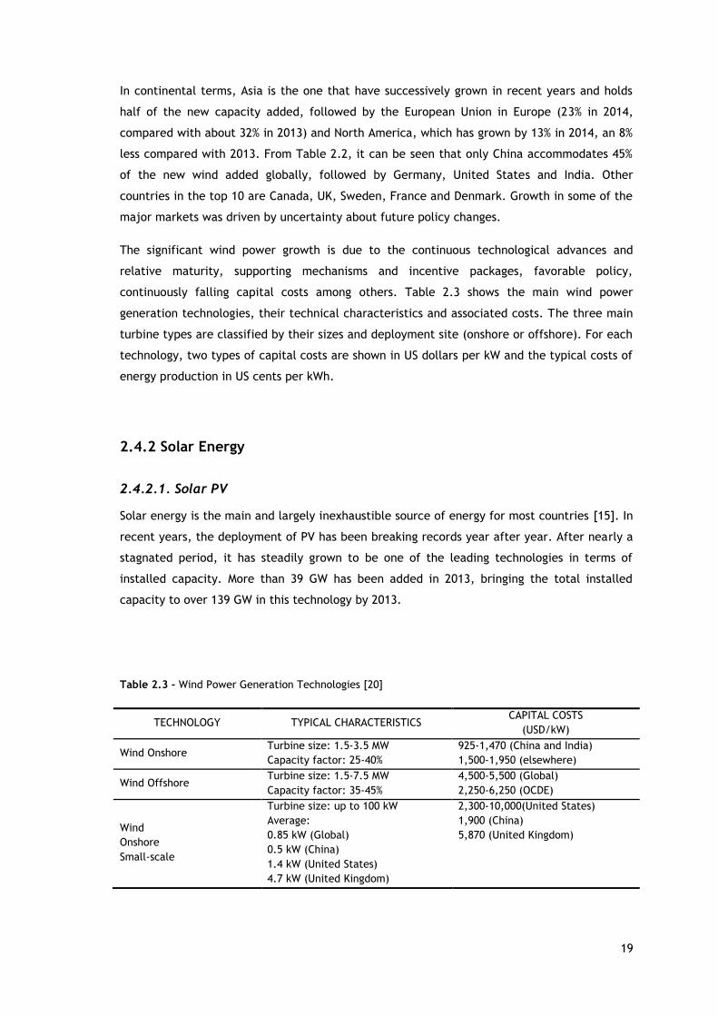
19

In continental terms, Asia is the one that have successively grown in recent years and holds

half of the new capacity added, followed by the European Union in Europe (23% in 2014,

compared with about 32% in 2013) and North America, which has grown by 13% in 2014, an 8%

less compared with 2013. From Table 2.2, it can be seen that only China accommodates 45%

of the new wind added globally, followed by Germany, United States and India. Other

countries in the top 10 are Canada, UK, Sweden, France and Denmark. Growth in some of the

major markets was driven by uncertainty about future policy changes.

The significant wind power growth is due to the continuous technological advances and

relative maturity, supporting mechanisms and incentive packages, favorable policy,

continuously falling capital costs among others. Table 2.3 shows the main wind power

generation technologies, their technical characteristics and associated costs. The three main

turbine types are classified by their sizes and deployment site (onshore or offshore). For each

technology, two types of capital costs are shown in US dollars per kW and the typical costs of

energy production in US cents per kWh.

2.4.2 Solar Energy

2.4.2.1. Solar PV

Solar energy is the main and largely inexhaustible source of energy for most countries [15]. In

recent years, the deployment of PV has been breaking records year after year. After nearly a

stagnated period, it has steadily grown to be one of the leading technologies in terms of

installed capacity. More than 39 GW has been added in 2013, bringing the total installed

capacity to over 139 GW in this technology by 2013.

Table 2.3 - Wind Power Generation Technologies [20]

TECHNOLOGY TYPICAL CHARACTERISTICS CAPITAL COSTS

(USD/kW)

Wind Onshore Turbine size: 1.5-3.5 MW

Capacity factor: 25-40%

925-1,470 (China and India)

1,500-1,950 (elsewhere)

Wind Offshore Turbine size: 1.5-7.5 MW


4,500-5,500 (Global)

2,250-6,250 (OCDE)

Wind

Onshore

Small-scale

Turbine size: up to 100 kW

Average:

0.85 kW (Global)

0.5 kW (China)

1.4 kW (United States)

4.7 kW (United Kingdom)

2,300-10,000(United States)

1,900 (China)

5,870 (United Kingdom)

20

There has been a geographical shift of the biggest installers, led by China, Japan and the

United States, and Asia is becoming the largest solar PV market worldwide instead of Europe.

China have witnessed higher growth than Europe, and other promising markets such as the US

and others have experienced an extremely slow growth [16].

In 2013, nine countries added more than 1.0 GW of solar PV to their networks, and new

facilities continue to appear as can be seen in Table 2.4. At the end of 2013, at least 10 GW

of total capacity was added in five countries instead of two in 2012. The leaders of solar

energy per capita were Germany, Italy, Greece, Czech Republic and Australia [20].

Asia added 22.7 GW at the end of 2013, bringing the total amount of solar PV in operation to

almost 42 GW. China had almost a one third share of the global installed capacity.

Apart from Asia, about 16.7 GW were added around the world, mainly in the EU (about

10.4 GW) and North America (5.4 GW) in which the United States led became the third largest

market in 2013.

The Solar PV technologies can be divided into two main types depending on where they are

placed, rooftop or ground-mounted. Each has a set of characteristics. However, it can be said

that there are three transverse characteristics of both types of technologies: the peak

capacity, the capacity factor and the conversion efficiency (as depicted in Table 2.5).

These technologies are also distinguished based on where/how they are being deployed:

residential, commercial and industrial consumer in particular with respect to peak capacity.

Note that the receptivity of each type of technology varies greatly from one geographical

area to another mainly due to the differences in energy cost of each of these areas, and often

the incentives/compensation for the adherence to these technologies [15].

2.4.2.2. Solar CSP

The concentrated solar power (CSP) is a market that is so far small but it is growing mainly

thanks to the increased efficiency levels in places with direct sunlight and low humidity.

This technology continues to spread to new markets with significant projects already

completed in late 2013 in Australia, Italy and the United States and progress in Chile,

Namibia, Portugal, Saudi Arabia, among others [20].

The biggest market is China with 50 MW. More than 165 MW were added in systems operating

in over 20 countries led by China and the United States, as can be seen in Table 2.6.

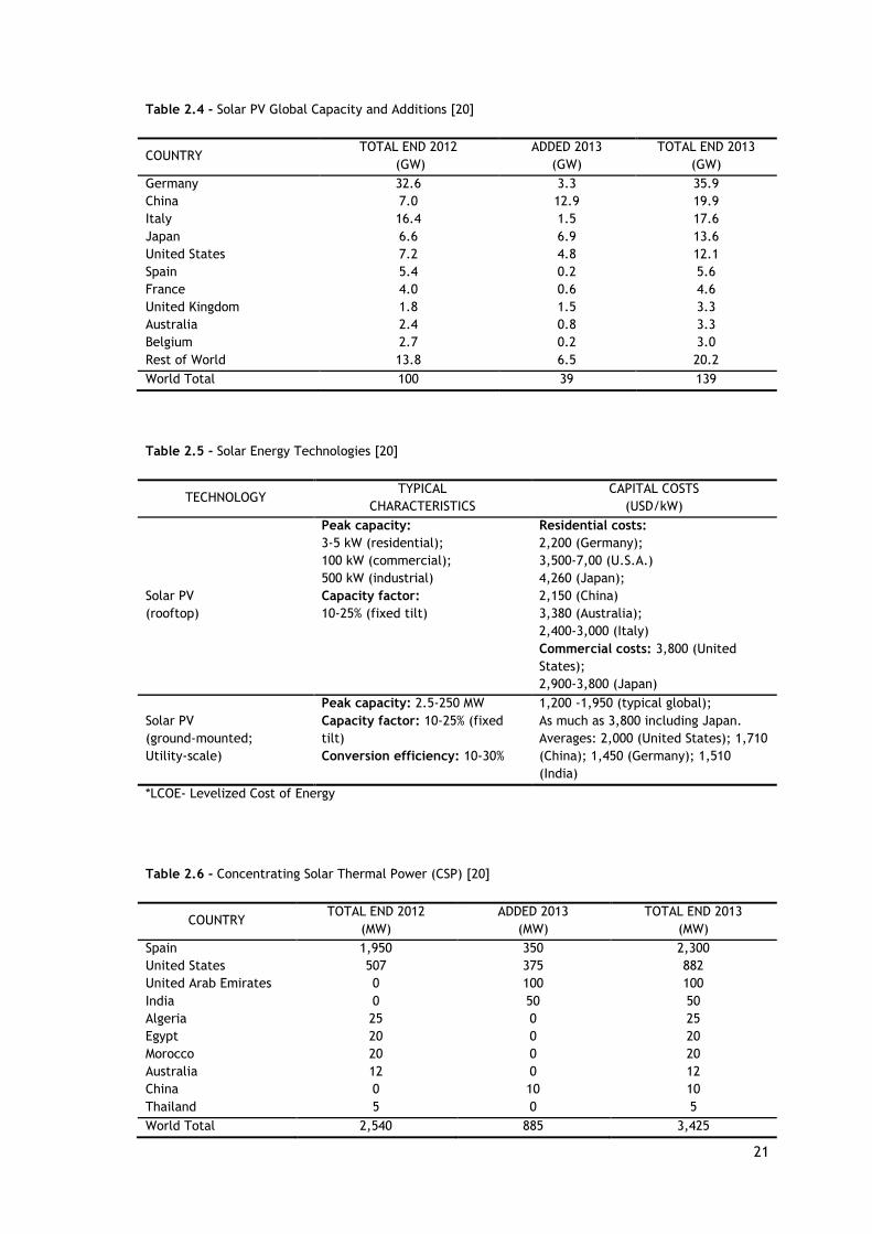
21

Table 2.4 - Solar PV Global Capacity and Additions [20]

COUNTRY TOTAL END 2012

(GW)

ADDED 2013

(GW)

TOTAL END 2013

(GW)

Germany 32.6 3.3 35.9

China 7.0 12.9 19.9

Italy 16.4 1.5 17.6

Japan 6.6 6.9 13.6

United States 7.2 4.8 12.1

Spain 5.4 0.2 5.6

France 4.0 0.6 4.6

United Kingdom 1.8 1.5 3.3

Australia 2.4 0.8 3.3

Belgium 2.7 0.2 3.0

Rest of World 13.8 6.5 20.2

World Total 100 39 139

Table 2.5 - Solar Energy Technologies [20]

TECHNOLOGY TYPICAL

CHARACTERISTICS

CAPITAL COSTS

(USD/kW)

Solar PV

(rooftop)

Peak capacity:

3-5 kW (residential);

100 kW (commercial);

500 kW (industrial)

Capacity factor:

10-25% (fixed tilt)

Residential costs:

2,200 (Germany);

3,500-7,00 (U.S.A.)

4,260 (Japan);

2,150 (China)

3,380 (Australia);

2,400-3,000 (Italy)

Commercial costs: 3,800 (United

States);

2,900-3,800 (Japan)

Solar PV

(ground-mounted;

Utility-scale)

Peak capacity: 2.5-250 MW

Capacity factor: 10-25% (fixed

tilt)

Conversion efficiency: 10-30%

1,200 -1,950 (typical global);

As much as 3,800 including Japan.

Averages: 2,000 (United States); 1,710

(China); 1,450 (Germany); 1,510

(India)

*LCOE- Levelized Cost of Energy

Table 2.6 - Concentrating Solar Thermal Power (CSP) [20]

COUNTRY TOTAL END 2012

(MW)

ADDED 2013

(MW)

TOTAL END 2013

(MW)

Spain 1,950 350 2,300

United States 507 375 882

United Arab Emirates 0 100 100

India 0 50 50

Algeria 25 0 25

Egypt 20 0 20

Morocco 20 0 20

Australia 12 0 12

China 0 10 10

Thailand 5 0 5

World Total 2,540 885 3,425

22

The solar thermal power market continues to grow after the record in 2012. In 2013, the

overall capacity grew by 36%, more than 3.4 GW, with Spain and the United States being the

major markets [15].

A summary of the main CSP technologies can be found in Table 2.7, which shows the main

characteristics as well as the cost of these technologies by country or area. In the typical

characteristics, the main types of CSP, the size of the plants and the capacity factor are

shown.

2.4.3 Geothermal Energy

Geothermal energy can be used efficiently in the development of networks whether they are

connected or not, and is especially useful in rural electrification schemes and direct

applications such as district heating, cooking, bathing and industrial processes, etc. [17].

Geothermal resources provide energy in electrical form and heating/ direct cooling. Global

electricity generation from geothermal sources is estimated to be just under half of the total

geothermal production of 76 TWh, with the remaining 91 TWh accounting for direct use [17].

From Table 2.8, it can be seen that, in 2013, the estimated generation capacity added was at

least 530 MW, bringing the total global capacity to 12 GW, with an estimated annual

generation of 76 TWh [20].

The countries that added more production capacity in 2013 were New Zealand, Turkey, the

United States, Kenya, Mexico, Philippines, Germany, Italy and Australia. By the end of 2013,

the countries with the largest installed generation capacity were the United States with

3.4 GW, the Philippines with 1.9 GW, Indonesia with 1.3 GW, Mexico with 1.0 GW, Italy with

0.9 GW, New Zealand with 0.9 GW, Iceland with 0.7 GW and Japan with 0.5 GW.

Table 2.7 - Solar CSP Energy Technologies [20]


(USD/kW)

Concentrating solar

thermal power

(CSP)

Types: parabolic, trough, tower,

dis

Plant size:

50-250 MW (trough);

20-250 MW (tower);

10-100 MW (Fresnel)

Capacity factor:

20-40% (so storage);

35-75% (with storage)

Trough, no storage:

4,000-7,300 (OCDE)

3,100-4,050 (not OCDE)

Trough, 6 hours storage:

7,100-9,800

Tower: 5,600 (United States without

storage)

9,000 (United States with storage)

*LCOE- Levelized Cost of Energy

23

This resource can be classified into two categories [27]:

High temperature (T> 150°C): This resource is usually associated with areas of

volcanic activity, seismic or magma. At these temperatures, it is possible to use the

geothermal resource for power generation purpose;

Low temperature (T <100°C) generally results from the meteoric rise of water

circulation in faults and fractures as well as resident water inside porous rocks at

deep underground.

The geothermal energy conversion process involves energy transfer by convection,

transforming the heat produced and contained inside the earth into a useful energy in the

form of electricity or other forms. The energy can also be extracted using the water injection

technology from the surface in hot rock formations. Table 2.9 summarizes some general

characteristics of geothermal technologies.

Table 2.8 - Geothermal Power Global Capacity and Additions [20]

NET ADDED 2013 TOTAL END 2013

Top Countries by Total Capacity (MW) (MW)

United States 507 375

Philippines 0 100

Indonesia 0 50

Mexico 25 0

New Zealand 20 0

Top Countries by New Additions MW MW

New Zealand 196 0.9

Turkey 112 0.3

United States 84 3.4

Kenya 36 0.2

Philippines 20 1.9

Mexico 10 1.0

World Total 465 12

Table 2.9 - Geothermal Power Technology [20]


(USD/kW)

Geothermal Power

Plant size: 1-100 MW


Condensing flash: 1,900-

3800

Binary: 2,250 - 2,200

24

2.4.4 Hydro Energy

The production of hydroelectricity is mainly through hydroelectric plants, which are

associated with large or medium capacity dams, forming a reservoir of water by interrupting

the flow of water. Also, this energy has been exploited by applying the so-called small hydro

plants, which consist of the construction of small reservoirs or dams that divert part of rivers

for an unleveled location (where the turbines are installed), thereby producing electricity.

The production of hydroelectricity is the most efficient and one of the least polluting

processes. Many of the effects are reversible, and nature with the human contribution,

ultimately find a new balance.

The capacity of global hydropower production in 2013 increased by 4% (approximately

40 GW), which varies every year according to the metrological conditions of the places where

they are located, was estimated at 3,750 TWh in 2013.

The countries with the highest production capacity are China (260 GW/ 905 TWh), Brazil

(85.7 GW/ 415 TWh), the US (78.4 GW/ 269 TWh), Canada (76.2 GW/ 388 TWh), Russia

(46.7 GW/ 174.7 TWh), India and Norway, which together have 62% of global installed

capacity [3].

It is estimated that a pumped storage capacity in the order of 2 GW was added in 2013,

bringing the global hydropower to 135-140 GW. The country that installed more hydropower

capacity in 2013 was China. Other countries with significant installed hydropower capacity

were Turkey, Brazil, Vietnam, India and Russia as can be seen in Table 2.10.

Table 2.10 - Hydro Power Global Capacity and Additions [20]

NET ADDED 2013 TOTAL END 2013

Top Countries by Total Capacity (GW) (GW)

China 28.7 260

Brazil 1.5 86

United States 0.2 78

Canada 0.5 76

Russia 0.7 47

India 0.8 44

Top Countries by New Additions GW GW

China 28.7 260

Turkey 2.9 22

Brazil 1.5 86

Vietnam 1.3 14

India 0.8 44

Russia 0.7 47

World Total 40 1,000

25

Hydropower is the most developed technology among the renewables, reaching levels of

optimality when coupled with the wind. The summary of the main technological

characteristics can be found in Table 2.11, including the typical technology cost for each

type. It can be emphasized that, among the presented technologies, it is the one that has the

lowest typical cost.

2.4.5 Bioenergy

Bioenergy is the designation for the energy obtained from biomass. There are three forms of

fundamental energy: heat energy, mechanical energy and electricity, all of which can be

obtained from biomass sources.

The systems that produce mechanical energy as combustion engines or turbines of direct and

indirect combustion are coupled to electrical generators, which convert mechanical energy

into electrical energy. The conversion of mechanical energy to electrical energy generates

heat approximately two-third to one-third of the generated electricity, which demonstrates

the increased economic efficiency of cogeneration (simultaneous production of heat and

electricity) in stationary applications. The biogas from landfills, recycling of agricultural

wastes and other organic wastes can be used in stationary power plants for energy production

[28].

Bioenergy has shown steady growth rates in the last years and it is expected to keep on this

path in the future. In EU, the consumption of biomass energy is projected to increase by at

least 33 Mtoe by 2020, as shown in Figure 2.4. The electricity generation in the EU from solid

biomass in 2014 was approximately 81.6 TWh. The five top producers were the US followed by

Germany, Finland, United Kingdom, Sweden and Poland having a total production in Europe of

63% [29].

Table 2.11 – Hydro Power Technologies [20]


(USD/kW)

Hydropower

(grid-based)

Plant size: 1 MW -18,000 MW

Plant type:

reservoir, run-of-river


Projects > 300 MW: 1,000-

2,250

Projects 20-300 MW: 750-

2,500

Projects < 20 MW: 750-

4,000

Hydropower

(off-grid/rural)

Plant size:0.1-1,000 kW

Plant type: run-of-river,

hydrokinetic, diurnal storage

1,175-6,000

26

Figure 2.4 - Final energy consumption for Bioenergy in EU [30].

The estimated growth of bioenergy market in 2014 was 5 GW, bringing the total capacity

worldwide to approximately 93 GW. Country wise, the bio-generation leaders are the United

States with 69.1 TWh, Germany with 49.1 TWh, China with 41.6 TWh, Brazil with 32.9 TWh

and Japan with 30.2 TWh.

2.4.6 Ocean Energy

Ocean power refers to any energy harnessed from the ocean waves, tidal range (up and

down), tidal currents, ocean currents, temperature gradients and salinity gradients [31]. The

development of this emerging sector can contribute to the achievement set targets for

renewable energy integration, reduction of GHGs and their harmful effects, and

simultaneously boost economic growth through innovation and new job creation [32].

At the end of 2013, the capacity of the ocean energy was about 530 MW, most of this coming

from the tidal power category [3]. Majority of ocean power projects currently in operation

generate power from ocean tides. Among these is the Sihwa plant in Korea, completed in

2011 with a capacity of 254 MW, the central Rance in France with a capacity of 240 MW, the

central Annapolis Nova Scotia, Canada with a capacity of 3.9 MW and Jiangxia in China with

the capacity of 3.9 MW. Other projects are smaller, and many of them are pre-commercial

demonstration projects with a remarkable concentration of wave and tidal development

facilities (in the order of 11 MW) in the UK [20]. Some of the tidal technology characteristics

are summarized in Table 2.12.

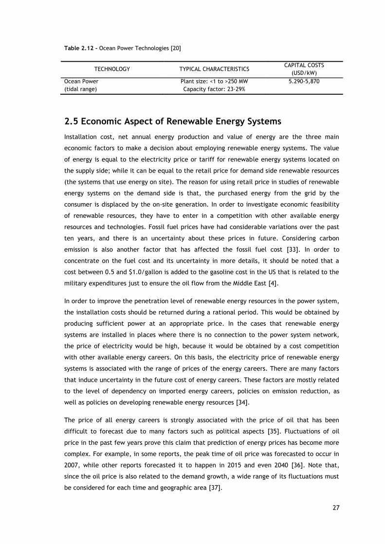
27

Table 2.12 - Ocean Power Technologies [20]


(USD/kW)

Ocean Power

(tidal range)

Plant size: <1 to >250 MW


5.290-5,870

2.5 Economic Aspect of Renewable Energy Systems

Installation cost, net annual energy production and value of energy are the three main

economic factors to make a decision about employing renewable energy systems. The value

of energy is equal to the electricity price or tariff for renewable energy systems located on

the supply side; while it can be equal to the retail price for demand side renewable resources

(the systems that use energy on site). The reason for using retail price in studies of renewable

energy systems on the demand side is that, the purchased energy from the grid by the

consumer is displaced by the on-site generation. In order to investigate economic feasibility

of renewable resources, they have to enter in a competition with other available energy

resources and technologies. Fossil fuel prices have had considerable variations over the past

ten years, and there is an uncertainty about these prices in future. Considering carbon

emission is also another factor that has affected the fossil fuel cost [33]. In order to

concentrate on the fuel cost and its uncertainty in more details, it should be noted that a

cost between 0.5 and $1.0/gallon is added to the gasoline cost in the US that is related to the

military expenditures just to ensure the oil flow from the Middle East [4].

In order to improve the penetration level of renewable energy resources in the power system,

the installation costs should be returned during a rational period. This would be obtained by

producing sufficient power at an appropriate price. In the cases that renewable energy

systems are installed in places where there is no connection to the power system network,

the price of electricity would be high, because it would be obtained by a cost competition

with other available energy careers. On this basis, the electricity price of renewable energy

systems is associated with the range of prices of the energy careers. There are many factors

that induce uncertainty in the future cost of energy careers. These factors are mostly related

to the level of dependency on imported energy careers, policies on emission reduction, as

well as policies on developing renewable energy resources [34].

The price of all energy careers is strongly associated with the price of oil that has been

difficult to forecast due to many factors such as political aspects [35]. Fluctuations of oil

price in the past few years prove this claim that prediction of energy prices has become more

complex. For example, in some reports, the peak time of oil price was forecasted to occur in

2007, while other reports forecasted it to happen in 2015 and even 2040 [36]. Note that,

since the oil price is also related to the demand growth, a wide range of its fluctuations must

be considered for each time and geographic area [37].

28

It should be noted that, energy economics is highly dependent on incentive- and penalty-

driven policies. On this basis, it is very difficult to impose life cycle costs without considering

the impacts of emission and government supports that motivate investors for investing in

renewable energy systems [38]. According to the aforementioned description, the regulatory

supports for renewable energy systems have been driving the world market.

2.5.1 Driving Factors

Many factors affect investments in renewable energies systems. Incentives are a key element

in choosing the renewable systems, since both type and size of renewable energy systems are

determined by investors based on the differences between market incentives. Another

affecting factor is the cost of land that has an important impact on type and number of

renewable energy systems. In order to have the optimal rate of return, renewable energy

systems should have the highest amount of availability to ensure they can produce an

appropriate level of energy. On this basis, they should have the capability to be operated as

much time as possible. To this end, the reliability of the network and consequently the

unavailability to transfer generated power due to network failures should be estimated.

It should be noted that, if the renewable energy system generates when the demand peak

occurs, the income of the system is augmented due to the increase in energy price. Owners of

on-site renewable resources can also benefit more when the generated energy by the systems

is required by the on-site demand. For example, the wind power generator produces

electricity at nights when the space heating systems are highly required during winter.

Renewable energy systems are able to generate power to supply the on-site demand, or to

inject to the grid. The amount of energy that is consumed by on-site demand is replaced with

the supplied energy by the grid. On this basis, if the amount of generation is less than the on-

site demand, using renewable energy systems can reduce the net load. On the contrary, if the

on-site consumption is less than the generated energy, the surplus is injected into the grid at

a price/tariff based on an agreement with the utility.

Externalities are also an important factor for making a decision about renewable energy

resources. This is due to the fact that in life-cycle cost analysis emission and carbon dioxide

costs should be considered [39], [40]. There is a wide range of rates of externalities that

depends on the rules and regulations in various countries. Since power producers do not like

paying the cost of externalities, in the US there are litigations by all sides to decrease the

externality rates based on the reason that there is no reliable evidence to prove carbon

dioxide emission is harmful to society. In European countries, there are various costs for

carbon dioxide emission that provide a better base for renewable energy resources by making

them more cost competitive [40].

29

2.5.2 Life-Cycle Costs

The life-cycle cost is a method that analyzes the total cost of the system by considering the

expenditures during the system life and salvage value [25]. By using a life-cycle cost analysis

different investment options can be compared. Moreover, the most economic design for the

system can be achieved. There are some other options that the renewable energy systems

must compete with such as small-scale diesel generators and electrical energy storage

systems. In this case, the effective factors are the initial cost, the electricity price, and the

required infrastructures [41], [42]. It is noteworthy that, the life-cycle cost is also useful to

compare different plans even if the renewable energy system is the only choice. Furthermore,

this analysis is employed to determine if a hybrid renewable-based system can be the most

economic plan. The life-cycle cost analysis enables to investigate impacts of employing

several components with various reliability and lifetimes.

Discount rate indicates how much increase or decrease in finance happens over the time.

Note that, using the inaccurate amount of discount rate for calculating life-cycle cost can

cause to unrealistic solutions. Although most of the renewable energy systems are

economical, in order to select the best plan between all available options, the life-cycle cost

analysis is the best method [41], [42]. The financial assessment can be carried out over an

annual base to calculate economic indices such as payback period and cash flow.

It should be mentioned that, annualized cost of energy considered for renewable energy

systems should be compared with that for other resources. In other words, the annualized

cost of energy should not be directly compared with the current cost of energy, since it is not

sensible. The mentioned costs of energy create an appropriate base to compare different

plans considering alternative resources and to select the best resource of energy.

There are some calculating tools to analyze renewable energy projects and assess the

life-cycle cost, and even emission considerations [43]. These calculations prove that the

current renewable energy systems are economical.

2.5.3 Economic Trend of Renewable Energy Systems

Renewable energy systems are strongly promoted by policy makers, because they are a key

element for economic development. The renewable systems are able to compete with current

thermal power plants [35]. They can also improve the economy by job creation, since more

than 100 jobs for installing a wind power plant and more than 10 jobs for its operation are

required for each 100 MW project [4]. There are some attempts to reduce the property tax of

wind power plants in order to better motivate the investor to invest in the renewable system

and consequently the economic development [44].

30

Wind power generation is one of the most economic renewable energy systems, since its cost

of energy (COE) is about $70/MWh that can compete with thermal units. Trend studies have

shown that before 2003, COE of wind power plants was higher than fuel fossil units; however,

in the period of 2003 to 2009, it approximately equaled to the thermal units [4]. In 2009, the

COE of wind farms dropped to the levels lower than conventional power.

The studies on various resources indicate that annualized COE of wind power plants can even

compete with the one of combined cycle gas turbines, although the fuel price of these

thermal units is low [45]. In some countries, such as the US, conventional power plants

benefit from that the fuel costs are not taxed, whereas the renewable energy systems do not

have the cost of fuel at all. On this basis, the main issue of renewable resources is the high

investment cost, which causes people to prefer paying for the fuels. It should be noted that,

in the case of on-site renewable energy systems, the small-scale wind power generation

cannot compete with the retail prices [46].

In the case of supply side, another barrier to integration of renewable energy systems is the

capacity of transmission network that may cause the power curtailment in order to ensure the

system security [47]. Since most of the renewable energies such as wind, solar and

geothermal resources are far from the load centers, they can impose an extra cost on the

transmission system [48].

Although the future of energy is uncertain and ambiguous, and every prediction can be risky,

as oil price forecast has been a challenge, the trend of renewable energies is almost evident

[37]. On this basis it can be expected that in future distributed renewable energy systems will

have more penetration and even some new distributed electricity markets will help these new

resources [46].

In addition, with developments of the high-voltage transmission network, large farms of

renewable energy systems will be installed much far from the load centers [47]. In near

future, renewable energy resources can better compete with other energy alternatives just

due to the carbon cost. Even other air emission costs such as NOX and SOX will motivate

people to invest in systems without fuel and emission costs. This can cause that renewable

energies, particularly wind power, become the most economic resource of producing

electricity [41], [42].

It should be noted that one part of the installation cost of renewable energy systems has been

supplied by the income resulted from carbon trading. The future of energy without renewable

energy system developments would be an unsolvable problem due to the growth of

environmental concerns. In order to avoid this problem and to provide a sustainable energy,

policy makers should put more weight on the renewable energy as well as conservation and

energy efficiency.

31

2.6 Benefits and Barriers of RESs

2.6.1 RES Integration Opportunities

Most of the electric energy consumed come from non-renewable energy sources (mainly,

fossil fuels). This has led to a series of questions from energy dependence concerns to climate

change issues, which are some of the major drivers of RES integrations in many power systems

across the world. It is now widely recognized that integrating RESs in power systems brings

about a lot of economic, environmental, societal and technical benefits to all stakeholders.

These are some of the reasons behind the rapid growth of RES integrations in many power

systems across the world, as indicated in a 2015 report by the International Energy Agency

(IEA). The report further shows that, in 2013, an approximately 19.1% of global electric

energy consumption came from RESs, most of which was from hydropower [3].

Among the wide-range benefits of RESs is their significant contribution to the GHGs which are

leading to not only climate change and its dire consequences but also series environmental

and health problems. Most RES technologies (wind and solar PV, for instance) have very low

carbon footprints, making them very suitable to mitigate climate change and reduce its

consequences. Hence, integrating RESs in power systems partly replaces polluting

(conventional) power generation sources, resulting in a “cleaner” energy mix i.e. one with

lower emission levels.

RES integration also has an undisputable positive impact on the social and economic

development of nations. It is widely understood that the three socio-economic indicators, per

capita income, per capita energy use and economic growth, are highly correlated with each

other. Economic growth can be considered, for instance, as the main driver for energy

consumption. Therefore, RESs can spur economic growth and create job opportunities.

Because of their distributed nature, RES integration can also be integrated into a national

policy (especially, in developing countries) to foster rural development. Currently, the RES

business currently employs an estimated 7.7 million people throughout the world [3]. RESs

also play a crucial role in energy access. Currently, more than 1.2 billion people do not have

access to electricity globally (85% of which are in rural areas where RESs are abundant) [3].

Exploiting the potential of RESs should be at the forefront to address this societal problem.

Energy security concern is also one of the main drivers of RES integration. Current electric

energy production scheme is dominated by conventional generation sources, which use fossil

fuels whose prices are subject to significant volatilities. In addition to these volatilities,

geopolitical availability of fossil fuels is also becoming a concern for many countries. The

combination of all these can have significant impacts on the energy supply security. Because

of this, generation of electricity locally using RESs can significantly contribute to the energy

security of nations. As a result, this can reduce the heavy dependence on fossil fuels for

power generation.

32

In addition to the benefits briefly explained above, RESs can bring technical benefits such as

improved system stability and voltage profiles, reduced losses and electricity prices, etc. The

combination of conventional generation capacity with the renewable generation capacity will

be able to address the continuous increase in demand, in opposition to the scenario of

conventional generation capacity only, which according to forecasts would not be able to

meet the demand, Figure 2.5.

2.6.2 RES Integration Challenges and Barriers

Despite the robust growth of integration RES in many power systems, there are still certain

challenges and barriers that impede the smooth integration of RESs. These challenges and

barriers can be broadly classified into two categories: technical and non-technical. The non-

technical category includes challenges and barriers related to capital costs, market and

economic issues, information and public awareness, socio-cultural matters, the conflict

between stakeholders, regulation and policy.

The variable cost of energy production by RESs is very small (close to zero); however, they

are generally capital intensive. Even if the capital costs are declining for most RES

technologies, their levelized costs of electricity (LCOE) are yet to be competitive with that of

conventional energy sources. This can make investing in RESs less attractive for potential

investors. However, this is likely to change as RES costs continue to fall while that of

conventional energy sources become more expensive amid resource depletion and policies to

internalize external costs such as environmental pollution costs.

Market and economic barriers exist when there is a lack of clearly designed economic and

financial instruments to support RES integration efforts. For instance, whenever there is

market failure associated with internalizing the cost of environmental pollution, it is very

difficult to expect a lot of investments coming in from RES developers.

Figure 2.5 - Development and future trend of generation capacity, demand and wholesale electricity

market price in Central Europe from 2010 [49].

33

Information gap and lack of public awareness on RESs and their benefits can also significantly

hinder RES integration. Moreover, socio-cultural issues such as conflicting land use

requirements can sometimes lead to contentious issues regarding RES development, directly

affecting the level of penetration. The conflict between stakeholders is another barrier, more

specifically the lack of communication, as shown in Figure 2.6. The challenges and barriers

related to the regulatory and policy issues emanate from the structure of energy industries

and existing technical regulations, the level of support for technology transfer and R&D, etc.

Technical limitations (barriers), on the other hand, are related to the nature of the resources

and the power systems. Some of the most common RESs depend on primary energy sources

such as wind speed, solar radiation and wave, which are subject to high level variability and

unpredictability (the latter also known as uncertainty), resulting in considerable grid

integration challenges [51]. This is because the uncontrollable variability and uncertainty of

such sources introduce a lot of technical problems in the system, making the real-time

operation of the system very challenging. The intermittent nature of power production from

these resources also dramatically affects the reliability of energy supply. Moreover, such

sources are found geographically dispersed across a vast area, and their availability is

site-specific. Unlike conventional power sources, these energy sources cannot be transported

to areas close to demand centers. This means harnessing these resources requires the higher

need for network investments than conventional ones.

Figure 2.6 - Main reasons in the EU 27 for issue “Lack of communication” [50].

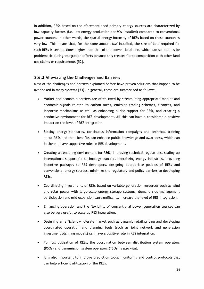
34

In addition, RESs based on the aforementioned primary energy sources are characterized by

low capacity factors (i.e. low energy production per MW installed) compared to conventional

power sources. In other words, the spatial energy intensity of RESs based on these sources is

very low. This means that, for the same amount MW installed, the size of land required for

such RESs is several times higher than that of the conventional one, which can sometimes be

problematic during integration efforts because this creates fierce competition with other land

use claims or requirements [52].

2.6.3 Alleviating the Challenges and Barriers

Most of the challenges and barriers explained before have proven solutions that happen to be

overlooked in many systems [53]. In general, these are summarized as follows:

Market and economic barriers are often fixed by streamlining appropriate market and

economic signals related to carbon taxes, emission trading schemes, finances, and

incentive mechanisms as well as enhancing public support for R&D, and creating a

conducive environment for RES development. All this can have a considerable positive

impact on the level of RES integration.

Setting energy standards, continuous information campaigns and technical training

about RESs and their benefits can enhance public knowledge and awareness, which can

in the end have supportive roles in RES development.

Creating an enabling environment for R&D, improving technical regulations, scaling up

international support for technology transfer, liberalizing energy industries, providing

incentive packages to RES developers, designing appropriate policies of RESs and

conventional energy sources, minimize the regulatory and policy barriers to developing

RESs.

Coordinating investments of RESs based on variable generation resources such as wind

and solar power with large-scale energy storage systems, demand side management

participation and grid expansion can significantly increase the level of RES integration.

Enhancing operation and the flexibility of conventional power generation sources can

also be very useful to scale up RES integration.

Designing an efficient wholesale market such as dynamic retail pricing and developing

coordinated operation and planning tools (such as joint network and generation

investment planning models) can have a positive role in RES integration.

For full utilization of RESs, the coordination between distribution system operators

(DSOs) and transmission system operators (TSOs) is also vital.

It is also important to improve prediction tools, monitoring and control protocols that

can help efficient utilization of the RESs.

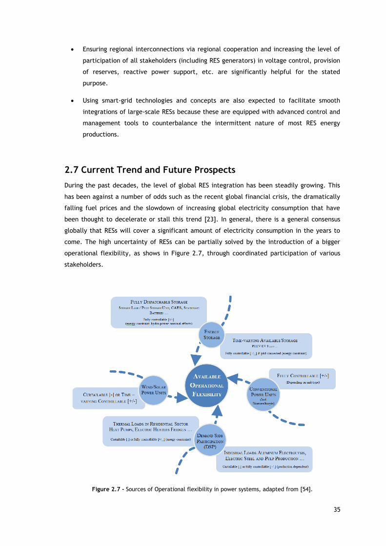
35

Ensuring regional interconnections via regional cooperation and increasing the level of

participation of all stakeholders (including RES generators) in voltage control, provision

of reserves, reactive power support, etc. are significantly helpful for the stated

purpose.

Using smart-grid technologies and concepts are also expected to facilitate smooth

integrations of large-scale RESs because these are equipped with advanced control and

management tools to counterbalance the intermittent nature of most RES energy

productions.

2.7 Current Trend and Future Prospects

During the past decades, the level of global RES integration has been steadily growing. This

has been against a number of odds such as the recent global financial crisis, the dramatically

falling fuel prices and the slowdown of increasing global electricity consumption that have

been thought to decelerate or stall this trend [23]. In general, there is a general consensus

globally that RESs will cover a significant amount of electricity consumption in the years to

come. The high uncertainty of RESs can be partially solved by the introduction of a bigger

operational flexibility, as shows in Figure 2.7, through coordinated participation of various

stakeholders.

Figure 2.7 - Sources of Operational flexibility in power systems, adapted from [54].

36

The recent developments in the 2015 Paris climate conference (COP-21), overall trends in

international policy on RESs, energy dependence concerns, the falling capital costs of several

matured RES technologies, and other techno-economic factors are all favorably expected to

further accelerate the level RES integrated into power systems.

2.8 Chapter Conclusions

The potential of RESs is huge because in principle they can meet several times the world’s

demand. RESs such as wind, biomass, hydro, biomass and geothermal can provide sustainable

energy services based on available resources in all parts of the world. The transition to

renewable energy based power systems tends to increase, while their costs continuously

decline as gas and oil prices continue to oscillate. In the last half century, the demand for

wind and solar systems has been continuously increasing, experiencing a reduction in capital

costs and generated electricity costs. There have been continuous performance improvement

and R&D undergoing in the sector in the past decades. As a result, the prices of renewable

energy and fossil fuels, as well as social and environmental costs are to diverge in opposite

directions. Economic and political mechanisms must support the wide spread of sustainable

markets for the rapid development of RES. At this point, it is clear that the present and

future growth will occur mainly in renewable energy and in some natural gas-based systems,

and not common sources like coal or oil. The progress of RESs can increase diversity in the

electricity markets, contributing to obtain long-term sustainable energy, helping reduce local

and global GHG emissions and promote attractive trade options to meet specific energy

needs, particularly in developing countries and rural areas, helping to create new

opportunities.

37

Chapter 3

Impact of Operational Variability and Uncertainty on

Distributed Generation Investment Planning: A

Comprehensive Sensitivity Analysis

This chapter presents a DG investment planning model formulated as a novel multi-stage and

multi-scenario optimization problem, in order to perform a comprehensive sensitivity

analysis and identify the uncertain parameters which significantly influence the decision-

making in distributed generation investments and quantify their degree of influence.

3.1 Introduction

Driven by techno-economic and environmental factors, nowadays, there is a global drive to

integrate more distributed energy resources (DERs) in power systems, particularly at the

distribution level. These typically include DG, storage technologies, and demand side

management [55]. Especially, the scale of DG sources (mainly, renewables such as wind and

solar) integrated in many distribution networks is steadily increasing. This trend is more likely

to continue in the years to come due to the advent of emerging solutions such as active

management of distribution networks [56], [57], which are expected to alleviate existing

technical limitations, and facilitate smooth integration of DGs. The favorable agreement of

countries in the recent climate change conference in Paris (COP21) is also expected to

accelerate the integration of RESs. As a result, the level of electricity demand covered by

energy coming from RESs is expected to dramatically increase, and such energy sources will

play a significant role in distribution systems.

As a result, the issue of DG investment planning (DGIP) is becoming critical. This is especially

more relevant in the case of insular network systems because new regulations are put in

place to reduce the heavy dependence of such systems on fossil fuels for energy production.

Tapping available energy resources (wind, solar, hydro, etc.) is inevitable to meet not only

the increasing demand for electricity, but also environmental constraints and renewable

energy source (RES) integration targets set forth either globally or locally through

Government initiatives.

However, the intermittent nature of most of these RESs (particularly, wind and solar) makes

their integration in distribution networks a more challenging task. This is because such

resources introduce significant operational variability and uncertainty to the system. Hence,

the development of efficient methods and tools is mandatory to realize an optimal or a

cost-efficient integration of such DGs and minimize their side effects.

38

In addition, the increasing level of DG integration in distribution systems is already leading to

substantial changes in the traditional role of distribution systems, which has predominantly

been to carry power unidirectionally from substations to consumers in a radial scheme.

In other words, distribution network systems are slowly evolving from passive to active

networks [56]. This paradigm shift will make sure that they are adequately equipped with the

necessary, flexible and intelligent tools which have the capability to minimize the underlining

challenges of integrating DERs in such network systems, and, hence, pave the way to high

level integration of DERs, RES-based DGs in particular. The advent of modern-day

technological advances (such as smart grid technologies with state-of-the-art control and

protection mechanisms) combined with conventional power system management systems

(such as active and reactive power management tools) will make active networks effectively

materialize [58].

Generally, the broad-range transformations in distribution networks are largely expected to

effectively address current limitations of integrating DERs. As a result, the highly needed

benefits of DERs, extensively discussed in [55] and [59], will be optimally exploited. In this

regard, previous works on investment planning of DGs in distribution systems such as [60],

[61] highlight the multi-faceted benefits of DGIP. In particular, the work in [61] demonstrate

that “investment in DG is an attractive distribution planning option for adding flexibility to an

expansion plan, mainly by deferring network reinforcements”. Other wide-range benefits of

DGs have been extensively discussed in [62]–[66] . As mentioned earlier, the integration of DG

in distribution systems comes with certain challenges [67]–[69]. For example, if DGs are not

properly planned and operated, they can pose considerable technical problems such as

reduced voltage quality and stability. However, these are expected to be adequately

mitigated in active distribution networks [61].

From a modeling perspective, DGIP has been carried out in previous works jointly with

distribution network expansion planning [70]–[76] or independently [60], [61], [77], [78].

Either way, the decision variables encompass the type of DG, its capacity and location as well

as the time of investment when a dynamic planning scheme is adopted as in [60], [70], [71],

[74]–[78]. In the context of micro-grid or autonomous/insular systems, the prospects of DG

planning, scheduling and operation have been gaining attention. Authors in [79] present a

community-based long-term planning tool for RESs in insular systems with an ultimate

objective of maximizing social welfare perceived by the community. The work in [80]

proposes a methodology for siting and sizing of DGs from a micro-grid context, and the

resulting problem is solved using the prospects of particle swarm optimization and genetic

algorithm methods.

Due to the inherent uncertainty and variability, stochastic programming has been used in

operation and planning of distribution systems [81]–[85]. Authors in [81] propose a stochastic

model for a bidding strategy in the day-ahead market of microgrids in the presence of energy

storage systems, RES-based and conventional DGs.

39

A stochastic energy management of microgrids, consisting of conventional and RES-based DGs

as well as price-sensitive loads, is proposed in [82]. Similarly, the work in [83] presents a

stochastic operation model to coordinate vehicle-to-grid services with energy trading in the

presence of conventional and wind type DGs. Reference [84] develops a stochastic DGIP

model based on a mixed integer linear programming (MILP) framework. Uncertainties related

to energy price, electricity demand, wind and solar PV power outputs are accounted by

forming and dividing the corresponding duration curves.

A DG allocation problem in radial distribution networks is solved using genetic algorithm in

[86]. Here, uncertainty due to forecasting errors in load and generation is modeled using a

fuzzy approach. A dynamic expansion planning of distribution systems with DGs is proposed in

[87], and a relatively new meta-heuristic algorithm is employed to solve the resulting

problem. Uncertainty and operational variability are not accounted for in this work. The use

of non-exact methods such as the meta-heuristic solution methods used in [80], [86], [87] do

neither guarantee global optimality nor a measure to the global optimal solution. Since DG

includes intermittent energy sources, the planning model should adequately take into account

the uncertainty and variability introduced as a result, including that of electricity demand.

In this respect, variability in load [60], [61], [70], [71], [74]–[77], [86] and [88], electricity

prices [60], [61], [70], [71], [77], wind power output [71], [77], [79], [86], solar power output

[77], [79], [86], fuel prices [77], demand growth [60], [61], and DG failures [72] are among

several sources of uncertainties which have been given some attention in distribution

planning works in the literature. The compound effect of all these relevant uncertainty and

variability issues requires designing new methods and tools in order to have an optimal or a

cost-efficient integration of DGs. To guide the development of such methods and tools, it is

necessary to investigate first the impact of variability and/or uncertainty of different model

parameters on DG investment decisions, which is the main objective of this chapter.

In this chapter, a comprehensive sensitivity analysis is carried out to meet the

aforementioned objective is presented. The ultimate goal is to identify those parameters

which influence the decision-making process and quantify their degree of influence.

To perform the analyses, a DGIP model, formulated as a multi-stage and multi-scenario

optimization problem, is used. In addition, to ensure tractability and make use of exact

solution methods, the entire problem is formulated as a mixed integer linear programming

(MILP) optimization. The resulting DGIP problem minimizes the net present value of

investment, operation and maintenance, unserved energy and emission costs taking into

account a number of technical and economic constraints. Note that the problem here is

formulated from the distribution system operator’s (DSO) point of view and with a particular

focus on insular networks. In such networks, where there does not often exist a functional

market, in addition to managing the network system, the DSO may own and operate some

utility-based DGs, and/or oversee DG investments to keep reliability, stability and power

quality in the system at the required levels.

40

The remainder of this chapter is organized as follows: Section 3.2 presents the terminologies;

and, the approaches for management of uncertainty and operational variability including

their definitions are also briefly described in this section. Subsequently, in Section 3.3, the

mathematical formulation and description of the DGIP model are presented. Section 3.4

discusses the results of case studies. Finally, relevant conclusions are drawn in Section 3.5.

3.2 Uncertainty and Variability in DGIP

3.2.1 Terminology

The terminologies uncertainty and variability are often incorrectly used interchangeably in

the literature despite the fact that they are different [89]. Variability, as defined in [90]

refers to the natural variation in time of a specific uncertain parameter, whereas uncertainty

refers to “the degree of precision with which the parameter is measured” or predicted. We

follow these terminologies in the thesis when referring to operational variability and

uncertainty, which are introduced by model parameters. For example, wind power output is

characterized by both phenomena; its hourly variation corresponds to the variability while its

partial unpredictability (i.e. the error introduced in predicting the wind power output) is

related to uncertainty.

The schematic illustration in Figure 3.1 clearly distinguishes both terminologies.

As demonstrated in this figure, the hourly differences in wind power outputs are due to the

natural variability of primary energy source (wind speed); whereas, the likelihood of having

different power outputs at a given hour is a result of uncertainty (partial unpredictability) in

the wind speed. Other terminologies used in this thesis are snapshot and scenario. A snapshot

refers to an hourly operational situation. Alternatively, it can be understood as a demand—

generation pattern at a given hour. A scenario, on the other hand, denotes the evolution of

an uncertain parameter over a given time horizon (often yearly). For example, the hourly

variations of wind power production and electricity consumption collectively form a group of

snapshots; whereas, the annual demand growth (which is subject to uncertainty) and RES

power output uncertainty are represented by a number of possible storylines (scenarios) [89].

Operational snapshots (hours)

Win

d p

ow

er o

utp

ut

Uncertainty

Variability

Scenario 1

Scenario s

Snapshot in scenario s

Snapshot in scenario 1

Figure 3.1 - Illustration of variability and uncertainty in wind power output.

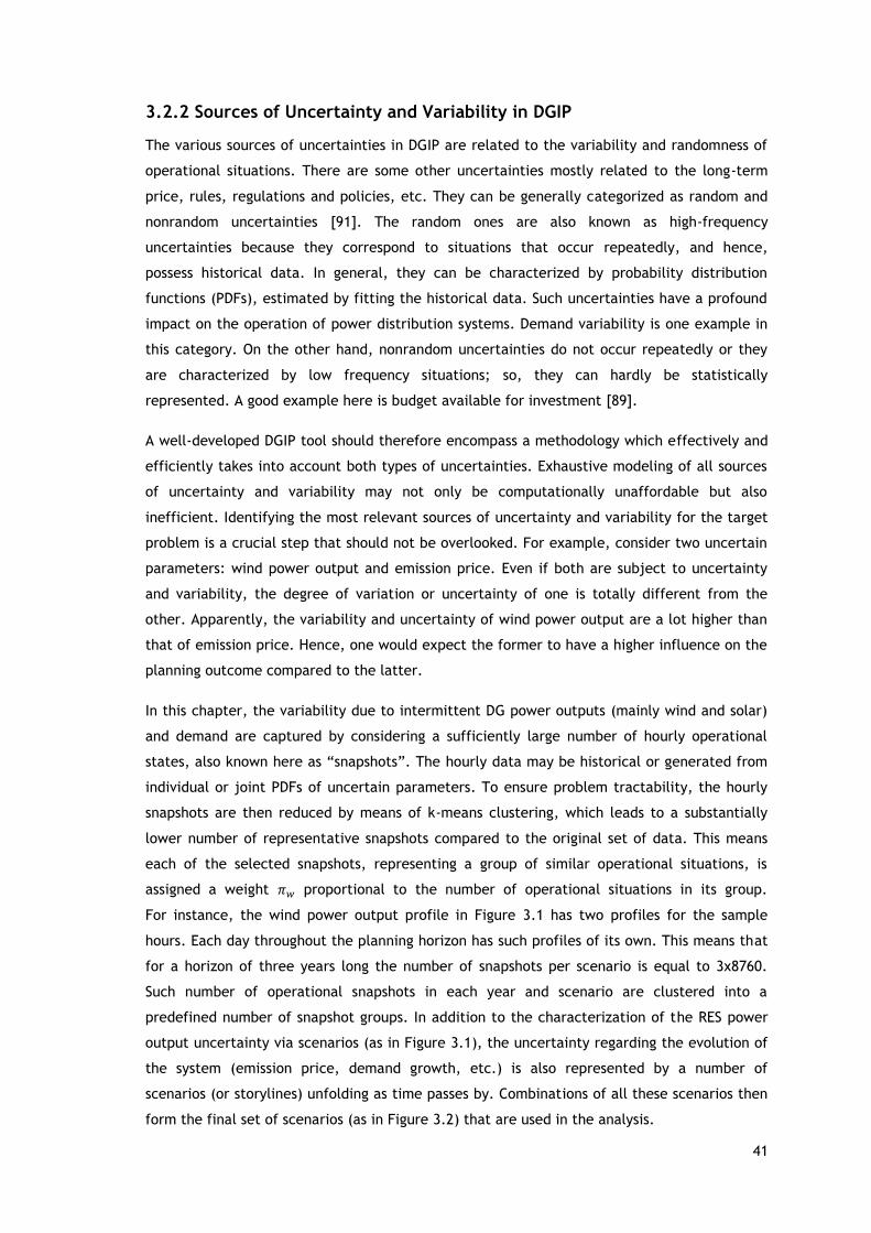
41

3.2.2 Sources of Uncertainty and Variability in DGIP

The various sources of uncertainties in DGIP are related to the variability and randomness of

operational situations. There are some other uncertainties mostly related to the long-term

price, rules, regulations and policies, etc. They can be generally categorized as random and

nonrandom uncertainties [91]. The random ones are also known as high-frequency

uncertainties because they correspond to situations that occur repeatedly, and hence,

possess historical data. In general, they can be characterized by probability distribution

functions (PDFs), estimated by fitting the historical data. Such uncertainties have a profound

impact on the operation of power distribution systems. Demand variability is one example in

this category. On the other hand, nonrandom uncertainties do not occur repeatedly or they

are characterized by low frequency situations; so, they can hardly be statistically

represented. A good example here is budget available for investment [89].

A well-developed DGIP tool should therefore encompass a methodology which effectively and

efficiently takes into account both types of uncertainties. Exhaustive modeling of all sources

of uncertainty and variability may not only be computationally unaffordable but also

inefficient. Identifying the most relevant sources of uncertainty and variability for the target

problem is a crucial step that should not be overlooked. For example, consider two uncertain

parameters: wind power output and emission price. Even if both are subject to uncertainty

and variability, the degree of variation or uncertainty of one is totally different from the

other. Apparently, the variability and uncertainty of wind power output are a lot higher than

that of emission price. Hence, one would expect the former to have a higher influence on the

planning outcome compared to the latter.

In this chapter, the variability due to intermittent DG power outputs (mainly wind and solar)

and demand are captured by considering a sufficiently large number of hourly operational

states, also known here as “snapshots”. The hourly data may be historical or generated from

individual or joint PDFs of uncertain parameters. To ensure problem tractability, the hourly

snapshots are then reduced by means of k-means clustering, which leads to a substantially

lower number of representative snapshots compared to the original set of data. This means

each of the selected snapshots, representing a group of similar operational situations, is

assigned a weight 𝜋𝑤 proportional to the number of operational situations in its group.

For instance, the wind power output profile in Figure 3.1 has two profiles for the sample

hours. Each day throughout the planning horizon has such profiles of its own. This means that

for a horizon of three years long the number of snapshots per scenario is equal to 3x8760.

Such number of operational snapshots in each year and scenario are clustered into a

predefined number of snapshot groups. In addition to the characterization of the RES power

output uncertainty via scenarios (as in Figure 3.1), the uncertainty regarding the evolution of

the system (emission price, demand growth, etc.) is also represented by a number of

scenarios (or storylines) unfolding as time passes by. Combinations of all these scenarios then

form the final set of scenarios (as in Figure 3.2) that are used in the analysis.

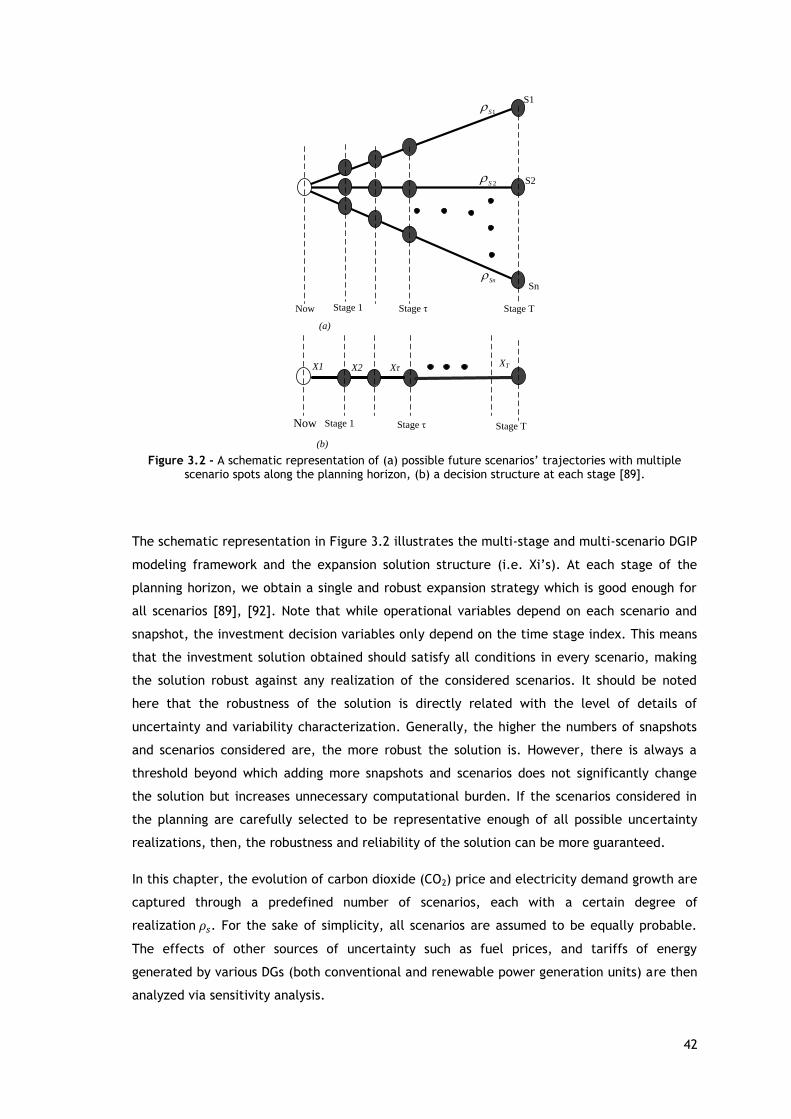
42

S1

S2

Sn

Now Stage τ Stage T

(a)

1S

2S

Sn

Stage 1

Now Stage τ

X1

(b)

X2 Xτ

Stage 1

XT

Stage T

Figure 3.2 - A schematic representation of (a) possible future scenarios’ trajectories with multiple

scenario spots along the planning horizon, (b) a decision structure at each stage [89].

The schematic representation in Figure 3.2 illustrates the multi-stage and multi-scenario DGIP

modeling framework and the expansion solution structure (i.e. Xi’s). At each stage of the

planning horizon, we obtain a single and robust expansion strategy which is good enough for

all scenarios [89], [92]. Note that while operational variables depend on each scenario and

snapshot, the investment decision variables only depend on the time stage index. This means

that the investment solution obtained should satisfy all conditions in every scenario, making

the solution robust against any realization of the considered scenarios. It should be noted

here that the robustness of the solution is directly related with the level of details of

uncertainty and variability characterization. Generally, the higher the numbers of snapshots

and scenarios considered are, the more robust the solution is. However, there is always a

threshold beyond which adding more snapshots and scenarios does not significantly change

the solution but increases unnecessary computational burden. If the scenarios considered in

the planning are carefully selected to be representative enough of all possible uncertainty

realizations, then, the robustness and reliability of the solution can be more guaranteed.

In this chapter, the evolution of carbon dioxide (CO2) price and electricity demand growth are

captured through a predefined number of scenarios, each with a certain degree of

realization 𝜌𝑠. For the sake of simplicity, all scenarios are assumed to be equally probable.

The effects of other sources of uncertainty such as fuel prices, and tariffs of energy

generated by various DGs (both conventional and renewable power generation units) are then

analyzed via sensitivity analysis.

43

3.3 Mathematical Model

3.3.1 Brief Description of the problem

This chapter focuses on investigating how sensitive DG investment decisions are with respect

to variations of selected uncertain parameters. This is relevant for identifying the parameters

with the highest influence on DG investment so as to design a DGIP model by adequately

factoring the variability and the uncertainty of the most relevant parameters. Eventually, this

helps to ensure an optimal integration of DG in network systems.

A DGIP problem is naturally dynamic because the solution has to explicitly provide the

necessary information regarding when DG investments are needed. Regarding the planning

horizon and decision stages, accounting for the dynamic nature of the problem, a more

realistic approach would be to formulate the problem with multiple decision stages (i.e.

multi-year decision framework) while accounting for all possible future scenarios. However,

to ensure tractability, the numbers of stages and scenarios are usually limited.

In this chapter, the DGIP problem is formulated as a multi-stage and multi-scenario

optimization model within a given planning window (horizon). This modeling framework

assumes that there are n probable future storylines (or scenarios) each associated with a

probability of realization 𝜌𝑠 that stochastically represents relevant sources of uncertainties.

3.3.2 Objective Function

The resulting DGIP model, a MILP optimization problem, minimizes the sum of net present

value (NPV) of four cost terms as in (3.1). Here, the binary investment and utilization

variables as well as the operational variables such as generated power, flows, etc. constitute

the set of decision variables of the optimization.

The first term in (3.1), 𝑇𝐼𝐶, represents the total NPV of the investment costs of DG,

constituting conventional and various renewable energy sources, under the assumption of a

perpetual planning horizon [93]. In other words, “the investment cost is amortized in annual

installments throughout the lifetime of the installed DG”, as is done in [71]. The second term

𝑇𝑂𝑀𝑅𝐶 corresponds to the total sum of NPV: (i) operation, maintenance and reliability (OMR)

costs throughout the planning stages, and (ii) the OMR costs incurred after the last planning

stage. Note that the costs in (ii) rely on the OMR costs of the last planning stage and a

perpetual planning horizon is assumed when spreading these costs after the last planning

stage. To further clarify this, consider the illustrative example in Figure 3.3. It is understood

that investments are made in a specific year within the planning horizon (the second year in

this case) and the investment costs are amortized throughout its lifetime. However, the OMR

costs are incurred every year within and after the planning horizon. To balance these cost

terms, a perpetual planning horizon, i.e. an endless payment of fixed payments is assumed.

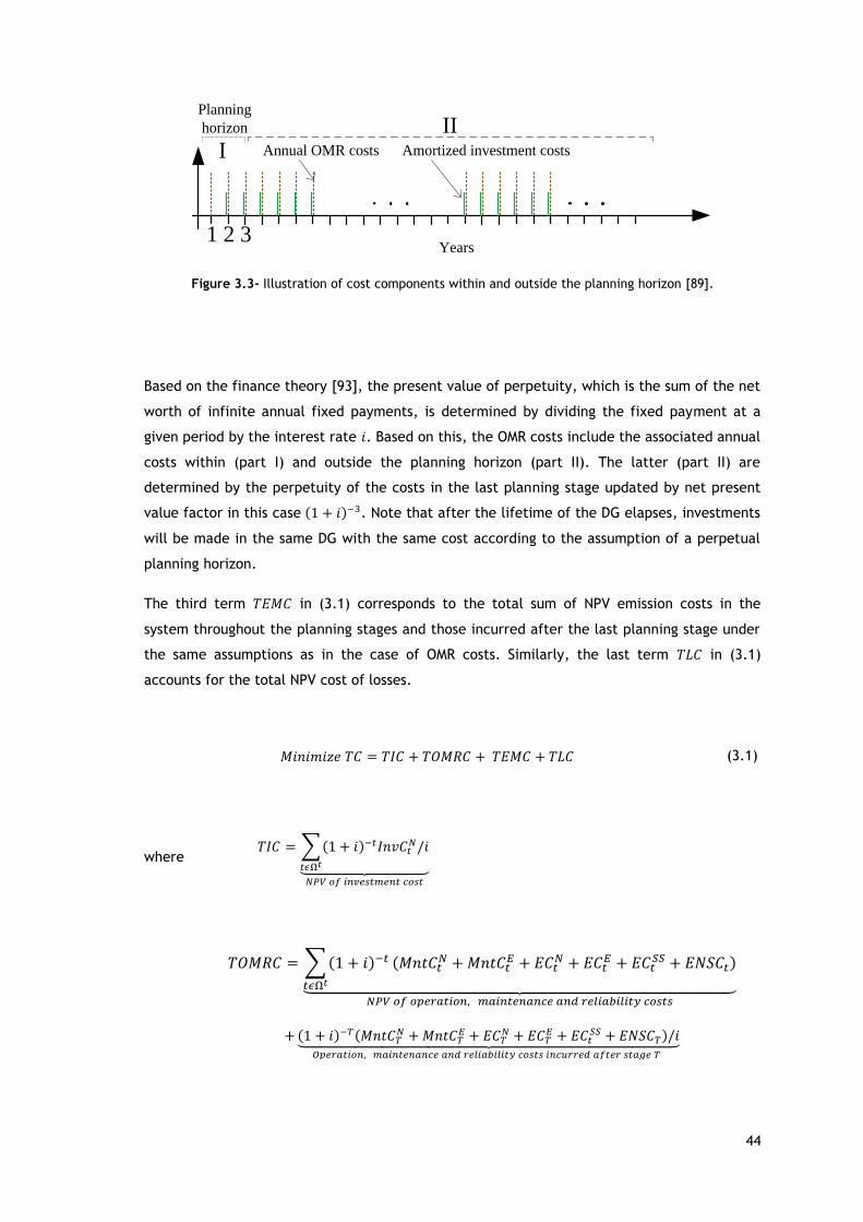
44

Years1 2 3

Planning

horizon

Annual OMR costs Amortized investment costs

III

Figure 3.3- Illustration of cost components within and outside the planning horizon [89].

Based on the finance theory [93], the present value of perpetuity, which is the sum of the net

worth of infinite annual fixed payments, is determined by dividing the fixed payment at a

given period by the interest rate 𝑖. Based on this, the OMR costs include the associated annual

costs within (part I) and outside the planning horizon (part II). The latter (part II) are

determined by the perpetuity of the costs in the last planning stage updated by net present

value factor in this case (1 + 𝑖)−3. Note that after the lifetime of the DG elapses, investments

will be made in the same DG with the same cost according to the assumption of a perpetual

planning horizon.

The third term 𝑇𝐸𝑀𝐶 in (3.1) corresponds to the total sum of NPV emission costs in the

system throughout the planning stages and those incurred after the last planning stage under

the same assumptions as in the case of OMR costs. Similarly, the last term 𝑇𝐿𝐶 in (3.1)

accounts for the total NPV cost of losses.

𝑀𝑖𝑛𝑖𝑚𝑖𝑧𝑒 𝑇𝐶 = 𝑇𝐼𝐶 + 𝑇𝑂𝑀𝑅𝐶 + 𝑇𝐸𝑀𝐶 + 𝑇𝐿𝐶 (3.1)

where

𝑇𝐼𝐶 = ∑(1 + 𝑖)−𝑡𝐼𝑛𝑣𝐶𝑡𝑁/𝑖

𝑡𝜖Ω𝑡⏟ 𝑁𝑃𝑉 𝑜𝑓 𝑖𝑛𝑣𝑒𝑠𝑡𝑚𝑒𝑛𝑡 𝑐𝑜𝑠𝑡

𝑇𝑂𝑀𝑅𝐶 = ∑(1 + 𝑖)−𝑡

𝑡𝜖Ω𝑡

(𝑀𝑛𝑡𝐶𝑡𝑁 +𝑀𝑛𝑡𝐶𝑡

𝐸 + 𝐸𝐶𝑡𝑁 + 𝐸𝐶𝑡

𝐸 + 𝐸𝐶𝑡𝑆𝑆 + 𝐸𝑁𝑆𝐶𝑡)

⏟ 𝑁𝑃𝑉 𝑜𝑓 𝑜𝑝𝑒𝑟𝑎𝑡𝑖𝑜𝑛, 𝑚𝑎𝑖𝑛𝑡𝑒𝑛𝑎𝑛𝑐𝑒 𝑎𝑛𝑑 𝑟𝑒𝑙𝑖𝑎𝑏𝑖𝑙𝑖𝑡𝑦 𝑐𝑜𝑠𝑡𝑠

+(1 + 𝑖)−𝑇(𝑀𝑛𝑡𝐶𝑇

𝑁 +𝑀𝑛𝑡𝐶𝑇𝐸 + 𝐸𝐶𝑇

𝑁 + 𝐸𝐶𝑇𝐸 + 𝐸𝐶𝑡

𝑆𝑆 + 𝐸𝑁𝑆𝐶𝑇)/𝑖⏟ 𝑂𝑝𝑒𝑟𝑎𝑡𝑖𝑜𝑛, 𝑚𝑎𝑖𝑛𝑡𝑒𝑛𝑎𝑛𝑐𝑒 𝑎𝑛𝑑 𝑟𝑒𝑙𝑖𝑎𝑏𝑖𝑙𝑖𝑡𝑦 𝑐𝑜𝑠𝑡𝑠 𝑖𝑛𝑐𝑢𝑟𝑟𝑒𝑑 𝑎𝑓𝑡𝑒𝑟 𝑠𝑡𝑎𝑔𝑒 𝑇

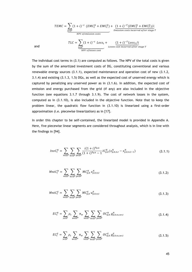
45

𝑇𝐸𝑀𝐶 = ∑(1 + 𝑖)−𝑡

𝑡𝜖Ω𝑡

(𝐸𝑀𝐶𝑡𝑁 + 𝐸𝑀𝐶𝑡

𝐸)⏟

𝑁𝑃𝑉 𝑜𝑓𝑒𝑚𝑖𝑠𝑠𝑖𝑜𝑛 𝑐𝑜𝑠𝑡𝑠

+ (1 + 𝑖)−𝑇(𝐸𝑀𝐶𝑇𝑁 + 𝐸𝑀𝐶𝑇

𝐸)/𝑖⏟ 𝐸𝑚𝑖𝑠𝑠𝑖𝑜𝑛 𝑐𝑜𝑠𝑡𝑠 𝑖𝑛𝑐𝑢𝑟𝑟𝑒𝑑 𝑎𝑓𝑡𝑒𝑟 𝑠𝑡𝑎𝑔𝑒 𝑇

and

𝑇𝐿𝐶 = ∑(1 + 𝑖)−𝑡

𝑡𝜖Ω𝑡

𝐿𝑜𝑠𝑠𝑡⏟ 𝑁𝑃𝑉 𝑜𝑓𝑙𝑜𝑠𝑠𝑒𝑠 𝑐𝑜𝑠𝑡

+ (1 + 𝑖)−𝑇𝐿𝑜𝑠𝑠𝑇/𝑖⏟ 𝐿𝑜𝑠𝑠𝑒𝑠 𝑐𝑜𝑠𝑡 𝑖𝑛𝑐𝑢𝑟𝑟𝑒𝑑 𝑎𝑓𝑡𝑒𝑟 𝑠𝑡𝑎𝑔𝑒 𝑇

The individual cost terms in (3.1) are computed as follows. The NPV of the total costs is given

by the sum of the amortized investment costs of DG, constituting conventional and various

renewable energy sources (3.1.1), expected maintenance and operation cost of new (3.1.2,

3.1.4) and existing (3.1.3, 1.5) DGs, as well as the expected cost of unserved energy which is

captured by penalizing any unserved power as in (3.1.6). In addition, the expected cost of

emission and energy purchased from the grid (if any) are also included in the objective

function (see equations 3.1.7 through 3.1.9). The cost of network losses in the system,

computed as in (3.1.10), is also included in the objective function. Note that to keep the

problem linear, the quadratic flow function in (3.1.10) is linearized using a first-order

approximation (i.e. piecewise linearization) as in [17].

In order this chapter to be self-contained, the linearized model is provided in Appendix A.

Here, five piecewise linear segments are considered throughout analysis, which is in line with

the findings in [94].

𝐼𝑛𝑣𝐶𝑡𝑁 = ∑ ∑ ∑

𝑖(1 + 𝑖)𝜂𝑝,𝑘

(1 + 𝑖)𝜂𝑝,𝑘 − 1𝐼𝐶𝑝,𝑘

𝑁 (𝑥𝑝,𝑘,𝑛,𝑡𝑁 − 𝑥𝑝,𝑘,𝑛,𝑡−1

𝑁 )

𝑝𝜖Ω𝑝𝑘𝜖Ω𝑘

𝑛∈Ω𝑛

(3.1.1)

𝑀𝑛𝑡𝐶𝑡𝑁 = ∑ ∑ ∑ 𝑀𝐶𝑝,𝑘

𝑁


𝑥𝑝,𝑘,𝑛,𝑡𝑁

𝑛∈Ω𝑛

(3.1.2)

𝑀𝑛𝑡𝐶𝑡𝐸 = ∑ ∑ ∑ 𝑀𝐶𝑝,𝑘

𝐸


𝑢𝑝,𝑘,𝑛,𝑡𝐸

𝑛∈Ω𝑛

(3.1.3)

𝐸𝐶𝑡𝑁 = ∑ 𝜌𝑠 ∑ 𝜋𝑤 ∑ ∑ ∑ 𝑂𝐶𝑝,𝑘

𝑁


𝑔𝑝,𝑘,𝑛,𝑠,𝑤,𝑡𝑁

𝑛∈Ω𝑛𝑤𝜖Ω𝑤𝑠𝜖Ω𝑠

(3.1.4)

𝐸𝐶𝑡𝐸 = ∑ 𝜌𝑠 ∑ 𝜋𝑤 ∑ ∑ ∑ 𝑂𝐶𝑝,𝑘

𝐸

𝑝∈Ω𝑝𝑘𝜖Ω𝑘

𝑔𝑝,𝑘,𝑛,𝑠,𝑤,𝑡𝐸


(3.1.5)

46

𝐸𝑁𝑆𝐶𝑡 = ∑ ∑ 𝜌𝑠 ∑ 𝜋𝑤𝜐𝑠,𝑤,𝑡𝛿𝑛,𝑠,𝑤,𝑡𝑤𝜖Ω𝑤𝑠𝜖Ω𝑠𝑛∈Ω𝑛

(3.1.6)

𝐸𝑀𝐶𝑡𝑁 = ∑ 𝜌𝑠 ∑ 𝜋𝑤 ∑ ∑ ∑ 𝜆𝑠,𝑤,𝑡

𝐸𝑀𝐼

𝑝𝜖Ω𝑝

𝐸𝑅𝑝,𝑘𝑁

𝑘𝜖Ω𝑘

𝑔𝑝,𝑘,𝑛,𝑠,𝑤,𝑡𝑁


(3.1.7)

𝐸𝑀𝐶𝑡𝐸 = ∑ 𝜌𝑠 ∑ 𝜋𝑤 ∑ ∑ ∑ 𝜆𝑠,𝑤,𝑡

𝐸𝑀𝐼

𝑝𝜖Ω𝑝

𝐸𝑅𝑝,𝑘𝐸

𝑘𝜖Ω𝑘



(3.1.8)

𝐸𝐶𝑡𝑆𝑆 = ∑ 𝜌𝑠 ∑ 𝜋𝑤 ∑ 𝜆𝑠𝑠,𝑠,𝑤,𝑡𝑔𝑠𝑠,𝑠,𝑤,𝑡

𝑆𝑆

𝑠𝑠∈Ω𝑠𝑠𝑤𝜖Ω𝑤𝑠𝜖Ω𝑠

(3.1.9)

𝐿𝑜𝑠𝑠𝑡 = ∑ 𝜌𝑠 ∑ 𝜋𝑤 ∑ λs,w,t𝑔𝑛𝑚

(𝑉𝑛𝑜𝑚𝑖𝑛𝑎𝑙∗𝑏𝑛𝑚)2(𝑓𝑛𝑚,𝑠,𝑤,𝑡)

2

𝑛,𝑚∈Ω𝑛𝑤𝜖Ω𝑤𝑠𝜖Ω𝑠

(3.1.10)

Notice that equation (3.1.1) is weighted by the capital recovery factor 𝑖(1+𝑖)

𝜂𝑝,𝑘

(1+𝑖)𝜂𝑝,𝑘−1

. Besides,

𝑥𝑝,𝑘,𝑛,0𝑁 is defined to be zero, and the formulation in (3.1.1) ensures that the investment cost of

each DG is considered only once in the summation. For example, suppose an investment in a

particular DG is made in the fourth year of a five-year planning horizon. This means the DG

will be available during the fourth and the fifth years because of the logical constraint in

(3.8). Hence, the binary variables associated to this DG in those years will be 1 while the rest

will be zero i.e. 𝑥𝑝,𝑘,𝑛,𝑡𝑁 = 0,0,0,1,1. In this particular case, only the difference (𝑥𝑝,𝑘,𝑛,4

𝑁 −

𝑥𝑝,𝑘,𝑛,3𝑁 ) equals 1 while the remaining ones are all zero, i.e. (𝑥𝑝,𝑘,𝑛,𝑡

𝑁 − 𝑥𝑝,𝑘,𝑛,𝑡−1𝑁 ) = 0, ∀𝑡 ≠ 4, and

hence the investment cost is considered only once. Equations (3.1.2) and (3.1.3) stand for the

annual maintenance costs of candidate and existing DGs, respectively. These cost components

are multiplied by the corresponding binary variables to determine whether each DG is being

utilized or not. Note that the binary investment variable is also used for this purpose because

there is no economic explanation or justification as to why it cannot be utilized immediately

after an investment is made on a given asset. For the case example given above, the DG will

incur maintenance costs in the last two years. For existing generators, binary variables are

used to indicate their respective utilizations. The operation costs given by (3.1.4) and (3.1.5)

for candidate and existing DGs, respectively, depend on the amount of power generated for

each scenario, snapshot, stage and DG type. Therefore, these costs represent the expected

costs of operation. Similarly, the penalty term for the unserved power, given by (3.1.6), is

dependent on the scenarios, snapshots and time stages. Equation (3.1.6) therefore gives the

expected cost of unserved energy. The expected emission costs of candidate and existing

generators are given by (3.1.7) and (3.1.8), respectively.

47

3.3.3 Constraints

3.3.3.1 Load Balance Constraints

The load balance at each node is given by equation (3.2).

∑ ∑(𝑔𝑛,𝑝,𝑘,𝑠,𝑤,𝑡𝐸


+ 𝑔𝑛,𝑝,𝑘,𝑠,𝑤,𝑡𝑁 ) + ∑ 𝑔𝑠𝑠,𝑠,𝑤,𝑡

𝑆𝑆

𝑠𝑠∈Ω𝑠𝑠

+ 𝛿𝑛,𝑠,𝑤,𝑡 − ∑ 𝑓𝑛𝑚,𝑠,𝑤,𝑡𝑛,𝑚∈Ω𝑛

+ ∑ 𝑓𝑚𝑛,𝑠,𝑤,𝑡𝑛,𝑚∈Ω𝑛

≥ 𝑑𝑛,𝑠,𝑤,𝑡 ; ∀𝑠 ∈ 𝑛 (3.2)

3.3.3.2 Investment Limits

In real problems, there always exist financial constraints; therefore, the maximum allowable

budget for investment in DGs for a given year is limited by (3.3).

∑ ∑ ∑ 𝐼𝐶𝑝,𝑘𝑁 (𝑥𝑝,𝑘,𝑛,𝑡

𝑁


− 𝑥𝑝,𝑘,𝑛,𝑡−1𝑁 )

𝑛∈Ω𝑛

≤ 𝐼𝑛𝑣𝐿𝑖𝑚𝑡 (3.3)

3.3.3.3 Generation Capacity Limits

The minimum and maximum capacity limits of existing and candidate generators are

represented by (3.4) and (3.5), respectively. Note that the binary variables also appear here

and multiply these bounds. This is to make sure that the power generation variable is zero

when the generator remains either unutilized or unselected for investment. In the case of

intermittent power source, the lower generation limits 𝐺𝑝,𝑘,𝑠,𝑤,𝑚𝑖𝑛𝐸 and 𝐺𝑝,𝑘,𝑠,𝑤,𝑚𝑖𝑛

𝑁 is often set to

0 while the corresponding upper limits are set equal to the actual power output of the DG

corresponding to the level of primary energy source (wind speed and solar radiation, for

instance). Hence, the upper bound in this case depends on the operational state (i.e. the

snapshot) and the scenario.

𝑢𝑛,𝑝,𝑘,𝑡𝐸 𝐺𝑝,𝑘,𝑠,𝑤,𝑚𝑖𝑛

𝐸 ≤ 𝑔𝑝,𝑘,𝑛,𝑠,𝑤,𝑡𝐸 ≤ 𝑢𝑛,𝑝,𝑘,𝑡

𝐸 𝐺𝑝,𝑘,𝑠,𝑤,𝑚𝑎𝑥𝐸 (3.4)

𝑥𝑛,𝑝,𝑘,𝑡𝑁 𝐺𝑝,𝑘,𝑠,𝑤,𝑚𝑖𝑛

𝑁 ≤ 𝑔𝑝,𝑘,𝑛,𝑠,𝑤,𝑡𝑁 ≤ 𝑥𝑛,𝑝,𝑘,𝑡

𝑁 𝐺𝑝,𝑘,𝑠,𝑤,𝑚𝑎𝑥𝑁 (3.5)

48

3.3.3.4 Unserved Power Limit

The upper and lower limits of the unserved power are given by (3.6). Normally, the maximum

unserved power one can have at a certain node is the demand at that node. However, the

upper bound may be superfluous because, under normal circumstances, when a sufficiently

large penalty factor is used in the objective function, the unserved power variable will tend

to be very close to zero by optimality.

0 ≤ 𝛿𝑛,𝑠,𝑤,𝑡 ≤ 𝑑𝑛,𝑠,𝑤,𝑡 (3.6)

3.3.3.5 DG Penetration Level Limit

Mainly due to technical reasons, there can be a maximum penetration level of DG integration

(or, equivalently saying, the maximum percentage of demand covered by DG power). This is

ensured by adding the constraints in (3.7).

∑ ∑ ∑(

𝑘𝜖𝛺𝑘𝑝𝜖𝛺𝑝

𝑔𝑝,𝑘,𝑛,𝑠,𝑤,𝑡𝐸 + 𝑔𝑝,𝑘,𝑛,𝑠,𝑤,𝑡

𝑁 )

𝑛∈Ω𝑛

≤ 𝜑𝑑𝑛,𝑠,𝑤,𝑡 (3.7)

3.3.3.6 Logical Constraints

Logically, an investment made at time stage t cannot be reversed or divested in the

subsequent time stages; hence, the asset should be available for utilization immediately after

the investment is made. Such constraints can be realized using (3.8).

𝑥𝑝,𝑘,𝑛,𝑡𝑁 ≥ 𝑥𝑝,𝑘,𝑛,𝑡−1

𝑁 (3.8)

3.3.3.7 Network Model Constraints

As mentioned earlier, integrating DGs could in some cases result in technical problems in the

system such as congestion, voltage rise and stability issues. Therefore, if these issues are

deemed critical, it may be desirable to include network constraints so that power flows and

node voltages remain within their respective permissible ranges. To this end, a linearized

network model, first proposed in [95] in the context of transmission expansion planning and

further extended to distribution network system planning in [96], is used here. In distribution

systems, since active power flow dominates the apparent power flow, reactive power flow

can be neglected. Hence, without loss of generality, only the active power flow through a

given line, given by (3.9), can be considered. Equation (3.10) ensures that the flow through

the distribution lines do not exceed their corresponding thermal capacities.

49

𝑀𝑛𝑚(𝑧𝑛𝑚 − 1) ≤ 𝑓𝑛𝑚,𝑠,𝑤,𝑡 − 𝑉𝑛𝑜𝑚𝑖𝑛𝑎𝑙(∆𝑉𝑛,𝑠,𝑤,𝑡 − ∆𝑉𝑚,𝑠,𝑤,𝑡)𝑔𝑛𝑚 − 𝑉𝑛𝑜𝑚𝑖𝑛𝑎𝑙2 𝑏𝑛𝑚휃𝑛𝑚,𝑠,𝑤,𝑡

≤ 𝑀𝑛𝑚(1 − 𝑧𝑛𝑚) (3.9)

−𝑓𝑛𝑚𝑚𝑎𝑥𝑧𝑛𝑚 ≤ 𝑓𝑛𝑚,𝑠,𝑤,𝑡 ≤ 𝑧𝑛𝑚𝑓𝑛𝑚

𝑚𝑎𝑥 (3.10)

Note that the voltage at each node is assumed to be equal to 𝑉𝑛𝑜𝑚 + ∆𝑉𝑛,𝑠,𝑤,𝑡 where

∆𝑉𝑛,𝑠,𝑤,𝑡 stands for the voltage deviation at each node which is bounded as −휀 ∗ 𝑉𝑛𝑜𝑚𝑖𝑛𝑎𝑙 ≤

∆𝑉𝑛,𝑠,𝑤,𝑡 ≤ 휀 ∗ 𝑉𝑛𝑜𝑚𝑖𝑛𝑎𝑙. For the analysis throughout this chapter, the tolerance factor ε is set to

0.05, and the voltage magnitude and angle at all substations are set to 1.05𝑉𝑛𝑜𝑚𝑖𝑛𝑎𝑙 and 0,

respectively.

3.3.3.8 Radiality Constraints

The traditional radiality constraint in (3.11) [97], along with the load balance equation, gives

the necessary condition for a distribution network to be radial and connected. The analysis in

this chapter considers a radial network, and does not include grid expansion or switching.

Therefore, equation (3.11) is sufficient to keep the radiality of the network and ensure that

all nodes are connected.

∑ 𝑧𝑛𝑚𝑛,𝑚∈𝛺𝑛

= 𝑁𝑛 − 𝑁𝑆𝑆 (3.11)

3.4 Case Studies

3.4.1 System Data

The system considered in the study is a real-life insular distribution network in São Miguel

Island, Azores, Portugal. In this system, currently, there is no electricity market, and there is

no energy imported (purchased) from the transmission grid. The system has a peak demand

of 70.2 MW, and information about existing generators is shown in Table 3.1. The investment

limit in each year is set to 120 M€. The average cost of electricity 𝜆𝑠,𝑤,𝑡 used for estimating

cost of losses is assumed to be the average of all marginal costs of power production of DGs.

In this system, various DG types with capacities ranging from 1 to 30 MW are considered as

candidates for investment (see in Table 3.2). These fall into small-to medium-scale DG

categories according to the capacity-based classification of DGs in [98]. The installation and

maintenance costs of each DG are either directly obtained from [98] and [99] or estimated

using the so-called six-tenths rule [100], which e stablishes a relationship between cost and

quantity (in this case, installed capacity).

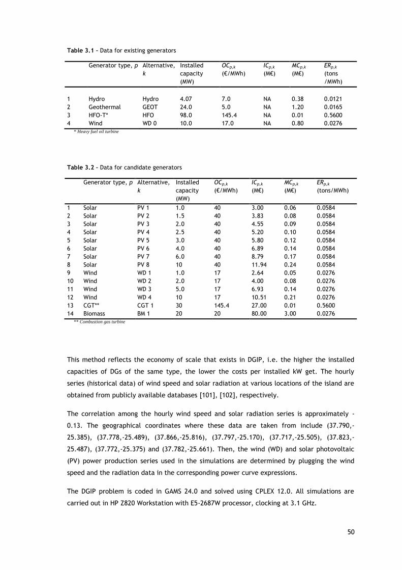
50

Table 3.1 – Data for existing generators

Generator type, p Alternative,

k

Installed

capacity

(MW)

OCp,k

(€/MWh)

ICp,k

(M€)

MCp,k

(M€)

ERp,k

(tons

/MWh)

1 Hydro Hydro 4.07 7.0 NA 0.38 0.0121

2 Geothermal GEOT 24.0 5.0 NA 1.20 0.0165

3 HFO-T* HFO 98.0 145.4 NA 0.01 0.5600

4 Wind WD 0 10.0 17.0 NA 0.80 0.0276

* Heavy fuel oil turbine

Table 3.2 – Data for candidate generators

Generator type, p Alternative,

k

Installed

capacity

(MW)

OCp,k

(€/MWh)

ICp,k

(M€)

MCp,k

(M€)

ERp,k

(tons/MWh)

1 Solar PV 1 1.0 40 3.00 0.06 0.0584

2 Solar PV 2 1.5 40 3.83 0.08 0.0584

3 Solar PV 3 2.0 40 4.55 0.09 0.0584

4 Solar PV 4 2.5 40 5.20 0.10 0.0584

5 Solar PV 5 3.0 40 5.80 0.12 0.0584

6 Solar PV 6 4.0 40 6.89 0.14 0.0584

7 Solar PV 7 6.0 40 8.79 0.17 0.0584

8 Solar PV 8 10 40 11.94 0.24 0.0584

9 Wind WD 1 1.0 17 2.64 0.05 0.0276

10 Wind WD 2 2.0 17 4.00 0.08 0.0276

11 Wind WD 3 5.0 17 6.93 0.14 0.0276

12 Wind WD 4 10 17 10.51 0.21 0.0276

13 CGT** CGT 1 30 145.4 27.00 0.01 0.5600

14 Biomass BM 1 20 20 80.00 3.00 0.0276

** Combustion gas turbine

This method reflects the economy of scale that exists in DGIP, i.e. the higher the installed

capacities of DGs of the same type, the lower the costs per installed kW get. The hourly

series (historical data) of wind speed and solar radiation at various locations of the island are

obtained from publicly available databases [101], [102], respectively.

The correlation among the hourly wind speed and solar radiation series is approximately -

0.13. The geographical coordinates where these data are taken from include (37.790,-

25.385), (37.778,-25.489), (37.866,-25.816), (37.797,-25.170), (37.717,-25.505), (37.823,-

25.487), (37.772,-25.375) and (37.782,-25.661). Then, the wind (WD) and solar photovoltaic

(PV) power production series used in the simulations are determined by plugging the wind

speed and the radiation data in the corresponding power curve expressions.

The DGIP problem is coded in GAMS 24.0 and solved using CPLEX 12.0. All simulations are

carried out in HP Z820 Workstation with E5-2687W processor, clocking at 3.1 GHz.

51

3.4.2 Scenario Definition

Defining scenarios is in itself a complex problem, which requires exhaustive research and

sufficient knowledge of the evolution of the system under consideration. Because of this, the

number and the nature of scenarios are mostly predefined, and, to do this, planners often

rely on expert knowledge. In this work, three scenarios (storylines) are defined in connection

to the possible evolutions of two relevant uncertain parameters over the planning horizon,

namely, electricity demand growth and emission price. Table 3.3 shows the three evolutions

of demand growth, denoted as Low, Moderate and High, having an equal degree of

realization. Similarly, the emission price is represented by three equally probable storylines

(scenarios), as depicted in Table 3.3. Out of these individual scenarios, assuming the two

uncertain parameters are independent, we can get nine different combinations, which form

the new set of scenarios used in the simulations. With this as a base-case, sensitivity analyses

are carried out to study the impact of several system parameters other than these, which

involve some degree of uncertainty, on DG investment decisions. These parameters include

interest rate, DG penetration limit, solar PV and wind power output uncertainty, generator

availability, electricity tariffs and fuel prices.

3.4.3 Impact of Network Inclusion/Exclusion on DGIP Solution

To assess the impacts on the DGIP solution, the formulated problem is solved with and

without network. The former considers the entire network system but the latter assumes that

the electricity demand is aggregated and connected to a hypothetical node and all generators

are assumed to be connected to this node. One of the main differences lies in the network

losses which are only accounted for when considering the network. However, since

distribution networks span over a small geographical area, the feeders and distribution lines

are usually short. Therefore, in properly designed distribution networks, power losses are

negligible and, hence, they are not expected to significantly change DG investment planning

solution. This argument has been experimentally verified by running simulations with and

without a network on two insular networks (the distribution networks of São Miguel Island

described before and La Graciosa Island presented in [103]). In both cases, the DGIP results

with and without network are very similar, only differing in one DG investment. Moreover, the

differences in total investment cost throughout a three-year planning horizon are 2.2 and

3.5%, respectively.

Table 3.3 – Demand growth and CO2 price scenarios

Stages

Demand growth scenarios CO2 price scenarios

(€/ton of CO2)

Low Moderate High Low Moderate High

T0 0% 0% 0% 5 5 5

T1 2% 5% 10% 7 12 20

T2 5% 10% 20% 10 18 30

T3 7% 15% 30% 13 25 45

52

Generally, excluding the network slightly results in overinvestment. This is because

neglecting the network would naturally mean neglecting the voltage constraints. As a result,

this would lead to an increase in the size of DG integrated to the system that would otherwise

be impossible when considering the network due to voltage rise issues.

In the systems studied, the increase in DG investments as a result of not considering the

network is negligible. Moreover, the cost of losses in both test cases is too small (accounting

for less than 0.02 % of the total system cost) to have an impact on the solution. Based on

these results, the sensitivity analysis here is carried out without considering the network. This

is not expected to affect the analysis work since the main aim of the work here is to identify

the parameters that significantly influence DGIP solutions.

It should be clearly understood that the work in this chapter is not to make investment

decisions; it should rather be understood as an important step that provides relevant input to

the development of robust planning tools. The exclusion of network (i.e. collapsing the whole

system into one node) reduces the computation burden and helps one to increase the level of

details of other relevant issues such as uncertainty and variability of uncertain parameters. It

should however be noted that the aforementioned findings may largely depend on the size

and the type the system being considered.

3.4.4 Results and Discussion

The analysis results with regards to the sensitivity of investment decisions on DGs with

variations of selected system parameters are presented and discussed as follows.

3.4.4.1 Demand Growth and CO2 Price

The total investment cost for every combination of demand growth and emission price

scenarios are shown in Table 3.4, along with the corresponding overall system costs as in

Table 3.5. We can see in these tables that DG investments are more sensitive to emission

price uncertainty than to demand growth. The DG investment decisions corresponding to each

scenario and time stage are given in Table B.1 of Appendix B.

Table 3.4 – Impact of demand growth and CO2 price uncertainty on DG investments

TIC

(M€)

CO2 price scenarios

Low Moderate High

Demand growth

scenarios

Low 38.462 46.220 54.540

Moderate 38.462 46.996 64.245

High 38.462 53.078 64.757

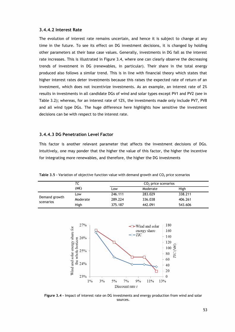
53

3.4.4.2 Interest Rate

The evolution of interest rate remains uncertain, and hence it is subject to change at any

time in the future. To see its effect on DG investment decisions, it is changed by holding

other parameters at their base case values. Generally, investments in DG fall as the interest

rate increases. This is illustrated in Figure 3.4, where one can clearly observe the decreasing

trends of investment in DG (renewables, in particular). Their share in the total energy

produced also follows a similar trend. This is in line with financial theory which states that

higher interest rates deter investments because this raises the expected rate of return of an

investment, which does not incentivize investments. As an example, an interest rate of 2%

results in investments in all candidate DGs of wind and solar types except PV1 and PV2 (see in

Table 3.2); whereas, for an interest rate of 12%, the investments made only include PV7, PV8

and all wind type DGs. The huge difference here highlights how sensitive the investment

decisions can be with respect to the interest rate.

3.4.4.3 DG Penetration Level Factor

This factor is another relevant parameter that affects the investment decisions of DGs.

Intuitively, one may ponder that the higher the value of this factor, the higher the incentive

for integrating more renewables, and therefore, the higher the DG investments

Table 3.5 – Variation of objective function value with demand growth and CO2 price scenarios

TC

(M€)

CO2 price scenarios

Low Moderate High

Demand growth

scenarios

Low 246.111 283.029 338.211

Moderate 289.224 336.038 406.261

High 375.187 442.091 543.606

Figure 3.4 - Impact of interest rate on DG investments and energy production from wind and solar sources.

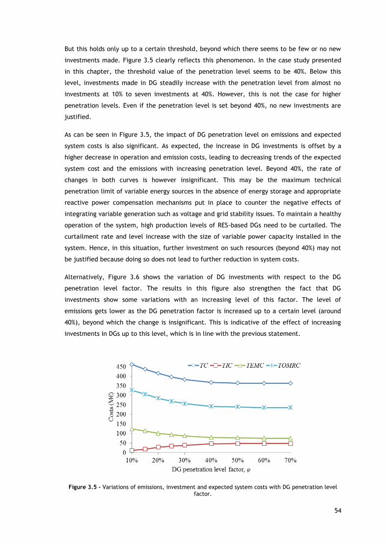
54

But this holds only up to a certain threshold, beyond which there seems to be few or no new

investments made. Figure 3.5 clearly reflects this phenomenon. In the case study presented

in this chapter, the threshold value of the penetration level seems to be 40%. Below this

level, investments made in DG steadily increase with the penetration level from almost no

investments at 10% to seven investments at 40%. However, this is not the case for higher

penetration levels. Even if the penetration level is set beyond 40%, no new investments are

justified.

As can be seen in Figure 3.5, the impact of DG penetration level on emissions and expected

system costs is also significant. As expected, the increase in DG investments is offset by a

higher decrease in operation and emission costs, leading to decreasing trends of the expected

system cost and the emissions with increasing penetration level. Beyond 40%, the rate of

changes in both curves is however insignificant. This may be the maximum technical

penetration limit of variable energy sources in the absence of energy storage and appropriate

reactive power compensation mechanisms put in place to counter the negative effects of

integrating variable generation such as voltage and grid stability issues. To maintain a healthy

operation of the system, high production levels of RES-based DGs need to be curtailed. The

curtailment rate and level increase with the size of variable power capacity installed in the

system. Hence, in this situation, further investment on such resources (beyond 40%) may not

be justified because doing so does not lead to further reduction in system costs.

Alternatively, Figure 3.6 shows the variation of DG investments with respect to the DG

penetration level factor. The results in this figure also strengthen the fact that DG

investments show some variations with an increasing level of this factor. The level of

emissions gets lower as the DG penetration factor is increased up to a certain level (around

40%), beyond which the change is insignificant. This is indicative of the effect of increasing

investments in DGs up to this level, which is in line with the previous statement.

Figure 3.5 - Variations of emissions, investment and expected system costs with DG penetration level factor.

55

Figure 3.6 - Variation of DG investments with penetration level and their effect on total CO2 emissions.

3.4.4.4 Fuel Prices and Electricity Tariffs

The impact of fuel prices and electricity tariffs of renewable generators are also analyzed by

varying the levels of these parameters. The results of this sensitivity analysis are summarized

in Table 3.6. As it can be seen in this table, DG investment decisions are very sensitive to fuel

prices. For example, when the fuel price is considered to be 30% lower than that of the base

case, it becomes less attractive to invest on DG (especially solar photovoltaics). But a fuel

price 30% higher results in more investments in PV.

In addition to fuel prices, electricity tariffs also play a significant role in the decision-making

process, particularly in the context of DG investment planning. In general terms, the price of

electricity generated from wind or solar DG highly depends on the initial level of capital

invested on these DG technologies. Once the investments are made, operation costs are

normally very low. Nowadays, the capital costs of the main components pertaining to these

technologies are continuously falling, with a learning rate of more than 20% per annum.

This trend will most likely be sustained [99], resulting in a dramatically lower final cost of

electricity (tariff) generated from such resources.

The effects of variations in PV energy tariffs on DG investments are especially investigated in

this chapter. As shown in Table 3.6, when solar PV generators are considered to be as

competitive as wind power generators, i.e. with a tariff of €20/MWh, more investments in PV

are made compared to the base case. On the other hand, if the electricity tariff of energy

coming from PV turns out to be twice that of the base case (€80/MWh), the number of

investments made in solar PV declines. However, this is not likely to happen given the current

learning rate of solar PV technology. It is also worth mentioning that the planning solution in

the case of +100% tariff for PV energy is exactly the same as the solution in the -30% fuel

price case, which shows the importance of energy tariff arrangement by the regulatory body.

56

The crowding of investment decisions in the first stage in Table 3.6 may be due to two

reasons. The first reason could be because of the absence of investment constraints related

to financial and logistic matters. The second reason could be because of the relatively higher

net present value of operation, maintenance and emission costs in the first stage when

compared with that of any other stage. This, along with the first reason, may justify more

investments to be made in the first stage rather than in any one of the subsequent stages.

3.4.4.5 Wind and Solar Power Output Uncertainty

To analyze the effect of uncertainty in wind and solar power outputs, two scenarios are

created for each. One scenario is taken to be above the average hourly profile (roughly 30%

higher than that of the base case), and the other one is taken below the average profile

(approximately 30% lower than that of the base case) in each case. The results of the analysis

are summarized in Table 3.7. One can observe that when the B-wind scenario is considered,

the number of investments on wind type DGs becomes lower than these of the base case (see

in Table 3.6). This is because of the lower yield of wind resources. In contrast, more

investments are made on wind type DGs when the A-wind scenario is considered.

The sensitivity of investments in solar PVs with respect to the uncertainty of PV outputs is

even higher, as can be seen in this table. Note that the reasons mentioned before in the case

of Table 3.6 could explain the crowding of investments in the first stage in Table 3.7.

Table 3.6 – Impact of price and DG tariffs on DG investment decisions

Stages

Changes in fuel price

Changes in PV energy

tariff

+0% -30% +30% -50% +100%

Investment in

wind and solar

DGs

T1

PV8, WD1,

WD2, WD3,

WD4

WD1,

WD2,

WD3,

WD4

PV7, PV8,

WD1, WD2,

WD3, WD4

PV7, PV8,

WD1, WD2,

WD3, WD4

WD1,

WD2,

WD3, WD4

T2 PV7 PV8 PV6 - PV8

T3 - - PV5 PV6 -

TC (M€) 364 312 412 358 372

Total expected emissions

(x 1000 tons of CO2)

268.8 296.4 256.5

263.1 296.4

Table 3.7 – Impact of wind and solar PV output uncertainty on DG investment decisions

Scenarios Time stages

TIC (M€)

TC (M€) T1 T2 T3

Wind Scenarios Below average (B) PV8,WD2, WD3,WD4 PV7 - 44.81 412

Above average (A) PV8, WD1,WD2, WD3,WD4 - - 38.46 339

Solar Scenarios Below average (B) PV8, WD1,WD2, WD3,WD4 - - 38.46 373

Above average (A) PV8, WD1,WD2, WD3,WD4 PV7 PV6 47.00 360

57

3.4.4.6 Demand and RES Power Output Uncertainty

As stated earlier, the natural variation with time that exists in some of the system

parameters such as demand and renewable energy source (RES) outputs leads to a large

number of operational situations, adding extra complexity to the DGIP problem. Because of

this, a significantly reduced number of snapshots are usually considered in such problems. For

example, demand variability is commonly represented by a load duration curve, which is then

aggregated into three to five load blocks.

Unfortunately, this may compromise the quality of solution obtained. In light of this, we

investigate how the reduction of operational situations, via clustering, affects the DG

investment solution. To do this, we make use of k-means clustering algorithm, a popular

clustering analysis method in data mining, to obtain different number of data clusters

(aggregates). The representative snapshot in each cluster is assumed to be the mean of the

snapshots grouped together. For different number of clusters, the investments made, along

with total cost and average simulation time, are summarized in Table 3.8.

According to the results in this table, there seems to be a tendency to overinvest when the

snapshots are further reduced. This may be due to an overestimation of the operation costs,

which triggers more investments. Basically, investments are justified if the net reduction in

operation costs (which may include cost of energy production, emission and losses) is higher

than or equal to the overall investment costs. Based on this, if the operation costs are

artificially overstated for some reason such as clustering inaccuracy, the net reduction in

operation costs may seemingly be high, leading to the justification of more investments.

However, it should be noted that this may not always be the case, i.e. a lower number of

clusters may not necessarily be associated with an overestimation of operation costs.

Depending on how the representative snapshots in all clusters are taken, the operation costs

may be overestimated or underestimated, resulting in overinvestment or underinvestment,

respectively.

Table 3.8 – Impact of snapshot aggregation on DG investment decisions

TIC (M€)

TC (M€)

Average simulation

time (seconds) Number of snapshots Stage 1 (T1) Stage 2 (T2) Stage 3 (T3)

Peak demand 47.849 6.691 5.118 - -

100 38.462 8.533 6.082 359.45 2

300 38.462 8.533 6.082 360.66 4

324 * [71] 38.462 8.533 6.082 362.98 6

500 38.462 8.533 6.082 361.56 7

1000 38.462 8.533 6.082 362.37 21

2000 38.462 8.533 6.082 363.09 60

4000 38.462 8.533 0.000 363.55 210

6000 38.462 8.533 0.000 363.70 420

8760 38.462 8.533 0.000 363.80 720

* Snapshots are reduced according to the method in the reference

58

Another important observation from Table 3.8 is that clustering the hourly operational

snapshots in a year shows little impact on the investment solution beyond a certain threshold

(which lies somewhere in the range of 300 and 400). This reflects that as far as the initially

large number snapshots are clustered into 300 or more and the representative snapshots are

carefully selected, the investment outcomes may not be influenced by clustering operational

situations but significantly facilitate the solution process.

3.4.4.7 Generator Availability

It is understood that a generator can only produce power when it is available. There are two

main factors which affect generator’s availability: unplanned (forced) and planned

(scheduled) outages. Such outages may also condition DG investment solution. Especially,

more investments can be expected if, by chance, generator outages partially or fully coincide

with relatively high production times of DG candidates. For example, if outages essentially

occur during sunny hours, more investments could be made on solar PV candidate generators

to fill in the generation gap left behind as a result of the outages. However, the chance of

this happening can be very low since both processes are independent. In the particular

example presented earlier, the effects of forced outages of geothermal and hydro power

units on the solution are analyzed. The availability series of these units are generated using a

binomial distribution function, assuming generator outage rates of 15% and 10%, respectively.

Note that these rates consider both types of outages. When generating the series, an average

off-time of 4 hours is factored in for both generator types. Given this input information, the

DGIP problem is solved and its solution includes PV8 and all wind DG candidates in the first

stage, PV7 in the second stage, and PV6 in the third stage with a total investment cost of

53.08 M€. This solution differs from that of the base case by one investment (i.e. PV6).

But, in general, more investments could be justified if the generator outages occur

during/around the peak hours of renewable power productions.


This chapter has presented comprehensive experimental analyses to determine the sensitivity

of DG investments with variations of several uncertain parameters. The aim of such analyses

has been first to investigate the effect of variability and uncertainty in model parameters on

the investment decisions of DGs, and second to identify the parameters that have the highest

degree of influence on DG investments. The results of our analyses generally showed that

both uncertainty and variability have a meaningful influence on DG investment decisions.

In fact, the degree of influence varies from one parameter to another. Results from the case

study show that generator outages have little or no impact on the RES-based DG investments;

whereas, uncertainty in CO2 and fuel prices, interest rate and RES power outputs significantly

influence investment decisions especially in variable energy sources.

59

In particular, it has been found out that uncertainty in CO2 and fuel prices as well as interest

rate dramatically condition decisions compared to the uncertainty in demand growth and RES

power outputs. A thorough investigation on the number of clusters of the hourly operational

snapshots in a year shows that the clustering process results in little impact on the

investment solution beyond a certain threshold (somewhere in the range of 300 and 400). This

reflects that as far as the initially large number snapshots are clustered into 300 or more, and

the representative snapshots are carefully selected, the results may not be influenced by

clustering operational situations but significantly facilitate the solution process.

In general, the results reveal that ignoring or inadequately considering uncertainty and

variability in model parameters has a quantifiable cost. Based the extensive analysis, a

stochastic modeling of uncertainty related to emission and fuel prices, interest rate, RES

power outputs and demand growth is very critical for obtaining robust investment decisions.

The comprehensive analysis performed in this chapter can help planners to properly weigh

the effect of ignoring or considering the uncertainty and/or variability of one or more model

parameters. Accordingly, a realistic planning tool considering all relevant sources of

uncertainty and/or variability and solution methodologies can be developed, which leads to

high quality and robust investment solutions.

60

Chapter 4

Multi-Stage Stochastic DG Investment Planning with

Recourse

Taking the findings of the analysis in Chapter 3 as input, a detailed model is developed

in Chapter 4 to guide the complex decisions-making process of DG investment planning in

the distribution system in the face of uncertainty. The problem is formulated from a

coordinated system planning viewpoint and the operational variability and uncertainty

introduced by intermittent generation sources, electricity demand, emission prices, demand

growth and others are accounted for via probabilistic and stochastic methods, respectively.

4.1 Introduction

The advent of emerging solutions such as active management of distribution networks [57] or

fully automated and intelligent networks – the so-called smart grids [104] - is expected to

keep on facilitating smooth integration of DGs by alleviating existing technical limitations.

Hence, DG is expected to play an important role in distribution systems, making the issue of

DG investment planning (DGIP) highly important. This is because, throughout the world, new

regulations are put in place to reduce the heavy dependence of such systems on fossil fuels

for energy production. However, several DG sources are intermittent in nature, making the

operation and planning of distribution networks very challenging. This is because such sources

introduce significant operational variability and uncertainty to the system. The terms

(operational) variability and uncertainty in this chapter should be understood according to the

following definitions. Variability, as defined in [90], refers to the natural variation in time of

a specific uncertain parameter; whereas, uncertainty refers to “the degree of precision with

which the parameter is measured” or predicted. In addition to the aforementioned sources of

uncertainty, there are several other parameters (such as fuel prices, demand growth, etc.)

which are subject to high level uncertainty. The compounded effect of all these relevant

issues certainly requires crafting new methods and tools in order to realize an optimal or a

cost-efficient integration of DGs. Indeed, the robustness and reliability of the solutions

obtained from DGIP models highly depends on the level of details of the methods and tools

embedded in such models and their effectiveness in managing uncertainty and variability.

This chapter aims to introduce a novel multi-stage stochastic DGIP model with recourse under

a high penetration level of stochastic generation resources in distribution systems. The model

incorporates methods to manage uncertainty and operational variability introduced by the

variable energy sources (such as wind and solar) as well as demand. This enhances the

robustness of the decisions made.

61

The problem, formulated as a mixed integer linear programming (MILP) optimization,

simultaneously minimizes the net present value of losses, emission, operation and

maintenance as well as unserved energy costs, while fulfilling a number of technical and

economic constraints. Note that the DGIP problem here is formulated from the system

perspective (i.e. a coordinated planning approach).

This chapter is organized as follows: In section 4.2, the uncertainty and the operational

variability facing a DGIP problem are briefly explained. Subsequently, section 4.3 presents

the mathematical formulation and detailed description of the DGIP model. Section 4.4

discusses the results of the case studies. Finally, in Section 4.5, the relevant conclusions and

implications based on the outcome are drawn.

4.2 Modeling Uncertainty and Variability in DGIP

The various sources of uncertainty and variability in a DGIP problem are related to the

variability in time and the randomness of operational situations [105]. In addition, there are

some other uncertainties mostly related to the long-term electricity, emission and fuel

prices, rules, regulations and policies, etc.

A well-developed DGIP tool should therefore encompass a methodology which effectively and

efficiently takes account of operational variability and uncertainty. Exhaustive modeling of all

sources of uncertainty and variability may not only be computationally unaffordable but also

inefficient. A systemic approach is required to handle these issues in an efficient and

effective manner. In this thesis, the variability due to intermittent DG power outputs (mainly,

wind and solar) and demand are captured by considering a sufficiently large number of

operational states, also known as here “snapshots”. The hourly data may be historical or

generated from individual or joint PDFs of uncertain parameters.

To ensure tractability, a standard clustering technique is used to reduce the number of

snapshots. Here, each cluster represents a group of similar operational situations.

A representative snapshot is then selected from each cluster based on certain criteria (for

example, the medoid). Then, each of the selected snapshots, representing a group of similar

operational situations, is assigned a weight 𝜋𝑤 proportional to the number of operational

situations in its group. In addition to variability, demand and RES outputs are subject to

uncertainty due to partially unpredictable nature (especially variable energy sources such as

wind and solar). In other words, the realizations of these parameters cannot be perfectly

forecast. This relevant issue (i.e. uncertainty) is accounted for considering a sufficiently large

number of scenarios for each individual uncertain parameter. In the case of wind power

output uncertainty, for instance, each scenario represents a possible hourly wind power

output profile throughout the planning horizon. Hence, one can generate multiple profiles of

this type, each with a certain degree of realization.

62

However, for computational reasons, the number of scenarios needs to be limited. Similarly,

a number of scenarios are also defined to characterize the solar power output uncertainty.

In addition, the evolutions of emission price and demand growth can be each represented by

many scenario trajectories, each showing the considered parameter’s data realizations.

Combinations of all these individual scenarios then form the final set of global scenarios that

are used in the analysis. This is schematically illustrated in Figure 4.1. The global scenarios

(S1 through Sn) are formed by combining individual scenarios. Note that the profiles in this

figure are shown only for the purpose of illustrating the concepts; the profiles used in the

analysis are actually different from these. The actual ones, for instance, span over the entire

planning horizon.


4.3.1 Overview and Modeling Assumptions

Although many studies have been carried out on DGIP, most of them focus on a small subset of the

vast sources of variability and uncertainty when formulating the DGIP problem. As it can be

observed in the literature presented in Chapter 3, dealing with the variability pertaining to

electricity demand seems to be considered in many works in the literature (often by aggregating

it into 3 to 5 demand levels) while the others are largely ignored or represented in an overly

simplified manner. Moreover, analyses in previous works are mostly limited to one or two DG

types; the possible investment options pertaining to the size and technology type of DGs are not

sufficiently explored in most of them. Therefore, a comprehensive DGIP model, equipped with

appropriate tools for managing the most relevant sources of variability and uncertainty as well as

considering various DG types and sizes, is still needed to guide the complex decision making

process of DGIP. This way, an optimal integration of DGs can be guaranteed.

Figure 4.1 - A graphical illustration of scenario generation.

63

Furthermore, the issue of combining robust and flexible investment decisions has not been

addressed so far. It is understood that most real-world problems often require two types of

investment decisions to be made: robust decisions (short-term) and adaptive decisions (medium to

long-term) both in the face of high level uncertainty. The former are sometimes called “here and

now” decisions while the latter are referred to as “wait and see” decisions.

In the present work, to emulate such a decision-making process, a two-period planning framework

is proposed. Each period has multiple planning stages. The first period is a short-term horizon in

which robust decisions, good enough for all scenarios, are pursued. The second one spans over a

medium to long-term horizon involving exploratory and/or flexible investment decisions that are

scenario-dependent [89].

Note that the investment solution in the second period can also be understood as a set of

investments required to make adjustments to the first-period decisions depending on the scenario

unveiled in the second period. In other words, the proposed model combines both robust (short-

term) and adaptive (medium to long-term) decisions, which is one of its salient features.

4.3.2 Brief Description of the Problem

As stated in the previous sections, the DGIP problem is formulated considering the dynamic

nature of the problem i.e. featuring multiple planning stages. In addition, in order to combine

“here and now” and “wait and see” investment decisions, a two-period stochastic

optimization framework is proposed in this chapter.

This modeling framework assumes that there are n probable future storylines (or scenarios)

each associated with a probability of realization ρs that stochastically represents relevant

sources of uncertainties. Note that the terminologies snapshot and scenario, as defined in this

chapter, correspond to an operational situation at a particular hour, and the evolution of an

uncertain parameter over a given time horizon (often yearly), respectively.

The whole modeling scheme adopted in this chapter (i.e. the multi-stage and multi-scenario

DGIP modeling framework and the expansion solution structure) is illustrated in Figure 4.2.

This figure schematically represents possible future scenario trajectories with multiple

scenario spots along the planning horizon. The figure also illustrates the decision structure,

involving investment decisions independent of the scenarios and decisions, adapted to every

scenario in every stage of the second period in a “what-if” fashion.

The decisions in the first period form a set of stochastic solutions which should be good

enough for all scenarios. Those in the second period can be regarded as a set of adaptive

solutions because the investment decisions made depend on the scenarios.

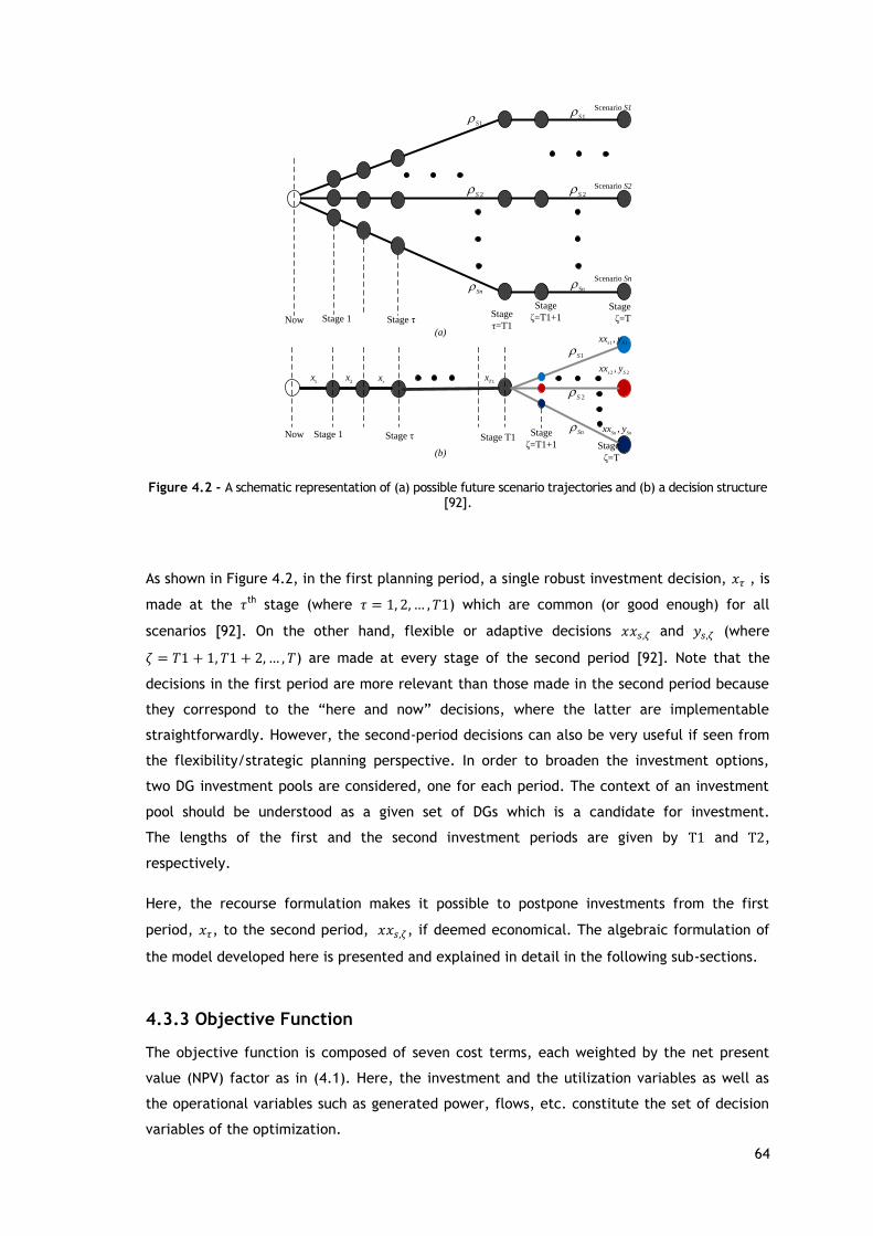
64

Now Stage τ Stage

τ=T1(a)

1S

2S

Sn

Stage 1

Now Stage τ

(b)

Stage 1 Stage T1

Stage

ζ=T

1S

2S

Sn

Stage

ζ=T

Sn

2S

1S

,Sn Sn

xx y

2 2,

s Sxx y

1 1,

s Sxx y

Stage

ζ=T1+1

Stage

ζ=T1+1

Scenario Sn

Scenario S2

Scenario S1

1Txx

2x

1x

Figure 4.2 - A schematic representation of (a) possible future scenario trajectories and (b) a decision structure [92].

As shown in Figure 4.2, in the first planning period, a single robust investment decision, 𝑥𝜏 , is

made at the 𝜏th stage (where 𝜏 = 1, 2, … , 𝑇1) which are common (or good enough) for all

scenarios [92]. On the other hand, flexible or adaptive decisions 𝑥𝑥𝑠,𝜁 and 𝑦𝑠,𝜁 (where

휁 = 𝑇1 + 1, 𝑇1 + 2,… , 𝑇) are made at every stage of the second period [92]. Note that the

decisions in the first period are more relevant than those made in the second period because

they correspond to the “here and now” decisions, where the latter are implementable

straightforwardly. However, the second-period decisions can also be very useful if seen from

the flexibility/strategic planning perspective. In order to broaden the investment options,

two DG investment pools are considered, one for each period. The context of an investment

pool should be understood as a given set of DGs which is a candidate for investment.

The lengths of the first and the second investment periods are given by T1 and T2,

respectively.

Here, the recourse formulation makes it possible to postpone investments from the first

period, 𝑥𝜏, to the second period, 𝑥𝑥𝑠,𝜁, if deemed economical. The algebraic formulation of

the model developed here is presented and explained in detail in the following sub-sections.


The objective function is composed of seven cost terms, each weighted by the net present

value (NPV) factor as in (4.1). Here, the investment and the utilization variables as well as

the operational variables such as generated power, flows, etc. constitute the set of decision

variables of the optimization.

65

min𝐼𝑛𝑣𝑉𝑎𝑟,𝑂𝑝𝑉𝑎𝑟

𝑇𝐶 = 𝛼 ∗ 𝑇𝐼𝐶 + 𝛽 ∗ 𝑇𝑂𝑀𝑈𝐸𝐶 + 𝛾 ∗ 𝑇𝐸𝑀𝐶 + 𝜉 ∗ 𝑇𝐿𝐶 (4.1)

where 𝐼𝑛𝑣𝑉𝑎𝑟 and 𝑂𝑝𝑉𝑎𝑟 denote all investment and operational variables. Moreover, the

subtotal costs related to investment (𝑇𝐼𝐶), operation, maintenance and unnerved energy

(𝑇𝑂𝑀𝑈𝐸𝐶), emissions (𝑇𝐸𝑀𝐶) and losses (𝑇𝐿𝐶) in (4.1) are computed using the corresponding

expressions in Table 4.1.

The first term in (4.1) represents the NPV of DG investment costs under the assumption of


installments throughout the lifetime of the installed DG”, as is done in [71].

The second term corresponds to the sum of NPV operation, maintenance and energy not

served (OM&ENS) costs throughout the planning stages. The third one gathers the

corresponding OM&ENS costs incurred after the last planning stage, which rely on the OM&ENS

costs of the last planning stage. Note that a perpetual planning horizon is assumed when

spreading these costs over the horizon following the last planning stage. The fourth term in

(4.1) refers to the sum of NPV emission costs in the system throughout the planning stages.

Table 4.1 – Expression of cost components in the objective function.

Cost terms Expression

𝑇𝐼𝐶 ∑

𝐼𝑛𝑣𝐶𝑡𝑁

𝑖(1 + 𝑖)𝑡𝑡𝜖Ω𝑡⏟

𝑁𝑃𝑉 𝑜𝑓 𝑖𝑛𝑣𝑒𝑠𝑡𝑚𝑒𝑛𝑡 𝑐𝑜𝑠𝑡

𝑇𝑂𝑀𝑈𝐸𝐶

∑(𝑀𝑛𝑡𝐶𝑡

𝑁 +𝑀𝑛𝑡𝐶𝑡𝐸 + 𝐸𝐶𝑡

𝑁 + 𝐸𝐶𝑡𝐸 + 𝐸𝐶𝑡

𝑆𝑆 + 𝐸𝑁𝑆𝐶𝑡)

(1 + 𝑖)𝑡𝑡𝜖Ω𝑡⏟

𝑁𝑃𝑉 𝑜𝑓 𝑜𝑝𝑒𝑟𝑎𝑡𝑖𝑜𝑛, 𝑚𝑎𝑖𝑛𝑡𝑒𝑛𝑎𝑛𝑐𝑒 𝑎𝑛𝑑 𝑃𝑁𝑆 𝑐𝑜𝑠𝑡𝑠

+(𝑀𝑛𝑡𝐶𝑇

𝑁 +𝑀𝑛𝑡𝐶𝑇𝐸 + 𝐸𝐶𝑇

𝑁 + 𝐸𝐶𝑇𝐸 + 𝐸𝐶𝑡

𝑆𝑆 + 𝐸𝑁𝑆𝐶𝑇)

𝑖(1 + 𝑖)𝑇⏟ 𝑂𝑝𝑒𝑟𝑎𝑡𝑖𝑜𝑛, 𝑚𝑎𝑖𝑛𝑡𝑒𝑛𝑎𝑛𝑐𝑒 𝑎𝑛𝑑 𝑃𝑁𝑆 𝑐𝑜𝑠𝑡𝑠 𝑖𝑛𝑐𝑢𝑟𝑟𝑒𝑑 𝑎𝑓𝑡𝑒𝑟 𝑠𝑡𝑎𝑔𝑒 𝑇

𝑇𝐸𝑀𝐶 ∑

(𝐸𝑀𝐶𝑡𝑁 + 𝐸𝑀𝐶𝑡

𝐸 + 𝐸𝑀𝐶𝑡𝑆𝑆)

(1 + 𝑖)𝑡𝑡𝜖𝛺𝑡

⏟

𝑁𝑃𝑉 𝑜𝑓𝑒𝑚𝑖𝑠𝑠𝑖𝑜𝑛 𝑐𝑜𝑠𝑡𝑠

+(𝐸𝑀𝐶𝑇

𝑁 + 𝐸𝑀𝐶𝑇.𝐸 + 𝐸𝑀𝐶𝑇

𝑆𝑆)

𝑖(1 + 𝑖)𝑇⏟ 𝐶𝑜𝑠𝑡𝑠 𝑖𝑛𝑐𝑢𝑟𝑟𝑒𝑑 𝑎𝑓𝑡𝑒𝑟 𝑠𝑡𝑎𝑔𝑒 𝑇

𝑇𝐿𝐶 ∑

𝐿𝑜𝑠𝑠𝑡(1 + 𝑖)𝑡

𝑡𝜖Ω𝑡

⏟ 𝑁𝑃𝑉 𝑜𝑓𝑙𝑜𝑠𝑠𝑒𝑠 𝑐𝑜𝑠𝑡

+(1 + 𝑖)−𝑇𝐿𝑜𝑠𝑠𝑇

𝑖⏟ 𝐿𝑜𝑠𝑠𝑒𝑠 𝑐𝑜𝑠𝑡 𝑖𝑛𝑐𝑢𝑟𝑟𝑒𝑑 𝑎𝑓𝑡𝑒𝑟 𝑠𝑡𝑎𝑔𝑒 𝑇

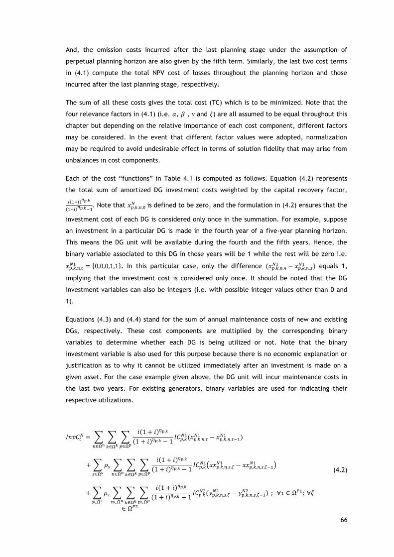
66

And, the emission costs incurred after the last planning stage under the assumption of

perpetual planning horizon are also given by the fifth term. Similarly, the last two cost terms

in (4.1) compute the total NPV cost of losses throughout the planning horizon and those

incurred after the last planning stage, respectively.

The sum of all these costs gives the total cost (TC) which is to be minimized. Note that the

four relevance factors in (4.1) (i.e. 𝛼, 𝛽 , γ and 𝜉) are all assumed to be equal throughout this

chapter but depending on the relative importance of each cost component, different factors

may be considered. In the event that different factor values were adopted, normalization

may be required to avoid undesirable effect in terms of solution fidelity that may arise from

unbalances in cost components.

Each of the cost “functions” in Table 4.1 is computed as follows. Equation (4.2) represents

the total sum of amortized DG investment costs weighted by the capital recovery factor,

𝑖(1+𝑖)𝜂𝑝,𝑘

(1+𝑖)𝜂𝑝,𝑘−1

. Note that 𝑥𝑝,𝑘,𝑛,0𝑁 is defined to be zero, and the formulation in (4.2) ensures that the

investment cost of each DG is considered only once in the summation. For example, suppose

an investment in a particular DG is made in the fourth year of a five-year planning horizon.

This means the DG unit will be available during the fourth and the fifth years. Hence, the

binary variable associated to this DG in those years will be 1 while the rest will be zero i.e.

𝑥𝑝,𝑘,𝑛,𝑡𝑁1 = 0,0,0,1,1. In this particular case, only the difference (𝑥𝑝,𝑘,𝑛,4

𝑁1 − 𝑥𝑝,𝑘,𝑛,3𝑁1 ) equals 1,

implying that the investment cost is considered only once. It should be noted that the DG

investment variables can also be integers (i.e. with possible integer values other than 0 and

1).

Equations (4.3) and (4.4) stand for the sum of annual maintenance costs of new and existing

DGs, respectively. These cost components are multiplied by the corresponding binary

variables to determine whether each DG is being utilized or not. Note that the binary

investment variable is also used for this purpose because there is no economic explanation or

justification as to why it cannot be utilized immediately after an investment is made on a

given asset. For the case example given above, the DG unit will incur maintenance costs in

the last two years. For existing generators, binary variables are used for indicating their

respective utilizations.

𝐼𝑛𝑣𝐶𝑡𝑁 = ∑ ∑ ∑

𝑖(1 + 𝑖)𝜂𝑝,𝑘


𝑁1(𝑥𝑝,𝑘,𝑛,𝜏𝑁1 − 𝑥𝑝,𝑘,𝑛,𝜏−1

𝑁1 )

𝑝∈Ω𝑝𝑘∈Ω𝑘𝑛∈Ω𝑛

+ ∑ 𝜌𝑠𝑠∈Ω𝑠

∑ ∑ ∑𝑖(1 + 𝑖)𝜂𝑝,𝑘


𝑁1(𝑥𝑥𝑝,𝑘,𝑛,𝑠,𝜁𝑁1 − 𝑥𝑥𝑝,𝑘,𝑛,𝑠,𝜁−1

𝑁1 )



∑ ∑ ∑𝑖(1 + 𝑖)𝜂𝑝,𝑘


𝑁2(𝑦𝑝,𝑘,𝑛,𝑠,𝜁𝑁2 − 𝑦𝑝,𝑘,𝑛,𝑠,𝜁−1

𝑁2 )


; ∀𝜏 ∈ Ω𝑃1; ∀휁

∈ Ω𝑃2

(4.2)

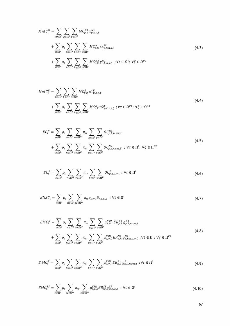
67

𝑀𝑛𝑡𝐶𝑡𝑁 = ∑ ∑ ∑ 𝑀𝐶𝑝,𝑘

𝑁1

𝑝∈Ω𝑝𝑘∈Ω𝑘

𝑥𝑝,𝑘,𝑛,𝑡𝑁1

𝑛∈Ω𝑛


∑ ∑ ∑ 𝑀𝐶𝑝,𝑘𝑁1


𝑥𝑥𝑝,𝑘,𝑛,𝑠,𝜁𝑁1

𝑛∈Ω𝑛


∑ ∑ ∑ 𝑀𝐶𝑝,𝑘𝑁2


𝑦𝑝,𝑘,𝑛,𝑠,𝜁𝑁2

𝑛∈Ω𝑛

; ∀𝑡 ∈ Ω𝑡; ∀휁 ∈ Ω𝑃2

(4.3)

𝑀𝑛𝑡𝐶𝑡𝐸 = ∑ ∑ ∑ 𝑀𝐶𝑝,𝑘

𝐸


𝑢1𝑝,𝑘,𝑛,𝜏𝐸

𝑛∈Ω𝑛


∑ ∑ ∑ 𝑀𝐶𝑝,𝑘𝐸


𝑢2𝑝,𝑘,𝑛,𝑠,𝜁𝐸

𝑛∈Ω𝑛

; ∀𝜏 ∈ Ω𝑃1; ∀휁 ∈ Ω𝑃2

(4.4)

𝐸𝐶𝑡𝑁 = ∑ 𝜌𝑠 ∑ ∑ 𝜋𝑤 ∑ ∑ 𝑂𝐶𝑝,𝑘,𝑛,𝑠,𝑤,𝜏

𝑁1

𝑝∈Ω𝑝𝑘∈Ω𝑘𝑤∈Ω𝑤𝑛∈Ω𝑛𝑠∈Ω𝑠

+ ∑ 𝜌𝑠 ∑ ∑ 𝜋𝑤 ∑ ∑ 𝑂𝐶𝑝,𝑘,𝑛,𝑠,𝑤,𝜁𝑁2


; ∀𝜏 ∈ Ω𝑡; ∀휁 ∈ Ω𝑃2

(4.5)

𝐸𝐶𝑡𝐸 = ∑ 𝜌𝑠 ∑ ∑ 𝜋𝑤 ∑ ∑ 𝑂𝐶𝑝,𝑘,𝑠,𝑤,𝑡

𝐸


; ∀𝑡 ∈ Ω𝑡 (4.6)

𝐸𝑁𝑆𝐶𝑡 = ∑ 𝜌𝑠 ∑ ∑ 𝜋𝑤𝜐𝑠,𝑤,𝑡𝛿𝑛,𝑠,𝑤,𝑡𝑤∈Ω𝑤𝑛∈Ω𝑛𝑠∈Ω𝑠

; ∀𝑡 ∈ Ω𝑡 (4.7)

𝐸𝑀𝐶𝑡𝑁 = ∑ 𝜌𝑠 ∑ ∑ 𝜋𝑤 ∑ ∑ 𝜇𝑠,𝑤,𝑡

𝐸𝑀𝐼

𝑝∈Ω𝑝

𝐸𝑅𝑝,𝑘𝑁1

𝑘∈Ω𝑘

𝑔𝑝,𝑘,𝑛,𝑠,𝑤,𝑡𝑁1

𝑤∈Ω𝑤𝑛∈Ω𝑛𝑠∈Ω𝑠

+ ∑ 𝜌𝑠 ∑ ∑ 𝜋𝑤 ∑ ∑ 𝜇𝑠,𝑤,𝜁𝐸𝑀𝐼

𝑝∈Ω𝑝

𝐸𝑅𝑝,𝑘𝑁2

𝑘∈Ω𝑘

𝑔𝑝,𝑘,𝑛,𝑠,𝑤,𝜁𝑁2


; ∀𝑡 ∈ Ω𝑡; ∀휁 ∈ Ω𝑃2

(4.8)

𝐸 𝑀𝐶𝑡𝐸 = ∑ 𝜌𝑠 ∑ ∑ 𝜋𝑤 ∑ ∑ 𝜇𝑠,𝑤,𝑡

𝐸𝑀𝐼

𝑝∈Ω𝑝

𝐸𝑅𝑝,𝑘𝐸

𝑘∈Ω𝑘



; ∀𝑡 ∈ Ω𝑡 (4.9)

𝐸𝑀𝐶𝑡𝑆𝑆 = ∑ 𝜌𝑠 ∑ 𝜋𝑤 ∑ 𝜇𝑠,𝑤,𝑡

𝐸𝑀𝐼 𝐸𝑅𝑠𝑠𝑆𝑆𝑔𝑠𝑠,𝑠,𝑤,𝑡

𝑆𝑆

𝑠𝑠∈Ω𝑠𝑠𝑤∈Ω𝑤𝑠∈Ω𝑠

; ∀𝑡 ∈ Ω𝑡 (4.10)

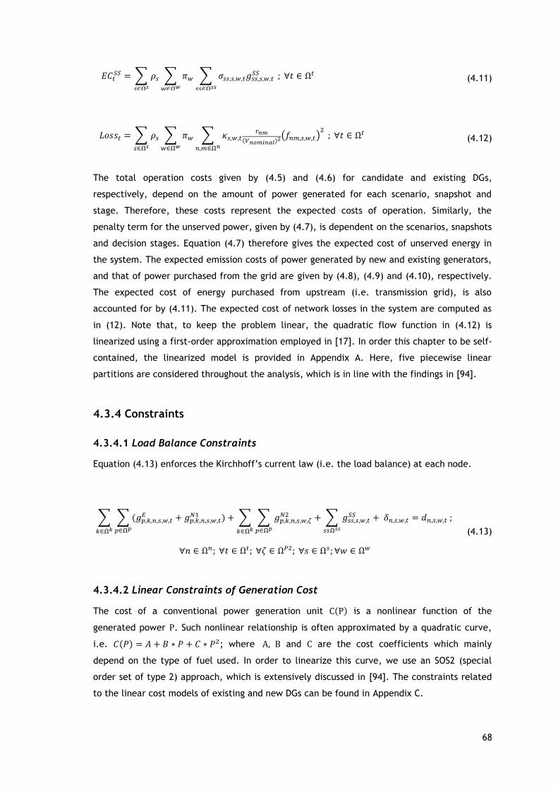
68

𝐸𝐶𝑡𝑆𝑆 = ∑ 𝜌𝑠 ∑ 𝜋𝑤 ∑ 𝜎𝑠𝑠,𝑠,𝑤,𝑡𝑔𝑠𝑠,𝑠,𝑤,𝑡

𝑆𝑆

𝑠𝑠∈Ω𝑠𝑠𝑤∈Ω𝑤𝑠∈Ω𝑠

; ∀𝑡 ∈ Ω𝑡 (4.11)

𝐿𝑜𝑠𝑠𝑡 = ∑ 𝜌𝑠 ∑ 𝜋𝑤 ∑ 𝜅𝑠,𝑤,𝑡𝑟𝑛𝑚

(𝑉𝑛𝑜𝑚𝑖𝑛𝑎𝑙)2(𝑓𝑛𝑚,𝑠,𝑤,𝑡)

2

𝑛,𝑚∈Ω𝑛𝑤∈Ω𝑤𝑠∈Ω𝑠

; ∀𝑡 ∈ Ω𝑡 (4.12)

The total operation costs given by (4.5) and (4.6) for candidate and existing DGs,

respectively, depend on the amount of power generated for each scenario, snapshot and

stage. Therefore, these costs represent the expected costs of operation. Similarly, the

penalty term for the unserved power, given by (4.7), is dependent on the scenarios, snapshots

and decision stages. Equation (4.7) therefore gives the expected cost of unserved energy in

the system. The expected emission costs of power generated by new and existing generators,

and that of power purchased from the grid are given by (4.8), (4.9) and (4.10), respectively.

The expected cost of energy purchased from upstream (i.e. transmission grid), is also

accounted for by (4.11). The expected cost of network losses in the system are computed as

in (12). Note that, to keep the problem linear, the quadratic flow function in (4.12) is

linearized using a first-order approximation employed in [17]. In order this chapter to be self-

contained, the linearized model is provided in Appendix A. Here, five piecewise linear

partitions are considered throughout the analysis, which is in line with the findings in [94].

4.3.4 Constraints

4.3.4.1 Load Balance Constraints

Equation (4.13) enforces the Kirchhoff’s current law (i.e. the load balance) at each node.

∑ ∑ (𝑔𝑝,𝑘,𝑛,𝑠,𝑤,𝑡𝐸


+ 𝑔𝑝,𝑘,𝑛,𝑠,𝑤,𝑡𝑁1 ) + ∑ ∑ 𝑔𝑝,𝑘,𝑛,𝑠,𝑤,𝜁

𝑁2


+ ∑ 𝑔𝑠𝑠,𝑠,𝑤,𝑡𝑆𝑆

𝑠𝑠Ω𝑠𝑠

+ 𝛿𝑛,𝑠,𝑤,𝑡 = 𝑑𝑛,𝑠,𝑤,𝑡 ;

∀𝑛 ∈ Ω𝑛; ∀𝑡 ∈ Ω𝑡; ∀휁 ∈ Ω𝑃2; ∀𝑠 ∈ Ω𝑠; ∀𝑤 ∈ Ω𝑤

(4.13)

4.3.4.2 Linear Constraints of Generation Cost

The cost of a conventional power generation unit C(P) is a nonlinear function of the

generated power P. Such nonlinear relationship is often approximated by a quadratic curve,

i.e. 𝐶(𝑃) = 𝐴 + 𝐵 ∗ 𝑃 + 𝐶 ∗ 𝑃2; where A, B and C are the cost coefficients which mainly

depend on the type of fuel used. In order to linearize this curve, we use an SOS2 (special

order set of type 2) approach, which is extensively discussed in [94]. The constraints related

to the linear cost models of existing and new DGs can be found in Appendix C.

69

4.3.4.3 Investment Limits

A budget constraint for investing in DGs is enforced by adding constraint (4.14) for the first

period and (4.15) for the second one.

∑ ∑ ∑ 𝐼𝐶𝑝,𝑘𝑁1(𝑥𝑝,𝑘,𝑛,𝜏

𝑁1


− 𝑥𝑝,𝑘,𝑛,𝜏−1𝑁1 )

𝑛∈Ω𝑛

≤ 𝐼𝑛𝑣𝐿𝑖𝑚𝜏 ; ∀𝜏 ∈ Ω𝑃1 (4.14)

∑ ∑ ∑ 𝐼𝐶𝑝,𝑘𝑁1(𝑦𝑝,𝑘,𝑛,𝑠,𝜁

𝑁2


− 𝑦𝑝,𝑘,𝑛,𝑠,𝜁−1𝑁2 )

𝑛∈Ω𝑛

+ ∑ ∑ ∑ 𝐼𝐶𝑝,𝑘𝑁1(𝑥𝑥𝑝,𝑘,𝑛,𝑠,𝜁

𝑁1


− 𝑥𝑥𝑝,𝑘,𝑛,𝑠,𝜁−1𝑁1 )

𝑛∈Ω𝑛

≤ 𝐼𝑛𝑣𝐿𝑖𝑚𝑠,𝜁 ; ∀휁 ∈ Ω𝑃2; ∀𝑠 ∈ Ω𝑠

(4.15)

4.3.4.4 Generation Capacity Limits

The capacity limits of existing generators in the first and the second periods are given by (16)

and (4.17), respectively. In the case of candidate generators, the corresponding constraints

are (4.18)—(4.20). Note that the binary variable associated to a given generator multiplies the

corresponding generation limits. This is to make sure that the power generation variable is

zero when the generator remains either unutilized or unselected for investment.

𝑢1𝑝,𝑘,𝑛,𝜏𝐸 𝐺𝑚𝑖𝑛𝑝,𝑘,𝑠,𝑤

𝐸 ≤ 𝑔𝑝,𝑘,𝑛,𝑠,𝑤,𝜏𝐸 ≤ 𝑢1𝑝,𝑘,𝑛,𝜏

𝐸 𝐺𝑚𝑎𝑥𝑝,𝑘,𝑠,𝑤𝐸 ;

∀𝑛 ∈ Ω𝑛; ∀𝜏 ∈ Ω𝑃1; ∀𝑠 ∈ Ω𝑠; ∀𝑤 ∈ Ω𝑤; ∀𝑘 ∈ Ω𝑘 ; ∀𝑝 ∈ Ω𝑝

(4.16)

𝑢2𝑝,𝑘,𝑛,𝜁𝐸 𝐺𝑚𝑖𝑛𝑝,𝑘,𝑠,𝑤

𝐸 ≤ 𝑔𝑝,𝑘,𝑛,𝑠,𝑤,𝜁𝐸 ≤ 𝑢2𝑝,𝑘,𝑛,𝜁

𝐸 𝐺𝑚𝑎𝑥𝑝,𝑘,𝑠,𝑤𝐸 ;

∀𝑛 ∈ Ω𝑛; ∀휁 ∈ Ω𝑃2; ∀𝑠 ∈ Ω𝑠; ∀𝑤 ∈ Ω𝑤; ∀𝑘 ∈ Ω𝑘; ∀𝑝 ∈ Ω𝑝

(4.17)

𝑥𝑝,𝑘,𝑛,𝑡𝑁1 𝐺𝑚𝑖𝑛𝑝,𝑘,𝑠,𝑤

𝑁1 ≤ 𝑔𝑝,𝑘,𝑛,𝑠,𝑤,𝑡𝑁1 ≤ 𝑥𝑝,𝑘,𝑛,𝑡

𝑁1 𝐺𝑚𝑎𝑥𝑝,𝑘,𝑠,𝑤𝑁1 ;

∀𝑛 ∈ Ω𝑛; ∀𝑡 ∈ Ω𝑃1; ∀𝑠 ∈ Ω𝑠; ∀𝑤 ∈ Ω𝑤; ∀𝑘 ∈ Ω𝑘; ∀𝑝 ∈ Ω𝑝

(4.18)

𝑥𝑥𝑝,𝑘,𝑛,𝑠,𝜁𝑁1 𝐺𝑚𝑖𝑛𝑝,𝑘,𝑠,𝑤

𝑁1 ≤ 𝑔𝑝,𝑘,𝑛,𝑠,𝑤,𝜁𝑁1 ≤ 𝑥𝑥𝑝,𝑘,𝑛,𝑠,𝜁



(4.19)

70

𝑦𝑝,𝑘,𝑛,𝑠,𝜁𝑁2 𝐺𝑚𝑖𝑛𝑝,𝑘,𝑠,𝑤

𝑁2 ≤ 𝑔𝑝,𝑘,𝑛,𝑠,𝑤,𝜁𝑁2 ≤ 𝑦𝑝,𝑘,𝑛,𝑠,𝜁



(4.20)

It should be noted that the above constraints are in generalized forms because the upper

and the lower limits are scenario and snapshot dependent. These constraints need to

otherwise be different for different types of DGs. For instance, for conventional DGs, both

the upper and the lower power generation limits are often fixed; they do not usually vary

with the yearly scenarios or hourly snapshots. However, this is different in the case of

intermittent generators such as solar and wind types, whose upper bounds are determined by

the availability of the primary energy sources (solar radiation and wind speed, in this case)

while the lower bounds are often set to zero.

4.3.4.5 Unserved Power Limit

The unserved power at any given node cannot exceed the demand at that node, and this is

enforced by:

0 ≤ 𝛿𝑛,𝑠,𝑤,𝑡 ≤ 𝑑𝑛,𝑠,𝑤,𝑡 ;

∀𝑛 ∈ Ω𝑛; ∀𝑡 ∈ Ω𝑡; ∀𝑠 ∈ Ω𝑠; ∀𝑤 ∈ Ω𝑤

(4.21)

4.3.4.6 DG Penetration Limit

It has been stated earlier that DG integration may in some cases negatively influence

stability, power quality and security of distribution systems. In order to alleviate such

technical problems, the penetration level of DG power is often limited. This is enforced by

adding the constraints in (4.22). This constraint ensures that the total power generated by

existing and new DGs at any operation time should be less than a certain percentage of the

demand at the same time. Note that the second term in (4.22) is considered in the

summation only when t > 𝑇1.

∑ ∑ ∑(

𝑘∈𝛺𝑘𝑝∈𝛺𝑝

𝑔𝑝,𝑘,𝑛,𝑠,𝑤,𝑡𝐸 + 𝑔𝑝,𝑘,𝑛,𝑠,𝑤,𝑡

𝑁1 )

𝑛∈Ω𝑛

+ ∑ ∑ ∑ 𝑔𝑝,𝑘,𝑛,𝑠,𝑤,𝜁𝑁2

𝑘∈𝛺𝑘𝑝∈𝛺𝑝𝑛∈Ω𝑛

≤ 𝜑𝐷𝑠,𝑤,𝑡

; ∀𝑡 ∈ Ω𝑡; ∀휁 ∈ Ω𝑃2; ∀𝑠 ∈ Ω𝑠; ∀𝑤 ∈ Ω𝑤; ∀𝑘 ∈ Ω𝑘; ∀𝑝 ∈ Ω𝑝

(4.22)

71


The set of constraints in (4.23)—(4.28) ensure that an investment made at decision stage t

cannot be reversed or divested in the subsequent stages; instead, the asset should be

available for utilization immediately after the investment is made. The logical constraints in

(4.23) guarantee that investment decisions made at a given stage in the first period are

available in the immediate stages in the first stage.

𝑥𝑝,𝑘,𝑛,𝜏𝑁1 ≥ 𝑥𝑝,𝑘,𝑛,𝜏−1

𝑁1 ;

∀𝑛 ∈ Ω𝑛; ∀𝜏 ∈ Ω𝑃1; ∀𝑘 ∈ Ω𝑘; ∀𝑝 ∈ Ω𝑝 (4.23)

𝑥𝑝,𝑘,𝑛,𝜁𝑁1 = 𝑥𝑝,𝑘,𝑛,𝑇1

𝑁1 ;

∀𝑛 ∈ Ω𝑛; ∀휁 ∈ Ω𝑃2; ∀𝑘 ∈ Ω𝑘; ∀𝑝 ∈ Ω𝑝

(4.24)

𝑥𝑥𝑝,𝑘,𝑛,𝑠,𝜁𝑁1 ≥ 𝑥𝑥𝑝,𝑘,𝑛,𝑠,𝜁−1

𝑁1 ;

∀𝑛 ∈ Ω𝑛; ∀휁 ∈ Ω𝑃2; ∀𝑠 ∈ Ω𝑠; ∀𝑘 ∈ Ω𝑘 ; ∀𝑝 ∈ Ω𝑝 (4.25)

𝑥𝑥𝑝,𝑘,𝑛,𝑠,𝑇1𝑁1 = 𝑥𝑝,𝑘,𝑛,𝑇1

𝑁1 ;

∀𝑛 ∈ Ω𝑛; ∀𝑠 ∈ Ω𝑠; ∀𝑘 ∈ Ω𝑘; ∀𝑝 ∈ Ω𝑝

(4.26)

𝑦𝑝,𝑘,𝑛,𝑠,𝜁𝑁2 ≥ 𝑦𝑝,𝑘,𝑛,𝑠,𝜁−1

𝑁2 ;

∀𝑛 ∈ Ω𝑛; ∀휁 ∈ Ω𝑃2; ∀𝑠 ∈ Ω𝑠; ∀𝑘 ∈ Ω𝑘; ∀𝑝 ∈ Ω𝑝; ∀𝑛 ∈ Ω𝑛

(4.27)

𝑦𝑝,𝑘,𝑛,𝑠,𝑇1𝑁2 = 0 ;

∀𝑛 ∈ Ω𝑛; ∀𝑠 ∈ Ω𝑠; ∀𝑘 ∈ Ω𝑘; ∀𝑝 ∈ Ω𝑝 (4.28)

4.3.4.8 Network Model Constraints

The active power flow through each line in the network is represented by a linearized AC

network model, first proposed in [95] in the context of transmission expansion planning and

further extended to distribution network system planning in [96].

Modeling both active and reactive power flows is the most elegant approach. The importance

of reactive power in a system is unquestionable. However, unlike active power, it is widely

accepted that reactive power “does not travel very far”; it can be produced (compensated)

locally.

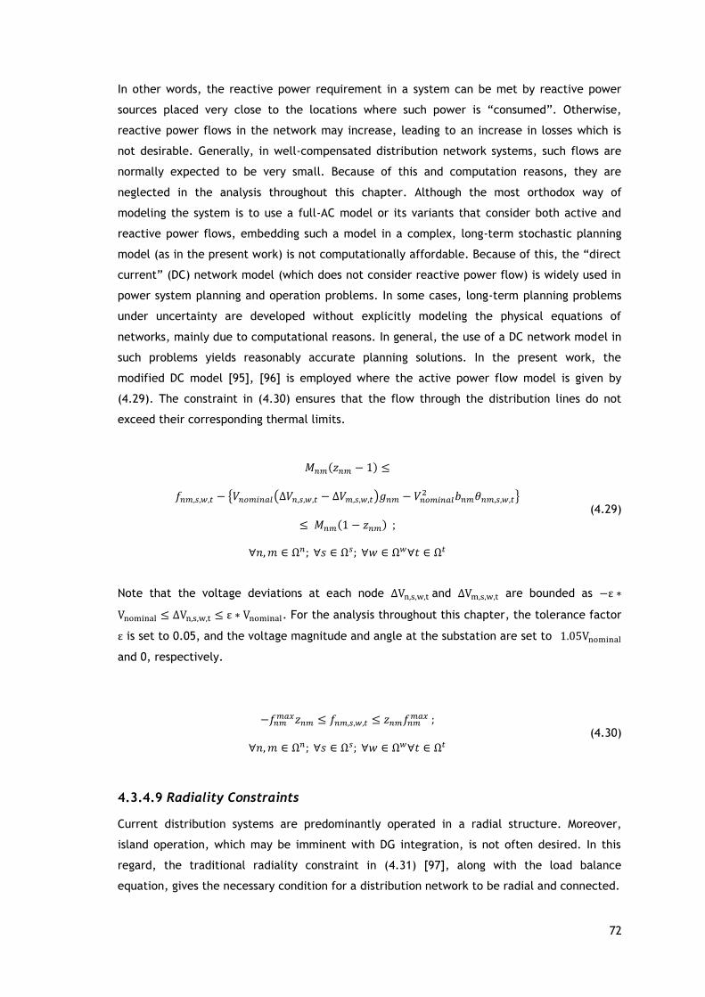
72

In other words, the reactive power requirement in a system can be met by reactive power

sources placed very close to the locations where such power is “consumed”. Otherwise,

reactive power flows in the network may increase, leading to an increase in losses which is

not desirable. Generally, in well-compensated distribution network systems, such flows are

normally expected to be very small. Because of this and computation reasons, they are

neglected in the analysis throughout this chapter. Although the most orthodox way of

modeling the system is to use a full-AC model or its variants that consider both active and

reactive power flows, embedding such a model in a complex, long-term stochastic planning

model (as in the present work) is not computationally affordable. Because of this, the “direct

current” (DC) network model (which does not consider reactive power flow) is widely used in

power system planning and operation problems. In some cases, long-term planning problems

under uncertainty are developed without explicitly modeling the physical equations of

networks, mainly due to computational reasons. In general, the use of a DC network model in

such problems yields reasonably accurate planning solutions. In the present work, the

modified DC model [95], [96] is employed where the active power flow model is given by

(4.29). The constraint in (4.30) ensures that the flow through the distribution lines do not

exceed their corresponding thermal limits.

𝑀𝑛𝑚(𝑧𝑛𝑚 − 1) ≤

𝑓𝑛𝑚,𝑠,𝑤,𝑡 − 𝑉𝑛𝑜𝑚𝑖𝑛𝑎𝑙(∆𝑉𝑛,𝑠,𝑤,𝑡 − ∆𝑉𝑚,𝑠,𝑤,𝑡)𝑔𝑛𝑚 − 𝑉𝑛𝑜𝑚𝑖𝑛𝑎𝑙2 𝑏𝑛𝑚휃𝑛𝑚,𝑠,𝑤,𝑡

≤ 𝑀𝑛𝑚(1 − 𝑧𝑛𝑚) ;

∀𝑛,𝑚 ∈ Ω𝑛; ∀𝑠 ∈ Ω𝑠; ∀𝑤 ∈ Ω𝑤∀𝑡 ∈ Ω𝑡

(4.29)

Note that the voltage deviations at each node ∆Vn,s,w,t and ∆Vm,s,w,t are bounded as −ε ∗

Vnominal ≤ ∆Vn,s,w,t ≤ ε ∗ Vnominal. For the analysis throughout this chapter, the tolerance factor

ε is set to 0.05, and the voltage magnitude and angle at the substation are set to 1.05Vnominal

and 0, respectively.

−𝑓𝑛𝑚𝑚𝑎𝑥𝑧𝑛𝑚 ≤ 𝑓𝑛𝑚,𝑠,𝑤,𝑡 ≤ 𝑧𝑛𝑚𝑓𝑛𝑚

𝑚𝑎𝑥 ;

∀𝑛,𝑚 ∈ Ω𝑛; ∀𝑠 ∈ Ω𝑠; ∀𝑤 ∈ Ω𝑤∀𝑡 ∈ Ω𝑡

(4.30)


Current distribution systems are predominantly operated in a radial structure. Moreover,

island operation, which may be imminent with DG integration, is not often desired. In this

regard, the traditional radiality constraint in (4.31) [97], along with the load balance

equation, gives the necessary condition for a distribution network to be radial and connected.

73

However, this constraint alone is not sufficient to fulfill the aforementioned requirements

(i.e. to keep radiality and all nodes connected) particularly in planning problems involving

grid expansion, switching and integration of DGs or reactive power sources [106]. Additional

constraints as in [97] needs to be incorporated to guarantee that all nodes in the system are

connected. However, this is out of the scope of this thesis, and will be addressed in future

works considering grid expansion and switching.

The work in this chapter considers a radial network. Therefore, for this case, Equation (4.31)

is sufficient to keep the radiality of the network and ensure that all nodes are connected.

∑ 𝑧𝑛𝑚𝑛,𝑚∈𝛺𝑛 = 𝑁𝑛 − 𝑁𝑆𝑆 ;

∀(𝑛,𝑚) ∈ Ω𝑐

(4.31)

4.4 Case Studies

4.4.1 System Data and Assumptions

The system considered in the study is a real-life distribution network in São Miguel Island,

Portugal. The system has a peak demand of 70.2 MW, and info about existing generators is

shown in Table 4.2.

In this system, various DG types with capacities ranging from 1 to 30 MW are considered as

candidates for investment (see Table 4.3). These fall into small to medium-scale DG

categories according to the capacity-based classification of DGs in [98]. The installation and

maintenance costs of each DG are either directly obtained from [98] and [99] or estimated

using the so-called six-tenths rule [100], which establishes a relationship between cost and

quantity (in this case, the installed capacity). This method reflects the economy of scale that

exists in DGIP i.e. the higher the installed capacities of DGs of the same type are, the lower

the costs per installed kW get.

Table 4.2 – Data for existing generators

No. Generator type,

p

Alternative,

k

Installed

capacity

(MW)

OCp,k

(€/MWh)

ICp,k

(M€)

MCp,k

(M€)

ERp,k

(tons/MWh)

1 Hydro Hydro 4.07 7.0 NA 0.38 0.0121

2 Geothermal GEOT 24.0 5.0 NA 1.20 0.0165

3 HFO-T* HFO 98.0 145.4 NA 0.01 0.5600

4 Wind WD 0 10.0 17.0 NA 0.80 0.0276

* Heavy fuel oil turbine, NA = Not applicable

74

Table 4.3 – Data for candidate generators

No. DG type, p DG

alternative

k

Installed capacity

[MW]

OCp,k

[€/MWh]

ICp,k

[M€]

MCp,k

[M€]

ERp,k

[tons/

MWh]

1 Solar PV 1 1.0 40 3.00 0.06 0.0584

2 Solar PV 2 1.5 40 3.83 0.08 0.0584

3 Solar PV 3 2.0 40 4.55 0.09 0.0584

4 Solar PV 4 2.5 40 5.20 0.10 0.0584

5 Solar PV 5 3.0 40 5.80 0.12 0.0584

6 Solar PV 6 4.0 40 6.89 0.14 0.0584

7 Solar PV 7 6.0 40 8.79 0.17 0.0584

8 Solar PV 8 10 40 11.94 0.24 0.0584

9 Wind WD 1 1.0 17 2.64 0.05 0.0276

10 Wind WD 2 2.0 17 4.00 0.08 0.0276

11 Wind WD 3 5.0 17 6.93 0.14 0.0276

12 Wind WD 4 10 17 10.51 0.21 0.0276

13 CGT* CGT 1 30 145.4 27.00 0.01 0.5600

14 BM** BM 1 20 20 80.00 3.00 0.0900

* Combustion gas turbine; ** Biomass

The hourly series (historical data) of wind speed and solar radiation at various locations of the

island are obtained from publicly available databases [101], [102], respectively.

The geographical coordinates where these data are taken from include (37.790,-25.385),

(37.778,-25.489), (37.866,-25.816), (37.797,-25.170), (37.717,-25.505), (37.823,-25.487),

(37.772,-25.375) and (37.782,-25.661). Then, the wind (WD) and solar photovoltaic (PV)

power production series, used in the simulations, are determined by plugging in the wind

speed and radiation data in the corresponding power curve expressions. Note that two wind-

speed regimes (offshore and onshore) are considered in the case study.

4.4.2 Scenario Definition

In this chapter, the uncertainty introduced by four most relevant uncertain parameters

namely, electricity demand growth, emission price, wind and solar PV power output is taken

into consideration. In other words, the evolutions of emission price, electricity demand

growth as well as uncertainty due to intermittent energy sources (solar PV and wind, in

particular) are captured through a predefined number of scenarios, each with a certain

probability. The demand growth for a certain year can be somehow estimated via forecasting

tools but this introduces some uncertainty due to the forecasting error. As illustrated in

Figure 4.3, this leads to a confidence interval in which the demand profile is likely to lie.

Similarly, the confidence intervals of wind and solar power outputs are formed, as shown in

Figure 4.4. And, for the analysis in this work, three demand growth scenarios are considered

corresponding to the middle, top and bottom curves which form the band in Figure 4.3.

In a similar manner, the wind and solar power output scenarios are defined.

75

Figure 4.3 - A sample demand profile for day 11 in the second stage (i.e. τ = 2) of the first period, reflecting demand growth uncertainty.

Figure 4.4 - Wind and solar PV power output uncertainty characterization example.

The following assumptions are made for the case study:

Discount rate is set to 7% and kept the same throughout the planning horizon.

DG penetration limit factor is assumed to be 40%.

The lifetime of all DGs is considered to be 20 years.

In order to take account of the variability introduced by electricity demand, solar PV

and wind power sources, an initial set of 8760 snapshots (either historical data,

obtained using forecasting tools or generated via Monte Carlo methods), corresponding

to the hourly operational situations in a single year, is assumed to be available.

An ordinary clustering methodology (k-means algorithm) is employed to reduce these

snapshots to 300 representative ones (see in the following subsection how this is

decided).

76

For the sake of simplicity, the same candidate DG pools are considered in the first and

the second periods.

Investment decisions in the first period can be postponed to the second period, if

deemed economical.

The planning horizon is considered to be 8 years, in which the length of the first period

is three years.

The cost coefficients (𝐴, 𝐵 and 𝐶) of the conventional generation units are assumed to

be 0.74 €/h, 35 €/MWh and 550 €/h/(MW)2. For the RES-based generation units, 𝐴

and 𝐶 are both zero while 𝐵 is set equal to 𝑂𝐶𝑝,𝑘 in Table 4.3.

The cost of unserved energy is assumed to be 3000 €/MWh.

In general, a total of 81 scenarios (storylines) are defined in connection to the possible

evolutions of the aforementioned parameters over the planning horizon. Table 4.4 shows the

three evolutions of demand growth, denoted as Low, Moderate and High, having equal degree

of realization. To further illustrate this, hourly demand profiles of a sample day in the second

stage, corresponding to the three demand growth scenarios, are shown in Fig. 4.3. Similarly,

the emission price is represented by three equally probable storylines (scenarios), as shown in

Table 4.4. Wind and solar PV power output uncertainties are also represented by three

equiprobable scenarios as explained above. Given these individual scenarios, assuming all

uncertain parameters are independent, 81 different combinations are obtained, which form

the new set of scenarios used in the simulations.


The formulated DGIP problem is coded in GAMS 24.0, and solved using CPLEX 12.0. The

optimality gap is set to zero in all cases. All simulations are carried out in an HP Z820

Workstation having E5-2687W processor with two cores, clocking at 3.1GHz speed.

Table 4.4 – Demand growth and emissions scenarios

Stage Demand growth scenarios

Emission price scenarios

(€/tons)

Low Moderate High Low Moderate High

τ=0 0.0% 0% 0% 7 7 7

τ=1 2.0% 5% 10% 9 12 20

τ=2 5.0% 10% 20% 12 18 30

τ=3 7.0% 15% 30% 16 25 45

ζ=4 9.0% 20% 40% 20 30 50

ζ=5 11.0% 25% 50% 20 30 50

ζ=6 13.0% 30% 60% 20 30 50

ζ=7 14.5% 35% 70% 20 30 50

ζ=8 16.0% 40% 80% 20 30 50

77

4.4.3.1 Deciding the number of representative clusters

It has already been stated earlier that the large number of snapshots (operational situations)

should be reduced to ensure problem tractability. This is accomplished by clustering the large

initial set of snapshots. The minimum number of clusters, which sufficiently balances

accuracy and computational burden, is often decided by trial and error. A famous rule of

thumb in this case is the “Elbow” method, which is commonly used in clustering analysis. This

method simply approximates the minimum number of clusters by plotting the objective value

of the clustering algorithm for different number of clusters. Instead of using the objective

value of the algorithm, the values of certain system variables, namely, investment and total

costs, expected emissions and simulation time are used here. We analyze the impact of

reducing the snapshots on these system variables.

The analysis results are summarized in Table 4.5. For the sake of clarity, Figure 4.5 also plots

the computational time and investment cost against the number of clusters. It is evident to

see that the higher the number of clusters is, the more accurately the aforementioned

variables are optimized but the higher the computational requirement is.

Table 4.5 – Impact of snapshot reduction on system variables

Number of

clusters Total investment

cost (M€)

Total cost

(M€)

CPU time

(h)

Expected emissions (tons)

Period 1 Period 2 Entire

horizon

100 70.01 468.40 0.20 293142 877712 877712

200 69.93 469.67 0.58 294279 882015 882015

300 69.74 470.41 1.50 295122 885118 885118

400 69.58 470.79 3.87 295530 887225 887225

500 69.55 471.10 6.50 295935 888015 888015

1000 69.53 472.25 25.50 297215 892531 892531

Figure 4.5 – Effect of snapshot reduction on the investment cost.

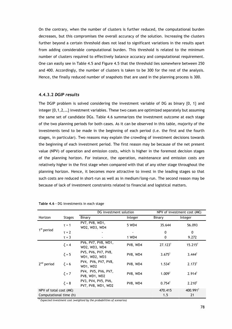
78

On the contrary, when the number of clusters is further reduced, the computational burden

decreases, but this compromises the overall accuracy of the solution. Increasing the clusters

further beyond a certain threshold does not lead to significant variations in the results apart

from adding considerable computational burden. This threshold is related to the minimum

number of clusters required to effectively balance accuracy and computational requirement.

One can easily see in Table 4.5 and Figure 4.5 that the threshold lies somewhere between 250

and 400. Accordingly, the number of clusters is taken to be 300 for the rest of the analysis.

Hence, the finally reduced number of snapshots that are used in the planning process is 300.

4.4.3.2 DGIP results

The DGIP problem is solved considering the investment variable of DG as binary 0, 1 and

integer 0, 1, 2, … investment variables. These two cases are optimized separately but assuming

the same set of candidate DGs. Table 4.6 summarizes the investment outcome at each stage

of the two planning periods for both cases. As it can be observed in this table, majority of the

investments tend to be made in the beginning of each period (i.e. the first and the fourth

stages, in particular). Two reasons may explain the crowding of investment decisions towards

the beginning of each investment period. The first reason may be because of the net present

value (NPV) of operation and emission costs, which is higher in the foremost decision stages

of the planning horizon. For instance, the operation, maintenance and emission costs are

relatively higher in the first stage when compared with that of any other stage throughout the

planning horizon. Hence, it becomes more attractive to invest in the leading stages so that

such costs are reduced in short-run as well as in medium/long-run. The second reason may be

because of lack of investment constraints related to financial and logistical matters.

Table 4.6 – DG investments in each stage

Horizon Stages

DG investment solution NPV of investment cost (M€)

Binary Integer Binary Integer

1st period

τ = 1 PV7, PV8, WD1,

WD2, WD3, WD4 5 WD4 35.644 56.093

τ = 2 - - 0 0

τ = 3 - 1 WD4 0 9.272

2nd period

ζ = 4 PV6, PV7, PV8, WD1,

WD2, WD3, WD4 PV8, WD4 27.123† 15.215†

ζ = 5 PV5, PV6, PV7, PV8,

WD1, WD2, WD3 PV8, WD4 3.675† 3.444†

ζ = 6 PV4, PV6, PV7, PV8,

WD1, WD2 PV8, WD4 1.534† 2.173†

ζ = 7 PV4, PV5, PV6, PV7,

PV8, WD1, WD2 PV8, WD4 1.009† 2.914†

ζ = 8 PV3, PV4, PV5, PV6,

PV7, PV8, WD1, WD2 PV8, WD4 0.754† 2.210†

NPV of total cost (M€) 470.415 400.991†

Computational time (h) 1.5 21 † Expected investment cost (weighted by the probabilities of scenarios)

79

Figure 4.6 – Evolution of emissions over the planning stages.

In line with the investments made, the evolution of expected emissions over the entire

planning horizon also follows a predictable trend. For instance, because of the huge

investments in stage 1, the expected (average) emissions are significantly reduced, and a

similar phenomenon can be observed in stage 4. Apart from these two stages, emissions tend

to slightly increase. Such increase in emissions can be explained by the increasing trend of

demand because, in the absence of more investments in RESs, conventional generators should

generate more to meet the increasing demand. However, as illustrated in Figure 4.6, the

average emissions curve remains far below that of the “do-nothing” scenario, where no

investments are assumed to be made. Table 4.6 clearly shows the differences between the

binary and the integer solutions. The overall impact of each solution on the expected

emissions is also illustrated in Figure 4.6. One can infer from Table 4.6 that the model based

on integer variables better exploits the benefits of economy of scale as there is a tendency of

avoiding investment in DGs with low capacities. As shown in this table, the integer investment

solution only encompasses multiples of WD4 in the first period, and WD4 and PV8 in the

second period. Even if this means higher investment cost, the overall/total cost is found out

to be about 15% lower than that of the model with binary ones. In addition, when using the

integer-based model, the overall reduction in emissions is higher than when using the binary-

based model, as illustrated in Figure 4.6. However, it is worth mentioning here that solving

the general integer-based model is much harder (about 14 times according to the results in

Table 4.6) than the binary-based one.

4.4.3.3 The significance of the proposed models

The importance of planning under uncertainty i.e. the significance of the proposed stochastic

model can be shown by comparing decisions made under uncertainty and by ignoring

uncertainty. Also, relevant metrics can be used to quantify the importance of uncertainty and

demonstrate the practicality of the stochastic model. Here, we employ two metrics, expected

value of perfect information (EVPI) and expected cost of ignoring uncertainty (ECIU), which

are commonly used in stochastic programming applications for similar purposes.

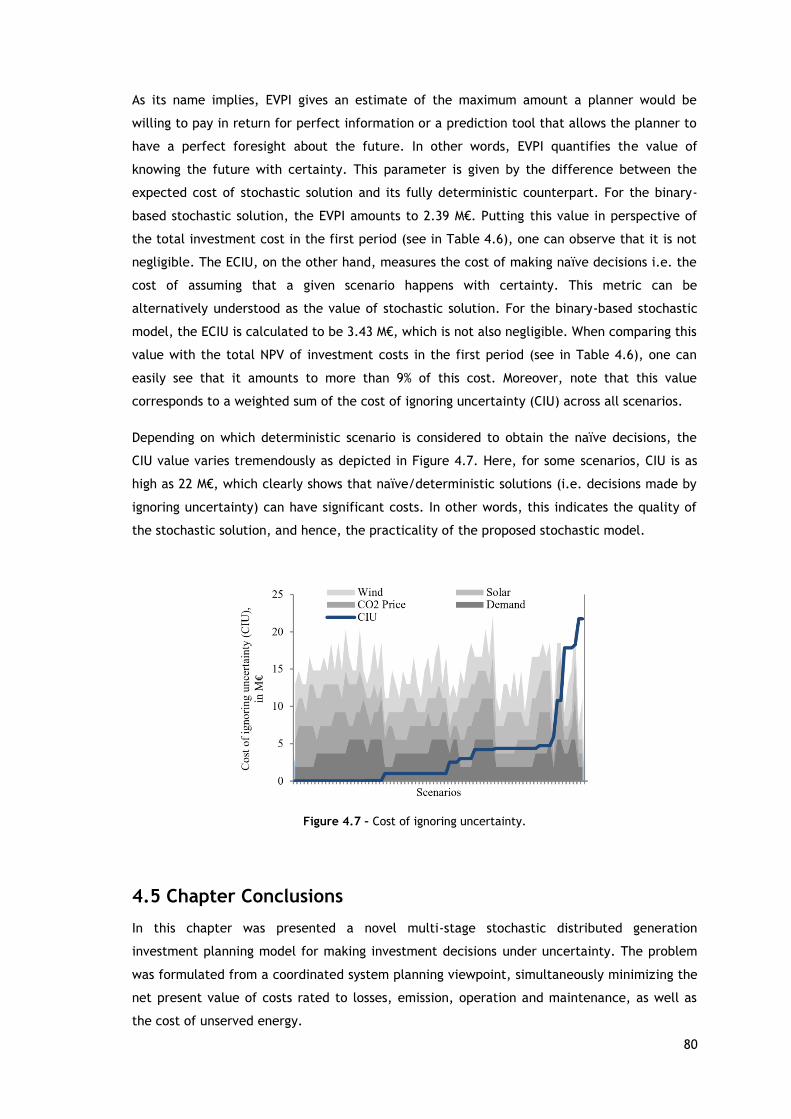
80

As its name implies, EVPI gives an estimate of the maximum amount a planner would be

willing to pay in return for perfect information or a prediction tool that allows the planner to

have a perfect foresight about the future. In other words, EVPI quantifies the value of

knowing the future with certainty. This parameter is given by the difference between the

expected cost of stochastic solution and its fully deterministic counterpart. For the binary-

based stochastic solution, the EVPI amounts to 2.39 M€. Putting this value in perspective of

the total investment cost in the first period (see in Table 4.6), one can observe that it is not

negligible. The ECIU, on the other hand, measures the cost of making naïve decisions i.e. the

cost of assuming that a given scenario happens with certainty. This metric can be

alternatively understood as the value of stochastic solution. For the binary-based stochastic

model, the ECIU is calculated to be 3.43 M€, which is not also negligible. When comparing this

value with the total NPV of investment costs in the first period (see in Table 4.6), one can

easily see that it amounts to more than 9% of this cost. Moreover, note that this value

corresponds to a weighted sum of the cost of ignoring uncertainty (CIU) across all scenarios.

Depending on which deterministic scenario is considered to obtain the naïve decisions, the

CIU value varies tremendously as depicted in Figure 4.7. Here, for some scenarios, CIU is as

high as 22 M€, which clearly shows that naïve/deterministic solutions (i.e. decisions made by

ignoring uncertainty) can have significant costs. In other words, this indicates the quality of

the stochastic solution, and hence, the practicality of the proposed stochastic model.

Figure 4.7 – Cost of ignoring uncertainty.


In this chapter was presented a novel multi-stage stochastic distributed generation

investment planning model for making investment decisions under uncertainty. The problem

was formulated from a coordinated system planning viewpoint, simultaneously minimizing the

net present value of costs rated to losses, emission, operation and maintenance, as well as

the cost of unserved energy.

81

The formulation was anchored on a two-period planning horizon, each having multiple stages.

The first period was a short-term horizon in which robust decisions were pursued in the face

of uncertainty; whereas, the second one spans over a medium to long-term horizon involving

exploratory and/or flexible investment decisions. The operational variability and uncertainty

introduced by intermittent generation sources, electricity demand, emission prices, demand

growth and others were accounted for via probabilistic and stochastic methods, respectively.

Metrics such as cost of ignoring uncertainty and value of perfect information were used to

clearly demonstrate the benefits of the proposed stochastic model. A real-life distribution

network system was used as a case study, and the results showed the effectiveness of the

proposed model.

82

Chapter 5

Impacts of Optimal Energy Storage Deployment and

Network Reconfiguration on Renewable Integration

Level in Distribution System

This chapter is based on the previous chapter but gives a step ahead by adding network

switching to the problem and a novel mechanism to quantify the impacts of network

switching and/or reinforcement as well as deployment of ESSs on the level of renewable

power integrated in the system. To carry out this analysis, a dynamic and multi-objective

stochastic mixed integer linear programming (S-MILP) model is presented, which jointly takes

the optimal deployment of RES-based DGs and ESSs into account in coordination with

distribution network reinforcement and/or reconfiguration.

5.1 Introduction

To overcome or alleviate the negative consequences of RES integration in distribution systems, a

number of smart-grid related technologies and concepts are available which can be rolled out in

coordination with the variable energy sources. Among these technologies, energy storage systems

(ESSs) have been poised to be viable solutions to increase the level of penetration of RES-based

distributed generations while minimizing their side effects [107]. The use of ESS “levels” the gap

between renewable generation and demand by storing energy in periods of low electricity

demand or high production from renewable energy sources, and releasing the stored energy in

periods of higher demand [108]. Such a practice brings about several technical and economic

benefits especially in terms of cost reduction as well as reliability, power quality and stability

improvements in the system. Distribution reconfiguration can also increase the flexibility of the

system, possibly paving the way to an increased penetration level of variable energy sources.

The increased penetration of variable renewable DGs will have a positive and/or negative impact

based on system conditions. Conventional electrical networks carry a unidirectional power flow.

The introduction of DGs implies a bidirectional power flow and increased variability and

uncertainty in the system. Such variability and uncertainty of RES power production can be partly

counterbalanced by deploying ESSs. In other words, integrating ESSs in the network systems can

counteract the unpredictable variation of the energy supplied by intermittent RESs. In addition,

ESSs balance demand and power generation. Excess energy is stored during periods of high RES

power production and low demand, and is released during periods of peak demand [108]. The

placement and sizing optimization of ESSs is important to mitigate the unpredictable variation of

the energy supplied by RESs. In [109], a detailed review is presented, including the individual ESS

applications with respect to several storage options, settings, sizing methodologies and control.

83

Previous studies in the literature about DSR have traditionally focused on the minimization of

system losses [110]. However, the DSR problem needs to address not only the classic objectives,

i.e. minimizing losses, the voltage profile improvement and/or system reliability, but also two

additional problems complementary to these issues: the massive RES integration and the paradigm

of smart grid from the perspective of intelligent reconfiguration [111], [112], [113]. Because of

all this, performing reconfiguration is becoming one of the most relevant topics in connection

with the distribution network systems.

Given the background, this chapter develops a new joint optimization model that maximizes the

RES integration in distribution network systems. The model simultaneously determines the

optimal allocation, sizing and timing of DGs as well as ESSs. In addition, this chapter presents a

comprehensive analysis on the impacts of distribution reconfiguration and joint deployment of

ESSs on the RES-based integration level.

The remainder of this chapter is organized as follows: In Section 5.2, a description of the

developed mathematical model is presented. Subsequently, Section 5.3 presents and

discusses the obtained results. Finally, in Section 5.4, the relevant conclusions and

implications based on the outcome are drawn.



The problem is formulated as a multi-objective stochastic MILP optimization with an overall cost

minimization as in (5.1). The objective function in (5.1) is composed of NPV of five cost terms

each weighted by a certain relevance factor 𝛾𝑗; ∀𝑗 ∈ 1,2, … ,5.

The first term in (1), TInvC, represents the total investment cost under the assumption of a

perpetual planning horizon. In other words, “the investment cost is amortized in annual

instalments throughout the lifetime of the installed component”.

Here, the total investment cost is the sum of investment costs of DGs, distribution network system

(DNS) components (feeders and transformers) and ESSs, as in (5.2). This cost is computed as in

(5.7)—(5.9).

The second term, TMC, in (5.1) denotes the total maintenance costs which is given by the sum of

maintenance costs of new and existing DGs as well as that of DNS components and ESSs at each

stage plus the corresponding costs incurred after the last time stage, as in (5.3). Note that the

latter depend on the maintenance costs of the last stage according to a perpetual planning

horizon. These maintenance costs are computed using equations (5.10)—(5.12).

84

The third term, TEC, in (5.1) refers to the total cost of energy in the system, which is the sum of

the cost of power produced by new and existing DGs, supplied by ESSs and purchased from

upstream at each stage as in (5.4). Equation (5.4) also includes the total energy costs incurred

after the last time stage under the assumption of a perpetual planning horizon. Note that these

costs depend on the energy costs of the last stage. The detailed mathematical expressions for

computing the cost of DG power produced and ESS power supplied as well as that of purchased

power are given in (5.13), (5.14) and (5.15), respectively. The fourth term TENSC represents the

total cost of unserved power in the system, given as in (5.5). This is computed using equation

(5.16). The last term, TEmiC, gathers the total emission costs in the system, given by the sum of

emission costs for the existing and new DGs in equations (5.17)—(5.19) as well that of purchased

power (5.20).

𝑀𝑖𝑛𝑖𝑚𝑖𝑧𝑒 𝑇𝐶 = 𝛾1 ∗ 𝑇𝐼𝑛𝑣𝐶 + 𝛾2 ∗ 𝑇𝑀𝐶 + 𝛾3 ∗ 𝑇𝐸𝐶 + 𝛾4 ∗ 𝑇𝐸𝑁𝑆𝐶 + 𝛾5 ∗ 𝑇𝐸𝑚𝑖𝐶 (5.1)

As mentioned earlier, the objective function is composed of five terms, each associated with a

certain relevance factor. These factors can have dual purposes. The first one is to provide the

planner with the needed flexibility for the planner to include/exclude each cost term in/from the

objective function. In this case, the associated relevance factor is set to 1 if the cost term is

included; otherwise the factor is set to 0. Another purpose of these factors boils down to the

relative weight in which the planner wants to apply on each cost term. To emphasize the

importance of a given cost term, a relatively higher value can be assigned than any other term in

the objective function.

𝑇𝐼𝑛𝑣𝐶 = ∑(1 + 𝑟)−𝑡

𝑟𝑡𝜖Ω𝑡

(𝐼𝑛𝑣𝐶𝑡𝐷𝐺 + 𝐼𝑛𝑣𝐶𝑡

𝐿𝑁 + 𝐼𝑛𝑣𝐶𝑡𝐸𝑆 + 𝐼𝑛𝑣𝐶𝑡

𝐶𝐴𝑃)⏟


(5.2)

𝑇𝑀𝐶 = ∑(1 + 𝑟)−𝑡

𝑡𝜖Ω𝑡

(𝑀𝑛𝑡𝐶𝑡𝐷𝐺 +𝑀𝑛𝑡𝐶𝑡

𝐿𝑁 +𝑀𝑛𝑡𝐶𝑡𝐸𝑆 +𝑀𝑛𝑡𝐶𝑡

𝐶𝑎𝑝)

⏟ 𝑁𝑃𝑉 𝑜𝑓 𝑚𝑎𝑖𝑛𝑡𝑒𝑛𝑎𝑛𝑐𝑒 𝑐𝑜𝑠𝑡𝑠

+ (1 + 𝑟)−𝑇

𝑟(𝑀𝑛𝑡𝐶𝑇

𝐷𝐺 +𝑀𝑛𝑡𝐶𝑇𝐿𝑁 +𝑀𝑛𝑡𝐶𝑇

𝐸𝑆 +𝑀𝑛𝑡𝐶𝑇𝐶𝑎𝑝)

⏟ 𝑁𝑃𝑉 𝑚𝑎𝑖𝑛𝑡𝑒𝑛𝑎𝑛𝑐𝑒 𝑐𝑜𝑠𝑡𝑠 𝑖𝑛𝑐𝑢𝑟𝑒𝑑 𝑎𝑓𝑡𝑒𝑟 𝑠𝑡𝑎𝑔𝑒 𝑇

(5.3)

𝑇𝐸𝐶 = ∑(1 + 𝑟)−𝑡

𝑡𝜖Ω𝑡

(𝐸𝐶𝑡𝐷𝐺 + 𝐸𝐶𝑡

𝐸𝑆 + 𝐸𝐶𝑡𝑆𝑆)

⏟ 𝑁𝑃𝑉 𝑜𝑓 𝑜𝑝𝑒𝑟𝑎𝑡𝑖𝑜𝑛 𝑐𝑜𝑠𝑡𝑠

+(1 + 𝑟)−𝑇

𝑟(𝐸𝐶𝑇

𝐷𝐺 + 𝐸𝐶𝑇𝐸𝑆 + 𝐸𝐶𝑇

𝑆𝑆)⏟ 𝑁𝑃𝑉 𝑜𝑝𝑒𝑟𝑎𝑡𝑖𝑜𝑛 𝑐𝑜𝑠𝑡𝑠 𝑖𝑛𝑐𝑢𝑟𝑒𝑑 𝑎𝑓𝑡𝑒𝑟 𝑠𝑡𝑎𝑔𝑒 𝑇

(5.4)

85

𝐸𝑁𝑆𝐶 = ∑(1 + 𝑟)−𝑡

𝑡𝜖Ω𝑡

𝐸𝑁𝑆𝐶𝑡⏟ 𝑁𝑃𝑉 𝑜𝑓 𝑟𝑒𝑙𝑖𝑎𝑏𝑖𝑙𝑖𝑡𝑦 𝑐𝑜𝑠𝑡𝑠

+(1 + 𝑟)−𝑇

𝑟𝐸𝑁𝑆𝐶𝑇⏟

𝑁𝑃𝑉 𝑟𝑒𝑙𝑖𝑎𝑏𝑖𝑙𝑖𝑡𝑦 𝑐𝑜𝑠𝑡𝑠 𝑖𝑛𝑐𝑢𝑟𝑒𝑑 𝑎𝑓𝑡𝑒𝑟 𝑠𝑡𝑎𝑔𝑒 𝑇

(5.5)

𝑇𝐸𝑚𝑖𝐶 = ∑(1 + 𝑟)−𝑡

𝑡𝜖Ω𝑡

(𝐸𝑚𝑖𝐶𝑡𝐷𝐺 + 𝐸𝑚𝑖𝐶𝑡

𝑆𝑆)⏟

𝑁𝑃𝑉 𝑒𝑚𝑖𝑠𝑠𝑖𝑜𝑛 𝑐𝑜𝑠𝑡𝑠

+(1 + 𝑟)−𝑇

𝑟(𝐸𝑚𝑖𝐶𝑇

𝐷𝐺 + 𝐸𝑚𝑖𝐶𝑇𝑆𝑆)

⏟ 𝑁𝑃𝑉 𝑒𝑚𝑖𝑠𝑠𝑖𝑜𝑛 𝑐𝑜𝑠𝑡𝑠 𝑖𝑛𝑐𝑢𝑟𝑒𝑑 𝑎𝑓𝑡𝑒𝑟 𝑠𝑡𝑎𝑔𝑒 𝑇

(5.6)

Equation (5.2) translates the total investment costs within the planning horizon, where InvCtDG

denotes the investment costs of DGs, InvCtDNS is the investment costs in the distribution network

system and InvCtES is the investment cost in ESS. Equation (5.3) represents the total maintenance

costs of new and existing DGs, DNS components and ESSs at each stage. These costs are updated

by the NPV factor associated to each year. Here, MntCtDG denotes the maintenance cost of DGs

while MntCtDNS and MntCt

EScorrespond to the maintenance costs of distribution network system

and ESSs, respectively. Equation (5.4) shows the total cost of energy in the system, which is the

sum of the cost of power produced by new and existing DGs, supplied by ESSs and purchased from

upstream at each stage. TENSC in (5.5) represents the total cost of unserved power in the system.

This is interpreted as the energy not supplied costs (ENSC). The total emission cost of power

production using DGs (EmiCtDG) and that of purchased power (EmiCt

SS) is given by (5.6).

Equations (5.7)—(5.9) represent the investment costs of DGs, feeders and energy storage system,

respectively. Notice that all investment costs are weighted by the capital recovery factor,

r(1+r)LT

(1+r)LT−1. The formulations in (5.7)—(5.10) ensure that the investment cost of each component

added to the system is considered only once in the summation.

𝐼𝑛𝑣𝐶𝑡𝐷𝐺 = ∑ ∑

𝑟(1 + 𝑟)𝐿𝑇𝑔

(1 + 𝑟)𝐿𝑇𝑔 − 1𝐼𝐶𝑔,𝑖(𝑥𝑔,𝑖,𝑡 − 𝑥𝑔,𝑖,𝑡−1)

𝑖𝜖𝛺𝑖𝑔𝜖𝛺𝑔

; 𝑤ℎ𝑒𝑟𝑒 𝑥𝑔,𝑖,0 = 0 (5.7)

𝐼𝑛𝑣𝐶𝑡𝐷𝑁𝑆 = ∑

𝑟(1 + 𝑟)𝐿𝑇𝑘

(1 + 𝑟)𝐿𝑇𝑘 − 1𝐼𝐶𝑘(𝑥𝑘,𝑡 − 𝑥𝑘,𝑡−1

𝑘𝜖𝛺ℓ

)

+ ∑ ∑𝑖(1 + 𝑖)𝐿𝑇𝑡𝑟

(1 + 𝑖)𝐿𝑇𝑡𝑟 − 1𝑡𝑟𝜖𝛺𝑡𝑟𝑠𝑠𝜖𝛺𝑠𝑠

𝐼𝐶𝑡𝑟(𝑥𝑡𝑟,𝑠𝑠,𝑡 − 𝑥𝑡𝑟,𝑠𝑠,𝑡−1) ;

(5.8)

𝐼𝑛𝑣𝐶𝑡𝐸𝑆 = ∑∑

𝑟(1 + 𝑟)𝐿𝑇𝑒𝑠

(1 + 𝑟)𝐿𝑇𝑒𝑠 − 1𝐼𝐶𝑒𝑠,𝑖(𝑥𝑒𝑠,𝑖,𝑡 − 𝑥𝑒𝑠,𝑖,𝑡−1)

𝑖𝜖𝛺𝑖𝑐𝜖𝛺𝑐

; 𝑤ℎ𝑒𝑟𝑒 𝑥𝑒𝑠,𝑖,0 = 0 (5.9)

86

Equation (5.10) stands for the maintenance costs of new and existing DGs at each time stage.

The maintenance cost of a new/existing feeder is included only when its corresponding

investment/utilization variable is different from zero, as shown in (5.11). Equation (5.12) is

related to the maintenance costs of energy storage at each stage.

𝑀𝑛𝑡𝐶𝑡𝐷𝐺 = ∑ ∑𝑀𝐶𝑔

𝑁


𝑥𝑔,𝑖,𝑡 + ∑ ∑𝑀𝐶𝑔𝐸


𝑢𝑔,𝑖,𝑡 (5.10)

𝑀𝑛𝑡𝐶𝑡𝐷𝑁𝑆 = ∑ 𝑀𝐶𝑘

𝐸

𝑘𝜖𝛺𝑒ℓ

𝑢𝑘,𝑡 + ∑ 𝑀𝐶𝑘𝑁𝑥𝑘,𝑡

𝑘𝜖𝛺𝑛ℓ

+ ∑ 𝑀𝐶𝑡𝑟𝐸

𝑡𝑟𝜖𝛺𝐸_𝑡𝑟

𝑢𝑡𝑟,𝑠𝑠,𝑡 + ∑ 𝑀𝐶𝑡𝑟𝑁𝑥𝑡𝑟,𝑠𝑠,𝑡

𝑡𝑟𝜖𝛺𝑁_𝑡𝑟

(5.11)

𝑀𝑛𝑡𝐶𝑡𝐸𝑆 = ∑∑𝑀𝐶𝑒𝑠𝑥𝑒𝑠,𝑖,𝑡


(5.12)

The total cost of power produced by new and existing DGs is given by equation (5.13). Note that

these costs depend on the amount of power generated in each scenario, snapshot and stage.

Therefore, they represent the expected costs of operation. Similarly, equations (5.14) and (5.15)

account for the expected costs of energy supplied by the energy storage system, and that

purchased from upstream (i.e. transmission grid), respectively.

𝐸𝐶𝑡𝐷𝐺 = ∑ 𝜌𝑠 ∑ 𝜋𝑤 ∑ ∑(𝑂𝐶𝑔,𝑖,𝑠,𝑤,𝑡

𝑁 𝑃𝑔,𝑖,𝑠,𝑤,𝑡𝑁


+ 𝑂𝐶𝑔,𝑖,𝑠,𝑤,𝑡𝐸

𝑤𝜖𝛺𝑤

𝑃𝑔,𝑖,𝑠,𝑤,𝑡𝐸 )

𝑠𝜖𝛺𝑠

(5.13)

𝐸𝐶𝑡𝐸𝑆 = ∑ 𝜌𝑠 ∑ 𝜋𝑤 ∑ 𝜆𝑠,𝑤,𝑡

𝑒𝑠 𝑃𝑒𝑠,𝑖,𝑠,𝑤,𝑡𝑑𝑐ℎ

𝑒𝑠∈𝛺𝑒𝑠𝑤𝜖𝛺𝑤𝑠𝜖𝛺𝑠

(5.14)

𝐸𝐶𝑡𝑆𝑆 = ∑ 𝜌𝑠 ∑ 𝜋𝑤 ∑ 𝜆𝑠,𝑤,𝑡

𝜍𝑃𝜍,𝑠,𝑤,𝑡𝑆𝑆

𝜍∈𝛺𝜍𝑤𝜖𝛺𝑤𝑠𝜖𝛺𝑠

(5.15)

The penalty for the unserved power, given by (5.16), is also dependent on the scenarios,

snapshots and time stages. Therefore, equation (5.16) gives the expected cost of unserved energy

in the system.

𝐸𝑁𝑆𝐶𝑡 = ∑ 𝜌𝑠 ∑ ∑𝜋𝑤𝜐𝑠,𝑤,𝑡𝛿𝑖,𝑠,𝑤,𝑡𝑖𝜖𝛺𝑖𝑤𝜖𝛺𝑤𝑠𝜖𝛺𝑠

(5.16)

87

The expected emission costs of power generated by new and existing DGs are given by (5.17)—

(5.19), and that of energy purchased from the grid is calculated using (5.20). Note that, for the

sake of simplicity, a linear emission cost function is assumed here. In reality, the emission cost

function is highly nonlinear and nonconvex.

𝐸𝑚𝑖𝐶𝑡𝐷𝐺 = 𝐸𝑚𝑖𝐶𝑡

𝑁 + 𝐸𝑚𝑖𝐶𝑡𝐸 (5.17)

𝐸𝑚𝑖𝐶𝑡𝑁 = ∑ 𝜌𝑠 ∑ 𝜋𝑤 ∑ ∑𝜆𝑠,𝑤,𝑡

𝐶𝑂2𝑒𝐸𝑅𝑔𝑁𝑃𝑔,𝑖,𝑠,𝑤,𝑡

𝑁

𝑖𝜖𝛺𝑖𝑔𝜖𝛺𝑔𝑤𝜖𝛺𝑤𝑠𝜖𝛺𝑠

(5.18)

𝐸𝑚𝑖𝐶𝑡𝐸 = ∑ 𝜌𝑠 ∑ 𝜋𝑤 ∑ ∑𝜆𝑠,𝑤,𝑡

𝐶𝑂2𝑒𝐸𝑅𝑔𝐸𝑃𝑔,𝑖,𝑠,𝑤,𝑡

𝐸


(5.19)

𝐸𝑚𝑖𝐶𝑡𝑆𝑆 = ∑ 𝜌𝑠 ∑ 𝜋𝑤 ∑∑𝜆𝑠,𝑤,𝑡

𝐶𝑂2𝑒𝐸𝑅𝜍𝑆𝑆𝑃𝜍,𝑠,𝑤,𝑡

𝑆𝑆

𝑖𝜖𝛺𝑖𝜍𝜖𝛺𝜍𝑤𝜖𝛺𝑤𝑠𝜖𝛺𝑠

(5.20)

Note that ρs denotes the probability of each scenario while πw is the weight associated with each

representative snapshot. These parameters appear in equations (5.13)—(5.20). Setting values for

these parameters is not generally straightforward. For the sake of simplicity, all scenarios are

assumed to be equally probable. The steps being followed to determine the value of each

representative snapshot are described as follows. First, a large number of snapshots are clustered

into a predefined number of groups, substantially lower than the original number of snapshots.

The number of groups needs to ideally strike the right balance between accuracy and numerical

feasibility. Each group contains a set of snapshots with similar characteristics. Then, a

representative snapshot (for instance, the medoid) is selected in each group. This snapshot is used

in the analysis by assigning a weight 𝜋𝑤 proportional to the number of snapshots grouped

together.

5.2.2 Constraints

5.2.2.1 Kirchhoff’s Current Law (Active Power Balances)

The active power balance at each node is enforced by equation (5.21):

∑ (𝑃𝑔,𝑖,𝑠,𝑤,𝑡𝐸 + 𝑃𝑔,𝑖,𝑠,𝑤,𝑡

𝑁 )

𝑔𝜖Ω𝐷𝐺

+ ∑ (𝑃𝑒𝑠,𝑖,𝑠,𝑤,𝑡𝑑𝑐ℎ − 𝑃𝑒𝑠,𝑖,𝑠,𝑤,𝑡

𝑐ℎ )

𝑒𝑠𝜖Ω𝑒𝑠

+ 𝑃𝜍,𝑠,𝑤,𝑡𝑆𝑆 + ∑ 𝑃𝑘,𝑠,𝑤,𝑡

𝑖𝑛,𝑘𝜖𝑖

− ∑ 𝑃𝑘,𝑠,𝑤,𝑡𝑜𝑢𝑡,𝑘𝜖𝑖

+ 𝛿𝑖,𝑠,𝑤,𝑡

= ∑ 0.5𝜑𝑘,𝑠,𝑤,𝑡𝑖𝑛,𝑘𝜖𝑖

+ ∑ 0.5𝜑𝑘,𝑠,𝑤,𝑡𝑜𝑢𝑡,𝑘𝜖𝑖

+ 𝐷𝑠,𝑤,𝑡𝑖 ; ∀𝜍, ∀𝜍𝜖𝑖.

(5.21)

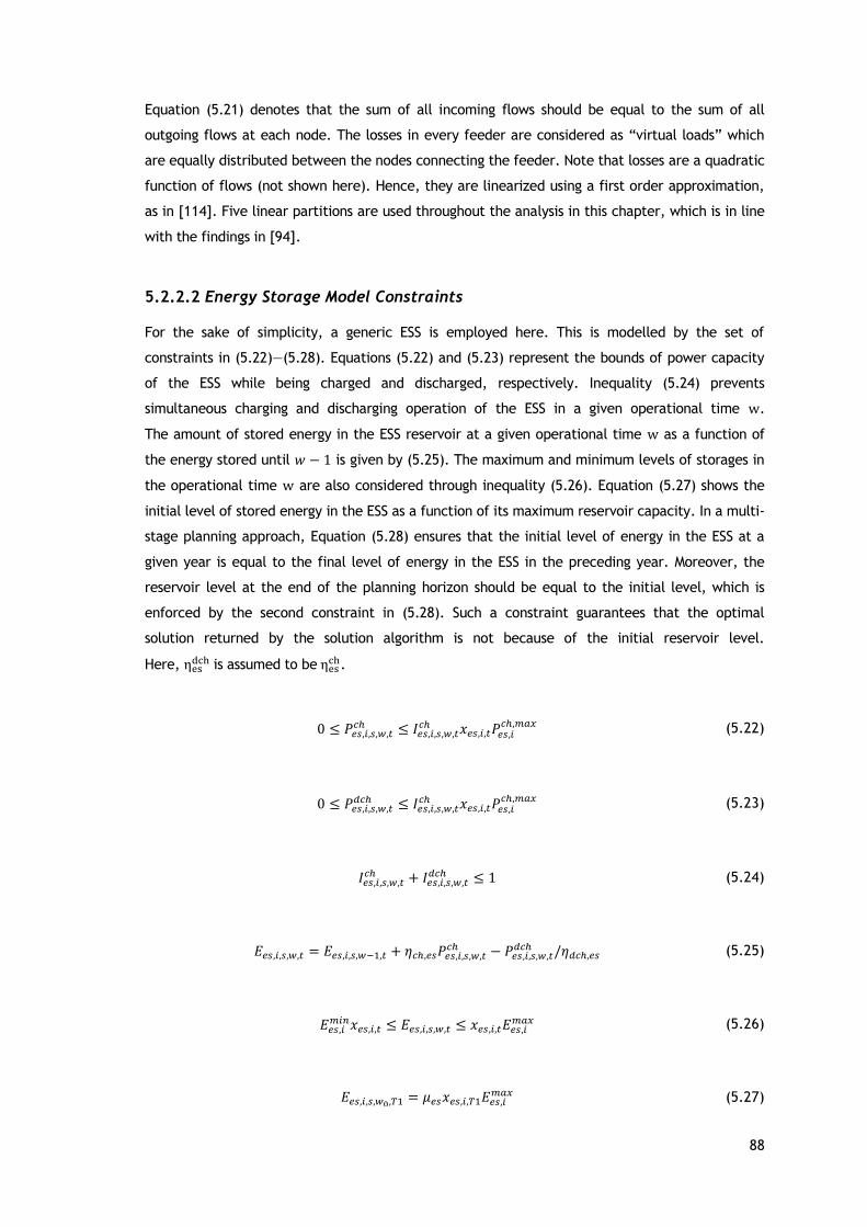
88

Equation (5.21) denotes that the sum of all incoming flows should be equal to the sum of all

outgoing flows at each node. The losses in every feeder are considered as “virtual loads” which

are equally distributed between the nodes connecting the feeder. Note that losses are a quadratic

function of flows (not shown here). Hence, they are linearized using a first order approximation,

as in [114]. Five linear partitions are used throughout the analysis in this chapter, which is in line

with the findings in [94].

5.2.2.2 Energy Storage Model Constraints

For the sake of simplicity, a generic ESS is employed here. This is modelled by the set of

constraints in (5.22)—(5.28). Equations (5.22) and (5.23) represent the bounds of power capacity

of the ESS while being charged and discharged, respectively. Inequality (5.24) prevents

simultaneous charging and discharging operation of the ESS in a given operational time w.

The amount of stored energy in the ESS reservoir at a given operational time w as a function of

the energy stored until 𝑤 − 1 is given by (5.25). The maximum and minimum levels of storages in

the operational time w are also considered through inequality (5.26). Equation (5.27) shows the

initial level of stored energy in the ESS as a function of its maximum reservoir capacity. In a multi-

stage planning approach, Equation (5.28) ensures that the initial level of energy in the ESS at a

given year is equal to the final level of energy in the ESS in the preceding year. Moreover, the

reservoir level at the end of the planning horizon should be equal to the initial level, which is

enforced by the second constraint in (5.28). Such a constraint guarantees that the optimal

solution returned by the solution algorithm is not because of the initial reservoir level.

Here, ηesdch is assumed to be ηes

ch.

0 ≤ 𝑃𝑒𝑠,𝑖,𝑠,𝑤,𝑡𝑐ℎ ≤ 𝐼𝑒𝑠,𝑖,𝑠,𝑤,𝑡

𝑐ℎ 𝑥𝑒𝑠,𝑖,𝑡𝑃𝑒𝑠,𝑖𝑐ℎ,𝑚𝑎𝑥

(5.22)

0 ≤ 𝑃𝑒𝑠,𝑖,𝑠,𝑤,𝑡𝑑𝑐ℎ ≤ 𝐼𝑒𝑠,𝑖,𝑠,𝑤,𝑡


(5.23)

𝐼𝑒𝑠,𝑖,𝑠,𝑤,𝑡𝑐ℎ + 𝐼𝑒𝑠,𝑖,𝑠,𝑤,𝑡

𝑑𝑐ℎ ≤ 1 (5.24)

𝐸𝑒𝑠,𝑖,𝑠,𝑤,𝑡 = 𝐸𝑒𝑠,𝑖,𝑠,𝑤−1,𝑡 + 휂𝑐ℎ,𝑒𝑠𝑃𝑒𝑠,𝑖,𝑠,𝑤,𝑡𝑐ℎ − 𝑃𝑒𝑠,𝑖,𝑠,𝑤,𝑡

𝑑𝑐ℎ /휂𝑑𝑐ℎ,𝑒𝑠 (5.25)

𝐸𝑒𝑠,𝑖𝑚𝑖𝑛𝑥𝑒𝑠,𝑖,𝑡 ≤ 𝐸𝑒𝑠,𝑖,𝑠,𝑤,𝑡 ≤ 𝑥𝑒𝑠,𝑖,𝑡𝐸𝑒𝑠,𝑖

𝑚𝑎𝑥 (5.26)

𝐸𝑒𝑠,𝑖,𝑠,𝑤0,𝑇1 = 𝜇𝑒𝑠𝑥𝑒𝑠,𝑖,𝑇1𝐸𝑒𝑠,𝑖𝑚𝑎𝑥 (5.27)

89

𝐸𝑒𝑠,𝑖,𝑠,𝑤1,𝑡+1 = 𝐸𝑒𝑠,𝑖,𝑠,𝑊,𝑡; 𝐸𝑒𝑠,𝑖,𝑠,𝑊,𝑇 = 𝐸𝑒𝑠,𝑖,𝑠,𝑤0,𝑇1 (5.28)

Notice that inequalities (5.22) and (5.23) involve products of charging/discharging indicator

variables and investment variable. In order to overcome these nonlinearities, new continuous

positive variables 𝑧𝑒𝑠,𝑖,𝑠,𝑤,𝑡𝑐ℎ , and 𝑧𝑒𝑠,𝑖,𝑠,𝑤,𝑡

𝑑𝑐ℎ , which replace the bilinear products in each constraint,

are introduced such that the set of linear constraints in (5.29) and (5.30) hold. For instance, the

product 𝐼𝑒𝑠,𝑖,𝑠,𝑤,𝑡𝑑𝑐ℎ 𝑥𝑒𝑠,𝑖,𝑡 is replaced by the positive variable 𝑧𝑒𝑠,𝑖,𝑠,𝑤,𝑡

𝑑𝑐ℎ . Then, the bilinear product is

decoupled by introducing the set of constraints in (5.29) [115]. Similarly, the product

𝐼𝑒𝑠,𝑖,𝑠,𝑤,𝑡𝑐ℎ 𝑥𝑒𝑠,𝑖,𝑡is decoupled by including the set of constraints in (5.30).

𝑧𝑒𝑠,𝑖,𝑠,𝑤,𝑡𝑑𝑐ℎ ≤ 𝑥𝑒𝑠

𝑚𝑎𝑥𝐼𝑒𝑠,𝑖,𝑠,𝑤,𝑡𝑑𝑐ℎ ; 𝑧𝑒𝑠,𝑖,𝑠,𝑤,𝑡

𝑑𝑐ℎ ≤ 𝑥𝑒𝑠,𝑖,𝑡 ; 𝑧𝑒𝑠,𝑖,𝑠,𝑤,𝑡𝑑𝑐ℎ ≥ 𝑥𝑒𝑠,𝑖,𝑡 − (1 − 𝐼𝑒𝑠,𝑖,𝑠,𝑤,𝑡

𝑑𝑐ℎ )𝑥𝑒𝑠𝑚𝑎𝑥 (5.29)

𝑧𝑒𝑠,𝑖,𝑠,𝑤,𝑡𝑐ℎ ≤ 𝑥𝑒𝑠

𝑚𝑎𝑥𝐼𝑒𝑠,𝑖,𝑠,𝑤,𝑡𝑐ℎ ; 𝑧𝑒𝑠,𝑖,𝑠,𝑤,𝑡

𝑐ℎ ≤ 𝑥𝑒𝑠,𝑖,𝑡 ; 𝑧𝑒𝑠,𝑖,𝑠,𝑤,𝑡𝑐ℎ ≥ 𝑥𝑒𝑠,𝑖,𝑡 − (1 − 𝐼𝑒𝑠,𝑖,𝑠,𝑤,𝑡

𝑐ℎ )𝑥𝑒𝑠𝑚𝑎𝑥 (5.30)

5.2.2.3 Active Power Limits of DGs

The active power limits of existing generators are given by (5.31). Inequality (5.32) represents the

corresponding constraints in the case of new generators. Note that the binary variables multiply

both bounds to make sure that the power generation variable is zero when the generator remains

either unutilized or unselected for investment.

𝑃𝑔,𝑖,𝑠,𝑤,𝑡𝐸,𝑚𝑖𝑛 𝑢𝑔,𝑖,𝑡 ≤ 𝑃𝑔,𝑖,𝑠,𝑤,𝑡

𝐸 ≤ 𝑃𝑔,𝑖,𝑠,𝑤,𝑡𝐸,𝑚𝑎𝑥 𝑢𝑔,𝑖,𝑡 (5.31)

𝑃𝑔,𝑖,𝑠,𝑤,𝑡𝑁,𝑚𝑖𝑛 𝑥𝑔,𝑖,𝑡 ≤ 𝑃𝑔,𝑖,𝑠,𝑤,𝑡

𝑁 ≤ 𝑃𝑔,𝑖,𝑠,𝑤,𝑡𝑁,𝑚𝑎𝑥 𝑥𝑔,𝑖,𝑡 (5.32)

It should be noted that these constraints are applicable only for conventional DGs. In the case of

variable generation sources (such as wind and solar PV), the upper bound 𝑃𝑔,𝑖,𝑠,𝑤,𝑡𝑚𝑎𝑥 should be set

equal to the minimum of the actual production level at a given hour, which is dependent on the

level of primary energy source (wind speed and solar radiation), and the rated (installed) capacity

of the generating unit. The lower bound 𝑃𝑔,𝑖,𝑠,𝑤,𝑡𝑚𝑎𝑥 in this case is simply set to zero.

5.2.2.4 Active Power Limits of Power Purchased



90

For technical reasons, the power that can be purchased from the transmission grid could have

minimum and maximum limits, which is enforced by (5.33). However, it is understood that setting

such limits is difficult. These constraints are included here for the sake of completeness. In this

chapter, these limits are set to 1.5 times the minimum and maximum levels of the total load in

the system.


The set of logical constraints in (5.34) ensure that an investment decision already made cannot be

reversed. In addition to the constraints described above, the direct current (DC) based network

model and radiality related constraints presented in [114] are used here.

𝑥𝑘,𝑡 ≥ 𝑥𝑘,𝑡−1; 𝑥𝑔,𝑖,𝑡 ≥ 𝑥𝑔,𝑖,𝑡−1; 𝑥𝑒𝑠,𝑖,𝑡 ≥ 𝑥𝑒𝑠,𝑖,𝑡−1 (5.34)


There are two conditions that must be fulfilled in order a distribution network system (DNS) to be

radial. First, the solution must have 𝑁𝑖 − 𝑁𝑆𝑆 circuits. Second, the final topology should be

connected. Equation (5.35) represents the first necessary condition for maintaining the radial

topology of a DNS.

∑ 𝑂𝑅(𝑥𝑘,𝑡 , 𝑢𝑘,𝑡)

𝑘∈Ω𝑖𝑗

= 𝑁𝑖 −𝑁𝑆𝑆 ; ∀𝑡 (5.35)

Note that the above equation assumes that a line investment is possible in all corridors. Hence, in

a given corridor, we can have either an existing branch or a new one, or both connected in

parallel, depending on the economic benefits of the final setup (solution) brings about to the

system. The radiality constraint in (5.35) then has to accommodate this condition. One way to do

this is using the Boolean logic operation given as in (5.35). Unfortunately, this introduces

nonlinearity. We show how this logic can be linearized using an additional auxiliary variable 𝑧𝑘,𝑡

and the binary variables associated to existing and new branches i.e. 𝑢𝑘,𝑡 and 𝑥𝑘,𝑡, respectively.

Given𝑧𝑘,𝑡: = 𝑂𝑅(𝑥𝑘,𝑡 , 𝑢𝑘,𝑡), this Boolean operation can be expressed using the following set of

linear constraints:

𝑧𝑘,𝑡 ≤ 𝑥𝑘,𝑡 + 𝑢𝑘,𝑡; 𝑧𝑘,𝑡 ≥ 𝑥𝑘,𝑡; 𝑧𝑘,𝑡 ≥ 𝑢𝑘,𝑡; 0 ≤ 𝑧𝑘,𝑡 ≤ 1 ; ∀𝑡 (5.36)

91

Then, the radiality constraints in (5.35) can be reformulated using the zk,t variables as:

∑ 𝑧𝑘,𝑡𝑘∈𝛺𝑖𝑗

= 𝑁𝑖 − 𝑁𝑆𝑆 ; ∀𝑡 (5.37)

When all loads in the DNS are only powered up by power imported through a number of

substations, the final solution obtained automatically satisfies the two aforementioned conditions;

hence, no additional constraints are required i.e. (5.36) along with (5.37) are sufficient to

guarantee radiality. However, it should be noted that, in the presence of DGs and reactive power

sources, these constraints alone may not ensure the radiality of the distribution network, as

pointed out in [106] and further discussed in [97].

5.3 Case Studies


The standard IEEE 119-bus distribution network, shown in Figure 5.1, is used here for carrying out

the required analysis mentioned earlier. The system has a rated voltage of 11.0 kV, and a total

demand of 22709.72 kW and 17041.068 kVAr. Network data and other related information about

this test system can be found in [116] and the data are in the Appendix E. According to [117], the

active power losses in this system is 1298.09 kW, and the minimum node voltage of the system is

0.8783 p.u., which occurs at bus 116.

Other data and assumptions made throughout this chapter are as follows. The planning horizon is

3 years long, which is divided into yearly decision stages, and a fixed interest rate of 7% is used.

The expected lifetime of the generic ESS is assumed to be 15 years while that of DGs and feeders

is 25 years. Two investment options with installed capacities of 0.5 and 1.0 MVA are considered

for each wind and solar PV type DG units. The installation cost and emission related data of these

DG units in [118] are used here. For the sake of simplicity, all maintenance cost of each DG is

assumed to be 2% of the corresponding investment cost while that of any feeder is

450 €/km/year. The investment cost of each feeder is 38700 €/km. The current flow limits of

each feeder are considered to be as follows. The current limit in each of the feeders (1,2); (2,4);

(1,66); (66,67) is 1200 A while the set of feeders (4,5); (5,6); (6,7); (4,29); (29,30); (30,31);

(67,68); (67,81); (81,82); (1,105); (105,106); (106,107) have each 800 A capacity limit. The

current flow limits of the remaining feeders are considered to be 400 A. Moreover, it is assumed

that all feeders can be switched on/off, if deemed necessary. In addition, it is assumed that the

availability of wind and solar power sources is uniform throughout the system nodes.

The operational variability and uncertainty introduced by wind and solar PV type DGs, demand

and electricity price are accounted for via the clustering method proposed in [103].

92

Figure 5.1 - Single line diagram of the test system in base case.

The maximum allowable bus voltage deviation in the system is set to 5%, and node 1 is considered

as a reference with a voltage magnitude of 1.0. Taking the base case demand as a reference,

annual demand growths of 0%, 5% and 10% are also considered in all simulations. Emission prices

in the first, second and third time stages are set to 25, 45 and 60 €/tCO2e, respectively, and the

emission rate of power purchased from upstream is arbitrarily set to 0.4 tCO2e/MWh. The cost of

unserved energy is 2000 €/MWh. A power factor of 0.9 is considered throughout the system, and is

assumed to be the same throughout. The base power is set to 1 MVA. An ESS with a 1 MW power

and a 5 MWh reservoir capacity is considered for investment.


Given the aforementioned data and assumptions, the developed optimization problem has been

solved considering six different cases (designated as A though F). Case A represents the base case

topology where no investments are made. This case can be alternatively understood as the “do-

nothing” scenario. Case B is similar to the base case (i.e. with no investments) but considers the

network reconfiguration problem. Case C corresponds to a scenario where only DG investments

are made on the base case topology (i.e. without reconfiguration).

93

Case D is similar to Case C except that the former simultaneously considers optimal

reconfiguration and DG investments. The last two cases (Cases E and F) correspond to scenarios

where optimal investment planning in DGs is coordinated with that of ESSs. The difference is that

Case E uses the base case topology (i.e. without reconfiguration) while Case F optimizes the

network via reconfiguration. Table 5.1 clearly summarizes the different cases.

The values of the most relevant variables are analyzed (as depicted in Table 5.2) over the three

years planning horizon. The results in Table 5.2 reveal the significant differences in overall NPV

cost in the system, share of the combined energy supplied by RES and ESS, cost of total network

losses and unserved power among the aforementioned cases. The results are also compared with

the base case system where no investments are made and the network topology is held the same

(i.e. the “do-nothing” scenario). Carrying out an optimal reconfiguration of the network alone, as

in Case B, results in about 5.44 % reduction in the cost of losses, and a 15.9% reduction in the NPV

overall system cost compared with that of Case A. In addition, network reconfiguration reduces a

total of 1.18 p.u. average load curtailment in the third year to 0.57 p.u. in Case B that would

otherwise occur at nodes 52, 53, 54, 55, 56 and 116 due to a number of factors such as technical

constraints and high demand level.

Another more interesting observation from Table 5.2 is that Cases C and D lead to (approximately)

50% reduction in the overall system cost, and a 75% reduction in the amount of imported energy.

Wind and solar power sources are complementary by nature. This natural phenomenon seems to

be exploited when DG investments are not accompanied by investments in ESSs (i.e. Cases C and

D). This is because, according to the DG investment solution in Table 5.2, the operational

variability in the system seems to be handled by investing an appreciable amount in both

complementary power sources (wind and solar). The level of demand covered by RESs in both

cases amounts to nearly 75%. Moreover, as a result of investing in DGs, losses in the system are

slashed down by about 82%. Generally, the corresponding reductions in Case D are slightly higher

than those in Case C. This is due to the network reconfiguration which has been considered in

Case D.

Table 5.1 - Distinguishing the different cases

Cases Reconfiguration

Investment

DGs ESSs

A No No No

B Yes No No

C No Yes No

D Yes Yes No

E No Yes Yes

F Yes Yes Yes

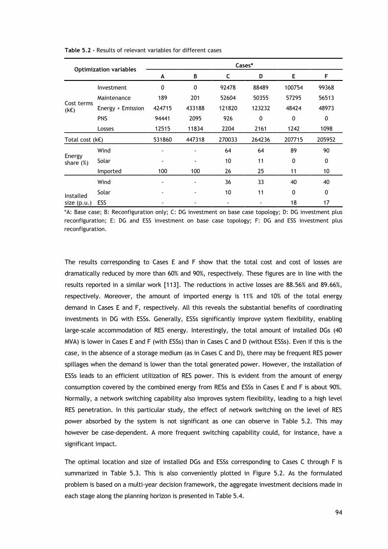
94

Table 5.2 - Results of relevant variables for different cases

Optimization variables Cases*

A B C D E F

Cost terms (k€)

Investment 0 0 92478 88489 100754 99368

Maintenance 189 201 52604 50355 57295 56513

Energy + Emission 424715 433188 121820 123232 48424 48973

PNS 94441 2095 926 0 0 0

Losses 12515 11834 2204 2161 1242 1098

Total cost (k€) 531860 447318 270033 264236 207715 205952

Energy share (%)

Wind - - 64 64 89 90

Solar - - 10 11 0 0

Imported 100 100 26 25 11 10

Installed size (p.u.)

Wind - - 36 33 40 40

Solar - - 10 11 0 0

ESS - - - - 18 17

*A: Base case; B: Reconfiguration only; C: DG investment on base case topology; D: DG investment plus

reconfiguration; E: DG and ESS investment on base case topology; F: DG and ESS investment plus

reconfiguration.

The results corresponding to Cases E and F show that the total cost and cost of losses are

dramatically reduced by more than 60% and 90%, respectively. These figures are in line with the

results reported in a similar work [113]. The reductions in active losses are 88.56% and 89.66%,

respectively. Moreover, the amount of imported energy is 11% and 10% of the total energy

demand in Cases E and F, respectively. All this reveals the substantial benefits of coordinating

investments in DG with ESSs. Generally, ESSs significantly improve system flexibility, enabling

large-scale accommodation of RES energy. Interestingly, the total amount of installed DGs (40

MVA) is lower in Cases E and F (with ESSs) than in Cases C and D (without ESSs). Even if this is the

case, in the absence of a storage medium (as in Cases C and D), there may be frequent RES power

spillages when the demand is lower than the total generated power. However, the installation of

ESSs leads to an efficient utilization of RES power. This is evident from the amount of energy

consumption covered by the combined energy from RESs and ESSs in Cases E and F is about 90%.

Normally, a network switching capability also improves system flexibility, leading to a high level

RES penetration. In this particular study, the effect of network switching on the level of RES

power absorbed by the system is not significant as one can observe in Table 5.2. This may

however be case-dependent. A more frequent switching capability could, for instance, have a

significant impact.

The optimal location and size of installed DGs and ESSs corresponding to Cases C through F is

summarized in Table 5.3. This is also conveniently plotted in Figure 5.2. As the formulated

problem is based on a multi-year decision framework, the aggregate investment decisions made in

each stage along the planning horizon is presented in Table 5.4.

95

Table 5.3 - Optimal sizes and locations of DGs and ESSs for different cases

Wind * Solar *, § ESS *, †

Nodes Case C Case D Case E Case F Case C Case D Case E Case F

14 1 1 1 1 0 0 0 0

19 1 0 1 0 0 0 0 0

20 1 0 2 1 0 0 1 1

21 0 1 0 1 0 0 0 0

24 0 1 1 1 0 0 0 0

25 1 0 0 0 0 0 0 0

29 0 0 0 0 0 0 2 1

32 1 1 1 2 0 0 0 0

33 1 1 1 1 0 0 1 1

34 0 0 1 0 0 0 0 0

35 1 0 0 1 1 1 0 0

37 1 1 1 1 0 0 0 0

38 1 1 1 1 0 0 0 1

42 0 1 2 1 0 0 0 0

43 1 0 0 1 0 0 1 1

44 1 1 2 1 1 1 0 0

52 2 2 2 2 1 2 2 1

53 1 1 1 1 0 0 0 0

56 3 1 1 1 0 0 1 1

61 1 1 1 1 0 0 1 1

66 0 0 0 0 0 0 1 1

69 1 1 1 1 0 0 0 0

73 1 1 1 1 1 1 1 1

74 1 1 1 1 0 0 0 0

77 1 1 1 2 1 1 1 1

79 1 1 1 1 0 0 0 0

82 0 0 1 1 0 0 0 0

83 1 1 1 1 0 0 1 1

84 0 0 0 0 1 1 0 0

85 1 1 1 1 0 0 0 0

89 1 1 1 1 0 0 1 1

96 1 1 1 1 0 0 0 0

100 0 1 0 1 1 1 1 1

101 1 1 2 1 0 0 0 0

106 1 1 1 1 0 0 0 0

107 0 0 0 0 0 0 1 1

108 1 1 1 1 0 0 0 0

109 0 0 0 1 0 0 0 0

112 1 1 1 1 1 1 1 1

113 0 0 0 0 0 0 0 0

114 1 1 1 1 0 1 0 0

115 0 0 0 0 1 0 0 0

116 2 2 3 2 1 1 1 1

117 1 1 1 1 0 0 0 0

119 0 1 1 1 0 0 0 0

121 1 0 0 0 0 0 0 0

Total (p.u.) 34 31 38 38 10 11 18 17 *A: Base case; B: Reconfiguration only; C: DG investment on base case topology; D: DG investment plus

reconfiguration; E: DG and ESS investment on base case topology; F: DG and ESS investment plus

reconfiguration. § No solar type investment decisions in cases E and F; † ESS investments are not

considered in the cases other than E and F.

96

Table 5.4 – Total DGs and ESSs for different cases

Case C

Case D

Case E

Case E

Year

Wind Solar

Wind Solar

Wind Solar ESS

Wind Solar ESS

1

31 9

29 7

36 0 17

36 0 15

2

2 0

2 2

2 0 0

1 0 2

3

3 1

2 2

2 0 1

3 0 0

Total

36 10

33 11

40 0 18

40 0 17

Figure 5.2 - Optimal placement and size of DGs and ESSs for different cases (* only in cases E and F).

As it can be seen in this table, majority of the investments are made in the first stage. This may

be because of two reasons. The first one could be due to lack of appropriate financial and

logistical constraints in the optimization model. The second and most plausible reason could be

due to higher NPV factor of the first stage than any subsequent one. Note that the higher this

factor is, the more relevant the associated costs in the objective function are, hence, leading to

more investments in DGs and ESSs.

The average voltage profiles at each node and for each case are depicted in Figure 5.3.

A cumulative distribution of the average voltage values, corresponding to different cases, is also

conveniently represented in Figure 5.4. In both figures, it is interesting to see the substantial

contributions of DG and ESS installations to voltage profile improvement. As shown in Figure 5.3,

the coordinated integration of DGs and ESSs along with reconfiguration (i.e. Case F), especially

leads to the best voltage profile which is almost flat throughout the system.

0

1

2

3

4

5

6

7

8

9

10

11

12

13

14 20 24 29 33 35 38 43 52 56 66 73 77 82 84 89 100 106 108 112 114 116 119

Inst

alled a

mount

(pu)

Node

ESS*

Case F

Case E

Case D

Case C

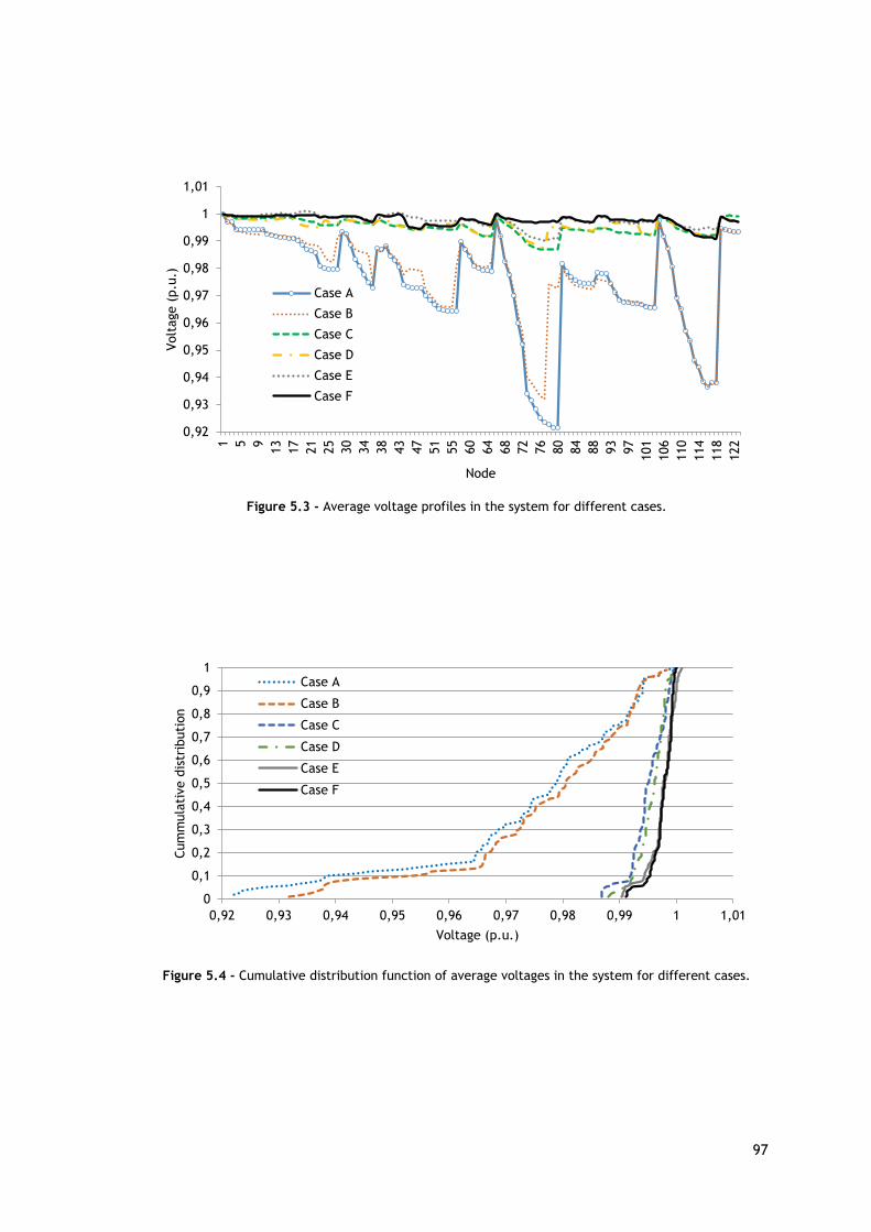
97

Figure 5.3 - Average voltage profiles in the system for different cases.

Figure 5.4 - Cumulative distribution function of average voltages in the system for different cases.

0,92

0,93

0,94

0,95

0,96

0,97

0,98

0,99

1

1,01

1 5 9

13

17

21

25

30

34

38

43

47

51

55

60

64

68

72

76

80

84

88

93

97

101

106

110

114

118

122

Volt

age (

p.u

.)

Node

Case A

Case B

Case C

Case D

Case E

Case F

0

0,1

0,2

0,3

0,4

0,5

0,6

0,7

0,8

0,9

1

0,92 0,93 0,94 0,95 0,96 0,97 0,98 0,99 1 1,01

Cum

mula

tive d

istr

ibuti

on

Voltage (p.u.)

Case A

Case B

Case C

Case D

Case E

Case F

98

Table 5.5 compares the optimal network topologies (i.e. the switches to be opened)

corresponding to the different cases with that of the base case topology. The benefit of joint DG

and ESS investments along with network reconfiguration in terms of losses reduction (over 89% on

average) can be seen in Figure 5.5. The spikes observed in cases D and F are because of the

variability in the RES power injected into the system.

Table 5.5 - Optimal reconfiguration outcome for different cases (List of switches to be opened)

Year

Case A Case B Case D Case F

1

(8,24); (9,42); (17,27); (25,36); (38,65); (48,27); (56,45); (61,100); (65,56); (76,95); (91,78);

(103,80); (113,86); (110,89); (115,123)

(23,24); (26,27); (35,36); (41,42); (44,45); (48,27);

(54,56); (61,100); (64,65); (76,95); (77,78);

(103,80); (110,89); (113,86); (115,123)

(17,27); (23,24); (35,36); (41,42); (48,27); (54,56);

(56,45); (61,100); (64,65); (76,95); (77,78);

(103,80); (110,89); (113,86); (115,123)

(9,42); (17,27); (23,24); (25,36); (38,65); (48,27);

(54,56); (56,45); (61,100); (76,95); (91,78); (103,80); (110,89); (113,86);

(115,123)

2

(8,24); (9,42); (17,27); (25,36); (38,65); (48,27); (56,45); (61,100); (65,56); (76,95); (91,78);

(103,80); (113,86); (110,89); (115,123)

(9,42); (23,24); (26,27); (35,36); (44,45); (48,27);

(54,56); (61,100); (64,65); (76,95); (77,78);

(103,80); (110,89); (113,86); (115,123)

(17,27); (23,24); (35,36); (38,65); (41,42); (48,27); (54,56); (56,45); (76,95);

(77,78); (95,100); (103,80); (110,89); (113,86); (115,123)

(9,42); (17,27); (23,24); (25,36); (44,45); (48,27);

(54,56); (61,100); (64,65); (76,95); (91,78);

(103,80); (110,89); (113,86); (115,123)

3

(8,24); (9,42); (17,27); (25,36); (38,65); (48,27); (56,45); (61,100); (65,56); (76,95); (91,78);

(103,80); (113,86); (110,89); (115,123)

(9,42); (23,24); (26,27); (35,36); (44,45); (48,27);

(54,56); (61,100); (64,65); (76,95); (77,78);

(103,80); (110,89); (113,86); (115,123)

(17,27); (23,24); (35,36); (41,42); (48,27); (54,56); (56,45); (64,65); (76,95);

(77,78); (95,100); (103,80); (110,89); (113,86); (115,123)

(9,42); (17,27); (23,24); (25,36); (38,65); (44,45);

(48,27); (54,56); (61,100); (76,95); (91,78); (103,80); (110,89); (113,86);

(115,123)

Figure 5.5 - Total system losses profile.

0

0,2

0,4

0,6

0,8

1

1,2

1 5 9

13

17

21

25

29

33

37

41

45

49

53

57

61

65

69

73

77

81

85

89

93

97

101

105

Loss

es

(pu)

Snapshot

Case A Case F

Case B Case D

99

As stated earlier, stability concern is one of the major issues that are associated with high level

RES integration in distribution systems. The controllability of voltage and frequency can be

dramatically undermined or even sometimes become out of reach. Because of these reasons, the

penetration level of DGs (including RESs) in many distribution systems is limited to a value often

less than about 25%. However, this contradicts with the ambition to meet other objectives such as

reducing the carbon footprint of power production and ensuring energy security among others.

The integration of RESs is likely to be supported with enabling technologies that have the

capability to effectively address the integration challenges and consequently increase the

penetration level. The results in this chapter largely demonstrate the fact that large-scale

integration of variable energy sources is possible when such energy sources are optimally

deployed with ESSs and a mechanism that improve the flexibility of the network is put in place.


There is a wide consensus about integrating more renewable energy sources—RESs to solve a

multitude of global concerns such as meeting an increasing demand for electricity, reducing

energy security and heavy dependence on fossil fuels for energy production, and reducing the

overall carbon footprint of power production. Framed in this context, the coordination of RES

integration with ESSs, along with the network’s switching capability and/or reinforcement, is

expected to significantly improve system flexibility, thereby increasing the capability of the

system in accommodating large-scale RES power. Hence, in this chapter a novel mechanism to

quantify the impacts of network switching and/or reinforcement as well as deployment of ESSs on

the level of renewable power integrated in the system was presented. To carry out this analysis, a

dynamic and multi-objective stochastic mixed integer linear programming model was developed,

which jointly takes the optimal deployment of RES-based DGs and ESSs into account in

coordination with distribution network reinforcement and/or reconfiguration. The IEEE 119-bus

test system was used as a case study. The results clearly show the capability of ESS deployment in

dramatically increasing the level of renewable DGs integrated in the system. Although case-

dependent, the impact of network reconfiguration on RES power integration is not significant.

100

Chapter 6

New Multi-stage and Stochastic Mathematical

Model for Maximizing RES Hosting Capacity

This chapter presents a new coordinated multi-stage and stochastic mathematical model,

developed to support the decision-making process of planning distribution network systems

(DNSs) for integrating large-scale “clean” energy sources. The model, formulated from the

system operator’s viewpoint, determines the optimal sizing, timing and placement of

distributed energy technologies (particularly, renewables) in coordination with energy

storage systems and reactive power sources. The ultimate goal of this optimization work is

to maximize the size of renewable power absorbed by the system while maintaining the

required/standard levels of power quality and system stability at a minimum possible cost.

One of the points that distinguish this chapter from the predecessors is the use of a

linearized AC network model, which captures the inherent characteristics of electric

networks, and balances well accuracy with computational burden.

6.1 Introduction

Nowadays, the issue of integrating distributed generations (DGs) (renewable DGs, in particular) is

globally gaining momentum because of several techno-economic and environmental factors. Since

recent years, the size of DGs integrated into distribution systems has been increasing. This trend

is more likely to continue in the years to come because it is now widely accepted that DGs bring

wide-range benefits to the system. However, given the current set-up of distribution networks

(which are generally passive), large-scale DG integration is not technically possible because this

brings about tremendous challenges to the system operation, especially in undermining the power

system quality and stability.

Such challenges/limitations are expected to be alleviated when distribution networks undergo the

anticipated evolutionary process from passive to active networks or smart grids. This transition is

expected to result in a system that is adequately equipped with appropriate technologies, state-

of-the-art solutions and a new operational philosophy that is totally different from the current ‘fit

and forget’ approach. This is expected to offer sufficient flexibility and control mechanism in the

system. Nevertheless, the process is not straightforward as it demands exceptionally huge

investments in smart-grid technologies and concepts to fully automate the system, and this should

be accompanied by a new operational philosophy. Therefore, the whole transformation process

(i.e., the transformation of current distribution systems to full-scale smart-grids) might be very

slow, and its realization might take several decades.

101

However, given the techno-economic factors and global concerns about environmental issues, the

integration of renewable energy sources (RESs) cannot be postponed. It is likely that the

integration of DGs in distribution systems will go ahead along with smart-grid enabling

technologies that have the capability to alleviate the negative consequences of large-scale

integration of DGs. In other words, in order to facilitate (speed up) the much-needed

transformation of conventional (passive) DNSs and support large-scale RES integration, different

smart-grid enabling technologies such as reactive power sources, advanced switching and storage

devices are expected to be massively deployed in the near term.

To this end, developing strategies, methods and tools to maximize the penetration level of DGs

(particularly, RESs) has become very crucial to guide such a complex decision-making process.

In this respect, this chapter focuses on the development of multi-stage mathematical models to

determine the optimal sizing, timing and placement of energy storage systems and reactive power

sources as well as that of RESs in distribution networks. The ultimate goal of this optimization

work is to maximize the RES power absorbed by the system at a minimum cost while maintaining

the power quality and stability at the required/standard levels.

The problem is formulated from the system perspective (i.e. in centralized planning framework).

In a deregulated environment and from the smart-grid context where the current regulatory and

technical challenges are expected to be fully resolved, planning will most likely involve

distributed decision-making processes. One may rightfully argue that the investment decisions

obtained from a coordinated planning model may not be implemented in reality. This is because

distributed decisions often lead to sub-optimal solutions, which may be different from the ones

obtained by the centralized planning model. However, this does not mean that the outcomes of

the coordinated planning model cannot be used. For instance, these outcomes can be regarded as

the best investment targets. Given these targets, distributed decisions (solutions) can be

systematically made to approach one or more of these targets (for example, via incentive or

market-based mechanisms).

From another perspective, in the absence of “attractive” market environment (seen from the

private investors), distribution network systems may not see significant breakthrough when it

comes to investments in DGs and energy storage systems (ESSs). In this case, DSOs may, instead,

be given additional roles and responsibilities that include investing in DGs and ESSs in coordination

with network investments. DSOs may also oversee investments in DGs and ESSs. In addition, DSOs

may also be required to manage these assets in a coordinated manner to keep the system

integrity, stability and power quality at the required/standard levels. Another issue which

explains the versatility of the coordinated approach is related to the realization of smart-grids.

Even if there is a general consensus on the smartification of power systems (distribution networks,

in particular), and there are signs that some systems are evolving into smart-grids, the whole

process is going to probably take very long time. Based on the aforementioned reasons, a

centralized (coordinated) approach of the planning problem can provide vital solutions.

102

Reducing fossil fuel dependence and mitigating climate change have led to an increased pressure

to change the current generation paradigm. The compounded effect of increasing demand for

electricity, environmental and climate change concerns is triggering a policy shift all over the

world, especially when it comes to energy production. Integration of DG, particularly, RESs, in

electric distribution network systems is gaining momentum. In particular, the recent

developments in a climate change conference held in Paris (COP21) are expected to accelerate

renewable integration. It is highly expected that large-scale DG integration will be one of the

solutions capable of mitigating the aforementioned problems and overcoming the challenges.

Because of this, Governments of various nations have introduced targets to achieve large-scale

integration of DGs. In particular, in the European Union, which strongly advocates the importance

of integrating renewables, RESs are expected to cover 20% and 50% of the overall energy

consumption by 2020 and 2050, respectively.

DGs offer a more environmentally friendly option through great opportunities with renewable-

enabling technologies such as wind, photovoltaic, biomass, etc. RESs are abundant in nature,

which, under a favorable RES integration policy and incentive mechanism, makes it attractive for

the large-scale power generation sector. Nevertheless, there is no rule or partial rule on the DG

unit’s connection; typically, these are traditionally connected at the end of radial feeder systems

or nodes with greater load on the distribution system. This is realized often with several impeding

restrictions put in place to alleviate the negative consequences of integrating DGs in the system.

The optimal and dynamic planning of the DG placement and sizing is becoming extremely

important for energy producers, consumers and network operators in technical and economic

terms. There are many studies in the literature on this topic, yet most of them only consider the

optimal location of a single DG unit or do not consider simultaneously positioning and sizing RES

units, mainly due to their high dispatch unpredictability. The increase in DG penetration increases

the uncertainty and the fluctuations of power production. If the placement and proper sizing is

not taken into account, the benefits of DG integration can be lost, leading to inefficient operation

and increasing the electricity cost and energy losses. Another major concern with the wide DG

penetration is system reliability. The penetration of distributed systems can result in the

degradation of power quality, particularly in cases of slightly meshed networks [119] or

microgrids. In this paradigm, the use of ESS has been seen as one of the viable options to mitigate

the aforementioned concerns.

The DG allocation and sizing subject have attracted special interest from researchers in recent

years. An excellent review of previous works related to this subject area, published prior to the

year 2013, is presented in [120]. In [120] and [121], an analysis of several techniques used on

the DG impact assessment in the electrical system is presented. Most of these techniques analyze

the distribution system to determine rules that can be used for DG integration [122]–[126].

Important issues related to the connection of DG units are the network topology, DG capacity and

suitable location; because, each bus in the system has an optimal level of DG integration. If the

value surpasses this level, system losses can increase [127], [128].

103

Recently, several methods have been proposed for planning and operation or in some cases for

both location and sizing of DGs in the distribution system. In general, these methods can be

classified as heuristic [129]–[144], numerical [145]–[152] and analytical [153], [154] based

methods. Heuristic based methods apply advanced artificial intelligence algorithms, such as

genetic algorithms (GA) [129]–[132], particle swarm optimization (PSO) [133]–[137], harmony

search (HS) [138], [139] and big bang crunch (BBC) [140]–[142].

Numerical methods are algorithms that seek numerical results for different problems in particular

to the problem in question. Some of the most recently works use nonlinear mixed integer

programming (MINLP) [145]–[147], mixed integer linear programming (MILP) [148], [149],

quadratic programming (QP) [150] and AC optimal power flow (OPF)-based [151]. The exhaustive

search methods seek the optimal DG location for a given DG size under different load models.

Therefore, these methods fail to represent accurately the behavior of the DG optimization

problem involving two discrete variables, both for optimum DG size and optimal DG location.

In [153], authors present a technique with a probabilistic basis for determining the capacity and

optimal placement of wind DG units to minimize energy loss in the distribution system.

A sensitivity analysis is presented in [154] for DG placement and sizing in the network.

Despite many studies in the literature on areas related to DG placement and sizing problem, most

of them only consider the optimal location of a single DG unit, mostly of conventional DGs.

The simultaneous consideration of placement, timing and sizing of DG units (especially RESs),

along with the placement, timing and sizing of smart-grid enabling technologies, seems to be far

from being addressed in the literature. The increase in RES-based DG penetration increases the

uncertainty and the fluctuations of the system production. If the placement and proper sizing is

not taken into account, the benefits of DG integration may not be exploited; instead, this may

result in the degradation of system efficiency, increased cost of electricity and energy losses.

Another major concern with the wide-range DG penetration is system reliability. However, the

simultaneous investment planning of DGs, ESSs and reactive power sources is expected to

significantly alleviate these challenges and increase the penetration level of RES-based DGs.

A new multi-stage and stochastic mathematical model is developed in this chapter to support the

decision-making process of planning distribution network systems (DNSs) for integrating large-

scale “clean” energy sources. The proposed model, formulated from the system operator’s

viewpoint, determines the optimal sizing, timing and placement of distributed energy

technologies (particularly, renewables) in coordination with energy storage systems and reactive

power sources. The ultimate goal is to maximize the size of renewable power absorbed by the

system while maintaining the required/standard levels of power quality and system stability at a

minimum possible cost. From the methodological perspective, the entire problem is formulated as

a mixed integer linear programming optimization, allowing one to obtain an exact solution within

a finite simulation time. Moreover, it employs a linearized AC network model which captures the

inherent characteristics of electric networks, and balances well accuracy with computational

burden.

104

This chapter is organized as follows: Section 6.2 presents a brief description of the uncertainty

and variability pertaining to variable energy sources and electricity demand, and how these issues

are handled in the planning process. The mathematical formulation and detailed description of

the proposed model are presented in section 6.3. Subsequently, in section 6.4, the results are

presented and discussed. Finally, relevant conclusions are drawn in Section 6.5.

6.2 Uncertainty and Variability Management

There are various sources of uncertainty and variability in a distribution systems planning

problem, particularly with intermittent renewable sources. These are related to the variability in

time and the randomness of operational situations [105]. In addition, there are other

uncertainties mostly related to the long-term electricity, carbon and fuel prices, rules,

regulations and policies, etc. To account for uncertainty in demand, two demand scenarios are

formed by assuming a ±5% prediction error margin from a long real-life demand profile (which is

8760 long). This gives a total of three demand profile scenarios, which are kept the same

throughout the planning horizon. Due to the lack of sufficient historical data, first, synthetic

hourly wind speed and solar radiation series (20 for each) are generated using the methods in

[119] and [120], respectively considering the autocorrelations and diurnal patterns of each

parameter. Then, the average wind speed and solar radiation profiles are determined from the

generated series. The power outputs corresponding to each wind speed and solar radiation are

then determined by plugging in these values in the respective power curves given by equations

(6.1) and (6.2). Note that these power output samples (snapshots) cannot be used directly in the

planning process because the resulting wind power output profiles may not respect the natural

correlations that exist between them and the average electricity demand profile. These samples

should be readjusted to reflect the temporal correlations that naturally exist among demand,

solar radiation and wind speed series. To this end, the correlation between wind and solar sources

is considered to be -0.3 while that of wind and demand is 0.28, which is in line with the results in

[155]. A correlation of 0.5 is assumed between solar and demand, according to [156].

Given this desired correlation matrix, the wind and the solar power output profiles can be

transformed into new ones, respecting the correlation among them. Such adjustments in the

correlation of data series are performed using Cholesky factorization, a method used for

generating correlated random variables. The method works as follows. Given a desired correlation

matrix R, and uncorrelated data D, a new data Z whose correlation matrix is R can be generated

by simply multiplying the Cholesky decomposition of R by D. Then, the hourly wind and solar

power output are determined by plugging in these readjusted series into their corresponding

power curves given by equations (6.1) and (6.2).

𝑃𝑤𝑛𝑑,ℎ =

0 ; 0 ≤ 𝑣ℎ ≤ 𝑣𝑐𝑖𝑃𝑟(𝐴 + 𝐵𝑣ℎ

3) ; 𝑣𝑐𝑖 ≤ 𝑣ℎ ≤ 𝑣𝑟𝑃𝑟 ; 𝑣𝑟 ≤ 𝑣ℎ ≤ 𝑣𝑐𝑜0 ; 𝑣ℎ ≤ 𝑣𝑐𝑜

(6.1)

105

In the above equation, A and B are parameters represented by the expressions in [157] and [158].

Similarly, the hourly solar power output 𝑃𝑠𝑜𝑙,ℎ is determined by plugging in the hourly solar

radiation levels in the solar power output expression given in (6.2) [159].

𝑃𝑠𝑜𝑙,ℎ =

𝑃𝑟𝑅ℎ2

𝑅𝑠𝑡𝑑 ∗ 𝑅𝑐 ; 0 ≤ 𝑅ℎ ≤ 𝑅𝑐

𝑃𝑟𝑅ℎ𝑅𝑠𝑡𝑑

; 𝑅𝑐 ≤ 𝑅ℎ ≤ 𝑅𝑠𝑡𝑑

𝑃𝑟 ; 𝑅ℎ ≥ 𝑅𝑠𝑡𝑑

(6.2)

In the present work, uncertainty in wind speed and solar radiation is assumed to lead to a ±15%

deviation on average from the corresponding average power output profiles. This approximately

translates to ±5% forecasting error in wind speed or solar radiation. Note that such error or higher

is induced even by the most advanced forecasting tools available today. Based on the

assumptions, two hourly profiles of wind power output are generated by considering the ±15%

margin (one above the average and one below the average profile). In total, this leads to 3 wind

power output profiles (including the average profile). These are defined as wind scenarios.

Similarly, to account for the uncertainty in solar power outputs, two profiles are generated for

each by considering a ±15% uncertainty margin. The two generated solar power output profiles

along with the average profile form the set of solar scenarios. An illustration of uncertainty

characterization of wind and solar power outputs was shown in Fig. 4.4.

Note that each of these scenarios has 8760 snapshots of demand, wind and solar power outputs.

These individual scenarios are combined to form a set of 27 scenarios (3x3x3), which are used in

the analysis. These scenarios are assumed to be equally probable; hence, the probability of

realization of each scenario 𝜌𝑠 is given by 1/27.

To ensure problem tractability, the multi-dimensional input data (27x8760) is clustered into

27x200 groups via a standard clustering technique (k-means algorithm [160], which has been

applied in investment planning problems as in [161]). Here, each cluster represents a group of

similar operational situations. A representative snapshot, the medoid in this case, is then selected

from each cluster. A weight is assigned to each representative snapshot, which is proportional to

the number of operational situations in its group. Note that while clustering such a large number

of operational situations in this manner is critically important to guarantee problem tractability,

the chronological orders (and by implication the autocorrelations) of the considered data (time

series) are not unfortunately preserved in the reduced number of operational situations. In other

words, such information is lost during the clustering process. In the context of medium- to long-

term planning problems, the impact of such information loss on the planning outcome may not be

significant. However, if this is a concern, the chronological information can be somehow

recovered by methods as in [162] and [163].

106


6.3.1 Brief Description of the Problem

As mentioned earlier, this chapter develops an integrated optimization model that simultaneously

finds the optimal locations and sizes of installed DG power (particularly, focusing on wind and

solar), energy storage systems and reactive power sources such as capacitor banks. The optimal

deployment of the aforementioned enabling technologies should inherently meet the goal of

maximizing the renewable power integrated/absorbed into the system. The entire model is

formulated as a stochastic mixed integer linear programming (SMILP) optimization. In addition,

instead of the customary direct current (DC) network models, a linearized AC model is used here

to better capture the inherent characteristics of the network system. An ideal representation of

the network system would be to use the full AC network model. However, embedding this model

in planning problems is computationally unaffordable. Because of their appealing computational

performances, DC based optimization models are commonly used in distribution systems planning

problems. However, the DC network model does not consider reactive power flows, which can

have significant impact on planning solutions, such as investment decisions related to capacitor

banks. In addition, voltage magnitudes are often considered to be the same throughout the system.

Voltage angles are also sometimes neglected in DC models. All these simplifying assumptions may

result in sub-optimal solutions (often underinvestment) when embedded in planning models. The

linearized AC model on the contrary acknowledges the presence of both active and reactive

power flows, voltage magnitude and angle differences among nodes in the system.

The model captures the physical characteristics of the network system in a better way when

compared to DC network models, and very close to the ideal AC network model. Computationally

speaking, the linearized AC model is more expensive than the DC network model because it

involves a more detailed network representation than the DC model. However, embedding the

linearized AC model in planning problems yields far better solutions than when using the DC one.

Hence, the linearized AC model can be generally regarded as a bridge between the DC and the AC

network models. Planning models based on this linearized AC model are tractable enough, and the

results are accurate enough.

The schematic representation in Figure 3.2 illustrates the multi-stage and multi-scenario modeling

framework and the expansion solution structure (i.e. 𝑋𝑡’s, where 𝑋𝑡 represents the solution

vectors of several investment variables). At each stage of the planning horizon, we obtain a single

investment solution which is good enough for all scenarios [89], [92]. Note that while operational

variables depend on each scenario and snapshot, the investment decision variables only depend

on the time stage index. This means that the investment solution obtained should satisfy all

conditions in every scenario, making the solution robust against any realization of the considered

scenarios. It should be noted here that the robustness of the solution is directly related with the

level of details of uncertainty and variability characterization.

107

Generally, the higher the numbers of snapshots and scenarios considered are, the more robust the

solution is. However, there is always a threshold beyond which adding more snapshots and

scenarios does not significantly change the solution but increases unnecessary computational

burden. If the scenarios considered in the planning are carefully selected to be representative

enough of all possible uncertainty realizations, then, the robustness and reliability of the solution

can be more guaranteed.

The length of the planning horizon in the present work is assumed to be three years, which is then

divided into yearly decision stages. In each stage, investment decisions related to DGs, ESSs,

capacitor banks and lines are made. These decisions can be regarded as here-and-now because

such decisions are independent of any scenario or snapshot. However, operation variables (such as

actual power productions, storage level, power flows, etc.) depend on scenarios and snapshots, as

well as decision stages.


As mentioned earlier, the objective of this chapter is to maximize RES integration in DNS from the

system perspective (or, from the Distribution System Operators’ point of view) by optimally

deploying different smart-grid enabling technologies at a minimum cost. Here, it is assumed that

the DSO owns some generation sources and ESSs.

The resulting problem is formulated as a multi-stage stochastic MILP an overall cost minimization

as an objective (6.3). The objective function in (6.3) is composed of Net Present Value (NPV) of

five cost terms each multiplied by a certain relevance factor 𝛼𝑗; ∀𝑗 ∈ 1,2, … ,5. Note that, in this

chapter, all cost terms are assumed to be equally important; hence, these factors are set equal.

However, depending on the relative importance of the considered costs, different coefficients

(relevance factors) can be adopted in the objective function. Note that all cost terms have the

same units (Euros). In reality, the objective function is one: the total cost in the system which is

the sum of various cost components (operation, maintenance, emission, investment, etc.).

However, a decision-maker may not be interested in some of these costs, for instance, because

their values (and/their expected influences on the solution) are negligible compared with others.

Such cost terms would then have their relevance factors set to zero. It is for this sole purpose that

the relevance factors (which should not be confused with weights like in the Pareto-type

optimization) are included in the formulation.

In the present work, a perpetual planning horizon [93] is assumed when formulating the

integrated planning problem, as in [71]. This is purposely done to balance different cost terms

within and outside the actual planning horizon. To further clarify this, consider the illustrative

example in Figure 3.3 It is understood that investments are made in a specific year within the

planning horizon (the second year in this case) and the investment costs are prorated throughout

its lifetime i.e. distributed into equal payments among the years within the life span of the asset.

108

However, the maintenance and operation (O&M) related costs are incurred every year within and

after the planning horizon. To balance these cost terms, a perpetual planning horizon, i.e. an

endless payment of fixed payments is assumed. Based on the finance theory [93], the present

value of perpetuity, which is the sum of the net worth of infinite annual fixed payments, is

determined by dividing the fixed payment at a given period by the interest rate r. Based on this,

the O&M costs include the associated annual costs within (part I) and outside the planning horizon

(part II). The latter (part II) are determined by the perpetuity of the costs in the last planning

stage updated by net present value factor in this case (1 + 𝑟)−3. Note that after the lifetime of a

given asset elapses, investments will be made in the same asset with the same cost, leading to a

seemingly perpetual planning horizon.

The first term in (6.3), 𝑇𝐼𝑛𝑣𝐶, represents the total investment costs under the assumption of


installments throughout the lifetime of the installed component”, as is done in [71]. Here, the

total investment cost is the sum of investment costs of new and existing DGs, feeders, energy

storage system and capacitor banks, as in (6.4).

The second term, 𝑇𝑀𝐶, in (6.3) denotes the total maintenance costs, which is given by the sum of

individual maintenance costs of new and existing DGs as well as that of feeders, energy storage

system and capacitor banks in the system at each stage and the corresponding costs incurred after

the last planning stage, as in (6.5). Note that the latter costs depend on the maintenance costs of

the last planning stage. Here, a perpetual planning horizon is assumed.

The third term 𝑇𝐸𝐶 in (6.3) refers to the total cost of energy in the system, which is the sum of

the cost of power produced by new and existing DGs, purchased from upstream and supplied by

energy storage system at each stage as in (6.6). Equation (6.6) also includes the total energy costs

incurred after the last planning stage under a perpetual planning horizon. These depend on the

energy costs of the last planning stage.

The fourth term 𝑇𝐸𝑁𝑆𝐶 represents the total cost of unserved power in the system and is

calculated as in (6.7).

The last term TImiC gathers the total emission costs in the system, given by the sum of emission

costs for the existing and new DGs as well that of power purchased from the grid at the

substations.

𝑀𝑖𝑛𝑖𝑚𝑖𝑧𝑒 𝑇𝐶 = 𝛼1 ∗ 𝑇𝐼𝑛𝑣𝐶 + 𝛼2 ∗ 𝑇𝑀𝐶 + 𝛼3 ∗ 𝑇𝐸𝐶 + 𝛼4 ∗ 𝑇𝐸𝑁𝑆𝐶 + 𝛼5 ∗ 𝑇𝐼𝑚𝑖𝐶 (6.3)

𝑇𝐼𝑛𝑣𝐶 = ∑(1 + 𝑟)−𝑡

𝑟𝑡𝜖Ω𝑡

(𝐼𝑛𝑣𝐶𝑡𝐷𝐺 + 𝐼𝑛𝑣𝐶𝑡

𝐿𝑁 + 𝐼𝑛𝑣𝐶𝑡𝐸𝑆 + 𝐼𝑛𝑣𝐶𝑡

𝐶𝐴𝑃)⏟


(6.4)

109

𝑇𝑀𝐶 = ∑(1 + 𝑟)−𝑡

𝑡𝜖Ω𝑡

(𝑀𝑛𝑡𝐶𝑡𝐷𝐺 +𝑀𝑛𝑡𝐶𝑡

𝐿𝑁 +𝑀𝑛𝑡𝐶𝑡𝐸𝑆 +𝑀𝑛𝑡𝐶𝑡

𝐶𝑎𝑝)

⏟ 𝑁𝑃𝑉 𝑜𝑓 𝑚𝑎𝑖𝑛𝑡𝑒𝑛𝑎𝑛𝑐𝑒 𝑐𝑜𝑠𝑡𝑠

+ (1 + 𝑟)−𝑇

𝑟(𝑀𝑛𝑡𝐶𝑇

𝐷𝐺 +𝑀𝑛𝑡𝐶𝑇𝐿𝑁 +𝑀𝑛𝑡𝐶𝑇

𝐸𝑆 +𝑀𝑛𝑡𝐶𝑇𝐶𝑎𝑝)

⏟ 𝑁𝑃𝑉 𝑚𝑎𝑖𝑛𝑡𝑒𝑛𝑎𝑛𝑐𝑒 𝑐𝑜𝑠𝑡𝑠 𝑖𝑛𝑐𝑢𝑟𝑒𝑑 𝑎𝑓𝑡𝑒𝑟 𝑠𝑡𝑎𝑔𝑒 𝑇

(6.5)

𝑇𝐸𝐶 = ∑(1 + 𝑟)−𝑡

𝑡𝜖Ω𝑡

(𝐸𝐶𝑡𝐷𝐺 + 𝐸𝐶𝑡

𝐸𝑆 + 𝐸𝐶𝑡𝑆𝑆)

⏟ 𝑁𝑃𝑉 𝑜𝑓 𝑜𝑝𝑒𝑟𝑎𝑡𝑖𝑜𝑛 𝑐𝑜𝑠𝑡𝑠

+(1 + 𝑟)−𝑇

𝑟(𝐸𝐶𝑇

𝐷𝐺 + 𝐸𝐶𝑇𝐸𝑆 + 𝐸𝐶𝑇

𝑆𝑆)⏟ 𝑁𝑃𝑉 𝑜𝑝𝑒𝑟𝑎𝑡𝑖𝑜𝑛 𝑐𝑜𝑠𝑡𝑠 𝑖𝑛𝑐𝑢𝑟𝑒𝑑 𝑎𝑓𝑡𝑒𝑟 𝑠𝑡𝑎𝑔𝑒 𝑇

(6.6)

𝐸𝑁𝑆𝐶 = ∑(1 + 𝑟)−𝑡

𝑡𝜖Ω𝑡

𝐸𝑁𝑆𝐶𝑡⏟ 𝑁𝑃𝑉 𝑜𝑓 𝑟𝑒𝑙𝑖𝑎𝑏𝑖𝑙𝑖𝑡𝑦 𝑐𝑜𝑠𝑡𝑠

+(1 + 𝑟)−𝑇

𝑟𝐸𝑁𝑆𝐶𝑇⏟

𝑁𝑃𝑉 𝑟𝑒𝑙𝑖𝑎𝑏𝑖𝑙𝑖𝑡𝑦 𝑐𝑜𝑠𝑡𝑠 𝑖𝑛𝑐𝑢𝑟𝑒𝑑 𝑎𝑓𝑡𝑒𝑟 𝑠𝑡𝑎𝑔𝑒 𝑇

(6.7)

𝑇𝐸𝑚𝑖𝐶 = ∑(1 + 𝑟)−𝑡

𝑡𝜖Ω𝑡

(𝐸𝑚𝑖𝐶𝑡𝐷𝐺 + 𝐸𝑚𝑖𝐶𝑡

𝑆𝑆)⏟

𝑁𝑃𝑉 𝑒𝑚𝑖𝑠𝑠𝑖𝑜𝑛 𝑐𝑜𝑠𝑡𝑠

+(1 + 𝑟)−𝑇

𝑟(𝐸𝑚𝑖𝐶𝑇

𝐷𝐺 + 𝐸𝑚𝑖𝐶𝑇𝑆𝑆)

⏟ 𝑁𝑃𝑉 𝑒𝑚𝑖𝑠𝑠𝑖𝑜𝑛 𝑐𝑜𝑠𝑡𝑠 𝑖𝑛𝑐𝑢𝑟𝑒𝑑 𝑎𝑓𝑡𝑒𝑟 𝑠𝑡𝑎𝑔𝑒 𝑇

(6.8)

The individual cost components in (6.4)—(6.8) are computed by the following expressions.

Equations (6.9)—(6.12) represent the investment costs of DGs, feeders, energy storage system and

capacitor banks, respectively. Notice that all investment costs are weighted by the capital

recovery factor, 𝑟(1+𝑟)𝐿𝑇

(1+𝑟)𝐿𝑇−1.

The formulations in (6.9)—(6.12) ensure that the investment cost of each asset added to the

system is considered only once in the summation. In this regard, there are two issues that need to

be taken care of in the formulation. On one hand, it is required that investment decisions already

made at a given stage cannot be reversed back (divested) in the subsequent stages. This condition

is met by the set of logical constraints described in the following subsection in the model

formulation, for example, 𝑥𝑔,𝑖,𝑡 ≥ 𝑥𝑔,𝑖,𝑡−1.

Such a logical constraint states that the investment decision at a planning stage t should be at

least equal to the investment decision in the preceding stage 𝑡 − 1. In other words, 𝑥𝑔,𝑖,𝑡 should be

equal to the investments made in the preceding stages plus the additional investment in stage 𝑡.

On the other hand, only the investment costs for the marginal (additional) investment made at

each stage should be considered in the investment cost summations in (6.9)—(6.12). In the

example, the additional (marginal) investments made at each stage are given by: (𝑥𝑔,𝑖,𝑡 − 𝑥𝑔,𝑖,𝑡−1).

This is why the investment cost function in (6.9) contains this expression.

110

Now, suppose the decision variable on DG investments 𝑥𝑔,𝑖,𝑡 is defined as a binary one. This means

that only one DG of type g can be installed at node i in either of the planning stages. Suppose it

becomes most economical to install it in the second year i.e. 𝑥𝑔,𝑖,2 = 0. The logical constraint in

(6.70) leads to 𝑥𝑔,𝑖,3 ≥ 𝑥𝑔,𝑖,2 i.e. 𝑥𝑔,𝑖,3 ≥ 1. For this particular example, the binary variable for each

stage i.e. 𝑥𝑔,𝑖,1; 𝑥𝑔,𝑖,2; 𝑥𝑔,𝑖,3 is equal to 0; 1; 1, respectively.

Recall that the investment cost of this DG should be considered only once (in the second year) in

the summation, and this is taken care of by the expression (𝑥𝑔,𝑖,𝑡 − 𝑥𝑔,𝑖,𝑡−1) in Equation (6.9).

All the differences for this particular example are (𝑥𝑔,𝑖,1 − 𝑥𝑔,𝑖,0) = 0, (𝑥𝑔,𝑖,2 − 𝑥𝑔,𝑖,1) = 1, and

(𝑥𝑔,𝑖,3 − 𝑥𝑔,𝑖,2) = 0, which indicates that the investment cost is considered only once at the second

stage. Instead of defining the variable xg,i,t as a binary variable, one may allow it to have any

integer value as far as it is deemed optimal.

In this case, for the above example, suppose the optimal solution is to install one DG in the

second stage and one more DG in the third stage which means 𝑥𝑔,𝑖,1; 𝑥𝑔,𝑖,2; 𝑥𝑔,𝑖,3 is equal to

0; 1; 2. Note that 𝑥𝑔,𝑖,3 should be equal to 2 because the investment decision made in the

preceding stages should be also available in the third stage. For this example, (𝑥𝑔,𝑖,1 − 𝑥𝑔,𝑖,0) = 0,

(𝑥𝑔,𝑖,2 − 𝑥𝑔,𝑖,1) = 1, and (𝑥𝑔,𝑖,3 − 𝑥𝑔,𝑖,2) = 1, showing that the investment cost each DG is

considered only once in the summation.

In general, the formulation remains valid regardless of how the investment variables are defined.

Note that investment variables refer to the decision variables corresponding to investments in

DGs, energy storage systems, capacitor banks and distribution lines in each of the decision stages

along the 3-year planning horizon.

Equation (6.13) stands for the maintenance costs of new and existing DGs at each time stage. The

maintenance cost of a new/existing feeder is included only when its corresponding investment/

utilization variable is different from zero. Similarly, the maintenance costs of new and existing

feeders at each stage are given by Equation (6.14). Equations (6.15) and (6.16) are related to the

maintenance costs at each stage of energy storage and capacitor banks, respectively.

𝐼𝑛𝑣𝐶𝑡𝐷𝐺 = ∑ ∑

𝑟(1 + 𝑟)𝐿𝑇𝑔

(1 + 𝑟)𝐿𝑇𝑔 − 1𝐼𝐶𝑔,𝑖(𝑥𝑔,𝑖,𝑡 − 𝑥𝑔,𝑖,𝑡−1)


; 𝑤ℎ𝑒𝑟𝑒 𝑥𝑔,𝑖,0 = 0 (6.9)

𝐼𝑛𝑣𝐶𝑡𝐿𝑁 = ∑

𝑟(1 + 𝑟)𝐿𝑇𝑘

(1 + 𝑟)𝐿𝑇𝑘 − 1𝐼𝐶𝑘(𝑥𝑘,𝑡 − 𝑥𝑘,𝑡−1

𝑘𝜖𝛺ℓ

) ; 𝑤ℎ𝑒𝑟𝑒 𝑥𝑘,0 = 0 (6.10)

𝐼𝑛𝑣𝐶𝑡𝐸𝑆 = ∑ ∑

𝑟(1+𝑟)𝐿𝑇𝑒𝑠

(1+𝑟)𝐿𝑇𝑒𝑠−1𝐼𝐶𝑒𝑠(𝑥𝑒𝑠,𝑖,𝑡 − 𝑥𝑒𝑠,𝑖,𝑡−1𝑖𝜖𝛺𝑖𝑒𝑠𝜖𝛺𝑒𝑠 ) ;

𝑤ℎ𝑒𝑟𝑒 𝑥𝑒𝑠,𝑖,0 = 0 (6.11)

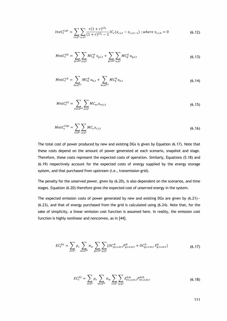
111

𝐼𝑛𝑣𝐶𝑡𝐶𝐴𝑃 = ∑∑

𝑟(1 + 𝑟)𝐿𝑇𝑐

(1 + 𝑟)𝐿𝑇𝑐 − 1𝐼𝐶𝑐(𝑥𝑐,𝑖,𝑡 − 𝑥𝑐,𝑖,𝑡−1)


; 𝑤ℎ𝑒𝑟𝑒 𝑥𝑐,𝑖,0 = 0 (6.12)

𝑀𝑛𝑡𝐶𝑡𝐷𝐺 = ∑ ∑𝑀𝐶𝑔

𝑁


𝑥𝑔,𝑖,𝑡 + ∑ ∑𝑀𝐶𝑔𝐸


𝑢𝑔,𝑖,𝑡 (6.13)

𝑀𝑛𝑡𝐶𝑡𝐿𝑁 = ∑ 𝑀𝐶𝑘

𝐸

𝑘𝜖𝛺𝑒ℓ

𝑢𝑘,𝑡 + ∑ 𝑀𝐶𝑘𝑁𝑥𝑘,𝑡

𝑘𝜖𝛺𝑛ℓ

(6.14)

𝑀𝑛𝑡𝐶𝑡𝐸𝑆 = ∑ ∑𝑀𝐶𝑒𝑠𝑥𝑒𝑠,𝑖,𝑡

𝑖𝜖𝛺𝑖𝑒𝑠𝜖𝛺𝑒𝑠

(6.15)

𝑀𝑛𝑡𝐶𝑡𝐶𝑎𝑝

= ∑ ∑𝑀𝐶𝑐𝑥𝑐,𝑖,𝑡𝑖𝜖𝛺𝑖𝑐𝜖𝛺𝑐

(6.16)

The total cost of power produced by new and existing DGs is given by Equation (6.17). Note that

these costs depend on the amount of power generated at each scenario, snapshot and stage.

Therefore, these costs represent the expected costs of operation. Similarly, Equations (5.18) and

(6.19) respectively account for the expected costs of energy supplied by the energy storage

system, and that purchased from upstream (i.e., transmission grid).

The penalty for the unserved power, given by (6.20), is also dependent on the scenarios, and time

stages. Equation (6.20) therefore gives the expected cost of unserved energy in the system.

The expected emission costs of power generated by new and existing DGs are given by (6.21)—

(6.23), and that of energy purchased from the grid is calculated using (6.24). Note that, for the

sake of simplicity, a linear emission cost function is assumed here. In reality, the emission cost

function is highly nonlinear and nonconvex, as in [44].

𝐸𝐶𝑡𝐷𝐺 = ∑ 𝜌𝑠 ∑ 𝜋𝑤 ∑ ∑(𝑂𝐶𝑔,𝑖,𝑠,𝑤,𝑡

𝑁 𝑃𝑔,𝑖,𝑠,𝑤,𝑡𝑁


+ 𝑂𝐶𝑔,𝑖,𝑠,𝑤,𝑡𝐸

𝑤𝜖𝛺𝑤

𝑃𝑔,𝑖,𝑠,𝑤,𝑡𝐸 )

𝑠𝜖𝛺𝑠

(6.17)

𝐸𝐶𝑡𝐸𝑆 = ∑ 𝜌𝑠 ∑ 𝜋𝑤 ∑∑𝜆𝑒𝑠,𝑖,𝑠,𝑤,𝑡

𝑑𝑐ℎ 𝑃𝑒𝑠,𝑖,𝑠,𝑤,𝑡𝑑𝑐ℎ

𝑖𝜖𝛺𝑖𝑐𝜖𝛺𝑐𝑤𝜖𝛺𝑤𝑠𝜖𝛺𝑠

(6.18)

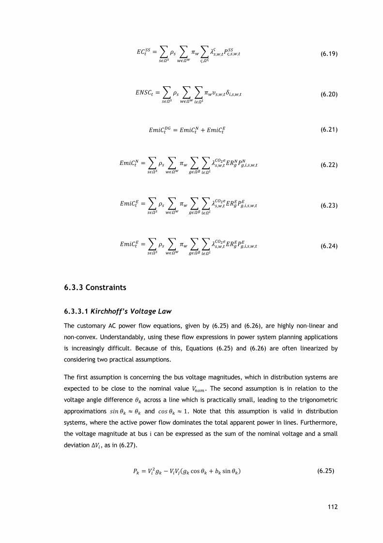
112

𝐸𝐶𝑡𝑆𝑆 = ∑ 𝜌𝑠 ∑ 𝜋𝑤∑𝜆𝑠,𝑤,𝑡

𝜍𝑃𝜍,𝑠,𝑤,𝑡𝑆𝑆

𝜍,𝛺𝜍𝑤𝜖𝛺𝑤𝑠𝜖𝛺𝑠

(6.19)

𝐸𝑁𝑆𝐶𝑡 = ∑ 𝜌𝑠 ∑ ∑𝜋𝑤𝜐𝑠,𝑤,𝑡𝛿𝑖,𝑠,𝑤,𝑡𝑖𝜖𝛺𝑖𝑤𝜖𝛺𝑤𝑠𝜖𝛺𝑠

(6.20)

𝐸𝑚𝑖𝐶𝑡𝐷𝐺 = 𝐸𝑚𝑖𝐶𝑡

𝑁 + 𝐸𝑚𝑖𝐶𝑡𝐸 (6.21)

𝐸𝑚𝑖𝐶𝑡𝑁 = ∑ 𝜌𝑠 ∑ 𝜋𝑤 ∑ ∑𝜆𝑠,𝑤,𝑡

𝐶𝑂2𝑒𝐸𝑅𝑔𝑁𝑃𝑔,𝑖,𝑠,𝑤,𝑡

𝑁


(6.22)



𝐸


(6.23)



𝐸


(6.24)

6.3.3 Constraints

6.3.3.1 Kirchhoff’s Voltage Law

The customary AC power flow equations, given by (6.25) and (6.26), are highly non-linear and

non-convex. Understandably, using these flow expressions in power system planning applications

is increasingly difficult. Because of this, Equations (6.25) and (6.26) are often linearized by

considering two practical assumptions.

The first assumption is concerning the bus voltage magnitudes, which in distribution systems are

expected to be close to the nominal value 𝑉𝑛𝑜𝑚. The second assumption is in relation to the

voltage angle difference 휃𝑘 across a line which is practically small, leading to the trigonometric

approximations 𝑠𝑖𝑛 휃𝑘 ≈ 휃𝑘 and 𝑐𝑜𝑠 휃𝑘 ≈ 1. Note that this assumption is valid in distribution

systems, where the active power flow dominates the total apparent power in lines. Furthermore,

the voltage magnitude at bus i can be expressed as the sum of the nominal voltage and a small

deviation ∆𝑉𝑖, as in (6.27).

𝑃𝑘 = 𝑉𝑖2𝑔𝑘 − 𝑉𝑖𝑉𝑗(𝑔𝑘 cos 휃𝑘 + 𝑏𝑘 sin 휃𝑘) (6.25)

113

𝑄𝑘 = −𝑉𝑖2𝑏𝑘 + 𝑉𝑖𝑉𝑗(𝑏𝑘 cos 휃𝑘 − 𝑔𝑘 sin 휃𝑘) (6.26)

𝑉𝑖 = 𝑉𝑛𝑜𝑚 + ∆𝑉𝑖 , 𝑤ℎ𝑒𝑟𝑒 ∆𝑉𝑚𝑖𝑛 ≤ ∆𝑉𝑖 ≤ ∆𝑉𝑚𝑎𝑥 (6.27)

Note that the voltage deviations at each node ∆𝑉𝑖 are expected to be very small. Substituting

(6.27) in (6.25) and (6.26) and neglecting higher order terms, we get:

𝑃𝑘 ≈ (𝑉𝑛𝑜𝑚2 + 2𝑉𝑛𝑜𝑚∆𝑉𝑖)𝑔𝑘 − (𝑉𝑛𝑜𝑚

2 + 𝑉𝑛𝑜𝑚∆𝑉𝑖 + 𝑉𝑛𝑜𝑚∆𝑉𝑗)(𝑔𝑘 + 𝑏𝑘휃𝑘) (6.28)

𝑄𝑘 ≈ −(𝑉𝑛𝑜𝑚2 + 2𝑉𝑛𝑜𝑚∆𝑉𝑖)𝑏𝑘 + (𝑉𝑛𝑜𝑚

2 + 𝑉𝑛𝑜𝑚∆𝑉𝑖 + 𝑉𝑛𝑜𝑚∆𝑉𝑗)(𝑏𝑘 − 𝑔𝑘휃𝑘) (6.29)

Note that Equations (6.28) and (6.29) still contain nonlinearities because of the products of two

continuous variables—voltage deviations and angle differences. However, since these variables

(∆𝑉𝑖, ∆𝑉𝑗 and 휃𝑘) are very small, their products can be neglected. Hence, the above flow

equations become:

𝑃𝑘 ≈ 𝑉𝑛𝑜𝑚(∆𝑉𝑖 − ∆𝑉𝑗)𝑔𝑘 − 𝑉𝑛𝑜𝑚2 𝑏𝑘휃𝑘 (6.30)

𝑄𝑘 ≈ −𝑉𝑛𝑜𝑚(∆𝑉𝑖 − ∆𝑉𝑗)𝑏𝑘 − 𝑉𝑛𝑜𝑚2 𝑔𝑘휃𝑘 (6.31)

The linear planning model proposed here is based on the above linearized flow equations.

This linearization approach was first introduced in [95] in the context of transmission expansion

planning problem. When the investment planning problem includes network switching,

reinforcement, replacement and expansion of feeders, Equations (6.30) and (6.31) must be

multiplied by the corresponding binary variables as in (6.32) —(6.35). This is to make sure the flow

through an existing/a new feeder is zero when its switching/investment variable is zero;

otherwise, the flow in that feeder should obey the Kirchhoff’s law.

𝑃𝑘 ≈ 𝑢𝑘,𝑡𝑉𝑛𝑜𝑚(∆𝑉𝑖 − ∆𝑉𝑗)𝑔𝑘 − 𝑉𝑛𝑜𝑚

2 𝑏𝑘휃𝑘 (6.32)

𝑄𝑘 ≈ 𝑢𝑘,𝑡−𝑉𝑛𝑜𝑚(∆𝑉𝑖 − ∆𝑉𝑗)𝑏𝑘 − 𝑉𝑛𝑜𝑚2 𝑔𝑘휃𝑘 (6.33)

114

𝑃𝑘 ≈ 𝑥𝑘,𝑡𝑉𝑛𝑜𝑚(∆𝑉𝑖 − ∆𝑉𝑗)𝑔𝑘 − 𝑉𝑛𝑜𝑚2 𝑏𝑘휃𝑘 (6.34)

𝑄𝑘 ≈ 𝑥𝑘,𝑡−𝑉𝑛𝑜𝑚(∆𝑉𝑖 − ∆𝑉𝑗)𝑏𝑘 − 𝑉𝑛𝑜𝑚2 𝑔𝑘휃𝑘 (6.35)

The bilinear products, involving binary with voltage deviation and angle difference variables,

introduces undesirable nonlinearity to the problem. This nonlinearity can be avoided using the

big-M formulation i.e. by reformulating the above equations into their respective disjunctive

equivalents as in (6.36)—(6.39). As a rule-of-thumb, the big-M parameter is often set to the

maximum transfer capacity in the system.

|𝑃𝑘,𝑠,𝑤,𝑡 − 𝑉𝑛𝑜𝑚(∆𝑉𝑖,𝑠,𝑤,𝑡 − ∆𝑉𝑗,𝑠,𝑤,𝑡)𝑔𝑘 − 𝑉𝑛𝑜𝑚2 𝑏𝑘휃𝑘,𝑠,𝑤,𝑡 )| ≤ 𝑀𝑃𝑘(1 − 𝑢𝑘,𝑡) (6.36)

|𝑄𝑘,𝑠,𝑤,𝑡 − −𝑉𝑛𝑜𝑚(∆𝑉𝑖,𝑠,𝑤,𝑡 − ∆𝑉𝑗,𝑠,𝑤,𝑡)𝑏𝑘 − 𝑉𝑛𝑜𝑚2 𝑔𝑘휃𝑘,𝑠,𝑤,𝑡 | ≤ 𝑀𝑄𝑘(1 − 𝑢𝑘,𝑡) (6.37)

|𝑃𝑘,𝑠,𝑤,𝑡 − 𝑉𝑛𝑜𝑚(∆𝑉𝑖,𝑠,𝑤,𝑡 − ∆𝑉𝑗,𝑠,𝑤,𝑡)𝑔𝑘 − 𝑉𝑛𝑜𝑚2 𝑏𝑘휃𝑘,𝑠,𝑤,𝑡| ≤ 𝑀𝑃𝑘(1 − 𝑥𝑘,𝑡) (6.38)

|𝑄𝑘,𝑠,𝑤,𝑡 − −𝑉𝑛𝑜𝑚(∆𝑉𝑖,𝑠,𝑤,𝑡 − ∆𝑉𝑗,𝑠,𝑤,𝑡)𝑏𝑘 − 𝑉𝑛𝑜𝑚2 𝑔𝑘휃𝑘,𝑠,𝑤,𝑡| ≤ 𝑀𝑄𝑘(1 − 𝑥𝑘,𝑡) (6.39)

6.3.3.2 Flow Limits

The apparent power flow through a line 𝑆𝑘is given by √𝑃𝑘2 + 𝑄𝑘

2 and this has to be less than or

equal to the rated value which is denoted as:

𝑃𝑘2 + 𝑄𝑘

2 ≤ (𝑆𝑘𝑚𝑎𝑥)2 (6.40)

Considering line switching/investment, Equation (6.40) can be rewritten as:

𝑃𝑘,𝑠,𝑤,𝑡2 + 𝑄𝑘,𝑠,𝑤,𝑡

2 ≤ 𝑢𝑘,𝑡(𝑆𝑘𝑚𝑎𝑥)2 (6.41)

𝑃𝑘,𝑠,𝑤,𝑡2 + 𝑄𝑘,𝑠,𝑤,𝑡

2 ≤ 𝑥𝑘,𝑡(𝑆𝑘𝑚𝑎𝑥)2 (6.42)

115

The quadratic expressions of active and reactive power flows in (6.41) through (6.42) can be

easily linearized using piecewise linearization, considering a sufficiently large number of linear

segments, 𝐿.

There are a number of ways of linearizing such functions such as incremental, multiple choice,

convex combination and other approaches in the literature [164]. Here, the first approach (which

is based on first-order approximation of the nonlinear curve) is used because of its relatively

simple formulation. To this end, two non-negative auxiliary variables are introduced for each of

the flows 𝑃𝑘 and 𝑄𝑘 such that 𝑃𝑘 = 𝑃𝑘+ − 𝑃𝑘

− and 𝑄𝑘 = 𝑄𝑘+ − 𝑄𝑘

−.

Note that these auxiliary variables (i.e., 𝑃𝑘+ , 𝑃𝑘

−, 𝑄𝑘+ and𝑄𝑘

−) represent the positive and negative

flows of 𝑃𝑘 and 𝑄𝑘, respectively. This helps one to consider only the positive quadrant of the

nonlinear curve, resulting in a significant reduction in the mathematical complexity, and by

implication the computational burden. In this case, the associated linear constraints are:

𝑃𝑘,𝑠,𝑤,𝑡2 ≈∑𝛼𝑘,𝑙𝑝𝑘,𝑠,𝑤,𝑡,𝑙

𝐿

𝑙=1

(6.43)

𝑄𝑘,𝑠,𝑤,𝑡2 ≈∑𝛽𝑘,𝑙𝑞𝑘,𝑠,𝑤,𝑡,𝑙

𝐿

𝑙=1

(6.44)

𝑃𝑘,𝑠,𝑤,𝑡+ + 𝑃𝑘,𝑠,𝑤,𝑡

− =∑𝑝𝑘,𝑠,𝑤,𝑡,𝑙

𝐿

𝑙=1

(6.45)

𝑄𝑘,𝑠,𝑤,𝑡+ + 𝑄𝑘,𝑠,𝑤,𝑡

− =∑𝑞𝑘,𝑠,𝑤,𝑡,𝑙

𝐿

𝑙=1

(6.46)

where 𝑝𝑘,𝑠,𝑤,𝑡,𝑙 ≤ 𝑃𝑘𝑚𝑎𝑥 𝐿⁄ and 𝑞𝑘,𝑠,𝑤,𝑡,𝑙 ≤ 𝑄𝑘

𝑚𝑎𝑥/𝐿.

116

6.3.3.3 Line Losses

The active and reactive power losses in line k can be approximated as follows:

𝑃𝐿𝑘 = 𝑃𝑘,𝑖𝑗 + 𝑃𝑘,𝑗𝑖 ≈ 2𝑉𝑛𝑜𝑚2 𝑔𝑘(1 − cos 휃𝑘) ≈ 𝑉𝑛𝑜𝑚

2 𝑔𝑘휃𝑘2 (6.47)

𝑄𝐿𝑘 = 𝑄𝑘,𝑖𝑗 + 𝑄𝑘,𝑗𝑖 ≈ −2𝑉𝑛𝑜𝑚2 𝑏𝑘(1 − cos 휃𝑘) ≈ −𝑏𝑘𝑉𝑛𝑜𝑚

2 휃𝑘2 (6.48)

Clearly, Equations (6.47) and (6.48) are nonlinear and nonconvex functions, making the problem

more complex to solve. This can be overcome by having the quadratic angle differences

piecewise-linearized, as it is done for the quadratic flows in the above. However, instead of doing

this, the expressions in (6.47) and (6.48) can be expressed in terms of the active and the reactive

power flows as in (6.49) and (6.50). Note that Equation (6.49) can be easily obtained by

multiplying the squared expressions of both sides of the equations in (6.30) and (6.31) by the

resistance of the branch, combining the resulting equations, neglecting higher order terms and

reordering both sides of the resulting equation. Equation (6.50) is also obtained in a similar

fashion but by multiplying the squared expressions by reactance. For the sake of completeness,

details concerning the derivations (6.49) and (6.50) are presented in Appendix D.

𝑃𝐿𝑘,𝑠,𝑤,𝑡 = 𝑟𝑘𝑃𝑘,𝑠,𝑤,𝑡2 + 𝑄𝑘,𝑠,𝑤,𝑡

2 /𝑉𝑛𝑜𝑚2 (6.49)

𝑄𝐿𝑘,𝑠,𝑤,𝑡 = 𝑥𝑘𝑃𝑘,𝑠,𝑤,𝑡2 + 𝑄𝑘,𝑠,𝑤,𝑡

2 /𝑉𝑛𝑜𝑚2 (6.50)

Note that expressing the losses as a function of flows has two advantages. First, doing so reduces

the number of nonlinear terms that has to be linearized, which in turn results in a model with a

reduced number of equations and variables. For example, if Equations (6.47) and (6.48) are used

instead, in addition to the quadratic power flow terms 𝑃𝑘2 and 𝑄𝑘

2, the quadratic angle differences

휃𝑘2 should also be linearized to make the problem linear and convex. On the contrary, when Eqs.

(6.49) and (6.50) are used, one is only required to linearize 𝑃𝑘2 and 𝑄𝑘

2. Second, it avoids

unnecessary constraints on the angle differences when a line between two nodes is not connected

or remains not selected for investment. This is often avoided by introducing binary variables and

using a so-called big-M formulation [95]. However, this adds extra complexity to the problem.

5.3.3.4 Kirchhoff’s Current Law (Active and Reactive Load Balances)

All the time, load balance should be respected at each node i.e. the sum of all injections should

be equal to the sum of all withdrawals at each node. This is enforced by adding the following two

constraints:

117

∑ (𝑃𝑔,𝑖,𝑠,𝑤,𝑡𝐸 + 𝑃𝑔,𝑖,𝑠,𝑤,𝑡

𝑁 )

𝑔𝜖Ω𝐷𝐺

+ ∑ (𝑃𝑒𝑠,𝑖,𝑠,𝑤,𝑡𝑑𝑐ℎ − 𝑃𝑒𝑠,𝑖,𝑠,𝑤,𝑡

𝑐ℎ )

𝑒𝑠𝜖Ω𝑒𝑠

+ 𝑃𝜍,𝑠,𝑤,𝑡𝑆𝑆 + ∑ 𝑃𝑘,𝑠,𝑤,𝑡


− ∑ 𝑃𝑘,𝑠,𝑤,𝑡𝑜𝑢𝑡,𝑘𝜖𝑖

+ 𝛿𝑖,𝑠,𝑤,𝑡 = 𝐷𝑠,𝑤,𝑡𝑖 + 𝑃𝐿𝜍,𝑠,𝑤,𝑡 +∑

1

2𝑃𝐿𝑘,𝑠,𝑤,𝑡

𝑘𝜖𝑖

; ∀𝜍, ∀𝜍𝜖𝑖 (6.51)

∑ (𝑄𝑔,𝑖,𝑠,𝑤,𝑡𝐸 + 𝑄𝑔,𝑖,𝑠,𝑤,𝑡

𝑁 )

𝑔𝜖Ω𝐷𝐺

+ ∑ 𝑄𝑖,𝑠,𝑤,𝑡𝑐

𝑐𝜖Ω𝑐

+ 𝑄𝜍,𝑠,𝑤,𝑡𝑆𝑆 + ∑ 𝑄𝑘,𝑠,𝑤,𝑡


− ∑ 𝑄𝑘,𝑠,𝑤,𝑡𝑜𝑢𝑡,𝑘𝜖𝑖

= 𝑄𝑠,𝑤,𝑡𝑖 + 𝑄𝐿𝜍,𝑠,𝑤,𝑡 + ∑

1

2𝑄𝐿𝑘,𝑠,𝑤,𝑡


+ ∑1

2𝑄𝐿𝑘,𝑠,𝑤,𝑡

𝑜𝑢𝑡,𝑘𝜖𝑖

; ∀𝜍, ∀𝜍𝜖𝑖 (6.52)

Equations (6.51) and (6.52) stand for the active and the reactive power balances at each node,

respectively.

6.3.3.5 Bulk Energy Storage Model Constraints

The generic bulk ESS is modeled by constraints (6.53) —(6.59).

0 ≤ 𝑃𝑒𝑠,𝑖,𝑠,𝑤,𝑡𝑐ℎ ≤ 𝐼𝑒𝑠,𝑖,𝑠,𝑤,𝑡


(6.53)

0 ≤ 𝑃𝑒𝑠,𝑖,𝑠,𝑤,𝑡𝑑𝑐ℎ ≤ 𝐼𝑒𝑠,𝑖,𝑠,𝑤,𝑡

𝑑𝑐ℎ 𝑥𝑒𝑠,𝑖,𝑡𝑃𝑒𝑠,𝑖𝑐ℎ,𝑚𝑎𝑥

(6.54)

𝐼𝑒𝑠,𝑖,𝑠,𝑤,𝑡𝑐ℎ + 𝐼𝑒𝑠,𝑖,𝑠,𝑤,𝑡

𝑑𝑐ℎ ≤ 1 (6.55)

𝐸𝑒𝑠,𝑖,𝑠,𝑤,𝑡 = 𝐸𝑒𝑠,𝑖,𝑠,𝑤−1,𝑡 + 휂𝑒𝑠 𝑐ℎ𝑃𝑒𝑠,𝑖,𝑠,𝑤,𝑡

𝑐ℎ − 𝛽𝑒𝑠 𝑑𝑐ℎ𝑃𝑒𝑠,𝑖,𝑠,𝑤,𝑡𝑑𝑐ℎ ; 𝑤ℎ𝑒𝑟𝑒 𝛽𝑒𝑠

𝑑𝑐ℎ = 1/휂𝑒𝑠 𝑑𝑐ℎ (6.56)

𝐸𝑒𝑠,𝑖𝑚𝑖𝑛𝑥𝑒𝑠,𝑖,𝑡 ≤ 𝐸𝑒𝑠,𝑖,𝑠,𝑤,𝑡 ≤ 𝑥𝑒𝑠,𝑖,𝑡𝐸𝑒𝑠,𝑖

𝑚𝑎𝑥 (6.57)

𝐸𝑒𝑠,𝑖,𝑠,𝑤0,𝑇1 = 𝜇𝑒𝑠𝑥𝑒𝑠,𝑖,𝑇1𝐸𝑒𝑠,𝑖𝑚𝑎𝑥 (6.58)

𝐸𝑒𝑠,𝑖,𝑠,𝑤1,𝑡+1 = 𝐸𝑒𝑠,𝑖,𝑠,𝑊,𝑡; 𝐸𝑒𝑠,𝑖,𝑠,𝑊,𝑇 = 𝐸𝑒𝑠,𝑖,𝑠,𝑤0,𝑇1 (6.59)

118

The limits on the capacity of ESS while being charged and discharged are considered in

Inequalities (6.53) and (6.54), respectively. Inequality (6.55) prevents simultaneous charging and

discharging operation of ESS at the same operational time w. The amount of stored energy within

the reservoir of bulk ESS at the operational time w as a function of energy stored until 𝑤 − 1 is

given by (6.56). The maximum and minimum levels of storages in operational time w are also

considered through inequality (6.57). Equation (6.58) shows the initial level of stored energy in

the bulk ESS as a function of its maximum reservoir capacity. In a multi-stage planning approach,

Equation (5.59) ensures that the initial level of energy in the bulk ESS at a given year is equal to

the final level of energy in the ESS in the preceding year and the reservoir level at the end of the

planning horizon should be equal to the initial level. The latter constraint guarantees that the

optimal solution returned by the solution algorithm is not because of the initial reservoir level.

For the sake of simplicity, 휂𝑒𝑠 𝑑𝑐ℎ is assumed to be equal to 휂𝑒𝑠

𝑐ℎ , as in [165], [166]. Both the charging

휂𝑒𝑠𝑐ℎ and discharging 휂𝑒𝑠

𝑑𝑐ℎ efficiencies are expressed in terms of the energy at the nodes where the

storage system is connected to. Because of this, a certain percentage of the energy fed to the

storage system will be stored while the remaining will be lost in the form of losses (electrical,

chemical, heat, etc.). This is related to the charging efficiency, which should then be less than 1.

On the other hand, in order to withdraw a given amount of energy from the storage system, more

energy is needed to cover the discharging losses. This is why we have 1/휂𝑒𝑠𝑑𝑐ℎ in Equation (6.56)

associated with the energy at the output side of the energy storage system.

Notice that inequalities (6.53) and (6.54) involve products of charging/discharging binary variables

and investment variable. In order to linearize these, new continuous positive variables 𝑧𝑒𝑠,𝑖,𝑠,𝑤,𝑡𝑐ℎ ,

and 𝑧𝑒𝑠,𝑖,𝑠,𝑤,𝑡𝑑𝑐ℎ , which replaces the bilinear products in each constraint, is introduced such that the

set of linear constraints in (6.60) and (6.61) hold. For instance, the product 𝐼𝑒𝑠,𝑖,𝑠,𝑤,𝑡𝑑𝑐ℎ 𝑥𝑒𝑠,𝑖,𝑡 is

replaced by the positive variable 𝑧𝑒𝑠,𝑖,𝑠,𝑤,𝑡𝑑𝑐ℎ . Then, the bilinear product is decoupled by introducing

the set of constraints in (6.60) [115].

𝑧𝑒𝑠,𝑖,𝑠,𝑤,𝑡𝑑𝑐ℎ ≤ 𝑥𝑒𝑠

𝑚𝑎𝑥𝐼𝑒𝑠,𝑖,𝑠,𝑤,𝑡𝑑𝑐ℎ ; 𝑧𝑒𝑠,𝑖,𝑠,𝑤,𝑡

𝑑𝑐ℎ ≤ 𝑥𝑒𝑠,𝑖,𝑡 ; 𝑧𝑒𝑠,𝑖,𝑠,𝑤,𝑡𝑑𝑐ℎ ≥ 𝑥𝑒𝑠,𝑖,𝑡 − (1 − 𝐼𝑒𝑠,𝑖,𝑠,𝑤,𝑡

𝑑𝑐ℎ )𝑥𝑒𝑠𝑚𝑎𝑥 (6.60)

Similarly, the product 𝐼𝑒𝑠,𝑖,𝑠,𝑤,𝑡𝑐ℎ 𝑥𝑒𝑠,𝑖,𝑡is decoupled by including the following set of constraints:

𝑧𝑒𝑠,𝑖,𝑠,𝑤,𝑡𝑐ℎ ≤ 𝑥𝑒𝑠

𝑚𝑎𝑥𝐼𝑒𝑠,𝑖,𝑠,𝑤,𝑡𝑐ℎ ; 𝑧𝑒𝑠,𝑖,𝑠,𝑤,𝑡

𝑐ℎ ≤ 𝑥𝑒𝑠,𝑖,𝑡 ; 𝑧𝑒𝑠,𝑖,𝑠,𝑤,𝑡𝑐ℎ ≥ 𝑥𝑒𝑠,𝑖,𝑡 − (1 − 𝐼𝑒𝑠,𝑖,𝑠,𝑤,𝑡

𝑐ℎ )𝑥𝑒𝑠𝑚𝑎𝑥 (6.61)

The large number of discrete variables in the storage model presented above can render

significant computational burden. To overcome this, a relaxed ESS model can be formed without

the charging and discharging indicator variables as:

0 ≤ 𝑃𝑒𝑠,𝑖,𝑠,𝑤,𝑡𝑐ℎ ≤ 𝑥𝑒𝑠,𝑖,𝑡𝑃𝑒𝑠,𝑖

𝑐ℎ,𝑚𝑎𝑥 (6.53’)

119

0 ≤ 𝑃𝑒𝑠,𝑖,𝑠,𝑤,𝑡𝑑𝑐ℎ ≤ 𝑥𝑒𝑠,𝑖,𝑡𝑃𝑒𝑠,𝑖

𝑐ℎ,𝑚𝑎𝑥 (6.54’)

𝐸𝑒𝑠,𝑖,𝑠,𝑤,𝑡 = 𝐸𝑒𝑠,𝑖,𝑠,𝑤−1,𝑡 + 휂𝑒𝑠 𝑐ℎ𝑃𝑒𝑠,𝑖,𝑠,𝑤,𝑡

𝑐ℎ − 𝛽𝑒𝑠 𝑑𝑐ℎ𝑃𝑒𝑠,𝑖,𝑠,𝑤,𝑡𝑑𝑐ℎ ; 𝑤ℎ𝑒𝑟𝑒 𝛽𝑒𝑠

𝑑𝑐ℎ = 1/휂𝑒𝑠 𝑑𝑐ℎ (6.56’)

Under normal conditions, the ESS model in (6.53’), (6.54’) and (6.56’) is exact because by the

principle of optimality, at most one of the variables 𝑃𝑒𝑠,𝑖,𝑠,𝑤,𝑡𝑐ℎ and 𝑃𝑒𝑠,𝑖,𝑠,𝑤,𝑡

𝑑𝑐ℎ can be greater than

zero. In other words, it does not economic sense to have both variables to be greater than zero at

the same time.

6.3.3.6 Active and Reactive Power Limits of DGs

The active and reactive power limits of existing generators are given by (6.62) and (6.63),

respectively. In the case of new (candidate) generators, the corresponding constraints are (6.64)

and (6.65). Note that the binary variables multiply the minimum and the maximum generation

limits to make sure that the power generation variable is zero when the generator remains either

unutilized or unselected for investment.



𝑄𝑔,𝑖,𝑠,𝑤,𝑡𝐸,𝑚𝑖𝑛 𝑢𝑔,𝑖,𝑡 ≤ 𝑄𝑔,𝑖,𝑠,𝑤,𝑡

𝐸 ≤ 𝑄𝑔,𝑖,𝑠,𝑤,𝑡𝐸,𝑚𝑎𝑥 𝑢𝑔,𝑖,𝑡 (6.63)

𝑃𝑔,𝑖,𝑠,𝑤,𝑡𝑁,𝑚𝑖𝑛 𝑥𝑔,𝑖,𝑡 ≤ 𝑃𝑔,𝑖,𝑠,𝑤,𝑡

𝑁 ≤ 𝑃𝑔,𝑖,𝑠,𝑤,𝑡𝑁,𝑚𝑎𝑥 𝑥𝑔,𝑖,𝑡 (6.64)

𝑄𝑔,𝑖,𝑠,𝑤,𝑡𝑁,𝑚𝑖𝑛 𝑥𝑔,𝑖,𝑡 ≤ 𝑄𝑔,𝑖,𝑠,𝑤,𝑡

𝑁 ≤ 𝑄𝑔,𝑖,𝑠,𝑤,𝑡𝑁,𝑚𝑎𝑥 𝑥𝑔,𝑖,𝑡 (6.65)

It should be noted that these constraints are applicable only for conventional DGs which have

reactive power support capabilities. In the case of variable generation sources, slight

modifications are required. For instance, for wind and solar PV generators, the upper bound

𝑃𝑔,𝑖,𝑠,𝑤,𝑡𝑚𝑎𝑥 should be equal to the actual production level at a specific hour, which in turn depends on

the level of primary energy source (wind speed and solar radiation). The lower bound 𝑃𝑔,𝑖,𝑠,𝑤,𝑡𝑚𝑖𝑛 in

this case is simply set to zero.

In addition, conventional wind and solar PV sources do not often have the capability to provide

reactive power support; hence, they are operated at a constant and lagging or unity power factor.

Under such an operation, the following constraints should be used:

120

𝑄𝑔,𝑖,𝑠,𝑤,𝑡𝐸 = tan (cos−1(𝑝𝑓𝑔)) ∗ 𝑃𝑔,𝑖,𝑠,𝑤,𝑡

𝐸 (6.63’)

𝑄𝑔,𝑖,𝑠,𝑤,𝑡𝑁 = tan (cos−1(𝑝𝑓𝑔)) ∗ 𝑃𝑔,𝑖,𝑠,𝑤,𝑡

𝑁 (6.65’)

where 𝑝𝑓𝑔is the power factor of the wind or solar type generator 𝑔. Under normal cases,

𝑃𝑔,𝑖,𝑠,𝑤,𝑡𝐸 = 𝑃𝑔,𝑖,𝑠,𝑤,𝑡

𝐸, 𝑚𝑎𝑥 and 𝑃𝑔,𝑖,𝑠,𝑤,𝑡𝑁 = 𝑃𝑔,𝑖,𝑠,𝑤,𝑡

𝑁, 𝑚𝑎𝑥.

On the other hand, for wind and solar PV type DGs with reactive power support capabilities such

as doubly fed induction generator (DFIG) based wind turbine and voltage source inverter (VSI)

based PV, the following constraints are used:

− tan(cos−1(𝑝𝑓𝑔)) ∗ 𝑃𝑔,𝑖,𝑠,𝑤,𝑡𝐸 ≤ 𝑄𝑔,𝑖,𝑠,𝑤,𝑡

𝐸 ≤ tan (cos−1(𝑝𝑓𝑔)) ∗ 𝑃𝑔,𝑖,𝑠,𝑤,𝑡𝐸 (6.63’’)

− tan(cos−1(𝑝𝑓𝑔)) ∗ 𝑃𝑔,𝑖,𝑠,𝑤,𝑡𝑁 ≤ 𝑄𝑔,𝑖,𝑠,𝑤,𝑡

𝑁 ≤ tan (cos−1(𝑝𝑓𝑔)) ∗ 𝑃𝑔,𝑖,𝑠,𝑤,𝑡𝑁 (6.65’’)

The above two inequalities show that the wind and solar type DGs are capable of operating

between 𝑝𝑓𝑔 leading power factor (capacitive) and 𝑝𝑓𝑔 lagging power factor (reactive). This

means such DGs are capable of “producing” and “consuming” reactive power depending on

operational situations in the system.

6.3.3.7 Reactive Power Limit of Capacitor Bank

Inequality (6.66) ensures that the reactive power produced by the reactive power sources

(capacitor banks) is bounded between zero and the maximum possible capacity.

0 ≤ 𝑄𝑖,𝑠,𝑤,𝑡𝑐 ≤ 𝑥𝑐,𝑖,𝑡𝑄𝑐

0 (6.66)

6.3.3.8 Active and Reactive Power Limits of Power Purchased

For technical reasons, the power that can be purchased from the transmission grid could have

minimum and maximum limits, which is enforced by (6.67) and (6.68). However, it is understood

that, in reality, setting such limits is difficult. They are included here only for the sake of

completeness.

𝑃𝜍,𝑠,𝑤,𝑡𝑆𝑆,𝑚𝑖𝑛 ≤ 𝑃𝜍,𝑠,𝑤,𝑡

𝑆𝑆 ≤ 𝑃𝜍,𝑠,𝑤,𝑡𝑆𝑆,𝑚𝑎𝑥

(6.67)

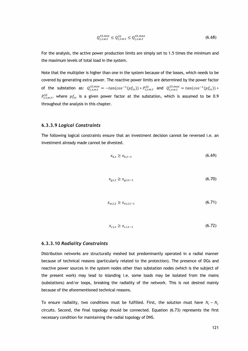
121

𝑄𝜍,𝑠,𝑤,𝑡𝑆𝑆,𝑚𝑖𝑛 ≤ 𝑄𝜍,𝑠,𝑤,𝑡

𝑆𝑆 ≤ 𝑄𝜍,𝑠,𝑤,𝑡𝑆𝑆,𝑚𝑎𝑥

(6.68)

For the analysis, the active power production limits are simply set to 1.5 times the minimum and

the maximum levels of total load in the system.

Note that the multiplier is higher than one in the system because of the losses, which needs to be

covered by generating extra power. The reactive power limits are determined by the power factor

of the substation as: 𝑄𝜍,𝑠,𝑤,𝑡𝑆𝑆,𝑚𝑖𝑛 = −𝑡𝑎𝑛 (𝑐𝑜𝑠−1(𝑝𝑓𝑠𝑠)) ∗ 𝑃𝜍,𝑠,𝑤,𝑡

𝑆𝑆 and 𝑄𝜍,𝑠,𝑤,𝑡𝑆𝑆,𝑚𝑎𝑥 = 𝑡𝑎𝑛 (𝑐𝑜𝑠−1(𝑝𝑓𝑠𝑠)) ∗

𝑃𝜍,𝑠,𝑤,𝑡𝑆𝑆 , where 𝑝𝑓𝑠𝑠 is a given power factor at the substation, which is assumed to be 0.9

throughout the analysis in this chapter.


The following logical constraints ensure that an investment decision cannot be reversed i.e. an

investment already made cannot be divested.

𝑥𝑘,𝑡 ≥ 𝑥𝑘,𝑡−1 (6.69)

𝑥𝑔,𝑖,𝑡 ≥ 𝑥𝑔,𝑖,𝑡−1 (6.70)

𝑥𝑒𝑠,𝑖,𝑡 ≥ 𝑥𝑒𝑠,𝑖,𝑡−1 (6.71)

𝑥𝑐,𝑖,𝑡 ≥ 𝑥𝑐,𝑖,𝑡−1 (6.72)


Distribution networks are structurally meshed but predominantly operated in a radial manner

because of technical reasons (particularly related to the protection). The presence of DGs and

reactive power sources in the system nodes other than substation nodes (which is the subject of

the present work) may lead to islanding i.e. some loads may be isolated from the mains

(substations) and/or loops, breaking the radiality of the network. This is not desired mainly

because of the aforementioned technical reasons.

To ensure radiality, two conditions must be fulfilled. First, the solution must have 𝑁𝑖 − 𝑁𝜍

circuits. Second, the final topology should be connected. Equation (6.73) represents the first

necessary condition for maintaining the radial topology of DNS.

122


𝑘∈Ω𝑖𝑗

= 𝑁𝑖 −𝑁𝜍 ; ∀𝑡 (6.73)

Note that the above equation assumes line investment is possible in all corridors. Hence, in a

given corridor, we can have either an existing branch, a new one, or both connected in parallel,

depending on the economic benefits of the final setup (solution) brings about to the system.

The radiality constraint in (6.73) then has to accommodate this condition. One way to do this is

using the Boolean logic operation, as in (6.73). Unfortunately, this introduces nonlinearity.

We show how this logic can be linearized using an additional auxiliary variable zk,t and the

binary variables associated to existing and new branches (i.e., 𝑢𝑘,𝑡 and 𝑥𝑘,𝑡), respectively.

Given 𝑧𝑘,𝑡: = 𝑂𝑅(𝑥𝑘,𝑡 , 𝑢𝑘,𝑡), this Boolean operation can be expressed using the following set of

linear constraints:


𝑘∈Ω𝑖𝑗

= 𝑁𝑖 −𝑁𝜍 ; ∀𝑡 (6.74)

Note that the auxiliary variable 𝑧𝑘,𝑡 is automatically constrained to be binary. Hence, it is not

necessary to explicitly define 𝑧𝑘,𝑡 as a binary variable; instead, defining it as a continuous positive

variable is sufficient.

Alternatively, if 𝑧𝑘,𝑡 is defined to be binary variable from the outset, then, Equation (6.73) can be

converted into a single range constraint as:

0 ≤ 2𝑧𝑘,𝑡 − 𝑥𝑘,𝑡 − 𝑢𝑘,𝑡 ≤ 1 ; ∀𝑡 (6.75)

Then, the radiality constraints in (6.73) can be reformulated using the 𝑧𝑘,𝑡 variables as:

∑ 𝑧𝑘,𝑡𝑘∈𝛺𝑖𝑗

= 𝑁𝑖 − 𝑁𝜍 ; ∀𝑡 (6.76)

When all loads in the DNS are only fed by power from substations, the final solution obtained

automatically satisfies the two aforementioned conditions; hence, no additional constraints are

required i.e. (6.74) or (6.75) along with (6.76) are sufficient to guarantee radiality.

However, it should be noted that in the presence of DGs and reactive power sources, these

constraints alone may not ensure the radiality of the distribution network, as pointed out in [106]

and further discussed in [97], [167]-[168]. This is however out of the scope of this chapter. If this

is a critical issue, additional constraints need to be added to guarantee that all buses are linked,

as proposed in [71], [53]–[55].

123

The optimization problem, developed here, encompasses Equations (6.3)—(6.24) and constraints

(6.36)—(6.39), (6.41)—(6.46), (6.49)—(6.61), (6.62), (6.63), (6.64), (6.65), (6.66)—(6.72), (6.74) or

(6.75) and (6.76) when all considered DGs are conventional generators with reactive power

support capabilities. Otherwise, constraints (6.63’) and (6.65’) need to be added in case

RES-based DGs which do not have such capabilities are present in the system or included in the

planning. In addition, if there are RES-based DGs which are instead capable of operating as

“generators” or “consumers” of reactive power depending on system operational situations,

constraints (6.63’’) and (6.65’’) should be included and applied. In addition, if a relaxed ESS

model is sought, constraints (6.53)—(6.61) can be replaced with the constraints in (6.53’), (6.54’)

and (6.56’).

6.4 Case Studies


The radial DNS, shown in Figure 6.1, is used to test the proposed planning model. The total active

and reactive loads of the system are 4.635 MW and 3.25 MVAr, respectively. The nominal voltage

of the system is 12.66 kV. Information regarding network and demand data is provided in [169]

and the data it is also available in the Appendix D. This system is selected for our case study

because it is highly lossy and not properly compensated. The voltage profile in the base case,

obtained from power flow analysis, can be found in [170]. For the sake of clarity, these nodal

voltages are also reproduced in Figure 6.2 in the form of cumulative distribution function. Note

that these results correspond to a substation power factor of 0.894 and with no lower voltage

limit restrictions imposed on the system. As it can observed in Figure 6.2, more than 70% of the

nodal voltages are below 0.95 per unit. However, this contradicts with the minimum voltage set in

distribution systems (often above this limit) for stability reasons. Running power flows by imposing

minimum voltage limits while keeping the substation power factor at 0.894 leads to infeasibility.

1 2

3

4 5 6 7 8 9 10 11 12 13 14 15 16 17 18

23

24

25

19

20

21

22

2627

28 29

3031

32 33

34

35

36

37 38 3940

41

Figure 6.1 - Single-line diagram of the IEEE 41-bus distribution network system.

124

Figure 6.2 - Cumulative distribution function (CDF) of voltages in the base case.

This may be because of the high reactive power requirement in the system, which has to be

provided by the substation given the fact that there the system is not well-compensated.

Reducing the power factor of the substation to 0.706 results in a feasible solution but around 40%

of the voltages are yet very close to the minimum value.

The following assumptions are made when carrying out the simulations:

A 3-year planning horizon is considered, which is divided into yearly decision stages.

The interest rate is set to 7%.

Electricity price at the substation follows the same trend as the demand i.e.

electricity price and demand profile are 100% correlated.

For the sake of simplicity, maintenance costs are taken to be 2% of the corresponding

investment costs.

The expected lifetime of capacitor banks and energy storage systems is assumed to be

15 years [171], [172], while that of DGs and feeders is 25 years [71].

A 5% voltage deviation is considered to be the maximum allowable deviation from the

nominal value that one can have in the system nodes i.e. −0.95𝑉𝑛𝑜𝑚 ≤ 𝑉𝑖 ≤ 1.05𝑉𝑛𝑜𝑚.

The power transfer capacity of all feeders is assumed to be 6.986 MVA.

All big-M parameters in the model formulation are set to 10, which is sufficiently

higher than the power transfer capacity of all feeders.

When linearizing quadratic terms in the developed planning model, the number of

partitions is set equal to 5. This balances well accuracy with computation burden, as

concluded in [94].

The efficiency of the bulk ES is assumed to be 90%.

The unit cost of capacitor banks is assumed to be €25/kVAr.

The size of the minimum deployable capacitor bank is considered to be 0.1 MVAr.

The investment cost of a 1.0 MW bulk ES, whose energy reservoir is 5 MWh, is

considered to be 1.0 M€.

125

The emission rate of power purchased is arbitrarily set equal to 0.4 tCO2e/MWh.

The investment cost of a given feeder is assumed to be directly proportional to its

impedance i.e. 𝐶𝑖𝑗 = 𝛼 ∗ 𝑍𝑖𝑗 where the proportionality constant 𝛼 is 10,000 €/Ω.

Wind and solar type DGs, each with a 1 MW installed capacity, are considered as

potential candidates to be deployed in the system. The investment costs of these

generators are assumed to be 2.64 M€ and 3.00 M€, respectively.

Electricity demand in the first, the second and the third planning stages is assumed to

be 5%, 10% and 15% higher than the demand in the base-case, respectively.

The emission prices in the first, second and third stages are set to 25, 45 and 60

€/tCO2e, respectively.

Variable power generation sources (wind and solar, in particular) are assumed to be

available in every node. This assumption emanates from the fact that distribution

networks span over a small geographical area. Hence, the distribution of resources in

this area can be considered to be the same.

The substation node (node 1) is considered as a reference; hence, its voltage

magnitude and angle are set to 1.02 ∗ 𝑉𝑛𝑜𝑚and 0, respectively.

The cost of unserved energy is set to 3000 €/MWh.

6.4.2 A Strategy for Reducing Combinatorial Solution Search Space

In the case study presented above, all nodes in the system are assumed to be candidates for the

placement of DGs, ESS and capacitor banks. However, this is not possible when the planning work

is carried out on large-scale DNSs because the size of the problem becomes huge as a result of

combinatorial explosion, rendering difficulty in solving the problem.

Owing to this fact, the potential candidate nodes are often predetermined either arbitrarily or

using some criteria for the selection such as the level of load, availability of resources, etc.

For example, the possible connection points of RES-based DGs are often known a priori based on

the availability of primary energy sources (such as wind speed and solar radiation). However, the

variation in the availability of wind speed and solar radiation among the connection points in the

DNS is not expected to be significant because it normally spans over a geographically small area,

where the weather situation is more or less the same.

Here, we show how the combinatorial solution search space can be substantially reduced using a

simple heuristic method [89]. The method is based on solving a relaxed version of the original

problem. This is done by treating all (normally integer) investment variables as continuous ones,

with the exception of the line reinforcement variables. This effectively means fractional

investment decisions are allowed.

The method here works by first establishing a threshold for each fractional investment solution

(i.e., corresponding to DGs, ESS and capacitor banks).

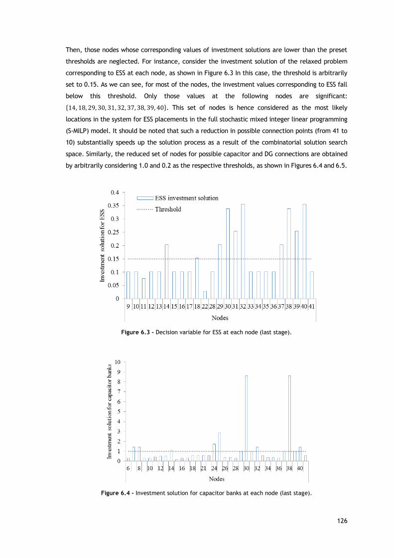
126

Then, those nodes whose corresponding values of investment solutions are lower than the preset

thresholds are neglected. For instance, consider the investment solution of the relaxed problem

corresponding to ESS at each node, as shown in Figure 6.3 In this case, the threshold is arbitrarily

set to 0.15. As we can see, for most of the nodes, the investment values corresponding to ESS fall

below this threshold. Only those values at the following nodes are significant:

14, 18, 29, 30, 31, 32, 37, 38, 39, 40. This set of nodes is hence considered as the most likely

locations in the system for ESS placements in the full stochastic mixed integer linear programming

(S-MILP) model. It should be noted that such a reduction in possible connection points (from 41 to

10) substantially speeds up the solution process as a result of the combinatorial solution search

space. Similarly, the reduced set of nodes for possible capacitor and DG connections are obtained

by arbitrarily considering 1.0 and 0.2 as the respective thresholds, as shown in Figures 6.4 and 6.5.

Figure 6.3 - Decision variable for ESS at each node (last stage).

Figure 6.4 - Investment solution for capacitor banks at each node (last stage).

127

Figure 6.5 - Investment solution for DGs at each node (last stage).

In this case, 7, 8, 14, 24, 25, 29, 30, 31, 32, 37, 38, 39, 40 is the reduced set of nodes for capacitor

bank connections, while that of DGs is 7, 8, 14, 18, 25, 29, 30, 31, 32, 37, 38, 39, 40. Note that the

procedure/criterion for setting the threshold in each case is an open question. It may also depend

on the nature and the size of the system under consideration. In general, each threshold should

be carefully set to a sufficiently low value so that relevant information is not lost (i.e. potential

candidate nodes are not excluded). The thresholds in this chapter are set based on the intuition

that those nodes, whose investment values are zero or close to zero, are less likely to appear in

the final set of solutions.

A deterministic planning model (i.e. considering a single scenario corresponding to the average

demand, wind and solar PV power output profiles) is used to evaluate the performance of the

heuristic approach proposed here. The results of the deterministic model obtained by applying the

heuristic method are compared with that of the “brute force” model i.e. without reducing the set

of candidate nodes for DG, ESS and capacitor placements. The investment decisions obtained are

the same in both cases but the computational requirements substantially differ from one another.

The proposed method helps to significantly reduce the combinatorial solution search space, and

thus the computational effort by more than sevenfold. In general, for distribution networks of this

size, the proposed heuristic approach may not be needed or a short-list of candidate nodes for

DG, ESS and capacitor placement may be made available based on expert knowledge.

The problem is tractable without the need of reducing the solution search space as shown in

Table 6.1. However, one cannot rely on expert knowledge when the planning involves large-scale

distribution network systems. In such problems, and when there is a lack of adequate computing

machine, it is critical to employ mechanisms that reduce the combinatorial solution search space.

In our case, this relates to reducing the number of candidate nodes for allocating DGs, ESSs and

capacitor banks.

128

Table 6.1 – Computational size of the optimization problem

Brute-force Reduced

Number of equations 11,032,828 9,039,895

Number of variables 9,315,028 8,100,028

Discrete variables 720 387

Simulation time (hours) 26.2 3.7

For the case study considered in this chapter, the results obtained by applying the heuristic

approach are the same as those obtained with the “brute-force” model which treats every node

as a candidate for placement of DGs, ESSs and capacitor banks. However, it should be noted that

since the proposed method is heuristic, its performance can be different for different systems.

The approach contributes a lot to the solution process; yet, the conclusions drawn from the test

results in this chapter cannot be generalized. The authors acknowledge that vital information

could be excluded when setting the threshold to reduce the number of candidate nodes.

For instance, even if the investment solution at a certain node in the relaxed problem is close to

zero, the node could still be feasible for DG, ESS and/or capacitor placement in the full-scale

stochastic model. As a final remark, careful analysis of the system under consideration is required

when applying the reduction method proposed in this chapter. Table 6.1 compares the size of the

problem before and after applying the heuristic combinatorial solution search space reduction

method. We can see that the combinatorial solution search space is reduced from 2720 to 2387,

and this also helps to reduce the number of equations and continuous variables by more than 18%

and 13%, respectively.


Intermittent power generation sources such as wind and solar PV type DGs normally operate with

a fixed lagging power factor [173]. In other words, such generators “consume” reactive power,

instead of “producing” and contributing to the voltage regulation in the system (also known as

reactive power support). For instance, wind turbines installed in power systems throughout the

world are predominantly based on asynchronous generators (also known as induction generators).

As mentioned above, one of the typical characteristics of such machines is that they always

“consume” reactive power. Because of this, such wind turbines are often operated at a constant

power factor. It is well-known that, in power systems, voltage regulation has been traditionally

supported by conventional (synchronous) generators. However, this is likely to change in the near

future given the upward trend of integrating such resources in power systems. Variable power

generators, equipped with reactive power support devices predominantly based on power

electronics, are expected to be deployed to enhance their capability to provide reactive power

when it is needed in the system. We have carried out the system expansion for two cases: DGs

without and with reactive power support capabilities.

129

The first case assumes that all wind and solar PV generators always “consume” reactive power,

and they are operated at a fixed lagging power factor 𝑝𝑓𝑔. The reactive power 𝑄𝑔, in this case, is

given by the product of the actual production of the DG and the tangent of the phase angle

between voltage and current i.e. 𝑄𝑔 = 𝑃𝑔 ∗ 𝑡𝑎𝑛(𝑐𝑜𝑠 −1(𝑝𝑓𝑔)). In other words, the ratio between

active and apparent power is kept constant. For instance, asynchronous (induction) generators

used in conventional wind turbines have such characteristics. Most solar PVs also “consume”

reactive power because of the power electronics involved. The second case assumes that all wind

and solar PV generators have the capability to “produce” or “consume” reactive power depending

on the operational situations, in a “similar” way as conventional power generators. For instance, a

variable generation source g in this category is capable of operating between 𝑝𝑓𝑔 lagging power

factor (reactive) to pfg leading power factor (capacitive) depending on system requirements i.e.

–𝑃𝑔 ∗ 𝑡𝑎𝑛(𝑐𝑜𝑠−1(𝑝𝑓𝑔)) ≤ 𝑄𝑔 ≤ 𝑃𝑔 ∗ 𝑡𝑎𝑛(𝑐𝑜𝑠

−1(𝑝𝑓𝑔)) where 𝑃𝑔 is the actual power output of the

generator at a particular time and Qg is the reactive power “produced” or “consumed”.

The results corresponding for each case are discussed as follows.

6.4.3.1 Considering DGs Without Reactive Power Support

The power factor of wind and solar PV type DGs is varied from 0.8 lagging power factor (reactive)

to unity power factor [173]. This means such DGs consume reactive power all the time.

The system is expanded considering this case, and the expansion results are discussed below.

The optimal solution for capacitor banks, DGs and bulk ES in the system are shown in Tables 6.2

through 6.4, respectively. In general, majority of the investments are made in the first stage.

This is because the NPV of operation and emission costs are higher in the first stage than those in

any of the subsequent stages. This makes it attractive to invest more in renewables in the first

stage than in the other stages so that these costs are drastically reduced.

Table 6.2 – Optimal investment solution of capacitor banks at the end of the planning horizon.

Location Power factor

1.0 0.95 0.9 0.85 0.8

7 6 9 13 3 7

8 1 0 0 5 11

14 3 13 16 20 20

24 0 1 2 2 10

25 3 3 3 9 10

29 0 3 1 12 20

30 8 10 13 9 10

31 1 2 1 7 1

32 2 5 7 2 2

37 1 1 1 8 4

38 9 20 13 8 20

39 1 1 10 7 8

40 2 6 2 2 2

Total MVAr 3.7 7.4 8.2 9.4 12.5

130

Table 6.3 – Optimal investment solution of DGs at the end of the planning horizon

DG type Location Power factor

1.0 0.95 0.9 0.85 0.8

PV 29 0 0 0 1 0

PV 32 0 1 0 0 0

PV 38 1 1 0 0 1

PV 39 0 0 1 0 0

Wind 7 0 1 1 0 1

Wind 14 3 3 3 3 3

Wind 25 0 0 0 1 1

Wind 29 0 1 0 1 3

Wind 30 2 0 1 0 0

Wind 31 0 0 0 1 0

Wind 32 1 1 1 0 0

Wind 37 0 0 0 1 0

Wind 38 2 1 1 0 1

Wind 39 0 1 1 1 1

Total (MW) 9 10 9 9 11

Table 6.4 – Optimal investment solution of ESS at the end of the planning horizon

Location Power factor

1.00 0.95 0.90 0.85 0.80

14 2 2 2 2 2

30 0 1 2 0 0

31 0 0 0 1 0

32 2 1 1 0 2

38 2 0 0 2 0

40 0 1 1 1 1

Total (MW) 6 5 6 6 5

As we can see in Table 6.2, the optimal location of capacitor banks mostly coincides with high

load connection points (nodes) as well as with those closer to the end nodes. This is expected

from the system operation point of view because capacitor banks are required at such nodes to

meet the reactive power requirements and thus keep the corresponding voltages within allowable

operational limits. Otherwise, the voltages are expected to drop at these nodes without a

reactive power compensation mechanism put in place. As shown in Table 6.2, the total size of

investment in capacitor banks required throughout the planning horizon varies from 3.7 MVAr at

unity power factor to 12.5 MVAr at 0.8 lagging power factor, most of which are installed in the

first stage of the planning horizon.

As shown in Table 6.4, more investments are made in wind than in solar PV type DGs. This is

because of the higher capacity factor of potential wind power generators compared to solar PV

ones. In general, the total MW of DG power installed at each node throughout the planning

horizon is shown in Table 6.4.

131

Here, it can be observed that the overall optimal size of DGs integrated into the system remains

more or less the same regardless of the power factor setting. However, the optimal placements of

the installed DGs are in some cases different for different power factor settings. It is worth

mentioning here that majority of these investments are made in the first stage of the planning

horizon. This may be due to the absence of investment constraints or because the NPV cost of

operation and emissions is higher in the foremost stages than in the following ones. The results in

Tables 6.2 through 6.4 show the strong relationships among the optimal investment solutions.

For instance, Table 6.2 indicates that the lower the power factor is, the higher the investment

requirement in capacitor banks is. This is due to the increasing reactive power consumption by

the DGs. Unlike in capacitor banks, the total amount of DGs and ESSs installed in the system (see

Tables 6.3 and 6.4) do not show significant variations with the reactive power settings. This is an

indication that capacitor banks play a vital role in maintaining system integrity and stability as

well as ensuring essentially the same level of DG integration regardless of the power factor

setting. The results in Tables 6.3 and 6.4 also reveal that, the bulk ESSs and DGs in particular are

optimally located close to one another. This is mainly because placing the ESSs close to the RES-

based DG connection points ensures optimal utilization and integration of such DGs in the system.

It is well known that bulk ESS can bring significant benefits such as load following, power stability

improvements, and enhancing the dispatchability of RESs from the system operator’s point of

view according to their operation modes. Likewise, the optimal deployment of capacitor banks

also brings substantial benefits to the system. The combination of all these entirely helps one to

dramatically increase the size of RES-based DGs (up to 11 MW) that can be integrated into the

system without violating system constraints. The optimal size of DGs would, otherwise, be limited

to less than 3 MW [174]. It is interesting to see here that the integration of ESSs and capacitor

banks has such a dramatic impact on the level of DG integration. This is due to the fact that ESSs

and capacitor banks bring about significant flexibility and control mechanism to the system.

Substantial improvements in voltage controllability are also clearly visible in Figures. 6.6 and 6.7

corresponding to a power factor setting of 0.95. These figures show the voltage deviation profiles

at each node with the selected operational situations (which can alternatively be understood as

“long hours”) without and with system expansion, respectively. In the base case (shown in

Figure 6.6), one can see that some of the node voltage deviations (especially those at the

extreme nodes) tend to be very close to the minimum allowable limit. On the contrary, all node

voltages largely stay very close to the nominal one (with an average deviation of approximately

1.5 %), leaving significant margins to the operational limits. Alternatively, Figure 6.8 conveniently

shows the variance of the voltage deviations at each node. It is also evident to see here that the

variance of most of the deviations is very low. The highest variances at nodes 20 to 22 are due to

high impedance of the feeder connected between nodes 19 and 20. The same reasoning explains

the relatively high variances in the voltage deviations between nodes 13 and 18. However, these

variances are negligible when put in perspective with the square of maximum deviation, i.e.

(2 ∗ ∆𝑉𝑚𝑎𝑥/𝑉𝑛𝑜𝑚)2, which in this case is approximately (2 ∗ 0.05)2 ≈ 1.0 %. In general, such a

substantial improvement in voltage controllability has come from the combined effect of

expansion decisions in DGs, ESSs and capacitor banks.

132

Figure 6.6 - Profiles of voltage deviations without system expansion in the first stage.

Figure 6.7 - Profiles of voltage deviations at each node after expansion in the first stage.

-6

-5

-4

-3

-2

-1

0

1

2

3

1 7

13

19

25

31

37

43

49

55

61

67

73

79

85

91

97

10

3

10

9

11

5

12

1

12

7

13

3

13

9

14

5

15

1

15

7

16

3

16

9

17

5

18

1

18

7

19

3

19

9

Nodes

Volt

age

dev

iati

on

(%

) Node 1

-3

-2

-1

0

1

2

3

4

5

1 7

13

19

25

31

37

43

49

55

61

67

73

79

85

91

97

10

3

10

9

11

5

12

1

12

7

13

3

13

9

14

5

15

1

15

7

16

3

16

9

17

5

18

1

18

7

19

3

19

9

Nodes

Volt

age

dev

iati

on

(%

)

Node 1

i2

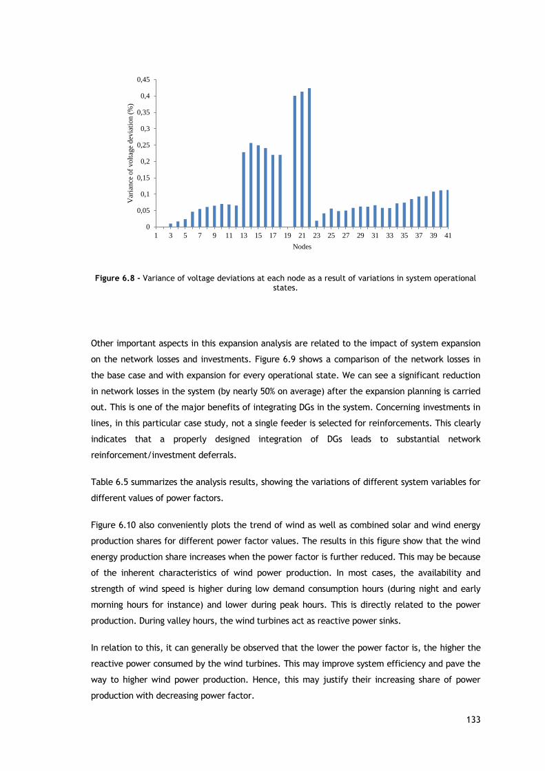
133

Figure 6.8 - Variance of voltage deviations at each node as a result of variations in system operational states.

Other important aspects in this expansion analysis are related to the impact of system expansion

on the network losses and investments. Figure 6.9 shows a comparison of the network losses in

the base case and with expansion for every operational state. We can see a significant reduction

in network losses in the system (by nearly 50% on average) after the expansion planning is carried

out. This is one of the major benefits of integrating DGs in the system. Concerning investments in

lines, in this particular case study, not a single feeder is selected for reinforcements. This clearly

indicates that a properly designed integration of DGs leads to substantial network

reinforcement/investment deferrals.

Table 6.5 summarizes the analysis results, showing the variations of different system variables for

different values of power factors.

Figure 6.10 also conveniently plots the trend of wind as well as combined solar and wind energy

production shares for different power factor values. The results in this figure show that the wind

energy production share increases when the power factor is further reduced. This may be because

of the inherent characteristics of wind power production. In most cases, the availability and

strength of wind speed is higher during low demand consumption hours (during night and early

morning hours for instance) and lower during peak hours. This is directly related to the power

production. During valley hours, the wind turbines act as reactive power sinks.

In relation to this, it can generally be observed that the lower the power factor is, the higher the

reactive power consumed by the wind turbines. This may improve system efficiency and pave the

way to higher wind power production. Hence, this may justify their increasing share of power

production with decreasing power factor.

0

0,05

0,1

0,15

0,2

0,25

0,3

0,35

0,4

0,45

1 3 5 7 9 11 13 15 17 19 21 23 25 27 29 31 33 35 37 39 41

Var

ian

ce o

f volt

age

dev

iati

on

(%

)

Nodes

134

Figure 6.9 - Network losses with and without system expansion (first stage).

Table 6.5 – Values of system variables with varying power factor of RES-based DGs

Power factor 1.0 0.95 0.9 0.85 0.8

Total energy production (MWh) 179329 175545 176024 178848 172037

RES energy

production share

(%)

Wind 44.00 45.08 45.23 46.31 46.90

PV 0.71 2.02 4.31 2.39 1.96

Wind+PV 44.71 47.10 49.54 48.69 48.86

Cost terms (M€)

Investment cost 33.94 35.88 34.35 35.69 38.91

Maintenance Cost 9.47 9.47 9.53 9.43 10.10

Emission Cost 9.44 8.10 8.08 8.12 6.76

Energy Cost 29.31 27.10 27.65 27.20 25.22

Total cost (M€) 82.16 80.55 79.61 80.44 80.99

Investment

decisions

Storage (MW) 6 5 6 6 5

Capacitor (MVAr) 3.7 7.4 8.2 9.4 12.5

DG (MW) 9 10 9 9 11

Line reinforcements 1 3 1 1 2

Average active power losses in stage 1 (MW) 0.448 0.440 0.430 0.441 0.448

Average reactive power losses in stage 1

(MVAr) 0.339 0.745 0.983 1.098 1.602

135

Contrary to the case with wind type DGs, the peak power production of solar PV based DGs occur

around the peak hours of consumption. This means that, unlike the wind type DGs, their

contribution to the system as reactive power sinks during valley hours is limited.

Hence, as can be seen in Figure 6.11, the optimal power factor setting for such DGs seems to be

0.9. In general, this also seems to be the optimal power factor setting for the system because this

results in the highest share of combined wind and solar PV energy production (see Figure 6.10).

Besides, as can be seen in Table 6.5, the lowest overall cost (79.61 M€) as well as the lowest

active power losses (0.430 MW) are achieved when the power factor is set to 0.9.

Figure 6.10 - Evolution of solar and wind energy production share with varying power factor.

Figure 6.11 - Evolution of solar PV energy production share with varying power factor.

136

As shown in Table 6.5, the amount of installed reactive power sources (capacitor banks, in this

case) as well as the reactive power losses in the system increase with decreasing power factor.

This is expected because the lower the power factor is, the higher the reactive power

requirement of the DGs is. Transporting the reactive power generated by such reactive power

sources increases the reactive power losses in the system.

The impact of varying power factor on the voltage profile in the system is also investigated.

Figures 6.12 and 6.13 illustrate the changes in the voltage profiles as a result of changing the

power factor during peak and valley hours, respectively. In both cases, there are no significantly

visible variations in voltage profiles regardless of the power factor settings, except for some nodes

as in Figure 6.13.

The average voltage deviations at each node for different power factor settings are also shown in

Figure 6.14. In general, based on the results in Figures 6.13 and 6.14, there is no clear indication

to say that one power factor setting is better than the other; it can be observed that what is

deemed good for one node may be “bad” for another one. However, it is worth mentioning here

that the voltage profiles are significantly improved as a result of simultaneously integrating DG,

ESS and capacitor banks. The voltage deviations for those nodes, where DGs and capacitor banks

are connected to, seem to be higher in absolute terms; yet, they remain within the permissible

range.

Figure 6.12 - Voltage deviation at each node during peak demand hour for different power factor values.

137

Figure 6.13 - Voltage deviation at each node during valley hour for different power factor values.

Figure 6.14 - Average voltage deviations at each node for different power factor values.

138

6.4.3.2 Considering DGs With Reactive Power Support

Nowadays, RES-based DGs (wind and solar types) are required to adhere to certain grid codes such

as reactive power support, voltage ride through, etc. to alleviate the negative impacts of

integrating such DGs in the system. Examples in this case are doubly fed induction generator

(DFIG) based wind turbines and voltage-source inverter (VSI) based PV generators. In some

systems, the grid codes are already being enforced, and consequently wind/solar PV farms are

required to operate from 0.95 lagging to 0.95 leading power factor [175].

For the analysis in this section, wind and solar PV type DGs with reactive power support capability

are considered in the simulations. The power factor is varied to investigate its effects on selected

system variables, and the results are summarized in Table 6.6. The results here show that the

optimal power factor setting for the wind type DGs seems to be 0.95 because this leads to the

highest wind energy production level (47.13%) compared to any other setting. This is also clearly

shown in Figure 6.15. The combined share of wind and solar PV energy production also peaks

when the power factor is set to 0.95, as depicted in Figure 6.15.

From Table 6.6 and Figure 6.16, one can see that the overall cost (which is the sum of

investment, maintenance, emission and energy costs) is the lowest at the same power factor

(79.40 M€). The lowest active power losses seem to however occur at a power factor of 0.9.

The profiles of average voltage deviations at each node corresponding to different power factor

settings are shown in Figure 6.17. Figure 6.18 also depicts the voltage deviations at each node

corresponding to the valley hour of electricity consumption. One can see that there are no

significant differences in these profiles, except for nodes where the distributed energy resources

(DG, ESS and reactive sources) are connected to. The voltage variations at these nodes with the

changes in power factor settings can be explained by the fact that the amount of each distributed

energy resource installed at these nodes is different for different power factor values (see

Table 6.6).

Figure 6.15 - Evolution of wind and solar PV energy production share with varying power factor.

139

Table 6.6 – Values of system variables with varying power factor of RES-based DGs

Power factor 1.00 0.95 0.9 0.85 0.80

Total energy (MWh) 179329 179329 179851 175527 176027

RES energy

production share

(%)

Wind 44.00 47.13 42.90 42.76 41.41

PV 0.71 0.00 1.91 1.91 3.40

Wind+PV 44.71 47.13 44.82 44.67 44.81

Cost terms (M€)

Investment cost 33.94 33.18 33.09 31.68 32.56

Maintenance Cost 9.47 9.98 8.92 9.00 8.48

Emission Cost 9.44 8.07 9.38 9.44 9.40

Energy Cost 29.31 28.17 29.04 29.49 28.76

Total cost (M€) 82.16 79.40 80.43 79.61 79.20

Investment

decisions

Storage (MW) 6 8 5 6 4

Capacitor (MVAr) 3.7 3.4 3.3 7.9 5

RES (MW) 9 8 9 8 9

Line reinforcements 1 1 8 0 7

Average active power losses in stage 1 (MW) 0.448 0.437 0.425 0.427 0.448

Average reactive power losses in stage 1

(MVAr) 0.339 0.629 0.797 0.904 1.06

Figure 6.16 - Evolution of total energy and emission costs with varying power factor.

140

Figure 6.17 - Average voltage deviations at each node for different power factor values.

Figure 6.18 - Voltage deviations at each node during valley hour for different power factor values.

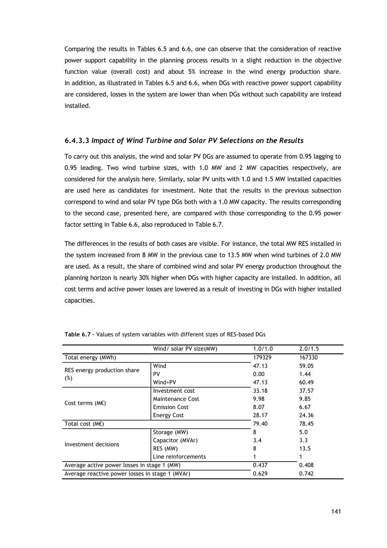
141

Comparing the results in Tables 6.5 and 6.6, one can observe that the consideration of reactive

power support capability in the planning process results in a slight reduction in the objective

function value (overall cost) and about 5% increase in the wind energy production share.

In addition, as illustrated in Tables 6.5 and 6.6, when DGs with reactive power support capability

are considered, losses in the system are lower than when DGs without such capability are instead

installed.

6.4.3.3 Impact of Wind Turbine and Solar PV Selections on the Results

To carry out this analysis, the wind and solar PV DGs are assumed to operate from 0.95 lagging to

0.95 leading. Two wind turbine sizes, with 1.0 MW and 2 MW capacities respectively, are

considered for the analysis here. Similarly, solar PV units with 1.0 and 1.5 MW installed capacities

are used here as candidates for investment. Note that the results in the previous subsection

correspond to wind and solar PV type DGs both with a 1.0 MW capacity. The results corresponding

to the second case, presented here, are compared with those corresponding to the 0.95 power

factor setting in Table 6.6, also reproduced in Table 6.7.

The differences in the results of both cases are visible. For instance, the total MW RES installed in

the system increased from 8 MW in the previous case to 13.5 MW when wind turbines of 2.0 MW

are used. As a result, the share of combined wind and solar PV energy production throughout the

planning horizon is nearly 30% higher when DGs with higher capacity are installed. In addition, all

cost terms and active power losses are lowered as a result of investing in DGs with higher installed

capacities.

Table 6.7 – Values of system variables with different sizes of RES-based DGs

Wind/ solar PV size(MW) 1.0/1.0 2.0/1.5

Total energy (MWh) 179329 167330

RES energy production share

(%)

Wind 47.13 59.05

PV 0.00 1.44

Wind+PV 47.13 60.49

Cost terms (M€)

Investment cost 33.18 37.57

Maintenance Cost 9.98 9.85

Emission Cost 8.07 6.67

Energy Cost 28.17 24.36

Total cost (M€) 79.40 78.45

Investment decisions

Storage (MW) 8 5.0

Capacitor (MVAr) 3.4 3.3

RES (MW) 8 13.5

Line reinforcements 1 1

Average active power losses in stage 1 (MW) 0.437 0.408

Average reactive power losses in stage 1 (MVAr) 0.629 0.742

142

Surprisingly, the storage requirement (5 MW) is significantly lower when wind turbines with higher

installed capacity are used than in the other case (8 MW) as shown in Table 6.7, while the

reactive power requirement is almost the same for both cases. The average voltage profiles of

both cases in the system are also very similar (as shown in Figure 6.19).

Figure 6.19 - Average voltage deviations at each node for different DG sizes.


A new dynamic and stochastic mathematical model of an integrated distribution system planning

problem was proposed in this chapter. The results showed that the simultaneous integration of

ESSs and reactive power sources largely enabled a substantially increased penetration of variable

generation (wind and solar) in the system, and consequently reduced system costs and network

losses as well as deferred network expansion or reinforcement needs, which is of crucial

importance. For the case study, up to 13.5 MW installed capacity of wind and solar power has

been added to the system within a three-years planning horizon. One can put this into perspective

with the base-case peak load of 4.635 MW in the system. This means it has been possible to

integrate RES power more than twice the peak demand in the base case. Generally, it has been

unequivocally demonstrated that the joint planning of DGs, reactive power sources and ESS,

proposed in this chapter, brings about significant improvements to the system, such as reduction

of losses, electricity cost and emissions. Besides, the proposed modeling framework considerably

contributes to improved voltage profile in the system. This in turn leads to an increased voltage

stability margin in the system, which is essential for a normal/secure operation of the system as a

whole. Overall, the novel planning model proposed here can be considered as a major leap

forward towards developing controllable grids, supporting large-scale integration of RESs.

143

Chapter 7

Conclusions, Directions for Future Work and

Contributions

In this chapter, the main conclusions of the thesis are highlighted on the basis of answering

the research questions that constituted the main motivation of this research. The limitations

of the work in this thesis, and some directions of future work are also discussed. Finally, the

contributions of this work are highlighted by presenting the set of publications, in journals

with high impact factor (first quartile), as book chapters or in conference proceedings of

high standard (IEEE), leading to this thesis work.

7.1 Main Conclusions

The main conclusions drawn from the thesis work, pertaining to the research questions

presented in Section 1.6, are summarized as follows. For the sake of clarity the research

questions are reproduced here.

What is the current status of RES penetration across the world (with a special

focus at distribution levels)? What are the main impeding factors for RES

integration? How can the potential benefits of RESs be reaped without significant

negative consequences?

An increase in an overall world trend in the awareness of climate change and the

need for mitigation efforts is bringing forth huge increase in the deployment of

renewable energy in comparison to fossil fuel energy sources. The landmark that

signals the dawning of this “renewables age” goes hand in hand with the degree of

advancement in technologies and a higher level of RES penetration, which is being

achieved around the world. Furthermore, there are several driving factors for these

remarkable growths, among which are favorable government support policies and

increasing competitiveness in costs. After several decades of efforts in research and

continuous development in RESs, the yearly growth in the capacity of these plants is

becoming greater than the total investment capacity added in power plants based on

coal, natural gas and oil, all combined together. Nowadays, RESs have reached a

significant level of share in energy supply options, becoming one of the prominent

global alternative power supply sources. This trend will continue to increase at faster

rates as long as the world’s desire for industrial-scale clean energy sources is on the

higher side.

144

Thus, there is a global consensus on climate change mitigation and curbing GHG

emissions which along with energy dependence, security and other structural issues

are forcing states to create new market policies and the introduction of new energy

policies (in particular, policies related to RESs that support the development and

effective utilization of RESs). The integration of RESs in the electrical systems

(particularly at distribution levels) is expected to accelerate in the years to come as a

result of the recent agreement among several countries to limit GHG emissions and

mitigate climate change. The level of DG integrated in distribution systems follows an

upward trend, and there is a general consensus that DGs will contribute immensely to

the effort of solving a multitude of global and local concerns, including the

realization of RES integration goals set forth by different entities.

The latest global trends in RES investment status reports indicate that renewables

represented a 58.5% of net additions to global power capacity in 2014, with

significant growth in all regions, which represents an estimated 27.7% of the world’s

power generating capacity, enough to supply an estimated 22.8% of global electricity

demand. Wind, solar and biomass power generations reached an estimated 9.1% of

the world’s electricity in 2014, up from 8.5% in 2013. According to a renewables

status report, the overall cost-cutting achieved to date helped to ensure such a strong

momentum in 2014, reaching an investment boom up to 29% in solar, and 11% in wind

technologies, and geothermal managing to raise 23%. Among the several renewable

energy types, large-scale hydro was the one that showed the highest growth in terms

of new investments. However, excluding this one, wind and solar were the ones that

grew the most (62 and 56 GW respectively) in terms of new installed capacity, well

above the corresponding values in 2014. For the first time in 2015, the amount of

investment in RES generation made in the developing countries worldwide exceeded

the investment made in developed economies. However, with the new capacity

conventional generation added, the generation from clean energy in the world in

2015 covered only 10% of world’s electricity demand. However, this avoided an

amount of CO2 emissions equivalent to 1.5 Gigatons in 2015.

Moreover, despite the robust growth of integration RESs in many power systems,

there are still certain challenges and barriers that impede the smooth integration of

RESs. These challenges and barriers can be broadly classified into two categories:

technical and non-technical. The non-technical category includes challenges and

barriers related to capital costs, market and economic issues, information and public

awareness, socio-cultural matters, the conflict between stakeholders, regulation and

policy. Most of the challenges and barriers explained before have proven solutions

that happen to be overlooked in many systems; therefore, they are preventing the

spread of RES development across the world.

145

In general, arising from the comprehensive overview of RES carried out in Chapter 2,

these are summarized as follows:

1. Market and economic barriers can be fixed by streamlining appropriate

market and economic signals related to carbon taxes, emission trading

schemes, finances and incentive mechanisms, as well as enhancing public

support for R&D and creating a conducive environment for RES development.

All this can have a considerable positive impact on the level of RES

integration.

2. Setting energy standards, continuous information campaigns and technical

training about RESs and their benefits can enhance public knowledge and

awareness, which can in the end have supportive roles in RES development.

3. Creating an enabling environment for R&D, improving technical regulations,

scaling up international support for technology transfer, liberalizing energy

industries, providing incentive packages to RES developers, designing

appropriate policies of RESs and conventional energy sources to minimize the

regulatory and policy barriers to developing RESs.

4. Coordinating investments of RESs based on variable generation resources such

as wind and solar power with large-scale energy storage systems, demand side

management participation and grid expansion can significantly increase the

level of RES integration.

5. Enhancing operation and the flexibility of conventional power generation

sources can also be very useful to scale up RES integration.

6. Designing an efficient wholesale market such as dynamic retail pricing and

developing coordinated operation and planning tools (such as joint network

and generation investment planning models) can have a positive role in RES

integration.

7. For full utilization of RESs, the coordination between distribution system

operators (DSOs) and transmission system operators (TSOs) is also vital.

8. It is also important to improve prediction tools, monitoring and control

protocols that can help efficient utilization of the RESs.

9. Ensuring regional interconnections via regional cooperation and increasing the

level of participation of all stakeholders (including RES generators) in voltage

control, provision of reserves, reactive power support, etc., are significantly

helpful for the stated purpose.

10. Using smart-grid technologies and concepts are also expected to facilitate a

smooth integration of large-scale RESs because these are equipped with

advanced control and management tools to counterbalance the intermittent

nature of most RES energy productions.

146

What are the parameters of uncertainty and/or variability that most influence

the decision-making process in terms of investment solutions in DGs (especially,

renewables)?

The various sources of uncertainties and/or variability in DG investment planning are

related to the variability and randomness of operational situations. Therefore, the

combined effect of the variability and uncertainty is of utmost importance so that an

economic integration of DGs can be carried out in distribution network systems.

Accordingly, in Chapter 3, a comprehensive sensitivity analysis was carried out to

identify the uncertain parameters which significantly influence the decision-making

process in DG investments and quantify their degree of influence. To perform the

analysis, a DG investment planning model was formulated as a novel multi-stage and

multi-scenario optimization problem. Based on the numerical studies, the following

conclusions can be drawn:

1. The results of the numerical analyses generally show that both uncertainty

and variability have a meaningful influence on DG investment decisions.

In fact, the degree of influence varies from one parameter to another.

2. The results from the particular case study show that generator outages have

little or no impact on the RES-based DG investments; whereas, uncertainty in

CO2 and fuel prices, interest rate and RES power outputs significantly

influence investment decisions, especially in variable energy sources. In

particular, it has been found out that uncertainty in CO2 and fuel prices as

well as in the interest rate seem to dramatically condition decisions

compared to the uncertainty in demand growth and RES power outputs.

3. In general, the results revealed that ignoring or inadequately considering

uncertainty and variability in model parameters has a quantifiable cost.

4. Based on the extensive analysis, a stochastic modeling of uncertainty related

to emission and fuel prices, interest rate, RES power outputs and demand

growth is very critical for obtaining robust investment decisions.

How should different sources of uncertainty be modeled in the complex decision-

making problem concerning DG investment planning?

The advent of emerging solutions such as active management of distribution networks

or fully automated and intelligent networks ― the so-called smart grids ― is expected

to keep on facilitating smooth integration of DGs by alleviating existing technical

limitations. However, several DG sources are intermittent in nature, making the

operation and planning of distribution networks very challenging. This is because such

sources introduce significant operational variability and uncertainty to the system.

147

Hence, in Chapter 4, a novel multi-stage stochastic MILP model has been developed

to guide the complex decision-making process of DG investment planning in

distribution systems in the face of uncertainty. Chapter 4 used the outputs of Chapter

3 to improve the developed model, and make it more robust. The established model

features a number of important aspects that should be considered in the decision-

making process of a DG investment planning problem:

1. It has an objective function which jointly minimizes cost of emission,

operation, maintenance and energy not served;

2. It accounts for the operational variability due to intermittent power sources

and electricity demand via probabilistic methods.

3. Uncertainty related to emission price, demand growth and the

unpredictability of intermittent generation sources is handled via a stochastic

approach.

4. It is based on a dynamic decision framework, i.e., involving a multi-year

decision structure.

5. It is anchored on a two-period planning framework, involving short-term and

medium/long-term planning windows. This allows obtaining robust short-term

decisions in the face of uncertainty along with strategic (or flexible) decisions

in the medium to long-term planning horizon.

From a quantitative and qualitative point of view, what are the impacts of

network switching and/or reinforcement, as well as deployment of ESSs on the

level of renewable power integrated in the system?

There is a global consensus for the integration of DG sources, especially RESs, as a

way to meet the growing demand for electric energy and to reduce the carbon

footprint of energy production. Nevertheless, the realization of this considerable

objective faces two big challenges. The first challenge is related to the variability and

uncertainty introduced on the system by RESs. The second one is related to the

stability of the system and quality of energy supplied. To overcome these challenges,

it is necessary to integrate a set of enabling technologies, as well as to design an

effective coordination mechanism among different technologies in distribution

systems.

Hence, in Chapter 5, a stochastic MILP optimization model has been developed to

investigate the impacts of installing ESSs as well as network switching on the level of

renewable power integration in a distribution network system. The resulting model is

equipped with the necessary tools to jointly optimize the placement, timing and

sizing of RES-based DGs and ESSs in coordination with optimal network

reconfiguration, while respecting a number of technical, economic and environmental

constraints.

148

The results have showed that:

1. The capability of ESS integration dramatically increased the level and the

optimal exploitation of renewable DGs. According to the results obtained, the

simultaneous integration of DGs and ESSs resulted in an overall cost and

average losses reduction of 60% and 90%, respectively, which is significant.

2. Moreover, as high as 90% RES penetration level seems to be largely possible

provided that this is supported by ESS deployments, again noteworthy.

3. The contributions of DG and ESS installations to voltage profile improvement

and overall system stability is substantial. The coordinated integration of DGs

and ESSs along with reconfiguration leads to the best voltage profile, which is

almost flat throughout the system.

4. It was largely demonstrated the fact that large-scale integration of variable

energy sources is possible when such energy sources are optimally deployed

with ESSs and a mechanism that improve the flexibility of the network is put

in place.

5. Therefore, the optimal network reconfiguration, DG and ESS installations

(jointly or separately) substantially contributed to voltage stability. In this

particular case study, the impact of network switching on RES power

integration has not been significant. However, it should be noted that this can

be case-dependent; a more frequent switching operation can substantially

influence the level of renewable integration.

How can the penetration of renewable energy sources in the power distribution

system be maximized with currently available technologies?

Given the techno-economic factors and global concerns about environmental issues,

the integration of renewable energy sources (RESs) cannot be postponed. It is likely

that the integration of DGs in distribution systems will go ahead along with smart-grid

enabling technologies that have the capability to alleviate the negative consequences

of large-scale integration of DGs. In other words, in order to facilitate (speed up) the

much-needed transformation of conventional (passive) DNSs and support large-scale

RES integration, different smart-grid enabling technologies such as reactive power

sources, advanced switching and storage devices are expected to be massively

deployed in the near term. To this end, developing strategies, methods and tools to

maximize the penetration level of DGs (particularly, RESs) has become very crucial to

guide such a complex decision-making process.

Therefore, in Chapter 6, a new multi-stage and stochastic model for jointly

optimizing the integration of smart-grid enabling technologies such as ESS, reactive

power sources, and network switching, reinforcement and/or expansion has been

developed to support large-scale renewable integration.

149

Due the complexity of the issue, this one was analyzed according the several problem

aspects, giving rise to the following sub-questions:

o What is the effect of reactive power support capability on the RES-based DG

integration level?

Intermittent power generation sources such as wind and solar PV type DGs

normally operate with a fixed lagging power factor. In other words, such

generators “consume” reactive power, instead of “producing” and

contributing to the voltage regulation in the system (also known as reactive

power support). For instance, wind turbines installed in power systems

throughout the world are predominantly based on asynchronous generators

(also known as induction generators). As mentioned above, one of the typical

characteristics of such machines is that they always “consume” reactive

power. Because of this, such wind turbines are often operated at a constant

power factor. It is well-known that, in power systems, voltage regulation has

been traditionally supported by conventional (synchronous) generators.

The results of considering DGs without reactive power support show a strong

relationship among the optimal investments. That is, the lower the power

factor is the higher the investment requirement in capacitor banks is. This is

due to the increasing reactive power consumption by DGs. Unlike in capacitor

banks, the total amount of DGs and ESSs installed in the system do not

significantly vary with the reactive power settings. This is an indication that

capacitor banks play a vital role in maintaining systems integrity and stability

as well as ensuring essentially the same level of DG integration regardless of

the power factor setting. The results of considering DGs with reactive power

support show that the optimal power factor for wind type DG seems to be

0.95 because this leads to the highest wind energy production level compared

to any other setting. The combined share of wind and solar PV energy

production also peaks when the power factor is set to 0.95. In general, it is

demonstrated that the simultaneous integration of ESSs and reactive power

sources largely enables a substantially increased penetration of variable

generation (wind and solar) in the system.

o What are the implications of integrating smart-grid enabling technologies in

the distribution systems with respect to maximizing RES integration,

reducing energy losses, costs and improving voltage profiles?

The results showed a substantial improvement in voltage controllability due

to the combined effect of expansion decisions in DGs, ESSs and capacitor

banks. Such an investment also leads to a significant reduction in network

losses in the system (by nearly 50%, on average).

150

Generally, it has been unequivocally demonstrated that the joint planning of

DGs, reactive power sources and ESS, proposed in this thesis, brings about

significant improvements to the system, such as reduction of losses,

electricity cost and emissions. Besides, the proposed modeling framework

considerably contributes to an improved voltage profile in the system. This in

turn leads to an increased voltage stability margin in the system, which is

essential for a normal/secure operation of the system as a whole.

Comparing the results, it was observed that the consideration of reactive

power support capability in the planning process results in a slight reduction

in the objective function value (overall cost) and about 5% increase in the

wind energy production share. In addition, when DGs with reactive power

support capability are considered, losses in the system are lower than when

DGs without such capability are instead installed.

7.2 Directions for Future Works

The following points may be further studied in order to broaden the understanding of the

topics treated in this thesis:

With the introduction of enabling technologies, it is necessary to structure the system

response in transient state having in view the smart grids implementation.

Investigate the application of new cluster techniques to improve the performance of

the developed algorithms.

Stochastic models may bear a significant computational burden that may hamper

their applicability. Several measures can be applied in order to reduce the

computational time required to solve such models. First, modern computing

techniques such as grid and cloud computing may be used. Since there are already

companies that provide computational power at affordable prices, this proposal

promises tractability even for large-scale mathematical programming problems.

7.3 Contributions of the Thesis

7.3.1 Book Chapters

1. S. F. Santos, D. Z. Fitiwi, M. Shafie-khah, A. W. Bizuayehu, J. P. S. Catalão,

"Optimal sizing and placement of smart grid enabling technologies for maximizing

renewable integration", in: Smart Energy Grid Engineering, UK: ACADEMIC Press

(ELSEVIER), ISBN: 978-0-12-805343-0, pp. 47-81, 2017.

http://dx.doi.org/10.1016/B978-0-12-805343-0.00003-6

http://dx.doi.org/10.1016/B978-0-12-805343-0.00003-6

151

2. S. F. Santos, D. Z. Fitiwi, M. Shafie-khah, A. W. Bizuayehu, J. P. S. Catalão,

"Introduction to renewable energy systems", in: Optimization in Renewable

Energy Systems, London, UK: ACADEMIC Press (ELSEVIER), 2016 (aceite).

http://dx.doi.org/TBD

3. S. F. Santos, N. Paterakis, J. P. S. Catalão, "New multi-objective decision

support methodology to solve problems of reconfiguration in the electric

distribution systems", in: Technological Innovation for Cloud-based Engineering

Systems, Germany: SPRINGER, ISBN: 978-3-319-16765-7, pp. 395-404, April 2015.

http://dx.doi.org/10.1007/978-3-319-16766-4_42

7.3.2 Publications in Peer-Reviewed Journals

1. S. F. Santos, D. Z. Fitiwi, M. R. M. Cruz, C. M. P. Cabrita, J. P. S. Catalão, "Impacts

of Optimal Energy Storage Deployment and Network Reconfiguration on Renewable

Integration Level in Distribution Systems", Applied Energy (ELSEVIER), Vol. 185,

pp. 44-55, January 2017.

http://dx.doi.org/10.1016/j.apenergy.2016.10.053

Impact factor: 5.746; Q1 (First Quartile) journal in ISI Web of Science and Scopus

2. S. F. Santos, D. Z. Fitiwi, A. W. Bizuayehu, M. Shafie-khah, M. Asensio, J. Contreras,

C. M. P. Cabrita, J. P. S. Catalão, "Impacts of Operational Variability and Uncertainty

on Distributed Generation Investment Planning: A Comprehensive Sensitivity Analysis",

IEEE Transactions on Sustainable Energy, 2016 (aceite).

http://dx.doi.org/10.1109/TSTE.2016.2624506


3. S. F. Santos, D. Z. Fitiwi, A.W. Bizuayehu, M. Shafie-khah, M. Asensio, J. Contreras,

C.M.P. Cabrita, J.P.S. Catalão, "Novel Multi-Stage Stochastic DG Investment Planning

with Recourse", IEEE Transactions on Sustainable Energy, 2016 (aceite).



4. S. F. Santos, D. Z. Fitiwi, M. Shafie-khah, A. W. Bizuayehu, C. M. P. Cabrita,

J. P. S. Catalão, "New Multi-Stage and Stochastic Mathematical Model for Maximizing

RES Hosting Capacity—Part II: Numerical Results", IEEE Transactions on Sustainable

Energy, 2016 (aceite).



http://dx.doi.org/TBD

http://dx.doi.org/10.1007/978-3-319-16766-4_42

http://dx.doi.org/10.1016/j.apenergy.2016.10.053


http://webx.ubi.pt/~catalao/07509683.pdf




152

5. S. F. Santos, D. Z. Fitiwi, M. Shafie-khah, A. W. Bizuayehu, C. M. P. Cabrita,

J. P. S. Catalão, "New Multi-Stage and Stochastic Mathematical Model for Maximizing

RES Hosting Capacity—Part I: Problem Formulation", IEEE Transactions on

Sustainable Energy, 2016 (aceite).



6. N. G. Paterakis, A. Mazza, S. F. Santos, O. Erdinc, G. Chicco, A. G. Bakirtzis,

J. P. S. Catalão, "Multi-Objective Reconfiguration of Radial Distribution Systems using

Reliability Indices", IEEE Transactions on Power Systems, Vol. 31, No. 2, pp. 1048-

1062, March 2016.

http://dx.doi.org/10.1109/TPWRS.2015.2425801


7.3.3 Publications in International Conference Proceedings

1. S. F. Santos, D. Z. Fitiwi, A. W. Bizuayehu, J. P. S. Catalão, M. Shafie-khah, "Optimal

Integration of RES-based DGs with Reactive Power Support Capabilities in Distribution

Network Systems", in Proceedings of the 13th International Conference on the

European Energy Market — EEM 2016 (technically co-sponsored by IEEE), Porto,

Portugal, USB flash drive, 6-9 June, 2016.

http://dx.doi.org/10.1109/EEM.2016.7521317

2. D. Z. Fitiwi, S. F. Santos, A. W. Bizuayehu, M. Shafie-khah, J.P.S. Catalão, "A New

Dynamic and Stochastic Distributed Generation Investment Planning Model with

Recourse", in: Proceedings of the 2016 IEEE Power & Energy Society General

Meeting — PESGM 2016, Boston, Massachusetts, USA, USB flash drive, July 17-21,

2016.

http://dx.doi.org/10.1109/PESGM.2016.7741093

3. M. R. M. Cruz, D. Z. Fitiwi, S. F. Santos, J. P. S. Catalão, "Influence of Distributed

Storage Systems and Network Switching/Reinforcement on RES-based DG Integration

Level", in Proceedings of the 13th International Conference on the European Energy

Market — EEM 2016 (technically co-sponsored by IEEE), Porto, Portugal, USB flash

drive, 6-9 June, 2016.





http://dx.doi.org/10.1109/TPWRS.2015.2425801




153

4. D. Z. Fitiwi, S. F. Santos, A. W. Bizuayehu, M. Shafie-khah, J. P. S. Catalão,

M. Asensio, J. Contreras, "DG Investment Planning Analysis with Renewable

Integration and Considering Emission Costs", in: Proceedings of the IEEE Region 8

International Conference on Computer as a Tool — EUROCON 2015, Salamanca, Spain,

USB flash drive, 8-11 September, 2015.

http://dx.doi.org/10.1109/EUROCON.2015.7313735

5. N. G. Paterakis, S. F. Santos, J. P. S. Catalão, A. Mazza, G. Chicco, O. Erdinc,

A. G. Bakirtzis, "Multi-Objective Distribution System Reconfiguration for Reliability

Enhancement and Loss Reduction", in: Proceedings of the 2015 IEEE Power & Energy

Society General Meeting — PESGM 2015, Denver, Colorado, USA, USB flash drive, July

26-30, 2015.


http://dx.doi.org/10.1109/EUROCON.2015.7313735


154

Appendices

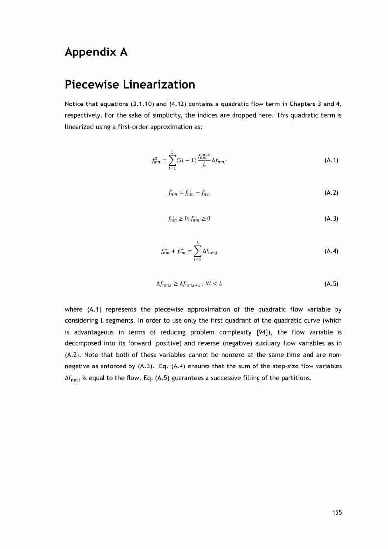
155

Appendix A

Piecewise Linearization

Notice that equations (3.1.10) and (4.12) contains a quadratic flow term in Chapters 3 and 4,

respectively. For the sake of simplicity, the indices are dropped here. This quadratic term is

linearized using a first-order approximation as:

𝑓𝑛𝑚2 =∑(2𝑙 − 1)

𝑓𝑛𝑚𝑚𝑎𝑥

𝐿

𝐿

𝑙=1

∆𝑓𝑛𝑚,𝑙 (A.1)

𝑓𝑛𝑚 = 𝑓𝑛𝑚+ − 𝑓𝑛𝑚

− (A.2)

𝑓𝑛𝑚+ ≥ 0; 𝑓𝑛𝑚

− ≥ 0 (A.3)

𝑓𝑛𝑚+ + 𝑓𝑛𝑚

− =∑∆𝑓𝑛𝑚,𝑙

𝐿

𝑙=1

(A.4)

∆𝑓𝑛𝑚,𝑙 ≥ ∆𝑓𝑛𝑚,𝑙+1 ; ∀𝑙 < 𝐿 (A.5)

where (A.1) represents the piecewise approximation of the quadratic flow variable by

considering L segments. In order to use only the first quadrant of the quadratic curve (which

is advantageous in terms of reducing problem complexity [94]), the flow variable is

decomposed into its forward (positive) and reverse (negative) auxiliary flow variables as in

(A.2). Note that both of these variables cannot be nonzero at the same time and are non-

negative as enforced by (A.3). Eq. (A.4) ensures that the sum of the step-size flow variables

∆fnm,l is equal to the flow. Eq. (A.5) guarantees a successive filling of the partitions.

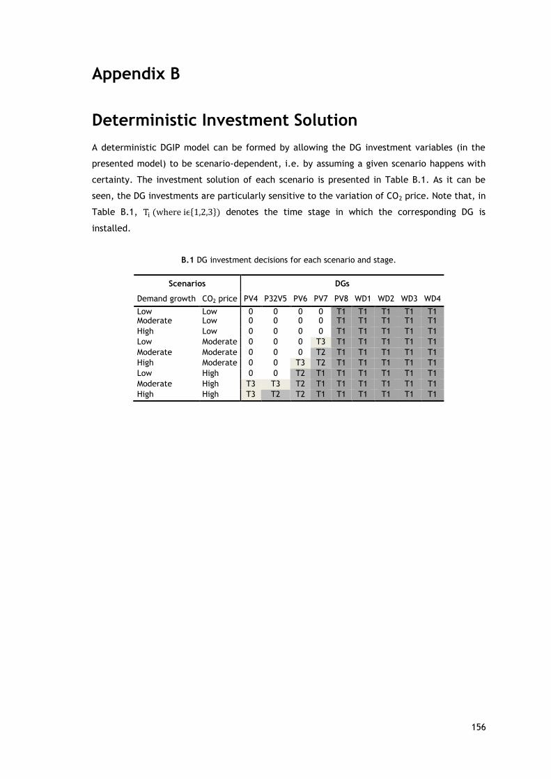
156

Appendix B

Deterministic Investment Solution

A deterministic DGIP model can be formed by allowing the DG investment variables (in the

presented model) to be scenario-dependent, i.e. by assuming a given scenario happens with

certainty. The investment solution of each scenario is presented in Table B.1. As it can be

seen, the DG investments are particularly sensitive to the variation of CO2 price. Note that, in

Table B.1, Ti (where iϵ1,2,3) denotes the time stage in which the corresponding DG is

installed.

B.1 DG investment decisions for each scenario and stage.

Scenarios DGs

Demand growth CO2 price PV4 P32V5 PV6 PV7 PV8 WD1 WD2 WD3 WD4

Low Low 0 0 0 0 T1 T1 T1 T1 T1 Moderate Low 0 0 0 0 T1 T1 T1 T1 T1

High Low 0 0 0 0 T1 T1 T1 T1 T1

Low Moderate 0 0 0 T3 T1 T1 T1 T1 T1

Moderate Moderate 0 0 0 T2 T1 T1 T1 T1 T1

High Moderate 0 0 T3 T2 T1 T1 T1 T1 T1

Low High 0 0 T2 T1 T1 T1 T1 T1 T1

Moderate High T3 T3 T2 T1 T1 T1 T1 T1 T1

High High T3 T2 T2 T1 T1 T1 T1 T1 T1

157

Appendix C

SOS2-Based Generation Cost Linearization

As mentioned in Chapter 4, generation costs are assumed to be quadratic functions of the

generated power. Such nonlinear cost functions are linearly represented by making use of

SOS2 variables [176]. This linearization technique leads to a set of convex combinations of

piecewise linear segments of each quadratic generation cost curve. The set of constraints

required in the linear cost model include the “function rows” related to existing DGs (C.1),

and new DGs (C.2) and (C.3) corresponding to the first and the second periods. And, the

respective “reference rows” are given by (C.4)—(C.6). Eqs. (C.7)—(C.9) ensure that the sum

of all SOS2 variables used to linearize a particular generation cost curve is equal to 1. Such

constraints are also referred to as “convexity rows”. Finally, Eq. (C.10) guarantees that no

more than two adjacent SOS2 variables can have non-zero values.

𝑂𝐶𝑝,𝑘,𝑛,𝑠,𝑤,𝑡𝐸 = ∑ 𝜆𝑝,𝑘,𝑛,𝑠,𝑤,𝑡,𝑙

𝐸 ∗ 𝐺𝐶𝑝,𝑘,𝑠,𝑛,𝑤,𝑡,𝑙𝐸

𝑙∈Ω𝑙

;

∀𝑛 ∈ Ω𝑛; ∀𝑡 ∈ Ω𝑡; ∀𝑠 ∈ Ω𝑠; ∀𝑤 ∈ Ω𝑤; ∀𝑘 ∈ Ω𝑘; ∀𝑝 ∈ Ω𝑝

(C.1)

𝑂𝐶𝑝,𝑘,𝑛,𝑠,𝑤,𝑡𝑁1 = ∑ 𝜆𝑝,𝑘,𝑛,𝑠,𝑤,𝑡,𝑙

𝑁1 ∗ 𝐺𝐶𝑝,𝑘,𝑛,𝑠,𝑤,𝑡,𝑙𝑁1

𝑙∈Ω𝑙

;

∀𝑛 ∈ Ω𝑛; ∀𝑡 ∈ Ω𝑡; ∀𝑠 ∈ Ω𝑠; ∀𝑤 ∈ Ω𝑤 ; ∀𝑘 ∈ Ω𝑘; ∀𝑝 ∈ Ω𝑝

(C.2)

𝑂𝐶𝑝,𝑘,𝑛,𝑠,𝑤,𝜁𝑁2 = ∑ 𝜆𝑝,𝑘,𝑛,𝑠,𝑤,𝜁,𝑙

𝑁2 ∗ 𝐺𝐶𝑝,𝑘,𝑛,𝑠,𝑤,𝜁,𝑙𝑁2

𝑙∈Ω𝑙

;


(C.3)

𝑔𝑝,𝑘,𝑛,𝑠,𝑤,𝑡𝐸 = ∑ 𝜆𝑝,𝑘,𝑛,𝑠,𝑤,𝑡,𝑙

𝐸 ∗ (𝑙 ∗ 𝐺𝑚𝑎𝑥𝑝,𝑘,𝑠,𝑤𝐸

𝑙∈Ω𝑙

/𝐿) ;


(C.4)

𝑔𝑝,𝑘,𝑛,𝑠,𝑤,𝑡𝑁1 = ∑ 𝜆𝑝,𝑘,𝑛,𝑠,𝑤,𝑡,𝑙

𝑁1 ∗ (𝑙 ∗𝐺𝑚𝑎𝑥𝑝,𝑘,𝑠,𝑤

𝑁1

𝐿)

𝑙∈Ω𝑙

;


(C.5)

𝑔𝑝,𝑘,𝑛,𝑠,𝑤,𝜁𝑁2 = ∑ 𝜆𝑝,𝑘,𝑛,𝑠,𝑤,𝜁,𝑙

𝑁2 ∗ (𝑙 ∗ 𝐺𝑚𝑎𝑥𝑝,𝑘,𝑠,𝑤𝑁2 /𝐿)

𝑙∈Ω𝑙

;


(C.6)

158

∑𝜆𝑝,𝑘,𝑛,𝑠,𝑤,𝑡,𝑙𝐸

𝑙∈Ω𝑙

= 1 ;

∀𝑛 ∈ Ω𝑛 ; ∀𝑡 ∈ Ω𝑡; ∀𝑠 ∈ Ω𝑠; ∀𝑤 ∈ Ω𝑤; ∀𝑘 ∈ Ω𝑘; ∀𝑝 ∈ Ω𝑝

(C.7)

∑𝜆𝑝,𝑘,𝑛,𝑠,𝑤,𝑡,𝑙𝑁1

𝑙∈Ω𝑙

= 1 ;


(C.8)

∑𝜆𝑝,𝑘,𝑛,𝑠,𝑤,𝜁,𝑙𝑁2

𝑙∈Ω𝑙

= 1 ;

∀𝑛 ∈ Ω𝑛; ∀휁 ∈ Ω𝑃2 ; ∀𝑠 ∈ Ω𝑠; ∀𝑤 ∈ Ω𝑤; ∀𝑘 ∈ Ω𝑘; ∀𝑝 ∈ Ω𝑝 (C.9)

𝜆𝑝,𝑘,𝑛,𝑠,𝑤,𝑡,𝑙𝐸 , 𝜆𝑝,𝑘,𝑛,𝑠,𝑤,𝑡,𝑙

𝑁1 , 𝜆𝑝,𝑘,𝑛,𝑠,𝑤,𝜁,𝑙𝑁2 are SOS2 variables;

∀𝑛 ∈ Ω𝑛; ∀𝑡 ∈ Ω𝑡; ∀휁 ∈ Ω𝑃2; ∀𝑠 ∈ Ω𝑠; ∀𝑤 ∈ Ω𝑤; ∀𝑘 ∈ Ω𝑘; ∀𝑝 ∈ Ω𝑝 (C.10)

where 𝐺𝐶𝑝,𝑘,𝑛,𝑠,𝑤,𝑡,𝑙𝐸 = 𝐴𝑝,𝑘

𝐸 + (𝐵𝑝,𝑘𝐸 ∗ 𝑙 ∗ 𝐺𝑚𝑎𝑥𝑝,𝑘,𝑠,𝑤

𝐸 /𝐿) + 𝐶𝑝,𝑘𝐸 ∗ (𝑙 ∗ 𝐺𝑚𝑎𝑥𝑝,𝑘,𝑠,𝑤

𝐸 /𝐿)2

𝐺𝐶𝑝,𝑘,𝑠,𝑛,𝑤,𝑡,𝑙𝑁1 = 𝐴𝑝,𝑘

𝑁1 + (𝐵𝑝,𝑘𝑁1 ∗ 𝑙 ∗ 𝐺𝑚𝑎𝑥𝑝,𝑘,𝑠,𝑤

𝑁1 /𝐿) + 𝐶𝑝,𝑘𝑁1 ∗ (𝑙 ∗ 𝐺𝑚𝑎𝑥𝑝,𝑘,𝑠,𝑤

𝑁1 /𝐿)2

and 𝐺𝐶𝑝,𝑘,𝑛,𝑠,𝑤,𝜁,𝑙𝑁2 = 𝐴𝑝,𝑘

𝑁2 + (𝐵𝑝,𝑘𝑁2 ∗ 𝑙 ∗ 𝐺𝑚𝑎𝑥𝑝,𝑘,𝑠,𝑤

𝑁2 /𝐿) + 𝐶𝑝,𝑘𝑁2 ∗ (𝑙 ∗ 𝐺𝑚𝑎𝑥𝑝,𝑘,𝑠,𝑤

𝑁2 /𝐿)2.,

159

Appendix D

The derivations related to the losses equations in (6.49) and (6.50) are provided here. Squaring

both sides of the flow equations in (6.49) and (6.50) and dividing each by Vnom2 , we get:

(𝑃𝑘)2

𝑉𝑛𝑜𝑚2

≈ [(∆𝑉𝑖 − ∆𝑉𝑗)𝑔𝑘]2

⏟ 𝐼

− 2 ∗ 𝑔𝑘𝑉𝑛𝑜𝑚𝑏𝑘휃𝑘 ∗ (∆𝑉𝑖 − ∆𝑉𝑗)⏟ 𝐼𝐼

+ (𝑉𝑛𝑜𝑚𝑏𝑘휃𝑘)2 (D.1)

(𝑄𝑘)2

𝑉𝑛𝑜𝑚2

≈ [(∆𝑉𝑖 − ∆𝑉𝑗)𝑏𝑘]2

⏟ 𝐼

+ 2 ∗ 𝑏𝑘𝑉𝑛𝑜𝑚𝑔𝑘휃𝑘 ∗ (∆𝑉𝑖 − ∆𝑉𝑗)⏟ 𝐼𝐼

+ (𝑉𝑛𝑜𝑚𝑔𝑘휃𝑘)2 (D.2)

Since the variables θk, ∆Vi and ∆Vj are very small, the second order terms (i.e. products of these

variables) are close to zero. Hence, the first and the second terms in (D.1) and (D.2) can be

neglected, leading to the following expressions, respectively.

(𝑃𝑘)2

𝑉𝑛𝑜𝑚2

≈ (𝑉𝑛𝑜𝑚𝑏𝑘휃𝑘)2 (D.3)

(𝑄𝑘)2

𝑉𝑛𝑜𝑚2

≈ (𝑉𝑛𝑜𝑚𝑔𝑘휃𝑘)2 (D.4)

Multiplying both sides of (D.3) and (D.4) by rk and summing gives:

𝑟𝑘 (𝑃𝑘𝑉𝑛𝑜𝑚

)2

+ 𝑟𝑘 (𝑄𝑘𝑉𝑛𝑜𝑚

)2

≈ 𝑟𝑘(𝑉𝑛𝑜𝑚𝑏𝑘휃𝑘)2 + 𝑟𝑘(𝑉𝑛𝑜𝑚𝑔𝑘휃𝑘)

2 (D.5)

After rearranging Eq. (D.5), we get:

𝑟𝑘(𝑃𝑘2 + 𝑄𝑘

2)/𝑉𝑛𝑜𝑚2 ≈ 𝑔𝑘(𝑉𝑛𝑜𝑚휃𝑘)

2𝑟𝑘 ((𝑏𝑘)

2

𝑔𝑘+ 𝑔𝑘) (D.6)

One can easily verify that rk ((bk)

2

gk+ gk) = 1, reducing Eq. (D.5) to:


2)/𝑉𝑛𝑜𝑚2 ≈ 𝑔𝑘(𝑉𝑛𝑜𝑚휃𝑘)

2 (D.7)

160

Recall that the right hand side of (D.7) corresponds to the active power losses expression in

(6.49), which proves the derivation. The flow-based reactive power losses in (6.50) are derived in

a similar way. Multiplying both sides of (D.3) and (D.4) by xk instead of rk, adding both and

rearranging the resulting equation leads to:


2)/𝑉𝑛𝑜𝑚2 ≈ −𝑏𝑘𝑉𝑛𝑜𝑚

2 휃𝑘2𝑥𝑘[−𝑏𝑘 + (𝑔𝑘)

2/(−𝑏𝑘)] (D.8)

Note that, in Eq. (D.8), xk[−bk + (gk)2/(−bk)] = 1. Hence, the equation reduces to:


2)/𝑉𝑛𝑜𝑚2 ≈ −𝑏𝑘𝑉𝑛𝑜𝑚

2 휃𝑘2 (D.9)

Notice that the right hand side of Eq. (D.8) is equal to the reactive losses expression in (6.50).

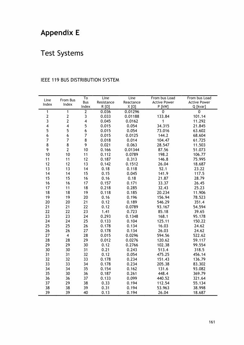
161

Appendix E

Test Systems

IEEE 119 BUS DISTRIBUTION SYSTEM

Line Index

From Bus Index

To Bus

Index

Line Resistance

R [Ω]

Line Reactance

X [Ω]

From bus Load Active Power

P [kW]


Q [kvar]

1 1 2 0.036 0.01296 0 0 2 2 3 0.033 0.01188 133.84 101.14 3 2 4 0.045 0.0162 1 11.292 4 4 5 0.015 0.054 34.315 21.845 5 5 6 0.015 0.054 73.016 63.602 6 6 7 0.015 0.0125 144.2 68.604 7 7 8 0.018 0.014 104.47 61.725 8 8 9 0.021 0.063 28.547 11.503 9 2 10 0.166 0.01344 87.56 51.073 10 10 11 0.112 0.0789 198.2 106.77 11 11 12 0.187 0.313 146.8 75.995 12 12 13 0.142 0.1512 26.04 18.687 13 13 14 0.18 0.118 52.1 23.22 14 14 15 0.15 0.045 141.9 117.5 15 15 16 0.16 0.18 21.87 28.79 16 16 17 0.157 0.171 33.37 26.45 17 11 18 0.218 0.285 32.43 25.23 18 18 19 0.118 0.185 20.234 11.906 19 19 20 0.16 0.196 156.94 78.523 20 20 21 0.12 0.189 546.29 351.4 21 21 22 0.12 0.0789 93.167 54.594 22 22 23 1.41 0.723 85.18 39.65 23 23 24 0.293 0.1348 168.1 95.178 24 24 25 0.133 0.104 125.11 150.22 25 25 26 0.178 0.134 16.03 24.62 26 26 27 0.178 0.134 26.03 24.62 27 4 28 0.015 0.0296 594.56 522.62 28 28 29 0.012 0.0276 120.62 59.117 29 29 30 0.12 0.2766 102.38 99.554 30 30 31 0.21 0.243 513.4 318.5 31 31 32 0.12 0.054 475.25 456.14 32 32 33 0.178 0.234 151.43 136.79 33 33 34 0.178 0.234 205.38 83.302 34 34 35 0.154 0.162 131.6 93.082 35 30 36 0.187 0.261 448.4 369.79 36 36 37 0.133 0.099 440.52 321.64 37 29 38 0.33 0.194 112.54 55.134 38 38 39 0.31 0.194 53.963 38.998 39 39 40 0.13 0.194 26.04 18.687

162

(Continuation of the previous table)

Line Index

From Bus Index

To Bus

Index

Line Resistance

R [Ω]

Line Reactance

X [Ω]


P [kW]


Q [kvar]

40 40 41 0.28 0.15 393.05 342.6 41 41 42 1.18 0.85 326.74 278.56 42 42 43 0.42 0.2436 536.26 240.24 43 43 44 0.27 0.0972 76.247 66.562 44 44 45 0.339 0.1221 53.52 39.76 45 45 46 0.27 0.1779 40.328 31.964 46 35 47 0.21 0.1383 39.653 20.758 47 47 48 0.12 0.0789 66.195 42.361 48 48 49 0.15 0.0987 73.904 51.653 49 49 50 0.15 0.0987 114.77 57.965 50 50 51 0.24 0.1581 918.37 1205.1 51 51 52 0.12 0.0789 210.3 146.66 52 52 53 0.405 0.1458 66.68 56.608 53 53 54 0.405 0.1458 42.207 40.184 54 29 55 0.391 0.141 433.74 283.41 55 55 56 0.406 0.1461 62.1 26.86 56 56 57 0.406 0.1461 92.46 88.38 57 57 58 0.706 0.5461 85.188 55.436 58 58 59 0.338 0.1218 345.3 332.4 59 59 60 0.338 0.1218 22.5 16.83 60 60 61 0.207 0.0747 467.5 395.14 61 61 62 0.247 0.8922 95.86 90.758 62 1 63 0.028 0.0418 62.92 47.7 63 63 64 0.117 0.2016 478.8 463.74 64 64 65 0.255 0.0918 120.94 52.006 65 65 66 0.21 0.0759 139.11 100.34 66 66 67 0.383 0.138 391.78 193.5 67 67 68 0.504 0.3303 27.741 26.713 68 68 69 0.406 0.1461 52.814 25.257 69 69 70 0.962 0.761 66.89 38.713 70 70 71 0.165 0.06 467.5 395.14 71 71 72 0.303 0.1092 594.85 239.74 72 72 73 0.303 0.1092 132.5 84.363 73 73 74 0.206 0.144 52.699 22.482 74 74 75 0.233 0.084 869.79 614.775 75 75 76 0.591 0.1773 31.349 29.817 76 76 77 0.126 0.0453 192.39 122.43 77 64 78 0.559 0.3687 65.75 45.37 78 78 79 0.186 0.1227 238.15 223.22 79 79 80 0.186 0.1227 294.55 162.47

163

(Continuation of the previous table)

Line Index

From Bus Index

To Bus

Index

Line Resistance

R [Ω]

Line Reactance

X [Ω]


P [kW]


Q [kvar]

80 80 81 0.26 0.139 485.57 437.92 81 81 82 0.154 0.148 243.53 183.03 82 82 83 0.23 0.128 243.53 183.03 83 83 84 0.252 0.106 134.25 119.29 84 84 85 0.18 0.148 22.71 27.96 85 79 86 0.16 0.182 49.513 26.515 86 86 87 0.2 0.23 383.78 257.16 87 87 88 0.16 0.393 49.64 20.6 88 65 89 0.669 0.2412 22.473 11.806 89 89 90 0.266 0.1227 62.93 42.96 90 90 91 0.266 0.1227 30.67 34.93 91 91 92 0.266 0.1227 62.53 66.79 92 92 93 0.226 0.1227 114.57 81.748 93 93 94 0.233 0.115 81.292 66.526 94 94 95 0.496 0.138 31.733 15.96 95 91 96 0.196 0.18 33.32 60.48 96 96 97 0.196 0.18 531.28 224.85 97 97 98 0.1866 0.122 507.03 367.42 98 98 99 0.0746 0.318 26.39 11.7 99 1 100 0.0625 0.0265 96.793 83.647 100 100 101 0.1501 0.234 100.66 47.572 101 101 102 0.1347 0.0888 456.48 350.3 102 102 103 0.2307 0.1203 522.56 449.29 103 103 104 0.447 0.1608 408.43 168.46 104 104 105 0.1632 0.0588 141.48 134.25 105 105 106 0.33 0.099 104.43 66.024 106 106 107 0.156 0.0561 96.793 83.647 107 107 108 0.3819 0.1374 493.92 419.34 108 108 109 0.1626 0.0585 225.38 135.88 109 109 110 0.3819 0.1374 509.21 387.21 110 110 111 0.2445 0.0879 188.5 173.46 111 109 112 0.2088 0.0753 918.03 898.55 112 112 113 0.2301 0.0828 305.08 215.37 113 100 114 0.6102 0.2196 54.38 40.97 114 114 115 0.1866 0.127 211.14 192.9 115 115 116 0.3732 0.246 67.009 53.336 116 116 117 0.405 0.367 162.07 90.321 117 117 118 0.489 0.438 48.785 29.156

118 33.9 18.98

164

IEEE 41 BUS DISTRIBUTION SYSTEM

Line Index

To Bus Index

From Bus

Index

Line Resistance

R [Ω]

Line Reactance

X [Ω]


P [kW]


Q [kvar]

1 1 2 0.0992 0.0470 100 60 2 2 3 0.4930 0.2511 90 40 3 3 4 0.3660 0.1864 120 80 4 4 5 0.3811 1.1941 60 30 5 5 6 0.8190 0.7070 60 20 6 6 7 0.1872 0.6188 200 100 7 7 8 0.7114 0.2351 200 100 8 8 9 1.0300 0.7400 60 20 9 9 10 1.0440 0.7400 60 20 10 10 11 0.1966 0.0650 45 30 11 11 12 0.3744 0.1238 60 35 12 12 13 1.4680 1.1550 60 35 13 13 14 0.5416 0.7129 120 80 14 14 15 0.5910 0.5260 60 10 15 15 16 0.7463 0.5450 60 20 16 16 17 1.2890 1.7210 60 20 17 17 18 0.7320 0.5470 90 40 18 2 19 0.1640 0.1565 90 40 19 19 20 1.5042 1.3554 90 40 20 20 21 0.4095 0.4784 90 40 21 21 22 0.7089 0.9373 90 40 22 3 23 0.4512 0.3083 90 50 23 23 24 0.8980 0.7091 420 200 24 24 25 0.8960 0.7011 420 200 25 6 26 0.2030 0.1034 60 25 26 26 27 0.2842 0.1447 60 25 27 27 28 1.0590 0.9337 60 20 28 28 29 0.8042 0.7006 120 70 29 29 30 0.5075 0.2585 200 600 30 30 31 0.9744 0.9630 150 70 31 31 32 0.3105 0.3619 210 100 32 32 33 0.3410 0.5302 60 40 33 10 34 0.2030 0.1034 60 25 34 34 35 0.2842 0.1447 60 25 35 35 36 1.0590 0.9337 60 20 36 36 37 0.8042 0.7006 120 70 37 37 38 0.5075 0.2585 200 600 38 38 39 0.9744 0.9630 150 70 39 39 40 0.3105 0.3619 210 100 40 40 41 0.3410 0.5302 60 40

165

Bibliography

[1] A. McCrone, U. Moslener, and F. Grüning, “Global Trends in Renewable Energy

Investment 2016l,” Frankfurt School-UNEP Collaborating Centre for Climate, Frankfurt,

Germany, Mar. 2016.

[2] “Energy Climate and Change - World Energy Outlook Special Briefing for COP21,”

International Energy Agency (IEA), 2015.

[3] World Energy Outlook 2015 - Special Reporton. Paris, France: International Enjergy

Agency.

[4] V. C. Nelson and K. L. Starcher, Introduction to Renewable Energy. New Mexico, USA:

CRC Press, 2011.

[5] “Renewables 20116 - Global Status Report,” Renewable Energy Policy Network for 21st

Century, Paris, France, 20016.

[6] S. F. Santos, D. Z. Fitiwi, M. Shafie-khah, A. W. Bizuayehu, and J. P. S. Catalão,

“Introduction to renewable energy systems,” in Optimization in Renewable Energy

Systems, London, UK: ACADEMIC Press (ELSEVIER), 2016 (aceite).

[7] S. F. Santos, D. Z. Fitiwi, A. W. Bizuayehu, M. Shafie-khah, M. Asensio, J. Contreras,

C. M. P. Cabrita, J. P. S. Catalão, “Impacts of Operational Variability and Uncertainty

on Distributed Generation Investment Planning: A Comprehensive Sensitivity Analysis,”

IEEE Trans. Sustain. Energy, 2016 (aceite), DOI:10.1109/TSTE.2016.2624506.

[8] S. F. Santos, D. Z. Fitiwi, A. W. Bizuayehu, M. Shafie-khah, M. Asensio, J. Contreras,

C. M. P. Cabrita, J. P. S. Catalão, “Novel Multi-Stage Stochastic DG Investment

Planning with Recourse,” IEEE Trans. Sustain. Energy, 2016 (aceite), DOI:

10.1109/TSTE.2016.2590460.

[9] S. F. Santos, D. Z. Fitiwi, M. R. M. Cruz, C. M. P. Cabrita, and J. P. S. Catalão, “Impacts

of Optimal Energy Storage Deployment and Network Reconfiguration on Renewable

Integration Level in Distribution Systems,” Appl. Energy, Vol. 185, pp. 44-55, January

2017, DOI: 10.1016/j.apenergy.2016.10.053.

[10] S. F. Santos, D. Z. Fitiwi, M. Shafie-khah, A. W. Bizuayehu, C. M. P. Cabrita, and J. P. S.

Catalao, “New Multi-Stage and Stochastic Mathematical Model for Maximizing RES

Hosting Capacity—Part I: Problem Formulation,” IEEE Trans. Sustain. Energy, 2016

(aceite), DOI: 10.1109/TSTE.2016.2598400.

166

[11] S. F. Santos, D. Z. Fitiwi, M. Shafie-khah, A. W. Bizuayehu, C. M. P. Cabrita, and J. P. S.

Catalao, “New Multi-Stage and Stochastic Mathematical Model for Maximizing RES

Hosting Capacity—Part II: Numerical Results,” IEEE Trans. Sustain. Energy, 2016

(aceite), DOI: 10.1109/TSTE.2016.2584122.

[12] C. J. Cleveland, R. Costanza, C. A. S. Hall, and R. K. Kaufmann, “Energy and the U:S:

Economy: A Biophysical Prespective,” Science, vol. 225, pp. 890–897.

[13] L. Brookes, “Energy efficiency fallacies revisited,” Energy Policy, vol. 28, no. 6, pp.

355–366, 2000.

[14] R. K. Kaufmann, “The mechanisms for autonomous energy efficiency increases: A

cointegration analysis of the US energy/GDP ratio,” Energy J., pp. 63–86, 2004.

[15] J. Khan and M. H. Arsalan, “Solar power technologies for sustainable electricity

generation – A review,” Renew. Sustain. Energy Rev., vol. 55, pp. 414–425, Mar. 2016.

[16] S. Comello and S. Reichelstein, “The U.S. investment tax credit for solar energy:

Alternatives to the anticipated 2017 step-down,” Renew. Sustain. Energy Rev., vol. 55,

pp. 591–602, Mar. 2016.

[17] R. Bertani, “Geothermal power generation in the world 2010–2014 update report,”

Geothermics, vol. 60, pp. 31–43, Mar. 2016.

[18] R. K. Pachauri and Intergovernmental Panel on Climate Change, Eds., Climate change

2007:: contribution of ... to the fourth assessment report of the Intergovernmental

Panel on Climate Change. 4: Synthesis report: [a report of the Intergovernmental Panel

on Climate Change]. Geneva: IPCC, 2008.

[19] P. Del Duca et al., “MEXICO UPDATE,” 2011.

[20] Renewables 2014 - Global Status Report. Renewable Energy Policy Network for the 21st

Century.

[21] European Commission, “Paris climate change conference (COP21/CMP11).” [Online].

Available: http://ec.europa.eu/clima/events/articles/0107_en.htm. [Accessed: 29-Jan-

2016].

[22] Climate Change 2014: Synthesis Report. Geneva, Switzerland: Intergovernmental Panel

on Climate Change -IPCC.

[23] Renewables 2015 - Global Status Report, Renewable Energy Policy Network for the 21st

Century. .

167

[24] Renewable Power Generation Costs in 2014. International Renewable Energy Agency.

[25] S. Tegen, E. Lantz, M. Hand, B. Maples, A. Smith, and P. Schwabe, “2011 Cost of Wind

Energy Review.” National Renewable Energy Laboratory, 2011.

[26] N. Gupta, “A review on the inclusion of wind generation in power system studies,”

Renew. Sustain. Energy Rev., vol. 59, pp. 530–543, Jun. 2016.

[27] M. Finster, C. Clark, J. Schroeder, and L. Martino, “Geothermal produced fluids:

Characteristics, treatment technologies, and management options,” Renew. Sustain.

Energy Rev., vol. 50, pp. 952–966, Oct. 2015.

[28] B. Sung, “Public policy supports and export performance of bioenergy technologies: A

dynamic panel approach,” Renew. Sustain. Energy Rev., vol. 42, pp. 477–495, Feb.

2015.

[29] G. Fiorese, M. Catenacci, V. Bosetti, and E. Verdolini, “The power of biomass: Experts

disclose the potential for success of bioenergy technologies,” Energy Policy, vol. 65, pp.

94–114, 2014.

[30] European Biomass and Association (AEBIOM), “AEBIOM-Statistical-Report-2015: European

Bioenergy Outlook,” European Biomass Association, Brussels.

[31] A. F. de O. Falcão, “Wave energy utilization: A review of the technologies,” Renew.

Sustain. Energy Rev., vol. 14, no. 3, pp. 899–918, Apr. 2010.

[32] European Commission, “Harnessing the power of the sea: The future of ocean energy.”

European Commission, 2014.

[33] Wissenschaftlicher Beirat Globale Umweltveränderungen, Ed., Welt im Wandel -

Sicherheitsrisiko Klimawandel. Berlin: Springer, 2008.

[34] Müller, Brown, and S. Ölz, “Renew_Policies -Policy considerations for deploying

renewables,” International Energy Agency, Paris, 2011.

[35] J. Lilliestam and S. Ellenbeck, “Energy security and renewable electricity trade—Will

Desertec make Europe vulnerable to the ‘energy weapon’?,” Energy Policy, vol. 39, no.

6, pp. 3380–3391, Jun. 2011.

[36] “The oil age poster,” The oil age poster. [Online]. Available: http://www.oilposter.org.

[Accessed: 25-Jan-2016].

168

[37] F. Hedenus, C. Azar, and D. J. A. Johansson, “Energy security policies in EU-25—The

expected cost of oil supply disruptions,” Energy Policy, vol. 38, no. 3, pp. 1241–1250,

Mar. 2010.

[38] European Comission, “Impact Assessment, Accompanying the document to Energy

Roadmap 2050,” European Comission, Brussels, 2011.

[39] W. Lacher and D. Kumetat, “The security of energy infrastructure and supply in North

Africa: Hydrocarbons and renewable energies in comparative perspective,” Energy

Policy, vol. 39, no. 8, pp. 4466–4478, Aug. 2011.

[40] M. Mobjörk, M. Eriksson, and H. Carlsen, “On connecting climate change with security

and armed conflict,” Investig. Knowl. Sci. Community FOI Stockh., 2010.

[41] M. Z. Jacobson and M. A. Delucchi, “Providing all global energy with wind, water, and

solar power, Part I: Technologies, energy resources, quantities and areas of

infrastructure, and materials,” Energy Policy, vol. 39, no. 3, pp. 1154–1169, Mar. 2011.

[42] M. A. Delucchi and M. Z. Jacobson, “Providing all global energy with wind, water, and

solar power, Part II: Reliability, system and transmission costs, and policies,” Energy

Policy, vol. 39, no. 3, pp. 1170–1190, Mar. 2011.

[43] D. S. Parakh and M. M. D. Ross, “Clean Energy Management Software,” Canada.

[44] A. L. R. Jackson, “Renewable energy vs. biodiversity: Policy conflicts and the future of

nature conservation,” Glob. Environ. Change, vol. 21, no. 4, pp. 1195–1208, Oct. 2011.

[45] Lazard, “Levelized Cost of Energy -Vergion 2.0,” Jun-2008.

[46] J. Glassmire, P. Komor, and P. Lilienthal, “Electricity demand savings from distributed

solar photovoltaics,” Energy Policy, vol. 51, pp. 323–331, Dec. 2012.

[47] H. Lund and B. V. Mathiesen, “Energy system analysis of 100% renewable energy

systems—The case of Denmark in years 2030 and 2050,” Energy, vol. 34, no. 5, pp. 524–

531, May 2009.

[48] R. Bove, M. Bucher, and F. Ferretti, “Integrating large shares of wind energy in macro-

economical cost-effective way,” Energy, vol. 43, no. 1, pp. 438–447, Jul. 2012.

[49] H. Auer and B. Burgholzer, “D2. 1 Opportunities, Challenges and Risks for RES-E

Deployment in a fully Integrated European Electricity Market,” 2015.

169

[50] E. B. Zane, R. Brückmann, and D. Bauknecht, “Integration of electricity from

renewables to the electricity grid and to the electricity market - RES - Integration,”

Berlin, Final Report, 2012.

[51] International, Electrotechnical, and International Electrotechnical Commission, “Grid

integration of large-capacity Renewable Energy sources and use of large-capacity

Electrical Energy Storage.” .

[52] GEA, Global Energy Assessment - Toward a Sustainable Future. Cambridge University

Press, Cambridge, UK and New York, NY, USA and the International Institute for Applied

Systems Analysis, Laxenburg, Austria, 2012.

[53] M. Stappel and A. Energiewende, “The European power system in 2030: flexibility

challenges and integration benefits: an analysis with a focus on the pentalateral energy

forum region.”

[54] A. Ulbig and others, “Analyzing operational flexibility of power systems,” ArXiv Prepr.

ArXiv13127618, 2013.

[55] R. Poudineh and T. Jamasb, “Distributed generation, storage, demand response and

energy efficiency as alternatives to grid capacity enhancement,” Energy Policy, vol. 67,

pp. 222–231, Apr. 2014.

[56] C. L. T. Borges and V. F. Martins, “Multistage expansion planning for active distribution

networks under demand and Distributed Generation uncertainties,” Int. J. Electr. Power

Energy Syst., vol. 36, no. 1, pp. 107–116, Mar. 2012.

[57] J. A. P. Lopes, N. Hatziargyriou, J. Mutale, P. Djapic, and N. Jenkins, “Integrating

distributed generation into electric power systems: A review of drivers, challenges and

opportunities,” Electr. Power Syst. Res., vol. 77, no. 9, pp. 1189–1203, Jul. 2007.

[58] M. O. W. Grond, J. Morren, and J. G. Slootweg, “Integrating smart grid solutions into

distribution network planning,” in PowerTech (POWERTECH), 2013 IEEE Grenoble, 2013,

pp. 1–6.

[59] A. Yadav and L. Srivastava, “Optimal placement of distributed generation: An overview

and key issues,” in 2014 International Conference on Power Signals Control and

Computations (EPSCICON), 2014, pp. 1–6.

[60] M. E. Samper and A. Vargas, “Investment Decisions in Distribution Networks Under

Uncertainty With Distributed Generation - Part I: Model Formulation,” IEEE Trans. Power

Syst., vol. 28, no. 3, pp. 2331–2340, Aug. 2013.

170

[61] M. E. Samper and A. Vargas, “Investment Decisions in Distribution Networks Under

Uncertainty With Distributed Generation - Part II: Implementation and Results,” IEEE

Trans. Power Syst., vol. 28, no. 3, pp. 2341–2351, Aug. 2013.

[62] A. Piccolo and P. Siano, “Evaluating the Impact of Network Investment Deferral on

Distributed Generation Expansion,” IEEE Trans. Power Syst., vol. 24, no. 3, pp. 1559–

1567, Aug. 2009.

[63] T. Niknam, S. I. Taheri, J. Aghaei, S. Tabatabaei, and M. Nayeripour, “A modified honey

bee mating optimization algorithm for multiobjective placement of renewable energy

resources,” Appl. Energy, vol. 88, no. 12, pp. 4817–4830, Dec. 2011.

[64] H. Hedayati, S. A. Nabaviniaki, and A. Akbarimajd, “A Method for Placement of DG Units

in Distribution Networks,” IEEE Trans. Power Deliv., vol. 23, no. 3, pp. 1620–1628, Jul.

2008.

[65] C. L. T. Borges and D. M. Falcão, “Optimal distributed generation allocation for

reliability, losses, and voltage improvement,” Int. J. Electr. Power Energy Syst., vol.

28, no. 6, pp. 413–420, Jul. 2006.

[66] M. A. Abdullah, A. P. Agalgaonkar, and K. M. Muttaqi, “Assessment of energy supply and

continuity of service in distribution network with renewable distributed generation,”

Appl. Energy, vol. 113, pp. 1015–1026, Jan. 2014.

[67] J. Liu, W. Zhang, R. Zhou, and J. Zhong, “Impacts of distributed renewable energy

generations on smart grid operation and dispatch,” in 2012 IEEE Power and Energy

Society General Meeting, 2012, pp. 1–5.

[68] F. Katiraei and J. R. Agüero, “Solar PV Integration Challenges,” IEEE Power Energy Mag.,

vol. 9, no. 3, pp. 62–71, May 2011.

[69] S. Eftekharnejad, V. Vittal, G. T. Heydt, B. Keel, and J. Loehr, “Impact of increased

penetration of photovoltaic generation on power systems,” IEEE Trans. Power Syst., vol.

28, no. 2, pp. 893–901, May 2013.

[70] M. Shivaie, M. T. Ameli, M. S. Sepasian, P. D. Weinsier, and V. Vahidinasab, “A

multistage framework for reliability-based distribution expansion planning considering

distributed generations by A self-adaptive global-based harmony search algorithm,”

Reliab. Eng. Syst. Saf., Mar. 2015.

[71] G. Munoz-Delgado, J. Contreras, and J. M. Arroyo, “Joint Expansion Planning of

Distributed Generation and Distribution Networks,” IEEE Trans. Power Syst., vol. 30, no.

5, pp. 2579–2590, Sep. 2015.

171

[72] Ž. N. Popović, V. D. Kerleta, and D. S. Popović, “Hybrid simulated annealing and mixed

integer linear programming algorithm for optimal planning of radial distribution

networks with distributed generation,” Electr. Power Syst. Res., vol. 108, pp. 211–222,

Mar. 2014.

[73] M.-C. Alvarez-Herault, N. N’Doye, C. Gandioli, N. Hadjsaid, and P. Tixador, “Meshed

distribution network vs reinforcement to increase the distributed generation

connection,” Sustain. Energy Grids Netw., vol. 1, pp. 20–27, Mar. 2015.

[74] M. Jalali, K. Zare, and M. T. Hagh, “A multi-stage MINLP-based model for sub-

transmission system expansion planning considering the placement of DG units,” Int. J.

Electr. Power Energy Syst., vol. 63, pp. 8–16, Dec. 2014.

[75] H. Shayeghi and A. Bagheri, “Dynamic sub-transmission system expansion planning

incorporating distributed generation using hybrid DCGA and LP technique,” Int. J.

Electr. Power Energy Syst., vol. 48, pp. 111–122, Jun. 2013.

[76] M. Sedghi, M. Aliakbar-Golkar, and M.-R. Haghifam, “Distribution network expansion

considering distributed generation and storage units using modified PSO algorithm,” Int.

J. Electr. Power Energy Syst., vol. 52, pp. 221–230, Nov. 2013.

[77] M. Sadeghi and M. Kalantar, “Multi types DG expansion dynamic planning in distribution

system under stochastic conditions using Covariance Matrix Adaptation Evolutionary

Strategy and Monte-Carlo simulation,” Energy Convers. Manag., vol. 87, pp. 455–471,

Nov. 2014.

[78] M. Ahmadigorji and N. Amjady, “A new evolutionary solution method for dynamic

expansion planning of DG-integrated primary distribution networks,” Energy Convers.

Manag., vol. 82, pp. 61–70, Jun. 2014.

[79] M. Arriaga, C. A. Canizares, and M. Kazerani, “Long-Term Renewable Energy Planning

Model for Remote Communities,” IEEE Trans. Sustain. Energy, vol. 7, no. 1, pp. 221–

231, Jan. 2016.

[80] M. V. Kirthiga, S. A. Daniel, and S. Gurunathan, “A Methodology for Transforming an

Existing Distribution Network Into a Sustainable Autonomous Micro-Grid,” IEEE Trans.

Sustain. Energy, vol. 4, no. 1, pp. 31–41, Jan. 2013.

[81] G. Liu, Y. Xu, and K. Tomsovic, “Bidding Strategy for Microgrid in Day-Ahead Market

Based on Hybrid Stochastic/Robust Optimization,” IEEE Trans. Smart Grid, vol. 7, no. 1,

pp. 227–237, Jan. 2016.

172

[82] G. Martinez, N. Gatsis, and G. Giannakis, “Stochastic programming for energy planning

in microgrids with renewables,” in 2013 IEEE 5th International Workshop on

Computational Advances in Multi-Sensor Adaptive Processing (CAMSAP), 2013, pp. 472–

475.

[83] A. T. Al-Awami and E. Sortomme, “Coordinating Vehicle-to-Grid Services With Energy

Trading,” IEEE Trans. Smart Grid, vol. 3, no. 1, pp. 453–462, Mar. 2012.

[84] S. Montoya-Bueno, J. I. Munoz, and J. Contreras, “A Stochastic Investment Model for

Renewable Generation in Distribution Systems,” IEEE Trans. Sustain. Energy, vol. 6, no.

4, pp. 1466–1474, Oct. 2015.

[85] H. Moghimi, A. Ahmadi, J. Aghaei, and A. Rabiee, “Stochastic techno-economic

operation of power systems in the presence of distributed energy resources,” Int. J.

Electr. Power Energy Syst., vol. 45, no. 1, pp. 477–488, Feb. 2013.

[86] S. Ganguly and D. Samajpati, “Distributed Generation Allocation on Radial Distribution

Networks Under Uncertainties of Load and Generation Using Genetic Algorithm,” IEEE

Trans. Sustain. Energy, vol. 6, no. 3, pp. 688–697, Jul. 2015.

[87] M. Ahmadigorji and N. Amjady, “A multiyear DG-incorporated framework for expansion

planning of distribution networks using binary chaotic shark smell optimization

algorithm,” Energy, vol. 102, pp. 199–215, May 2016.

[88] D. Q. Hung, N. Mithulananthan, and R. C. Bansal, “An optimal investment planning

framework for multiple distributed generation units in industrial distribution systems,”

Appl. Energy, vol. 124, pp. 62–72, Jul. 2014.

[89] D. Z. Fitiwi, “Strategy, Methods and Tools for Solving Long-term Transmission Expansion

Planning in Large-scale Power Systems,” Comillas Pontifical University, 2016.

[90] Gerald van Belle, Statistical Rules of Thumb, 2nd ed. Wiley, 2008.

[91] M. O. Buygi, G. Balzer, H. M. Shanechi, and M. Shahidehpour, “Market-Based

Transmission Expansion Planning,” IEEE Trans. Power Syst., vol. 19, no. 4, pp. 2060–

2067, Nov. 2004.

[92] F. Desta Zahlay, F. de Cuadra, L. Olmos, M. Rivier, and I. J. Perez-Arriaga, “A

formulation for large-scale transmission expansion planning problem and a solution

strategy,” in 10th International Conference on the European Energy Market (EEM),

2013, pp. 1–8.

[93] L. Blank and A. Tarquin, Engineering Economy, 7th ed. New York: McGraw-Hill

Science/Engineering/Math, 2011.

173

[94] D. Z. Fitiwi, L. Olmos, M. Rivier, F. de Cuadra, and I. J. Pérez-Arriaga, “Finding a

representative network losses model for large-scale transmission expansion planning

with renewable energy sources,” Energy, vol. 101, pp. 343–358, Apr. 2016.

[95] H. Zhang, G. T. Heydt, V. Vittal, and J. Quintero, “An Improved Network Model for

Transmission Expansion Planning Considering Reactive Power and Network Losses,” IEEE

Trans. Power Syst., vol. 28, no. 3, pp. 3471–3479, Aug. 2013.

[96] S. F. Santos, D. Z. Fitiwi, M. Shafie-khah, A. W. Bizuayehu, and J. P. S. Catalão,

“Optimal Sizing and Placement of Smart Grid Enabling Technologies for Maximizing

Renewable Integration,” in Smart Energy Grid Engineering, In press., 2015.

[97] M. Lavorato, J. F. Franco, M. J. Rider, and R. Romero, “Imposing Radiality Constraints in

Distribution System Optimization Problems,” IEEE Trans. Power Syst., vol. 27, no. 1, pp.

172–180, Feb. 2012.

[98] R. Viral and D. K. Khatod, “Optimal planning of distributed generation systems in

distribution system: A review,” Renew. Sustain. Energy Rev., vol. 16, no. 7, pp. 5146–

5165, Sep. 2012.

[99] M. Bazilian et al., “Re-considering the economics of photovoltaic power,” Renew.

Energy, vol. 53, pp. 329–338, May 2013.

[100] J. Sweeting, Project Cost Estimating: Principles and Practice. IChemE, 1997.

[101] The World Data Center for Remote Sensing of the Atmosphere, “SOLEMI database for

long-term global and direct irradiance at WDC-RSAT.” [Online]. Available:

https://wdc.dlr.de/data_products/SERVICES/SOLARENERGY/description.php.

[Accessed: 02-Nov-2015].

[102] The SoDa Service, “Solar Radiation Data.” [Online]. Available: http://www.soda-

is.com/eng/index.html. [Accessed: 02-Nov-2015].

[103] Gregorio Muñoz-Delgado, Sergio Montoya-Bueno, Miguel Asensio, Javier Contreras, JoséI

Muñoz, and JoséM Arroyo, “Renewable Generation and Distribution Grid Expansion

Planning,” in Smart and Sustainable Power Systems, 0 vols., CRC Press, 2015, pp. 345–

404.

[104] J. Momoh, Smart Grid: Fundamentals of Design and Analysis. John Wiley & Sons, 2012.

[105] P. S. Georgilakis and N. D. Hatziargyriou, “A review of power distribution planning in

the modern power systems era: Models, methods and future research,” Electr. Power

Syst. Res., vol. 121, pp. 89–100, Apr. 2015.

174

[106] E. Romero-Ramos, J. Riquelme-Santos, and J. Reyes, “A simpler and exact

mathematical model for the computation of the minimal power losses tree,” Electr.

Power Syst. Res., vol. 80, no. 5, pp. 562–571, May 2010.

[107] A. Chauhan and R. P. Saini, “A review on Integrated Renewable Energy System based

power generation for stand-alone applications: Configurations, storage options, sizing

methodologies and control,” Renew. Sustain. Energy Rev., vol. 38, pp. 99–120, Oct.

2014.

[108] M. Aneke and M. Wang, “Energy storage technologies and real life applications – A state

of the art review,” Appl. Energy, vol. 179, pp. 350–377, Oct. 2016.

[109] A. Chauhan and R. P. Saini, “A review on Integrated Renewable Energy System based

power generation for stand-alone applications: Configurations, storage options, sizing

methodologies and control,” Renew. Sustain. Energy Rev., vol. 38, pp. 99–120, Oct.

2014.

[110] D. Q. Hung and N. Mithulananthan, “Loss reduction and loadability enhancement with

DG: A dual-index analytical approach,” Appl. Energy, vol. 115, pp. 233–241, Feb. 2014.

[111] M. R. Dorostkar-Ghamsari, M. Fotuhi-Firuzabad, M. Lehtonen, and A. Safdarian, “Value

of Distribution Network Reconfiguration in Presence of Renewable Energy Resources,”

IEEE Trans. Power Syst., vol. 31, no. 3, pp. 1879–1888, May 2016.

[112] I.-K. Song, W.-W. Jung, J.-Y. Kim, S.-Y. Yun, J.-H. Choi, and S.-J. Ahn, “Operation

Schemes of Smart Distribution Networks With Distributed Energy Resources for Loss

Reduction and Service Restoration,” IEEE Trans. Smart Grid, vol. 4, no. 1, pp. 367–374,

Mar. 2013.

[113] D. Q. Hung, N. Mithulananthan, and R. C. Bansal, “A combined practical approach for

distribution system loss reduction,” Int. J. Ambient Energy, vol. 36, no. 3, pp. 123–131,

May 2015.

[114] G. Munoz-Delgado, J. Contreras, and J. M. Arroyo, “Joint Expansion Planning of

Distributed Generation and Distribution Networks,” IEEE Trans. Power Syst., vol. 30, no.

5, pp. 2579–2590, Sep. 2015.

[115] H. P. Williams, Model Building in Mathematical Programming, 4th ed. Wiley, 1999.

[116] D. Zhang, Z. Fu, and L. Zhang, “An improved TS algorithm for loss-minimum

reconfiguration in large-scale distribution systems,” Electr. Power Syst. Res., vol. 77,

no. 5–6, pp. 685–694, Apr. 2007.

175

[117] R. S. Rao, S. V. L. Narasimham, M. R. Raju, and A. S. Rao, “Optimal Network

Reconfiguration of Large-Scale Distribution System Using Harmony Search Algorithm,”

IEEE Trans. Power Syst., vol. 26, no. 3, pp. 1080–1088, Aug. 2011.

[118] D. Z. Fitiwi, A. W. Bizuayehu, M. Shafie-khah, J. P. S. Catalão, M. Asenso, and

J. Contreras, “DG Investment Planning Analysis with Renewable Integration and

Considering Emission Costs,” in the 16th Int. Conf. on Computer as a Tool,

EuroCon2015, Salamanca, 2015.

[119] P. K. Ray, S. R. Mohanty, and N. Kishor, “Classification of Power Quality Disturbances

Due to Environmental Characteristics in Distributed Generation System,” IEEE Trans.

Sustain. Energy, vol. 4, no. 2, pp. 302–313, Apr. 2013.

[120] P. S. Georgilakis and N. D. Hatziargyriou, “Optimal Distributed Generation Placement in

Power Distribution Networks: Models, Methods, and Future Research,” IEEE Trans.

Power Syst., vol. 28, no. 3, pp. 3420–3428, Aug. 2013.

[121] P. Paliwal, N. P. Patidar, and R. K. Nema, “Planning of grid integrated distributed

generators: A review of technology, objectives and techniques,” Renew. Sustain. Energy

Rev., vol. 40, pp. 557–570, Dec. 2014.

[122] D. Q. Hung, N. Mithulananthan, and R. C. Bansal, “An optimal investment planning

framework for multiple distributed generation units in industrial distribution systems,”

Appl. Energy, vol. 124, pp. 62–72, Jul. 2014.

[123] F. S. Abu-Mouti and M. E. El-Hawary, “Heuristic curve-fitted technique for distributed

generation optimisation in radial distribution feeder systems,” IET Gener. Transm.

Distrib., vol. 5, no. 2, p. 172, 2011.

[124] B. C. Pal and R. A. Jabr, “Ordinal optimisation approach for locating and sizing of

distributed generation,” IET Gener. Transm. Distrib., vol. 3, no. 8, pp. 713–723, Aug.

2009.

[125] R. S. Maciel, M. Rosa, V. Miranda, and A. Padilha-Feltrin, “Multi-objective evolutionary

particle swarm optimization in the assessment of the impact of distributed generation,”

Electr. Power Syst. Res., vol. 89, pp. 100–108, Aug. 2012.

[126] K. Vinothkumar and M. P. Selvan, “Fuzzy Embedded Genetic Algorithm Method for

Distributed Generation Planning,” Electr. Power Compon. Syst., vol. 39, no. 4, pp. 346–

366, Feb. 2011.

[127] F. Ugranlı and E. Karatepe, “Convergence of rule-of-thumb sizing and allocating rules of

distributed generation in meshed power networks,” Renew. Sustain. Energy Rev., vol.

16, no. 1, pp. 582–590, Jan. 2012.

176

[128] V. V. S. N. Murty and A. Kumar, “Optimal placement of DG in radial distribution systems

based on new voltage stability index under load growth,” Int. J. Electr. Power Energy

Syst., vol. 69, pp. 246–256, Jul. 2015.

[129] A. Bagheri, H. Monsef, and H. Lesani, “Integrated distribution network expansion

planning incorporating distributed generation considering uncertainties, reliability, and

operational conditions,” Int. J. Electr. Power Energy Syst., vol. 73, pp. 56–70, Dec.

2015.

[130] W. Sheng, K. Liu, Y. Liu, X. Meng, and Y. Li, “Optimal Placement and Sizing of

Distributed Generation via an Improved Nondominated Sorting Genetic Algorithm II,”

IEEE Trans. Power Deliv., vol. 30, no. 2, pp. 569–578, Apr. 2015.

[131] R. Mena, M. Hennebel, Y.-F. Li, C. Ruiz, and E. Zio, “A risk-based simulation and multi-

objective optimization framework for the integration of distributed renewable

generation and storage,” Renew. Sustain. Energy Rev., vol. 37, pp. 778–793, Sep. 2014.

[132] J. D. Foster, A. M. Berry, N. Boland, and H. Waterer, “Comparison of Mixed-Integer

Programming and Genetic Algorithm Methods for Distributed Generation Planning,” IEEE

Trans. Power Syst., vol. 29, no. 2, pp. 833–843, Mar. 2014.

[133] A. Ameli, S. Bahrami, F. Khazaeli, and M.-R. Haghifam, “A Multiobjective Particle

Swarm Optimization for Sizing and Placement of DGs from DG Owner’s and Distribution

Company’s Viewpoints,” IEEE Trans. Power Deliv., vol. 29, no. 4, pp. 1831–1840, Aug.

2014.

[134] S. Wen, H. Lan, Q. Fu, D. C. Yu, and L. Zhang, “Economic Allocation for Energy Storage

System Considering Wind Power Distribution,” IEEE Trans. Power Syst., vol. 30, no. 2,

pp. 644–652, Mar. 2015.

[135] M. Sedghi, M. Aliakbar-Golkar, and M.-R. Haghifam, “Distribution network expansion

considering distributed generation and storage units using modified PSO algorithm,” Int.

J. Electr. Power Energy Syst., vol. 52, pp. 221–230, Nov. 2013.

[136] H. Saboori, R. Hemmati, and V. Abbasi, “Multistage distribution network expansion

planning considering the emerging energy storage systems,” Energy Convers. Manag.,

vol. 105, pp. 938–945, Nov. 2015.

[137] M. M. Aman, G. B. Jasmon, A. H. A. Bakar, and H. Mokhlis, “A new approach for

optimum simultaneous multi-DG distributed generation Units placement and sizing

based on maximization of system loadability using HPSO (hybrid particle swarm

optimization) algorithm,” Energy, vol. 66, pp. 202–215, Mar. 2014.

177

[138] R. S. Rao, K. Ravindra, K. Satish, and S. V. L. Narasimham, “Power Loss Minimization in

Distribution System Using Network Reconfiguration in the Presence of Distributed

Generation,” IEEE Trans. Power Syst., vol. 28, no. 1, pp. 317–325, Feb. 2013.

[139] K. Nekooei, M. M. Farsangi, H. Nezamabadi-Pour, and K. Y. Lee, “An Improved Multi-

Objective Harmony Search for Optimal Placement of DGs in Distribution Systems,” IEEE

Trans. Smart Grid, vol. 4, no. 1, pp. 557–567, Mar. 2013.

[140] M. Sedighizadeh, M. Esmaili, and M. Esmaeili, “Application of the hybrid Big Bang-Big

Crunch algorithm to optimal reconfiguration and distributed generation power allocation

in distribution systems,” Energy, vol. 76, pp. 920–930, Nov. 2014.

[141] A. Y. Abdelaziz, Y. G. Hegazy, W. El-Khattam, and M. M. Othman, “Optimal allocation

of stochastically dependent renewable energy based distributed generators in

unbalanced distribution networks,” Electr. Power Syst. Res., vol. 119, pp. 34–44, Feb.

2015.

[142] M. M. Othman, W. El-Khattam, Y. G. Hegazy, and A. Y. Abdelaziz, “Optimal Placement

and Sizing of Distributed Generators in Unbalanced Distribution Systems Using

Supervised Big Bang-Big Crunch Method,” IEEE Trans. Power Syst., vol. 30, no. 2, pp.

911–919, Mar. 2015.

[143] D. Rama Prabha, T. Jayabarathi, R. Umamageswari, and S. Saranya, “Optimal location

and sizing of distributed generation unit using intelligent water drop algorithm,”

Sustain. Energy Technol. Assess., vol. 11, pp. 106–113, Sep. 2015.

[144] A. Mohamed Imran, M. Kowsalya, and D. P. Kothari, “A novel integration technique for

optimal network reconfiguration and distributed generation placement in power

distribution networks,” Int. J. Electr. Power Energy Syst., vol. 63, pp. 461–472, Dec.

2014.

[145] A. K. Singh and S. K. Parida, “Allocation of distributed generation using proposed DMSP

approach based on utility and customers aspects under deregulated environment,” Int.

J. Electr. Power Energy Syst., vol. 68, pp. 159–169, Jun. 2015.

[146] R. S. Al Abri, E. F. El-Saadany, and Y. M. Atwa, “Optimal Placement and Sizing Method

to Improve the Voltage Stability Margin in a Distribution System Using Distributed

Generation,” IEEE Trans. Power Syst., vol. 28, no. 1, pp. 326–334, Feb. 2013.

[147] Y. M. Atwa, E. F. El-Saadany, M. M. A. Salama, and R. Seethapathy, “Optimal

Renewable Resources Mix for Distribution System Energy Loss Minimization,” IEEE Trans.

Power Syst., vol. 25, no. 1, pp. 360–370, Feb. 2010.

178

[148] Y. Yang, S. Zhang, and Y. Xiao, “An MILP (mixed integer linear programming) model for

optimal design of district-scale distributed energy resource systems,” Energy, Jul. 2015.

[149] S. Montoya-Bueno, J. I. Munoz, and J. Contreras, “A Stochastic Investment Model for

Renewable Generation in Distribution Systems,” IEEE Trans. Sustain. Energy, vol. 6, no.

4, pp. 1466–1474, Oct. 2015.

[150] E. E. Sfikas, Y. A. Katsigiannis, and P. S. Georgilakis, “Simultaneous capacity

optimization of distributed generation and storage in medium voltage microgrids,” Int.

J. Electr. Power Energy Syst., vol. 67, pp. 101–113, May 2015.

[151] K. Mahmoud, N. Yorino, and A. Ahmed, “Optimal Distributed Generation Allocation in

Distribution Systems for Loss Minimization,” IEEE Trans. Power Syst., pp. 1–10, 2015.

[152] K. Vinothkumar and M. P. Selvan, “Hierarchical Agglomerative Clustering Algorithm

method for distributed generation planning,” Int. J. Electr. Power Energy Syst., vol. 56,

pp. 259–269, Mar. 2014.

[153] Y. M. Atwa and E. F. El-Saadany, “Probabilistic approach for optimal allocation of wind-

based distributed generation in distribution systems,” IET Renew. Power Gener., vol. 5,

no. 1, p. 79, 2011.

[154] V. V. S. . Murty and A. Kumar, “Mesh distribution system analysis in presence of

distributed generation with time varying load model,” Int. J. Electr. Power Energy

Syst., vol. 62, pp. 836–854, Nov. 2014.

[155] G. Sinden, “Characteristics of the UK wind resource: Long-term patterns and

relationship to electricity demand,” Energy Policy, vol. 35, no. 1, pp. 112–127, Jan.

2007.

[156] S. Subhadarshi, “Minding the P’s and Q’s: Real and reactive power assessment of hybrid

energy conversion systems with wind and solar resources,” Iowa State University, 2013.

[157] Y. Z. Li, Q. H. Wu, M. S. Li, and J. P. Zhan, “Mean-variance model for power system

economic dispatch with wind power integrated,” Energy, vol. 72, pp. 510–520, Aug.

2014.

[158] M. Zhao, Z. Chen, and F. Blaabjerg, “Probabilistic capacity of a grid connected wind

farm based on optimization method,” Renew. Energy, vol. 31, no. 13, pp. 2171–2187,

Oct. 2006.

[159] M. Aien, M. Rashidinejad, and M. Fotuhi-Firuzabad, “On possibilistic and probabilistic

uncertainty assessment of power flow problem: A review and a new approach,” Renew.

Sustain. Energy Rev., vol. 37, pp. 883–895, Sep. 2014.

179

[160] J. Hartigan and M. Wong, “Algorithm AS 136: A k-means clustering algorithm,” Appl.

Stat., vol. 28, no. 1, pp. 100–108, 1979.

[161] L. Baringo and A. J. Conejo, “Correlated wind-power production and electric load

scenarios for investment decisions,” Appl. Energy, vol. 101, pp. 475–482, Jan. 2013.

[162] S. Wogrin, P. Duenas, A. Delgadillo, and J. Reneses, “A New Approach to Model Load

Levels in Electric Power Systems With High Renewable Penetration,” IEEE Trans. Power

Syst., vol. 29, no. 5, pp. 2210–2218, Sep. 2014.

[163] P. Phonrattanasak, “Optimal placement of DG using multiobjective particle swarm

optimization,” in 2010 2nd International Conference on Mechanical and Electrical

Technology (ICMET), 2010, pp. 342–346.

[164] J. P. Vielma, S. Ahmed, and G. Nemhauser, “Mixed-Integer Models for Nonseparable

Piecewise-Linear Optimization: Unifying Framework and Extensions,” Oper. Res., vol.

58, no. 2, pp. 303–315, Oct. 2009.

[165] C. Abbey and G. Joos, “A Stochastic Optimization Approach to Rating of Energy Storage

Systems in Wind-Diesel Isolated Grids,” IEEE Trans. Power Syst., vol. 24, no. 1, pp. 418–

426, Feb. 2009.

[166] D. Pozo, J. Contreras, and E. E. Sauma, “Unit Commitment With Ideal and Generic

Energy Storage Units,” IEEE Trans. Power Syst., vol. 29, no. 6, pp. 2974–2984, Nov.

2014.

[167] J. Zhang, X. Yuan, and Y. Yuan, “A novel genetic algorithm based on all spanning trees

of undirected graph for distribution network reconfiguration,” J. Mod. Power Syst.

Clean Energy, vol. 2, no. 2, pp. 143–149, Jun. 2014.

[168] H. Ahmadi and J. R. Martí, “Mathematical representation of radiality constraint in

distribution system reconfiguration problem,” Int. J. Electr. Power Energy Syst., vol.

64, pp. 293–299, Jan. 2015.

[169] M. Wang and J. Zhong, “Islanding of systems of distributed generation using

optimization methodology,” in 2012 IEEE Power and Energy Society General Meeting,

2012, pp. 1–7.

[170] M. E. Baran and F. F. Wu, “Network reconfiguration in distribution systems for loss

reduction and load balancing,” Power Deliv. IEEE Trans. On, vol. 4, no. 2, pp. 1401–

1407, 1989.

180

[171] F. Díaz-González, A. Sumper, O. Gomis-Bellmunt, and R. Villafáfila-Robles, “A review of

energy storage technologies for wind power applications,” Renew. Sustain. Energy Rev.,

vol. 16, no. 4, pp. 2154–2171, May 2012.

[172] B. Zakeri and S. Syri, “Electrical energy storage systems: A comparative life cycle cost

analysis,” Renew. Sustain. Energy Rev., vol. 42, pp. 569–596, Feb. 2015.

[173] A. Ellis et al., “Reactive power performance requirements for wind and solar plants,” in

2012 IEEE Power and Energy Society General Meeting, 2012, pp. 1–8.

[174] A. Sadighmanesh, K. Zare, and M. Sabahi, “Distributed Generation unit and Capacitor

Placement for Loss, Voltage profile and ATC Optimization,” Int. J. Electr. Comput. Eng.

IJECE, vol. 2, no. 6, pp. 774–780, Dec. 2012.

[175] Jenkins et al., Wind Power Integration: Connection and system operational aspects.

Institution of Engineering and Technology, 2007.

[176] D. Z. Fitiwi, L. Olmos, M. Rivier, F. de Cuadra, and I. J. Pérez-Arriaga, “Finding a

representative network losses model for large-scale transmission expansion planning

with renewable energy sources,” Energy, vol. 101, pp. 343–358, Apr. 2016.

Documents

Planning of Power Distribution Systems with High ... · Penetration of Renewable Energy Sources Using Stochastic Optimization Sérgio da Fonseca Santos ... Planning of Power Distribution