Planetary waves in a coupled chemistry-climate model

HAL Id: hal-00303904https://hal.archives-ouvertes.fr/hal-00303904

Submitted on 3 May 2005

HAL is a multi-disciplinary open accessarchive for the deposit and dissemination of sci-entific research documents, whether they are pub-lished or not. The documents may come fromteaching and research institutions in France orabroad, or from public or private research centers.

L’archive ouverte pluridisciplinaire HAL, estdestinée au dépôt et à la diffusion de documentsscientifiques de niveau recherche, publiés ou non,émanant des établissements d’enseignement et derecherche français ou étrangers, des laboratoirespublics ou privés.

Planetary waves in a coupled chemistry-climate model:analysis techniques and comparison with reanalysis data

F. Mager, M. Dameris

To cite this version:F. Mager, M. Dameris. Planetary waves in a coupled chemistry-climate model: analysis techniquesand comparison with reanalysis data. Atmospheric Chemistry and Physics Discussions, EuropeanGeosciences Union, 2005, 5 (3), pp.2559-2598. hal-00303904

https://hal.archives-ouvertes.fr/hal-00303904

https://hal.archives-ouvertes.fr

ACPD5, 2559–2598, 2005

Planetary waves inmodel and reanalysis

F. Mager and M. Dameris

Title Page

Abstract Introduction

Conclusions References

Tables Figures

J I

J I

Back Close

Full Screen / Esc

Print Version

Interactive Discussion

EGU

Atmos. Chem. Phys. Discuss., 5, 2559–2598, 2005www.atmos-chem-phys.org/acpd/5/2559/SRef-ID: 1680-7375/acpd/2005-5-2559European Geosciences Union

AtmosphericChemistry

and PhysicsDiscussions

Planetary waves in a coupledchemistry-climate model: analysistechniques and comparison withreanalysis data

F. Mager1,* and M. Dameris1

1Institut fur Physik der Atmosphare, DLR Oberpfaffenhofen, Munchner Str. 20, D-82234Wessling, Germany*now at: Department of Geography, University of Cambridge, Downing Place, Cambridge CB23EN, UK

Received: 24 January 2005 – Accepted: 17 March 2005 – Published: 3 May 2005

Correspondence to: F. Mager ([email protected])

© 2005 Author(s). This work is licensed under a Creative Commons License.

2559

http://www.atmos-chem-phys.org/acpd.htm

http://www.atmos-chem-phys.org/acpd/5/2559/acpd-5-2559_p.pdf

http://www.atmos-chem-phys.org/acpd/5/2559/comments.php

http://www.copernicus.org/EGU/EGU.html

ACPD5, 2559–2598, 2005



Title Page



Tables Figures

J I

J I

Back Close

Full Screen / Esc

Print Version


EGU

Abstract

This paper presents several analysis techniques relating to large-scale atmosphericwaves. Such analysis tools allow the extraction of planetary waves from reanalysis ormodel datasets, and can contribute to a detailed insight into the forcing, propagation,and vertical structure of planetary waves, and their dynamic impact on the atmosphere.5

The different tools presented here use time series of space Fourier coefficients in orderto extract transient and stationary wave parts by zonal wavenumbers, and to quantifytheir dynamic effect in the form of sensible heat and momentum fluxes. In this work,they have been applied to model results from the coupled chemistry-climate modelECHAM4.L39(DLR)/CHEM (E39/C) (Hein et al., 2001) and to the ERA-15 reanalysis10

dataset from ECMWF. We show that E39/C qualitatively matches the variance distribu-tion and vertical structure of transient waves from reanalysis data; quantitative differ-ences can be traced back to the horizontal model resolution and the modelled zonalwinds. The modelled polar vortex during Northern Hemisphere winter has previouslybeen shown to be colder and more stable than observed (Hein et al., 2001; Schnadt15

et al., 2002); a possible explanation is that in the model experiment, a reduced heat fluxby long transient waves at high latitudes disturbs and warms the polar vortex less thanERA-15 suggests, thereby leading to an overestimated stationary wavenumber 1 inE39/C. The results show that the tools used are well suited to investigate and estimatethe impact of various dynamic processes related to large-scale waves.20

1. Introduction

The interactions of physical, dynamical and chemical processes are manifold. There-fore, it is often difficult to assess and especially to quantify the rate at which thesedistinct processes are contributing to observed changes and trends in the atmosphere.A typical question is to what extend the reduction/recovery of the ozone layer has25

been/will be influenced by the greenhouse effect. Since the greenhouse effect yields

2560





ACPD5, 2559–2598, 2005



Title Page



Tables Figures

J I

J I

Back Close

Full Screen / Esc

Print Version


EGU

a warming of the troposphere and a cooling of the stratosphere (e.g. IPCC, 2001;Shine et al., 2003) the answer is not trivial. Whereas the cooling of the stratosphereincreases the amount of polar stratospheric clouds (PSCs) and therefore the potentialof enhanced ozone reduction, the warming of the troposphere modifies the forcing andupward propagation of large-scale planetary waves. Changes in the “dynamical heat-5

ing” of the stratosphere can strongly impact the (dynamical and chemical) behaviour ofthe ozone layer (e.g. Schnadt et al., 2002).

Fully coupled chemistry-climate models (CCMs) can be used to address some ofthese questions. Recently, a number of CCMs have been established to simulate past,present and future atmospheric conditions (e.g. Rozanov et al., 2001; Austin, 2002;10

Schnadt et al., 2002; Nagashima et al., 2002; Pitari et al., 2002; Steil et al., 2003). Theuncertainties and assessments of currently available CCMs have been discussed inAustin et al. (2003).

There are obvious differences between the results of the employed CCMs. Severaldeficiencies have been indicated, for example, the models did not uniformly reproduce15

the observed ozone changes (trends) in different latitudinal regions and were not ableto simulate the observed water vapour trends in the stratosphere. An important dis-advantage of most models is the “cold bias” problem, i.e., much too low temperaturessimulated in the lower stratosphere, particularly at polar latitudes in winter and spring.It was shown that most CCMs underestimate the meridional heat fluxes, which cer-20

tainly has an impact on the distribution of chemical species (tracers) (e.g. Newmanand Nash, 2000). This is an indication that the forcing of large-scale planetary waves,their propagation through the stratosphere and their interaction with the mean flow isnot adequately represented by the models. Therefore, it is no surprise that the progno-sis of the distinct CCMs significantly differs with regards to the recovery of the ozone25

layer. Particularly in the Northern Hemisphere (NH), where dynamical processes playa dominant role, the models show large differences, indicating that future assessmentsare currently highly unreliable.

This paper aims to investigate the large-scale (planetary) wave activity during NH

2561





ACPD5, 2559–2598, 2005



Title Page



Tables Figures

J I

J I

Back Close

Full Screen / Esc

Print Version


EGU

winter (DJF) in the fully coupled chemistry-climate model ECHAM4.L39(DLR)/CHEM(E39/C). The results of a time-slice experiment, representing “1990” atmospheric con-ditions (Hein et al., 2001), are analysed and compared to ECMWF reanalysis data(ERA-15, 1984–1993). In particular, a wavenumber-frequency analysis (WFA) is usedto detect the types of planetary waves (i.e., standing and transient waves; forced and5

normal modes) which are in-situ generated in the model. Hayashi (1977) presenteda spectral analysis applied to a given space-time series to classify atmospheric (plan-etary) waves. The power spectra are decomposed into standing and travelling parts,and the power of the travelling waves is partitioned into pure eastward and westwardsmoving components (see Sects. 2). This space-time spectral analysis represents a10

powerful diagnostic tool to detect and to study how atmospheric waves are maintainedin multi-year observations and long-term numerical model simulations, e.g., simula-tions with climate models over years or decades. It can ideally be employed to checkthe model’s ability to generate a reasonable wave spectrum, which itself is the basisfor a realistic representation of atmospheric dynamics. In spite of this, it is a diagnostic15

technique that has rarely been used. An update was given by Hayashi (1982). Hayashiand coworkers themselves make use of it for several studies (e.g. Hayashi and Golder,1977, 1983a,b, 1994; Hayashi et al., 1997), in particular for the analysis of differentwaves in the GFDL GCM (“SKYHI”). Speth and Kirk (1981) and Speth and Madden(1983) employed the Hayashi method for space-time spectral analyses of long time20

series of observed geopotential heights to establish typical periods and structures oflarge-scale wave-like disturbances. Model data were investigated by Jakobs and Hass(1987). They used this analysis technique to show that large-scale perturbations inthe mesopause region of their model correspond to normal modes. Recently, Miyoshi(1999) and Miyoshi and Hirooka (1999) examined the behaviour of the 5-day and the25

16-day wave in the mesopause region of their GCM (Kyushu University).The different techniques to extract transient and stationary waves and to assess their

properties are described in Sect. 2 of this paper. In the following section, the employedmodel E39/C is briefly presented, as well as the model and reanalysis data (ERA-15)

2562





ACPD5, 2559–2598, 2005



Title Page



Tables Figures

J I

J I

Back Close

Full Screen / Esc

Print Version


EGU

used for the investigations. Section 4 shows a validation of E39/C that is based on thecomparison of the “1990” time-slice simulation and ERA-15 data, in order to assess themodel’s ability to reproduce the observed wave activity and its dynamic impact. Thissection also tries to answer the question of why the northern polar vortex in the modelis colder and stabler than observed. A discussion and conclusion is given in the last5

section.

2. Methodology

2.1. Description of the wavenumber-frequency analysis

In this section, we will briefly describe the space-time spectral analysis after Hayashi(1977, 1982). The method resolves transient waves at distinct wavenumbers into10

standing and eastward and westward travelling waves at different frequencies and,additionally, computes the coherence and phase difference between two time series.Such a wavenumber-frequency analysis (WFA) can be performed by using power spec-tra, cospectra and quadrature spectra of the time series to be considered. The spectrahave to be derived by time spectral analysis methods such as the maximum entropy15

method, the direct Fourier transform method or the lag correlation method. We will usethe lag correlation method in the following to compute the mentioned spectra.

For this analysis, transient waves are assumed to propagate along latitude circles(W=W (x, t)). The respective time series of space-Fourier coefficients have to be ex-tracted or computed from observational, reanalysis or model datasets for discrete zonal20

wavenumbers k and on latitude circles.

2563





ACPD5, 2559–2598, 2005



Title Page



Tables Figures

J I

J I

Back Close

Full Screen / Esc

Print Version


EGU

2.1.1. Spectra from lag correlation

For two real Fourier coefficient time series x and y , spectral analysis defines the auto-covariance CVxx and crosscovariance CVxy as

CVxx(τ) = limT→∞

12T

T∫−T

x(t)x(t + τ)dt (1)

CVxy (τ) = limT→∞

12T

T∫−T

x(t)y(t + τ)dt (2)5

where T and τ denote the length of the time series and a chosen lag, respectively.In reality, time series will be limited in time, and spectral values will not be calculated

for single frequencies ω but for frequency intervals. The interval width ∆ω=(2τmax)−1

depends on the chosen maximal lag τmax which should not exceed one-third of the timeseries length. For convenience, we will use ω instead of ∆ω in the following equations.10

The Fourier transform of the autocovariance function

Pxx(ω) =1

2π

∞∫−∞

CVxx(τ)e−iωτdτ (3)

and its symmetry CVxx(τ)=CVxx(−τ) lead to the real power spectrum

Px(ω) := Pxx(ω) =1

2π

∞∫−∞

CVxx(τ) cos(ωτ)dτ (4)

2564





ACPD5, 2559–2598, 2005



Title Page



Tables Figures

J I

J I

Back Close

Full Screen / Esc

Print Version


EGU

which contains the variance per circular frequency ω. The Fourier transform of thecrosscovariance yields the cospectrum Kxy and the quadrature spectrum Qxy

Kxy (ω) = Re(Pxy (ω)) =1

2π

∞∫−∞

CVxy (τ) cos(ωτ)dτ (5)

Qxy (ω) = −Im(Pxy (ω)) =1

2π

∞∫−∞

CVxy (τ) sin(ωτ)dτ (6)

where Kxy describes whether two oscillations propagate with equal or opposite phase;5

Qxy contains information about the phase difference between two time series.

2.1.2. Transient wave analysis after Hayashi

In order to separate standing waves from eastward and westward travelling waves,Hayashi (1977, 1982) proposed a method based on the following assumptions:

a) Standing waves consist of eastward and westward moving coherent components10

of equal amplitudes.

b) Travelling waves consist of eastward and westward moving incoherent compo-nents.

c) Standing and travelling waves are incoherent to each other and of different origin.

The total variance of a time series, including standing as well as eastward and west-15

ward travelling waves, is given by

Ptot(k,±ω) =14

[Pak (ω) + Pbk(ω) ± 2Qakbk

(ω)] (7)

2565





ACPD5, 2559–2598, 2005



Title Page



Tables Figures

J I

J I

Back Close

Full Screen / Esc

Print Version


EGU

where k is an integer wavenumber and ak and bk are the cosine/sine Fourier coeffi-cient time series. Pak and Pbk

denote their power spectra, Qakbkis the quadrature spec-

trum (see Sect. 2.1.1). Using the assumptions mentioned above, Hayashi deduced thestanding part

Pst(k,ω) =

√14

(Pak (ω) − Pbk(ω))2 + K 2

akbk(ω) (8)5

and the purely eastward or westward travelling parts (±ω)

Pprog(k,±ω) = Ptot(k,±ω) − 12Pst(k, |ω|). (9)

As stated above in assumption a), standing waves are formed by eastward and west-ward travelling waves that are coherent with each other. Therefore, the variance ofstanding wave parts is noise-free, contrary to travelling parts, because the noise com-10

ponent results from travelling wave parts which are incoherent with each other (seeFig. 1).

The cospectrum K Rϕ and the quadrature spectrum QRϕ

K Rϕ(k,±ω) =14

[KaRk aϕk(ω) + KbR

k bϕk(ω)

±QaRk bϕk(ω) ∓QbR

k aϕk(ω)] (10)15

QRϕ(k,±ω) =14

[KbRk a

ϕk(ω) − KaRk b

ϕk(ω)

±QaRk aϕk(ω) ±QbR

k bϕk(ω)] (11)

allow the coherence Coh(k,±ω) and phase difference ∆P h(k,±ω)

Coh2(k,±ω) =[K Rϕ(k,±ω)]2 + [QRϕ(k,±ω)]2

P Rtot(k,±ω) · P ϕ

tot(k,±ω)(12)

20

2566





ACPD5, 2559–2598, 2005



Title Page



Tables Figures

J I

J I

Back Close

Full Screen / Esc

Print Version


EGU

∆P h(k,±ω) = tan−1 QRϕ(k,±ω)

K Rϕ(k,±ω)(13)

to be computed for some reference time series R and a secondary time series ϕ,e.g. when comparing waves on two latitude circles or two pressure levels.

2.1.3. Properties of transient waves5

After Hartmann (1994), the mean meridional heat flux can be approximated by

[ν′T ′] ≈g2A2

0kp0

2f R∆psinδ (14)

where g, A0, k and p0 denote gravity, wave amplitude of geopotential height, wavenum-ber and pressure at a distinct pressure level; f , R, ∆p and δ denote the Coriolis param-eter, gas constant, pressure difference and phase difference with respect to a higher10

pressure level. A baroclinic wave with a vertical tilt to the west will result in a positivesinδ and hence in a positive heat flux towards the polar regions. Barotropic (or exter-nal) modes tend to have little or no phase tilt and therefore contribute very little to themeridional heat flux.

The amplitude A of a barotropic wave in an isothermal atmosphere increases expo-15

nentially with height:

A(p) = A(p0) exp[Rcp

lnp0

p] (15)

where p0, p and cp denote pressure at some starting level 0, pressure at a higherpressure level and the specific heat of air. If the tropospheric amplitude increase ofa certain wave is greater than that of the corresponding exponentially growing mode,20

then conversion from available potential to kinetic energy must take place, as is thecase for baroclinic waves (Speth and Madden, 1983). These waves will often show

2567





ACPD5, 2559–2598, 2005



Title Page



Tables Figures

J I

J I

Back Close

Full Screen / Esc

Print Version


EGU

a stratospheric amplitude decrease, because they derive a large part of their energyfrom the tropospheric mean flow at frontal zones (Salby, 1982).

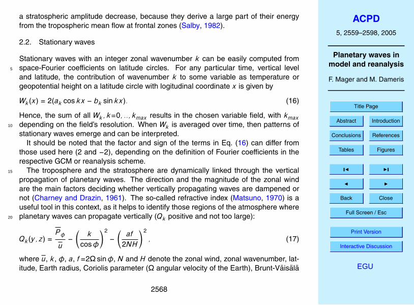
2.2. Stationary waves

Stationary waves with an integer zonal wavenumber k can be easily computed fromspace-Fourier coefficients on latitude circles. For any particular time, vertical level5

and latitude, the contribution of wavenumber k to some variable as temperature orgeopotential height on a latitude circle with logitudinal coordinate x is given by

Wk(x) = 2(ak coskx − bk sinkx). (16)

Hence, the sum of all Wk , k=0, .., kmax results in the chosen variable field, with kmaxdepending on the field’s resolution. When Wk is averaged over time, then patterns of10

stationary waves emerge and can be interpreted.It should be noted that the factor and sign of the terms in Eq. (16) can differ from

those used here (2 and −2), depending on the definition of Fourier coefficients in therespective GCM or reanalysis scheme.

The troposphere and the stratosphere are dynamically linked through the vertical15

propagation of planetary waves. The direction and the magnitude of the zonal windare the main factors deciding whether vertically propagating waves are dampened ornot (Charney and Drazin, 1961). The so-called refractive index (Matsuno, 1970) is auseful tool in this context, as it helps to identify those regions of the atmosphere whereplanetary waves can propagate vertically (Qk positive and not too large):20

Qk(y, z) =P φ

u−(

kcosφ

)2

−(

af2NH

)2

, (17)

where u, k, φ, a, f=2Ω sinφ, N and H denote the zonal wind, zonal wavenumber, lat-itude, Earth radius, Coriolis parameter (Ω angular velocity of the Earth), Brunt-Vaisala

2568





ACPD5, 2559–2598, 2005



Title Page



Tables Figures

J I

J I

Back Close

Full Screen / Esc

Print Version


EGU

frequency and scale height. The meridional derivative of potential vorticity is given by

P φ = 2Ωa cosφ −

[u cosφ

]φ

cosφ

φ

− a2f 2

ρ0

[ρ0

uz

N2

]z

(18)

where [ ]φ and [ ]z denote meridional and vertical partial derivatives, respectively.It should be noted that the refractive index must be used with care, since it is a rela-

tively limited tool insofar as it only indicates how favourable the underlying atmospheric5

conditions (and especially the zonal wind) are for the transmission of waves. It cannotconclusively answer the question of how the atmosphere will exactly modify the wavebehaviour, i.e. by dampening waves, by deviating them or by reflecting them back intothe troposphere (Harnik and Lindzen, 2001; Perlwitz and Harnik, 2003).

2.3. Heat and momentum fluxes10

Baroclinic planetary waves are essential for the meridional transport of eddy heat andmomentum flux. A simple method to quantify the contribution of stationary and tran-sient Rossby waves to the meridional heat flux is given by Peixoto and Oort (1992):[vT

]= [ v ][ T ] +

[v ∗ T ∗

]+[v ′T ′

], (19)

where the total heat flux is partitioned into the mean circulation and the contributions by15

stationary and transient waves (momentum fluxes can be computed analogously). Thismethod can be further refined by computing the contributions of single wavenumbersto the transient and stationary heat flux (Newman and Nash, 2000).

3. Model description and experimental setup

In this study the interactively coupled chemistry-climate model20

ECHAM4.L39(DLR)/CHEM (E39/C) is used. More detailed descriptions of the2569





ACPD5, 2559–2598, 2005



Title Page



Tables Figures

J I

J I

Back Close

Full Screen / Esc

Print Version


EGU

model are given in Hein et al. (2001) and Schnadt et al. (2002). The horizontalresolution of the model is T30 (3.75×3.75). E39/C has 39 layers from the surface tothe top layer centered at 10 hPa (Land et al., 2002).

CHEM (Steil et al., 1998) is based on the family concept. It describes relevantstratospheric and tropospheric O3 related homogeneous chemical reactions and het-5

erogeneous chemistry on PSCs and sulfate aerosols. It does not consider brominechemistry. E39/C includes online feedbacks of dynamics, chemistry, and radiative pro-cesses: chemical tracers are advected by the simulated winds. The net heating rates,in turn, are calculated using the actual 3-D distributions of the radiatively active gasesO3, CH4, N2O, H2O, and CFCs.10

In this work, a time-slice experiment representing conditions for 1990 is evaluated.The time-slice has been integrated over 24 years under steady state conditions, withthe first four years taken as spin-up. Sea surface temperatures (SST) are prescribedfrom observations (Gates, 1992). Additionally, natural and anthropogenic NOx emis-sions at the surface, from lighthing, and by aircraft are considered. At the model top,15

mixing ratios of NOy and ClX (=ClOx+ClONO2+HCl) are prescribed to account forhigher altitude chemistry above the upper boundary. Mixing ratios for the most relevantgreenhouse gases CH4 and N2O (at the surface) and CO2 are specified according toobservations. The specific boundary fields are given in Table 1 (Hein et al., 2001).

The climatology of E39/C has been extensively validated in several previous works20

(e.g. Hein et al., 2001; Schnadt et al., 2002; Austin et al., 2003).

4. Data

As stated in Sect. 2, time series of space-Fourier coefficients for integer wavenumbersof geopotential height are used to derive properties of transient and stationary waves.These Fourier coefficients have been extracted from reanalysis and model data. Re-25

analysis data are derived from the ERA-15 ECMWF reanalysis project (Gibson et al.,1997). The original ERA-15 data have a spectral T106 resolution (1.1×1.1) with 31

2570





ACPD5, 2559–2598, 2005



Title Page



Tables Figures

J I

J I

Back Close

Full Screen / Esc

Print Version


EGU

vertical hybrid levels from the ground to an upper boundary at 10 hPa. Data exist at0, 6, 12, and 18 UTC for the period from 1979 to 1993. These analyses of ERA-15data were processed in order to compare them with the E39/C model data. Thus, thespectral resolution was reduced to T30 (3.75×3.75) and data were interpolated onto17 appropriate pressure levels between 1000 and 10 hPa. As mentioned above, this5

study only focuses on NH winter (DJF). One single measurement per day was chosenat 0 UTC for DJF and the considered period was shortened by five years (1984–1993)so as to allow a comparison with the model time-slice for the year 1990. All 20 availablemodel winters have been analysed, with space and time resolutions corresponding toERA.10

5. Results and discussion

In this section we address the question of how accurately E39/C simulates the transientand stationary wave activity during NH winter. This is done by comparing modelledand reanalysed quantities which are made available by the methodology described inSect. 2: the geopotential height variance of stationary and transient waves, their dis-15

tribution over frequencies and wavenumbers, their vertical structure and their dynamicimpact through meridional fluxes of sensible heat. Additionally, we use the methodol-ogy to explain why the modelled polar vortex in the winter stratosphere is stronger andmore stable than suggested by the reanalysis data.

5.1. Transient wave properties in model and reanalysis data20

In the following we shall discuss the properties of transient waves that have been ex-tracted from model and ERA-15 data.

Figure 2 displays the distribution of geopotential height variance over latitudes andzonal wavenumbers, as a sum over frequencies and directions of zonal propagation;this quantity can be considered as a rough measure for the energy of travelling waves.25

2571





ACPD5, 2559–2598, 2005



Title Page



Tables Figures

J I

J I

Back Close

Full Screen / Esc

Print Version


EGU

The variances from ERA-15 data (left panel) show some well-known properties of tran-sient waves: The largest variances can be found in the extratropics, where Rossbywaves come into being through the conservation of potential vorticity. With increasingwavenumber, the meridional variance maximum tilts towards lower latitudes at all threepressure levels. This should partly arise through the fact that ultra-long waves (ZWN 15

and 2) come into being at high latitudes whereas shorter waves on the synoptic scaleare mostly forced at middle latitudes; another reason for this meridional distribution ofwave activity may be that shorter waves have the tendency to be refracted towardsregions with a higher refractive index, the index decreasing with increasing wavenum-ber and latitude (see middle term of Eq. 17). The variances at 500 and 150 hPa are10

qualitatively similar, whereas those at 50 hPa distinctly differ: in the northern (winter)stratosphere, the variance is shifted towards small wavenumbers through the strongwesterlies. These act as a low-pass filter on planetary waves (Charney and Drazin,1961) by allowing waves of the smallest wavenumbers (typically 1 and 2) to prop-agate vertically unhindered whereas waves at higher wavenumbers are dampened.15

In the southern (summer) hemisphere, the stratospheric variances are reduced at allwavenumbers with respect to the lowermost stratosphere (150 hPa); here, the easterlywinds (in approximate thermal wind balance with the temperature) impose a barrier onthe vertical propagation of all planetary waves.

The comparison of absolute ERA and E39/C variances (left and middle panels)20

shows that E39/C accurately simulates the variance distribution of transient wavesover latitudes and wavenumbers. The model reproduces the wave properties men-tioned above, e.g. the tropical variance minimum, the equatorward variance tilt withincreasing wavenumber or the dampening of waves according to their wavenumberand the zonal wind. Although the model variances match the ERA-15 variances quan-25

titatively, the variance differences (right panels) yield some valuable information aboutthe model.

E39/C simulates approximately 25% (50%) less tropospheric transient wave activityin the Northern (Southern) Hemisphere at all considered wavenumbers (bottom right).

2572





ACPD5, 2559–2598, 2005



Title Page



Tables Figures

J I

J I

Back Close

Full Screen / Esc

Print Version


EGU

The reason for smaller tropospheric model variances is again related to the horizontalresolution, namely the insufficient representation of cyclonic activity at resolution T30(Senior, 1995). Although there is less forcing of tropospheric transient waves in E39/C,the modelled variances in the tropopause region at middle latitudes are higher at allwavenumbers than in ERA-15 data. This is most probably due to the stronger subtrop-5

ical jets in E39/C (Fig. 6, right panel) which induce higher shear instabilities and, sub-sequently, more transient waves in the jet region. The reduced modelled wave activitywith wavenumbers 1–3 at high northern latitudes seems to arise in the troposphere andpropagates with less variance into the stratosphere. The higher stratospheric modelvariances at middle northern latitudes appear to be low-pass filtered modes that have10

been forced by the stronger model jet and have then propagated vertically. One of themost striking stratospheric features is, however, that E39/C allows a much larger verti-cal wave propagation into the summer stratosphere than ERA. This occurs because ofthe model’s inability to correctly reproduce eastern stratospheric winds in the southernhemisphere during summer (Hein et al., 2001).15

The WFA not only allows analysis of the geopotential height variance of transientwaves into contributions by single wavenumbers, as done for the previous discussion,but also into variance parts by frequency intervals. Figure 3 shows how the waveactivity of eastward and westward travelling waves is distributed over the consideredfrequency range. The 300 hPa level has been selected because it features the largest20

variances of all levels (with the exception of the lower and middle stratosphere close tothe northern polar vortex), and because it allows an insight into the structure of upwardtravelling tropospheric waves before they get partially dampened in the stratosphere.Some of the properties that have been mentioned in the discussion of Fig. 2 are obvi-ous in the representation of ERA-15 results (left panels), e.g. that the greatest part of25

planetary wave activity takes place in the extratropics, or that the meridional variancemaximum is displaced equatorwards with increasing wavenumber, from approximately70 (wavenumber 1) to 40 (wavenumber 8).

The largest variances of westward travelling waves in the NH occur at wavenumber

2573





ACPD5, 2559–2598, 2005



Title Page



Tables Figures

J I

J I

Back Close

Full Screen / Esc

Print Version


EGU

1 and decrease monotonically with the wavenumber. In the SH, the variances arevery similar for the first three wavenumbers and then also decrease with increasingwavenumber. The strong wavenumber 1 in the NH appears to be the signature ofthe polar vortex with its stratospheric pressure dipole (aleutian high/vortex low). TheNH variance of the westward travelling wave 2, being much greater than in the SH,5

is probably enhanced by orographic forcing and land-sea contrast. In the southernhemisphere, the wave activity of eastward travelling waves with wavenumbers 4–7is greater than in the NH. The comparatively weak orography at southern middlelatitudes allows higher windspeeds over the oceans and, subsequently, stronger syn-optic disturbances at these wavenumbers which propagate vertically. With increasing10

wavenumber, less variance occurs in the westward direction. The transition of maximafrom large westward periods (>20 days at wavenumber 1) first to medium eastward(8 days at wavenumber 3) and then to small eastward periods (wavenumber >3) isa consequence of the dispersive nature of Rossby waves, which causes the phasespeed to decrease rapidly with increasing wavenumber.15

The E39/C model fairly reproduces the total variance sum of transient waves quanti-tatively and qualitatively, as seen in Fig. 2. Hence, the model approximates the contri-bution of transient waves to the total kinetic energy of the atmosphere. How well doesit represent the wave activity for single frequencies?20

The comparison shows that the model results (right panels) are in good agreementwith reanalysis variances at this particular pressure level (300 hPa). The model cor-rectly reproduces how meridional variance maxima are displaced equatorwards withincreasing wavenumber. E39/C also accounts very accurately for the dispersion ofplanetary waves. Additionally, the larger NH amplitudes of westward travelling waves25

at wavenumbers 1 and 2 match those that have been derived from ERA-15. Furtheragreements between model and reanalysis can be seen in smaller structures. Somequantitative differences can be detected: the most prominent feature is certainly theoverall smaller variances in the model results at 300 hPa. These have already been

2574





ACPD5, 2559–2598, 2005



Title Page



Tables Figures

J I

J I

Back Close

Full Screen / Esc

Print Version


EGU

noted in the discussion of the previous figure, where E39/C was shown to simulateless tropospheric wave activity (500 hPa) at all considered wavenumbers. Figure 3 al-lows the conclusion that the model’s underestimation of the tropospheric large-scalewave activity is mostly independent of wavenumber or period. Although the overallpattern of modelled variance matches the reanalysis variance structures, some merid-5

ional shifts of 5 to 10 occur (e.g. wavenumber 2). A few frequency shifts can also beobserved, especially at the smallest wavenumbers. The patterns derived from the mod-elled geopotential height, despite some minor differences, are in good agreement withthe results derived from reanalyses and prove that E39/C can adequately reproducethe dynamic phenomena arising from transient wave formation.10

Vertical profiles of wave amplitudes and phase differences are useful tools to gain aninsight into the barotropic or baroclinic nature of single waves or wave groups. The am-plitude can easily be derived from already computed variances under the assumptionthat single waves (each with a particular wavenumber in a single frequency interval)perform purely harmonic oscillations; phase differences with respect to a certain pres-15

sure level can be calculated with Eq. (13).Figure 4 shows the vertical structure of transient waves at 70 N (westward)

resp. 50 N (eastward). Summing (amplitude) resp. averaging (phases) over allwavenumbers and periods can give an overview of the overall transient wave struc-ture. In the present case, such an averaging was possible because the characteristics20

of individual east- and westward components were found to correspond closely to thesum resp. average.

The westward travelling wave parts from ERA-15 (solid line) show a vertical tro-pospheric amplitude growth which is closer to the corresponding exponential growth(straight lines) than that of the eastward travelling parts, which is a sign of the stronger25

baroclinicity of the eastward oriented modes. This is not surprising insofar as synoptic,eastward travelling disturbances with zonal wavenumbers >3 are associated with baro-clinic waves (Farrell, 1982). Thus, their vertical amplitude increase in the troposphereis distinctly higher than that of westward travelling wave parts. The phase differences

2575





ACPD5, 2559–2598, 2005



Title Page



Tables Figures

J I

J I

Back Close

Full Screen / Esc

Print Version


EGU

underline this conclusion: the mean (and individual) phase difference(s) of the west-ward travelling waves nearly vanish(es), indicating that these modes do not significantlycontribute to the meridional heat flux (Eq. 14) and are mostly barotropic. The eastwardtravelling wave components, on the contrary, have a very pronounced westward phasetilt with height and therefore achieve a net poleward transport of sensible heat which is5

typical for baroclinic waves.The comparison of the vertical structures of transient waves between ERA-15 (solid)

and E39/C (dashed) at the chosen latitudes reveals that the model reproduces theERA-15 phase differences with a high degree of similarity. The model underestimatesthe amplitudes of westward travelling waves in the troposphere and lower stratosphere10

by about 10% between 850 and 70 hPa; above 70 hPa, the simulated and modelledamplitudes of these modes are nearly identical. The modelled eastward travelling waveparts match the ones from ERA-15 in the troposphere up to 300 hPa. Above this level,they are overestimated by E39/C.

A possible cause of the higher model amplitudes above 300 hPa might be the height15

of the modelled tropopause, which lies higher than in reanalyses and observations(Santer et al., 2003). A higher tropopause could allow the model to simulate baroclinicprocesses higher in the troposphere than in the case of reanalysis data (roughly be-tween 300 and 250 hPa), thereby inducing a higher activity of baroclinic waves withlarger amplitudes. As these stronger disturbances propagate vertically, they could be20

the reason for the higher stratospheric wave amplitudes in the model. On the otherhand, there are arguments against this interpretation which were made by Lindzen(1993). Based on theoretical assessments he found strong supporting results that theatmosphere (troposphere) tends toward baroclinic neutrality.

This analysis shows that E39/C reproduces the vertical structure of transient waves25

in a qualitatively satisfying way. The barotropic and baroclinic characteristics are espe-cially well represented.

Although most atmospheric oscillations are initiated by specific causes, such ase.g. a pronounced stationary wave-2 pattern from orographic forcing, some wave

2576





ACPD5, 2559–2598, 2005



Title Page



Tables Figures

J I

J I

Back Close

Full Screen / Esc

Print Version


EGU

modes can be identified which come into existence without a specific external exci-tation mechanism. The so-called atmospheric “normal modes” described in Sect. 2.1.3are such oscillations. They have been predicted theoretically (Kasahara, 1976), ob-served (Madden, 1979) and repeatedly simulated (e.g. Miyoshi, 1999; Miyoshi and Hi-rooka, 1999). Three observed modes exist for wavenumber 1, with periods of 5, 10 and5

16 days. Figure 5 displays the corresponding periods for model and reanalysis data.These modes are barotropic waves as predicted, as they show an exponential ampli-tude increase with height and phase differences close to 0. ERA and E39/C normalmodes have very similar amplitudes and phase differences, indicating that the modelpossesses similar eigenvalues as observed. The methods used here are certainly not10

the most precise instruments to detect normal modes, but they are nevertheless usefulto check the performance of climate models with regard to single wave components.

5.2. Stationary waves and the polar vortex

This section is devoted to the comparison of stationary waves in reanalysis and modeldata, and especially aims to clarify why E39/C simulates a polar vortex in the time-slice15

“1990” which is stronger and longer-lived than in the reanalysis.Figure 6 shows the geopotential height at 50 hPa for NH winter. The modelled polar

vortex is wider and deeper, and its centre is slightly displaced towards the South ascompared to ERA (left, “WN0-8”). The differences are mainly due to the overestima-tion of stationary wavenumber 1 by E39/C (centre, “WN1”). The modelled wavenum-20

bers 2 and 3 are weaker than in the reanalysis. Although the stronger wavenumber 1displaces the vortex slightly southwards, weaker wavenumbers 2 and 3 imply smallerpoleward heat fluxes and therefore a reduced heating of the polar region. Despite theobvious differences at all three wavenumbers, E39/C reasonably simulates the posi-tions of extreme values as compared to ERA, with a small eastward displacement at all25

three wavenumbers. These differences imply that the model vortex is too strong, butthat at least the position of its centre is well approximated by E39/C.

What could be the cause of the overestimated stationary wavenumber 1 as modelled2577





ACPD5, 2559–2598, 2005



Title Page



Tables Figures

J I

J I

Back Close

Full Screen / Esc

Print Version


EGU

by E39/C in DJF? Figure 7 allows the variance of stationary waves and the zonal meanzonal wind in E39/C and ERA to be compared.

The zonal wind derived from ERA (bottom left) shows the characteristic subtropicalmaxima at the tropopause. The NH jet is stronger than in the SH because of thelarger meridional temperature gradient. The southern stratosphere is dominated by5

easterlies, whereas westerlies prevail in the northern stratosphere. The stratosphericwind maximum around 65 N is the signature of the polar vortex.

Stationary waves forming in the troposphere are mainly forced by orography andland-sea contrast, which explains why the variances are larger in the NH and distributedover a wider meridional range than in the SH (top left, variance over wavenumber 1–10

8). The effect of the zonal wind on the stationary wave activity is most apparent inthe stratosphere, where vertically propagating waves are dampened in the SH by theeasterly wind. In the NH, westerlies dominate the entire extratropical stratosphereand allow stationary waves of the smallest wavenumbers (see discussion of Fig. 2)to propagate vertically without any significant hindrance, thereby contributing to the15

characteristic shape of the northern polar vortex.The variance of stationary modes as simulated by E39/C significantly differs from

the corresponding reanalysis variance (top right). In the troposphere, the cause of thereduced resp. enhanced model variance is obvious. Here, the zonal wind differenceis the dominating factor; less/more stationary waves are forced in E39/C where the20

modelled wind is weaker/stronger than in ERA (bottom right). The model overestimatesthe stationary wave variance by a factor 5–20 in the southern middle stratosphere.This fact has already been discussed analogously for transient waves (Fig. 2), and is aconsequence of the incorrect simulation of stratospheric easterly winds.

In the northern middle stratosphere, the model equally overestimates the stationary25

wave activity by a factor 2–5; this signal is exclusively due to the wavenumber 1 (notshown). The representation suggests that in E39/C, too strong a zonal wind inducesmore tropospheric stationary wave activity between 30 and 50 N. This signal seemsto travel into the stratosphere where it is enhanced by the stronger model westerlies.

2578





ACPD5, 2559–2598, 2005



Title Page



Tables Figures

J I

J I

Back Close

Full Screen / Esc

Print Version


EGU

Such a conclusion could possibly hold for the SH case, where the variance is stronglyenhanced by a missing change of sign of the zonal wind. It does not seem to bevalid for the northern stratosphere, because the model overestimates the zonal wind(westerly for E39/C and ERA) by 10–30% only, while the variance increases by abouta factor 2–5; neither does this conclusion explain how such a signal between 30 and5

50 N can spread over the whole arctic region above 100 hPa. The diffusion in the twohighest model levels is increased (sponge layer) in E39/C in order to avoid reflectionof waves at the upper model boundary (Hein et al., 2001), and could therefore leadto a slightly geographically wider variance distribution at these levels. However, it isdoubtful that this effect should vertically and meridionally affect the mentioned region10

to such a large extent as Fig. 7 suggests. General circulation models with spongelayers are susceptible to e.g. an imposed local force or diabatic heating inasmuch asthe relaxational properties of the sponge induce changes in the dynamics outside thesponge region (Shepherd et al., 1996); however, they absorb upwelling waves realisti-cally without causing a direct feedback on the dynamics below.15

The refractive index (Eq. 17) allows us to determine those regions of the atmospherewhere stationary waves with a specific wavenumber k can travel vertically without be-ing dampened. Figure 8 shows the index for ERA and E39/C for wavenumber 1, whichis largely overestimated in the model simulation “1990” as discussed above. The mod-elled extratropical northern stratosphere is characterised by very similar, moderately20

positive values of the refractive index as compared to ERA and, therefore, does not ob-viously offer fundamentally different conditions for the vertical propagation of stationarymodes with wavenumber 1. Thus, the cause of the strong wavenumber 1 in E39/C doesnot appear to be primarily related to the underlying atmospheric conditions like zonalwind or vorticity. Note also the index sign in the southern extratropical stratosphere25

above 50 hPa; as the index is dominated by the sign of the zonal wind, it is negativefor ERA and positive for E39/C, which explains why the model simulates much morestationary wave activity in the SH summer than the reanalysis data suggest.

Stationary waves have been shown to have larger variances in the troposphere and

2579





ACPD5, 2559–2598, 2005



Title Page



Tables Figures

J I

J I

Back Close

Full Screen / Esc

Print Version


EGU

stratosphere than transient waves at the smallest wavenumbers (1–3). The varianceitself can give indications of the dynamic properties of specific wave modes, but doesnot allow us to quantify their dynamic impact. The meridional fluxes of momentum andsensible heat by planetary waves can be useful in this respect (Sect. 2.3), and providea plausible explanation of the stratospheric wavenumber 1 bias in E39/C.5

Figure 9 shows a comparison of the variance difference (model-reanalysis) of east-ward travelling waves with zonal wavenumber 1–3 to the heat flux difference by tran-sient waves with the same wavenumbers. The comparison of meridional heat fluxes bytransient and stationary waves in E39/C and ERA reveals that the model approximatesthe reanalysis heat flux by stationary waves rather well (not shown). In contrast to10

this, the model clearly underestimates the NH heat flux by transient waves in the uppertroposphere and stratosphere at high latitudes (right panel). Nearly the total heat fluxdifference (>95%) is due to the wavenumbers 1–3, which are the dominant wavenum-bers at these latitudes. The vertical wave structure analysis (Sect. 5.1) has shown thatthe eastward travelling modes, in both model simulation and reanalysis, are predomi-15

nantly baroclinic, contrary to the westward travelling wave parts. This means that mostof the reduced model heat flux is likely to arise from an underestimation of eastwardtravelling modes. This conclusion is supported by the fact that in comparison to ERA,the tropospheric and stratospheric model variance of these modes at wavenumbers1–3 is reduced by 30–50% at high latitudes (left panel).20

These results suggest the following interpretation: at high northern latitudes, E39/Csimulates less eastward travelling, baroclinic waves in the troposphere than seen in thereanalysis data. These ultralong modes propagate into the stratosphere (Hartmann,1979; Randel, 1988) and induce a weaker meridional heat flux than in ERA-15, by in-troducing less wave disturbances into the vortex region. If the vortex is less disturbed25

by a reduced heat flux, then it can cool more efficiently, leading to lower temperaturesand lower pressure inside the vortex, and stronger circumpolar winds. Thus, the mod-elled northern polar vortex, being dominated by a quasi-permanent wavenumber 1,exhibits a stronger stationary wavenumber 1 pattern than in the reanalysis data. This

2580





ACPD5, 2559–2598, 2005



Title Page



Tables Figures

J I

J I

Back Close

Full Screen / Esc

Print Version


EGU

interpretation suggests an interaction between transient and stationary waves throughthe transport of sensible heat.

6. Conclusions

In this work, we have investigated the ability of the coupled CCM E39/C to simulateplanetary waves. The methodology that has been used allows a detailed insight in the5

forcing, propagation and dynamic effect of these long atmospheric modes. The differ-ent analysis methods all use time series of space-Fourier coefficients from model sim-ulations, observational or reanalysis data; the derived quantities provide the possibilityto categorise planetary waves according to specific criteria, e.g. barotropic/baroclinicmodes, transient/stationary wave parts, or their distribution over wavenumbers and10

frequencies. Additionally, meridional fluxes of momentum and sensible heat can bederived.

The analysis tools have been applied to a E39/C model simulation which corre-sponds to boundary conditions for the year “1990”, as well as to the ERA-15 reanalysisdata set from the ECMWF.15

The comparison reveals that E39/C reproduces the qualitative distribution of geopo-tential height variance over wavenumbers, periods, latitudes and pressure levels in afairly accurate way. However, too little transient wave forcing takes place in the modeltroposphere, which is mainly due to the underrepresentation of cyclonic activity. E39/Crealistically simulates the vertical structure of transient waves, and possesses single20

wave modes that correspond to theoretically predicted and observed natural oscilla-tions of the atmosphere.

Regarding the simulation of stationary waves, it has been shown that the forcingand propagation of this wave type is determined by the strength and sign of the zonalwind, especially in the troposphere. E39/C exhibits a polar vortex too strong and cold,25

with an overestimated stationary wavenumber 1 in the northern stratosphere. Thecause appears to be an interaction of long, eastward travelling waves at high northern

2581





ACPD5, 2559–2598, 2005



Title Page



Tables Figures

J I

J I

Back Close

Full Screen / Esc

Print Version


EGU

latitudes with the stationary wavenumber 1, linked through the meridional transport ofsensible heat.

The different methods that we have presented and applied here are not fundamen-tally new, and have previously been used to analyse planetary wave properties in ob-servational data as well as in simple and more complex models. However, the method-5

ology has been employed for the first time to verify how a coupled chemistry-climatemodel simulates these large-scale waves both qualitatively and quantitatively. It hasbeen demonstrated with this work that the different tools are useful in identifying andquantifying some important dynamic mechanisms which relate to planetary waves in acoupled CCM. The results allow us to draw conclusions about possible model improve-10

ments that could contribute to more realistic dynamics.The crucial factor for the correct representation of the vertical propagation of tran-

sient and stationary planetary waves in large-scale models is an accurately modelledzonal wind. Several inconsistencies of the zonal wind in E39/C have been identi-fied and can be attributed to different physical causes. Thus, the subtropical jets at15

the tropopause are too strong in both hemispheres and, therefore, lead to more tran-sient wave modes. The primary cause of this wind bias is an underestimation of highand middle latitude tropopause temperatures (cold bias) and a slight overestimationof equatorial temperatures in the upper troposphere (probably due to a rather rudi-mentary parametrisation of small-scale convective processes, see Hein et al., 2001).20

The inaccurately modelled easterlies in the southern stratosphere affect transient andstationary wave propagation, and most probably originate as well from the unrealistictemperature distribution at high latitudes (cold bias). The modelled stratospheric polarvortex in the high northern latitudes is characterised by zonal winds that are strongerthan in ERA-15, which seems to be indirectly due to a reduced heat flux from eastward25

travelling transient waves.A higher model boundary would allow for wave reflection in the middle stratosphere

(Harnik and Lindzen, 2001; Perlwitz and Harnik, 2003). Using a higher horizontal modelresolution (e.g. T63) would certainly contribute to a more realistic representation of

2582





ACPD5, 2559–2598, 2005



Title Page



Tables Figures

J I

J I

Back Close

Full Screen / Esc

Print Version


EGU

cyclonic activity at middle latitudes, thereby improving the modelled transient waveactivity. Additionally, an increased horizontal resolution would imply a less idealisedorography; this should improve the orographic forcing of stationary waves.

Appendix: Tools

All the tools presented above are available as FORTRAN code and UNIX/Linux shell5

scripts and can be obtained from the authors ([email protected]).

Acknowledgements. We would like to thank M. Klawa for technical support and C. Schnadtfor helpful discussions. This work was supported by the Bundesministerium fur Bildung undForschung (07ATF43).

References10

Austin, J.: A three-dimensional coupled chemistry-climate model simulation of past strato-spheric trends, J. Atmos. Sci., 59, 218–232, 2002. 2561

Austin, J., Shindell, D., Beagley, S. R., Bruhl, C., Dameris, M., Manzini, E., Nagashima, T.,Newman, P., Pawson, S., Pitari, G., Rozanov, E., Schnadt, C., and Shepherd, T. G.: Uncer-tainties and assessments of chemistry-climate models of the stratosphere, Atmos. Chem.15

Phys., 3, 1–27, 2003,SRef-ID: 1680-7324/acp/2003-3-1. 2561, 2570

Charney, J. G. and Drazin, P. G.: Propagation of planetary-scale disturbances from the lowerinto the upper atmosphere, J. Geophys. Res., 66, 83–109, 1961. 2568, 2572

Farrell, B.: The initial growth of disturbances in a baroclinic flow, J. Atmos. Sci., 39, 1663–1686,20

1982. 2575Gates, W. L.: AMIP: The atmospheric model intercomparison project, Bull. Amer. Meteor. Soc.,

73, 1962–1970, 1992. 2570Gibson, J. K., Kallberg, P., Uppala, S., Hernandez, A., Nomura, A., and Serrano, E.: ERA

description, ECMWF Re-Analysis Project Report Series, 1, 1–72, 1997. 257025

2583





http://direct.sref.org/1680-7324/acp/2003-3-1

ACPD5, 2559–2598, 2005



Title Page



Tables Figures

J I

J I

Back Close

Full Screen / Esc

Print Version


EGU

Harnik, N. and Lindzen, R. S.: The effect of reflecting surfaces on the vertical structure andvariability of stratospheric planetary waves, J. Atmos. Sci., 58, 2872–2894, 2001. 2569,2582

Hartmann, D. L.: Baroclinic instability of realistic zonal mean states to planetary waves, J.Atmos. Sci., 36, 2336–2349, 1979. 25805

Hartmann, D. L.: Global Physical Climatology, Academic Press, International Geophysics Se-ries, 56, 411, 1994. 2567

Hayashi, Y.: On the coherence between progressive and retrogressive waves and a partitionof space-time power-spectra into standing parts, J. Meteor. Soc. Japan, 16, 368–373, 1977.2562, 2563, 256510

Hayashi, Y.: A generalized method of resolving transient disturbances into standing and travel-ing waves by space-time spectral analysis, J. Atmos. Sci., 36, 1017–1029, 1979. 2589

Hayashi, Y.: Space-time spectral analysis and its applications to atmospheric waves, J. Meteor.Soc. Japan, 60, 156–171, 1982. 2562, 2563, 2565

Hayashi, Y. and Golder, D. G.: Space-time spectral analysis of mid-latitude disturbances ap-15

pearing in a GFDL general circulation model, J. Atmos. Sci., 34(2), 237–262, 1977. 2562Hayashi, Y. and Golder, D. G.: Transient planetary waves simulated by GFDL spectral general

circulation models. Part 1: Effects of montains, J. Atmos. Sci., 40(4), 941–950, 1983a. 2562Hayashi, Y. and Golder, D. G.: Transient planetary waves simulated by GFDL spectral general

circulation models. Part 2: Effects of nonlinear energy transfer, J. Atmos. Sci., 40(4), 951–20

957, 1983b. 2562Hayashi, Y. and Golder, D. G.: Kelvin and mixed Rossby-gravity waves appearing in the GFDL

“SKYHI” general circulation model and the FGGE dataset: Implications for their generationmechanismn and role in the QBO, J. Meteorol. Soc. Japan, 72(6), 901–935, 1994. 2562

Hayashi, Y., Golder, D. G., and Jones P. W.: Tropical gravity waves and superclusters simulated25

by high-horizontal-resolution SKYHI general circulation models, J. Meteorol. Soc. Japan,75(6), 1125–1139, 1997. 2562

Hein, R., Dameris, M., Schnadt, C., Land, C., Grewe, V., Kohler, I., Ponater, M., Sausen,R., Steil, B., Landgraf, J., and Bruhl, C.: Results of an interactively coupled atmosphericchemistry-general circulation model: Comparison with observations, Ann. Geophys., 19,30

435–457, 2001,SRef-ID: 1432-0576/ag/2001-19-435. 2560, 2562, 2570, 2573, 2579, 2582

IPCC (Intergovernmental Panel on Climate Change): Climate change 2001; the scientific basis,

2584





http://direct.sref.org/1432-0576/ag/2001-19-435

ACPD5, 2559–2598, 2005



Title Page



Tables Figures

J I

J I

Back Close

Full Screen / Esc

Print Version


EGU

contribution of working group I to the Third Assessment Report of IPCC, edited by: Houghton,J. T., Ding, Y., Griggs, D. J., Noguer, M., van der Linden, P. J. Dai, X., Maskell, K., andJohnson, C. A., Cambridge University Press, 2001. 2561

Jakobs, H. J. and Hass, H.: Normal modes as simulated in a three-dimensional circulationmodel of the middle atmosphere including regional gravity wave activity, Ann. Geophys., 5A,5

103–114, 1987. 2562Kasahara, A.: Normal modes of ultralong waves in the atmosphere, Mon. Wea. Rev., 104,

669–690, 1976. 2577Land, C., Feichter, J., and Sausen, R.: Impact of vertical resolution on the transport of passive

tracers in the ECHAM4 model, Tellus, 54B, 344–360, 2002. 257010

Lindzen, R. S.: Baroclinic neutrality and the tropopause, J. Atmos. Sci., 50, 1148–1151, 1993.2576

Madden, R.: Observations of large-scale traveling Rossby waves, Rev. Geophys. Space Phys.,17, 1935–1949, 1979. 2577

Matsuno, T.: Vertical propagation of stationary planetary waves in the winter Northern Hemi-15

sphere, J. Atmos. Sci., 27, 871–888, 1970. 2568Miyoshi, Y.: Numerical simulation of the 5-day and 16-day waves in the mesopause region,

Earth Planets Space, 51, 763–772, 1999. 2562, 2577Miyoshi, Y. and Hirooka, T.: A numerical experiment of excitation of the 5-day wave by a GCM,

J. Atmos. Sci., 56, 1698–1707, 1999. 2562, 257720

Nagashima, T., Takahashi, M., Takigawa, M., and Akiyoshi, H.: Future development of theozone layer calculated by a general circulation model with fully interactive chemistry, Geo-phys. Res. Lett., 29(8), 1162, doi:10.1029/2001GL014026, 2002. 2561

Newman, P. A. and Nash, E. R.: Quantifying the wave driving of the stratosphere, J. Geophys.Res., 105, 12 485–12 497, 2000. 2561, 256925

Peixoto, J. P. and Oort, A. H.: Physics of climate, Springer Verlag, 61–64, 1992. 2569Perlwitz, J. and Harnik, N.: Observational evidence of a stratospheric influence on the tropo-

sphere by planetary wave reflection, J. Climate, 16, 3011–3026, 2003. 2569, 2582Pitari, G., Mancini, E., Rizi, V., and Shindell, D.: Impact of future climate and emission changes

on stratospheric aerosols and ozone, J. Atmos. Sci., 59, 414–440, 2002. 256130

Randel, W. J.: The seasonal evolution of planetary waves in the Southern Hemisphere strato-sphere and troposphere, Quart. J. Roy. Meteorol. Soc., 114, 1385–1409, 1988. 2580

Rozanov, E. V., Schlesinger, M. E., and Zubov, V. A.: The Universtiy of Illinois at Urbana-

2585





ACPD5, 2559–2598, 2005



Title Page



Tables Figures

J I

J I

Back Close

Full Screen / Esc

Print Version


EGU

Champaign three-dimensional stratosphere-troposphere general circulation model with in-teractive ozone photochemistry: Fifteen-year control run climatology, J. Geophys. Res., 106,27 233–27 254, 2001. 2561

Salby, M. L.: A ubiquitous wavenumber-5 anomaly in the southern hemisphere during FGGE,Mon. Wea. Rev., 110, 1712–1720, 1982. 25685

Santer, B. D., Sausen, R., Wigley, T. M. L., Boyle, J. S., AchutaRao, K., Doutriaux, C., Hansen,J. E., Meehl, G. A., Roeckner, E., Ruedy, R., Schmidt, G., and Taylor, K. E.: Behavior oftropopause height and atmospheric temperature in models, reanalyses, and observations:Decadal changes, J. Geophys. Res., 108(D1), 4002, doi:10.1029/2002JD002258, 2003.257610

Shepherd, T. G., Semeniuk, K., and Koshyk, J. N.: Sponge layer feedbacks in middle atmo-sphere models, J. Geophys. Res., 101, 23 447–23 464, 1996. 2579

Schnadt, C., Dameris, M., Ponater, M., Hein, R., Grewe, V., and Steil, B.: Interaction of at-mospheric chemistry and climate and its impact on stratospheric ozone, Clim. Dyn., 18,501–517, 2002. 2560, 2561, 257015

Senior, C. A.: The dependence of climate sensitivity on the horizontal resolution of a GCM, J.Climate, 8, 2860–2880, 1995. 2573

Shine, K. P., Bourqui, M. S., Forster, P. M. de F., Hare, S. H. E., Langematz, U., Braesicke,P., Grewe, V., Ponater, M., Schnadt, C., Smith, C. A., Haigh, J. D., Austin, J., Butchart,N., Shindell, D. T., Randel, W. J., Nagashima, T., Portmann, R. W., Solomon, S., Seidel,20

D. J., Lanzante, J., Klein, S., Ramaswamy, V., and Schwarzkopf, M. D.: A comparison ofmodel-simulated trends in stratospheric temperatures, Q. J. R. Meteorol. Soc., 129(590),1565–1588, 2003. 2561

Speth, P. and Kirk, E.: A one-year study of power spectra in wavenumber-frequency domain,Beitr. Phys. Atmosph., 54, 186–206, 1981. 256225

Speth, P. and Madden, R. A.: Space-time spectral analyses of northern hemisphere geopoten-tial heights, J. Atmos. Sci., 40, 1086–1100, 1983. 2562, 2567

Steil, B., Dameris, M., Bruhl, C., Crutzen, P. J., Grewe, V., Ponater, M., and Sausen, R.: De-velopment of a chemistry module for GCMs: first results of a multiannual integration, Ann.Geophys., 16, 205–228, 1998,30

SRef-ID: 1432-0576/ag/1998-16-205. 2570Steil, B., Bruhl, C., Manzini, E., Crutzen, P. J., Lelieveld, J., Rasch, P. J., Roeckner, E., and

Kruger, K.: A new interactive chemistry climate model. 1: Present day climatology and inter-

2586





http://direct.sref.org/1432-0576/ag/1998-16-205

ACPD5, 2559–2598, 2005



Title Page



Tables Figures

J I

J I

Back Close

Full Screen / Esc

Print Version


EGU

annual variability of the middle atmosphere using the model and 9 years of HALOE/UARSdata, J. Geophys. Res., 108(D9), 4290, doi:10.1029/2002JD002971, 2003. 2561

Zangvil, A.: On the presentation and interpretation of spectra of large-scale disturbances, Mon.Wea. Rev., 105, 1469–1473, 1977. 2592

2587





ACPD5, 2559–2598, 2005



Title Page



Tables Figures

J I

J I

Back Close

Full Screen / Esc

Print Version


EGU

Table 1. Mixing ratios of greenhouse gases, inorganic chlorine, and NOx emissions of differentnatural and anthropogenic sources for the “1990” simulation.

CO2 (ppmv) 353CH4 (ppmv) 1.69N2O (ppbv) 310Cly (ppbv) 3.4NOx lightning (Tg(N)/year) 5.3NOx air traffic (Tg(N)/year) 0.6NOx surface (total) (Tg(N)/year) 33.1NOx surface (industry, traffic) 22.6NOx surface (soils) 5.5NOx surface (biomass burning) 5.0

2588





ACPD5, 2559–2598, 2005



Title Page



Tables Figures

J I

J I

Back Close

Full Screen / Esc

Print Version


EGU

NOISE

STANDING

12 Pst k ω 1

2 Pst k ω

WESTWARDTRAVELINGPprog k ω

EASTWARDTRAVELINGPprog k ω

Ptot k ω Ptot k ω

Fig. 1. Decomposition of standing and travelling wave parts after Hayashi (1979). The varianceof progressive waves is obtained by substracting the standing parts from the total variance.

2589





ACPD5, 2559–2598, 2005



Title Page



Tables Figures

J I

J I

Back Close

Full Screen / Esc

Print Version


EGU

10

10

10

10

2020

20

20

50

50

50

50

100

100

100

100

200

200

200

500

5001000

2000

5000

50 hPa

1

2

3

4

5

6

7

8

1

2

3

4

5

6

7

8

-80 -60 -40 -20 0 20 40 60 80

-80 -60 -40 -20 0 20 40 60 80

ERA 1984-93

10

10

10

2020

20

20

50 50

50

50

100 100

100100

200 200

200

200

500

500

500

500

1000

1000

1000

1000

2000

2000

2000

150 hPa

1

2

3

4

5

6

7

8

1

2

3

4

5

6

7

8

wav

enum

ber

10

10

10

20 20

20

50

50

50

50

100 100

100100

200 200

200200

500

500 50

0

500

1000

1000

1000

1000

2000

2000

2000

500 hPa

1

2

3

4

5

6

7

8

1

2

3

4

5

6

7

8

-80 -60 -40 -20 0 20 40 60 80

-80 -60 -40 -20 0 20 40 60 80

10

10

10

20

20

20

20

50

50

50

50

50

100

100 100

100

200

200

200

200

500

500

1000

1000

2000

20005000 1

2

3

4

5

6

7

8

-80 -60 -40 -20 0 20 40 60 80

-80 -60 -40 -20 0 20 40 60 80

E39/C „1990”

1010

20

20

20 50

50

50

50

100 100

100

100

200 200

200

200

500

500

500 5001000

1000

1000

1000

2000

2000

2000

1

2

3

4

5

6

7

8

10

10

2020

2020

50 50

50

50

100 100

100100

200 200

200

200

500

500

500

500

1000

1000

1000

10002000

1

2

3

4

5

6

7

8

-80 -60 -40 -20 0 20 40 60 80

-80 -60 -40 -20 0 20 40 60 80

latitude

20

20

20

20

20

50

50

50

100

100

200

200500

1000

-20

-20

-50

-50

-100

-200-500

1

2

3

4

5

6

7

8

-80 -60 -40 -20 0 20 40 60 80

-80 -60 -40 -20 0 20 40 60 80

E39/C - ERA

20

20

20

20

20

20

50

50 50

50

100 100

100

100

200

200

200

200

500

500

500

-20-50-100-200

1

2

3

4

5

6

7

8

20

20

50

50

-20 -20

-20

-20

-50

-50 -50

-50

-100

-100 -100

-100-200

-200

-200

-200

-500

-500

-500

-10001

2

3

4

5

6

7

8

-80 -60 -40 -20 0 20 40 60 80

-80 -60 -40 -20 0 20 40 60 80

Fig. 2. Variance of geopotential height in gpm2 at 500, 150 and 50 hPa as computed by theWFA for DJF (Eqs. 8 and 9). Shown is the variance sum of standing and eastward and westwardtravelling waves as sum over 23 frequency bands with periods from 2.7 to 32 days, averagedover 10 winters for ERA data (left) and 20 winters for E39/C data (center). The right panelsshow the difference between ERA and E39/C variances; note that colours and contour valuesare different from those in left and centre panels. Isolines at 5, 10, 20, 50, 100, 200, 500, 1000,2000, 5000, 10 000 and 20 000 resp. ±20, 50, 1000, 200, 500, 1000 and 2000 gpm2.

2590





ACPD5, 2559–2598, 2005



Title Page



Tables Figures

J I

J I

Back Close

Full Screen / Esc

Print Version


EGU

0.1

0.1

0.5

0.5

1

1

1

2

2

2

2 5

5

55

1010

10

20

60˚S

30˚S

EQ

30˚N

60˚N

3 4 5 7 9 12 16 24 32

WEST 10.1

0.1

0.5

0.5

1

12

22

2

5

5

5

10

60˚S

30˚S

EQ

30˚N

60˚N

3457912162432

EAST 1

0.10.1

0.1

0.5

0.5

0.5

0.5

0.50.5

1

1

1

1

11

2

2

2

2

5

5

5

1020

WEST 2

60˚S

30˚S

EQ

30˚N

60˚N

0.1

0.10.5 0.5

0.5

0.5

1

11

1

1

2

2

2

2

5

5 5

5

5 5

10

10 60˚S

30˚S

EQ

30˚N

60˚N

EAST 2

0.1

0.1

0.1

0.1

0.10.1

0.5

0.5

0.5

0.5

0.5

0.5

1

1

1

1

1

1

2

2

2

2

5

560˚S

30˚S

EQ

30˚N

60˚N

WEST 3

0.1

0.1

0.1

0.1

0.5

0.5

0.5

0.5 0.5

1

1

1

1

2

2

2

2

55

5

5

10

1010 60˚S

30˚S

EQ

30˚N

60˚N

EAST 3

0.1

0.1

0.1

0.1

0.10.1

0.5

0.50.5

0.5

0.50.5

1

1

11

22

260˚S

30˚S

EQ

30˚N

60˚N

WEST 4

0.1

0.1

0.1

0.1

0.5

0.5

0.5

0.5

1

1

1

1

2

2

2

2

5

5

5

5

10

10

10 1020

20 60˚S

30˚S

EQ

30˚N

60˚N

EAST 4

0.1

0.1

0.1

0.1

0.1

0.1

0.1

0.5

0.5

0.50.5

1

1

2

60˚S

30˚S

EQ

30˚N

60˚N

WEST 5

0.1

0.1

0.1

0.1

0.5

0.5

0.5

0.5

1

1

1

1

2

2

2

2

5

5

510

10

202050 60˚S

30˚S

EQ

30˚N

60˚N

EAST 5

0.1

0.1

0.1

0.1

0.10.1

0.5

60˚S

30˚S

EQ

30˚N

60˚N

WEST 6

0.1

0.1

0.1

0.1

0.5

0.5

0.5

0.5

1

1

1

1

2

2

2

5

5

10

10 2050

60˚S

30˚S

EQ

30˚N

60˚N

EAST 6

0.1

0.1

0.1

0.1

0.160˚S

30˚S

EQ

30˚N

60˚N

WEST 7

0.1

0.1

0.1

0.1

0.5

0.5

0.5

0.5

1

1

1

2

2

5

5 60˚S

30˚S

EQ

30˚N

60˚N

EAST 7

0.1

0.10.1

0.160˚S

30˚S

EQ

30˚N

60˚N

WEST 8

3 4 5 7 9 12 16 24 32

0.1

0.1

0.1

0.1

0.5

0.5

0.5

0.5

1

1

2

2 60˚S

30˚S

EQ

30˚N

60˚N

3457912162432

EAST 8

period [d]

0.1

0.10.5

0.5

0.5

1

1

1

2

25

5

5

10

20

3 4 5 7 9 12 16 24 32

WEST 10.1

0.1

0.5

0.5

1

1

1

2

2

2

5

5

5 60˚S

30˚S

EQ

30˚N

60˚N

3457912162432

EAST 1

0.10.1

0.1

0.5

0.5

0.5

0.5

0.5

1

1

1

1

1

1

2

2

2

2

55

10

WEST 20.1

0.1

0.5

0.5 0.5

1

1

1

1

2

2

2

2

2

5

5

55

10

10 60˚S

30˚S

EQ

30˚N

60˚N

EAST 2

0.1

0.1

0.1

0.10.1

0.1

0.5

0.5

0.5

0.5

0.5

0.50.5

1

1

1

1

22

2

WEST 3

0.1

0.1

0.1

0.10.1

0.5

0.5

0.5

0.5

1

1

1

1

2

2

2

2

5

5

55

10

1060˚S

30˚S

EQ

30˚N

60˚N

EAST 3

period [d]0.1

0.1

0.1

0.1

0.10.1

0.1

0.5

0.5

0.5

0.50.5

1

1

1

2

2

WEST 4

0.1

0.1

0.1

0.1

0.5

0.5

0.5

0.5

1

1

1

1

2

2

2

2

55

5

5

10

10 1060˚S

30˚S

EQ

30˚N

60˚N

EAST 4

Periode [d]0.1

0.1

0.1

0.10.1

0.1

0.50.5

0.5

1

WEST 5

0.1

0.1

0.1

0.1

0.5

0.5

0.5

0.5

1

1

1

1

2

2

2

2

55

5 10

10

20 60˚S

30˚S

EQ

30˚N

60˚N

EAST 5

Periode [d]0.1

0.1

0.1

WEST 6

0.1

0.1

0.1

0.1

0.5

0.5

0.5

0.5

1

1

1

22

2

5

5

10

10 60˚S

30˚S

EQ

30˚N

60˚N

EAST 6

Periode [d]0.10.1

0.1

WEST 7

0.1

0.1

0.1

0.1

0.5

0.5

0.5

1

1

2

2

5

60˚S

30˚S

EQ

30˚N

60˚N

EAST 7

Periode [d]0.1

WEST 8

3 4 5 7 9 12 16 24 32

0.1

0.1

0.1

0.1

0.5

0.5

1

1 60˚S

30˚S

EQ

30˚N

60˚N

3457912162432

EAST 8

ERA-15 (1984-1993) E39/C ”1990”

2591





ACPD5, 2559–2598, 2005



Title Page



Tables Figures

J I

J I

Back Close

Full Screen / Esc

Print Version


EGU

Fig. 3. DJF variance of geopotential height per day at 300 hPa for east- and westward travellingwaves of wavenumbers 1–8 (top to bottom), for ERA-15 (10-year mean) and E39/C (20-yearmean) as computed by the WFA. Variances have been multiplied by the corresponding fre-quency and plotted logarithmically over frequency so as to allow an area-conserving represen-tation which respects the correct position of the dominant scale (Zangvil, 1977). Isolines at 0.1,0.2, 0.5, 1, 2, 5, 10, 20 and 50 gpm2d−1.

2592





ACPD5, 2559–2598, 2005



Title Page



Tables Figures

J I

J I

Back Close

Full Screen / Esc

Print Version


EGU

50 100 200

50 100 200

West

800

600500400

300

200

100

50

30

20

amplitude [gpm]

pres

sure

[hP

a]

-30 0 30

-30 0 30

phase difference [deg]50 100 200

50 100 200

East

800

600500400

300

200

100

50

30

20

amplitude [gpm]-30 0 30

-30 0 30

800

600500400

300

200

100

50

30

20

phase difference [deg]

Fig. 4. Amplitudes [gpm] and phase differences [deg] of west- and eastward travelling dis-turbances of the geopotential height as computed by the WFA, for ERA (solid) and E39/C(dashed), as sum (amplitude) resp. mean (phase) over the first eight wavenumbers and all con-sidered period intervals. The wave amplitude is computed from the square root of the doubledand previously summed variance. The vertical growth of the Lamb mode from the initial ampli-tude at 850 hPa is seen as a straight line. Phase differences relative to 250 hPa are given byEq. (13). The respective latitude has been chosen to correspond to the NH meridional variancemaximum (70 N for WEST, 50 N for EAST).

2593





ACPD5, 2559–2598, 2005



Title Page



Tables Figures

J I

J I

Back Close

Full Screen / Esc

Print Version


EGU

11 2 5 10

11 2 5 10

5d

800

600500400

300

200

100

50

30

20

amplitude [gpm]

pres

sure

[hP

a]

-30 0 30

-30 0 30

800

600500400

300

200

100

50

30

20

phase difference [deg]5 10 20 50

5 10 20 50

10d


-30 0 30

800

600500400

300

200

100

50

30

20

phase difference [deg]1010 20 50 100

1010 20 50 100

16d


-30 0 30

800

600500400

300

200

100

50

30

20

phase difference [deg]

Fig. 5. Amplitudes and phase differences of geopotential height at 70 N from ERA (solid) andE39/C (dashed) for “normal modes” as computed by the WFA. These modes correspond towestward travelling waves of wavenumber 1 with approximate periods of 5, 10 and 16 days.

2594





ACPD5, 2559–2598, 2005



Title Page



Tables Figures

J I

J I

Back Close

Full Screen / Esc

Print Version


EGU

WN0-8 WN0 WN1 WN2 WN3

0˚30˚

60˚

90˚120˚

150˚180˚

210˚

240˚

270˚300˚

330˚0˚

30˚

60˚

90˚120˚

150˚180˚

210˚

240˚

270˚300˚

330˚0˚

30˚

60˚

90˚120˚

150˚180˚

210˚

240˚

270˚300˚

330˚0˚

30˚

60˚

90˚120˚

150˚180˚

210˚

240˚

270˚300˚

330˚0˚

30˚

60˚

90˚120˚

150˚180˚

210˚

240˚

270˚300˚

330˚

0˚30˚

60˚

90˚120˚

150˚180˚

210˚

240˚

270˚300˚

330˚0˚

30˚

60˚

90˚120˚

150˚180˚

210˚

240˚

270˚300˚

330˚0˚

30˚

60˚

90˚120˚

150˚180˚

210˚

240˚

270˚300˚

330˚0˚

30˚

60˚

90˚120˚

150˚180˚

210˚

240˚

270˚300˚

330˚0˚

30˚

60˚

90˚120˚

150˚180˚

210˚

240˚

270˚300˚

330˚

18.6 18.8 19.0 19.2 19.4 19.6 19.8 20.0 20.2 20.4 20.6 -500 -200 -100 -50 -20 20 50 100 200 500

ERA

“1990”

[gpkm] [gpm]

Fig. 6. Geopotential height amplitudes of stationary waves at 50 hPa, derived for DJF fromERA (top, 10 year mean) and E39/C (bottom, 20 year mean) data, in polar stereographic pro-jection from 30 N to 90 N. Wavenumbers 0 to 3 are directly computed from space-Fouriercoefficients whereas WN0-8 denotes the sum of the geopotential height zonal mean (WN0)and wavenumbers 1 to 8.

2595





ACPD5, 2559–2598, 2005



Title Page



Tables Figures

J I

J I

Back Close

Full Screen / Esc

Print Version


EGU

100

200 20

0

200

200

500

500

500

500

1000 1000

1000

1000

2000

2000

2000

2000

5000

5000

5000

10000

1000

0

2000

0

850700

500400300

200

100

50

10

850700

500400300

200

100

50

10

-60 -30 0 30 60

-60 -30 0 30 60

pres

sure

[hP

a]va

rian

ceERA

2

2

2

5

55

5 10 10

10

10

20 20

20

30

-2

-2

-2

-2

-5 -5-10

850700

500400300

200

100

50

10

850700

500400300

200

100

50

10

-60 -30 0 30 60

zona

l win

d

100

100

100

100

200

200

200

500500

100010

00

10001000

20005000

10000 100001000020000 20

000

50000100000200000

-100

-100

-100

-200

-200

-200

-500

-500

-500

-100

0

-1000

-200

0

850700

500400300

200

100

50

10

-60 -30 0 30 60

-60 -30 0 30 60

E39/C - ERA

0.5

0.5

0.5

0.5

0.5

11

1

1

11 2

2

2

2

2

5

5

5

5

10

10 -0.5

-0.5

-0.5

-1

-1

-1

-2

-2

-60 -30 0 30 60

-60 -30 0 30 60

850700

500400300

200

100

50

10

latitude

Fig. 7. Variance sum of stationary waves over wavenumbers 1–8 (top) and zonal mean ofthe zonal wind (bottom) for DJF. Top left: variance sum for ERA, isolines at 100, 200, 500,1000, 2000, 5000, 10 000, 20 000, 50 000, 1·105, and 2·105 gpm2. Top right: variance sumas difference between model and reanalysis (E39/C-ERA), red colors indicate higher modelvariances, isolines at ±100, 200, 500, 1000, 2000, 5000, 10 000, 20 000, 50 000, 1·105, 2·105,and 5·105 gpm2. Bottom left: zonal wind for ERA, dotted areas denote easterlies, isolines at−20, −10, −5, −2, 2, 5, 10, 20, 30, and 40 ms−1. Bottom right: zonal wind as difference “E39/C-ERA”, dotted areas denote lower model windspeeds, isolines at −2, −1, −0.5, 0.5, 1, 2, 5, and10 ms−1.

2596





ACPD5, 2559–2598, 2005



Title Page



Tables Figures

J I

J I

Back Close

Full Screen / Esc

Print Version


EGU

-60 -30 0 30 60

-60 -30 0 30 60

850700

500400300

200

100

50

10

850700

500400300

200

100

50

10

ERA

pres

sure

[hP

a]

-60 -30 0 30 60

-60 -30 0 30 60

850700

500400300

200

100

50

10

latitude

E39/C

-1000-500 -200 -100 -50 -20 -10 10 20 50 100 200 500 1000

Fig. 8. Refractive index for wavenumber 1 as computed by Eq. (17). Positive values charac-terise regions where stationary waves can propagate vertically.

2597





ACPD5, 2559–2598, 2005



Title Page



Tables Figures

J I

J I

Back Close

Full Screen / Esc

Print Version


EGU

100

100

100

100

100

100

200

200

200

500

500

500

500

1000 1000

2000

-2000

-100

0

-1000

-1000

-500

-500

-500 -2

00-200

-100

-100

-100850700

500400

300

200

100

50

10

pres

sure

[hP

a]

variance

-60 -30 0 30 60

-60 -30 0 30 60

0.5

0.5

0.5

0.5

1

-0.5

-0.5-0

.5

-1

-1

-2

-2

-5

850700

500400

300

200

100

50

10

850700

500400

300

200

100

50

10

heat flux

latitude-60 -30 0 30 60

-60 -30 0 30 60

Fig. 9. “E39/C”-“ERA” differences of the variance of geopotential height (left, isolines at ±50,100, 200, 500, 1000, 2000, 5000 and 10 000 gpm2) and heat flux (right, isolines at ±0.5, 1, 2,5, and 10 K) by transient waves with wavenumbers 1–3. The variance is calculated by the WFAfor eastward traveling waves and summed up over all considered periods. Negative varianceand heat flux differences are shaded.

2598





Documents

Planetary waves in a coupled chemistry-climate model