Planck-Scale Mass Equidistribution of Toral Laplace

1 23

Communications in MathematicalPhysics ISSN 0010-3616Volume 355Number 2 Commun. Math. Phys. (2017)355:767-802DOI 10.1007/s00220-017-2953-3

Planck-Scale Mass Equidistribution ofToral Laplace Eigenfunctions

Andrew Granville & Igor Wigman

1 23

Your article is published under the CreativeCommons Attribution license which allowsusers to read, copy, distribute and makederivative works, as long as the author ofthe original work is cited. You may self-archive this article on your own website, aninstitutional repository or funder’s repositoryand make it publicly available immediately.

Digital Object Identifier (DOI) 10.1007/s00220-017-2953-3Commun. Math. Phys. 355, 767–802 (2017) Communications in

MathematicalPhysics

Planck-Scale Mass Equidistribution of Toral LaplaceEigenfunctions

Andrew Granville1,2, Igor Wigman3

1 Département de mathématiques et de statistique, Université de Montréal, CP 6128 succ. Centre-Ville,Montreal, QC H3C 3J7, Canada. E-mail: [email protected]

2 Department of Mathematics, University College London, Gower Street, London WC1E 6BT, England3 Department of Mathematics, King’s College London, Strand, London WC2R 2LS, England, UK.E-mail: [email protected]

Received: 27 December 2016 / Accepted: 15 May 2017Published online: 10 July 2017 – © The Author(s) 2017. This article is an open access publication

Dedicated to the memory of Javier Cilleruelo

Abstract: We study the small scale distribution of the L2-mass of eigenfunctions ofthe Laplacian on the two-dimensional flat torus. Given an orthonormal basis of eigen-functions, Lester and Rudnick (Commun. Math. Phys. 350(1):279–300, 2017) showedthe existence of a density one subsequence whose L2-mass equidistributes more-or-lessdown to the Planck scale.We give a more precise version of their result showing equidis-tribution holds down to a small power of log above Planck scale, and also showing thatthe L2-mass fails to equidistribute at a slightly smaller power of log above the Planckscale. This article rests on a number of results about the proximity of lattice points oncircles, much of it based on foundational work of Javier Cilleruelo.

1. Introduction

1.1. Backgroundandmotivation. LetMbe a smooth, compact,d-dimensionalRiemannmanifold, and with no loss of generality we assume that Vol(M) = 1. We are interestedin the Laplace spectrum of M (also called “energy levels”): these are the eigenvalues,E , of the equation

! f + E f = 0.

It is well-known that the eigenvalue spectrum {E j } j≥1 is discrete, that E j → ∞, and welet φ j be a corresponding orthonormal basis of eigenfunctions. Shnirelman’s Theorem[7,16,18] asserts that if M is chaotic (that is, the geodesic flow on M is ergodic),then there is a subsequence {E jk } j≥k of {E j } j≥1, of density one, for which the φ j areL2-equidistributed in the phase-space; in particular, for every “nice” domain on theconfiguration space A ⊆ M we have

∫

Aφ2jk(y)dy

Vol(A)→ 1, (1)

http://crossmark.crossref.org/dialog/?doi=10.1007/s00220-017-2953-3&domain=pdf

http://orcid.org/0000-0002-6152-4743

768 A. Granville, I. Wigman

where Vol(A) is the (d-dimensional) volume of A.Berry’s widely believed conjecture [1,2] goes beyond Shnirelman’s Theorem, as-

serting that ifM is chaotic then (1) holds for anyA = A jk which shrinks slightly slowerthan the Planck scale E−1/2

jk. More precisely, let

Bx (r) ⊆ M

be the radius r > 0 geodesic ball centred at x . Then there should exist a density 1subsequence {φ jk }k≥1 of energy levels, such that (1) holds uniformly for all x ∈ M,r > r0(E jk ) with Bx (r) in place of A, as long as

limE→∞

r0(E) · E1/2 = ∞, (2)

i.e.

supr>r0(E)x∈M

∣∣∣∣∣∣∣

∫

Bx (r)φ2jk(y)dy

Vol(Bx (r))− 1

∣∣∣∣∣∣∣→ 0. (3)

There are only a few such results in the literature with r small:— Luo and Sarnak [15] showed this for r > E−α for some small α > 0, for the

modular surface, where the eigenfunctions are the eigenfunctions of all Hecke operators,and Young [17] showed this for all eigenfunctions for r > E−1/4+o(1), assuming theGeneralized Riemann Hypothesis;

— Hezari and Rivière [11] and Han [9] showed the integral is the expected valueup to a multiplicative constant, for r > (log E)−α for some small α > 0, on negativelycurvedmanifolds. Han [10] also showed this for “symmetric”manifolds (i.e., manifoldsonwhich the group of isometries act transitively) onwhich the lower bound on r dependson the growth rate of the eigenspace dimensions (the “spectral degeneracy”).

— Small scale mass equidistribution of toral eigenfunctions (on Td = (R/Z)d ) wasstudied for the first time by Hezari and Rivière [12, Corollary 1.5], who proved thatfor “most” of the eigenfunctions the left-hand side of (3) is bounded on shrinking ballsof radius r = E−1/(7d+4). This result was improved to equidistribution (3) holdinguniformly for all r > E−1/2(d−1)+o(1) in the important paper of Lester and Rudnick [14]and, therein, this exponent was shown to be “best possible” by Bourgain [14, Theorem4.1].

1.2. Toral eigenfunctions. Our starting point is the work of Lester and Rudnick [14,Theorem 1.1], who considered the small-scale equidistribution (3) of Laplace eigen-functions on the (completely integrable) d-dimensional torus Td = (R/Z)d (but whichdoes not satisfy the chaotic condition from Berry’s conjecture). For d = 2 they provedthat if {φ j } is an orthonormal basis of L2(T2), then there exists a density one subse-quence { jk} of the positive integers, for which (3) holds provided that r0 > E−1/2+o(1),which is close to the full (optimal) “Planck range” (2); we prove a strong version of thisresult below (see Theorem 1.2).

Let

S = {a2 + b2 : a, b ∈ Z}

Planck-Scale Mass Equidistribution of Toral Laplace Eigenfunctions 769

be the set of all integers expressible as the sum of two squares. For n ∈ S let En be theset of lattice points lying on the circle of radius

√n, namely

En = {λ ∈ Z2 : ∥λ∥2 = n},

which has size #En = r2(n), the number of different ways of expressing n as the sum oftwo squares.

The eigenvalues of the Laplacian of T2 are the numbers E = 4π2n with1 n ∈ S, andthe corresponding space of (complex-valued) eigenfunctions is

fn(x) =∑

λ∈Encλe (⟨x, λ⟩) (4)

of dimension r2(n). We will further assume that the fn are real-valued, so that

c−λ = cλ, (5)

and multiply through by a constant so that

∥ fn∥22 =∑

λ∈En|cλ|2 = 1. (6)

Landau [4,13, §1.8] proved that

|{n ∈ S : n ≤ N }| ∼ κLR · N√log N

(1 + O

(1

log N

)), (7)

where κLR := π4 κ ′ = 0.76422 . . . with

κ ′ :=∏

p≡1 (mod 4)

(1 − 1/p2)1/2. (8)

Ramanujan rediscovered this, and observed that

r2(n) = Oϵ(nϵ) for every ϵ > 0. (9)

1.3. Planck-scale mass equidistribution for Bourgain–Rudnick sequences.

Definition 1.1. For δ > 0we say that a sequence {n} ⊆ S satisfies theBourgain–Rudnickcondition, denoted by BR(δ), if there exists C > 0 such that

minλ,λ′∈Enλ̸=λ′

∥λ − λ′∥ > C · n1/2−δ. (10)

1 By an abuse of notation, n is commonly referred to as an “energy level” rather than the correspondingE = 4π2n.


Bourgain–Rudnick [3, Lemma 5] proved that for every C > 0,

B(N ; δ) := #

⎧⎪⎨

⎪⎩n ≤ N , n ∈ S : min

λ,λ′∈Enλ̸=λ′

∥λ − λ′∥ ≤ C · n1/2−δ

⎫⎪⎬

⎪⎭≪ N 1−δ/3. (11)

(The B(N ; δ) is also implicitly dependent on C .) Together with Landau’s estimate (7),this implies that a generic sequence {n} ⊆ S satisfies the BR(δ) condition, for arbitraryδ > 0. Theorem 1.4 below allows us to improve this bound to

B(N ; δ) ≪ N 1−δ(log N )1/2,

which is perhaps close to the true number of exceptional n. For all eigenfunctionscorresponding to energy levels satisfying the BR(δ) condition we prove the followinguniform equidistribution result with a strong upper bound on the discrepancy, for closeto the full Planck range:

Theorem 1.2. Let ϵ > δ > 0 and 0 < η < ϵ − δ. For all sufficiently large n satisfyingBourgain–Rudnick’s BR(δ) condition and all f for which ∥ f ∥ = 1 we have

supx∈T, r>n−1/2+ϵ

∣∣∣∣∣∣∣

∫

Bx (r)f (y)2dy

πr2− 1

∣∣∣∣∣∣∣≪ n−3η/2. (12)

Theorem 1.2 implies Lester and Rudnick’s result [14] for 2-dimensional tori (men-tioned at the beginning of section 1.2), as (11) is so much smaller than (7).

1.4. On the number of exceptional energy levels. Our goal is to estimate the number ofexceptions to BR(δ), for given δ > 0. To do this we obtain a precise estimate for

B∗(N ; δ) := #{(λ, λ′) : ∥λ∥2 = ∥λ′∥2 ≤ N , 0 < ∥λ − λ′∥ ≤ C∥λ∥1−2δ}, (13)

which yields a better bound than (11) for the number of exceptions to BR(δ), asB(N ; δ) ≤ B∗(N ; δ).Theorem 1.3. Fix 0 < δ < 1

2 , and a constant C > 0. Then

B∗(N ; δ) = 4Cπ

· 1 − 2δ1 − δ

· N 1−δ log N(1 + O

(1√log N

)).

The proof of Theorem 1.3, given in section 6.1, is a relatively straightforward ap-plication of a more general Theorem 6.1. Theorem 1.3 implies in particular the upperbound

B(N ; δ) ≪ N 1−δ log N (14)

for the number of n ∈ S not satisfying BR(δ), but not a lower bound. This is becauseTheorem 1.3 evaluates the number of close-by pairs of lattice points rather than thecorresponding radii, which a priori can result in substantial over-counting in B(N ; δ)as a particular radius might correspond to many different pairs. That, in fact, this is so,follows from the following theorem; it implies that the average number of close-by pairs


corresponding to radii not satisfying BR(δ) is growing to infinity (cf. (17) vs. (14)). Wedefine

G∗(N ;M) := #{n ≤ N : ∃ λ, λ′ ∈ En . 0 < ∥λ − λ′∥ < M}. (15)

Theorem 1.4. Let M = M(N ) be a function of N .

(1) Under the assumption

(log N )3 ≤ M ≤ N 1/2

(log N )21, (16)

G∗(N ;M) satisfies the asymptotic law

G∗(N ;M) = 2κ ′

π·√NM((2 logM)1/2 + O(1)),

where κ ′ is as in (8).(2) With no assumption on M we have the upper bound

G∗(N ;M) ≤ 2κ ′

π·√NM((2 logM)1/2 + O(1)).

The proof of Theorem 1.4, given in section 6.3, is a straightforward application ofthe more general Theorem 6.2 below. It also yields the aforementioned upper bound

B(N ; δ) ≪ N 1−δ(log N )1/2 (17)

for the number of n ∈ S not satisfying BR(δ), stronger than (14) above. Comparing thesecond part of Theorem 1.4 to (7) we see that if

ψ(n) = o(n1/2/(log n)),

then, for almost all n, we have ∥λ − λ′∥ > ψ(n) whenever

∥λ∥2 = ∥λ′∥2 = n

with λ ̸= λ′. (Therefore BR((1 + ϵ)

log log nlog n

)holds for almost all n.)

1.5. Planck-scale equidistribution for flat functions, valid for arbitrary energies. With-out ruling out the possible existence of close-by pairs of lattice points we will not be ableto prove a uniform result for all energy levels, though we do get fairly precise results interms of

minλ̸=λ′∈En

∥λ − λ′∥.

In Corollary 2.2 we show that Berry’s conjecture is generically true for all

r ≥ r2(n)2/3(log n)ϵ/minλ̸=λ′

∥λ − λ′∥,


while in Proposition 3.1 we show that Berry’s conjecture is generically false for some

r ≫ 1/minλ̸=λ′

∥λ − λ′∥.

There is not much difference in these two bounds as r2(n) is bounded by a small powerof log n, for almost all n.

We might instead ask for the typical error term when considering the ball centrex ∈ T as random, uniformly distributed on the torus. By evaluating the variance of thecorresponding variable we will be able to infer that the L2 mass is equidistributed formost x (see Corollaries 1.7 and 1.10 below).

For f = fn of the form (4) and r > 0 we define

X = X f,r = X f,r;x = Xx =∫

Bx (r)

f (y)2dy, (18)

thinking of X as a random variable with the ball centre x ∈ T drawn at random,uniformly, on the torus. The expectation

E[X ] =∫

T

X f,r;xdx,

of the L2 mass is simply the area of Bx (r), as ∥ f ∥ = 1. Therefore:

Lemma 1.5. For every r > 0 we have

E[X ] = πr2.

The corresponding variance is defined as

V(X) =∫

T

X2f,r;xdx − E[X ]2 =

∫

T

⎛

⎜⎝∫

Bx (r)

f (y)2dy − πr2

⎞

⎟⎠

2

dx . (19)

The following result implies that the L2-mass of any “flat” f is equidistributed on “most”of the balls, i.e.,

V(X) = o(r4) = o(E[X ]2)

(see Corollaries 1.7 and 1.10).

Theorem 1.6. For every n ∈ S, f = fn a function of the form (4), satisfying (6), andany small ξ = ξ(n) > 0, we have the following bound on the variance (19)

V(X) ≪

⎛

⎝∑

0<∥λ−λ′∥<1/(ξr)

|cλcλ′ |2 + ξ3

⎞

⎠ · r4, (20)

where the constant in the ‘≪’-notation is absolute.


Note that if V(X) ≪ δ4r4 then the measure of the set

X = X ( fn, r; δ) =

⎧⎪⎨

⎪⎩x ∈ T :

∣∣∣∣∣∣∣

∫

Bx (r)

f (y)2dy − πr2

∣∣∣∣∣∣∣> δr2

⎫⎪⎬

⎪⎭

of centres x ∈ T violating equidistribution, is ≪ δ2. The following corollary showsthat if the “weights” of the coefficients cλ are smoothly distributed around the circle ofradius

√n, then V(X) = o(r4). To formulate it we will need the notation η as follows.

Suppose that for some ϵ we have |cλ|2 ≤ ϵ for every λ ∈ En . Let

η = η({cλ}λ∈En ; ϵ) > 0

be the maximal possible number such that for all α ∈ C with |α| = √n we have

∑

λ: ∥λ−α∥<η√n

|cλ|2 ≤ ϵ; (21)

that such η exists follows from that fact that (21) is satisfied for all

η <1√2√n.

One expects that for “most” functions fn in (4) satisfying (6), the inequality (21) issatisfied with η ≫ϵ 1 sufficiently small.

Corollary 1.7. Fix ϵ > 0 and assume that for each λ ∈ En we have |cλ|2 ≤ ϵ. Then forall r ≥ 1/(ϵη

√n) with η as in (21), we have

V(X) ≪ ϵr4,

where the constant in the ‘≪’-notation is absolute.

That the assumptions of Corollary 1.7 are “usually” satisfied (i.e., that the weight ofthe coefficients cλ are smoothly distributed for “most” f ) is supported by the followingresult which shows that the lattice points on the circle of radius

√n are not overly

crowded together:

Theorem 1.8. Fix ϵ > 0 sufficiently small. For every integer n ∈ S with r2(n) > 0 wehave

#{α,β ∈ En : |α − β| ≤ n1/2−ϵ

}≪ϵ r2(n)2−ϵ . (22)

One can show that if

ϵn := log log r2(n)log r2(n)

,

the bound is

#{α,β ∈ En : |α − β| ≤ n1/2−ϵn

}≪ r2(n)2

log r2(n). (23)


The proof yields that the upper bound in Theorem 1.8 may be improved to

#{α,β ∈ En : |α − β| ≤ n1/2−ϵ

}≪ϵ r2(n)2−τϵ

for any fixed τ < 4.Theorem 1.8 suggests that for all “reasonable” choice of coefficients cλ the r.h.s. of

(20) is o(r4). Here we propose a possible notion of “reasonable”.

Definition 1.9. (Flat and ultraflat functions).

(1) Let { fn}n∈S be a sequence of functions as in (4), and

ϵn := log log r2(n)log r2(n)

. (24)

We say that { fn} is flat if

maxα∈C

|α|=√n

∑

λ∈En : ∥λ−α∥<n1/2−ϵn

|cλ|2 = on→∞(1). (25)

(2) Let f = fn be a function as in (4). For ϵ > 0 we say that f is ϵ-ultraflat if forevery λ ∈ En ,

|cλ|2 ≤ 1r2(n)1−ϵ

. (26)

Corollary 1.10. (1) For all { fn}n∈S flat with r ≫ 1/n1/2−2ϵn , where ϵn is given by(24), we have

V(X) = o(r4).

(2) If f is ϵ-ultraflat then for all r ≫ 1/n1/2−4ϵ we have

V(X) ≪ r2(n)−ϵr4.

1.6. Outline of the paper. In section 2, we give a proof of Theorem 1.2. In section 3 weconstruct a counterpoint to Theorem 1.2: a sequence of eigenfunctions correspondingto a density one sequence of energy levels, and balls with radii satisfying (2) that donot possess a “fair” share of the L2-mass (see Corollary 3.2 and also Remark 3.3).Section 4 is dedicated to the proofs of Theorem 1.6, and Corollaries 1.7 and 1.10.The proof of Theorem 1.8 is given towards the end of section 5, after some considerablepreparatorywork. The proofs of theorems 1.3 and 1.4will be given in sections 6.1 and 6.3respectively; these are straightforward applications of the more general theorems 6.1and 6.2 respectively.


2. Proof of Theorem 1.2

The following lemma gives an exact formula for the error term and so will be useful inthe proof of Theorem 1.2, and beyond.

Lemma 2.1. Let fn be given by (4) with (6) satisfied, x ∈ T and r > 0. We have theidentity

∫

Bx (r)

f 2n dy − πr2 = 2πr2∑

λ̸=λ′cλc′

λe(⟨x, λ − λ′⟩) J1(r∥λ − λ′∥)r∥λ − λ′∥ ,

where J1 is the Bessel function of the first kind.

We note that J1(t) oscillates between positive and negative values, and that for allT > 0,

maxT≤t<2T

|J1(t)| ≍ min{T,

1T 1/2

}. (27)

Before giving a proof of Lemma2.1we formulate the following corollary establishingan explicit relation between the closest pairs of lattice points and radii satisfying theequidistribution (3), of independent interest, towards proving Theorem 1.2.

Corollary 2.2. Given fn ∈ En as in (4), satisfying (6), x ∈ T, P ≥ 1 sufficiently large,and

r ≥ H · r2(n)2/3

minλ̸=λ′ ∥λ − λ′∥ , (28)

we have∫

Bx (r)

f 2n dy ={π + O

(1

H3/2

)}r2, (29)

where the constant involved in the ‘O ′-notation is absolute.

Corollary 2.2 yields that for H = H(n) → ∞ we have∫

Bx (r)

f 2n dy = {π + o(1)} r2,

uniformly for all r satisfying (28).

Proof of Corollary 2.2 assuming Lemma 2.1. Let

R = r · minλ̸=λ′

∥λ − λ′∥

so that (28) is

R ≥ H · r2(n)2/3. (30)


Lemma 2.1 together with (27) then yield∣∣∣∣∣∣∣

∫

Bx (r)

f 2n dy − πr2

∣∣∣∣∣∣∣≪ r2 · R−3/2

(∑

λ

|cλ|)2

. (31)

But(∑

λ

|cλ|)2

≤∑

λ

1 ·∑

λ

|cλ|2 = r2(n)

by (6) and the Cauchy–Schwarz inequality, so the upper bound in (31) is∣∣∣∣∣∣∣

∫

Bx (r)

f 2n dy − πr2

∣∣∣∣∣∣∣≪ r2 · r2(n)

R3/2 ≪ r2

H3/2

by (30). The latter inequality is precisely the statement (29) of Corollary 2.2. ⊓6Proof of Theorem 1.2. Since we assumed the BR(δ) condition (10), an application ofCorollary 2.2 with H = nη yields that

∣∣∣∣∣∣∣

∫

Bx (r)f (y)2dy

πr2− 1

∣∣∣∣∣∣∣≪ n−3η/2 (32)

holds uniformly for all

r > n−1/2+(δ+η) · r2(n)2/3.That (32), in particular, holds for all r > n−1/2+ϵ , as claimed (12) in Theorem 1.2,follows from (9) and our assumption 0 < η < ϵ − δ. ⊓6

Now we finally prove Lemma 2.1.

Proof of Lemma 2.1. Upon multiplying (4) with its conjugate, and separating the diag-onal summands from the off diagonal, for x ∈ T and r > 0 we have that

∫

Bx (r)

f (y)2dy = πr2 +∑

λ̸=λ′cλcλ′

∫

Bx (r)

e(⟨λ − λ′, y⟩)dy.

Therefore, transforming the variables y = r · z + x with z ∈ B0(1), we have∫

Bx (r)

f (y)2dy − πr2 = r2∑

λ̸=λ′cλcλ′e(⟨λ − λ′, x⟩)

∫

B(1)

e(⟨r(λ − λ′), z⟩)dz.

where this time B(1) ⊆ R2 is the Euclidian centred unit ball. This yields the identity∫

Bx (r)

f (y)2dy − πr2 = r2∑

λ̸=λ′cλcλ′e(⟨λ − λ′, x⟩) · χ̂(r(λ − λ′)), (33)


whereχ is the characteristic of the unit disc. Asχ is rotationally invariant so is its Fouriertransform; a direct computation shows that its Fourier transform is given explicitly by

χ̂(ξ) = 2πJ1(∥ξ∥)

∥ξ∥ .

Substituting the latter into (33) yields the statement of Lemma 2.1. ⊓6

Nextwe prove a strong version of Berry’s conjecture for toral Laplace eigenfunctions.

Corollary 2.3. For almost all n ∈ S, if fn is as in (4), satisfying (6), and

r ≥ (log n)1+log 23 +ϵ

√n

,

then for all x ∈ T we have

∫

Bx (r)

f 2n dy = {π + o(1)}r2.

Proof. If n ∈ S then we can write n = Nm2, in which m has only prime factors ≡ 3(mod 4), and N has no such prime factors, and then r2(n) = r2(N ). Note that if N = 2kℓwhere ℓ is odd, then r2(N ) = 4τ (ℓ), where τ (.) is the divisor function. If N is squarefreethen τ (N ) = 4 · 2ωo(N ) where ωo(N ) denotes the number of distinct odd prime factorsof N . A famous result of Hardy and Ramanujan states that

ω(N ) = {1 + o(1)} log log N

for almost all integers N . However our integers N only have odd prime factors that are≡ 1 (mod 4) so

ω(N ) ={12+ o(1)

}log log N

for almost all such integers N ∈ S. Since most integers have only a small part involvingsquares, one can then deduce that for almost all integers n ∈ S, one has

r2(n) = 2{12 +o(1)

}log log n = (log n)

log 22 +o(1) (34)

As discussed after its statement, Theorem 1.4 implies that for almost all n ∈ S, allλ ̸= λ′ ∈ En satisfy

∥λ − λ′∥ ≫√n

(log n)1+o(1). (35)

The statement of Corollary 2.3 then follows upon substituting the above two results (34)and (35) into Corollary 2.2. ⊓6


3. Limitations on Berry’s Conjecture

Next we prove the counterpoint to Corollary 2.2:

Proposition 3.1. For all n ∈ S there exists an fn as in (4), satisfying (6), and a value of

r ≫ 1minλ̸=λ′ ∥λ − λ′∥

for which∣∣∣∣∣∣∣

∫

B0(r)

f 2n dy − πr2

∣∣∣∣∣∣∣≫ r2.

In fact we get this lower bound for almost all x ∈ T.

Proof. Selectλ ̸= λ′ ∈ E(n) forwhich |λ−λ′| isminimal. Let c j = 0 unless j = λ, λ′, λor λ′, in which case we have c j = 1/2 (with obvious modifications if λ or λ′ ∈ R orλ′ = λ). By Lemma 2.1, we then have

∫

Bx (r)

f 2n dy − πr2 = πr2 cos(2π⟨x, λ − λ′⟩) J1(r∥λ − λ′∥)r∥λ − λ′∥ .

By (27) we deduce that there exists r ≍ 1/∥λ − λ′∥ for which∣∣∣∣∣∣∣

∫

Bx (r)

f 2n dy − πr2

∣∣∣∣∣∣∣≍ πr2| cos(2π⟨x, λ − λ′⟩)|.

The right-hand side will be big for most choices of x , but, in particular, taking x = 0we obtain

∣∣∣∣∣∣∣

∫

B0(r)

f 2n dy − πr2

∣∣∣∣∣∣∣≍ r2.

⊓6Corollary 3.2. For almost all n ∈ S, there exists an fn as in (4), satisfying (6), and avalue of

r ≥ (log n)log 22 −ϵ

√n

,

for which∫

B0(r)

f 2n dy − πr2 ≫ r2.

In fact we get this lower bound for almost all x ∈ T.


Proof. There are r2(n) elements of E(n) on a circle of perimeter 2π√n, and so

minλ̸=λ′

∥λ − λ′∥ < 2π ·√n

r2(n).

We substitute this bound into Proposition 3.1 to obtain the lower bound r ≫ r2(n)/√n

for all n ∈ S. The result now follows from (34). ⊓6

Remark 3.3. We can infer from Corollaries 2.3 and 3.2 that our interpretation of Berry’sconjecture is generically true for

r >(log n)A√

n,

for any

A > 1 +log 23

= 1.23104906 . . . ,

and generically false for

r > (log n)B/√n,

with

B <log 22

= 0.34657359 . . . .

We would guess that there exists some critical exponent C > 0 such that the conjectureis generically true for

r >(log n)A√

n

for every A > C , and is generically false for

r ≤ (log n)B√n

for every B < C . However we do not have a guess for the value of C .It should be possible to improve Corollary 3.2 with the exponent

log 32

= 0.54930614 . . .

in place of log 22 , as follows: Almost all n ∈ S can be written as Nm where N is

product of distinct primes ≡ 1 (mod 4), and N has a particular structure: It consist of( 12 − o(1)) log log n prime factors each of which lies in the interval

[exp((log n)o(1)), exp((log n)1−o(1))

].

We split this interval into dyadic intervals, and run though the integers N composed ofsuch primes. If p = a2 + b2 then the a + ib should be more-or-less equidistributed in


angle, so the set of elements of E(N ), in which N has exactly k prime factors can bemodelled by the random model

{√N e

(k∑

i=1

δiφi

)

; δ1, . . . , δk ∈ {−1, 1}}

where each φi is an iirv, uniformly distributed in R/Z.Suppose that λ, λ′ are the closest two elements of EN . If |α|2 = m then αλ,αλ′ ∈

E(n), and

|αλ − αλ′|/√n = |λ − λ′|/√N .

Now this, according to the random model, should be roughly the expected value of theminimum of

{∣∣∣∣∣

k∑

i=1

ηiφi

∣∣∣∣∣ : η1, . . . , ηk ∈ {−1, 0, 1}}

(where 2ηi = δi − δ′i ). We can use Fourier analysis to ask for the expected number of

such elements in an interval [−ϵ, ϵ]. As these are iirv’s, all but the main term disappears,and so the answer as 2ϵ · 3k . Therefore we should be able to take

ϵ ≈ 3−k = (log n)−log 32 +o(1),

and so the claim. One would expect this to be unconditionally provable using the secondmoment method, though we leave this for other authors. ⊓6

4. Proof of Theorem 1.6 and Corollaries 1.7 and 1.10

Lemma 4.1. Assume (6). The variance (19) of X is given by

V(X) = 8π2r4∑

λ̸=λ′|cλcλ′ |2 J1(r∥λ − λ′∥)2

r2∥λ − λ′∥2 .

Proof of Theorem 1.6 assuming Lemma 4.1. We invoke Lemma 4.1 and separate thenear-diagonal terms

0 < |λ − λ′| < 1ξr

from the rest to yield

V(X)r4

≪∑

0<|λ−λ′|< 1ξr

|cλcλ′ |2 J1(r2∥λ − λ′∥2)

r2∥λ − λ′∥2

+∑

|λ−λ′|≥ 1ξr

|cλcλ′ |2 J1(r2∥λ − λ′∥2)

r2∥λ − λ′∥2 .


Upon using the bound J1(t) ≪ t for the range |λ−λ′| < 1ξr , and the bound J1(t) ≪ 1√

t

for |λ − λ′| ≥ 1ξr (see (27)), we obtain the estimate

V(X)r4

≪∑

0<|λ−λ′|< 1ξr

|cλcλ′ |2 +∑

|λ−λ′|≥ 1ξr

|cλcλ′ |2 1r3∥λ − λ′∥3 . (36)

For the latter summation in (36) we have

∑

|λ−λ′|≥ 1ξr

|cλcλ′ |2 1r3∥λ − λ′∥3 ≤ ξ3 ·

∑

λ,λ′∈En|cλcλ′ |2 = ξ3

by (6). The result follows. ⊓6

Proof of Lemma 4.1. We use the notation X = Xx from (18). By Lemma 2.1 we have

(Xx − E[Xx ])2 = 4π2r4∑

λ̸=λ′,λ′′ ̸=λ′′′cλcλ′cλ′′c′′′

λ e(⟨x, λ − λ′ + λ′′ − λ′′′⟩)×

× J1(r∥λ − λ′∥)J1(r∥λ′′ − λ′′′∥)r2∥λ − λ′∥ · ∥λ′′ − λ′′′∥ .

(37)

Integrating w.r.t. x ∈ T we are only left with the diagonal:

V(X) =∫

T

(Xx − E[Xx ])2dx

= 4π2r4∑

λ̸=λ′,λ′′ ̸=λ′′′λ−λ′+λ′′−λ′′′=0

cλcλ′cλ′′c′′′λ

J1(r∥λ − λ′∥)J1(r∥λ′′ − λ′′′∥)r2∥λ − λ′∥ · ∥λ′′ − λ′′′∥ .

Now, as λ ̸= λ′ and λ′′ ̸= λ′′′ we have λ − λ′ + λ′′ − λ′′′ = 0 if and only if either(λ = −λ′′ and λ′ = −λ′′′) or (λ = λ′′′ and λ′ = λ′′). Using this together with (5) wededuce the statement of Lemma 4.1. ⊓6

4.1. Proof of Corollaries 1.7 and 1.10.

Proof of Corollary 1.7. An application of Theorem 1.6 with ξ = ϵ yields the bound

V(X) ≪

⎛

⎝∑

0<|λ−λ′|<η√n

|cλ|2|cλ′ |2 + ϵ3

⎞

⎠ r4. (38)

Now∑

0<|λ−λ′|<η√n

|cλ|2|cλ′ |2 ≤∑

λ∈En|cλ|2

∑

|λ−λ′|<η√n

|cλ′ |2 ≤ ϵ∑

λ∈En|cλ|2 = ϵ,

by (21) and (6). The statement of Corollary 1.7 then follows upon substitute the latterinequality into (38). ⊓6


Proof of Corollary 1.10. The assumption that f is flat implies that (21) holds with η =n−ϵn . A straightforward application of Corollary 1.7 with η = n−ϵn and any fixed ϵyields the first statement of this corollary.

For the second part we apply Theorem 1.6 with ξ = r2(n)−ϵ to yield the bound

V(X) ≪

⎛

⎝∑

0<|λ−λ′|<r2(n)ϵ/r

|cλcλ′ |2 + r2(n)−3ϵ

⎞

⎠ · r4, (39)

and for ϵ-ultraflat functions (26) we have

∑

0<|λ−λ′|<r2(n)ϵ/r

|cλcλ′ |2≤ 1r2(n)2−2ϵ #

{λ ̸= λ′ ∈ En : |λ − λ′| < r2(n)ϵ

r

}. (40)

For

r ≫ 1n1/2−4ϵ ≥ r2(n)ϵ

n1/2−3ϵ

we may bound the latter as

#{λ ̸= λ′ ∈ En : |λ − λ′| < r2(n)ϵ

r

}

≤ #{λ ̸= λ′ ∈ En : |λ − λ′| < n1/2−3ϵ

}≪ r2(n)2−3ϵ

by Theorem 1.8. The result finally follows upon substituting the latter estimate into (40),and then finally into (39). ⊓6

5. Close Lattice Points on a Given Circle

Our goal is to prove Theorem 1.8. Our proof yields the more explicit upper bound,

#{α,β ∈ En : |α − β| ≤ n1/2−ϵ

}≪ r2(n)2−ϵ +

1ϵ· r2(n)2−2ϵ .

In particular if ϵ = log log |En |log |En | the bound is

#{α,β ∈ En : |α − β| ≤ n1/2−ϵ

}≪ r2(n)2

log r2(n).

Wewill also show, using the result of Cilleruelo and Cordoba [5], that we can replacethe “−ϵ” in the exponent on the right-hand side of (22) by “−τϵ” for any fixed τ < 4.


5.1. The structure of the sets En. If α ∈ En then so are uα for each u ∈ U :={1,−1, i,−i}, the set of units of Z[i]. Note that there is therefore a unique uα = a + ibin first quadrant, so that a > 0 and b ≥ 0. We now describe the structure of the quotientset

E∗(n) := En/U .

The key observation is that these sets are multiplicative; that is,

E∗(mn) = E∗(m) · E∗(n)

if (m, n) = 1 and all of the products are distinct, and so, in particular,

r2(mn)/4 = (r2(m)/4) · (r2(n)/4).

Therefore to fully understand the sets En we need only focus on E∗(pk). If p ≡ 3(mod 4) then E∗(pk) = ∅ if k is odd, and E∗(pk) = {pk/2} if k is even. Also

E∗(2k) = {(1 + i)k}

for all k ≥ 1. If p ≡ 1 (mod 4) then, as is well known, there are integers a, b, uniqueup to sign and swapping their order, for which p = a2 + b2. Therefore if P = a + ibthen E∗(p) = {P, P}, and

E∗(pk) = {Pk, Pk−1P, . . . , PPk−1

, Pk}.

5.2. A first bound, using the structure. Throughout this section we will assume, withoutloss of generality, that

n =k∏

i=1

pnii (41)

where each p j ≡ 1 (mod 4), at first in no particular order, then later for non-increasing{log(ni+1)ni log pi

}(see section 5.3).

Lemma 5.1. For every n of the form (41), let m be given by

m =ℓ∏

i=1

pnii (42)

and θ ∈ R/Z. The number of λ ∈ En satisfying

|λ − √ne2iπθ | <

√n/2m (43)

is ≤ 4∏k

i=ℓ+1(ni + 1).


Proof. Suppose there are > 4∏k

i=ℓ+1(ni + 1) numbers λ ∈ En satisfying (43) for someθ ∈ R/Z. We write each λ ∈ En as

λ := uk∏

i=1

Peii Pi

ni−ei.

For at least two of the λ with

|λ − √ne2iπθ | <

√n/2m,

the u, and the ei are the same for all i > ℓ, by the pigeonhole principle; we write thetwo numbers as λ = γβ and λ′ = γβ ′ where

γ := uk∏

i=ℓ+1

Peii Pi

ni−ei.

Now β − β ′ ∈ Z[i] with |β| = |β ′| so that |β − β ′| ≥√2. Therefore

2√n/2m > |λ − √

ne2iπθ | + |λ′ − √ne2iπθ | ≥ |λ − λ′|

≥√2|γ | =

√2

k∏

i=ℓ+1

pni /2i =√2n/m,

(44)

a contradiction. ⊓6Wecan revisit Lemma5.1 putting a better lower boundon |β−β ′|byusingCilleruelo–

Cordoba [5]:

Lemma 5.2. Fix ϵ > 0, and let n be of the form (41) and m of the form (42). Then forevery θ ∈ R/Z the number of λ ∈ En satisfying

|λ − √ne2iπθ | < √

n/m1/4−ϵ

is ≪ (1/ϵ)τ (n/m).

Proof. Cilleruelo and Cordoba [5] proved that an arc on a circle of radius R, whichcontains more than 2r lattice points, has length > 21/2Rr/(2r+1). Therefore if our arc inthe proof of Lemma 5.1, contains > 8r

∏ki=ℓ+1(ni + 1) numbers λ ∈ En , then we have

more than 2r with the same γ , and so more than 2r lattice points β lie on a circle ofradius m1/2. Thus the β-arc has width> 21/2mr/2(2r+1), and after multiplying by γ thistransforms to an arc of width

> 21/2√n/m · mr/2(2r+1) = (2n)1/2

m(r+1)/2(2r+1)

on the radius-√n circle.

We therefore deduce that on the radius-√n circle any arc of width ≤ (2n)1/2

m(r+1)/2(2r+1)

contains no more than 8r∏k

i=ℓ+1(ni + 1) numbers λ ∈ En . Hence, upon losing a factor12 via a triangle inequality similar to (44), the number of λ ∈ En with

|λ − √ne2iπθ | < 1

2(2n)1/2

m(r+1)/2(2r+1) = (n/2)1/2

m(r+1)/2(2r+1)


is also

≤ 8rk∏

i=ℓ+1

(ni + 1),

which is ≤ n1/2/m1/4−ϵ if r ≫ 1/ϵ. ⊓6

5.3. Balancing a prime power and its power. For the rest of this sectionwewill organizethe pi so that the

log(ni+1)ni log pi

are non-increasing. This will allow us to generalize the aboveargument to the case in which m and n/m are not necessarily coprime. We have thefollowing corollary of Lemma 5.1.

Corollary 5.3. Let n be of the form (41) and m of the form (42) so that (m, n/m) = 1,with l chosen to be the largest integer for which

m ≤ n2ϵ/2. (45)

If m ≥ nϵ or nℓ+1 ≪ 1/ϵ then

#{(u, v) ∈ En : |u − v| ≤ n1/2−ϵ} ≪ϵ |En|2−ϵ +1ϵ· |En|2−2ϵ .

Proof. Putting

m∗ = mpnℓ+1ℓ+1

we have m∗ > n2ϵ/2 by the definition of l, and hence m. Define δ so that n/m = nδ .We claim that τ (n/m) ≤ τ (n)δ . To see this define the real numbers ei to satisfy theequation ni + 1 = (pnii )ei ; the ei are ordered so that e1 ≥ e2 ≥ . . .. Then τ (n/m) =∏k

i=ℓ+1(pnii )ei = (n/m)E say, and τ (m) = mF , where E ≤ eℓ+1 ≤ eℓ ≤ F . Now

(n/m,m) = 1 and so τ (n) = τ (n/m)τ (m) = (n/m)EmF = nG where E ≤ G ≤ F .Therefore τ (n/M) = (n/m)E = nδE ≤ nδG = τ (n)δ , and the claim follows

Now n/m∗ ≤ 2n1−2ϵ and so τ (n/m∗) ≤ 2τ (n)1−2ϵ , by the argument in the firstparagraph. This implies

τ (n/m) = τ (n/m∗)(nℓ+1 + 1) ≪ τ (n)1−2ϵ/ϵ,

assuming that nℓ+1 ≪ 1/ϵ.Otherwise m ≥ nϵ in which case n/m ≤ n1−ϵ , and so τ (n/m) ≤ τ (n)1−ϵ , by the

first paragraph. Therefore, by (45) and Lemma 5.1,

#{(u, v) ∈ En : |u − v| ≤ n1/2−ϵ} =∑

u∈En#{v ∈ En : |u − v| ≤ n1/2−ϵ}

≤ r2(n) maxθ∈R/Z

#{v ∈ En : |v − √ne2iπθ | ≤

√n/2m} ≤ r2(n) · 4τ (n/m),

and the result follows from the bounds on τ (n/m) given above. ⊓6


Proof of Theorem 1.8. Corollary 5.3 yields the result at once, unlessm < nϵ and nℓ+1 ≥10/ϵ. In this case pnℓ+1

ℓ+1 > nϵ/2, else n2ϵ/2 < m∗ = mpnℓ+1ℓ+1 ≤ mnϵ/2, so that m ≥ nϵ .

For ease of notation, we write q = pℓ+1 corresponding to the Gaussian prime Q = Pℓ+1,and N = nℓ+1, so that m∗ = mqN :

We let d be the largest integer for which

m† := mqd ≤ n2ϵ/2.

We now show that ϵN/2 < d < N : first we recall that by the definition of m∗ we havethat m∗ > n2ϵ/2, hence, by the definition of N , we have d < N . Now N ≥ 10/ϵ, andqN ≤ n, so q < nϵ/10. By definition qd+1 > n2ϵ/2m > nϵ/2 > q10/2, and so d ≥ 9.Moreover

(qd+1)1/ϵ+1 > (nϵ/2)1/ϵ+1 ≥ n ≥ qN ,

and so d ≥ ϵN/2For a given integer d, let w be the smallest integer with wd ≥ N . If we have w + 1

integers amongst 0, . . . , N then two of them differ by at most d. We have w ≤ 2/ϵ + 1since d > ϵN/2.

We now prove that there are ≤ 4(w + 1)τ (n/m∗) numbers α ∈ En with

|α − √ne2iπθ | <

√n/2m†

for every θ ∈ R/Z: For if not thenwe haveα,α′ with ei = e′i for all i > ℓ+1, and u = u′,

but the exponents of Q and Q are QeQn−e

and Qe+!Qn−e−!

, for some!, 0 ≤ ! ≤ d.The contribution to γ is therefore QeQ

n−e−!which has norm q

n−!2 ≥ q

n−d2 . Therefore

|γ | ≥√n/m†. We recover the same contradiction as in Lemma 5.1.

Proceeding as in the proof of Corollary 5.3, and recalling from these that τ (n/m∗) ≤2τ (n)1−2ϵ ≤ 2r2(n)1−2ϵ , we then deduce that

#{(u, v) ∈ En : |u − v| ≤ n1/2−ϵ} ≤ 8(w + 1)τ (n)2−2ϵ ≪ 1ϵ· |En|2−2ϵ .

We have proved both Theorem 1.8 and the claim (23). ⊓6Remark 5.4. We can improve Theorem 1.8 unconditionally to

#{(u, v) ∈ En : |u − v| ≤ n1/2−ϵ} ≪ϵ |En|2−τϵ, (46)

for any fixed τ < 4, by choosing ℓ so that m ≤ nτϵ , and using Lemma 5.2 in place ofLemma 5.1 in the proof above.

5.4. On conjectured bounds for lattice points in short arcs. In Conjecture 15 of [6] it isconjectured that for any fixed ϵ > 0, there are ≪ϵ 1 lattice points on an arc of lengthR1−ϵ of a circle of radius R, in which case the upper bound in Theorem 1.8 would be≪ |En|, for any fixed ϵ > 0.

In the special case that n = pg is a prime power, we can use ideas of Diophantineapproximation to lower bound |Im((a + ib)g)| where a2 + b2 = p: Let

f (t) := 12i((t + i)g − (t − i)g)


so that

Im((a + ib)g) = F(a, b)

where F(x, y) := yg f (x/y) is a homogenous polynomial of degree g. Now

2i f ′(t) = g((t + i)g−1 − (t − i)g−1)

and so ( f, f ′) = 1. This implies that f has no repeated roots, and that F has no repeatedfactors.

Roth’s Theorem gives that | f (a/b)| ≫g,η 1/|b|2+2η, for each fixed g, which impliesthat

Im(Pg) ≫g,ϵ pg/2/|b|2+2ϵ ≥ pg/2−1−ϵ . (47)

We can obtain a uniform version of this result by using the abc-conjecture in the fieldZ[i] (see [8]): Suppose that a + b = c with a, b, c coprime elements of Z[i]. Then

∏

Q|abc|Q| ≫ϵ max{|a|, |b|, |c|}1−ϵ,

where the product runs over the distinct primes Q in Z[i]. We have the equation

(a + bi)g − (a − bi)g = 2i Im(Pg),

and the terms are coprime if p > 2. The abc-conjecture then implies

Im(Pg)p = Im(Pg)(a + bi)(a − bi) ≥∏

Q|(a+bi)g(a−bi)g · Im(Pg)

|Q|

≫ϵ (|a + ib|g)1−ϵ = (pg/2)1−ϵ,

and therefore we recover (47), in which the implicit constant is independent of g.

6. Pairs of Close-By Lattice Points, Over All Radii ≤√

N

6.1. Reformulation, and automorphisms of pairs of close lattice points. If a, b ∈ En and|a − b| ≤ M then let α = gcd(a, b) (determined up to a unit, cf. (52) below) in Z[i],and β = a/α. Then b = uαβ where (β,β) = 1 so that β is not divisible by any integer> 1 and u ∈ U . Therefore the elements of S(n,M), defined as the set

S(n,M) := {(α,β, u) ∈ Z[i]2 × U : |α| · |β| = √n, |α| · |β − uβ| ≤ M, (β,β) = 1},

are in 1-to-1 correspondence with the pairs

{(a, b) ∈ En : |a − b| ≤ M}.

Our goal is to estimate the number of exceptions to BR(δ), for given δ > 0. Moregenerally, given N and M ≤ 2

√N define the set of close pairs

G(N ;M) = {(λ, λ′) : ∥λ∥2 = ∥λ′∥2 ≤ N , 0 < ∥λ − λ′∥ < M}. (48)


Define the function I (c) : [0, 1] → R by

I (c) := 4π

1∫

0

(1 − ct2)1/2dt. (49)

Note that I (c) is decreasing from I (0) = 4π to I (1) = 1, as c goes from 0 to 1.Moreover

I (c) = 4π

+ O(c). (50)

Theorem 6.1. Let N → ∞ be a large parameter, M = M(N ), and G(N ;M) definedin (48). We have

G(N ;M) = 4 · I(M2

4N

)·√NM logM ·

(1 + O

(1

logM

)), (51)

which is an asymptotic as long as M → ∞.

The proof of Theorem 6.1 will be given in section 6.2.

Proof of Theorem 1.3 assuming Theorem 6.1. Let J = [√log N ] and select ϵ > 0 sothat

(1 − ϵ)J = 1/2.

We write N ′ = (1 − ϵ)N with L = CN 1/2−δ and L ′ = C(N ′)1/2−δ , and C > 0 is theconstant in definition (13) of B∗(N ; δ). By the definitions (13) and (48) of B∗(·; ·) andG(·; ·) respectively, we have

G(N ; L ′) ≤ G(N ; L) = B∗(N ; δ)

and

G(N ′; L ′) = B∗(N ′; δ) ≤ G(N ′; L),

we have that

G(N ; L ′) − G(N ′; L ′) ≤ B∗(N ; δ) − B∗(N ′; δ) ≤ G(N ; L) − G(N ′; L).

Substituting in the estimate from Theorem 6.1 we obtain

B∗(N ; δ) − B∗((1 − ϵ)N ; δ) = 4Cπ

(1 − 2δ)N 1−δ log N · ϵ (1 + O (ϵ)) .

Replacing N by (1 − ϵ) j N for j = 0, 1, 2, . . . , J − 1 and summing, we obtain

B∗(N ; δ) − B∗(N/2; δ) = 4Cπ

(1 − 2δ) · N 1−δ − (N/2)1−δ

(1 − δ)ϵ(1 + O(ϵ))log N · ϵ (1 + O (ϵ)) .

Finally replacing N by N/2 j for j = 0, 1, 2, . . . and summing, we obtain the claimedresult.


6.2. The number of close-by pairs.

Proof of Theorem 6.1. We will use the “if and only if” criterion above, so we wish tocount

G(N ,M)=∑

n≤N

|S(n,M)|

= 14

∑

u∈{1,i,−1,−i}#{α,β ∈ Z[i] : |β|≤

√N

|α| , |β − uβ| ≤ M|α| , (β,β)=1

},

(52)

since α is determined up to a unit. If u = 1 then |β − uβ| = 2|Im(β)|, so if we writeβ = x + iy, the condition (β,β) = 1 is equivalent to (x, y) = 1 and x + y is odd (notethat (1 + i)2 = 2i so that 1 + i is a prime factor of 2 in Z[i], and so if x + y is even then1 + i = i(1 − i) would divide both β and β), the conditions on the r.h.s. of (52) are

|y| ≤ M/2|α| and x2 ≤ N/|α|2 − y2, with (x, y) = 1 and x + y odd. (53)

To count this we fix y and vary over x . Now x runs through an interval of length X , say.Moreover

x ≡ y + 1 (mod 2),

and (x, y) = 1. Hence, by the inclusion exclusion principle, given y, the number of xsatisfying (53) is

ϕ(2y)2y

· X + O(τ (y)),

where τ (y) denotes the number of squarefree divisors of y. Therefore, in total, thesummand on the r.h.s. of (52) corresponding to u = 1 equals

#{α,β ∈ Z[i] : |β| ≤

√N

|α| , |β − β| ≤ M|α| , (β,β) = 1

}

= 4∑

|α|≤M/2

∑

1≤y≤M/2|α|

ϕ(2y)2y

·(

N|α|2 − y2

)1/2

+ O

⎛

⎝∑

|α|≤M/2

∑

|y|≤M/2|α|τ (y)

⎞

⎠ .

(54)

The inner summation of the error terms on the r.h.s. of (54) is

∑

y: |y|≤M/2|α|τ (y) ≪ M

2|α| · log(M/2|α|).

Now, the number of such α with M2k+1 < |α| ≤ M

2k is ≪ M2

22k , so our bound for the totalerror term in (54) is

∑

M/2k+1<|α|≤M/2k

∑

|y|≤M/2|α|τ (y) ≪

∑

k≥1

M2

22k· 2kk ≪ M2.


Substituting the latter into (54) it reads (this is the summand in (52) correspondingto u = 1)

#{α,β ∈ Z[i] : |β| ≤

√N

|α| , |β − β| ≤ M|α| , (β,β) = 1

}

= 4∑

y: 1≤y≤M/2

ϕ(2y)2y

∑

α∈Z[i]|α|≤M/2y

(N|α|2 − y2

)1/2

+ O(M2).(55)

Now define R(t) := ∑α∈Z[i], |α|≤T 1 = πT 2 + O(T ), and use summation by parts to

evaluate the inner sum on the r.h.s. of (55). We have

∑


(N|α|2 − y2

)1/2

=∫ M/2y

1

(Nt2

− y2)1/2

dR(t)

=∫ M/2y

1

(Nt2

− y2)1/2

d(π t2 + O(t))

= 2πN 1/2∫ M/2y

1

(1 − y2t2

N

)1/2

dt + O(N 1/2 log(M/2y)),

(56)

where the above formal treatment in the last equality in (56) hides applying summationby parts followed by integration by parts in “opposite direction”, noting that the boundaryterms cancel each other upon the sequential applications of the summation by parts, andthe relevant summands are of the same sign (so that we can differentiate the error term).To evaluate the integral on the r.h.s. of (56) we transform the variables Mv = 2yt, sothat

∫ M/2y

1

(1 − y2t2

N

)1/2

dt = M2y

1∫

2y/M

(1 − M2

4Nv2

)1/2

dv = M2y

(I(M2

4N

)+ O

( yM

)),

upon extending the range of the integral and recalling the definition (49) of I (c). Sub-stituting the latter into (56) yields

∑


(N|α|2 − y2

)1/2

= π2N 1/2M4y

I(M2

4N

)+ O

(N 1/2

(log

(M2y

)+ 1

)).

(57)

We then find that the sum of the error terms on the r.h.s. of (57) along the range ofsummation of (55) is bounded by


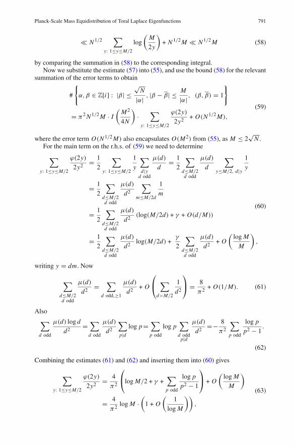
≪ N 1/2∑

y: 1≤y≤M/2

log(M2y

)+ N 1/2M ≪ N 1/2M (58)

by comparing the summation in (58) to the corresponding integral.Now we substitute the estimate (57) into (55), and use the bound (58) for the relevant

summation of the error terms to obtain

#

{

α,β ∈ Z[i] : |β| ≤√N

|α| , |β − β| ≤ M|α| , (β,β) = 1

}

= π2N 1/2M · I(M2

4N

)·

∑

y: 1≤y≤M/2

ϕ(2y)2y2

+ O(N 1/2M),

(59)

where the error term O(N 1/2M) also encapsulates O(M2) from (55), as M ≤ 2√N .

For the main term on the r.h.s. of (59) we need to determine

∑

y: 1≤y≤M/2

ϕ(2y)2y2

= 12

∑

y: 1≤y≤M/2

1y

∑

d|yd odd

µ(d)d

= 12

∑

d≤M/2d odd

µ(d)d

∑

y≤M/2, d|y

1y

= 12

∑

d≤M/2d odd

µ(d)d2

∑

m≤M/2d

1m

= 12

∑

d≤M/2d odd

µ(d)d2

(log(M/2d) + γ + O(d/M))

= 12

∑

d≤M/2d odd

µ(d)d2

log(M/2d) +γ

2

∑

d≤M/2d odd

µ(d)d2

+ O(logMM

),

(60)

writing y = dm. Now

∑

d≤M/2d odd

µ(d)d2

=∑

d odd,≥1

µ(d)d2

+ O

⎛

⎝∑

d>M/2

1d2

⎞

⎠ = 8π2 + O(1/M). (61)

Also∑

d odd

µ(d) log dd2

=∑

d odd

µ(d)d2

∑

p|dlog p=

∑

p odd

log p∑

d oddp|d

µ(d)d2

=− 8π2

∑

p odd

log pp2 − 1

.

(62)

Combining the estimates (61) and (62) and inserting them into (60) gives

∑

y: 1≤y≤M/2

ϕ(2y)2y2

= 4π2

⎛

⎝logM/2 + γ +∑

p odd

log pp2 − 1

⎞

⎠ + O(logMM

)

= 4π2 logM ·

(1 + O

(1

logM

)),

(63)


so that (59) is

#{α,β ∈ Z[i] : |β| ≤

√N

|α| , |β − β| ≤ M|α|

}

= 4N 1/2M logM · I(M2

4N

)·(1 + O

(1

logM

)),

(64)

where the error term in the latter estimate also encapsulates the one in (59). The estimate(64) means that the term in the sum on the r.h.s. of (52) corresponding to u = 1contributes 1

4 of what is claimed in the statement (51) of Theorem 6.1.We claim that the contribution of each of the other three terms in (52) is also given

by the r.h.s. of (64). While the proofs are very similar we highlight the differences forthe convenience of the reader. The u = −1 term yields the conditions

|x | ≤ M/2|α| and y2 ≤ N/|α|2 − x2, with (x, y) = 1 and x + y odd;

that is, the roles of x and y are reversed as compared to (53); one then gets the sameestimate. If u = i then β − uβ = (1− i)(x − y), so let y = x +! so that x2 + y2 ≤ T 2

becomes (2x +!)2 ≤ 2T 2−!2. Therefore we have the conditions, for X = (2N/|α|2−!2)1/2

|!| ≤ M/√2|α| and

−X − !

2≤ x ≤ X − !

2with (x,!) = 1 and ! odd.

We now have a slightly different calculation from before; we will note the differences:Again x runs through an interval of length X , and so the number of such x is

ϕ(!)

!· X + O(τ (!)).

Running through the calculation we get a main term of

∑

!≤M/√2

! odd

ϕ(!)

!2 · πN 1/2My

with the same error terms. An analogous calculation reveals that

∑

!≤M/√2

! odd

ϕ(!)

!2 = 4π2

⎛

⎝log√2M + γ +

∑

p odd

log pp2 − 1

⎞

⎠ + O(logMM

).

A similar calculation ensues for u = −i . Therefore, as mentioned above and similar to(64), each summand of (52) contribute a quarter of the total claimed (51), and the resultfollows.


6.3. Automorphisms of pairs of close lattice points. We observe that if (α,β, u) ∈S(n,M) corresponds to (a, b) ∈ En then, taking conjugates,

(α,β, u) ∈ S(n,M) (65)

corresponds to (a, b) ∈ En . More interestingly, given (α,β, u) ∈ S(n,M) we see that

A(α,β, u) := {(α′,βw, uw2) : α′ ∈ Z[i] with |α′| = |α| and w ∈ U} (66)

is a subset of S(n,M). Hence we can partition S(n,M) up into sets

A∗(α,β, u) := A(α,β, u) ∪ A(α,β, u). (67)

How often S(n,m) is equal to some unique A∗(α,β, u)? We can re-formulate thisquestion by letting

A(n,M) := {A∗(α,β, u) : (α,β, u) ∈ S(n,M)}and asking how often |A(n,M)| > 1.

Theorem 6.2. Suppose that M ≤ 2√N and let

c = M2

4N. (68)

(1) The number of distinct sets A∗(α,β, u) with |α| · |β| ≤√N is asymptotic to

∑

n≤N

|A(n,M)| = κ ′

2· I (c) · MN 1/2 · ((2 logM)1/2 + O(1)).

(2) The number of pairs of distinct close-by pairs is

∑

n≤N

(|A(n,M)|2

)≪ N 1/3M4/3(log N )7 + N 1/2(log N )3. (69)

Proof of Theorem 1.4 assuming Theorem 6.2. If m is a non-negative integer then thecharacteristic function

1≥1(m) ={1 m ≥ 10 m = 0

satisfies

1≥1(m) = m + O((

m2

))(70)

and

1≥1(m) ≤ m. (71)

Now for a given n ∈ S, andM > 0, there exists a pair λ, λ′ ∈ En with 0 < ∥λ−λ′∥ < M ,if and only if |A(n,M)| ≥ 1. Hence, bearing in mind the definition (15) of G∗(N ;M),we have

G∗(N ;M) =∑

n≤N

1≥1(|A(n,M)|). (72)


Substituting (70) into (72) we obtain

G∗(N ;M) =∑

n≤N

|A(n,M)| + O

⎛

⎝∑

n≤N

(|A(n,M)|2

)⎞

⎠

= κ ′

2· I (c) · MN 1/2((2 logM)1/2 + O(1))

+ O(N 1/3M4/3(log N )7 + N 1/2(log N )3

),

by both parts of Theorem 6.2. The first part of Theorem 1.4 finally follows from substi-tuting (50) into the latter estimate, recalling that here we assumed (16), and noting

N 1/3M4/3 = MN 1/2

(√N/M)1/3

.

To prove the second part of Theorem 1.4 we substitute (71) into (72) to yield

G∗(N ;M) ≤∑

n≤N

|A(n,M)| = κ ′

2· I (c) · MN 1/2((2 logM)1/2 + O(1)).

The desired result follows at once from the fact that I (c) is decreasing on [0, 1], so thatfor every c ∈ [0, 1], I (c) ≤ I (0) = 4

π . ⊓6

6.4. Proof of Theorem 6.2, part I.

Proof. Write |α|2 = a and β = p + iq; evidently a ∈ S. In (65), (66), (67), we see thatthe setA(n,M) is designed to take care of an automorphism group (of pairs of close-bylattice points on the circle of radius

√n) of order 8. Therefore

∑

n≤N

|A(n,M)|

= 18

∑

u∈U

∑

a∈S#{(β, u) ∈ Z[i] × U : |β| ≤

√N/a, |β − uβ| ≤ M√

a, (β,β) = 1

},

(73)

where, as before, S denotes the set of integers that are sums of two squares. Letβ = x+iyso that x + y is odd, and (x, y) = 1.

In the case u = 1 we have |y| ≤ M/2√a and then x2 ≤ N/a − y2. We will proceed

analogously to the proof of Theorem 6.1, but now we have, thanks to Landau (7),

S(t) :=∑

n∈S, n≤t

1 = κLRt

(log t)1/2

(1 + O

(1

log t

)), (74)


so that the term on the r.h.s. of the summation in (73) corresponding to u = 1 contributes

∑

a∈S#{(β, 1) ∈ Z[i] × U : |β| ≤

√N/a, |β − β| ≤ M√

aand (β,β) = 1

}

= 4∑

y: 1≤y≤M/2

ϕ(2y)2y

∑

a≤(M/2y)2a∈S

(Na

− y2)1/2

+ O(

M2

(logM)1/2

)

= 4∑

y: 1≤y≤M/2−1

ϕ(2y)2y

∑

a≤(M/2y)2a∈S

(Na

− y2)1/2

+ O(N ) + O(

M2

(logM)1/2

);

(75)

here, to avoid vanishing denominator later, we separated the contribution of y ≤ M2 −1,

using the trivial bound O(N ) to each of the summands with y > M2 − 1, whose number

is O(1). In this case the inner sum is more complicated as compared to (56): we formallywrite (again hiding summation by parts followed by integration by parts in “oppositedirection”, much in the spirit of (56))

∑

a≤(M/2y)2a∈S

(Na

− y2)1/2

=(M/2y)2∫

1

(Nt

− y2)1/2

dS(t)

via (74) to yield

∑

a≤(M/2y)2a∈S

(Na

− y2)1/2

= κLR

∫ (M/2y)2

1

(Nt

− y2)1/2 dt

(log t)1/2+ O

(MN 1/2

y(logM/2y)3/2

)

= κLRMN 1/2

y(2 log(M/2y))1/2

∫ 1

2y/M

(1 − M2

4Nv2

)1/2

dv + O(

MN 1/2

y(logM/2y)3/2

),

(76)

and letting t = (Mv/2y)2. Extending the range of the latter integral to 0, we see that itequals

∫ 1

2y/M

(1 − M2

4Nv2

)1/2

dv = π

4I (c) + O

( yM

),

by the definition (49) of I (c), (68), and the boundedness of the integrand. We then haveupon substituting the latter estimate into (76), and then into (75), that the u = 1 term in(73) contributes to the sum

∑

a∈S#{(β, 1) ∈ Z[i] × U : |β| ≤

√N/a, |β − β| ≤ M√

aand (β,β) = 1

}

= πκLRMN 1/2 · I (c)∑

y: 1≤y≤M/2−1

ϕ(2y)2y2

1(2 log(M/2y))1/2

+ E,(77)


where the error term E = E(N ,M) is bounded by

|E | ≪∑

y: 1≤y≤M/2

ϕ(2y)2y

(MN 1/2

y(logM/2y)3/2+

N 1/2

(log(M/2y))1/2

)+

M2

(logM)1/2

≪ MN 1/2.

(78)

To evaluate the main term we reuse our estimate

P(t) :=∑

y≤t

ϕ(2y)2y2

= 4π2

(log t + C + O

(log tt

))

for some constantC (cf. (63)), and plan to use summation byparts followedby integrationby parts, again in the spirit of (56). And so we get, formally manipulating (assume forsimplicity that M/2 ∈ Z, otherwise further restrict the range of integration),

∑

y: 1≤y≤M/2−1

ϕ(2y)2y2

1(2 log(M/2y))1/2

=∫ M/2−1

1

dP(y)(2 log(M/2y))1/2

= 4π2

M/2−1∫

1

d(log y + C + O((log y)/y))(2 log(M/2y))1/2

= 4π2

M/2−1∫

1

dyy(2 log(M/2y))1/2

+ E ′, (79)

where the error term is

|E ′| ≤ log yy(log(M/2y))1/2

∣∣∣∣y=M/2−1

y=1+∫ M/2−1

1

log ydyy2(log(M/2y))3/2

≪ logMM1/2 + 1,

(80)

by changing the variables t = M2y and separating the contribution of the range y ∈

[1, ϵM] and [ϵM,M/2].We may then evaluate the latter integral in (79) explicitly to be

M/2−1∫

1

dyy(2 log(M/2y))1/2

= (2 log(M))1/2 + O(1),

and, with the help of (80), obtain

∑

y: 1≤y≤M/2−1

ϕ(2y)2y2

1(2 log(M/2y))1/2

= 4π2 (2 logM + O(1))1/2.


Substituting the latter estimate into (77) and bearing in mind (78) we finally obtain

∑

a∈S#{(β, 1) ∈ Z[i] × U : |β| ≤

√N/a, |β − β| ≤ M√

aand (β,β) = 1

}

= 4π

κLRMN 1/2 · I (c) · (2 logM + O(1))1/2,

which contributes a quarter in (73) of what is stated in part I of Theorem 6.2. We geta similar quantity for u = −1; and by suitably modifying the proof, we get the samequantity for u = i and u = −i , modifying the proof much like we did in Theorem 6.1.⊓6

6.5. Many pairs—proof of Theorem 6.2, part II.

Lemma 6.3. For any θ we have, uniformly,

#{x + iy ∈ Z[i] : |x + iy| ≤ N , (x, y) = 1 & |arg(x + iy) − θ | < ϵ} ≪ 1 + ϵN 2.

In fact if ϵ ≤ 1/2N 2 there is no more than one solution.

The proof of Lemma 6.3 will be given immediately after the proof of Theorem 6.2,part II.

Proof of Theorem 6.2, part II assuming Lemma 6.3. We treat separately those n ≍ N ,which are either a square nor twice a square. These contribute at most

∑

m2≍N

r2(m2)2 +∑

2m2≍N

r2(2m2)2 ≪ N 1/2(log N )3. (81)

Now suppose we have two pairs a1, b1 and a2, b2 not belonging to the same classA∗(α,β, u), but with the same n ≍ N , which is neither a square nor twice a square.We use the identification between the close-by pairs and triples (α,β, u) ∈ S(n,M)as in the beginning of section 6.1, so that a couple of close-by pairs yields two triples(α j ,β j , u j ) ∈ S(n,M), j = 1, 2. It is then possible to write

β1 = γ δθ1 and β2 = γ δθ2 (82)

where (β1,β2) = (γ ) and (β1/γ ,β2/γ ) = (δ), and the norms of θ1 and θ2 are coprime.Since |α1β1| = |α2β2| =

√n, we have

α1 = t2v1 and α2 = t1v2, (83)

where

|t1| = |θ1|, |t2| = |θ2| and |v1| = |v2|. (84)

Hence we must have

|γ δθ1θ2v1| = |β1α1| =√n ≍

√N , (85)

and we in addition have

|θ1v1| = |α2| =M

|β2 − uβ2|≤ M, and |θ2v1| = |α1| ≤ M (86)


in a similar fashion. Substituting the estimates (86) into (85) we conclude that

|γ δθ1|, |γ δθ2| ≫√NM

. (87)

Next we use the condition that

|α j | · |β j − u jβ j | ≤ M.

Since |α j | · |β j | =√n ≍

√N , this yields

|1 − u j · exp(−2i · arg(β j ))| =∣∣∣∣∣1 − u j

β j

β j

∣∣∣∣∣ ≪ M√N.

Recalling that u j are units, this implies that 2 arg(β j ) are small modulo π2 , or, more

precisely

|arg(β j )| ≪ M√N

modπ

4.

Therefore, bearing in mind (82), we have

arg(θ1) = − arg γ − arg δ (mod π/4) + O(M/√N )

arg(θ2) = − arg γ + arg δ (mod π/4) + O(M/√N )

We have two linearly independent equations in four unknowns. This allows us to deter-mine arg γ , arg δ in terms of arg(θ1), arg(θ2) mod π/4, with error O(M/

√N ):

2 arg γ + (arg(θ1) + arg(θ2)) (mod π/4) = O(M/√N )

2 arg δ + (arg(θ1) − arg(θ2)) (mod π/4) = O(M/√N ).

(88)

The inequalities (88) imply that there exist w,w′ ∈ ±{1, i, 1 + i, 1 − i} such that

arg(wδ2θ1θ2), arg(w′γ 2θ1θ2) = O(

M√N

). (89)

We argue that neither of the numbers on the l.h.s. of (89) can vanish precisely: Forif we suppose that arg(wδ2θ1θ2) = 0, then, as θ1 and θ2 are coprime, we can writeθ j = r jφ2

jω j for j = 1, 2 with δ = φ1φ2, where each ωi divides ω, and the r j areintegers. Now (r jω j ) divides (θ j , θ j ), which divides (β j ,β j ) = 1, and so r jω j is a unit.Moreover

φ1φ2|(δθ1, δθ2) = (β1/γ ,β2/γ ) = (1),

and so φ1 = φ2 = 1, and therefore δ = φ1φ2 = 1. Therefore θ1, θ2 are units. Wemay then select γ so that θ2 = 1, and so β2 = wβ1 for some unit w, and |α1| = |α2|.Therefore (α2,β2, u2) ∈ A(α1,β1, u1) in contradiction to our assumption that thesetriples belong to different classes A∗(α,β, u). Similarly if arg(w′γ 2θ1θ2) = 0 thenwe take the conjugate of (α2,β2), so that the roles of γ and δ are exchanged, and so(α2,β2, u2) ∈ A(α1,β1, u1). In either case we get a contradiction to our assumptionthat (α j ,β j , u j ), j = 1, 2 belong to different classes A∗(α,β, u).


Therefore we may assume

0 ̸= arg(wδ2θ1θ2) = O(

M√N

),

and so

1 ≤ |Im(wδ2θ1θ2)| ≍ | arg(wδ2θ1θ2)| · |δ2θ1θ2| ≪ |δ2θ1θ2| ·M√N,

and so we deduce that

|γ 2θ1θ2| ≫√NM

, and |δ2θ1θ2| ≫√NM

. (90)

To summarize all the above, a pair of triples (α j ,β j , u j ) that satisfy the conditionsabove and belong to different classes A∗(·, ·, ·) determines an 8-tuple (γ , δ, θ1, θ2, t1, t2,v1, v2) ∈ Z[i]8 that satisfies (84), (85), (86), (87) and (90). Conversely, such a 8-tuple corresponds to a unique (α j ,β j ) via (82) and (83), hence, for our purposes itis sufficient to bound their number (bearing in mind that the group of units is finite).Let C, D, T1, T2, V be powers of 2 that are greater than and closest to |γ |, |δ|, |θ1| =|t1|, |θ2| = |t2|, and |v1| = |v2| respectively; hence their product is CDT1T2V ≍

√N

with T1V, T2V ≪ M , and

CDT1, CDT2, C2T1T2, D2T1T2 ≫√N/M. (91)

We note that∑

n≤N r2(n)2 ≍ N log N . First select an integer v ≍ V 2 and any v1, v2

with |v1|2 = |v2|2 = v, so the total number of possible choices for v1, v2 is

≤∑

v≪V 2

r2(v)2 ≪ V 2 log V ≪ V 2 logM. (92)

Let A be the largest of C, D, T1, T2, and B be the second largest. By (91), we have

AB ≫(√

NM

)2/3

and B ≫(√

NM

)1/4

, (93)

the former following from the fact that the product AB must appear in either of CDT1,CDT2, and the latter is a consequence of the fact that B must appear in one of the 4products on the l.h.s. of (91) without A. If the two largest are, say, C and D, then weselect any θ1, t1 with |θ1|2 = |t1|2 = r ≍ T 2

1 , and θ2, t2 with |θ2|2 = |t2|2 = s ≍ T 22 ,

so the number of choices of these are

≪ T 21 log T1 · T 2

2 log T2 ≪ (T1T2 logM)2,

similar to (92). Next we select γ with |γ | ≍ C , and δ with |δ| ≍ D, with their argumentsin the narrow intervals, of width O(M/

√N ), given by the equations (88) above. Then,

by Lemma 6.3, the number of such γ is ≪ 1 + C2 M√N, and the number of such δ is

≪ 1 + D2 M√N. Hence, the ordering assumptions on C, D, T1, T2, V above, the total


number of possible (γ , δ, θ1, θ2, t1, t2, v1, v2) (and hence the corresponding (α j ,β j ),j = 1, 2) is

≪ (V 2 logM) · (T1T2 logM)2 ·(1 + C2 M√

N

)·(1 + D2 M√

N

)

= (CDT1T2V )2(logM)3 ·(

1C2 +

M√N

)·(

1D2 +

M√N

)

≪ N(

1A2 +

M√N

)·(

1B2 +

M√N

)· (logM)3,

and the analogous expression is proved for everyorderingofC, D, T1, T2. Thanks to (93),each of these expressions is≪ N 1/3M4/3(log N )3, and, since the numbersC, D, T1, T2,whose product is ≪ N , are all powers of 2, the number of possibilities for choosingthem is ≪ (log N )4, which implies (cf. (81))

∑

n≤N

(|A(n,M)|2

)≪ N 1/3M4/3(log N )7 + N 1/2(log N )3,

claimed in (69). ⊓6Remark 6.1. There are≍ M2(logM)7 solutions withC, D, T1, T2 ≫ (

√N/M)1/2, and

we expect this to be the correct number of solutions, provided that M > Nc for somec > 0.

Proof of Lemma 6.3. Multiplying through by the units we can place θ in the first quad-rant; swapping x and y if necessary we may assume that 0 < y < x < N . Since thederivative of arctan is bounded away from 0, our set cardinality is bounded by

#{x + iy ∈ Z[i] : |x + iy| ≤ N , (x, y) = 1 & |arg(x + iy) − θ | < ϵ}≪ #{0 < y < x < N : |y/x − θ | < ϵ}. (94)

If there is no solution to (94) we are done, otherwise we choose one, i.e. a tuple(a, b) ∈ Z2 with 0 < b < a < N and (a, b) = 1 such that |b/a − θ | < ϵ. Any othersolution (x, y) of (94) satisfies

1N 2 <

1xb

≤∣∣∣yx

− ab

∣∣∣ ≤∣∣∣yx

− θ∣∣∣ +

∣∣∣θ − ab

∣∣∣ < 2ϵ,

hence there is at most one solution unless ϵ > 1/2N 2. The above implies that everyother solution (x, y) of (94) necessarily satisfies

|ax − by| < 2ϵbx . (95)

Now, since (a, b) = 1, there exists an integer solution (u, v) = (u0, v0) to au−bv =1, and hence for d ∈ Z the tuple (x, y) = (du0, dv0) is one solution to

ax − by = d. (96)

Hence the general solution to (96) is given by x = du0 +kb, y = dv0 +ka with k integer;a solution of (95) is a solution to (96) with |d| < 2ϵbx ≪ ϵbN , and, given a value of d,the condition 0 < y = dv0 + ka < N forces k to lie in an interval of length O(N/a).Therefore the total number of solutions to (95) is

≪ ϵbN · Na

≪ ϵN 2,

which implies the statement of Lemma 6.3. ⊓6


7. Best Possible?

7.1. Squarefree n: best possible?. It is believed that there are lots of primes of the forma2 + 1. Say p1, . . . , pk are primes, close to y2, with p j = a2j +1 so each a j is very closeto y.

Then Pj = a j + i , and these are each complex numbers with | arg(a j ± i)| ≪ 1/y.Therefore any product (a1± i) · · · .(ak± i) has argument≪ k/y. Therefore these pointsappear in four arcs of width ≪ k/y centered around 1, i,−1,−i . Here n = p1 . . . pk ≈y2k and so the width of these arcs is ≪ k/n1/2k . This yields examples of n with n issquarefree and r2(n) → ∞ for which

#{α,β ∈ En : |α − β| ≤ n1/2−o(1)} ≫ |En|2,where o(1) is going to 0 arbitrarily slowly.

7.2. Very short arcs. Fix an integer a composed of many prime factors ≡ 1 (mod 4),and select m arbitrarily large, for which b = m2 + 1 has ≤ 3 prime factors.2 Let u = 1.If |α|2 = a then A∗(α,m + i, 1) ⊂ S(ab, 2a1/2), which embeds into D(ab, 2/b1/2) ⊂D(ab, 2/m). Now |A∗(α,m + i, 1)| ≫ r2(a) ≫ |D(ab)|. Therefore, for n = ab, wehave given infinitely many examples with

#{(u, v) ∈ En : |u − v| ≤ no(1)} ≫ |En|.

Acknowledgements. The authors would like to thank Mike Bennett, Valentin Blomer, Jerry Buckley, StephenLester, Zeév Rudnick, Mikhail Sodin, and Peter Sarnak for a number of stimulating and fruitful conversationsand their remarks. It is a pleasure to thank the anonymous referee, whose numerous comments have helpedus improve the presentation of the results. The research leading to these results has received funding from theEuropean Research Council under the European Union’s Seventh Framework Programme (FP7/2007-2013),ERC grant agreement no 670239 (A.G.) and no 335141 (I.W.), as well as from NSERC Canada under theCRC program (A.G.).

Open Access This article is distributed under the terms of the Creative Commons Attribution 4.0 Inter-national License (http://creativecommons.org/licenses/by/4.0/), which permits unrestricted use, distribution,and reproduction in any medium, provided you give appropriate credit to the original author(s) and the source,provide a link to the Creative Commons license, and indicate if changes were made.

References

1. Berry, M.: Regular and irregular semiclassical wavefunctions. J. Phys. A. 10(12), 2083–2091 (1997)2. Berry, M.: Semiclassical mechanics of regular and irregular motion. Chaotic behavior of deterministic

systems (Les Houches, 1981), pp. 171–271, North-Holland, Amsterdam (1983)3. Bourgain, J., Rudnick, Z.: On the geometry of the nodal lines of eigenfunctions of the two-dimensional

torus. Ann. Henri Poincaré. 12(6), 1027–1053 (2011)4. Brüdern, J.: Einführung in die analytische Zahlentheorie. Springer, Berlin (1995)5. Cilleruelo, J., Cordoba, A.: Trigonometric polynomials and lattice points. Proc. Am. Math.

Soc. 115(4), 899–905 (1992)6. Cilleruelo, J., Granville, A.: Lattice points on circles, squares in arithmetic progressions, and sumsets of

squares. In: Additive Combinatorics, CRM Proceedings & Lecture Notes, Vol. 43, pp. 241–262 (2007)7. Colin de Verdière, Y.: Ergodicité et fonctions propres du Laplacien. Commun. Math. Phys. 102, 497–

502 (1985)8. Granville, A., Stark, H.M.: ABC implies no “Siegel Zeroes” for L-functions of characters with negative

discriminant. Invent. Math. 139, 509–523 (2000)

2 We know such b exist by sieve methods; though we believe there are infinitely many such primes, whichis as yet unproved.

http://creativecommons.org/licenses/by/4.0/


9. Han, X.: Small scale quantum ergodicity in negatively curved manifolds. Nonlinearity 28(9), 3263–3288 (2015)

10. Han, X.: Small scale equidistribution of random eigenbases. Commun. Math. Phys. 349(1), 425–440 (2017)

11. Hezari, H., Rivière, G.: L p norms, nodal sets, and quantum ergodicity. Adv. Math. 290, 938–966 (2016)12. Hezari, H., Rivière, G.: Quantitative equidistribution properties of toral eigenfunctions. J. Spectr. The-

ory 7(2), 471–485 (2017)13. Landau, E.: Über die Einteilung der positiven ganzen Zahlen in vier Klassen nach der Mindeszahl der zu

ihrer additiven Zusammensetzung erforderlichen Quadrate. Arch. Math. Phys. 13, 305–312 (1908)14. Lester, S., Rudnick, Z.: Small scale equidistribution of eigenfunctions on the torus. Commun. Math.

Phys. 350(1), 279–300 (2017)15. Luo Zhi, W., Sarnak, P.: Quantum ergodicity of eigenfunctions on PSL2(Z)\H2. Inst. Hautes Tudes Sci.

Publ. Math. No. 81, 207–237 (1995)16. Snirel’man, A.: Ergodic properties of eigenfunctions. Uspekhi Mat. Nauk 180, 181–182 (1974)17. Young, M.: The quantum unique ergodicity conjecture for thin sets. Adv. Math. 286, 958–1016 (2016)18. Zelditch, S.: Uniform distribution of eigenfunctions on compact hyperbolic surfaces. Duke Math.

J. 55, 919–941 (1987)

Communicated by J. Marklof

Documents

Planck-Scale Mass Equidistribution of Toral Laplace