Embed Size (px)
Citation preview

Raphael Flauger
KICP Colloquium, Chicago, December 2, 2015
Planck, BICEP, and the Early Universe

measurement of excess antenna temperature and interpretation in terms of CMB published in July 1965
CMB@50

COBRACOBE
CMB@50
Spectrum

(Planck 2015: )
CMB@50
Dipole
3.3645± 0.0020 mK

2015
CMB@50
Planck 100 GHzWMAP 94 GHz
Planck & WMAP
• Planck and WMAP temperature data agree very well at WMAP resolution
(Nside=512)

Planck 100 GHz
- WMAP 94 GHz =
Planck & WMAP

Planck 100 GHz
- WMAP 94 GHz =
vs Planck CO( ) map1− 0
Planck & WMAP
The small but visible difference is due to a CO emission line

Planck 100 GHzWMAP 94 GHz
• Planck and WMAP temperature data agrees very well at WMAP resolution
• Planck is much more powerful
Planck & WMAP
(Nside=1024)
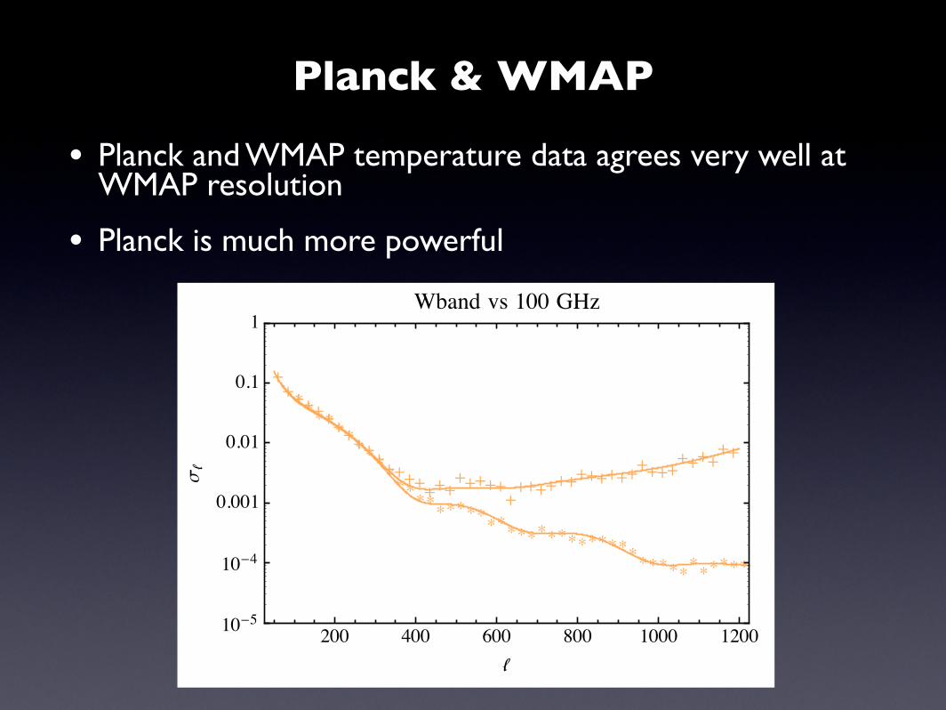
200 400 600 800 1000 1200105
104
0.001
0.01
0.1
1
Σ
Wband vs 100 GHz
Planck & WMAP
• Planck and WMAP temperature data agrees very well at WMAP resolution
• Planck is much more powerful

LCDM
The early universe is remarkably simple and the CMB temperature data is in good agreement with the six-parameter LCDM model.
* the sum of the neutrino masses is kept fixed at 0.06 eV
(Ade et al. 2015)

LCDM+X(A
de et al. 2015)

LCDM
In the context of LCDM, we can predict the TE and EE angular power spectra and compare with the Planck measurements
(systematics remain to be understood)(Ade et al. 2015)

In addition, LCDM is consistent with all low redshift large-scale structure* and supernova data
LCDM
(Betoule et al. 2014)(Anderson et al. 2013)
* on small scales baryonic feedback should be understood better to assess whether there are departures from LCDM
BAO Supernovae

Parameter Constraints
Parameter constraints from TT
• Good consistency between 2013 and 2015 parameters

Parameter Constraints
Parameter constraints from TT
• The optical depth is one exception. It has shifted due to dust polarization data at 353 GHz

0.06 0.08 0.10 0.12 0.140.0
0.2
0.4
0.6
0.8
1.0
Τ
PΤ Ka, Q, V cleaned with K-band and 353 GHz data, then coadded
Ka, Q, V cleaned with K-band and WMAP dust model, then coadded
hybrid-cleaned cross-halfmissionspectra
high- temperature data
low- polarization data
Parameter Constraints
• Most parameters are degenerate with . The old measurement of optical depth would have led to ~0.5 shifts in parameters.
τ
σ
Shift in optical depth for WMAP due to 353 GHz data

Parameter Constraints
LFI and WMAP polarization currently do not agree on large scales
50300.01
0.1
1
10
100
ΝGHz
C,EEΜK R
J2
25
50300.01
0.1
1
10
100
ΝGHz
C,BBΜK RJ
2
25
5030
0.010.02
0.050.100.20
0.501.00
ΝGHz
C,EEΜK R
J2
623
5030
0.010.02
0.050.100.20
0.501.00
ΝGHz
C,BBΜK RJ
2
623
WMAP
LFI

Parameter Constraints
Parameter constraints from TT
• The scalar spectral index has shifted between 2013 and 2015
• much of the shift in the spectral index between 2013 and 2015 can be traced to systematics in 2013 217 GHz detector set spectra.

Parameter Constraints
Parameter constraints from TT
500 1000 1500 2000 2500
6.0 108
8.0 108
1.0 109
1.2 109
1.4 109
1.6 109
1.8 109
2.0 109
21
2 C2ΠΜ
K2
217x217 predicted from 100x100, 143x143, and 143x217
predictedmeasured

Analysis
8
Fig. 7.— Constraints on key parameters in the ΛCDM model and extensions in the presence of high-frequency foreground cleaning.
Left panel: The top, middle and bottom panels show the marginalized one-dimensional likelihoods for the scalar spectral index, ns,
the matter density Ωm and the Hubble constant H0 in the ΛCDM model. The solid blue line is the standard Planck result for the
CAMSpec likelihood including the 100×100, 143×143, 217×217 and 143×217 spectra. The dashed blue line shows the results when
the 217 × 217 spectra are not used; these correspond to results presented in Figure B3 of (Planck Collaboration (XVI) 2013). The
solid and dashed black lines show the same for the cleaned spectra presented here. Right panel : Constraints on the tensor-to-scalar
ratio (top left panel) and mass of the neutrino (top right panel) are weakened with cleaning of the spectra, and Neff (bottom right
hand panel) shifts to values slightly more consistent with three neutrino species. The cleaned spectra do not show a preference for
running of the scalar spectral index.
computed from the cleaned season crosses, the power spectrum amplitude is higher for > 1500. This increasedamplitude leads to a shift in cosmological parameters. The most notable shifts are along a modest degeneracyline between ns, H0 and Ωm:
0.285 0.295 0.305 0.315
Ωm
0.957
0.960
0.963
0.966
0.969
0.972
0.975
ns
Hybrid cleaning - SA47
Hybrid cleaning - SA50
Hybrid cleaning SA47 - no 217x217 GHz
353 cleaning - SA47
545 cleaning - SA47
65 66 67 68 69 70
H0
0.285
0.295
0.305
0.315
Ωm
Planck+WP
Planck+WP no 217x217 GHz
Uncleaned Survey Crosses
Hybrid cleaning - SA24
Hybrid cleaning - SA38
Hybrid cleaning - SA44
Fig. 8.— Constraints in the Ωm −ns plane (left) and H0 −Ωm plane (right) for various cleaning strategies and datasets, compared
to the Planck results. The circles show results obtained with the nominal Planck data, the squares show results from the hybrid
cleaning procedure, the diamond are obtained when only cleaning with the 353 GHz data, and the triangle when using the 545 GHz
data to clean the lower frequencies. For comparison, the results are shown for the season cross-spectra without additional cleaning
(upside-down triangle). The cosmological results are robust to a change in the cleaning procedure.
Planck 2013 CYE
Analysis
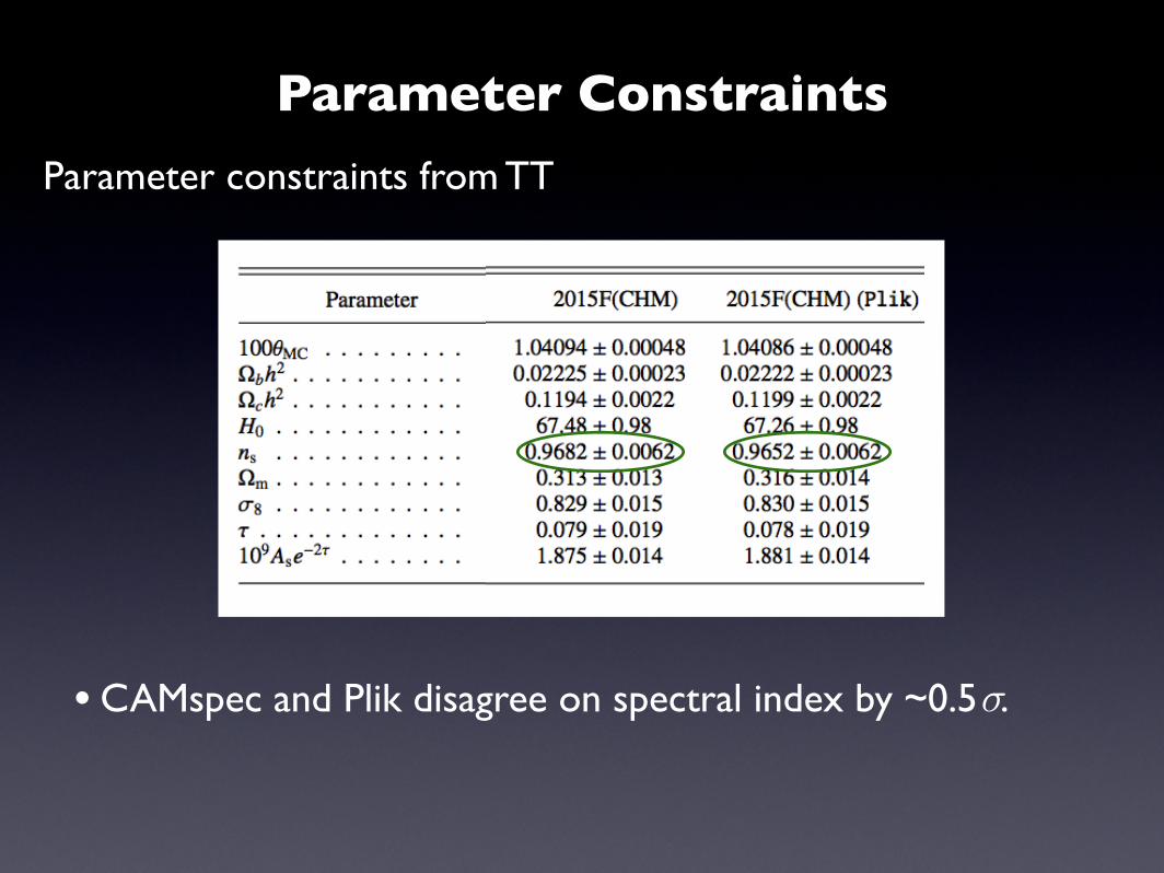
Parameter Constraints
Parameter constraints from TT
• CAMspec and Plik disagree on spectral index by ~0.5 .σ

Parameter Constraints
Parameter constraints from TT
• also disagreement on calibration and foreground parameters
• CAMspec tSZ and CIB(+PS) amplitude in good agreement with ACT/SPT
c100c217ns
YP
AtSZ143
ACIB217
AkSZ
Parameter Constraints
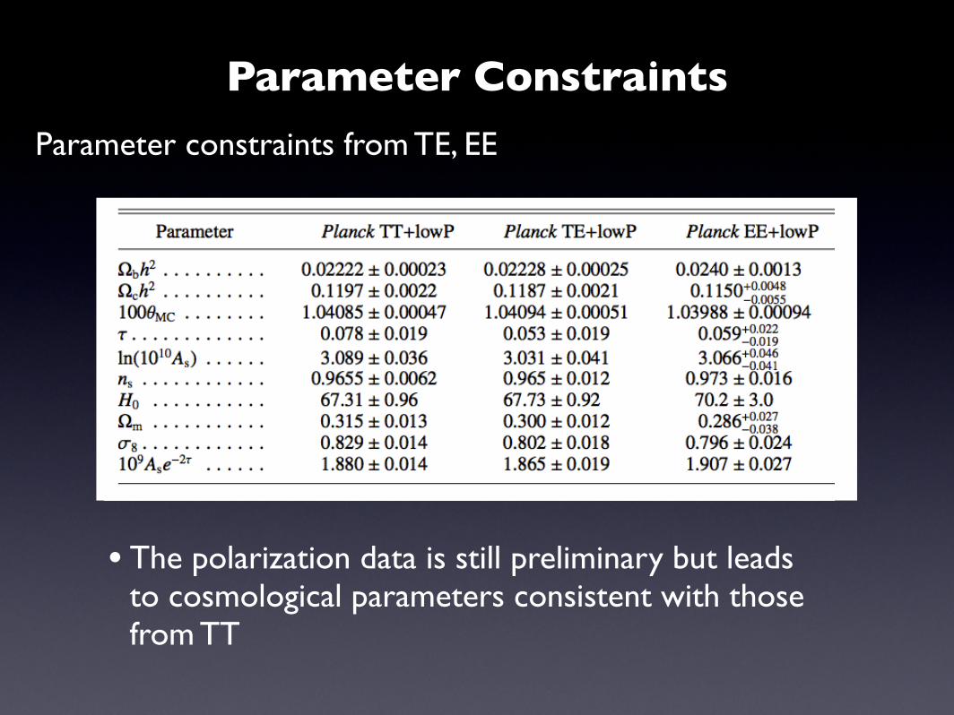
Parameter constraints from TE, EE
• The polarization data is still preliminary but leads to cosmological parameters consistent with those from TT

Parameter Constraints
Parameter constraints from TE, EE
• Although consistent with TT, the polarization data favors lower matter density and . σ8Ωm

Paper XIII
Clustering
P/P
max
Planck 2015 TT+lowP
σ8
Ωm
0.282
0.26
(Hill, Spergel 2013)tSZ power spectrum
• similar tensions exist between the Planck TT data and a number of other low redshift observations
0.75 0.80 0.85 0.90

Clustering
P/P
max
Planck 2015 TT+lowP
• A milder tension also exists between Planck lensing and cosmology predicted by Planck TT
0.70 0.75 0.80 0.85 0.90
σ8
Ωm
0.3
0.25
Planck 2015 lensing

Clustering
P/P
max
Planck 2015 TT+lowP
σ8
Ωm
0.3
0.25
Planck 2015 lensing
0.70 0.75 0.80 0.85 0.90
Planck 2015 TE+lowEB
Planck 2015 EE+lowEB
• however, both Planck TE and Planck EE cosmologies in excellent agreement with Planck lensing

Parameter Constraints
Parameter constraints from TT marginalized over AL and TE
• The TT power spectrum data favors ~2 higher AL
than expected theoretically or observed in lensing power spectrum.
AL
Planck TT+ lowP− AL Planck TE + lowEB
1
σ

Parameter Constraints
Parameter constraints from TT marginalized over AL and TE
• Marginalization over AL leads to higher value of Hubble parameter, lower value of matter density and , and better agreement with polarization.σ8
Ωm
AL
Planck TT+ lowP− AL Planck TE + lowEB
1

Reid et al. 2013
Riess et al. 2011
Ade et al. 2015
Efstathiou 2013
Spergel, Flauger, Hlozek 2013
NGC 4258LMCMW
NGC 4258LMCMW
UGC 3789
Planck TT
Planck
70.0 75.065.0
H0/(km/s/Mpc)
The Hubble Constant
Hinshaw et al. 2013 WMAP+ACT
Planck TEPlanck TT - AL

Measurements of the CMB have taught us that the primordial perturbations
• existed before the hot big bang
• are nearly scale invariant
• are very close to Gaussian
• are adiabatic
What generated them?
Primordial Perturbations

Inflation
Assuming inflation took place, what can we learn about it beyond and ?
• What is the energy scale of inflation?
• How far did the field travel?
• Are there additional light degrees of freedom?
• What is the propagation speed of the inflaton quanta?
tensor modes
non-Gaussianity
ns ∆2R

In addition to the scalar modes, inflation also predicts a nearly scale invariant spectrum of gravitational waves
∆2h(k) =
2H2(tk)π2
A measurement of the tensor contribution would provide a direct measurement of the expansion rate of the universe during inflation, as well as the energy scale
Energy Scale of Inflation
V 1/4inf = 1.06× 10¹⁶ GeV
r
0.01
1/4
r =∆2
h
∆2R
with
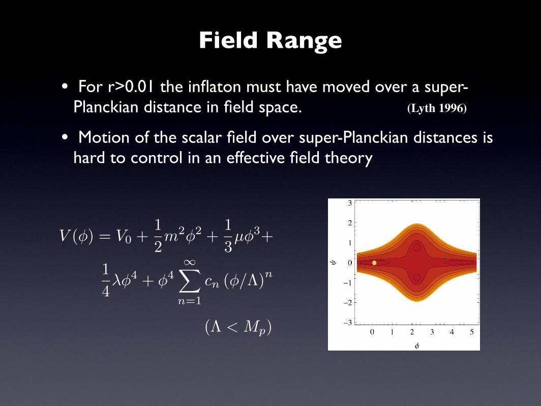
• For r>0.01 the inflaton must have moved over a super-Planckian distance in field space.
• Motion of the scalar field over super-Planckian distances is hard to control in an effective field theory
(Lyth 1996)
Field Range
V (φ) = V0 +1
2m2φ2 +
1
3µφ3+
1
4λφ4 + φ4
∞
n=1
cn (φ/Λ)n
(Λ < Mp)

Use a field with a shift symmetry and break the shift symmetry in a controlled way.
Possible Solution:
Freese, Frieman, Olinto, PRL 65 (1990)
V (φ) = Λ4
1 + cos
φ
f
natural inflation
f Mpwith
e.g. Linde’s chaotic inflation with
with m MpV (φ) =1
2m2φ2
Field Range

In fact, the most naive implementation of an axion with seems hard to realize string theory.
Banks, Dine, Fox, Gorbatov hep-th/0303252
In field theory we may simply postulate such a symmetry, but it is far from obvious that such shift symmetries exist in a theory of quantum gravity.
f Mp
Field Range
Heidenreich, Reece, Rudelius 1506.03447, 1509.06374
Arkani-Hamed, Motl, Nicolis, Vafa hep-th/0601001
more recently
Brown, Cotrell, Shiu, Soler 1503.04783, 1504.00659Rudelius 1503.00795
Bachlechner, Long, McAllister 1412.1093, 1503.07853...
This motivates a systematic study of large field models of inflation in quantum gravity/string theory

One mechanism that allows super-Planckian excursions with sub-Planckian is monodromy
0.6 0.4 0.2 0.0 0.2 0.4 0.60
2. 1011
4. 1011
6. 1011
8. 1011
1. 1010
ΦMp
VΦM
p4
Axion Monodromy Inflation
So far there is no systematic study, but a number of lamp posts
f

Axion Monodromy Inflation
Monodromy occurs in various contexts
• in non-Abelian gauge theories
• in string theory
• in the presence of branes
• in the presence of fluxes

anti5B
5B
5B
!C(2) = c
anti5B
Figure 2: Schematic of tadpole cancellation. Blue: Two-real-parameter family of two-cycles Σ1, drawn as spheres, extending into warped regions of the Calabi-Yau. Red: We haveplaced a fivebrane in a local minimum of the warp factor, and an anti-fivebrane at a distantlocal minimum of the warp factor. In the lower figure, Σ1 is drawn as the cycle threaded byC(2), and global tadpole cancellation is manifest.
Moduli stabilization is essential for any realization of inflation in string theory, and wemust check its compatibility with inflation in each class of examples. In type IIB compactifi-cations on Calabi-Yau threefolds, inclusion of generic three-form fluxes stabilizes the complexstructure moduli and dilaton [19]. A subset of these three-form fluxes – imaginary self-dualfluxes – respect a no scale structure [19, 18]. This suffices to cancel the otherwise dangerousflux couplings described in §3.2.1.
4.2 An Eta Problem for B
In this class of compactifications, however, the stabilization of the Kahler moduli leads to anη problem in the b direction. This problem arises because the nonperturbative effects (e.g.
19
NS5anti-NS5
Axion Monodromy Inflation
Comic version of axion monodromy inflation

The original axion monodromy model is just one example of a larger class of models with potentials
V (φ) = µ4−pφp
so far with p = 23 , 1,
43 , 2, 3
Axion Monodromy Inflation

Instanton corrections may lead to oscillatory contributions to the potential.
V (φ) = µ3φ+ Λ4 cos
φf
These lead to oscillations in the power spectrum that can be searched for.
anti5B
5B
5B
!C(2) = c
anti5B
Figure 2: Schematic of tadpole cancellation. Blue: Two-real-parameter family of two-cycles Σ1, drawn as spheres, extending into warped regions of the Calabi-Yau. Red: We haveplaced a fivebrane in a local minimum of the warp factor, and an anti-fivebrane at a distantlocal minimum of the warp factor. In the lower figure, Σ1 is drawn as the cycle threaded byC(2), and global tadpole cancellation is manifest.
Moduli stabilization is essential for any realization of inflation in string theory, and wemust check its compatibility with inflation in each class of examples. In type IIB compactifi-cations on Calabi-Yau threefolds, inclusion of generic three-form fluxes stabilizes the complexstructure moduli and dilaton [19]. A subset of these three-form fluxes – imaginary self-dualfluxes – respect a no scale structure [19, 18]. This suffices to cancel the otherwise dangerousflux couplings described in §3.2.1.
4.2 An Eta Problem for B
In this class of compactifications, however, the stabilization of the Kahler moduli leads to anη problem in the b direction. This problem arises because the nonperturbative effects (e.g.
19
NS5 anti-NS5
ED1
These models often make additional predictions
Axion Monodromy Inflation

In the larger class of models they are of the form
V (φ) = µ4−pφp + Λ(φ)4 cos
φ0
f0
φφ0
1+pf
+∆ϕ
δns = 3b2πα
1/2with α = (1 + pf )
φ0
2fN0
√2pN0
φ0
1+pf
This can be shown to lead to a power spectrum of the form
∆2R(k) = ∆2
R
kk
ns−11 + δns cos
φ0
f
φk
φ0
pf+1+∆ϕ
Axion Monodromy Inflation

Search for oscillations with drifting period in Planck nominal mission data and full mission data
Figure 3: Points that lead to an improvement over ΛCDM of ∆χ2 ≥ 4 for the first template,
(6.3). The left panel shows the results for the public Planck likelihood [25], and the right
panel shows the results for the likelihood discussed in [27]. The sizes of the dots and their
color indicate the amount of improvement. Larger blue points represent larger values of
∆χ2. The solid lines indicate constant α = ω/H. The red solid line represents ω/H = 28.8,
the best-fit frequency found by the Planck collaboration [26]. A significant contribution to
the improvement derives from the region around = 1800 in the 217 GHz data. This range
of multipoles of the 217 GHz data is known to be affected by interference between the 4K
cooler and the read-out electronics [27, 25].
As expected, the improvement at ω/H ≈ 28.8 is absent, but there are some frequencies
that lead to improvements in both likelihoods, such as ω/H ≈ 60 and ω/H ≈ 210. For
the linear axion monodromy model, the latter corresponds to an axion decay constant of
f = 4.37 × 10⁻⁴Mp and is the frequency that led to the improvement of ∆χ2 ≈ 20 in the
WMAP9 data. The improvement seen in both likelihoods is ∆χ2 10.
We can also use our searches to derive constraints on the amplitude of oscillations allowed
by the data. The results are shown in Figure 4 for both likelihoods. When interpreting them,
it should be kept in mind both that we restricted to −3/4 < pf < 1/2 in our search, and
that the limits are approximate given the limited number of simulations we have performed.
The results for our second template (6.6) are shown in Figure 5 for both likelihoods. As
before, no improvement is observed for ω/H = 28.8 for the likelihood described in [27], and
improvements at ω/H ≈ 60 and ω/H ≈ 210 are seen in both likelihoods, but with ∆χ2 10.
While the plots show a dependence on c1 for the frequencies that lead to the most notable
41
Axion Monodromy Inflation

Improvement of the fit over CDM: Λ ∆χ2 = 18
Expectation based on simulations in the absenceof a signal: ∆χ2 = 16.5± 3.5
One should keep in mind that not the entire parameter space was searched and more work is required, but as of now there is no evidence for oscillations in the primordial power spectrum.
The amplitude is very model dependent, and a non-detection does not rule out these models, but it means for now* we are stuck with and . ns r
(*) LSS may some day dramatically improve the constraints
Axion Monodromy Inflation
BICEP2: E signal
1.7µK
−65
−60
−55
−50
Simulation: E from lensed−ΛCDM+noise
1.7µK
Right ascension [deg.]
Dec
linat
ion
[deg
.]
BICEP2: B signal
0.3µK
−50050
−65
−60
−55
−50
Simulation: B from lensed−ΛCDM+noise
0.3µK
−50050
−1.8
0
1.8
−0.3
0
0.3
µK
µK
Noise level: 87 nK deg - the deepest map at 150 GHz of this patch of sky
(Planck noise level: few K deg)µ
BICEP2 polarization data
Experimental Constraints on r

Foreground models made in collaboration with David Spergel, Colin Hill, and Aurelien Fraisse
BICEP2
BICEP2xKeck
BICEP2
BICEP2xKeck
BICEP2
BICEP2xKeck
Experimental Constraints on r
Planck Collaboration: Dust polarization at high latitudes
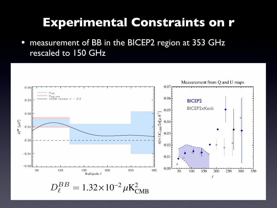
Fig. 9: Planck 353 GHz DBB angular power spectrum computed on MB2 defined in Sect. 6.1 and extrapolated to 150 GHz (box
centres). The shaded boxes represent the ±1σ uncertainties: blue for the statistical uncertainties from noise; and red adding inquadrature the uncertainty from the extrapolation to 150 GHz. The Planck 2013 best-fit ΛCDMDBB
CMB model based on temper-ature anisotropies, with a tensor amplitude fixed at r = 0.2, is overplotted as a black line.
in Sects. 5.2 and 6.2. This indicates that MB2 is not one of theoutliers of Fig. 7 and therefore its dust B-mode power is well rep-resented by its mean dust intensity through the empirical scalinglawD ∝ I3531.9.
These values of the DBB amplitude in the range of the pri-
mordial recombination bump are of the same magnitude as thosereported by BICEP2 Collaboration (2014b). Our results empha-size the need for a dedicated joint analysis of the B-mode po-larization in this region incorporating all pertinent observationaldetails of the Planck and BICEP2 data sets, which is in progress.
6.4. Frequency dependence
We complement the power spectrum analysis of the 353 GHzmap with Planck data at lower frequencies. As in the analysisin Sect. 4.5, we compute the frequency dependence of the BBpower measured by Planck at HFI frequencies in the BICEP2field, using the patch MB2 as defined in Sect. 6.1.
We compute on MB2 the Planck DBB auto- and cross-power
spectra from the three Planck HFI bands at 100, 143, 217, and353 GHz, using the two DetSets with independent noise at eachfrequency, resulting in ten angular power spectra (100 × 100,100×143, 100×217, 100×353, 143×143, 143×217, 143×353,217 × 217, 217 × 353, and 353 × 353), constructed by combin-ing the cross-spectra as presented in Sect. 3.2. We use the samemultipole binning as in Sect. 6.3. To each of these DBB
spectra,we fit the amplitude of a power law in with a fixed exponentαBB = −0.42 (see Sect. 4.2). In Fig. 10 we plot these amplitudesas a function of the effective frequency from 143 to 353 GHz, inunits of sky brightness squared, like in Sect. 4.5. Data points ateffective frequencies below 143 GHz are not presented, because
the dust polarization is not detected at these frequencies. An up-per limit on the synchrotron contribution at 150 GHz from thePlanck LFI data is given in Appendix C.4.
We can see that the frequency dependence of the amplitudesof the Planck HFI DBB
spectra is in very good agreement witha squared dust modified blackbody spectrum having βd = 1.59and Td = 19.6 K (Planck Collaboration Int. XXII 2014). We notethat this emission model was normalized only to the 353 GHzpoint and that no global fit has been performed. Nevertheless,the χ2 value from the amplitudes relative to this model is 4.56(Ndof = 7). This shows that dust dominates in the specific MB2region defined where these cross-spectra have been computed.This result emphasizes the need for a dedicated joint Planck–BICEP2 analysis.
7. Conclusions
We have presented the first nearly all-sky statistical analysis ofthe polarized emission from interstellar dust, focussing mostlyon the characterization of this emission as a foreground contam-inant at frequencies above 100 GHz. Our quantitative analysis ofthe angular dependence of the dust polarization relies on mea-surements at 353 GHz of the CEE
and CBB (alternatively DEE
andDBB ) angular power spectra for multipoles 40 < < 500. At
this frequency only two polarized components are present: dustemission; and the CMB, which is subdominant in this multipolerange. We have found that the statistical, spatial, and spectraldistribution properties can be represented accurately by a sim-ple model over most of the sky, and for all frequencies at whichPlanck HFI measures polarization.
15
BICEP2
BICEP2xKeck
• measurement of BB in the BICEP2 region at 353 GHz rescaled to 150 GHz
Planck Collaboration: Dust polarization at high latitudes
Fig. 10: Frequency dependence of the amplitude ABB of the angular power spectrum DBB computed on MB2 defined in Sect. 6.1,
normalized to the 353 GHz amplitude (red points); amplitudes for cross-power spectra are plotted at the geometric mean frequency.The square of the adopted dust SED, a modified blackbody spectrum with βd = 1.59 and Td = 19.6 K, is over-plotted as a blackdashed-line, again normalized to the 353 GHz point. The ±1σ error area arising from the expected dispersion of βd, 0.11 for theMB2 patch size (Sect. 2.2.1), is displayed in light grey.
– The angular power spectra CEE and CBB
at 353 GHz arewell fit by power laws in with exponents consistent withαEE,BB = −2.42 ± 0.02, for sky fractions ranging from 24 %to 72 % for the LR regions used.
– The amplitudes ofDEE andDBB
in the LR regions vary withmean dust intensity at 353 GHz, I353, roughly as I3531.9.
– The frequency dependence of the dust DEE and DBB
from353 GHz down to 100 GHz, obtained after removal of theDEE prediction from the Planck best-fit CMB model (Planck
Collaboration XVI 2014), is accurately described by themodified blackbody dust emission law derived in PlanckCollaboration Int. XXII (2014), with βd = 1.59 and Td =19.6 K.
– The ratio between the amplitudes of the two polarizationpower spectra is CBB
/CEE = 0.53, which is not consistent
with current theoretical models.– Dust DEE
and DBB spectra computed for 352 high Galactic
latitude 400 deg2 patches satisfy the above general propertiesat 353 GHz and have the same frequency dependence.
We have shown that Planck’s determination of the 353 GHzdust polarization properties is unaffected by systematic errorsfor > 40. This enables us to draw the following conclusionsrelevant for CMB polarization experiments aimed at detectionof primordial CMB tensor B-modes.
– Extrapolating the Planck 353 GHz DBB spectra computed
on the 400 deg2 circular patches at high Galactic latitude to150 GHz shows that we expect significant contamination bydust over most of the high Galactic latitude sky in the rangeof interest for detecting a primordialDBB
spectrum.
– Even for the cleanest of these regions, the Planck statisticalerror on the estimate of DBB
amplitude at = 80 for suchsmall regions is at best 0.17 (3σ) in units of rd.
– Our results show that subtraction of polarized dust emissionwill be essential for detecting primordial B-modes at a levelof around 0.1 or below.
– There is a significant dispersion of the polarizationDBB am-
plitude for a given dust total intensity. Choices of the cleanestareas of the polarized sky cannot be made accurately usingthe Planck total intensity maps alone.
– Component separation, or template cleaning, can best bedone at present with the Planck HFI 353 GHz data, but theaccuracy of such cleaning is limited by Planck noise in smallfields. Ground-based or balloon-borne experiments shouldinclude dust channels at high frequency. Alternatively, if theyintend to rely on the Planck data to remove the dust emis-sion, they should optimize the integration time and area soas to have a similar signal-to-noise level for the CMB anddust power spectra.
Turning specifically to the part of the sky mapped by theBICEP2 experiment, our analysis of the MB2 region indicatesthe following results.
– Over the multipole range 40 < < 120, the Planck 353 GHzDBB power spectrum extrapolated to 150 GHz yields a value
1.32×10⁻² µK2CMB, with statistical error ±0.29×10⁻² µK2
CMBand a further uncertainty (+0.28,−0.24) × 10−2 µK2
CMB fromthe extrapolation. This value is comparable in magnitude tothe BICEP2 measurements at these multipoles that corre-spond to the recombination bump.
16
DBB =
Experimental Constraints on r
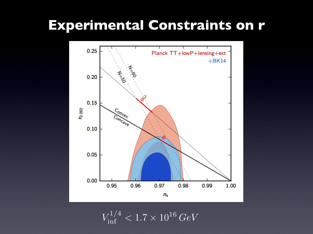
Experimental Constraints on r
V 1/4inf < 1.7× 10¹⁶ GeV

Experimental Progress on r
• the tensor contribution to the temperature anisotropies on large angular scales
• the B-mode polarization generated by tensors.
With the current data, we can constrain with
The two likelihood are essentially independent
Typically we talk about
L(rTT , rBB) = LTT (rTT )LBB(rBB)
L(r, r)
r
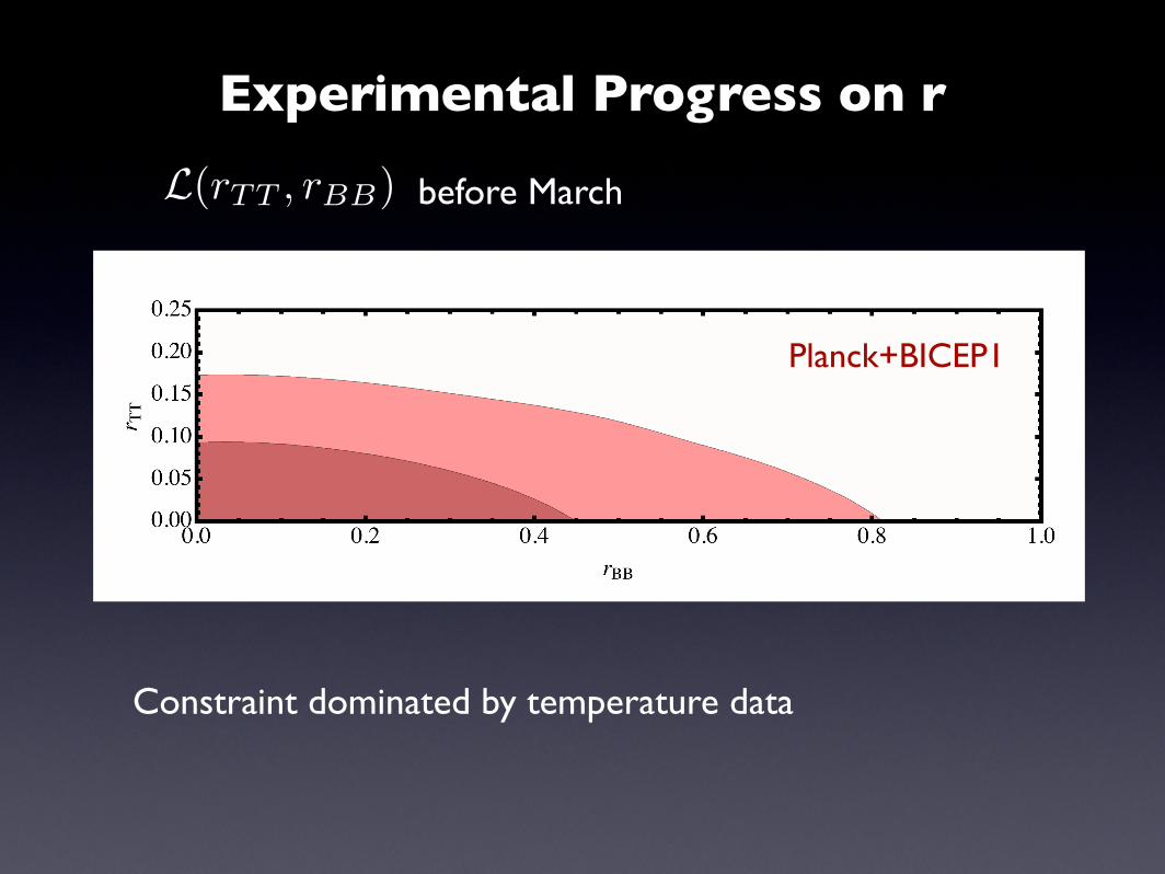
Planck+BICEP1
before March
Constraint dominated by temperature data
L(rTT , rBB)
Experimental Progress on r

after BICEP2L(rTT , rBB)
Planck+BICEP1Planck+BICEP2
Experimental Progress on r
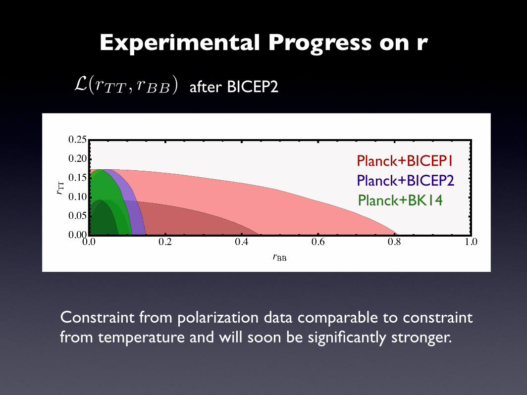
after BICEP2L(rTT , rBB)
Constraint from polarization data comparable to constraint from temperature and will soon be significantly stronger.
Planck+BICEP1Planck+BICEP2
Experimental Progress on r
Planck+BICEP1Planck+BICEP2Planck+BK14
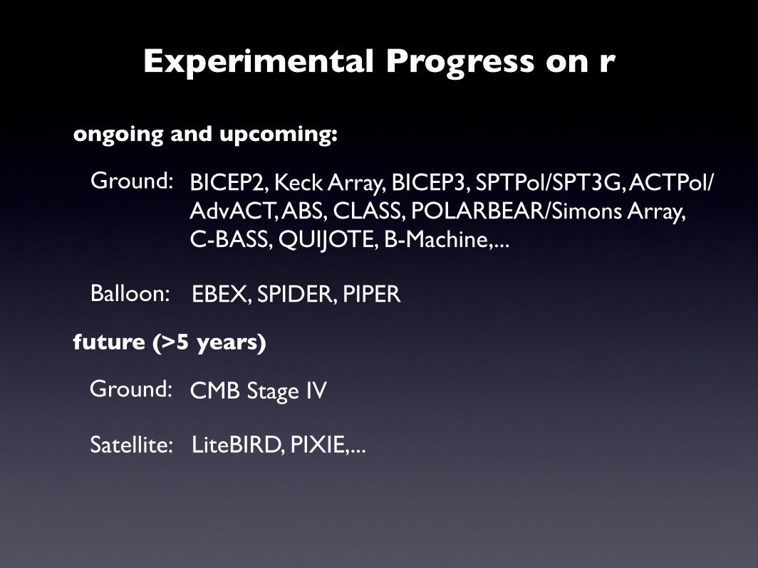
Experimental Progress on r
ongoing and upcoming:
BICEP2, Keck Array, BICEP3, SPTPol/SPT3G, ACTPol/AdvACT, ABS, CLASS, POLARBEAR/Simons Array, C-BASS, QUIJOTE, B-Machine,...
EBEX, SPIDER, PIPER
future (>5 years)
LiteBIRD, PIXIE,...
CMB Stage IV
Ground:
Balloon:
Ground:
Satellite:
10 100 1000106
104
0.01
1
100
1C 2
ΠΜK2
preliminary E-modes
lensing B-modes
residuallensing B-modes
cleanest 30% at 150 GHz
cleanest 1% at 150 GHz
r=0.01
r=0.001
Experimental Progress on r
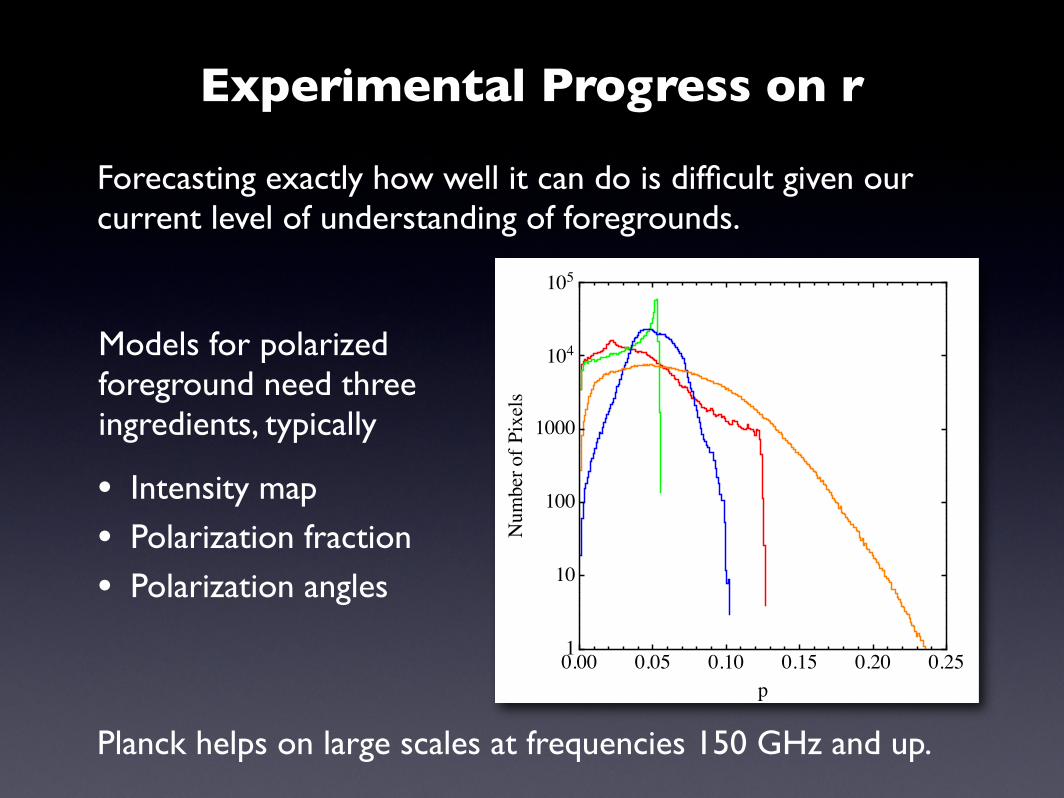
Forecasting exactly how well it can do is difficult given our current level of understanding of foregrounds.
• Intensity map
• Polarization fraction
• Polarization angles
Models for polarized foreground need three ingredients, typically
0.00 0.05 0.10 0.15 0.20 0.251
10
100
1000
104
105
p
NumberofPixels
Planck helps on large scales at frequencies 150 GHz and up.
Experimental Progress on r

Brust, Kaplan, Walters 1303.5079
Neff
σCMBS4(Neff) ≈ 0.02

Conclusions
• The LCDM model with inflationary spectrum of perturbations is consistent with all current cosmological data.
• The CMB will continue to provide valuable information about primordial gravitational waves, neutrino masses, the number of effective relativistic degrees of freedom, dark matter, ...
• Large scale structure surveys will provide a useful counter part
• The next decade should be very interesting in cosmology

Thank you