Embed Size (px)
Citation preview
Progress In Electromagnetics Research, Vol. 138, 65–82, 2013
PLANAR MAGNETIC INDUCTION TOMOGRAPHYFOR 3D NEAR SUBSURFACE IMAGING
Lu Ma, Hsin-Yu Wei, and Manuchehr Soleimani*
Engineering Tomography Laboratory (ETL), Department of Electronicand Electrical Engineering, University of Bath, Bath, UK
Abstract—Magnetic induction tomography (MIT) is a tomographictechnique utilising inductive coils and eddy currents to map the passiveelectromagnetic properties of an object. Eddy current methods arewidely used for non-destructive testing (NDT) in inspection of metallicstructures. Eddy current based NDT uses a single coil or a pair of coilsto scan the samples. As an emerging NDT technique, MIT scans thesample with a coil array through an eddy current based tomographicapproach. In this paper, a planar array MIT system (PMIT) isproposed for 3D near subsurface imaging. This is of great importanceas there are large numbers of potential applications for MIT that allowlimited access to the materials under testing. The system development,practical implication, capability and limitations of PMIT are discussed.The fundamental principles are demonstrated through simulations.Experimental data are used to evaluate the capability and detectabilitythis system has as a potential 3D subsurface imaging tool.
1. INTRODUCTION
Magnetic Induction Tomography (MIT) is an emerging non-destructiveevaluation technique that is able to map passive electromagneticproperties without causing material damage. In recent years, MIThas had applications ranging from biomedical imaging to industrialinspection. Many previous MIT systems were developed using coilsthat are arranged around the imaging periphery [1–7]. This typeof coil arrangement has a circular geometry and free access aroundthe complete periphery, thus full access tomography can be achieved.However, there are numerous applications where access is restrictedand non-invasive measurements can only be taken from one surface [8].
Received 7 November 2012, Accepted 4 March 2013, Scheduled 15 March 2013* Corresponding author: Manuchehr Soleimani ([email protected]).

66 Ma, Wei, and Soleimani
Consequently, the imaging process cannot be carried out by usinga MIT system with a circular or near circular sensor array. Planargeometry can overcome this difficulty. As such, recent research hasfocused on developing planar sensors and estimating near-surfacematerial properties using them [9, 10]. Inspecting product quality usingplanar sensors is also possible [11]. A simulation study of planar MITwas reported in [8], where the 2D cross-sectional images of conductivebars were obtained using an iterative SIRT reconstruction. Paper [12]presented a planar MIT system for the detection of conductivityinhomogeneity on the surface of a metallic plate. The sensors wereplaced in a circular shape with their axes perpendicular to the plate.The 2D images were reconstructed using experimental data. It wasshown that a spatial distinguish ability of 10–20% of the array diameterwas possible. In this paper, a planar MIT (PMIT) is developed as atype of limited access tomography, which realises 3D reconstructionfor near subsurface imaging. Recently, we have developed a 3D MITsystem [13], and the techniques developed in 3D MIT enabled thedevelopment of a 3D PMIT, which offers an insight into the structuresunderneath the sensors by depth detection. The observations in thispaper can be extended to other types of tomography and inverseproblems [14–20]. The development of planar sensor model and systemsetup are presented, followed by simulation results and experimentalevaluation. The paper presents the first 3D PMIT study for subsurfaceimaging. The PMIT has two main advantages over traditional scanningbased eddy current NDT methods. Firstly, PMIT employs an arrayof coils so that the scanning speed can be improved. Secondly,measurements from non-neighboring coils offer greater depth detectioncompared to single coil or double coil based eddy current scanningtechniques, which will help to gain information about the materialsunder testing.
Table 1. Sensor model parameters.
Parameters ValueNumber of coils 16
Number of turns for each coil 100Inner diameter for each coil: di (cm) 3.9Outer diameter for each coil: do (cm) 4.1
Coil height: H (cm) 5Coil side length: l (cm) 3.4
Self-inductance of each coil (µH) 380

Progress In Electromagnetics Research, Vol. 138, 2013 67
(a) (b)
Figure 1. (a) Coil dimensions, (b) coil sequence.
2. SYSTEM DESCRIPTION
2.1. Sensor Model
The planar sensor array consists of 16 air-core cylindrical coils. The16 coils are arranged in a 4 × 4 matrix form, and mounted on a non-conductive square board with a surface area of 18 × 18 cm2. Thethickness of the board is t = 0.3 cm. The distance between each coil is0.3 cm. The important parameters for this sensor model are listed inTable 1. Figure 1(a) shows the coil dimensions, and Figure 1(b) showsthe arrangement of coil sequence.
2.2. System Setup
This PMIT system consists of (i) a Topward 8112 digital functiongenerator, (ii) a matrix of 16 equally spaced inductive coils, witheach coil axis perpendicular to the materials under testing, (iii) anADG406 16-channel multiplexer, (iv) a National Instrument (NI-6295)data acquisition card, and (v) a host computer. The block diagramof this system is given in Figure 2. Each of the 16 inductive coils isindividually supplied with a 15 V peak, 50 kHz sinusoidal-signal fromthe digital function generator, while the remaining coils are floatedas receivers. An ADG406 16-channel multiplexer is connected in thesystem to accomplish the channel switching process. A NI USB-6295data acquisition device is connected through USB ports to interfacebetween the ADG406 multiplexer and a host PC, where the imagereconstruction takes place. The NI USB-6295 has four analog outputsat 16 bits and an input of max rate of 1.25 MS/s. The aim of thisdevice is to collect individual data efficiently, combine data effectivelyand display data in images to suit the need for imaging process. ThisPMIT system has 120 unique coil pairs: 1-2, 1-3, . . ., 1-16, 2-3, 2-4,. . ., 15-16, giving a total number of 120 independent measurements.

68 Ma, Wei, and Soleimani
Figure 2. Block diagram of the proposed PMIT system.
All the measurements are averaged three times before being displayedto ensure low noise perturbation. The image reconstruction moduleextracts 120 independent measurements, performs the reconstructionalgorithms, displays and updates the images.
The signal to noise ratio (SNR) is taken to indicate the signal levelof this system to the background noise level, which can be defined usingamplitude ratio as [21].
SNR = 20 log10
US
UN(1)
where US is the mean signal amplitude and UN is the standarddeviation of measured signal amplitude. It can be seen from Figure 3that the highest SNR of this PMIT system is 63.1 dB (for measurementbetween coil 1 and coil 2) and the lowest SNR is 33.4 dB (formeasurements between coil 1 and coil 16). The coil arrangement canbe seen in Figure 1(b).
3. METHOD
The forward problem in PMIT is a well-known eddy currentproblem [22–25]. In this study, the eddy current problem is solvedusing a magnetic potential vector A.
∇× 1µ∇×A + jσωA = Js (2)
where µ is the magnetic permeability, σ the electrical conductivity, ωthe angular frequency of the excitation current, and Js the excitation

Progress In Electromagnetics Research, Vol. 138, 2013 69
Figure 3. Signal to noise ratio of first cycle measurements when firstcoil used as excitation.
current density. The results from the forward problem will be usedto calculate the induced voltages in sensing coils [26], as well as theJacobian matrix which is needed for the inverse problem. An efficientformulation for the sensitivity map is used. If the total current inthe excitation coil is I0, the sensitivity of the induced voltage to theconductivity change can be written as [22, 25]:
∂Vmn
∂σk= −ω2
∫Ωk
Am ·Andv
I0(3)
where Vmn is the measured voltage, σk the conductivity of voxel k,Ωk the volume of the perturbation (voxel k), and Am and An arerespectively solutions of the forward solver when the excitation coil (m)is excited by I0 and the sensing coil (n) excited with unit current. Thesensitivity matrix J is constructed by subdividing the imaging regioninto small voxels and determining the change in measured voltage ofeach pair of sensors ∆V due to perturbations of the volume in eachvoxel.
In the previous section, the SNR is shown to indicate the signallevel of the PMIT system. In this part, the sensitivity map will be usedto evaluate how a pair of coils couple with each other. The sensitivitymap of the electromagnetic imaging problem describes the systemresponse to every voxel perturbation for a selected excitation/detectioncoil pair [5, 8, 22]. When the coils are close together, the systemis sensitive to the surface layers, and as the coils become furtherapart, the sensitivity penetrates deeper underneath the object undertesting [8]. This can be demonstrated by Figure 4, where a selection

70 Ma, Wei, and Soleimani
(a) (b) (c)
Figure 4. Sensitivity map coupling between: (a) coil 1 and coil 2, (b)coil 1 and coil 11 and (c) coil 1 and coil 16, the coil number sequencecan be seen in Figure 1(b).
of sensitivity maps of this system are shown. When receiving coilsare at an increased distanced from excitation coils, a relatively largersensitive region and a greater penetration can be observed in the systemresponse. A decreased sensitive contour can also be observed due tothe decreased strength of signals from the receiving coils. This can beseen in Figure 4(c), showing a pair of coils with the greatest distancebetween them. The sensitive contour in Figure 4(c) has the deepestpenetration and the largest area, but the sensitivity in the middle islower compared to other patterns, as shown in Figures 4(a) and 4(b).
In this study, a linear inverse solver is used for 3D nearsubsurface imaging. In linear inversion, the forward problem isassumed to have a linear form: ∆V = J∆σ. The Tikhonovregularization method has been commonly implemented for the MITimage reconstruction [4, 26, 27], particularly in [4]. Experimentalvalidation of the Tikhonov method was shown using linear imagereconstruction and in [26], where a nonlinear image reconstruction wasdemonstrated using both Tikhonov and total variation regularizationmethods. In this study, a standard Tikhonov regularization method isused as an inverse solver to calculate the conductivity distribution inthe following manner:
∆σ =(JT J + αR
)−1JT (∆V ) (4)
where ∆V is a column vector consisting of 120× 1 changes of inducedvoltages, ∆σ also a column vector representing conductivity changes in193 × 1 voxels, J a 120× 193 matrix of the sensitivity field calculatedfrom Equation (3), α the regularization parameter which is chosenempirically, and R an identity matrix.

Progress In Electromagnetics Research, Vol. 138, 2013 71
4. SIMULATION AND EXPERIMENTAL EVALUATION
4.1. Detectability of PMIT System
The PMIT is a challenging 3D inverse problem, in particular, becauseof limited access to the object. The simulations presented in thissection are used to study the underlying inverse problems in the contextof a linear model. The end view of a number of simulation models arepresented in Figure 5 to evaluate the capability and detectability ofthe PMIT system. The planar sensor array is simulated in (x, z) planeat y = 0. The first column in Figure 5 shows the simulated inclusionsin different locations. The second column in Figure 5 includes thereconstructed images for each simulated case. The reconstructed 3Dcontour images in the third column in Figure 5 provide an insight asto where the inclusion is with respect to the planar sensor array.
Inclusions Sliced images 3D contour images
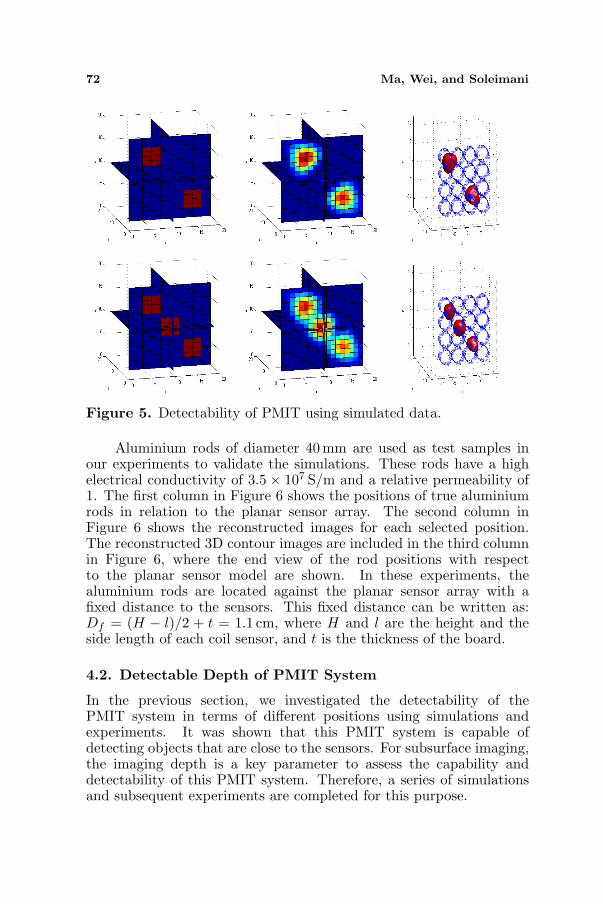
72 Ma, Wei, and Soleimani
Figure 5. Detectability of PMIT using simulated data.
Aluminium rods of diameter 40 mm are used as test samples inour experiments to validate the simulations. These rods have a highelectrical conductivity of 3.5× 10⁷ S/m and a relative permeability of1. The first column in Figure 6 shows the positions of true aluminiumrods in relation to the planar sensor array. The second column inFigure 6 shows the reconstructed images for each selected position.The reconstructed 3D contour images are included in the third columnin Figure 6, where the end view of the rod positions with respectto the planar sensor model are shown. In these experiments, thealuminium rods are located against the planar sensor array with afixed distance to the sensors. This fixed distance can be written as:Df = (H − l)/2 + t = 1.1 cm, where H and l are the height and theside length of each coil sensor, and t is the thickness of the board.
4.2. Detectable Depth of PMIT System
In the previous section, we investigated the detectability of thePMIT system in terms of different positions using simulations andexperiments. It was shown that this PMIT system is capable ofdetecting objects that are close to the sensors. For subsurface imaging,the imaging depth is a key parameter to assess the capability anddetectability of this PMIT system. Therefore, a series of simulationsand subsequent experiments are completed for this purpose.

Progress In Electromagnetics Research, Vol. 138, 2013 73
In Figure 7, the top view of the simulation models are shownto demonstrate the principle of near subsurface imaging using PMITsystem. The planar sensor model is simulated in (x, z) plane at y = 0.
True samples Sliced images 3D contour images

74 Ma, Wei, and Soleimani
Figure 6. Detectability of PMIT using experimental data.
Figure 7. Depth detection using simulated data.
The first row in Figure 7 shows one simulated inclusion with highlightedlines indicating the distance between the sensors and the inclusion atfour selected depths: y = 3, y = 5, y = 8, and y = 10. The second row

Progress In Electromagnetics Research, Vol. 138, 2013 75
in Figure 7 presents the reconstruction of one inclusion at each selecteddepth. The same simulation procedures are adopted for simulating twoinclusions, as shown in the third row in Figure 7. The reconstructedimages are demonstrated in the bottom row in Figure 7. It can be seenfrom Figure 7 that the image quality degrades as the depth increases.
We have solved the inverse problem and detect a maximumimaging depth of 8–10 cm using simulations. In order to verify thesimulation models and evaluate the detectable depth of the PMITsystem using measured data, two sets of experiments are completed.Same aluminium rods are used as test samples. Figure 8 presents theexperimental setup and the reconstructed images using one rod forsubsurface imaging. The first row in Figure 8 shows the top view ofthe true samples with respect to the planar sensors.
As mentioned in Section 4.1, there is a fixed distance ofDf = 1.1 cm between the sensor array and the samples due to theconstruction of the sensor model and the thickness of the board.Although short, it is crucial to take this distance into considerationwhen evaluating the depth of this system, as it poses an additionalbarrier for eddy current in MIT, particularly as the skin depth is verylimited under a low driving frequency of 50 kHz. Therefore, it cannotbe neglected. The structure and layout of the sensor model need tobe considered carefully if a highly accurate system is required. Themoving distances from the planar sensors Dm are: 0 cm, 1 cm, 2 cm,3 cm and 4 cm respectively. Therefore, the total distance between thetrue sample and the front of the sensor array is D = Df + Dm. The
D = 1.1 cm D = 2.1 cm D = 3.1 cm D = 4.1 cm D = 5.1 cm
Figure 8. Depth detection using one object.
76 Ma, Wei, and Soleimani
D = 1.1 cm D = 2.1 cm D = 3.1 cm D = 4.1 cm D = 5.1 cm
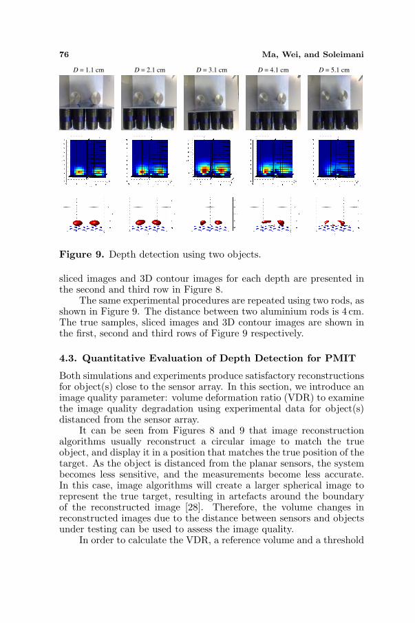
Figure 9. Depth detection using two objects.
sliced images and 3D contour images for each depth are presented inthe second and third row in Figure 8.
The same experimental procedures are repeated using two rods, asshown in Figure 9. The distance between two aluminium rods is 4 cm.The true samples, sliced images and 3D contour images are shown inthe first, second and third rows of Figure 9 respectively.
4.3. Quantitative Evaluation of Depth Detection for PMIT
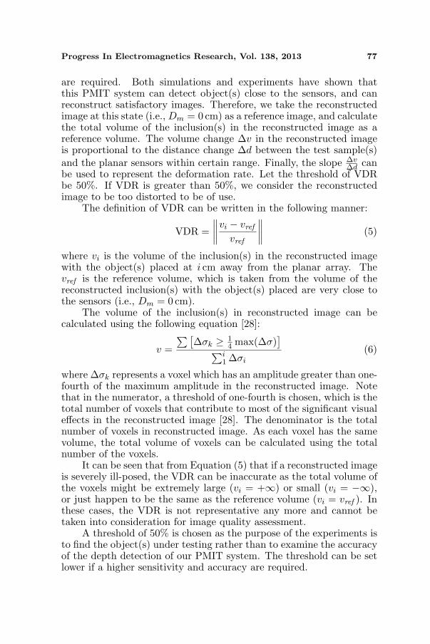
Both simulations and experiments produce satisfactory reconstructionsfor object(s) close to the sensor array. In this section, we introduce animage quality parameter: volume deformation ratio (VDR) to examinethe image quality degradation using experimental data for object(s)distanced from the sensor array.
It can be seen from Figures 8 and 9 that image reconstructionalgorithms usually reconstruct a circular image to match the trueobject, and display it in a position that matches the true position of thetarget. As the object is distanced from the planar sensors, the systembecomes less sensitive, and the measurements become less accurate.In this case, image algorithms will create a larger spherical image torepresent the true target, resulting in artefacts around the boundaryof the reconstructed image [28]. Therefore, the volume changes inreconstructed images due to the distance between sensors and objectsunder testing can be used to assess the image quality.
In order to calculate the VDR, a reference volume and a threshold
Progress In Electromagnetics Research, Vol. 138, 2013 77
are required. Both simulations and experiments have shown thatthis PMIT system can detect object(s) close to the sensors, and canreconstruct satisfactory images. Therefore, we take the reconstructedimage at this state (i.e., Dm = 0 cm) as a reference image, and calculatethe total volume of the inclusion(s) in the reconstructed image as areference volume. The volume change ∆v in the reconstructed imageis proportional to the distance change ∆d between the test sample(s)and the planar sensors within certain range. Finally, the slope ∆v
∆d canbe used to represent the deformation rate. Let the threshold of VDRbe 50%. If VDR is greater than 50%, we consider the reconstructedimage to be too distorted to be of use.
The definition of VDR can be written in the following manner:
VDR =∥∥∥∥vi − vref
vref
∥∥∥∥ (5)
where vi is the volume of the inclusion(s) in the reconstructed imagewith the object(s) placed at i cm away from the planar array. Thevref is the reference volume, which is taken from the volume of thereconstructed inclusion(s) with the object(s) placed are very close tothe sensors (i.e., Dm = 0 cm).
The volume of the inclusion(s) in reconstructed image can becalculated using the following equation [28]:
v =∑[
∆σk ≥ 14 max(∆σ)
]∑i
1 ∆σi
(6)
where ∆σk represents a voxel which has an amplitude greater than one-fourth of the maximum amplitude in the reconstructed image. Notethat in the numerator, a threshold of one-fourth is chosen, which is thetotal number of voxels that contribute to most of the significant visualeffects in the reconstructed image [28]. The denominator is the totalnumber of voxels in reconstructed image. As each voxel has the samevolume, the total volume of voxels can be calculated using the totalnumber of the voxels.
It can be seen that from Equation (5) that if a reconstructed imageis severely ill-posed, the VDR can be inaccurate as the total volume ofthe voxels might be extremely large (vi = +∞) or small (vi = −∞),or just happen to be the same as the reference volume (vi = vref ). Inthese cases, the VDR is not representative any more and cannot betaken into consideration for image quality assessment.
A threshold of 50% is chosen as the purpose of the experiments isto find the object(s) under testing rather than to examine the accuracyof the depth detection of our PMIT system. The threshold can be setlower if a higher sensitivity and accuracy are required.
78 Ma, Wei, and Soleimani
4.4. Discussion
It can be seen from Figures 5 and 6 that the PMIT system is capable ofdetecting both single and multiple conductive objects, which are placedwith an approximate fixed distance of 1 cm away from the sensors.However, the reconstructed images using experimental data showing inFigure 6 are generally compromised compared to the results presentedin Figure 5.
A number of simulation models in Figure 7 demonstrate theprinciples of near subsurface imaging using a PMIT system. It can beseen from Figure 7 that a depth of 8–10 cm can be achieved throughsimulations. This further validates our system sensitivity analysis, aspresented in Figure 4, where the sensitive contour does not penetratemore than 10 cm into the imaging region. The experimental resultspresented in Figures 8 and 9 reveal that the PMIT system can detecta depth of approximately 3–4 cm beneath the planar array.
It is clear from the 3D contour images shown in Figure 8 thatthe true sample can only be detected partially as the distance fromthe sensors increases. Moreover, comparing the reconstructed imagesfrom two sets of experiments for evaluating depth detection, a rapiddegradation in image quality can be observed in Figure 9 compared tothe results in Figure 8. This image degradation is also quantitatively
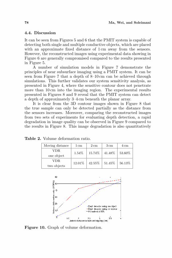
Table 2. Volume deformation ratio.
Moving distance 1 cm 2 cm 3 cm 4 cm
VDR
one object1.54% 15.74% 41.48% 53.60%
VDR
two objects12.01% 42.55% 51.45% 56.13%
Figure 10. Graph of volume deformation.

Progress In Electromagnetics Research, Vol. 138, 2013 79
evaluated through an image quality measure VDR, as shown in Table 2and Figure 10. The VDR of the reconstructed image at incrementallyincreased distance of 1 cm for one object is 1.54%, while the VDRfor two objects at the same distance away from planar sensors is12.01%, significantly higher. As the distance is increased to 3 cm, theVDR for two objects exceeds the threshold of VDR, which means thereconstructed image is severely degraded. However, this degradationin image quality is not associated with the number of objects undertesting. The system detectability depends on the distribution of thesensitive region and the locations of the object(s) under testing.
In general, uniform detectability can be observed in the region thatis close to the sensors. As the imaging depth increases, the sensitivitydegrades from uniform detectability. The detectable area can beconsidered similar to a spherical region due to the decreased signalsbetween coil pairs that are further away. It is shown in Figure 4(c)that the measurement from the furthest coil pair contribute to mostof the significant depth. However, the furthest coil pairs also have thelowest SNR, as shown in Figure 3, which means the sensitivity of sucha coil pair is reduced compared to the sensitivity of neighbouring coilpairs. As the object moves further away from the planar sensors, theoverall sensitivity decreases. The areas that are close to the edge of theplanar array is comparatively less covered by the sensor array. Hence,the sensitive region tends to have a trapezoidal or spherical shape, asshown in Figure 11.
The level of detectability between simulated and measured datadiffers for two reasons: noise in measured data, and the skin deptheffect. In this study, at a driving frequency of 50 kHz, aluminiumhas a skin depth of approximately 366µm [4], which is far less thanthe diameter of the aluminium rod. This results in the eddy currentthreading on the surface of the object. As such, very little informationcan be obtained from the back of the test sample. The simulatedmodels do not have issues associated with depth penetration as a linearmodel is assumed.
Figure 11. The distribution of sensitive region against the imagingdepth.
80 Ma, Wei, and Soleimani
5. CONCLUSIONS
This paper investigates the capability and detectability of a novelPMIT system. This geometry makes it possible to study the nearsubsurface imaging using an eddy current method. It is a verychallenging imaging setup as access to the targeted object is limitedto one surface only. The fundamental principles are verified throughsimulation studies. Experimental results detect a limited depth inthis PMIT system. Nevertheless, it demonstrates the potential thissystem has as a non-invasive subsurface imaging tool. In our futurework, we will aim to improve the depth detection by developing amulti-frequency PMIT system. Non-linear image reconstruction in 3DPMIT will also be a subject of our future study.
REFERENCES
1. Wei, H.-Y. and M. Soleimani, “Two-phase low conductivityflow imaging using magnetic induction tomography,” Progress InElectromagnetics Research, Vol. 131, 97–115, 2012.
2. Ma, L., H.-Y. Wei, and M. Soleimani, “Pipeline inspectionusing magnetic induction tomography based on a narrowbandpass filtering method,” Progress In Electromagnetics Research M,Vol. 23, 65–78, 2012.
3. Lyon, G. M., Z. Z. Yu, A. J. Peyton, and M. S. Beck,“Developments in electro-magnetic tomography instrumentation,”IEEE Colloguium on Advances in Electrical Tomography, Vol. 12,1–4, 1993.
4. Ma, X., A. J. Peyton, S. R. Higson, A. Lyons, and S. J. Dickinson,“Hardware and software design for an electromagnetic inductiontomography (EMT) system for high contrast metal processapplications,” Measurement Science and Technology, Vol. 17,No. 1, 111–118, 2006.
5. Peyton, A. J., Z. Z. Yu, G. Lyon, S. Al-Zeibak, J. Ferreira, J. Velez,F. Linhares, A. R. Borges, H. L. Xiong, N. H. Saunders, andM. S. Beck, “An overview of electromagnetic induction tomogra-phy: Description of three different systems,” Measurement Scienceand Technology, Vol. 7, 261–271, 1996.
6. Yu, Z. Z., A. J. Peyton, W. F. Conway, L. A. Xu, and M. S. Beck,“Imaging system based on electromagnetic tomography (EMT),”Electronics Letters, Vol. 29, No. 7, 625–626, 1993.
7. Korjenevsky, A., V. Cherepenin, and S. Sapetsky, “Magnetic
Progress In Electromagnetics Research, Vol. 138, 2013 81
induction tomography: Experimental realization,” PhysiologicalMeasurement, Vol. 21, No. 1, 89, 2000.
8. Ramli, S. and A. J. Peyton, “Feasibility study of planar-array electromagnetic inductance tomography (EMT),” 1st WorldCongress on Industrial Process Tomography, Buxton, GreaterManchester, Apr. 14–17, 1999.
9. Mukhopadhyay, S. C., S. Yamada, and M. Iwahara, “Inspectionof electro-plated materials-performance comparison with planarmeander and mesh type magnetic sensor,” International Journalof Applied Electromagnetics and Mechanics, Vol. 15, No. 1, 323–330, 2002.
10. Mukhopadhyay, S. C., S. Yamada, and M. Iwahara, “Investiga-tion of near-surface material properties using planar type meandercoil,” JSAEM Studies on Applied Electromagnetics and Mechan-ics, Vol. 11, 61–69, 2001.
11. Mukhopadhyay, S. C., “Novel planar electromagnetic sensors:Modeling and performance evaluation,” Sensors, Vol. 5, No. 12,546–579, 2005.
12. Yin, W. and A. J. Peyton, “A planar EMT system forthe detection of faults on thin metallic plates,” PhysiologicalMeasurement, Vol. 17, No. 8, 2130–2135, 2006.
13. Wei, H. Y., L. Ma, and M. Soleimani, “Volumetric magneticinduction tomography,” Measurement Science and Technology,Vol. 23, No. 5, 055401, 2012.
14. Hajihashemi, M. R. and M. El-Shenawee, “Inverse scatteringof three-dimensional PEC objects using the level-set method,”Progress In Electromagnetics Research, Vol. 116, 23–47, 2011.
15. Park, W.-K., “On the imaging of thin dielectric inclusions viatopological derivative concept,” Progress In ElectromagneticsResearch, Vol. 110, 237–252, 2010.
16. Banasiak, R., Z. Ye, and M. Soleimani, “Improving three-dimensional electrical capacitance tomography imaging usingapproximation error model theory,” Journal of ElectromagneticWaves and Applications, Vol. 23, Nos. 2–3, 411–421, 2012.
17. AlShehri, S. A., S. Khatun, A. B. Jantan, R. S. A. Raja Abdullah,R. Mahmood, and Z. Awang, “3D experimental detection anddiscrimination of malignant and benign breast tumor usingNN-based UWB imaging system,” Progress In ElectromagneticsResearch, Vol. 116, 221–237, 2011.
18. Ren, S., W. Chang, T. Jin, and Z. Wang, “AutomatedSAR reference image preparation for navigation,” Progress In

82 Ma, Wei, and Soleimani
Electromagnetics Research, Vol. 121, 535–555, 2011.19. Wei, S.-J., X.-L. Zhang, J. Shi, and G. Xiang, “Sparse
reconstruction for SAR imaging based on compressed sensing,”Progress In Electromagnetics Research, Vol. 109, 63–81, 2010.
20. Chang, Y.-L., C.-Y. Chiang, and K.-S. Chen, “SAR imagesimulation with application to target recognition,” Progress InElectromagnetics Research, Vol. 119, 35–57, 2011.
21. Merwa, R. and H. Scharfetter, “Magnetic-induction-tomography:Evaluation of the point-spread-function and analysis of resolutionand image distortion,” Physiological Measurement, Vol. 28, 313–324, 2007.
22. Dyck, D. N., D. A. Lowther, and E. M. Freeman, “A methodof computing the sensitivity of the electromagnetic quantitiesto changes in the material and sources,” IEEE Transactions onMagnetics, Vol. 30, 3415–3418, 1994.
23. Griffiths, H., “Magnetic induction tomography,” MeasurementScience and Technology, Vol. 12, 1126–1131, 2001.
24. Ktistis, C., D. W. Armitage, and A. J. Peyton, “Calculation ofthe forward problem for absolute image reconstruction in mit,”Physiological Measurement, Vol. 29, S455–S464, 2008.
25. Soleimani, M. and W. R. B. Lionheart, “Image reconstructionin three-dimensional magnetostatic permeability tomography,”IEEE Transactions on Magnetics, Vol. 41, 1274–1279, 2005.
26. Soleimani, M., W. R. B. Lionheart, A. J. Peyton, X. Ma,and S. R. Higson, “A three-dimensional inverse finite-elementmethod applied to experimental eddy-current imaging data,”IEEE Transactions on Magnetics, Vol. 42, No. 5, 1560–1567, 2006.
27. Ziolkowski, M., S. Gratkowski, and R. Palka, “Solution of threedimensional inverse problem of magnetic induction tomographyusing Tikhonov regularization method,” International Journal ofApplied Electromagnetics and Mechanics, Vol. 30, No. 3–4, 245–253, 2009.
28. Adler, A., J. H. Arnold, R. Bayford, A. Borsic, B. Brwon,P. Dixon, T. J. C. Faes, I. Frerichs, H. Gagnon, Y. Garbr,B. Grychtol, G. Hahn, W. R. B. Lionheart, A. Malik,R. P. Patterson, J. Stocks, A. Tizzard, N. Weiler, and G. K. Wolf,“Greit: A unified approach to 2D linear EIT reconstruction oflung images,” Physiological Measurement, Vol. 30, S33–S55, 2009.