Embed Size (px)
Citation preview
Pitch Modelling for Speech Coding at 4.8 kbitsls
Gebrael Chahine
B. Eng.
A thesis submitted to the Faculty of Graduate Studies and
Research in partial fulfillment of the requirements
for the degree of Master of Engineering
Department of Electrical Engineering
McGill University
MontrCal, Canada
July, 1993
@ Gebrael Chahine, 1993
Abstract
The purpose of this thesis is to examine techniques of efficiently modelling the
Long-Term Predictor (LTP) or the pitch filter in low rate speech coders. The emphasis
in this thesis is on a class of coders which are referred to as Linear Prediction (LP)
based analysis-by-synthesis coders, and more specifically on the Code-Excited Linear
Prediction (CELP) coder which is currently the most commonly used in low rate
transmission. The experiments are performed on a CELP based coder developed by
the U.S. Department of Defense (DoD) and Bell Labs, with an output bit rate of 4.8
kbits/s.
A multi-tap LTP outperforms a single-tap LTP, but at the expense of a greater
number of bits. A single-tap LTP can be improved by increasing the time resolution of
the LTP. This results in a fractional delay LTP, which produces a significant increase
in prediction gain and perceived periodicity at the cost of more bits, but less than for
the multi-tap case.
The first new approach in this work is to use a pseudo-three-tap pitch filter with
one or two degrees of freedom of the predictor coefficients, which gives a better quality
reconstructed speech and also a more desirable frequency response than a one-tap
pitch prediction filter. The pseudo-three-t ap pitch filter with one degree of freedom
is of particular interest as no extra bits are needed to code the pitch coefficients.
The second new approach is to perform time scalinglshifting on the original
speech minimizing further the minimum mean square error and allowing a smoother
and more accurate reconstruction of the pitch structure. The time scaling technique
allows a saving of 1 bit in coding the pitch parameters while maintaining very closely
the quality of the reconstructed speech. In addition, no extra bits are needed for
the time scaling operation as no extra side information has to be transmitted to the
receiver.
Sommaire
L'objet de cette thkse est d'examiner des techniques pour modeliser efficacement
la PrCdiction B Long Terme (PLT) pour les codeurs de parole B faible dCbit. Cette
thkse Ctudie principalement une certaine classe de codeurs oh la prCdiction linCaire est
basCe sur l'analyse-par-synthkse et plus spdcialement le Code-Excited Linear Predic-
tion (CELP) qui est actuellemnt le plus utilisC pour les transmissions B faible dCbit.
Les simulations utilisent un codeur CELP developpC par le dCpartement de la dCfense
des E.U. et les laboratoires Bell ayant un dCbit de 4.8 kbitsls.
Un PLT B coefficients multiples surclasse le PLT B coefficient unique au prix d'un
nombre plus important de bits. Le PLT B coefficient unique peut ttre amCliorC en
augmentant la rCsolution en temps du PLT. Ceci rCsulte en un PLT B delai fractionnel
qui produit une amClioration significative du gain de prediction et de la pCriodicitCe
percue au cout de plus de bits mais moins que le PLT B coefficients multiples.
La premikre nouvelle approche de ce travail est d'utiliser un filtre B trois coeff-
cients accordant un ou deux degrCs de libertC aux coefficients du predicteur. Ce filtre,
connu sous le nom de pseudo-trois-coefficient, permet ainsi une meilleure qualit6 de
reconstruction et Cgalement une meilleure rCponse en frCquence qu'un filtre B coef-
ficient unique. Le filtre B pseudo-trois-coefficient avec un degrd de libertC offre un
inttret particulier puisque qu'il ne nCcessite pas des bits suppkmentaires pour coder
les coefficients supplCment aires.
La seconde nouvelle approche est d'utiliser un changement d'dchelle et un dCcalage
en temps du signal original pour minimiser l'erreur quadratique moyenne minimale
et permettre une reproduction plus fidkle de la structure de la frdquence fondamen-
tale. La technique de changement d'Cchelle en temps permet d'Climiner un bit au
codage des paramares de la frequence fondamentale tout en permettant une qualit6
du signal reproduit trks proche. De plus, aucun bit supplementaire n'est requis pour
le changement d'dchelle en temps puisque qu'aucune information supplementaire ne
doit ttre transmise au rCcepteur.
Acknowledgements
I would like to thank my supervisor Dr. Peter Kabal for his guidance throughout
my undergraduate and graduate studies. The first part of the research was conducted
at Institut National de la Recherche Scientifique (1NRS)-TC1Ccommunications labo-
ratories, and the second part was accomplished at Telecommunications and Signal
Processing (TSP) laboratory at McGill University. The financial support provided
by my supervisor and from the National Science and Engineering Research Council
(NSERC) was infinitely appreciated.
This thesis could not have been completed without the constant support and
love of my parents, my brother and my sister. Finally, I am most grateful for the
companionship provided by many friends at McGill.

Contents
1 Introduction
. . . . . . . . . . . . . . . . . . . . . . . . . 1.1 Digital Coding of Speech
. . . . . . . . . . . . . . . . . . . 1.2 The Evolution of Waveform Coders
. . . . . . . . . . . . . . . . . . . . . . . . 1.3 Organization of the Thesis
2 Analysis-by-Synthesis Linear Prediction Coders
. . . . . . . . . . . . . . . . . . . . . . . . . . . . . 2.1 Linear Prediction
. . . . . . . . . . . . . . . . . . . . . . 2.1.1 Short-Term Prediction
. . . . . . . . . . . . . . . . . . . . . . 2.1.2 Long-Term Prediction
. . . . . . . . . . . . . . . . . 2.2 Estimation of the Predictor Parameters
. . . . . . . . . . . . . . . . . . 2.2.1 Linear Prediction Coefficients
2.2.2 Predictor Order and Windowing ShapeISize . . . . . . . . . . . . . . . . . . . . . . . . . . . . . . 2.2.3 Line Spectral Frequencies
. . . . . . . . . . . . . . . . . . . . 2.3 Adaptive Predictive Coder (APC)
. . . . . . . . . . . . . . . . . . . . . . . . 2.4 Analysis-by-Synthesis APC
. . . . . . . . . . . . . 2.4.1 Analysis-by-Synt hesis Coder Structure
2.4.2 Codebook Excited Linear Prediction Structure . . . . . . . . . . . . . . . . . . . . . . . . . . . . . . . 2.4.3 The CELP Algorithm
3 Pitch Filtering in CELP Coders
. . . . . . . . . . . . . . . . . . . . . . . . . . . . . . . . 3.1 Introduction
. . . . . . . . . . . . . . . . . . . 3.2 Synthesis Parameters Optimization 31
. . . . . . . . . . . . . . . . 3.3 OptimizationforaOne-TapPitchFilter 34
. . . . . . . . . . . . . . . . . . . 3.3.1 Recycling the LP Excitation 35
3.3.2 Creating a Periodic Extension of a Pitch Cycle . . . . . . . . . 38
. . . . . . . . . . . . . . . . . . . . 3.4 Increased Resolution Pitch Filters 39
. . . . . . . . . . . . . . . . . . . . . . 3.4.1 Multi-Tap Pitch Filters 39
. . . . . . . . . . . . . . . . . . . . . . 3.4.2 Fractional Delay Filter 41
. . . . . . . . . . . . . . . . . . 3.5 Interpolation of the LTP Parameters 45
3.5.1 Generalized Analysis-by-Synthesis Procedure . . . . . . . . . . 46
. . . . . . . . . . . . . . 3.5.2 LTP with Continuous Delay Contour 47
3.5.3 Continuous Interpolation of the Pitch Predictor . . . . . . . . 49
3.5.4 Stepped Interpolation of the Pitch Predictor . . . . . . . . . . 52
4 Improved CELP Coder at 4.8 kbits/s 54
4.1 Introduction . . . . . . . . . . . . . . . . . . . . . . . . . . . . . . . . 54
. . . . . . . . . . . . . . . . . 4.2 The FS-1016 Standard Coder Structure 55
. . . . . . . . . . . . . . . . . . . . . . 4.2.1 Short Delay Prediction 56
. . . . . . . . . . . . . . . . . . . . . 4.2.2 Long Delay Pitch Search 57
. . . . . . . . . . . . . . . . . . . . . . . . . 4.2.3 Codebook Search 59
. . . . . . . . . . . . . . . . . . . . . 4.3 Pseudo-Three-Tap Pitch Filters 63
. . . . . . . 4.3.1 Three-Tap Pitch Filter with 2 Degrees of Freedom 65
. . . . . . . 4.3.2 Three-Tap Pitch Filter with 1 Degree of Freedom 67
. . . . . . . . 4.3.3 Frequency Response of Pseudo-Tap Pitch Filters 67
. . . . . . . . . . . . . . . . . . . . . . 4.4 PitchSynthesisFilterStability 68
. . . . . . . . . . . . . . . . . . . . . . . . . . . 4.4.1 StabilityTests 70
. . . . . . . . . . . . . . . . . . . . . 4.4.2 Stabilization Procedures 71
. . . . . . . . . . . . . . 4.5 Performance of Pitch Predictors in FS-1016 73
. . . . . . . . . . . . 4.6 Pitch Filtering Using a Time Scaling Approach 80
. . . . . . . . . . . . . . . . . . . 4.6.1 Motivation For Time Scaling 80
4.6.2 Time Scaling Algorithm in CELP . . . . . . . . . . . . . . . . 81
4.6.3 Performance of the Time Scaling Approach . . . . . . . . . . . 83
5 Summary and Conclusions 85
A System of Sampling Rate Increase 89
List of Figures
2.1 Formant Prediction . . . . . . . . . . . . . . . . . . . . . . . . . . . . 2.2 Pitch Prediction . . . . . . . . . . . . . . . . . . . . . . . . . . . . . .
. . . . . . . . . . . . . . . . 2.3 Analysis model for transversal predictors
2.4 Block diagram of an APC coder with noise feedback . (a) Analysis
phase . (b) Synthesis phase . . . . . . . . . . . . . . . . . . . . . . . . 2.5 Analysis-by-synthesis coder . . . . . . . . . . . . . . . . . . . . . . . . 2.6 Basic CELP configuration . . . . . . . . . . . . . . . . . . . . . . . .
3.1 Single-tap pitch predictor; adaptive codebook illustration . . . . . . . 3.2 Synthesis parameters optimization . . . . . . . . . . . . . . . . . . . .
3.3 Structure for realizing a fixed fractional delay of I / D samples . . . . . 3.4 Polyphase implementation of a fractional sample delay . . . . . . . . . 3.5 (a) Conventional analysis-by-synthesis coder . (b) Generalized analysis-
by-synthesis coder [l 11 . . . . . . . . . . . . . . . . . . . . . . . . . . 3.6 Time mismatched in the sample excitation signal . . . . . . . . . . .
3.7 CELP configuration used in interpolating the delay contour . . . . . .
4.1 FS-1016 CELP coder structure . . . . . . . . . . . . . . . . . . . . . . 4.2 Frequency response of a one-tap pitch synthesis filter with M = 78
samples and p = 0.57. . . . . . . . . . . . . . . . . . . . . . . . . . . 4.3 Frequency response of a three-tap pitch synthesis filter with M = 78
samples and coefficients (0.27 0.52 .0.055). . . . . . . . . . . . . . .
vii
4.4 Frequency response of a 3TlDF pitch synthesis filter with a = 0.25,
p = 0 . 5 2 a n d M = 7 8 . . . . . . . . . . . . . . . . . . . . . . . . . . . 68
4.5 Original and decoded speech segments; (a) original segment, (b) de-
coded segment without stabilization. (c) decoded segment for stabilized
pitch synthesis filter . . . . . . . . . . . . . . . . . . . . . . . . . . . . 77
4.6 Histogram of a in a 3T2DF configuration for a female speech file . . . 79
4.7 Motivation for time scaling . . . . . . . . . . . . . . . . . . . . . . . . 80
A.l General system for sampling rate increase by D . . . . . . . . . . . . 89
... Vll l
List of Tables
. . . . . . . . . . . . . . . . . . . . . . . . . . 4.1 LSF subframe structure 57
. . . . . . . . . . . . . . . 4.2 Bit allocation for the FS-1016 CELP coder 63
. . . . . . . . . . . . . . . 4.3 Performance of pseudo-tap pitch predictors 76
Chapter 1
Introduction
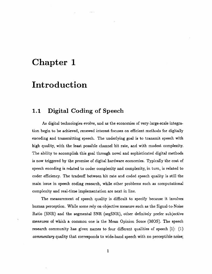
1.1 Digital Coding of Speech
As digital technologies evolve, and as the economies of very-large-scale integra-
tion begin to be achieved, renewed interest focuses on efficient methods for digitally
encoding and transmitting speech. The underlying goal is to transmit speech with
high quality, with the least possible channel bit rate, and with modest complexity.
The ability to accomplish this goal through novel and sophisticated digital methods
is now triggered by the promise of digital hardware economies. Typically the cost of
speech encoding is related to coder complexity and complexity, in turn, is related to
coder efficiency. The tradeoff between bit rate and coded speech quality is still the
main issue in speech coding research, while other problems such as computational
complexity and real-time implementation are next in line.
The measurement of speech quality is difficult to specify because it involves
human perception. While some rely on objective measure such as the Signal-to-Noise
Ratio (SNR) and the segmental SNR (segSNR), other definitely prefer subjective
measures of which a common one is the Mean Opinion Score (MOS). The speech
research community has
commentary quality that
given names to four different qualities of speech [I]: (1)
corresponds to wide-band speech with no perceptible noise;

(2) toll quality that refers to high-quality narrow-band speech that corresponds to
the quality of an all-digital telephone network; (3) communication quality that is
intelligible but has noticeable quality reduction; and finally (4) synthetic quality that
remains intelligible but loses naturalness.
Two classes of coding schemes can be distinguished: waveform coders and vocoders.
Waveform coders, as the name implies, essentially strive for facsimile reproduction of
the signal waveform. In principle, they are designed to be signal-independent, hence
they can code a variety of signals-speech, music and tones. They also tend to be ro-
bust for a wide range of talker characteristics and for noisy channel environment. To
preserve these advantages with minimal complexity, waveform coders typically aim
for moderate economies in transmission bit rate.
Vocoders, on the other hand, exploit the human speech production mechanism
and the human auditory system. Such coders derive a speech model characterized
by key parameters which are transmitted to the receiver so that the speech can
be reconstructed using the same model. Vocoders tend to be fragile (in terms of
parameters), the performance is often talker-dependent and the output speech has a
synthetic (less than natural) quality. Typical examples of vocoders are the channel
vocoder where the parameters are the values of the short-time amplitude spectrum of
the speech signal evaluated at specific frequencies, and the formant vocoder where the
parameters are the frequency values of major spectral resonances. By virtue of their
signal parameterization, vocoders can achieve very high economies in transmission
bandwidth. They are very useful in mobile telephony and satellite communications
where very low bit rate coders (2.4-8 kbits/s) are desired because of the bandwidth
constraints.
The Evolution of Waveform Coders
As the main focus in this thesis is on waveform coders, it is useful to mention
several speech properties that can be utilized in an efficient waveform coder design.
The most basic property of speech waveforms is that they are band-limited with a
bandwidth between 200 and 3200 Hz meaning that they can be time sampled at
8000 Hz 151. The redundancies in natural speech are a direct result of human vocal
tract structure and the limitations of the generation of speech as well as human
hearing and perception. The main redundancies are due to the distribution of the
waveform amplitude, concentration of most of the energy at low frequencies, the non-
flat characteristics of speech spectra, the quasi-periodicity of voiced speech (during
voiced sounds), and the presence of silent intervals in the signal. Various coding
methods exploit these redundancies for realizing coding economies, either in the time-
domain or the frequency-domain.
The simplest waveform coder is the Pulse Code Modulation (PCM) coder with the
p-law or A-law companding. A logarithmic quantization is used because the average
density of speech amplitudes are decreasing functions of amplitude and is better than
the uniform quantizer in terms of dynamic range and idle channel noise performance
[I]. A 7-bit p-law (p = 255) log-PCM yields an SNR of about 34 dB and toll quality
speech over a wide input range. Compared to uniform PCM, log-PCM needs about 4
fewer bits for equivalent perceived quality. Adaptive Pulse Code Modulation (APCM)
is also used, where the quantizer step size A is varied in proportion to the short time
average speech amplitude. APCM improves SNR performance and speech quality
when compared to log-PCM systems.
Coding efficiency is increased by taking advantage of the correlation existing
between successive speech samples where the waveform coders allow significant bit
savings while preserving very high speech quality. Diflerential Pulse Code Modulation
(DPCM) and adaptive DPCM (ADPCM) belong to the set of differential coders,
a subclass of waveform coders. In these schemes, a predictor filter estimates the
upcoming speech sample to be reconstructed. The parameters of the predictor filter
are usually obtained by a procedure that minimizes the mean squared error between
the original and the reconstructed speech. Prediction methods are introduced more
formally in the next chapter. The difference between the original speech sample and
the estimated speech sample is quantized, thus reducing the quantization noise and
improving the SNR. The coding scheme might incorporate quantizer level and gain
adaptation techniques. As a result, coding rates down to 32 kbits/s are capable of
yielding the quality equivalent to toll quality 64 kbits/s log-PCM coders. By further
exploiting the correlation existing between adjacent pitch periods, further savings
in bits is achieved while preserving high quality speech. Adaptive Predictive Coding
(APC) is a typical example and produces high quality speech at bit rates between 16
and 32 kbits/s [4]. The signal that remains after filtering the speech signal with the
prediction filters is called the residual, which has a lower variance than the speech
signal.
In the above coding algorithms, speech is treated as a single full band signal.
Another approach is to divide the speech signal into a number of separate frequency
components (bands) and to encode them separately. This "frequency domain cod-
ing technique" has the additional advantage that the number of bits used to encode
each band can be varied dynamically. Lower frequency bands are transmitted with
more bits than higher frequency bands because the former are more important to pre-
serve accurately the speech quality. Sub-Band- Coding (SB C) and Adaptive Transform
Coding (ATC) [16] are examples.
At lower bit rates (below 12 kbitsls), the number of bits available for encod-
ing the residual is small (less than 1.5 bitslsample) and the key issue in designing
coders for these rates is finding efficient ways of representing the residual. A coarse
quantization of the residual introduces nonwhite noise in the quantized signal, and
minimizing the residual and its quantized version no longer guarantees that the error
between the original and reconstructed signal is also minimized. To have a better
control over the distortion in the reconstructed speech signal, the residual signal has
to be quantized to minimize the error between the original and reconstructed speech
[6]. Such a procedure is referred to as analysis-by-synthesis adaptive predictive cod-
ing. Different analysis-by-synthesis based coders operating in the range of 4.8-12
kbits/s have achieved high communication quality, namely Residual-Excited Linear
Prediction (RELP) [30], the Multipulse-Excited Linear prediction (MELP) [29], and
Single-Pulse-Excitation (SPE) [32] coders. Atal & Shroeder [15] were the first to in-
troduce the Code-Excited Linear Prediction (CELP) scheme which is now the most
commonly used analysis-by-synthesis coder. The next chapter will give a detailed
description of the CELP coding algorithm.
The Consultative Committee for Telephone and Telegraph (CCITT) has stan-
dardized a Low-Delay CELP (LD-CELP) operating at 16 kbits/s and achieving high
quality speech at a cost of only 2 ms delay [13]. The next goal for CCITT is to
standardize the low delay coding at 8 kbits/s.
In 1989, a 4.8 kbits/s standard 1016 (FS-1016) CELP speech coder was defined
by the United States Department of Defense with the help of Bell Labs[l4]. While
FS-1016 offers highly intelligible speech reproduction it is unnatural sounding and
distorted. Research for a high quality 4.8 kbits/s (or lower) speech coder continues.
This thesis investigates a promising method for improving a low-rate coder.
Starting from the foundations set by a conventional CELP coder, all of the CELP
coder components will then be re-examined either individually or jointly depend-
ing on their subjective and objective'performances, before being integrated in the
coder. The principal goal is to improve the quality of the FS-1016 CELP coder while
maintaining or reducing the overall bit rate. This task is accomplished by using two
different models to represent the pitch filter which plays an important role in low
rate speech coders. The first model consists of using a pseudo-multi-tap pitch filter
with one degree of freedom for the predictor coefficients. It improves the quality of
the reconstructed speech of the FS-1016. In this model, the stability of the pitch
synthesis filter cannot be neglected. The effect of instability degrades considerably
the perceptual quality of the output speech. Several stabilization procedures are de-
scribed and implemented in order to minimize the loss in the pitch prediction gain.
A second pitch model performs the standard pitch filtering operation in addition to a
time scalinglshifting on the original speech in order to produce a smoother and more
accurate reconstruction of the pitch structure. This technique results in reducing the
bit rate of the FS-1016 while maintaining very closely the same quality as the original
one. The bit rate is reduced by representing the pitch lag more coarsely, and noting
that no extra bits are needed for the time scalinglshifting operation as no extra side
information has to be transmitted to the receiver.
Organization of the Thesis
With the ultimate aim of improving the quality of a CELP coder, the present thesis
is structured as follows. The various components that constitutes a CELP coder are
separately considered and then assembled in such a way to operate efficiently. Chap-
ter 2 reviews the theoretical background of linear prediction and introduces the basic
concepts of analysis-by-synthesis based linear predictive coders, the general class to
which the CELP coding algorithm belongs. Pitch prediction techniques are discussed
in Chapter 3. Different pitch parameters optimization schemes are discussed. The
chapter includes discussions on increased resolution pitch predictors. Increased res-
olution is achieved by increasing the number of filter taps or by allowing subsample
resolution of the predictor delay. A new technique based on a generalized analysis-
by-synthesis procedure where the pitch parameters are transmitted once every few
subframes, and the parameters interpolated in between is also discussed. By focusing
only on the pitch filter module, two new pitch models are analyzed in Chapter 4 and
incorporated in the current Federal Standard 1016 coder. The first model consists of
using pseudo-multi-tap pitch predictors, and the second model consists of performing

the pitch filtering using a time scaling approach. The performance of these two mod-
els is also discussed at the end of Chapter. Finally, the last chapter concludes with a
summary of the results and the improvements suggested in this thesis.
Chapter 2
Analysis- by- Synt hesis Linear
Prediction Coders
2.1 Linear Prediction
One of the most powerful speech analysis techniques is based on linear prediction.
This method has become the predominant technique for estimating the basic speech
parameters such as the fundamental frequency FO, vocal tract area functions, and
the frequencies and bandwidth of spectral poles and zeros (e.g formants), and for
representing speech for low bit rate transmission. The basic idea in linear prediction is
that a speech sample is approximated as a linear combination of past speech samples.
By minimizing the sum of the squared difference (over a finite interval) between
the actual speech samples and the linearly predicted ones, a unique set of predictor
coefficients can be determined. For speech, the prediction is done most conveniently
in two separate stages: a first prediction based on the short-time spectral envelope of
speech known as short-term prediction, and a second prediction based on the periodic
nature of the spectral fine structure known as long-term prediction. The short-time
spectral envelope of speech is determined by the frequency response of the vocal
tract and for voiced speech also by the spectrum of the glottal pulse. The spectral
fine structure arising from the quasi-periodic nature of voiced speech is determined
mainly by the pitch period. The fine structure for unvoiced speech tends to be random
and cannot be used for prediction.
2.1.1 Short-Term Prediction
A speech signal b(n) can be considered to be the output of some system with some
unknown input excitation u(n) such that the following relation holds:
with G being a gain factor and ak and bk being two sets of filter coefficients. The signal
S(n) is predicted as the linear combinations of past outputs and inputs. Eq. (2.1) can
also be specified in the frequency domain by taking the z-transform on both sides of
Eq. (2.1). The transfer function of the system, H(z), will be expressed as:
k = l
where S(z) and U(z) are the z-transforms of s(n) and u(n) respectively. H(z) in
Eq. (2.2) is the general pole-zero model, known also as the Auto-Regressive Moving
Average (ARMA) model. There are two special cases of interest: (1) the all-zero
model known as the Moving Average (MA) model and (2) the all-pole model known
as the Auto-Regressive (AR) model. The latter model is preferred in most applications
of speech analysis because it reduces the amount of computations required to derive
the set of filter coefficients and fits an acoustic tube model for speech production. But
this simplification can be a drawback since the actual speech spectrum has zeros from
the vocal tract response and the glot t a1 source. Nevertheless, human ear sensitivity
is high at spectral formants (poles) and low at spectral valleys (zeros) making the
all-pole model a desirable choice [3]. The reduced prediction operation is of the form: r
b(n) = aks(n - k).
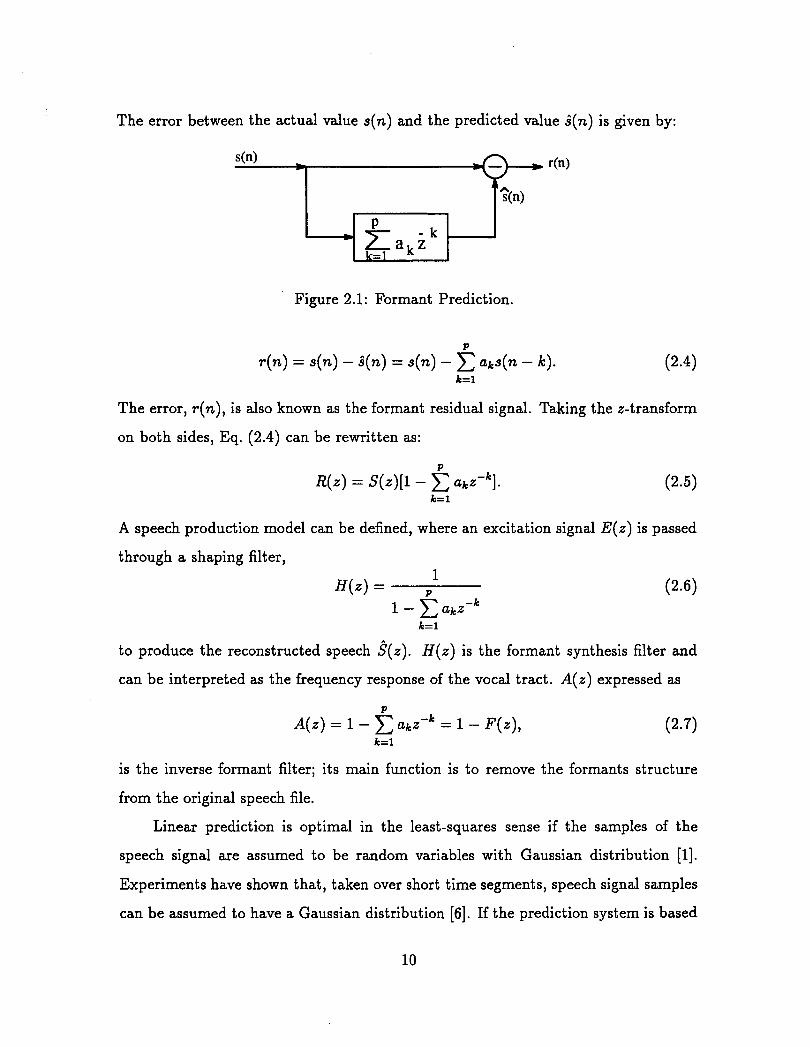
The error between the actual value s(n) and the predicted value B(n) is given by:
Figure 2.1: Formant Prediction.
P
~ ( n ) = s(n) - i (n) = s(n) - C aks(n - k). k=l
(2.4)
The error, r(n), is also known as the formant residual signal. Taking the z-transform
on both sides, Eq. (2.4) can be rewritten as:
A speech production model can be defined, where an excitation signal E(z) is passed
through a shaping filter, 1
H ( 4 = p
1 - C ak.Yk k = l
to produce the reconstructed speech ~ ( z ) . H(z) is the formant synthesis filter and
can be interpreted as the frequency response of the vocal tract. A(z) expressed as
is the inverse formant filter; its main function is to remove the formants structure
from the original speech file.
Linear prediction is optimal in the least-squares sense if the samples of the
speech signal are assumed to be random variables with Gaussian distribution [I].
Experiments have shown that, taken over short time segments, speech signal samples
can be assumed to have a Gaussian distribution [6]. If the prediction system is based

on past original speech samples, we refer to it as forward adapted prediction because
the predictor coefficients have to be sent to the receiver as side information. However,
if the prediction system is based on past reconstructed speech samples, we refer to it
as backward adaptive prediction and no side information is transmitted because the
predictor coefficients can be calculated both at the transmitter and the receiver.
The performance of the formant predictor is usually assessed by the formant
prediction gain Gf which is expressed in dB units and given by
where a: and a: are the variances of the input speech and the residual respectively.
For a high prediction gain a: should be small, for a fixed input variance. The problem
is to determine the best predictor coefficients ak, the optimal predictor order p and
the best window size in order to minimize the energy of the error while also keeping
the synthesis filter stable.
2.1.2 Long-Term Prediction
The residual signal from the formant analysis filter, A(z), still shows pitch periodicity.
Another important feature in linear predictive coders is to remove the far-sample
redundancy from the original speech. Pitch prediction can be handled by a filter with
Figure 2.2: Pitch Prediction.
only one coefficient of the following form:
where p is a scaling factor related to the degree of waveform periodicity and M is
the estimated period in samples. This predictor has a time response of a unit sample
delayed by M samples; so the pitch predictor estimates that the previous pitch period
repeats itself. For unvoiced speech segments, no clear pitch period exists. In general
the pitch lag is allowed to vary between 20 and 147 samples (at 8 kHz sampling rate).
The error signal is
e ( n ) = ~ ( n ) - pr(n - M) (2.10)
and is called the pitch residual signal. Taking the z-transform on both sides, and
rearranging the terms, the inverse pitch filter is defined to be
Its main function is to remove the pitch structure from the original speech. At the
decoder stage, the pitch synthesis filter defined as
is excited by the formant residual signal in order to introduce a periodic structure,
matching as close as possible that of the original speech. The performance of the
pitch predictor is also assessed by the pitch prediction gain G, given by
The problem in pitch predictors is to determine the best pitch coefficient along with
the optimal matching pitch period M in order to minimize the energy of the pitch
residual e (n ) .
2.2 Estimation of the Predictor Parameters
2.2.1 Linear Prediction Coefficients
The least-squares method is used in order to determine the Linear Prediction Coeffi-
cients (LPC) and is based on minimizing the total squared error with respect to each
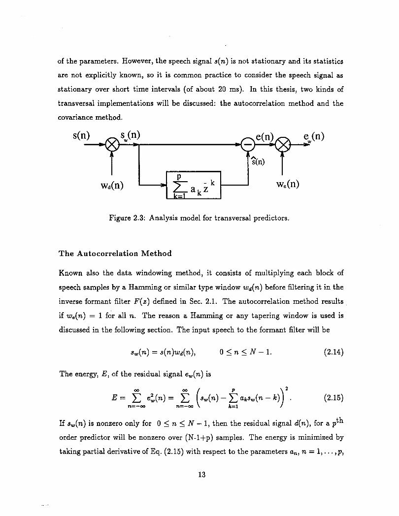
of the parameters. However, the speech signal s(n) is not stationary and its statistics
are not explicitly known, so it is common practice to consider the speech signal as
stationary over short time intervals (of about 20 ms). In this thesis, two kinds of
transversal implementations will be discussed: the autocorrelation method and the
covariance method.
Figure 2.3: Analysis model for transversal predictors.
The Autocorrelation Method
Known also the data windowing method, it consists of multiplying each block of
speech samples by a Hamming or similar type window wd(n) before filtering it in the
inverse formant filter F ( z ) defined in Sec. 2.1. The autocorrelation method results
if w,(n) = 1 for all n. The reason a Hamming or any tapering window is used is
discussed in the following section. The input speech to the formant filter will be
The energy, E, of the residual signal ew(n) is
If sw(n) is nonzero only for 0 2 n 5 N - 1, then the residual signal d(n), for a p th
order predictor will be nonzero over (N-l+p) samples. The energy is minimized by
taking partial derivative of Eq. (2.15) with respect to the parameters a,, n = 1, . . . , p,
and setting each of the resulting p equations to zero. The system of equations to solve
a; x sw(k - n)sw(k - i) = sw(k)sw(k - n), n = 1, . . . , p . (2.16)
Defining the autocorrelation function of s,(n) as
N-1
R(n) = x x(k)x(k - n), k=n
and noting that R(n) = R(-n), then the system of equations can be expressed in
matrix form as Ra = r. The expanded form of the system is:
where each entry in the autocorrelation is given by = R( li - j 1). The system
of Eqs. (2.18) is in fact the Yule-Walker equations with the autocorrelation matrix R
being symmetric and Toeplitz. A fast method for solving the Yule-Walker equations
is the Levinson-Durbin recursion [8]. The predictor coefficients are used in both all-
zero filtering operation to obtain residual signals and in all-pole filtering operations to
reconstruct speech signals. Stability of the synthesis filter is of premium importance.
The autocorrelation method always results in a stable synthesis filter associated with
the predictor coefficients ak.
The Covariance Method
The covariance method results if wd(n) = 1 for all n. The window w,(n) is usually
chosen such that w,(n) # 0 for 0 5 n 5 N - 1. Applying the least-squares method,
the mean square energy of the error is,
By substituting the value of e,(n) in the equation above, the error energy
is minimized by taking the derivatives of Eq. (2.20) with respect to all ak's, and
setting the result equal to zero. The resulting system of equations is writ ten as
Defining the covariance function of s(k) as
then the system of equations can be expressed in matrix form as @a=+ or in an
expanded form as
The covariance matrix preserves is symmetric. The Cholesky decomposition method
is usually used to solve for the predictor coefficients aks in the linear system of
Eqs. (2.23). The choice of the error window w,(k) will also be discussed in the
following section. The covariance method, unfortunately, does not guarantee stabil-
ity of the synthesis filter. In many cases it results in higher prediction gains than the
autocorrelation method.
When the autocorrelation and the covariance methods are applied to determine
the parameters of the pitch filter, a system of equations similar to Eqs. (2.18) and
(2.23) is obtained, with of course the appropriate filter delay values. The conventional
approach is to determine the pitch lag M separately from the predictor coefficient
(single-tap pitch filter) by searching over a range of pitch periods encountered in
human speech (typically between 20 and 147 samples at 8 kHz). The optimal lag,
Mopr, is the lag that corresponds to the smallest mean square error
where R( autocorrelation method
Popt = R(O) ' ' ( 0 1 covariance method. d(M1 M) '
It is important to note that for multi-tap pitch filters, the autocorrelation method
does not guarantee that B(z) is minimum phase[l9].
2.2.2 Predictor Order and Windowing Shape/Size
The choice of the predictor order p is a compromise between spectral accuracy and
computation time/memory. The number of poles in the formant predictor filter is
a function of the number of formants to be modelled. Each formant requires two
poles[3]; two extra poles are added to compensate for the glottal effects and radiation
of the lips. Typically 10 poles are enough to model the formant structure of a standard
8 kHz sampled speech. As p increases, a better fit is achieved but a the cost of extra
computation and side information.
For the pitch predictor filter, a larger number of taps is necessary due to the
fact that the pitch lag is unlikely to be an exact multiple of the sampling frequency.
Multiple predictor coefficients allow interpolation of speech samples in the delayed
version to more precisely match the original, and provide an improvement in the
prediction gain. After experiments, Atal [6] found that it is useful to use a third-
order predictor of the form
The prediction methods are based on an estimate of the correlation. The length
of the window must be large enough to provide a valid estimate of the correlations.
The minimum formant frequency is around 270 Hz (males); this corresponds to a
sample lag of 30 samples. A suitable formant analysis frame is around 80-160 sam-
ples. In most linear predictive coders the formant filter and the pitch filters are
used in cascade. Rectangular and Hamming windows are commonly used in forward
adaptation, whereas exponential windows lead to higher prediction gain seem in back-
ward adaptation. Rectangular windows are not recommended in the autocorrelation
method because of frame edge effects. By truncating the input speech, the residual
signal tends to be large at the beginning of the interval because prediction is based on
previous samples that have been arbitrarily set to zero, and at the end of the interval
because zero amplitude samples are predicted from samples that are nonzero. By
increasing the window size, the edge effects can be reduced.
In contrast to the formant predictor, the delays used for a pitch predictor are
comparable to, or even larger than, the window length. For a pitch filter, frame edge
effects are no longer negligible. The problem is not solved by using windows that are
longer than the largest delay of the pitch predictor since too much time-averaging
greatly reduces the performance and, changes in the pitch lag are not adequately
tracked. The covariance method is preferred over the autocorrelation method to
determine the pitch parameters and gives higher pitch prediction gains, but does not
guarantee stability of the pitch synthesis filter [25].
Better prediction gains are obtained when Barnwell autocorrelation windows are
used instead of Hamming windows in backward adaptive LPC analysis [25]. The main
reason for the better performance of exponential windows is the heavier emphasis
applied to immediate past samples compared to Hamming or rectangular widows.
2.2.3 Line Spectral Frequencies
Line Spectral Frequencies (LSF) is a very popular set for representing the LPC coef-
ficients, because they are related to the speech spectrum characteristics in a straight-
forward way. The LSF represents the phase angles of an ordered set of poles on
the unit circle that describes the spectral shape of the inverse formant filter A(z)
defined in Eq. (2.7). They were first introduced by Itakura in 1975 [36]. The main
advantages of the LSF are that they can provide easy stability checking procedures,
spectral manipulations, and convenient re-conversion to predictor coefficients.
Conversion of the LPC coefficients ak to the LSF domain relies on the inverse
formant filter A(z). Given A(z), its corresponding LSF are defined to be the zeros of
the polynomials P(z) and Q(z) defined as:
If A(z) is minimum phase, all the roots of P(z) and Q(z) will lie on the unit circle, al-
ternating between the two polynomials with increasing frequency. Several approaches
for solving for the roots of P(z) and Q(z) have been presented [37, 38, 391. The roots
occur in complex conjugate pairs and hence there are p LSF lying between 0 and T.
The value of the LSF can be converted to Hertz (Hz) by multiplying by the factor
F,/27r where F, is the sampling frequency. Another important characteristic about
the LSF is the localized spectral sensitivity. For the predictor coefficients, a small
distortion in one coefficient could dramatically distort the spectral shape and even
lead to an unstable synthesis filter. Whereas, if one the LSF is distorted, the spectral
distortion occurs only in the neighborhood of the modified LSF.
In many LPC speech coders, the LPC filtering is carried out by interpolating
the predictor coefficients between two~successive analysis frames into a subframe level
such that a smoother transition is achieved. The interpolation can be performed in
the LSF domain to guarantee the stability of the resulting filters.
2.3 Adaptive Predictive Coder (APC)
Low bit rate speech coders often employ both formant and pitch predictors to remove
near-sample and distant-sample redundancies in the speech signal. The resulting
prediction residual signal is of smaller amplitude and can be coded more efficiently
than the original waveform. The predictors coefficients in the two filters are updated
by updating them at fixed intervals to follow the time-varying correlation of the speech
signal. A basic system which uses the two predictors arrangement is the Adaptive
Predictive Coder (APC). .
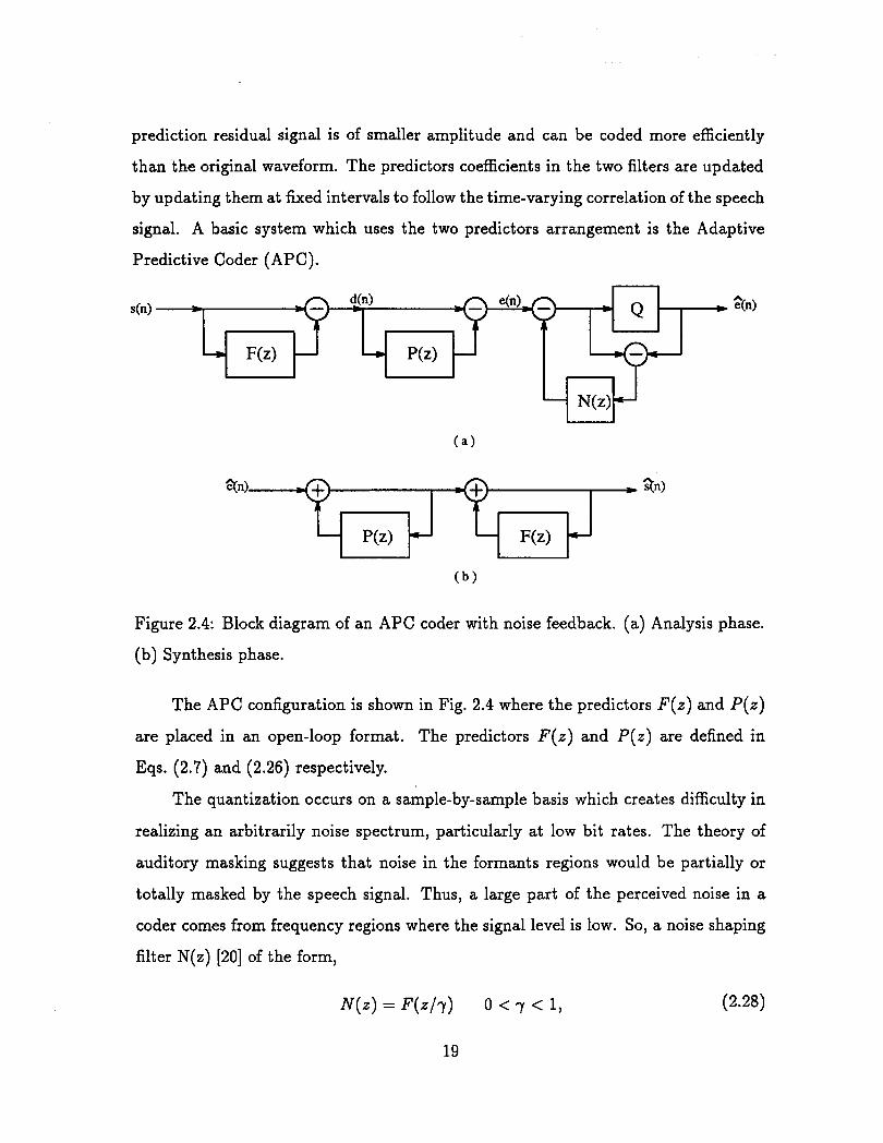
Figure 2.4: Block diagram of an APC coder with noise feedback. (a) Analysis phase.
(b) Synthesis phase.
The APC configuration is shown in Fig. 2.4 where the predictors F(z) and P(z)
are placed in an open-loop format. The predictors F(z) and P(z) are defined in
Eqs. (2.7) and (2.26) respectively.
The quantization occurs on a sample-by-sample basis which creates difficulty in
realizing an arbitrarily noise spectrum, particularly at low bit rates. The theory of
auditory masking suggests that noise in the formants regions would be partially or
totally masked by the speech signal. Thus, a large part of the perceived noise in a
coder comes from frequency regions where the signal level is low. So, a noise shaping
filter N(z) [20] of the form,
is included in order to reduce the perceptual distortion of the output speech by
redistributing the quantization noise spectrum [17].
The order in which the two predictors are combined is important for time-varying
predictors. The conventional predictor configuration uses a cascade of formant predic-
tor and a pitch predictor, referred to as an F-P cascade [20]. The cascade connection
can also have the pitch predictor precede the formant predictor, referred to as a P-
F cascade. The filters coefficients for the two filters in the cascade are determined
in a sequential fashion. The coefficients of the first filter are found from the input
speech s(n), and then the coefficients of the second filter are determined from the
intermediate residual d(n) formed by the filtering action of the first predictor. In
terms of prediction gain, the F-P cascade stands out as being superior to the P-F
cascade [20], and will be used throughout this thesis. For the formant filter, the au-
tocorrelation method can be used to determine the filter coefficients a k which ensures
stability of the formant synthesis filter. The covariance method used to determine a
set of pitch predictor coefficients can result in an unstable pitch synthesis filter. This
usually arises when a transition from an unvoiced to a voiced segment takes place,
and causes degradation (pops and clicks) in the decoded speech. The stability of the
pitch filter is checked by several tests detailed in [19]. If found to be unstable, the
coefficients are scaled downward in magnitude to the point at which they satisfy the
stability test. For a fixed formant frame size, the number of frames with unstable
pitch filters increases with decreasing pitch frame size [19]. For fixed frame sizes, the
number of unstable frames also generally increases as the number of pitch taps is
increased.
The digital channel in an APC system carries information both about the quan-
tized prediction residual and the time-varying parameters of the adaptive predictors
and the quantizer (often referred to as side information). Efficient encoding of the
parameters is necessary to keep the total bit rate to a minimum. According to Atal
[6], the distortion is small although audible when a total of 40 bits are used for en-
coding 20 LSF with an update rate of 10 ms. The total bit rate for the coefficients
depend both on the number of coefficients and the time intervals at which a new
set of coefficients are determined. Typically, the bit rate for the formant predictor
parameters varies between 2300 and 4600 bits/s. The delay parameter M of the
long-delay predictor P ( z ) needs approximately 7 bits of quantization accuracy, and
13 extra bits are needed for the pitch coefficients (assuming a 3rd order predictor).
The pitch predictor must be reset once every 10 ms to be effective resulting in a bit
rate of 2000 bits/s for the pitch predictor parameters.
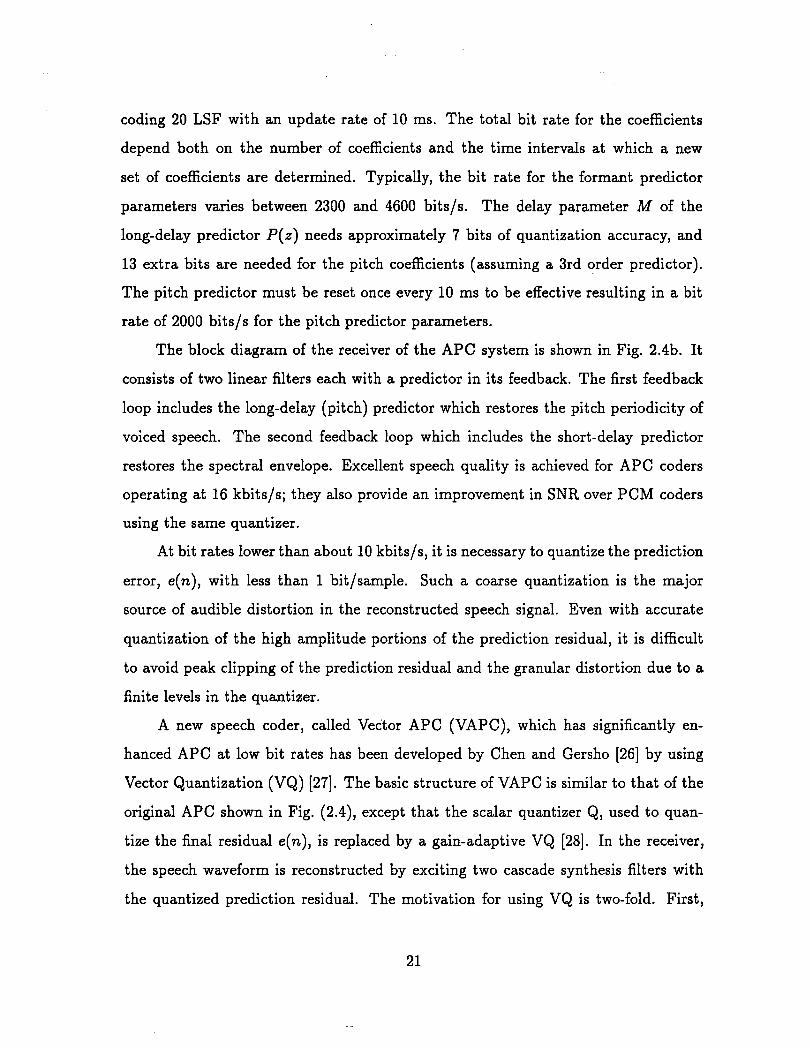
The block diagram of the receiver of the APC system is shown in Fig. 2.4b. It
consists of two linear filters each with a predictor in its feedback. The first feedback
loop includes the long-delay (pitch) predictor which restores the pitch periodicity of
voiced speech. The second feedback loop which includes the short-delay predictor
restores the spectral envelope. Excellent speech quality is achieved for APC coders
operating at 16 kbitsls; they also provide an improvement in SNR over PCM coders
using the same quantizer.
At bit rates lower than about 10 kbitsls, it is necessary to quantize the prediction
error, e(n), with less than 1 bitlsample. Such a coarse quantization is the major
source of audible distortion in the reconstructed speech signal. Even with accurate
quantization of the high amplitude portions of the prediction residual, it is difficult
to avoid peak clipping of the prediction residual and the granular distortion due to a
finite levels in the quantizer.
A new speech coder, called Vector APC (VAPC), which has significantly en-
hanced APC at low bit rates has been developed by Chen and Gersho [26] by using
Vector Quantization (VQ) [27]. The basic structure of VAPC is similar to that of the
original APC shown in Fig. (2.4), except that the scalar quantizer Q, used to quan-
tize the final residual e(n), is replaced by a gain-adaptive VQ [28]. In the receiver,
the speech waveform is reconstructed by exciting two cascade synthesis filters with
the quantized prediction residual. The motivation for using VQ is two-fold. First,
adjacent � re diction residual samples may still have nonlinear dependency [17] which
can be exploited by VQ. Secondly, VQ can operate at rates below 1 bitlsample.
Once pitch and formant prediction are performed, the resulting prediction resid-
ual is normalized by a gain derived from the predictor residual in the current frame.
The normalized vector is then vector quantized using a fixed VQ codebook, and the
selected VQ codevector is multiplied by the estimated gain to obtain the quantized
prediction residual vector. The estimated gain is quantized and sent as part of the
side information. Very good speech quality is obtained at 9.6 kbitsls and reasonably
good quality at 4.8 kbits/s [26].
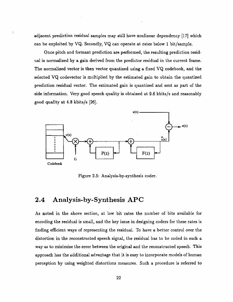
Figure 2.5: Analysis-by-synthesis coder.
2.4 Analysis-by- S ynt hesis AP C
As noted in the above section, at low bit rates the number of bits available for
encoding the residual is small, and the key issue in designing coders for these rates is
finding efficient ways of representing the residual. To have a better control over the
distortion in the reconstructed speech signal, the residual has to be coded in such a
way as to minimize the error between the original and the reconstructed speech. This
approach has the additional advantage that it is easy to incorporate models of human
perception by using weighted distortions measures. Such a procedure is referred to
as analysis-by-synthesis adaptive predictive coding.
2.4.1 Analysis-by-Synthesis Coder Structure
The basic structure of an analysis-by-synthesis coder is depicted in Fig. 2.5. The
predictors P ( z ) and F ( z ) , add respectively the formant structure and periodicity
structure to the excitation vector c(n).
The formant predictor coefficients ak's are determined from the speech signal
using the autocorrelation method described in Sec. 2.2. The pitch filter coefficients
( M , P ) can be determined either by the covariance method using the residual signal
obtained after the LPC analysis, or by the analysis-by-synthesis method illustrated
in Fig. 2.5 as will be explained later in this section.
Once the coefficients of the predictors are determined, the excitation function for
the filters is determined in a block-wise manner. For every N samples, the excitation
is determined such that the weighted mean squared error between the original and
the reconstructed speech is minimal. The filter W ( z ) is a perceptual error weighting
filter which deemphasizes the error near the formant frequencies.
There are different ways to represent the excitation, which form the main dis-
tinction between different coders. The first practical linear prediction-based analysis-
by-synthesis coding system was the Multi-Pulse Linear Prediction (MPLP) coder [29].
The MPLP represents the excitation as a sequence of pulses not uniformly spaced.
The excitation analysis procedure has to determine the amplitudes of the pulses.
MPLP coder can produce good quality speech between 4.8 and 16 kbits/s. The
Regular-Pulse Linear prediction (RPLP) [30] is similar to the MPLP method. The
excitation is a set of uniformly spaced pulses. The offset of the pulse set is selected
first during the encoding process, and then the individual amplitudes of the pulses
are determined.
The most popular method for analysis-by-synthesis is Codebook Excited Linear
Prediction (CELP) which is the main interest in this thesis and is explained separately
in the next section.
2.4.2 Codebook Excited Linear Prediction Structure
Conceptually, the easiest way of applying VQ techniques to represent the excitations
in the block diagram of Fig. 2.5 is to store a collection of possible sequences and
systematically try each sequence, then select the one that produces the lowest error
between the original and reconstructed speech signal. If the collection of sequences,
which is either stored or generated deterministically, is available at both the encoder
and the decoder, only the index of the sequence that results in the smallest error has
to be transmitted.
The coder performance is related to the number and shape of the codebook
excitations. The codebook is populated with samples of a source that reflect the
statistics of the signal to be encoded. Schroeder and Atal [31] have suggested that a
unit-variance Gaussian source is a good choice because it has been shown in [31] that
the probability density function of the prediction error samples (after both short-delay
and long-delay prediction) is nearly Gaussian.
The gain G plays also an important role in the CELP coder. Its sign effectively
increases the codebook size by one bit. It's absolute value is adjusted such that the
filtered excitation optimally matches the error signal. The effective codebook size is
the sum of the number of bits used for encoding and the index i, and the number of
bits used for encoding the gain G.
The spectral weighting filter W(z) is introduced to take advantage of the proper-
ties of human auditory perception. Since more noise can be tolerated in the formant
regions than in the valleys between formants, a weighting filter which deemphasizes
the formant regions is chosen to be of the following form
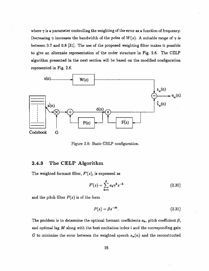
where 7 is a parameter controlling the weighting of the error as a function of frequency.
Decreasing 7 increases the bandwidth of the poles of W(z) . A suitable range of 7 is
between 0.7 and 0.8 [31]. The use of the proposed weighting filter makes it possible
to give an alternate representation of the coder structure in Fig. 2.6. The CELP
algorithm presented in the next section will be based on the modified configuration
represented in Fig. 2.6.
Figure 2.6: Basic CELP configuration.
2.4.3 The CELP Algorithm
The weighted formant filter, F1(z), is expressed as
and the pitch filter P(z) is of the form
The problem is to determine the optimal formant coefficients ak, pitch coefficient P , and optimal lag M along with the best excitation index i and the corresponding gain
G to minimize the error between the weighted speech s,(n) and the reconstructed

speech i(n). The reconstructed speech can be expressed as
The excitations xi(n) in the codebook, indexed by i, are scaled by the appropriate
gain G resulting in v;(n). The general form of the weighted error is
By substituting the value of i (n) in the above equation, e,(n) can be expressed as
and the resulting weighted mean squared error can be written as
Applying the concept of analysis-by-synthesis approach, the coder should per-
form a search over all the quantized residual vectors, all the available gain factors
for the residual vector, and all the available filter parameters to select the best set.
Theoretically the CELP coder does not directly need an analysis stage. However, the
disadvantage of an analysis-by-synthesis approach is, of course, the computational
effort required by the exhaustive search.
Ideally, the predictor filters P ( z ) and F ( z ) would be optimized for each trial
waveform. The formulation of an optimal formant synthesis filter leads to a highly
non-linear set of equations which is not amenable to a solution. Some simplifications
are often made to reduce the search complexity. The basic simplification is to deter-
mine the formant filter predictor coefficients by the analysis techniques as discussed in
Sec. 2.2. The pitch predictor parameters ( M , P ) can be determined either by analysis
or using the analysis-by-synthesis diagram of Fig. 2.6. When the analysis approach
is used to determine the pitch filter parameters, the expression of the weighted error,
e,(n), in Eq. (2.35) has only the index i and the gain G to be determined. This is
done by performing an exhaustive search over all allowable values of i and G in order
to obtain the best match by minimizing the weighted mean squared error.
However, if the analysis-by-synthesis approach is chosen to determine the pitch
filter parameters, any of the two following procedures can be followed. The first
procedure jointly optimizes (i, G) and (My p). It consists of performing an exhaustive
search over all allowable indexes i and delays M, then determine the optimal gain G
and pitch coefficient /3 to minimize E. The second alternative procedure is to use the
sequential optimization. During the first search, (M, P) are optimized considering a
zero input excitation to the inverse synthesis pitch filter, that is, G = 0. Then keeping
(M, p) fixed, a second search is performed to determine (i, G).
Chapter 3
Pitch Filtering in CELP Coders
3.1 Introduction
The addition of a pitch prediction stage to a CELP coder contributes a major part to
its success especially at rates between 4 and 10 kbits/s. At high bit rates, a substantial
number of bits is assigned to the excitation signal to enable the coder to reconstruct
the harmonic structure that the long term predictor fails to model. However, at low
bit rates, the synthetic speech is much more dependent on the performance of the
pitch predictor.
The pitch predictor, also known as the Long-Term Predictor (LTP), was intro-
duced in Chapter 2 as a technique to generate periodicity in the reconstruction of
voiced speech . The pitch predictor is characterized by the delay M, closely related
to the pitch lag of the current speech frame, and its coefficients ,Oj. The multi-tap
LTP enhances the periodicity of the coded speech and outperforms the single-tap
LTP at the expense of a greater number of bits that have to be allocated for the
quantization of the multiple coefficients. The single-tap LTP can be generalized by
increasing the time resolution of the LTP delay to less than 1 sample [22]. This results
in a fractional delay LTP, which produces a significant increase in prediction gain and
perceived periodicity, at the cost of more bits, but less than for the multi-tap case.

In CELP coders, the LTP parameters are usually determined using an analysis-
by-synthesis procedure which can be considered to be an adaptive codebook. The
adaptive codebook interpretation of the LTP is illustrated in Fig. 3.1.
r LP excitation
P LTP contribution
Figure 3.1: Single-tap pitch predictor; adaptive codebook illustration.
The excitation v(n), known as the LTP excitation is generated by appropriately
scaling a signal vector from a codebook of fixed entries (stochastic codebook intro-
duced in the CELP algorithm in Chapter 2). This LTP excitation drives the LTP to
yield an LP excitation d(n) with periodic structure. The resulting signal d(n) is used
to excite an all-pole synthesis filter which adds the formant structure to the speech
signal.
The LTP parameters and the LTP excitation signal, which is characterized by
a fixed codebook index i and a gain G, are determined on a subframe basis, whereas
the LPC are updated on a frame basis. Joint optimization of all parameters gives the
best coding performance, but the extensive f-med excitation codebook search while
optimizing the LTP parameters is very expensive computationally. A sequential op-
timization procedure is applied, where the periodic contribution to the LP excitation
is determined first assuming a zero LTP excitation. Once the LTP optimal delay and
coefficients values are obtained, the current LP excitation is further improved with
the optimal LTP excitation selected from the codebook and scaled by G. In the case
of a one-tap pitch predictor, the LTP contribution to the LP excitation can be viewed
as a past delayed version of the LP excitation scaled by the filter coefficient P. The
past LP excitations can be stored in a codebook, the so-called adaptive codebook, in
which each entry differs by a shift of one sample, see in Fig. 3.1.
The limitation that the pitch lag be greater than the subframe size causes some
problems for high pitched female speech. The delay will in effect assume pitch doubled
and tripled values on many occasions. Remedies to this problem consist in allowing
the LTP delay to take values smaller than the subframe size and to recycle the current
LP excitation through the pitch filter, or to include periodic extensions of a pitch cycle
in the adaptive codebook.
At rates below 5 kbits/s, the number of coding bits for the LTP parameters
decreases and the interval at which updates occur increases. Thus, the LTP perfor-
mance degrades as it becomes harder to recreate a smooth evolution of the pitch cycle
waveform. The perceptual quality of the reconstructed speech can be improved by in-
creasing the correlation between adjacent pitch cycles in voiced speech with heuristic
rules [33, 341.
For a conventional CELP coder operating at 4.8 kbits/s, approximately 1.6
kbits/s are needed to code the pitch parameters. Bit savings can be obtained by
encoding only the offset from the previous delay every other subframe [14] or by us-
ing differential encoding techniques [12]. Although these procedures decrease the bit
rate, they have in common that new information about the LTP delay is transmit-
ted for each individual frame. Kleijn [Ill has introduced a new technique where the
LTP parameters are transmitted once every few subframes, and the parameters are
interpolated between them. Straightforward interpolation of the LTP delay does not
work well, because even small deviations from the optimal delay can severely affect
the performance of the analysis-by-synthesis mechanism.
Kleijn [ll] exploited a generalization of the conventional analysis-by-synthesis
method. In a conventional analysis-by-synt hesis, as illustrated in Chapter 2, the
reference signal is the original speech signal. In the generalized analysis-by-synt hesis
procedure, the original speech signal is modified (time-warped) with the constraint
that the signal remains perceptually close to the original speech signal. The modified
signal which results in the best coding performance is selected. The model parameters
corresponding to this modified signal are transmitted to the receiver.
3.2 Synthesis Parameters Optimization
Codebook G
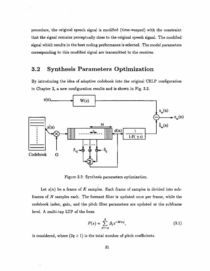
By introducing the idea of adaptive codebook into the original CELP configuration
in Chapter 2, a new configuration results and is shown in Fig. 3.2.
Figure 3.2: Synthesis parameters optimization.
s(n) D
Let s(n) be a frame of K samples. Each frame of samples is divided into sub-
W(z)
frames of N samples each. The formant filter is updated once per frame, while the
codebook index, gain, and the pitch filter parameters are updated at the subframe
level. A multi-tap LTP of the form
I
is considered, where (29 + 1) is the total number of pitch coefficients.
The waveform index i, the gain factor G and the pitch filter parameters will be
chosen to minimize the mean square frequency weighted reconstruction error in the
interval 0 5 n 2 N - 1,
where the weighted error is given by
and sw(n) and h(n) denote the weighted speech and the impulse response of the
bandwidth-expanded synthesis filter respectively. The out put of the pitch synthesis
filter can be written as
In real time applications, the response of a linear filter is the sum of the Zero Input
Response (ZIR) and the Zero State Response (ZSR) of the corresponding filter. The
ZIR based on zero excitation input takes care of the filter memory which consists of
the past excitation samples, whereas in the ZSR the memory of the filter is set to
zero while calculating the response. By decomposing the response of h(n) into the
ZIR and the ZSR, the weighted error ew(n) can be expressed as
- 1 00
eW(n) = sW(n) - C d(k)h(n - k) - x d ( k ) h ( n - k). (3.5)
The weighted speech sw(n) and the ZIR of the weighted synthesis filter can be grouped
into one term denoted by s',(n) because they do not affect the optimization procedure.
The weighted error can be rewritten as
ew(n) = ZW(n) - d(k)h(n - k). k=O
Substituting for d(n) in the above equation, the expression of ew(n) becomes
q
ew(n) = %(n) - G Z ' ( ~ ) - pjd(n, M + j),
where the filtered versions of x'(n) and d(n) have been defined as
k=O N-1
d(n, m) = d(k - m)h(n - k).
The values of the gain factor G and the coefficients Pj which minimize the squared-
error are to be found. This is accomplished by 'finding the optimal coefficients for
each allowable pair (i, M). By setting the partials derivatives of the squared error
with respect to the coefficients to zero, a system of (2q + 2) equations results. In
matrix form, the system can be written as @a = b, where <P is the autocorrelation
matrix expressed as
with v(") defined to be
The coefficients vector a is defined as
and the cross-correlation vector b is found to be
It is clear that if the minimum LTP delay M is constrained to be greater than the
subframe length N, the filtered LTP contribution E(n, M) which appears in v(')
depends only on past LP excitation samples, that is, d(n) for n < 0. At the beginning
of the current subframe, the matrix i@ and the right hand side vector b are known
quantities. Finding the optimal set of LTP coefficients and codebook gain amounts
therefore to solving the above linear system of equations.
However for LTP delays smaller than N, the matrix i@ and the vector b will de-
pend on LP excitation samples d(n) where n > 0, which in turn can only be obtained
with the knowledge of the optimal synthesis parameters. The set of equations to be
solved becomes nonlinear and not conveniently implementable in practice.
In CELP coders operating at low bit rates (5 kbits/s and below), the subframe
length is two or three times larger than the minimum delay M; so the joint opti-
mization procedure is not recommended. The sequential approach remains the only
alternative to determine the synthesis parameters.
3.3 Optimization for a One-Tap Pitch Filter
Referring to the configuration shown in Fig. 3.2, The current LP excitation d(n) can
be written as the sum of the fixed codebook excitation Gxi(n) and the adaptive LTP
codebook excitation as:
where Po is the only pitch coefficient. The gain G and the pitch coefficient Po are
sequentially optimized using the following strategy. First the LTP parameters are
determined independently using a zero input from the fixed codebook (G=O). With
the optimum lag and pitch coefficient determined for a zero excitation, the coefficients
are kept fixed at these values. Then, another search is conducted over the waveform
indexes. For each index, the optimum gain G is found.
By allowing the LTP delay to take values smaller than the subframe size, two
solutions are considered: 1) recycling the current LP excitation through the pitch
filter; 2) including periodic extensions of a pitch cycle in the adaptive codebook.
3.3.1 Recycling the LP Excitation
In CELP coders operating at low bit rates (below 5 kbits/s) the minimum LTP delay
(around 24 samples), encountered mainly in female speakers, can be up to 3 times
smaller than the subframe size N. By setting G = 0, the weighted error ew(n) given
in Eq. (3.6) can be rewritten as
00
ew(n) = iw(n) - d(k)h(n - k). k=O
Three cases arise in solving for the pitch coefficient Po depending on the value of the
lag M.
1. Lags between N/3 and N/2
The LP excitation signal takes one of the three forms
The weighted error ew(n) can now be split into three terms e w l ( n ) , ew2(n) ,
ew3(n). Using Eq. ( 3 . 8 ) , the weighted error terms can be expressed as
= L ( n ) - &&(n, M ) .
The total mean squared error is the sum of the squares of the above contributions
given by: M-1 2M-1 N
Substituting Eqs. (3.16-3.18) into Eq. (3 .19) and expanding, the tot a1 squared
error to minimize becomes:
2. Lags between N/2 and N
The LP excitation takes one of the two forms
In this case, the weighted error e,(n) is decomposed into two terms:
F o r O < n < M - 1 ,
eul(n) = jw(n) - @o& (n, M). (3.22)
For M < n < N - 1 ,
The total mean square error is the sum of the squares of the above two terms.
After substitution, the total error will become [23]:
3. Lags greater than N
The LP excitation takes the form
The corresponding mean square weighted error is
where
e, (n) = 5,(n) - pod(n, M).
Expanding Eq. (3.26),
In the first two cases, the mean square weighted error e is given by two different
nonlinear equations (Eq. (3.20) and Eq. (3.24)) in the pitch coefficient Po. Generally,
in order to minimize E , the derivative of e with respect to Po is set to zero, then
the optimal pitch coefficient POpt is solved. Depending on the value of the lag, a
polynomial of the fifth, third, or first degree in Po is obtained. The solutions to the
high order polynomials may be very complex. A simplified method based on the
quantized values of Po can be used. Each of the possible quantized values for Po is
substituted into the mean square error equations; the value of Po which gives the
smallest value of E is chosen.
In the case where the lag is larger than the subframe, the solution for Po results
in a linear equation. By setting d e / d P o = 0 in Eq. (3.28), the optimal lag Pop, is
found to be
Popt =
The minimum mean square weighted error is of the form
N-1 N-1
e-. = (~,(n))' - x iw(n)J(n, M).
The excitation codebook parameters are then found using the standard analysis-
by-synthesis search procedure. The codebook search algorithm will be explained in
details in the next chapter.
3.3.2 Creating a Periodic Extension of a Pitch Cycle
In order to avoid solving high degree polynomials, an alternative scheme based on
periodic continuation of the LP excitation instead of recycling can be used. The LP
excitation takes the following form
Let N-1
4 n , m) = d((k mod M) - m)h(n - k). k=O
(3.32)
The new weighted error will be
With this formulation, the solution for Po results in a linear equation. A small degra-
dation in the reconstructed speech quality is expected because the amplitude of suc-
cessive pitch pulses in the subframe can not vary.
3.4 Increased Resolution Pitch Filters
3.4.1 Multi-Tap Pitch Filters
So far, the behavior of a single-tap LTP is discussed. Better performance is obtained
when a multi-tap LTP is used instead of a single-tap LTP. Nevertheless, the improve-
ment will come at cost of an increased bit rate needed to encode the additional pitch
parameters. Three-tap pitch predictors have been proposed for medium rate (8-12
kbitsls) CELP coders because of the improved speech quality they produce at the
cost of an acceptable increase in bit rate.
Three-Tap Pitch Predictor
Referring again to the configuration shown in Fig. 3.2, the three-tap pitch predictor
can be expressed as 1
P(z) = C , O j ~ ' ~ + j j=-1
The sequential approach will also be used to determine the synthesis parameters.
Assuming a zero input excitation to the pitch synthesis filter, and using the "periodic
extension technique" for LTP delays less than the subframe, the LP excitation signal
can be written as 1
d(n) = P,d((n mod M) - M + j). (3.35) j=-1
The weighted error ew(n) can be written as
ew(n) = jw(n) - d(k)h(n - k),
where sw(n) is defined in Eq. (3.5). Using the notation defined in Eq. (3.32)) ew(n)
can be rewritten as 1
ew(n) = jw(n) - x &djn, M + j). j=-1
The objective is to solve for the pitch coefficients by minimizing the squared weighted
error. By setting the partial derivatives of the squared error with respect to the pitch
coefficients to zero, a system of linear equations results. In matrix form, the system
is equivalent to
\Ep =a,
where Q is a matrix of correlation terms of the form
p is the vector of predictor coefficients, and a is a vector of correlation terms of the
following form
Using the following notations
Eq. (3.38) can be rewritten as
The minimum mean square weighted error corresponding to the optimal pitch pre-
dictor coefficients popt is
emin = $(O, 0) - ~ : r a (3.43)
3.4.2 Fractional Delay Filter
High order (multi-tap) predictors yield higher prediction gains than single tap LTPs
mainly because the use of multiple coefficients effectively achieves inter-sample inter-
polation. But the major drawback in multi-tap LTPs is that more bits are needed to
encode the additional pitch coefficients. On average two to three bits are needed for
each coefficient.
In this section, a generalized form of the single-tap LTP is presented where the
time resolution of the LTP delay is increased to less than one sample. This results
in the fractional delay LTP, which produces a significant increase in pitch prediction
gain and perceived periodicity at much lower bit allocation requirements than the
three-tap LTP. Two basic structures illustrating fractional LTP are described next.
Basic structure of a fractional LTP delay
In the basic single tap LTP, presented in Section 3.3, the LTP delay M was represented
by an integer number of samples at the current sampling frequency Fa. The pitch
prediction filter was simply expressed as a cascade of unit delays. A higher temporal
resolution can be obtained by specifying the delay as an integer number of samples
at rate F, plus a fraction of a sample I/D, where 1 = 0,1,. . . , D - 1 and I and D are
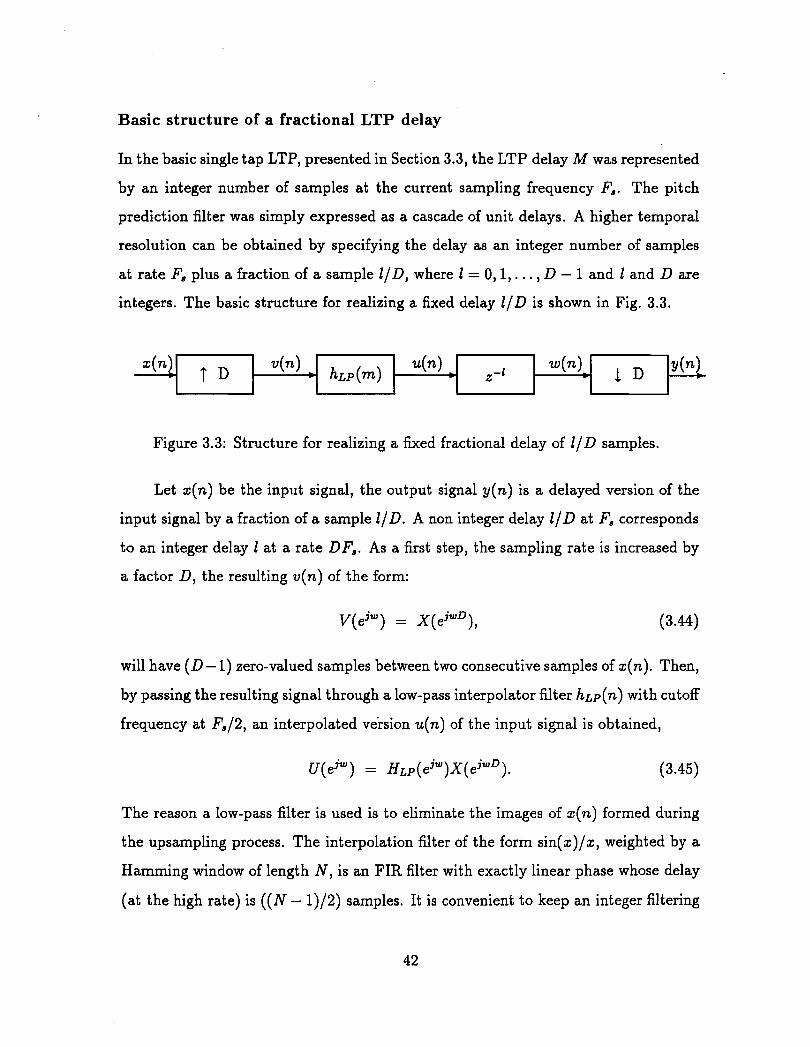
integers. The basic structure for realizing a fixed delay l /D is shown in Fig. 3.3.
Figure 3.3: Structure for realizing a fixed fractional delay of 1/ D samples.
Let x(n) be the input signal, the output signal y(n) is a delayed version of the
input signal by a fraction of a sample 1/D. A non integer delay l /D at F, corresponds
to an integer delay 1 at a rate DF,. As a first step, the sampling rate is increased by
a factor D, the resulting v(n) of the form:
will have (D- 1) zero-valued samples between two consecutive samples of x(n). Then,
by passing the resulting signal through a low-pass interpolator filter hLp(n) with cutoff
frequency at F,/2, an interpolated version u(n) of the input signal is obtained,
The reason a low-pass filter is used is to eliminate the images of x(n) formed during
the upsampling process. The interpolation filter of the form sin(x)/x, weighted by a
Hamming window of length N, is an FIR filter with exactly linear phase whose delay
(at the high rate) is ((N - 1)/2) samples. It is convenient to keep an integer filtering
delay at the low sampling rate F,, so N is chosen such that the delay is a multiple of
N - 1 -- 2
- ID;
where I is the delay at the low bit rate. This interpolated signal is delayed by I
samples at the high sampling rate to give
Finally, the delayed output is down-sampled to the original sampling frequency F,,
and the resulting y(n) is
By considering the following two assumptions :
1. HLp(ejw) sufficiently attenuates the images of X(eJw), i.e., only the r = 0 term
is significant.
2. The magnitude response of HLp(ejw) is approximately equal to D in the pass-
band.
Eq. (3.48) becomes: -jwI -jwl/DX j w y ( e j w ) = e e (e 1-
So, y(n) will be a delayed version of x(n) by:
N - 1 ($ + -) samples
at the original sampling rate F,. The ideal system to achieve this operation is seen
from Eq. (3.49) to be an all-pass filter with a linear phase 4(w) = ZwlD. In the
next subsection, it will be shown that an FIR polyphase filter approximates the
characteristics of the desired system. Thus, FIR polyphase filters will be the basis of
the fractional delay practical implementations.
FIR Polyphase Structure
The polyphase structure is used to realize the sampling rate increase and low-pass
filtering. The general form for the input-to-output time domain relationship for the
1-to- D interpolator, derived in Appendix A is:
where,
gm(n) = hLp(nD + m mod D)
is a periodically time-varying filter with period D. The term (m/D) in Eq. (3.51)
increases by one for every D samples of y(m). Each output sample y(m), m =
0,1,2,. . . , D - 1, is generated by using a different set of coefficients gm(n). After D
outputs are generated, the coefficient pat tern repeats. The low-pass filter coefficients
g,(n) are separated into D linear time invariant filters
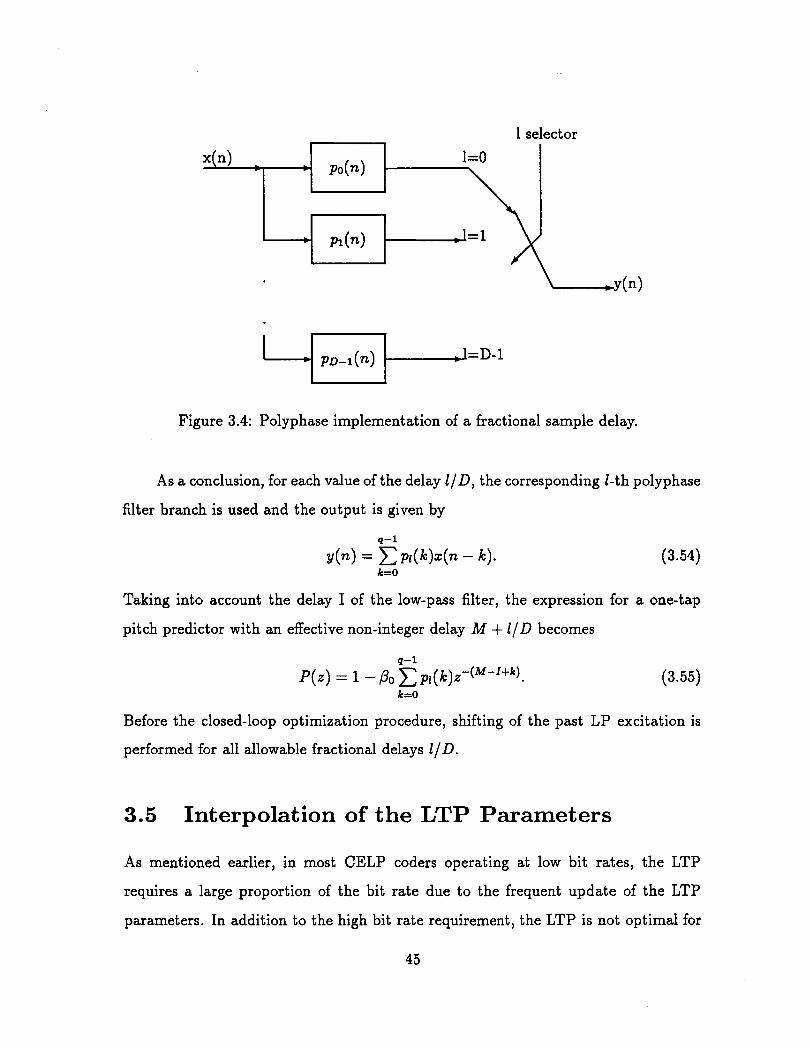
The filters pl(n) will be referred to as the polyphase filters. It is convenient to use the
commutator model, shown in Fig. 3.4, based on polyphase filters because the filtering
is performed at a low sampling rate. For each input sample x(n), there are D output
samples of y(m), and each of the D branches of the polyphase network contributes
one nonzero output which corresponds to one of the D outputs of the network. The
impulse responses of the polyphase filters pl(n) correspond to decimated delayed
versions of the impulse response of the interpolated filter hLp(n). Assuming that the
frequency response of hLp(n) approximates an ideal low-pass with a cut-off frequency
we= n/D, the frequency response of pr(n) will approximate an all-pass function, where
each value of I corresponds to a certain phase shift. If the interpolator filter hLp(n)
is an FIR filter of length N, the filters ~ [ ( n ) for 1 # 0 will be FIR filters of length
q = N/D where N = 2 0 - 1.
1 select
1=0 I p o ( 4
I
Figure 3.4: Polyphase implementation of a fractional sample delay.
As a conclusion, for each value of the delay I ID, the corresponding l-th polyphase
filter branch is used and the output is given by
Taking into account the delay I of the low-pass filter, the expression for a one-tap
pitch predictor with an effective non-integer delay M + ZID becomes
Before the closed-loop optimization procedure, shifting of the past LP excitation is
performed for all allowable fractional delays IID.
3.5 Interpolation of the LTP Parameters
As mentioned earlier, in most CELP coders operating at low bit rates, the LTP
requires a large proportion of the bit rate due to the frequent update of the LTP
parameters. In addition to the high bit rate requirement, the LTP is not optimal for
representing the dynamics of the pitch cycle waveform because of increased fluctua-
tions in the correlations. Kleijn .[I11 presented a new method based on interpolating
the LTP parameters which results in smoothing the evolution of the pitch-cycle wave-
form, reducing the bit rate, and/or improving the speech quality. This interpolation
procedure exploits a generalization of the conventional analysis-by-synthesis method
which will be explained in the first part of this section. In the second part, the idea
of continuous delay contour is mentioned in order to explain in the third part, the
basic principle of interpolating the continuous delay contour using the generalized
analysis-by-synthesis procedure. In the last part, an interpolation method with a
conventional stepped delay contour is introduced.
3.5.1 Generalized Analysis-by-Synt hesis Procedure
In a conventional analysis-by-synthesis procedure, as illustrated in Fig. 3.5a, a vector
of model parameters is obtained by synthesizing a signal for each of a set of such vec-
tors, and selecting the vector for which the synthesized signal resembles a reference
signal most closely [ll]. The reference signal is the original speech signal. Straightfor-
ward interpolation of the LTP delay leads to suboptimal delay values in the individual
subframes. In a conventional closed-loop LTP, the LP excitation tries to match as
closely as possible the LP residual by trying to locate the exact pitch pulse locations.
However, if the delay values are quantized, a time mismatch between the LP residual
signal and the LP excitation signal occurs. An illustration of time mismatch resulting
from interpolation is illustrated in Fig. 3.6. The first LP excitation is reconstructed
based on optimal pitch coefficient and delay. The error between the LP residual and
the LP excitation is very small. However, if the optimal delay is changed such that
the new value is one sample less than the optimal value, then the reconstructed LP
excitation differs by one sample and the error difference increases. In order to prevent
this time mismatch, a generalized analysis-by-synthesis principle can be used and is
illustrated in Fig. 3.5b. The fundamental principle is to modify the original speech
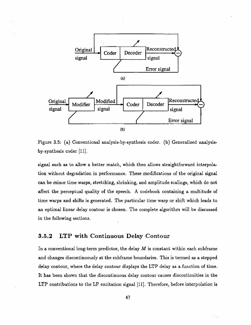
Error signal
(4
original 1 I
0"gina'. Modifier Modified - Coder Decoder signal signal
Error signal
-
Figure 3.5: (a) Conventional analysis-by-synthesis coder. (b) Generalized analysis-
by-synthesis coder [ll].
signal such as to allow a better match, which then allows straightforward interpola-
tion without degradation in performance. These modifications of the original signal
can be minor time warps, stretching, shrinking, and amplitude scalings, which do not
affect the perceptual quality of the speech. A codebook containing a multitude of
time warps and shifts is generated. The particular time warp or shift which leads to
an optimal linear delay contour is chosen. The complete algorithm will be discussed
in the following sections.
signal /
Coder
3.5.2 LTP with Continuous Delay Contour
Decoder
In a conventional long-term predictor, the delay M is constant within each subframe
and changes discontinuously at the subframe boundaries. This is termed as a stepped
delay contour, where the delay contour displays the LTP delay as a function of time.
It has been shown that the discontinuous delay contour causes discontinuities in the
LTP contributions to the LP excitation signal [ll]. Therefore, before interpolation is
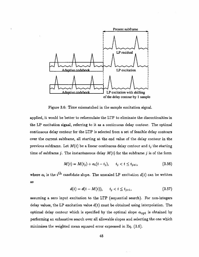
Present subframe rc .I I I
I I LP excitation I I I
I I LP excitation with shifting of the delay contour by 1 sample
Figure 3.6: Time mismatched in the sample excitation signal.
applied, it would be better to reformulate the LTP to eliminate the discontinuities in
the LP excitation signal, referring to it as a continuous delay contour. The optimal
continuous delay contour for the LTP is selected from a set of feasible delay contours
over the current subframe, all starting at the end value of the delay contour in the
previous subframe. Let M(t) be a linear continuous delay contour and t j the starting
time of subframe j . The instantaneous delay M(t) for the subframe j is of the form
where cq is the ith candidate slope. The unscaled LP excitation d(t) can be written
as
d(t) = d(t - M(t)), t j < t 2 tj+l, (3.57)
assuming a zero input excitation to the LTP (sequential search). For non-integers
delay values, the LP excitation value d(t) must be obtained using interpolation. The
optimal delay contour which is specified by the optimal slope aOpt is obtained by
performing an exhaustive search over all allowable slopes and selecting the one which
minimizes the weighted mean squared error expressed in Eq. (3.6).
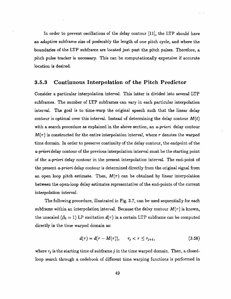
In order to prevent oscillations of the delay contour [ll], the LTP should have
an adaptive subframe size of preferably the length of one pitch cycle, and where the
boundaries of the LTP subframe are located just past the pitch pulses. Therefore, a
pitch pulse tracker is necessary. This can be computationally expensive if accurate
location is desired.
3.5.3 Continuous Interpolation of the Pitch Predictor
Consider a particular interpolation interval. This latter is divided into several LTP
subframes. The number of LTP subframes can vary in each particular interpolation
interval. The goal is to time-warp the original speech such that the linear delay
contour is optimal over this interval. Instead of determining the delay contour M(t)
with a search procedure as explained in the above section, an a-priori delay contour
M(T) is constructed for the entire interpolation interval, where T denotes the warped
time domain. In order to preserve continuity of the delay contour, the endpoint of the
a-priori delay contour of the previous interpolation interval must be the starting point
of the a-priori delay contour in the present interpolation interval. The end-point of
the present a-priori delay contour is determined directly from the original signal from
an open loop pitch estimate. Then, M(T) can be obtained by linear interpolation
between the open-loop delay estimates representative of the end-points of the current
interpolation interval.
The following procedure, illustrated in Fig. 3.7, can be used sequentially for each
subframe within an interpolation interval. Because the delay contour M(T) is known,
the unscaled (Oo = 1) LP excitation d(r) in a certain LTP subframe can be computed
directly in the time warped domain as:
where ~j is the starting time of subframe j in the time warped domain. Then, a closed-
loop search through a codebook of different time warping functions is performed in
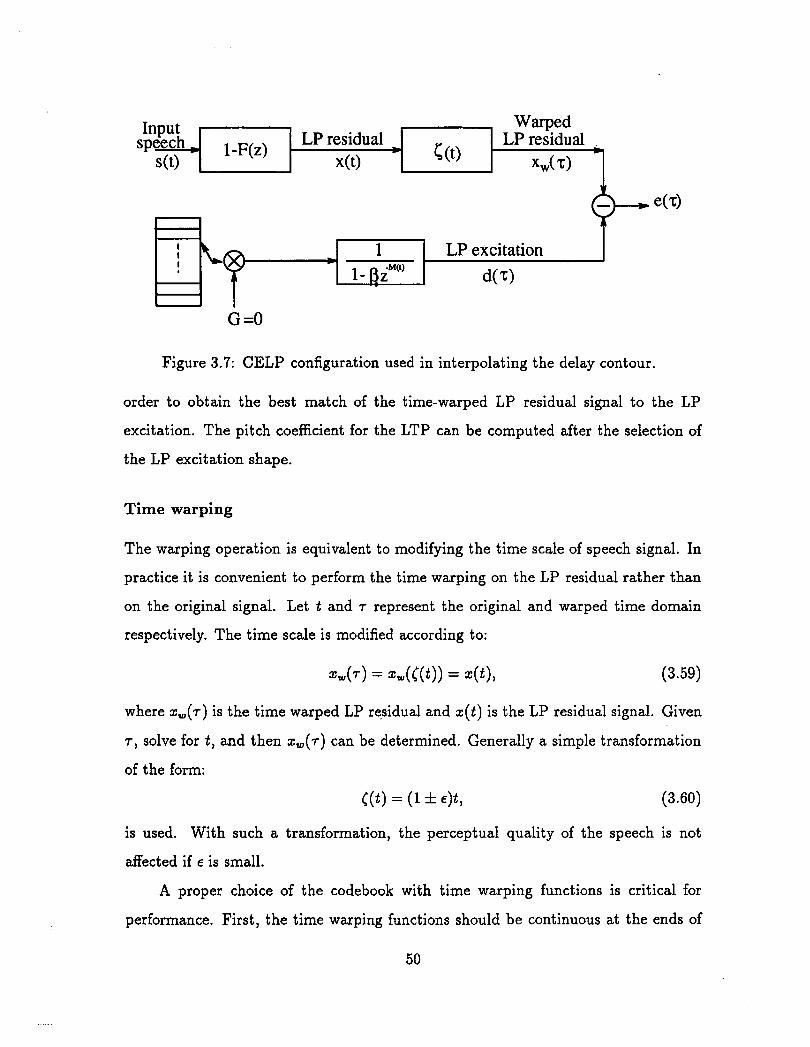
Figure 3.7: CELP configuration used in interpolating the delay contour.
Input Warped
order to obtain the best match of the time-warped LP residual signal to the LP
excitation. The pitch coefficient for the LTP can be computed after the selection of
the LP excitation shape.
speech , Nt)
Time warping
The warping operation is equivalent to modifying the time scale of speech signal. In
1 -F(z)
practice it is convenient to perform the time warping on the LP residual rather than
on the original signal. Let t and T represent the original and warped time domain
respectively. The time scale is modified according to:
LP residual x(t)
where x W ( r ) is the time warped LP residual and x ( t ) is the LP residual signal. Given
T , solve for t , and then x W ( r ) can be determined. Generally a simple transformation
is used. With such a transformation, the perceptual quality of the speech is not
affected if E is small.
A proper choice of the codebook with time warping functions is critical for
6 ( 0
performance. First, the time warping functions should be continuous at the ends of
LP residual xw< 0
the interpolation interval. Second, the pitch pulses must be located near the LTP
subframe boundaries in the warped speech signal. The location of the pitch pulses
is very important because that is where most of the energy of the signal resides. A
variety of time warping functions can satisfy the above two conditions. Good results
were obtained in [ll] with the following family of time warping functions:
where A, B, C, a ~ , a= are constants. The values of A and B are determined in
order to satisfy the first condition, whereas C is determined to ensure the second
condition. The major drawbacks in using time warping in real-time applications
result in asynchrony between the original and the reconstructed speech signal and
pitch doubling or halving of the delay. An approximate synchrony is analyzed in [35].
As concerning the second problem, if the open-loop delay estimate for the endpoint of
the interpolation interval is close to a multiple or sub-multiple of the open-loop delay
estimate of the previous interpolation interval, then delay multiples or sub-multiples
is assumed to have occurred.
Once x , (T) is calculated, it is then sampled. The criterion used for the selection
of a particular time warping function [ ( t ) is closely related to that of Eq. (3 .6) . The
criterion in Eq. (3 .6 ) is modified to select only for the shape. For that reason a nor-
malization factor is added to the weighted mean square error in order to compensate
for this assumption.
The size of the time warping codebook is limited only by the computational
requirements, since no information concerning the best entry is transmitted. The
variable LTP subframe rate is also of no consequence for the bit rate of the LTP,
because of interpolating the LTP parameters, but will affect the overall rate of the
coder because of using a fixed codebook in CELP type coders. In order to maintain
a fixed rate coder, it is necessary to determine the fixed codebook contribution at a
fixed subframe rate which is very cumbersome to apply especially when an adaptive
codebook is used to model the LTP. An alternative method is to use a variable bit
allocation to the LTP subframe or to split long LTP subframes into two sequential
subframes for the fixed codebook contribution [ll].
3.5.4 Stepped Interpolation of the Pitch Predictor
In conventional CELP coders, the LTP uses a stepped delay contour where time
warping of the original signal is not necessary. Instead, time shifting is performed on
the original subframes. In the time shifting method, the LP residual is modified by
repeating and removing very small segments.
Because the delay contour is constant within a subframe, the location of the
subframe boundaries is not critical and the subframe size does not need to be a
function of the pitch period. To obtain a good match, it is necessary to make sure
that the subframe size is always less than a pitch period. In practice, a subframe size
of 2.5 ms is used.
The following procedure is used in interpolation with a stepped delay contour.
Let ta and t b denote the beginning and end of the present interpolation interval, for
the original signal. Further, let ja be the index to the first LTP subframe of the
present interpolation interval and jb the first LTP subframe of the next interpolation
interval. An open-loop estimate of the delay at the end of the present interpolation
interval is performed and denoted by Ma. Let Ma denotes the open-loop delay at the
end of the previous interpolation interval. The delay of subframe j can be expressed
The unscaled LP excitation can be written as:
where ~j is the beginning of the subframe j in the shifted time domain T. Then, a
closed-loop search through a codebook of different time shifting coefficients is per-
formed in order to obtain the best match of the time-warped LP residual signal to the
LP excitation. The pitch coefficient for the LTP can be computed after the selection
of the LP excitation shape. The shifting procedure is:
where B is the time shift and ti is the start of the subframe j in the original signal.
The optimal shift Bopt is determined by minimizing an error criterion very similar to
Eq. (3.6). The maximum allowable time shift is 0.25 ms. A constant overall bit rate
coder can be achieved because the LTP subframe size is fixed, and the subframe rate
does not affect the bit rate because of interpolation of the LTP parameters. However,
in CELP coders operating at low bit rates, the LTP subframe size should be greater
than 2.5 ms for the fixed codebook. So, 5 or 7.5 ms LTP subframes is used instead
while taking into account the LTP delays which are less than the subframe size by
using the "recycling" technique explained in Section 3.3.
Chapter 4
Improved CELP Coder at
4.1 Introduction
The main focus of the thesis is on improving the quality of a CELP based coder
developed by the U.S. Department of Defense (DoD) and Bell Labs. It has been re-
cently selected as the U.S. Government Standard voice coder. This coder is known as
the Federal Standard (FS)-1016 coder. The FS-1016 is a robust, moderate complex-
ity voice coding algorithm with an output bit rate of 4.8 kbits/s and is an excellent
reference point for further work in the low rate CELP research area. While the FS-
1016 coder provides quality that is sufficient for many current applications, it may
not be appropriate for telephone applications. In this thesis, several modifications to
the original algorithm are proposed, with the intent of improving the quality of the
coder that may be suitable for the second generation of digital cellular applications.
The modifications fall into two general areas: 1) improving the performance of the
pitch predictor by increasing the resolution of the delay or the number of taps or
more efficiently by using a pseudo-tap pitch predictor which increases the quality of
the reconstructed speech for a minimum cost in bit rate; and 2) performing small
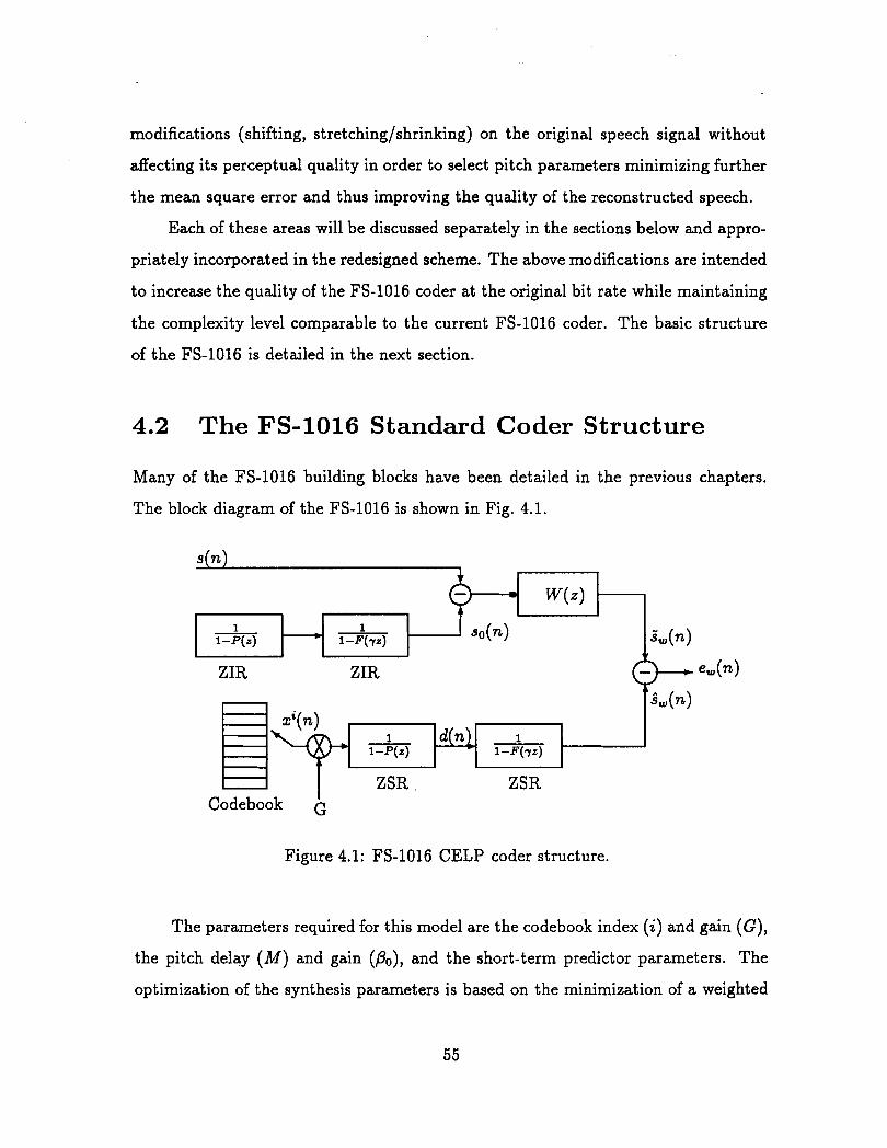
modifications (shifting, stretching/shrinking) on the original speech signal without
affecting its perceptual quality in order to select pitch parameters minimizing further
the mean square error and thus improving the quality of the reconstructed speech.
Each of these areas will be discussed separately in the sections below and appro-
priately incorporated in the redesigned scheme. The above modifications are intended
to increase the quality of the FS-1016 coder at the original bit rate while maintaining
the complexity level comparable to the current FS-1016 coder. The basic structure
of the FS-1016 is detailed in the next section.
4.2 The FS-1016 Standard Coder Structure
Many of the FS-1016 building blocks have been detailed in the previous chapters.
The block diagram of the FS-1016 is shown in Fig. 4.1.
s n
Codebook 6
xi(n)
Figure 4.1: FS-1016 CELP coder structure.
W ( 4
1 1-P(z)
The parameters required for this model are the codebook index (i) and gain (G),
the pitch delay (M) and gain ( P o ) , and the short-term predictor parameters. The
ZSR ZSR
.&Q
optimization of the synthesis parameters is based on the minimization of a weighted
aw(n)
- , 1 1-F(7z)
i
ZIR ZIR
1 l-F(V)
1 1 -P(z) -
mean squared error criterion. The weighting consists of a spectral noise weighting
filter
whose task is to relocate the coding distortions to high energy regions of the spectrum
where they are less audible.
The FS-1016 coder is based on a narrowband speech coding where the input
speech bandwidth is limited to 3.4 kHz. The frame length is 30 ms, corresponding
to 240 samples at a speech sampling rate of 8 kHz. The speech frame is further
subdivided into four subframes of 30 samples each (7.5 ms). The CELP analysis
consists of three basic functions: 1) short delay formant prediction, 2) long delay
pitch search, and 3) residual codebook search.
4.2.1 Short Delay Prediction
The spectrum analysis is performed once per frame with a 10th order autocorrelation
LPC analysis using a 30 ms Hamming window. The window which is of the same
length as the frame is centered at the end of each frame. In other words, the two last
subframes of the past frame and the two first subframes of the present frame con-
tribute to the calculation of the LPC coefficients of the present frame. The predictor
parameters ak have to be efficiently coded, and transmitted as side information to the
decoder. The Line Spectral Frequencies (LSF) parameters representation is used. Let
Lo and L1 denote the LSF vectors for.the previous and present frame respectively. In
order to allow a smoother transition in each subframe, weighting averaging between
Lo and L1 is recommended in order to form an intermediate set of LSF for each of
the four subframes. The LSF in a certain subframe k will be denoted as lk. The
subframe LSF will be determined as follows:
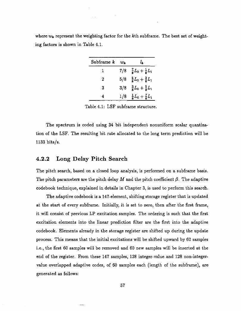
where wk represent the weighting factor for the kth subframe. The best set of weight-
ing factors is shown in Table 4.1.
Subframe k wk lk -
1 718 fLo + iL1
2 518 i L o + f L l
3 318 f L o + f L l
4 118 ! L o + f L l
Table 4.1: LSF subframe structure.
The spectrum is coded using 34 bit independent nonuniform scalar quantiza-
tion of the LSF. The resulting bit rate allocated to the long term prediction will be
1133 bits/s.
4.2.2 Long Delay Pitch Search
The pitch search, based on a closed loop analysis, is performed on a subframe basis.
The pitch parameters are the pitch delay M and the pitch coefficient P. The adaptive
codebook technique, explained in details in Chapter 3, is used to perform this search.
The adaptive codebook is a 147-element, shifting storage register that is updated
at the start of every subframe. Initially, it is set to zero, then after the first frame,
it will consist of previous LP excitation samples. The ordering is such that the first
excitation elements into the linear prediction filter are the first into the adaptive
codebook. Elements already in the storage register are shifted up during the update
process. This means that the initial excitations will be shifted upward by 60 samples
i.e., the first 60 samples will be removed and 60 new samples will be inserted at the
end of the register. From these 147 samples, 128 integer-value and 128 non-integer-
value overlapped adaptive codes, of 60 samples each (length of the subframe), are
generated as follows:
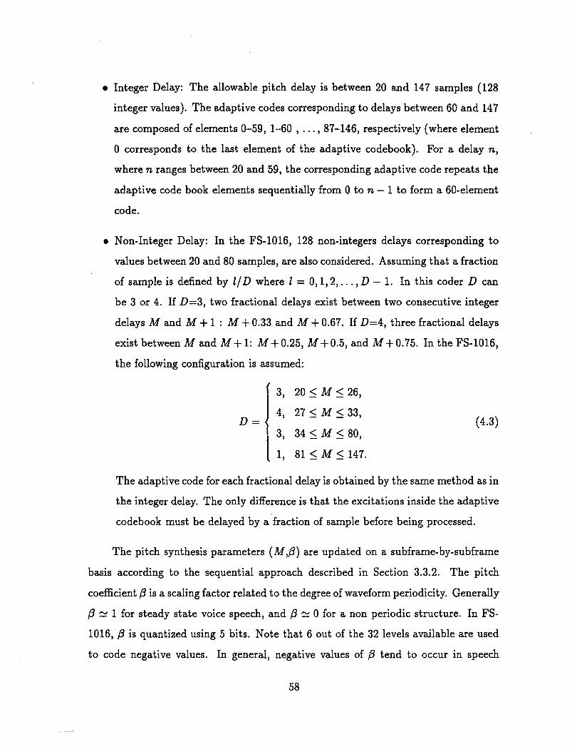
Integer Delay: The allowable pitch delay is between 20 and 147 samples (128
integer values). The adaptive codes corresponding to delays between 60 and 147
are composed of elements 0-59, 1-60 , . . . , 87-146, respectively (where element
0 corresponds to the last element of the adaptive codebook). For a delay n,
where n ranges between 20 and 59, the corresponding adaptive code repeats the
adaptive code book elements sequentially from 0 to n - 1 to form a 60-element
code.
0 Non-Integer Delay: In the FS-1016, 128 non-integers delays corresponding to
values between 20 and 80 samples, are also considered. Assuming that a fraction
of sample is defined by 1/D where 1 = 0,1,2,. . . , D - 1. In this coder D can
be 3 or 4. If D=3, two fractional delays exist between two consecutive integer
delays M and M + 1 : M + 0.33 and M + 0.67. If D=4, three fractional delays
exist between M and M + 1: M + 0.25, M + 0.5, and M + 0.75. In the FS-1016,
the following configuration is assumed:
The adaptive code for each fractional delay is obtained by the same method as in
the integer delay. The only difference is that the excitations inside the adaptive
codebook must be delayed by a'fraction of sample before being processed.
The pitch synthesis parameters ( M , P ) are updated on a subframe-by-subframe
basis according to the sequential approach described in Section 3.3.2. The pitch
coefficient p is a scaling factor related to the degree of waveform periodicity. Generally
p zt 1 for steady state voice speech, and p E 0 for a non periodic structure. In FS-
1016, P is quantized using 5 bits. Note that 6 out of the 32 levels available are used
to code negative values. In general, negative values of P tend to occur in speech
regions with low energy, and large values of P occur in transition regions from silence
to voiced speech. The quantized values of P are between -1 and 2.
Theoretically, when IPI > 1, the pitch synthesis filter, *, will become un-
stable leading to an enhancement of the noise and a noticeable degradation in the
reconstructed speech quality. For a single tap pitch filter, stability is guaranteed by
restricting the magnitude of P. This result is easily extended to fractional delay pitch
predictor. A detailed analysis on pitch synthesis filter stability will be discussed later
in this Chapter.
The pitch delay M is coded in function of the subframe. For odd subframes, the
pitch delay ranges from 20 to 147 samples (including non-integer values). In total 8
bits are needed to code the delays. For even subframes, the pitch delay will range
within 64 lags (6 bits) relative to the previous subframe delay.
During one frame period, 22 (8+6+8+6) bits are needed for coding the pitch
delay and 20 (5 x 4) bits are needed to code the pitch coefficient. The resulting bit
rate for the pitch parameters is 1600 bits/s.
4.2.3 Codebook Search
The codebook search, based also on a closed-loop analysis, is performed four times
per frame in order to estimate the index i of the codebook, containing the excitation
waveforms, and the corresponding gain G to denormalize these excitations.
Codebook structure
The stochastic codebook used in FS-1016 is considered as a codebook vector contain-
ing sparse ternary elements. These excitations are generated by center clipping and
limiting a zero-mean unit-variance Gaussian distributed sequence. The center clip-
ping threshold is set to f 1.2 in order to satisfy a sparsity of 75% inside the vector.
All values between t1 .2 and -1.2 in the Gaussian distribution are set to 0, values
greater than $1.2 are set to +1, and values less than -1.2 are set to -1. There
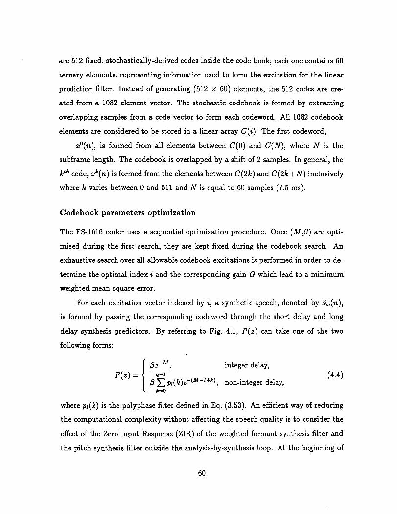
are 512 fixed, stochastically-derived codes inside the code book; each one contains 60
ternary elements, representing information used to form the excitation for the linear
prediction filter. Instead of generating (512 x 60) elements, the 512 codes are cre-
ated from a 1082 element vector. The stochastic codebook is formed by extracting
overlapping samples from a code vector to form each codeword. All 1082 codebook
elements are considered to be stored in a linear array C(i). The first codeword,
xO(n), is formed from all elements between C(0) and C(N), where N is the
subframe length. The codebook is overlapped by a shift of 2 samples. In general, the
kth code, xk(n) is formed from the elements between C(2k) and C(2k+ N) inclusively
where k varies between 0 and 511 and N is equal to 60 samples (7.5 ms).
Codebook parameters optimization
The FS-1016 coder uses a sequential optimization procedure. Once ( M , P ) are opti-
mized during the first search, they are kept fixed during the codebook search. An
exhaustive search over all allowable codebook excitations is performed in order to de-
termine the optimal index i and the corresponding gain G which lead to a minimum
weighted mean square error.
For each excitation vector indexed by i, a synthetic speech, denoted by S,(n),
is formed by passing the corresponding codeword through the short delay and long
delay synthesis predictors. By referring to Fig. 4.1, P ( z ) can take one of the two
following forms:
I w", integer delay,
pr(k)z-(M-'+k), non-integer delay,
where pl(k) is the polyphase filter defined in Eq. (3.53). An efficient way of reducing
the computational complexity without affecting the speech quality is to consider the
effect of the Zero Input Response (ZIR) of the weighted formant synthesis filter and
the pitch synthesis filter outside the analysis-by-synt hesis loop. At the beginning of
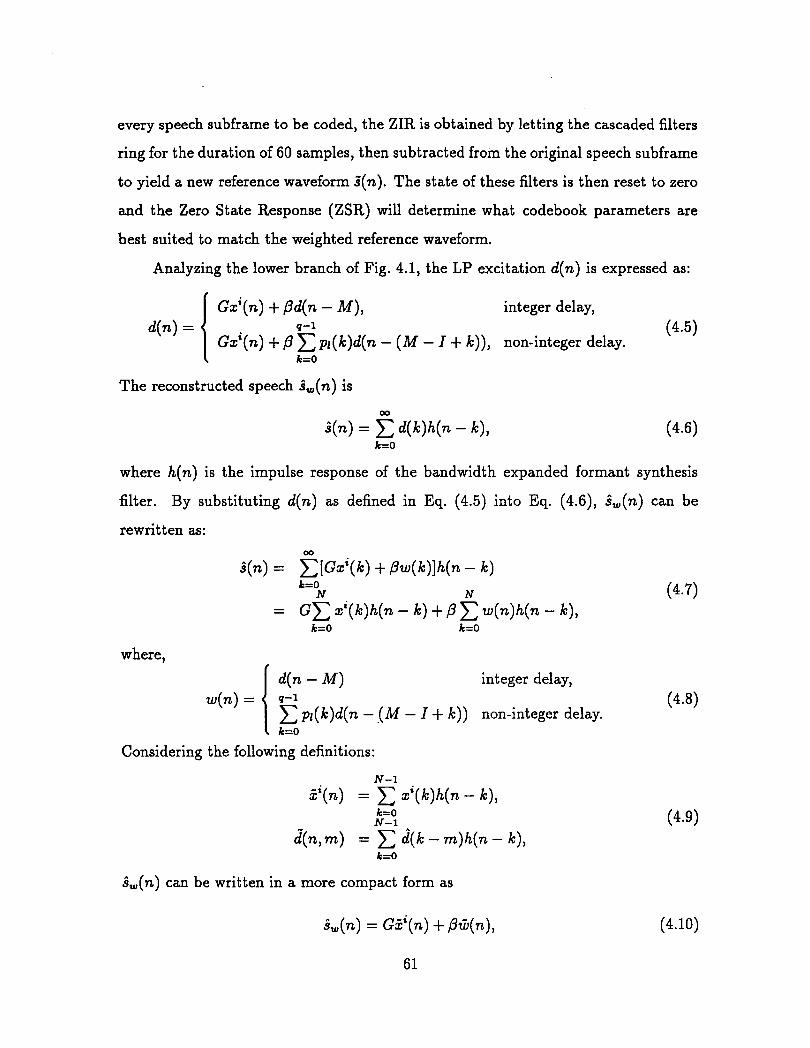
every speech subframe to be coded, the ZIR is obtained by letting the cascaded filters
ring for the duration of 60 samples, then subtracted from the original speech subframe
to yield a new reference waveform s'(n). The state of these filters is then reset to zero
and the Zero State Response (ZSR) will determine what codebook parameters are
best suited to match the weighted reference waveform.
Analyzing the lower branch of Fig. 4.1, the LP excitation d(n) is expressed as:
( Gxi(n) + pd(n - M), integer delay, d(n) = q-1 I Gxi(n) 4- p ~l (k)d(n - ( M - I + k)), non-integer delay.
(4.5)
The reconstructed speech dw(n) is
00
i (n) = d(k)h(n - k), k=O
where h(n) is the impulse response of the bandwidth expanded formant synthesis
filter. By substituting d(n) as defined in Eq. (4.5) into Eq. (4.6), iw(n) can be
rewritten as:
d(n) =
- - GC xi(k)h(n - k) + ,f? 2 w(n)h(n - k), k=O k=O
where,
( 4.-M) integer delay,
w(n) = I 2 pl(k)d(n - (M - I + 6)) non-integer delay. \ k=O
Considering the following definitions:
N-1
%'(n) = x xi(k)h(n- k), k=O N-1
d(n,rn) = x 6(k-rn)h(n- k), k=O
d,(n) can be written in a more compact form as

where G(n) is defined as
I d(% M), integer delay, (4.11)
d(n, M - I + k)pl(k), non-integer delay.
Referring to the upper branch of Fig. (4.1), so(n) is the contribution from the
past codewords, and can be considered as the ZIR of the cascade pitch and formant
filters, - 1
U n ) = [ ~ x ' ( k ) + pw(k)] h(n - k). (4.12) k = - w
Recall that xi(k) is the codeword excitation and is only non-zero for k > 0. So,
io(n) will be - 1
io(n) = pw(k)h(n - k). k=-m
The reference weighted speech s',(n) is formed by subtracting so(n) from the original
speech and passing the resulting signal s'(n) into the weighting filter to yield 3,(n).
The codebook search is based on minimizing the weighted mean squared error
Substituting Eq. (4.10) into the above equation and lumping the terms that remain
constant during the search into a single term denoted by r'(n), the weighted error can
be rewritten as: N-1
E = C (r'(n) - GX'(~)) ' , n = O
where
By setting &/8G = 0, G is found to be,
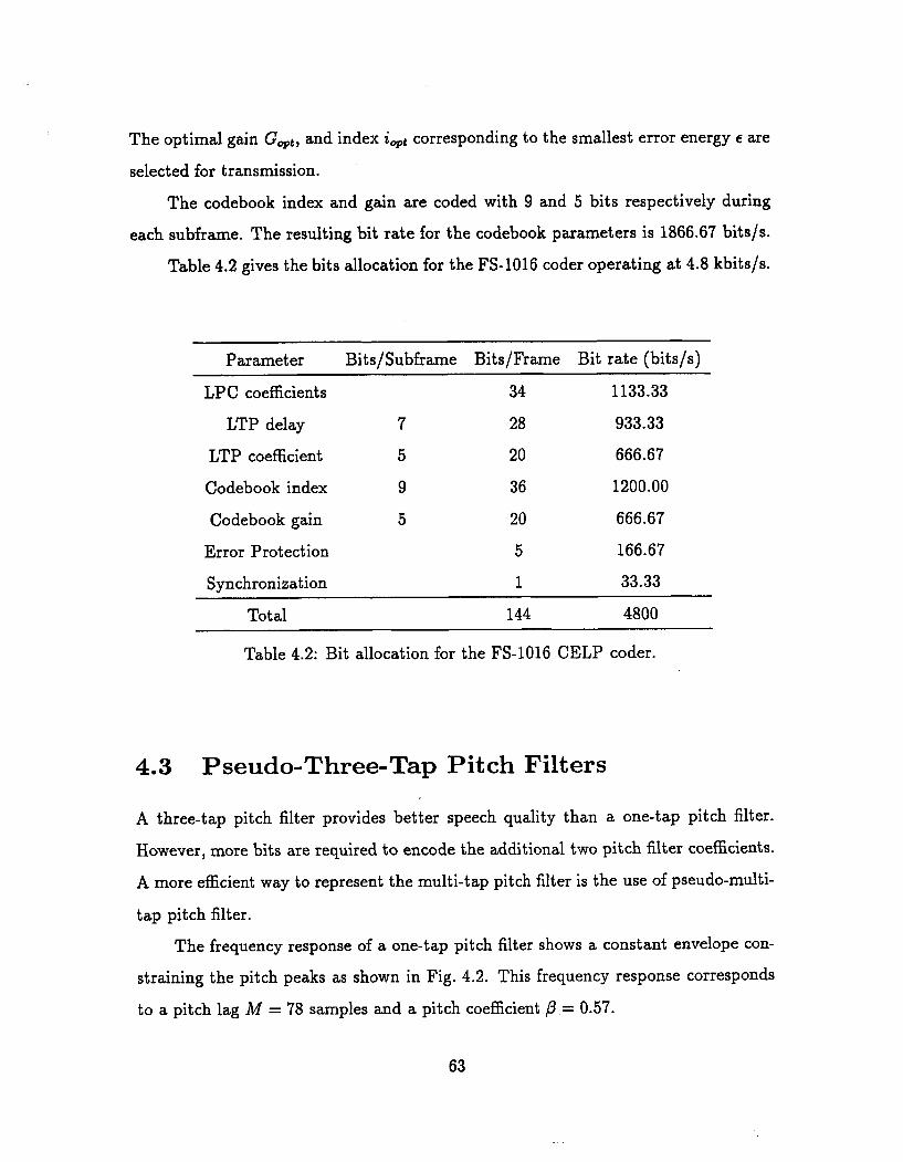
The optimal gain Gqt, and index iqt corresponding to the smallest error energy e are
selected for transmission.
The codebook index and gain are coded with 9 and 5 bits respectively during
each subframe. The resulting bit rate for the codebook parameters is 1866.67 bitsls.
Table 4.2 gives the bits allocation for the FS-1016 coder operating at 4.8 kbitsjs.
Parameter BitsISubframe BitsjFrame Bit rate (bitsjs)
LPC coefficients 34 1133.33
LTP delay 7 28 933.33
LTP coefficient 5 20 666.67
Codebook index 9 36 1200.00
Codebook gain 5 20 666.67
Error Protection 5 166.67
Synchronization 1 33.33
Total 144 4800 - -
Table 4.2: Bit allocation for the FS-1016 CELP coder.
4.3 Pseudo-Three-Tap Pitch Filters
A three-tap pitch filter provides better speech quality than a one-tap pitch filter.
However, more bits are required to encode the additional two pitch filter coefficients.
A more efficient way to represent the multi-tap pitch filter is the use of pseudo-multi-
tap pitch filter.
The frequency response of a one-tap pitch filter shows a constant envelope con-
straining the pitch peaks as shown in Fig. 4.2. This frequency response corresponds
to a pitch lag M = 78 samples and a pitch coefficient /3 = 0.57.
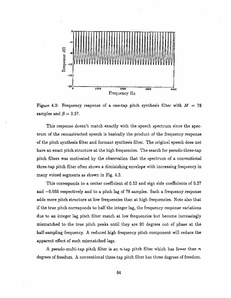
0
I
0
Frequency Hz
Figure 4.2: Frequency response of a one-tap pitch synthesis filter with M = 78
samples and p = 0.57.
This response doesn't match exactly with the speech spectrum since the spec-
trum of the reconstructed speech is basically the product of the frequency response
of the pitch synthesis filter and formant synthesis filter. The original speech does not
have an exact pitch structure at the high frequencies. The search for pseudo-three-tap
pitch filters was motivated by the observation that the spectrum of a conventional
three-tap pitch filter often shows a diminishing envelope with increasing frequency in
many voiced segments as shown in Fig. 4.3.
This corresponds to a center coefficient of 0.52 and sign side coefficients of 0.27
and -0.055 respectively and to a pitch lag of 78 samples. Such a frequency response
adds more pitch structure at low frequencies than at high frequencies. Note also that
if the true pitch corresponds to half the integer lag, the frequency response variations
due to an integer lag pitch filter match at low frequencies but become increasingly
mismatched to the true pitch peaks until they are 90 degrees out of phase at the
half-sampling frequency. A reduced high frequency pitch component will reduce the
apparent effect of such mismatched lags.
A pseudo-multi-tap pitch filter is an n-tap pitch filter which has fewer than n
degrees of freedom. A conventional three-tap pitch filter has three degrees of freedom.
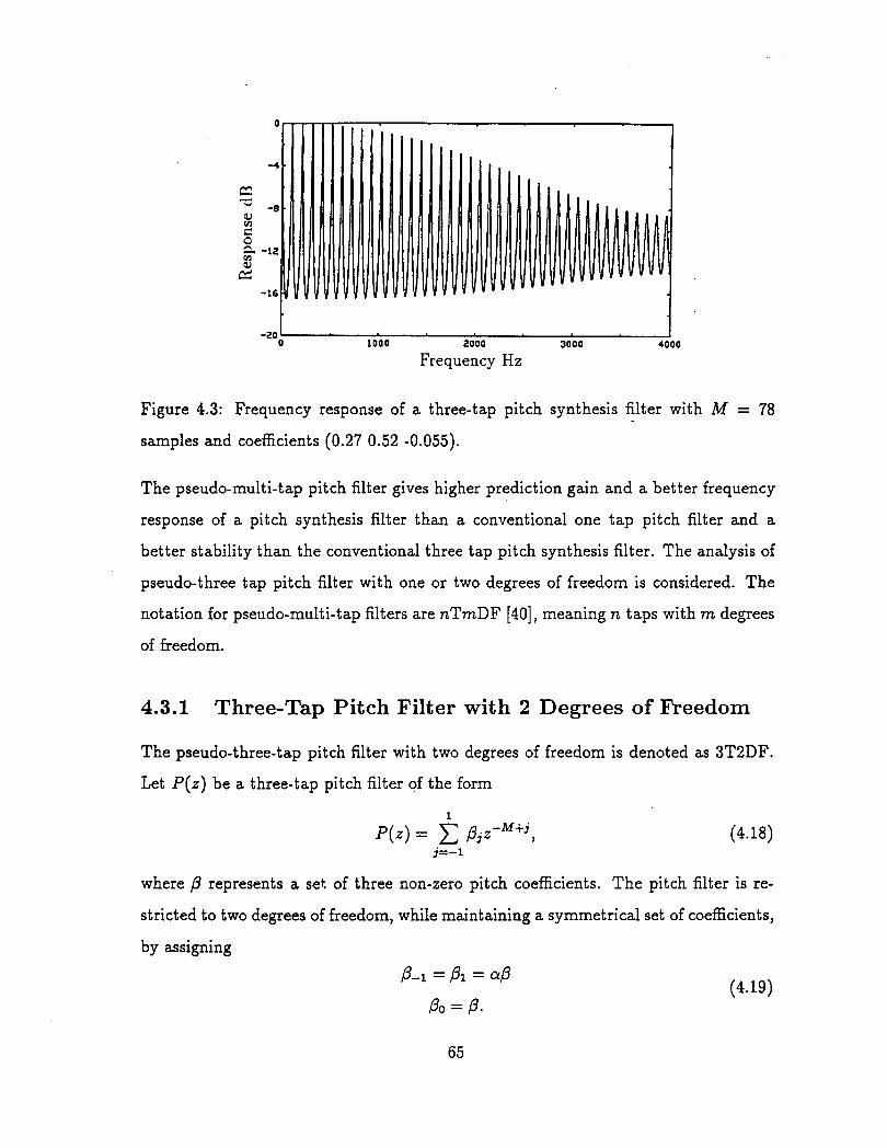
Frequency Hz
Figure 4.3: Frequency response of a three-tap pitch synthesis filter with M = 78
samples and coefficients (0.27 0.52 -0.055).
The pseudo-multi-tap pitch filter gives higher prediction gain and a better frequency
response of a pitch synthesis filter than a conventional one tap pitch filter and a
better stability than the conventional three tap pitch synthesis filter. The analysis of
pseudo-three tap pitch filter with one or two degrees of freedom is considered. The
notation for pseudo-multi-tap filters are nTmDF [40], meaning n taps with m degrees
of freedom.
4.3.1 Three-Tap Pitch Filter with 2 Degrees of Freedom
The pseudo-three-tap pitch filter with two degrees of freedom is denoted as 3T2DF.
Let P(z) be a three-tap pitch filter of the form
where p represents a set, of three non-zero pitch coefficients. The pitch filter is re-
stricted to two degrees of freedom, while maintaining a symmetrical set of coefficients,
by assigning
Both @ and a! have to be optimized. The configuration shown in Fig. 3.2 will be
used as a reference for the analysis of the pseudo-three-tap pitch filters. By still
assuming a zero-input excitation to the pitch synthesis filter (sequential search), the
LP excitation d(n) is of the form:
d(n) = a@d((n mod ( M - 1)) - ( M - 1)) + pd((n mod M ) - M)+ (4.20)
cupd((n mod M + 1) - (M + I)),
for 0 5 n 5 N - 1. In order to avoid solving high degree polynomials, a periodic
extension of a pitch cycle is added to the LP excitation when the delay is less than
the subframe length. By generalizing the expression of the weighted mean square
error given in Eq. (3.33), the new weighted error will be:
where 7 = a@, and din, .) is defined in Eq. (3.32). The pitch lag M corresponds to
the middle tap and is chosen as that which is optimal for a one-tap pitch predictor.
The resulting summed squared prediction error is
The minimization of E leads to a set of two different linear equations which can be
written in a matrix form. By setting the partial derivatives of E with respect to 7 and
p to zero, the following system is obtained
[: :] [:I = [ s ] . where
and 4(i, j ) is defined as
By using Cramer's rule to solve the above system, the optimal pitch coefficients are
found to be
4.3.2 Three-Tap Pitch Filter with 1 Degree of Freedom
The pseudo-three tap pitch filter with one degree of freedom will be denoted as
3TlDF. In this case, a! in Eq. (4.19) is set to a constant. The only unknown is P. By
following the same procedure as in the above section, the optimal pitch coefficient is
found to be:
Popt = 4 ( O , M - 1) + 4(O,M) + 4 ( O , M + 1)
a 2 A + #(M, M) + 2aB I
where A and B are defined in Eq. (4.24).
4.3.3 Frequency Response of Pseudo-Tap Pitch Filters
The general expression of the frequency response of a 3T3DF pitch synthesis filter is
The amplitude of the above frequency response can be written as
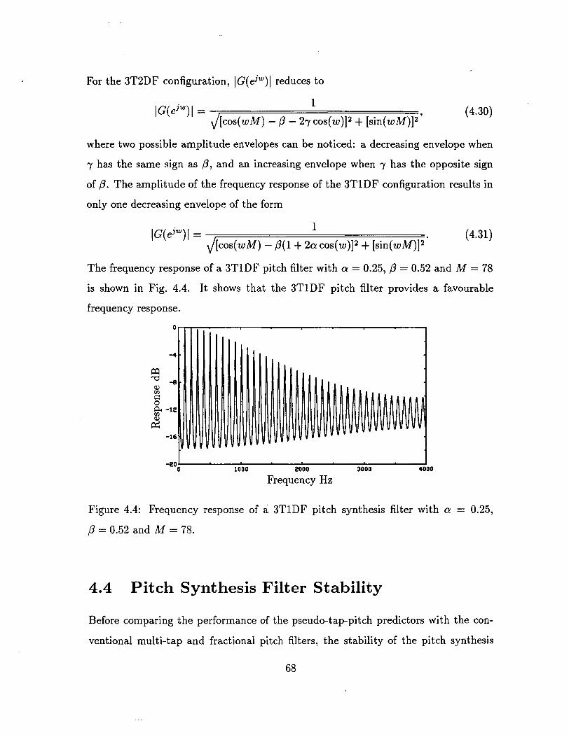
For the 3T2DF configuration, IG(ejw)l reduces to
where two possible amplitude envelopes can be noticed: a decreasing envelope when
y has the same sign as p, and an increasing envelope when y has the opposite sign
of p. The amplitude of the frequency response of the 3TlDF configuration results in
only one decreasing envelope of the form
The frequency response of a 3TlDF pitch filter with a = 0.25, P = 0.52 and M = 78
is shown in Fig. 4.4. It shows that the 3TlDF pitch filter provides a favourable
frequency response.
0
-4
a a -e 8
gi -12
2 -16.
-201 I 0 1000 2000 3000 4000
Frequency Hz
Figure 4.4: Frequency response of a 3TlDF pitch synthesis filter with a = 0.25,
,B = 0.52 and hl = 78.
4.4 Pitch Synthesis Filter Stability
Before comparing the performance of the pseudo-tap-pitch predictors with the con-
ventional multi-tap and fractional pitch filters, the stability of the pitch synthesis
filter is considered in this section. The pitch synthesis filter has a transfer function
The procedure used to determine the set of pitch predictor coefficients can result in
an unstable pitch synthesis filter.
In the APC type coder, discussed in Section
quantized residual error &(n) can be expressed as
= e(n> + d n ) ,
where e(n) is the exact residual error and q(n) is
2.3) and shown in Fig. 2.4, the
(4.33)
the quantization noise. At the
decoder stage, the reconstructed speech i (n) can be written as
where Q(n) is the noise in the reconstructed speech obtained after exciting q(n) by the
cascade pitch and formant synthesis filters. For an unquantized residual e(n), stability
of the pitch filter is not a necessity because of pole/zero cancellation. However, an
unstable synthesis filter can cause the output quantization noise to build up during
the period of instability and can lead to degraded speech quality. If the quantization
noise is modeled as white noise, the output noise power can be expressed as the input
noise power multiplied by the power gain of the filter. The power gain is the sum of
the squares of the filter coefficients.
In analysis-by-synthesis configurations, stability remains an issue that must be
considered. The adaptive codebook contains the shifted versions of the past pitch
filter output. It can be viewed as the summation of the pitch filter output excited by
an exact prediction residual plus a quantization noise. For the prediction residual,
stability is also not a problem because of pole/zero cancellation. However, the quan-
tization noise passes through only the unstable synthesis filter. The real problem is
that the effect of unstable pitch filters propagates into subsequent frames; quantiza-
tion noise is further augmented because the adaptive codebook is updated with the
accumulated noise due to previous unstable filters.
In this section, two stability tests are formulated and several procedures for
stabilization are proposed in case of instability.
4.4.1 Stability Tests
To ensure stability of the pitch synthesis filter, the denominator D(z) of G(z) in
Eq. (4.32) must have all its zeros within the unit circle in the z-plane. The polynomial
D(z) is of high order (lag order) but has few non-zero coefficients. Two different
sufficient tests are developed in [19]. First a simple sufficient condition for stability is
that the moduli of the pitch coefficients be less than one. Second, an alternative test
based on an asymptotically tight sufficient condition is developed for a 3-tap pitch
filter. The tight sufficient test is summarized below.
Let a = p-1 + PI and b = p-1 - pl. Two cases are considered:
1. If la1 2 Ibl, then the sufficient condition for stability is:
2. If la1 < Ibl, the satisfaction of the two following conditions is sufficient for
stability:
( 4 P o l + lal < 1
(b) i. b2 5 la1 or
ii. b2@,2 - (1 - b2)(b2 - a') < 0.
The second part of this stability test is tighter than the simple sufficient test. This
part is invoked when la1 < Ibl or equivalently when Pl and P-1 have opposite signs.
Experiments in [19] show that the number of voiced frames in which P1 and P-1 have
opposite signs is about 3.7 times the number of voiced frames in which they have the
same signs. Therefore, the presence of a tighter test when la1 < I bl is important for
speech coders. The test for 3 taps subsumes the tests for two-tap, single-tap, and
pseudo-three-tap filters. For 2T2DF = 0) and lTlDF (P-1 = P1=O), la1 = Ibl.
For 3T2DF or 3TlDF (P-1 = PI), I bJ = 0 and the condition la1 2 b is always satisfied.
In the above cases, the stability test involves checking that the sum of the moduli of
the coefficients is less than one which is equivalent to the first simple sufficient test.
4.4.2 Stabilization Procedures
The stability test is used to determine whether the corresponding pitch synthesis
filter is stable. If the filter is found to be stable, no modification to the coefficients
is made. However, if the filter is unstable, the pitch coefficients can be considered
locally optimal but not globally as pops and clicks will be heard in the reconstructed
speech. So, a stabilization procedure is used to find a new set of pitch coefficients.
Obviously, the new set of coefficients lead to a decrease in the prediction gain for that
frame. A major concern in performing stabilization is to keep the loss in prediction
gain to a minimum.
The first technique involves scaling each of the poles radially inward. This is
equivalent to scaling the pitch coefficients by different factors which have to be de-
termined iteratively in order to obtain the best set. This method is found to be
unnecessarily complex. The second technique consists of replacing each pole outside
the unit circle by its reciprocal. This technique preserves the frequency response of
the pitch filter but involves factoring the high degree denominator polynomial which
may be impractical for filters with more than a single coefficient. The third technique,
derived directly from the stability test, and judged to be the most practical, is the
common scaling factor method. It consists of multiplying each predictor coefficient
by a factor c determined in a way to so as to guarantee that all the poles lie within
the unit circle. The value of the scaling factor c for the lTlDF, 2T2DF) 3T2DF,
and 3TlDF cases is easily determined since the stability test involves only a single
condition. Let S denotes the stabilization factor and is defined as
If S < 1 stability is ensured and no scaling factor is used. However, if S 2 1 instability
is assumed. The scaling factor c must force IP-ll + + IPII to be at most equal to
one. The value of c which gives marginal stability, derived directly from Eq. (4.36),
If the tight sufficient test is used for the 3T3DF configuration, several values of S are
obtained depending on the values of a and b,
The scaling factor c must force S to be equal to one in case where instability is
detected (S 2 1). Three cases arise and are formulated as follows
The values of c in Eq. (4.39) correspond to solving for the scaled conditions of the
tight sufficient test given earlier. After scaling the pitch coefficients by the factor c,
the new vector of the predictor coefficients @'can be expressed as
where POpt is the vector of optimal pitch predictor coefficients. This results in a
sub-optimum predictor for which the weighted mean square error is
where a is defined in Eq. (3.40), and e;,, given in Eq. (3.43), is the minimum mean
square error for the optimum pitch predictor. The quantity (1 - c)P&a represents
the excess in the mean square error resulting from the use of a sub-optimum predictor.
It is observed that as c deviates from one, E increases and the loss in prediction gain
increases. In order to minimize the loss in prediction gain, c must be as close to one
as possible and at the same time give a stable pitch synthesis filter.
4.5 Performance of Pitch Predictors in FS-1016
To compare the pseudo-three-tap pitch filter with conventional single-tap, multi-tap,
and fractional pitch filters, a pitch prediction gain measure is introduced to calculate
the performance. During the first closed-loop pitch search, G is set to zero. By
referring to Fig. 3.2, the pitch prediction gain, denoted by Pg (expressed in dB's), is
defined to be zw(n) Pg = 10 log - ew (n) '
where iW(n) is the reference weighted speech and ew(n) is the weighted residual error.
The pitch prediction gain indicates the performance of the adaptive codebook, that
is the pitch filter excitation without the codebook influence . A high Pg means that
the quality of the pitch filter is good: In computing the prediction gain, subframes
whose prediction gain was below 1.2 dB were not included since those subframes
usually represent silence or unvoiced sounds. The performance of the various pitch
predictors delays was evaluated from a wide variety of speakers (male and female). In
the experiment, all the CELP parameters are quantized except the pitch coefficients.
The pitch coefficients remain unquantized in order to avoid the design of codebooks,
and to verify and observe the effect of instability in the multi-tap and pseudo-multi-
tap configurations.
The st ability of the pitch synthesis filter affects tremendously the performance
and the quality of the reconstructed speech signal. As described before, the pitch
predictor parameters are updated every subframe. The pitch synthesis filter is a
time-varying filter and stability test is required after each subframe. The stability of
the pitch synthesis filter is checked once the pitch coefficients are obtained, by using
the tight sufficient stability test described in the previous section.
By increasing the resolution of the lag and/or the number of pitch coefficients
for a certain pitch predictor, the stability of the pitch synthesis filter becomes harder
to control and the number of reconstruction speech subframes based on unstable
pitch synthesis filter increases. Experiments have shown that when a 3T3DF pitch
synthesis filter is used, half of the reconstructed subframes of a female speech file are
based on unstable pitch synthesis filter.
The performance of the pitch predictors is evaluated by first computing the pitch
prediction gain defined in Eq. (4.42) then by measuring the objective quality of the
reconstructed speech signal represented by the overall and segmental SNR, and finally
by listening to the quality of the reconstructed speech which is the most important
evaluation. Table 4.3 shows the performance of various pitch predictors with the
corresponding average pitch prediction gain (P,), the overall SNR and SEGSNR of
the reconstructed speech.
A stability test can be applied to the pitch filter. Stabilization would normally
be accomplished by choosing a scaling factor to bring the filter into the stable region.
However, during the simulations, it was noted that for many unstable pitch filters,
the scaling factor c is very much less than 1 leading to a considerable loss in the pitch
prediction gain. A relaxation of the tight sufficient test is introduced. In the tight
sufficient test, S is not allowed to exceed unity. In the relaxed sufficient test, S is
allowed to take on values up to a threshold A.
The new scaling factors for stabilization can be rewritten as
In Table 4.3, a subscript describes the stabilization procedure used. For instance, the
subscript X = 1.2 indicates that S was allowed to take on values up to 1.2. The case
of no stabilization can be denoted as X = oo.
The first part of Table 4.3 illustrates the performance of a single-tap pitch pre-
dictor with different configurations. In the ( IT 1 DF)x,, configuration, the threshold
of the stabilization factor (S) is equal to infinity. In a single tap pitch predictor, it
has been noticed, that in average, 25% of speech subframes are reconstructed from
unstable pitch synthesis filters. These subframes show some pops and clicks and a
noticeable enhancement of the energy of the subframes. In a single-tap predictor, the
degradation in the subjective quality of the reconstructed speech due to the instabil-
ity problem is not very important unlike the case of a three-tap pitch filter which is
going to be illustrated later in this section. Several thresholds for the stabilization
factors are then considered for the (1TlDF) configuration. The (lTIDF)x,l.o shows
a higher SNR and SNRSEG than the (lTIDF)x,,. Increasing the threshold of the
stabilization factor doesn't increase much the SNR and SNRSEG of the reconstructed
speech as shown in Table 4.3. By using the stabilization technique, all the pops and
clicks which were noted in the reconstructed speech of (lTIDF)x,, are completely
eliminated.
The second part of Table 4.3 shows the performance of the 3T3DF configuration.
By increasing the number of pitch coefficients, the tight sufficient test for stability
becomes harder to satisfy.
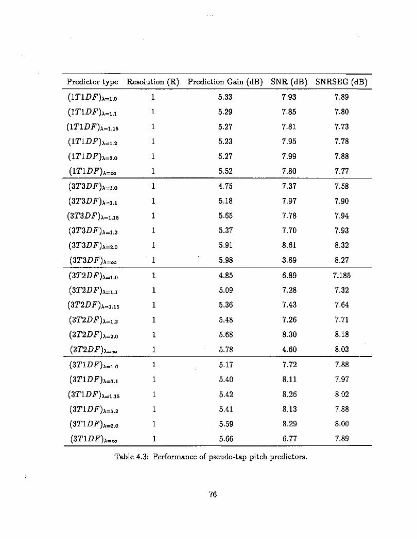
Predictor type Resolution (R) Prediction Gain (dB) SNR (dB) SNRSEG (dB)
Table 4.3: Performance of pseudo-tap pitch predictors.
76
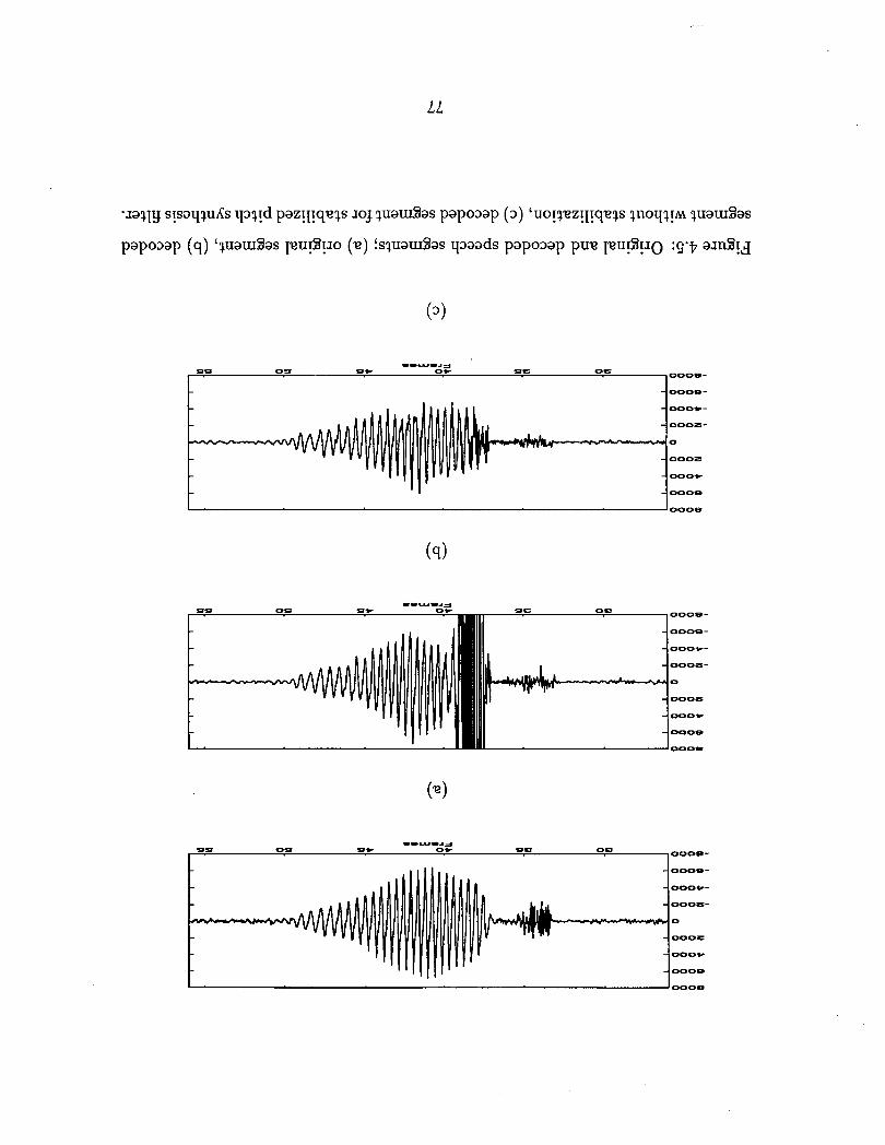
'Jaqlg s!sayqulCs y3q!d paz!pqaqs JOJ quau13as papoDap (3) 'uo!qaz!~~qaqs qnoyqp quawSas
papo~ap (q) '~uaw8as ~su!S!~o (a) !squau~Sas p a d s papo3ap puo ~su!S!~o : y ~ a~nS!d
W O L U I J j
99 09 9* O P 9E O E oooe-
ooom-
ooo*-
o o o a -
0
OOOZ
OOOP
t I 1°00-
- - U S A 3 99 09 o* O E 000a-
ooom-
ooo*-
OOOZ-
0
oooaz
OOOP
o o o m
L I L I o e
ooom-
0001r-
oooaz-
0
OOOZ
OOOP
]ooom
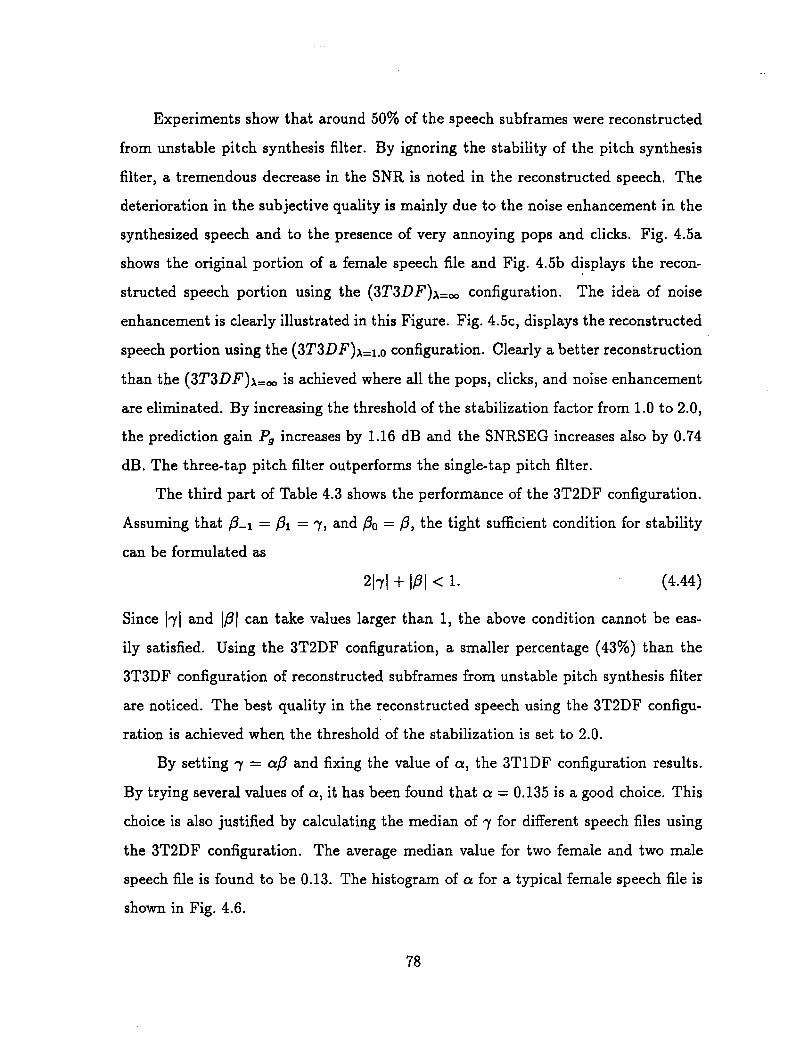
Experiments show that around 50% of the speech subframes were reconstructed
from unstable pitch synthesis filter. By ignoring the stability of the pitch synthesis
filter, a tremendous decrease in the SNR is noted in the reconstructed speech. The
deterioration in the subjective quality is mainly due to the noise enhancement in the
synthesized speech and to the presence of very annoying pops and clicks. Fig. 4.5a
shows the original portion of a female speech file and Fig. 4.5b displays the recon-
structed speech portion using the (3T3DF)x,, configuration. The idea of noise
enhancement is clearly illustrated in this Figure. Fig. 4.5c, displays the reconstructed
speech portion using the (3T3DF)x,l.o configuration. Clearly a better reconstruction
than the (3T3DF)x,, is achieved where all the pops, clicks, and noise enhancement
are eliminated. By increasing the threshold of the stabilization factor from 1.0 to 2.0,
the prediction gain P, increases by 1.16 dB and the SNRSEG increases also by 0.74
dB. The three-tap pitch filter outperforms the single-tap pitch filter.
The third part of Table 4.3 shows the performance of the 3T2DF configuration.
Assuming that P-1 = P1 = 7, and Po = P, the tight sufficient condition for stability
can be formulated as
2171 + IPI < 1-
Since 171 and I/?( can take values larger than 1, the above condition cannot be eas-
ily satisfied. Using the 3T2DF configuration, a smaller percentage (43%) than the
3T3DF configuration of reconstructed subframes from unstable pitch synthesis filter
are noticed. The best quality in the reconstructed speech using the 3T2DF configu-
ration is achieved when the threshold of the stabilization is set to 2.0.
By setting 7 = ap and fixing the value of a, the 3TlDF configuration results.
By trying several values of a, it has been found that a = 0.135 is a good choice. This
choice is also justified by calculating the median of 7 for different speech files using
the 3T2DF configuration. The average median value for two female and two male
speech file is found to be 0.13. The histogram of a for a typical female speech file is
shown in Fig. 4.6.
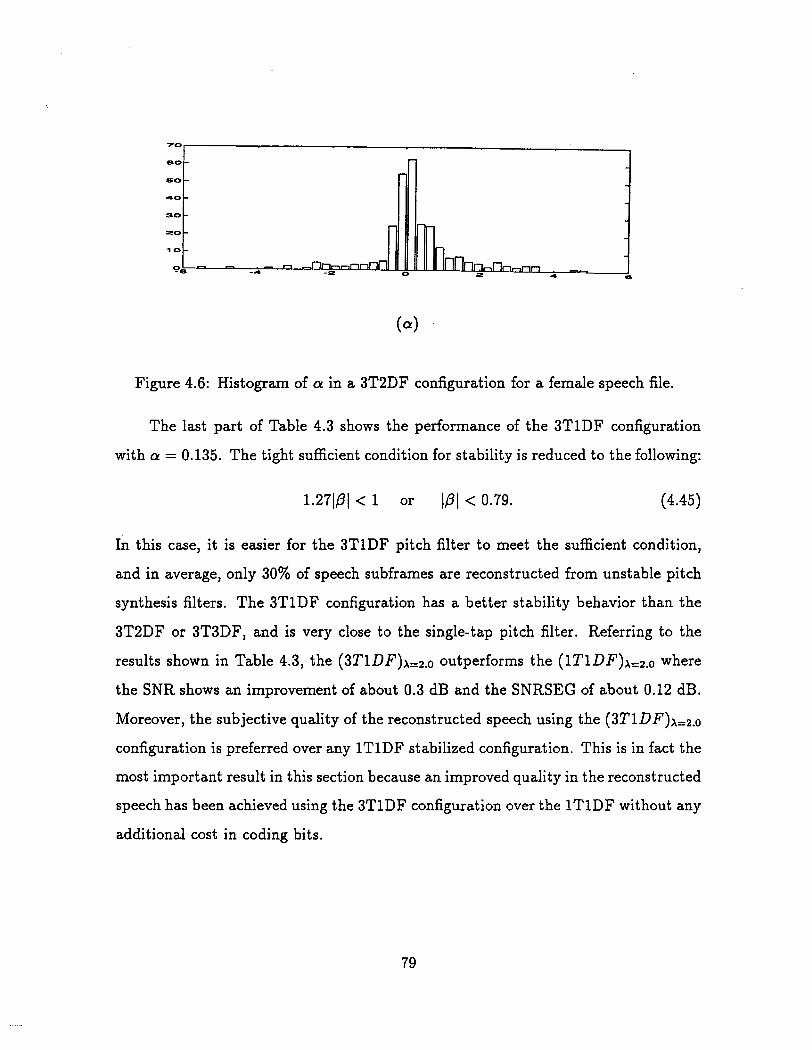
Figure 4.6: Histogram of a! in a 3T2DF configuration for a female speech file.
The last part of Table 4.3 shows the performance of the 3TlDF configuration
with a = 0.135. The tight sufficient condition for stability is reduced to the following:
In this case, it is easier for the 3TlDF pitch filter to meet the sufficient condition,
and in average, only 30% of speech subframes are reconstructed from unstable pitch
synthesis filters. The 3TlDF configuration has a better stability behavior than the
3T2DF or 3T3DF, and is very close to the single-tap pitch filter. Referring to the
results shown in Table 4.3, the (3T1DF)x,2.0 outperforms the (1T1DF)x,2.0 where
the SNR shows an improvement of about 0.3 dB and the SNRSEG of about 0.12 dB.
Moreover, the subjective quality of the reconstructed speech using the (ST 1 D F)x=2.0
configuration is preferred over any lT lDF stabilized configuration. This is in fact the
most important result in this section because an improved quality in the reconstructed
speech has been achieved using the 3TlDF configuration over the l T l D F without any
additional cost in coding bits.
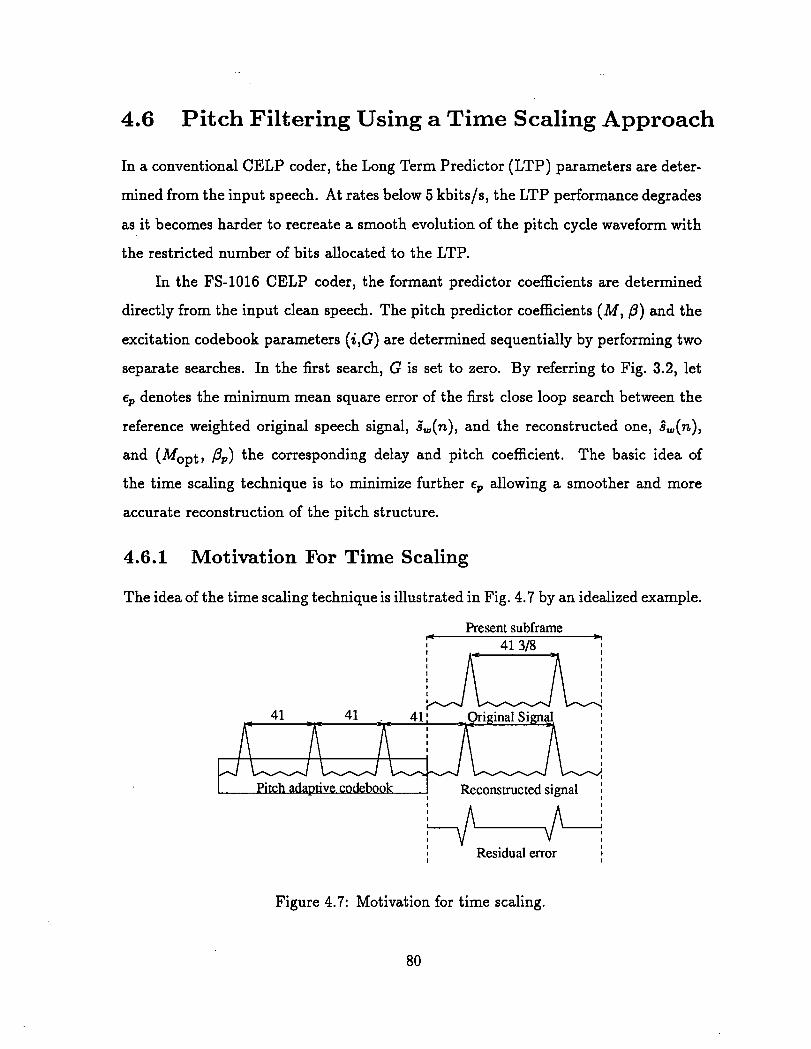
4.6 Pitch Filtering Using a Time Scaling Approach
In a conventional CELP coder, the Long Term Predictor (LTP) parameters are deter-
mined from the input speech. At rates below 5 kbitsls, the LTP performance degrades
as it becomes harder to recreate a smooth evolution of the pitch cycle waveform with
the restricted number of bits allocated to the LTP.
In the FS-1016 CELP coder, the formant predictor coefficients are determined
directly from the input clean speech. The pitch predictor coefficients (M, P) and the
excitation codebook parameters (i,G) are determined sequentially by performing two
separate searches. In the first search, G is set to zero. By referring to Fig. 3.2, let
ep denotes the minimum mean square error of the first close loop search between the
reference weighted original speech signal, s',(n), and the reconstructed one, B,(n),
and (Mopt, ,LIP) the corresponding delay and pitch coefficient. The basic idea of
the time scaling technique is to minimize further E, allowing a smoother and more
accurate reconstruction of the pitch structure.
4.6.1 Motivation For Time Scaling
The idea of the time scaling technique is illustrated in Fig. 4.7 by an idealized example.
Present subframe I- * I 41 318 1
I Pitdudapthe codebook Reconstructed signal I
I 1 I I Residual error I I I
Figure 4.7: Motivation for time scaling.
Let the reference weighted original speech signal s',(n), be periodic with a period
of 41 318 samples. Assuming that only integer delays are transmitted and the pitch
adaptive codebook known, the reconstructed signal, B,(n) will be as shown in Fig. 4.7.
Note that the residual error e,(n), which is the difference between the original and
the reconstructed signal, shows vestiges of the pitch pulses. The random codebook
entry would try to remove these pulses and thereby effectively shift the pitch adaptive
codebook with the correct position. The alternative is to time scale the original signal
by the factor (41.375141) to make the distance between the two pitch pulses equal
in both the original and the reconstructed signals. A shift is also needed in order to
synchronize the pitch pulses. With time scaling and shifting, the residual error will
decrease and hence a better reconstruction is achieved. The shift and scaling factors
will not be transmitted to the receiver.
In practice, the amount of time scaling must be determined by trial and error. To
this end, a table containing combinations of time stretcheslshrinks and shifts is gen-
erated. This table is considered to modify the original signal and if the modifications
are slight, the changes on the perceptual quality will not be perceived. Moreover, the
size of the table is limited only by the computational considerations.
4.6.2 Time Scaling Algorithm in CELP
The time scaling operation is done on the original speech on a subframe basis ignoring
continuity considerations. To counteract this, the allowable time scaling coefficients
are kept very small so that the perceived quality of the speech is not affected. After
performing the first pitch search to determine the best set (MOpt, &), the optimal
lag Mopt is kept constant. An additional intermediate search is performed over all
allowable time scaling and shifting values and pitch coefficients in order to determine
the optimal pitch coefficient POpt and the best time scaling and shifting factors denoted
by wopt and sopt respectively. The new minimum mean square error will be denoted
as emin. If emin is not smaller than ep, the time scaling and shifting operations will
not be performed, and the optimal pitch coefficient Popt is equal to P,. Once the pitch and scaling parameters are determined, the stochastic codebook
search is performed to determine the optimal set (iopt, Gopt). The goal of these
codebook parameters is to give a better quality reconstructed speech than the one
obtained from the codebook parameters without applying the time scaling technique.
Time scaling operation
The time scaling operation in the above algorithm corresponds to stretching or shrink-
ing the original speech subframes by a factor w, and an additional shifting by a factor
s. In the case of stretching or shrinking, the original sampling frequency changes;
whereas, the shifting operation keeps it constant. In all of these situations, the prob-
lem consists of finding new sample values in between the original samples either by
interpolation or extrapolation. Except for a special case where the output sample
positions coincide with some of the input samples, high order filters are required in
order to obtain a reasonable accuracy. A way to reduce or almost eliminate the coef-
ficient storage incorporates coefficient design during the filtering process based on the
current relative positions of the input and output samples. The drawback of such a
method is the complexity of the coefficient calculations which would easily far exceed
the calculations involved in the filtering operation itself. A direct method is to in-
terpolate digitally to an extremely high frequency using an Finite Impulse Response
(FIR) filter, and then choose the closest sample to the correct sampling instant. This
method has been pursued by am st ad [42] to include linear interpolation between the
neighboring samples to the wanted sampling point. This scheme is implemented in
the above algorithm because it has certain advantages, such as a lower necessary digi-
tal filter sampling rate and smaller coefficient memory, but will require one coefficient
calculation for each output and more filtering operations.
The time scaling factor w is expressed as
The time scalinglshifting range values have been chosen after performing tests on
clean speech. These restrictions are necessary in order to preserve the perceptual
quality of the input speech. The small range of the scalinglshifting factors is justified
by the fact that the scaling and shifting operations are performed on a subframe basis
ignoring continuity considerations. Ideally, all the allowed values of w and s must
be stored in the scalinglshifting table. The size of the table is limited only by the
allowable computational complexity of the search. The search complexity has been
reduced without affecting the choice of the scaling/shifting factor by storing integer
values of s and the values of w which correspond to the 0.01 resolution of x.
Using x and s limited to f 1 and f 51100 of a sample respectively, a direct im-
plementation of the above algorithm does not perform as expected. The degradation
in the reconstructed speech quality is due to the following consideration: It is not
always worth performing the scalinglshifting operation even if ~ d , is less than q.
This is mainly due to the jittering effect occurring between consecutive subframes.
So a threshold on the mean square error is introduced. If E- exceeds this threshold,
time scalinglshifting is allowed. The threshold, denoted by t, is chosen to be a linear
function of 1x1:
t = 1 - 1x1. (4.47)
So, in other words, the scaling operation is allowed iff E-, < t E,. For example, in
the idealized case illustrated in Fig. 4.7, scaling by the factor 41.375141 is performed
only if em;, < 0.625~~.
The above time scalinglshifting technique is inserted in the FS-1016 coder, and
the performance results are summarized in the following section.
4.6.3 Performance of the Time Scaling Approach
In the FS-1016 CELP coder, the pitch delay M is coded with 8 bits capturing integer
and fractional delays between 20 and 147 samples. By using the time scalinglshifting
technique, 1 bit from the bits allocated to the coding delay can be saved while pre-
serving approximately the same subjective quality of the reconstructed speech as for
the 8 bit case. So, during the first pitch closed-loop search, only integer delays are
allowed to be transmitted. Then, by varying the range of x, the best performance
is achieved when -0.4 5 x 5 0.4. The quality of the reconstructed speech degrades
slightly when the scaling range increases. It is mainly due to the scaling itself which
is performed on a subframe basis ignoring the continuity considerations. The SNR
and SNRSEG are not the optimal indicators of the performance of the time scaling
technique because the original speech file is being modified during the synthesis pa-
rameters search. The subjective quality of the reconstructed speech remains the only
judgement on the time scaling/shifting performance.
Similarly, by allowing only even or odd delays to be transmitted and using the
above technique, a quality close to that for the integer delay is obtained when -0.8 5
x 1 0.8.
As a conclusion, the time scaling technique allows a saving of 1 bit in coding
the pitch parameters while maintaining the quality of the reconstructed speech. In
addition, no extra bits are needed for the time scaling/shifting operation as no extra
side information has to be transmitted to the receiver.
Chapter 5
Summary and Conclusions
The purpose of this thesis was to examine the implementation of pitch filtering models
in low bit rate speech coders. The objective of the incorporated pitch models is not
only to keep or reduce the bit rate, but also to achieve higher quality, more natural
sounding speech than current coders with standard pitch models.
The implemented scheme relied on the Code Excited Linear Prediction (CELP)
coding algorithm designed by the U.S. Department of Defense and Bell Labs with
an output bit rate of 4.8 kbits/s. The CELP coder, which is based on an analysis-
by-synthesis coding approach, is commonly used when low bit rate transmission is
needed because it maintains a high reconstructed speech quality. The reconstruction
of the speech signal is accomplished by exciting a cascade of a formant synthesis filter
and a pitch synthesis filter with an excitation waveform. The excitation waveform is
selected from a dictionary of waveforms using a frequency weighted mean-square error
criterion. The coefficients of the formant synthesis filter are derived by analyzing the
input speech. Although the covariance method results in higher objective results than
the autocorrelation method, the unstable behavior of the covariance scheme bends
the choice toward the autocorrelation method for which the formant synthesis filter
stability is guaranteed.
Pitch filters play an important role in high quality medium and low rate speech
coders. The analysis-by-synthesis aspect of the pitch predictor search results in a more
accurate modelling of the periodicity of the (voiced) speech waveform and better
speech quality than the pitch predictor search based on clean speech. The pitch
predictor in the analysis-by-synthesis configuration can be interpreted as an adaptive
codebook of overlapping candidates as detailed in Chapter 3. The sequential approach
to choosing the pitch filter parameters is computationally attractive. In this approach,
the pitch filter parameters are chosen with no input waveform. The pitch filter tries
to generate an excitation waveform which is a scaled and delayed version of previous
excitation waveforms. The waveform selected from the codebook then fills in the
missing details.
The quality of the reconstructed speech can further be enhanced by increasing
the number of taps or by allowing subsample resolution of the Long Term Predictor
(LTP) delay. At low bit rates, the fractional delay predictor is preferred because fewer
additional bits than the multi-tap case are needed to code the increased resolution
delay.
However, at low bit rates, the LTP performance degrades as it becomes harder
to recreate a smooth evolution of the pitch cycle waveform as not enough bits are
available to code the LTP parameters. The smoothing of the pitch-cycle waveform is
improved when the LTP parameters are interpolated. Then, a simultaneous increase
in speech quality and reduction in bit rate can be obtained. The interpolation of the
LTP delay and gain are facilitated by a generalization of the analysis-by-synthesis
procedure which is introduced by Kleijn. In Kleijn's paradigm, the coding algorithm
is allowed to select one signal from a set of transformed original signals. Each of
these transformed signals represents excellent speech quality and is attained by time
warping or subframe-based time shifting of the original signal. By selecting from
these transformed signals that one for which the speech coding algorithm performs
best, a significant increase in coding efficiency is obtained with no additional bit rate.
The first new pitch filtering model developed in this thesis, is the pseudo-multi-
tap pitch filter configuration. More interest is focused on the pseudo-three-tap pitch
filters and the formulations of the optimal parameters are derived. The pseudo-
three-tap pitch filter has fewer degrees of freedom than a traditional three-tap pitch
filter, that is, fewer parameters need to be coded for transmission. The 3TlDF is
essentially a three-tap pitch filter with the first and third coefficients set to a fixed
ratio of the second coefficient. A noticeable improvement of the 3TlDF is obtained
compared to a one-tap pitch filter with no additional bit rate required. In addition,
the improved frequency response of the 3TlDF configuration may be beneficial in low
bit rate speech coders to obtain a better reconstructed speech quality. The 3T2DF
can be considered as a 3TlDF with an adaptive optimal ratio of the outer and middle
coefficients. The extra degree of freedom buys a better performance.
The pitch closed-loop search based on the adaptive codebook approach can result
in an unstable pitch synthesis filter and a considerable degradation in the speech
quality. These degradations manifest themselves either as background noise or as
pops which are very annoying. Ramachandran and Kabal provided a computationally
simple but tight sufficient test for pitch synthesis filters that is independent of the
pitch predictor order. From the stability test, a stabilization technique based on
scaling the predictor coefficients by a common factor, is derived and is judged to be the
most practical and performable because the common factor is chosen to minimize the
loss in the pitch prediction gain. It is finally observed that decoded speech generated
by the FS-1016 CELP coder improves in quality when stable pitch synthesis filters
are used. By slightly relaxing the tight sufficient condition, even better subjective
and objective improvements are noticed in the output speech.
The second new pitch filtering model utilizes a conventional single tap pitch
filter with a time scalinglshifting operation on the original speech. The basic idea of
the time scaling/shifting technique is to minimize further the minimum mean square
error, and to allow a smoother and more accurate reconstruction of the pitch structure.
So, an intermediate closed-loop search is introduced in the CELP algorithm in order
to choose the best time scalinglshifting factors and the predictor coefficient. As
the time scalinglshifting operation is done on a subframe basis, the allowable time
scaling/shifting parameters are kept small in order to preserve the perceptual quality
of the original speech, and a threshold on the mean square error is introduced. The
time scaling technique saves 1 bit in coding the pitch parameters while maintaining
very closely the quality of the reconstructed speech. No extra bits are needed for the
time scaling operation as no extra side information is transmitted to the receiver.
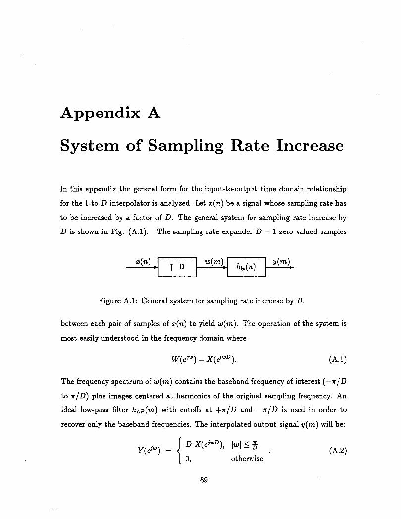
Appendix A
System of Sampling Rate Increase
In this appendix the general form for the input-to-output time domain relationship
for the 1-to-D interpolator is analyzed. Let x(n) be a signal whose sampling rate has
to be increased by a factor of D. The general system for sampling rate increase by
D is shown in Fig. (A.l). The sampling rate expander D - 1 zero valued samples
Figure A.l: General system for sampling rate increase by D.
between each pair of samples of x(n) to yield w(m). The operation of the system is
most easily understood in the frequency domain where
The frequency spectrum of w(m) contains the baseband frequency of interest (-a/D
to a /D) plus images centered at harmonics of the original sampling frequency. An
ideal low-pass filter htp(m) with cutoffs at +a/D and -a/D is used in order to
recover only the baseband frequencies. The interpolated output signal y(m) will be:
DX(ejwD), / w I < z y(ejW) =
otherwise
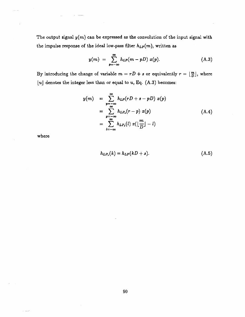
The output signal y(m) can be expressed as the convolution of the input signal with
the impulse response of the ideal low-pass filter hLp(m), written as
By introducing the change of variable m = r D + s or equivalently r = 151, where
LuJ denotes the integer less than or equal to u, Eq. (A.3) becomes:
where
Bibliography
[I] J.L. Flanagan, M.R. Schroeder, B .S. Atal, R.E. Crochiere, "Speech coding,"
IEEE Trans. Comm., COM-27(4), pp. 710-737 (1979).
[2] P. Kroon and E.F. Deprette, "A class of analysis-by-synthesis predictive coders
for high quality speech coding at rates between 4.8 and 16 kb/s," IEEE Journal
on Selected Areas in Comm., Vol. 6 (2), pp. 353-362 (1988).
[3] D. O'Shaughnessy, Speech communication. Englewood Cliffs, NJ (1975).
141 N. S. Jayant and P. Noll, Digital coding of waveforms, Englewood Cliffs, NJ
(1984).
[5] R. E. Ziemer, W. H. Tranten and D.R. Fannin, Signals and systems: continuous
and discrete, 2nd Edition, Macmillan Publishing Company, NY (1990).
[6] B. S. Atal, "Predictive coding of speech signals at low bit rates," IEEE Trans.
Comm., COM-30(4), pp. 600-614 (1982).
[7] J. Turner, Recursive least-squares estimation and lattice filters in adaptive filters,
Englewood Cliffs, NJ (1985).
[8] P. Strobach, Linear prediction theory, Springer-Verlag, NY (1990).
[9] J. Makhoul, "Linear prediction: a tutorial review," Proc. IEEE, vol. 63, no. 4,
April (1975).
[lo] B. Atal and S. Hanauer, "Speech analysis and synthesis by linear prediction of
the speech wave," J. Acoust. Soc. Am., 50 , pp. 637-655 (1971).
[ll] W. B. Kleijn, "Analysis-by-synthesis speech coding based on relaxed waveform-
matching Constraints," Doctorate Thesis, Delft University of Technology, (1991).
[12] J-H. Chen, "An 8 kb/s low-delay CELP speech coder," GLOBECOM '91, pp.
1894-1897 (1991).
[13] J-H. Chen, "High-quality 16 kb/s speech coding with a one-way delay less than
2 ms," Proc. Int. Conf. Acoust. Speech and Signal Processing, Albuquerque,
(1990).
[14] J. P. Campbell, V. C. Welch, and T.E. Tremain, CELP documentation version
3.2, U.S. DoD, Fort Mead, MD (1990).
[15] B. S. Atal and M. R. Schroeder, "Code-excited linear prediction (CELP): high
quality speech at very low bit rates," Proc. Int. Conf. Acoust., Speech and Signal
P~ocessing, San Diego, pp. 937-940, March (1984).
[16] J. Tribolet and R. Crochiere, "Frequency domain coding of speech," Proc. IEEE
Trans. Acoust. Speech and Signal Processing., ASSP-27(3), pp. 512-530 (1979).
[17] B. S. Atal and M. S. Schroeder, "Predictive coding of speech signals and sub-
jective error criteria," Proc. IEEE Trans. Acoust. Speech and Signal Processing,
ASSP-27(3), pp. 247-254 (1979):
[18] P. Kabal and R. P. Ramachandran, "Joint optimization of linear predictors in
speech coders,'' Proc. IEEE Trans. Acoust. Speech and Signal Processing, ASSP-
37, pp. 642-650 (1989).
[19] R. P. Ramachandran and P. Kabal, "Stability and performance of pitch filters in
speech coders," Proc. IEEE Trans. Acoust. Speech and Signal Processing, ASSP-
35, pp. 937-945 (1987).
[20] R. P. Ramachandran .and P. Kabal, "Pitch prediction filters in speech coding,"
Proc. IEEE Trans. Acowt. Speech Signal Processing, ASSP-37, pp. 467-478
(1989).
[21] R. Viswanathan and J. Makhoul, "Quantization properties of transmission pa-
rameters in linear predictive systems," Proc. IEEE Trans. Acoust. Speech Signal
Processing, ASSP-23, pp. 309-321 (1975).
1221 P. Kroon and B. S. Atal, "On the use of pitch predictors with high temporal
resolution," Proc. IEEE Bans. Acoust. Speech Signal Proc. ASSP-39(3), pp.
733-736 (1991).
[23] J-L. Moncet and P. Kabal, "Codeword selection for CELP coders," Proc. Int.
Conf. Acoust. Speech and Signal Processing, New-York, pp. 147-150 (1988).
[24] R. Crochiere and L. Rabiner, Multirate digital signal processing, Prentice-Hall,
Englewood Cliffs, NJ (1983).
[25] M. Foodeei and P. Kabal, "Backward adaptive prediction: high-order predictors
and formant-pitch configurations," Proc. Int. Conf Acoust. Speech and Signal
Processing, Toronto, pp. 2405-2409 (1991).
[26] J. H. Chen and A. Gersho, "Vector adaptive predictive coding of speech at 9.6
Kb/s," Proc. Int. Conf. Acoust. Speech and Signal Processing, Tokyo, pp. 1693-
1696 (1986).
[27] J. Makhoul, S. Roucos, and H. Gish, "Vector quantization in speech coding,"
Proc. IEEE, vol. 73, no. 11, November (1985).
[28] J. H. Chen and A. Gersho, L'Gain-adaptive vector quantization for medium-rate
speech coding," Conf. Record, IEEE Int. Conf. on Communications, Chicago,
June (1985).
1291 B. S. Atal and J. R. Remde, "A new model of LPC excitation for producing
natural sounding speech at low bit rates," Proc. Int. Conf. Acoust. Speech and
Signal Processing, Paris, pp. 614-61 7 (1982).
[30] P. Kroon, Ed. F. Deprettere, and R. J. Sluyter, "Regular-pulse excitation - a
novel approach to effective and efficient multipulse coding of speech," Proc. Int.
Conf. Acoust. Speech and Signal Processing, Tampa, pp. 965-968 (1985).
[31] M. R. Schroeder, B. S. Atal, "Code-Excited Linear Prediction (CELP): high-
quality speech at very low bit rates", Proc. Int. Conf. Acoust. Speech and Signal
Processing, Tampa , pp. 937-940 (1985).
[32] W. Granzow and B. S. Atal, "High quality digital speech at 4 k/s," Proc. Global
Telecomm. Conf. , San Diego, pp. 941-945, (1990).
[33] Y. Shoham, "Constrained stochastic excitation coding of speech at 4.8 kb/s,"
Advances in Speech Coding, pp. 339-348, Kluwer Academic Publishers (1991).
[34] T. Tanigushi, M. Johnson, and Y. Ohta, "Pitch sharpening for perceptually
improved CELP, and the sparse-delta codebook for reduced computation," Proc.
Int. Conf. Acoust. Speech and Signal Processing, Toronto, pp. 337-340 (1992).
[35] W. Kleijn, R. Ramachandran, and P. Kroon, "Generalized analysis-by-synthesis
coding and its application to pitch prediction," Proc. Int. Conf. Acoust. Speech
and Signal Processing, Toronto, .pp. 241-244 (1991).
[36] F. Itakura, "Line Spectrum Representation of Linear Predictive Coefficients," J.
Acoust. Soc. Am. 57 Supplement(l), pp. S.35 (1975).
[37] G. S. Kang and L. S. Fransen, "Application of line spectrum pairs to low bit
rates speech encoders," Proc. Int. Conf. Acoust. Speech and Signal Processing,
Tampa, pp. 7.3.1-7.3.4 (1985).
[38] F. K. Soong and B. H. Juang, "Line Spectrum Pairs (LSP) and speech data
compression," Proc. Int. Conf. Acoust. Speech and Signal Processing, San Diego,
pp. 1.10.1-1.10.4 (1984).
[39] P. Kabal and R. P. Ramachandran, "The computation of line spectral frequencies
using chebyshev polynomials," Proc. IEEE Trans. Acowt. Speech and Signal
Processing, ASSP-34(3), pp. 1419-1426 (1986).
[40] Q. Yasheng, P. Kabal, "Pseudo-three-tap pitch prediction filters," Proc. Int.
Conf. Acoud. Speech and Signal Processing, Minneapolis, pp. 523-526, (1993).
[41] E. Jury, Theory and application of the z-transfomn method, Wiley, NY (1964).
[42] T. Ramstad, "Sample-rate conversion by arbitrary ratios," Proc. IEEE Trans.
Acoust. Speech and Signal Processing, pp. 577-591 (1984).


![[XLS]f01.justanswer.com · Web view2012/01/29 · 8916 6060 4.8 42 26 31 8916 6060 4.8 42 26 31 8916 6110 4.8 42 26 31 8916 4306 4.8 42 26 31 8916 2024 4.8 42 26 31 8916 2162 4.8](https://img.pdfslide.us/doc/110x75/5b1d0bfa7f8b9aad5d8be633/xlsf01-web-view20120129-8916-6060-48-42-26-31-8916-6060-48-42-26.jpg)


![vertical neck regular [VNR] - Implant System · 2017. 7. 4. · XIC10 1.9 10 4.8 4.1 0.7 4.1 4.8 XIC12 1.9 12 4.8 4.1 0.7 4.1 4.8 XIC14 1.9 14 4.8 4.1 0.7 4.1 4.8 XIC16 1.9 16 4.8](https://img.pdfslide.us/doc/110x75/60c62ef912a4697e3b3f34ad/vertical-neck-regular-vnr-implant-2017-7-4-xic10-19-10-48-41-07-41.jpg)