PISCEES

Progress Toward Advanced

Ice Sheet Models Phil Jones (LANL), acting PI for Bill Lipscomb

PISCEES

Progress Toward Advanced

Ice Sheet Models Phil Jones (LANL), acting PI for Bill Lipscomb

Representing work by • LANL

– Bill Lipscomb, Steve Price, Xylar Asay-Davis, Jeremy Fyke, Matt Hoffman,

Gunter Leguy, Doug Ranken, John Dukowicz

• LBL

– Dan Martin, Esmond Ng (Chombo/FASTMath/ASCR)

• SNL

– Irina Kalashnikova, Mauro Perego, Andy Salinger, Ray Tuminaro (Trilinos/

FASTMath/ASCR), Michael Eldred, John Jakeman (QUEST/ASCR)

• ORNL

– Kate Evans, Matt Norman, Ben Mayer, Adrianna Boghozian (V&V), Pat Worley

(SUPER)

• NCAR

– Bill Sacks, Mariana Vertenstein

• Academic partners

– Charles Jackson, G. Stadler, G. Gutowski (U. Texas), Max Gunzburger (FSU), Lili

Ju (U. S. Carolina), Patrick Heimbach (MIT), Tony Payne, Stephen Cornford (U

Bristol)

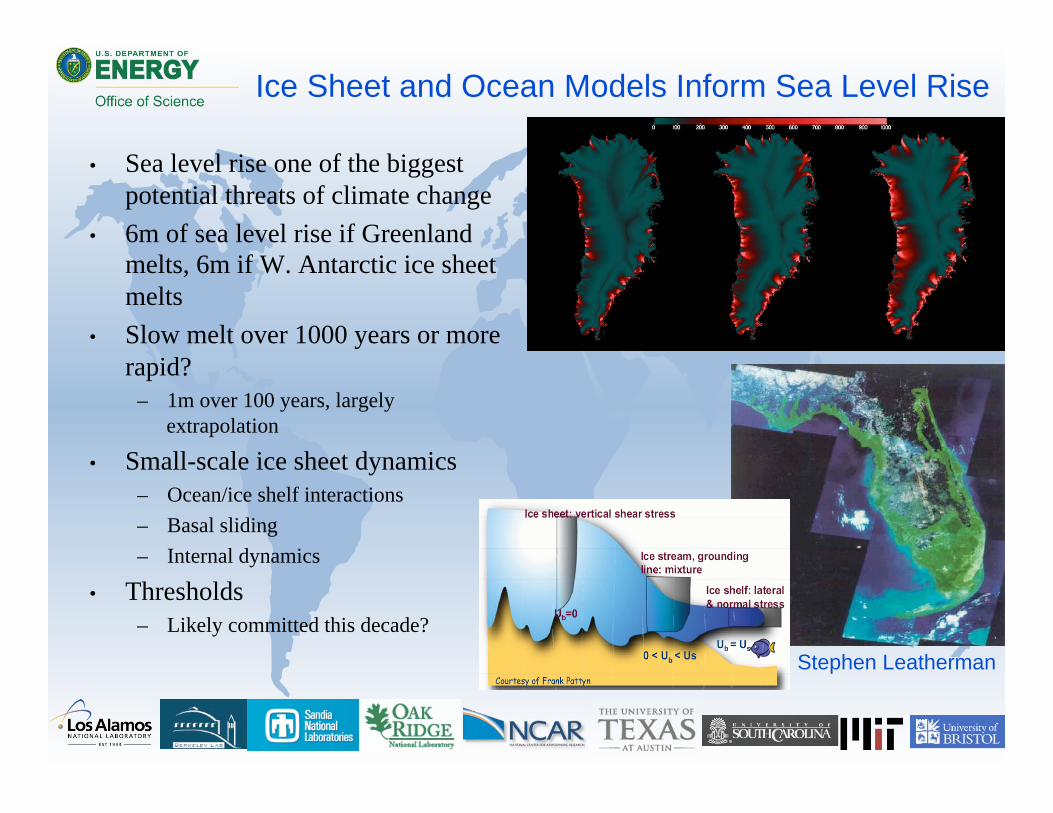
Ice Sheet and Ocean Models Inform Sea Level Rise

• Sea level rise one of the biggest

potential threats of climate change

• 6m of sea level rise if Greenland

melts, 6m if W. Antarctic ice sheet

melts

• Slow melt over 1000 years or more

rapid?

– 1m over 100 years, largely

extrapolation

• Small-scale ice sheet dynamics

– Ocean/ice shelf interactions

– Basal sliding

– Internal dynamics

• Thresholds

– Likely committed this decade?

Stephen Leatherman

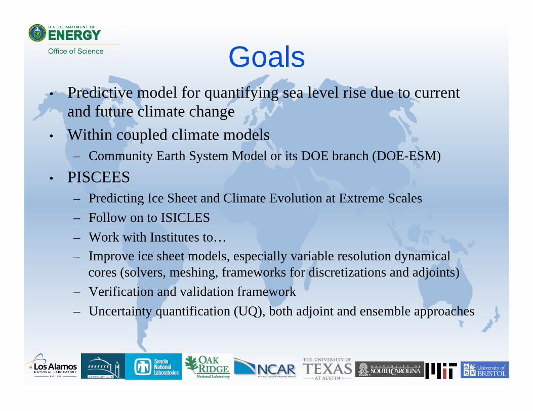
Goals • Predictive model for quantifying sea level rise due to current

and future climate change

• Within coupled climate models

– Community Earth System Model or its DOE branch (DOE-ESM)

• PISCEES

– Predicting Ice Sheet and Climate Evolution at Extreme Scales

– Follow on to ISICLES

– Work with Institutes to…

– Improve ice sheet models, especially variable resolution dynamical

cores (solvers, meshing, frameworks for discretizations and adjoints)

– Verification and validation framework

– Uncertainty quantification (UQ), both adjoint and ensemble approaches

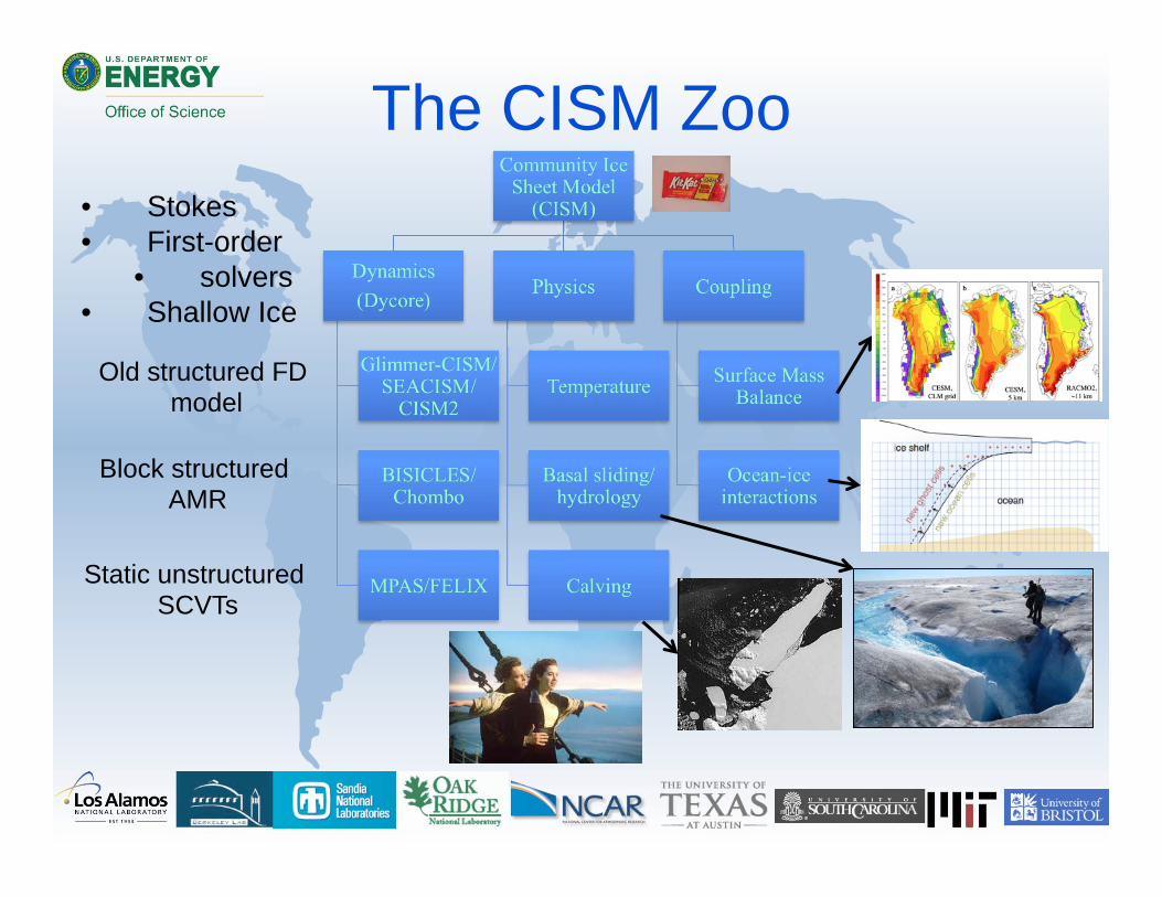
The CISM Zoo Community Ice

Sheet Model (CISM)

Dynamics

(Dycore)

Glimmer-CISM/SEACISM/

CISM2

BISICLES/Chombo

MPAS/FELIX

Physics

Temperature

Basal sliding/hydrology

Calving

Coupling

Surface Mass Balance

Ocean-ice interactions

• Stokes

• First-order

• solvers

• Shallow Ice

Old structured FD model

Block structured AMR

Static unstructured SCVTs

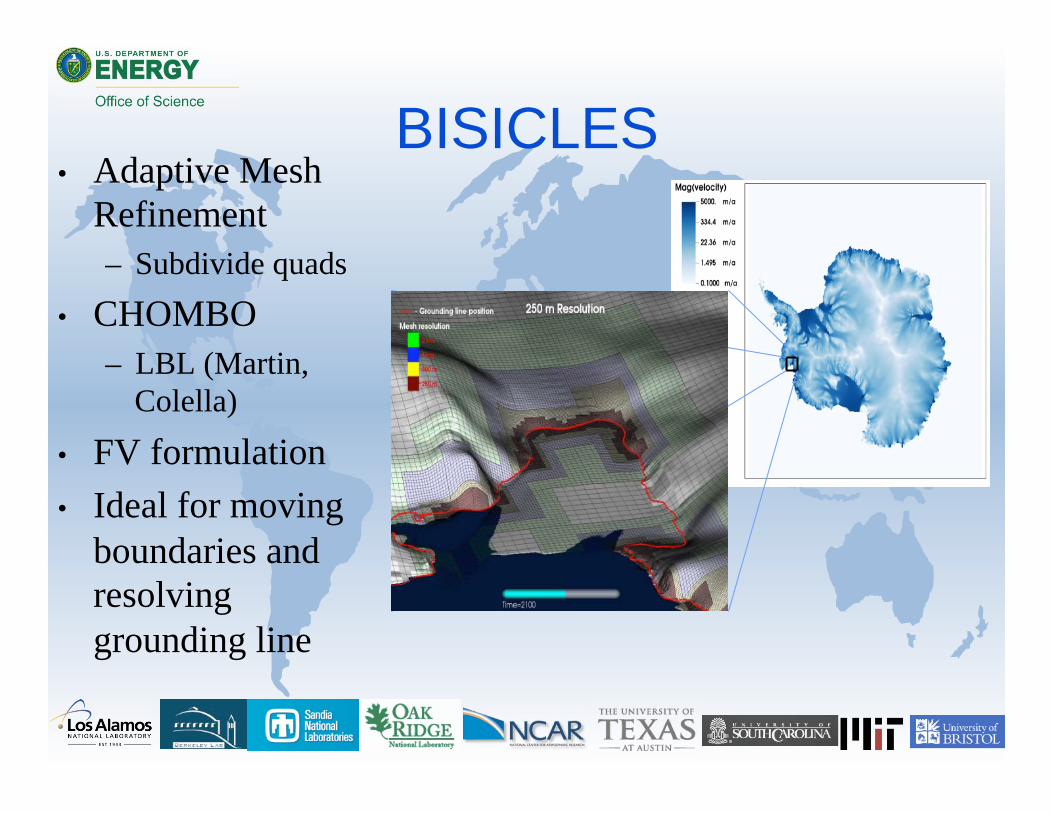
BISICLES • Adaptive Mesh

Refinement

– Subdivide quads

• CHOMBO

– LBL (Martin,

Colella)

• FV formulation

• Ideal for moving

boundaries and

resolving

grounding line

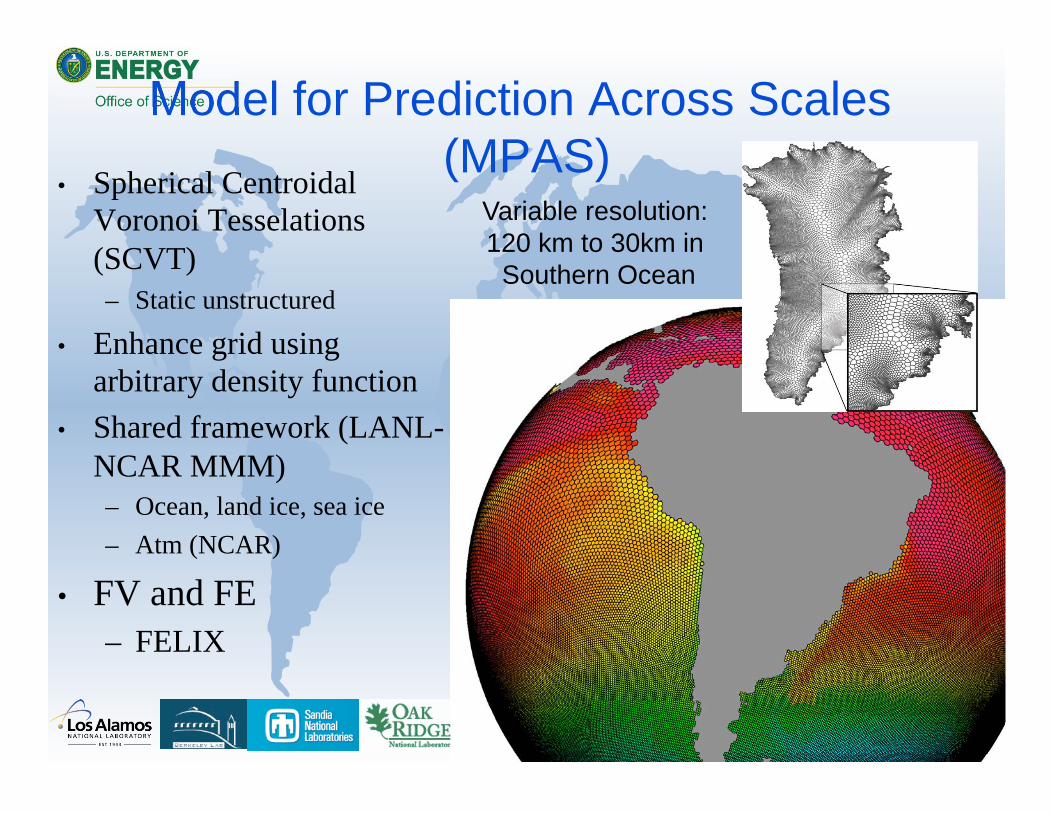
Model for Prediction Across Scales

(MPAS) • Spherical Centroidal

Voronoi Tesselations

(SCVT)

– Static unstructured

• Enhance grid using

arbitrary density function

• Shared framework (LANL-

NCAR MMM)

– Ocean, land ice, sea ice

– Atm (NCAR)

• FV and FE

– FELIX

Variable resolution:

120 km to 30km in

Southern Ocean

MPAS Dycore

MPAS and FASTMath

• Extensive use of Trilinos (SNL) and related

software

– FE discretizations with operators, solvers

– Natural treatment of stress boundary conditions

– Connections to adjoints, UQ (Dakota) tools

• Full Newton with analytic derivatives

– Robust, efficient for steady-state solves

– Matrix available for preconditioners and mat-vec

operations

– Analytic sensitivity analysis

– Analytic gradients for inversion

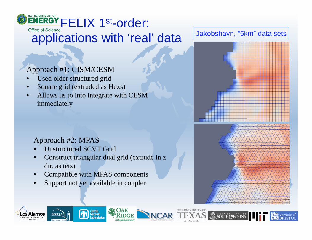
Approach #1: CISM/CESM • Used older structured grid

• Square grid (extruded as Hexs)

• Allows us to into integrate with CESM

immediately

Approach #2: MPAS • Unstructured SCVT Grid

• Construct triangular dual grid (extrude in z

dir. as tets)

• Compatible with MPAS components

• Support not yet available in coupler

Jakobshavn, “5km” data sets

FELIX 1st-order:

applications with ‘real’ data

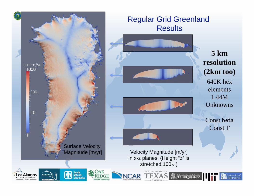
Regular Grid Greenland Results

Velocity Magnitude [m/yr]

in x-z planes. (Height “z” is

stretched 100x.)

5 km

resolution

(2km too)

640K hex

elements

1.44M

Unknowns

Const

Const T

Surface Velocity

Magnitude [m/yr]

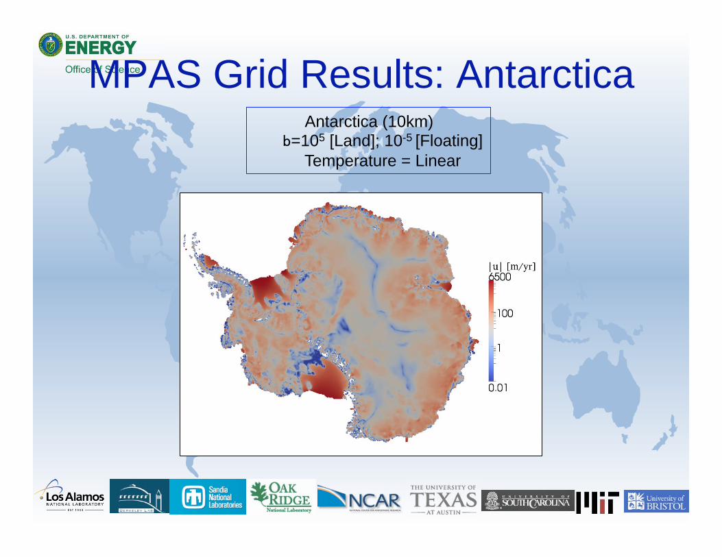
MPAS Grid Results: Antarctica

Antarctica (10km) =105 [Land]; 10-5 [Floating]

Temperature = Linear

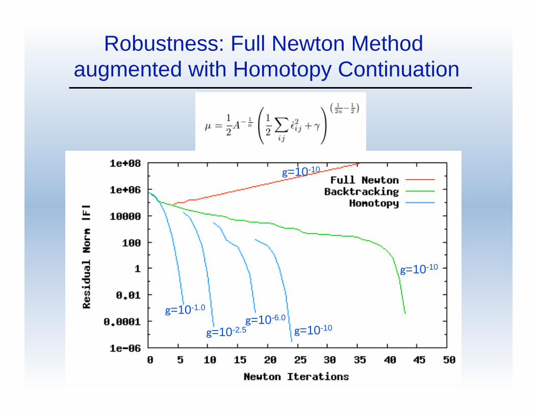
Robustness: Full Newton Method

augmented with Homotopy Continuation

=10-1.0

=10-2.5 =10-6.0

=10-10

=10-10

=10-10

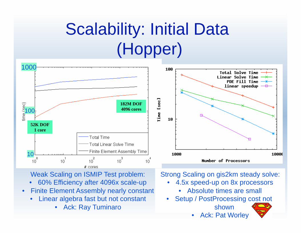
Scalability: Initial Data

(Hopper)

52K DOF

1 core

182M DOF

4096 cores

Weak Scaling on ISMIP Test problem: • 60% Efficiency after 4096x scale-up

• Finite Element Assembly nearly constant • Linear algebra fast but not constant

• Ack: Ray Tuminaro

1000

100

10

Strong Scaling on gis2km steady solve: • 4.5x speed-up on 8x processors

• Absolute times are small • Setup / PostProcessing cost not

shown • Ack: Pat Worley

BISICLES Dycore

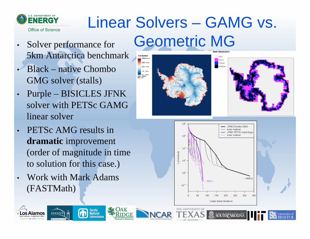
• Solver performance for

5km Antarctica benchmark

• Black – native Chombo

GMG solver (stalls)

• Purple – BISICLES JFNK

solver with PETSc GAMG

linear solver

• PETSc AMG results in

dramatic improvement

(order of magnitude in time

to solution for this case.)

• Work with Mark Adams

(FASTMath)

Linear Solvers – GAMG vs.

Geometric MG

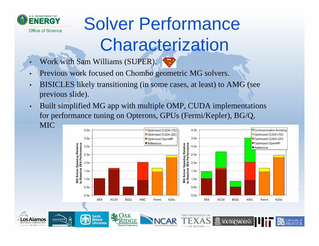
Solver Performance

Characterization • Work with Sam Williams (SUPER).

• Previous work focused on Chombo geometric MG solvers.

• BISICLES likely transitioning (in some cases, at least) to AMG (see

previous slide).

• Built simplified MG app with multiple OMP, CUDA implementations

for performance tuning on Opterons, GPUs (Fermi/Kepler), BG/Q,

MIC

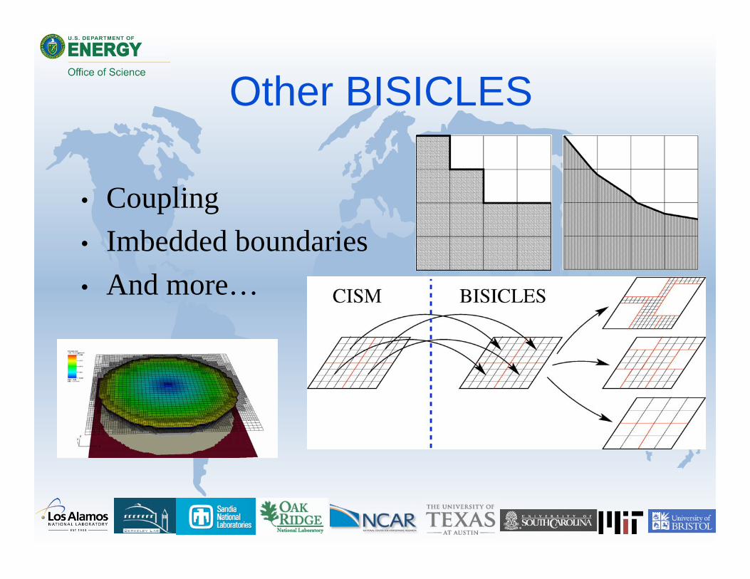
Other BISICLES

• Coupling

• Imbedded boundaries

• And more…

LIVV:

Verification and Validation

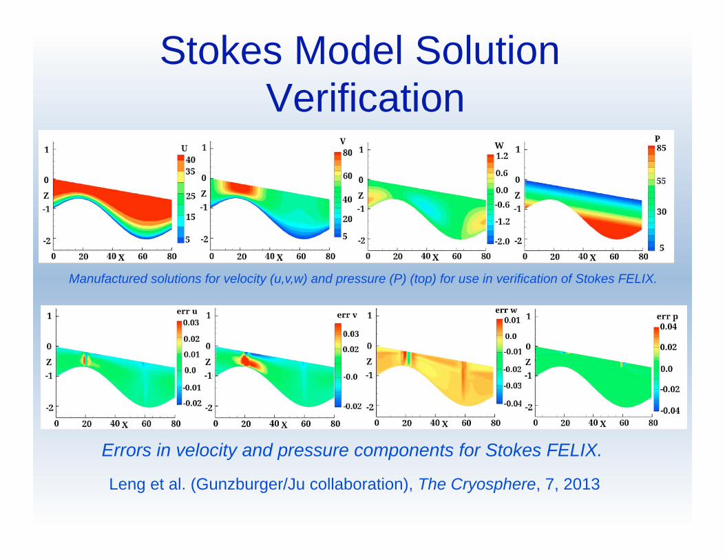
Stokes Model Solution

Verification

Manufactured solutions for velocity (u,v,w) and pressure (P) (top) for use in verification of Stokes FELIX.

Errors in velocity and pressure components for Stokes FELIX.

Leng et al. (Gunzburger/Ju collaboration), The Cryosphere, 7, 2013

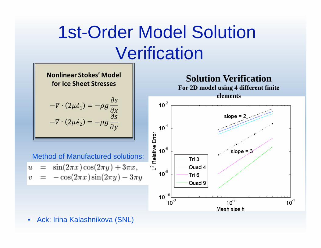
1st-Order Model Solution

Verification

Solution Verification For 2D model using 4 different finite

elements

Method of Manufactured solutions:

• Ack: Irina Kalashnikova (SNL)

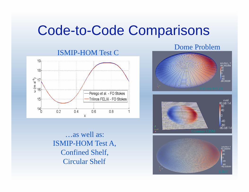
Code-to-Code Comparisons

Dome Problem ISMIP-HOM Test C

…as well as:

ISMIP-HOM Test A,

Confined Shelf,

Circular Shelf

Trilinos FELIX

Glimmer CISM

LifeV

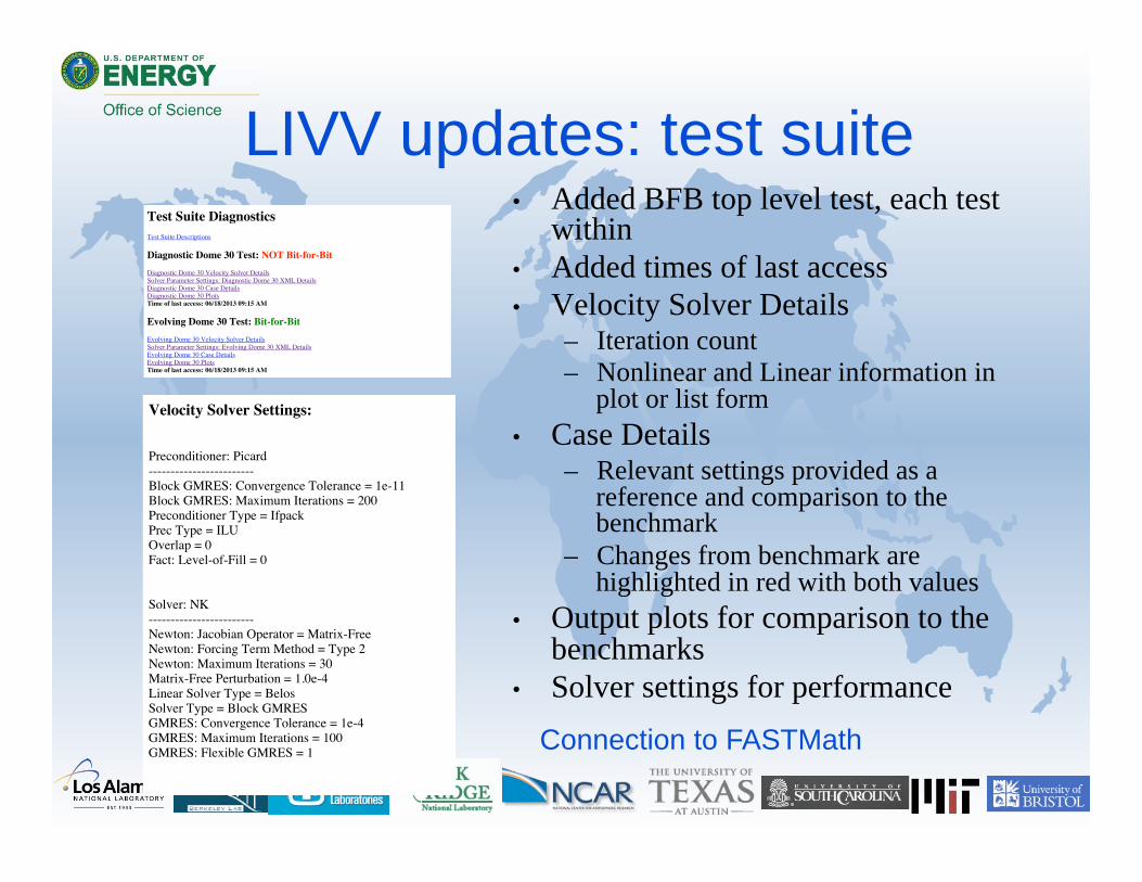
LIVV updates: test suite • Added BFB top level test, each test

within

• Added times of last access

• Velocity Solver Details – Iteration count

– Nonlinear and Linear information in plot or list form

• Case Details – Relevant settings provided as a

reference and comparison to the benchmark

– Changes from benchmark are highlighted in red with both values

• Output plots for comparison to the benchmarks

• Solver settings for performance

Test Suite DiagnosticsTest Suite Descriptions

Diagnostic Dome 30 Test: NOT Bit-for-Bit

Diagnostic Dome 30 Velocity Solver Details Solver Parameter Settings: Diagnostic Dome 30 XML Details Diagnostic Dome 30 Case Details Diagnostic Dome 30 Plots Time of last access: 06/18/2013 09:15 AM

Evolving Dome 30 Test: Bit-for-Bit

Evolving Dome 30 Velocity Solver Details Solver Parameter Settings: Evolving Dome 30 XML Details Evolving Dome 30 Case Details Evolving Dome 30 Plots Time of last access: 06/18/2013 09:15 AM

Velocity Solver Settings:

Preconditioner: Picard------------------------Block GMRES: Convergence Tolerance = 1e-11Block GMRES: Maximum Iterations = 200Preconditioner Type = IfpackPrec Type = ILUOverlap = 0Fact: Level-of-Fill = 0

Solver: NK------------------------Newton: Jacobian Operator = Matrix-FreeNewton: Forcing Term Method = Type 2Newton: Maximum Iterations = 30Matrix-Free Perturbation = 1.0e-4Linear Solver Type = BelosSolver Type = Block GMRESGMRES: Convergence Tolerance = 1e-4GMRES: Maximum Iterations = 100GMRES: Flexible GMRES = 1

Connection to FASTMath

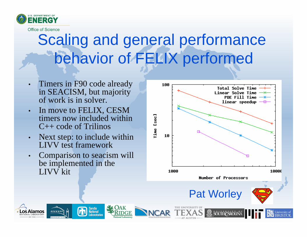
Scaling and general performance

behavior of FELIX performed

• Timers in F90 code already in SEACISM, but majority of work is in solver.

• In move to FELIX, CESM timers now included within C++ code of Trilinos

• Next step: to include within LIVV test framework

• Comparison to seacism will be implemented in the LIVV kit

Pat Worley

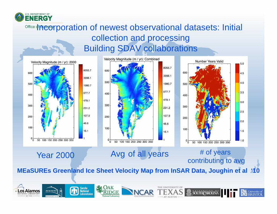
Incorporation of newest observational datasets: Initial

collection and processing

Building SDAV collaborations

MEaSUREs Greenland Ice Sheet Velocity Map from InSAR Data, Joughin et al ‘10

Year 2000 Avg of all years # of years

contributing to avg

Uncertainty Quantification

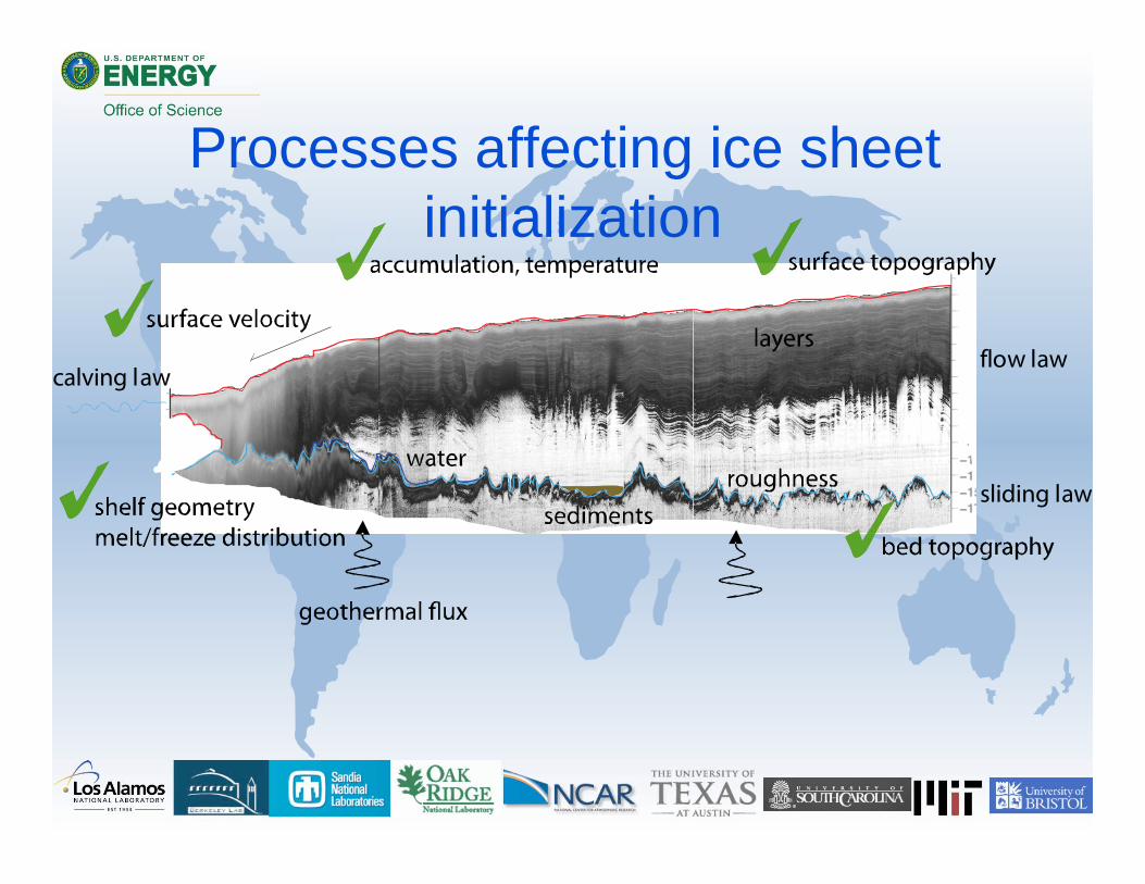
Processes affecting ice sheet

initialization

calving lawflow law

sliding law

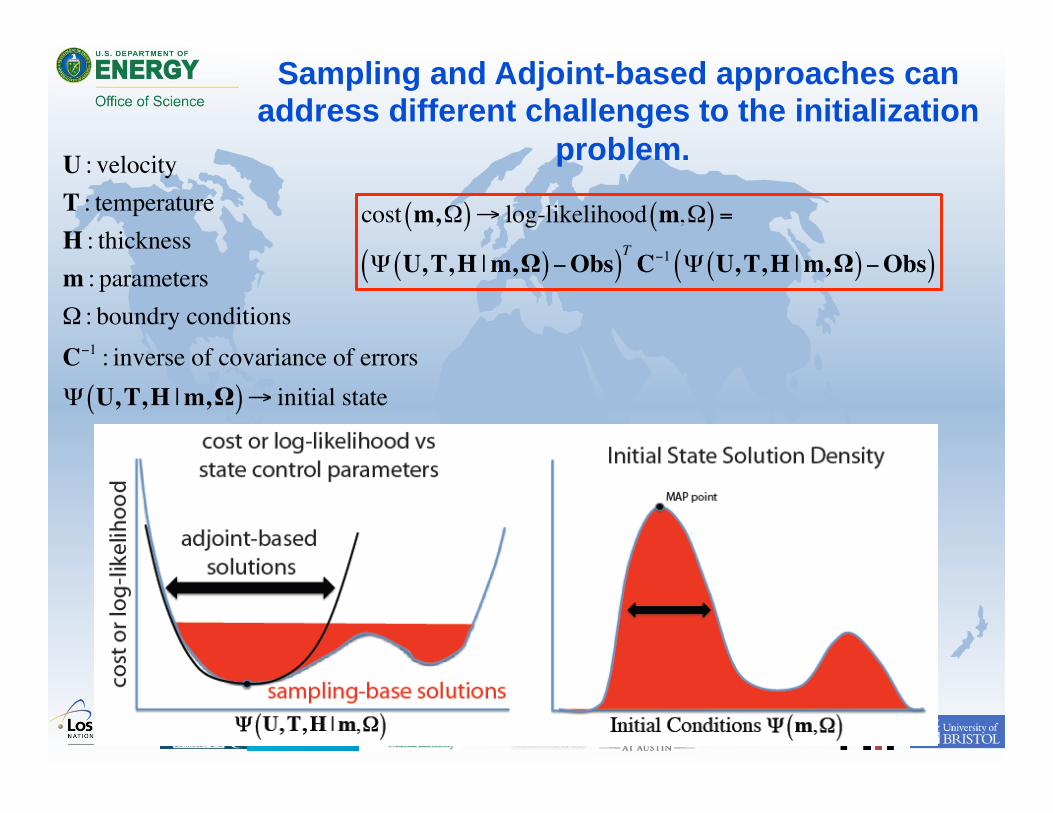
cost m,( ) log-likelihood m,( ) =

U,T,H |m,( ) Obs( )TC 1 U,T,H |m,( ) Obs( )

U : velocity

T : temperature

H : thickness

m : parameters

: boundry conditions

C 1 : inverse of covariance of errors

U,T,H |m,( ) initial state

Sampling and Adjoint-based approaches can address different challenges to the initialization

problem.

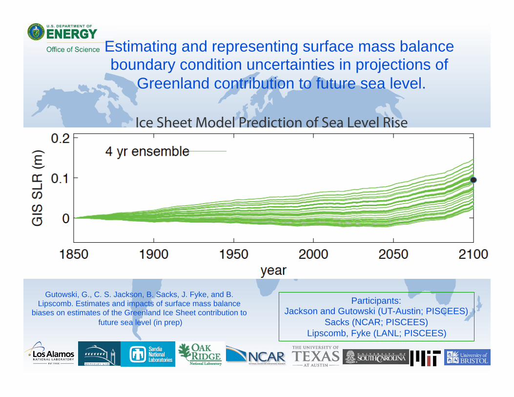
Ice Sheet Model Prediction of Sea Level Rise

Participants: Jackson and Gutowski (UT-Austin; PISCEES)

Sacks (NCAR; PISCEES)

Lipscomb, Fyke (LANL; PISCEES)

Gutowski, G., C. S. Jackson, B. Sacks, J. Fyke, and B. Lipscomb. Estimates and impacts of surface mass balance

biases on estimates of the Greenland Ice Sheet contribution to

future sea level (in prep)

Estimating and representing surface mass balance boundary condition uncertainties in projections of

Greenland contribution to future sea level.

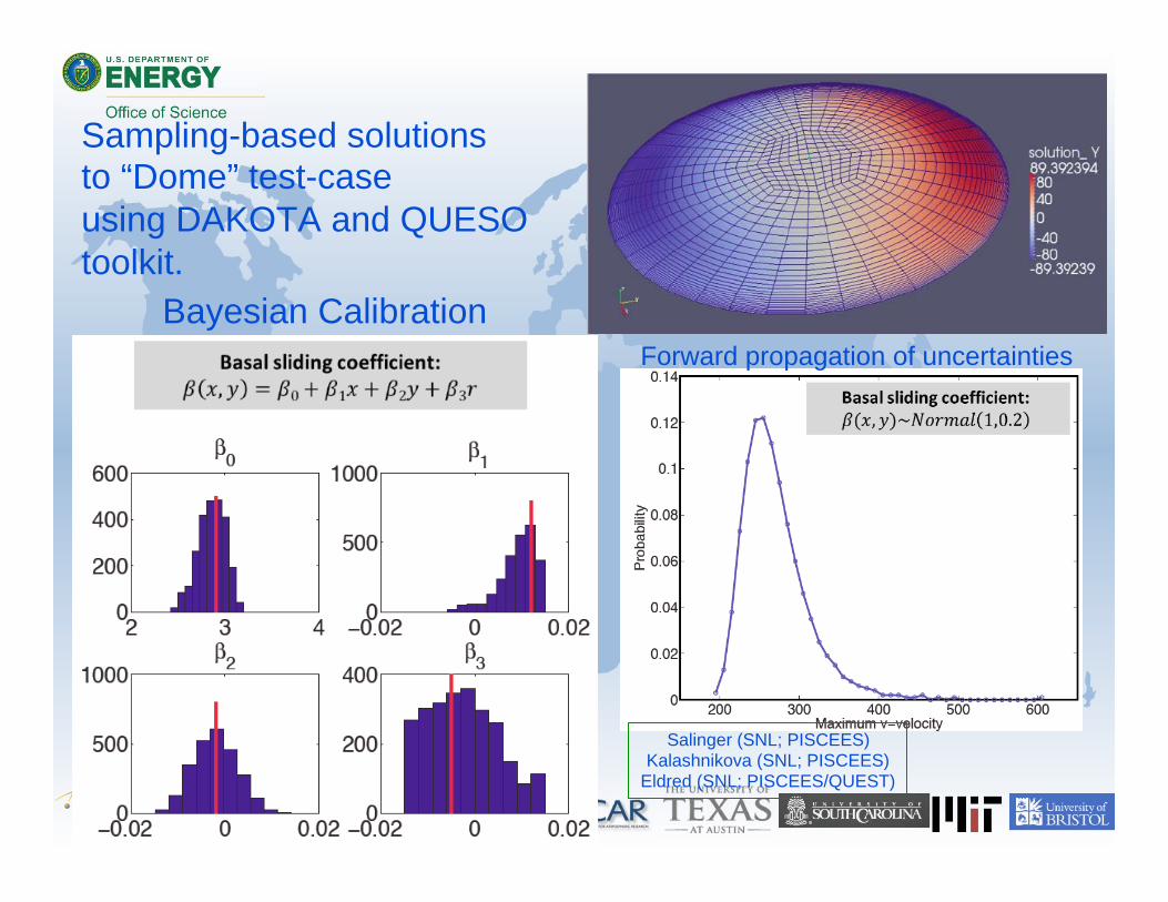
Sampling-based solutions to “Dome” test-case

using DAKOTA and QUESO

toolkit.

Forward propagation of uncertainties Bayesian Calibration

Salinger (SNL; PISCEES) Kalashnikova (SNL; PISCEES)

Eldred (SNL; PISCEES/QUEST)

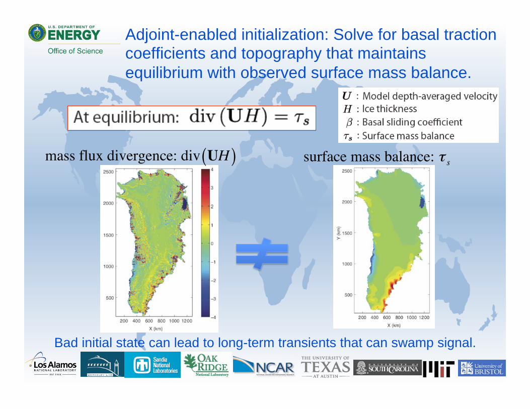
Adjoint-enabled initialization: Solve for basal traction coefficients and topography that maintains

equilibrium with observed surface mass balance.

mass flux divergence: div UH( ) surface mass balance: s

Bad initial state can lead to long-term transients that can swamp signal.

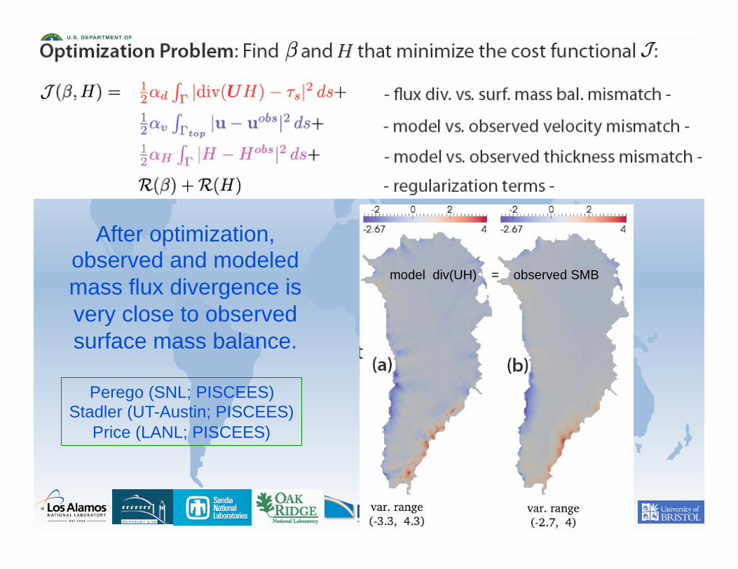
After optimization, observed and modeled

mass flux divergence is

very close to observed

surface mass balance.

model div(UH) = observed SMB

Perego (SNL; PISCEES) Stadler (UT-Austin; PISCEES)

Price (LANL; PISCEES)

• Open research question.

• Feasibility with DAKOTA is being discussed between PISCEES’s Heimbach (MIT), Stadler (UT Austin), and Salinger (SNL) and QUEST’s Eldred (SNL).

• Demonstrated capacity for estimating basal traction uncertainty (Stadler and colleagues at UT Austin) and ice-ocean coupling (Heimbach and colleagues at MIT)

Adjoint-based Uncertainty

Heimbach (MIT; PISCEES) Stadler (UT-Austin; PISCEES)

Ghattas (UT-Austin; PISCEES/QUEST)

Salinger (SNL; PISCEES)

Eldred (SNL; PISCEES/QUEST)

Conclusions • Much progress in creating advanced

dynamical cores

– Not Mezzacappa level, but…

– Significant contributions from Institutes

– Capabilities that we haven’t had before

• Improved V&V

• Significant application of UQ techniques

– Beyond parameter estimation

– Initialization problem

So long and thanks for all the

fish