The Instantaneous Wall Viscosity in Pipe Flow of Power Law

Fluids:

Case Study for a Theory of Turbulence in Time-Independent

Non-Newtonian Fluids

Trinh, Khanh Tuoc

Institute of Food Nutrition and Human Health

Massey University, New Zealand

K.T.Trinh@massey.ac.nz

ABSTRACT

This paper presents a new theory of turbulence in time-independent non-Newtonian

fluids. The wall layer is modelled in terms of unsteady exchange of viscous momentum

between the wall and the main stream, following the classic visualisation of inrush-

sweep-ejection/burst. The thickness of the wall layer is found to be the same for

Newtonian and purely viscous non-Newtonian fluids, when normalised with the

instantaneous wall parameters at the onset of bursting. The results indicate that the

mechanisms of turbulence in Newtonian and time-independent fluids are identical when

structural similarity relations in turbulence are based on phase-locked parameters linked

with the development of secondary flows rather than on time-averaged wall parameters.

This similarity analysis collapses the local critical instantaneous friction factor data of

both Newtonian and non-Newtonian fluids at the point of bursting into a single curve.

The method greatly simplifies the analysis of turbulent transport phenomena in non-

Newtonian fluids.

Keywords: Turbulence, time-independent non-Newtonian, Power law, pipe flow, wall

layer

1

1

Introduction

Non-Newtonian turbulent flow has applications in the processing of food, mineral, oil and

polymer products. Early research efforts were directed towards defining an equivalent

viscosity, which could be substituted into Newtonian correlations to give estimates of the

friction factor. For example Weltmann (1956) used the limiting viscosity at “limiting shear

rate” μ∞. Alves et al . (1952) used a “turbulent viscosity” associated with measurements of

equivalent viscosity in turbulent flow. Metzner and Reed (1955) used an “effective viscosity”

to define a so called Meztner-Reed generalised Reynolds number Reg required to collapse all

data of the friction factor f against the Reynolds number into the Newtonian curve. They

argued that plots of f against Reg would also collapse the data for turbulent flow onto the

Newtonian curves modelled by Nikuradse (1932). This was disproved by the subsequent data

of Dodge (1959). Bogue (1961) and later on Edwards and Smith (1980) argued that the use of

the apparent viscosity at the wall shear rate μw collapsed the non-Newtonian data onto the

Newtonian curve. But the procedure only really worked for fluids in the measurements of

Bogue (1961) and Eissenberg and Bogue (1964) with a relatively high value of behaviour

index n>0.89 where departure from Newtonian behaviour was small anyway. The method

failed to correlate friction factor for Carbopol solutions obtained by Dodge (1959)and Shaver

(1957)at high concentrations and therefore lower values of n. Edwards and Smith blamed

viscoelastic effects but Dodge had argued that Carbopol used to generate the data used by

Edwards and Smith showed very little viscoelasticity.

Major efforts were made in the 1960s to analyse the problem. Bowen (1961) proposed a

method of scale up for turbulent pipe flow that is useful if some data of turbulent flow is

available for one pipe diameter. Tomita (1959) used the Nikuradse formula (Nikuradse, 1932)

but redefined both the friction factor and the Reynolds number for power law fluids from

similarity considerations (Table 1). Clapp (1961) followed the technique of Prandtl(1935) and

Karman (1934) to derive the friction factor from a model of the velocity profile consisting of a

turbulent core following the well-known log law (Millikan, 1939), Prandtl (1935)) and a

laminar sub-layer (Prandtl, 1935) which he assumed has the same thickness in Newtonian and

power law fluids. Experimental measurements of the velocity profile in turbulent pipe flow

have never been accurate and repeatable enough to verify this key assumption. More

2

importantly Metzner (Clapp, 1961) pointed out that the rheological data used by Clapp cover a

lower range of shear rates than those encountered in the actual flow experiments. Since it is

always dangerous to extrapolate non-Newtonian rheological data, this uncertainty in the values

of the consistency coefficient K and the behaviour index n may explain why there is a small

difference between the data presented by Clapp(1961) and others like Dodge (1959), Bogue

(1961) and Yoo (1974)

Dodge & Metzner (1959) used dimensional analysis to extend Millikan's logarithmic law to

time independent non-Newtonian fluids. The term time-independent means that the fluids do

not thin (thixotropy) or thicken (rheopexy) with duration of shear and do not exhibit

viscoelasticity. While Dodge and Metzner showed that a certain amount of drag reduction

exists for time independent non-Newtonian fluids compared with Newtonian fluids at the same

Reynolds drag reduction in the presence of viscoelasticity is much more pronounced as

identified by Toms (1949) a distinction not made by their contemporary Shaver and Merrill

(1959). A second distinctive feature of the Dodge and Metzner correlations is that they are

expressed in terms of the behaviour index n′ , the slope of the log-log plot between the shear

stress τ and the flow function )/8( DV=Γ where V is the average flow velocity and D the

pipe diameter and not the index n which is the slope of the log-log plot between τ and the

shear rate γ . Therefore the correlations are not restricted only to power law fluids obeying the

correlation but can be applied to time-independent fluids following any rheological

model. Dodge and Metzner found that their correlation fit their data best when the slope of the

log-law

nKγτ =

κ/1=A , where κ is called Karman’s universal constant, is expressed as 75.0/5.2 nA ′= . Tennekes (1966) argued that the Dodge and Metzner correlation implied that

the mechanism of turbulence in non-Newtonian fluids is different from that in Newtonian

fluids. Dodge and Metzner also proposed an empirical extension to the Blasius (1913) power

law correlation. The Dodge and Metzner correlations have been widely accepted from the

moment they were published and are routinely quoted in books on non-Newtonian fluid

technology e.g. (Chabra & Richardson, 1999; Skelland, 1967; Steffe, 1996) and remain highly

recommended even in recent evaluations of correlations for friction factors in power law fluids

e.g. Gao and Zhang (2007).

3

However, the predictions of velocity profiles proposed by Dodge & Metzner, based on the

success of their friction factor correlation, did not agree with the subsequent measurements of

Bogue and Metzner (1963) where the slope of the log-law is described by nA ′= /5.2 . This

discrepancy between results of researchers in the Metzner group has encouraged others to

attempt to proposed improved correlations notably by Thomas (1960), Torrance (1963),

Kemblowski and Kolodzieski(1973), Hancks and Ricks (1975), Szilas et al.(1981), Shenoy

and Saini(1982), Kawase et al (1994), Wilson and Thomas(1985), Darby (1988), Desouky

(Desouky, 2002; 1990), Hemeida (1993) and El-Emam et al. (2003)as shown in Table 1.

Many of these correlations are empirical or semi-empirical. Indeed El-Amam et al tested 11

correlations against published data and noted that many correlations fitted the experimental

data of their authors well enough but not that of others indicating a lack of generality. El-

Amman et al. (op. cit.) proposed their own empirical correlation with fitted most of the

literature data they used but the improved correlation gave no clue on the underlying

mechanisms.

Wilson and Thomas (1985) proposed that the normalised Kolmogorov energy dissipating

eddies (Kolmogorov, 1941) were larger in power law fluids than in Newtonian fluids by a

factor of 2/(n+1) because of the integration of the shear rate into the local

velocity ( )∫ ∫== dyKdyu n/1τγ .They proposed that the scale of the Kolmogorov eddies

normalised with the friction velocity ρτ wu =* and the apparent viscosity at the wall

nnww K /1/11−= τμ is ( )[ ]1/21.12* +==+ nu wμρλλ . However, their prediction of friction

factors fell 5% to 15% below the well-accepted measurements of Dodge. A particular

weakness of the Wilson and Thomas integration procedure is that it does not involve

boundary conditions and therefore delivers the same result for different geometries like

cylindrical pipes, parallel plates and annuli. These authors only tested their theory against

pipe flow. Fifteen years earlier Trinh (1969) had also argued that the integration of the wall

shear rate resulted in a different value for the intercept between the log-law and the curve

4

representative of purely viscous flow, obeying the relation with , was

different in Newtonian and non-Newtonian flows. He argued that the result of the

integration process was the same as that obtained in the widely used Mooney-

Rabinowitsch procedure(Skelland, 1967) The shift factor for pipe flow of power law fluid

is therefore . This correlation predicted the data of Dodge and Bogue with

accuracy similar with the Metzner-Dodge correlation. Trinh also showed that the technique

could be applied easily to other rheological models and that the shift factor also correlated

very well the delay in the transition to turbulence when dimensionless flow rate was

expressed as the Metzner-Reed Reynolds number. This work was never published because

the author returned to Vietnam, a country then at war.

++ = yu *u/uu =+

( ) )4/(13 nn ′+′

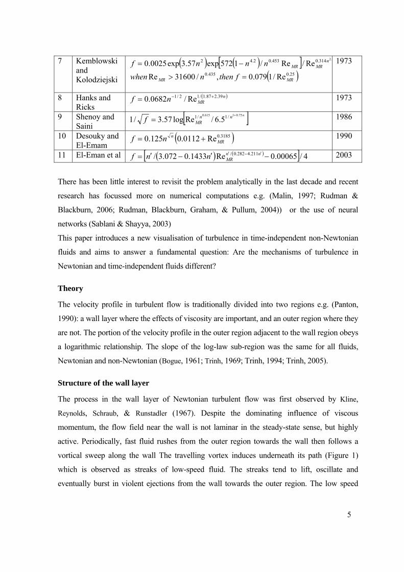
Table1. A number of friction factor correlations for pipe flow of power law fluids

No.

Authors Equation Year

( ) [ ] ( ) 2.12/175.0 /4.0Relog/0.41 nfnf nMR ′−′= ′− 1 Dodge and 1959

Metzner bMRaf Re= where a=0.066 5+0.011 75n′

and 2062.0177.0365.0 nnb ′+′−=( ) n

MRnf 5.10/63.2,Re/079.0 5 == αα2 Shaver and Merilll

1959

( )( ) ( ) ( )[ ]( ) ( ) ( )[ ] MRTo

To

ToToTo

nnfnnf

ff

Re21/314/3Re31/213/4

4.0Relog41

++=++=

−= 1959 3 Tomita

( ) nfnf nMR ′−′= ′− 4.0Relog/41 2/14 Thomas 1960

5 Clapp ( ) [ ] ( ) 1961 /8568.0/69.2Relog53.41 2/1 ′−′+′+′= ′− nnnfnf nMR

( ) ( ) nfnf n

MR ′−+′= ′− /78.216.2Relog/06.41 2/1 6 Trinh 1969

( )( ) ( )( ) ( ) ( ) ( )[ ] ( )

max

13/713/413/713/6 /24138.11

131,Re/

UVnn

nf

nnnnnnnn

MR

=

′+′=

+′==

+′′+′′++′′−+′′−

φφα

βα β

5

7 Kemblowski and

( ) ( )[ ]( )25.0435.0

314.0453.02.42

Re/1079.0,/31600Re

Re/Re/1572exp57.3exp0025.03.2

MRMR

nMRMR

fthennwhen

nnnf

=>

−= 1973

Kolodziejski

( )nMRnf 39.287.1/12/1 Re/0682.0 +−=8 Hanks and

Ricks 1973

[ ]nnnMRf

75.01615.0 /1/1 5.6/Relog57.3/1+

=9 Shenoy and Saini

1986

( )3185.0Re0112.0125.0 MRnnf +=10 Desouky and

El-Emam 1990

( ) ( )[ ] 4/00065.0Re1433.0072.3/ 211.4282.0/ −′−′= ′−′ nnMRnnf 11 El-Eman et al 2003

There has been little interest to revisit the problem analytically in the last decade and recent

research has focussed more on numerical computations e.g. (Malin, 1997; Rudman &

Blackburn, 2006; Rudman, Blackburn, Graham, & Pullum, 2004)) or the use of neural

networks (Sablani & Shayya, 2003)

This paper introduces a new visualisation of turbulence in time-independent non-Newtonian

fluids and aims to answer a fundamental question: Are the mechanisms of turbulence in

Newtonian and time-independent fluids different?

Theory

The velocity profile in turbulent flow is traditionally divided into two regions e.g. (Panton,

1990): a wall layer where the effects of viscosity are important, and an outer region where they

are not. The portion of the velocity profile in the outer region adjacent to the wall region obeys

a logarithmic relationship. The slope of the log-law sub-region was the same for all fluids,

Newtonian and non-Newtonian (Bogue, 1961; Trinh, 1969; Trinh, 1994; Trinh, 2005).

Structure of the wall layer

The process in the wall layer of Newtonian turbulent flow was first observed by Kline,

Reynolds, Schraub, & Runstadler (1967). Despite the dominating influence of viscous

momentum, the flow field near the wall is not laminar in the steady-state sense, but highly

active. Periodically, fast fluid rushes from the outer region towards the wall then follows a

vortical sweep along the wall The travelling vortex induces underneath its path (Figure 1)

which is observed as streaks of low-speed fluid. The streaks tend to lift, oscillate and

eventually burst in violent ejections from the wall towards the outer region. The low speed

6

streak phase is much more persistent than the ejection phase and dominates the contribution to

the time-averaged profile (Walker, Abbott, Scharnhorst, R.K., & Weigand, 1989). This inrush-

sweep-burst cycle is now regarded as central to the production of turbulence near a wall.

Einstein and Li (1956)were the first to propose that the intermittent wall layer should be

modelled with as an unsteady state developing viscous layer in constrast to Prandtl’s

concept of a steady state viscous sublayer. They used the Stokes’ solution for an

impulsively started flat plate.with the governing equation

y1

tu

∂τ∂

ρ−=

∂∂ (1)

Many authors have subsequently used the Einstein-Li approach with further refinements to

model the wall layer e.g. (Black, 1969; Hanratty, 1956, 1989; Meek & Baer, 1970). Reichardt

(1971) has included the effect of the pressure gradient

Start of viscoussub-boundary

layer

Inrush (time-linescontorted by a

transverse vortex)

Main flow

Ejection (burst)

Sweep

Lift-up of wall dye:developing sub-boundary layer

Critical instantaneous wallshear stress τe estimated here

Wallδe

Figure 1. A cycle of the wall layer process. Drawn after the observations of

Kline et.al. (1967)

Many researchers could not reconcile the concept of a laminar wall-layer, even intermittent,

with the intense activity that Kline et al. (1967)first identified in the wall layer and confirmed

by many others (Corino & Brodkey, 1969; Kim, Kline, & Reynolds, 1971; Offen & Kline,

7

1975). In particular the Stokes solution looked incompatible with the coherent structures that

dominated the studies of turbulence in the last fifty years e.g.(Adrian, 2007; Cantwell, 1981;

Carlier & Stanislas, 2005; Jeong & Hussain, 1995; Jeong, Hussain, Schoppa, & Kim, 1997;

Robinson, 1991; Smith & Walker, 1995; Swearingen & Blackwelder, 1987). Indeed even a

cursory search in The Web of Knowledge database returned thousands of papers devoted to

coherent structures and entire books have been devoted to their understanding e.g. (Holmes,

Lumley, & Berkooz, 1998). Particular attention has been paid to the horseshoe or hairpin

vortices that have been seen by many as crucial to an understanding of wall turbulence e.g.

(Arcalar & Smith, 1987b; Gad-el-Hak & Hussain, 1986; Schoppa & Hussain, 2000;

Suponitsky, et al., 2005).and one researcher (McNaughton & Brunet, 2002)) stated the

common “hope that understanding these 'coherent structures' will give insight into the

mechanism of turbulence, and so useful information for explaining phenomena and

formulating models.” In the same breadth he acknowledged that “Unfortunately little of

practical value has been achieved in the 50 years of research into turbulence structure

because of the very complexity of turbulence, so that there is still no accepted explanation

of what the observed structures are and how they are formed, evolve and interact.”

Statement of theory

A better understanding is obtained by decomposing the instantaneous velocity in the wall layer

Reynolds (1895) proposed that the instantaneous velocity at any point may be

decomposed into a long-time average value and a fluctuating term .

iu

iU ′iU

U+U=u iii ′ (2)

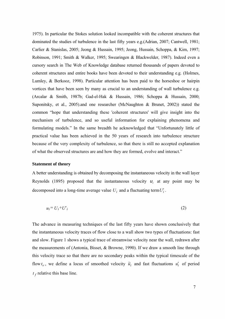
The advance in measuring techniques of the last fifty years have shown conclusively that

the instantaneous velocity traces of flow close to a wall show two types of fluctuations: fast

and slow. Figure 1 shows a typical trace of streamwise velocity near the wall, redrawn after

the measurements of (Antonia, Bisset, & Browne, 1990). If we draw a smooth line through

this velocity trace so that there are no secondary peaks within the typical timescale of the

flow , we define a locus of smoothed velocity iu~νt and fast fluctuations of period

relative this base line.

iu′

ft

8

U

Figure 1 Trace of instantaneous streamwise velocity after measurements by Antonia et al.

(1990).

The instantaneous velocity may be decomposed in an alternate manner as:

u+u=u iii ′~ (3)

Then we may write

0 = dtui∫∞

′0

(4)

u+U~=U iii ′′′ (5)

where

iii -Uu~=U~ ′ (6)

then

u+U~+U=u iiii ′′ (7)

We may average the Navier-Stokes equations over the period of the fast fluctuations.

Bird, Stewart, & Lightfoot (1960, p.158) give the results as

ft

xuu-

xu~u~-

xu~+

xp-=

t)u~(

j

ji

j

ji2j

i2

i

i

∂′′∂

∂∂

∂∂

∂∂

∂∂ μρ (8)

9

Equation (8) defines a second set of Reynolds stresses uu ji ′′ which we will call "fast"

Reynolds stresses to differentiate them from the standard Reynolds stresses UU ji ′′ . In

perio

general Uu ′<′ and the fast Reynolds stresses are smaller in magnitude than the standard

Reynolds stresses.

Within a νt , the smoothed velocity iu

ii

d ~ varies slowly with time but the fluctuations iu′

may be assumed to be periodic with a ti escale . We may write the fast fluctuations in

eynolds stresses become

e(uu = uu j0,i0,t-2i2i

j0,i0,jiωω′′

e fl periodic motion

ftm

the form

( )e+eu = u t-itiii

ωω,0′ (9)

The fast R jiuu ′′

+t uu2+)e (10)

iu′Equation (10) shows that th uctuating generates two components of

the "fast" Reynolds stresses: one is oscillating and cancels out upon long-time-averaging,

stream

denly set in motion that we will call here solution1 and

the other, j,0i,0 uu is persistent in the sense that it does not depend on the period ft .The term

j,0i,0 uu indicates the startling possibility that a purely oscillating motion can generate a

steady mo hich is not aligned in the direction of the oscillations. The qualification

must be understood as independent of the frequency ω of the fast fluctuations. If the

flow is averaged over a longer time than the period νt of the bursting process, the term

j,0i,0 uu must be understood as transient but non-oscillating. This term indicates the

presence of transient shear layers embedded in turbulent flow fields and not aligned in the

wise direction similar to those associated with the streaming flow in oscillating

laminar boundary layers (Schneck & Walburn, 1976; Tetlionis, 1981). Schoppa and

Hussain(2002)also observed that sinusoidal velocity fluctuations in turbulent flows led to

the production of intense shear layers associated with the streaming flow, that they call

transient stress growth TSG.

Thus to describe the process of the wall layer we need to superimpose two solutions: Stokes’

solution for a flat plate sud

tion w

steady

Stokes’solution for an oscillating flat plate that we call solution2.

10

an oscillating flow with a

e define a stream function ψ such that

We first look at the effect of the fast fluctuations by analysing

zero-mean velocity . In this case one may thus investigate the effect of the amplitude and

frequency of the fluctuations separately because the basic velocity fluctuations imposed by

external means do not grow with time.. The following treatment of the problem is taken

from the excellent book of (Tetlionis, 1981).

W

x=v =u ∂∂

y ∂∂ψψ (11)

Where and are the components o local instantaneous velocity in the x, y directions. vu

The basic variables are made non-dimensional

ωt=t y=y x=x *** ων/2L (12)

⎟⎟⎠

⎞⎜⎜⎝

⎛∞

∞ ωνψψ

2U = t)(x,

UU=t)(x,U

-1

*e*e (13)

where is the approach velocity for ∞→x∞U , eU is the local mainstream velocity and L is

The sy ema characteristic dimension of the body. st of coordinates x, y is attached to the

body. The Navier-Stokes equation may be transformed as:

⎟⎟

⎠

⎞

⎜⎜⎛ ∂∂∂∂∂∂∂ UU1 2**2*

e*e

*3*2 ψψψψψ

⎝ ∂∂

∂∂∂∂∂∂∂∂∂ xUU+

yx+

xyy-

L=

t-

y2-

ty *

*e*

e*2

*

******3**

ψω

(14)

with boundary conditions

0 =y 0=y

= **

* ∂′ ψψ *∂

(15)

For large frequencies, the RHS of equation (14) can be neglected since

1 LU = e <<ω

ε (16)

In this case, Tetlioni eports the solution of equation (14) as: s r

C+e2

yU)x(U ti**

0yi)+(1**

0* ** ⎤⎡+]e-i)[1-(1

2 =

⎥⎥⎦⎢

⎢⎣

ψ (17)

Tetlionis (op. cit. p. 157) points out that equation (17) may be regarded as a generalisation of

11

Stokes' solution (1851) for an oscillating flat plate.

Equation (17) is accurate only to an error of order ε rts a more accurate . Tetlionis repo

solution for the case when ε cannot be neglected (i.e. for lower frequencies):

)( 0 +] e+e)y,x([+]e)y( e)y([)x(U = *1

it-**0

it**0

**0* ** ψεψψψ2

2it2-*0

it2** **εψ (18)

where ε0ψ and 1ψ are the components of the stream function of order and 0ε .

Substituting this more accurate solution into equation (14), we find that the multiplication

f coefficients of and forms terms that are independent of the oscillating

cy, ).

*ite *ite−o

frequen ω, imposed on the flow field and were not anticipated in equation (18 Thus the

full solution of equation (14) is normally written (Stuart, 1966; Tetlionis, 1981) as

)( O +] e)y,x(+e)y,x([+[ +

] e)y( + e)[2

)xU =

2it2-*1

it2*1st

it-**it*

*

**

**

εψψψε

ψψψ (19)

y((

*****

0**

0

*0

where the overbar denotes the complex conjugate and *ite *stψ results from cancelling of

and terms.

*ite−

The quantity *stψ shows that the interaction of convected inertial effects of forced oscil on

with viscous effects near

lati s

a wall results in a non-oscillating motion that is referred to in the

terature as "Streaming". The problem has been known for over a century (Faraday, 1831;

ainly on

minar oscillating boundary layers but could not capture all the elements of the flow field

li

Dvorak, 1874; Rayleigh, 1880, 1884; Carriere, 1929; Andrade, 1931; Schlichting, 1932) and

studied theoretically (Riley, 1967; Schlichting, 1960; Stuart, 1966; Tetlionis, 1981).

When the smoothed phase velocity cannot be neglected, the problem becomes much more

complex. Early analytical investigations (Riley, 1975; Stuart, 1966)) focused m

la

because of many simplifications and omissions were required to overcome the considerable

mathematical difficulties. They did give insight into the role of different terms in the NS

equations. Numerical solutions (Schneck & Walburn, 1976) could capture the patterns of

viscous and streaming flow but gave less insight into the role of the different terms in the NS

12

equations. Yet more information was provided in the rational numerical simulations RNS

(nomenclacutre of Zhang (1991)) that study the interactions between the different structures

embedded in a turbulent flow field. In particular, the effect of vortices as they move above the

wall has been studied in a number of “kernels” (nomenclature of Smith et al (1991)). These

kernel studies show that a vortex moving above a wall will induce a laminar sub-boundary

layer underneath its path by viscous diffusion of momentum, even if the vortex is introduced

into a fluid which was originally at rest (Smith, Walker, Haidari, & Sobrun, 1991). The vortex

impresses a periodic disturbance onto the laminar sub-boundary layer underneath. which

oscillates then erupts in a violent ejection that Peridier et al (1991) call viscous-inviscid

interaction The problem is thus very similar to the streaming flow discussed by Tetlionis. In

these kernel studies the configuration of the vortex must be specified a priori. In the work of

Walker (1978) it is a rectilinear vortex, in Chu and Falco (1988) ring vortices, in Liu et al.

(1991) hairpin vortices, in Swearingen and Blackwelder (1987), streamwise Goertler vortices.

But recently in their numerical simulation Suponitsky, Cohen, & Bar-Yoseph (2005) have

shown that vortical disturbances evolve into a hairpin vortex independently of their original

geometry over a wide range of orientations. The eruptions are linked with the growth of the

vortex as it moves down the wall, seen clearly in hydrogen bubble visualisations e.g. (Offen &

Kline, 1974)and the growth of the fast velocity fluctuations impressed on the viscous sub-

boundary layer. It occurs at a critical value of the term ε in equation (16), which is a

combination of the Reynolds number of the sub-boundary layer and the Strouhal number of

the fluctuations.Thus we can use the Stokes solution1 which is a particular form of the solution

of order 0ε as Einstein and Li proposed to model the sweep phase of the wall layer but it must

be expressed in terms of the smoothed velocity i

yu

∂∂

∂∂ τ

ρ1~

A more detailed discussion of these issues in pre

t−= (20)

sented in (Trinh, 2009)

It is now proposed that the development of instabilities leading to ejections, in other words the

re specifically, it is

ostulated that the ejections always occur when the ratio of kinetic to viscous energy in the

bursting process, is the same for Newtonian and non-Newtonian fluids. Mo

p

transient sub-boundary layer reaches a critical value, which is not dependent on the nature of

13

easurements through a solution of equation (20). The analysis is made

ere for fluids that obey the Ostwald de Waele power law rheological model

the shear rate

in subsequent publications.

the fluid. This critical ratio can be estimated by a kind of local instantaneous friction factor. It

is calculated from the critical instantaneous wall shear stress and the local approach velocity to

the sub-boundary layer at the end of the low-speed streak phase, just prior to ejection (as

shown in Figure 1).

Since direct measurements of this critical instantaneous shear stress are difficult, it is estimated

from time-averaged m

h

γτ n K = (21)

where K is called the consistency coefficient,

n the flow behaviour index, and

γ

Application to other fluids models is presented

Substituting equation (21) into (20) gives

yy K n =

t 2∂⎟⎟⎠

⎜⎜⎝ ∂∂

ρ uuu 21-n∂⎞⎛ ∂∂ ~~~

(22)

The relative distance ( )yt,η into the viscous sub-boundary layer near the wall )(tiδ is

defined as

(t) = y)(t,

iδη (2

and the velo

y3)

city φ relative to the velocity eU~ at the edge of the wall layer is

Uu =

e~~

φ (24)

Substituting these new variables into equ ion (22) and integrating with reat spect to η gives

MN

UK=

dtd 1-n

ein

i~

ρδδ (25)

in which

])[(=y)(t,)d()n(=N 10

n1-n10 φηφφ ′′′′∫ (26a)

and

14

re the primes denote derivatives with respect to η.

y)(t,d-1=y)(t,y)d(t,)(=M 10

10 ηφηηφ ∫′∫ (26b)

whe

Equation (25) can now be integrated separately with respect to the variables δi and t

characteristic time :

over a

νt

dtMU=d 1-n

eini ∫∫ ρδδ

00 (27)

The instantaneous al

NKte νδ ~

w l-layer thickness at time , which coincides with the onset of ejection,

is

νt

⎥⎦

⎢⎣

νν ρδδ tMN

U1)+(nK = )(t = 1-neie

~ (28)

The

⎤⎡1)+1/(n

instantaneous wall shear stress is:

iw,y

u- K = iw,⎥⎥⎦

⎤

⎢⎢⎣

⎡⎟⎟⎠

⎞⎜⎜⎝

⎛∂∂~ n

τ (29a)

n

weiw yUK ⎥

⎦

⎤⎢⎣

⎡∂∂′=ηφτ )(~

, (29b)

[ ])(

~, ti

UKN n

ne

iw δτ = (29c)

The time-averaged wall sh ar stress is given by e

dtt 0wτν∫

1 = iw,t τν (30a)

δτ n

e

ne

wU1~

+(n N K = ) (30b)

( ) ew n ττ 1+= (30c)

15

where τe = τw,T is the instantaneous wall-shear stress at time which coincides with the end

of the low-speed-streak phase and the onset of ejection, as shown in Figure 1. Henceforth, this

all shear stress will be called the critical local instantaneous wall-shear stress at the point of

ejection or simply the ritical shear stress.

to the critical approach velocity

νt

w

c

The transient unsteady state sub-boundary layer has been called a Stokes layer and can

often be found embedded in other flows (Tetlionis, 1981). The thickness of the Stokes layer

δ eU~e at the end of the period νt is related by putting

= in equation (29c) and rearranging: t νt

e

n

e Ue

KN ~/

⎥⎦

⎤⎢⎣

⎡=

τδ

1 (31)

The time-averaged shear velocity is usually given the symbol *u and defined a s:

ρτ= wu * (32)

We define a new normalising parameter, the critical shear velocity *eu

1nu

)1n(/u *w

e*e+

=+ρ

τ=ρτ= (33)

The thickness of the Stokes layer may be normalised with the critical wall shear stress as:

Kuu nn

eeee/11/2

** ρδδ −+ ==

ne

e /1νδ (34)

The normalised critical approach velocity at the point of bursting is

uU

U ee

e*

~~ =+ (35)

Combining equations (31), (33), (34) and (35) gives

UN en

e~++ = 1δ (36)

The coefficients M and N can be determined once the relative velocity φ as a function of

is known. Following Polhausen (1921) and Bird, Stewart, & Lightfoot (1960), we assume that

y a third-order polynomial:

η

the velocity profile can be described approximately b

ηηφ 3-= 5051 .. (37)

Back-substitution into equations (26a) and (26b) respectively yields the unknown

16

coefficients:

( )23 n=N (38)

and

83=M

Substitution o

(39)

f equation (38) into (36) gives

U ee~. ++ = 51δ (40)

Equation (40) shows clearly that the relation between the wall layer thickness and the

critical approach velocity of the Stokes layer at the point of bursting is independent of the

our index, when normalised with the critical

instantaneous shear velocity.

fluid rheology, specifically the flow behavi

We should note that for Newtonian fluids, n=1, equation (38) gives

)(N = = N 1/n=1n 23 / (41)

Therefore equation (40) may be written as: +

=+ = ene UN ~

1δ (42)

elocity profile assumed.

For example, the same derivation leading to equation (42) may be performed with a fourth-

(1921). Of course the numerical value of the

coefficient N changes with the velocity profile assumed but equation (40) does not. In

s

s

). Since the edge of the wall layer is defined by the

maximum penetration of viscous momentum from the wall then the time averaged wall

Thus the previous conclusion is not dependent on the form of the v

order polynomial also proposed by Polhausen

the

exact Stokes solution (Bird, 1959)

(43)08 21 .==nN

Because instantaneous shear and velocity profiles are very difficult to measure, it i

convenient to re-express these instability criteria in terms of time-averaged shear stresse

through the use of equation (30c

layer thickness is equal to the thickness of the transient viscous sub-boundary layer at the

point of ejection eδδν = and eUU ~=ν . Then the velocity at the edge of the wall layer,

normalised with the time-averaged shear velocity, becomes

1+==

++

nUUU e

w

e~

/

~

ρτν (44)

Similarly

17

( )1 22

1

112

== ++

Ku n

n

ne δδδ /

/* (45) +

−−

nn

e

nρν

/

Combining equations (42), (44) and (4527) gives

(42) and (46) indicate that the apparent thickening of the wall layer, seen in

traditional velocity plots normalised with the time-averaged shear velocity u*, such as those

of (Bogue (1961), are not real. This apparent thickening is the consequence of an integration

ll shear stress, the normalising parameter

with physical significance, to the time-averaged wall shear stress, which is traditional

more easily measured.

( ) Un n ++ += ννδ 1082 1 /. (46)

Equations

process, which relates the critical instantaneous wa

ly

Friction factors and Reynolds numbers

The critical apparent (non-Newtonian) kinematic viscosity at the wall eν is defined as

τρ

τν 1)/n-(ne

1/nee K=

)y/u(-=

∂∂~ (47

The critical instantaneous

e)

Reynolds number becomes

( ) nnee K τν n 11 (48)

and the critical instantaneous friction factor is

eDVDV=Re −

=

V2 = f 2

ee ρ

τ (49)

These definitions can be compared with the more conventional definitions of the time-

averaged friction factor

2Vf w

ρ2τ

= (50)

and the generalised Metzner-Reed Reynolds number (Metzner & Reed, 1955)

n1-n

g

43n

8K

VD =

⎜⎝⎛

ρRe

(51)

n-2n

n1+⎟⎠⎞

The relation betw n the critical instantaneous Reynolds number and the generalised M -

Reed Reynolds number can be derived from equations (30c), (48), (49), (50) and (51):

ee etzner

18

( )⎟⎠⎞

⎜⎝⎛ +⎟⎠⎞

⎜⎝⎛ +

⎟⎠⎞⎜

⎝⎛ −=

−

−

21

413

21ReRe1

)1(5 n1

nn

nnfgn

n

nn

e

(1959),

Bogue (1961) and (Yoo, 1974). Figure 3 shows a plot of time-averaged friction factor against

the Metzner-Dodge Reynolds number.

the flow behaviour index, n, falls on different lines. Figure 4

(52)

Verification of theory

The friction factor in viscous non-Newtonian pipe flow has been measured by Dodge

The data for different values of

shows a plot of the critical instantaneous friction factor against the critical instantaneous

Reynolds number, defined in terms of the critical wall shear stress. All the data falls on a

unique plot.

Figure 3. Plot of time-averaged friction factor against generalized Metzner-Reed

Reynolds number.

19

0.001

0.01

0.1

100 1000 10000 100000 1000000Critical instantaneous Reynolds number, Ree

Crit

ical

inst

anta

neou

s fr

ictio

n fa

ctor e

Do d

Bo gu

Yo o

450flogRe665f

1ee

e.. +=

fe=8/R ee

Figure 4. Similarity plot of instantaneous critical friction factor against Reynolds number.

For Newtonian fluids, the critical friction velocity is related to the time averaged friction

velocity by putting in equation (33) and: 1=n

2 u= u **e (53)

Similarly equation (30c) gives

ew ττ 2= (54)

eff 2= (55)

Prandtl's logarithmic law (Prandtl, 1935; Nikuradse, 1932)

40log0.41 . )fRe( =f

− (56)

may be rewritten in terms of the critical wall shear stress

.45 + )fRe( 5.66 =f ee

e

0log1 (57)

Equation (57) fits the data of Dodge, Bogue and Yoo quite closely, as shown in Figure 4. The

agreement is not perfect because the wall layer analysis has been made for flow past a flat

surface. The application of this analysis to circular pipe flow implies that the curvature effects

can be neglected, which is true only at high Reynolds numbers when the wall layer is very thin

compared to the pipe radius.

Similarly, the Blasius power law (Blasius, 1913)

20

Re0.079 = f

1/4 (58)

may be rewritten as

Re0.04= f 1/4

ee (59)

Equation (59) also fits the data presented in Figure 4.

Discussion and Conclusion

The apparent viscosity of non-Newtonian fluids changes with the applied shear stress or shear

rate. Therefore, it is important for engineering correlations to identify exactly the shear stress

(or shear rate) at which the viscosity should be evaluted. It can then be used to normalise the

velocity , the distance y and to calculate the Reynolds number. Experimental data shows that

both the velocity profile (e.g. (D. C. Bogue & Metzner, 1963)) and the friction factor-

Reynolds number curves (Figure3) of power law fluids are shifted when the velocity and

distance are normalised with the viscosity calculated at the time averaged value of the wall

shear stress. The data gathered by Bogue (D.C. Bogue, 1961) and others e.g.(Trinh, 2005)

show that the wall thickness , normalised with the time averaged wall shear stress, becomes

thicker as the behaviour index n decreases. In an effort to collapse the non-Newtonian data

onto their Newtonian counterpart many authors have resorted to different definitions of

effective viscosity (e.g. Acrivos et al., Metzner and Reed, Edwards and Smith op. cit.). The

present paper argues that since turbulence is a time-dependent phenomenon, the viscosity

should be estimated at the value of the local instantaneous wall shear stress, not the time

averaged value. When this is done, there is no need to define an effective viscosity. Even in

laminar, Trinh and Keey(Trinh & Keey, 1992) argued that the diffusion of viscous momentum

from the wall into the main flow is a time-dependent phenomenon: elements of fluid are

convected along the main direction of flow and viscous momentum is diffused between

adjacent fluid particles. Therefore the front of diffusion of viscous momentum moves across

the pipe or laminar boundary layer only once but the process repeats itself regularly so that the

time averaged profile looks steady.

u

+νδ

The collapse of non-Newtonian laminar critical instantaneous friction factors of power law

fluids onto the Poiseuille solution is not perfect because the Stokes solution was derived for an

21

impulsively started flat plate and does not account for the curvature of the wall in pipe flow.

This neglect is not important in turbulent flow when the wall layer is thin but becomes

important for laminar flow that covers the entire pipe radius. An unsteady solution that

accounts for curvature has been derived by Szymansky(Szymanski, 1932) and can be applied

to models of turbulent flow ((Trinh, 1992; Trinh, 2009).) but the solution involves a Bessel

series which is more cumbersome to handle mathematically.

The collapse of all turbulent friction factors expressed in terms of the critical instantaneous

wall shear stress into a single curve suggests strongly that the mechanism of turbulence is the

same for both Newtonian and power law fluids. In fact the same exercise can be repeated for

other fluid models, for example the Bingham plastic and Herschel-Bulkley models, and the

observation can be generally applied to all time-independent fluids. The shift observed when

the time averaged shear stress is used as a normalising parameter arises from an integration

constant and does not relate to the behaviour of polymer molecules in turbulent flow as

sometimes postulated (e.g. (Wilson & Thomas, 1985)) or a pseudo-slip effect (Kozicki &

Tiu,(1967) similar to the well documented observations in rheometric measurements of

particulate suspensions (Steffe, 1996). An exception must be made for viscoelastic fluids

because the elasticity of the polymers do dampen the periodic velocity fluctuations impressed

on the wall layer by the travelling vortex ((Stone, Roy, Larson, Waleffe, & Graham, 2004;

Trinh, 1969; Trinh, 1992; Trinh, 2009)) and reduce the value of the transient turbulent stresses

responsible for the bursts.

In another report that summarises the writer’s body of work on turbulence over a period of 40

years it is shown that the velocity profiles in the inner region (wall layer + log law region) of

turbulent flows of Newtonian and non-Newtonian fluidsin many geometrical situations all

collapse into a unique master curve when normalised with and (Trinh, 2009),p.84).

The same similarity analysis also collapses the skin drag friction factors of Newtonian and

non-Newtonian fluids unto a uniques master curve (Trinh, 2009), p.160). This evidence further

supports the main argument presented in this paper: that the mechanism of turbulence is the

same in Newtonian and time-independent fluids and that graphical differences arise from the

different ways that the normalisation process is handled mathemathematically.

+νU +

νδ

22

The present analysis has also demonstrated the existence of a similarity plot between the

critical friction factor and the critical non-Newtonian Reynolds number for turbulent pipe

flow of purely viscous power law fluids. Instabilities leading to the ejection of low-speed

fluid from the wall layer are local phenomena and should be studied in terms of local

instantaneous parameters. The critical point noted in this theory is that turbulence cannot be

adequately explained by measurements and analysis of time-averaged shear stresses and

velocities only. A great confusion has resulted from starting the theoretical analysis with

the time-averaged Navier-Stokes equations, the Reynolds equations, whereas the present

theory starts with the unsteady state Navier-Stokes equations and then time-averages the

solution.

Nomenclature

D Pipe diameter

f Time-averaged friction factor defined by equation (50)

fe Critical (local instantaneous) friction factor defined by equation (49)

K Consistency coefficient in power law model

M, N Coefficients defined by equations (26a) and (26b)

n Flow behaviour index in power law model

eDV νRee Critical instantaneous Reynolds number,

Reg Metzner-Reed generalised Reynolds number, equation (51)

t Time

u~ Local instantaneous velocity smoothed with respect to fluctuations imposed by a

travelling vortex

u* Time-averaged friction velocity

u Critical (instantaneous) friction velocity e*

eU~ Approach velocity to transient viscous sub-boundary layer

(velocity at wall layer edge at the moment of ejection)

Uν+ Approach velocity normalised with time-averaged friction velocity, Ue/u*+eU~

*/~ee uU Approach velocity normalised with the critical shear velocity,

V Mixing cup average discharge velocity

y Normal distance from the wall

23

δi (t) Instantaneous thickness of (Stokes) transient sub-boundary layer

δe+ Wall layer normalised with the critical shear velocity

δv+ Wall layer thickness normalised with the time-averaged shear velocity

Shear rate γ

η Dimensionless distance defined by equation (23)

νe Apparent critical kinematic viscosity defined by equation (47)

ρ Density

τ Shear stress

φ Dimensionless velocity defined by equation (24)

Subscripts

ν Viscous, or at the edge of the wall layer

e At the onset of ejection or at the end of the low-speed streak phase, see also T

i instantaneous

νt At the end of the low-speed-streak phase

w Wall

Superscript

+ Normalised with wall shear stress

References

Adrian, R. J. (2007). Hairpin vortex organization in wall turbulence. Physics of Fluids, 19(4).

Alves, G. E., Boucher, D. F., & Pigford, R. L. (1952). Pipe-line design - for non-newtonian solutions and suspensions. Chemical Engineering Progress, 48(8), 385-393.

Black, T. J. (1969). Viscous drag reduction examined in the light of a new model of wall turbulence. In W. C.S. (Ed.), Viscous Drag Reduction. New York: Plenum Press.

Blasius, H. (1913). Mitt. Forschungsarb.,, 131, 1. Bogue, D. C. (1961). Velocity profiles in turbulent non-Newtonian pipe flow, Ph.D. Thesis.

University of Delaware. Bogue, D. C., & Metzner, A. B. (1963). Velocity Profiles in Turbulent Pipe Flow -

Newtonian and Non-Newtonian Fluids. Industrial & Engineering Chemistry Fundamentals, 2(2), 143.

Bowen, R. L. (1961). Scale-up for non-Newtonian fluid flow: Part 4, Designing turbulent-flow systems. Chem. Eng. Prog, 68(15), 143-150.

Cantwell, B. J. (1981). Organised Motion in Turbulent Flow. Annual Review of Fluid Mechanics, 13, 457.

24

Carlier, J., & Stanislas, M. (2005). Experimental study of eddy structures in a turbulent boundary layer using particle image velocimetry. Journal of Fluid Mechanics, 535, 143-188.

Chabra, R. P., & Richardson, J. F. (1999). Non-Newrtonian flow in the process industries. Oxford, Great Britain: Butterworth-Heinemann,.

Clapp, R. M. (1961). Turbulent heat transfer in pseudoplastic nonNewtonian fluids. Int. Developments in Heat Transfer, ASME, Part III, Sec. A, 652.

Corino, E. R., & Brodkey, R. S. (1969). A Visual investigation of the wall region in turbulent flow. Journal of Fluid Mechanics, 37, 1.

Darby, R. (1988). Laminar and turbulent pipe flows of non-Newtonian fluids in Encycopedia of Fluid Mechanics (Vol. 7). Houston: Gulf Pub. Co.

Desouky, S. E. M. (2002). New method predicts turbulence for non-Newtonian fluids in pipelines. Oil & Gas Journal, 100(19), 66-69.

Desouky, S. E. M., & El-Emam, N. A. (1990). A generalised pipeline design correlation for pseudoplastic fluids. Journal of Canadian Petroleum Technology, 29(5), 48-54.

Dodge, D. W. (1959). Turbulent flow of non-Newtonian fluids in smooth round tubes, Ph.D. Thesis. US: University of Delaware.

Dodge, D. W., & Metzner, A. B. (1959). Turbulent Flow of Non-Newtonian Systems. AICHE Journal, 5(2), 189-204.

Edwards, M. F., & Smith, R. (1980). The Turbulent-Flow of Non-Newtonian Fluids in the Absence of Anomalous Wall Effects. Journal of Non-Newtonian Fluid Mechanics, 7(1), 77-90.

Einstein, H. A., & Li, H. (1956). The viscous sublayer along a smooth boundary. J. Eng. Mech. Div. ASCE 82(EM2) Pap. No 945.

Eissenberg, D. M., & Bogue, D. C. (1964). Velocity profiles of Thoria suspensions in turbulent pipe flow. AIChE J., 10, 723-727.

El-Emam, N., Kamel, A. H., El-Shafei, M., & El-Batrawy, A. (2003). New equation calculates friction factor for turbulent flow of non-Newtonian fluids. Oil & Gas Journal, 101(36), 74-+.

Gao, P., & Zhang, J. J. (2007). New assessment of friction factor correlations for power law fluids in turbulent pipe flow: A statistical approach. Journal of Central South University of Technology, 14, 77-81.

Hanks, R. W., & Ricks, B. L. (1975). Transitional and turbulent pipe flow of pseudoplastic fluids. Journal of Hydronautics, 9, 39-44.

Hanratty, T. J. (1956). Turbulent exchange of mass and momentum with a boundary. AIChE J., 2, 359.

Hanratty, T. J. (1989). A conceptual model of the viscous wall layer. In S. J. Kline & N. H. Afgan (Eds.), Near wall turbulence (pp. 81-103). New york: Hemisphere.

Hemeida, A. M. (1993). Friction Factors For Yieldless Fluids In Turbulent Pipe-Flow. Journal Of Canadian Petroleum Technology, 32(1), 32-35.

Holmes, P., Lumley, J. L., & Berkooz, G. (1998). Turbulence, Coherent Structures, Dynamical Systems and Symmetry: Cambridge University Press.

Jeong, J., & Hussain, F. (1995). On The Identification Of A Vortex. Journal Of Fluid Mechanics, 285, 69-94.

Jeong, J., Hussain, F., Schoppa, W., & Kim, J. (1997). Coherent stuctures near the wall in a turbulent channel flow. Journal of Fluid Mechanics, 332, 185-214.

Karman, v. T. (1934). Turbulence and skin friction. J. Aeronaut. Sci., 1, 1-20.

25

Kawase, Y., Shenoy, A. V., & Wakabayashi, K. (1994). Friction And Heat And Mass-Transfer For Turbulent Pseudoplastic Non-Newtonian Fluid-Flows In Rough Pipes. Canadian Journal Of Chemical Engineering, 72(5), 798-804.

Kemblowski, Z., & Kolodzie, J. (1973). Flow Resistances of Non-Newtonian Fluids in Transitional and Turbulent-Flow. International Chemical Engineering, 13(2), 265-279.

Kim, H. T., Kline, S. J., & Reynolds, W. C. (1971). The Production of the Wall Region in Turbulent Flow. Journal of Fluid Mechanics, 50, 133.

Kline, S. J., Reynolds, W. C., Schraub, F. A., & Runstadler, P. W. (1967). The structure of turbulent boundary layers. Journal of Fluid Mechanics, 30, 741.

Kolmogorov, A. N. (1941). The local structure of turbulence in incompressible flow for very large Reynolds number. C. R. Acad. Sci. U.S.S.R. , 30, 4.also Proc.Roy.Soc.London A (1991) 1434, 1999-1913.

Kozicki, W., & Tiu, C. (1967). Non-Newtonian flow through open channels. Can. J. Chem. Eng., 45, 127.

Malin, M. R. (1997). Turbulent pipe flow of power-law fluids. International Communications in Heat and Mass Transfer, 24(7), 977-988.

McNaughton, K. G., & Brunet, Y. (2002). Townsend's hypothesis, coherent structures and Monin-Obukhov similarity. Boundary-Layer Meteorology, 102(2), 161-175.

Meek, R. L., & Baer, A. D. (1970). The Periodic viscous sublayer in turbulent flow. AIChE J., 16, 841.

Metzner, A. B., & Reed, J. C. (1955). Flow of Non-Newtonian Fluids - Correlation of the Laminar, Transition, and Turbulent-Flow Regions. Aiche Journal, 1(4), 434-440.

Millikan, C. B. (1939). A critical discussion of turbulent flows in channels and circular tubes. Appl. Mech. Proc. Int. Congr. 5th, 386.

Nikuradse, J. (1932). Gesetzmäßigkeit der turbulenten Strömung in glatten Rohren. Forsch. Arb. Ing.-Wes. N0. 356.

Offen, G. R., & Kline, S. J. (1974). Combined dyestreak and hydrogenbubble visual observations of a turbulent boundary layer. Journal of Fluid Mechanics, 62, 223.

Offen, G. R., & Kline, S. J. (1975). A proposed model of the bursting process in turbulent boundary layers. Journal of Fluid Mechanics, 70, 209.

Peridier, V. J., Smith, F. T., & Walker, J. D. A. (1991). Vortex-induced Boundary-layer Separation. Part 1. The Unsteady Limit Problem Re. Journal of Fluid Mechanics, 232, 99-131.

Prandtl, L. (1935). The Mechanics of Viscous Fluids. In D. W.F (Ed.), Aerodynamic Theory III (pp. 142). Berlin: Springer.

Reichardt, H. (1971). MPI für Strömungsforschung: Göttingen, Rep. No 6a/1971. Riley, N. (1975). Unsteady Laminar Boundary Layers. SIAM Rev., 17, 274-297. Robinson, S. K. (1991). Coherent Motions in the Turbulent Boundary Layer. Annual

Review of Fluid Mechanics, 23, 601. Rudman, M., & Blackburn, H. M. (2006). Direct numerical simulation of turbulent non-

Newtonian flow using a spectral element method. Applied Mathematical Modelling, 30(11), 1229-1248.

Rudman, M., Blackburn, H. M., Graham, L. J. W., & Pullum, L. (2004). Turbulent pipe flow of shear-thinning fluids. Journal Of Non-Newtonian Fluid Mechanics, 118(1), 33-48.

26

Sablani, S. S., & Shayya, W. H. (2003). Neural network based non-iterative calculation of the friction factor for power law fluids. Journal Of Food Engineering, 57(4), 327-335.

Schneck, D. J., & Walburn, F. J. (1976). Pulsatile blood flow in a channel of small exponential divergence Part II: Steady streaming due to the interaction of viscous effects with convected inertia. Journal of Fluids Engineering, 707.

Schoppa, W., & Hussain, F. (2002). Coherent structure generation in near-wall turbulence. Journal Of Fluid Mechanics, 453, 57-108.

Shaver, R. G. (1957). PhD Thesis. M.I.T., Cambridge, Mass. Shaver, R. G., & Merrill, E. W. (1959). Turbulent of pseudoplastic polymer solutions in

straight cylindrical tubes. A. I. Ch. E. J, 5. Shenoy, A. V., & Saini, D. R. (1982). A New Velocity Profile Model for Turbulent Pipe-

Flow of Power-Law Fluids. Canadian Journal of Chemical Engineering, 60(5), 694-696.

Skelland, A. H. P. (1967). Non-Newtonian Flow and Heat transfer. New York: John Wiley and Sons.

Smith, C. R., & Walker, J. D. A. (1995). Turbulent wall-layer vortices. Fluid Mech. Applic., 30.

Smith, C. R., Walker, J. D. A., Haidari, A. H., & Sobrun, U. (1991). On the Dynamics of near-wall Turbulence. Phil. Trans. R. Soc. Lond., A336, 131-175.

Steffe, J. F. (1996). Rheological Methods in Food Process Engineering. USA: Freeman Press.

Stone, P. A., Roy, A., Larson, R. G., Waleffe, F., & Graham, M. D. (2004). Polymer drag reduction in exact coherent structures of plane shear flow. Physics Of Fluids, 16(9), 3470-3482.

Stuart, J. T. (1966). Double boundary layers in oscillatory viscous flow. Journal of Fluid Mechanics, 24, 673.

Swearingen, J. D., & Blackwelder, R. F. (1987). The Growth and Breakdown of Streamwise Vortices in the presence of a Wall. Journal of Fluid Mechanics, 182, 255-290.

Szilas, A. P., Bobok, E., & Navratil, L. (1981). Determination of Turbulent Pressure Loss of Non-Newtonian Oil Flow in Rough Pipes. Rheologica Acta, 20(5), 487-496.

Szymanski, P. (1932). Quelques solutions exactes des équations de l'hydrodynamique de fluide visqueux dans le cas d'un tube cylindrique. J. des Mathematiques Pures et Appliquées, 11 series 9, 67.

Tennekes. (1966). Wall region in turbulent shear flow of nonNewtonian fluids. Physics of Fluids, 9, 872.

Thomas, A. D. (1960). Heat and momentum transport characteristics of of non-Newtonian aqueous Thorium oxide suspensions. AIChEJ, 8.

Tomita, Y. (1959). A study of non-Newtonian flow in pipelines. Bulletin J.S.M.E., 2. Toms, B. A. (1949). Some observations on the flow of linear polymer solutions through

straight tubes at large Reynolds numbers. Paper presented at the Proc. Int. Cong. on Rheology, Vol II, p.135.North Holland Publishing Co.

Torrance, B. M. (1963). Friction factors for turbulent non-Newtonian fluid flow in circular pipes. S. Afr. Mech. Eng., 13.

Trinh, K. T. (1969). A boundary layer theory for turbulent transport phenomena, M.E. Thesis, . New Zealand: University of Canterbury.

27

Trinh, K. T. (1992). Turbulent transport near the wall in Newtonian and non-Newtonian pipe flow, Ph.D. Thesis. New Zealand: University of Canterbury.

Trinh, K. T. (2005). A zonal similarity analysis of wall-bounded turbulent shear flows. Paper presented at the 7th World Congress of Chemical Engineering

Trinh, K. T. (2009). A Theory Of Turbulence Part I: Towards Solutions Of The Navier-Stokes Equations. arXiv.org, 0910.2072v0911 [physics.flu.dyn.]

Trinh, K. T., & Keey, R. B. (1992). A Time-Space Transformation for Non-Newtonian Laminar Boundary Layers. Trans. IChemE, ser. A, 70, 604-609.

Weltmann, R. N. (1956). Friction factors for flow of non-newtonian materials in pipelines. Industrial and Engineering Chemistry, 48(3), 386-387.

Wilson, K. C., & Thomas, A. D. (1985). A New Analysis of the Turbulent-Flow of Non-Newtonian Fluids. Canadian Journal of Chemical Engineering, 63(4), 539-546.

Yoo, S. S. (1974). Heat transfer and friction factors for non-Newtonian fluids in turbulent flow, PhD thesis. US: University of Illinois at Chicago Circle.

Zhang, T. A. (1991). Numerical simulation of the dynamics of turbulent boundary layers : perpectives of a transition simulator. Phil. Trans. R. Soc. Lond., A(336), 95-102.