Picking and Curves Week 6 David Breen Department of Computer Science Drexel University Based on material from Ed Angel, University of New Mexico CS 480/680

Picking and CurvesWeek 6

David Breen

Department of Computer Science

Drexel University

Based on material from Ed Angel, University of New Mexico

CS 480/680INTERACTIVE COMPUTER GRAPHICS

Angel: Interactive Computer Graphics 3E © Addison-Wesley 2002

2

Objectives

• Picking– Select objects from the display

• Introduce types of curves and surfaces– Explicit– Implicit– Parametric– Strengths and weaknesses

• Discuss Modeling and Approximations– Conditions– Stability


3

Picking• Identify a user-defined object on the display• In principle, it should be simple because the

mouse gives the position and we should be able to determine to which object(s) a position corresponds

• Practical difficulties– Pipeline architecture is feed forward, hard to go

from screen back to world– Complicated by screen being 2D, world is 3D– How close do we have to come to object to say we

selected it?


4

Three Approaches

• Hit list– Most general approach but most difficult to

implement

• Use back or some other buffer to store object ids as the objects are rendered

• Rectangular maps – Easy to implement for many applications– Divide screen into rectangular regions


5

Using another buffer and colors for picking

• For a small number of objects, we can assign a unique color (often in color index mode) to each object

• We then render the scene to a color buffer other than the front buffer so the results of the rendering are not visible

• We then get the mouse position and use glReadPixels() to read the color in the buffer we just wrote at the position of the mouse

• The returned color gives the id of the object


6

Using Regions of the Screen• Many applications use a simple rectangular arrangement of the screen

– Example: paint/CAD program

• Easier to look at mouse position and determine which area of screen it is in that using selection mode picking

drawing area

tools

menus


7

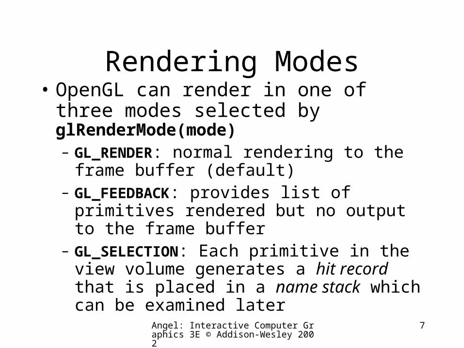
Rendering Modes• OpenGL can render in one of three

modes selected by glRenderMode(mode)– GL_RENDER: normal rendering to the frame

buffer (default)– GL_FEEDBACK: provides list of primitives

rendered but no output to the frame buffer– GL_SELECTION: Each primitive in the view

volume generates a hit record that is placed in a name stack which can be examined later


8

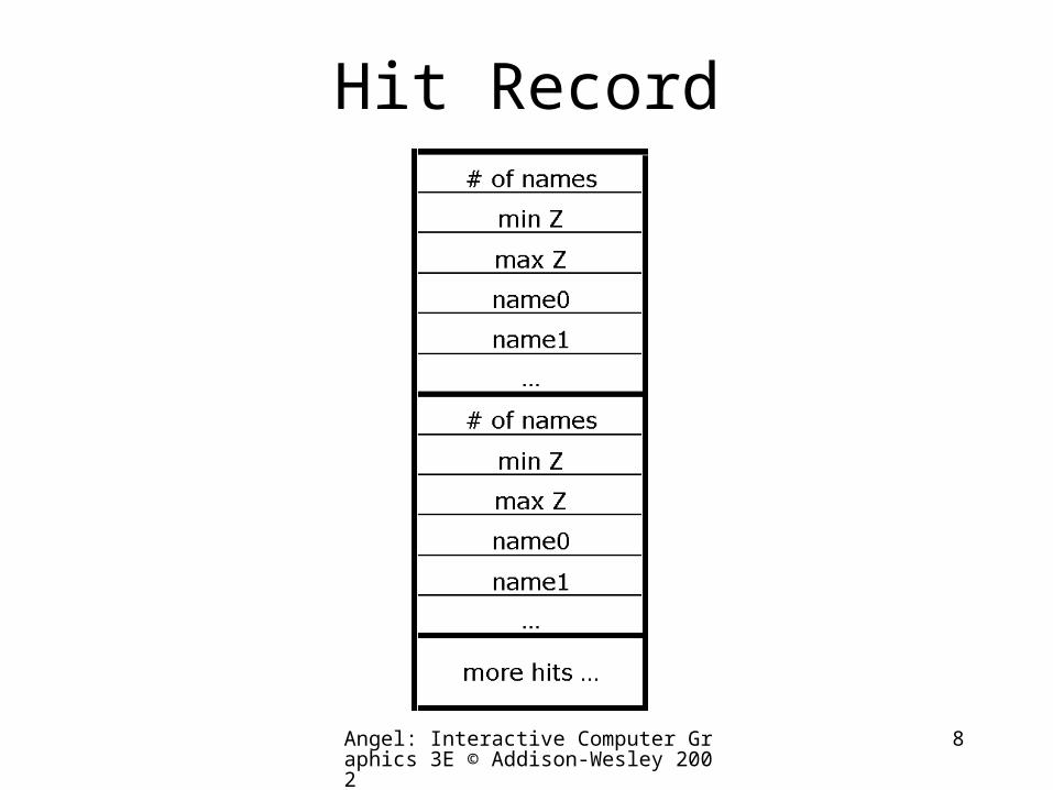
Hit Record


9

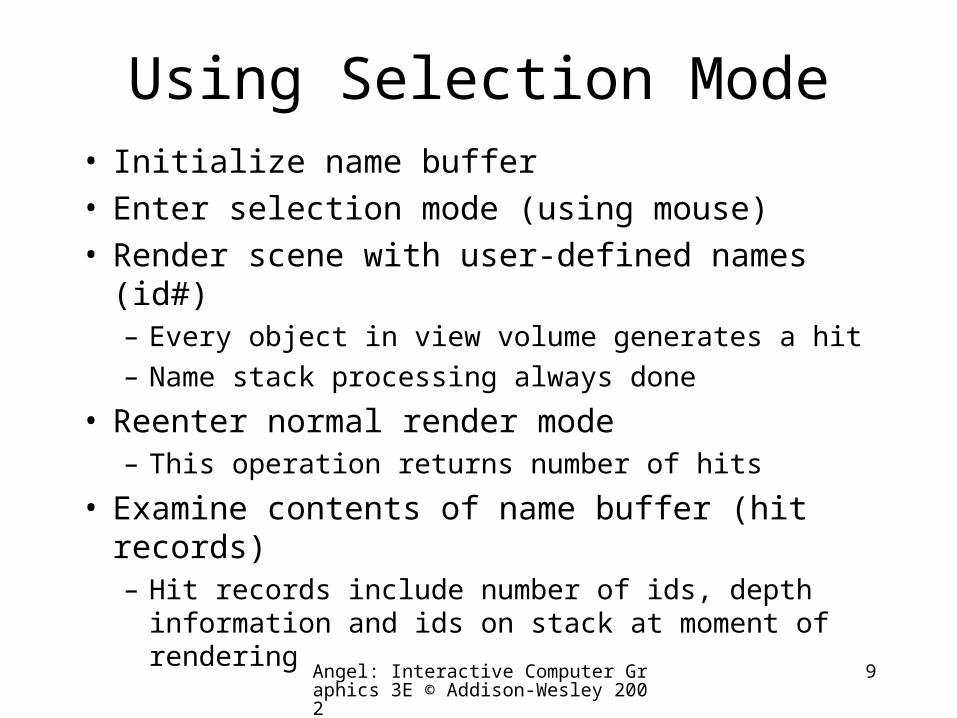
Using Selection Mode• Initialize name buffer• Enter selection mode (using mouse)• Render scene with user-defined names (id#)

– Every object in view volume generates a hit– Name stack processing always done

• Reenter normal render mode– This operation returns number of hits

• Examine contents of name buffer (hit records)– Hit records include number of ids, depth

information and ids on stack at moment of rendering


10

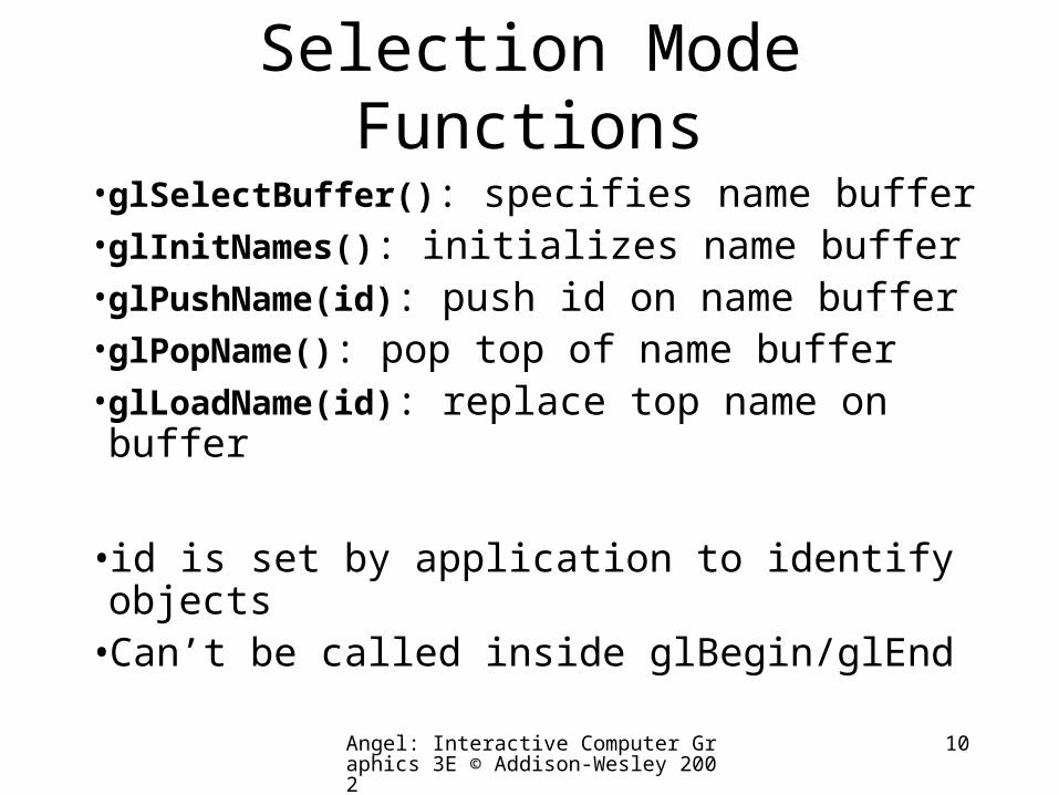
Selection Mode Functions

•glSelectBuffer(): specifies name buffer•glInitNames(): initializes name buffer•glPushName(id): push id on name buffer•glPopName(): pop top of name buffer•glLoadName(id): replace top name on buffer

• id is set by application to identify objects•Can’t be called inside glBegin/glEnd


11

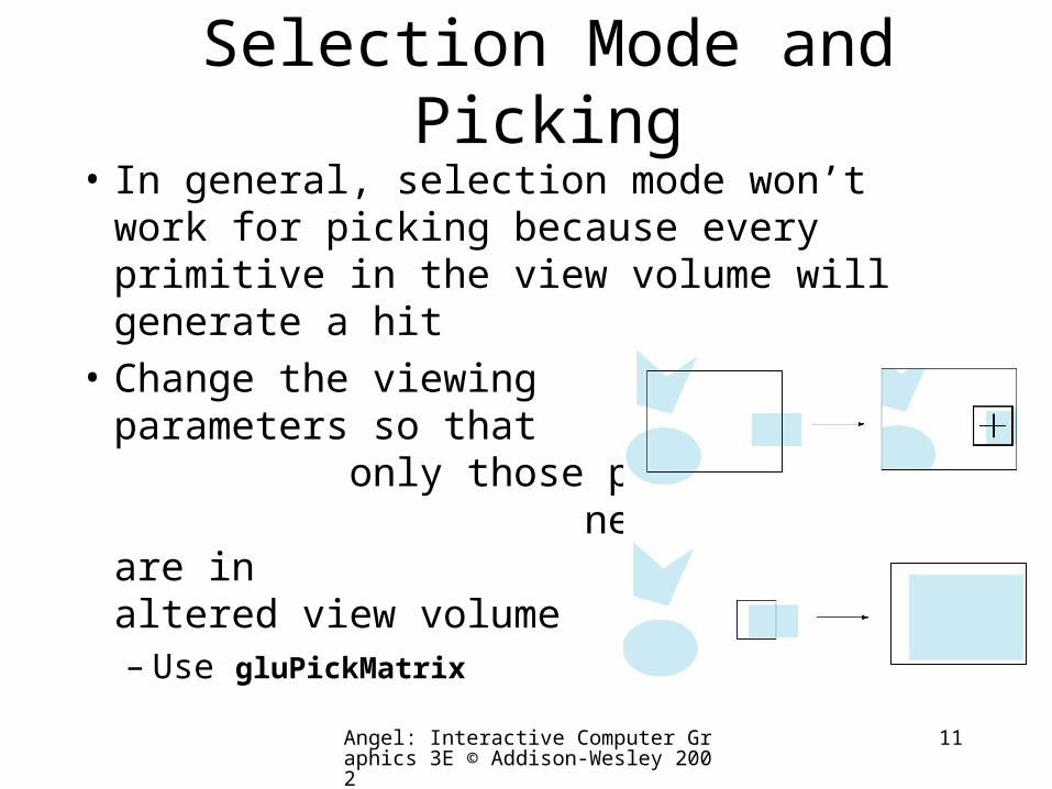
Selection Mode and Picking

• In general, selection mode won’t work for picking because every primitive in the view volume will generate a hit

• Change the viewing parameters so that only those primitives near the cursor are in the altered view volume– Use gluPickMatrix


12

gluPickMatrix()

• gluPickMatrix(Gldouble x, Gldouble y, Gldouble w, Gldouble h, Glint *vp)

– k

– Creates a projection matrix for picking that restricts drawing to a w x h area centered at (x,y) in the window coordinates within the viewport vp

Go to pick.c

Introduction to Curves


15

Escaping Flatland• Until now we have worked with flat entities

such as lines and flat polygons– Fit well with graphics hardware– Mathematically simple

• But the world is not composed of flat entities– Need curves and curved surfaces– May only have need at the application level– Implementation can render them

approximately with flat primitives


16

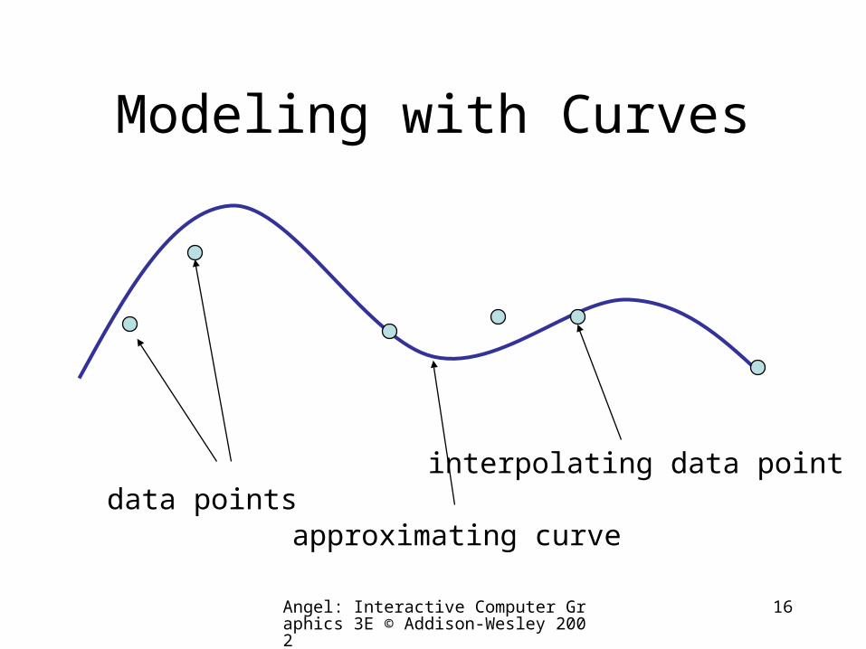
Modeling with Curves

data pointsapproximating curve

interpolating data point


17

What Makes a Good Representation?

• There are many ways to represent curves and surfaces

• Want a representation that is– Stable– Smooth– Easy to evaluate– Must we interpolate or can we just come close to

data?– Do we need derivatives?


18

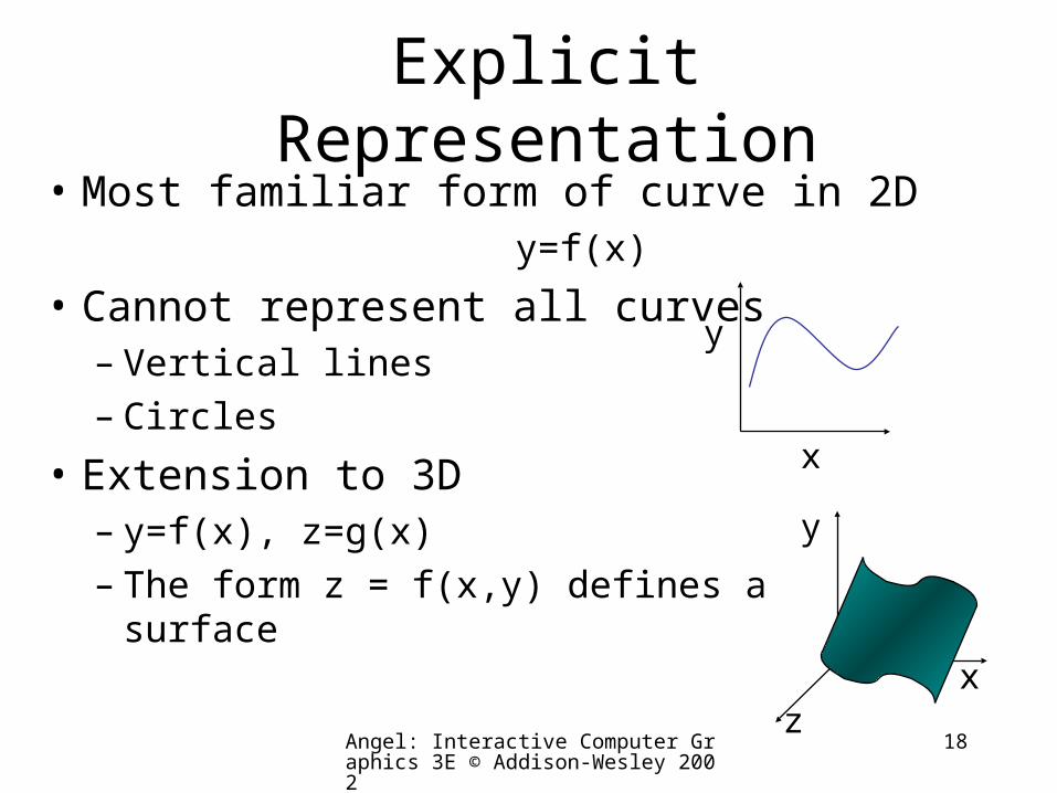
Explicit Representation• Most familiar form of curve in 2D

y=f(x)

• Cannot represent all curves– Vertical lines– Circles

• Extension to 3D – y=f(x), z=g(x)

– The form z = f(x,y) defines a surface

x

y

x

y

z


19

Implicit Representation

• Two dimensional curve(s)

g(x,y)=0

• Much more robust– All lines ax+by+c=0

– Circles x2+y2-r2=0

• Three dimensions g(x,y,z)=0 defines a surface– Intersect two surface to get a curve

• In general, we cannot solve for points that satisfy the equation


20

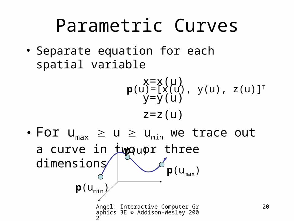
Parametric Curves• Separate equation for each spatial variable

x=x(u)

y=y(u)

z=z(u)

• For umax u umin we trace out a curve in two

or three dimensions

p(u)=[x(u), y(u), z(u)]T

p(u)

p(umin)

p(umax)


21

Selecting Functions

• Usually we can select “good” functions – not unique for a given spatial curve– Approximate or interpolate known data– Want functions which are easy to evaluate– Want functions which are easy to differentiate

• Computation of normals• Connecting pieces (segments)

– Want functions which are smooth


22

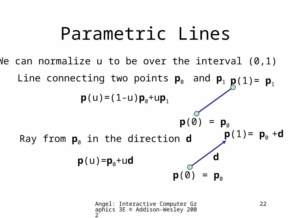
Parametric Lines

Line connecting two points p0 and p1

p(u)=(1-u)p0+up1

We can normalize u to be over the interval (0,1)

p(0) = p0

p(1)= p1

Ray from p0 in the direction d

p(u)=p0+ud

p(0) = p0

p(1)= p0 +d

d


23

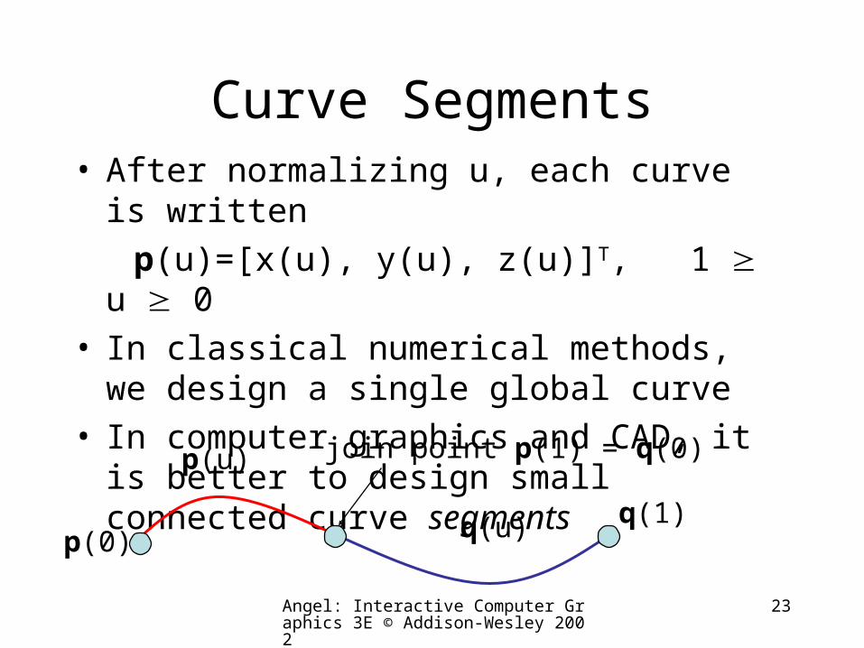
Curve Segments• After normalizing u, each curve is written

p(u)=[x(u), y(u), z(u)]T, 1 u 0• In classical numerical methods, we design a

single global curve• In computer graphics and CAD, it is better to

design small connected curve segments

p(u)

q(u)p(0)q(1)

join point p(1) = q(0)


24

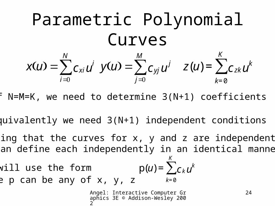
Parametric Polynomial Curves

ucux iN

ixi∑

=

=0

)( ucuy jM

jyj∑

=

=0

)(

€

z(u) = zkck= 0

K

∑ ku

•If N=M=K, we need to determine 3(N+1) coefficients

•Equivalently we need 3(N+1) independent conditions

•Noting that the curves for x, y and z are independent,we can define each independently in an identical manner

•We will use the form where p can be any of x, y, z

€

p(u) = kck= 0

K

∑ ku


25

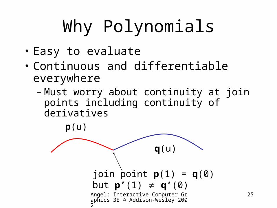
Why Polynomials• Easy to evaluate• Continuous and differentiable

everywhere– Must worry about continuity at join points

including continuity of derivatives

p(u)

q(u)

join point p(1) = q(0)but p’(1) q’(0)


26

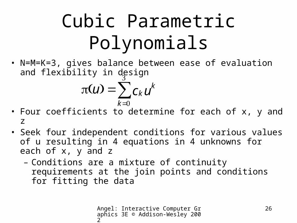
Cubic Parametric Polynomials

• N=M=K=3, gives balance between ease of evaluation and flexibility in design

• Four coefficients to determine for each of x, y and z• Seek four independent conditions for various values of u

resulting in 4 equations in 4 unknowns for each of x, y and z– Conditions are a mixture of continuity requirements at

the join points and conditions for fitting the data

ucu k

kk∑

=

=3

0

)(p

Designing Parametric Cubic Curves


28

Objectives

• Introduce the types of curves– Interpolating– Hermite– Bezier– B-spline

• Analyze their performance


29

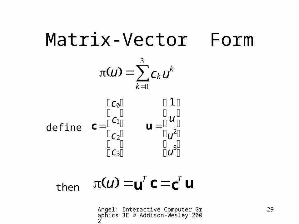
Matrix-Vector Form

ucu k

kk∑

=

=3

0

)(p

⎥⎥⎥⎥

⎦

⎤

⎢⎢⎢⎢

⎣

⎡

=

c

c

c

c

3

2

1

0

c

⎥⎥⎥⎥

⎦

⎤

⎢⎢⎢⎢

⎣

⎡

=

u

u

u

3

2

1

udefine

uccu TTu ==)(pthen


30

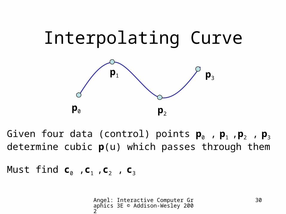
Interpolating Curve

p0

p1

p2

p3

Given four data (control) points p0 , p1 ,p2 , p3

determine cubic p(u) which passes through them

Must find c0 ,c1 ,c2 , c3


31

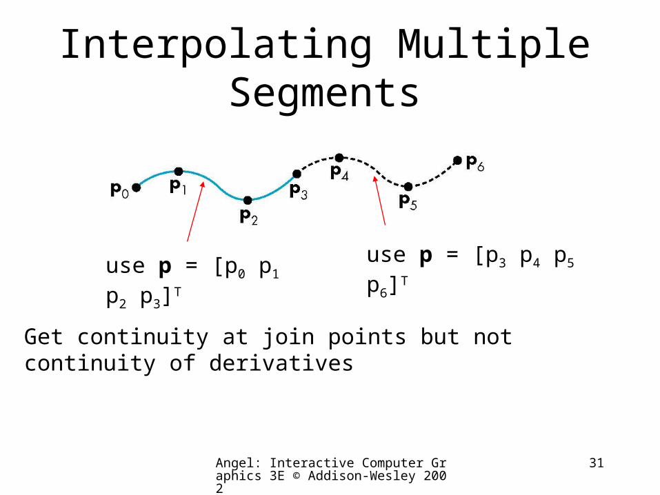
Interpolating Multiple Segments

use p = [p0 p1 p2 p3]T use p = [p3 p4 p5 p6]T

Get continuity at join points but notcontinuity of derivatives


32

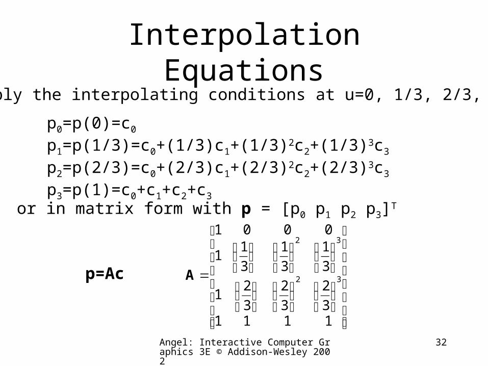
Interpolation Equationsapply the interpolating conditions at u=0, 1/3, 2/3, 1

p0=p(0)=c0

p1=p(1/3)=c0+(1/3)c1+(1/3)2c2+(1/3)3c3

p2=p(2/3)=c0+(2/3)c1+(2/3)2c2+(2/3)3c3

p3=p(1)=c0+c1+c2+c3

or in matrix form with p = [p0 p1 p2 p3]T

p=Ac

⎥⎥⎥⎥⎥⎥⎥

⎦

⎤

⎢⎢⎢⎢⎢⎢⎢

⎣

⎡

⎟⎠

⎞⎜⎝

⎛⎟⎠

⎞⎜⎝

⎛⎟⎠

⎞⎜⎝

⎛

⎟⎠

⎞⎜⎝

⎛⎟⎠

⎞⎜⎝

⎛⎟⎠

⎞⎜⎝

⎛

=

11113

2

3

2

3

21

3

1

3

1

3

11

0001

32

32

A


33

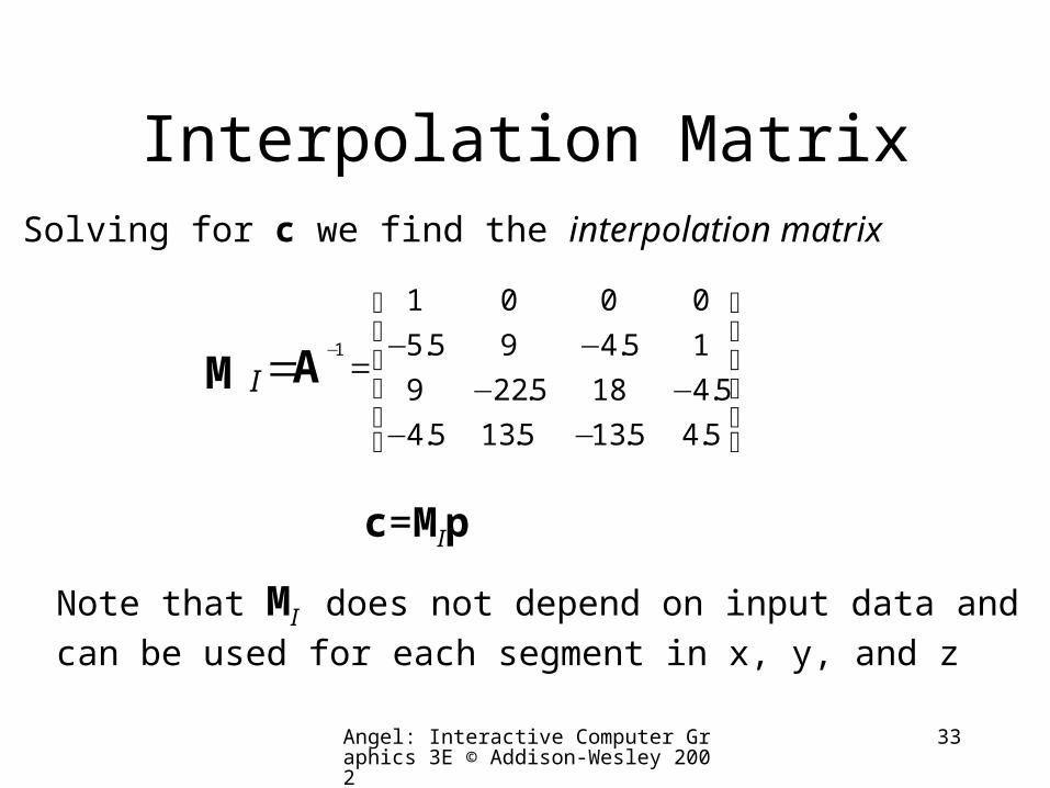
Interpolation MatrixSolving for c we find the interpolation matrix

⎥⎥⎥⎥

⎦

⎤

⎢⎢⎢⎢

⎣

⎡

−−−−

−−== −

5.45.135.135.4

5.4185.229

15.495.5

0001

1

AM I

c=MIp

Note that MI does not depend on input data and

can be used for each segment in x, y, and z


34

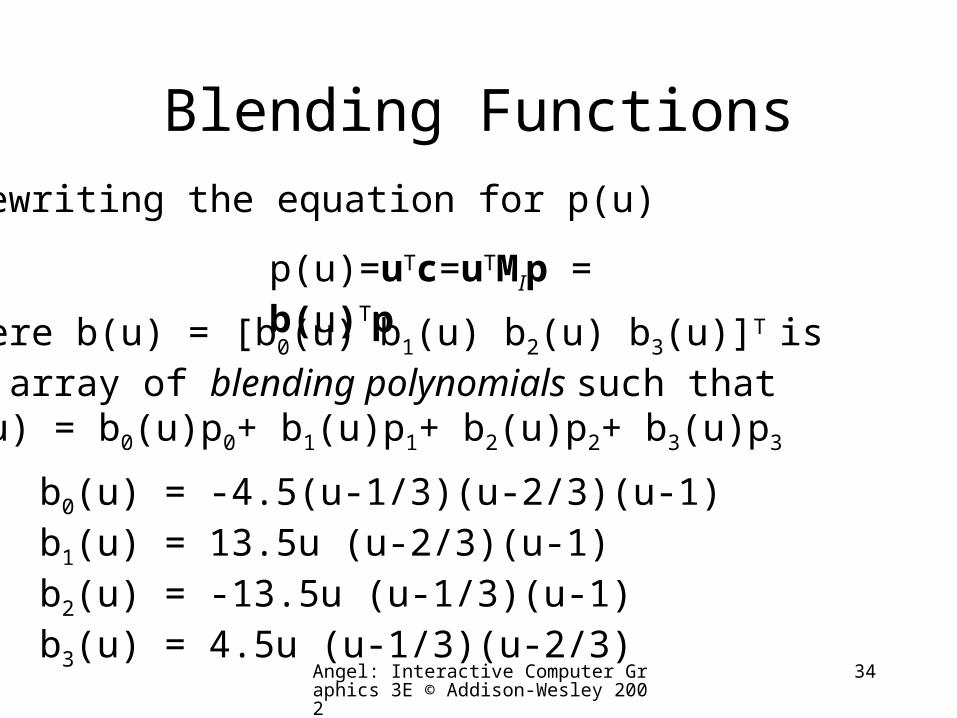
Blending FunctionsRewriting the equation for p(u)

p(u)=uTc=uTMIp = b(u)Tp

where b(u) = [b0(u) b1(u) b2(u) b3(u)]T isan array of blending polynomials such thatp(u) = b0(u)p0+ b1(u)p1+ b2(u)p2+ b3(u)p3

b0(u) = -4.5(u-1/3)(u-2/3)(u-1)b1(u) = 13.5u (u-2/3)(u-1)b2(u) = -13.5u (u-1/3)(u-1)b3(u) = 4.5u (u-1/3)(u-2/3)


35

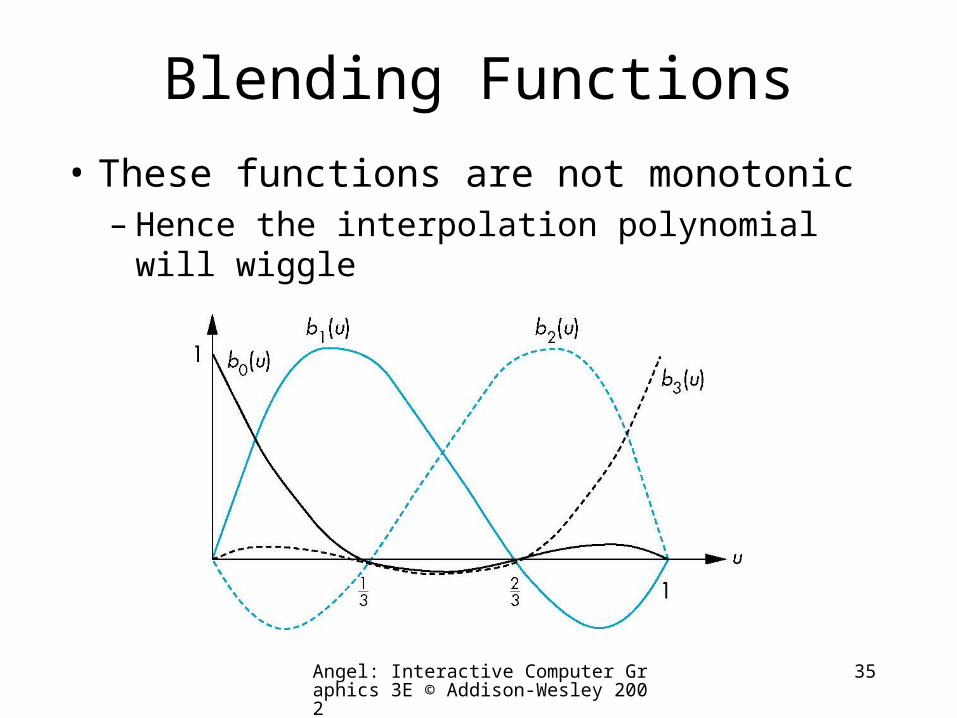
Blending Functions

• These functions are not monotonic– Hence the interpolation polynomial will wiggle


36

Other Types of Curves and Surfaces

• How can we get around the limitations of the interpolating form– Lack of smoothness– Discontinuous derivatives at join points

• We have four conditions (for cubics) that we can apply to each segment– Use them other than for interpolation– Need only come close to the data


37

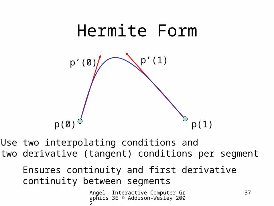
Hermite Form

p(0) p(1)

p’(0) p’(1)

Use two interpolating conditions andtwo derivative (tangent) conditions per segment

Ensures continuity and first derivativecontinuity between segments


38

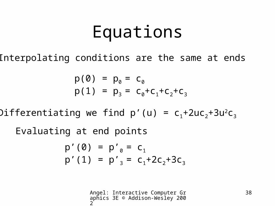
EquationsInterpolating conditions are the same at ends

p(0) = p0 = c0

p(1) = p3 = c0+c1+c2+c3

Differentiating we find p’(u) = c1+2uc2+3u2c3

Evaluating at end points

p’(0) = p’0 = c1

p’(1) = p’3 = c1+2c2+3c3


39

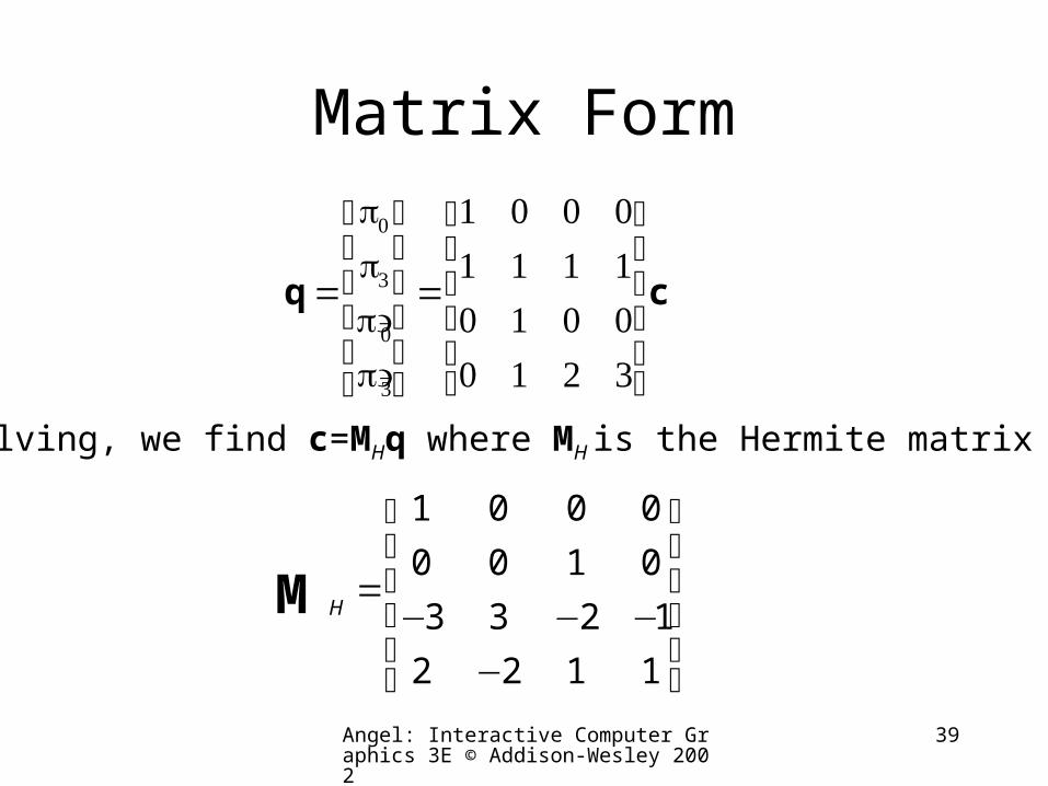
Matrix Form

cq

⎥⎥⎥⎥

⎦

⎤

⎢⎢⎢⎢

⎣

⎡

=

⎥⎥⎥⎥

⎦

⎤

⎢⎢⎢⎢

⎣

⎡

=

3210001011110001

p'

p'

p

p

3

0

3

0

Solving, we find c=MHq where MH is the Hermite matrix

⎥⎥⎥⎥

⎦

⎤

⎢⎢⎢⎢

⎣

⎡

−−−−

=

1122

1233

0100

0001

MH


40

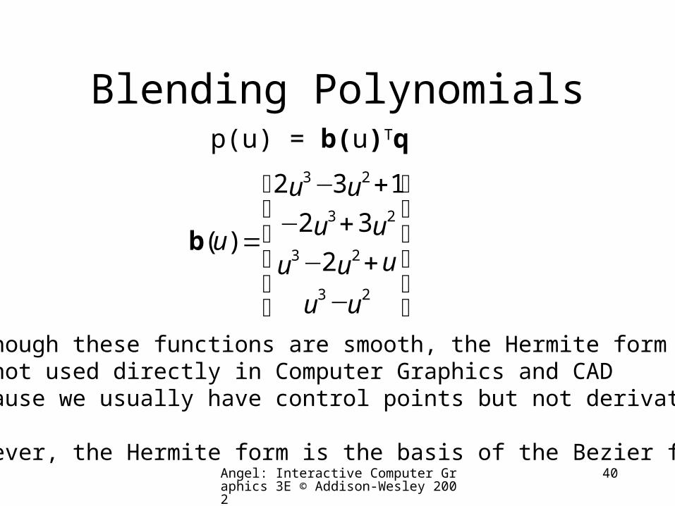
Blending Polynomialsp(u) = b(u)Tq

⎥⎥⎥⎥

⎦

⎤

⎢⎢⎢⎢

⎣

⎡

−+−

+−+−

=

uu

uuu

uu

uu

u

23

23

23

23

2

32

132

)(b

Although these functions are smooth, the Hermite formis not used directly in Computer Graphics and CAD because we usually have control points but not derivatives

However, the Hermite form is the basis of the Bezier form


41

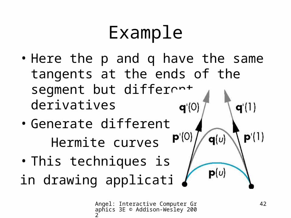
Parametric and Geometric Continuity

• We can require the derivatives of x, y,and z to each be continuous at join points (parametric continuity)

• Alternately, we can only require that the tangents of the resulting curve be continuous (geometry continuity)

• The latter gives more flexibility as we have need satisfy only two conditions rather than three at each join point


42

Example• Here the p and q have the same

tangents at the ends of the segment but different derivatives

• Generate different

Hermite curves

• This techniques is used

in drawing applications

Bezier and Spline Curves


44

Objectives

• Introduce the Bezier curves

• Derive the required matrices

• Introduce the B-spline and compare it to the standard cubic Bezier


45

Bezier’s Idea

• In graphics and CAD, we do not usually have derivative data

• Bezier suggested using the same 4 data points as with the cubic interpolating curve to approximate the derivatives in the Hermite form


46

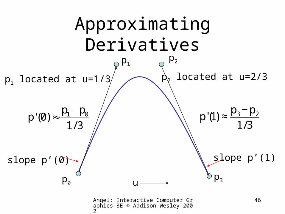
Approximating Derivatives

p0

p1p2

p3

p1 located at u=1/3 p2 located at u=2/3

3/1

pp)0('p 01−≈

€

p'(1) ≈ 3p − 2p

1/3

slope p’(0) slope p’(1)

u


47

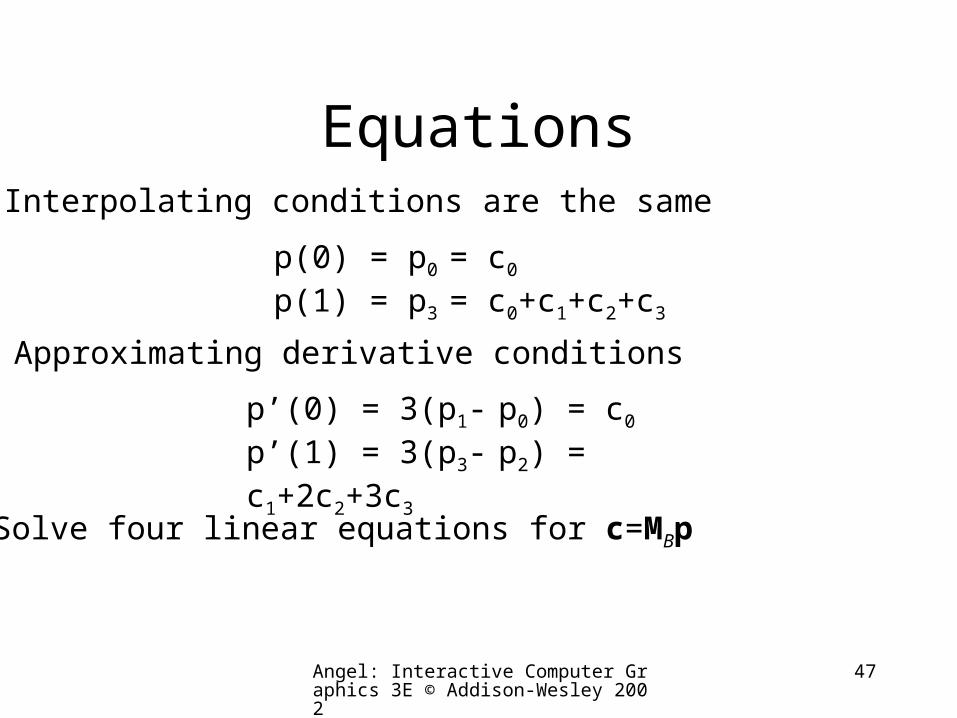
Equations

p(0) = p0 = c0

p(1) = p3 = c0+c1+c2+c3

p’(0) = 3(p1- p0) = c0

p’(1) = 3(p3- p2) = c1+2c2+3c3

Interpolating conditions are the same

Approximating derivative conditions

Solve four linear equations for c=MBp


48

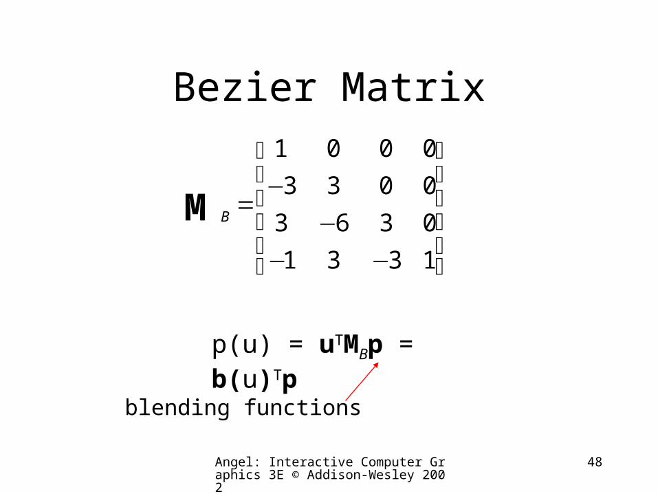
Bezier Matrix

⎥⎥⎥⎥

⎦

⎤

⎢⎢⎢⎢

⎣

⎡

−−−

−=

1331

0363

0033

0001

MB

p(u) = uTMBp = b(u)Tp

blending functions


49

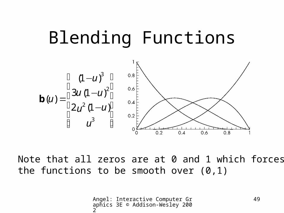
Blending Functions

⎥⎥⎥⎥⎥

⎦

⎤

⎢⎢⎢⎢⎢

⎣

⎡

−−

−

=

u

uu

uu

u

u

3

2

2

3

)1(2

)1(3

)1(

)(b

Note that all zeros are at 0 and 1 which forcesthe functions to be smooth over (0,1)


50

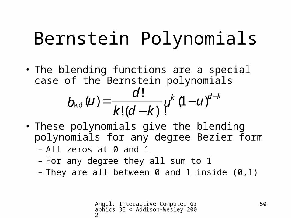
Bernstein Polynomials

• The blending functions are a special case of the Bernstein polynomials

• These polynomials give the blending polynomials for any degree Bezier form– All zeros at 0 and 1– For any degree they all sum to 1– They are all between 0 and 1 inside (0,1)

)1()!(!

!)(kd uu

kdk

dub

kdk −−

= −


51

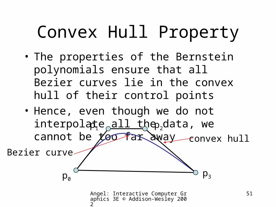
Convex Hull Property• The properties of the Bernstein polynomials

ensure that all Bezier curves lie in the convex hull of their control points

• Hence, even though we do not interpolate all the data, we cannot be too far away

p0

p1 p2

p3

convex hull

Bezier curve


52

Analysis• Although the Bezier form is much better than

the interpolating form, we have the derivatives are not continuous at join points

• Can we do better?– Go to higher order Bezier

• More work• Derivative continuity still only approximate• Supported by OpenGL

– Apply different conditions • Tricky without letting order increase


53

B-Splines

• Basis splines: use the data at p=[pi-2 pi-1 pi pi-1]T to define curve only between pi-1 and pi

• Allows us to apply more continuity conditions to each segment

• For cubics, we can have continuity of function, first and second derivatives at join points

• Cost is 3 times as much work for curves– Add one new point each time rather than three

• For surfaces, we do 9 times as much work


54

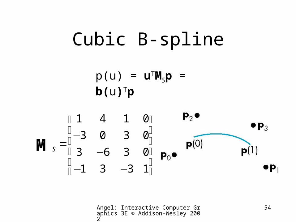
Cubic B-spline

⎥⎥⎥⎥

⎦

⎤

⎢⎢⎢⎢

⎣

⎡

−−−

−=

1331

0363

0303

0141

MS

p(u) = uTMSp = b(u)Tp


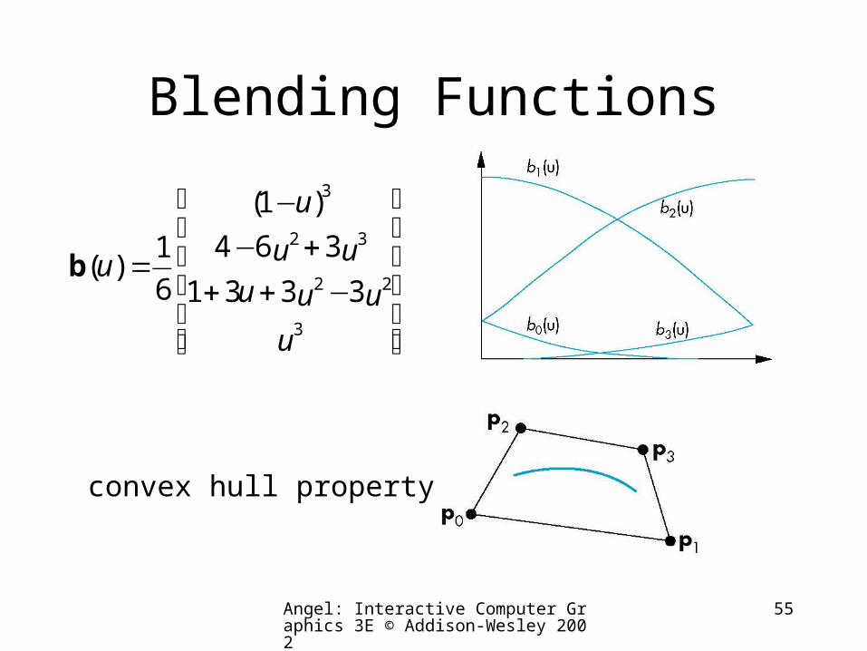
55

Blending Functions

⎥⎥⎥⎥⎥

⎦

⎤

⎢⎢⎢⎢⎢

⎣

⎡

−+++−

−

=

u

uuuuu

u

u

3

22

32

3

3331

364

)1(

6

1)(b

convex hull property


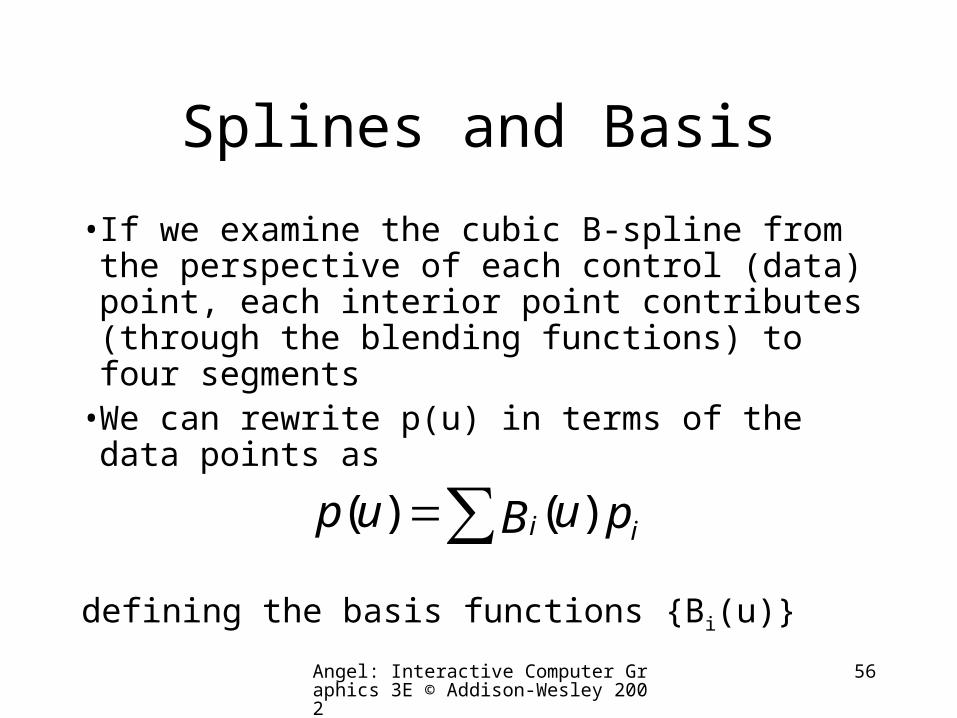
56

Splines and Basis

• If we examine the cubic B-spline from the perspective of each control (data) point, each interior point contributes (through the blending functions) to four segments

• We can rewrite p(u) in terms of the data points as

defining the basis functions {Bi(u)}

puBup ii )()( ∑=


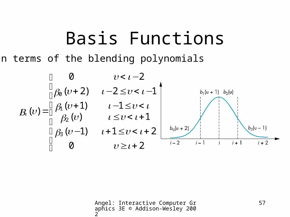
57

Basis Functions

2

21

11

12

2

0

)1(

)()1(

)2(

0

)(

3

2

1

0

+≥+<≤+

+<≤<≤−−<≤−

−<

⎪⎪⎪

⎩

⎪⎪⎪

⎨

⎧

−

++

=

iuiuiiuiiuiiui

iu

ub

ubub

ub

uBi

In terms of the blending polynomials


58

Generalizing Splines

• We can extend to splines of any degree • Data and conditions to not have to given at

equally spaced values (the knots)– Nonuniform and uniform splines– Can have repeated knots

• Can force spline to interpolate points

• Cox-deBoor recursion gives method of evaluation


59

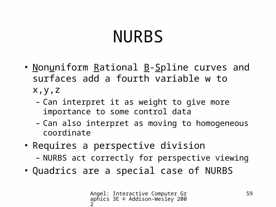
NURBS

• Nonuniform Rational B-Spline curves and surfaces add a fourth variable w to x,y,z– Can interpret it as weight to give more importance

to some control data– Can also interpret as moving to homogeneous

coordinate

• Requires a perspective division– NURBS act correctly for perspective viewing

• Quadrics are a special case of NURBS


60

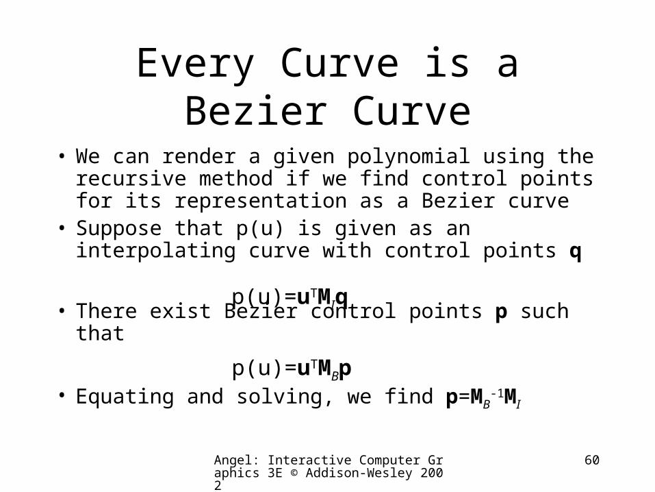
Every Curve is a Bezier Curve

• We can render a given polynomial using the recursive method if we find control points for its representation as a Bezier curve

• Suppose that p(u) is given as an interpolating curve with control points q

• There exist Bezier control points p such that

• Equating and solving, we find p=MB-1MI

p(u)=uTMIq

p(u)=uTMBp


61

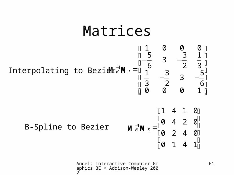
Matrices

Interpolating to Bezier

B-Spline to Bezier

⎥⎥⎥⎥⎥⎥

⎦

⎤

⎢⎢⎢⎢⎢⎢

⎣

⎡

−−

−−=−

10006

53

2

3

3

13

1

2

33

6

50001

1MM IB

⎥⎥⎥⎥

⎦

⎤

⎢⎢⎢⎢

⎣

⎡

=−

1410

0420

0240

0141

1MM SB


62

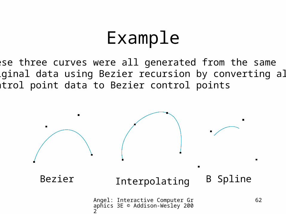
ExampleThese three curves were all generated from the sameoriginal data using Bezier recursion by converting allcontrol point data to Bezier control points

Bezier Interpolating B Spline

Drawing Bezier Curves in OpenGL


64

Basic Procedure

• Enable an evaluator (glEnable)– For vertices, normals and colors

• Define Bezier parameters (glMap1f)

• Evaluate Bezier curve (glEvalCoord1f, or glMapGrid1f and glEvalMesh1)


65

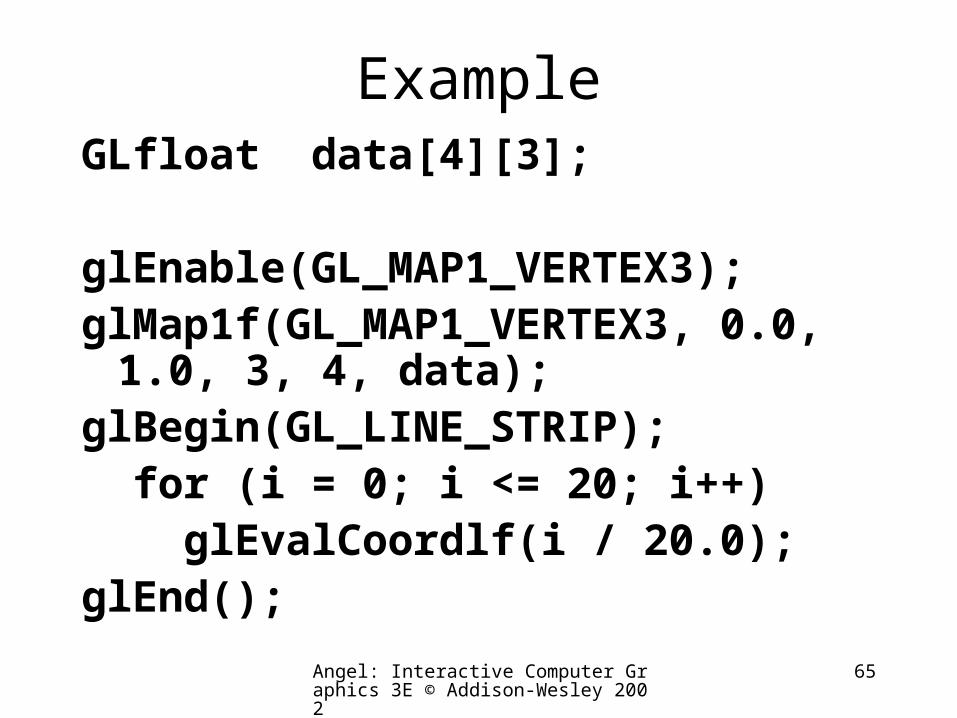
ExampleGLfloat data[4][3];

glEnable(GL_MAP1_VERTEX3);glMap1f(GL_MAP1_VERTEX3, 0.0, 1.0, 3, 4, data);

glBegin(GL_LINE_STRIP); for (i = 0; i <= 20; i++) glEvalCoordlf(i / 20.0);glEnd();


66

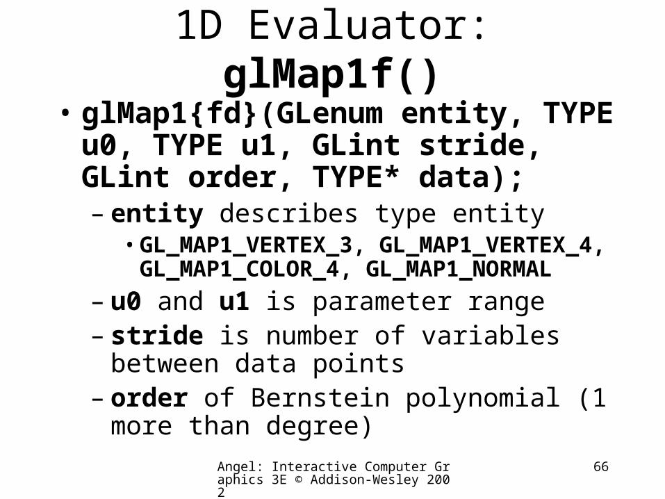
1D Evaluator: glMap1f()• glMap1{fd}(GLenum entity, TYPE u0, TYPE u1, GLint stride, GLint order, TYPE* data);– entity describes type entity

•GL_MAP1_VERTEX_3, GL_MAP1_VERTEX_4, GL_MAP1_COLOR_4, GL_MAP1_NORMAL

– u0 and u1 is parameter range– stride is number of variables between

data points– order of Bernstein polynomial (1 more than

degree)


67

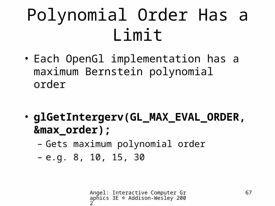
Polynomial Order Has a Limit

• Each OpenGl implementation has a maximum Bernstein polynomial order

• glGetIntergerv(GL_MAX_EVAL_ORDER, &max_order);– Gets maximum polynomial order – e.g. 8, 10, 15, 30


68

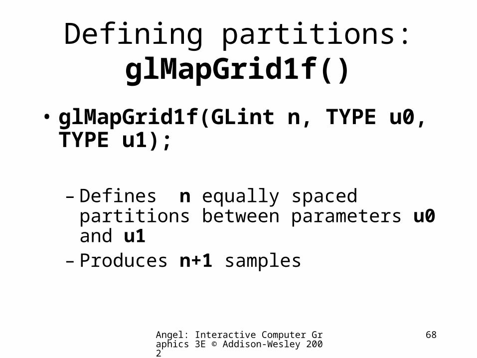
Defining partitions: glMapGrid1f()

• glMapGrid1f(GLint n, TYPE u0, TYPE u1);

– Defines n equally spaced partitions between parameters u0 and u1

– Produces n+1 samples


69

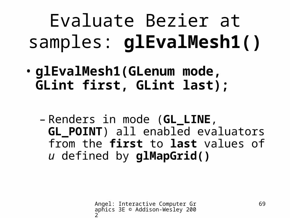
Evaluate Bezier at samples: glEvalMesh1()

• glEvalMesh1(GLenum mode, GLint first, GLint last);

– Renders in mode (GL_LINE, GL_POINT) all enabled evaluators from the first to last values of u defined by glMapGrid()


70

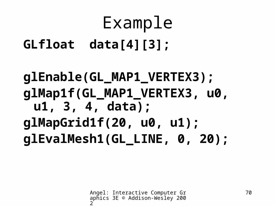
ExampleGLfloat data[4][3];

glEnable(GL_MAP1_VERTEX3);glMap1f(GL_MAP1_VERTEX3, u0, u1, 3, 4, data);

glMapGrid1f(20, u0, u1);glEvalMesh1(GL_LINE, 0, 20);

Go to bezier.c

Documents

Picking and Curves Week 6 David Breen Department of Computer Science Drexel University Based on material from Ed Angel, University of New Mexico CS 480/680