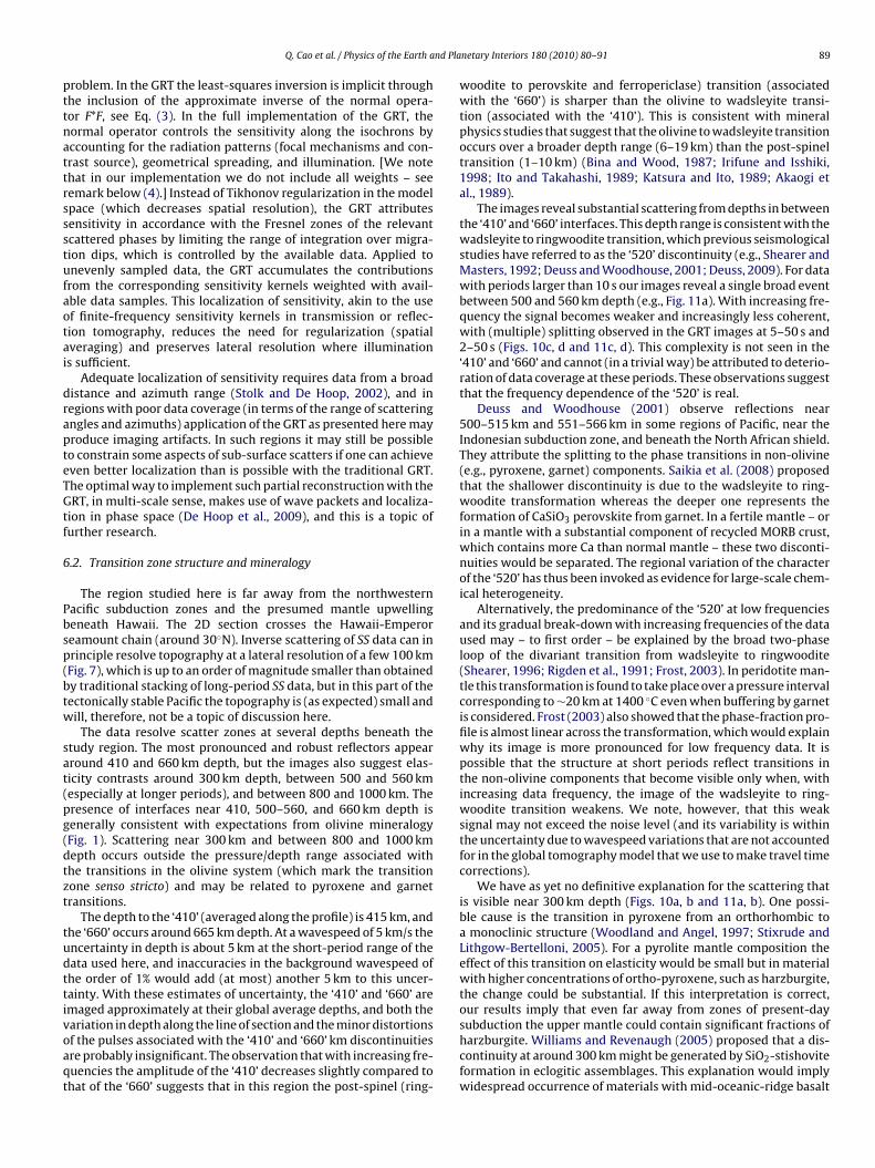
Physics of the Earth and Planetary Interiors 180 (2010) 80–91

Contents lists available at ScienceDirect

Physics of the Earth and Planetary Interiors

journa l homepage: www.e lsev ier .com/ locate /pepi

Imaging the upper mantle transition zone with a generalized Radon transform ofSS precursors

Q. Caoa,∗, P. Wanga, R.D. van der Hilsta, M.V. de Hoopb, S.-H. Shima

a Earth, Atmospheric, and Planetary Sciences, Massachusetts Inst. of Technology, Cambridge, MA 02139, USAb Center for Computational and Applied Mathematics, Purdue University, West Lafayette, IN 47907, USA

a r t i c l e i n f o

Article history:Received 2 February 2009Received in revised form 9 February 2010Accepted 9 February 2010

Edited by: G. Helffrich.

Keywords:Transition zoneUpper mantle discontinuitiesInverse scatteringGeneralized Radon transformSS precursors

a b s t r a c t

We demonstrate the feasibility of using inverse scattering for high-resolution imaging of discontinuitiesin the upper mantle beneath oceanic regions (far from sources and receivers) using broadband wave-field observations consisting of SS and its precursors. The generalized Radon transform (GRT) that wedeveloped for this purpose detects (in the broadband data) signals due to scattering from elasticity con-trasts in Earth’s mantle. Synthetic tests with realistic source–receiver distributions demonstrate that theGRT is able to detect and image deep mantle interfaces, even in the presence of noise, depth phases(‘ghosts’), phase conversions, and multiples generated by reverberation within the transition zone. Asa proof of concept, we apply the GRT to ∼50,000 broadband seismograms to delineate interfaces in thedepth range from 300 to 1000 km beneath the northwest Pacific. We account for smooth 3D mantle het-erogeneity using first-order perturbation theory and independently obtained global tomography models.The preliminary results reveal laterally continuous (but undulating) scatter zones near 410 and 660 kmdepth and a weaker, broader, and more complex structure near 520 km depth. The images also suggestthe presence of multiple, laterally intermittent interfaces near 350 km and between 800 and 1000 kmdepth, that is, above and below the transition zone sensu stricto. Filtering of the data (we consider four

pass-bands: 20–50 s, 10–50 s, 5–50 s, and 2–50 s) reveals a prominent frequency dependence of the mag-nitude, width, and complexity of the interfaces, in particular of the scatter zone near 520 km depth; suchdependencies may put important constraints on the mineralogy and phase chemistry of the transition

1

drtWmeboglHa

AM

0d

zone.

. Introduction

The upper mantle transition zone, here taken broadly as theepth interval between 300 and 1000 km depth, is marked by rapidadial changes in elasticity and mass density associated with phaseransformations in mantle silicates (Fig. 1) (e.g., Ringwood, 1975;

eidner and Wang, 2000; Li and Liebermann, 2007). With seis-ic imaging one can estimate the depth to and the change in

lasticity and mass density across such phase boundaries. Com-ined with mineral physics data this information puts constraintsn local temperature, composition, and mineral phase, and the

eographic variation of these parameters provides insight intoarge-scale geodynamical processes (Jeanloz and Thompson, 1983;elffrich, 2000; Shearer, 2000; Weidner and Wang, 2000; Schmerrnd Garnero, 2006; Li and Liebermann, 2007).

∗ Corresponding author at: Massachusetts Inst. of Technology, Earth,tmospheric, and Planetary Sciences, 54-517A, 77 Mass. Ave. M.I.T., Cambridge,A 02139, USA.

E-mail address: qinc@mit.edu (Q. Cao).

031-9201/$ – see front matter © 2010 Elsevier B.V. All rights reserved.oi:10.1016/j.pepi.2010.02.006

© 2010 Elsevier B.V. All rights reserved.

Using a variety of top- and underside reflections and phase-converted waves, a number of seismic investigations have observedthe global existence of what are usually referred to as ‘410’ and ‘660’discontinuities (e.g., Shearer and Masters, 1992; Shearer, 1993;Gossler and Kind, 1996; Flanagan and Shearer, 1998a,b; Gu etal., 1998; Flanagan and Shearer, 1999; Gu and Dziewonski, 2002;Lebedev et al., 2002, 2003; Chambers et al., 2005a,b; Deuss etal., 2006; Schmerr and Garnero, 2006; An et al., 2007; Rost andThomas, 2009), and a ‘520’ discontinuity has been reported insome regions (e.g., Shearer, 1990; Deuss and Woodhouse, 2001).Many aspects of these discontinuities can be explained by phasetransitions in the olivine system (olivine to wadsleyite, wadsleyiteto ringwoodite, and ringwoodite to perovskite and ferropericlase,respectively) (Ringwood, 1969, 1975, 1991; Katsura and Ito, 1989;Bina and Helffrich, 1994; Shim et al., 2001; Lebedev et al., 2002,2003; Fei et al., 2004; Weidner and Wang, 2000; Weidner et

al., 2005; Li and Liebermann, 2007), but not all seismic obser-vations are consistent with transformations in a simple, isolatedMgO–FeO–SiO2 system. For example, despite the opposite signs oftheir Clapeyron slopes, on a global scale the ‘410’ and ‘660’ topogra-phies are not convincingly anti-correlated (Gu et al., 1998, 2003;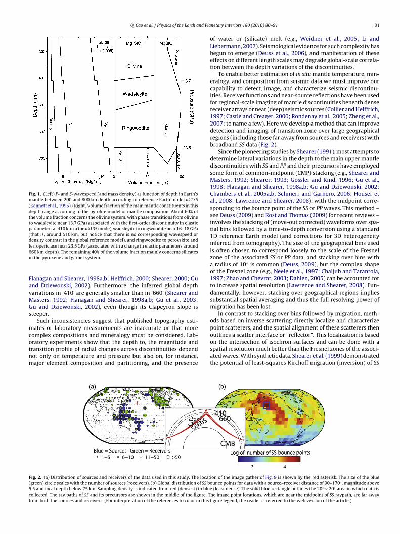

Q. Cao et al. / Physics of the Earth and Pla

Fig. 1. (Left) P- and S-wavespeed (and mass density) as function of depth in Earth’smantle between 200 and 800 km depth according to reference Earth model ak135(Kennett et al., 1995). (Right) Volume fraction of the main mantle constituents in thisdepth range according to the pyrolite model of mantle composition. About 60% ofthe volume fraction concerns the olivine system, with phase transitions from olivineto wadsleyite near 13.7 GPa (associated with the first-order discontinuity in elasticparameters at 410 km in the ak135 mode), wadsleyite to ringwoodite near 16–18 GPa(that is, around 510 km, but notice that there is no corresponding wavespeed ordensity contrast in the global reference model), and ringwoodite to perovskite andf6i

FavMGs

mcotnm

outlines a scatter interface or “reflector”. This localization is based

F(5cf

erropericlase near 23.5 GPa (associated with a change in elastic parameters around60 km depth). The remaining 40% of the volume fraction mainly concerns silicates

n the pyroxene and garnet system.

lanagan and Shearer, 1998a,b; Helffrich, 2000; Shearer, 2000; Gund Dziewonski, 2002). Furthermore, the inferred global depthariations in ‘410’ are generally smaller than in ‘660’ (Shearer andasters, 1992; Flanagan and Shearer, 1998a,b; Gu et al., 2003;u and Dziewonski, 2002), even though its Clapeyron slope isteeper.

Such inconsistencies suggest that published topography esti-ates or laboratory measurements are inaccurate or that more

omplex compositions and mineralogy must be considered. Lab-

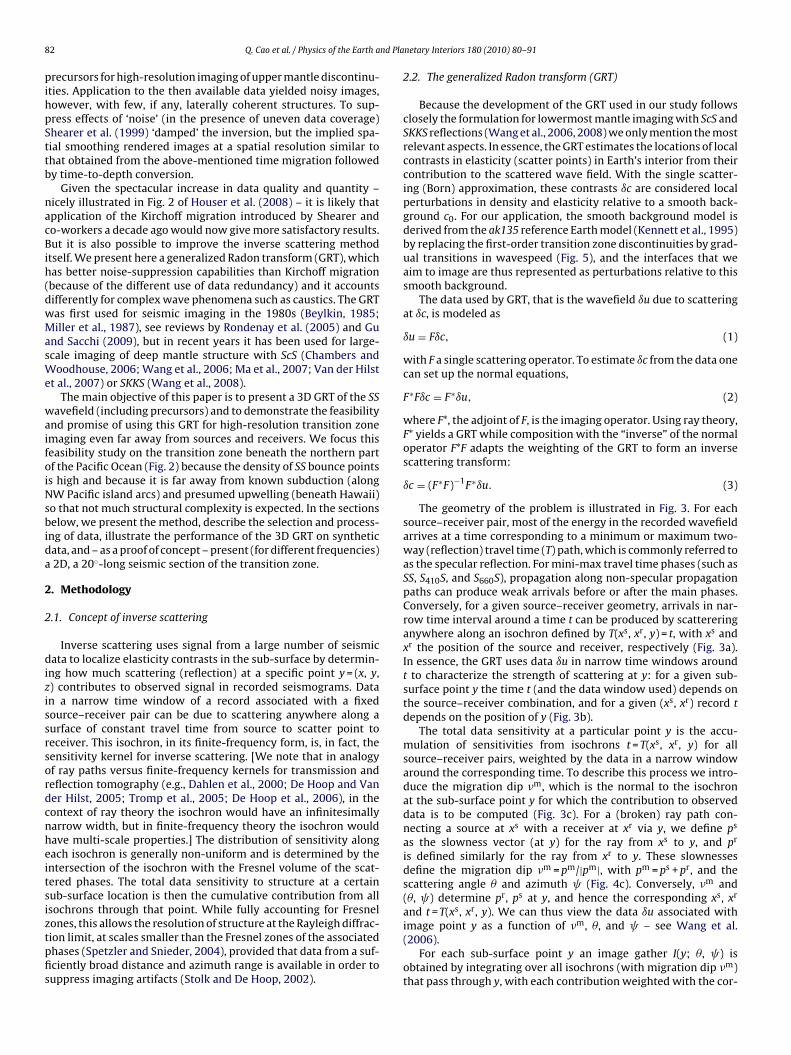
ratory experiments show that the depth to, the magnitude andransition profile of radial changes across discontinuities dependot only on temperature and pressure but also on, for instance,ajor element composition and partitioning, and the presence

ig. 2. (a) Distribution of sources and receivers of the data used in this study. The locatgreen) circle scales with the number of sources (receivers). (b) Global distribution of SS b.5 and focal depth below 75 km. Sampling density is indicated from red (densest) to bluollected. The ray paths of SS and its precursors are shown in the middle of the figure. Trom both the sources and receivers. (For interpretation of the references to color in this

netary Interiors 180 (2010) 80–91 81

of water or (silicate) melt (e.g., Weidner et al., 2005; Li andLiebermann, 2007). Seismological evidence for such complexity hasbegun to emerge (Deuss et al., 2006), and manifestation of theseeffects on different length scales may degrade global-scale correla-tion between the depth variations of the discontinuities.

To enable better estimation of in situ mantle temperature, min-eralogy, and composition from seismic data we must improve ourcapability to detect, image, and characterize seismic discontinu-ities. Receiver functions and near-source reflections have been usedfor regional-scale imaging of mantle discontinuities beneath densereceiver arrays or near (deep) seismic sources (Collier and Helffrich,1997; Castle and Creager, 2000; Rondenay et al., 2005; Zheng et al.,2007; to name a few). Here we develop a method that can improvedetection and imaging of transition zone over large geographicalregions (including those far away from sources and receivers) withbroadband SS data (Fig. 2).

Since the pioneering studies by Shearer (1991), most attempts todetermine lateral variations in the depth to the main upper mantlediscontinuities with SS and PP and their precursors have employedsome form of common-midpoint (CMP) stacking (e.g., Shearer andMasters, 1992; Shearer, 1993; Gossler and Kind, 1996; Gu et al.,1998; Flanagan and Shearer, 1998a,b; Gu and Dziewonski, 2002;Chambers et al., 2005a,b; Schmerr and Garnero, 2006; Houser etal., 2008; Lawrence and Shearer, 2008), with the midpoint corre-sponding to the bounce point of the SS or PP waves. This method –see Deuss (2009) and Rost and Thomas (2009) for recent reviews –involves the stacking of (move-out corrected) waveforms over spa-tial bins followed by a time-to-depth conversion using a standard1D reference Earth model (and corrections for 3D heterogeneityinferred from tomography). The size of the geographical bins usedis often chosen to correspond loosely to the scale of the Fresnelzone of the associated SS or PP data, and stacking over bins witha radius of 10◦ is common (Deuss, 2009), but the complex shapeof the Fresnel zone (e.g., Neele et al., 1997; Chaljub and Tarantola,1997; Zhao and Chevrot, 2003; Dahlen, 2005) can be accounted forto increase spatial resolution (Lawrence and Shearer, 2008). Fun-damentally, however, stacking over geographical regions impliessubstantial spatial averaging and thus the full resolving power ofmigration has been lost.

In contrast to stacking over bins followed by migration, meth-ods based on inverse scattering directly localize and characterizepoint scatterers, and the spatial alignment of these scatterers then

on the intersection of isochron surfaces and can be done with aspatial resolution much better than the Fresnel zones of the associ-ated waves. With synthetic data, Shearer et al. (1999) demonstratedthe potential of least-squares Kirchoff migration (inversion) of SS

ion of the image gather of Fig. 9 is shown by the red asterisk. The size of the blueounce points for data with a source–receiver distance of 90–170◦ , magnitude abovee (least dense). The solid blue rectangle outlines the 20◦ × 20◦ area in which data ishe image point locations, which are near the midpoint of SS raypath, are far awayfigure legend, the reader is referred to the web version of the article.)

8 nd Pla

pihpSttb

nacBih(dwMasWe

waifoiNsbida

2

2

dizissrsordcnheitsiztpfis

2 Q. Cao et al. / Physics of the Earth a

recursors for high-resolution imaging of upper mantle discontinu-ties. Application to the then available data yielded noisy images,owever, with few, if any, laterally coherent structures. To sup-ress effects of ‘noise’ (in the presence of uneven data coverage)hearer et al. (1999) ‘damped’ the inversion, but the implied spa-ial smoothing rendered images at a spatial resolution similar tohat obtained from the above-mentioned time migration followedy time-to-depth conversion.

Given the spectacular increase in data quality and quantity –icely illustrated in Fig. 2 of Houser et al. (2008) – it is likely thatpplication of the Kirchoff migration introduced by Shearer ando-workers a decade ago would now give more satisfactory results.ut it is also possible to improve the inverse scattering method

tself. We present here a generalized Radon transform (GRT), whichas better noise-suppression capabilities than Kirchoff migrationbecause of the different use of data redundancy) and it accountsifferently for complex wave phenomena such as caustics. The GRTas first used for seismic imaging in the 1980s (Beylkin, 1985;iller et al., 1987), see reviews by Rondenay et al. (2005) and Gu

nd Sacchi (2009), but in recent years it has been used for large-cale imaging of deep mantle structure with ScS (Chambers and

oodhouse, 2006; Wang et al., 2006; Ma et al., 2007; Van der Hilstt al., 2007) or SKKS (Wang et al., 2008).

The main objective of this paper is to present a 3D GRT of the SSavefield (including precursors) and to demonstrate the feasibility

nd promise of using this GRT for high-resolution transition zonemaging even far away from sources and receivers. We focus thiseasibility study on the transition zone beneath the northern partf the Pacific Ocean (Fig. 2) because the density of SS bounce pointss high and because it is far away from known subduction (alongW Pacific island arcs) and presumed upwelling (beneath Hawaii)

o that not much structural complexity is expected. In the sectionselow, we present the method, describe the selection and process-

ng of data, illustrate the performance of the 3D GRT on syntheticata, and – as a proof of concept – present (for different frequencies)2D, a 20◦-long seismic section of the transition zone.

. Methodology

.1. Concept of inverse scattering

Inverse scattering uses signal from a large number of seismicata to localize elasticity contrasts in the sub-surface by determin-

ng how much scattering (reflection) at a specific point y = (x, y,) contributes to observed signal in recorded seismograms. Datan a narrow time window of a record associated with a fixedource–receiver pair can be due to scattering anywhere along aurface of constant travel time from source to scatter point toeceiver. This isochron, in its finite-frequency form, is, in fact, theensitivity kernel for inverse scattering. [We note that in analogyf ray paths versus finite-frequency kernels for transmission andeflection tomography (e.g., Dahlen et al., 2000; De Hoop and Vaner Hilst, 2005; Tromp et al., 2005; De Hoop et al., 2006), in theontext of ray theory the isochron would have an infinitesimallyarrow width, but in finite-frequency theory the isochron wouldave multi-scale properties.] The distribution of sensitivity alongach isochron is generally non-uniform and is determined by thentersection of the isochron with the Fresnel volume of the scat-ered phases. The total data sensitivity to structure at a certainub-surface location is then the cumulative contribution from allsochrons through that point. While fully accounting for Fresnel

ones, this allows the resolution of structure at the Rayleigh diffrac-ion limit, at scales smaller than the Fresnel zones of the associatedhases (Spetzler and Snieder, 2004), provided that data from a suf-ciently broad distance and azimuth range is available in order touppress imaging artifacts (Stolk and De Hoop, 2002).

netary Interiors 180 (2010) 80–91

2.2. The generalized Radon transform (GRT)

Because the development of the GRT used in our study followsclosely the formulation for lowermost mantle imaging with ScS andSKKS reflections (Wang et al., 2006, 2008) we only mention the mostrelevant aspects. In essence, the GRT estimates the locations of localcontrasts in elasticity (scatter points) in Earth’s interior from theircontribution to the scattered wave field. With the single scatter-ing (Born) approximation, these contrasts ıc are considered localperturbations in density and elasticity relative to a smooth back-ground c0. For our application, the smooth background model isderived from the ak135 reference Earth model (Kennett et al., 1995)by replacing the first-order transition zone discontinuities by grad-ual transitions in wavespeed (Fig. 5), and the interfaces that weaim to image are thus represented as perturbations relative to thissmooth background.

The data used by GRT, that is the wavefield ıu due to scatteringat ıc, is modeled as

ıu = Fıc, (1)

with F a single scattering operator. To estimate ıc from the data onecan set up the normal equations,

F∗Fıc = F∗ıu, (2)

where F*, the adjoint of F, is the imaging operator. Using ray theory,F* yields a GRT while composition with the “inverse” of the normaloperator F*F adapts the weighting of the GRT to form an inversescattering transform:

ıc = (F∗F)−1F∗ıu. (3)

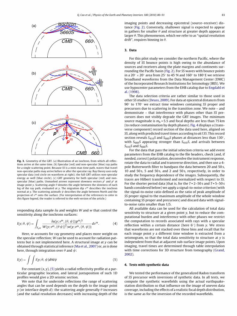
The geometry of the problem is illustrated in Fig. 3. For eachsource–receiver pair, most of the energy in the recorded wavefieldarrives at a time corresponding to a minimum or maximum two-way (reflection) travel time (T) path, which is commonly referred toas the specular reflection. For mini-max travel time phases (such asSS, S410S, and S660S), propagation along non-specular propagationpaths can produce weak arrivals before or after the main phases.Conversely, for a given source–receiver geometry, arrivals in nar-row time interval around a time t can be produced by scattereringanywhere along an isochron defined by T(xs, xr, y) = t, with xs andxr the position of the source and receiver, respectively (Fig. 3a).In essence, the GRT uses data ıu in narrow time windows aroundt to characterize the strength of scattering at y: for a given sub-surface point y the time t (and the data window used) depends onthe source–receiver combination, and for a given (xs, xr) record tdepends on the position of y (Fig. 3b).

The total data sensitivity at a particular point y is the accu-mulation of sensitivities from isochrons t = T(xs, xr, y) for allsource–receiver pairs, weighted by the data in a narrow windowaround the corresponding time. To describe this process we intro-duce the migration dip �m, which is the normal to the isochronat the sub-surface point y for which the contribution to observeddata is to be computed (Fig. 3c). For a (broken) ray path con-necting a source at xs with a receiver at xr via y, we define ps

as the slowness vector (at y) for the ray from xs to y, and pr

is defined similarly for the ray from xr to y. These slownessesdefine the migration dip �m = pm/|pm|, with pm = ps + pr, and thescattering angle � and azimuth (Fig. 4c). Conversely, �m and(�, ) determine pr, ps at y, and hence the corresponding xs, xr

and t = T(xs, xr, y). We can thus view the data ıu associated with

image point y as a function of �m, �, and – see Wang et al.(2006).

For each sub-surface point y an image gather I(y; �, ) isobtained by integrating over all isochrons (with migration dip �m)that pass through y, with each contribution weighted with the cor-

Q. Cao et al. / Physics of the Earth and Pla

Fig. 3. Geometry of the GRT. (a) Illustration of an isochron, from which all reflec-tions arrive at the same time. (b) Specular (red) and non-specular (blue) ray pathsfor a single scattering point. Because SS is a mini-max time path, waves that travelnon-specular paths may arrive before or after the specular ray. Ray theory uses onlyspecular data (red circle on waveform at right); the full GRT utilizes non-specularenergy as well (blue circle). (c) GRT geometry for both specular (red) and non-specular (blue) paths. Unmarked arrows represent slowness vectors pr and ps atimage point y. Scattering angle � denotes the angle between the slowness of eachleg of the ray path, evaluated at y. The migration dip �m describes the isochronnpt

rs

I

ttoh

I

tp

ay(

ormal at y. The scattering azimuth describes the angle between North and therojection of �m onto the surface. (For interpretation of the references to color inhis figure legend, the reader is referred to the web version of the article.)

esponding data sample ıu and weights W and w that control theensitivity along the isochrons surfaces:

(y; �, ) =∫Evm

ıu(y; vm, (�, ))|pm|3W(y; vm, (� ))2|w(y; vm, (�, ))|

d�m. (4)

Here, w accounts for ray geometry and places more weight onhe specular reflection; W can be used to account for radiation pat-erns but is not implemented here. A structural image at y can bebtained through statistical inference (Ma et al., 2007) or, as is doneere, through integration over � and :

(y) =∫ ∫

I(y; �, )d�d (5)

For constant (x, y), (5) yields a radial reflectivity profile at a par-icular geographic location, and lateral juxtaposition of such 1D

rofiles would give a 2D seismic section.

We note that for underside reflections the range of scatteringngles that can be used depends on the depth to the image point(or interface depth d): the scattering angle generally � increases

and the radial resolution decreases) with increasing depth of the

netary Interiors 180 (2010) 80–91 83

imaging points and decreasing epicentral (source–receiver) dis-tance (Fig. 2). Conversely, shallower signal is expected to appearin gathers for smaller � and structure at greater depth appears atlarger �. This phenomenon, which we refer to as “spatial resolutiondrift”, requires binning in �.

3. Data

For this pilot study we consider the northern Pacific, where thedensity of SS bounce points is high owing to the abundance ofsources and receivers along the plate margins and continents sur-rounding the Pacific basin (Fig. 2). For SS waves with bounce pointsin a 20◦ × 20◦ area from 25◦ to 45◦N and 160◦ to 180◦E we retrievebroadband waveforms from the Data Management Center (DMC)of the Incorporated Research Institutions for Seismology (IRIS). Weuse hypocenter parameters from the EHB catalog due to Engdahl etal. (1998).

The data selection criteria are rather similar to those used inother SS studies (Deuss, 2009). For data at epicentral distances from90◦ to 170◦ we extract time windows containing SS proper andprecursors due to scattering in the transition zone. We note – anddemonstrate – that interference with phases other than SS pre-cursors does not visibly degrade the GRT images. The minimumsource magnitude is mb = 5.5 and focal depths are less than 75 km(to reduce contamination by depth phases). Fig. 4 displays a (trans-verse component) record section of the data used here, aligned onSS, along with predicted travel times according to ak135. This recordsection reveals S410S and S660S phases at distances less than 130◦,with S660S appearing stronger than S410S, and arrivals betweenS410S and S660S.

For the data that pass the initial selection criteria we add eventparameters from the EHB catalog to the file headers, check (and, ifneeded, correct) polarization, deconvolve the instrument response,rotate the data to radial and transverse direction, and then use a 4-pole Butterworth filter to bandpass the data between 20 and 50 s,10 and 50 s, 5 and 50 s, and 2 and 50 s, respectively, in order tostudy the frequency dependence of the images. Subsequently, thetraces are Hilbert transformed and normalized with respect to SS.For the shorter period data (that is, for the T = 2–50 s and T = 5–50 sbands considered below) we apply a signal-to-noise criterion (withthe signal-to-noise ratio defined as the ratio of peak amplitude ofSS proper signal to the maximum amplitude of the whole windowcontaining SS proper and precursors) and discard data with signal-to-noise ratio smaller than 1/5.

All available data can be used for the calculation of total datasensitivity to structure at a given point y, but to reduce the com-putational burden and interference with other phases we restrictthe computation to records associated with rays with a specularreflection within a certain distance (here 6◦) from y. We stressthat waveforms are not stacked over these bins and recall that foreach image point y a different time window is extracted from aseismogram, so that the total data sensitivity to structure at y isindependent from that at adjacent sub-surface image points. Uponimaging, travel times are determined through table interpolationwith time corrections for 3D structure from tomography (Grand,2002).

4. Tests with synthetic data

We tested the performance of the generalized Radon transform

of SS precursor with inversions of synthetic data. In all tests, wecompute the synthetic wavefields using the actual earthquake-station distribution so that influence on the image of uneven datacoverage, including the effects of a realistic focal depth distribution,is the same as for the inversion of the recorded wavefields.

84 Q. Cao et al. / Physics of the Earth and Planetary Interiors 180 (2010) 80–91

F ig. 2. Tt to avofi datai

tcPFat2Utwt

raaf

4

6a6pw4

ysf s

of � but with varying sensitivity to structure at different depths(Fig. 5). The latter is a manifestation of “spatial resolution drift”(see note at the end of Section 2.2): shallow interfaces appear

Fig. 5. GRT applied to synthetic (WKBJ) data with actual source–receiver distribu-tion and focal depth (periods 20–80 s). Traces are normalized so that signal strengthcannot be compared across scattering angle. Side lobes of the surface signal are sim-ilar in amplitude to the 410 and 660 signals. The common image gather (right) isamplified (4×) below the dash line. Inset at lower left: the thick dark line repre-

ig. 4. (a) Record section of data with reflection points in the study area shown in Fo ak135). We use data beyond 90◦ (to avoid polarity reversal of S660S) up to 170◦ (ltered between 20 and 80 s. For this geographic bin (Fig. 2) there are relatively few

s weaker than in global stacks due to, for instance Shearer and Masters (1992).

In a first series of tests we use WKBJ (Chapman, 1978) syntheticso show that the generalized Radon transform of SS precursor dataan detect and locate elasticity contrasts in the presence of noise,-to-S phase conversions, depth phases, and multiple reflections.or this purpose synthetics for the SS wavefield (including S410Snd S660S) are computed for ak135; we use the same source func-ion for all waveforms and the data are filtered using a pass-band of0–80 s. These synthetics represent the total wavefield u = u0 + ıu.pon inversion, we seek to infer from ıu the elasticity perturba-

ions ıc relative to a smooth reference model c0 (associated with u0)hich, as mentioned above, is obtained from ak135 by smoothing

he step-wise velocity increases over a broad depth range.With another type of test we demonstrate that the GRT can

esolve structure at scales smaller than the Fresnel zones of thessociated scattered waves. For this purpose we follow Shearer etl. (1999) and invert data generated (using the Born approximation)or interfaces with topography and gaps.

.1. Image gathers

We first use WKBJ synthetics to see how interfaces at 410 and60 km appear in the image gathers. Synthetics are computed fork135 (that is, with step increases in shear wavespeed at 410 and60 km depth, but no contrast near 520 km). The GRT seeks to locateerturbations with respect to the smooth back ground. This testould be considered successful if the GRT yields contrasts near

10 and 660 km (and nowhere else).Using (4) we form image gathers I(y; �, ) for image points

at 5 km depth intervals along 1D (radial) profiles from Earth’surface to 1000 km depth—note the amplification (by factor of 4)or depths larger than 100 km. Integration over scattering azimuth

and combining the results in bins of scattering angle � yields aeries of common image point gathers spanning the whole range

he stack is relative to the SS phase. (b) Corresponding travel time curves (accordingid non-specular rays interacting with the outercore). The data has been bandpass

for epicenter distance larger than 115◦; as a result the expression of the precursors

sents the original ak135 velocity model (with first-order discontinuities at 410 and660 km depth), from which the synthetic wavefield is computed; the thin green linerepresents the smooth model which we used as the background model c0 for theGRT. (NB because they are replaced by broad gradients, the results do not depend ondiscontinuity depth and strength of the original ak135 model.) The structure around150 km depth is a blow up of one of the side lobes of the surface reflection SS.

Q. Cao et al. / Physics of the Earth and Planetary Interiors 180 (2010) 80–91 85

F convet S410S,

f6‘ctoawowam

4s

goibpr6wfatGt

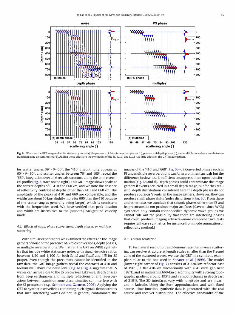
ig. 6. Effects on the GRT images of white stationary noise (a), the presence of P-to-Sransition zone discontinuities (d). Adding these effects to the synthetics of the SS,

or scatter angles 39◦ < � < 60◦, the ‘410’ discontinuity appears at0◦ < � < 90◦, and scatter angles between 70◦ and 105◦ reveal the

660’. Integration over all � reveals structure along the entire verti-al profile (Fig. 5, trace on the right). This GRT image shows peaks athe correct depths of 0, 410 and 660 km, and we note the absencef reflectivity contrast at depths other than 410 and 660 km. Themplitude of the peaks at 410 and 660 are comparable, and theidths are about 50 km (slightly more for 660 than the 410 because

f the scatter angles generally being larger) which is consistentith the frequencies used. We have verified that peak location

nd width are insensitive to the (smooth) background velocityodel.

.2. Effects of noise, phase conversions, depth phases, or multiplecattering

With similar experiments we examined the effects on the imageathers of noise or the presence of P-to-S conversions, depth phases,r multiple reverberations. We first ran the GRT on WKBJ synthet-cs that include white stationary noise, with signal-to-noise ratiosetween 1/20 and 1/100 for both S410S and S660S and 1/5 for SSroper. Even though the precursors cannot be identified in theaw data, the GRT image gathers reveal the contrasts at 410 and60 km well above the noise level (Fig. 6a). Fig. 4 suggests that PSaves can arrive close to the SS precursors. Likewise, depth phases

rom deep earthquakes and multiple reflections of and reverber-tions between transition zone discontinuities can interfere withhe SS precursors (e.g., Schmerr and Garnero, 2006). Applying theRT to synthetic wavefields containing such signals demonstrates

hat such interfering waves do not, in general, contaminate the

rted phases (b), presence of depth phases (c), and multiples reverberations betweenand S660S has little effect on the GRT image gathers.

images of the ‘410’ and ‘660’ (Fig. 6b–d). Converted phases such asPS and multiple reverberations can form prominent arrivals but thedifference in slowness is sufficient to suppress them upon transfor-mation (Fig. 6b and d). Depth phases could contaminate the imagegathers if events occurred in a small depth range, but for the (real-istic) depth distributions considered here the depth phases do notproduce spurious ‘events’ in the image gathers. However, they canproduce small phase shifts (pulse distortions) (Fig. 6c). From theseand other tests we conclude that seismic phases other than SS andits precursors do not produce major artifacts. [Caveat: since WKBJsynthetics only contain user-specified dynamic wave groups wecannot rule out the possibility that there are interfering phasesthat could produce imaging artifacts—more comprehensive testsrequire full wave synthetics, for instance from mode summation orreflectivity method.]

4.3. Lateral resolution

To test lateral resolution, and demonstrate that inverse scatter-ing can resolve structure at length scales smaller than the Fresnelzone of the scattered waves, we use the GRT in a synthetic exam-ple similar to the one used in Shearer et al. (1999). The model(lower right corner of Fig. 7) consists of a 220-km reflector eastof 196◦E, a flat 410-km discontinuity with a 4◦ wide gap near192◦E, and an undulating 660-km discontinuity with a strong topo-

graphic gradient around 195◦E and a smooth change in depth eastof 210◦E. The 2D interfaces vary with longitude and are invari-ant in latitude. Using the Born approximation, and with fixedsource—time function, synthetic data is generated with the realsource and receiver distribution. The effective bandwidth of the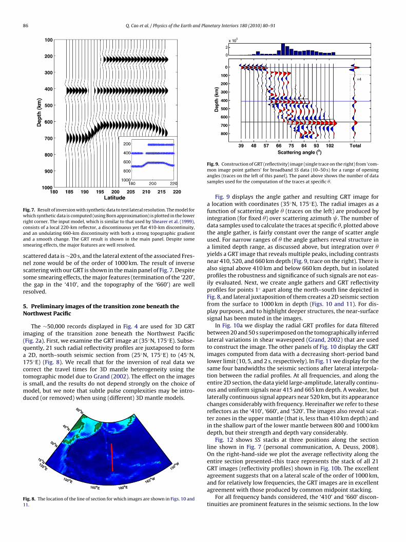

86 Q. Cao et al. / Physics of the Earth and Planetary Interiors 180 (2010) 80–91

Fig. 7. Result of inversion with synthetic data to test lateral resolution. The model forwhich synthetic data is computed (using Born approximation) is plotted in the lowerrcaas

snsstr

5N

i(qa1ctimd

F1

ight corner. The input model, which is similar to that used by Shearer et al. (1999),onsists of a local 220-km reflector, a discontinuous yet flat 410-km discontinuity,nd an undulating 660-km discontinuity with both a strong topographic gradientnd a smooth change. The GRT result is shown in the main panel. Despite somemearing effects, the major features are well resolved.

cattered data is ∼20 s, and the lateral extent of the associated Fres-el zone would be of the order of 1000 km. The result of inversecattering with our GRT is shown in the main panel of Fig. 7. Despiteome smearing effects, the major features (termination of the ‘220’,he gap in the ‘410’, and the topography of the ‘660’) are wellesolved.

. Preliminary images of the transition zone beneath theorthwest Pacific

The ∼50,000 records displayed in Fig. 4 are used for 3D GRTmaging of the transition zone beneath the Northwest PacificFig. 2a). First, we examine the GRT image at (35◦N, 175◦E). Subse-uently, 21 such radial reflectivity profiles are juxtaposed to form2D, north–south seismic section from (25◦N, 175◦E) to (45◦N,

75◦E) (Fig. 8). We recall that for the inversion of real data we

orrect the travel times for 3D mantle heterogeneity using theomographic model due to Grand (2002). The effect on the imagess small, and the results do not depend strongly on the choice of

odel, but we note that subtle pulse complexities may be intro-uced (or removed) when using (different) 3D mantle models.

ig. 8. The location of the line of section for which images are shown in Figs. 10 and1.

Fig. 9. Construction of GRT (reflectivity) image (single trace on the right) from ‘com-mon image point gathers’ for broadband SS data (10–50 s) for a range of openingangles (traces on the left of this panel). The panel above shows the number of datasamples used for the computation of the traces at specific �.

Fig. 9 displays the angle gather and resulting GRT image fora location with coordinates (35◦N, 175◦E). The radial images as afunction of scattering angle � (traces on the left) are produced byintegration (for fixed �) over scattering azimuth . The number ofdata samples used to calculate the traces at specific �, plotted abovethe angle gather, is fairly constant over the range of scatter angleused. For narrow ranges of � the angle gathers reveal structure ina limited depth range, as discussed above, but integration over �yields a GRT image that reveals multiple peaks, including contrastsnear 410, 520, and 660 km depth (Fig. 9, trace on the right). There isalso signal above 410 km and below 660 km depth, but in isolatedprofiles the robustness and significance of such signals are not eas-ily evaluated. Next, we create angle gathers and GRT reflectivityprofiles for points 1◦ apart along the north–south line depicted inFig. 8, and lateral juxtaposition of them creates a 2D seismic sectionfrom the surface to 1000 km in depth (Figs. 10 and 11). For dis-play purposes, and to highlight deeper structures, the near-surfacesignal has been muted in the images.

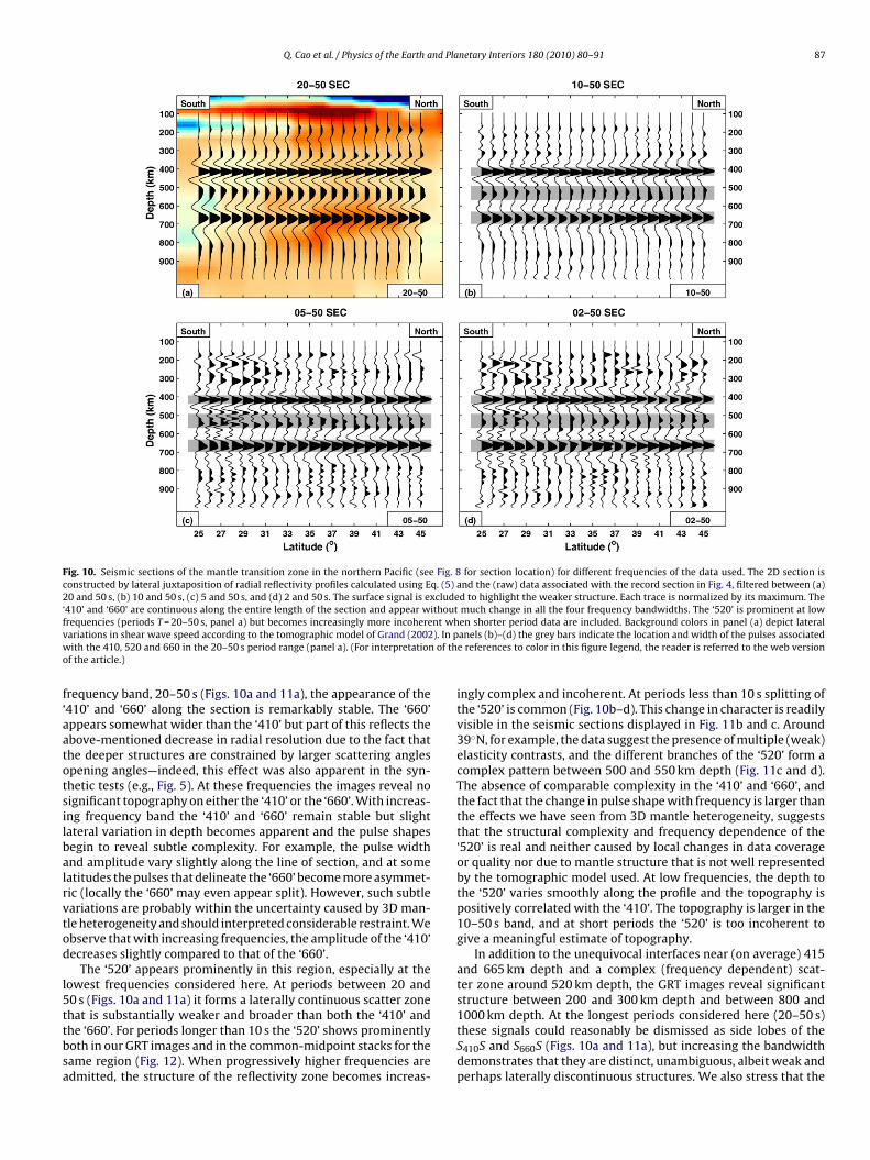
In Fig. 10a we display the radial GRT profiles for data filteredbetween 20 and 50 s superimposed on the tomographically inferredlateral variations in shear wavespeed (Grand, 2002) that are usedto construct the image. The other panels of Fig. 10 display the GRTimages computed from data with a decreasing short-period bandlower limit (10, 5, and 2 s, respectively). In Fig. 11 we display for thesame four bandwidths the seismic sections after lateral interpola-tion between the radial profiles. At all frequencies, and along theentire 2D section, the data yield large-amplitude, laterally continu-ous and uniform signals near 415 and 665 km depth. A weaker, butlaterally continuous signal appears near 520 km, but its appearancechanges considerably with frequency. Hereinafter we refer to thesereflectors as the ‘410’, ‘660’, and ‘520’. The images also reveal scat-ter zones in the upper mantle (that is, less than 410 km depth) andin the shallow part of the lower mantle between 800 and 1000 kmdepth, but their strength and depth vary considerably.

Fig. 12 shows SS stacks at three positions along the sectionline shown in Fig. 7 (personal communication, A. Deuss, 2008).On the right-hand-side we plot the average reflectivity along theentire section presented–this trace represents the stack of all 21GRT images (reflectivity profiles) shown in Fig. 10b. The excellent

agreement suggests that on a lateral scale of the order of 1000 km,and for relatively low frequencies, the GRT images are in excellentagreement with those produced by common midpoint stacking.

For all frequency bands considered, the ‘410’ and ‘660’ discon-tinuities are prominent features in the seismic sections. In the low

Q. Cao et al. / Physics of the Earth and Planetary Interiors 180 (2010) 80–91 87

Fig. 10. Seismic sections of the mantle transition zone in the northern Pacific (see Fig. 8 for section location) for different frequencies of the data used. The 2D section isconstructed by lateral juxtaposition of radial reflectivity profiles calculated using Eq. (5) and the (raw) data associated with the record section in Fig. 4, filtered between (a)20 and 50 s, (b) 10 and 50 s, (c) 5 and 50 s, and (d) 2 and 50 s. The surface signal is excluded to highlight the weaker structure. Each trace is normalized by its maximum. The‘410’ and ‘660’ are continuous along the entire length of the section and appear without much change in all the four frequency bandwidths. The ‘520’ is prominent at lowf nt whv ). In pw of tho

f‘aatotsilbalrvtod

l5ttbsa

requencies (periods T = 20–50 s, panel a) but becomes increasingly more incohereariations in shear wave speed according to the tomographic model of Grand (2002ith the 410, 520 and 660 in the 20–50 s period range (panel a). (For interpretation

f the article.)

requency band, 20–50 s (Figs. 10a and 11a), the appearance of the410’ and ‘660’ along the section is remarkably stable. The ‘660’ppears somewhat wider than the ‘410’ but part of this reflects thebove-mentioned decrease in radial resolution due to the fact thathe deeper structures are constrained by larger scattering anglespening angles—indeed, this effect was also apparent in the syn-hetic tests (e.g., Fig. 5). At these frequencies the images reveal noignificant topography on either the ‘410’ or the ‘660’. With increas-ng frequency band the ‘410’ and ‘660’ remain stable but slightateral variation in depth becomes apparent and the pulse shapesegin to reveal subtle complexity. For example, the pulse widthnd amplitude vary slightly along the line of section, and at someatitudes the pulses that delineate the ‘660’ become more asymmet-ic (locally the ‘660’ may even appear split). However, such subtleariations are probably within the uncertainty caused by 3D man-le heterogeneity and should interpreted considerable restraint. Webserve that with increasing frequencies, the amplitude of the ‘410’ecreases slightly compared to that of the ‘660’.

The ‘520’ appears prominently in this region, especially at theowest frequencies considered here. At periods between 20 and0 s (Figs. 10a and 11a) it forms a laterally continuous scatter zone

hat is substantially weaker and broader than both the ‘410’ andhe ‘660’. For periods longer than 10 s the ‘520’ shows prominentlyoth in our GRT images and in the common-midpoint stacks for theame region (Fig. 12). When progressively higher frequencies aredmitted, the structure of the reflectivity zone becomes increas-

en shorter period data are included. Background colors in panel (a) depict lateralanels (b)–(d) the grey bars indicate the location and width of the pulses associatede references to color in this figure legend, the reader is referred to the web version

ingly complex and incoherent. At periods less than 10 s splitting ofthe ‘520’ is common (Fig. 10b–d). This change in character is readilyvisible in the seismic sections displayed in Fig. 11b and c. Around39◦N, for example, the data suggest the presence of multiple (weak)elasticity contrasts, and the different branches of the ‘520’ form acomplex pattern between 500 and 550 km depth (Fig. 11c and d).The absence of comparable complexity in the ‘410’ and ‘660’, andthe fact that the change in pulse shape with frequency is larger thanthe effects we have seen from 3D mantle heterogeneity, suggeststhat the structural complexity and frequency dependence of the‘520’ is real and neither caused by local changes in data coverageor quality nor due to mantle structure that is not well representedby the tomographic model used. At low frequencies, the depth tothe ‘520’ varies smoothly along the profile and the topography ispositively correlated with the ‘410’. The topography is larger in the10–50 s band, and at short periods the ‘520’ is too incoherent togive a meaningful estimate of topography.

In addition to the unequivocal interfaces near (on average) 415and 665 km depth and a complex (frequency dependent) scat-ter zone around 520 km depth, the GRT images reveal significantstructure between 200 and 300 km depth and between 800 and

1000 km depth. At the longest periods considered here (20–50 s)these signals could reasonably be dismissed as side lobes of theS410S and S660S (Figs. 10a and 11a), but increasing the bandwidthdemonstrates that they are distinct, unambiguous, albeit weak andperhaps laterally discontinuous structures. We also stress that the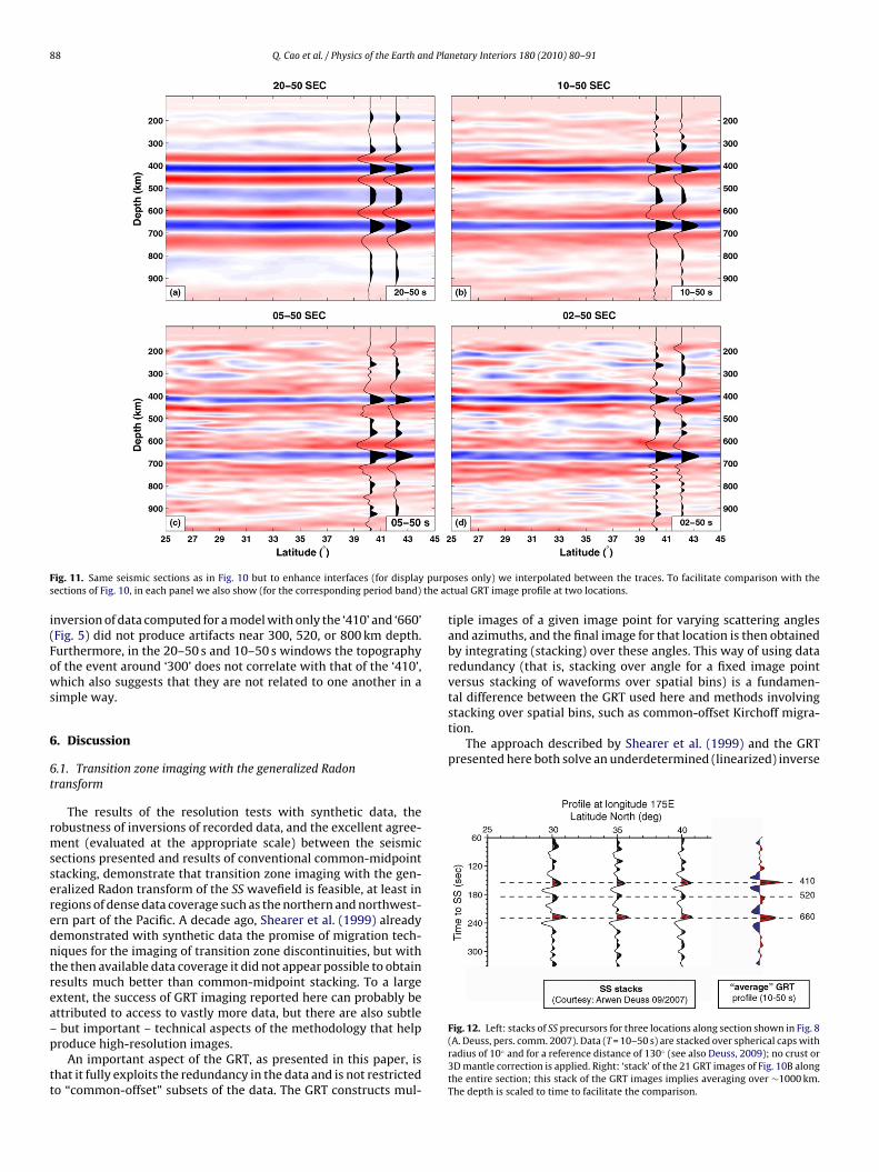

88 Q. Cao et al. / Physics of the Earth and Planetary Interiors 180 (2010) 80–91

F purps the ac

i(Fows

6

6t

rmsseredntrea–p

tt

stacking over spatial bins, such as common-offset Kirchoff migra-tion.

The approach described by Shearer et al. (1999) and the GRTpresented here both solve an underdetermined (linearized) inverse

ig. 11. Same seismic sections as in Fig. 10 but to enhance interfaces (for displayections of Fig. 10, in each panel we also show (for the corresponding period band)

nversion of data computed for a model with only the ‘410’ and ‘660’Fig. 5) did not produce artifacts near 300, 520, or 800 km depth.urthermore, in the 20–50 s and 10–50 s windows the topographyf the event around ‘300’ does not correlate with that of the ‘410’,hich also suggests that they are not related to one another in a

imple way.

. Discussion

.1. Transition zone imaging with the generalized Radonransform

The results of the resolution tests with synthetic data, theobustness of inversions of recorded data, and the excellent agree-ent (evaluated at the appropriate scale) between the seismic

ections presented and results of conventional common-midpointtacking, demonstrate that transition zone imaging with the gen-ralized Radon transform of the SS wavefield is feasible, at least inegions of dense data coverage such as the northern and northwest-rn part of the Pacific. A decade ago, Shearer et al. (1999) alreadyemonstrated with synthetic data the promise of migration tech-iques for the imaging of transition zone discontinuities, but withhe then available data coverage it did not appear possible to obtainesults much better than common-midpoint stacking. To a largextent, the success of GRT imaging reported here can probably bettributed to access to vastly more data, but there are also subtle

but important – technical aspects of the methodology that help

roduce high-resolution images.An important aspect of the GRT, as presented in this paper, is

hat it fully exploits the redundancy in the data and is not restrictedo “common-offset” subsets of the data. The GRT constructs mul-

oses only) we interpolated between the traces. To facilitate comparison with thetual GRT image profile at two locations.

tiple images of a given image point for varying scattering anglesand azimuths, and the final image for that location is then obtainedby integrating (stacking) over these angles. This way of using dataredundancy (that is, stacking over angle for a fixed image pointversus stacking of waveforms over spatial bins) is a fundamen-tal difference between the GRT used here and methods involving

Fig. 12. Left: stacks of SS precursors for three locations along section shown in Fig. 8(A. Deuss, pers. comm. 2007). Data (T = 10–50 s) are stacked over spherical caps withradius of 10◦ and for a reference distance of 130◦ (see also Deuss, 2009); no crust or3D mantle correction is applied. Right: ‘stack’ of the 21 GRT images of Fig. 10B alongthe entire section; this stack of the GRT images implies averaging over ∼1000 km.The depth is scaled to time to facilitate the comparison.

nd Pla

pttnattrssstufaotai

drapteTGtf

6

Pbsp(btw

sat(pg(dtzt

tudttivoaqt

Q. Cao et al. / Physics of the Earth a

roblem. In the GRT the least-squares inversion is implicit throughhe inclusion of the approximate inverse of the normal opera-or F*F, see Eq. (3). In the full implementation of the GRT, theormal operator controls the sensitivity along the isochrons byccounting for the radiation patterns (focal mechanisms and con-rast source), geometrical spreading, and illumination. [We notehat in our implementation we do not include all weights – seeemark below (4).] Instead of Tikhonov regularization in the modelpace (which decreases spatial resolution), the GRT attributesensitivity in accordance with the Fresnel zones of the relevantcattered phases by limiting the range of integration over migra-ion dips, which is controlled by the available data. Applied tonevenly sampled data, the GRT accumulates the contributionsrom the corresponding sensitivity kernels weighted with avail-ble data samples. This localization of sensitivity, akin to the usef finite-frequency sensitivity kernels in transmission or reflec-ion tomography, reduces the need for regularization (spatialveraging) and preserves lateral resolution where illuminations sufficient.

Adequate localization of sensitivity requires data from a broadistance and azimuth range (Stolk and De Hoop, 2002), and inegions with poor data coverage (in terms of the range of scatteringngles and azimuths) application of the GRT as presented here mayroduce imaging artifacts. In such regions it may still be possibleo constrain some aspects of sub-surface scatters if one can achieveven better localization than is possible with the traditional GRT.he optimal way to implement such partial reconstruction with theRT, in multi-scale sense, makes use of wave packets and localiza-

ion in phase space (De Hoop et al., 2009), and this is a topic ofurther research.

.2. Transition zone structure and mineralogy

The region studied here is far away from the northwesternacific subduction zones and the presumed mantle upwellingeneath Hawaii. The 2D section crosses the Hawaii-Emperoreamount chain (around 30◦N). Inverse scattering of SS data can inrinciple resolve topography at a lateral resolution of a few 100 kmFig. 7), which is up to an order of magnitude smaller than obtainedy traditional stacking of long-period SS data, but in this part of theectonically stable Pacific the topography is (as expected) small andill, therefore, not be a topic of discussion here.

The data resolve scatter zones at several depths beneath thetudy region. The most pronounced and robust reflectors appearround 410 and 660 km depth, but the images also suggest elas-icity contrasts around 300 km depth, between 500 and 560 kmespecially at longer periods), and between 800 and 1000 km. Theresence of interfaces near 410, 500–560, and 660 km depth isenerally consistent with expectations from olivine mineralogyFig. 1). Scattering near 300 km and between 800 and 1000 kmepth occurs outside the pressure/depth range associated withhe transitions in the olivine system (which mark the transitionone senso stricto) and may be related to pyroxene and garnetransitions.

The depth to the ‘410’ (averaged along the profile) is 415 km, andhe ‘660’ occurs around 665 km depth. At a wavespeed of 5 km/s thencertainty in depth is about 5 km at the short-period range of theata used here, and inaccuracies in the background wavespeed ofhe order of 1% would add (at most) another 5 km to this uncer-ainty. With these estimates of uncertainty, the ‘410’ and ‘660’ aremaged approximately at their global average depths, and both the

ariation in depth along the line of section and the minor distortionsf the pulses associated with the ‘410’ and ‘660’ km discontinuitiesre probably insignificant. The observation that with increasing fre-uencies the amplitude of the ‘410’ decreases slightly compared tohat of the ‘660’ suggests that in this region the post-spinel (ring-

netary Interiors 180 (2010) 80–91 89

woodite to perovskite and ferropericlase) transition (associatedwith the ‘660’) is sharper than the olivine to wadsleyite transi-tion (associated with the ‘410’). This is consistent with mineralphysics studies that suggest that the olivine to wadsleyite transitionoccurs over a broader depth range (6–19 km) than the post-spineltransition (1–10 km) (Bina and Wood, 1987; Irifune and Isshiki,1998; Ito and Takahashi, 1989; Katsura and Ito, 1989; Akaogi etal., 1989).

The images reveal substantial scattering from depths in betweenthe ‘410’ and ‘660’ interfaces. This depth range is consistent with thewadsleyite to ringwoodite transition, which previous seismologicalstudies have referred to as the ‘520’ discontinuity (e.g., Shearer andMasters, 1992; Deuss and Woodhouse, 2001; Deuss, 2009). For datawith periods larger than 10 s our images reveal a single broad eventbetween 500 and 560 km depth (e.g., Fig. 11a). With increasing fre-quency the signal becomes weaker and increasingly less coherent,with (multiple) splitting observed in the GRT images at 5–50 s and2–50 s (Figs. 10c, d and 11c, d). This complexity is not seen in the‘410’ and ‘660’ and cannot (in a trivial way) be attributed to deterio-ration of data coverage at these periods. These observations suggestthat the frequency dependence of the ‘520’ is real.

Deuss and Woodhouse (2001) observe reflections near500–515 km and 551–566 km in some regions of Pacific, near theIndonesian subduction zone, and beneath the North African shield.They attribute the splitting to the phase transitions in non-olivine(e.g., pyroxene, garnet) components. Saikia et al. (2008) proposedthat the shallower discontinuity is due to the wadsleyite to ring-woodite transformation whereas the deeper one represents theformation of CaSiO3 perovskite from garnet. In a fertile mantle – orin a mantle with a substantial component of recycled MORB crust,which contains more Ca than normal mantle – these two disconti-nuities would be separated. The regional variation of the characterof the ‘520’ has thus been invoked as evidence for large-scale chem-ical heterogeneity.

Alternatively, the predominance of the ‘520’ at low frequenciesand its gradual break-down with increasing frequencies of the dataused may – to first order – be explained by the broad two-phaseloop of the divariant transition from wadsleyite to ringwoodite(Shearer, 1996; Rigden et al., 1991; Frost, 2003). In peridotite man-tle this transformation is found to take place over a pressure intervalcorresponding to ∼20 km at 1400 ◦C even when buffering by garnetis considered. Frost (2003) also showed that the phase-fraction pro-file is almost linear across the transformation, which would explainwhy its image is more pronounced for low frequency data. It ispossible that the structure at short periods reflect transitions inthe non-olivine components that become visible only when, withincreasing data frequency, the image of the wadsleyite to ring-woodite transition weakens. We note, however, that this weaksignal may not exceed the noise level (and its variability is withinthe uncertainty due to wavespeed variations that are not accountedfor in the global tomography model that we use to make travel timecorrections).

We have as yet no definitive explanation for the scattering thatis visible near 300 km depth (Figs. 10a, b and 11a, b). One possi-ble cause is the transition in pyroxene from an orthorhombic toa monoclinic structure (Woodland and Angel, 1997; Stixrude andLithgow-Bertelloni, 2005). For a pyrolite mantle composition theeffect of this transition on elasticity would be small but in materialwith higher concentrations of ortho-pyroxene, such as harzburgite,the change could be substantial. If this interpretation is correct,our results imply that even far away from zones of present-day

subduction the upper mantle could contain significant fractions ofharzburgite. Williams and Revenaugh (2005) proposed that a dis-continuity at around 300 km might be generated by SiO2-stishoviteformation in eclogitic assemblages. This explanation would implywidespread occurrence of materials with mid-oceanic-ridge basalt

9 nd Pla

ccc

chodaoata

7

tfisrartddsfbf

recsscttgittairp

‘i1ifils

dssa2ibai

0 Q. Cao et al. / Physics of the Earth a

hemistry. Finally, the ‘300’ could signify the base of a zone ofarbonatite melting in the asthenosphere (J.-P. Morgan, personalommunication, 2009).

These are exciting possibilities, both with far reaching impli-ations for our understanding of mantle flow and mixing. We areesitant, however, to push the interpretation of the observationf scattering near 300 km depth beyond these speculations andefer further discussion to a later time when robust evidence isvailable for a larger geographical region. Yet we note that mostf the above explanations require a chemistry that is distinct frompyrolitic composition, which may suggest significant composi-

ional heterogeneity in a region is (at present day) far away fromctive subduction systems.

. Conclusions

We have developed a generalized Radon transform to constructhe images of mantle transition zone with the broadband wave-eld of SS and its precursors. The GRT is a technique for inversecattering and it exploits the redundancy in the data in that for aange of scattering angle and azimuth it creates multiple images ofsingle point. Combined, these common image point gathers rep-

esent a GRT image (i.e., the radial reflectivity profile) which revealshe position of scatterers as a function of geographic location andepth beneath the surface. The main objective of this paper was toemonstrate the feasibility of high-resolution imaging of the tran-ition zone beneath geographic regions (such as oceans) far awayrom sources and receivers. In future studies this new capability wille used for high-resolution studies of the transition zone beneath,or instance, Hawaii.

The GRT images of the transition zone beneath the north Pacificeveal a pronounced ‘410’ and ‘660’ for all frequencies consid-red. For periods T > 10 s our results are consistent with that ofonventional SS stacking. With increasing frequency there is alight increase in structural complexity and depth variation, and atrengthening of the ‘660’ compared to the ‘410’ (which may indi-ate that the former is sharper than the latter). The average depthso the ‘410’ and ‘660’ are 415 ± 5 and 665 ± 7 km, respectively, andhe small (∼10 km peak-to-peak) depth variation is insignificantiven the depth resolution of the data. The ‘520’ is pronouncedn the low frequency band, and broader and weaker than eitherhe ‘410’ or ‘660’, but there is an increase in the complexity ofhe ‘520’ with increasing frequency, even when the ‘410’ and ‘660’re not similarly affected. The frequency dependence of the ‘520’s consistent with the broad two-phase loop of the wadsleyite toingwoodite transition, but structure that becomes visible at shorteriods may reflect transitions in non-olivine components.

In addition to the usual suspects (that is, the ‘410’, ‘520’, and660’), the transition zone images also reveal substantial scatter-ng from structures at around 300 km depth and between 800 and000 km depth. The prominence of the event near 300 km could

ndicate the presence of harzburgite or MORB material far awayrom sites of active subduction. These structures may be laterallyntermittent, however, and larger scale imaging is needed to estab-ish the geographical distribution and lateral continuity of thesetructures.

The vast and rapidly growing amount of high quality waveformata that is available through IRIS DMC has begun to allow large-cale exploration seismology of the deep mantle. Following ourtudies of the lowermost mantle with inverse scattering of the ScSnd SKKS wavefields (Wang et al., 2006, 2008; Van der Hilst et al.,

007) we have demonstrated here the feasibility of transition zone

maging with the SS wavefield. This is opening exciting new possi-ilities for collaborative studies of Earth’s deep interior in generalnd for detailed investigations of the upper mantle transition zone,n particular.

netary Interiors 180 (2010) 80–91

Acknowledgments

We thank Jason Phipps Morgan and Greg Hirth for stimulatingdiscussions and excellent suggestions on various aspects of ourwork, and we are grateful to Arwen Deuss for computing the SSstacks shown in Fig. 12. We thank Rosalee Lamm (MSc, MIT) for hercontribution to the early stages of this project. The revision of theoriginal manuscript benefited greatly from insightful commentsby Peter Shearer, an anonymous reviewer, and the Editor (GeorgeHelffrich). This research has been supported by the CSEDI programof the US National Science Foundation under grant EAR-0757871and would not have been possible without the open availabilityof waveform data through the Data Management Center of theIncorporated Research Institutions for Seismology (IRIS).

References

Akaogi, M., Ito, E., Navrotsky, A., 1989. Olivine-modified spinelspinel transitionsin the system Mg2SiO4–Fe2SiO4: calorimetric measurements, thermochemi-cal calculations, and geophysical application. J. Geophys. Res. 94 (15), 671–685.

An, Y., Gu, Y.J., Sacchi, M.D., 2007. Imaging mantle discontinuities using least squaresRadon transform. J. Geophys. Res. 112, doi:10.1029/2007JB005009, B10303.

Beylkin, G., 1985. Imaging of discontinuities in the inverse scattering problem byinversion of a causal generalized Radon transform. J. Math. Phys. 26, 99–108.

Bina, C.R., Wood, B.J., 1987. The olivine–spinel transitions: experimental and ther-modynamic. Constraints and implications for the nature of the 400 km seismicdiscontinuity. J. Geophys. Res. 92, 4853–4866.

Bina, C.R., Helffrich, G., 1994. Phase transition Clapeyron slopes and transition zoneseismic discontinuity topography. J. Geophys. Res. 99 (B8), 15853–15860.

Castle, J.C., Creager, K.C., 2000. Local sharpness and shear wave speed jump acrossthe 660-km discontinuity. J. Geophys. Res. 105, 6191–6200.

Chaljub, E., Tarantola, A., 1997. Sensitivity of SS precursors to topography on theupper mantle 660-km discontinuity. Geophys. Res. Lett. 24, 2613–2616.

Chambers, K., Woodhouse, J.H., Deuss, A., 2005a. Reflectivity of the 410-km discontinuity from PP and SS precursors. J. Geophys. Res. 110,doi:10.1029/2004JB003345 (B02301).

Chambers, K., Woodhouse, J.H., Deuss, A., 2005b. Topography of the 410-km discon-tinuity from PP and SS precursors. Earth Planet. Sci. Lett. 235, 610–622.

Chambers, K., Woodhouse, J.H., 2006. Investigating the lowermost mantle usingmigrations of long-period S-ScS data. Geophys. J. Int. 166, 667–678.

Chapman, C.H., 1978. New method for computing synthetic seismograms. Geophys.J. Int. 54, 481–518.

Collier, J., Helffrich, G., 1997. Topography of the “410” and “660” km seismic discon-tinuities in the Izu-Bonin subduction zone. Geophys. Res. Lett. 24, 1535–1538.

Dahlen, F.A., Hungh, S.-H., Nolet, G., 2000. Fréchet kernels for finite-frequency traveltimes—I. Theory. Geophys. J. Int. 141, 175–203.

Dahlen, F.A., 2005. Finite-frequency sensitivity kernels for boundary topographyperturbations. Geophys. J. Int. 162, 525–540.

De Hoop, M.V., Van der Hilst, R.D., 2005. On sensitivity kernels for waveequation transmission tomography. Geophys. J. Int. 160, doi:10.1111/j.1365-246X.2004.02509.

De Hoop, M.V., Van der Hilst, R.D., Shen, P., 2006. Wave-equation reflectiontomography: annihilators and sensitivity kernels. Geophys. J. Int. 167, 1332–1352.

De Hoop, M.V., Smith, H., Uhlmann, G., Van der Hilst, R.D., 2009. Seismic imagingwith the generalized Radon transform: a curvelet transform perspective. InverseProblems 25, doi:10.1088/0266-5611/25/2/025005, 025005 (21 pp).

Deuss, A., Woodhouse, J.H., 2001. Seismic observations of splitting of the mid-transition zone discontinuity in earth’s mantle. Science 294, 354–357.

Deuss, A., 2009. Global observations of mantle discontinuities using SS and PP pre-cursors. Surv. Geophys. 30 (4–5), 301–326.

Deuss, A., Redfern, S.A.T., Chambers, K., Woodhouse, J.H., 2006. The nature of the660-kilometer discontinuity in Earth’s mantle from global seismic observationsof PP precursors. Science 311, 198–201.

Engdahl, E.R., Van der Hilst, R.D., Buland, R.P., 1998. Global teleseismic Earthquakerelocation from improved travel times and procedures for depth determination.Bull. Seis. Soc. Am. 88 (3), 722–743.

Fei, Y., van Orman, J., Li, J., van Westrenen, W., Sanloup, C., Minarik, W., Hirose,K., Komabayashi, T., Walter, M., Funakoshi, K., 2004. Experimentally deter-mined postspinel transformation boundary in Mg2SiO4 using MgO as an internalpressure standard and its geophysical implications. J. Geophys. Res. 103,doi:10.1029/2003JB002562, B02305.

Flanagan, M.P., Shearer, P.M., 1998a. Global mapping of topography on transitionzone velocity discontinuities by stacking SS precursors. J. Geophys. Res. 103,

2673–2692.

Flanagan, M.P., Shearer, P.M., 1998b. Topography on the 410-km seismic velocitydiscontinuity near subduction zones from stacking of sS, sP, and pP precursors.J. Geophys. Res. 103, 21165–21182.

Flanagan, M.P., Shearer, P.M., 1999. A map of topography on the 410-km disconti-nuity from PP precursors. Geophys. Res. Lett. 26, 549–552.

nd Pla

F

G

G

G

G

G

G

H

H

I

I

J

K

K

L

L

L

L

M

M

N

R

R

R

R

R

Q. Cao et al. / Physics of the Earth a

rost, D.J., 2003. The structure and sharpness of (Mg,Fe)2SiO4 phase transformationsin the transition zone. Earth Planet. Sci. Lett. 216, 313–328.

ossler, J., Kind, R., 1996. Seismic evidence for very deep roots of continents. EarthPlanet. Sci. Lett. 138 (1–4), 1–13.

rand, S.P., 2002. Mantle shear-wave tomography and the fate of subducted slabs.Phil. Trans. R. Soc. Lond. A 360, 2475–2491.

u, Y.J., Dziewonski, A.M., Agee, C.B., 1998. Global de-correlation of the topographyof transition zone discontinuities. Earth Planet. Sci. Lett. 157, 57–67.

u, Y.J., Dziewonski, A.M., 2002. Global variability of transition zone thickness. J.Geophys. Res. 107 (B7), doi:10.1029/2001JB000489.

u, Y.J., Dziewonski, A.M., Ekström, G., 2003. Simultaneous inversion for mantleshear velocity and topography of transition zone discontinuities. Geophys. J. Int.154, 559–583.

u, Y.J., Sacchi, M., 2009. Radon transform methods and their applications inmapping mantle reflectivity structure. Surv. Geophys., doi:10.1007/s10712.009-9076-0.

elffrich, G., 2000. Topography of the transition zone seismic discontinuities. Rev.Geophys. 38, 141–158.

ouser, C., Masters, G., Flanagan, M., et al., 2008. Determination and analysis of long-wavelength transition zone structure using SS precursors. Geophys. J. Int. 174(1), 178–194.

rifune, T., Isshiki, M., 1998. Iron partitioning in a pyrolite mantle and the nature ofthe 410-km seismic discontinuity. Nature 392, 702–705.

to, E., Takahashi, E., 1989. Postspinel transformations in the systemMg2SiO4–Fe·SiO4 and some geophysical implications. J. Geophys. Res. 9,10637–10646.

eanloz, R., Thompson, A.B., 1983. Phase transitions and mantle discontinuities. Rev.Geophys. 21, 51–74.

atsura, T., Ito, E., 1989. The system Mg2SiO4–Fe2SiO4 at high pressures and tem-peratures: precise determination of stabilities of olivine, modified spinel, andspinel. J. Geophys. Res. 94, 15663–15670.

ennett, B.L.N., Engdahl, E.R., Buland, R.P., 1995. Constraints on seismic velocities inthe Earth from travel times. Geophys. J. Int. 122, 108–124.

awrence, J.F., Shearer, P.M., 2008. Imaging mantle transition zone thickness withSdS-SS finite-frequency sensitivity kernels. Geophys. J. Int. 174, 143–158.

ebedev, S., Chevrot, S., van der Hilst, R.D., 2002. Seismic evidence for olivinephase change at the 410- and 660-kilometer discontinuities. Science 296, 1300–1302.

ebedev, S., Chevrot, S., Van der Hilst, R.D., 2003. Correlation between the shear-speed structure and thickness of the mantle transition zone. Phys. Earth Planet.Int. 136, 25–40.

i, B., Liebermann, R., 2007. Indoor seismology by probing the Earth’s interior byusing sound velocity measurements at high pressures and temperatures. Proc.Natl. Acad. Sci. 104, 9145–9150.

a, P., Wang, P., Tenorio, L., De Hoop, M.V., Van der Hilst, R.D., 2007. Imag-ing of structure at and near the core-mantle boundary using a generalizedradon transform: 2. Statistical inference of singularities. J. Geophys. Res. 112,doi:10.1029/2006JB004513, B08303.

iller, D., Oristaglio, M., Beylkin, G., 1987. A new slant on seismic imaging: migrationand integral geometry. Geophysics 52, 943–964.

eele, F., de Regt, H., Van Decar, J., 1997. Gross errors in upper-mantle discon-tinuity topography from underside reflection data. Geophys. J. Int. 129, 194–204.

igden, S.M., Gwanmesia, G.D., FitzGerald, J.D., Jackson, I., Liebermann, R.C., 1991.Spinel elasticity and seismic structure of the transition zone of the mantle.Nature 354, 143–145.

ingwood, A.E., 1969. Phase transformations in the mantle. Earth Planet. Sci. Lett. 5,401–412.

ingwood, A.E., 1975. Composition and Petrology of the Earth’s Mantle. McGraw-Hill, New York.

ingwood, A.E., 1991. Phase transformations and their bearing on the constitutionand dynamics of the mantle. Geochim. Cosmochim. Acta 55, 2083–2110.

ondenay, S., Bostock, M.G., Fischer K.M., 2005. Multichannel inversion of scatteredteleseismic body waves: practical considerations and applicability, in Seismic

netary Interiors 180 (2010) 80–91 91

Earth: array analysis of broadband seismograms. In: Levander, A., Nolet, G. (Eds.),AGU Geophysical Monograph Series, 157.

Rost, S., Thomas, C., 2009. Improving seismic resolution through array processingtechniques. Surveys in Geophysics 30 (4-5), 271–299.

Saikia, A., Frost, D., Rubie, D., 2008. Splitting of the 520-kilometer seismic disconti-nuity and chemical heterogeneity in the mantle. Science 319, 1515–1518.

Schmerr, N., Garnero, E., 2006. Investigation of upper mantle discontinuity struc-ture beneath the central Pacific using SS precursors. J. Geophys. Res. 111,doi:10.1029/2005JB004197, B08305.

Shearer, P.M., 1990. Seismic imaging of upper-mantle structure with new evidencefor a 520-km discontinuity. Nature 344, 121–126.

Shearer, P.M., 1991. Constraints on upper-mantle discontinuities from observationsof long-period reflected and converted phases. J. Geophys. Res. 96, 18147–18182.

Shearer, P.M., Masters, T.G., 1992. Global mapping of topography on the 660-kmdiscontinuity. Nature 355, 791–796.

Shearer, P.M., 1993. Global mapping of upper mantle reflectors from long-period SSprecursors. Geophys. J. Int. 115, 878–904.

Shearer, P.M., 1996. Transition zone velocity gradients and the 520-km discontinu-ity. J. Geophys. Res. 101, 3053–3066.

Shearer, P.M., Flanagan, M.P., Hedlin, M.A.H., 1999. Experiments in migration pro-cessing of SS precursor data to image upper mantle discontinuity structure. J.Geophys. Res. 104, 7229–7242.

Shearer, P.M., 2000. Upper mantle seismic discontinuities, Earth’s deep interior:mineral physics and tomography from the atomic to the global scale. Geophys.Monogr. 117, 115–131.

Shim, S.-H, Duffy, T.S., Shen, G., 2001. The post-spinel transformation in Mg2SiO4

and its relation to the 660-km seismic discontinuity. Nature 411, 571–574.Spetzler, J., Snieder, R., 2004. The Fresnel volume and transmitted waves. Geophysics

69, 653–663.Stixrude, L., Lithgow-Bertelloni, C., 2005. Mineralogy and elasticity of the

upper mantle: origin of the low velocity zone. J. Geophys. Res. 110,doi:10.1029/2004JB002965, B03204.

Stolk, C.C., De Hoop, M.V., 2002. Microlocal analysis of seismic inverse scattering inanisotropic, elastic media. Commun. Pure Appl. Math. 55, 261–301.

Tromp, J., Tape, C., Liu, Q., 2005. Seismic tomography, adjoint methods, time reversal,and banana-donut kernels. Geophys. J. Int. 160, 195–216, doi:10.1111/j.1365-246X.2004.02456.x.

Van der Hilst, R.D., De, Hoop., Wang, M.V., Shim, S.-H., Tenorio, L., Ma, P., 2007.Seismo-stratigraphy and thermal structure of Earth’s core-mantle boundaryregion. Science 315, 1813–1817.

Wang, P., de Hoop, M.V., van der Hilst, R.D., Ma, P., Tenorio, L., 2006. GeneralizedRadon transform imaging of the core mantle boundary: I—Construction of imagegathers. Geophys. Res. 111, doi:10.1029/2005JB004241, B1230.

Wang, P., de Hoop, M.V., Van der Hilst, R.D., 2008. Imaging of the lowermost mantle(D′′) and the core-mantle boundary with SKKS coda waves. Geophys. J. Int. 175,103–115.

Weidner, D.J., Wang, Y.S., 2000. Phase transformations: implications for mantlestructure. In: Karato et al. (Eds.), Earth’s Deep Interior, Am. Geoph. Un., Geophys.Monogr., pp. 215–235.

Weidner, D., Li, L., Durham, W., Chen, J., 2005. In: Chen, J., et al. (Eds.),High-temperature Plasticity Measurements using Sychrotron X-rays. High-pressure Technology for Geophysical Applications. Elsevier Inc., San Diego, pp.123–136.

Williams, Q., Revenaugh, J., 2005. Ancient subduction, mantle eclogite, and the300 km seismic discontinuity. Geology 33, 1–4.

Woodland, A.B., Angel, R.J., 1997. Reversal of the orthoferrosilite-high-P clino-ferrosilite transition, a phase diagram for FeSiO3 and implications for themineralogy of the Earth’s upper mantle. Eur. J. Mineral. 9, 245–254.

Zhao, L., Chevrot, S., 2003. SS-wave sensitivity to upper mantle structure: implica-tions for the mapping of transition zone discontinuity topographies. Geophys.Res. Lett. 30 (11), doi:10.1029/2003GL017223.

Zheng, Y., Lay, T., Flanagan, M.P., Williams, Q., 2007. Pervasive seismic wave reflec-tivity and metasomatism of the Tonga mantle wedge. Science 11, 855–859, 316,no. 5826.