Physics for the Life Sciences II

Physics for the Life Sciences II Version 0.5, January 2, 2011

Author:

Timothy McKay

University of Michigan

Table of Contents:

20. Charges and their interactions 2 21. Electric fields 10 22. Electric potential energy and potential 30 23. Capacitors, dielectrics and membranes 41 24. Moving charge: current and resistance 50 25. The living circuit: nerve transmission 66 26. Magnets and moving charge 74 27. Fields from fields: electromagnetic induction 91 28. Making waves: their description 104 29. Mixing waves: superposition and interference 132 30. Spreading waves: diffraction and structure 166 31. Waves and media: reflection and refraction 198 32. Forming images: a multitude of eyes 230 33. Seeing the invisible: extending the senses 257 34. Inside the atom: nuclei and their transformations 271 35. Nuclear reactions 285 36. Origins: the cosmos and elements 290 37. Life in the universe 305 38. Conclusions 310

Copyright Timothy McKay 2011 1

Physics of the Life Sciences II: Chapter 20

20.0: Electricity and Life

Many important aspects of science involve recognizing something so common that it remains hidden. Electricity and magnetism provide a great example. Electromagnetic forces hold together atoms, are responsible for all of chemistry, underlie all the forces you’ll experience (except gravity…), and, through electromagnetic waves, enable most of the energy and information exchange in the universe.

Yet for most of human history, electricity and magnetism were thought little more than curiosities. Strange, nearly magical effects could be coaxed into appearance by rubbing amber with fur, after which the amber would become “charged” with influence. Such charged amber could reach out across empty space and pick up small feathers or bits of paper. This same static cling acting today makes your socks stick to shirts, and brightens winter nights with sparks beneath wool blankets. These phenomena seemed inconstant; rubbing the amber would produce strong effects one day, and none the next. This inconstancy, combined with the clear ability of this influence to act at a distance, made these effects seem especially magical. They came to be known as “electricity”, from the Greek word for amber: elektron.

A second set of similarly striking phenomena were associated with bits of rock which could attract one another, or bits of metal. These rocks, found extensively in the Greek region of Magnesia, came to be called magnets, and the phenomena associated with them “magnetism”. Their ability to always point North was first recorded in China before about 1100. While some Greeks speculated about connections between electricity and magnetism, early scientists saw that they were clearly separate, and their subtle unity was not clearly understood until the second half of the 19th century. Today we speak of the two as one, and call all these phenomena “electromagnetic”.

The great steps in understanding electromagnetic interactions began in the 18th century with the work of people like Benjamin Franklin. It was essentially completed by Scottish physicist James Clerk Maxwell 100 years later. All the important physics of electromagnetism has been known since the 1870s, though the incredible connections of electromagnetism to life were not clear until much more recently.

An appreciation for the importance of electromagnetic interactions for life was hinted at by Galvani in the 1780s (when he showed that electricity could make dead frog legs move as if alive), but the real revelations didn’t emerge until the 1950s, when the structure of proteins and mechanism of nerve function began to be understood. Today we know that protein structure, determined by electromagnetic interactions, governs their function. Every biochemical process, all the workings of life, relies on electromagnetic interactions. The very brain (yours) which contemplates what you’re reading is an elaborate networks of neurons in which information is


stored in patterns of electrical connectivity. Just as electromagnetic forces play a central role in inanimate matter, they enable all of life.

Our approach to the study of electromagnetism will focus largely on the basic physics, but we will on occasion emerge to hint at the central importance of this topic for life. Most especially, we will point out some of the ways in which the applications of electricity and magnetism important for life differ from those often encountered in engineering and human technology.

20.1 Electrostatics: charge

We begin with an extensive study of electrostatics. In this we will learn about the interactions among electrically charged objects which aren’t moving. We will see that much of what’s important about electrical phenomena can be usefully discussed even in these static cases. After treating this in some detail, we will turn to cases where charges move, but in steady ways. Finally we will bring in magnetism, and show that it is closely connected to electricity, and in fact is another aspect of the same thing.

The first fact to introduce in electrostatics is that there are two ways an object can be electrically “charged”. When Ben Franklin discovered there were two types of charge, he called them “positive” and “negative”, because he thought they represented an excess or a deficit of some mysterious substance in a material. We now know that these charges exist in all matter in the form of positive protons in the nuclei of atoms and negative electrons which orbit them. Most of the time, matter is found with quite precisely balanced numbers of electrons and protons. Matter like this we call “neutral”. When this balance is disturbed, and an object contains either too many or too few electrons, we say it is “charged”. Since electrons carry negative charge, an excess of electrons makes an object negatively charged, while a deficit of electrons (relative to protons) makes an object positively charged.

Before quantifying things, let’s note a few basic facts about the behavior of charged objects:

• Objects with like charges (either both positive or both negative) repel one another, even when they’re not in contact. This repulsion weakens as the distance between them increases.

• Objects with different charges (one positive and one negative) attract one another, even when not in contact. This attraction weakens as the distance between the objects increases.

• Charged objects of either type will attract neutral objects, some weakly, and others rather strongly. They do this by inducing charge separation in the neutral objects, as we’ll discuss in detail in the next section.

Electrostatics: conductors and insulators

All objects are made of many, many, electric charges. A penny, for example, contains about 7x1023 positive charges in protons, and an equal number of negative charges in electrons. This is


a lot of charge. In some materials, charges (usually the electrons) can move around rather freely, jumping freely from atom to atom and moving from one part of the material to another (like one edge of the penny to the other). Such materials are called “conductors”, because the conduct electricity through freely. In other materials, the charges are all tightly locked to the atoms or molecules that they started with. These materials are called “insulators” because they insulate against the flow of charge.

The freedom with which charge moves in a material can be quantified by its “conductivity”; a parameter we will define in detail a little later. This conductivity is one of the physical properties of materials which varies most dramatically. Consider two apparently comparable materials, like copper and sulfer. They differ rather modestly in density, Cu is 9 g/cm3 and S is about 5 g/cm3 (in crystalline form). Despite this, they have wildly different conductivities; copper has a conductivity of 6x107 in appropriate units, while that for sulfur is 5x10-18. This conductivity varies by a factor of 1025. In case you’re not used to scientific notation, that’s a lot: 10,000,000,000,000,000,000,000,000.

This very wide range in conductivities means that most materials are either far on the conducting side (all the metals for example) or far on the insulating side. So even though this property varies continuously among different materials, it is often useful to speak of materials as being in one class or another: conductors or insulators.

The ability of a charged object to attract a neutral object comes about because of “induced charge separation”. This can happen in either insulators or conductors, but is much more effective in conductors. Here’s the idea. When you move a positively charged object near a neutral object, all the positive charges in the neutral thing are pushed away, while all the negative charges are attracted. These forces cause charges to move in the neutral object. This is illustrated in the picture below.

Since the electrostatic force weakens with distance, the negative charges which are close to the positive rod are attracted strongly to it, while the positive charges which are far away are weakly repelled. The net force on the neutral object is then an attraction. If the rod you bring close is negatively charged instead of positively the same thing happens, though the induced charge separation is reverse. The important point is that an attraction still occurs. Since the charge separation is much greater on the conductor, the attraction of a neutral conductor to a charged

-

-

+++++

++++++++++++

Positively charged object

Conductor

-

-

+++++

++++++++++++

Positively charged object

Insulator

-

-

+++++

-

-

+++++

-

-

+++++

-

-

+++++

-

-

+++++


object is stronger than it would be for an insulator. But the same sort of attraction happens in either case.

20.2 Coulomb forces

Experiments to quantify the nature of electrostatic interactions are very difficult to conduct. This is due to their very ubiquity; everything is made of incredible numbers of charges. So anytime you have some unbalanced charge around, it interacts with everything else which is nearby. Touch a charged object to a conductor and the charge may race away, flowing through it. To remove these complications, we’ll talk first about how “point charges” behave. These are charged objects so small that things like the induced charge separation described above can’t happen. In practice, point charges don’t need to be literal points. They need only be much smaller than the separation between them to make the point charge characterization below a good approximation to reality.

Quantifying electric charge

During the 1780s, French physicist August Coulomb finally developed experiments which allowed him to reliably quantify the force between two point charges. He discovered that this force takes a simple form which depends on the magnitude of each charge (q1 and q2), the distance between the charges (r12), and a ‘strength constant’ (k):

This equation tells us several things:

• The magnitude of the force is proportional to the product of the two charges q1 and q2. Charges are quantified in units now called “Coulombs”, usually denoted with the symbol C.

• The magnitude of the force is inversely proportional to the square of the distance between the two charges r12.

• The direction of the force is along the line between the two charges. This is noted in the equation above by the little unit vector ‘r-hat’, which points in the direction of the vector going from q1 to q2. If the charges have the same sign this force is repulsive (they are pushed apart). If they have opposite signs it is attractive (they are pulled together).

• The strength constant k in this equation relates the definition of charge to the prior definitions of force (in Newtons) and distance (in meters), and in the usual units has the numerical value 9x109 Nm2/C2.

• Like all forces, this “Coulomb force” is an interaction, and works both ways. If q1 pushes q2 away, then q2 pushes q1 back the other way with an equal and opposite force.

Also, this interaction occurs between every pair of charges. To find the total force on any one charge you must calculate the vector sum of the force on this charge due to each of the other

rr

qkqF ˆ212

2112 = q1 q2

r12

r̂F1F2


charges which are around. In principle, this sum should always include all the other charges in the universe. Fortunately, the force weakens with distance, falling off like 1/r2. As a result, charges which are near the object of interest will usually create most of the force. We will regularly, in fact always, ignore the reality that all other charges elsewhere contribute something to the total force.

The strength constant k in the Coulomb equation is sometimes written in terms of another constant according to the definition k = 1/4πε0. This new constant ε0 is called the “permittivity of free space” or simply the electric constant. From the comparison to k, you can see that its value is ε0 = 8.9x10-12 C2/Nm2.

Comparing Coulomb and Newton

It is interesting to compare the relative strength of the gravitational force (Newton) to the electromagnetic force (Coulomb). To do so, we have to choose some sensible system in which to compare them. Since hydrogen is far and away the most common atom in the universe, we might start by thinking about a hydrogen atom, which consists of one proton and one electron, typically separated by a distance of about 5x10-11 m. The electron and proton attract one another through the Coulomb force. They also attract one another through the gravitational force because both have mass. In this interesting case we find the ratio of these two forces is:

FCoulomb / FGravitational = 2x1039

That is, the electromagnetic force is unbelievably stronger than the gravitational force. This is so because the intrinsic strength of the electromagnetic force is much, much larger than that of gravity. It is for this reason that our bodies are held together by electromagnetic forces (realized as chemical bonds) rather than by gravity.

Measuring charge: the Coulomb

The official definition of the unit for charge, the Coulomb, is today derived from the flow of charge (from electric currents) rather than from the Coulomb force law. This is for practical reasons. Measuring electrostatic forces accurately is really difficult, as we have noted above.

The basic unit of charge is the amount possessed by a negative electron or a positive proton. In either case, this is about 1.6x10-19 C. That is, the total charge on a single electron is -1.6x10-19 C and the total charge on a single proton is +1.6x10-19 C. From this, you can determine the electrostatic attraction between an electron and a proton in a hydrogen atom:

N 9.2x10 8-

2 ==ep

peep r

qkqF


When you see macroscopic electric charges around, you’re usually looking at tiny fractions of a C. You can see that this is so if you image how large the Coulomb force would be between a pair of one Coulomb charges separated by one meter: 9x109 N. That’s a really big force, about twice the weight of all the 6.5 billion people on the planet. This just reiterates the extraordinary strength of the electromagnetic force. You will never encounter a pair of 1 C charges separated by a small distance, because they would immediately either smash together or fly violently apart.

The great strength of this force is responsible for the usual neutrality of matter; it is the reason that most matter contains such a very close balance of positive and negative charges. Any time things charges become a little unbalanced, large forces appear which move charges around until equality is restored.

Learning how to put these large forces to work for us, learning how to use the extreme forces available from electricity, opened up the modern world.

1.3 Electrostatics in life: screening

We pause here to point out that although apparently simple electrostatic forces are important for living systems, they occur in a complex environment which has important effects. Instead of charges interacting in empty space, in life they interact in complex surroundings which continually affect their behavior. In many cases these complexities play a central role in enabling life. We will consider here just one example, the way water reduces the strength of electromagnetic interactions, reducing the cost of many interactions in the molecules of life.

Life is wet. Cells are filled with water that contains a complex mixture of dissolved molecules. Under ordinary circumstances for life, water will exist mostly as H2O, but also partly as H+ and OH- ions. This happens because there is adequate thermal energy around in the liquid water to occasionally break up a water molecule. This condition can be described by pH, defined for this case as pH = –log10(H+ molarity). For water at 300 K the pH is about 7, which, for this reason, is described as neutral. The point is that even in pure water, there are many free positive and negative charges around. Electrostatic interactions in living cells take place with many free charges nearby.

There is another, even more important effect. Water is a polar molecule. In its stable form one end of the molecule is positive while the other is negative. Such an object is called a “dipole”, and can be thought of as having a positive end and a negative end. Put a thing like that near a free positive charge and it will spin around until its negative end is toward the charge and its positive end is away from it.


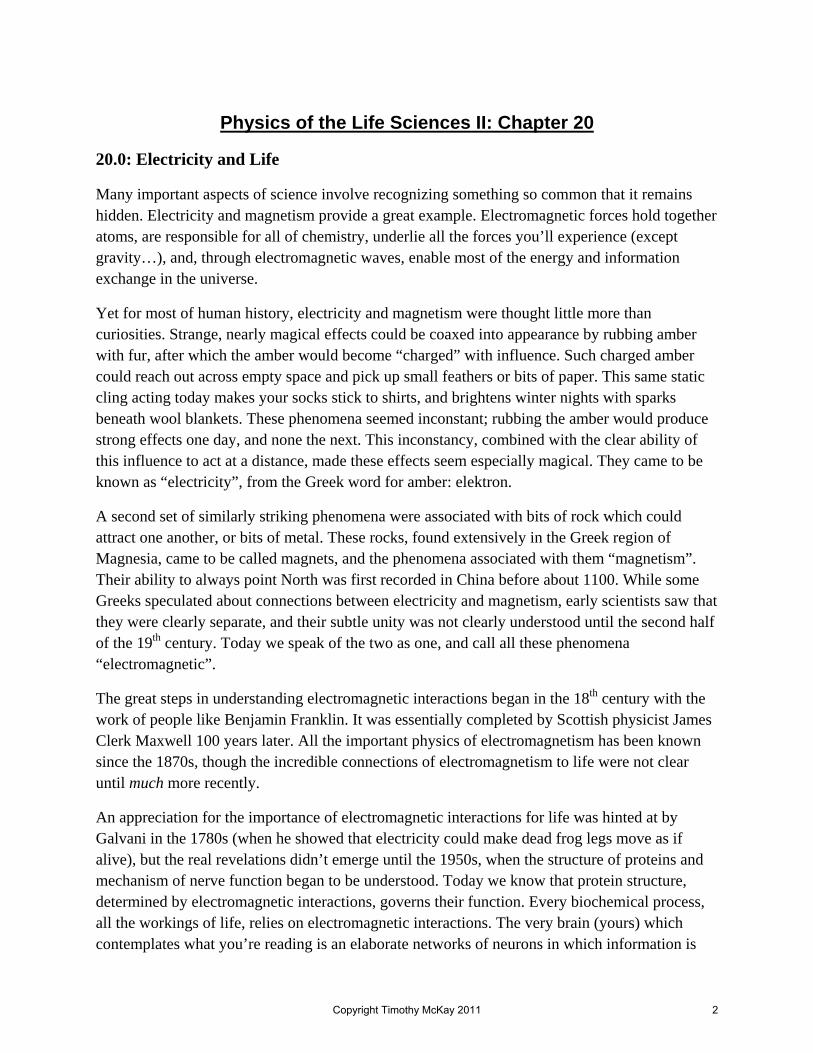
What happens to the Coulomb interaction in this kind of watery environment? The presence of a polar medium and a bunch of free charges leads to electrostatic “screening”. This picture illustrates what happens. Negative ends bunch around the positive charge, while positive ends bunch around the negative charge. The details of what happens are complex (there are a lot of charges to consider here!), but the overall effect can be usefully estimated by noting that this screening effect simply reduces the force between the charges. For electrostatics, we can quantify this by introducing a “dielectric constant” for the medium.

When charges interact in a ‘medium’ like water, the usual Coulomb law is altered in a simple way:

For a non-polar medium like air, this dielectric constant is very close to one, and we can ignore it. For a highly polar medium like water (life’s medium), D is about 80, and obviously this is an important effect.

One approximate way to account for this dielectric effect is by adjusting the constant which describes the strength of the electromagnetic force. We could do this in one of two ways, by changing “k” or by changing ε0.

As we will see, the reduction of the effective strength of the Coulomb force through screening is essential for life. Without it, the energies required to construct and manipulate large molecules like DNA would be much larger, and the mechanisms of life would be unavailable at room temperature. Water helps things along, allowing electrostatic forces to act, but reducing their violence to a point which makes them manageable. Without this medium, many of the processes of life wouldn’t work. This is why many scientists suspect that water will play an essential role in any life we might discover elsewhere in the universe.

1 22

12

ˆvacuummedium

medium medium

F q qkF rD D r

= =

00

1 1 or 4 4

vacuummedium

medium

medium mediummedium medium

kkD

DD

ε επε πε

=

= =


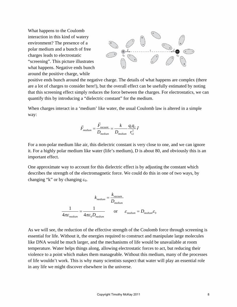
A Quick Summary of Some Important Relations

Charge in conductors and insulators:

All materials are made of electric charges. Electric charge is measured in Coulombs, and the fundamental unit of charge is that of the electron: -1.6x10-19 C.

In most materials that charge is not free to move on scales much larger than an atom. In some charge is free to move large distances. Conductivity varies enormously among materials, so there are many in which charge motion is so free as to seem effortless (conductors), and many in which it charge motion is so limited as to seem impossible (insulators).

Coulomb’s Law and the electrostatic interaction between charges:

There is a very precise model for the force between two electric charges called Coulomb’s law.

9 2 21 2Coulomb 2

ˆ with 8.99 10 Nm /Ckq qF r kr

= = ×

This strength constant k is also sometimes written:

12 2 20

0

1 with 8.9 10 C /Nm4

k επε

−= = ×

Electrostatics in a material and screening:

In a material, the interaction between two charges may be reduced. This is a complex effect that can be reasonably modeled using the ‘dielectric constant’ for the material mediumD .

1 22

12

ˆvacuummedium

medium medium

F q qkF rD D r

= =



To understand electromagnetism correctly, we have to spend a bit of time on what will seem, at first, an abstraction; the idea of an electric “field”. As you will see, this abstraction turns out to be an incredibly useful way to think about electrical interactions, and will aid your understanding of electromagnetism. But this approach is more than just practical.

The idea of a field, introduced first in electrostatics, has become central in physics. It was introduced initially as a convenience for understanding electrostatics and magnetostatics, but it rapidly became clear that these ‘fields’ were more than mere mental constructs. They are real entities in themselves, as real as the charges associated with them. As physics progressed through the 20th century it became clear that in fact the fields themselves are the real things, and modern theoretical physics is based on “quantum field theory”. Today we will see how this development got started.

21.1 “Spooky action-at-a-distance”

Forces act in a lot of ways, but most of the familiar ones (sliding friction, normal forces, air friction, tension, a shove, etc.) involve mechanical contact. A few are clearly different, because they act without contact, at a distance. The most obvious is gravity. When you step off a chair, the Earth somehow reaches up and grabs you, pulling you downward quite violently, even though there is no material connection between you. More dramatically, the Earth does the same thing to the Moon, the Sun to the Earth, and so on.

The Coulomb force is obviously similar. One charge reaches out, even across empty space, and attracts or repels another. Something about this is troublingly magical. It seems somehow outside a mechanical, connected description of how things work. This is called the “action-at-a-distance” problem, and it has troubled physicists since before Newton. Einstein called the problem “spooky”. How does the Earth know that it should reach up and grab you? How does it decide how large a force to grab with? In a Coulomb interaction, what happens if you suddenly remove one of the charges? Does the other instantly know you’ve done this? The resolution of these mysteries lies in the concept of a field.

Fields in general

First, what is a ‘field’ in a general, mathematical sense? A field is something quantifiable which has a value at every point in space (and in fact at every point in time as well). In this sense, a field is a limitless thing, a kind of map or description of some property everywhere and for all time. In practice, we’ll typically be concerned with a field over some limited region of space and for some specified period of time, often just at a particular instant. We will also consider two types of fields; scalar fields and vector fields. Fortunately, weather maps provide us with familiar examples of both.


A scalar field is some quantity (defined at every point in space and time) which has only a magnitude and no sense of direction. Nice examples of this include temperature, pressure, or density. When you look at a weather map, it can show you the value of temperature at each point on the map. The whole thing, the temperature everywhere, is the temperature “field”, and we might write it as T(x,y,z,t0). On a weather map we might only represent the field at the ground surface (maybe z=0) and at a particular instant (t=t0), but in fact the field itself is a thing which exists at all points and times. The weather map on the left in the picture below represents such a scalar field.

A vector field, by contrast, is something defined at every point of space and time which has both a magnitude and a direction. A good example from a weather map is wind, which has both a speed and a direction at every point on the map, and an example is shown in the right above. This might be represented as v(x,y,z,t), where v is the velocity vector at a particular point (x,y,z,t).

Electric force and fields

The idea of an electric field was brought into physics by Michael Faraday, one of the great experimentalists of the 19th century. Playing with charged objects, Faraday began to believe that there was something there around a charge, some kind of region of influence, which existed even if no other charge was around to experience it. This something, this “electric field” was present even if only one charge was around. It was there even if there was no Coulomb interaction happening and no forces being applied.

Now imagine bringing in a new “test” charge qtest. If you set this charge down at some particular point in space, it might experience an electric force, an ordinary Coulomb force. In the old, pre-field way of thinking about this, we would have said that this happens because each nearby charge reaches out and grabs qtest, acting at a distance to apply a force on it.


But in Faraday’s new conception something quite different happens. Now you bring in qtest, and the force which acts on it is due not to distant charges noticing it is there and grabbing it, but instead to the electric field right at the location where qtest sits. In Faraday’s field conception, the force which qtest feels comes about because of a local phenomenon, rather than action-at-a-distance. The electric field at the location of the charge qtest determines the force on it.

With this idea in mind, Faraday defined the electric field in this simple way:

This definition tells you of course how to measure the field. Just take a little charge, move it around, and measure the force on it. Divide this force by the magnitude of the test charge (qtest), and you have the field E. Where there is a large force, there is a large field. Where there is a small force, there is a small field. Note that this electric field is a vector field. Since the force on qtest has both a magnitude and a direction, so too does the electric field.

In this formulation, you imagine measuring the force F on qtest and using it to determine the field E. If, instead, you know what the field E is, you can use this to determine the force exerted on qtest: F = qtestE.

Representing electric field

Since the electric field is a vector field, creating an image of it requires us to specify both a magnitude and a direction at every point in space (and time!). There are two common ways of doing this. Each samples the field at a subset of points rather than actually giving you the value at absolutely every point. Since fields usually vary continuously, your eye can approximately interpolate to get an idea of the field at points between those which are explicitly shown.

The first method, introduced by Faraday, involves drawing continuous electric field lines. These field lines come out of positive charges and go into negative charges. In this sense positive charges are sources of field and negative charges are sinks of field. At each point they pass through, they point along the direction of the force a positive test charge would feel if you placed it there. The strength of the electric field is loosely represented in this case by the density of the field lines. In places where field lines are all packed together, the field is large. In places where they are far apart, the field is small.

The second way to represent field is more like what you do on a weather map. At some more or less regular grid on the map you place an arrow. The direction of the arrow represents the direction of the field at that point, while the magnitude of the field can be shown either by the length of the arrow or by some other property of the arrows, like their color. Displaying magnitude with arrow length is often problematic, because in places where the field is large, the arrows overlap one another. In other places, where the field is small, the arrows become points

( ) ( )test

test

qtzyxFtzyxE ,,,,,, =


and you can’t see their directions. So using something like color or shade to show magnitude is convenient.

When you look at these field maps, remember how to interpret them. At each point, the map has arrows which point in the direction of the force a positive test charge would feel if placed at that point. The strength of this force is indicated by the color (or length) of the arrow (as on the left) in the more modern maps, or by the density of field lines (in the older Faraday style).

21.2 Fields from arrangements of charges: A single charge, the monopole

Imagine that you are interested in the electric field due to a single point charge of magnitude q. To determine the field, we bring in a test charge qtest, measure the force exerted on it F, and divide this by qtest. This gives us a field:

The electric field from a point charge has a magnitude kq/r2. If the point charge is positive, it will always point outward, directly away from the charge. If the point charge is negative, the magnitude is the same, but the field always points toward the point charge. For this reason, we will refer to positive charges as “sources” of electric field, and to negative charges as “sinks” of electric field; as if field comes out of positive charges and goes into negative charges.

To determine the field from a distribution of charges, we will once again use the principle of superposition. The electric field created by many charges is simply the vector sum of the electric field produced by each individual charge. In the next sections, we will examine the field produced by various simple and symmetric arrangements. These special arrangements provide models we can use as approximations for more complex, realistic arrangements of charge. We’ll return to this idea after we develop a few special models.

Field represented by vectors with color

Field lines in the Faraday style

Point charge q 2 2

1 ˆ ˆtest test

test test

F kqq kqE r rq r q r

= = =


Fields from neutral charge arrangements: the electric dipole

A good, important, example of the field from an arrangement of more than one charge is the field due to an electric dipole. A dipole is an object with no net charge, but which is made of equal amounts of positive and negative charge +q and -q separated from one another. The simplest case is two point charges separated by a distance d.

The total electric field due to this dipole at any point is just the vector sum of the electric field due to each of the two charges, as shown in the figure to the right.

Just to take a specific example, consider the electric field at a point G right along the axis which runs through both the positive and negative charges. This point G is a distance z from the center of the dipole, above the positive charge. The geometry for this case is shown in the figure.

For this particular case, we can write the field exactly, choosing the direction up as the positive y-direction:

This exact result can be approximated by a simpler form in the case when the separation of the charges d is much less than the distance z to the point we’re interested in. In this case, we can expand the squares, keeping all terms which are linear in the small parameter d/z, and dropping those which are quadratic in this small parameter (d2/z2), since these will be much smaller. Using this approximation, we can simplify the equations as shown on the right.

−+ += EEE

d

( ) ( )

( ) ( )

2 22 22 2

2 22 22 2

ˆ ˆ ˆ ˆ

ˆ ˆ1 1

d d

d dz z

kq kq kq kqE y y y yr r z z

kq kqE y yz z

+ −

= − = −− +

= −− +

2 2ˆ ˆkq kqE y y

r r+ −

= −+q

-q

d

G

z

( ) ( ) ( )( ) ( ) ( )

( )( )( )

( )( )( )

2

2

2

2

22

22

2

2 3 3

Using 1 1 1

Using 1 1 1

1 1ˆ

1 1 1 1

2 2 2ˆ ˆ ˆ

d d d dz z zz

d d d dz z zz

d dz z

d d d dz z z z

kqE yz

kq d kqd kpE y y yz z z z

− = − + ≅ −

+ = + + ≅ +

⎛ ⎞+ −= −⎜ ⎟⎜ ⎟− + + −⎝ ⎠

= = =


The quantity “qd”, the product of the charge on each of the positive and negative charges multiplied by the distance between them is called the “electric dipole moment” of this dipole, represented here by the symbol “p”. Often this dipole moment is written as a vector which points from the negative charge to the positive charge, and which has magnitude qd, in which case we can further simplify how we write the field due to the dipole (along its axis, and when z d ) as:

( )along axis of the dipole 3

2kpE zz

=

From this calculation you can see that the electric field due to the dipole at some distance z (assumed large compared to d) depends on both q and d. So you can have a dipole make a large field either by constructing it of large charges (increasing q), or by keeping those charges far apart (increasing d).

For fun, if you have that sort of sense of humor, you can show that the magnitude of the electric field due to the dipole at a distance x to the right of the center of the dipole is just half as large as it is along the axis. In other words:

Note that here the field points straight down, rather than up as in our first example. In both cases, we see that the electric field due to a dipole decreases like the distance from the center of the dipole cubed. It fades more quickly than the field due to a point charge, which weakens like distance squared.

More complex neutral arrangements, quadrupole and beyond…

The dipole example is important for several reasons. First of all, it gives a hint to the nature of electromagnetic interactions between electrically neutral objects. A point charge creates a field around it which weakens as 1/r2. A neutral point object, with no charge at all, creates no electric field. While the dipole is neutral, with no net charge, the small separation between its positive and negative parts allows electric field from it to extend some distance away, but not as far as it would from a point charge. For a dipole the field weakens as 1/r3.

The next most complex intrinsically neutral object is the quadrupole, an object made of two pairs of positive and negative charge. The figure shows one version of this, a balanced arrangement of charges which nevertheless produces a net electric field when you’re near it.

( )perpendicular to dipole axis 3 3ˆ ˆkqd kpE x y y

x x= − = −

-q +q

+q

d

d

z-q

G


Using exactly the same approach we used above, you can show that the electric field at a point G located a distance z from the center of the square along one of its centerlines, when z d , is given by:

4

3kqdEz

=

Here are the details of the calculation. It begins by recognizing that each of the pairs of charges is a dipole, which allows us to use the relation for the field of a dipole perpendicular to its axis (given above) as a starting point. The one closest to G creates a field pointing up, the one farthest away creates a field pointing down. The rest is algebra and application of the condition z d .

Notice that the field from a quadrupole fades with distance still more rapidly than the dipole, as 4z− . It is easy to image more complex, still neutral, arrangements of positive and negative

charge; with 3, 4, or more pairs of positive and negative charge. As the number of charges in such neutral arrangements increases, the net electric field falls off more and more rapidly with distance. Exactly how this happens depends on the precise arrangement of the charges. But in general, if you examine the field at distances z d , where d is the typical distance between the charges, it will fall of with distance more and more rapidly.

Fields from normal neutral matter and contact forces

The trend seen here continues in neutral objects made of still more charges. The electric field for a neutral electric quadrupole (2 plus and 2 minus charges with the same magnitude) falls off like distance to the fourth power, etc. Ordinary matter made of atoms is an analogous equal mix of positive and negative charges. But instead of two or four charges, there might by 1020. The electric field from such a set of many charges falls off with distance incredibly rapidly. So that as soon as you are some distance greater than the typical separation of the positive and negative charges, the electric field is effectively zero.

Remember the limits to this statement. Our derivation of this 1/r3 fall-off for the dipole applies when the parameter d/z (the ratio between the separation of the charges and the distance to the

( ) ( ) ( )( ) ( ) ( )

3 3 3 3 3 32 2 2 2

2 2 33 32 2 2 2 2 2 2

2 2 33 32 2 2 2 2 2 2

3 3 32 2

ˆ ˆ( ) ( ) (1 ) (1 )

Using (1 ) 1 1

Using (1 ) 1 1

(1 ) (1

G d d d dz z

d d d d d d d d dz z z z z z z z z

d d d d d d d d dz z z z z z z z z

G d dz z

kqd kqd kqd kqdE y yz z z z

kqd kqdEz z

⎛ ⎞ ⎛ ⎞= − = −⎜ ⎟ ⎜ ⎟− + − +⎝ ⎠ ⎝ ⎠

− = − − + + + − ≈ −

+ = + + + + + + ≈ +

= −− + 3 3 33 3

2 2

3 32 2

3 3 4

ˆ ˆ) (1 ) (1 )

(1 ) (1 ) 3ˆ ˆ

d dz z

d dz z

kqd kqdy yz z

kqd kqd kqdy yz z z

⎛ ⎞ ⎛ ⎞≅ −⎜ ⎟ ⎜ ⎟− +⎝ ⎠ ⎝ ⎠

+ −⎛ ⎞= − =⎜ ⎟⎝ ⎠


point you’re interested in) is small, smaller than one. When d/z approaches 1, the approximation we made in this derivation no longer applies, and you have to go back to the exact relation instead. In ordinary matter, the typical separation between positive protons in the nucleus and the negative electrons which orbit it is the atomic radius; d is typically 10-10 m. If you are interested in the electric field from a charge separation like this at greater distances, even something very small like 10-8 m, the kind of approximation we’ve made here is perfectly appropriate.

Consider the surface of your finger, for example. It is made of atoms, with slightly separated positive and negative charges. As soon as you are more than about an atomic radius away, the net electric field has fallen to essentially zero. If you bring two fingers close together they don’t reach out and affect one another with electric fields until they are an atomic radius or so apart. Then the electric forces between them become very large indeed. In fact it is just these forces that prevent one finger from passing through the other. These electric forces are the normal force which prevents one solid from passing through another.

This is why all the familiar forces like friction and the normal force seem like ‘contact’ forces, even though their ultimate source is the long range electromagnetic force. Mixes of positive and negative particles shield one another at a distance. You will experience electromagnetic forces from a material which is on average neutral only when you are close enough to notice that the individual charges are separated from one another.

21.3 Electric fields from non-neutral charge distributions

Now let’s consider the electric fields produced by some distributions of charge which are not neutral. We’re going to do this for a set of examples, including a ring, a sphere, an infinite line, and an infinite plane. We do this not because the world is filled with perfect spheres or infinite planes of charge. We develop these simple models because there are cases where a charge distribution is roughly spherical, or a plane of charge might appear to be infinite. In such real cases, the perfect, and simple, models we calculate here will provide useful approximations for what really happens.

If the electric field is created by more than one charge (or a continuous distribution of charge) we can calculate it by adding up the electric field contributed by each little bit of charge. For each little bit, the electric field produced is just that produced by a point charge. If we can compute the vector sum of all these little electric field contributions, we can find the total electric field.

Electric field due to a positive ring along its axis

We begin with a simple example; a positive ring of charge. Just to get a feeling for this, we will calculate the magnitude and direction of the electric field only along the axis which passes through the center of the ring. The picture below shows the geometry. We have a ring with total charge +Q and radius R, and we wish to know the magnitude of the electric field at a point P located a distance z above the center of the ring along the axis. Each little piece with length dL


along the ring will have a charge dQ = dL(Q/2πR). If we define λ = Q / 2πR as the charge per unit length on the ring, we have dQ = λdL. The magnitude of the field from this little piece of the ring is given by the point charge value: E = kdQ/r2 = kλdL/r2.

Symmetry arguments suggest that any horizontal components of the E field from this ring will cancel. Why? For each bit of ring on the left which would create an E field component to the right (like the one shown), there is a balancing little bit of ring on the right which would create E field to the left. Recognizing this simplifies the calculation; we only need to add up the E field components along the z-axis, and every one of these has exactly the same magnitude.

Notice that in this calculation we have made no assumptions about where along the axis we’re doing this. Our answer should work as well for the case where z R as it does for the case where z R . Does this answer make sense? As always we should check the limiting cases.

If we go very far from the ring, the R << z, and we can say that (R2 + z2) ~ z2. In this case the electric field reduces to E = kQ/z2, exactly what we would expect for a point charge. This makes sense, because at these large distances the ring looks like a point, and the answer we get is just that for a point charge. What about when z = 0? In this case, the electric field should be zero (from symmetry), and indeed this is what our equation gives. Both these limiting cases check out.

So if you are far away from a ring of charge like this, you can’t really tell it is a ring. The field it creates is just like a point charge. But when you get close, the field becomes very different. If you go to the center of the ring, the field falls to zero; an answer infinitely different from what you would get for a point charge.

What is the field produced by this ring at other places? You can use the same approach applied above to calculate the field at any other point as well. Find the electric field magnitude and

+ +

+

+ Total charge = +Q

Radius of ring = R

P

z

R

r

θ 2rdlkEd λ

= ( )

( ) 2322

2

2 cos

zR

zdlkdE

rz

rdlkdE

rdlkdE

z

z

z

+=

=

=

λ

λ

θλ

( )

( )

( ) 2322

2322

2

0 2322

)2(

zR

kQzE

zR

RzkE

zR

zdlkER

+=

+=

+= ∫

πλ

λπ


direction from each little piece of the ring, then add up all the field vectors to get the answer. At points off the z axis, this is much harder, because the simple symmetry argument we used above does not apply. But determining the field at any point is not really any more difficult than in this simple case; it’s just more complicated. Now that we have computers, determining the field from arbitrary arrangements of charges can always be done, and we will examine some examples in class.

Field due to a perfect sphere of charge

Another important example is the field due to a perfect sphere of charge. Imagine a hollow sphere with radius R and a total charge Q. What would the field from such a sphere look like? We can start by making simple arguments. Far from the sphere, at distances r R , the field from the sphere must look like that of a point charge Q. What is the field like near the sphere? We can see from symmetry that the field must remain purely radial; pointing out away from the center when Q is positive and in toward the center when Q is negative. But what is its magnitude?

It turns out that a perfect sphere of charge Q produces a field which looks exactly like the field due to a point charge Q located at the center of the sphere! This remains precisely true right up to the radius of the sphere R. The field inside such a perfect sphere is precisely zero, everywhere inside the sphere, from the center right up to the surface of the sphere. These two remarkable facts can of course be proven by direct calculation. When we discuss electric potential in the next chapter we will see how to do this in a way which is much simpler than forming the vector sum of all the field components from the sphere would be.

What if we had a solid sphere of charge? In this case, we could treat each little shell of this solid sphere using the result we just learned, and you can see that such a solid sphere would also appear exactly as a point charge at its center, until you reach the surface of the sphere. Then the field would begin to change.

Field due to an infinite line or an infinite plane of charge

What if we have a perfectly infinite line of charge with charge per unit length λ? In this case, any component of the electric field along the line would have to cancel, because any little piece below this point producing electric field with an upward component would be balanced by a piece above the point producing field with a component down. As a result, we need only add up the contributions of electric field from each point in the direction away from the line.

We find those components by expressing:

2 2 2r x y= +

and the cosine of the angle θ between the horizontal axis and the line to the charge element dQ as


2 2

cos x xr x y

θ = =+

Putting all this together, we find a surprisingly simple answer. The electric field due to an infinite line of charge depends on the charge per unit length λ, and falls off with distance away from the line as 1/r.

A similar result, somewhat more complex to derive, can be obtained for an infinite plane of charge. We describe this plane with the “surface charge density” σ, which is the charge per unit area on the surface of the plane. In this case, you find that the electric field doesn’t fall off at all, but instead is constant throughout all of space! Here is a comparison that will be useful to bear in mind:

It’s interesting to contrast this to the pattern we saw for neutral matter made of increasingly large numbers of charges. There we saw that increasing the complexity of the system made the field fall off faster and faster, as 2r− for a point charge, 3r− for a dipole, 4r− for a quadrupole, and so on.

2rdykEd

dydQ

λ

λ

=

=

( )

( ) 2322

2 cos

yx

xdykrdykdEx

+=

=

λ

θλ ( )

rkE

yx

xdykE

r

r

λ

λ

2

2322

=

+= ∫

∞

∞−

+

+

+

+

+ + + +

x

y r

θ

Y components cancel by symmetry

2Point or sphere of charge: kQEr

=

2Infinite Line: kErλ

=

Infinite Plane: 2E kπ σ=


Now in our consideration of charged objects, we find that a zero dimensional point charge has a field with falls off as 2r− , a one-dimensional infinite line of charge produces a field which falls off as 1r− , and a two dimensional infinite plane of charge produces a field which doesn’t fall off at all (it is proportional to 0r if you like).

Approximations: when is a line or a plane infinite?

What’s the point of studying all these infinite things? After all, nothing is really infinite. While that is true, these solutions provide very good approximations in cases where the line or plane of charge would look infinite. This happens when you are considering the field much closer to the line or plane than its size. So if a line of charge really has length L, and you ask about the field at a distance d from it where d << L, then the line might as well be infinite, and this solution is a good approximation. In a similar way, if you’re close to a charged disk with radius R and you ask about the field at a distance d << R, this relation will give a good approximation for the field.

Two good examples of these geometries important for the life sciences are DNA and cell membranes. DNA is a strong acid, and in water at normal pH freely releases the electrons bound to the two phosphate groups on each base pair. This leaves behind a net charge of +2e / 0.34 nm, or about 9.4x10-10 C/m. A small molecule near such a long DNA chain might well ‘see’ it as an essentially infinite line with a constant charge density. Such a long chain would have a net electric field pointing away from it which falls off in the manner we have seen in our calculation, as 1r− , and this will remain true so long as you examine the field in regions where the DNA still appears to be a nearly infinite line.

Cell membranes are quite often lined with charge, positive on one side and negative on the other. The electric field near such membranes can be nearly constant in space, just as it is near an infinite plane. We will use this idea in a moment to better understand the electric field within the membrane.

21.4 Electric fields and conductors

What happens with electric fields in conductors? A conductor is a material in which charges can move freely. If you put an electric field inside a conductor, the charges inside experience a force, and since they’re free to move, they do. In fact they keep moving until they electric field they produce completely cancels electric field you’re trying to put in from the outside.

This has two important effects. First, it guarantees that the electric field inside a conductor placed in a static external field is always zero. If it wasn’t, charges would move until it was. Second, to make this happen charges will move around in the conductor. They will end up distributed on the surface of the conductor in just the right way to cancel the external field perfectly. Electric field will reach the surface of the conductor where these charges are. It will come out where there are positive surface charges and go in where there are negative charges.


Anywhere this happens, the direction of the electric field will have to be perpendicular to the surface. If it wasn’t, if it had any component along the surface, the field would create a force that would pull charges through the conductor. They’d keep moving until there were no components along the surface.

Why must the charges all be distributed on the surface? If there were any single charge inside the bulk of the conductor, it would have to have electric field lines coming out of it (if it were positive) or going into it (if it were negative). This would mean there would have to be field in the conductor, and that would make charges move until the field was canceled. Charges at the surface can, and do, have field lines come out of and into them, but they extend only outside the conductor, rather than in it.

These effects are illustrated in the figures below. The figure on the left shows the initial setup, an essentially constant electric field produced between a positively charged plate and a negatively charged plate. In the panel on the right, a neutral conductor is put between the two. In it, negative charges move toward the positive plate, leaving behind positive charges near the negative plate. This is shown as a gray scale charge density on the surface of the conductor. Inside the conductor, the electric field is exactly zero. Everywhere along the edge of the conductor, the electric field enters or exits perpendicular to the surface.

21.5 Two infinite planes: the capacitor

We have learned that the electric field from an infinite plane of charge with surface charge density σ is a constant in space and has a magnitude E = 2πkσ = σ/2ε0. An especially important application of this is the “capacitor”. Most capacitors we use in our technology are an arrangement of two conducting plates placed close together, separated by some sort of insulator. A simple version is two plates, each with area A, separated by a distance d. As long as d << A1/2,

Positive charges

Positive charges

Negative charges

Negative charges

Positive charges

Negative charges

Neutral Conductor


the region between the plates will have an electric field like that from an infinite plane. Imagine we charge these two plates so that one has charge +Q and the other has charge –Q.

The top plate makes electric field E = Q/2Aε0 which always points away from it, up above the plate and down below it. The bottom plate makes a field of the same magnitude, but the field points toward this plate, down above it and up below. Combining these two fields as a vector sum, we find that the field between the plates points down and has a magnitude E = Q/Aε0. Above the top plate and below the bottom plate the two fields cancel perfectly and the field is

zero.

Such a capacitor has many attractive features, as we shall see. For the moment, notice that it is a nice tool for producing a region (between the plates) with a spatially uniform electric field.

Gel electrophoresis

One widely used application of this kind of spatially uniform electric field is gel electrophoresis. This method is used to separate a mix containing large molecules of different sizes. Doing this is very useful in forensics, genetics, molecular biology and other fields. Because electrophoresis is simple and cheap, it is very widely used.

To understand how electrophoresis works, think about how a charge would move if you placed it in the constant field region between the plates of a capacitor. The force exerted on a charge in an electric field is always just the charge times the field, so in this case it would be:

0

testtest

q QF q EAε

= =

The force would be constant, independent of position, and the charge would accelerate with an acceleration given by:

0

testq QFam Amε

= =

A positive charge like this would accelerate toward the bottom plate with a constant acceleration.

+++++++++++++++++++++++++++++++++++++++++++++

-------------------------------------------------------------------------

Zero field above the plates

Zero field below the plates

Field = Q/Aε0 between the plates


If, instead of moving freely, the charge is also subject to an additional, velocity dependent ‘frictional’ force, as it might be if it were moving through some material. In this case the charge will start out with the acceleration described above. As its speed increases the resisting force will grow larger (it depends on velocity) until the resisting force equals the electrostatic force. After this, the charge will move along at constant velocity. Notice that this is just the same as the problem of the terminal velocity of a falling object you drop through a fluid like air.

In gel electrophoresis the material between the capacitor plates is a cross-linked polymer, made of long chain molecules linked together into a kind of random mesh. Charged molecules are pulled downward by the electrostatic force, while their motion is resisted by the gel network. Small molecules suffer little resistance and move quickly, large molecules are always getting tied up and move slowly. As you can imagine from the picture at right, this is a case where terminal velocity is reached very quickly, and so that the total distance traveled accurately reflects vterm according to d = vtermΔt.

How is this used? Imagine you take several DNA samples, perhaps one from a crime scene and several from possible suspects. Each sample is treated with a “restriction enzyme” which cuts the DNA into pieces by snipping it everywhere a certain sequence appears. Two DNA samples which are the same will be snipped into the same size pieces. If the samples are different, the mix of DNA segment lengths will be different. Now you put these cut up DNA samples into wells cut into the gel and turn on the electric field. The DNA fragments will be negatively charged, and will begin moving, each reaching its own vterm almost immediately. If you let this run for a while, DNA segments of different lengths will have gone different distances. Find a way to measure where they are (through fluorescence for example), and you can see what mix of segment sizes was in each sample. Find the one which matches the sample from the crime scene and you have your criminal (well, at least someone who left DNA at the crime scene, after that you’re on your own).

A polymer gel with two different sized strands of DNA moving though it.

Gel electrophoresis


21.6: Electric flux and Gauss’s Law

We noted above that positive charges act as ‘sources’ of electric field and that negative charges act as ‘sinks’ of field. One might say that electric field lines begin on positive charges and end of negative charges. They can only come out of positive sources, and eventually must return to negative sinks. This idea for how field lines begin and end is put to use in a very useful theorem of electrostatics called Gauss’ Law.

The basic idea of Gauss’s Law is simple. Imagine a surface which encloses some volume. It can be any shape; a sphere, a cylinder, an asymmetric cellular blob. Now picture the electric field lines which might pass through that surface. If there is positive charge inside the surface, field lines will come out of it, and flow outward through the surface. If there is negative charge inside the surface, field lines will end on it, and those lines must flow in through the surface to get there.

In words, Gauss’s Law says that if field lines flow out of a surface, there must be positive sources inside, and if field lines flow into a surface, there must be negative sinks inside.

What if there is no charge inside the surface? In this case, any field lines which enter the surface must leave somewhere else, and any field lines which exit the surface must have entered somewhere else. What if there are both positive and negative charges inside? The answer depends on the net charge. If there are more positive than negative charges, more field lines will have to leave the surface. If there are more negative than positive, more field lines will have to enter the surface. If the positive and negative charges are balanced, there will be no net flow of field lines into or out of the surface.

Gauss’s law is quantified in a way which relies on measuring the flow of electric field into or out of the surface. This flow is called the ‘electric flux’ through the surface, and it is calculated as follows. Imagine breaking the surface into many small pieces with area dA. We define a ‘direction’ of this little piece of surface as the direction perpendicular to the surface and pointing out of the volume which the surface encloses. To measure the flux of electric field through this little area element dA, we take the dot product:

d E dAΦ = ⋅

When the electric field is in the ‘direction’ of this little area element, electric field is flowing out, and this little flux contribution dΦ is positive. When the electric field is opposite the direction of this little area element, the flux is negative. When the field is perpendicular to the direction of the area element (meaning that it skims the surface of this area element), the electric flux is zero.


Now, imagine that we take the whole surface, and add up the flux dΦ through the whole thing. This total flux is related, as we have already argued, to the total charge within the surface in the following very simple way:

0

insideQE dAε

Φ = ⋅ =∫

This relation, connecting the electric flux through a surface to the total charge inside, is the formal statement of Gauss’s Law. Note that it is true for any surface that you draw, anywhere in space. It doesn’t have to be a sphere, or a cylinder, or anything. It doesn’t have to be centered on anything or symmetric. It merely says that, for any surface, the flow of electric field through it is directly determined by the net charge inside. If there is no net charge inside, there will be no net flux through the surface. If there is a positive net charge inside, electric field will flow out. If there is a negative net charge, electric field will flow in.

This is a nice way to think about field, but it also proves useful in calculations of some kinds. Let’s see how Gauss’s Law can simply our determination of the electric field from a point charge, a line of charge, and an infinite plane.

For a positive point charge, we can choose as our surface a sphere, centered on the charge, with radius r. For such a sphere each little area element dA points straight out from the center. The electric field from the point charge has the same magnitude at each point on the sphere, and always points straight out. So for each little area element the electric flux is just:

( ) ( )E r dA E r dA⋅ =

And the total electric flux is just what you get by summing this over the whole sphere. Gauss’s Law tells us this is equal to the total charge inside over 0ε . So now we have:

2

0

Point charge 2 20

4

4

inside

inside inside

QE dA E dA r E

Q kQEr r

πε

πε

Φ = ⋅ = = =

= =

∫ ∫

From this, you can see that in a sense Gauss’s Law and Coulomb’s law are equivalent.

What about the infinite line of charge? Recall that for such an infinite line, we argued that the electric field must, from symmetry arguments, point straight out from the line. This suggests that for simplicity we should choose a cylinder for our “Gaussian surface”. So let’s take a cylinder of length L, and radius r, centered on the line of charge. Such a surface has two parts; the endcaps and the outer cylinder.


The electric flux through the endcaps will be zero, as the electric field skims right along their surfaces. The electric flux through the outer cylinder will be just

( ) ( ) ( )

( )

Outer cylinder0

Infinite line0 0 0

2

22 2 2

inside

inside

QE r dA E r dA rLE r

Q L kE rrL rL r r

πε

λ λ λπ ε π ε π ε

Φ = ⋅ = = =

= = = =

∫ ∫

And again, we reproduce the result we found, by somewhat more cumbersome means, above.

How can we do this for an infinite plane of charge? Here we can argue from symmetry what any field will have to point directly toward or away from the plane. It might (as far as we know) change in magnitude as we move toward or away from the plane, but it must always be perpendicular to it. Now image we define a Gaussian surface which is a cylinder of radius r, and length L. We place this cylinder so that the plane passes directly through its center, with its two circular ends parallel to the plane.

The electric field from the plane will be parallel to the sides of the cylinder (no flux there!) and perpendicular to the ends. So now we can write:

2Outer cylinder

0

Infinite plane 20 0

22 2 2

22 2 2

inside

inside

QL L LE dA E dA E r

QLE kr

πε

σ π σπ ε ε

⎛ ⎞ ⎛ ⎞ ⎛ ⎞Φ = ⋅ = = =⎜ ⎟ ⎜ ⎟ ⎜ ⎟⎝ ⎠ ⎝ ⎠ ⎝ ⎠

⎛ ⎞ = = =⎜ ⎟⎝ ⎠

∫ ∫

Again, this is the same result we cited above for an infinite plane. Gauss’s Law simply makes arriving at this result quite a bit simpler than doing it by starting from Coulomb’s law.

Gauss’s Law can be a useful way to determine electric fields in cases like this with a lot of symmetry. When that symmetry is lacking, you can always go back to the field of a point charge and add up the contributions in a vector sum. Gauss’s Law is, however, an elegant theorem, illustrating a deep connection between the flow of electric field and the locations of charges.



Electric field:

The long-range interaction between two charges encapsulated in the Coulomb force can be envisioned as arising from a local interaction between the electric field which exists at every point in space and time and a charge. Electric field is defined by measuring its effect on a test charge:

test charge

test charge

FE

q=

Combining this with the Coulomb force, we can find the electric field produced by a point charge ‘source’:

sourcepoint charge 2 ˆkqE r

r=

Electric fields from more complex arrangements of charge can be constructed from this.

Electric fields from neutral arrangements of charge:

Electric fields from neutral combinations of charges like the dipole, quadrupole, etc. have more complex shapes, and fade in magnitude more rapidly than the field from a point charge. This explains why electric fields from neutral matter extend only very short, atomic scale, distances from their surfaces.

Electric fields from non-neutral arrangements of charge:

Fields from arrangements of charge are determined by adding up the field from each of their constituent point charges. There are several important examples:

• Charged sphere: acts like a point charge at its center, field inside is zero • Infinite line of charge with linear charge densityλ :

( ) 2 ˆkE r rrλ

=

• Infinite plane of charge with surface charge density σ :

(away from plane)2E kπ σ=

Electric fields in conductors:


In conductors charges move until they cancel out any electric field. In static cases, the electric field inside any conductor is zero.

Gauss’s Law and electric field calculation:

Electric fields lines begin on positive sources and end on negative sinks. This can be quantified with Gauss’s Law, which connects the net flow of electric field lines into or out of a surface with the charge contained within that surface.

0

insideQE dAε

Φ = ⋅ =∫

This law can be useful in calculating the fields from some simple charge distributions, but it also provides important insight into the structure of electric fields.



22.1 Energy in electrostatics

There is one more crucial element to include in our discussion of electrostatics: energy. We have seen before that the effect of a force on the energy of an object can often be usefully accounted for by defining a “potential energy” associated with that force. To do this, you calculate the work done on a test particle by the force as the test object moves from one place to another. If you find that this work is path-independent, if the same work is done no matter how you get from one place to another, then the force is a conservative force and it is useful to talk about a potential energy associated with it.

Electric potential energy of two point charges

Consider the work done moving a test charge qtest from one place to another near a point charge qsource. The work is defined by

It cares only about motion of the test charge either toward or away from the source point charge. Any motion which is goes ‘around’ the source charge has displacement perpendicular to the force, and no work is done. All that will matter is how the distance from the source charge to the test charge (r) changes. Imagine we’re moving out from point r1 to point r2. In this case the force is along the direction of motion, and

Imagine both qtest and qsource are positive. The electrostatic force pushing the two apart does negative work on the test charge as it moves closer, taking energy away from it.

Recalling the definition of potential energy:

This tells us that as we move the test charge away from the source charge (r2 > r1) its potential energy change is negative; it has less and less potential energy. If we move it closer (r2 < r1), the change in potential energy is positive, and it gets more and more potential energy. Remember that absolute potential energy means nothing. Our definition of potential energy can only tell us

∫ ⋅= sdFW

21

2

1

2

1212

2

1rqkq

rqkq

rqkqdr

rqkqsdFW sourcetestsourcetest

r

r

sourcetestsourcetest −=⎟⎠⎞

⎜⎝⎛−==⋅= ∫ ∫

121212 r

qkqrqkqWPE sourcetestsourcetest −=−=Δ


how energy changes. If we want to talk about absolute values, we have to define the potential energy relative to some reference position.

22.2 Potential energy relative to a reference at infinity

It is often useful to measure the potential energy relative to what it would be at some particular reference point. For example, we measure all our gravitational potential energies relative to what the potential energy would be at the ground. In such a case we might say:

“The potential energy at a point h meters above the ground is mgh”

When we do this we’re actually still measuring only changes in PE. This statement really says that ΔPEground-h = mgh, but since we’re always comparing to a prearranged reference point we often loosely say what the PE “is” at a point. There is a similar somewhat loose linguistic custom for electric potential energy, though this one is based on a somewhat less arbitrary reference point.

In electrostatics, it is often useful to talk about the potential energy at some point compared to what it would be at infinity. When two charges are infinitely far apart, they’re really not interacting. So examining the ΔPE going from infinity to some new point captures essentially the complete interaction between these particles. For this purpose we use the above relation and say, what would the potential energy be at some position r if we started at a point r1 = ∞?

What does this tell us?

Imagine first the case where qtest and qsource have the same sign. If we start at infinity and bring our test charge in to a position r, the Coulomb force will do negative work, increasing the potential energy of the system. As r becomes smaller, the increase in potential energy becomes larger. This makes a lot of sense. If you do this, bring the test charge in from infinity, you store up some energy in the repulsive interaction between the charges. If you bring it in to some distance r, then let it go, the Coulomb force will push the test charge outward, converting the stored potential energy into kinetic energy. How much kinetic energy would the charges have when they are again far apart?

ΔKE + ΔPE = 0

ΔKE = KEf – KEi = -ΔPE = PEi – PEf

KEf = PEi

rqkqqkq

rqkqWPE sourcetestsourcetestsourcetest

rr =∞

−=−=Δ ∞∞


What if qtest and qsource have opposite signs? In this case the Coulomb force is attractive. As you bring the particles closer together, the Coulomb force does positive work, decreasing the potential energy of the system. If you bring two oppositely charged particles together like this you are releasing some potential energy. If you want to get them apart again, you have to put energy in to split them up, you have to pay back what you got out when they first came together. Systems with potential energy lower than they would be if the particles were infinitely far away are “bound” systems. They won’t fall apart of their own accord. If you want to separate them you have to put some energy in to take them apart.

22.3 Electric potential energy and binding energy

To find the total potential energy of a system of charges, you have to imagine assembling it from scratch. Imagine doing that for the simple three charge system shown at right. Let’s build it in steps:

1. Put down charge 1. Since no other charges are around, there is no potential energy associated with this.

2. Now add charge 2. To do this you have to push it into place. In doing this you store potential energy in it in the amount PE12 = kQ2/r.

3. Now add charge 3. When you do this it will be attracted to both charge 1 and charge 2. For each you will get a potential energy contribution: PE13 = -kQ2/r and PE23 = -kQ2/r.

4. Now add all these contributions together: PE12 + PE13 + PE23 = -kQ2/r

The total potential energy of this system, compared to what it would be if the particles were all infinitely far apart is negative. If you want to split these charges up, you have to put energy into the system. This is a “bound” system.

A toy model for an atom

In a slightly more realistic case, we might consider a little planetary model of an atom. In this model, an electron (charge –qe) orbits a proton (charge +qe) at some radius r. The electron has kinetic energy because it is orbiting. It also has electric potential energy due to the attraction between the electron and proton. How might these two balance?

r r

r+Q

+Q

-Q

1

2

3


From this we can see that the total energy (KE + PE) of this orbiting electron is negative. Such an atom is bound, and you have to add energy to it if you want to remove the electron from the atom (to ionize it). This toy model gives a hint to the way in which electrostatic potential energy underlies all chemical bonding and produces matter.

22.4 Further abstraction: the electric potential

It’s time for one more abstraction. Faraday suggested that the electric force actually arose from interactions with an extended electric field, and made the definition for point charges:

In doing this, he defined a vector electric field which depends only on the source charge and exists at every point in space.

We’re going to do something analogous for energy, defining “electric potential”:

This electric potential is a new field, defined at every point in space. This one is a scalar field, just a number with no direction. Like the electric field, it too depends only on the source charges and is defined for every point in space. Since this electric potential is defined to be an energy (ΔPE) divided by a charge (qtest) it has units of Joules/Coulomb, which we will call “Volts”.

rkqE

PEKEEr

kqvm

rkq

rvmF

rkqPE

e

eee

eeec

e

2

2

2

total

total

22

21

2

22

2

−=

+=

=

==

−=

rr

kqrqr

qkqqFE source

test

testsource

test

test ˆˆ122 ===

rkq

qPEV source

test

r =Δ

= ∞


Force and Field, Potential Energy and Potential

Let’s stop for a moment to emphasize the pieces we have in place now. The basic thing is the Coulomb electrostatic force between two point charges. From this, we defined the electric field associated with a point charge. Then we considered the electrostatic potential energy associated with the Coulomb force when two point charges are brought together starting from infinity. From this, we defined the electric potential associated with a point charge.

Electric force: rrqkqF sourcetest ˆ2= Electric potential energy:

rqkqPE sourcetest

r =Δ ∞

Electric field: rr

kqE source ˆ2= Electric potential:r

kqV sourcer =Δ ∞

Each of these four things is very different from the others, but the words are awfully similar. For this reason you have to be absolutely clear about what each of these is.

Imagine how we might treat some object made up of a distribution of charges in this new view. All around this object, there is a vector electric field, defined at every point in space. We could calculate it by adding up the electric field produced by each little bit of charge in the object, just as we did for several examples in the last lecture. If we set down a new charge anywhere in this space, we could immediately determine the electric force on it from F = qtestE.

Now there is something new. All around this object, there is also a scalar electric potential, defined at every point in space. We could calculate it by adding up the electric potential produced by each little bit of charge in the object. If we set down a new charge anywhere in this space, we could immediately determine the electric potential energy of the arrangement from PE = qtestV.

Because electric potential is a scalar field, it can be represented by a single number at each point in space. This makes visualizing it quite a bit easier than visualizing the vector electric field. For electric potential we can take advantage of the contour map, which allows us to show the pattern of change in a scalar field in a particularly simple and familiar way. The figure at the right shows a contour map of elevation in the Nichol’s Arboretum, just to give an example.


Electric potential in conductors

We know from earlier discussions that the electric field in a conductor must be everywhere zero, otherwise charges would move in the conductor until it became zero. Since the electric field is everywhere zero, there can be no changes in electric potential anywhere inside a conductor. As a result, every point in any conductor must be at the same electric potential. Remember, it doesn’t have to be at an electric potential of zero, it can have any value. But whatever the electric potential in the conductor, it will be the same everywhere in it. A conductor is like a big flat plane in our contour map of electric potential.

22.5 Potential and field

We have defined both electric field and electric potential. We know how to calculate both of these for any arrangement of charges. To find the electric field at each point you calculate the electric field from each little bit of source charge which is around and form the vector sum of all the individual contributions. This is a little complicated because it is a vector sum.

To find the electric potential at each point you find the electric potential from each little bit of source charge which is around and form the scalar sum of all the individual contributions. This is quite easy because it is a scalar sum. There are not components to keep track of. This is an important part of the power of using the electric potential instead of the field. One quick

example: three point charges in a triangle.

To find the all the components of the electric field in this case requires keeping track of three non-colinear vectors. To get the electric potential at the center you just have to add up some numbers. As we will see, the ease of calculating the potential provides a hint about its usefulness.

Relating electric potential and electric field

Both electric field and electric potential are defined at every point in space. What is the relationship between them? Electric potential energy changes when the electric force does work. This happens when the motion is along (or opposite) the direction of the electric field.

+

+ -

+

+ -

E field from vector sum V potential from scalar sum

kq/r + kq/r – kq/r


Now imagine you’re sitting at some point in space. At this point the electric potential has some value. The electric field is also defined at this point, and has both a magnitude and a direction. Now imagine you move away from this point. How does the electric potential change?

If you move in direction along the direction of the electric field, ΔV will be negative; the electric potential will decrease. If you move in a direction opposite the direction of the electric field, ΔV will be positive; the electric potential will increase. If you move in either direction which is perpendicular to the electric field, ΔV will be zero; the electric potential will remain the same. This is illustrated in the little picture.

Now this pattern that we just outlined happens at every point on the map of electric potential. On our potential contour map, the electric field always points “downhill”, in the direction along which the potential decreases most rapidly. The “uphill” direction, in which the potential increases most rapidly, is opposite the electric field. Meanwhile, the lines of constant electric potential, the contour lines on our map, are always perpendicular to the electric field.

The figures below show an example of these alternative representations. The first shows the vector electric field around two positive charges. The second shows a contour map of the electric potential of these two charges. The third combines the two. On it you can see that the electric field always points downhill on the electric potential contours, and that the equipotential lines are always perpendicular to this field.

∫

∫∫⋅−=

Δ=Δ

⋅−=⋅−=−=Δ

sdEqPEV

sdEqsdFWPE

test

test

E

V

VV

V


Calculating field from potential

Because potential is a scalar, it’s often easy to calculate the values of the potential at all points in space. This gives you the kind of contour map of the electric potential that we discussed last time. Today we will be more specific about how to determine electric field at all points in space if you’re given electric potential map, and how to find electric potential at all points in space if you’re given an electric field map.

The electric field always points downhill on the electric potential map. It actually measures the slope of the electric potential landscape. Anywhere the electric potential is changing quickly in space, the electric field is large. Anywhere the electric potential is constant in space, the electric field is zero. We use this fact to find the three components of the electric field (it is a vector, so we need them all!) if we’re given the electric potential.

To find the component of the electric field in any direction (x, y, or z), we need to measure how rapidly the electric potential changes in that direction; we need to measure the slope of the electric potential. This slope has units of volts/meter, or J/Cm, or N/C, which is the right unit for electric field, so the units agree. This measuring the slope in each direction is a common thing in calculus, and can be represented by partial derivatives. Such a partial derivative δV/δx means “measure how rapidly V changes when you change x while keeping the other variables y and z constant. So you move only along x and see how V changes. Then, since we know the E field points downhill, we put a minus sign in front, and we get the components of the electric field:

Each one of these partial derivatives tells you how rapidly the potential changes along that direction. Putting them together, we get a vector which points in the direction of the most rapid change; a vector which points downhill. If the potential is changing rapidly in space, the electric field is large. If it changes slowly, or not at all, the electric field is small.

This idea is illustrated in the picture to the right, which includes two point charges and an extended, charged conductor. The contour lines are contours of constant electric potential. The vectors then show the direction of the electric field at various points, while their intensity shows the strength of the field.

zVE

yVE

xVE zyx δ

δδδ

δδ

−=−=−=


Calculating potential from field

If you have the electric field instead of the potential, and you want to find how the potential changes from place to place, you just reverse this process. Since the field points in the direction of smaller potential, and tells you how rapidly it changes, you just have to add up all the potential changes going from point to point. For any little motion ds, the change in potential dV is just –E-⋅ds. The minus sign is because E points toward lower V, so if you go along the direction of the field E, dV is negative and if you move opposite the direction of E, dV is positive.

To map out the full potential, to find its value at every point in space, you just choose a reference point, define a value there (this may be calling the potential at ∞ zero) and use the relation:

To find out how the potential changes as you go from this reference to every other point.

22.6 Potentials, fields, and infinities: approximate models

If you are mathematically curious, you may have noticed a problem in the definitions of the electric field and electric potential from a point charge:

Each of these becomes infinite when the distance r goes to zero. This would suggest that the electric field and electric potential at the location of a point charge (with r = 0) would be infinite. If we place a test charge there, the force exerted on it (qtestE) and the potential energy associated with it (qtestV) would be infinite.

What to make of this? Would there really be infinite force and infinite energy? That’s what the straight theory, all derived from the Coulomb force law, would predict. But would it really happen that way? Could there be infinite energy?

In this classical picture we have, an electron is a purely point object, existing at just one mathematical point. With two such objects, you could put them in exactly the same place, and encounter these infinities. This is a great example of the limitations of physical laws, and physicists (unlike mathematicians) have learned to loathe these infinities; to expect that where they occur in the equations we’re using to describe nature, the equations must in some way be wrong. In this case, the problem of infinities is eliminated by fact that on very small scales, the world doesn’t behave in this “classical” way. Very tiny things are governed instead by “quantum mechanics”. In quantum mechanics objects like electrons cannot be thought of as completely “localized”. They don’t exist at just one point, but instead are best thought of as being spread out

∫ ⋅−=Δ sdEV

2ˆsource

source

kqE rr

kqVr

=

=


over a (usually very small) region in a manner which can be precisely described by quantum mechanics. Such a spread out ‘wave function’ doesn’t have the same problems of infinities which plague true point charges, and it’s for this reason that there isn’t an infinite force or infinite energy anywhere in the universe.

The lesson of this is that even in essential physics like static electricity, the equations used describe approximate models for reality. When we use them, we must always be cognizant of their limitations, and ever aware that they may fail, especially if we apply them in situations far from those for which they were established.



Electric potential energy of a pair of point charges:

In accounting for electric potential energy, we almost always define the potential energy at infinite separation to be zero. With this definition, we can write the potential energy associated with two point charges as:

1 2kq qPEr

=

The total potential energy of any arrangement of charges is then the sum of the potential energy associate with each pair of charges.

Electric potential:

Just as electric field provides an alternate accounting for the Coulomb force, electric potential provides an alternate accounting for the electric potential energy. It is defined as:

test

rPEVq

∞Δ=

And the electric potential from a point charge is:

sourcepoint charge

kqVr

=

Relations between potential and field:

Both potential and field are defined at every point. They are related by simple relations:

( )2

121

V E r drΔ = −∫ i

And

x y zV V VE E Ex y z

δ δ δδ δ δ

= = =

Change in potential is found by adding up how much you go ‘up or down’ along the field lines. Electric field is given by the slope of the electric potential at each position, and points toward lower potential.



Now that we have some understanding of the basics of electrostatics and have developed the ideas of electric field and electric potential, we’d like to start working on how electricity gets things done, both in our technology and in the workings of life. It turns out there are a variety of tools, functional elements, which appear in analogous form in both technology and life. We’re going to learn about the first of these today, the capacitor.

23.1 Capacitors

In its most essential form, a capacitor is some structure which can hold some amount of positive and negative electric charge separate from one another, usually by placing each of the charges on some piece of conductor. When it does this, we say that it “stores charge” in an amount equal to the amount of positive charge pulled away from negative charge. Separating positive and negative charge in this way also stores some energy, energy which would be released if we allowed the positive and negative charges to come together again. So we also say that a capacitor “stores energy” in the separated charge.

The picture to the right shows an example of an abstract capacitor. Since we have positive charges in one part and negative charges in the other, we know that electric field lines will come out of the positive part (where the sources are) and then go into the negative part (where the sinks are). Since those field lines point toward regions of lower electric potential, we know that there must be some potential difference V between these two pools of charge. Since each sign of charge is on a piece of conductor, we know that the electric potential of all the positive charges are the same and all the negative charges are the same. As a result, just one potential difference represents all the charges.

This fact allows us to define a convenient measure of how efficiently this particular arrangement stores electric charge. We will call this measure of “efficiency of charge storage” the capacitance of the system. The measure we want compares how much charge is already stored (Q) to how much energy per unit charge it would take to separate some more charge. The energy required to move a little bit of positive charge dQ from the –Q side to the +Q is E = dQ*V. So the amount of energy per unit charge is E/dQ = V. Putting these together, we find the simple relation:

or Q QC CE VdQ= =

+Q

-Q

E


If the capacitance is large, it is very efficient to store charge in this system. That is, it will take very little energy for you to separate some amount of charge Q (compared to what it would take in a low capacitance system. The units of capacitance are Coulombs/Volt, and we give this unit the name “Farads” in honor of Michael Faraday, the great 19th century electrical experimenter who introduced the idea of the electric field. Typical capacitors that you might encounter in modern electronics are small on this scale, like micro-Farads.

How do you make a large capacitance? There are generally two things you can do. First, make the parts where you store the positive and negative charges as large as possible. This gives these like charges room to spread out and reduces the energy you need to supply to cram them together. Second, keep the parts where you store the positive and negative charges close together. This too helps to reduce the energy you have to put in.

Whenever you move a new bit of positive charge to the positive side it is being repelled by the positive charges already there, but if you keep the positive and negative sides close together, the new positive charge will also be pretty well attracted by the negative charges on the other side.

The parallel plate capacitor: an example

One useful example is the “parallel plate capacitor”. In this device, two flat conducting surfaces with area A (= L2), and separation d, hold charge +Q and –Q. To find the capacitance of this arrangement, we need to know the potential difference V between the two plates. We can find this if we have knowledge of the electric field between them.

If we assume that d << L (that the two plates are close to one another relative to their size), then the two plates will look infinite, and the field between them (as we saw a few lectures ago) will be a constant with magnitude:

0 0

QEA

σε ε

= =

With this constant electric field, the change in electric potential going from the negative to the positive plate is

0

QdV E ds EdAε

Δ = − ⋅ = =∫

Now since C = Q / V, we find that the capacitance of the parallel plate capacitor is:

0

0

AQC Qd dA

ε

ε

= =


Notice what this says. The capacitance of this pair of parallel plates depends purely on the geometry of the arrangement. To find its value we need only look at the area of the plates A and the separation of them d. Remember too what we said about how to make capacitance large: make the individual storage pieces large (increase A) and keep them close together (decrease d). This explicit calculation bears out our general principle just fine.

Sometimes, for example in cell membranes, it is useful to talk about the “specific capacitance”, the capacitance per unit area. For parallel plates this would be C/A = ε0/d. Note that this specific capacitance depends only on the separation between the plates d.

Energy storage in capacitors

How much energy is stored in a capacitor? As you charge the capacitor you move each little bit of positive charge dQ from the negative side to the positive side. This takes an amount of energy dE = VdQ. But we know from the definition of the capacitance that V = Q/C, so we can write dE = (Q/C)dQ. If we then imagine charging up a capacitor from Q0 = 0 to Qf = Q, we get a total energy:

21

2Q QE VdQ dQC C

= = =∫ ∫

Since we have the defining relation Q = CV, we can rewrite this in three ways, eliminating either Q, C, or V

2

21 1 12 2 2

QE CV QVC

= = =

The energy we can store in a capacitor can be used in many ways. Often, capacitors are used as devices in which you store up energy slowly, then release it suddenly. Examples include flash bulbs and defibrillators.

There is one more way important and suggestive way of looking at the energy stored in a capacitor. Let’s calculate the energy stored per unit volume inside the capacitor. The volume inside it is given by A*d, and the energy by 1/2CV2:

Energy / Volume = 22 2

20 002

12 2 2 2

A VCV V EAd d Ad d

ε ε ε= = =

Where the final E is the electric field inside the capacitor (which has a magnitude equal to the slope of the potential with distance: V/d). What this relation tells us is that the energy per unit volume in the capacitor is solely determined by the size of the electric field. It suggests that the


electric field, but itself, corresponds to an energy density. It tells us that the presence of electric field is equivalent to the presence of energy, that electric field is energy.

Batteries and potential difference

To continue the discussion it is useful to introduce a new functional element, a new kind of device we might encounter in our electrical toolkit: the battery. A battery is a device designed to produce and maintain a specific potential difference. Each has a different potential associated with it, and we might call this Vbattery. To make and maintain this potential difference the battery is capable of using its own internal energy resources to pump charge from one place to another. A battery will always do whatever it can to achieve the goal of maintaining a particular potential difference across it. A perfect, ideal, battery will always be able to do whatever it must to create this potential difference. While such an ideal never really exists, there are many cases in which this is a decent approximate.

Imagine what happens when you connect such a battery to a capacitor. Initially, there is no charge on the capacitor and no voltage across it. This is not what the battery likes to see, so it begins pumping charge onto the capacitor until the potential across the capacitor is what the battery wants: Vbattery. At this point the pump stops working, and things settle down. Now the total charge on the capacitor is Q = CV = CVbattery, and the battery has converted some of its internal energy into energy stored on the capacitor Ecap = 1/2CVbattery

2.

The picture above shows this setup, something we will come to call a “circuit”. The symbol with two unequal lines is used to denote a battery, while the symbol with two equal lines is used to show a capacitor. If, once you charge the capacitor, you remove the battery, the capacitor will remain charged, at least until you provide a way for the positive and negative charge on the capacitor to come together again, perhaps by touching both sides with a conducting wire.

23.2 Combining capacitors in series and parallel

We can use this simple battery circuit to understand what happens if we combine several capacitors together in different ways. Do two capacitors combined make a better capacitor (equivalent to a single larger capacitor) or is this worse (equivalent to a single smaller capacitor).

First we will consider what happens if we combine them in parallel with one another. This situation is shown in the figure below:

Vbattery C (Q =


We’d like to know what Ceq would have the same effect on the battery as the two capacitors C1 and C2 in parallel with one another. In the left hand case, the battery would have to pump charge onto capacitor C1 until the voltage across it is equal to Vbattery, then it would also have to pump charge onto capacitor C2 until the voltage across it is Vbattery. So the total charge it has to pump is:

Qtotal = Q1 + Q2 = C1Vbattery + C2Vbattery

In the equivalent circuit on the right, I want to pick a Ceq so that it acts just like the first circuit, so that it makes the battery pump out exactly the same amount of charge. So again I want:

Qtotal = CeqVbattery = (C1 + C2)Vbattery or Ceq = C1 + C2

So, if I place two capacitors in parallel with one another, that’s the same as having a single capacitor with capacitance equal to the sum of the original two. There’s no big surprise in this. Putting them in parallel is just like adding more area A to the capacitor. If there are more than two in parallel, the same idea works, so that Ceq = ΣCparallel. The equivalent capacitance when you put capacitors in parallel is larger than the capacitance of any of the individual pieces.

Now let’s consider what happens if I combine them in series (one after the other) instead. This is illustrated in the next figure. In this case the battery pumps some charge from the bottom of C2 to the top of C1. What happens in between the two? If a charge +Q shows up on the top of C1, it will attract a charge –Q to the bottom of C1. Meanwhile the –Q at the bottom of C2 will attract a charge +Q to the top of C2. This leaves the segment in the middle neutral, which it has to be since charge can’t flow into or out of it. In this way, whatever charge Q the battery pumps ends up across both C1 and C2. How much charge is this? The potential rise across the battery must be equaled by the potential drop across the two capacitors, so

1 21 2

batteryQ QV V VC C

= + = +

This implies:

1 2

1 1batteryV

QC C

=+

Now for the equivalent circuit; here we want the battery to pump out the same charge Q, and for this simpler circuit we have Q = CeqVbattery. Setting these two charges equal, we find:

Vbattery C1 C2 Vbattery

Ceq

Vbattery C1

C2 Vbattery

Ceq

+Q

+Q -Q

-Q


eq 1 2

1 2

1 1 1 or 1 1 Cbattery

eq battery

VC V

C CC C= = +

+

If there are more capacitors in series, this continues as 1/Ceq = Σ(1/Cseries). For the particular case of just two in series, we can write this in a more intuitive form as:

1 2

1 2eq

C CCC C

=+

From this you can see that if C1 = C2, Ceq = C1/2, while if C1 >> C2, Ceq ~ C2. The equivalent capacitance of some capacitors in series is less than the sizes of the capacitors you put in series, and if one is much larger than the other, the equivalent capacitance is approximately that of the larger capacitor.

Capacitors and dielectrics

How can you make a capacitor better? Well, you do the obvious things first; make the area A as big as possible and the gap d as small as possible. The limit on the gap is usually that you have to prevent the two conductors from touching, as this would let the capacitor discharge. So usually you fill the gap between the conductors with an insulating material, and this can be a big plus for the capacitance. The reason has come up before: dielectric shielding. The idea is illustrated in the picture to the right. When you put charge on the plates of the capacitor, the electric field created tugs on the charges in the internal medium. This polarizes it in a way which helps to reduce the electric field in the capacitor. This reduction in field implies a reduced potential across the capacitor, and makes it easier to put charge on it. Viola! You get a larger capacitance. Remember that one way of accounting for changes in electricity in a material is to just imagine that the strength of electrostatic forces changes. We can do this by replacing the usual permittivity of free space ε0 with a new value ε = Dε0. What does this do to a capacitor?

The capacitance of the parallel plate capacitor is normally C = (A/d)ε0, so now that it is filled with a dielectric material the new capacitance will be C = (A/d)Dε0. It is increased by a factor equal to the dielectric constant. Here are dielectric constants for a variety of materials. In our microelectronic technology dielectrics can be very important. They allow you to make capacitors which are 300 times smaller if you fill them with something like Strontium titinate. Notice the relatively high dielectric constant of water. This large value is due to the same polar nature of water that makes it an excellent solvent. It is worth noting that for liquids the dielectric constant is quite temperature dependent. The value given for here is at 20° C.


Material D

Vacuum 1.0

Air 1.0005

Paper 3.5

Silicon 12

Water 80.4

Titanium dioxide 130

Strontium titinate 310

23.3 The cell membrane as a capacitor

One of the remarkable ways in which life uses electricity is in signaling, sending messages, mostly along nerve cells. To do this, the cell has to store up some energy slowly which it can release suddenly. Capacitance is a great way to do this, and that’s what cells use. The capacitance is provided by the cell membrane, which acts for all the world like a parallel plate capacitor. Typical membranes are around 5 nm thick. We might expect such a thing to have a specific capacitance:

2122

09 2

C9 10 0.002

5 10

xC FNmA d x m m

ε−

−= = =

In fact the specific capacitance of cell membranes is higher than this by a factor of a few. This is because the membrane is itself a dielectric, with a constant Dmembrane ~ 2, so the specific capacitance is more like.

020.004membrane membraneDC F

A d d mε ε

= = ≈

23.4 Dielectric breakdown and lightning

Imagine a dielectric molecule inside the plates of a capacitor. The positive charge in this molecule is pulled one way, while the negative charge is pulled the other. The internal attraction between the positive and negative parts of the molecule balances this, and there is no net motion. But if the external electric field becomes too large, the internal strength of the molecule isn’t large enough to keep the positive and negative charge together, and the molecule gets ripped


apart. This is called “dielectric breakdown”, and will happen for each material at some particular field value called the “dielectric strength” of the material. It’s usually measured in Megavolts per m, or 106 V/m. Typical values range from a few MV/m (air is 3, strontium titinate is 8) to a few tens of MV/m (teflon is 60).

When this happens, the charges are now subject to large unbalanced forces, and accelerate away from one another toward the plates. Along the way, they smash into other molecules, helping to split them up too. This leads to a flow of charge (negative toward the positive plate, positive toward the negative plate) which acts to discharge the capacitor. This sudden, rapid flow heats the material dramatically, giving rise to a glowing spark, like a lightning flash. In fact, lightning is nothing more than dielectric breakdown of the atmosphere.

Dielectric breakdown limits the maximum voltage you can use on a capacitor. Since it is really a restriction on the maximum field, it can be expressed as a restriction on the total energy stored in the capacitor.



Capacitance:

Capacitance measures the efficiency with which charge can be separated on two conductors. It is defined as:

separated

between conductors

QC

V=

Our most common example of a capacitor is the parallel-place capacitor, made of two plates separated by a distance (d) much less than their size. For two plates with area A and separation d:

0parallel plate inside

0 0

A QC Ed Aε σ

ε ε= = =

Energy stored in any capacitor:

2

21 1stored 2 2 2

QE CV QVC

= = =

Thinking about the energy stored in a capacitor suggests that electric field itself represents energy.

Combining capacitors in series and parallel:

parallelequivalent series

equivalent

1 1 and ii

C CC C

= Σ =∑

Improving capacitors with dielectrics:

Filling the part of the capacitor where there is electric field with a dielectric material improves the capacitance according to the relation:

filled material emptyC D C=



It’s time to move a little beyond electrostatics. We’re going to talk about what happens when you make electric charges flow, when you create an electric current.

24.1 Moving beyond electrostatics: steady currents

How to create a flow of charge? First of all, you have to have a material in which charge is relatively free to move, something which is at least a reasonable conductor. As we said when we introduced conductors and insulators, conductivity varies continuously over a very wide range for different materials. To have a reasonable current, you need only have some material with reasonably high conductivity.

Take a piece of some such material and turn on an electric field. This field applies a force on the charges in the conductor and they begin to move. If the conductor is not connected to anything, these charges will pile up at one end of the conductor (leaving charges of the other sign behind) until they create a new contribution to the field which cancels the external field. How long this takes to happen depends on how high the conductivity of the material is. For most things we’d call conductors, like metals, the time it takes for this to happen is very short.

Now imagine that we change things, providing a place at one end of the conductor for charges to escape, then we connect up the other end to a source of new charges, so that whenever one leaves another can enter. Now when you turn on the field they start to move, but they never build up at the downstream end and cancel the field, so they just keep flowing at a steady pace. All the time new charges enter at one end and flow out the other. You have a steady current, drive by the non-zero electric field in the material.

One way to make this happen, for a while at least, is to connect your conductor to a capacitor. A charged capacitor contains an amount of charge Q separated by a potential difference V. If you hook a conductor across this capacitor, current will start to flow. How long this will continue depends on the size of the capacitor (C) and the conductivity of the material. If the capacitor is large, or the conductivity is small, then it may last a long time. But if the capacitance is small and/or the conductivity is large then this will be brief.

For many years, discharging a laboriously charged capacitor was the only way to generate an electrical current. In systems like this, current was a transient thing. This made it nearly impossible to reliably study what happens when charges flow. To do that, a better way to make currents flow was required.

To make a current flow continuously what you need is a ‘charge pump’, something which can take the charges out of the bottom of the conductor and put them back in at the top. To do this,


the pump has to be able to raise the electric potential of the charges. As they move through the conductor, the move along the electric field. Since the electric field points down the potential, this means they’re moving to lower and lower potential. To send them through again the battery must lift the charges back up to a higher potential before sending them back though. This is what a battery does. It pumps charges from low to high potential, using up its internal energy, in order to maintain a specific potential difference between its two ends.

Here are schematic pictures of these two different ways of making currents flow. There are four elements with different symbols here:

• The capacitor (shown as two equal length lines) • The battery (shown as two unequal length horizontal lines) • Some conducting wires (shown as thin straight lines). These are for connecting things, we

assume their conductivity is perfect. • A “resistor” (shown as the zig-zag line)

This last, the resistor, is actually a material with reasonably high conductivity, something through which you can make current flow, though with more difficulty than through the conducting wires in the system. This resistor is neither a great insulator nor an excellent conductor, but something in between.

Current: charge in motion

The direction of current is conventionally taken to be the direction in which positive charges would flow through the circuit; from high electric potential to low. But in fact the moving charges could also be negative, in which case they would flow from low electric potential to high, in the opposite direction that positive charges would flow. In both cases, they are flowing from high electric potential energy to low electric potential energy, then the battery pumps them from low electric potential energy back to high electric potential energy and they go around again.

Ben Franklin defined the conventional current direction without any way of knowing whether the actual flow was positive charges flowing one way, negative charges the other, or both. We still use this convention, though in fact the flow of charge in most materials is carried by negative electrons moving in the direction opposite the conventional current.

C Resistor Vbattery

Resistor

Transient current Continuous


Electric current is measured in units of Coulombs per second, and one C/s is called one “Ampere” of current, in honor of a French experimentalist who did much of the early exploration of current. Sustained currents typically flow in circuits like those above, and there are two common forms. Direct currents (DC) always travel through the loop in the same direction. Alternating currents (AC) actually flow back and forth, first one direction, then the opposite. Such AC currents have many advantages as we will see in a bit.

Electrical potential, resistance, and current

Imagine that you make a resistor from a cylinder of some material which has cross-sectional area A and length d, then connect this resistor across the terminals of a battery. The battery creates an electric potential difference between the two ends of the material. This potential difference corresponds to an electric field in the material E = dV/dx = V/d. This internal electric field accelerates any free charges that are available to flow in the material. Rather than continuously accelerate rapidly to high speed, the charges instead are quickly subject to internal friction in the material. As a result, they rapidly reach a relatively slow, but steady, terminal velocity. Notice the similarity of this electric current flow to the slowly migrating pieces of DNA rattling through the matrix in gel electrophoresis.

When you connect this object to a battery, a constant, steady current starts to flow. The rate at which it will flow depends on the potential, but also on the properties of the resistor. The basic relation is a simple one, codified in Ohm’s Law:

V = IR or I = V/R or R = V/I

where R is the “resistance” of the resistor you hooked up to the battery, V is the potential of the battery, and I is the current. Resistance is measured in units of “Ohms”, where 1 Ohm = 1 V / 1 A, and the symbol Ω is usually used to represent them. A 1 Ω resistance is quite small.

The resistance depends on the properties of this little cylindrical resistor in three ways:

• If the resistor is thicker (A is larger), more current will flow. The potential difference across it will be the same whether A is large or small, so if A is large there will be more material with charges being pushed through. This will increase the current.

• If the resistor is longer (d is larger), less current will flow. The potential is fixed, so the internal electric field, which pushes the charges is V/d. When d is larger, this is smaller, the charges are not pushed as hard, and don’t flow as rapidly. This will decrease the current.

• The internal structure of the material also matters. In some materials charges can flow very freely, the internal friction opposing flow is small. In other materials this internal friction is large. The magnitude of this internal friction is quantified by the “resistivity” of the material, for which the symbol ρ is typically used. When this resistivity is large, the charges will flow slower, and the current will be smaller. When the resistivity is small, the current will be larger.


These three properties come together to create the resistance R of this resistor in a simple way:

R = ρ(d/A)

From this definition, you can see that resistivity has units of Ohm*meters. It is this property (the resistivity of a material) that varies so much among different types of substances. Some example values range from 1.7x10-8 Ωm for copper (a decent conductor) to 1017 for paraffin wax (a good insulator). If you construct identical cylinders of copper and paraffin, they will have electrical resistances which differ by a factor of 1025. Hook each up across a battery and the currents through them will differ by the same truly enormous factor.

This fact allows us, by wisely choosing the right materials, to very effectively channel the flow of electrical current. For example, we can build a wire through which electrical current flows very freely, with essentially none of the current leaking out through the sides. If the resistivities of materials varied by less, it would be very hard to control electricity, and we would not have been able to create the extraordinary array of electronic technologies we enjoy today.

Conductivity and current

There is a completely equivalent, alternate way to discuss the relation between potential and current. Instead of talking about resistance, you can talk about conductance. The relation between the conductance and resistance is trivial:

Conductance = 1 / Resistance

From this you can see that conductance is measured in units of Ω-1, and the symbol G is often used for this. Officially, this unit is called the “Siemans”. In a particularly geeky little engineering joke, this unit, the inverse Ohm, is sometimes referred to as the Mho, with the symbol , especially by electrical engineers.

Another version of Ohm’s Law can be written for this: V = IR becomes V = I/G, or as an alternate I = VG. Notice that this means G is the slope of a graph of current vs. applied voltage.

Just as the conductance is the inverse of the resistance, so too the conductivity is the inverse of the resistivity:

σ = 1 / ρ

Conductivity is measured in units of Ω-1m-1 or Siemans/meter. With these new variables, you can write:

Conductance = σ(A/d)


Conductance is often used in water purity measurements. The conductivity of pure water is very low, as there are not many free charges around in it. But as soon as you dissolve something else in it, like salt, the conductivity jumps up dramatically. This makes conductivity measurements a simple test of water purity, and this approach is often used in pollution monitoring projects, for example.

24.2 What is current really like? How fast do charges flow?

To get a feeling for what current is really like, it is useful to figure out how fast charges actually move. To do this, consider a cylinder of conductor with length L, cross-sectional area A, and a charge carrier density n. This “n” tells us the number of charge carriers per unit volume in the material. It is usually a very large number. In copper, for example, there is one free charge carrier per copper atom. To find the charge carrier density, we use the molar mass and density of copper to find the number density of copper atoms per m3. With one charge carrier per atom, the charge carrier density is the same: ncopper = 9x1028 / m3

The total amount of charge in this cylinder of material is:

qtotal = (nAL)qe

The qe is the charge of a single electron. The amount of time it takes the charges in this tube to pass all the way through, traveling at a constant speed v, is t = L/v. Combining these we write the electric current:

e e

( ) I J or nAq nq

total ee

q nAL q vI nAq v vt L

= = = = =

In this last, we have written the velocity in terms of the “current density” J = I/A. What is a typical value for this drift velocity? Consider a copper wire, 1 mm in diameter (and hence with A = 7.9x10-7 m2) carrying a rather large current of 1 Amp. Putting these numbers in, we get:

-528 3 -7 2 -19

1 Ampv = = 9x10 m/s(9x10 /m )(7.9x10 m )(1.6x10 C)

This is really slow. Electrons moving this fast take three hours to travel a meter! This electron velocity is really at odds with our sense of the quickness of electricity. When you turn on a switch, you don’t have to wait three hours for the electrons to get to the light bulb. What’s going on?

There is no such large delay in electric circuits because they don’t work like this. When you turn on an electric current in a circuit, it almost instantly begins to flow everywhere. The speed with which charges actually move is quite slow, but the whole circuit is filled with them in advance


and they immediately begin moving everywhere in the circuit at once. It’s like a pipe prefilled with water. When you turn on the faucet, it immediately begins to flow.

24.3 Resistors in simple circuits

When resistors are combined in series or in parallel they act collectively as if some equivalent resistance were in the circuit. For resistors it’s relatively easy to see how this works.

Imagine first two resistors, R1 and R2, in series in a circuit. The current goes first through R1, then through R2. In this case the equivalent resistance is simply the sum of the resistances.

Reqseries

= ΣRi

One way to see this is to recall that the resistance of each resistor is R = ρ(d/A). Putting these resistors in series is like creating a new resistor which is longer, which has a larger “d”. So resistors placed in series always increase the equivalent resistance.

Now imagine two resistors R1 and R2 in parallel in a circuit. In this case current will flow either through R1 or through R2, but not through both. This will tend to reduce the equivalent resistance, giving the charges more ways to get through the circuit. For parallel resistors, the equivalent resistance is:

1 / Reqparallel

= Σ(1/Ri)

Again, you can understand the origin of this by recalling that R = ρ(d/A). What you do when you put resistors in parallel is to keep d the same, but increase A, the area through which charge can flow. Other things being equal, you would have

eqtotal

dR = A

with Atotal = A1 + A2. So

1 2

1 2

1 2

R

1 1 1

eq

eq

dA A

A AR d d R R

ρ

ρ ρ

=+

= + = +

Power and current flow

When current is flowing, electric charges are moving from regions of higher to regions of lower electric potential. Potential energy is being lost. How rapidly does this happen? Each bit of charge dQ that flows through the system undergoes a change in electrical potential energy dE = VdQ. The rate of energy loss is the power P = dE/dt = VdQ/dt = IV. Where Ohm’s Law applies,


for instance in describing the flow of current through a single resistor R, we can use V = IR to write this in three equivalent forms:

P = IV P = I2R P = V2/R

Where does the energy lost by the charges go? It can’t just disappear. Remember that this energy is being lost to friction as the charges move through the resistor. As a result, it appears as heat in the resistor. This conversion of electrical potential energy to heat is called “Ohmic heating”, and it is one of the important ways in which we use electrical energy. In toasters, space heaters, hair driers, electric stoves, and incandescent light bulbs, we directly use the conversion of electrical potential energy into heat.

24.4 Analyzing simple circuits: Kirchoff’s rules

In this section we will focus on the analysis of circuits constructed of batteries, resistors, and capacitors. Analyzing circuits is important for obvious practical reasons (we use them a lot in our technology), but it is also a classic sort of a logic puzzle, a good place to learn how to systematically pick apart a problem and analyze it in detail. This makes circuits a favorite of the authors of standardized tests. Study of circuits is useful for both reasons.

Much of what we can do in analyzing electrical circuits derives from two nearly obvious rules called Kirchoff’s rules:

1. The sum of electric potential differences around any loop in a circuit must be equal to zero (this is an energy conservation statement).

2. At any junction in a circuit, the sum of the electrical currents into and out of the junction must be equal (this is a charge conservation statement).

These two rules can be applied to a circuit to generate a set of coupled equations relating the various circuit elements and the currents flowing through them. Solving these equations can allow us to determine just how the circuit will behave when we turn it on.

Basic applications

Let’s consider a few examples to show how this works. First we will look at a circuit with just a few resistors. We begin by applying the loop rule around three loops. Each goes up through the battery, then down through one of the resistors. When you go up through the battery, the electric potential rises by V. When you go down through a resistor, the electric potential falls by an amount given by Ohms law Vdrop = IR. Here are the three equations:

V – I1R1 = 0 V – I2R2 = 0 V – I3R3 = 0

R1 R2 R3 V


Now let’s use the junction rule. We know that whatever current the battery Ibat will then go out and pass through the resistors. Consider the two junctions at the top of the circuit:

Ibat = I1 + Inext Inext = I2 + I3

In these equations I’ve used Inext to refer to the current in the segment between the first and second junctions. Note that we could also have done the junctions at the bottom of the circuit, but they would give exactly the same information. Now we’re done with Kirchoff’s rules, and all that’s left is to solve the equations. There are currents through four circuit elements that we want to know (Ibat, I1, I2, and I3) and we have enough information to find them all.

First use the loop rule equations to find the currents through each resistor:

1 2 31 2 3

V V VI = I = I = R R R

Now combine the junction equations to get the rest:

bat 1 2 31 2 3

1 1 1I = I + I + I = V( + + )R R R

Notice what this says. Hooking this battery up to these three resistors in parallel requires the same current we would use in the simpler equivalent circuit with one resistor that has:

1 2 3

1 1 1 1

eqR R R R= + +

which is of course just the equation for the equivalent resistance of resistors in parallel we had before. In fact, it is often useful to start a circuit analysis by first using the relations for resistors and capacitors in series and parallel to simplify the circuit first.

Parallel paths and dividing up current

There’s another comment worth making here, about how current divides up among the different paths that it might follow. The current through each resistor in this circuit is given by Ii = V/Ri. If the resistance of this path is large, very little current will flow through it. If the resistance is small, a lot of current will flow. This “seeking the path of least resistance” is what flowing charge will do. It’s also a metaphor for the natural, statistically most likely, evolution of any system.

It is worth thinking about this model of parallel resistors in a more general way. Imagine a battery sitting on the table, not connected to anything else. The two ends are connected, at least by the air in the room. This provides a path through which charge might flow. But the resistance of the air is so large that the corresponding current is tiny. If you connect a wire between the two


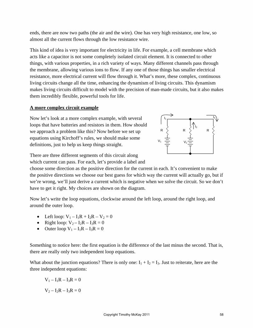
ends, there are now two paths (the air and the wire). One has very high resistance, one low, so almost all the current flows through the low resistance wire.

This kind of idea is very important for electricity in life. For example, a cell membrane which acts like a capacitor is not some completely isolated circuit element. It is connected to other things, with various properties, in a rich variety of ways. Many different channels pass through the membrane, allowing various ions to flow. If any one of those things has smaller electrical resistance, more electrical current will flow through it. What’s more, these complex, continuous living circuits change all the time, enhancing the dynamism of living circuits. This dynamism makes living circuits difficult to model with the precision of man-made circuits, but it also makes them incredibly flexible, powerful tools for life.

A more complex circuit example

Now let’s look at a more complex example, with several loops that have batteries and resistors in them. How should we approach a problem like this? Now before we set up equations using Kirchoff’s rules, we should make some definitions, just to help us keep things straight.

There are three different segments of this circuit along which current can pass. For each, let’s provide a label and choose some direction as the positive direction for the current in each. It’s convenient to make the positive directions we choose our best guess for which way the current will actually go, but if we’re wrong, we’ll just derive a current which is negative when we solve the circuit. So we don’t have to get it right. My choices are shown on the diagram.

Now let’s write the loop equations, clockwise around the left loop, around the right loop, and around the outer loop.

• Left loop: V1 – I1R + I2R – V2 = 0 • Right loop: V2 – I2R – I3R = 0 • Outer loop V1 – I1R – I3R = 0

Something to notice here: the first equation is the difference of the last minus the second. That is, there are really only two independent loop equations.

What about the junction equations? There is only one: I1 + I2 = I3. Just to reiterate, here are the three independent equations:

V1 – I1R – I3R = 0

V2 – I2R – I3R = 0

V1

R R R

V2

I1

I2

I3


I1 + I2 = I3

There are three unknowns here, the three currents. So this is clearly a solvable problem.

Solving these: First, substitute for I3 in terms of I1 and I2 using the third equation in the first

V1 – I1R – (I1+I2)R = 0

I2 = (1/R)[V1 – 2I1R]

Now use this for I2 in the second equation

V2 – I2R – (I1+I2)R = 0

V2 – 2I2R – I1R = 0

V2 – 2[V1 – 2I1R] – I1R = 0

V2 – 2V1 + 3I1R = 0

I1 = (2V1 – V2)/3R

I2 = (1/R)[V1 – 2/3(2V1-V2)] = (2V2 – V1)/3R

I3 = (1/3R)(V1 + V2)

Here they are all laid out:

I1 = (2V1 – V2)/3R I2 = (2V2 – V1)/3R I3 = (V1 + V2)/3R

Do these make sense? In each case, the current has units of V/R, which Ohms law says it must. I3 will always be positive, which makes sense. These batteries both want to push current in the direction we chose. I1 and I2 have the same form, which also makes sense. They’re really interchangeable.

But both I1 and I2 can be either positive or negative. For example, if V1 > 2V2, then I2 will be negative. In this case, the potential difference across V1 is so big that it not only pushes current I3 down through the right hand branch, it also pushes current I2 down backwards through the battery in the central branch.

This is an essentially random example, just meant to show how you do this kind of analysis. You will be presented with a variety of these examples. With a little practice you can pick apart just about any circuit you make up.


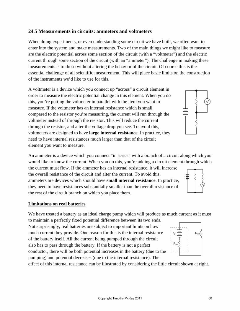
24.5 Measurements in circuits: ammeters and voltmeters

When doing experiments, or even understanding some circuit we have built, we often want to enter into the system and make measurements. Two of the main things we might like to measure are the electric potential across some section of the circuit (with a “voltmeter”) and the electric current through some section of the circuit (with an “ammeter”). The challenge in making these measurements is to do so without altering the behavior of the circuit. Of course this is the essential challenge of all scientific measurement. This will place basic limits on the construction of the instruments we’d like to use for this.

A voltmeter is a device which you connect up “across” a circuit element in order to measure the electric potential change in this element. When you do this, you’re putting the voltmeter in parallel with the item you want to measure. If the voltmeter has an internal resistance which is small compared to the resistor you’re measuring, the current will run through the voltmeter instead of through the resistor. This will reduce the current through the resistor, and alter the voltage drop you see. To avoid this, voltmeters are designed to have large internal resistance. In practice, they need to have internal resistances much larger than that of the circuit element you want to measure.

An ammeter is a device which you connect “in series” with a branch of a circuit along which you would like to know the current. When you do this, you’re adding a circuit element through which the current must flow. If the ammeter has an internal resistance, it will increase the overall resistance of the circuit and alter the current. To avoid this, ammeters are devices which should have small internal resistance. In practice, they need to have resistances substantially smaller than the overall resistance of the rest of the circuit branch on which you place them.

Limitations on real batteries

We have treated a battery as an ideal charge pump which will produce as much current as it must to maintain a perfectly fixed potential difference between its two ends. Not surprisingly, real batteries are subject to important limits on how much current they provide. One reason for this is the internal resistance of the battery itself. All the current being pumped through the circuit also has to pass through the battery. If the battery is not a perfect conductor, there will be both potential increases in the battery (due to the pumping) and potential decreases (due to the internal resistance). The effect of this internal resistance can be illustrated by considering the little circuit shown at right.

V

Rint

Rext


This one loop circuit has V – IRext – IRint = 0, and a total current given by I = V/(Rint + Rext). As usual, it’s useful to consider a couple of limits.

If Rext >> Rint, then we have what we usually assume. Essentially the whole potential rise put in by the battery shows up as a potential drop across Rext, and the current is I~V/Rext.

If Rint >> Rext, then things look very different. In this case, the whole potential rise being put in by the battery shows up as potential drop across Rint within the battery! The external resistor now has essentially no potential drop across it, even though a current I~V/Rint is flowing through it. After all, our condition requires that Rint>>Rext, so the voltage drop across Rext would be Vext = IRext = V(Rext/Rint) ~ 0.

So if a battery is to work as you’d like it to, you want the internal resistance of the battery to be small compared to whatever you hook it up to. If you violate this principle, the battery won’t function the way you would like. For example, if you “short circuit” the battery by connecting a conducting wire across its two terminals, the battery will pump a large current I=V/Rint. This will heat up the battery due to the power V2/Rint. Since Rint is probably small, the power consumed will be large, and the battery will rapidly use up its full store of internal energy.

If, instead, you hook it up to a large external resistance Rext, the current will be a much smaller I=V/Rext, the power consumed in the external resistance will be a much smaller V2/Rext. There will still be power consumed in the battery itself, but this will be small, approximately I2Rint = V2/Rext*(Rint/Rext).

24.6 Time dependence: RC circuits

So far we’ve looked at static cases: at currents and voltages that don’t change with time. This is easy for circuits which contain only batteries and resistors. Resistors “start resisting” immediately when you turn on a voltage, and stop immediately when you remove it.

Introducing capacitors in circuits changes this: they take time to build up or drain off charge. The charge on them at any instant determines the electric potential across them according to V = Q/C. The charge built up on (or removed from) a capacitor is a time integral of the electric current flowing in the circuit. In this sense, it’s a kind of memory of what has happened in the circuit, and imposes time dependence in circuits.

The basic features of this time dependence can be explored by analyzing the simple circuit at right. This circuit has a battery with potential V, a resistor R, and a capacitor C. The switch in the circuit allows us to connect the battery in a loop with the resistor and the capacitor, or to switch over to a case where only the resistor and capacitor is in the loop.

V

C

R


Consider the case with the battery in the loop (the position shown) first. For this loop, we have the loop equation:

0QV IRC

− − =

At the first instant there will be no charge on the capacitor at all, and the loop equation will reduce to:

V – I0R = 0 or 0VIR

=

As time goes on, this current will dump more and more charge onto the capacitor, until eventually the capacitor is filled, and the current falls to zero. Now, at this final time, we’ll have I=0, and:

0 or ff

QV Q CV

C− = =

So we’re going to start with a large current I0, which will then gradually fall off until we have some total charge Qf on the capacitor.

We can work this out in general too, if we recognize that the current I is given by the time rate of

change of the charge dQdt

. Now we can write the general loop equation as:

0 or dQ Q dQ Q VV Rdt C dt RC R

− − = + =

This is a linear differential equation for the charge as a function of time. Any function Q(t) which satisfies this equation would tell us how the charge changes as a function of time. Just looking at this, it says the time derivative of Q(t), plus the function Q(t) times a constant, is equal to some constant value. What sort of function has this property?

( ) ( )1 has a derivative t t

RC RCdQ VQ t CV e I t edt R

− −⎛ ⎞= − = =⎜ ⎟

⎝ ⎠

plugging this into the loop equation we find that it works:

1 1t t

RC RCdQ Q V Ve CV edt RC R RC R

− −⎛ ⎞+ = + − =⎜ ⎟

⎝ ⎠

So this solution works. It tells us exactly how the charge Q builds up with time, starting at zero and increasing to a final value CV:


( ) 1t

RCQ t CV e−⎛ ⎞

= −⎜ ⎟⎝ ⎠

And how the current starts at a large value and V/R and falls off to a final value of zero

( )t

RCdQ VI t edt R

−= =

What’s important here is how the time dependence works. We already knew what the initial and final states would be, but now we can see exactly how it will change from one to the other. It will vary exponentially.

How long will the change take? Looking at the equation for current, you can see that the current will drop off from its initial value V/R to a value (V/R)e-1 in a time τ = RC. This particular amount of time is called the “RC” time of this particular circuit. The time τ is how long it takes the current to fall to e-1 (or 0.37) of its initial maximum. It doesn’t tell us how long it will take the current to fall to zero. That actually takes infinitely long, but it does tell us how long it takes the current to change substantially. It characterizes the time variability of the system, tells us about how long things take to change.

The two processes, increase in charge and decrease in current, are shown in the figure to the right. The top curve shows how the charge (and hence voltage) builds up with time, while the bottom curve shows how the current falls off with time.

On this figure the time axis is labeled with an alternative “characteristic time”: t1/2. This is the time it takes the current to fall to ½ its original value, or the time it takes the charge to reach ½ its final value. This is related to the time constant t1/2 = ln(2)RC = τln(2) ~ 0.7τ.



Batteries and electric potential difference:

A battery is a device which will do what it must (including moving charge) to maintain a potential difference V between its poles. An ideal battery does this perfectly.

Resistance, potential, and current:

V IR=

Resistance and resistivity:

Resistivity ρ is a material property (like density or elastic modulus). A cylindrical resistor with length d and cross-sectional area A has resistance:

dRAρ

=

Resistors in series and parallel:

seriesequivalent parallel

equivalent

1 1 and ii

R RR R

= =∑ ∑

Power in current flows:

2

2 VP I R IVR

= = =

Kirchoff’s rules for circuit analysis:

• The Loop Rule: The sum of electric potential differences around any loop in a circuit must be equal to zero

• The Junction Rule: At any junction in a circuit, the sum of the electrical currents into and out of the junction must be equal

Real batteries and their limitations:

Real batteries have some internal resistance. When the current flowing through them becomes large, this internal resistance can have an important effect on circuits.

Time dependence in RC circuits:

Circuits containing resistors (which limit current) and capacitors (which must be charged) exhibit transient behavior, changing from an initial state steady state to a final steady state in a smooth


and continuous manner. The simplest ‘RC’ circuit in which the capacitor begins uncharged obeys the following relations:

batterycapacitor battery 1 and

t tRC RC

VQ CV e I e

R

− −⎛ ⎞= − =⎜ ⎟

⎝ ⎠

In general, such circuits will have time constants (in this case t = RC) which depend on the relevant resistors and capacitors.



25.1 Signaling and life

Later in this class we will talk extensively about how sensing the outside world is important for life. Organisms need to be able to sense what’s out there beyond them so that they can find what they need and avoid what they must. For this purpose they often use passive sensing, waiting for signals (light, sound) produced elsewhere to arrive at them. When that doesn’t work, many organisms switch over to active sensing; sending out signals which elicit response from what’s out there. Often the response is as simple as echoes or reflections, but sometimes it involves more subtle things like variations in the electric field. In all of this sensing, signals are being sent from one place to another. Usually these signals are electromagnetic or acoustic, mostly because signals like this travel so fast.

Living things need to do more than just sense the outside world. They need also to both sense and control their inner world. They need to send signals to and receive information from the many different parts of their own bodies. And these signals need to be extremely specific. The message that light has been sensed by a particular rod in your eye needs to go to just the right place in your brain. It’s not enough, for example, for each rod cell to just use sound, letting out an “I’ve detected light!” shout. The resulting cacophony would be useless. Specific messages have to reliably, and very quickly, get to specific places.

Likewise the control messages have to be extremely specific. Catching a ball requires an exquisitely precise, carefully coordinated series of control signals. Every one has to get to the right place at the right time. These signals coordinate the myriad muscles in your arm with the rapidly changing signals coming from your eye in just the right way to have your hand end up, open and oriented the correct way, at just the moment the ball arrives.

Accomplishing all this requires a system which knows what to do and can rapidly transmit signals very specifically from one place to another; a network of independently operable message channels which work rapidly and reliably. It requires a brain and a nervous system. The brain and the nervous systems are iconically complex; the ideal example of something we are still unable to analyze in detail. Exploring how they really work is well beyond this class. But we can at least get a sense for one key physical mechanism which allows these systems to work. So today we’ll discuss a simple model for how an electrical signal propagates within a nerve cell.

25.2 Nerve cells: basic structure

Like all cells, nerve cells have an interior partially isolated from their surroundings by a membrane. This membrane is incredibly important, as it enables the cell to control the conditions in which it conducts its business, making possible all the complex biochemistry needed to stay


alive. Cell membranes are also extremely complex, and include many mechanisms for controlling the transport of different materials into and out of the cell. These mechanisms will play a key role in signal transmission on nerves.

Nerve cells are very different from other cells in their shape. Instead of a compact spherical or oval shape, nerve cells have extraordinary, often very long, thin, cylindrical extensions called “axons”. This is illustrated in the figure above. The figure is way out of scale. The typical size of the main cell body (the Soma) is a few to a hundred microns across, while the axons are about one micron thick and range in length from one millimeter (103 microns) to more than a meter (106 microns). On the far end the axon branches out, terminating at a number of “synapses”. At synapses the nerve cell ends, and is separated by a very narrow gap, typically only about 20 nanometers, from a neighboring cell.

It may help to compare this to a road system. Imagine the axon were a typical two lane road, let’s say 10 m across. On this scale, the Soma might be stadium sized, a few hundred meters in diameter. The axon road would stretch from this stadium at least 10 kilometers (like across Ann Arbor), and perhaps as far as 10,000 kilometers (or about ¼ of the way around the Earth). On the far end, the axon road would end and be separated from connecting axons by synaptic gaps which are about 20 centimeters (less than a foot) wide. Nerve cells take on these crazily elongated shapes to guarantee specific connections for communication.

Signals travel rapidly down the axons as electrical disturbances. When they reach the synapse they trigger the release of special chemicals called “neurotransmitters”, which diffuse across the gap, carrying the control signal through the next step. Since the gap between the two synapses is very thin, this chemical diffusion happens very quickly. This combination, rapid electrical transport through outrageously elongated cells, combined with rapid chemical diffusion from synapse to synapse, is what allows your body to send signals from the brain to a distant cell incredibly quickly.

Many animals have additional structures on their axons called “Schwann cells”. Each of these is a little segment, typically about 1 mm long, wrapped in myelin. Myelin is a phosolipid membrane which encloses these regions. This myelin wrapping changes the properties of the axon in these regions, increasing the electrical resistance by a large factor (perhaps 5000) while decreasing the capacitance (by something like a factor of 50).

Schwann cells are separated by short (~ 1 μm) gaps called the “nodes of Ranvier”. At these locations the normal axon membrane is exposed to the intercellular fluid. As we’ll see, the Schwann cells allow the nerve signal to travel very rapidly. This being the case, you’d think the best nerve cell would just have the whole axon wrapped in myelin. But unfortunately, the signal


amplitude drops as it travels down the myelinated Schwann cell. After a millimeter or so, it’s really dropping off. That’s where the nodes of Ranvier come in. They act as little signal amplifiers, boosting the nerve impulse back up and sending it off into the next Schwann cell.

That’s a descriptive picture for how a nerve cell works. Let’s look now at the specifics of a few pieces of their physical function.

6.3 Membranes, ion transport, and the Nernst equation

In most of our technology, electrical signals are carried by traveling electrons. In nerve cells, electrical signals are related instead to the motion of positive and negative ions. To understand how this works, we need to return to a basic idea from Physics 135, the entropic origin of diffusion.

Imagine a cell membrane surrounded on both sides by electrically neutral mixes of positive and negative ions. Now imagine that the positive ions can penetrate the membrane, while negative ions cannot. Here’s a picture taken from an upcoming book “Physical Biology of the Cell” by Phillips, Kondev, and Theriot which gives the idea:

If the concentration of ions on the two sides of the membrane (C1 and C2) are the same, then equal numbers of positive ions will move left and right, and nothing very interesting will happen.

But imagine that the concentrations are different, so that C1 < C2. Remember, though both sides still start electrically neutral, there are just more ions (both positive and negative) on the outside than the inside. What will happen now? In this case, more positive ions will move to the left than the right, just by random chance, only because there are more of them available on the right ready to move left than vice versa. This directed motion (to the left) emerging from a purely random process is what I mean when I speak of the ‘entropic origin of diffusion’. Other things being equal, positive charge would continue to flow until the concentration of positive charges is equal on the two sides, at which point they would flow back and forth, left and right, in equal amounts.


But things are not equal. If more positive charge moves left than right, the two sides will no longer remain electrically neutral. Instead, the left side will gradually become positive, while the right side will become negative. In the end there will be an electric potential difference between the two. This has a consequence. Once positive charge starts to build up on the left, it acts to prevent new positive charge from entering, pushing it back toward the right.

If the electric potential difference between the two sides is ΔV, the energy required for an ion to move from right to left is ΔE = qionΔV. The only thing which will allow a positive ion to climb that barrier, to move upstream to the left, is the fact that each ion possesses thermal energy, the random motion associated with heat. Recall that the typical amount of thermal energy possessed by such an ion is given by Ethermal = kBT, with kB the Boltzmann constant 1.38x10-23 J/K.

These two effects, the random thermal motion and the cost of climbing into a higher electric potential, are balanced in the following way. The probability of a new positive ion moving to the left can be written:

Does this make sense? If the change in potential energy qionΔV is zero (as it is at the start), this probability is one. If the change potential energy qionΔV is very large, this probability becomes zero. But if the change in potential energy qionΔV is about equal to the typical thermal energy kBT, the probability of moving from right to left is decent; roughly e-1 or around 34%. So what happens is that positive charge builds up on the left until qionΔV ~ kBT.

This probability allows us to write the ratio of the final concentrations on the two sides in the following form:

And turning this around, we can find what potential difference ΔV will emerge given a certain concentration ratio c1/c2:

Let’s look closely at this equation, which is one form of what is called the Nernst equation.

TkVq

leftB

ion

epΔ

−

∝

1

2

ion

B

q Vk Tc e

c

− Δ

=

⎟⎟⎠

⎞⎜⎜⎝

⎛−=−=Δ

2

121 ln

cc

qTkVVV

ion

B


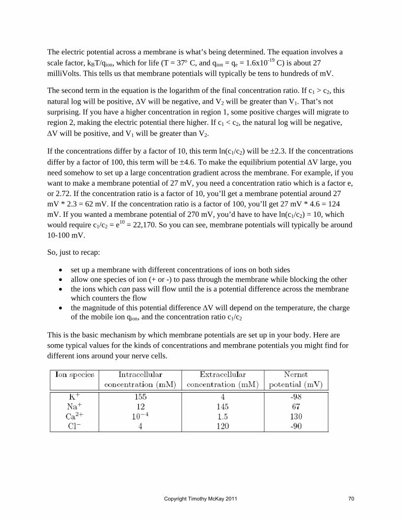
The electric potential across a membrane is what’s being determined. The equation involves a scale factor, kBT/qion, which for life (T = 37° C, and qion = qe = 1.6x10-19 C) is about 27 milliVolts. This tells us that membrane potentials will typically be tens to hundreds of mV.

The second term in the equation is the logarithm of the final concentration ratio. If c1 > c2, this natural log will be positive, ΔV will be negative, and V2 will be greater than V1. That’s not surprising. If you have a higher concentration in region 1, some positive charges will migrate to region 2, making the electric potential there higher. If c1 < c2, the natural log will be negative, ΔV will be positive, and V1 will be greater than V2.

If the concentrations differ by a factor of 10, this term ln(c1/c2) will be ±2.3. If the concentrations differ by a factor of 100, this term will be ±4.6. To make the equilibrium potential ΔV large, you need somehow to set up a large concentration gradient across the membrane. For example, if you want to make a membrane potential of 27 mV, you need a concentration ratio which is a factor e, or 2.72. If the concentration ratio is a factor of 10, you’ll get a membrane potential around 27 mV * 2.3 = 62 mV. If the concentration ratio is a factor of 100, you’ll get 27 mV * 4.6 = 124 mV. If you wanted a membrane potential of 270 mV, you’d have to have ln(c1/c2) = 10, which would require c1/c2 = e10 = 22,170. So you can see, membrane potentials will typically be around 10-100 mV.

So, just to recap:

• set up a membrane with different concentrations of ions on both sides • allow one species of ion (+ or -) to pass through the membrane while blocking the other • the ions which can pass will flow until the is a potential difference across the membrane

which counters the flow • the magnitude of this potential difference ΔV will depend on the temperature, the charge

of the mobile ion qion, and the concentration ratio c1/c2

This is the basic mechanism by which membrane potentials are set up in your body. Here are some typical values for the kinds of concentrations and membrane potentials you might find for different ions around your nerve cells.


Controlling transport and setting the “resting potential”

The simple picture presented above explains how a potential difference can be generated across a cell membrane, and gives an approximate calculation for how large this will be. To understand what really happens in a cell, we must remember several things:

• there are many ions in play, a few of the most important are listed above • transport of ions through the cell membrane can be changed rapidly, turning on and off

the flow of various ions • there are several hundred different kinds of ion channels in your cell membranes, each of

which has different selectivity for ions

All of this complexity allows nerve cells to function in a wide variety of ways.

Excitable membranes and the “action potential”

Through the mechanisms describe above, a membrane can become “polarized”, with each little bit of it acting like a charged capacitor. Concentration gradients between the inside and outside of the cell drive the charging of this membrane as discussed above. The charge state of this membrane capacitor at any time is governed by the inside and outside concentration of each of the many ions which is around, along with the ease with which each passes through the membrane.

This last bit is the key. The conductivity of various ions through the membrane can be changed in large and rapid ways. By altering this conductivity, the polarization of the membrane can be altered. Signals are sent in nerves by altering the membrane polarization in a transient way. Let’s look first at what happens, then try to get a sense of how it happens.

Now a repeated caution; what happens in nerve cells is, like many biological circumstances, complicated. It’s different in detail in different kinds of cells. But it always acts something like this, and is always governed by the same basic physics of charge flow described above.

Imagine a long axon sitting undisturbed. If everything is working right, there should be a resting potential of around -90 mV all along it. This is set up primarily by transport of Potassium and Sodium across the membrane. The cell can sit there like this, nice and stable, for as long as conditions (ion concentrations, temperature, etc.) remain the same. So long as any changes to the membrane polarization (from, for example, flow of other ions) which occur are small, this situation is stable. The mechanisms which set up this resting potential in the first place will restore equilibrium for small disturbances.

If, however, something happens to alter the membrane potential beyond a modest threshold, a new effect may spring into action. If the local polarization of the membrane is reduced, so that it rises above a threshold state, a new channel for ion transport is suddenly opened. When this happens, positive Sodium (Na+) ions are suddenly able to diffuse through the membrane, and


they rush into the cell, driving the potential from negative to positive, reversing the polarization. This sudden flood stops when the membrane reaches the sodium equilibrium potential of about +67 mV (see the table above). After this the sodium conduction channels which opened the floodgates are closed, and the process which originally created the negative membrane takes over again, gradually pumping things back to the roughly -90mV resting potential seen before.

This pattern is illustrated for both weak (subthreshold) and strong stimuli in the figure below:

This figure shows the membrane potential at one particular location on the axon. What happens through the neuron is a chain reaction. When one patch is pulled high, it races higher still (as shown above). This drags up the potential of the neighboring patch, causing it to go over the threshold, which drags up the next one, etc.

This transient depolarization of the membrane moves along it with a speed set by the specific capacitance of the membrane and the conductance of the ion channels (remember that conductance is the inverse of resistance). If the conductance is high or the capacitance is low, this can all happen fast. If the conductance is low, or the capacitance is high, it will take longer.



Diffusion, concentration gradients, and the charging of a membrane:

When only one sign of ion can diffuse across a membrane and a concentration gradient exists, it will diffuse until an electric potential builds up across the membrane.

inin-out

out

lnB

ion

k T cVq c

⎛ ⎞Δ = − ⎜ ⎟

⎝ ⎠

This basic mechanism is what charges membranes. The membrane potential can be altered by altering the conductivity of the membrane, opening and closing ion channels which allow different ions to pass.

The difference between diffusion of charge and diffusion of neutral atoms:

Neutral atoms will always continue to diffuse until concentration gradients are eliminated. These ions do not, instead their random flow is quickly halted by the emergence of potential differences which resist their flow.



26.0 Adding a new element: magnetism

Today we’re going to begin adding a crucial new element to our existing discussion of electricity: magnetism. Some of the phenomena of both electricity and magnetism were known in ancient times. At the time they seemed completely separate. A magnet doesn’t attract electric charges, and electric charges don’t affect compass needles.

There was one similarity. Both electricity and magnetism involved “action-at-a-distance” forces. Both had the ability to reach out across empty space and grab things. We have seen for electricity that this mysterious ability to affect distant objects can be understood as a consequence of an electric field which is present at every point in space. Not surprisingly, we will soon be introducing a “magnetic field”.

By the time we are done, we will see that electricity and magnetism are not just similar, and not just related in a variety of ways. They’re actually just different aspects of one underlying phenomenon: electromagnetism. The connections between electricity and magnetism were initially overlooked because in purely static circumstances, there are no connections. Electricity and magnetism come together only in dynamic situations, at times when something is changing. Electric charges will affect magnetism only when they are moving. Magnets will affect electric charges only when they are moving. This leads to many beautiful and subtle connections between the two. It also means that calculus, which describes motion and other change, will be central to expressing these connections.

But we will begin again with the simple: magnetostatics.

7.1 Mapping a magnetic field

Experimentation with magnetism began in the ancient world, with natural magnets: stones which exhibit magnetic phenomena. In Greece, these stones were commonly found in the region called Magnesia; hence the name. Such magnets have two “poles”, called a north pole and a south pole. A little piece of this sort of rock, if suspended so that it can spin without friction, will align itself so that its ‘north pole’ points toward geographic North.

Two of these magnets will interact with one another, with north poles repelling north poles, south poles repelling south poles, and north poles attracting south poles. This ability to reach out and act at a distance suggested to Faraday that a magnetic field existed in addition to an electric field.

To map an electric field, you take a test charge to each point, measure the force on it, then the electric field E = F/q. To map the magnetic field, Faraday took advantage of the tendency of little magnets, compass needles if you like, to align with a local field. Taking a little magnet to each point and looking at how they line up you can map the magnetic field. What you find when you do


this is magnetic field lines which come out of the north pole of a magnet and loop around to go back into the south pole. Note the similarity between this magnetic field and the electric “dipole” field created by one positive and one negative charge.

It is useful to compare directly electric and magnetic fields, just to emphasize their similarities and differences.

Electric charges can be separated into positive and negative charges

North and South magnetic poles always come in pairs

Electric field lines emerge from positive charges, the sources of electric field

Magnetic field lines emerge from the north poles of magnets

Electric field lines go into negative charges, the sinks of electric field

Magnetic field lines go into the south poles of magnets

Electric field is mapped by measuring the force on test charges

Magnetic field is by examining the alignment of magnetic dipoles

One remarkable difference between electric and magnetic charges is that in magnetism you never find “monopoles”. You can never take a magnet which starts with a north and south pole, split it in half, and end up with a separate north pole and south pole. This is perfectly possible with electric charge, but not the magnet poles. The reasons for this asymmetry remain unknown, though many suspect they are related to very fundamental questions in physics.

The Earth as a magnet

The Earth itself is such a dipole magnet. If you think a bit about what the magnets in compasses do when you use them, you should be able to see that the north pole of the Earth’s internal magnet is at the geographic South pole (where the penguins live), rather than at the geographic North pole (where the polar bears live). The Earth’s magnetic dipole is not perfectly aligned with its axis of rotation; there is an angle of about 7.3° between them.

This intrinsic magnetic field of the Earth is thought to be generated by internal electric currents associated with the Earth’s molten core. We will see later that electric currents can indeed create magnetic fields. The Earth’s field plays several important roles for life. First, it helps to shield life on Earth from damaging high energy protons from the solar wind and cosmic rays by deflecting them toward the North and South magnetic poles. Second, the magnetic field of the Earth is present all the time, day and night, cloudy and clear. As a result, many organisms use the Earth’s field to navigate over distances both very large and quite small.

On long timescales, the Earth’s magnetic field is rather unstable. The magnetic poles wander relative to the geographic poles on timescales measured in years. Meanwhile there are also much rarer and more


dramatic changes. Every so often, typically once a million years, the magnetic field of the Earth actually reverses direction. These magnetic field reversals are not completely understood, though the geological evidence for their reality is incontrovertible.

26.2 Magnetic forces on a moving charge

The first connection between electricity and magnetism involves electric charges moving through a magnetic field. An electric charge in a magnetic field will experience a force if it is moving through the field and the velocity of the charge has at least some component perpendicular to the magnetic field direction. We can quantify this force by writing:

We’ve used the cross product notation here to signify that this force depends on the perpendicularity of the particle velocity and the magnetic field. In addition, this notation tells us the direction of this magnetic force. It’s useful to single out a number of features of this:

• The force acts in direction perpendicular to both the particle velocity v and the magnetic field B • The magnitude of this force can be written qvBsin(θ) (where θ is the angle between v and B), or

qv⊥B (where v⊥ is the component of v perpendicular to B), or as qvB⊥. In any case, it depends on the charge, and the velocity, the magnetic field, and the degree to which v is ⊥ to B

• If the velocity of the particle is entirely along the direction of the magnetic field, there will be no magnetic force

• Since the force always acts perpendicular to the direction of motion, it can never do work on the charge, it can never change its energy

In fact this magnetic force is just a part of a larger “electromagnetic” force usually called the Lorentz force on a charge. This can be written more generally:

This Lorentz force includes both electric and magnetic forces which a charge q might experience.

Quantifying the magnetic field

This magnetic force can be (and is) used to quantify the magnetic field, rather than simply to map it. It defines the magnitude of the magnetic field as:

FBqv⊥

=

The units for magnetic field are N/C(m/s) = Ns/Cm. One Newton-second per Coulomb-meter is called one “Tesla” (T), a unit named for electrical inventor Nikolai Tesla. It turns out that one Tesla is a pretty large field, so it is common to use an alternative unit, the Gauss. They are simply related:

BvqFMagnetic ×=

( )BvEqFLorentz ×+=


1 Gauss = 10-4 Tesla

What happens to a charge moving in a magnetic field? Let’s take a simple example, a charged particle moving with velocity v in a plane perpendicular to a constant magnetic field B. In this case, since the angle between v and B is 90°, the magnitude of the force is F=qvB. It acts perpendicular to the velocity, and will cause the particle to travel in a circle, with the magnetic force providing the “centripetal force” required for it to circulate. The radius of the circle it will orbit in is given by:

2mv mvqvB = or r =

qBr

Notice that the top of this is the momentum of the charged particle. If this momentum is large it is difficult to change the direction of motion of the particle, and the radius of the circle it orbits in will be large. If the magnetic field or the charge of the particle is large, then there will be a lot of force available to turn the particle. This will cause the radius of the circle in which it orbits be smaller.

One thing to beware of in this: the magnetic force depends on the electric charge of the moving particle. Since electric charges come in both signs (positive and negative) the direction of the magnetic force depends on the sign of this charge. A moving positive charge and a moving negative charge with the same velocity will experience forces in opposite directions. In the example above, while a positive charge will circulate clockwise, a negative charge would circulate counterclockwise.

If the velocity of the particle is not completely perpendicular to the magnetic field then the particle will travel in a helical path, rather than a circle. The part of the velocity along the field continues unchanged, while the part perpendicular to the field turns around and around, with the particle spiraling along the field line. If field lines bend gradually, the particles may spiral along the lines, following them. This effect is important for guiding solar wind particles into the atmosphere near the North and South poles of the Earth, where they smash into the atmosphere, producing the Aurora. This mechanism is also important for solar flares.

26.3 Mass spectrometers: an important application

There is one very important practical application of the magnetic force on moving particles: the mass spectrometer. Just as an optical spectrometer takes light and analyzes its content by spreading it out, the magnetic spectrometer takes charged particles and analyzes them by spreading them out.

The basic mass spectrometer begins with some charged particles with charge qi and masses mi which you want to identify. The process begins by accelerating the particles with an electric field. Once they have been sped up, the


particles are injected into a region of constant magnetic field. Once in this region with field the paths of the charged particles bend, with a radius of curvature which depends on both the charge and momentum of the particle according to the equation r = mv/qB.

By recording where the ions land, you can determine what kinds of particles are present in the beam. Mass spectrometry of this kind is particularly good for identifying the composition of very small samples, since it effectively counts very small numbers of atoms. Let’s work out the details for a simple example.

First atoms you’re interested in have to be vaporized, so they are free to move, and ionized, so they may be accelerated and analyzed. There are various ways to do this, but let’s assume it is done and that each is ionized and has a positive charge +qion. The process then continues by accelerating the ions across an electric potential difference V. This gives them an energy qionV = 1/2mionv2. This can be used to find the velocity:

v = (2qionV/mion)1/2

The particles then enter the region of constant magnetic field and have their paths bent with radii that depend on their charge and mass. Putting in the velocity from the accelerating stage, we find

ion ion ion ion

ion

m m 2q 2m1r = = = q Bion ion ion

v V Vq B B m q

If you then measure r, B, and V, the charge to mass ratio of the ions is

2 2

2ion

ion

q Vm r B

=

Notice that all you can really measure with this is the “charge-to-mass” ratio of the ions, rather than their masses. Since the ions can only be charge in integer multiples of the electron charge, you can often work out from this the actual masses of the ions as well.

Applications of mass spectrometry

Mass spectrometry is used in many applications where identification of small samples is needed. It is especially useful, nearly essential, for the identification of different isotopes of an element in a sample. Isotopes are atoms with the same number of protons, and hence electrons, but different numbers of neutrons. These are denoted by adding to the chemical symbol the combined number of protons and neutrons in the nucleus. For example 12C is “carbon 12”, the usual type of Carbon with 6 protons and 6 neutrons. Alternative forms include 13C and 14C.

Because they have the same numbers of electrons different isotopes are chemically almost identical, though they may have quite different masses. Their chemical similarity makes it very difficult to separate them out using chemical methods. Mass spectrographs, which separate based solely on the charge to mass ratio, are much more useful for this purpose. As a result, they are the essential tool for determining isotopic composition. Knowing the isotopic composition of an object can provide important clues about the origin of an object. A few applications follow.


Isotopic Dating

Carbon appears in the atmosphere in three isotopic forms. 12C is the most common, making up 98.93% of naturally occurring carbon. 13C is also relatively common, making up almost all of the remaining 1.07%. A very small amount of 14C is also present, about one part in a trillion (10-12). It is rare because it is radioactive, decaying into 14N with a time constant of 5730 years. This means that if you begin with some number of 14C atoms N0, you will find after some time t that the amount remaining is:

N(t) = N0e-(t/5730 years)

This decay is the reason for the rarity of 14C. Any 14C which might have been present at the formation of the Earth is long gone. The only way to have any in the atmosphere now is to produce it anew. This happens on Earth when energy ions called cosmic rays smash into the top of the atmosphere. This production mechanism is adequate to maintain the tiny pool of 14C which we typically find.

Living things are built partly of carbon, which they absorb from the atmosphere. So you and I have about a part in a trillion of our carbon in this radioactive 14C form. Once you die, your body stops incorporating new carbon. From then on, the fraction of 14C in your remains falls according to the decay law above.

If you find organic remains and can accurately measure this 14C content, you can tell how long ago they died. This is a prime means for measuring the age of organic remains, and is accurate for organic material with ages less than about 40,000 years.

Other forms of isotopic dating exist, similar in spirit, but differing in the half-lives of the radioactive elements they rely on. For example, 238U has a half-life of about 80,000 years. Various techniques of this kind have been used to determine the age of the rocks which make up the Earth, currently best estimated as 4.56 billion years.

Material analysis

Mass spectrometers are increasingly important for protein characterization, and essential part of modern biochemistry. They are also extensively used in space exploration, where they provide a simple and reliable method for identifying the composition of materials in space and in the atmospheres of other solar system bodies.

26.4 Magnetic force on a current carrying wire

We have seen last time that a magnetic force is created when a charged particle moves through a magnetic field with a velocity at least partly perpendicular to the field. The same force acts when charges travel in a wire which carries a current. A little piece of such a wire with length ΔL has a total charge passing in some time:

totLq I t I

vΔ

= Δ =


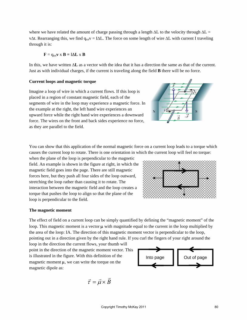
where we have related the amount of charge passing through a length ΔL to the velocity through ΔL = vΔt. Rearranging this, we find qtotv = IΔL. The force on some length of wire ΔL with current I traveling through it is:

F = qtotv x B = IΔL x B

In this, we have written ΔL as a vector with the idea that it has a direction the same as that of the current. Just as with individual charges, if the current is traveling along the field B there will be no force.

Current loops and magnetic torque

Imagine a loop of wire in which a current flows. If this loop is placed in a region of constant magnetic field, each of the segments of wire in the loop may experience a magnetic force. In the example at the right, the left hand wire experiences an upward force while the right hand wire experiences a downward force. The wires on the front and back sides experience no force, as they are parallel to the field.

You can show that this application of the normal magnetic force on a current loop leads to a torque which causes the current loop to rotate. There is one orientation in which the current loop will feel no torque: when the plane of the loop is perpendicular to the magnetic field. An example is shown in the figure at right, in which the magnetic field goes into the page. There are still magnetic forces here, but they push all four sides of the loop outward, stretching the loop rather than causing it to rotate. The interaction between the magnetic field and the loop creates a torque that pushes the loop to align so that the plane of the loop is perpendicular to the field.

The magnetic moment

The effect of field on a current loop can be simply quantified by defining the “magnetic moment” of the loop. This magnetic moment is a vector μ with magnitude equal to the current in the loop multiplied by the area of the loop: IA. The direction of this magnetic moment vector is perpendicular to the loop, pointing out in a direction given by the right hand rule. If you curl the fingers of your right around the loop in the direction the current flows, your thumb will point in the direction of the magnetic moment vector. This is illustrated in the figure. With this definition of the magnetic moment μ, we can write the torque on the magnetic dipole as:

Into page Out of page

B×= μτ


When μ is parallel to B, the torque on the loop is zero. When μ is not parallel to B, there is a magnetic torque which tends to align the magnetic moment of the loop with the field B.

In this way, a little current loop acts exactly like a little compass needle. Both are pushed to align with a magnetic field, but are able to remain at rest so long as they are so aligned. As it turns out, we can treat a little current loop like this exactly as if it were a little magnet. Even more than this, we will see that such a little current loop actually is a little magnet. We care about such little current loops both because some of our technology (especially electrical generators) uses such loops. But also because electrons orbiting atoms are also little current loops, and these can give atoms magnetic moments which tend to make them align with fields.

26.5 Moving charges produce magnetic fields: the law of Biot-Savart

The next major connection between electricity and magnetism has to do with the way in which magnetic fields are produced. It was first discovered by Oersted, who was experimenting with currents produced by batteries for the first time. He noticed, apparently by accident, that when he turned a current on in a wire, nearby compass needles changed the direction they pointed, and when he turned it off, they returned to their original orientation. He correctly surmised that the current was actually producing a new magnetic field.

The magnetic field produced by a little piece of current with length dL carrying current I is given by the Biot-Savart law, which we give here compared to the familiar form for the electric field due to a charge dQ:

There are a few things to notice. First, there’s a new strength constant here. Instead of k=1/4πε0=9x109Nm2/C2, we have μ0/4π = 10-7 Tm/A. The constant μ0 which shows up here is called the “permeability of free space”, and has a magnitude μ0 = 4πx10-7 Ns2/C2. Second, the direction of this little bit of magnetic field dB is perpendicular to both dL, and r, the vector which extends from the current segment to the point where you want to know the field. In the case shown in the figure here dL x r is a vector into the page, so that’s the direction of the bit of magnetic field produced at point P by this bit of current.

Just as we can use the formula for electric field from a charge to find the electric field from any charge distribution, so too we can use this Biot-Savart formula to determine the magnetic field from any set of currents that might flow. There are a few important, simple arrangements for which it is useful to know the answers.

20 ˆ

4 rrLIdBd ×

=πμ

20

ˆ4

1r

rdQEdπε

=


Field due to an infinite wire

The magnetic field due to an infinite wire is very simple. It circulates around the wire in rings, with a magnitude that falls off as you go farther from the wire. The magnitude of the field is given by the simple relation:

The direction of the magnetic field produced by this wire is given by the right hand rule, as shown in the figure. As usual, we can use this result even when the wire isn’t actually infinite, so long as we are interested in the field at distances from the wire much less than the actual length of the wire.

Field due to a current loop

A current loop produces magnetic field which looks like that of a magnetic dipole. It has magnetic field lines which come out the top of the loop and circulate back into the bottom of the loop. From the Biot-Savart law, it is easy to show that the field right at the center of the loop with radius rloop has magnitude:

Be careful with this result. This is only the field at the center of the loop. The shape of the field at other points is shown in the figure, but its magnitude varies in a relatively complex way. Notice that the shape of this field produced by a current loop is just like the dipole magnetic field produced by a permanent magnet. They are in fact precisely the same, and permanent magnets are actually due to little atomic current loops from a bunch of atoms with magnetic moments aligned.

Field due to a solenoid: a whole stack of loops

If we take a whole series of loops and stack them on top of one another, as we might do if we made a tightly wound coil of wire, we would make a “solenoid”. If we assume that this stack of coils is infinite in length (impossible, but possible to reasonably approximate) then we can show that the internal magnetic field, inside the coil, is constant in space everywhere in the coil and has magnitude:

where N is the total number of loops of wire stacked up in the solenoid and L is the total length. This is sometimes written in the second form

rIB

πμ2

0=

looprIB

20μ=

InLNIB 00 μμ ==


with n=N/L equal to the number of coils per unit length. The solenoid, like a single loop, looks and acts like a normal bar magnet. It too is a magnetic dipole and will generally want to align with a magnetic field.

A nice tool for these calculations: Ampere’s Law

There is a powerful theorem relating magnetic field to currents which can be used in deriving some of the results above called Ampere’s Law. It says that if you imagine a loop in space and can go around that loop adding up at every point the amount by which the magnetic field is along the loop, that sum will be related to the total current which passes through the loop. We write this mathematically as:

The left hand side of this is called a contour integral or a line integral, and it means what we said above. Choose a loop in space, then go all the way around it, calculating B⋅dl for each little segment and adding it up. This integral is then equal to a constant (it’s just a sum of scalar dot products) which is related to the amount of current which passes through the loop.

Now while this is always true, it’s not always so useful. But let’s look at one example where it is; the magnetic field due to an infinite wire. In this case, we know the magnetic field will circulate around the wire. Symmetry argues that it should not vary along the wire, though it might vary as you move away from the wire. Let’s take the loop on top of the picture. Here B is always along dl, so B⋅dl is just Bdl, and the loop integral is just B(2πr). Ampere’s law tells us:

B(2πr) = μ0I or 2

o IBr

μπ

=

This is just the result we saw above. It can also be derived from the Biot-Savart relation, but this much more general Ampere’s law makes it simpler to show.

26.6 Magnetic forces between wires, in loops, and in solenoids

Now we can combine two ideas from above; the notion that a current carrying wire in a magnetic field will experience a force, and that a current carrying wire will produce a magnetic field. Let’s consider two parallel wires, separated by a distance r, with a current I traveling in each of them. Wire 1 will produce a magnetic field at the location of wire 2. In our picture here both currents go into the page. For this, the field from wire 1 circulates clockwise, making the ILxB force pull wire 2 to the right. Not surprisingly, the field produced by wire 2 and wire 1 creates an equal and opposite force on wire 1, pulling it toward wire 2. The magnitude of each force is:

∫ =⋅ enclosedIldB 0μ


Any two wires in which the current runs in the same direction are attracted to one another, while any two wires in which the currents run opposite one another are repelled.

This effect has an important impact on current loops and solenoids. First consider a loop. Every point on the loop has another point straight across from it on which current flows in the opposite direction. This means each piece of the loop is being pushed outward. This magnetic self interaction pushes the loop to expand. Only some mechanical strength prevents the loop from pushing itself apart.

In a solenoid it’s even more complex and interesting. Each individual loop is pushed outward just as before, but now you also have one loop stacked up on another. These neighboring loops have currents flowing in the same direction. So even while each loop is trying to expand, the neighboring loops are being pulled together, creating forces which endeavor to squash the solenoid.

These internal forces can become very large in loops and solenoids in which large currents circulate. This is a major factor which must be considered in the design of large magnets like those used in magnetic resonance imaging in hospitals.

7.7 Dipoles in fields both uniform and not

We have seen that magnetic dipoles experience a torque if they are placed in a uniform magnetic field. This torque pushes the dipole to “align” with the field. It is helpful to remember that exactly the same thing happens with electric dipoles in electric fields. Here are the two laid out side by side:

LIrr

IILILBF 200

22 πμ

πμ

===

•

x

This is a magnetic dipole in a uniform magnetic field. There is no net force on the dipole, but there is a net torque which tends to align it with the field. The dipole moment μ=IA.

μ

Fx

F•

-

+

This is an electric dipole in a uniform electric field. There is no net force on the dipole, but there is a net torque which tends to align it with the field. The dipole moment p=qd.

p

F+

F-


In each case, the dipole won’t move in any direction on average, because there is no net force acting on it. But it will experience a torque that will make it rotate until its moment is aligned with the external field. When it does this, it will be at equilibrium. The net torque on such an aligned dipole is zero and the potential energy it has will be at a minimum.

There is one more thing to notice. In addition to the uniform external field, each dipole produces its own electric or magnetic field; a dipole field. When the dipole reaches its equilibrium, aligned state, the field from the dipole will be arranged to partly cancel the uniform external field. It is this fact that makes the aligned state the lowest energy state. In this aligned state there is actually less field, and since the field contains energy, there is less total energy around. This is shown in the figure to the right. In it, a uniform electric field (pointing down) is disturbed locally by the presence of an aligned electric dipole. In the region of the dipole the electric field strength is reduced. This reduction in field strength due to dipole response to a field is why electrostatic effects are so reduced in a polar medium like water. It is why we write the permittivity of water εwater = Dε0 with the factor D ~ 80. In water you need a LOT more external field to get the same effect as you would in a vacuum.

What happens if the dipoles are in non-uniform electric and magnetic fields? To see this, let’s draw a picture of such a situation for each:

When you put a dipole in a non-uniform field like this, it experiences both a net torque and a net force. It is this fact that actually causes magnets to attract one another, pulling one another together, instead of merely aligning with one another. When two magnets are far apart, the magnetic field the 2nd magnet sees from the first is nearly uniform. When they get closer, the 2nd magnet sees that the magnetic field from the

-

+

This is an electric dipole in a non-uniform electric field. Now there is a net force on the dipole. It will be pushed to the left and a little up. There is also a net torque which tends to align it with the field.

p

F+

F- •

x

This is a magnetic dipole in a non-uniform magnetic field. Now there is a net force on the dipole, it will be pushed up and a little right. There is also a net torque which tends to align it with the field.

μ

Fx

F•


first changes; it no longer looks like a uniform field. The effect gets stronger as they get closer. This is why two magnets aligned N to S and S to N will slowly move together, then once they get close they will “snap” into one another.

Just the opposite happens when the magnets are aligned N to N and S to S. Then when they get close they strongly repel one another.

Magnetic dipole oscillations

We have seen that a magnetic dipole in a uniform magnetic field will experience a torque which tends to align it with the external field. Imagine how the dynamics of this work:

• You start with a dipole and no field, then turn on the field in a direction not aligned with the dipole.

• It experiences a torque which starts it rotating toward the equilibrium alignment, rotating faster and faster

• It gets to the equilibrium alignment, but it’s moving fast, so it swings past. Now the torque is slowing it down

• Eventually, it stops moving past the aligned state, the torque pulls it back, and it swings back the other way

• It will continue oscillating back and forth around the equilibrium alignment, just like any oscillator

• The frequency of oscillation will depend (as it always does) on the strength of the restoring force and the inertia. In this “rotational oscillator” the restoring force is the torque due to the field, and the inertia due to the mass and shape of the dipole itself. Smaller, lower mass dipoles will oscillate more quickly. Larger, higher mass dipoles will oscillate more slowly.

• If there is damping (some way for energy to be drained from this oscillator) then the oscillations will either slowly die away (if it is underdamped) or will never occur (if it is overdamped).

Each dipole magnetic oscillator of this type will oscillate with an angular frequency known as the Larmor frequency: ω = γB. In this relation, both the strength of the magnetic moment of the dipole μ, and the inertia of the dipole (which slows oscillations) are included in the single factor γ. This factor γ is called the “gyromagnetic ratio” of the dipole. This angular frequency ω corresponds to a frequency of f = ω/2π = (γ/2π)B. It is fairly common to tabulate this factor γ/2π rather than γ.

This way of quantifying things is very useful when talking about the dipole moments of atomic nuclei because they are all quite precisely the same. Any two Hydrogen nuclei have the same magnetic properties, with γ/2π = 42.6 MHz / Tesla. If you put a Hydrogen nucleus in a 1 Tesla magnetic field, then bump it away from equilibrium, it will oscillate back and forth with a frequency of 42.6 MHz. That is, it will oscillate 42.6 million times per second. You can see that the more massive nuclei all have smaller frequencies of oscillation. This shouldn’t be surprising, as they all have more inertia.

Nucleus γ / 2π (MHz/T)

1H 42.576

3He 32.434

7Li 16.546

13C 10.705

14N 3.0766


Magnetic resonance imaging

These magnetic resonances are now one of the most important tools of medical imaging. Here’s how it works. You put the object (a person perhaps) you want to study in a strong magnetic field and wait a bit for all the magnetic dipoles in the sample to settle to equilibrium. Then you introduce a sudden change to a new stable field. This leaves all the magnetic dipoles in a non-aligned state. They all begin to oscillate, just as described above. As it turns out, an oscillating magnetic dipole like this will emit electromagnetic waves which have the frequency it oscillates with. So, an oscillating Hydrogen nucleus will emit radio waves with a frequency f = (γH/2π)B.

If you detect emission of radio waves with this frequency you know there is Hydrogen in the sample, and the magnitude of the signal tells you something about how much there is. To tell where the Hydrogen is in the sample (which you obviously need if you’re going to image the person), you make the magnetic field the person is in vary in space B(x,y,z). Each Hydrogen dipole oscillates with a frequency determined by its local field. Measuring how much radiation you get with each frequency tells you how much Hydrogen there is in each position (x,y,z). Measuring the mix of frequencies tells you about the distribution of Hydrogen nuclei in space.

Magnetic dipoles and life

Life on Earth lives embedded within the magnetic field of the Earth. Not surprisingly, living things have evolved ways to take advantage of this. Most of these involve navigation. The full range of animals able to sense magnetic fields in a manner adequate for navigation is unclear, but it is certain that many migratory species, including birds and probably marine mammals do. It is also clear that while the magnetic sense is useful to them, they actually navigate using a rich array of clues drawn from all their senses, very much as you might.

One surprising group of magnetic navigators is the magnetotatic bacteria. These are single-celled organisms which live in aquatic environments. They are motile, able to propel themselves through the water. They live in the anaerobic environments which characterize many marine sediments. So as a rule they want to swim to the bottom. But bacteria are not what you’d call smart, and lack very complex senses. Usually they just swim at random and stop if they land somewhere which seems better.

The trick of magnetotatic bacteria is to grow within themselves a little inorganic needle of magnetic material, usually Fe3O4 or Fe3S4. The magnetic dipole moment of this needle is large. When it interacts with the Earth’s magnetic field it generates a torque large enough to align the entire bacterium with the Earth’s field. Since the Earth’s magnetic field lines actually point down into or up out of the Earth (except at the equator), pointing along the field line can very nicely lead you into the muck on the bottom.

How to choose which way to go? Bacteria in the Northern hemisphere, where the field lines point down into the Earth would like to swim down along the direction of the field. Bacteria in the Southern hemisphere, where the field lines point up out of the Earth would like to swim opposite the direction of the field. So that’s just what they do. The picture below shows the arrangement of the needle for Northern


hemisphere examples and Southern hemisphere examples. The picture shows one of these beasts, inside of which you can easily see the little magnetic needle.

Northern Hemisphere

Southern Hemisphere



Mapping magnetic field:

Magnetic field can be mapped by placing small test magnets at each point; they will align with the magnetic field. The field of a typical bar magnet, or the Earth, is a dipole field, with a magnetic north pole that is a source of field lines, and a south pole that is a sink of field lines.

Magnetic forces on moving charges:

magneticF qv B= ×

Circular motion of a charge in a constant magnetic field:

mvrqB

⊥=

Mass spectrometry:

The circular motion created when a charged particle moves in a magnetic field can be used to separate particles with different properties in a mass spectrometer. A typical mass spectrometer might accelerate ions through an electric potential difference V, then measure their magnetic gyroradius r in a magnetic field B to find a charge to mass ratio:

2 2

2q Vm r B=

Force on a current carrying wire:

F i L B= Δ ×

Torque on a current loop:

with B IAτ μ μ= × =

Magnetic field produced by a current:

The general relation (analogous to Coulomb’s law) is the Biot-Savart law:

02

ˆ4

IdL rdBr

μπ

×=

This is used to find the magnetic field from a long wire, a loop at its center, and a solenoid.


0 0long wire center of loop solenoid 0 loops per meter

loop

ˆ and B and B2 2

I IB r Inr r

μ μ μπ

= = =

Currents and magnetic circulation – Ampere’s Law:

The fact that a current produces magnetic field that loops around it can be expressed as Ampere’s Law for magnetic circulation, which is closely related to Gauss’s Law for electric flux.

0 enclosedB dl Iμ=∫ i

Magnetic forces between wires:

Since currents created magnetic fields, and currents experience forces when in fields, currents induce magnetic forces on one another. Two parallel currents will attract one another, while antiparallel currents will repel one another. The size of this force depends generally on the product of the currents and the inverse of the distance between the wires.

Magnetic dipoles in magnetic fields:

A dipole in a constant field may experience a torque attempting to align it with the field. A dipole in a varying field may experience both a torque tending to align it with the field and a net force pushing it through the field. It is this effect, a net force exerted on a dipole in a non-unifrom magnetic field that causes two bar magnets to attract one another, rather than simply aligning with one another.

Oscillations of magnetic dipoles around magnetic field alignment:

If a magnetic dipole is moved out of alignment with the local magnetic field, it will oscillate around the aligned direction with an angular frequency determined by the gyromagnetic ratio of the dipole γ, which depends on both its dipole moment and its rotational inertia.

Bω γ=



Another connection: changing magnetic fields produce electric fields

We have seen already two connections between electric and magnetic phenomena:

• a charge moving in a magnetic field experiences a force F = qv x B (and as a result a current carrying wire also experiences a force Fwire = iL x B)

• a current produces a magnetic field

We now introduce a third connection between the two. The magnetic fields produced by currents were discovered by accident, by noticing that compass needles were deflected whenever sizable currents were turned off or on nearby. As soon as this was discovered, Michael Faraday set out to determine whether the opposite was true as well, whether a magnetic field could somehow produce a current.

He discovered very rapidly that if be moved a magnet around somewhere near a coil of wire, a current would be induced in the wire. This current came about as a result of an “electromotive force” or EMF. This EMF is really very like a voltage, in the sense that, if the loop has a total resistance R, the current in the loop will obey the relation:

EMF = IR or EMFIR

=

EMF is different from the voltage on a battery though.

Normally when we go around a loop in a circuit like we have done before, the total change in electric potential is zero. This is just Kirchoff’s loop rule. Now we’re saying that, in going around the loop once, the potential goes up by some amount equal to the EMF. You can think of it as being spread all the way around the loop, kind of like a distributed battery. It makes each little part of the loop like a small battery with

2dLV EMF

rπ=

in series with a little resistor

2dLdR R

rπ=

20 ˆ

4 rrLIdBd ×

=πμ


In a quick series of experiments he uncovered the main phenomenological features of the “magnetic induction”. These include:

1. A static, unchanging magnetic field induces no current at all 2. If the magnetic field going through the loop increases, the EMF increases. If the magnetic

field through the loop decreases the RMF is reversed, pushing current in the opposite direction.

3. The magnitude of the EMF depends on how rapidly the field through the loop is changing 4. The magnitude of the EMF depends on how many times the wire goes around the loop 5. Stronger magnetic fields produce bigger EMFs

27.1 Magnetic flux and Faraday’s law

To understand this magnetic induction in detail we need to define the “magnetic flux”. This magnetic flux measures how much magnetic field passes through some surface (like the interior of the loop). It is calculated by defining, for each little bit of the surface, an area vector dA. This vector has a magnitude equal to the area dA and a direction which is perpendicular to this little piece of surface. If the surface is a closed surface (like a sphere), the direction of dA is usually taken to be out of the surface. If it is not a closed surface (like a loop) the direction has to be clearly defined.

If some magnetic field is passing through this surface, then at the center of each little element dA there will be some magnetic field B. If the magnetic field goes straight out through the surface, the flux will be dA*B. If it goes straight along the surface, the magnetic flux will be zero. From these limits you can guess that the magnetic flux in general will be given by dΦB = dA⋅B = dA*B*cos(θ).

The total flux through the surface is then found by adding up the flux through each little bit dA:

In the example figure to the right you have B parallel to dA everywhere, so the total flux ΦB = BA. If we turned this loop sideways in the field, so the B would always be perpendicular to dA, then the magnetic flux through the loop would be zero.

Once you know how to calculate this flux, Faraday’s law tells you that the EMF induced in any loop is given by:

∫ ⋅=Φ AdBB

dtd BΦ

−== ξEMF


How might the magnetic flux through a loop change? There are three independent ways to do this:

• change the magnitude of the magnetic field • change the angle between the magnetic field and the loop • change the area of the loop

Of course it’s possible to do all three at once, but any one of them will result in a changing flux and consequently in a non-zero EMF.

The minus sign in Faraday’s law is really a reminder that the EMF will be induced in a way which resists this change in magnetic flux. How does this work? The EMF in the loop will produce a current IL = EMF / R. When this current in the loop flows, it will produce its own magnetic field. The field from the loop will itself produce some amount of magnetic flux through the loop. And here’s the connection: the current will flow in the loop in whatever direction is required to so that the flux from the loop will act to reduce the change in flux which is driving the EMF in the first place.

Let’s say that another way. If the flux through the loop due to the external field is reduced, the induced EMF will produce a current which will create flux that tries to replace the external flux which has disappeared. If the flux through the loop due to the external field is increased, the induced EMF will produce a current which will create flux that tries to eliminate the increase in external flux.

The figure at right shows an example. The magnet, with north pole down, is moving toward the loop. This increases the magnetic flux going down through the loop. The EMF will be induced so that it attempts to prevent this change. Since more magnetic field is going down through the loop, the current created by the EMF will flow to send field back up through the loop, trying to cancel the increase. To accomplish this, the current in the loop has to go counterclockwise as we see it here. If we pulled the magnet back upward, all of this would reverse. The external flux would decrease and the induced EMF would drive current the other direction, trying to replace the flux which has been lost.

How is EMF related to electric field? Remember back to our discussion of the relation between electrical potential V and electric field E. We said that the electrical field always points toward lower electric potential, and that if you add up the product of E⋅dl along a path from one place to


another you get the potential change ΔV. What we have here in the EMF is really adding up E⋅dl all the way around a loop. This allows us to write Faraday’s law of induction in another way:

When you have the magnetic flux through a loop changing, it means the sum of E⋅dl around that loop is non-zero. It means there is some net “circulation” of electric field around that loop. This alternate way of thinking about the EMF will be very important at the end of our discussion of electricity and magnetism next time.

Lenz’s law and energy

The direction of the induced EMF discussed above is sometimes called “Lenz’s Law”. There is a simple way to see, from energy conservation, that it must be so. Imagine a loop dropped into a region of uniform magnetic field pointing out of the page.

When the loop is at position A, falling downward, the magnetic flux through the loop is zero and not changing. No EMF is induced. When the loop starts to enter the field region (as at point B), the magnetic flux out through it begins to increase. A current is induced which resists this. The induced current produces magnetic field back into the page, to resist the increase coming out of the page. To do this, it must be a clockwise current.

At point C, in the midst of the fall, the magnetic flux is positive but unchanging. At this point again no EMF is produced. At point D, as it is leaving the magnetic field, the magnetic flux out through the loop is decreasing, and the induced current acts to try to replace the flux which is being lost. To do this, the induced current must be counterclockwise. Finally, at E, the flux is zero and unchanging so no current is induced.

Now we have to think about another aspect of this. After all, when the loop is at B it has a current flowing in it, and that current is actually in a magnetic field! Any current in a magnetic field experiences a force F = iL x B.

For this case, the net force on the loop due to this is:

• Point A: zero (there is no current and no field) • Point B: upward (it will tend to slow the fall of the loop)

A

B

C

D

E

dtdldE BΦ

−=⋅= ∫EMF


• Point C: zero (there is no current though there is field) • Point D: upward again! (it will also tend to slow the fall of the loop) • Point E: zero (there is again no current and no field)

Every time there is a magnetic force coming about because of the induced currents, it resists the motion, slowing the fall in this case.

Imagine what would happen if it worked the other way. This loop would reach the field region, be shoved forward by the magnetic force, cruise through the middle, then be accelerated again, falling faster in the presence of the field than without. All the time it would extract no energy from the external field, which doesn’t change at all. So this couldn’t happen; you can’t just create energy in the falling loop without paying for it!

You can, however, take energy out. Where does it go? The energy removed from the loop by slowing it shows up as Ohmic I2R energy losses in the loop itself. So of course it’s not lost, it’s just converted into thermal energy in the loop.

This is the real reason for Lenz’s Law, the minus sign in Faraday’s law of induction. If it weren’t there, Faraday’s law would violate the conservation of energy. While this would be cool, and would give us a source of free energy, it’s impossible.

Interestingly, the slowing observed in this falling ring occurs any time you move metal in a magnetic field. Imagine that, instead of a loop, you drop a solid piece of metal; something like a coin. Any time the magnetic flux through the coin changes, currents will be induced in the loop resisting this change, and as we have seen, they will flow in a direction which slows the fall of the coin. When fields are large these “eddy currents” and the energy losses associated with them can be huge. Try a search like “MRI magic” on you-tube if you want to see this in action.

27.2 Applications of magnetic induction

There are many different applications of magnetic induction. They include:

• Motion sensors (guitar pickups and microphones) • Metal detectors (like those you walk through at the airport or use at the beach to search

for pirate treasure) • Induction heating (eddy currents in a metal produce resistive heating, this can be used to

produce heat without a heat source)

But far and away the most important application of induction is in the process of transforming mechanical motion into electric current (as in electrical generators) and transforming electric current into mechanical motion (as in electric motors). The two are exact opposites of one another. Let’s look at generators first.


Electric ‘generators’

One simple form of electric generator has two main parts, a flat coil of wire and a permanent magnet. The coil is placed between the poles of the magnet so that the magnetic field going from north to south poles passes through the loop. The magnetic flux through this loop is then:

ΦB = ABcos(θ)

If the coil now rotates at a constant angular velocity so that θ = ωt, the magnetic flux will change with time:

dΦB/dt = -ABωsin(ωt)

and this makes the EMF in the loop :

ξ = -dΦB/dt = ABωsin(ωt)

There are several things to notice about this. First, the magnitude of the induced EMF depends on the area of the loop A, the magnitude of the magnetic field B, and the rate of rotation of the loop ω. To get a large EMF, make all three of these large. Another thing to notice, the EMF is not constant, it varies in time sinusoidally, from a maximum of ABω to a minimum of zero. It also changes direction, going first one way around the loop then the other. Notice too, the EMF is maximum with the angle θ is 90°.

This EMF causes current to flow in the loop. The size of the current depends on the resistance of the loop I(t) = ξ(t) / Rloop. So, it the loop has a large resistance (like if it’s made of an insulator), the current will be very small. If the loop has a small resistance (like it it’s a good conductor), the current will be large.

This is all very well, but having a loop spinning in a magnetic field with a current flowing in it is not especially useful. To be useful we want to take that EMF and put it to work outside the generator. To do that, we have to connect the spinning loop, which has EMF shoving charge back and forth around it, to an exterior circuit. This is done with something generically called a commutator. One example, shown in the figure, is a “split-ring” commutator. This device is ring split into two parts which is attached to the loop which rotates in the field. On either side of the ring is a brush, able to make continuous electrical contact with the ring while letting it slide by almost freely. The two brushes are then connected through an exterior circuit

N

S

θ


which includes something we want to run current through (like the light bulb shown here). Splitting the commutator like this means that, although the induced current rises and falls, it is always going in the same direction.

Energy is required!

Once again, you don’t get something for nothing, so turning this coil in the magnetic field to make electric current is going to require an input of energy. Turning the coil will require working against some force which resists the motion. Where does this force come from? Just as in the falling loop case, once currents are induced, you have wires with currents in magnetic fields, and they experience iL x B forces. Not surprisingly, these forces will oppose the motion. They will create a torque which resists the rotation of the loop.

To see all these factors consider the picture. In it a square coil with edge length L is turning in a clockwise fashion, so the flux through the coil is increasing. The current in the coil flows to resist this increase, so the coil makes field back up toward the top. To do this, current must flow in the direction of the dashed arrow.

With current flowing that way, it goes into the page on the upper right of the loop and out on the lower left. That’s where the forces that create torque act. You can see that these forces act opposite the direction of rotation. The size of the torque depends on not only the size of the force F, but also on how far the two end wires are from the center.

Details of the calculation of this torque and the power required to maintain it are presented in the box to the right. What we see is that the total torque which must be applied depends not only on the parameters of the generator (B, A, and ω), but also on the resistance of the circuit the generator loop is attached to. In this fashion, the generator “senses” the load which it’s attached to. If that external resistance is large, the currents flowing will be small and only a small torque will be required to turn the coil. If the external resistance is small, currents will be large, and a large torque will be required to turn it.

How much power, how much energy per unit time, is required to keep the coil turning? In 135 we learned that when a force F is applied to an object moving with speed v, the power (work per unit time) is given by the relation P = Fv. There is an analogous relation for rotational motion

N

S

θ

Direction of rotation

Forces resisting rotation

( ) ( ) ( )( ) ( )( ) ( ) ( )

( )( ) ( )

( ) ( )tAB

tLAB

tFFr

tALBtFLBtItF

tNBAtI

Rtotal

total

LR

L

R

R

ωωτ

ττωωτ

ωτ

ωω

ωω

2221

side one

22

21 wireone

2 wireone

21

1

sin

2sin

sin

sin

sin

=

==

=×=

=

=

=


which we need to use here. In rotation, when a torque τ is applied to an object which is rotating with angular velocity ω, the power is given by the relation P = τω. When we use this, we can calculate the total power we have to put in to keep the coil turning.

It is interesting to compare this power put in to the power you get out of the electric circuit beyond the generator. The power in this electric circuit, for our simple example, is just I2R. If we insert what we know for I and calculate this we find, not surprisingly, that the power we put into the generator is just equal to the power we get out.

It would probably be more sensible, more honest, to call these devices “converters” instead of “generators”. Perhaps that would make what they are actually doing, converting one form of energy to another, more transparent. Recognizing this reality, that electrical energy doesn’t get “generated” by magic, but is energy of another kind converted to electrical form, is essential if we’re ever going to get a handle on human energy consumption.

Our electrical generators are largely turned by extracting energy from burning coal. This accounts for a bit more than half our electrical power generation. In 2006, the US burned about 900 billion kilograms of coal for this purpose. Yep, that’s a lot. It comes to about 3000 kilograms of coal a year for every single person in the US, including you.

Electric motors: generators in reverse

An electrical generator can take mechanical power (forces and torques) and turn it into electrical power. If you reverse the process you can put in electrical power (current) and get out mechanical power (torque). This reversed generator is an electric motor. You push current through the coil, then because it’s in a magnetic field, the coil experiences a torque which starts it rotating.

You can see that electric motors intrinsically produce rotation. Some very simple applications include fans, electric drills, etc.

( ) ( )( ) ( )

outin

Rout

Rin

PPtABRIP

tABP

===

==

ωω

ωωτω222212

22221

sin

sin


27.3 The final connection: displacement current

To complete our discussion of electricity and magnetism we have to recognize one more connection. So far, we have seen that:

• a charge moving in a magnetic field experiences a force • a current produces a magnetic field • a changing magnetic field can produce an electric field, an EMF

Now we need to add the fact that a changing electric field produces a magnetic field. To do this, let’s think back to an old problem: a little circuit with a battery, a switch, a resistor and a capacitor. Imagine the capacitor begins uncharged. When you close the switch, current will begin to flow out of the battery causing charge to build up on the top of the capacitor, it will gradually fall off, with a time constant RC, until the capacitor is fully charged with voltage Vbattery.

Wait a minute though. How does current flow through the capacitor? After all, it is made of conducting plates separated by an insulator. So it’s not physical current that goes through the capacitor, no charges flow through there. As it turns out, there’s another kind of current in there, something called “displacement current”. This idea was first introduced by James Clerk Maxwell, a Scottish physicist who is the single person most responsible for our modern understanding of E&M.

To see what this is, consider a capacitor with voltage V across it. This voltage is related to the electric field in the capacitor through the relation V = Ed. We also know that the voltage is related to the charge on the capacitor through the relation Q = CV. Putting these together, we can write:


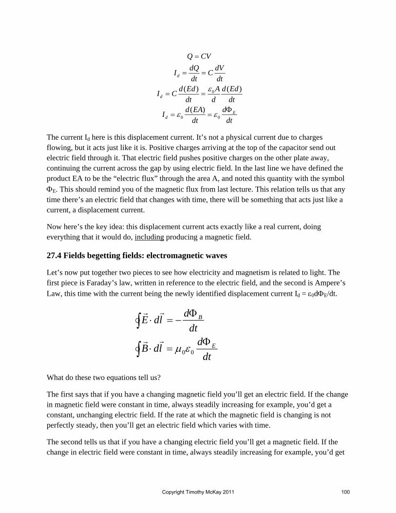
The current Id here is this displacement current. It’s not a physical current due to charges flowing, but it acts just like it is. Positive charges arriving at the top of the capacitor send out electric field through it. That electric field pushes positive charges on the other plate away, continuing the current across the gap by using electric field. In the last line we have defined the product EA to be the “electric flux” through the area A, and noted this quantity with the symbol ΦE. This should remind you of the magnetic flux from last lecture. This relation tells us that any time there’s an electric field that changes with time, there will be something that acts just like a current, a displacement current.

Now here’s the key idea: this displacement current acts exactly like a real current, doing everything that it would do, including producing a magnetic field.

27.4 Fields begetting fields: electromagnetic waves

Let’s now put together two pieces to see how electricity and magnetism is related to light. The first piece is Faraday’s law, written in reference to the electric field, and the second is Ampere’s Law, this time with the current being the newly identified displacement current Id = ε0dΦE/dt.

What do these two equations tell us?

The first says that if you have a changing magnetic field you’ll get an electric field. If the change in magnetic field were constant in time, always steadily increasing for example, you’d get a constant, unchanging electric field. If the rate at which the magnetic field is changing is not perfectly steady, then you’ll get an electric field which varies with time.

The second tells us that if you have a changing electric field you’ll get a magnetic field. If the change in electric field were constant in time, always steadily increasing for example, you’d get

dtd

dtEAdI

dtEdd

dA

dtEddCI

dtdVC

dtdQI

CVQ

Ed

d

d

Φ==

==

==

=

00

0

)(

)()(

εε

ε

dtdldB

dtdldE

E

B

Φ=⋅

Φ−=⋅

∫

∫

00εμ


a constant, unchanging magnetic field. If the rate at which the electric field is changing is not perfectly steady, then you’ll get a magnetic field which varies with time.

It’s hard to miss the symmetry here. Changing magnetic fields produce changing electric fields which produce changing magnetic fields which…You get the idea. Fields can create fields, and keep doing this over and over, with no charges at all around! Maxwell was able to work out the nature of these fields feeding on fields. He showed that, rather than just trading back and forth in one spot, the are always leaping forward, propagating out through space as a traveling wave.

The great surprise was in the speed of these waves. Maxwell was able to predict that the speed of these electromagnetic waves should be simply v = (1/μ0ε0)1/2. Putting in the numbers we get:

v = [1/(4π * 10-7 * 8.85x10-12)]1/2 = 3x108 m/s

Amazingly, this is just the speed of light, a quantity already well known by the time Maxwell was working on this. Not surprisingly, he realized that electromagnetic waves, these electric and magnetic fields feeding off one another as they race through space, must actually be what light really is.

Unlooked-for connections and dreams of unification

It’s hard to imagine what a big deal this was. Here was Maxwell, working on electricity and magnetism, on how charges attract one another and magnets work. This subject was going great, with two seemingly disparate phenomena (electricity and magnetism) coming together into one intimately connected, unified framework. Just at the end of this process, he discovers that not only are electricity and magnetism unified, but in fact they include another huge, well established area of physics.

Maxwell’s successin unifying electricity and magnetism with light is one of a number of great examples of ‘unification’ in physics; a recognition that a wide range of phenomena can sometimes be explained with just one simple idea. The example set here continues to provide a model for the intellectual sensibilities of physicists. Most hope that the world will one day be explainable using a minimal set of rules, or perhaps just one. Particle physicists seek a ‘grand unified theory’ which might explain it all.

Over the last five or six weeks we have really only sketched out the framework of this grandly unified field of electricity and magnetism. But hopefully even this glimpse gives you some idea of the beauty and elegance of the subject. E&M is an iconic success for science, a subject of both great theoretical charm and enormous practical importance. If you have any serious interest in physical science, I strongly encourage you to consider studying this subject further, perhaps taking a more advanced course in electricity and magnetism.



Magnetic flux and Faraday’s Law:

When the flux of magnetic field lines through a loop changes, an electromotive force (EMF, or a circulation of electric field) is created according to Faraday’s Law:

EMF BdE dldt

ξ Φ= = = −∫ i

The minus sign in this relation is essential. It encodes Lenz’s Law, and ensures that the EMF induced acts to resist the change in magnetic flux through the loop. It is a requirement of energy conservation.

Electric ‘generators’:

Electromotive force (potential difference) can be created using induction. If a coil with area A is located in a constant magnetic field B and rotates with angular velocity ω, it will generate an EMF:

( )sinAB tξ ω ω=

To create a large EMF, you can use a large loop, wrap many turns of wire around it, place it in a large magnetic field, or rotate it really rapidly. Generators don’t create anything: they convert mechanical motion to EMF and then electric current. Electric motors are generators run in reverse: current is put in and converted to rotational motion.

Displacement current:

While changing magnetic flux produces EMF (circulation of electric field), a changing electric flux produces circulation of magnetic field. This is described by making an equivalence between changing electric flux and a current called the displacement current:

displacement 0EdI

dtε Φ

=

This displacement current produces a circulating magnetic field around it, just as an ordinary current in a wire does.

Induction and electromagnetic radiation:

The coupling of changing magnetic fields to electric fields, and changing electric fields to magnetic fields, creates the possibility of electromagnetic waves in which energy trades between electric and magnetic fields, propagating through space far from any electric charges. Such electromagnetic waves are predicted to have a speed:


8

0 0

1 3 10 m/svμ ε

= = ×

in empty space. These electromagnetic waves play an incredibly important role in the physical world, as we will see in the next set of chapters.


POLS Chapter 28: Waves and the flow of energy and information

All living things are connected to their environment; they are open systems, continually exchanging energy, information, and matter with their surroundings. Animals which move around face a special challenge - they must find what they need, see what (and who) is coming, and not least, communicate with one another. Fortunately, the laws of physics provide a wonderfully flexible tool for sending and receiving such messages. Sound and light waves allow animals to sense the world around them with remarkable precision. They carry energy and information from place to place with no net motion of matter, enabling animals to communicate with one another in a rich variety of ways.

In this chapter we will explore the basics of waves, putting in place essentials you need to understand how living things use waves to reveal the world around them. In this chapter we will introduce several examples of waves. We will learn how to describe them using a wave function which varies in space and time, and define a set of parameters which characterize periodic waves. We will see how rapidly various waves travel, explore the way they fade with distance and through absorption, and discover how moving sources and receivers of waves alter their appearance. This chapter concludes with an extended discussion of how bats and other animals use the properties of sound waves to probe the world around them.

Subsequent chapters will build on these basics; discussing how waves interact with one

another and with their surroundings. Our central goal throughout is to learn how the properties of waves enable the formation of images. Living things form images of their world using eyes and ears. Modern scientific instruments, enabled by our understanding of waves, extend our evolved senses enormously, allowing us to see and hear things previously beyond our imaginations. We will conclude our discussion of waves with an introduction to a few of these methods of modern imaging.

28.1 Waves are traveling disturbances

Consider first a familiar example: the ripples which spread from a stone dropped in puddle. The water in the puddle begins at equilibrium; flat and smooth. It starts there because it has had time to settle to this lowest energy state, allowing any excess energy it might have had to spread to its surroundings.

When the stone strikes the surface, it briefly pushes down on the spot where it hits. This spot, connected to the water around it by the cohesion of the liquid, pulls the neighboring surface down. As Newton’s third law requires, this neighboring region pulls the original spot back up. A ring around the impact point begins to descend, pulling the ring beyond it down. Meanwhile, the original point of impact responds to the upward pull of its neighbors, and begins a return to equilibrium. The ripple, a ring of descending then recovering points, spreads from the original point of impact, passed from place to place across the connected surface of the water. After a time the surface returns to its original equilibrium position. No water has, in the end, moved anywhere. Yet something has happened; a disturbance has traveled across the surface. This is a


wave in its most basic sense; a disturbance passed from point to point through a continuous, connected medium. Illustration: sequence of images of a drop striking a surface, coupled with a diagram showing the motion of material in a water wave

Now consider a less familiar example. When you strike a table with a hammer, something happens which is very like what happened with the pebble in the pond. The table begins at rest, with every atom oscillating gently about its equilibrium position. At the instant the hammer hits, bits of the table very close to the impact are displaced significantly downward. These points, solidly connected to their neighbors, pull them down strongly. These neighbors pull their neighbors, and the displacement created by the hammer strike at one spot ripples out across the table. It takes time for the hammer strike to be felt at the far end of the table. The disturbance you created in one location spreads across the table top as a wave. Illustration: hammer striking a table, coupled with a diagram showing the motion of material along the surface, in the bulk of the table, and in the air

When the hammer strikes the table, it also pushes air out from beneath its head. Rushing

away, this expelled air pushes into the air around the hammer head, increasing its density and pressure. The resulting ring of enhanced pressure expands outward from the source, each ring pushing on the next. This wave of enhanced pressure is a propagating sound. After it passes, the air returns to its original, uniform pressure. There has been no net movement of air, but something happened. A wave has traveled out from the impact of the hammer.

In each case, the material in which the disturbance travels oscillates around equilibrium,

moving side to side, forward and back; always returning to where it began. The disturbance, by contrast, travels forward continuously, spreading from its point of origin. You should keep the difference between the motion of the material and the motion of the wave clearly in mind when learning about waves.

Light too is a wave, a traveling disturbance with all the same essential qualitative

properties as water waves and sound. Light waves are not fluctuations in the density or position of a substance (as sound and water waves are), but rather variations in the electric and magnetic field. While the mechanisms by which light waves travel are different, they share a rich set of essential phenomena with all other waves, and we will consider them waves equally here.

Waves as a way of transmitting energy and information

We have already learned about two ways to move energy from place to place; through organized bulk motion and through random thermal conduction. A ball thrown through a room carries energy in bulk motion. Its energy transport can be rather rapid - faster than a speeding bullet even - and quite directed. Convection is another form of organized bulk motion: once again, material which contains the energy moves from one place to another. Both matter and energy flow.


Energy may also flow through completely disorganized motion. When one part of a material is hot, with atoms moving fast, while another part is cold, with atoms moving slowly, energy flows from the hot to the cool side, passed from atom to atom as they interact. This kind of flow is random and disorderly, so it happens rather slowly, and cannot be directed at all. In thermal conduction, energy flows without matter going anywhere.

Waves provide a third way to transfer energy. Like bulk flow, they involve organized motion, all the atoms in a region move back and forth together, but like conduction, they transmit only energy. Because they involve organized motion, energy transmitted as waves travels rapidly, especially compared to transport by conduction. All three modes of energy transport are important for life. Solar energy arrives on Earth as light waves, is transported through air and water in enormous convective flows, and works its way through the solid Earth by conduction. Beyond the Earth, most energy is transported through the universe with light waves, because only they travel freely through a vacuum.

Waves also carry much of the information which travels from place to place. Everything you know about the world beyond your skin, from sunsets you have seen to the text you’re reading now, you learned by judiciously sampling the waves which wash over you. These waves, emitted by or reflected from distant objects, carry a record of their source. Your eyes and ears help you to extract the tale they tell. Your eyes measure precisely where light comes from, perceive its frequencies as color, and its intensity as brightness. Your ears perceive frequency as pitch and intensity as loudness. Other animals do the same, often with a facility far greater than our own.

Scientific instruments like microscopes and telescopes allow humans to extend our

senses, reading the information encoded in waves ever more precisely, often in ways no other living thing can. Much of our discussion of waves will focus on how to extract information from them, measuring where they come from and what kind of waves they are. If we cared only about absorbing the energy they deliver, rather than decoding the information they carry, our study of waves would be much more concise.

28.2: Describing a wave: the ‘wave function’

A wave is a disturbance in a continuous medium that varies in space and time. As a result, we describe it mathematically as a function recording the size of the disturbance at each point in space and each instant of time. For our initial example of ripples in a puddle, we might write this as ( ), ,z x y t . This function expresses how far the water is above or below equilibrium (the size of the disturbance) at every position (x,y) and for every time t. The figure below shows an example of what such a function might look like for all positions x, and y at some particular instant t.


The concept of a wave function is very general, and can be applied to all sorts of waves, not just ripples on the surface of water. It may describe a changing pattern of disturbance of any kind. Instead of water moving above and below a level surface, it might be variations in the pressure of the air, oscillating above and below an equilibrium value, as in sound waves, or variations in the strength of the electric field from place to place, as it would be for light waves. It is worth noting that this ‘wave function’ is another kind of a field, very like those we discussed when studying electricity and magnetism. Like those fields, the wave function is a quantity defined at all points in space and time.

Most often, we will visualize wave functions by taking snapshots of them. One of your challenges is to imagine not only what the wave function looks like at a particular instant, but also how it changes with time. The figures below, for example, show three snapshots in the evolution of a wave which begins at the top center of the grey area and spreads downward with time. The picture at each of these three instants is a snapshot of the wave function at each moment.

A generalized model for a traveling wave

It is easy to imagine describing these snapshots of waves with mathematical functions. The tricky part is thinking of a mathematical function which describes how this snapshot changes with time; how the wave travels. There is a simple way to do this. Imagine a one-dimensional

( )1, ,z x y t ( )2, ,z x y t ( )3, ,z x y t


wave described by the wave function ( ),y x t . A snapshot of this wave at a particular instant

0t = is just some function of position ( )f x :

( ) ( ),0y x f x= How could we alter this snapshot function ( )f x to make it travel to the right at a constant

speed v? To see this, imagine some location xmax where, at the instant t = 0, the wave function has a local maximum; a peak in the wave. We want that peak to move to the right at speed v, so its location should obey this equation:

In fact every location on the original snapshot y(x,0) should also move in the same way. The entire wave function simply slides to the right. If this is the case, we can write a general form for a wave traveling to the right by replacing x in the original function ( )f x with x-vt:

( ) ( )traveling right ,y x t f x vt= − Using a similar argument, we would expect a wave traveling to the left to take on the form:

( ) ( )traveling left ,y x t f x vt= + Here is one concrete example of how to do this. Imagine a snapshot of a wave which at time t = 0 is a Gaussian function with width σ centered at x = 0. We would write this:

( ) ( )( )2

2, 0x

y x f x e σ−

= = If this pulse were traveling to the right as a wave with speed v, we would rewrite this equation for all times as:

( ) ( )( )2

2,x vt

y x t f x vt e σ− −

= − = The peak of this function will always occur where the argument x – vt = 0, so

( ) ( ) ( ) ( )max max max max0 or 0x t x vt x x t vt= + = −


it will move the right according to the equation maxx vt= . A snapshot of a wave expressed as a function ( )f x can be transformed into a traveling wave by replacing the argument x with the combination x-vt.

28.2: Periodic waves: frequency and wavelength

If you disturb a material in a regular, periodic way, perhaps by shaking the end of a rope, you will create a wave which has a particular frequency. This frequency is determined by how many times a second you shake the rope. Frequency is usually denoted with the symbol f, and measured in units of 1/seconds, or “Hertz”; one oscillation per second is one Hertz. The inverse of the frequency is the period, a measure of how long each oscillation lasts. Period is measured in seconds and we will often use a capital T to denote it.

Each time you shake the rope, the disturbance you apply to the end travels down the rope. Between the time of one upward shake and the next, the first disturbance will travel some distance. How far it gets before the next shake depends on the wave speed. The distance from one peak to the next we will call the wavelength, for which we will usually use the Greek symbol lambda (λ ). This description implies a guaranteed relation between frequency, velocity, and wavelength:

= distance traveled in a cycle wave

wavevv T

fλ = =

Or

wavev f

Tλλ= =

This is how most periodic waves come about. The frequency of the wave is set by an outside source, while the velocity (and hence the wavelength) are set by how rapidly the disturbance can ‘flee’ the source. This is something that’s true for all kinds of periodic waves; an important general relation.

Wave travel: how fast do they go?

To explore how rapidly waves travel, consider a simple example. Imagine a rope held in your hand, attached firmly to a wall at the other end. You pull the rope rather tight, let it settle to rest, then shake your end sharply up and down once. The bit of rope in your hand tugs on the next piece of rope, which in turn tugs on the next; allowing the disturbance to travel. What determines the speed with which this disturbance travels?

The force returning the material to its original state plays an important role. The strength

of this restoring force can be expressed by an appropriate measure of the ‘stiffness’ of the material. If a material is difficult to distort, it will spring back to its original shape with great


force. This forceful return to equilibrium will tend to make waves travel through the material more rapidly. For the rope, tension is the appropriate measure of stiffness. The more tightly you stretch the rope, the more rapidly a disturbance will travel through it. For sound waves, the appropriate measure of stiffness is a form of the elastic modulus (bulk, shear, or Young’s modulus, depending on the application). For surface water waves, the restoring force may be either surface tension, as it is for small ripples, or gravity, as it is for larger waves.

A second property which affects the rate at which waves travel is the inertia of the material. If it is extremely dense, then it will take longer for it to return to equilibrium even when the restoring force is large. For the rope, inertia is best expressed as a linear density, a mass per unit length. For sound waves, inertia is best expressed as the usual density, mass per unit volume. So we expect the velocity of a wave in a material to depend on both stiffness and its inertia.

Here are some more specific examples of how this competition between restoring force and inertia plays out in different circumstances. These relations describe waves traveling on a rope, sound waves in a solid or gas, and large water waves in deep water.

Material Restoring Force Inertia Wave Speed

Rope Tension ML

μ = Tμ

Sound in Gases Bulk Modulus MV

ρ = Bρ

Sound in 1D Solids Elastic modulus (Shear or Young’s)

MV

ρ = or S Eρ ρ

Sound in 3D Solids Elastic modulus (Bulk and Shear)

MV

ρ = 43

B S

ρ

⎛ ⎞+⎜ ⎟⎝ ⎠

Large Water Waves in Deep Water with Wavelength λ

Gravity MV

ρ = 2gλπ

Notice that for sound and waves on a rope the speed of travel is independent of the wavelength or frequency of the waves. All waves like these travel at the same, constant speed. In this sense their motion is very simple. Water waves, while more familiar to most of us, are actually very complex, with wave speeds which depend strongly on wavelength. As a result, we won’t say a lot more about water waves here. One interesting thing to note before leaving them behind; long wavelength swells travel more rapidly than short wavelengths. This is why a storm far out as sea is often announced first at shore by large, long wavelength swells which gradually become shorter as the storm approaches.


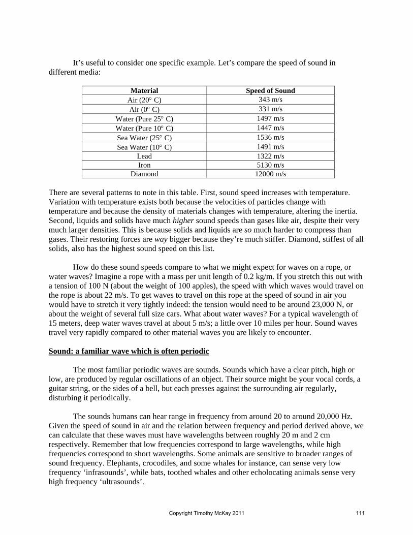
It’s useful to consider one specific example. Let’s compare the speed of sound in

different media:

Material Speed of Sound Air (20° C) 343 m/s Air (0° C) 331 m/s

Water (Pure 25° C) 1497 m/s Water (Pure 10° C) 1447 m/s Sea Water (25° C) 1536 m/s Sea Water (10° C) 1491 m/s

Lead 1322 m/s Iron 5130 m/s

Diamond 12000 m/s There are several patterns to note in this table. First, sound speed increases with temperature. Variation with temperature exists both because the velocities of particles change with temperature and because the density of materials changes with temperature, altering the inertia. Second, liquids and solids have much higher sound speeds than gases like air, despite their very much larger densities. This is because solids and liquids are so much harder to compress than gases. Their restoring forces are way bigger because they’re much stiffer. Diamond, stiffest of all solids, also has the highest sound speed on this list.

How do these sound speeds compare to what we might expect for waves on a rope, or water waves? Imagine a rope with a mass per unit length of 0.2 kg/m. If you stretch this out with a tension of 100 N (about the weight of 100 apples), the speed with which waves would travel on the rope is about 22 m/s. To get waves to travel on this rope at the speed of sound in air you would have to stretch it very tightly indeed: the tension would need to be around 23,000 N, or about the weight of several full size cars. What about water waves? For a typical wavelength of 15 meters, deep water waves travel at about 5 m/s; a little over 10 miles per hour. Sound waves travel very rapidly compared to other material waves you are likely to encounter. Sound: a familiar wave which is often periodic The most familiar periodic waves are sounds. Sounds which have a clear pitch, high or low, are produced by regular oscillations of an object. Their source might be your vocal cords, a guitar string, or the sides of a bell, but each presses against the surrounding air regularly, disturbing it periodically.

The sounds humans can hear range in frequency from around 20 to around 20,000 Hz. Given the speed of sound in air and the relation between frequency and period derived above, we can calculate that these waves must have wavelengths between roughly 20 m and 2 cm respectively. Remember that low frequencies correspond to large wavelengths, while high frequencies correspond to short wavelengths. Some animals are sensitive to broader ranges of sound frequency. Elephants, crocodiles, and some whales for instance, can sense very low frequency ‘infrasounds’, while bats, toothed whales and other echolocating animals sense very high frequency ‘ultrasounds’.


Light: another wave which is often periodic

Light too is a wave, a traveling disturbance with all the same qualitative properties as sound. Light waves are not fluctuations in the density of a substance (as sound waves are), but rather periodic variations in the electric and magnetic fields. For these “electromagnetic waves” we can also write wave functions which tell us the magnitude and direction of the electric (or magnetic) field at each point in space and time:

Light differs from sound and other mechanical waves in one important sense: it does not travel because of forces applied by one part of a material on its neighbors. Light travels because changing electric fields generate changing magnetic fields, which in turn generate changing electric fields. No material is needed for light to travel; it propagates freely through completely empty space. This is essential for life, as it allows energy from the Sun to travel to the Earth. The speed with which light waves propagate has nothing to do with restoring forces and inertia, but instead is set by the nature of electromagnetic induction. Their speed in empty space, as shown by Maxwell, is given by the relation:

8

0 0

1 3 10 m/scμ ε

= = ×

Light waves are produced by accelerating electric charges. Electric charges (like

electrons and protons) are sources of electric field. When you shake an electric charge up and down, you cause the electric field in that region to change with a regular frequency. These changes in the electric field then travel out from their source at the speed of light. Just as in sound waves, there is a tight connection between the frequency of the disturbance, the speed with which it travels, and the wavelength which is produced:

This is one place where there’s a quantitative difference between sound and light. The speed of light is much larger than the speed of sound: c = 3x108 m/s, or about a million times faster than sound. While light does not require a medium to travel, it can propagate through transparent materials like air and water. When it does, its progress is slowed. We account for this with a material parameter called the ‘index of refraction’ which relates the speed of light in the material to its speed in a vacuum:

light in a vacuumlight in a material

material material

v cvn n

= =

The index of refraction of air is about 1.0003, for fresh water it is about 1.33. While light moves very freely through air, its progress is significantly slowed in water.

( ), , ,E x y z t

lightv c fλ= =


There are in principle no limits to the wavelengths and frequencies of electromagnetic radiation. If you disturb the electric field with a frequency f, you’ll get waves with a wavelength λ = c/f. Shake an electron up and down at 1 Hz and you’ll produce waves with λ = 3x108 m. That’s a really huge wave, with a wavelength about the distance from the Earth to the Moon.

The figure below shows some of the kinds of EM radiation you might encounter in

nature. There are several things to note here:

1. The range of wavelengths encountered with light, from 10-14 m to 10 m, is extremely large, varying by a factor of 1015 at least.

2. The frequencies, of course, vary over a similar range, from 107 Hz to 1022 Hz. Notice that even the low frequency waves are still pretty high: the lowest frequencies represent oscillations which occur around ten million times per second!

3. Visible light makes up only a small portion of this broad spectrum. The visible light regime runs from around 400 nm to around 700 nm in wavelength, and from 4.3x1014 Hz to 7.5x1014 Hz. Within that region, each wavelength corresponds to a different color, running from blue at the short wavelength end to red on the long end.

4. All of the other EM waves have names which are familiar because we use essentially all of the EM spectrum for some purpose or another in our technology.

The wavelengths of visible light are tiny, smaller than the smallest bacteria. On the other

hand, their frequencies are very high, much higher than we can easily sense; oscillations which happen 400 trillion times a second! These facts explain why it is not easy to notice the wave properties of light, though of course it is possible. We will see in the next chapter how to show experimentally that light is a wave.

Sound and Light: longitudinal and transverse waves

Sound and light differ in another important way. A sound wave in air is made from variations in the pressure of the air as the air moves back and forth along the direction in which the wave is traveling. Such a wave, in which the disturbance happens in the direction the wave


moves, is called a longitudinal wave. Air can really only be disturbed in compression; it is a fluid. Fluids respond to shear forces by flowing rather than stretching elastically, so if you were to try to shake air from side to side (rather than shoving it forward and back) it would merely flow: no wave would propagate. So sound waves are longitudinal, with the air moving forward and back along the direction in which the wave travels. In this sense sound waves are simple: once you know the direction of motion of the sound wave, you know the direction along which the air moves as well.

Light waves are different. In a light wave, the changing electric and magnetic fields are always perpendicular to the direction of motion of the wave. The direction of the electric field associated with a light wave is never along the direction of motion of the wave, but always perpendicular to it. This fact adds a level of complexity to the light wave. We can see the problem from an example. Imagine that a light wave travels in the x-direction. Because the light wave is transverse, the changing electric field associated with it must lie somewhere in the yz-plane, but we don’t, without additional information, know which way it points.

To keep track of this additional factor associated with light we record the direction along which the electric field changes in addition to the direction in which the wave travels. The light wave described above travels along the x-axis. If its electric field varies only along the y-axis, we would say this light is ‘linearly polarized’ in the y direction. If the field varies only along the z-axis, we would say it is linearly polarized in the z-direction. Of course it is possible for the light to vary along any other direction in the yz-plane, or even to vary randomly along every other direction in the yz-plane. If the electric field varies along all directions, we say the light is ‘unpolarized’. Most light encountered in nature is unpolarized in this way. Polarized light is sometimes produced in reflections, and as we will see, quite a few organisms use the polarization of light to learn about the world around them.

28.3: A specific and very useful example: a traveling sine wave

One important model of a traveling wave function is the traveling sine wave; a wave with the shape of a sine function which travels by sliding at a constant speed either right or left. There are two reasons to focus on this specific case. First, a traveling sine wave provides a concrete example, useful for calculation in some explicit exercises; it is a simple model with which to work. But there is a more important reason for considering such sine waves. Surprisingly, any wave function can be constructed as a sum of appropriate sine waves; they can be used to build up any wave at all. In the next chapter, we will describe in some detail how this works. So when we study sine waves, we are actually studying a kind of ‘atom’ from which all other waves can be constructed.

A wave function for a sinusoidal wave traveling to the right can be constructed using the prescription developed in Section 28.1. We start with a snapshot of a completely general sinusoidal function at time t=0.


This function is characterized by three numbers. The first is an amplitude A, which describes how large the minima and maxima of the function are. The second is a wavelength λ, which tells us how far along the x-direction we must travel to go from one peak to the next. The third is a ‘phase angle’φ. Changing this phase angle allows us to shift the points where the sine function passes through zero, sliding the entire function left (for positive φ) or right (for negative φ). We can write an equation for this function in the form:

( ) 2,0 siny x A xπ φ

λ⎛ ⎞= +⎜ ⎟⎝ ⎠

Since the sine function varies between plus one and minus one, this function varies between +A and –A, as it should. When we move a distance λ along the x-direction, the argument of the sine function changes by 2π; it passes through one cycle and returns again to its original value. The presence of the phase angle φ allows us to slide the whole function left or right. Given this snapshot of the wave, we know how to turn it into a wave traveling to the right with a constant speed v: simply replace the argument x with x-vt. When we do this, we get the equation for the traveling sine wave:

( ) ( )2 2 2, sin sin vy x t A x vt A x tπ π πφ φ

λ λ λ⎛ ⎞ ⎛ ⎞= − + = − +⎜ ⎟ ⎜ ⎟⎝ ⎠ ⎝ ⎠

We simplify this equation a little using the relation v fλ = and defining two new parameters, the wave number k and the angular frequency ω using the relations:

2 and 2k π ω πλ

= =

Doing this allows us to write the wave function for a sinusoidal wave traveling to the right in the following clean and general form:

We might also note that, in terms of these new parameters, the speed of the wave can be written:

( ) ( ), siny x t A kx tω φ= − +

λ

x

y A

φ


v f

kωλ= =

Let’s review the four parameters which define this wave:

• The amplitude A represents the maximum size of the disturbance. • The angular frequency ω is another way of writing the frequency f. • The wave number k is another way of writing the wavelength λ. In fancier terms we

might call λ the spatial period and k the spatial frequency. • The phase angle φ defines where the peaks and zeros of the sine wave occur.

This phase angle φ deserves a little extra comment. It shifts the location of the wave left or right. This arbitrary, fixed shift is needed if one is to describe all possible waves within one fixed coordinate system. If the coordinate system is ours to define, and we’re concerned with just a single wave, we can always choose coordinates so that φ is zero. For this reason, we will often leave the phase angle out in further discussions. It will return, and become very important, when we consider more than one wave traveling in the same medium. In this case, it may not be possible to shift coordinates so the φ will be zero for all the waves. With multiple waves, these phase angles will describe irreducible relative shifts between the waves. How could we express a similar, sinusoidal wave moving to the left? To do this, we would like to have the velocity be negative instead of positive. This makes the sign of the ωt term the same as the sign of the kx term. In the function describing a wave traveling to the right, the parameters k and ω have opposite signs. To construct a wave function for a wave traveling to the left, k and ω must have the same sign. Here are two examples:

So remember, when k and ω have the same sign, the wave travels left, and when they have opposite signs, the wave travels to the right.

28.4: Wave fronts and rays, intensities, dimensionality, and absorption

The simplest waves to imagine are those traveling in just one dimension, like waves on a string. But most waves, like sound waves, will actually travel in three dimensions. It is often useful to consider a simple picture of a point source of sound waves and describe "wavefronts" and "rays" for this. The wavefronts are the actual peaks of the waves produced by the source. They move forward, out from the source, and along this direction of motion we define rays which are perpendicular to the wavefronts. Near the source, the spherical nature of wavefronts is obvious; they are clearly curved. If you are very far from the source, the curvature of the wavefronts is no longer so apparent, and the waves begin to look like “plane waves”. We will often talk about these plane waves in later chapters. They are produced naturally by point sources, so long as the sources are far away.

( ) ( ) ( ) ( )traveling left traveling left, sin or , siny x t A kx t y x t A kx tω φ ω φ= + + = − − +


As these waves spread out over a larger and larger area, the energy put in by the source is dispersed and their ‘intensity’ declines. Intensity is a measure of how much energy is delivered by the wave per unit area per unit time; a power per unit area. As a result, the intensity of 3D waves is measured in W / m2. For a wave propagating in three dimensions, as sounds typically do, the energy released by the source as an initial power 0P must spread out over a sphere with area 4πr2, and the intensity will decline with distance in this way:

( ) 0

3 24dPI r

rπ=

If the wave is propagating in two dimensions, as surface water waves do, the energy released by the source must spread out over a circle, and the intensity (here measured as power per unit length rather than area) falls off more gradually: If the wave is propagating in just one dimension, as waves on a string do, all of the energy released by the source travels through all points on the string, and the intensity (here measured simply as power) doesn’t decrease at all.

Often the real propagation of a wave is intermediate among these three possibilities. We will see in later chapters how wave sources can be arranged to form a ‘beam’. In this case, a wave propagating in three dimensions is confined for a while to a narrower two dimensional region, only more slowly spreading into the third dimension. This phenomenon may be familiar from playing with flashlights and laser pointers. These sources send out their light waves in a way which allows them to arrive at a distant point little diminished from when they left their source. This is very different from the way the intensity of a point source like a light bulb or the Sun fades with distance.

( ) 02 2D

PI rrπ

=

( ) 03 24D

PI rrπ

=

( )1 0DI r P=

Waves from a point source “Plane” waves far from a point source


Motion and energy in sound How does the intensity of a sound relate to its wave function? We can determine this precisely for sound. In a sound, we describe the displacement of the air from its equilibrium position as:

where s is the distance (forward and back) that the air is moving Now that we have determined the motion of the air, we can work out the kinetic energy associated with it: Some amount of mass moves with this velocity, and it has KE In this equation we use A for the area of a little pad of air moving forward and back, and dx for the thickness of it, so that ρAdx is the amount of mass that’s moving. Note that the area A used here is nothing to do with the amplitude of the wave As!

This calculation tells us how much kinetic energy is present in a little part of the wave. If we divide this little dKE by the short time it takes to arrive dt, we find:

or

Light propagating in 3 dimensions

Light propagating in a 1 dimensional beam

cos( - )sdsv A kx tdt

ω ω= =

( ) ( )( )2 2 2 21 12 2 cossdKE mv Adx A kx tρ ω ω= = −

( )( )2 2 212 coss

dKE dxA A kx tdt dt

ρ ω ω⎛ ⎞= −⎜ ⎟⎝ ⎠

( ) ( )( )2 2 212 cosKE s sP Av A kx tρ ω ω= −

( ) ( ), sinss x t A kx tω= −


If we now ask for the average amount of kinetic energy arriving per unit area per unit time, and recognize that the average value of cos2 is one half, we find:

This is a prediction for the kinetic energy arriving in the wave. What's the total energy arriving? The air here is oscillating back and forth. In oscillators the energy, averaged over time, is equally shared between kinetic and potential energy. This idea of ‘equipartition’ suggests that

average averageKE PE= , so the total intensity is twice that arriving as kinetic energy: This equation tells us how the intensity of a sound, the amount of energy per unit time per unit area which it delivers, is related to the properties of the wave and the material through which it travels. The intensity depends on some properties of the wave itself; the angular frequency squared and the amplitude squared. It also depends on some properties of the material, its density and the speed of sound in it.

This product of density and speed of sound is called the “characteristic acoustic impedance” of the material, often denoted by the symbol Z. We will see later that this quantity plays a very important role in the reflection and transmission of sound. It measures a part of how freely sound energy travels through a material.

Intensity expressed in decibels

Because waves traveling in three dimensions fade in intensity relatively rapidly (when you go 10x farther away a sound typically becomes 100x fainter), we will talk about sounds which vary in intensity a lot. To do this, it is common to use a logarithmic scale for intensities of sound. The standard system works by comparing the intensity of a sound to something very faint. Most often we compare to a sound which is about the faintest a typical person can hear. This Imin is chosen to be 10-12 W/m2, a very small amount of energy per unit area. You can actually just barely hear such a sound, at least if you don’t use your Ipod headphones too much…. So given the intensity of a sound I, measured in W/m2, you can determine the intensity in decibels from this equation. If a sound is 10x as loud as you can possibly hear, so that I10 = 10*Imin, the intensity in decibels is:

( )average

2 214

KEs s

P v AA

ρ ω=

( )2 21sound 2

Totals s

P I v AA

ρ ω= =

( )min10 10 10

min

1010log 10log 10 10 dBIII

⎛ ⎞= = =⎜ ⎟

⎝ ⎠

10min

Loudness in decibels 10log II

β⎛ ⎞

= = ⎜ ⎟⎝ ⎠


If the sound is 1000 times as intense as Imin, it is The loudest sounds you can comfortably hear are around 100 dB. Working backward, you can see that this sound is: This intensity is 10 billion times louder than the faintest sound you can hear. Sounds with intensities of 120 decibels can quickly damage your ears.

Absorption of sound Another important consideration in the propagation of sound is absorption. The energy contained in a traveling disturbance is not passed from one point to another with perfect fidelity. Some of the energy is lost from the wave as it travels through the material. As always, the total energy is actually conserved, but it is converted from the organized motion of the wave to random thermal motion. Sound absorption is a complex phenomenon, dependent both on the frequency of the sound and the detailed properties of the air or water through which it passes. The rate at which sound is absorbed during travel is often tabulated in decibels per kilometer. This measure has a value of around 1.5 dB / km for 1 kHz sounds in dry air. A sound with this frequency will fall in intensity by a factor of 0.71 when traveling through one kilometer. The figures below show the rate of attenuation for sound in air and water as a function of frequency. The rate of attenuation for sound is much larger in air than in fresh water, and much larger in sea water than in fresh water. You can also see that attenuation in air depends on humidity, especially at low frequency. The increased attenuation of sound at high frequencies explains why thunder from distant lightning strikes is heard as a low rumble, while nearby strikes are heard as high frequency crashes.

( )min1000 10 10

min

100010log 10log 1000 30 dBIII

⎛ ⎞= = =⎜ ⎟

⎝ ⎠

10 10min min

10 2min 2

100 10log or log 10

W10 10 m

I II I

I I −

⎛ ⎞ ⎛ ⎞= =⎜ ⎟ ⎜ ⎟

⎝ ⎠ ⎝ ⎠

= =


The absorption rates shown here are the minimum. Often the full absorption of sound is dominated by the presence of small concentrations of impurities, like dust or water droplets in air, or air bubbles in water.

28.5: The Doppler effect: There is one last wave phenomenon to introduce in this chapter, one especially relevant with sound: the Doppler effect. This familiar effect involves a change in frequency which occurs when there is relative motion between a source and recipient of sound. When an ambulance drives towards you, or you drive towards it, the frequency of its siren appears higher. If the ambulance is driving away from you, or you are moving away from it, the frequency you hear is lower.

Let’s work out how large the effect is. First imagine the source of sound is sitting still and so are you. In this case waves from the source are traveling through the medium with a speed vsound. The number of waves you hear per second is the frequency. You can think of it as determined by how many wave peaks pass by you per second: Now imagine you are moving directly towards a stationary source with a velocity whose magnitude we write vreceiver. Now since you’re moving towards the wave, peaks will pass you more often. How large an effect will this be? The total distance which waves move past you is (vsound+vreceiver)t, and the frequency with which peaks arrive at your ear is:

traveled#

s

s

d v tvf

s t tλ λ

λ= = = =

( )sound receiver

sound receiver sound sound receiver

sound

sound receiver0

sound

v v tv v v v vf

t vv vf f

v

λλ λ

++ +

= = =

+=

From Denny, Air and Water, Princeton, 1993.


(Source stationary, detector moving towards) What if you’re moving away from a source which is stationary? This is the same, except that now vreciever changes sign, so

(Source stationary, detector moving away) It should be clear from these calculations that the Doppler effect can either increase or decrease the frequency of the sound you hear.

The situation is a little different if the source is moving and the detector is stationary. In this case the sound still moves through the medium at the same rate; what changes is the apparent wavelength. The source is always ‘catching up’ to the waves it has just emitted, making the distance between them now: What does the detector receive? It observes waves arriving with frequency:

(Source moving towards, detector stationary) If the source is moving away, we just reverse the sign of vsource to get the analogous relation. Combining these various relations we can obtain two general Doppler shift equations: where the ± and ∓ imply motion toward and motion away respectively. So if the receiver moves toward the source, you use the + sign in the numerator of the frequency equation. If the

sound receiver0

sound

v vf fv−

=

( ) ( ) ( )

( )

sound source sound sourcesoundsound source

sound

sound source0

sound

v v v vvv vf f v

v vv

λ τ

λ λ

− −= − = =

−=

( ) ( )sound sound sound sound

00 sound source sound source

v v v vf fv v v vλ λ

= = =− −

sound receiver sound source0 0

sound source sound receiver

and v v v vf fv v v v

λ λ±= =

±∓

∓


source moves toward the receiver, you use the – sign in the denominator of the frequency equation. When the source and detector move closer together, frequency increases and wavelength decreases. When the source and detector move apart, frequency decreases and wavelength increases.

It is often true that the speeds of the source and receiver are substantially less than the speed of sound. In this case, we can approximate the frequency shift as:

relative0 relative source receiver

sound

1 where uf f u v vv

⎛ ⎞= − = −⎜ ⎟

⎝ ⎠ The fractional change in frequency for this case is given by the ratio of the relative velocity of source and receiver divided by the speed of sound:

0 relative

0 0 sound

f f uff f v− Δ

= =

We can see why the Doppler effect is more often important for sound than for light. The

magnitude of the effect is dependent on source and receiver velocity divided by the speed of the wave. While sound travels rapidly, it is not unusual for living things to move at speeds a few percent of the speed of sound. When they do, they experience Doppler frequency shifts of a few percent. People encounter these most commonly in mechanized transport, but many animals, particularly fliers like birds and bats, regularly travel at tens of meters per second. As we will see, these Doppler shifts can create interesting challenges for them. You can also see why the Doppler effect is not commonly observed with light. The speed of light is so large that even the fastest living thing, a Peregrine Falcon diving at 90 m/s, cannot significantly approach it. Doppler shifts of light for this speeding bullet of a bird are on the order of 90 m/s / 3x108 m/s ≈ 3x10-7, or 0.3 parts per million; hardly noticeable.

Traveling faster than the speed of a wave

Motion through the medium of wave travel also gives rise to the interesting possibility of traveling faster than the waves you emit. When a source of waves does this, it produces a wake: a cone shaped front along which waves emitted from the traveling object pile up. Within this cone, waves from the source are present. Outside the cone, no waves from the source have yet arrived. The angle which this wake follows depends on the relative speed of the wave source and the wave itself.

vwt

vt

θ

sin wave

source

vv

θ =


This phenomenon is most familiar where it occurs most freely; on the surface of water.

Surface water waves travel relatively slowly, with typical speeds around a meter per second. Many objects, man-made and natural (like ducks), travel across the surface of water more quickly than this, trailing behind them the familiar wake. These water waves provide a nice familiar example, but it’s important to remember that water waves are actually quite complex, with velocities that are different for different wavelengths. So remember that applying these ideas to water waves will provide only a rough approximation for what’s really happening.

While this phenomenon is most familiar for surface water waves, it occurs for all kinds of waves. When an object like a jet plane travels faster than the sound it emits, the sound piles up in a shock wave of large amplitude along a cone. Imagine listening to the sound from such a jet flying directly over your location on the ground. Before front edge of the cone arrived, you would hear no sound at all. When the cone passed over, a sudden surge of sound would arrive, the famous ‘sonic boom’. Once you are inside the cone, you would hear the sound of the plane in a more-or-less familiar form, though the sound you hear would be coming from where the plane used to be, rather than where it is at this moment.

28.6: An application of sound propagation: biosonar

At the start of this chapter, we noted that waves provide the only opportunity for living things to learn about the world beyond their skins. Most of the time, these waves are used in a passive way. You only hear those things which produce sound and send it to you. Most of what you see is visible only because objects reflect the light from another source; especially the sun. In both cases, you are the passive recipient of external signals. When a source of light is absent, things which want to remain hidden need only remain quiet. If there is no light to reflect, and they send you no sounds, you are unable to discover they are present.

Because of this, the dark provides an opportunity – not only for those who would remain hidden, but also for those adapted to hunt in an unilluminated world. Most animals which hunt in the dark simply enhance their senses, growing larger eyes and more sensitive ears; trying to make the most of the paltry clues which are available. Adaptations for enhancing passive vision and hearing are found throughout the animal world, including the large and hypersensitive eyes and ears of owls, bush-babies, and the Fennec Fox. We tend to think of night as the primary


world of darkness, but for life the eternal darkness of the deep ocean is a much larger ecosystem. In this permanent darkness, the Colossal Squid Mesonychoteuthis hamiltoni carries sensory enhancement to the extreme. Its eyes, eleven inches in diameter, are larger than a dinner plate.

The most remarkable hunters of the dark, even more precisely adapted for this gloomy life, actively illuminate their world with sounds they produce. Bats, toothed whales, shrews, and even a few birds obtain images of the world around them by sending out sounds and listening for their echoes. This active imaging is remarkably effective, enabling the pursuit and capture of targets as tiny and silent as moths, and allowing bats to fly flawlessly through caves and forests in pitch darkness. The subtlety of the methods these ‘echolocators’ use have only recently been exposed, and it is quite likely that important aspects of this remarkable ability remain to be discovered. As we learn more about the physics of waves, we will return to this rich biosonar phenomenon. We will use bats as our prime example, but include some discussion of toothed whales to illustrate how different this problem can be in water.

The ‘first order’ way to use sound to understand a distant object is to bounce waves off it. If you do this, and measure how long it takes the waves to go out and back, you can measure how far away something is.

1

echo2 sd v t= Echolocating animals use this fact as a core element in their efforts to ‘see’ with sound. It’s also the central principle in our technological analogs, including radar (bouncing radio waves off distant objects) and sonar (bouncing sound waves off distant objects). We use it to measure many distances, including the distance to the moon, which is now known to a few centimeters.

The Doppler effect allows echolocators to carry this method one step further. Imagine that I send out a short pulse of sound, consisting of 100 oscillations of a single frequency sound wave. If I wait a bit, this pulse will bounce back off my target. The time the pulse train takes to return will encode the distance to the target. If I also measure the wavelength of the returning pulse train, any shifts in it will reveal any the relative motion between me and the target. So not only do I learn how far away things are, but also how fast they’re moving relative to me. This is what’s used in the ‘Doppler radar’ so much discussed on the Weather Channel today. It allows measurement not only of the locations of weather systems, but also of their velocities. As a result it aids in spotting extreme, and very localized, weather; like thunderstorm fronts and tornados.

Shifts in wavelength or frequency relate to the relative velocity of source and recipient according to the relation given early in this chapter. The problem for echolocation by a bat is, however, a little more complex. The sound in echolocation goes through two stages. First, the initial sound is sent out by a possibly moving bat. This sound is then received by a target, again possibly moving. As a result the sound received by the target may Doppler shifted. The sound this target reflects emerges with no delay on reflection, so waves head back out with the same frequency they are received. Now, in a second stage, the reflected sound is transmitted by the target and is received by the moving bat. These two stages of transmission and receipt imply a larger total frequency shift:


Challenges of biosonar, intensity

These two elements, timing of echoes and measurement of relative motion through Doppler shifts, are the basic elements of this approach to sensing the world. There are also a number of challenges inherent in biosonar. The first is the intensity. To hear an echo from an object a bat must send out a sound, which typically will propagate out in every direction. This outgoing sound fades in intensity as

When this sound arrives at the target, part of it will bounce off and return toward the source, but again its intensity will fade with distance. As a result: The returned intensity falls off with target distance like distance to the fourth power! A target twice as far away returns a sound with 16 times smaller intensity smaller than the transmitted signal.

Bats address this fundamental problem in a large variety of ways. First, the sounds they produce are very loud. Some reach intensities of 110 dB. This helps, but also presents a problem. A bat which is busy producing such an intense sound is unlikely to be able to detect a much fainter echo. For this reason, bats produce their sounds in short pulses, ranging in length from 0.2 ms to as much as 100 ms. They transmit a short, intense pulse, then wait for echoes to return. Since echoes from distant objects take longer to return, bats provide long gaps between pulses when targets are far away, and make the pulses closer and closer as they approach their targets.

Pulse duration also affects the ability of the bat to tell how far away the target is. A pulse of length tp emitted by the bat travels through space as a band of sound with pulse length Lpulse = vstp. For typical conditions, such a pulse might be a few meters long when the bat is searching, then shrink to a few centimeters as the bat closes in. The figure below shows an example of the search and capture sequence of sounds produced by a hunting bat. You can see from this how the pulses become shorter and closer together as the bat closes in on its target.

0at target 24

IIrπ

=

2 2target 0 target

02 2 2 4

14 4 4 16reflected

returned

I r I rI I

r r r rπ

π π π π= = =

1

21 1 1 1

received transmitteds

returned received transmitted transmitteds s s s

uf fv

u u u uf f f fv v v v

⎛ ⎞= −⎜ ⎟

⎝ ⎠⎛ ⎞ ⎛ ⎞⎛ ⎞ ⎛ ⎞

= − = − − ≈ −⎜ ⎟ ⎜ ⎟⎜ ⎟ ⎜ ⎟⎝ ⎠ ⎝ ⎠⎝ ⎠ ⎝ ⎠


Another approach to the intensity problem is to make the transmitted signal very special, so that its echo stands out from all possibly confusing ambient sounds. A common approach is to transmit sound in a narrow band of frequencies; a single tone ‘continuous frequency’ signal. Any incoming sounds which do not have this frequency can be safely ignored. The advantage this provides for filtering out all the other noise is very strong. This approach has driven adaptation in the hearing of many bats to be sensitive to only the same narrow band of frequencies they transmit. Sounds with the ‘wrong’ frequencies are simply not heard.

Challenges of biosonar: timing, location, and Doppler shifts How is a bat to tell where an echo came from? First, it finds a distance by measuring the

time between transmission and return. Doing this is a serious challenge. Sound travels rapidly in air, so that the time delay between transmission and receipt of an echo from a target 2 meters away is only about 5 milliseconds. Clearly the timing sensitivity of the bat must be in the millisecond range, quite substantially better than your own. Bats have highly structured neural networks in their auditory cortex specifically tuned to particular delays between transmission and receipt of an echo. The bat ‘measures’ the time delay by seeing which of its many tuned neural circuits is fired by a particular transmission and echo pair.

Once a bat measures the distance to a source, it must still determine what direction it

comes from. Binaural hearing, with time delays between the receipt of sound at one ear and the other, provides good sensitivity to angle within the horizontal plane. Localization in the vertical plane is a greater challenge for most bats. Many ameliorate this problem by flying directly at a chosen target. Using these basic tools, echolocating animals like bats can image the dark world with remarkable precision. As we will see, there are other subtleties to consider. We will return to echolocation, and our more technological use of it in ultrasound medical imaging, in future chapters.

While narrow-band hearing helps to filter noise during echolocation, it also creates a problem. If a bat is flying toward a target, the echo returned will experience a Doppler shift. If this shift is too large, it will drive the return sound out of the narrow band of the bat’s most sensitive hearing. Some bats, like the Mustached bats (Pteronotus parnellii), handle this by continuously controlling the frequency they transmit, lowering it when traveling toward a target so that the echo they receive back is kept right in their most sensitive range of hearing. An example of this frequency compensation in living bats is shown below. This bat seems to understand Doppler shifts well. For a relative velocity of -4 m/s and a desired receipt frequency

From Schnitzler & Kalko, 2001, Bioscience, 57, 557.


of 61.92 kHz, we would predict an increase a shift in transmission frequency of 1440 Hz, just about what the bat actually does. This is shown in the figure below, which illustrates how a bat changes the frequency it transmits as its velocity relative to the target (in this case a wall) increases.

Looking ahead

Waves are extremely important for life, and we will continue to explore them through all of the next five chapters. In the next chapter, we will consider some important, even defining, features of what happens when multiple waves travel in the same region. This will allow us to understand what makes the sounds produced by musical instruments special. After this, we need to see what happens when traveling in some medium (air, water…) encounter boundaries. We will learn how they may reflect off boundaries and refract around corners. We’ll see how, remarkably, these phenomena enable us to measure the structures of important biological molecules like proteins and DNA. A fourth wave chapter will expand on what happens when waves reach boundaries, exploring not only reflection, but also transmission and refraction. In it we will learn how the complex structures in your ears ease the way for sound to enter your body.

From Keating et al., 1993, J. Exp. Biology, 188, 115

Shift

from

rest

ing

freq

uenc

y (H

z)

Bat velocity relative to the wall (m/s)

relativereceived transmitted

sound

1

transmitted

received transmitted

61.92kHz 1 2

4m/s61.92kHz 1 2 60.48 kHz343 m/s

1440 Hz

uf fv

f

f f

−

⎛ ⎞= = −⎜ ⎟

⎝ ⎠

−⎛ ⎞= − =⎜ ⎟⎝ ⎠

− =


With all the essentials in place, we will finally be ready to explore the ways living things image the world using their eyes. While most eyes share some basic features, we will see that evolution has attacked this important problem in a wild diversity of ways. By exploring the extreme variety of eyes, we will see physics and life in intimate connection. As a final topic, we will see how humans have applied an understanding of waves to generate a wide array of new, extrasensory imaging tools: magnifiers, microscopes, telescopes, and a wide array of modern medical imaging technologies. These tools, which allow us to see the invisible, are the lynchpins of modern science. They are in some real sense the ultimate reward for learning about waves. Once we know how waves work, we can put them to use.


A Quick Summary of Some Important Relations Waves as traveling disturbances:

This chapter explored some of the basic properties of waves. In it, we stressed that waves are traveling disturbances, explained how a wave function provides a description of a wave at all locations and times, and mentioned the often useful distinction between longitudinal and transverse waves. Sound is longitudinal while light is transverse.

Periodic waves:

Many waves are approximately periodic. For these, there are simple relations among frequency, wavelength, period, and propagation speed. Light is a wave like others. It is distinguished by a very broad range of wavelengths and frequencies and a very large propagation speed. Predicting wave speeds:

For mechanical waves, the speed of propagation is dependent on both the resistance of the medium to distortion and its inertia. We considered some particular cases of wave speed for sound, finding that it travels more rapidly in liquids and solids than in the air. We also encountered cases where wave speeds are not so simple. Speeds for water waves are very complicated, depending on wavelength, amplitude, and water depth. Light waves have speeds set by the connections between electricity and magnetism, and by the interactions between electric fields and the matter through which it travels. One model wave, the traveling sine wave:

A particularly useful example wave function is the travelling sine wave, characterized by four parameters: a wavelengthλ , frequency f , a phase angleφ , and an amplitude A. This wave function can be written in general as:

( ) ( ) 2, sin with and 2y x t A kx t k fπω φ ω π

λ= − + = =

Such a wave travels at a speed

v fTλλ= =

wave on string sound in air and water T Bv vμ ρ

= =

lightmaterial

cvn

=

wavev f kλ ω= =


Wave propagation and intensity:

The intensity of a sound wave measures the energy it delivers per unit area per unit time. It is given by:

2 21

sound acoustic2 with I v A Z vρ ω ρ= = Waves which spread out in two and three dimensions fade in amplitude even when no absorption is present. Their falling intensity can be predicted when the initial power emitted by the source is known: Waves may also be absorbed when they propagate through a material, where their energy may be converted into other forms in the material. The intensity of sound is often reported on a logarithmic scale which approximately reflects the perceptual response of human hearing. This scale is defined as:

Source and receiver motion, the Doppler effect:

Relative motion between sources and recipients of waves causes shifts between emitted and observed frequencies and wavelengths which are collectively called Doppler shifts. These are governed by the general relation: In both numerator and denominator the top sign is chosen with the motion brings source and receiver closer together. This effect can be used to determine relative motion of source and observer. Sources which travel through a medium more rapidly than the waves they produce in it create ‘wakes’ which trail behind them. Echolocation and the challenges it poses: Organisms which hunt in lightless conditions have repeatedly developed the ability to image the world around them using echolocation. This application of wave motion relies on the timing of echoes and the measurement of Doppler frequency shifts. Successful echolocation requires overcoming several challenges, including the intensity problem and the need to identify the direction to the source of an echo.

( ) ( )0 03 22 and

4 2d dP PI r I r

r rπ π= =

12 2sounddecibels reference

reference

10 log with 10 W/mII II

−⎛ ⎞= =⎜ ⎟

⎝ ⎠

and s receiver s sourcereceived emitted received emitted

s source s receiver

v v v vf fv v v v

λ λ±= =

±∓

∓


POLS Waves Chapter 29:

29.0: When Waves Collide Waves of sound and light fill the air around us. We use them to sense the world beyond our skin. Starting from many sources, these waves rain down upon us from every direction. What happens when waves from all these independent sources arrive at one location? How do they affect one another? You can get some idea from everyday experience. When one person talks to you, you hear clearly what they say. When two people speak at once, you hear both together. The sound from one doesn’t alter the sound from the other; they simply combine. In a crowd this combination gets louder and more difficult to understand, but even now the sound from every speaker is present; each unaffected by the others. This experience suggests that when two waves come together in a material, each is unaltered; the new wave they create is just the sum of them all. Stated more precisely, this rule is a “principle of superposition”. If two waves traveling in a region are defined by wave functions y1(x,t) and y2(x,t), their combined effect will be just the linear sum of the two: ytotal(x,t) = y1(x,t) + y2(x,t) This simple rule is very often an accurate reflection of reality, especially for the sound and light waves we use to sense the world. The principal of superposition does fail sometimes, usually when the combined amplitude of the waves becomes so large that the physics of the situation changes. A familiar example occurs with water waves. Near the shore, the amplitude of a wave may become so large that the wave breaks; it tumbles over. When this happens, the water moves in a manner very different from the rolling swells you might see in deeper water. To make superposition fail with sound and light we’d have to make the amplitude of the waves large enough to rip apart the material the waves are traveling through. This can happen (as when a singer shatters a wineglass) but it isn’t encountered often. So we will use the principle of superposition very freely and without fear! In this chapter we will explore how the simple principle of superposition gives rise to interesting, often surprising phenomena. We will see that two waves, each delivering energy, can come together in one place and completely cancel one another out; almost as if 1 + 1 = 0. This


possibility is unique to waves; a phenomenon called ‘interference’. When it happens, we know for sure that waves are involved. Sound has been understood to be a wave for at least 2000 years; it is extensively discussed by the Roman architect Vitruvius. Around 1800, British polymath Thomas Young showed that light also exhibits interference, demonstrating that it too is a wave. In the early 20th century it was recognized that tiny bits of matter, things like electrons and protons, also exhibit interference. These tiny building blocks of matter, the icons of particles, in fact possess a previously unsuspected but undeniable wave nature. Waves are not, as they might seem at first, a fringe topic. Understanding them is essential for appreciating reality.

Superposition and interference in one dimension One of the best ways to appreciate the nature of the principle of superposition is to examine some simple examples. In the picture on this page, you see two pulses traveling through a material, perhaps ripples on a rope, captured in a series of snapshots labeled 1-5. In the top snapshots the two pulses enter the picture, one from the right and one from the left. Each pulse is a wave described by a wave function like the Gaussian wave packet first discussed in Section 1.1.2: The first pulse, y1, begins at time t = 0 as a little Gaussian centered at x = 0, with a width σ. This pulse moves to the right with speed v. We can tell it moves to the right because the position and time terms in the wave function have opposite signs. The second pulse, y2, starts out at location x0, and also has width σ . Unlike y1 it is traveling to the left; position and time here have the same sign. Eventually, at time t = x0/2v (see if you can figure out why), they will arrive at the same location. As time goes on, we see the pulses coming together. When they arrive at the same point their amplitudes just add together. In snapshot 3, where they completely overlap, their combined amplitude is twice as large as the individual pulses which originally entered. After they come together, they move apart again. Each just continues on its way, unaffected, as if they had never encountered one another. With waves that aren’t too large, this kind of simple superposition is just what happens. Let's consider a second example. Imagine that one pulse is in the upward direction, while the other is downward. What will happen now? When the pulses are far apart, they travel along undisturbed, just as they did before. But now when they come together, just at the moment when their centers perfectly align, they completely cancel one another. If you took a snapshot of this rope at just this instant, it would show no deviation from equilibrium at all! This is shown in the second 5 snapshot illustration. The ability of two waves to add together and cancel one another out is unique to waves. It is diagnostic of the presence of waves. When you see this happening, you know for sure that waves are involved.

( )( )

( )( )22

02 2

1 2, and , x x vtx vt

y x t e y x t eσ σ

− +−− −

= =


29.1: One-D superposition or nearly identical waves, phase matters Now let’s consider a little more complicated case: 2 nearly identical harmonic waves traveling in the same direction in a single medium. You might think of these as two waves traveling on an infinite rope. To understand how this might come about, imagine the following situation. Waves with the same frequency are generated by two different sources located at different points along a line. For now, we’re going to ask what this combined wave will look like to the right of source 2, where things are fairly simple. We will go back in a bit and examine the waves between the sources. Source 1 produces a wave which travels out, eventually passing by source 2. If source 2 is producing a peak each time a peak from source 1 arrives, the waves produced by the two are synchronized and are said to be "in phase". Peaks line up with peaks, valleys with valleys, and the combined wave is twice the size of each original wave. This is called "constructive interference". This result is illustrated in the figure on the left. A more surprising case occurs when the waves are exactly out of step with one another, what we would call "out of phase". In this case, source 2 is producing a valley each time a peak from source 1 arrives. The result is illustrated in the figure on the right. In this case two waves, each of

1

2

3

4

5

1

2

3

4

5

Examine combined wave here Source 1 Source 2


which has a positive amplitude, add together to produce a zero amplitude disturbance. Two waves can add together and completely cancel one another out. This phenomenon is called “destructive interference”. It's a key feature of waves.

The possibility of destructive interference has striking implications. If I project a sound into the room it will be heard everywhere. Imagine that I now want to get rid of it somewhere, to cancel it out. I can do this by a means other than just shutting off the original source. I can also get rid of this sound by adding another sound! Two waves with nonzero amplitudes can be added together to completely cancel one another. There are now a wide variety of ‘noise canceling’ headphones which work in exactly this way; eliminating one sound by actively creating another. Destructive interference is a surprising, defining feature of waves. To illustrate the importance of this interference phenomenon, consider the following dilemma. How could we prove that sounds travel as waves, and not as little particles of noise which fly through the air from their source to your ears? To separate these two possibilities, we should imagine how sound would behave in each case; we should make predictions based on each of these two models for sound. If I take two sources and add them together, the predictions of the wave and particle theories of sound differ substantially:

• In the particle theory: we will always get twice the amplitude. Particles of sound can never cancel one another out; they can only add together

• Wave theory: we will sometimes get twice the amplitude (when in phase), but sometimes we will get nothing (when out of phase).

The stark difference between these predictions, purely a consequence of the fact that wave can interfere destructively, is how we discriminate between phenomena best described as waves and particles. When we see destructive interference happen, we know for sure that the entity we’re examining travels as a wave, and not as a particle. So to show that sound or light (or anything else) has a wave nature, we have only to demonstrate that it exhibits destructive interference. Anything that does is a wave.

Wave 1

Wave 2

The sum


1D superposition of nearly identical waves, the details Imagine that we have two waves with the same wavelength λ traveling in a one-dimensional medium. Since they have the same wavelength and travel in the same medium, they will also have the same angular frequency ω. The first will be a simple traveling wave of the kind we discussed in the last chapter. ( ) ( )1 , siny x t A kx tω= − The second will be very similar, but with an offset expressed by an additional parameter φ. ( ) ( )2 , siny x t A kx tω φ= − + The constant φ in this second wave function is the relative “phase shift” between the two waves. It represents an offset in position of the peaks of the wave y2. Increasing φ amounts to sliding the sine wave which makes up y2 to the right. This is illustrated in the figure, which shows a snapshot of the wave y2 for different values of the phase shift φ. This shift moves y2 relative to y1, so that the peaks of the two waves may not be at the same place. What happens when these two waves travel in the same medium? As the principle of superposition tells us, their combined effect is simply their sum:

( ) ( ) ( ) ( ) ( )1 2, , , sin sintotaly x t y x t y x t A kx t A kx tω ω ϕ= + = − + − + When φ = 0 (or 2π, 4π, etc.), the two waves are perfectly in step, with peaks from y1 located exactly in line with peaks from y2. If φ = π (or 3π, 5π, etc.), the waves are perfectly out of step, with peaks from y1 arriving with valleys from y2.The nature of the interference between the two waves in this case depends entirely on this offset φ: φ=0, the sum has twice the amplitude ( ) ( )1 2, 2 sintotaly x t y y A kx tω= + = −

φ=π, the amplitude of the sum is zero ( ) 1 2, 0totaly x t y y= + =

φ=2π, the sum has twice the amplitude ( ) ( )1 2, 2 sintotaly x t y y A kx tω= + = −


Because nature of the combined wave depends so dramatically on this phase angle, we will often talk about whether two waves are completely “in phase” (with a relative phase of zero) or completely “out of phase” (with a relative phase of π ). Of course it’s perfectly possible for the phase to be somewhere between these two extremes, in which case the resulting totaly will be intermediate in amplitude. How should we understand what this phase angle represents physically? Imagine that we shift wave y2 in time, perhaps by starting the oscillations which produce it later by a delay Δt.This is like replacing the time t with (t + Δt). If this time shift obeys the relation

2 2

t ϕ ϕ ϕω π π

Δ = = = Γυ

it would be perfectly equivalent to adding a phase angle ϕ . Notice what this offset is. When φ between 0 and 2π, this delay time Δt is a fraction between 0 and 1 multiplied by the period of the wave Γ. So you can think of a phase shift as delaying the wave by some fraction of a period. Alternatively, we could imagine shifting the wave in position without delaying it. We could do this by substituting ( )x x+ Δ for x . So long as we choose the position shift Δx to be:

2x

kϕ ϕ

πΔ = = λ

this position shift would also be the same as having a phase angle ϕ . This would amount to shifting the wave right or left by some fraction of a wavelength. We can also think of a phase shift as an offset in position. So you see, we can interpret a phase angle ϕ as a shift of one wave relative to the other, with the offset either in time or in space. φ=0 or time shift = 0 or spatial offset = 0 φ=π or time shift = 1/2 period or spatial offset = 1/2 wavelength φ=2π or time shift = period or spatial offset = wavelength

1D superposition: harmonic waves differing in frequency Another simple case in which waves interfere interestingly occurs when their frequencies and wavelengths are different. In this case they may start out in phase, but one is oscillating faster than the other. As a time goes on, this more frequent wave gets ahead of the other, and they gradually slip from being in phase, to being out of phase, to in phase, to out of phase... This will cause the amplitude of the resulting total wave to change with time. The overall amplitude will oscillate from large, to small, to large. In effect, it will generate a new wave. The pictures below illustrate this effect.


The frequency of changes in the overall amplitude of this summed wave is called the ‘beat frequency’. It is equal to the difference between the frequencies of the two component waves:

1 2beatf f f= − . The beat frequency will be relatively low compared to the frequency of each component. It is the rate with which the overall wave oscillates at large amplitude, shrinks down to zero amplitude, then rises to large amplitude again. Sometimes this is referred to as the ‘envelope’ of the wave amplitude. There is a second frequency apparent in this kind of interference; the high frequency oscillations inside the larger, more slowly varying, amplitude envelope. This ‘carrier’ frequency is much closer to the original frequency of the two input waves; in fact it is their average:

( )112carrierf f f= + .

We can derive these relations using a little trigonometry. We begin with two sinusoidal, harmonic waves with different angular frequencies ω1 and ω2. Note that these differing frequencies imply different wavelengths, and hence different wave numbers k1 and k2. The principle of superposition tells us how to combine these two waves: ( ) ( ) ( ) ( )1 2 1 1 2 2, , sin sintotaly y x t y x t A k x t A k x tω ω= + = + + + There is a trigonometric identity we can apply to this. It states that, for any arguments A and B: Applying this to the equation above, we find:

( ) 1 2 1 2 1 2 1 2, 2 sin cos2 2 2 2total

k k k ky x t A x t x tω ω ω ω+ + − −⎛ ⎞ ⎛ ⎞= − −⎜ ⎟ ⎜ ⎟⎝ ⎠ ⎝ ⎠

( ) ( )sin sin 2sin cos2 2

A B A BA B + −⎛ ⎞ ⎛ ⎞+ = ⎜ ⎟ ⎜ ⎟⎝ ⎠ ⎝ ⎠


In examining this sum you can imagine it possessing two parts. The first is an amplitude wave. It describes how the overall envelope of the wave changes with time. The second part is a more rapidly oscillating wave, very like the two original waves. We might call this the carrier wave. Decomposing the total wave in this way give us:

( )1 2 1 2

1 2 1 2

,

2 sin2 2

cos2 2

totaly x t amplitude carrier

k kamplitude A x t

k kcarrier x t

ω ω

ω ω

= ×

− −⎛ ⎞= −⎜ ⎟⎝ ⎠+ +⎛ ⎞= −⎜ ⎟

⎝ ⎠

Notice that in the “amplitude wave” the angular frequency is:

1 2 1 2 or 2 2amplitude amplitude

f ffω ωω − −= =

Since the two wave frequencies are close, the frequency for this oscillation of amplitude is low. This is related to the “beat frequency”, but there is a subtlety to be careful of. What you hear in the beat frequency is the amplitude of the wave going to zero regularly, let’s say once each second. But since the sine function in the “amplitude wave” passes through zero twice in each cycle, the zeros occur with twice the frequency of the amplitude wave. This is why we say the beat frequency is: 1 22beat amplitudef f f f= = − and not

1 2

2beatf ff −

≠

In the “carrier wave”, the new angular frequency is:

1 2 1 2 and 2 2carrier carrier

f ffω ωω + += =

As long as the two original frequencies 1ω and 2ω are close, this is essentially 1 2carrierω ω ω≅ ≅ , and 1 2carrierf f f≅ ≅ . When might you encounter this funny kind of interference? Musicians who play ‘in tune’ generate very nearly the same frequency when they play the same notes. The note which is the A above middle C on the piano, for example, has a frequency of 440 Hz. Imagine that two musicians attempt to play this, but one actually plays at 439.5 Hz, while the other plays at 440.5 Hz. When this happens, their sounds will interfere with one another in just the manner described


in this section. If you listened to the sound they produce, you would probably first notice a 440 Hz tone, the average of their two frequencies. This is the carrier frequency. But in addition, the amplitude of this tone would oscillate up and down with a frequency given by the beat frequency, or 1 Hz. This throbbing ‘beat’ in the amplitude is the principal reason ‘out of tune’ music sound so unattractive. As the musicians tune their instruments, the frequencies they play become closer, and the beat frequency decreases. Ultimately, when they’re perfectly in tune and their frequencies are equal, the beat frequency goes to zero, and beautiful concord emerges.

1D superposition: harmonic waves traveling in opposite directions Let’s consider another case, seemingly obscure, but actually very important: two identical waves traveling in opposite directions. The interference effects which emerge here are quite surprising. We can work this out in the usual way, by simply adding together two waves traveling opposite directions, but otherwise identical: ( ) ( ) ( ), sin sintotaly x t A kx t A kx tω ω= − + + If we apply the same trigonometric identity we used to derive the beat frequency in the last section, we see that the sum of these two identical waves traveling in opposite directions can be written: ( ) ( ) ( ) ( ) ( ), 2 sin cos 2 sin costotaly x t A kx t A kx tω ω= − = What is this function? Amazingly, it is NOT a traveling wave! To make the wave travel, you have to have an argument like kx tω− in the trig function. Without it there is no connection between position x and time t. This combined wave function totaly is just an oscillation, something which varies like ( )cos tω , with a position dependent amplitude ( )2 sinA kx . The oscillations sit still, with large amplitudes in some places and small amplitudes in others. This stable, unmoving pattern of oscillation is called a "standing wave". It is produced by having two nearly identical waves traveling along in opposite directions. The standing wave seems kind of arcane. After all, how often do carefully similar waves travel through a material in opposite directions? As it turns out, standing waves are very important and happen very often. This is so because of another important wave phenomenon we will introduce now. What happens when a disturbance traveling in a medium encounters a boundary, when the disturbance tries to travel from one medium to another?

29.2 Material mismatches and reflection

Step back a moment and remember what these waves are; they are disturbances traveling through a material because of the coupling between its various parts. Many materials are more or less homogeneous; they are the same everywhere. When the density and stiffness of the material remains the same, the wave travels freely through it. But eventually all materials end. What happens when a wave comes to the end of the material in which it’s traveling?


We will probe what happens at such boundaries by considering two extreme cases. These will illustrate the range of what’s possible.

1. At one extreme, we imagine that beyond the end of the material there is nothing. When the wave reaches the surface it finds the material there completely free to move, unattached to any exterior material.

2. At the other extreme, we picture the edge of the material firmly attached to something much "stiffer" than the material itself. Now the wave reaches the end and finds the material there completely fixed in place and unable to move at all.

It is useful in considering these to keep a mental picture of wave pulse approaching the end of a rope. In the first case we might picture the rope attached to a rod with a little loose ring allowing the end to slip up and down very freely. In the second case we picture the rope tied firmly to the rod so that the end of the rope can't move up or down at all. Both cases are illustrated as a series of snapshots in the figure to the right. In the first case, as the wave reaches the end, a peak rises up. But unlike what happens when a peak arrives at a location in the material, the end isn't "held down" by any material beyond it, so it flies up farther than a normal bit of rope would. At some instant (the point illustrated in the middle snapshot of the picture) the end of the rope is quite far from equilibrium; it is disturbed. This is just what would happen if we had grabbed the end of the rope and jerked it upward. This disturbance which now starts here at the end travels back into the material. A wave which arrived traveling left-to-right is "reflected" from the end and heads back out traveling right-to-left. This reflected wave is just like the wave which was sent out, upright if the incoming pulse is upright. In a somewhat loose mixing of terminology, we describe such a reflected pulse "in phase" with the input wave. If the incoming wave were a harmonic wave, it would simply turn around and head back in the opposite direction. The second case is a little trickier. Now the wave comes to the end where the material is completely pinned in place by the stiffer material beyond. The very end of the rope can't oscillate at all. So the wave comes towards the end, pulling up on the firmly fixed point on the end. When the rope pulls up on the rod, the rod must pull down on the rope. So when a peak comes in, pulling up on the rod, the rod will push the rope down and a valley will be reflected. This means the reflected wave will be inverted relative to the incoming wave. We would describe this as being "out of phase" with the input wave. For a harmonic wave, this would imply a shift in the phase angle of the wave of 180°; the reflected wave would be inverted relative to the incoming wave. While these two cases are a little different, they are the same in one crucially important way. In either case, a wave is reflected back through the material which (other than a possible phase shift) is identical to the wave coming in.

Free end

Fixed end


As a result, reflections at material boundaries provide an easy way to generate identical waves traveling in opposite directions. This is the reason the standing waves discussed above are so important. It is quite common for a wave to travel inside a material which is limited in extent. When this happens, the wave may rattle back and forth through the material, traveling in both directions simultaneously. We will look at several specific examples of this in the next sections. We have considered what happens when waves encounter material boundaries where oscillations are either much easier than usual (the free boundary) or much more difficult than usual (the fixed boundary). At most real boundaries between one material and the next, the transition is more subtle than either of these extremes. In these intermediate cases, something intermediate will happen. Unless the match between materials is perfect, at least some of the wave will still be reflected. The nature of the reflected wave will still depend on the relative stiffness of the two materials. If the first is generally stiffer than the second, there will be an upright (in phase) reflection. If the first is less stiff than the second, there will be an inverted (out of phase) reflection. In all these intermediate cases, part of the wave also continues on from one material to the next, it is “transmitted”. What happens when the old and new materials are perfectly matched in their properties? In this case the wave is not reflected at all, but instead passes freely into the new material, it is completely transmitted. This point should sound familiar. It is closely related to the idea of resonance in oscillators. A wave traveling through a material is energy begin transferred from one bit of the material to the next. The rate at which this energy travels is determined by a balance of the inertia of the material (its density) and its stiffness (the strength of the connection of one bit of the material to another). When this energy arrives at a material boundary it must go somewhere. If the new material has wave properties well matched to the original material, it can receive this energy and pass it on as freely as it arrives. If they are not matched, the arriving energy can only be reflected back into the original material. Reflections at boundaries play an essential role in our ability to sense the world using waves. If it did not occur, we would see only those objects which actually emit light. In fact, we see most objects because light which strikes them reflects from their surfaces, sending waves from the objects to our eyes. Those materials which don’t reflect light, like good window glass, or the air itself, don’t send light to our eyes. They are invisible to us; we can’t sense them with light waves. Those organisms which use biosonar to image the world around them need reflections in the same way. For bats the problem is relatively simple. Sound waves traveling in air reflect very well off most solids, which are in general much stiffer than air. The problem is much more serious for the toothed whales. Imagine sound traveling in water encountering a fish, for example. The fish is a new material, but it’s mostly water, and waves travel through it almost as they do through the water nearby. As a result, little of the sound which strikes the fish reflects; most of it passes straight through. We will return to this interesting challenge and its impact on the use of biosonar underwater at the end of this chapter. This problem also plays an important role in the ultrasound imaging we use in medical imaging.


Standing waves, reflections, and the sound from a guitar string Now that we have learned about standing waves and reflections from boundaries, we have all the pieces we need to understand the lovely sound produced by a guitar string. Imagine we have a string with some length L, a mass M, and a mass per unit length M Lμ = . It is stretched with some tension T, so that the speed with which waves travel on it is given by v T μ= . The string is fixed at both ends; attached firmly to a structure much stiffer than the string itself. A wave sent down this string will encounter the end where much of it will be reflected; sent back along the way it came. If we pluck this string, we might stretch it upward into an inverted “v”, then release it. When we do this oscillations with all kinds of frequencies will be produced. You will have to take that statement a little on faith until we learn about Fourier analysis a bit later in this chapter. Each of the many frequencies in this wave corresponds to a particular wavelength. They are related to the speed of the wave on the string according to the relation v f= λ . Waves race out in both directions, reflect off the ends and generally bounce back and forth between the ends interfering with one another. Most of these waves will die off quickly, expending their energy trying to pull the fixed ends of the string up and down. But a few special frequencies (with corresponding wavelengths) are immune to this and will last much longer. These are the frequencies will make up the sound you hear from the guitar. We know that the string is fixed at the end. Waves which try to make this end move, tugging it up and down, will dissipate energy into the support and rapidly die off. But any wave which has "nodes" (points of zero oscillation) located at the ends of the string won’t tug the supports up and down. Waves like this can continue to oscillate, bouncing back and forth along the string, for a long time. All the other wavelengths and frequencies rapidly lose their energy to the supports and quickly disappear. This a key point. A guitar string like this can be "excited" with a wide range of frequencies, and ONLY those for which these conditions are met will remain with large amplitude. The string "selects" particular frequencies. This is essential for a musician. It means we don't have to pluck a guitar string at a particular frequency to make it oscillate at the right pitch. We just get it started with a big mix of frequencies, and the structure of the guitar itself picks out the pitch we want to hear.

Selected frequencies for standing waves on a string In the last section, we saw some special waves which rattle back and forth on a guitar string. These waves, which don’t try to tug the supports up and down, can oscillate back and forth on the string for a long time. What kinds of waves will have “nodes” at the two ends of the string? What will be the frequencies and wavelengths of these waves? As it turns out, there are many. For a string with length L, we show here the first three. The first wave, which is kind of the ‘jump-rope’ mode, has only half a wavelength on the string, so it’s full wavelength is 2L. The second fits one full wave on the string, the third one and a half.


Lowest mode: / 2 Lλ = 2Lλ = 2nd harmonic: Lλ = 3rd harmonic: 3 / 2 Lλ = 2 / 3Lλ = You might discern a pattern in this, and in general we can write a relationship which describes the whole pattern as:

2Ln

λ =

where ‘n’ here is any integer; one or higher. Notice that there are, in principle at least, infinitely many of these different waves, each with a wavelength shorter than the last. Consider this lowest mode: 2Lλ = We know the string has some wave speed v T μ= , so the frequency of the oscillations in this string, and hence of the sound it will produce, is:

2

Tvf

Lμ

λ= =

In general, since we can write the wavelength condition as: 2L

nλ = with n = 1,2,3…

we can write a general frequency relation:

with 2 2fundamental fundamental

T Tvf n nf f

L Lμ μ

λ= = = =

What’s the central point here? The string will vibrate with a whole set of different frequencies, each of which is an integer multiple of some lowest, fundamental frequency. This fundamental frequency is analogous to the natural frequency of an oscillator. It is determined by the properties of the string; its tension, mass per unit length, and length. To change the frequencies of the sound the string will produce, we might change any of these three parameters. When the guitar is tuned,


we change the tension of the string. When the guitarist ‘fingers’ the string, she changes its length. And when the guitar is produced, heavier strings, with larger mass-per-unit-length μ , are used to produce lower notes. Your voice works in a fashion closely related to this. Inside your throat there is a set of flaps, your vocal cords, which can be made to oscillate when air passes over them. They oscillate with certain specific frequencies, very much along the lines we have just described. You then alter their frequency by adjusting the tension of these cords. This alters the velocity of the waves on the cords, and hence changes the frequency. Tightening up your vocal cords increases the tension, increasing the wave velocity on them, and increasing the frequency you hear.

Standing waves in pipes and rods There is another common standing wave example, relevant for both wind instruments and for the production of sound by many animals. Imagine a sound wave traveling in the air contained in a pipe which closed at one end and open at the other. In this case, sound reflects from the closed end because it is stiffer than the air, and from the open end because the unrestricted air outside the pipe is poorly matched to the restricted air inside. The reflection at this open end is less complete than at the closed end, and some of the sound escapes. If it didn’t no sound would ever leave the pipe, and you wouldn’t be able to hear it. The air cannot move at the closed end, so just like the end of a guitar string that spot must be a node. The air moves freely at the open end. There's nothing to prevent it from moving there, so that should be a maximum in the oscillation, an “antinode”. As a result, the frequencies of waves which can oscillate with large amplitude in such a pipe have a pattern like that of the guitar: / 4 Lλ = or 4Lλ = 3 / 4 Lλ = or 4 / 3Lλ = 5 / 4 Lλ = or 4 / 5Lλ = This pattern can be summarized in general as:

( )2 14

L n λ= + with n=0,1,2….

Which makes the pattern of wavelengths:

42 1

Ln

λ =+

with n=0,1,2….

And of frequencies:


( )2 14

sound soundv vf nLλ

= = + with n=0,1,2…

So just like a fixed string, a pipe like this will produce a set of discrete frequencies which are well separated from one another. In this case, they are only the odd multiples of a fundamental frequency 0 / 4soundf v L= . If we want to change the fundamental frequency for sound in this pipe, we must change either its length (which is easy) or the speed of sound in the air in the pipe (which is harder…). So “tuning” a pipe like this usually amounts to altering its length. There are many simple variants on this. Imagine a pipe open on both ends. With both ends free to oscillate, and we would expect to have amplitude maxima at both ends. The first few modes of oscillation for this are shown in the figure below. The oscillation frequencies for this open pipe would be (be sure you can work this out yourself!):

with n=1,2,3...2soundvf n

L=

Another example is the ‘singing rod’. This is a solid metal rod, held fixed in the center. Sound waves produced in the rod itself bounce back and forth off the ends, producing standing waves inside the metal. Since the ends are free, while the center is fixed, this rod will have a node at the center, and antinodes at the ends. This system would allow a set of oscillations like those shown in the figure below. These would have frequencies:

( ) sound in metal2 1 with n=0,1,2...2

vf nL

= +

These examples provide models for musical wind instruments, like flutes, clarinets, and organ pipes. These specific cases all differ in detail, especially because oscillations in them are excited in different ways. Nevertheless, these simple models give a clear sense of why each picks out and produces a set of discrete frequencies, well separated from one another. Notice that all of these standing wave examples involve waves bouncing back and forth in ‘cavities’. The waves are confined to some region, inside which they travel in both directions,

Tube open on both ends Rod fixed in the middle


producing the standing wave. The fundamental frequencies of oscillation allowed in each cavity are determined by the speed of the wave in the relevant material (string, air, or metal) and the size of the cavity. In a string instrument, the wave speed can be easily controlled; either by changing the tension or the mass-per-unit-length of the string. As a result, these instruments can be tuned by keeping the length of the strings constant and altering their tension. Wind instruments are different. The waves in them are traveling in air, and the wave speed can’t be easily altered. So they are tuned by altering their length. This implies a characteristic scale for the sounds produced by air filled cavities. A wind instrument 1 meter long would have a typical fundamental frequency on the order of / 2soundv L , or around 175 Hz. Halving the length doubles the frequency. Doubling the length halves the frequency. Humans hear sounds from around 20 Hz to around 20,000 Hz. Such sounds would be produced in cavities ranging in length from around 10 m for the lowest frequencies to 1 mm for the highest. The singing rod is similar, but now the sound travels in metal, and much more rapidly. For an aluminum rod 1 meter long and clamped in the middle, we might expect a fundamental frequency of vsound in metal/2L ~ 4900 m/s / 2 m = 2500 Hz. The physics of musical instruments is a very rich, beautiful topic, all built around the essentials presented in this chapter. Here are just a few of the many additional points we might make about this topic. • Musicians will know that you need to "warm up" an instrument before you can tune it. Why

is this? If you tune the instrument, then its temperature changes significantly, both its length, and more important, the speed of sound in the air inside, will change, changing the frequencies, and throwing it out of tune. So first you warm it up, then you tune it.

• We have stressed that in order to make a standing wave we have to have the wave reflect back and forth between the ends of the system. But what would happen if the entire wave bounced back at the opening? You wouldn't hear such an instrument at all, because no sound would come out. So a compromise has to be reached, with some sound reflecting back and some coming out. Often the escape of the sound from an instrument is aided by a creating a more gradual transition from inside to outside. This is why there are "bells" at the ends of most wind instruments.

• For string instruments the problem is similar. An oscillating string doesn't create a lot of

sound. To make it more audible, the string has to be "coupled" to something large which can oscillate back and forth. Hence the large body of a violin, cello, or guitar. The string makes the sound, the body then couples the string more smoothly to the room to release the sound.

• To produce the sound we don't have to excite the system with a particular frequency. If we

excite it with a broad range of frequencies only those for which the system is resonant in this way will remain with large amplitude. If you play a wind instrument you probably know that the bit which creates the sound (the mouthpiece) produces a broad range of frequencies, a kind of buzzy sound. It is the standing waves, caused by interference of two waves traveling in opposite directions, that are responsible for the functioning of musical instruments, and with just a bit of knowledge of how waves work, we can predict just what notes they will


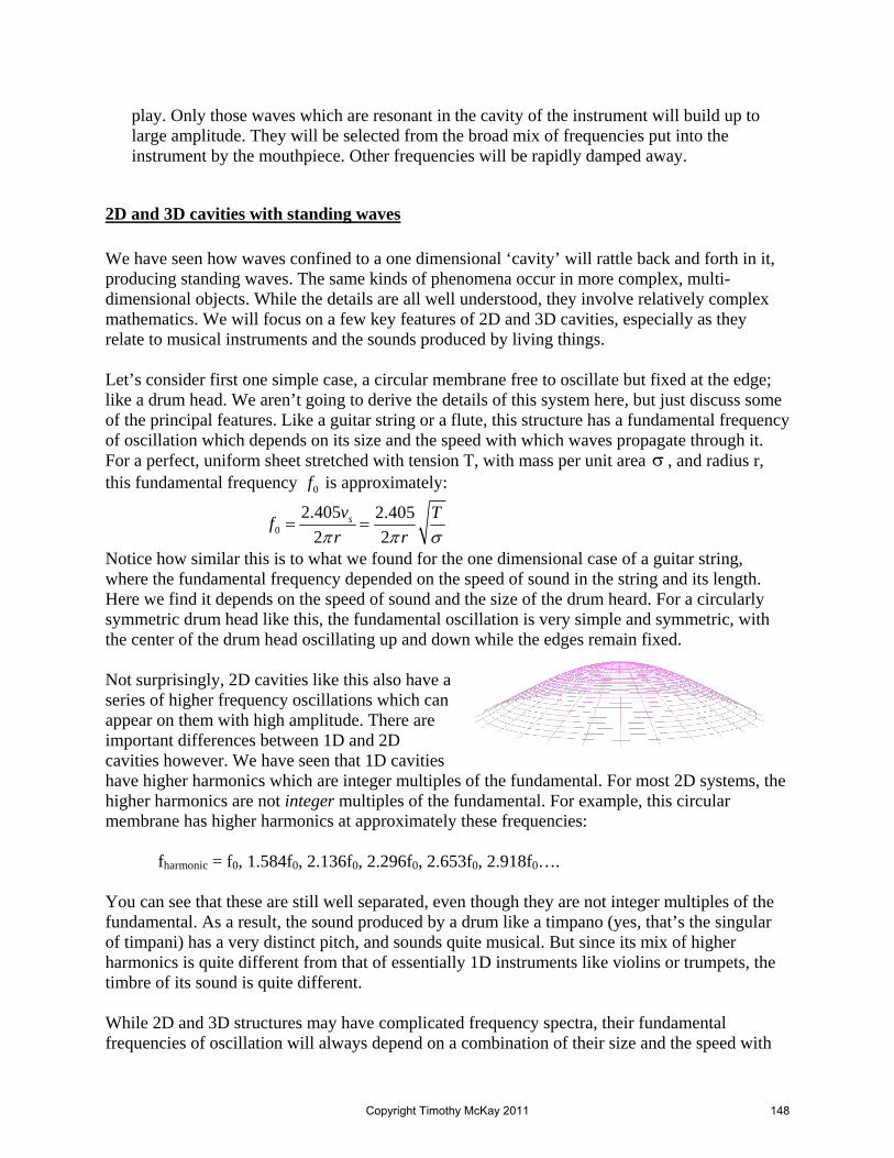
play. Only those waves which are resonant in the cavity of the instrument will build up to large amplitude. They will be selected from the broad mix of frequencies put into the instrument by the mouthpiece. Other frequencies will be rapidly damped away.

2D and 3D cavities with standing waves We have seen how waves confined to a one dimensional ‘cavity’ will rattle back and forth in it, producing standing waves. The same kinds of phenomena occur in more complex, multi-dimensional objects. While the details are all well understood, they involve relatively complex mathematics. We will focus on a few key features of 2D and 3D cavities, especially as they relate to musical instruments and the sounds produced by living things. Let’s consider first one simple case, a circular membrane free to oscillate but fixed at the edge; like a drum head. We aren’t going to derive the details of this system here, but just discuss some of the principal features. Like a guitar string or a flute, this structure has a fundamental frequency of oscillation which depends on its size and the speed with which waves propagate through it. For a perfect, uniform sheet stretched with tension T, with mass per unit area σ , and radius r, this fundamental frequency 0f is approximately:

02.405 2.405

2 2sv Tf

r rπ π σ= =

Notice how similar this is to what we found for the one dimensional case of a guitar string, where the fundamental frequency depended on the speed of sound in the string and its length. Here we find it depends on the speed of sound and the size of the drum heard. For a circularly symmetric drum head like this, the fundamental oscillation is very simple and symmetric, with the center of the drum head oscillating up and down while the edges remain fixed. Not surprisingly, 2D cavities like this also have a series of higher frequency oscillations which can appear on them with high amplitude. There are important differences between 1D and 2D cavities however. We have seen that 1D cavities have higher harmonics which are integer multiples of the fundamental. For most 2D systems, the higher harmonics are not integer multiples of the fundamental. For example, this circular membrane has higher harmonics at approximately these frequencies: fharmonic = f0, 1.584f0, 2.136f0, 2.296f0, 2.653f0, 2.918f0…. You can see that these are still well separated, even though they are not integer multiples of the fundamental. As a result, the sound produced by a drum like a timpano (yes, that’s the singular of timpani) has a very distinct pitch, and sounds quite musical. But since its mix of higher harmonics is quite different from that of essentially 1D instruments like violins or trumpets, the timbre of its sound is quite different. While 2D and 3D structures may have complicated frequency spectra, their fundamental frequencies of oscillation will always depend on a combination of their size and the speed with


which waves propagate through them. Imagine a thin, rectangular plate with side lengths L1 and L2, through which sound travels at a speed vs. If the plate is clamped at the edges like a guitar string, we would expect this plate to have two fundamental frequencies with: 01 1/sf v L∝ and 02 2/sf v L∝ If one of these lengths becomes very short, its fundamental frequency becomes very large, and the system begins to act like a 1D oscillator; a simple bar. When a system lacks the symmetry of a circular drum head or a rectangular plate, we might still estimate its fundamental frequency of oscillation by noting its rough size L and speed of sound: ( )/ 2est sf v L∼ Imagine an air filled cavity, roughly spherical, 1 cm in size. We might expect such a cavity to have resonant frequencies around f ~ (343 m/s /2*0.01 m) ~ 17,000 Hz. What does this tell us about bats and their biosonar? If they use air filled cavities to amplify their sound, we might expect their size to be less than about 1 cm.

29.3: Sound and musical sound We have all the pieces in place now to discuss a very old mystery. There are a lot of different kinds of sounds in the world, and yet only a very restricted set of these are what we would call musical. What is the difference between musical and non-musical sounds, and how could we quantify it? To understand the difference, we might begin with a "pure" tone, a pure harmonic wave, made of just one frequency. The wave function for such a pure, single frequency, wave is simple: it is just the harmonic sine wave we've been using as an example. Such a pure, single frequency sound is not what we would call musical though; it lacks the warmth and timbre of a musical instrument. You are most likely to have heard this sound emanating from a computer; the electronic ‘beeeeep’ of the modern world. No one would go to a concert to listen to this kind of sound, even if it was used to play the loveliest melody you know. At the other extreme, with no particular frequency at all, is the nasty sound we would call "noise". The wave function for noise doesn't look at all like our smooth, regular, sinusoidal wave. Instead it bounces up and down seemingly at random. It is still a wave; a traveling disturbance, but it is definitely not a harmonic wave with a single frequency, and it is definitely not musical. A musical sound lies somewhere in between. The figure below shows examples of wave functions for all three kinds of sounds, including the sound from a violin string. The pure tone is a perfect harmonic wave, already familiar to us. The wave function for the noise is jagged and random. The violin wave is intermediate. Here we see a wave that has a very periodic looking pattern; certainly it's not random like the noise. It's also certainly not a sine wave.


But we know what it is! We have just calculated what frequencies a violin string like this can oscillate at. The sound you hear from a violin (or see in its wave function) is the sum of a bunch of sine waves, each of which is a multiple of some lowest, fundamental frequency. Sounds from a wind instrument, like a flute or bassoon, also look very periodic. But like this violin, they are always more than just a pure sine wave.

Musical sounds are constructed from a sum of harmonic sine waves, each of which is a multiple of some fundamental frequency. This is the key to musical sound. A sound has the lovely nature of music sound if it is made up of a set of pure harmonic waves which have frequencies well separated from one another. In one dimensional wind and string instruments, these sounds are integer multiples of a fundamental frequency. A large frequency separation is essential to the attractiveness of musical sound. Without it, we might have two tones of almost the same frequency. Two waves separated by just a little in frequency produce “beats”; the interference in time we discussed earlier in this chapter. This beat phenomenon sounds nasty rather than nice. So for sounds to be musical they have to have more than one frequency, this is what gives them complexity and warmth, but the various frequencies cannot be too close together. The "resonant cavities" which make up musical instruments produce these mixes of harmonic waves in a completely natural way. They can be excited by oscillators which produce a broad array of different frequencies. Think for example of the buzzy, noisy sounds produced by a bare oboe reed or a trumpet mouthpiece. The instruments then select a set of specific, well separated frequencies, allowing only these to oscillate with large amplitude. Because they generate a mix of different frequencies, none of which are too close together, musical instruments produce sounds which are rich without becoming noisy. Truly musical sound requires both elements.

Wave function for noise

Wave function for a violin playing a G

Wave function for a pure tone


Frequency analysis Looking at wave functions can give us an idea of their nature, but there is a more quantitative way to examine the nature of a sound, or indeed of any wave; by frequency analysis. To better understand a sound, we might see what set of perfect harmonic sine waves could be added together to produce it. Remarkably, every sound can be accurately expressed as some sum of sine waves. The difference between different sounds is then just a matter of how much of each pure frequency the sounds contain. The results of frequency analysis are often displayed in ‘spectrograms’, 2 dimensional plots which allow us to visualize the changing mix of frequencies present in a sound. A typical spectrogram has time on the x-axis and frequency on the y axis. The intensity of each frequency at each moment in time is typically displayed as a gray-scale intensity. Sometimes another color scheme, or even a projected third dimension is used. Spectrograms are used extensively in the analysis of the natural sounds made by humans and other organisms. They also play an essential role in many forms of image analysis. A few examples are provided below.

Wave functions and spectrograms: On the left we see a pure tone, containing just one frequency. This kind of sound is called ‘narrow-band’, because it involves a narrow band of frequencies. On the right we see the wave function and spectrogram for ‘noise’, containing nearly equal amounts of every frequency. This kind of sound is called ‘broad-band’ because it contains a broad range of different frequencies.


Can every sound be constructed as a sum of sine waves? Most sounds are not simple harmonic waves, but something more complex. Is it really possible to construct every imaginable sound as a sum of sine waves with particular frequencies? Let’s look a little at how this might be done. The ability to construct any sound from a sum of sine waves is expressed clearly in a very powerful theorem first proven by Jean-Baptiste Fourier, a man whose life neatly spanned the French Revolution (1768-1830). It states that any arbitrary function which is periodic with angular frequency ω can be accurately represented by a "Fourier Series":

( ) ( ) ( )0

1 1cos sin

2 n naF t a n t b n tω ω

∞ ∞

= + +∑ ∑

In this equation, the variables an and bn are coefficients which express how much of each frequency needs to be included. We’re not going to prove this theorem here, but we’ll see what it means for the frequency analysis of our waves. Since every wave function is written as some continuous F(x,t), we can represent any wave function as a sum of differing amounts of sines and cosines. Every sound can be accurately thought of as being “made up of” a set of pure tones, each appearing with different strength. If a sound is a pure tone, only one frequency will contribute. If a sound is musical, a set of well

This is the wave function for a bassoon playing a b flat. The wave is periodic, with a period of 0.002 seconds. This implies a fundamental frequency of about 500 Hz.

This is the ‘spectrogram’ of the bassoon sound. It shows, in gray scale, the amount of the sound made of each frequency, as a function of time. Note the strong fundamental at about 500 Hz, and the strong integer multiples of this fundamental.


separated frequencies will all appear. If a sound is “noise” many closely spaced frequencies will contribute in nearly equal amounts. Before going further, we should look more closely at the conditions we set. Fourier’s theorem requires that the function we’re trying to express should be periodic with angular frequency ω . Does this mean that some sound, like random noise, cannot be expressed as a sum of sines and cosines? Imagine that a sound is nearly aperiodic, and essentially never repeats. The frequency of such a sound, as always, would be the inverse of its period. Since the period approaches infinity, the fundamental frequency approaches zero. We can still use Fourier’s theorem to describe such a sound, we just need to note that its fundamental frequency is close to zero. For such a wave, the higher harmonics, multiples of the fundamental frequency, will be very close together. Such a sound will be made of almost every frequency; it will be noisy. So in practice, this method of frequency analysis works for all waves, whether obviously periodic or not.

How much of each sine wave is in a sound? Frequency analysis How do we determine the coefficients needed to construct a particular sound F(t)? To do this, we take advantage of what are called the “orthogonality conditions” for the trigonometric functions. Each of these relations is an integral which sums the product of two sine or cosine functions with frequencies which are integer multiples of some fundamental ω across one fundamental period of oscillationτ . If the two functions are the same, both sines with the same frequency, or both cosines with the same frequency, this integral has the value / 2τ . If they are different, the integral is zero. We can write out these relations formally as follows.

( ) ( )

( ) ( )

( ) ( )

0

0

0

sin sin or 0 if 02

cos cos or if 02

sin cos 0

mn

mn

m t n t dt m

m t n t dt m n

m t n t dt

τ

τ

τ

τω ω δ

τω ω δ τ

ω ω

= =

= = =

=

∫

∫

∫

What is this new symbol mnδ ? This is called the “Kronecker delta”. This symbol stands for something which has a value of 1 when m n= , and 0 when m n≠ . The symbol is just a shorthand notation for this. These mathematical facts are known in general as ‘orthogonality conditions’, as they express the fact that each function is in some sense independent of (kind of perpendicular to) all the others. Using these, we can find the coefficients in the Fourier expansion:


( )

( ) ( )

( ) ( )

00

0

0

1

1 sin

1 cos

n

n

a F t dt

a F t n t dt

b F t n t dt

τ

τ

τ

τ

ωτ

ωτ

=

=

=

∫

∫

∫

So it is not only possible, but pretty easy, to figure out what coefficients are required to expand any periodic function in terms of a set of sinusoidal functions. Each of the "Fourier components" of such a function is called a "harmonic". Understanding a wave function for a periodic wave can then be reduced to listing the amplitudes (the coefficients ai and bi) of its harmonics. The process of figuring out what set of frequencies make up a sound, how much of each harmonic is present, is called ‘analyzing’ the sound. Reversing this process, assembling the sound from its individual harmonic components, is called ‘synthesizing’ the sound. Indeed, the synthesizer used in modern electronic music is just a device able to approximate any sound by adding appropriate mixes of pure tones. The sines and cosines in the Fourier series all have frequencies which are integer multiples of the fundamental angular frequency ω of the function F(t). This angular frequency is 2 fπ , where f is the fundamental frequency of F(t), one over its period of repetition. So far, we have discussed how you can construct any periodic sound from a sum of sines and cosines. But no real sound is perfectly periodic. To be so, it would have to have always been happening, and to continue forever into the future. Real sounds start and stop, and hence aren’t perfectly periodic. How can they possibly be represented in this form, as a sum of sinusoids? To represent such real, temporary sounds, we must add sines and cosines in a more flexible way. To begin with, they need to have different frequencies, the already familiar spectrogram. But now they must also have a mix of different phases. To top it off, we need to use both real and imaginary sinusoids (imaginary in the 1− mathematical sense, not in the unicorn sense). Adding this additional freedom allows us to express any sound at all in terms of a mix of frequencies which changes in time. The mathematics required to do this is more complex than would be fruitful to discuss here. But it is important for you to understand that any sound really can be assembled from a sum of sines and cosines. In some real sense, every sound is a sum of sines and cosines. There are (at least!) two ways to analyze a sound. The first is mathematically. Each of the coefficients can be calculated, sometimes analytically, but always at least numerically. If we measure the wave function of a sound and express it digitally, we can use this approach to give us a good idea of what harmonics make up various sounds. An example of this is shown in the figure below, which illustrates how you can construct a good approximation for a square wave by adding up a series of sine waves. The second way to analyze a sound is physically. To do this, we return to the idea of resonance. If we drive a system with a natural frequency of oscillation at the resonant frequency, it will


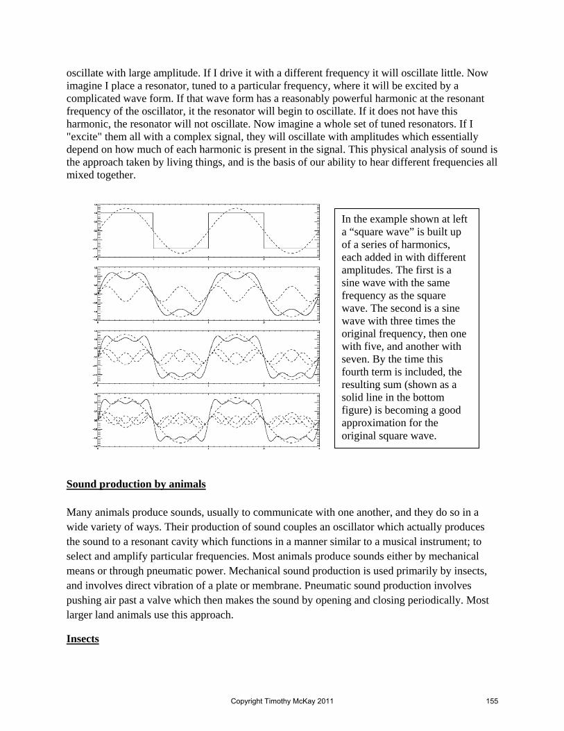
oscillate with large amplitude. If I drive it with a different frequency it will oscillate little. Now imagine I place a resonator, tuned to a particular frequency, where it will be excited by a complicated wave form. If that wave form has a reasonably powerful harmonic at the resonant frequency of the oscillator, it the resonator will begin to oscillate. If it does not have this harmonic, the resonator will not oscillate. Now imagine a whole set of tuned resonators. If I "excite" them all with a complex signal, they will oscillate with amplitudes which essentially depend on how much of each harmonic is present in the signal. This physical analysis of sound is the approach taken by living things, and is the basis of our ability to hear different frequencies all mixed together.

Sound production by animals Many animals produce sounds, usually to communicate with one another, and they do so in a wide variety of ways. Their production of sound couples an oscillator which actually produces the sound to a resonant cavity which functions in a manner similar to a musical instrument; to select and amplify particular frequencies. Most animals produce sounds either by mechanical means or through pneumatic power. Mechanical sound production is used primarily by insects, and involves direct vibration of a plate or membrane. Pneumatic sound production involves pushing air past a valve which then makes the sound by opening and closing periodically. Most larger land animals use this approach.

Insects

In the example shown at left a “square wave” is built up of a series of harmonics, each added in with different amplitudes. The first is a sine wave with the same frequency as the square wave. The second is a sine wave with three times the original frequency, then one with five, and another with seven. By the time this fourth term is included, the resulting sum (shown as a solid line in the bottom figure) is becoming a good approximation for the original square wave.


Mechanical sound production often involves applying a steady force to push one body part over a series of regularly spaced notches in another. Each time the part being pushed slips over a notch, a very short, impulsive sound is produced; a click. If this implement is dragged at a steady rate over a series of notches, a very pure sound, made of almost one frequency can be produced. This process is known by the wonderful name ‘stridulation’.

In male crickets, one of the most familiar summer insects, a ‘scraper’ on one wing is dragged over a ‘file’ on the other. The impulses associated with each slip of the scraper over the file drive oscillations in fibers within the wings of the cricket. These resonant oscillations then nicely couple the sounds being produced in the file to the surrounding air, in very much the same manner that a guitar body couples the vibrations of a string to the air.

Cicadas, the loudest of insect singers, produce their sounds in a different way. The ribs of a cicada form a ‘tymbal’, a kind of curved shell which can be made to suddenly buckle when a force is applied to it. This mechanism is emulated in the small metal ‘crickets’ which you may have clicked as a child. The sound produced by this buckling tymbal is then amplified in the large resonant cavity which makes up most of the cicada’s fat abdomen. A typical cicada, just an inch or so long, produces a very intense sound. It can be well over 100 dB a few feet away.

Vertebrates: people, birds, and bats

Pneumatic sound production, used by most vertebrates, involves three principle parts;

1. Lungs provide a reservoir of air that can be forced through the respiratory tract at a pressure higher than atmospheric

2. A valve within the respiratory tract that oscillates open and closed as air passes through 3. A chamber in which the sound may resonate and build up to large amplitude

Your own voice provides an instructive example. When you speak, you compress the air in your lungs using you diaphragm, forcing it slowly outward through your trachea. Just at the point where your trachea joins your esophagus, in your larynx, a pair of matched vocal ‘folds’ extend across the opening. These folds, sometimes called vocal cords, are muscular, and can be held across the trachea to prevent air from leaving. This is called a glottal stop. If you loosen the folds a little, air will push through. As soon as a little air goes through, the pressure behind the folds drops, and they close. Then pressure builds again, forcing them open, and a vibration ensues. The frequency of the resulting vibration depends both on how vigorously


you force air through, and especially how tightly the folds are stretched. If you loosen the folds still further, air can exit without causing vibrations, as it usually does when you breathe.

The vibrations produced by the vocal folds feed a resonating chamber formed from your throat and mouth, interacting with them just as a musical instrument interacts with its mouthpiece. This resonating chamber selects and amplifies particular frequencies in a way which depends on its size and shape. All the elements of this system are remarkably flexible and dynamically controlled: lungs, vocal folds, throat and mouth. The enormous freedom provided by this highly adaptable system is what enables the full virtuosity of language and singing. Every time you speak a sentence, tell a story, or sing a song, you play your vocal instrument with a level of expression and variety which instrumental musicians, with their much less flexible apparatus, struggle for years to emulate. The ability to speak in such rich and complex ways is one of the defining features of humans, we’re really good at this, and a substantial fraction of your brain is dedicated to making the whole system work precisely and reliably.

Many other animals have remarkable voices. Birds, for example, are perhaps nature’s most remarkable singers. Like us, their vocal systems have three parts; lungs, a ‘syrinx’, in which oscillations make sounds, and resonant cavities. The syrinx of a bird lies lower in the respiratory tract than the larynx, at the bottom of the trachea rather than the top. It has two channels, one extending to each lung. Parts of these tubes are lined with flexible membranes, and the whole syrinx is embedded in an external air sack, independent of the lungs. In this case the membranes which oscillate lack muscle, and instead have their tension adjusted by changing the pressure in the external air sack. Pitch is controlled by varying both this membrane pressure and the flow of air through the bronchial tubes. Since there are two sides to the syrinx, it is possible for birds to sing two different fundamental frequencies at once; something we cannot do with our single set of vocal folds.

Birds, more than most other kinds of animals, make many sounds for communication. They use sound to mark their territories, find mates, maintain social connections, and train their young. The details of bird song are often learned, rather than instinctual, making them a kind of culture. Quite a few bird species are also mimics; with vocal and neural systems capable of imitating nearly any sound they hear. In this sense they surely surpass people. In a songbird like the Northern Cardinal, the entire system of sound production is about the size of a kernel of corn. This small size, of course, accounts for the relatively high frequency of most bird song.

Echolocating animals take sound production one step further. Not only do they use sound to communicate in complex ways, they use the sound they produce to image the silent world around them. This places intense new demands on their ability to produce sounds. Bats must produce very high frequency sounds (we will see why in the next chapter). While their small size is part of what allows this, they must also stretch their vocal folds to very high tension, and for this


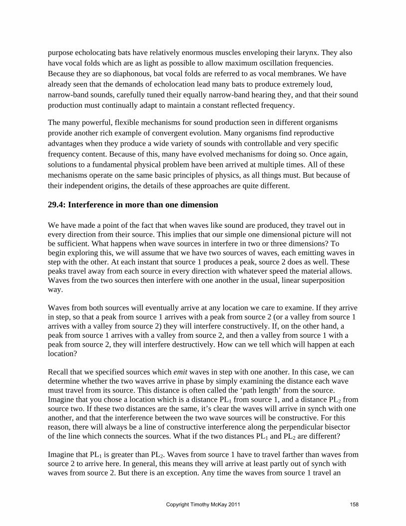
purpose echolocating bats have relatively enormous muscles enveloping their larynx. They also have vocal folds which are as light as possible to allow maximum oscillation frequencies. Because they are so diaphonous, bat vocal folds are referred to as vocal membranes. We have already seen that the demands of echolocation lead many bats to produce extremely loud, narrow-band sounds, carefully tuned their equally narrow-band hearing they, and that their sound production must continually adapt to maintain a constant reflected frequency.

The many powerful, flexible mechanisms for sound production seen in different organisms provide another rich example of convergent evolution. Many organisms find reproductive advantages when they produce a wide variety of sounds with controllable and very specific frequency content. Because of this, many have evolved mechanisms for doing so. Once again, solutions to a fundamental physical problem have been arrived at multiple times. All of these mechanisms operate on the same basic principles of physics, as all things must. But because of their independent origins, the details of these approaches are quite different.

29.4: Interference in more than one dimension We have made a point of the fact that when waves like sound are produced, they travel out in every direction from their source. This implies that our simple one dimensional picture will not be sufficient. What happens when wave sources in interfere in two or three dimensions? To begin exploring this, we will assume that we have two sources of waves, each emitting waves in step with the other. At each instant that source 1 produces a peak, source 2 does as well. These peaks travel away from each source in every direction with whatever speed the material allows. Waves from the two sources then interfere with one another in the usual, linear superposition way. Waves from both sources will eventually arrive at any location we care to examine. If they arrive in step, so that a peak from source 1 arrives with a peak from source 2 (or a valley from source 1 arrives with a valley from source 2) they will interfere constructively. If, on the other hand, a peak from source 1 arrives with a valley from source 2, and then a valley from source 1 with a peak from source 2, they will interfere destructively. How can we tell which will happen at each location? Recall that we specified sources which emit waves in step with one another. In this case, we can determine whether the two waves arrive in phase by simply examining the distance each wave must travel from its source. This distance is often called the ‘path length’ from the source. Imagine that you chose a location which is a distance PL1 from source 1, and a distance PL2 from source two. If these two distances are the same, it’s clear the waves will arrive in synch with one another, and that the interference between the two wave sources will be constructive. For this reason, there will always be a line of constructive interference along the perpendicular bisector of the line which connects the sources. What if the two distances PL1 and PL2 are different? Imagine that PL1 is greater than PL2. Waves from source 1 have to travel farther than waves from source 2 to arrive here. In general, this means they will arrive at least partly out of synch with waves from source 2. But there is an exception. Any time the waves from source 1 travel an


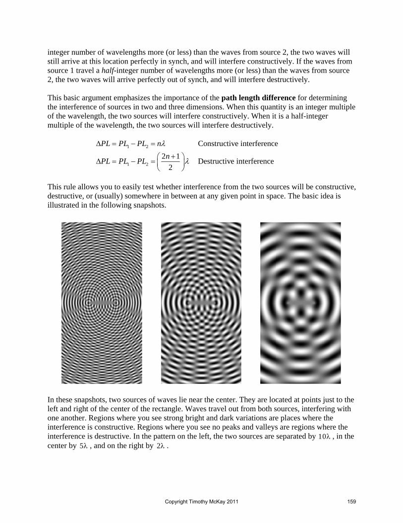
integer number of wavelengths more (or less) than the waves from source 2, the two waves will still arrive at this location perfectly in synch, and will interfere constructively. If the waves from source 1 travel a half-integer number of wavelengths more (or less) than the waves from source 2, the two waves will arrive perfectly out of synch, and will interfere destructively. This basic argument emphasizes the importance of the path length difference for determining the interference of sources in two and three dimensions. When this quantity is an integer multiple of the wavelength, the two sources will interfere constructively. When it is a half-integer multiple of the wavelength, the two sources will interfere destructively.

1 2

1 2

Constructive interference2 1 Destructive interference

2

PL PL PL nnPL PL PL

λ

λ

Δ = − =

+⎛ ⎞Δ = − = ⎜ ⎟⎝ ⎠

This rule allows you to easily test whether interference from the two sources will be constructive, destructive, or (usually) somewhere in between at any given point in space. The basic idea is illustrated in the following snapshots.

In these snapshots, two sources of waves lie near the center. They are located at points just to the left and right of the center of the rectangle. Waves travel out from both sources, interfering with one another. Regions where you see strong bright and dark variations are places where the interference is constructive. Regions where you see no peaks and valleys are regions where the interference is destructive. In the pattern on the left, the two sources are separated by 10λ , in the center by 5λ , and on the right by 2λ .


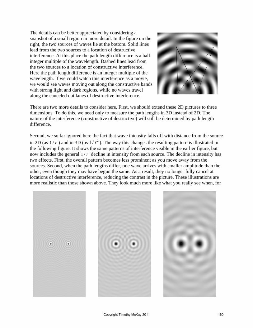
The details can be better appreciated by considering a snapshot of a small region in more detail. In the figure on the right, the two sources of waves lie at the bottom. Solid lines lead from the two sources to a location of destructive interference. At this place the path length difference is a half integer multiple of the wavelength. Dashed lines lead from the two sources to a location of constructive interference. Here the path length difference is an integer multiple of the wavelength. If we could watch this interference as a movie, we would see waves moving out along the constructive bands with strong light and dark regions, while no waves travel along the canceled out lanes of destructive interference. There are two more details to consider here. First, we should extend these 2D pictures to three dimensions. To do this, we need only to measure the path lengths in 3D instead of 2D. The nature of the interference (constructive of destructive) will still be determined by path length difference. Second, we so far ignored here the fact that wave intensity falls off with distance from the source in 2D (as 1 / r ) and in 3D (as 21/ r ). The way this changes the resulting pattern is illustrated in the following figure. It shows the same patterns of interference visible in the earlier figure, but now includes the general 1 / r decline in intensity from each source. The decline in intensity has two effects. First, the overall pattern becomes less prominent as you move away from the sources. Second, when the path lengths differ, one wave arrives with smaller amplitude than the other, even though they may have begun the same. As a result, they no longer fully cancel at locations of destructive interference, reducing the contrast in the picture. These illustrations are more realistic than those shown above. They look much more like what you really see when, for


example, you throw two stones onto the surface of a puddle. The patterns observed are similar to those shown above, but the interference effects are somewhat less obvious. Interestingly, the effects of intensity falloff are most obvious near the sources, where the difference in path length between the two can be a substantial fraction of the total path length. In this ‘near field’ region, the nature of the interference between two sources is significantly complicated by intensity changes. Imagine instead that you examine the wave far from the sources. This is the so-called ‘far field’ region, at distances much greater than the source separation. In this region, the path length differences from the two sources are always a small fraction of the total path length from the sources to any point. When this is the case, the intensity of the waves from the two sources will be almost the same. So although both will have faded, their intensities will be nearly matched. The resulting pattern of interference will be almost as complete as it was when we ignored intensity changes. This fact will be very important in the next chapter, when learn about X-ray diffraction and its use in the determination of the structure of biomolecules.

Why have you never noticed interference before? We use sound and light constantly. Why is this defining phenomenon of interference not more readily apparent? Of course one aspect of interference is familiar; the way waves from multiple sources add together in linear superposition. We use this to pick out a friends voice within the cacophony of a party. But destructive interference, the cancellation of one wave by another, is much less familiar. The explanation lies in several details. First, most sources of sound and light do not emit pure, single frequency waves. Instead, they emit broad-band sounds, made up of a mix of many frequencies. Go back and imagine the two source interference we considered in the last section, but now allow the two sources to emit waves of many frequencies. At some particular location, the path length difference from the two sources may be a half integer multiple of one of the wavelengths emitted by the sources, so that waves of that frequency will interfere destructively. But these waves now contain many frequencies, each with a corresponding wavelength. These other frequencies will not experience completely destructive interference at this point. Indeed, some will experience completely constructuctive interference at this point. As a result, there will be no particular location where all the waves from the two sources completely cancel. This is one reason why destructive interference, the defining feature of waves, is usually not obvious. It’s there, but is being washed out. When we wish to demonstrate interference of either sound or light, we will use waves with basically a single frequency; either a pure tone or the light from a narrow-band laser. Second, the sound and light arriving at any point usually comes from many different sources, rather than just two as we have discussed. If interference from many sources is to be completely destructive, all of the waves arriving there must be very precisely coordinated, so that each peak from one source is carefully cancelled by a valley from another. The variation in intensity with distance which we noted in the previous section plays a role in this as well. Not only must there


be a valley for every peak, they must also have the same amplitudes. While this careful coordination can occur (we will see very important examples in the next chapter) it is rare. Third, interference maxima and minima will typically be separated by about a wavelength of the wave in question. For sound, with wavelengths from millimeters to meters, this is not too big an impediment. But for light, with wavelengths from 350 – 700 billionths of a meter, this makes maxima and minima very close together indeed. All of these confusing factors make testing the fundamental wave nature of things a challenge. The required observations for light were difficult enough to elude even Newton, who remained convinced that light was particulate. After Newton, 130 years would elapse before Thomas Young would convince the physics community, through convincing demonstrations of interference, that light was, like sound, a wave phenomenon.

29.5: Conclusions Wave motion is a method of moving energy and momentum, and more generally, information rapidly without moving any matter. Because of its speed, it is one of the major ways energy flows in the universe. The speed of waves in materials is governed by a balance between restoring force and inertia in the medium. The most important feature of waves to remember is that they so often combine in linear superposition. This gives rise to somewhat surprising 'interference effects', such as cancellation, beating, and standing waves. There is a very important piece of history connected with this chapter as well. We have seen how a particular kind of sound, with a number of well separated frequencies added together, produces a pleasant sensation for people, a musical sound. The discovery of perfect ratios in the frequencies which make up musical sounds was the great triumph of the Pythagoreans in ancient Greece. That something beautiful and real was connected to simple mathematical fornulae fostered the initial connection between mathematics and science. It led them to think that perhaps mathematical relationships might model other phenomena of nature, and in this sense gave rise to quantitative science. For many years, until well into the 20th century, the use of mathematical models was largely limited to the physical sciences, where it was wildly successful. Physics and chemistry often provide systems simple enough to conform to analytic models, described with great precision by very simple equations. Over the last 100 years, some of the fundamental mechanisms of life have been discovered, things like the cell, the gene, evolution, and biochemistryi. Unlike complete organisms, these mechanisms often admit detailed mathematical models. In response, biology has grown increasingly quantitative and mathematical, joining the physical sciences in the use of mathematics as a meaningful language for expressing how the world works. The deep connection between mathematics, an abstract system of postulates and theorems, and the real phenomena of the world, remains unexplained. Why should the world be so well described by equations? As Eugene Wigner, one of the 20th centuries leading physicists once put it:


The miracle of the appropriateness of the language of mathematics for the formulation of the laws of physics is a wonderful gift which we neither understand nor deserveii.

Whatever its origin, this connection, played out in the minds of millions of people over three thousand years, is ultimately responsible for the technological lives you lead today. And it all began with the mysterious beauty of music and the strings of a lute.


A Quick Summary of Some Important Relations When waves combine, superposition: So long as wave amplitudes are not large, two waves passing through the same region simply add together in superposition: ( ) ( ) ( )total 1 2, , ,y x t y x t y x t= + In this superposition the two waves may reinforce one another or cancel one another out. These cases are called constructive and destructive interference. 1D Superposition of two sine waves going the same direction: For the special case of adding two 1D sine waves with the same amplitude and frequency, the nature of the interference depends on the relative phase of the two waves:

( ) ( ) ( )( ) ( )

( )( ) ( )

total

total

total

total

, sin sin

0 , 2 sin

, 0

2 , 2 sin

y x t A kx t A kx t

y x t A kx t

y x t

y x t A kx t

ω ω φ

φ ω

φ π

φ π ω

= − + − +

= ⇒ = −

= ⇒ =

= ⇒ = −

1D Superposition of two sine waves going the opposite direction:

This produces a ‘standing wave’, with all points oscillating up and down with the frequency of the original wave. The amplitudes of oscillation vary, with peaks in amplitude separated by the original wavelength of the combined waves. Interference in time – beats:

For the special case of two waves beginning in phase, but with different frequencies, new wave is produced with a carrier frequency which is the average of the input frequencies and a ‘beating’ amplitude oscillation with a frequency equal to the difference of the two frequencies.

Wave reflections at boundaries:

When waves reach a boundary with a new material, they may reflect. If the boundary is ‘stiff’ they will reflect out of phase. If it is ‘free’, they will reflect in phase. For sound stiffness is expressed by the acoustic impedance, for light by the index of refraction. Waves reflecting back and forth in confined cavities are the primary example of standing waves.

Cavity standing waves and musical instruments:

Constraints placed on waves by the cavities in which they oscillate permit only certain frequencies to oscillate with large amplitudes. Two examples:


closed string pipe open at 1 end sound2 1

2 4n T nf f vL Lμ

+= =

Sound and musical sound:

The nature of a sound, its timbre, is determined by the mix of frequencies (and hence wavelengths) which it is made of. When a sound is made of multiple, well separated frequencies, all multiples of a single fundamental frequency, it will be a musical sound. Light can also be separated into a mix of frequencies – these determine its color. Sounds are produced by animals in cavities, roughly like what musical instruments do.

Interference in two and three dimensions:

Waves from two sources interfere in a way which is governed by the path length from each source to the location of interest.

1 2

1 2

Constructive interference

Destructive interference

2 1

2

PL PL PL nnPL PL PL

λ

λ

Δ = − =

+⎛ ⎞Δ = − = ⎜ ⎟⎝ ⎠

Whether they can fully cancel one another at a particular point depends also on the intensity decline with distance for two and three dimensional waves discussed above.

i Paul Nurse, 2003, “The great ideas of biology”, Clinical Medicine, 3, 560.

ii Eugene Wigner, 1960, "The Unreasonable Effectiveness of Mathematics in the Natural Sciences," Communications on Pure and Applied Mathematics 13(1): 1–14.


POLS Waves Chapter 30

30.0: How waves really travel: the Huygen’s construct To understand in detail how waves travel, it is helpful to think about the surface water waves you’re used to seeing. You’re probably used to two forms of these waves. The first are the ripples which spread in circles when you toss a pebble in a pond. Waves travel out in circles from this ‘point source’ disturbance in every direction. But there is a second kind of wave you have probably seen; the straight lines of ‘plane waves’ which roll into shore in a long set of parallel lines. In each case, we see that the wavefronts themselves are perpendicular to the direction of motion of the waves.

How are these two kinds of waves related? There is a first, relatively obvious connection. As the waves travel out from a point source, their circular nature becomes less and less apparent. When the distance from a source is many times the wavelength of the wave, you might begin to think they were, in fact, plane waves. For large scale surface water waves, with wavelengths like 10 m, you have to be pretty far away (like 100 meters or more) before they start to look like plane waves. For visible light waves, however, wavelengths are very short, like 5x10-7 m. For these, you have only to be a few millimeters from a source before they really start to seem like parallel plane waves. So in a sense, plane waves are naturally produced by point sources. But there is a deeper, more surprising connection; plane waves can themselves become point sources. This less obvious connection was first expressed around 1690 by Christian Huygens, a very versatile Dutch contemporary of Newton. Huygens recognized each point along a plane wave acts just like the single point above, sending out disturbances in every direction. The waves from all of these separate points spread over one another, and their net effect is the superposition of the disturbances spreading out from each of these points.

Ripples spreading in a circle from a point disturbance

Parallel plane waves coming in to shore at a beach


What happens when we add up the waves produced by all of these little spots? As usual, there are places where they add constructively, and places where they add destructively, canceling one another out. If you look closely, you will see that there are straight lines integer numbers of wavelengths above and below the centerline. At these points all of the waves from the points along the original wave front come together to add constructively. So the net result of this line of sources, each sending out waves independently in every direction, is a plane wave, a series of peaks and troughs where the peaks stretch out perpendicular to the direction of motion. The figure shows how a set of 20 sources, each independently sending out waves in all directions, come together to make a plane wave. This is compared in the picture on the right to some plane waves coming in at the beach.

Slits, obstacles, and diffraction Huygens’s recognition that each point on a plane wave is itself a point source of new waves opens the door to another set of important wave phenomena: the effects of diffraction. Diffraction is really just another interference phenomenon, just the adding up of several waves to make a new one. This different name is typically used for a particular set of interference phenomena which occur when a plane wave encounters an obstacle, something like a barrier with a hole in it, or conversely an obstacle of limited size. We will think about these cases first using qualitatively, using Huygens principle. Later we will work out the details mathematically, from the basic principle of superposition. Imagine first a barrier with a hole. There are two limiting cases, when the hole is small compared to the wavelength, and when it is large compared to the wavelength. On the left is an illustration of a small hole. In this case, the hole is small enough to contain just one ‘oscillating spot’. From this one source, the waves on the right of the barrier spread out nearly uniformly in every direction. To the area on the right, it looks like this hole is just a point source of waves. Notice what this means. A plane wave coming from the left arrives at the barrier. This plane wave seems to travel only straight to the right. Then, after the hole, the wave spreads out not just to the right, but also up, down, and in every direction in between. On passing through the hole, the wave seems to ‘bend’ around the corners and go in every direction. This effect, this spreading out in every direction, is called diffraction. It is another phenomenon unique to waves. If a row of particles arrived at this slit instead of a wave, they wouldn’t bend around the corner at all. Some would pass straight through, traveling purely to the right in a straight line, while all the others were blocked. Like the interference phenomena we discussed before, diffraction is diagnostic of the presence of waves. When you see it, you know you’re dealing with a wave.


On the right is an illustration of what happens with a larger hole. In this case, there are a lot of points acting like individual sources which fit in the hole. Most of the wave within that whole region marches along as if nothing had happened. Now there’s a plane wave which continues forward, just about as wide as the hole, marching off in a straight line toward the right. Such a large hole, struck by a plane wave, produces a beam of wave, about the width of the hole. Notice that just at the edge there are points that do send a bit of wave off to the side; there is a some diffraction. How much there is, compared to the wave which travels forward unimpeded, depends on the ratio of the hole size to the wavelength of the wave. When this ratio is large, almost all the wave just keeps going to the right as if nothing happened; only a tiny bit diffracts around the corner. When this ratio is small, little of the wave proceeds unimpeded, and much of what passes through is diffracted. What if, instead of little holes, we have obstacles of different sizes? The situation is remarkably similar, as these illustrations in this figure suggest. When you have a really small barrier, as on the left, only a bit of the wave front is blocked, and the diffraction of waves from both sides of the obstacle essentially replaces the little that was lost. This wave ‘washes around’ the obstacle, passing on almost as if it weren’t there. This is what happens if you stand in Lake Michigan. The waves coming in, with wavelengths much larger than your size, pass by almost as if you weren’t there. When a barrier is large compared to the wavelength, as on the right, the situation is different. In this case, a lot of the wave will be blocked. A little bit, from the edges of the barrier, diffracts around it and tries to fill in what was blocked, but it has little effect. Above and below the barrier the wave continues unabated, but in the region behind the barrier the wave is gone. It has been blocked. This large barrier has produced a shadow, a region from which the incoming plane wave is excluded.

Be sure to notice the parallel structure in these two cases. A plane wave arriving at a hole small compared to its wavelength diffracts dramatically on passing through the hole, spreading out


almost equally in every direction. A plane wave arriving at an obstacle small compared to its wavelength washes right around it, continuing on almost as if the obstacle were not there. A plane wave arriving at a hole large compared to its wavelength will send forward from the hole a beam, a plane wave of fixed width, which continues on in the original direction of the plane wave. A plane wave arriving at an obstacle large compared to its wavelength will produce a shadow, going straight past the edges of the obstacle and leaving an almost completely blank space behind it.

Diffraction and the propagation of sound and light In the previous section we saw that when waves encounter barriers diffraction can allow them to pass around them. When waves encounter a hole in a barrier or an obstacle which is small compared to their wavelength, diffraction will be a dramatic and obvious. When they encounter a hole or an obstacle which is large compared to their wavelength, they will mostly continue on in straight lines, forming a beam through a large slit and marching on smoothly while being effectively shadowed by a large obstacle. How do these phenomena affect the propagation of sound and light? The sounds humans can hear have frequencies ranging from 20-20,000 Hz. Traveling in air, these waves have wavelengths from 1.7 m to 1.7 cm; they are comparable in size to us. Waves like this, encountering holes like doorways, diffract beyond them very effectively. This is why you can hear your roommate approaching down the hall. When sound waves like this encounter tree trunks in a forest, they wash smoothly around them, almost is if they weren’t there. The ability of sound to travel around corners and past obstacles makes it an especially useful tool for communication among animals. Visible light, by contrast, has wavelengths that range from 4x10-7 m and 7x10-7 m. These are very tiny, meaning that almost any aperture through which light passes or obstacle which it encounters will be much larger than the wavelength. As a result, light will pass straight through most holes it encounters, continuing to travel in straight lines in a beam, rather than diffracting


around corners. Likewise when light encounters obstacles they are almost always much larger than the wavelength. As a result, light passes the edges of the obstacles in straight lines, leaving an empty, nearly light free shadow beyond. There’s no surprise here. You’ve known all your lives that light “travels in straight lines” and that sound travels bends around corners. You can often hear something that you can’t see. Now that you know about diffraction (and the very different wavelengths of sound and light) you know why.

30.1: Diffraction from a single hole: where are the minima? The discussion above gives a good general idea of the physics of diffraction through holes and around obstacles. In what follows we will work out some details for a few cases. Let’s look at diffraction of a 2D wave, like a surface water wave, through a single hole in a barrier. The diagram below describes the variables we will use. We start with the Huygens’ construct, which tells us that each point in the opening acts like a source of waves. We’re going to consider each of the points in the opening, add up the contributions from them all just as the principle of superposition suggests, and see what we get. In doing this, we will make an approximation: that the distance D from the hole to the point where we measure the wave is very large compared to the size of the hole d. When this is true, the two lines marked r and R in the figure are approximately parallel, both going off at the same angle θ . This may not seem at all obvious, because in this picture, the distance D is not much larger than the hole size d. To see how this can be true, try imagining how things change when you make D much larger, keeping ymin the same.

We start by considering just two points in the opening: one at the center, and one a distance y above it. Notice that the waves from the lower of these points travels farther to reach point P on the screen at distance D. The extra distance the waves from the lower point travel, the path

Distant screen

D

ymin

d


length difference is ( )sinPL y θΔ = . This is the path length difference for waves from the two sources. Since there is a path length difference, there can be either constructive or destructive interference. If the path length difference is a half integer multiple of the wavelength, waves from these two points will interfere destructively. If the path length difference is an integer multiple of the wavelength, they will interfere constructively. To take the next step, let’s apply a little logic. If we consider a separation 2y d= , every point on the bottom half of the hole will be matched by another from the top. For a separation 4y d= each point in the second quarter is matched by a point in the first, while each in the fourth is matched by one in the third. The same is true for 8, 16y d d= etc. Now, if waves from the two points in each of these matched pairs interfere destructively at point P, no waves at all will arrive there! Waves from every point in the hole will be canceled by waves from some other point. If this happens, the wave intensity at point P will fall to zero. What conditions are required if this is to happen? The basic requirement is that the path length difference should be a half integer multiple of the wavelength. Here are the conditions for the first two of our sets of matched point pairs:

( ) ( )

( ) ( )

min min min

min min min

sin sin 2 1 or sin 2 12 2

sin sin 2 1 or sin 2 2 14 2

...

dy n nd

dy n nd

etc

λ λθ θ θ

λ λθ θ θ

⎛ ⎞= = + = + ⎜ ⎟⎝ ⎠⎛ ⎞= = + = + ⎜ ⎟⎝ ⎠

where the ‘n’ in these equations can be 0, 1, 2, 3± ± ± and so on. What does this mean? Each case gives us a condition on the angle θ. The first says that minsinθ should be an odd multiple of the

ratio dλ . The second says that minsinθ should be an even integer multiple of the ratio dλ .

Since we can always pair up points separated by 2d or 4d , both these conditions apply, and we should get fully destructive interference anytime:

minsin mdλθ =

Where now the ‘m’ is any integer except zero. This is a remarkably simple condition, which tells us at what angles we expect to see no waves at all emerge. Let’s see what it implies. First, if d λ< : then the ratio dλ is always bigger than one, and there is no angle θ for which this condition is met. That’s just what we expected from our Huygens construct arguments above; when the hole is smaller than the wavelength, the wave washes out in every direction. In this case, there is no direction in which the wave amplitude is exactly zero. Yes, the intensity of the wave falls as you move farther from the slit, but it never drops to zero. Some of the wave fans out in every direction.


Second, when d λ> : now it is possible to meet the criterion above, and there will be one or more angles for which waves from different parts of the hole completely cancel one another. If we consider the case where d λ , we will find such minima when minsinθ is small. When

that’s true, we can sensibly use the estimate min minsinθ θ , and minmin

yD

θ . Within these limits

the first minimum will be located where:

minmin min minsin and we can write y m m Dy

D d dλ λθ θ≈ ≈ = =

When will this condition ( minsinθ is really small) apply? This is applicable when the hole size is much bigger than the wavelength, d λ , a condition which will often be met for light. For example, a very narrow single slit 10-5 m wide will still have 0.05dλ ∼ . For a case like this the angle to the first minimum in the diffraction pattern will be min 0.05θ ∼ , or around 2.9°. In this case, the approximations used above are quite precise. What does this diffraction pattern from a single hole look like? There will always be a central peak. The wave amplitude directly in front of the hole will always be large. This central peak will then be surrounded by a series of minima and maxima. You can see this in the picture on the left (which has a slit just a bit bigger than the wavelength, d λ≥ ) and in the figure on the right (which must come from a slit quite a bit bigger than the wavelength; it shows many minima).

Picture of water wave diffraction from a single slit. The slit width here is perhaps twice the wavelength, so the minima occur when sinθ = ½, or at angles θ = ±30°.

The figure above shows an example of the single slit diffraction pattern of intensity seen on a distant screen for a case where d λ . Note the central maximum surrounded by a sequence of minima and weaker maxima.


The intensity pattern for a single hole In the preceding section we worked out some features of the diffraction of plane waves through a single hole. In particular, we identified the angles at which we expect to find no waves at all. It is important to remember that the conditions we derived are true only in a limiting case, when plane waves of one wavelength arrive perpendicular to the hole, and when we examine them a distance D from the hole which is large compared to the hole size d. If we extend our analysis further, it is possible to derive the full intensity pattern, and not just the location of the minima. All that is required is the principle of superposition and some clever arguments, originally due to an 18th century German optician named Joseph von Frauenhofer. We will skip the details, and simply present the result:

( )

( )

( )

2

0 2

sinsin

sin

d

I Id

π θλ

θπ θ

λ

⎛ ⎞⎜ ⎟⎝ ⎠=

⎛ ⎞⎜ ⎟⎝ ⎠

You should check that this relation agrees with what we found above for the locations of the

minima. Does it indeed go to zero intensity when sin mdλθ = ?

It is useful to see what these patterns look like. The figure below shows the patterns for four different conditions; when , 2 ,4 , and 8d d d dλ = .


When the hole becomes very wide compared to the wavelength, the wave travels essentially straight through in a beam, hardly spreading out through diffraction at all.

Holes for 2D water waves are ‘slits’ for 3D sound and light Before we go on, a note about terminology. It is common to refer in the physics literature to the ‘hole’ we’ve been talking about as a ‘slit’, and to call this diffraction through a single hole ‘single-slit’ diffraction. There is a reason for this. In experiments with sound and light, waves travel in 3D. In this case, a plane wave really is a plane (the water waves we’ve been thinking about should probably be called ‘line waves’). To make the 3D wave look like the 2D case we’re talking about, you can have the wave strike a ‘slit’, a rectangle which is very thin on one side, and much longer on the other. The 3D wave, encountering this slit, sees a narrow opening in one direction, and diffracts out strongly along that direction. It also sees a wide opening in the other direction, and passes through it as a beam. When you look at the result along the direction in which the slit is narrow, it behaves just like the 1D hole encountered by a 2D wave we discussed above.

dλ =

2dλ =

4dλ =

8dλ =


To get a better sense of what this means, let’s consider a few examples. Imagine a light wave with wavelength λ landing on a rectangular slit with a short edge of length Lshort along the x-axis and a long edge Llong along the y-axis. After this wave reaches the opening, it will pass through, diffracting out from all the edges. The first diffraction minimum along the x and y-axes will occur at these angles:

min minsin and sinx y

short longL Lλ λθ θ= =

The light passing through such a slit will spread to larger angles in the x-direction than it does in the y-direction. The narrower the slit, the wider the wave will spread. This reciprocal relation is a very basic and fundamental feature of diffraction. When we discuss X-ray diffraction later in this chapter we will use this idea extensively. It is useful to consider a one special kind of two-dimensional hole: a circular aperture with diameter D. For such a circular aperture, the calculation we did above to find the angle to the first minimum does not precisely apply. The basic approach is the same: treat every point in the hole as a point source of waves, add the contributions from all points in superposition, then find the angle from the center of the hole at which the contribution from each point is cancelled by another. When we do this, we find:

min1.22sin circle

Dλθ

The figure below shows the diffraction patterns produced by a rectangular slit with

1 14 20short longL Lλ = = , a square hole with 1

4 Lλ = , and a circular hole with 14 Dλ = .

MAKE THIS FIGURE

30.2: Interference from two point sources or very narrow slits: the details Imagine that you have a barrier with two narrow slits, each with width less than the wavelength, separated by a distance d. As we have seen, narrow slits like this act as point sources of waves, spreading them out in every direction. So the situation here is just like what happens when you have two point sources of waves. You get an interference pattern.

d D

y Maximum

Maximum

Maximum

Minimum

Minimum

Minimum

Minimum


If you place a screen out at some distance D from the plane of the slits (like the vertical line above) you will see an interference pattern of bright and dark lines on the screen. Where are the maxima and minima? This problem is very similar to the above diffraction problem, except simpler. We will start by again assuming that the screen is very distant from the two sources, at least in comparison to their separation: we assume D d . When we do this, the path length difference between waves from the two holes to a point on the screen is well approximation by: sinPL d θΔ = The condition for maxima is then when this path length difference is an integer multiple of the wavelength: ( )sin where 0, 1, 2, 3sepd n nθ λ= = ± ± ± … and the condition for mimina is when the path length difference is a half integer multiple of the wavelength: ( )1

2sin ( ) with 0, 1, 2, 3,sepd n nθ λ= + = ± ± ± … When the angles are small ( D y ) then, you can rewrite these conditions in a simple form:

( ) ( ) ( )

maxmax max

1 1 12 2 2max

min max

sin or or

sin or or

sep sep sep

sep sep sep

yn n n Dyd D d d

n n n Dy yd D d d

λ λ λθ

λ λ λθ

= = =

+ + += = =

Notice what this means. Two narrow slits of this kind will act like point sources of waves. The interference between them, observed on a distant screen, will produce a regularly spaced seris of maxima and minima. The spacing between these maxima depends on the ratio sepdλ . If the spacing between the two slits is reduced, the maxima move farther apart. If the spacing between the two slits is increased, the maxima move closer together. You should note the similarity between this reciprocal relation and that we found for the single-slit diffraction above. In both cases, smaller holes and holes closer together produce interference features which are farther apart. Larger holes and holes farther apart produce interference features which are closer together. The figure below shows the interference patterns produced by a pair of very narrow slits with wavelength much greater than the slit size; 20slitd λ= . In the first case, the two slits are separated by a large distance, 40sepd λ= , in the second by a smaller distance 20sepd λ= . Once again, as the slits move closer together, the maxima move farther apart.


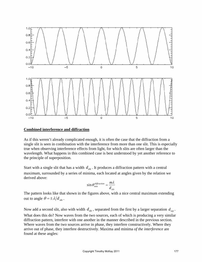
Combined interference and diffraction As if this weren’t already complicated enough, it is often the case that the diffraction from a single slit is seen in combination with the interference from more than one slit. This is especially true when observing interference effects from light, for which slits are often larger than the wavelength. What happens in this combined case is best understood by yet another reference to the principle of superposition. Start with a single slit that has a width slitd . It produces a diffraction pattern with a central maximum, surrounded by a series of minima, each located at angles given by the relation we derived above:

minsin diffraction

slit

mdλθ =

The pattern looks like that shown in the figures above, with a nice central maximum extending out to angle slitdθ λ= ± . Now add a second slit, also with width slitd , separated from the first by a larger separation sepd . What does this do? Now waves from the two sources, each of which is producing a very similar diffraction pattern, interfere with one another in the manner described in the previous section. Where waves from the two sources arrive in phase, they interfere constructively. Where they arrive out of phase, they interfere destructively. Maxima and minima of the interference are found at these angles:


( )12interference interference

max minsin and sinsep sep

nnd d

λλθ θ+

= =

There is something to notice here. The separation between the slits sepd must always be larger

than the width of the slits slitd . If it were not, the slits would overlap. This implies that the angle to the first maximum of the interference pattern interference

maxθ is smaller than the angle for the first minimum in the diffraction pattern diffraction

minθ . The combined pattern which emerges has regularly

spaced interference maxima (at angles where interferencemaxsin

sep

nd

λθ = ) superimposed on the overall

intensity pattern of the diffraction, which has minima (at angles where diffractionminsin

slit

md

λθ = ). A

picture of this overall pattern, for a case where 1 14 20slit sepd dλ = = , is shown in the figure.

In this figure you see interference from the two slits leaving maxima at the angles

interferencemaxsin

20sep

n ndλθ = = and diffraction minima at the larger angles diffraction

minsin4slit

m mdλθ = = . The

first diffraction minimum occurs exactly where the 5th interference maximum would occur. We don’t see this 5th interference maximum because neither of the two slits actually sends any light there at all: diffraction effects within each slit cause complete cancellation.


Often this pattern is described as a regularly spaced interference pattern superimposed on an intensity “envelope” determined by the single slit diffraction pattern. It is useful to consider how this pattern changes as you alter each of the parameters, and slit sepd d . Start by imagining what happens if you hold the slit separation fixed and change only the slit width. If the slits are very narrow, with slitd λ , then there will be no diffraction minima, and the waves from each slit will spread in every direction. The interference from the two slits will still occur, leading to a set of regular maxima and minima, but there will be no diffraction ‘envelope’ enclosing the interference pattern. As the slits are made larger, the diffraction envelope becomes more obvious. A first diffraction minimum enters the picture when slitd λ= , and as the slits become larger, this first minimum moves in toward the center and new minima appear. This progression is illustrated in the following picture, which shows the combined interference and diffraction pattern with 20 and 0.5 , 1.0 , and 2.0sep slitd dλ λ λ λ= = .

Now imagine instead that we hold the slit width fixed and vary only the slit separation. Imagine that the slit width is fixed at 4slitd λ= , and the slit separation is gradually increased from

4sepd λ= to 8sepd λ= and then to 16sepd λ= . These three cases are shown in the figure below. Notice that the diffraction envelope now remains fixed, while the locations of the interference maxima shift closer together each time the slit separation becomes larger. This reciprocal relation is the most fundamental thing to remember. When sources are far apart, features in the interference/diffraction pattern are close together, and when the sources are close together, features in the interference/diffraction pattern are far apart.


Multiple slits: the diffraction grating There is a device often used in laboratories called a ‘diffraction grating’, a device made from a large number of very regularly spaced slits. In a way it is odd that this name is used, as the important effect seen from a diffraction grating is interference from the large number of slits. When there are a large number of slits instead of just two, the pattern of interference seen in double slit diffraction is strongly sharpened. The interference maxima, however, remain unchanged; they are still found at the same locations. The condition for these maxima is given by the same relation:

interferencemaxsin

sep

ndλθ =

with the index n taking on values of 0, ± 1, 2± , etc. As the number of slits increases, the separation of the maxima stays the same, but the width of the interference maxima decreases: the pattern sharpens. This is illustrated in the picture below, where the first shows combined diffraction and interference from two slits with 4slitd λ= and 20sepd λ= d. The second pattern has the same slit width and separation, but now includes three slits instead of two. If we were to increase the number of slits further, the maxima would continue to narrow, eventually becoming very sharp lines, separated by regions almost completely devoid of waves. This ability to send all of the incident waves to a few well separated places makes the diffraction grating an extremely useful tool for laboratory analysis of waves, as the next section will describe in some detail.


Such diffraction gratings can be made using almost any regularly spaced pattern of things which either transmit (through slits) or reflect light. Here are pictures of so-called transmission and reflection gratings:

Using diffraction to analyze waves Imagine that you have a source of light and you would like to know what wavelengths it contains. One way to find out would be to use a diffraction grating made of many very narrow slits, each separated from the next by a fixed distance sepd . As long as each slit is sufficiently narrow (less than any of the wavelengths in the light) diffraction will spread the light from each slit in every direction; the diffraction envelope will be wide and approximately flat.

Transmission grating

Reflection grating


We could use as an example a transmission grating like that shown in the picture above. Let’s assume that this grating has a slit width 40 nmslitd = , and a slit separation 100 times as large, about 4000 nmsepd = . Imagine that plane waves of blue light, with a mix of wavelengths from

400 450 nmλ = − , shine on this grating. Since the slit width is 1/10th the wavelength, there will be no minima in the diffraction envelope; light from each slit will diffract out in every direction. Light passing through each of the slits will, however, interfere with light from the others. This interference will cause a series of maxima at the angles where:

interferencemax

400sin4000 10sep

n nm nnd nmλθ = = =

The first maximum is at interference

max 0θ = ° , the second at interferencemax 5.74θ = ° , and so on. Because there

are many slits here, all the 400 nm light in the original source will be very tightly confined to a narrow region at this angle. Light with a slightly different wavelength, like 410 nm light, will have interference maxima at slightly different locations. For this light,

interferencemax

410sin 0.10254000sep

n nmn nd nmλθ = = =

This has a first maximum is at interference

max 0θ = ° , the second at interferencemax 5.88θ = ° , and so on.

Notice first that all wavelengths of light which hit the diffraction grating have an interference minimum at interference

max 0θ = ° . At this location there is no distinction made among the different wavelengths of light. The location of the next interference maximum however (where 1n = ), is different for the two wavelengths of light. The 400 and 410 nm light, which started mixed together, are now separated, with the longer wavelength light appearing at a different angle from the shorter. The separation produced by the diffraction grating allows us to take a light source with a mix of wavelengths and ‘analyze’ it, to measure how much light of each wavelength is present in the original light source. Here is an example of a spectrum created by a diffraction grating. This ability to determine the wavelength composition of light, to analyze it, makes diffraction gratings an extremely important tool in the laboratory. They often lie at the core of instruments called ‘spectrographs’, for their ability to draw the spectrum of some light.


Using diffraction to determine structure In the last section, we saw how a diffraction grating with a known microstructure (slit separation) can be used to analyze light; to determine its wavelength content. In the modern life sciences, diffraction is often used in just the opposite way as well; light with a known wavelength is used to determine the microstructure of something it diffracts from. To see how this works, we will begin with a very simple case; determining the unknown slit separation in a diffraction grating. Imagine that we are given a diffraction grating, but don’t know the slit separation. If we also have a light source with known wavelength (like a laser), we can determine the line spacing. We shine the light through the grating, measure the angles at which diffraction maxima occur, and rearrange the relations described above to get:

interferencemaxsinsepnd λ

θ=

Notice again the reciprocal relation. If the angles are large, the separation of the slits is small; they are close together. If the angles are small, the separation of the slits is large; they are far apart.

Spectrum of the Sun as observed with a diffraction grating. Light of each wavelength (and hence color) diffracts at a different angle, landing on the film at a different place. Notice the dark lines at many locations. Each represents a particular wavelength which is absent from the spectrum of the Sun. These dark ‘Frauenhofer lines’ are caused by ions in the very hot atmosphere of the sun which absorb the light at these particular wavelengths. Each ion absorbs a particular set of wavelengths. These patterns allow us to determine the chemical composition of the Sun’s atmosphere.


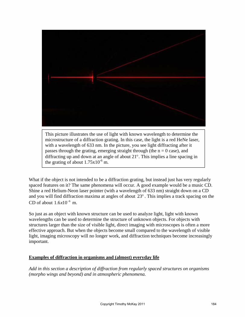
What if the object is not intended to be a diffraction grating, but instead just has very regularly spaced features on it? The same phenomena will occur. A good example would be a music CD. Shine a red Helium-Neon laser pointer (with a wavelength of 633 nm) straight down on a CD and you will find diffraction maxima at angles of about 23° . This implies a track spacing on the CD of about 61.6 10x − m. So just as an object with known structure can be used to analyze light, light with known wavelengths can be used to determine the structure of unknown objects. For objects with structures larger than the size of visible light, direct imaging with microscopes is often a more effective approach. But when the objects become small compared to the wavelength of visible light, imaging microscopy will no longer work, and diffraction techniques become increasingly important.

Examples of diffraction in organisms and (almost) everyday life Add in this section a description of diffraction from regularly spaced structures on organisms (morpho wings and beyond) and in atmospheric phenomena.

This picture illustrates the use of light with known wavelength to determine the microstructure of a diffraction grating. In this case, the light is a red HeNe laser, with a wavelength of 633 nm. In the picture, you see light diffracting after it passes through the grating, emerging straight through (the n = 0 case), and diffracting up and down at an angle of about 21°. This implies a line spacing in the grating of about 1.75x10-6 m.


30.3 X-ray diffraction and structure determination

One of the great discoveries of biochemistry is the close connection between protein structure and function. Much of the business of life within the cell is carried out using large macromolecules. The “primary structure” of these molecules is a simple map of connectivity, a network showing which other atoms each atom in the molecule is attached to. While information about primary structure is central to the identity and nature of a molecule, it tells us remarkably little about how it will function. Function is often determined by the so-called “tertiary structure”, the full three dimensional distribution of atoms in the equilibrium state of the molecule. Since this 3D shape plays such a central role in the function of biomolecules, determining structure is an essential task for the life sciences. There are several different ways to do this, all of which depend on fundamental physics principles. The most important of these, both historically and today, is X-ray diffraction. Since it is so important, we will spend a little time going over the basic principles of this method, using as our central example the most famous determination of the structure of a biomolecule: the discovery of the DNA double helix by Francis Crick and James Watson in 1953. We saw in the last section that light with a known wavelength could be used to determine the microstructure of a diffraction grating with unknown slit spacing. In this section we will see how the same essential approach allows us to determine the microstructural arrangement of atoms in molecules. If you want to see diffraction from individual atoms, you need to use light waves with wavelengths about the size of the spacing between atoms. This is typically a few times 10-10 m. These wavelengths are much smaller than those of visible light, and even smaller than the wavelengths of ultraviolet light; they are X-rays. Bouncing X-rays off of atoms and looking at the diffraction patterns they produce can tell us how the atoms are arranged. Examining the X-ray diffraction pattern produced by DNA allowed Watson and Crick to determine its double-helical structure. In what follows we will see, in some detail, how they did this.

X-ray scattering from atoms X-rays are electromagnetic radiation with wavelengths in the range from 0.01-10 nanometers. The longest wavelength X-rays are about 40 times shorter than the shortest visible light, so X-rays cannot be detected by your eyes. But waves they are, and they exhibit all the usual wave phenomena of interference and diffraction. X-rays also interact with matter, sometimes being scattered from it and sometimes being absorbed. Because their wavelengths are so short, about the size of atoms, they tend to bounce off individual atoms, emerging from this interaction as spherical waves. When this happens, each atom in a material appears as a new source of waves. This idea is illustrated in the figure below:


To understand how this kind of X-ray scattering can reveal the arrangement of atoms in a material, consider what happens if you shine X-rays on a simple crystal, a material which has all its atoms arranged in an extremely regular array.

In this case, the array of atoms becomes an array of sources for scattered waves. This should look familiar. It’s very much the same situation created by a regular grid of very narrow slits, a diffraction grating. Each atom here (like a slit in the plate) is the source of spherical waves which travel out in every direction. Waves scattered from each of the many atoms then interfere with one another. If we then examine intensity of waves far from this scattering we will find something like what is shown in the next picture. In this picture, the entire scattering region shown above is very tiny, hidden down in the box on the left.

Incoming plane waves

Outgong plane waves

Scattered waves

Incoming plane waves

Outgong plane waves

Scattered waves

d

d

d

d


The key idea is that the angle θ to the bright spots on a distant screen, combined with knowledge of the X-ray wavelength λ, allows us to find the distance “d” between the atoms in the crystal. This is the essence of how we use X-ray diffraction to learn about the distribution of atoms in a material.

The basics: diffraction from a line of evenly spaced atoms The simplest case is the one illustrated above. A regularly spaced set of atoms will produce a diffraction pattern on a screen at a distance D which has points at these angles and positions:

interferencemax

ysin or or D

n n n Dyd d dλ λ λθ = = =

Notice again that the spacing of maxima on the distant screen depends on the inverse of the spacing between the atoms in the crystal “d”. For this reason, the distribution of the bright points on the screen is sometimes called the “reciprocal” of the actual distribution of the atoms in the material. When the atoms in the material are close together, the bright points on the screen are far apart. When the atoms in the material are far apart, the bright points on the screen are close together. This point will be essential in understanding what follows! There is another key point here. We have assumed a perfectly regular array of atoms; a crystal in which the spacings between atoms are quite precisely repeated over and over. A nice feature of crystals is that they contain many, many atoms, many scattering centers. As we saw for diffraction gratings earlier in this chapter, many sources of waves create very narrow, sharply defined diffraction peaks. What happens if you don’t have a crystal in which all the atoms are lined up, but instead have something with no regular order, like a liquid? In this case, there are no favored interatomic

Scattering region (everything from above)

Direct, unscattered waves (very bright)

1st max at sinθ = λ/d

2nd max at sinθ = 2λ/d

2nd max at sinθ = 2λ/d

1st max at sinθ = λ/d


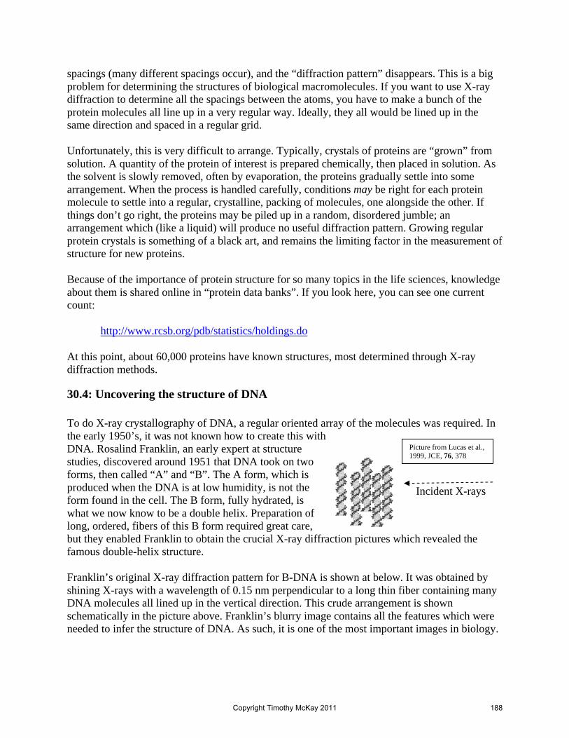
spacings (many different spacings occur), and the “diffraction pattern” disappears. This is a big problem for determining the structures of biological macromolecules. If you want to use X-ray diffraction to determine all the spacings between the atoms, you have to make a bunch of the protein molecules all line up in a very regular way. Ideally, they all would be lined up in the same direction and spaced in a regular grid. Unfortunately, this is very difficult to arrange. Typically, crystals of proteins are “grown” from solution. A quantity of the protein of interest is prepared chemically, then placed in solution. As the solvent is slowly removed, often by evaporation, the proteins gradually settle into some arrangement. When the process is handled carefully, conditions may be right for each protein molecule to settle into a regular, crystalline, packing of molecules, one alongside the other. If things don’t go right, the proteins may be piled up in a random, disordered jumble; an arrangement which (like a liquid) will produce no useful diffraction pattern. Growing regular protein crystals is something of a black art, and remains the limiting factor in the measurement of structure for new proteins. Because of the importance of protein structure for so many topics in the life sciences, knowledge about them is shared online in “protein data banks”. If you look here, you can see one current count: http://www.rcsb.org/pdb/statistics/holdings.do At this point, about 60,000 proteins have known structures, most determined through X-ray diffraction methods.

30.4: Uncovering the structure of DNA To do X-ray crystallography of DNA, a regular oriented array of the molecules was required. In the early 1950’s, it was not known how to create this with DNA. Rosalind Franklin, an early expert at structure studies, discovered around 1951 that DNA took on two forms, then called “A” and “B”. The A form, which is produced when the DNA is at low humidity, is not the form found in the cell. The B form, fully hydrated, is what we now know to be a double helix. Preparation of long, ordered, fibers of this B form required great care, but they enabled Franklin to obtain the crucial X-ray diffraction pictures which revealed the famous double-helix structure. Franklin’s original X-ray diffraction pattern for B-DNA is shown at below. It was obtained by shining X-rays with a wavelength of 0.15 nm perpendicular to a long thin fiber containing many DNA molecules all lined up in the vertical direction. This crude arrangement is shown schematically in the picture above. Franklin’s blurry image contains all the features which were needed to infer the structure of DNA. As such, it is one of the most important images in biology.

Picture from Lucas et al., 1999, JCE, 76, 378

Incident X-rays


Our discussion of the Franklin image and its interpretation relies heavily on an article by Lucas, Lambin, Mairesse, and Mathot in the Journal of Chemical Education, 1999, 76, 378. There are four aspects of this image that I want you to notice, and which we will try to explain. To recognize these features, compare the schematic diagram in the center to the actual X-ray diffraction pattern on the left. The four key features are:

1. The “layer lines”: Starting from the center, there are a series of dots along regularly spaced horizontal lines.

2. The “cross” in the middle: The bright spots which define the horizontal layer lines are found at increasing distances from a vertical centerline as you move away from the center of the image.

3. The outer “diamond”: the bright points at the top and bottom and the sides of the image are connected by a diamond shaped continuous structure

4. The “missing 4th layer line”: When you look at the layer lines you can see that the fourth line from the center is missing.

Every one of these features provides important information about the structure of DNA, so the following sections go through each in turn and explain its origin. It will help in understanding this to refer to the model shown in the picture on the right, which emphasizes several key spacings in the structure of the DNA double helix. All are expressed in terms to the spiral spacing “P”, which is the distance along the strand you have to go before one of the two helices returns back around to where it started. The other two distances are 3/8P, the distance between the two intertwined helices, P/10, the distance between base pairs along the chains, and 0.3P, the radius from the center to the outer edge of the helix. Given this background, let’s examine each of the features in the Franklin image.

The closely spaced layer lines

Picture from Lucas et al., 1999, JCE, 76, 378


To understand the layer lines, remember that as the helix of DNA spirals around it goes through repeated cycles, once for each time it spirals around. This makes a repeated pattern of X-ray scattering centers lined up along the vertical direction, spaced by a distance P. These act like a regularly spaced set of sources of X-rays, lined up vertically. Such a line of sources will produce an array of diffraction spots on a screen at a distance D located at positions y n D Pλ= . This is the spacing of the layer lines. Remember how the diffraction spots are “reciprocal” to the actual array of atoms? In this case, we have a set of separations in DNA molecules which are large, with size P. An arrangement with large separations will produce diffraction spots close together. Since this is the largest repetition scale in the DNA structure, it produces the diffraction features which are closest together.

The central cross The cross pattern was key to Watson and Crick recognizing that DNA had a helical structure. Remember that a simple vertical stack of sources separated by the spacing P would produce a vertical set of diffraction peaks separated by distances

layer linesy D PλΔ = . Now imagine that, instead of a set of horizontal slits separated by a distance P, you have a set of long tilted slits, still separated by the same vertical distance P. This is illustrated in the picture at right. Such a set of tilted slits will still make a pattern of diffraction features separated along the vertical direction by a distance layer linesy D PλΔ = , but now instead of lining up vertically, the diffraction peaks would line up perpendicular to the orientation of the slits themselves. Why is this? Each line in this pattern acts like a single slit which is wider than the wavelength of the X-rays scattering it. For DNA, the length of each tilted segment is about 2 nm, while the wavelength of Franklin’s X-rays was only 0.15 nm. For such an individual wide slit, light can be seen with large amplitude only along the direction perpendicular to the slit; it doesn’t diffract out to the side. This was discussed in some detail in section 3.1.0. A single long slit produces a beam of light perpendicular to the slit with an angular width

diffractionminsin slitdθ λ= . For the case of a “slit” 2 nm wide and λ = 0.15 nm, this is an angle θ = 0.07

in radians, which is about 4°. Light from each slit will appear only within about 4° of a line perpendicular to the slit. What’s the effect of this? The set of tilted lines, spaced by a separation P, will produce a set of points split by layer linesy D PλΔ = , but they will not appear along a vertical line. Instead, you will find them only along a line tilted so that it is perpendicular to the slits. If we had lines tilted the other way, we’d get the same pattern, only tilted the other direction.

P


Now perhaps you can get an idea of where the cross comes from. Imagine you put these two sets of tilted lines together in a zig-zag pattern. That would give you both of the above patterns on top of one another, and would create the combined cross shape. What could make a zig-zag pattern like this? If you picture a helix, a spiral, seen from the side, you get something very like this zig-zag pattern. And in fact it was well known by the time Franklin took her DNA diffraction picture that helical structures produced crosses in diffraction patterns. So there you have it. The cross in the middle, made up of a set of features positioned along the so-called “layer lines”, is caused by the helical structure of the DNA. The angle of the cross tells us the “pitch” of the helix. If it was more stretched out the cross would be wider. But this cross by itself wasn’t enough to tell Watson and Crick that it was a double helix. For that, we have to go a little further along and consider the remaining two key features.

The outer diamond and the spacing between base pairs Perhaps the most obvious feature in Franklin’s picture is the pair of bright blobs at the top and bottom, which are connected by the rather fainter outer diamond. These features, which are far

Pictures from Lucas et al., 1999, JCE, 76, 378

P

Δy = λD/P

Δy = λD/P

P


apart on the diffraction pattern, must correspond to some repeated features in the molecule which are close together. The two big splashes at the top and bottom of Franklin’s image, as well as the diamond framing it all, are due to the small spacing of base pairs along the sequence which has a typical spacing of

10P . Since the spacing is ten times smaller than the spacing of cycles of the helix, the distance between points in the diffraction pattern is given by the equation:

base pairs10

10D Dy

P Pλ λ

Δ = =

Note that this is just 10 times as large as the spacing between the layer lines. The two points at the top and bottom come from all the pairs aligned above one another, while the rest of the diamond is filled in by pairs aligned along the zigs and zags of the helix.

The missing 4th layer line Nothing so far has told us that DNA is a double helix, or said anything about the relation between the two helices. That’s where the missing spots along the 4th layer line play the key role. In the figure on the left, with a single set of sources separated by the distance P, you get constructive interference every time you find interference

maxsinP mθ λ= . Now consider something very similar on the right. Now you have two separate sequences of slits. Each sequence is spaced by

distant P, and the two are offset from one another by a distance3 8P . Because each sequence by itself is spaced by P, they would is happy to give you peaks wherever sinP mθ λ= . This gives you peaks at angles where sin m Pθ λ= .

P

Produces spots when Psinθ = mλ

Psinθ

θ

P

(3P/8)sinθ θ 3P/8


But now the two sequences can also interfere with one another. If the path length difference shown on the right, ( )3 8 sinPL P θΔ = , is a half integer multiple of the wavelength, then the bottom holes will always interfere destructively with the top holes. Notice that when m=4, the condition above for constructive interference from each individual sequence will give us:

4sinPλθ =

Putting this into the equation for the path length difference between the two offset sequences, we find:

3 3 4 3sin8 8 2P PPL

Pλ λθΔ = = =

This means the path length difference between the two sequences of holes is a half integer multiple of the wavelength and the two sequences of holes will cancel one another out completely! In the DNA double helix, we have a situation exactly mirroring this set of slits. Each of the two helices acts as one of the sets of slits spaced by distance P. The two helices are offset from one another by a distance 3 8P . These two helices will experience destructive interference which will perfectly wipe out the 4th layer line. This missing 4th layer line was the final key clue which Watson and Crick needed to discover that the structure of DNA was a double helix. The paired double helix plays an essential role in the replication of DNA, and hence in its function as the mechanism of inheritance. That this essential double helical structure is revealed by a subtle feature missing in the diffraction pattern has a delightful irony.

Some reminders and a quick summary What’s the crucial lesson here? Most important, diffraction of X-rays from a regular, repeated structure can provide the clues which allow us to determine the 3D structure of complex biological macromolecules. The basic physics behind this is just the simplest feature of waves; that two waves arriving in phase add constructively, while those arriving out of phase add destructively. This simple fact, applied in some details to understand how arrays of sources (like diffraction gratings) interfere, allows us to determine the structure of DNA. To make this work, the DNA had to be arranged in a more or less regular, ordered form. For Franklin, this was done by lining them all up in a thin fiber, so that at least all the DNA helices were pointed the same way. There are four key features of the Franklin DNA image, each of which contains key clues to the structure of DNA:

1. The layer lines, which show the repetition length of the DNA helix P. For DNA this distance is about 3.4 nm.

2. The cross pattern, which shows that DNA is a helical structure, with each of the sloping sides tilted from the horizontal by about 26°


3. The outer diamond: which shows the smallest spacing in the molecule, the interbase spacing, which for DNA is about 10P , or 0.34 nm.

4. The missing 4th layer line, which shows that there we in fact two intertwined helices, offset from one another by a distance 3P/8, or about 1.3 nm for DNA.

Layer lines, spaced by distances given by Δy = λD/P

Missing 4th layer line!

Missing 4th layer line!

This larger figure points out each of the features used in determining the structure of DNA from X-ray diffraction: the layer lines, the central cross, the external diamond, and the missing 4th layer line.

Outer diamond with spacing Δy = 10λD/P

Central cross, showing pitch of the DNA helix


Diffraction of X-rays from regular arrays of atoms, as you might see in a crystal of regularly arranged proteins, allows us to determine their structures. This example of DNA shows how, even with relatively simple data, we can use our understanding of waves to determine structures that we can never directly see.


A Quick Summary of Some Important Relations Huygen’s construct – waves passing through holes and around obstacles: When waves encounter holes in barriers or obstacles the outcome depends on the size of the hole/obstacle compared to the wavelength λ of the wave. If the hole/obstacle is small compared to λ, the wave will ‘diffract’ through or around it. If the hole/obstacle is large compared to λ, the wave will continue in straight rays, leaving sharp shadows around the boundaries of the hole and edges of the obstacle. Minima from a wave with wavelength λ passing through a single slit of width d:

( )minimumsin mdλθ =

First minimum for a wave with wavelength λ passing through a circular hole of diameter d:

( )minimum1.22sin

dλθ =

Interference from two point sources: Examining interference patterns from two narrow slits (width < λ) separated by dsep on a screen a distant D away:

( )( ) ( )

max

1min 2

sin

sinsep

sep

d n

d n

θ λ

θ λ

=

= +

Or in terms of distance y on the screen:

( )

max

12

min

sep

sep

n Dyd

n Dy

d

λ

λ

=

+=

Combined interference and diffraction: When two slits not smaller than the wavelength interfere, you get both interference and diffraction effects. Multiple slits and diffraction gratings: When more than two slits, still separated by the same dsep, all act. The interference maxima remain in the same places, but the peaks are made narrower. With many slits, they become tiny, well separated dots with locations determined by wavelength and slip spacing.


Diffraction gratings can be used to analyze light waves, measuring the wavelengths that make them up. The reverse is also possible. Waves of known wavelength can be used to determine ths structure of a small regular object. X-ray diffraction and protein structure: Diffraction of x-rays from regular arrays of atoms in crystals produce diffraction patterns which can be used to determine the distribution of atoms in the crystal. This method plays an essential role in modern biology, a development that really took off with the discovery of the structure of DNA. Four features in the original X-ray diffraction image revealed the double helix structure of DNA

1. The layer lines 2. The central cross 3. The outer diamond 4. The missing 4th layer line

You should understand what each revealed and how they indicate a double helix.



31.1 Waves at boundaries: material mismatch When we introduced waves, we imagined them traveling in a uniform material. Their amplitudes might fade as they spread in two or three dimensions, but otherwise they would propagate freely, spreading directly away from their sources forever. In the last chapter we considered a first variation on this; what happens when propagating waves encounter obstacles. We talked about walls with slits through which the wave may pass, and about small objects from which a wave may scatter. In this chapter we will examine how waves travel in more realistically complicated circumstances. First, waves in media don’t actually continue forever. Instead they interact with the material through which they travel, gradually giving up their energy and shrinking in amplitude. Second, very interesting things happen when waves traveling in one material reach the boundary with another. To illuminate these two ideas, let’s start with a familiar example, light waves traveling through the air. Light travels pretty freely through air. Most days it propagates from the top of the atmosphere to the bottom without much loss, a distance of roughly 30 kilometers. But the losses are there. Think about how bright the sun is when directly overhead. Compare this to a sunset, when the light travels through much more air to reach you. At this lovely crepuscular moment, much of the sun’s light is either absorbed or scattered away by the atmosphere. With so little of the sun’s light getting through, you can look directly at it without pain. This is an example of the losses incurred by a wave even when it travels in an essentially uniform medium. The air through which light waves travel ends when the light encounters an object; a table, the wall, or a piece of window glass. When this happens, there are two possible outcomes. The light may bounce off, reflecting back into the air from which it came. If it doesn’t reflect, it must continue on into the new material. In this new material, it may either be quickly absorbed, as it is in many solids, or continue on as a wave, as it does in window glass or water. We should guess that the arriving waves must either reflect or continue on because of the conservation of energy. These waves carry energy. That energy, upon arriving, must go somewhere. In reflection it bounces off in a new direction. If it does not reflect, it must pass into the new material, for it cannot simply disappear. Light reflected from objects enables most of our view of the world. Most things are visible only because they reflect ambient light which then passes into our eyes. Turn off the lights and there’s nothing to reflect: everything disappears. Of course there are objects which actually emit visible


light produced within them: things like the sun, light bulbs, wildfires, lightning, and fireflies. Light emitting objects we see directly. But most of our view of the world depends on reflected light. If light does not reflect off something, we cannot see it; such an object is literally invisible. A remarkable group of cold-water adapted ‘ice-fish’ are very nearly transparent. In this chapter we will consider first how waves traveling through a material are gradually absorbed, paying special attention to light and sound in life’s media, air and water. Then we’ll learn about what happens when waves reach a boundary where they may either reflect or continue on. The outcome depends only on how waves propagate in the two materials. When the wave travels in similar ways through the two materials (when they are well matched), waves slip across the boundary from one material to the next as if nothing had happened. When the wave travels very differently through the two materials, at least some of the wave will be reflected, and that which passes on will change direction, a phenomenon called refraction. All of these phenomena, basic features of waves, have important implications for life.

Absorption and scattering of light To understand the absorption of waves in a material, we will consider a concrete example, the propagation of a parallel beam of light waves. To start, recall that the intensity of a wave, the amount of energy it delivers per unit area per unit time, is proportional to the square of the amplitude of the wave: ( ) ( )2I Aλ λ∝ A beam of light is a set of parallel light waves, all propagating in the same direction. Two examples help to illustrate the case. One is the light from the sun. Because the Earth is so far from the sun, waves of light from it arrive as very nearly parallel plane waves. Another example familiar from classrooms today is the laser pointer. Because the waves all travel in the same direction, their intensity does not appreciably decrease with distance, as it would for waves spreading from a point source in two or three dimensions (where intensity would fall off as 1 ror 21 r ). Even though such a beam of light does not spread, its intensity decreases when travelling through a material. This decrease is due to a combination of absorption and scattering. Absorption converts part of the energy the light carries to other forms; typically thermal energy in the material. Scattering sends some of the wave off in new directions, also removing it from the original beam. Scattering is essentially reflection from small objects (like dust) in the beam. The decay of intensity with distance caused by these combined affects can often be accurately described as an exponential for each wavelength: ( ) ( ) ( ), , 0 xI x I e α λλ λ −=


In this relation, ( ),I xλ it the intensity of the wave as a function of wavelength and distance in

the medium, ( ),0I λ is the initial intensity as a function of wavelength, the parameter α(λ) is a property of the material through which the light passes, called the “attenuation coefficient”. From the form of this equation we can see that if α is large, the intensity will fall off very suddenly, and light won’t travel far. If, by contrast, α is small, the light will travel a long way before being absorbed. How far will the light go? As with all exponentials, this is a question of degree: while the beam immediately starts to fade, it never completely disappears. To sensibly characterize how far light goes in a material, we might determine how far it travels before it is reduced by some fixed amount. By convention, we select a reduction factor of 1e− , and define the “absorption length”

( )absL λ to be the distance the light must travel before its intensity is reduced by this factor. From

the relation above, we see that this happens when ( ) ( ) 1absLα λ λ = . This suggests a clear

interpretation of the parameter α: ( )α λ is the inverse of the absorption length. Where the absorption length is small, alpha is large. Where the absorption length is large, alpha is small. For the purposes of life on Earth, we need first to understand the propagation of light through air and water. The figures below show the wavelength dependence of the attenuation coefficient for air and water, as well as the comparing how the intensity of light falls off with distance in air and water, for different wavelengths of light.

Look first at the attenuation coefficient of air as a function of wavelength. The attenuation coefficient for red light ( ) 6 1600 nm 9 10 mxα − −≅ , which implies an absorption length of about 110 kilometers. Red light like this must pass through about 110 kilometers of atmosphere before its intensity falls by a factor of 1e− . Passing through a more typical distance of 30 km, we might expect;

From Denny, Air and Water, Princeton Press


( ) ( ) ( )6 49 10 *3 10600 nm,30 km 600 nm, 0 km 0.76 600 nm, 0 kmx xI I e xI

−−= = The intensity after traveling through 30 km of air is reduced by about 25%. The energy lost from the beam is either absorbed by the atmosphere or scattered off in new directions. You can see from the figure that 600 nm red light has an attenuation coefficient α which is about seven times less than that for 400 nm blue light. This means that red light penetrates air about seven times as effectively as blue light. When light from the sun passes through 30 km of the Earth’s atmosphere, about 25% of the red light is lost from the beam. Meanwhile, about 88% of the blue light is absorbed or scattered in the same distance. This difference is responsible for two familiar phenomena. The first is the daytime blue sky. When you look at the sky in directions away from the sun, you see a nice, smooth distribution of blue light coming to you. This blue light was originally headed from the sun toward the ground far away from you, but instead has been scattered from that beam toward your eye. The red light, which scatters less, mostly continues on toward its original destination. Since short wavelength light scatters more than long wavelength light, what you see looks “blue” compared to the white light of the sun. The wavelength dependence of absorption and scattering also explains the typical redness of a sunset. When you look at a sunset, you’re looking in the direction of the sun, but through a much longer path of atmosphere than usual. Along this very long path, almost all of the blue light is absorbed or scattered out of the beam from the sun. What’s left is the red light, and hence the sunset looks red. The same thing happens to a full moon low in the sky. Looking back at figures showing the attenuation coefficients for air and water, you can see that light penetrates air much more freely than it does water: it will travel 100 to 1000 times farther in air than water. Also, the wavelength dependence of absorption is reversed for water, red light is absorbed much more strongly than blue. This means that underwater, the primary light arriving from the sun will be blue; the red light will be largely absorbed. The short absorption length for light in water has huge consequences for life. Life directly dependent on light from the sun is restricted by this absorption to a layer about 100 m thick at the surface of the ocean. This region makes up less than 3% of the ocean’s volume. To live in the remaining 97% of the ocean, life must adapt to survive without the sun. In this immense dark zone, many organisms produce their own light through a wide variety of bioluminescent


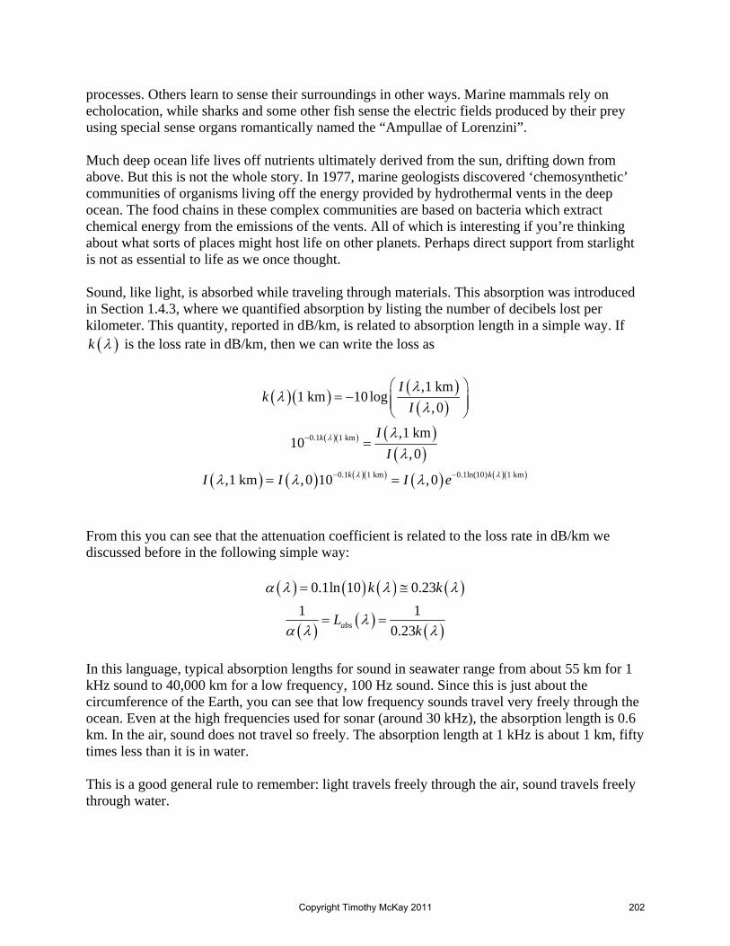
processes. Others learn to sense their surroundings in other ways. Marine mammals rely on echolocation, while sharks and some other fish sense the electric fields produced by their prey using special sense organs romantically named the “Ampullae of Lorenzini”. Much deep ocean life lives off nutrients ultimately derived from the sun, drifting down from above. But this is not the whole story. In 1977, marine geologists discovered ‘chemosynthetic’ communities of organisms living off the energy provided by hydrothermal vents in the deep ocean. The food chains in these complex communities are based on bacteria which extract chemical energy from the emissions of the vents. All of which is interesting if you’re thinking about what sorts of places might host life on other planets. Perhaps direct support from starlight is not as essential to life as we once thought. Sound, like light, is absorbed while traveling through materials. This absorption was introduced in Section 1.4.3, where we quantified absorption by listing the number of decibels lost per kilometer. This quantity, reported in dB/km, is related to absorption length in a simple way. If ( )k λ is the loss rate in dB/km, then we can write the loss as

( ) ( ) ( )( )

( )( ) ( )( )

( ) ( ) ( )( ) ( ) ( )( )

0.1 1 km

0.1 1 km 0.1ln(10) 1 km

,1 km1 km 10 log

,0

,1 km10

,0

,1 km ,0 10 ,0

k

k k

Ik

I

II

I I I e

λ

λ λ

λλ

λ

λλ

λ λ λ

−

− −

⎛ ⎞= − ⎜ ⎟⎜ ⎟

⎝ ⎠

=

= =

From this you can see that the attenuation coefficient is related to the loss rate in dB/km we discussed before in the following simple way:

( ) ( ) ( ) ( )

( ) ( ) ( )

0.1ln 10 0.231 1

0.23abs

k k

Lk

α λ λ λ

λα λ λ

= ≅

= =

In this language, typical absorption lengths for sound in seawater range from about 55 km for 1 kHz sound to 40,000 km for a low frequency, 100 Hz sound. Since this is just about the circumference of the Earth, you can see that low frequency sounds travel very freely through the ocean. Even at the high frequencies used for sonar (around 30 kHz), the absorption length is 0.6 km. In the air, sound does not travel so freely. The absorption length at 1 kHz is about 1 km, fifty times less than it is in water. This is a good general rule to remember: light travels freely through the air, sound travels freely through water.


Waves at boundaries: reflection or transmission? The fate of a wave arriving at a boundary between two materials depends on the nature of the transition. We introduced this idea earlier in our discussion of waves, back in Section 2.2.0. We saw there that what happens at a boundary depends on the physical properties of the two media. If they are very different, the wave will almost completely reflect. If they are very similar, the wave will almost completely pass through. What are the material properties that matter for light and sound? What is it we need to compare? For light, the material property which governs reflection and transmission is called the “index of refraction” of the material. This parameter, usually written with the symbol n, can be expressed in a simple way which relates the speed of light in the material to the speed of light in a vacuum (usually expressed with the symbol c):

medium mediumlight

cnv

=

Notice that this quantity is unitless; the ratio of two velocities. It is a pure number. Light traveling in a medium always propagates more slowly than in empty space. So this index will always be a number larger than one. Why is light slowed when it travels through a material? When light travels through a medium it is actually undergoing a continuous and very complex process of absorption and remission. These processes take a little time, and this delay between absorption and re-emission slows the rate at which it moves through the material. Air is not very dense, and does relatively little to impede the progress of light. It’s index of refraction is very close to one, 1.0003airn ≅ . Water, by contrast, is dense, and slows light more substantially. As a result, the index of refraction of pure water is larger, 1.33watern ≅ . To determine whether light will be reflected at or will cross a boundary, we compare the index of refraction of the two materials. For sound, the material property to consider is called the “characteristic acoustic impedance”. This parameter, usually denoted with the symbol Z, is given by the product of the density of the medium ρ multiplied by the velocity of sound in the medium medium

soundv : medium

medium medium soundZ vρ= The SI units for acoustic impedance are ‘rayls’, with

21 rayl 1 kgm s

=

Acoustic impedance, depending both on density and speed of sound, varies quite substantially among the media of life. The acoustic impedance of air is small, about 415 rayls, while that of


water is very large, about 1.5x106 rayls. As we will see, this enormous difference has major implications for hearing and the propagation of sound in life. We turn now to the question of how much wave intensity reflects at a boundary between two media, A and B. If the important material property (index of refraction or acoustic impedance) changes very little across a boundary, most of the wave will propagate from one medium to the next. If the important property changes a lot, most of the wave will be reflected. While the detailed behavior is complex, we can get a basic quantification of this in one limiting case. When the wave traveling in medium A arrives perpendicular to the boundary with medium B, the reflected intensity can be calculated by:

2 2

and A B A Blight sound

A B A B

n n Z ZR Rn n Z Z

⊥ ⊥⎛ ⎞ ⎛ ⎞− −= =⎜ ⎟ ⎜ ⎟+ +⎝ ⎠ ⎝ ⎠

What are the implications of this? When light propagates straight down from air into water in this way, we calculate a reflection amplitude 0.02lightR = . Most, but not quite all, of the light passes on into the water. The same is true (as you can see from the equation) for light passing from water into air. The situation for sound is very different. When sound propagates straight down from air into water, we find a reflection coefficient 0.9999soundR⊥ = . Almost every bit of the sound arriving at the boundary between air and water is reflected, virtually none passes across the boundary. Likewise, sound does not travel freely from water into air. The implications of this are many, as we will see when we discuss hearing in air and water.

Changing the direction of waves: reflection There are two ways in which the direction of wave travel can be changed at boundaries between materials; by reflection or by refraction. Each can be understood in terms of the Huygens’ construct we used to discuss diffraction. Consider first what happens when wave fronts bounce off a surface. Imagine first that the surface is flat on the scale of the wavelength.

θi θr

Incoming wave

Outgoing wave


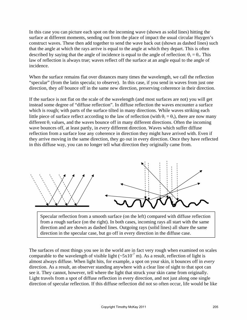
In this case you can picture each spot on the incoming wave (shown as solid lines) hitting the surface at different moments, sending out from the place of impact the usual circular Huygen’s construct waves. These then add together to send the wave back out (shown as dashed lines) such that the angle at which the rays arrive is equal to the angle at which they depart. This is often described by saying that the angle of incidence is equal to the angle of reflection: θi = θr. This law of reflection is always true; waves reflect off the surface at an angle equal to the angle of incidence. When the surface remains flat over distances many times the wavelength, we call the reflection “specular” (from the latin specula; to observe). In this case, if you send in waves from just one direction, they all bounce off in the same new direction, preserving coherence in their direction. If the surface is not flat on the scale of the wavelength (and most surfaces are not) you will get instead some degree of “diffuse reflection”. In diffuse reflection the waves encounter a surface which is rough; with parts of the surface tilted in many directions. While waves striking each little piece of surface reflect according to the law of reflection (with θi = θr), there are now many different θi values, and the waves bounce off in many different directions. Often the incoming wave bounces off, at least partly, in every different direction. Waves which suffer diffuse reflection from a surface lose any coherence in direction they might have arrived with. Even if they arrive moving in the same direction, they go out in every direction. Once they have reflected in this diffuse way, you can no longer tell what direction they originally came from.

The surfaces of most things you see in the world are in fact very rough when examined on scales comparable to the wavelength of visible light (~5x10-7 m). As a result, reflection of light is almost always diffuse. When light hits, for example, a spot on your skin, it bounces off in every direction. As a result, an observer standing anywhere with a clear line of sight to that spot can see it. They cannot, however, tell where the light that struck your skin came from originally. Light travels from a spot of diffuse reflection in every direction, and not just along one single direction of specular reflection. If this diffuse reflection did not so often occur, life would be like

Specular reflection from a smooth surface (on the left) compared with diffuse reflection from a rough surface (on the right). In both cases, incoming rays all start with the same direction and are shown as dashed lines. Outgoing rays (solid lines) all share the same direction in the specular case, but go off in every direction in the diffuse case.


living in a continuous hall of mirrors. Nothing would be where it seemed to be and it would be impossible to use the direction from which light comes as a reliable indicator of where things are. There are some natural surfaces smooth enough to create specular reflection. Perhaps the most familiar is water. The combined effects of gravity and surface tension conspire to make undisturbed water surfaces very flat indeed. Light coming from these smooth surfaces is all reflected specularly. What you see is not the surface itself, but images of more distant points. If you don’t understand this, you could end up like Narcissus, the character from Greek mythology who fell in love with his own reflection; just one more terrible fate from which knowledge of physics can save you.

Changing the direction of waves through refraction Waves which cross the boundary between one material and another may also have their direction changed. We call this phenomenon refraction. Imagine waves arriving at the boundary of two

materials, one in which they travel rapidly and another in which they travel more slowly. As each wave front hits the interface, it produces new waves which travel out from the points of impact in every direction. Above the interface the waves produced travel out at the old speed vout, below the interface they travel at a new speed vmedium. You can see from the picture that the net effect of slowing the wave in the new medium is to bend the direction of wave travel. If the waves arrive at the interface with an angle of incidence θi, they will propagate through into the new region at a different angle of refraction θr. The two angles are related to the speed of the wave in each of the two media through some simple trigonometry, as shown in the figure below.

θi

θr


It may help to rewrite this in a simpler form:

( ) ( )sin sinrr i

i

vv

θ θ=

If r iv v< , the angle of refraction will be smaller than the angle of incidence. So when the wave moves into a region where it travels more slowly, its path bends toward a line which is perpendicular to the interface between the two media; it bends toward the normal. When, on the other hand, r iv v> , the path of the wave will bend away from the normal. This law for refraction is true for any wave, including light and sound. For light, this general rule is usually written in another, equivalent form, taking advantage of the index of refraction we already defined for light: n c v= :

sin sin

sin sin

sin sin

i r

i r

i ri r

i i r r

v vc cv vn n

θ θ

θ θ

θ θ

=

=

=

This relation describing how light changes direction when crossing an interface is called Snell’s law, for Dutch mathematician Willebord Snellius (1580-1623). Let’s look at what this means:

sin sinir i

r

nn

θ θ=

θi viΔt

vrΔt

θr

θr θi

sin

sin

sin sin

ii

rr

i r

i r

vLvL

v v

θ

θ

θ θ

=

=

=

L


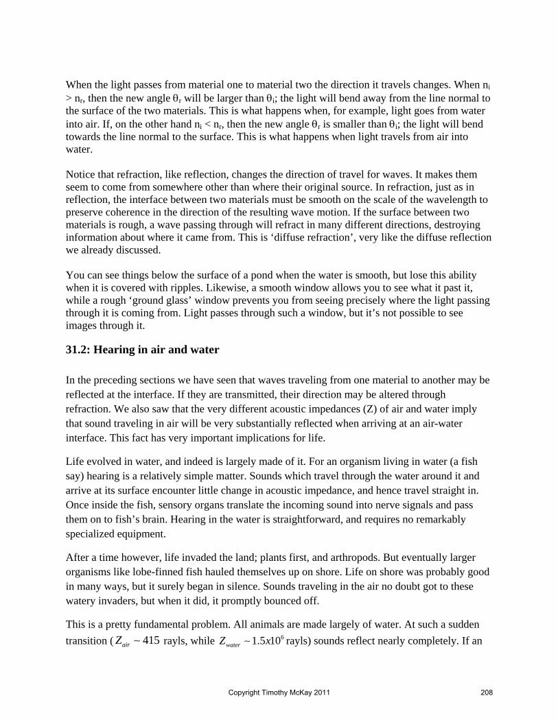
When the light passes from material one to material two the direction it travels changes. When ni > nr, then the new angle θr will be larger than θi; the light will bend away from the line normal to the surface of the two materials. This is what happens when, for example, light goes from water into air. If, on the other hand ni < nr, then the new angle θr is smaller than θi; the light will bend towards the line normal to the surface. This is what happens when light travels from air into water. Notice that refraction, like reflection, changes the direction of travel for waves. It makes them seem to come from somewhere other than where their original source. In refraction, just as in reflection, the interface between two materials must be smooth on the scale of the wavelength to preserve coherence in the direction of the resulting wave motion. If the surface between two materials is rough, a wave passing through will refract in many different directions, destroying information about where it came from. This is ‘diffuse refraction’, very like the diffuse reflection we already discussed. You can see things below the surface of a pond when the water is smooth, but lose this ability when it is covered with ripples. Likewise, a smooth window allows you to see what it past it, while a rough ‘ground glass’ window prevents you from seeing precisely where the light passing through it is coming from. Light passes through such a window, but it’s not possible to see images through it.

31.2: Hearing in air and water In the preceding sections we have seen that waves traveling from one material to another may be reflected at the interface. If they are transmitted, their direction may be altered through refraction. We also saw that the very different acoustic impedances (Z) of air and water imply that sound traveling in air will be very substantially reflected when arriving at an air-water interface. This fact has very important implications for life.

Life evolved in water, and indeed is largely made of it. For an organism living in water (a fish say) hearing is a relatively simple matter. Sounds which travel through the water around it and arrive at its surface encounter little change in acoustic impedance, and hence travel straight in. Once inside the fish, sensory organs translate the incoming sound into nerve signals and pass them on to fish’s brain. Hearing in the water is straightforward, and requires no remarkably specialized equipment.

After a time however, life invaded the land; plants first, and arthropods. But eventually larger organisms like lobe-finned fish hauled themselves up on shore. Life on shore was probably good in many ways, but it surely began in silence. Sounds traveling in the air no doubt got to these watery invaders, but when it did, it promptly bounced off.

This is a pretty fundamental problem. All animals are made largely of water. At such a sudden transition ( 415airZ ∼ rayls, while 61.5 10waterZ x∼ rayls) sounds reflect nearly completely. If an


animal wishes to hear, it must somehow smooth the transition in acoustic impedance from outside to in. How does this smoothing work?

Imagine a sudden transition across which the impedance changes by a factor of ten; from 1Z to

2 110Z Z= . This would result in a reflected intensity given by:

2 2 2

1 2 1 10 0 0 0

1 2 1 1

10 9 0.6710 11reflected

Z Z Z ZI I I I IZ Z Z Z

⎛ ⎞ ⎛ ⎞− − ⎛ ⎞= = = =⎜ ⎟ ⎜ ⎟ ⎜ ⎟+ + ⎝ ⎠⎝ ⎠ ⎝ ⎠

If, instead, the sound went through two transitions, from 1Z to 15Z and then from 15Z to 110Z , the reflected intensity would be:

2 2 2 2 2 2

1 1 1 1 1 10 0 0 0

1 1 1 1 1 1

5 5 5 10 4 4 5 0.495 5 5 10 6 6 15

totalreflected

Z Z Z Z Z ZI I I I IZ Z Z Z Z Z

⎛ ⎞⎛ ⎞ ⎛ ⎞ ⎛ ⎞− − − ⎛ ⎞ ⎛ ⎞ ⎛ ⎞= + = + =⎜ ⎟⎜ ⎟ ⎜ ⎟ ⎜ ⎟ ⎜ ⎟ ⎜ ⎟ ⎜ ⎟⎜ ⎟+ + + ⎝ ⎠ ⎝ ⎠ ⎝ ⎠⎝ ⎠ ⎝ ⎠ ⎝ ⎠ ⎝ ⎠

When the same total change in impedance is accomplished in two steps instead of one, the amount of sound reflected is reduced! If we make the same factor of ten impedance change in 10 equal steps, only 17% of the sound is reflected; in 100 steps, only 2%.

This idea, that the transmission of a wave across a boundary is eased when the impedance change is gradual rather than sudden is an important one. It is the solution to the problem of hearing when you’re made of water. To get sounds in to where the appropriate sensory organs lay, animals living in air had to smooth the transition from air to water: they had to evolve middle ears.

Impedance transitions in mammalian ears

The ears of mammals that live primarily in air have three functional units. This division is present to deal with the challenge of smoothly coupling sounds in air to the watery interior of the body. The three principal parts are:

1. The outer ear: including the pinna (the cartilaginous stuff you usually call “the ear”), the ear canal, and the outer layer of the ear drum (the tympanic membrane).

2. The middle ear: an air filled cavity in which an articulated set of three tiny bones (the malleus, incus and stapes) connect the ear drum on one side to the so-called oval window on the other

3. The inner ear: a water filled coil made of bone, called the cochlea, down the center of which runs the basilar membrane.


The middle ear is what couples free air sounds outside the body to the water filled cochlea, where the sounds are sensed. This is where the all-important impedance transition takes place. It takes the tiny pressures associated with sounds in air and amplifies them by two means.

The first is hydraulic. The ear drum on one side of the middle ear is large, while the oval window on the other is small. If the force associated with a small pressure on the large ear drum is transmitted to the smaller oval window, it produces a correspondingly larger pressure there. The second method of amplification is through mechanical leverage. When the ear drum moves, it moves the relatively large malleus, which in turn moves the incus, which then moves the tiny stapes. The arrangement of these bones, the smallest in the human body, transmits smoothly exterior sound in air into the fluid which fills the cochlea.

All other animals that live in the air face the same problem, and must solve it in analogous ways. The central importance of this problem is emphasized in marine mammals like toothed whales and dolphins. These animals have ancestors well adapted to life on land, with hearing capable of smoothing the transition from air to water. Such ears don’t work when submerged, as you may know from your own experience as a swimmer. To solve this problem, whale ears have evolved away from their airy origin. Though they still have outer ears, they serve no function. Instead, sound is coupled directly to the middle ear (now filled with fluid!) through their jaws and a specially adapted acoustic fat which fills them. Further adaptations include detaching the bone of the cochlea from the skull, so that vibrations of the skull are not directly transmitted to the inner ear.

The whole topic of hearing and seeing for organisms which regularly cross the boundary between air and water is a fascinating one, and impossible to properly appreciate without a basic understanding of the physics of waves.

Analysis of sound in mammalian ears

To take full advantage of the information carried by the sound, we would like to “analyze” it; measure how much of each frequency the sound contains, as well as where it comes from. How is it analyzed? There are three big tasks: amplitude measurement, frequency analysis, and determination of directionality.

Sound amplitude measurement is accomplished in mammals by specially adapted long thin ‘hair cells’. Each hair cell has at one end a bundle of a few hundred cilia which extend out into the fluid-filled cochlea. The other end of the hair cell is attached to the basilar membrane which runs down the center of the cochlea. The cilia on the hair cell are transducers; they convert a tiny mechanical motion into an ion flow, which sends glutamate neurotransmitters to auditory nerve cells. These nerve cells then pass the signals on to the brain.

The frequency analysis of a sound is determined by a mix of two approaches. The first relies on the mechanical properties of the basilar membrane which runs down the center of the cochlea,


separating the fluid in the cochlea into two chambers. At the entrance to the cochlea, the basilar membrane is narrow in width, thick, and very stiff. At the far end of the cochlea, it is wide, thin, and flexible. When waves of different frequencies propagate in the fluid surrounding this complex, continuously varying membrane, they produce different patterns of oscillation. High frequency waves generally excite large oscillations in the thick, stiff part of the membrane, while low frequency waves typically excite large oscillations in the thin, flexible part of the membrane. These oscillations in turn trigger hair cells, which eventually send signals to the brain.

By noting which hair cells are excited, the brain learns where on the membrane oscillations are large, which in turn reveals what frequencies were present in the original sound. This transformation from frequency to location on the basilar membrane provides one way for your brain to analyze the frequencies of sounds. This is called the ‘place principle’ in the literature of sensation.

There is a second approach to frequency analysis, which relies on the ability of hair cells to fire in synch with the sound waves which excite them. If they respond to a 100 Hz sound by stimulating auditory nerves to fire at 100 Hz, they directly encode the frequency information in the sound for interpretation by the brain. This functionality is limited by the mechanical response of the cilia to frequencies lower than about 500 Hz in humans, but can be extended to somewhat higher frequency. This happens when different cells fire on every other, or every third, or every fourth cycle; producing a volley of nerve signals at the still higher incoming frequency. This is called the “volley principle”.

A rich combination of the place principle and the volley principle allows for the analysis of frequencies in sound. In humans, frequency sensitivity is quite sophisticated. Humans can detect shifts in frequency of about 10 Hz in a 3000 Hz signal (a shift of 0.3%). Frequency precision is less at the high and low frequency ends of our hearing, but is still about 3% at 100 Hz.

Determining the arrival direction of sound relies on having two separated ears. People are quite good at this, and can typically determine the direction to a sound with errors of about 3° . Once again, two different clues are used.

The first is shadowing. A sound arriving from the right reaches the right ear directly. To reach the left ear, such a sound must diffract around the head. In doing so, its amplitude becomes noticeably smaller. By comparing right and left amplitudes, information about direction can be extracted. Naturally this shadowing is most useful at high frequencies, which have wavelengths smaller than your head, and hence are more effectively shadowed. A typical head is about 0.2 m in diameter. A wavelength of 0.2 m corresponds to a sound frequency of 1500 Hz; sounds above this frequency will be quite effectively shadowed.

The second clue to directionality is time delay. Peaks in a sound arriving from the right will reach the right ear first, and then the left. Given the speed of sound in air and a typical head size


of about 0.2 m, the maximum time delay between the ears is 0.6 msears soundt d vΔ = ≈ . Since the time delay measurement made in your brain relies on the volley principle, it is most useful where the frequencies of sound are not too high, typically below around 1000 Hz.

Since human ears are separated in only the horizontal plane, we have relatively poor ability to tell whether sounds come at us straight on, from above, or from below. Of course we can always turn our heads to find out, and you will often see someone listening intently tip their head at an angle. Now you have a better idea why.

31.3: Things are not where they seem; bent paths for light We have seen that the directions of wave propagation can change when they arrive at the boundary between two materials. Whether a wave will reflect off of or pass through a boundary is determined by the properties of the two materials: their acoustic impedances for sound and their indices of refraction for light. For both reflection and refraction, simple relations govern how the direction of wave travel will change. When the boundaries between the two materials are flat on the scale of the wavelength, reflection and refraction will be specular, and information about the original arrival direction will be preserved over large areas. In this case, it will still be possible to determine where the original wave came from. When the boundaries are rough on the scale of the wavelength, this directionality information will be lost.

Specular reflection and images When reflection is specular, we can see ‘images’ of real objects formed at new locations. Let’s explore how this works with flat mirrors to gain a sense of what we mean by an image and of how it forms. We’ll start with a simple case, a point source of light which we view in a mirror. Everything we will examine in this case is large compared to the wavelength of light. In this limit, we can ignore diffraction, and assume that the light travels in perfectly straight lines, except when it encounters a boundary between air and some other material and reflects or refracts. This is what normally happens in life. Light from an object travels in straight lines from it to your eye. You freely assume the object is out there in the direction from which light arrives, and most of the time you’re correct. But when reflection or refraction occur, the path of the light is changed. If you don’t know this has happened, you see the light coming from some other direction, and incorrectly assume that the object is in the direction from which light comes. What you are seeing in this case is not the original object, but an “image” of it; a location from which light comes as if it were coming from the actual object. You see the object there, at the location of the image, just as you would if the object were actually there. This situation is illustrated below for a simple case, with a flat mirror.


Light leaves the actual object traveling out in every direction, either because the object emits it in every direction, or because it reflects light in a diffuse way. Most of this light never reaches your eye, and hence you don’t see it. There are two exceptions. Some light travels straight from the object to your eye. This is the normal case, and because of this light you see the object where it really is. But there is more. Some of the light from the object reflects from the mirror in such a way that it also reaches your eye. When you look back along this direction, you again see the object, but this time it appears to be somewhere other than where it really is. This location, where the object appears to be, is called an image of the object. The direction you must look to see the image is clear from the law of reflection. The first figure below shows how this works. How far away does it appear to be? You can get a sense of this by examining the second figure below. If the actual object is a distance objectd in front of the mirror, the image will be seen the same distance behind the mirror: image objectd d= . Place an object close in front of the mirror, its image appears close behind it. Place an object far from the mirror and its image will appear far behind it. How large does this image appear to be? Since you see it just as far behind the mirror as it is in front, it looks just the same size as it would if you looked at it directly provided you’re the same distance away. A simple example will give the idea. Imagine you stand next to your friend, one meter in front of a flat mirror. If you look at your friend in the mirror, she will seem to be two meters away; you will see her image one meter behind the mirror, which is itself one meter from you. She will appear to be just the size she would be if she was actually two meters from you.So the location and size of the images produced by a flat mirror are relatively simple.


Reflected view: you also see the source here. This is the “image” of the original object

Direct view: you see the source here

Your eye determines distance to these from their angular separation

These appear to be as far behind the mirror as they are actually in front


Images formed by reflection from flat mirrors can be remarkably faithful reproductions of the real thing. Reflected images are increasingly realistic as the reflecting surfaces become more perfectly smooth, and as the fraction of incident light reflected becomes more complete. Good examples of partial cases include reflections from smooth stone surfaces like the Vietnam Memorial in Washington DC or from glass windows, where part of the light is transmitted and only a bit reflected.

To better understand the images formed by flat mirrors, it is useful to consider a few examples. First, what happens when you look at yourself in a mirror? If you are a distance objectd in front of the mirror, you will see an image of yourself which appears to be a distance image objectd d= behind the mirror. Move closer to the mirror, and the image moves closer to the mirror; move farther away, and the image moves farther away. Everything else you see in the mirror likewise appears to be just as far behind the mirror as it actually is in front. Combine this idea with the law of

Which set of mountains and trees is the real object, and which is the image?


reflection, and you can figure out where you will see the image of any object because of reflections in a mirror.

Into the funhouse: reflections from curved mirrors Specular reflection requires that the surface of a mirror be smooth on the scale of the wavelength of light. But it need not be globally flat. The surface can be curved on large scales, so long as it is smooth locally. Whatever the large scale shape of the mirror, each light ray is reflected according to the law of reflection wherever it strikes. The angle of incidence, measured relative to the local surface, is equal to the angle of reflection. Images are formed in reflections from smooth but curved surfaces. Unlike those for flat mirrors, these images may be magnified or distorted. The famous Cloud Gate sculpture in the City of Chicago provides a particularly beautiful example. First let’s consider the general case. Any curved mirror has a radius of curvature which defines it, a measure of how dramatically it is curved. If the mirror is actually spherical, this radius of curvature is the same everywhere, and is the radius of the sphere. If the mirror is not spherical, the radius of curvature at any point is the radius of the sphere which best approximates the surface in a region close to that point. Such a mirror may be convex, bulging out toward the object, or concave, bent inward away from the object. Imagine light emerging from an object and heading toward the mirror. Once again, this might be light actually emitted by the object, or just light diffusely reflected from it. Each ray of light from the object reflects when it reaches the surface of the mirror according to the law of reflection: the angle of incidence, measured relative to the local surface, is equal to the angle of reflection. To find the location of the image, we examine the rays emerging from a single point on the object, find out how they reflect from the mirror, and see where they come together again. The place where these reflected rays come together again is a point on the image which corresponds to the point on the object from which the light emerged. This procedure is used to produce the three figures below, which show reflections from flat, convex, and concave mirrors. In the flat case, light from the top point of the object reflects from the mirror, at each point according to the law of reflection. The reflected rays all seem to come from a point just as far behind the mirror as the object is in front. A flat mirror produces an image which is upright (oriented in the same way as the object), and appears just as far behind the mirror as it actually is in front. The size of the object and the size of the image are the same. When systems form images we will often speak of magnification. For these systems, we will define a linear magnification which is the ratio of the image height to the object height. In the flat mirror case this ratio is one.


Now consider the convex case. It may help to imagine taking the flat mirror and simply bending it away from the object. This will always, no matter what the curvature, make the reflected rays diverge more strongly than in the flat case, as if they were all coming from a point which is closer to the mirror. Such a convex mirror always produces an image which is upright, and reduced in size. Such a convex mirror has a magnification which is positive, but less than one. It makes images which are smaller than the objects that produce them. The concave case is a little trickier. Imagine taking the flat mirror and now bending it toward the object. Initially, when the curvature is small, the rays reflected from the mirror will still diverge, though less dramatically than they do in the flat mirror case. When this is true, the reflected rays will still seem to come from somewhere behind the mirror. These rays diverge less than they would with a flat mirror, as if coming from a point farther behind the mirror. Such an image will still appear upright, but be larger than the object. For this case, the magnification is positive and larger than one. Things change when we bend this concave mirror toward the object still more strongly. Eventually, the rays reflected from the object will cease to diverge, in fact, they will begin to converge. When this happens, the rays reflected from the mirror come together at a point in front of the mirror, rather than behind. These rays appear to come from this point of convergence, just as they originally did from the point on the object. This point of convergence is where the image is formed. The image formed by such an object in a concave mirror will be inverted and reduced in size. The magnification in this case is negative and less than one. What determines which of the two possibilities will happen for the concave mirror? What matters is whether the object is close to or far from the concave mirror. In this case, ‘close to’ and ‘far from’ are in some way determined by comparison of the object distance to the radius of curvature of the mirror. A qualitative transition will occur when rays from the object reflected from the mirror cross over from diverging (as they do in the first case) to converging, as they do in the second. When this happens, rays from the object neither diverge nor converge; they emerge from reflection off the mirror perfectly parallel. When an object is at this special location, all the light which emerges from it will reflect from the mirror in a parallel beam. If we reverse the direction of the light, we gain an important insight into the meaning of this special distance. Send a beam of parallel light into the mirror. What happens to it? All of this parallel light comes together at a single point. This point toward which parallel light is all directed is called the focus of the mirror. Send in parallel light, and it all comes together at the focus. Reverse things, place an object at the focus, and light from the object will reflect off the mirror in a parallel beam. Where is this focal point? The answer depends on the details of the mirror shape. There are two simple shapes which are frequently used; spherical mirrors and parabolic mirrors. Each has an ‘optical axis’ of symmetry. For the sphere this axis passes through the center of the sphere, for the parabola it is the axis of symmetry. Spherical mirrors have a focal point located at a point half the radius of the sphere from its surface: 1

2spheref R= . For a parabolic mirror, the focal point


is located at the ‘focus’ of the parabola. For a parabolic mirror defined by the equation 2y ax= , the focus is located along the y axis a distance ( )1 4f a= from the origin. Neither the spherical mirror nor the parabolic mirror are perfect focusers of light coming from any direction however; in both cases there are limits. For the spherical mirror light will be focused well (concentrated to a small point) if it arrives parallel to the optical axis and if the beam is much smaller than the diameter of the sphere. Light rays which arrive parallel to the optical axis are called paraxial rays. For the parabola, the light must arrive parallel to the optical axis, but the beam may be as large as the mirror aperture with no degradation in the focus. This is shown in the figure below. These failures to perfectly focus parallel light are examples of optical aberrations.

This shows imperfect focusing of parallel light along the optical axis from a spherical mirror. Light far from the axis (in terms of the radius of curvature of the mirror) is not brought properly into focus. Spherical mirrors are easy to make, but do not concentrate light as well as parabolas.

This shows perfect focusing of parallel light along the optical axis from a parabolic mirror. Parabolas can tightly focus paraxial light even when it arrives far from the optical axis. This makes parabolas excellent light concentrators.



What about the images formed by spherical mirrors? In the limited case of light from objects which are close to the optical axis, and to reflections from just a small fraction of the diameter of the sphere, there are simple relations which relate the location of the object and the radius of curvature of the sphere to the location of the image. These also provide predictions for the linear magnification of the mirror. The form of the equations is the same for both convex and concave mirrors, but there are differences in the sign convention which you must be aware of.

image

object image object

1 1 2 and d

md d R d

+ = = −

For a convex lens, the radius of curvature is defined to be negative, while for a concave lens, the radius of curvature is defined to be positive. Object distances are positive, and image distances are positive when the images are real (on the same side of the mirror as the object) and negative when they are virtual (when the images are behind the mirror). It is useful to work through this for our few special cases. We can always solve for imaged and find

objectimage

object object

and 2 2

Rd Rd md R d R

−= =

− −

First consider the convex case. Since R is defined to be negative for a convex mirror, and objectd is positive, imaged must always be negative. It also implies that the magnification will always be positive and less than one; the image is upright. When the object distance is very large, the image distance approaches 1

image 2d R= . When the object distance is very small, the image distance approaches image objectd d= − and the magnification becomes one. When an object is very close to the mirror it looks flat and produces the usual upright unmagnified image of a flat mirror. What about the concave case? Here the radius of curvature is defined to be positive, so things are more interesting. When the object is far from the mirror, in particular when object2d R> , the image distance is always positive. This means the image is on the same side of the mirror as the object, and is real. For this case, the magnification is always negative; the image is inverted. As the object distance becomes very large, the light coming in is parallel, and the image forms at the focal point, with 1

image 2d R= . When the object is closer, with object2d R< , the object distance becomes negative. Now the image is virtual, on the opposite side of the mirror from the object. The magnification in this case is positive (the image is upright), and can become very large when the object2d R≈ . Once again, when the object is very close to the mirror, image objectd d= − , and the image is upright and unmagnified, as if the mirror were flat.


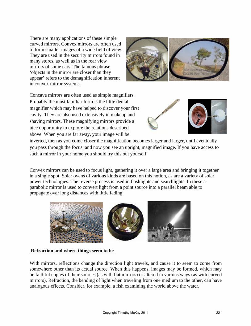
There are many applications of these simple curved mirrors. Convex mirrors are often used to form smaller images of a wide field of view. They are used in the security mirrors found in many stores, as well as in the rear view mirrors of some cars. The famous phrase ‘objects in the mirror are closer than they appear’ refers to the demagnification inherent in convex mirror systems. Concave mirrors are often used as simple magnifiers. Probably the most familiar form is the little dental magnifier which may have helped to discover your first cavity. They are also used extensively in makeup and shaving mirrors. These magnifying mirrors provide a nice opportunity to explore the relations described above. When you are far away, your image will be inverted, then as you come closer the magnification becomes larger and larger, until eventually you pass through the focus, and now you see an upright, magnified image. If you have access to such a mirror in your home you should try this out yourself.

Convex mirrors can be used to focus light, gathering it over a large area and bringing it together in a single spot. Solar ovens of various kinds are based on this notion, as are a variety of solar power technologies. The reverse process is used in flashlights and searchlights. In these a parabolic mirror is used to convert light from a point source into a parallel beam able to propagate over long distances with little fading.

Refraction and where things seem to be With mirrors, reflections change the direction light travels, and cause it to seem to come from somewhere other than its actual source. When this happens, images may be formed, which may be faithful copies of their sources (as with flat mirrors) or altered in various ways (as with curved mirrors). Refraction, the bending of light when traveling from one medium to the other, can have analogous effects. Consider, for example, a fish examining the world above the water.


Rather than see light from things above the surface coming directly from its source, the fish sees light from objects in the air only after its path has been bent in the transition from air to water. The fish might think that an object is in a certain direction, because that is where it seems to be, while in fact it is in another place entirely. A similar phenomenon happens for someone looking into the water, rather than out. When you see a fish underwater, it is not actually where it appears to be, but is instead somewhat closer to you. The fish examples all involve a single sudden transition in index of refraction, so that the light changes direction at just one point. A number of interesting phenomena occur when the index of refraction varies gradually and continuously. In the atmosphere, the index of refraction is dependent on temperature, pressure, and humidity. Since these properties vary through the atmosphere, the index of refraction does as well. As light travels through the atmosphere its path bends into regions of higher index of refraction. One interesting example of this is the familiar mirage. Originally seen in deserts, but now more familiar from summertime road surfaces, a mirage is caused by a temperature inversion; when hot air (with a lower index of refraction) is found under cool air (with a higher index). This typically happens when bright sunlight heats a ground surface, like the desert sands or a paved road, which in turn heats the air near it. Light from the sky which would have struck the ground instead bends away from it (toward the cooler air). An observer looking at this region from small angles sees light from the sky where they might have expected to see the road. Here in Michigan we often see the opposite effect when looking out over the Great Lakes. The water in the lakes is often (always) cold. It cools the air over the water. Once again, the light turns toward the cooler, higher index of refraction air. Since this time the cool air is below the hot air, light which was headed up above your head is turned downward, and you see it coming from somewhere above where it actually emerges. We will see in the next chapter that refraction, like reflection, can be used to form images which accurately reproduce objects.

What the fish sees

What the fisherman sees

Image

Object Image

Object


31.4 Capturing waves: Refraction and total internal reflection Refraction can also make it possible to completely capture a set of waves, to guide them along a channel to anywhere you would like them to go, When light moves from a medium with a large index of refraction (like water) into one with a small index (like air) it bends away from the direction normal to the interface. If we blindly apply Snell’s law to this case, we might find:

12 1

2

sin sinnn

θ θ=

When 1 2n n> , it is possible for this equation to predict 2sin 1θ > . Now the sine of an angle can never be larger than one, so something else must occur. What happens instead is that the light heading out of the high index material (n1 > n2) never actually leaves, but is instead completely reflected at the interface. For the transition between any two materials, there is a critical angle for light arriving at the surface for which this will be true:

11 2 2c

2 1 1

sin 1 or sin or sinc cn n nn n n

θ θ θ − ⎛ ⎞= = = ⎜ ⎟

⎝ ⎠

If light arrives at the interface at an angle greater than this, it will not leave the high index material at all, but instead will be completely reflected, staying in the material it started in. This effect has important implications. First it has a major effect on what organisms see when looking into or out of water. If you are underwater and looking up, you see things straight over you essentially undistorted. As you look out to the side, you see the whole world above the water, right down to the horizon, packed within a circle significantly smaller than a hemisphere. Looking out to greater angles, you see only light reflected from things below the surface. If you are out of the water looking in, you can see light coming from an object only if it gets to you. This means it has to be in a place where light leaving the object can exit the water and get to you. Sometimes this is impossible. There are regions underwater which an observer above the water cannot see. When you stand on the edge of a pool looking in, for instance, you can see through

Every beam in this region is totally reflected

Every beam in this region is refracted out into the low index material

θc What the fish can see

What the fisherman can see


the water surface only near your feet. As you look farther out, eventually you reach a point where light coming from below the surface suffers total internal reflection and never reaches you.

Total internal reflection and optical fibers One very important application of total internal reflection is in optical fibers. Such fibers are made of glasses with relatively high index of refraction (1.5-2.0). You put light more or less straight into the end and it will head down the fiber. Each time the light strikes the wall it reflects off through TIR, staying completely within the fiber. This will happen even if you bend the fiber through rather large angles, because the critical angle for such a fiber may be as large as 30°. This allows optical fibers to become “light pipes” which can guide light around corners. This is all you need to know in principal, but in practice making an effective optical fiber is much more challenging. The difficulty is that the surface of the fiber may not be perfectly smooth on the wavelength of light. Small scratches created in the production and handling of a fiber provide places where the conditions for total internal reflection are not met locally. This allows some of the light to escape each time it reaches the surface. Since the light bounces back and forth through the fiber many many times, even a small loss at each reflection leads to rapid escape. The solution to this problem is to prevent the light from ever reaching the surface. It was invented at the University of Michigan by undergraduate researcher Larry Curtis in 1956. Imagine an optical fiber with index of refraction inn . Curtis thought that perhaps he could keep the light in the fiber, and protect the surface of the fiber from damage, by hiding the interface where the internal reflection occurred inside the fiber. To do this, he coated the fiber with a ‘cladding’ of another glass, with index of refraction in claddingn n> . Now the internal reflection happens at the boundary between the two glasses, rather than at the outer surface of the fibers. Today, fancier versions of Curtis’ idea are used. Instead of a single lower index coating placed around the central fiber, the fiber has a high index core surrounded by layers with continuously decreasing index. Rather than have any sudden reflections, such a graded index fiber smoothly turns the light so that it wiggles back and forth down the fiber.

Conventional optical fiber with significant loss of light on each reflection

Cladded optical fiber with very little loss of light on each reflection

A graded index optical fiber: in this there are no discrete reflections at all


Optical fibers and endoscopes

Once you have a pipe in which you can capture light, delivering it wherever you like, you can use it to see into places previously invisible to you. Endoscopes are devices designed to do this. To make an endoscope you can bundle together a large number of optical fibers. Light striking the end of each fiber becomes trapped in it, and can be sent around corners until it emerges on the far end. If you keep the arrangement of fibers the same on both ends, the pattern of light which enters the fiber bundle on one end emerges in the same pattern on the other. In such a fiber bundle, cladding is especially important. If you just pack the fibers next to one another without cladding, light might pass freely from fiber to fiber, creating ‘cross-talk’ which would ruin the image. Endoscopes are now used in a very wide variety of applications in medicine and industry. They allow the user to guide light into and out of places previously inaccessible to imaging, such as your intestines, a wall, or an engine block. Fiber optics, cables for trapping light and delivering it from one place to another, make this all possible. Often the same tube which contains the fiber optic bundle will contain a second bundle designed to send in light, micromanipulators to steer the tip, and even tiny microscopes.

Capturing sound in the ocean Interestingly, something very like the transmission of light in an optical fiber happens naturally for sound in the ocean. The speed of sound in the ocean varies with temperature, salinity, and pressure in a complex way. Most of the time, a graph of the sound speed as a function of depth looks something like the figure below. After increasing a little very near the surface, the speed of sound falls by about 10 % before beginning to rise again at greater depths. This broad minimum in sound speed can capture and guide sound in very much the same way that a graded index fiber can capture and direct light. This sound pipe is called the SOFAR channel (SOund Fixing And Ranging) for historical reasons. It was discovered and originally explored as a way for downed World War II pilots to advertise their location. By dropping a small explosive into this channel, sound from it would


propagate out to great distances. By picking up the sound and recording its arrival time, rescue ships might find the downed pilot. While it was never used in this way during the war, it has since been put to use in a wide variety of other applications. Living things make use of the SOFAR channel as well. Some whales communicate with one another using an array of sounds, even singing what many would call songs. The sounds they produce can travel through the SOFAR channel and be heard at very great distances. Recall from earlier in this chapter the general rule that light travels very freely through air while sound travels relatively freely through water. Singing a song is a great way to advertise your presence in the ocean.

31.5 Dispersion: refraction is often wavelength dependent

In real material the speed of wave propagation is often wavelength dependent. Since the index of refraction is n = c/v, if speed is a function of wavelength, then so is the index n. So in general, we have something like:

( ) ( )cn

vλ

λ=

Since the index of refraction is related to the bending of light through Snell’s law, this means that light of different wavelengths (different colors) will be bent by different amounts when passing from one material to another. This phenomenon, which tends to spread out the different colors, is called “dispersion”. It may be familiar to you from playing with prisms. Recalling that “white” light is actually made up of a mixture of all the different colors, you can see how dispersion allows a beam of white light to be broken up into all its constituent colors. It is usually the case that shorter wavelength (bluer) light is bent more than longer wavelength (redder) light when passing into glass, so when this white beam is broken up you typically get the red-to-blue spectrum illustrated in the image above. Perhaps you will recall the mnemonic “Roy G Biv” for keeping track of which color goes where. In this scheme, “indigo” is added to the red-orange-yellow, green, blue-indigo-violet accounting.


Like most things in life, dispersion can be good or bad. If you want to know what colors make up the light you’re looking at, if you want to “analyze” it, dispersion can be very useful. Dispersive elements like this are at the heart of every spectrograph; instruments which allows us to precisely measure the mixture of wavelengths we see in light we want to study. While some spectrographs rely on prisms, many use diffraction gratings as dispersive elements rather than prisms, as described in the previous chapter. Some use ‘grisms’, which combine both a grating and a prism. But in every case some dispersive element, something which separates light of different wavelengths, is present. Spectroscopy, the detailed analysis of light emitted from or absorbed by various things, plays a central role in the great scientific discoveries of the 20th century, including quantum mechanics, chemistry, biology, astrophysics, and cosmology. Dispersion is a problem if you’re trying to form an image (we’ll say more about this below). Forming an image requires taking all the light coming from some point on an object and directing it to a single spot. Dispersion, which bends light of different colors in different ways, often makes this difficult. The different bending of different colors can create blurry images, with the red light on one side and the blue on the other. This is called “chromatic aberration”. Clever arrangements of different materials, which bend light in different ways, can be used to create “achromatic” systems for focusing light.


A Quick Summary of Some Important Relations Fading of intensity of light and sound due to absorption: Both light and sound are subject to absorption when passing through material media. The importance of this absorption is characterized by a wavelength dependent attenuation coefficient( )α λ or absorption length ( ) ( )1/absL λ α λ= :

( ) ( ) ( ) ( ) ( ), ,0 ,0 abs

xx LI x I e I eα λ λλ λ λ

−−= =

Material mismatch and reflection:

When the medium a wave is traveling in changes, they may reflect. The material property which matters for light is the index of refraction, for sound it is the acoustic impedance:

medium acoustic medium sound in mediumlight in the medium

cn Z vv

ρ= =

When waves encounter a boundary between two media perpendicular to the interface, the fraction reflected is:

2 2

and A B A Blight sound

A B A B

n n Z ZR Rn n Z Z

⊥ ⊥⎛ ⎞ ⎛ ⎞− −= =⎜ ⎟ ⎜ ⎟+ +⎝ ⎠ ⎝ ⎠

Reflection and refraction:

At the interface between two materials, reflection occurs so that the angle of incidence equals the angle of reflection. The part of the wave which doesn’t reflect at the boundary enters the new material, and changes direction in a way governed by the law of refraction:

( ) ( ) ( ) ( )sin sinsin sin or i r

i i r ri r

n nv vθ θ

θ θ= =

Total internal reflection:

When light encounters a medium with lower index of refraction, there is a minimum angle below which it will be completely reflected:

( )minsin low

high

nn

θ =


Polarization of light by reflection and ‘polarizers’:

When light reflects off a surface, it may emerge partly polarized. At one particular angle, the reflected light is perfectly polarized, in a plane parallel to the surface:

( ) highmax polarizationBrewster

low

tannn

θ =

There are also materials, called polarizers, which polarize light on transmission. Any light which passes through them is fully polarized along the direction selected by the polarizer. The amount of light transmitted depends on the polarization of the incident light. If it is polarized, the transmitted fraction depends on the angle ipθ between the polarization of the incident light and

the polarizer angle. If the incident light is unpolarized, the fraction transmitted is 50%.

( )polarized 2 unpolarized1transmitted incident transmitted incident2cos or ipI I I Iθ= =



32.1 How to sense the world around you: sorting light and forming images Organisms have a desperate need to know what’s happening beyond their skins. Both sound and light carry information from one place to another. So many animals have evolved structures which allow them to see and hear their surroundings. We have seen that sound, with relatively large wavelengths, often diffracts past obstacles and through openings. As a result, sound may arrive at a listener from directions other than a straight line to its source. This makes sensing the direction from which sound comes in great detail is not especially useful. Visible light, which has very short wavelengths, diffracts very little around typical objects, traveling almost entirely in straight lines from its source. This makes sensing the direction from which light arrives an especially useful thing to do.

32.2 Eyes and their components If an animal is going to get useful information about the world around it using light, its eyes ought to do three things:

1. Detect the light 2. Measure it’s properties (the mix of wavelengths and intensities) 3. Find out what direction the light is coming from

Different animals have visual systems which span the full range from no light sensitivity at all to highly developed and complex eyes. Eyes are incredibly useful, they can provide an enormous selective advantage. So perhaps it’s not surprising that eyes of different kinds can be shown to have evolved independently a large number of times. One of the clearest suggestions of this is the very wide diversity in types of eyes which exist; from the very simple eyes of the octopus or the nautilus, though the remarkable compound eyes of many insects, to the sensitive and highly precise eyes of some birds. Understanding the strengths and weaknesses of these various designs is much easier when the basic features of their function are kept in mind.

Detecting the light

The first step in vision is the raw detection of light. ‘Detecting’ light requires absorbing the energy in it and converting it into an electrical signal which can be transmitted through the nervous system to the brain. This process of taking a signal from one form (light) and converting it to another (a nerve impulse) is generically called signal transduction. This transduction typically takes place in specialized kinds of neurons called photoreceptors.


Most animals detect light using a group of related protein molecules called opsins. A light detecting cell will typically contain many of these opsin molecules. In each, absorption of a particle of light (a photon) causes a structural change, raising it from its low energy ground state to a different, higher energy state. In this state energy state, the opsin molecule can start a cascade of amplified response. Each activated opsin will generate about 100 activated “transducin” proteins. In turn, each of these starts an additional process in which about 1000 additional active molecules are produced. So for each absorbed bit of light, a signal 105 times as large is produced. The net effect of the production of all these proteins is to close off Na+ ion channels into the cells. Photoreceptors usually send signals continuously to the brain. Receipt of light shuts this transmitted signal off. So interestingly, the photoreceptors in your eyes send signals to your brain constantly in the dark, and actually shut them off when they detect light. This is in contrast to most of your other senses (like touch) which only begin to send signals when they are stimulated. Of course your brain can as easily interpret the turning off of a transmission as it can the turning on of a signal.

Measuring the properties of the light

To measure the properties of the light (intensity and distribution of wavelengths) the receptors have to create different signals when the light changes intensity or color. As it happens, there are many ways eyes do this. To give an example, we will consider a few details of what happens in your primate eyes. To determine the nature of the light reaching you, there are actually four kinds of opsins in your eye. The first is rhodopsin, a highly sensitive form which in your eye appears in the very numerous ‘rod’ cells on your retina. These rods are especially important in night vision, in the detection of faint light. They are good for telling whether light is there when it’s faint, but provide no information about its color. The other three types of opsins in your eyes are found in the smaller, rarer ‘cone’ cells on your retina. Each of these opsins has sensitivity to different, though overlapping, ranges of light wavelengths. In each cell, the detection of some light completely triggers the cell; each one is only on or off. Each cone contains all three opsins, but in each cell one of the three dominates. When many of the cones dominated by blue sensitive opsin (labeled S in the figure below) are activated, your brain knows that the light it is sensing is blueish. When the cones firing are predominantly the L type, your brain can tell it is reddish. Putting all this together gives you the color sensitivity you experience. The rhodopsin in your rod cells has a particular wavelength response too, which not surprisingly is kind of in the middle of the others, allowing good sensitivity to light whether it is redder or bluer. The rhodopsin sensitivity is shown as the dashed “R” curve in the figure below. But since the rods have only this one type of opsin, they provide no color information, only intensity information. You can see from the picture of rods and cones below why the cones provide the low light level sensitivity. They cover much more of the area and they have the more sensitive rhodopsin in them.


Interestingly, most mammals have only two color vision, the S and L types shown below. Old world primates, though a simple mutation, evolved a third form of opsin, the M type, which allows them to better sense the difference between red and green. This adaptation may have been especially useful for selection of young, more easily digested leaves. More remarkably, the same tricolor vision mutation evolved independently in one new world primate; the Central American Howler Monkey. This story is beautifully told in Sean Carroll’s recent book “Making of the Fittest”i.

Finding out which direction the light comes from Imagine an ‘eye’ built just of a light sensor; something which can tell how much light is striking it and pass that information on to a nervous system. Such an eye can tell whether it’s light or dark, but can’t ‘see’ anything. It can’t tell you what direction the light is coming from or form an image. To build a real eye you have to couple this kind of light sensor with a system for sorting out what direction each bit of life comes from. Perhaps the simplest system just uses geometry. If you block the light from some directions and still see something, you know what direction the light is coming from. There’s a simple version shown in the figure labeled (a). In this eye, a set of sensors represented by little rectangles is spread across the inside of an open pit. Sensors on the left hand side can be hit only by light from the right, while sensors on the right can be hit only by light from the left. By noticing which sensors are hit, an animal with an eye like this can tell, crudely, which direction light is coming from. The ‘resolution’ of this eye, its ability to distinguish light from different directions, is limited by the size of that hole on the front. If you make the hole really small, you get what’s called a “pinhole camera”, which produces very nice images indeed. The example in the figure labeled (b) should give the idea. As you make the hole smaller and smaller, you squeeze the light from each direction onto a smaller and smaller group of sensors. Eventually the pattern of light on the detectors is a completely reliable map of how much light comes from each direction.


This is a very important idea. A system which can produce a reliable map of how much light is coming from each direction is an “imager”, and the map of the light it produces is called an image. If you want to be able to see, you need to have a way of forming such an image and of detecting the light. What is the drawback of a pinhole camera? The main problem is that a sharp image requires a very small hole, and a very small hole means that very little light will be let in. So while a pinhole camera does make a nice sharp image, there has to be a LOT of light around for it to be very useful. To avoid this problem, you’d like to have a way to use all the light striking some large area from every direction. This eye should map all the light arriving from each direction and somehow sort it so that all the light from each direction hits a particular point on the field of light detectors.

One way to do this is to somehow bend the path of the light, so that although the light from one direction comes in parallel, all of it gets pulled together to a single spot on the detectors. The idea is shown in the figure below.

An image formed by a pinhole in a coffee can and detected by a flat piece of film. Since the pinhole is small, it produces a reliable map of how much light came from each direction; an image of the scene outside.

An example of a pinhole eye: this kind of eye can form a very reliable image and is quite simple.


To do this requires a more complex, but also much more efficient structure in the eye involving a “lens”. The word derives from the Latin word “lentil” which refers to small beans with the same general shape, which is often narrow at the edge and thick in the middle.

The purpose of a lens is to gather all the light coming from one direction and bring it together at a point. When this happens, all the incoming coming from each direction goes to a particular point in the image. This map is the image. An ideal lens might do this perfectly well for light of any kind coming from any direction at all. As we will see, making such a perfect lens is a challenge. There is another widespread approach to gathering the light from each direction without a tiny pinhole; the many variants of a compound eye. A compound eye is constructed of many very similar elements called ommatidia, each an eye in itself. Each of the many elements of such a compound eye detects light from a particular direction. Combining information from all of them provides the animal with the direction sensing it needs. This kind of eye can be extremely effective, often allowing vision in all directions at once.

All the light coming from the bottom gathers together here

All the light coming from the top gathers together

A lens

Lentils


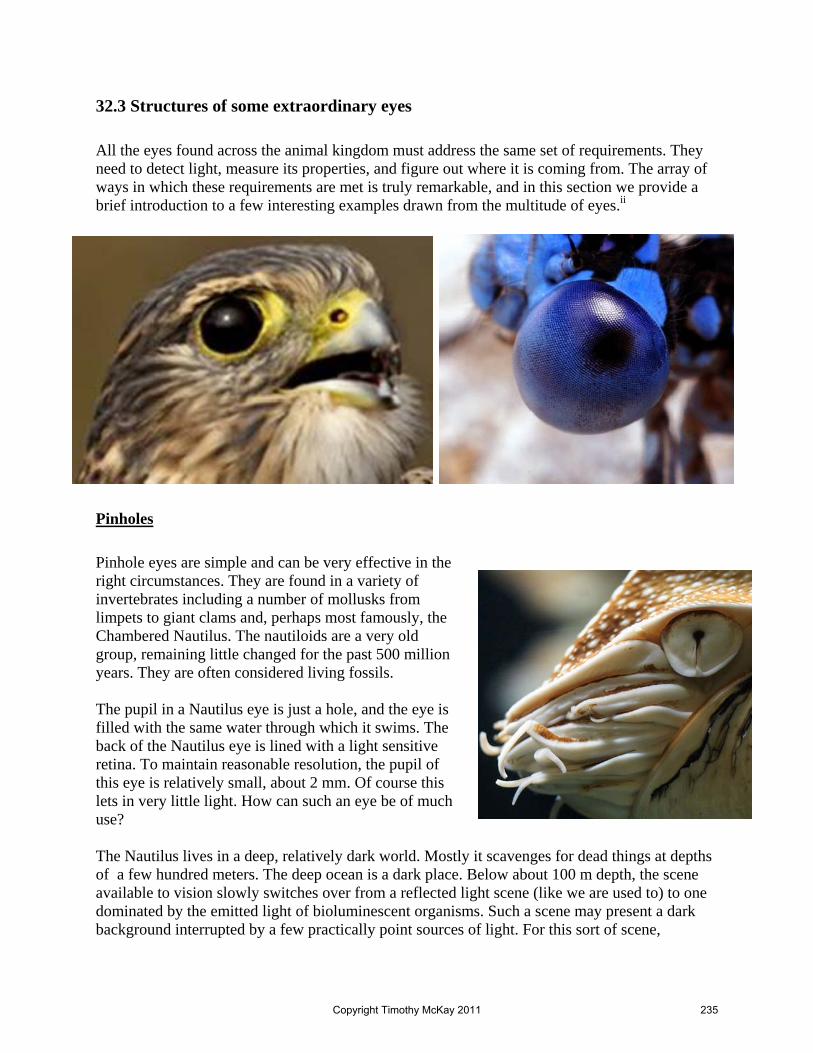
32.3 Structures of some extraordinary eyes All the eyes found across the animal kingdom must address the same set of requirements. They need to detect light, measure its properties, and figure out where it is coming from. The array of ways in which these requirements are met is truly remarkable, and in this section we provide a brief introduction to a few interesting examples drawn from the multitude of eyes.ii

Pinholes Pinhole eyes are simple and can be very effective in the right circumstances. They are found in a variety of invertebrates including a number of mollusks from limpets to giant clams and, perhaps most famously, the Chambered Nautilus. The nautiloids are a very old group, remaining little changed for the past 500 million years. They are often considered living fossils. The pupil in a Nautilus eye is just a hole, and the eye is filled with the same water through which it swims. The back of the Nautilus eye is lined with a light sensitive retina. To maintain reasonable resolution, the pupil of this eye is relatively small, about 2 mm. Of course this lets in very little light. How can such an eye be of much use? The Nautilus lives in a deep, relatively dark world. Mostly it scavenges for dead things at depths of a few hundred meters. The deep ocean is a dark place. Below about 100 m depth, the scene available to vision slowly switches over from a reflected light scene (like we are used to) to one dominated by the emitted light of bioluminescent organisms. Such a scene may present a dark background interrupted by a few practically point sources of light. For this sort of scene,


dominated by just a few points of light, a pinhole can actually capture most of the available information.iii

Compound eyes Compound eyes are both widespread and extremely various among the arthropods. All are constructed of many individual units, typically spread out over a convex surface. The individual lenses of these ommatidia are small, typically less than a hundred microns across. Since this is not too much larger than the wavelength of visible light, diffraction through this relatively small aperture limits the resolution of each individual element. To give a sense of scale, imagine a case with a 25 μm aperture. For 400 nm light, the first diffraction minimum will occur at an angle of about:

7

5

4 10sin 0.016 radians 0.92.5 10

x mD x mλθ θ

−

−≈ = = = = °

Compare this to the diffraction limit for the resolution of a human eye, with a single aperture of about 2.5 mm and you’ll find it is 100 times better. Many compound eyes can be sensibly placed into one of two categories. Apposition compound eyes are the simplest and most common. In these eyes, each long tubular ommatidium is capped with a lens which forms an image of a small region on a light sensitive region at the base. Though an image is formed here, most animals with these eyes do not sense the image, but instead just record a single measure of brightness for each element of the eye. They then assemble an image of the whole field of view one element at a time. This is remarkably like what is done when imaging with a fiber bundle in an endoscope. Each fiber contains no information about the distribution of light within it; it only records how much light there is. The resolution is then set by how many fibers you have. In the apposition compound eye, the resolution is set by the angle observed by each of the many ommatidia. Typical eyes include thousands of elements, providing angular resolution of a few degrees. The second main class is called superposition compound eyes. In these, the light sensing surface is separated from the individual ommatidia by some transparent material, and instead forms a continuous sheet. Light from the individual ommatidia is then imaged on this continuous sheet (rather than detected independently in each element). In many cases the focusing of light in each ommatidium is refractive, through a cylindrical lens. But in some cases, particularly in marine arthropods, the focusing is reflective.


Extreme vision Color vision is achieved through the varying sensitivity of mutated opsin proteins to light of different wavelengths. While most animals have relatively limited color vision compared to humans, some far surpass us. Insert a short summary about mantis shrimp polarization and color sensitivity.

Vertebrate eyes Vertebrates are more conservative in their ocular design than invertebrates. Most vertebrates have a pair of single eyes, each with a refractive focusing element. To get a better idea of the features of the vertebrate eye, we will consider the human eye in some detail below. In the meantime, its worth noting that even among the relatively conservative vertebrates there are some remarkable variants. Most of these involve adaptations which handle unusual circumstances. One famous variant is a group of fish in the genus Anableps who live near the surface of the water. These fish still have two eyes, but they have divided each in two, with a lower half which remains below the surface (and is adapted to focusing underwater), and an upper half which remains in the air and is adapted to focus in the air. This allows them to see both above the water (where most of the insects they eat come from) and below (where many of the things which eat them live). The eyes of nocturnal vertebrates are, just to collect more light, very large. In some cases, like the tiny south-Asian primates called Tarsiers, eyes become a really substantial fraction of the size of the head.


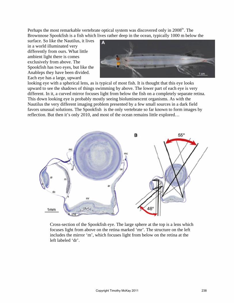
Perhaps the most remarkable vertebrate optical system was discovered only in 2008iv. The Brownnose Spookfish is a fish which lives rather deep in the ocean, typically 1000 m below the surface. So like the Nautilus, it lives in a world illuminated very differently from ours. What little ambient light there is comes exclusively from above. The Spookfish has two eyes, but like the Anableps they have been divided. Each eye has a large, upward looking eye with a spherical lens, as is typical of most fish. It is thought that this eye looks upward to see the shadows of things swimming by above. The lower part of each eye is very different. In it, a curved mirror focuses light from below the fish on a completely separate retina. This down looking eye is probably mostly seeing bioluminescent organisms. As with the Nautilus the very different imaging problem presented by a few small sources in a dark field favors unusual solutions. The Spookfish is the only vertebrate so far known to form images by reflection. But then it’s only 2010, and most of the ocean remains little explored…

Cross-section of the Spookfish eye. The large sphere at the top is a lens which focuses light from above on the retina marked ‘mr’. The structure on the left includes the mirror ‘m’, which focuses light from below on the retina at the left labeled ‘dr’.


32.4 Focusing light: gathering all the light from one direction to a point

The basic goal is to take all the light coming in one direction and bring it together at a point; to focus the ligh. To bring together light rays which enter parallel, some must be bent substantially while others continue straight through. To see how this might work, consider the simple case of light coming straight into the lens. How to accomplish this? The lens in the picture gives the clue. You take a material with higher index than air, so that light passing into it will have its path bent. Then curve the surface of this material, so that light hitting it far from the center will be bent a lot, and light hitting in the middle will go straight through. Everywhere the light strikes, it just follows Snell’s law of refraction. The curvature of the surface is what allows all the light to bend differently at different places and come to focus at one point.

Light at the outer edge is bent a lot

Light at the center goes straight through

Light at the outer edge is bent a lot

All the light coming straight in gathers at this point; the focus


Now this example shows what the lens will do for light coming in straight along the axis. What about light which comes in at an angle? What happens is illustrated in the picture below. All the light from this off-axis direction is still gathered together at a single point, but that point is now offset from the central axis. This is the goal of course, to bring the light coming from each direction together at a different point on the focal plane. If an organism measured how much light landed at each point on this focal plane, it would know how much light was coming from each direction; it would form an “image” of what’s out there in the world. Because the lens gathers light from a large area, it helps in imaging (seeing) things when light levels are low. This is why an eye constructed with a lens can be more effective than a pinhole eye.

Focal length and the lensmakers equation There are two main types of lenses; those which bring parallel rays of light together (converging lenses), and those which spread them out (diverging lenses). Examples of each are shown in the figure below. In both cases, it is useful to define a “focal length” for the lens. For converging lenses, this is distance from the center of the lens to the point at which rays parallel to the axis of the lens are brought together. In diverging lenses, rays parallel to the axis of the lens are not brought together, but instead are spread out. So rather than measure how far past the lens the rays come together, we measure how far in front of the lens the rays would come together when projected straight back through the lens.

Bent less

Bent more

Straight through

Bent less

Bent more

Straight through

Focal point is now “off axis”


Many simple lenses are made of pieces of transparent material polished on one or both sides into surfaces which form parts of spheres. The focal lengths for this kind of lens can be predicted simply using the properties of the lens; including the index of refraction of the lens material (n), the radii of curvature of the two surfaces of the lens (R1 and R2), and the thickness of the lens at the center (d). In doing this, there are some important sign conventions. These conventions vary among different statements of these rules, so be careful. We will use this convention:

• The radius R1 will be positive if the first surface is convex (bent outward) and negative if the first surface is concave (bent inward)

• The radius R2 will be just the opposite, positive if the second surface is concave (bent inward) and negative if the second surface is convex (bent outward)

• A positive focal length f implies a focal point beyond the lens (a converging lens), while a negative focal length implies a focal point before the lens (a diverging lens)

With these sign conventions, we can describe lenses in air with the “lens maker’s equation”:

( )1 2 1 2

11 1 1( 1)lensair

n dn

f R R nR R−⎛ ⎞

= − − +⎜ ⎟⎝ ⎠

In the (reasonably common) case where d << R1 and d << R2, this simplifies to what is called the “thin lens” version of the lensmakers equation:

1 2

1 1 1( 1)lenslens

nf R R

⎛ ⎞≅ − −⎜ ⎟

⎝ ⎠

How would this differ if the lens were not in air, but were in water (the other common possibility for life)? Before looking at the details, think about how this changes things. Light bends when striking the lens because of the change in index of refraction from outside the lens to in. If you surround the lens with water, the change in index will be less than it was when surrounded by air. The light will bend less, and this will surely make the focal length longer. It is even possible that a lens which is converging in air will become diverging when placed in water. This will happen if the index of refraction of the lens material is less than that for water. So how does the thin lens equation change in water?


1 2

1 1 1( )lens waterwater

n nf R R

⎛ ⎞≅ − −⎜ ⎟

⎝ ⎠

Lenses which work well for focusing light in air will not generally do the job in water. This creates special challenges for organisms which live partly in air and partly in water, as we will discuss a bit below.

Lenses, imaging, and sources not infinitely far away When a source of light is “infinitely” far away, all the light coming from it arrives in parallel rays. Now it doesn’t have to be infinitely far away for the rays to be very nearly parallel, it just

has to be far away in comparison to other important distances in the problem, like the focal length of a lens. If such a source really is far away, then the light from it will arrive very nearly parallel, and will all be brought together at the focal point f. What if the source is closer, so that the light arriving at the lens is not parallel? Rays farther from the center will still be bent more, but no longer by enough to bring them together at the focal point. Instead, they will meet farther away. This point where the light from a point source comes back together again is called the location of the image. The point the light comes from is called the object.

Object and image locations are related for these “thin lenses” according to the so-called thin lens equation:

1 1 1

O ID D f+ =

Source of light Focal point Image

location

DI D0

Nearly parallel rays

Clearly diverging rays


Think about some limits, if DO is very large (approaching infinity), then DI = f, and the parallel incoming light comes together at the focal length f. If DO is equal to f, then DI becomes infinite. In this case light coming from the source enters the lens spreading out, and is turned into a set of parallel rays leaving of the lens. They never come together. What if DO is less than f, if the object is closer to the lens than the focal length f? In this case:

0

1 1 1 0ID f D= − <

This means the image distance DI is negative. When this happens, the image is actually in front of the lens rather than behind, rather like in a diverging lens. This case is illustrated in the picture below.

So, for a thin converging lens, the position of an image depends on the location of the source. It is always described by this thin lens equation. If DO > f, then DI is positive, and an image is formed to the right of the lens. If DO = f, the image is at infinity. If DO < f, the image is actually in front of the lens. A very useful way to identify image locations and understand lenses is called ray tracing. Ray tracing is essentially just following the path of several rays of light, accounting for bending which occurs due to refraction or reflection along the way. We did this qualitatively in the last chapter while examining images in flat and curved mirrors. While this technique is intrinsically general, it is especially easy to apply to cases where the lens has a well defined focal point. In this case, a few simple rules apply. From any object location, you can easily draw three so-called principal rays through the lens to find the image location.

1. From the object location to the lens parallel to the axis, then from that point down to the focal point beyond the lens

2. From the object location, through the focal point on the near side of the lens, to the lens, then out of the lens parallel to the axis

3. From the object location to the center of the lens, then straight out the other side. Here are examples of the three:

Source of light Focal pointImage

location


If, instead of a converging lens, you have a diverging lens, the three rays are very similar, except now the one going in parallel (1) comes out as if it had come from the near side focus and the line which comes out parallel (2) starts out heading for the focal point on the far side of the lens. The line through the center (3) remains the same.

Ray tracing of this kind can be a very useful way of understanding simple lenses. Remember that ray tracing can always be extended to optical systems of arbitrary complexity, but that this ‘principal ray’ approach so useful will not work unless applied to elements which have a well defined focal point.

Images of extended objects and the nature of images Most of the time, we’re forming images of extended objects (a tree, a lion…) instead of single points. In fact this is not very different. Each point on the object (the top of the tree for example) is an object point. Light comes from each such point, spreading out in every direction. Each point on the object (the tree) has its own image point. When you put all the image points together you get the complete image of the object. An example is given in the next figure. In this picture, two different points, the top of the tree and the bottom of the leafy part, are traced through the lens. From this you can see that their image locations each form part of a complete, inverted, smaller image of the original tree.

Source of light

Focal point

Image location

Focal point

1

2

3

Source of light

Focal point

Image location

Focal point

1

2

3


In this way, any extended object is “mapped” through a lens to a focal plane where it is reproduced, with all the light from each spot on the object (the top of the tree for instance) redirected to a single point on the image. With each object point mapped to one image point, a complete, unblurred image is created. To understand the nature of an image formed by an optical system, it’s useful to think about what the image looks like. Imagine your eye off the right in the image above, where the smiley face is. What would you see? Your eye would sees light coming from each point on the image of the tree exactly as it would if the tree was really there! When your eye detects light coming in along this set of directions, your brain thinks the object really is at the image location. Notice too what your eye does not see. In the example above you wouldn’t see any light coming directly from the actual tree. Light rays from the actual tree don’t get to your eye traveling in straight lines. So you can’t tell, by looking, that the original tree is there at all. In this sense it is as hidden as it would be behind a wall. What would happen if you put a screen, perhaps a piece of paper, just at the location of the image of the tree? If you did this, light from each point on the real tree would hit the screen at a single point. When it did it would bounce off the screen diffusely, heading out from the point it hit in every direction. If you looked at this paper, you would see light coming from points on the paper in just the way you would if you drew a picture of the tree on the paper. You would see a tree, right there on the paper. So an “image” is a more-or-less faithful reproduction of an actual object, but constructed entirely by making light come from some location just as it would if the object were really there. When you look at an image, what you see looks like the object, because light comes from it just as it would if the object was really there. In this sense, an image is a classic sort of optical illusion.

Magnification Images produced by optical systems are rarely perfect replicas of the objects they mimic. Instead they may be larger, smaller, inverted, or distorted in a wide variety of ways. Needless to say, this ability to change the appearance of an object is one of the main reasons we use optical systems like microscopes and binoculars; to change the way things look. The simplest change an optical system produces is magnification. For a simple case like the thin lens imaging the tree above you can see that the lens produces an image which is both somewhat

Source of light

Focal point

Image location

Focal point

1

2


smaller than the object and inverted. For a system like this, we would say that the magnification is negative and less than one. It flips the image over and makes it somewhat smaller. There is a simple relation which defines the magnification of an image for an optical system:

I

O O

D fmD f D

= − =−

In this relation you have just the object and image distances, and in these you have to remember the sign convention. If the object is real, with the light actually coming from it or passing through it, then DO is positive. If the image is “real”, with light actually passing through it, then DI is positive. What does this equation tell us for a simple lens like the one above, with a positive focal length f? Look at the second version of the magnification equation to see. There are two possibilities here, when DO < f and when DO > f. In the first case, the lens is up close to the object. Here we have m > 1, and always positive. The value of m is largest when DO ~ f, and gradually shrinks to 1 when DO goes to zero. What happens when DO approaches f from below? In this case, the magnification becomes very large and positive. Such an image is upright (not flipped) and bigger than the original object. When DO > f, the magnification will be negative and the image will be inverted relative to the original object. If DO is just slightly larger than f, then the magnification will be large, but still negative. An inverted image will be observed. What happens when DO = f? Now the magnification is infinite. Looking at the first version of the magnification equation you can see what this means; the image distance DI has become infinite. The rays coming out from the object pass through the lens and emerge parallel, never coming together to form an image. If DO is just a little less than f, the rays do come together, but very far from the lens, producing a seriously magnified uninverted image. If DO is just a little more than f, the rays do come together, producing a seriously magnified inverted image. When DO = f, the rays never come together. As a little test for yourself, figure out whether the distance from this lens to the eye behind it (which is the object here) is a little less, or a little greater, than the focal length of the lens.

Imperfections in lenses We have noted before that optical systems rarely produce images which are perfect replicas of their objects. In general this is a good thing, as magnification allows us to map big scenes onto small detectors (as in eyes or cameras) or to map tiny things onto larger images (as in magnifying glasses or microscopes). But usually optical systems do not only magnify images, they also distort them. This is something we generally don’t want. It is worth noting a few of the


more common kinds of distortions, just so that you’ll have heard about them. Distortions like these are usually called “optical aberrations”. Here are three common examples:

1. Spherical aberration: All the lens equations we have used (the lens-maker’s equation and the thin lens equation) are accurate for small angles of incidence on the spherical lenses only. They work fine for objects close to the center of the lens. As objects get farther out, these relations begin to fail. Points far from the axis come to a focus sooner than those close to the axis. Since the light from an object does not all come to a focus at the same place, this creates blurring in the image of an object. Note the similarity between this and the aberration which affects spherical mirrors.

2. Chromatic aberration: Because of dispersion, different wavelengths of light bend in the lens differently, usually with blue light bending more and red light bending less. This too causes some of the light to come to a focus before the rest, again blurring the image. Note that this has a noticeable color effect. It could be that the blue light is in perfect focus, while the red light is blurry. Because there is no dispersion in reflections, chromatic aberration is not an issue for systems which form images by reflection. This is one reason many telescopes use mirrors to form images rather than lenses.

3. Coma: If all the light from an object comes into the lens at a steep angle, if it is not paraxial, it will not all come to a focus at the same point. This off-axis distortion produces comma shaped images of points of light and hence has the name “coma”.

So light will typically be well focused by a lens system when it is in a narrow beam close to the center of the lens, consists of mostly one color, and arrives essentially parallel to the optical axis of the system. All of these (and many other) distortions limit the fidelity of optical images. By blurring images they can place practical limits on magnification. Nothing is gained by making indistinguishable blobs larger. By distorting images these aberrations can confuse.


32.5 The human eye as an optical instrument To get an appreciation for how organisms use optics to image the world around them, we need to pick apart an example. Just to keep this close to home, it’s useful to consider the human eye as a model system. Your eye is basically a spherical body, with a bulge on the front held in place by the cornea. The part behind the bulge is filled with a watery substance called “aqueous humor”. Then there is an aperture (the iris) which limits the light that can come in. Behind this is a rather stiff lens made of transparent proteins. Behind the lens is a transparent region and a nearly spherical surface lined with the light sensing retina. Let’s look at each of these pieces in more detail.

The parts: cornea, iris, and lens The function of all of these pieces is to produce an image of the outside world focused on the retina. The eye is obviously not just a single thin lens, so how is the image formed? Remember that an image is formed by bringing together all the light arriving from one point on an object together at a single point on the image. To do this, diverging light rays which arrive at the eye must be bent so that they come back together at a point. In your eye, the bending occurs at several places. The most important is at the transition from the air (with an index of refraction

1.0airn ≈ ) into the cornea (which has 1.377cornean ≈ ). Since this is a relatively large change in index, the bending here is substantial. Notice too that the surface of the cornea is curved dramatically. As a result, rays reaching the outer parts of the eye will be bent much more than rays passing through the center. After passing through the cornea, the light enters the aqueous humor, which has an index almost matched to the cornea ( aqueous humor 1.337n = , very like that of water, since that’s mostly what it is). Since the index change at this transition is small, there is very little bending here. The function of the aqueous humor is mostly mechanical; it provides a small pressure which keeps the cornea bulging outward in the right shape. The iris which is encountered next acts as a variable aperture; opening wide to allow a lot of light through when light levels are low and closing down to limit the light flow when the scene being viewed is dim. Notice too that when light levels are adequate it can ‘stop down’ the entering light, ensuring that it remains close to the optical axis of the eye, and avoiding some of the aberrations described above. In the extreme case of very high light levels, the iris can make the eye rather like the simple pinhole, and regain the advantages that provides. Sitting just behind the iris is the biconvex lens about 4 mm think and 9 mm in diameter. The lenses in your eyes are relatively flexible crystals of protein, built up like an onion from many


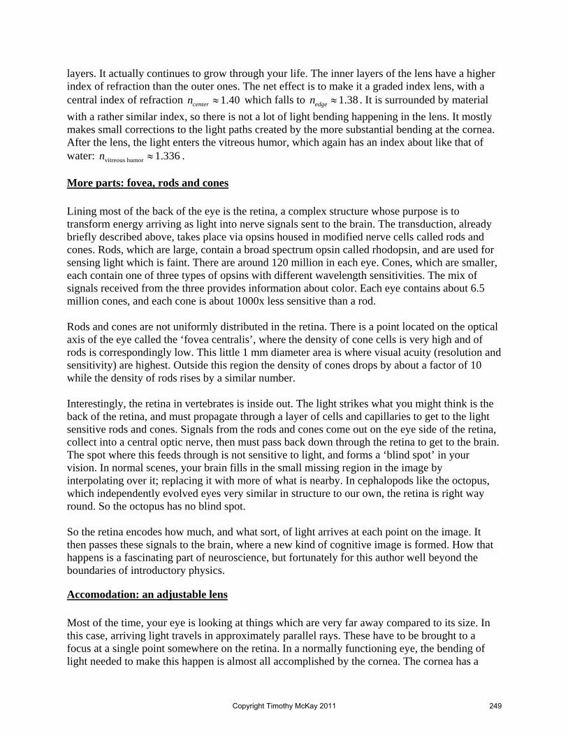
layers. It actually continues to grow through your life. The inner layers of the lens have a higher index of refraction than the outer ones. The net effect is to make it a graded index lens, with a central index of refraction 1.40centern ≈ which falls to 1.38edgen ≈ . It is surrounded by material with a rather similar index, so there is not a lot of light bending happening in the lens. It mostly makes small corrections to the light paths created by the more substantial bending at the cornea. After the lens, the light enters the vitreous humor, which again has an index about like that of water: vitreous humor 1.336n ≈ .

More parts: fovea, rods and cones Lining most of the back of the eye is the retina, a complex structure whose purpose is to transform energy arriving as light into nerve signals sent to the brain. The transduction, already briefly described above, takes place via opsins housed in modified nerve cells called rods and cones. Rods, which are large, contain a broad spectrum opsin called rhodopsin, and are used for sensing light which is faint. There are around 120 million in each eye. Cones, which are smaller, each contain one of three types of opsins with different wavelength sensitivities. The mix of signals received from the three provides information about color. Each eye contains about 6.5 million cones, and each cone is about 1000x less sensitive than a rod. Rods and cones are not uniformly distributed in the retina. There is a point located on the optical axis of the eye called the ‘fovea centralis’, where the density of cone cells is very high and of rods is correspondingly low. This little 1 mm diameter area is where visual acuity (resolution and sensitivity) are highest. Outside this region the density of cones drops by about a factor of 10 while the density of rods rises by a similar number. Interestingly, the retina in vertebrates is inside out. The light strikes what you might think is the back of the retina, and must propagate through a layer of cells and capillaries to get to the light sensitive rods and cones. Signals from the rods and cones come out on the eye side of the retina, collect into a central optic nerve, then must pass back down through the retina to get to the brain. The spot where this feeds through is not sensitive to light, and forms a ‘blind spot’ in your vision. In normal scenes, your brain fills in the small missing region in the image by interpolating over it; replacing it with more of what is nearby. In cephalopods like the octopus, which independently evolved eyes very similar in structure to our own, the retina is right way round. So the octopus has no blind spot. So the retina encodes how much, and what sort, of light arrives at each point on the image. It then passes these signals to the brain, where a new kind of cognitive image is formed. How that happens is a fascinating part of neuroscience, but fortunately for this author well beyond the boundaries of introductory physics.

Accomodation: an adjustable lens Most of the time, your eye is looking at things which are very far away compared to its size. In this case, arriving light travels in approximately parallel rays. These have to be brought to a focus at a single point somewhere on the retina. In a normally functioning eye, the bending of light needed to make this happen is almost all accomplished by the cornea. The cornea has a


basically static shape optimized to provide this focusing for light which enters the eye in parallel beams. So to view unblurred images of distant things, a well functioning eye can simply relax and let the natural shape of the cornea do all the focusing. In this relaxed form, the lens (which after all has nearly the same index of refraction as its surroundings, and hence bends the light little) hardly alters the path of rays passing through it. Things change if the eye wants to examine something up close, perhaps a small object held in the hand while you work on it. In this case, light rays arriving from the object are still diverging noticeably, and the eye needs to bend the rays more to bring them to a focus. For this purpose, your eye can “accommodate” the shape of the lens, making it bunch up, have more dramatically curved surfaces, and bend the light more. By bending more, the eye pulls the focus point inward until it lands on the retina again. Understanding this accommodation of the eye was the first important scientific discovery of the great British physicist and physician Thomas Young. He worked this out and published it at the age of 20. He later went on to establish the wave theory of light, to introduce the modern ideas of energy and stress and strain into physics, and to aid in the first translations of Egyptian hieroglyphics.

All human eyes, even those working as well as ever, have many limitations. One of the most obvious is the near point. Accommodation allows the light diverging from a nearby object to be focused only so far. When an object is too close, the lens will not be able to bend enough to focus the light. Images of objects too close to your eye will, as a result, always be blurred. The near point for most people is about 25 cm, or about 10”. As your eye ages, the crystalline lens usually becomes less flexible, and you may find your near point moving outward. When you see your parents move a book farther away to read it, or put on ‘reading glasses’, they are responding to this gradually migrating near point.

Relaxed eye focusing parallel light on the retina almost entirely because of the shape of the cornea

Accommodation in the eye: diverging light is focused by adding additional bending of light in the lens.


32.6 Failures of the eye as an optical device: malfunctions There are many ways an eye can fail, but it’s useful to consider at least a few in more detail. What if, when fully relaxed, the eye bends parallel light too much, bringing it to focus in front of the retina? When this happens, the images of all distant things objects look blurry, while things which are nearby (so that light from them needs more bending) can be focused just fine. If you have this problem, you are “near-sighted”, or myopic. You can see things which are nearby well, but not things which are distant. For a near-sighted person there is some “far point” beyond which it is impossible for the eye to correctly focus light onto the retina. Beyond this point, images of distant objects become increasingly blurry. The opposite is possible as well. It may be that your relaxed eye does not bend parallel light enough to bring it to focus on your retina. This is somewhat simpler, as your eye can use its power of accommodation to bunch up the lens and bend the light more, bringing it to a proper focus. If you have this problem, you are “far-sighted”, or hyperopic. The real issue here is that there is a limit to the power of accommodation. When you bring objects closer, eventually you can’t bend the light enough to bring it to a focus, and the image becomes blurry. Far-sighted people see distant things well, but have trouble focusing on objects which are nearby. Like everyone else they have a “near point” inside of which they cannot focus their eyes adequately. But for those with hyperopic eyes, the near point is unusually distant. Inside this near point, images of objects become increasingly blurry. How can these pathologies be fixed? In these cases the task is relatively simple. Near-sighted people have eyes which bend incoming light too much. So for them we add a diverging lens to the system. This pushes incoming light rays apart a bit before they enter the eye. This preparation provides the eye with beams of light it can comfortably focus, making it possible for it to produce sharp images of distant objects.

Far-sighted people have eyes which bend the incoming light too little. For them we need to add a little more bending. So in this case we add a converging lens which brings together incoming

Fixing hyperopic eyes Fixing myopic eyes


light rays a bit before sending them on into the eye. This allows the far-sighted person’s eye to relax completely when looking at distant objects, retaining the additional bending power of accommodation for examination of nearby objects, and pulling the far-sighted persons near point back to a more typical distance. As the eye ages and accommodation becomes weaker, many near sighted people begin to find their near point moving farther away. Normally, their eyes need a diverging lens to help them see distant things. Now they find they need a converging lens to help them see nearby things. When this happened to Ben Franklin, he decided to put both kinds of lenses in a single pair of glasses and became one of the first to wear ‘bifocals’.

32.7 Failures of the eye as an optical instrument: inadequacies Even when your eyes are functioning just as they evolved to, they are limited in a variety of ways. Overcoming these limitations, allowing us to see what was previously invisible, has been perhaps the single most important instrumental step for modern science. Let’s consider several limits and see how an understanding of optics has allowed us to enhance the performance of our eyes.

Resolution limits: seeing things which are small The eye is limited in how small an object it can resolve. This limit, fundamentally, is not really a limit on size, but on angle. You may think of it as a limit on the minimum angular size an object must have before you can tell it is not a single point. When you look at a distant sheet of text, each letter may appear to be just a point, as you bring it closer, the letters aren’t any physically larger, but they cover a larger and larger angle. Eventually the angle they cover is large enough for you to resolve, and you can read the letter. All optical systems have such resolution limits. The most fundamental limitation is the “diffraction limit”. We have seen that parallel rays of light passing through an opening with size d will diffract, spreading out once they pass through the opening into a blob with an angular width roughly given by: sinθ = (λ/d). Since for light λ is so small, we’re almost always talking about small angles, and we can write θ ~ (λ/d). What kind of angle is this? The iris of your eye has a diameter of around 1 cm, so the fundamental limit on your angular resolution is θ ~ 5x10-7 m / 1x10-2 m = 5x10-5 radians, or around 0.003°. This is around 10 arcseconds, for those of you who divide each degree into 60 arcminutes, and each arcminute into 60 arcseconds (as astronomers do). In fact though, your eye is limited to resolving only much larger angles by its imperfections. For example, the imperfect shape of your cornea and lens, as well as inhomogeneities in the index of refraction in the fluid of your eye make it impossible for you to focus as well as you might expect to. In addition, the angular resolution of your eye varies strongly with position on your retina. Images in the fovea are quite sharp, with an angular resolution of about 0.02° or 3.5x10-4 radians. This resolution degrades rapidly as you move away from the center. Your body includes a very complex set of muscles capable of turning your eye in its socket, steering the high resolution center of your vision from place to place. It does this much more rapidly than you can


move your head. Many animals, most birds for example, lack this ability, even though otherwise their vision may be much better than ours. Now all eyes have a near point inside of which they cannot focus. For healthy eyes the near point is about 25 cm. This unavoidable near point limits our ability to see the tiny details in anything we might work with. If you hold an object at the near point of 25 cm, and can resolve an angle of 3.5x10-4 radians, the smallest spot you can see on that object, staring as hard as you can, is about 0.25*3.5x10-4 ~ 0.1 mm. If you bring the object closer, to increase the angular size of its features, it just becomes blurrier. Using just our own eyes, there’s no way to discover cells. The very largest plant cells are just barely large enough to notice. Everything smaller looks like a smooth mess. Overcoming this limitation has been essential for the life sciences, where now much of the attention is focused on things too small to see. Imaging devices from magnifiers to microscopes, designed with our understanding of how waves interact with the world, have enabled all this progress. An introduction to how these devices work is presented in the next chapter.

Sensitivity: seeing things which are faint Another important limitation of your eyes is their relative insensitivity. They are optimized to view scenes illuminated by ordinary daylight. Your eyes adjust to brighter or fainter illumination by decreasing or increasing the size of the opening in the iris. The combination of the light sensitivity of your retina and the collecting area of the eye provides the bounds for scenes you can effectively image. If the light is too bright, the rods and cones in your eyes will saturate, all turning on and giving you no information (other than the fact that there is a bright light out there!). If the light is too faint you won’t collect enough light to be able to reconstruct the scene. Many organisms which live in dark environments have unusually large eyes. Owls are perhaps the most familiar example. Their remarkably large eyes have a different structure from ours. They are tubular rather than spherical, and hence can’t be turned in their sockets. To look at something new the owl must turn its head. Owl eyes have very large corneas, irises which can open completely, and retinas paved with rods. They do have a small number of cones, and some color sensitivity, but most of the retina is covered with the more light sensitive rods. Other extraordinary eyes include those of the swordfish, which include a special mechanism to heat the retina, increasing their speed of response, and the giant squid. At almost 16 inches in diameter these are currently the largest eyes in the animal world. Why do sea creatures push the limits for eyes? Because light is so strongly absorbed in water; it’s just darker there. Scientific technology has enabled us to see fainter things using artificial eyes which improve on ours in two ways. First, they are really large, and hence able to collect a lot of light. Second, they can integrate, adding up all the light which arrives over a long period of time. Constructing large eyes is technically hard only because the whole, big eye has to have a surface regular and smooth enough to bring all the light collected over the whole aperture to a single focus. This means the lens (or mirror) which is focusing the light must have the correct shape, over its whole area, with deviations that are much smaller than the wavelength of light (5x10-7 m).


Telescopes are the most dramatic giant light collectors in our technological toolkit. They are designed primarily to detect the faintest, most distant objects possible. They do magnify a bit, but mostly they are “light buckets”, designed to collect as much light of the light from faint objects as possible. The largest today are all reflecting telescopes, which used curved mirrors to focus the light. This is for engineering reasons. If you use a lens through which light must pass, you can support it only around the edge. When a lens like this gets really large (like more than 1 meter in diameter) it sags under its own weight, and can no longer be maintained in just the right shape to focus the light. Mirrors can be supported from the back side, all the way across. The largest telescopes today are the twin Keck telescopes, on Mauna Kea, in Hawaii. Each has a 10 meter diameter, giving them a collecting area about 106 times larger than your eye. Telescopes (and other scientific imagers) can also integrate, adding up the light which lands over a long period of time. While they used to do this with film, they now do it with electronic sensors like the charge-coupled devices (CCDs) which are also used in your digital cameras. CCDs start out almost 90 times more efficient for detecting light than your eyes, and add to this the ability to sum up all the light detected over several hours. These factors combined allow these artificial eyes to detect objects about 10 billion times fainter than your eyes can. Just like the microscope, this enhanced sensitivity has literally revealed new worlds, showing us planets in other solar systems and galaxies out to the edges of the universe.

Sensitivity: seeing things which are invisible The most extraordinary frontier of expanding our vision involves detecting electromagnetic radiation with wavelengths very different from optical light. Since around 1890, it has become possible to detect EM radiation across the spectrum. This has allowed us to image ourselves, our world, and the universe using everything from radio waves to gamma-rays. Our eyes, evolved to observe a world illuminated by the Sun, detect only a tiny bit of this enormous range. Expanding our senses in this new way has been especially important in astronomy and astrophysics, but has impacted the rest of science as well. It has allowed us to discover the left over heat of the big bang, look through our bodies with x-rays, and detect the glow of distant black holes. The challenges for imaging using electromagnetic radiation other than visible light are the same as those outlined above for light. To get useful information about the world from this other radiation, we must detect it, measure its properties (intensities and wavelengths), and carefully determine where it comes from. For this purpose, we have built a wide variety of imagers, artificial eyes, which do for the rest of the electromagnetic spectrum what our eyes do for visible light. Many of these look relatively familiar, focusing the radiation with mirrors and lenses. Some, especially those used for the highest energy radiation, are essentially complex pinhole cameras. Once again, the physical constraints imposed by the laws of nature give rise to an array of remarkably similar solutions.


Radio telescope Infrared telescope

Ultraviolet telescope

X-ray telescope Gamma-ray telescope


A Quick Summary of Some Important Relations Components of eyes:

Eyes have three components: a method for detecting light, a system for analyzing it (measuring its mix of wavelengths, its intensity, and possibly its polarization), and a system for determining what direction it comes from.

Lenses and focusing of light from distant sources:

A lens bends light so that all the light arriving from one direction comes together at a point. Any light detected at that point must have come from the same direction. For a thin lens made of a material with index of refraction n immersed in air, the focal length can be predicted from:

( )1 2

1 1 11nf R R

⎛ ⎞= − −⎜ ⎟

⎝ ⎠

where R1 and R2 are the radii of curvature of the front and back surface of the lens. Be careful of the sign conventions for these radii. Focusing light from nearby sources:

When a source (the object) is not infinitely far away, the light from it will come to a focus at an image point different from the focal length. They are related by the thin lens equation:

object image

1 1 1d d f

+ =

Magnification of an image like this is measured by:

image

object

dm

d= −

The eye as an optical instrument:

The human eye is a very effective imager, combining a shutter, a pupil, a variable focal length lens and a spherical focal plane lined with light sensing cells which measure intensity at several wavelengths. When operating correctly, the eye can focus light from infinitely distant sources all the way down to objects about 25 cm from the eye. The most common eye malfunctions involve failure to focus near or distant objects properly, and can be repaired with corrective lenses.

Eyes also have intrinsic limitations in resolution, sensitivity, and their ability to see wavelengths longer or shorter than the visible range. i Carroll, S., 2007, “The Making of the Fittest: DNA and the Ultimate Forensic Record of Evolution”, W.W. Norton, USA. ii Land, M., and Nillson, D., 2002, “Animal Eyes”, Oxford University Press, USA. iii Colicchia, G., 2006, Physics Education, 41, 15. iv Wagner, H., et al., 2009, Current Biology, 19, 108.



During its first few millennia, science was built on what people could see and hear with their own unaided senses. The human senses are, as we have seen, remarkably sensitive; able to record tiny fluctuations in the pressure of the air and to resolve objects separated by only 0.02°. They are, however, limited in many ways. Billions of stars and galaxies are too faint for us to see. Much of life’s machinery takes place on scales too small to perceive. Many important things happen in places hidden from the view of our senses; inside your skull or deep within the ocean.

Many factors played a role in the dramatic rise of science in 17th century Europe. One of the most important was the invention and rapid dissemination of instruments which expand our senses, enabling us to perceive the previously invisible.

33.1 A bit of imaging history

The idea that one might be able to augment vision with lenses and mirrors seems to have been known since ancient times. Simple magnifying lenses have been found in archeological sites back to at least 1000 BC. The use of these simple lenses for correcting vision in eyeglasses seems to have become widespread between about 900 and 1100 AD. But the real impact of imaging on science began in the 17th century, when several lensmakers in the Netherlands hit on the idea of combining two lenses to create a telescope. They applied for patents on this in 1608.

Galileo Galilei heard about this invention in 1609. Having studied optics extensively, he immediately built his own telescope and quickly refined the design. What he saw with this telescope, which magnified distant objects thirty times and collected substantially more light than his eye, changed our understanding of the universe dramatically. Over a period of just a few months he discovered the moons of Jupiter, the rings of Saturn, mountains and craters on the Moon, and a Milky Way filled with many thousands of previously invisible stars. He published what he had seen in March 1610 in a small book called The Starry Messenger. It remains one of the most remarkable little documents in the history of science. It begins:

“Great indeed are the things which in this brief treatise I propose for observation and consideration by all students of nature. I say great, because of the excellence of the subject itself, the entirely unexpected and novel character of these things, and finally because of the instrument by means of which they have been revealed to our senses.”

In these few sentences he says much about what was beginning to happen in science. He announces discoveries “for observation and consideration by all students of nature”. He isn’t just going to tell you about these things, he’s going to let you see for yourself; and while these things are remarkable in themselves, so too is the technology which enables us to see them. Galileo knew what he was onto, and was quite sure instruments like this would lead to many more discoveries.

Galileo would similarly improve a widespread simple variant of the telescope, capable of magnifying objects which are very nearby; though it would be decades before one of his friends


christened it a “microscope”. It would take longer still for a complete realization of what the microscope had to say about life. It was more than 50 years before Robert Hooke published Micrographia, the first widely distributed volume of drawings showing what the microscope revealed. His work was followed by many others, perhaps most significantly by the impossibly careful observations of Anton Van Leeuwenhoek. Using tiny glass spheres as simple magnifiers, Leeuwenhoek discovered bacteria, the teeming life in drops of pond water, and single lines of blood cells shuttling through capillaries. His discoveries, communicated to the scientific societies of Europe by letter, helped to open the eyes of the scientific community to a new aspect of life, and to set in motion what would become much of the life sciences today.

Physics, imaging, and science

Since the time of Galileo and Leeuwenhoek the tools we use to present the world to our senses have advanced enormously. A deeper understanding of how waves interact with the world, and of how to manipulate them, has enabled us to ‘see’ everything from individual atoms to the remnant light from the big bang. Remarkably, almost all of these devices still rely, in their final stage, on our own senses. When we finally digest what these instruments provide, we do so through our own eyes. All of the scientific instrumentation described in this chapter ultimately produces an image which our eyes then deliver.

33.2 Simple magnifiers

Your eyes, like all human eyes, possess a near point, a minimum distance within which the light from an object cannot be focused correctly. This near point, combined with the limited angular resolution of your eye, limits the size of the smallest things you can see; anything smaller than about 0.1 mm is simply blurred into its surroundings. How to fix this problem? Fundamentally this is the same as the near point problem seen in hyperopic eyes. If you are far-sighted, your eyes can’t bend the light from a nearby object enough to bring it to a focus on your retina. To fix this, we have to add some additional bending of light. This is what a simple magnifier like a magnifying glass does. When you place an object near the focal point of a magnifying glass, light spreading out from the object and passing through the lens emerges in nearly parallel rays. Your eye is well constructed to focus parallel light. So when the light coming from the magnifying glass arrives at your eye as nearly parallel rays, you can focus them easily. The parallel rays of light emerging from the magnifying glass come into your eye as if they came from an object much closer to your eye than it actually is. In fact it now seems like the object is a distance from your eye equal to the focal length of the magnifying glass, instead of the usual 25 cm near point distance. This is shown in the figure below. If you set things up like this, with the object near the focal point of the magnifying glass, the angular magnification you get from the lens is:

0.25 mmf

=

Magnifying glasses with small focal lengths give big magnifications.


Notice that there is a big difference between this and what we discussed above when we talked about thin lenses forming images. In this case, the magnifying glass is NOT forming an image. In fact, it is sending out parallel light, which would travel to infinity before ever forming an image. That parallel light, nicely prepared by the magnifying glass, is then fed into your eye, and that’s where the image is formed. As we will see, many optical instruments use ‘eyepieces’ to prepare the light from a system for imaging with your eye. They will generally do just this; produce parallel light which your eye then focuses.

The first microscopes, especially the ones used by Leeuwenhoek, were very simple spherical lenses with very short focal lengths. Basically they were tiny drops of glass, with radii of curvature as small as possible. These tiny radii correspond (from the lens-maker’s equation) to very small focal lengths, and consequently large magnifications. Using these tiny lenses, he discovered many single celled organisms, including protists, bacteria, spermatozoa, muscle fibers and more. Early microscopists like Robert Hooke and Leeuwenhoek were able to “see” a world which was previously hidden from human senses. They discovered a new world. By using their understanding of light, they expanded the limits of their evolved senses, and changed biology and our vision of life forever.

33.3 Microscopy Modern microscopes are much more complex than Leeuwenhoek’s. In fact most of you will have already used microscopes which are vastly more complex than his little spheres of glass. To get a sense of how they work, we will consider a basic compound microscope made of two lenses. This is essentially the design Galileo and his contemporaries used.

h θ

25 cm

h θ′

f θ′

tan25 cm

hθ θ≈ =

tan hf

θ θ′ ′≈ =

25 cmMagnificationf

θθ′

= =


Compound microscopes combine two lenses to increase magnification. They provide a nice example of more complex optical systems made of multiple lenses. The first lens, called the “objective” magnifies the object substantially, placing an inverted image of it at a specified location inside the microscope tube. A second lens, called the eyepiece, is placed so that the image from the first lens lies at its focal distance. The eyepiece then converts light from this internal image into a parallel beam of just the kind your eye has evolved to focus. Thus the eyepiece prepares the light for your eye to act as the final optical element of the system. The “objective lens” in this arrangement has a relatively short focal length, typically a few to a few tens of millimeters. This lens is lowered until the object is close to the focal point of the lens, producing a substantially magnified image at a distance L behind the objective. This distance L is set by the design of the microscope. As we will see, you want this initial image to land just at

the focal point of the eyepiece lens. Since IO

O

Dm D= − , and in this case ID L= and O OD f≅ ,

we can write OO

Lm f= − for the objective.

Once this image is formed by the objective, the eyepiece is used as a second stage of magnification. The image produced by the objective is placed at the focus of the eyepiece. Light coming from the internal image is converted by the eyepiece into parallel beams. Then the final optical element is your eye, which focuses the parallel beams emerging from the eyepiece onto your cornea, allowing you to see the image. The eyepiece acts much like a magnifying glass, again magnifying the image, this time by an amount

0.25 mE

Em f= . The combination of object and eyepiece is then a total

magnification of around:

Combined0.25 m

O E

Lmf f

= −

For reasonable combinations, it is easy to achieve magnifications of 100, and possible to reach 1000.

33.4 Compound telescopes The basic idea of a telescope is very similar; an objective lens forms an internal image which is then viewed by an eyepiece. The difference is purely practical; for telescopes the objects of interest lie essentially at infinity. Light from the object arrives at the objective lens in just about perfectly parallel beams. So the objective lens forms an image of the object right at its focal point. The eyepiece then views and magnifies this image, presenting it again to your eye as parallel beams of light, ready to be focused by your eye on the cornea.

L


Cameras on microscopes and telescopes These days, many telescopes and microscopes lack eyepieces. This eyepiece is designed to prepare the light for your eye, providing a nice parallel beam like those your eye evolved to focus. If you use a camera, instead of your eye, to record the image, you want the optical system to provide focused light on the film or CCD which will record the image. Usually this means replacing the eyepiece with a lens which takes the internal image produced by the objective and focuses light from that image onto the focal plane, just like the lens in your eye focuses light onto the spherical light detecting surface of your retina.

33.5 Medical imaging: seeing inside your body One of the most interesting unknown territories which has been explored using instruments which expand our senses is our own bodies. The ability to see what is happening inside us has revolutionized medicine. Modern medical imaging has largely eliminated the need for “exploratory surgery”, the old practice of cutting you open just to see what’s there. These techniques were largely developed by physicists, and even today a large number of physicists are employed in the medical imaging field, developing and refining new technologies and operating these advanced imagers in hospitals. This is a very large field, and we will touch on only a few of the most important kinds of medical imaging.

X-ray imaging X-rays are very high frequency, very short wavelength (10-8 m > λ > 10-11 m) electromagnetic radiation. Fundamentally, they’re the same as visible light, differing only in wavelength. Because their wavelengths are so short, however, they interact with matter quite differently from visible light. When visible light strikes solid matter it is usually either reflected or absorbed within 10-6 m of the surface. A few materials (like air and water) are relatively transparent, and allow visible light to pass through them. Your body, for example, does not. X-rays are different. They penetrate solid matter rather effectively, and are often able to pass right through your body. When they come out the opposite side, they can be detected in a variety of ways; on fluorescent screens, on film, and in electronic sensors like Charge-Coupled Device (CCDs). X-rays passing along different paths through your body will encounter different materials. Some may pass through nothing but flesh, while others will strike bone, organs, or tendons. Because the material along each path is different, the amount of absorption along each path will differ. An X-ray image then is a “shadow” image. Any path through your body which suffers a lot of absorption will leave a strong shadow. Paths with little absorption will leave faint shadows.

Lots of absorption Little

absorption


X-ray absorption, like that of optical light, can be described by an absorption length Labs, such that: Here are a few example absorption lengths for typical X-rays in medically interesting materials:

Material Absorption length

Air 3.4 m Fat 0.052 m

Water 0.047 m Bone 0.017 m

Contrast in an X-ray image is produced by differential absorption. X-rays passing through equal amounts of fat and bone will have an intensity ratio on the other side of: This contrast is what makes x-rays effective, especially for imaging skeletal features.

X-ray production X-rays are produced primarily by accelerating a beam of electrons to high energies using a high electrical voltage, then smashing those electrons into a target, usually made of metal. When the electrons decelerate suddenly they emit electromagnetic radiation with many different wavelengths, including the short wavelengths corresponding to X-rays. The “braking radiation” which is produced in this process has the great is German name “bremmstrahlung”. This is all done inside glass vacuum tubes, so that the electrons don’t run into air molecules while being accelerated. This picture shows a dental X-ray tube. The structure on the right is the “cathode” which includes a hot filament from which electrons emerge. The massive structure on the left is the “anode” into which the electrons smash, producing the electrons. The electrons are accelerated across that short gap using a very high voltage, in this case about 50,000 volts. X-ray production by this mechanism is very inefficient. Only about 1% of the energy which goes into an X-ray tube comes out as X-rays. Most of the rest is deposited in the anode as heat. This heating is a major problem for X-ray production. It requires the use of high melting point metals (like Tungsten) as anodes. In addition, some thought must be paid to extracting the heat. A very common

absLx

eIxI−

= 0)(

05.03

0

0 ==== −−

−

−

eeeI

eIII

boneLfatL

fatLx

boneLx

fat

bone


kind of tube uses a “rotating anode”. This is a large, disk shaped target which is rotated while the tube operates. This makes the electron beam spot move to new places on the anode continuously, preventing any one spot from heating too dramatically.

X-ray detection X-rays can be detected by many means. In the early days, fluorescent screens were used. These are translucent ground glass screens coated with or containing materials that convert incident X-rays into visible light. When an X-rays hit the screen, it glowed with a brightness related to the X-ray intensity. These were often used in early X-ray imaging applications. They had many safety related drawbacks. First, they were inefficient, requiring intense X-ray dosages. Second, the doctor had to look straight into the screen, taking much of the transmitted X-ray flux straight into their head! The picture at the right shows such a device. The doctor looks into the viewer on the left, the person is put in front of the screen, and the X-ray tube is placed to the right of the person. X-rays blast on through patient, some strike the screen and the doctor sees what’s going on, then the rest of the X-rays plow through the doctor’s head. Many modern X-ray imagers still use chemical film. These chemical films have relatively low efficiency, so they are often boosted by placing them in fluorescent lined x-ray “screen film cassettes”. This way, the film detects some x-rays directly, and is further exposed by visible light produced when the x-rays strike the fluorescent lining of the cassette. Just as optical film is being replaced by electronic visible light detectors, X-ray film is being replaced by a variety of much more sensitive and precise electronic sensors. The high sensitivity of these sensors allows them to make high quality images with much smaller doses of X-rays, making the whole process much safer.

X-ray health concerns X-rays are biologically much more dangerous than you might guess. When you get an X-ray at the doctor’s office, you don’t feel the arrival of a large quantity of energy. Your jaw doesn’t heat up at the dentist for example. Since so little energy is deposited, you might think the X-ray is harmless. They are more dangerous than you expect because their very short wavelengths allow them to be dump all their energy in small spots, damaging important individual molecules like DNA. For this reason, X-ray dosages need to be carefully controlled and minimized wherever possible.

33.6 Ultrasound imaging

A newer, very common form of medical imaging takes its cue from naval sonar the acoustic imaging so effectively used by marine mammals and bats. Ultrasound imaging looks inside you using sound waves. This kind of imaging provides a great example for this class because so


many important wave phenomena are involved in making it work. We’ll look into several details of ultrasound imaging. First, why “ultra”-sound? You would like to be able to image small things inside you, to see features that are perhaps 1 mm in size. If you use sound waves with wavelengths much larger than this, the waves will diffract around your target just as water waves pass around you at the beach. So you need to use wavelengths of around 1 mm or less. The speed of sound in various tissues is given in this table:

Material Speed of sound (m/s) Acoustic impedance (ρv, kg/m2s) Air 340 4x102

Lung 600 1.8x105 Fat 1450 1.3x106

Muscle 1540 1.7x106 Bone 4080 7.8x106

For a typical 1000 m/s speed (like those within your body), a 1 mm wavelength implies a frequency υ = v/λ = 106 Hz. You can’t hear any frequencies higher than about 2x104 Hz, so this is indeed sound with “ultra” frequencies. Ultrasound propagating in your body experiences all the usual features of wave propagation, including absorption, reflection at material boundaries (with θi = θr), and refraction when passing from materials with one wave speed to another. Absorption is dependent on frequency and the material the sound is passing through, and this can be a significant factor. The intensity of ultrasound traveling through your body might decrease by around 10% as it passes through a centimeter of flesh. Absorption is typically worse at higher frequencies, so the frequencies chosen usually emerge from trading of resolution (which favors high frequency) and transmission (which favors low frequency). Typical medical ultrasound imaging uses frequencies from 2 to 20 MHz.

Impedance matching and ultrasound reflection Ultrasound reflection happens whenever the waves pass from one material to another. How much sound will be reflected can be determined from the “acoustic impedance” of the two materials. Acoustic impedance is the product of the density of the material and the velocity of sound in the material: Z = acoustic impedance = ρv Numerical values for the acoustic impedance of several materials in your body are given in the table above. The fraction of sound reflected when it reaches a boundary between materials is governed by the impedance mismatch between the materials. For the particular case of sound arriving perpendicular to the interface a simple formula governs the reflected fraction:

2

21

21

0⎟⎟⎠

⎞⎜⎜⎝

⎛+−

==⊥ ZZZZ

IIR R


When the sound reaches a boundary where the acoustic impedance changes, some of it will be reflected back. The fraction reflected depends strongly on how large the impedance change is. To get a sense for what this means, consider a few examples. If you have ultrasound in the air, outside your body, and it reaches your surface, what fraction will be reflected? Since Zair ~ 4x102 kg/m2s and Zflesh ~ 1.5x106 kg/m2s, the reflected fraction should be very close to one. Just about all the sound reaching you in the air will reflect, rather than passing into your body. We note in passing that this is great for bats. Sound they send out to image their surroundings almost all bounces off, giving them a chance to get it back and hear it. If you are doing ultrasound imaging, the huge reflection of sound at your surface is a problem. To avoid it, you don’t send the sound in through the air, but instead couple the wand which produces the sound to your body with a material much more closely matched in acoustic impedance to your body. Usually this is a kind of gel which is spread on both the sound producing wand and your skin. If you have had any ultrasound imaging done on yourself you will know what I mean. Once the sound is in your body, you do want it to bounce off things, giving you the chance to image them. This is a problem too, because many of your tissues are pretty closely matched to one another in impedance. For example, at an interface between fat and muscle you might expect reflection of R = (1.3-1.7 / 1.3+1.7)2 = 0.017 of the incident sound. This small reflected intensity makes producing a high contrast image difficult. Ultrasound images are sometimes enhanced by introducing “contrast agents” designed to increase reflectivity. This is most common in efforts to image the circulatory system. To do this, tiny spheres of nitrogen are injected into the blood. When they spread through the circulatory system, they make arteries and veins much more “visible” than they were before. A common contrast agent consists of tiny 1-4 μm balloons made of albumin (egg white!) filled with nitrogen.

Ultrasound methods

Ultrasound imaging is primarily based on a simple idea; produce a sound, send it in, and see how long it takes to bounce off something and return. The sound itself (inaudible to you of course) is produced by a “transducer”; a device which converts electrical signals into acoustic oscillations and vice versa. This device both produces the output sounds and detects the reflections. It is most often contained in a hand-held “wand” which is coupled to your body using an impedance matched gel. Timing of reflections allows reconstruction of an image. But this is not completely simple. Remember that the speed of sound varies in different materials, making the conversion between return time and distance dependent on which materials the sound is passing through. An ultrasound wand is usually a linear array of transducers, so instead of acting like a point source, with sound going out in every direction, it produces a beam of sound, traveling out primarily in one direction. Because the array

One transducer: like a point source An array of

transducers: produces a beam


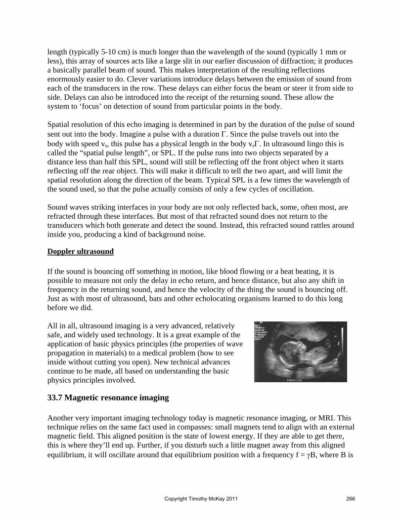
length (typically 5-10 cm) is much longer than the wavelength of the sound (typically 1 mm or less), this array of sources acts like a large slit in our earlier discussion of diffraction; it produces a basically parallel beam of sound. This makes interpretation of the resulting reflections enormously easier to do. Clever variations introduce delays between the emission of sound from each of the transducers in the row. These delays can either focus the beam or steer it from side to side. Delays can also be introduced into the receipt of the returning sound. These allow the system to ‘focus’ on detection of sound from particular points in the body. Spatial resolution of this echo imaging is determined in part by the duration of the pulse of sound sent out into the body. Imagine a pulse with a duration Γ. Since the pulse travels out into the body with speed vs, this pulse has a physical length in the body vsΓ. In ultrasound lingo this is called the “spatial pulse length”, or SPL. If the pulse runs into two objects separated by a distance less than half this SPL, sound will still be reflecting off the front object when it starts reflecting off the rear object. This will make it difficult to tell the two apart, and will limit the spatial resolution along the direction of the beam. Typical SPL is a few times the wavelength of the sound used, so that the pulse actually consists of only a few cycles of oscillation. Sound waves striking interfaces in your body are not only reflected back, some, often most, are refracted through these interfaces. But most of that refracted sound does not return to the transducers which both generate and detect the sound. Instead, this refracted sound rattles around inside you, producing a kind of background noise.

Doppler ultrasound If the sound is bouncing off something in motion, like blood flowing or a heat beating, it is possible to measure not only the delay in echo return, and hence distance, but also any shift in frequency in the returning sound, and hence the velocity of the thing the sound is bouncing off. Just as with most of ultrasound, bats and other echolocating organisms learned to do this long before we did. All in all, ultrasound imaging is a very advanced, relatively safe, and widely used technology. It is a great example of the application of basic physics principles (the properties of wave propagation in materials) to a medical problem (how to see inside without cutting you open). New technical advances continue to be made, all based on understanding the basic physics principles involved.

33.7 Magnetic resonance imaging Another very important imaging technology today is magnetic resonance imaging, or MRI. This technique relies on the same fact used in compasses: small magnets tend to align with an external magnetic field. This aligned position is the state of lowest energy. If they are able to get there, this is where they’ll end up. Further, if you disturb such a little magnet away from this aligned equilibrium, it will oscillate around that equilibrium position with a frequency f = γB, where B is


the strength of the magnetic field and γ is a property (its gyromagnetic ratio) of the little magnet which involves both the strength of its own magnet and its mechanical inertia. As it turns out, the nuclei of many atoms have non-zero “magnetic moments”; they act just like very tiny magnets. If you put these atoms in a magnetic field, they will tend to align with it. If you “bump” them away from this equilibrium orientation, they will oscillate around it. Now here’s the key: oscillating magnets emit electromagnetic radiation just like oscillating charges. So, if you put a material (perhaps a patient) in a magnetic field and then disturb the field a bit, many of the atomic nuclei in the object will start oscillating. When they do, they send out little electromagnetic signals saying “we are here, we are here…”. If you are prepared to receive these signals, you can determine whether this material is there inside a person. For this reason MRI used to be called “Nuclear Magnetic Resonance” imaging, or NMR, but the word “nuclear” in the name scared people and limited profits, so the name was changed to exclude it. The primary tool for MRI imaging in people is hydrogen. The proton which makes up the nucleus of hydrogen has a gyromagnetic ratio γ = 42.6 MHz / Tesla. In practice there is another detail. Rather than simply bumping the nuclei away from equilibrium, they are actually driven away from it by pushing them back and forth at just their resonant frequency. This is done using a “radio frequency” (RF) pulse which gets the nuclei oscillating. Then this is turned off and the emission from the oscillations is measured. The ‘imaging’ part of MRI is accomplished by putting the person in a magnetic field which varies in space, so that B = B(x,y,z). Since the oscillation frequency of the disturbed nuclei depends on both γ and B, nuclei in different places will oscillate at different frequencies. Since you excite a particular resonant frequency, you will excite oscillators only in a particular place. You can change where you create oscillations by altering the frequency to match the resonant frequency you drive. If you know just how the field varies, you can tell just where the oscillating nuclei are! MRI scanning is complex, requiring large and carefully controlled magnetic fields. Energy use concerns often drive the use of large, superconducting magnets which must be cooled to very low temperatures. MRI scanning is also rather slow, because the oscillating nuclei take a little time to settle down, and there are many regions to scan. New variants of MRI are always being developed. One especially important one is called “functional MRI”, or FMRI. This method takes advantage of the fact that oxygenated blood has a different MRI signal from non-oxygenated blood. By taking a scan of the brain before, during, and after an activity, and looking for changes, it is possible to obtain information about what parts of the brain are active during different kinds of activities. While this doesn’t exactly reveal all the secrets of how the brain works, it does provide fascinating new insight into brain function.

Radionuclide imaging: positron emission tomography


A third approach to imaging involves sending in molecules which will go where you want and then send you a message to let you know where they are. One common approach is to send in radioactive forms of molecules your body would like to use, like various forms of sugar. These go into your system just like their non-radioactive equivalents, get transported to where they might be used, then decay. The right sorts of radioactive atoms will send out gamma-rays; electromagnetic radiation like x-rays only with still more energy. These γ-rays punch their way out of your body and can be detected. Since they travel in straight lines it is possible to trace them back to their points of origin and find out where in your body the tracer you put in has settled. These methods are particularly effective for examining metabolic processes. For this purpose things like 18F-Flourodeoxyglucose are used. This is a glucose analog. When injected in the body, it finds its way to glucose using very active cells like those in the brain or in cancerous tumors. This particular radioactive isotope of Flourine (18F) decays by emission of a positron. The positron is the antimatter equivalent of an electron. When the fluorine nucleus emits the positron, it becomes an 18O nucleus. The positron quickly finds an electron (they are oppositely charged and strongly attract one another). When they come together they annihilate, converting their mass into energy according to Einstein’s famous E = mc2. This energy emerges as two gamma-rays which emerge back-to-back, helping to localize where the fluorine decayed. This feature of positron emission makes it particularly attractive for this kind of imaging, and one major form of radionuclide imaging is Positron Emission Tomography, or PET scanning. The image at right shows a PET scan of a patient with multiple bone cancer tumors. These tumors use glucose like crazy, and show up as very hot spots in the PET scan.


A Quick Summary of Some Important Relations Simple magnifiers: Magnifiers are lenses with short focal lengths used to prepare light for your eyes to properly focus. They effectively allow you to bring an object closer to your eye than your near point. The typical magnification of such a device is:

0.25 mmf

=

Compound microscopes:

A compound microscope uses two lenses, an objective which forms a magnified image of the object, then an eyepiece to magnify the light from the image and prepare it for the eye to focus. In the normal mode of operation, the objective uses a fixed image distance L, and the magnification is:

objective eyepiece

0.25 mLmf f

= −

Cameras instead of eyepieces:

The purpose of the eyepiece is to present your eye with parallel light which it might easily focus. This is useful only when your eye is part of the optical system. It is more common today for microscopes and telescopes to detect the light with film or an electronic sensor like a charge coupled device (CCD). In this case, the optical system should, instead of putting out parallel light, generate a final image at the location of the light sensor.

X-ray imaging:

X-ray imaging is shadow imaging, taking advantage of the relative absorption of x-rays as they pass through different kinds of tissues. X-ray absorption, like other light absorption, is given by:

( )transmitted incident

abs

xLI I e λ−

=

The contrast in an x-ray image depends on the difference in absorption length along different paths through your body. This is why X-rays are especially good for imaging skeletal features.

Ultrasound imaging:

High frequency sound can be used very effectively for non-invasive imaging. It relies on the reflection of sound from places in your body where the acoustic impedance changes. This is an example of imaging where the wave nature of the method is especially obvious, much more than in optical or x-ray imaging.

Magnetic resonance and radionuclide imaging:


Both of these methods rely on inducing particular locations in your body to emit signals. In magnetic resonance, the magnetic moments of atomic nuclei are made to oscillate around an equilibrium alignment with a field. In radionuclide imaging, radioactive substances are attached to molecules which are bioactive, like glucose, then decay in locations where those molecules are used in the body. Each sends out a signal announcing where it is.



In these last few chapters, we’re going to take a quick look at a few topics drawn from what is often called “modern physics”. Ironically, this title has little to do with chronology; it is not the label for all the latest discoveries in The Physical Review. It is instead given to work based on a series of fundamental discoveries made around the beginning of the 20th century. There are two great themes in modern physics; quantum mechanics and relativity. Quantum mechanics describes the behavior of atoms and their interactions with light with extraordinary precision. Einsteinian relativity shifts fundamentally our conception of the space and time in which the rest of physics happens.

Research into physical phenomena which relies heavily on these two areas is called “modern physics”, while all the rest, including virtually everything learned so far in this course, is called “classical physics”. Both sorts of physics remain the subject of extensive research, with new discoveries published every week. In fact most current research requires extensive use of both classical and modern physics. A particularly rich and beautiful example of this synergy is the field of astrophysics and its quest to understand the origins of things.

Everything has an origin – nothing comes from nothing. Speculation about the origins of things is a deeply human activity, pursued in every culture and present as far back as history goes. There is a scientific quest to understand origins as well; indeed explaining why things are the way they are is one of our central goals. The decades spanning the beginning of the 21st century were a crucial time for this work, the period in which the main features of the history of the universe, our first truly scientific cosmology, were first confidently established. Developing and testing this cosmology involves application of all parts of physics, both classical and modern, not only in explaining observations, but also in constructing the instrumentation which enables this research.

During the next few chapters we will explore some of what is known about how everything came to be: our galaxy, the Sun, the Earth, its atmosphere and oceans, life, even the atoms of which we are all made. This will be just a brief introduction to an enormous body of contemporary physics. But it is an essential story for understanding life here on Earth, and for sensibly approaching the search for life elsewhere in the cosmos. We will begin not on the largest scales, but on the smallest, with some study of the nuclei which lie at the hearts of atoms.

Nuclear physics determines what sorts of atoms can exist. These ‘possible’ atoms are what’s available for chemistry, and provide the framework for life. We will find that most possible nuclei are unstable, they are radioactive, and transform themselves spontaneously into other forms. This radioactivity is important for life directly, and provides especially useful tools to the


modern life sciences. Finally, what we learn about nuclear physics will help us to understand the origin of the elements.

34.1 Atoms and their nuclei

In the early 20th century many properties of atoms were known:

• they are small, around 10-10 meters in size • they contain negative electrons which carry very little of their mass • they are electrically neutral • they are stable

All of these observations emerged from classical physics. Atomic sizes had been determined from measurements of diffusion and an understanding of statistical physics. But there was little information about their internal structure. It was clear that very tiny electrons could emerge from atoms, leaving behind equally charged positive ions which still contained almost all the mass of the atom. One theory of the time held that the atom was like a “plum pudding”, a kind of smooth blob of positive charge studded with electrons which were sort of like raisins in the pudding.

To see whether this was the case, something had to be sent down into the atom to find out. This probe had, of course, to be very small, much smaller than an atom. Fortunately, such a probe had recently been discovered, in the form of alpha particles. Some naturally occurring materials are radioactive: they spontaneously emit “rays” of one kind of another. During the 1890’s these materials and the rays they emit were the subject of intense study. It was found that while many substances were involved, they emitted only a few kinds of rays, which were labeled alpha, beta, and gamma rays; names intended to acknowledge how little was really known about each.

The α rays were known to consist of positively charged, massive, and energetic particles; each carrying (for something so very tiny) quite a lot of momentum. To study the inside of atoms, New Zealand born physicist Ernst Rutherford directed a beam of these α particles at a thin foil made of gold. He expected these high momentum alpha particles to plow through the smooth pudding of the atoms and emerge on the other side almost undeflected. Mostly, that’s what he found. Almost all of the α’s went more or less straight through the foil. But some did not. Occasionally, about 1 time in 8000, they would bounce more or less straight back. This was a great surprise. As Rutherford put it “It was quite the most incredible event that ever happened to me in my life. It was as incredible as if you fired a 15-inch shell at a piece of tissue paper and it came back and hit you.”

These ricochets implied that, instead of a diffuse pudding, the positive charge in the atom must be concentrated in a tiny, massive, lumps at the center of each atom; in a dense nucleus. As it turns out, most of the atom is a nearly empty cloud of electrons, while right down at the center is a tiny nut containing all the positive charge and almost all the mass. The concentration of positive charge in the center is quite extreme. The typical size for a nucleus is 10-14 m, while the


typical size of an atom is 10-10 m. So the atom is this cloud of diffuse electrons which is 10,000 times bigger than the nucleus which lies at its center. This is really empty. If the nucleus where the size of a period on this page, about 0.5 mm, the atom would be 10,000 times larger, or about 5 meters across.

34.2 Constructing the nucleus: protons and neutrons

The discovery of the nucleus revealed the basic structure of the atom, but raised a number of strange new questions.

• How could all the positive charge, which after all would like to fly apart, be crammed together into this really tiny space?

• Why is there a limit to which kinds of atoms exist? Why are there not giant atoms with 1000 electrons?

• Why are there isotopes? These are atoms with the same number of electrons, and the same chemistry, but different masses.

The answers to these questions lie in understanding the constituents of nuclei and their interactions.

Nuclei are made up of protons and neutrons, objects collectively called nucleons. Protons have a positive charge equal in magnitude to the electron charge, +1.6x10-19 C. Neutrons are electrically neutral. The two are very similar in mass, with mass ~ 1.67×10-27 kg. The neutron is actually slightly more massive than the proton, by about .13%. Here are more precise values:

mproton = 1.672622 × 10−27 kg

mneutron = 1.674927 × 10−27 kg

Each kind of nucleus is identified by knowing how many protons and neutrons it contains. The number of protons is called the “atomic number” of the nucleus. This is because the charge of the nucleus determines how many electrons the atom will have, and the number of electrons in turn determines the chemistry of the atom. The “atomic mass number” of the nucleus is the combined number of protons and neutrons, the total number of nucleons in the nucleus. Such a nucleus is described symbolically as:

Where the “X” is the symbol for the chemical element (like H, He, O, etc.), A is the atomic mass number, and Z is the atomic number. Now the atomic number actually tells you the same thing as the name of the element, so this notation is a bit redundant, but including Z is still a useful reminder of how many neutrons there are (since Nneutrons = A – Z).

XAZ


Isotopes

Nuclei with a particular number of protons (and hence the same number of electrons) are all examples of the same chemical element. They are dressed with the same coating of electrons, and hence interact chemically with other atoms in essentially the same way. In this sense, all nuclei with the same number of protons are the same. But they can differ. In particular, they may have different numbers of neutrons. Nuclei with the same numbers of protons but different numbers of neutrons are called “isotopes” of one another.

Take carbon as an example. There are two permanently stable forms of carbon: 126C and 13

6C. On Earth most of the carbon, about 99%, is the former, while about 1% is the latter. There are other isotopes too. Some have fewer neutrons (like 96C – 11

6C) and some have more (like 146C - 21

6C). These are unstable nuclei. While they stick together for a while, if you wait around each will eventually fall apart.

It is worth stressing that any two nuclei with the same number of protons and neutrons are truly identical. There is no fundamental way to label a nucleus with another property which would make them different. They are completely, perfectly interchangeable.

The strong nuclear force

It is useful to think of a nucleus as built up of very tiny hard, spherical protons and neutrons, all packed in together like oranges in a bowl. These spheres stick to one another: they are attracted together by a new force called the “strong nuclear force”. This force differs substantially from other fundamental forces like gravity and the electromagnetic force because it has a very short range. It pulls together any two nucleons, but only if they are very close, separated by less than about 10-15 m. As a result, each nucleon sticks to its neighbors only, as if they were coated with Velcro.

So when you assemble a nucleus, it’s like a ball of nucleons. The radius of the nucleus then should depend on the number of nucleons as r = r0A1/3. The parameter r0 is a characteristic size for a nucleon, and the cube root of the atomic mass number A is there to recognize that each additional nucleon will fill more volume, and that the radius scales like Volume1/3. The characteristic size r0 is determined from experiment to be around 1.2x10-15 m. So that’s about the size of an 11H nucleus, while a 64

30Zn nucleus is about four times large (641/3 = 4).

The stability of a nucleus comes about from a balance between forces. The strong nuclear force, by gluing together neighboring nucleons, holds it together. Meanwhile, the electromagnetic force, by pushing protons apart, tries to break it apart. There is a essential difference between these two forces. The strong force has a very short range, acting


only on nearest neighbors, but the electromagnetic force is long range, allowing protons on one side of the nucleus to push on those which are far away.

As a result, when nuclei get bigger, they need to add more and more neutrons relative to protons. Adding neutrons increases the available binding from the strong force while not increasing the repulsive electromagnetic force. This is shown in the figure, where stable nuclei are represented by the little squares. At low Z, the number of neutrons is roughly equal to the number of protons. At higher Z, the fraction of neutrons increases for stable isotopes.

34.3 Binding energy and the mass defect

Nuclei are bound together by the strong nuclear force. We call it the strong force because it really is strong! It takes a LOT of energy to break up an atomic nucleus. This is, of course, the reason for the seeming permanence of the elements. What would happen if nucleons were not very tightly bound? If the thermal energy which is always around (~kT) was comparable to the binding energy of nucleons, then nuclei would spontaneously break up and reform all the time, just as the bonds between water molecules do in liquid water. In such a world, elements wouldn’t be stable. But instead, the binding energies of nucleons are much, much greater than typical thermal energies. As a result, nuclei are stable over very long periods of time.

One way to see the large amount of binding energy in nucleons is by examining the so-called mass defect. It takes energy to break apart a nucleus. It is as if the nucleons in the nucleus have negative energies, they’re in an energy well, and if we want to take the nucleus apart, we must give them energy adequate to get out. This “binding energy” is actually measurable without even breaking up the nucleus. Einstein’s most famous equation, E=mc2, provides the key.

Imagine a bunch of N neutrons and P protons, all far apart. While they are separated, they will have mass

total neutron protonm Nm Pm= +

Einstein tells us this corresponds to a total energy:

( ) 2separated neutron protonE Nm Pm c= +

Now imagine the nucleons come close together. As they do, the powerful attraction of the strong force pulls them together along the direction in which they’re moving. It does positive work, raising the kinetic energy of the nucleons. This force pulls them together and they zoom into one another moving fast. If they don’t give up this extra energy, they will zoom in fast, bounce off one another, and end up far apart again. But if they do give up this energy, emitting it in the form of energetic light, they can slow down, stick together, and remain bound to one another.


This process is exactly analogous to what happens when an electron is bound to a positive ion. As it approaches, it is pulled inward by the electromagnetic force. This does work on it, speeding it up. If it did not lose this increased kinetic energy it would zoom right past the ion and emerge again losing that kinetic energy on the way out. If the electron is to remain in the atom, it must fall inward, gaining kinetic energy, then lose that energy, again in the form of emitted light, to remain bound in the atom.

Energy must be released every time a bond is formed, whether the force involved is the strong nuclear force (as in the formation of a nucleus), the electromagnetic force (as in the formation of an atom), or the gravitational force (as in the formation of a planet, star, or galaxy). As we have seen, this release of energy is essential to the spontaneous formation of all these things. Since entropy will always increase, it is only by releasing this energy that new, more ordered structures like large nuclei, atoms, and stars can spontaneously form.

Returning to our nucleons; once they stick together, they actually have less energy than they did when widely separated, they gave it up in the process of forming. This lowered energy shows up as a lower mass! You can calculate it from:

deficit neutron proton nucleus

2binding deficit

m Nm Pm m

E m c

= + −

=

This is a very real effect. If you stick two protons and two neutrons together to form a 42He nucleus, quite a substantial quantity of energy is released, and about 0.75% of the total mass disappears. Of course this mass doesn’t really disappear; it is converted (according to Einstein’s

2E mc= ) to energy and released when the He is formed. If you want to break apart this 42He nucleus, you have to return this energy. You have to add back this binding energy to separate its nucleons.

The larger the nucleus, the larger the binding energy: this is just because every strong force bond between neighboring nucleons increases the binding. As a result it is often useful to compare the binding of different nuclei by measuring the binding energy per nucleon, rather than the total binding energy per nucleus.

( ) 2

neutron proton nucleusbinding

nucleon

Nm Pm m cEN P

+ −=

+

Those nuclei with the largest binding energy per nucleon are, pound for pound, the most stable. Each of the nucleons inside such a nucleus is most tightly held in place, and you would have to supply a lot of energy to break them up. This varying stability is well illustrated in the famous “curve of binding energy” shown in the figure below. It graphs, for the most common stable forms of some elements, the amount of binding energy per nucleon as a function of atomic number.


You can see in this figure that very small nuclei have rather low BE/nucleon. This is because they are not yet taking full advantage of binding the strong force can provide. Each nucleon in them could bind to more nucleons, adding more binding without much cost. Once you reach 56

26Fe, the isotope called Iron-56, every nucleon is doing its level best to bind to neighbors, and you’re getting the best binding energy per nucleon possible. Nuclei larger than this are losing the battle between the attractive strong force and the repulsive long range electromagnetic force. As you add more protons, the proton-proton repulsion increases faster than you can increase the nucleon binding, and the BE/nucleon slowly drops.

Since neutrons add strong force attraction without contributing to Coulomb repulsion, you might wonder why there are not nuclei with many neutrons and few (or no!) protons. As we will see below, the neutron is not, on its own, stable. Left alone, it spontaneously decays into a proton and an electron. When a neutron is close to a proton, this decay doesn’t happen, and the neutron is stable. This makes a nucleus with a roughly equal balance of protons and neutrons stable. A neutron rich nucleus (with the number of neutrons much bigger than the number of protons) is unstable. One of its neutrons will decay relatively quickly, spitting out an electron and leaving behind another proton in the nucleus. This changes the atomic number, and elemental identity of the nucleus, moving it closer to a balanced number of protons and neutrons.

The scale of nuclear binding energy compared to electromagnetic and gravitational binding

When thinking about how matter is constructed, it is important to understand the very different energy scales associated with nuclear, electromagnetic, and gravitational binding. To make this comparison, let’s consider the binding energies associated with a single helium atom. The total

Most tightly bound nucleus

The Sun generates heat by ‘fusing’ Hydrogen into Helium

The inside of the Earth stays warm, and atomic bombs release energy, by ‘fissioning’ these heavy atoms


binding energy of this 42He nucleus is about 28.3 million electron volts. The binding energy associated with the two electrons attached to this atom is about 100 electron volts, three hundred thousand times less. Meanwhile, the gravitational energy binding the nucleons in this atom is about 7x10-31 electron volts. This is almost inconceivably less than the other relevant energies.

As a useful shorthand, you should remember that the energies associated with nuclear physics will typically be tens of millions of electron volts, the energies associated with atomic physics will be tens of electron volts, and the energies associated with gravity will be completely negligible within atoms and molecules. To make gravity important, you must have truly enormous collections of matter; something the size of a planet. In this regard, it might be worth noting that the gravitational potential energy of this helium atom in interaction with the Earth is about 0.26 electron volts. Only when interacting with something enormous, like the Earth, is the gravitational energy of a single atom relevant.

Nuclear fusion: combining light nuclei to release binding energy - the Coulomb barrier

The curve of binding energy tells us many things. If, for example, we take two 21H nuclei and stick them together into a 42He nucleus, the amount of binding energy per nucleon will increase. The creation of this more tightly bound object will be associated with a release of energy. The energy that comes out is the same as what we would have to put in to break up that 42He nucleus. This process, fusing together two light elements to make heavier ones, releases energy. It can continue to work, providing more and more energy, until you reach 56

26Fe. Given that energy is released when light nuclei bind together into heavier ones, why is it that so much hydrogen remains? What prevents fusion from quickly eating up all the hydrogen in the universe?

The challenge for fusion lies in the long range nature of the electromagnetic force and the short range nature of the strong nuclear force. To see this, let’s imagine the process of fusing two ‘heavy hydrogen’ 21H nuclei (also called deuterons) together to form one 42He nucleus. When far apart the two 21H nuclei scarcely interact. As they come closer together, the electromagnetic force pushes the two apart, trying to prevent them from coming closer together. If they manage to get very close together, then the strong force can begin to act, suddenly latching on, holding the deuterons together much more strongly than the electromagnetic force attempts to push them apart, and releasing a substantial amount of binding energy. To fuse together, these deuterons must first overcome a substantial ‘Coulomb barrier’.

We can estimate the size of this barrier using what we know about the potential energy associated with the Coulomb force and the approximate range of the strong nuclear force (around 10-14 m).


( )( )9 2 192

protonCoulomb barrier 14

strong force range

14 5Coulomb barrier

9 10 Jm/C 1.6 10 C10 m

2.3 10 J 1.4 10 eV 0.14 MeV

kqE

r

E

−

−

−

× ×≈ =

≈ × = × =

This sounds like a tiny energy, but recall that this is the energy associated with a single deuteron. We have learned that the typical kinetic energy of an atom is determined by the temperature to be

32 BKE k T=

At room temperature, this is about 6.3x10-21 J or 0.04 eV; about 3.7 million times less than is required to climb the Coulomb barrier for deuteron fusion. Nuclei like these don’t fuse under ordinary conditions because they lack the energy to cross the Coulomb barrier.

What is required to allow fusion to happen? If the temperature is high enough, it will happen freely, but it must be much hotter than room temperature, a few tens of millions of degrees Kelvin will do the trick. Put hydrogen in these conditions, and fusion will begin to occur, releasing more and more energy. What happens when this occurs? The temperature of this material is very high. Fusion occurs, releasing still more energy, raising the temperature further. This very high temperature material creates a huge pressure, and it will expand explosively outward unless held in by a truly enormous force.

This explosive expansion is exactly what occurs in a hydrogen bomb. The hydrogen fuel burns through fusion, releasing enormous amounts of energy and raising the temperature further. This superhot, high pressure material expands rapidly, cooling as it does, until the temperature drops below that required for fusion. After this, no new energy is released, and the further expansion of the components of the bomb are continues only because it is already so hot.

It is possible to have fusion provide a continuous, stable source of energy. Indeed it powers every star. To do this, the enormous outward pressure generated by matter at temperatures of tens of millions of Kelvin must be balanced by an equally gigantic inward force. In a star, this is provided by gravity. We will discuss this balance a bit more in Chapter 36.

Nuclear fission: splitting heavy nuclei to release binding energy

Fusion of light nuclei into heavier ones releases energy right up to the top of the curve of binding energy, at 56

26Fe. After this, fusing together two nuclei doesn’t release energy, it requires energy. Of course nuclei heavier than iron can be created, but since doing so requires an input of energy it won’t happen spontaneously. These heavier nuclei can only be created in an environment awash in excess energy, energy which could be used to pay for their decreased binding energy


per nucleon. We will see in Chapter 36 when and where the conditions which allowed this came about.

There is still a way to extract energy from nuclei on the high side of the curve of binding energy. Instead of fusing such nuclei together, we can split them apart, separating them into pieces with higher total binding energy per nucleon than the original nucleus had. A very heavy nucleus, like 235

92U, can potentially be split into two lighter nuclei, each of which has higher binding energy per nucleon, resulting in a release of energy. This nuclear “fission” is a natural, exothermic, process for heavy nuclei. You can split light nuclei like 12

6C, but it costs energy to do so, rather than releasing it.

Note that there is no Coulomb barrier problem for nuclear fission, no need to push two positively charged nuclei close together before the action can start. Fission, in contrast to fusion, can begin at any temperature. Of course once it does begin, it releases quite a lot of energy, heating whatever is around suddenly and possibly dramatically. This is how a fission bomb works. It is also the process which drives nuclear power plants. Fission, running in a controlled way, releases energy, which is used to heat water. The hot water is then used to drive turbines, just as water heated with gas or coal would be.

34.4 Heavy nuclei and nuclear stability

Nuclei which aren’t very tightly bound, which don’t have a very good balance of neutrons and protons,are unstable. It is possible for them to simply fall apart in one way or another. These nuclear “decays” are the cause of natural radioactivity. They happen in many ways, but must always obey a set of conservation laws, including:

• Conservation of energy • Conservation of linear and angular momentum • Conservation of electric charge • Conservation of “baryon number” • Conservation of “lepton number”

These rules allow many different decays, but three basic forms are especially important:

1. Alpha decay 2. Beta decay and electron capture 3. Spontaneous fission

The first is alpha decay, in which a heavy nucleus turns into a lighter one by spontaneously spitting out a 42He nucleus. One example is the reaction:

HeThU 4

2234

9023892 +→


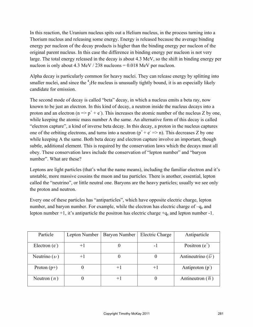
In this reaction, the Uranium nucleus spits out a Helium nucleus, in the process turning into a Thorium nucleus and releasing some energy. Energy is released because the average binding energy per nucleon of the decay products is higher than the binding energy per nucleon of the original parent nucleus. In this case the difference in binding energy per nucleon is not very large. The total energy released in the decay is about 4.3 MeV, so the shift in binding energy per nucleon is only about 4.3 MeV / 238 nucleons = 0.018 MeV per nucleon.

Alpha decay is particularly common for heavy nuclei. They can release energy by splitting into smaller nuclei, and since the 42He nucleus is unusually tightly bound, it is an especially likely candidate for emission.

The second mode of decay is called “beta” decay, in which a nucleus emits a beta ray, now known to be just an electron. In this kind of decay, a neutron inside the nucleus decays into a proton and an electron (n => p+ + e-). This increases the atomic number of the nucleus Z by one, while keeping the atomic mass number A the same. An alternative form of this decay is called “electron capture”, a kind of inverse beta decay. In this decay, a proton in the nucleus captures one of the orbiting electrons, and turns into a neutron (p+

+ e- => n). This decreases Z by one while keeping A the same. Both beta decay and electron capture involve an important, though subtle, additional element. This is required by the conservation laws which the decays must all obey. These conservation laws include the conservation of “lepton number” and “baryon number”. What are these?

Leptons are light particles (that’s what the name means), including the familiar electron and it’s unstable, more massive cousins the muon and tau particles. There is another, essential, lepton called the “neutrino”, or little neutral one. Baryons are the heavy particles; usually we see only the proton and neutron.

Every one of these particles has “antiparticles”, which have opposite electric charge, lepton number, and baryon number. For example, while the electron has electric charge of –qe and lepton number +1, it’s antiparticle the positron has electric charge +qe and lepton number -1.

Particle Lepton Number Baryon Number Electric Charge Antiparticle

Electron (e-) +1 0 -1 Positron (e+)

Neutrino (υ ) +1 0 0 Antineutrino (υ )

Proton (p+) 0 +1 +1 Antiproton (p-)

Neutron ( n ) 0 +1 0 Antineutron ( n )


Just as you can’t create positive or negative electric charge, so too you can’t just create new leptons or baryons. The accounting is done by counting lepton number and baryon number just as we count electric charge. Every nuclear decay must have the same electric charge, lepton number, and baryon number both before and after the decay.

For beta decay, these conservation laws imply that the decay must include an additional element. You can’t just turn a neutron into a proton and an electron, as this would change lepton number. So in fact the basic relations for beta decay and electron capture look like this:

and n p e p e nυ υ+ − + −⇒ + + + ⇒ +

The presence of these “neutrinos”, which interact very little with matter, was first predicted fully thirty years before they were directly detected. But now it is clear that they are just as real as the protons and neutrons.

The third major form of decay is spontaneous fission. Very heavy nuclei are weakly bound, and sometimes they just split apart into a variety of roughly equal parts. This process is

All of these decays happen in a way which allows the nuclei to move more toward a stable balance in their number of protons and neutrons. For example, a neutron rich isotope like 14

6C will decay by converting a neutron to a proton through beta decay, becoming 14

7N. A neutron poor isotope, like 11

6C will decay by electron capture to 115B. Nuclei that are heavy, but not too

heavy, will emit alphas, while the really heavy ones will just fall apart in fission. This instability at the high end is the reason that the periodic table for stable isotopes is limited. You can’t make heavier nuclei and have them hang around. As soon as you stick one of these together, it falls apart.

Isotopes and their modes of decay are recorded in a table of isotopes which mirrors the periodic table, but is charted not simply as a function of atomic number, but of both proton and neutron number . In this table of isotopes there is a ‘valley of stability’, a line of isotopes which are stable, surrounded by nearby isotopes which are not. The farther from the central set of stable elements the more unstable the isotopes are. The decays which will occur are generally those which transform the nucleus towards the line of stability in an obvious way.

For example, nuclei with too many neutrons beta decay, converting one of the neutrons into a proton and emitting an electron and an electron anti-neutrino. Nuclei with too many protons do the opposite, typically capturing an electron, converting a proton to a neutron, and emitting an electron neutrino. Nuclei far from stability, especially those well beyond iron, often decay by alpha emission. The heaviest nuclei are barely held together at all, and are likely to fall apart in spontaneous fission. These ideas are illustrated in the two figures below, which show a subset of a detailed table of isotopes and a cartoon sketch of the whole valley of stability.


Number of neutrons

Number of protons


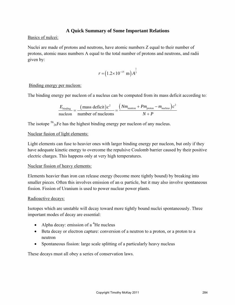
A Quick Summary of Some Important Relations Basics of nulcei:

Nuclei are made of protons and neutrons, have atomic numbers Z equal to their number of protons, atomic mass numbers A equal to the total number of protons and neutrons, and radii given by:

( )1

15 31.2 10 mr A−= ×

Binding energy per nucleon:

The binding energy per nucleon of a nucleus can be computed from its mass deficit according to:

( ) ( ) 22neutron proton nucleusbinding

nucleonmass deficit

number of nucleonsNm Pm m cE c

N P+ −

= =+

The isotope 5626Fe has the highest binding energy per nucleon of any nucleus.

Nuclear fusion of light elements:

Light elements can fuse to heavier ones with larger binding energy per nucleon, but only if they have adequate kinetic energy to overcome the repulsive Coulomb barrier caused by their positive electric charges. This happens only at very high temperatures.

Nuclear fission of heavy elements:

Elements heavier than iron can release energy (become more tightly bound) by breaking into smaller pieces. Often this involves emission of an α particle, but it may also involve spontaneous fission. Fission of Uranium is used to power nuclear power plants.

Radioactive decays:

Isotopes which are unstable will decay toward more tightly bound nuclei spontaneously. Three important modes of decay are essential:

• Alpha decay: emission of a 4He nucleus • Beta decay or electron capture: conversion of a neutron to a proton, or a proton to a

neutron • Spontaneous fission: large scale splitting of a particularly heavy nucleus

These decays must all obey a series of conservation laws.



35.1 Radioactive decay and decay chains

Unstable, radioactive elements often decay through a series of reactions, each happening spontaneously so long as it releases energy. It is typical for such a chain to have a long series of reactions before all the pieces left are themselves stable. For example, the alpha decay:

Is then followed by the beta decay reaction

Each step on the decay chain, which is like a cascade, takes different amounts of time to occur. In each case the time required is related to the amount of energy which is released. Reactions which release a lot of energy will typically happen very quickly, while reactions involving very little release of energy have longer lifetimes.

Looking at the 238U decay chain, you can see it is dominated in time by the first decay, with a very long 4.5 billion year half life. Even the 233,000 year half life of 234

92U is small compared to this.

Gamma decay of excited nuclei

Sometimes during these decay chains a “daughter” nucleus will be produced in an excited state. This excited nucleus is very like an excited state of an atom. Such an excited state decays to a ground state through emission of a photon. Because nuclear energies are large, the photons from the nuclear decays tend to be very energetic, and are typically gamma-rays. So in addition to lots of alpha and beta rays, radioactive decay chains often emit some gamma-rays too.

Unlike alpha and beta decays, gamma ray emitting transitions do not mark a change in the identity of the nucleus. They emerge from a change in state of the nucleus (from higher to lower energy) but do not involve a transition from one isotope to another.

Half-life and decay

Radioactive decay is a purely statistical phenomenon. There is no way to predict exactly when a particular nucleus will decay. In this sense it is like other statistical phenomena we have touched

HeThU 42

23490

23892 +→

eePaTh υ++→ −01

23491

23490


on in this course. For example, in a diffusive process, you don’t predict which atoms will be where, but you can make strong and simple statements about how many atoms will be in each location. Radioactive decay is a similarly statistical phenomenon.

Predictions for radioactive decay begin with an assertion very like the fundamental principle of statistical mechanics. We start by asserting that each nucleus has exactly the same probability of decaying in each period of time (we will call this probability λ), and that the decay of each nucleus is completely unaffected by the state of any other. When this is true, the change in the number of nuclei dN in some period of time dt is proportional to the number of nuclei present N:

dN NdtdN Ndt

λ

λ

= −

= −

Our assertion that the probability of decay is constant, and unaffected by any outside influence is a strong one. It says, for example, that the decay probability of a nucleus is independent of the temperature of the material, the ionization state of the atom, or the decays of any other nuclei in the sample. This assumption of independence is quite good, in large part because the nuclei are quite isolated, tiny little nuggets strongly bound deep within each atom.

The relation relation for the decay rate derived above is a differential equation for the number N of nuclei remaining in the sample. Solving this equations implies that if you start with a number of nuclei N0, after a time t you will now have:

( ) 0tN t N e λ−=

The decay constant λ, which measures the probability that each nucleus will decay in any given second, also tells us how long we will have to wait to see the number of remaining nuclei fall to a particular value. It is typical to ask, for example, how long we must wait before half of the nuclei originally present decay. This time, called the half-life, is related to the decay constant in a simple way:

( )

1/2

0

12

1/2

12ln 0.693

tN eN

t

λ

λ λ

−= =

= =

When the time constant λ is small, the half-life is large. When the time constant λ is large, the half-life is short.

Radionuclide dating: general issues


Radionuclide dating: Carbon 14 dating and human history

Radionuclide dating: age of the Earth

If you know N0, and you measure N, you can determine the age of a sample:

This method is used with 146C, which has a half-life of about 5730 years, to measure the ages of

organic remains which died sometime in the last 40,000 years.

Longer lived isotopes provide the opportunity to date older things. For example, this sort of radionuclide dating has been used to provide relatively precise age for the Earth. One decay useful for this purpose is the chain from 238

92U => 20682Pb. This chain, shown in the figure above,

has an overall half-life of around 4.5 billion years.

35.2 Radiation and life

Radioactive elements, when they decay, release energetic particles which tend to smash through the material around them. All three common kinds of radiation (α, β, and γ) can cause important damage to biomolecules in cells. This damage can prevent the cells from working correctly, and even lead to death. It is important to understand why this subatomic radiation is harmful. It’s not that the total energy in each particle is a problem. If you had the same amount of energy in the form of heat, for example, no harm would be done. These subatomic particles are dangerous because they are very localized; able to deliver their whole load of energy to a single spot.

The three forms of radiation differ dramatically in their penetrating power too. Each is absorbed by matter, and again a useful way to describe this effect is by talking about the absorption length. If the initial intensity of some radiation (in particles per square meter per second) is I0, then the intensity after passing through some material of thickness x is given by I(x) = I0e-x/x0, where x0 is the “absorption length” for this kind of radiation in this kind of material. Not surprisingly, these absorption lengths also depend on energy, with more energetic particles penetrating more deeply.

Typical values for absorption in water are:

• 1 mm for α rays • 1 cm for β rays • 10 cm for γ rays

This sort of absorption is used in shielding, allowing a person to be protected from radiation, sometimes by a very small amount of material. It also suggests that, for example, α emitters are

⎟⎠⎞

⎜⎝⎛=⎟

⎠⎞

⎜⎝⎛=

NNt

NNt 00 ln

693.0ln1 2

1

λ


not a big danger. They are easily shielded against, unless, for example, you eat them. γ emitters, on the other hand, are a lot more difficult to shield.

Energy loss rates Dependence on charge squared over velocity squared gives a good sense of alpha vs. proton vs. electron…

Measuring exposure

Damage from radiation is caused by ionization, by removing electrons from molecules. This ionization deposits energy, and the most basic measure of radiation exposure is a measure of the total energy deposited per unit mass: the “rad”.

One rad is defined as 0.01 J/kg. Not so very much energy, but it is delivered in this particularly nasty, localized way. An exposure of about 104 rads, or 100 J/kg in the form of ionizing radiation, is enough to kill almost any living tissue.

Not all doses are the same, and the simplest adjustment to account for this fact uses the “relative biological effectiveness”, or RBE, factor. This factor accounts for the reality that alpha particles, Joule for Joule, do much more harm than the others. RBE is defined to be one for beta rays. It is somewhere between 10 and 20 for α rays, and about 0.6 for γ rays. In other words, 1 rad of α exposure is roughly 15 times worse than 1 rad of β exposure.

Putting these together gives the exposure in “biologically equivalent dose” or rems. You get this my multiply dose in rads * RBE. So a 1 rad dose in β rays is 1 rem, while a 1 rad dose in α rays is 10-20 rem.

Natural exposure

Radiation is natural phenomenon. We do harness it sometimes and manipulate it for our own purposes, but it is around us no matter what. We are all exposed to radiation from many sources. One of the dominant sources is cosmic rays, energetic particles smashing into the Earth from outer space. Cosmic rays give the typical person a dose of about 45 millirems per year.

Additional radiation comes from radioactive rocks and other materials in your environment, as well as radioactive elements in your body. These give an additional dose of about the same level 40-50 millirems per year. A total dose of 500 millirems, or 0.5 rems per year is considered safe.

There are ways you can face much more radiation. High altitudes, especially flights, expose you to substantially more cosmic radiation, though this is important only if you spend a lot of time flying. Radon, a heavy, highly radioactive gas naturally produced in the soil in some places can build up in basements, leading to very large radiation doses. X-rays and various radionuclide based medical treatments can lead to substantially greater exposures as well.



Radioactive decays and half lives:

In radioactive decays the decay rate is proportional to the number of available nuclei:

dN Ndt

λ= −

This implies that the number of nuclei remaining at time t is related to the number at time t=0 according to:

( ) 0tN t N e λ−=

At some point called the half-life, only half of the original nuclei remain. This time is related to the decay constant λ by:

( )12

ln 2 0.693tλ λ

= =

Radioactive dating:

If you know how much of a nucleus was originally present, and you measure how much remains, you can discover the age of a sample, according to the relation:

1

20 0age

1 ln ln0.693

tN NtN Nλ

⎛ ⎞ ⎛ ⎞= =⎜ ⎟ ⎜ ⎟⎝ ⎠ ⎝ ⎠

Radiation damage and exposure:

Radiation exposure is measured by total energy deposited. One ‘rad’ is 0.01 J/kg. More relevant biologically is the biologically equivalent dose, measured in ‘rems’. One rem is one rad multiplied by the ‘relative biological efficiency’ of the type of radiation.



Once we understand how nuclei work we can see why the elements which make up our Earthly periodic table are all that exist. We also expect them to be all of the elements that can exist. All the possible nuclei are built up of just the two constituents, protons and neutrons, and even among these only a narrow subset are bound together tightly enough to be stable. So that’s it, the familiar periodic table includes the full list of elements. Every single one can be found here on Earth, and we don’t expect there to be any new ones found anywhere else in the universe.

Nuclear physicists continue to test our understanding of how nucleons come together into nuclei, and every once and a while you may hear about them creating a new element. This means they’ve made at least one nucleus with atomic number greater than any seen before. Unfortunately, all of these new nuclei are much too large to be stable, and they decay with extraordinary alacrity. There are other unstable nuclei to be (briefly) constructed and studied, farther and farther from the ridge of stability. But unfortunately none are of practical importance.

36.1 What is the universe made of, and how do we know?

How do we know that these same earthly elements are the only ones that exist in the universe? One of the principle analytic techniques in our earth bound laboratories is spectroscopy. Measurements of the light emitted or absorbed by a material, particularly when that material is in a diffuse, gaseous form, show specific lines of emission and absorption, spectral fingerprints, revealing the elemental composition of the material. The origin of these spectral fingerprints lies in quantum mechanics: atoms can only emit and absorb light with a very specific set of energies.

Early in the history of spectroscopy, Josef Frauenhofer examined the spectrum of the Sun in some detail, and found it extremely rich in information; a smooth continuum of light interrupted by a forest of hundreds of dark absorption lines (this is shown in the figure below). Similar patterns of lines were discovered in the spectra of distant stars.


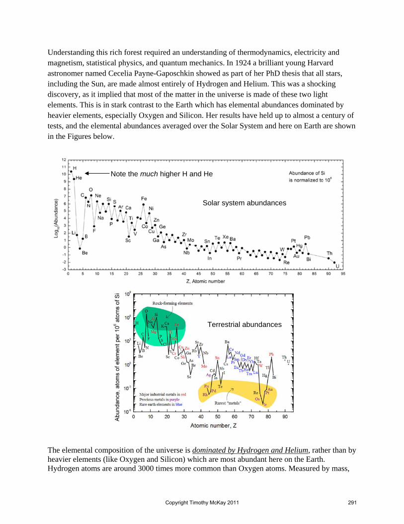
Understanding this rich forest required an understanding of thermodynamics, electricity and magnetism, statistical physics, and quantum mechanics. In 1924 a brilliant young Harvard astronomer named Cecelia Payne-Gaposchkin showed as part of her PhD thesis that all stars, including the Sun, are made almost entirely of Hydrogen and Helium. This was a shocking discovery, as it implied that most of the matter in the universe is made of these two light elements. This is in stark contrast to the Earth which has elemental abundances dominated by heavier elements, especially Oxygen and Silicon. Her results have held up to almost a century of tests, and the elemental abundances averaged over the Solar System and here on Earth are shown in the Figures below.

The elemental composition of the universe is dominated by Hydrogen and Helium, rather than by heavier elements (like Oxygen and Silicon) which are most abundant here on the Earth. Hydrogen atoms are around 3000 times more common than Oxygen atoms. Measured by mass,

Solar system abundances

Terrestrial abundances

Note the much higher H and He


rather than by number of atoms, Hydrogen makes up 74% of the mass of atoms in the universe, with Helium taking up another 24%. Less than 2% of the elemental composition of the universe, by mass, is elements heavier than Helium. The dominance of light elements is one of the main facts about the universe. Any theory which aims to describe origins will have to explain why the elements have the abundances they do, and in particular why the light elements are so remarkably dominant.

36.1 Origin of the elements: the big bang and stars

We know why the elements we have exist, but where did they all come from? Where and how were they made, and why do they appear in the particular mix of abundances which we find today? To make nuclei you need the ingredients (protons and neutrons), and you need to be able to get them close enough together for the short range strong nuclear force to grab hold: you must overcome the Coulomb barrier. Usually, this requires having the nucleons move in very rapid thermal motion, so that their momentum can overcome the repulsion and let the positively charge bits get close enough for the strong force to kick in. So to understand the origin of the elements, we need to know when (and where) in the history of the universe matter was hot and dense enough for this to happen.

How to see the history of the universe

Scientific study of historical subjects, like the history of the universe, or of life on Earth, is a challenge because we were not present when this history occurred. We must instead take advantage of all the remaining information about those distant times. In this study of life on Earth this involves examining fossil evidence found in datable layers within the Earth, and increasingly within the genetic material of living descendents. When we study the history of the Universe our task is actually simpler; we can actually see the past directly.

Light travels at a large but finite speed. Because of this, light arriving from a distant source right now was actually emitted by that source at some time in the past. The more distant a source is, the farther back in time you see it. Since light travels very rapidly (about 1 foot per nanosecond) this time delay is not apparent in everyday life. Only when you look beyond the Earth do these delays begin to pile up. When you examine the moon, you see it as it was about 1 second ago. The Sun is more remote. Sunlight arriving at the Earth is about 8.4 minutes old. You can never see the Sun now. You can only see it as it was 8.4 minutes ago. The nearest stars are much more distant, we can see them only as they were three or four years ago. The Andromeda galaxy, our nearest sizeable neighbor, is so far away that we see it as it was 2.9 million years in the past.

This strange consequence of the finite speed of light is a bonanza for scientists wanting to study how things came to be in the universe. We don’t have to rely on limited and hidden fossil evidence; we can observe the past directly!


There are two caveats to this exciting prospect. The first is fundamental - we can’t actually see our own history. Light which shows the Earth as it was 2.9 million years ago isn’t here anymore; it’s spreading out from us, and just now arriving at the Andromeda galaxy. So we don’t see the Earth’s specific history, instead we see what some parts of the universe looked like at each point in the past. This is fine for studying the average history of the universe, and to the extent that our own history is typical, fine for us.

The second caveat is technical. Since earlier epochs in history are seen from very far away, observing them precisely is quite a challenge. Light from such distant objects is extremely faint, and the angular sizes of things become very small. To observe the past, we must precisely measure the very distant. This technical challenge held up the development until, in the 1980’s and 1990’s, an array of new technologies enabled us to finally make the measurements required to solidly establish cosmology as an empirical science.

First hints of cosmic history: Hubble’s velocity distance relation

Scientific study of the origins of the universe began as pure speculation, without evidence. Once the finite speed of light was known (and it was first accurately measured by Ole Romer in the 1670’s), it was apparent that cosmic history could be seen in the sky. But for centuries it remained too remote to observe. With the creation of the first large telescopes in the early 20th century, it became possible to measure the light from galaxies more distant than Andromeda, and many people began doing so.

Methods were developed for estimating the distances to remote galaxies. The most important, refined for use by Henrietta Leavitt at the Harvard Observatory, involved the use of pulsating variable stars as brightness standards. These Cepheid variable stars pulsate, growing brighter and fainter with a regular period. The period of each star is closely related to the total power it emits. By observing how the star pulsates, and measuring the intensity of light which arrives from it, it is possible to determine the distance to it. By defining the relation between period and total power, Leavitt provided a yardstick for measuring the distances to galaxies.

This new measuring tool was quickly put to work by Edwin Hubble and his colleagues, who used the new 200” Hooker telescope in California to measure distances to a few dozen galaxies. In addition to measuring distances to the galaxies, they recorded their spectra. Galaxy spectra are somewhat different from stellar spectra, but only because a galaxy spectrum is constructed by adding together the stellar spectra of billions of individual stars. Hubble discovered a surprising relationship between the distance to a galaxy and the nature of its spectrum. First, the spectrum of almost every galaxy he examined was ‘stretched’ relative to what you might expect. Every spectral line he could identify was found at a wavelength longer than it would have been in the lab, and in each galaxy, the same stretch factor, now called the redshift, was the same for all spectral lines.


At the time, Hubble and his colleagues interpreted this shifting, this increase of all wavelengths relative to what was expected, as a Doppler shift. Recall that in Chapter 28 we wrote:

source sourceemitted emitted 1observed

c v vc c

λ λ λ+ ⎛ ⎞= = +⎜ ⎟⎝ ⎠

In this interpretation, a galaxy with wavelengths all 10% higher than they seems to be moving with a speed:

observed source

emitted

source

1.1 1

0.1

vc

v c

λλ

= = +

=

Using this interpretation, Hubble constructed a diagram comparing the distance to each galaxy and each galaxies ‘velocity’. The original diagram he published in the Proceedings of the National Academy of Sciences in 1929 is presented below:

This strange relation suggested that somehow, almost every galaxy is moving away from us. Not only that, there is a relation between distance and recession velocity. The more distant a galaxy is, the more rapidly it seems to move away from us.


Reinterpreting Hubble’s diagram: measurements of expansion history

Since Hubble’s time, we have come to understand this relation between distance and stretching in a new, much clearer way. The stretching seen in each galaxy spectrum is now called the redshift of the galaxy, usually given the symbol z, and defined in the following way:

observed

emitted

1 zλλ

= +

If the stretching observed in the spectrum of a galaxy is 3%, then the redshift 0.03z = .

We no longer think of redshift as a measure of velocity. It is instead a measure of how much the universe expanded during the time while the light was traveling from its source to the Earth. Hubble’s velocity-distance relation is actually the first sign that the universe is expanding today. The space between any two galaxies is growing larger with time.

To understand what an expanding universe is like, it may be useful to think of something like a giant chocolate chip cookie. In this cookie there are chips, which we shall think of as galaxies. Now imagine this cookie expanding; becoming larger in every dimension. The distance between every pair of chips grows larger with time. More than that, the farther apart two chips are, the more rapidly they move apart.

In an expanding universe, everything moves apart from everything else. When Hubble saw that the spectrum of each galaxy was stretched, and that the stretching was proportional to distance, he had found evidence that the universe is expanding. Since Hubble’s time, we have continued to measure the relationship between redshift and distance. Instead of calling this a velocity-distance diagram, we now think of it as a measurement of expansion history. When we look at a distant object, we know we see it in the past. The more distant the object is, the farther back in time we are probing. In this way of thinking, the distance plotted on the x-axis of Hubble’s diagram is


really a measure of time back into the past. When we also reinterpret the y-axis of Hubble’s diagram as a measure of integrated expansion, the velocity-distance diagram is redefined as a measure of expansion as a function of time: it’s really an expansion history diagram.

Observation of expansion, perhaps best represented as this expansion history diagram, provided the first observational evidence for what is now called the hot big bang cosmology. We will call it the ‘first observational pillar’ of big bang cosmology.

Consequences of expansion today: a hot dense beginning?

The universe is expanding today, the space between galaxies growing larger and larger. This suggests something about the past: in the past, everything we see today should have been much closer together, all the matter and energy we see in the universe today packed closer together. Running the clock back far enough, there ought to have been a time when the universe was much smaller, and the density of matter and energy much higher – the universe ought to have had a beginning which was hot, dense, and expanding. This ‘big bang’ origin is a logical consequence of seeing a universe which is expanding today. But is it true? How do we know that it really happened?

To test ideas about the history of the universe, we need only examine it – the history is laid out before us. There should be places so distant that the light they emitted when the universe was hot and dense is just arriving at the Earth now. Indeed we should be able to look in any direction at all and see this hot early universe. What should it look like? Hot, dense material emits blackbody radiation with a peak wavelength and intensity dependent on temperature. How hot should it be? At some point matter should have been hot enough to be ionized, so that light could not pass through it. This happens at temperatures of a few thousand Kelvin. This hot plasma should look rather like the surface of the Sun. The peak wavelength for 3000 K blackbody radiation is given by:

3 3

7peak

2.8 10 mK 2.8 10 mK 9.3 10 m3000 KT

λ− −

−× ×= = = ×

This 930 nm light lies off the red end of the visible spectrum; a blackbody emitter at this temperature would look deep red. There is a caveat however: the universe has expanded a lot since this hot dense time, so this light will have been stretched in wavelength enormously, by perhaps a factor of 1000. Instead of red visible light we should expect to find the sky filled with roughly 1 millimeter radio waves (1000 x 9.3x10-7 m ≅ 1x10-3 m).

The observation of cosmic expansion in the universe today led to a simple prediction. When we look at the sky, in every direction, we should see an early universe which is hot, dense, and emitting blackbody radiation with a peak wavelength typical of thousands of degrees Kelvin, stretched out by about a factor of 1000 so that it arrives as millimeter radio waves.


This so-called Cosmic Microwave Background Radiation (CMBR) was first confidently observed in 1964 by Arno Penzias and Robert Wilson at Bell Labs in New Jersey. This CMBR has since been measured with ever increasing precision by a long series of experiments, including most importantly the Wilkinson Microwave Anisotropy Probe, named for leading cosmologist and University of Michigan graduate David Wilkinson. The CMBR, an inescapable prediction of a hot big bang universe, provides striking experimental confirmation of this model for cosmic origins. The detection of the CMBR, and the precise agreement between its predicted and observed properties, provides the second observational pillar of the big bang cosmology.

This part of the story, about the big bang and how we know it really happened, is a great story which we don’t have time to cover. If you would like to know more, you can go online and watch several lectures which I gave on the subject a few years ago. You will find them at the Web Lecture Archive Project:

http://lecb.physics.lsa.umich.edu/CWIS/browser.php?ResourceId=2106

http://lecb.physics.lsa.umich.edu/CWIS/browser.php?ResourceId=2107

The hot early universe and the dominance of light elements

We now know that the universe began about 13.7 billion years ago. At that time, everything was much closer together, with both the matter density and the energy density much higher than today. In addition, the universe was expanding, with the space between things increasing, and the density of both matter and energy dropping drastically.

In this superhot, dense environment, enough energy existed to continuously create matter. For example, if a bit of light has adequate energy, it can convert its energy into mass according to Einstein’s famous 2E mc= , creating particles. In a typical example, a particle of light can create an electron-positron pair. This energy into matter conversion always produces pairs. It has to because of charge conservation. Creating just an electron would violate the conservation of electric charge. In the very early universe, while everything was very hot and dense, matter was freely created and destroyed.

If the universe weren’t expanding, nothing else would ever have happened. Everything would have stayed hot, dense, and uniform forever. There would be microscopic change, with energy becoming matter and matter energy, participles moving around, and light being emitted and absorbed. But on the large scale, everything would remain at equilibrium, a uniform density and temperature. It would have been a dull universe indeed, and we would surely not be here to ponder it.

Fortunately the universe was not static at this time, it was expanding, and as it expanded it cooled, stretching the wavelengths of all the light around until with the average energy in particles of light becoming too low to create new matter. Huge numbers of protons, neutrons, and


electrons were around, already created, and zooming along. Initially, these moved too fast to stick together, but as the universe continued to expand and cool, they eventually slowed down enough to be able to stick together.

For a time, they still had enough energy to get close enough to bind, protons could overcome the Coulomb barrier and fuse, but not so much that they simply smashed past one another. Many of the protons found neutrons and other protons and merged together into Helium. Remember that this bonding is exothermic, it releases energy, and that means it will happen very freely if it can. If conditions had stayed like this for a long time, all the Hydrogen available would have merged into Helium, and Helium into heavier things, until everything ended up at the top of the curve of binding energy. We’d have had a universe full of Iron; also fairly dull.

But conditions didn’t stay like this for long. When fusion begam, the universe was still expanding and cooling, and rather quickly it became so cool and diffuse that nuclear fusion stopped. The positively charged nuclei now were moving too slowly to reach one another, and the nuclear cooking ceased. As a result, this early burst of nuclear creation, called “big bang nucleosynthesis” left most (about 76% by mass) of the nucleons as Hydrogen nuclei (just protons), with most of the remaining 24% in Helium. Tiny bits were in different forms, like 21H (deuterium) and 32He (Helium-3).

That was it. The big bang first made all the nucleons, cooled and cooked them for a bit until some of them were stuck together in Helium nuclei, then cooled further and stopped. It left us with a universe dominated by light elements. The universe is still very strongly dominated by light elements. Hydrogen remains the dominant element, still making up nearly the same 76%. Helium is also incredibly common, still about 24% of the mass.

The ability of a big bang cosmology to naturally accommodate the dominance of the light elements in the mass budget of the universe is another strong observational confirmation of the big bang model. Not only does it qualitatively predict a lot of Hydrogen and some Helium, it makes precise predictions for the abundances of some rare light elements, like Deuterium (2

1H) and Helium-3 (3

2He). Abundances of these rare elements, reliably measured for the first time in the late 1990’s, confirm these predictions. This makes the dominance of the light elements the ‘third observational pillar’ of the big bang cosmology.

If nothing else happened, if there were no other way to “cook” elements, the universe would still be just about only Hydrogen and Helium, and again, we certainly would not be here to study this.

Gravity, stellar furnaces, and supernova pollution

The rest of the story of the origin of the elements is, in one sense, not very important. Most of the ordinary matter in the universe is just as it was when the Big Bang nucleosynthesis ended. In another sense, the rest of the story is everything, because we couldn’t exist without large amounts of the heavier elements like carbon, nitrogen, and oxygen.


After the universe cooled enough for nucleosynthesis to end, nothing much happened for a while. The universe continued to expand and cool, with a nearly uniform density. But there were, from the beginning, very small differences in density from place to place, perhaps originally created by quantum fluctuations. Whatever their cause, we know these small fluctuations existed because we have measured them. The intensity of light seen in the CMBR is very slightly different from place to place, differences of a few parts in 100,000. These tiny initial fluctuations in density provide the seeds for the formation of all the structures we see today. Everywhere there was a little more matter, the inexorable pull of gravity began to draw more matter in. As these lumps became more dense, they pulled harder, and the growth proceeded faster and faster.

Images of the tiny variations in temperature seen in the Cosmic Microwave Background Radiation, initially seen crudely by the ‘Cosmic Background Experiment’ around 1992, then measured more precisely by the ‘Wilkinson Microwave Anisotropy Probe’ in 2003.


Eventually, the pull of gravity allowed clouds of gas to become more and more compressed, and stars formed. A star is a cloud of gas stopped in the process of collapse. It is stopped, held up, by the release of fusion energy. How does this happen? As the gas falls inward it is squashed by gravity, compressed, and heated. If the star is large enough, the gravity is substantial enough to increase the internal pressure and temperature until, once again, conditions were adequate for nuclear fusion to begin!

When this happens, the core of the star suddenly has a wonderful, very efficient, new source of heat. The heat which comes out from fusion generates more than enough thermal pressure to resist the inward pull of gravity, the star stalls in its collapse and becomes, for a time, stable. If the core burns too fast for a bit, the star expands and cools, settling back to equilibrium. If the core burns too slowly, the star collapses a bit and heats, burning faster. So this equilibrium is stable.

And there it sits, gradually cooking its Hydrogen into Helium, Helium into Carbon, and so on, until eventually the star starts to build up a core of Iron. Big stars with a lot of mass (and hence gravity) will do this quickly, in as little as a few million years. Small stars don’t have so much gravity to resist, so they can last much longer. The most common kinds of stars, red dwarf stars, have lifetimes more than 10 times the age of the universe so far, so they’ll be around for a long time. The Sun, which is actually pretty large for a star (though far from the largest) ought to last for more than 9 billion years. It’s about 4.57 billion years old now, so it will last for a while.

Inside these stars, elements up to Iron are gradually constructed. Nothing beyond that though, because creating elements beyond Iron takes you down the curve of binding energy, and requires an input of energy. So we have two problems left. We have to get the heavy elements out of these stars, to places where they can create planets and people, and we must somehow create the really heavy elements, those heavier than iron. Supernova explosions are responsible for both.

36.2 Stellar death and supernovae

Once a star burns up most of its fuel, it no longer has a source of internal energy. At this point, there’s nothing to resist the gravitational pressure to collapse, and collapse it does. All the matter in the star falls inward, with pressure and temperature rising higher and higher until some new resisting force emerges. At this point there are three possible outcomes.

Smallish stars, those up to a bit more massive than the Sun, will shrink down into “white dwarf” stellar remnants. When this happens to the Sun, it will shrink to around down until it is about the size of the Earth, at which point a quantum mechanical effect called “electron degeneracy pressure” will suddenly resist the pull of gravity, and collapse will cease. Before this final collapse, such stars will cast off some of their outer layers, creating beautiful “planetary nebulae”. This mechanism is one way in which heavy elements get spread through the universe.


More massive stars have too much gravity to stop as a white dwarf. Their gravity actually squashes the electrons into the protons converting them into neutrons. This process is the same as the electron capture decay we discussed when talking about nuclear physics. The whole star continues to collapse until it becomes about 10 km across, about the size of Ann Arbor. At this point, a new resistive force can act; “neutron degeneracy pressure”. This is one stiff force, and stops the collapse of the rest of the star in its tracks. In fact, the outer layers of the star, falling onto this stiff core, actually bounce back out, and the star explodes as a “supernova”.

The supernova does two things. First, it blasts a substantial fraction of the star’s mass, including lots of these heavy elements, off into space. Second, because a lot of extra energy is available from the infalling material, a sudden burst of endothermic nucleosynthesis can occur. It’s during this brief period that all the nuclei heavier than Iron are produced, and then immediately blasted back out into space. Supernovae are really the key. Not only do they create the heavy, trans-iron elements, they also blast the lot back out into space.

These are images of some planetary nebulae, the cast off outer layers of stars late in their lives. These expelled layers help to spread matter enriched in heavy elements which can later be incorporated in new stars, planets, and even people


If a star is even more massive, the gravitational pressure is too much for even neutron degeneracy pressure to stop. These stars collapse completely, never stopping, and become black holes. Any heavy elements they produce are lost, fallen into the black hole, never to return.

Summing up the origin of the elements

To summarize: the light elements, Hydrogen and Helium were made in the big bang’s brief but universal nuclear furnace. They remain the dominant components of the universe. All the heavier elements were made in later generations of stars. Good estimates of cosmic abundances of some of these elements are given in the table to the below.

The presence of all these elements on the Earth is possible because the solar system formed from preprocessed material, stuff which had already passed through the cores of stars, suffered the violence of stellar collapse, and been cast back out into space. Every heavy atom in your body

X-ray images of the expansion of the cast off shell of material from Supernova 1987a, the first to explode near the Milky Way in almost 400 years. The upper left image shows the remnant in January 2000, and the lower right shows it in January 2005. The neutron star remnant at the center has not yet been observed.


has been through this. All those heavier than Iron were formed only in the wild, non-equilibrium, endothermic reactions which took place as part of the explosion.

Why is the Earth not still dominated in mass by Hydrogen and Helium? These two elements, at the typical temperature of the Earth, have kinetic energies larger than their gravitational potential energies at the Earth’s surface. As a result, they are free to escape into space. Some Hydrogen remains of course, but only because it is chemically bound to heavier atoms which help to bind it gravitationally to the Earth. Larger planets, like Jupiter, have more than enough gravity to hang onto their light elements, and indeed their composition is dominated by them.

It is remarkable that we know this, how all the elements found on the Earth, or in fact anywhere in the cosmos, are formed. Understanding the origin of the elements is a great accomplishment. We know where it all came from.

Atomic number

Element Cosmic mass fraction in parts per million

1 Hydrogen 739,000

2 Helium 240,000

8 Oxygen 10,700

6 Carbon 4,600

10 Neon 1,340

26 Iron 1,090

7 Nitrogen 950

14 Silicon 650

12 Magnesium 580

16 Sulfur 440

All Others 650



Elemental composition of the universe:

The universe is dominated by the light elements Hydrogen and Helium, which make up about 74% and 24% of the atoms in the universe respectively.

Observational cosmology and expansion:

Because light travels at a finite speed distant objects are seen in the past. This allows us to view the history of the universe. Distant objects (from which light has traveled a long time) have spectra which are stretched relative to nearby objects. This is the basic evidence for expansion, and is often viewed in a Hubble velocity-distance diagram. We have argued that this is actually an expansion history diagram.

Cosmological redshift:

The redshift z defined as:

observed

emitted

1 zλλ

= +

Expansion and a hot dense early universe:

The existence of expansion implies a hot dense early phase. Evidence for this is clearly seen in the cosmic microwave background radiation which arrives from every direction on the sky. It has a characteristic temperature of about 3 K.

The hot dense early universe and light element dominance:

The Hydrogen and Helium which so dominate the universe were made in this brief hot, dense, expanding period. Fusion stopped with them because expansion caused the universe to cool below the temperatures required to continue it.

Stars and the heavier elements:

All the elements up to iron are slowly cooked in the cores of stars, where the inward pressure of gravity is balanced by the outward thermal pressure generated by fusion.

Stellar death and element enrichment:

When stars run out of fuel they collapse, but ironically also often shed their outer layers as planetary nebulae or supernovae. Supernovae are especially important, because their violent explosions briefly provide the excess energy required to make the elements heavier than iron.



37.1 Life in the Universe

During the past nine months we’ve been learning how the laws of nature envelop life, limiting what is possible and providing it with mechanisms to accomplish its goals. Everything we know about life is based on just one example: the life here on Earth. Though life on Earth is remarkably diverse, there is also overwhelming evidence that all life on Earth is intimately related, and all descended from a single origin. We also know that life on Earth emerged quite quickly, appearing almost as soon as the most extreme violence of the Earth’s formation came to an end.

We have no convincing reason to suspect that life is rare. There is nothing extraordinarily unusual about the Earth, and life emerged quickly here, so perhaps it should emerge eventually wherever conditions are adequate. Such conditions are likely to be rather common, and perhaps life is too. Unfortunately, we’re still at a very early stage in this study. Though we know much about stars, it’s only in the last fifteen years that we have been able to detect any planets at all around other stars. Exploration even of our own solar system is still in its infancy. For now, the expectation that life ought to be common is difficult to test. We know our current tools aren’t yet adequate to find life beyond the solar system, and they’re a very long way from being able to prove it doesn’t exist.

This question of “astrobiology” is one of the great questions for the next generation of scientists. Nothing, really nothing, will be more important that the first discovery of extraterrestrial life which emerged independent of life on Earth. There’s a good chance it will happen in your lives, especially if some of you dedicate yourselves to it.

This chapter will consider what conditions seem necessary for life, and ask where they exist in the universe. This will help you to form your own opinions about the likelihood of finding life beyond the Earth.

What is life really?

Is understand what life needs, we must first ask what life is, where we draw the line between the living and the non-living. There is no complete consensus about what marks this line. The Oxford English Dictionary waffles, defining life as:


“The property which constitutes the essential difference between a living animal or plant, or a living portion of organic tissue, and dead or non-living matter; the assemblage of the functional activities by which the presence of this property is manifested.1”

Not too satisfying. This definition says life is what makes the difference between living and non-living matter. Ernst Mayr, one of the 20th century’s leading biologists, expressed his exasperation with the problem this way: “Attempts have been made again and again to define `life'. These endeavours are rather futile since it is now quite clear that there is no special substance, object, or force that can be identified with life.2”

Still it seems useful to try. Probably the narrowest, most widely accepted definition of life is something which reproduces itself with the possibility of modification. This definition at least lets in most widely accepted living things, though of course it is limited. Surely a neutered pet remains alive. But the idea of life as something which can reproduce itself with modification is a good place to start.

Some prefer a longer list of criteria. Here’s the Wikipedia version3, which captures most of the properties usually raised. Something is probably alive if it has most of these properties…

1. Homeostasis: Regulation of the internal environment to maintain a constant state; for example, sweating to reduce temperature.

2. Organization: Being composed of one or more cells, which are the basic units of life. 3. Metabolism: Consumption of energy by converting nonliving material into cellular

components (anabolism) and decomposing organic matter (catabolism). Living things require energy to maintain internal organization (homeostasis) and to produce the other phenomena associated with life.

4. Growth: Maintenance of a higher rate of synthesis than catalysis. A growing organism increases in size in all of its parts, rather than simply accumulating matter. The particular species begins to multiply and expand as the evolution continues to flourish.

5. Adaptation: The ability to change over a period of time in response to the environment. This ability is fundamental to the process of evolution and is determined by the organism's heredity as well as the composition of metabolized substances, and external factors present.

6. Response to stimuli: A response can take many forms, from the contraction of a unicellular organism when touched to complex reactions involving all the senses of higher animals. A response is often expressed by motion, for example, the leaves of a plant turning toward the sun or an animal chasing its prey.

7. Reproduction: The ability to produce new organisms. Reproduction can be the division of one cell to form two new cells. Usually the term is applied to the production of a new individual (either asexually, from a single parent organism, or sexually, from at least two

1 Oxford English Dictionary online 2 Mayr, E. 1982. The Growth of Biological Thought. Diversity, Evolution, and Inheritance. Harvard University, Cambridge: The Belknap Press, . 3 http://en.wikipedia.org/wiki/Life


differing parent organisms), although strictly speaking it also describes the production of new cells in the process of growth.

Looking at this list, the feature most difficult to mimic with engineering is reproduction. Life is particularly good at this, and so perhaps this is remains the best dividing line between the living and the non-living.

A long discussion offering a variety of alternate definitions of life in the Encyclopedia Brittanica concludes by pointing out the more essential problem biology currently faces; we only know about one form of life, that on Earth, and all of the life on Earth seems completely related.

“The existence of diverse definitions of life surely means that life is something complicated. A fundamental understanding of biological systems has existed since the second half of the 19th century. But the number and diversity of definitions suggest something else as well. As detailed below, all the organisms on the Earth are extremely closely related, despite superficial differences. The fundamental ground pattern, both in form and in matter, of all life on Earth is essentially identical. As will emerge below, this identity probably implies that all organisms on Earth are evolved from a single instance of the origin of life. It is difficult to generalize from a single example, and in this respect the biologist is fundamentally handicapped as compared, say, to the chemist or physicist or geologist or meteorologist, who now can study aspects of his discipline beyond the Earth. If there is truly only one sort of life on Earth, then perspective is lacking in the most fundamental way.4”

Among all this confusion there is a clear consensus that, whatever life is exactly, all living things exist in open thermodynamic circumstances in which they take in resources, use them to construct themselves and near replicas of themselves, then expend these resources, always at the expense of substantial increases in entropy. This tells us what life (at least in its familiar guise) needs to exist.

37.2 The evolution of the cosmos: setting the stage for life

What are the basic requirements for life? Given that life is hard to even define, it is difficult to say for sure. But we can at least think about what’s needed for life similar that that we find on Earth. Such life requires at least three things:

• A regular flow of energy. This regular flow of energy is what makes possible all sorts of cyclic processes, both living and not. Without this flow of energy, equilibrium will be quickly reached, and nothing much will ever happen.

4 life. (2007). In Encyclopædia Britannica. Retrieved August 25, 2007, from Encyclopædia Britannica Online: http://search.eb.com/eb/article-9106478


• An enriched mix of chemical elements, including probably the “organic” compounds (Carbon, Oxygen, Nitrogen, Hydrogen, Phosphorus, Sulfur, etc.). It’s certainly not enough to have only Hydrogen and Helium.

• Liquid water. Why is this so important? The highly polar nature of water makes it a great matrix for complex chemistry. The electrostatic shielding water provides is a big part of what makes complex protein chemistry possible for life.

In addition to these essential ingredients, there presumably has to be some level of stability. If the conditions last for only a short time and then change dramatically, it may not be possible for life to emerge and adapt with adequate speed. So where might we find stable flows of energy, a rich mix of chemicals, and liquid water on which both liveliness and life might subsist? This stability is provided by planets, especially those which orbit stars. These planets, in stable orbits around long-lived stars, may provide conditions which remain stable for billions of years. So we’re looking for planets, but the flows of energy involved might come from any one of several different sources.

• Planets orbiting stars: On the Earth's surface, action is driven the flow of energy from the Sun. This flow powers weather and the water cycle. It also enables life. So the traditional place to seek life is on planets with surfaces heated by nearby stars. There is a Goldilocks problem though. The arrangement has to be just right; not too hot and not too cold. Within the solar system, only the Earth will do.

• Molten cores: One new possibility has emerged that is literally beneath our feet. The

core of the Earth is heated by radioactive decays of heavy elements trapped within it when it formed. Energy from this inner glow, emerging from below, fuels life in the deep oceans. Take away the Sun, and this flow of heat would remain, providing, perhaps, enough to keep life cooking. Planets heated by this sort of radioactive glow, even if far from any star, might simmer with life beneath their surfaces. Perhaps only surface life is rare…

• Tormented moons: Closer to home, in our own solar system, a more exotic flow of

energy exists in moons of the outer planets: tidal heating. Io and Europa, moons orbiting Jupiter, provide a good example. Io swings around Jupiter every 42 hours or so. A little farther out, Europa takes just about twice as long. Every time Io passes between Jupiter and Europa, it is tugged outward a little. Trapped in this struggle, Io is repeatedly stretched and squashed by the varying tug of Jupiter and Europa’s combined gravity. This cyclic stress heats Io, just as you might warm a ball of clay by squashing and stretching it with your hands. In the case of Io, the effect is extreme, making this poor little moon (with about a quarter the radius and 2% of the mass of the Earth) the most violently volcanic body in the solar system. Europa, too, is heated in this dance, enough to maintain a 60-mile-thick ocean of liquid water beneath a deep layer of ice. The same process is active in the moons of Saturn as well, most spectacularly on Enceladus, where


dramatic plumes of water vapor were discovered spewing from this tiny moon's South Pole in 2005.

These three examples, all based on what we know from the our own Solar system, make it clear that various possibilities exist supplying the conditions needed for life. The first extra-solar planets were discovered only a dozen years ago. Now more than 500 have been found, and the pace of discovery is accelerating rapidly. New planets are discovered every week. So far, nearly all of these planets are “gas giants”, rather like Jupiter, and not thought to be likely hosts of life. We’d like to find earth-like, rocky little planets orbiting other stars. It is extremely likely that they exist, but our experiments are just now becoming sensitive enough to detect them.

Even worse, we have no technology for traveling to another star in less than a lifetime. We will search from afar. But life, something we can’t even properly define, is going to be hard to definitively identify from a distance of many light years. I’m not betting we'll find it in our lifetimes. So the best hope for confidently identifying life beyond the Earth still lies here in the Solar System. Unmanned exploration of Mars and the moons of Jupiter and Saturn probably hold the most promise.



Some final conclusions

The purpose of this 135/235 course sequence has been to teach you about some of the most important principles of physics within which life must accomplish its goals. Doing this helps a lot in explaining why life is the way it is. You should know now:

• why children so rarely break their bones • why gorillas don’t grow as large as King Kong • why warm blooded animals aren’t smaller than shrews • why lungs have such complicated networks of aveoli • why blood pressure is high before and after an occlusion • why the largest animals live in the water • why bats use ultrasound to detect their prey • why eyes have muscles for accommodation • why magnetic resonance imagers can see inside you • why the highly polarized medium of water is essential for life’s chemistry • why you can hear but not see around corners • why your body uses bizarrely shaped nerve cells to reliably transmit messages • why a bacteria might labor to grow a magnetic needle inside itself • why all the carbon in you was created in a star • why life might be common

and, one hopes, quite a few other things.

Physical laws of nature frame everything about life, including the sizes, shapes, structures, required conditions, and modes of communication for all living things. Nothing can violate these laws, whether living or dead. And nothing, living or not, can do anything not allowed by these laws. Appreciating these physical influences is as essential as evolution for understanding life. Without understanding these physical limitations, it is impossible to understand the diversity and limitations of life.

This is the lesson to take from these classes. It’s OK if you forget the details, but you have to remember that life is physical, that everything it does is subject to the same physical constraints as all nonliving processes. If someone asks you what physics has to do with life, you should have no trouble answering at length.


Documents

Physics for the Life Sciences II