Embed Size (px)
Citation preview

PHYSICS-BASED
ANIMATION
Colin VellaCSA2207

Animated Graphics
Presentations
Entertainment Media
Simulations
Computer Games

Digital Animation Approaches
Ideal for predetermined sequences
Requires prescription of the complete sequence
Can be designed for dramatic effect
Requires skilled animators for realistic effects
Animator resources / effort must scale in proportion to complexity
Ideal for interactive applications
Requires a physical model and initial conditions
Animation cannot be controlled directly
Realism is a by-product of physics modelling
Computation resources must scale in proportion to complexity
Scripted Animation Interactive Animation

Interactive Animation Applications
Engineering Design
Virtual Reality
Training Simulators
Computer Games

Existing Solutions
Commercial / Closed Source
Havoc Physics™
Nvidia PhysX™
Community Driven / Open Source
Bullet
Open Dynamics Engine™
Farseer
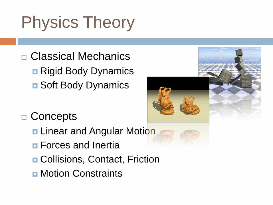
Physics Theory
Classical Mechanics
Rigid Body Dynamics
Soft Body Dynamics
Concepts
Linear and Angular Motion
Forces and Inertia
Collisions, Contact, Friction
Motion Constraints

Physical Models for Animation
Analytical Models Numerical Models
Analytical
Solutiontime state
Numerical
Solution
start
time
next
statestart
state
next
time

Physical Models for Animation
Compute state as a function of time
Computationally efficient
Very accurate (no error accumulation)
Limited to simple predictable configurations with no interaction
Requires solution for every class of problem
Iteratively update state over small timeframes
Polynomial complexity
Numerical errors creep into simulations over time
Can handle interactive configurations of arbitrary complexity
Generic approach suitable to many problems
Analytical Models Numerical Models

Analytical Model Example
Algorithm(1) Let t := 0
(2) Set initial velocity u
(3) Compute p(t)
(4) Let t := t + ∆t
(5) Draw projectile
(6) Go to step (3)
tutp xx
yx ppp
2
2
1gttutp yy
xx utv
gtutv yy
yx vvv
0tax
gtay
yx uu uv 0
2
2
1ttt aup tt auv
g 0a
gt 0a
Vector Equations of Motion
Component Equations of Motion
Y
X
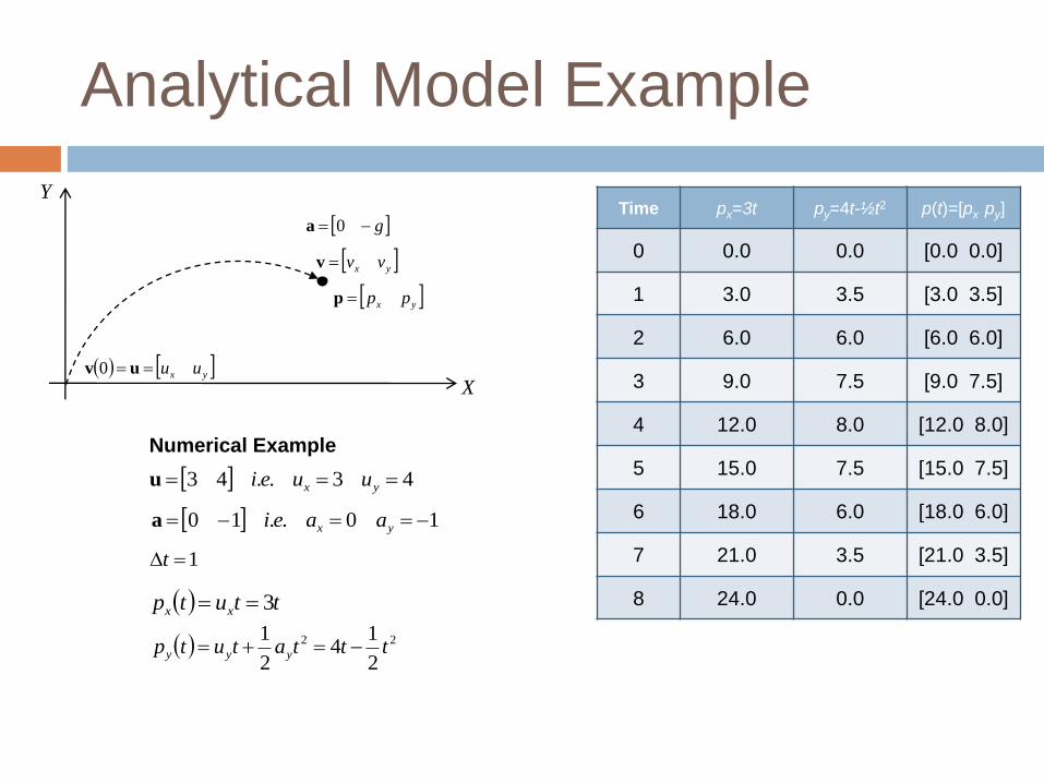
Analytical Model Example
Numerical Example
Time px=3t py=4t-½t2 p(t)=[px py]
0 0.0 0.0 [0.0 0.0]
1 3.0 3.5 [3.0 3.5]
2 6.0 6.0 [6.0 6.0]
3 9.0 7.5 [9.0 7.5]
4 12.0 8.0 [12.0 8.0]
5 15.0 7.5 [15.0 7.5]
6 18.0 6.0 [18.0 6.0]
7 21.0 3.5 [21.0 3.5]
8 24.0 0.0 [24.0 0.0]
yx ppp
yx vvv
yx uu uv 0
g 0a
Y
X
43..43 yx uueiu
1t
ttutp xx 3
22
2
14
2
1tttatutp yyy
10..10 yx aaeia

Numerical Animation Algorithm
Initialise
State
End of
animation?
Process User /
Agent Input
Update State
Visualise
EndYes
No
NumericalSolution
start
time
next
statestart
state
next
time

State Initialisation
What constitutes state?
For each element (body)
Position
Orientation
But also
Linear / Angular Velocity
Linear / Angular Acceleration
External Forces
(will deal with angular motion later...)
Initialise
State

Representing Position
Position Vectors
2D Vectors for 2D Animations
3D Vectors for 3D Animations
yx ppp
zyx pppp
p
Y
Xxp
yp
Y
Xxp
yp
Z
zp
p

Representing Orientation
Various representation options
Bodies rotate around axis passing through a
‘central’ point (centre of mass)
More on this later...

State Update
For each body
Position changes due to linear
velocity
Orientation changes due to
angular velocity
Linear / angular velocity changes
due to linear / angular acceleration
due to some event, e.g. collision
Linear / angular acceleration
results from external forces
Update State

Representing Linear Velocity
2D or 3D Vectors
Velocity is rate of change of position
i.e. integrating velocity over time gives position
and if velocity constant, then
zyx vvvv
dt
dpv
dt
dpv
dt
dpvei
dt
d zz
y
yx
x ..p
v
dtvspdtvspdtvspeidtt
zzz
t
yyy
t
xxx
t
..vsp
tvsptvsptvspeit zzzyyyxxx ..vsp

Representing Linear Acceleration
2D or 3D Vectors
Acceleration is rate of change of velocity
i.e. integrating acceleration over time gives velocity
and if acceleration constant, then
zyx aaaa
dt
dva
dt
dva
dt
dvaei
dt
d zz
y
yx
x ..v
a
dtauvdtauvdtauveidtt
zzz
t
yyy
t
xxx
t
..auv
tauvtauvtauveit zzzyyyxxx ..auv

Numerical Integration
Equations p = s + vt and v = u + at valid only when v and a constant
If v and a are variable, but t sufficiently small (t = ∆t), we can use
these equations to calculate approximations for p and v
We can calculate new value for a and repeat previous step
This results in a first order approximation of the path taken by
position p
tp tt p
ttvt )(p
ttttt vpp
ttttt avv

Numerical Integration Example
Algorithm(1) Let p := s, v := u, a := [0 -g]
(2) Let p’ := p + v∆t, v’ := v + a∆t
(3) Let p := p’, v := v’
(4) Draw projectile
(5) Go to step (2)
yx ppp
yx vvv
Vector Equations of Motion
Component Equations of Motion
yx uu uv 0
Y
X
g 0a
ttttt vpp
ttttt avv
000 sp
uv 0
00 xxp s
00 yyp s
xx uv
yy uv 0
ttvtpttp xxx
ttvtpttp yyy
tgtvttv yy

Numerical Model Example
yx ppp
yx vvv
430 v
10 a
10 a
Numerical Example
000 p
1,0 tt
430 uv
Y
X
Time p v a p’=p+v v’=v+a
0 [0 0] [3 4] [0 -1] [3 4] [3 3]
1 [3 4] [3 3] [0 -1] [6 7] [3 2]
2 [6 7] [3 2] [0 -1] [9 9] [3 1]
3 [9 9] [3 1] [0 -1] [12 10] [3 0]
4 [12 10] [3 0] [0 -1] [15 10] [3 -1]
5 [15 10] [3 -1] [0 -1] [18 9] [3 -2]
6 [18 9] [3 -2] [0 -1] [21 7] [3 -3]
7 [21 7] [3 -3] [0 -1] [24 4] [3 -4]
8 [24 4] [3 -4] [0 -1] [27 0] [3 -5]
9 [27 0] [3 -5] [0 -1]

Analytic vs Numeric Results
0
3.5
6
7.58
7.5
6
3.5
00
4
7
9
10 10
9
7
4
00
2
4
6
8
10
12
0 3 6 9 12 15 18 21 24 27
Y
X
Analytic Model
Numeric Model

Angular Motion
We have angular equivalents of numerical
equations for linear motion
φ is orientation
ω is angular velocity
α is angular acceleration
ttttt αωω
ttttt ωφφ
Linear Equations Angular Equations
ttttt vpp
ttttt avv

2D Angular Motion
Option 1: Scalar Angles
φ, ω, α expressed as scalars (in radians)
φ must be reduced to range [-π.. π] by adding /
subtracting 2π
ttαtωttω ttωtφttφ
Y
X
dt
d
dt
d

2D Angular Motion
Option 2: 2D Rotation Matrices
Φ expressed as 2D rotation matrix
Angle of Φ automatically falls within [-π.. π]
ω, α still expressed as scalars
Must convert ω to rotation matrix to update φ
Angular velocity still updated as scalar
φ loses orthogonality after a while, need renormalisation
ttαtωttω
ttωttω
ttωttωttt
cossin
sincos
φφ
φφ
cossin
sincos

2D Angular Motion
Option 3: Complex Angles
φ expressed as complex number of unit length
Angle of φ automatically falls within [-π.. π]
ω, α still expressed as scalars
Must convert ω to complex number to update φ
Angular velocity integration still computed as scalar
May need to renormalise φ after a while
ttαtωttω
ttiωettt φφ
tφitφe tiφ sincosφ
φφ
φ1

Comparison of 2D Rotation Structures
Scalar Angles2D Rotation
MatricesComplex Angles
Pros• Very compact representation (1
scalar element)
• Very cheap computation
• Solves angle discontinuity
• Can reuse for visualisation
• Solves angle discontinuity
• Compact representation (2
scalar elements)
• Cheap ω conversion
• Cheap conversion to matrix for
visualisation
• Cheap renormalisation
Cons• Must handle angle discontinuity
• Very costly conversion to matrix
for visualisation
• Waste storage space (4 scalar
elements
• Expensive computations
• Costly ω conversion
• Costly renormalisation
• Less compact than scalar
angles
• Visualisation matrix still needs
to be computed, but cheap
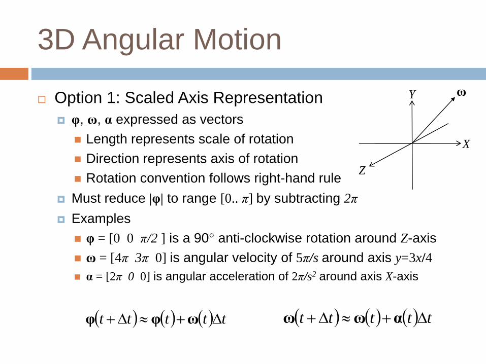
3D Angular Motion
Option 1: Scaled Axis Representation
φ, ω, α expressed as vectors
Length represents scale of rotation
Direction represents axis of rotation
Rotation convention follows right-hand rule
Must reduce |φ| to range [0.. π] by subtracting 2π
Examples
φ = [0 0 π/2 ] is a 90° anti-clockwise rotation around Z-axis
ω = [4π 3π 0] is angular velocity of 5π/s around axis y=3x/4
α = [2π 0 0] is angular acceleration of 2π/s2 around axis X-axis
ttttt αωω ttttt ωφφ
X
Y
Z
ω
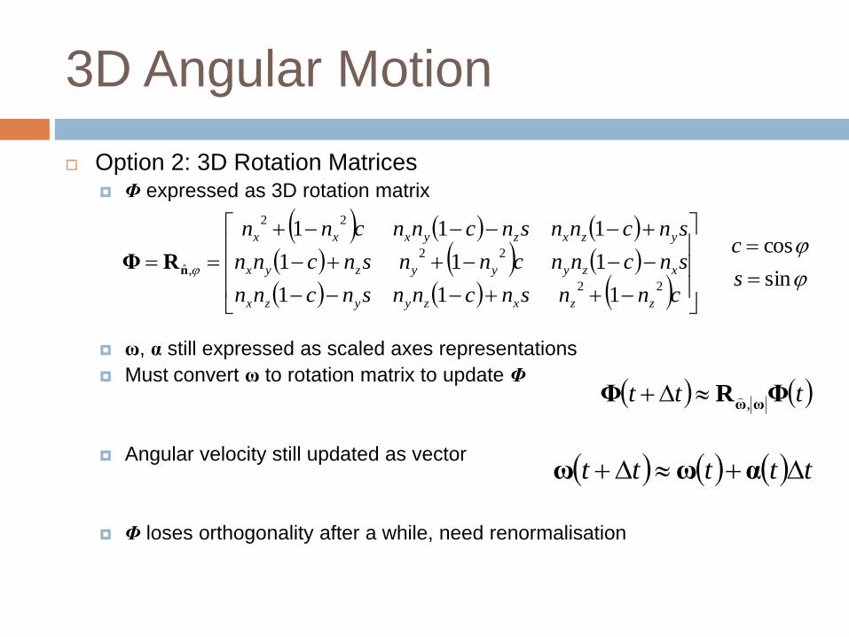
3D Angular Motion
Option 2: 3D Rotation Matrices Φ expressed as 3D rotation matrix
ω, α still expressed as scaled axes representations
Must convert ω to rotation matrix to update Φ
Angular velocity still updated as vector
Φ loses orthogonality after a while, need renormalisation
ttttt αωω
ttt ΦRΦωω,
sin
cos
111
111
111
22
22
22
,ˆ
s
c
cnnsncnnsncnn
sncnncnnsncnn
sncnnsncnncnn
zzxzyyzx
xzyyyzyx
yzxzyxxx
nRΦ

3D Angular Motion
Option 3: Quaternion Angles
About Quaternions Like complex numbers, but in 4D
Have rules for addition, subtraction, multiplication etc.
Quaternions for Rotation 3D equivalent of complex angles for 2D
Pros and cons analogous to complex numbers for 2D angular
motion

Quaternions
4D vectors with a special multiplicative operation
Can be represented as a 4-element vector or a scalar / 3D vector
pair
Norm (Magnitude)
Conjugate
Multiplication
Inverse
zyx vvvss vq
22222
zyx vvvsss vvvq
zyx vvvsss vvq**
2112212121221121 vvvvvvvvqq ssssss
vv
v
q
2
*1
s
s
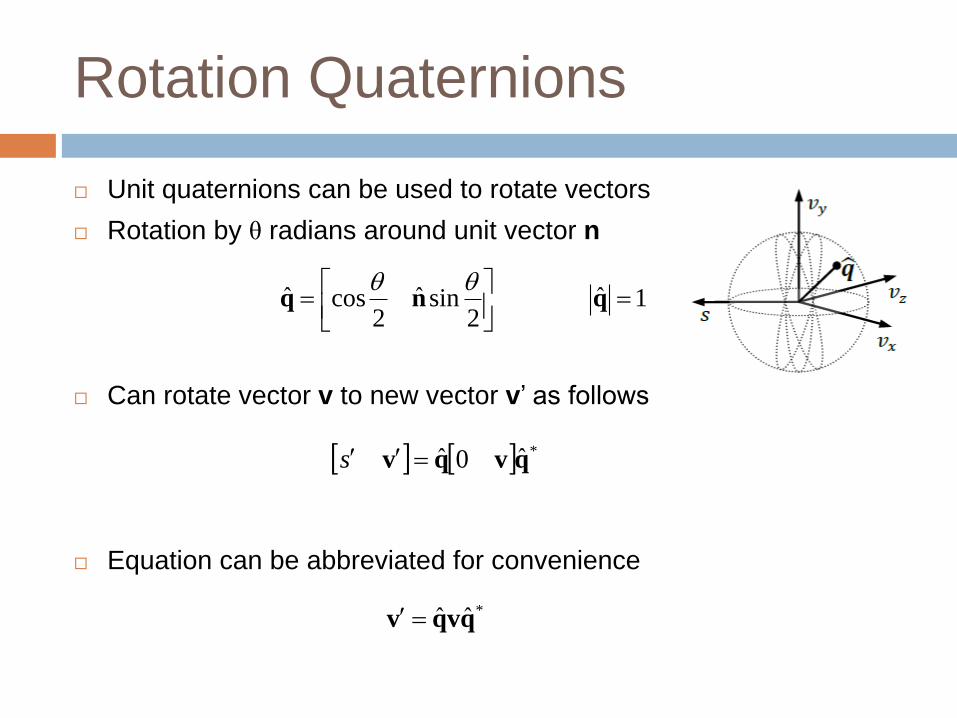
Rotation Quaternions
Unit quaternions can be used to rotate vectors
Rotation by θ radians around unit vector n
Can rotate vector v to new vector v’ as follows
Equation can be abbreviated for convenience
1ˆ2
sinˆ2
cosˆ
qnq
*ˆ0ˆ qvqv s
*ˆˆ qvqv

Quaternion-Based Orientation
Option 3: Quaternion Angles
φ expressed as a quaternion of unit norm
Angle of φ automatically falls within [-π.. π]
ω, α still expressed as scaled axis representations
Must wrap ω in quaternion to update φ
Angular velocity integration still computed as scalar
May need to renormalise φ after a while
ttαtωttω
tt
ttt φωφφ 02
2sinˆ
2cos,ˆ
nqφ n
φφ
φ1

Comparison of 3D Rotation Structures
Scaled Axis
Representations
3D Rotation
Matrices
Quaternion
Angles
Pros• Very compact representation (3
scalar elements)
• Very cheap computation
• Solves angle discontinuity
• Can reuse for visualisation or
cheaply convert to 4D
homogenous matrix
• Solves angle discontinuity
• Compact representation (4
scalar elements)
• Cheap ω conversion
• Reasonably cheap conversion
to matrix for visualisation
• Cheap renormalisation
Cons• Must handle angle discontinuity
• Very costly conversion to
3D/4D matrix for visualisation
• Wastes storage space (9 scalar
elements
• Expensive matrix computations
• Costly ω conversion
• Costly renormalisation
• Less compact than scaled axis
representation
• Visualisation matrix still needs
to be computed, but relatively
cheap

State Update (Take 2)
For each body
Get current linear and angular
acceleration (will tackle this next...)
Update position and orientation
Update linear and angular velocities
Handle collisions (will tackle this later...)
Update State ttttt vpp
ttttt avv
ttαtωttω
tt
ttt φωφφ 02

User / Agent Input
Human users / autonomous agents
influence physical simulation
Examples
User / AI controlling simulated vehicle
Natural phenomena (e.g. gravity or
friction)
Chain of events (e.g. collisions)
The above result in applied forces
Forces are source of linear and
angular acceleration
Process User
/ Agent Input

Force
Has magnitude and direction (is a vector)
Induce linear acceleration
Induce angular acceleration (when acting off-centre)
Thrusterf
Gravityf
Rotaryf
Rotaryf
Gravityf
FrictionfReactionf

Effects of Force
Force induces linear acceleration
Greater force => greater acceleration
Greater mass => lesser acceleration
Acceleration parallel to force
Application of multiple forces
Forces can be summed up as vectors
Can work in tandem or cancel out
faafm
eim1
..
i
iffTotal Totalf
1f
2f
3f

Torque
Torque is ‘angular’ force
Magnitude of torque vector gives scale
Direction gives axis of rotation
greater force => greater torque
greater perpendicular distance => greater torque
Scalar Form
Vector Form
fr sin
frτ
Note: c is centre of mass
fr
τc
sinr
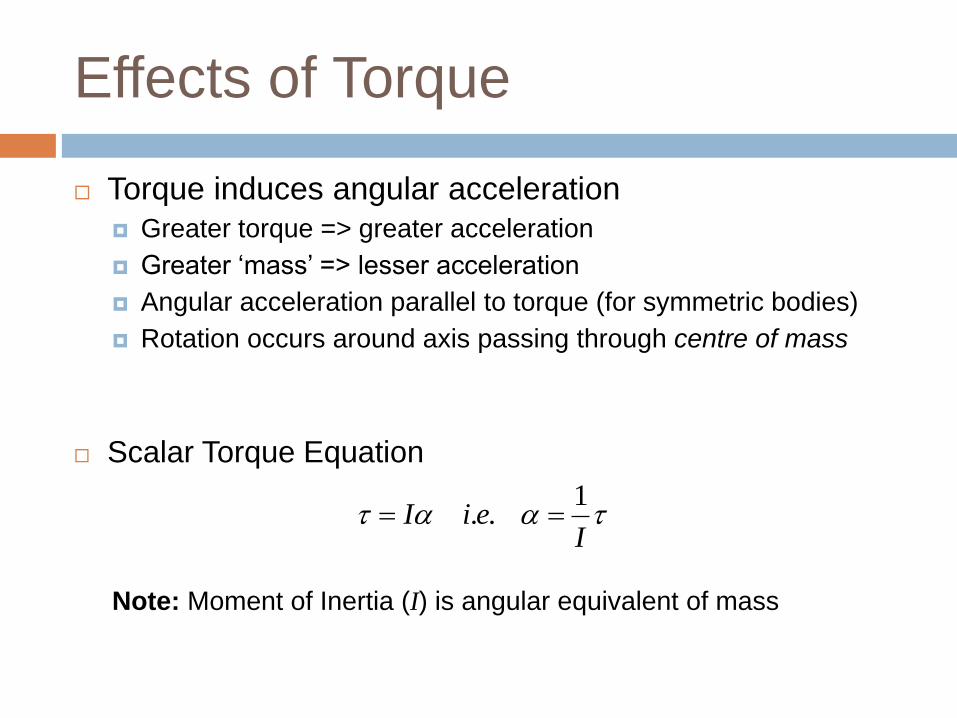
Effects of Torque
Torque induces angular acceleration
Greater torque => greater acceleration
Greater ‘mass’ => lesser acceleration
Angular acceleration parallel to torque (for symmetric bodies)
Rotation occurs around axis passing through centre of mass
Scalar Torque Equation
Note: Moment of Inertia (I) is angular equivalent of mass
I
eiI1
..

Centre of Mass
A point in (or outside) body around which mass is evenly distributed
System of point masses mi at positions ri
Continuous body mass m, density function ρ, volume V
i
i
i
ii
m
m r
c
V
dm
r
rrrc 1
X
Y 1m2m
3m
1r 2r
3r
c
X
Ym
cV

Centre of Mass Example
X
Y
kgm 11 kgm 22
m0.01 r m6.02 r
mmm
mm4.0
3
2.1
21
6.0201
21
2211
rrc
?c

Moment of Inertia
A measure of mass quantity and distribution around a given axis
(usually through centre of mass)
System of point masses mi at perp. distance ri from axis
Solid body with density function ρ, volume V
i
iirmI2
V
dIr
rrr2
1m
2m
3m1r
2r
3r
axis
X
Y
Vaxis

Moment of Inertia Example
kgm 11 kgm 22
mr 4.01
2222
22
2
11 36.04.022.01 kgmmm rrc
m4.0c
mr 2.02

General Torque Equations
For 2D, can use scalar forms of I, τ and α
For 3D
Axis of rotation varies over time
Moment of inertia needs to be recalculated every time
Torque must take axis into account
Elegant Solution:
the Inertia Tensor matrix I
vector form of the torque equations
τIαIατ 1.. ei
i
ii
i
i frττ total

Moment of Inertia Tensor
A 3 x 3 matrix of the form
Ixx, Iyy, Izz are principal moments of inertia around X, Y, Z axes
Ixy, Ixz, Iyx, Iyz, Izx, Izy are products of inertia, usually zero for symmetrical
bodies
zzzyzx
yzyyyx
xzxyxx
III
III
III
I
dVrrI zy
V
xx
22 r dVrrI zx
V
yy
22 r dVrrI yx
V
zz
22 r
dVrrII yx
V
yxxy r dVrrII zx
V
zxxz r
dVrrII zy
V
zyyz r

Inertia Tensor Example: Sphere
Solid sphere of uniform density, mass m, radius r
2
2
2
5
200
05
20
005
2
mr
mr
mr
I
2
5
2mrIII zzyyxx
0 zyyzzxxzyxxy IIIIII
X
Y
Z
r
xxI
yyI
zzI
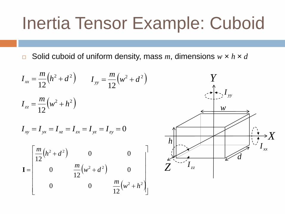
Inertia Tensor Example: Cuboid
Solid cuboid of uniform density, mass m, dimensions w × h × d
22
22
22
1200
012
0
0012
hwm
dwm
dhm
I
22
12dh
mI xx
0 zyyzzxxzyxxy IIIIII
22
12dw
mI yy
22
12hw
mI zz
X
Y
Z
w
xxI
yyI
zzI
h
d

Inertia Tensor Example: Cylinder
Solid cylinder of uniform density, mass m, height h, radius r
22
2
22
312
00
02
0
00312
hrm
mr
hrm
I
22312
hrm
II zzxx
0 zyyzzxxzyxxy IIIIII
X
Y
Z
xxI
yyI
zzI
2
2mrI yy
h
r

State Initialisation (Take 2)
For each body, initialise
Mass m
Moment of inertia tensor I
Position vector p
Orientation quaternion φ
Linear velocity vector v
Angular velocity vector ω
Initialise
State

User / Agent Input (Take 2)
For each body
Determine applied forces fi from user /
agent input
Accumulate force
Determine torques τi
Accumulate torque
Process User
/ Agent Input
i
iffTotal
iii frτ
i
iττ total

State Update (Take 3)
For each body
Compute linear and angular accelerations
Update position and orientation
Update linear and angular velocities
Update State
ttttt vpp
ttttt avv
ttαtωttω
tt
ttt φωφφ 02
total
1fa
m
total
1τIα

Collision Detection and Response
Need to prevent bodies from interpenetrating
Need to maintain realism
Two problems:
How to detect a collision?
What to do when a collision occurs?

Collision Detection
Bodies occupy volume in space
Collision occurs when volumes overlap on at least one point in space
Two possible approaches
Conservative Advancement: Estimate time of collision before it occurs
Retroactive Detection: Let bodies overlap and fix penetration afterwards

Conservative Advancement
In current state update
For all possible collisions, estimate time of impact Δtimpact (less than usual update interval Δt)
If there is such collision
update motion equations by Δtimpact (instead of Δt)
handle collision (e.g. update velocities)
resume normally
Otherwise if no collision
Update motion equations by Δt as usual
Problems of this approach
Time of impact estimation is harder than testing if bodies overlap
Simulation comes to virtual stop when lots of bodies in contact
More difficult to keep constant animation rate

Retroactive Collision Detection
In current state update
Update motion of all bodies by Δt
For each overlapping pair of bodies
Fix penetration (e.g. back off bodies to earlier position)
Handle collision (e.g. update velocities)
Problems with this approach
Must deal with interpenetration
Tunnelling problem (small bodies, high velocities, large Δt)
Stacking problem (will talk about this later...)

Collision Manifolds
Area of contact (manifold) between colliding bodies can be
a single point
a discreet number of points
a continuum of points (line / area)
a mix of the above
Common occurrences
corner with side (vertex – face)
edge with edge (edge – edge)
edge with surface (edge – face)
Other types (rare)
corner with corner
corner with edge
Lines / areas of contacts simplified to discreet points
point of contact line of contact
area of contact multiple areas of contact

Collision Detection Output
For each discreet point of collision we need
Point of contact
Location where collision has occurred
Contact normal vector ň
Direction of the collision
Penetration distance p
For resolving interpenetrationn̂
p

Sphere Collision Detection Example
Sphere 1, centre at p1, radius r1
Sphere 2, centre at p2, radius r2
Spheres in contact / overlapping when
If overlapping, then penetration p is
Contact normal ň is
Point of contact pc is (approximately)
1r
2r
1p
2p
d
2112 rrd pp
n̂
drrp 21
12
1ˆ ppn
d
cp
npp ˆ2
11
prc

Collision Detection Performance
Simplest solution: test all possible body pairs – n(n-1)/2
combinations!
Better approaches: partition space for better
performance, for example:
Regular grids
Quadtrees (2D) / octrees (3D)
KD-trees
co-ordinate sorting
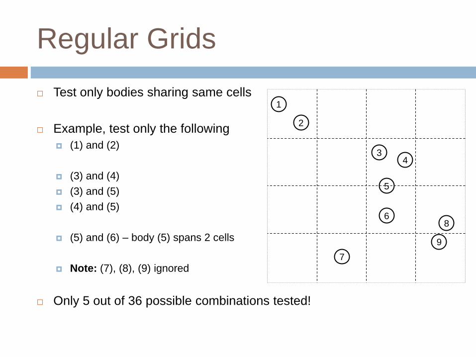
Regular Grids
Test only bodies sharing same cells
Example, test only the following
(1) and (2)
(3) and (4)
(3) and (5)
(4) and (5)
(5) and (6) – body (5) spans 2 cells
Note: (7), (8), (9) ignored
Only 5 out of 36 possible combinations tested!
1
2
34
5
6
7
8
9

Collision Response
In a real collision
Bodies undergo compression, followed by expansion before breaking contact, over short
period of time
During compression and expansion phases, repulsive forces (along contact normal)
accelerate bodies apart
Linear and angular velocities change gradually throughout collision
In a simulated collision between perfectly rigid bodies
We avoid simulating compression and expansion phases
We model repulsive force by instantaneous change in momentum (impulse)
Linear and angular velocities change instantly
22221111 nnnn mm vvJvvJ
1J2J

Coefficient of Restitution
In a frictionless rigid body collision, relative velocity of contact points
changes only along contact normal
is unaffected along perpendicular direction to normal (surface tangent)
Collision modelled by restitution coefficient e with value between 0 and 1
e = 1 => perfectly elastic collision
e = 0 => perfectly inelastic (sticky) collision
measured empirically e.g. wooden ball hitting concrete e ≈ 0.6
nnvvv
v
v
ˆ1ˆ e
en
n
tv
nv
nv
tv
v
vn̂

Collision Effects
Relative velocity of contact points changes according to coefficient e (as per
previous slide)
Can compute contact point velocity from linear and angular body velocity
Then compute relative velocity of contact points
Several substitutions later lead to...
bodycontactbodycontact ωrvv
bodyv
bodyω
pointv
pointrcontact1contact2 vvv r
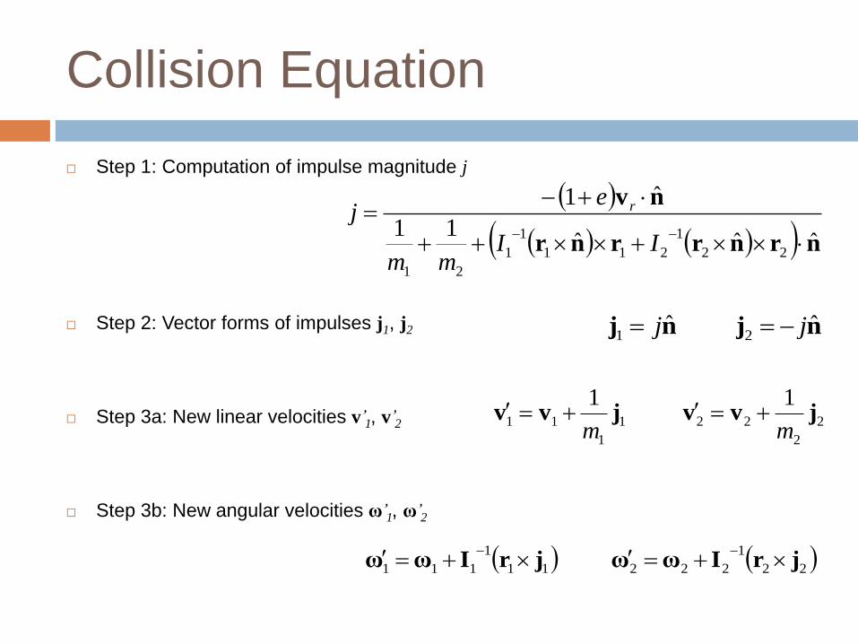
Collision Equation
Step 1: Computation of impulse magnitude j
Step 2: Vector forms of impulses j1, j2
Step 3a: New linear velocities v’1, v’2
Step 3b: New angular velocities ω’1, ω’2
nrnrrnr
nv
ˆˆˆ11
ˆ1
22
1
211
1
1
21
II
mm
ej r
njnj ˆˆ21 jj
2
2
221
1
11
11jvvjvv
mm
22
1
22211
1
111 jrIωωjrIωω

Solving Interpenetration
Option 1 (Simple)
Move each body away by half penetration along contact normal
Option 2 (Better)
Move each body away taking mass into consideration
Option 3 (Even Better)
Apply ‘impulse’ equation at positional level (handles rotation)
nppnpp ˆ2
ˆ2
2211
pp
nppnpp ˆˆ21
122
21
211 p
mm
mp
mm
m

Collision Algorithm
For each collision
(1) Compute collision impulse
(2) Update linear velocities
(3) Update angular velocities
(4) Solve body interpenetration
Problems
Solving one interpenetration may cause another
Cannot handle stacks of bodies

The Stacking Problem
Frame 0: Initial State Frame 1: Motion Frame 1: Collision Detection Frame 1: Collision Resolution
Frame 2: Motion Frame 2: Collision Detection Frame 2: Collision Resolution Frame 3: Motion
Frame 3: Collision Detection Frame 3: Collision Resolution After several frames... Stack topples!
...

Simultaneous Collision Resolution
All collisions considered simultaneously
Solves (or minimises) stacking problem
Various solutions (look up for fun...)
Shock Propagation
Iterative Solver
Linear Complementary Problem Formulation
Further Topics on Physics Animation
Simulating friction, for example: Static box on inclined plane
Tyre traction
Joints, for example: Ball-and-socket
Hinges
Motors
Modelling Forces, for example: Springs
Buoyancy

Some References
Physics Engines
http://en.wikipedia.org/wiki/Physics_engine
Collision Detection
http://en.wikipedia.org/wiki/Collision_detection
Collision Response
http://en.wikipedia.org/wiki/Collision_response
List of Inertia Tensors
http://en.wikipedia.org/wiki/List_of_moment_of_inertia_tensors
Octrees
http://en.wikipedia.org/wiki/Octree
Open Source / Free Physics Engines
http://www.thefreecountry.com/sourcecode/physics.shtml
Farseer Physics Engine (XNA Friendly)
http://www.farseergames.com/storage/farseerphysics/Manual2.1.htm