Embed Size (px)
Citation preview

Critical point in the phase diagram of primordial quark-gluon matter from black holephysics
Renato Critelli,1, ∗ Jorge Noronha,1, † Jacquelyn Noronha-Hostler,2, 3, ‡
Israel Portillo,3, § Claudia Ratti,3, ¶ and Romulo Rougemont4, ∗∗
1Instituto de Fısica, Universidade de Sao Paulo, Rua do Matao,1371, Butanta, CEP 05508-090, Sao Paulo, Sao Paulo, Brazil2Department of Physics and Astronomy, Rutgers University,
136 Frelinghuysen Rd, Piscataway, NJ 08854, USA3Department of Physics, University of Houston, Houston TX 77204, USA
4International Institute of Physics, Federal University of Rio Grande do Norte,Campus Universitario - Lagoa Nova, CEP 59078-970, Natal, Rio Grande do Norte, Brazil
Strongly interacting matter undergoes a crossover phase transition at high temperatures T ∼ 1012
K and zero net-baryon density. A fundamental question in the theory of strong interactions, Quan-tum Chromodynamics (QCD), is whether a hot and dense system of quarks and gluons displayscritical phenomena when doped with more quarks than antiquarks, where net-baryon number fluc-tuations diverge. Recent lattice QCD work indicates that such a critical point can only occur in thebaryon dense regime of the theory, which defies a description from first principles calculations. Herewe use the holographic gauge/gravity correspondence to map the fluctuations of baryon charge inthe dense quark-gluon liquid onto a numerically tractable gravitational problem involving the chargefluctuations of holographic black holes. This approach quantitatively reproduces ab initio resultsfor the lowest order moments of the baryon fluctuations and makes predictions for the higher orderbaryon susceptibilities and also for the location of the critical point, which is found to be within thereach of heavy ion collision experiments.
Keywords: Quark-gluon plasma, QCD phase diagram, phase transition, critical point, chemical freeze-out,holography, gauge/gravity duality, baryon chemical potential, finite temperature.
I. INTRODUCTION
The rapid crossover transition found in lattice QCDcalculations [1] characterizes the change in the degreesof freedom of the theory from hadrons to a novel de-confined state composed of quarks and gluons. The ex-treme conditions needed for this phenomenon took placein our Universe ∼ 20 microseconds after the Big Bang [2]and have been constantly reproduced over the last decadein ultrarelativistic heavy ion collisions at the Relativis-tic Heavy Ion Collider (RHIC) and the Large HadronCollider (LHC). These experiments have provided over-whelming evidence that at high temperatures quarks andgluons form a new type of strongly interacting liquidcalled the quark-gluon plasma (QGP) [3]. Since its dis-covery in the early 2000’s (see, e.g., Ref. [4] for a re-view), it has become clear that the femtoscopic versionof the primordial liquid recreated in these experimentspossesses novel many-body properties, including nearlyinviscid flow behavior characterized by a surprisinglysmall value [5] of its shear viscosity to entropy densityratio (η/s), which makes the QGP the smallest (and thehottest) most perfect fluid ever observed.
∗ [email protected]† [email protected]‡ [email protected]§ [email protected]¶ [email protected]∗∗ [email protected]
Despite the steady progress over the years in the de-termination of the QGP’s equilibrium properties throughlattice simulations, most regions of the QCD phase dia-gram remain vastly unexplored. In fact, ab initio calcula-tions in the baryon dense regime of QCD are hindered bythe fermion sign problem, a fundamental technical obsta-cle inherent to any path integral representation of Fermisystems at finite density [6]. By breaking the balancebetween baryonic matter and anti-matter at high tem-peratures in QCD, the crossover is expected to end at acritical end point (CEP) and then evolve into a first-orderphase transition. The CEP is characterized by the diver-gence of net-baryon number fluctuations. Understand-ing the emergence of critical phenomena in the theoryof strong interactions has become a cardinal challengenot only for theory but also for experiments. Dependingon the location of the CEP in the temperature (T ) andbaryon chemical potential (µB) axes of the QCD phasediagram, its effects may be probed using heavy ion colli-sions [7]. An experimentally-driven search for the QCDcritical point is possible [8] by systematically decreasingthe center-of-mass energy/per nucleon (
√s) of colliding
ion beams, which enhances the amount of matter overanti-matter produced in these reactions. The first phaseof such a beam energy scan (BES) program took placeat RHIC and future runs with increased luminosity arescheduled for 2019-2020 after an upgrade of the machine.Fixed target experiments, reaching even larger baryondensities, will become fully operational in the near fu-ture [9, 10].
In the absence of first principle lattice results in the
arX
iv:1
706.
0045
5v3
[nu
cl-t
h] 1
0 N
ov 2
017
2
baryon rich regime of QCD, effective approaches mustbe used to guide the experimental search for the criti-cal point in heavy ion collisions. To be deemed realistic,such models must meet the following necessary require-ments. First, the effective approaches must reproduce thethermodynamics of QCD in the crossover region at zerobaryon density, as determined by lattice QCD. The other(more stringent) requirement is that for the tempera-tures probed in heavy ion collisions the system behaves asnearly perfect liquid. In this work we show that a modelconstructed using the holographic correspondence [11], awell-known tool developed in string theory, fulfills theserequirements allowing one to determine the properties ofthe hot and baryon rich QGP liquid with unprecedentedprecision.
II. RESULTS
Through the holographic correspondence, calculationsin strongly coupled non-Abelian gauge theories in fourspace-time dimensions at finite temperature and densitycan be performed using black hole solutions of classi-cal theories of gravity in higher space-time dimensions.This approach has been previously applied to study someimportant aspects of the strongly coupled quark-gluonplasma [12] and also a variety of problems in condensedmatter physics [13]. One of its main successes is the ex-plicit derivation of nearly perfect fluid behavior at strongcoupling, quantified by η/s = 1/4π [14] (in natural unitswhere c = ~ = kB = 1), which is broadly compatible withrecently extracted bounds for this quantity in heavy ioncollisions [15].
In the holographic approach used in this work, confor-mal invariance in the plasma is dynamically broken by areal scalar field in the bulk, which roughly takes into ac-count effects from the QCD running coupling, and an ad-ditional U(1) gauge field is introduced in the dual gravitymodel to simulate the baryon charge and its correspond-ing chemical potential µB . A similar approach was usedin [16], but contrary to that case, our construction pro-vides a self-consistent gravitational setup with no extrafree parameters besides the ones already featured in thegravity action. We numerically solve the correspondingfive dimensional holographic equations of motion for themetric, the scalar field, and the gauge field to constructover two million charged black hole solutions (see the ap-pendix), each one of them corresponding to a point inthe T − µB phase diagram of the dual strongly coupledplasma. The parameters of the dual gravitational theoryare fixed in order to reproduce two crucial quantities ob-tained through lattice simulations of QCD with 2+1 fla-vors with physical quark masses at zero baryon density:the entropy density [17] and the second-order baryon sus-ceptibility [18] χ2, which measures the equilibrium re-sponse of the baryonic density to a change in the chem-ical potential. After imposing these constraints at zerobaryon density, the model correctly predicts many other
thermodynamic quantities compared to Lattice QCD atµB = 0. Additionally, predictions can also be made forthe behavior of thermodynamic and transport quantitiesat finite µB . This procedure, which we call black holeengineering, is uniquely suited to investigate the baryonrich regime of QCD since it not only quantitatively repro-duces the relevant results from the theory of strong inter-actions at finite temperature, but it also naturally incor-porates the nearly perfect fluid property of the plasma(see the appendix).
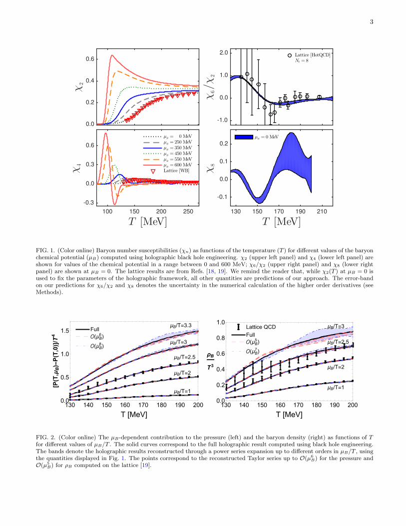
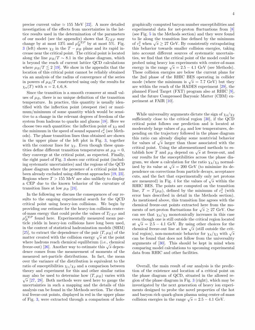
In the vicinity of the critical point, the higher orderbaryon number susceptibilities defined as χn(T, µB) =∂n(P/T 4)/∂(µB/T )n, where P = P (T, µB) is the pres-sure of the system, diverge with different powers of thecorrelation length ξ [20]. To investigate the onset of crit-ical behavior, after determining the pressure via holog-raphy, numerical derivatives are taken to determine thesecond, fourth, sixth, and eight order baryon number sus-ceptibilities shown in Fig. 1. One can see that χ2(T, µB)begins to develop a peak for large chemical potentials,which will then evolve into a divergence at the criticalpoint. The figure also shows the available lattice resultsfor χ2, χ4 [18] and χ6/χ2 [19] as a function of T . Ourpredictions for χ4(T ) and χ6(T )/χ2(T ) have a remark-able agreement with lattice QCD results. As for χ8(T ),our prediction exhibits the features expected from uni-versality arguments [21] and can be readily compared tolattice QCD results once they become available.
Using the higher order susceptibilities one may recon-struct the system’s pressure and baryon density ρB =χ1T
3 as a Taylor series in powers of µB/T as follows
P (T, µB)− P (T, µB = 0)
T 4=
∞∑n=1
1
(2n!)χ2n(T )
(µBT
)2n
,
(1)
ρB(T, µB)
T 3=
∞∑n=1
1
(2n− 1)!χ2n(T )
(µBT
)2n−1
. (2)
In Fig. 2 the pressure difference in (1), calculated in theholographic model with no truncations, is compared tothe lattice QCD results from Ref. [19]. Additionally,the reconstructed holographic pressure truncated at or-der O(µ6
B) and O(µ8B) is also shown (the bands reflect
the numerical uncertainties in the calculations of χ6(T )and χ8(T ), see Methods). Our analysis not only confirmsthe applicability of the O(µ6
B) truncation done in [19] forµB/T ≤ 2 but it also predicts that the inclusion of χ8(T )into the expansion extends the domain of applicability ofthe Taylor series to at least µB/T ∼ 2.5 (further discus-sion can be found in the appendix).
By carefully inspecting the behavior of χ2 and ρB , us-ing the best set of parameters for the holographic model(see the appendix), we find a critical point in the phasediagram at TCEP = 89 MeV and µCEPB = 724 MeV,which should be compared to the original holographicstudy in Ref. [16] that found (TCEP , µ
CEPB ) = (143, 783)
MeV using previous lattice results for which the transi-tion temperature was ∼ 190 MeV, instead of the more
3
T [MeV]100 150 200 250
χ4
-0.3
0.0
0.3
0.6
µB = 0 MeVµB = 250 MeVµB = 350 MeVµB = 450 MeVµB = 550 MeVµB = 600 MeVLattice [WB]
χ2
0.0
0.2
0.4
0.6
T [MeV]130 150 170 190 210
χ8
-0.1
0.0
0.1
0.2
µB = 0 MeV
χ6/χ
2
-1.0
0.0
1.0
2.0 Lattice [HotQCD]Nt = 8
FIG. 1. (Color online) Baryon number susceptibilities (χn) as functions of the temperature (T ) for different values of the baryonchemical potential (µB) computed using holographic black hole engineering. χ2 (upper left panel) and χ4 (lower left panel) areshown for values of the chemical potential in a range between 0 and 600 MeV; χ6/χ2 (upper right panel) and χ8 (lower rightpanel) are shown at µB = 0. The lattice results are from Refs. [18, 19]. We remind the reader that, while χ2(T ) at µB = 0 isused to fix the parameters of the holographic framework, all other quantities are predictions of our approach. The error-bandon our predictions for χ6/χ2 and χ8 denotes the uncertainty in the numerical calculation of the higher order derivatives (seeMethods).
μB/T=1
μB/T=2
μB/T=2.5
μB/T=3
μB/T=3.3Full
(μB6 )
(μB8 )
130 140 150 160 170 180 190 2000.0
0.5
1.0
1.5
T [MeV]
[P(T,μB)-P(T,0)]/T4
μB/T=1
μB/T=2
μB/T=2.5
μB/T=3
Full
(μB5 )
(μB7 )
Lattice QCD
130 140 150 160 170 180 190 2000.0
0.2
0.4
0.6
0.8
1.0
T [MeV]
ρB
T3
FIG. 2. (Color online) The µB-dependent contribution to the pressure (left) and the baryon density (right) as functions of Tfor different values of µB/T . The solid curves correspond to the full holographic result computed using black hole engineering.The bands denote the holographic results reconstructed through a power series expansion up to different orders in µB/T , usingthe quantities displayed in Fig. 1. The points correspond to the reconstructed Taylor series up to O(µ6
B) for the pressure andO(µ5
B) for ρB computed on the lattice [19].
4
precise current value ' 155 MeV [22]. A more detailedinvestigation of the effects from uncertainties in the lat-tice results used in the determination of the parametersof our model (see the appendix) shows that TCEP maychange by at most 13% and µCEPB by at most 5%. Fig.3 (left) shows χ2 in the T − µB plane and its rapid in-crease near the critical point. The critical point is locatedalong the line µB/T ∼ 8.1 in the phase diagram, whichis beyond the reach of current lattice QCD calculationswhere µB/T . 2 [19]. We show in the appendix that thelocation of this critical point cannot be reliably obtainedvia an analysis of the radius of convergence of the seriesin powers of µB/T constructed using only the results forχn(T ) with n = 2, 4, 6, 8.
Since the transition is a smooth crossover at small val-ues of µB , there is no unique definition of the transitiontemperature. In practice, this quantity is usually iden-tified with the inflection point (steepest rise) or maxi-mum/minimum of some quantity which would be sensi-tive to a change in the relevant degrees of freedom of thesystem from hadrons to quarks and gluons [18]. Here wechoose two such quantities: the inflection point of χ2 andthe minimum in the speed of sound squared c2s (see Meth-ods). The phase transition lines thus obtained are shownin the upper plane of the left plot in Fig. 3, togetherwith the contour lines for χ2. Even though these quan-tities define different transition temperatures at µB = 0,they converge at the critical point, as expected. Finally,the right panel of Fig. 3 shows our critical point (includ-ing systematic uncertainties) and the regions of the QCDphase diagram where the presence of a critical point hasbeen already excluded using different approaches [19, 23].Regions where T > 155 MeV are also unlikely to displaya CEP due to the known behavior of the curvature oftransition lines at low µB [24].
In the following we discuss the consequences of our re-sults to the ongoing experimental search for the QCDcritical point using heavy-ion collisions. We begin byproviding our estimate for the heavy-ion collision center-of-mass energy that could probe the values of TCEP andµCEPB found here. Experimentally measured mean par-ticle yields in heavy-ion collisions have long been used,in the context of statistical hadronization models (SHM)[25], to extract the dependence of the pair (T, µB) of thematter created with the collision energy
√s at the point
where hadrons reach chemical equilibrium (i.e., chemicalfreeze-out) [26]. Another way to estimate this
√s depen-
dence comes from the measurement of moments of themeasured net-particle distributions. In fact, the meanover the variance of the distribution is equivalent to theratio of susceptibilities χ1/χ2 and a comparison betweentheory and experiment for this and other similar ratiosmay also be used to determine how (T, µB) varies with√s [27, 28]. Both methods were used here to gauge the
uncertainties in such a mapping and the details of thisanalysis can be found in the Methods section. The chem-ical freeze-out points, displayed in red in the upper planeof Fig. 3, were extracted through a comparison of holo-
graphically computed baryon number susceptibilities andexperimental data for net-proton fluctuations from [8](see Fig. 5 in the Methods section) and they were foundto lie along the transition line defined by the minimumof c2s when
√s ≥ 27 GeV. By consistently extrapolating
this behavior towards smaller collision energies, takinginto account different sources of systematic uncertain-ties, we find that the critical point of the model could beprobed using heavy ion experiments with center-of-massenergy in the range
√s = 2.5 − 4.1 GeV (see Methods).
These collision energies are below the current plans forthe 2nd phase of the RHIC BES operating in collidermode (where the minimum is
√s = 7.7 GeV) but they
are within the reach of the HADES experiment [29], theplanned Fixed Target (FXT) program also at RHIC [9],and the future Compressed Baryonic Matter (CBM) ex-periment at FAIR [10].
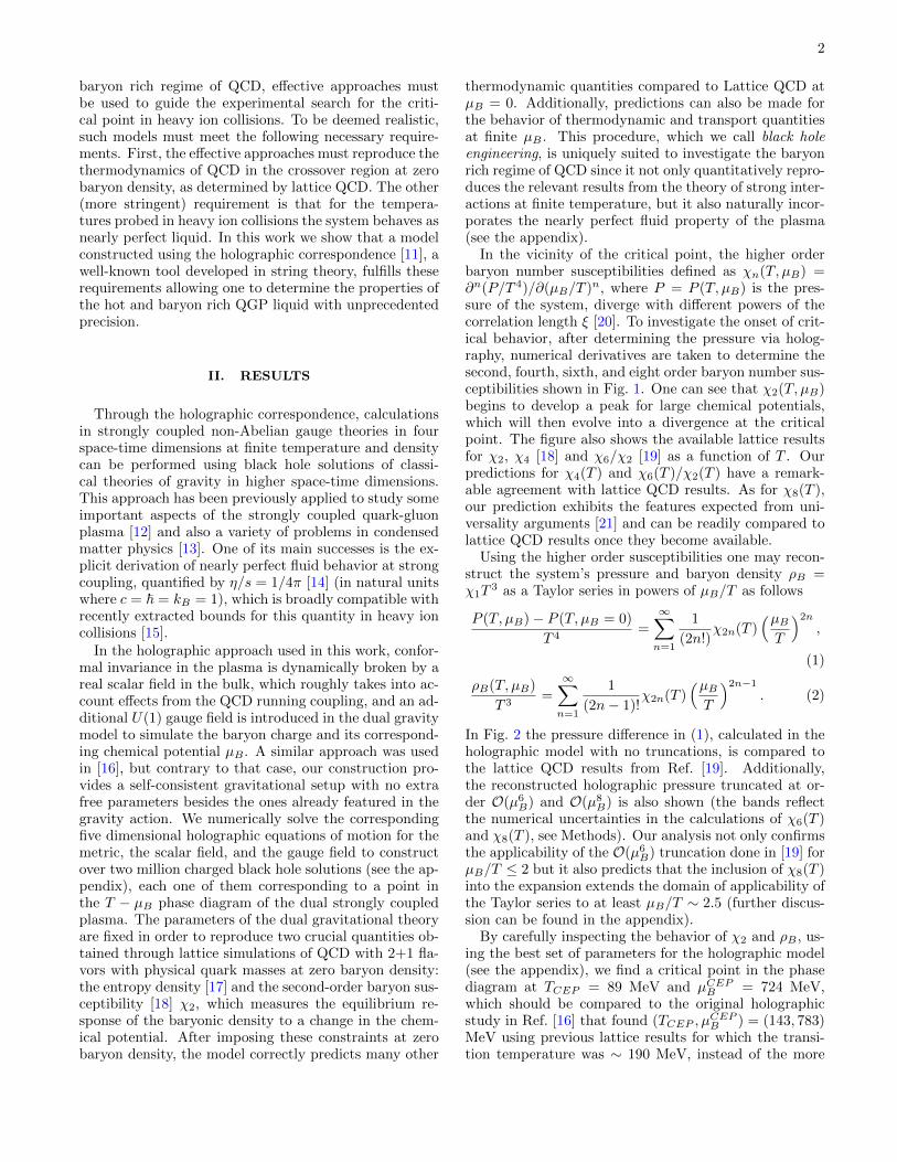
While universality arguments dictate the sign of χ4/χ2
sufficiently close to the critical region [30], if the QCDcritical point follows our prediction and is located atmoderately large values of µB and low temperatures, de-pending on the trajectory followed in the phase diagramthis ratio can already display some nontrivial behaviorfor values of
√s larger than those associated with the
critical point. Using the aforementioned methods to es-tablish how T and µB depend on
√s at freeze-out, and
our results for the susceptibilities across the phase dia-gram, we show a calculation for the ratio χ4/χ2 normal-ized by its value at
√s = 200 GeV (to minimize its de-
pendence on corrections from particle decays, acceptancecuts, and the fact that experimentally only net protonsare measured) in Fig. 4 for the values of
√s within the
RHIC BES. The points are computed on the transitionline, T = T (µB), defined by the minimum of c2s (witherror bars described in detail in the Methods section).As mentioned above, this transition line agrees with thechemical freeze-out points extracted here from the mo-ments of net-proton fluctuations for
√s ≥ 27 GeV. One
can see that χ4/χ2 monotonically increases in this caseeven though one is still outside the critical region locatedat√s = 2.5 − 4.1 GeV. By using other choices for the
chemical freeze-out line at low√s (still outside the crit-
ical region), non-monotonic behavior for χ4/χ2 with√s
can be found that does not follow from the universalityarguments of [30]. This should be kept in mind whencomparing model calculations to upcoming experimentaldata from RHIC and other facilities.
Overall, the main result of our analysis is the predic-tion of the existence and location of a critical point onthe phase diagram of QCD, situated in the allowed re-gion of the phase diagram in Fig. 3 (right), which may beinvestigated by the next generation of heavy ion experi-ments designed to probe the novel properties of the hotand baryon rich quark-gluon plasma using center-of-masscollision energies in the range
√s = 2.5− 4.1 GeV.

5
●●
CEP
Black Hole
Engineering
Lattice QCD
Finite-Size Scaling
Unlikely due to
transition line curvature
Allowed Region
0 200 400 600 8000
50
100
150
200
μB [MeV]
T[MeV]
FIG. 3. (Color online) The left plot shows the behavior of the baryon susceptibility χ2 in the T − µB plane determined fromblack hole engineering. As the chemical potential increases χ2(T, µB) develops a peak, which turns into a divergence at thecritical point located at TCEP = 89 MeV and µCEPB = 724 MeV (see the appendix). The upper plane in the left plot showsthe phase diagram obtained through our method, with our chemical freeze-out points in red. The dashed line corresponds tothe location of the inflection point of χ2 in the T − µB plane, one of the quantities chosen to characterize the phase transitionline. The dotted line gives the location of the minimum of the speed of sound squared, c2s, in the phase diagram. The rightpanel shows the regions in the QCD phase diagram where the presence of a critical point has been excluded by current latticeQCD constraints [19] and a finite-size scaling analysis [23]. Temperatures above 155 MeV are also unlikely due to constraintsfrom the curvature of transition lines [24]. The location of the critical point in the phase diagram that we found in this work,taking into account our systematic uncertainties (see the appendix), is also shown.
III. METHODS
Numerical calculation of higher order baryonnumber susceptibilities
The higher order baryon susceptibilities may also becomputed through the derivatives of the baryon density,which is proportional to the first baryonic susceptibility(χ1), with respect to µB/T for fixed T . The baryon den-sity is calculated using N = 2 × 10⁶ holographic blackhole solutions (see the appendix). The original data setfor χ1 is not equally spaced in the (T, µB) plane and anadditional procedure has to be used to determine χ1 ona regular grid. This is done by interpolating χ1 and thencomputing its value on an equally spaced grid. The highprecision derivatives themselves are calculated within asmaller range of temperatures and chemical potentials inthe interval T = [65−450] MeV and µB = [0−600] MeV.A master grid is created in the (T, µB) plane, which isdivided into square nodes of width ∆T = 5 MeV and∆µB = 20 MeV. Each node is individually interpolatedusing the points inside the node and its neighbor nodesusing thin-plate splines. The thin-plate splines interpo-lation was chosen over nearest neighbor, polynomial, cu-bic spline, and bi-harmonic interpolations because it pro-vided the best surface interpolation for the baryonic sus-ceptibilities. The neighbor node points are used to elimi-nate boundary effects in the interpolation. On the master
grid, we create extra nodes outside its boundary and im-pose several constraints. For the µB = 0 axis we reflectthe points depending on the symmetry of the given sus-ceptibility (even (odd) susceptibilities have even (odd)parity when reflected along the µB = 0 axis). For theT = 65 MeV axis, the extra nodes are set to zero, whilefor the other two axes, (µB = 600 MeV and T = 450MeV), the nodes are set to have a constant derivativeequal to the value of the one at the corresponding bound-ary of the master grid. Using this interpolation scheme,χ1 is obtained via the master grid using an equally spacedgrid of points with separation 0.25 MeV in T and µB .
The next order susceptibility, in this case χ2, is also ob-tained from the interpolation scheme; however this sus-ceptibility, which is the derivative with respect to µB ofthe interpolated points for χ1, contains noise associatedwith the interpolation. The noise makes it impossibleto calculate the next derivative (χ3) starting from thisraw data set for χ2 and a filtering procedure must beemployed. In this paper the noise is removed by using aSavitzky-Golay (SG) filter, a low-pass filter well adaptedfor smoothing out noisy data. Once the filter has beenapplied to the signal, a smooth χ2 is available to seedthe master grid, which will then repeat the procedure tocalculate the next susceptibility.
The SG-filter preserves the original shape and featuresof the signal better than other common types of filters.This method performs a least squares fit of the NT and
6
●●●●
●
●
●
●
●
●
●
Black Hole Engineering
One possible trajectory along min. cs
2
101 1020.5
1.0
1.5
2.0
2.5
3.0
3.5
s [GeV]
(χ4/χ
2) n
orm
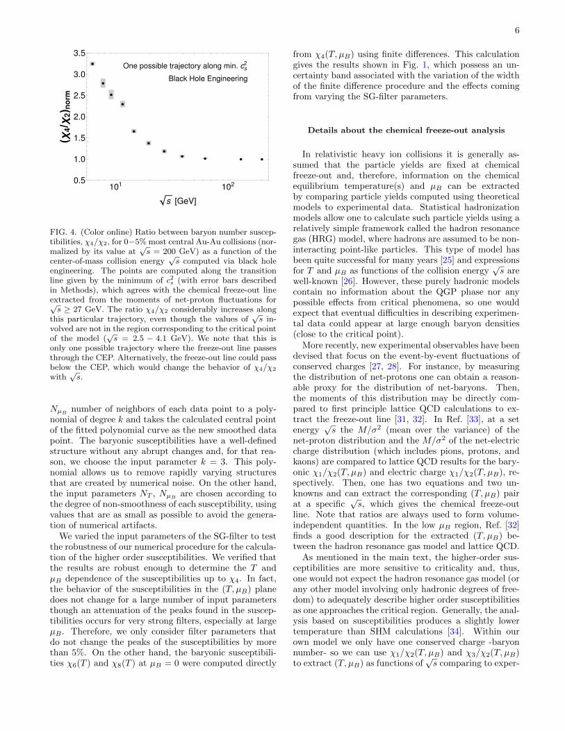
FIG. 4. (Color online) Ratio between baryon number suscep-tibilities, χ4/χ2, for 0−5% most central Au-Au collisions (nor-malized by its value at
√s = 200 GeV) as a function of the
center-of-mass collision energy√s computed via black hole
engineering. The points are computed along the transitionline given by the minimum of c2s (with error bars describedin Methods), which agrees with the chemical freeze-out lineextracted from the moments of net-proton fluctuations for√s ≥ 27 GeV. The ratio χ4/χ2 considerably increases along
this particular trajectory, even though the values of√s in-
volved are not in the region corresponding to the critical pointof the model (
√s = 2.5 − 4.1 GeV). We note that this is
only one possible trajectory where the freeze-out line passesthrough the CEP. Alternatively, the freeze-out line could passbelow the CEP, which would change the behavior of χ4/χ2
with√s.
NµBnumber of neighbors of each data point to a poly-
nomial of degree k and takes the calculated central pointof the fitted polynomial curve as the new smoothed datapoint. The baryonic susceptibilities have a well-definedstructure without any abrupt changes and, for that rea-son, we choose the input parameter k = 3. This poly-nomial allows us to remove rapidly varying structuresthat are created by numerical noise. On the other hand,the input parameters NT , NµB
are chosen according tothe degree of non-smoothness of each susceptibility, usingvalues that are as small as possible to avoid the genera-tion of numerical artifacts.
We varied the input parameters of the SG-filter to testthe robustness of our numerical procedure for the calcula-tion of the higher order susceptibilities. We verified thatthe results are robust enough to determine the T andµB dependence of the susceptibilities up to χ4. In fact,the behavior of the susceptibilities in the (T, µB) planedoes not change for a large number of input parametersthough an attenuation of the peaks found in the suscep-tibilities occurs for very strong filters, especially at largeµB . Therefore, we only consider filter parameters thatdo not change the peaks of the susceptibilities by morethan 5%. On the other hand, the baryonic susceptibili-ties χ6(T ) and χ8(T ) at µB = 0 were computed directly
from χ4(T, µB) using finite differences. This calculationgives the results shown in Fig. 1, which possess an un-certainty band associated with the variation of the widthof the finite difference procedure and the effects comingfrom varying the SG-filter parameters.
Details about the chemical freeze-out analysis
In relativistic heavy ion collisions it is generally as-sumed that the particle yields are fixed at chemicalfreeze-out and, therefore, information on the chemicalequilibrium temperature(s) and µB can be extractedby comparing particle yields computed using theoreticalmodels to experimental data. Statistical hadronizationmodels allow one to calculate such particle yields using arelatively simple framework called the hadron resonancegas (HRG) model, where hadrons are assumed to be non-interacting point-like particles. This type of model hasbeen quite successful for many years [25] and expressionsfor T and µB as functions of the collision energy
√s are
well-known [26]. However, these purely hadronic modelscontain no information about the QGP phase nor anypossible effects from critical phenomena, so one wouldexpect that eventual difficulties in describing experimen-tal data could appear at large enough baryon densities(close to the critical point).
More recently, new experimental observables have beendevised that focus on the event-by-event fluctuations ofconserved charges [27, 28]. For instance, by measuringthe distribution of net-protons one can obtain a reason-able proxy for the distribution of net-baryons. Then,the moments of this distribution may be directly com-pared to first principle lattice QCD calculations to ex-tract the freeze-out line [31, 32]. In Ref. [33], at a setenergy
√s the M/σ2 (mean over the variance) of the
net-proton distribution and the M/σ2 of the net-electriccharge distribution (which includes pions, protons, andkaons) are compared to lattice QCD results for the bary-onic χ1/χ2(T, µB) and electric charge χ1/χ2(T, µB), re-spectively. Then, one has two equations and two un-knowns and can extract the corresponding (T, µB) pairat a specific
√s, which gives the chemical freeze-out
line. Note that ratios are always used to form volume-independent quantities. In the low µB region, Ref. [32]finds a good description for the extracted (T, µB) be-tween the hadron resonance gas model and lattice QCD.
As mentioned in the main text, the higher-order sus-ceptibilities are more sensitive to criticality and, thus,one would not expect the hadron resonance gas model (orany other model involving only hadronic degrees of free-dom) to adequately describe higher order susceptibilitiesas one approaches the critical region. Generally, the anal-ysis based on susceptibilities produces a slightly lowertemperature than SHM calculations [34]. Within ourown model we only have one conserved charge -baryonnumber- so we can use χ1/χ2(T, µB) and χ3/χ2(T, µB)to extract (T, µB) as functions of
√s comparing to exper-
7
imental data of M/σ2 and Sσ (skewness times standarddeviation) of the net-proton distribution. We compareour results for χ1/χ2 at freeze-out to the mean over thevariance (M/σ2) of net-protons and χ3/χ2 to the skew-ness times the variance (Sσ) of net-protons measured bySTAR [8] in Fig. 5. This could not be done in the hadronresonance gas model where χ1/χ2 ∼ χ3/χ2 ∼ 1 and, infact, hadronic models are known to miss the
√s depen-
dence of higher order susceptibilities [8]. One can see thatour results can be reasonably matched to STAR data.
When comparing χ1/χ2(T, µB) to M/σ2 andχ3/χ2(T, µB) to Sσ, one produces two different bands in(T, µB) after the inclusion of the experimental error. Wethen look for the point where either the bands overlap(or their nearest point) to extract the correspondingfreeze-out pair (T, µB) at a certain
√s and our error bars
are extracted from the width of the two bands at thatpoint. We remark that we are aware of the limitations ofour model, which does not include strangeness or electriccharge chemical potentials, or the acceptance cuts whichmatch the experimental setup. For these reasons, whenextracting the chemical freeze-out points we limit ouranalysis to the large collision energies
√s ≥ 27 GeV
where such effects are expected to be small. In the end,we find chemical freeze-out temperatures and chemicalpotentials which are compatible to the ones obtainedfrom the analysis of fluctuations in the HRG model [34]and lattice QCD [32].
In Fig. 6 (left) we show µB(√s) (purple squares) ex-
tracted using the susceptibilities calculated within theHRG model [34]; T (
√s) for the same model is shown on
the right panel. Our results using black hole engineeringand χ1/χ2 and χ3/χ2 to extract µB as a function of
√s
lead to the red triangles shown in Fig. 6, which are com-patible with the results from the statistical hadroniza-tion models [26] (SHM1) and [35] (SHM2). Thus, in or-der to estimate µB(
√s) at lower energies we use the two
parametrizations, SHM1 and SHM2, mentioned above.In Fig. 6 (right) T (
√s) from SHM1 is shown in solid
black.
Another method to determine the phase transitionfrom the QGP to the hadron gas phase involves lookingat inflection points or extrema of thermodynamic quan-tities. Thus, we also consider the minimum of c2s, whichallows us to determine a different curve T = T (µB) inthe phase diagram. Using the two SHM parametriza-tions for µB(
√s) one obtains the solid and dashed blue
T (√s) curves, which are shown in Fig. 6 (right). We note
that our freeze-out points for√s ≥ 27 GeV lie along this
c2s transition line. In our calculations of the normalizedratio χ4/χ2 of net-baryon number shown in Fig. 4 we in-cluded both the different transition lines defined by theminimum of c2s and the inflection point of χ2 and also thedifference between the two different SHM parametriza-tions for µB(
√s) into our error bars. Furthermore, in
Fig. 6 one can find the vertical colored bands we usedto estimate the values of
√s corresponding to TCEP and
µCEPB of the critical point, which include the combined ef-
fect from uncertainties coming from the parametrizationsT (√s) and µB(
√s) and also the other sources of uncer-
tainty associated with the holographic calculations dis-cussed in the appendix. The latter generate the dashedhorizontal lines in Fig. 6 while the vertical colored bandsare obtained by finding the values of
√s in both plots
where these horizontal lines cross the T (√s) and µB(
√s)
curves from statistical models and from our curve corre-sponding to the minimum of c2s. The final range for thevalues of
√s corresponding to the critical point region
mentioned in the main text,√s = 2.5 − 4.1 GeV, is ob-
tained by combining the colored systematic uncertaintybands in Fig. 6 (right).
ACKNOWLEDGMENTS
We thank R. Bellwied, P. Parotto, and K. Meehan forhelpful comments and S. Sharma for providing the ta-bles that contain the publicly available results of Ref.[19]. J.N., R.R., and R.C. thank S. Finazzo for insight-ful discussions on the gauge/gravity duality at nonzerobaryon density. J.N. thanks the Fundacao de Am-paro a Pesquisa do Estado de Sao Paulo (FAPESP)and Conselho Nacional de Desenvolvimento Cientıfico eTecnologico (CNPq) for support. R.C. was supportedby FAPESP grant 2016/09263-2. R.R. acknowledgesfinancial support by Fundacao Norte Riograndense dePesquisa e Cultura (FUNPEC). This material is basedupon work supported by the National Science Founda-tion under grant no. PHY-1654219 and OAC-1531814and by the U.S. Department of Energy, Office of Sci-ence, Office of Nuclear Physics, within the framework ofthe Beam Energy Scan Theory (BEST) Topical Collab-oration. The authors gratefully acknowledge the use ofthe Maxwell Cluster and the advanced support from theCenter of Advanced Computing and Data Systems at theUniversity of Houston.
APPENDIX
In this appendix we give the details of the work pre-sented in the main text and also provide some additionaldiscussion about the topics covered. This is done in threemain sections. In Section A we discuss in detail the holo-graphic model we used, how the equations of motion aresolved, and also how its parameters are fixed. We showthe comparison to lattice thermodynamic data at zerochemical potential, extend the analysis to nonzero chem-ical potential, and discuss how to estimate the uncertain-ties in the location of the critical point in our holographicmodel. In Section B we give additional details about thecomparison of our model calculations at finite chemicalpotential to the available lattice calculations. In SectionC an analysis of the radius of convergence of the Tay-lor series for the thermodynamic quantities in powers ofµB/T is performed.
8
√
s [GeV]10
110
2
χ1/χ2
0.0
0.2
0.4
0.6
0.8
1.0
√
s [GeV]10
110
2
χ3/χ2
0.0
0.2
0.4
0.6
0.8
1.0 STARBH
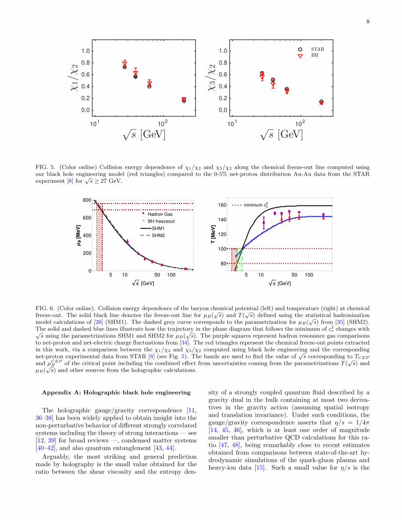
FIG. 5. (Color online) Collision energy dependence of χ1/χ2 and χ3/χ2 along the chemical freeze-out line computed usingour black hole engineering model (red triangles) compared to the 0-5% net-proton distribution Au-Au data from the STARexperiment [8] for
√s ≥ 27 GeV.
Hadron Gas
SHM1
SHM2
BH freezeout
5 10 50 1000
200
400
600
800
s [GeV]
μB[M
eV]
△ △ △ △■
■ ■ ■ ■■
minimum cs
2
5 10 50 100
80
100
120
140
160
s [GeV]
T[M
eV]
FIG. 6. (Color online). Collision energy dependence of the baryon chemical potential (left) and temperature (right) at chemicalfreeze-out. The solid black line denotes the freeze-out line for µB(
√s) and T (
√s) defined using the statistical hadronization
model calculations of [26] (SHM1). The dashed grey curve corresponds to the parametrization for µB(√s) from [35] (SHM2).
The solid and dashed blue lines illustrate how the trajectory in the phase diagram that follows the minimum of c2s changes with√s using the parametrizations SHM1 and SHM2 for µB(
√s). The purple squares represent hadron resonance gas comparisons
to net-proton and net-electric charge fluctuations from [34]. The red triangles represent the chemical freeze-out points extractedin this work, via a comparison between the χ1/χ2 and χ3/χ2 computed using black hole engineering and the correspondingnet-proton experimental data from STAR [8] (see Fig. 5). The bands are used to find the value of
√s corresponding to TCEP
and µCEPB of the critical point including the combined effect from uncertainties coming from the parametrizations T (√s) and
µB(√s) and other sources from the holographic calculations.
Appendix A: Holographic black hole engineering
The holographic gauge/gravity correspondence [11,36–38] has been widely applied to obtain insight into thenon-perturbative behavior of different strongly correlatedsystems including the theory of strong interactions — see[12, 39] for broad reviews —, condensed matter systems[40–42], and also quantum entanglement [43, 44].
Arguably, the most striking and general predictionmade by holography is the small value obtained for theratio between the shear viscosity and the entropy den-
sity of a strongly coupled quantum fluid described by agravity dual in the bulk containing at most two deriva-tives in the gravity action (assuming spatial isotropyand translation invariance). Under such conditions, thegauge/gravity correspondence asserts that η/s = 1/4π[14, 45, 46], which is at least one order of magnitudesmaller than perturbative QCD calculations for this ra-tio [47, 48], being remarkably close to recent estimatesobtained from comparisons between state-of-the-art hy-drodynamic simulations of the quark-gluon plasma andheavy-ion data [15]. Such a small value for η/s is the

9
defining property of the QGP produced by collidingheavy nuclei at RHIC and LHC [4, 5, 49–54].
The fact that η/s in the strongly coupled regime of theQGP appears to be in the ballpark of the holographic re-sult [14] greatly increased the interest in applications ofholographic models to the study of real time phenomenain the strongly coupled QGP, which are otherwise in-accessible to weak coupling techniques and are also verychallenging to first principle lattice QCD simulations [55]both at zero and nonzero baryon density [6, 56]. On theother hand, most of the holographic studies conducted inthis regard [12, 39] have focused on studying propertiesof the so-called N = 4 super Yang-Mills (SYM) plasma,which turns out to be fairly different than the real-worldQGP, especially in the crossover region [1, 57] where theQGP is highly nonconformal (see, for instance, the dis-cussion in [58]).
More recently, bottom-up dilatonic gauge/gravity du-als have been engineered with the aim of providing arealistic description of the physics of the nonconformalQGP [59]. These constructions are mainly based on thecoupling between the bulk metric field gµν and a realscalar field φ (which may be thought of as the dilaton),with the latter being responsible to break the conformalsymmetry of the theory in the infrared regime, emulat-ing the effects of a dynamically generated ΛQCD scale.This dynamical breaking of the conformal symmetry iscontrolled in the holographic model by the potential ofthe dilaton field, V (φ), which is a free function of thebottom-up construction that may be dynamically fixedby solving the Einstein-dilaton equations of motion withthe constraint that the holographic equation of state atfinite temperature (T ) and zero baryon chemical poten-tial (µB) matches the corresponding lattice QCD result.Such a construction may then be employed to make pre-dictions for a variety of observables relevant to charac-terize the physics of the QGP at zero baryon density[60–69].
Effects due to a nonzero baryon chemical potential(or any other kind of Abelian chemical potential, suchas the ones associated with the conservation of electriccharge and strangeness) may be taken into account byadding a Maxwell field Aµ to the Einstein-dilaton ac-tion in the bulk, defining an Einstein-Maxwell-dilaton(EMD) model [16]. In this case, another free functionis added to the model, corresponding to the coupling be-tween the Maxwell and dilaton fields, f(φ). This couplingmay be fixed by matching the holographically determinedsecond order baryon susceptibility to the correspondinglattice result calculated at µB = 0. In this way, fol-lowing the work of Ref. [16], the EMD model becomescompletely specified and may be used to provide predic-tions for many equilibrium and non-equilibrium observ-ables at finite baryon density [70–75]. More recently, ananisotropic version of the EMD model at finite magneticfield (B) and zero chemical potential has been developedand applied to determine the behavior of many physicalquantities for the QGP across the (T,B) plane [76–78].
Among the previous successes of bottom-up EMDholography applied to the QGP phenomenology, we high-light the following:
i. The EMD holographic model of Ref. [71] was shownin Refs. [73, 75, 79] to produce the results for theelectric conductivity of the QGP which, among theresults from different model calculations available inthe literature (see e.g. the comparisons in Fig. 6of [80] and in Fig. 4 of [81]), are the closest (bothqualitatively and quantitatively) to the lattice QCDresults with 2+1 flavors obtained in [82]. Indeed,as discussed in Ref. [75], there is room for furtherimprovements in the agreement between the EMDpredictions for the electric conductivity and electriccharge diffusion and the corresponding lattice QCDresults from [82], once the latter are refined by takingthe continuum limit and by also considering physicalquark masses (as in the case of the lattice inputs usedto fix the free parameters of the EMD holographicmodel).
ii. In Ref. [75] it was shown that the bulk viscosityof the EMD holographic model of Ref. [71] is veryclose, both qualitatively and quantitatively, to theresult recently obtained in [83] through a Bayesiananalysis of hydrodynamic simulations of the space-time evolution of the QGP simultaneously matchingdifferent heavy ion experimental data.
iii. The anisotropic EMD holographic model at finitetemperature and magnetic field of Ref. [77] wasshown to quantitatively describe the anisotropicmagnetized QCD equation of state and the mag-netic field dependence of the pseudocritical crossovertemperature obtained in state-of-the-art lattice QCDsimulations at nonzero magnetic fields in [84].
iv. In Ref. [78], the same anisotropic EMD model of Ref.[77] was shown to quantitatively describe the renor-malized Polyakov loop at finite magnetic field andthe heavy quark entropy obtained in lattice QCDsimulations in [85–87] for the QGP regime of theQCD phase diagram (i.e., for temperatures above thehadron gas regime).
Moreover, as shown before in Figs. 1 and 2 of the maintext, the EMD model at finite temperature and baryonchemical potential constructed in the present work is ableto quantitatively match state-of-the-art lattice results forthe QCD equation of state with 2+1 flavors with physicalquark masses up to the highest values of baryon chemicalpotential currently reached in lattice simulations [19].1
The holographic equation of state at finite baryon den-sity is not a result of any fitting procedure to lattice
1 Note that the lattice simulations of Ref. [19] reach baryon chem-ical potentials up to µB ∼ 600 MeV.
10
QCD data (which is only conducted at µB = 0 to fix thefree parameters of the model, as aforementioned), butinstead, it corresponds to a true prediction of the EMDmodel. Therefore, the quantitative agreement found inthis work between the holographic equation of state andfirst principle lattice QCD results at finite baryon densitycorresponds to a highly nontrivial test of the phenomeno-logical applicability of the EMD model to describe QCDdata far from the region of the phase diagram where thefree parameters of the bottom-up EMD model were fixed.
On the other hand, as it is well known, one cannotdescribe asymptotic freedom (setting in at very high en-ergies in QCD) using gravity duals, since such construc-tions typically display strongly coupled instead of trivialultraviolet fixed points. However, if there is a CEP in theQCD phase diagram at finite temperature and baryondensity, as widely believed, it must be in the stronglycoupled regime of QCD, otherwise it would has alreadybeen found in perturbative QCD calculations. Moreover,there are different model calculations which obtain a re-duction in the shear viscosity times temperature to en-thalpy density ratio as one increases the baryon densityof the medium (see e.g., [88] and also Refs. [71, 75]),indicating that the QGP becomes more strongly coupledand closer to the perfect fluidity regime when it is dopedwith a nonzero baryon chemical potential. Consequently,the lack of asymptotic freedom in gravity duals is of nopractical relevance for the phenomenological plausibilityof the prediction we gave in the present work for theQCD CEP location. Instead, the quantitative agreementfound between the holographic and lattice QCD equa-tions of state at finite baryon density gives us confidencein the phenomenological reliability of such prediction.
The general form of the EMD action including finiteµB effects employed in the present work, which we shalldefine in what follows, was first discussed in [16]. Inthat reference, now outdated lattice results for the equa-tion of state and baryon susceptibility [89] were used inthe determination of the functions V (φ) and f(φ), whichmust then be revised to accommodate more precise lat-tice results. In [71] a new version of the EMD model wasconstructed which, contrary to the one originally devisedin [16], does not introduce any additional free parame-ters in the holographic model besides the ones alreadyfeatured in the EMD action, making it a self-consistentgravitational setup. Furthermore, this new model em-ployed more recent lattice QCD results for the equationof state [90] and the dimensionless second order baryonsusceptibility (χ2) [91] with 2+1 flavors with physicalquark masses. The new version of the EMD model pa-rameters proposed in the present work (to be discussedin details in what follows) provides a much more precisedescription of state-of-the-art lattice results for χ2 ands/T 3 at µB = 0, where we match to the latest latticeQCD calculations from [17].2
2 Note also that the results for the QCD equation of state at
1. EMD action and equations of motion
The bulk EMD action is given by,
S =
∫M5
d5xL =1
2κ25
∫M5
d5x√−g[R− (∂µφ)2
2
−V (φ)−f(φ)F 2
µν
4
], (A1)
where κ25 ≡ 8πG5 is the Newton’s constant in five space-
time dimensions. The bulk action (A1) is complementedby some boundary terms which are, however, not neces-sary for the calculations done in the present work. In abottom-up approach to the EMD model, one takes thedilaton potential V (φ) and the Maxwell-dilaton couplingf(φ) as free functions and there are also two free param-eters, corresponding to the gravitational constant κ2
5 anda characteristic energy scale, which we denote by Λ, usedto convert physical observables calculated on the gravityside of the holographic duality in terms of inverse pow-ers of the AdS radius L to physical units (expressed inpowers of MeV). By setting L = 1 for simplicity, and in-troducing the energy scale Λ, we are simply exchangingthe freedom to fix L by the freedom to fix Λ and, thus,the number of free parameters of the model is not aug-mented. In A 3 we show how to fix these free parametersby matching lattice QCD results at µB = 0.
According to the holographic dictionary at finite tem-perature, thermal states of the 4-dimensional gauge the-ory with finite chemical potential are associated withcharged black holes in the 5-dimensional bulk spacetime.We are interested here in static charged black hole back-grounds that are spatially isotropic and translationallyinvariant, which can be described by the following Ansatzfor the EMD fields [16],
ds2 = e2A(r)[−h(r)dt2 + d~x2
]+e2B(r)dr2
h(r),
φ = φ(r), A = Aµdxµ = Φ(r)dt, (A2)
with the radial location of the black hole horizon givenby the largest root of h(rH) = 0. We employ coordinateswhere the boundary of the asymptotically AdS5 space-time is at r →∞.
The equations of motion obtained by extremizing theaction (A1) with respect to the EMD fields in the form
µB = 0 obtained by the HotQCD Collaboration in [92] havenow finally converged to the results of the Wuppertal-BudapestCollaboration [17].
11
given by the Ansatz (A2) are given by [16],
φ′′(r) +
[h′(r)
h(r)+ 4A′(r)−B′(r)
]φ′(r)− e2B(r)
h(r)
[∂V (φ)
∂φ
−e−2[A(r)+B(r)]Φ′(r)2
2
∂f(φ)
∂φ
]= 0, (A3)
Φ′′(r) +
[2A′(r)−B′(r) +
d [ln (f(φ))]
dφφ′(r)
]Φ′(r) = 0,
(A4)
A′′(r)−A′(r)B′(r) +φ′(r)2
6= 0, (A5)
h′′(r) + [4A′(r)−B′(r)]h′(r)− e−2A(r)f(φ)Φ′(r)2 = 0,(A6)
h(r)[24A′(r)2 − φ′(r)2] + 6A′(r)h′(r) + 2e2B(r)V (φ)
+ e−2A(r)f(φ)Φ′(r)2 = 0, (A7)
where the last equation is a useful constraint obtainedby combining the independent components of Einstein’sequations. Also, from the equations above, it is clear thatthe background function B(r) has no dynamics. Indeed,due to reparametrization invariance of the radial coordi-nate, one has the freedom to fix B(r) in order to simplifynumerical calculations, as we are going to do in the nextsection. We also remark that there are two conservedcharges in the radial direction, both associated with theEMD equations of motions, the Gauss charge QG, andthe Noether charge QN [16],
QG(r) = f(φ)e2A(r)−B(r)Φ′(r),
QN (r) = e2A(r)−B(r)[e2A(r)h′(r)− f(φ)Φ(r)Φ′(r)].(A8)
The equation of motion (A4) for the gauge field Φ(r) maybe written as dQG/dr = 0, while the equation of motion(A6) for the blackening function h(r) may be written asdQN/dr = 0.
2. Numerical aspects and calculation ofthermodynamic quantities
In order to numerically solve the EMD equations ofmotion and calculate physical observables we use two dif-ferent sets of coordinates, both of them defined in thegauge where B(r) = 0. We call coordinates with a tildethe “standard coordinates”, while coordinates denotedwithout a tilde will be called “numerical coordinates”.In the standard coordinates the blackening function goesto unity at the boundary, as usual, and one may cal-culate physical quantities such as the temperature or theentropy density using standard holographic formulas. Onthe other hand, for numerically solving the EMD equa-tions of motion one needs to rescale these standard coor-dinates to specify definite values for some of the Taylorcoefficients obtained by expanding the EMD fields nearthe black hole horizon, which is necessary to initialize the
numerical integration of the equations of motion close tothe horizon evolving them up to boundary of the asymp-totically AdS5 spacetime. This type of rescaling definesthe numerical coordinates, as explained below.
a. Thermodynamical functions in the standard coordinates
Let us first review the derivation of the holographic for-mulas for the temperature (T ), baryon chemical poten-tial (µB), entropy density (s), and baryon charge density(ρB) in the standard coordinates (denoted with a tilde).
As mentioned above, we work in the B(r) = 0 gauge, interms of which the EMD fields (A2) take the form
ds2 = e2A(r)[−h(r)dt2 + d~x2
]+
dr2
h(r),
φ = φ(r), A = Aµdxµ = Φ(r)dt. (A9)
Physical quantities in the gauge theory are usually ob-tained from the far-from-the-horizon, near-boundary be-havior of the bulk fields. One may obtain the ultravioletbehavior of these fields by first considering φ(r →∞)→0, V (0) = −12, f(0) = const, h(r → ∞) → 1, and thensubstituting these results into the EMD equations of mo-tion, solving them close to the boundary r →∞ in termsof A(r) (with the requirement that the background met-ric goes back to the AdS5 geometry at the boundary) and
Φ(r). After this is done, one may consider the backreac-tion of these fields into the dynamics of the dilaton field,as one slowly starts to go into the interior of the bulk,by plugging these results back into the EMD equations ofmotion and solving them for φ(r) with the dilaton poten-tial now truncated at quadratic order. This backreactedprocess may be repeated to obtain the following ultravi-olet expansion of the EMD fields close to the boundaryin the standard coordinates, first derived in [16],
A(r) = r +O(e−2νr
),
h(r) = 1 +O(e−4r
),
φ(r) = e−νr +O(e−2νr
),
Φ(r) = Φfar0 + Φfar
2 e−2r +O(e−(2+ν)r
), (A10)
where ν ≡ d − ∆, d = 4 being the number of space-time dimensions of the dual gauge theory. ∆ = (d +√d2 + 4m2)/2 is the scaling dimension of the gauge the-
ory operator dual to the bulk dilaton field and m is themass of the dilaton obtained by Taylor expanding thedilaton potential close to the boundary. For the poten-tial we shall consider here (to be discussed in section A 3)∆ < d and, thus, the dilaton is dual to a relevant gaugetheory operator responsible for triggering a renormaliza-tion group flow from an ultraviolet fixed point towards anonconformal state as one goes to the infrared regime ofthe quantum gauge theory.
12
Now we are ready to obtain standard holographic for-mulas for the thermodynamical variables. The tempera-ture in the gauge theory equals the Hawking’s tempera-ture of the black hole,
T =
√−g′
ttgrr ′
4π
∣∣∣∣r=rH
Λ =eA(rH)
4π|h′(rH)|Λ, (A11)
where we have introduced the energy scale Λ (to be fixedin section A 3) to express T in physical units (corre-spondingly, any gauge/gravity observable with energydimension p will be multiplied by Λp when expressedin physical units). Note that such procedure, contraryto the one employed in [16], naturally respects the factthat dimensionless combinations of dimensionful observ-ables should be independent of the units used to mea-sure them; this is clearly violated when one introducesdifferent energy scales to express different dimensionfulobservables in powers of MeV as done in [16], besidesalso artificially augmenting the number of free parame-ters of the holographic model. The entropy density in thegauge theory is holographically associated with the areaof the bulk black hole horizon by means of the well-knownBekenstein-Hawking formula [93, 94],
s =AH
4G5VΛ3 =
2π
κ25
e3A(rH)Λ3. (A12)
By following the holographic dictionary, one extracts thebaryon chemical potential in the gauge theory from theboundary value of the bulk gauge field,
µB = limr→∞
Φ(r)Λ = Φfar0 Λ, (A13)
while the baryon charge density is obtained from theboundary value of the radial momentum conjugate tothe bulk Maxwell field,
ρB = limr→∞
∂L
∂(∂rΦ
)Λ3 =QG(r →∞)
2κ25
Λ3 = − Φfar2
κ25
Λ3.
(A14)
b. Thermodynamical functions in the numerical coordinates
In order to numerically solve the EMD equations ofmotion, we now shift to numerical coordinates definedby the following procedure. We first consider near hori-zon Taylor expansions of the bulk EMD fields, X(r) =∑∞n=0Xn(r − rH)n, where X = {A, h, φ,Φ}. Then, by
rescaling the holographic coordinate one may fix rH = 0;h0 = 0 follows from the fact that the blackening func-tion has a simple zero at the black hole horizon; h1 = 1may be fixed by rescaling the time coordinate whileA0 = 0 may be fixed by rescaling the spacetime coor-dinates parallel to the boundary, (t, ~x), by a commonfactor. Moreover, since dt has infinite norm at the hori-zon, if Φ(rH) = Φ0 6= 0 one would obtain an ill defined
Maxwell field at the black hole horizon, which imposesΦ0 = 0 for consistency. With the near horizon Taylorcoefficients h0, h1, A0, and Φ0 determined as above, onemay find the remaining Taylor expansion coefficients asfunctions of two initial conditions, (φ0,Φ1), by solvingthe EMD equations of motion order by order in the afore-mentioned expansions.
One avoids the singular point of the differential equa-tions at the horizon, rH = 0, by starting the numer-ical integration at a slightly shifted position, for in-stance, at rstart = 10−8. Additionally, second order near-horizon Taylor expansions may be employed, X(rstart) =X0 +X1rstart +X2r
2start +O(r3
start), to numerically inte-grate the EMD equations of motion from the shifted hori-zon rstart up to the boundary, which may be numericallyparametrized by some ultraviolet cutoff, e.g., rmax = 2,corresponding to a value of the radial coordinate wherethe numerically generated black hole backgrounds havealready reached the ultraviolet fixed point correspond-ing to the AdS5 spacetime. The six unknown secondorder Taylor coefficients, h2, A1, A2, φ1, φ2, and Φ2 maybe then determined as functions of the initial conditions(φ0,Φ1) by substituting the second order near horizonexpansions into the differential equations (A3) — (A7)and setting to zero each power of rstart in the resultingalgebraic system. The near horizon boundary conditionsnecessary to initialize the numerical integration of theEMD equations of motion (A3) — (A6) are then givenby X(rstart) and X ′(rstart).
We remark that for each possible value of the initialcondition φ0 there is a bound on the maximum value al-lowed for the initial condition Φ1 above which the numer-ical solutions fail to be asymptotically AdS5. This boundmay be derived by noting that in the B(r) = 0 gauge theequation of motion (A5) gives A′′(r) = −φ′(r)2/6 ≤ 0,implying that A(r) is a concave function of the holo-graphic coordinate. As done in [16, 71], we restrict ourcalculations in the present work to positive values ofthe initial condition φ0, which is enough to generate aholographic phase diagram in close agreement to whatis uncovered in state-of-the-art lattice QCD simulations.Taking also into account that for asymptotically AdS5
geometries the background function A(r) must increasefor large values of r, it turns out that A(r) must bea monotonically increasing function. This implies thatthe derivative of A(r) at the horizon must be positive,A1 > 0. By plugging the near horizon expansions intothe constraint (A7) and evaluating it at the black holehorizon one obtains,
A1 = −1
6
[2V (φ0) + f(φ0)Φ2
1
]. (A15)
We work with a negative-definite dilaton potential V (φ)and a positive-definite Maxwell-dilaton coupling f(φ)and, since for asymptotically AdS5 spacetimes one must
13
have A1 > 0, Eq. (A15) leads to the following bound [16],
Φ1 <
√−2V (φ0)
f(φ0)≡ Φmax
1 (φ0). (A16)
As mentioned before, physical quantities on the gaugetheory side of the correspondence are usually calculatedfrom the near boundary, far from the horizon behavior ofthe bulk fields. In the numerical coordinates, the ultra-violet behavior of these fields reads [16],
A(r) = α(r) +O(e−2να(r)
),
h(r) = hfar0 +O
(e−4α(r)
),
φ(r) = φAe−να(r) +O
(e−2να(r)
),
Φ(r) = Φfar0 + Φfar
2 e−2α(r) +O(e−(2+ν)α(r)
), (A17)
where α(r) = Afar−1r + Afar
0 . Evaluation of the constraint
(A7) at the boundary gives Afar−1 = 1/
√hfar
0 . By equatingthe radially conserved Gauss charge in Eq. (A8) evalu-ated at the horizon and at the boundary, one finds
Φfar2 = −
√hfar
0
2f(0)f(φ0)Φ1. (A18)
For the calculations carried out here, one just needs toobtain the behavior of a few ultraviolet expansion coef-ficients of the EMD fields close the boundary. These co-efficients are hfar
0 , Φfar0 , Φfar
2 , and φA. One may reliablyfix hfar
0 = h(rmax) and Φfar0 = Φ(rmax), since the black-
ening function and the Maxwell field quickly reach thevalues corresponding to a conformal theory. With hfar
0
now determined, Φfar2 may be obtained from Eq. (A18).
The ultraviolet coefficient φA is more complicated to fixin a reliable way because it multiplies an exponentiallydecreasing function. In the present work, we employ thesame procedure originally devised in [77], which is moregeneral and efficient than the one used in [71]. Bothprocedures give the same results for the dilaton poten-tial and Maxwell-dilaton coupling used in [71]; however,for the dilaton potential and Maxwell-dilaton couplingused in the present work (to be discussed in section A 3),the procedure used in [71] can only reliably cover a verynarrow region of the plane of initial conditions (φ0,Φ1),while the numerical procedure used in [77] to obtain φAprovides a reliable covering of a much wider region. Thereliability in the extraction of φA is checked by compar-ing the numerical results for the dilaton field close tothe boundary with its analytical near boundary expan-sion given in Eq. (A17). We use the ultraviolet fittingprofile φUV
fit (r) = φAe−να(r), defined within the adap-
tive interval r ∈ [rIR(φ0,Φ1) = φ−1(10−3), rUV(φ0,Φ1) =φ−1(10−5)], to fit the numerically generated dilaton fieldφ(r) close the boundary, with the ultraviolet coefficientφA emerging as the outcome of this fitting procedure.
Finally, in order to directly evaluate the thermody-namical functions in Eqs. (A11) — (A14) in terms of
the numerically generated black hole backgrounds, oneneeds to relate the standard and the numerical coordi-nates of the B(r) = 0 gauge. This may be done by
setting φ(r) = φ(r), ds2 = ds2, Φ(r)dt = Φ(r)dt andby comparing the ultraviolet asymptotics given in Eqs.(A10) and (A17), from which it follows that [16],
r =r√hfar
0
+Afar0 − ln(φ
1/νA ), A(r) = A(r)− ln(φ
1/νA ),
(A19)
~x = φ1/νA ~x, t = φ
1/νA
√hfar
0 t, h(r) =h(r)
hfar0
, (A20)
Φ(r)=Φ(r)
φ1/νA
√hfar
0
, Φfar0 =
Φfar0
φ1/νA
√hfar
0
, Φfar2 =
Φfar2
φ3/νA
√hfar
0
.
(A21)
With this one finally obtains
T =1
4πφ1/νA
√hfar
0
Λ, (A22)
µB =Φfar
0
φ1/νA
√hfar
0
Λ, (A23)
s =2π
κ25 φ
3/νA
Λ3, (A24)
ρB = − Φfar2
κ25 φ
3/νA
√hfar
0
Λ3. (A25)
3. Fixing the free parameters of the EMD modelvia black hole engineering
In order to dynamically fix the free parameters of thebottom-up EMD model, we match the holographic en-tropy density and the second order baryon susceptibilityto the corresponding lattice QCD results with 2 + 1 fla-vors and physical quark masses calculated at µB = 0.We already have in Eqs. (A22) — (A25) what is neededto deal with the equation of state. Regarding the dimen-sionless baryon susceptibility χ2, one may derive a simpleintegral expression for it at vanishing baryon density (thedetails of this derivation may be found in [16, 71]),
χ2(µB = 0) =1
16π2
s
T 3
1
f(0)∫∞rHdr e−2A(r)f−1(φ(r))
,
(A26)
which is to be evaluated using the neutral black holebackgrounds defined at µB = 0 obtained by setting theinitial condition Φ1 to zero. In numerical calculations,one replaces in Eq. (A26) rH 7→ rstart and ∞ 7→ rmax.
Each pair of initial conditions (φ0,Φ1) generates a 5-dimensional black hole geometry that is asymptoticallyAdS5 corresponding, through the holographic dictionarygiven by Eqs. (A22) - (A25), to a thermodynamical statewith definite values of (T, µB , s, ρB) in the strongly cou-pled gauge theory. Then, by spanning many different

14
values of (φ0,Φ1) one generates an ensemble of chargedblack hole backgrounds, each one of them correspondingto a point in the phase diagram of the holographic model.
The free parameters of the model are fixed at µB =0 by lattice QCD inputs for the equation of state andsecond order baryon susceptibility such that the EMDresults for these observables at vanishing baryon densityare not to be taken as predictions of the model - theystem from a simultaneous dynamical fitting procedureused to constrain the free parameters of the bottom-upconstruction. In this context, we say that this procedurecorresponds to holographic black hole engineering [78],i.e., black hole solutions are engineered to display therelevant properties of the QGP found on the lattice atµB = 0. On the other hand, everything calculated inthe holographic model at nonzero µB , as well as otherphysical quantities calculated at µB = 0 which were notused to fix the free parameters of the EMD setup suchas transport coefficients, follow as bonafide predictions ofour model.
In this paper, we simultaneously match the holo-graphic results for the entropy density (s/T 3) and secondorder baryon susceptibility (χ2) to state-of-the-art latticeQCD results for these quantities computed using 2 + 1flavors and physical quark masses from Refs. [17, 18, 91].The other thermodynamic quantities follow directly us-ing well known thermodynamic identities. The free pa-rameters of the EMD holographic model fixed in this wayare given by
V (φ) = −12 cosh(0.63φ) + 0.65φ2 − 0.05φ4 + 0.003φ6,
κ25 = 8πG5 = 8π(0.46), Λ = 1058.83 MeV,
f(φ) =sech
(c1φ+ c2φ
2)
1 + c3+
c31 + c3
sech(c4φ), (A27)
where c1 = −0.27, c2 = 0.4, c3 = 1.7, and c4 = 100,with the corresponding results displayed in Fig. 7 (theexcellent agreement obtained for χ2 was already shownin Fig. 1 of the main text). We note that V (φ), κ2
5, andΛ were originally fixed in [77]. We also remark that theeffective mass of the dilaton field obtained from V (φ),m2 ≈ −3.46, satisfies the Breitenlohner-Freedman boundfor massive scalar fields defined on asymptotically AdS5
spacetimes [95, 96]. The scaling dimension of the gaugetheory operator dual to the dilaton field is ∆ ≈ 2.73,which corresponds to a relevant deformation as antici-pated in previous sections.
We close this section by remarking that the holo-graphic pressure was calculated here by integrating theentropy density with respect to the temperature by usingthe following approximation (this is actually a pressuredifference),
P (T, µB = 0) ≈∫ T
Tlow
dT s(T , µB = 0), (A28)
where we took Tlow = 70 MeV. Clearly, this approxima-tion will no longer be adequate to determine the pres-sure when T → Tlow. However, for the values of T
we used to present the EMD results for the pressure inthis work, this approximation gives fairly stable results.We checked, for instance, that the results obtained us-ing Tlow = 10 MeV are to a very good approximation thesame obtained using Tlow = 70 MeV in (A28). The reasonwhy we employ Tlow = 70 MeV throughout the presentwork to calculate the pressure is because, for the gridof initial conditions we were able to numerically generatecovering the region of the critical point of the EMD phasediagram (to be discussed in the next section), there arenot too many points with T < 70 MeV. Points at lowervalues of T may be generated by changing the bordersof the rectangle of initial conditions in the (φ0,Φ1) planebut, in this case, we were not able to adequately coverthe region of the (T, µB) plane where the critical pointof the model is located.
4. Holographic thermodynamics at finite baryondensity
Using Eqs. (A22) - (A25) one is able to calculate sev-eral thermodynamical quantities at finite temperatureand baryon density. The internal and free energy den-sities at finite µB are given by, respectively,
ε(s, ρB) = Ts− P + µBρB , (A29)
F(T, µB) = −P (T, µB) = ε(s, ρB)− Ts− µBρB .(A30)
From the above equations one obtains the following dif-ferential relations,
dε(s, ρB) = Tds+ µBdρB , (A31)
dF(T, µB) = −dP (T, µB) = −sdT − ρBdµB , (A32)
such that at fixed µB ,
dP (T, fixedµB) = sdT, (A33)
and the speed of sound squared at a fixed value of µB isgiven by
c2s(T, µB) =dP
dε
∣∣∣∣µB
=
(T
s
∂s(T, µB)
∂T
∣∣∣∣µB
+µBs
∂ρB(T, µB)
∂T
∣∣∣∣µB
)−1
.
(A34)
This equation was used to obtain the transition line cor-responding to the minimum of c2s used in the main text.For completeness, we remind the reader that the expres-sion for the trace anomaly at finite µB includes the effectof the baryon density
I(T, µB) = ε(T, µB)− 3P (T, µB)
= Ts(T, µB) + µBρB(T, µB)− 4P (T, µB).(A35)
15
●●●●●●●●●●●●●●●●●●●●●●●●●●●●●
●●●●
●●●●●●●
●●●●●●●●●●●●●●●●●●●●●●
● [1309.5258]
100 200 300 400 5000
5
10
15
T [MeV]
s(T,μB=0)/T3
(a)
●
●●●●●●●●●
●●●●●●●●●●●●●●●
●●●●●●
●●●●●●
●●●●●●●●●●●●●●●
●●●●●●●●●●
◆◆◆◆
◆◆◆◆◆◆◆◆◆◆◆
◆◆
◆ ◆◆
◆ ◆◆ ◆ ◆
● [1309.5258]◆ [1204.6710]
100 200 300 400 5000.05
0.10
0.15
0.20
0.25
0.30
0.35
0.40
T [MeV]
cs2(T,μB=0)
(b)
●●●●●●●●●●●●●●●●●●●●●●●●●●
●●●●●
●●●●●●●
●●●●●●●●●●●●●●●●●●●●●●●●
● [1309.5258]
100 200 300 400 5000
2
4
6
8
10
12
T [MeV]
ϵ(T,μB=0)/T4
(c)
●●●●●●●●●●●●●●●●●●●●●●●●●●●●●
●●●●●●●●●●●●●●●●●●●●●●●●●
●●●●●●●●
◆◆◆◆◆◆◆◆◆◆◆◆◆◆◆
◆
◆
◆◆
◆◆
◆◆ ◆ ◆
● [1309.5258]◆ [1204.6710]
100 200 300 400 5000
1
2
3
4
T [MeV]
P(T,μB=0)/T4
(d)
●●●●●●●●
●
●
●
●●●●●●●●●●●●●●●●●●
●●●●
●●●●●●●●●●●●●●●●●●●●●●●●●●●●●
◆◆◆
◆
◆
◆
◆
◆
◆◆◆◆◆◆◆
◆
◆
◆◆
◆
◆◆
◆◆
◆
● [1309.5258]◆ [1204.6710]
100 200 300 400 5000
1
2
3
4
T [MeV]
I(T,μB=0)/T4
(e)
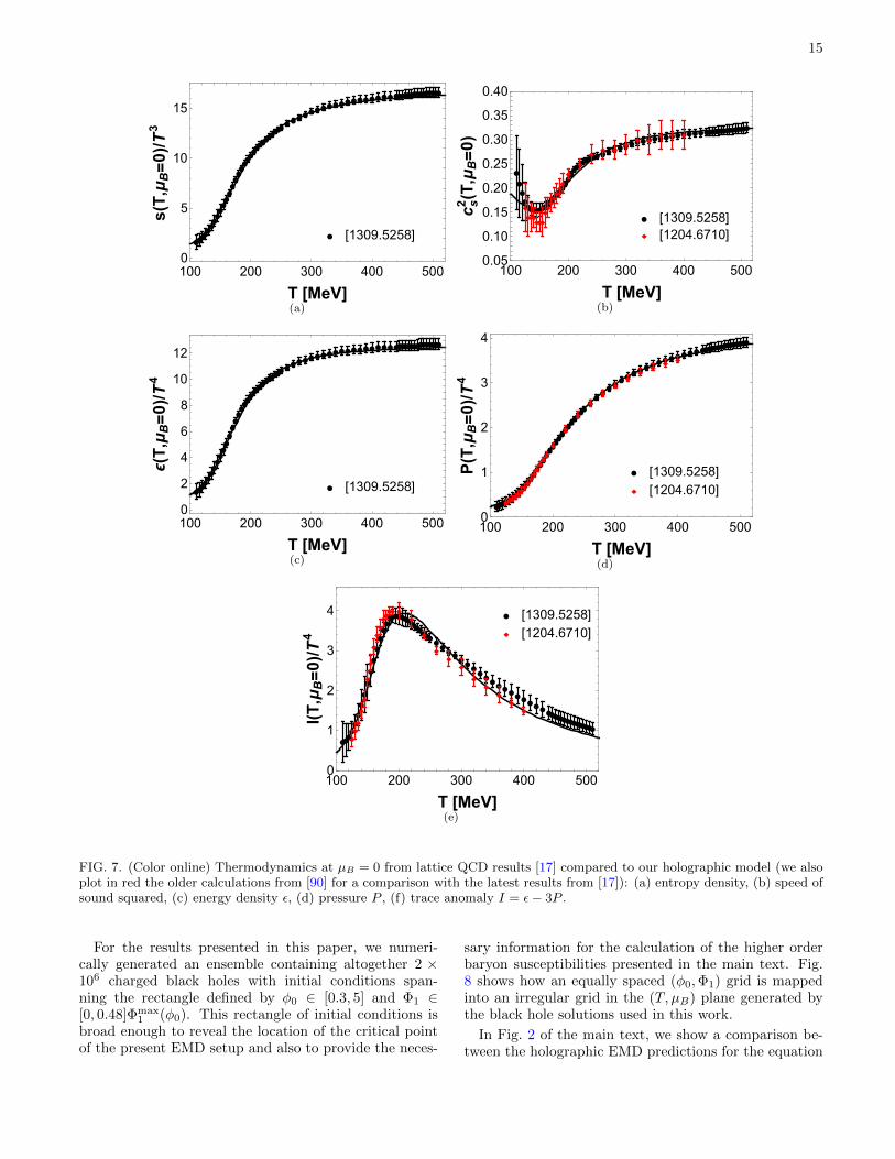
FIG. 7. (Color online) Thermodynamics at µB = 0 from lattice QCD results [17] compared to our holographic model (we alsoplot in red the older calculations from [90] for a comparison with the latest results from [17]): (a) entropy density, (b) speed ofsound squared, (c) energy density ε, (d) pressure P , (f) trace anomaly I = ε− 3P .
For the results presented in this paper, we numeri-cally generated an ensemble containing altogether 2 ×10⁶ charged black holes with initial conditions span-ning the rectangle defined by φ0 ∈ [0.3, 5] and Φ1 ∈[0, 0.48]Φmax
1 (φ0). This rectangle of initial conditions isbroad enough to reveal the location of the critical pointof the present EMD setup and also to provide the neces-
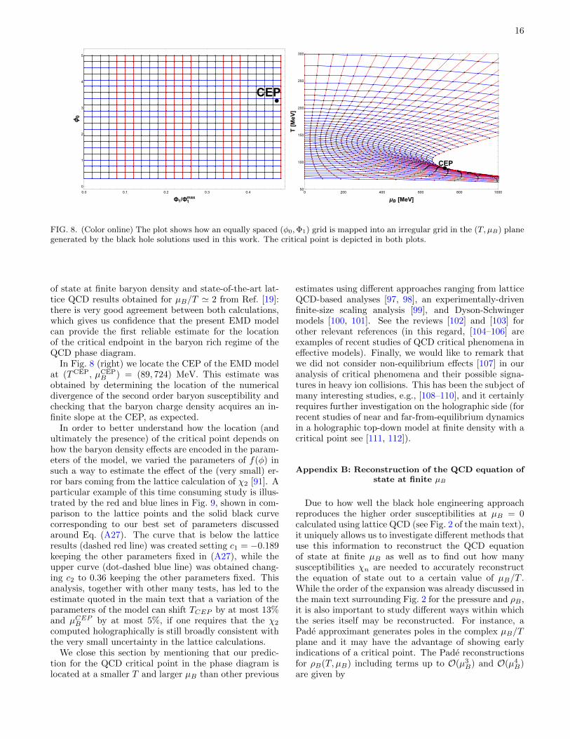
sary information for the calculation of the higher orderbaryon susceptibilities presented in the main text. Fig.8 shows how an equally spaced (φ0,Φ1) grid is mappedinto an irregular grid in the (T, µB) plane generated bythe black hole solutions used in this work.
In Fig. 2 of the main text, we show a comparison be-tween the holographic EMD predictions for the equation
16
CEP
0.0 0.1 0.2 0.3 0.4
0
1
2
3
4
5
Φ1/Φ1max
ϕ0
CEP
0 200 400 600 800 100050
100
150
200
250
300
μB [MeV]
T[MeV
]
FIG. 8. (Color online) The plot shows how an equally spaced (φ0,Φ1) grid is mapped into an irregular grid in the (T, µB) planegenerated by the black hole solutions used in this work. The critical point is depicted in both plots.
of state at finite baryon density and state-of-the-art lat-tice QCD results obtained for µB/T ' 2 from Ref. [19]:there is very good agreement between both calculations,which gives us confidence that the present EMD modelcan provide the first reliable estimate for the locationof the critical endpoint in the baryon rich regime of theQCD phase diagram.
In Fig. 8 (right) we locate the CEP of the EMD modelat (TCEP, µCEP
B ) = (89, 724) MeV. This estimate wasobtained by determining the location of the numericaldivergence of the second order baryon susceptibility andchecking that the baryon charge density acquires an in-finite slope at the CEP, as expected.
In order to better understand how the location (andultimately the presence) of the critical point depends onhow the baryon density effects are encoded in the param-eters of the model, we varied the parameters of f(φ) insuch a way to estimate the effect of the (very small) er-ror bars coming from the lattice calculation of χ2 [91]. Aparticular example of this time consuming study is illus-trated by the red and blue lines in Fig. 9, shown in com-parison to the lattice points and the solid black curvecorresponding to our best set of parameters discussedaround Eq. (A27). The curve that is below the latticeresults (dashed red line) was created setting c1 = −0.189keeping the other parameters fixed in (A27), while theupper curve (dot-dashed blue line) was obtained chang-ing c2 to 0.36 keeping the other parameters fixed. Thisanalysis, together with other many tests, has led to theestimate quoted in the main text that a variation of theparameters of the model can shift TCEP by at most 13%and µCEPB by at most 5%, if one requires that the χ2
computed holographically is still broadly consistent withthe very small uncertainty in the lattice calculations.
We close this section by mentioning that our predic-tion for the QCD critical point in the phase diagram islocated at a smaller T and larger µB than other previous
estimates using different approaches ranging from latticeQCD-based analyses [97, 98], an experimentally-drivenfinite-size scaling analysis [99], and Dyson-Schwingermodels [100, 101]. See the reviews [102] and [103] forother relevant references (in this regard, [104–106] areexamples of recent studies of QCD critical phenomena ineffective models). Finally, we would like to remark thatwe did not consider non-equilibrium effects [107] in ouranalysis of critical phenomena and their possible signa-tures in heavy ion collisions. This has been the subject ofmany interesting studies, e.g., [108–110], and it certainlyrequires further investigation on the holographic side (forrecent studies of near and far-from-equilibrium dynamicsin a holographic top-down model at finite density with acritical point see [111, 112]).
Appendix B: Reconstruction of the QCD equation ofstate at finite µB
Due to how well the black hole engineering approachreproduces the higher order susceptibilities at µB = 0calculated using lattice QCD (see Fig. 2 of the main text),it uniquely allows us to investigate different methods thatuse this information to reconstruct the QCD equationof state at finite µB as well as to find out how manysusceptibilities χn are needed to accurately reconstructthe equation of state out to a certain value of µB/T .While the order of the expansion was already discussed inthe main text surrounding Fig. 2 for the pressure and ρB ,it is also important to study different ways within whichthe series itself may be reconstructed. For instance, aPade approximant generates poles in the complex µB/Tplane and it may have the advantage of showing earlyindications of a critical point. The Pade reconstructionsfor ρB(T, µB) including terms up to O(µ3
B) and O(µ4B)
are given by

17
ρB(T, µB) =χ2
(µB
T
)+ 10(χ4)2−3χ2χ6
60χ4
(µB
T
)31− χ6
(µB
T
)2/(20χ4)
, ρB(T, µB) =χ2
(µB
T
)+ 70(χ4)3−42χ2χ4χ6+3(χ2)2χ8
42(10(χ4)2−3χ2χ6)
(µB
T
)31 + −7χ4χ6+χ2χ8
14(10(χ4)2−3χ2χ6)
(µB
T
)2+ 21(χ6)2−10χ4χ8
840(10(χ4)2−3χ2χ6)
(µB
T
)4 ,(B1)
100 120 140 160 180 200 220 240
0.00
0.05
0.10
0.15
0.20
0.25
T [MeV]
χ2(T,μB=0)
FIG. 9. (Color online) Examples that illustrate how variationsof the model parameters, performed to assess the effects of thesmall error bars in the lattice calculations [91], change theholographic result for the second order baryon susceptibility.The dashed red and dot-dashed blue curves are generatedby varying either c1 and c2 in (A27). The solid black curverepresents our best set of parameters used in this work thatgives a CEP at TCEP = 89 MeV and µCEPB = 724 MeV.
respectively.
In Fig. 10 (top left) a comparison between the directlycalculated baryon density, ρB , and the reconstructed ρBusing either the usual Taylor series or (B1) are shown.At large µB the Taylor series converges more quickly tothe actual ρB and gives a reasonable approximation upto almost µB/T ∼ 3. Looking at the ratios of the re-constructed ρB to the actual ρB one can see that up toµB/T ∼ 2 both methods work reasonably well and theerror is at most only 1− 2%. However, when µB/T ∼ 3for the Taylor series there is less than a 10% error whilethe Pade approximation has a significant deviation atµB/T ∼ 3 with an error up to 40% in the low tempera-ture region. In this case, the Taylor series is more ade-quate to reconstruct the equation of state and this willbe used in the calculations below.
Next, the truncation order of the Taylor series neededto reconstruct χ2(T, µB) and χ4(T, µB) is studied, mo-tivated by the fact that higher order susceptibilitiesare more strongly affected by the critical point (χ2 di-verges at the critical point and, therefore, any poten-tial peak displayed by χ2 is relevant for investigationsabout critical phenomena in QCD). In Fig. 11 (left)the reconstructed χ2 is shown across different values of
µB/T where there is a reasonable good description upto µB/T ∼ 2 using terms up to O(µ6
B). The slope ofµB/T ∼ 2 at O(µ4
B) artificially stiffens due to the lim-ited number of terms in the Taylor series, which can leadto misleading conclusions. At larger µB/T the curvatureis distorted even at O(µ6
B). Even though it is not surpris-ing that the validity of the Taylor series for χ2 is limitedto a smaller region of µB/T compared to ρB , this high-lights the need to extend the current lattice calculationsto even higher order susceptibilities. As a matter of fact,the series for χ4 has an even smaller range in µB/T andalready struggles to reproduce the directly calculated χ4
at µB/T = 1, as shown in Fig. 11 (right). Therefore, Fig.11 shows that additional higher order susceptibilities atµB = 0 beyond χ8 are needed to simultaneously obtainreasonable descriptions of χ2(T, µB) and χ4(T, µB) usingTaylor expansions for µB/T > 1.
Interestingly enough, the reconstructed ratio χ4/χ2
(normalized by its value at√s = 200 GeV), along the
transition lines defined near Fig. 6 of the Methods, worksvery well using terms up to O(µ4
B) down to energies aslow as
√s = 14.5 GeV, as shown in Fig. 12. However,
it is also clear from Fig. 12 that a truncation at O(µ2B)
can only reasonably reconstruct the ratio χ4/χ2 in anextremely limited range, which is not enough to coverall the values of
√s probed in the Beam Energy Scan at
RHIC. While the inclusion of terms up to O(µ4B) can be
used to determine the χ4/χ2 ratio at energies as low as√s = 14.5 GeV, Fig. 12 clearly demonstrates that lat-
tice QCD calculations will need to determine this ratioat least up to O(µ6
B) or higher to describe large values ofχ4/χ2 at low
√s.
Appendix C: Analysis of the radius of convergenceof the Taylor series
Since we know where the critical point of the blackhole engineering model is located in the phase diagram,one can use this information to determine that the radiusof convergence of the Taylor series is µCEPB /TCEP ∼ 8.1,assuming that the critical point is the first singularityencountered increasing µB/T . This allows us to directlycheck some methods to determine the radius of conver-gence using the results from the low order baryon sus-ceptibilities. For instance, in the recent paper [113], esti-mates for the radius of convergence were made using the
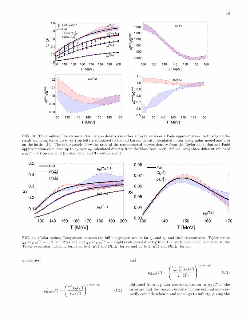
18
μB/T=1
μB/T=2
μB/T=3
μB/T=2.5
Full
Taylor (μB7 )
Pade (μB4 )
Lattice QCD
130 140 150 160 170 180 190 2000.0
0.2
0.4
0.6
0.8
1.0
T [MeV]
ρB
T3
μB/T=1
130 135 140 145 150 155 160
0.999
1.000
1.001
1.002
1.003
1.004
T [MeV]
ρBconst/ρBactual
μB/T=2
130 135 140 145 150 155 160
0.98
0.99
1.00
1.01
1.02
T [MeV]
ρBconst/ρBactual
μB/T=3
130 135 140 145 150 155 1600.5
0.6
0.7
0.8
0.9
1.0
1.1
T [MeV]
ρBconst/ρBactual
FIG. 10. (Color online) The reconstructed baryon density via either a Taylor series or a Pade approximation. In this figure theresult including terms up to χ8 (top left) is compared to the full baryon density calculated in our holographic model and alsoon the lattice [19]. The other panels show the ratio of the reconstructed baryon density from the Taylor expansion and Padeapproximation calculated up to χ8 over ρB calculated directly from the black hole model defined using three different values ofµB/T = 1 (top right), 2 (bottom left), and 3 (bottom right).
Full
(μB4 )
(μB6 )
μB/T=2.5
μB/T=2
μB/T=1
130 140 150 160 170 180 190 200
0.1
0.2
0.3
0.4
0.5
T [MeV]
χ2
μB/T=1
Full
(μB2 )
(μB4 )
130 140 150 160 1700.03
0.04
0.05
0.06
0.07
0.08
T [MeV]
χ4
FIG. 11. (Color online) Comparison between the full holographic results for χ2 and χ4 and their reconstructed Taylor series:χ2 at µB/T = 1, 2, and 2.5 (left) and χ4 at µB/T = 1 (right) calculated directly from the black hole model compared to theTaylor expansion including terms up to O(µ4
B) and O(µ6B) for χ2 and up to O(µ2
B) and O(µ4B) for χ4.
quantities,
ρfn,m(T ) =
(m!n! χn(T )
χm(T )
)1/(m−n)
(C1)
and
ρχn,m(T ) =
(m−2)!(n−2)! χn(T )
χm(T )
1/(m−n)
(C2)
obtained from a power series expansion in µB/T of thepressure and the baryon density. These estimates neces-sarily coincide when n and/or m go to infinity, giving the
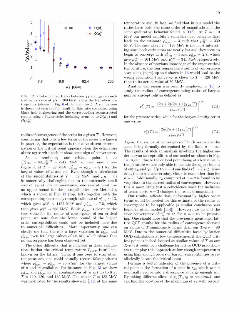
19
○○○○○○
○
○○
○
○
○
▯▯▯▯▯
▯
▯
▯
▯▯
▯
▯
△△△△△△
△
△
△
O(μB2 )
O(μB4 )
full
7.7 19.6 62.4 2000
1
2
3
4
5
s [GeV]
(χ4/χ2) norm
FIG. 12. (Color online) Ratio between χ4 and χ2 (normal-ized by its value at
√s = 200 GeV) along the transition line
trajectory (shown in Fig. 6 of the main text). A comparisonis shown between the full result for this ratio computed usingblack hole engineering and the corresponding reconstructedresults using a Taylor series including terms up to O(µ2
B) andO(µ4
B).
radius of convergence of the series for a given T . However,considering that only a few terms of the series are knownin practice, the expectation is that a consistent determi-nation of the critical point appears when the estimatorsabove agree with each or show some sign of convergence.
As a reminder, our critical point is at(TCEP = 89, µCEPB = 724
)MeV so one may inves-
tigate if, at T = 89 MeV, ρfn,m ∼ ρχn,m ∼ 8.1 for thelargest values of n and m. Even though a calculationof the susceptibilities at T = 89 MeV (and µB = 0)is numerically challenging due to the extremely smallsize of χ2 at low temperatures, one can at least usean upper bound for the susceptibilities (see Methods),which is shown in Fig. 13 (top, left) together with thecorresponding (extremely) rough estimate of ρχn,m ∼ 13,
which gives µestB ∼ 1157 MeV and ρfn,m ∼ 7.5, which
then gives µestB ∼ 668 MeV. While ρfn,m is closer to thetrue value for the radius of convergence of our criticalpoint, we note that the lower bound of the higherorder susceptibilities could not be included here dueto numerical difficulties. More importantly, one canclearly see that there is a large variation in ρfn,m andρχn,m even for large values of (n,m), which shows thatno convergence has been observed yet.
The other difficulty that is inherent in these calcula-tions is that the critical temperature TCEP is still un-known on the lattice. Thus, if one were to scan othertemperatures, one could actually receive false positiveswhere ρfn,m ∼ ρχn,m ∼ constant for the largest valuesof n and m available. For instance, in Fig. 13 we showρχn,m and ρfn,m for all combinations of (n,m) up to 8 atT = 110, 126, and 135 MeV. The choice T = 135 MeVwas motivated by the results shown in [113] at the same
temperature and, in fact, we find that in our model theratios have both the same order of magnitude and thesame qualitative behavior found in [113]. At T = 110MeV our model exhibits a somewhat flat behavior thatleads to the estimate ρfn,m ∼ 3 such that µestB ∼ 339MeV. The case where T = 126 MeV is the most interest-ing since both estimators are nearly flat and they seem tobegin to converge with ρfn,m ∼ 4 and ρχn,m ∼ 2.7, which
give µestB = 504 MeV and µestB = 341 MeV, respectively.In the absence of previous knowledge of the exact criticaltemperature, the four temperature radius of convergencescan using (n,m) up to 8 shown in 13 would lead to thewrong conclusion that TCEP is closer to T = 126 MeVthan to its actual value of 89 MeV.
Another expression was recently employed in [19] tostudy the radius of convergence using ratios of baryonnumber susceptibilities defined as
rPn (T ) =
∣∣∣∣ (2n+ 2)(2n+ 1)χ2n(T )
χ2n+2(T )
∣∣∣∣1/2 (C3)
for the pressure series, while for the baryon density seriesone writes
rχn(T ) =
∣∣∣∣2n(2n+ 1)χ2n(T )
χ2n+2(T )
∣∣∣∣1/2 . (C4)
Again, the radius of convergence of both series are thesame being formally determined by the limit n → ∞.The results of such an analysis involving the higher or-der baryon susceptibilities of our model are shown in Fig.14. Again, due to the critical point being at a low value intemperature we are only able to include the upper boundof our χ6 and χ8. Up to n = 3 one finds rPn ∼ 2.7rχn, how-ever, the results are certainly closer to each other than forn = 2. Additionally, rχn computed at n = 2 is found to bevery close to the correct radius of convergence. However,this is most likely just a coincidence since the inclusionof terms up to n = 3 changes the result dramatically.
Our results indicate that, unfortunately, higher orderterms would be needed for this estimate of the radius ofconvergence to be applicable (a similar conclusion wasfound in other models [114]). However, we do find theclose convergence of rPn to rχn for n = 3 to be promis-ing. One should note that the previously mentioned lat-tice QCD results for the radius of convergence focusedon values of T significantly larger than our TCEP = 89MeV. Due to the numerical difficulties faced by latticeQCD calculations at low temperatures, if the QCD crit-ical point is indeed located at similar values of T as ourTCEP , it would be a challenge for lattice QCD practition-ers to employ this approach at low enough temperaturesusing high enough orders of baryon susceptibilities to re-alistically locate the critical point.
Perhaps a better indicator of the presence of a criti-cal point is the formation of a peak in χ2, which wouldeventually evolve into a divergence at large enough µB .By taking different slices of χ2(T, µB = constant), onecan find the location of the maximum of χ2 with respect
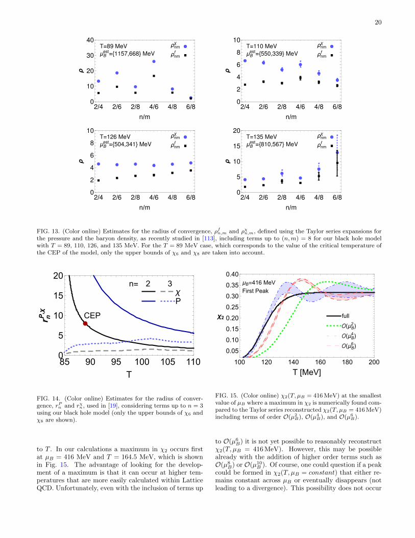
20
●
●
●
●
●
●■
■■
■
■■
T=89 MeV ρnmχ
ρnmfμB
est={1157,668} MeV
●●
■■
2/4 2/6 2/8 4/6 4/8 6/80
10
20
30
40
n/m
ρ
● ●
●●
●
●■
■ ■■
■■
T=110 MeV
μB
est={550,339} MeV
ρnmχ
ρnmf
●●
■■
2/4 2/6 2/8 4/6 4/8 6/80
2
4
6
8
10
n/m
ρ
● ● ● ● ● ●
■ ■ ■ ■ ■ ■
T=126 MeV
μB
est={504,341} MeV
ρnmχ
ρnmf
●●
■■
2/4 2/6 2/8 4/6 4/8 6/80
2
4
6
8
10
n/m
ρ
● ●●
●
●
●
■ ■■ ■
■
■
T=135 MeV
μB
est={810,567} MeV
ρnmχ
ρnmf
●●
■■
2/4 2/6 2/8 4/6 4/8 6/80
5
10
15
20
n/m
ρFIG. 13. (Color online) Estimates for the radius of convergence, ρfn,m and ρχn,m, defined using the Taylor series expansions forthe pressure and the baryon density, as recently studied in [113], including terms up to (n,m) = 8 for our black hole modelwith T = 89, 110, 126, and 135 MeV. For the T = 89 MeV case, which corresponds to the value of the critical temperature ofthe CEP of the model, only the upper bounds of χ6 and χ8 are taken into account.
●●
χP
n= 32
CEP
85 90 95 100 105 1100
5
10
15
20
T
rnP,χ
FIG. 14. (Color online) Estimates for the radius of conver-gence, rPn and rχn, used in [19], considering terms up to n = 3using our black hole model (only the upper bounds of χ6 andχ8 are shown).
to T . In our calculations a maximum in χ2 occurs firstat µB = 416 MeV and T = 164.5 MeV, which is shownin Fig. 15. The advantage of looking for the develop-ment of a maximum is that it can occur at higher tem-peratures that are more easily calculated within LatticeQCD. Unfortunately, even with the inclusion of terms up
full
(μB2 )
(μB4 )
(μB6 )
First Peak
μB=416 MeV
100 120 140 160 180 200
0.05
0.10
0.15
0.20
0.25
0.30
0.35
0.40
T [MeV]
χ2
FIG. 15. (Color online) χ2(T, µB = 416 MeV) at the smallestvalue of µB where a maximum in χ2 is numerically found com-pared to the Taylor series reconstructed χ2(T, µB = 416 MeV)including terms of order O(µ2
B), O(µ4B), and O(µ6
B).
to O(µ6B) it is not yet possible to reasonably reconstruct
χ2(T, µB = 416 MeV). However, this may be possiblealready with the addition of higher order terms such asO(µ8
B) or O(µ10B ). Of course, one could question if a peak
could be formed in χ2(T, µB = constant) that either re-mains constant across µB or eventually disappears (notleading to a divergence). This possibility does not occur
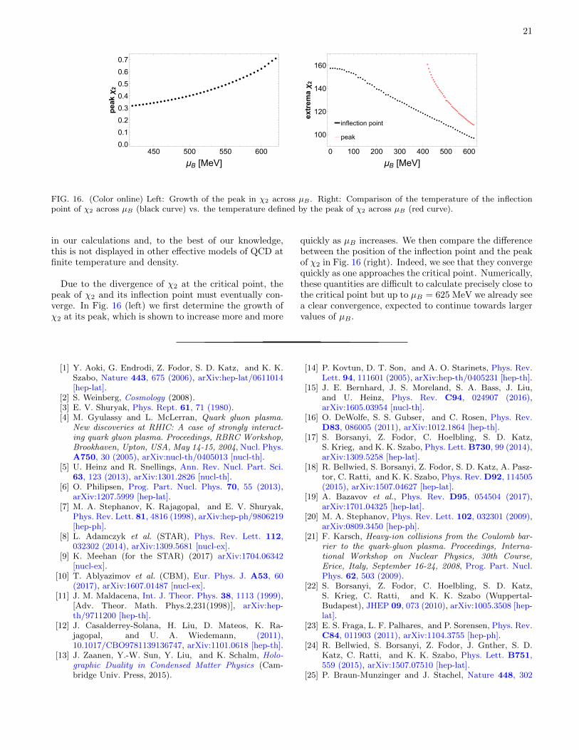
21
450 500 550 6000.0
0.1
0.2
0.3
0.4
0.5
0.6
0.7
μB [MeV]
peakχ2
inflection point
peak
0 100 200 300 400 500 600
100
120
140
160
μB [MeV]
extremaχ2
FIG. 16. (Color online) Left: Growth of the peak in χ2 across µB . Right: Comparison of the temperature of the inflectionpoint of χ2 across µB (black curve) vs. the temperature defined by the peak of χ2 across µB (red curve).
in our calculations and, to the best of our knowledge,this is not displayed in other effective models of QCD atfinite temperature and density.
Due to the divergence of χ2 at the critical point, thepeak of χ2 and its inflection point must eventually con-verge. In Fig. 16 (left) we first determine the growth ofχ2 at its peak, which is shown to increase more and more
quickly as µB increases. We then compare the differencebetween the position of the inflection point and the peakof χ2 in Fig. 16 (right). Indeed, we see that they convergequickly as one approaches the critical point. Numerically,these quantities are difficult to calculate precisely close tothe critical point but up to µB = 625 MeV we already seea clear convergence, expected to continue towards largervalues of µB .
[1] Y. Aoki, G. Endrodi, Z. Fodor, S. D. Katz, and K. K.Szabo, Nature 443, 675 (2006), arXiv:hep-lat/0611014[hep-lat].
[2] S. Weinberg, Cosmology (2008).[3] E. V. Shuryak, Phys. Rept. 61, 71 (1980).[4] M. Gyulassy and L. McLerran, Quark gluon plasma.
New discoveries at RHIC: A case of strongly interact-ing quark gluon plasma. Proceedings, RBRC Workshop,Brookhaven, Upton, USA, May 14-15, 2004, Nucl. Phys.A750, 30 (2005), arXiv:nucl-th/0405013 [nucl-th].
[5] U. Heinz and R. Snellings, Ann. Rev. Nucl. Part. Sci.63, 123 (2013), arXiv:1301.2826 [nucl-th].
[6] O. Philipsen, Prog. Part. Nucl. Phys. 70, 55 (2013),arXiv:1207.5999 [hep-lat].
[7] M. A. Stephanov, K. Rajagopal, and E. V. Shuryak,Phys. Rev. Lett. 81, 4816 (1998), arXiv:hep-ph/9806219[hep-ph].
[8] L. Adamczyk et al. (STAR), Phys. Rev. Lett. 112,032302 (2014), arXiv:1309.5681 [nucl-ex].
[9] K. Meehan (for the STAR) (2017) arXiv:1704.06342[nucl-ex].
[10] T. Ablyazimov et al. (CBM), Eur. Phys. J. A53, 60(2017), arXiv:1607.01487 [nucl-ex].
[11] J. M. Maldacena, Int. J. Theor. Phys. 38, 1113 (1999),[Adv. Theor. Math. Phys.2,231(1998)], arXiv:hep-th/9711200 [hep-th].
[12] J. Casalderrey-Solana, H. Liu, D. Mateos, K. Ra-jagopal, and U. A. Wiedemann, (2011),10.1017/CBO9781139136747, arXiv:1101.0618 [hep-th].
[13] J. Zaanen, Y.-W. Sun, Y. Liu, and K. Schalm, Holo-graphic Duality in Condensed Matter Physics (Cam-bridge Univ. Press, 2015).
[14] P. Kovtun, D. T. Son, and A. O. Starinets, Phys. Rev.Lett. 94, 111601 (2005), arXiv:hep-th/0405231 [hep-th].
[15] J. E. Bernhard, J. S. Moreland, S. A. Bass, J. Liu,and U. Heinz, Phys. Rev. C94, 024907 (2016),arXiv:1605.03954 [nucl-th].
[16] O. DeWolfe, S. S. Gubser, and C. Rosen, Phys. Rev.D83, 086005 (2011), arXiv:1012.1864 [hep-th].
[17] S. Borsanyi, Z. Fodor, C. Hoelbling, S. D. Katz,S. Krieg, and K. K. Szabo, Phys. Lett. B730, 99 (2014),arXiv:1309.5258 [hep-lat].
[18] R. Bellwied, S. Borsanyi, Z. Fodor, S. D. Katz, A. Pasz-tor, C. Ratti, and K. K. Szabo, Phys. Rev. D92, 114505(2015), arXiv:1507.04627 [hep-lat].
[19] A. Bazavov et al., Phys. Rev. D95, 054504 (2017),arXiv:1701.04325 [hep-lat].
[20] M. A. Stephanov, Phys. Rev. Lett. 102, 032301 (2009),arXiv:0809.3450 [hep-ph].
[21] F. Karsch, Heavy-ion collisions from the Coulomb bar-rier to the quark-gluon plasma. Proceedings, Interna-tional Workshop on Nuclear Physics, 30th Course,Erice, Italy, September 16-24, 2008, Prog. Part. Nucl.Phys. 62, 503 (2009).
[22] S. Borsanyi, Z. Fodor, C. Hoelbling, S. D. Katz,S. Krieg, C. Ratti, and K. K. Szabo (Wuppertal-Budapest), JHEP 09, 073 (2010), arXiv:1005.3508 [hep-lat].
[23] E. S. Fraga, L. F. Palhares, and P. Sorensen, Phys. Rev.C84, 011903 (2011), arXiv:1104.3755 [hep-ph].
[24] R. Bellwied, S. Borsanyi, Z. Fodor, J. Gnther, S. D.Katz, C. Ratti, and K. K. Szabo, Phys. Lett. B751,559 (2015), arXiv:1507.07510 [hep-lat].
[25] P. Braun-Munzinger and J. Stachel, Nature 448, 302

22
(2007).[26] A. Andronic, P. Braun-Munzinger, and J. Stachel,
Phys. Lett. B673, 142 (2009), [Erratum: Phys.Lett.B678,516(2009)], arXiv:0812.1186 [nucl-th].
[27] F. Karsch and K. Redlich, Phys. Lett. B695, 136 (2011),arXiv:1007.2581 [hep-ph].
[28] S. Gupta, X. Luo, B. Mohanty, H. G. Ritter, and N. Xu,Science 332, 1525 (2011), arXiv:1105.3934 [hep-ph].
[29] G. Agakishiev et al. (HADES), Eur. Phys. J. A52, 178(2016), arXiv:1512.07070 [nucl-ex].
[30] M. A. Stephanov, Phys. Rev. Lett. 107, 052301 (2011),arXiv:1104.1627 [hep-ph].
[31] A. Bazavov et al., Phys. Rev. Lett. 109, 192302 (2012),arXiv:1208.1220 [hep-lat].
[32] S. Borsanyi, Z. Fodor, S. D. Katz, S. Krieg, C. Ratti,and K. K. Szabo, Phys. Rev. Lett. 111, 062005 (2013),arXiv:1305.5161 [hep-lat].
[33] S. Borsanyi, Z. Fodor, S. D. Katz, S. Krieg, C. Ratti,and K. K. Szabo, Phys. Rev. Lett. 113, 052301 (2014),arXiv:1403.4576 [hep-lat].
[34] P. Alba, W. Alberico, R. Bellwied, M. Bluhm, V. Man-tovani Sarti, M. Nahrgang, and C. Ratti, Phys. Lett.B738, 305 (2014), arXiv:1403.4903 [hep-ph].
[35] J. Cleymans, H. Oeschler, K. Redlich, and S. Wheaton,Phys. Rev. C73, 034905 (2006), arXiv:hep-ph/0511094[hep-ph].
[36] S. S. Gubser, I. R. Klebanov, and A. M. Polyakov, Phys.Lett. B428, 105 (1998), arXiv:hep-th/9802109 [hep-th].
[37] E. Witten, Adv. Theor. Math. Phys. 2, 253 (1998),arXiv:hep-th/9802150 [hep-th].
[38] E. Witten, Adv. Theor. Math. Phys. 2, 505 (1998),arXiv:hep-th/9803131 [hep-th].
[39] A. Adams, L. D. Carr, T. Schafer, P. Steinberg,and J. E. Thomas, New J. Phys. 14, 115009 (2012),arXiv:1205.5180 [hep-th].
[40] A. Donos and S. A. Hartnoll, Nature Phys. 9, 649(2013), arXiv:1212.2998 [hep-th].
[41] S. A. Hartnoll, Nature Phys. 11, 54 (2015),arXiv:1405.3651 [cond-mat.str-el].
[42] S. Sachdev, Ann. Rev. Condensed Matter Phys. 3, 9(2012), arXiv:1108.1197 [cond-mat.str-el].
[43] T. Nishioka, S. Ryu, and T. Takayanagi, J. Phys. A42,504008 (2009), arXiv:0905.0932 [hep-th].
[44] J. Maldacena and L. Susskind, Fortsch. Phys. 61, 781(2013), arXiv:1306.0533 [hep-th].
[45] G. Policastro, D. T. Son, and A. O. Starinets, Phys.Rev. Lett. 87, 081601 (2001), arXiv:hep-th/0104066[hep-th].
[46] A. Buchel and J. T. Liu, Phys. Rev. Lett. 93, 090602(2004), arXiv:hep-th/0311175 [hep-th].
[47] P. B. Arnold, G. D. Moore, and L. G. Yaffe, JHEP 11,001 (2000), arXiv:hep-ph/0010177 [hep-ph].
[48] P. B. Arnold, G. D. Moore, and L. G. Yaffe, JHEP 05,051 (2003), arXiv:hep-ph/0302165 [hep-ph].
[49] I. Arsene et al. (BRAHMS), Nucl. Phys. A757, 1(2005), arXiv:nucl-ex/0410020 [nucl-ex].
[50] K. Adcox et al. (PHENIX), Nucl. Phys. A757, 184(2005), arXiv:nucl-ex/0410003 [nucl-ex].
[51] B. B. Back et al., Nucl. Phys. A757, 28 (2005),arXiv:nucl-ex/0410022 [nucl-ex].
[52] J. Adams et al. (STAR), Nucl. Phys. A757, 102 (2005),arXiv:nucl-ex/0501009 [nucl-ex].
[53] G. Aad et al. (ATLAS), JHEP 11, 183 (2013),arXiv:1305.2942 [hep-ex].
[54] E. Shuryak, (2014), arXiv:1412.8393 [hep-ph].[55] H. B. Meyer, Eur. Phys. J. A47, 86 (2011),
arXiv:1104.3708 [hep-lat].[56] G. Aarts, F. A. James, E. Seiler, and I.-O. Stamatescu,
Eur. Phys. J. C71, 1756 (2011), arXiv:1101.3270 [hep-lat].
[57] S. Borsanyi et al., Nature 539, 69 (2016),arXiv:1606.07494 [hep-lat].
[58] R. Rougemont, Proceedings, Hot Quarks 2016: Work-shop for Young Scientists on the Physics of Ultrarel-ativistic Nucleus-Nucleus Collisions (HQ2016): SouthPadre Island, Texas, September 12-17, 2016, J. Phys.Conf. Ser. 832, 012048 (2017), arXiv:1610.06124 [nucl-th].
[59] S. S. Gubser and A. Nellore, Phys. Rev. D78, 086007(2008), arXiv:0804.0434 [hep-th].
[60] S. S. Gubser, A. Nellore, S. S. Pufu, and F. D. Rocha,Phys. Rev. Lett. 101, 131601 (2008), arXiv:0804.1950[hep-th].
[61] S. S. Gubser, S. S. Pufu, and F. D. Rocha, JHEP 08,085 (2008), arXiv:0806.0407 [hep-th].
[62] J. Noronha, Phys. Rev. D81, 045011 (2010),arXiv:0910.1261 [hep-th].
[63] A. Ficnar, J. Noronha, and M. Gyulassy, Quark matter.Proceedings, 22nd International Conference on Ultra-Relativistic Nucleus-Nucleus Collisions, Quark Matter2011, Annecy, France, May 23-28, 2011, J. Phys. G38,124176 (2011), arXiv:1106.6303 [hep-ph].
[64] A. Ficnar, J. Noronha, and M. Gyulassy, Proceedings,5th International Conference on Hard and Electromag-netic Probes of High-Energy Nuclear Collisions (HardProbes 2012): Cagliari, Italy, May 27-June 1, 2012,Nucl. Phys. A910-911, 252 (2013), arXiv:1208.0305[hep-ph].
[65] S. I. Finazzo, R. Rougemont, H. Marrochio, andJ. Noronha, JHEP 02, 051 (2015), arXiv:1412.2968[hep-ph].
[66] R. A. Janik, G. Plewa, H. Soltanpanahi, and M. Spalin-ski, Phys. Rev. D91, 126013 (2015), arXiv:1503.07149[hep-th].
[67] R. A. Janik, J. Jankowski, and H. Soltanpanahi, Phys.Rev. Lett. 117, 091603 (2016), arXiv:1512.06871 [hep-th].
[68] M. Attems, J. Casalderrey-Solana, D. Mateos, I. Pa-padimitriou, D. Santos-Olivan, C. F. Sopuerta, M. Tri-ana, and M. Zilhao, JHEP 10, 155 (2016),arXiv:1603.01254 [hep-th].
[69] M. Attems, J. Casalderrey-Solana, D. Mateos,D. Santos-Olivan, C. F. Sopuerta, M. Triana, andM. Zilhao, JHEP 01, 026 (2017), arXiv:1604.06439 [hep-th].
[70] O. DeWolfe, S. S. Gubser, and C. Rosen, Phys. Rev.D84, 126014 (2011), arXiv:1108.2029 [hep-th].
[71] R. Rougemont, A. Ficnar, S. Finazzo, and J. Noronha,JHEP 04, 102 (2016), arXiv:1507.06556 [hep-th].
[72] R. Rougemont, J. Noronha, and J. Noronha-Hostler,Phys. Rev. Lett. 115, 202301 (2015), arXiv:1507.06972[hep-ph].
[73] S. I. Finazzo and R. Rougemont, Phys. Rev. D93,034017 (2016), arXiv:1510.03321 [hep-ph].
[74] J. Knaute, R. Yaresko, and B. Kampfer, (2017),arXiv:1702.06731 [hep-ph].
[75] R. Rougemont, R. Critelli, J. Noronha-Hostler,J. Noronha, and C. Ratti, Phys. Rev. D96, 014032
23
(2017), arXiv:1704.05558 [hep-ph].[76] R. Rougemont, R. Critelli, and J. Noronha, Phys. Rev.
D93, 045013 (2016), arXiv:1505.07894 [hep-th].[77] S. I. Finazzo, R. Critelli, R. Rougemont, and
J. Noronha, Phys. Rev. D94, 054020 (2016), [Erratum:Phys. Rev.D96,no.1,019903(2017)], arXiv:1605.06061[hep-ph].
[78] R. Critelli, R. Rougemont, S. I. Finazzo, andJ. Noronha, Phys. Rev. D94, 125019 (2016),arXiv:1606.09484 [hep-ph].
[79] S. I. Finazzo and J. Noronha, Phys. Rev. D89, 106008(2014), arXiv:1311.6675 [hep-th].
[80] M. Greif, I. Bouras, C. Greiner, and Z. Xu, Phys. Rev.D90, 094014 (2014), arXiv:1408.7049 [nucl-th].
[81] M. Greif, C. Greiner, and G. S. Denicol,Phys. Rev. D93, 096012 (2016), [Erratum: Phys.Rev.D96,no.5,059902(2017)], arXiv:1602.05085 [nucl-th].
[82] G. Aarts, C. Allton, A. Amato, P. Giudice,S. Hands, and J.-I. Skullerud, JHEP 02, 186 (2015),arXiv:1412.6411 [hep-lat].
[83] J. E. Bernhard, J. S. Moreland, and S. A. Bass, Proceed-ings, 26th International Conference on Ultrarelativis-tic Nucleus-Nucleus Collisions (Quark Matter 2017):Chicago,Illinois, USA, February 6-11, 2017, Nucl. Phys.A967, 293 (2017), arXiv:1704.04462 [nucl-th].
[84] G. S. Bali, F. Bruckmann, G. Endrdi, S. D. Katz, andA. Schfer, JHEP 08, 177 (2014), arXiv:1406.0269 [hep-lat].
[85] F. Bruckmann, G. Endrodi, and T. G. Kovacs, JHEP04, 112 (2013), arXiv:1303.3972 [hep-lat].
[86] G. Endrodi, JHEP 07, 173 (2015), arXiv:1504.08280[hep-lat].
[87] A. Bazavov, N. Brambilla, H. T. Ding, P. Petreczky,H. P. Schadler, A. Vairo, and J. H. Weber, Phys. Rev.D93, 114502 (2016), arXiv:1603.06637 [hep-lat].
[88] G. S. Denicol, C. Gale, S. Jeon, and J. Noronha, Phys.Rev. C88, 064901 (2013), arXiv:1308.1923 [nucl-th].
[89] F. Karsch, Proceedings, 4th International Workshop onCritical point and onset of deconfinement (CPOD07):Darmstadt, Germany, July 9-13, 2007, PoS CPOD07,026 (2007), arXiv:0711.0656 [hep-lat].
[90] S. Borsanyi, G. Endrodi, Z. Fodor, S. D. Katz, S. Krieg,C. Ratti, and K. K. Szabo, JHEP 08, 053 (2012),arXiv:1204.6710 [hep-lat].
[91] S. Borsanyi, Z. Fodor, S. D. Katz, S. Krieg, C. Ratti,and K. Szabo, JHEP 01, 138 (2012), arXiv:1112.4416[hep-lat].
[92] A. Bazavov et al. (HotQCD), Phys. Rev. D90, 094503(2014), arXiv:1407.6387 [hep-lat].
[93] J. D. Bekenstein, Phys. Rev. D7, 2333 (1973).[94] S. W. Hawking, In *Gibbons, G.W. (ed.), Hawking,
S.W. (ed.): Euclidean quantum gravity* 167-188, Com-mun. Math. Phys. 43, 199 (1975), [,167(1975)].
[95] P. Breitenlohner and D. Z. Freedman, Annals Phys.144, 249 (1982).
[96] P. Breitenlohner and D. Z. Freedman, Phys. Lett. B115,197 (1982).
[97] Z. Fodor and S. D. Katz, JHEP 04, 050 (2004),arXiv:hep-lat/0402006 [hep-lat].
[98] S. Datta, R. V. Gavai, and S. Gupta, Phys. Rev. D95,054512 (2017), arXiv:1612.06673 [hep-lat].
[99] R. A. Lacey, Phys. Rev. Lett. 114, 142301 (2015),arXiv:1411.7931 [nucl-ex].
[100] X.-y. Xin, S.-x. Qin, and Y.-x. Liu, Phys. Rev. D90,076006 (2014).
[101] C. S. Fischer, J. Luecker, and C. A. Welzbacher, Phys.Rev. D90, 034022 (2014), arXiv:1405.4762 [hep-ph].
[102] M. A. Stephanov, Non-perturbative quantum chromo-dynamics. Proceedings, 8th Workshop, Paris, France,June 7-11, 2004, Prog. Theor. Phys. Suppl. 153, 139(2004), [Int. J. Mod. Phys.A20,4387(2005)], arXiv:hep-ph/0402115 [hep-ph].
[103] X. Luo and N. Xu, (2017), arXiv:1701.02105 [nucl-ex].[104] W.-j. Fu and J. M. Pawlowski, Phys. Rev. D93, 091501
(2016), arXiv:1512.08461 [hep-ph].[105] W.-j. Fu, J. M. Pawlowski, F. Rennecke, and
B.-J. Schaefer, Phys. Rev. D94, 116020 (2016),arXiv:1608.04302 [hep-ph].
[106] W. Fan, X. Luo, and H.-S. Zong, Int. J. Mod. Phys.A32, 1750061 (2017), arXiv:1608.07903 [hep-ph].
[107] B. Berdnikov and K. Rajagopal, Phys. Rev. D61,105017 (2000), arXiv:hep-ph/9912274 [hep-ph].
[108] L. Jiang, P. Li, and H. Song, Phys. Rev. C94, 024918(2016), arXiv:1512.06164 [nucl-th].
[109] C. Herold, M. Nahrgang, Y. Yan, and C. Kobdaj, Phys.Rev. C93, 021902 (2016), arXiv:1601.04839 [hep-ph].
[110] S. Mukherjee, R. Venugopalan, and Y. Yin, Phys. Rev.Lett. 117, 222301 (2016), arXiv:1605.09341 [hep-ph].
[111] S. I. Finazzo, R. Rougemont, M. Zaniboni, R. Critelli,and J. Noronha, JHEP 01, 137 (2017), arXiv:1610.01519[hep-th].
[112] R. Critelli, R. Rougemont, and J. Noronha, (2017),arXiv:1709.03131 [hep-th].
[113] M. D’Elia, G. Gagliardi, and F. Sanfilippo, Phys. Rev.D95, 094503 (2017), arXiv:1611.08285 [hep-lat].
[114] F. Karsch, B.-J. Schaefer, M. Wagner, and J. Wambach,Phys. Lett. B698, 256 (2011), arXiv:1009.5211 [hep-ph].