Physics 54 Modern Physics Laboratory · 2010-01-22 · Physics—ModernPhysicsLab É É Spring Ê È É È .Procedure eFranck-HertzExperiment that small temperature changes will aﬀect

Physics 54

Modern Physics Laboratory

19 January 2010

Chih-Yung ChenPeter N. Saeta

CONTENTS

. Schedule . . . . . . . . . . . . . . . . . . . . . . . . . . . . . . . . . . . . . . . . . . . .

. General Instructions . . . . . . . . . . . . . . . . . . . . . . . . . . . . . . . . . . . .

e Franck-Hertz Experiment. Apparatus . . . . . . . . . . . . . . . . . . . . . . . . . . . . . . . . . . . . . . . . . . .. Procedure . . . . . . . . . . . . . . . . . . . . . . . . . . . . . . . . . . . . . . . . . . .

ermal Radiation. General . . . . . . . . . . . . . . . . . . . . . . . . . . . . . . . . . . . . . . . . . . . .. ermistor calibration . . . . . . . . . . . . . . . . . . . . . . . . . . . . . . . . . . . .. Experimental procedure . . . . . . . . . . . . . . . . . . . . . . . . . . . . . . . . . .

Rutherford Sca ering. Detector . . . . . . . . . . . . . . . . . . . . . . . . . . . . . . . . . . . . . . . . . . . .. Addendum . . . . . . . . . . . . . . . . . . . . . . . . . . . . . . . . . . . . . . . . . .

e Hall Effect. eoretical Background . . . . . . . . . . . . . . . . . . . . . . . . . . . . . . . . . .. Measurement of the Hall Potential . . . . . . . . . . . . . . . . . . . . . . . . . . . .

GammaRadiation Interactions. Introduction . . . . . . . . . . . . . . . . . . . . . . . . . . . . . . . . . . . . . . . . .. Experiment . . . . . . . . . . . . . . . . . . . . . . . . . . . . . . . . . . . . . . . . . .

Barrier Penetration. Introduction . . . . . . . . . . . . . . . . . . . . . . . . . . . . . . . . . . . . . . . . .. Preliminary Measurements . . . . . . . . . . . . . . . . . . . . . . . . . . . . . . . . .. Barrier penetration measurement . . . . . . . . . . . . . . . . . . . . . . . . . . . . .

Photoelectric Effect. Background . . . . . . . . . . . . . . . . . . . . . . . . . . . . . . . . . . . . . . . . . .. Experiment . . . . . . . . . . . . . . . . . . . . . . . . . . . . . . . . . . . . . . . . . .

e Cavendish Experiment. Background . . . . . . . . . . . . . . . . . . . . . . . . . . . . . . . . . . . . . . . . . .. eory . . . . . . . . . . . . . . . . . . . . . . . . . . . . . . . . . . . . . . . . . . . . .. Procedure . . . . . . . . . . . . . . . . . . . . . . . . . . . . . . . . . . . . . . . . . . .

ChaoticMotion. Overview . . . . . . . . . . . . . . . . . . . . . . . . . . . . . . . . . . . . . . . . . . .. Details . . . . . . . . . . . . . . . . . . . . . . . . . . . . . . . . . . . . . . . . . . . . .

. Schedule

You will conduct four two-week experiments and extend one of the experiments for your tech-nical report. e experiments will be done in pairs and in a rotation to be established a er the Ori-entationmeeting in the rst week, in which youwill be introduced to each experiment. emanualdescribes more experiments than are currently available. Some of those unavailable at the time thismanual was prepared may become serviceable during the term. If so, we can use a lo ery system todecide which teams may conduct them, if more than one team is interested.

Currently, the following experiments are working and available:

. Rutherford sca ering ( )

. e Hall effect ( ) + the photoelectric effect ( ) (each lasts only one week)

. Gamma radiation interactions ( )

. Barrier penetration ( )

. e Cavendish experiment ( )

. Chaotic motion ( )

A vacuum system has been ordered for the ermal Radiation experiment (Expt. ), but it may notarrive before spring break. e Franck-Hertz experiment (Expt. ) may replace the photoelectricexperiment at some point during the semester, if the la er gets sick.

Week Section ( urs.) Section (Fri.)

January – Orientation OrientationJanuary – A AFebruary – B B

February – A AFebruary – B B

February – A AMarch – B B

March – A Tech Report Data

March – Spring Break Spring Break

March – B Cesar Chavez DayApril – Tech Report Data Tech Report WorkApril Tech Report DueApril – Tech Report Work AApril – Tech Report Due BApril - Free Revised Tech Report DueApril – Revised Tech Report Due Free

. General Instructions

In preparing for the rst laboratory meeting for each experiment, you should carefully read theinstructions for a scheduled experiment before reporting to the laboratory meeting. In many cases,you will also nd it useful to do some background reading on the subject, in your Physics text-book, in various sources found in the library, or on the internet. (Beware ofmaterial on the internet.Someof it is very good, but there is no guarantee that the information is relevant, useful, or correct!)You are encouraged to take notes on your reading and a ach these notes in your lab book. Be sureto include references to your sources.While youmay nd some details of the instructions will havebeen changed in the lab (as we are constantly tweaking the equipment), complete familiarity withthe objectives and general procedures of the experiment before the laboratory period will help youin working efficiently in lab.

Please observe the precautions emphasized in the laboratory instructions and appendices andaccord the research-type equipment the respect it deserves.Note thatmuchof the equipment in thislaboratory is one-of-a-kind, delicate, difficult to repair, and expensive! Much of it can be damagedif used incorrectly. If you have any questions about how to use the equipment, be sure to ask theinstructor before turning it on or starting a new procedure. Report any damaged equipment to yourinstructor immediately.

• Always bring your lab manual, a calculator, a (non-erasable) pen, and a laboratory notebook(brown-cover National - “Computation Notebook” or spiral-bound version, e.g., Am-pad - ) with you to lab.

Laboratory Notebook

You will follow the same general rules for your laboratory notebook that were used in Physics. e notebook will be an essential part of your laboratory work this year, and it should contain a

running account of the work you do. Entries should be made while the experiment is in progress, and youshould use a standard format. Your notebook should:

. provide the reader with a table of contents at the back page, listing the number and title of theexperiment, the date or dates when it was done, the page numbers in the notebook, and thename of your partner (see below);

. contain all pertinent information, schematic diagrams, observations, data, rough calculations,results, and conclusions. ink of your entries as being those in an informal diary or journalrelating daily experiences.In the laboratory, each experiment will be performed by a team of two investigators. Eachperson is responsible for the complete documentation of the work performed and its analy-sis. at is, while youmay discuss the experimental results with your lab partner, your analysisof the experiment should be done individually.Remember, you will write a technical report basedon one of the experiments, and therefore a complete record of your observations and conclu-sions is essential.Computers are available for data gathering, plo ing, and analysis. Do not alter the computeroperating system or programs in any way. Any such tampering, even if intended to be harm-less, is considered a serious offense.

ere are some general rules for making entries in your laboratory notebook:

. Use permanent ink, not pencil or erasable ink.

. Do not use scratch paper—all records must be made directly in the notebook. (Le -handpages may be used for scratch work.)

. Do not erase or use “white out”—draw a single line through an incorrect entry and write thecorrect value nearby. Apparent errors sometimes later prove to be important.

. Record data in tabular form when possible with uncertainties and give units in the headingof each column.

. De ne all symbols used in diagrams, graphs, and equations.

. Determine the uncertainties in your data and results as you go, and let the calculations deter-mine the number of measurements needed.

. Record qualitative observations as well as numbers and diagrams.

. Plot as you take data. is will help you understand the experiment in real time. Save o en!Append clearly and fully labelled computer-generated or hand-drawn graphs securely to thenotebook pages. Describe these graphs in your narrative. Place the graphs in your lab booksas close aspossible to the relevantdata, preferablyon le -handpages facing the correspondingdata tables. Include error bars and properly weighted ts to the data wherever possible. Alsoinclude plots of residuals (with appropriate error bars) where applicable.

. Do not fall into the habit of recording only your data in lab, leaving blank pages or spaces fordescription and calculation to be nished later. Entries should be made in order correspond-ing to the work you are doing, much like a diary report, although complicated computationsand analyses are usually undertaken a er the data taking procedures have been completed.

. While not everyone can produce a showcase-type notebook, yourwork should be as neat andorderly as possible. Sloppiness and carelessness cannot be overlooked even when the resultsare good.

. Your notebook will be a success if you or a colleague could use it as a guide in repeating orexpanding upon the particular experiment at a much later date.

Because your success in the laboratorywill depend to a large extent upon your notebook and thewrite-up you produce from it, the following speci c instructions for your notebook are provided.

Notebook e physics laboratory books (National - “Computation Notebook”) are boundnotebooks ruled horizontally and vertically into squares. Leave two pages at the beginningof the notebook for a table of contents. Pages are numbered in the upper right-hand corner,beginning with the rst page in the book. Put your table of contents on the last page of thenotebook, but start your lab entries on the rst page. When the table of contents meets theactual contents, somewhere in the middle, the notebook is complete. e table of contentsshould contain the following column headings:

Expt. Title Partner Dates Pages Grade

Expt. Delta Radiation Marge Innovera / – / / –

You should date each page of your notebook. Also date any entry added a er lab.

Description of Intent and Proposed Procedure Head each experiment with the material used inthe Table of Contents. Begin with a brief statement of the purpose of the experiment and abrief outline of the procedure your intended procedure. Two or three sentences should beenough. ere is no need to copy that contained in the laboratory manual.Please note that you do not always have at the beginning all the information you need toprepare a full description of purpose or procedure. e objectives may be poorly de ned atthe start and become crystallized only in the nal stages of the experiment. Your notion abouthow to proceed may change a er you have proved something else. For these reasons we arereluctant to prescribe very de nite.rules about laboratory work and laboratory records

Sketch of Apparatus Whenever practical, include a large, clear drawing, sketch, and/or block di-agram of your experimental arrangement, to scale when necessary. Indicate clearly on thesketch critical quantities such as dimensions, volumes, masses, etc. Avoid excessive detail; in-clude only essential features. Record the manufacturer, model name or number, and HMCidenti cation number and, if appropriate, the accuracy of all apparatus you use, as it may beessential that you get the same apparatus later, or someone else may wish to compare theirresults with yours.

Preliminary Data Frequently there are certain preliminary data that must be measured or lookedup in the tables and recorded, such as switch se ings on equipment.Collect such informationin a single table in your notebook and devote a separate line to each quantity. Include unitsand uncertainty where relevant.

Tabulation of Data Put data in tabular formwhere practical. e easiest andmost frequently usedprocedure is to organize the data in clear tabular form, leaving empty columns if necessaryfor calculated results that will be made later. is requires advanced planning. At the headof each column should appear a symbol or notation for the quantity that is to be recordedin that column, with the units in which this quantity is measured in parentheses, thus orT (K) or E (mV). is avoids the necessity of writing the unit a er each entry. Always use oneself-consistent system of units. Uncertainties must be included for all measurements (unlessyou’re told otherwise). If the uncertainties vary from datum to datum, each should be fol-lowed by its own uncertainty. Uncertainties should also be listed at the top of each column ifpossible. us, T (C) (±0.1C), E (mV) (±0.2mV), wt (g) (±0.2 mg)

Computation and Results A er the data are recorded, there will generally be some calculationsto be made. Make calculations as you go along to verify that your data is giving reasonableresults; do not postpone all calculations until the nal week of the experiment. If the data areall treated by some standard procedure, describe the procedure brie y for each calculation,giving any formulas that are to be used. (De ne any quantities appearing in the formula thathave not previously been de ned.) Always give a sample calculation, starting with the for-mula, substituting experimental numbers, and carry the numerical work down to the result.

D a computer program in lieu of a sample calculation. Your results should becompared with accepted values if possible. Information from a handbook or any referencesource must be identi ed by book and page.

Summary of the Experiment At the end of an experiment you should type a summary of one totwo pages containing a concise discussion of important points of the experiment, includingthe purpose, theoretical predictions you are testing (if appropriate), a brief outline of exper-imental methods, results, analysis, and conclusions. ere is no need to put in detailed pro-cedural discussions unless they bear directly on understanding some aspect of the data. Indiscussing results, you canmake references (with page numbers) to speci c entries—such astables, gures, and calculations—in your lab notebook. Be sure to refer to or include in yoursummary well-documented graphs of important ndings. Discuss the major sources of ran-domand systematic errors, including possiblemethods of reducing them. If you have a hunchabout the source of a discrepancy, make some order of magnitude estimates, make some ap-proximations, and check quantitatively to see if hunch could reasonably explain the discrep-ancy. If relevant, compare your results with theoretical predictions. Your results should be asquantitative and precise as possible. Your conclusions should also be as speci c as possible,given your experimental results and analysis. is summary should be a ached to the end ofyour lab notebook write-up; it is a signi cant part of the record of your experiment.

Honor System All work that is handed in for credit in this course, including laboratory reports,is regulated by the Harvey Mudd Honor Code, which is described in general terms in thestudent handbook. In application, this Code means simply that all work submi ed for creditshall be your own. You should not hesitate to consult texts, the instructor, or other studentsfor general aid in the preparation of laboratory reports. However, you must not transcribeanother student’s work without direct credit to him or her, and you must give proper creditfor any substantial aid from outside your partnership. Again remember that while you maydiscuss the experiment with your lab partner, your analysis of the experiment should be doneindividually.

EXPERIMENTONE

e Franck-Hertz Experiment

is experimentwas performed byFranck andHertz in , following by one year Bohr’s pub-lication of the theory of the hydrogen spectrum. e Bohr theory, using Rutherford’s nuclear atom,is based upon a mechanical model—an electron circling about a proton in a manner described bya new law of mechanics. e observations supporting the theory, and which necessitated a new de-scription of atomic systems, were electromagnetic. Light is emi ed and absorbed by atoms. eBohr theory of hydrogen was a success because the energy difference between the variousmechan-ical states of the electron-proton system corresponded, through the Einstein frequency conditionE = hν, to observed frequencies of emi ed and absorbed radiation. e Franck-Hertz experiment,on the other hand, was a direct mechanical con rmation of an essentially mechanical theory.

e optical spectrum of mercury vapor shows distinct emission and absorption lines corre-sponding to transitionsbetweendiscrete energy levels of themercury atom.Franck andHertz foundthat discrete transitions of the mercury atom could also be produced by the inelastic sca ering ofelectrons from the atom. Consider the system of an electron with some initial kinetic energy inci-dent upon a mercury atom at rest in the ground state. If the electron energy is less than the energyrequired to excite the atom to its rst excited state, the collision must be elastic. e kinetic energyof the electron-atom system cannot change.Due to the disparity ofmasses, the kinetic energy of theelectron itself is essentially unchanged in the collision. If the electron energy equals or exceeds theenergy for exciting the rst level, however, the collision may in some cases be inelastic. e kineticenergy of the system is, in these cases, different a er the collision than before. In an inelastic colli-sion some of the initial kinetic energy is converted to potential or “excitation” energy of the atom. Indue course, this energy is radiated from the excited atoms as light, but the primary interaction is onedescribed in mechanical terms. Franck and Hertz observed such inelastic collisions by monitoringthe current of electrons passing through a mercury vapor.

. Apparatus

e apparatus consists of a special electron tube containing a small quantity of mercury. evapor pressure of mercury in the tube is adjusted by placing the tube in a furnace whose tempera-ture may be varied. Electrons emi ed from the cathode must, then, traverse a controlled mercuryatmosphere in reaching the anode of the tube (see Fig. .).

e anode is perforated so that many of the electrons will pass through it and collect on the

. Apparatus e Franck-Hertz Experiment

Figure . : Franck-Hertz Electron Tube and Circuit.

counter-electrode.Emission current from the cathode is controlled by the temperature of the cathode and by the

potential applied to the anode. A diaphragm connected to the cathode limits the current and elim-inates secondary and re ected electrons, making the electric eld more uniform.

Electrons which pass through the hole in the diaphragm are accelerated through the mercuryatmosphere by the positive potential applied to the anode. e counter-electrode is maintained at apotential of approximately −1.5 Vwith respect to the anode. us no electrons which pass throughthe perforated anode with energy less than 1.5 eV can reach the counter-electrode.

If the electrode and the cathode were of the same material and if all electrons were releasedfrom the cathode with zero kinetic energy, then the current of electrons collected by the counter-electrode would vary with the anode potential in the following way. No current would be observeduntil the potential of the anode exceeded 1.5 V. As the potential is increased, all electrons passingthrough the anodewould reach the counter-electrode and the current would show a continuous in-creasewith rising potential until a potential corresponding to the energy transition from the groundto the rst excited state of mercury is reached. At this point the current would drop abruptly withincreasing potential, since many electrons would make inelastic collisions with mercury atoms andhave insufficient kinetic energy to reach the counter-electrode. If the potential were sufficiently in-creased, however, the electrons would again reach the counter-electrode even a er making an in-elastic collision. is second increase in current would continue until the electrons gained enoughenergy to make two inelastic collisions, again not being le with enough kinetic energy to reachthe counter-electrode. is would result in a second sharp drop in current. If the above conditionswere satis ed, a succession of currentmaximawith sharp breaks would be observedwith increasingpotential.

e fact that the counter-electrode and the cathode may not be of the same material makes therst maximum an unreliable measure of the excitation potential of mercury. A so-called “contact”

potential must be added to or subtracted from the observed potential. Evaluation of the contactpotential is avoided by measuring potential differences between succeeding maxima. e fact thatelectrons are not emi ed from the cathode with zero kinetic energy means that the actual energydistribution is superimposed upon that established by the anode potential. Sharp breaks are thuswashed out of the current-voltage curve.

Physics —Modern Physics Lab Spring

. Procedure e Franck-Hertz Experiment

. Electrical Circuit

e circuit employed in this experiment is shown in Fig. . All voltage sources indicated in thegure are located in a power supply which is connected to the furnace by means of various power

cables. e measuring ampli er is a separate unit, but the microammeter which reads the counter-electrode current is mounted in the front of the power supply. A voltmeter ( – V) on the front ofthe power supply reads the anode potential, and a third small voltmeter is used for the bias voltageand the voltage across the lament. Filament current is supplied by a 6.3 V transformer and bridgerecti er. e anode and bias potentials are derived from dry cells mounted inside the power supply.All potentials are controlled by knobs on the front of the power supply. ere are also two switcheson the front of the power supply, the “P ” switch and the “A ” switch. Filament potentialalone is supplied with only the P switch on. e A switch must be on for both anodeand bias potentials.

. Procedure

e oven in which the tube is mounted should be turned on immediately upon entering thelaboratory. e temperature inside the oven is controlled by an external regulator. A thermometerprotruding from the topof the cabinet provides ameasurementof the temperaturenear themercurytube. Close a ention should be given to the reading of the thermometer so that a temperature of180C is at no time exceeded. Bymeans of the thermostat control knob, the temperature of the ovenshould be adjusted initially to 170C ±5C. Check the oven temperature every few minutes.

e Leyboldmeasuring ampli er should also be turned on immediately so that it will have am-ple time to stabilize. As the temperature of the tube approaches its operating value, the power supplyP switch should be turned on.

Set the sensitivity range of the measuring ampli er at 30 × 10−10, turn the sensitivity controlknob to its central position, and zero themicroammeter bymeans of the “zero” control knob on theampli er. e input signal to the ampli ermay be grounded at the time these se ings aremade, butthe grounding connection on the front of the ampli er must be turned off, θ, before any currentmeasurements can be made.

When the operating temperature is reached, first make sure that the Anode voltage con-trol knob is turned to the full counterclockwise (zero) position; then turn theA switchon.

Increase the lament voltage to the value suggested at your station. Slowly increase the anodepotential to about 35 V. Watch the microammeter carefully. If the current increases suddenly,an electrical breakdown has occurred in the tube, and the potential must be reduced tozero immediately. If such a breakdown has occurred, reduce the lament voltage very slightly andagain try to raise the anodepotential to 35V. (If the tube still breaks down, see your instructor.)Nowvery slowly increase the anode potential to 40 V and adjust the sensitivity knob to give a full scalede ection of the microammeter for the maximum current observed in the – V range. Allowtime for the current to stabilize a er each small adjustment and watch out for the onset of electricalbreakdown.

e apparatus is now ready for taking measurements. Slowly decrease the anode potential andobserve themicroammeterde ection.Dips andpeaks in the current shouldbeobvious in the – Vrange. e sensitivity range of the ampli er may have to be changed in order to de ne the maximaclearly at the lower anode voltages. Record counter-electrode currents vs. anode potential. Note


. Procedure e Franck-Hertz Experiment

that small temperature changes will affect the current at a given voltage (why?), so monitor theoven temperature as you make your measurements. Plot your data and determine the excitationenergy of mercury. Repeat your measurements while slowly increasing the anode voltage from to40 V. Repeat with different oven temperatures. (Do not exceed 180C.) For each temperature youshould reset the sensitivity knob following the original procedure. From all your data obtain yourbest estimate of the excitation energy of mercury.


EXPERIMENTTWO

ermal Radiation

. General

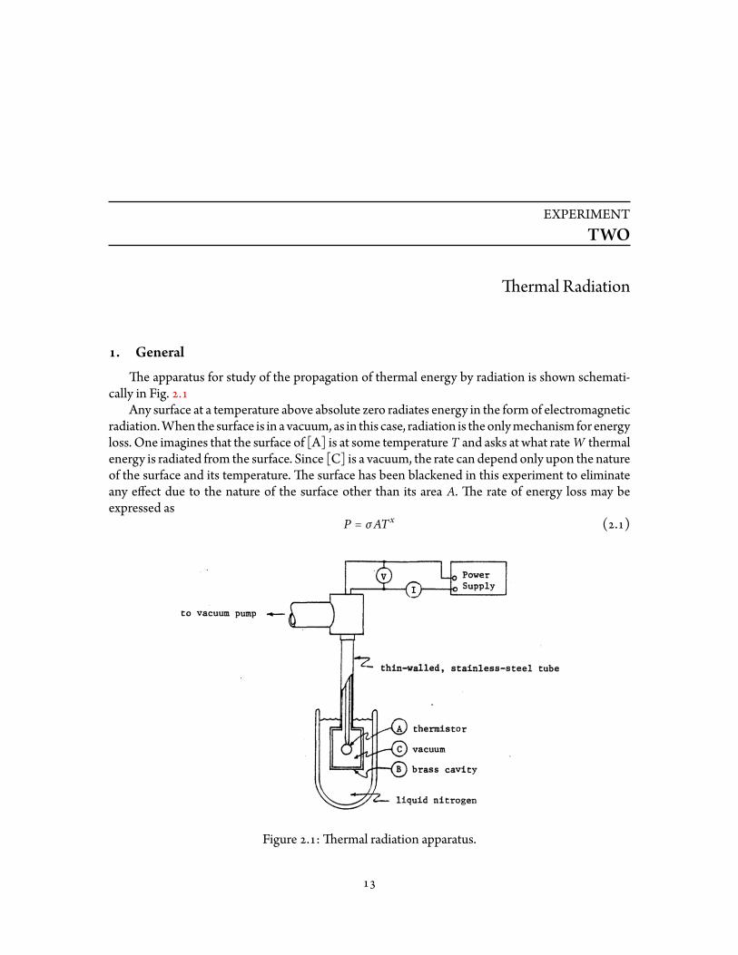
e apparatus for study of the propagation of thermal energy by radiation is shown schemati-cally in Fig. .

Any surface at a temperature above absolute zero radiates energy in the formof electromagneticradiation.When the surface is in a vacuum, as in this case, radiation is theonlymechanism for energyloss. One imagines that the surface of [A] is at some temperature T and asks at what rateW thermalenergy is radiated from the surface. Since [C] is a vacuum, the rate can depend only upon the natureof the surface and its temperature. e surface has been blackened in this experiment to eliminateany effect due to the nature of the surface other than its area A. e rate of energy loss may beexpressed as

P = σATx ( . )

Figure . : ermal radiation apparatus.

. ermistor calibration ermal Radiation

e universal constant σ is called the Stefan-Boltzmann constant. We are to determine σ and theexponent x relatingW to the surface temperature.

e interior surface of the brass cavity [B] also radiates thermal energy to [A]. is surface,however, is maintained at a sufficiently low temperature ( K) by contact with liquid nitrogen thatthe energy received by [A] from [B] is negligible. Further, [A] is suspended by wires of very smallcross-section to reduce conduction of energy to [A] from the room. In equilibrium, then, the rate atwhich energy is radiated through the vacuum from [A] must equal the rate at which it is generatedelectrically within [A].

e radiating element [A] in this experiment is a thermistor. ermal energy (in wa s) is gen-erated within it at a rate given by

P = VI ( . )

whereV (in volts) and I (in amperes) aremeasured by themeters “V” and “I” shown. e resistanceR of a thermistor varies as a function of its temperature. Since

R = V/I ( . )

measurement of V and I determines not only P but R as well.

. ermistor calibration

e conductivity of a thermistor (semiconductor) is proportional to the Boltzmann factor,exp(−E/kT),whereT is the temperature (inkelvins), k theBoltzmannconstant (8.616×10−5 eVK−1)and E the “band-gap” energy of the semiconductor—the energywhichmust be acquired by an elec-tron for it to participate in electrical conduction. e resistivity is the reciprocal of the conductivityso that the thermistor resistance may be expressed as

R = aeb/T (b = E/k) ( . )

e two constants, a and b, are determined by measurement of R at two different temperatures.us, if R1 and R2 are the resistances of the thermistor at temperatures T1 and T2, then

ln(R1/R2) = b (1T1− 1T2) a = R1e−b/T1 = R2e−b/T2 ( . )

Calibration is performedwith atmosphericpressure in the apparatus tohastenequilibrium.Firstmeasure R at room temperature as indicated by a thermometer. e following circuit is used witha large (10 kΩ) series decade resistor to limit the power dissipation in the thermistor to the orderof microwa s: e leads of one voltmeter are connected to points [ ] and [ ] to give the poten-tial across the thermistor. e second voltmeter reads the voltage drop across the decade resistor(points [ ] and [ ]), from which you can determine the current in the thermistor.¹ Use the poten-tial and current to determine R1 at room temperature. en surround the thermistor bath to obtainR2 at T2 = 273 K. (Record the potential across the 10 kΩ resistor at one- or two-minute intervalsto determine when equilibrium at ice temperature is reached.) Determine a and b (and E) fromthese data and equations Eq. ( . ). Equation ( . ) is then used to determine T in the experimentas wri en.

¹ e 1 kΩ resistor between the power supply and the thermistor is included to protect the thermistor fromdamagewhen the decade resistance is changed.


. Experimental procedure ermal Radiation

Figure . : ermistor circuit.

As soon as these data are obtained, have the instructor start the rough and molecular drag vac-uum pumps. Approximately minutes are required to reach the operating pressure of a few times10−5 Torr. Use this time to analyze your calibration measurements and determine the constants aand b.

. Experimental procedure

e same circuit used to calibrate the thermistor is used tomeasureV and I (and thus R and P)in the remainder of the experiment except that the series resistor is reduced from 10 kΩ to 1 kΩ.

When a sufficient vacuum is obtained, establish a current of ∼ 10 nA just before immersingthe brass cavity in liquid nitrogen. (If power is not applied to the thermistor before cooling, it willrapidly cool a er immersion to a resistance so high that sufficient power cannot be applied to con-trol its temperature.) Slowly raise the dewar of liquid nitrogen to cover the brass cavity. e currentthrough the thermistorwill drop abit as its resistance increases.Wait severalminutes for the temper-ature of the thermistor to stabilize. Record several voltage readings during this equilibration periodto document the approach to equilibrium. Determine the thermistor temperature and the powerradiated by the thermistor at equilibrium.

Vary the current slightly and again wait for equilibrium. Calculate T and P. Proceed in this wayto generate data for P vs. T over a temperature range of approximately 0C to – C.

e exponent x is most easily found by using a log-log plot of equation ( ):

log P = log(σA) + x logT ( . )

e slope of the plot log P vs. logT yields the exponent in the “Stefan-Boltzmann radiation law.”De-termine this law from your data and evaluate the Stefan-Boltzmann constant σ , given A = 0.52 cm2.

ink carefully about the best way to get a value for σ .


EXPERIMENTTHREE

Rutherford Sca ering

By general agreement existed that atoms contain a small number of electrons with mostof the atomicmass associated with positive charge. e problemwas to determine how the positivecharge and mass are distributed. Two extreme views were proposed by J. J. omson and ErnestRutherford. omson considered the atom to bemade of a space lling sphere of positive charge inwhich the electrons were embedded–the “plum pudding” model. Rutherford considered the pos-itive charge and mass to be contained within a central, very dense nucleus—the “nuclear atom”model.

e test of these views was suggested by Rutherford and carried out by H. Geiger and E. Mars-den in . e experiment is the prototype for a greatmany contemporary “particle experiments”of the so-called “sca ering” type. Experiments by Hofstadter, et al., on the special distribution ofcharge within the nucleus itself are of this type. e experimental procedure is to send known parti-cles (known mass, charge, etc.) with a given momentum into a thin target of the material under in-vestigation and to observe the sca ering (the change of momentum) of the emergent beam. Givenany model of the target such that the forces arising between the particle and the target are known,the expected sca ering can be calculated. e observed sca ering then serves to eliminate thosemodels for which the predictions disagree with experiment. Rutherford’s particles were alpha par-ticles of relatively low energy arising in natural radioactive decay. Since only electromagnetic forcesare signi cant in this case, the experiments served to eliminate models of the positive charge distri-bution in an atom. e plumpuddingmodel was de nitely crossed off. e nuclear atommodel, onthe other hand, predicted results in very good agreement with the data.

. e Rutherford model with which the results of this experiment are compared is that of apositive charge distribution which is represented as a point charge of magnitude Ze, where Zis the atomic number of the target material. e mass distribution was considered to be thesame as that of the charge or, at any rate, the center of mass was assumed rigidly a ached tothe point charge. e predicted angular distribution of particles of mass m and charge Z′esca ered from an incident beam of particles with velocity υ by atoms of atomic number Zand mass M initially at rest is

σ(θ) = ( ZZ′e2

8πє0µν20)2 1sin4(θ/2)

µ = mMm +M

( . )


Figure . : Sca ering geometry.

e “cross section,” σ(θ), is a measure of the probability that an incident particle will be scat-tered in a single collision into the angle θ to θ + dθ measured with respect to the direction ofthe initial velocity.A sketch of the relation of the source, sca erer, and detector of the alpha particles in the lab-oratory apparatus is shown in Fig. . . e apparatus may be disassembled at the anged endby removing the four knurled nuts. First, however, read the following description. e sourceand sca erer aremounted together in amovable cage such that the angle β is xed. e sourceis radioactive americium , which decays primarily by emi ing a 5.29-MeV alpha particle.¹

e sca erer is an annulus of gold foil about 3.5 µm thick. Neither the americium source northe gold foil may be touched, for obvious reasons.

e detector is a solid-state device consisting of a silicon wafer with a thin (0.02 µm) goldsurface covering on one side and an aluminum surface on the other side. A potential differ-ence of 30 V is placed across this “sandwich.” When an ionizing particle passes through thesilicon, electrons are ejected by collision with the particle from the lled band to the emptyconduction band of the silicon semiconductor. Both the electrons in the conduction bandand the “holes” le in the valence bandmove under the applied eld: the electron to the goldsurface, the holes to the aluminum. Hence a pulse of charge is collected, with size propor-tional to the number of electrons injected into the conduction band, and thus to the energyloss of the ionizing particle in the silicon. Youwill count this pulse of chargewith a scaler a erit is ampli ed. Further details are given in the appendix to this experiment.

Donot touch the detector! e gold coating is fragile, the silicon can beruined by contamination, and static electricity could damage the detec-tor irreversibly.

e distance from the sca ering foil to the detector may be varied from about to cm bymeans of the vacuum sealed plunger a ached to the source cage and extending outside the

¹A thin cover over the radioactive source reduces the energy of the alpha particle somewhat.



apparatus. e sca ering angle θ may thus be varied from about 27 to 90.Since the range of the alpha particles in air at normal pressure is only a few centimeters, it isnecessary to evacuate the entire apparatus. e brass vacuum chamber is closed at one end bythe sliding plunger and ange. e other end is closedby themounting bracket of the detectorseated against an O-ring seal.Current pulses from the silicon detector generate voltage pulses in the ampli er circuit. esepulses are counted by a scaler. e experiment consists in determining the number of countsregistered by the scaler in a measured time interval as the source cage plunger is moved in orout to vary the sca ering angle θ.

. Carefully study the apparatus prior to its evacuation. You will be given the minimum valueof d (i.e., when the plunger is in as far as possible) for your apparatus. You will need thisvalue together with your measurements of the external position of the plunger to computethe sca ering angle θ and to correct for changes in the detector solid angle (see below). Begincollection of data with the plunger withdrawn as far as possible to measure the counting ratefor the smallest sca ering angle. Record the time necessary to accumulate at least countsat all sca ering angles.² e standard deviation for N counts is

√N so that statistics are

obtained with counts. e counting rate at minimum sca ering angle will probably be ofthe order of counts per minute, falling to some counts per minute at the largest angles.

e counting ratemust be corrected for the change in the solid angle subtended by the detec-tor at the gold annulus. e apparent size of the detector as seen from the annulus is a functionof their separation, d. Ignoring the nite size of the detector and the annulus width, this cor-rection consists of two factors. First, the detector size would vary as 1/d2 were it viewed “headon” from the annulus. is is very nearly the case when d is much greater than the radius ofthe annulus. For small separations, however, the projection of the detector into the line ofsight from the annulus must be taken into account. e projected area goes as cos α, or as

d/D. Combining these two factors, the apparent size of the detector varies as dD

1D2 .

e counting rate ismultipliedby the reciprocal of this factor toobtain a counting ratepropor-tional to that which would have been measured with a detector whose size appeared alwaysthe same to the sca ering annulus. e counting rate corrected for solid angle is proportionalto the cross section σ(θ).To compare your results with the predictions of the Rutherford model, plot the logarithmof the corrected counting rate vs. the logarithm of sin(θ/2). (What should this plot look like

²In taking data, choose intermediate plunger positions in light of the plot you will be making. (See below)


. Detector Rutherford Sca ering

according to the Rutherford model?) Enter your data in this plot with bars to indicate thestandard deviations resulting from counting statistics.

. e EGGOrtec Silicon Charged Particle Detector

Silicon is a semiconductor with a gap of . electron volts between the top of the lled band andthe bo om of the (nearly empty) conduction band. At any temperature above absolute zero, someelectrons will have enough thermal energy to reach the conduction band; for the detector you use,with volts potential difference across the silicon wafer, this gives rise to a “dark current” of about300 nA or 1 × 1012 electrons/second. (Incidentally, since the silicon wafer is about 150 µm thick, theelectric eld is 30 V/1.5 × 10−4 m = 200, 000 V/m.)

When there is no voltage across the silicon wafer, the Fermi energies (see Eisberg and Resnick,Chapter , pp. et seq.) of the electrons in the gold, aluminum, and silicon are equal; electronsmove between these layers to change the potential of these layers until this equality is reached. eparticular silicon wafer we use has donor impurities (see E & R, p. ), so the Fermi energy inthe silicon lies 0.16 eV below the bo om of the conduction band. ere are, accordingly, thermallyinjected electrons in the conduction band.Once the 30V power supply is turned on, these electronsare swept away, giving rise to the “dark current.”

When an α particle enters the silicon, it collides with electrons in the silicon la ice, givingmanyof them enough energy to reach the conduction band. e average energy lost by the α-particle tocreate an electron-hole pair is measured to be 3.6 eV. us a 5 MeV α-particle, completely stoppedin the silicon, gives rise to 5 × 106/3.6 = 1.4 × 106 electron-hole pairs, or 2.2 × 10−13 coulombs. ecapacitance of the detector is picofarads (7 × 10−11 F), so collecting this charge causes a voltagechange ∆V = (2 × 10−13 C) / (7 × 10−11 F) = 3mV. e detector voltage is supplied through a 20-MΩresistor, so the recovery time is RC = (7 × 10−4 F) 2 × 107 Ω = 1.4 ms.

Figure . shows a circuit diagram of the detector, its power supply, and the rst (preampli er)stage of ampli cation. Here RL is the “equivalent resistance” of the silicon wafer; since the “darkcurrent” is about 3 × 10−7 A for a potential of 30 V, RL = 100 MΩ. e Model A preampli erset at 10× gain gives a pulse of 150 mV/MeV for a Si detector. is preamp also reduces the pulsewidth to approximately 50 µs. e ampli er following the preamp further reduces the pulse width

Figure . : Circuit


. Addendum Rutherford Sca ering

and increases the peak voltage.

. Addendum

Since the laboratorynoteswerewri en, thebrass cylinderhasbeen replacedby aplastic (Lexan)cylinder, which is semitransparent and slightly shorter. Accordingly, the angle of sca ering of thealpha particles must be calculated with the new dimensions. e dimension you need to know is dPage - of the notes. d the distance from the plane of the gold sca ering foil to the surface of thedetector. It is also the distance between the two knurled knobs, one the handle on the plunger andthe other the one the rod slides through, less . cm. We have placed a sleeve of length . cmon the plunger rod (to keep a bump on the can carrying the americium source and the foil fromstriking the detector), and therefore the shortest d available to you is . cm.

Why the Lexan cylinder, and these changes?For reasons I did not understand, this experiment usually produced an exponent in the range of

−4.3 to−4.5 instead of the−4which Professor Rutherford had inmind.MarkChalice, ’ , askedmetwo years ago if any of the alpha particles which go through the foil unde ected might then strikethe brass cylinder wall and be sca ered there. Indeed, most of the alpha particles that strike the foildo go through essentially unde ected, having lost some energy by many collisions with electrons,thus ionizing gold atoms. ese alpha particles enter the brass. Most spend out their range losingenergy inmore electron collisions, but a fewof themmay indeedbe sca ered by the copper and zincnuclei of atoms whichmake up brass. From the cross-section equation on Page - of the notes, wesee that the sca ering cross section depends on Z2. For gold, Z = 79; for copper, Z = 29, and forzinc, Z = 30. Accordingly, these brass nuclei are only about as effective as gold in Rutherfordsca ering, but the path length in the brass can be considerable. From the same equation on Page- , we also learn that as the alpha particle slows down, the probability of sca ering increases. us

the cylinder walls in front of the gold foil may constitute a signi cant second sca erer. e angleof sca ering at which the alpha particle is detected is greater for these brass-sca ered alphas, andhence they are no longer much detected as the foil nears the detector. Accordingly, we are led tobelieve that the power law is greater than .

e solution to the problem is not to use brass, but a plastic, for which the atoms in the wall arepredominately carbon, hydrogen and oxygen. ese have at most of the sca ering cross sectionof gold. Essentially all the alpha particles striking the wall lose their kinetic energy through electroncollisions and are not sca ered.

J. B. Pla , January


EXPERIMENTFOUR

e Hall Effect

In , American physicist Edwin Herbert Hall ( – ) observed a small potential dif-ference across a conducting sample through which a current owed perpendicular to an appliedmagnetic eld. In this experiment you will study this phenomenon, called theHall effect, in a semi-conductor. Measurements of theHall potential will yield the sign and density of the charge carriersin the semiconductor.

. eoretical Background

Figure . : e Hall effect.

e charge carriers that conduct electricity inmetals areelectrons. If a metal strip is placed in a magnetic eld anda current is established in the strip, then a small transverseelectric eld is set up across the strip. e resulting differ-ence of potential is the Hall potential. Note that this poten-tial is perpendicular to both the current ow and the mag-netic eld (see Fig. . ). When semiconducting materialsare used in place of the metal, the Hall potential is generallymuch larger andmay be of opposite sign. e change in signimplies that, in such cases, the charge carriers are positiveand that a different conduction process is occurring than inmetals.

Two quantities are of interest here. First, the sign of theHall potential, which depends on the sign of the charge car-riers. Second, the magnitude of the potential, from whichmay be deduced the density of charge carriers. is deduc-tion is brie y the following:LetEH be the transverse electriceld generated in the strip carrying a current of density j in a eld B in the geometry shown above.e quantity

R = EH

jB

is called theHall coefficient. In equilibrium, the transverse force of qEH acting on the charge carriersof charge magnitude q must just compensate the Lorentz force of qυB acting upon these charges

. Measurement of the Hall Potential e Hall Effect

moving with dri velocity υ. Since also j = qnυ, where n is the density of charge carriers, we have

R = EH

jB= υBqnυB

= 1qn

For bothmetals and semiconductors, it turns out that ∣q∣ = e, the magnitude of the charge of anelectron. us n may be calculated from measured values of R.

For a strip of width w and thickness d, carrying a uniform current density j, the conductioncurrent is I = jwd.

e Hall potential is ∆V = EHw. us,

R = ∆Vw

wdI

1B= ∆V

IBd ( . )

. Measurement of the Hall Potential

Circuits Figs. . (a) and . (b) show the circuits used in obtaining the Hall potential. Fig. . (a)shows the circuit used to produce the required magnetic eld and Fig. . (b) shows the Halleffect circuit itself.Concerning these gures, note:

• eHall effect requires both a current I passing through the sample andamagnetic eld.e magnetic eld is not shown in Fig. b, but the sample is oriented in the magnet to

give the geometry shown in Fig. . .

(a) Electromagnet circuit

(b)

Figure . : Circuits


. Measurement of the Hall Potential e Hall Effect

• Two reversing switches (RS and RS ) are present in the circuits, one to reverse thecurrent in the magnet, the other to reverse the direction of current ow I in the Halleffect device. e reason for RS is to compensate for thermal emf ’s which can lead tosmall zero offsets.

• e reversing switch RS is included for a rather subtle reason: In an ideal Hall effectdevice ∆V = 0 if there is no magnetic eld. But you will nd that ∆V ≠ 0 even whenB = 0. is occurs because the sample has a nite resistance and therefore a voltagedropoccurs along the direction of current ow; the potential leads are soldered onto thesample at points which are not quite on the same equipotential line (in zero magneticeld). is potential difference between the two leads, which we’ll call the IR effect,

adds onto the Hall potential ∆V . In order to eliminate the IR effect, the magnetic elddirection is reversedbyusingRS . is changes the signof∆V , but since I is still owingin the same direction, the IR effect will not change sign. e results for both magneticeld directions are averaged to get ∆V .

Ramp the current through the electromagnet down to zerobefore reversing RS .

Gaussmeter You will measure the magnetic eld using the LakeShore gaussmeter. It may be usedin either SI mode (in milliteslas) or Gaussian mode (in gauss). Note that 1 T = 104 G.

Measurements Establish a eld of some to gauss and determine its polarity by meansof a compass. The current in the magnet circuit must not exceed 1.9 amps!! With acurrent of some mA to mA in the Hall probe, measure the potential difference acrosstheHall-effect sample. Vary both the current andmagnetic eld to establish the constancy ofR and obtain a best value from your data. Evaluate the sign and density of charge carriers inthe sample of indium arsenide.Note: Consider the physical signi cance of your value for n.


EXPERIMENTFIVE

Gamma Radiation Interactions

. Introduction

Electromagnetic radiation of wavelength greater than 1 pm interacts with ma er in just twoways: the photoelectric effect and Compton sca ering. Both are nonclassical and most simply de-scribed as the interaction of a particle—the photon, or gamma ray—with an atom.

Both interactions remove an electron from the atom, and each is observed by detecting thiselectron. e identifying feature of the photoelectric interaction is that the electron emerges witha single energy E = hc/λ, since the photon is destroyed in the interaction then, for energy con-servation, E is the photon energy. Compton sca ering, on the other hand, is interpreted as elasticsca ering of the photon of energy E and momentum p = h/λ = E/c from an atomic electron. If thephoton is sca ered by an angle θ from its original direction, then its newwavelength λ′ is related toits original wavelength θ by the Compton formula

λ′ − λ = hmc(1 − cos θ) ( . )

You may readily show, then, that the electron acquires the energy

Ee =E

1 + mc2E(1−cos θ)

( . )

where mc2 for an electron is 511 keV.e experiment is performed with radiation from a radioactive source such as cesium in-

cident upon the atoms in a -inch-diameter by -inch-thick crystal of sodium iodide. e radia-tion fromCs137 consists of gamma rays of energy 662 keV. Compton and photoelectrons freed fromatoms of the crystal by this radiation rapidly come to rest within the crystal, converting their en-ergy into that of low energy photons. In sodium iodide, these secondary photons are in the visiblespectrum and are detected by a photomultiplier tube. e photomultiplier converts them into anelectrical pulse of amplitude proportional to the total energy of the secondary photons—hence alsoproportional to the initial electron energy. By observing the amplitude distribution of these pulses,we determine the energy distribution of electrons freed from atoms of the crystal by interactionswith the incident radiation.

. Experiment Gamma Radiation Interactions

. Experiment

e apparatus is shown schematically in Fig. . .

Figure . : Schematic representation of the apparatus.

e source S is taped to the front of the sodium iodide crystal. e enlargement illustrates pho-toelectric and Compton interactions within it. Secondary photons are generated as the electronse− come to rest. ese photons are detected by the photomultiplier tube PMT mounted in a com-mon housing with the crystal. e preampli er generates a negative output pulse as shown in theinset with amplitude proportional to the energy of the Compton or photoelectron feed within thecrystal. e ampli er then inverts, shapes and ampli es the pulse as shown.

Figure . : Discriminator levels.

e ampli er output is directed to a single channel analyzerSCA. is is the instrument with which the pulse amplitudedistribution is determined. You will control two se ings of theSCA—its lower level discriminator LLD and its window. efunction of these controls is shown in Fig. . . A, B, and C areamplitude three pulses from the ampli er to the SCA. e con-trols set the height of the line LLD and the width of the gap la-beled “window.” As set, only pulse B will trigger an output win-dow pulse from the SCA. emaximum amplitudes of A andClie outside the window and neither pulse is sent on to the scaler.Were the LLD lowered so that the window embraced only pulseA, then only pulses of this maximum amplitude would be regis-tered by the scaler. Were the window opened to include the maxima of both Band C, then both ofthese pulseswould be registered. e scaler is started and stoppedby a timer and counts the numberof pulses it receives from the SCA within this time which satisfy the condition:

LLD ≤ maximum pulse amplitude ≤ LLD +window

We wish to observe the amplitude distribution of pulses generated by electrons from gamma in-teractions within the sodium iodide crystal. First, connect an oscilloscope to the output of the am-pli er. You will see a broad amplitude distribution, with a bright band of pulses of nearly the samemaximumamplitude. ese are generatedbyphotoelectric interactions in the crystal. Set the ampli-er gain so that these pulses have∼ – voltsmaximumamplitude. Remove the scope and reconnect

the ampli er to the SCA. Set the SCAwindow¹ to . volts and the LLD somewhat below themax-imum voltage of the bright band observed on the scope. Set the timer for 10 s or so and count the

¹In “window” mode, the Window pot goes from – V, while the Lower Level pot goes from – V.


. Experiment Gamma Radiation Interactions

number of pulses received by the scaler at this se ing of the SCA. Advance the LLD by 0.2 V, leav-ing thewindow xed, and count again. Proceed in this way through the “photopeak.” You nowknowhow to use the apparatus.

For Cs137, the photopeak observed above occurs at 662 keV. Since each component of the ap-paratus is linear, this number calibrates the entire voltage range of the LLD in electron-volts. Youare now prepared to study the entire energy spectrum of electrons resulting from photoelectric andCompton interactions of gamma radiation fromCs137 with atoms of the sodium iodide crystal. Startwith theLLDat zero volts andmake three or fourmeasurements at gradually increasingLLD.Whenyou have completed this task and understand how the apparatus works, you have a choice: youmayeither proceed through the photopeak, one channel at a time. Or, youmay get checked out by yourinstructor and switch to using the Maestro multichannel data acquisition system, which willallow you to record the entire spectrum simultaneously. Instructions on usingMaestro are avail-able at the apparatus.

If you choose themanual approach, be sure toplot as yougo!Where thedistribution is quite at,you should increase the increments by which the LLD is advanced. Where it changes rapidly, youmay wish to decrease them. Set the timer to obtain good statistics. Remember that the uncertaintyin the number N of pulses counted in a given time interval is ±

√N .

. ings to observe

Classically, one would expect no structure in the pulse amplitude distribution at all. e promi-nent peak you observe a ests to the nonclassical photoelectric interaction rst accounted for byEinstein.

e Compton interaction produces electrons of energy from zero, θ = 0, to a maximum forθ = π (Eq. ( . )). emaximumde nes the “Compton edge.” Calculate where you expect the edgeto appear and locate it in your experimental distribution. You will probably also observe a ratherbroad peak at the energy E−Ee . is is the energy of a gamma ray which has sca ered at θ ≅ π. isoccurs for gammas emi ed by the source away from the crystal, which are then sca ered from thetable, oor, walls, etc. back into the crystal. e peakmaybe enhanced by placing an aluminumplateimmediately behind the source. You should also observe a narrowpeak at an energy of ∼30 keV. eradiation responsible is an x-ray from barium, the decay product of cesiumwithin the source. Lookup the known energy of this x-ray and compare it to your result. You may wish to place a lead brickbehind the source and observe x-rays from lead (∼ 70 keV) which arise with each photoelectricinteraction in the lead.


EXPERIMENTSIX

Barrier Penetration

. Introduction

A striking consequence of quantum mechanics is the prediction that a particle of total energyE located in a potential well of depth V0 > E has a nite probability of escaping if the walls of thepotential well have a nite thickness. is phenomenon, known as barrier penetration or tunneling,is not uncommon at the atomic or subatomic scale; for example, α decay occurs via tunneling of theα particle through the Coulomb barrier of the radioactive nucleus (see Section . of Townsendor Section - of Eisberg and Resnick). While barrier penetration is hardly commonplace on themacroscopic scale, it can be seen; in fact, barrier penetration is a property of both classical andquantum mechanical wave motion.

An optical analog of barrier penetration, known as “frustrated total internal re ection,” is de-scribed formally by the same equations that describe quantum mechanical tunneling. In this phe-nomenon, a light beam traveling through glass (or any other transparent medium with an index ofrefraction n > 1) is incident on the glass-air interface. For sufficiently small angles of incidence, thelight is partly re ected and partly transmi ed into the air. But for angles of incidence greater thanthe “critical angle” sin−1(1/n), the beam is totally re ected back into the glass; no light is transmi edinto the air. e oscillating electromagnetic eld of the light does not stop precisely at the interface,however; it extends some distance into the air. Ifanother piece of glass is brought close enough tothe interface, this electromagnetic eld can then propagate away from the interface (thus the totalinternal re ection is “frustrated”). e trick is ge ing the second piece of glass close enough, towithin about a wavelength of the interface. Unless the interface is very at, the effect won’t occur;in any case, the gap is so small as to be invisible. One can change the scale of electromagnetic radi-ation to the microwave region, where wavelengths are on the order of centimeters. en this phe-nomenon can be easily observed. For radiationwithwavelengths of a few centimeters, polyethylenebecomes a good substitute for glass; it is almost transparent to microwaves and has an index of re-fraction very similar to that of glass for optical frequencies. A microwave beam traveling through apolyethylene block and incident on the polyethylene-air interface at an angle of 45 undergoes totalinternal re ection, provided the interface is isolated. Again, there is an oscillating electromagneticeld extending into the air beyond the interface, as you will see. If another polyethylene block is

brought close enough to the interface, it should allow a transmi ed wave to propagate away fromthe interface. You will study this phenomenon.

. Preliminary Measurements Barrier Penetration

In the experiment there are two 45-45-90 polyethylene prisms arranged so that the two hy-potenuse faces can be brought close together. A microwave beam is incident on the rst prism per-pendicular to one base, travels through the prism and strikes the hypotenuse at 45. If the perpen-dicular separation of the two prisms is d, then the fraction of themicrowave radiation intensity thatcan penetrate the gap between the prisms (T) is given by

T = (1 + α sinh2 βd)−1 ( . )

e form of this equation is identical to that seen for quantummechanical barrier penetration (seeSection . of Townsend). e coefficients α and β can be obtained from classical electromagnetictheory. For the geometry of this experiment one obtains¹

α = (n2 − 1)2

n2(n2 − 2)( . )

β = 2πλ

√(n2 − 2)/2 ( . )

where n is the index of refraction of the polyethylene and λ is the wavelength in air.

. PreliminaryMeasurements

Topredict the intensity of themicrowave radiation transmi ed across the gap, youneed to knowthemicrowavewavelength and the index of refraction of polyethylene. And there is onemore subtlequestion, namely, does the detector measure the intensity of themicrowave radiation? at is, doesthedetector respond linearly to the square of themicrowave electric eld strength?Youwill performsome preliminary measurements to determine these three parameters.

Transmi er and receiver emicrowave transmi er operates at . GHz. emicrowaves emit-ted from the horn are polarized parallel to the long axis of the Gunn diode (the slender shinycylinder located at the base of the horn). While the transmi er can be rotated to change thepolarization axis, for this experiment theGunn diode should be kept vertical ( on the scale).

e microwave receiver consists of a detector diode mounted similarly at the base of the de-tector horn. e diode responds only to the component of the microwave signal that is par-allel to the diode axis. ere are four ampli cation ranges and a variable gain control on thereceiver. Always start at the least sensitive range (30×) to avoid damaging the elec-tronics.

Wavelength A good way to measure the wavelength is to use a Fabry-Perot interferometer. Followthe procedures in the PASCO Instructions and Experiments Manual, Experiment , p. .Compare your result with the expected value for 10.5-GHz radiation.

Receiver Response You can check to what extent the meter reading on the microwave receiver isproportional to the intensity by seeing how themeter reading changes as the diode axis of thereceiver is rotated relative to the polarization direction of the transmi ed electric eld (trans-mi er diode axis). If the meter responds directly to the electric eld strength, then the meterreading should be proportional to cos θ, where θ is the angle of the detector diode relative to

¹See, e.g., J. Strong, Concepts of Classical Optics ( ), Section - .


. Barrier penetration measurement Barrier Penetration

the E eld. If the meter responds to intensity, then the meter reading should be proportionalE2, hence to cos2 θ. In fact, the detector diode is a nonlinear device, so that the way the me-ter responds can vary with the strength of the eld. To test the meter in the relevant range,you should separate the transmi er and receiver by about 2.5 m, roughly the same distanceyou will be using in the barrier penetration experiment. ( e goniometer arm on which thetransmi er and receiver weremounted for the wavelength determination should be removedfrom the table to minimize spurious re ections.) Adjust the detector position to get a maxi-mum signal when both transmi er and receiver diodes are vertical. Set the meter reading tofull scale. en rotate the receiver in 15 increments up to 90 and record the meter readings.Comparewith cos θ and cos2 θ. emeter response should be quite close to cos2 θ (intensity)at this separation. If it is not, see your instructor.

Index of refraction Light (ormicrowave radiation) incident on a prism is refractedon entering andleaving the prism. If the prism is oriented so that the angle with which the beam leaves theprism (where as usual the angle is measured relative to the normal to the surface it is exiting)is the same as the angle at which it enters (relative to the normal to the front surface)—seethe gure—then the index of refraction is given by

n ≡ sin θ isin θr

= sin(ψ + α/2)sin(α/2)

( . )

where θ i is the angle of incidence, θr is the angle of refraction, α is the apex angle of the prism,and ψ is de ned as shown in Fig. . .

Figure . : Symmetric propagation.

(Note: As part of your writeup for this experiment, you should derive this formula.) Two ro-tating goniometer arms are a ached to the platform supporting the xed polyethylene prism.(Youmayhave to roll back the secondpolyethyleneprism to see the secondgoniometer arm.)

e angle scales marked for each arm correspond to the angle ψ in the gure above. Positionthe transmi er on one arm and the receiver on the other. Rotate the arms symmetrically rel-ative to the 45 apex angle of the prism (i.e., both angles must be the same) and locate theangle ψ where the receiver signal is a maximum. Use this to determine the index of refractionof the prism.

. Barrier penetrationmeasurement

Remove the transmi er and receiver from the goniometer arms and rotate the arms so that theyare parallel to the base of the prism. Use the pegs provided to x these arms in position. Now roll


. Barrier penetration measurement Barrier Penetration

the second prism all the way up to the rst prism. Place the receiver in the guides on the movableplatformbehind the secondprism. ( e separation of the prism and the receiver should be aboutcm to the base of the receiver horn.) Place the source about 190 cm from the front face of the xedprism and align it carefully to give a maximum reading on the receiver meter. Slide the receiverforward and backward a few centimeters in the guides tomaximize the signal. Set the sensitivity forfull-scale reading when the two prisms are touching. Now roll the prism back. You should see themeter reading drop quickly, with essentially reading for a separation of several centimeters.

If the readingdoesnot drop to atmost - of the initial reading, youneed to realign the sourceand detector and look for any causes of extraneous re ections. With the second prism still severalcentimeters away, adjust the position of the second receiver, located to detect the beam re ectedfrom the hypotenuse of the xed prism. is detector should be about cm from the xed prism.Adjust its position for a maximum meter reading and set this to when the movable prism is “far”away. Now roll the second prism toward the xed prism and note the meter readings on the tworeceivers. Describe qualitatively what you see.

Since the receiver monitoring the re ected beam can produce spurious re ections which affectthe transmi ed beam receiver, it should be removed for the rest of the experiment. Be sure to turnoff the receivers after you are finished with them, as their batteries run down quickly.Recheck the transmi er receiver for the extreme positions of the movable prism, and if necessaryreadjust and reset before taking quantitativemeasurements. Vary themovable prism location, mea-sure the perpendicular separation d of the prisms, and plot the resulting transmission coefficient T .On the same graph, plot the predicted transmission coefficient. Compare the two and comment.


EXPERIMENTSEVEN

Photoelectric Effect

. Background

Around the turn of the century, Philipp von Lenard, studying a phenomenon originally ob-served by Heinrich Hertz, showed that ultraviolet light falling on a metal can result in the ejectionof electrons from the surface.¹ is light-induced ejection of electrons is now known as the pho-toelectric effect. Einstein’s explanation of this effect in (the year he also developed specialrelativity!) is one of the cornerstones of quantum physics.

According to the classical theory of electromagnetic elds, the intensity of a lightwave is directlyproportional to the square of the electric eld of the wave. An electron in some material exposedto this light wave should feel a force proportional to this electric eld. For an intense enough illu-minating light, the electron should be able to gain sufficient kinetic energy to escape the material.

e energy gained by the electron depends only on the intensity of the light (and the nature of thematerial), not on the wavelength.

at, however, is not what is observed experimentally. In a series of very careful experiments inthe s, Robert Millikan showed that the maximum kinetic energy Kmax the ejected electron isindependent of the intensity but linearly dependent on the frequency ν of the incident light:

Kmax = hν −W0 ( . )

where h is a constant and W0 is the “work function” characteristic of the material. Millikan foundexperimentally that h is numerically equal to the constantMaxPlanck introduced in his explanationof blackbody radiation.

In fact, Einstein’s theory of the photoelectric effect in (hypothesized before Millikan’s ex-periments) predicted just such a relationship, with h being identical to Planck’s constant. In this the-ory, light exists in individual quanta, or photons. e energy of a photon is given by its frequency,E = hν. In the photoelectric effect a photon is absorbed by an electron, which then acquires theenergy lost by the photon. If the electron is right at the surface (so it doesn’t lose any energy ininelastic collisions on the way to the surface), then the electron can escape, provided its kinetic en-ergy is greater than the work function W0. Increasing the intensity of the incident light of a givenfrequency would simply mean that more electrons are produced with sufficient kinetic energy to

¹See, e.g., Robert Eisberg, Robert Resnick,Quantum Physics of Atoms, Molecules, Solids, Nuclei, and Particles, nd ed.(Wiley, New York, ) Ch. .

. Experiment Photoelectric Effect

escape; the maximum kinetic energy of the escaping electrons would remain constant. However, ifthe frequency of the incident light is so low that the photon energy is less than the work functionthen no electrons will have sufficient energy to escape the material.² e simple linear relation-ship between photon frequency and energy thus predictsMillikan’s results. TwoNobel Prizes wereawarded for work done on the photoelectric effect—one in to Einstein for his theoretical ex-planation, and one in to Millikan for his experimental work on this effect and for his morefamous experiments establishing the charge of the electron.

. Experiment

In this experiment you will determine the maximum kinetic energy of electrons photoejectedfromametallic cathode in a vacuum tubeunder various illuminations. emaximumkinetic energyis determined bymeasuring the “stopping potential,” theminimum reverse potentialV between thecathode and the anode which reduces the photoelectric current in the tube to zero. In this case,

Kmax = eV ( . )

where e is the magnitude of the electron charge. Substituting this expression for K into Eq. ( . )and solving for the stopping potential V gives

V = (he) ν − W0

e( . )

us a plot of V vs. ν should give a straight line with a slope of h/e and an intercept of −W0/e.e experiment consists of two parts. In the rst you will study the effect of light intensity on

the stopping potential and test the predictions of the classical theory of electromagnetic radiation.In the second you will look carefully at the effect of light frequency on the stopping potential as atest of the quantum theory.

e experimental apparatus, made by PASCO Scienti c, consists basically of a mercury va-por light source, diffraction grating, and a photodiode tube and associated electronics. e lightsource/diffraction grating setup allows you to study ve spectral lines, from the near ultravioletthrough yellow. Read quickly through the PASCO lab manual to get familiar with the equipmentand procedures. You should assume that the basic alignment of the apparatus has already been ac-complished, so that you will only need to properly locate the grating and photodiode detector foroptimal performance. Consult with your instructor before you make any other alterations.

e mercury vapor lamp is a strong source of UV light. Never look di-rectly into the beam, and always use UV-absorbing safety glasses whenthe lamp is on.

Using the PASCOmanual as a rough guide, study the dependence of the stopping potential.onboth the intensity and frequency of the illuminating light. Your nal analysis should include a de-termination of Planck’s constant and also the work function of the photocathode.³

²For sufficiently intense illumination, it is, in fact, possible for two “sub-threshold” photons to be absorbed by agiven electron, allowing it to escape the material, even though the individual incident photon energies are less thanthe work function. Such nonlinear effects require very intense laser beams.

³Note from Eq. ( . ) that h/e has the dimensions of volt-sec (V s) and W0/e has the dimensions of volts (V).From these results you can directly express h in terms of eV s and W0 in terms of electron volts, where 1 eV ≡(charge of electron) × (1 volt). If you had some independent determination of electron charge, you could then givethese results in terms of, say, joules rather than electron volts, but that’s not necessary here.


EXPERIMENTEIGHT

e Cavendish Experiment

. Background

Isaac Newton’s ( – ) theory of gravitation explained the motion of terrestrial objectsand celestial bodies bypositing amutual a ractionbetween all pairs ofmassive objects proportionalto the product of the two masses and inversely proportional to the square of the distance betweenthem. In modern notation, the law of universal gravitation is expressed

F = GMmr2

( . )

where M and m are the masses of the two objects, r the distance separating them, and G is theuniversal constant of gravitation. Newton was not particularly concerned to evaluate the constantof proportionality, G, for two reasons. First, a consistent unit of mass was not in widespread use atthe time. Second, he judged that since the gravitational a raction was so weak between any pair ofobjects whose mass he could sensibly measure, being so overwhelmed by the a raction each feelstoward the center of the Earth, any measurement of G was impractical.

Notwithstanding Newton’s pessimism, towards the la er half of the th century several scien-tists a empted to weigh the Earth by observing the gravitational force on a test mass from a nearbylargemountain. ese effortswere hampered, however, by very imperfect knowledge of the compo-sition and average density of the rock composing themountain. Spurred by his interest in the struc-ture and composition of the interior of theEarth,HenryCavendish in a le er to his friendRev.John Michell discussed the possibility of devising an experiment to “weigh the Earth.” Borrowingan idea from the French scientist Coulomb who had investigated the electrical force between smallcharged metal spheres, Michell suggested using a torsion balance to detect the tiny gravitationala raction between metal spheres and set about constructing an appropriate apparatus. He died in

, however, before conducting experiments with the apparatus.e apparatus eventually made its way to Cavendish’s home/laboratory, where he rebuilt most

of it. His balance was constructed from a -foot wooden rod suspended by a metal ber, with -inch-diameter lead spheresmountedon each endof the rod. esewere a racted to -pound leadspheres brought close to the enclosure housing the rod, roughly as illustrated in the gure below.Hebegan his experiments to “weigh theworld” in at the age of , and published his result inthat the average density of the Earth is . times that of water. His work was done with such care

. eory e Cavendish Experiment

that this value was not improved upon for over a century. e modern value forthemean density ofthe Earth is . times the density of water. Cavendish’s extraordinary a ention to detail and to thequanti cation of the errors in this experiment has leadC.W.F. Everi to describe this experiment asthe rst modern physics experiment. In this experiment you will use a torsional balance similar toCavendish’s to “weigh the Earth” by determining a value for G.¹

. eory

m

m

M

M

torsion ber

Figure . : e Cavendishtorsional balance.

eCavendish torsional balance is illustrated inFig. . . Two smallmetal balls ofmassm are a ached toopposite ends of a light, rigid, hor-izontal rod which is suspended from a torsion ber. When the “dumb-bell” formedby the rod andmasses is twisted away from its equilibriumposition (angle), the ber generates a restoring torque proportional tothe angle of twist, τ = −κθ. In the absence of damping, the dumbbellexecutes an oscillatory motion whose period is given by T = 2π

√Iκ ,

where I is the rotational inertia of the dumbbell, I = 2m (d2 + 25 r

2). Inthis expression, r is the radius of the small masses m, and d is the dis-tance from the center of the rod to the center of one of themasses, andwe have neglected the mass of the thin rod. Knowledge of m, d, andr, and a careful measurement of the period of oscillation T allows oneto calibrate the torsion ber, obtaining its spring constant κ. From κand a measurement of the twist caused by the large masses M you candeduce the gravitational force between the masses, and hence G.

. Gravitational Torque

db

Figure . : Top view.

When the large metal spheres are positioned as shown in the g-ure, the gravitational a raction between the large and small spheresproduces a torque that rotates the dumbbell clockwise. Only the com-ponent of the force on eachmass that is perpendicular to the horizon-tal bar produces a torque about the center of the rod. e magnitudeof the torque between the two adjacent masses is given by τg = 2F⊥d,where the factor of 2 comes from the fact that the torque is equal onthe two masses m. is torque displaces the equilibrium angle of thedumbbell by an amount given by τ = −κθ0. Hence, if one canmeasurethe equilibrium angle θ0 very carefully, one can deduce the gravita-tional force that produces the torque and nally G.

. Light Lever

Cavendishmounted a nely ruled scale near the end of the dumbbell, which he could read witha telescope to one-hundredth of an inch. e telescope allowed him to remain outside the experi-

¹In the accepted value for G was known to only . precision, a surprisingly crude number, re ectingthe miniscule forces involved. In May in an experimental tour de force, Jens Gundlach and Stephen Merkowitzof University of Washington improved on that precision by a factor of , nding a value of (6.67390 ± 0.00009) ×10−11 Nm2kg−2.


. eory e Cavendish Experiment

mental chamber, thus eliminating air currents and his gravitational in uence on the oscillator.We will take advantage of a light lever to magnify the dumbbell’s tiny rotation into an easily

observed displacement on a far screen. e light lever is produced by bouncing a laser beam off amirror mounted to the dumbbell. When light bounces off a mirror, the angle the incoming beammakeswith the normal (perpendicular) of themirror is equal to the angle the outgoing beammakeswith thenormal. If themirror rotates through a small angle α, the outgoingbeamrotates through theangle 2α, since both the incoming and outgoing angles change by the same amount. By measuringthe motion of the laser spot on a far screen, and knowing the distance between the mirror and thescreen, you can determine the angle α, from which you can infer the rotation of the dumbbell, θ.

. Damping

In the absenceof damping, themotionof thedumbbell is a sinusoidal oscillationwith theperiodgiven by

T = 2π√

Iκ

( . )

Viscous damping of the pendulum’s motion caused by air resistance produces a drag torque pro-portional to the angular speed of the dumbbell. is causes the sinusoidal oscillation to decay ex-ponentially, with a time constant τ that is long compared to the oscillation period. e motion isdescribed by the function

θ = θ0 + Ae−t/τ sin(2πt/T + ϕ0) ( . )

where ϕ0 is the initial phase of the motion, θ0 is the equilibrium position, A is the amplitude of themotion, and τ is the time for the oscillation to fall to 1/e of its original value. (Note that this time hasnothing to dowith the torques, which, unfortunately use the same symbol!) Bymeasuring θ(t) and

ing your data to this equation, you can determine both T and θ0, fromwhich you can determineG.

. Parameters

According to the Pasco manual, the parameters of the apparatus include the following:

Variable Value

m (38.3 ± 0.2) gr 9.53 mmd 50.0 mmb 46.5 mm

Nouncertainties are given for the last three values. Sincem ∝ r3, one could infer an uncertaintyin r of . mm resulting from the uncertainty inm given above. Based on the precision of the valuegiven for d one might reasonably assume an uncertainty of . mm in that value. e uncertaintyin b depends on the accuracy of the horizontal alignment of the pendulum (See the Pasco manualfor the proper alignment procedure; your check of the alignment should give you an estimate of theuncertainty in b.)


. Procedure e Cavendish Experiment

. Safety

e laser pointer that forms the light lever for this experiment is a classIII laser capable of damaging retinas. Do not look directly into thebeam. Please ensure that nobody looks into the beam. Note that it issafe to look at the diffuse spot the beam produces as it re ects from anobject, such as a meter stick.

. Procedure

. See the instructions next to the apparatus for proper alignment of the oscillator. You shouldbe sure that when the freely suspended dumbbell remains at rest, it is equidistant from thefront and back faces of the enclosure. is alignment should be done with the large lead ballsremoved.

. Carefully weigh the large lead balls. Place a styrofoam tray on the electronic scale and tare it.en gently place the lead ball into the tray. I he lead balls are dropped, they will become

misshapen, which will severely compromise the accuracy o he experiment.

. Lock the dumbbell using the screws on the bo om of the enclosure, then gently place thelarge lead balls in the armature. Rotate the armature until the balls just touch the sides of theenclosure. Gently lower the support screws until the dumbbell rotates freely. I t rotates somuch that the dumbbell bounces off the sides of the enclosure, use the support screws tose le the motion.

. Once the dumbbell oscillates freely, begin recording the position of the re ected laser spot asa function of time. Record at least two full periods.

. Gently rotate the armature until the large balls once again touch the sides of the enclosure inthe opposite orientation and record the position of the re ected laser spot as a function oftime for at least another two periods.

. If youhave timeyou should nally return the armature to its original position andagain recordthe position of the laser spot as a function of time for at least another two periods.

. From the distance between the mirror and the screen on which you measured the laser spotposition, you can deduce the angle of rotation of the dumbbell. As described above, t adamped sinusoid to each set of data and extract the centers of rotation. From their differenceand the data given in the parameters table above, you can deduce the value of G.

Created / / by Peter N. Saetaupdated / / by Daniel C. Petersen.


EXPERIMENTNINE

ChaoticMotion

Newton’s equations and the extensions supplied by Euler, d’Alembert, and Lagrange, built amighty edi ce able to explain the motions of planets and apples, pendulums and piano wires. egreatFrenchmathematician andastronomer,Pierre-Simon,marquisdeLaplace ( – ), sum-med up mechanical philosophy in A Philosophical Essay on Probabilities (Fi h edition, ):

We may regard the present state of the universe as the effect of its past and thecause of its future. An intellect which at a certain moment would know all forces thatset nature in motion, and all positions of all items of which nature is composed, if thisintellect were also vast enough to submit these data to analysis, it would embrace in asingle formula the movements of the greatest bodies of the universe and those of thetiniest atom; for such an intellect nothing would be uncertain and the future just likethe past would be present before its eyes.

Towards the end of the nineteenth century, Henri Poincaré ( – ) came to appreciate thatseemingly simple systems, such as planets orbiting the Sun, could exhibit quite complicated mo-tions. We now know that the behavior of many (most?) mechanical systems shows very strong de-pendence on initial conditions: systems starting from nearly the same state evolve into later statesthat differ widely. Imperfect knowledge of the initial conditions prevents us frommaking valid pre-dictions beyond a limited time interval. erefore, Laplace’s classical determinism is a delusion.

To be chaotic, a system must be nonlinear and have more than one degree of freedom. In thisexperiment you will investigate the motion of a damped, driven, nonlinear pendulum.

. Overview

e pendulum consists of an aluminum disk ( . -cm diameter, g) with an eccentric mass( g) mounted near the edge. A pulley is a ached to the disk and a string a ached to two springswinds around the pulley. e string is adjusted so that the tension in each spring is equal whenthe eccentric mass is rotated to its highest position (the position of unstable equilibrium). A smallmagnet can be positioned near the disk to provide eddy-current damping, which is proportional tothe angular velocity.

For small oscillations about either stable equilibrium position, the natural frequency should beindependent of amplitude and depend only on the rotational inertia of the rotor and the effective

. Details Chaotic Motion

spring constant of the restoring torque (provided by the combination of springs and gravity on theeccentric mass).

. Procedure Overview

. Investigate the symmetry of the potential by releasing the rotor from rest near its unstableequilibrium position when the motor arm is in a horizontal position, once on each side ofvertical. If it is asymmetric, carefully adjust the string on the clamp holding the string on theright-hand spring to symmetrize.

. Measure the natural frequency in each potential well with the damping magnet far from thedisk. Are they the same? Why or why not?

. Brie y investigate the in uenceof thedamperby recording a sequenceof releases as youbringthe magnet closer to the rotor.

. Set the drive amplitude to about 2.5 cm and themagnet about – mm from the rotor. Set thevoltage on the DC power supply to about 3 V. You should observe stable oscillation of therotor in one of the potential wells. Is the motion sinusoidal? You may wish to perform a fastFourier transform (FFT) to calculate the spectrum.

. Gradually increase the drive voltage, allowing plenty of time for the oscillator to se le a ereach small change. Eventually the oscillator may begin to explore both wells. If it hasn’t lethewell by the time the frequency approaches the natural frequency, then either the dampingis too great or the drive amplitude is too small to generate interesting behavior. Reduce thedamping and try again.

. Set the voltage just barely above the chaos threshold and record a long run (several minutes),observing the Poincaré plot. Alter the frequency a small amount and record again.

. Prepare a few phase plots and Poincaré plots for drive frequencies just below and just abovethe chaos threshold.

. Play and explore!

. Details

e Pasco so ware that operates the ScienceWorkshop interface is called Data Studio. Youwill set it up to record angular position, θ, and angular velocity, ω, as functions of time, as well asthe period of the drive. You can then create live plots to show θ vs. t, ω vs. t, a phase plot (ω vs. θ),and a Poincaré plot, which is a phase plot with discrete points plo ed once per cycle of the drive.Of course, you can also export data in text format to Igor Pro or other analysis packages.

. Setup

Hardware con guration

. Plug the rotary motion sensor into channels one (yellow) and two (black) of the Science-Workshop interface.

. Plug the photogate into channel .



. Ensure that the interface’s USB cable is connected to the computer. en power on the Sci-enceWorkshop interface.

. Connect the red and black banana jacks of the DC motor to the DC power supply. You maynd it useful to connect a digitalmultimeter rst, so you canmonitor the supply voltagemore

precisely than is possible with the analog meter on the power supply.. Adjust the rotating arm on the drivemotor to be about 2.5 cm off axis, and rotate the arm to ahorizontal position (so that the bo omendof the drive spring is approximately in themiddleof its range of travel).

So ware con guration

. OpenData Studio and create a new activity. You should see a picture of the ScienceWorkshopinterfacewith its ports outlined in yellow. [Youwill only need to go through the following

setup procedure once. Once you have created an activity with all the appropriate measure-ments and calculations, you can use it for subsequent data les. Just Save As a different le,then remove all the data using the Experiment menu.]

. Click on Port and add a RotaryMotion Sensor from the Digital Sensors tab.

. Set it up to measure angular position (θ) in degrees, angular velocity (ω) in radians/s.

. Set the sample rate to 50 Hz.

. Set the Resolution to High (on the Rotary Motion Sensor tab). is corresponds to an an-gular resolution of 0.25.

. Add a photogate to Port , and have it measure “Velocity in Gate” (even though this makesno sense).Wewill use it instead tomeasure the period and to strobe θ and ω for the Poincaréplot.

. Click the Setup Timers… bu on and label the timer Period. Using the Timing SequenceChoices area create a sequence of blocked–unblocked–blocked. is will record the periodeach time the drive motor completes a revolution.

. Minimize the Experiment Setup window. Youmay need to come back to it later if you decideto change the sample rate or the resolution of the rotary motion sensor.

Calculations

. You now need to set up a few calculations to be made from the data you will acquire. ClicktheCalculate bu on.

. To calculate the frequency, enter in theDe nition box: f = 1/T. Click on the Variables popup,select unde ned variable,whichwill still be referring to “x”. Itwill nowmention theunde nedvariation “T”, which you should tie to the Period measurement (Data source).

. You now need to set up two additional calculations for the Poincaré plot, and one for thepotential. e values of θ and ω are stored at the sample rate. In addition, we would like torecord their values once each cycle, using the photogate measurements. To manage this, weuse a trick. We multiply the measurement of Channel by zero and add the value of eitherθ or ω. Channel is recorded only once per revolution of the drive, so including it in thecalculation produces the desired strobing of θ and ω. Create these two calculated quantities,then close the Calculate window.



. Potential Well

To explore the shape of the potential well, back the damping magnet all the way out, rotate theeccentric mass to the top, and release it from rest. If damping is negligible, then

E = U(θ) + 12Iω2 ( . )

where E is constant. erefore, by plo ing−ω2 vs. θ, you can explore the shape of the potential well.Set up a calculation for −ω2. en prepare a graph of −ω2 vs. θ:

. Drag the Data entry for −ω2 onto the Graph entry in the Displays panel.

. Mouse over the label for the x axis and popup the menu to select θ.

. Raise the eccentric mass to the top, click the Start bu on, and release the disk. Stop themea-surement a er one complete oscillation.

. Raise the eccentric mass to the top, but make sure it will fall on the opposite side, and repeatthe procedure. Are the two potential wells symmetric? If not, adjust the string to symmetrize.

. Measurements

Set the damping magnet to be somewhere between and mm from the disk and determinethe undriven period of the oscillator. en turn on the power supply and set the voltage to aboutV. A er an initial transient, you should see the pendulum oscillate in a periodic fashion. Record

data for a minute or so. Are the oscillations sinusoidal?You’ll probably want to set up a temporal plot (θ vs. t) and a phase plot (ω vs. θ) to observe

the changing behavior of the oscillator as you gradually increase the voltage, allowing the behaviorto se le down a er each small change. (You’ll probably also want to turn off individual data pointsin these two plots.) Make a rough determination of the voltage/frequency at which the pendulumbegins to explore both potential wells. You should also set up the Poincaré plot at this point andmake sure that your activity le has been saved.

A few last tips about graphs in Data Studio:. Graphs have an option called Full Color. When selected, each visible trace gets colored; whenunselected, all traces are grayed except the selected trace.

. You can use the “Smart Tool” to make measurements directly on a graph.

. You can copy the selected trace to the clipboard. Both graphical and textual representations ofthe data are copied, so you can paste directly into a word processor document or into a dataanalysis program. A script is available to permit Igor Pro to load the data on the clipboard,preserving the run number from the Data Studio activity.


Documents

Physics 54 Modern Physics Laboratory · 2010-01-22 · Physics—ModernPhysicsLab É É Spring Ê È É È .Procedure eFranck-HertzExperiment that small temperature changes will aﬀect