Physics 505 Fall 2003

G. Raithel

December 18, 2003

Disclaimer: The purpose of these notes is to provide you with a general list of topics that werecovered in class. The notes are not a substitute for reading the textbook, nor is it guaranteed thatthey are complete. If you find typos, please report them to me.

1 9/2/2003

Units in Jackson. Gaussian and SI units were discussed. The equations for the electric field of a pointcharge and the magnetic field of a line current were written down for both systems. Units of charge,length, E-field, B-field, current, time, and force were discussed. Pages 781ff of the textbook were pointedout.

Example. Fine-structure constant in Gauss units, α = e2

~c , equals fine-structure constant in SI units,α = e2

4πε0~c . The explicit calculations yielding 1137 in both systems (unit-less) were sketched.

The fine-structure formula for the energy levels of hydrogen-like ions was presented. The role of α2 as ameasure for the strength of EM interactions was discussed. The diagram of the lowest H-levels (n = 1and 2) was shown and various effects (FS, Lamb-shift) were addressed.

Range of validity of Coulomb’s law. Qualitative limits are given by Lamb-shift QED calculations,which indicate deviations from Coulomb’s law at lengths < λe

2π = ~mec = α a0 = 0.4 pm. A lower limit for

the validity range of Coulomb’s law is given by the order of the earth’s radius.

Math background. Some pieces of vector calculus were reviewed, including three integral theorems,parametrization of line and area integrals, coordinate transformation in volume integrals, Jacobi deter-minant.

(see http://www.ima.umn.edu/ esedoglu/teaching/math-2374/example1/example1.html for some exam-ples).

Basic laws. Coulomb’s law for force and electric field. Superposition principle. E-field of a continuouscharge distribution ρ(x). Atomic electric-field unit.

Reading assignment: Section about the δ-function.

2 9/4/2003

Gauss’s law. Geometrical derivation using the 1/r2-dependence of the field of a point charge and the

1

superposition principle. Analytical derivation of the differential form of the law by evaluating

∇x · 14πε0

∫ρ(x′)

(x− x′)|x− x′|3 d3x′ = ... =

ρ(x)ε0

. (1)

The derivation has also provided the following insights:

∇x1

|x− x′| = − (x− x′)|x− x′|3

∇x′1

|x− x′| =(x− x′)|x− x′|3

∇x · (x− x′)|x− x′|3 = 4πδ(x− x′)

∇x′ · (x− x′)|x− x′|3 = −4πδ(x− x′)

∇2x

1|x− x′| = ∇2

x′1

|x− x′| = −4πδ(x− x′) (2)

Electrostatic potential. Brief review.

Boundary conditions for field E and potential Φ on charged sheets and layers of dipoles.

Poisson and Laplace equation.

Derivation of Green’s identities.

Boundary conditions for determination of Φ(x). Dirichlet and Neumann boundary conditions. Deriva-tion of Uniqueness theorems.

3 9/9/2003

In context with Jackson, Problem 1.11, it was shown that any curved surface can be locally parametrizedusing a function

H(x′, y′) = αx′2 + βy′2 =1

2R1x′2 +

12R2

y′2 . (3)

Review of uniqueness theorems for Dirichlet and Neumann boundary conditions, and for a situation ofn conductors with specified charges Qn on them.

Integral relation from Green I:

Φ(x) =1

4πε0

∫

V

ρ(x′)|x− x′|d

3x′ +14π

∫

∂V

1|x− x′|

∂

∂n′Φ(x′)− Φ(x′)

∂

∂n′1

|x− x′| da′ (4)

The uselessness of this relation was discussed.

2

Green’s function for Dirichlet Boundary Conditions (BC):

∆′G(x,x′) = −4πδ(x− x′) ∀ x′ ∈ V

G(x,x′) = 0 ∀ x′ ∈ ∂V (5)

is, by the uniqueness theorem, uniquely solved via

F (x,x′) := G(x,x′)− 1|x− x′|

∆′F (x,x′) = 0 ∀ x′ ∈ V

F (x,x′) = − 1|x− x′| ∀ x′ ∈ ∂V (6)

The significance of x and x′ (parameter / variable of PDE) was discussed. The universality of G, whichonly depends on the geometry, was pointed out.

The generality and usefulness of the resultant solution for Φ(x) was discussed:

Φ(x) =1

4πε0

∫

V

ρ(x′)G(x,x′)d3x′ − 14π

∫

∂V

Φ(x′)∂

∂n′G(x,x′)da′ (7)

A interpretation of G(x,x′) and of the auxiliary function F (x,x′) in terms of image charges was provided.

Green’s function for Neumann BC:

The corresponding formalism for Neumann BC is:

∆′G(x,x′) = −4πδ(x− x′) ∀ x′ ∈ V

∂

∂n′G(x,x′) = −4π

S∀ x′ ∈ ∂V , (8)

where S is the area of ∂V . This boundary value problem for G is, by the uniqueness theorems, solved via

F (x,x′) := G(x,x′)− 1|x− x′|

∆′F (x,x′) = 0 ∀ x′ ∈ V

∂

∂n′F (x,x′) = −4π

S− ∂

∂n′1

|x− x′| ∀ x′ ∈ ∂V (9)

yielding

Φ(x) =1

4πε0

∫

V

ρ(x′)G(x,x′)d3x′ +14π

∫

∂V

G(x,x′)∂

∂n′Φ(x′)da′ + 〈Φ(x′)〉∂V (10)

3

with the average value of Φ on ∂V denoted 〈Φ(x′)〉∂V . The usefulness of this solution for Φ(x) for“exterior problems” with S →∞ and Φ(x →∞) = 0 was discussed.

Electrostatic energy: Basic equations for the energy of a set of point charges, of a continuous chargedistribution ρ(x) with potential Φ(x), and of a given electric field E(x) were reviewed. The self-energycontribution in the latter two was pointed out. It was noted that the energy density related to an electricfield leads to an electrostatic pressure, p = σ2

2ε0n, on charged conductor surfaces.

Using the uniqueness theorem for charged conductors, it was shown that a set of n conductors withpotentials Vi and charges Qi satisfies the capacitor equation Vj =

∑ni=1 pj,iQi and its inverse, Qi =∑n

j=1 Ci,jVj . The reasoning for the nomenclature for the capacitances Ci,i and the induction coefficientsCi,j with i 6= j was explained. Expressions for the energy were given:

W =12

n∑

i,j=1

pi,jQiQj =12

n∑

i,j=1

Ci,jViVj (11)

A brief review of how to calculate the capacitance of a conductor pair was provided (assume charges ±Q,find E(x), calculate V = − ∫ 2

1E(x) · dl, then C = Q/V ).

4 9/11/2003

Some questions concerning the proof of the capacitor equation, Vi =∑n

j=1 pi,jQj , which is the onlynon-trivial part of the discussion on page 43 of the textbook, have been clarified.

Variational principles. It has been shown that the functional

I[ψ] =12

∫

V

|∇ψ|2d3x−∫

V

ρ(x)ε0

ψd3x (12)

becomes minimal if the test function ψ(x) satisfies the Poission Equation and Dirichlet BC.

The benefit is two-fold: firstly, it is seen that a variational principle exists that leads to the PoissionEquation. Secondly, it follows that variational methods can be used to find approximate solutions tothe electrostatic boundary-value problem. To see this, consider a given set of test functions ψα,β,...(x)satisfying the Dirichlet BC of the problem, with parameters α, β, .... Then, within the chosen set of testfunctions the function ψα0,β0,...(x) for which I[ψ] becomes minimal represents the best approximationto the actual solution Ψ(x). To identify ψα0,β0,...(x), calculate I(α, β, ...) := I[ψα,β,...] and find theparameters (α0, β0, ...) for which ∂

∂αI(α, β, ...) = 0, ∂∂β I(α, β, ...) = 0 etc., and for which the value of I is

lowest.

A functional suitable for Neumann BC has been given. The class has been advised to read the examplesprovided in the textbook.

Relaxation methods. For charge-free volumes with Dirichlet BC, the “cross-averaging method” andits foundation in the previously discussed variational principle has been explained. The Jacobi andthe Gauss-Seidel iteration methods have been shown. A hyper-relaxation method yielding significantlyimproved convergence has been presented.

The accuracy of cross-average relaxation method in terms of the grid size has been derived.

Improved methods that use weighted cross- and square-averages and a method that allows for the incor-poration of non-zero charge densities have been pointed out.

4

5 9/16/2003

The connection between the image charge method and the Dirichlet Green’s function GD hasbeen explained. Assume that a charge q at location x′ in the volume of interest produces image chargesqi(x′) at locations xi outside the volume of interest. Since the image charges are proportional to q, wemay write qi(x′) = q qi(x′), with the normalized image charges qi(x′) measuring the values of the imagecharges relative to q. Then,

GD(x,x′) =1

|x− x′| + FD(x,x′) =1

|x− x′| +∑

i

qi(x′)|x− xi(x′)| (13)

The equations and boundary conditions for GD and FD are:

∆′G(x,x′) = −4πδ(x− x′) ∀ x′ ∈ V

G(x,x′) = 0 ∀ x′ ∈ ∂V (14)

and

∆′F (x,x′) = 0 ∀ x′ ∈ V

F (x,x′) = − 1|x− x′| ∀ x′ ∈ ∂V . (15)

These equations make it evident that FD plays the role of the potential of image charges generated by a“charge” 4πε0.

An important consequence of the connection between Green’s function and image charges is that oncea Dirichlet problem has been solved with the image charge method, its Green’s function is also known,and a larger class of problems can be solved.

Example. The case of a conducting plane at x = 0 and the volume of interest being the half-spacex > 0 has been discussed. A charge q at location x′ produces one image charge q1 = −q at locationx1(x′) = x′ − (2x′ · x)x. The normalized value of the image charge is −1, and consequently

GD(x,x′) =1

|x− x′| −1

|x− x′ + (2x′ · x)x| . (16)

According to the Green’s function formalism for Dirichlet BC, it is

Φ(x) =1

4πε0

∫

volume x′>0

ρ(x′)

1|x− x′| −

1|x− x′ + (2x′ · x)x|

dx′dy′dz′

+14π

∫

plane x′=0

Φ(0, y′, z′)∂

∂x′

1

|x− x′| −1

|x− x′ + (2x′ · x)x|

dy′dz′ (17)

Note that in this problem ∂∂n′ = − ∂

∂x′ , and that x′ is the cartesian x-coordinate of x′ (not the radialcoordinate of x′, as in numerous other equations in the textbook).

The first line in Eq. 17 represents the term that immediately follows from the image charge method andthe superposition principle. The second line requires knowledge of the Green’s function formalism, and

5

allows one to treat the extended class of problems in which an arbitrary potential on the surface ∂V isspecified.

The image-charge problem of a charge q outside a grounded, conducting sphere with radius a hasbeen discussed. We have obtained the potential Φ(x), the induced surface charge density σ on the sphere,the total induced charge, and the forces on the charge and the sphere. The superposition principle allowsfor some straightforward extensions. These include the cases of a charge q outside a conducting spherewith a given potential V or with a given total charge Q.

The basic method is explained in the following for fixed V . We identify quantities obtained for the caseof a charge q outside the grounded sphere with a subscript I. Consider the solutions of the followingproblems: I=grounded sphere with charge q outside. II=sphere on potential V and no charge outsidethe sphere. The solution of case II is a constant potential V on and inside the sphere, and ΦII(x) = V a

|x|outside the sphere, with a total charge of 4πε0V a evenly distributed over the surface of the sphere. Thesum of the charge densities of cases I and II, and the sum of the potentials, Φ = ΦI + ΦII , satisfy theboundary conditions. That is: the sums produce the correct external charge distribution and the correctpotential on the boundary, respectively. Also, due to the superposition principle, the sum potential andthe sum charge distribution are a solution of the Poisson equation. Due to the uniqueness theorem,this must be the only solution for the given surface potential V and the given charge distribution in thevolume of interest.

Thus, outside the sphere it is Φ = ΦI + ΦII = ΦI + V a|x| . The surface charge density on the surface is

σ = σI + σII = σI + ε0Va , and the total charge is −q + 4πε0V a. Since the electric fields also follow the

superposition principle, the force is F = FI + qV ay2 y.

Sometimes, simple tricks allow for the treatment of seemingly unrelated problems. In the present instance,the problem of a charge q outside a grounded, conducting sphere can be easily twisted in a way that allowsfor a simple calculation of the potential and the charge densities of a conducting sphere in a homogeneouselectric field. Read textbook.

The Dirichlet Green’s function of a spherical surface has been deduced form the corresponding image-charge problem. In a system of spherical coordinates with z-axis pointing to the location of interest x,and denoting the angle between the vectors x and x′ by γ, the Green’s function is seen to be

GD(x,x′) = GD(x, x′, cos γ) =1√

x2 + x′2 − 2xx′ cos γ− 1√

x2x′2a2 + a2 − 2xx′ cos γ

, (18)

which is symmetric (as must be), and on the surface it is

∂

∂n′GD(x,x′)|x′=a = − ∂

∂x′GD(x, x′, cos γ)|x′=a = − x2 − a2

a√

x2 + a2 − 2ax cos γ3 . (19)

Noting that the spherical coordinates of the source location in the chosen frame are (x′, γ, φ′), for thecalculation of the potential one writes

6

Φ(x) =1

4πε0

∫

volume x′>a

ρ(x′, γ, φ′)GD(x, x′, cos γ)x′2dx′dφ′d cos γ

+14π

∫

surface x′=a

Φ(a, γ, φ′)a(x2 − a2)

√x2 + a2 − 2ax cos γ

3 dφ′d cos γ . (20)

It was shown that cos γ = cos θ cos θ′ + sin θ sin θ′ cos(φ − φ′). To disentangle the reference frame fromthe point of interest x, one can then write

Φ(x) =1

4πε0

∫

volume x′>a

ρ(x′, θ′, φ′)GD(x, x′, cos γ(θ, θ′, φ, φ′))x′2dx′d cos θ′dφ′

+14π

∫

surface x′=a

Φ(a, θ′, φ′)a(x2 − a2)

√x2 + a2 − 2ax [cos θ cos θ′ + sin θ sin θ′ cos(φ− φ′)]

3 dφ′d cos θ′

(21)

The class has been advised to read the example of two hemispheres on opposite potentials discussedin the textbook.

6 9/18/2003

Basic concepts of electrostatics have been reviewed: Uniqueness theorems, Green’s function, relationsbetween Green’s function and image charges.

The problem of two hemispheres with radius a on potentials V and −V in a charge-free spacehas been briefly discussed. The resultant potential follows from the surface part of Eq. 21, and is

Φ(x) =V a(x2 − a2)

4π

∫ 2π

φ′=0

dφ′∫ 1

cos θ′=−1

d cos θ′

1√

x2 + a2 − 2ax cos γ3 −

1√

x2 + a2 + 2ax cos γ3

,

(22)

where cos γ = cos θ cos θ′+sin θ sin θ′ cos(φ−φ′). The integral can be calculated along the +z-axis, whereγ = θ′.

Two methods of how to obtain an approximate solution for x À a, valid for all θ, have been pointed out:

1) The exact potential can be expanded along the +z-axis, yielding an expression of the form Φ(z) =∑n=1,3,... anz−n−1 with expansion coefficients an. In the given problem, the coefficients an for even n van-

ish because of symmetry. The general potential is then given by Φ(x, θ) =∑

n=1,3,... anx−n−1Pn(cos θ).This method will be further discussed later.

2) The square root under the integral may be expanded in terms of a small parameter ε that involvescos θ. One may write, for instance,

(x2 + a2 − 2ax cos γ)−3/2 = (x2 + a2)−3/2(1− ε)−3/2 with ε =2ax cos γ

x2 + a2¿ 1 (23)

7

The expansion in ε leads to solvable integrals, and, eventually, to a power series involving odd powers ofcos θ.

The general strategy of solving the Laplace equation using the variable separation methodhas been outlined. Usually, there are three main steps involved:

1) Find a complete set of orthogonal functions that solve the Laplace equation and fit the given geometryand the BC. This can often be accomplished using the method of variable separation, which usuallyinvolves the following steps:

1a) Consider the symmetry of problem to make the best choice of a coordinate system. Box problems andother problems involving (mostly) right angles and straight surfaces are treated with cartesian coordinates.Problems with circles, circle segments, cylinders etc. are usually treated in cylindrical coordinates, andproblems involving spheres or sections of spheres with spherical coordinates.

1b) Write ∆Φ = 0 in the coordinates identified in step 1a).

1c) Write down a set of solutions obtained from the variable separation method. Completeness maymatter.

1d) Elimination process. To simplify the further steps, use “simple” boundary conditions to reduce thenumber of basis functions and expansion coefficients from the result of 1c). “Simple” BC are, for instance,surface portions that are entirely on zero potential. Often, the formation of certain linear combinationshelps (see, for instance, the sinh(γz) term in Eq. 2.53). Eliminate diverging terms as appropriate.

2) Write the potential as a linear superposition of the functions left over after step 1d).

3) Find the expansion coefficients by surface integrals over surfaces with known boundary values. Usethe orthogonality of the complete set of functions.

As a specific example, a rectangular three-dimensional box with five faces on zero potentialand the upper xy-face on a potential V (x, y) was discussed. This problem is treated using cartesiancoordinates. The proper use of sin, cos, exp, sinh and cosh for the basis functions was explained. It wasexplained why the superposition principle allows one to generalize the result to arbitrary Dirichlet BCon the box (all sides on arbitrary potential, not just one).

As another example, the two-dimensional Laplace equation has been separated in cylindricalcoordinates, and proper basis solutions for the case of a two-dimensional grounded corner or edge havebeen obtained.

In addition to your regular reading of the textbook, make sure you take special care of the followingReading assignments:

• Refresh undergraduate knowledge of the separation method. If necessary, consult an undergraduatetextbook such as Griffiths, Introduction to Electrodynamics.

• Read section 2.8 in the textbook (about orthogonal function sets). Review the orthonormality andthe completeness properties, and the given examples (discrete Fourier series, Fourier transform...).

• Read the portions of sections 2.9 - 2.11 that were skipped in class.

8

7 9/25/2003

The separation method has been reviewed. In connection with Chapter 2.10 of the textbook, the relationbetween the Laplace Equation and analytic functions has been discussed. Proofs for the followingfacts have been outlined:

• For any analytic function f(z) = u(x, y) + iv(x, y), with z = x + iy, the Cauchy-Rieman equationsapply: ∂u(x,y)

∂x = ∂v(x,y)∂y and ∂v(x,y)

∂x = −∂u(x,y)∂y .

• ∆u = ∆v = 0.

Therefore, the imaginary and reals parts of analytic functions often coincide with the solutions of 2Dpotential problems.

More examples were discussed:

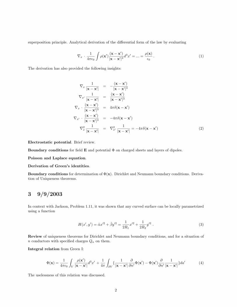
• The separation method has been used to treat the 2D potential problem of corners and edges withstraight surfaces on a constant potential V0 and a potential V (φ) on the cylindrical section of thesurface. The solution is

Φ(ρ, φ) =∞∑

n=1

anρnπβ sin

(nπ

βφ

)with an =

2βR

nπβ

∫ β

φ=0

V (φ) sin(

nπ

βφ

)dφ (24)

V( )f

V0

V0

F r,f( )

V0

V0

V0

V0

V( )=V( )-Vf f 0

0

0

F r,f( )=F r,f( )-V0

~

~= +

Rb

Figure 1: 2D problem of a corner on potential V0 on the straight sections of the surface and potentialV (φ) on the cylindrical section. The figure shows how to use the superposition principle to reduce theproblem to the case of zero potential on the straight surfaces.

As example illustrating the use of the results, we have estimated the outcome of a molecular-beamdeflection experiment in which molecules with a linear polarizability are deflected when travelingparallel to the edge of a thin, grounded conducting plate surrounded by a cylinder on a potentialV .

• Two concentric cylinders with radii a < b and surface potentials Va(φ) and Vb(φ) on the surfaces.Discussion of the general solution

Φ(ρ, φ) = a0 + b0 ln ρ +±∞∑

n=±1,±2,...

(anρn + bnρ−n) (An cos(nφ) + Bn sin(nφ)) , (25)

which is analogous to Eq. 2.71 in the textbook. (issues: which terms to drop in what case, how tofind the remaining coefficients).

Finite element method. The 2D case of finite-element functions of pyramidal shape that are arrangedon a square grid has been discussed.

Reading: improved method using triangular shape functions.

9

8 9/30/2003

Solution of ∆Φ = 0 by separation of variables in spherical coordinates: It has been outlined howthe φ-, the r- and the θ-equations are obtained and solved. The solution of the θ-equation has beenlimited, for now, to the case of azimuthal symmetry (m = 0 all over).

One may add that for the φ- and r-equations and for given values of the separation variables m2 andl(l + 1) two linearly independent solutions contribute, which is the maximum number possible becausethe underlying linear homogeneous differential equations are of 2nd order. For the θ-equation only onesolution Pl(cos θ) is considered as physically relevant solution. The other solution, which formally exists,is obtained by making the other possible choice of α (textbook, Eqn. 3.13, 1st line). That other solutiondiverges at x = cos θ = ±1 and is therefore discarded.

Reading: Properties of Legendre polynomials.

Orthogonality:∫ 1

−1Pl(x)Pl′(x) dx = 2

2l+1δl l′

Function Expansions: From orthogonality and completeness it follows that for well-behaved f(x) on[−1, 1] it is f(x) =

∑∞l=0,1,.. AlPl(x) with Al = 2l+1

2

∫ 1

−1Pl(x)f(x) dx.

Closure: It has been explained how to obtain the closure relation δ(x− x′) =∑∞

l=0,1,..2l+1

2 Pl(x)Pl(x′).

The use of recursion relations between Pl’s has been briefly discussed.

Potential boundary value problems with azimuthal symmetry: The potential is of the generalform Φ(r, θ) =

∑∞l=0,1,..(Alr

l + Blr−l−1)Pl(cos θ), where the Al and Bl are determined from BC.

Example: For given potential V (θ) on a sphere with radius a, the interior solution has Bl = 0and Al = 2l+1

2al

∫ 1

−1V (θ)Pl(cos θ) d cos θ. (I believe I had the factor 2l+1

2 up-side-down when I wrotethis on the board - if so please correct in your notes). For the exterior solution, Al = 0 andBl = (2l+1)al+1

2

∫ 1

−1V (θ)Pl(cos θ) d cos θ.

Another Method of obtaining the expansion coefficients Al and Bl is to perform an exact calcula-tion of Φ(z) along the z-axis, where Pl ≡ 1. Then, expand Φ(z) in either negative or positive powers of z,dependent on whether you seek an exterior or interior solution, respectively. For an interior solution, youmay find, for instance, Φ(z) =

∑∞l=0,1,.. Alz

l. If the problem has azimuthal symmetry, then the potentialat a general location is Φ(r, θ) =

∑∞l=0,1,.. Alr

lPl(cos θ), with the same coefficients Al as in the expansionof Φ along the z-axis. The reason why the method works is the uniqueness of the expansion of both Φ(z)along the z-axis and Φ(r, θ).

As an application, we have derived the following important expansion of 1|x−x′| :

1|x− x′| =

∞∑

l=0,1,...

rl<

rl+1>

Pl(cos θ) , where r< = min(r, r′) and r> = max(r, r′) (26)

As an application of the expansion Eq. 26, we have expanded the potential of a ring charge Q that isconcentric with the z-axis, has a radius a, and has a height b above the xy-plane. This example is coveredin the textbook on page 103. What’s most important to note about this example is that the use of theexpansion Eq. 26 saves us from having to expand 1√

z2+c2−2cz cos αas an infinite power series of z:

The hard way to find Φ(r, θ) would be to first write Φ(z, θ = 0) = q4πε0

1√z2+c2−2cz cos α

, to then

10

expand this either in powers of z for small z or in powers of 1z for large z, to write the result in

the form Φ(z) =∑∞

l=0,1,.. Alzl or Φ(z) =

∑∞l=0,1,.. Blz

−l−1, and to write the general potential asΦ(r, θ) =

∑∞l=0,1,.. Alr

lPl(cos θ) or Φ(r, θ) =∑∞

l=0,1,.. Blr−l−1Pl(cos θ). It will finally be left to show

that the coefficients can be written in the concise form Al1

cl+1 Pl(cos α) and Bl = clPl(cos α), respectively.

Easy way: The use of Eq. 26 yields, after a few lines of just writing down facts rather than doingcalculations, Φ(r, θ) = Q

4πε0

∑∞l=0,1,...

rl<

rl+1>

Pl(cos α)Pl(cos θ), where r< = min(r, c) and r> = max(r, c).

9 10/02/2003

To illustrate the use of the expansion 1|x−x′| =

∑∞l=0

rl<

rl+1>

Pl(cos θ), the problem of a ring with radius a,

charge Q and center at zb has been discussed (see page 103 of textbook). By direct expansion of the exactpotential Φ(z) along the z-axis written as a closed square-root expression, we have obtained the termsl = 0, 1, 2 in the exterior case z > c and seen that the resultant power series has coefficients involvingPl(cos α). It was then shown that an application of the expansion 1

|x−x′| =∑∞

l=0rl

<

rl+1>

Pl(cos γ) for the

case x = zz and x′ = ρa + zb immediately leads to the expansion of the potential up to arbitrary l, validfor arbitrary x.

Cones and tips with azimuthal symmetry. It was outlined how to solve the Legendre differentialequation for Dirichlet BC P (cos β) = 0, with 0 < β < π. The solutions Pν(cos θ) are called the Legendrefunctions of the 1st kind of (generally non-integer) order ν, and they are equivalent to hypergeometricfunctions 2F1(−ν;−ν + 1; 1; cos θ). Some properties of the Pν(cos θ) were pointed out. For given β, acountable set of such functions Pνk

(cos θ)|k = 1, 2, ... satisfies the BC Pν(cos β) = 0. The significanceof the counting index k is that Pνk

(cos θ) has its k-th zero at cos β. The set Pνk(cos θ)|k = 1, 2, ... is a

complete and orthogonal set of functions on the interval [cosβ, 1] (with f(cos β) = 0). Thus, the generalpotential near tips and cones is of the form

Φ(x) =∞∑

k=1

AkrνkPνk(cos θ) (27)

Reading assignment: Properties of the leading term k = 1 of that expansion (textbook p. 106f).Criticality of the lowest order ν1(β). Qualitative change of field behavior at β = π/2.

Potential expansion in spherical coordinates - general case without azimuthal symmetry.

Φ(x) =∞∑

l=0

l∑m=−1

(Almrl + Blmr−l−1

)Ylm(θ, φ) (28)

Some properties of the spherical harmonics Ylm(θ, φ) were reviewed, including orthogonality and closurerelations. The method of how to determine the expansion coefficients in the case of Dirichlet BC on asphere with radius r = a was briefly reviewed.

Reading assignment: Chapter 3.5 of the textbook (properties of spherical harmonics).

The following important expansion of the free-space Green’s function has been pointed out:

11

1|x− x′| =

∞∑

l=0

rl<

rl+1>

Pl(cos γ) =∞∑

l=0

l∑m=−1

4π

2l + 1rl<

rl+1>

Ylm(θ, φ)Y ∗lm(θ′, φ′) (29)

The separation of the Laplace equation in cylindrical coordinates was explained. Two cases ofphysical significance exist:

Case 1: We consider the case that the potential is zero on a cylinder mantle of radius a. Then, thesolutions are of the form Φ(ρ, z, φ) = exp(±iνφ) exp(±kz)Ων(kρ), and linear combinations thereof. Theindex ν usually is 0, 1, 2..., and the variable k is real and ≥ 0. The radial function Ων(kρ) is a Besselfunction (a solution of the Bessel differential equation).

The properties - asymptotic behavior, roots, etc. - of the Bessel functions Jν(x), J−ν(x), the Neumannfunctions Nν(x), and the Hankel functions H

(1)ν (x) = Jν(x) + iNν(x) and H

(2)ν (x) = Jν(x) − iNν(x)

were discussed. The pair Jν(x), Nν(x) is always independent, and so is

H(1)ν (x),H(2)

ν (x)

. Mostimportantly, the function set

√ρ Jν(ρ

xνn

a) | ν ≥ −1 and fixed, andn = 1, 2, 3...

(30)

is a complete orthogonal set on the interval [0, a] with BC f(ρ) = 0 at ρ = a. Thereby, xνn stands forthe n-th root of Jν(x) = 0. Note that each value of ν generates a complete orthogonal set. Using theorthogonality relation

∫ a

0

ρJν(ρxνn

a)Jν(ρ

xνn′

a)dρ =

a2

2J2

ν+1(xνn)δn,n′ (31)

any function f(ρ) that vanishes at ρ = a can be expanded as f(ρ) =∑∞

n=1 AνnJν(ρxνn

a ) with coefficients

Aνn =2

a2 J2ν+1(xνn)

∫ a

0

ρf(ρ)Jν(ρxνn

a)dρ (32)

These findings can be used to expand the potential in cylindrical volumes of radius a with V = 0 on thecylinder mantle. If the cylinder is closed on both top and bottom, we can also - by the superpositionprinciple - require that only the top or the bottom lid is on a non-zero potential. To be specific, assumea bottom lid with V = 0 at z = 0 and a top lid at z = L with potential V (ρ, φ). Convince yourself by acalculation that the potential in the cylinder can be expanded as

Φ(x) =∞∑

m=0

∞∑n=1

Jm(kmnρ) sinh(kmnz) (Amn sin(mφ) + Bmn cos(mφ)) (33)

with kmn = xmn

a and

12

Amn =2

πa2Jm+1(kmna) sinh(kmnL)

∫ 2π

0

∫ a

0

ρV (ρ, φ)Jm(kmnρ) sin(mφ)dρ , n = 1, 2, ...

Bmn =2

πa2Jm+1(kmna) sinh(kmnL)

∫ 2π

0

∫ a

0

ρV (ρ, φ)Jm(kmnρ) cos(mφ)dρ ×

1 , n = 1, 2, ...1/2 , n = 0

(34)

Case 2: The other case of significance is that the potential is zero on the top and the bottom of thecylinder volume, while on the mantle of radius a the potential is non-zero and equal to V (z, φ). Assumingthat the bottom of the cylinder is located in the plane z = 0 and the top in the plane z = L, the interiorsolutions are then of the form exp(±iνφ) sin(kz)Ων(kρ). There, Ων(kρ) is a modified Bessel function, andthe value of k satisfies a quantization condition ka = nπ with integer n.

The commonly used modified Bessel functions are Iν(x) = i−νJν(ix) and Kν(x) = π2 iν+1H

(1)ν (ix). They

are both real and linearly independent. Iν(x) is regular at x = 0 and diverging for x →∞, while Kν(x)is regular for x →∞, and diverging for x → 0.

If there is no radial restriction to the volume of interest, expansions of the potential in non-countablefunction sets characterized by one or more continuous indices are useful. The potential can, for instance,be expanded into a Fourier integral.

In cases of cylindrically symmetric BC without radial restriction we can use the complete orthogonal setof functions

√ρJm(kρ) | k real and k ≥ 0

, which has the orthogonality relation

∫ ∞

0

ρJm(kρ)Jm(k′ρ)dρ =1k

δ(k − k′) ∀m . (35)

Thus, in the (charge-free) volume z > 0 and boundary conditions Φ(ρ, z = 0, φ) = V (ρ, φ) the potentialis given by a Fourier-Bessel integral

Φ(ρ, z, φ) =∞∑

m=0

∫ ∞

0

dk exp(−kz)Jm(kρ) (Am(k) sin(mφ) + Bm cos(mφ)) , (36)

where the coefficient functions are

Am(k) =k

π

∫ ∞

ρ=0

∫ 2π

φ=0

ρV (ρ, φ)Jm(kρ) sin(mφ)dρdφ , m = 1, 2, ...

Bm(k) =k

π

∫ ∞

ρ=0

∫ 2π

φ=0

ρV (ρ, φ)Jm(kρ) cos(mφ)dρdφ ×

1 , m = 1, 2, ...1/2 , m = 0 (37)

Reading: Similar methods involving spherical Bessel functions (p119 of textbook).

Good exercise: Derive completeness relations for complete orthogonal sets (CONS) of Bessel functionson a finite interval [0, a], on [0,∞[, and for CONS of spherical Bessel functions on [0,∞[.

13

Expansion of Green’s functions using complete sets of orthogonal functions. The general usefulnessof the Green’s function has already been discussed earlier. The purpose of the following is to extend theapplication of expansion methods from mere solutions of the Laplace equation to the Green’s function.

Previous example: The free-space Green’s function can be expanded in spherical harmonics as

G(x,x′) =1

|x− x′| =∞∑

l=0

l∑m=−1

4π

2l + 1rl<

rl+1>

Ylm(θ, φ)Y ∗lm(θ′, φ′) . (38)

This result is important in the multipole expansion (Chapter 4 of the textbook). It can also be used toexpand the Green’s functions of problems that can be treated with the image charge method.

Example: Dirichlet Green’s function for the exterior volume of a sphere with radius a. Forthe term in the Green’s function that corresponds to the image charge we use the following:

• Relative image charge size = − ar′ with r′ being the radial coordinate of the source location x′.

• r> = r, where r is the radial coordinate of the observation coordinate x.

• r< = a2

r′

Inserting these figures it is found:

G(x,x′) =∞∑

l=0

l∑m=−1

4π

2l + 1Ylm(θ, φ)Y ∗

lm(θ′, φ′)(

rl<

rl+1>

− 1a

(a2

rr′)l+1

). (39)

10 10/07/2003

Systematic methods of how to expand Green’s functions. As an example, we consider the Green’sfunction of the volume between two concentric shells with radii a < b. This example is lengthier thanmost homework or exam problems of this kind.

Step 1: Write down the differential equation for the Green’s function with δ-function in spherical coordi-nates,

∆G(x,x′) = −4πδ(x− x′) = −4πδ(r − r′)

r′2δ(φ− φ′)δ(cos θ − cos θ′)

Step 2: On right side, use completeness relations for two out of the three involved δ-functions. Inthe present case of spherical coordinates, we only have completeness relations for the angular coordinates.Therefore, we write

∆G(x,x′) = −4πδ(r − r′)

r′2

∞∑

l=0

l∑

m=−l

Y ∗lm(θ′, φ′)Ylm(θ, φ)

14

and re-sort:

∆G(x,x′) =∞∑

l=0

l∑

m=−l

−4π

δ(r − r′)r′2

Y ∗lm(θ′, φ′)

Ylm(θ, φ) (40)

Note: In cylindrical or cartesian coordinates, completeness relations are often known for all three of theinvolved δ-functions, and a choice must be made. Depending on that choice, different but equally validexpansions of the Green’s function are obtained (see homework problems).

Step 3: On left side, expand the Green’s function using the orthogonal function sets that have also beenused in Step 2. Note that x′ only enters as a parameter of the calculation; ∆ acts on x.

∆G(x,x′) = ∆∞∑

l=0

l∑

m=−l

Alm(r|r′, θ′, φ′)Ylm(θ, φ)

Step 4: Write Laplacian in the proper coordinates and take derivatives of all orthogonal functions thathave been introduced in Steps 2 and 3. It many cases you will have to use a known differential equationto take these derivatives. Typically, you will have to use the (plain or generalized) Legendre differentialequation to eliminate angular derivatives of spherical harmonics or Legendre functions. To eliminateradial derivatives of Bessel functions, employ the Bessel differential equation. In the present example, weuse the generalized Legendre differential equation.

∆G(x,x′) =∞∑

l=0

l∑

m=−l

[1r

∂2

∂r2r +

1r2 sin θ

∂

∂θsin θ

∂

∂θ+

1r2 sin2 θ

∂2

∂φ2

]Alm(r|r′, θ′, φ′)Ylm(θ, φ)

Using x = cos θ, it is

∆G(x,x′) =∞∑

l=0

l∑

m=−l

[1r

∂2

∂r2r +

1r2

∂

∂x(1− x2)

∂

∂x− m2

r2 sin2 θ

]Alm(r|r′, θ′, φ′)Ylm(θ, φ)

The generalized Legendre differential equation allows us to write ddx (1 − x2) d

dxPml (x) =[

−l(l + 1) + m2

1−x2

]Pm

l (x), and also ∂∂x (1−x2) ∂

∂xYlm =[−l(l + 1) + m2

1−x2

]Ylm. Thus, with 1−x2 = sin2 θ

∆G(x,x′) =∞∑

l=0

l∑

m=−l

[1r

∂2

∂r2r − l(l + 1)

r2+

m2

r2 sin2 θ− m2

r2 sin2 θ

]Alm(r|r′, θ′, φ′)Ylm(θ, φ)

∆G(x,x′) =∞∑

l=0

l∑

m=−l

[1r

d2

dr2r − l(l + 1)

r2

]Alm(r|r′, θ′, φ′)

Ylm(θ, φ) (41)

Step 5: Expansions in orthogonal sets of functions are unique. Thus, we can separately equate thecoefficients of the Ylm in Eq. 40 and Eq. 41. Dividing the resultant equation by Y ∗

lm(θ′, φ′), we find

[1r

d2

dr2r − l(l + 1)

r2

] Alm(r|r′, θ′, φ′)

Y ∗lm(θ′, φ′)

= −4π

δ(r − r′)r′2

15

Step 6: Noticing that the expression in the curly brackets of the last equation can possibly only dependl, r and r′, we define the reduced (radial) Green’s function

gl(r, r′) =Alm(r|r′, θ′, φ′)

Y ∗lm(θ′, φ′)

.

Note that the radial Green’s function only depends on one of the two indices of the orthogonal functionset employed in Steps 2 and 3. This is an exception. In most other cases, reduced Green’s functions willdepend on all indices of the utilized orthogonal function sets.

We proceed to solve

[1r

d2

dr2r − l(l + 1)

r2

]gl(r, r′) = −4π

δ(r − r′)r′2

(42)

Outside the location of the δ-function inhomogeneity, the solutions are of the form gl(r, r′) = Arl−Br−l−1.More specifically, to match the boundary condition gl(r = a, r′) = 0, for r < r′ it must be gl(r, r′) ∝rl− a2l+1

rl+1 . To match the boundary condition gl(r = b, r′) = 0, for r > r′ it must be gl(r, r′) ∝ r−l−1− rl

b2l+1 .Further, gl(r, r′) must be symmetric in r and r′, and it must be continuous at r = r′. To satisfy all theseconditions, gl(r, r′) must be of the form

gl(r, r′) = C

(rl< −

a2l+1

rl+1<

) (r−l−1> − rl

>

b2l+1

),

with a constant C to be determined to match the behavior near the δ-function inhomogeneity. Also,r< = min(r, r′) and r> = max(r, r′).

Step 7: Find C. Integrating Eq. 42 from r′− ε to r′+ ε with ε → 0 and dropping vanishing terms we find

d

dr(rgl(r, r′))|r=r′+ε − d

dr(rgl(r, r′))|r=r′−ε = −4π

r′

A lengthy but simple calculation yields

C =4π

(2l + 1)(1− (

ab

)2l+1)

Step 8:

Going backward through all steps, the Green’s function expansion is assembled into the final result:

gl(r, r′) =4π

(2l + 1)(1− (

ab

)2l+1)

(rl< −

a2l+1

rl+1<

) (r−l−1> − rl

>

b2l+1

),

Alm(r|r′, θ′, φ′) =4π

(2l + 1)(1− (

ab

)2l+1)

(rl< −

a2l+1

rl+1<

) (r−l−1> − rl

>

b2l+1

)Y ∗

lm(θ′, φ′)

16

and finally

G(x,x′) = 4π

∞∑

l=0

l∑

m=−l

Y ∗lm(θ′, φ′)Ylm(θ, φ)

(2l + 1)(1− (

ab

)2l+1)

(rl< −

a2l+1

rl+1<

) (1

rl+1>

− rl>

b2l+1

)

Reading: Use of the above Green’s function to calculate the potential produced by charge distributions(Chapter 3.10 of the textbook).

Reading: Application of the expansion method to expand the free-space Green’s function in cylindricalcoordinates (Chapter 3.11 of the textbook).

Eigenfunction expansion of the Green’s function.

General method. The solutions ψ(x) of the eigenvalue problem

(∆ + f(x) + λ)ψ(x) = 0

with eigenvalues λ can be arranged to form an orthonormal, complete set of functions on the def-inition rage of the equation. Boundary conditions may apply. Closed volumes lead to count-able sets ψn(x), n = 1, 2, .. with corresponding eigenvalues λn, while open volumes have sets withat least one continuous parameter. In free space and f(x) = 0, for instance, one may choose

ψk(x) = 1√2π

3 exp(ik · x),k ∈ R3

with eigenvalues λk = k2.

The analogy of the situation to quantum mechanics has been discussed. In that language, ∆ + f(x) is aHermitian linear differential operator. As is well known, such operators plus their boundary conditionsgenerate orthonormal, complete sets of eigenfunctions.

It has been shown that orthogonality and completeness of the set ψn(x) with eigenvalues λn lead toan expansion of the Green’s function. Assume

(∆ + f(x) + λn)ψn(x) = 0 ,

with ψn(x) satisfying any boundary conditions that may apply. The Green’s function is defined as thesolution of

(∆ + f(x) + λ)G(x,x′) = −4πδ(x− x′) ,

with G(x,x′) satisfying the same boundary conditions as the ψn(x). It follows

Gλ(x,x′) = 4π∑

n

ψ∗n(x′)ψn(x)λn − λ

.

In the special context of the Laplace equation, set f(x) = 0 and λ = 0 in the above equations. Then,for discrete sets of eigenfunctions satisfying (∆ + λn)ψn(x) = 0, n = 1, 2, .., boundary conditions, andorthonormality

∫ψ∗n(x)ψn′(x)d3x = δn,n′ we have

17

G(x,x′) = 4π∑

n

ψ∗n(x′) ψn(x)λn

.

For sets of eigenfunctions with continuous eigenvalues satisfying (∆ + λk)ψk(x) = 0, continuous k ,boundary conditions (if any), and orthonormality

∫ψ∗k(x) ψk′(x)d3x = δ(k − k′) we have

G(x,x′) = 4π

∫

k

ψ∗k(x′) ψk(x)λk

dk .

Sometimes there is more than one continuously variable index for the eigenfunctions. Also, combinationsof continuous and discrete indices exist. In all these cases, add integrals or sums in the above equationsas appropriate.

Two examples have been briefly discussed (rectangular box and free space).

11 10/16/2003

Multipole expansion. The first case in which such expansions are useful is if we are concerned withthe potential generated by a small charge distribution in an otherwise charge- and field-free space. Weconsider the potential of a charge distribution ρ(x′) of typical extension R at locations x with |x| = r > R.Then, application of the free-space Green’s function expansion Eq. 38 yields

Φ(x) =1

4πε0

∞∑

l=0

l∑

m=−l

4π

2l + 1qlm

1rl+1

Ylm(θ, φ) (43)

with spherical multipole moments

qlm =∫

ρ(x′) r′l Y ∗lm(θ′, φ′) d3x′ (44)

Alternately, an expansion of 1|x−x′| in cartesian coordinates for fixed x around x′ = 0 yields

Φ(x) =1

4πε0

∞∑

l=0

l∑

k,m, n = 0k + m + n = l

[1

k!m!n!∂k

∂x′k∂m

∂y′m∂n

∂z′n

(1

|x− x′|)]

x′=0

∫ρ(x′)x′ky′mz′n dx′dy′dz′

=1

4πε0

∞∑

l=0

l∑

k,m, n = 0k + m + n = l

P(l)kmn(x, y, z, r)

r2l+1Q

(l)kmn

(45)

18

Thereby, l identifies the order of the expansion terms (as in the expansion in spherical coordinates). P(l)kmn

is a l-th order polynomial in the observation point coordinates (x, y, z, r =√

x2 + y2 + z2), leading to anoverall radial dependence of the l-th order terms ∝ 1

rl+1 (as in the expansion in spherical coordinates).Further, Q

(l)kmn is the l-th cartesian multipole moment

Q(l)kmn =

∫ρ(x′)x′ky′mz′n dx′dy′dz′ (46)

The monopole (l = 0) and dipole (l = 1) terms have been stated. It has been shown in class that afterresorting of terms the quadrupole (l = 2) contribution takes the form given in Eq. 4.10 of the textbook,with the quadrupole tensor given in Eq. 4.9. Unless noted otherwise, Eq. 4.9 and 4.10 are used to calculatecartesian quadrupole moments and their potentials and fields.

To further demonstrate the systematics in the cartesian multipole expansion, in the following the nextterms are given. You may check that the term l = 3 is

Φ3(x) =1

4πε0

3∑

i, j, k = 1i ≤ j ≤ k

[1

Aijk

∂

∂x′i

∂

∂x′j

∂

∂x′k

(1

|x− x′|)]

x′=0

∫ρ(x′)x′ix

′jx′k d3x′

=1

4πε0

3∑

i, j, k = 1i ≤ j ≤ k

15xixjxk − 3r2(δijxk + δjkxi + δkixj)Aijk r7

Qijk

where the indices i, j, k refer to the three components of cartesian coordinates, Qijk is the octupolemoment Qijk =

∫ρ(x′)x′ix

′jx′k d3x′, and Aijk = 1 if all indices are different, Aijk = 2 if exactly two

indices are equal and Aijk = 6 if all indices are equal. The general form of this result conforms with thel = 3-term of Eq. 45; note, however, the different meanings of the indices. It is, for instance, Q122 = Q

(3)120.

Similarly, you should find for l = 4

Φ4(x) =1

4πε0

3∑

i, j, k, m = 1i ≤ j ≤ k ≤ m

[1

Aijkm

∂

∂x′i

∂

∂x′j

∂

∂x′k

∂

∂x′m

(1

|x− x′|)]

x′=0

∫ρ(x′)x′ix

′jx′kx′m d3x′

=1

4πε0

3∑

i, j, k, m = 1i ≤ j ≤ k ≤ m

Hijkm(x)Ahijk r9

Qijkm with

Hijkm(x) = 105xixjxkxm − 15r2(δijxkxm + δjkxixm + δikxjxm + δimxjxk + δjmxixk + δkmxixj)+ 3r4(δijδkm + δjkδim + δikδjm) (47)

There, Qijkm =∫

ρ(x′)x′ix′jx′kx′m d3x′, and Aijkm = 2 if exactly two indices are equal, Aijkm = 6 if

exactly three indices are equal, and Aijkm = 24 if all indices are equal. This result is of the same form

19

as the l = 4-term in Eq. 45. Again, note the different meanings of the indices. It is, for instance,Q1123 = Q

(4)211.

Important fact a: Out of the (l + 2)(l + 1)/2 cartesian multipole moments Q(l)kmn of order l, defined in

Eq. 46, there are only 2l + 1 independent ones. This number equals the number of spherical moments oforder l; the latter are all independent from each other.

Important fact b: The lowest-order non-vanishing multipole moments are invariant under translationsof the origin (not under rotations).

For the cartesian moments, this fact follows from a transformation rule obtained in the following. Assumethat the multipole moments in a certain frame are labeled Q

(l)kmn. The origin is then translated by

x0 = (x0, y0, z0). Then, the transformed moments Q(l)kmn are

Q(l)kmn =

∫ρ(x)(x− x0)k(y − y0)m(z − z0)n dxdydz

=k∑

a=0

m∑

b=0

n∑c=0

(ka

)(mb

)(nc

)(−x0)k−a (−y0)m−b (−z0)n−c

∫ρ(x)xaybzc dxdydz

=k∑

a=0

m∑

b=0

n∑c=0

(ka

)(mb

)(nc

)(−x0)k−a (−y0)m−b (−z0)n−c Q

(a+b+c)abc

=

k∑a=0

m∑

b=0

n∑c=0

∣∣∣∣∣a+b+c<l

(ka

)(mb

)(nc

)(−x0)k−a (−y0)m−b (−z0)n−c Q

(a+b+c)abc

+ Q

(l)kmn

(48)

There, the (∗) are binomial coefficients. Since the expression in the curly brackets only contains multipolemoments of orders lower than l, it is shown that the lowest-order non-vanishing multipole moments areindependent of translations of the origin.

Important fact c: The contributions of the multipoles to the potential scale as ∼ 1r

(Rr

)l, where R is

the size of the source and the origin is assumed to be chosen inside the source (which is a prerequisite forthe expansion to make sense). This scaling behavior explains why the multipole expansion is a powerfultool.

Review the following:

• Electric fields associated with multipole moments.

• Potentials and fields of an electric dipole.

• Distinction and relation between idealized multipoles and their approximate realizations. Thematter has been discussed in class for an electric dipole.

20

In preparation of future subjects, the following results have been obtained. Consider the integral overthe electric field inside a sphere with radius R. If the sphere includes all charges ρ(x), then

∫

r<R

E(x)d3x = − p3ε0

with dipole moment p =∫

r<R

xρ(x)d3x . (49)

If all charges are outside the sphere, then the average electric field in the sphere equals the field at thecenter, i.e.

∫

r<R

E(x)d3x =4π

3R3 E(0) . (50)

Reading: detailed derivation of these equations in Chapter 4.1.

The second case in which multipole expansions are useful is if one is concerned with the energy of a chargedistribution ρ(x) of typical size R in an external electric field that varies over length scales much largerthan R. We assume that the shape of the distribution ρ(x) is fixed, while its position and orientationwith respect to the external sources may be varied. The situation is analyzed in a body frame of thecharge distribution; the origin of that frame should be chosen inside the distribution. Expansion of theexternal potential around the origin of the body frame yields

W = qΦ(0)− p ·E(0)− 16

3∑

i,j=1

Qij∂Ej

∂xj(0) + ... with

q =∫

ρ(x) d3x

p =∫

x ρ(x) d3x

Qij =∫

(3xixj − r2δij) ρ(x) d3x (51)

There, Φ(0), E(0) and ∂Ej

∂xj(0) are the potential, the field and the field derivatives due to the external

sources at the origin (which is fixed with respect to the charge distribution). The self-energy of the chargedistribution is not included in this result. The energy W depends on the location and the orientation ofthe body and its charge distribution relative to the external field sources.

The following applications of Eq. 51 have been discussed:

• Interaction energy between two electric dipoles. See Eq. 4.26 in textbook.

• Hyperfine structure (HFS) of atoms. The HFS is due to the interactions between the multipolesof the nuclear charge distribution with the field produced by the electron system at the nucleus.The magnetic-dipole interaction, which presently is not of interest, has been pointed out because itnormally dominates the HFS. Electric-dipole and magnetic-quadrupole interactions between nucleiand electron shells are identical zero due to the well-defined parity of the nuclear wavefunction.Therefore, the next-higher HFS term, which we are concerned with in the present context, isthe electric-quadrupole interaction. The Casimir formula, derived 1936, was quoted (H. B. G.

21

Casimir, On the Interaction Between Atomic Nuclei and Electrons, reprinted by W. H. Freeman,San Francisco (1963)):

WHFS,E2 = −14

∂Ez

∂z

∣∣∣∣x=0

eQ0

32C(C + 1)− 2I(I + 1)J(J + 1)

I(2I − 1)J(2J − 1)with

C = F (F + 1)− I(I + 1)− J(J + 1) . (52)

There, I, J , and F are the nuclear spin, total electronic spin (orbital plus intrinsic), and hyperfinequantum numbers, respectively. Further, ∂Ez

∂z

∣∣x=0

is the z-derivative of the z-electric field producedby the electron system at the location of the nucleus, whereby the z-axis is taken parallel to the totalelectronic spin J. Finally, Q0 is the nuclear quadrupole moment Q0 = 1

e

∫(3z′2 − r′2)ρ(x′) d3x′,

calculated in a body frame the z-axis of which coincides with the nuclear symmetry axis (if onemodels the nucleus as a classical charge distribution). The homework problem 4.6 corresponds tothe case F = I + J .Note. To solve the homework problem, the above details are not required. You only need thecylindrical symmetry of the electric field and of the nuclear charge distribution about the z-axis.

Electrostatics in dielectric media. In dielectric media, it is desirable to have differential equationsfor a macroscopic electric field. The macroscopic field is the volume average of the microscopic field,E(x) = 〈Emicro(x)〉volume. The averaging volume is small on a macroscopic scale, but contains manymolecules. In contrast to the microscopic field, which is complicated and normally unnecessary to know,the macroscopic field follows simple equations. The microscopically valid (and therefore always valid)homogeneous equation ∇× Emicro = 0 can be averaged: 0 = 〈∇ × Emicro〉volume = ∇× 〈Emicro〉volume =∇×E. Thus, it is

∇×E = 0 ,

which is the same equation as in free space. We conclude that in dielectric media the electric field willstill be derivable from an electric potential Φ(x).

The inhomogeneous equation ∇ · E = ρ/ε0 is modified as follows. The dielectric medium is assumed tocontain molecules of species i with corresponding volume densities Ni. One molecule of species i carriesan average charge qi (which is usually zero) and an average molecular dipole pi. Higher-order multipolesof the molecules are neglected (which is an exceedingly good approximation). We account for free charges(and molecular charges, if 6= 0) in the free-charge density ρfree(x); the subscript is usually omitted andwe just write ρ(x). The molecular dipole moments are accounted for via a macroscopic polarizationP(x) =

∑i Ni(x)pi(x). It was then derived in class that

∇ · [ε0E(x) + P(x)] = ∇ ·D(x) = ρ(x) ,

where [ε0E + P] = D defines the electric displacement field D.

Once the polarization P(x) is known, the volume polarization charge ρpol(x) = −∇ · P(x) can becalculated. On boundaries of polarized media to the vacuum, there is a surface polarization chargeσpol(x) = n ·P(x), where the normal vector n is pointing from the medium outward. These polarizationcharges are not included in the density of free charges ρ(x). In contrast, the variable ρall in the equationfor the microscopic field, ∇ · E(x) = ρall

ε0, includes both free and polarization charge. Thus, questions

22

about charge densities in dielectric media have to be handled very carefully, and a clear distinctionbetween free and polarization charges must be made.

Reading and review: Definition of linear and isotropic dielectric media. Definitions of electric permit-tivity, dielectric constant and electric susceptibility.

Boundary conditions at interfaces between dielectric media. Assume fields E1 and D1 at theboundary of region 1 and fields E2 and D2 at the boundary of region 2. Then,

[D2(x)−D1(x)] · n = σ(x)[E2(x)−E1(x)]× n = 0 , (53)

with the normal vector n pointing from region 1 to region 2. Thus, the component of D normal to theinterface displays a discontinuity of size σ - the surface density of free charges -, while the components ofE in plane with the interface are continuous. The validity of these boundary conditions does not requirelinear and / or isotropic behavior of the dielectric.

Examples discussed in class:

• In infinite volumes with constant permittivity ε, the electric field follows the equations ∇× E = 0and ∇ · E = ρ(x)

ε . Thus, in electrostatic equations containing ε0 - such as the potentials andfields due to localized charges, the potentials and fields due to charge distributions, capacitances,electrostatic energy, energy of capacitors - the dielectric medium is accounted for by replacing ε0by the permittivity ε = ε0εr (where εr is the dielectric constant).

• The polarization charge at a dielectric interface with given E- and D-fields on both sides and withzero free charges has been calculated.

• The potential Φ(x) due to a polarized object with given polarization P (x) in an otherwise source-and field-free volume can be obtained by calculation of the polarization charges and subsequent useof a microscopic equation for Φ(x):

Φ(x) =1

4πε0

(∫

V \∂V

−∇′ · P (x′)|x− x′| d3x′ +

∫

∂V

n′ · P (x′)|x− x′| da′

), (54)

where the volume integral is only over the interior of the polarized object. That is, don’t extendthe volume integral over the discontinuity of P (x), because that would amount to double-countingthe effect of the surface polarization charge.

• The solution of the following image charge problem has been outlined: The volume z > 0 haspermittivity ε1, and the volume z < 0 has permittivity ε2. A (free) point charge q is locatedat (0, 0, d) with d > 0. The problem can be solved by assuming two image charges at locations(0, 0,±d) and consideration of the boundary conditions for Dz and for Ex, Ey on the interface planez = 0.Reading: Details of this example in Chapter 4.4 of the textbook.

23

12 10/21/2003

The image charge problem from the previous lecture was used in order to demonstrate how volume andpolarization charges are obtained once the electric potential Φ(x) is established:

1) Obtain the polarization P(x) = −(εi − ε0)∇Φ(x) for the involved regions with permittivities εi.

2) The polarization volume charge is then ρpol = −∇ ·P(x).

3) The surface polarization charge at interfaces between regions labeled 1 and 2 is σpol = n · (P1 −P2),where n is the normal vector pointing from region 1 to region 2.

3) Via integration of result 2) over a small volume including a point charge and use of Eq. 2, or via aconsideration based on Gauss’s law in integral form, it is seen that point charges of size q are surroundedby a δ−function polarization charge qpol = q( ε0

ε − 1), where ε is the permittivity of the medium.

Other example. These concepts have been further explained using the example of a dielectric sphere withradius a and permittivity ε placed in an initially homogeneous electric field zE0. There, the potential isobtained via variable separation in spherical coordinates:

Inside: Φin =∑∞

l=0 AlrlPl(cos θ)

Outside: Φin =∑∞

l=0 Clr−l−1Pl(cos θ)− E0rP1(cos θ)

The boundary condition for D is ε ∂∂r Φin|r=a = ε0

∂∂r Φout|r=a, and the boundary condition for E is

∂r∂θ Φin|r=a = ∂

r∂θ Φout|r=a. The latter, together with A0 = C0 = 0, is equivalent with Φin|r=a = Φout|r=a.Equating the coefficients of the Legendre polynomials (or the derivatives of these), an algebraic equationfor the coefficients Al, Cl is found:

(εlal−1 ε0(l + 1)a−l−2

al−1 −a−l−2

)(Al

Cl

)=

( −ε0E0δl,1

−E0δl,1

)

The solution can be found with Kramer’s rule, and is given in the textbook (page 158f). The resultantfields and polarization charges have been obtained.

Molecular polarizability. The Clausius-Mossotti equation has been derived. This equation relatesthe microscopic molecular polarizability γmol with the macroscopic electric permittivity ε. There, γmol isdefined through the linear relation between microscopic electric dipole moment (per molecule) p and themicroscopic electric field Emol at the exact location of the molecule, p = ε0γmolEmol. An important findingleading to the Clausius-Mossotti equation is a relation between macroscopic (volume-averaged) fieldE, the macroscopic polarization P and the microscopic electric field Emol, stating

Emol = E +P3ε0

.

This equation is valid for most crystalline and amorphous media, and has been derived in class in threeways. Using this equation, P = Np with N denoting the number of molecules per volume, and P =(ε− ε0)E, the Clausius-Mossotti equation is obtained:

24

γmol =3N

(εε0− 1

εε0

+ 2

).

The equation is important because it relates the microscopic molecular parameter γmol with a macroscopic,phenomenological quantity (the dielectric constant ε

ε0).

Microscopic models for the molecular polarizability γmol, based on classical mechanics and classicalstatistical mechanics, have been briefly discussed. The distinction between induced and orientationpolarization has been pointed out.Reading: Chapter 4.6 of the textbook.

13 10/23/2003

Energy considerations in dielectric media. Various important equations and their range of applicabilityhave been discussed:

A charge distribution ρ(x) is assumed to generate a potential Φ(x), and no charges other than thoseincluded in ρ(x) are supposed to be present. The positive-definite total electrostatic energy, which canbe interpreted as the self-energy of the whole distribution ρ(x), then is

W =12

∫ρ(x)Φ(x)d3x =

12

∫E(x) ·D(x)d3x . (55)

This equation is valid in vacuum and in linear dielectric media. In the latter case, polarization energyand field energy is included in the total electrostatic energy W , and ρ(x) denotes free charge and excludespolarization charges (as usual).

A more general equation, valid for electrostatic energy in any dielectric, is

W =∫

V

∫ D

D=0

E [D, path] · δD

d3x .

This equation also covers cases of nonlinear behavior and/or hysteresis.

Eq. 55 can be used to show the following. The introduction of a linear dielectric body from a field-freeregion into a field region with initial value E0(x), generated by fixed sources, results in a change ofelectrostatic energy by the amount

W = −12

∫

V

P(x) ·E0(x)d3x

where the integral goes over the volume of the dielectric, and P(x) denotes its final-state polarization.Thus, electrostatic energy is reduced when a dielectric body is brought into a region with increased electricfield. The energy balance is converted into translational and/or rotational kinetic energy. Therefore,mechanical forces can be derived from

25

Fξ = −(

∂W

∂ξ

)

Q

,

where the subscript reminds us that the charges are held fixed (in capacitor problems, this is the caseof “disconnected batteries”). The coordinate ξ can be any generalized coordinate of the dielectric body(position, angle, etc.); the force equation can therefore also be used to derive torques, for instance.

A complementary equation for the case of fixed potentials on the boundaries exists:

Fξ = +(

∂W

∂ξ

)

V

,

where the subscript indicates that the boundary potentials are kept fixed. In capacitor problems, thiscorresponds to the case of “connected batteries”.

When a dielectric body moves into a region of increased electric field while the boundary potentials arekept fixed, the kinetic energy of the body and the total electrostatic energy increase by the same amount.Thus, the change in total energy (electrostatic plus kinetic) equals twice the change in electrostatic energy.The energy is provided by the (connected) batteries, which supply the boundary surfaces with chargesrequired to maintain their fixed potentials while the dielectric moves into the field.

14 10/21/2003 (Review session)

Some specific information on the exam material was provided (see e-mailed and posted exam information).

Elements of the lecture notes were reviewed.

The example of a dielectric sphere with radius a and permittivity ε placed in an initially homogeneouselectric field zE0 was explained in more detail.

Potential inside: Φin =∑∞

l=0 AlrlPl(cos θ)

Potential outside: Φin =∑∞

l=0 Clr−l−1Pl(cos θ)− E0rP1(cos θ)

The boundary condition for D is ε ∂∂r Φin|r=a = ε0

∂∂r Φout|r=a, and the boundary condition for E is

∂r∂θ Φin|r=a = ∂

r∂θ Φout|r=a. The latter, together with A0 = C0 = 0, is equivalent with Φin|r=a = Φout|r=a.Equating the coefficients of the Legendre polynomials (or the derivatives of these), an algebraic equationfor the coefficients Al, Cl is found:

(εlal−1 ε0(l + 1)a−l−2

al−1 −a−l−2

)(Al

Cl

)=

( −ε0E0δl,1

−E0δl,1

)

Determinant: D(l) = −(lε + (l + 1)ε0)a−3. Since D 6= 0 ∀ l, it is Al = Cl = 0 unless l = 1.

In the case l = 1, use Kramer’s rule to find

26

A1 =3ε0E0a

−3

−(ε + 2ε0)a−3= −E0

32 + ε/ε0

.

C1 =−(ε− ε0)E0

−(ε + 2ε0)a−3= E0a

3 ε/ε0 − 12 + ε/ε0

.

The similarity of this example with homework problem 4.8 was pointed out.

In context with electrostatic energy in dielectrics, the following example has been discussed. A planarcapacitor with plate separation d, length L À d and width b À d is initially filled with air (ε = ε0).A dielectric material with permittivity ε > ε0, thickness d, length L and width b is then allowed tomove without friction into the capacitor until it fills its entire interior. One capacitor plate is on a fixedpotential 0, the other on a fixed potential V .

Force: All fields are perpendicular to the field plates. The electric field is E = V/d, the electricdisplacement D = ε0E in the air-filled region and D = εE in the region filled with the dielectric.Denoting the length of the dielectric that is already inside the capacitor as x, the dielectric energy is

W (x) =12

∫E(x) ·D(x)d3x =

V 2 b

2d(εx + ε0(L− x)) ,

and the force that pulls the dielectric further into the capacitor is

Fx =(

∂W

∂x

)

V

=V 2 b

2d(ε− ε0) .

Change in electrostatic energy (field plus polarization): As the dielectric moves from entirelyoutside to entirely inside the capacitor, the electrostatic energy changes by

∆Wel = W (L)−W (0) =V 2Lb

2d(ε− ε0) =

V 2

2(Cf − Ci) ,

with Cf and Ci denoting final and initial capacitances.

The kinetic energy of the dielectric increases by the same amount,

∆Wkin = FxL =V 2Lb

2d(ε− ε0) =

V 2

2(Cf − Ci) .

The work done by the battery keeping the capacitor plates on fixed potentials is

∆Wbat = ∆Wel + ∆Wkin =V 2Lb

d(ε− ε0) = V 2 (Cf − Ci) .

The charge densities on the more positive plate are σfree = ε0E and σfree = εE in the air-filled anddielectric-filled portions, respectively. The polarization surface charge density in the dielectric-filledportion is σpol = −(ε − ε0)E and zero elsewhere. Reverse all signs to obtain the surface charges on the

27

more negative plate and the adjacent dielectric surface. The volume polarization charge density iszero everywhere.

The amount of free charge flowing onto the capacitor plates during the process is ∆q = Lb∆σfree =Lb(ε− ε0)E = V (ε− ε0)Lb

d = V (Cf − Ci). The work done by the battery then is ∆Wbat = V ∆q =V 2 (Cf − Ci), in agreement with the result above.

15 10/28/2003 (Midterm exam)

16 10/30/2003

Continuity equation. Due to conservation of electric charge, it is generally

∇ · j(x, t) = − ∂

∂tρ(x, t)

Magnetostatics. The range of validity of this theory covers static current distributions (i.e. the case∇ · j = 0). Magnetic fields of current distributions that vary on time scales much slower than R/c areapproximately described (R = max(|x−x′|) with the maximum taken over all source coordinates x′ andobservation coordinates of interest x′).

Basics. Biot-Savart’s law:

dB =µ0

4π

dj× (x− x′)|x− x′|3 and B =

∫dB .

To integrate, substitute dj = jd3x′, = Kda′, = Idl′, or = qv0(t)δ(x − x0(t))d3x′ for volume currents,surface currents, line currents and moving charges, respectively. In the last case, which is only valid aslong as v0 ¿ c, x0(t) and v0(t) characterize the particle trajectory.

Some examples amenable to direct calculation were mentioned (B-fields of line currents and circular-loopcurrents along loop axis; review if necessary).

Forces F and torques N of an external field B(x) on a current distribution:

dF = dj×B and F =∫

dF .

dN = x× dF and N =∫

dN .

To integrate, substitute dj = jd3x′, = Kda′, = Idl′, or = qv0(t)δ(x − x0(t))d3x′ for volume currents,surface currents, line currents and moving charges, respectively. The last case is not restricted to v0 ¿ c.

Some examples amenable to direct calculation were mentioned (forces between two parallel line currentsand between to general loop currents).

Differential equations for B. Gauss’s law and Ampere’s law were derived from Biot-Savart’s law andthe right-hand-rule pertinent to the use of Ampere’s law in integral form were discussed.

28

∇ ·B = 0 ⇔ ∮SB · da = 0

∇×B = µ0j ⇔ ∮∂S

B · dl = µ0

∫Sj · da = µ0Ienclosed

(56)

Boundary conditions. Consider two regions 1 and 2 connected via a surface carrying a surface currentK. The respective B-fields at the interface are B1 and B2. Then, the boundary conditions

n · (B2 −B1) = 0n× (B2 −B1) = µ0K , (57)

where n denotes the unit vector pointing from region 1 to region 2. Note the sensitivity of the secondequation to the direction of n.Exercise: Derive these conditions from Eqs. 56.

Vector potential. From Gauss’s law it follows that there exists a vector field A(x) such that B =∇×A(x).

There actually is an infinite number of valid vector potentials delivering the same magnetic field. Vectorpotentials A and A′ for the same B-field are connected via a gauge transformation

A′ = A +∇ψ ,

with ψ(x) being a well-behaved function. It was shown that there always exists a gauge transformationsuch that A′ is in the Coulomb gauge:

∇ ·A′ = 0

There also is an infinite number of vector potentials in the Coulomb gauge, since an A′′ with A′′ =A′ +∇ψ, A′ in the Coulomb gauge, and ψ satisfying the Laplace equation, will also be in the Coulombgauge.

The B-field, which - at least in classical physics - is the physically relevant observable, is independent ofthe gauge. Thus, there is no fundamental advantage of the Coulomb gauge. There is, however, a greattechnical advantage which is that in the Coulomb gauge a relatively simple differential equation for Aapplies. From Ampere’s law it quickly follows that

∇2A = −µ0j ⇔∆Ai = −µ0ji for i = 1, 2, 3 (58)

apply for vector potentials in the Coulomb gauge. In analogy with the solution of the Poisson equationin free space, the standard solution is

A(x) =µ0

4π

∫j(x′)|x− x′|d

3x′ (59)

The solution is a vector potential in the Coulomb gauge. While this is by no means the only possiblevector potential, it is sufficient to subsequently calculate the B-field (which is unique).

29

As an example, the vector potential of a circular current loop was calculated in detail.Read Chapter 5.5 in textbook.

Multipole expansion of the B-fields of localized current distributions. Expanding 1|x−x′| in

Eq. 59 using familiar methods, the leading term of the expansion is found to be the magnetic-dipoleterm; there is no monopole term because of ∇ · j = 0. The magnetic-dipole field with the (cartesian)magnetic-dipole moment m is given by

A(x) =µ0

4π

m× x|x|3

B(x) =µ0

4π

3(m · n)n−m|x|3

where m =12

∫x′ × j(x′)d3x′ (60)

with n = x/|x|.Examples. For loop currents with current I, the magnetic-dipole moment is m = I

2

∮x × dl, and for

planar loop currents it is m = IAn. There, A is the loop area and n the area normal vector. Thedirection of n is defined by the current direction and a right-hand rule.

17 11/4/2003

Multipole expansion of the vector potential: The objective of the method is to obtain an expansionof A(x) for localized current distributions observed at distances larger than the current distribution.Methods: To obtain spherical magnetic multipole moments, insert Eq. 29 into Eq. 59. The leading termis the dipole term (l = 1); there is no monopole term. Cartesian multipole moments are obtained bystarting with a Taylor expansion of 1

|x−x′| in Eq. 59 around x′ = 0. Properties of the dipole term werebriefly reviewed.

Atomic and nuclear dipole moments: The connection between angular momentum and magneticmoment was discussed.

Miscellaneous useful relations: For spherical volumes of radius R containing all currents of interestit is

∫

r<R

B(x)d3x =2µ0

3m ,

where m is the dipole moment of the current distribution. The finding leads to a δ-function correctionto the magnetic field of a point dipole located at the origin,

B(x) =µ0

4π

[3n(m · n)−m

|x|3 +8π

3δ(x)

](61)

with n = x/|x|.

30

For spherical volumes of radius R with all currents located outside it is

∫

r<R

B(x)d3x =4π

3R3B(0)

Interaction of localized current distributions with external fields that vary slowly within thevolume of the current distributions: Expanding the B-field around a point inside the distribution,one finds expressions for the potential energy, the force and the torque on the leading multipole momentof the current distribution, which is the dipole moment m of Eq. 60. The equations are analogous tothose in electrostatics (replace E, p with B, m).

As an example, the magnetic-dipole hyperfine interaction was discussed. It was pointed out thatthe δ-function term of Eq. 61 in the magnetic field of the electron magnetic moment is important toexplain the S-state magnetic hyperfine structure.

18 11/6/2003

Magnetostatics in magnetically active media. Definitions of the macroscopic magnetization, themacroscopic B-field and the H-field,

M =∑

i

Ni〈mi〉time,100a0

B = 〈Bmicro〉time,100a0

H =1µ0

B−M ,

the fundamental equations

∇ ·B = 0∇×H = jfree = j , (62)

the bound current density

jbound = ∇×M ,

and the applicable boundary conditions,

n · (B2 −B1) = 0n× (H2 −H1) = Kfree = K , (63)

were reviewed. In the last two equations, two regions 1 and 2 connected via a surface carrying a freesurface current K are considered. The respective fields at the interface are B1 and B2 and H1 and H2,

31

and n denotes the unit vector pointing from region 1 to region 2. Note that currents occurring in themacroscopic equations are free currents; the subscripts “free” are usually dropped. Free currents mustnot be confused with the currents in the microscopic equations (for B); the latter are free plus boundcurrents.

The significance of the fields (the fundamental B-field and the auxiliary H-field) and different types oflinear magnetic behavior (paramagnetic, diamagnetic) and non-linear behavior (hysteresis, soft ferromag-netic, hard ferromagnetic) were discussed.

The behavior of B- and H-lines at a (free-)current-free interface between different linear, magneticallyactive media was sketched.

Methods to solve the magnetostatic equations.

• Linear material with known free current: Solve

∇2A = −µj ,

and obtain B = ∇×A and H = B/µ. An equation analogous to Eq. 59 and expansions of 1|x−x′|

may be useful. If there is different domains with different µ, connect the solutions in the differentdomains using the boundary conditions Eq. 63 at the interfaces. From the fields, the magnetizationis M = ( µ

µ0− 1)H, the (bound) volume magnetization current is jM = ∇ ×M, and the surface

magnetization current KM = M× n.

• Linear material with zero free current: Find the magnetostatic potential from

∆Φm = 0 ,

and obtain H = −∇Φm and B = µH. Variable separation methods may be useful. If thereis different domains with different µ, connect the solutions in the different domains using theboundary conditions Eq. 63 at the interfaces. From the fields, the magnetization is M = ( µ

µ0−1)H,

the (bound) volume magnetization current is jM = ∇×M, and the surface magnetization currentKM = M× n.

• Fixed magnetization and zero free current:

Find the magnetostatic potential from

∆Φm = −ρM ,

where the volume “magnetic charge” is ρM = −∇ ·M. Under absence of boundary conditions it is

Φm =14π

∫

all space

ρM (x′)|x− x′|d

3x′ .

As always, variable separation methods and expansions of Green’s functions may be useful. ObtainH = −∇Φm and B = µ0(H + M). If there is different domains with different µ, connect thesolutions in the different domains using the boundary conditions Eq. 63 at the interfaces.

Special case: For a magnetized object of volume V and discontinuous surface ∂V , one can use thevolume “charge” density ρM = −∇·M and the surface “charge” density σM = M · n, with n beingthe normal vector on the object, to write

32

Φm =14π

∫

V \∂V

ρM (x′)|x− x′|d

3x′ +14π

∫

∂V

σM (x′)|x− x′|da′ .

Alternately, one may calculate the vector potential by inserting the (bound) volume magnetizationcurrent jM = ∇×M and the surface magnetization current KM = M× n into Eq. 59, yielding

A =µ0

4π

∫

V \∂V

jM (x′)|x− x′|d

3x′ +µ0

4π

∫

∂V

KM (x′)|x− x′| da′ .

Reading: Sphere with homogeneous magnetization (various examples; Chapter 5.10 and 5.11). Magneticshielding with permeable shell (Chapter 5.12).

Some solution methods for highly permeable materials.

• Current-free volume outside a highly permeable medium. A highly permeable medium with surface∂V located in an external magnetic field acts as an equipotential surface for the magnetic potentialoutside the medium. A solution for the magnetic potential can be obtained by solving ∆Φm = 0with the Dirichlet boundary condition Φm = 0 on ∂V .

• Volume inside a linear highly permeable medium. Consider the two-dimensional case that themedium has a surface ∂V in the xy-plane, is invariant under z-translation, and carries a currentj(x, y) = jz(x, y)z. Then, the vector potential can be chosen as A(x) = Az(x, y)z. The problem re-duces to a Poisson equation ∆Az(x, y) = −µjz(x, y) with Dirichlet boundary condition Az(x, y) = 0on ∂V . Solution methods known from electrostatics can be employed, including numerical ones suchas the iteration method Eq 1.82 of the textbook (set g(x, y) = µjz(x, y)).

19 11/11/2003

Faraday’s law.

∮E · dl = − d

dt

∫B · da ⇔ ∇×E = − ∂

∂tB

Assuming Galilean invariance of the magnetic field, a transformation law for the electric field was derivedfrom Faraday’s law in integral form. In a frame moving with velocity v0 with respect to an inertial framein which the electric field is E and the magnetic field is B, the electric field is E′ = E + v0 × B. Thisis correct in first order in v0/c (compare with Eq. 11.149 in Jackson). In the context of this proof, learnabout the convective derivative, explained in class and in the textbook.

It was derived that the magnetostatic energy, including magnetization energy, is

W =∫

V

d3x

∫ B(x)

B=0

H(B, path) · δB

33

This equation is generally valid (including nonlinear materials and materials with hysteresis).

In linear materials, it is

W =12

∫

V

H ·Bd3x =12

∫

V

j ·Ad3x .

The energy of a linear object brought from a field-free region into a region with magnetic fields producedby fixed currents and initial values of the field Binitial(x) and final values of the magnetization Mfinal(x)is

W =12

∫

V

Binitial(x) ·Mfinal(x)d3x .

The component of the force on such an object corresponding to a generalized coordinate ξ is

Fξ = +(

∂W

∂ξ

)

currents fixed

.

These equations have strong analogies with equations from electrostatics, which may be exploited formemorization.

For systems of current loops with currents Ii, the magnetostatic energy

W =12

∫

V

j ·Ad3x =µ0

8π

∫

V

∫

V

j(x) · j(x′)|x− x′| d3x d3x′

can be rewritten by substituting j(x)d3x → Iidli and j(x′)d3x′ → Ijdlj into a practical form:

W =12

∑

i

Li I2i +

12

∑

i,j(i 6=j)

Mij Ii Ij =12

∑

i

Li I2i +

∑

i>j

Mij Ii Ij

Li =µ0

4π

∮

i

∮

i

dli · dl′i|xi − x′i|

Mij =µ0

4π

∮

i

∮

j

dli · dlj|xi − xj |

There, Li are self-inductances and Mij mutual inductances. Obviously, the self energy of loop i is 12Li I2

i .The Mij are mutual inductances that describe the loop interaction energies, which are Mij Ii Ij .

The voltage induced at loop i due to current variations in any loop, including its own current, are givenby

Ui = −∑

j

Mijd

dtIj .

34

All equations can be written in a comprehensive matrix form, as shown in class.

Magnetic-field diffusion. As well known, the spread of magnetic-field lines in conducting media ishampered by induction and Lenz’s rule. In effect, in many situations magnetic-field lines spread muchslower than the speed of light, and the time variation of the fields is slow enough that the displacementcurrent in Ampere’s law pays no significant role. From Maxwell’s equations (less the displacement current)and Ohm’s law, j = σE with conductivity σ, it then follows for media with uniform and time-independentpermeability µ

∇2A(x, t) = µσ∂

∂tA(x, t)

This is a diffusion equation. The same equation applies to the electric field E(x, t). It was then estimatedthat the typical penetration time of B-fields through a system of spatial size L is

τ ∼ µσL2 .

If the conductivity is homogeneous, too, the same diffusion equation applies to B(x, t) and j(x, t).

Example. The case of a magnetic field with harmonic time dependence incident on a conducting mediumwas discussed (Jackson, p220f). The fields and the resultant Ohm heating power in the medium weregiven, and the significance of the skin depth,

δ =√

2µσω

,

was explained. Study this example and derive the results.

20 11/13/2003

Maxwell’s equations. It was shown how to properly add the displacement current ∂∂tD into Ampere’s

law. The resultant complete set of Maxwell’s equations in media was noted, and their temporal, spatialand energetic ranges of validity were discussed (the microscopic equations are valid over wider ranges).

Partial solution via potentials. The homogeneous equations are automatically solved by writing

B(x, t) = ∇×A(x, t)

E(x, t) = −∇Φ(x, t)− ∂

∂tA(x, t)

The scalar potential Φ and the vector potential A follow a smaller set of coupled partial differentialequations, which in free space (D = ε0E, H = µ−1

0 B) reads

35

∇2Φ(x, t) +∂

∂t(∇ ·A(x, t)) = −ρ(x, t)

ε0

∇2A(x, t)− ∂2

c2∂t2A(x, t)−∇

(∇ ·A(x, t) +

∂

c2∂tΦ(x, t)

)= −µ0j(x, t) (64)

where the vacuum velocity of light c = 1/√

ε0µ0. Note that Eq. 64 applies to potentials in any gauge.

Gauge transformations and Lorentz gauge. Using a gauge transformation with an arbitrary scalarfunction ψ, one can introduce new sets of potentials that yield the same fields as the original ones andare therefore equally valid:

A′(x, t) = A(x, t) +∇ψ(x, t)

Φ′(x, t) = Φ(x, t)− ∂

∂tψ(x, t)

For any set of potentials Ψ,A, the scalar function ψ can be chosen such that it satisfies an inhomogeneouswave equation

[∇2 − ∂2

c2∂t2

]ψ(x, t) = −

[∇ ·A(x, t) +

∂

c2∂tΦ(x, t)

],

which is solvable (see Eq. 6.32ff), and yields gauge-transformed potentials with

∇ ·A′(x, t) +∂

c2∂tΦ′(x, t) = 0

Potentials satisfying this condition are said to be in the Lorenz gauge. It is thus always possible toadopt the Lorenz gauge.

Note. Gauge transformations of potentials that are already in the Lorenz gauge with functions ψ thatsolve the homogeneous wave equation yield new potentials that are also in the Lorenz gauge.

In the Lorenz gauge, the equations for the potentials reduce to inhomogeneous wave equations,

[∇2 − ∂2

c2∂t2

]Φ(x, t) = −ρ(x, t)

ε0[∇2 − ∂2

c2∂t2

]A(x, t) = −µ0j(x, t) in Lorenz gauge (65)

The equations for Φ and A are automatically decoupled.

Note. One can always adopt the Lorenz gauge. The solution of Eq. 65 will then, of course, yieldpotentials in the Lorenz gauge. While these potentials are not unique in any way, the fields derived fromthem are.

36

Coulomb gauge. As shown before, one may also require ∇ · A = 0. Any set of potentials Ψ, Acan be gauge-transformed into the Coulomb gauge by finding a ψ that satisfies the Poisson equation∆ψ = −∇ ·A.

In the Coulomb gauge, the scalar potential is identical with the instantaneous Coulomb potential (hencethe name Coulomb gauge), and the vector potential follows from a wave equation the inhomogeneity ofwhich contains a term depending on the scalar potential:

∇2Φ(x, t) = −ρ(x, t)ε0

⇒ Ψ(x, t) =1

4πε0

∫

V

ρ(x′, t)|x− x′|d

3x′

[∇2 − ∂2

c2∂t2

]A(x, t) = −µ0j(x, t) +

1c2∇ ∂

∂tΨ(x, t) in Coulomb gauge (66)

Thus, if one intends to use these equations to find Ψ and A, the scalar potential Ψ should be determinedfirst.

The Coulomb gauge is particularly useful if there are only radiation fields (hence the alternate nameradiation gauge). With ρ = 0 and j = 0 it is

Φ(x, t) = 0[∇2 − ∂2

c2∂t2

]A(x, t) = 0 Coulombgauge without sources (67)

Thus, only the vector potential needs to be determined, and it follows from a homogeneous wave equation.

Coulomb gauge using transverse current. The equations for Ψ and A in the Coulomb gauge canbe decoupled using a decomposition of the current j(x, t) into a longitudinal part jl(x, t) and a transversepart jt(x, t) with ∇× jl(x, t) = 0 and ∇ · jt(x, t) = 0 (hence the alternate name transverse gauge for theCoulomb gauge). According to the Helmholtz theorem, such a decomposition always exists. Explicitly,one may obtain the transverse current jt and the longitudinal current jl from

j(x, t) = jl(x, t) + jt(x, t)

jt(x, t) =14π∇×∇×

∫

V

j(x′, t)|x− x′|d

3x′

jl(x, t) = − 14π∇

∫

V

∇′ · j(x′, t)|x− x′| d3x′

It then becomes

37

∇2Φ(x, t) = −ρ(x, t)ε0[

∇2 − ∂2

c2∂t2

]A(x, t) = −µ0jt(x, t)

where jt(x, t) =14π∇×∇×

∫

V

j(x′, t)|x− x′|d

3x′

Coulombgauge using transverse current (68)

Noting that the solution of Maxwell’s equations (both directly or via potentials) often requires the solutionof inhomogeneous wave equations, the Green’s function of the wave equation will be a useful instrument.It was derived in class for systems without boundary conditions and constant, frequency-independent εand µ (in most cases of interest, ε = ε0 and µ = µ0).

Helmholtz equation and its Green’s function. Inserting the temporal Fourier transform of thesolution ψ(x, t) and the inhomogeneity f(x, t) into the wave equation, we find, using the orthogonalitycondition

∫∞−∞ exp(i(ω − ω′)t)dt = 2πδ(ω − ω′),

[∇2 − ∂2

c2∂t2

]ψ(x, t) = −4πf(x, t)

ψ(x, t) =12π

∫ ∞

−∞ψ(x, ω) exp(−iωt)dω with ψ(x, ω) =

∫ ∞

−∞ψ(x, t) exp(iωt)dt

f(x, t) =12π

∫ ∞

−∞f(x, ω) exp(−iωt)dω with f(x, ω) =

∫ ∞

−∞f(x, t) exp(iωt)dt

⇒ [∇2 + k2]ψ(x, ω) = −4πf(x, ω) . (69)

The last equation is an inhomogeneous Helmholtz equation; k = ωc . Its free-space Green’s function,

defined as

[∇2 + k2]Gk(x,x′) = −4πδ3(x− x′) , (70)

depends only on k and R := |x− x′| and is

Gk(R) = Aexp(ikR)

R+ (1−A)

− exp(ikR)R

=: AG+(R) + (1−A)G−(R)

with constant A. This result has been derived in class, and it has been explained why G+(R) is associatedwith an outgoing wave (from a source location x′), and G−(R) with an ingoing wave.

Note: Using the Green’s function, the solution to Eq. 69 in free space is

ψ(x, ω) =∫

V

f(x′, ω)Gk(x,x′)d3x′ ,

because

38

[∇2 + k2]ψ(x, ω) =

[∇2 + k2] ∫ ∞

−∞f(x′, ω)Gk(x,x′)d3x′

=∫ ∞

−∞f(x′, ω)

[∇2 + k2]Gk(x,x′)

d3x′

=∫ ∞

−∞f(x′, ω)(−4π)δ3(x− x′) dω

= −4πf(x, ω)

Green’s function of wave equation. Per def., the Green’s function satisfies

[∇2 − ∂2

c2∂t2

]G(x, t,x′, t′) = −4πδ3(x− x′)δ(t− t′)

Inserting temporal Fourier transforms wrt. to t for G(x, t,x′, t′) and δ3(x − x′)δ(t − t′) and using theorthogonality of the exp(iωt), the reduced Green’s function for k = ω/c is seen to satisfy

[∇2 + k2]Gk(x,x′) = −4πδ3(x− x′) exp(iωt′)

[∇2 + k2] (

Gk(x,x′)exp(iωt′)

)= −4πδ3(x− x′) . (71)

Comparison with Eq. 70ff shows that

Gk(x,x′) = G±k (R) =exp(±ikR)

Rexp(iωt′) .

The inverse Fourier transform then yields G±(R, t− t′):

G±(R, t− t′) =12π

∫ ∞

−∞G±k (R) exp(−iωt)dω

=12π

1R

∫ ∞

−∞exp

[iω(t′ − t± R

c)]

dω

=δ(t′ − [

t∓ Rc

])

R. (72)

.

There, the upper signs correspond to the retarded Green’s function, in which a source at locationx′ and time t′ produces an outgoing wave that arrives at the observation point x at a delayed timet = t′ + R/c. The lower signs correspond to the advanced Green’s function, in which a signalobserved at an observation point x at a time t produces an ingoing wave that converges towards a sourceat location x′ and time t′ = t + R/c. Physical interpretations of the two types of Green’s functions,consistent with causality, will be given later.

39

With the Green’s functions, we can write down two particular solutions of

[∇2 − ∂2

c2∂t2

]ψ(x, t) = −4πf(x, t) ,

namely

ψ±(x, t) =∫

V

∫ ∞

t′=−∞f(x′, t′)G±(x, t,x′, t′)d3x′dt′

ψ±(x, t) =∫

V

∫ ∞

t′=−∞f(x′, t′)

δ(t′ − [t∓ R

c

])

Rd3x′dt′

ψ±(x, t) =∫

V

f(x′, t′ =[t∓ R

c

])

Rd3x′ . (73)

There, in the last line the time integral over the source time t′ have been evaluated using the temporalδ-function part in the Green’s functions.

The following notations are used. For solutions involving retarded particular solutions constructed withthe retarded Green’s function we write

ψ(x, t) = ψ0(x, t) + ψ+(x, t) = ψ0(x, t) +∫

V

[f(x′, t′)]retR

d3x′ . (74)

The notation implies that the time variable t′ is not an integration variable. It is to be constructed fromthe observation coordinates x and t and from the source location x′, over which we take the integral,following

t′ = t− R

c= t− |x− x′|

c< t .

In Eq. 74 we have added a solution ψ0(x, t) of the homogeneous wave equation to match any boundaryconditions, if needed (discussed later).

Similarly, for solutions involving particular solutions constructed with the advanced Green’s function wewrite

ψ(x, t) = ψ0(x, t) + ψ−(x, t) = ψ0(x, t) +∫

V

[f(x′, t′)]adv

Rd3x′ . (75)

Here, t′ is to be constructed from the observation coordinates x and t and from the source location x′

using

t′ = t +R

c= t +

|x− x′|c

> t .

Again, in Eq. 75 we have added a solution ψ0(x, t) of the homogeneous wave equation to match anyboundary conditions (discussed later).

40

21 11/18/2003

The physical significance of retarded and advanced Green’s functions was discussed. Generally,

ψ±(x, t) = ψ0(x, t) +∫

V

G±(x, t,x′, t′)f(x′, t′)d3x′dt′ . (76)

• If ψ0(x, t) in Eq. 76 represents a solution of the homogeneous wave equation before sources turnon, the retarded Green’s function G+ must be used. In that case, during and at any time afterthe activity of the sources the integral term in Eq. 76 generates the source-induced waves. Due tothe retardation condition t′ = t − |x − x′|/c, the relation between observation coordinates (ct,x)and source coordinates (ct′,x′) is explicitly causal, meaning that in vacuum signals propagate atthe velocity of light.

• If ψ0(x, t) in Eq. 76 represents a solution of the homogeneous wave equation after the sources haveturned off, ψ0(x, t) already includes the source-induced waves. In that case, the advanced Green’sfunction must be used. The integral term in Eq. 76 then annihilates the source-induced waves atobservation times before the sources turn on. Thus, the effect of the advanced Green’s function isto keep source-induced waves from propagating into the past of the source time.

In any case, both types of Green’s functions - retarded and advanced - are, when used properly, consistentwith the principle of causality.

It was outlined how one can find from either the Maxwell equations or form the potentials Φ, A thefollowing wave equations (in vacuum):

[∇2 − ∂2

c2∂t2

] (EB

)=

( − 1ε0

[−∇ρ− ∂c2∂t j

]−µ0 [∇× j]

)(77)

Using the previously found expressions for the Green’s functions for the case that there are no fields priorto source activation, it is

E(x, t) =1

4πε0

∫d3x′

1R

[−∇′ρ(x′, t′)− ∂

c2∂t′j(x′, t′)

]

ret

B(x, t) =µ0

4π

∫d3x′

1R

[∇′ × j(x′, t′)]ret (78)

Driven by a desire to remove the ∇ from these equations, it was first shown that for functions f(x′, t′)and vector fields f(x′, t′)

[∇′f(x′, t′)]ret = ∇′ [f(x′, t′)]ret −Rc

[∂

∂t′f(x′, t′)

]

ret

[∇′ × f(x′, t′)]ret = ∇′ × [f(x′, t′)]ret −Rc×

[∂

∂t′f(x′, t′)

]

ret

,

41

from which it follows that

E(x, t) =1

4πε0

∫d3x′

RR2

[ρ(x′, t′)]ret +RcR

[∂

∂t′ρ(x′, t′)

]

ret

− 1c2R

[∂

∂t′j(x′, t′)

]

ret

B(x, t) =µ0

4π

∫d3x′

[j(x′, t′)]ret ×

RR2

+[

∂

∂t′j(x′, t′)

]

ret

× RcR

. (79)

Since t′ret = t−R/c and R = |x− x′| does not include time variables, this equals

E(x, t) =1

4πε0

∫d3x′

RR2

[ρ(x′, t′)]ret +RcR

∂

∂t[ρ(x′, t′)]ret −

1c2R

∂

∂t[j(x′, t′)]ret

B(x, t) =µ0

4π

∫d3x′

[j(x′, t′)]ret ×

RR2

+∂

∂t[j(x′, t′)]ret ×

RcR

. (80)

These expressions were then specified to the field of a moving point charge q with trajectory r0(t) andvelocity v(t) = d

dtr0(t). Then,

ρ(x′, t′) = q δ3(x′ − r0(t′))j(x′, t′) = q v(t′) δ3(x′ − r0(t′))

Some hints were given for homework problem 6.2, which is to obtain the fields

E(x, t) =q

4πε0

[R

κR2

]

ret

+∂

c∂t

[RκR

]

ret

− ∂

c2∂t

[ vκR

]ret

B(x, t) =µ0 q

4π

[v × RκR2

]

ret

+∂

c∂t

[v × R

κR

]

ret

. (81)

There, κ =[1− v·R

c

]ret

results from a Jacobi determinant that incurs when the spatial integral in Eq. 80

is executed using the δ3(x′ − r0(t′)). It was noted that the independent variables of R in Eq. 81 are xand t.

Eq. 81 was discussed using space-time diagrams. The initial steps of a field calculation for a point chargemoving with constant velocity along the z-axis were presented. To see the fields for that specific case,refer to Sec. 11.10.

22 11/20/2003

Conservation laws for energy. Poynting theorem’s for linear materials with time-independent (=frequency-independent) and real ε and µ was derived and written in differential and integral forms,

42

∫

V

E · jd3x +∫

V

∂

∂tud3x = −

∫

V

∇ · (E×H)d3x =: −∫

V

∇ · Sd3x = −∫

∂V

S · da

E · j +∂

∂tu = −∇ · (E×H) = −∇ · S (82)

where S = E×H is the Poynting vector and u is the electromagnetic energy density, which includes allpolarization energies and equals u = 1

2 (E ·D + B ·H).

All terms in this energy conservation law have physical meanings, which were discussed. The powerdensity of Ohm heating is E · j, the rate at which the EM energy density varies is ∂

∂tu, and the powerdensity due to radiation is ∇ · S. The significance of the latter largely is that the radiation intensity (=energy per area per time) through a surface element da is S · da. In Eq. 82, da points out of the volumeof interest.

Note the restrictions of this result. In particular, real ε and µ implies that there are no polarizationlosses in the medium.

Poynting theorem’s for linear materials with frequency-dependent ε(ω) and µ(ω). In the caseof frequency-dependence (dispersion), ε(ω) and µ(ω) necessarily have imaginary parts, as dictated by theKramers-Kronig relations discussed later. Assuming that the spectral intensity of the fields cover only asmall ω-range centered around a carrier frequency ω0, a fairly simple energy conservation law similar toEq. 82 can be derived (Eqs. 6.126f in Jackson). A notable new feature is the occurrence of a new termaccounting for energy losses caused by phase lags between fields and polarizations (“polarization losses”;second term on the rhs of Eq. 6.127).

Conservation laws for momentum. The derivation of a conservation law for the momentum ofparticles and fields in vacuum was sketched. The result,

d

dt(Pmech + Pfield)α =

∮

∂V

∑

β

Tαβ nβ da (83)

was interpreted in detail. There, α and β are indices for cartesian coordinate directions, Pmech =∑

i pi

is the sum of all momenta pi of the particles, labeled i, inside the volume of interest,

Pfield = ε0

∫

V

E×Bd3x =1c2

∫

V

Sd3x

is the momentum associated with the electromagnetic field,

ε0E×B =1c2

S

is the momentum density associated with the electromagnetic field, nβ are the cartesian components ofthe normal vector of the surface ∂V of the volume of interest V , and

Tαβ = ε0

(EαEβ + c2BαBβ − 1

2

(|E|2 + c2 |B|2

)δαβ

)

43

are the elements of the Maxwell stress tensor. To develop some intuition of the stress tensor, the effect ofthe rhs of Eq. 83 was compared with hydrostatic pressure. Thereby, note that the hydrostatic pressurein tensor notation would be diagonal with all diagonal elements being equal.

23 11/25/2003

Energy conservation in the case of harmonic fields. Fields and sources are written as

E(x, t) = Re [E(x) exp(−iωt)] ,

where the E on the left is real and dependent on x and t, while the E on the right is complex anddependent on x only. Similar arrangements are made for the other fields and the sources. The Maxwellequations then yield the following set of equations for the complex field quantities and sources:

∇ ·B = 0∇ ·D = ρ

∇×H + iωD = j

∇×E− iωB = 0 . (84)

Upon solution, real fields are obtained from

E(x, t) =12

(E(x) exp(−iωt) + c.c.) =12

(E(x) exp(−iωt) + E∗(x) exp(+iωt)) etc.

The energy conservation laws involve products of field quantities. Since for harmonic fields thecycle-averages of such products follow

〈E(x, t) · j(x, t)〉 =12Re [E(x) · J∗(x)] =

12Re [E(x)∗ · J(x)] etc.,

expressions involving this and and other (including cross) products of real fields can be translated intoforms for the complex spatial parts of the fields/sources by complex-conjugating one of the two factors andmultiplying with 1/2. It does not matter which one of the variables in products is complex-conjugated.Physically meaningful laws are extracted by taking the real part.

The following definitions are common:

• Complex Poynting vector: S(x) = 12E(x)×H∗(x)

• Complex magnetic energy density: um(x) = 14B(x) ·H∗(x)

• Complex electric energy density: ue(x) = 14E(x) ·D∗(x)

Application to energy conservation. The Ohm heating power density, E(x, t) · j(x, t), has been seento follow

44

E · j +∇ · (E×H) + E∂

∂tD + H

∂

∂tB . (85)

Inserting complex fields, taking the time derivatives, and then applying the described translation proce-dure yields

12E · j∗ +

12∇ · (E×H∗) +

12E · [−iωD]∗ +

12

[−iωB] ·H∗ = 0 .

Using the above definitions for the complex Poynting vector and the complex field energy densities, weobtain the complex Poynting theorem,

12E · j∗ +∇ · S + 2iω [ue − um] = 0 (86)

A physical law is extracted by taking the real part. Assuming complex ε and µ and integrating overspace, it is seen that

∫

V

12Re [E · j∗] d3x +

∫

∂V

S · da +∫

V

ω

2

[Im(ε) |E|2 + Im(µ) |H|2

]d3x = 0 (87)

The physical meaning of the terms was discussed (Ohm heating, radiation transport, polarization loss;same order as in equation). The steady-state-nature of the situation described by Eq. 87 was stressed.

Exercise. Show that for the possible choices of which field variables in the products in Eq. 85 arecomplex-conjugated the extracted physical law always is Eq. 87.

Reading. Determination of the impedance of a linear circuit (Sec. 6.9).

Transformation properties of the laws of classical electromagnetism. The objective of this unitis to show the invariance of classical electromagnetism under rotation (not discussed explicitly but true),spatial inversion and time reversal.

The theory of orthogonal transformations was briefly reviewed. Detailed elaborations can be found inlinear algebra textbooks.

Definitions. We assume that a system is actively transformed using a rotation described by a matrixA with elements aαβ . The transformed position vectors are denoted x′ = Ax; transformed functions oftransformed position vectors are also identified with a ’.

• Scalar = tensor of rank 0 = a scalar function with S′(x′) = S(x)Examples: electric potential, charge (density), divergence of vectors as defined in the next item.

• Vector = tensor of rank 1 = a vector field satisfying V′(x′) = AV(x)Examples: position, momentum, gradient of scalars as defined in the first item.

• Tensor of rank 2 = a quantity the components of which transform as T ′αβ(x′) =∑

γδ aαγaβδTαβ(x)Example: Maxwell stress tensor.

45

The scheme can be continued to arbitrary rank-N tensors,

T ′αβγ...(x′) =

∑

α′β′γ′...

aαα′aββ′aγγ′ ...Tα′β′γ′...(x)

Spatial inversion. All orthogonal transformations with det(A) = −1 involve a reflection or an inversion;the latter is characterized by

A =

−1 0 00 −1 00 0 −1

Physical quantities characterized as scalars, vectors etc. under rotations can be sub-categorized furtherdependent on their behavior under spatial inversion:

• True scalar = even scalar = a scalar with S′(−x) = S(x)Examples: mass, kinetic energy, potential energy, electric potential, charge (density).

• Pseudo-scalar = odd scalar = a scalar with S′(−x) = −S(x)

• Polar vector = true vector = odd vector = a vector satisfying V′(−x) = −V(x)Examples: position, velocity, momentum, gradient of true scalars, force, E, P, D, current j, Poynt-ing vector S.

• Axial vector = pseudo-vector = even vector = a vector satisfying V′(−x) = V(x)Examples: cross products of true vectors (angular momentum, torque, etc.), B, M, H.

• Even tensor = a tensor that transforms as T ′αβ...(−x) = Tαβ...(x)

• Odd tensor = a tensor that transforms as T ′αβ...(−x) = −Tαβ...(x)

• True tensor of rank N = a tensor that transforms as T ′αβ...(−x) = (−1)NTαβ...(x)

• Pseudo-tensor of rank N = a tensor that transforms as T ′αβ...(−x) = (−1)N+1Tαβ...(x)

Note. From the above it follows that the transformation law for cross products of true vectors for allorthogonal transformations (including reflection and inversion) is

A,B true vectors and C = A×B ⇒ C′(x′) = det(A)AC(x)

Time reversal. Physical quantities T are characterized as

• (Time-)even if T ′(−t) = T (t).Examples: mass, position, force, torque, potential, kinetic energy, charge (density), E, P, D,Maxwell stress tensor.

• (Time-)odd if T ′(−t) = −T (t).Examples: velocity, momentum, current(density), B, M, H, Poynting vector S.

46

24 12/2/2003

Invariance of physical laws under spatial (I) and time (T) inversions. It was demonstratedthat the canonical equations for a particle in a conservative potential V (x) are invariant under thesetransformations: d

dtx = ∂∂pH(x,p) is T-odd and I-odd, while d

dtp = − ∂∂xH(x,p) is T-even and I-odd.

Exercise: Show this. Also, you may verify that Newton’s II law is I-odd and T-even.Note: For the physical system to be T-invariant, it is sufficient that each of its equations of motiontransforms consistently as either odd or even under time reversal; the same applies for invariance underspatial inversion. (“Consistently” means that all individual terms in any given equation must transformthe same way.) It is not necessary that all equations of motion transform the same way.

Transformation behavior of the Maxwell equations. It was shown that

• ∇ ·D = ρ is T-even and I-even.

• ∇ ·B = 0 is T-odd and I-odd.

• ∇ ×E + ∂∂tB = 0 is T-even and I-even.

• ∇ ×H− ∂∂tD = j is T-odd and I-odd.

Thus, I- and T-invariance of classical electrodynamics is established. (Invariance under rotation andcharge conjugation also applies.)Note. In case that there are “external” fields, the sources causing the external fields must also besubjected to the transformations.

Application. Elimination of fundamentally impossible terms from postulated physical laws. In a pos-tulated physical law, a term is fundamentally impossible and must be eliminated if it does not transformin the same way as other terms for which the transformation behavior is known. (Examples: Jackson,p. 272f and homework.)

Magnetic charge. Assuming that there was magnetic charges ρm and currents jm, Maxwell’s equationswould be

∇ ·D = ρe

∇ ·B = ρm

∇×E +∂

∂tB = −jm

∇×H− ∂

∂tD = je . (88)

Also, ρm would have to be T-odd and I-odd, and jm T-even and I-even.

Maxwell’s equations are invariant under a duality transformation

(E

Z0H

)= A

(E′

Z0H′

)

47

and analogous for(

Z0DB

),(

Z0ρe

ρm

)and

(Z0jejm

). There, A =

(cos ξ sin ξ

− sin ξ cos ξ

)with ξ T-

odd and I-odd. If there were magnetic charges and there was always a constant ratio between magneticand electric charge, a suitable duality transformation could be made to cast Maxwell’s equation into theirnormal, magnetic-charge-free from. Consequently, in view of the duality transformation the statementthat there exist no magnetic charges can be relaxed to stating that all matter has a constant ratio ofmagnetic to electric charge. For convenience, we usually work in a frame in which the magnetic chargehas been transformed to identical zero by the means of a suitable duality transformation.

Magnetic monopoles. In the usual frame in which “normal matter” has no magnetic charge, hypo-thetical magnetic charges - magnetic monopoles - would have to satisfy a quantization condition

g =nh

ewith n ∈ N .

The derivation of this result, following Dirac’s construction of the vector potential of a monopole, waspresented and discussed in detail (Jackson, p. 278ff). The result was related to magnetic-flux quantizationand the Aharonov-Bohm effect.

25 12/4/2004

Harmonic pane electromagnetic waves in source-free, loss-free linear media. Use the ansatzfor the complex electric and magnetic fields,

E(x, t) = E exp(ikn · x− iωt)B(x, t) = B exp(ikn · x− iωt) (89)

with complex constant vectors E , B, n, real k =√

εµω = nc0

ω, real refractive index n and vacuum velocityof light c0. Insert into the homogeneous Helmholtz equation, the divergence Maxwell equations, and thecurl equations to find, in that order,

n · n =εµω2

k2

E · n = B · n = 0B =

√εµn× E (90)

In the most important cases n is real. In that case one finds for frequency ω, wavevector k = nk, andcomplex amplitude E0 two linearly independent plane-wave solutions with orthogonal linear polarizations,namely

E = ε1E0 and B = ε2n

c0E0

and

48

E = ε2E0 and B = −ε1n

c0E0 .

There, ε1, ε2,n form a right-handed system of real orthonormal unit vectors.

The complex pointing vector of any of these is

S =12E×H∗ =

12µ

n

c0|E0|2n

and the complex energy density

u =14

(εE ·E∗ +

1µB ·B∗

)=

ε

2|E0|2

Since in the present case ε and µ are real, the physical quantities Re(S) = S and Re(u) = u. (In certainprints of Jackson, a factor 1/2 is missing in Eqn. 7.13).

General field for given ω and k = nk: E(x, t) = (ε1E1 + ε2E2) exp(ik · x− iωt). There, k =√

εµω andE1, E2 complex constants.

The special cases of linear polarization and circular polarization have been discussed in some detail.The characterization of the polarization state using the Stokes parameters has been briefly outlined.

Reflection and refraction laws. We refer to Fig. 7.5 in Jackson. It has been shown that considerationof any of the boundary conditions on the fields, e.g. z ·D(x, t) + z ·D′′(x, t) = z ·D′(x, t) ∀ x =(x, y, z = 0) yields the following:

• k, k′, k′′ and z all lie in one plane, called the plane of incidence.

• i = r′ (Reflection law)

• n sin(i) = n′ sin(r) (Snell’s law)

The matter is discussed exhaustively in textbooks such as Griffiths, Introduction to Electrodynamics.

26 12/9/2004

Fresnel’s equations. Expressions for the electric-field amplitudes of reflected and transmitted wavesrelative to that of the incident wave are obtained from the boundary conditions for E, D, B and H forz = 0, σ = 0, K = 0, and the plane-wave relation between complex electric and magnetic-field amplitudes,B = 1

ωk × E. The resultant six equations (Eqn. 7.37 in Jackson) are not all independent, and some ofthem are identical zero (dependent on the polarization of the incident wave).

It is customary to quote the reflection and transmission coefficients for the electric-field amplitudes forelectric fields in and transverse to the plane of incidence. In any case, the boundary conditions (Eqn. 7.37)and the known reflection and transmission angles lead to two equations for the reflection and transmission

49

coefficients. The result (Fresnel equations) is given in Eqns. 7.39 and 7.41 of Jackson. Note that theseequations and their limits for i = 0 have to be viewed in context with the definition of the field directionsin Fig. 7.6.. Also, note that the equations are also valid for complex refractive index and in cases withimaginary sin(r′). Phase jumps of π of the reflected beam, most commonly seen upon normal reflectionat an optically denser medium, were briefly mentioned.

Special phenomena. Brewster’s angle, iB = tan−1(n′/n) and total internal reflection were discussed.The latter phenomenon occurs when n′ < n and i > i0 = sin−1(n′/n). The nature of the wave inthe primed region, called evanescent wave, its energy flow, Poynting vector and penetration depth werediscussed. Note that the evanescent wave can be written in the form Eev = E exp(ikn ·x− iωt) etc. with

complex n = sin(i)sin(i0)

x + i√

( sin(i)sin(i0)

)2 − 1z. There, the surface normal is z and the plane of incidence isthe xz-plane. The planes of constant phase and the wavelength of evanescent waves were explained. Thephenomenon of frustrated total internal reflection was explained (see homework problem).

Classical model for the complex dielectric function ε(ω). The expression

εr(ω) = 1 +Ne2

ε0m

∑

j

fj1

ω2j − ω2 − iωγj

(91)

with particle density N , electron mass m, oscillator strength fj of resonance j, frequency ωj of resonancej and damping rate γj of resonance j was derived and discussed in detail. The typical behavior of thereal and imaginary parts of εr(ω) was sketched. It was further pointed out that the imaginary part inεr(ω) corresponds to absorption, and the corresponding 1/e field decay depth was derived.

Low-frequency behavior. Various limiting cases of Eq. 91 can be considered. The case ω → 0 wastreated in detail, with special emphasis on the case that there are free charge carriers in the system (thatis, the lowest resonance frequency in Eq. 91 is ω0 = 0). Then, it makes sense to distinguish betweenbound electrons with ωi À ω & 0, i = 1, 2, 3.., and the free carries, the density of which is labeled Nin the following. The bound charges give rise to a “background” dielectric function εb(ω), which can bedetermined using Eq. 91 by summing over i = 1, 2, 3... For the most usual case that f0 = 1 we then find

ε(ω) = εb(ω) + iNe2

mω(γ0 − iω).

It was shown that this can also be written in terms of the complex conductivity σ(ω), defined throughthe complex current density and electric field j = σ(ω)E:

ε(ω) = εb(ω) + iσ(ω)

ωwith σ(ω) =

Ne2

m(γ0 − iω).

The role of γ0 as an effective charge-carrier collision rate was discussed.

High-frequency behavior. In plasmas and if ω À ωi ∀i the dielectric function can be written inform of a dispersion relation

50

c0k =√

ω2εr,b(ω)− ω2p

with plasma frequency ωp =√

Ne2

ε0m and vacuum velocity of light c0. There, N is the total density ofcharge carriers, m their (effective) mass, and εr,b(ω) an optional background relative dielectric function.The latter equals 1 in plasmas; in a metal, εr,b(ω) accounts for the dielectric properties of the metal ioniccores.

The plasma dispersion relation, the plasma frequency, Langmuir plasma oscillations, and the phase andgroup velocities of plasma waves were discussed. The reflective property of plasmas for incident waveswith ω < ωp was mentioned.

27 Review session 12/16/2004

Information about the exam:

• Read information posted on website.

• Recommended materials: Jackson, lecture notes, homework solutions of this class, calculator, writ-ing materials, ruler.

• Additional allowed materials: Another textbook (Griffiths or similar), mathematical reference book.

• Not allowed materials: Worked out solutions to problems other than the homework problems ofthis course.

• Exam material (general): Whole course up to and including Chapter 7.5 plus materials of thesenotes.

• Excluded materials: Numerical methods, Sub-Chapters 6.5 and 6.6.

• Exam problems: Three problems. One on electrostatics (keywords: Laplace equation, variableseparation, dielectrics, Green’s function). One on magnetostatics (keywords: magnetic potential,vector potential, gauges, solution methods). One on plane waves (keywords: polarization, reflectionand refraction, dielectric function). Other keywords: Maxwell’s equations and general solutions,wave equation, Helmholtz equation, respective Green’s functions, gauges of time-dependent fields.

Items discussed in some detail (some of the discussions originated in specific questions).

Problem 6.8 of the last homework; see posted solution.

Transformation properties of EM quantities and Problem 6.15 of the latest homework; see posted solution.

Spherical and cartesian multipole moments; relations between them.

Polarization states of plane waves:

In isotropic media, a plane wave of frequency ω and wave vector k has an electric field of the form

51

E(x) = [ε1E1 + ε2E2] exp(ik · x) .

There, E1 and E2 are complex constants, ε1 and ε2 are orthogonal polarization vectors, and the timedependence has been omitted. Note that

ε1, ε2, k

forms a right-handed system of orthogonal unit

vectors.

Birefringence. Certain non-isotropic dielectric media have the property that for a certain propagationdirection of the EM wave there exist two well-defined linear-polarization directions ε1 and ε2 for whichthe wavenumbers at fixed frequency are well defined but different (call the wavenumbers k1 and k2,respectively). The electric field in this situation is of the form

E(x) = [ε1E1 exp(ik1 · x) + ε2E2 exp(ik2 · x)] .

There, k1 and k2 are parallel vectors with different magnitude, and the time dependence has been omitted.Typical applications are waveplates etc..

Circular polarization. Pages 299 and 230 of the textbook. For any field described by a pair of fieldamplitudes (E1, E2) there exists a well-defined pair of amplitudes (E+, E−) that describe the same fieldin the circular basis (and vice versa).

Faraday effect; birefringence for circular basis. Some dielectric media have the property that fora certain propagation direction of EM waves and fixed frequency the circular unit vectors ε+ and ε−correspond to different wavenumbers k+ and k−. The electric field in this situation is of the form

E(x) = [ε+E+ exp(ik+ · x) + ε−E− exp(ik− · x)] .

There, k+ and k− are parallel vectors with different magnitude, and the time dependence has beenomitted.

Other matters briefly reviewed:

Chapter 6.7 (Energy- and momentum-conservation of systems involving time-dependent fields in loss-lessdielectric media and particle systems).

Potentials Φ,A and Coulomb- and Lorentz-gauge for time-dependent fields.

Macroscopic Maxwell’s equations and applicable boundary conditions at interfaces with different electricand magnetic properties.

Eigenfunction expansion of Green’s functions. Expansions of the free-space Green’s fucntion of theLaplace equation, 1

|x−x′| .

52