*Corr. Author’s Address: Atılım University Metal Forming Centre of Excellence, Turkey, deniz.duran@atilim.edu.tr 243

Strojniški vestnik - Journal of Mechanical Engineering 62(2016)4, 243-251 Received for review: 2015-10-25© 2016 Journal of Mechanical Engineering. All rights reserved. Received revised form: 2016-01-12DOI:10.5545/sv-jme.2015.3141 Original Scientific Paper Accepted for publication: 2016-03-09

0 INTRODUCTION

One of the most important factors for metal forming simulations is the selection of correct friction coefficients for the tool-workpiece interface since it considerably affects the material flow. Friction coefficients may depend on various parameters, such as contact pressure, material flow stress, relative sliding velocity, and other factors [1]. It is also well known that the friction coefficient may change during the process [2]; however, evaluation of this complicated phenomenon is subject to devoted tribological tests [3] and [4]. This challenge is usually overcome by a simple friction model with single and easy-to-determine friction coefficients.

Practically, there are three methodologies to determine friction coefficients. The first one is based on a direct computation of the friction coefficient from the experimental loads. The pin-on-disc test is a very conventional example of this category. Although this methodology is easy and elegant, the created physical conditions do not satisfactorily represent the tribology of metal-forming processes. Furthermore, the issue of virtual correctness is ignored in this approach. For a virtually-correct simulation, the numerical value of the virtual friction coefficient (or parameters) should yield a simulation result comparable to the conducted

experiment. This issue is clearly shown in the studies of Tan [5], and Hatzenbichler et al. [6]. The second methodology is an inverse approach, in which the simulation is replaced by an analytical computation, such as an upper-bound analysis, as demonstrated in [7] and [8]. Most of the practical problems are, however, difficult to solve with analytical methods due to their complicated nature. Therefore, this second methodology again lacks virtual correctness because the obtained friction coefficient is to be used in a numerical computation instead. The third methodology makes use of inverse approaches, in which various numerical simulations corresponding to a defined experiment are conducted to determine the friction coefficient, usually by comparing either the geometry of the part or the process forces. For example, ring compression tests and double-cup extrusion tests are designed to assess the geometry of the parts [9] and [10]; whereas in process tests, such as forward rod extrusion or backward can extrusion, the force-displacement history is used for the evaluation [11] and [12]. The use of strain distribution for comparison is also not uncommon [13] and [14]. This methodology, in general, requires the flow curves of the material covering the investigated process range to be known prior to the friction evaluation [2], [15] and [16]. For instance, the flow curve obtained from

Determination of Coulomb’s Friction Coefficient Directly from Cylinder Compression Tests

Duran, D. – Karadogan, C.Deniz Duran* – Celalettin Karadogan

Atılım University Metal Forming Centre of Excellence, Turkey

In this paper, a new method is proposed for the determination of Coulomb’s friction coefficient directly from cylinder compression tests. It is based on measuring the immigrated contact area (ICA), which is defined as the lateral surface that comes into contact with the platens after deformation. Preliminary sensitivity analyses showed that ICA is only a function of friction and the strain-hardening exponent at room temperature when a power law relation between the true stress and the true plastic strain is considered. Through intensive numerical simulations by using a code-driven simulation environment, an inverse calculation is done which makes the determination of the friction coefficient possible by using ICA and the strain-hardening exponent of the investigated material. At the end of compression, ICA is usually clearly visible without any precautions; thus, a simplified script is supplied which calculates ICA through digital image analysis made on the end faces of the compressed specimens. This paper includes the complete procedure to determine Coulomb’s friction coefficient and a script in which the proposed method is embedded entirely. In addition, practical case studies demonstrated the ease of applicability of the proposed method by employing different materials.Keywords: Coulomb’s friction coefficient, cylinder compression test, immigrated contact area, digital image analysis

Highlights• Immigrated contact area (ICA) is clearly visible after a cylinder compression test.• ICA is found to depend only on the friction and the strain-hardening exponent.• A directly applicable procedure is developed to evaluate friction coefficients.• Associated digital image analysis-based source code is provided.

Strojniški vestnik - Journal of Mechanical Engineering 62(2016)4, 243-251

244 Duran, D. – Karadogan, C.

tensile tests is usually not sufficient in terms of strain when analysing bulk metal-forming processes. Therefore, compression tests are mostly preferred. On the other hand, compression tests suffer from an inhomogeneous distribution of field variables due to friction in the platen-specimen interface which is typically disregarded or evaluated simultaneously with the flow curve by finite element-based inverse analysis methods [17].

Laborious inverse numerical analyses are, therefore, necessary to obtain virtually correct friction coefficients. This can be overcome if a forging-like friction experiment in which friction-sensitive behaviour is independent of material behaviour exists. Such an approach allows the determination of the functional relations between the experimental results and the friction coefficients through inverse numerical analyses only once. These functional relations later enable a quick and direct use, still being based on intensive inverse analyses. In cylinder compression tests, the term immigrated contact area (ICA) is introduced by Tan [18] and defined as the lateral surface portion that comes into contact with the platens as deformation proceeds. The preliminary sensitivity analyses show that, at room temperature, ICA is practically independent of material flow curve to a certain extent. Considering the power law formula σf = Kεn as the material flow curve, ICA is independent of strength coefficient K and only depends on the strain-hardening exponent n. Based on this material independence, this study aims to build an environment where one can directly determine the friction coefficient in compression tests using ICA and n as the inputs of a set of equations derived from intensive numerical inverse analyses and µ as the ultimate output.

Accurate measurement of the ICA is considered to be a crucial matter and, therefore, should be addressed. In the literature, many successful implementations of digital image correlation (DIC) techniques can be found. For instance, Skozrit et al. [19] investigated the damage behaviour of aluminium alloys under different load cases and at different strain rates. In order to precisely calibrate the parameters of the constitutive models, the displacement and temperature distribution of the specimens have been measured by DIC and infrared thermography (IT), respectively. Min et al. [20] developed a procedure to accurately obtain principal stresses and strains, radius and sheet thickness at the pole of bulge specimens by means of DIC. Another DIC-based method has been introduced in [21] to detect forming limit strains correctly in case of multiple local necks occurrence

while testing sheet metal formability. Knysh and Korkolis [22] measured the inelastic heat fraction during the plastic deformation of different metals at different strain rates. Local kinematics have been measured using a non-contact DIC system; whereas temperature gradients have been measured with an infrared camera. DIC techniques take part in many more applications in various fields [23] to [29] and thus became a trusted method for experimental measurements. For this reason, the authors decided to use DIC to appropriately and objectively measure the ICA.

The rest of the paper is structured as follows: In the second section on Material and Method, the numerical investigation of the cylinder compression test for a specified broad range of materials and process parameters are introduced. Then, this numerical investigation is used to analyse the dependency of ICA on the material parameters and the friction coefficient. Finally, a complete procedure for the evaluation of friction coefficients based on the cylinder compression test results is developed. The third section, on Experimental Study, provides cases in which the developed procedure is utilized, and ICA is measured by DIC. The necessary tools for the application of the procedure are explained, and a complete MATLAB script is provided in the Appendix. The paper concludes in the fourth section on Discussions and Conclusion, where a critique of the developed methodology is supplied.

1 MATERIAL AND METHOD

A numerical study based on an inverse analysis is performed in order to investigate the relationship between the ICA, material parameters, and friction coefficient. Covering a practical range of material parameters and friction coefficients relying on literature, various cylinder compression test simulations are executed and evaluated in an automated manner. Based on the simulation results, the relationship between the ICA, friction coefficient, and strain-hardening exponent n, is formulated. Utilizing the developed formulas, a procedure for the evaluation of the friction coefficient is provided.

1.1 Finite Element Model

Based on the suggested specimen dimensions in [30], a cylinder of 10 mm diameter and 15 mm height is considered as the compression test specimen. Cylindrical geometry and the loading condition are both rotationally and axially symmetrical. Therefore,

Strojniški vestnik - Journal of Mechanical Engineering 62(2016)4, 243-251

245Determination of Coulomb’s Friction Coefficient Directly from Cylinder Compression Tests

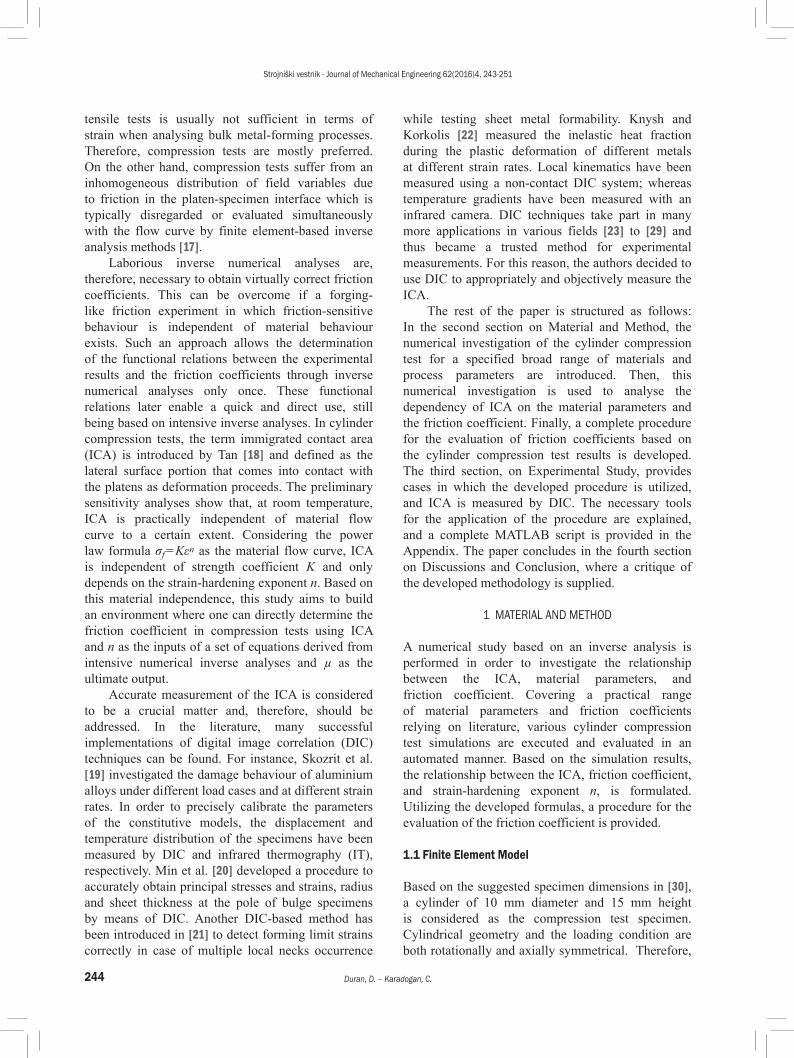
a quarter section of the cylinder is modelled and discretized by four-noded full integration quadrilateral elements. Based on the conducted convergence studies for the finite element model, a special mesh structure is used, with which a precise calculation of ICA is sought, see Fig. 1. The mesh is gradually and consecutively refined four times in the region where immigration of the lateral surface to the end face takes place. This refinement corresponds to an element size decrease from 0.25 mm to 0.0156 mm. With the used mesh, simulations run free of problems up to 50 % compression, i.e. 7.5 mm total axial displacement.

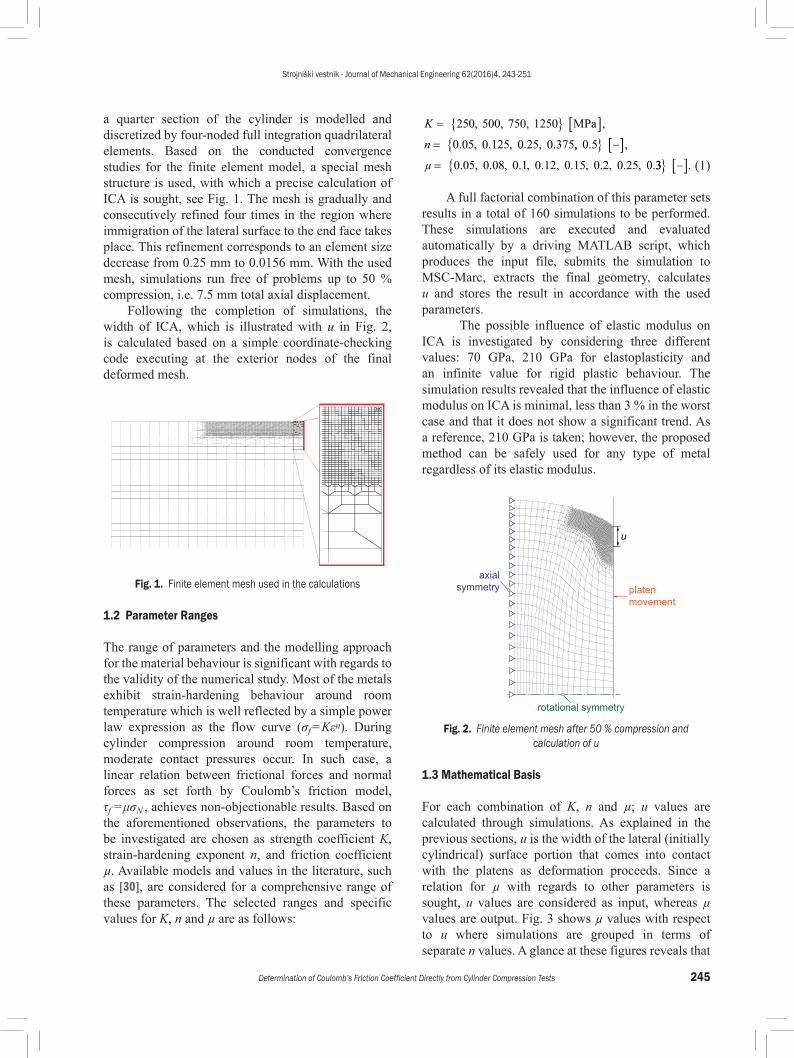
Following the completion of simulations, the width of ICA, which is illustrated with u in Fig. 2, is calculated based on a simple coordinate-checking code executing at the exterior nodes of the final deformed mesh.

Fig. 1. Finite element mesh used in the calculations

1.2 Parameter Ranges

The range of parameters and the modelling approach for the material behaviour is significant with regards to the validity of the numerical study. Most of the metals exhibit strain-hardening behaviour around room temperature which is well reflected by a simple power law expression as the flow curve (σf = Kεn). During cylinder compression around room temperature, moderate contact pressures occur. In such case, a linear relation between frictional forces and normal forces as set forth by Coulomb’s friction model, τf = μσN , achieves non-objectionable results. Based on the aforementioned observations, the parameters to be investigated are chosen as strength coefficient K, strain-hardening exponent n, and friction coefficient µ. Available models and values in the literature, such as [30], are considered for a comprehensive range of these parameters. The selected ranges and specific values for K, n and µ are as follows:

K

n

= { } [ ]=

25 5 75 125 MPa

5 125 25 375

0 00 0 0

0 0 0 0 0

, , , ,

. , . , . , . ,, . ,

. , . , . , . , . , . , . , .

5

5 8 1 12 15 2 25

0

0 0 0 0 0 0 0 0 0 0

{ } −[ ]=µ 33 { } −[ ]. (1)

A full factorial combination of this parameter sets results in a total of 160 simulations to be performed. These simulations are executed and evaluated automatically by a driving MATLAB script, which produces the input file, submits the simulation to MSC-Marc, extracts the final geometry, calculates u and stores the result in accordance with the used parameters.

The possible influence of elastic modulus on ICA is investigated by considering three different values: 70 GPa, 210 GPa for elastoplasticity and an infinite value for rigid plastic behaviour. The simulation results revealed that the influence of elastic modulus on ICA is minimal, less than 3 % in the worst case and that it does not show a significant trend. As a reference, 210 GPa is taken; however, the proposed method can be safely used for any type of metal regardless of its elastic modulus.

rotational symmetry

axialsymmetry platen

movement

u

Fig. 2. Finite element mesh after 50 % compression and calculation of u

1.3 Mathematical Basis

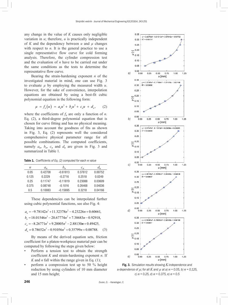
For each combination of K, n and µ; u values are calculated through simulations. As explained in the previous sections, u is the width of the lateral (initially cylindrical) surface portion that comes into contact with the platens as deformation proceeds. Since a relation for µ with regards to other parameters is sought, u values are considered as input, whereas µ values are output. Fig. 3 shows µ values with respect to u where simulations are grouped in terms of separate n values. A glance at these figures reveals that

Strojniški vestnik - Journal of Mechanical Engineering 62(2016)4, 243-251

246 Duran, D. – Karadogan, C.

any change in the value of K causes only negligible variation in u; therefore, u is practically independent of K and the dependency between u and µ changes with respect to n. It is the general practice to use a single representative flow curve for cold forming analysis. Therefore, the cylinder compression test and the evaluation of n have to be carried out under the same conditions as the tests to determine the representative flow curve.

Bearing the strain-hardening exponent n of the investigated material in mind, one can use Fig. 3 to evaluate µ by employing the measured width u. However, for the sake of convenience, interpolation equations are obtained by using a best-fit cubic polynomial equation in the following form:

µ f u a u b u c u dn n n n n = ( ) = + + +3 2, (2)

where the coefficients of fn are only a function of n. Eq. (2), a third-degree polynomial equation that is chosen for curve fitting and has no physical meaning. Taking into account the goodness of fits as shown in Fig. 3, Eq. (2) represents well the considered comprehensive physical parameter range for all possible combinations. The computed coefficients, namely an, bn, cn and dn are given in Fig. 3 and summarized in Table 1.

Table 1. Coefficients of Eq. (2) computed for each n value

n an bn cn dn0.05 0.42708 -0.61813 0.37612 0.00752

0.125 0.2229 -0.2716 0.2518 0.02490.25 0.11747 -0.11819 0.23088 0.03609

0.375 0.08748 -0.1016 0.26468 0.040360.5 0.10083 -0.15695 0.3218 0.04166

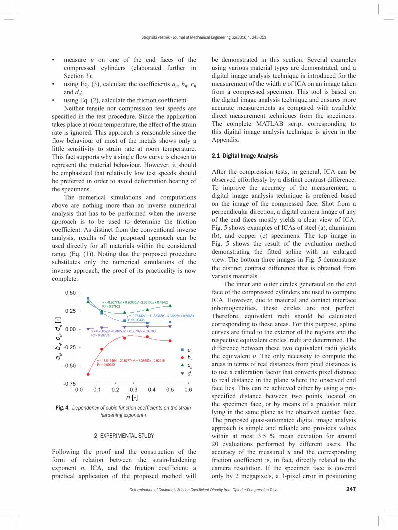
These dependencies can be interpolated further using cubic polynomial functions, see also Fig. 4:

a n n nb nn

n

= − + − +

= −

9 78142 11 32378 4 23226 0 60661

18 01546 20

3 2

3

. . . . ,

. .. . . ,

. . .

67774 7 38683 0 92918

8 26771 9 20005 2 88130

2

3 2

n nc n nn

+ −

= − + − nnd n n nn

+

= − + +

0 49425

0 78652 0 91056 0 35799 0 007883 2

. ,

. . . . . (3)

By means of the derived equation sets, friction coefficient for a platen-workpiece material pair can be computed by following the steps given below:• Perform a tension test to obtain the strength

coefficient K and strain-hardening exponent n. If K and n fall within the range given in Eq. (1);

• perform a compression test up to 50 % height reduction by using cylinders of 10 mm diameter and 15 mm height;

a)

b)

c)

d)

e)

Fig. 3. Simulation results showing K-independence and u-dependence of µ; for all K and µ at a) n = 0.05, b) n = 0.125,

c) n = 0.25, d) n = 0.375, e) n = 0.5

Strojniški vestnik - Journal of Mechanical Engineering 62(2016)4, 243-251

247Determination of Coulomb’s Friction Coefficient Directly from Cylinder Compression Tests

• measure u on one of the end faces of the compressed cylinders (elaborated further in Section 3);

• using Eq. (3), calculate the coefficients an, bn, cn and dn;

• using Eq. (2), calculate the friction coefficient.Neither tensile nor compression test speeds are

specified in the test procedure. Since the application takes place at room temperature, the effect of the strain rate is ignored. This approach is reasonable since the flow behaviour of most of the metals shows only a little sensitivity to strain rate at room temperature. This fact supports why a single flow curve is chosen to represent the material behaviour. However, it should be emphasized that relatively low test speeds should be preferred in order to avoid deformation heating of the specimens.

The numerical simulations and computations above are nothing more than an inverse numerical analysis that has to be performed when the inverse approach is to be used to determine the friction coefficient. As distinct from the conventional inverse analysis, results of the proposed approach can be used directly for all materials within the considered range (Eq. (1)). Noting that the proposed procedure substitutes only the numerical simulations of the inverse approach, the proof of its practicality is now complete.

n [-]

a n, b n,

c n, d n [

-]

y = 18.01546x3 - 20.67774x2 + 7.38683x - 0.92918R2 = 0.99222

y = 0.78652x3 - 0.91056x2 + 0.35799x - 0.00788R2 = 0.99763

y = -9.78142x3 + 11.32378x2 - 4.23226x + 0.60661R2 = 0.99438

y = -8.26771x3 + 9.20005x2 - 2.88130x + 0.49425R2 = 0.97952

an

bn

cn

dn

Fig. 4. Dependency of cubic function coefficients on the strain-hardening exponent n

2 EXPERIMENTAL STUDY

Following the proof and the construction of the form of relation between the strain-hardening exponent n, ICA, and the friction coefficient; a practical application of the proposed method will

be demonstrated in this section. Several examples using various material types are demonstrated, and a digital image analysis technique is introduced for the measurement of the width u of ICA on an image taken from a compressed specimen. This tool is based on the digital image analysis technique and ensures more accurate measurements as compared with available direct measurement techniques from the specimens. The complete MATLAB script corresponding to this digital image analysis technique is given in the Appendix.

2.1 Digital Image Analysis

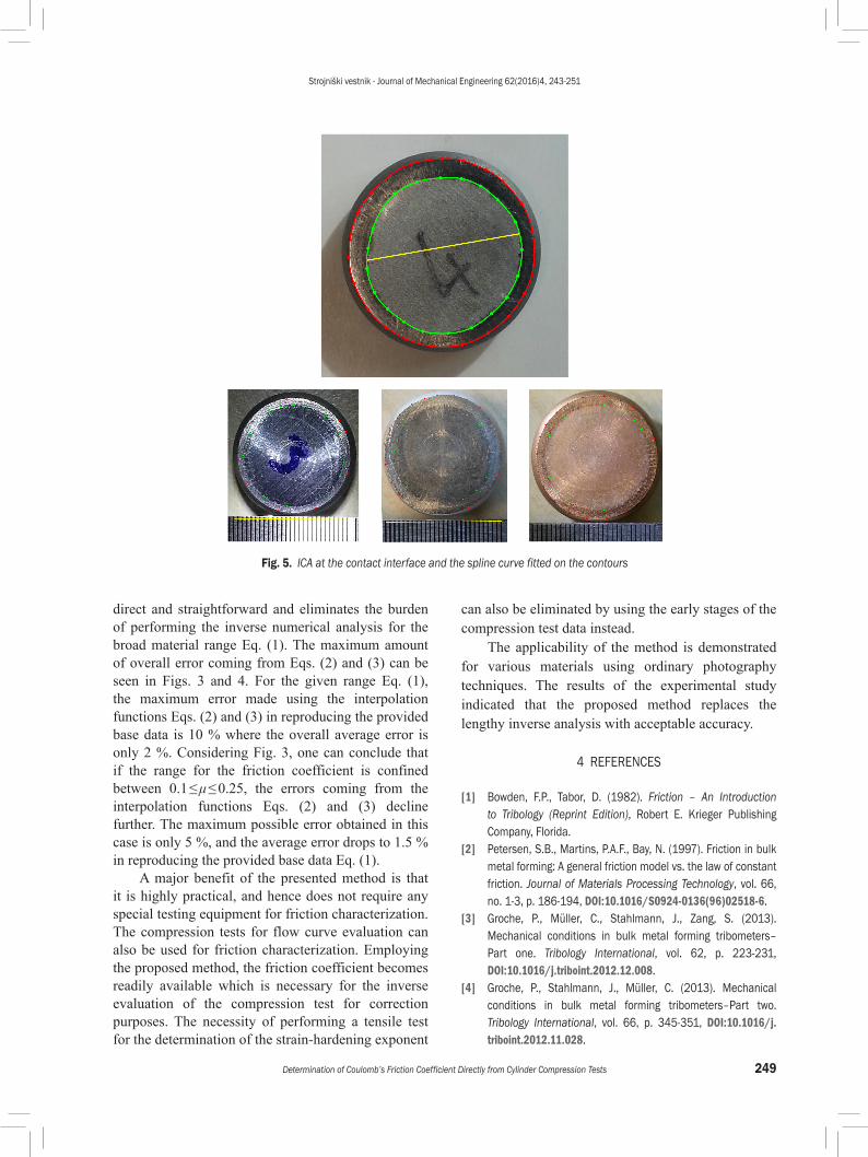
After the compression tests, in general, ICA can be observed effortlessly by a distinct contrast difference. To improve the accuracy of the measurement, a digital image analysis technique is preferred based on the image of the compressed face. Shot from a perpendicular direction, a digital camera image of any of the end faces mostly yields a clear view of ICA. Fig. 5 shows examples of ICAs of steel (a), aluminum (b), and copper (c) specimens. The top image in Fig. 5 shows the result of the evaluation method demonstrating the fitted spline with an enlarged view. The bottom three images in Fig. 5 demonstrate the distinct contrast difference that is obtained from various materials.

The inner and outer circles generated on the end face of the compressed cylinders are used to compute ICA. However, due to material and contact interface inhomogeneities, these circles are not perfect. Therefore, equivalent radii should be calculated corresponding to these areas. For this purpose, spline curves are fitted to the exterior of the regions and the respective equivalent circles’ radii are determined. The difference between these two equivalent radii yields the equivalent u. The only necessity to compute the areas in terms of real distances from pixel distances is to use a calibration factor that converts pixel distance to real distance in the plane where the observed end face lies. This can be achieved either by using a pre-specified distance between two points located on the specimen face, or by means of a precision ruler lying in the same plane as the observed contact face. The proposed quasi-automated digital image analysis approach is simple and reliable and provides values within at most 3.5 % mean deviation for around 20 evaluations performed by different users. The accuracy of the measured u and the corresponding friction coefficient is, in fact, directly related to the camera resolution. If the specimen face is covered only by 2 megapixels, a 3-pixel error in positioning

Strojniški vestnik - Journal of Mechanical Engineering 62(2016)4, 243-251

248 Duran, D. – Karadogan, C.

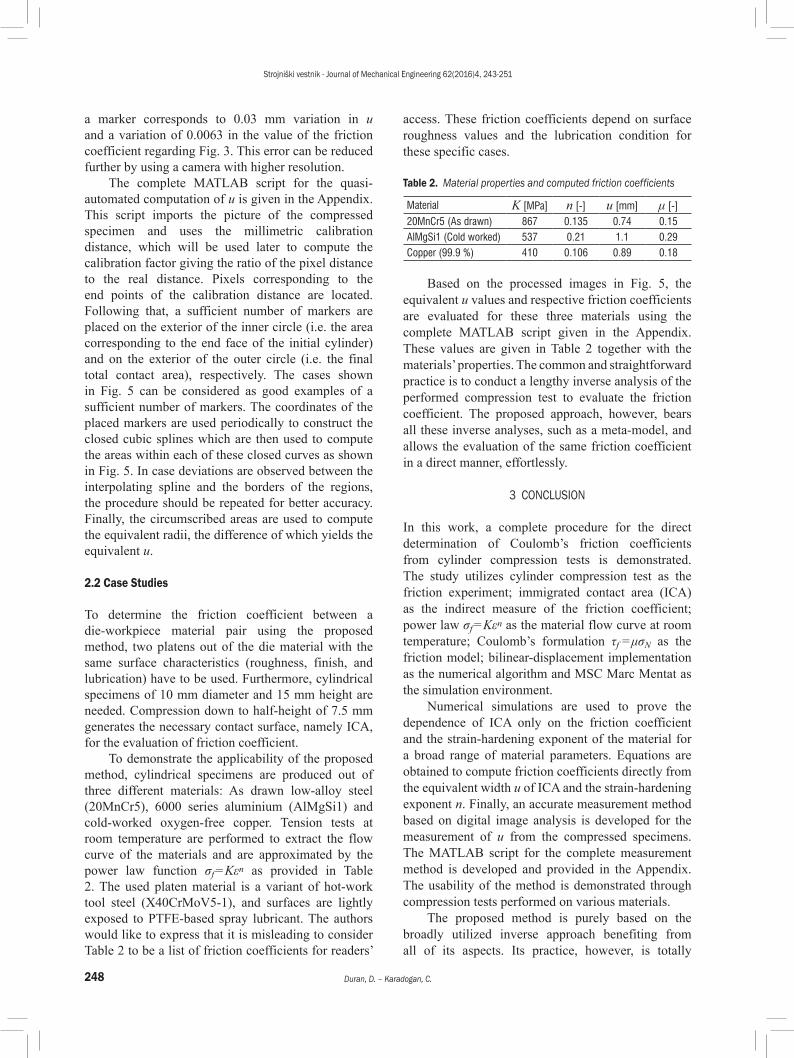
a marker corresponds to 0.03 mm variation in u and a variation of 0.0063 in the value of the friction coefficient regarding Fig. 3. This error can be reduced further by using a camera with higher resolution.

The complete MATLAB script for the quasi-automated computation of u is given in the Appendix. This script imports the picture of the compressed specimen and uses the millimetric calibration distance, which will be used later to compute the calibration factor giving the ratio of the pixel distance to the real distance. Pixels corresponding to the end points of the calibration distance are located. Following that, a sufficient number of markers are placed on the exterior of the inner circle (i.e. the area corresponding to the end face of the initial cylinder) and on the exterior of the outer circle (i.e. the final total contact area), respectively. The cases shown in Fig. 5 can be considered as good examples of a sufficient number of markers. The coordinates of the placed markers are used periodically to construct the closed cubic splines which are then used to compute the areas within each of these closed curves as shown in Fig. 5. In case deviations are observed between the interpolating spline and the borders of the regions, the procedure should be repeated for better accuracy. Finally, the circumscribed areas are used to compute the equivalent radii, the difference of which yields the equivalent u.

2.2 Case Studies

To determine the friction coefficient between a die-workpiece material pair using the proposed method, two platens out of the die material with the same surface characteristics (roughness, finish, and lubrication) have to be used. Furthermore, cylindrical specimens of 10 mm diameter and 15 mm height are needed. Compression down to half-height of 7.5 mm generates the necessary contact surface, namely ICA, for the evaluation of friction coefficient.

To demonstrate the applicability of the proposed method, cylindrical specimens are produced out of three different materials: As drawn low-alloy steel (20MnCr5), 6000 series aluminium (AlMgSi1) and cold-worked oxygen-free copper. Tension tests at room temperature are performed to extract the flow curve of the materials and are approximated by the power law function σf = Kεn as provided in Table 2. The used platen material is a variant of hot-work tool steel (X40CrMoV5-1), and surfaces are lightly exposed to PTFE-based spray lubricant. The authors would like to express that it is misleading to consider Table 2 to be a list of friction coefficients for readers’

access. These friction coefficients depend on surface roughness values and the lubrication condition for these specific cases.

Table 2. Material properties and computed friction coefficients

Material K [MPa] n [-] u [mm] μ [-]20MnCr5 (As drawn) 867 0.135 0.74 0.15AlMgSi1 (Cold worked) 537 0.21 1.1 0.29Copper (99.9 %) 410 0.106 0.89 0.18

Based on the processed images in Fig. 5, the equivalent u values and respective friction coefficients are evaluated for these three materials using the complete MATLAB script given in the Appendix. These values are given in Table 2 together with the materials’ properties. The common and straightforward practice is to conduct a lengthy inverse analysis of the performed compression test to evaluate the friction coefficient. The proposed approach, however, bears all these inverse analyses, such as a meta-model, and allows the evaluation of the same friction coefficient in a direct manner, effortlessly.

3 CONCLUSION

In this work, a complete procedure for the direct determination of Coulomb’s friction coefficients from cylinder compression tests is demonstrated. The study utilizes cylinder compression test as the friction experiment; immigrated contact area (ICA) as the indirect measure of the friction coefficient; power law σf = Kεn as the material flow curve at room temperature; Coulomb’s formulation τf = μσN as the friction model; bilinear-displacement implementation as the numerical algorithm and MSC Marc Mentat as the simulation environment.

Numerical simulations are used to prove the dependence of ICA only on the friction coefficient and the strain-hardening exponent of the material for a broad range of material parameters. Equations are obtained to compute friction coefficients directly from the equivalent width u of ICA and the strain-hardening exponent n. Finally, an accurate measurement method based on digital image analysis is developed for the measurement of u from the compressed specimens. The MATLAB script for the complete measurement method is developed and provided in the Appendix. The usability of the method is demonstrated through compression tests performed on various materials.

The proposed method is purely based on the broadly utilized inverse approach benefiting from all of its aspects. Its practice, however, is totally

Strojniški vestnik - Journal of Mechanical Engineering 62(2016)4, 243-251

249Determination of Coulomb’s Friction Coefficient Directly from Cylinder Compression Tests

direct and straightforward and eliminates the burden of performing the inverse numerical analysis for the broad material range Eq. (1). The maximum amount of overall error coming from Eqs. (2) and (3) can be seen in Figs. 3 and 4. For the given range Eq. (1), the maximum error made using the interpolation functions Eqs. (2) and (3) in reproducing the provided base data is 10 % where the overall average error is only 2 %. Considering Fig. 3, one can conclude that if the range for the friction coefficient is confined between 0.1 ≤ μ ≤ 0.25, the errors coming from the interpolation functions Eqs. (2) and (3) decline further. The maximum possible error obtained in this case is only 5 %, and the average error drops to 1.5 % in reproducing the provided base data Eq. (1).

A major benefit of the presented method is that it is highly practical, and hence does not require any special testing equipment for friction characterization. The compression tests for flow curve evaluation can also be used for friction characterization. Employing the proposed method, the friction coefficient becomes readily available which is necessary for the inverse evaluation of the compression test for correction purposes. The necessity of performing a tensile test for the determination of the strain-hardening exponent

can also be eliminated by using the early stages of the compression test data instead.

The applicability of the method is demonstrated for various materials using ordinary photography techniques. The results of the experimental study indicated that the proposed method replaces the lengthy inverse analysis with acceptable accuracy.

4 REFERENCES

[1] Bowden, F.P., Tabor, D. (1982). Friction – An Introduction to Tribology (Reprint Edition), Robert E. Krieger Publishing Company, Florida.

[2] Petersen, S.B., Martins, P.A.F., Bay, N. (1997). Friction in bulk metal forming: A general friction model vs. the law of constant friction. Journal of Materials Processing Technology, vol. 66, no. 1-3, p. 186-194, DOI:10.1016/S0924-0136(96)02518-6.

[3] Groche, P., Müller, C., Stahlmann, J., Zang, S. (2013). Mechanical conditions in bulk metal forming tribometers–Part one. Tribology International, vol. 62, p. 223-231, DOI:10.1016/j.triboint.2012.12.008.

[4] Groche, P., Stahlmann, J., Müller, C. (2013). Mechanical conditions in bulk metal forming tribometers–Part two. Tribology International, vol. 66, p. 345-351, DOI:10.1016/j.triboint.2012.11.028.

Fig. 5. ICA at the contact interface and the spline curve fitted on the contours

Strojniški vestnik - Journal of Mechanical Engineering 62(2016)4, 243-251

250 Duran, D. – Karadogan, C.

[5] Tan, X. (2002). Comparisons of friction models in bulk metal forming. Tribology International, vol. 35, no. 6, p. 385-393, DOI:10.1016/S0301-679X(02)00020-8.

[6] Hatzenbichler, T., Harrer, O., Wallner, S., Planitzer, F., Kuss, M., Pschera, R., Buchmayr, B. (2012). Deviation of the results obtained from different commercial finite element solvers due to friction formulation. Tribology International, vol. 49, p. 75-79, DOI:10.1016/j.triboint.2011.12.020.

[7] Ebrahimi, R., Najafizadeh, A. (2004). A new method for evaluation of friction in bulk metal forming. Journal of Materials Processing Technology, vol. 152, no. 2, p. 136-143, DOI:10.1016/j.jmatprotec.2004.03.029.

[8] Martin, F., Sevilla, L., Camacho, A., Sebastian, M.A. (2013). Upper bound solutions of ring compression test. Procedia Engineering, vol. 63, p. 413-420, DOI:10.1016/j.proeng.2013.08.211.

[9] Robinson, T., Ou, H., Armstrong, C.G. (2004). Study on ring compression test using physical modelling and FE simulation. Journal of Materials Processing Technology, vol. 153-154, p. 54-59, DOI:10.1016/j.jmatprotec.2004.04.045.

[10] Schrader, T., Shirgaokar, M., Altan, T. (2007). A critical evaluation of the double cup extrusion test for selection of cold forging lubricants. Journal of Materials Processing Technology, vol. 189, no. 1-3, p. 36-44, DOI:10.1016/j.jmatprotec.2006.11.229.

[11] Hsu, T.C., Huang, C.C. (2003). The friction modeling of different tribological interfaces in extrusion process. Journal of Materials Processing Technology, vol. 140, no. 1-3, p. 49-53, DOI:10.1016/S0924-0136(03)00724-6.

[12] Kuzman, K., Pfeifer, E., Bay, N. Hunding, J. (1996). Control of material flow in a combined backward can–forward rod extrusion. Journal of Materials Processing Technology, vol. 60, no. 1-4, p. 141-147, DOI:10.1016/0924-0136(96)02319-9.

[13] Giuliano, G. (2015). Evaluation of the Coulomb Friction Coefficient in DC05 Sheet Metal Forming. Strojniški vestnik - Journal of Mechanical Engineering, vol. 61, no. 12, p. 709-713, DOI:10.5545/sv-jme.2015.2733.

[14] Hatipoglu, H.A., Karadogan, C. (2014). A Methodology to determine friction coefficient in stretch forming of sheet aircraft panels. Conference Proceedings of International Deep-Drawing Research Group.

[15] Hu, C.L., Ou, H.A., Zhao, Z. (2015). An alternative evaluation method for friction condition in cold forging by ring with boss compression test. Journal of Materials Processing Technology, vol. 224, p. 18-25, DOI:10.1016/j.jmatprotec.2015.04.010.

[16] Bay, N., Gerved, G. (1987). Tool/workpiece interface stresses in simple upsetting. Journal of Mechanical Working Technology, vol. 14, no. 3, p. 263-282, DOI:10.1016/0378-3804(87)90013-1.

[17] Cho, H., Ngaile, G., Altan, T. (2003). Simultaneous determination of flow stress and interface friction by finite element based inverse analysis technique. CIRP Annals - Manufacturing Technology, vol. 52, no. 1, p. 221-224, DOI:10.1016/S0007-8506(07)60570-8.

[18] Tan, X. (2001). Friction reducing contact area expansion in upsetting. Proceedings of the Institution of Mechanical Engineers, Part J: Journal of Engineering Tribology, vol. 215, no. 2, p. 189-200, DOI:10.1243/1350650011541828.

[19] Skozrit, I., Frančeski, J., Tonković, Z., Surjak, M., Krstulović-Opara, L., Vesenjak, M., Kodvanj, J., Gunjević, B., Lončarić, D. (2015). Validation of numerical model by means of digital image correlation and thermography. Procedia Engineering, vol. 101, p. 450-458, DOI:10.1016/j.proeng.2015.02.054.

[20] Min, J., Stoughton, T.B., Carsley, J.E., Carlson, B.E, Lin, J., Gao, X. (2016). Accurate characterization of biaxial stress-strain response of sheet metal from bulge testing. International Journal of Plasticity, in Press, DOI:10.1016/j.ijplas.2016.02.005.

[21] Vysochinskiy, D., Coudert, T., Hopperstad, O.S., Lademo, O.G., Reyes, A. (2016). Experimental detection of forming limit strains on samples with multiple local necks. Journal of Materials Processing Technology, vol. 227, p. 216-226, DOI:10.1016/j.jmatprotec.2015.08.019.

[22] Knysh, P., Korkolis, Y.P. (2015). Determination of the fraction of plastic work converted into heat in metals. Mechanics of Materials, vol. 86, 71-80, DOI:10.1016/j.mechmat.2015.03.006.

[23] Sutton, M.A., Schreier, H.W, Orteu, J-J.(2009). Image Correlation for Shape, Motion and Deformation Measurements: Basic Concepts, Theory and Applications, Springer, New York.

[24] Milosevic, M., Milosevic, N., Sedmak, S., Tatic, U., Mitrovic, N., Hloch, S., Jovicic, R. (2016). Digital image correlation in analysis of stiffness in local zones of welded joints. Technical Gazette - Tehnički vjesnik, vol. 23, no. 1, p. 19-24, DOI:10.17559/TV-20140123151546.

[25] Majnaric, I., Hladnik, A., Muck, T., Bolanca Mirkovic, I. (2015). The influence of ink concentration and layer thickness on yellow colour reproduction in liquid electrophotography toner. Technical Gazette - Tehnički vjesnik, vol. 22, no. 1, p. 145-149, DOI:10.17559/TV-20140321230455.

[26] Foldyna J., Zelenak M., Klich J., Hlavacek P., Sitek L., Riha Z. (2015). The measurement of the velocity of abrasive particles at the suction part of cutting head. Technical Gazette - Tehnicki vjesnik, vol. 22, no. 6, p. 1441-1446, DOI:10.17559/TV-20140214152925.

[27] Klancnik, S., Ficko, M., Balic, J., Pahole, I. (2015). Computer Vision-Based Approach to End Mill Tool Monitoring. International Journal of Simulation Modelling, vol. 14, no. 4, p. 571-583, DOI:10.2507/IJSIMM14(4)1.301.

[28] Cajal, C., Santolaria, J., Samper, D., Garrido, A. (2015). Simulation of Laser Triangulation Sensors Scanning for Design and Evaluation Purposes. International Journal of Simulation Modelling, vol. 14, no. 2, p. 250-264, DOI:10.2507/IJSIMM14(2)6.296.

[29] Chrysochoos, A., Huon, V., Jourdan, F., Muracciole, J.M., Peyroux, R., Wattrisse, B. (2010). Use of full-field digital image correlation and infrared thermography measurements for the thermomechanical analysis of material behaviour, Strain, vol. 46, no. 1, p. 117-130, DOI:10.1111/j.1475-1305.2009.00635.x.

[30] Banabic, D., Bunge, H.-J., Pöhlandt, K., Tekkaya, A.E. (2000). Formability of Metallic Materials, Springer-Verlag Berlin/Heidelberg/New York/Tokyo, DOI:10.1007/978-3-662-04013-3.

Strojniški vestnik - Journal of Mechanical Engineering 62(2016)4, 243-251

251Determination of Coulomb’s Friction Coefficient Directly from Cylinder Compression Tests

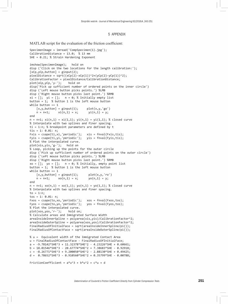
5 APPENDIX

MATLAB script for the evaluation of the friction coefficient:

SpecimenImage = imread('CompSpecimen(1).jpg');CalibrationDistance = 13.0; % 13 mmSHE = 0.21; % Strain Hardening Exponent

imshow(SpecimenImage); hold ondisp ('Click on the two locations for the length calibration:');[xCp,yCp,button] = ginput(2);pixelDistance = sqrt((xCp(2)-xCp(1))^2+(yCp(2)-yCp(1))^2);CalibrationFactor = pixelDistance/CalibrationDistance;plot(xCp,yCp,'y-'); hold ondisp('Pick up sufficient number of ordered points on the inner circle')disp ('Left mouse button picks points.') %LMBdisp ('Right mouse button picks last point.') %RMBxi = []; yi = []; n = 0; % Initially empty listbutton = 1; % button 1 is the left mouse buttonwhile button == 1 [x,y,button] = ginput(1); plot(x,y,'go') n = n+1; xi(n,1) = x; yi(n,1) = y;endn = n+1; xi(n,1) = xi(1,1); yi(n,1) = yi(1,1); % closed curve% Interpolate with two splines and finer spacing.ti = 1:n; % breakpoint parameters are defined by ttis = 1: 0.01: n;Fxis = csape(ti,xi,'periodic'); xis = fnval(Fxis,tis);Fyis = csape(ti,yi,'periodic'); yis = fnval(Fyis,tis);% Plot the interpolated curve.plot(xis,yis,'g-'); hold on% Loop, picking up the points for the outer circledisp ('Pick up sufficient number of ordered points on the outer circle')disp ('Left mouse button picks points.') %LMBdisp ('Right mouse button picks last point.') %RMBxo = []; yo = []; n = 0; % Initially, empty point listbutton = 1; % button 1 is the left mouse buttonwhile button == 1 [x,y,button] = ginput(1); plot(x,y,'ro') n = n+1; xo(n,1) = x; yo(n,1) = y;endn = n+1; xo(n,1) = xo(1,1); yo(n,1) = yo(1,1); % closed curve% Interpolate with two splines and finer spacing.to = 1:n;tos = 1: 0.01: n;Fxos = csape(to,xo,'periodic'); xos = fnval(Fxos,tos);Fyos = csape(to,yo,'periodic'); yos = fnval(Fyos,tos);% Plot the interpolated curve.plot(xos,yos,'r-'); hold on;% Calculate areas and Immigrated Surface WidthareaInsideInnerSpline = polyarea(xis,yis)/CalibrationFactor^2;areaInsideOuterSpline = polyarea(xos,yos)/CalibrationFactor^2;FinalRadiusOfInitialFace = sqrt(areaInsideInnerSpline/pi());FinalRadiusOfContactFace = sqrt(areaInsideOuterSpline/pi());

% u = Equivalent width of the Immigrated Contact Areau = FinalRadiusOfContactFace - FinalRadiusOfInitialFace; a = -9.78142*SHE^3 + 11.32378*SHE^2 - 4.23226*SHE + 0.60661;b = 18.01546*SHE^3 - 20.67774*SHE^2 + 7.38683*SHE - 0.92918;c = -8.26771*SHE^3 + 9.200050*SHE^2 - 2.88130*SHE + 0.49425;d = 0.78652*SHE^3 - 0.910560*SHE^2 + 0.35799*SHE - 0.00788;

FrictionCoefficient = a*u^3 + b*u^2 + c*u + d