Physical System Modeling - University of Waterloojzelek/teaching/syde361/0066ch07.pdf · Physical System Modeling ... 7.8 Dynamic Principles for Electric and Magnetic Circuits

IIPhysical System Modeling

7 Modeling Electromechanical Systems Francis C. MoonIntroduction • Models for Electromechanical Systems • Rigid Body Models •Basic Equations of Dynamics of Rigid Bodies • Simple Dynamic Models • Elastic System Modeling • Electromagnetic Forces • Dynamic Principles for Electric and Magnetic Circuits • Earnshaw’s Theorem and Electromechanical Stability

8 Structures and Materials Eniko T. Enikov Fundamental Laws of Mechanics • Common Structures in Mechatronic Systems •Vibration and Modal Analysis • Buckling Analysis • Transducers • Future Trends

9 Modeling of Mechanical Systems for Mechatronics Applications Raul G. LongoriaIntroduction • Mechanical System Modeling in Mechatronic Systems • Descriptions of Basic Mechanical Model Components • Physical Laws for Model Formulation • EnergyMethods for Mechanical System Model Formulation • Rigid Body MultidimensionalDynamics • Lagrange’s Equations

10 Fluid Power Systems Qin Zhang and Carroll E. GoeringIntroduction • Hydraulic Fluids • Hydraulic Control Valves • Hydraulic Pumps • Hydraulic Cylinders • Fluid Power Systems Control • Programmable Electrohydraulic Valves

11 Electrical Engineering Giorgio Rizzoni Introduction • Fundamentals of Electric Circuits • Resistive Network Analysis •AC Network Analysis

12 Engineering Thermodynamics Michael J. MoranFundamentals • Extensive Property Balances • Property Relations and Data • Vapor and Gas Power Cycles

©2002 CRC Press LLC

13 Modeling and Simulation for MEMS Carla PurdyIntroduction • The Digital Circuit Development Process: Modeling and Simulating Systems with Micro- (or Nano-) Scale Feature Sizes • Analog and Mixed-Signal Circuit Development: Modeling and Simulating Systems with Micro- (or Nano-) Scale Feature Sizes and Mixed Digital (Discrete) and Analog (Continuous) Input, Output, and Signals • Basic Techniques and Available Tools for MEMS Modeling and Simulation • Modeling and Simulating MEMS, i.e., Systems with Micro- (or Nano-) Scale Feature Sizes, Mixed Digital (Discrete) and Analog (Continuous) Input, Output, and Signals, Two- and Three-Dimensional Phenomena, and Inclusion and Interaction of Multiple Domains and Technologies • A “Recipe” for Successful MEMS Simulation • Conclusion: Continuing Progress in MEMS Modeling and Simulation

14 Rotational and Translational Microelectromechanical Systems: MEMS Synthesis, Microfabrication, Analysis, and Optimization Sergey Edward LyshevskiIntroduction • MEMS Motion Microdevice Classifier and Structural Synthesis • MEMS Fabrication • MEMS Electromagnetic Fundamentals and Modeling • MEMS Mathematical Models • Control of MEMS • Conclusions

15 The Physical Basis of Analogies in Physical System Models Neville Hogan and Peter C. BreedveldIntroduction • History • The Force-Current Analogy: Across and Through Variables • Maxwell’s Force-Voltage Analogy: Effort and Flow Variables • A Thermodynamic Basis for Analogies • Graphical Representations • Concluding Remarks

©2002 CRC Press LLC

7.1 Int

Mechatronicduce devicefamiliar condevices. A diis the miniatronic sensofor integratibut also forductors havmotors, and(MEMS), elgreat strides

While theNewton andthe theory oapplications

Francis C.

Cornell Unive

0066_Frame_C07 Page 1 Wednesday, January 9, 2002 3:39 PM

©2002 CRC P

7Modeling Electro-

mechanical Systems

7.1 Introduction7.2 Models for Electromechanical Systems 7.3 Rigid Body Models

Kinematics of Rigid Bodies • Constraints and Generalized Coordinates • Kinematic versus Dynamic Problems

7.4 Basic Equations of Dynamics of Rigid Bodies Newton–Euler Equation • Multibody Dynamics

7.5 Simple Dynamic Models Compound Pendulum • Gyroscopic Motions

7.6 Elastic System ModelingPiezoelastic Beam

7.7 Electromagnetic Forces7.8 Dynamic Principles for Electric

and Magnetic Circuits Lagrange’s Equations of Motion for Electromechanical Systems

7.9 Earnshaw’s Theorem and ElectromechanicalStability

roduction

s describes the integration of mechanical, electromagnetic, and computer elements to pro-s and systems that monitor and control machine and structural systems. Examples includesumer machines such as VCRs, automatic cameras, automobile air bags, and cruise controlstinguishing feature of modern mechatronic devices compared to earlier controlled machinesturization of electronic information processing equipment. Increasingly computer and elec-rs and actuators can be embedded in the structures and machines. This has led to the needon of mechanical and electrical design. This is true not only for sensing and signal processing actuator design. In human size devices, more powerful magnetic materials and supercon-e led to the replacement of hydraulic and pneumatic actuators with servo motors, linear other electromagnetic actuators. At the material scale and in microelectromechanical systemsectric charge force actuators, piezoelectric actuators, and ferroelectric actuators have made. materials used in electromechanical design are often new, the basic dynamic principles of Maxwell still apply. In spatially extended systems one must solve continuum problems usingf elasticity and the partial differential equations of electromagnetic field theory. For many, however, it is sufficient to use lumped parameter modeling based on i) rigid body dynamics

Moonrsity

ress LLC

for inertial components, ii) Kirchhoff circuit laws for current-charge components, and iii) magnet circuitlaws for magnetic flux devices.

In this chcircuits, whinteractionsthese principin electrome

7.2 Mo

The fundamwhich descrbeams and pboth spatialNavier–StokElectromagnand fluids mbe found in

Many praor inductancordinary difproblems hacalled

separa

eigenmodesthese coupleelectric and

7.3 Rig

Kinemati

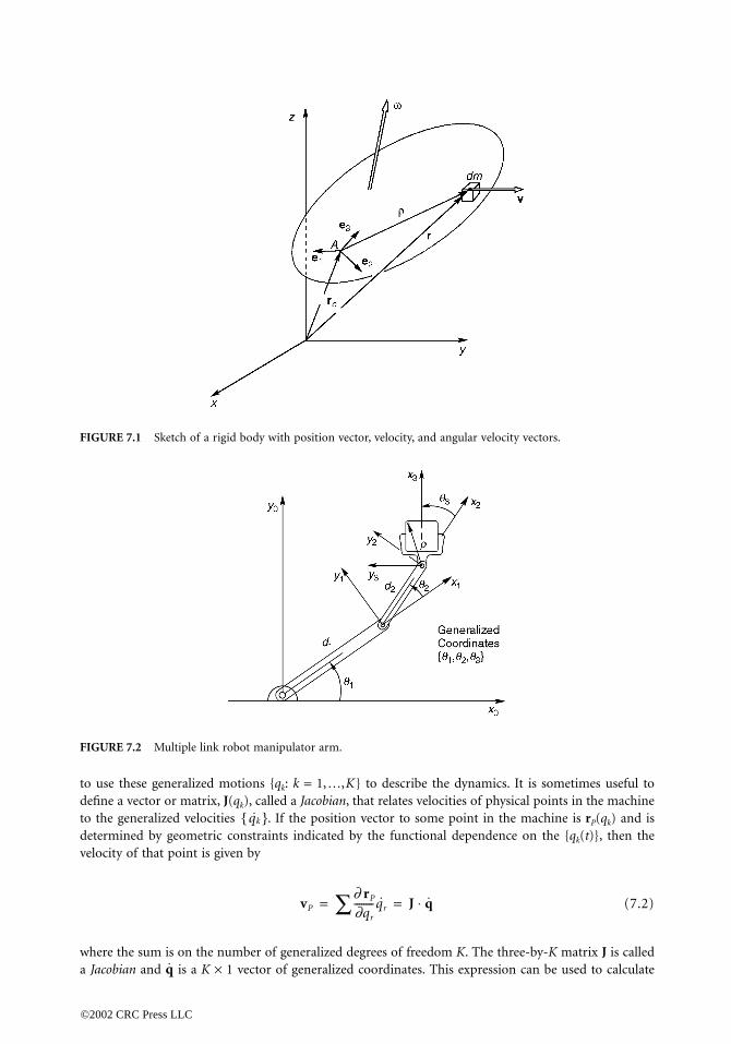
Kinematics i

rate vector

ω

in a machinthe center of

by angle setMoon, 1999

rigid body o

where the se

rigid body. elements are

Constrain

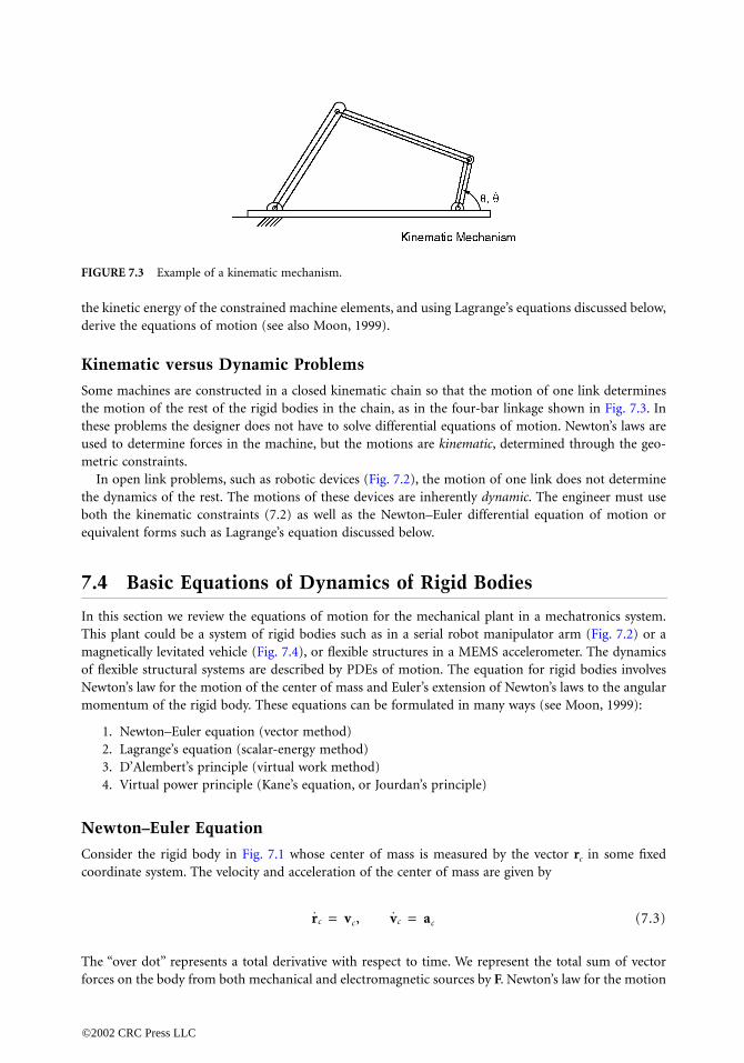
Machines arone degree oin Fig. 7.2, eare constrain


©2002 CRC P

apter we will examine the basic modeling assumptions for inertial, electric, and magneticich are typical of mechatronic systems, and will summarize the dynamic principles and between the mechanical motion, circuit, and magnetic state variables. We will also illustrate

les with a few examples as well as provide some bibliography to more advanced referenceschanics.

dels for Electromechanical Systems

ental equations of motion for physical continua are partial differential equations (PDEs),ibe dynamic behavior in both time and space. For example, the motions of strings, elasticlates, fluid flow around and through bodies, as well as magnetic and electric fields require

and temporal information. These equations include those of elasticity, elastodynamics, thees equations of fluid mechanics, and the Maxwell–Faraday equations of electromagnetics.etic field problems may be found in Jackson (1968). Coupled field problems in electric fieldsay be found in Melcher (1980) and problems in magnetic fields and elastic structures may

the monograph by Moon (1984). This short article will only treat solid systems. ctical electromechanical devices can be modeled by lumped physical elements such as masse. The equations of motion are then integral forms of the basic PDEs and result in coupled

ferential equations (ODEs). This methodology will be explored in this chapter. Where physicalve spatial distributions, one can often separate the problem into spatial and temporal partstion of variables. The spatial description is represented by a finite number of spatial or

each of which has its modal amplitude. This method again results in a set of ODEs. Oftend equations can be understood in the context of simple lumped mechanical masses andmagnetic circuits.

id Body Models

cs of Rigid Bodies

s the description of motion in terms of position vectors r, velocities v, acceleration a, rotation, and generalized coordinates {qk(t)} such as relative angular positions of one part to another

e (Fig. 7.1). In a rigid body one generally specifies the position vector of one point, such as mass rc, and the velocity of that point, say vc. The angular position of a rigid body is specifieds call Euler angles. For example, in vehicles there are pitch, roll, and yaw angles (see, e.g.,). The angular velocity vector of a rigid body is denoted by ω. The velocity of a point in ather than the center of mass, rp = rc + ρ, is given by

vP = vc + ω × ρ (7.1)

cond term is a vector cross product. The angular velocity vector w is a property of the entireIn general a rigid body, such as a satellite, has six degrees of freedom. But when machine modeled as a rigid body, kinematic constraints often limit the number of degrees of freedom.

ts and Generalized Coordinates

e often collections of rigid body elements in which each component is constrained to havef freedom relative to each of its neighbors. For example, in a multi-link robot arm shownach rigid link has a revolute degree of freedom. The degrees of freedom of each rigid linked by bearings, guides, and gearing to have one type of relative motion. Thus, it is convenient

ress LLC

to use these

define a vect

to the gener

determined

velocity of t

where the su

a

Jacobian

a

FIGURE 7.1

FIGURE 7.2


©2002 CRC P

generalized motions {qk: k = 1,…,K} to describe the dynamics. It is sometimes useful toor or matrix, J(qk), called a Jacobian, that relates velocities of physical points in the machinealized velocities . If the position vector to some point in the machine is rP(qk) and isby geometric constraints indicated by the functional dependence on the {qk(t)}, then thehat point is given by

(7.2)

m is on the number of generalized degrees of freedom K. The three-by-K matrix J is callednd is a K × 1 vector of generalized coordinates. This expression can be used to calculate

Sketch of a rigid body with position vector, velocity, and angular velocity vectors.

Multiple link robot manipulator arm.

qk{ }

vP

∂ rP

∂qr

--------qr˙∑ J q⋅= =

q

ress LLC

the kinetic ederive the eq

Kinemati

Some machthe motion these probleused to dete

metric constIn open l

the dynamic

both the kinequivalent fo

7.4 Ba

In this sectiThis plant cmagneticallyof flexible stNewton’s lawmomentum

1. Newt2. Lagra3. D’Ale4. Virtu

Newton–

Consider th

coordinate s

The “over dforces on the

FIGURE 7.3


©2002 CRC P

nergy of the constrained machine elements, and using Lagrange’s equations discussed below,uations of motion (see also Moon, 1999).

c versus Dynamic Problems

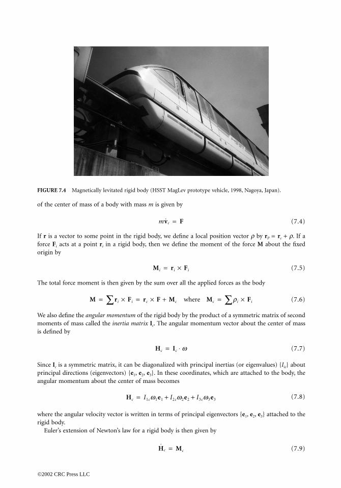
ines are constructed in a closed kinematic chain so that the motion of one link determinesof the rest of the rigid bodies in the chain, as in the four-bar linkage shown in Fig. 7.3. Inms the designer does not have to solve differential equations of motion. Newton’s laws arermine forces in the machine, but the motions are kinematic, determined through the geo-raints.

ink problems, such as robotic devices (Fig. 7.2), the motion of one link does not determines of the rest. The motions of these devices are inherently dynamic. The engineer must useematic constraints (7.2) as well as the Newton–Euler differential equation of motion orrms such as Lagrange’s equation discussed below.

sic Equations of Dynamics of Rigid Bodies

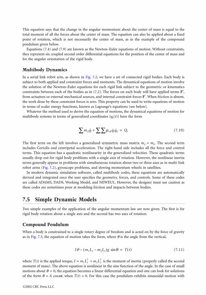
on we review the equations of motion for the mechanical plant in a mechatronics system.ould be a system of rigid bodies such as in a serial robot manipulator arm (Fig. 7.2) or a levitated vehicle (Fig. 7.4), or flexible structures in a MEMS accelerometer. The dynamicsructural systems are described by PDEs of motion. The equation for rigid bodies involves for the motion of the center of mass and Euler’s extension of Newton’s laws to the angular

of the rigid body. These equations can be formulated in many ways (see Moon, 1999):

on–Euler equation (vector method)nge’s equation (scalar-energy method)mbert’s principle (virtual work method)al power principle (Kane’s equation, or Jourdan’s principle)

Euler Equation

e rigid body in Fig. 7.1 whose center of mass is measured by the vector rc in some fixedystem. The velocity and acceleration of the center of mass are given by

(7.3)

ot” represents a total derivative with respect to time. We represent the total sum of vector body from both mechanical and electromagnetic sources by F. Newton’s law for the motion

Example of a kinematic mechanism.

rc vc, vc ac= =

ress LLC

of the cente

If

r

is a vect

force

F

i

acts

origin by

The total fo

We also defi

moments of

is defined by

Since

I

c

is a

principal dir

angular mom

where the an

rigid body.Euler’s ex

FIGURE 7.4


©2002 CRC P

r of mass of a body with mass m is given by

(7.4)

or to some point in the rigid body, we define a local position vector ρ by rP = rc + ρ. If a at a point ri in a rigid body, then we define the moment of the force M about the fixed

(7.5)

rce moment is then given by the sum over all the applied forces as the body

(7.6)

ne the angular momentum of the rigid body by the product of a symmetric matrix of second mass called the inertia matrix Ic. The angular momentum vector about the center of mass

(7.7)

symmetric matrix, it can be diagonalized with principal inertias (or eigenvalues) {Iic} aboutections (eigenvectors) {e1, e2, e3}. In these coordinates, which are attached to the body, theentum about the center of mass becomes

(7.8)

gular velocity vector is written in terms of principal eigenvectors {e1, e2, e3} attached to the

tension of Newton’s law for a rigid body is then given by

(7.9)

Magnetically levitated rigid body (HSST MagLev prototype vehicle, 1998, Nagoya, Japan).

mvc F=

Mi ri Fi×=

M ri Fi×∑ rc F Mc+× where Mc ri Fi×∑= = =

Hc Ic w⋅=

Hc I1cw1e1 I2cw2e2 I3cw3e3+ +=

Hc Mc=

ress LLC

This equation says that the change in the angular momentum about the center of mass is equal to thetotal moment of all the forces about the center of mass. The equation can also be applied about a fixedpoint of rotpendulum g

Equationsthey represefor the angu

Multibod

In a serial lisubject to bothe solutionconstraints bfrom actuatothe work doin terms of

Whatevermultibody s

The first terincludes Coterms. This usually dropterms generrobot arms

In moderderived andare called Athese codes

7.5 Sim

Two simple rigid body r

Compoun

When a bodas in Fig. 7.5

where T(t) imoment of motions aboof the form


©2002 CRC P

ation, which is not necessarily the center of mass, as in the example of the compoundiven below. (7.4) and (7.9) are known as the Newton–Euler equations of motion. Without constraints,

nt six coupled second order differential equations for the position of the center of mass andlar orientation of the rigid body.

y Dynamics

nk robot arm, as shown in Fig. 7.2, we have a set of connected rigid bodies. Each body isth applied and constraint forces and moments. The dynamical equations of motion involve

of the Newton–Euler equations for each rigid link subject to the geometric or kinematicsetween each of the bodies as in (7.2). The forces on each body will have applied terms Fa,rs or external mechanical sources, and internal constraint forces Fc. When friction is absent,

ne by these constraint forces is zero. This property can be used to write equations of motionscalar energy functions, known as Lagrange’s equations (see below). the method used to derive the equation of motions, the dynamical equations of motion forystems in terms of generalized coordinates {qk(t)} have the form

(7.10)

m on the left involves a generalized symmetric mass matrix mij = mji. The second termriolis and centripetal acceleration. The right-hand side includes all the force and controlequation has a quadratic nonlinearity in the generalized velocities. These quadratic terms out for rigid body problems with a single axis of rotation. However, the nonlinear inertia

ally appear in problems with simultaneous rotation about two or three axes as in multi-link(Fig. 7.2), gyroscope problems, and slewing momentum wheels in satellites.n dynamic simulation software, called multibody codes, these equations are automatically integrated once the user specifies the geometry, forces, and controls. Some of these codesDAMS, DADS, Working Model, and NEWEUL. However, the designer must use caution asare sometimes poor at modeling friction and impacts between bodies.

ple Dynamic Models

examples of the application of the angular momentum law are now given. The first is forotation about a single axis and the second has two axes of rotation.

d Pendulum

y is constrained to a single rotary degree of freedom and is acted on by the force of gravity, the equation of motion takes the form, where θ is the angle from the vertical,

(7.11)

s the applied torque, I = m1 + m2 is the moment of inertia (properly called the secondmass). The above equation is nonlinear in the sine function of the angle. In the case of smallut θ = 0, the equation becomes a linear differential equation and one can look for solutions

θ = A cosωt, when T(t) = 0. For this case the pendulum exhibits sinusoidal motion with

mijqj mijkqjqk∑∑+∑ Qi=

IJ m1L1 m2L2–( )g qsin– T t( )=

L12 L2

2

ress LLC

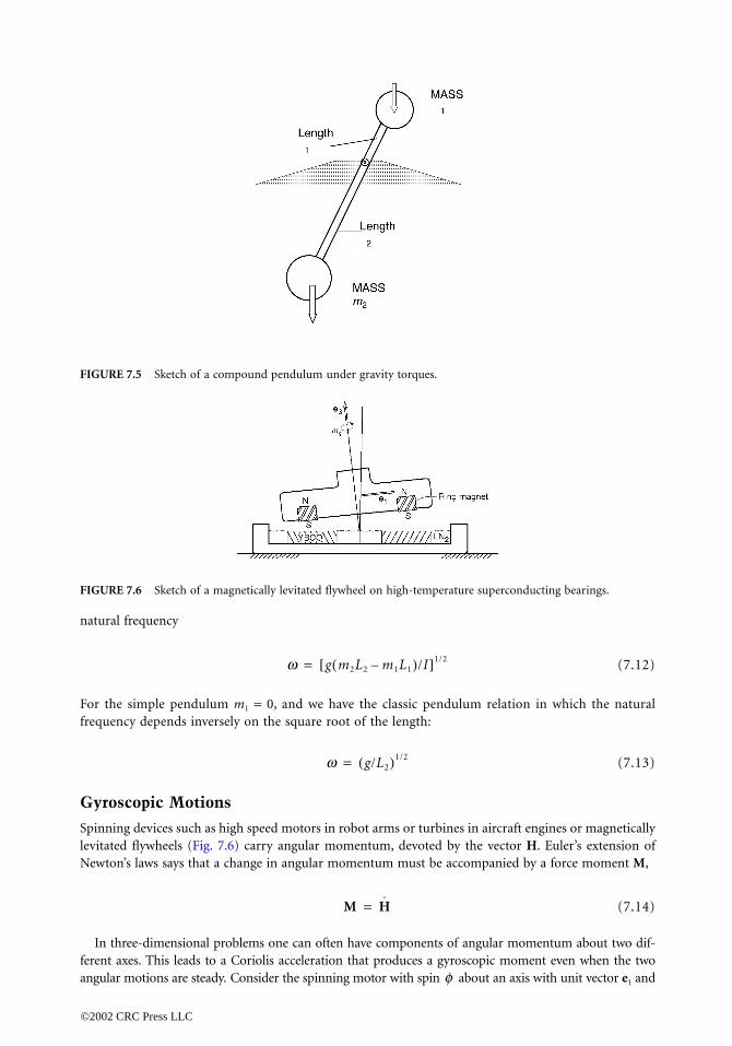
natural freq

For the simfrequency d

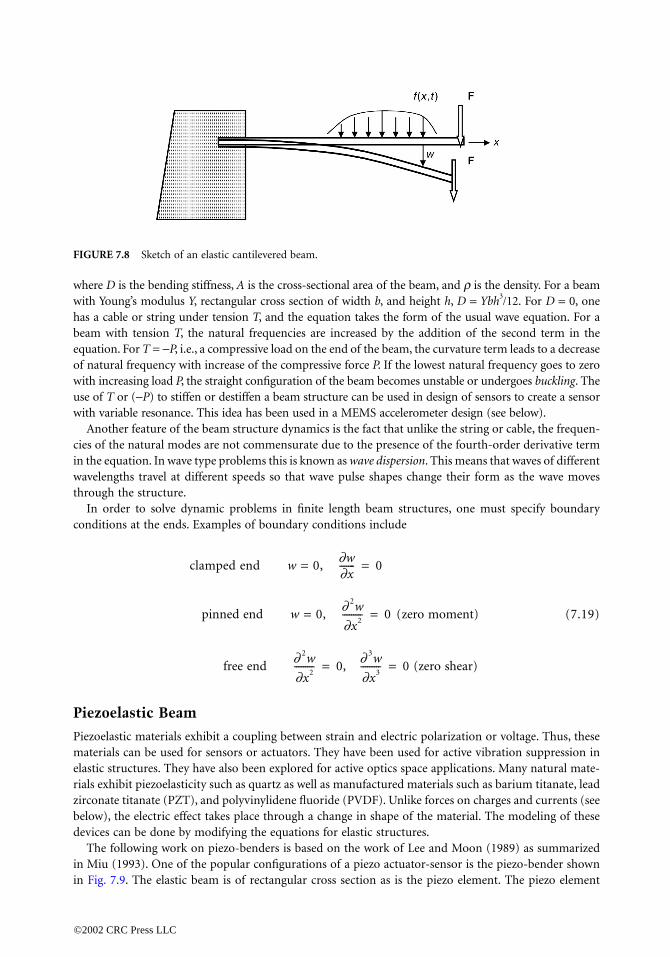
Gyroscop

Spinning delevitated flyNewton’s law

In three-dferent axes. angular mot

FIGURE 7.5

FIGURE 7.6


©2002 CRC P

uency

(7.12)

ple pendulum m1 = 0, and we have the classic pendulum relation in which the naturalepends inversely on the square root of the length:

(7.13)

ic Motions

vices such as high speed motors in robot arms or turbines in aircraft engines or magneticallywheels (Fig. 7.6) carry angular momentum, devoted by the vector H. Euler’s extension of

s says that a change in angular momentum must be accompanied by a force moment M,

(7.14)

imensional problems one can often have components of angular momentum about two dif-This leads to a Coriolis acceleration that produces a gyroscopic moment even when the twoions are steady. Consider the spinning motor with spin about an axis with unit vector e1 and

Sketch of a compound pendulum under gravity torques.

Sketch of a magnetically levitated flywheel on high-temperature superconducting bearings.

w g m2L2 m1L1–( )/I[ ]1/2=

w g/L2( )1/2=

M H=

f

ress LLC

let us imaginin gyroscope

and the rate

There must tThis momenthe rotation

This has thethe moment

7.6 Ela

Elastic strucuse the metgeneralized structure (se

The simpmotions we One usually resultants oftrated forceelectromagn

FIGURE 7.7


©2002 CRC P

e an angular motion of the e1 axis, about a perpendicular axis ez called the precession axis parlance. Then one can show that the angular momentum is given by

(7.15)

of change of angular momentum for constant spin and presession rates is given by

(7.16)

hen exist a gyroscopic moment, often produced by forces on the bearings of the axel (Fig. 7.7).t is perpendicular to the plane formed by e1 and ez, and is proportional to the product of

rates:

(7.17)

same form as Eq. (7.10), when the generalized force Q is identified with the moment M, i.e., is the product of generalized velocities when the second derivative acceleration terms are zero.

stic System Modeling

tures take the form of cables, beams, plates, shells, and frames. For linear problems one canhod of eigenmodes to represent the dynamics with a finite set of modal amplitudes fordegrees of freedom. These eigenmodes are found as solutions to the PDEs of the elastice, e.g., Yu, 1996).lest elastic structure after the cable is a one-dimensional beam shown in Fig. 7.8. For smallassume only transverse displacements w(x, t), where x is a spatial coordinate along the beam.assumes that the stresses on the beam cross section can be integrated to obtain stress vector

shear V, bending moment M, and axial load T. The beam can be loaded with point or concen-s, end forces or moment or distributed forces as in the case of gravity, fluid forces, oretic forces. For a distributed transverse load f(x, t), the equation of motion is given by

(7.18)

Gyroscopic moment on a precessing, spinning rigid body.

y

H I1fe1 Izyez+=

H y˙ez H×=

M I1fyez e1×=

D∂ 4w

∂x4--------- T

∂ 2w

∂x2---------– rA

∂ 2w

∂t2---------+ f x, t( )=

ress LLC

where D is thwith Young’shas a cable obeam with tequation. Foof natural frwith increasiuse of T or (with variable

Another fcies of the nin the equatiwavelengthsthrough the

In order conditions a

Piezoelas

Piezoelastic materials caelastic structrials exhibit zirconate titbelow), the devices can

The followin Miu (199in Fig. 7.9. T

FIGURE 7.8


©2002 CRC P

e bending stiffness, A is the cross-sectional area of the beam, and ρ is the density. For a beam modulus Y, rectangular cross section of width b, and height h, D = Ybh3/12. For D = 0, oner string under tension T, and the equation takes the form of the usual wave equation. For aension T, the natural frequencies are increased by the addition of the second term in ther T = −P, i.e., a compressive load on the end of the beam, the curvature term leads to a decreaseequency with increase of the compressive force P. If the lowest natural frequency goes to zerong load P, the straight configuration of the beam becomes unstable or undergoes buckling. The−P) to stiffen or destiffen a beam structure can be used in design of sensors to create a sensor resonance. This idea has been used in a MEMS accelerometer design (see below).eature of the beam structure dynamics is the fact that unlike the string or cable, the frequen-atural modes are not commensurate due to the presence of the fourth-order derivative termon. In wave type problems this is known as wave dispersion. This means that waves of different travel at different speeds so that wave pulse shapes change their form as the wave moves structure. to solve dynamic problems in finite length beam structures, one must specify boundaryt the ends. Examples of boundary conditions include

clamped end w = 0,

pinned end w = 0, (zero moment) (7.19)

free end , (zero shear)

tic Beam

materials exhibit a coupling between strain and electric polarization or voltage. Thus, thesen be used for sensors or actuators. They have been used for active vibration suppression inures. They have also been explored for active optics space applications. Many natural mate-piezoelasticity such as quartz as well as manufactured materials such as barium titanate, leadanate (PZT), and polyvinylidene fluoride (PVDF). Unlike forces on charges and currents (seeelectric effect takes place through a change in shape of the material. The modeling of thesebe done by modifying the equations for elastic structures.

ing work on piezo-benders is based on the work of Lee and Moon (1989) as summarized3). One of the popular configurations of a piezo actuator-sensor is the piezo-bender shownhe elastic beam is of rectangular cross section as is the piezo element. The piezo element

Sketch of an elastic cantilevered beam.

∂w∂x------- 0=

∂ 2w

∂x2--------- 0=

∂ 2w

∂x2--------- 0= ∂ 3w

∂x3--------- 0=

ress LLC

can be cemenon-piezo s

In generaproduced bytion is coupaxial stress abending stif

The constanpermittivity,

If the piezproduce a stan applied mcan also be scase the equ

where zo = (The z term

then the rigtransverse v

7.7 Ele

One of the kElectric forccurrents andelectric or mor magnetic

Electric aenergy princdescribed be

FIGURE 7.9


©2002 CRC P

nted on one or both sides of the beam either partially or totally covering the surface of theubstructure.l the local electric dipole polarization depends on the six independent strain components normal and shear stresses. However, we will assume that the transverse voltage or polariza-led to the axial strain in the plate-shaped piezo layers. The constitutive relations betweennd strain, T, S, electric field and electric displacement, E3, D3 (not to be confused with the

fness D), are given by

(7.20)

ts c11, e31, ε3, are the elastic stiffness modulus, piezoelectric coupling constant, and the electric respectively.o layers are polled in the opposite directions, as shown in the Fig. 7.9, an applied voltage willrain extention in one layer and a strain contraction in the other layer, which has the effect ofoment on the beam. The electrodes applied to the top and bottom layers of the piezo layershaped so that there can be a gradient in the average voltage across the beam width. For thisation of motion of the composite beam can be written in the form

(7.21)

hS + hP)/2. is the average of piezo plate and substructure thicknesses. When the voltage is uniform,

ht-hand term results in an applied moment at the end of the beam proportional to theoltage.

ctromagnetic Forces

eys to modeling mechatronic systems is the identification of the electric and magnetic forces.es act on charges and electric polarization (electric dipoles). Magnetic forces act on electric magnetic polarization. Electric charge and current can experience a force in a uniformagnetic field; however, electric and magnetic dipoles will only produce a force in an electric

field gradient.nd magnetic forces can also be calculated using both direct vector methods as well as fromiples. One of the more popular methods is Lagrange’s equation for electromechanical systemslow.

Elastic beam with two piezoelectric layers (Lee and Moon, 1989).

T1 c11S1 e31E3, D3– e31S1 e3E3+= =

D∂ 4w

∂x4--------- rA

∂ 2w

∂t2---------+ 2e31zo

∂ 2V3

∂x2-----------–=

ress LLC

Electromaor magneticcharge Q is

When E is g

and is directone another

The magn

where the mvector. The tcircuits are p

Forces prcalculated uwhich was dan area surdistributiontension, tn = normal to thif the field is

In genera

• direct

• electr

FIGURE 7.10


©2002 CRC P

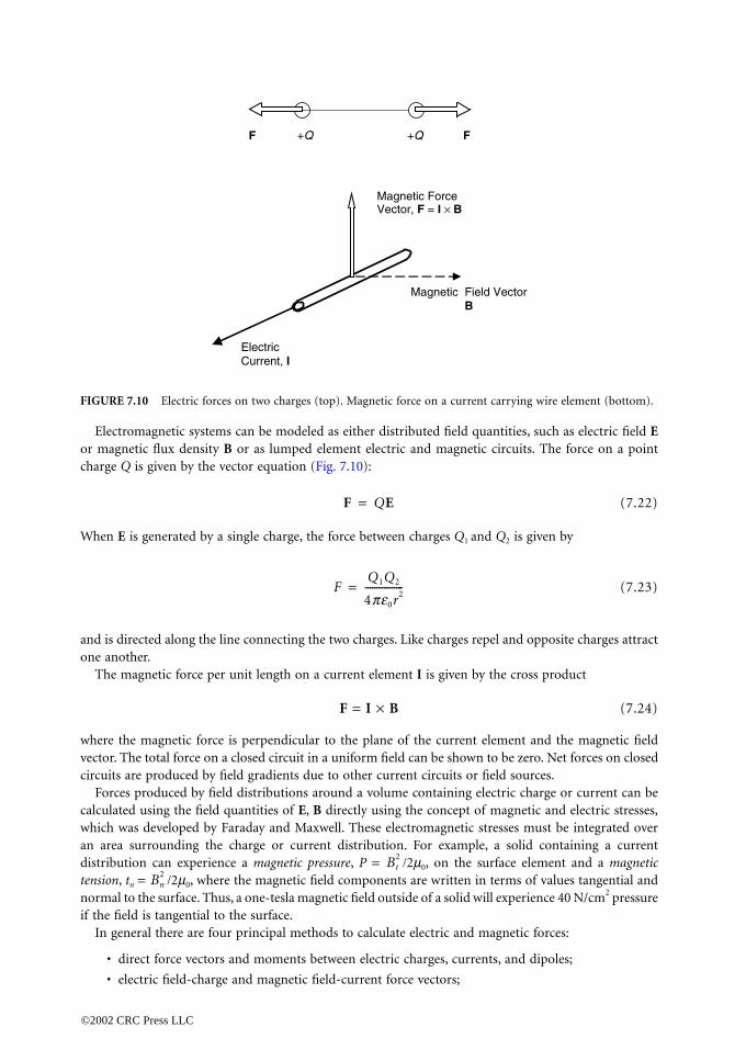
gnetic systems can be modeled as either distributed field quantities, such as electric field E flux density B or as lumped element electric and magnetic circuits. The force on a pointgiven by the vector equation (Fig. 7.10):

(7.22)

enerated by a single charge, the force between charges Q1 and Q2 is given by

(7.23)

ed along the line connecting the two charges. Like charges repel and opposite charges attract. etic force per unit length on a current element I is given by the cross product

F = I × B (7.24)

agnetic force is perpendicular to the plane of the current element and the magnetic fieldotal force on a closed circuit in a uniform field can be shown to be zero. Net forces on closedroduced by field gradients due to other current circuits or field sources.

oduced by field distributions around a volume containing electric charge or current can besing the field quantities of E, B directly using the concept of magnetic and electric stresses,eveloped by Faraday and Maxwell. These electromagnetic stresses must be integrated over

rounding the charge or current distribution. For example, a solid containing a current can experience a magnetic pressure, P = /2µ0, on the surface element and a magnetic

/2µ0, where the magnetic field components are written in terms of values tangential ande surface. Thus, a one-tesla magnetic field outside of a solid will experience 40 N/cm2 pressure tangential to the surface.l there are four principal methods to calculate electric and magnetic forces:

force vectors and moments between electric charges, currents, and dipoles;

ic field-charge and magnetic field-current force vectors;

Electric forces on two charges (top). Magnetic force on a current carrying wire element (bottom).

F +Q F

ElectricCurrent, I

Magnetic Field VectorB

Magnetic ForceVector, F = I × B

+Q

F QE=

FQ1Q2

4pe0r2----------------=

Bt2

Bn2

ress LLC

• electrmater

• energ

Examples ofin the sectio

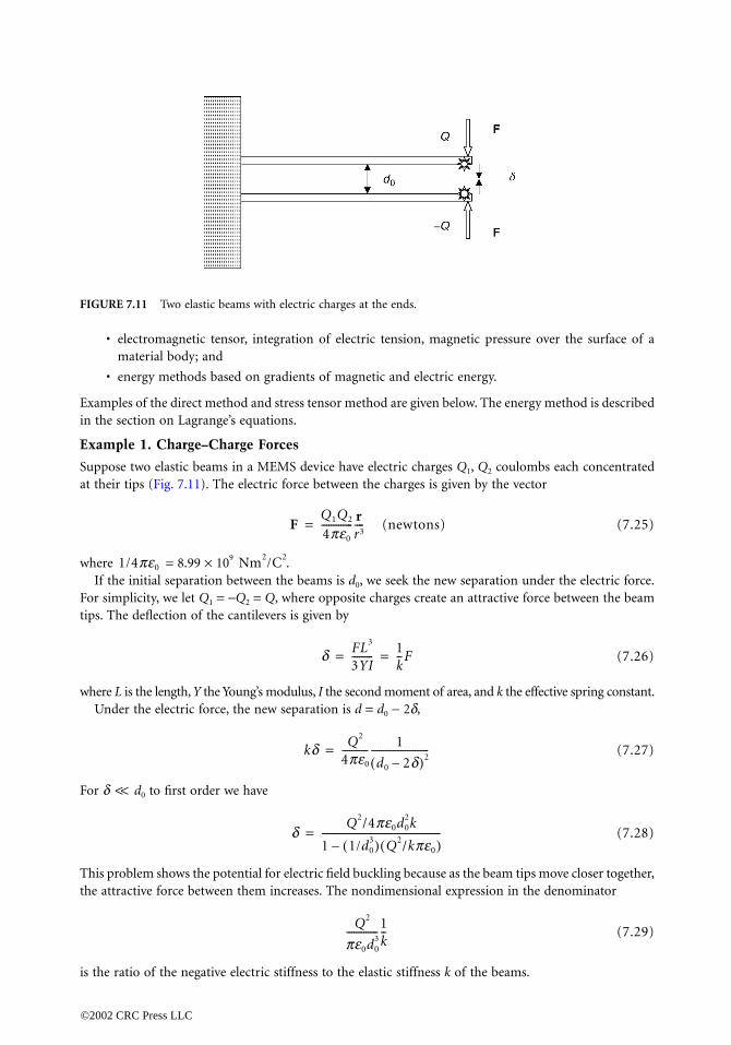
Example 1

Suppose twoat their tips

where If the init

For simplicitips. The de

where L is thUnder the

For δ d0

This problemthe attractiv

is the ratio o

FIGURE 7.11

1/4p

<<


©2002 CRC P

omagnetic tensor, integration of electric tension, magnetic pressure over the surface of aial body; and

y methods based on gradients of magnetic and electric energy.

the direct method and stress tensor method are given below. The energy method is describedn on Lagrange’s equations.

. Charge–Charge Forces

elastic beams in a MEMS device have electric charges Q1, Q2 coulombs each concentrated(Fig. 7.11). The electric force between the charges is given by the vector

(newtons) (7.25)

= 8.99 × 109 .ial separation between the beams is d0, we seek the new separation under the electric force.ty, we let Q1 = −Q2 = Q, where opposite charges create an attractive force between the beamflection of the cantilevers is given by

(7.26)

e length, Y the Young’s modulus, I the second moment of area, and k the effective spring constant. electric force, the new separation is d = d0 − 2δ,

(7.27)

to first order we have

(7.28)

shows the potential for electric field buckling because as the beam tips move closer together,e force between them increases. The nondimensional expression in the denominator

(7.29)

f the negative electric stiffness to the elastic stiffness k of the beams.

Two elastic beams with electric charges at the ends.

FQ1Q2

4pe0

------------- rr3----=

e0 Nm2/C2

d FL3

3YI--------- 1

k--F= =

kδ Q2

4pe0

----------- 1

d0 2d–( )2------------------------=

dQ2/4pe0d0

2k

1 1/d03( ) Q2/kπε0( )–

-------------------------------------------------=

Q2

pe0d03

-------------1k--

ress LLC

Example 2

Imagine a fesoft magnetferromagnet

The magFaraday (seethe stress ve

For high mafield outsidefrom the int

and is A (neglect

where Bg is t

where the re

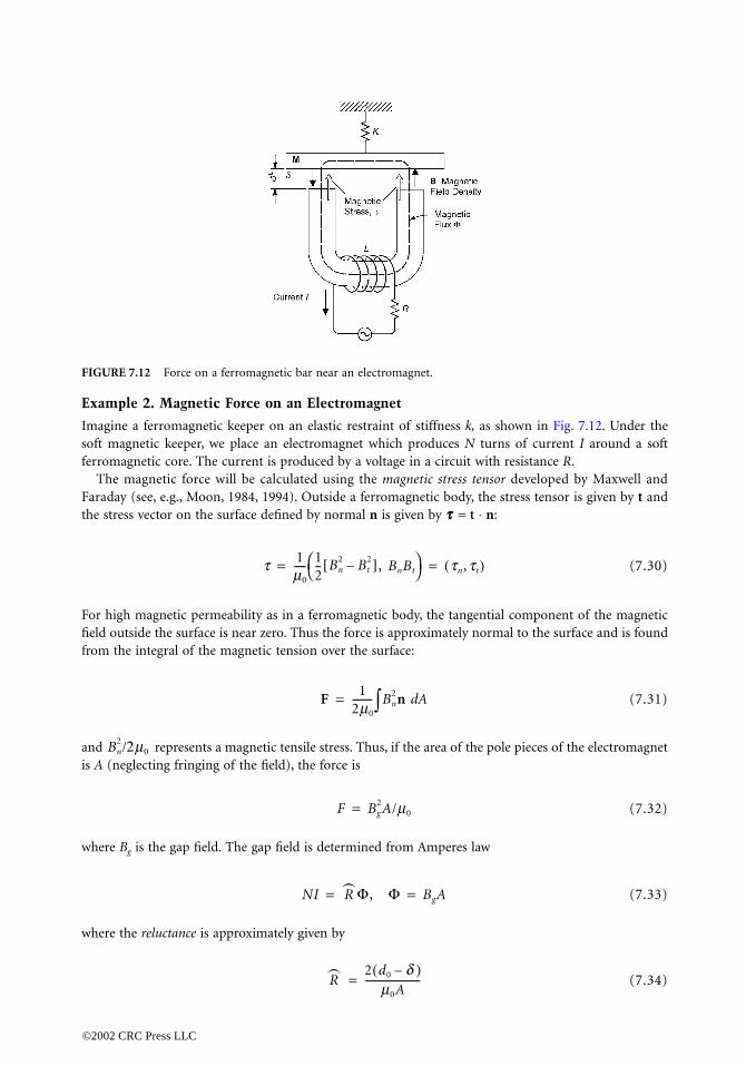
FIGURE 7.12

Bn2 /2m0


©2002 CRC P

. Magnetic Force on an Electromagnet

rromagnetic keeper on an elastic restraint of stiffness k, as shown in Fig. 7.12. Under theic keeper, we place an electromagnet which produces N turns of current I around a softic core. The current is produced by a voltage in a circuit with resistance R.netic force will be calculated using the magnetic stress tensor developed by Maxwell and, e.g., Moon, 1984, 1994). Outside a ferromagnetic body, the stress tensor is given by t andctor on the surface defined by normal n is given by ττττ = t ⋅ n:

(7.30)

gnetic permeability as in a ferromagnetic body, the tangential component of the magnetic the surface is near zero. Thus the force is approximately normal to the surface and is foundegral of the magnetic tension over the surface:

(7.31)

represents a magnetic tensile stress. Thus, if the area of the pole pieces of the electromagneting fringing of the field), the force is

(7.32)

he gap field. The gap field is determined from Amperes law

(7.33)

luctance is approximately given by

(7.34)

Force on a ferromagnetic bar near an electromagnet.

t 1m0

----- 12-- Bn

2 Bt2–[ ], BnBt

tn, tt( )= =

F1

2m0

-------- Bn2 n Ad∫=

F Bg2A/m0=

NI R Φ, Φ BgA= =

)

R2 d0 d–( )

m0A----------------------=

)

ress LLC

The balance of magnetic and elastic forces is then given by

or

(Note that tand electric

7.8 Dy

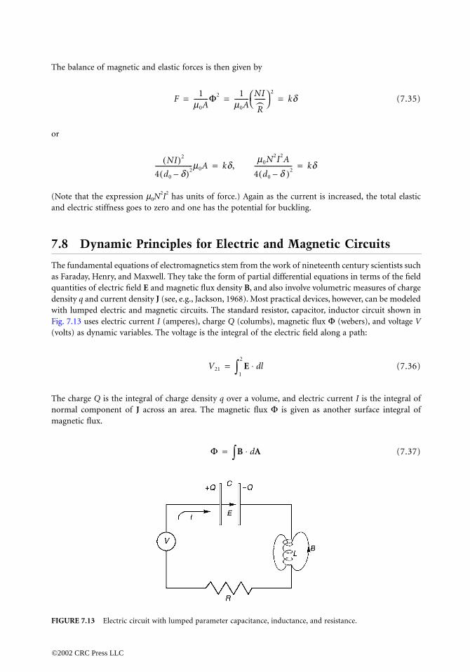
The fundamas Faraday, Hquantities ofdensity q anwith lumpedFig. 7.13 use(volts) as dy

The charge normal commagnetic flu

FIGURE 7.13


©2002 CRC P

(7.35)

he expression µ0N2I2 has units of force.) Again as the current is increased, the total elastic

stiffness goes to zero and one has the potential for buckling.

namic Principles for Electric and Magnetic Circuits

ental equations of electromagnetics stem from the work of nineteenth century scientists suchenry, and Maxwell. They take the form of partial differential equations in terms of the field

electric field E and magnetic flux density B, and also involve volumetric measures of charged current density J (see, e.g., Jackson, 1968). Most practical devices, however, can be modeled electric and magnetic circuits. The standard resistor, capacitor, inductor circuit shown in

s electric current I (amperes), charge Q (columbs), magnetic flux Φ (webers), and voltage Vnamic variables. The voltage is the integral of the electric field along a path:

(7.36)

Q is the integral of charge density q over a volume, and electric current I is the integral ofponent of J across an area. The magnetic flux Φ is given as another surface integral ofx.

(7.37)

Electric circuit with lumped parameter capacitance, inductance, and resistance.

F1

m0A---------Φ2 1

m0A--------- NI

R-------

2

kd= = =)

NI( )2

4 d0 d–( )2------------------------m0A kd,

m0N2I2A

4 d0 d–( )2------------------------ kd= =

V21 E ld⋅1

2

∫=

Φ B Ad⋅∫=

ress LLC

When there are no mechanical elements in the system, the dynamical equations take the form ofconservation of charge and the Faraday–Henry law of flux change.

where φ = Nanalog of minductor, for

For a linear state variabl

In charge

In MEMS dmechanical

The voltamaintain a elements as

Lagrange

It is well knoan energy p{qk}, not to generalized conservativeforces, whicgeneralized

For exampleconstant c, a

, W =is that it can

As an exaconsider thecapacitance

12-- mx

2


©2002 CRC P

(Conservation of charge) (7.38)

(Law of flux change) (7.39)

Φ is called the number of flux linkages, and N is an integer. In electromagnetic circuits theechanical constitutive properties is inductance L and capacitance C. The magnetic flux in an example, often depends on the current I.

(7.40)

inductor we have a definition of inductance L, i.e., φ = LI. If the system has a mechanicale such as displacement x, as in a magnetic solenoid actuator, then L may be a function of x. storage circuit elements, the capacitance C is defined as

(7.41)

evices and in microphones, the capacitance may also be a function of some generalizeddisplacement variable.ges across the different circuit elements can be active or passive. A pure voltage source cangiven voltage, but the current depends on the passive voltages across the different circuitsummarized in the Kirchhoff circuit law:

(7.42)

’s Equations of Motion for Electromechanical Systems

wn that the Newton–Euler equations of motion for mechanical systems can be derived usingrinciple called Lagrange’s equation. In this method one identifies generalized coordinatesbe confused with electric charges, and writes the kinetic energy of the system T in terms ofvelocities and coordinates, T( , qk). Next the mechanical forces are split into so-called forces, which can be derived from a potential energy function W(qk) and the rest of theh are represented by a generalized force Qk corresponding to the work done by the kthcoordinate. Lagrange’s equations for mechanical systems then take the form:

(7.43)

, in a linear spring–mass–damper system, with mass m, spring constant k, viscous dampingnd one generalized coordinate q1 = x, the equation of motion can be derived using, T = kx2, Q1 = −c , in Lagrange’s equation above. What is remarkable about this formulation be extended to treat both electromagnetic circuits and coupled electromechanical problems.mple of the application of Lagrange’s equations to a coupled electromechanical problem, one-dimensional mechanical device, shown in Fig. 7.14, with a magnetic actuator and aactuator driven by a circuit with applied voltage V(t). We can extend Lagrange’s equation to

dQdt------- I=

dfdt------ V=

f f I( )=

Q CV=

ddt----- L x( )I

QC x( )----------- RI+ + V t( )=

qk

ddt-----

∂T qk, qk( )∂qk

------------------------ ∂T∂qk

--------–∂W qk( )

∂qk

------------------+ Qk=

12-- x

ress LLC

circuits by din Lagrange’function Wm

equations of

The generalienergy inpuenergy is proto the capamagnetic an

These remarknowing theoften be fou

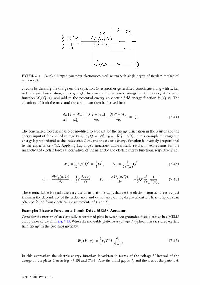
Example: E

Consider thecomb-drive field energy

In this exprcharge on th

FIGURE 7.14motion x(t).


©2002 CRC P

efining the charge on the capacitor, Q, as another generalized coordinate along with x, i.e.,s formulation, q1 = x, q2 = Q. Then we add to the kinetic energy function a magnetic energy( , x), and add to the potential energy an electric field energy function We(Q, x). The both the mass and the circuit can then be derived from

(7.44)

zed force must also be modified to account for the energy dissipation in the resistor and thet of the applied voltage V(t), i.e., Q1 = , Q2 = + V(t). In this example the magneticportional to the inductance L(x), and the electric energy function is inversely proportional

citance C(x). Applying Lagrange’s equations automatically results in expressions for thed electric forces as derivatives of the magnetic and electric energy functions, respectively, i.e.,

(7.45)

(7.46)

kable formulii are very useful in that one can calculate the electromagnetic forces by just dependence of the inductance and capacitance on the displacement x. These functions cannd from electrical measurements of L and C.

lectric Force on a Comb-Drive MEMS Actuator

motion of an elastically constrained plate between two grounded fixed plates as in a MEMSactuator in Fig. 7.15. When the moveable plate has a voltage V applied, there is stored electricin the two gaps given by

(7.47)

ession the electric energy function is written in terms of the voltage V instead of thee plates Q as in Eqs. (7.45) and (7.46). Also the initial gap is d0, and the area of the plate is A.

Coupled lumped parameter electromechanical system with single degree of freedom mechanical

Q

d∂dt------

T Wm+[ ]∂qk

-----------------------∂ T Wm+[ ]

∂qk

--------------------------–∂ W We+[ ]

∂qk

---------------------------+ Qk=

cx– RQ–

Wm12--L x( )Q

2 12--LI2, We

12C x( )---------------Q2= = =

Fm

∂Wm x, Q( )∂x

-------------------------- 12--I2dL x( )

dx-------------- , Fe

∂We x, Q( )∂x

-------------------------– −12--Q2 d

dx------ 1

C x( )-----------= = = =

We∗ V, x( ) 1

2--e0V 2A

d0

d02 x2–

---------------=

ress LLC

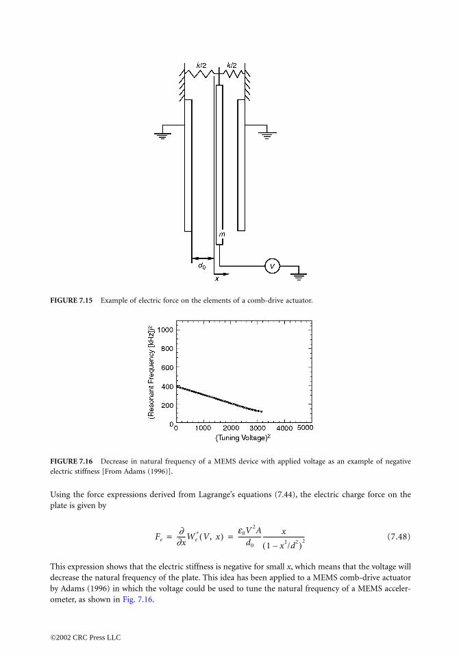
Using the foplate is given

This expressdecrease theby Adams (1ometer, as sh

FIGURE 7.15

FIGURE 7.16electric stiffne


©2002 CRC P

rce expressions derived from Lagrange’s equations (7.44), the electric charge force on the by

(7.48)

ion shows that the electric stiffness is negative for small x, which means that the voltage will natural frequency of the plate. This idea has been applied to a MEMS comb-drive actuator996) in which the voltage could be used to tune the natural frequency of a MEMS acceler-own in Fig. 7.16.

Example of electric force on the elements of a comb-drive actuator.

Decrease in natural frequency of a MEMS device with applied voltage as an example of negativess [From Adams (1996)].

Fe∂

∂x------We

∗ V, x( )e0V 2A

d0

--------------- x

1 x2/d2–( )2---------------------------= =

ress LLC

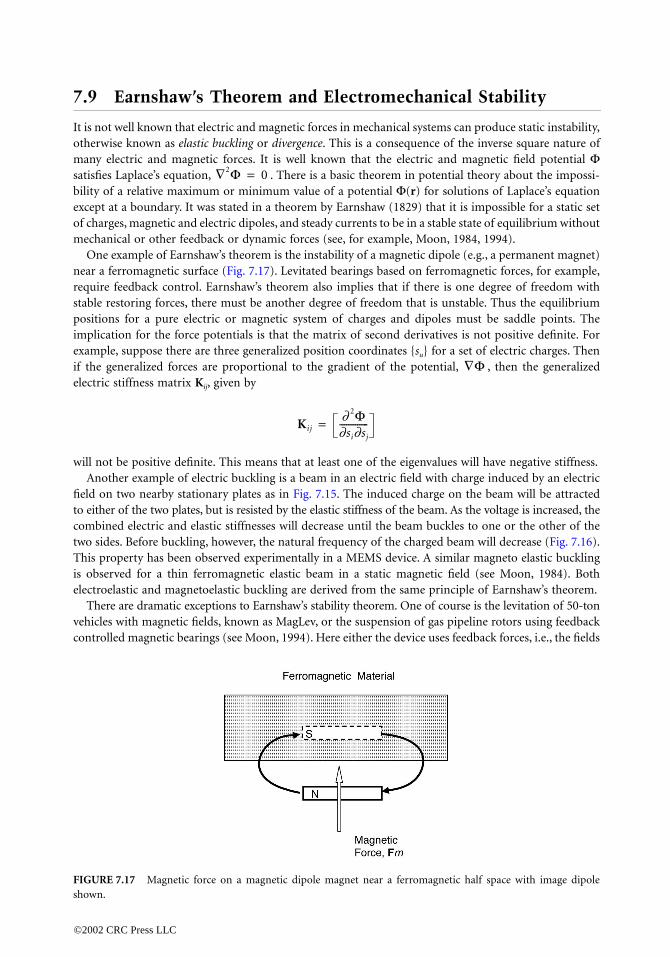
7.9 Earnshaw’s Theorem and Electromechanical Stability

It is not wellotherwise knmany electrsatisfies Lapbility of a reexcept at a bof charges, mmechanical

One examnear a ferromrequire feedstable restorpositions foimplication example, supif the generelectric stiffn

will not be pAnother e

field on twoto either of tcombined eltwo sides. BeThis properis observed electroelastic

There arevehicles withcontrolled m

FIGURE 7.17shown.


©2002 CRC P

known that electric and magnetic forces in mechanical systems can produce static instability,own as elastic buckling or divergence. This is a consequence of the inverse square nature of

ic and magnetic forces. It is well known that the electric and magnetic field potential Φlace’s equation, . There is a basic theorem in potential theory about the impossi-lative maximum or minimum value of a potential Φ(r) for solutions of Laplace’s equationoundary. It was stated in a theorem by Earnshaw (1829) that it is impossible for a static setagnetic and electric dipoles, and steady currents to be in a stable state of equilibrium without

or other feedback or dynamic forces (see, for example, Moon, 1984, 1994).ple of Earnshaw’s theorem is the instability of a magnetic dipole (e.g., a permanent magnet)agnetic surface (Fig. 7.17). Levitated bearings based on ferromagnetic forces, for example,

back control. Earnshaw’s theorem also implies that if there is one degree of freedom withing forces, there must be another degree of freedom that is unstable. Thus the equilibriumr a pure electric or magnetic system of charges and dipoles must be saddle points. Thefor the force potentials is that the matrix of second derivatives is not positive definite. Forpose there are three generalized position coordinates {su} for a set of electric charges. Then

alized forces are proportional to the gradient of the potential, , then the generalizedess matrix Kij, given by

ositive definite. This means that at least one of the eigenvalues will have negative stiffness.xample of electric buckling is a beam in an electric field with charge induced by an electric nearby stationary plates as in Fig. 7.15. The induced charge on the beam will be attractedhe two plates, but is resisted by the elastic stiffness of the beam. As the voltage is increased, theectric and elastic stiffnesses will decrease until the beam buckles to one or the other of thefore buckling, however, the natural frequency of the charged beam will decrease (Fig. 7.16).

ty has been observed experimentally in a MEMS device. A similar magneto elastic bucklingfor a thin ferromagnetic elastic beam in a static magnetic field (see Moon, 1984). Both and magnetoelastic buckling are derived from the same principle of Earnshaw’s theorem.

dramatic exceptions to Earnshaw’s stability theorem. One of course is the levitation of 50-ton magnetic fields, known as MagLev, or the suspension of gas pipeline rotors using feedbackagnetic bearings (see Moon, 1994). Here either the device uses feedback forces, i.e., the fields

Magnetic force on a magnetic dipole magnet near a ferromagnetic half space with image dipole

∇2Φ 0=

∇Φ

Kij∂ 2Φ

∂si∂sj

-------------=

ress LLC

are not static, or the source of one of the magnetic fields is a superconductor. Diamagnetic forces areexceptions to Earnshaw’s theorem, and superconducting materials have properties that behave like dia-magnetic mmagnetic flufeedback (se

Reference

Adams, S. GSystem

Goldstein, HJackson, J. DLee, C. K. an

J. AcoMelcher, J. RMiu, D. K. (Moon, F. C. Moon, F. C. Moon, F. C. Yu, Y.-Y. (19


©2002 CRC P

aterials. Also new high-temperature superconductivity materials, such as YBaCuO, exhibitx pinning forces that can be utilized for stable levitation in magnetic bearings without

e Moon, 1994).

s

. (1996), Design of Electrostatic Actuators to Tune the Effective Stiffness of Micro-Mechanicals, Ph.D. Dissertation, Cornell Unversity, Ithaca, New York.. (1980), Classical Mechanics, Addison-Wesley, Reading, MA.. (1968), Classical Electrodynamics, J. Wiley & Sons, New York.d Moon, F. C. (1989), “Laminated piezopolymer plates for bending sensors and actuators,”

ust. Soc. Am., 85(6), June 1989.. (1981), Continuum Electrodynamics, MIT Press, Cambridge, MA.

1993), Mechatronics, Springer-Verlag, New York.(1984), Magneto-Solid Mechanics, J. Wiley & Sons, New York.(1994), Superconducting Levitation, J. Wiley & Sons, New York.(1999), Applied Dynamics, J. Wiley & Sons, New York.96), Vibrations of Elastic Plates, Springer-Verlag, New York.

ress LLC

Documents

Physical System Modeling - University of Waterloojzelek/teaching/syde361/0066ch07.pdf · Physical System Modeling ... 7.8 Dynamic Principles for Electric and Magnetic Circuits