PHYSICAL REVIEW ACCELERATORS AND BEAMS 24, 054001 (2021)

Trapping of neutral molecules by the beam electromagnetic field

G. Franchetti *

GSI Helmholtzzentrum für Schwerionenforschung GmbH, 64291 Darmstadt, Germany,Goethe University Frankfurt, Max-von-Laue-Straße 7, 60438 Frankfurt am Main, Germany,

and Helmholtz Research Academy Hesse for FAIR (HFHF), GSI Helmholtz Center,Campus Frankfurt, Max-von-Laue-Straße 12, 60438 Frankfurt, Germany

F. ZimmermannEuropean Organization for Nuclear Research (CERN),Esplanade des Particules 1, 1217 Meyrin, Switzerland

M. A. RehmanHigh Energy Accelerator Research Organization (KEK),1-1 Oho, Tsukuba, Ibaraki, Japan, 305-0801, Japan,

and The Graduate University for Advanced Studies (SOKENDAI),School of High Energy Accelerator Science, Tsukuba, Ibaraki 305-0801, Japan

(Received 12 January 2021; accepted 8 March 2021; published 12 May 2021)

Neutral uncharged molecules are affected by the electromagnetic field of a charged particle beam if theycarry either an electric or a magnetic dipole moment. The residual gas in an accelerator beam pipe consistsof such molecules. In this paper we study their dynamics. Under a few approximations, whose validity weexplore and justify, we derive the equations of motion of neutral molecules and their invariants, determinethe conditions for these neutral molecules to become trapped in the field of the beams as a function ofbeam-pipe temperature, and compute the resulting enhancement of molecule density in the vicinity of thebeam. We demonstrate that large agglomerates of molecules, “flakes,” are much more likely to be pulledinto the beam than single molecules, and suggest that this phenomenon might help explain some beamobservations at the Large Hadron Collider.

DOI: 10.1103/PhysRevAccelBeams.24.054001

I. INTRODUCTION

During the 2017 and 2018 runs of the Large HadronCollider (LHC), abnormal beam losses, some leading toemergency beam aborts, were observed at one particularlocation, in half-cell no. 16 left of LHC interaction point 2(“16L2”) [1,2]. These losses, occasionally accompaniedby a fast beam instability [3], were later attributed to anaccidental in-leak of air into the beam vacuum, which hadoccurred while the beam screen was at a temperature of20 K. This in-leak had resulted in a surface layer of frozenair molecules, including oxygen, nitrogen, and water [4,5].Molecules of such a frozen surface layer could have beendetached by beam-induced heating, synchrotron radiation,

or by the beam field. Detached molecules which approachthe beam may interact with the circulating protons.Molecules of oxygen or nitrogen are either paramagnetic

or diamagnetic, respectively, having either a permanent oran induced magnetic dipole moment. Water molecules, onthe other hand, carry a permanent electric dipole moment,which makes them “polar.”The electromagnetic force exerted on molecules exhib-

iting an induced magnetic or electric dipole moment ismuch weaker than the force experienced by paramagneticor polar molecules, i.e., molecules with a permanentdipole moment. For this reason, in the following, we willnot further discuss the motion of molecules with onlyinduced dipole moments. Instead, our objective is tosimulate and analyze the motion of neutral moleculescarrying a permanent magnetic or electric dipole moment,in particular of the paramagnetic oxygen and of thepolar water molecules, subjected to the charged-particlebeam field.If interactions with the residual gas limit the beam

lifetime, the motion of neutral molecules inside the vacuumchamber becomes important. The motion of paramagnetic

*[email protected]

Published by the American Physical Society under the terms ofthe Creative Commons Attribution 4.0 International license.Further distribution of this work must maintain attribution tothe author(s) and the published article’s title, journal citation,and DOI.

PHYSICAL REVIEW ACCELERATORS AND BEAMS 24, 054001 (2021)Editors' Suggestion

2469-9888=21=24(5)=054001(24) 054001-1 Published by the American Physical Society

https://orcid.org/0000-0001-9792-5234

https://orcid.org/0000-0001-9787-8917

https://orcid.org/0000-0002-6534-8409

https://crossmark.crossref.org/dialog/?doi=10.1103/PhysRevAccelBeams.24.054001&domain=pdf&date_stamp=2021-05-12

https://doi.org/10.1103/PhysRevAccelBeams.24.054001




https://creativecommons.org/licenses/by/4.0/

https://creativecommons.org/licenses/by/4.0/

or polar molecules in an electromagnetic field is governedby their electric and magnetic dipole moments.We start this article by surveying the electric and

magnetic dipole moments of a few relevant molecules.Then we construct the equations of motion for such neutralmolecules subjected to the electromagnetic field of thebeam, at first crudely approximated by a thin-wire model.We solve these equations numerically, using a Runge-Kuttamethod, for different initial conditions, in order to identifythe critical parameters for the molecule motion. Next,considering a more realistic Gaussian beam distribution,and recognizing important constants of motion, we estimatethe position-dependent critical temperature for molecules tobe trapped by the electric or magnetic field of the charged-particle beam. Expanding this analytical treatment, wederive the general trapping efficiency as a function oftemperature, and the local density enhancement resultingfrom the gas molecules’ permanent dipole moments, whichdepends on beam current and temperature. Finally, weconsider the special case of “flakes,” i.e., agglomerates orclusters of many molecules carrying a dipole moment, andshow that such flakes are more easily trapped in the field ofthe beam than their individual constituent molecules.To simplify the equations, we are assuming the electric

or magnetic dipole moments to always be aligned with thecorresponding local field of the beam. In the Appendix weinvestigate the validity of this assumption.

II. PERMANENT DIPOLE MOMENTS OFNEUTRAL MOLECULES

The electric dipole moment (EDM) p for a pairof charges of the same magnitude but opposite sign isdefined as

p ¼ QL; ð1Þ

where Q denotes the magnitude of charges and L is thedisplacement vector pointing from the negative chargeto the positive charge. The SI unit of the EDM is theCoulomb meter (C m). In atomic physics also the unitDebye (D) is used (1 D ≈ 0.21 eÅ with e the electroncharge and 1 Å ¼ 0.1 nm).If a molecule with nonzero EDM is exposed to an

external electric field the molecule experiences a torque τgiven by

τ ¼ p × E: ð2Þ

Through the effect of τ, the electric dipole of the molecule,hence the molecule itself, tends to align its axis with thedirection of the applied electric field. The amount of thetorque is maximum if the dipole moment is oriented atan angle of 90 degrees with respect to the externalelectric field.

Molecules with an asymmetric internal chargeseparation like H2O or CO feature a permanent nonzeroEDM. In fact, we can decompose the dipole momentof H2O, into an effective charge Q and distance L, forexample, as Q ¼ 10e and jLj ¼ 3.9 × 10−12 m, and hencejpH2Oj ¼ 6.2 × 10−30 Cm, where e ≈ 1.6 × 10−19 Cdenotes the elementary electron charge. For the watermolecule, it should be noted that L is a distance chosento reproduce the measured dipole moment, for a givencharge Q. However, the actual geometry of the H2Omolecule resembles an isosceles triangle with two equalsides of about 1 Å each, and one longer side of 1.6 Å. Thiscircumstance should be carefully considered in futuremodeling. Similarly, for CO, we can assign Q ¼ 14e, andjLj ¼ 1.8 × 10−13 m, to obtain jpCOj ¼ 4.06 × 10−31 Cm.On the other hand, molecules with a mirror-symmetriccharge distribution, like N2, O2, or CO2, exhibit zeropermanent EDM ([6,7] and Chapter 3 of [8]).Like the electric dipole moment, also the magnetic

dipole moment (MDM) μ is known as a property of bothfundamental and less fundamental particles. The MDM canbe expressed as a vector μ,

μ ¼ e2M

ηv; ð3Þ

where e, M and η are the charge, mass and reduced Planckconstant of a particle, respectively. The unit vector vrepresents the direction of the MDM. In the case of theelectron, μe is known as a Bohr magneton (BM) and itsvalue is 9.27 × 10−24 J=T.Molecules can also feature a nonzero MDM. Similar to

the case of the EDM in an electric field, a molecule with acertain MDM exposed to an external magnetic field issubject to a torque τ, according to

τ ¼ μ × B: ð4Þ

For both EDM and MDM, the torque is zero only if thedipole moment axis is aligned with the field direction.The magnitude of the molecular MDM depends on the

electron configuration in the valence shell. The magneticdipole moment arising due to unpaired electron spins is [9]

μs ¼ffiffiffiffiffiffiffiffiffiffiffiffiffiffiffiffiffiffinðnþ 2Þ

pμe; ð5Þ

where n denotes the number of unpaired electrons. In thecase of an oxygen molecule, O2, two unpaired electrons arepresent, n ¼ 2, so that the μs for oxygen is 2.8 μe. Dueto this nonzero value of its MDM, the oxygen moleculeexhibits paramagnetic properties.Other molecules, like N2, CO2, CO and H2O, do not

possess any unpaired electron in their respective valenceshell. Therefore, the spin magnetic dipole moment of these

FRANCHETTI, ZIMMERMANN, and REHMAN PHYS. REV. ACCEL. BEAMS 24, 054001 (2021)

054001-2

molecules is zero [6,8,10]. These molecules are calleddiamagnetic.In the case of an air in-leak into the vacuum system of

an accelerator beam pipe, air molecules flowing into thevacuum pipe consist of nitrogen, oxygen, carbon dioxide,and water vapors, which carry specific electric and mag-netic dipole moments. Table I shows relevant dipolemoments for such air molecules, with their respectivemagnitude.

III. MOLECULE MOTION ARISING FROMTHE DIPOLE MOMENTS

If a neutral molecule is exposed to an electric field E andto a magnetic field B, its center of mass experiences theforce

Ft ¼ ðμ ·∇ÞBþ ðp ·∇ÞE; ð6Þ

where p and μ denote the molecule’s electric and magneticdipole moment, respectively. In the following we assumethat the magnetic and electric dipole moments are inde-pendent of location and, in particular, independent of themagnitude of the external fields.As a next step, we now consider the force experienced by

a molecule when subjected to the electric E and magnetic Bfield generated by the beam. As p and μ oscillate around thedirection of E, and B, respectively, the motion of moleculesmay become quite complex.The dynamics of the molecules is characterized by

multiple timescales. The shortest timescale correspondsto the vibrations of the atoms around their equilibriumposition. The next, longer, timescale refers to the frequencyat which the molecule’s electric or magnetic dipole momentoscillates around the respective field. Lastly, the longesttimescale refers to the periodicity of a molecule’s center-of-mass motion under the influence of the field gradient.If the period of oscillation of p and μ is shorter than

the characteristic time of change of B and E—this changebeing due either to the molecule dynamics or due thevariation of the beam fields (individual bunch passages,injection, etc.)—we may assume that p and μ are and

remain aligned with their respective beam field. In theAppendix we present a detailed discussion on the validityof this approximation.Our simplifying assumption would also imply a highly

specific relation between p and μ, if both were simulta-neously present, which, however, is not the case for any ofthe air molecules in question (compare Table I).We note that in the case of a complete alignment of their

magnetic and electric dipole moment with the correspond-ing beam field, the force on the molecules will bemaximum, hence leading to the largest possible excursionof the molecule motion, and therefore, to a conservativeassessment of the potential impact. In the Appendix, weexamine the validity of the alignment assumption.Without any other external field, or in close proximity to

the beam, the dominant component of the electric ormagnetic field is the one produced by the circulating beam.In this section, we model the magnetic field by approxi-

mating the beam current as concentrated in a delta-function-like manner into one transverse point at the centerof the vacuum chamber, corresponding to the magneticfield of an extremely thin current-carrying wire. In latersections, we will consider the field of a more realistic beamdistribution.The thin-wire model properly describes the field at a

radial distance r outside of a round (or approximatelyround) beam. This field reads

B ¼ μ0I2πr

rr× z; ð7Þ

where z is a unit vector in the direction of the beam motionand I denotes the average beam current. The quantity μ0 ¼4π × 10−7 H=m is the permeability of free space. Themotion of the neutral molecules typically is extremely slowcompared with the time interval between the passage ofindividual bunches of the beam. For this reason, it issufficient to consider the average beam current I, withouttaking into account any bunch structure. The magnetic fieldstrength and field pattern are illustrated in Fig. 1.Also the electric field generated by the round or

approximately round beam, outside the beam core canapproximately be described in a thin-wire approximation,as the field of a line charge distribution, namely as

E ¼ λ

2πϵ0

1

rrr; ð8Þ

where λ ¼ Q=C is the line charge density, with Q the totalcharge in the accelerator and C the accelerator circum-ference, ϵ0 ¼ 8.85 × 10−12 F=m the permittivity of freespace, and r the radial distance. For an ultrarelativisticbeam we have I ¼ cλ, and hence

E ¼ I2πϵ0c

1

rrr: ð9Þ

TABLE I. Permanent electric (EDM) and magnetic dipolemoments (MDM) of various air molecules in units of Debye(D) and Bohr magneton (BM), respectively, along with themolecule mass M in atomic mass units (amu).

Molecule EDM [D] MDM [BM] M [amu]

H2O 0.39 0 18O2 0 2.8 32CO 0.025 0 28N2 0 0 28CO2 0 0 44

TRAPPING OF NEUTRAL MOLECULES BY THE … PHYS. REV. ACCEL. BEAMS 24, 054001 (2021)

054001-3

Figure 2 displays the magnitude of the magnetic andelectric fields for a beam with I ¼ 1 A current as a functionof radial position and Fig. 3 illustrates the electric fieldpattern around the beam.The equations of motion for molecules with electric and

magnetic dipole moment are constructed under the approxi-mation previously discussed. Namely we use our ansatzthat the EDM and MDM are aligned with the electric andmagnetic field generated by the beam, respectively. Namelywe write

p ¼ prr

and μ ¼ μrr× z: ð10Þ

Inserting these equations, together with Eqs. (9) and (7),into Eq. (6), we obtain

Fx ¼ −�μμ0I2π

þ pI2πϵ0c

�x

ðx2 þ y2Þ3=2 ;

Fy ¼ −�μμ0I2π

þ pI2πϵ0c

�y

ðx2 þ y2Þ3=2 : ð11Þ

Hence, the equations of motion become

dvxdt

¼ −pI

2πϵ0Mcx

ðx2 þ y2Þ3=2 ;dvydt

¼ −pI

2πϵ0Mcy

ðx2 þ y2Þ3=2 ; ð12Þ

where I is the beam current,M is the molecule mass, and pis an “effective” dipole moment, defined as

p ¼ pþ μ

c: ð13Þ

In order to integrate the equations of motion, the initialconditions of a molecule are required, namely its initialvelocity and initial position, r0 and v0.For our study we consider molecules having an initial

velocity consistent with a certain temperature T, and havingrandom component in the x, y directions. The rms thermaltransverse velocity of a molecule, in the x-y plane, can beestimated by the classical formula,

vth ¼ffiffiffiffiffiffiffiffikbTM

r; ð14Þ

where kb designates the Boltzmann constant, T is thetemperature and M is the mass of the molecule.

0.050.05

0.05

0.00.075

0.1

0.1250.15

0.175

0.20.225

0.25

000

5

.225

0 000

1

2

0 50.

–3 –2 –1 0 1 2 3–3

–2

–1

0

1

2

3

X (mm)

Y(m

m)

B (mT)

0.050

0.075

0.100

0.125

0.150

0.175

0.200

0.225

0.250

FIG. 1. Magnetic field line pattern around a beam. Magneticfield strength decreases as 1=r with radial distance r from theorigin. The red spot at the center indicates the position of a protonbeam leaving the picture plane towards the reader.

Electric Field

Magnetic Field

0.5 1.0 1.5 2.0 2.5 3.00

50

100

150

200

0.00

0.10

0.20

0.30

0.40

0.50

0.60

0.70

r (mm)

E(V

/mm

)

B(m

T)

FIG. 2. Electric and magnetic field of the beam as a function ofradial distance as generated by a pointlike thin-wire beam ofcurrent 1 A.

20

3040

50

60

70

06606

5

40

–3 –2 –1 0 1 2 3–3

–2

–1

0

1

2

3

X (mm)

Y(m

m)

E (V/mm)

20

30

40

50

60

70

FIG. 3. Electric field lines around the round beam for a beamcurrent of 1 A.


054001-4

The top panel of Fig. 4 represents the variation of vth as afunction of temperature. The bottom panel shows thekinetic energy E in units of meV as a function of vth.

IV. MOTION PHENOMENOLOGY

A numerical solution of the equations of motion hasbeen implemented using the software packageMathematica [11]. SI units are used for all physicalquantities. Different initial thermal velocities and positionsare considered for the simulation of molecules motion inthe electromagnetic field of the beam in order to identifythe critical parameters. In the simulation we can vary, forexample, the initial velocity and the initial position of amolecule.The beam current is taken to be 1 Ampere. In all cases,

we assume that a molecule’s electric or magnetic dipolemoment is always completely aligned with the electricor magnetic field of the beam, respectively (see theAppendix).We first consider molecules at 1 mm distance from the

beam with zero initial velocity. Such molecules will gettrapped in the electromagnetic field of the beam andundergo an oscillatory motion. Figure 5 shows the hori-zontal motion of such H2O, CO, and O2 molecules, initially

at rest, as a function of time. The oscillation period dependson the dipole moment and on the mass of the molecules.In particular, the oxygen molecules perform oscillatorymotion, if subjected to the magnetic field of the beam, dueto their magnetic dipole moment, while they are notaffected by the electric beam field, since they possess zeroEDM. By contrast, water and carbon monoxide moleculesundergo an oscillatory motion due to the electric field of thebeam, since they carry a nonzero electric dipole moment.Figure 6 displays the molecule motion in the x-y plane.We now add an extremely small random initial velocity

corresponding to a temperature of order 1 mK. Sinceparticles are launched with different initial velocities inthe x and y direction, the vertical and horizontal motion arenot identical. Figure 7 presents some examples of x and ymotion with respect to time, for this case of a small initial

O2

H2O

CO

0 5 10 15 20

0

20

40

60

80

100

Temperature (K)

Vth

( m/s

)

O2

H2O

CO

0 20 40 60 80 100

0.0

0.5

1.0

1.5

Vth (m/s)

E(m

eV)

FIG. 4. The rms transverse thermal velocity of a molecule, vth,as a function of temperature (top) and the average kinetic energyversus the rms thermal velocity vth (bottom).

FIG. 5. Motion of neutral molecules initially 1 mm from thebeam, at rest, and subjected to the electromagnetic field of thebeam, as seen in the horizontal direction. Different colorscorrespond to different molecules as indicated.

– 6 – 4 – 2 0 2 4 6– 6

– 4

– 2

0

2

4

6

X (mm)

Y(m

m)

Electric Field

Magnetic Field

O2

H2O

CO

FIG. 6. The motion of neutral oxygen, water and carbonmonoxide molecules initially at rest, 1 mm from the beam,and subjected to the electromagnetic field of a beam, in thetransverse plane.With zero initial velocity, all molecules pos-sessing either a magnetic or electric dipole moment undergo anoscillatory motion.


054001-5

velocity, and Fig. 8 the corresponding picture of motion inthe transverse plane.We next increase the temperature to 15 K, a typical

temperature of the LHC beamscreen (which is heldbetween about 5 and 20 K). Molecules are again launchedat a distance of 1 mm from the beam. Figures 9 and 10present the molecule motion for this case. Under theseconditions, single molecules of oxygen, water, and carbonmonoxide do not get trapped in the electromagnetic fieldof the beam, as their large thermal velocity overcomes theeffective potential created by the beam field. Instead ofgetting trapped in the beam field, these molecules hit thevacuum chamber wall. In our simple model here, weassume that the molecules then bounce back from the wallelastically. The wall is set at 6 mm, about 3 times closerthan the actual LHC beam pipe, which has a radius of about20 mm. Trapping at 15 K would still be possible if theinitial distance of a molecule from the beam were just1 nm (!).Another possibility for molecules to be trapped is to

increase their mass M, and, thereby, reduce their initialthermal velocity, according to Eq. (14). Indeed, it isextremely likely that molecules with a permanent dipolemoment form flakes or clusters, consisting of 10,000 ormany more oxygen or water molecules; see Sec. X. Weshould then explore the motion of such flakes. Again we

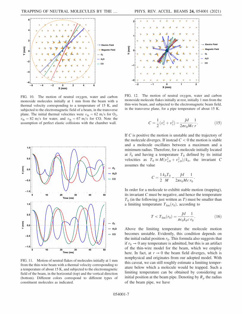
may assume that the magnetic or electric dipole moment ofa flake of molecules is completely aligned with thedirection of the beam’s electric or magnetic field. Oursimple simulation shows that, in equilibrium at 15 K, aflake of 104 molecules will be captured by the beam field,even when its starting position is at a radial distance of1 mm. Figures 11 and 12 display the time evolution ofx and y centroid coordinates and the corresponding phasespace for a flake of molecules.

V. TRAPPING BY BEAM POTENTIAL

We observe that the dynamics described by the equationsof motion (12) admit a constant of motion:

FIG. 7. Motion of neutral molecules initially at 1 mm from thebeam with a thermal velocity corresponding to a temperature of0.9 mK, and subjected to the electromagnetic field of the beam, inthe horizontal (top) and the vertical direction (bottom). Differentcolors correspond to different molecules as indicated.

– 6 – 4 – 2 0 2 4 6X (mm)

– 6

– 4

– 2

0

2

4

6

Y(m

m)

Electric Field

Magnetic Field

O2

H2O

CO

FIG. 8. The motion of neutral oxygen, water and carbonmonoxide molecules initially at 1 mm from the beam with athermal velocity corresponding to a temperature of order 1 mK,and subjected to the electromagnetic field of a beam, in thetransverse plane. The initial thermal velocities were for O2 vth ¼0.2 m=s (0.1 mK), for water vth ¼ 3 m=s (20 mK), and for COvth ¼ 0.3 m=s (0.3 mK).

0.0 0.2 0.4 0.6 0.8 1.0–6

–4

–2

0

2

4

Time (ms)

Y(m

m)

O2

H2O

CO

FIG. 9. Motion of neutral molecules initially at 1 mm from thebeam with a thermal velocity corresponding to a temperature of15 K, and subjected to the electromagnetic field of the beam, inthe vertical direction, with a hypothetical chamber wall at a radiusof 6 mm. Different colors correspond to different molecules asindicated.


054001-6

C ¼ 1

2ðv2x þ v2yÞ −

pI2πϵ0Mc

1

r: ð15Þ

If C is positive the motion is unstable and the trajectory ofthe molecule diverges. If instead C < 0 the motion is stableand a molecule oscillates between a maximum and aminimum radius. Therefore, for a molecule initially locatedat r0 and having a temperature T0 defined by its initialvelocities as T0 ≡Mðv2x;0 þ v2y;0Þ=kb, the invariant Cassumes the value

C ¼ 1

2

kbT0

M−

pI2πϵ0Mc

1

r0:

In order for a molecule to exhibit stable motion (trapping),its invariant C must be negative, and hence the temperatureT0 (in the following just written as T) must be smaller thana limiting temperature T limðr0Þ, according to

T < T limðr0Þ ¼pI

πϵ0kbc1

r0: ð16Þ

Above the limiting temperature the molecule motionbecomes unstable. Evidently, this condition depends onthe initial radial position r0. This formula also suggests thatif r0 → 0 any temperature is admitted, but this is an artifactof the thin-wire model for the beam, which we employhere. In fact, at r → 0 the beam field diverges, which isnonphysical and originates from our adopted model. Withthis caveat, we can still roughly estimate a limiting temper-ature below which a molecule would be trapped. Such alimiting temperature can be obtained by considering aninitial position at the beam pipe. Denoting by Rp the radiusof the beam pipe, we have

– 6 – 4 – 2 0 2 4 6–6

–4

–2

0

2

4

6

X (mm)

Y(m

m)

Electric Field

Magnetic Field

O2

H2O

CO

FIG. 10. The motion of neutral oxygen, water and carbonmonoxide molecules initially at 1 mm from the beam with athermal velocity corresponding to a temperature of 15 K, andsubjected to the electromagnetic field of a beam, in the transverseplane. The initial thermal velocities were vth ¼ 62 m=s for O2,vth ¼ 82 m=s for water, and vth ¼ 67 m=s for CO. Note theassumption of perfect elastic collisions with the chamber wall.

FIG. 11. Motion of neutral flakes of molecules initially at 1 mmfrom the thin-wire beam with a thermal velocity corresponding toa temperature of about 15 K, and subjected to the electromagneticfield of the beam, in the horizontal (top) and the vertical direction(bottom). Different colors correspond to different types ofconstituent molecules as indicated.

– 2 – 1 0 1 2

–2

–1

0

1

2

X (mm)

Y(m

m)

Electric Field

Magnetic Field

O2

H2O

CO

FIG. 12. The motion of neutral oxygen, water and carbonmonoxide molecule flakes initially at rest, initially 1 mm from thethin-wire beam, and subjected to the electromagnetic beam field,in the transverse plane, for a pipe temperature of about 15 K.


054001-7

T lim ¼ pIπϵ0kbc

1

Rp: ð17Þ

However, even some molecules with T < T lim may still belost, and hit the beam pipe, even if they could not escape toinfinity. By requiring that the maximum radius reached by amolecule be less than the beam pipe Rp, we can furtherconstrain the set of initial positions of molecules withtemperature T, in order for them to remain trapped by thebeam field. With a little bit of algebra we find that amolecule with initial position r0 and temperature T istrapped inside the beam pipe, if

r0Rp

≤1

1þ πϵ0kbcp

TRp

I

¼ f: ð18Þ

For an initially uniform distribution of molecules, thefraction of molecules trapped with respect to all moleculespresent in the beam pipe is f2. Therefore, if n signifies thedensity of the molecules at temperature T, the number ofmolecules trapped per unit length, i.e., the line density oftrapped molecules, is

λtrapped ¼ nf2πR2p:

Note that πϵ0kbc ¼ 1.1 × 10−25 C2=ðKsÞ.For example, considering H2O molecules, with p≃

6.2 × 10−30 Cm, we find

f ¼ 1

1þ 18.5 × 103TRp

I

:

Further, with I ¼ 1 A, and Rp ¼ 0.1 m the expression forf becomes

f ¼ 1

1þ 1.85 × 103 T½K� ;

which implies that only extremely cold molecules can betrapped by the beam. At T ¼ 54 mK the normalizedtrapping radius would be f ¼ 0.5, and, consequently,25% of the molecules of this temperature present in thepipe would be trapped. If instead we require that a moleculetrapped remains inside the beam of radius Rb ¼ 3σ (with σthe true rms beam size), then we need to demand

r0Rb

≤1

1þ πϵ0kbcp

TRbI

:

For σ ¼ 0.333 mm, we find Rb ¼ 1 mm and

r03σ

≤1

1þ 18.5 T½K� :

Therefore, if T ¼ 0.108 K, a molecule initially at r0=σ ≤ 1will be trapped within the radius Rb ¼ 3σ. Basically, thehotter molecules have to be closer to the beam center,where the fields are stronger, in order to be trapped.Conversely, molecules at a distance r0 ¼ Rb ¼ 3σ wouldneed to be extremely cold to remain inside the beam. This,however, is an artifact of the adopted thin-wire model forthe beam field. A more realistic model will be developed inthe next section.

VI. ARBITRARY AXISYMMETRIC BEAM

Next we consider an axisymmetric beam with charge linedistribution,

ρðrÞ ¼ Iπσ2c

n�r2

σ2

�; ð19Þ

defined for an ultrarelativistic beam, with nðuÞ a function ofu satisfying the normalizationZ

∞

0

nðuÞ du ¼ 1: ð20Þ

For a Gaussian distribution, this function assumes the form

nðuÞ ¼ 1

2e−

u2: ð21Þ

By applying Gauss’ law, we find the electric fieldEðrÞ ¼ EðrÞr=r, with

EðrÞ ¼ 1

2πϵ0cI1

rN�r2

σ2

�; ð22Þ

where for convenience we define the function

NðuÞ ¼Z

u

0

nðu0Þdu0: ð23Þ

The magnetic field is computed by applying Ampere’slaw, yielding

BðrÞ ¼ BðrÞ rr× z; ð24Þ

with

BðrÞ ¼ μ02π

I1

rN�r2

σ2

�: ð25Þ

Next we apply Eq. (6) to the magnetic field case for analigned MDM to obtain

ðμ ·∇ÞB ¼ μXi

�rr× z

�i∂i

�BðrÞ r

r× z

�: ð26Þ


054001-8

With some straightforward algebra we obtain

ðμ · ∇ÞB ¼ −μBðrÞr

rr: ð27Þ

Instead, for the electric field, and, as before, consideringthe EDM to be aligned with the field, the force on themolecule becomes

ðp ·∇ÞE ¼ pXi

�rr

�i∂i

�EðrÞ r

r

�; ð28Þ

which, again with straightforward algebra, becomes

ðp · ∇ÞE ¼ pE0ðrÞ rr: ð29Þ

Therefore, the general force acting on a moleculeexposed to the electric and magnetic field of an axisym-metric beam is

Ft ¼ ðp ·∇ÞEþ ðμ ·∇ÞB ¼�pE0ðrÞ − μ

BðrÞr

�rr: ð30Þ

Nowwe substitute the expressions for EðrÞ and BðrÞ to find

Ft ¼1

2πϵ0cI

�p

�1

rN�r2

σ2

��0−μ

c1

r2N�r2

σ2

��rr;

that is

Ft ¼1

2πϵ0cIσ2

�2pn

�r2

σ2

�− p

σ2

r2N�r2

σ2

��rr; ð31Þ

with the previous definition of the effective dipole moment,p ¼ ðpþ μ=cÞ [see Eq. (13)].We note that for particles outside a beam of rms size σ,

namely at r ≫ σ, we have nðr2=σ2Þ ≈ 0 and Nðr2=σ2Þ ≈ 1,so that outside the beam the formula for the force equals theone of the thin-wire model.In Eq. (31), the term in square brackets is a geometric

term, specific to the type of beam distribution. If in the coreof the beam the radial charge density is uniform, we expect

nðuÞ ≈ n0 and NðuÞ ≈ n0u; ð32Þ

with n0 ¼ nð0Þ, so that Eq. (31) reads

Ft ≈1

2πϵ0cIσ2

n0½2p − p� rr

and the force for the EDM is of opposite sign to the one forthe MDM.

For the EDM, we obtain

Ft ≈1

2πϵ0cIσ2

n0prr;

while, for the MDM, we have

Ft ≈ −1

2πϵ0cIσ2

n0μ

crr:

So, it seems that molecules with EDM cannot be trapped inthe core of the beam where the beam density is uniform.This situation is unusual, because, once EDM moleculesleave the beam core, they experience a stabilizing force,corresponding to the force of the thin-wire model.Figure 13 illustrates the horizontal forces experienced by

molecules with either an EDM or a MDM, as a functionof the horizontal position x along an axis passing throughthe center of the Gaussian beam, located at x ¼ 0. Forconvenience, the forces [Eq. (31)] are normalized bymultiplying with ð2σÞ=ðkbT�

pÞ or ð2σÞ=ðkbT�μÞ, where we

define the reference temperature

T�p ¼ 1

πϵ0kbcIσp; ð33Þ

or, respectively,

T�μ ¼

1

πϵ0kbcμ

cIσ: ð34Þ

We will refer to T�p, Eq. (33), and T�

μ, Eq. (34), as the“trapping temperature.” The shape of the force in Fig. 13suggests that the EDM molecules may oscillate not aroundthe beam center, but rather around an equilibrium radius re,which is of the order of the beam size.Incidentally, the trapping temperatures T�

p and T�μ

resemble the limiting temperature T limðr0Þ defined inEq. (16) or T lim of Eq. (17). The various characteristictemperatures simply correspond to different areas of trap-ping. While T�

p and T�μ refer to trapping over a radial length

scale equal to the rms beam size, the temperature T limindicates trapping within the beam pipe Rp, for the thin-wire model. A universal trapping temperature could beintroduced as T� ¼ pI=ðπϵ0kbcSÞ, with S denoting thecharacteristic length scale of trapping.In general, from (31), the equilibrium radius re for the

EDM is the solution of the equation

2n�r2

σ2

�¼ σ2

r2N�r2

σ2

�: ð35Þ

For a Gaussian beam


054001-9

nðuÞ ¼ 1

2e−

u2; NðuÞ ¼

Zu=2

0

e−wdw ¼ 1 − e−u=2;

so that Eq. (35) becomes

w2e−w2=2 ¼ 1 − e−w

2=2

with w2 ¼ r2e=σ2. Its solution is re=σ ¼ 1.585201 ≃ π=2.For a beam with a Kapchinskij-Vladimirskij (K-V)

distribution [12,13], instead, such equilibrium solutiondoes not exist, and the force acting on an EDM moleculewill be subject to a discontinuity at the beam edge. Namely,for a K-V beam, at r < Rb the force is constant anddefocusing, whereas at r > Rb it is attractive and non-linearly decreasing with amplitude.

VII. OSCILLATION FREQUENCY

According to (31), and introducing the radial velocityv≡ dr=dt, for EDM molecules the equation of motionreads

dvdt

¼ 1

2πϵ0McIσ2

p

�2n

�r2

σ2

�−σ2

r2N�r2

σ2

��rr: ð36Þ

Expanding around the equilibrium radius re we find

dvdt

¼ 1

2πϵ0McIσ2

p

�4reσn0�r2eσ2

�þ 2

σ

ren�r2eσ2

��r − reσ

rr:

ð37Þ

Using the equilibrium radius re and nðuÞ for a Gaussiandistribution, to good approximation, the term in thesquare bracket is equal to −e=10 (the exact number is−0.2716776662…). Then Eq. (37) becomes

dvdt

≈ −e10

p2πϵ0Mc

Iσ2

ðr − reÞσ

rr: ð38Þ

Therefore, the angular oscillation frequency is

ω ≈ffiffiffiffiffiffiffiffiffiffiffiffiffiffiffiffiffiffiffiffiffiffiffiffiffiffiffiffiffie10

p2πϵ0Mcσ3

Ir

: ð39Þ

For a water molecule, H2O, characterized by M ¼3 × 10−26 kg and p ¼ 6.2 × 10−30 Cm, and a beam withσ ¼ 3 × 10−4 m and I ¼ 1 A, we find ω ¼ 11189 rad=s.Hence, in this case, the frequency of oscillation around theequilibrium radius re is f ¼ ω=ð2πÞ ¼ 1780 Hz, which,for the LHC, is of the order of the fractional betatronfrequency.For a molecule featuring an MDM, instead of Eq. (38)

we have

dvdt

¼ −1

2πϵ0McIσ2

μ

cσ2

r2N�r2

σ2

�rr: ð40Þ

Now the equilibrium radius is the beam center r ¼ 0. Closeto this point, with a central beam density n0, the oscillatorymotion follows the equation

dvdt

¼ −1

2πϵ0McIσ2

μ

cn0

rr; ð41Þ

and so the beam seems to create a constant central forcepointing towards the beam center. Here, an MDMmoleculeoscillates at a frequency which depends on the square rootof the maximum oscillation amplitude.

VIII. INVARIANTS AND TRAPPING

Starting again from (31) and multiplying with the radialvelocity v≡ vr=r, we can rewrite the equation of motion as

ddt

1

2v2

¼ 1

2πϵ0McIσ

�pσ

rd

dðr=σÞN�r2

σ2

�− p

σ2

r2N�r2

σ2

��ddt

�rσ

�:

For EDM molecules we have

ddt

1

2v2 ¼ 1

2πϵ0McIσpddt

�σ

rN�r2

σ2

��; ð42Þ

and the integral of motion becomes

FIG. 13. The horizontal normalized force acting on an EDM(black) or MDM molecule (red), respectively, as a function of thetransverse ðx; 0Þ coordinate. The equilibrium position for theEDM case is indicated by the label re. Note that for both types ofdipole moment the force is discontinuous at x ¼ 0.


054001-10

1

2v2 −

kbT�p

2Mσ

rN�r2

σ2

�¼ D; ð43Þ

where we have used the reference temperature T�p, defined

in Eq. (33). The constant D is determined by the initialconditions, namely

1

2v20 −

kbT�p

2Mσ

r0N�r20σ2

�¼ D: ð44Þ

Now, the condition for a particle with initial conditions(r0, v0) to be trapped within the radius Rb is

v20 <kbT�

p

M

�σ

r0N�r20σ2

�−

σ

RbN�R2b

σ2

��: ð45Þ

Note that not all values of r0 are admitted. In fact, forr0 → 0 we find

σ

r0N�r20σ2

�→ 0:

Therefore, as could be guessed by looking at Fig. 13, thereis a minimum r0;min associated with Rb so that

σ

r0;minN�r20;min

σ2

�¼ σ

RbN�R2b

σ2

�: ð46Þ

Molecules with a smaller initial value of r0 cannot betrapped.Equation (45) sets a constraint on the trapping for a gas

of molecules of temperature T. At a given value of r0, thefraction f of the particles that can be trapped is obtained byintegrating the Maxwell-Boltzmann distribution:

f ¼Zv2xþv2y<v20

1

2π

MkbT

e−Mv22kbTdvxdvy ¼ 1 − exp

�−1

2

Mv20kbT

�

as

f ¼ 1 − exp

�−1

2

T�p

T

�σ

r0N�r20σ2

�−

σ

RbN�R2b

σ2

��: ð47Þ

The total amount of gas trapped in the beam at Rb ¼ 3σ isdetermined by integrating over the initial radii:

Ntrap ¼ nZ

Rb

r0;min(1 − exp

�−1

2

T�p

T

�σ

r0N�r20σ2

�

−σ

RbN�R2b

σ2

��)2πr0dr0; ð48Þ

where n denotes the gas density (molecules per volume).This can be further transformed to

Ntrap

nπR2b

¼ 1 −�r0;min

Rb

�2 − 2

σ2

R2b

exp

�1

2

T�p

Tσ

RbN�R2b

σ2

��

×Z

Rb=σ

r0;min=σexp

�−1

2

T�p

TNðu2Þu

�u du: ð49Þ

This formula can be integrated numerically with resultsshown in Fig. 14, for the case of a Gaussian distribution.For H2O with a beam of 1 A beam current and

σ ¼ 3 × 10−4 m rms beam size we find T�p ¼ 0.18 K.

This temperature is of similar magnitude as the trappingtemperature predicted earlier by the thin-wire model, butthe trapping efficiency is much reduced for this morerealistic Gaussian beam distribution. Indeed, the right panelof Fig. 14 suggests that for a gas of H2O molecules withtemperature T ¼ 2 K, corresponding to T=T�

p ¼ 11.1, thefractional trapping is ≃0.016, or only about 1.6%. If insteadT ¼ T�

p, Fig. 14 (right) shows that the fraction of trappedparticles would be ≃0.067 or close to 7%.For MDM molecules, the equation of motion becomes

ddt

1

2v2 ¼ −

1

2πϵ0McIσ

μ

cddt

Zr=σ

0

1

u2Nðu2Þdu;

yielding the constant of motion E,

1

2v2 þ kbT�

μ

2MN2

�rσ

�¼ E;

where we have used the trapping temperature T�μ, defined in

Eq. (34), and the new function

N2ðuÞ ¼Z

u

0

1

v2Nðv2Þdv: ð50Þ

In this case, the motion may be confined for E > 0. Inparticular, for a molecule to be trapped inside the beamradius Rb, its phase-space coordinates r, v should satisfy

FIG. 14. Fraction of EDM molecules trapped in the beam as afunction of T=T�

p, for T from 0 to 2T�p (left) and through 20T�

p(right). For this calculation we considered trapping inside a radiusof Rb ¼ 3σ, with σ the rms beam size.


054001-11

v2 þ kbT�μ

MN2

�rσ

�≤kbT�

μ

MN2

�Rb

σ

�;

or

v2 ≤kbT�

μ

M

�N2

�Rb

σ

�− N2

�rσ

��:

In this case the fraction of trapped particles in a Maxwelliangas is

f ¼ 1 − exp

�−1

2

T�μ

T

�N2

�Rb

σ

�− N2

�rσ

��: ð51Þ

As before, this result applies to particles located at r=σ.Again, the total fraction of trapped particles is obtained byintegrating over all locations in the beam pipe, that is

Ntrap

nπR2b

¼ 1 − 2σ2

R2b

exp

�−1

2

T�μ

TN2

�Rb

σ

��

×Z

Rb=σ

0

exp

�1

2

T�μ

TN2ðuÞ

�udu:

Figure 15 displays the total fraction of trapped moleculesas a function of T=T�

μ for the case of a beam with anaxisymmetric Gaussian distribution.As an example, considering oxygen molecules, O2, an

rms beam size σ ¼ 3 × 10−4 m and an average beamcurrent I ¼ 1 A, we find T�

μ ¼ 2.5 mK. So, for moleculesat a temperature of T ¼ 2 K, we have T=T�

μ ¼ 800 andthe fraction of trapped molecules is only 1.21 × 10−4 or0.0121%, while for T=T�

μ ¼ 1 the fractional trapping is≃0.088 or about 8.8%.

IX. PINCH OF NEUTRAL MOLECULES

The fraction of trapped molecules, extracted from theconstant of motion and the temperature, is an importantindicator, but it does not provide any prediction forthe average particle density as a function of radial position.

To obtain such a prediction, we need to integrate theequation of motion. For molecules equipped with an EDMwe start from Eq. (36). Using the definition of T�

p (33), thisbecomes

dv=σdt

¼ 1

2

kbMσ2

T�p

�2n

�r2

σ2

�−σ2

r2N�r2

σ2

��r=σr=σ

: ð52Þ

Defining r≡ r=σ, this transforms to

d2rdt2

¼ 1

2

kbT�p

Mσ2

�2nðr2Þ − 1

r2Nðr2Þ

�rjrj : ð53Þ

Employing the rms transverse thermal velocity of the gasmolecules,

vth ¼ffiffiffiffiffiffiffiffikbTM

r; ð54Þ

we normalize the time coordinate as

t ¼ tvth=σ; ð55Þ

and find

d2rdt2

v2thσ2

¼ 1

2

kbT�p

Mσ2

�2nðr2Þ − 1

r2Nðr2Þ

�rjrj : ð56Þ

Note that vth=σ is the rms inverse time a molecule wouldneed to travel across the beam size σ.Using the definition of the gas temperature, we obtain

d2rdt2

¼ 1

2

T�p

T

�2nðr2Þ − 1

r2Nðr2Þ

�rjrj : ð57Þ

We observe that, in these dimensionless scaled coordinates,the velocity of the molecule is

drdt

¼ drdt

1

σ¼ v

dtdt

1

σ¼ v

vth; ð58Þ

which means that the initial distribution of the normalizedvelocities dr=dt has a standard deviation 1.Recalling (39), the velocity vth and temperature are

related via

�vthσ

�2

¼ kbTMσ2

¼ kbT�p

Mσ2TT�p

¼ pπϵ0Mc

Iσ3

TT�p¼ 20

eω2

TT�p:

Combining this with the definition of vth, Eq. (55),and integrating the dynamics up to a certain time tmax,the corresponding tmax becomes

FIG. 15. Fraction of MDM molecules trapped in the beam as afunction of T=T�

μ, for T from 0 to 2T�μ (left) and through 1000T�

μ

(right). For this calculation we assumed Rb ¼ 3σ.


054001-12

tmax ¼ffiffiffiffiffi20

e

r ffiffiffiffiffiffiTT�p

sωtmax: ð59Þ

Note that the product ωtmax=ð2πÞ is the number ofoscillations ne performed by molecules near the equilib-rium radius re during the time interval tmax. We nowconsider time intervals for which the number of oscillationsaround re is constant, equal to ne, so that ωtmax ¼ 2πne.The corresponding tmax is

tmax ¼ffiffiffiffiffiffiffiffiffiffiffi20

eTT�p

s2πne: ð60Þ

This formula allows us to set tmax as a function of T=T�p,

so as to keep the same number of oscillations aroundthe equilibrium radius re. In this way we can comparethe molecular gas response to the beam for differenttemperatures T.Figure 16 shows the simulated dynamics of few particles

at zero temperature, T ¼ 0. In the left panel, the particlesare launched only in the x plane. The dynamics of themolecule pinch resembles the one of the electron-cloudpinch, e.g., the density evolution of cloud electrons during abunch passage [14–16]. However, note that, in this case forthe EDM, the particles oscillate linearly around the equi-librium radius re ¼ ðπ=2Þσ, and not around r ¼ 0.The right panel of Fig. 16 shows the same case of a cold

molecule gas, but now distributed in the full circular beampipe. The panel reveals a complex pattern, not easilyinterpreted.A better way to visualize the process is to carry out

simulations with many more particles and to compute themolecule density as a function of the radius. The result ofsuch a simulation is shown in Fig. 17.This simulation, along with all those that follow, con-

siders an ensemble of Nmac ¼ 4 × 105 macroparticles.The dynamics is computed with a leapfrog schemeapplied over 201 steps per oscillation length. At a given

integration step the local density ρðrÞ is obtained asρðrÞ ¼ ΔNmac=ð2πrΔrÞ, with ΔNmac denoting the numberof macroparticles found in the radial shell ½r − Δr=2;rþ Δr=2�. The number of such shells in the interval½0; rmax� is 400. Initially the molecules are distributedrandomly and uniformly in the (x=σ, y=σ) plane. Theinitial normalized velocities are chosen randomlyaccording to a Gaussian distribution of standarddeviation 1. For convenience, we normalize the particledensity by division with the initial particle density ρ0,computed as ρ0 ¼ Nmac=ðπr2maxÞ.In the top panel of Fig. 17, we see the evolution of the

local density normalized to the initial one. We observe avery pronounced pinch. The bottom panel instead displays

FIG. 16. Simulated pinch of the neutral EDM molecules in acold gas, i.e., T=T�

p ¼ 0. The particles are distributed eitheruniformly only in the x plane (left) or randomly distributed (right)in a circular beam pipe of radius Rp ¼ 10σ.

FIG. 17. EDM molecule density as a function of the radiusand “time” (top) and the end time-averaged local moleculedensity versus radius (bottom). The molecule density isnormalized with respect to the initial (or space-averaged)molecule density. The molecules are cold T=T�

p ¼ 10−5. Inthis simulation, the particles were distributed throughout thetransverse x-y space. At the bottom, the large peak of density is∼20 times the initial uniform distribution. Note the smallerpeak of density, which reflects the local oscillations ofmolecules around the equilibrium radius r=σ ≃ π=2; this phe-nomenon is clearly visible in the top panel as well.


054001-13

the time-average density, normalized to the initial densityρ0 (which always is equal to the average density), as afunction of radial position r, revealing a peak averagedensity close to the beam almost 20 times higher than theinitial one. This simulation was performed at a temperaturesuch that T=T�

p ¼ 10−5.The density evolution strongly depends on the temper-

ature, T=T�p. To illustrate this point, Fig. 18 shows the same

set of pictures for a gas temperature T=T�p ¼ 0.1. We see

that the nonzero temperature limits the effect of the pinch,and, in this case, we find a peak of only ≃2.4ρ0, i.e., twoand a half times the initial density.In view of the strong dependence of pinch density

enhancement on T=T�p, we summarize the situation in a

global picture presented in Fig. 19, where we have averagedover a time interval corresponding to ten oscillations nearposition re. The black markers indicate the normalizedpeak molecule density, with black values on the left verticalaxis. For example, at T=T�

p ¼ 0.1, we have ρmax=ρ0 ≃ 1.9,while for T=T�

p > 1 this ratio approaches ρmax=ρ0 ≃ 1: Togood approximation, for T=T�

p > 5 we find ρmax=ρ0 ≃ 1.The blue markers, with values on the right vertical axis,indicate the radial position at which the molecule densityassumes its maximum value. We see that for T=T�

p > 5 themaximum molecule density spreads around re ¼ ðπ=2Þσ.We also analyze the statistical properties of the distributionby computing the moments hrni ¼ R

rnPðrÞdr using theprobability density function PðrÞ ¼ cnρðrÞ, with cn anormalization constant ensuring that

RPðrÞdr ¼ 1. The

dash-dotted blue curve is the corresponding “averageposition” hri, computed as hri ¼ R

PðrÞdr with theintegral extending over the radial range from 0 to 10σ.For T=T�

p > 5 this curve is locked at a value of about 5,

FIG. 18. Molecule density as a function of the radius and time(top), and the end time-averaged local molecule density versusradius (bottom). The center panel shows the x-y structure of themolecule density at the point of maximum density. The moleculedensity is normalized with respect to the initial (or space-averaged) molecule density. In this simulation, the moleculesare at a temperature T=T�

p ¼ 0.1, and the particles initiallydistributed throughout the transverse x-y space. According tothe top panel (color scale), the peak density is ∼2.4 times theinitial uniform density.

FIG. 19. Variation of the radial density distribution of EDMmolecules with temperature T=T�

p. Shown are the densityenhancement due to the pinch in the beam field (black markers,left axis), the radial location of the maximum (blue markers, rightaxis), the average radial position of molecules (dash-dotted blueline), and the rms value of the radial position (dashed blue line).


054001-14

due to the fact that in this case the distribution ρðrÞ isuniform in r. For T=T�

p < 3, this curve tends towards thevalue 2.65, reflecting the presence of a peak in the density.

The dashed blue curve shows the standard deviation of r,i.e., ðhr2i − hri2Þ1=2, which indicates the width of the localpeak. For a uniform distribution this value would be10=

ffiffiffiffiffi12

p ¼ 2.88, which indeed is reached at high temper-atures in Fig. 19. For T=T�

p < 3 the standard deviationbecomes smaller, assuming a value of ∼2.3 for T=T�

p ¼ 0,again signaling a nonuniformity in the distribution, namelythe presence of a density peak, as is seen in Fig. 17.Similar analyses can be carried out for molecules

possessing a MDM and results analogous to those forthe EDM are shown in Figs. 20–23. In Fig. 23 we observethat the cold gas limit for the MDM is an order ofmagnitude higher than for the EDM.

X. DYNAMICS AND FORMATION OF FLAKES

Inspired by our phenomenological discussion in Sec. IV,we now consider the possible presence of neutral flakes inthe accelerator beam vacuum system.The physical interactions between molecules which give

rise to the formation of large and complex structures havelong been the subject of extensive studies in the researchfield of “aggregation phenomena” [17,18]. Aggregationmechanisms are being investigated through particle-clusterand cluster-cluster models [19]. In particular, the dynamicsof agglomeration for the case of particle-cluster modelswith dipolar interactions was studied in Refs. [20,21],which predicted the size and fractal dimension of theresulting clusters. Experiments and simulation modelsindicate that polar particles experience aggregations inwhich the original dipole moments are assembled into acluster, whose specifics depend on the physical nature ofthe particles’ dipole field. Studies of dust coagulation for

FIG. 20. Simulated pinch of the neutral MDM molecules in acold gas, i.e., T=T�

μ ¼ 0. The particles are distributed eitheruniformly only in the x plane (left) or randomly distributed (right)in a circular beam pipe of radius Rp ¼ 10σ.

FIG. 22. MDMmolecule density as a function of the radius andtime (left) and the end time-averaged local molecule densityversus radius (right). The molecule density is normalized withrespect to the initial (or space-averaged) molecule density. In thissimulation, the molecules are at a low temperature ofT=T�

μ ¼ 10−5, and the particles initially distributed throughoutthe transverse x-y space.

FIG. 23. Variation of the radial density distribution of MDMmolecules with temperature T=T�

μ. Shown are the densityenhancement due to the pinch in the beam field (black markers,left axis), the radial location of the maximum (blue markers, rightaxis), the average radial position of molecules (dash-dotted blueline), and the rms value of the radial position (dashed blue line).

FIG. 21. MDM molecule density as a function of the radiusand time (left) and the end time-averaged local moleculedensity versus radius (right). The molecule density is normal-ized with respect to the initial (or space-averaged) moleculedensity. In this simulation, the molecules are at a temperatureT=T�

μ ¼ 0.1, and the particles initially distributed throughoutthe transverse x-y space.


054001-15

particles carrying a MDM [22] revealed that the emergingcluster exhibits a total magnetic dipole moment whichscales as μ ∝ μ0N0.53, while for coagulating particles withan EDM the total dipole moment is only weakly dependenton N, in either case considering a plasma environment, notan accelerator-type vacuum. These studies also demon-strated that clustering starts when the velocity of theparticles is sufficiently slow to permit “dipole-dipoletrapping” [22].We here suggest the possibility of agglomerate formation

in particle accelerators, which would be driven by thehistory of an accelerator’s beam vacuum system: sequencesof events such as air leakage followed by cooling toultralow temperature and subsequent intermediate warm-up periods may foster the formation of aggregates, orflakes, in an ultrahigh vacuum at low temperature.In the context of our discussion, we consider flakes of

molecules as agglomerates composed of a large number Nof single molecules, each having a mass M and EDM p orMDM μ. A flake may be held together by the forcesbetween the (aligned) molecular dipole moments. A gen-eral flake thus has a mass Mf ¼ NM, and a maximumelectric dipole moment pf ¼ Np or magnetic dipolemoment μf ¼ Nμ. In either case, the initial condition isagain determined by the thermal equilibrium temperatureT, which remains the same as for the single molecules.The characteristic temperatures T�

p, T�μ defined in Eqs. (33)

and (34), respectively, are related to the correspondingtrapping temperature of the flakes (suffix “f”) via

T�p;f ¼ NT�

p; T�μ;f ¼ NT�

μ: ð61Þ

This reflects the fact that, at the same temperature, the flakehas a much lower thermal velocity than a single molecule,and that it can more easily be trapped in the beam potential.Namely, if in Figs. 14 and 15 a single particle has a certaintemperature T=T�

p, the corresponding flake would havean N times higher trapping temperature T�

p;f ¼ NT�p, or

T=T�p;f ¼ ðT=T�

pÞ=N. Hence, the point describing the flakelies much closer towards zero, on the left side of thediagrams, and, therefore, a significantly larger fraction ofthe flakes will be trapped, as indicated in the aforemen-tioned panels.As a concrete example, in the previously discussed case

with molecules of H2O, we found that T�p ¼ 0.18 K and for

this gas at T ¼ 2 K we had T=T�p ¼ 11.1; in the case these

molecules cluster to form a flake, for instance eachcontaining N¼10;000 molecules, we have T�

p;f¼180K,so that at T ¼ 2 K we find T=T�

p;f ¼ 0.0011, and themajority of the flakes will be trapped.More generally, in Figs. 19 and 23 it is quite evident that

for T=T�p;f → 0 or T=T�

μ;f → 0, respectively, the maximumdensity of the pinched flakes becomes large, with potentialconsequences for the effective vacuum pressure and

interaction with the beam. For the case of polar H2Oflakes, the peak density in the pinch reaches about 20 timesthe initial value, whereas for paramagnetic O2 flakes thepeak density even increases by a factor of 250. Theseestimates suggest that large polar flakes, clusters or dustparticles in an accelerator along with the mechanisms oftheir formation deserve a more thorough investigation, asthe process of dipolar assembly will lead to clusters subjectto the flake dynamics presented, with a consequent risk ofpinch and trapping in the beam field.

XI. CONCLUSIONS AND OUTLOOK

Many neutral molecules possess a permanent electric ormagnetic dipole moment. Their motion in an acceleratorvacuum system will be perturbed by the electromagneticfield of the beam, leading to a possible trapping and densityenhancement of such particles in the vicinity of the beam,especially in cold environments.In this paper, we have analyzed the equations of motion of

electrically or magnetically polar molecules, and identifiedthe respective constants of motion.We derived the fraction ofmolecules, with either electric or magnetic dipole moment,trapped by the beam field, as a function of temperature,expressed in terms of a characteristic trapping temperature.The resulting local density enhancement was calculated as afunction of radial position and time.In particular, we have shown that molecules with a

magnetic dipole moment oscillate around the transversecenter of the particle beam, whereas molecules with anelectric dipole moment oscillate around a radial equilibriumposition located at the edge of the beam.Observations of beam loss and beam instabilities in the

2017 and 2018 LHC runs cannot be explained by themotion of single neutral molecules, which, at a temper-ature of 5 K, would mostly not be trapped by the fieldof the beam. However, the trapping of larger neutralflakes, or agglomerates of a large number of polarwater or paramagnetic oxygen molecules, is indeedpossible, and, if such flakes had been formed in theLHC, this could well have contributed to the magnitudeof the observed phenomena. Such an explanationmight also be consistent with the degraded situationencountered after a beam screen warm-up from about5 to 80–90 K (“regeneration”) around the LHC location16L2 executed in August 2017 [5], since the highertemperature during the warm-up could have facilitatedthe formation of flakes.Regarding the possible presence of flakes, the tools and

methodologies developed for modeling aggregation phe-nomena [17–22] may serve as a starting point for futurestudies of cluster formation and flake characteristics inaccelerator beam vacuum systems.Throughout this article, we have analyzed the motion of

uncharged objects carrying a dipole moment. Evidently,once a molecule or a flake comes close to the beam it may


054001-16

be ionized [23], from which point onward its dynamics isradically altered. For ionized molecules or ionized singleatoms interacting with a charged particle beam the equa-tions of motion are well known [24]. On the other hand, alarger flake staying near the core of the beam would heatup, be charged, and then either evaporate or melt andexplode [25], leaving behind a localized high-densitymixture of ions, electrons, and molecules or atoms. Asoftware package is under development at CERN, to studythe interaction of such a complex mixture of species withthe LHC proton beam [26].In general, the trapping and accumulation of individual

neutral molecules or flakes of molecules in the vicinityof the beam enhances the effective gas density and canaggravate ion-induced beam instabilities, such as thosediscussed in Refs. [27–30]. The effect considered isparticularly important in cryogenic vacuum systems, forhigh beam currents or for small beam sizes. Consequently,it will become more important for future generations ofaccelerators.

ACKNOWLEDGMENTS

This work was supported, in part, by the EuropeanCommission under the HORIZON2020 IntegratingActivity project ARIES, Grant Agreement No. 730871.M. A. Rehman’s research stay at CERN was supported by agrant from the Graduate University for Advanced Studies(SOKENDAI), Japan, by K. Furukawa of KEK, and by G.Arduini, M. Giovannozzi, and M. Vretenar of CERN. Theauthors also thank M. Bai and M. Steck of GSI, and U.Ratzinger of Goethe University Frankfurt for continuousencouragement.

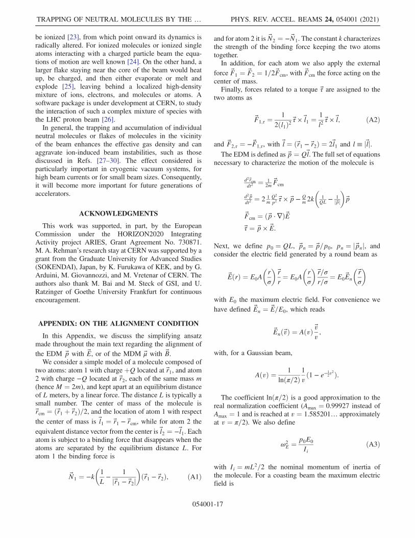
APPENDIX: ON THE ALIGNMENT CONDITION

In this Appendix, we discuss the simplifying ansatzmade throughout the main text regarding the alignment ofthe EDM p with E, or of the MDM μ with B.We consider a simple model of a molecule composed of

two atoms: atom 1 with charge þQ located at r1, and atom2 with charge −Q located at r2, each of the same mass m(hence M ¼ 2m), and kept apart at an equilibrium distanceof L meters, by a linear force. The distance L is typically asmall number. The center of mass of the molecule isrcm ¼ ðr1 þ r2Þ=2, and the location of atom 1 with respectthe center of mass is l1 ¼ r1 − rcm, while for atom 2 theequivalent distance vector from the center is l2 ¼ −l1. Eachatom is subject to a binding force that disappears when theatoms are separated by the equilibrium distance L. Foratom 1 the binding force is

N1 ¼ −k�1

L−

1

jr1 − r2j�ðr1 − r2Þ; ðA1Þ

and for atom 2 it is N2 ¼ −N1. The constant k characterizesthe strength of the binding force keeping the two atomstogether.In addition, for each atom we also apply the external

force F1 ¼ F2 ¼ 1=2Fcm, with Fcm the force acting on thecenter of mass.Finally, forces related to a torque τ are assigned to the

two atoms as

F1;τ ¼1

2ðl1Þ2τ × l1 ¼

1

l2τ × l; ðA2Þ

and F2;τ ¼ −F1;τ, with l ¼ ðr1 − r2Þ ¼ 2l1 and l≡ jlj.The EDM is defined as p ¼ Ql. The full set of equations

necessary to characterize the motion of the molecule is

d2 rcmdt2 ¼ 1

2m Fcm

d2pdt2 ¼ 2 1

mQ2

p2 τ × p − Qm 2k

�1QL −

1jpj

�p

Fcm ¼ ðp ·∇ÞEτ ¼ p × E:

Next, we define p0 ¼ QL, pn ¼ p=p0, pn ¼ jpnj, andconsider the electric field generated by a round beam as

EðrÞ ¼ E0A

�rσ

�rr¼ E0A

�rσ

�r=σr=σ

¼ E0En

�rσ

�

with E0 the maximum electric field. For convenience wehave defined En ¼ E=E0, which reads

EnðvÞ ¼ AðvÞ vv;

with, for a Gaussian beam,

AðvÞ ¼ 1

lnðπ=2Þ1

vð1 − e−

12v2Þ:

The coefficient lnðπ=2Þ is a good approximation to thereal normalization coefficient (Amax ¼ 0.99927 instead ofAmax ¼ 1 and is reached at v ¼ 1.585201… approximatelyat v ¼ π=2). We also define

ω2E ¼ p0E0

IiðA3Þ

with Ii ¼ mL2=2 the nominal momentum of inertia ofthe molecule. For a coasting beam the maximum electricfield is


054001-17

E0 ¼ ln

�π

2

�I

2πϵ0cσ; ðA4Þ

with I the beam current and σ the transverse rms beam size.By transforming the time t to τ ¼ tωE=ð2πÞ and normal-

izing the position with the rms beam size σ, i.e.,rn ¼ rcm=σ, the equations of motion become

d2 rndτ2 ¼ π2 L2

σ2ðpn ·∇rnÞEnðrnÞ

d2pndτ2 ¼ ð2πÞ2½pn × EnðrnÞ� × pn

− ð2πÞ2 kQE0

1 − 1

pn

pn:

ðA5Þ

A similar approach can be adopted for the equations ofmotion of binary molecules with a MDM. However, in thiscase we choose the molecule with l orthogonal to z, andalso μ orthogonal to z. We further define ln ¼ l=L. We candecompose μ as μ ¼ jμjðμplþ μol × zÞ with μ2p þ μ2o ¼ 1.In analogy to the EDM case, we introduce a normalized

magnetic field,

Bn ¼ AðvÞrn × z; ðA6Þ

so that B ¼ B0Bn, with B0 designating the maximummagnetic field generated by the beam. Note that in thisappendix the symbol ν means ν ¼ ν=jνj. Setting

ω2B ¼ jμjB0

Ii; ðA7Þ

we can write the equations of motion of the molecule as

d2 rndτ2 ¼ π2 L2

σ2½μ ·∇n�Bn

d2 lndτ2 ¼ ð2πÞ2 1

l2n½μ × Bn� × ln

− ð2πÞ2 kLjμjB0

1 − 1

jlnj

ln

μ ¼ μpln þ μoln × z;

ðA8Þ

where now τ ¼ tωB=ð2πÞ. We note that τ is a dimensionlessvariable, which counts the phase advance in units of 2π.Following the same argumentation, as for the electric

field, we estimate the maximum magnetic field for acoasting beam to be

B0 ¼ ln

�π

2

�Iμ02πσ

: ðA9Þ

From the above systems of equations, it is straightfor-ward to show that if pn is slightly tilted with respect to En,it oscillates around En at a frequency ωE. The identical

behavior occurs for μ, which oscillates at a frequency ωBaround Bn.The two equations, (A5) and (A8), also reveal that the

acceleration of the center of mass rn is proportional toπ2L2=σ2. This means that the motion of the center of massis slow. During one oscillation period of the EDM orMDM, the center of mass practically does not move. Wealso see that the binding force enters into the dynamics.However, we assume that this internal restoring force ismuch bigger than the additional forces exerted by theexternal beam magnetic or electric fields. This assumptionimplies that, to good approximation, jlnj is constant, equalto 1. Expanding the force on the center of mass acting on amolecule with MDM we find

F ¼ ðμ ·∇ÞB ¼ ½μ · r�B0ðrÞB − ½μ · B�BðrÞr

r:

If instead the molecule has an EDM we find the analogousequation

F ¼ ðp ·∇ÞE ¼ ½p · r�E0ðrÞrþ ½p · B�EðrÞr

B;

where r ¼ r=r; B ¼ r=r × z and p ¼ pxxþ pyy andμ ¼ μxxþ μyy and the electric and magnetic fields

EðrÞ ¼ EðrÞr; BðrÞ ¼ BðrÞB. During the time of oneoscillation of μ or p around their equilibrium position,the maximum displacement of the center of mass isproportional to the ratio π2L2=σ2 which is immenselysmall, typically L ¼ 10−10 m, and σ ¼ 10−3 m, henceπ2L2=σ2 ∼ 10−13.Therefore, we can look at the system on a timescale T

during which many oscillations of μn or pn around theirequilibrium position occur, while the center of mass stillmoves little. This, in turn, implies that the quantities BðrÞ,EðrÞ, and r are practically constant over the interval oftime T. Hence, defining h·i as an average over the timeinterval T, we find

hFi ¼ hμ · riB0ðrÞB − hμ · BiBðrÞr

r

for the MDM and

hFi ¼ hp · riE0ðrÞrþ hp · BiEðrÞr

B

for the EDM. However, because the number of oscillationsof μ, p is huge on the timescale T, we can simplify someterms as hμ · ri ¼ 0, hμ · Bi ¼ μeff and hp · ri ¼ peff ,hp · Bi ¼ 0, and we only remain with

hFi ¼ −μeffBðrÞr

r


054001-18

and

hFi ¼ peffE0ðrÞr:

In other words, we can replace the force acting on the centerof mass by an effective force resulting from an effectiveEDM, and an effective MDM aligned with the respectivefields. By making this approximation we give up anyattempt at resolving the tiny fluctuations of the center ofmass deriving from the coupling with the fast oscillationsof the MDM, or EDM, in the plane orthogonal to thefield lines.In addition, we note that the electric or magnetic field

generated by the stored particle beam never appearssuddenly, but rather is turned on slowly as the beamparticles are injected or accumulated. This means thatthe fields E and B appear mostly adiabatically. Thisadditional effect further fosters the alignment of theEDM and MDM to their respective field. We show thisby a simulation, which illustrates that μ, and p sponta-neously align with the local magnetic or electric field,respectively. Unfortunately, simulations for the real param-eters are beyond computational reach, as they wouldrequire resolving the vibrational motion and the centerof mass dynamics for π2L2=σ2 ∼ 10−13. Instead, we test themodel dynamics for the previously described bi-atomicmodel with the “relaxed simulation parameters” ofL2=σ2 ¼ 10−4 and k=ðQE0Þ ¼ 103.The two top panels in Fig. 24 compare the angle of the

electric field at the location of the molecule (red) and theangle of the electric dipole moment p (blue), both withrespect to the horizontal direction, on two different time-scales. Figure 24 top left shows, in blue color, the angle ofthe electric dipole moment. For this simulation, the initialangle of p was chosen at 180° with respect to En, and themolecule was launched with zero rotational energy. This isthe worst possible scenario. The picture reveals an oscil-lation of p, whose angle more and more closely approachesthe angle of the electric field. The center-left panel presentsthe situation at the end of the adiabatic turn-on, clearlydemonstrating an alignment of p with En. Note that,although the length of the time interval is the same asfor the top panel, the red curve (the electrical field at thelocation of the molecule) now exhibits a larger change ofangle. This feature stems from the dynamics experiencedby the molecule’s center of mass. At the end of the adiabaticramping, the gradient of EðrÞ is much larger than at the startof the field ramp, leading to a faster motion of the moleculearound and across the beam. Consequently the red curveappears with a more pronounced slope, and the thickness ofthe blue curve reflects an extremely rapid oscillation of theresidual orthogonal component of the dipole momentaround the electric field line. Exactly the same reasoningapplies to the example of a molecule equipped with amagnetic dipole moment and the simulation results for such

a case are quite similar, as is shown in the three pictures onthe right-hand side of Fig. 24. Also here a nearly perfectalignment is reached at the end of the adiabatic ramp-up ofthe magnetic field.The simulations of Fig. 24 consider a slow turn-on of the

electric field over a time interval T corresponding toτmax ¼ 105, or to the equivalent of 105 oscillation periodsfor the maximum field at the end of the adiabatic ramp,where jEnj ¼ 1. Note that although this number of oscil-lations seems large, it does correspond to a rather shortactual time interval, typically below a microsecond.

FIG. 24. Simulated angles of a molecule’s p (blue) and localelectric field E (red), with respect to the horizontal direction, atthe start (top left) and end (center left) of an adiabatic increase ofthe electric field of the beam, over a total time T that wouldcorrespond to τ ¼ 105 periods of phase advance ωET. The panelson the right present the simulated angular direction of amolecule’s magnetic dipole moment μ (blue) and of the localmagnetic field B (red) during an analogous ramp-up of the beam’smagnetic field, over the same number of periods of phase advanceωBT. The top and center panels each present the behavior over atime interval Δτ ¼ 200. The bottom panels show the molecules’trajectories over the full simulation. The red circle in the bottomleft panel indicates the equilibrium position re—compare Fig. 13and Eq. (35).


054001-19

Using Eq. (A4), which yields the maximum field for aGaussian beam, and the definition of T�

p we find for acoasting beam

ω2E ≃ ln

�π

2

�kbmL2

T�p: ðA10Þ

Then, as an example, considering H2O and T�p ¼ 0.18 K,

and by choosing the L so as to obtain the correct momentof inertia for the equivalent bi-atomic model, namely L ¼0.65 Å we find ωE ¼ 1.33 × 1011 rad=s; one oscillationperiod is δt ¼ 4.7 × 10−11 s. Therefore, in this example 105

oscillations correspond to Δt ¼ 4.7 × 10−6 s, and we haveshown this to be sufficiently adiabatic for ensuring thealignment of EDM with E, in the case of the relaxedsimulation parameters. Note that even with a 10 times fasterramp as in Δt ¼ 4.7 × 10−7 s, the alignment would still bereached to a good approximation. This timescale is com-parable to the bunch spacing in the LHC.The analysis for the MDM molecules can follow the

same line of thought. Considering the maximum B fieldgiven by Eq. (A9), and using the definition of T�

μ, we find

ω2B ≃ ln

�π

2

�kbmL2

T�μ:

As an example, for O2 we had T�μ ¼ 2.5 mK; hence ωB ¼

6.34 × 109 rad=sec and one oscillation period at the peakfield is δt ¼ 9.91 × 10−10 s. The duration of an adiabaticramp over 105 such oscillation periods corresponds toΔt ¼ 9.91 × 10−5 s. This suggests a stiffer behavior of theMDM, compared with the EDM. In consequence, the EDMmotion may not resolve individual bunch passages, but willalign to a mean B field.We can analyze the process of alignment by using the

concept of adiabatic invariants. In fact, the MDM and EDMoscillate around their respective equilibrium directionwith angular frequencies ωE or ωB, defined in Eqs. (A3)and (A7). For the orthogonal components of the dipolemoments, the corresponding equations of motion are

d2p⊥dt2

þ ω2Ep⊥ ¼ 0;

d2μ⊥dt2

þ ω2Bμ⊥ ¼ 0: ðA11Þ

After transforming (A11) to the scaled time coordinate τ,and, for convenience using the normalized variablespn ¼ p=jpj, μn ¼ μ=jμj, the equivalent set of equationsreads

d2pn;⊥dτ2

þΩ2Epn;⊥ ¼ 0;

d2μn;⊥dτ2

þ Ω2Bμn;⊥ ¼ 0; ðA12Þ

where ΩE and ΩB vary with the normalized time τ and atmaximum field (in our examples typically reached atτ ¼ τmax) assume the value 2π.

Therefore, for small oscillation amplitudes, the dimen-sionless scaled time τ indicates how many oscillations theEDM, or MDM, would perform around the equilibriumdirection if the field were maximum, i.e., for E ¼ E0

or B ¼ B0.For example, taking the example of the electric field E,

the adiabatic condition is

jEjj _Ej

≫2π

ωE; ðA13Þ

where _E is the time derivative. Considering an electricfield that linearly rises from 0 to a value E0 during thetime interval tmax, the adiabatic condition is fulfilled ift3=2ωE0

=ð2πÞ ≫ t1=2max. This inequality constrains the time tat which the field change becomes adiabatic.An adiabatically rising En or Bn slowly changes the

angular frequencies ωE and ωB until they approach theirfinal values. In the new coordinate frame, the slowlyvarying ΩE or ΩB will grow from an initial value of zeroto adiabatically reach the final value ΩB ¼ 2π or ΩE ¼ 2πat τ ¼ τmax.We have introduced the symbols pn;⊥ and μn;⊥, which

denote the projections of pn, μn onto the transverse axisperpendicular to E or B, respectively. In the orthogonaldipole moment “phase space” ðpn;⊥; dpn;⊥=dtÞ orðμn;⊥; dμn;⊥=dtÞ, we can recognize the key features ofadiabatic invariance. For the case of an EDM molecule,the top-left panel of Fig. 25 presents the dipole-momentevolution in the perpendicular “normalized” phase spaceobtained by using the time coordinate τ. The modelparameters for this simulation are the same as those forFig. 24. The picture clearly reveals that the trace of thephase-space coordinate ðpn;⊥; dpn;⊥=dτÞ convergestowards an ellipse. Based on the same set of simulationdata, the top-right panel of Fig. 25 illustrates the evolutionof the normalized dipole-moment total energy

E⊥ΩE

¼ 1

ΩE

�1

2

�dpn;⊥dτ

�2

þ 1

2Ω2

Ep2n;⊥

�: ðA14Þ

This picture confirms that, to good approximation,Ainv ≡ E⊥=ΩE ≃ constant, once the field change hasbecome adiabatic.The actual value of Ainv is determined by the initial

conditions of the particle’s dipole moment considered, i.e.,by the initial value of rn; drn=dτ; pn; dpn=dτ, and by theinitial speed of turning on the electric or magnetic field,proportional to 1=τmax. The field turn-on corresponds to aphysical ramp time of

Tramp ¼2π

ωEτmax; ðA15Þ


054001-20

which unveils the equivalence of the dynamics for corre-sponding pairs of ðTramp; E0Þ. The dependence of Ainv onτmax is examined in Fig. 25 (bottom left) for a linear rampconsidering a particle with the same initial condition (in theτ frame). The bottom-right panel of Fig. 25 illustrates thedependence of Ainv on τmax for a Gaussian ramp starting at atime of 5σz=c before the arrival of the bunch center, whereσz denotes the rms bunch length. Comparing the evolution

for several different τmax, the top-right panel of Fig. 25shows that the value of Ainv decreases as τmax increases.These findings reveal that τmax directly relates to the degreeof alignment with respect to the field. In fact, the maximumexcursion of pn;⊥ at the end of the ramp, which wedesignate as pn;⊥;max, is given by

pn;⊥;max ¼ffiffiffiffiffiffiffiffiffiffiffiffiffiffiffiffiffiffiffiffiAinvðτmaxÞ

π

r: ðA16Þ

Therefore, if Ainv shrinks with increasing τmax, so doespn;⊥;max.To shed some light on the dependence of Ainv on τmax, we

again consider the case of a linear ramp, where the electricfield increases linearly in time, and the frequency ΩEevolves as

ΩðτÞ ¼ 2π

ffiffiffiffiffiffiffiffiffiτ

τmax

r: ðA17Þ

At the beginning of the ramp, the fields are too weak tomeet the adiabatic condition, (A13), which in thesecoordinates assumes the particularly simple form

τ ≫ τ1=3max: ðA18Þ

This condition will start to hold true after a time τ largeenough to allow for a significant phase advance of theoscillation of the perpendicular dipole-moment componentaround the electric or magnetic field. The phase advance ofthis oscillation is estimated as

ΦðτÞ ¼Z

τ

0

ΩEðxÞdx ¼ 2π2

3

τ3=2ffiffiffiffiffiffiffiffiffiτmax

p : ðA19Þ

We denote by f the phase advance in unit of 2π requiredto enter into the adiabatic domain, so that the adiabaticprocess will start when

ΦðτÞ ¼ 2πf;

that is, by the time

τ ¼ f2=3�3

2

�2=3

τ1=3max:

At this moment the corresponding ΩE is

ΩEðτÞ ¼ 2π

ffiffiffiffiffiffiffiffiffiτ

τmax

r¼ 2πf1=3

�3

2

�1=3

τ−1=3max :

This corresponds to the value of Ω which sets the value ofAinv. In fact, from

FIG. 25. Electric dipole moment phase space orthogonal tothe local field direction, ðp⊥, dp⊥=dτÞ (top left), and theadiabatic invariant Ainv as a function of the number of oscillations(top right). The right panel presents data for three different valuesof τmax. The middle two panels present analogous simulationresults for the case of the magnetic dipole moment. At thebeginning of each simulation, large oscillations of p⊥ or μ⊥ areseen, which later on converge onto an ellipse. The width ofthis ellipse in the direction of p⊥, or μ⊥, becomes smaller thelarger τmax is. Recalling Eq. (A15), τmax can be expressed asτmax ¼ Tramp=ð2πÞðjpjE0=IiÞ1=2, and, therefore, the width of theellipse in the direction of p⊥ becomes smaller the moreadiabatically the field changes (larger Tramp) and the higherthe final field is (higher E0). This is demonstrated in the bottompanel by the dependence of Ainv on τmax, both for a linear (left)and for a Gaussian ramp (right).


054001-21

Ainv ¼1

ΩE

�1

2

�dpn;⊥dτ

�2

þ 1

2Ω2

Ep2⊥�; ðA20Þ

and neglecting the kinetic term, which is small for our testparticle (defined below), we find

Ainv ¼1

2ΩEðτÞp2⊥: ðA21Þ

We note that our test particle is launched at a distance farfrom the beam center and with a velocity sufficiently lowsuch that at the time by which the phase advance becomes2πf, i.e., by when the adiabatic condition is met, theparticle still remains far away, with p⊥ unchanged.Substituting for ΩE the value at which the adiabatic

process starts, we obtain

Ainv ¼ πf1=3p2⊥�3

2

�1=3

τ−1=3max : ðA22Þ

Our simulation results are shown by the markers in Fig. 25(bottom left). Although the previous model is valid onlyfor small oscillations around the equilibrium angle of thedipole moment, we find that choosing the values f ¼ 20and p⊥ ¼ 1, Eq. (A22) fits these simulation resultsextremely well.Note that this discussion, including the results shown

in Fig. 25, is carried out in the reference system withnormalized time τ. This implies that the initial condition inphysical coordinates, drn=dt, is related to the initialcondition in normalized space, drn=dτ, according to

drndt

¼ drndτ

dτdt

¼ drndτ

ωE

2π: ðA23Þ

The initial rms velocity of a molecule follows fromthe thermal equilibrium with the environment as vth ¼ffiffiffiffiffiffiffiffiffiffiffiffiffiffiffikbT=M

p, and ωE is given by Eq. (A10). Therefore,

Eq. (A23) becomes

�drndτ

�rms

¼ 2πffiffiffiffiffiffiffiffiffiffiffiffiffiffiffilnðπ=2Þp L

σ

ffiffiffiffiffiffiffiffiffiffiffimM

TT�p

s: ðA24Þ

As L is of the order of magnitude ∼10−10 m andσ ∼ 10−3 m, and as m=M ≤ 1 is always fulfilled, evenfor T=T�

p ¼ 106 we would find ðdrn=dτÞrms ∼ 6 × 10−4.Hence, we may consider the initial condition of moleculesin the system of coordinates τ as effectively frozen. Thesame argument applies to theMDM case, after replacing T�

p

with T�μ.

It follows that when the electric field rises adiabatically,the oscillation amplitude of p⊥ slowly decreases, so that pmore and more aligns with E, independently of the motionof the center of mass. The same argument applies to the

MDM case as is illustrated in the center panels and by thegreen markers in the bottom panels of Fig. 25.The previous analysis is now discussed for bunched

beams. Considering the passage of a single round bunch,the maximum electric field is obtained from Eq. (A4) with Inow the maximum current at the bunch center and σ thetransverse rms beam size. For a Gaussian bunch profile, thelongitudinal charge distribution is

ρzðzÞ ¼qNbffiffiffiffiffiffi2π

pσz

e−12z2

σ2z ; ðA25Þ

with Nb the number of particles in the bunch, q the chargeper beam particle, and σz the rms bunch length. Hence, forthis case the peak current reads I ¼ cqNb=ð

ffiffiffiffiffiffi2π

pσzÞ, and,

finally, we can express the maximum electric field as

E0 ¼lnðπ=2Þð2πÞ3=2

qNb

ϵ0σσz: ðA26Þ

For LHC bunches at top energy with σ ¼ 2 × 10−4 m,σz ¼ 0.076 m, Nb ¼ 1.2 × 1011 protons, we obtain amaximum electric field of E0 ≈ 4 × 106 V=m.Following the same argumentation, as for the electric

field, we estimate the maximum magnetic field during abunch passage from Eq. (A9), and using the maximumbeam current, we now find

B0 ¼lnðπ=2Þð2πÞ3=2

μ0cqNb

σσz: ðA27Þ

Inserting the same reference LHC beam parameters asbefore yields the estimate B0¼137×10−4 T¼137 Gauss.Considering the LHC bunches, for H2O molecules

Eq. (A3) yields a maximum angular oscillation frequencyωE ≈ 9.0 × 1011 rad=s, corresponding to T�

p ≈ 8.1 K,and, with a ramp time Tramp ¼ 5σz=c, Eq. (A15) yieldsτmax ≈ 181. On the other hand, for an O2 molecule, the peakangular oscillation frequency is ωB ¼ 4.27 × 1010 rad=s,corresponding to T�

μ ¼ 0.11 K and τmax ≃ 8.6. InspectingFig. 25, for example, at τmax ≃ 181 we find Ainv ≃ 0.5, and,for the perpendicular dipole moment at the end of the fieldramp, i.e., at the passage of the bunch center, this impliespn;⊥;max ≃ 0.4, which corresponds to a residual misalign-ment of Δθ ≃ 23.5 degree.These numbers suggest that for the short bunches of

the LHC the alignment condition is not strictly fulfilledand that, therefore, a residual oscillation of the dipolemoments may affect the dynamics. However, the simula-tions presented in this Appendix were performed primarilyin order to confirm that a process of alignment takes placeat all, and these numerical studies were carried out forunrealistically “relaxed” model parameters, which allowed


054001-22

a full exploration of the complex dynamics, but did notcorrespond to the actual parameter regime.Against this background, as a next step to further examine

our alignment ansatz,we now take into account that the forceresponsible for the molecular vibrations is much larger thanall the other forces, and, consequently, the timescale of thesevibrations far shorter than all other timescales. Hence, wemay take the distance between a molecule’s atoms to befrozen and consider a rigid model of the molecule.Simulation using a rigid model are numerically much easierto carry out. For the situation in question, where the electricand magnetic fields are all transverse, the motion of onemolecule is described by three dynamical variables, namelythe normalized transverse center-of-mass coordinates xn andyn, and the angle of the dipole moment with respect to therelevant field θ, and their conjugated momenta.In simulations using the rigid molecule model, the initial

centroid velocity spread of the molecules is chosen inaccordance with the thermal equilibrium temperature, andso is the initial rotational velocity spread of the dipole-moment angle, dθ=dτ, while the starting angle θ itself istaken to be initially aligned with θE (for the case of anelectric dipole moment). Simulations result for the rigid-molecule model with the parameters of Fig. 18 (center) areshown in Fig. 26, at a time corresponding to nosc: ¼ 1. Bothfigures, obtained with the aligned dipole-moment modeland with the rigid-molecule model, respectively, exhibit asimilar annular structure in phase space, with a densitymaximum located at the same radial position. This

similarity of results lends further support to our simplifyingalignment ansatz.In this Appendix, we have shown that the molecular

electric or magnetic dipole moments p or μ tend to alignwith the corresponding external field, as the external field isincreased. In particular, we have demonstrated the validityof the alignment assumption in various simulations per-formed under different assumptions (e.g., with and withoutinternal molecule vibrations) and timescales (mean fieldapproximation or resolving individual bunch passages).However, an exact simulation of repeated passages of

short bunches through a region populated by EDM orMDMmolecules with internal vibration modes requires thedevelopment of additional methods and tools to investigatethe complete nonlinear dynamics of this complicatedmultiscale system.

[1] J. Wenninger for the Operations group, LHC Report:Operation with Holes, CERN News.

[2] B. Salvant, 16L2. BE-ABP information meeting, 2017.[3] B. Salvant, S. Antipov, G. Arduini, N. Biancacci, X.

Buffat, L. Carver, P. Collier, A. Gorzawski, W. Hfle, G.Iadarola, G. Kotzian, A. Lechner, T. Levens, L. Mether, D.Mirarchi, E. Mtral, G. Rumolo, and D. Valuch, Exper-imental characterization of a fast instability linked to lossesin the 16L2 cryogenic half-cell in the CERN LHC, ReportNo. CERN-ACC-2018-175, THPAF058, 2018.

[4] F. Bordry, Summary of LHC performance workshop,Chamonix, 2018.

[5] J. M. Jimenez et al., Observations, analysis and mitigationof recurrent LHC beam dumps caused by fast losses inarc half-cell 16L2, Report No. CERN-ACC-2018-164,MOPMF053, 2018.

[6] Encyclopædia Britannica (Addison-Wesley, Reading,Massachusetts, 1993).

[7] D. Halliday, R. Resnick, and J. Walker, Fundamentals ofPhysics, 10th ed. (Wiley, New York, 2004).

[8] D. J. Griffiths, Introduction to Electrodynamics, 3rd ed.(Prentice-Hall, Upper Saddle River, NJ, 1999).

[9] M. Getzlaff, Fundamentals of Magnetism (Springer-Verlag, Berlin, 2008).

[10] W. S. C. Williams, Nuclear and Particles Physics (OxfordUniversity Press, New York, 1991).

[11] Wolfram Mathematica, https://www.wolfram.com/mathematica.

[12] I. M. Kapchinskij and V. V. Vladimirskij, Limitations ofproton beam current in a strong focusing linear acceleratorassociated with the beam space charge, in the 2ndInternational Conference on High-Energy Accelerators(CERN, Geneva, 1959), pp. 274–287.

[13] I. Hofmann, L. J. Laslett, L. Smith, and I. Haber, Stabilityof the Kapchinskij-Vladimirskij (K-V) distribution in longperiodic transport systems, Part. Accel. 13, 145 (1982),http://cds.cern.ch/record/140869/files/p145.pdf.

[14] E. Benedetto and F. Zimmermann, Dynamics of theelectron pinch and incoherent tune shift induced byelectron cloud, in Proceedings of the 9th European

FIG. 26. Simulated density based on a rigid-molecule model,for a temperature T=T�

p ¼ 0.1, at the normalized time nosc: ¼ 1,which is approximately the moment of maximum peak density.The picture presents a snapshot of the molecule distribution inthe x-y plane. The molecule density is normalized with respectto the initial (or space-averaged) molecule density. The par-ticles are initially distributed uniformly throughout the trans-verse x-y plane. For this simulation, we tracked 1.2 × 107

molecules with L2=σ2 ¼ 10−5. The density is estimated on agrid of 400 × 400 bins.


054001-23

https://www.wolfram.com/mathematica




http://cds.cern.ch/record/140869/files/p145.pdf




Particle Accelerator Conference, Lucerne, 2004 (EPS-AG,Lucerne, 2004), p. 7.

[15] E. Benedetto, G. Franchetti, and F. Zimmermann, Incoher-ent Effects of Electron Clouds in Proton Storage Rings,Phys. Rev. Lett. 97, 034801 (2006).

[16] F. Zimmermann and G. Franchetti, Electron-cloud pinchdynamics in presence of lattice magnet fields, Conf. Proc.C 110904, 586 (2011), https://accelconf.web.cern.ch/IPAC2011/papers/MOPS001.pdf.

[17] F. Family and D. P. Landau, Kinetics of Aggregation andGelation (North-Holland, Amsterdam, 2012).

[18] R. Jullien and R. Botet, Aggregation and Fractal Aggre-gates (World Scientific, Singapore, 1987).

[19] P. M. Mors, R. Botet and R. Jullien, Cluster-cluster aggre-gation with dipolar interactions, J. Phys. A 20, L975 (1987).

[20] R. Pastor-Satorras and J. M. Rubí, Particle-cluster aggre-gation with dipolar interactions, Phys. Rev. E 51, 5994(1995).

[21] M.-Carmen Miguel and R. Pastor-Satorras, Kinetic growthof field-oriented chains in dipolar colloidal solutions, Phys.Rev. E 59, 826 (1999).

[22] J. D. Perry, L. S. Matthews and T.W. Hyde , Dipole-dipoleinteractions of charged-magnetic grains, IEEE Trans.Plasma Sci. 38, 792 (2010).

[23] Y. Baconnier, A. Poncet, and P. Tavares, Neutralization ofaccelerator beams by ionization of the residual gas, in

CERN Accelerator School: Course on General AcceleratorPhysics (CERN, Geneva, 1994), pp. 525–564.

[24] Y. Baconnier and G. Brianti, The stability of ions inbunched beam machines, in 1983 CERN 1st AcceleratorSchool: Antiprotons for Colliding Beam Facilities (CERN,Geneva, 1980), p. 369.

[25] F. Zimmermann, J. T. Seeman, M. S. Zolotorev, and W.Stoeffl, Trapped macroparticles in electron storage rings,Report No. SLAC-95-6788, 1995.

[26] L. Mether, G. Iadarola, K. Poland, G. Rumolo, and G.Skripka, Multi-species electron-ion simulations and theirapplication to the LHC, Report No. CERN-ACC-2019-113, 2019, WEPTS050.

[27] D. G. Koshkarev and P. R. Zenkevich, Resonance ofcoupled transverse oscillations in two circular beams, Part.Accel. 3, 1 (1972), http://cds.cern.ch/record/1107898/files/p1.pdf.

[28] T. O. Raubenheimer and F. Zimmermann, A fast beam-ioninstability in linear accelerators and storage rings, Phys.Rev. E 52, 5487 (1995).

[29] G. V. Stupakov, T. O. Raubenheimer, and F. Zimmermann,Fast beam ion instability. 2. Effect of ion decoherence,Phys. Rev. E 52, 5499 (1995).

[30] R. A. Bosch, Spread-frequency model of the fast beam-ioninstability in an electron storage ring, Phys. Rev. STAccel.Beams 3, 034402 (2000).


054001-24

https://doi.org/10.1103/PhysRevLett.97.034801

https://accelconf.web.cern.ch/IPAC2011/papers/MOPS001.pdf






https://doi.org/10.1088/0305-4470/20/15/008

https://doi.org/10.1103/PhysRevE.51.5994




https://doi.org/10.1109/TPS.2009.2034967

https://doi.org/10.1109/TPS.2009.2034967









https://doi.org/10.1103/PhysRevSTAB.3.034402

https://doi.org/10.1103/PhysRevSTAB.3.034402

Documents

PHYSICAL REVIEW ACCELERATORS AND BEAMS 24, 054001 (2021)