Physics 220 Homework #6 Spring 2016 Due Friday 5/13/16

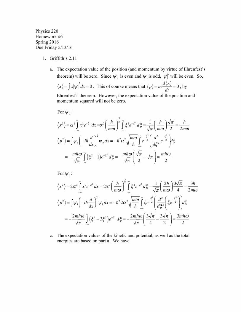
1. Griffith’s 2.11

a. The expectation value of the position (and momentum by virtue of Ehrenfest’s theorem) will be zero. Since ψ 0 is even and ψ 1 is odd, ψ 2will be even. So,

x = xψ∫2dx = 0 . This of course means that p = m

d xdt

= 0 , by

Ehrenfest’s theorem. However, the expectation value of the position and momentum squared will not be zero.

Forψ 0 :

x2 =α 2 x2e−ξ2

dx =−∞

∞

∫ α 2 !mω

⎛⎝⎜

⎞⎠⎟

32

ξ 2e−ξ2

dξ =−∞

∞

∫1π

!mω

⎛⎝⎜

⎞⎠⎟

π2

= !2mω

p2 = ψ o −i! ddx

⎛⎝⎜

⎞⎠⎟2

ψ o dx∫ = −!2α 2 mω!

e−ξ

2

2 d 2

dξ 2e−ξ

2

2⎛

⎝⎜⎞

⎠⎟−∞

∞

∫ dξ

= − m!ωπ

ξ 2 −1( )e−ξ 2 dξ = −−∞

∞

∫m!ωπ

π2

− π⎛⎝⎜

⎞⎠⎟= m!ω

2

Forψ 1 :

x2 = 2α 2 x2e−ξ2

dx = 2−∞

∞

∫ α 2 !mω

⎛⎝⎜

⎞⎠⎟

32

ξ 4e−ξ2

dξ =−∞

∞

∫1π

2!mω

⎛⎝⎜

⎞⎠⎟3 π4

= 3!2mω

p2 = ψ 1 −i! ddx

⎛⎝⎜

⎞⎠⎟2

ψ 1 dx∫ = −!2 2α 2 mω!

ξe−ξ

2

2 d 2

dξ 2ξe

−ξ2

2⎛

⎝⎜⎞

⎠⎟⎛

⎝⎜

⎞

⎠⎟

−∞

∞

∫ dξ

= − 2m!ωπ

ξ 4 − 3ξ 2( )e−ξ 2 dξ = −−∞

∞

∫2m!ω

π3 π4

− 3 π2

⎛⎝⎜

⎞⎠⎟= 3m!ω

2

c. The expectation values of the kinetic and potential, as well as the total

energies are based on part a. We have

T =p2

2m=

!ω4

forψ 0

3!ω4

forψ 1

⎧

⎨⎪⎪

⎩⎪⎪

V = 12mω 2 x2 =

!ω4

forψ 0

3!ω4

forψ 1

⎧

⎨⎪⎪

⎩⎪⎪

H = T + V =

!ω2

forψ 0

3!ω2

forψ 1

⎧

⎨⎪⎪

⎩⎪⎪

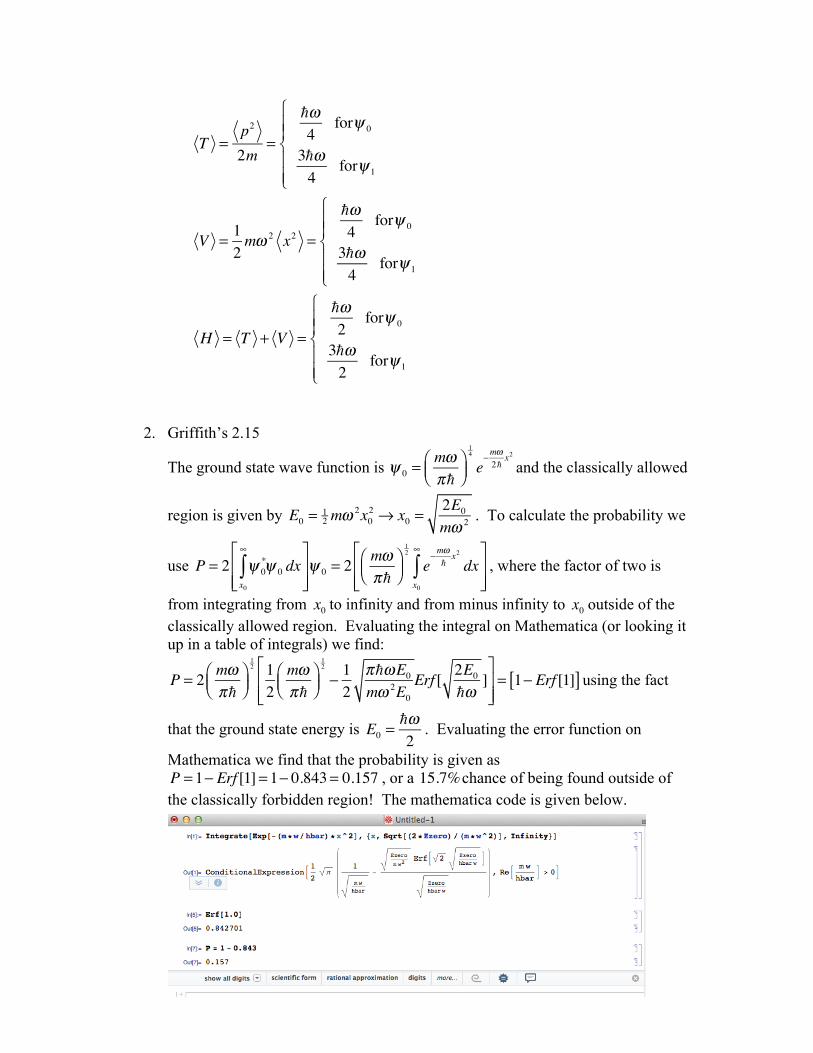
2. Griffith’s 2.15

The ground state wave function is ψ 0 =

mωπ!

⎛⎝⎜

⎞⎠⎟

14

e−mω2!

x2

and the classically allowed

region is given by E0 = 12 mω

2x02 → x0 =

2E0mω 2 . To calculate the probability we

use P = 2 ψ 0

*ψ 0 dxx0

∞

∫⎡

⎣⎢⎢

⎤

⎦⎥⎥ψ 0 = 2

mωπ!

⎛⎝⎜

⎞⎠⎟

12

e−mω!x2

dxx0

∞

∫⎡

⎣⎢⎢

⎤

⎦⎥⎥

, where the factor of two is

from integrating from x0 to infinity and from minus infinity to x0 outside of the classically allowed region. Evaluating the integral on Mathematica (or looking it up in a table of integrals) we find:

P = 2 mω

π!⎛⎝⎜

⎞⎠⎟

12 12

mωπ!

⎛⎝⎜

⎞⎠⎟

12

− 12

π!ωE0mω 2E0

Erf [ 2E0!ω

]⎡

⎣⎢⎢

⎤

⎦⎥⎥= 1− Erf [1][ ] using the fact

that the ground state energy is E0 =

!ω2

. Evaluating the error function on

Mathematica we find that the probability is given as P = 1− Erf [1]= 1− 0.843= 0.157 , or a 15.7%chance of being found outside of the classically forbidden region! The mathematica code is given below.

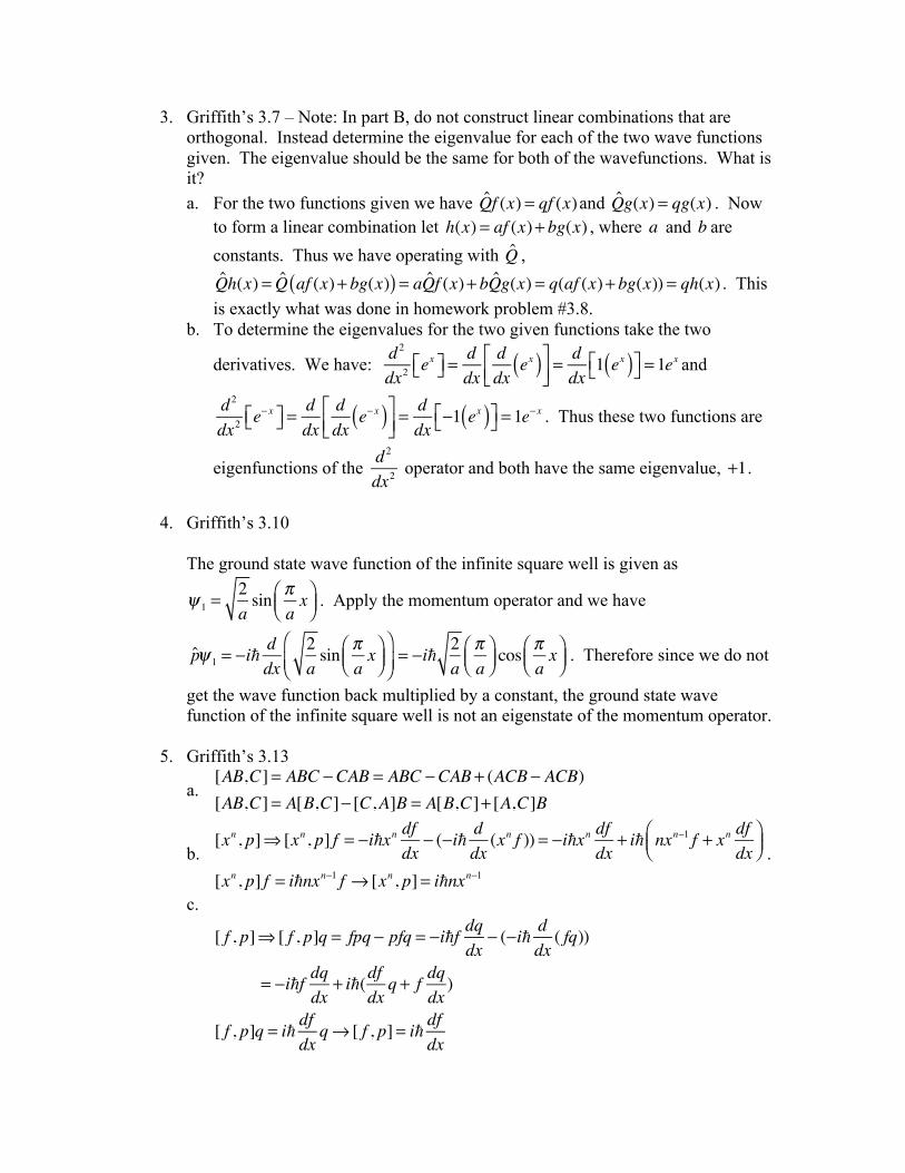
3. Griffith’s 3.7 – Note: In part B, do not construct linear combinations that are orthogonal. Instead determine the eigenvalue for each of the two wave functions given. The eigenvalue should be the same for both of the wavefunctions. What is it? a. For the two functions given we have Q̂f (x) = qf (x)and Q̂g(x) = qg(x) . Now

to form a linear combination let h(x) = af (x)+ bg(x) , where a and b are constants. Thus we have operating with Q̂ , Q̂h(x) = Q̂ af (x)+ bg(x)( ) = aQ̂f (x)+ bQ̂g(x) = q(af (x)+ bg(x)) = qh(x) . This is exactly what was done in homework problem #3.8.

b. To determine the eigenvalues for the two given functions take the two

derivatives. We have: d2

dx2ex⎡⎣ ⎤⎦ =

ddx

ddx

ex( )⎡⎣⎢

⎤⎦⎥= ddx

1 ex( )⎡⎣ ⎤⎦ = 1ex and

d 2

dx2e− x⎡⎣ ⎤⎦ =

ddx

ddx

e− x( )⎡⎣⎢

⎤⎦⎥= ddx

−1 ex( )⎡⎣ ⎤⎦ = 1e− x . Thus these two functions are

eigenfunctions of the d2

dx2 operator and both have the same eigenvalue, +1.

4. Griffith’s 3.10

The ground state wave function of the infinite square well is given as

ψ 1 =2asin π

ax⎛

⎝⎜⎞⎠⎟ . Apply the momentum operator and we have

p̂ψ 1 = −i! d

dx2asin π

ax⎛

⎝⎜⎞⎠⎟

⎛⎝⎜

⎞⎠⎟= −i! 2

aπa

⎛⎝⎜

⎞⎠⎟ cos

πax⎛

⎝⎜⎞⎠⎟ . Therefore since we do not

get the wave function back multiplied by a constant, the ground state wave function of the infinite square well is not an eigenstate of the momentum operator.

5. Griffith’s 3.13

a. [AB,C]= ABC −CAB = ABC −CAB + (ACB − ACB)[AB,C]= A[B,C]− [C,A]B = A[B,C]+ [A,C]B

b.

[xn , p]⇒ [xn , p] f = −i!xn dfdx

− (−i! ddx(xn f )) = −i!xn df

dx+ i! nxn−1 f + xn df

dx⎛⎝⎜

⎞⎠⎟

[xn , p] f = i!nxn−1 f → [xn , p]= i!nxn−1.

c.

[ f , p]⇒ [ f , p]q = fpq − pfq = −i!f dqdx

− (−i! ddx( fq))

= −i!f dqdx

+ i!(dfdxq + f dq

dx)

[ f , p]q = i! dfdxq→ [ f , p]= i! df

dx

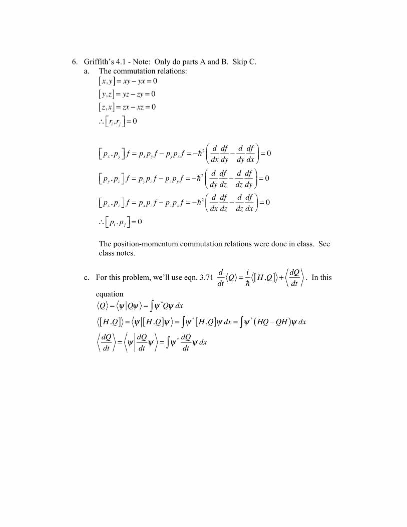
6. Griffith’s 4.1 - Note: Only do parts A and B. Skip C.

a. The commutation relations:

x, y[ ] = xy − yx = 0y, z[ ] = yz − zy = 0z, x[ ] = zx − xz = 0∴ ri ,rj⎡⎣ ⎤⎦ = 0

px , py⎡⎣ ⎤⎦ f = px py f − py px f = −!2 ddx

dfdy

− ddydfdx

⎛⎝⎜

⎞⎠⎟= 0

py , pz⎡⎣ ⎤⎦ f = py pz f − pz py f = −!2 ddydfdz

− ddzdfdy

⎛⎝⎜

⎞⎠⎟= 0

px , pz⎡⎣ ⎤⎦ f = px pz f − pz px f = −!2 ddx

dfdz

− ddzdfdx

⎛⎝⎜

⎞⎠⎟ = 0

∴ pi , pj⎡⎣ ⎤⎦ = 0

The position-momentum commutation relations were done in class. See class notes.

c. For this problem, we’ll use eqn. 3.71

ddt

Q = i!

H ,Q[ ] + dQdt

. In this

equation Q = ψ Qψ = ψ *Qψ dx∫H ,Q[ ] = ψ H ,Q[ ]ψ = ψ * H ,Q[ ]ψ dx∫ = ψ * HQ −QH( )ψ dx∫dQdt

= ψ dQdt

ψ = ψ * dQdt

ψ dx∫

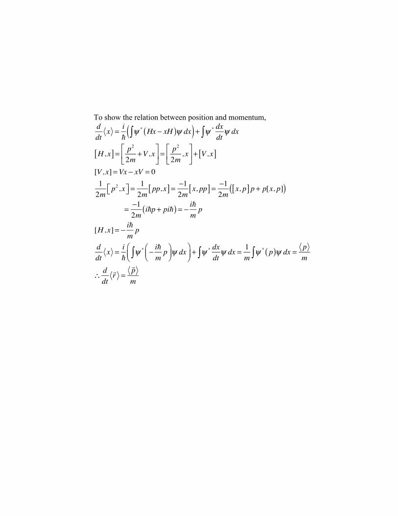
To show the relation between position and momentum,

ddt

x = i!

ψ * Hx − xH( )ψ dx∫( ) + ψ * dxdtψ dx∫

H , x[ ] = p2

2m+V , x⎡

⎣⎢

⎤

⎦⎥ =

p2

2m, x⎡

⎣⎢

⎤

⎦⎥ + V , x[ ]

[V , x]=Vx − xV = 012m

p2, x⎡⎣ ⎤⎦ =12m

pp, x[ ] = −12m

x, pp[ ] = −12m

x, p[ ] p + p[x, p]( )

= −12m

i!p + pi!( ) = − i!mp

[H , x]= − i!mp

ddt

x = i!

ψ * − i!mp⎛

⎝⎜⎞⎠⎟ψ dx∫⎛⎝⎜

⎞⎠⎟+ ψ * dx

dtψ dx∫ = 1

mψ * p( )ψ dx∫ =

pm

∴ ddt"r =

"pm

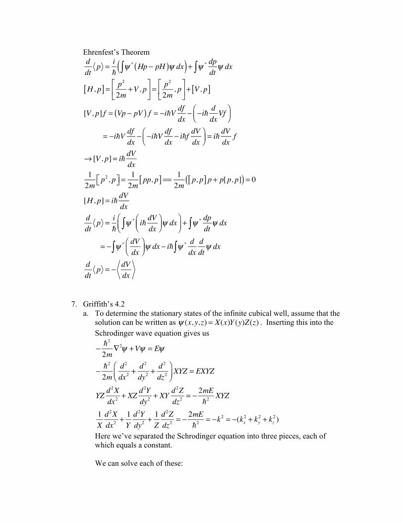
Ehrenfest’s Theorem

ddt

p = i!

ψ * Hp − pH( )ψ dx∫( ) + ψ * dpdtψ dx∫

H , p[ ] = p2

2m+V , p⎡

⎣⎢

⎤

⎦⎥ =

p2

2m, p⎡

⎣⎢

⎤

⎦⎥ + V , p[ ]

[V , p] f = Vp − pV( ) f = −i!V dfdx

− −i! ddxVf⎛

⎝⎜⎞⎠⎟

= −i!V dfdx

− −i!V dfdx

− i!f dVdx

⎛⎝⎜

⎞⎠⎟ = i!

dVdx

f

→ [V , p]= i! dVdx

12m

p2, p⎡⎣ ⎤⎦ =12m

pp, p[ ] == 12m

p, p[ ] p + p[p, p]( ) = 0

[H , p]= i! dVdx

ddt

p = i!

ψ * i! dVdx

⎛⎝⎜

⎞⎠⎟ψ dx∫⎛⎝⎜

⎞⎠⎟+ ψ * dp

dtψ dx∫

= − ψ * dVdx

⎛⎝⎜

⎞⎠⎟ψ dx∫ − i! ψ * d

dxddtψ dx∫

ddt

p = − dVdx

7. Griffith’s 4.2

a. To determine the stationary states of the infinite cubical well, assume that the solution can be written as ψ (x, y, z) = X(x)Y (y)Z(z) . Inserting this into the Schrodinger wave equation gives us

− !2

2m∇2ψ +Vψ = Eψ

− !2

2md 2

dx2+ d 2

dy2+ d 2

dz2⎛⎝⎜

⎞⎠⎟XYZ = EXYZ

YZ d2Xdx2

+ XZ d2Ydy2

+ XY d2Zdz2

= − 2mE!2

XYZ

1Xd 2Xdx2

+ 1Yd 2Ydy2

+ 1Zd 2Zdz2

= − 2mE!2

= −k2 = −(kx2 + ky

2 + kz2 )

Here we’ve separated the Schrodinger equation into three pieces, each of which equals a constant. We can solve each of these:

1Xd 2Xdx2

= −kx2 → d 2X

dx2= −k2X→ X(x) = Ax sin(kxx)+ Bx cos(kxx)

1Yd 2Ydy2

= −ky2 → d 2Y

dy2= −k2Y →Y (y) = Ay sin(kyy)+ By cos(kyy)

1Zd 2Zdz2

= −kz2 → d 2Z

dz2= −k2Z→ Z(z) = Az sin(kzx)+ Bz cos(kzx)

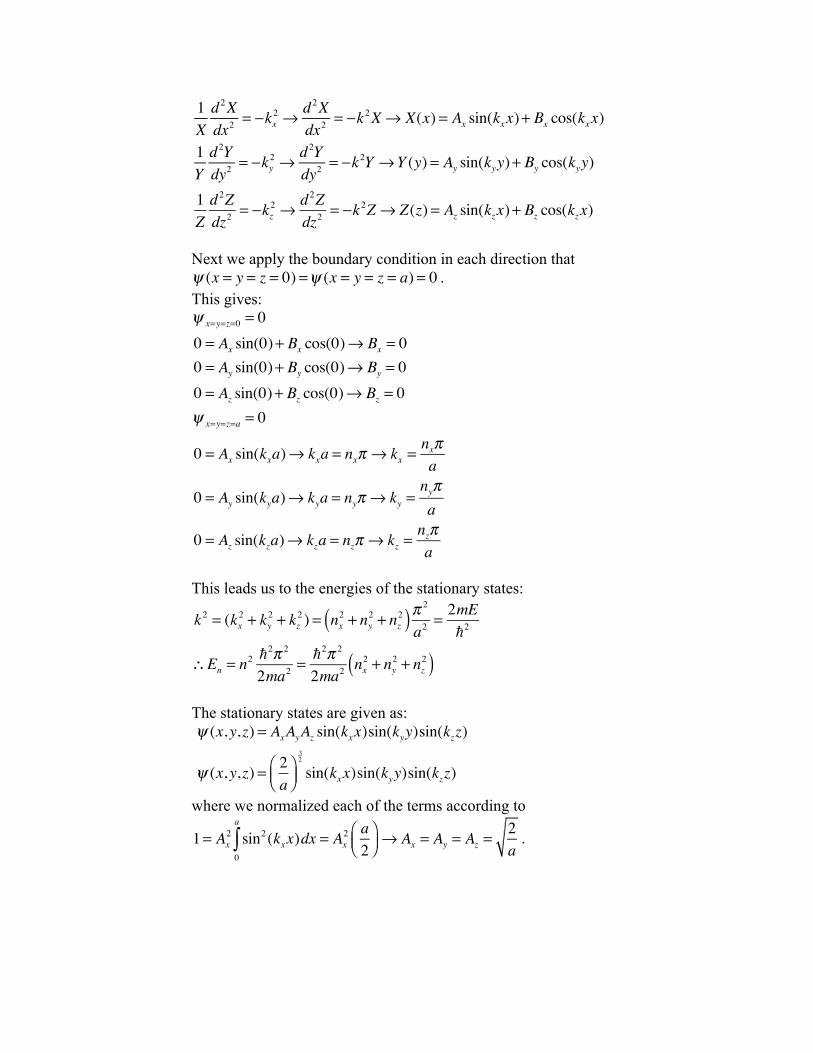
Next we apply the boundary condition in each direction that ψ (x = y = z = 0) =ψ (x = y = z = a) = 0 . This gives: ψ x=y=z=0 = 00 = Ax sin(0)+ Bx cos(0)→ Bx = 00 = Ay sin(0)+ By cos(0)→ By = 00 = Az sin(0)+ Bz cos(0)→ Bz = 0ψ x=y=z=a = 0

0 = Ax sin(kxa)→ kxa = nxπ → kx =nxπa

0 = Ay sin(kya)→ kya = nyπ → ky =nyπa

0 = Az sin(kza)→ kza = nzπ → kz =nzπa

This leads us to the energies of the stationary states:

k2 = (kx2 + ky

2 + kz2 ) = nx

2 + ny2 + nz

2( )π2

a2= 2mE!2

∴En = n2 !

2π 2

2ma2= !

2π 2

2ma2nx2 + ny

2 + nz2( )

The stationary states are given as:

ψ (x, y, z) = AxAyAz sin(kxx)sin(kyy)sin(kzz)

ψ (x, y, z) = 2a

⎛⎝⎜

⎞⎠⎟

32

sin(kxx)sin(kyy)sin(kzz)

where we normalized each of the terms according to

1= Ax2 sin2(kxx)dx0

a

∫ = Ax2 a2

⎛⎝⎜

⎞⎠⎟ → Ax = Ay = Az =

2a

.

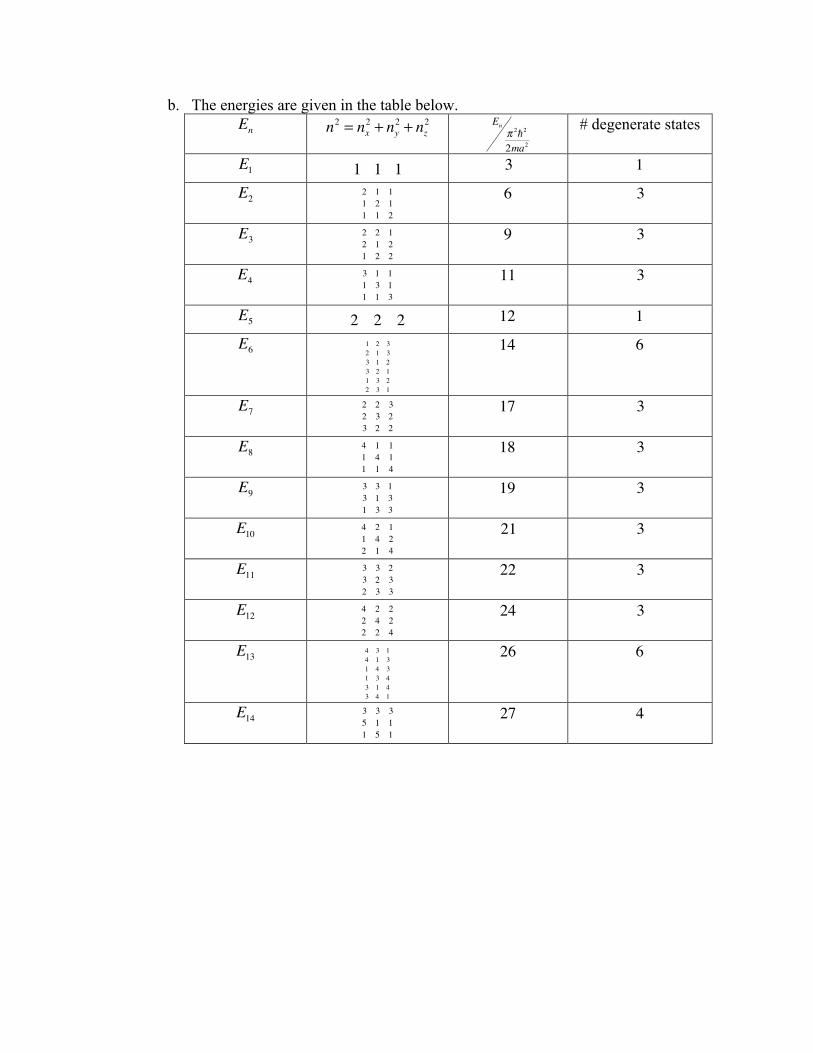
b. The energies are given in the table below. En n2 = nx

2 + ny2 + nz

2

Enπ 2!2

2ma2

# degenerate states

E1 1 1 1 3 1

E2 2 1 11 2 11 1 2

6 3

E3 2 2 12 1 21 2 2

9 3

E4 3 1 11 3 11 1 3

11 3

E5 2 2 2 12 1

E6 1 2 32 1 33 1 23 2 11 3 22 3 1

14 6

E7 2 2 32 3 23 2 2

17 3

E8 4 1 11 4 11 1 4

18 3

E9 3 3 13 1 31 3 3

19 3

E10 4 2 11 4 22 1 4

21 3

E11 3 3 23 2 32 3 3

22 3

E12 4 2 22 4 22 2 4

24 3

E13 4 3 14 1 31 4 31 3 43 1 43 4 1

26 6

E14 3 3 35 1 11 5 11 1 5

27 4