Embed Size (px)
Citation preview

CS 563 Advanced Topics in Computer Graphics
Photon Mapping
by Emmanuel Agu
Introduction
Presentation Divided into two parts. Overview of Photon Mapping Detail look into the first pass of the Photon
Mapping algorithm.
Overview
Photon Mapping More efficient alternative to pure Monte Carlo
raytracing techniques. Not a replacement! Two pass global illumination algorithm.
Photon tracing Rendering
Illumination is decoupled from geometry. Best used in combination with other techniques such
as path or ray tracing. Easy to integrate into existing renderers.

Two-Pass Method
Two pass algorithm Pass 1 - Photon tracing
Emit photons from light sources Trace photons through scene. Populate photon maps
Pass 2 - Rendering Render scene using information in the photon
maps to estimate: Reflected radiance at surfaces Out-scattered radiance from volumes In-scattered radiance from translucent materials.
Photon Tracing
Pass 1 - Photon tracing Photon emission
Emit photons from light sources.
Photon scattering Determine how photons are scattered through out the
scene.
Photon storing How do we keep track of photons that are absorbed by
diffuse surfaces.
Photon Tracing
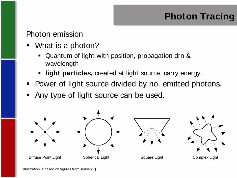
Photon emission What is a photon?
Quantum of light with position, propagation drn & wavelength
light particles, created at light source, carry energy.
Power of light source divided by no. emitted photons. Any type of light source can be used.
Diffuse Point Light Square Light Complex LightSpherical Light
Illustration is based on figures from Jensen[1].
Photon Tracing
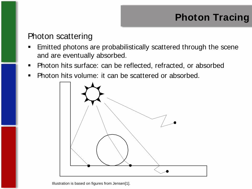
Photon scattering Emitted photons are probabilistically scattered through the scene
and are eventually absorbed. Photon hits surface: can be reflected, refracted, or absorbed Photon hits volume: it can be scattered or absorbed.
Illustration is based on figures from Jensen[1].
Photon Tracing
Photon storage Absorbed photons are stored in a spatial data
structure called a “Photon Map”. Photon’s power, position & incident direction stored Photon map data structure
Fast spatial access to handle millions of queries during rendering phase.
Memory usage needs to be compact and aligned properly.

Photon Tracing
Photon storage Caustics and participating media would require large
localized concentrations of photons. Single global photon map needs to be evenly
distributed for better radiance estimates. Solution: Multiple photons maps are necessary.
Global photon map Caustics map Volume photon map (for participating media)

Photon Tracing
Photon storage Caustics Photon Map
Generated by shooting photons directly at specular objects in the scene and are absorbed when they reach a diffuse surface.
Photons are highly focused into a small area. Requires fewer photons to be emitted.
Photon Tracing
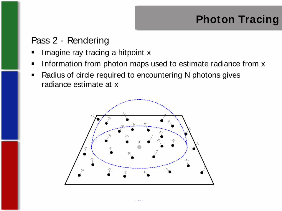
Pass 2 - Rendering Imagine ray tracing a hitpoint x Information from photon maps used to estimate radiance from x Radius of circle required to encountering N photons gives
radiance estimate at x
x
Photon Tracing
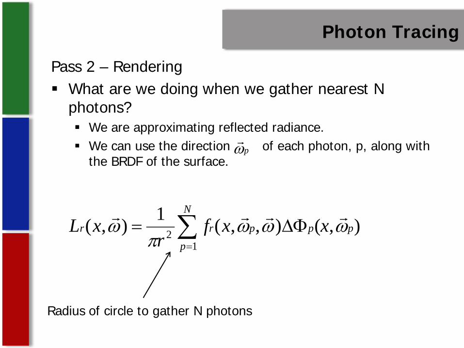
Pass 2 – Rendering What are we doing when we gather nearest N
photons? We are approximating reflected radiance. We can use the direction of each photon, p, along with
the BRDF of the surface.
),(),,(1),(1
2 p
N
ppprr xxf
rxL ωωω
πω
∑=
∆Φ=
pω
Radius of circle to gather N photons
Photon Tracing
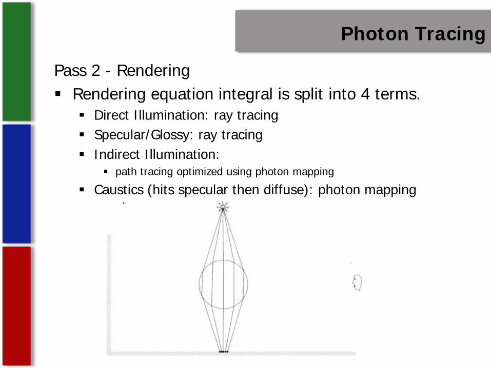
Pass 2 - Rendering Rendering equation integral is split into 4 terms.
Direct Illumination: ray tracing Specular/Glossy: ray tracing Indirect Illumination:
path tracing optimized using photon mapping
Caustics (hits specular then diffuse): photon mapping
Rendering
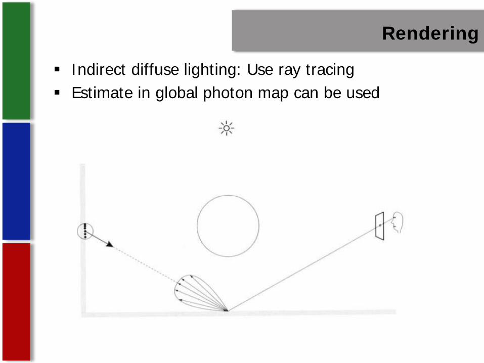
Indirect diffuse lighting: Use ray tracing Estimate in global photon map can be used
Photon Tracing
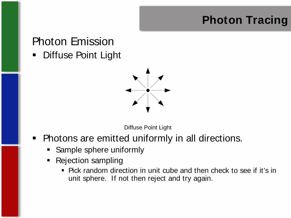
Photon Emission Diffuse Point Light
Photons are emitted uniformly in all directions. Sample sphere uniformly Rejection sampling
Pick random direction in unit cube and then check to see if it’s in unit sphere. If not then reject and try again.
Diffuse Point Light
Photon Tracing
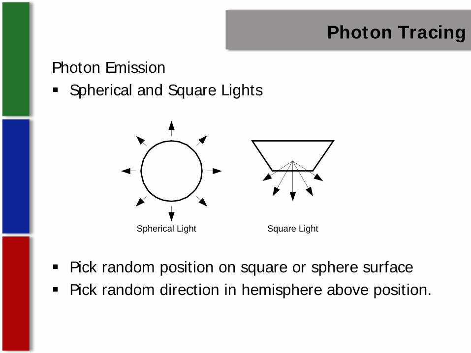
Photon Emission Spherical and Square Lights
Pick random position on square or sphere surface Pick random direction in hemisphere above position.
Square LightSpherical Light

Photon Tracing
Photon Emission Multiple Lights
Photons emitted from each light source Total number of photons in scene same as for single light Less photons are needed per light source since each light
contributes less to overall illumination. More photons emitted from brighter lights than dim lights Complexity not increased with the more lights.
Photon Tracing
Photon Emission Projection Maps
Map of scene geometry as seen from light source Cells have information on whether objects in that direction Photons emitted in directions with objects
Improves efficiency in scene’s with sparse geometry In caustic generation, the projection map directs
photons toward specular surfaces
Photon Tracing
Photon Scattering Specular reflection
Photons hitting specular surfaces are reflected in mirror drn Calculated same as specularly reflected rays in raytracing. Power of photon should be scaled by the reflectivity or the
mirror. Unless using Russian Roulette.

Photon Tracing
Photon Scattering Diffuse reflection
Pick random direction in hemisphere above hit point probability proportional to cosine of angle with normal
Power scaled by diffuse reflectance. Unless using Russian Roulette
Photons only stored in photon map at diffuse surfaces
Arbitrary BRDF reflection New photon direction is computed by importance sampling
the BRDF. Power scaled according to BRDF as well as reflectivity.
Unless using Russian Roulette.
Photon Tracing
Photon Scattering Russian Roulette
Stochastic technique to remove unimportant photons and allow the effort to be focused on important photons.
Standard Monte Carlo technique Basic Concept
Use probabilistic sampling to eliminate work and still get the correct result.
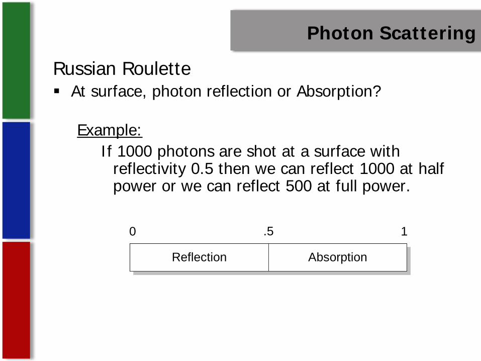
Photon Scattering
Russian Roulette At surface, photon reflection or Absorption?
Example:If 1000 photons are shot at a surface with
reflectivity 0.5 then we can reflect 1000 at half power or we can reflect 500 at full power.
Reflection Absorption
0 1.5
Photon Tracing
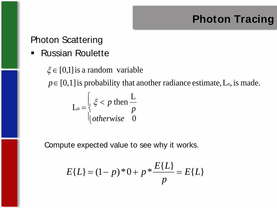
Photon Scattering Russian Roulette
Compute expected value to see why it works.
<
=
∈∈
0
L then L
made. is ,Lestimate, radianceanother y that probabilit is [0,1] variablerandom a is ]1,0[
n
n
otherwisep
p
p
ξ
ξ
*0*)1( LEpLEppLE =+−=
Photon Scattering
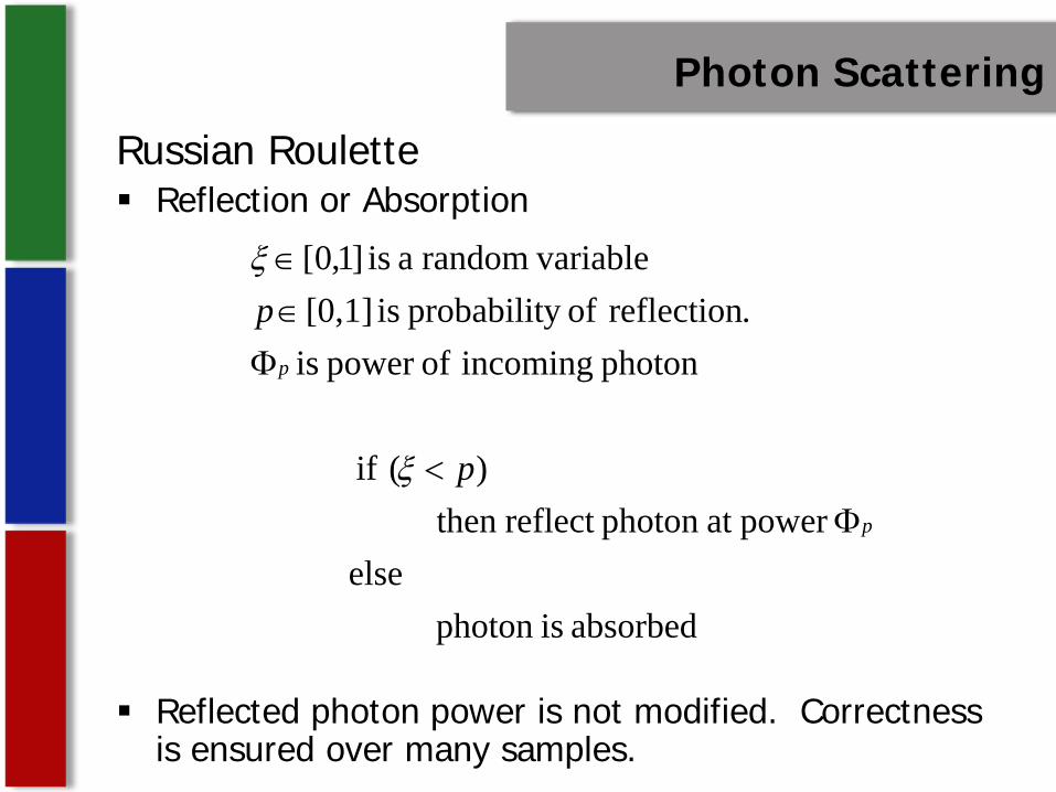
Russian Roulette Reflection or Absorption
Reflected photon power is not modified. Correctness is ensured over many samples.
absorbed isphoton else
power at photon reflect then )( if
photon incoming ofpower is .reflection ofy probabilit is [0,1]
variablerandom a is ]1,0[
p
p
p
p
Φ<
Φ∈∈
ξ
ξ

Photon Scattering
Russian Roulette Specular or Diffuse Reflection
Decision is made
)1( where.reflectionspecular ofy probabilit is ]1,0[
.reflection diffuse ofy probabilit is [0,1] variablerandom a is ]1,0[
≤+∈∈∈
sd
s
d
ppppξ
absorption ]1,(reflectionspecular ],(
reflection diffuse ],0[
s
s
ppppp
p
d
dd
d
+∈+∈
∈
ξξξ
Diffuse Absorption
0 1
Specular
dp sp
Photon Scattering
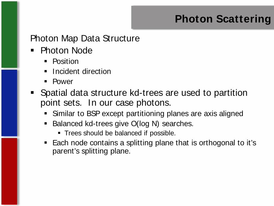
Photon Map Data Structure Photon Node
Position Incident direction Power
Spatial data structure kd-trees are used to partition point sets. In our case photons. Similar to BSP except partitioning planes are axis aligned Balanced kd-trees give O(log N) searches.
Trees should be balanced if possible. Each node contains a splitting plane that is orthogonal to it’s
parent’s splitting plane.

Applications of Photon Mapping
Photon Mapping can be used for Caustics
Color Bleeding
Participating Media
Subsurface Scattering
Motion Blur

Applications of Photon Mapping
Practical 2 pass algorithm
the rendering equation for surface radiance:),(),(),( wxLwxLwxL reo
+=

Applications of Photon Mapping
Expand the reflected radiance
BRDF component
Incoming Radiance
rL
),,(),,(),,( ,, wwxfwwxfwwxf DrSrr ′+′=′
),(),(),(),( ,,, wxLwxLwxLwxL dicilii ′+′+′=′
∫Ω
′⋅′′′= wdnwwxLwwxfwxL irr ))(,(),,(),(
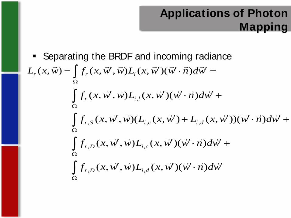
Applications of Photon Mapping
Separating the BRDF and incoming radiance=′⋅′′′= ∫
Ω
wdnwwxLwwxfwxL irr ))(,(),,(),(
∫
∫
∫
∫
Ω
Ω
Ω
Ω
′⋅′′′
+′⋅′′′
+′⋅′′+′′
+′⋅′′′
wdnwwxLwwxf
wdnwwxLwwxf
wdnwwxLwxLwwxf
wdnwwxLwwxf
diDr
ciDr
diciSr
lir
))(,(),,(
))(,(),,(
)))(,(),()(,,(
))(,(),,(
,,
,,
,,,
,

Applications of Photon Mapping
Was broken down into the Direct Illumination Specular and Glossy Reflections Caustics Indirect Illumination
An accurate and approximate
Applications of Photon Mapping
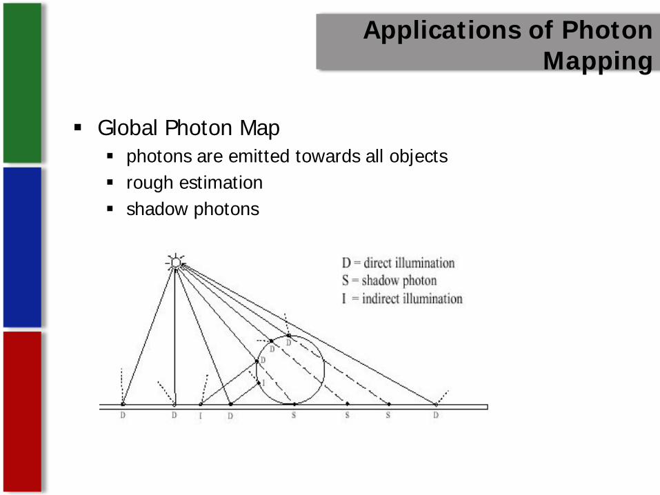
Global Photon Map photons are emitted towards all objects rough estimation shadow photons
Applications of Photon Mapping
Caustic Photon Map only stores caustics photons are emitted towards specular objects high density

Applications of Photon Mapping
Radiance Estimation is also applied variable size sphere fixed size sphere
Filtering is also applied to the Caustics Cone filter applied to the right Caustic
Applications of Photon Mapping
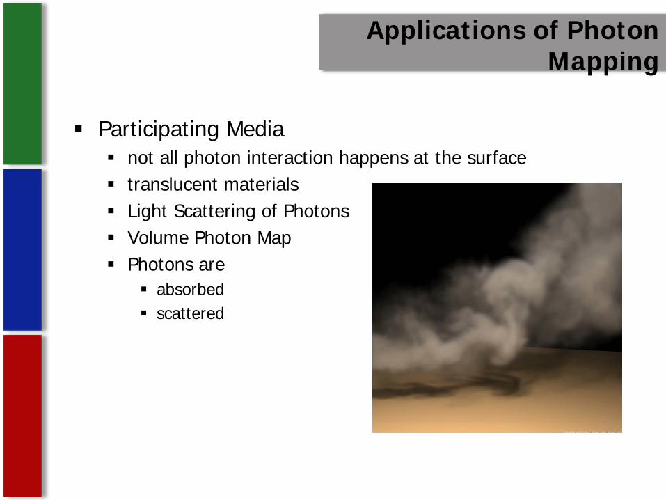
Participating Media not all photon interaction happens at the surface translucent materials Light Scattering of Photons Volume Photon Map Photons are
absorbed scattered
Applications of Photon Mapping
Previous Rendering Algorithms assumed that light traveling in a vacuum
participating media allows: dust air clouds
marble skin plants
Applications of Photon Mapping
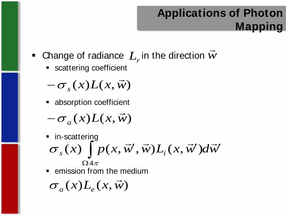
Change of radiance in the direction scattering coefficient
absorption coefficient
in-scattering
emission from the medium
rL w
),()( wxLxsσ−
),()( wxLxaσ−
wdwxLwwxpx is ′′′∫Ω
π
σ4
),(),,()(
),()( wxLx eaσ

Applications of Photon Mapping
Volume Rendering Equation
for an optical depth
+′′′= ∫ ′− xdxLxewxLs
eaxxr )()(),(
0
),( σ
),(
),(),,()(
),(
04
),(
wwsxLe
xdwdwxLwwxpxe
wsxxr
s
isxxr
′+
+′′′′′′′
+−
Ω
′−∫ ∫π
σ
∫′
=′x
x t dttxxr )(),( σ
Applications of Photon Mapping
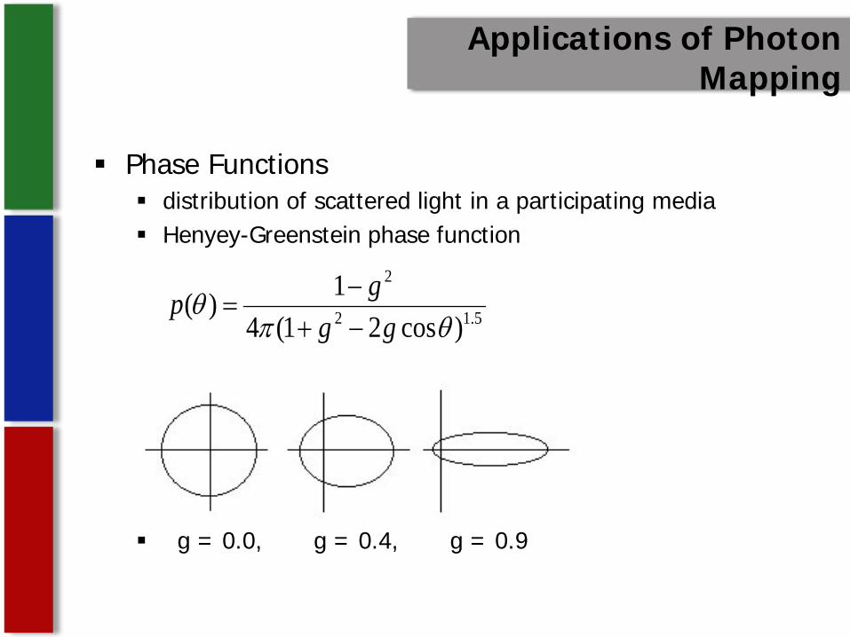
Phase Functions distribution of scattered light in a participating media Henyey-Greenstein phase function
g = 0.0, g = 0.4, g = 0.9
5.12
2
)cos21(41)(
θπθ
gggp
−+−
=
Applications of Photon Mapping
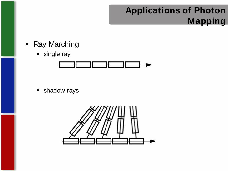
Ray Marching single ray
shadow rays
Applications of Photon Mapping
Adaptive Ray Marching non-homogeneous media shadows caustics
Ray marching estimates in-scattered light
Applications of Photon Mapping
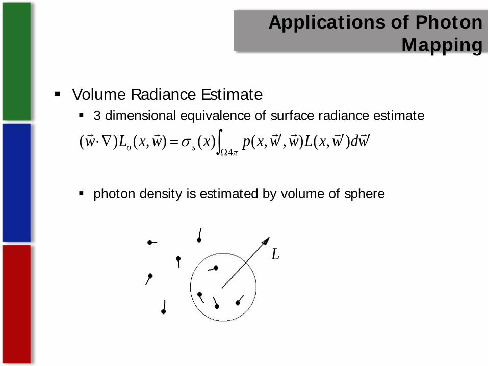
Volume Radiance Estimate 3 dimensional equivalence of surface radiance estimate
photon density is estimated by volume of sphere
∫Ω ′′′=∇⋅π
σ4
),(),,()(),()( wdwxLwwxpxwxLw so
L
Applications of Photon Mapping

Applications of Photon Mapping
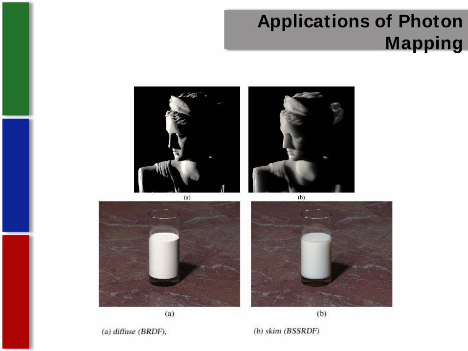
Subsurface Scattering denser version of participating media Photon Tracing

Applications of Photon Mapping
Rendering of Subsurface Scattering uses ray marching Russian roulette sampling in-scattered radiance

Applications of Photon Mapping
Motion Blur temporal supersampling
Applications of Photon Mapping
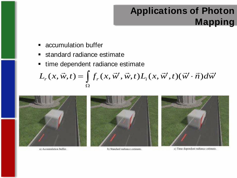
accumulation buffer standard radiance estimate time dependent radiance estimate
∫Ω
′⋅′′′= wdnwtwxLtwwxftwxL irr ))(,,(),,,(),,(
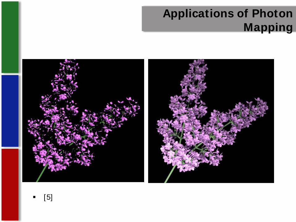
Applications of Photon Mapping
[5]
References
[1] Jensen, Henrik W. Realistic Image Synthesis Using Photon Mapping. A K Peters, Ltd, Massachusetts, 2001
[2] Shirley, Peter Realistic Raytracing A K Peters, Ltd. Massachusetts, 2000.
[3] Shirley, Peter Fundamentals of Computer Graphics A K Peters, Ltd, Massachusetts, 2002
[4] Zack Waters, Photon mapping presentation, CS 563, Spring 2003
[5] Curt Ferguson, Photon mapping presentation part II, CS 563, Spring 2003

Applications of Photon Mapping
6. Henrik Wann Jensen: "Global Illumination using Photon Maps". In "Rendering Techniques '96". Eds. X. Pueyo and P. Schröder. Springer-Verlag, pp. 21-30, 1996
7. Henrik Wann Jensen: "Rendering Caustics on Non-Lambertian Surfaces". In Proceedings of Graphics Interface '96, pp. 116-121, Toronto 1996.
8. Henrik Wann Jensen, Stephen R. Marschner, Marc Levoy and Pat Hanrahan: "A Practical Model for Subsurface Light Transport". Proceedings of SIGGRAPH'2001.
9. Henrik Wann Jensen and Per H. Christensen: "Efficient Simulation of Light Transport in Scenes with Participating Media using Photon Maps". In Proceedings of SIGGRAPH'98, pages 311-320, Orlando, July 1998
10. Martin Fuhrer: “CPSC 651 Project: Photon Mapping” <http://pages.cpsc.ucalgary.ca/~fuhrer/courses/651/project/> 2003
11. Mike Cammarano and Henrik Wann Jensen. "Time Dependent Photon Mapping". Proceedings of the 13th Eurographics Workshop on Rendering, Pisa, Italy, June 2002