Embed Size (px)
Citation preview
Monte Carlo Ray Tracing& Irradiance Caching& Photon Mapping
Announcements: Quiz• On Friday (3/10), in class• One 8.5x11 sheet of notes allowed• Sample quiz (from a previous year) on website• Focus on “reading comprehension” and
material for Homeworks 0, 1, & 2
Announcements: Final Projects• Everyone should post two ideas
for a final project on LMS(“due” Monday 3/20 @ 11:59pm)
• Connect with potential teammates(teams of 2 strongly recommended)
• Start finding & reading background papers• Proposal & summary of background research
are due April 3rd • See webpage for details on brainstorming post,
proposal, and overall project requirements
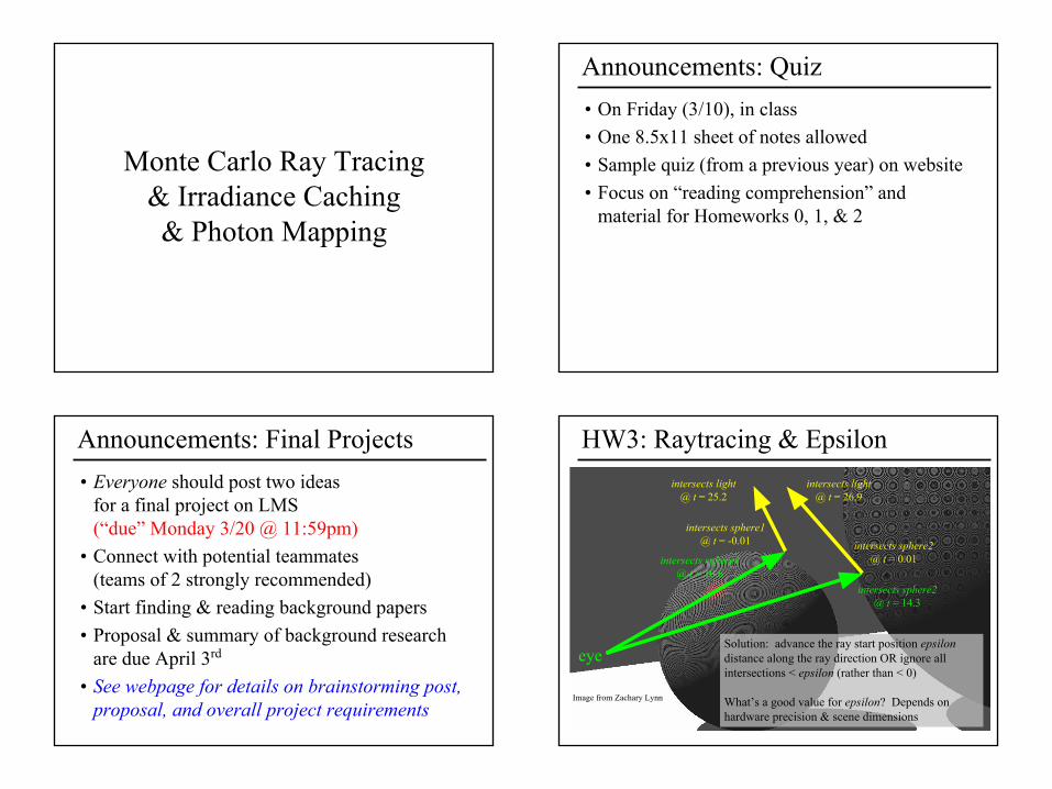
HW3: Raytracing & Epsilon
intersects sphere2 @ t = 0.01
intersects sphere1 @ t = -0.01
Image from Zachary Lynn
intersects sphere1 @ t = 10.6
intersects sphere2 @ t = 14.3
intersects light @ t = 25.2
intersects light @ t = 26.9
eyeSolution: advance the ray start position epsilon distance along the ray direction OR ignore all intersections < epsilon (rather than < 0)
What’s a good value for epsilon? Depends on hardware precision & scene dimensions
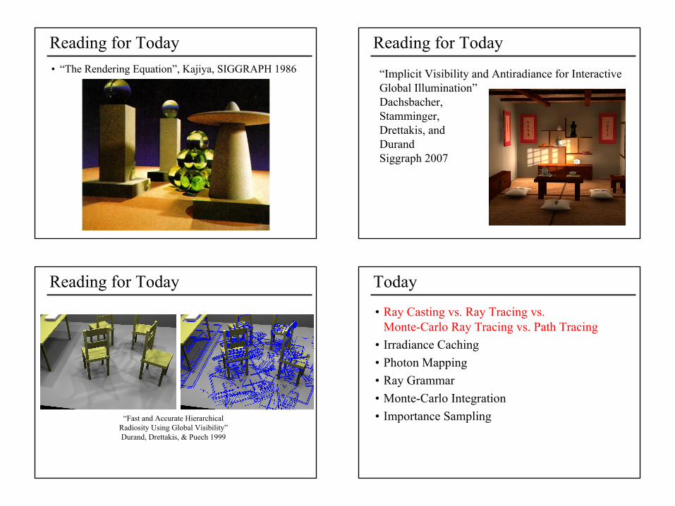
• “The Rendering Equation”, Kajiya, SIGGRAPH 1986
Reading for Today Reading for Today
“Implicit Visibility and Antiradiance for Interactive Global Illumination” Dachsbacher, Stamminger, Drettakis, and Durand Siggraph 2007
Reading for Today
“Fast and Accurate Hierarchical Radiosity Using Global Visibility”Durand, Drettakis, & Puech 1999
Today
• Ray Casting vs. Ray Tracing vs. Monte-Carlo Ray Tracing vs. Path Tracing
• Irradiance Caching• Photon Mapping• Ray Grammar• Monte-Carlo Integration• Importance Sampling
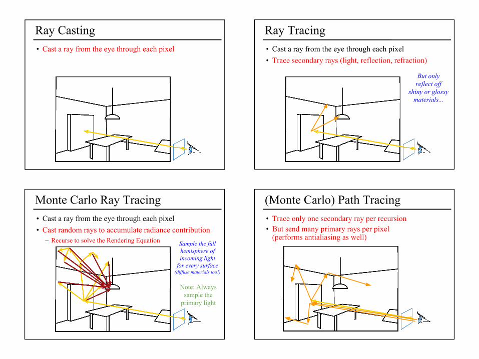
Ray Casting• Cast a ray from the eye through each pixel
Ray Tracing• Cast a ray from the eye through each pixel • Trace secondary rays (light, reflection, refraction)
But only reflect off
shiny or glossymaterials...
Monte Carlo Ray Tracing• Cast a ray from the eye through each pixel• Cast random rays to accumulate radiance contribution
– Recurse to solve the Rendering Equation
Note: Alwayssample the
primary light
Sample the full hemisphere of incoming light
for every surface (diffuse materials too!)
(Monte Carlo) Path Tracing• Trace only one secondary ray per recursion• But send many primary rays per pixel
(performs antialiasing as well)
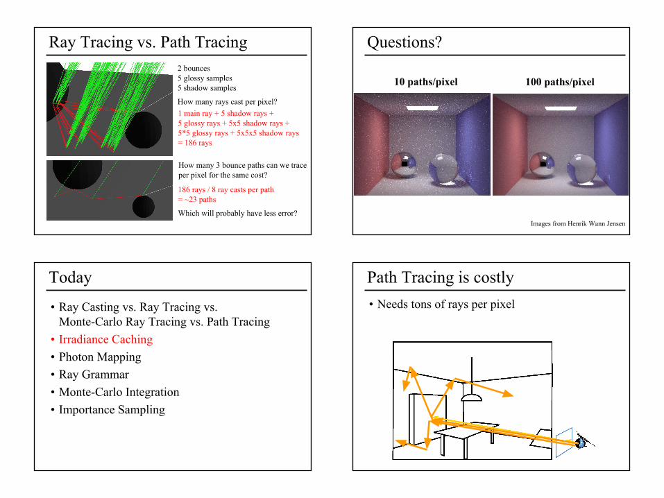
Ray Tracing vs. Path Tracing
1 main ray + 5 shadow rays +5 glossy rays + 5x5 shadow rays +5*5 glossy rays + 5x5x5 shadow rays = 186 rays
2 bounces5 glossy samples 5 shadow samples
How many rays cast per pixel?
186 rays / 8 ray casts per path = ~23 paths
Which will probably have less error?
How many 3 bounce paths can we trace per pixel for the same cost?
Questions?
10 paths/pixel 100 paths/pixel
Images from Henrik Wann Jensen
Today
• Ray Casting vs. Ray Tracing vs. Monte-Carlo Ray Tracing vs. Path Tracing
• Irradiance Caching• Photon Mapping• Ray Grammar• Monte-Carlo Integration• Importance Sampling
Path Tracing is costly• Needs tons of rays per pixel
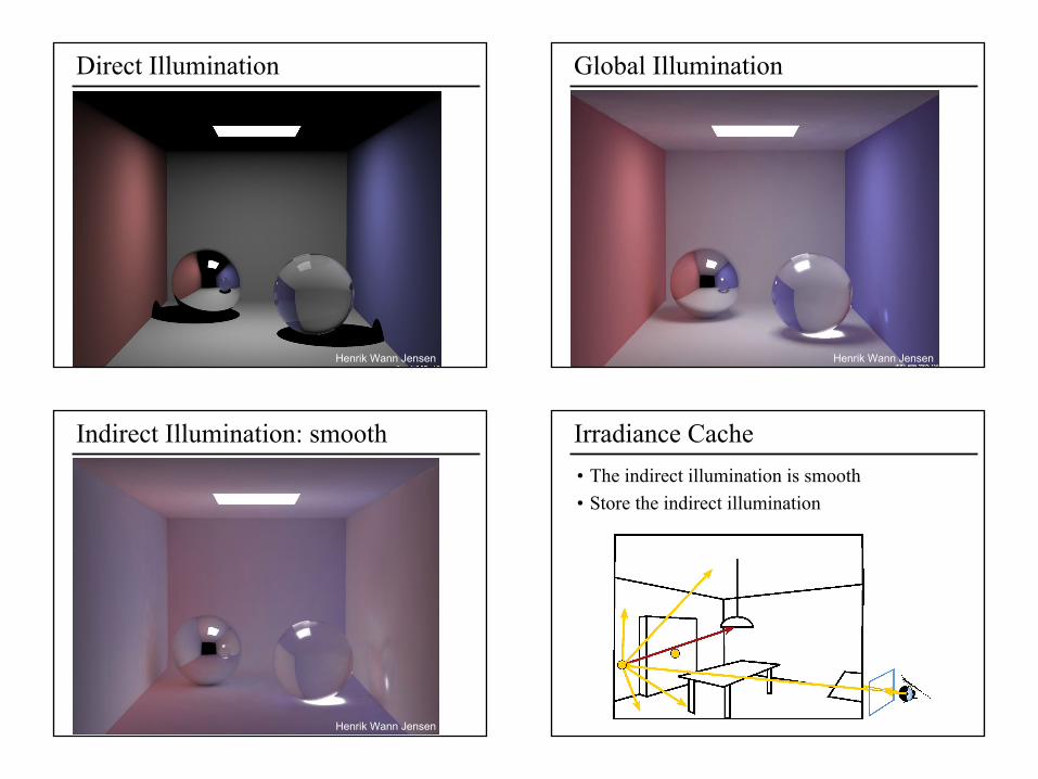
Direct Illumination
Henrik Wann Jensen
Global Illumination
Henrik Wann Jensen
Indirect Illumination: smooth
Henrik Wann Jensen
Irradiance Cache• The indirect illumination is smooth• Store the indirect illumination
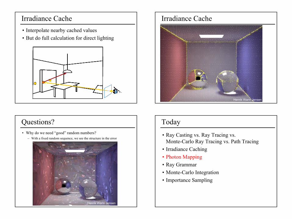
Irradiance Cache• Interpolate nearby cached values• But do full calculation for direct lighting
Irradiance Cache
Henrik Wann Jensen
Questions?• Why do we need “good” random numbers?
– With a fixed random sequence, we see the structure in the error
Henrik Wann Jensen
Today
• Ray Casting vs. Ray Tracing vs. Monte-Carlo Ray Tracing vs. Path Tracing
• Irradiance Caching• Photon Mapping• Ray Grammar• Monte-Carlo Integration• Importance Sampling
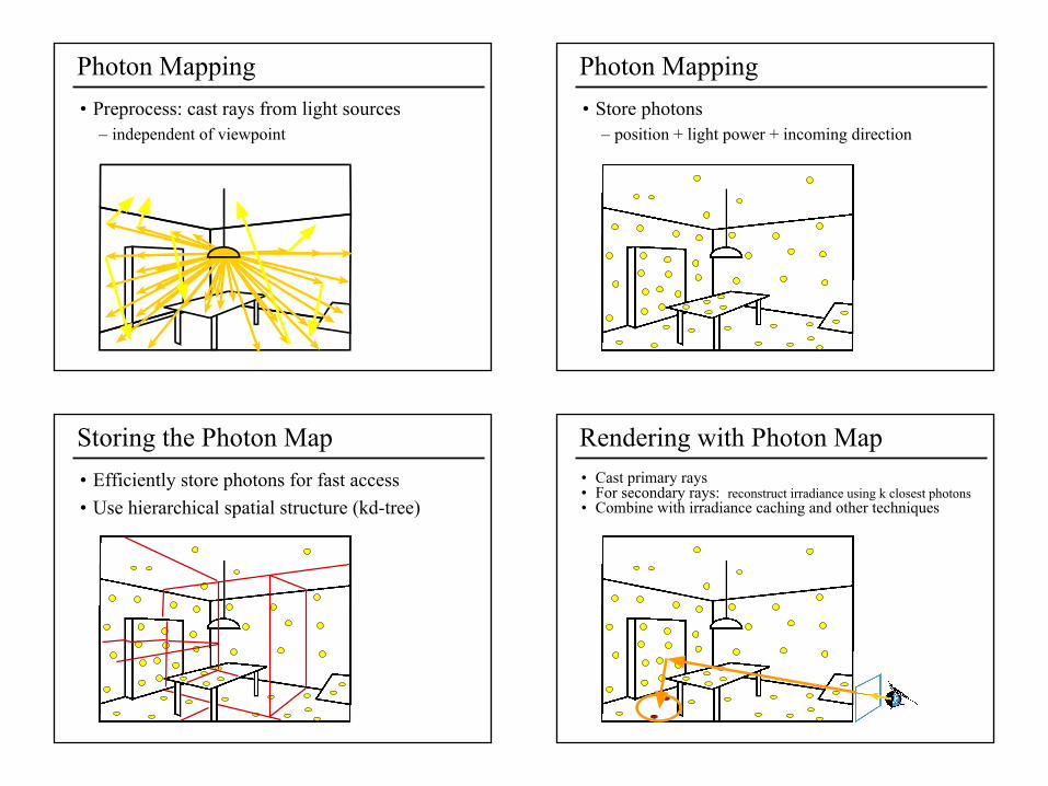
Photon Mapping• Preprocess: cast rays from light sources
– independent of viewpoint
Photon Mapping• Store photons
– position + light power + incoming direction
Storing the Photon Map• Efficiently store photons for fast access• Use hierarchical spatial structure (kd-tree)
Rendering with Photon Map• Cast primary rays• For secondary rays: reconstruct irradiance using k closest photons• Combine with irradiance caching and other techniques
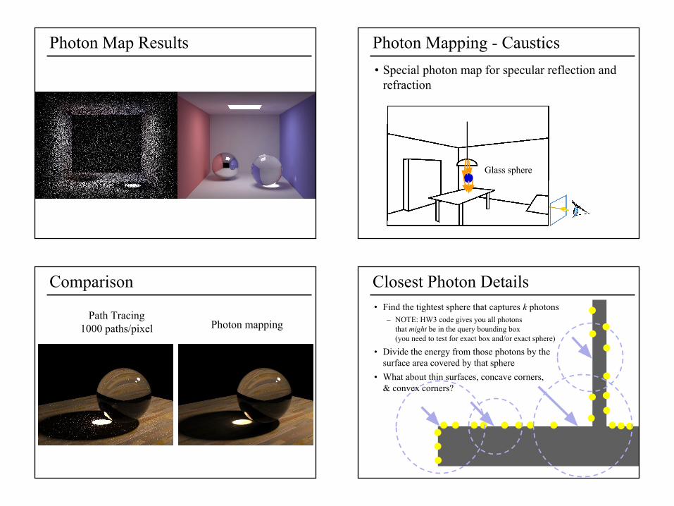
Photon Map Results Photon Mapping - Caustics• Special photon map for specular reflection and
refraction
Glass sphere
Comparison
Path Tracing1000 paths/pixel Photon mapping
Closest Photon Details• Find the tightest sphere that captures k photons
– NOTE: HW3 code gives you all photons that might be in the query bounding box (you need to test for exact box and/or exact sphere)
• Divide the energy from those photons by the surface area covered by that sphere
• What about thin surfaces, concave corners,& convex corners?
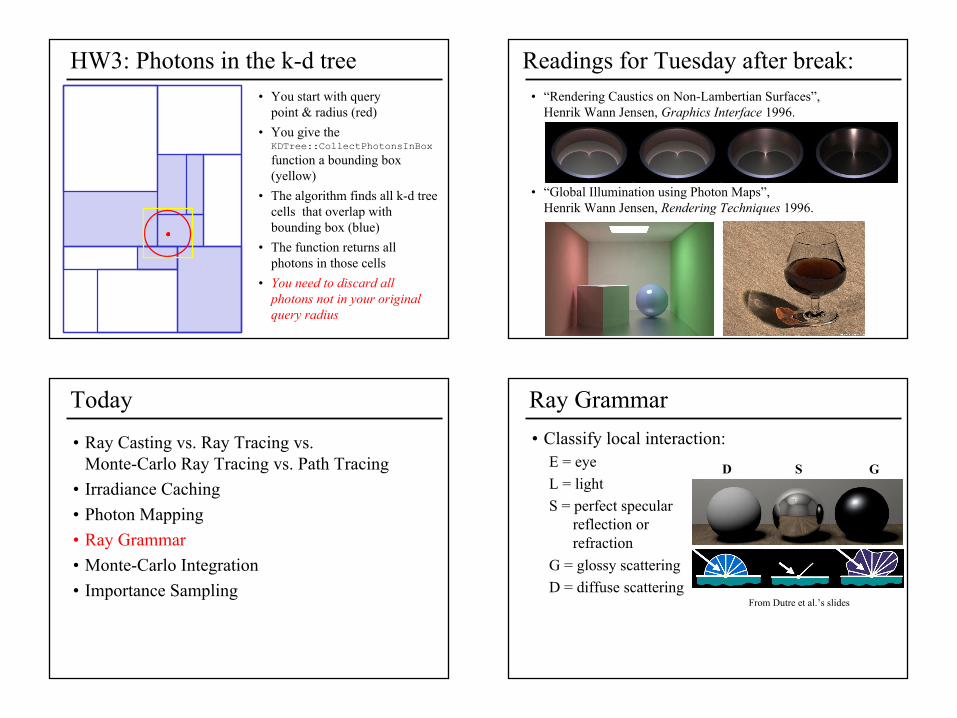
HW3: Photons in the k-d tree• You start with query
point & radius (red)• You give the
KDTree::CollectPhotonsInBox
function a bounding box (yellow)
• The algorithm finds all k-d tree cells that overlap with bounding box (blue)
• The function returns all photons in those cells
• You need to discard all photons not in your original query radius
• “Rendering Caustics on Non-Lambertian Surfaces”, Henrik Wann Jensen, Graphics Interface 1996.
• “Global Illumination using Photon Maps”, Henrik Wann Jensen, Rendering Techniques 1996.
Readings for Tuesday after break:
Today
• Ray Casting vs. Ray Tracing vs. Monte-Carlo Ray Tracing vs. Path Tracing
• Irradiance Caching• Photon Mapping• Ray Grammar• Monte-Carlo Integration• Importance Sampling
Ray Grammar• Classify local interaction:
E = eyeL = lightS = perfect specular
reflection or refraction
G = glossy scatteringD = diffuse scattering
D S G
From Dutre et al.’s slides
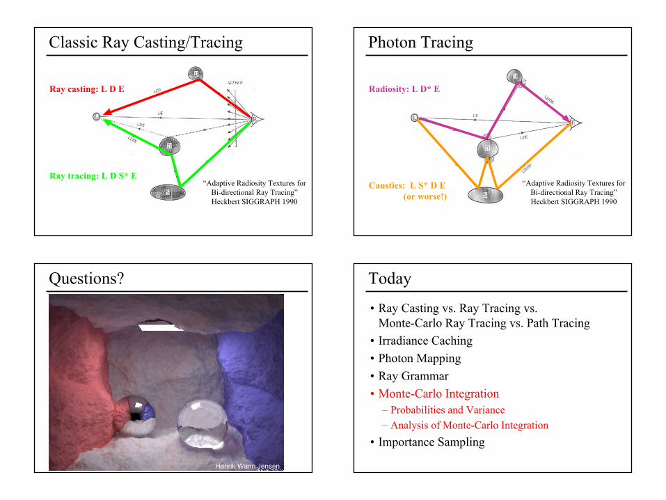
Classic Ray Casting/Tracing
Ray tracing: L D S* E
Ray casting: L D E
“Adaptive Radiosity Textures for Bi-directional Ray Tracing”Heckbert SIGGRAPH 1990
Photon Tracing
“Adaptive Radiosity Textures for Bi-directional Ray Tracing”Heckbert SIGGRAPH 1990
Caustics: L S* D E (or worse!)
Radiosity: L D* E
Questions?
Henrik Wann Jensen
Today
• Ray Casting vs. Ray Tracing vs. Monte-Carlo Ray Tracing vs. Path Tracing
• Irradiance Caching• Photon Mapping• Ray Grammar• Monte-Carlo Integration
– Probabilities and Variance– Analysis of Monte-Carlo Integration
• Importance Sampling
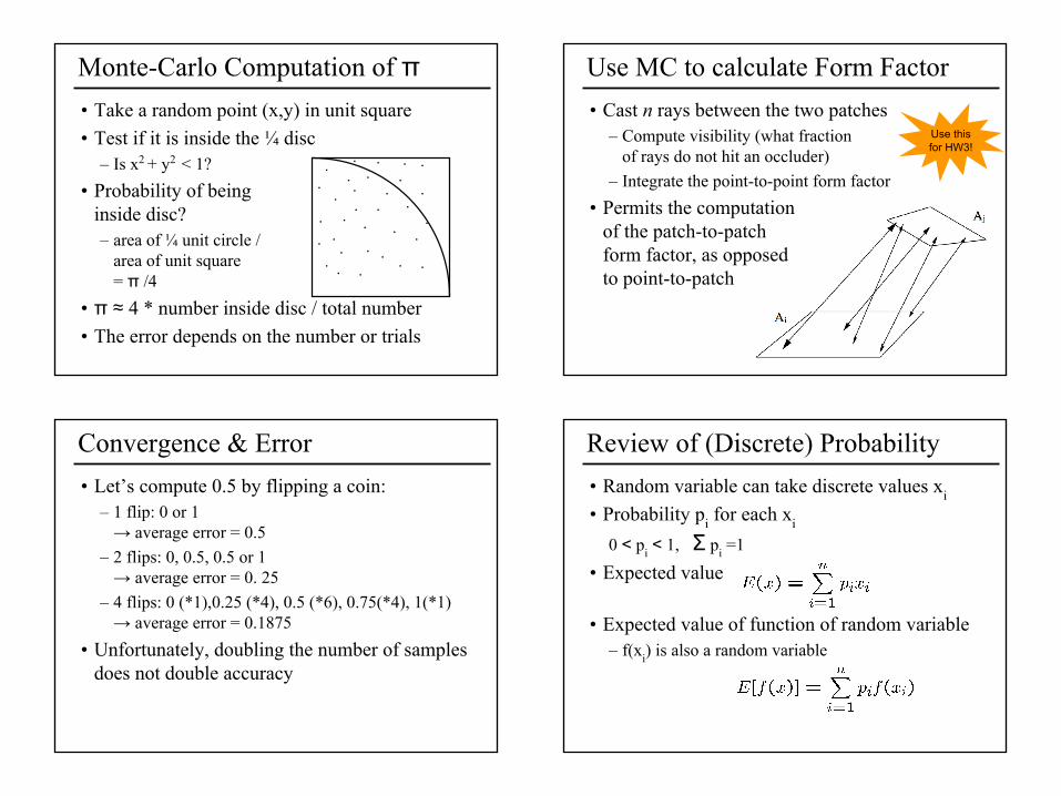
Monte-Carlo Computation of π• Take a random point (x,y) in unit square• Test if it is inside the ¼ disc
– Is x2 + y2 < 1?• Probability of being
inside disc? – area of ¼ unit circle /
area of unit square= π /4
• π ≈ 4 * number inside disc / total number• The error depends on the number or trials
• Cast n rays between the two patches– Compute visibility (what fraction
of rays do not hit an occluder)– Integrate the point-to-point form factor
• Permits the computation of the patch-to-patch form factor, as opposed to point-to-patch
Use MC to calculate Form Factor
Use this for HW3!
Convergence & Error• Let’s compute 0.5 by flipping a coin:
– 1 flip: 0 or 1 → average error = 0.5
– 2 flips: 0, 0.5, 0.5 or 1 → average error = 0. 25
– 4 flips: 0 (*1),0.25 (*4), 0.5 (*6), 0.75(*4), 1(*1) → average error = 0.1875
• Unfortunately, doubling the number of samples does not double accuracy
Review of (Discrete) Probability• Random variable can take discrete values xi• Probability pi for each xi
0 < pi < 1, Σ pi =1
• Expected value
• Expected value of function of random variable– f(xi) is also a random variable
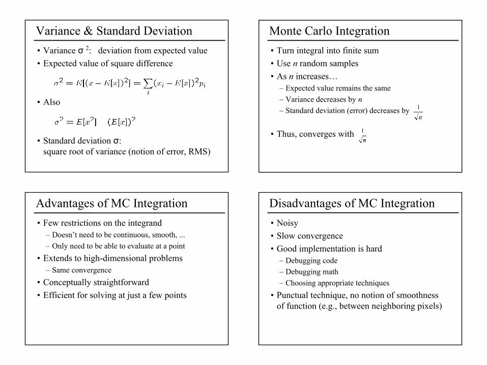
Variance & Standard Deviation• Variance σ 2: deviation from expected value• Expected value of square difference
• Also
• Standard deviation σ: square root of variance (notion of error, RMS)
Monte Carlo Integration• Turn integral into finite sum• Use n random samples• As n increases…
– Expected value remains the same– Variance decreases by n– Standard deviation (error) decreases by
• Thus, converges with
Advantages of MC Integration• Few restrictions on the integrand
– Doesn’t need to be continuous, smooth, ...– Only need to be able to evaluate at a point
• Extends to high-dimensional problems– Same convergence
• Conceptually straightforward• Efficient for solving at just a few points
Disadvantages of MC Integration• Noisy• Slow convergence • Good implementation is hard
– Debugging code– Debugging math– Choosing appropriate techniques
• Punctual technique, no notion of smoothness of function (e.g., between neighboring pixels)
Today
• Ray Casting vs. Ray Tracing vs. Monte-Carlo Ray Tracing vs. Path Tracing
• Irradiance Caching• Photon Mapping• Ray Grammar• Monte-Carlo Integration• Importance Sampling
– Stratified Sampling– Importance Sampling
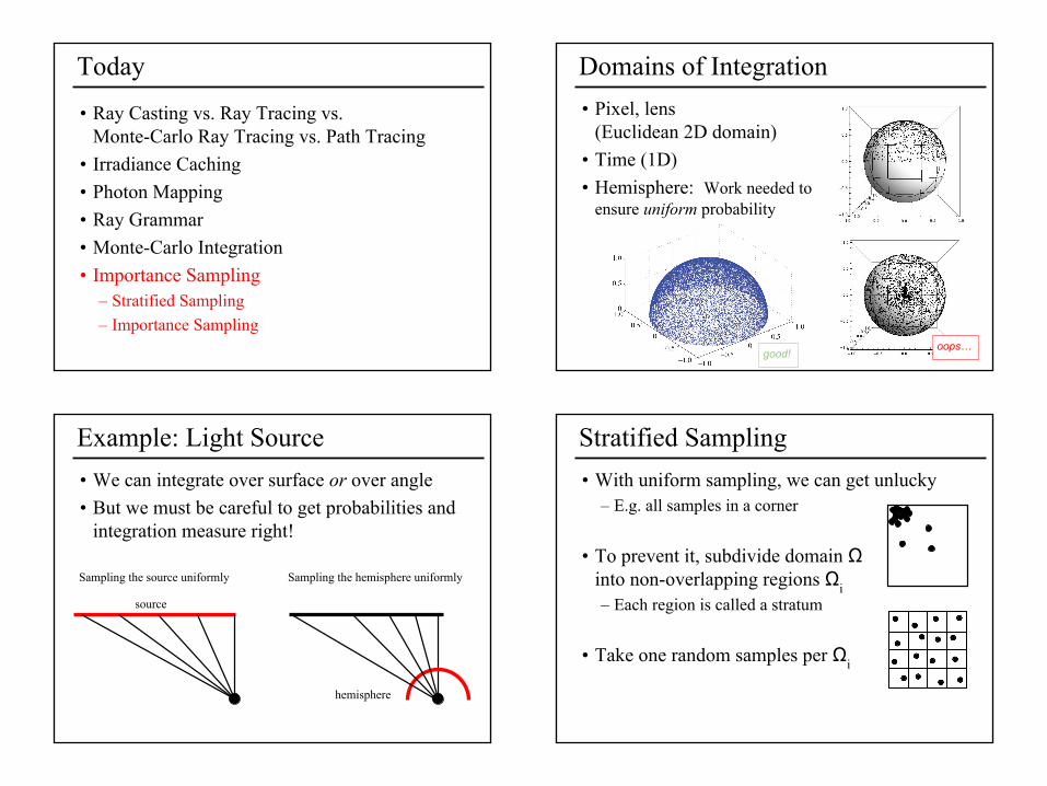
Domains of Integration• Pixel, lens
(Euclidean 2D domain)• Time (1D)• Hemisphere: Work needed to
ensure uniform probability
oops…good!
Example: Light Source• We can integrate over surface or over angle• But we must be careful to get probabilities and
integration measure right!
source
hemisphere
Sampling the source uniformly Sampling the hemisphere uniformly
Stratified Sampling• With uniform sampling, we can get unlucky
– E.g. all samples in a corner
• To prevent it, subdivide domain Ω into non-overlapping regions Ωi– Each region is called a stratum
• Take one random samples per Ωi
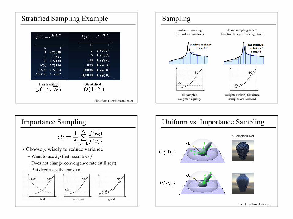
Stratified Sampling Example
Unstratified Stratified
Slide from Henrik Wann Jensen
Samplinguniform sampling
(or uniform random)dense sampling where
function has greater magnitude
all samples weighted equally
weights (width) for dense samples are reduced
uniformbad good
Importance Sampling
• Choose p wisely to reduce variance– Want to use a p that resembles f– Does not change convergence rate (still sqrt)– But decreases the constant
Uniform vs. Importance Sampling
5 Samples/Pixel
Slide from Jason Lawrence
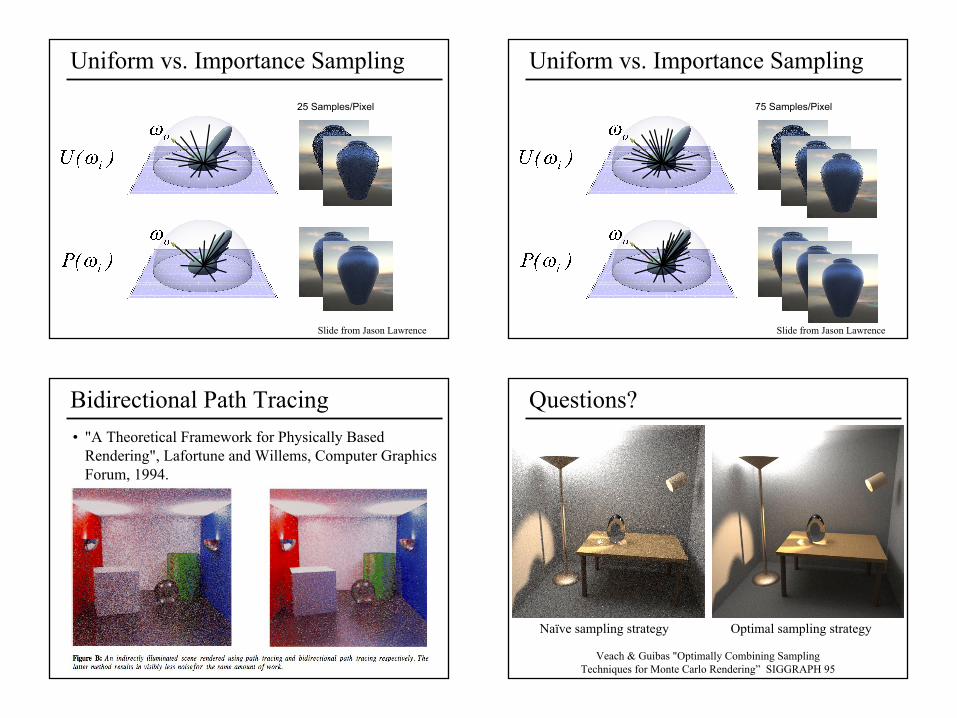
Uniform vs. Importance Sampling
25 Samples/Pixel
Slide from Jason Lawrence
Uniform vs. Importance Sampling
75 Samples/Pixel
Slide from Jason Lawrence
• "A Theoretical Framework for Physically Based Rendering", Lafortune and Willems, Computer Graphics Forum, 1994.
Bidirectional Path Tracing
Veach & Guibas "Optimally Combining Sampling Techniques for Monte Carlo Rendering” SIGGRAPH 95
Naïve sampling strategy Optimal sampling strategy
Questions?


![Inter-hour direct normal irradiance forecast with multiple ... · ahead solar irradiance forecast [11, 12] and long-term solar irradiance estimation [13]. However, for an inter-hour](https://img.pdfslide.us/doc/110x75/5f43655640b4404ee374a6b6/inter-hour-direct-normal-irradiance-forecast-with-multiple-ahead-solar-irradiance.jpg)