Photometry

…Getting the most from your photon

Very Brief History:

• Hipparcos in 130 B.C. created catalog of stars and the magnitude scale used to this day

• In 1800s astronomers decided that the magnitude scale should be logarithmic, determined by physiological response of eye

m1 – m2 = –2.5 log (f1/f2)

m = 5 → 100 x decrease in brightness

Remember: Larger magnitude, the fainter the object

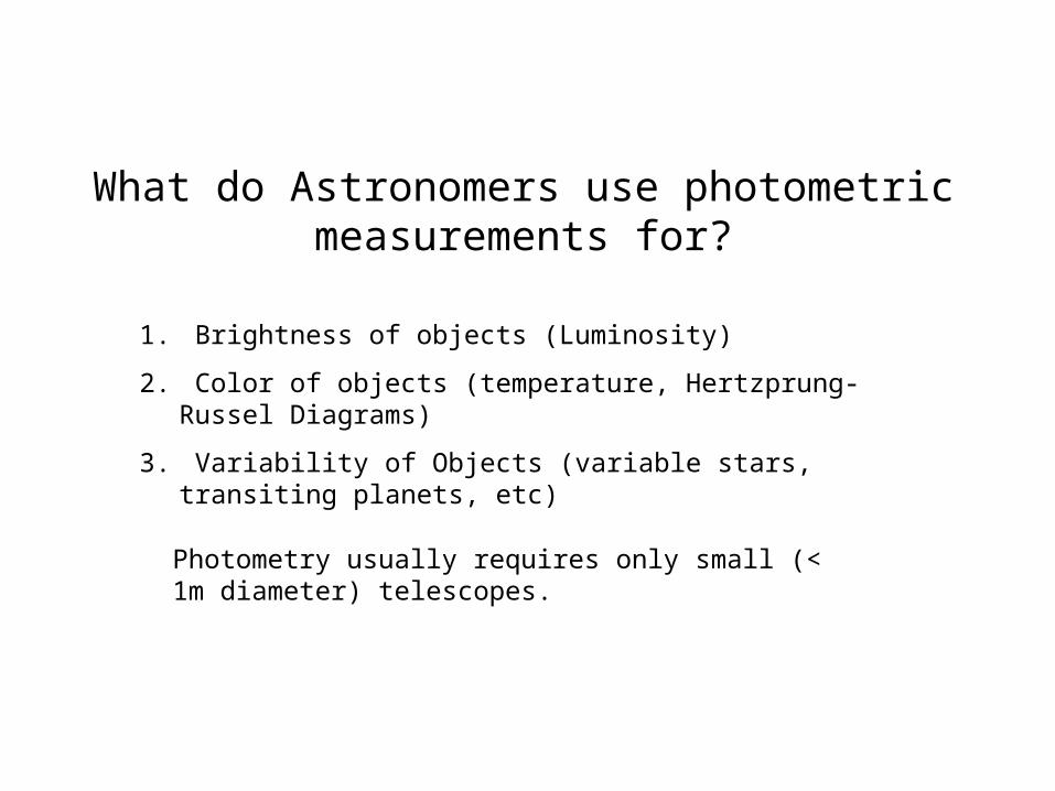
What do Astronomers use photometric measurements for?

1. Brightness of objects (Luminosity)

2. Color of objects (temperature, Hertzprung-Russel Diagrams)

3. Variability of Objects (variable stars, transiting planets, etc)

Photometry usually requires only small (< 1m diameter) telescopes.

Useful terms

Apparent magnitude m: the brightness of a star in traditional magnitude system

standard magnitude U,B,V, I, R: the standard brightness of a star in traditional magnitude system

absolute magnitude M: the magnitude of a star if it is at a distance of 10 parsecs

Bolometric magnitude: Total power of the source

Bolometric correction: must be added to the visual magnitude to get the bolometric magnitude.

Useful terms

Bandwidth : wavelength range over which observations are made:

Color index: difference of two magnitudes at two different wavelengths

Metallicity index m1 : index that is a measure of the relative abundance of a star

Extinction k: reduction in light due to passage through the Earth‘s atmosphere

Broadband: ~ 1/4

Narrow band: ~ 10–2

Standard star: star that provide a reference to a magnitude system

Interstellar extinction: reduction in light due to passage through interstellar material (dust, gas).

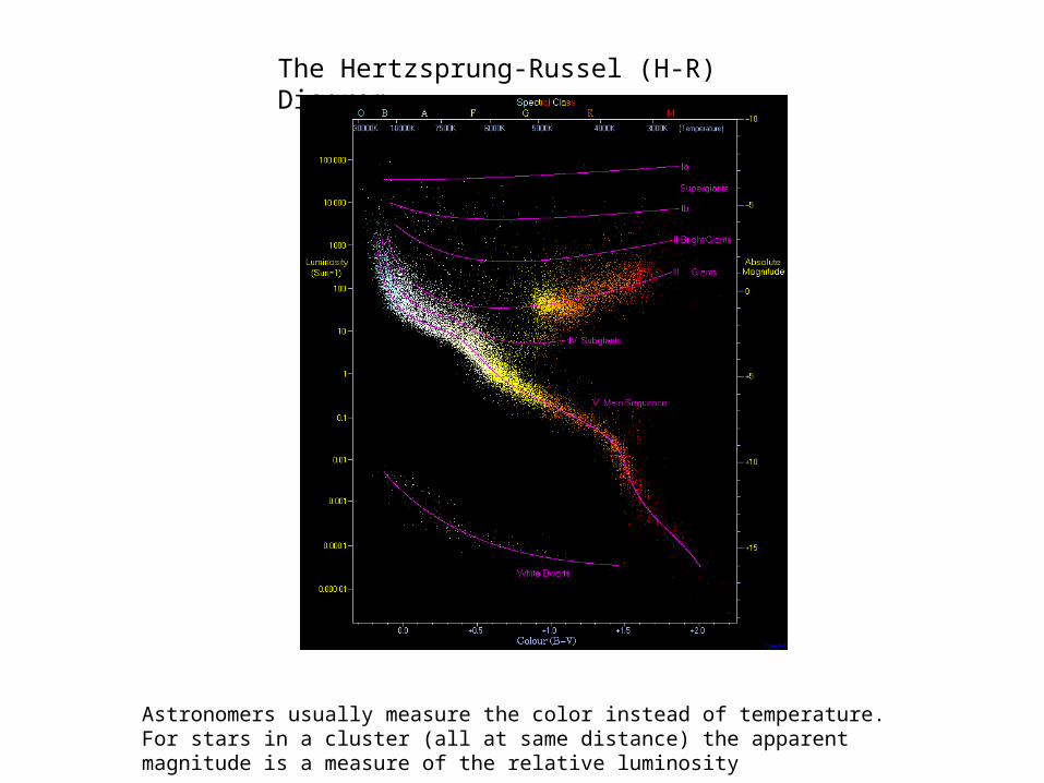
The Hertzsprung-Russel (H-R) Diagram

Astronomers usually measure the color instead of temperature. For stars in a cluster (all at same distance) the apparent magnitude is a measure of the relative luminosity

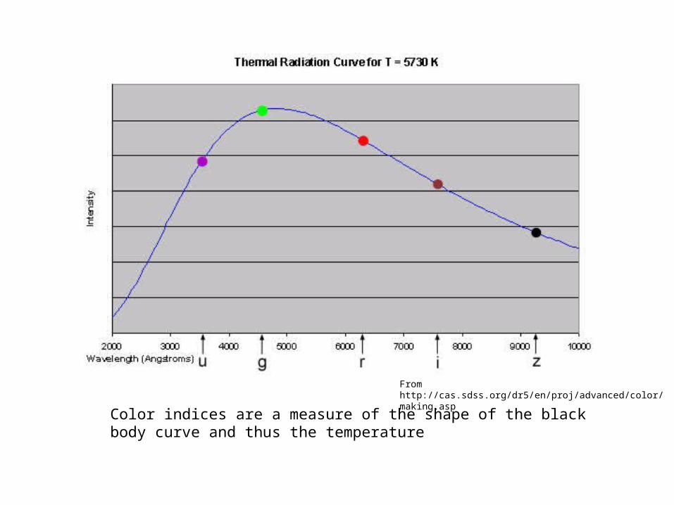
Color indices are a measure of the shape of the black body curve and thus the temperature

From http://cas.sdss.org/dr5/en/proj/advanced/color/making.asp

Magnitudes and color indices

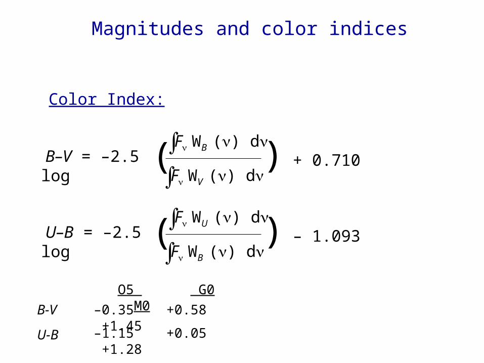
Color Index:

B–V = –2.5 log∫FWB () d

(∫FWV () d

) + 0.710

U–B = –2.5 log∫FWU () d

(∫FWB () d

) – 1.093

B-V

U-B

O5 G0 M0

–0.35 +0.58 +1.45

–1.15 +0.05 +1.28

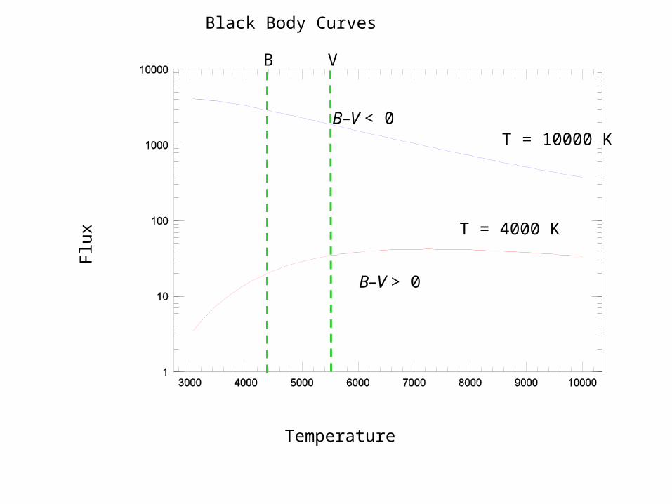
Temperature

Flu

x

B V

B–V < 0

B–V > 0

Black Body Curves

T = 10000 K

T = 4000 K

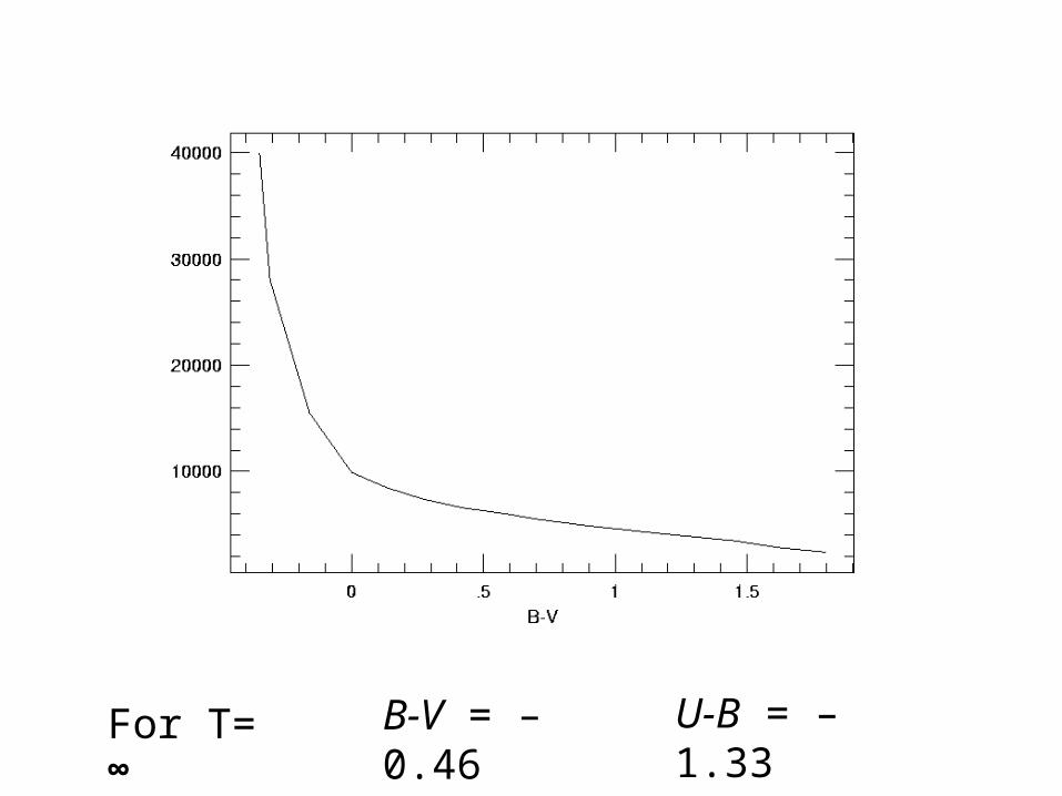
For T= ∞ B-V = –0.46 U-B = –1.33

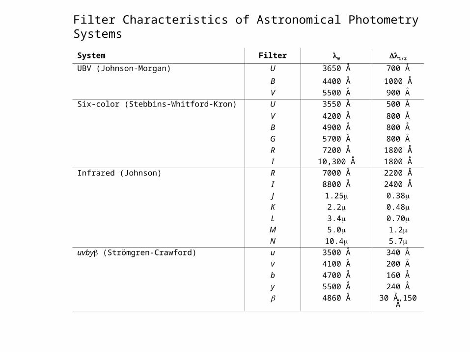
System Filter 0 1/2

UBV (Johnson-Morgan) U 3650 Å 700 Å

B 4400 Å 1000 Å

V 5500 Å 900 Å

Six-color (Stebbins-Whitford-Kron) U 3550 Å 500 Å

V 4200 Å 800 Å

B 4900 Å 800 Å

G 5700 Å 800 Å

R 7200 Å 1800 Å

I 10,300 Å 1800 Å

Infrared (Johnson) R 7000 Å 2200 Å

I 8800 Å 2400 Å

J 1.25 0.38

K 2.2 0.48

L 3.4 0.70

M 5.0 1.2

N 10.4 5.7

uvby (Strömgren-Crawford) u 3500 Å 340 Å

v 4100 Å 200 Å

b 4700 Å 160 Å

y 5500 Å 240 Å

4860 Å 30 Å,150 Å

Filter Characteristics of Astronomical Photometry Systems

For field stars the apparent magnitude does not tell you the true luminosity. Therefore, color-color magnitude diagrams are often employed

From http://www.ucolick.org/~kcooksey/CTIOreu.html

Giant starsMain sequence stars

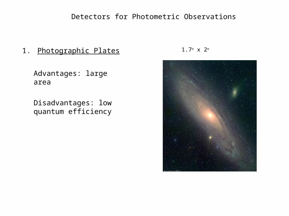
Detectors for Photometric Observations

1. Photographic Plates 1.7o x 2o

Advantages: large area

Disadvantages: low quantum efficiency

Detectors for Photometric Observations

2. Photomultiplier Tubes

Advantages: blue sensitive, fast response

Disadvantages: Only one object at a time

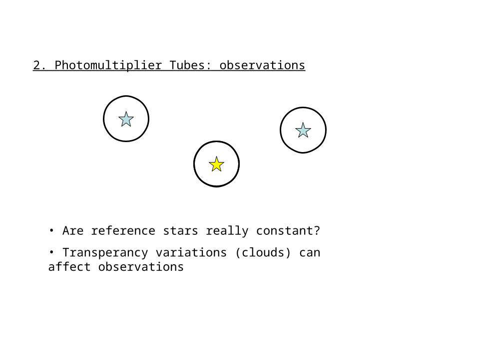
2. Photomultiplier Tubes: observations

• Are reference stars really constant?

• Transperancy variations (clouds) can affect observations

Detectors for Photometric Observations

3. Charge Coupled Devices

Advantages: high quantum efficiency, digital data, large number of reference stars, recorded simultaneously

Disadvantages: Red sensitive, readout time

From wikipedia

Get data (star) counts

Get sky counts

Magnitude = constant –2.5 x log [Σ(data – sky)/(exposure time)]

Instrumental magnitude can be converted to real magnitude by looking at standard stars

Aperture Photometry

Aperture photometry is useless for crowded fields

Term: Point Spread Function

PSF: Image produced by the instrument + atmosphere = point spread function

CameraAtmosphere

Most photometric reduction programs require modeling of the PSF

Crowded field Photometry: DAOPHOT

Computer program developed to obtain accurate photometry of blended images (Stetson 1987, Publications of the Astronomical Society of the Pacific, 99, 191)

DAOPHOT software is part of the IRAF (Image Reduction and Analysis Facility)

IRAF can be dowloaded from http://iraf.net (Windows, Mac, Intel)

or

http://star-www.rl.ac.uk/iraf/web/iraf-homepage.html (mostly Linux)

In iraf: load packages: noao -> digiphot -> daophot

Users manuals: http://www.iac.es/galeria/ncaon/IRAFSoporte/Iraf-Manuals.html

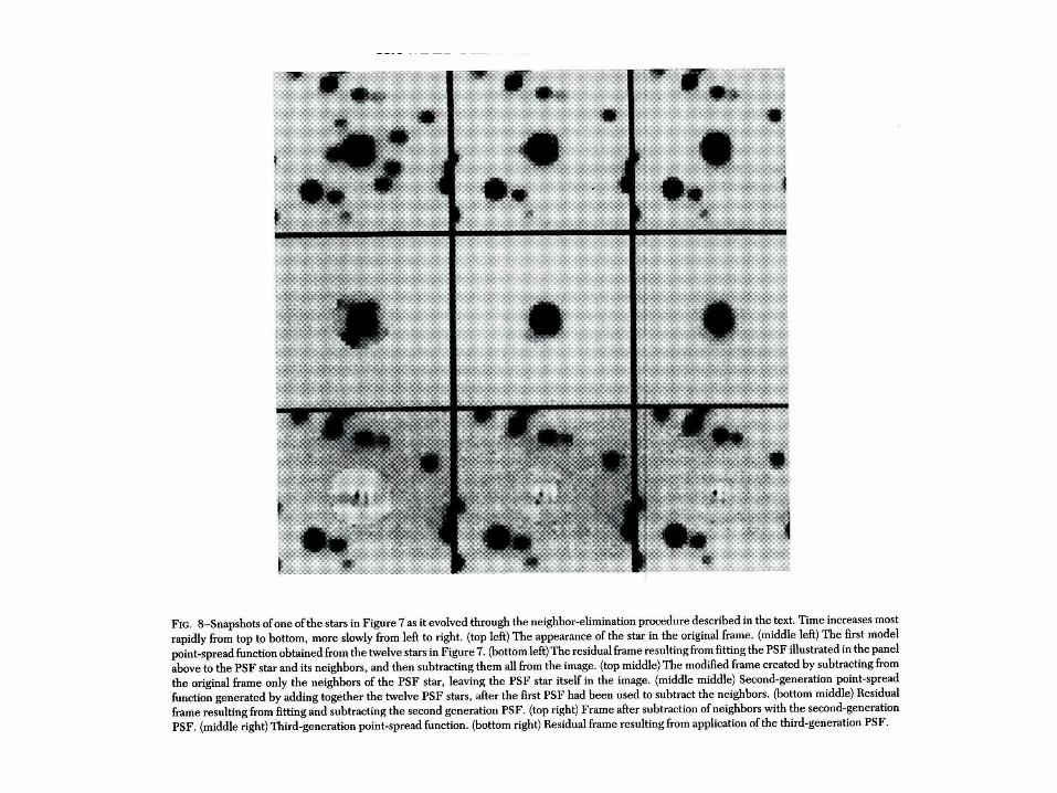
1. Choose several stars as „psf“ stars

2. Fit psf

3. Subtract neighbors

4. Refit PSF

5. Iterate

6. Stop after 2-3 iterations

In DAOPHOT modeling of the PSF is done through an iterative process:

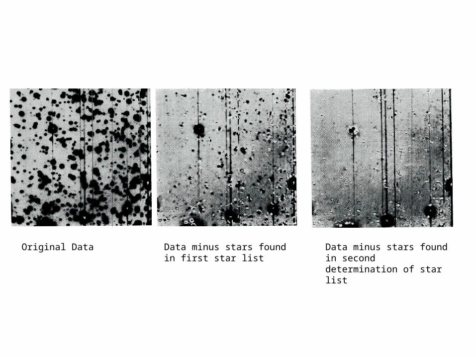
Original Data Data minus stars found in first star list

Data minus stars found in second determination of star list

Improvements to daophot and psf fitting: SExtractor (Source Extractor). Allows for elliptical apertures. Better at finding galaxies which can have none circular shapes

Bertin & Arnouts, Astron. Astroph. Suppl. Ser 117, 393-404, 1996

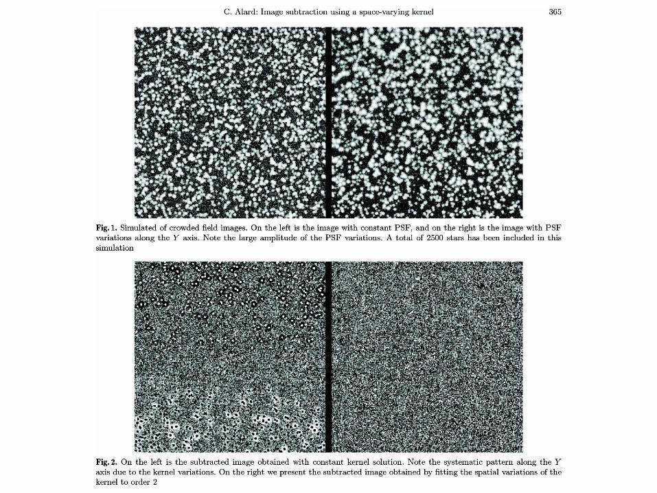
Special Techniques: Image Subtraction

If you are only interested in changes in the brightness (differential photometry) of an object one can use image subtraction (Alard, Astronomy and Astrophysics Suppl. Ser. 144, 363, 2000)

Applications:

• Nova and Supernova searches

• Microlensing

• Transit detections

Image subtraction: Basic Technique

• Get a reference image R. This is either a synthetic image (point sources) or a real data frame taken under good seeing conditions (usually your best frame).

• Find a convolution Kernal, K, that will transform R to fit your observed

image, I. Your fit image is R * I where * is the convolution (i.e. smoothing)

• Solve in a least squares manner the Kernal that will minimize the sum:

([R * K](xi,yi) – I(xi,yi))2i

Kernal is usually taken to be a Gaussian whose width can vary across the frame.

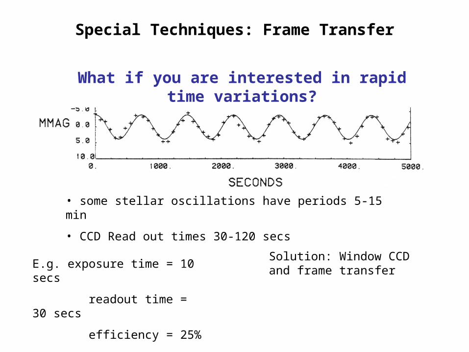
• some stellar oscillations have periods 5-15 min

• CCD Read out times 30-120 secs

What if you are interested in rapid time variations?

E.g. exposure time = 10 secs

readout time = 30 secs

efficiency = 25%

Solution: Window CCD and frame transfer

Special Techniques: Frame Transfer

Frame Transfer

Target

Reference

Mask

Transfer images to masked portion of the CCD. This is fast (msecs)

While masked portion is reading out, you expose on unmasked regions

Can achieve 100% efficiency

Store data

Dat

a s

hift

ed a

long

col

umns

Sources of Errors

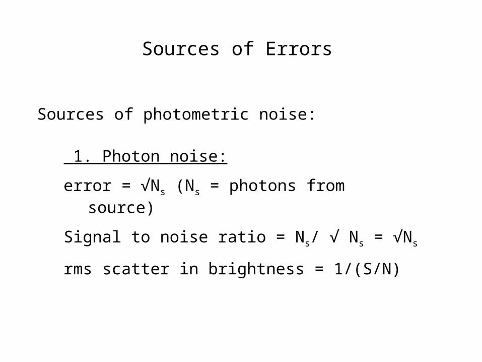
Sources of photometric noise:

1. Photon noise:

error = √Ns (Ns = photons from source)

Signal to noise ratio = Ns/ √ Ns = √Ns

rms scatter in brightness = 1/(S/N)

Sources of Errors

2. Sky:

Sky is bright, adds noise, best not to observe under full moon or in downtown Jena.

Ndata = counts from star

Nsky = background

Error = (Ndata + Nsky)1/2

S/N = (Ndata)/(Ndata + Nsky)1/2

rms scatter = 1/(S/N)

Ndata

rms

Nsky = 0

Nsky = 10

Nsky = 100

Nsky = 1000

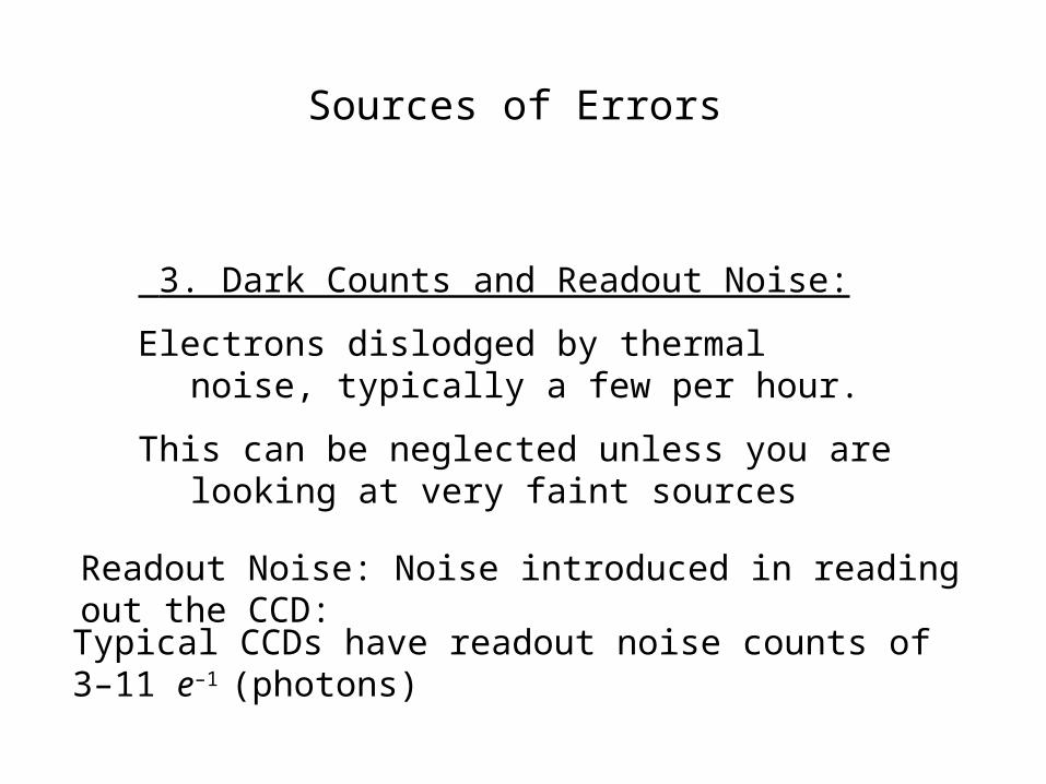
3. Dark Counts and Readout Noise:

Electrons dislodged by thermal noise, typically a few per hour.

This can be neglected unless you are looking at very faint sources

Sources of Errors

Typical CCDs have readout noise counts of 3–11 e–1

(photons)

Readout Noise: Noise introduced in reading out the CCD:

Sources of Errors

4. Scintillation Noise:

Amplitude variations due to Earth‘s atmosphere

~ [1 + 1.07(kD2/4L)7/6]–1

D is the telescope diameter

L is the length scale of the atmospheric turbulence

For larger telescopes the diameter of the telescope is much larger than the length scale of the turbulence. This reduces the scintillation noise.

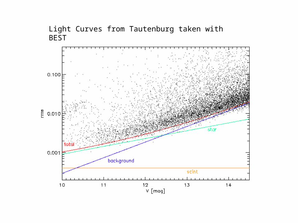
Light Curves from Tautenburg taken with BEST

Sources of Errors

4. Atmospheric Extinction

Atmospheric Extinction can affect colors of stars and photometric precision of differential photometry since observations are done at different air masses

• Rayleigh scattering: cross section per molecule ∝ –4

Major sources of extinction:

• Absorption by gases

• Aerosol Extinction

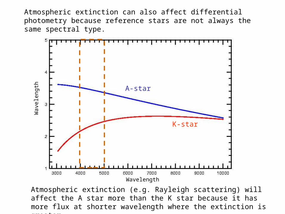
A-star

K-star

Atmospheric extinction can also affect differential photometry because reference stars are not always the same spectral type.

Atmospheric extinction (e.g. Rayleigh scattering) will affect the A star more than the K star because it has more flux at shorter wavelength where the extinction is greater

Wavelength

Wav

elen

gth

6. Interstellar reddening (extinction):

One of the problems of the 1920s was that the observation of O-B stars had red colors. This was later found to be caused by interstellar material.

To measure accurate „real“ colors and to put a star in the Hertzprung-Russel diagram this must be corrected

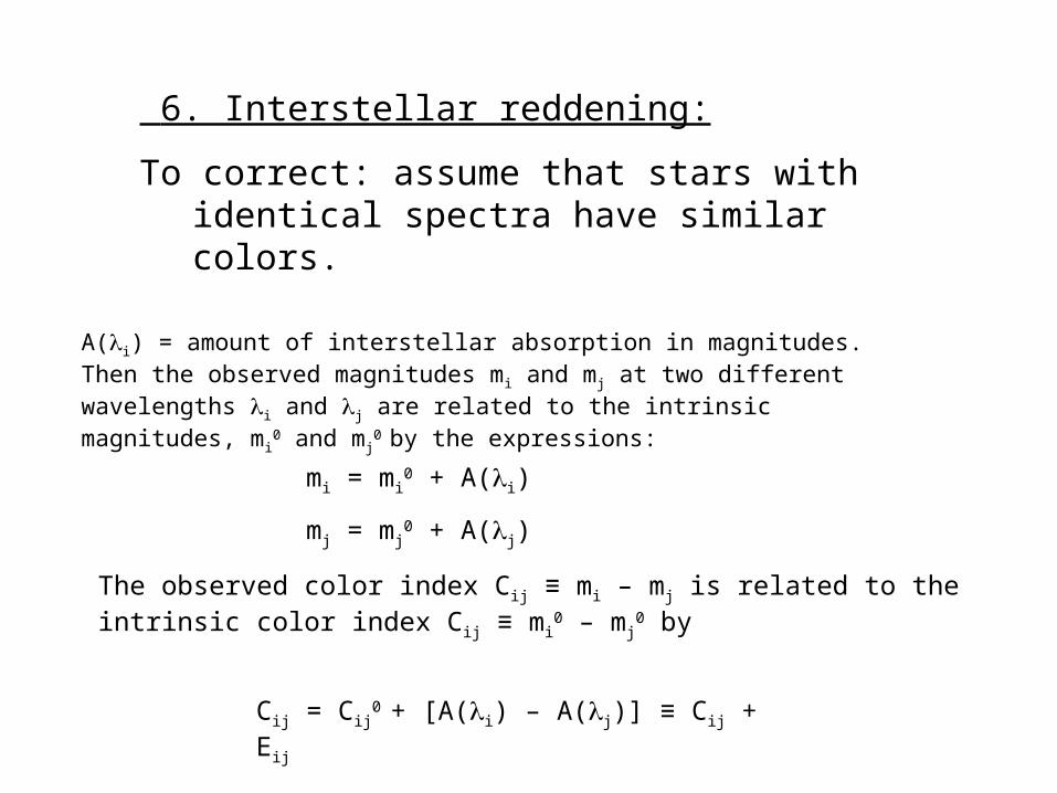
6. Interstellar reddening:

To correct: assume that stars with identical spectra have similar colors.

A(i) = amount of interstellar absorption in magnitudes. Then the observed magnitudes mi and mj at two different wavelengths i and j are related to the intrinsic magnitudes, mi

0 and mj0 by the expressions:

mi = mi0 + A(i)

mj = mj0 + A(j)

The observed color index Cij ≡ mi – mj is related to the intrinsic color index Cij ≡ mi

0 – mj0 by

Cij = Cij0 + [A(i) – A(j)] ≡ Cij + Eij

6. Interstellar reddening:

In the UBV system the notation for color excess is:

E(B – V) ≡ (B – V) – (B – V)0

E(U – B) ≡ (U – B) – (U – B)0

Eij is postive, i.e. colors become redder

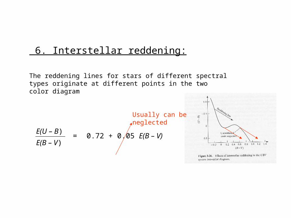
6. Interstellar reddening:

The reddening lines for stars of different spectral types originate at different points in the two color diagram

E(U – B)

E(B – V)= 0.72 + 0.05 E(B – V)

Usually can be neglected

6. Interstellar reddening:In many cases we do not have spectral types of the stars. The slope of the reddening line can be used to define a photometric parameter that depends only on spectral type and independent of the amount of reddening. In the UBV system:

Q ≡ (U – B) – E(U – B)

E(B – V)(B – V)

Q ≡ (U – B) – 0.72(B – V)

6. Interstellar reddening:

Using expressions for color excess:

Q = (U – B)0 + E(U – B)E(B – V)

[(B – V)0 + E(B – V)]– E(U – B)

Q = (U – B)0 E(B – V)

(B – V)0– E(U – B)

≡ Qo

6. Interstellar reddening:

Spectral Type Q Spectral Type Q

O5 –0.93 B3 –0.57

O6 –0.93 B5 –0.44

O8 –0.93 B6 –0.37

O9 –0.90 B7 –0.32

B0 –0.90 B8 –0.27

B0.5 –0.85 B9 –0.13

B1 –0.78 A0 0.00

B2 –0.70

(B – V)0 = 0.322 Q

We can determine (B – V)0 (= intrinsic color) for early-type stars from Q

6. Interstellar reddening:

We can determine (B – V)0 (= intrinsic color) for early-type stars from Q (measured from UBV). Once (B – V)0 and (U – V)0 are known we find E(B – V) from (B – V).

This only works for stars up to spectral type A0. Reason: The reddening happens to have the same slope as unreddened main sequence stars for late-type stars.

Reddening free indices can also be defined for other photometric systems as well.

6. Interstellar reddening: Extinction in magnitudes (A)

Intensity drop of light Ithrough a slab of thickness dx:

dI = –In(x)kdx

n = number density of grains along the line of sight

k = cross section per particle

nkdx is often called the incremental optical depth d

Optical depth

I I+ dI

The radiation sees neither or dx, but a the combination of the two over some path length L.

=∫o

L

dx Optical depth

L

Units: cm2

gmgmcm3

cm

6. Interstellar reddening: Extinction in magnitudes (A)

A ≡ –2.5 log10(I/I(0)) = –2.5 (log10 e)ln(e–) = 1.086

Intensity drop of light Ithrough a slab of thickness dx:

dI = –Id

IIe

–

0

Absorption of the starlight in magnitudes:

6. Interstellar reddening: Extinction in magnitudes (A)

Using expressions for A, Cij, and

RV ≡AV

E(B – V)=

V

– V)

kV

(k– kV)=

The absorption AV is proportional to color excess E(B–V) and the constant of proportionality, RV, is fixed by the wavelength dependence of the extinction coefficient. Once you determine RV, observe E(B–V) to determine AV

Need to determine RV

To determine RV compare at several wavelengths the energy distribution of a reddened star to one with no reddening and that has the same spectral type. A comparison of the colors results in color excess in each band referenced to one (V for instance). Since different stars have different color excess it is customary to normalize E(B–V) to unity.

Assume that E(X-V) goes to zero at infinite wavelengths (extrapolate). This gives AV

Standard Stars

For most photometric measurements (exception: differential measurements for variable star work) you need to put your relative photometric measurements on a reference magnitude scale.

What about fainter stars? Use Landolt standards.

Observations of standard stars should be made as close in time and at similar air mass as your other observations

Landolt standards.