Embed Size (px)
Citation preview
don’t
panic
!
Advanced Topicsof Theoretical Physics I
The electronic structure of matter
Peter E. Blöchl
Caution! This is an unfinished draft version
Errors are unavoidable!
Institute of Theoretical Physics; Clausthal University of Technology;
D-38678 Clausthal Zellerfeld; Germany;
http://www.pt.tu-clausthal.de/atp/
2
© Peter Blöchl, 2000-December 3, 2015Source: http://www2.pt.tu-clausthal.de/atp/phisx.html
Permission to make digital or hard copies of this work or portions thereof for personal or classroomuse is granted provided that copies are not made or distributed for profit or commercial advantage andthat copies bear this notice and the full citation. To copy otherwise requires prior specific permissionby the author.
1
1To the title page: What is the meaning of ΦSX? Firstly, it sounds like “Physics”. Secondly, the symbols stand forthe three main pillars of theoretical physics: “X” is the symbol for the coordinate of a particle and represents ClassicalMechanics. “Φ” is the symbol for the wave function and represents Quantum Mechanics and “S” is the symbol for theEntropy and represents Statistical Physics.
Foreword and Outlook
This book is work in progress. This book is not completed and not proofread. You can use this bookcurrently as a basis for following through the material presented in the course. However, you shouldnever blindly copy formulas an apply them. The chances that there are still errors is too large.
This book provides an introduction into the quantum mechanics of the interacting electron gas.It aims at students at the graduate level, that already have a good understanding on one-particlequantum mechanics. My aim is to include all proofs in a comprehensive and hopefully water-tightmanner. I am also avoiding special systems of units. I consider this important in view of a large varietyof notations, differing definitions etc. While the proofs have the advantage to train the student toperform the typical operations, it clutters the course with material far from applications. Therefore,I have placed many of the more detailed derivations into appendices. On the graduate level, thestudent should be able to follow the proofs without problem. It is strongly recommended to followthrough the derivations.
A recommended reading are the Lecture notes[1] by Wolf-Dieter Schöne, which has been usedin the preparation of this text. Another book that is very recommendable is the one by Fetter andWalecka[2]. Very useful has been also the book by Nolting[3]. While I did not follow the book ofMattuck[4]. A recommendable book for the reader, who wants to dig a little deeper into the density-functional theory is the Book by Eschrig[5]. Another excellent book on many particle physics, whichhowever takes a quite different route from this text is the book by Negele and Orland[6].
The goal of the lecture is that the student
• understands the Born-Oppenheimer approximation and its main limitations,
• is able to construct the band structure of a non-interacting problem using the tight-bindingmethod and is able to interpret a band structure,
• has a sound understanding of the connection between wave functions and the operator formal-ism of second quantization, i.e. creation and annihilation operators,
• understand the foundation of density functional theory, the dominant tool for first-principleselectronic structure calculations,
• understands the role of Green’s functions in many-particle physics and its relation to one-particlephysics, and that he
• understands the main theorems underlying the perturbation expansion fo Green’s functions,including Feynman diagrams.
I have tried to provide detailed and complete derivations of everything presented in this course.Some of the more extensive derivations are placed into an appendix. I strongly encourage the studentto understand and rationalize these derivations. Only this will make the student familiar with thelimitations of the theory and also with its flexibility. For a theoretical physicist this is of centralimportance, because he needs to be able to extend the existing theory, if necessary.
In the online version, there are many hyperreferences that allow to jump to the relevant informationin the book. To avoid the additional cost for color printouts just for the references they are not visible.They still work, when you click on them. Here is a list of links set:
3

4
• List of contents
• references to equation numbers, figures, tables, sections, appendices, etc.
• citations will take you to the corresponding position in the list of references
Contents
I Introduction to solid state physics 13
1 The Standard model of solid-state physics 17
2 Born-Oppenheimer approximation and beyond 21
2.1 Separation of electronic and nuclear degrees of freedom . . . . . . . . . . . . . . . 21
2.2 Approximations . . . . . . . . . . . . . . . . . . . . . . . . . . . . . . . . . . . . . 27
2.2.1 Born-Oppenheimer approximation . . . . . . . . . . . . . . . . . . . . . . . 27
2.2.2 Classical approximation . . . . . . . . . . . . . . . . . . . . . . . . . . . . . 27
2.3 Non-adiabatic corrections . . . . . . . . . . . . . . . . . . . . . . . . . . . . . . . . 28
2.3.1 Non-diagonal derivative couplings . . . . . . . . . . . . . . . . . . . . . . . 28
2.3.2 Topology of crossings of Born-Oppenheimer surfaces . . . . . . . . . . . . . 29
2.3.3 Avoided crossings . . . . . . . . . . . . . . . . . . . . . . . . . . . . . . . . 30
2.3.4 Conical intersections: Jahn-Teller model . . . . . . . . . . . . . . . . . . . . 31
2.3.5 From a conical intersection to an avoided crossing . . . . . . . . . . . . . . 41
2.4 Further reading . . . . . . . . . . . . . . . . . . . . . . . . . . . . . . . . . . . . . 42
3 Many-particle wave functions 45
3.1 Spin orbitals . . . . . . . . . . . . . . . . . . . . . . . . . . . . . . . . . . . . . . . 45
3.2 Symmetry and quantum mechanics . . . . . . . . . . . . . . . . . . . . . . . . . . . 49
3.3 Identical particles . . . . . . . . . . . . . . . . . . . . . . . . . . . . . . . . . . . . 51
3.3.1 Levi-Civita Symbol or the fully antisymmetric tensor . . . . . . . . . . . . . 52
3.3.2 Permutation operator . . . . . . . . . . . . . . . . . . . . . . . . . . . . . . 53
3.3.3 Antisymmetrize wave functions . . . . . . . . . . . . . . . . . . . . . . . . . 54
3.3.4 Slater determinants . . . . . . . . . . . . . . . . . . . . . . . . . . . . . . . 55
3.3.5 Bose wave functions . . . . . . . . . . . . . . . . . . . . . . . . . . . . . . 56
3.3.6 General many-fermion wave function . . . . . . . . . . . . . . . . . . . . . . 56
3.3.7 Number representation . . . . . . . . . . . . . . . . . . . . . . . . . . . . . 56
4 Non-interacting electrons 57
4.1 Dispersion relations . . . . . . . . . . . . . . . . . . . . . . . . . . . . . . . . . . . 57
4.2 Crystal lattices . . . . . . . . . . . . . . . . . . . . . . . . . . . . . . . . . . . . . 61
4.2.1 Reciprocal space revisited . . . . . . . . . . . . . . . . . . . . . . . . . . . 62
4.2.2 Bloch Theorem . . . . . . . . . . . . . . . . . . . . . . . . . . . . . . . . . 64
4.2.3 Non-interacting electrons in an external potential . . . . . . . . . . . . . . . 65
4.3 Bands and orbitals . . . . . . . . . . . . . . . . . . . . . . . . . . . . . . . . . . . 68
4.4 Calculating band structures in the tight-binding model . . . . . . . . . . . . . . . . 70
5
6 CONTENTS
4.5 Thermodynamics of non-interacting electrons . . . . . . . . . . . . . . . . . . . . . 734.5.1 Thermodynamics revisited . . . . . . . . . . . . . . . . . . . . . . . . . . . 734.5.2 Maximum entropy, minimum free energy principle and the meaning of the grand potential 744.5.3 Many-particle states of non-interacting electrons . . . . . . . . . . . . . . . 754.5.4 Density of States . . . . . . . . . . . . . . . . . . . . . . . . . . . . . . . . 764.5.5 Fermi distribution . . . . . . . . . . . . . . . . . . . . . . . . . . . . . . . . 77
4.6 Jellium model . . . . . . . . . . . . . . . . . . . . . . . . . . . . . . . . . . . . . . 824.6.1 Dispersion relation . . . . . . . . . . . . . . . . . . . . . . . . . . . . . . . 824.6.2 Boundary conditions . . . . . . . . . . . . . . . . . . . . . . . . . . . . . . 82
4.7 Properties of the electron gas . . . . . . . . . . . . . . . . . . . . . . . . . . . . . 874.7.1 Fermi velocity . . . . . . . . . . . . . . . . . . . . . . . . . . . . . . . . . . 87
4.8 Tour trough band structures and densities of states of real materials . . . . . . . . . 874.8.1 Free-electron like metals . . . . . . . . . . . . . . . . . . . . . . . . . . . . 874.8.2 Noble metals . . . . . . . . . . . . . . . . . . . . . . . . . . . . . . . . . . 884.8.3 Transition metals . . . . . . . . . . . . . . . . . . . . . . . . . . . . . . . . 894.8.4 Diamond, Zinc-blende and wurtzite-type semiconductors . . . . . . . . . . . 904.8.5 Simple oxides . . . . . . . . . . . . . . . . . . . . . . . . . . . . . . . . . . 914.8.6 PCMO an example for a complex oxide . . . . . . . . . . . . . . . . . . . . 92
4.9 What band structures are good for . . . . . . . . . . . . . . . . . . . . . . . . . . . 924.9.1 Chemical stability . . . . . . . . . . . . . . . . . . . . . . . . . . . . . . . . 924.9.2 Dispersion relations . . . . . . . . . . . . . . . . . . . . . . . . . . . . . . . 924.9.3 Boltzmann equation . . . . . . . . . . . . . . . . . . . . . . . . . . . . . . 93
5 Magnetism 95
5.1 Charged particles in a magnetic field . . . . . . . . . . . . . . . . . . . . . . . . . . 955.2 Dirac equation and magnetic moment . . . . . . . . . . . . . . . . . . . . . . . . . 955.3 Magnetism of the free electron gas . . . . . . . . . . . . . . . . . . . . . . . . . . . 955.4 Magnetic order . . . . . . . . . . . . . . . . . . . . . . . . . . . . . . . . . . . . . 95
6 The Hartree-Fock approximation and exchange 97
6.1 One-electron and two-particle operators . . . . . . . . . . . . . . . . . . . . . . . . 976.2 Expectation values of Slater determinants . . . . . . . . . . . . . . . . . . . . . . . 99
6.2.1 Expectation value of a one-particle operator . . . . . . . . . . . . . . . . . . 996.2.2 Expectation value of a two-particle operator . . . . . . . . . . . . . . . . . . 102
6.3 Hartree energy . . . . . . . . . . . . . . . . . . . . . . . . . . . . . . . . . . . . . . 1046.4 Exchange energy . . . . . . . . . . . . . . . . . . . . . . . . . . . . . . . . . . . . 1046.5 Hartree-Fock equations . . . . . . . . . . . . . . . . . . . . . . . . . . . . . . . . . 1066.6 Hartree-Fock of the free-electron gas . . . . . . . . . . . . . . . . . . . . . . . . . 1106.7 Beyond the Hartree-Fock Theory: Correlations . . . . . . . . . . . . . . . . . . . . 111
6.7.1 Left-right and in-out correlation . . . . . . . . . . . . . . . . . . . . . . . . 1126.7.2 In-out correlation . . . . . . . . . . . . . . . . . . . . . . . . . . . . . . . . 1136.7.3 Spin contamination . . . . . . . . . . . . . . . . . . . . . . . . . . . . . . . 1136.7.4 Dynamic and static correlation . . . . . . . . . . . . . . . . . . . . . . . . . 113
7 Density-functional theory 115
7.1 One-particle and two-particle densities . . . . . . . . . . . . . . . . . . . . . . . . . 1167.1.1 N-particle density matrix . . . . . . . . . . . . . . . . . . . . . . . . . . . . 116
CONTENTS 7
7.1.2 One-particle reduced density matrix . . . . . . . . . . . . . . . . . . . . . . 116
7.1.3 Two-particle density . . . . . . . . . . . . . . . . . . . . . . . . . . . . . . 119
7.1.4 Two-particle density of the free electron gas . . . . . . . . . . . . . . . . . 122
7.1.5 Pair-correlation function and hole function . . . . . . . . . . . . . . . . . . 124
7.2 Self-made density functional . . . . . . . . . . . . . . . . . . . . . . . . . . . . . . 125
7.3 Constrained search . . . . . . . . . . . . . . . . . . . . . . . . . . . . . . . . . . . 130
7.4 Self-consistent equations . . . . . . . . . . . . . . . . . . . . . . . . . . . . . . . . 132
7.4.1 Universal Functional . . . . . . . . . . . . . . . . . . . . . . . . . . . . . . 132
7.4.2 Exchange-correlation functional . . . . . . . . . . . . . . . . . . . . . . . . 133
7.4.3 The self-consistency condition . . . . . . . . . . . . . . . . . . . . . . . . . 133
7.4.4 Flow chart for a conventional self-consistency loop . . . . . . . . . . . . . . 136
7.4.5 Another Minimum principle . . . . . . . . . . . . . . . . . . . . . . . . . . . 136
7.5 Adiabatic connection . . . . . . . . . . . . . . . . . . . . . . . . . . . . . . . . . . 137
7.5.1 Screened interaction . . . . . . . . . . . . . . . . . . . . . . . . . . . . . . 139
7.5.2 Hybrid functionals . . . . . . . . . . . . . . . . . . . . . . . . . . . . . . . . 140
7.6 Functionals . . . . . . . . . . . . . . . . . . . . . . . . . . . . . . . . . . . . . . . 141
7.7 Xα method . . . . . . . . . . . . . . . . . . . . . . . . . . . . . . . . . . . . . . . 142
7.8 Local density functionals . . . . . . . . . . . . . . . . . . . . . . . . . . . . . . . . 143
7.9 Local spin-density approximation . . . . . . . . . . . . . . . . . . . . . . . . . . . . 144
7.10 Non-collinear local spin-density approximation . . . . . . . . . . . . . . . . . . . . . 144
7.11 Generalized gradient functionals . . . . . . . . . . . . . . . . . . . . . . . . . . . . 144
7.12 Additional material . . . . . . . . . . . . . . . . . . . . . . . . . . . . . . . . . . . 149
7.12.1 Relevance of the highest occupied Kohn-Sham orbital . . . . . . . . . . . . 149
7.12.2 Correlation inequality and lower bound of the exact density functional . . . . 149
7.13 Functionals . . . . . . . . . . . . . . . . . . . . . . . . . . . . . . . . . . . . . . . 149
7.14 Reliability of DFT . . . . . . . . . . . . . . . . . . . . . . . . . . . . . . . . . . . . 149
7.15 Deficiencies of DFT . . . . . . . . . . . . . . . . . . . . . . . . . . . . . . . . . . . 150
II Advanced solid state physics 151
8 Second quantization 153
8.1 Fock space . . . . . . . . . . . . . . . . . . . . . . . . . . . . . . . . . . . . . . . 153
8.2 Number representation . . . . . . . . . . . . . . . . . . . . . . . . . . . . . . . . . 153
8.2.1 Excursion: Integer representation representation of Slater determinants . . . 155
8.3 Creation and annihilation operators . . . . . . . . . . . . . . . . . . . . . . . . . . . 156
8.4 Commutator and anticommutator relations . . . . . . . . . . . . . . . . . . . . . . 158
8.4.1 Anticommutator relations with the same one-particle orbital . . . . . . . . . 159
8.4.2 Anticommutator relations with different one-particle orbitals . . . . . . . . . 159
8.5 Slater-Condon rules . . . . . . . . . . . . . . . . . . . . . . . . . . . . . . . . . . . 160
8.6 Operators expressed by field operators . . . . . . . . . . . . . . . . . . . . . . . . . 162
8.7 Real-space representation of field operators . . . . . . . . . . . . . . . . . . . . . . 162
9 Ground state and excitations 167
9.1 Hole excitations . . . . . . . . . . . . . . . . . . . . . . . . . . . . . . . . . . . . . 167
9.2 Two-particle excitations . . . . . . . . . . . . . . . . . . . . . . . . . . . . . . . . . 168
8 CONTENTS
10 Green’s functions in one-particle quantum mechanics 169
10.1 Green’s function as inverse of a differential operator . . . . . . . . . . . . . . . . . 16910.2 Green’s function of a time-independent Hamiltonian . . . . . . . . . . . . . . . . . . 172
10.2.1 Green’s function in the energy representation . . . . . . . . . . . . . . . . . 17310.3 Projected Density of States . . . . . . . . . . . . . . . . . . . . . . . . . . . . . . . 174
11 Perturbation theory in the one-particle theory 179
11.1 Feynman diagrams . . . . . . . . . . . . . . . . . . . . . . . . . . . . . . . . . . . 18011.2 Time-dependent Perturbation . . . . . . . . . . . . . . . . . . . . . . . . . . . . . . 180
11.2.1 Perturbation series . . . . . . . . . . . . . . . . . . . . . . . . . . . . . . . 18111.2.2 Propagator of a time-independent Hamiltonian . . . . . . . . . . . . . . . . 18111.2.3 Interaction picture . . . . . . . . . . . . . . . . . . . . . . . . . . . . . . . 18211.2.4 Series expansion . . . . . . . . . . . . . . . . . . . . . . . . . . . . . . . . 182
11.3 Green’s function as propagator . . . . . . . . . . . . . . . . . . . . . . . . . . . . . 18511.4 Retarded Potentials . . . . . . . . . . . . . . . . . . . . . . . . . . . . . . . . . . . 187
12 Green’s functions in many-particle physics 189
12.1 Heisenberg picture . . . . . . . . . . . . . . . . . . . . . . . . . . . . . . . . . . . . 18912.1.1 Pictures in comparison . . . . . . . . . . . . . . . . . . . . . . . . . . . . . 190
12.2 One-particle Green’s function expressed by the many-particle Hamiltonian . . . . . . 19112.3 Many-particle Green’s function . . . . . . . . . . . . . . . . . . . . . . . . . . . . . 19212.4 Differential equation for the many-particle Green’s function . . . . . . . . . . . . . . 19312.5 Self energy . . . . . . . . . . . . . . . . . . . . . . . . . . . . . . . . . . . . . . . . 19612.6 Physical meaning of the Green’s function . . . . . . . . . . . . . . . . . . . . . . . 196
12.6.1 Expectation value of single particle operators . . . . . . . . . . . . . . . . . 19612.6.2 Excitation spectrum and Lehmann Representation . . . . . . . . . . . . . . 197
12.7 Non-interacting Green’s function . . . . . . . . . . . . . . . . . . . . . . . . . . . . 19812.8 Migdal-Galitskii-Koltun (MGK) sum rule and total energy . . . . . . . . . . . . . . . 20012.9 Spectral function . . . . . . . . . . . . . . . . . . . . . . . . . . . . . . . . . . . . 20012.10Variations of the Green’s function . . . . . . . . . . . . . . . . . . . . . . . . . . . 200
13 Diagrammatic expansion of the Green’s function 203
13.1 Adiabatic switching on . . . . . . . . . . . . . . . . . . . . . . . . . . . . . . . . . 20313.2 Interacting Green’s function expressed by non-interacting ground states . . . . . . . 20613.3 Wick’s theorem . . . . . . . . . . . . . . . . . . . . . . . . . . . . . . . . . . . . . 207
13.3.1 Prelude . . . . . . . . . . . . . . . . . . . . . . . . . . . . . . . . . . . . . 20713.3.2 Some definitions . . . . . . . . . . . . . . . . . . . . . . . . . . . . . . . . 20813.3.3 Wick’s Theorem . . . . . . . . . . . . . . . . . . . . . . . . . . . . . . . . 210
14 Feynman diagrams 215
14.1 Linked Cluster theorem . . . . . . . . . . . . . . . . . . . . . . . . . . . . . . . . . 21914.2 Dyson’s equation . . . . . . . . . . . . . . . . . . . . . . . . . . . . . . . . . . . . 219
14.2.1 Self energy . . . . . . . . . . . . . . . . . . . . . . . . . . . . . . . . . . . 21914.2.2 Polarization . . . . . . . . . . . . . . . . . . . . . . . . . . . . . . . . . . . 220
15 Some typical approximations 221
15.1 Hartree-Fock . . . . . . . . . . . . . . . . . . . . . . . . . . . . . . . . . . . . . . 221
CONTENTS 9
15.2 GW Approximation . . . . . . . . . . . . . . . . . . . . . . . . . . . . . . . . . . . 222
15.3 Random Phase approximation (RPA) . . . . . . . . . . . . . . . . . . . . . . . . . . 224
16 Models in many-particle theory 227
16.1 Dominant interactions . . . . . . . . . . . . . . . . . . . . . . . . . . . . . . . . . 227
16.2 Hubbard model . . . . . . . . . . . . . . . . . . . . . . . . . . . . . . . . . . . . . 229
16.3 t-J model . . . . . . . . . . . . . . . . . . . . . . . . . . . . . . . . . . . . . . . . 230
16.4 Heisenberg model . . . . . . . . . . . . . . . . . . . . . . . . . . . . . . . . . . . . 230
16.5 Anderson impurity model . . . . . . . . . . . . . . . . . . . . . . . . . . . . . . . . 230
16.5.1 The interaction energy . . . . . . . . . . . . . . . . . . . . . . . . . . . . . 231
16.5.2 Mean field approximation . . . . . . . . . . . . . . . . . . . . . . . . . . . . 231
17 Zoo of Concepts from Solid State Physics 233
17.1 Kondo effect . . . . . . . . . . . . . . . . . . . . . . . . . . . . . . . . . . . . . . . 235
17.1.1 Kondo model . . . . . . . . . . . . . . . . . . . . . . . . . . . . . . . . . . 236
A Notation 241
A.1 Fermions and Bosons . . . . . . . . . . . . . . . . . . . . . . . . . . . . . . . . . . 241
A.2 Vectors, matrices, operators, functions, etc. . . . . . . . . . . . . . . . . . . . . . . 241
A.3 Comparison with Fetter Walecka . . . . . . . . . . . . . . . . . . . . . . . . . . . . 241
B Derivations of mathematical expressions 243
B.1 Fourier transform of the step function . . . . . . . . . . . . . . . . . . . . . . . . . 243
C Adiabatic decoupling in the Born-Oppenheimer approximation 245
C.1 Justification for the Born-Oppenheimer approximation . . . . . . . . . . . . . . . . 245
D Non-adiabatic effects 249
D.1 The off-diagonal terms of the first-derivative couplings ~An,m,j . . . . . . . . . . . . . 249
D.2 Diagonal terms of the derivative couplings . . . . . . . . . . . . . . . . . . . . . . . 250
D.3 The diabatic picture . . . . . . . . . . . . . . . . . . . . . . . . . . . . . . . . . . . 252
E Non-crossing rule 255
E.1 Proof of the non-crossing rule . . . . . . . . . . . . . . . . . . . . . . . . . . . . . 255
F Landau-Zener Formula 259
G Supplementary material for the Jahn-Teller model 263
G.1 Relation of stationary wave functions for m and −m − 1 . . . . . . . . . . . . . . . 263
G.2 Behavior of the radial nuclear wave function at the origin . . . . . . . . . . . . . . . 265
G.3 Optimization of the radial wave functions . . . . . . . . . . . . . . . . . . . . . . . 267
G.4 Integration of the Schrödinger equation for the radial nuclear wave functions . . . . 269
H Notation for spin indices 273
I Some group theory for symmetries 275
I.0.1 Definitin of a group . . . . . . . . . . . . . . . . . . . . . . . . . . . . . . . 275
I.0.2 Symmetry class . . . . . . . . . . . . . . . . . . . . . . . . . . . . . . . . . 275
10 CONTENTS
J Downfolding 277
J.1 Downfolding with Green’s functions . . . . . . . . . . . . . . . . . . . . . . . . . . 279J.2 Taylor expansion in the energy . . . . . . . . . . . . . . . . . . . . . . . . . . . . . 279
K Sum rules related to the f-sum rule 281
K.1 General derivation by Wang . . . . . . . . . . . . . . . . . . . . . . . . . . . . . . . 281K.1.1 f-sum rule or Thomas-Reiche-Kuhn sum rule . . . . . . . . . . . . . . . . . 282K.1.2 Bethe sum rule . . . . . . . . . . . . . . . . . . . . . . . . . . . . . . . . . 283
L Time-inversion symmetry 285
L.1 Schrödinger equation . . . . . . . . . . . . . . . . . . . . . . . . . . . . . . . . . . 285L.2 Pauli equation . . . . . . . . . . . . . . . . . . . . . . . . . . . . . . . . . . . . . . 286L.3 Time inversion for Bloch states . . . . . . . . . . . . . . . . . . . . . . . . . . . . . 288
M Slater determinants for parallel and antiparallel spins 289
M.1 Spatial symmetry for parallel and antiparallel spins . . . . . . . . . . . . . . . . . . . 290M.2 An intuitive analogy for particle with spin . . . . . . . . . . . . . . . . . . . . . . . 292
N Hartree-Fock of the free-electron gas 293
N.1 Exchange potential as non-local potential . . . . . . . . . . . . . . . . . . . . . . . 293N.2 Energy-level shifts by the exchange potential . . . . . . . . . . . . . . . . . . . . . . 294
O Derivation of Slater-Condon rules 299
O.1 Identical Slater determinants . . . . . . . . . . . . . . . . . . . . . . . . . . . . . . 299O.2 One-particle operator with one different orbital . . . . . . . . . . . . . . . . . . . . 299O.3 Two-particle operator with one different orbital . . . . . . . . . . . . . . . . . . . . 300O.4 One-particle operator with two different orbitals . . . . . . . . . . . . . . . . . . . . 302O.5 Two-particle operator with two different orbitals . . . . . . . . . . . . . . . . . . . . 302O.6 More than two different one-particle orbitals . . . . . . . . . . . . . . . . . . . . . . 302
P One- and two-particle operators expressed by field operators 303
P.1 Matrix elements between identical Slater determinants . . . . . . . . . . . . . . . . 303P.2 Matrix elements between Slater determinants differing by one orbital . . . . . . . . . 304P.3 Matrix elements between Slater determinants differing by two orbitals . . . . . . . . 306
Q Green’s function and division of systems 309
Q.1 Relation to a Schrödinger equation . . . . . . . . . . . . . . . . . . . . . . . . . . . 310Q.1.1 Another derivation of the effective Schrödinger equation . . . . . . . . . . . 311
R Time-ordered exponential, Propagators etc. 313
R.1 Time-ordered exponential . . . . . . . . . . . . . . . . . . . . . . . . . . . . . . . . 313R.2 Wick’s time ordering operator . . . . . . . . . . . . . . . . . . . . . . . . . . . . . 314R.3 Propagator in real time . . . . . . . . . . . . . . . . . . . . . . . . . . . . . . . . . 314
R.3.1 Propagator in the Schrödinger picture . . . . . . . . . . . . . . . . . . . . . 314R.4 Propagator in imaginary time . . . . . . . . . . . . . . . . . . . . . . . . . . . . . . 315
R.4.1 Imaginary-time propagator in the Schrödinger picture . . . . . . . . . . . . . 315
S Field operators in the interaction picture 319
CONTENTS 11
T Baker-Hausdorff Theorem 321
T.1 Baker-Hausdorff Theorem . . . . . . . . . . . . . . . . . . . . . . . . . . . . . . . . 321T.2 Hadamard Lemma . . . . . . . . . . . . . . . . . . . . . . . . . . . . . . . . . . . . 322
U Stuff 325
U.1 Collection of links . . . . . . . . . . . . . . . . . . . . . . . . . . . . . . . . . . . . 325U.2 Electrons and holes . . . . . . . . . . . . . . . . . . . . . . . . . . . . . . . . . . . 325
V Dictionary 329
V.1 Explanations . . . . . . . . . . . . . . . . . . . . . . . . . . . . . . . . . . . . . . . 329V.2 Symbols . . . . . . . . . . . . . . . . . . . . . . . . . . . . . . . . . . . . . . . . . 329
W Greek Alphabet 331
X Philosophy of the ΦSX Series 333
Y About the Author 335

12 CONTENTS
Part I
Introduction to solid state physics
13


15
Topics:
1. Separate nuclear and electron dynamics
2. Spin-orbitals ans many-particle wave functions
3. non-interacting electrons: band structure
4. Hartree-Fock approximation
5. Density functional theory
6. Phonons
7. Transport theory: Boltzmann equation
• Open systems
• Decoherence
8. Magnetism

16
Chapter 1
The Standard model of solid-statephysics
Solid state physics has, in contrast to elementary particle physics, the big advantage that the funda-mental particles and their interactions are completely known. The particles are electrons and nuclei1
and their interaction is described by electromagnetism. Gravitation is such a weak force at small dis-tances that it is completely dominated by the electromagnetic interaction. The strong force, whichis active inside the nucleus, has such a short range that it does not affect the relative motion ofelectrons and nuclei.
Some argue that solid-state physics is not at the very frontier of research, because its particlesand interactions are fully known. However, a second look shows the contrary: While the constituentsare simple, the complexity develops via the interaction of many of these simple particles. The simpleconstituents act together to form an entire zoo of phenomena of fascinating complexity.
The dynamics is described by the Schrödinger equation:
i~∂t |Φ〉 = H|Φ〉 (1.1)
where the wave function depends on the coordinates of all electrons and nuclei in the system. Inaddition it depends on the spin degrees of freedom of the electrons. Thus, a wave function for Nelectrons and M nuclei has the form
Φσ1,...,σN (~r1, . . . , ~rN , ~R1, . . . , ~RM)
where we denote the electronic coordinates by a lower-case ~r and the nuclear positions by an uppercase~R. The symbols σj are the spin indices, which may assume values σj ∈ − 12 ,+ 12. We will often usethe notation σj ∈ ↓, ↑. The spin quantum number in z-direction is sz = ~σ.
Often we will also combine position and spin index of the electrons in the form ~x = (σ,~r), so that
Φ(~x1, . . . , ~xN , ~R1, . . . , ~RM)def=Φσ1,...,σN (~r1, . . . , ~rN , ~R1, . . . , ~RM)
For the integrations and summations we use the short-hand notation∫
d4xdef=∑
σ∈↑,↓
∫
d3r (1.2)
1The cautious reader may object that the nuclei are objects that are far from being fully understood. However, theonly properties that are relevant for us are their charge, their mass, and their size.
17
18 1 THE STANDARD MODEL OF SOLID-STATE PHYSICS
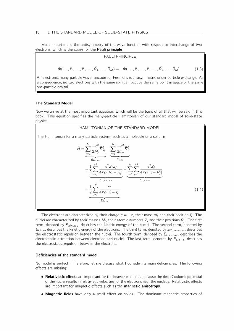
Most important is the antisymmetry of the wave function with respect to interchange of twoelectrons, which is the cause for the Pauli principle
PAULI PRINCIPLE
Φ(. . . , ~xi , . . . , ~xj , . . . , ~R1, . . . , ~RM) = −Φ(. . . , ~xj , . . . , ~xi , . . . , ~R1, . . . , ~RM) (1.3)
An electronic many-particle wave function for Fermions is antisymmetric under particle exchange. Asa consequence, no two electrons with the same spin can occupy the same point in space or the sameone-particle orbital.
The Standard Model
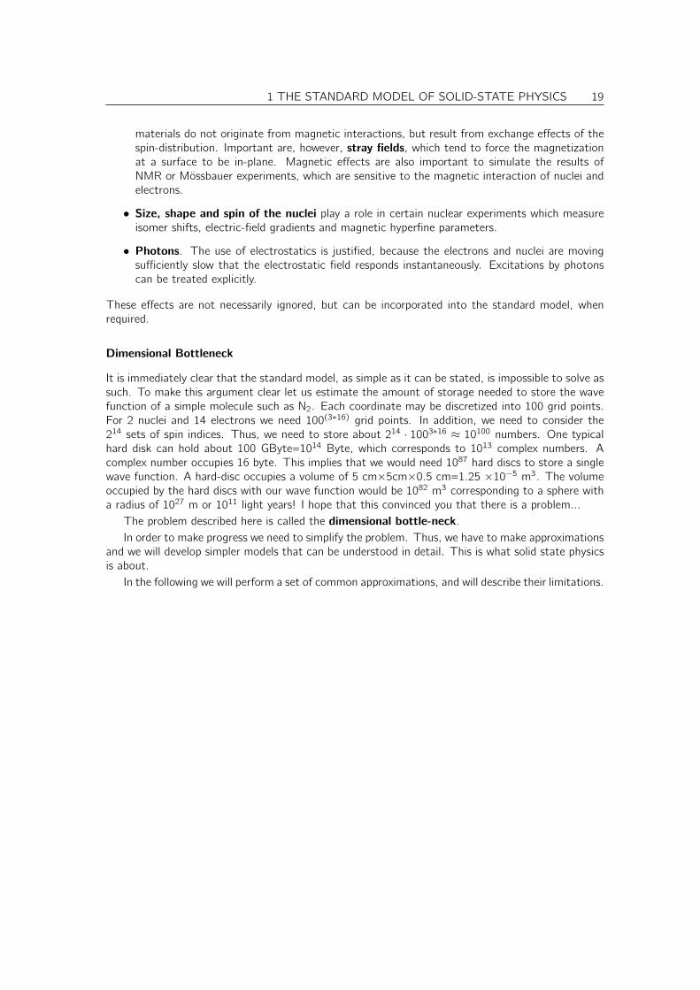
Now we arrive at the most important equation, which will be the basis of all that will be said in thisbook. This equation specifies the many-particle Hamiltonian of our standard model of solid-statephysics.
HAMILTONIAN OF THE STANDARD MODEL
The Hamiltonian for a many particle system, such as a molecule or a solid, is
H =
M∑
j=1
−~22Mj
~∇2~Rj︸ ︷︷ ︸
Ekin,nuc
+
N∑
i=1
−~22me
~∇2~ri︸ ︷︷ ︸
Ekin,e
+1
2
M∑
i 6=j
e2ZiZj
4πǫ0|~Ri − ~Rj |︸ ︷︷ ︸
EC,nuc−nuc
−N∑
i=1
M∑
j=1
e2Zj
4πǫ0|~ri − ~Rj |︸ ︷︷ ︸
EC,e−nuc
+1
2
N∑
i 6=j
e2
4πǫ0|~ri − ~rj |︸ ︷︷ ︸
EC,e−e
(1.4)
The electrons are characterized by their charge q = −e, their mass me and their position ~rj . Thenuclei are characterized by their masses Mj , their atomic numbers Zj and their positions ~Rj . The firstterm, denoted by Ekin,nuc , describes the kinetic energy of the nuclei. The second term, denoted byEkin,e , describes the kinetic energy of the electrons. The third term, denoted by EC,nuc−nuc , describesthe electrostatic repulsion between the nuclei. The fourth term, denoted by EC,e−nuc , describes theelectrostatic attraction between electrons and nuclei. The last term, denoted by EC,e−e , describesthe electrostatic repulsion between the electrons.
Deficiencies of the standard model
No model is perfect. Therefore, let me discuss what I consider its main deficiencies. The followingeffects are missing:
• Relativistic effects are important for the heavier elements, because the deep Coulomb potentialof the nuclei results in relativistic velocities for the electrons near the nucleus. Relativistic effectsare important for magnetic effects such as the magnetic anisotropy.
• Magnetic fields have only a small effect on solids. The dominant magnetic properties of
1 THE STANDARD MODEL OF SOLID-STATE PHYSICS 19
materials do not originate from magnetic interactions, but result from exchange effects of thespin-distribution. Important are, however, stray fields, which tend to force the magnetizationat a surface to be in-plane. Magnetic effects are also important to simulate the results ofNMR or Mössbauer experiments, which are sensitive to the magnetic interaction of nuclei andelectrons.
• Size, shape and spin of the nuclei play a role in certain nuclear experiments which measureisomer shifts, electric-field gradients and magnetic hyperfine parameters.
• Photons. The use of electrostatics is justified, because the electrons and nuclei are movingsufficiently slow that the electrostatic field responds instantaneously. Excitations by photonscan be treated explicitly.
These effects are not necessarily ignored, but can be incorporated into the standard model, whenrequired.
Dimensional Bottleneck
It is immediately clear that the standard model, as simple as it can be stated, is impossible to solve assuch. To make this argument clear let us estimate the amount of storage needed to store the wavefunction of a simple molecule such as N2. Each coordinate may be discretized into 100 grid points.For 2 nuclei and 14 electrons we need 100(3∗16) grid points. In addition, we need to consider the214 sets of spin indices. Thus, we need to store about 214 · 1003∗16 ≈ 10100 numbers. One typicalhard disk can hold about 100 GByte=1014 Byte, which corresponds to 1013 complex numbers. Acomplex number occupies 16 byte. This implies that we would need 1087 hard discs to store a singlewave function. A hard-disc occupies a volume of 5 cm×5cm×0.5 cm=1.25 ×10⁻⁵ m3. The volumeoccupied by the hard discs with our wave function would be 1082 m3 corresponding to a sphere witha radius of 1027 m or 1011 light years! I hope that this convinced you that there is a problem...
The problem described here is called the dimensional bottle-neck.In order to make progress we need to simplify the problem. Thus, we have to make approximations
and we will develop simpler models that can be understood in detail. This is what solid state physicsis about.
In the following we will perform a set of common approximations, and will describe their limitations.

20 1 THE STANDARD MODEL OF SOLID-STATE PHYSICS
Chapter 2
Born-Oppenheimer approximationand beyond
The Born-Oppenheimer approximation[7, 8] simplifies the many-particle problem considerably byseparating the electronic and nuclear coordinates. This method is similar, but not identical to themethod of separation of variables. We refer here to the formalism as described in appendix VIII ofthe Book of Born and Huang[8].
2.1 Separation of electronic and nuclear degrees of freedom
Our ultimate goal is to determine the wave function Φ(~x1, . . . , ~xN , ~R1, . . . , ~RM , t), which describesthe electronic degrees of freedom ~x1, . . . , ~xN and the atomic positions ~R1, . . . , ~RM on the basis ofthe time-dependent Schrödinger equation Eq. 1.1
i~∂t |Φ(t)〉 Eq. 1.1= H|Φ(t)〉 (2.1)
The Hamiltonian H is the one given in Eq. 1.4.In the Born-Oppenheimer approximation, one first determines the electronic eigenstates for a fixed
set of atomic positions. This solution forms the starting point for the description of the dynamics ofthe nuclei.
We will formulate an ansatz for the time-dependent many-particle wave functions. For this ansatzwe need the Born-Oppenheimer wave functions, which are the electronic wave function for a frozenset of nuclear positions.
Born-Oppenheimer wave functions and Born-Oppenheimer surfaces
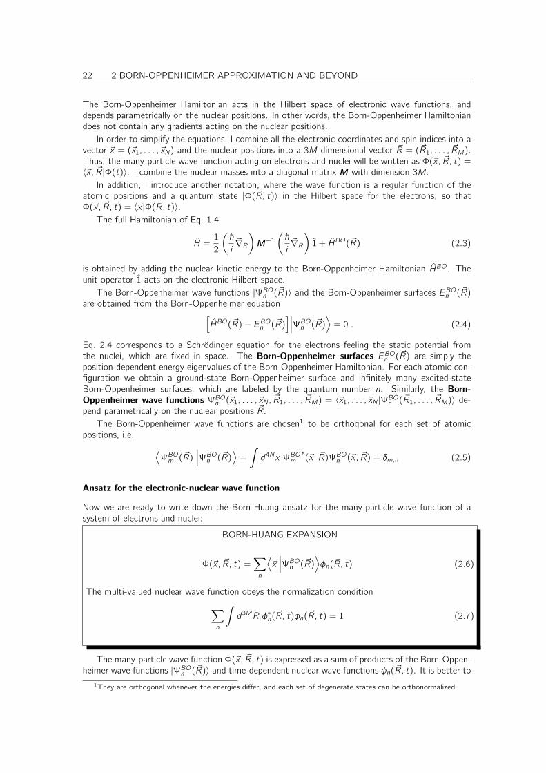
Firstly, we construct the Born-Oppenheimer Hamiltonian HBO by removing all terms that depend onthe momenta of the nuclei from the many-particle Hamiltonian given in Eq. 1.4.
HBO(~R1, . . . , ~RM) =
N∑
i=1
−~22me
~∇2~ri︸ ︷︷ ︸
Ekin,e
+1
2
M∑
i 6=j
e2ZiZj
4πǫ0|~Ri − ~Rj |︸ ︷︷ ︸
EC,nuc−nuc
−N∑
i=1
M∑
j=1
e2Zj
4πǫ0|~ri − ~Rj |︸ ︷︷ ︸
EC ,e−nuc
+1
2
N∑
i 6=j
e2
4πǫ0|~ri − ~rj |︸ ︷︷ ︸
EC ,e−e
(2.2)
21
22 2 BORN-OPPENHEIMER APPROXIMATION AND BEYOND
The Born-Oppenheimer Hamiltonian acts in the Hilbert space of electronic wave functions, anddepends parametrically on the nuclear positions. In other words, the Born-Oppenheimer Hamiltoniandoes not contain any gradients acting on the nuclear positions.
In order to simplify the equations, I combine all the electronic coordinates and spin indices into avector ~x = (~x1, . . . , ~xN) and the nuclear positions into a 3M dimensional vector ~R = (~R1, . . . , ~RM).Thus, the many-particle wave function acting on electrons and nuclei will be written as Φ(~x, ~R, t) =〈~x, ~R|Φ(t)〉. I combine the nuclear masses into a diagonal matrix M with dimension 3M.
In addition, I introduce another notation, where the wave function is a regular function of theatomic positions and a quantum state |Φ(~R, t)〉 in the Hilbert space for the electrons, so thatΦ(~x, ~R, t) = 〈~x |Φ(~R, t)〉.
The full Hamiltonian of Eq. 1.4
H =1
2
(~
i~∇R)
M−1(~
i~∇R)
1 + HBO(~R) (2.3)
is obtained by adding the nuclear kinetic energy to the Born-Oppenheimer Hamiltonian HBO. Theunit operator 1 acts on the electronic Hilbert space.
The Born-Oppenheimer wave functions |ΨBOn (~R)〉 and the Born-Oppenheimer surfaces EBOn (~R)are obtained from the Born-Oppenheimer equation
[
HBO(~R)− EBOn (~R)]∣∣∣ΨBOn (~R)
⟩
= 0 . (2.4)
Eq. 2.4 corresponds to a Schrödinger equation for the electrons feeling the static potential fromthe nuclei, which are fixed in space. The Born-Oppenheimer surfaces EBOn (~R) are simply theposition-dependent energy eigenvalues of the Born-Oppenheimer Hamiltonian. For each atomic con-figuration we obtain a ground-state Born-Oppenheimer surface and infinitely many excited-stateBorn-Oppenheimer surfaces, which are labeled by the quantum number n. Similarly, the Born-Oppenheimer wave functions ΨBOn (~x1, . . . , ~xN , ~R1, . . . , ~RM) = 〈~x1, . . . , ~xN |ΨBOn (~R1, . . . , ~RM)〉 de-pend parametrically on the nuclear positions ~R.
The Born-Oppenheimer wave functions are chosen1 to be orthogonal for each set of atomicpositions, i.e.
⟨
ΨBOm (~R)∣∣∣ΨBOn (~R)
⟩
=
∫
d4Nx ΨBOm∗(~x, ~R)ΨBOn (~x, ~R) = δm,n (2.5)
Ansatz for the electronic-nuclear wave function
Now we are ready to write down the Born-Huang ansatz for the many-particle wave function of asystem of electrons and nuclei:
BORN-HUANG EXPANSION
Φ(~x, ~R, t) =∑
n
⟨
~x∣∣∣ΨBOn (~R)
⟩
φn(~R, t) (2.6)
The multi-valued nuclear wave function obeys the normalization condition
∑
n
∫
d3MR φ∗n(~R, t)φn(~R, t) = 1 (2.7)
The many-particle wave function Φ(~x, ~R, t) is expressed as a sum of products of the Born-Oppen-heimer wave functions |ΨBOn (~R)〉 and time-dependent nuclear wave functions φn(~R, t). It is better to
1They are orthogonal whenever the energies differ, and each set of degenerate states can be orthonormalized.
2 BORN-OPPENHEIMER APPROXIMATION AND BEYOND 23
think of Born-Oppenheimer wave functions and nuclear wave functions as multi-valued wave functionswith a component for each ground or excited state labelled by n. While the Born-Oppenheimer wavefunctions depend on the positions of the nuclei, the nuclear wave functions φn(~R1, . . . , ~RM , t) do nomore refer to the electronic positions, except for the state index n.
Some caution is required to keep the symbols for the different types of wave functions apart
Φ(~x, ~R, t) many-particle wave function of electrons and nucleiΨBOn (~x, ~R) Born-Oppenheimer wave function of electronsφn(~R, t) component of the nuclear wave function
Physical meaning of the Born-Huang expansion: In order to convey some of the physical meaningof the quantities defined in the Born-Huang ansatz, let me anticipate a few observations that will bederived and stated more rigorously in the following sections.
• One Born-Oppenheimer surface can be considered as the potential energy surface governingthe motion of the nuclei. The forces acting on the atoms are the negative gradients of theBorn-Oppenheimer surface. The Born-Oppenheimer surface is the object that is parameterizedin classical molecular dynamics simulations.
• The squared nuclear wave function describes the probability density pn(~R, t)def= φ∗n(~R, t)φn(~R, t)
for the nuclei to be at positions ~R and for the electrons to be in the n-th excited state.
• If the electrons remain in the ground state, only the nuclear wave function φ0(~R, t) with n = 0differs from zero, and the atomic motion is entirely determined by the single valued potentialenergy EBO0 (~R).
• An optical absorption event is usually sufficiently rapid, that the nuclei do not move by anyappreciable distance during that process. This is the Franck-Condon principle. In that casewe can estimate the absorption energy as the energy difference between two Born-Oppenheimersurfaces for the same nuclear coordinates.
The Born-Huang Expansion is not an approximation: It is important to realize that the Born-Huang expansion for the wave function is not an approximation. Every wave function can exactlybe represented in this form. For any given vector R and time t, the wave function Φ(~x, ~R, t) is afunction of the electronic coordinates ~x . This function can be expanded into any complete basisset|Ψn〉 in the form
Φ(~x, ~R, t) =∑
n
⟨
~x∣∣∣Ψn
⟩
cn(~R, t) (2.8)
with complex coefficients c(~R). Because the wave function changes with ~R and t, the coefficientsdepend on nuclear positions and time.
With the same right, one can choose a different complete basisset |Ψn(~R)〉 for every set ofnuclear coordinates, so that
Φ(~x, ~R, t) =∑
n
⟨
~x∣∣∣Ψn(~R)
⟩
cn(~R, t) (2.9)
The eigenstates of the Born-Oppenheimer approximation form such a complete basisset. Thuswe can replace |Ψn(~R)〉 by the Born-Oppenheimer wave functions. The corresponding coefficientsare the nuclear wave functions
Φ(~x, ~R, t) =∑
n
⟨
~x∣∣∣ΨBOn (~R)
⟩
φn(~R, t) (2.10)
which is nothing but the Born-Huang expansion Eq. 2.6.
24 2 BORN-OPPENHEIMER APPROXIMATION AND BEYOND
Nuclear Schrödinger equation
When the Born-Huang expansion, Eq. 2.6, is inserted into the many-particle Schrödinger equationEq. 1.1 with the full Hamiltonian Eq. 1.4, we obtain
i~∂t
[∑
n
∣∣∣ΨBOn (~R)
⟩
φn(~R, t)
]
Eq. 1.1= H
[∑
n
∣∣∣ΨBOn (~R)
⟩
φn(~R, t)
]
Eq. 2.3=
[1
2
(~
i~∇R)
M−1(~
i~∇R)
+ HBO] [∑
n
∣∣∣ΨBOn (~R)
⟩
φn(~R, t)
]
Eq. 2.4=
∑
n
∣∣∣ΨBOn (~R)
⟩[1
2
(~
i~∇R)
M−1(~
i~∇R)
+ EBOn (~R)
]
φn(~R, t)
+∑
n
[(~
i~∇R) ∣∣∣ΨBOn (~R)
⟩]
M−1(~
i~∇R)
+1
2
(~
i~∇R)
M−1(~
i~∇R) ∣∣∣ΨBOn (~R)
⟩
φn(~R, t)
(2.11)
Now we multiply Eq. 2.11 from the left with the bra of the Born-Oppenheimer wave function⟨
ΨBOm (~R)∣∣∣ and integrate over the electronic coordinates. Hereby, we exploit the orthonormality
Eq. 2.5 of the Born-Oppenheimer wave functions.As the result, we obtain a Schrödinger equation for the nuclear motion alone.
i~∂tφm(~R, t)Eqs. 2.11,2.5
=
[~
i~∇RM−1
~
i~∇R + EBOm (~R)
]
φm(~R, t)
+∑
n
[⟨ΨBOm
∣∣~
i~∇R∣∣ΨBOn
⟩M−1 ~
i~∇R +
1
2
⟨ΨBOm
∣∣~
i~∇RM−1
~
i~∇R∣∣ΨBOn
⟩]
︸ ︷︷ ︸
derivative couplings
φn(~R, t)
(2.12)
Note, that the brackets 〈. . .〉 are evaluated by integrating over the electronic degrees of freedomonly. Thus, the matrix elements still depend explicitly on the nuclear coordinates. Note also, thatthe gradients ~∇R in the parentheses act on the nuclear and not the electronic wave functions, whichis easily overlooked. The gradients ~∇R inside the matrix elements only act on the ket |ΨBOn 〉, butnot on the functions outside the matrix element.
Up to now, we did not introduce any approximations to arrive at the nuclear Schrödinger equationEq. 2.12. We are still on solid ground.
Derivative couplings
In the following, we will discuss the individual terms of Eq. 2.12. Before we continue, however, letus simplify the notation again: The general structure of Eq. 2.12 is
i~∂tφm(~R, t) =
[1
2~PM−1 ~P + EBOm (~R)
]
φm(~R, t) +∑
n
[
~Am,n(~R)M−1 ~P + Bm,n(~R)
]
φn(~R, t)
(2.13)
where ~P = ~
i~∇R is the momentum vector of the nuclear coordinates and the first- and second-
derivative couplings are defined by
~Am,n(~R) :=⟨
ΨBOm (~R)∣∣∣~
i~∇R∣∣∣ΨBOn (~R)
⟩
(2.14)
Bm,n(~R) :=1
2
⟨
ΨBOm (~R)∣∣∣
(~
i~∇R)
M−1(~
i~∇R) ∣∣∣ΨBOn (~R)
⟩
(2.15)
2 BORN-OPPENHEIMER APPROXIMATION AND BEYOND 25
Second-order couplings from first-order derivative couplings: The first and the second-derivativecouplings are not independent of each other: The second-derivative coupling Bm,n(~R) can be ex-pressed by the first-derivative couplings ~Am,n(~R). This is shown as follows (see [9]):
~
i~∇RM−1 ~Am,n(~R)
Eq. 2.14=
~
i~∇RM−1
⟨
ΨBOm (~R)
∣∣∣∣
~
i~∇R∣∣∣∣ΨBOn (~R)
⟩
= −⟨~
i~∇RΨBOm (~R)
∣∣∣∣M−1 ~
i~∇R∣∣∣∣ΨBOn (~R)
⟩
+
⟨
ΨBOm (~R)
∣∣∣∣
(~
i~∇R)
M−1(~
i~∇R)∣∣∣∣ΨBOn (~R)
⟩
︸ ︷︷ ︸
2Bm,n(~R
Eq. 2.15= −
⟨~
i~∇RΨBOm (~R)
∣∣∣∣
(∑
k
∣∣∣∣ΨBOk (~R)
⟩⟨
ΨBOk (~R)
∣∣∣∣
)
︸ ︷︷ ︸
=1
M−1 ~
i~∇R∣∣∣∣ΨBOn (~R)
⟩
+ 2Bm,n(~R)
= −∑
k
⟨~
i~∇RΨBOm (~R)
∣∣∣∣ΨBOk (~R)
⟩
M−1⟨
ΨBOk (~R)
∣∣∣∣
~
i~∇R∣∣∣∣ΨBOn (~R)
⟩
+ 2Bm,n(~R)
= −∑
k
⟨
ΨBOk (~R)
∣∣∣∣
~
i~∇R∣∣∣∣ΨBOm (~R)
⟩∗M−1⟨
ΨBOk (~R)
∣∣∣∣
~
i~∇R∣∣∣∣ΨBOn (~R)
⟩
+ 2Bm,n(~R)
= −∑
k
~A∗k,m(~R)M−1 ~Ak,n(~R) + 2Bm,n(~R)
Next, we exploit that the first-derivative couplings ~Am,n are hermitian in the band indices, i.e.~A∗k,m(~R) = ~Am,k(~R), which can be shown as follows: We start from the orthonormality conditionEq. 2.5 of the Born-Oppenheimer wave functions, which holds for all ~R. Thus the nucler gradient ofthe scalar products vanishes
0Eq. 2.5= ~∇R
δm,n︷ ︸︸ ︷
〈ΨBOm |ΨBOn 〉= 〈~∇RΨBOm |ΨBOn 〉+ 〈ΨBOm |~∇R|ΨBOn 〉= 〈ΨBOn |~∇RΨBOm 〉∗ + 〈ΨBOm |~∇R|ΨBOn 〉
⇒ 0 = −〈ΨBOn |~
i~∇RΨBOm 〉∗ + 〈ΨBOm |
~
i~∇R|ΨBOn 〉
⇒ ~A∗k,m(~R) =⟨
ΨBOk
∣∣∣~
i~∇R∣∣∣ΨBOm
⟩∗=⟨
ΨBOm
∣∣∣~
i~∇R∣∣∣ΨBOk
⟩
= ~Am,k(~R) (2.16)
This allows us to rewrite Eq. 2.16 in the form
2Bm,n(~R) =~
i~∇RM−1 ~Am,n(~R) +
∑
k
~Am,k(~R)M−1 ~Ak,n(~R) (2.17)
Thus, we only need to evaluate the first-derivative couplings, while the second-derivative couplingscan be obtained from the former via Eq. 2.17.
Final form for the nuclear Schrödinger equation
Insertion of the second derivative couplings from Eq. 2.17 into the nuclear Schrödinger equationEq. 2.13 into the final form of Eq. 2.20.
Let me sketch here the line of thought schematically. I am dropping the matrix structure of theequation for the sake of clarity. The terms in Eq. 2.13 related to momenta and derivative couplings
26 2 BORN-OPPENHEIMER APPROXIMATION AND BEYOND
have the form
(1
2~PM−1 ~P + ~AM−1 ~P + B
)
|φ〉 Eq. 2.17=
1
2
(
~PM−1 ~P + 2~AM−1 ~P + (~PM−1 ~A) + ~AM−1 ~A)
|φ〉
=1
2
(
~PM−1 ~P + ~AM−1 ~P + ~PM−1 ~A+ ~AM−1 ~A)
|φ〉
=1
2
(
~P + ~A)
M−1(
~P + ~A)
|φ〉 (2.18)
We used the the chain rule for ~P , which is a gradient operator.
~PM−1 ~A|φ〉 = (~PM−1 ~A)|φ〉+ ~AM−1 ~P |φ〉 (2.19)
In this manner one arrives at our final form Eq. 2.20 for the nuclear Schrödinger equation.
SCHRÖDINGER EQUATION FOR THE NUCLEAR WAVE FUNCTIONS IN TERMS OFBORN-OPPENHEIMER WAVE FUNCTIONS
i~∂tφm(~R, t) =∑
n
[1
2
∑
k
(
δm,k~
i~∇R + ~Am,k(~R)
)
M−1(
δk,n~
i~∇R + ~Ak,n(~R)
)
+δm,nEBOm (~R)
]
φn(~R, t) (2.20)
or, combining the components of the nuclear wave functions in a vector-matrix notation – using asingle underline to denote a vector and a double underline for a matrix –
i~∂tφ(~R, t) =
(
1 ~P + ~A(~R))2
2M+ EBO(~R)
φ(~R, t) (2.21)
EBO denotes the diagonal matrix with the Born-Oppenheimer energies as diagonal elements and
~P = ~
i~∇R is the 3M-dimensional momentum operator of the nuclei. The kinetic energy expression in
Eq. 2.21 is mathematically not allowed, because I wrote a vector-matrix-vector expression as vector-squared-divided-by-matrix. I used it here to allude to the corresponding equation from electrodynamicsso that it can be memorized more easily, and because the matrix M is a diagonal matrix so that theexpression can be evaluated component by component.The first-derivative couplings ~Am,k(~R) are defined in Eq. 2.14.
~Am,n(~R)Eq. 2.14:=
⟨
ΨBOm (~R)∣∣∣~
i~∇R∣∣∣ΨBOn (~R)
⟩
=⟨
ΨBOm (~R)∣∣∣ ~P∣∣∣ΨBOn (~R)
⟩
(2.22)
As shown in Eq. 2.16, each vector component of the first-derivative couplings is a hermitian matrixin the indices m, n.
This form of the nuclear Schrödinger equation, i.e. Eq. 2.21, has been mentioned2 already in1969 by F. Smith[10].
We have not introduced any approximations to bring Eq. 2.12 into the new form given by Eq. 2.21.That is, we are still on solid grounds.
2see his Eq. 10. His ~P (R) are the first-derivative couplings.
2 BORN-OPPENHEIMER APPROXIMATION AND BEYOND 27
Relation to electrodynamics
Interesting is the formal similarity of the nuclear Hamilton function in Eq. 2.14 with that of a chargedparticle in a electromagnetic field, which has the form
H(~p,~r) =1
2m
(
~p − q ~A(~r))2
+ qΦ(~r)
This analogy shows that the diagonal terms (in the band indices) of the derivative couplings act likea magnetic field ~B expressed by the vector potential ~A as ~B = ~∇ × ~A and an electric potential Φ.We will discuss this analogy later in somewhat more detail in the appendix D.2.
2.2 Approximations
2.2.1 Born-Oppenheimer approximation
The Born-Oppenheimer approximation amounts to ignoring the derivative couplings in Eq. 2.20
BORN-OPPENHEIMER APPROXIMATION FOR THE NUCLEAR WAVE FUNCTION
i~∂tφn(~R, t) =
M∑
j=1
−~22Mj
~∇2Rj + EBOn (~R)
φn(~R, t) (2.23)
This equation describes nuclei that move on a given total energy surface EBOn (~R), which is calledthe Born-Oppenheimer surface. The Born-Oppenheimer surface may be an excited-state surface orthe ground-state surface. The wave function may also have contributions simultaneously on differenttotal energy surfaces. However, within the Born-Oppenheimer approximation, the contributions ondifferent surfaces do not influence each other.
In other words, the system is with probability Pn =∫d3MR φ∗n(~R)φn(~R) on the excited state
surface EBOn (~R). In the Born-Oppenheimer approximation, this probability does not change withtime.
The neglect of the non-adiabatic effects is the essence of the Born-Oppenheimer approximation.In the absence of the non-adiabatic effects, we could start the system in a particular eigenstate ofthe Born-Oppenheimer Hamiltonian, and the system would always evolve on the same total energysurface EBOn (~R). Thus, if we start the system in the electronic ground state, it will remain exactlyin the instantaneous electronic ground state, while the nuclei are moving. Band crossings are theexceptions: Here, the Born-Oppenheimer approximation does not give a unique answer.
The separation of nuclear and electronic degrees of freedom have already been in use before theoriginal Born-Oppenheimer approximation[11]. Born and Oppenheimer [7] gave a justification for ne-glecting the non-adiabatic effects in many cases. As we will see the Born-Oppenheimer approximationbreaks down when Born-Oppenheimer surfaces come very close or even cross.
2.2.2 Classical approximation
Classical approximation in the Born-Oppenheimer approximation
The most simple approach to the classical approximation is to take the Hamilton operator in theBorn-Oppenheimer approximation from Eq. 2.23, constrain it to a particular total-energy surfacespecified by n, and to form the corresponding Hamilton function.
Hn(~P , ~R) =∑
j
~P 2j2Mj
+ EBOn (~R)
28 2 BORN-OPPENHEIMER APPROXIMATION AND BEYOND
The Hamilton function defines the classical Hamilton equations of motion
∂t ~Rj = ~∇PjHn(~P , ~R, t) =1
Mj
~Pj
∂t ~Pj = −~∇RjHn(~P , ~R, t) = −~∇RjEBOn (~R)
This in turn leads to the Newton’s equations of motion for the nuclei
Mj∂2t~Rj = −~∇RjEBOn (~R)
This is the approximation that is most widely used to study the dynamics of the atoms ina molecule or a solid. A simulation of classical atoms using some kind of parameterized Born-Oppenheimer surface is called molecular dynamics simulation. When the Born-Oppenheimer sur-face is obtained on the fly from a quantum mechanical electronic structure method, the method iscalled ab-initio molecular dynamics.
The Born-Oppenheimer surface EBOn (~R) acts just like a total-energy surface for the motion ofthe nuclei. Once EBOn (~R) is known, the electrons are taken completely out of the picture. Withinthe Born-Oppenheimer approximation, no transitions between the ground-state and the excited-statesurface take place. This implies not only that a system in the electronic ground state remains inthe ground state. It also implies that a system in the excited state will remain there for ever.Transitions between different sheets EBOn (~R) of the Born-Oppenheimer energy are only possiblewhen non-adiabatic effects are included.
2.3 Non-adiabatic corrections
While the Born-Oppenheimer approximation is a widely used and tremendously successful approach,its limitations are important for relaxation processes, photochemistry, charge transfer processes andmany more interesting processes. They shall be briefly discussed here.
We will see that the derivative couplings governing the non-adiabatic effects are singular wheretwo Born-Oppenheimer surface meet. Unfortunately, these are exactly the points of physical interest,namely those where a system makes a non-radiative transition from one Born-Oppenheimer surfaceto another. Even worse, these singular points have non-local consequences, so-called topologicaleffects.
Interesting is a close formal similarity between non-adiabatic effects and field theory[12]. Relatedtopics are the Aharonov-Bohm effect[13] and Yang-Mills fields[14].
Under normal circumstances, the diagonal terms of the derivative couplings are of secondary im-portance. The diagonal term of the derivative couplings are discussed in the appendix D.2. Theybecome, however, important in the presence of conical intersections and in the presence of a geo-metrical phase.
2.3.1 Non-diagonal derivative couplings
The off-diagonal elements of the first-derivative couplings defined in Eq. 2.22 can be brought intothe form
~Am,n =
⟨
ΨBOm
∣∣∣
(~
i~∇RHBO(~R)
)∣∣∣ΨBOn
⟩
EBOn (~R)− EBOm (~R)for EBOm 6= EBOn (2.24)
The gradient acts only on the Born-Oppenheimer Hamiltonian but not further to the state on theright. This expression makes it evident that non-adiabatic effects are important when two Born-Oppenheimer surfaces become degenerate, i.e. when EBOm = EBOn .
2 BORN-OPPENHEIMER APPROXIMATION AND BEYOND 29
Derivation of Eq. D.2 The off-diagonal elements of ~An,m(~R) of the first-derivative couplings areobtained as follows: We begin with the Schrödinger equation for the Born-Oppenheimer wave function
(
HBO(~R)− EBOn (~R))
|ΨBOn (~R)〉Eq. 2.4= 0
Because this equation is valid for all atomic positions, the gradient of the above expression vanishes.
0 = ~∇R(
HBO(~R)− EBOn (~R)) ∣∣∣ΨBOn (~R)
⟩
=(
~∇R, HBO(~R)) ∣∣∣ΨBOn (~R)
⟩
−∣∣∣ΨBOn (~R)
⟩
~∇REBOn (~R) +(
HBO(~R)− EBOn (~R))
~∇R∣∣∣ΨBOn (~R)
⟩
Now, we multiply from the left with the bra 〈ΨBOm | and form the scalar products in the electronicHilbert space.3
0 =⟨ΨBOm
∣∣
(
~∇RHBO(~R)) ∣∣ΨBOn
⟩−⟨ΨBOm
∣∣ΨBOn
⟩~∇REBOn (~R) +
⟨ΨBOm
∣∣
(
HBO(~R)− EBOn (~R))
~∇R∣∣ΨBOn
⟩
=⟨ΨBOm
∣∣
(
~∇R, HBO(~R)) ∣∣ΨBOn
⟩− δm,n~∇REBOn (~R)︸ ︷︷ ︸
=0for m 6= n
+
(
EBOm (~R)− EBOn (~R))⟨ΨBOm
∣∣ ~∇R
∣∣ΨBOn
⟩
If the indices m, n differ, the middle term containing gradient of the Born-Oppenheimer surfacesvanishes. If the energies EBOm , EBOn furthermore differ, we can divide by their difference which bringsus to the desired result.
~Am,nEq. 2.14=
⟨ΨBOm
∣∣~
i~∇R∣∣ΨBOn
⟩=〈ΨBOm |
(~
i~∇RHBO(~R)
)
|ΨBOn 〉EBOn (~R)− EBOm (~R)
for En 6= Em (2.25)
This is the proof for Eq. 2.24 given above. Unfortunately, no information can be extracted for thediagonal elements of the first-derivative couplings.
2.3.2 Topology of crossings of Born-Oppenheimer surfaces
The off-diagonal non-adiabatic effects Eq. 2.24 become important, when the different Born-Oppenheimersurfaces come close or even cross. Therefore we need to understand the topology of crossings ofBorn-Oppenheimer surfaces.
Non-crossing rule and conical intersections
The most important information on the topology of surface crossings is provided by the non-crossingrule of von Neumann and Wigner[15]. It is derived in appendix E on p. 255.
NON-CROSSING RULE
Consider a Hamiltonian H(Q1, . . . , Qm) which depends on m parameters Q1, . . . , Qm. For eachaccidental crossing of two eigenvalues, there is a three-dimensional subspace of the parameter spacein which the degeneracy is lifted except for a single point.If the hamiltonian is real for all parameters, the subspace where the degeneracy is lifted has twodimensions.
• In our case, the Hamiltonian is the Born-Oppenheimer Hamiltonian and the parameters are thenuclear positions.
3The Born-Oppenheimer wave functions depend on electronic and nuclear coordinates. The nuclear coordinates,however, play a different role, because they are treated like external parameters.
30 2 BORN-OPPENHEIMER APPROXIMATION AND BEYOND
• Two energy surfaces that meet in a point within a two-dimensional space form two cones.Therefore the crossing is called a conical intersection.
• The hamiltonian is usually4 real in the absence of magnetic fields and relativistic effects. Spin-orbit coupling, a relativistic effect, and magnetic fields that act on the orbital motion of chargedparticles introduce complex contributions. The question whether the Hamiltonian is real isrelated to time inversion symmetry discussed in Appendix L on p. L.
• The limitation of the non-crossing rule to accidental crossings implies that there are no limita-tions on crossings that occur because two states have different symmetry.
• The non-crossing rule implies that there are no accidental crossings for dimeric molecules
Let me consider a conical intersection related to the motion of a single atom in a molecule or solid.Let me furthermore consider real Hamiltonians. For this example, the conical intersection would forma one-dimensional line. The two displacements perpendicular to this line lift the degeneracy. If weplot the energy surfaces in the plane of these two distortions, the Born-Oppenheimer surfaces wouldhave the shape of a double cone, a conical intersection. A change of a coordinate along the linewill change the shape of the cone, but it will not affect the qualitative cone-like topology.
More generally, there is a two-dimensional plane of coordinates relevant to the conical intersection.Distortions of distan nuclei will not affect the general shape of the conical intersection, while theydo have an effect on the total energy.
2.3.3 Avoided crossings
Often, the symmetries that are responsible for a degeneracy, which is a surface crossing, are onlyapproximately present. A small matrix element lifts the degeneracy “a little”. This is called an avoidedavoided crossing. Due to an avoided crossing two Born-Oppenheimer sheets may be come so closethat the non-adiabatic effects can no more be ignored. Thus, regions with avoided crossings areimportant for the relaxation of the system onto a Born-Oppenheimer surface with lower energy.
What is an avoided crossing? Let me start with a position-dependent Hamiltonian for a one-dimensional nuclear coordinate R, for which the energy levels cross for a certain position R0 = 0. Inaddition we add non-diagonal terms ∆.
The Hamilton has the form
H =P 2
2M+
(
|a〉|b〉
)(
E0 + FQ −∆−∆ E0 − FQ
)(
〈a|〈b|
)
︸ ︷︷ ︸
HBO
(2.26)
The Born-Oppenheimer Hamiltonian is obtained by stripping away the nuclear kinetic energy andby converting the coordinate operator Q into a parameter.
HBO(Q) =
(
|a〉|b〉
)(
E0 + FQ −∆−∆ E0 − FQ
)(
〈a|〈b|
)
(2.27)
Diagonalization of the Born-Oppenheimer Hamiltonian yields the two Born-Oppenheimer surfaces
EBO± (Q) = E0 ± ∆
√
1 +
(F
∆Q
)2
(2.28)
where the minus sign applies for the lower and the plus sign for the upper Born-Oppenheimer surface.
4There are other interactions that are similar to a magnetic field. They are, however, not very important for solidstate physics.
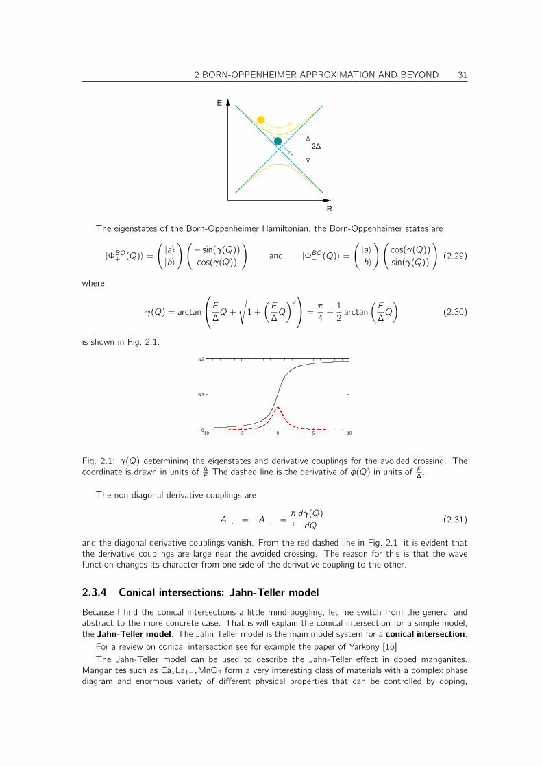
2 BORN-OPPENHEIMER APPROXIMATION AND BEYOND 31
R
E
2∆
The eigenstates of the Born-Oppenheimer Hamiltonian, the Born-Oppenheimer states are
|ΦBO+ (Q)〉 =(
|a〉|b〉
)(
− sin(γ(Q))cos(γ(Q))
)
and |ΦBO− (Q)〉 =(
|a〉|b〉
)(
cos(γ(Q))
sin(γ(Q))
)
(2.29)
where
γ(Q) = arctan
F
∆Q+
√
1 +
(F
∆Q
)2
=π
4+1
2arctan
(F
∆Q
)
(2.30)
is shown in Fig. 2.1.
-10 -5 0 5 100
π/2
π/4
Fig. 2.1: γ(Q) determining the eigenstates and derivative couplings for the avoided crossing. Thecoordinate is drawn in units of ∆F The dashed line is the derivative of φ(Q) in units of F
∆ .
The non-diagonal derivative couplings are
A−,+ = −A+,− =~
i
dγ(Q)
dQ(2.31)
and the diagonal derivative couplings vanish. From the red dashed line in Fig. 2.1, it is evident thatthe derivative couplings are large near the avoided crossing. The reason for this is that the wavefunction changes its character from one side of the derivative coupling to the other.
2.3.4 Conical intersections: Jahn-Teller model
Because I find the conical intersections a little mind-boggling, let me switch from the general andabstract to the more concrete case. That is will explain the conical intersection for a simple model,the Jahn-Teller model. The Jahn Teller model is the main model system for a conical intersection.
For a review on conical intersection see for example the paper of Yarkony [16]The Jahn-Teller model can be used to describe the Jahn-Teller effect in doped manganites.
Manganites such as CaxLa1−xMnO3 form a very interesting class of materials with a complex phasediagram and enormous variety of different physical properties that can be controlled by doping,
32 2 BORN-OPPENHEIMER APPROXIMATION AND BEYOND
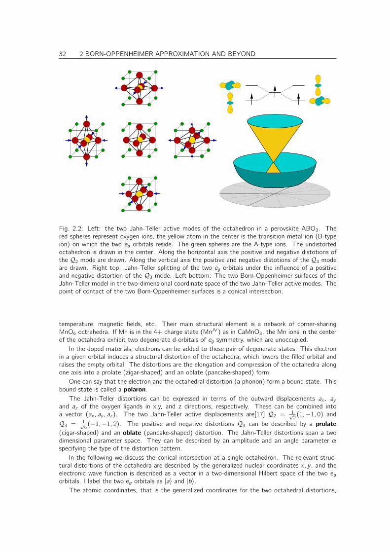
Fig. 2.2: Left: the two Jahn-Teller active modes of the octahedron in a perovskite ABO3. Thered spheres represent oxygen ions, the yellow atom in the center is the transition metal ion (B-typeion) on which the two eg orbitals reside. The green spheres are the A-type ions. The undistortedoctahedron is drawn in the center. Along the horizontal axis the positive and negative distotions ofthe Q2 mode are drawn. Along the vertical axis the positive and negative distotions of the Q3 modeare drawn. Right top: Jahn-Teller splitting of the two eg orbitals under the influence of a positiveand negative distortion of the Q3 mode. Left bottom: The two Born-Oppenheimer surfaces of theJahn-Teller model in the two-dimensional coordinate space of the two Jahn-Teller active modes. Thepoint of contact of the two Born-Oppenheimer surfaces is a conical intersection.
temperature, magnetic fields, etc. Their main structural element is a network of corner-sharingMnO6 octrahedra. If Mn is in the 4+ charge state (MnIV ) as in CaMnO3, the Mn ions in the centerof the octahedra exhibit two degenerate d-orbitals of eg symmetry, which are unoccupied.
In the doped materials, electrons can be added to these pair of degenerate states. This electronin a given orbital induces a structural distortion of the octahedra, which lowers the filled orbital andraises the empty orbital. The distortions are the elongation and compression of the octahedra alongone axis into a prolate (zigar-shaped) and an oblate (pancake-shaped) form.
One can say that the electron and the octahedral distortion (a phonon) form a bound state. Thisbound state is called a polaron.
The Jahn-Teller distortions can be expressed in terms of the outward displacements ax , ayand az of the oxygen ligands in x,y, and z directions, respectively. These can be combined intoa vector (ax , ay , az). The two Jahn-Teller active displacements are[17] Q2 = 1√
2(1,−1, 0) and
Q3 = 1√6(−1,−1, 2). The positive and negative distortions Q3 can be described by a prolate
(cigar-shaped) and an oblate (pancake-shaped) distortion. The Jahn-Teller distortions span a twodimensional parameter space. They can be described by an amplitude and an angle parameter αspecifying the type of the distortion pattern.
In the following we discuss the conical intersection at a single octahedron. The relevant struc-tural distortions of the octahedra are described by the generalized nuclear coordinates x, y , and theelectronic wave function is described as a vector in a two-dimensional Hilbert space of the two egorbitals. I label the two eg orbitals as |a〉 and |b〉.
The atomic coordinates, that is the generalized coordinates for the two octahedral distortions,
2 BORN-OPPENHEIMER APPROXIMATION AND BEYOND 33
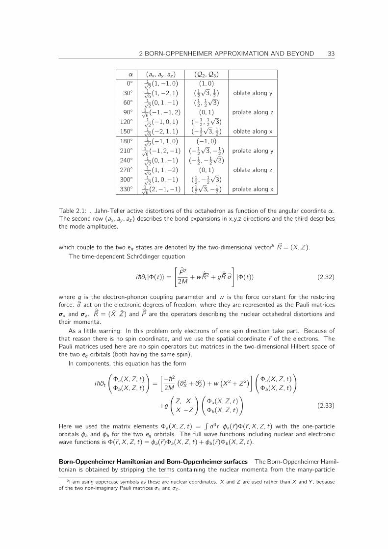
α (ax , ay , az) (Q2,Q3)0 1√
2(1,−1, 0) (1, 0)
30 1√6(1,−2, 1) ( 12
√3, 12) oblate along y
60 1√2(0, 1,−1) ( 12 ,
12
√3)
90 1√6(−1,−1, 2) (0, 1) prolate along z
120 1√2(−1, 0, 1) (− 12 , 12
√3)
150 1√6(−2, 1, 1) (− 12
√3, 12) oblate along x
180 1√2(−1, 1, 0) (−1, 0)
210 1√6(−1, 2,−1) (− 12
√3,− 12) prolate along y
240 1√2(0, 1,−1) (− 12 ,− 12
√3)
270 1√6(1, 1,−2) (0, 1) oblate along z
300 1√2(1, 0,−1) ( 12 ,− 12
√3)
330 1√6(2,−1,−1) ( 12
√3,− 12) prolate along x
Table 2.1: . Jahn-Teller active distortions of the octahedron as function of the angular coordinte α.The second row (ax , ay , az) describes the bond expansions in x,y,z directions and the third describesthe mode amplitudes.
which couple to the two eg states are denoted by the two-dimensional vector5 ~R = (X,Z).The time-dependent Schrödinger equation
i~∂t |Φ(t)〉 =[~P 2
2M+ w ~R2 + g ~R ~σ
]
|Φ(t)〉 (2.32)
where g is the electron-phonon coupling parameter and w is the force constant for the restoringforce. ~σ act on the electronic degrees of freedom, where they are represented as the Pauli matrices
σx and σz . ~R = (X, Z) and ~P are the operators describing the nuclear octahedral distortions andtheir momenta.
As a little warning: In this problem only electrons of one spin direction take part. Because ofthat reason there is no spin coordinate, and we use the spatial coordinate ~r of the electrons. ThePauli matrices used here are no spin operators but matrices in the two-dimensional Hilbert space ofthe two eg orbitals (both having the same spin).
In components, this equation has the form
i~∂t
(
Φa(X,Z, t)
Φb(X,Z, t)
)
=
[−~22M
(∂2X + ∂
2Z
)+ w
(X2 + Z2
)](
Φa(X,Z, t)
Φb(X,Z, t)
)
+g
(
Z, X
X −Z
)(
Φa(X,Z, t)
Φb(X,Z, t)
)
(2.33)
Here we used the matrix elements Φa(X,Z, t) =∫d3r φa(~r)Φ(~r , X,Z, t) with the one-particle
orbitals φa and φb for the two eg orbitals. The full wave functions including nuclear and electronicwave functions is Φ(~r , X,Z, t) = φa(~r)Φa(X,Z, t) + φb(~r)Φb(X,Z, t).
Born-Oppenheimer Hamiltonian and Born-Oppenheimer surfaces The Born-Oppenheimer Hamil-tonian is obtained by stripping the terms containing the nuclear momenta from the many-particle
5I am using uppercase symbols as these are nuclear coordinates. X and Z are used rather than X and Y , becauseof the two non-imaginary Pauli matrices σx and σz .
34 2 BORN-OPPENHEIMER APPROXIMATION AND BEYOND
Hamiltonian.6
HBO(~R) = g
(
Z X
X −Z
)
+ w
(
X2 + Z2, 0
0, X2 + Z2
)
= g ~R · ~σ + w ~R2111 (2.34)
The first term describes the electronic Hamiltonian, that is the splitting of the degenerate electronicstates upon distortion, while the second term is a simple restoring potential for the nuclear distortions.
The characteristic equation for the eigenvalues EBO± (~R) is(
+gZ + w ~R2 − EBO± (~R) gX
gX −gZ + w ~R2 − EBO± (~R)
)(
φa,±φb,±
)
= 0 (2.35)
This yields the two Born-Oppenheimer surfaces of the Jahn-Teller model
BORN-OPPENHEIMER SURFACES OF THE JAHN-TELLER MODEL
EBO± (~R) = ±g|~R|+ w ~R 2 (2.36)
The Born-Oppenheimer surfaces EBO± (~R) are shown in Fig. 2.2. The two surfaces meet at a singlepoint, which is the conical intersection.
Born-Oppenheimer wave functions To construct the eigenstates we take the first line of Eq. 2.35and construct the orthogonal vector according to the rule (u, v) ⊥ (−v , u), and then we normalizeit. This yields the Born-Oppenheimer states |ΨBO± 〉 with components ΨBOa,± = 〈a|ΨBO± 〉 and ΨBOb,± =〈b|ΨBO± 〉.
(
ΨBOa,±ΨBOb,±
)
=
(
−gXgZ + w ~R2 ∓ g|~R| − w ~R2
)
1√
g2X2 +(
gZ + w ~R2 ∓ g|~R| − w ~R2)2
=
(
−XZ ∓ |~R|
)
1√
X2 +(
Z ∓ |~R|)2
(2.37)
The bar ontop of the symbol for the Born-Oppenheimer state is there to distinguish it from the finalresult, which is multiplied with an additional phase factor.
Now we switch to polar coordinates
X(R,α) = R sin(α)
Z(R,α) = R cos(α) (2.38)
which yields(
ΨBOa,±ΨBOb,±
)
=
(
− sin(α)∓(1∓ cos(α))
)
1√
2(1∓ cos(α))(2.39)
We use the triginometric identities∣∣∣sin
(x
2
)∣∣∣ =
√
1
2
(
1− cos(x))
∣∣∣cos
(x
2
)∣∣∣ =
√
1
2
(
1 + cos(x))
(2.40)
6 ~R~σ = Xσx + Y σy .
2 BORN-OPPENHEIMER APPROXIMATION AND BEYOND 35
to obtain(
ΨBOa,+ΨBOb,+
)
=
(
−2 sin(α2
)cos(α2
)
−2 sin2(α2
)
)
1
2| sin(α2
)| =
(
− cos(α2
)
− sin(α2
)
)
sgn(
sin(α/2))
(
ΨBOa,−ΨBOb,−
)
=
(
−2 sin(α2
)cos(α2
)
2 cos2(α2
)
)
1
2| cos(α2
)| =
(
− sin(α2
)
cos(α2
)
)
sgn(
cos(α/2))
(2.41)
where the sign function “sgn” is positive for positive arguments and negative for negative arguments.7
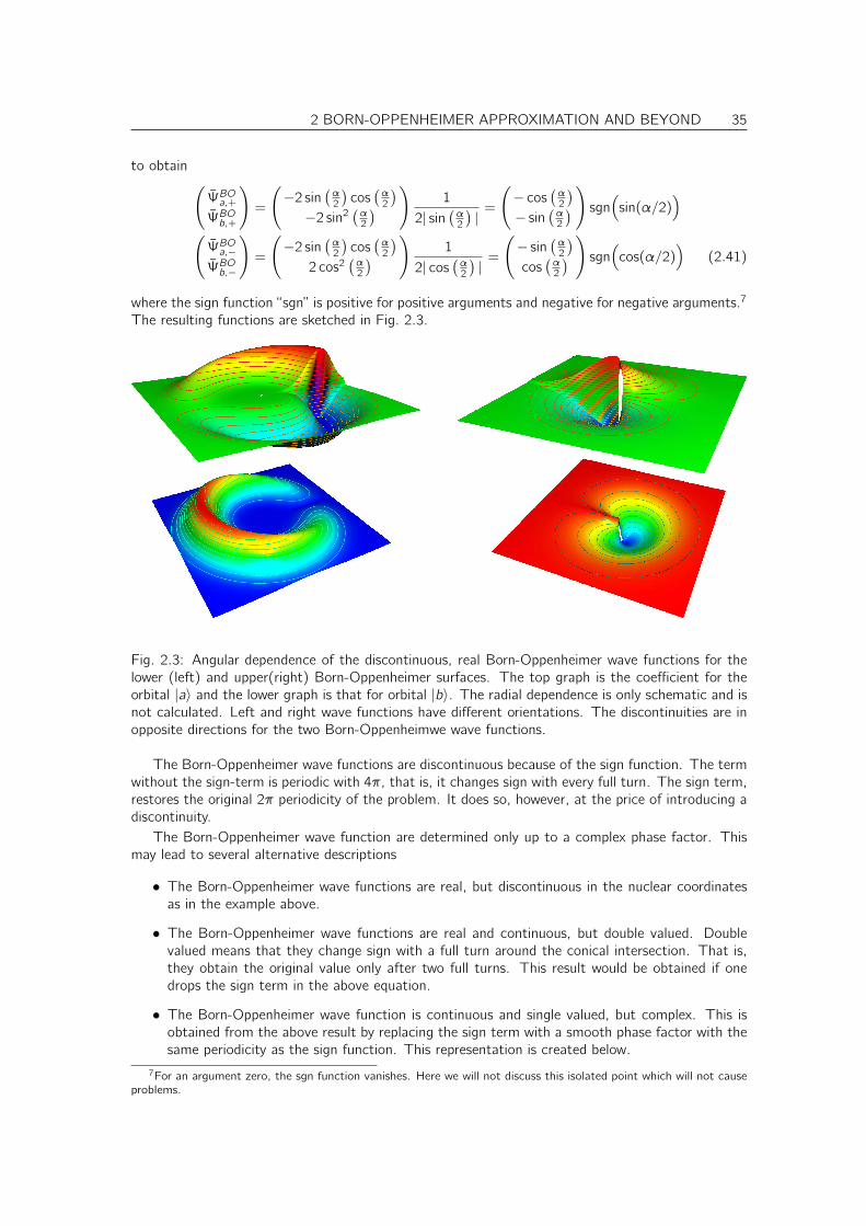
The resulting functions are sketched in Fig. 2.3.
Fig. 2.3: Angular dependence of the discontinuous, real Born-Oppenheimer wave functions for thelower (left) and upper(right) Born-Oppenheimer surfaces. The top graph is the coefficient for theorbital |a〉 and the lower graph is that for orbital |b〉. The radial dependence is only schematic and isnot calculated. Left and right wave functions have different orientations. The discontinuities are inopposite directions for the two Born-Oppenheimwe wave functions.
The Born-Oppenheimer wave functions are discontinuous because of the sign function. The termwithout the sign-term is periodic with 4π, that is, it changes sign with every full turn. The sign term,restores the original 2π periodicity of the problem. It does so, however, at the price of introducing adiscontinuity.
The Born-Oppenheimer wave function are determined only up to a complex phase factor. Thismay lead to several alternative descriptions
• The Born-Oppenheimer wave functions are real, but discontinuous in the nuclear coordinatesas in the example above.
• The Born-Oppenheimer wave functions are real and continuous, but double valued. Doublevalued means that they change sign with a full turn around the conical intersection. That is,they obtain the original value only after two full turns. This result would be obtained if onedrops the sign term in the above equation.
• The Born-Oppenheimer wave function is continuous and single valued, but complex. This isobtained from the above result by replacing the sign term with a smooth phase factor with thesame periodicity as the sign function. This representation is created below.
7For an argument zero, the sgn function vanishes. Here we will not discuss this isolated point which will not causeproblems.
36 2 BORN-OPPENHEIMER APPROXIMATION AND BEYOND
In the literature the first choice, namely real Born-Oppenheimer wave functions are usually as-sumed, explicitely or implicitely. In order to avoid discontinuities, half-integer spins are introduced.While this may have some intellectural appeal, I find the resulting double-valuedness of the wave func-tion highly ambiguous. Therefore, I follow a different path and admit that the Born-Oppenheimerwave functions are complex-valued.
By replacing the sign function by8 ∓eiα/2, i.e.
|ΨBO+ 〉 = −|ΨBO+ 〉sgn(
sin(α/2))
eiα/2
|ΨBO− 〉 = +|ΨBO− 〉sgn(
cos(α/2))
eiα/2 (2.42)
we obtain9 Born-Oppenheimer states
(
ΨBOa,+ΨBOb,+
)
=
(
cos(α/2)
sin(α/2)
)
eiα/2 =1
2
(
eiα + 1
−i(eiα − 1)
)
(
ΨBOa,−ΨBOb,−
)
=
(
− sin(α/2)cos(α/2)
)
eiα/2 =1
2
(
+i(eiα − 1)eiα + 1
)
(2.43)
BORN-OPPENHEIMER STATES OF THE JAHN-TELLER MODEL
(
ΨBOa,+ΨBOb,+
)
=1
2
(
eiα + 1
−i(eiα − 1)
)
and
(
ΨBOa,−ΨBOb,−
)
=1
2
(
+i(eiα − 1)eiα + 1
)
(2.44)
The abstract states are obtained from these coefficients as
|ΨBO± (~R)〉 = |~a〉ΨBOa,±(~R) + |~b〉ΨBOb,±(~R) (2.45)
where α is determined by the nuclear coordinates ~R via Eq. 2.38
Eq. 2.42 is a gauge transformation, which removes the discontinuities except for the one at theconical intersection, i.e. for at the origin R = 0. At the conical intersection, the Born-Oppenheimerwave function is undetermined, which reflects that any unitary transformation of a degenerate setof eigenstates produces another, equally valid, set of eigenstates. We may fix this ambiguity by thechoice that for R = 0 the value α = 0 is taken.
Nevertheless the discontinuity at the origin remains. Discontinuities in the Born-Oppenheimerwave functions lead to δ-function-like contributions in the derivative couplings.
The important message is that the Born-Oppenheimer wave function near a conical intersec-tion cannot be chosen real without introducing steps in the wave function. This invalidates manyarguments which indicate that the derivative couplings may be neglegible.
Derivative couplings The next step towards the equation of motion for the nuclear wave functionsis to evaluate the derivative couplings.
~Am,nEq. 2.22=
⟨
ΨBOm (~R)∣∣∣~
i~∇~R
∣∣∣ΨBOn (~R)
⟩
(2.46)
with m, n ∈ −,+.8The additional sign change has been introduced to make the equations appear simpler. It is permitted because it
is a global sign change.9Using cos(x) = 1
2(eix + e−ix ) and sin(x) = 1
2i(eix − e−ix )
2 BORN-OPPENHEIMER APPROXIMATION AND BEYOND 37
We transform the gradient into polar coordinates defined in Eq. 2.38(
∂R
∂α
)
=
(∂X∂R; ∂Z∂R
∂X∂α; ∂Z∂α
)(
∂X
∂Z
)
=
(
sin(α); cos(α)
R cos(α); −R sin(α)
)(
∂X
∂Z
)
⇒ ~∇~R =
(
∂X
∂Z
)
=
(
sin(α); + 1R cos(α)
cos(α); − 1R sin(α)
)(
∂R
∂α
)
(2.47)
~Am,nEq. 2.22=
⟨
ΨBOm (~R)∣∣∣~
i~∇∣∣∣ΨBOn (~R)
⟩
Eq. 2.44=
~
iR
(
cos(α)
− sin(α)
)⟨
ΨBOm (~R)∣∣∣ ∂α
∣∣∣ΨBOn (~R)
⟩
(2.48)
With the Born-Oppenheimer wave functions from Eq. 2.44 we obtain
⟨
ΨBO+ (~R)∣∣∣ ∂α
∣∣∣ΨBO+ (~R)
⟩
=(1
2(eiα + 1)
)∗( i
2eiα)
+(
− i2(eiα − 1)
)∗(1
2eiα)
=i
2⟨
ΨBO+ (~R)∣∣∣ ∂α
∣∣∣ΨBO− (~R)
⟩
=(1
2(eiα + 1)
)∗(−12eiα)
+(
− i2(eiα − 1)
)∗( i
2eiα)
= −12
⟨
ΨBO− (~R)∣∣∣ ∂α
∣∣∣ΨBO+ (~R)
⟩
=( i
2(eiα − 1)
)∗( i
2eiα)
+(1
2(eiα + 1)
)∗(1
2eiα)
=1
2⟨
ΨBO− (~R)∣∣∣ ∂α
∣∣∣ΨBO− (~R)
⟩
=( i
2(eiα − 1)
)∗(−12eiα)
+(1
2(eiα + 1)
)∗( i
2eiα)
=i
2(2.49)
which yields the first-derivative couplings
~A+,+ =~
2R
(
cos(α)
− sin(α)
)
=~
2R2
(
Z
−X
)
~A+,− =i~
2R
(
cos(α)
− sin(α)
)
=i~
2R2
(
Z
−X
)
~A−,+ =−i~2R
(
cos(α)
− sin(α)
)
=−i~2R2
(
Z
−X
)
~A−,− =~
2R
(
cos(α)
− sin(α)
)
=~
2R2
(
Z
−X
)
(2.50)
FIRST-DERIVATIVE COUPLINGS OF THE JAHN-TELLER MODEL
(~A++ ~A+−~A−+ ~A−−
)
=~
2R2
(
Z
−X
)
⊗(
1 +i
−i 1
)
(2.51)
The outer product between a vector and a matrix is defined as (~a⊗B)i ,j,k = aiBj,k . It can be writtena matrix
~a ⊗B =(
~a B1,1 ~a B1,2
~a B2,1 ~a B2,2
)
(2.52)
with vectors as matrix elements.
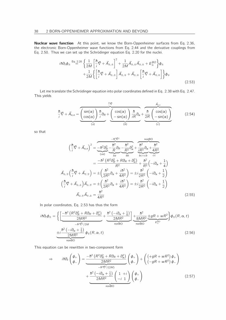
38 2 BORN-OPPENHEIMER APPROXIMATION AND BEYOND
Nuclear wave function At this point, we know the Born-Oppenheimer surfaces from Eq. 2.36,the electronic Born-Oppenheimer wave functions from Eq. 2.44 and the derivative couplings fromEq. 2.50. Thus we can set up the Schrödinger equation Eq. 2.20 for the nuclei.
i~∂tφ±Eq. 2.20=
1
2M
[~
i~∇+ ~A±,±
]2
+1
2M~A±,∓ ~A∓,± + E
BO±
φ±
+1
2M
[~
i~∇+ ~A±,±
]
~A±,∓ + ~A±,∓
[~
i~∇+ ~A∓,∓
]
φ∓
(2.53)
Let me translate the Schrödinger equation into polar coordinates defined in Eq. 2.38 with Eq. 2.47.This yields
~
i~∇+ ~An,n =
~
i~∇
︷ ︸︸ ︷(
sin(α)
cos(α)
)
~
i∂R
︸ ︷︷ ︸
(a)
+
(
cos(α)
− sin(α)
)
~
iR∂α
︸ ︷︷ ︸
(b)
+
~An,n︷ ︸︸ ︷
~
2R
(
cos(α)
− sin(α)
)
︸ ︷︷ ︸
(c)
(2.54)
so that
(~
i~∇+ ~An,n
)2
=
−~2 ~∇2︷ ︸︸ ︷
−~2∂2R︸ ︷︷ ︸
(aa)
−~2
R∂R
︸ ︷︷ ︸
ba
− ~2
R2∂2α
︸ ︷︷ ︸
bb
+
nonBO︷ ︸︸ ︷
~2
iR2∂α
︸ ︷︷ ︸
bc+cb
+~2
4R2︸ ︷︷ ︸cc
=−~2
(R2∂2R + R∂R + ∂
2α
)
R2+~2
R2
(
−i∂α +1
4
)
~A±,∓(~
i~∇+ ~A∓,∓
)
= ±(~2
2R2∂α +
i~2
4R2
)
= ±i ~2
2R2
(
−i∂α +1
2
)
(~
i~∇+ ~A±,±
)
~A±,∓ = ±(~2
2R2∂α +
i~2
4R2
)
= ±i ~2
2R2
(
−i∂α +1
2
)
~A±,∓ ~A∓,± =~2
4R2(2.55)
In polar coordinates, Eq. 2.53 has thus the form
i~∂tφ± =
[−~2(R2∂2R + R∂R + ∂
2α
)
2MR2︸ ︷︷ ︸
−~2 ~∇2/2M
+~2(−i∂α + 14
)
2MR2︸ ︷︷ ︸
nonBO
]
+~2
8MR2︸ ︷︷ ︸
nonBO
±gR + wR2︸ ︷︷ ︸
EBO±
φ±(R,α, t)
±i ~2(−i∂α + 12
)
2MR2︸ ︷︷ ︸
nonBO
φ∓(R,α, t) (2.56)
This equation can be rewritten in two-component form
⇒ i~∂t
(
φ+
φ−
)
=−~2
(R2∂2R + R∂R + ∂
2α
)
2MR2︸ ︷︷ ︸
−~2 ~∇2/(2M)
(
φ+
φ−
)
+
((+gR + wR2
)φ+
(−gR + wR2
)φ−
)
+~2(−i∂α + 12
)
2MR2
(
1 +i
−i 1
)
︸ ︷︷ ︸
nonBO
(
φ+
φ−
)
(2.57)
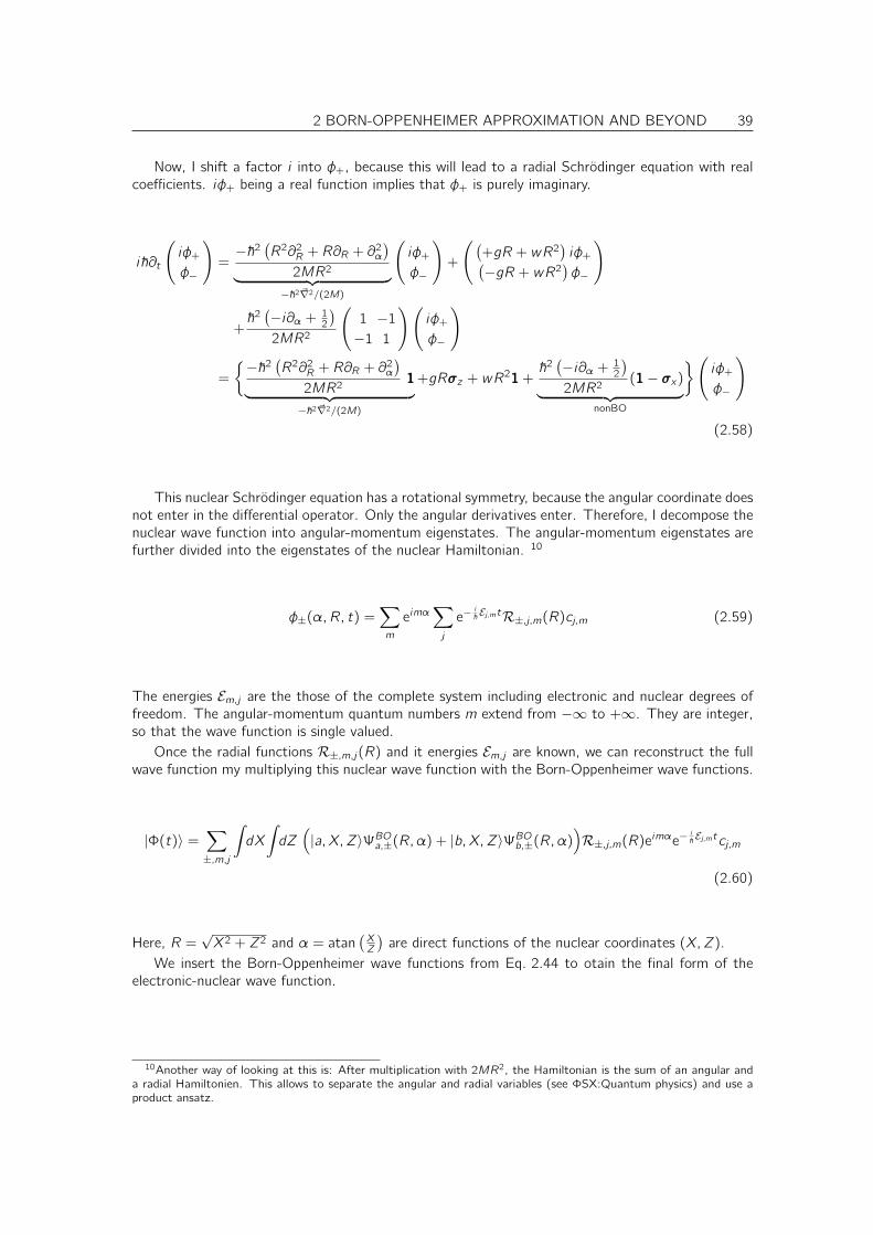
2 BORN-OPPENHEIMER APPROXIMATION AND BEYOND 39
Now, I shift a factor i into φ+, because this will lead to a radial Schrödinger equation with realcoefficients. iφ+ being a real function implies that φ+ is purely imaginary.
i~∂t
(
iφ+
φ−
)
=−~2
(R2∂2R + R∂R + ∂
2α
)
2MR2︸ ︷︷ ︸
−~2 ~∇2/(2M)
(
iφ+
φ−
)
+
((+gR + wR2
)iφ+
(−gR + wR2
)φ−
)
+~2(−i∂α + 12
)
2MR2
(
1 −1−1 1
)(
iφ+
φ−
)
=
−~2(R2∂2R + R∂R + ∂
2α
)
2MR2111
︸ ︷︷ ︸
−~2 ~∇2/(2M)
+gRσz + wR2111 +
~2(−i∂α + 12
)
2MR2(111− σx)
︸ ︷︷ ︸
nonBO
(
iφ+
φ−
)
(2.58)
This nuclear Schrödinger equation has a rotational symmetry, because the angular coordinate doesnot enter in the differential operator. Only the angular derivatives enter. Therefore, I decompose thenuclear wave function into angular-momentum eigenstates. The angular-momentum eigenstates arefurther divided into the eigenstates of the nuclear Hamiltonian. 10
φ±(α,R, t) =∑
m
eimα∑
j
e−i~Ej,mtR±,j,m(R)cj,m (2.59)
The energies Em,j are the those of the complete system including electronic and nuclear degrees offreedom. The angular-momentum quantum numbers m extend from −∞ to +∞. They are integer,so that the wave function is single valued.
Once the radial functions R±,m,j(R) and it energies Em,j are known, we can reconstruct the fullwave function my multiplying this nuclear wave function with the Born-Oppenheimer wave functions.
|Φ(t)〉 =∑
±,m,j
∫
dX
∫
dZ(
|a,X,Z〉ΨBOa,±(R,α) + |b,X,Z〉ΨBOb,±(R,α))
R±,j,m(R)eimαe−i~Ej,mtcj,m
(2.60)
Here, R =√X2 + Z2 and α = atan
(XZ
)are direct functions of the nuclear coordinates (X,Z).
We insert the Born-Oppenheimer wave functions from Eq. 2.44 to otain the final form of theelectronic-nuclear wave function.
10Another way of looking at this is: After multiplication with 2MR2, the Hamiltonian is the sum of an angular anda radial Hamiltonien. This allows to separate the angular and radial variables (see ΦSX:Quantum physics) and use aproduct ansatz.
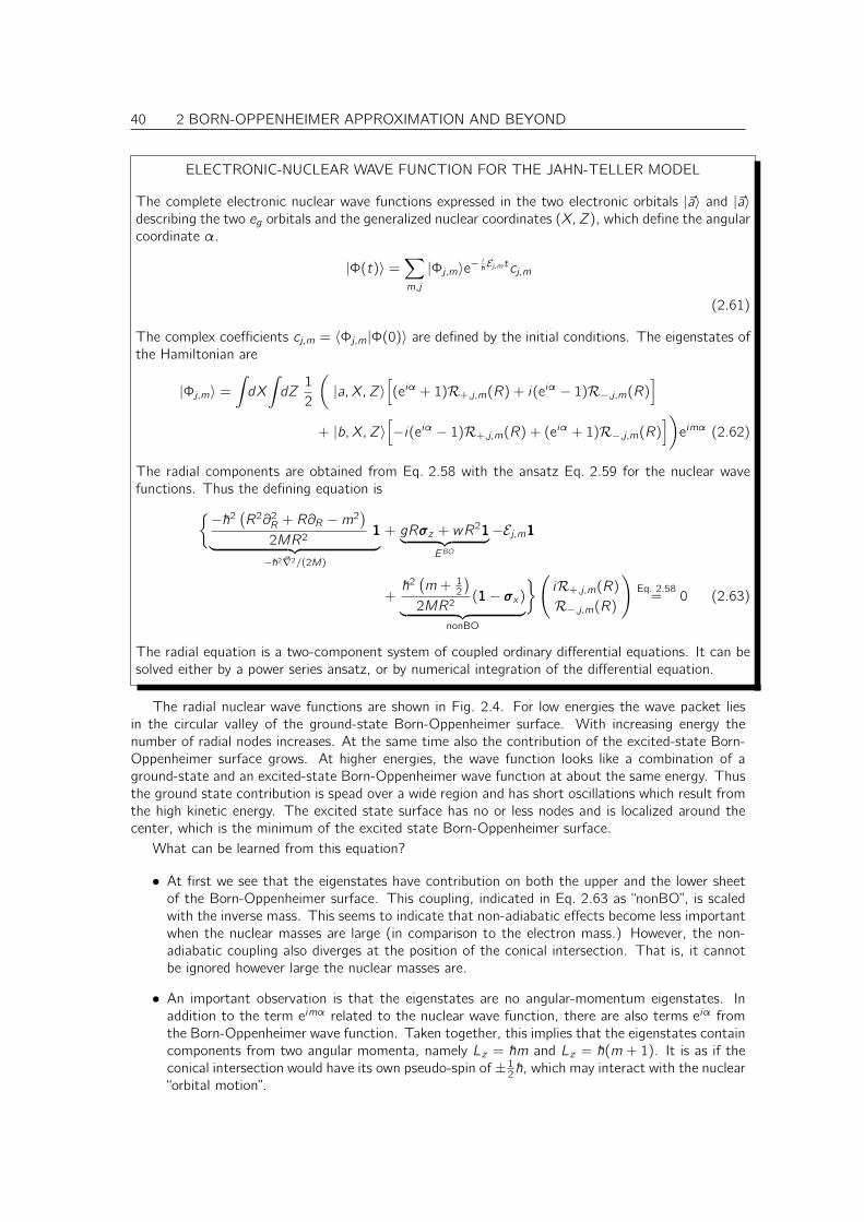
40 2 BORN-OPPENHEIMER APPROXIMATION AND BEYOND
ELECTRONIC-NUCLEAR WAVE FUNCTION FOR THE JAHN-TELLER MODEL
The complete electronic nuclear wave functions expressed in the two electronic orbitals |~a〉 and |~a〉describing the two eg orbitals and the generalized nuclear coordinates (X,Z), which define the angularcoordinate α.
|Φ(t)〉 =∑
m,j
|Φj,m〉e−i~Ej,mtcj,m
(2.61)
The complex coefficients cj,m = 〈Φj,m|Φ(0)〉 are defined by the initial conditions. The eigenstates ofthe Hamiltonian are
|Φj,m〉 =∫
dX
∫
dZ1
2
(
|a,X,Z〉[
(eiα + 1)R+,j,m(R) + i(eiα − 1)R−,j,m(R)]
+ |b,X,Z〉[
−i(eiα − 1)R+,j,m(R) + (eiα + 1)R−,j,m(R)])
eimα (2.62)
The radial components are obtained from Eq. 2.58 with the ansatz Eq. 2.59 for the nuclear wavefunctions. Thus the defining equation is
−~2(R2∂2R + R∂R −m2
)
2MR2111
︸ ︷︷ ︸
−~2 ~∇2/(2M)
+ gRσz + wR2111
︸ ︷︷ ︸
EBO
−Ej,m111
+~2(m + 12
)
2MR2(111− σx)
︸ ︷︷ ︸
nonBO
(
iR+,j,m(R)R−,j,m(R)
)
Eq. 2.58= 0 (2.63)
The radial equation is a two-component system of coupled ordinary differential equations. It can besolved either by a power series ansatz, or by numerical integration of the differential equation.
The radial nuclear wave functions are shown in Fig. 2.4. For low energies the wave packet liesin the circular valley of the ground-state Born-Oppenheimer surface. With increasing energy thenumber of radial nodes increases. At the same time also the contribution of the excited-state Born-Oppenheimer surface grows. At higher energies, the wave function looks like a combination of aground-state and an excited-state Born-Oppenheimer wave function at about the same energy. Thusthe ground state contribution is spead over a wide region and has short oscillations which result fromthe high kinetic energy. The excited state surface has no or less nodes and is localized around thecenter, which is the minimum of the excited state Born-Oppenheimer surface.
What can be learned from this equation?
• At first we see that the eigenstates have contribution on both the upper and the lower sheetof the Born-Oppenheimer surface. This coupling, indicated in Eq. 2.63 as “nonBO”, is scaledwith the inverse mass. This seems to indicate that non-adiabatic effects become less importantwhen the nuclear masses are large (in comparison to the electron mass.) However, the non-adiabatic coupling also diverges at the position of the conical intersection. That is, it cannotbe ignored however large the nuclear masses are.
• An important observation is that the eigenstates are no angular-momentum eigenstates. Inaddition to the term eimα related to the nuclear wave function, there are also terms eiα fromthe Born-Oppenheimer wave function. Taken together, this implies that the eigenstates containcomponents from two angular momenta, namely Lz = ~m and Lz = ~(m + 1). It is as if theconical intersection would have its own pseudo-spin of± 12~, which may interact with the nuclear“orbital motion”.
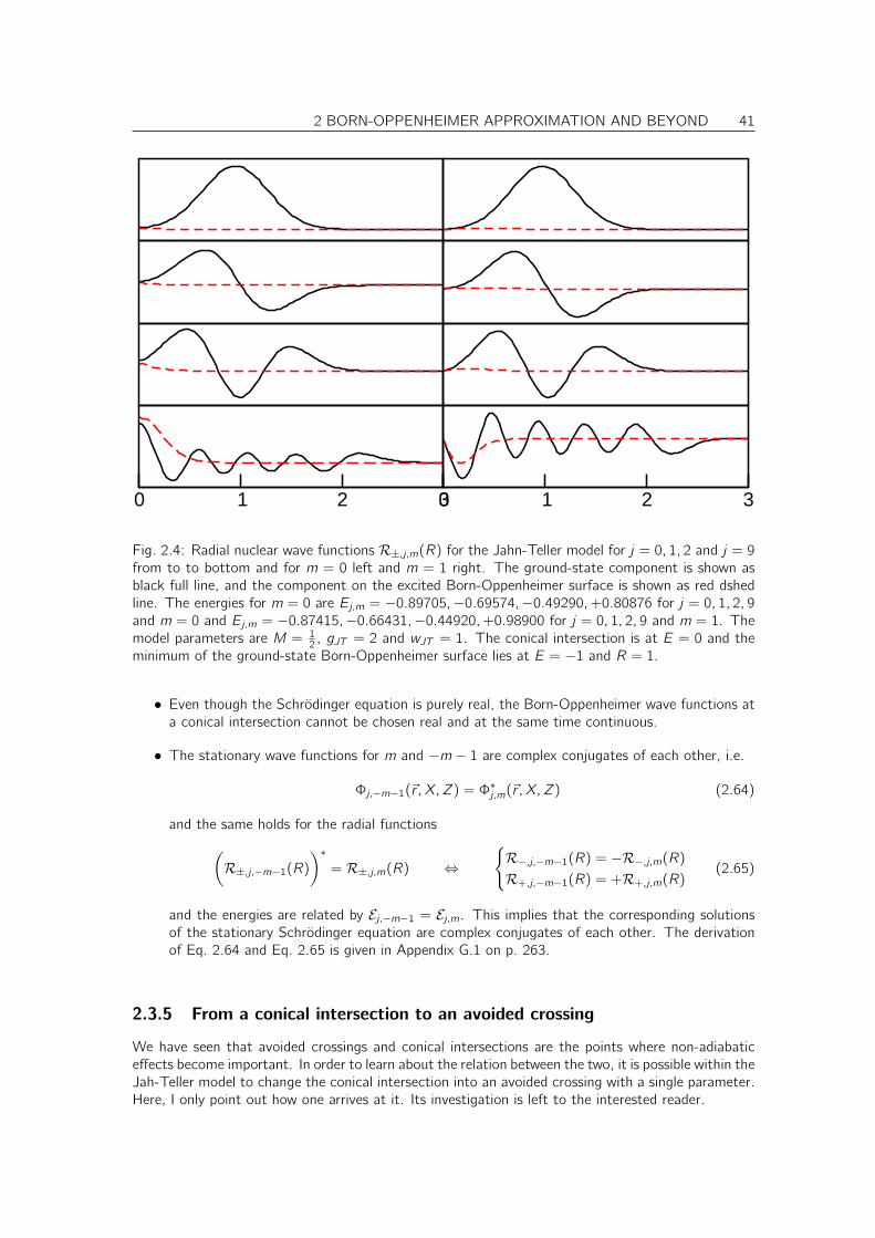
2 BORN-OPPENHEIMER APPROXIMATION AND BEYOND 41
0 1 2 30 1 2 3
Fig. 2.4: Radial nuclear wave functions R±,j,m(R) for the Jahn-Teller model for j = 0, 1, 2 and j = 9from to to bottom and for m = 0 left and m = 1 right. The ground-state component is shown asblack full line, and the component on the excited Born-Oppenheimer surface is shown as red dshedline. The energies for m = 0 are Ej,m = −0.89705,−0.69574,−0.49290,+0.80876 for j = 0, 1, 2, 9and m = 0 and Ej,m = −0.87415,−0.66431,−0.44920,+0.98900 for j = 0, 1, 2, 9 and m = 1. Themodel parameters are M = 1
2 , gJT = 2 and wJT = 1. The conical intersection is at E = 0 and theminimum of the ground-state Born-Oppenheimer surface lies at E = −1 and R = 1.
• Even though the Schrödinger equation is purely real, the Born-Oppenheimer wave functions ata conical intersection cannot be chosen real and at the same time continuous.
• The stationary wave functions for m and −m − 1 are complex conjugates of each other, i.e.
Φj,−m−1(~r , X,Z) = Φ∗j,m(~r , X,Z) (2.64)
and the same holds for the radial functions
(
R±,j,−m−1(R))∗= R±,j,m(R) ⇔
R−,j,−m−1(R) = −R−,j,m(R)R+,j,−m−1(R) = +R+,j,m(R)
(2.65)
and the energies are related by Ej,−m−1 = Ej,m. This implies that the corresponding solutionsof the stationary Schrödinger equation are complex conjugates of each other. The derivationof Eq. 2.64 and Eq. 2.65 is given in Appendix G.1 on p. 263.
2.3.5 From a conical intersection to an avoided crossing
We have seen that avoided crossings and conical intersections are the points where non-adiabaticeffects become important. In order to learn about the relation between the two, it is possible within theJah-Teller model to change the conical intersection into an avoided crossing with a single parameter.Here, I only point out how one arrives at it. Its investigation is left to the interested reader.
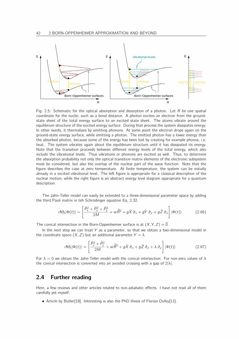
42 2 BORN-OPPENHEIMER APPROXIMATION AND BEYOND
vibrational levelsE
Born−Oppenheimer surfaces
R
E
Born−Oppenheimer surfaces
R
E
Fig. 2.5: Schematic for the optical absorption and desorption of a photon. Let R be one spatialcoordinate for the nuclei, such as a bond distance. A photon excites an electron from the ground-state sheet of the total energy surface to an excited state sheet. The atoms vibrate around theequilibrium structure of the excited energy surface. During that process the system dissipates energy.In other words, it thermalizes by emitting phonons. At some point the electron drops again on theground-state energy surface, while emitting a photon. The emitted photon has a lower energy thanthe absorbed photon, because some of the energy has been lost by creating for example phonos, i.e.heat. The system vibrates again about the equilibrium structure until it has dissipated its energy.Note that the transition proceeds between different energy levels of the total energy, which alsoinclude the vibrational levels. Thus vibrations or phonons are excited as well. Thus, to determinethe absorption probability not only the optical transition matrix elements of the electronic subsystemmust be considered, but also the overlap of the nuclear part of the wave function. Note that thefigure describes the case at zero temperature. At finite temperature, the system can be initiallyalready in a excited vibrational level. The left figure is appropriate for a classical description of thenuclear motion, while the right figure is an abstract energy level diagram appropriate for a quantumdescription.
The Jahn-Teller model can easily be extended to a three-dimensional parameter space by addingthe third Pauli matrix in teh Schrödinger equation Eq. 2.32.
i~∂t |Φ(t)〉 =[
P 2x + P2y + P
2z
2M+ w ~R2 + gX σx + gY σy + gZ σz
]
|Φ(t)〉 (2.66)
The conical intersection in the Born-Oppenheimer surface is at (X, Y, Z) = ~0.In the next step we can treat Y as a parameter, so that we obtain a two-dimensional model in
the coordinate space (X,Z) but an additional parameter Y = λ
i~∂t |Φ(t)〉 =[
P 2x + P2y
2M+ w ~R2 + gX σx + gZ σz + λ σy
]
|Φ(t)〉 (2.67)
For λ = 0 we obtain the Jahn-Teller model with the conical intersection. For non-zero values of λthe conical intersection is converted into an avoided crossing with a gap of 2|λ|.
2.4 Further reading
Here, a few reviews and other articles related to non-adiabatic effects. I have not read all of themcarefully yet myself.
• Article by Butler[18]. Interesting is also the PhD thesis of Florian Dufey[11].

2 BORN-OPPENHEIMER APPROXIMATION AND BEYOND 43
• A good introduction given in the special volume of the Journal “Advances in Chemical Physics”from 2002[19]. In particular, I liked the article of Child[20] and that by Worth and Robb[9]
• the book “Beyond Born-Oppenheimer: Conical Intersections and Electronic Nonadiabatic Coul-ing Terms” by Michael Baer[21]. Baer uses a very compact notation, but he describes thetopological effects in a very elegant manner.
• Review article by Worth and Cederbaum[22]
• Herzberg[23]
• For the role of the so-called geometrical phase or Berry phase see Berry’s original paper[24].For the role of the Berry phase in chemical reactions see the short article by Clary[25].

44 2 BORN-OPPENHEIMER APPROXIMATION AND BEYOND
Chapter 3
Many-particle wave functions
In the previous section we have shown how we can split the description into two parts, one for theelectrons and another one for the nuclei. The dynamics of the nuclei requires the knowledge ofthe electronic problem, namely the Born-Oppenheimer surfaces EBOn (~R) and the derivative couplings~Am,n(~R) obtained from the Born-Oppenheimer wave functions |ΨBO(~R)〉. The Born-Oppenheimerwave functions are states in the electronic Hilbert space and the atomic positions ~R are parametersand not coordinates in the quantum mechanical sense.
The next difficulty is to obtain the Born-Oppenheimer wave functions. For non-interacting elec-trons this is of the same complexity as a one-particle problem, while the interaction makes thisproblem usually untractable. Therefore we will start with non-interacting electrons before we turn tothe more complicated interacting systems.
In the present section, I will describe the basics of many-particle wave functions. I will start outhow to describe one-particle wave functions wityh spin. Then I will describe the underlying symmetryof identical particles, which resuls in the concept of Fermions and Bosons. Finally, I will make the turnback to one-particle wave functions, by showing how the wave function of a noninteracting systemof fermions and bosons can be expressed by one-particle wave functions.
This will form the basis of the following sections that adress non-interacting electrons.
3.1 Spin orbitals
Before I continue with many-particle wave functions, let me discuss one-particle orbitals. I willintroduce a notation for treating the electron spin which, on the one hand, simplifies the expressions,and on the other hand it is more rigorous.
When I first learned about spins and magnetic moments, I was puzzled by the special role, whichwas attributed to the z-coordinate. I learned that an electron can have a spin pointing parallel orantiparallel to the z-axis. The direction of the z-axis, however, is arbitrary. It seemed as if the physicschanged, when I turned my head.
Indeed, there is nothing special about the z-coordinate. Here, I present a more general formu-lation, which describes electrons by two-component spinor wave functions. With this formulation,one can form wave functions with a spin pointing in an arbitrary direction in each point in space.This description restores the rotational symmetry that appears to be broken in the simple-mindedformulation used commonly.
We use here two-component spinor wave functions, which are also called spin-orbitals
φ(~x) = φ(~r , σ) = 〈~r , σ|φ〉
Spin-orbitals actually consists of two complex wave functions, one for the spin-down φ(~r , ↓) and one
45
46 3 MANY-PARTICLE WAVE FUNCTIONS
for the spin up contribution φ(~r , ↑). One can write the spin orbitals also as two-component spinor
(
φ(~r , ↑)φ(~r , ↓)
)
def=
(
〈~r , ↑ |φ〉〈~r , ↓ |φ〉
)
PHYSICAL MEANING OF A SPIN WAVEFUNCTION
The square of a component of a spin wavefunction is the probability density Pσ(~r) for finding aparticle with the specified spin orientation at a specific position ~r .
This rule is completely analogous to the rule that the absolute square of a scalar wave functionis the probability density P (~r) = ψ∗(~r)ψ(~r) of finding a particle at a given position ~r .
Note, however, that the wave function contains much more information than that just men-tioned. Below, we will see that the spin wave function does not only provide the information on theprobabilities for the spin projection on the z-axis but also for any other axis.1
Relation to spin eigenstates
This notation is a little puzzling at first, because one usually works with spin-eigenfunctions, for whichone of the components vanishes. The spin is defined as
~S =~
2~σ (3.1)
where the three components of the vector ~σ are
σi =
∫
d3r
2∑
σ,σ′=1
|~r , σ〉σi ,σ,σ′〈~r , σ′|
Somewhat confusing are the different indices for the different vector spaces: The index i can havethe values x, y , z and refers to the components of the vector ~σ. Each component of the vector ~σ isa scalar operator. The indices σ, σ′ of σi ,σ,σ′ can assume the values ↑ or ↓, which are the coordinatesof the two-dimensional spinor space. That is, σi is a (2×2) matrix for each value of i . These (2×2)matrices are the Pauli matrices2
σx =
(
0 1
1 0
)
, σy =
(
0 −ii 0
)
, σz =
(
1 0
0 −1
)
(3.2)
1This is analogous to the fact that a wave function in configuration space contains information also on the mo-mentum.
2The matrices are made of the matrix elements σi ,σ,σ′ = 〈σ|σi |σ′〉 of the operator σi with σ ∈ ↑, ↓, σ′ ∈ ↑, ↓and i ∈ x, y , z.
3 MANY-PARTICLE WAVE FUNCTIONS 47
As a worked example, let us determine the expectation value of the operator Sx for a one-particlestate |φ〉. The states |~r , ↑〉 and |~r , ↑〉 are still eigenstates of Sz .
〈φ|Sx |φ〉 = 〈φ|[
~
2
∫
d3r
2∑
σ,σ′=1
|~r , σ〉σx,σ,σ′〈~r , σ′|]
|φ〉
=~
2
∫
d3r
[2∑
σ,σ′=1
〈φ|~r , σ〉σx,σ,σ′〈~r , σ′|φ〉]
=~
2
∫
d3r
[(
〈φ|~r , ↑〉〈φ|~r , ↓〉
)(
0 1
1 0
)(
〈~r , ↑ |φ〉〈~r , ↓ |φ〉
)]
=~
2
∫
d3r [〈φ|~r , ↑〉〈~r , ↓ |φ〉+ 〈φ|~r , ↓〉〈~r , ↑ |φ〉]
=~
2
∫
d3r [φ∗(~r , ↑)φ(~r , ↓) + φ∗(~r , ↓)φ(~r , ↑)]
We obtain the spin density, that is the probability that we find a particle at position ~r multiplied withthe average spin expectation value in x-direction of that particle.
For a spin orbital that is an eigenstate of Sz , one of the spinor components vanishes.
Sz |φ↑〉 = |φ↑〉(
+~
2
)
⇒(
〈~r , ↑ |φ↑〉〈~r , ↓ |φ↑〉
)
=
(
φ↑(~r , ↑)0
)
Sz |φ↓〉 = |φ↓〉(
−~2
)
⇒(
〈~r , ↑ |φ↓〉〈~r , ↓ |φ↓〉
)
=
(
0
φ↓(~r , ↓)
)
Note that the indices ↑, ↓ indicate the quantum number, while the pointers to the spinor componentsare treated as argument, so that they can be distinguished from the quantum numbers. The quantumnumber indicates that the orbital is an eigenstate to some symmetry operator.
The spin-orbitals have the advantage that they allow to describe orbitals, for which the spin doesnot point along the z-axis, but it can also point, for example, to the right or in any other direction.For a spin orbital the spin direction can actually vary in space. Such an orbital is called non-collinear,because the spins are not aligned.
Problem with conventional notation
In the literature, one usually uses another notation, namely
φσ(~r)def=φ(~r , σ)
Here, it is difficult to distinguish the role of σ as a coordinate and as quantum number. One usuallyuses one-particle orbitals with only one spin component, for which σ is a quantum number. In ournotation this would be – for a spin-up particle –
φ↑(~r , σ) = 〈~r , σ|φ↑〉=(
〈~r , ↑ |φ↑〉0
)
The orbital still has two components, but one of them, namely φ↑(~r , ↓), vanishes. With the commonnotation, it is difficult to write down expressions that do not break the rotational symmetry for thespin direction.
48 3 MANY-PARTICLE WAVE FUNCTIONS
Magnetization
So-far we used the spin operator to determine the expectation value of the spin. Now we would liketo obtain the spin density or the magnetization respectively. In order to describe the principles, letus work out the charge density as a trivial example:
We know the projector P (~r) onto a certain point in space ~r , which is
P (~r)def=∑
σ
|~r , σ〉〈~r , σ| = |~r , ↓〉〈~r , ↓ |+ |~r , ↑〉〈~r , ↑ |
We obtain the charge density as expectation value of P (~r), multiplied with the electron chargeqe = −e.
ρ(~r) = 〈φ|[qP (~r)
]|φ〉 = q〈φ|
[∑
σ
|~r , σ〉〈~r , σ|]
|φ〉
= q∑
σ
〈φ|~r , σ〉〈~r , σ|φ〉
= q(
〈φ|~r , ↓〉〈~r , ↓ |φ〉+ 〈φ|~r , ↑〉〈~r , ↑ |φ〉)
Hence, the charge density is, up to the factor q, the sum of the spin-up and spin-down densities.After this introduction, we can analogously determine the magnetization.
The magnetization operator is obtained as product of the factor3 qm , the spin operator and the
projection operator onto a point in space.
mi(~r)def=
q
mP (~r)Si =
q~
2mP (~r)σi
=q~
2m
[∑
σ
|~r , σ〉〈~r , σ|]
︸ ︷︷ ︸
P (~r)
[∫
d3r ′∑
σ′,σ′′
|~r ′, σ′〉σi ,σ′,σ′′〈~r ′, σ′′|]
︸ ︷︷ ︸
σi
=q~
2m
∑
σ
∫
d3r ′∑
σ′,σ′′
|~r , σ〉 〈~r , σ|~r ′, σ′〉︸ ︷︷ ︸
δ(~r−~r ′)δσ,σ′
σi ,σ′,σ′′〈~r ′, σ′′|
=q~
2m
∑
σ,σ′′
|~r , σ〉σi ,σ,σ′′〈~r , σ′′|
The factor µBdef= e~2me
is the Bohr magneton, which is approximately equal to the magnetic momentof an electron. Spin and magnetic moment of the electron point in opposite directions due to thenegative charge of the electron.
MAGNETIZATION OPERATOR
~m(~r) =q~
2m
∑
σ,σ′
|~r , σ〉~σσ,σ′〈~r , σ′| (3.3)
with the Pauli matrices ~σ defined in Eq. 3.2.
3The classical ratio of magnetic moment and angular momentum is q2m
, which however assumes a constant ratiothe mass- and charge distribution in space. While the “distribution” of electrons leads to such a constant ratio, theproperties of a single electron may differ in a classical picture. In a quantum mechanical description the electron ispoint-like with a certain gyromagnetic ratio, that follows directly from the relativistic Dirac equation.
3 MANY-PARTICLE WAVE FUNCTIONS 49
More explicitly we obtain
ρ(r) = q
(
〈φ|~r , ↑〉〈φ|~r , ↓〉
)(
1 0
0 1
)(
〈~r , ↑ |φ〉〈~r , ↓ |φ〉
)
= q [φ∗(~r , ↑)φ(~r , ↑) + φ∗(~r , ↓)φ(~r , ↓)]
mx(r) =q~
2m
(
〈φ|~r , ↑〉〈φ|~r , ↓〉
)(
0 1
1 0
)(
〈~r , ↑ |φ〉〈~r , ↓ |φ〉
)
=q~
2me[φ∗(~r , ↑)φ(~r , ↓) + φ∗(~r , ↓)φ(~r , ↑)]
my (r) =q~
2m
(
〈φ|~r , ↑〉〈φ|~r , ↓〉
)(
0 −ii 0
)(
〈~r , ↑ |φ〉〈~r , ↓ |φ〉
)
= −i q~2m[φ∗(~r , ↑)φ(~r , ↓)− φ∗(~r , ↓)φ(~r , ↑)]
mz(r) =q~
2m
(
〈φ|~r , ↑〉〈φ|~r , ↓〉
)(
1 0
0 −1
)(
〈~r , ↑ |φ〉〈~r , ↓ |φ〉
)
=q~
2m[φ∗(~r , ↑)φ(~r , ↑)− φ∗(~r , ↓)φ(~r , ↓)]
The two-component spinor descriptions follows from the Pauli equation. The Pauli equation isthe non-relativistic limit of the Dirac equation, the relativistic one-particle equation for electrons.In the Dirac equation each particle has four components. Two components describe spin-up andspin-down electrons, and the two other components describe spin-up and spin-down positrons. Thepositron[26] is the anti-particle of the electron. In the non-relativistic limit, the electronic andpositronic components become independent of each other, so that the electrons can be described bya two-component spinor wave function.
A Slater determinant of N spin-orbitals corresponds to 2N Slater determinants of one-componentone-particle orbitals, according to the N spin indices.
3.2 Symmetry and quantum mechanics
In the following, we will be concerned with the symmetry of the Hamilton operator under permuta-tion of particles. Therefore, I will revisit the main symmetry arguments discussed in section 9 ofΦSX:Quantum Theory [27]. This is a series of arguments may be worthwhile to keep in mind.
A symmetry of an object is a transformation, that leaves the appearance of the object unchanged.For example a square is symmetric under four-fold rotation.
A physical system is characterized4 by its Hamiltonian, which determines the dynamics of thesystem by the Schrödinger equation. The system is symmetric under a given transformation, if everysolution of the Schrödinger equation, is transformed into another solution of the same Schrödingerequation.
Let me formalize this:
1. Definition of a transformation operator: An operator S can be called a transformation, if itconserves the norm for any state, that is if
∀|ψ〉 〈ψ|ψ〉 |φ〉=S|ψ〉= 〈φ|φ〉 (3.4)
2. A transformation operator S is unitary, that is
S†S = 1 (3.5)4The argument is not limited to quantum systems. The Schrödinger equation can be replaced by any other equation
of motion governing the dynamics or other properties.
50 3 MANY-PARTICLE WAVE FUNCTIONS
Proof:
∀|ψ〉 〈ψ|S†S|ψ〉Eq. 3.4= 〈ψ|ψ〉 ⇒ S†S = 1
3. Definition of a symmetry: A system is called symmetric under the transformation S, if, forany solution of the Schrödinger equation describing that system, also S|Ψ〉 is a solution of thesame Schrödinger equation. That is, if
(i~∂t |Ψ〉 = H|Ψ〉
) |Φ〉def=S|Ψ〉⇒
(i~∂t |Φ〉 = H|Φ〉
)(3.6)
4. The commutator of the Hamilton operator with its symmetry operator vanishes, that is [H, S]− =0:
Proof:
i~∂t |Φ〉 = H|Φ〉|Φ〉def=S|Ψ〉⇒ i~∂t S|Ψ〉 = HS|Ψ〉
∂t S=0⇒ S (i~∂t |Ψ〉) = HS|Ψ〉i~∂t |Ψ〉=H|Ψ〉⇒ SH|Ψ〉 = HS|Ψ〉(HS − SH
)
︸ ︷︷ ︸
[H,S]−
|Ψ〉 = 0
Because this equation holds for any solution of the Schrödinger equation, it holds for any wavefunction, because any function can be written as superposition of solutions of the Schrödingerequation. (The latter form a complete set of functions.) Therefore
SYMMETRY AND COMMUTATOR
The commutator between the Hamilton operator H with its (time-independenta) symmetryoperators S vanishes.
[H, S]− = 0
Thus, one usually identifies a symmetry by working out the commutator with the Hamiltonian.
aFor time-dependent symmetry operators, the more general rule is [H, S]− = i~∂t S. An example for atime-dependent symmetry is that between two relatively moving frames of inertia.
5. The matrix elements of the Hamilton operator between two eigenstates of the symmetry op-erator with different eigenvalues vanish. That is
(S|Ψs〉 = |Ψs〉s ∧ S|Ψs ′〉 = |Ψs ′〉s ′ ∧ s 6= s ′
)⇒ 〈Ψs |H|Ψs ′〉 = 0
Thus, the Hamilton operator is block diagonal in a representation of eigenstates of its symmetryoperators. The eigenstates of the Hamilton operator can be obtained for each block individually.Because the effort to diagonalize a matrix increases rapidly with the matrix size, this simplifiesthe calculation of Hamilton eigenstates substantially, both for analytical and for numericalcalculations.
If the Hamiltonian is block diagonal, the time dependent Schrödinger equation does not mixstates from different subspaces. A wave function that starts out as an eigenstate of a symmetryoperator with a given eigenvalue, will always be an eigenstate with the same eigenvalue. In other
3 MANY-PARTICLE WAVE FUNCTIONS 51
words, the eigenvalue of the symmetry operator is a conserved quantity. (Note, however, thatthe eigenvalue of a symmetry operator is usually complex.)
The eigenvalues of the symmetry operators are related to the quantum numbers.
Proof: In the following we will need an expression for 〈ψs |S, which we will work out first:
• We start by showing that the absolute value of an eigenvalue of a unitary operator is equalto one, that is s = eiφ where φ is real. With an eigenstate |ψs〉 of S we obtain
s∗〈ψs |ψs〉sS|ψs 〉=|ψs 〉s= 〈Sψs |Sψs〉 = 〈ψs | S†S︸︷︷︸
1
|ψs〉 = 〈ψs |ψs〉 ⇒ |s | = 1(3.7)
• Next, we show that the eigenvalues of the Hermitian conjugate operator S† of a unitaryoperator S are the complex conjugates of the eigenvalues of S.
⇒ |ψs〉Eq. 3.5= S†S
︸︷︷︸
=1
|ψs〉S|ψs 〉=|ψs 〉s= S†|ψs〉s
⇒ S†|ψs〉sEq. 3.7= |ψs〉 s∗s︸︷︷︸
=1
⇒ S†|ψs〉 = |ψs〉s∗
⇒ 〈ψs |S = s〈ψs |
• With this, we are ready to show that the matrix elements of the Hamilton operator betweentwo eigenstates of the symmetry operator with different eigenvalues vanish.
0[H,S]−=0= 〈Ψs |[H, S]−|Ψs ′〉 = 〈Ψs |HS|Ψs ′〉 − 〈Ψs |SH|Ψs ′〉
S|Ψs 〉=|Ψs 〉s,etc.= 〈Ψs |H|Ψs ′〉s ′ − s〈Ψs |H|Ψs ′〉 = 〈Ψs |H|Ψs ′〉(s ′ − s)s 6=s ′⇒ 〈Ψs |H|Ψs ′〉 = 0
q.e.d
6. For a operator S with the property SN = 1 for a finite N, one can decompose any wave function|χ〉 into eigenstates |ψα〉 of the symmetry operation S with eigenvalue sα = ei
2πNα
|ψα〉 =N∑
n=0
Sn|χ〉s−nα =
N∑
n=0
(S†)n |χ〉s+nα (3.8)
3.3 Identical particles
Electrons with the same spin are indistinguishable. This says that there is no conceivable experimentthat discriminates between two electrons, except for their spin. Thus, there is a symmetry withrespect to exchange of two particles, and the Hamiltonian for indistinguishable particles commuteswith the permutation operator of two particles.
Editor: introduce symbol P for the permutation operator to avoid confusion with
a projection operator P (~r) used later.
The two-particle permutation operator is defined as
P(2)i ,j Ψ(. . . , ~xi , . . . , ~xj . . .) = Ψ(. . . , ~xj , . . . , ~xi . . .)
The eigenstates of the Hamiltonian are eigenstates of the permutation operator. Because(
P(2)i ,j)2
=
1, the permutation operator has the two eigenvalues, namely +1 and −1. Thus, the wave functions
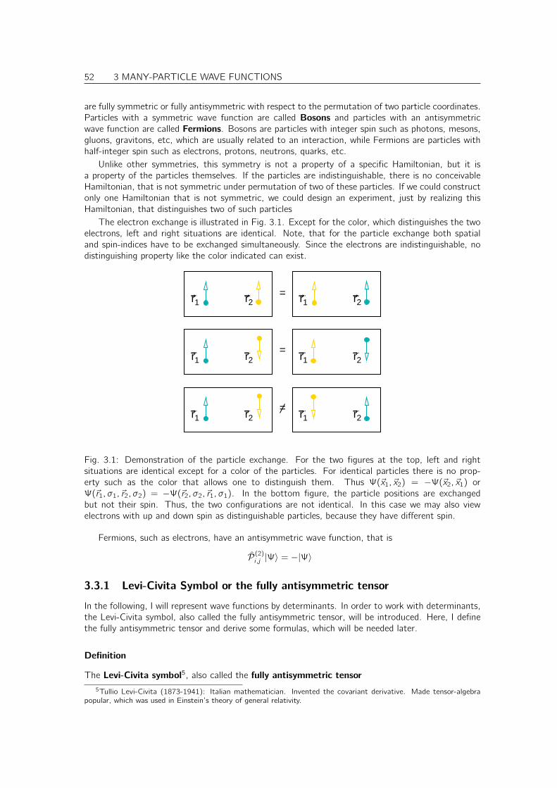
52 3 MANY-PARTICLE WAVE FUNCTIONS
are fully symmetric or fully antisymmetric with respect to the permutation of two particle coordinates.Particles with a symmetric wave function are called Bosons and particles with an antisymmetricwave function are called Fermions. Bosons are particles with integer spin such as photons, mesons,gluons, gravitons, etc, which are usually related to an interaction, while Fermions are particles withhalf-integer spin such as electrons, protons, neutrons, quarks, etc.
Unlike other symmetries, this symmetry is not a property of a specific Hamiltonian, but it isa property of the particles themselves. If the particles are indistinguishable, there is no conceivableHamiltonian, that is not symmetric under permutation of two of these particles. If we could constructonly one Hamiltonian that is not symmetric, we could design an experiment, just by realizing thisHamiltonian, that distinguishes two of such particles
The electron exchange is illustrated in Fig. 3.1. Except for the color, which distinguishes the twoelectrons, left and right situations are identical. Note, that for the particle exchange both spatialand spin-indices have to be exchanged simultaneously. Since the electrons are indistinguishable, nodistinguishing property like the color indicated can exist.
=
r1 r2 r1 r2
r1 r2 r1 r2=
r1 r2 r1 r2
=
Fig. 3.1: Demonstration of the particle exchange. For the two figures at the top, left and rightsituations are identical except for a color of the particles. For identical particles there is no prop-erty such as the color that allows one to distinguish them. Thus Ψ(~x1, ~x2) = −Ψ(~x2, ~x1) orΨ(~r1, σ1, ~r2, σ2) = −Ψ(~r2, σ2, ~r1, σ1). In the bottom figure, the particle positions are exchangedbut not their spin. Thus, the two configurations are not identical. In this case we may also viewelectrons with up and down spin as distinguishable particles, because they have different spin.
Fermions, such as electrons, have an antisymmetric wave function, that is
P(2)i ,j |Ψ〉 = −|Ψ〉
3.3.1 Levi-Civita Symbol or the fully antisymmetric tensor
In the following, I will represent wave functions by determinants. In order to work with determinants,the Levi-Civita symbol, also called the fully antisymmetric tensor, will be introduced. Here, I definethe fully antisymmetric tensor and derive some formulas, which will be needed later.
Definition
The Levi-Civita symbol5, also called the fully antisymmetric tensor
5Tullio Levi-Civita (1873-1941): Italian mathematician. Invented the covariant derivative. Made tensor-algebrapopular, which was used in Einstein’s theory of general relativity.
3 MANY-PARTICLE WAVE FUNCTIONS 53
is a rank6 N Tensor defined by the following properties
• For ascending indices the Levi-Civita symbol has the value one:
ǫ1,2,3,...,N = 1
• The Levi-Civita symbol changes sign with any pairwise permutation of its indices
• The Levi-Civita symbol vanishes whenever at least two indices are pairwise identical
Relation to determinants
The determinant of a N × N matrix A is defined by the Levi-Civita symbol εi ,j,k,l ,... as
det[A] =∑
i ,j,k,...
εi ,j,k,...A1,iA2,jA3,k · · ·
Vector product (not needed)
A common and useful application of the Levi-Civita Symbol is to express the vector product in threedimensions by its components.
~a = ~b × ~c ⇔ ai =∑
j,k
εi ,j,kbjck
3.3.2 Permutation operator
The most simple way to construct a many-particle wave function, is to take the product of one-particle wave functions φj(~x), such as
Ψ(~x1, ~x2, . . .) = φa(~x1)φb(~x2) · · ·This is a product wave function.
Such a product wave function is neither symmetric nor antisymmetric with respect to permutation.Therefore, we need to antisymmetrize it. We use the N-particle permutation operator Pi1,...,iN thatis defined as follows
N-PARTICLE PERMUTATION OPERATOR
Pi1,...,iN :=∫
d4x1 · · ·∫
d4xN |~xi1 , . . . , ~xiN 〉〈~x1, . . . , ~xN | (3.9)
The permutation operator reorders the coordinates so that the first particle is placed onto the positionof the particle i1 and so on. This implies that the coordinates of the i1-th particle are placed on thefirst position, which is the one of the first particle.
In order to make the function of the operator more transparent, let us rewrite it as an operator ofreal-space functions. Consider a state |~y1, . . . , ~yN〉, which describes a particle distribution where thefirst particle is at position ~y2, the second at ~y2 and so on. Application of the permutation operatorPi1,...,iN yields
Pi1,...,iNΨ(~x1, . . . , ~xN) = 〈~x1, . . . , ~xN |Pi1,...,iN |Ψ〉 (3.10)
Eq. 3.9=
∫
d4y1 · · ·∫
d4yN 〈~x1, . . . , ~xN |~yi1 , . . . , ~yiN 〉︸ ︷︷ ︸
δ(~x1−~yi1 )···δ(~xN−~yiN )
〈~y1, . . . , ~yN |Ψ〉︸ ︷︷ ︸
Ψ(~y1,...,~yN)
(3.11)
6The rank is the number of indices that define a tensor element. Note, that there is another more limited definitionof the word rank.
54 3 MANY-PARTICLE WAVE FUNCTIONS
Let me rename the coordinates so that the δ-functions can be resolved more conveniently
Pi1,...,iNΨ(~xi1 , . . . , ~xiN ) =∫
d4y1 · · ·∫
d4yN 〈~xi1 , . . . , ~xiN |~yi1 , . . . , ~yiN 〉︸ ︷︷ ︸
δ(~xi1−~yi1 )···δ(~xiN−~yiN )
〈~y1, . . . , ~yN |Ψ〉︸ ︷︷ ︸
Ψ(~y1,...,~yN)
(3.12)
= Ψ(~x1, . . . , ~xN) (3.13)
In the new state the first particle (first vector in the state) is at ~yi1 , that is at the position wherethe particle i1 has been before the permutation.
In the following it will be more convenient to work with the adjoint permutation operator.
P†i1,...,iNEq. 3.9=
∫
d4x1 · · ·∫
d4xN |~x1, . . . , ~xN〉〈~xi1 , . . . , ~xiN | (3.14)
Because the permutation operator is unitary, its adjoint is at the same time its inverse. The applicationof the adjoint permutation operator on an arbitrary wave function yields
P†i1,...,iNΨ(~y1, . . . , ~yN) = 〈~y1, . . . , ~yN |P†i1,...,iN |Ψ〉Eq. 3.14=
∫
d4x1 · · ·∫
d4xN 〈~y1, . . . , ~yN |~x1, . . . , ~xN〉︸ ︷︷ ︸
δ(~y1−~xi1 )···δ(~yN−~xiN )
〈~xi1 , . . . , ~xiN |Ψ〉︸ ︷︷ ︸
Ψ(~x1,...,~xN)
= Ψ(~yi1 , . . . , ~xiN )
3.3.3 Antisymmetrize wave functions
The exchange or permutation operator Pi1,...,iN applied to a fermionic wave function has the eigenvalue−1 if the sequence i1, . . . , iN is obtained by an odd number of permutations from regular order1, 2, 3, . . . N, and it has the eigenvalue +1 for an even number of permutations. These values arethose of the fully antisymmetric tensor or the Levi-Civita symbol.
EIGENVALUES OF THE PERMUTATION OPERATOR
A many-fermion state is an eigenstate of the permutation operators
Pi1,...,iN |ΨF 〉 = |ΨF 〉ǫi1,...,in (3.15)
with eigenvalues given by the fully antisymmetric tensor defined in section 3.3.1.A many-boson state can be defined similarly, but the eigenvalues are +1 for any permutation of theparticle coordinates.
Pi1,...,iN |ΨB〉 = |ΨB〉ǫ2i1,...,in (3.16)
Using Eq. 3.8 one can construct symmetry eigenstates. In a simlar way we will construct Fermionicand Bosonic wave functions from a product state. In this case, however, we do not only have a singlesymmetry operation with a given multiplicity, but a set of non-commutating operations that froma symmetry group. Thus, Eq. 3.8 can not be applied directly: after having symetrized the wavefunction with respect to one permutation, the symmetrization with respect to another permutationmay destroy the first symmetrization.
Editor: Here we need a proper derivation for symmetrized states using non-abelian
symmetry groups. I have started an appendix on symmetry groups for that purpose.
|ΦF 〉 =N∑
i1,...,iN=1
P†i1,...,iN |χ〉ǫi1,...,iN (3.17)
3 MANY-PARTICLE WAVE FUNCTIONS 55
3.3.4 Slater determinants
The most simple many-particle wave function is a product state |φ1, . . . , φN〉, which can be writtenas
〈~x1, . . . , ~xN |φ1, . . . , φN〉 = 〈~x1|φ1〉 · · · 〈~xN |φN〉 = φ1(~x1) · · ·φN(~xN) (3.18)
A product state is not yet antisymmetric with respect to particle exchange, but with Eq. 3.8 it canbe antisymmetrized. Using the N-particle permutation operator Pi1,...,iN and the fully antisymmetrictensor ǫi1,...,iN we can antisymmetrize a product wave function.
|ΦF 〉 Eq. 3.19=
1√N!
N∑
i1,...,iN=1
P†i1,...,iN |φ1, φ2, . . . , φN〉ǫi1,...,iN (3.19)
The pre-factor 1√N!
is the required normalization for an orthonormal set of one-particle wavefunctions: there are N! distinct permutations of the N orbitals. Product states that differ by apermutation are orthonormal, if the one-particle states are orthonormal.
The corresponding wave function is
ΦF (~x1, ~x2, . . . , ~xN) =1√N!
N∑
i1,...,iN
ǫi1,...,iN P†i1,...,iNφ1(~x1) · · ·φN(~xN)
=1√N!
N∑
i1,...,iN
ǫi1,...,iNφ1(~xi1) · · ·φN(~xiN ) (3.20)
When one exploits the connection between Levi-Civita Symbol and the determinant discussed insection 3.3.1, the wave function Eq. 3.20 can also be written as a Slater determinant[28, 29]7
ΨF (~x1, . . . , ~xN) =1√N!det
∣∣∣∣∣∣∣∣∣∣
φ1(~x1) φ1(~x2) . . . φ1(~xN)
φ2(~x1) φ2(~x2) . . . φ2(~xN)...
......
...φN(~x1) φN(~x2) . . . φN(~xN)
∣∣∣∣∣∣∣∣∣∣
(3.21)
where ǫi ,j,k,... is the fully antisymmetric tensor defined in Sec. 3.3.1. The Slater determinant exploitsthe property of the determinant, that it changes its sign unter permutation of two columns of amatrix. In the Slater determinant the exchange of two columns corresponds to the exchange of twoparticle coordinates.
An antisymmetric wave function can be constructed even from a non-orthogonal set of one-particle orbitals by forming the corresponding determinant. However, unless the one-particle orbitalsare orthonormal, the evaluation of matrix elements between Slater determinants is a nearly hopelessundertaking. Therefore, Slater determinants are usually built from an orthonormal set of one-particleorbitals.
As an example, the two-particle Slater determinant |Sa,b〉 of two one-particle states φa(~x) andφb(~x) is
Sa,b(~x1, ~x2) = 〈~x1, ~x2|Sa,b〉 =1√2
(
φa(~x1)φb(~x2)− φb(~x1)φa(~x2))
7According to a remark on Wikipedia, Heisenberg and Dirac proposed already in 1926 to write the antisymmetricwave function in a form of a determinant.
56 3 MANY-PARTICLE WAVE FUNCTIONS
3.3.5 Bose wave functions
Analogous to the Slater determinant we can represent symmetrized product wave functions as apermanent. The permanent of a matrix [[[A] can be written as
perm[A] =N∑
i1,...,iN=1
ǫ2i1,...,iNA1,i1A2,i2 · · ·AN,iN
We see from Eq. 3.16 that the permanent plays for bosons the same role as the determinant forFermions.
A Bose wave function obtained by symmetrization of a product wave function has the form
ΨB(~x1, . . . , ~xN) =1√N!
N∑
i1,...,iN=1
ǫ2i1,...,iNφ1(~xi1) · · ·φiN (~xN)
If the one-particle states are orthonormal, also the resulting “Permanent-wave functions” built fromthe same one-particle basisset are orthonormal.
3.3.6 General many-fermion wave function
It is important to realize that not every antisymmetric wave function can be represented as a Slaterdeterminant. Slater determinants are derived from product wave functions and thus have a ratherrestricted form.
However, the Slater determinants that can be constructed from a complete, orthonormal set ofone-particle wave functions |φ1〉, |φ1〉, . . . form a complete orthonormal basis for antisymmetricmany-particle states. (without proof)8
A general N-particle state can be constructed as follows: Let us consider a complete and orthonor-mal one-particle basis set |φ1〉, |φ2〉, . . .. A subset of N such basis functions, namely |φi1〉, |φi2〉, . . . , |φiN 〉defines a particular Slater determinant |Si1,i2,...,iN 〉. A general antisymmetric N-particle state |Ψ〉 canbe written as a sum9. over all Slater determinants
|Ψ〉 =∞∑
i1,i2,...,iN=1;i1<i2<i3...
|Si1,i2,...〉ci1,i2,...
where the ci1,i2,... are the (complex) expansion coefficients.
3.3.7 Number representation
We have learned that a Slater determinant is defined by a subset of N states from a given one-particlebasis. Thus, we can form a vector with one-component for each one-particle orbital. If we set thecomponents equal to one for the orbitals in the set and equal to zero for all orbitals not in the set,we arrive at the number representation for Slater determinants
|Si1,...,in〉 = |0, 0, 1︸︷︷︸posi1
, 0, 0, 0, 1︸︷︷︸
posi2
, 1︸︷︷︸
posi3
, 0, . . .〉
This allows to write a general fermionic state in the form
|Ψ〉 =1∑
σ1=0
1∑
σ2=0
. . .
1∑
σ∞=0
|σ1, σ2, . . . , σ∞〉cσ1,σ2,··· ,σ∞ =∑
~σ
|~σ〉c~σ
8The one-particle states need not be orthonormal to fulfill the completeness condition. The requirement of orthonor-mal wave functions is a convenience to make the evaluation of matrix elements for many-particle states constructedfrom these one-particles states efficient. These will become clear later when the Slater-Condon rules are derived.
9The sum goes over all N-tuples (i1, . . . , iN) with 1 ≤ i1 < i2 < . . . < iN . The indices can go up to infinity.
Chapter 4
Non-interacting electrons
Because the electrons interact strongly by their Coulomb repulsion, their description is a most difficultquantum mechanical problem.
Before we enter into the difficulties of the many-particle physics, let us for the moment ignorethe interaction and study one-particle problems. At first, this sounds like intolerable approximation.However, if we consider, instead of bare electrons, quasi-particles that carry with them a distortionof the surrounding electrons, the effective interaction becomes screened. As a result, the interactionbecomes sufficiently small that the picture og non-interacting quasi electrons becomes appropriate formost physical systems. This picture breaks down in a fundamental way for materials with so-calledstrong correlations. Examples of materials with strong correlations are the High-Tc superconductors,manganates which exhibit colossal magnetoresistance, heavy Fermion systems, and many more.
4.1 Dispersion relations
In solid state physics we often deal with crystals, which exhibit discrete translation symmetry. As aconsequence of Bloch’s theorem, this is sufficient to make the momentum a conserved quantity fornon-interacting electrons. Thus we can characterize the states by their crystal momentum or wavevector.
The one-particle energy as function of the crystal momentum or the wave vector is the dispersionrelation or the band structure .
quasiparticles: The dispersion relation is a very general concept in solid state physics, which appliesto
• electrons, as free particles or ina material
• phonons, i.e. lattice vibrations,
• photons, i.e. light,
• holes, i.e. "missing electrons",
• excitons, i.e. electron-hole pairs,
• polariton, i.e. a photon interacting with electrons etc.,
• plasmons, i.e. charge oscillations,
• magnons, i.e. oscillations of the magnetization,
• polarons, i.e. electron-phonon pairs
57
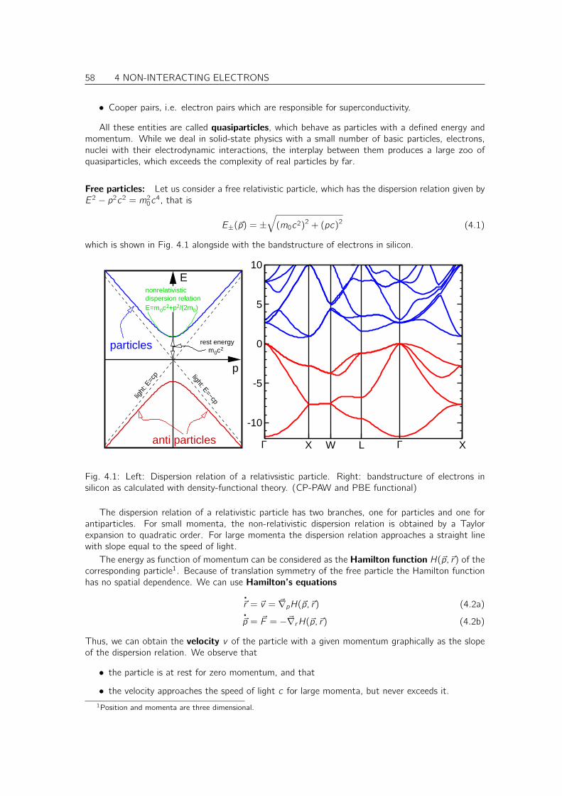
58 4 NON-INTERACTING ELECTRONS
• Cooper pairs, i.e. electron pairs which are responsible for superconductivity.
All these entities are called quasiparticles, which behave as particles with a defined energy andmomentum. While we deal in solid-state physics with a small number of basic particles, electrons,nuclei with their electrodynamic interactions, the interplay between them produces a large zoo ofquasiparticles, which exceeds the complexity of real particles by far.
Free particles: Let us consider a free relativistic particle, which has the dispersion relation given byE2 − p2c2 = m20c4, that is
E±(~p) = ±√
(m0c2)2 + (pc)2 (4.1)
which is shown in Fig. 4.1 alongside with the bandstructure of electrons in silicon.
p
anti particles
particles
E
light
: E=c
p light: E=−cpm0c2
rest energy
nonrelativisticdispersion relationE=m0c2+p2/(2m0)
Γ X W L Γ X
-10
-5
0
5
10
Fig. 4.1: Left: Dispersion relation of a relativsistic particle. Right: bandstructure of electrons insilicon as calculated with density-functional theory. (CP-PAW and PBE functional)
The dispersion relation of a relativistic particle has two branches, one for particles and one forantiparticles. For small momenta, the non-relativistic dispersion relation is obtained by a Taylorexpansion to quadratic order. For large momenta the dispersion relation approaches a straight linewith slope equal to the speed of light.
The energy as function of momentum can be considered as the Hamilton function H(~p,~r) of thecorresponding particle1. Because of translation symmetry of the free particle the Hamilton functionhas no spatial dependence. We can use Hamilton’s equations
.~r = ~v = ~∇pH(~p,~r) (4.2a).~p = ~F = −~∇rH(~p,~r) (4.2b)
Thus, we can obtain the velocity v of the particle with a given momentum graphically as the slopeof the dispersion relation. We observe that
• the particle is at rest for zero momentum, and that
• the velocity approaches the speed of light c for large momenta, but never exceeds it.
1Position and momenta are three dimensional.
4 NON-INTERACTING ELECTRONS 59
Observe also that the slope in the anti-particle branch, that is the velocity, is opposite to thedirection of the momentum. This is something to be taken seriously.2
The second Hamilton’s equation is Newton’s law. If the system is translationally symmetric, thereare no forces and the momentum is a constant of motion, i.e. it does not change with time. However,we may also consider external forces. A constant force implies that the momentum changes linearlywith time. By observing the change of the slope, that is the velocity, over time while the momentumis shifted to the right, we can extract the dynamics of the system under a constant force.
As an example, we may follow a skyrocket, which accelerates under the constant thrust createdby its rocket engines. Initially, that is for small momenta, the dispersion relation is quadratic, so thatthe velocity changes linear with momentum. Under a constant force, the velocity increases linearlywith time with an acceleration a obtained from ~F = m0~a. The curvature of the dispersion relationis the inverse mass. As the rocket continues to accelerate, its speed grows less and less, while themomentum still grows continuously. This captures that the speed of light is the absolute maximumvelocity for particles.
The dispersion relation of the relativistic particle has two branches. The upper one is identifiedwith particles and the other is identified with antiparticles. In order to avoid the problem, thatan antiparticle could accelerate indefinitely while emitting light, the concept of the Dirac sea hasbeen introduced. The problem finds a more satisfactory solution in the context of quantm fieldtheory. However, here we employ it, because it is analogous to the conventional view in solid statephysics. The idea is that all states of the antiparticle band are filled with electrons under normalcircumstances. Due to Pauli principle a fermionic particle cannot lower its energy by occupying analready filled state of the antiparticle band and thus emit light. Thus an antiparticle is a "missingelectron in the antiparticle band" or a hole.
A particle anti-particle pair can annihilate by emitting to quanta of light, which carry away energyand momentum of the particle antiparticle pair. This is an example of the interplay of two bandstructures, one for electrons and one for photons, i.e. light. Their only difference is the mass whichvanishes for photons. Let us consider the process in detail. Initially there is a particle, say withmomentum zero and a "hole" in the antiparticle branch. The particle can drop in the hole. In thatprocess the rest energy 2m0c2 of both particles and the momentum p′ = 0 needs to be carried away.Therefore we turn to the bandstructure for photons, that is for mass-less particles. We observe thatthe energy cannot be placed into a single photon, because that would also absorb a finite momentum.However it can be placed into two photons with opposite momentum and each having an energy equalto the rest mass of the annihilated particle. This is an example for a scattering process of particlesas they are present in solids.
Real band structure: The interpretation of the band structure of a real material is analogous tothat of the dispersion relation of the free particle. Therefore, the band structure of electrons insilicon are shown in Fig. 4.1 alongside the dispersion relation of the free particle.
There are two apparent difference to the free particle:
• there are even more more branches
• the momenta are drawn into several finite sections
The reason is the reduced symmetry of the solid compared to a particle in vacuum. The dispersionrelation of a free particle is isotropic, so that it is suffient to draw it in one direction. In a crystal,the bands depend on the direction of the momentum.
Because the translational symmetry of a lattice is discrete, the coordinate axis for the momentumis folded up into a finite region. The resulting section of momentum space is thus finite. Furthermorethe folded bands add to the bands already present in this finite region. Each segment describes theband structure along a so-called high-symmetry line in momentum space.
Now, we can translate the observations made for the free particle to the band structure of silicon:2However, the interpretation of antiparticles can be changed so that the energies are positive.
60 4 NON-INTERACTING ELECTRONS
• The bands at negative energies shown in red in Fig. 4.1 describe the valence electrons. Thesebands are filled with electrons as the antiparticle bands in the Dirac sea.
• The bands at positive energies shown in blue in Fig. 4.1 describe the conduction electrons.
• Valence and conduction states are separated by a band gap, a region where no electrons canexist in a perfect lattice.
• By heating up the crystal, a small number of electrons are created in the conduction band anda small number of holes, i.e. missing electrons, are formed in the valence band. In the followingwe often simply refer to electrons and holes. The electrons will relax towards the minima ofthe conduction band, near the point X.
• The curvature of the energy band at the minimum is related to the inverse effective mass ofthe conduction electron.
ǫ(~p) ≈ 12~pm−1eff ~p
mef f = ~2(
~∇k ⊗ ~∇k∣∣~k0ǫ)−1
(4.3)
The derivative is taken at the band extremum and for the band that forms it. This effective massis anisotropic, which can be seen from the curvature in Γ− X direction and the perpendiculardirection X −W . The holes are located at the maximum of the valence band, which lies atΓ. Flat bands indicate that the particle is heavy, while bands with large curvature indicate lightparticles. The effective masses of holes are obtained analytically, with the only difference thatthe sign in the definition changes.
• For metals, the slope of the bands at the Fermi level is a measure for the velocity of n electron,the Fermi velocity.
~vFermi(~k) =1
~~∇kǫ(~k) (4.4)
The Fermi velocity depends strongly on the partular band and the position at the Fermi surface.Typical Fermi velocity are 106 m/sec , which is only a factor 300 slower than the speed of light.3
• The number of thermally created holes and electrons and their effective masses determine theelectrical conductivity.
• A photon can be absorbed by the formation of electron-hole pairs, if its energy exceeds theband gap. Silicon is transparent to infrared radiation, but it reflects visible light. The bandgap of silicon is about Eg = 1.17 eV, while the photon energy of visible light ranges from 1.65to 3.26 eV. Because of the large speed of light, a photon has nearly infinite slope. Thus aexcitation or recombination is a vertical process.
• A lattice vibration can also be represented by a band structure. Opposite to the photon, thephonon has small energies and can have large momenta. This is consisten with the small speedof sound. Thus, the absorption of a phonon shifts the particle nearly horizontally in the bandstructure.
3Consider a free electron gas with dispersion relation ǫ(~p) = ~p2
2meAs shown below the particle number N in a
volume V is given by N = V∑
σ
∫
|~k |<kFd3k(2π)2
= 13π2
k3F V , so that kF =3
√
3π3 NV
. The velocity is vF = (~|kF |)/me =~
me3
√
3π3 NeV
. Let us estimate the quantities: Aluminium has a lattice constant of alat = 4.05 Å. Aluminium has theface centered cubic structure, with 4 atoms in the cubic unit cell. Each Al atom contributes three valence electrons.Thus the electron density is N/V = 12a−3lat = 0.18× 1030 m−3 With the electron mass of 0.911× 10⁻³⁰ kg. Thus weobtain
vF =~
me
3
√
3π3Ne
V≈ 2× 10⁶ m
s(4.5)
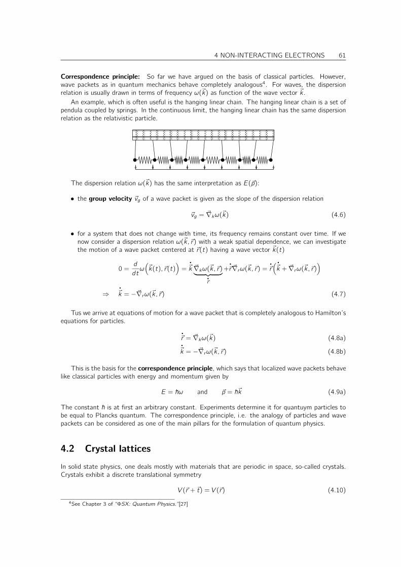
4 NON-INTERACTING ELECTRONS 61
Correspondence principle: So far we have argued on the basis of classical particles. However,wave packets as in quantum mechanics behave completely analogous4. For waves, the dispersionrelation is usually drawn in terms of frequency ω(~k) as function of the wave vector ~k .
An example, which is often useful is the hanging linear chain. The hanging linear chain is a set ofpendula coupled by springs. In the continuous limit, the hanging linear chain has the same dispersionrelation as the relativistic particle.
The dispersion relation ω(~k) has the same interpretation as E(~p):
• the group velocity ~vg of a wave packet is given as the slope of the dispersion relation
~vg = ~∇kω(~k) (4.6)
• for a system that does not change with time, its frequency remains constant over time. If wenow consider a dispersion relation ω(~k,~r) with a weak spatial dependence, we can investigatethe motion of a wave packet centered at ~r(t) having a wave vector ~k(t)
0 =d
dtω(
~k(t), ~r(t))
=.~k ~∇kω(~k,~r)︸ ︷︷ ︸
.~r
+.~r ~∇rω(~k,~r) =
.~r(.~k + ~∇rω(~k,~r)
)
⇒.~k = −~∇rω(~k,~r) (4.7)
Tus we arrive at equations of motion for a wave packet that is completely analogous to Hamilton’sequations for particles.
.~r = ~∇kω(~k) (4.8a).~k = −~∇rω(~k,~r) (4.8b)
This is the basis for the correspondence principle, which says that localized wave packets behavelike classical particles with energy and momentum given by
E = ~ω and ~p = ~~k (4.9a)
The constant ~ is at first an arbitrary constant. Experiments determine it for quantuym particles tobe equal to Plancks quantum. The correspondence principle, i.e. the analogy of particles and wavepackets can be considered as one of the main pillars for the formulation of quantum physics.
4.2 Crystal lattices
In solid state physics, one deals mostly with materials that are periodic in space, so-called crystals.Crystals exhibit a discrete translational symmetry
V (~r + ~t) = V (~r) (4.10)
4See Chapter 3 of “ΦSX: Quantum Physics.”[27]
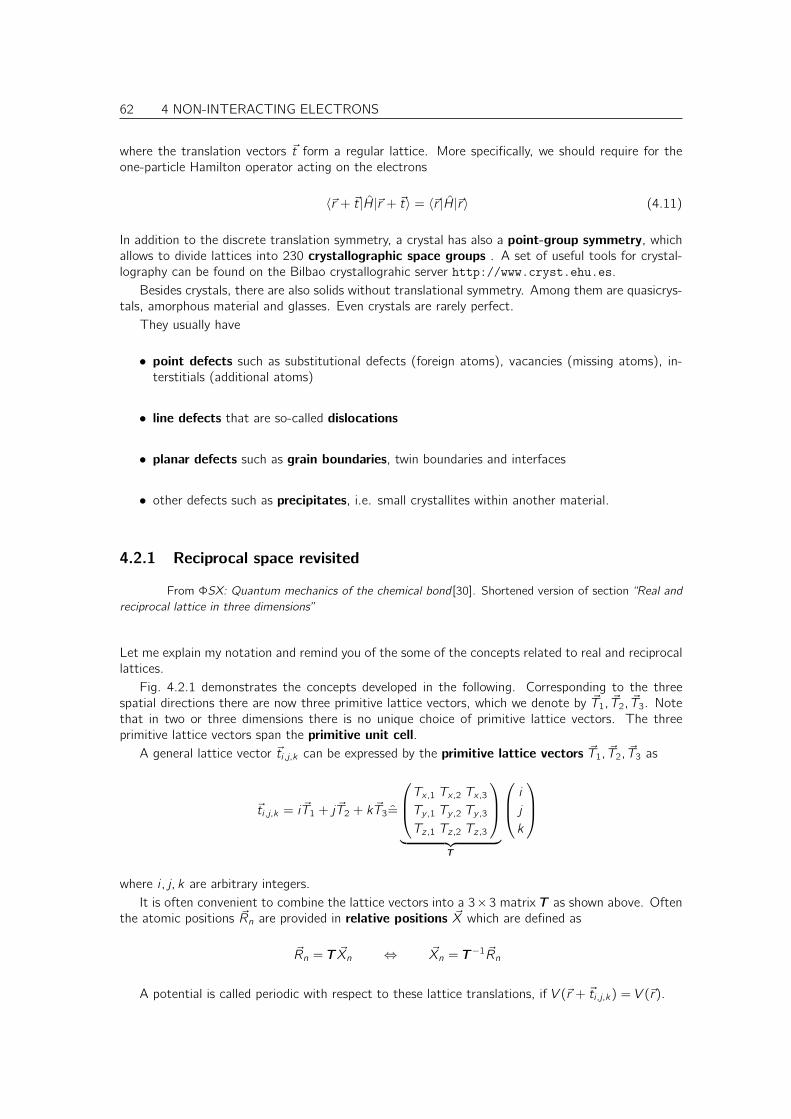
62 4 NON-INTERACTING ELECTRONS
where the translation vectors ~t form a regular lattice. More specifically, we should require for theone-particle Hamilton operator acting on the electrons
〈~r + ~t|H|~r + ~t〉 = 〈~r |H|~r〉 (4.11)
In addition to the discrete translation symmetry, a crystal has also a point-group symmetry, whichallows to divide lattices into 230 crystallographic space groups . A set of useful tools for crystal-lography can be found on the Bilbao crystallograhic server http://www.cryst.ehu.es.
Besides crystals, there are also solids without translational symmetry. Among them are quasicrys-tals, amorphous material and glasses. Even crystals are rarely perfect.
They usually have
• point defects such as substitutional defects (foreign atoms), vacancies (missing atoms), in-terstitials (additional atoms)
• line defects that are so-called dislocations
• planar defects such as grain boundaries, twin boundaries and interfaces
• other defects such as precipitates, i.e. small crystallites within another material.
4.2.1 Reciprocal space revisited
From ΦSX: Quantum mechanics of the chemical bond [30]. Shortened version of section “Real and
reciprocal lattice in three dimensions”
Let me explain my notation and remind you of the some of the concepts related to real and reciprocallattices.
Fig. 4.2.1 demonstrates the concepts developed in the following. Corresponding to the threespatial directions there are now three primitive lattice vectors, which we denote by ~T1, ~T2, ~T3. Notethat in two or three dimensions there is no unique choice of primitive lattice vectors. The threeprimitive lattice vectors span the primitive unit cell.
A general lattice vector ~ti ,j,k can be expressed by the primitive lattice vectors ~T1, ~T2, ~T3 as
~ti ,j,k = i ~T1 + j ~T2 + k ~T3=
Tx,1 Tx,2 Tx,3
Ty,1 Ty,2 Ty,3
Tz,1 Tz,2 Tz,3
︸ ︷︷ ︸
T
i
j
k
where i , j, k are arbitrary integers.It is often convenient to combine the lattice vectors into a 3×3 matrix T as shown above. Often
the atomic positions ~Rn are provided in relative positions ~X which are defined as
~Rn = T ~Xn ⇔ ~Xn = T−1 ~Rn
A potential is called periodic with respect to these lattice translations, if V (~r + ~ti ,j,k) = V (~r).
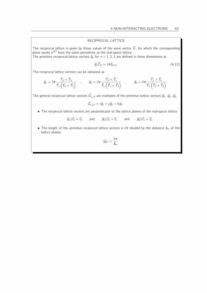
4 NON-INTERACTING ELECTRONS 63
RECIPROCAL LATTICE
The reciprocal lattice is given by those values of the wave vector ~G, for which the correspondingplane waves ei ~G~r have the same periodicity as the real-space lattice.The primitive reciprocal-lattice vectors ~gn for n = 1, 2, 3 are defined in three dimensions as
~gn~Tm = 2πδn,m (4.12)
The reciprocal lattice vectors can be obtained as
~g1 = 2π~T2 × ~T3
~T1
(
~T2 × ~T3) , ~g2 = 2π
~T3 × ~T1~T1
(
~T2 × ~T3) , ~g3 = 2π
~T1 × ~T2~T1
(
~T2 × ~T3)
The general reciprocal lattice vectors ~Gi ,j,k are multiples of the primitive lattice vectors ~g1, ~g2, ~g3.
~Gi ,j,k = i~g1 + j~g2 + k~g3
• The reciprocal lattice vectors are perpendicular to the lattice planes of the real-space lattice.
~g1||~t2 × ~t3 and ~g2||~t3 × ~t1 and ~g3||~t1 × ~t2
• The length of the primitive reciprocal lattice vectors is 2π divided by the distance ∆n of thelattice planes.
|~gn| =2π
∆n
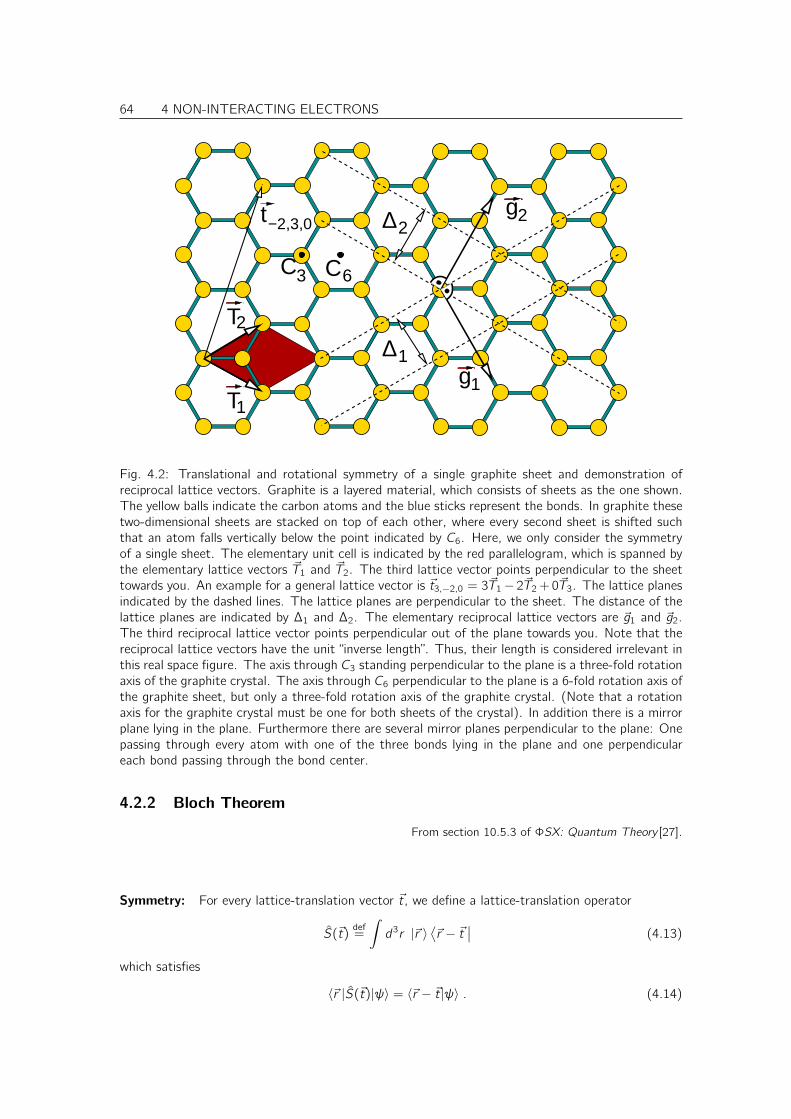
64 4 NON-INTERACTING ELECTRONS
∆1g
g2
2T
T1
C3 C6
t−2,3,0 ∆2
1
Fig. 4.2: Translational and rotational symmetry of a single graphite sheet and demonstration ofreciprocal lattice vectors. Graphite is a layered material, which consists of sheets as the one shown.The yellow balls indicate the carbon atoms and the blue sticks represent the bonds. In graphite thesetwo-dimensional sheets are stacked on top of each other, where every second sheet is shifted suchthat an atom falls vertically below the point indicated by C6. Here, we only consider the symmetryof a single sheet. The elementary unit cell is indicated by the red parallelogram, which is spanned bythe elementary lattice vectors ~T1 and ~T2. The third lattice vector points perpendicular to the sheettowards you. An example for a general lattice vector is ~t3,−2,0 = 3~T1− 2~T2+0~T3. The lattice planesindicated by the dashed lines. The lattice planes are perpendicular to the sheet. The distance of thelattice planes are indicated by ∆1 and ∆2. The elementary reciprocal lattice vectors are ~g1 and ~g2.The third reciprocal lattice vector points perpendicular out of the plane towards you. Note that thereciprocal lattice vectors have the unit “inverse length”. Thus, their length is considered irrelevant inthis real space figure. The axis through C3 standing perpendicular to the plane is a three-fold rotationaxis of the graphite crystal. The axis through C6 perpendicular to the plane is a 6-fold rotation axis ofthe graphite sheet, but only a three-fold rotation axis of the graphite crystal. (Note that a rotationaxis for the graphite crystal must be one for both sheets of the crystal). In addition there is a mirrorplane lying in the plane. Furthermore there are several mirror planes perpendicular to the plane: Onepassing through every atom with one of the three bonds lying in the plane and one perpendiculareach bond passing through the bond center.
4.2.2 Bloch Theorem
From section 10.5.3 of ΦSX: Quantum Theory [27].
Symmetry: For every lattice-translation vector ~t, we define a lattice-translation operator
S(~t)def=
∫
d3r |~r 〉⟨~r − ~t
∣∣ (4.13)
which satisfies
〈~r |S(~t)|ψ〉 = 〈~r − ~t|ψ〉 . (4.14)
4 NON-INTERACTING ELECTRONS 65
Let us investigate the eigenstates of the translation operator. Because the lattice-translationoperator is unitary, the absolute value of the eigenvalue is one, that is
S(~t)|ψϕ〉 = |ψϕ〉eiϕ (4.15)
where the phase shift depends on the translation vector.Because S(n~t) = Sn(~t), a similar relation must hold for the eigenvalues, i.e. ϕ(n~t) = nϕ(~t).
This requirement can be satisifed by choosing the form ϕ(~t) = ~k~t. In addition, this form works forsuperpositions of linearly indepdendent lattice vectors. The vector-parameter ~k is the so-called Blochvector or simply wave vector.
Thus, the eigenvalue equation for the lattice-translation operator is
S(~t)|φ~k〉 = |φ~k〉ei~k~t (4.16)
Let us now construct the eigenstates of the lattice translation operator:
〈~r |S(~t)|φ~k〉 = 〈~r |φ~k〉ei~k~t (4.17)
〈~r − ~t|φ~k〉 = 〈~r |φ~k〉ei~k~t
⇒ 〈~r − ~t|φ~k〉〉e−i~k~t
︸ ︷︷ ︸
u~k (~r−~t)
= 〈~r |φ~k〉〉 e−i~k~0
︸ ︷︷ ︸
=1︸ ︷︷ ︸
u~k (~r)
(4.18)
Thus, the function
u~k(~r)def= |φ~k〉e−i
~k~r (4.19)
which is defined for an eigenstate of the lattice translation operator S(~t) with eigenvalue ei~k~t isinvariant with the lattice translations. That is
u~k(~r − ~t) = u~k(~r) . (4.20)
Hence the eigenstates of the lattice-translation operators can be witten as product of a periodicfunction and a plane wave. Without limitation of generality, this Bloch vector can be chosen fromwithin the first reciprocal unit cell.
Lattice symmetry implies that the eigenstates of the lattice Hamiltonian can be chosen to beeigenstates of the lattice-translation operator, which immediately implies Bloch theorem.
BLOCH THEOREM
The eigenstates of a system with lattice symmetry can be written as product of a periodic functionu~k(~r), i.e.
uk(~r + ~t) = u~k(~r) , ‘ (4.21)
and a modulating plane wave ei~k~r , that is
ψk(~r) = u~k(~r)ei~k~r (4.22)
where the wave vector ~k , the Bloch vector, is a good quantum number of the system.
4.2.3 Non-interacting electrons in an external potential
Another way to obtain the Bloch theorem is to set up the Hamiltonian in a plane wave basis. Onthe one hand, this approach to the problem connects to some of the principles used in a plane
66 4 NON-INTERACTING ELECTRONS
wave pseudopotential method. On the other hand it shows that lattice potential leads to a couplingbetween points in the reciprocal space, which are separated by reciprocal lattice vectors.
Let us now consider the consequences of a weak external potential.
V (~r) =∑
~G
V~Gei ~G~r (4.23)
Since the potential shall be periodic, only reciprocal lattice vectors ~G occur in the sum. The Hamil-tonian can be written as
H =∑
σ
∫
d3r |~r , σ〉(
−~22me
~∇2 +∑
G
VGei ~G~r
)
〈~r , σ|
Let us now work out the matrix elements of the Hamiltonian between two plane waves,
φ~k,σ(~r , σ′)
Eq. 4.91= 〈~r , σ′|φ~k,σ〉 =
δσ,σ′√Ωei~k~r , (4.24)
which are the eigenstates of the free electron gas.
Hσ,σ′(~k, ~k ′) := 〈φ~k,σ|H|φ~k ′,σ′〉
=∑
σ′′
∫
Ω
d3r 〈φ~k,σ|~r , σ′′〉︸ ︷︷ ︸
φ∗~k,σ(~r ,σ′′)
(
−~22me
~∇2 +∑
G
VGei ~G~r
)
〈~r , σ′′|φ~k ′,σ′〉︸ ︷︷ ︸
φ~k,σ(~r ,σ′′)
Eq. 4.91=
δσ,σ′
Ω
∫
Ω
d3r e−i~k~r
(
−~22me
~∇2 +∑
G
VGei ~G~r
)
ei~k ′~r
=(~~k)2
2meδσ,σ′
1
Ω
∫
Ω
d3r ei(~k ′−~k)~r
︸ ︷︷ ︸
δ~k ′ ,~k
+∑
~G
V~Gδσ,σ′1
Ω
∫
Ω
d3r e−i~k~rei
~G~rei~k ′~r
︸ ︷︷ ︸
δ~k ′+~G,~k
= δσ,σ′∑
~G
[
(~~k)2
2meδ~G,~0 + V~G
]
δ~k ′+~G,~k (4.25)
We have used here the normalization condition5 corresponding to a finite, even though very large,volume Ω with side-lengths Lx , Ly , Lz . Correspondingly, the spectrum is discrete with wave vectors~ki ,j,k =
2πLxi + 2πLy j +
2πLzk .
Thus, there is only a coupling between states that are separated by a reciprocal lattice vector.This is one way to prove Bloch’s theorem.
BLOCH’S THEOREM
Bloch’s theorem says that the eigenstates in a periodic potential can be written as a product of afunction u~k,σ(~r , σ
′) that is periodic with the periodicity of the potential and a phase factor ei~k~r .
This can be shown as follows: Once we diagonalize the Hamiltonian, the eigenstates will bea superposition of the basis states, the plane waves, that are connected by a Hamiltonian matrixelement. Thus, the final wave function has the general form
ψ~k(~r) =∑
~G
ei(~k+~G)~rck,G =
∑
~G
ei~G~rck,G
︸ ︷︷ ︸
u~k (~r)
ei~k~r = u~k(~r)e
i~k~r (4.26)
5Other choices would normalize the wave function within the unit cell, or they would set the average density equalto one.
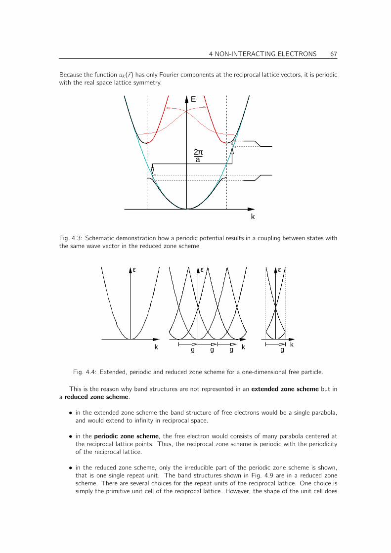
4 NON-INTERACTING ELECTRONS 67
Because the function uk(~r) has only Fourier components at the reciprocal lattice vectors, it is periodicwith the real space lattice symmetry.
2πa
E
k
Fig. 4.3: Schematic demonstration how a periodic potential results in a coupling between states withthe same wave vector in the reduced zone scheme
ggg g
ε εε
k k k
Fig. 4.4: Extended, periodic and reduced zone scheme for a one-dimensional free particle.
This is the reason why band structures are not represented in an extended zone scheme but ina reduced zone scheme.
• in the extended zone scheme the band structure of free electrons would be a single parabola,and would extend to infinity in reciprocal space.
• in the periodic zone scheme, the free electron would consists of many parabola centered atthe reciprocal lattice points. Thus, the reciprocal zone scheme is periodic with the periodicityof the reciprocal lattice.
• in the reduced zone scheme, only the irreducible part of the periodic zone scheme is shown,that is one single repeat unit. The band structures shown in Fig. 4.9 are in a reduced zonescheme. There are several choices for the repeat units of the reciprocal lattice. One choice issimply the primitive unit cell of the reciprocal lattice. However, the shape of the unit cell does
68 4 NON-INTERACTING ELECTRONS
not have the point-group symmetry of the reciprocal lattice. Therefore one instead choosesthe Wigner Seitz cell6 of the reciprocal lattice, which is called the Brillouin zone.
In the reduced zone scheme, all wave vectors connected by a reciprocal lattice vector, fall on topof the same point in the Brillouin zone. Thus, a Hamiltonian that has lattice periodicity couples allpoints that lie at the same point in the Brillouin zone. This is demonstrated in Fig. 4.3.
From perturbation theory we know that the splitting of two interacting states is large when thetwo states are close or even degenerate. Thus the largest effect in the band structure occurs rightat the boundary of the irreducible zone, where the degeneracy of the free electron gas is lifted by theperiodic potential. Thus, local band gaps appear at the surface of the Brillouin zone. This band gap,however, is usually warped, so that there is no energy window, that completely lies in all local bandgaps. In that case the material remains a metal.
4.3 Bands and orbitals
From ΦSX:Quantum mechanics of the chemical bond[30]
So far we discussed the band structures as a variation of the dispersion relation of the free-electronbands. However, this point of view obscures the relation to chemical binding and the local picture ofthe wave functions.
The band structure can also be constructed starting from local orbitals. This is demonstratedhere for the two-dimensional square lattice with atoms having s- and p-orbitals in the plane.
In order to simplify the work, we restrict ourselves to the high symmetry points Γ, X and M ofthe two-dimensional reciprocal unit cell.
The real space lattice vectors are
~T1 =
(
1
0
)
a and ~T2 =
(
0
1
)
a
The corresponding reciprocal space lattice vectors are
~g1 =
(
1
0
)
2π
aand ~g2 =
(
0
1
)
2π
a
The high-symmetry points are
kΓ = 0 =
(
0
0
)
2π
a; kX =
1
2~g1 =
(
1
0
)
π
aand kM =
1
2(~g1 + ~g2) =
(
1
1
)
π
a
The first step is to construct Bloch waves out of the atomic orbitals, by multiplying them withei~k~t , where ~t is the lattice translation of the atom relative to the original unit cell. This is illustrated
in Fig. 4.5 on page 69.
• At the Γ, the phase factor for a lattice translation of the orbital is one. Thus, we repeat theorbital from the central unit cell in all other unit cells.
• At the X point, the phase factor for a lattice translation along the first lattice vector is ei~kX ~T1 =eiπ = −1 and the phase factor for the lattice translation along the second lattice vector ~T2 isei~kX ~T2 = +1. Thus, if we go to the right the sign of the orbital alternates, while in the vertical
direction the orbital remains the same.6The Wigner Seitz cell of a lattice consists of all points that are closer to the origin than to any other lattice point.
Thus, it is enclosed by planes perpendicular to the lattice vectors cutting the lattice vector in half.
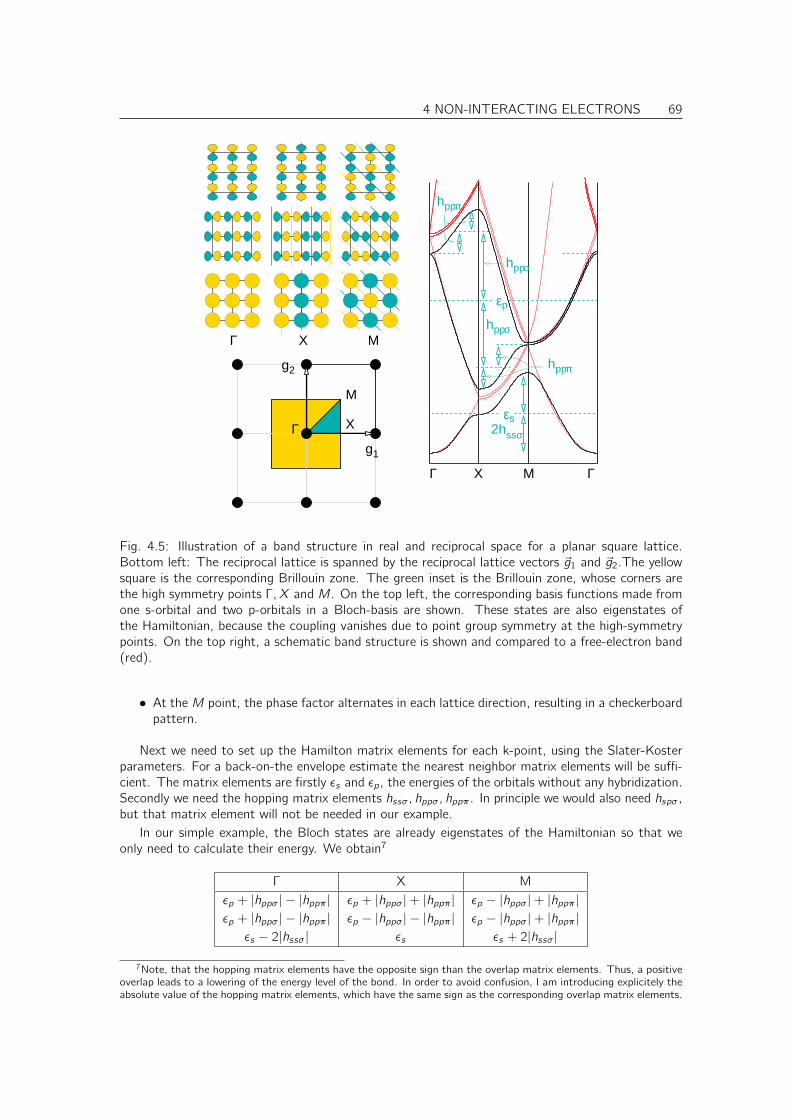
4 NON-INTERACTING ELECTRONS 69
MXΓ
Γ X
M
Γ X M Γ
g1
g2
εs
hppσ
hppπ
hppσ
hppπ
εp
ssσ2h
Fig. 4.5: Illustration of a band structure in real and reciprocal space for a planar square lattice.Bottom left: The reciprocal lattice is spanned by the reciprocal lattice vectors ~g1 and ~g2.The yellowsquare is the corresponding Brillouin zone. The green inset is the Brillouin zone, whose corners arethe high symmetry points Γ, X and M. On the top left, the corresponding basis functions made fromone s-orbital and two p-orbitals in a Bloch-basis are shown. These states are also eigenstates ofthe Hamiltonian, because the coupling vanishes due to point group symmetry at the high-symmetrypoints. On the top right, a schematic band structure is shown and compared to a free-electron band(red).
• At the M point, the phase factor alternates in each lattice direction, resulting in a checkerboardpattern.
Next we need to set up the Hamilton matrix elements for each k-point, using the Slater-Kosterparameters. For a back-on-the envelope estimate the nearest neighbor matrix elements will be suffi-cient. The matrix elements are firstly ǫs and ǫp, the energies of the orbitals without any hybridization.Secondly we need the hopping matrix elements hssσ, hppσ, hppπ. In principle we would also need hspσ,but that matrix element will not be needed in our example.
In our simple example, the Bloch states are already eigenstates of the Hamiltonian so that weonly need to calculate their energy. We obtain7
Γ X M
ǫp + |hppσ| − |hppπ| ǫp + |hppσ|+ |hppπ| ǫp − |hppσ|+ |hppπ|ǫp + |hppσ| − |hppπ| ǫp − |hppσ| − |hppπ| ǫp − |hppσ|+ |hppπ|
ǫs − 2|hssσ| ǫs ǫs + 2|hssσ|
7Note, that the hopping matrix elements have the opposite sign than the overlap matrix elements. Thus, a positiveoverlap leads to a lowering of the energy level of the bond. In order to avoid confusion, I am introducing explicitely theabsolute value of the hopping matrix elements, which have the same sign as the corresponding overlap matrix elements.
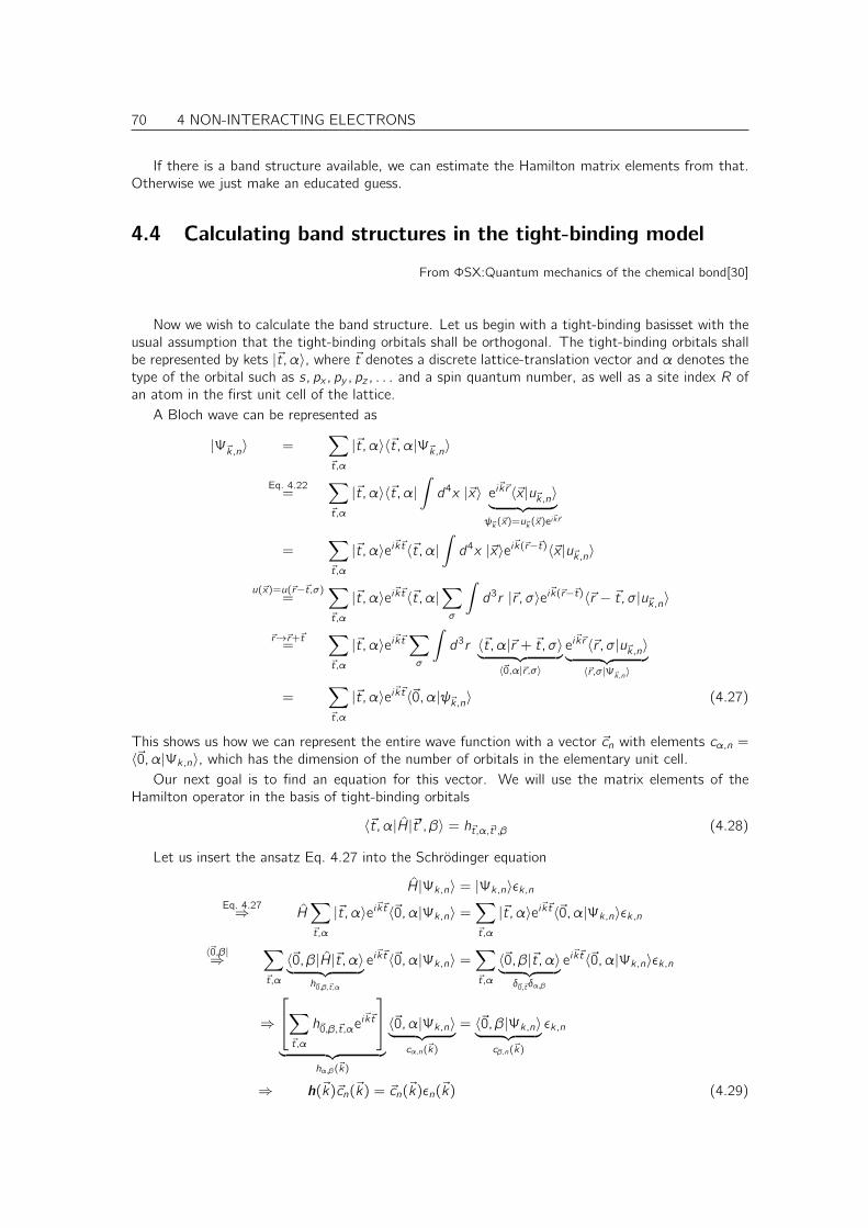
70 4 NON-INTERACTING ELECTRONS
If there is a band structure available, we can estimate the Hamilton matrix elements from that.Otherwise we just make an educated guess.
4.4 Calculating band structures in the tight-binding model
From ΦSX:Quantum mechanics of the chemical bond[30]
Now we wish to calculate the band structure. Let us begin with a tight-binding basisset with theusual assumption that the tight-binding orbitals shall be orthogonal. The tight-binding orbitals shallbe represented by kets |~t, α〉, where ~t denotes a discrete lattice-translation vector and α denotes thetype of the orbital such as s, px , py , pz , . . . and a spin quantum number, as well as a site index R ofan atom in the first unit cell of the lattice.
A Bloch wave can be represented as
|Ψ~k,n〉 =∑
~t,α
|~t, α〉〈~t, α|Ψ~k,n〉
Eq. 4.22=
∑
~t,α
|~t, α〉〈~t, α|∫
d4x |~x〉 ei~k~r 〈~x |u~k,n〉︸ ︷︷ ︸
ψ~k (~x)=u~k (~x)ei~k~r
=∑
~t,α
|~t, α〉ei~k~t〈~t, α|∫
d4x |~x〉ei~k(~r−~t)〈~x |u~k,n〉
u(~x)=u(~r−~t,σ)=
∑
~t,α
|~t, α〉ei~k~t〈~t, α|∑
σ
∫
d3r |~r , σ〉ei~k(~r−~t)〈~r − ~t, σ|u~k,n〉
~r→~r+~t=
∑
~t,α
|~t, α〉ei~k~t∑
σ
∫
d3r 〈~t, α|~r + ~t, σ〉︸ ︷︷ ︸
〈~0,α|~r ,σ〉
ei~k~r 〈~r , σ|u~k,n〉︸ ︷︷ ︸
〈~r ,σ|Ψ~k,n〉
=∑
~t,α
|~t, α〉ei~k~t〈~0, α|ψ~k,n〉 (4.27)
This shows us how we can represent the entire wave function with a vector ~cn with elements cα,n =〈~0, α|Ψk,n〉, which has the dimension of the number of orbitals in the elementary unit cell.
Our next goal is to find an equation for this vector. We will use the matrix elements of theHamilton operator in the basis of tight-binding orbitals
〈~t, α|H|~t ′, β〉 = h~t,α,~t ′,β (4.28)
Let us insert the ansatz Eq. 4.27 into the Schrödinger equation
H|Ψk,n〉 = |Ψk,n〉ǫk,nEq. 4.27⇒ H
∑
~t,α
|~t, α〉ei~k~t〈~0, α|Ψk,n〉 =∑
~t,α
|~t, α〉ei~k~t〈~0, α|Ψk,n〉ǫk,n
〈~0,β|⇒∑
~t,α
〈~0, β|H|~t, α〉︸ ︷︷ ︸
h~0,β,~t,α
ei~k~t〈~0, α|Ψk,n〉 =
∑
~t,α
〈~0, β|~t, α〉︸ ︷︷ ︸
δ~0,~tδα,β
ei~k~t〈~0, α|Ψk,n〉ǫk,n
⇒
∑
~t,α
h~0,β,~t,αei~k~t
︸ ︷︷ ︸
hα,β(~k)
〈~0, α|Ψk,n〉︸ ︷︷ ︸
cα,n(~k)
= 〈~0, β|Ψk,n〉︸ ︷︷ ︸
cβ,n(~k)
ǫk,n
⇒ h(~k)~cn(~k) = ~cn(~k)ǫn(~k) (4.29)
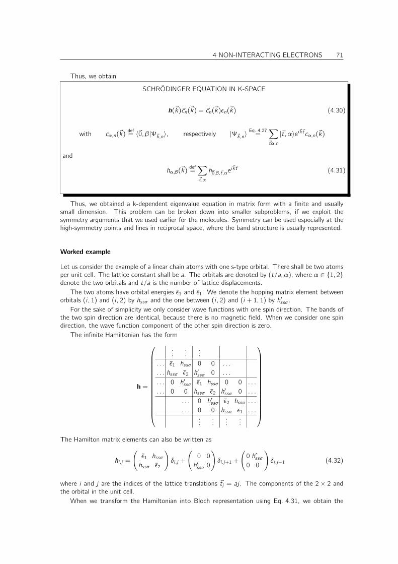
4 NON-INTERACTING ELECTRONS 71
Thus, we obtain
SCHRÖDINGER EQUATION IN K-SPACE
h(~k)~cn(~k) = ~cn(~k)ǫn(~k) (4.30)
with cα,n(~k)def= 〈~0, β|Ψ~k,n〉, respectively |Ψ~k,n〉
Eq. 4.27=
∑
~tα,n
|~t, α〉ei~k~tcα,n(~k)
and
hα,β(~k)def=∑
~t,α
h~0,β,~t,αei~k~t (4.31)
Thus, we obtained a k-dependent eigenvalue equation in matrix form with a finite and usuallysmall dimension. This problem can be broken down into smaller subproblems, if we exploit thesymmetry arguments that we used earlier for the molecules. Symmetry can be used especially at thehigh-symmetry points and lines in reciprocal space, where the band structure is usually represented.
Worked example
Let us consider the example of a linear chain atoms with one s-type orbital. There shall be two atomsper unit cell. The lattice constant shall be a. The orbitals are denoted by (t/a, α), where α ∈ 1, 2denote the two orbitals and t/a is the number of lattice displacements.
The two atoms have orbital energies ǫ1 and ǫ1. We denote the hopping matrix element betweenorbitals (i , 1) and (i , 2) by hssσ and the one between (i , 2) and (i + 1, 1) by h′ssσ.
For the sake of simplicity we only consider wave functions with one spin direction. The bands ofthe two spin direction are identical, because there is no magnetic field. When we consider one spindirection, the wave function component of the other spin direction is zero.
The infinite Hamiltonian has the form
h =
......
...
. . . ǫ1 hssσ 0 0 . . .
. . . hssσ ǫ2 h′ssσ 0 . . .
. . . 0 h′ssσ ǫ1 hssσ 0 0 . . .
. . . 0 0 hssσ ǫ2 h′ssσ 0 . . .
. . . 0 h′ssσ ǫ2 hssσ . . .
. . . 0 0 hssσ ǫ1 . . ....
......
...
The Hamilton matrix elements can also be written as
hi ,j =
(
ǫ1 hssσ
hssσ ǫ2
)
δi ,j +
(
0 0
h′ssσ 0
)
δi ,j+1 +
(
0 h′ssσ0 0
)
δi ,j−1 (4.32)
where i and j are the indices of the lattice translations ~tj = aj . The components of the 2 × 2 andthe orbital in the unit cell.
When we transform the Hamiltonian into Bloch representation using Eq. 4.31, we obtain the
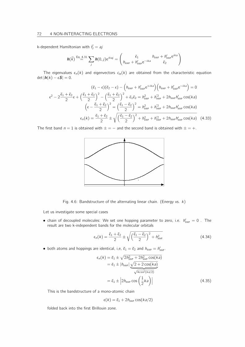
72 4 NON-INTERACTING ELECTRONS
k-dependent Hamiltonian with ~tj = aj
h(~k)Eq. 4.31=
∑
j
h(0, j)eikaj =
(
ǫ1 hssσ + h′ssσe
ika
hssσ + h′ssσe
−ika ǫ2
)
The eigenvalues ǫn(k) and eigenvectors cα(k) are obtained from the characteristic equationdet |h(k)− ǫS| = 0.
(ǫ1 − ǫ)(ǫ2 − ǫ)−(
hssσ + h′ssσe
+ika)(
hssσ + h′ssσe
−ika)
= 0
ǫ2 − 2 ǫ1 + ǫ22
ǫ+( ǫ1 + ǫ22
)2
−( ǫ1 + ǫ22
)2
+ ǫ1ǫ2 = h2ssσ + h
′2ssσ + 2hssσh
′ssσ cos(ka)
(
ǫ− ǫ1 + ǫ22
)2
=( ǫ1 − ǫ22
)2
= h2ssσ + h′2ssσ + 2hssσh
′ssσ cos(ka)
ǫn(k) =ǫ1 + ǫ22
±√( ǫ1 − ǫ22
)2
+ h2ssσ + h′2ssσ + 2hssσh
′ssσ cos(ka) (4.33)
The first band n = 1 is obtained with ± = − and the second band is obtained with ± = +.
Fig. 4.6: Bandstructure of the alternating linear chain. (Energy vs. k)
Let us investigate some special cases
• chain of decoupled molecules: We set one hopping parameter to zero, i.e. h′ssσ = 0 . Theresult are two k-independent bands for the molecular orbitals
ǫn(k) =ǫ1 + ǫ22
±√( ǫ1 − ǫ22
)2
+ h2ssσ (4.34)
• both atoms and hoppings are identical, i,e, ǫ1 = ǫ2 and hssσ = h′ssσ.
ǫn(k) = ǫ1 ±√
2h2ssσ + 2h2ssσ cos(ka)
= ǫ1 ± |hssσ|√
2 + 2 cos(ka)︸ ︷︷ ︸√
4cos2(ka/2)
= ǫ1 ±∣∣∣2hssσ cos
(1
2ka
)∣∣∣ (4.35)
This is the bandstructure of a mono-atomic chain
ǫ(k) = ǫ1 + 2hssσ cos(ka/2)
folded back into the first Brillouin zone.
4 NON-INTERACTING ELECTRONS 73
• for alternating orbital energies or alternating hopping matrix elements, The band gap at thezone boundary opens, so that an insulator is obtained if the orbitals are half filled.
Note that hssσ is negative, because it is approximately equal to the overlap matrix elementmultiplied with the potential in the bond-center. The potential is negative.
4.5 Thermodynamics of non-interacting electrons
What makes the many-electron problem so complicated is the interaction between the electrons. Asimilar problem is known from classical mechanics. While the Kepler problem, a two-body problem,can be solved analytically, no such solution exists for the three-body problem, where the gravitationalattraction between the planets is considered as well.
4.5.1 Thermodynamics revisited
General setup
For a system described by a Hamiltonian H, which is coupled to a heat bath and reservoirs for theobservables Xi, the free energy F (T, fj) is (Eq. 1.61 of [31])
F (T, fj) = −kBT ln[
Tr(
e−β(H+∑
j fj Xj ))]
(4.36)
The heat bath is characterized by the temperature T and the other reservoirs are characterized bythe other intrinsic variables fj .
From the free energy, we can obtain (Eqs. 1.65, 1.66, 1.67 of [31]) the expectation values forthe observables X and the internal energy U, the expectation value of the energy of the system by
S(T, fk) = −∂F (T, fk)
∂T(4.37)
Xi(T, fk) = +∂F (T, fk)
∂fi
U(T, fk) = F (T, fk) + TS(T, fk)−∑
i
fiXi(T, fk) (4.38)
Specific relations
For our purposes we will start from a grand canonical ensemble, which describes a system in thermalequilibrium with a heat bath and a particle reservoir.
extensive variable X f intensive variable
volume V p pressureparticle number N −µ chemical potential
The thermodynamic potential for the grand canonical ensemble is the grand potential Ω(T, V, µ).
Ω(T, V, µ) = −kBT ln[
Tr(
e−β(H+µN))]
(4.39)
which yields
S(T, V, µ) = −∂Ω(T, V, µ)∂T
(4.40)
N(T, V, µ) = −∂Ω(T, V, µ)∂µ
(4.41)
U(T, V, µ) = Ω(T, V, µ) + TS(T, V, µ) + µN(T, V, µ) (4.42)
74 4 NON-INTERACTING ELECTRONS
These equations can be put together to a Legendre transform to a quantity depending on theextensive variables
U(S, V, N) = statT,µ
(
Ω(T, V, µ) + TS + µN)
(4.43)
which yields the fundamental relation of thermodynamics
dU = TdS︸︷︷︸
heat
+
Work︷ ︸︸ ︷
dΩ
dV︸︷︷︸−p
dV + µdN (4.44)
which in turn defines Heat and Work.The pressure is defined as the derivative of the internal energy with respect to volume at fixed
entropy and particle number
pdef= −∂U(S, V, N)
∂V= −∂Ω(T, V, µ)
∂V(4.45)
4.5.2 Maximum entropy, minimum free energy principle and the meaning ofthe grand potential
The grand potential is related to the total energy of a composite system which consists of thematerial under study with an internal energy U(S, V, N), the the heat-bath with energy Uhb and aparticle reservoir with energy Upr = µNpr .
Consider a starting configuration where the entropy and the particle number on the system understudy vanish initially, that is (S = 0, N = 0). Also the particle number of the particle reservoir andthe energy of the heat bath vanish, i.e. (Uhb = 0, Npr = 0).
As the system is brought into contact with the heat bath and its reservoirs, particles are transferredfrom the reservoir to the system and heat ThbdShb is transferred from the heat bath to the system.Thus the energy of the heat bath is
Uhb(Shb) =
∫ Shb
0
dS′ Thb = ThbShb (4.46)
The energy conservation between heat bath and our system has the form
∂U
∂SdS + ThbdShb = 0
⇒ ∂U
∂SdS − ThbdS + Thb(dShb + dS) = 0
dStot :=S+Shb⇒ dUhb = −∂U
∂SdS = −ThbdS + ThbdStot (4.47)
where dStot is the total amount of entropy produced in the process. This entropy production iswhat drives the system into thermal equilibrium with its reservoirs. The entropy is produced duringthe heat transfer between heat bath and our system. Entropy is generally generated when heat istransferred along a temperature gradient or between two systems at different temperatures.
The total energy Etot and total number of particles is conserved, i.e. dEtot = 0, where the totalenergy is
Etot(Thb, V, µpr , S, N, Uhb, Npr ) = U(S, V, N)︸ ︷︷ ︸
system
+ Uhb︸︷︷︸
heat bath
+ µprNpr︸ ︷︷ ︸
particle reservoir
(4.48)
Using the particle conservation Npr = −N and Eq. 4.47, the total energy obtains the form
Etot(Thb, V, µpr ;S, Stot , N) = U(S, V, N)− ThbS + ThbStot − µprN (4.49)
4 NON-INTERACTING ELECTRONS 75
As the system evolves, the total entropy dStot increases until it reaches its maximum. While itevolves, the process obeys energy conservation, that is dEtot = 0. Hence the state evolves on ahypersurface defined by Etot = const in the S,N, Stot space. As a result, the total entropy can beexpressed as function of S and N.
−ThbStot(S, V, N) = U(S, V, N)− ThbS − µprN − U(0, V, 0) (4.50)
This is only valid though, if the state (S, V, N) is connected by an energy conserving process to theinitial state (S = 0, V, N = 0) defined above!
The thermal process comes to halt at a maximum of the total entropy. This is when an infinites-imal heat transfer from the heat bath does no more produce entropy in the system, which in turnimplies that our system has reached the same temperature as the heatbath. The maximum entropyprinciple translates into a minimum energy principle for the grand potential
Ω(Thb, V, µpr ) = U(0, V, 0)− TStot(S, V, N)= min
S,N
(
U(S, V, N)− ThbS − µprN)
− Etot (4.51)
The grand potential is therefore the total energy of the system under study and the reservoirs(heat bath and particle reservoir) which are in contact with our system, minus the heat generatedrespectively transported out of the entire system.
Ω(THB, V, µpr ) = minS,N
(
U(S, V, N)− ThbS − µprN)
(4.52)
4.5.3 Many-particle states of non-interacting electrons
Nevertheless, we should start with the most simple case, namely the non-interacting electron gas.The Hamiltonian for a non-interacting electron gas in a potential v(~r) has the form
H =
N∑
i=1
hi =
N∑
i=1
p2i2me
+ v(~ri)
=
N∑
i=1
∫
d4x1 · · ·∫
d4xN |~x1, . . . , ~xN〉(−~22me
~∇2i + v(~ri))
〈~x1, . . . , ~xN | (4.53)
Here, ~pi is the momentum operator acting on the i-th particle, and ~ri is the position operator of thei-th particle.
Even though the electrons do not interact, they do not move completely independently. Thereason is, again, the Pauli-principle or the antisymmetry requirement for the wave function. If oneelectron is at a certain position, no other electron with the same spin can approach it. There is norepulsive potential. The two electrons simply do not “like” each other.
In practice, this means that we have to use an antisymmetric wave function. Luckily, the eigen-states of a system of non-interacting electrons (with a non-degenerate ground state) is a single Slaterdeterminant. In contrast, the wave function for interacting electrons is, in general, a superpositionof many Slater determinants.
Here, we mention a few facts about the states of non-interacting electrons without proving them.Some are fundamental facts of statistical mechanics and others will be shown later in this book, inchapter 6.
Hamilton eigenstates: The eigenstates are Slater determinants made of eigenstates φn(~x) of the
one-particle Hamiltonian h = ~p2
2m + v(~r)[−~22m
~∇2 + v(~r)]
φn(~x)
︸ ︷︷ ︸
〈~x |h|φn〉
= φn(~x)ǫn (4.54)
76 4 NON-INTERACTING ELECTRONS
The Slater determinant, which is an eigenstate of the many-particle system, can be representedby its number representation. The occupations numbers, which may be zero or one, are combinedinto a vector ~σ. The i-th element of ~σ vector is the occupation number of the i-th eigenstate of theone-particle Hamiltonian.
Thus the eigenstates of the many-particle Hamiltonian can be labeled by the vector ~σ
|Φ~σ〉 = |σ1, σ2, . . .〉 (4.55)
Energy eigenvalues: A Slater determinant |Φ~σ〉 has the energy
E~σ =
∞∑
n=1
σnǫn
where the ǫni are the one-particle energies defined above in Eq. 4.54.
Particle number: A Slater determinant |Φ~σ〉 has the particle number
N~σ =
∞∑
n=1
σn
Editor: We came up to here on Wednesday, Dec. 2, 2015
Grand potential: The grand canonical ensemble describes a system in thermal equilibrium whichis in contact with a heat bath and a particle reservoir. A heat bath is characterized by a temperatureT and the particle reservoir is characterized by a chemical potential µ. The temperature is oftenrepresented by the thermodynamic beta β = 1
kBT. kB is the Boltzmann constant.
The thermodynamic potential for the grand-canonical ensemble is the grand potential. Thegrand potential for a system of non-interacting fermions is
Ω(T, µ)def= = −kBT ln Tr[e−β(H−µN)]
= −kBT ln[∑
~σ
exp
(
−β(
E~σ − µN~σ))
︸ ︷︷ ︸
partition sum
]
= −kBT ln[∑
~σ
e−β∑∞i=1 σi (ǫi−µ)
]
= −kBT ln[ ∞∏
i=1
1∑
σi=0
e−βσi (ǫi−µ)]
= −kBT ln[ ∞∏
i=1
(
1 + e−β(ǫi−µ))]
= −kBT∞∑
i=1
ln(
1 + e−β(ǫi−µ))
(4.56)
The interesting observation is that the thermodynamic potential of non-interacting particles, hereelectrons, is a sum over one-particle states.
4.5.4 Density of States
The grand potential turns out to be a simple sum over one-electron states with an integrand thatdepends on the one-particle energy ǫi , the chemical potential µ and the temperature T . This implies
4 NON-INTERACTING ELECTRONS 77
that the thermodynamics quantities, that are derivatives of the grand potential can be described asa sum over one-particle states as well. Therefore it is convenient to split off the spectrum of the oneparticle states. We can represent the one-particle spectrum by the density of states
DENSITY OF STATES
The one-particle density of states is defined as
D(ǫ)def=∑
n
δ(ǫ− ǫn) (4.57)
where δ(x) is Dirac’s δ-function and the one-particle energies are denoted by ǫn.
Note that the density of state as defined here is a macroscopic quantity. In practice one often usesthe density of state per volume or per unit cell.
With the density of states, we can separate the thermodynamic information from the system-specific information. The density of states is specific for the system, while the Fermi-distribution isindependent of the system and contains the thermodynamic information.
Projected Density of States: The total density of states discussed above is a special case of thedensity of states operator
D(ǫ) =∑
n
|ψn〉δ(ǫ− ǫn)〈ψn| (4.58)
which allows one to represent any thermal expectation value of one-particle operators by
〈A〉 =∑
n
f (ǫn)〈ψn|A|ψn〉 =∫
dǫ f (ǫ) Tr[D(ǫ)A
](4.59)
Grand potential expressed by the Density of States:
Ω(T, µ) = −kBT∞∑
n=1
ln(
1 + e−β(ǫn−µ))
=
∫ ∞
−∞dǫ D(ǫ)
[
−kBT ln(
1 + e−β(ǫ−µ))]
(4.60)
4.5.5 Fermi distribution
The mean occupations fi are given by the Fermi-distribution function evaluated for the one-particleenergy ǫi of the state.(see “ΦSX: Statistical Physics”)
fT,µ(ǫ)def=
1
1 + eβ(ǫ−µ)(4.61)
where β = 1/(kBT ). The Fermi function is shown in Fig. 4.7. In the absence of temperature effectswe set the temperature to zero, so that the Fermi distribution function is turned into a step function.
In the following we will also need the derivatives of the Fermi distribution with respect to temper-ature and chemical potential. They can be expressed by the energy derivative of the Fermi function.
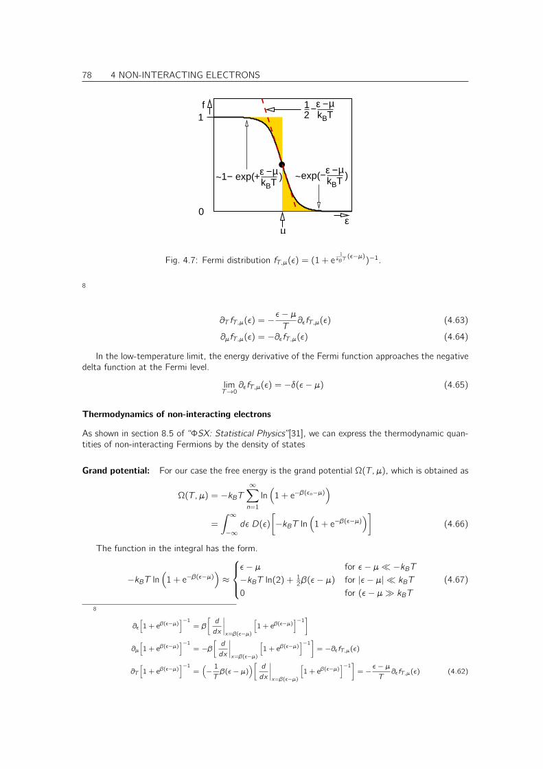
78 4 NON-INTERACTING ELECTRONS
1
0
kBTε µ−+
kBTε µ−−
kBTε µ−−
µ
f21
~1− exp( ) ~exp( )
ε
Fig. 4.7: Fermi distribution fT,µ(ǫ) = (1 + e1
kBT(ǫ−µ)
)−1.
8
∂T fT,µ(ǫ) = −ǫ− µT
∂ǫfT,µ(ǫ) (4.63)
∂µfT,µ(ǫ) = −∂ǫfT,µ(ǫ) (4.64)
In the low-temperature limit, the energy derivative of the Fermi function approaches the negativedelta function at the Fermi level.
limT→0
∂ǫfT,µ(ǫ) = −δ(ǫ− µ) (4.65)
Thermodynamics of non-interacting electrons
As shown in section 8.5 of “ΦSX: Statistical Physics”[31], we can express the thermodynamic quan-tities of non-interacting Fermions by the density of states
Grand potential: For our case the free energy is the grand potential Ω(T, µ), which is obtained as
Ω(T, µ) = −kBT∞∑
n=1
ln(
1 + e−β(ǫn−µ))
=
∫ ∞
−∞dǫ D(ǫ)
[
−kBT ln(
1 + e−β(ǫ−µ))]
(4.66)
The function in the integral has the form.
−kBT ln(
1 + e−β(ǫ−µ))
≈
ǫ− µ for ǫ− µ≪ −kBT−kBT ln(2) + 12β(ǫ− µ) for |ǫ− µ| ≪ kBT
0 for (ǫ− µ≫ kBT
(4.67)
8
∂ǫ
[
1 + eβ(ǫ−µ)]−1= β
[d
dx
∣∣∣∣x=β(ǫ−µ)
[
1 + eβ(ǫ−µ)]−1]
∂µ
[
1 + eβ(ǫ−µ)]−1= −β
[d
dx
∣∣∣∣x=β(ǫ−µ)
[
1 + eβ(ǫ−µ)]−1]
= −∂ǫfT,µ(ǫ)
∂T
[
1 + eβ(ǫ−µ)]−1=(
− 1Tβ(ǫ− µ)
)[ d
dx
∣∣∣∣x=β(ǫ−µ)
[
1 + eβ(ǫ−µ)]−1]
= − ǫ− µT
∂ǫfT,µ(ǫ) (4.62)
4 NON-INTERACTING ELECTRONS 79
In the following we express many quantities in terms of the occupations. Expressing the grandpotential by occupations is, however, not a good idea, because it depends extremely sensitive on theexact occupation if the orbital is nearly filled.
Particle number and chemical potential: The particle number N(T, µ) is obtained as
N(T, µ) = −∂Ω(T, µ)∂µ
(4.68)
=
∫ ∞
−∞dǫ D(ǫ)
[
−∂µ(
−kBT ln(
1 + e−β(ǫ−µ)))]
(4.69)
=
∫ ∞
−∞dǫ D(ǫ)fT,µ(ǫ) (4.70)
Usually, the particle number is provided instead of the chemical potential. The particle numberfollows typically from the charge neutrality condition. In order to extract the chemical potential onneeds to evaluate The partiale number as function of chemical potential and find that value for whichN(T, µ) = N.
Entropy:
S(T, µ) = −∂Ω(T, µ)∂T
=
∫ ∞
−∞dǫ D(ǫ)
[
−∂T(
−kBT ln(
1 + e−β(ǫ−µ)))]
=
∫ ∞
−∞dǫ D(ǫ)
[(
kB ln(
1 + e−β(ǫ−µ)))
︸ ︷︷ ︸
1/(1−f )
+
(
kBT1
1 + e−β(ǫ−µ)︸ ︷︷ ︸
f
( 1
kBT 2(ǫ− µ)
)
︸ ︷︷ ︸1Tln(f −1−1)
)]
=
∫ ∞
−∞dǫ D(ǫ)
[
kB
(
− ln(1− f ) + f ln(1− ff))]
=
∫ ∞
−∞dǫ D(ǫ)
[
−kB(
f ln(f ) + (1− f ) ln(1− f ))]
(4.71)
The entropy can be obtained from the occupations f = fβ,µ(ǫ).Eq. 4.71 tells us completely filled or completely empty orbitals do not contribute to the entropy
of a system. A half occupied orbital contributes kB ln(2) to the entropy. This is exactly the entropyof a yes-no decision, because the orbital can be either filled or empty with equal probability.
Internal energy: The internal energy U is the expectation value of the energy of the system.Before we continue, we express the grand potential by the occupations, because that will simplify
the equations.
Ω(T, µ) =
∫ ∞
−∞dǫ D(ǫ)
[
−kBT ln(
1 + e−β(ǫ−µ))]
=
∫ ∞
−∞dǫ D(ǫ)
[
kBT ln (1− fT,µ(ǫ))]
(4.72)
80 4 NON-INTERACTING ELECTRONS
U(T, µ) = Ω(T, µ) + TS(T, µ) + µN(T, µ)
=
∫ ∞
−∞dǫ D(ǫ)
[
kBT ln (1− f )︸ ︷︷ ︸
←Ω
−kBT(
f ln(f ) + (1− f ) ln(1− f ))
︸ ︷︷ ︸
←TS
+µf
]
=
∫ ∞
−∞dǫ D(ǫ)
[
f(
kBT ln(1− ff)
︸ ︷︷ ︸
β(ǫ−µ)
+µ
]
=
∫ ∞
−∞dǫ D(ǫ) fβ,µ(ǫ) ǫ (4.73)
where, again, f = fβ,µ(ǫ). The internal energy has a simply interpretation: it is the sum of theenergies of the occupied states.
Pressure
The pressure is defined as the derivative of the total energy upon contraction.
p = −∂U(S, V, N)∂V
(4.74)
Note, that it is not allowed to calculate the pressure as derivative of U(T, V, µ)! The pressure is thederivative of the total energy with fixed occupations.
However, we can calculate the pressure from the grand potential
p = −∂Ω(T, V, µ)∂V
=
∫ ∞
−∞dǫ
dD(ǫ)
dV
[
+kBT ln(
1 + e−β(ǫ−µ))]
(4.75)
Why does this give the same result as the derivative of U(S, V, N): The grand potential describesthe energy of the system and the reservoirs. If the volume expansion changes the entropy or theparticle number of the system, the corresponding energy change is exactly balanced to first order byan opposite energy change of the reservoirs. Thus including the energies of the reservoirs producesthe same energy change as keeping entropy and particle number fixed.
Bulk modulus: The bulk modulus is the measure of how a material can resist compression.
B0 = −V∂P
∂V= V
∂2U(S, V, N)
∂V 2(4.76)
Thus it is a second derivative of the internal energy.Heat capacity The heat capacity is the amount of energy required to raise the temperature by
one unit.
CV =∂U(T, V, N)
∂T(4.77)
When calculating the heat capacity from U(T, V, µ) we need to account for the shift of the
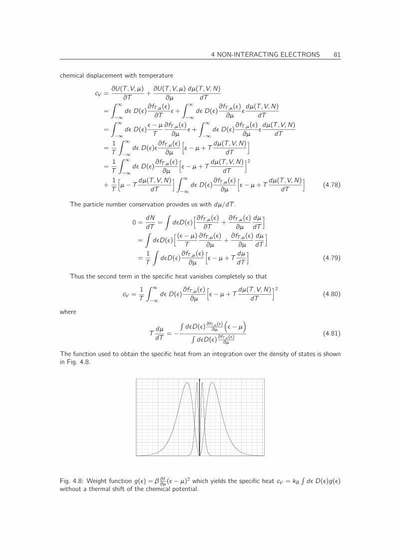
4 NON-INTERACTING ELECTRONS 81
chemical displacement with temperature
cV =∂U(T, V, µ)
∂T+∂U(T, V, µ)
∂µ
dµ(T, V, N)
dT
=
∫ ∞
−∞dǫ D(ǫ)
∂fT,µ(ǫ)
∂Tǫ+
∫ ∞
−∞dǫ D(ǫ)
∂fT,µ(ǫ)
∂µǫdµ(T, V, N)
dT
=
∫ ∞
−∞dǫ D(ǫ)
ǫ− µT
∂fT,µ(ǫ)
∂µǫ+
∫ ∞
−∞dǫ D(ǫ)
∂fT,µ(ǫ)
∂µǫdµ(T, V, N)
dT
=1
T
∫ ∞
−∞dǫ D(ǫ)ǫ
∂fT,µ(ǫ)
∂µ
[
ǫ− µ+ T dµ(T, V, N)dT
]
=1
T
∫ ∞
−∞dǫ D(ǫ)
∂fT,µ(ǫ)
∂µ
[
ǫ− µ+ T dµ(T, V, N)dT
]2
+1
T
[
µ− T dµ(T, V, N)dT
] ∫ ∞
−∞dǫ D(ǫ)
∂fT,µ(ǫ)
∂µ
[
ǫ− µ+ T dµ(T, V, N)dT
]
(4.78)
The particle number conservation provides us with dµ/dT .
0 =dN
dT=
∫
dǫD(ǫ)[∂fT,µ(ǫ)
∂T+∂fT,µ(ǫ)
∂µ
dµ
dT
]
=
∫
dǫD(ǫ)[(ǫ− µ)
T
∂fT,µ(ǫ)
∂µ+∂fT,µ(ǫ)
∂µ
dµ
dT
]
=1
T
∫
dǫD(ǫ)∂fT,µ(ǫ)
∂µ
[
ǫ− µ+ T dµdT
]
(4.79)
Thus the second term in the specific heat vanishes completely so that
cV =1
T
∫ ∞
−∞dǫ D(ǫ)
∂fT,µ(ǫ)
∂µ
[
ǫ− µ+ T dµ(T, V, N)dT
]2
(4.80)
where
Tdµ
dT= −
∫dǫD(ǫ)
∂fT,µ(ǫ)∂µ
(
ǫ− µ)
∫dǫD(ǫ)
∂fT,µ(ǫ)∂µ
(4.81)
The function used to obtain the specific heat from an integration over the density of states is shownin Fig. 4.8.
Fig. 4.8: Weight function g(ǫ) = β ∂f∂µ(ǫ− µ)2 which yields the specific heat cV = kB∫dǫ D(ǫ)g(ǫ)
without a thermal shift of the chemical potential.
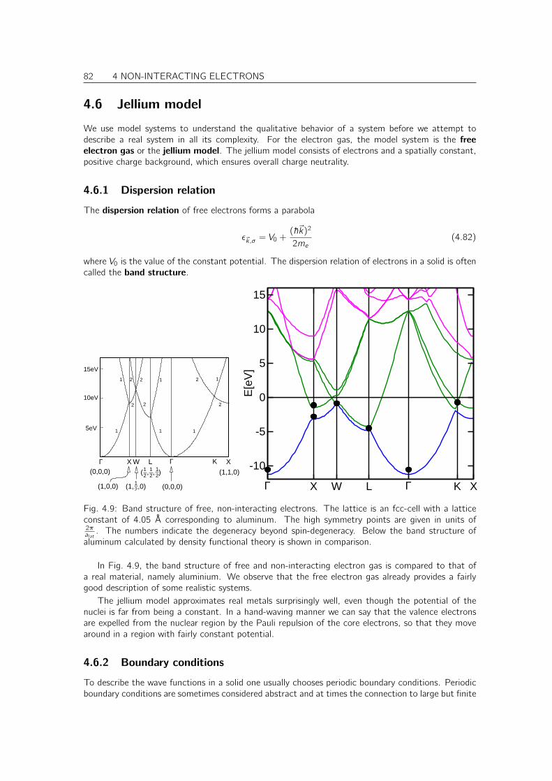
82 4 NON-INTERACTING ELECTRONS
4.6 Jellium model
We use model systems to understand the qualitative behavior of a system before we attempt todescribe a real system in all its complexity. For the electron gas, the model system is the freeelectron gas or the jellium model. The jellium model consists of electrons and a spatially constant,positive charge background, which ensures overall charge neutrality.
4.6.1 Dispersion relation
The dispersion relation of free electrons forms a parabola
ǫ~k,σ = V0 +(~~k)2
2me(4.82)
where V0 is the value of the constant potential. The dispersion relation of electrons in a solid is oftencalled the band structure.
21
21
21( , , )
21(1, ,0)
Γ Γ K XX W L
(1,0,0)
(0,0,0) (1,1,0)
(0,0,0)
1 1 1
2
2
21 2 11
2 210eV
5eV
15eV
Γ X W L Γ K X
-10
-5
0
5
10
15
E[e
V]
Fig. 4.9: Band structure of free, non-interacting electrons. The lattice is an fcc-cell with a latticeconstant of 4.05 Å corresponding to aluminum. The high symmetry points are given in units of2πalat
. The numbers indicate the degeneracy beyond spin-degeneracy. Below the band structure ofaluminum calculated by density functional theory is shown in comparison.
In Fig. 4.9, the band structure of free and non-interacting electron gas is compared to that ofa real material, namely aluminium. We observe that the free electron gas already provides a fairlygood description of some realistic systems.
The jellium model approximates real metals surprisingly well, even though the potential of thenuclei is far from being a constant. In a hand-waving manner we can say that the valence electronsare expelled from the nuclear region by the Pauli repulsion of the core electrons, so that they movearound in a region with fairly constant potential.
4.6.2 Boundary conditions
To describe the wave functions in a solid one usually chooses periodic boundary conditions. Periodicboundary conditions are sometimes considered abstract and at times the connection to large but finite
4 NON-INTERACTING ELECTRONS 83
systems is not immediately evident. This is the reason for contrasting periodic boundary conditionswith those of a finite system.
Particles in a box
Consider N electrons in a box with side-lengths Lx , Ly , Lz in the three spatial directions.
[~p2
2me+ V (~x)− ǫ
]
|φ〉 = 0 (4.83)
where the potential
V (~r) =
0 for ~r ∈ Ω∞ else
(4.84)
vanishes inside the box Ω, while the box is enclosed by impenetrable walls. The box represents amacroscopic crystal, which contains many unit cells of the material. The boundaries of the box arethe surfaces.
The one-particle eigenstates of the Hamiltonian are
φ~k,σ(~r , σ′) = 〈~r , σ′|φ~k,σ〉 =
δσ,σ′√8Ω sin(kxx) sin(kyy) sin(kzz) for ~r ∈ Ω
0 else(4.85)
where
~ki1,i2,i3 =
(π
Lxi1,
π
Lyi2,
π
Lzi3
)
with i1, i2, i3 = 1, 2, . . . (4.86)
We denote the size Ω = LxLyLz of the box with the same symbol as the box itself.The energy of the state is its kinetic energy
ǫσ,~k =~2~k2
2me(4.87)
Note here, that the lowest energy eigenvalue does not vanish. It is ǫσ,1,1,1 = ~2π2
2me
(1L2x+ 1
L2y+ 1
L2z
)
.
This is a consequence of Heisenberg’s uncertainty relation9 This is noteworthy, because using periodicboundary conditions, the wave functions are extended and the lowest state has energy zero. Thisbecomes relevant for the Bose-Einstein condensation, where the thermodynamic limit Li → ∞ andthe zero-temperature limit are taken simultenously. If the thermodynamic limit is taken first, theresult is paradoxical.
For a given spin, each state occupies a volume in reciprocal space, namely
∆kx∆ky∆kZ =π3
LxLyLz(4.88)
In the limit of large boxes, it is convenient to replace the sum over states by an integral. Let us
9Heisenberg’s uncertainty relation says that position and momentum cannot be certain at the same time. Aconfined space, such as the box, therefore leads to a spread of momenta, which implies that the expectation value ofthe momentum cannot vanish. This implies that the kinetic energy does not vanish. The wave functions of the particlein the box are no momentum eigenstates, because they are not extended over all space.
84 4 NON-INTERACTING ELECTRONS
evaluate the expectation value of a one-particle operator A. It is given
〈A〉 =∑
σ
∞∑
ix ,iy ,iz=1
fσ,kix ,iy ,iz 〈φσ,~kix ,iy ,iz |A|φσ,~kix ,iy ,iz 〉
=∑
σ
Ω
π3
∞∑
ix ,iy ,iz=1
∆kx∆ky∆kz
︸ ︷︷ ︸
→∫
ki >0d3k
fσ,kix ,iy ,iz 〈φσ,~kix ,iy ,iz |A|φσ,~kix ,iy ,iz 〉
Lx ,Ly ,Lz→∞−→∑
σ
Ω
π3
∫
ki>0
d3k f~k,σ〈φ~k,σ|A|φ~k,σ〉 (4.89)
Here the wave vectors ~k cover only the all-positive section of k-space. That is, only one-eighthof the k-space is occupied. if a component of the wave vector is reversed, the wave function reversesits sign, but it is still the same quantum state. Thus we may formally extend the integration over allspace, but we divide the integrand by eight. That is
〈A〉 Lx ,Ly ,Lz→∞−→∑
σ
∫
Ωd3k
(2π)3f~k,σ〈φ~k,σ|A|φ~k,σ〉 (4.90)
This construction appears artificial at first, but it will become more natural, when we study infinitesolids.
Periodic boundary conditions
For a solid in its pure sense the description of particles in a box is inconvenient, because the surfacesdistract from the essence of the bulk material. One of the inconveniencies is that the eigenstatesare standing waves and not propagating waves. The ability to act as medium for currents is howeveressential for the description.10
Therefore, one has introduced periodic boundary conditions. This implies that we connect theright side of the box with the left side, the back with the front and the bottom with the top. In otherwords, we consider solutions that extend over all space, but they repeat each other after a certaindistance L in each direction. This implies
=======================Because of the translational symmetry, the potential is spatially constant. Thus, the one-particle
states are simply plane waves.
〈~r , σ′|φ~k,σ〉 = φ~k,σ(~r , σ′) =1√Ωei~k~rδσ,σ′ (4.91)
We consider here states in a very large, but finite, volume Ω such as the universe. The states arenormalized to one within this volume.
This is an unusual notation for an ideally infinite system. Using this notation we avoid having todistinguish discrete and continuous sections of the spectrum and different normalization conditionsfor localized and extended states. A disadvantage is that extended states have a nearly vanishingamplitude, and that the spacing in k-space is extremely small. For a finite volume, only discrete valuesfor ~k are allowed. We will later see that in the final expression the factors Ω from the normalizationcan be translated into a volume element in k-space, so that the sums can be converted into integrals.
Now we face the problem, that the energy spectrum for the infinite electron gas is no morediscrete, but continuous. Therefore, let us study how to make the transition to an infinite system.There are several different ways to do this transition. One is to enclose the electron gas into a
10Such a description is also possible using particles in the box, but requires extra measures such as alternating andspatially varying currents.
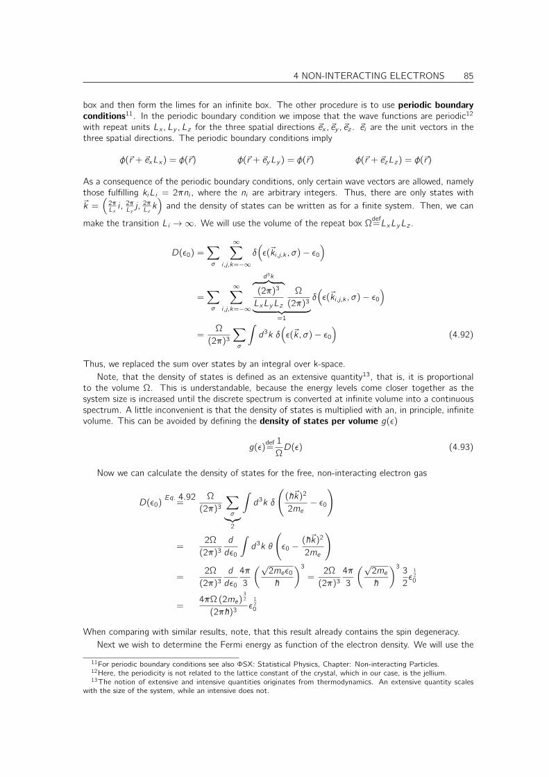
4 NON-INTERACTING ELECTRONS 85
box and then form the limes for an infinite box. The other procedure is to use periodic boundaryconditions11. In the periodic boundary condition we impose that the wave functions are periodic12
with repeat units Lx , Ly , Lz for the three spatial directions ~ex , ~ey , ~ez . ~ei are the unit vectors in thethree spatial directions. The periodic boundary conditions imply
φ(~r + ~exLx) = φ(~r) φ(~r + ~eyLy ) = φ(~r) φ(~r + ~ezLz) = φ(~r)
As a consequence of the periodic boundary conditions, only certain wave vectors are allowed, namelythose fulfilling kiLi = 2πni , where the ni are arbitrary integers. Thus, there are only states with~k =
(2πLxi , 2πLy j,
2πLzk)
and the density of states can be written as for a finite system. Then, we can
make the transition Li →∞. We will use the volume of the repeat box Ωdef=LxLyLz .
D(ǫ0) =∑
σ
∞∑
i ,j,k=−∞δ(
ǫ(~ki ,j,k , σ)− ǫ0)
=∑
σ
∞∑
i ,j,k=−∞
d3k︷ ︸︸ ︷
(2π)3
LxLyLz
Ω
(2π)3︸ ︷︷ ︸
=1
δ(
ǫ(~ki ,j,k , σ)− ǫ0)
=Ω
(2π)3
∑
σ
∫
d3k δ(
ǫ(~k, σ)− ǫ0)
(4.92)
Thus, we replaced the sum over states by an integral over k-space.Note, that the density of states is defined as an extensive quantity13, that is, it is proportional
to the volume Ω. This is understandable, because the energy levels come closer together as thesystem size is increased until the discrete spectrum is converted at infinite volume into a continuousspectrum. A little inconvenient is that the density of states is multiplied with an, in principle, infinitevolume. This can be avoided by defining the density of states per volume g(ǫ)
g(ǫ)def=1
ΩD(ǫ) (4.93)
Now we can calculate the density of states for the free, non-interacting electron gas
D(ǫ0)Eq. 4.92=
Ω
(2π)3
∑
σ︸︷︷︸
2
∫
d3k δ
(
(~~k)2
2me− ǫ0
)
=2Ω
(2π)3d
dǫ0
∫
d3k θ
(
ǫ0 −(~~k)2
2me
)
=2Ω
(2π)3d
dǫ0
4π
3
(√2meǫ0~
)3
=2Ω
(2π)34π
3
(√2me~
)33
2ǫ12
0
=4πΩ(2me)
32
(2π~)3ǫ12
0
When comparing with similar results, note, that this result already contains the spin degeneracy.Next we wish to determine the Fermi energy as function of the electron density. We will use the
11For periodic boundary conditions see also ΦSX: Statistical Physics, Chapter: Non-interacting Particles.12Here, the periodicity is not related to the lattice constant of the crystal, which in our case, is the jellium.13The notion of extensive and intensive quantities originates from thermodynamics. An extensive quantity scales
with the size of the system, while an intensive does not.
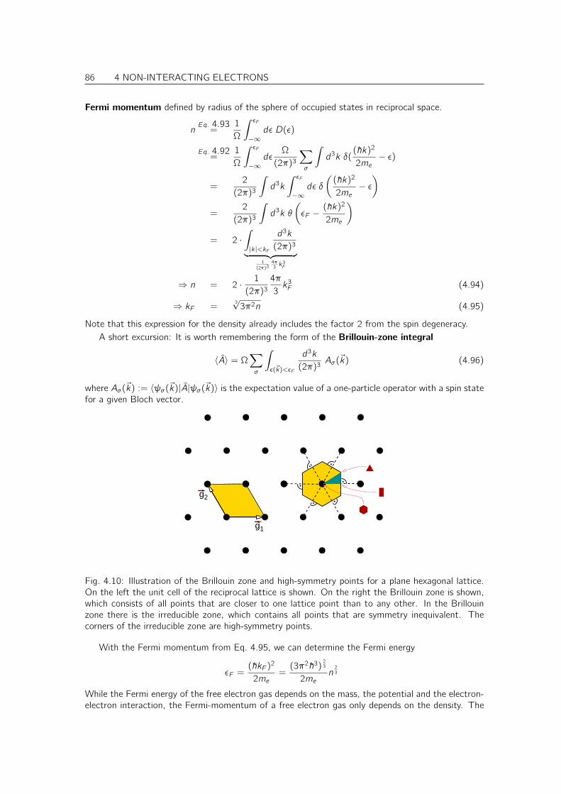
86 4 NON-INTERACTING ELECTRONS
Fermi momentum defined by radius of the sphere of occupied states in reciprocal space.
nEq. 4.93=
1
Ω
∫ ǫF
−∞dǫ D(ǫ)
Eq. 4.92=
1
Ω
∫ ǫF
−∞dǫΩ
(2π)3
∑
σ
∫
d3k δ((~k)2
2me− ǫ)
=2
(2π)3
∫
d3k
∫ ǫF
−∞dǫ δ
((~k)2
2me− ǫ)
=2
(2π)3
∫
d3k θ
(
ǫF −(~k)2
2me
)
= 2 ·∫
|k|<kF
d3k
(2π)3︸ ︷︷ ︸
1
(2π)34π3k3F
⇒ n = 2 · 1
(2π)34π
3k3F (4.94)
⇒ kF =3√3π2n (4.95)
Note that this expression for the density already includes the factor 2 from the spin degeneracy.A short excursion: It is worth remembering the form of the Brillouin-zone integral
〈A〉 = Ω∑
σ
∫
ǫ(~k)<ǫF
d3k
(2π)3Aσ(~k) (4.96)
where Aσ(~k) := 〈ψσ(~k)|A|ψσ(~k)〉 is the expectation value of a one-particle operator with a spin statefor a given Bloch vector.
g1
g2
Fig. 4.10: Illustration of the Brillouin zone and high-symmetry points for a plane hexagonal lattice.On the left the unit cell of the reciprocal lattice is shown. On the right the Brillouin zone is shown,which consists of all points that are closer to one lattice point than to any other. In the Brillouinzone there is the irreducible zone, which contains all points that are symmetry inequivalent. Thecorners of the irreducible zone are high-symmetry points.
With the Fermi momentum from Eq. 4.95, we can determine the Fermi energy
ǫF =(~kF )
2
2me=(3π2~3)
23
2men23
While the Fermi energy of the free electron gas depends on the mass, the potential and the electron-electron interaction, the Fermi-momentum of a free electron gas only depends on the density. The
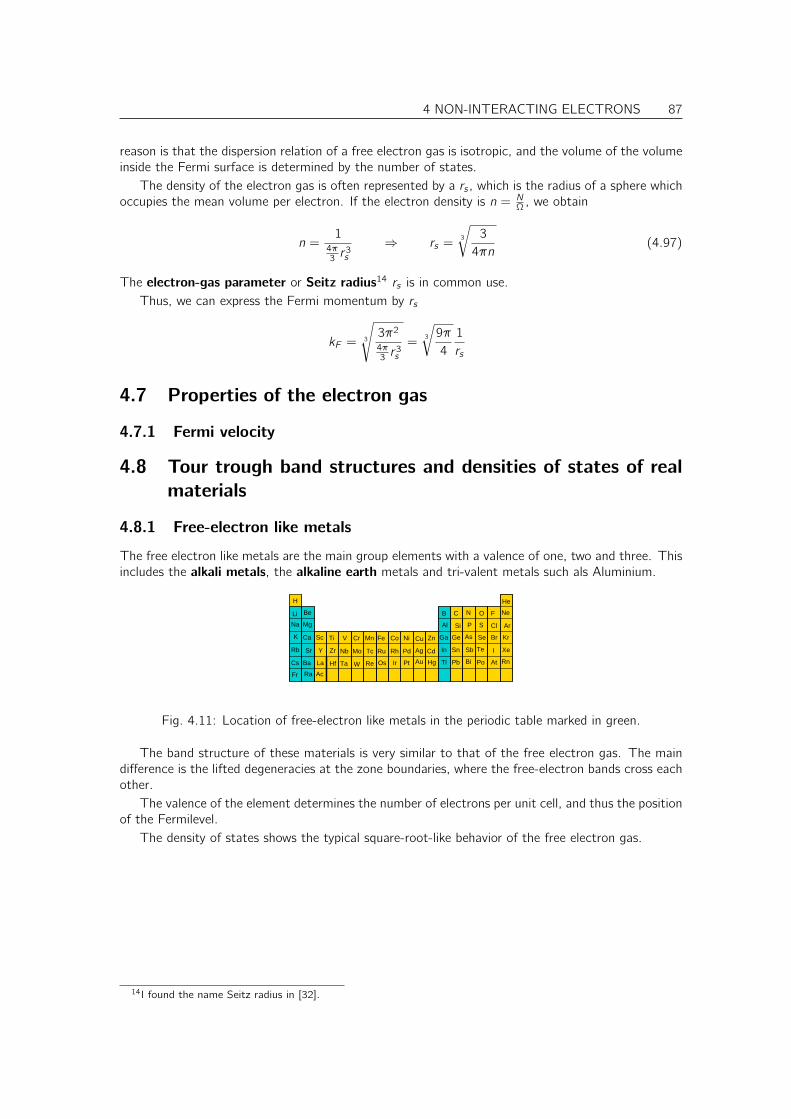
4 NON-INTERACTING ELECTRONS 87
reason is that the dispersion relation of a free electron gas is isotropic, and the volume of the volumeinside the Fermi surface is determined by the number of states.
The density of the electron gas is often represented by a rs , which is the radius of a sphere whichoccupies the mean volume per electron. If the electron density is n = N
Ω , we obtain
n =14π3 r3s
⇒ rs =3
√
3
4πn(4.97)
The electron-gas parameter or Seitz radius14 rs is in common use.Thus, we can express the Fermi momentum by rs
kF =3
√
3π2
4π3 r3s
=3
√
9π
4
1
rs
4.7 Properties of the electron gas
4.7.1 Fermi velocity
4.8 Tour trough band structures and densities of states of real
materials
4.8.1 Free-electron like metals
The free electron like metals are the main group elements with a valence of one, two and three. Thisincludes the alkali metals, the alkaline earth metals and tri-valent metals such als Aluminium.
Ba
Ra
Ge
Sn
Tl
Ga
Pb
In
Se
PoBi
Sb
As
Te
At
I
Br
Hg
Cd
Zn
Au
Ag
CuCr Mn Fe Co Ni
Y ZrSr Mo
TaHf
Ac
La
H
Tc
ReW Os Ir Pt
Ru PdRhNb
He
Li Be
Sc
Mg
Ti
Na
V
CB ON F Ne
Ar
Rn
Kr
Xe
ClSPSiAl
Ca
Cs
Fr
K
Rb
Fig. 4.11: Location of free-electron like metals in the periodic table marked in green.
The band structure of these materials is very similar to that of the free electron gas. The maindifference is the lifted degeneracies at the zone boundaries, where the free-electron bands cross eachother.
The valence of the element determines the number of electrons per unit cell, and thus the positionof the Fermilevel.
The density of states shows the typical square-root-like behavior of the free electron gas.
14I found the name Seitz radius in [32].
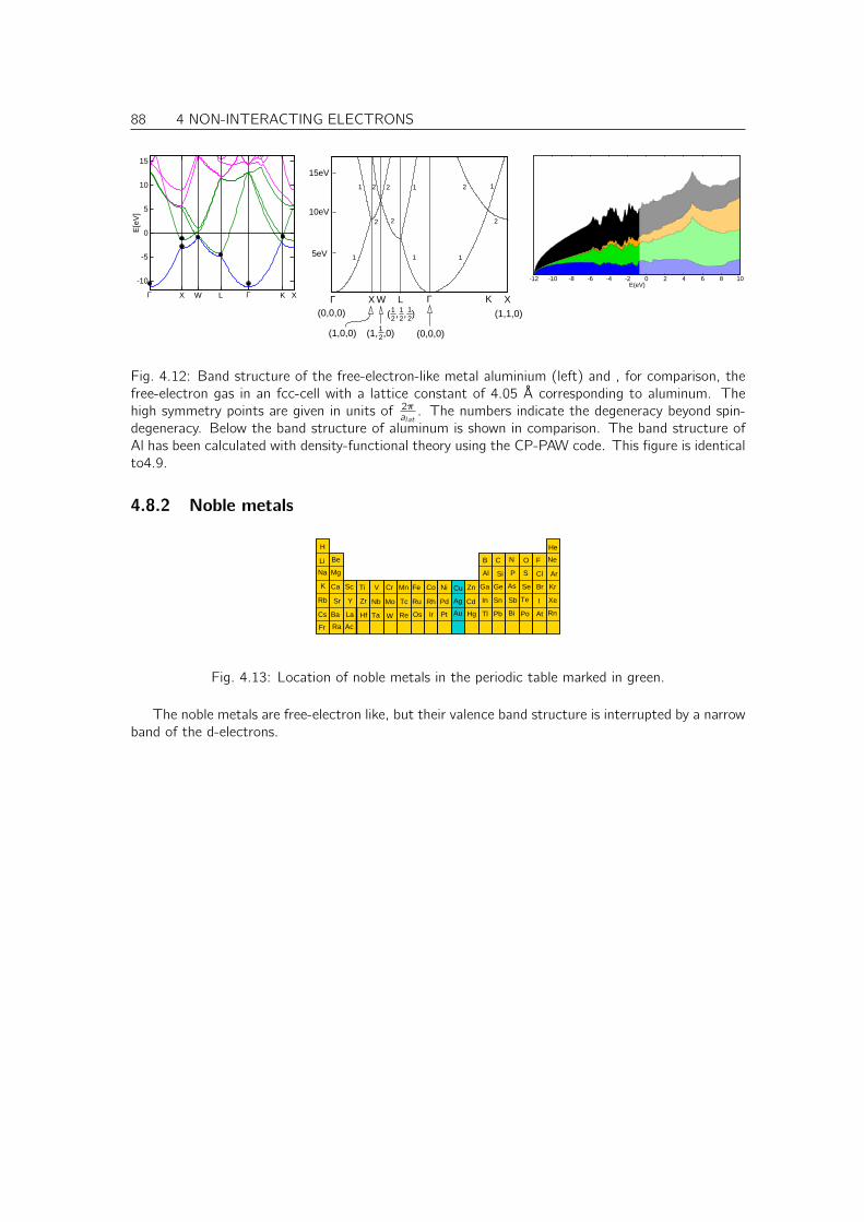
88 4 NON-INTERACTING ELECTRONS
Γ X W L Γ K X
-10
-5
0
5
10
15
E[e
V]
21
21
21( , , )
21(1, ,0)
Γ Γ K XX W L
(1,0,0)
(0,0,0) (1,1,0)
(0,0,0)
1 1 1
2
2
21 2 11
2 210eV
5eV
15eV
-12 -10 -8 -6 -4 -2 0 2 4 6 8 10E(eV)
Fig. 4.12: Band structure of the free-electron-like metal aluminium (left) and , for comparison, thefree-electron gas in an fcc-cell with a lattice constant of 4.05 Å corresponding to aluminum. Thehigh symmetry points are given in units of 2πalat . The numbers indicate the degeneracy beyond spin-degeneracy. Below the band structure of aluminum is shown in comparison. The band structure ofAl has been calculated with density-functional theory using the CP-PAW code. This figure is identicalto4.9.
4.8.2 Noble metals
Rb
Ba
Ra
Ge
Sn
Tl
Ga
Pb
In
Se
PoBi
Sb
As
Te
At
I
Br
Hg
Cd
Zn
Au
Ag
CuCr Mn Fe Co Ni
Y ZrSr Mo
TaHf
H
La
Nb Tc
ReW Os Ir Pt
Ru PdRh
Ac
He
Li Be
Sc
Mg
Ti
Na
V
CB ON F Ne
Ar
Rn
Kr
Xe
ClSPSiAl
Ca
Cs
Fr
K
Fig. 4.13: Location of noble metals in the periodic table marked in green.
The noble metals are free-electron like, but their valence band structure is interrupted by a narrowband of the d-electrons.
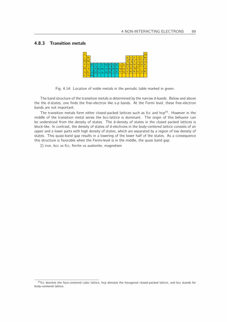
4 NON-INTERACTING ELECTRONS 89
4.8.3 Transition metals
Rb
Ba
Ra
Ge
Sn
Tl
Ga
Pb
In
Se
PoBi
Sb
As
Te
At
I
Br
Hg
Cd
Zn
Au
Ag
CuCr Mn Fe Co Ni
Y ZrSr Mo
TaHf
H
La
Nb Tc
ReW Os Ir Pt
Ru PdRh
Ac
He
Li Be
Sc
Mg
Ti
Na
V
CB ON F Ne
Ar
Rn
Kr
Xe
ClSPSiAl
Ca
Cs
Fr
K
Fig. 4.14: Location of noble metals in the periodic table marked in green.
The band structure of the transition metals is determined by the narrow d-bands. Below and abovethe the d-states, one finds the free-electron like s-p bands. At the Fermi level, these free-electronbands are not important.
The transition metals form either closed-packed lattices such as fcc and hcp15. However in themiddle of the transition metal series the bcc-lattice is dominant. The origin of this behavior canbe understood from the density of states. The d-denisty of states in the closed packed lattices isblock-like. In contrast, the density of states of d-electrons in the body-centered lattice consists of anupper and a lower parts with high density of states, which are separated by a region of low density ofstates. This quasi-band gap results in a lowering of the lower half of the states. As a consequencethis structure is favorable when the Fermi-level is in the middle, the quasi band gap.
2) iron, bcc vs fcc, ferrite vs austenite, magnetism
15fcc denotes the face-centered cubic lattice, hcp denotes the hexagonal closed-packed lattice, and bcc stands forbody-centered lattice.
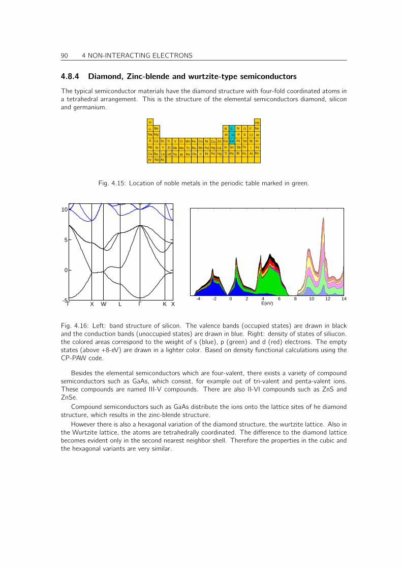
90 4 NON-INTERACTING ELECTRONS
4.8.4 Diamond, Zinc-blende and wurtzite-type semiconductors
The typical semiconductor materials have the diamond structure with four-fold coordinated atoms ina tetrahedral arrangement. This is the structure of the elemental semiconductors diamond, siliconand germanium.
Ba
Ra
Ge
Sn
Tl
Ga
Pb
In
Se
PoBi
Sb
As
Te
At
I
Br
Hg
Cd
Zn
Au
Ag
CuCr Mn Fe Co Ni
Y ZrSr Mo
TaHf
Ac
La
H
Tc
ReW Os Ir Pt
Ru PdRhNb
He
Li Be
Sc
Mg
Ti
Na
V
CB ON F Ne
Ar
Rn
Kr
Xe
ClSPSiAl
Ca
Cs
Fr
K
Rb
Fig. 4.15: Location of noble metals in the periodic table marked in green.
Γ X W L Γ K X-5
0
5
10
-4 -2 0 2 4 6 8 10 12 14E(eV)
Fig. 4.16: Left: band structure of silicon. The valence bands (occupied states) are drawn in blackand the conduction bands (unoccupied states) are drawn in blue. Right: density of states of siliucon.the colored areas correspond to the weight of s (blue), p (green) and d (red) electrons. The emptystates (above +8-eV) are drawn in a lighter color. Based on density functional calculations using theCP-PAW code.
Besides the elemental semiconductors which are four-valent, there exists a variety of compoundsemiconductors such as GaAs, which consist, for example out of tri-valent and penta-valent ions.These compounds are named III-V compounds. There are also II-VI compounds such as ZnS andZnSe.
Compound semiconductors such as GaAs distribute the ions onto the lattice sites of he diamondstructure, which results in the zinc-blende structure.
However there is also a hexagonal variation of the diamond structure, the wurtzite lattice. Also inthe Wurtzite lattice, the atoms are tetrahedrally coordinated. The difference to the diamond latticebecomes evident only in the second nearest neighbor shell. Therefore the properties in the cubic andthe hexagonal variants are very similar.
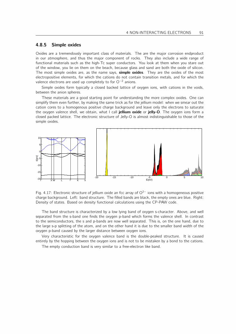
4 NON-INTERACTING ELECTRONS 91
4.8.5 Simple oxides
Oxides are a tremendously important class of materials. The are the major corrosion endproductin our atmosphere, and thus the major component of rocks. They also include a wide range offunctional materials such as the high-Tc super conductors. You look at them when you stare outof the window, you lie on them on the beach, because glass and sand are both the oxide of silicon.The most simple oxides are, as the name says, simple oxides. They are the oxides of the mostelectropositive elements, for which the cations do not contain transition metals, and for which thevalence electrons are used up completely to for O−2 anions.
Simple oxides form typically a closed backed lattice of oxygen ions, with cations in the voids,between the anion spheres.
These materials are a good starting point for understanding the more complex oxides. One cansimplify them even further, by making the same trick as for the jellium model: when we smear out thecation cores to a homogenous positive charge background and leave only the electrons to saturatethe oxygen valence shell, we obtain, what I call jellium oxide or jelly-O. The oxygen ions form aclosed packed lattice. The electronic structure of Jelly-O is almost indistinguishable to those of thesimple oxides.
Γ X W L Γ K X-20
-15
-10
-5
0
5
10
E[e
V]
-20 -15 -10 -5 0 5 10E(eV)
Fig. 4.17: Electronic structure of jellium oxide an fcc array of O2− ions with a homogeneous positivecharge background. Left: band structure. The filled bands are black, the empty ones are blue. Right:Density of states. Based on density functional calculations using the CP-PAW code.
The band structure is characterized by a low lying band of oxygen s-character. Above, and wellseparated from the s-band one finds the oxygen p-band which forms the valence shell. In contrastto the semiconductors, the s and p-bands are now well separated. This is, on the one hand, due tothe large s-p splitting of the atom, and on the other hand it is due to the smaller band width of theoxygen p-band caused by the larger distance between oxygen ions.
Very characteristic for the oxygen valence band is the double-peaked structure. It is causedentirely by the hopping between the oxygen ions and is not to be mistaken by a bond to the cations.
The empty conduction band is very similar to a free-electron like band.
92 4 NON-INTERACTING ELECTRONS
4.8.6 PCMO an example for a complex oxide
4.9 What band structures are good for
From ΦSX:Quantum mechanics of the chemical bond[30]
4.9.1 Chemical stability
4.9.2 Dispersion relations
The band structure tells us a lot about how particles move. the band structure is nothing but thedispersion relation for a particle. The dispersion relation is the relation of energy with momentumfor a particle.
Using Hamilton’s equation
~v = ∂t~r = ~∇pE(~p)~F = ∂t~p = −~∇rE(~p)
• velocity of a particle is the slope of E(p).
• momentum changes with time proportional to the force ~F = ∂t~p, which is Newton’s law
Thus, a particle experiencing a constant force F , will have momentum
~p(t) = ~p(0) + ~F t
~v(t) = ~∇pE(~p(0) + ~F t)
Dynamics of wave packets
Abrupt interfaces
While a dispersion relation is strictly defined only for translationally invariant systems, where theenergy eigenstates are also momentum eigenstates, we can also understand what happens at theinterface between materials. As a particle passes from one material to the other, it may gain or loosemomentum perpendicular to the interface, but we can use energy conservation and conservation ofthe momentum parallel to the interface to obtain some information on the interface crossing.
Slow spatial variation
Lifetime broadening
Sometimes the material has some randomness or other interactions that break translational symmetry.If these perturbations of translational symmetry are small, the eigenstates of the Hamiltonian are nomore momentym eigenstates. If we still project the energy eigenstates onto momentum eigenstates,each momentum will obtain contribution from several energies. Instrad of sharp energies for eachmomentym we have a broadened distribution. The width of the energy distribution is a measure forthe life time of a momentum: Scattering processes will redirect the particle.
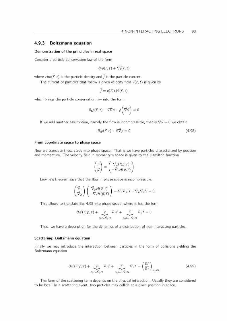
4 NON-INTERACTING ELECTRONS 93
4.9.3 Boltzmann equation
Demonstration of the principles in real space
Consider a particle conservation law of the form
∂tρ(~r , t) + ~∇~j(~r , t)
where rho(~r , t) is the particle density and ~j is the particle current.The current of particles that follow a given velocity field ~v(~r , t) is given by
~j = ρ(~r , t)~v(~r , t)
which brings the particle conservation law into the form
∂tρ(~r , t) + ~v ~∇ρ+ ρ(
~∇~v)
= 0
If we add another assumption, namely the flow is incompressible, that is ~∇~v = 0 we obtain
∂tρ(~r , t) + ~v ~∇ρ = 0 (4.98)
From coordinate space to phase space
Now we translate these steps into phase space. That is we have particles characterized by positionand momentum. The velocity field in momentym space is given by the Hamilton function
(
~r
~p
)
=
(~∇pH(~p,~r)−~∇rH(~p,~r)
)
Lioville’s theorem says that the flow in phase space is incompressible.(~∇r~∇p
)(~∇pH(~p,~r)−~∇rH(~p,~r)
)
= ~∇r ~∇pH − ~∇p ~∇rH = 0
This allows to translate Eq. 4.98 into phase space, where it has the form
∂t f (~r , ~p, t) + ~v︸︷︷︸
∂t~r=~∇pH
~∇r f + ~F︸︷︷︸
∂t~p=−~∇rH
~∇pf = 0
Thus, we have a description for the dynamics of a distribution of non-interacting particles.
Scattering: Boltzmann equation
Finally we may introduce the interaction between particles in the form of collisions yielding theBoltzmann equation
∂t f (~r , ~p, t) + ~v︸︷︷︸
∂t~r=~∇pH
~∇r f + ~F︸︷︷︸
∂t~p=−~∇rH
~∇pf =(∂f
∂t
)
scatt
(4.99)
The form of the scattering term depends on the physical interaction. Usually they are consideredto be local: In a scattering event, two particles may collide at a given position in space.
94 4 NON-INTERACTING ELECTRONS
Relaxation time approximation
The information on the scattering events is not contained in the band structure. A common andsimple approximation is the relaxation time approximation, which is based on the following form ofthe scattering term
(∂f
∂t
)
scatt
= −1τ
(
f (~r , ~p, t)− f eq(~r , ~p))
where τ is the relaxation time, and f eq is the equilibrium distribution in the form of a Boltmann,Fermi or Bose distribution.
Chapter 5
Magnetism
5.1 Charged particles in a magnetic field
5.2 Dirac equation and magnetic moment
Spin-orbit coupling responsible for magnetic anisotropy.
• Non-relativistic magnetic moment ~m of a charge rotating about a center
~mcl =q
2m~L (5.1)
• Dirac equation defines the gyromagnetic ratio of g = 2.
• Quantum field theory leads to g = 2.00232 . . .
5.3 Magnetism of the free electron gas
Landau levels
5.4 Magnetic order
Stoner criterion, Pauli paramagnetism,ferromagnetism, ferrimagnetism, antiferromagnetism, Ising model, Heisenberg model, Weiss re-
gions.
95

96 5 MAGNETISM
Chapter 6
The Hartree-Fock approximation andexchange
The Hartree-Fock method[28, 33, 34] is an electronic structure method that is the work-horseof quantum chemistry. Today it plays an important role as a starting point of more accurate andinvolved methods. The Hartree-Fock method had a predecessor, the Hartree method[35, 36], which,however, does not play an important role in practice.
The basic idea of the Hartree-Fock method is to restrict the wave functions to single Slaterdeterminants[28]. For this Slater determinant, the energy is determined as expectation value ofthe true many-particle Hamiltonian. That is, the Hartree-Fock approximation takes the completeelectron-electron interaction into account. Furthermore the one-particle orbitals are optimized toyield the lowest energy.
One can easily show that the Hartree-Fock energy always provides an upper bound for the energy.The Hamilton operator is, up to a constant, positive definite and the ground state is the state withthe lowest energy. As we restricted our wave function to single Slater determinants, the wave functionis, normally, not the ground state and therefore higher in energy than the ground-state energy.
After having defined Slater determinants in the previous section, in this section we will gain somefamiliarity with them. We will also see why systems of non-interacting many-particle problems canbe described by a set of one-particle wave functions alone, something that we implicitely assumedin the section about non-interacting electrons. Furthermore, we will become familiar with the mostimportant contributions of the electron correlation, namely Hartree energy and exchange.
6.1 One-electron and two-particle operators
The Born-Oppenheimer Hamiltonian Eq. 2.4 for an N-electron system has the form
E = ENN + 〈Ψ|N∑
i=1
hi +1
2
∑
i 6=jWi ,j |Ψ〉
Where
ENN(~R1, . . . , ~RM)def=1
2
M∑
i 6=j
e2ZiZj
4πǫ0|~Ri − ~Rj |(6.1)
is the electrostatic repulsion between the nuclei, and the operators acting on the electrons can bedivided into one-particle terms hi and two-particle terms Wi ,j .
97
98 6 THE HARTREE-FOCK APPROXIMATION AND EXCHANGE
The one-particle terms describe the kinetic and potential energy of the electrons in an externalpotential vext(~r)
hi =
∫
d4x1 · · ·∫
d4xN |~x1, . . . , ~xN〉[−~22me
~∇2~ri + vext(~ri)]
〈~x1, . . . , ~xN | (6.2)
The external potential describes the electrostatic attraction between electrons and nuclei.
vext(~r ; ~R1, . . . , ~RM) = −M∑
j=1
e2Zj
4πǫ0|~r − ~Rj |(6.3)
The two-particle operator describes the interaction between the electrons
Wi ,j =
∫
d4x1 · · ·∫
d4xN |~x1, . . . , ~xN〉e2
4πǫ0|~ri − ~rj |〈~x1, . . . , ~xN | (6.4)
The indices on hi and Wi ,j determine, onto which electron coordinates the operator acts.The one-particle operators act on the coordinates of one particle at a time. The kinetic energy
and the external potential are examples for one-particle operators, because they can be determinedfor each particle individually and then be summed up. The interaction energy Eq. 6.4 on the otherhand depends on the coordinates of two particles simultaneously and is therefore a true two-particleoperator. It is the two-particle term that is the cause for the dazzling complexity of many-particlephysics.
Let us consider a general operator in real space
A =
∫
d4x1 · · ·∫
d4xN |~x1, . . . , ~xN〉〈~x1, . . . , ~xN |︸ ︷︷ ︸
1
·A∫
d4x ′1 · · ·∫
d4x ′N |~x ′1, . . . , ~x ′N〉〈~x ′1, . . . , ~x ′N |︸ ︷︷ ︸
1
=
∫
d4x1 · · ·∫
d4xN
∫
d4x ′1 · · ·∫
d4x ′N |~x1, . . . , ~xN〉
·〈~x1, . . . , ~xN |A|~x ′1, . . . , ~x ′N〉〈~x ′1, . . . , ~x ′N |
A general matrix element has therefore 2N arguments.
• If the matrix element of an operator has the special form
〈~x1, . . . , ~xN |A|~x ′1, . . . , ~x ′N〉 =N∑
i=1
A(~xi , ~x′i )∏
j 6=iδ(~xj − ~x ′j)
we call the operator a one-particle operator.
• If furthermore the function A(~x, ~x ′) has the special form that it is diagonal in the primed andunprimed arguments, i.e.
A(~x, ~x ′) = a(~x)δ(~x − ~x ′)
we call the one-particle operator local.
• If the matrix element of an operator has the special form
〈~x1, . . . , ~xN |A|~x ′1, . . . , ~x ′N〉 =1
2
N∑
i ,j=1
A(~xi , ~xj , ~x′i , ~x′j)∏
k 6=i ,jδ(~xk − ~x ′k)
we call the operator a two-particle operator.
6 THE HARTREE-FOCK APPROXIMATION AND EXCHANGE 99
• If furthermore the function A(~x1, ~x2, ~x ′1, ~x ′2) has the special form that it is diagonal in theprimed and unprimed arguments, i.e.
A(~x1, ~x2, ~x ′1, ~x ′2) = a(~x1, ~x2)δ(~x1 − ~x ′1)δ(~x2 − ~x ′2)
we call the two-particle operator local.
6.2 Expectation values of Slater determinants
Let us now work out the expectation values for the one-particle and two-particle operators for aSlater determinant.
6.2.1 Expectation value of a one-particle operator
Here, we will work out the expectation value of a one-particle operator for a Slater determinant. Anexample for such a one-particle operator is the non-interacting part of the Hamiltonian.
Explicit example for the two-particle wave function
The two-particle Slater determinant of two one-particle orbitals |φa〉 and |φb〉 has the form
〈~r1~r2|Ψ〉︸ ︷︷ ︸
Ψ(~r1,~r2)
=1√2
[
〈~r1|φa〉〈~r2|φb〉 − 〈~r1|φb〉〈~r2|φa〉]
︸ ︷︷ ︸
φa(~r1)φb(~r2)−φb(~r1)φa(~r2)
(6.5)
To avoid unnecessary complication we drop the spin-coordinates, that is we consider spin-less fermions.As an specific example for a one-particle operator, we consider the particle-density operator n(~r)
defined as
n(~r) =
∫
d3r1
∫
d3r2 |~r1, ~r2〉[
δ(~r − ~r1) + δ(~r − ~r2)]
〈~r1, ~r2|
100 6 THE HARTREE-FOCK APPROXIMATION AND EXCHANGE
The electron density is
n(~r) = 〈Ψ|n(~r)|Ψ〉
=
∫
d3r1
∫
d3r2 Ψ∗(~r1, ~r2)
[
δ(~r − ~r1) + δ(~r − ~r2)]
Ψ(~r1, ~r2)
Ψ(~r1,~r2)=−Ψ(~r2,~r1)=
∫
d3r1
∫
d3r2 Ψ∗(~r1, ~r2)δ(~r − ~r1)Ψ(~r1, ~r2)
+
∫
d3r1
∫
d3r2 Ψ∗(~r2, ~r1)δ(~r − ~r2)Ψ(~r2, ~r1)
~r1↔~r2= 2
∫
d3r1
∫
d3r2 Ψ∗(~r1, ~r2)δ(~r1 − ~r)Ψ(~r1, ~r2)
Eq. 6.5= 2
∫
d3r1
∫
d3r21√2
[
φa(~r1)φb(~r2)− φa(~r2)φb(~r1)]∗
· δ(~r − ~r1)1√2
[
φa(~r1)φb(~r2)− φa(~r2)φb(~r1)]
=
∫
d3r1
∫
d3r2 φ∗a(~r1)φ
∗b(~r2)δ(~r − ~r1)φa(~r1)φb(~r2)
−∫
d3r1
∫
d3r2 φ∗a(~r1)φ
∗b(~r2)δ(~r − ~r1)φa(~r2)φb(~r1)
−∫
d3r1
∫
d3r2 φ∗a(~r2)φ
∗b(~r1)δ(~r − ~r1)φa(~r1)φb(~r2)
+
∫
d3r1
∫
d3r2 φ∗a(~r2)φ
∗b(~r1)δ(~r − ~r1)φa(~r2)φb(~r1)
= 〈φa|~r〉〈~r |φa〉 〈φb|φb〉︸ ︷︷ ︸
=1
−〈φa|~r〉〈~r |φb〉 〈φb|φa〉︸ ︷︷ ︸
=0
−〈φb|~r〉〈~r |φa〉 〈φa|φb〉︸ ︷︷ ︸
=0
+〈φb|~r〉〈~r |φb〉 〈φa|φa〉︸ ︷︷ ︸
=1
= φ∗a(~r)φa(~r) + φ∗b(~r)φb(~r)
Let us mention a few observations:
• The number of terms is drastically reduced just because we have used an orthonormal set ofone-particle wave functions. This is the sole reason for using orthonormal basissets in many-particle physics.
• The sum over particles is turned into a sum over orbitals. This is true for a Slater determinant,but not for a general many particle states.
• The antisymmetry of the wave function ensures that the same expectation value is obtained ifwe work out a property of the first or the second electron.1
General derivation
Now, we will determine the same result in its full generality: First, we evaluate only the matrix elementof the one-particle operator h1, that acts only on the coordinates of only one particle, namely thefirst. This result is then generalized for the other particles and then summed up. Thus, we obtainthe expectation value of the non-interacting part of the Hamiltonian.
1The wave function is, up to a sign, the same when the coordinates of the coordinates of the first and the secondelectron are interchanged. The sign drops out for expectation values, because the wave function enters twice. Example:Using the antisymmetry of the wave function ψ(x, x ′) = −ψ(x ′, x) one can convert the density ρ1 of the first particleρ1(x) =
∫dx ′ ψ∗(x, x ′)ψ(x, x ′) = (−1)2
∫dx ′ ψ∗(x ′, x)ψ(x ′, x) = ρ2(x) into the density ρ2(x) of the second.
6 THE HARTREE-FOCK APPROXIMATION AND EXCHANGE 101
To be concise, we write here the detailed expressions for the matrix elements of the one-particleHamilton operator, we have in mind
〈φ|h|φ〉 =∫
d4x
∫
d4x ′ 〈φ|~x〉
δ(~r − ~r ′)δσ,σ′(
− ~2
2me~∇2 + v(~r)
)
︸ ︷︷ ︸︷ ︸︸ ︷
〈~x |h|~x ′〉 〈~x ′|φ〉
=∑
σ
∫
d3r φ∗(~r , σ)
[−~22me
~∇2 + vext(~r)]
φ(~r , σ) (6.6)
The one-particle Hamiltonian hj acting on the j-th particle in a many particle wave function Ψ〉yields the expectation value
〈Ψ|hj |Ψ〉 =∫
d4x1 · · ·∫
d4xN Ψ∗(~x1, . . . , ~xN)
(−~22me
~∇2j + vext(~rj))
Ψ(~x1, . . . , ~xN)
so that the matrix element for two product wave functions is
〈φ1, . . . , φN |hj |ψ1, . . . , ψN〉 = 〈φ1|ψ1〉 · · · 〈φj |h|ψj 〉 · · · 〈φN |ψN〉 (6.7)
The Slater determinant, given in Eq. 3.21, has the form
〈~x1, . . . , ~xN |Ψ〉 =1√N!
N∑
i1,...,iN=1
ǫi1,...,iN 〈~x1|φi1〉 · · · 〈~xN |φiN 〉 (6.8)
Thus, the matrix element of a one-particle operator Eq. 6.2 is
〈Ψ|N∑
i=1
hi |Ψ〉 = N〈Ψ|h1|Ψ〉
Eq. 6.8= N · 1
N!
N∑
i1,i2,...,iN
N∑
j1,j2,...,jN
ǫi1,i2,...,iN 〈φi1 , . . . , φiN |h1|φj1 , . . . , φjN 〉ǫj1,j2,...,jN
Eq. 6.7= N
1
N!
N∑
i1,i2,...,iN
N∑
j1,j2,...,jN
ǫi1,i2,...,iN ǫj1,j2,...,jN 〈φi1 |h1|φj1〉 〈φi2 |φj2〉︸ ︷︷ ︸
δi2 ,j2
· · · 〈φiN |φjN 〉︸ ︷︷ ︸
δiN ,jN
= N1
N!
N∑
i1,j1=1
〈φi1 |h1|φj1〉N∑
i2,...,iN
ǫi1,i2,...,iN ǫj1,i2,...,iN
︸ ︷︷ ︸
δi1 ,j1 (N−1)!
=
N∑
j=1
〈φj |h1|φj 〉
In the last step we exploited, that the sum over j1 only contributes when j1 = i1. There is only oneorbital left if all the orbitals but the first are determined. Thus, the first orbital must be the samefor both Levi-Civita Symbols.
Thus, we obtain the expectation value of the one-particle Hamiltonian for a Slater determinant|Ψ〉 as
102 6 THE HARTREE-FOCK APPROXIMATION AND EXCHANGE
EXPECTATION VALUE OF A ONE-PARTICLE OPERATOR WITH A SLATER DETERMINANT
〈Ψ|N∑
i=1
hi |Ψ〉 =N∑
i=1
〈φi |h|φi 〉 (6.9)
Here, |Ψ〉 is a N-particle Slater determinant built from the one-particle orbitals |φi 〉, and∑N
i=1 hi isa one-particle operator.
Expectation values of common one-particle operators with Slater determinants
Analogously, the expectation value of any one-particle operator with a Slater determinant can berepresented by a sum over one-particle orbitals. Thus, we obtain the expression for the density
n(~r) = 〈Ψ|N∑
i=1
∑
σ
(
|~r , σ〉〈~r , σ|)
i|Ψ〉 =
N∑
i=1
∑
σ
φ∗i (~r , σ)φi(~r , σ) (6.10)
where
(
|~r〉〈~r |)
i
def=
∫
d4x1 · · ·∫
d4xN |~x1, . . . , ~xN〉δ(~r − ~ri)〈~x1, . . . , ~xN |
The expectation value of the kinetic energy for a Slater determinant has the form
Ekin = 〈Ψ|N∑
i=1
~p2i2me|Ψ〉 =
N∑
i=1
∑
σ
∫
d3r φ∗i (~r , σ)−~22me
~∇2φi(~r , σ) (6.11)
6.2.2 Expectation value of a two-particle operator
Let us now turn to the two-particle term. We introduce the symbol
W (~x, ~x ′) =e2
4πǫ0|~r − ~r ′|
The interaction is independent of the spin index. Furthermore it is local in the two coordinates.2
We proceed as for the expectation value of a one-particle operator and relate the interaction energybetween all particles to the interaction between the first two electrons. This is allowed because ofthe indistinguishability of the electrons: The interaction between any two electrons is identical to any
2A general two-particle operator has the form
W1,2 =
∫
dx1 · · ·∫
dxN
∫
dx ′1 · · ·∫
dx ′N |~x1, . . . , ~xN〉〈~x1, . . . , ~xN |W1,2|~x ′1, . . . , ~x ′N〉〈~x ′1, . . . , ~x ′N |
=
∫
dx1 · · ·∫
dxN
∫
dx ′1
∫
dx ′2|~x1, . . . , ~xN〉〈~x1, . . . , ~xN |W1,2|~x ′1, ~x ′2, ~x3, . . . , ~xN〉〈~x ′1, ~x ′2, ~x3, . . . , ~xN |
=
∫
dx1 · · ·∫
dxN
∫
dx ′1
∫
dx ′2|~x1, . . . , ~xN〉〈~x1, ~x2|W1,2|~x ′1, ~x ′2〉〈~x ′1, ~x ′2, ~x3, . . . , ~xN |
Thus, a general two-particle operator is nonlocal in the two particle coordinates and therefore its matrix elementsdepends on four arguments.
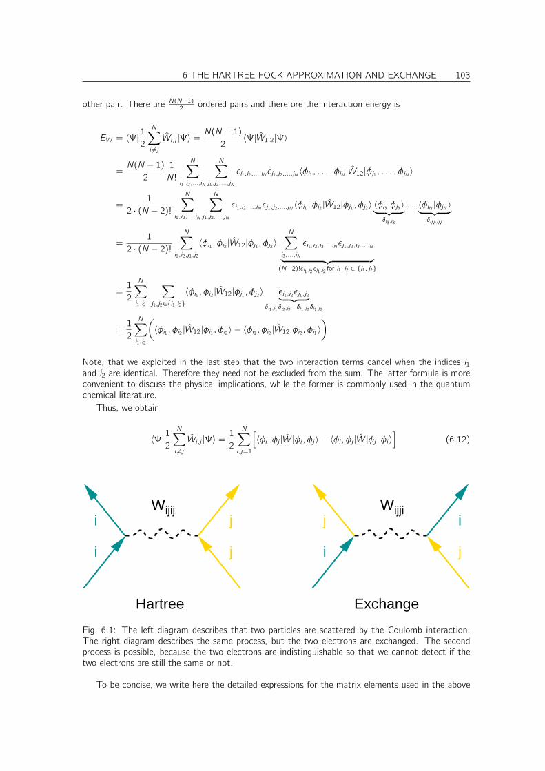
6 THE HARTREE-FOCK APPROXIMATION AND EXCHANGE 103
other pair. There are N(N−1)2 ordered pairs and therefore the interaction energy is
EW = 〈Ψ|1
2
N∑
i 6=jWi ,j |Ψ〉 =
N(N − 1)2
〈Ψ|W1,2|Ψ〉
=N(N − 1)2
1
N!
N∑
i1,i2,...,iN
N∑
j1,j2,...,jN
ǫi1,i2,...,iN ǫj1,j2,...,jN 〈φi1 , . . . , φiN |W12|φj1 , . . . , φjN 〉
=1
2 · (N − 2)!
N∑
i1,i2,...,iN
N∑
j1,j2,...,jN
ǫi1,i2,...,iN ǫj1,j2,...,jN 〈φi1 , φi2 |W12|φj1 , φj2〉 〈φi3 |φj3〉︸ ︷︷ ︸
δi3 ,j3
· · · 〈φiN |φjN 〉︸ ︷︷ ︸
δiN ,jN
=1
2 · (N − 2)!
N∑
i1,i2,j1,j2
〈φi1 , φi2 |W12|φj1 , φj2〉N∑
i3,...,iN
ǫi1,i2,i3...,iN ǫj1,j2,i3...,iN
︸ ︷︷ ︸
(N−2)!ǫi1 ,i2 ǫj1 ,j2 for i1, i2 ∈ j1, j2
=1
2
N∑
i1,i2
∑
j1,j2∈i1,i2〈φi1 , φi2 |W12|φj1 , φj2〉 ǫi1,i2ǫj1,j2
︸ ︷︷ ︸
δi1 ,j1 δi2 ,j2−δi1 ,j2 δi1 ,j2
=1
2
N∑
i1,i2
(
〈φi1 , φi2 |W12|φi1 , φi2〉 − 〈φi1 , φi2 |W12|φi2 , φi1〉)
Note, that we exploited in the last step that the two interaction terms cancel when the indices i1and i2 are identical. Therefore they need not be excluded from the sum. The latter formula is moreconvenient to discuss the physical implications, while the former is commonly used in the quantumchemical literature.
Thus, we obtain
〈Ψ|12
N∑
i 6=jWi ,j |Ψ〉 =
1
2
N∑
i ,j=1
[
〈φi , φj |W |φi , φj 〉 − 〈φi , φj |W |φj , φi 〉]
(6.12)
Hartree Exchange
Wijij Wijji
i
i
j
j
j
j
i
i
Fig. 6.1: The left diagram describes that two particles are scattered by the Coulomb interaction.The right diagram describes the same process, but the two electrons are exchanged. The secondprocess is possible, because the two electrons are indistinguishable so that we cannot detect if thetwo electrons are still the same or not.
To be concise, we write here the detailed expressions for the matrix elements used in the above
104 6 THE HARTREE-FOCK APPROXIMATION AND EXCHANGE
equation Eq. 6.12
〈φa, φb|W |φc , φd〉 =∑
σ,σ′
∫
d3r
∫
d3r ′ φ∗a(~r , σ)φ∗b(~r′, σ′)
e2
4πǫ0|~r − ~r ′|φc(~r , σ)φd(~r ′, σ
′)
(6.13)
Homework: Work out the expectation value of the Coulomb interaction between two electronsfor a two-electron Slater determinant. Consider once a Slater determinant from non-orthonormalone-particle orbitals and once for orthonormal one-particle orbitals. Investigate the role of the spinindices.
6.3 Hartree energy
The surprising fact of Eq. 6.12 is the appearance of two terms. Therefore let us try to give somephysical meaning to the two contributions.
The first interaction term in Eq. 6.12 is the so-called Hartree energy. The Hartree energy turnsout to be the classical electrostatic interaction of the electron density.
EH =1
2
∑
i ,j
∑
σ,σ′
∫
d3r
∫
d3r ′ φ∗i (~r , σ)φ∗j (~r′, σ′)
e2
4πǫ0|~r − ~r ′|φi(~r , σ)φj(~r ′, σ
′)
=1
2
∫
d3r
∫
d3r ′[∑
i ,σ
φ∗i (~r , σ)φi(~r , σ)
]
︸ ︷︷ ︸
n(~r)
e2
4πǫ0|~r − ~r ′|
∑
j,σ′
φ∗j (~r′, σ′)φj(~r ′, σ
′)
︸ ︷︷ ︸
n(~r ′)
(6.14)
The equation can be simplified using the definition of the charge density ρ(~r), or the electron densityn(~r), as
ρ(~r) = −en(~r) = −eN∑
i=1
∑
σ
φ∗i (~r , σ)φi(~r , σ)
︸ ︷︷ ︸
n(~r)
Thus, we obtain the final expression for the Hartree energy
HARTREE ENERGY
EH =1
2
∫
d3r
∫
d3r ′ρ(~r)ρ(~r ′)
4πǫ0|~r − ~r ′|(6.15)
6.4 Exchange energy
Exchange energy
The Hartree energy is clearly not the correct electrostatic energy, as it describes the interaction ofN electrons with N electrons. However, each electron can only interact with N − 1 electrons. Thus,the Hartree term also includes, incorrectly, the interaction of each electron with itself.
6 THE HARTREE-FOCK APPROXIMATION AND EXCHANGE 105
This so-called self interaction is subtracted by the so-called exchange energy, the second in-teraction term in Eq. 6.12
EX = −1
2
∑
i ,j
∑
σ,σ′
∫
d3r
∫
d3r ′ φ∗i (~r , σ)φ∗j (~r′, σ′)
e2
4πǫ0|~r − ~r ′|φj(~r , σ)φi(~r ′, σ
′)
(6.16)
The exchange term consists of the electrostatic interaction of densities3
ni ,j(~r)def=∑
σ
φi(~r , σ)φ∗j (~r , σ) (6.17)
The exchange energy can be written as
EX = −1
2
∑
i ,j
∫
d3r
∫
d3r ′e2nj,i(~r)ni ,j(~r ′)
4πǫ0|~r − ~r ′|(6.18)
while the Hartree term has the form
EH =1
2
∑
i ,j
∫
d3r
∫
d3r ′e2ni ,i(~r)nj,j(~r ′)
4πǫ0|~r − ~r ′|. (6.19)
Self interaction
All pair densities with different indices integrate to zero and the one with identical indices integrateto one, that is
∫
d3r ni ,j(~r)Eq. 6.17= 〈φj |φi 〉 = δi ,j
Thus, we can expect that the dominant contribution to the exchange energy results from the diagonalterms. This so-called self-interaction energy
ESI = −1
2
∑
i
∑
σ,σ′
∫
d3r
∫
d3r ′ φ∗i (~r , σ)φ∗i (~r′, σ′)
e2
4πǫ0|~r − ~r ′|φi(~r , σ)φi(~r ′, σ
′)
= −12
∑
i
∫
d3r
∫
d3r ′e2ni i(~r)ni i(~r ′)
4πǫ0|~r − ~r ′|
describes the electrostatic interaction of each electron with itself, that has been included in the Hartreecorrection. There is a well-known electronic structure method, based on density-functional theory,which uses the same trick to get rid of artificial self-interaction terms.[37] This theory subtractsthe self energy from the Hartree term and thus includes the so-called self-interaction correctionESIC = −ESI .
Exchange and spin alignment
Only electron pairs with the same spin contribute to the exchange energy. This can be shown whenone considers one-particle spin-orbitals with defined spin along the z-axis. That is, each one-particlespin-orbital has only one spin component, the other being zero.
3In the expression for ni ,j the complex conjugate of the right orbital is taken on purpose. This choice is analogousto that of the one-particle density matrix.
106 6 THE HARTREE-FOCK APPROXIMATION AND EXCHANGE
• If the two orbitals have the same spin, pointing for example into the ~ez direction, they can bewritten as
φi(~x) =
(
φi(~r , ↑)0
)
and φj(~x) =
(
φj(~r , ↑)0
)
The resulting exchange-energy would be formed from the pair densities
ni ,j(~r)Eq. 6.17=
∑
σ
φi(~r , σ)φ∗j (~r , σ) = φi(~r , ↑)φ∗j (~r , ↑) (6.20)
so that its contribution to the exchange energy has the form
∆EXEq. 6.18= −1
2
∑
i ,j
∫
d3r
∫
d3r ′e2nj,i(~r)ni ,j(~r ′)
4πǫ0|~r − ~r ′|
Eq. 6.20= −1
2
∫
d3r
∫
d3r ′e2φ∗i (~r , ↑)φj(~r , ↑)φ∗j (~r ′, ↑)φi(~r ′, ↑)
4πǫ0|~r − ~r ′|
• If the two orbitals have the opposite spin, they can be written as
φi(~x) =
(
φi ,↑(~r)
0
)
and φj(~x) =
(
0
φj,↓(~r)
)
The contribution to the exchange energy vanishes, because the pair densities vanish
ni ,j(~r)Eq. 6.17=
∑
σ
φi(~r , σ)φj(~r , σ) = φi(~r , ↑) · 0 + 0 · φj(~r , ↓) = 0
Note that this behavior of the exchange term is different from the one of the Hartree term: Thereis a Coulomb interaction between electrons of opposite spin, but no exchange term, because spin-upand spin-down electrons are distinguishable.
HUND’S RULE AND FERROMAGNETISM
Exchange acts only between electrons pairs with the same spin. Because exchange counteracts theCoulomb repulsion due to its changed sign, it favors if many electrons have the same spin.A result is Hund’s 1st rule: For a given electron configuration, the term with maximum multiplicity
has the lowest energy. The multiplicity is equal to , where is the total spin angular momentum for
all electrons. The term with lowest energy is also the term with maximum .
The same effect is responsible for the tendency of some solids to become ferromagnetic. Due tothe finite band width of metals, spin-alignment leads to some loss of kinetic energy. The balance ofkinetic energy and exchange determines whether ferromagnetism wins.
6.5 Hartree-Fock equations
The Hartree-Fock energy is an upper bound
The Hartree-Fock method yields an upper estimate EHF for the ground-state energy EGS.The ground state of an N-electron system is that state that minimizes the total energy for a
given Hamiltonian, i.e.
EGS = min|Φ〉,E
[
〈Φ|H|Φ〉 − E(
〈Φ|Φ〉 − 1)]
(6.21)
6 THE HARTREE-FOCK APPROXIMATION AND EXCHANGE 107
for all normalized many-particle wave functions |Φ〉. The normalization constraint has been addedwith the method of Lagrange multipliers and E is the corresponding Lagrange multiplier.4
The Hartree-Fock method restricts this search for the minimum to a subset S of wave functions,namely those that can be expressed in the form of a single Slater determinant.
EHF = min|Φ〉∈S,E′
[
〈Φ|H|Φ〉 − E′(
〈Φ|Φ〉 − 1)]
(6.22)
Because the search for the minimum is limited in the Hartree-Fock, the Hartree-Fock energy is alwaysabove the ground-state energy.
EGS ≤ EHF (6.23)
Hartree-Fock equations
Because every Slater determinant |Φ〉 ∈ S can be expressed by a set of one-particle orbitals |φj 〉, theHartree-Fock energy can be obtained by a minimum condition for the latter.
EHF = min|φ1〉,...,|φn〉,ΛΛΛ
[
ENN +
N∑
i=1
〈φi |h|φi 〉+1
2
N∑
i ,j=1
[
〈φi , φj |W |φi , φj 〉 − 〈φi , φj |W |φj , φi 〉]
−∑
i ,j
Λi ,j [〈φi |φj 〉 − δi ,j ]]
The last term ensures the orthonormality of the one-particle orbitals using the method of Lagrangemultipliers. The translation of the matrix elements between Slater determinants into those of theone-particle orbitals has been given in section 6.2. The matrix elements of one-particle Hamiltonianand interaction are defined in Eq. 6.6 and Eq. 6.13. The energy ENN is the Coulomb repulsion ofthe nuclei as defined in Eq. 6.1.
The minimum condition yields the Hartree-Fock equations. The derivation of the Hartree-Fockequations is analogous to the derivation of the Euler-Lagrange equations. Special is that here wework with fields, the one-particle wave functions, and that the variational parameters are complex.It is advantageous to use the Wirtinger derivatives, which are described briefly in ΦSX: KlassischeMechanik.
Wirtinger derivatives The essence of Wirtinger derivatives is that we can write the identity
df (Re[c ], Im[c ]) =df
dRe[c ]dRe[c ] +
df
d Im[c ]d Im[c ] =
df
dcdc +
df
dc∗dc∗ = df (c, c∗)
for the first variation of f . Thus, we can form the variations of a function of complex arguments, asif the variable and its complex conjugate were completely independent variables.For the functional derivatives we use
dΨ∗n(~r , σ)
dΨ∗k(~r0, σ0)= δ(~r − ~r0)δσ,σ0δn,k
dΨn(~r , σ)
dΨ∗k(~r0, σ0)= 0
4The expression is written a little sloppy, because the expression need not be be a minimum with respect to theLagrange multiplier. The requirement is only that the gradient vanishes.
108 6 THE HARTREE-FOCK APPROXIMATION AND EXCHANGE
−~22me
~∇2 +M∑
j=1
−e2Zj4πǫ0|~r − ~Rj |
+
∫
d3r ′e2n(~r ′)
4πǫ0|~r − ~r ′|
φi(~r , σ)
−N∑
j=1
∑
σ′
∫
d3r ′e2φ∗j (~r
′, σ′)φi(~r ′, σ′)
4πǫ0|~r − ~r ′|φj(~r , σ)−
N∑
j=1
φj(~r , σ)Λj,i = 0
Note that this is not a simple Schrödinger equation, because it mixes all orbitals.However, we can rewrite the equations to obtain a true Hamiltonian, which acts on all wave
functions in the same way:
−~22me
~∇2 +M∑
j=1
−e2Zj4πǫ0|~r − ~Rj |
+
∫
d3r ′e2n(~r ′)
4πǫ0|~r − ~r ′|
φi(~r , σ)
−∑
σ′
∫
d3r ′
N∑
j=1
e2φj(~r , σ)φ∗j (~r ′, σ′)
4πǫ0|~r − ~r ′|
︸ ︷︷ ︸
−VX,σ,σ′ (~r ,~r ′)
φi(~r ′, σ′)−
∑
j
φj(~r , σ)Λj,i = 0 (6.24)
This form actually shows that the one-particle orbitals can be superimposed so that the matrixΛΛΛ becomes diagonal. It can be shown that the system of equations is invariant under a unitarytransformation of the one-particle orbitals. Thus, one can use the matrix that diagonalizes ΛΛΛ, tobring the equations into a diagonal form. Hence, we can write the Hartree-Fock equations as trueeigenvalue equations.
The following observation provides some physical insight: The nonlocal exchange potential
VX,σ,σ′(~r , ~r ′) =
−N∑
j=1
e2φj(~r , σ)φ∗j (~r ′, σ′)
4πǫ0|~r − ~r ′|
(6.25)
contains a spin and angular momentum (ℓ,m) projection. Thus, every occupied atomic orbital isshifted towards lower energies, while empty atomic orbitals do not experience this exchange potential.The more compact the orbital, the larger the denominator and the stronger is the stabilization.
Non-local potential
However, the price to pay for the eigenvalue equation Eq. 6.24 is that we have to deal with a trulynon-local potential in the exchange term. What is a non-local potential? Consider an arbitraryoperator A
〈ψ|A|φ〉 = 〈ψ|[∫
d3r |~r〉〈~r |]
︸ ︷︷ ︸
1
A
[∫
d3r ′ |~r ′〉〈~r ′|]
︸ ︷︷ ︸
1
|φ〉
=
∫
d3r
∫
d3r ′ 〈ψ|~r〉︸ ︷︷ ︸
ψ∗(~r)
〈~r |A|~r ′〉︸ ︷︷ ︸
A(~r ,~r ′)
〈~r ′|φ〉︸ ︷︷ ︸
φ(~r ′)
=
∫
d3r
∫
d3r ′ ψ∗(~r)A(~r , ~r ′)φ(~r ′)
Thus, a general one-particle operator has always two sets of coordinates in its real space represen-tation. We call them non-local because they act on two positions at the same time. It is a special
6 THE HARTREE-FOCK APPROXIMATION AND EXCHANGE 109
property of most potentials, that they are local. For a local operator or local potential V the realspace matrix elements are diagonal in real space, that is
V (~r , ~r ′)def=〈~r |V |~r ′〉 = V (~r)δ(~r − ~r ′)
so that its matrix elements can be represented by a single real space integral.
Self-consistency cycle
The Hartree-Fock equations are self-consistent equations. This means that the Hamiltonian de-pends itself on the wave functions. Thus, the problem has to be solved iteratively.
• We start out with trial wave functions |φi 〉 to determine the Hamiltonian.
• Then, we obtain new wave functions from the eigenvalue problem Eq. 6.24.
• New and old wave functions are mixed, which is often necessary to obtain convergence of thecycle.
• The mixed wave functions are used as new trial functions to repeat the cycle.
If the new and old wave functions or the new and old Hamiltonian are identical, the wave functionsare consistent with the Hamiltonian and the Hartree-Fock equations are solved.
In the quantum chemical literature the term self-consistent equations is used synonymous withHartree-Fock equations. This is misleading because there are many other schemes that also requirea self-consistent cycle.
Fock operator
We can now write the Hamilton operator of the Hartree-Fock equation, namely the so-called Fockoperator
FOCK OPERATOR
HFock =∑
σ
∫
d3r |~r , σ〉
−~22me
~∇2 −M∑
j=1
Zje2
4πǫ0|~r − ~Rj |+
∫
d3r ′n(~r ′)e2
4πǫ0|~r − ~r ′|
〈~r , σ|
−n∑
i ,j=1
∑
σ,σ′
∫
d3r
∫
d3r ′ |~r , σ〉e2φ∗j,σ(~r)φj,σ′(~r
′)
4πǫ0|~r − ~r ′|〈~r ′, σ′|
+[
1−n∑
j=1
|φj 〉〈φj |]
C[
1−n∑
j=1
|φj 〉〈φj |]
The operator C in the last term is completely arbitrary. Because of the projection operator on bothsides, it only acts on the “unoccupied” one-particle wave functions. Because this Hamilton operatoris never applied to the unoccupied states, it is also irrelevant. We included this term here to showthat the Hartree-Fock operator contains a lot of arbitrariness and that furthermore the action of theoperator on the unoccupied states is arbitrary.
Note, that the Hartree-Fock total energy is not identical to the sum of one-particle energies asit is the case for non-interacting particles.
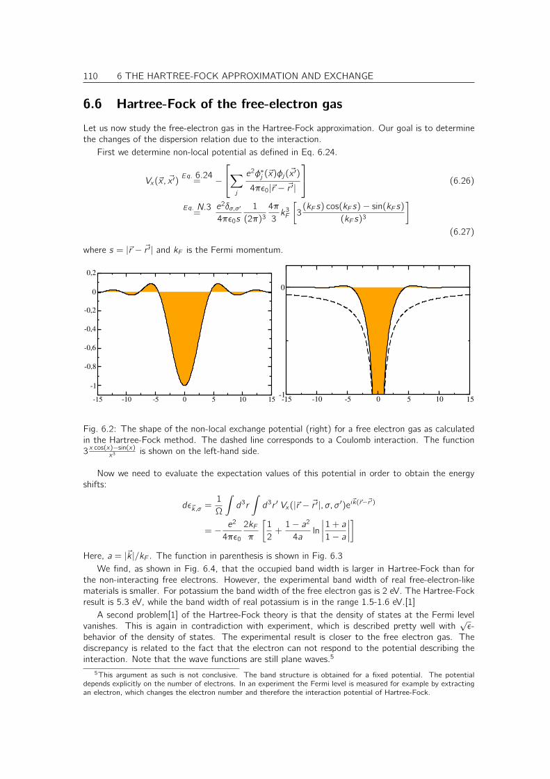
110 6 THE HARTREE-FOCK APPROXIMATION AND EXCHANGE
6.6 Hartree-Fock of the free-electron gas
Let us now study the free-electron gas in the Hartree-Fock approximation. Our goal is to determinethe changes of the dispersion relation due to the interaction.
First we determine non-local potential as defined in Eq. 6.24.
Vx(~x, ~x ′)Eq. 6.24= −
∑
j
e2φ∗j (~x)φj(~x′)
4πǫ0|~r − ~r ′|
(6.26)
Eq. N.3=
e2δσ,σ′
4πǫ0s
1
(2π)34π
3k3F
[
3(kF s) cos(kF s)− sin(kF s)
(kF s)3
]
(6.27)
where s = |~r − ~r ′| and kF is the Fermi momentum.
-15 -10 -5 0 5 10 15
-1
-0,8
-0,6
-0,4
-0,2
0
0,2
-15 -10 -5 0 5 10 15-1
0
Fig. 6.2: The shape of the non-local exchange potential (right) for a free electron gas as calculatedin the Hartree-Fock method. The dashed line corresponds to a Coulomb interaction. The function3 x cos(x)−sin(x)x3 is shown on the left-hand side.
Now we need to evaluate the expectation values of this potential in order to obtain the energyshifts:
dǫ~k,σ =1
Ω
∫
d3r
∫
d3r ′ Vx(|~r − ~r ′|, σ, σ′)ei~k(~r−~r′)
= − e2
4πǫ0
2kFπ
[1
2+1− a24a
ln
∣∣∣∣
1 + a
1− a
∣∣∣∣
]
Here, a = |~k |/kF . The function in parenthesis is shown in Fig. 6.3We find, as shown in Fig. 6.4, that the occupied band width is larger in Hartree-Fock than for
the non-interacting free electrons. However, the experimental band width of real free-electron-likematerials is smaller. For potassium the band width of the free electron gas is 2 eV. The Hartree-Fockresult is 5.3 eV, while the band width of real potassium is in the range 1.5-1.6 eV.[1]
A second problem[1] of the Hartree-Fock theory is that the density of states at the Fermi levelvanishes. This is again in contradiction with experiment, which is described pretty well with
√ǫ-
behavior of the density of states. The experimental result is closer to the free electron gas. Thediscrepancy is related to the fact that the electron can not respond to the potential describing theinteraction. Note that the wave functions are still plane waves.5
5This argument as such is not conclusive. The band structure is obtained for a fixed potential. The potentialdepends explicitly on the number of electrons. In an experiment the Fermi level is measured for example by extractingan electron, which changes the electron number and therefore the interaction potential of Hartree-Fock.
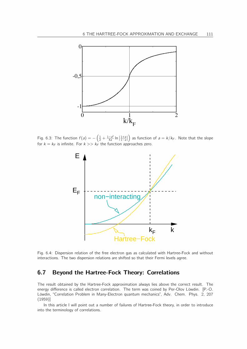
6 THE HARTREE-FOCK APPROXIMATION AND EXCHANGE 111
0 1 2
k/kF
-1
-0,5
0
Fig. 6.3: The function f (a) = −(12 +
1−a24a ln
∣∣ 1+a1−a∣∣
)
as function of a = k/kF . Note that the slope
for k = kF is infinite. For k >> kF the function approaches zero.
EFnon−interacting
E
kHartree−Fock
kF
Fig. 6.4: Dispersion relation of the free electron gas as calculated with Hartree-Fock and withoutinteractions. The two dispersion relations are shifted so that their Fermi levels agree.
6.7 Beyond the Hartree-Fock Theory: Correlations
The result obtained by the Hartree-Fock approximation always lies above the correct result. Theenergy difference is called electron correlation. The term was coined by Per-Olov Löwdin. [P.-O.Löwdin, “Correlation Problem in Many-Electron quantum mechanics”, Adv. Chem. Phys. 2, 207(1959)]
In this article I will point out a number of failures of Hartree-Fock theory, in order to introduceinto the terminology of correlations.
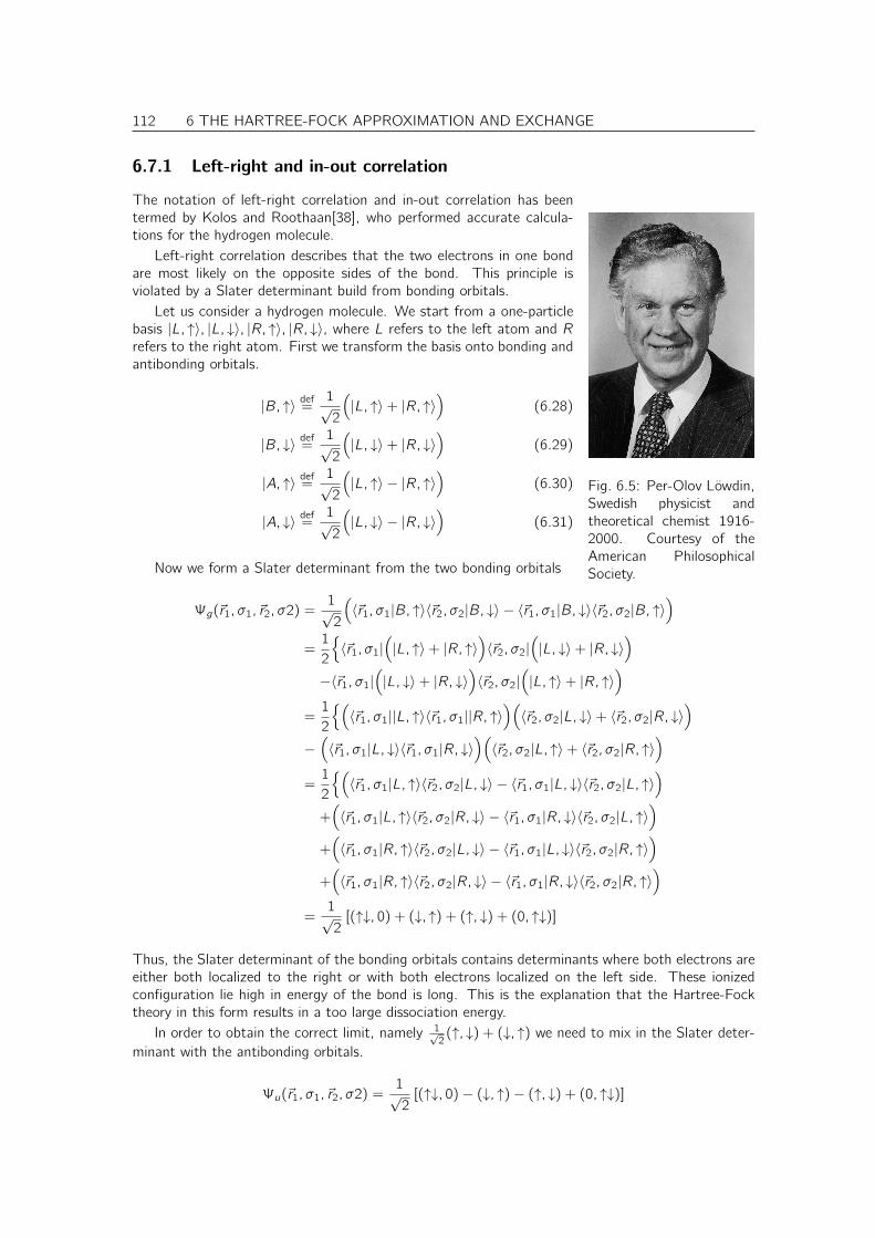
112 6 THE HARTREE-FOCK APPROXIMATION AND EXCHANGE
6.7.1 Left-right and in-out correlation
Fig. 6.5: Per-Olov Löwdin,Swedish physicist andtheoretical chemist 1916-2000. Courtesy of theAmerican PhilosophicalSociety.
The notation of left-right correlation and in-out correlation has beentermed by Kolos and Roothaan[38], who performed accurate calcula-tions for the hydrogen molecule.
Left-right correlation describes that the two electrons in one bondare most likely on the opposite sides of the bond. This principle isviolated by a Slater determinant build from bonding orbitals.
Let us consider a hydrogen molecule. We start from a one-particlebasis |L, ↑〉, |L, ↓〉, |R, ↑〉, |R, ↓〉, where L refers to the left atom and Rrefers to the right atom. First we transform the basis onto bonding andantibonding orbitals.
|B, ↑〉 def=1√2
(
|L, ↑〉+ |R, ↑〉)
(6.28)
|B, ↓〉 def=1√2
(
|L, ↓〉+ |R, ↓〉)
(6.29)
|A, ↑〉 def=1√2
(
|L, ↑〉 − |R, ↑〉)
(6.30)
|A, ↓〉 def=1√2
(
|L, ↓〉 − |R, ↓〉)
(6.31)
Now we form a Slater determinant from the two bonding orbitals
Ψg(~r1, σ1, ~r2, σ2) =1√2
(
〈~r1, σ1|B, ↑〉〈~r2, σ2|B, ↓〉 − 〈~r1, σ1|B, ↓〉〈~r2, σ2|B, ↑〉)
=1
2
〈~r1, σ1|(
|L, ↑〉+ |R, ↑〉)
〈~r2, σ2|(
|L, ↓〉+ |R, ↓〉)
−〈~r1, σ1|(
|L, ↓〉+ |R, ↓〉)
〈~r2, σ2|(
|L, ↑〉+ |R, ↑〉)
=1
2
(
〈~r1, σ1||L, ↑〉〈~r1, σ1||R, ↑〉)(
〈~r2, σ2|L, ↓〉+ 〈~r2, σ2|R, ↓〉)
−(
〈~r1, σ1|L, ↓〉〈~r1, σ1|R, ↓〉)(
〈~r2, σ2|L, ↑〉+ 〈~r2, σ2|R, ↑〉)
=1
2
(
〈~r1, σ1|L, ↑〉〈~r2, σ2|L, ↓〉 − 〈~r1, σ1|L, ↓〉〈~r2, σ2|L, ↑〉)
+(
〈~r1, σ1|L, ↑〉〈~r2, σ2|R, ↓〉 − 〈~r1, σ1|R, ↓〉〈~r2, σ2|L, ↑〉)
+(
〈~r1, σ1|R, ↑〉〈~r2, σ2|L, ↓〉 − 〈~r1, σ1|L, ↓〉〈~r2, σ2|R, ↑〉)
+(
〈~r1, σ1|R, ↑〉〈~r2, σ2|R, ↓〉 − 〈~r1, σ1|R, ↓〉〈~r2, σ2|R, ↑〉)
=1√2[(↑↓, 0) + (↓, ↑) + (↑, ↓) + (0, ↑↓)]
Thus, the Slater determinant of the bonding orbitals contains determinants where both electrons areeither both localized to the right or with both electrons localized on the left side. These ionizedconfiguration lie high in energy of the bond is long. This is the explanation that the Hartree-Focktheory in this form results in a too large dissociation energy.
In order to obtain the correct limit, namely 1√2(↑, ↓) + (↓, ↑) we need to mix in the Slater deter-
minant with the antibonding orbitals.
Ψu(~r1, σ1, ~r2, σ2) =1√2[(↑↓, 0)− (↓, ↑)− (↑, ↓) + (0, ↑↓)]
6 THE HARTREE-FOCK APPROXIMATION AND EXCHANGE 113
6.7.2 In-out correlation
• “in-out” correlation
• left-right correlation
• angular correlation
• radial correlation
• dynamic
• nondynamic
• near-degeneracy
• long-range
• shortrange
6.7.3 Spin contamination
6.7.4 Dynamic and static correlation
In quantum chemistry the definition of dynamic and static correlation is opposite to that used byphysicists. In Quantum chemistry, static correlation is the effect of very few Slater determinants thatcontribute to the ground state with approximately equal weight. That static correlation is present ifthe dominant Slater determinant has a weight less than about 95% of the complete wave function.
Dynamic correlation on the other hand are the small contribution of many Slater determinants,lowering the energy. Dynamic correlation is important to describe the cusp condition: The Coulombhole has a cusp in the density at the site of the observer electron. Because all one-particle orbitalsare smooth, many Slater determinants are required to build up this cusp as superposition of smoothwave functions.

114 6 THE HARTREE-FOCK APPROXIMATION AND EXCHANGE
Chapter 7
Density-functional theory
Density-functional theory[39, 40] is an extremely powerful technique. It is based on an exact theoremthat the ground-state energy is determined solely by the density alone.
The theorem says
• that all ground-state properties are unique functionals of the electron density and
• that the electron density can be obtained from a Schrödinger equation in an effective potential.
density-functional theory maps the interacting electron system onto a system of non-interactingelectrons in an effective potential. The effective potential depends in turn on the electron distributionand describes the interacting between the electrons in an effective way.
density-functional theory provides a total energy functional of the form
E[n(~r)] =∑
n
fn〈φn|p2
2me|φn〉
︸ ︷︷ ︸
Ts [n(~r)]
+
∫
d3r n(~r)vext(~r)
+1
2
∫
d3r
∫
d3r ′e2n(~r)n(~r ′)
4πǫ0|~r − ~r ′|︸ ︷︷ ︸
EHartree
+Exc [n(~r)]
Ts is not the kinetic energy of the many-electron system, but the one of the non-interacting referencesystem with density n(~r). We will see later that it can be written as functional of the density. Excis another functional of the density, called the exchange and correlation energy functional. Thisfunctional is not known in practice. Therefore, one uses approximate functionals, that are derivedfrom known analytical properties of the functional and/or even experimental data.
As a result of the minimum principle we obtain the following Kohn-Sham equation for the one-particle orbitals
[p2
2me+ vef f (r)− ǫn
]
|φn〉 = 0
where the effective potential is defined as
vef f (~r) = vext(~r) +e2
4πǫ0
∫
d3r ′n(~r ′)
|~r − ~r ′|+δExcδn(~r)︸ ︷︷ ︸
µxc (~r)
The proofs will be given later. Let us start out with the language used in the field of density-functional theory and the physical pictures that emerge.
115
116 7 DENSITY-FUNCTIONAL THEORY
7.1 One-particle and two-particle densities
In order to get used with the terminology, let me introduce a number of definitions related to densitymatrices[41].
7.1.1 N-particle density matrix
Let us start with the N-particle density matrix of an N-particle system
ρ(N)(~x1, . . . , ~xN ; ~x ′1, . . . , ~x ′N)def=Ψ(~x1, . . . , ~xN)Ψ
∗(~x ′1, . . . , ~x ′N)
The N-particle density matrix is formed from the matrix elements
ρ(N)(~x1, . . . , ~xN ; ~x ′1, . . . , ~x ′N) = 〈~x1, . . . , ~xN |ρ(N)|~x ′1, . . . , ~x ′N〉
of the density operator
ρ(N)def= |Ψ〉〈Ψ| (7.1)
This is the same density operator, that has been used in statistical mechanics a lot. In Eq. 7.1,however, we restricted ourselves to the density matrix of a pure state. A pure state can be describedby a single many-particle wave function, whereas a statistical mixture is an ensemble of many-particlestates, of which each contributes with a certain probability.
The N-particle density matrix contains all the information of the wave function itself, becauseone can determine the expectation value of any operator from it:
We use the representation of the unity operator in a N-particle Hilbert space of spin-orbitals
1 =
∫
d4x1 · · ·∫
d4xN |~x1, . . . , ~xN〉〈~x1, . . . , ~xN |
and obtain
〈Ψ|A|Ψ〉 = 〈Ψ|A|Ψ〉 = 〈Ψ|1A1|Ψ〉
=
∫
d4x1 · · ·∫
d4xN
∫
d4x ′1 · · ·∫
d4x ′N
· 〈~x1 . . . , ~xN |Ψ〉〈Ψ|~x ′1 . . . , ~x ′N〉︸ ︷︷ ︸
ρ(N)
〈~x ′1 . . . , ~x ′N |A|~x1 . . . , ~xN〉
=
∫
d4x1 · · ·∫
d4xN
∫
d4x ′1 · · ·∫
d4x ′N
·ρ(N)(~x1, . . . , ~xN ; ~x ′1, . . . , ~x ′N)〈~x ′1 . . . , ~x ′N |A|~x1 . . . , ~xN〉 (7.2)
For us the expectation value of the Hamilton operator plays a special role. The energy expectationvalue can be constructed from the N-particle density matrix. However, the special form of theHamilton operator relevant to us allows to use simpler, so-called reduced density matrices. We willdefine those in the following.
Fertig: WS06/07 8 Doppelstunde 27.Nov.06
7.1.2 One-particle reduced density matrix
From the N-particle density matrix we can form several contractions that are physically important,because they allow to represent expectation values of one-particle operators and the Coulomb inter-action in an elegant fashion.
7 DENSITY-FUNCTIONAL THEORY 117
For example, we do not need the full N-particle density matrix to determine the expectation valueof a one-particle operator, if we know the so-called one-particle density matrix.
A general one-particle operator has the matrix elements
〈~x1, . . . , ~xN |A|~x ′1, . . . , ~x ′N〉 =N∑
i=1
A(~xi , ~x′i )
N∏
k(k 6=i)δ(~xk − ~x ′k) (7.3)
This allows us to simplify the expression for the expectation value as follows
〈Ψ|A|Ψ〉 Eq. 7.2,7.3=
∫
d4x1 · · ·∫
d4xN
∫
d4x ′1 · · ·∫
d4x ′N
ρ(N)(~x1, . . . , ~xN ; ~x ′1, . . . , ~x ′N)N∑
i=1
A(~xi , ~x′i )
N∏
k(k 6=i)δ(~xk − ~x ′k)
(1)=
∫
d4x1 · · ·∫
d4xN
∫
d4x ′1 · · ·∫
d4x ′N
ρ(N)(~x1, . . . , ~xN ; ~x ′1, . . . , ~x ′N)NA(~x1, ~x ′1)N∏
k=2
δ(~xk − ~x ′k)
=
∫
d4x1
∫
d4x ′1 A(~x1, ~x′1)
·N∫
d4x2 · · ·∫
d4xN
∫
d4x ′2 · · ·∫
d4x ′N
·ρ(N)(~x1, . . . , ~xN ; ~x ′1, . . . , ~x ′N)N∏
k=2
δ(~xk − ~x ′k)
=
∫
d4x1
∫
d4x ′1 A(~x1, ~x′1)
·N∫
d4x2 · · ·∫
d4xN ρ(N)(~x1, ~x2, . . . , ~xN ; ~x ′1, ~x2 . . . , ~xN)
︸ ︷︷ ︸
ρ(1)(~x1,~x ′1)
(7.4)
In (1), we exploited that the density matrix describes identical particles. Thus, it is invariant underpermutation of two particle indices. (Simultaneously on both sides.)
Thus, if we define the one-particle reduced density matrix1 ρ(1)(~x, ~x ′), as2
ρ(1)(~x, ~x ′)def= N
∫
d4x2 · · ·∫
d4xN ρ(N)(~x, ~x2, . . . , ~xN ; ~x ′, ~x2, . . . , ~xN)
= N
∫
d4x2 · · ·∫
d4xN Ψ(~x, ~x2, . . . , ~xN)Ψ∗(~x ′, ~x2, . . . , ~xN) (7.5)
we can determine the expectation values of any one-particle operator as
〈Ψ|A|Ψ〉 Eq. 7.4=
∫
d4x
∫
d4x ′ ρ(1)(~x, ~x ′)A(~x ′, ~x) (7.6)
The integral in the first equation of the definition Eq. 7.5 provides the density of a single electron.This density is the same for all the electrons. Therefore, we obtain the total density by multiplicationby the number N of electrons, which explains the factor in front of the integral.
1 The word “reduced” is usually dropped. However the context must avoid confusion with the density matrix of aone-particle system.
2Note that this definition only holds for density matrices of indistinguishable particles.
118 7 DENSITY-FUNCTIONAL THEORY
Electron density
The operator for the electron density at a position ~r is
n(~r) =∑
σ
|~r , σ〉〈~r , σ| (7.7)
It has the matrix elements
〈~r , σ|n(~r0)|~r ′, σ′〉 = δ(~r − ~r0)δ(~r ′ − ~r0)δσ,σ′ (7.8)
in a one-particle, real-space and spin representation.The matrix elements of the operator in a N-particle, real-space and spin representation are
〈~x1, . . . , ~xN |n(~r0)|~x ′1, . . . , ~x ′N〉Eq. 7.3=
N∑
i=1
δ(~ri − ~r0)δ(~r ′ i − ~r0)δσi ,σ′i∏
k(k 6=i)δ(~xk − ~x ′k)
Thus, we obtain the electron density as
n(~r0) = 〈Ψ|n(~r0)|Ψ〉 Eq. 7.6=
∫
d4x
∫
d4x ′ ρ(1)(~x, ~x ′)δ(~r − ~r0)δ(~r ′ − ~r0)δσ,σ′
=∑
σ
ρ(1)(~r0, σ,~r0, σ) (7.9)
Magnetization
The magnetization operator has the form
~m =q
me~S =
~q
2me~σ (7.10)
Its matrix elements in a one-particle real-space representation are
〈~r , σ|mj |~r ′, σ′〉 =~q
2meδ(~r − ~r ′)σj,σ,σ′ (7.11)
where ~S is the spin operator, q is the electron charge and me is its mass. With σj we denote thePauli matrices defined in Eq. 3.2 for j ∈ x, y , z. Unfortunately, it is a little difficult not to getconfused by the many σ’s.
The matrix elements in the N-particle Hilbert space are
〈~x1, . . . , ~xN |mn(~r)|~x ′1, . . . , ~x ′N〉 Eq. 7.3=
N∑
i=1
δ(~ri − ~r ′ i)~q
2meσj,σ,σ′
︸ ︷︷ ︸
〈~ri ,σi |mj |~r ′ i ,σ′i 〉
∏
k(k 6=i)δ(~xk − ~x ′k)
Thus, we obtain the magnetization as
~m(~r0) = 〈Ψ| ~m(~r0)|Ψ〉 =∫
d4x
∫
d4x ′ ρ(1)(~x, ~x ′)δ(~r0 − ~r)~σσ,σ′
=∑
σ,σ′
ρ(1)(~r0, σ,~r0, σ′)~σσ′,σ
7 DENSITY-FUNCTIONAL THEORY 119
Kinetic energy
The matrix elements for the operator that provides the kinetic energy in a given direction at a givenpoint are
〈~x1, . . . , ~xN |T |~x ′1, . . . , ~x ′N〉 =N∑
i=1
δ(~xi − ~x ′ i)−~22me
~∇′2i∏
k(k 6=i)δ(~xk − ~x ′k)
This expression is weird: The matrix element is a differential operator that points no-where! Notreally. Let us investigate the meaning of this expression:
Consider a one-particle state |f 〉 and let us define a second one as |g〉def= ~p2
2me|f 〉. Then we find
g(~r) = 〈~r |g〉 = 〈~r | ~p2
2me|f 〉 = 〈~r | ~p
2
2me
∫
d3r ′ |~r ′〉〈~r ′|︸ ︷︷ ︸
1
|f 〉 =∫
d3r ′ 〈~r | ~p2
2me|~r ′〉 〈~r ′|f 〉︸ ︷︷ ︸
f (~r ′)
On the other hand, we know that g(~r) = −~22me
~∇2f (~r), so that we can formally identify the kineticenergy operator in a one-particle Hilbert space as
〈~r | ~p2me|~r ′〉 = δ(~r − ~r ′)−~
2
2me~∇′2
It is, however, important that the gradient stands in front of the function depending on ~r ′. I do notrecommend to use tricks like this, because one has to be awfully careful.
The gradient ~∇′i acts exclusively on the i-th primed position ~r ′ i . Note that the gradient cannotbe interchanged with the δ-function preceding it, because a gradient does not commutate with afunction of the corresponding coordinate.
Thus, we obtain the kinetic energy T as
Tdef= 〈Ψ|T |Ψ〉 =
∫
d4x
∫
d4x ′ δ(~x − ~x ′)−~2
2me
(
~∇′)2
ρ(1)(~x ′, ~x)
=∑
σ
∫
d3r lim~r→~r ′−~22me
~∇′2ρ(1)(~r ′, σ,~r , σ)
7.1.3 Two-particle density
In order to evaluate the Coulomb interaction energy between electrons, we need to know the two-particle density.
The matrix elements of the interaction in a real space representation are
〈~x1, . . . , ~xN |W |~x ′1, . . . , ~x ′N〉 =1
2
∑
i 6=jw(~xi , ~xj)
N∏
i=1
δ(~xi − ~x ′ i)
where w(x, x ′) = e2
4πǫ0|~r−~r ′|.
120 7 DENSITY-FUNCTIONAL THEORY
〈Ψ|W |Ψ〉 =∫
d4x1 · · ·∫
d4xN
∫
d4x ′1 · · ·∫
d4x ′N
ρ(N)(~x1, . . . , ~xN ; ~x ′1, . . . , ~x ′N)〈~x ′1, . . . , ~x ′N |W |~x1, . . . , ~xN〉
=
∫
d4x1 · · ·∫
d4xN
∫
d4x ′1 · · ·∫
d4x ′N
ρ(N)(~x1, . . . , ~xN ; ~x ′1, . . . , ~x ′N)1
2
∑
i 6=jw(~xi , ~xj)
N∏
i=1
δ(~xi − ~x ′ i)
=
∫
d4x1 · · ·∫
d4xN ρ(N)(~x1, . . . , ~xN ;~x1, . . . , ~xN)
1
2
∑
i 6=jw(~xi , ~xj)
=
∫
d4x1 · · ·∫
d4xN ρ(N)(~x1, . . . , ~xN ;~x1, . . . , ~xN)
N(N − 1)2
w(~x1, ~x2)
=1
2
∫
d4x
∫
d4x ′ w(~x, ~x ′)
N(N − 1)∫
d4x1 · · ·∫
d4xN ρ(N)(~x1, . . . , ~xN ;~x1, . . . , ~xN)δ(~x − ~x1)δ(~x ′ − ~x2)
︸ ︷︷ ︸
n(2)(~x ′,~x)
=1
2
∫
d4x
∫
d4x ′ n(2)(~x, ~x ′)w(~x, ~x ′)
Thus, we define the two-particle density3. n(2)(~x, ~x ′) as
n(2)(~x, ~x ′)def= N(N − 1)
∫
d4x1 · · ·∫
d4xN
ρ(N)(~x1, . . . , ~xN ;~x1, . . . , ~xN)δ(~x − ~x1)δ(~x ′ − ~x2) (7.12)
so that we can determine the interaction energy as
〈Ψ|W |Ψ〉 = 12
∫
d4x
∫
d4x ′ n(2)(~x, ~x ′)w(~x, ~x ′)
The two-particle density can also be expressed as expectation value as follows
n(2)(~x, ~x ′)Eq. 7.12=
∫
d4x1 · · ·∫
d4xN Ψ(~x1, . . . , ~xN)∑
i 6=jδ(~x − ~xi)δ(~x ′ − ~xj)Ψ∗(~x1, . . . , ~xN)
= 〈Ψ|∑
i 6=jδ(~x − ~xi)δ(~x ′ − ~xj)|Ψ〉 (7.13)
The two-particle density describes the probability density that there is one electron at ~r and another
one at ~r ′. It integrates up to the number of ordered pairs, namely N(N − 1).Note that the two-particle density is often confused with the one-particle density matrix. Both
have the same number of arguments, but they are fundamentally different quantities.The q-particle densities contain the information only about the probability to find a q-tuple of
electrons with a given set of coordinates. It is, however, not possible to extract for example themomentum or the kinetic energy from a given q-particle density. In contrast, the q-electron density
3There are different conventions in use, which differ by a factor 1/2. We follow here the choice of McWeeny[41],who does not have the factor 1
2. Here, the factor 1
2, which compensates for the double counting of two pairs at ~x
and ~x ′ (one obtained by exchanging the two particles from the other) must be done explicitly. On the other hand thetwo-particle density as defined by McWeeny has the simple physical interpretation of a density for one particle at ~x andanother one at ~x ′, irrespective of their order.
7 DENSITY-FUNCTIONAL THEORY 121
matrix contains the complete information on q-tuple of electrons. For a q-particle system, the q-particle density matrix contains the complete information on the system, that is the same informationcontained in the wave function. Already from the one-particle density matrix we can determine themomentum or the kinetic energy.
In the following we list various densities and density-matrices in comparison, to show the difference
• one-particle density matrix
ρ(1)(~x1, ~x ′1) = N
∫
d4x2 · · ·∫
d4xN ρ(N)(~x1, ~x2, . . . , ~xN ; ~x ′1, ~x2, . . . , ~xN)
• two-particle density matrix
ρ(2)(~x1, ~x2, ~x ′1~x ′2) = N(N − 1)∫
d4x3 · · ·∫
d4xN ρ(N)(~x1, ~x2, ~x3, . . . , ~xN ; ~x ′1, ~x ′2, ~x3, . . . , ~xN)
• one-particle density
n(1)(~x1) = N
∫
d4x2 · · ·∫
d4xN ρ(N)(~x1, . . . , ~xN ;~x1, . . . , ~xN)
• two-particle density
n(2)(~x1, ~x2) = N(N − 1)∫
d4x3 · · ·∫
d4xN ρ(N)(~x1, . . . , ~xN ;~x1, . . . , ~xN)
• N-particle density
n(N)(~x1, . . . , ~xN) = ρ(N)(~x1, . . . , ~xN ;~x1, . . . , ~xN)
The q-particle density can directly be obtained from the q-particle density matrix
n(q)(~x1, . . . , ~xq) = ρ(q)(~x1, . . . , ~xq, ~x1, . . . , ~xq)
The density matrix has always two arguments per particle while the density has only one per particle.The two-particle density is so important for many-particle physics, because we can directly express
the interaction energy by the two-particle density. The Coulomb interaction between electrons canbe written as
EH + EX = 〈Ψ|1
2
∑
i 6=j
e2
4πǫ0|~r − ~r ′||Ψ〉 = 1
2
∑
σ,σ′
∫
d3r
∫
d3re2n(2)(~x, ~x ′)
4πǫ0|~r − ~r ′|(7.14)
In chapter 6 we derived the expression for the expectation value of a two-particle operator with aSlater determinant. According to Eq. 7.13, the two-particle density can be expressed as an expectationvalue. For a single Slater determinant, the two-particle density would have the form
n(2)(~r , ~r ′)Eqs. 6.12,7.13
=
N∑
i ,j
∫
d4x1
∫
d4x2 φ∗i (~x1)φ
∗j (~x2)δ(~r − ~r1)δ(~r − ~r2)φi(~x1)φj(~x2)
−N∑
i ,j
∫
d4x1
∫
d4x2 φ∗i (~x1)φ
∗j (~x2)δ(~r − ~r1)δ(~r − ~r2)φj(~x1)φi(~x2)
= n(~r)n(~r ′)−N∑
i ,j
∑
σ,σ′
φ∗i (~r , σ)φj(~r , σ)φ∗j (~r′, σ′)φi(~r ′, σ
′) (7.15)
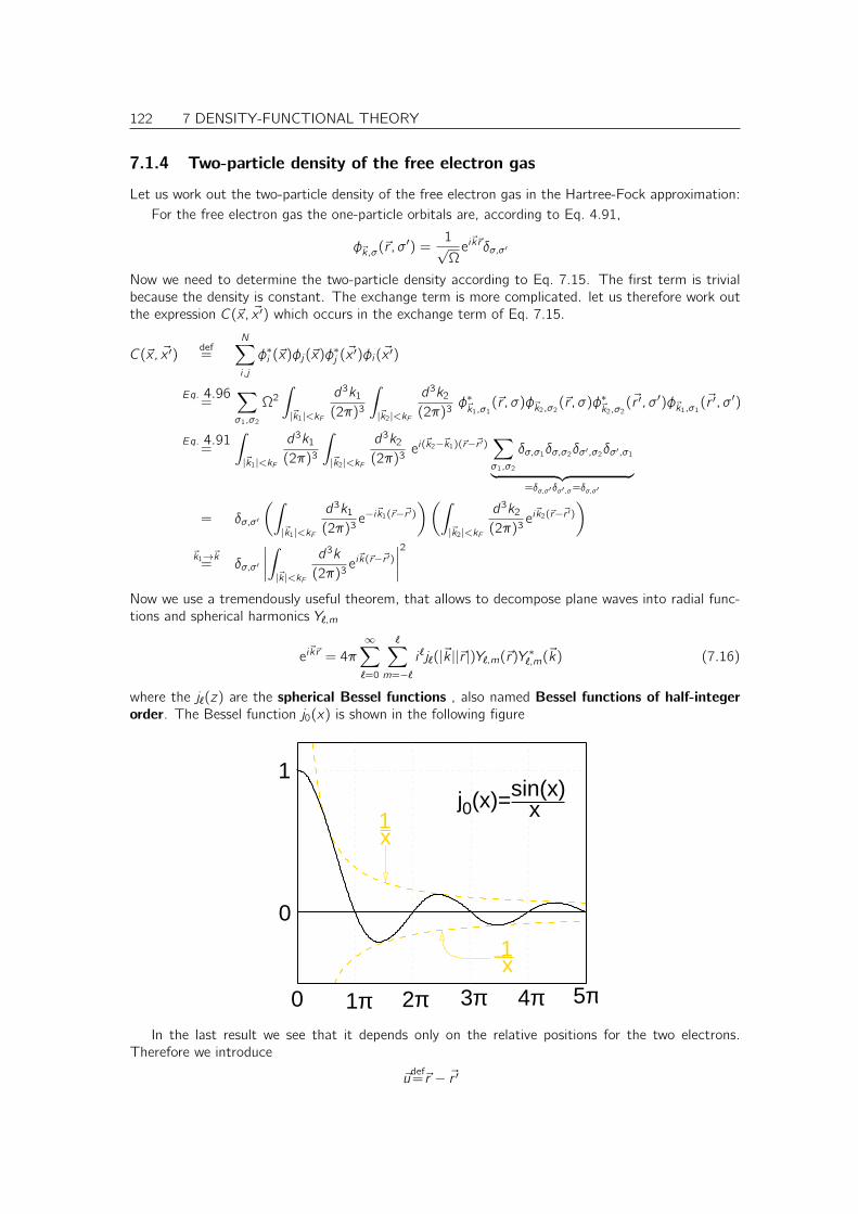
122 7 DENSITY-FUNCTIONAL THEORY
7.1.4 Two-particle density of the free electron gas
Let us work out the two-particle density of the free electron gas in the Hartree-Fock approximation:For the free electron gas the one-particle orbitals are, according to Eq. 4.91,
φ~k,σ(~r , σ′) =
1√Ωei~k~rδσ,σ′
Now we need to determine the two-particle density according to Eq. 7.15. The first term is trivialbecause the density is constant. The exchange term is more complicated. let us therefore work outthe expression C(~x, ~x ′) which occurs in the exchange term of Eq. 7.15.
C(~x, ~x ′)def=
N∑
i ,j
φ∗i (~x)φj(~x)φ∗j (~x′)φi(~x ′)
Eq. 4.96=
∑
σ1,σ2
Ω2∫
|~k1|<kF
d3k1(2π)3
∫
|~k2|<kF
d3k2(2π)3
φ∗~k1,σ1(~r , σ)φ~k2,σ2(~r , σ)φ∗~k2,σ2(~r ′, σ′)φ~k1,σ1(
~r ′, σ′)
Eq. 4.91=
∫
|~k1|<kF
d3k1(2π)3
∫
|~k2|<kF
d3k2(2π)3
ei(~k2−~k1)(~r−~r ′)
∑
σ1,σ2
δσ,σ1δσ,σ2δσ′,σ2δσ′,σ1
︸ ︷︷ ︸
=δσ,σ′δσ′ ,σ=δσ,σ′
= δσ,σ′
(∫
|~k1|<kF
d3k1(2π)3
e−i~k1(~r−~r ′)
)(∫
|~k2|<kF
d3k2(2π)3
ei~k2(~r−~r ′)
)
~k1→~k= δσ,σ′
∣∣∣∣
∫
|~k|<kF
d3k
(2π)3ei~k(~r−~r ′)
∣∣∣∣
2
Now we use a tremendously useful theorem, that allows to decompose plane waves into radial func-tions and spherical harmonics Yℓ,m
ei~k~r = 4π
∞∑
ℓ=0
ℓ∑
m=−ℓi ℓjℓ(|~k ||~r |)Yℓ,m(~r)Y ∗ℓ,m(~k) (7.16)
where the jℓ(z) are the spherical Bessel functions , also named Bessel functions of half-integerorder. The Bessel function j0(x) is shown in the following figure
1π 2π 3π 4π 5π
x1
x1−
1
0
0
j0(x)=sin(x)x
In the last result we see that it depends only on the relative positions for the two electrons.Therefore we introduce
~udef=~r − ~r ′
7 DENSITY-FUNCTIONAL THEORY 123
Since we integrate over a spherical volume in reciprocal space, only the terms with ℓ = 0 contributea finite value, because all other spherical harmonics integrate to zero.
C(~x, ~x ′)~r−~r ′→~u= δσ,σ′
∣∣∣∣
∫
|~k<kF
d3k
(2π)3ei~k~u
∣∣∣∣
2
Eq. 7.16= δσ,σ′
∣∣∣∣∣
∫
|~k<kF
d3k
(2π)34π
∞∑
ℓ=0
ℓ∑
m=−ℓi ℓjℓ(|~k ||~u|)Yℓ,m(~u)Y ∗ℓ,m(~k)
∣∣∣∣∣
2
= δσ,σ′
∣∣∣∣∣∣∣∣∣
1
(2π)3
∫
k<kF
dk k24πj0(|~k ||~u|)1
4π︸︷︷︸
Y0,0(~u)Y ∗0,0(~k)
∣∣∣∣∣∣∣∣∣
2
|~k|→k= δσ,σ′
1
(2π)6
(
4π
∫
k<kF
dk k2sin(k |~u|)k |~u|
)2
k|~u|→x= δσ,σ′
1
(2π)6
(4π
|~u|3∫
x<kF |u|dx x sin(x)
)2
The integral can be solved using
d
dx(x cos(x)− sin(x)) = cos(x)− x sin(x)− cos(x) = x sin(x)
Now we continue
C(~x, ~x ′)k|~u|→x= δσ,σ′
1
(2π)6
∣∣∣∣
1
|~u|3 (kF |~u| cos(kF |~u|)− sin(kF |~u|))∣∣∣∣
2
=δσ,σ′k
6F
(2π)6
(kF |~u| cos(kF |~u|)− sin(kF |~u|)
(kF |~u|)3)2
For the sake of esthetics4, let scale the expression in parenthesis such that it starts with value 1 atu = 0. (See footnote below5)
limx→0
x cos(x)− sin(x)x3
= limx→0
∞∑
n=0
((−1)n2n!
x2n−2 − (−1)n(2n + 1)!
x2n−2)
= limx→0
∞∑
n=0
(1
(2n)!− 1
(2n + 1)!
)
(−1)nx2n−2
= limx→0
∞∑
n=0
(1− 1) x−2 −(1
2− 16
)
x0 +O(x2) =1
3
4esthetics=Ästetik”5
ex =
∞∑
n=0
1
n!xn
⇒ eix =∞∑
n=0
1
n!inxn =
∞∑
n=0
(1
(2n)!(−1)nx2n + i 1
(2n + 1)!(−1)nx2n+1
)
= cos(x) + i sin(x)
⇒ cos(x) =∞∑
n=0
(−1)n2n!
x2n ; sin(x) =
∞∑
n=0
(−1)n+1(2n + 1)!
x2n+1
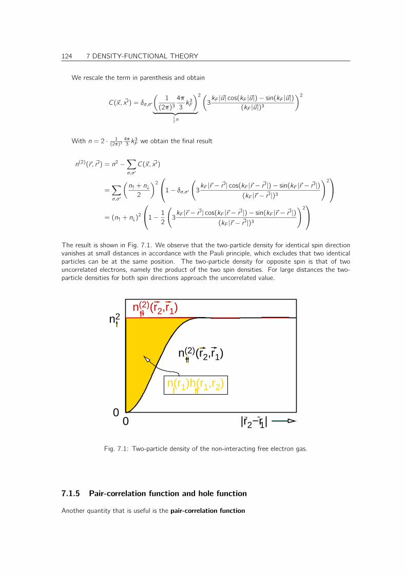
124 7 DENSITY-FUNCTIONAL THEORY
We rescale the term in parenthesis and obtain
C(~x, ~x ′) = δσ,σ′
(1
(2π)34π
3k3F
)
︸ ︷︷ ︸12n
2(
3kF |~u| cos(kF |~u|)− sin(kF |~u|)
(kF |~u|)3)2
With n = 2 · 1(2π)3
4π3 k3F we obtain the final result
n(2)(~r , ~r ′) = n2 −∑
σ,σ′
C(~x, ~x ′)
=∑
σ,σ′
(n↑ + n↓2
)2
1− δσ,σ′(
3kF |~r − ~r ′| cos(kF |~r − ~r ′|)− sin(kF |~r − ~r ′|)
(kF |~r − ~r ′|)3
)2
= (n↑ + n↓)2
1− 12
(
3kF |~r − ~r ′| cos(kF |~r − ~r ′|)− sin(kF |~r − ~r ′|)
(kF |~r − ~r ′|)3
)2
The result is shown in Fig. 7.1. We observe that the two-particle density for identical spin directionvanishes at small distances in accordance with the Pauli principle, which excludes that two identicalparticles can be at the same position. The two-particle density for opposite spin is that of twouncorrelated electrons, namely the product of the two spin densities. For large distances the two-particle densities for both spin directions approach the uncorrelated value.
n(r1)h(r1,r2)
|r2−r1|0
n2n(2)(r2,r1)
n(2)(r2,r1)
0
Fig. 7.1: Two-particle density of the non-interacting free electron gas.
7.1.5 Pair-correlation function and hole function
Another quantity that is useful is the pair-correlation function
7 DENSITY-FUNCTIONAL THEORY 125
PAIR-CORRELATION FUNCTION
g(~x, ~x0) =n(2)(~x, ~x0)
n(~x0)
The pair-correlation function describes the probability to find an electron with coordinates ~x , giventhat there is one at ~x0. The pair-correlation function is the electron density seen by one electron thatis located at ~x0. Consider an N-electron system. Pick out one electron and determine the density ofthe remaining N − 1 electrons.
Given that an electron will see at large distances nothing but the charge density itself, it makessense to define a more short-ranged quantity, namely the exchange-correlation hole functionh(~x, ~x0)
HOLE FUNCTION H( ~X, ~X0)
g(~x, ~x0) = n(~x) + h(~x, ~x0)
The physical picture of the hole function is that each electron “sees” the total density n(~x) and thedensity h(~x, ~x ′) of “one missing electron”. The density h(~x, ~x ′) is like a hole in the total charge densitydue to the fact that the remaining electrons do not come near to the electron in question. Thus, theCoulomb repulsion between the electrons is reduced relative to the Hartree energy by the attractionof the electron to its exchange-correlation hole.
Accurate calculations of the exchange-correlation hole have been obtained by quantum MonteCarlo calculations[42].
The two-particle density can now be expressed by the density and the exchange-correlation holefunction as
n(2)(~x, ~x0) = n(~x0) [n(~x) + h(~x, ~x0)]
Now we can also rewrite the interaction energy Eq. 7.14
Eint =1
2
∑
σ,σ′
∫
d3r
∫
d3r ′e2n(~x)n(~x ′)
4πǫ0|~r − ~r ′|︸ ︷︷ ︸
EH
+∑
σ
∫
d3r n(~x)1
2
∑
σ′
∫
d3r ′e2h(~x ′, ~x)
4πǫ0|~r − ~r ′|︸ ︷︷ ︸
Uxc
7.2 Self-made density functional
In order to understand, how density functionals are made, let us demonstrate the principle on a simpleexample. We will make our own, first-principles, density functional. It will not be terribly good, butit will not be a complete disaster either. However, it will be our own!
The typical process of creating a density functional is that we take all available information on thehole function, that may be relevant, and find an expression that reproduces this information as bestas possible. As more and more information about the hole function becomes available, the functionalsare continuously improved.
Apparently all the information about the interaction is contained in the hole function h(~r , ~r ′). Letus collect all we know so far about the hole function:
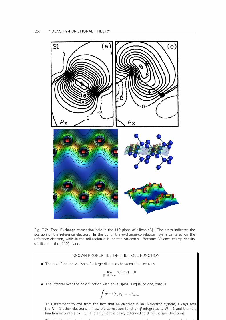
126 7 DENSITY-FUNCTIONAL THEORY
Fig. 7.2: Top: Exchange-correlation hole in the 110 plane of silicon[43]. The cross indicates theposition of the reference electron. In the bond, the exchange-correlation hole is centered on thereference electron, while in the tail region it is located off-center. Bottom: Valence charge densityof silicon in the (110) plane.
KNOWN PROPERTIES OF THE HOLE FUNCTION
• The hole function vanishes for large distances between the electrons
lim|~r−~r0|→∞
h(~x, ~x0) = 0
• The integral over the hole function with equal spins is equal to one, that is∫
d3r h(~x, ~x0) = −δσ,σ0
This statement follows from the fact that an electron in an N-electron system, always seesthe N − 1 other electrons. Thus, the correlation function ~g integrates to N − 1 and the holefunction integrates to −1. The argument is easily extended to different spin directions.
• The hole function for two electrons at the same position and spin must cancel the spin density
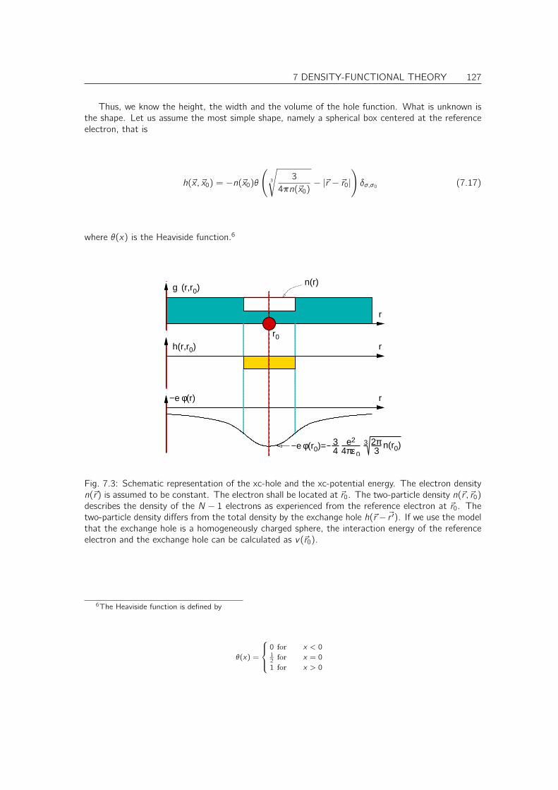
7 DENSITY-FUNCTIONAL THEORY 127
Thus, we know the height, the width and the volume of the hole function. What is unknown isthe shape. Let us assume the most simple shape, namely a spherical box centered at the referenceelectron, that is
h(~x, ~x0) = −n(~x0)θ(
3
√
3
4πn(~x0)− |~r − ~r0|
)
δσ,σ0 (7.17)
where θ(x) is the Heaviside function.6
(r0)=φ−e
φ(r)−e
h(r,r0)r0
4 0πεe2
n(r0)2π
g (r,r0)n(r)
r
r
r
3334
Fig. 7.3: Schematic representation of the xc-hole and the xc-potential energy. The electron densityn(~r) is assumed to be constant. The electron shall be located at ~r0. The two-particle density n(~r ,~r0)describes the density of the N − 1 electrons as experienced from the reference electron at ~r0. Thetwo-particle density differs from the total density by the exchange hole h(~r − ~r ′). If we use the modelthat the exchange hole is a homogeneously charged sphere, the interaction energy of the referenceelectron and the exchange hole can be calculated as v(~r0).
6The Heaviside function is defined by
θ(x) =
0 for x < 012
for x = 0
1 for x > 0
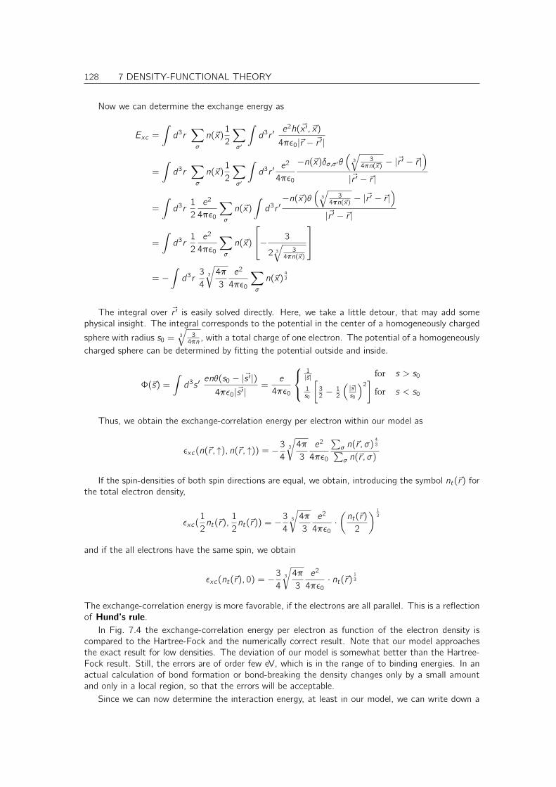
128 7 DENSITY-FUNCTIONAL THEORY
Now we can determine the exchange energy as
Exc =
∫
d3r∑
σ
n(~x)1
2
∑
σ′
∫
d3r ′e2h(~x ′, ~x)
4πǫ0|~r − ~r ′|
=
∫
d3r∑
σ
n(~x)1
2
∑
σ′
∫
d3r ′e2
4πǫ0
−n(~x)δσ,σ′θ(3
√3
4πn(~x) − |~r ′ − ~r |)
|~r ′ − ~r |
=
∫
d3r1
2
e2
4πǫ0
∑
σ
n(~x)
∫
d3r ′−n(~x)θ
(3
√3
4πn(~x) − |~r ′ − ~r |)
|~r ′ − ~r |
=
∫
d3r1
2
e2
4πǫ0
∑
σ
n(~x)
− 3
2 3√
34πn(~x)
= −∫
d3r3
43
√
4π
3
e2
4πǫ0
∑
σ
n(~x)43
The integral over ~r ′ is easily solved directly. Here, we take a little detour, that may add somephysical insight. The integral corresponds to the potential in the center of a homogeneously charged
sphere with radius s0 = 3
√34πn , with a total charge of one electron. The potential of a homogeneously
charged sphere can be determined by fitting the potential outside and inside.
Φ(~s) =
∫
d3s ′enθ(s0 − |~s ′|)4πǫ0|~s ′|
=e
4πǫ0
1|~s| for s > s0
1s0
[
32 − 12
(|~s|s0
)2]
for s < s0
Thus, we obtain the exchange-correlation energy per electron within our model as
ǫxc(n(~r , ↑), n(~r , ↑)) = −3
43
√
4π
3
e2
4πǫ0
∑
σ n(~r , σ)43
∑
σ n(~r , σ)
If the spin-densities of both spin directions are equal, we obtain, introducing the symbol nt(~r) forthe total electron density,
ǫxc(1
2nt(~r),
1
2nt(~r)) = −
3
43
√
4π
3
e2
4πǫ0·(nt(~r)
2
) 13
and if the all electrons have the same spin, we obtain
ǫxc(nt(~r), 0) = −3
43
√
4π
3
e2
4πǫ0· nt(~r)
13
The exchange-correlation energy is more favorable, if the electrons are all parallel. This is a reflectionof Hund’s rule.
In Fig. 7.4 the exchange-correlation energy per electron as function of the electron density iscompared to the Hartree-Fock and the numerically correct result. Note that our model approachesthe exact result for low densities. The deviation of our model is somewhat better than the Hartree-Fock result. Still, the errors are of order few eV, which is in the range of to binding energies. In anactual calculation of bond formation or bond-breaking the density changes only by a small amountand only in a local region, so that the errors will be acceptable.
Since we can now determine the interaction energy, at least in our model, we can write down a
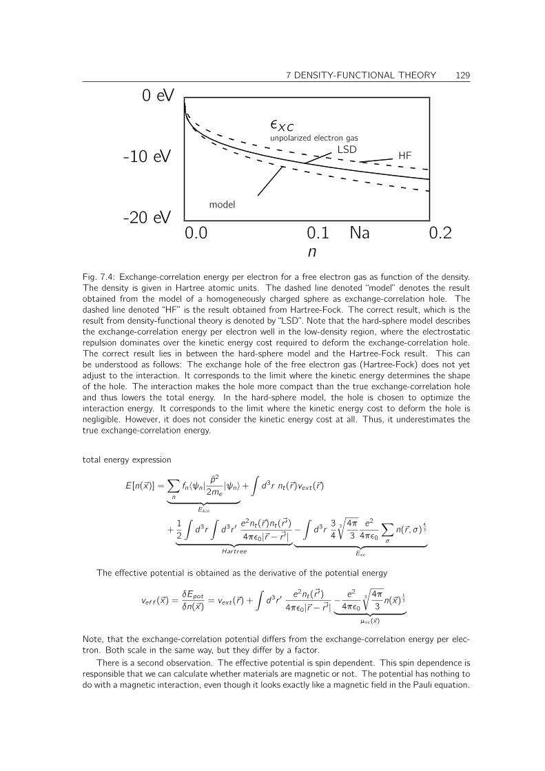
7 DENSITY-FUNCTIONAL THEORY 129
0.0 0.1 0.2Na
0 eV
-10 eV
-20 eV
n
ǫxcunpolarized electron gas
LSD.
............................................................ HF.
....................................................................
model.
...........................................................................
.....
..
..
.
..
..
.
..
..
..
..
..
..
...........
.
.........
..............
..............
...........
.........
...........
...........
...........
.............
..........
...........
..........
..........
. .........
. .........
. ...................
. .......... ..........
..
..
..
..
..
.
..
..
..
..
.
..
..
..
..
..
..
..
..
..
..
..
..
..
..
..
.
..
..
..
..
..
..
..
..
..
..
..
..
..
.
...................
......................
...........................
...............................
.....................................
..........................................
................................................
......................................................
.............................................................
..................
..................
..................
..............
....................
.....
......................
....
......................
.....
..
....
..
..
..
.
..
..
.
....
..
..
..
.
.
..
..
..
..
.
............
.
.........
.
........
.........
.............
...........
...........
..............
...........
...........
...........
.............
..........
..........
..........
..........
......................
....................
Fig. 7.4: Exchange-correlation energy per electron for a free electron gas as function of the density.The density is given in Hartree atomic units. The dashed line denoted “model” denotes the resultobtained from the model of a homogeneously charged sphere as exchange-correlation hole. Thedashed line denoted “HF” is the result obtained from Hartree-Fock. The correct result, which is theresult from density-functional theory is denoted by “LSD”. Note that the hard-sphere model describesthe exchange-correlation energy per electron well in the low-density region, where the electrostaticrepulsion dominates over the kinetic energy cost required to deform the exchange-correlation hole.The correct result lies in between the hard-sphere model and the Hartree-Fock result. This canbe understood as follows: The exchange hole of the free electron gas (Hartree-Fock) does not yetadjust to the interaction. It corresponds to the limit where the kinetic energy determines the shapeof the hole. The interaction makes the hole more compact than the true exchange-correlation holeand thus lowers the total energy. In the hard-sphere model, the hole is chosen to optimize theinteraction energy. It corresponds to the limit where the kinetic energy cost to deform the hole isnegligible. However, it does not consider the kinetic energy cost at all. Thus, it underestimates thetrue exchange-correlation energy.
total energy expression
E[n(~x)] =∑
n
fn〈ψn|p2
2me|ψn〉
︸ ︷︷ ︸
Ekin
+
∫
d3r nt(~r)vext(~r)
+1
2
∫
d3r
∫
d3r ′e2nt(~r)nt(~r ′)
4πǫ0|~r − ~r ′|︸ ︷︷ ︸
Hartree
−∫
d3r3
43
√
4π
3
e2
4πǫ0
∑
σ
n(~r , σ)43
︸ ︷︷ ︸
Exc
The effective potential is obtained as the derivative of the potential energy
vef f (~x) =δEpotδn(~x)
= vext(~r) +
∫
d3r ′e2nt(~r ′)
4πǫ0|~r − ~r ′|− e2
4πǫ0
3
√
4π
3n(~x)
13
︸ ︷︷ ︸
µxc (~x)
Note, that the exchange-correlation potential differs from the exchange-correlation energy per elec-tron. Both scale in the same way, but they differ by a factor.
There is a second observation. The effective potential is spin dependent. This spin dependence isresponsible that we can calculate whether materials are magnetic or not. The potential has nothing todo with a magnetic interaction, even though it looks exactly like a magnetic field in the Pauli equation.
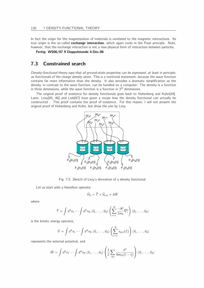
130 7 DENSITY-FUNCTIONAL THEORY
In fact the origin for the magnetization of materials is unrelated to the magnetic interactions. Itstrue origin is the so-called exchange interaction, which again roots in the Pauli principle. Note,however, that the exchange interaction is not a new physical form of interaction between particles.
Fertig: WS06/07 9 Doppelstunde 4.Dec.06
7.3 Constrained search
Density-functional theory says that all ground-state properties can be expressed, at least in principle,
as functionals of the charge density alone. This is a nontrivial statement, because the wave functioncontains far more information than the density. It also provides a dramatic simplification as thedensity, in contrast to the wave function, can be handled on a computer: The density is a functionin three dimensions, while the wave function is a function in 3N dimensions.
The original proof of existence for density functionals goes back to Hohenberg and Kohn[44].Later, Levy[45, 46] and Lieb[47] have given a recipe how the density functional can actually beconstructed . This proof contains the proof of existence. For this reason, I will not present theoriginal proof of Hohenberg and Kohn, but show the one by Levy.
n1(r) n2(r) n3(r) n4(r)
|ΨΑ>
|ΨΕ> |ΨΗ>
|ΨΚ>
|ΨΜ>
|ΨΒ>|ΨΙ >|ΨΧ>
F1[n1(r)]
F0[n1(r)]F0[n2(r)]
F1[n2(r)]
F0[n3(r)]
F1[n3(r)]
F0[n4(r)]
F1[n4(r)]
Fig. 7.5: Sketch of Levy’s derivation of a density functional.
Let us start with a Hamilton operator
Hλ = T + Vext + λW
where
T =
∫
d4x1 · · ·∫
d4xN |~x1, . . . , ~xN〉(
N∑
i=1
−~22me
~∇2i
)
〈~x1, . . . , ~xN |
is the kinetic energy operator,
V =
∫
d4x1 · · ·∫
d4xN |~x1, . . . , ~xN〉(
N∑
i=1
vext(~ri)
)
〈~x1, . . . , ~xN |
represents the external potential, and
W =
∫
d4x1 · · ·∫
d4xN |~x1, . . . , ~xN〉
1
2
∑
i 6=j
e2
4πǫ0|~ri − ~rj |
〈~x1, . . . , ~xN |
7 DENSITY-FUNCTIONAL THEORY 131
is the interaction energy operator. We have scaled the electron-electron interaction by a couplingparameter λ, which allows us later to switch the electron-electron interaction on an off. This is notrequired for the proof of Levy, but later on, we will often refer to Hamiltonians without interaction.
The idea of the proof is very simple:
1. Group all normalized, antisymmetric many-particle wave functions |Ψ〉 according to theirdensity. Each such subset A[n(~r)] contains all wave functions in the Fock space F with thesame density.
A[n(~r)] = |Ψ〉 ∈ F : 〈Ψ|n(~r)|Ψ〉 = n(~r)
The Fock space is the union7 of all N-particle Hilbert spaces HN , that is
Fdef=
∞⋃
N=0
HN
The Fock space will be introduced in more detail later. If the reader feels uncomfortable withthis concept, he may replace the Fock space with the N-particle Hilbert space for a specific N.
2. For each subset A[n(~r)], that is for each density, we determine that wave function |Ψ(0)λ [n(~r)]〉that provides the lowest energy 〈Ψ|Hλ|Ψ〉. The minimum of the total energy defines the totalenergy functional Eλ[n(~r)] of the electron density.
Eλ[n(~r)] = min|Ψ〉∈A[n(~r)]
〈Ψ|Hλ|Ψ〉 = 〈Ψ(0)λ [n(~r)]|Hλ|Ψ(0)λ [n(~r)]〉
3. The energy can be divided into universal density functional Fλ[n(~r)], which is a generalproperty of the electron gas, and a system-specific term, that depends on the external potential.
Eλ[n(~r)] = Fλ[n(~r)]︸ ︷︷ ︸
〈Ψ(0)λ [n]|T+λW |Ψ(0)λ [n]〉
+
∫
d3r n(~r)vext(~r)
︸ ︷︷ ︸
〈Ψ(0)λ [n]|V |Ψ(0)λ [n]〉
Because the energy related to the external potential only depends on the density, it is a constantwithin each group of a given density. Thus, we can directly determine the universal functionalFλ[n(~r)] as minimum of 〈Ψ|T + λW |Ψ〉 for all wave functions with the specified density.
UNIVERSAL DENSITY FUNCTIONAL
Fλ[n(~r)]def= min|Ψ〉∈A[n(~r)]
〈Ψ|T + λW |Ψ〉
4. To find the ground-state energy E(0)λ of an electron gas with N electrons in a given externalpotential, we minimize the total energy functional under the constraint of a specified totalnumber of electrons.
E(0)λ = min
n(~r):∫d3r n(~r)=N
Fλ[n(~r)] +
∫
d3r n(~r)vext(~r)
The Lagrange parameter µ is the chemical potential of the electrons. This minimization withrespect to the density provides us with the ground-state density and the ground-state energy.If we have remembered the wave function |Ψ0[n(~r)]〉 that minimized the total energy within agroup with given density n(~r), we can, in principle work our way back to the ground-state wavefunction, which contains all information about the electronic ground state.
7germ.:union=Vereinigung
132 7 DENSITY-FUNCTIONAL THEORY
This concludes the proof by Levy on the existence of a universal functional of the density, that allowsto determine the ground-state energy and, in principle, all other properties of the electronic groundstate.
7.4 Self-consistent equations
In the following I will discuss, how this proof can be used for a practical scheme to find the electronicground-state energy and density under the assumption that the universal functional is known.
We will be lead to a system of equations, that must be fulfilled simultaneously for the electronicground state. Then we will show, how this system of equations can be solved iteratively.
7.4.1 Universal Functional
Let us write down the universal functional Fλ[n(~r)] discussed in the proof of Levy more explicitly.
Fλ[n(~r)] = extr
η
extr
γ(~r)
min|Ψ〉
〈Ψ|T + λW |Ψ〉+∫d3r γ(~r)
[
〈Ψ|n(~r)|Ψ〉 − n(~r)]
−η[
〈ψ|ψ〉 − 1]
Instead of explicitly grouping the wave functions we enforce the constraints by the method of Lagrangemultipliers γ(~r) and η. Note, that we need not specify the chemical potential here, because theparticle number is fixed by the specification of the density n(~r).
The operator n(~r) yields the one-particle density of a many-particle wave function.8 It is definedby
n(~r) =
∫
d4x1 · · ·∫
d4xN |~x1, . . . , ~xN〉(
N∑
i=1
δ(~r − ~ri))
〈~x1, . . . , ~xN |
This means that we minimize the total energy 〈ψ|Hλ|ψ〉 under the constraint that the density ofthe wave function is identical to n(~r) specified beforehand, namely.
〈Ψ|n(~r)|Ψ〉 = n(~r)
The corresponding Lagrange multiplier is γ(~r). It is position dependent, because there is a constraintfor every position. In addition, we need to impose the constraint that the wave function is normalized,that is
〈Ψ|Ψ〉 = 1
This normalization condition is automatically fulfilled only if we restrict the search to N particle wavefunction and the density n(~r) integrates to N. However, if we allow for wave functions with variableparticle number, the norm-condition must be imposed as an extra condition.
8Thus
〈Ψ|n(~r)|Ψ〉 =∫
d4x1 · · ·∫
d4xN 〈Ψ|~x1, . . . , ~xN〉(
N∑
i=1
δ(~r − ~ri ))
〈~x1, . . . , ~xN |Ψ〉
=
N∑
i=1
∫
d4x1 · · ·∫
d4xN Ψ∗(~x1, . . . , ~xN)δ(~r − ~ri )Ψ(~x1, . . . , ~xN)
7 DENSITY-FUNCTIONAL THEORY 133
The equilibrium condition results in a Schrödinger equation[
T + λW +
∫
d3r γ(~r)n(~r)− η]
|Ψ〉 = 0
The wave function obeys a Schrödinger equation in an external potential γ(~r). The energy in thatpotential is η.
7.4.2 Exchange-correlation functional
Now we split off from the functional F1[n], that is the universal density functional of the interactingelectron gas, two terms that are fairly easy to evaluate. One is the Hartree energy EH and the otheris the kinetic energy of a non-interacting electron gas with the same density, which is simply F0[n].As a result, we obtain the exchange and correlation energy
EXCHANGE-CORRELATION FUNCTIONAL
Exc[n(~r)]def=F1[n(~r)]− F0[n(~r)]−
1
2
∫
d3r
∫
d3r ′e2n(~r)n(~r ′)
4πǫ0|~r − ~r ′|︸ ︷︷ ︸
EH
Note that F1 contains the kinetic energy of the interacting electron system and the electrostatic inter-action energy, while F0 is the kinetic energy of a non-interacting electron gas with the same density.Even though the wave functions of the interacting and the non-interacting electron gases have thesame density, they are different, because they minimize different Hamiltonians.
The total energy functional of the interacting electron system can be written with the help of theexchange and correlation energy as
E1[n(~r)] = F0[n(~r)] +1
2
∫
d3r
∫
d3r ′e2n(~r)n(~r ′)
4πǫ0|~r − ~r ′|
+
∫
d3r n(~r)vext(~r) + Exc[n(~r)] (7.18)
It seems as if we have not gained much because now we have to deal with two functionals F0 andExc . The advantage is that F0 is the functional for non-interacting electrons, which we can evaluate,and that Exc is a small term that can be approximated. Important is also the Exc can be expressedin physically intuitive terms, so that we can make reasonable assumptions about it.
7.4.3 The self-consistency condition
In order to determine the minimum of the total energy, we need to be able to determine the densitywhich fulfills
δE1δn(~r)
Eq. 7.18=
δF0δn(~r)
+
∫
d3r ′e2n(~r ′)
4πǫ0|~r − ~r ′|+ vext(~r) + µxc(~r)− µ = 0 (7.19)
where the exchange-correlation potential is defined as
µxc(~r)def=δExcδn(~r)
The exchange-correlation potential µxc should not be confused with the chemical potential µ.We can form all the functional derivatives of Eq. 7.19 with the exception of the functional
derivative of F0. In the following we will determine it.
134 7 DENSITY-FUNCTIONAL THEORY
We will make use of a Legendre transform of the universal density functional of the non-interacting electron gas.
As a reminder of the Legendre transform, let us take a little detour and repeat as examplefor a Legendre transform. We look into how the enthalpy H(p), which is a function of thepressure, is constructed from the total energy E(V ), given as function of the volume. Westart to define the enthalpy as the minimum total energy of a system connected to a volumereservoir. The latter is characterized by a pressure.
H(p) = minVE(V ) + pV
as minimum condition we obtain
dE
dV+ p = 0 ⇒ p(V (0)) = − dE
dV
∣∣∣∣V (0)
This equation is resolved to obtain the optimum volume V (0)(p) for a given pressure. Thus,we can express the enthalpy as a function of the pressure alone, namely
H(p) = E(V (0)(p)) + pV (0)(p)
Similarly we can obtain the energy from the enthalpy by a Legendre backtransform.
E(V ) = maxpH(p)− pV
which yields the minimum condition
dH
dp− V = 0
from which we obtain the pressure for a given volume p(0)(V ), which we insert to obtain theenergy as function of volume
E(V ) = H(p(0)(V ))− p(0)(V )V
Thus, we showed how the Legendre transform works back and forth. The Legendre transformis unique if the function is either fully concave or fully convex.
After this little detour, let us Legendre transform the universal density functional.
Q[u(~r ] = minn(~r)
F0[n] +
∫
d3r n(~r)u(~r)
The minimum condition with respect to the density yields
δF0δn(~r)
∣∣∣∣n(0)([vef f ],~r)
+ u(~r) = 0
which specifies a density n(0)([u], ~r) for each u(~r), so that
Q[u] = F0[n(0)] +
∫
d3r n(0)(~r) u(~r)
The functional Q[u] has an intuitive interpretation and can be calculated in a straightforwardmanner. It is simply the ground-state total energy of a non-interacting electron gas in an external
potential vef f (~r)def=u(~r)+µ, where the one-particle orbitals are occupied up to the chemical potential
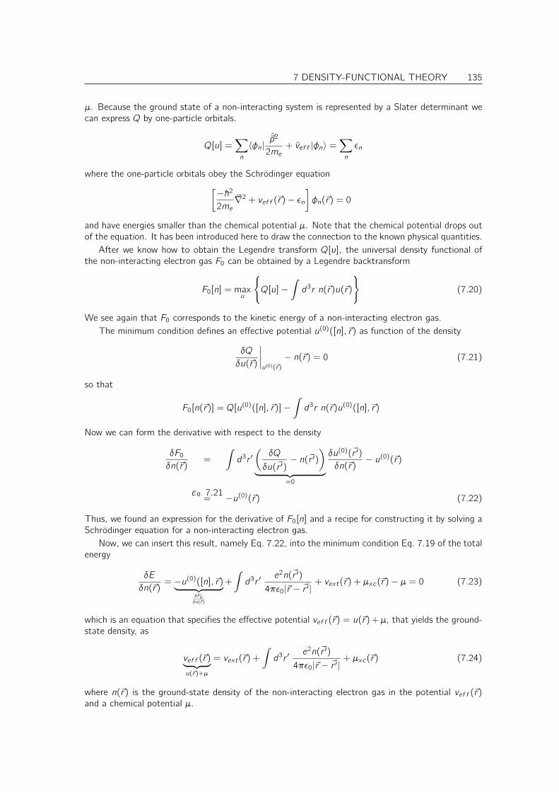
7 DENSITY-FUNCTIONAL THEORY 135
µ. Because the ground state of a non-interacting system is represented by a Slater determinant wecan express Q by one-particle orbitals.
Q[u] =∑
n
〈φn|~p2
2me+ vef f |φn〉 =
∑
n
ǫn
where the one-particle orbitals obey the Schrödinger equation[−~22me
~∇2 + vef f (~r)− ǫn]
φn(~r) = 0
and have energies smaller than the chemical potential µ. Note that the chemical potential drops outof the equation. It has been introduced here to draw the connection to the known physical quantities.
After we know how to obtain the Legendre transform Q[u], the universal density functional ofthe non-interacting electron gas F0 can be obtained by a Legendre backtransform
F0[n] = maxu
Q[u]−∫
d3r n(~r)u(~r)
(7.20)
We see again that F0 corresponds to the kinetic energy of a non-interacting electron gas.The minimum condition defines an effective potential u(0)([n], ~r) as function of the density
δQ
δu(~r)
∣∣∣∣u(0)(~r)
− n(~r) = 0 (7.21)
so that
F0[n(~r)] = Q[u(0)([n], ~r)]−
∫
d3r n(~r)u(0)([n], ~r)
Now we can form the derivative with respect to the density
δF0δn(~r)
=
∫
d3r ′(
δQ
δu(~r ′)− n(~r ′)
)
︸ ︷︷ ︸
=0
δu(0)(~r ′)
δn(~r)− u(0)(~r)
Eq. 7.21= −u(0)(~r) (7.22)
Thus, we found an expression for the derivative of F0[n] and a recipe for constructing it by solving aSchrödinger equation for a non-interacting electron gas.
Now, we can insert this result, namely Eq. 7.22, into the minimum condition Eq. 7.19 of the totalenergy
δE
δn(~r)= −u(0)([n], ~r)︸ ︷︷ ︸
δF0δn(~r)
+
∫
d3r ′e2n(~r ′)
4πǫ0|~r − ~r ′|+ vext(~r) + µxc(~r)− µ = 0 (7.23)
which is an equation that specifies the effective potential vef f (~r) = u(~r)+µ, that yields the ground-state density, as
vef f (~r)︸ ︷︷ ︸
u(~r)+µ
= vext(~r) +
∫
d3r ′e2n(~r ′)
4πǫ0|~r − ~r ′|+ µxc(~r) (7.24)
where n(~r) is the ground-state density of the non-interacting electron gas in the potential vef f (~r)and a chemical potential µ.
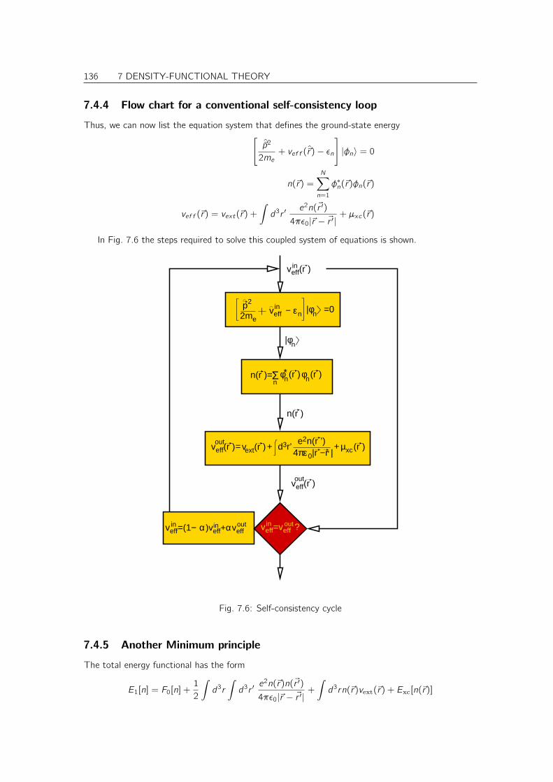
136 7 DENSITY-FUNCTIONAL THEORY
7.4.4 Flow chart for a conventional self-consistency loop
Thus, we can now list the equation system that defines the ground-state energy[
~p2
2me+ vef f (~r)− ǫn
]
|φn〉 = 0
n(~r) =
N∑
n=1
φ∗n(~r)φn(~r)
vef f (~r) = vext(~r) +
∫
d3r ′e2n(~r ′)
4πǫ0|~r − ~r ′|+ µxc(~r)
In Fig. 7.6 the steps required to solve this coupled system of equations is shown.
veff(r )
n(r )
veff(r )
v (r )extveff(r ) d3r’4 0πε ’|r −r |e2n(r ’)
xc(r )µ+= +
|φn
nn(r )=Σ *φn φn(r ) (r )
p2
2meveff εn =0|φn−
veff=veffoutin ?α )veff+αin veff
outveff=(1−in
in
out
out
in
Fig. 7.6: Self-consistency cycle
7.4.5 Another Minimum principle
The total energy functional has the form
E1[n] = F0[n] +1
2
∫
d3r
∫
d3r ′e2n(~r)n(~r ′)
4πǫ0|~r − ~r ′|+
∫
d3rn(~r)vext(~r) + Exc[n(~r)]
7 DENSITY-FUNCTIONAL THEORY 137
Because the ground state of a non-interacting electron gas is a Slater determinant, we can definethe functional F0[n] by minimizing over Slater determinants only. This allows us to describe F0 asminimum over one-particle wave functions.
The functional F0 can therefore be written as
F0[~n] = extr
Λn,m
extr
vef f (~r)
min|φn〉
∑
n
〈φn|~p2
2me|φn〉
+
∫
d3r vef f (~r)
[∑
n
φ∗n(~r)φn(~r)− n(~r)]
−∑
n,m
(〈φn|φm〉 − δn,m) Λm,n
where vef f plays the role of a Lagrange multiplier. This allows us to express the derivative of theuniversal density functional of the non-interacting electrons as
δF0δn(~r)
= vef f (~r)
In practical calculation we (1) chose an arbitrary potential vef f . Then (2) we solve the Schrödingerequation, to obtain the one-particle wave functions, and the kinetic energy of the non-interactingelectrons. Now (3) we evaluate the density. The kinetic energy and the density allows us (4) toevaluate the total energy. The density provides us (5) with a new expression for vef f . Out of thelast and the new effective potential one creates (6) a better choice for the effective potential, whichis used as new start potential for (1). If the effective potentials, the one used for the Schrödingerequation and the one obtained from the density, are identical, we have found the desired ground-stateenergy and density.
Fertig: WS06/07 10 Doppelstunde 10.Dec.06
7.5 Adiabatic connection
We have seen so far that one can reasonably estimate the exchange-correlation hole, and evaluatethe energy of the electron in the potential of the exchange-correlation hole. However, it is nearlyhopeless to estimate the kinetic energy contribution to the exchange-correlation energy.
If there would be no cost to deform the exchange-correlation hole, the latter would simply adjustsuch that the electrostatic energy is optimized. One can easily estimate how the hole would looklike: It would have the shape of a hard sphere centered at the reference electron. Its radius wouldbe determined by the sum rule that says that there is exactly one positive charge in the exchange-correlation hole. The reason for this shape is that the electron would repel its neighbors as much aspossible, in order to reduce its electrostatic interaction.
However as the exchange-correlation hole is deformed, there is a price to pay, namely that thekinetic energy goes up. In the extreme case of a hard-sphere like hole, the wave functions would havesteps, that is infinite curvature. The kinetic energy is just a measure of the curvature of the wavefunction. Thus, the deformation of the hole costs kinetic energy. The final shape of the XC-hole istherefore a balance between electrostatic gain and kinetic energy cost.
The adiabatic connection[48, 49, 50] is a theorem that allows to relate the net energy gain,including the kinetic energy cost, to the electrostatic energy gain only, but for variable strengths of theinteraction energy. While this theorem looks like mystery, it cannot be applied directly. Neverthelessit provides an important route that allows important approximations to be made. The theorem isdemonstrated in the following:
We consider a given electron density for which the non-interacting functional F0[n(~r)] is exactlyknown.
Fλ[n(~r)] = 〈Ψλ|T + λW |Ψλ〉
+
∫
d3r µλ(~r)(
〈Ψλ|n(~r)|Ψλ〉 − n(~r))
− Eλ(
〈Ψλ|Ψλ〉 − 1)
138 7 DENSITY-FUNCTIONAL THEORY
where |Ψλ〉 is the many electron wave function that minimizes Fλ under the constraint that the densityof the wave function is equal to n(~r). The function µλ(~r) represents the Lagrange parameters. Theoperator
n(~r)def=
∫
d4x1 · · ·∫
d4xN |~x1, . . . , ~xN〉(
N∑
i=1
δ(~r − ~ri))
〈~x1, . . . , ~xN |
is the operator that extracts the electron density from the wave function.The wave functions that minimize the functional obey the Schrödinger equation
[
T + λW +
∫
d3r µλ(~r)n(~r)− Eλ]
|Ψλ〉 = 0 (7.25)
This means that as the interaction strength is increased, a local potential, µλ(~r), is switched on thatensures that the electron density remains unchanged.
If we know the derivatives of the functional with respect to the interaction strength λ, and if weknow the functional for the non-interacting electron gas, we can determine the functional for theinteracting electron gas as
F1[n(~r)] = F0[n(~r)] +
∫ 1
0
dλdFλ[n(~r)]
dλ
= 〈Ψ0|T |Ψ0〉+∫ 1
0
dλdFλ[n(~r)]
dλ
The first term is simply the kinetic energy of the non-interacting electron gas with the same densityas the interacting system.
Now we can show that the derivative of the functional with respect to the interaction strengthcan be determined from the interaction energy alone. The proof rests on the Hellmann-Feynmantheorem.
dFλ[n(~r)]
dλ=
d
dλ
[
〈Ψλ|T + λW |Ψλ〉
+
∫
d3r µλ(~r)(
〈Ψλ|n(~r)|Ψλ〉 − n(~r))
− Eλ(
〈Ψλ|Ψλ〉 − 1)]
= 〈dΨλdλ|T + λW |Ψλ〉+ 〈Ψλ|W |Ψλ〉+ 〈Ψλ|T + λW |
dΨλdλ〉
+
∫
d3rdµλ(~r)
dλ(〈Ψλ|n(~r)|Ψλ〉 − n(~r))︸ ︷︷ ︸
=0
+
∫
d3r µλ(~r)
(
〈dΨλdλ|n(~r)|Ψλ〉+ 〈Ψλ|n(~r)|
dΨλdλ〉)
−dEλdλ
(
〈Ψλ|Ψλ〉 − 1)
︸ ︷︷ ︸
=0
−Eλ(
〈dΨλdλ|Ψλ〉+ 〈Ψλ|
dΨλdλ〉)
= 〈Ψλ|W |Ψλ〉
+〈dΨλdλ|[
T + λW +
∫
d3r µλ(~r)n(~r)− Eλ]
|Ψλ〉︸ ︷︷ ︸
=0
+ 〈Ψλ|[
T + λW +
∫
d3r µλ(~r)n(~r)− Eλ]
︸ ︷︷ ︸
=0
|dΨλdλ〉
Eq. 7.25= 〈Ψλ|W |Ψλ〉
7 DENSITY-FUNCTIONAL THEORY 139
Thus, we can express the functional for the finite interaction strength as
F1[n(~r)] = 〈Ψ0|T |Ψ0〉+∫ 1
0
dλ 〈Ψλ|W |Ψλ〉︸ ︷︷ ︸
EH [n(~r)]+Exc [n(~r)]
Thus, we have obtained an explicit expression for the exchange-correlation energy, that does notdirectly refer to the kinetic energy.
Exc [n(~r)] =
∫ 1
0
dλ 〈Ψλ|W |Ψλ〉 −1
2
∫
d3r
∫
d3r ′e2n(~r)n(~r ′)
4πǫ0|~r − ~r ′|︸ ︷︷ ︸
EH
This expression has the problem that we still need the wave functions |Ψλ〉 for all possible values forthe interaction strength.
The interaction energy can further be expressed by the exchange-correlation hole for a given valueof the interaction, namely
〈Ψλ|W |Ψλ〉 =1
2
∫
d3r
∫
d3r ′e2n(~r)n(~r ′)
4πǫ0|~r − ~r ′|+
∫
d3r n(~r)1
2
∫
d3r ′e2hλ(~r , ~r ′)
4πǫ0|~r − ~r ′|
so that
Exc =
∫
d3r n(~r)
∫ 1
0
dλ1
2
∫
d3r ′e2hλ(~r , ~r ′)
4πǫ0|~r − ~r ′|︸ ︷︷ ︸
=:ǫxc
(7.26)
The variable ǫxc , which itself is a functional of the density is the exchange-correlation energy perelectron.
7.5.1 Screened interaction
It is possible9 to reformulate the exchange-correlation energy by the exchange-only energy with ascreened interaction. This is a form that reminds of the so-called GW approximation, where theself-energy is expressed by Green’s-function times screened interaction.
ExcEq. 7.26=
1
2
∫
d3r
∫
d3r ′ n(r)h0(r, r′)
∫
dλhλ(~r , ~r ′)
h0(~r , ~r ′)
e2
4πǫ0|~r − ~r ′|︸ ︷︷ ︸
vscr (~r−~r ′)
=1
2
∑
i ,j
∫
d3r
∫
d3r ′ φ∗i (~r)φj(~r)vscr (~r − ~r ′)φ∗j (~r ′)φi(~r ′)
where the screened interaction is defined as
vscr (~r − ~r ′) def=
∫
dλhλ(~r , ~r ′)
h0(~r , ~r ′)
e2
4πǫ0|~r − ~r ′|
Note that, in contrast to the GW approximation, our expression is exact, but, on the other hand, itis limited to the ground state.
Note also that the screened interaction in this formulation only enters the exchange term, butnot the Hartree term. It also includes the kinetic energy correction.
The qualitative behavior can be understood easily:
9This is an idea from the author, that has not been crosschecked properly. Therefore some caution is required.
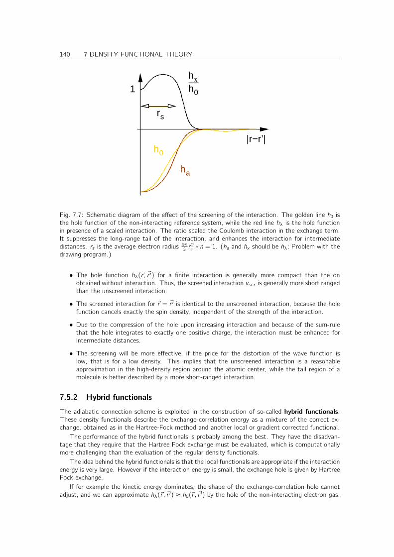
140 7 DENSITY-FUNCTIONAL THEORY
h0
ha
h0
rs
1
|r−r’|
hx
Fig. 7.7: Schematic diagram of the effect of the screening of the interaction. The golden line h0 isthe hole function of the non-interacting reference system, while the red line hλ is the hole functionin presence of a scaled interaction. The ratio scaled the Coulomb interaction in the exchange term.It suppresses the long-range tail of the interaction, and enhances the interaction for intermediatedistances. rs is the average electron radius 4π3 r
2s ∗ n = 1. (ha and hx should be hλ; Problem with the
drawing program.)
• The hole function hλ(~r , ~r ′) for a finite interaction is generally more compact than the onobtained without interaction. Thus, the screened interaction vscr is generally more short rangedthan the unscreened interaction.
• The screened interaction for ~r = ~r ′ is identical to the unscreened interaction, because the holefunction cancels exactly the spin density, independent of the strength of the interaction.
• Due to the compression of the hole upon increasing interaction and because of the sum-rulethat the hole integrates to exactly one positive charge, the interaction must be enhanced forintermediate distances.
• The screening will be more effective, if the price for the distortion of the wave function islow, that is for a low density. This implies that the unscreened interaction is a reasonableapproximation in the high-density region around the atomic center, while the tail region of amolecule is better described by a more short-ranged interaction.
7.5.2 Hybrid functionals
The adiabatic connection scheme is exploited in the construction of so-called hybrid functionals.These density functionals describe the exchange-correlation energy as a mixture of the correct ex-change, obtained as in the Hartree-Fock method and another local or gradient corrected functional.
The performance of the hybrid functionals is probably among the best. They have the disadvan-tage that they require that the Hartree Fock exchange must be evaluated, which is computationallymore challenging than the evaluation of the regular density functionals.
The idea behind the hybrid functionals is that the local functionals are appropriate if the interactionenergy is very large. However if the interaction energy is small, the exchange hole is given by HartreeFock exchange.
If for example the kinetic energy dominates, the shape of the exchange-correlation hole cannotadjust, and we can approximate hλ(~r , ~r ′) ≈ h0(~r , ~r ′) by the hole of the non-interacting electron gas.
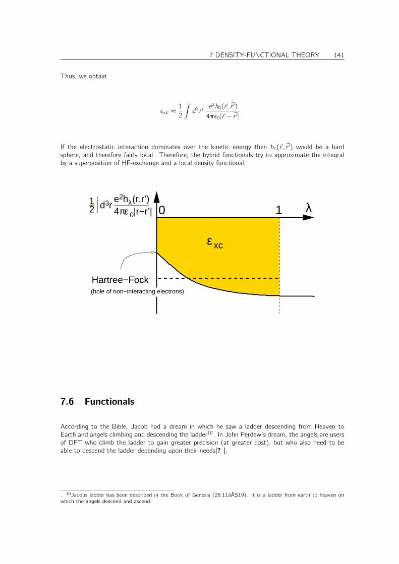
7 DENSITY-FUNCTIONAL THEORY 141
Thus, we obtain
ǫxc ≈1
2
∫
d3r ′e2h0(~r , ~r ′)
4πǫ0|~r − ~r ′|
If the electrostatic interaction dominates over the kinetic energy then h1(~r , ~r ′) would be a hardsphere, and therefore fairly local. Therefore, the hybrid functionals try to approximate the integralby a superposition of HF-exchange and a local density functional.
d3r4 0|r−r’|πεe2h (r,r’)λ
21
Hartree−Fock(hole of non−interacting electrons)
xcε
0 1 λ
7.6 Functionals
According to the Bible, Jacob had a dream in which he saw a ladder descending from Heaven toEarth and angels climbing and descending the ladder10. In John Perdew’s dream, the angels are usersof DFT who climb the ladder to gain greater precision (at greater cost), but who also need to beable to descend the ladder depending upon their needs[? ].
10Jacobs ladder has been described in the Book of Genesis (28:11âĂŞ19). It is a ladder from earth to heaven onwhich the angels descend and ascend.
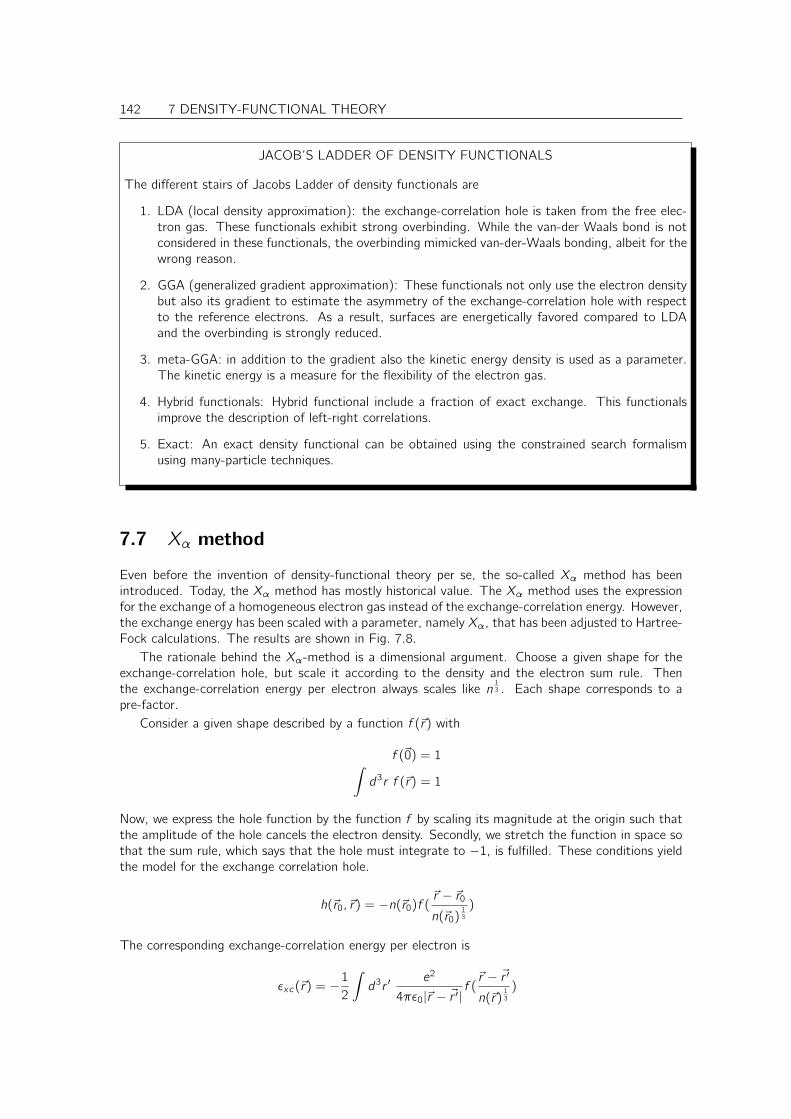
142 7 DENSITY-FUNCTIONAL THEORY
JACOB’S LADDER OF DENSITY FUNCTIONALS
The different stairs of Jacobs Ladder of density functionals are
1. LDA (local density approximation): the exchange-correlation hole is taken from the free elec-tron gas. These functionals exhibit strong overbinding. While the van-der Waals bond is notconsidered in these functionals, the overbinding mimicked van-der-Waals bonding, albeit for thewrong reason.
2. GGA (generalized gradient approximation): These functionals not only use the electron densitybut also its gradient to estimate the asymmetry of the exchange-correlation hole with respectto the reference electrons. As a result, surfaces are energetically favored compared to LDAand the overbinding is strongly reduced.
3. meta-GGA: in addition to the gradient also the kinetic energy density is used as a parameter.The kinetic energy is a measure for the flexibility of the electron gas.
4. Hybrid functionals: Hybrid functional include a fraction of exact exchange. This functionalsimprove the description of left-right correlations.
5. Exact: An exact density functional can be obtained using the constrained search formalismusing many-particle techniques.
7.7 Xα method
Even before the invention of density-functional theory per se, the so-called Xα method has beenintroduced. Today, the Xα method has mostly historical value. The Xα method uses the expressionfor the exchange of a homogeneous electron gas instead of the exchange-correlation energy. However,the exchange energy has been scaled with a parameter, namely Xα, that has been adjusted to Hartree-Fock calculations. The results are shown in Fig. 7.8.
The rationale behind the Xα-method is a dimensional argument. Choose a given shape for theexchange-correlation hole, but scale it according to the density and the electron sum rule. Thenthe exchange-correlation energy per electron always scales like n
13 . Each shape corresponds to a
pre-factor.Consider a given shape described by a function f (~r) with
f (~0) = 1∫
d3r f (~r) = 1
Now, we express the hole function by the function f by scaling its magnitude at the origin such thatthe amplitude of the hole cancels the electron density. Secondly, we stretch the function in space sothat the sum rule, which says that the hole must integrate to −1, is fulfilled. These conditions yieldthe model for the exchange correlation hole.
h(~r0, ~r) = −n(~r0)f (~r − ~r0n(~r0)
13
)
The corresponding exchange-correlation energy per electron is
ǫxc(~r) = −1
2
∫
d3r ′e2
4πǫ0|~r − ~r ′|f (~r − ~r ′n(~r)
13
)
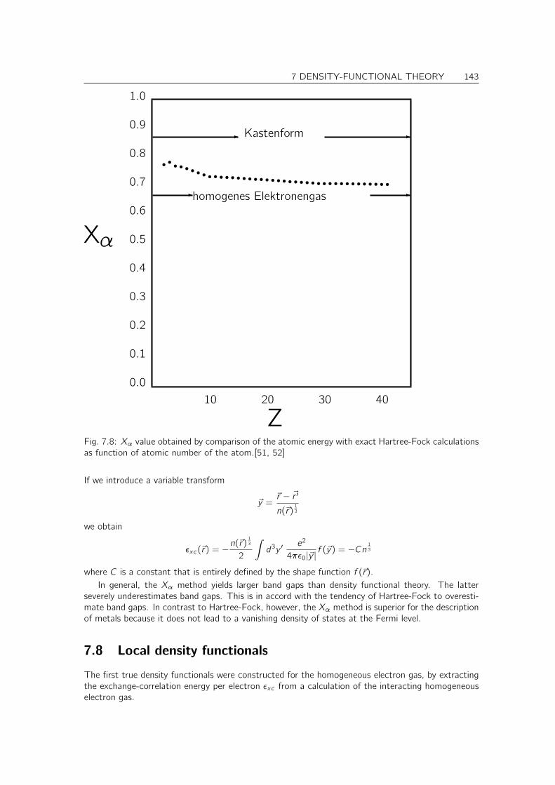
7 DENSITY-FUNCTIONAL THEORY 143
10 20 30 40
Z
0.0
0.1
0.2
0.3
0.4
0.5
0.6
0.7
0.8
0.9
1.0
Xα
Kastenform
homogenes Elektronengas
rr
r rrrrrr r r r r r r r r r r r r r r r r r r r r r r r r r r r r r r r
Fig. 7.8: Xα value obtained by comparison of the atomic energy with exact Hartree-Fock calculationsas function of atomic number of the atom.[51, 52]
If we introduce a variable transform
~y =~r − ~r ′n(~r)
13
we obtain
ǫxc(~r) = −n(~r)
13
2
∫
d3y ′e2
4πǫ0|~y |f (~y) = −Cn 13
where C is a constant that is entirely defined by the shape function f (~r).In general, the Xα method yields larger band gaps than density functional theory. The latter
severely underestimates band gaps. This is in accord with the tendency of Hartree-Fock to overesti-mate band gaps. In contrast to Hartree-Fock, however, the Xα method is superior for the descriptionof metals because it does not lead to a vanishing density of states at the Fermi level.
7.8 Local density functionals
The first true density functionals were constructed for the homogeneous electron gas, by extractingthe exchange-correlation energy per electron ǫxc from a calculation of the interacting homogeneouselectron gas.
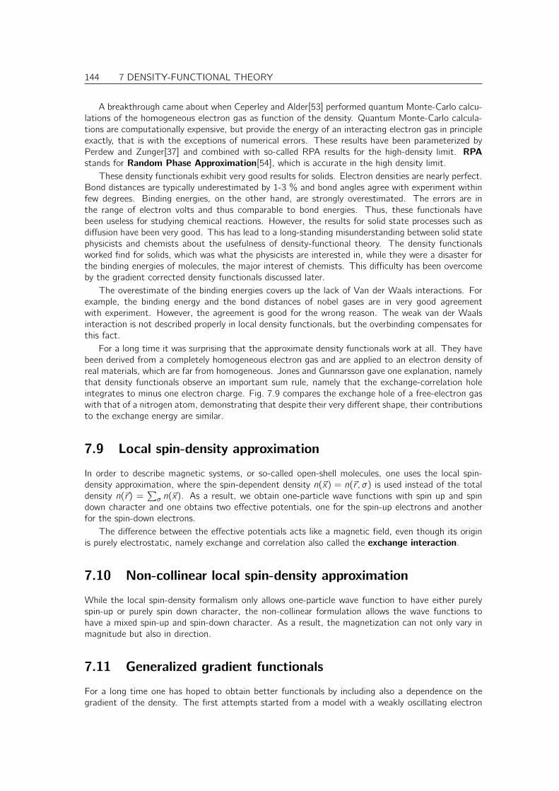
144 7 DENSITY-FUNCTIONAL THEORY
A breakthrough came about when Ceperley and Alder[53] performed quantum Monte-Carlo calcu-lations of the homogeneous electron gas as function of the density. Quantum Monte-Carlo calcula-tions are computationally expensive, but provide the energy of an interacting electron gas in principleexactly, that is with the exceptions of numerical errors. These results have been parameterized byPerdew and Zunger[37] and combined with so-called RPA results for the high-density limit. RPAstands for Random Phase Approximation[54], which is accurate in the high density limit.
These density functionals exhibit very good results for solids. Electron densities are nearly perfect.Bond distances are typically underestimated by 1-3 % and bond angles agree with experiment withinfew degrees. Binding energies, on the other hand, are strongly overestimated. The errors are inthe range of electron volts and thus comparable to bond energies. Thus, these functionals havebeen useless for studying chemical reactions. However, the results for solid state processes such asdiffusion have been very good. This has lead to a long-standing misunderstanding between solid statephysicists and chemists about the usefulness of density-functional theory. The density functionalsworked find for solids, which was what the physicists are interested in, while they were a disaster forthe binding energies of molecules, the major interest of chemists. This difficulty has been overcomeby the gradient corrected density functionals discussed later.
The overestimate of the binding energies covers up the lack of Van der Waals interactions. Forexample, the binding energy and the bond distances of nobel gases are in very good agreementwith experiment. However, the agreement is good for the wrong reason. The weak van der Waalsinteraction is not described properly in local density functionals, but the overbinding compensates forthis fact.
For a long time it was surprising that the approximate density functionals work at all. They havebeen derived from a completely homogeneous electron gas and are applied to an electron density ofreal materials, which are far from homogeneous. Jones and Gunnarsson gave one explanation, namelythat density functionals observe an important sum rule, namely that the exchange-correlation holeintegrates to minus one electron charge. Fig. 7.9 compares the exchange hole of a free-electron gaswith that of a nitrogen atom, demonstrating that despite their very different shape, their contributionsto the exchange energy are similar.
7.9 Local spin-density approximation
In order to describe magnetic systems, or so-called open-shell molecules, one uses the local spin-density approximation, where the spin-dependent density n(~x) = n(~r , σ) is used instead of the totaldensity n(~r) =
∑
σ n(~x). As a result, we obtain one-particle wave functions with spin up and spindown character and one obtains two effective potentials, one for the spin-up electrons and anotherfor the spin-down electrons.
The difference between the effective potentials acts like a magnetic field, even though its originis purely electrostatic, namely exchange and correlation also called the exchange interaction.
7.10 Non-collinear local spin-density approximation
While the local spin-density formalism only allows one-particle wave function to have either purelyspin-up or purely spin down character, the non-collinear formulation allows the wave functions tohave a mixed spin-up and spin-down character. As a result, the magnetization can not only vary inmagnitude but also in direction.
7.11 Generalized gradient functionals
For a long time one has hoped to obtain better functionals by including also a dependence on thegradient of the density. The first attempts started from a model with a weakly oscillating electron
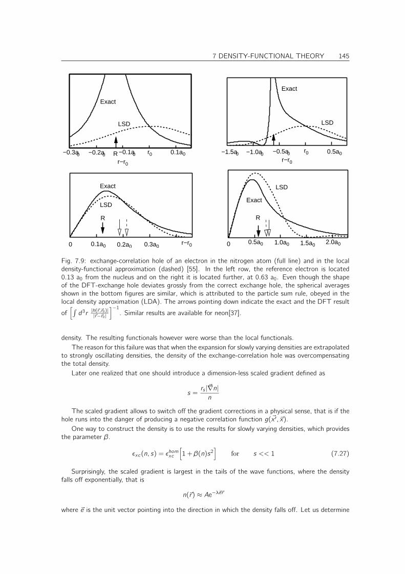
7 DENSITY-FUNCTIONAL THEORY 145
0 0
r−r0
0−0.3a 0−0.2a 00.1a0−0.1a r0
r−r000.3a00.2a00.1a
r−r0
−1.5a0 −1.0a0 −0.5a0 r0 00.5a
00.5a 01.0a 01.5a 02.0a
Exact
LSD
R
R
Exact
LSD
LSD
ExactLSD
Exact
R
Fig. 7.9: exchange-correlation hole of an electron in the nitrogen atom (full line) and in the localdensity-functional approximation (dashed) [55]. In the left row, the reference electron is located0.13 a0 from the nucleus and on the right it is located further, at 0.63 a0. Even though the shapeof the DFT-exchange hole deviates grossly from the correct exchange hole, the spherical averagesshown in the bottom figures are similar, which is attributed to the particle sum rule, obeyed in thelocal density approximation (LDA). The arrows pointing down indicate the exact and the DFT result
of[∫d3r |h(~r ,~r0)||~r−~r0|
]−1. Similar results are available for neon[37].
density. The resulting functionals however were worse than the local functionals.The reason for this failure was that when the expansion for slowly varying densities are extrapolated
to strongly oscillating densities, the density of the exchange-correlation hole was overcompensatingthe total density.
Later one realized that one should introduce a dimension-less scaled gradient defined as
s =rs |~∇n|n
The scaled gradient allows to switch off the gradient corrections in a physical sense, that is if thehole runs into the danger of producing a negative correlation function g(~x ′, ~x).
One way to construct the density is to use the results for slowly varying densities, which providesthe parameter β.
ǫxc(n, s) = ǫhomxc
[
1 + β(n)s2]
for s << 1 (7.27)
Surprisingly, the scaled gradient is largest in the tails of the wave functions, where the densityfalls off exponentially, that is
n(~r) ≈ Ae−λ~e~r
where ~e is the unit vector pointing into the direction in which the density falls off. Let us determine
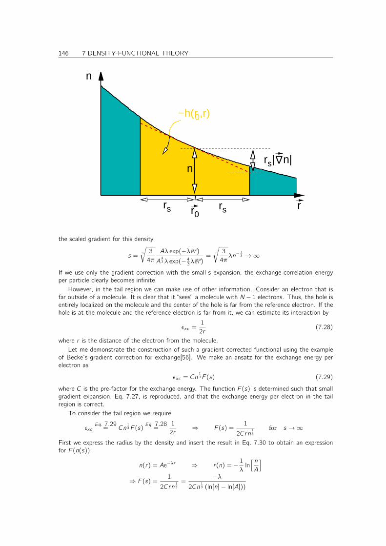
146 7 DENSITY-FUNCTIONAL THEORY
rs| n|
∆
rsrs r0
n
−h(r0,r)
r
n
the scaled gradient for this density
s =3
√
3
4π
Aλ exp(−λ~e~r)A43λ exp(− 43λ~e~r)
=3
√
3
4πλn−
13 →∞
If we use only the gradient correction with the small-s expansion, the exchange-correlation energyper particle clearly becomes infinite.
However, in the tail region we can make use of other information. Consider an electron that isfar outside of a molecule. It is clear that it “sees” a molecule with N − 1 electrons. Thus, the hole isentirely localized on the molecule and the center of the hole is far from the reference electron. If thehole is at the molecule and the reference electron is far from it, we can estimate its interaction by
ǫxc =1
2r(7.28)
where r is the distance of the electron from the molecule.Let me demonstrate the construction of such a gradient corrected functional using the example
of Becke’s gradient correction for exchange[56]. We make an ansatz for the exchange energy perelectron as
ǫxc = Cn13F (s) (7.29)
where C is the pre-factor for the exchange energy. The function F (s) is determined such that smallgradient expansion, Eq. 7.27, is reproduced, and that the exchange energy per electron in the tailregion is correct.
To consider the tail region we require
ǫxcEq. 7.29= Cn
13F (s)
Eq. 7.28=
1
2r⇒ F (s) =
1
2Crn13
for s →∞
First we express the radius by the density and insert the result in Eq. 7.30 to obtain an expressionfor F (n(s)).
n(r) = Ae−λr ⇒ r(n) = − 1λln[ n
A
]
⇒ F (s) =1
2Crn13
=−λ
2Cn13 (ln[n]− ln[A]))
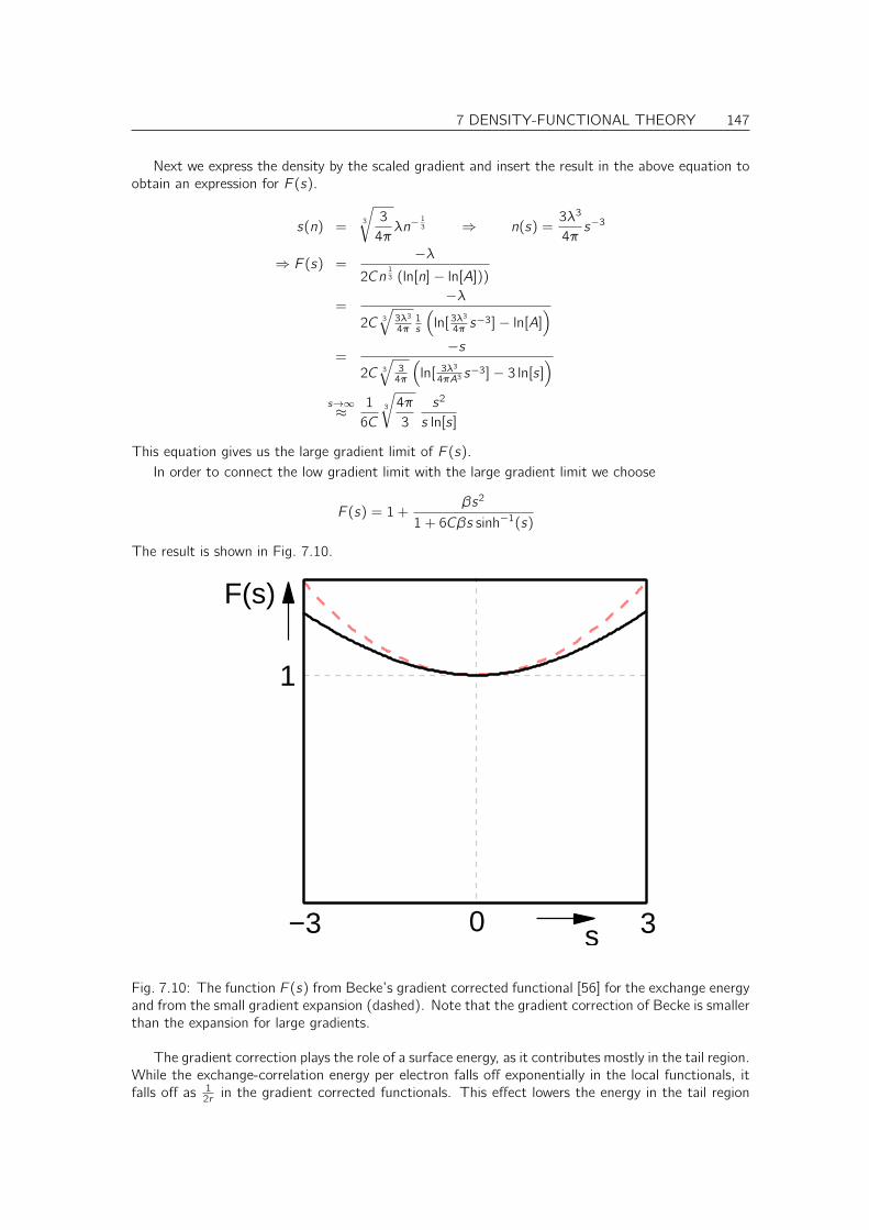
7 DENSITY-FUNCTIONAL THEORY 147
Next we express the density by the scaled gradient and insert the result in the above equation toobtain an expression for F (s).
s(n) =3
√
3
4πλn−
13 ⇒ n(s) =
3λ3
4πs−3
⇒ F (s) =−λ
2Cn13 (ln[n]− ln[A]))
=−λ
2C 3
√3λ3
4π1s
(
ln[ 3λ3
4π s−3]− ln[A]
)
=−s
2C 3
√34π
(
ln[ 3λ3
4πA3 s−3]− 3 ln[s]
)
s→∞≈ 1
6C3
√
4π
3
s2
s ln[s]
This equation gives us the large gradient limit of F (s).In order to connect the low gradient limit with the large gradient limit we choose
F (s) = 1 +βs2
1 + 6Cβs sinh−1(s)
The result is shown in Fig. 7.10.
s
F(s)
0
1
−3 3
Fig. 7.10: The function F (s) from Becke’s gradient corrected functional [56] for the exchange energyand from the small gradient expansion (dashed). Note that the gradient correction of Becke is smallerthan the expansion for large gradients.
The gradient correction plays the role of a surface energy, as it contributes mostly in the tail region.While the exchange-correlation energy per electron falls off exponentially in the local functionals, itfalls off as 1
2r in the gradient corrected functionals. This effect lowers the energy in the tail region
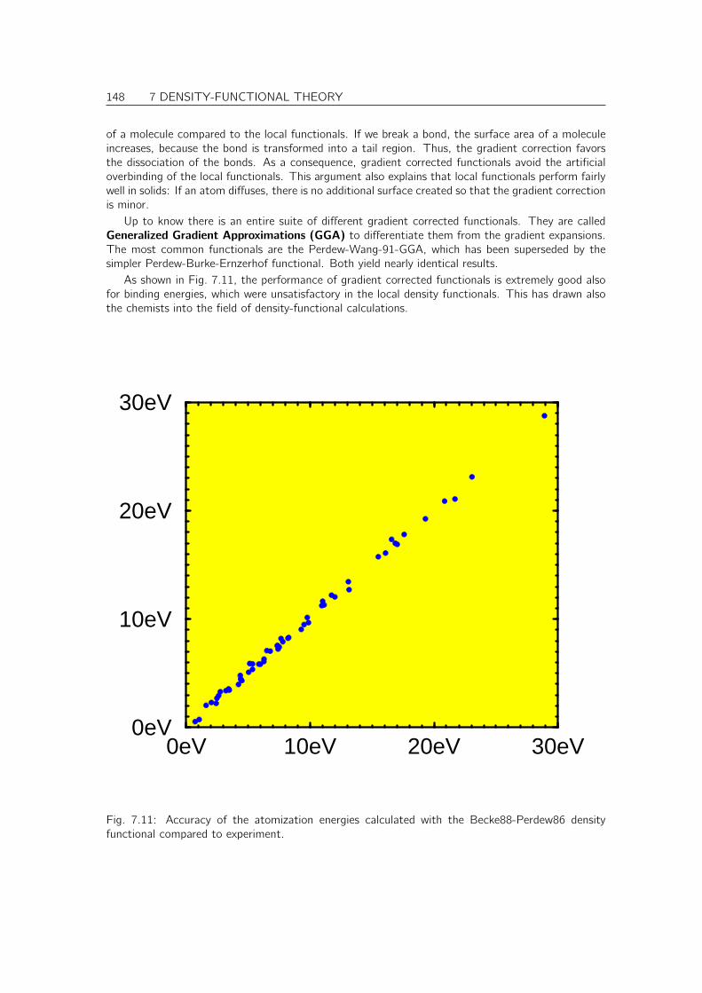
148 7 DENSITY-FUNCTIONAL THEORY
of a molecule compared to the local functionals. If we break a bond, the surface area of a moleculeincreases, because the bond is transformed into a tail region. Thus, the gradient correction favorsthe dissociation of the bonds. As a consequence, gradient corrected functionals avoid the artificialoverbinding of the local functionals. This argument also explains that local functionals perform fairlywell in solids: If an atom diffuses, there is no additional surface created so that the gradient correctionis minor.
Up to know there is an entire suite of different gradient corrected functionals. They are calledGeneralized Gradient Approximations (GGA) to differentiate them from the gradient expansions.The most common functionals are the Perdew-Wang-91-GGA, which has been superseded by thesimpler Perdew-Burke-Ernzerhof functional. Both yield nearly identical results.
As shown in Fig. 7.11, the performance of gradient corrected functionals is extremely good alsofor binding energies, which were unsatisfactory in the local density functionals. This has drawn alsothe chemists into the field of density-functional calculations.
0eV 10eV 20eV 30eV0eV
10eV
20eV
30eV
Fig. 7.11: Accuracy of the atomization energies calculated with the Becke88-Perdew86 densityfunctional compared to experiment.
7 DENSITY-FUNCTIONAL THEORY 149
7.12 Additional material
7.12.1 Relevance of the highest occupied Kohn-Sham orbital
According to Perdew[57? ], the energy of the highest occupied Kohn Sham orbital is the ionizationpotential of the material.
This statement has been disputed by Kleinman[? ].
7.12.2 Correlation inequality and lower bound of the exact density functional
7.13 Functionals
• [X-α] Uses a local expression for exchange as derived from the free electron gas, and scaledwith a factor α.
• [Barth-Hedin]
• [PZ (Perdew-Zunger)] parameterization of Ceperley and Alder’s quantum Monte Carlo dataof the free electron gas.
• [BP86 (Becke-Perdew)]
• [PW91 (Perdew-Wang)] First completely parameter free version of a gradient corrected den-sity functional
• [PBE (Perdew-Burke-Ernzerhof)]
• [B3LYP (Becke-Lee-Yang-Parr)] Hybrid functional.
• [GGA] (Generalized gradient approximation) General expression for gradient corrected func-tionals.
• [Hybrid functionals] General expression functionals employing a mixture of Hartree-Fock anda density functional
Fertig: WS06/07 11 Doppelstunde 13.Dec.06
7.14 Reliability of DFT
If we knew the exact density functional, we would be able to determine exactly
• the total energy
• the electron density and
• the energy of the highest occupied orbital
The argument that DFT predicts the highest occupied orbital, while the orbital energies of allother one-particle orbitals are, in principle, without physical meaning goes as follows: Far from thesurface of a crystal the density of a one-particle orbital falls off as e−λz where λ is related to theorbital energy by λ = 1
~
√−2meǫ, where the orbital energy is measured relative to the vacuum level,that is limz→∞ vef f (~r). For large distances the highest occupied orbital, which has the slowest decay,will dominate the electron density. Thus, if we would know the electron density very accurately farfrom a surface, we would be able to determine the dominant exponential decay constant and thus
150 7 DENSITY-FUNCTIONAL THEORY
the energy of the highest occupied orbital.11 Thus, the energy of the highest occupied orbital canbe determined from the density, which is an exact prediction of DFT.
Of course, even though exact DFT predicts these quantities accurately, it remains to be seen ineach case if that also holds for the approximate functionals used in practice.
• Bond energies: Local functionals overestimate binding by often more than 1 eV. Energies arefairly good as long as the effective surface area of the system is not changed. This poor resultis dramatically improved by the GGA’s.
• Structures: bond lengths are underestimated in LDA by 0-2 %. They are overestimated byGGA’s by 0-2 %.
• Dipole moments standard deviation 0.1 Debye[58]
7.15 Deficiencies of DFT
• Missing Van der Waals interaction: The van-der-Waals interaction is not included. Surpris-ingly the description of van der Waals bonds is nearly perfect with truly local density functionals.This however is an artifact of the tendency to overbinding in truly local density functionals onthe one hand, and the lack of van der Waals interactions on the other. Since the overbindingof covalent bonds introduces errors in the range of 1 eV, it is generally not a good idea to usetruly local density functionals instead of their gradient corrected counterparts.
A density functional for the van der Waals interaction has been developed by Dion et al.[59].It is named vdWDF (van-der-Waals density functional).
• Band-gap Problem: If we compare the spectrum of Kohn Sham states with optical absorptionspectra we observe that the band gaps are too small. This is not a deficiency of density-functional theory, but an over-interpretation of the Kohn Sham spectrum. The excited statesshould not be calculated from the same potential as the ground state.
• Reduced band width: Band width of alkaline metals.
• Mott insulators
• unstable negative ions
• Broken symmetry spin states: singlet O2 Molecule
• Transition states:
• High-energy spectrum: The high energy part if the Kohn-Sham spectrum is too low comparedto the measured optical spectrum. The reason is that the exchange-correlation hole cannotfollow the very fast electrons.????
11There is a caveat in the argument. Consider an insulator which may have surface states in the band gap. In thatcase the density would probe the highest occupied surface state, which may lie above the highest occupied bulk state.
Part II
Advanced solid state physics
151

Chapter 8
Second quantization
“Many workers, particularly those trained in field theory, advocate the language of second quantization.The author does not favor this method, and it will not be used in this article. He wishes to point outthat nothing is accomplished by the use of the second quantization formalism except to express in amore compact language results which we meet in an equivalent way in the determinantal method/Furthermore, he feels that the language of second quantization is likely to hide essential features suchas the fundamentally nonlinear nature of the total energy, when expressed in terms of the occupationnumbers, which are of primary importance, and which can be easily overlooked by one whose onlytraining is in the field theory.”
John C. Slater in “Statistical Exchange-correlation Correction in the self-consistent field”.
8.1 Fock space
There are several ways towards second quantization. The most simple one ist to define the Fockspace. The Fock space is the combination of the Hilbert spaces for 0-particle states, 1-particlestates, 2-particle states, etc. If HN is the Hilbert space of N-particle states the Fock space F is theunification of the Hilbert spaces for all integer N
F = H0 ∪H1 ∪H2 ∪ . . . =∞⋃
N=0
HN
What is missing is a definition of the scalar product between states with different particle numbers.We postulate that the scalar product of states with different particle numbers vanishes.1
As a curiosity, we introduced here also the 0-particle state, called vacuum state, that is notrepresented by a wave function at all.
8.2 Number representation
We are entering a new level of abstraction and it turned out to be useful to introduce a specialnotation for it. This will lead us to the number representation and to creation and annihilationoperators.
In order to work within the Fock space we need to select a suitable basis set. We have alreadylearned that Slater determinants resulting a complete orthonormal one-particle basis, form a completeset of many particle wave functions.
1This postulate is non-trivial and can be derived more naturally from the second quantization via introducing wavefunctions in the space of the fields describing the wave functions.
153
154 8 SECOND QUANTIZATION
Each slater determinant is uniquely defined, up to a sign, by the one-particle states used inits construction. Therefore, the Slater determinants can be written economically in the numberrepresentation. For a given, ordered, one-particle basisset, we form a vector, where each positioncorresponds to a particular one-particle orbital. Each entry can be zero or one, and describes if thatparticular orbital is present in the Slater determinant or not. If the number is one, we say that theorbital is occupied, and if it is not, we say that it is unoccupied. Thus, a Slater determinant can beexpressed in a form like
|0, 0, 0, 1︸︷︷︸
i1
, 0, 1︸︷︷︸
i2
, 0, . . .〉 = |Si1,i2,...〉 with i1 < i2 < . . .
where Si1,i2,... is a Slater determinant made of the one-particle orbitals |φi1〉, |φi2〉, . . ..Because the Slater determinant changes its sign under permutation of two one-particle wave
functions, we need to define the sign convention. The sign is fixed such that the one-particle orbitalsmust occur in the corresponding Slater determinant in the order of increasing index, that is i1 < i2, . . ..Thus
|1, 1, 0, 0, . . .〉 = |S1,2〉 = −|S2,1〉
〈~r , ~r ′|1, 1, 0, 0, . . .〉 = 1√2!
[φ1(~r)φ2(~r ′)− φ2(~r)φ1(~r ′)
]
Note also that there is an explicit vacuum state
|O〉 = |0, 0, 0, 0, 0, 0, 0, 0, 0, 0, . . .〉
The vacuum state describes a system without particles. Note that the vacuum state, which wedenote by a calligraphic “O”, |O〉, is different from the zero state |0〉. The latter is obtained bymultiplying an arbitrary state with zero.
The most general antisymmetric wave function has the form
|Φ〉 =1∑
n1,n2,...=0
|n1, n2, . . .〉cn1,n2,...
Let us consider as one example a hydrogen molecule with only one s-orbital per site. The s-orbitalsare orthogonalized so that we obtain a bonding and an antibonding orbital. Now we can form thelimited Fock space for this model. The ordered one-particle basis is |b, ↑〉, |b, ↓〉, |a, ↑〉, |a, ↓〉, where|b, σ〉 describes the bonding and |a, σ〉 describes the antibonding orbital. There are 24 = 16 Slaterdeterminants as shown in Fig. 8.1.
• |0000〉 is the zero-particle state. It describes just the two protons without electrons.
• |1000〉, |0100〉, |0010〉 and |0001〉 are the one-particle states. Thus, they describe the H+2 ion.The states |1000〉 and |0100〉 correspond to the bound H+2 ion, while the remaining two statescorrespond to the electron in the antibonding state. The molecule in the latter configurationwould be unstable.
• |1100〉 corresponds to the ground state of the H2 molecule with two paired electrons in thebonding orbital. There are in total 6 two-electron slater determinants of which 5 are excitedstates.
• There are four three-electron states, namely |1110〉 |1101〉, |1011〉,|01111〉. The three particlestates describe the negative H−2 ion.
• finally there is one four-electron state, |1111〉 which describes the H2−2 ion.
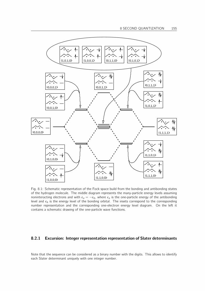
8 SECOND QUANTIZATION 155
0,0,0,0
1,0,0,0
0,1,0,0
0,0,1,0
0,0,0,1
1,1,0,01,1,1,0
1,1,0,1
1,0,1,1
0,1,1,1
1,1,1,1
0,0,1,1
1,0,1,0 1,0,0,1 0,1,1,0 0,1,0,1
Fig. 8.1: Schematic representation of the Fock space build from the bonding and antibonding statesof the hydrogen molecule. The middle diagram represents the many-particle energy levels assumingnoninteracting electrons and with ǫa = −ǫb, where ǫa is the one-particle energy of the antibondinglevel and ǫb is the energy level of the bonding orbital. The insets correspond to the correspondingnumber representation and the corresponding one-electron energy level diagram. On the left itcontains a schematic drawing of the one-particle wave functions.
8.2.1 Excursion: Integer representation representation of Slater determinants
Note that the sequence can be considered as a binary number with the digits. This allows to identifyeach Slater determinant uniquely with one integer number.
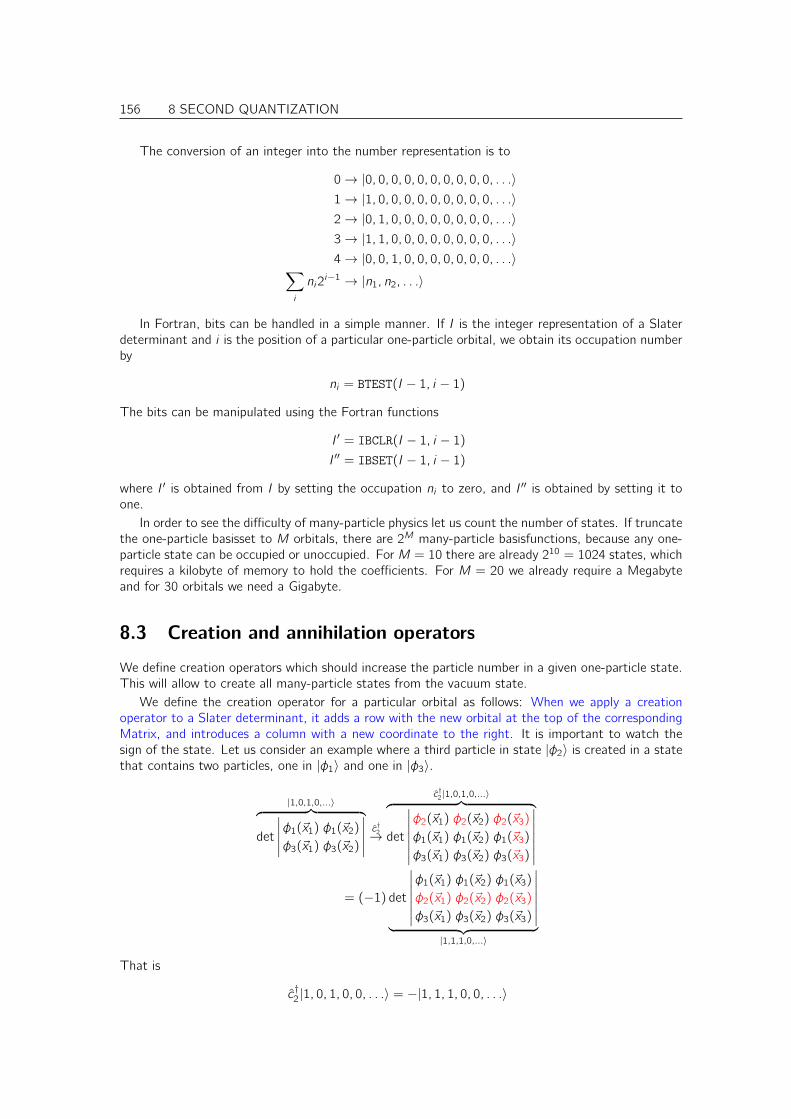
156 8 SECOND QUANTIZATION
The conversion of an integer into the number representation is to
0→ |0, 0, 0, 0, 0, 0, 0, 0, 0, 0, . . .〉1→ |1, 0, 0, 0, 0, 0, 0, 0, 0, 0, . . .〉2→ |0, 1, 0, 0, 0, 0, 0, 0, 0, 0, . . .〉3→ |1, 1, 0, 0, 0, 0, 0, 0, 0, 0, . . .〉4→ |0, 0, 1, 0, 0, 0, 0, 0, 0, 0, . . .〉
∑
i
ni2i−1 → |n1, n2, . . .〉
In Fortran, bits can be handled in a simple manner. If I is the integer representation of a Slaterdeterminant and i is the position of a particular one-particle orbital, we obtain its occupation numberby
ni = BTEST(I − 1, i − 1)
The bits can be manipulated using the Fortran functions
I ′ = IBCLR(I − 1, i − 1)I ′′ = IBSET(I − 1, i − 1)
where I ′ is obtained from I by setting the occupation ni to zero, and I ′′ is obtained by setting it toone.
In order to see the difficulty of many-particle physics let us count the number of states. If truncatethe one-particle basisset to M orbitals, there are 2M many-particle basisfunctions, because any one-particle state can be occupied or unoccupied. For M = 10 there are already 210 = 1024 states, whichrequires a kilobyte of memory to hold the coefficients. For M = 20 we already require a Megabyteand for 30 orbitals we need a Gigabyte.
8.3 Creation and annihilation operators
We define creation operators which should increase the particle number in a given one-particle state.This will allow to create all many-particle states from the vacuum state.
We define the creation operator for a particular orbital as follows: When we apply a creationoperator to a Slater determinant, it adds a row with the new orbital at the top of the correspondingMatrix, and introduces a column with a new coordinate to the right. It is important to watch thesign of the state. Let us consider an example where a third particle in state |φ2〉 is created in a statethat contains two particles, one in |φ1〉 and one in |φ3〉.
|1,0,1,0,...〉︷ ︸︸ ︷
det
∣∣∣∣∣
φ1(~x1) φ1(~x2)
φ3(~x1) φ3(~x2)
∣∣∣∣∣
c†2→
c†2 |1,0,1,0,...〉︷ ︸︸ ︷
det
∣∣∣∣∣∣∣
φ2(~x1) φ2(~x2) φ2(~x3)
φ1(~x1) φ1(~x2) φ1(~x3)
φ3(~x1) φ3(~x2) φ3(~x3)
∣∣∣∣∣∣∣
= (−1) det
∣∣∣∣∣∣∣
φ1(~x1) φ1(~x2) φ1(~x3)
φ2(~x1) φ2(~x2) φ2(~x3)
φ3(~x1) φ3(~x2) φ3(~x3)
∣∣∣∣∣∣∣
︸ ︷︷ ︸
|1,1,1,0,...〉
That is
c†2|1, 0, 1, 0, 0, . . .〉 = −|1, 1, 1, 0, 0, . . .〉
8 SECOND QUANTIZATION 157
We define the creation and annihilation operators by
c†i |n1, n2, . . . , 0︸︷︷︸ni
, . . .〉 = |n1, n2, . . . , 1︸︷︷︸ni
, . . .〉[
(−1)∑
j<i nj]
c†i |n1, n2, . . . , 1︸︷︷︸ni
. . .〉 = 0
ci |n1, n2, . . . , 1︸︷︷︸ni
, . . .〉 = |n1, n2, . . . , 0︸︷︷︸i
. . .〉 (−1)∑
j<i nj
ci |n1, n2, . . . , 0︸︷︷︸ni
. . .〉 = 0
In short, we may write
FERMIONIC CREATION AND ANNIHILATION OPERATORS
c†i |n1, n2, . . . , ni , . . .〉 = |n1, n2, . . . , ni + 1, . . .〉[
(−1)∑
j<i nj]
(1− ni)
ci |n1, n2, . . . , ni , . . .〉 = |n1, n2, . . . , ni − 1 . . .〉[
(−1)∑
j<i nj]
ni (8.1)
Note that the state with ni +1 does not exist for ni = 1. This does not matter because the stateis multiplied with zero. A conceptionally elegant solution to this problem is to define a state with anoccupation number other than zero or one as the zero state, that is.
|n1, n2, . . .〉def= |0〉 if there is an ni /∈ 0, 1
The matrix elements can be written as
(
〈. . . 0 . . . |c†i | . . . 0 . . .〉 〈. . . 0 . . . |c†i | . . . 1 . . .〉
〈. . . 1 . . . |c†i | . . . 0 . . .〉 〈. . . 1 . . . |c†i | . . . 1 . . .〉
)
=[
(−1)∑
j<i nj](
0 0
1 0
)
(
〈. . . 0 . . . |ci | . . . 0 . . .〉 〈. . . 0 . . . |ci | . . . 1 . . .〉〈. . . 1 . . . |ci | . . . 0 . . .〉 〈. . . 1 . . . |ci | . . . 1 . . .〉
)
=[
(−1)∑
j<i nj](
0 1
0 0
)
In this equation, we used a notation where we dropped all occupation numbers except ni .From this equation it is immediately clear that c and c† are Hermitian conjugate to each other.This immediately leads us to one other representation of the basis states, apart from the number
representation and the Slater determinants. Each state can be identified with a product of creationoperators. We start out from the vacuum state |O〉. The vacuum state represents the vacuum,that is a system without particles.2 Now we use the creation operators to fill in electrons.
The one-particle states are obtained from one creator
c†i1 |O〉 = |0, . . . , 0, 1︸︷︷︸pos.i1
, 0, . . .〉
2Note, that the vacuum state differs from a zero state.
158 8 SECOND QUANTIZATION
and the two-particle states are obtained form two creators
c†i2 c†i1|O〉 = c†i2 | . . . 0, 1︸︷︷︸
pos.i1
, 0 . . .〉
=
+| . . . , 0, 1︸︷︷︸
pos.i2
, 0, . . . , 0, 1︸︷︷︸
pos.i1
, 0, . . .〉 for i2 < i1
−| . . . , 0, 1︸︷︷︸
pos.i1
, 0, . . . , 0, 1︸︷︷︸
pos.i2
, 0, . . .〉 for i2 > i1
0 for ii = i2
For i2 < i1 the new one-particle orbital does not have to be commuted with the other orbital in orderto bring the orbitals in the Slater determinant into the correct order. For i2 > i1, on the other handthere is exactly one permutation, which leads to the negative sign.
We observe that the states so created only differ by a sign from the states in the number rep-resentation. We can get rid of the sign by ordering the creators such that indices of the creationoperators increase from left to right. In this case the creator for the highest orbital does not needto permuted with another one, because it is applied first. The second one does not undergo a signchange because there is no particle yet with a lower index. The argument just goes on. Thus
NUMBER REPRESENTATION AND CREATION OPERATORS
c†i1 c†i2. . . c†iN |O〉 = | . . . , 0, 1︸︷︷︸
pos.i1
, 0, . . . , 0, 1︸︷︷︸
pos.i2
, 0, . . . , 0, 1︸︷︷︸
pos.iN
, 0, . . .〉
with i1 < i2 < i3, . . . , iN .
8.4 Commutator and anticommutator relations
In the following we determine the anticommutator relation between creation and annihilation opera-tors, which will be essential for practical calculations.
The rules, we will arrive at are
ANTICOMMUTATION RULES FOR FERMIONIC CREATION AND ANNIHILATIONOPERATORS
[c†i , c†j ]+ = c
†i c†j + c
†j c†i = 0
[ci , cj ]+ = ci cj + cj ci = 0
[c†i , cj ]+ = c†i cj + cj c
†i = δi ,j (8.2)
Note that only the anticommutators are numbers, while the commutators are still operators, whoseresult depends on the state on which they are acting.
The reader will remember that the commutator relations
[xi , xj ]− = 0
[pi , pj ]− = 0
[pi , xj ]− =~
iδi ,j
8 SECOND QUANTIZATION 159
, between positions and momenta have been central to quantum mechanics. In the second quantiza-tion of Fermions the anticommutator relations above play a similarly important role.
If we consider the harmonic oscillator we found the commutator relations
[a†i , a†j ]− = 0
[ai , aj ]− = 0
[a†i , aj ]− = δi ,j
where the index refers to certain vibrational mode of a multidimensional harmonic oscillator. Theresulting energy spectrum was equidistant and only bounded from below. In the second quantizationof Bosons, we say that the creation operator a†i creates a particle in a certain vibrational mode. Wecan construct any number of excitations, or particles, in a given vibration. The quantization of Bosonsfollows naturally when one applies the correspondence principle to the wave function itself. Since theLagrangian and the Hamiltonian of a one-particle system is quadratic in the wave function, it is naturalthat the quantization of a field leads to a harmonic oscillator. The difference between Fermions andBosons shows up here that the creation and annihilation operators obey an anticommutator relationin one case and a commutator relation in the other.
Similarly to the normal, or Bosonic, harmonic oscillator one can also define a Fermionic harmonicoscillator by analogy. The Fermionic harmonic oscillator is described in ΦSX: Quantum Physics.
8.4.1 Anticommutator relations with the same one-particle orbital
We obtain with Eq. 8.1
c†i c†i | . . . , ni , . . .〉 = 0
ci ci | . . . , ni , . . .〉 = 0c†i ci | . . . , ni , . . .〉 = | . . . , ni , . . .〉nici c†i | . . . , ni , . . .〉 = | . . . , ni , . . .〉(1− ni)
Thus, we find for the pairs of creation and annihilation operators acting on the same one-particlestate
[ci , ci ]+ = 0
[c†i , ci ]+ = 1
[ci , c†i ]+ = 1
[ci†, ci†]+ = 0
which is consistent with Eq. 8.2 for i = j .As a byproduct, we can also find
c†i ci | . . . , ni , . . .〉 = ni | . . . , ni , . . .〉
This shows that the Slater determinants are eigenstates of the operators c†i ci .
8.4.2 Anticommutator relations with different one-particle orbitals
For i 6= j we obtain3
3The expressions are written such that the particle with the higher index is created or destroyed first, that is j > i .If the order is different, the number of states with index smaller than i has changed by one, which is taken care of bythe sgn function.
160 8 SECOND QUANTIZATION
with Eq. 8.1
c†i c†j | . . . , ni , . . . , nj , . . .〉 = | . . . , ni + 1, . . . , nj + 1, . . .〉
×[
(−1)∑
k<i nk]
(1− ni)[
(−1)∑
k<j nk]
(1− nj)sgn(j − i)
c†i cj | . . . , ni , . . . , nj , . . .〉 = | . . . , ni + 1, . . . , nj − 1, . . .〉×[
(−1)∑
k<i nk]
(1− ni)[
(−1)∑
k<j nk]
njsgn(j − i)
ci c†j | . . . , ni , . . . , nj , . . .〉 = | . . . , ni − 1, . . . , nj + 1, . . .〉
×[
(−1)∑
k<i nk]
ni
[
(−1)∑
k<j nk]
(1− nj)sgn(j − i)ci cj | . . . , ni , . . . , nj , . . .〉 = | . . . , ni − 1, . . . , nj − 1, . . .〉
×[
(−1)∑
k<i nk]
ni
[
(−1)∑
k<j nk]
njsgn(j − i)
where sgn(x) gives back the sign of the argument.
sgn(x) =
−1 for x < 0
+1 for x ≥ 0
The sign enters, because the number of occupation numbers has changed when the first operatorhas been applied. If the second orbital has a higher index than the first, this causes one additionalsign change.
The expressions with two creators are identical in magnitude when i and j are interchanged exceptfor the change of the sign. This is why the anticommutator of two creation operators vanishes. Thesame argument holds for the anticommutator of two annihilators. For the anticommutator of onecreation and one annihilation operator, we have to interchange the indices i , j in one of the twoexpressions which introduces a sign change. Other than that the expressions obtained for c†i cj andcj c†i are identical.We obtain
.[c†i , c†j ]+ = 0; [c†i , cj ]+ = 0; [ci , c
†j ]+ = 0; [ci , cj ]+ = 0 for i 6= j
which is consistent with Eq. 8.2 for i 6= j .In the case of the product of two creation operators, the factor sgn(j − i) comes in for i > j ,
because there is already an additional particle to the left of the state i from the first creation operator,which contributes the additional sign.
8.5 Slater-Condon rules
Once we have defined our basis functions we need to be able to work out the matrix elements ofoperators in the Fock space. The evaluation of matrix elements is non trivial. In the following weassume, as usual, that the one-particle orbitals form an orthonormal set.
The rules to determine matrix elements of Slater determinants are the so-called Slater rules orSlater-Condon rules[60].
Before the Slater rules can be used, the Slater determinants must be brought into the form ofmaximum coincidence. That is, we ensure that all one-particle orbitals, which are shared by thetwo Slater determinants stand in the same positions in both determinants. For example the followingdeterminants are in maximum coincidence with |abcd〉: |ef cd〉, |abcd〉 ,|aecd〉. The followingdeterminants are not: |bacd〉, |eacd〉. The determinants can be brought into maximum coincidenceby permuting one-particle orbitals, where each permutation contributes a factor (−1).
Let us start with the definition of one- and two-particle matrix elements.
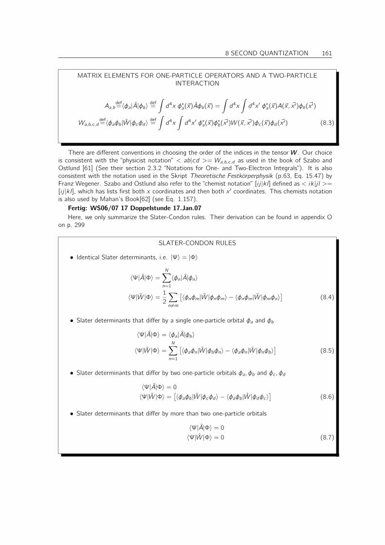
8 SECOND QUANTIZATION 161
MATRIX ELEMENTS FOR ONE-PARTICLE OPERATORS AND A TWO-PARTICLEINTERACTION
Aa,bdef=〈φa|A|φb〉 def
=
∫
d4x φ∗a(~x)Aφb(~x) =
∫
d4x
∫
d4x ′ φ∗a(~x)A(~x, ~x′)φb(~x ′)
Wa,b,c,ddef=〈φaφb|W |φcφd〉 def
=
∫
d4x
∫
d4x ′ φ∗a(~x)φ∗b(~x′)W (~x, ~x ′)φc(~x)φd(~x ′) (8.3)
There are different conventions in choosing the order of the indices in the tensor W . Our choiceis consistent with the “physicist notation” < ab|cd >= Wa,b,c,d as used in the book of Szabo andOstlund [61] (See their section 2.3.2 “Notations for One- and Two-Electron Integrals”). It is alsoconsistent with the notation used in the Skript Theoretische Festkörperphysik (p.63, Eq. 15.47) byFranz Wegener. Szabo and Ostlund also refer to the “chemist notation” [i j |kl ] defined as < ik |j l >=[i j |kl ], which has lists first both x coordinates and then both x ′ coordinates. This chemists notationis also used by Mahan’s Book[62] (see Eq. 1.157).
Fertig: WS06/07 17 Doppelstunde 17.Jan.07
Here, we only summarize the Slater-Condon rules. Their derivation can be found in appendix Oon p. 299
SLATER-CONDON RULES
• Identical Slater determinants, i.e. |Ψ〉 = |Φ〉
〈Ψ|A|Φ〉 =N∑
n=1
〈φn|A|φn〉
〈Ψ|W |Φ〉 = 12
∑
n 6=m
[〈φnφm|W |φnφm〉 − 〈φnφm|W |φmφn〉
](8.4)
• Slater determinants that differ by a single one-particle orbital φa and φb
〈Ψ|A|Φ〉 = 〈φa|A|φb〉
〈Ψ|W |Φ〉 =N∑
n=1
[〈φaφn|W |φbφn〉 − 〈φaφn|W |φnφb〉
](8.5)
• Slater determinants that differ by two one-particle orbitals φa, φb and φc , φd
〈Ψ|A|Φ〉 = 0〈Ψ|W |Φ〉 =
[〈φaφb|W |φcφd 〉 − 〈φaφb|W |φdφc〉
](8.6)
• Slater determinants that differ by more than two one-particle orbitals
〈Ψ|A|Φ〉 = 0〈Ψ|W |Φ〉 = 0 (8.7)
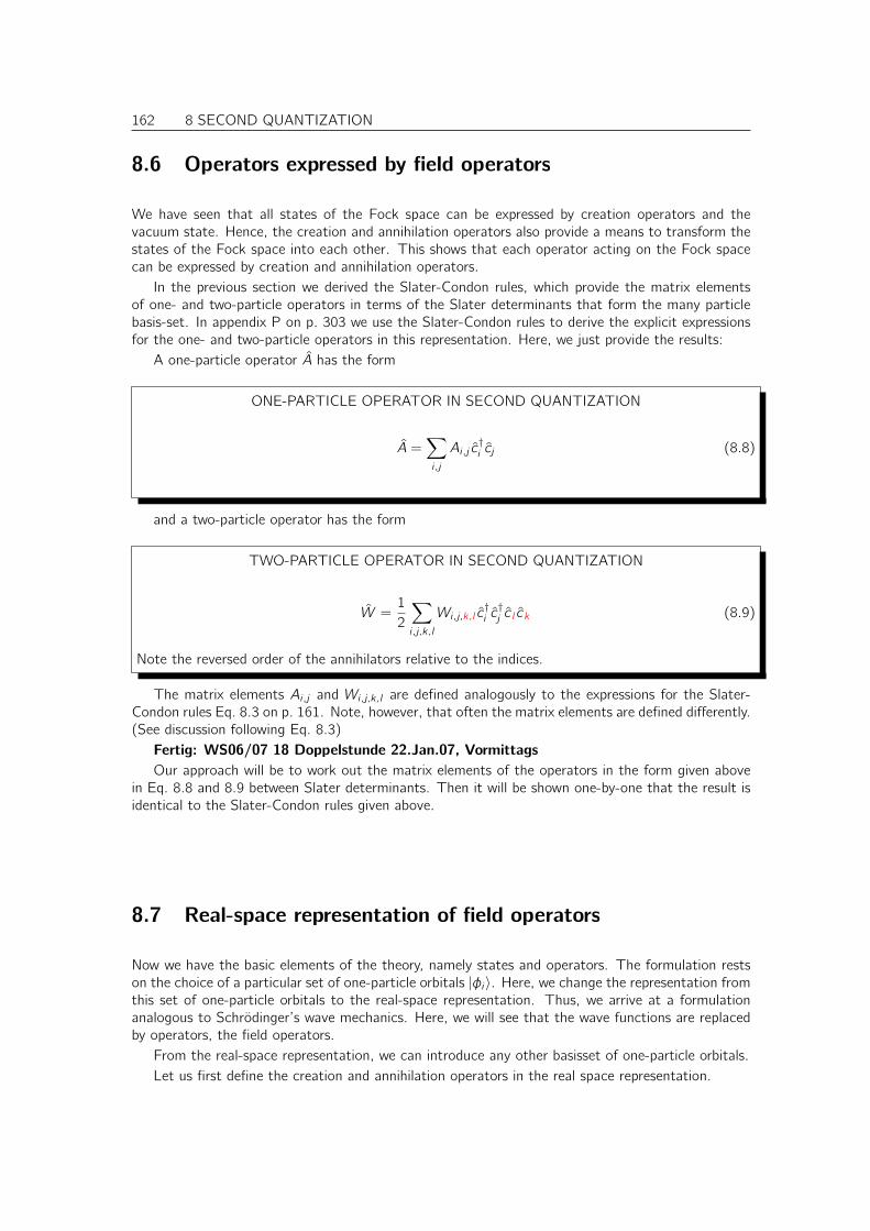
162 8 SECOND QUANTIZATION
8.6 Operators expressed by field operators
We have seen that all states of the Fock space can be expressed by creation operators and thevacuum state. Hence, the creation and annihilation operators also provide a means to transform thestates of the Fock space into each other. This shows that each operator acting on the Fock spacecan be expressed by creation and annihilation operators.
In the previous section we derived the Slater-Condon rules, which provide the matrix elementsof one- and two-particle operators in terms of the Slater determinants that form the many particlebasis-set. In appendix P on p. 303 we use the Slater-Condon rules to derive the explicit expressionsfor the one- and two-particle operators in this representation. Here, we just provide the results:
A one-particle operator A has the form
ONE-PARTICLE OPERATOR IN SECOND QUANTIZATION
A =∑
i ,j
Ai ,j c†i cj (8.8)
and a two-particle operator has the form
TWO-PARTICLE OPERATOR IN SECOND QUANTIZATION
W =1
2
∑
i ,j,k,l
Wi ,j,k,l c†i c†j c l ck (8.9)
Note the reversed order of the annihilators relative to the indices.
The matrix elements Ai ,j and Wi ,j,k,l are defined analogously to the expressions for the Slater-Condon rules Eq. 8.3 on p. 161. Note, however, that often the matrix elements are defined differently.(See discussion following Eq. 8.3)
Fertig: WS06/07 18 Doppelstunde 22.Jan.07, Vormittags
Our approach will be to work out the matrix elements of the operators in the form given abovein Eq. 8.8 and 8.9 between Slater determinants. Then it will be shown one-by-one that the result isidentical to the Slater-Condon rules given above.
8.7 Real-space representation of field operators
Now we have the basic elements of the theory, namely states and operators. The formulation restson the choice of a particular set of one-particle orbitals |φi 〉. Here, we change the representation fromthis set of one-particle orbitals to the real-space representation. Thus, we arrive at a formulationanalogous to Schrödinger’s wave mechanics. Here, we will see that the wave functions are replacedby operators, the field operators.
From the real-space representation, we can introduce any other basisset of one-particle orbitals.Let us first define the creation and annihilation operators in the real space representation.
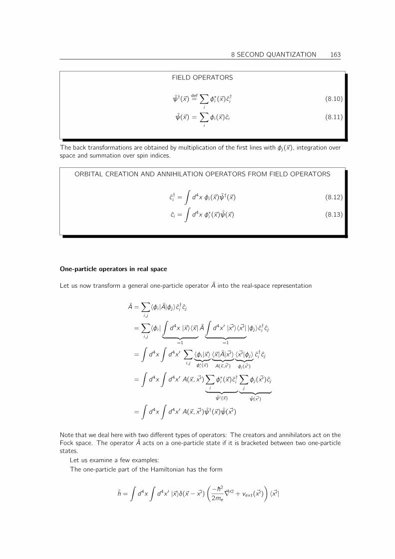
8 SECOND QUANTIZATION 163
FIELD OPERATORS
ψ†(~x)def=∑
i
φ∗i (~x)c†i (8.10)
ψ(~x) =∑
i
φi(~x)ci (8.11)
The back transformations are obtained by multiplication of the first lines with φj(~x), integration overspace and summation over spin indices.
ORBITAL CREATION AND ANNIHILATION OPERATORS FROM FIELD OPERATORS
c†i =
∫
d4x φi(~x)ψ†(~x) (8.12)
ci =
∫
d4x φ∗i (~x)ψ(~x) (8.13)
One-particle operators in real space
Let us now transform a general one-particle operator A into the real-space representation
A =∑
i ,j
〈φi |A|φj 〉c†i cj
=∑
i ,j
〈φi |∫
d4x |~x〉〈~x |︸ ︷︷ ︸
=1
A
∫
d4x ′ |~x ′〉〈~x ′|︸ ︷︷ ︸
=1
|φj 〉c†i cj
=
∫
d4x
∫
d4x ′∑
i ,j
〈φi |~x〉︸ ︷︷ ︸
φ∗i (~x)
〈~x |A|~x ′〉︸ ︷︷ ︸
A(~x,~x ′)
〈~x ′|φj 〉︸ ︷︷ ︸
φj (~x ′)
c†i cj
=
∫
d4x
∫
d4x ′ A(~x, ~x ′)∑
i
φ∗i (~x)c†i
︸ ︷︷ ︸
ψ†(~x)
∑
j
φj(~x ′)cj
︸ ︷︷ ︸
ψ(~x ′)
=
∫
d4x
∫
d4x ′ A(~x, ~x ′)ψ†(~x)ψ(~x ′)
Note that we deal here with two different types of operators: The creators and annihilators act on theFock space. The operator A acts on a one-particle state if it is bracketed between two one-particlestates.
Let us examine a few examples:The one-particle part of the Hamiltonian has the form
h =
∫
d4x
∫
d4x ′ |~x〉δ(~x − ~x ′)(−~22me
~∇′2 + vext(~x ′))
〈~x ′|
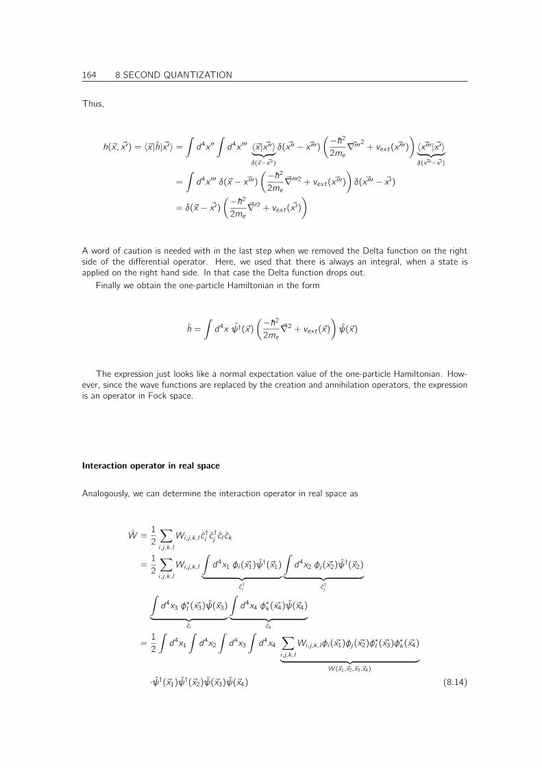
164 8 SECOND QUANTIZATION
Thus,
h(~x, ~x ′) = 〈~x |h|~x ′〉 =∫
d4x ′′∫
d4x ′′′ 〈~x | ~x ′′〉︸ ︷︷ ︸
δ(~x− ~x ′′)
δ( ~x ′′ − ~x ′′′)
(−~22me
~∇′′′2 + vext( ~x ′′′))
〈 ~x ′′′|~x ′〉︸ ︷︷ ︸
δ( ~x ′′′−~x ′)
=
∫
d4x ′′′ δ(~x − ~x ′′′)
(−~22me
~∇′′′2 + vext( ~x ′′′))
δ( ~x ′′′ − ~x ′)
= δ(~x − ~x ′)(−~22me
~∇′2 + vext(~x ′))
A word of caution is needed with in the last step when we removed the Delta function on the rightside of the differential operator. Here, we used that there is always an integral, when a state isapplied on the right hand side. In that case the Delta function drops out.
Finally we obtain the one-particle Hamiltonian in the form
h =
∫
d4x ψ†(~x)
(−~22me
~∇2 + vext(~x))
ψ(~x)
The expression just looks like a normal expectation value of the one-particle Hamiltonian. How-ever, since the wave functions are replaced by the creation and annihilation operators, the expressionis an operator in Fock space.
Interaction operator in real space
Analogously, we can determine the interaction operator in real space as
W =1
2
∑
i ,j,k,l
Wi ,j,k,l c†i c†j cl ck
=1
2
∑
i ,j,k,l
Wi ,j,k,l
∫
d4x1 φi(~x1)ψ†(~x1)
︸ ︷︷ ︸
c†i
∫
d4x2 φj(~x2)ψ†(~x2)
︸ ︷︷ ︸
c†j∫
d4x3 φ∗l (~x3)ψ(~x3)
︸ ︷︷ ︸
cl
∫
d4x4 φ∗k(~x4)ψ(~x4)
︸ ︷︷ ︸
ck
=1
2
∫
d4x1
∫
d4x2
∫
d4x3
∫
d4x4∑
i ,j,k,l
Wi ,j,k,lφi(~x1)φj(~x2)φ∗l (~x3)φ
∗k(~x4)
︸ ︷︷ ︸
W (~x1,~x2,~x3,~x4)
·ψ†(~x1)ψ†(~x2)ψ(~x3)ψ(~x4) (8.14)
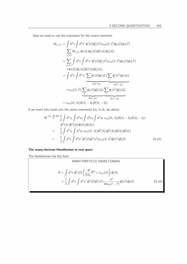
8 SECOND QUANTIZATION 165
Now we need to use the expression for the matrix elements
Wi ,j,k,l =
∫
d4x
∫
d4x ′ φ∗i (~x)φ∗j (~x′)vint(~x, ~x ′)φk(~x)φl(~x ′)
∑
i ,j,k,l
Wi ,j,k,lφi(~x1)φj(~x2)φ∗l (~x3)φ
∗k(~x4)
=∑
i ,j,k,l
∫
d4x
∫
d4x ′ φ∗i (~x)φ∗j (~x′)vint(~x, ~x ′)φk(~x)φl(~x ′)
×φi(~x1)φj(~x2)φ∗l (~x3)φ∗k(~x4)
=
∫
d4x
∫
d4x ′∑
i
φ∗i (~x)φi(~x1)
︸ ︷︷ ︸
δ(~x−~x1)
∑
j
φ∗j (~x′)φj(~x2)
︸ ︷︷ ︸
δ(~x ′−~x2)
×vint(~x, ~x ′)∑
k
φk(~x)φ∗k(~x4)
︸ ︷︷ ︸
δ(~x−~x4)
∑
l
φl(~x ′)φ∗l (~x3)
︸ ︷︷ ︸
δ(~x ′−~x3)
= vint(~x1, ~x2)δ(~x1 − ~x4)δ(~x2 − ~x3)
If we insert this result into the above expression Eq. 8.14, we obtain
WEq. 8.14=
1
2
∫
d4x1
∫
d4x2
∫
d4x3
∫
d4x4 vint(~x1, ~x2)δ(~x1 − ~x4)δ(~x2 − ~x3)
·ψ†(~x1)ψ†(~x2)ψ(~x3)ψ(~x4)
=1
2
∫
d4x1
∫
d4x2 vint(~x1, ~x2)ψ†(~x1)ψ
†(~x2)ψ(~x2)ψ(~x1)
=1
2
∫
d4x
∫
d4x ′ ψ†(~x)ψ†(~x ′)vint(~x, ~x ′)ψ(~x ′)ψ(~x) (8.15)
The many-electron Hamiltonian in real space
The Hamiltonian has the form
MANY-PARTICLE HAMILTONIAN
H =
∫
d4x ψ†(~x)
(−~22me
~∇2 + vext(~x))
ψ(~x)
+1
2
∫
d4x
∫
d4x ′ ψ†(~x)ψ†(~x ′)e2
4πǫ0|~r − ~r ′|ψ(~x ′)ψ(~x) (8.16)

166 8 SECOND QUANTIZATION
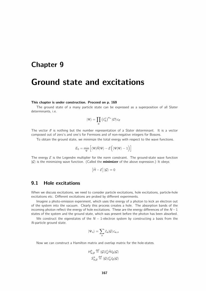
Chapter 9
Ground state and excitations
This chapter is under construction. Proceed on p. 169
The ground state of a many particle state can be expressed as a superposition of all Slaterdeterminants, i.e.
|Ψ〉 =∏
α
(c†α)σα |O〉c~σ
The vector ~σ is nothing but the number representation of a Slater determinant. It is a vectorcomposed out of zero’s and one’s for Fermions and of non-negative integers for Bosons.
To obtain the ground state, we minimize the total energy with respect to the wave functions.
E0 = minΨ
[
〈Ψ|H|Ψ〉 − E(
〈Ψ|Ψ〉 − 1)]
The energy E is the Legendre multiplier for the norm constraint. The ground-state wave function|G〉 is the minimizing wave function. (Called the minimizer of the above expression.) It obeys
[H − E
]|G〉 = 0
9.1 Hole excitations
When we discuss excitations, we need to consider particle excitations, hole excitations, particle-holeexcitations etc. Different excitations are probed by different experiments.
Imagine a photo-emission experiment, which uses the energy of a photon to kick an electron outof the system into the vacuum. Clearly this process creates a hole. The absorption bands of theincoming photon reflect the energy of hole excitations. These are the energy differences of the N−1states of the system and the ground state, which was present before the photon has been absorbed.
We construct the eigenstates of the N − 1-electron system by constructing a basis from theN-particle ground state.
|Ψn〉 =∑
n
cα|G〉cα,n
Now we can construct a Hamilton matrix and overlap matrix for the hole-states.
Hhα,βdef= 〈G|c†αHcβ |G〉
Shα,βdef= 〈G|c†αcβ |G〉
167
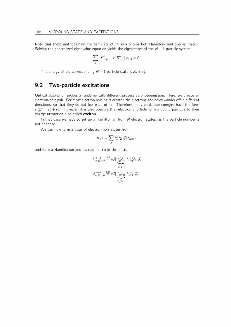
168 9 GROUND STATE AND EXCITATIONS
Note that these matrices have the same structure as a one-particle Hamilton- and overlap matrix.Solving the generalized eigenvalue equation yields the eigenstates of the N − 1 particle system.
∑
β
[Hhα,β − ǫhnShα,β
]cβ,n = 0
The energy of the corresponding N − 1 particle state is E0 + ǫhn.
9.2 Two-particle excitations
Optical absorption probes a fundamentally different process as photoemission. Here, we create anelectron-hole pair. For most electron hole pairs created the electrons and holes wander off in differentdirections, so that they do not feel each other. Therefore many excitation energies have the formǫe−hn,m = ǫ
hn + ǫ
em. However, it is also possible that electron and hole form a bound pair due to their
charge attraction a so-called exciton.In that case we have to set up a Hamiltonian from N electron states, as the particle number is
not changed.We can now form a basis of electron-hole states from
|Ψn〉 =∑
n
c†αcβ |G〉cα,β,n
and form a Hamiltonian and overlap matrix in this basis.
He−hα,β;γ,δ
def= 〈G| c†β cα
︸︷︷︸
(c†αcβ)†
Hc†γ cδ|G〉
Se−hα,β;γ,δ
def= 〈G| c†β cα
︸︷︷︸
(c†αcβ)†
c†γ cδ|G〉
Chapter 10
Green’s functions in one-particlequantum mechanics
10.1 Green’s function as inverse of a differential operator
Green’s functions are a powerful tool of many-particle physics. However, it also plays an importantrole in one-particle quantum mechanics. Even more, we use Green’s functions in many contexts,often without realizing that we deal with them.
Because explaining Green’s functions in the context of many-particle physics is a double difficulty,let us first become familiar with Green’s function in the context of one-particle quantum mechanics.
Definition
Consider a differential operator D(~x, ~∇). The vector ~x shall be an n-dimensional vector, where n mayalso be one. It may describe time coordinates, spatial coordinates, both or any other set of variables.A Green’s function G(~x, ~x ′) is defined by the equation
DEFINING EQUATION FOR A GREEN’S FUNCTION
D(~x, ~∇)G(~x, ~x0) = δ(~x − ~x0)
Green’s function and inhomogeneous differential equations
A Green’s function can be used to solve a general inhomogeneous differential equation
D(~x, ~∇)f (~x) = I(~x)
f (~x) =
∫
dnx0 G(~x, ~x0)I(~x0)
169
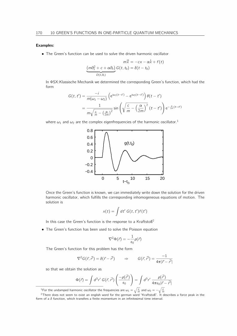
170 10 GREEN’S FUNCTIONS IN ONE-PARTICLE QUANTUM MECHANICS
Examples:
• The Green’s function can be used to solve the driven harmonic oscillator
m..x = −cx − α.
x + f (t)(m∂2t + c + α∂t
)
︸ ︷︷ ︸
D(t,∂t)
G(t, t0) = δ(t − t0)
In ΦSX:Klassische Mechanik we determined the corresponding Green’s function, which had theform
G(t, t ′) =−i
m(ω1 − ω2)(
eiω1(t−t′) − eiω2(t−t ′)
)
θ(t − t ′)
=1
m
√
cm −
(α2m
)2sin
(√
c
m−( α
2m
)2
(t − t ′))
e−α2m(t−t ′)
where ω1 and ω2 are the complex eigenfrequencies of the harmonic oscillator.1
g(t,t0)
t−t0
−0.4
−0.2
0
0.2
0.4
0.6
0.8
0 5 10 15 20
Once the Green’s function is known, we can immediately write down the solution for the drivenharmonic oscillator, which fulfills the corresponding inhomogeneous equations of motion. Thesolution is
x(t) =
∫
dt ′ G(t, t ′)f (t ′)
In this case the Green’s function is the response to a Kraftstoß2
• The Green’s function has been used to solve the Poisson equation
∇2Φ(~r) = − 1ǫ0ρ(~r)
The Green’s function for this problem has the form
∇2G(~r , ~r ′) = δ(~r − ~r ′) ⇒ G(~r , ~r ′) =−1
4π|~r − ~r ′|so that we obtain the solution as
Φ(~r) =
∫
d3r ′ G(~r , ~r ′)
(
−ρ(~r ′)ǫ0
)
=
∫
d3r ′ρ(~r ′)
4πǫ0|~r − ~r ′|1For the undamped harmonic oscillator the frequencies are ω1 =
√cm
and ω2 = −√
cm
2There does not seem to exist an english word for the german word “Kraftstoß”. It describes a force peak in theform of a δ function, which transfers a finite momentum in an infinitesimal time interval.
10 GREEN’S FUNCTIONS IN ONE-PARTICLE QUANTUM MECHANICS 171
• The Green’s function of the Schrödinger equation with a time-independent Hamilton operator[
i~∂t −(−~22m
~∇2 + v(~r))]
ψ(~r , t) = 0
is defined by[
i~∂t −(−~22m
~∇2 + v(~r))]
G(~r , t, ~r ′, t ′) = δ(t − t ′)δ(~r − ~r ′)
Using the eigenfunctions φn(~r) of the Hamilton operator and its eigenvalues ǫn we can representthe Green’s function as
G(~r , t, ~r ′, t ′) =1
i~
∑
n
φn(~r)φ∗n(~r′)e−
i~ǫn(t−t ′)θ(t − t ′)
Green’s function as inverse of an operator, a differential operator or a matrix
In the following we will show the role of the Green’s function in different contexts, that is once fora differential equation, once for an abstract operator and once for a matrix equation. The analogybetween these version will be used frequently in the future.
D(x, ~∇)G(~x, ~x0) = δ(~x − ~x0) : D(x, ~∇)f (~x) = I(x) ⇒ f (~x) =
∫
dnx ′ G(~x, ~x ′)I(~x ′) (10.1)
DG = 1 : D|f 〉 = |I〉 ⇒ |f 〉 = G|I〉 (10.2)
DG = 111 : D~f = ~I ⇒ ~f = G~I (10.3)
The analogy with the matrix form shows that the Green’s function can be considered the inverse of adifferential operator, a general operator or a matrix. In particular, we see that a differential equationis closely related to a system of regular equations.
The various forms can be transformed into each other. We start with the most general form, theabstract notation
DG = 1
and derive the corresponding other equations.
〈φi |D∑
k
|φk〉〈φk |︸ ︷︷ ︸
1
G|φj 〉 = 〈φi |1|φj 〉 〈~x |D∫
d4x ′ |~x ′〉〈~x ′|︸ ︷︷ ︸
1
G|~x0〉 = 〈~x |1|~x0〉
∑
k
Di ,kGk,j = δi ,j
∫
d4x ′ 〈~x |D|~x ′〉G(~x, ~x0) = δ(~x − ~x0) (10.4)
Here, we used the matrix elements of the Green’s function
Gi ,jdef=〈φi |G|φj 〉 G(~x, ~x ′)
def=〈~x |G|~x ′〉
A differential operator can be written as matrix elements of a special operator
D =
∫
d~x |~x〉D(~x, ~∇)〈~x |
which has the matrix elements
〈~x |D|~x ′〉 =∫
d ~x ′′ 〈~x | ~x ′′〉D( ~x ′′, ~∇′′)〈 ~x ′′|~x ′〉 = δ(~x − ~x ′)D(~x ′, ~∇′)
Insertion into Eq. 10.4 yields the first equations in Eq. 10.1 and Eq. 10.3 respectively.
172 10 GREEN’S FUNCTIONS IN ONE-PARTICLE QUANTUM MECHANICS
10.2 Green’s function of a time-independent Hamiltonian
Consider a time-independent Hamiltonian H, which has eigenstates |ψn〉 with eigenvalues ǫn. Thedifferential operator describing the Schrödinger equation has the form
D =[i~∂t − H
]= i~∂t −
∑
n
|ψn〉ǫn〈ψn|︸ ︷︷ ︸
H
=∑
n
|ψn〉 (i~∂t − ǫn) 〈ψn| (10.5)
The Green’s function, in its operator form with respect to the spatial variables, is defined by
DG(t, t0) = 1δ(t − t0) (10.6)
We can represent the Green’s function in eigenstates |ψn〉 of the Hamiltonian
G =∑
n
|ψn〉〈ψn|︸ ︷︷ ︸
1
G∑
m
|ψm〉〈ψm|︸ ︷︷ ︸
1
=∑
n,m
|ψn〉 〈ψn|G|ψm〉︸ ︷︷ ︸
Gn,m
〈ψm| =∑
n,m
|ψn〉Gn,m〈ψm|
where Gn,m(t, t ′) are the corresponding matrix elements of the Green’s function.Now we can work out the Green’s function
DG(t, t ′) = 1δ(t − t ′)∑
j
|ψj 〉 (i~∂t − ǫj) 〈ψj |︸ ︷︷ ︸
=D (See Eq. 10.5)
∑
n,m
|ψn〉Gn,m(t, t ′)〈ψm|︸ ︷︷ ︸
G
= 1δ(t − t ′)
∑
j,n,m
|ψj 〉 (i~∂t − ǫj) 〈ψj |ψn〉︸ ︷︷ ︸
δj,n
Gn,m(t, t′)〈ψm| = 1δ(t − t ′)
∑
n,m
|ψn〉 (i~∂t − ǫn)Gn,m(t, t ′)〈ψm| =∑
n,m
|ψn〉δn,m〈ψm|︸ ︷︷ ︸
1
⇒ (i~∂t − ǫn)Gn,m(t, t ′) = δn,mδ(t − t ′) (10.7)
In the last step we exploited that the eigenstates are linear independent, which implies that eachoperator cannot be represented by two different sets of matrix elements.
Thus, we arrived at an ordinary differential equation for the matrix elements, namely Eq. 10.7,which has the solution3
Gn,m(t, t′) =
1
i~e−
i~ǫn(t−t ′)θ(t − t ′)δn,m
with the matrix elements we can also express the Green’s function in operator form
3 Let us make the test (proof may continue on the next page):
[i~∂t − ǫn]1
i~e−
i~ǫn(t−t ′)θ(t − t ′)δn,m
=(
∂te− i~ǫn(t−t ′)
)
θ(t − t ′)δn,m + e−i~ǫn(t−t ′) (∂tθ(t − t ′)
)δn,m −
1
i~ǫne− i~ǫn(t−t ′)θ(t − t ′)δn,m
=
(1
i~ǫne− i~ǫn(t−t ′)
)
θ(t − t ′)δn,m︸ ︷︷ ︸
X
+e−i~ǫn(t−t ′)
︸ ︷︷ ︸
=1 for t=t ′
(δ(t − t ′)
)δn,m −
1
i~ǫne− i~ǫn(t−t ′)θ(t − t ′)δn,m
︸ ︷︷ ︸
X
= δ(t − t ′)δn,m
10 GREEN’S FUNCTIONS IN ONE-PARTICLE QUANTUM MECHANICS 173
G(t, t ′) =1
i~θ(t − t ′)
∑
n
|ψn〉e−i~ǫn(t−t ′)〈ψn| (10.8)
and we can determine the Green’s function in real space representation
G(~x, t, ~x ′, t ′)def= 〈~x |G(t, t ′)|~x ′〉 =
∑
n
〈~x |ψn〉1
i~θ(t − t0)e−
i~ǫn(t−t ′)〈ψn|~x ′〉
=1
i~
∑
n
ψn(~x)ψ∗n(~x′)θ(t − t0)e−
i~ǫn(t−t ′)
Fertig: WS06/07 19 Doppelstunde 22.Jan.07, Nachmittags
The Green’s function introduced here is the retarded Green’s function. The retarded Green’sfunction G(t, t ′) vanishes for t < t ′. There are also other Green’s function such as the advancedGreen’s function, which will become important in the many-particle formalism.
Note the Green’s function given above is not the only solution of the differential equation. Weare free to add a solution of the homogeneous equation to obtain another solution. For example wecan subtract
1
i~
∑
n
|ψn〉e−i~ǫn(t−t ′)〈ψn|
to obtain the advanced Green’s function
GA(t, t ′) =−1i~θ(t ′ − t)
∑
n
|ψn〉e−i~ǫn(t−t ′)〈ψn|
10.2.1 Green’s function in the energy representation
The Green’s function only depends on the difference of its time arguments, which is a consequenceof our requirement that the Hamiltonian is time-independent.
G(~x, t, ~x ′, t0) = G(~x, ~x ′, t − t0)
This allows to Fourier transform the Green’s function in the time-difference argument.
G(~x, ~x ′, ǫ)def=
∫ ∞
−∞dt G(~x, ~x ′, t) e
i~ǫt
Eq. 10.8=
1
i~
∑
n
ψn(~x)ψ∗n(~x′)
∫ ∞
−∞dt θ(t)e−
i~(ǫn−ǫ)t
=1
i~
∑
n
ψn(~x)ψ∗n(~x′)
∫ ∞
0
dt ′ e−i~(ǫn−ǫ)t ′ (10.9)
The integral does not converge if we let the upper limit of the integral go to infinity, while ǫ is real.If we consider the energy argument of the Green’s function to be a complex number, we see thatthe integral converges only, if the imaginary part of ǫ is positive. If it is real or if it has a negative
174 10 GREEN’S FUNCTIONS IN ONE-PARTICLE QUANTUM MECHANICS
imaginary part, the result is undefined.
G(~x, ~x ′, ǫ+ iη)Eq. 10.9=
1
i~
∑
n
ψn(~x)ψ∗n(~x′)
∫ ∞
0
dt ′ e−i~(ǫn−ǫ−iη)t ′
=1
i~
∑
n
ψn(~x)ψ∗n(~x′)
[i~
ǫn − ǫ− iηe−
i~(ǫn−ǫ−iη)t ′
]∞
0
η>0=
1
i~
∑
n
ψn(~x)ψ∗n(~x′)
−i~ǫn − ǫ− iη
= −∑
n
ψn(~x)ψ∗n(~x′)
ǫn − ǫ− iη
=∑
n
ψn(~x)ψ∗n(~x′)
ǫ− ǫn + iη
Notice the restriction that the imaginary part of ǫ+ iη must be positive. The Green’s function isonly defined in the upper half-plane of the complex plane. While we can evaluate the final expressionalso in the lower half plane, the Green’s function is simply not defined there.
Thus, we can express the Green’s function as
GREEN’S FUNCTION IN THE ENERGY REPRESENTATION
G(ǫ+ iη) =∑
n
|ψn〉1
ǫ− ǫn + iη〈ψn| = (ǫ+ iη − H)−1 for η > 0 (10.10)
Real and imaginary part of a schematic Green’s function are shown in Fig. 10.1.The Green’s function as function of energy obey’s the equation
(ǫ− H
)G(ǫ) = 1 (10.11)
which can be verified by insertion
(ǫ− H
)G(ǫ) =
(ǫ− H
)∑
n
|ψn〉1
ǫ− ǫn〈ψn|
=∑
n
|ψn〉ǫ− ǫnǫ− ǫn
〈ψn| =∑
n
|ψn〉〈ψn| = 1
10.3 Projected Density of States
So far the Green’s function is still a fairly abstract object. Let us therefore show a few physicalquantities that can be obtained from the Green’s function.
The Green’s function provides us with the density of states projected onto a state |χ〉 as
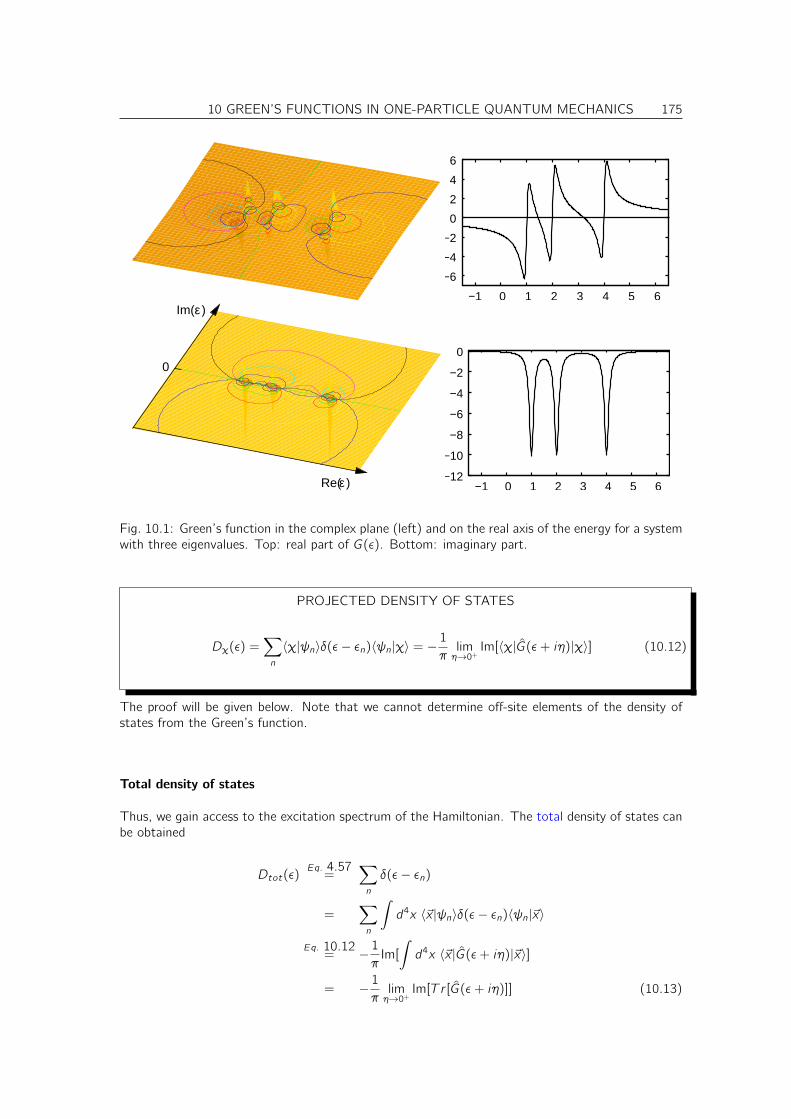
10 GREEN’S FUNCTIONS IN ONE-PARTICLE QUANTUM MECHANICS 175
−6
−4
−2
0
2
4
6
−1 0 1 2 3 4 5 6Im( )ε
Re( )ε
0
−12
−10
−8
−6
−4
−2
0
−1 0 1 2 3 4 5 6
Fig. 10.1: Green’s function in the complex plane (left) and on the real axis of the energy for a systemwith three eigenvalues. Top: real part of G(ǫ). Bottom: imaginary part.
PROJECTED DENSITY OF STATES
Dχ(ǫ) =∑
n
〈χ|ψn〉δ(ǫ− ǫn)〈ψn|χ〉 = −1
πlimη→0+
Im[〈χ|G(ǫ+ iη)|χ〉] (10.12)
The proof will be given below. Note that we cannot determine off-site elements of the density ofstates from the Green’s function.
Total density of states
Thus, we gain access to the excitation spectrum of the Hamiltonian. The total density of states canbe obtained
Dtot(ǫ)Eq. 4.57=
∑
n
δ(ǫ− ǫn)
=∑
n
∫
d4x 〈~x |ψn〉δ(ǫ− ǫn)〈ψn|~x〉
Eq. 10.12= − 1
πIm[
∫
d4x 〈~x |G(ǫ+ iη)|~x〉]
= − 1πlimη→0+
Im[T r [G(ǫ+ iη)]] (10.13)
176 10 GREEN’S FUNCTIONS IN ONE-PARTICLE QUANTUM MECHANICS
Electron density
Integration over the occupied states provides us with the probability that an electron is in a givenorbital. The orbital |χ〉 could also be |~x〉, in which case we obtain the electron density.
n(~r) =∑
σ
∑
n
∫ ǫF
dǫ 〈~r , σ|ψn〉δ(ǫ− ǫn)〈ψn|~r , σ〉
= − 1π
∑
σ
∫ ǫF
dǫ Im[〈~r , σ|G(ǫ)|~r , σ〉
Proof of Eq. 10.12
Let us derive this Eq. 10.12: First we determine the imaginary part of the expectation value of theGreen’s function with a one-particle orbital |χ〉
〈χ|G|χ〉 =∑
n
〈χ|ψn〉1
ǫ− ǫn + iη〈ψn|χ〉
=∑
n
〈χ|ψn〉ǫ− ǫn − iη(ǫ− ǫn)2 + η2
〈ψn|χ〉
⇒ Im[〈χ|G(ǫ)|χ〉] =∑
n
〈χ|ψn〉−η
(ǫ− ǫn)2 + η2〈ψn|χ〉
The last step works only for expectation values, that is the bra applied to the left must be correspondto the same orbital as the ket applied to the left. Only then we obtain a real contribution from theorbitals, namely |〈χ|ψn〉|2.
Below we will show that
limη→0
η
x2 + η2= πδ(x) (10.14)
With the identity Eq.10.14 we obtain directly Eq. 10.12.In the following we will prove Eq. 10.14. We can first show that the expression vanishes except
at the origin.
limη→0
η
x2 + η2x 6=0= lim
η→0η
x2= 0 for x 6= 0
For x = 0 the function diverges
limη→0
η
x2 + η2x=0= lim
η→01
η=∞ for x = 0
Now we need to show that the integral converges to a constant∫
dxη
x2 + η2=
∫dx
η
1(
1 + xη
)2
zdef= x
η=
∫
dz1
1 + z2
Now we introduce another variable transform from z to q
qdef= atan(z)
z = tan(q)
dz
dq=sin2(q) + cos2(q)
cos2(q)=sin2(q)
cos2(q)+ 1 = 1 + tan2(q) = 1 + z2
10 GREEN’S FUNCTIONS IN ONE-PARTICLE QUANTUM MECHANICS 177
which yields
∫
dz1
1 + z2=
∫ ∞
−∞dz
dq
dz=
∫ π2
− π2
dq = π
Thus, we have shown that 1π limη→0
ηx2+η2 vanishes everywhere except at the origin, and that it
integrates to one, which shows that it is the δ-function 4. This concludes the proof of Eq. 10.12.
4A proper proof would need to show f (0) = 1πlimη→0
∫dx f (x) η
x2+η2, which we have not done here. One can
construct distributions that fulfill the equations we have shown, that however are not the δ function. Thus, we cannotsay that we have proven the statement but shown it beyond reasonable doubt, whatever that means.

178 10 GREEN’S FUNCTIONS IN ONE-PARTICLE QUANTUM MECHANICS
Chapter 11
Perturbation theory in theone-particle theory
One of the main advantages of the Green’s function is that a perturbative treatment is relativelysimple.
Consider a Hamiltonian, that consists of an unperturbed part H0 and a perturbation W .
(
ǫ− H0 − W)
G(ǫ)Eq. 10.11= 1
We assume that we know the Green’s function G0(ǫ) of the unperturbed system, which fulfills
(
ǫ− H0)
G0(ǫ)Eq. 10.11= 1
Thus, we can determine the perturbed Green’s function as
(
ǫ− H0 − W)
G(ǫ) = 1
G0·⇒ G0(ǫ)(
ǫ− H0 − W)
G(ǫ) = G0(ǫ)
⇒ G0
(
ǫ− H0)
︸ ︷︷ ︸
=1
G(ǫ)− G0W G(ǫ) = G0
⇒(
1− G0W)
G(ǫ) = G0
From this equation we obtain the Green’s function for the perturbed system as
DYSON’S EQUATION
⇒ G(ǫ) =(
1− G0W)−1
G0 =(
G−10 − W)−1= G0 + G0W G (11.1)
I am showing here three different expressions for the full Green’s function, that are all equivalent.The first expression suggests immediately a perturbation series, using the Taylor expansion of (1 +x)−1 =
∑∞n=0(−x)n.
179
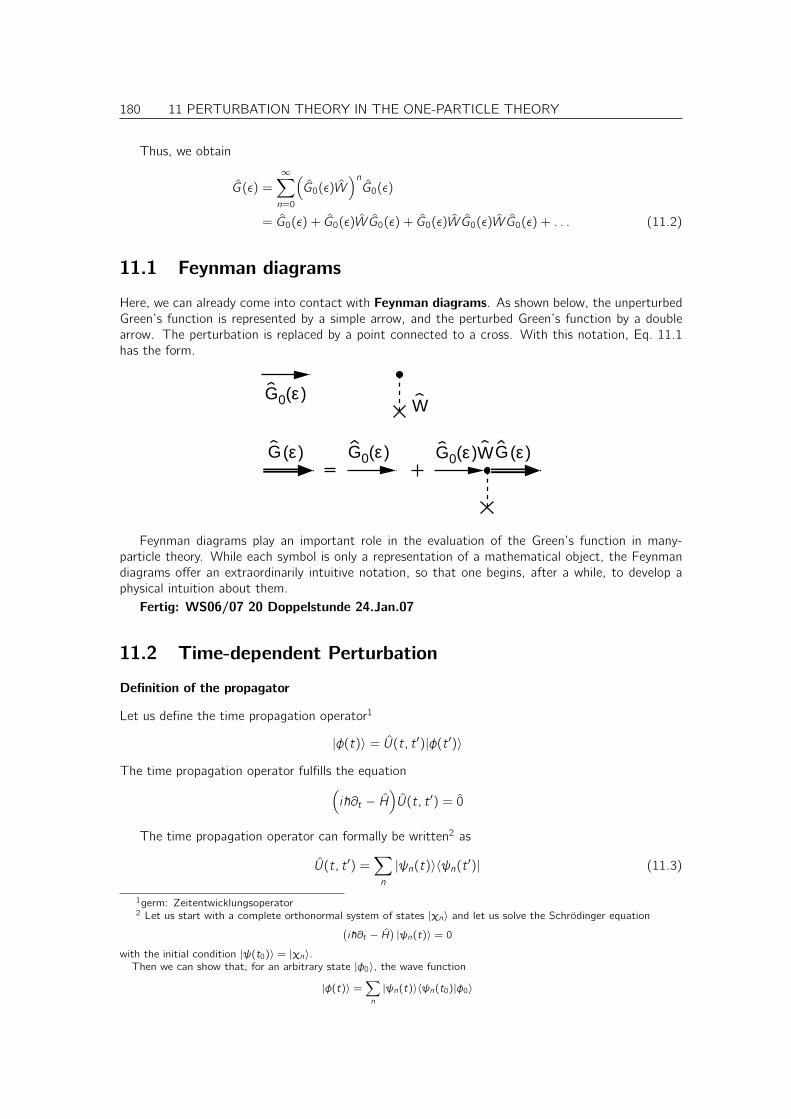
180 11 PERTURBATION THEORY IN THE ONE-PARTICLE THEORY
Thus, we obtain
G(ǫ) =
∞∑
n=0
(
G0(ǫ)W)n
G0(ǫ)
= G0(ǫ) + G0(ǫ)W G0(ǫ) + G0(ǫ)W G0(ǫ)W G0(ǫ) + . . . (11.2)
11.1 Feynman diagrams
Here, we can already come into contact with Feynman diagrams. As shown below, the unperturbedGreen’s function is represented by a simple arrow, and the perturbed Green’s function by a doublearrow. The perturbation is replaced by a point connected to a cross. With this notation, Eq. 11.1has the form.
G0( )εW
G( )ε G0( )ε G0( )ε G( )εW
Feynman diagrams play an important role in the evaluation of the Green’s function in many-particle theory. While each symbol is only a representation of a mathematical object, the Feynmandiagrams offer an extraordinarily intuitive notation, so that one begins, after a while, to develop aphysical intuition about them.
Fertig: WS06/07 20 Doppelstunde 24.Jan.07
11.2 Time-dependent Perturbation
Definition of the propagator
Let us define the time propagation operator1
|φ(t)〉 = U(t, t ′)|φ(t ′)〉
The time propagation operator fulfills the equation(
i~∂t − H)
U(t, t ′) = 0
The time propagation operator can formally be written2 as
U(t, t ′) =∑
n
|ψn(t)〉〈ψn(t ′)| (11.3)
1germ: Zeitentwicklungsoperator2 Let us start with a complete orthonormal system of states |χn〉 and let us solve the Schrödinger equation
(i~∂t − H
)|ψn(t)〉 = 0
with the initial condition |ψ(t0)〉 = |χn〉.Then we can show that, for an arbitrary state |φ0〉, the wave function
|φ(t)〉 =∑
n
|ψn(t)〉〈ψn(t0)|φ0〉
11 PERTURBATION THEORY IN THE ONE-PARTICLE THEORY 181
where the states |ψn(t)〉 are a complete orthonormal basis set which fulfills the time-dependentSchrödinger equation.
Properties of the Propagator
We can immediately write down some properties of UI(t)
U(t, t) = 1 (11.4)
U(t, t ′′)U(t ′′, t ′) = U(t, t ′) (11.5)
U(t ′, t)U(t, t ′)Eq. 11.5,= 1 (11.6)
U(t ′, t)Eq. 11.6= U−1(t, t ′) (11.7)
U(t ′, t)Eq. 11.3= U†(t, t ′) (11.8)
U†(t, t ′)Eq. 11.7,11.8
= U−1(t, t ′) Unitarity (11.9)
11.2.1 Perturbation series
Let us now consider a perturbation of the Hamiltonian, so that(
i~∂t − H0 − λW (t))
U(t, t ′) = 0
and let us assume that the propagator for the unperturbed system is known(
i~∂t − H0)
U(0)(t, t ′) = 0
11.2.2 Propagator of a time-independent Hamiltonian
While the formalism is more general, one usually uses a time-independent system as unperturbedsystem. Let us therefore examine the propagator for a time-independent Hamiltonian H(0).
U(0)(t, t ′) =∑
n
|ψ(0)n 〉e−i~ǫ(0)n (t−t ′)〈ψ(0)n | (11.10)
where |ψ(0)n 〉 are the eigenstates of the unperturbed Hamiltonian
H0|ψ(0)n 〉 = |ψ(0)n 〉ǫ(0)n
and ǫ(0)n are the corresponding energy eigenvalues. The time dependent wave functions have theform.
|ψ(0)n (t)〉 = |ψ(0)n 〉e−i~ǫ(0)n t
solves the Schrödinger equation(i~∂t − H
)|φ(t)〉 =
∑
n
(i~∂t − H
)|ψn(t)〉
︸ ︷︷ ︸
|0〉
〈ψn(t0)|φ0〉 = 0
with the initial condition |φ(t0)〉 = |φ0〉
|φ(t0)〉 =∑
n
|ψn(t0)〉〈ψn(t0)|φ0〉∑
n
|χn〉〈χn|︸ ︷︷ ︸
=1
φ0〉 = |φ0〉
Thus, the operator
U(t, t0) =∑
n
|ψn(t)〉〈ψn(t0)|
propagates any state from t0 to the time t.
182 11 PERTURBATION THEORY IN THE ONE-PARTICLE THEORY
which can be checked by insertion into the time-dependent Schrödinger equation.This propagator can be written3 as
U(0)(t, t ′) = e−i~H(0)(t−t ′)
11.2.3 Interaction picture
We would like to get rid of the unperturbed Hamiltonian, by using the unperturbed propagator.
(
i~∂t
−H(t)︷ ︸︸ ︷
−H0 − W (t))
U(0)(t, 0)U(0)(0, t)︸ ︷︷ ︸
=1
U(t, t ′) = 0
U(0)(t, 0)i~∂t
(
U(0)(0, t)U(t, t ′))
= W (t)U(0)(t, 0)U(0)(0, t)U(t, t ′)
We can give this expression a more symmetric form by multiplying the unperturbed propagator onthe left and the right.
U(0)(0, t)U(0)(t, 0)︸ ︷︷ ︸
1
i~∂t U(0)(0, t)U(t, t ′)U(0)(t ′, 0)︸ ︷︷ ︸
UI
= U(0)(0, t)W (t)U(0)(t, 0)︸ ︷︷ ︸
WI(t)
U(0)(0, t)U(t, t ′)U(0)(t ′, 0)︸ ︷︷ ︸
UI(t,t ′)
INTERACTION PICTURE
We introduce here the interaction picture where an operator has the form
AI(t) = U(0)(0, t)A(t)U(0)(t, 0) (11.11)
When we change the representation of the operators, we also need to change the representation ofthe wave functions
|ψI(t)〉 = U(0)(0, t)|ψ(t)〉 (11.12)
so that the expectation values are unchanged by changing the representation, that is
〈ΨI(t)|AI(t)|ΨI(t)〉 = 〈Ψ(t)|A(t)|Ψ(t)〉
11.2.4 Series expansion
The propagator in the interaction picture obeys the simple equation
3The proof that this result is identical to Eq. 11.10 goes as follows:
e−i~H(0)(t−t ′) =
=1︷ ︸︸ ︷∑
n
|ψ(0)n 〉〈ψ(0)n | e−i~H(0)(t−t ′)
=1︷ ︸︸ ︷∑
m
|ψ(0)m 〉〈ψ(0)m | =∑
n,m
|ψ(0)n 〉δn,me−i~ǫ(0)m (t−t ′)〈ψ(0)m |
=∑
n
|ψ(0)n 〉e−i~ǫ(0)n (t−t ′)〈ψ(0)n |
11 PERTURBATION THEORY IN THE ONE-PARTICLE THEORY 183
DYNAMICS OF THE PROPAGATOR IN THE INTERACTION PICTURE
i~∂t UI(t, t′) = WI(t)UI(t, t
′)
which can be solved as
UI(tf , ti) = UI(ti , ti)︸ ︷︷ ︸
=1
+1
i~
∫ tf
ti
dt ′ WI(t′)UI(t
′, ti)
= 1 +1
i~
∫ tf
ti
dt ′ WI(t′)UI(t
′, ti)
We can solve this equation iteratively. We introduce the propagator up to n-th order in W asU(n)I (t, t
′).In zeroth order we obtain the unperturbed propagator
U(0)I (t, t
′) = 1
which shows that the unperturbed wave functions in the interaction picture do not change with time.The higher orders fulfill
U(n)I (tf , ti) = 1 +
1
i~
∫ tf
ti
dt ′ WI(t′)U(n−1)I (t ′, ti)
which is obtained by removing all terms that are of higher order than W n. This equation allows usto determine the propagator for the perturbed system to all orders by an iterative procedure.
Let us write down the first few terms, in order to understand how the terms look like.
1. first order
U(1)I (tf , ti) = 1 +
1
i~
∫ tf
ti
dt ′ WI(t′) U(0)I (t
′, ti)︸ ︷︷ ︸
=1
= 1 +1
i~
∫ tf
ti
dt ′ WI(t′)
2. second order
U(2)I (tf , ti) = 1 +
1
i~
∫ tf
ti
dt ′ WI(t′)U(1)I (t
′, ti)
= 1 +1
i~
∫ tf
ti
dt ′ WI(t′) +
1
i~
∫ tf
ti
dt ′ WI(t′)1
i~
∫ t ′
ti
dt ′′ WI(t′′)
= 1 +1
i~
∫ tf
ti
dt ′ WI(t′) +
(1
i~
)2 ∫ tf
ti
dt ′∫ t ′
ti
dt ′′ WI(t′)WI(t
′′)
We can already generalize the building principle and construct the higher orders
UI(tf , ti) =
∞∑
n=0
(1
i~
)n ∫ tf
ti
dt1
∫ t1
ti
dt2 . . .
∫ tn−1
ti
dtn WI(t1) · · · WI(tn) (11.13)
Note that the interactions are occur such that the earlier interaction stands right from the laterinteraction. Thus, the time increases from right to left.
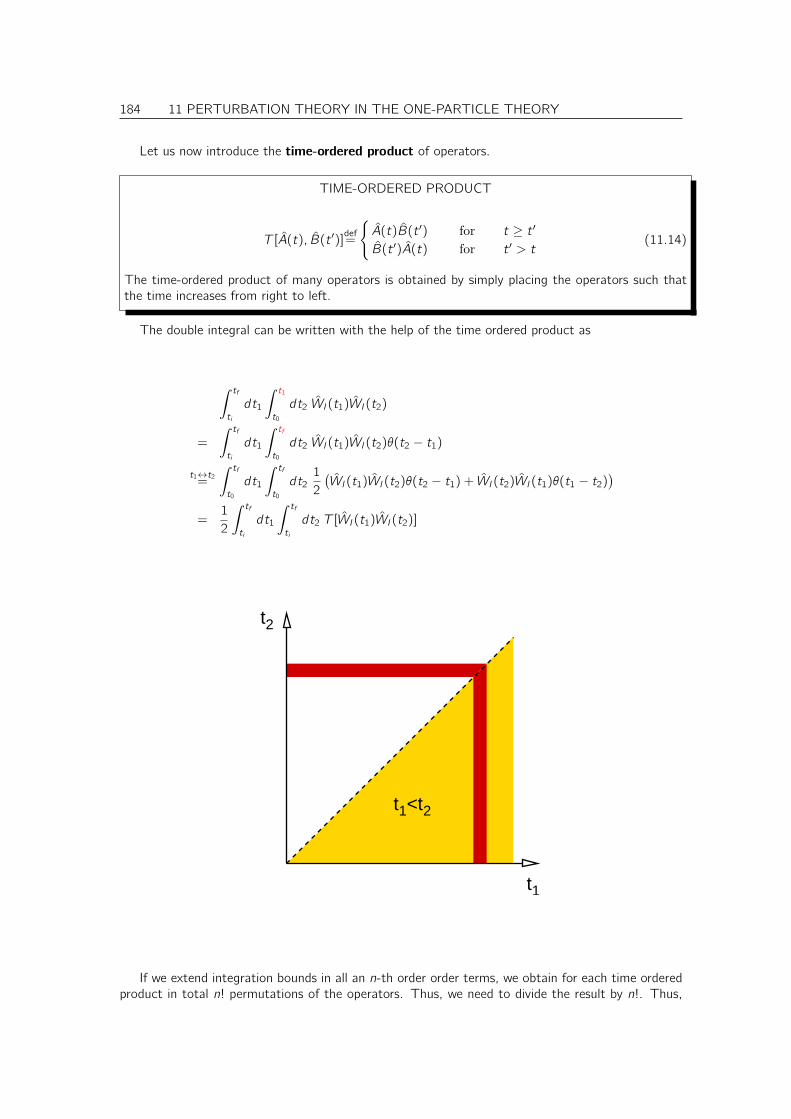
184 11 PERTURBATION THEORY IN THE ONE-PARTICLE THEORY
Let us now introduce the time-ordered product of operators.
TIME-ORDERED PRODUCT
T [A(t), B(t ′)]def=
A(t)B(t ′) for t ≥ t ′B(t ′)A(t) for t ′ > t
(11.14)
The time-ordered product of many operators is obtained by simply placing the operators such thatthe time increases from right to left.
The double integral can be written with the help of the time ordered product as
∫ tf
ti
dt1
∫ t1
t0
dt2 WI(t1)WI(t2)
=
∫ tf
ti
dt1
∫ tf
t0
dt2 WI(t1)WI(t2)θ(t2 − t1)
t1↔t2=
∫ tf
t0
dt1
∫ tf
t0
dt21
2
(WI(t1)WI(t2)θ(t2 − t1) + WI(t2)WI(t1)θ(t1 − t2)
)
=1
2
∫ tf
ti
dt1
∫ tf
ti
dt2 T [WI(t1)WI(t2)]
t1
t2
t 21<t
If we extend integration bounds in all an n-th order order terms, we obtain for each time orderedproduct in total n! permutations of the operators. Thus, we need to divide the result by n!. Thus,
11 PERTURBATION THEORY IN THE ONE-PARTICLE THEORY 185
we obtain
UI(tf , ti) =
∞∑
n=0
1
n!
(1
i~
)n ∫ tf
ti
dt1 . . .
∫ tf
ti
dtn T [WI(t1) · · · WI(tn)] (11.15)
= T
[ ∞∑
n=0
1
n!
(1
i~
)n ∫ tf
ti
dt1 . . .
∫ tf
ti
dtn WI(t1) · · · WI(tn)
]
= T
[ ∞∑
n=0
1
n!
(1
i~
∫ tf
ti
dt ′ WI(t′)
)n]
= T[
e1i~
∫ tftidt ′ WI(t
′)]
(11.16)
Fertig: WS06/07 21 Doppelstunde 8.Feb.07
11.3 Green’s function as propagator
The Green’s function is closely related to the propagator. Let us remember the equation Eq. 10.6that defined the Green’s function.
(
i~∂t − H)
G(t, t ′) = 1δ(t − t ′)
The propagator fulfills(
i~∂t − H)
U(t, t ′) = 0
This suggests that we can express the Green’s function by the propagator as
GREEN’S FUNCTION AND PROPAGATOR
G(t, t ′) =1
i~θ(t − t ′)U(t, t ′) (11.17)
Thus, we have a physical interpretation of the Green’s function:
INTERPRETATION OF THE GREEN’S FUNCTION
The Green’s function is related to the probability density P (x, t, x ′, t ′) of finding a particle at ~x attime t, if it has been at time t ′ at position ~x ′.
P (x, t, x ′, t ′) = |i~G(x, t, x ′, t ′)|2 (11.18)
Note however that this simplistic sentence does not capture that the Green’s function contains aphase information in addition to the probability.More accurately, the Green’s function propagates a wave function |ψ0〉 from time t ′ to its new stateat time t, that is
|ψ(t)〉 = i~G(t, t ′)|Ψ0〉 if |ψ(t ′)〉 = |ψ0〉 and t > t ′
Let us now return to Eq. 11.13 and determine the propagator in the regular Schrödinger picture.This will show that the Green’s function plays a central role for the perturbative treatment of anyquantity.
186 11 PERTURBATION THEORY IN THE ONE-PARTICLE THEORY
UI(tf , ti) = U(0)(0, tf )U(tf , ti)U
(0)(ti , 0) ⇒ U(tf , ti) = U(0)(tf , 0)UI(tf , ti)U
(0)(0, ti)
G(tf , ti) =1
i~θ(tf − ti)U(0)(tf , 0)UI(tf , ti)U(0)(0, ti)
Eq. 11.13=
1
i~θ(tf − ti)U(0)(tf , 0)
·∞∑
n=0
(1
i~
)n ∫ tf
ti
dt1
∫ t1
ti
dt2 . . .
∫ tn−1
ti
dtn WI(t1) · · · WI(tn)
︸ ︷︷ ︸
UI(tf ,ti )
U(0)(0, ti)
Now, we replace the integration bounds
θ(tf − ti)∫ tf
ti
dt1
∫ t1
ti
dt2 · · ·∫ tn−1
ti
dtn
=
∫ ∞
−∞dt1 · · ·
∫ ∞
−∞dtn θ(tf − t1)θ(t1 − t2) · · · θ(tn−1 − tn)θ(tn − ti) (11.19)
Later we will use the form of the Green’s function from Eq. 11.17 in slightly modified form
i~G(t, t ′)Eq. 11.17= θ(t − t)U(t, t ′) = U(t, 0)θ(t − t)U(0, t ′) (11.20)
With these considerations in mind, we proceed
G(tf , ti)Eq. 11.19=
∞∑
n=0
(1
i~
)n+1 ∫ ∞
−∞dt1 · · ·
∫ ∞
−∞dtn θ(tf − t1) · · · θ(tn − ti)
·U(0)(tf , 0) U(0)(0, t1)WS(t1)U(0)(t1, 0)
︸ ︷︷ ︸
WI(t1)
· · · U(0)(0, tn)WS(t1)U(0)(tn, 0)
︸ ︷︷ ︸
WI(tn)
U(0)(0, ti)
=
∞∑
n=0
(1
i~
)n+1 ∫ ∞
−∞dt1 · · ·
∫ ∞
−∞dtn
· U(0)(tf , 0)θ(tf − t1)U(0)(0, t1)︸ ︷︷ ︸
i~G(0)(tf ,t1)
WS(t1)U(0)(t1, 0) · · ·
· · · U(0)(0, tn)WS(t1) U(0)(tn, 0)θ(tn − ti)U(0)(0, ti)︸ ︷︷ ︸
i~G(0)(tn,ti )
Eq. 11.20=
∞∑
n=0
∫ ∞
−∞dt1 · · ·
∫ ∞
−∞dtn G
(0)(tf , t1)WS(t1)G(0)(t1, t2)WS(t2)G
(0)(t2, t3)
· · · G(0)(tn−1, tn)WS(tn)G(0)(tn, ti)
The Green’s function came into play via the integration bounds for the time integration and theconversion from the interaction picture to the Schrödinger picture.
We obtain realizing that our expression describes the Green’s function for the perturbed system
G(tf , ti) =
∞∑
n=0
∫ ∞
−∞dt1
∫ ∞
−∞dt2 . . .
∫ ∞
−∞dtn
·G(0)(tf , t1)W (t1)G(0)(t1, t2)W (t2) · · · W (tn)G(0)(tn, ti)
Note that this is identical to Eq. 11.2 after we Fourier transform from a time dependence to anenergy dependence. Remember that a convolution is converted by a Fourier transform into a simpleproduct.
11 PERTURBATION THEORY IN THE ONE-PARTICLE THEORY 187
11.4 Retarded Potentials
This is just a sketch of an idea and not intended for the reader....Consider a Schrödinger equation that has a nonlocal potential not only in space but also in time.
That is it would have a retarded potential.
[i~∂t − H0
]|ψ(t)〉 −
∫
dt ′v(t − t ′)|ψ(t ′)〉 = 0
Let us make an Ansatz
|ψ(t)〉 =∫
dǫ|ψ(ǫ)〉e− i~ǫt
and insert it into the above equation.∫
dǫ[i~∂t − H0
]|ψ(ǫ)〉e− i
~ǫt −
∫
dǫ
∫
dt ′ v(t − t ′)|ψ(ǫ)〉e− i~ǫt ′ = 0
∫
dǫ[ǫ− H0
]|ψ(ǫ)〉e− i
~ǫt −
∫
dǫ
(∫
dt ′ v(t − t ′)e i~ ǫ(t−t ′))
︸ ︷︷ ︸
=:v(ǫ)
|ψ(ǫ)〉e− i~ǫt = 0
∫
dǫ[ǫ− H0 − v(ǫ)
]|ψ(ǫ)〉e− i
~ǫt = 0
Thus, we obtain en energy dependent potential. If the potential were local in time, its Fouriertransform would be a constant in ǫ and therefore the potential would be energy independent.
In order to solve the above equation we must fulfill[ǫ− H0 − v(ǫ)
]|ψ(ǫ)〉 = 0
Note however, that the energies are, in general, complex and that the wave functions are notnecessarily orthonormal. (I do not have a proof either way.)
Questions: Compare this to the Lehmann representation. Can one identify the wave functionswith those of the Lehmann representation
φn(x)?= 〈G|ψ(x)|Ψn〉

188 11 PERTURBATION THEORY IN THE ONE-PARTICLE THEORY
Chapter 12
Green’s functions in many-particlephysics
12.1 Heisenberg picture
There are three pictures to represent the dynamics of expectation values. The Schrödinger picture,which is the one we are used to, the interaction picture that we have introduced previously (seep. 182) and the Heisenberg picture.
In the Schrödinger picture, the wave function is time dependent, but the operators are normallytime independent. The dynamics of the system is described by the Schrödinger equation
i~∂t |ΨS(t)〉 = H|ΨS(t)〉
The expectation value of an operator AS(t) has the form
〈A〉 = 〈Ψ(t)|AS(t)|Ψ(t)〉
There is no dynamical equation for the operators. The time dependence of a Schrödinger operatormay, for example, describe the time dependence of the Hamilton operator due to external interactions.
Now we use again the propagator U(t, 0)
|ΨS(t)〉 = U(t, 0)|ΨS(0)〉
Using the Schrödinger equation we obtain an equation for U(t, 0)
i~∂t U(t, 0)|ψ0〉 = HS(t)U(t, 0)|ψ0〉⇒ i~∂t U(t, 0) = HS(t)U(t, 0) (12.1)
i~∂t U(0, t) = i~∂t U†(t, 0) =
(−i~∂t U†(t, 0)
)= −
(HS(t)U(t, 0)
)†
= −U(t, 0)†HS(t)† = −U(0, t)HS(t) (12.2)
A state |ΨH(t)〉 in the Heisenberg picture is related to one in the Schrödinger picture by thepropagator U(t, 0)
|ΨS(t)〉 = U(t, 0)|ΨH(t)〉 (12.3)
We can easily see that the state in the Heisenberg picture is the Schrödinger state at t = 0. Thus,it is time independent.
189
190 12 GREEN’S FUNCTIONS IN MANY-PARTICLE PHYSICS
HEISENBERG STATE
|ΨH〉 = |ΨS(t = 0)〉
The dynamical equation for the Heisenberg states, which replaces the Schrödinger equation is
i~∂t |ΨH〉 = 0
If we want to express an expectation value as
〈A〉 = 〈Ψ(t)|AS(t)|Ψ(t)〉 = 〈ΨH|AH(t)|ΨH〉
we need to introduce
HEISENBERG OPERATORS
AH(t) = U(0, t)AS(t)U(t, 0) (12.4)
There is a non-trivial equation of motion for the Heisenberg operator, which replaces the Schrödingerequation.
i~∂t AH(t) =[i~∂t U(0, t)
]AS(t)U(t, 0) + U(0, t)
[i~∂t AS(t)
]U(t, 0) + U(0, t)AS(t)
[i~∂t U(t, 0)
]
= −U(0, t)HS(t)AS(t)U(t, 0) + i~U(0, t)(
∂AS∂t
)
U(t, 0) + U(0, t)AS(t)HS(t)U(t, 0)
=
(
[AS(t), HS(t)]− + i~∂AS∂t
)
H
= [AH(t), HH(t)]− + i~
(
∂AS∂t
)
H
12.1.1 Pictures in comparison
(i~∂t − H
)|ψS〉 = 0
(i~∂t − W
)|ψI〉 = 0
(i~∂t) |ψH〉 = 0
|ψS(t)〉 = 1|ψS(t)〉|ψI(t)〉 = U(0)(0, t)|ψS(t)〉|ψH(t)〉 = U(0, t)|ψS(t)〉 = |ψS(0)〉
〈A〉 = 〈ψS(t)|AS(t)|ψS(t)〉 = 〈ψI(t)|AI(t)|ψI(t)〉 = 〈ψH(t)|AH(t)|ψI(t)〉
12 GREEN’S FUNCTIONS IN MANY-PARTICLE PHYSICS 191
∂t AS =dASdt
∂t AI =
(
dASdt
)
I
+i
~[HI , AI ]−
∂t AH =
(
dASdt
)
H
+i
~[HH, AH]−
AI(t) = U(0)(0, t)AS(t)U
(0)(t, 0)
AH(t) = U(0, t)AS(t)U(t, 0)
12.2 One-particle Green’s function expressed by the many-particle
Hamiltonian
Here, we want to generalize the result Eq. 10.8 from p. 173 for the Green’s function in the Hilbertspace (one-particle quantum mechanics)
G(~x, t, ~x ′, t ′) =1
i~θ(t − t ′)
∑
n
〈~x |ψn〉e−i~ǫn(t−t ′)〈ψn|~x ′〉
to the Fock-space (many-particle quantum mechanics).We start out with the definition of the one-particle Green’s function Eq. 10.8 on p. 173. Here,
we show the principle for a time-independent Hamiltonian. The generalization to a time-dependentHamiltonian should not be too difficult.
We take Eq. 10.8 and rewrite it to make use of creation and annihilation operators. The Hamil-tonian of a one-particle system can be written as
H =∑
n
ǫnc†n cn
where c†n and cn are the creation and annihilation operators in the representation of energy eigenstates.If we apply this Hamiltonian to a one-particle state c†n |O〉, that is an eigenstate of the Hamiltonianwith eigenvalue ǫn we obtain
Hc†n |O〉 = c†n |O〉ǫn (12.5)
The Hamiltonian applied to a many-particle state gives
Hc†i1 · · · c†iN|O〉 = c†i1 · · · c
†iN|O〉
N∑
j=1
ǫij
This Hamiltonian is identical to the one-particle Hamiltonian H =∑
n |ψn〉ǫn〈ψn| =∑
n c†n |O〉ǫn〈O|cn
in the one-particle Hilbert space. For two or more particles, however, it differs from the one-particleHamiltonian, because the form
∑
n |ψn〉ǫn〈ψn| can only act on one-particle states.
192 12 GREEN’S FUNCTIONS IN MANY-PARTICLE PHYSICS
Let us now turn to the one-particle Green’s function Eq. 10.8
G(~x, t, ~x, t ′)Eq. 10.8= 〈~x |
[
1
i~θ(t − t ′)
∑
n
|ψn〉e−i~ǫn(t−t ′)〈ψn|
]
|~x ′〉
1=
1
i~θ(t − t ′)
∑
n,m
ψn(~x)
δn,me− i~ǫn(t−t′)
︷ ︸︸ ︷
〈O|cne−i~H(t−t ′)c†m|O〉ψ∗m(~x ′)
2=
1
i~θ(t − t ′)
∑
n,m
ψn(~x)〈O| ei~Ht cne
− i~Ht
︸ ︷︷ ︸
cH,n(t)
ei~Ht ′ c†me
− i~Ht ′
︸ ︷︷ ︸
c†H,m(t′)
|O〉ψ∗m(~x ′)
=1
i~θ(t − t ′)
∑
n,m
ψn(~x)〈O|cH,n(t)c†H,m(t ′)|O〉ψ∗m(~x ′)
Eq. 8.11=
1
i~θ(t − t ′)〈O|ψH(~x, t)ψ†H(~x, t ′)|O〉 (12.6)
• In step 1 (I refer to the number on top of the equal sign) we made use of the fact that c†m|O〉is a one-particle state with quantum number m. This state is an eigenstate of the Hamiltonoperator H =
∑
n ǫnc†n cn. We also exploited the orthonormality of the one-particle states,
namely 〈O|c†n cm|O〉 = 〈ψn|ψm〉 = δn,m.
• In step 2 we made use that the Hamiltonian of Eq. 12.5 applied to the vacuum state |O〉 givesthe zero state |∅〉 , that is H|O〉 = |∅〉. As a consequence, we obtain
ei~Ht |O〉 =
∞∑
n=0
1
n!
(i t
~t
)n
Hn|O〉 = |O〉+∞∑
n=1
|∅〉 = |O〉
which is then exploited in step 2.
The Green’s function can also be expressed in a representation of energy eigenstates as
G(~x, t, ~x ′, t ′) =∑
n,m
〈~x |ψn〉Gn,m(t, t ′)〈ψm|~x ′〉
Gn,m(t, t′) =
1
i~θ(t − t ′)〈O|cH,n(t)c†H,m(t ′)|O〉 (12.7)
The physical meaning of the Green’s function is completely analogous to that of the one-particleGreen’s function: It is the probability amplitude for a particle, which has been created at time t ′ atposition x ′, to turn up at time t at the position x .
12.3 Many-particle Green’s function
We define the Green’s function analogously to Eq. 12.6. However, now the vacuum state is replacedby the vacuum state for electrons and holes, which is the ground state |G〉 of the electron gas. TheGreen’s function is then generalized to electron and hole excitations.
Gn,m(t, t′) =
1
i~
[
θ(t − t ′)〈G|eH,n(t)e†H,m(t ′)|G〉 − θ(t ′ − t)〈G|hH,m(t ′)h†H,n(t)|G〉
]
Eq. ??=1
i~
[
θ(t − t ′)〈G|cH,n(t)c†H,m(t ′)|G〉 − θ(t ′ − t)〈G|c†H,m(t
′)cH,n(t)|G〉]
We simply mapped the electron and the hole Green’s function together so that we obtain the electronpropagator for t > t ′ and the hole propagator for t < t ′. The physical picture is that a holepropagating forward in time is identical to an electron propagating backward in time[63, 64].
12 GREEN’S FUNCTIONS IN MANY-PARTICLE PHYSICS 193
At first sight the negative sign in front of the hole contribution to the Green’s function seemsarbitrary. As we will see later, the negative sign is required because the non-interacting Green’sfunction shall still obey the inhomogeneous differential equation Eq. 12.23.
This expression of the Green’s function can be written in a more compact form using the time-ordered product T . The time ordered product orders the field operators from the right to the leftin ascending time. For each interchange of two Fermionic operators the result obtains a factor −1.
WICK’S TIME-ORDERED PRODUCT OF FERMION OPERATORS
For two Fermion operators A, B the time-ordered product is
T [A(t)B(t ′)] =
A(t)B(t ′) for t ≥ t ′−B(t ′)A(t) for t < t ′
A Fermion operator is either a Fermionica creation or annihilation operator.b
T is Wick’s time-ordering operator , which acts on all operators on the right of it. In general Wickstime-ordering operator reorders a product so that the time arguments ascent from right to left andit applies a sign change or every permutation of two fermion operators.
aFor bosonic creation and annihilation operators the minus sign would be replaced by a plus sign.bIn the previous definition, Eq. 11.14, the minus sign was missing. The reason is that it was specific to operators,
that contain products of an even number of Fermion operators. With this limitation the two definitions are identical.
We have introduced the time-ordered product earlier Eq. 11.14. In that case we did not mentionthe sign change. The reason is that in Eq. 11.14 the operators corresponded to even products offermionic operators, so that the sign changes canceled.
Thus, we arrive at the final definition of the Green’s function as
G(~x, t, ~x ′, t ′) =1
i~
〈G|T [ψH(~x, t)ψ†H(~x ′, t ′)]|G〉〈G|G〉 (12.8)
where the field operators are represented in the Heisenberg picture and G is the ground state of theinteracting electron gas.
We assumed here that the ground state is normalized. i.e. 〈G|G〉 = 1.
12.4 Differential equation for the many-particle Green’s function
The Green’s function of a many-particle system is not a Green’s function in the mathematical sense.In mathematics, a Green’s function is the inverse of a differential operator. This applies only tothe Green function of one-particle systems. In solid state physics, only the physical meaning of theGreen’s function has been kept, namely as probability amplitude between two events.
When we try to set up a differential equation analogous to the one-particle case, we are lead tohigher Green’s functions involving more and more particles. Nevertheless, we can define a retardedone-particle potential that replaces the action of the many-particle system. This potential is the selfenergy. If the self-energy is included, the Green’s function obeys a differential equation as in theone-particle case.
In the following we derive a differential equation for the interacting many-body Green’s function.The first step is to find a differential equation for a Heisenberg operator cα(t), because the time
derivative will act on this operator within the expression for the Green’s function
i~∂t cζ(t) = ei~Ht[
cζ, H]
−e−
i~Ht (12.9)
194 12 GREEN’S FUNCTIONS IN MANY-PARTICLE PHYSICS
In order to continue, we need the commutator of the annihilation operator in the Schrödingerpicture with the Hamiltonian.
H =∑
α,β
hα,β c†αcβ +
1
2
∑
α,β,γ,δ
Wα,β,δ,γ c†αc†β cγ cδ (12.10)
We begin with the one-particle operator
[
cζ,∑
α,β
hα,β c†αcβ
]
−=∑
α,β
hα,β
(
cζ c†α
︸︷︷︸
δζ,α−c†αcζ
cβ − c†α cβ cζ︸︷︷︸
−cζ cβ
)
=∑
α,β
hα,βδζ,αcβ
=∑
β
hζ,β cβ (12.11)
and continue with the interaction
[
cζ,1
2
∑
α,β,γ,δ
Wα,β,δ,γ c†αc†β cγ cδ
]
−
=1
2
∑
α,β,γ,δ
Wα,β,δ,γ
(
cζ c†αc†β cγ cδ −c†αc
†β cζ cγ cδ + c
†αc†β cζ cγ cδ
︸ ︷︷ ︸
=0
−c†αc†β cγ cδ cζ)
=1
2
∑
α,β,γ,δ
Wα,β,δ,γ
((
cζ c†α
︸︷︷︸
δζ,α−c†αcζ
c†β − c†α c†β cζ︸︷︷︸
δβ,ζ−cζ c†β
)
cγ cδ + c†αc†β
(
cζ cγ︸︷︷︸
−cγ cζ
cδ − cγ cδ cζ︸︷︷︸
−cζ cδ
))
=1
2
∑
α,β,γ,δ
Wα,β,δ,γ
(
δζ,αc†β − c†αδβ,ζ
)
cγ cδ
=1
2
∑
β,γ,δ
Wζ,β,δ,γ c†β cγ cδ −
∑
α,γ,δ
Wα,ζ,δ,γ c†αcγ cδ
=1
2
∑
β,γ,δ
(
Wζ,β,δ,γ −Wβ,ζ,δ,γ
)
c†β cγ cδ
=∑
β,γ,δ
Wζ,β,δ,γ c†β cγ cδ (12.12)
With the results Eqs. 12.11,12.12 we can return to Eq. 12.9 and evaluate the time derivative ofthe annihilator in the Heisenberg picture as
i~∂t cζ(t) = ei~Ht[
cζ, H]
−e−
i~Ht
Eqs. 12.11,12.12= e
i~Ht(∑
β
hζ,β cβ +∑
γ,δ,ρ
Wζ,β,δ,γ c†β cγ cδ
)
e−i~Ht
=∑
β
hζ,β cβ(t) +∑
β,γ,δ
Wζ,β,δ,γ c†β(t)cγ(t)cδ(t) (12.13)
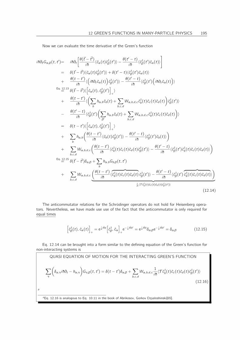
12 GREEN’S FUNCTIONS IN MANY-PARTICLE PHYSICS 195
Now we can evaluate the time derivative of the Green’s function
i~∂tGα,β(t, t′)= i~∂t
[θ(~t − ~t ′)
i~〈cα(t)c†β(t ′)〉 −
θ(t ′ − t)i~
〈c†β(t ′)cα(t)〉]
= δ(~t − ~t ′)〈cα(t)c†β(t ′)〉+ δ(t ′ − t)〈c†β(t′)cα(t)〉
+θ(t − t ′)
i~〈(
i~∂t cα(t))
c†β(t′)〉 − θ(t
′ − t)i~
〈c†β(t ′)(
i~∂t cα(t))
〉Eq. 12.13= δ(~t − ~t ′)〈
[
cα(t), c†β(t′)]
+〉
+θ(t − t ′)
i~〈(∑
b
hα,bcb(t) +∑
b,c,d
Wα,b,d,c c†b(t)cc(t)cd(t)
)
c†β(t′)〉
− θ(t ′ − t)i~
〈c†β(t ′)(∑
β′
hα,bcb(t) +∑
b,c,d
Wα,b,d,c c†b(t)cc(t)cd(t)
)
〉
= δ(t − t ′)〈[
cα(t), c†β(t′)]
+〉
+∑
b
hα,b
(θ(t − t ′)
i~〈cb(t)c†β(t ′)〉 −
θ(t ′ − t)i~
〈c†β(t ′)cb(t)〉)
+∑
b,c,d
Wα,b,d,c
(θ(t − t ′)
i~〈c†b(t)cc(t)cd(t)c
†β(t′)〉 − θ(t
′ − t)i~
〈c†β(t ′)c†b(t)cc(t)cd(t)〉
)
Eq. 12.15= δ(~t − ~t ′)δα,β +
∑
b
hα,bGb,β(t, t′)
+∑
b,c,d
Wα,b,d,c
(θ(t − t ′)
i~〈︷ ︸︸ ︷
c†b(t)cc(t)cd(t) c†β(t′)〉 − θ(t
′ − t)i~
〈c†β(t ′)︷ ︸︸ ︷
c†b(t)cc(t)cd(t)〉)
︸ ︷︷ ︸1i~〈T c†b(t)cc (t)cd (t)c
†β(t′)〉
(12.14)
The anticommutator relations for the Schrödinger operators do not hold for Heisenberg opera-tors. Nevertheless, we have made use use of the fact that the anticommutator is only required forequal times
[
c†β(t), cα(t)]
+= e
i~Ht[
c†β, cα]
+e−
i~Ht ′ = e
i~Htδα,βe
− i~Ht ′ = δα,β (12.15)
Eq. 12.14 can be brought into a form similar to the defining equation of the Green’s function fornon-interacting systems is
QUASI EQUATION OF MOTION FOR THE INTERACTING GREEN’S FUNCTION
∑
γ
(
δα,γ i~∂t − hα,γ)
Gγ,β(t, t′) = δ(t − t ′)δα,β +
∑
b,c,d
Wα,b,d,c1
i~〈T c†b(t)cc(t)cd(t)c
†β(t′)〉
(12.16)
a
aEq. 12.16 is analogous to Eq. 10.11 in the book of Abrikosov, Gorkov Dzyaloshinski[65].
196 12 GREEN’S FUNCTIONS IN MANY-PARTICLE PHYSICS
12.5 Self energy
Eq. 12.16 shows that unlike the non-interacting case the generalization of the Green’s function tointeracting systems does not obey an analogous differential equation. In order to obtain the equationfor the Green’s function matG, one needs the two-particle Green’s function, which contains fourcreation and annihilation operators. In order to determine the latter we obtain a differential equation,where even higher-order Green’s functions enter. We end up with a infinite sequence of increasinglymore complicated differential equations.
In order to recover a form more closely related to the defining equation of a Green’s function wedefine a self energy via
DEFINITION OF THE SELF ENERGY
∑
γ
∫
dt ′′ Σα,γ(t, t′′)Gγ,β(t
′′, t ′) =∑
b,c,d
Wα,b,d,c1
i~〈T c†b(t)cc(t)cd(t)c
†β(t′)〉 (12.17)
so that
∑
γ
∫
dt ′′(
δ(t − t ′′)(
δα,γ i~∂t ′′ − hα,γ)
−Σα,γ(t, t ′′))
Gγ,β(t′′, t ′) = δ(t − t ′)δα,β (12.18)
The self-energy acts like a retarded one-particle potential that describes the forces of remainingparticles system.
The defining equation Eq. 12.17 provides us with an expression for the interaction energy, namely
−i~2
∑
α,γ
∫
dt ′′ Σα,γ(t, t′′)Gγ,α(t
′′, t+) =⟨1
2
∑
α,b,c,d
Wα,b,d,c c†αc†b cc cd
⟩
(12.19)
This is a very strange way for calculating an energy: We use the information about the dynamics ofparticles immersed in the electron gas for all time, to extract a total energy at some initial time.
Eq. 12.18 is a Dyson equation
∫
dt ′′(
G−10 (t, t′′)− Σ(t, t ′′)
)
G(t ′′, t ′) = 1δ(t − t ′)
⇒ G(t, t ′) = G0(t, t′) +
∫
dt ′′∫
dt G0(t, t′′)Σ(t ′′, t)G(t , t ′) (12.20)
12.6 Physical meaning of the Green’s function
Note that the many-particle Green’s function can no more be written as the inverse of the Schrödingerequation.
12.6.1 Expectation value of single particle operators
Consider a one-particle operator, which can always be expressed as
A(t) =∑
n,m
An,mc†n cm =
∫
d4x
∫
d4x ′ A(~x, ~x ′, t)ψ†(x)ψ(~x ′)
12 GREEN’S FUNCTIONS IN MANY-PARTICLE PHYSICS 197
The ground-state expectation value is
〈G|A|G〉 =∫
d4x
∫
d4x ′ A(~x, ~x ′, t)〈G|ψ†(x)ψ(~x ′)|G〉
=
∫
d4x
∫
d4x ′ A(~x, ~x ′)〈G| U(0, t)︸ ︷︷ ︸
ei~EG t
ψ†(x) U(t, 0)U(0, t)︸ ︷︷ ︸
1
ψ(~x ′) U(t, 0)︸ ︷︷ ︸
e−i~EG t
|G〉
=
∫
d4x
∫
d4x ′ A(~x, ~x ′)〈G|ψ†H(~x, t)ψH(~x ′, t)|G〉
=
∫
d4x
∫
d4x ′ A(~x, ~x ′) limt ′→t+
(−1)〈G|T [ψH(~x, t)ψ†H(~x ′, t ′)]|G〉
= −i~ limt ′→t+
∫
d4x
∫
d4x ′ A(~x, ~x ′)G(~x, t, ~x ′, t ′)
Thus, we indirectly obtain the one-particle density matrix of the many-particle system as
ρ(1)(~x, ~x ′) = −i~ limt ′→t+
G(~x, t, ~x ′, t ′)
12.6.2 Excitation spectrum and Lehmann Representation
The Green’s function contains the information on the complete one-particle spectrum of the many-particle system.
Let us rewrite Eq. 12.8
G(~x, t, ~x ′, t ′) =1
i~
〈G|T [ψH(~x, t)ψ†H(~x ′, t ′)]|G〉〈G|G〉
=1
i~θ(t − t ′) 〈G|ψH(~x, t)ψ
†H(~x ′, t ′)|G〉
〈G|G〉 − 1i~θ(t ′ − t) 〈G|ψ
†H(~x ′, t ′)ψH(~x, t)|G〉〈G|G〉
Now we insert a complete many-particle basis |Ψn〉 of eigenstates of the many-particle Hamilto-nian, that is
H|Ψn〉 = |Ψn〉EnThus, we can write
U(t, 0)|Ψn〉 = |Ψn〉e−i~Ent
This basis set is complete in the Fock space, that is it contains the N-particle states for all N. Theunit operator in Fock space can then be written as
1 =∑
n
|Ψn〉〈Ψn|
G(~x, t, ~x ′, t ′) =1
i~
∑
n
θ(t − t ′)〈G|ψH(~x, t)|Ψn〉〈Ψn|ψ†H(~x ′, t ′)|G〉
− 1i~
∑
n
θ(t ′ − t)〈G|ψ†H(~x ′, t ′)|Ψn〉〈Ψn|ψH(~x, t)|G〉
=1
i~
∑
n
θ(t − t ′)e− i~(En−EG)(t−t ′)〈G|ψ(~x)|Ψn〉〈Ψn|ψ†(~x ′)|G〉
− 1i~
∑
n
θ(t − t ′)e i~ (En−EG)(t−t ′)〈G|ψ†(~x ′)|Ψn〉〈Ψn|ψ(~x)|G〉
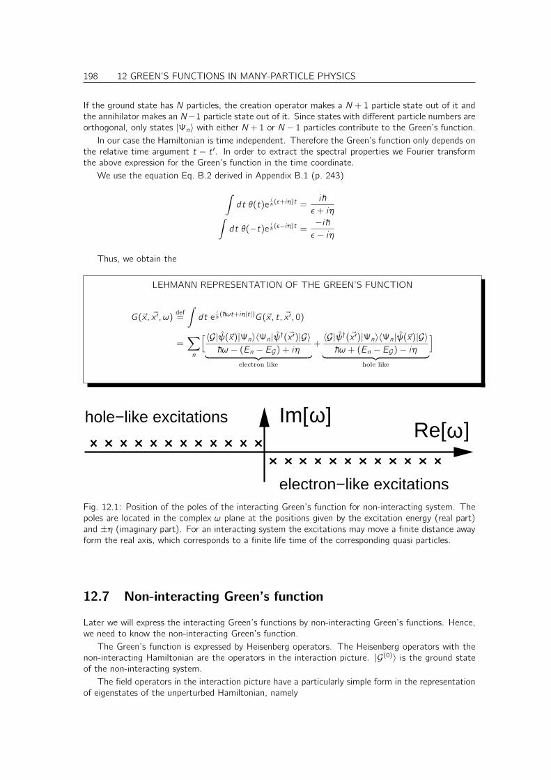
198 12 GREEN’S FUNCTIONS IN MANY-PARTICLE PHYSICS
If the ground state has N particles, the creation operator makes a N + 1 particle state out of it andthe annihilator makes an N−1 particle state out of it. Since states with different particle numbers areorthogonal, only states |Ψn〉 with either N +1 or N − 1 particles contribute to the Green’s function.
In our case the Hamiltonian is time independent. Therefore the Green’s function only depends onthe relative time argument t − t ′. In order to extract the spectral properties we Fourier transformthe above expression for the Green’s function in the time coordinate.
We use the equation Eq. B.2 derived in Appendix B.1 (p. 243)
∫
dt θ(t)ei~(ǫ+iη)t =
i~
ǫ+ iη∫
dt θ(−t)e i~ (ǫ−iη)t = −i~ǫ− iη
Thus, we obtain the
LEHMANN REPRESENTATION OF THE GREEN’S FUNCTION
G(~x, ~x ′, ω)def=
∫
dt ei~(~ωt+iη|t|)G(~x, t, ~x ′, 0)
=∑
n
[ 〈G|ψ(~x)|Ψn〉〈Ψn|ψ†(~x ′)|G〉~ω − (En − EG) + iη
︸ ︷︷ ︸
electron like
+〈G|ψ†(~x ′)|Ψn〉〈Ψn|ψ(~x)|G〉~ω + (En − EG)− iη
︸ ︷︷ ︸
hole like
]
Im[ ]ωRe[ ]ω
hole−like excitations
electron−like excitationsFig. 12.1: Position of the poles of the interacting Green’s function for non-interacting system. Thepoles are located in the complex ω plane at the positions given by the excitation energy (real part)and ±η (imaginary part). For an interacting system the excitations may move a finite distance awayform the real axis, which corresponds to a finite life time of the corresponding quasi particles.
12.7 Non-interacting Green’s function
Later we will express the interacting Green’s functions by non-interacting Green’s functions. Hence,we need to know the non-interacting Green’s function.
The Green’s function is expressed by Heisenberg operators. The Heisenberg operators with thenon-interacting Hamiltonian are the operators in the interaction picture. |G(0)〉 is the ground stateof the non-interacting system.
The field operators in the interaction picture have a particularly simple form in the representationof eigenstates of the unperturbed Hamiltonian, namely
12 GREEN’S FUNCTIONS IN MANY-PARTICLE PHYSICS 199
cn,I(t) = e− i~ǫnt cn
c†n,I(t) = e+ i~ǫnt c†n (12.21)
In contrast to the similar expression in the one-particle picture, the derivation of the Eq. 12.21is non-trivial. It is shown in appendix S on p. 319. The derivation is based on the Baker-Campbell-Hausdorff theorem[66, 67, 68, 69, 70, 71]. This theorem, which is used to derive a number of usefulrelations involving exponentials of operators is also shown in appendix. T.2.
Let us first bring the Green’s function in a representation of eigenstates of the non-interactingHamiltonian.
G(0)(~x, t, ~x ′, t ′)Eq. 12.8=
1
i~
〈G(0)|T [ψI(~x, t) ψ†I (~x ′, t ′)]|G(0)〉〈G(0)|G(0)〉
=1
i~
〈G(0)|T [∑
n φn(~x)cn,I(t)∑
m φ∗m(~x
′)c†m,I(t′)]|G(0)〉
〈G(0)|G(0)〉
=∑
n,m
φn(~x)φ∗m(~x
′)
(
1
i~
〈G(0)|T [cn,I(t)c†m,I(t ′)]|G(0)〉〈G(0)|G(0)〉
)
︸ ︷︷ ︸
G(0)n,m(t,t ′)
The Green’s function G(0)n,m(t, t ′) can now be worked out using Eq. 12.21
G(0)n,m(t, t′) =
1
i~
〈G(0)|T [cn,I(t)c†m,I(t ′)]|G(0)〉〈G(0)|G(0)〉
=1
i~e−
i~ǫn(t−t ′)δn,m (θ(µ− ǫn)θ(t − t ′)− θ(ǫn − µ)θ(t ′ − t))
Thus, we obtain the
NON-INTERACTING GREEN’S FUNCTION
G(0)(~x, t, ~x ′, t ′) =1
i~
∑
n
θ(µ− ǫn)φn(~x)θ(t − t ′)e−i~ǫn(t−t ′)φ∗n(~x
′)
︸ ︷︷ ︸
electron part
− 1i~
∑
n
θ(ǫn − µ)φn(~x)θ(t ′ − t)e−i~ǫn(t−t ′)φ∗n(~x
′)
︸ ︷︷ ︸
hole part
(12.22)
This expression is very similar to the unperturbed Green’s function Eq. 10.8 of one-particle quantummechanics. The main difference is that the contribution for the occupied states is similar to theadvanced Green’s function.
It is left to the reader to verify that the non-interacting Green’s function obeys the same differ-ential equation
200 12 GREEN’S FUNCTIONS IN MANY-PARTICLE PHYSICS
DIFFERENTIAL EQUATION FOR THE NON-INTERACTING GREEN’S FUNCTION
(i~∂t − H0
)G(0)(t, t ′) = 1δ(t − t ′) (12.23)
as the one for the one-particle system given in Eq. 10.6. Remember, however, that they are notidentical! (A differential equation has several solutions, which depend on the boundary conditions.The latter differ.) The derivation will make clear why the hole contribution of the Green’s functionenters with a negative sign.
12.8 Migdal-Galitskii-Koltun (MGK) sum rule and total energy
Eq. 12.14 leads to the Migdal-Galitskii-Koltun sum rule1, which gives the total energy in terms ofthe Green function.
limt ′→t+
δα,β i~∂tGβ,α(t, t′) =
1
i~〈H0 + 2W 〉
The contribution with the delta function does not contribute because we choose t ′ → t+ 6= t.MIGDAL-GALITSKII-KOLTUN SUM RULE
limt ′→t+
1
2
(
δα,β i~∂t + hα,β
)(
i~Gβ,α(t, t′)
)
= 〈H0 + W 〉 = Etot (12.24)
The positive sign is correct!
The Migdal-Galitsky sum rule can be used to obtain the total energy,if the self energy is known.For this purpose we use Eq. 12.18 to replace the time derivative in Eq. 12.24. This yields
Etot =∑
α,β
hα,β
(
i~Gβ,α(t, t+)
)
+1
2
∑
α,β
∫
dt ′ Σα,β(t, t′)
(
i~Gβ,α(t′, t+)
)
12.9 Spectral function
Do not read: sketch only
Aα,β(t, t′) =
⟨
G∣∣∣
[
ψ(~x, t), ψ†(~x ′, t ′)]
+
∣∣∣G⟩
12.10 Variations of the Green’s function
Do not read: sketch only
The Green’s function we introduced so-far is the so-called causal or time-ordered Green’s function.There are other types of Green functions. All of these Green’s function contain the same information.That is they can be converted into each other
1V.M. Galitskii, A.B. Migdal, Application of quantum field theory methods to the many body problem, Sov. Phys.,JETP 7, 96-104 (1958)
12 GREEN’S FUNCTIONS IN MANY-PARTICLE PHYSICS 201
The Green’s functions are the retarded Green’s function GR, the advanced Green’s functionGA, the greater Green’s function G>, and the lesser Green’s function G<.
GT (~x, t, ~x ′, t ′) =1
i~〈G|Tζψ(~x, t)ψ†(~x ′, t ′
∣∣∣G〉 (12.25)
GR(~x, t, ~x ′, t ′) =1
i~θ(t − t ′)〈G|
[
ψ(~x, t), ψ†(~x ′, t ′]
ζ|G〉 (12.26)
GA(~x, t, ~x ′, t ′) =−1i~θ(t ′ − t)〈G|
[
ψ(~x, t), ψ†(~x ′, t ′]
ζ|G〉 (12.27)
G>(~x, t, ~x ′, t ′) =1
i~〈G|ψ(~x, t), ψ†(~x ′, t ′|G〉 (12.28)
G<(~x, t, ~x ′, t ′) =ζ
i~〈G|ψ(~x, t), ψ†(~x ′, t ′|G〉 (12.29)
• The time-ordered Green’s function has a systematic perturbation theory
• The retarded and advanced Green’s functions have a nice analytical structure
• the retarded Green’s function is the classical response function.
• the lesser and greater Green’s function are directly linked to observables such as particle densitiesand currents.
(see http://www.phys.nthu.edu.tw/classnews/96intr_phys/Lecture)They are converted as follows
GR(~x, t, ~x ′, t ′) = θ(t − t ′)(
G>(~x, t, ~x ′, t ′)− G<(~x, t, ~x ′, t ′))
(12.30)
GA(~x, t, ~x ′, t ′) = θ(t ′ − t)(
G<(~x, t, ~x ′, t ′)− G>(~x, t, ~x ′, t ′))
(12.31)

202 12 GREEN’S FUNCTIONS IN MANY-PARTICLE PHYSICS
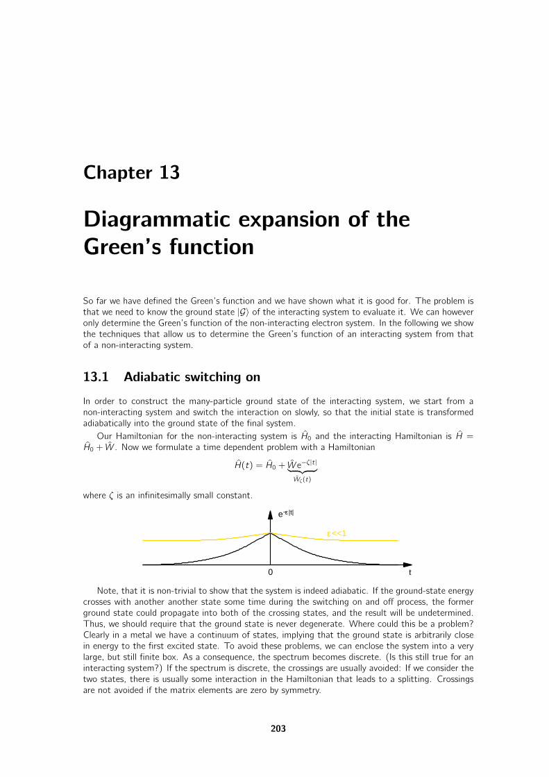
Chapter 13
Diagrammatic expansion of theGreen’s function
So far we have defined the Green’s function and we have shown what it is good for. The problem isthat we need to know the ground state |G〉 of the interacting system to evaluate it. We can howeveronly determine the Green’s function of the non-interacting electron system. In the following we showthe techniques that allow us to determine the Green’s function of an interacting system from thatof a non-interacting system.
13.1 Adiabatic switching on
In order to construct the many-particle ground state of the interacting system, we start from anon-interacting system and switch the interaction on slowly, so that the initial state is transformedadiabatically into the ground state of the final system.
Our Hamiltonian for the non-interacting system is H0 and the interacting Hamiltonian is H =H0 + W . Now we formulate a time dependent problem with a Hamiltonian
H(t) = H0 + W e−ζ|t|
︸ ︷︷ ︸
Wζ(t)
where ζ is an infinitesimally small constant.
e− |t|ε
<<1ε
0 t
Note, that it is non-trivial to show that the system is indeed adiabatic. If the ground-state energycrosses with another another state some time during the switching on and off process, the formerground state could propagate into both of the crossing states, and the result will be undetermined.Thus, we should require that the ground state is never degenerate. Where could this be a problem?Clearly in a metal we have a continuum of states, implying that the ground state is arbitrarily closein energy to the first excited state. To avoid these problems, we can enclose the system into a verylarge, but still finite box. As a consequence, the spectrum becomes discrete. (Is this still true for aninteracting system?) If the spectrum is discrete, the crossings are usually avoided: If we consider thetwo states, there is usually some interaction in the Hamiltonian that leads to a splitting. Crossingsare not avoided if the matrix elements are zero by symmetry.
203
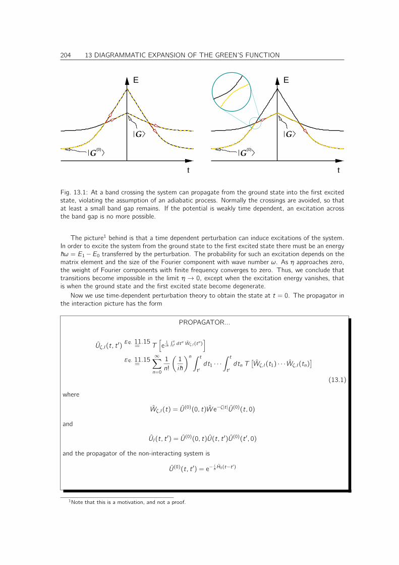
204 13 DIAGRAMMATIC EXPANSION OF THE GREEN’S FUNCTION
G(0)
G
t
E
G(0)
G
t
E
Fig. 13.1: At a band crossing the system can propagate from the ground state into the first excitedstate, violating the assumption of an adiabatic process. Normally the crossings are avoided, so thatat least a small band gap remains. If the potential is weakly time dependent, an excitation acrossthe band gap is no more possible.
The picture1 behind is that a time dependent perturbation can induce excitations of the system.In order to excite the system from the ground state to the first excited state there must be an energy~ω = E1−E0 transferred by the perturbation. The probability for such an excitation depends on thematrix element and the size of the Fourier component with wave number ω. As η approaches zero,the weight of Fourier components with finite frequency converges to zero. Thus, we conclude thattransitions become impossible in the limit η → 0, except when the excitation energy vanishes, thatis when the ground state and the first excited state become degenerate.
Now we use time-dependent perturbation theory to obtain the state at t = 0. The propagator inthe interaction picture has the form
PROPAGATOR...
Uζ,I(t, t′)Eq. 11.15= T
[
e1i~
∫ t
t′ dt′′ Wζ,I(t
′′)]
Eq. 11.15=
∞∑
n=0
1
n!
(1
i~
)n ∫ t
t ′dt1 · · ·
∫ t
t ′dtn T
[Wζ,I(t1) · · · Wζ,I(tn)
]
(13.1)
where
Wζ,I(t) = U(0)(0, t)W e−ζ|t|U(0)(t, 0)
and
UI(t, t′) = U(0)(0, t)U(t, t ′)U(0)(t ′, 0)
and the propagator of the non-interacting system is
U(0)(t, t ′) = e−i~H0(t−t ′)
1Note that this is a motivation, and not a proof.
13 DIAGRAMMATIC EXPANSION OF THE GREEN’S FUNCTION 205
Now we want to determine the ground state of the interacting system from that of the non-interacting system by adiabatically switching on the interaction. For t → −∞ the full Hamiltonianapproaches the unperturbed Hamiltonian. In that case the propagator becomes constant. This impliesthat the limes of Uζ,I(t,−∞) is well defined.
|ΨI(0)〉〉 = Uζ,I(0,−∞)|G(0)〉
At the origin of time, that is t = 0 the wave functions in the three pictures, Schrödinger-, Interaction-and Heisenberg Picture are identical according to Eq. 11.12 and Eq. 12.3, that is
|ΨI(0)〉 = |ΨS(0)〉 = |ΨH(0)〉
Thus, we obtain the ground state of the Heisenberg picture as
|G〉 = |GH〉 = Uζ,I(0,−∞)|G(0)〉
Note that |G〉 is the lowest eigenstate of the time independent, but interacting, Schrödinger equation.|G(0)〉 is defined analogously for the non-interacting Hamiltonian. None of them have an explicit timedependence.
The interesting point is that we have been able to start from the time-independent ground stateof the non-interacting system and obtain the stationary ground state of the interacting system.
We can represent the same state differently in a form that will be required in the following:
|G〉 = Uζ,I(0,−∞)|G(0)〉 = Uζ,I(0,∞)Uζ,I(∞,−∞)|G(0)〉= Uζ,I(0,∞)|G(0)〉〈G(0)|Uζ,I(∞,−∞)|G(0)〉
Here, we assumed that switching the interaction on and off adiabatically leads back to the samestate, even though the state may have a different phase. This is simply the requirement that theinteraction does not lead to persisting excitations from the ground state.
The operator that propagates from minus infinity to plus infinity has a special name, the
S-MATRIX
Sζ,Idef=Uζ,I(∞,−∞) (13.2)
The symbol S stands for Strahlung, Streumatrix or scattering. It relates a state in the infinite futureto a state in the infinite past.
Editor: check the proof of Molinari[72]
Concluding, we can express the ground state of the interacting system as
|G〉 = Uζ,I(0,−∞)|G(0)〉 (13.3)
〈G| = 1
〈G(0)|Sζ,I |G(0)〉〈G(0)|Uζ,I(∞, 0) (13.4)
In the last step we have exploited that 〈G(0)|Sζ,I |G(0)〉 is a simple phase factor so that 〈G(0)|Sζ,I |G(0)〉∗ =〈G(0)|Sζ,I |G(0)〉−1. This is valid, if the system behaves indeed adiabatic and is lead back, up to aphase factor, to the same state after the perturbation is switched off again.
206 13 DIAGRAMMATIC EXPANSION OF THE GREEN’S FUNCTION
13.2 Interacting Green’s function expressed by non-interacting
ground states
Next we wish to determine the Green’s function
G(x, t, x ′, t ′)Eq. 12.8=
1
i~
〈G|T [ψH(~x, t)ψ†H(~x ′, t ′)]|G〉〈G|G〉
Eq. 13.4=
1
i~
〈G(0)|Uζ,I(∞, 0)T [ψH(~x, t)ψ†H(~x ′, t ′)]Uζ,I(0,−∞)|G(0)〉〈G(0)|Sζ,I |G(0)〉
Let us now write down the time-ordered product in an explicit fashion
G(x, t, x ′, t ′) =1
i~θ(t − t ′) 〈G
(0)|Uζ,I(∞, 0)ψH(~x, t)ψ†H(~x ′, t ′)Uζ,I(0,−∞)|G(0)〉〈G(0)|Sζ,I |G(0)〉
− 1i~θ(t ′ − t) 〈G
(0)|Uζ,I(∞, 0)ψ†H(~x ′, t ′)ψH(~x, t)Uζ,I(0,−∞)|G(0)〉〈G(0)|Sζ,I |G(0)〉
Now we relate the Heisenberg operator to an interaction operator
AH(t) = U(0, t)AS(t)U(t, 0)
=
1︷ ︸︸ ︷
U(0)(0, 0) U(0, t)U(0)(t, 0)︸ ︷︷ ︸
Uζ,I(0,t)
AI(t) U(0)(0, t)U(t, 0)
1︷ ︸︸ ︷
U(0)(0, 0)︸ ︷︷ ︸
Uζ,I(t,0)
= UI(0, t)AI(t)UI(t, 0)
Here, I want to alert the reader to a subtle point.The expression for the Green’s function containsthe propagator UI and Uζ,I . In the following we use in all cases Uζ,I . Before, that is if we makethe distinction, the limes ζ → 0 leads to the true interacting Green’s function with an interactionthat is switched on all the time. The Green’s function propagates the particles with the completeinteraction. Once we replace UI by Uζ,I we determine the Green’s function with a time-dependentinteraction, that is switched off at ±∞. This is ok as long as the time arguments of the Green’sfunction are finite, because the limes ζ → 0 makes the difference arbitrarily small. However, we mustavoid any terms in which the time arguments approach ±∞.
Thus, we obtain
G(x, t, x ′, t ′)
=θ(t − t ′)
i~
〈G(0)|Uζ,I(∞, 0)ψH(~x,t)
︷ ︸︸ ︷
Uζ,I(0, t)ψI(~x, t)Uζ,I(t, 0)
ψ†H(~x,t′)
︷ ︸︸ ︷
Uζ,I(0, t′)ψ†I (~x
′, t ′)Uζ,I(t′, 0) Uζ,I(0,−∞)|G(0)〉
〈G(0)|Sζ,I |G(0)〉
− θ(t ′ − t)i~
〈G(0)|Uζ,I(∞, 0)
ψ†H(~x,t′)
︷ ︸︸ ︷
Uζ,I(0, t′)ψ†I (~x
′, t ′)Uζ,I(t′, 0)
ψH(~x,t)︷ ︸︸ ︷
Uζ,I(0, t)ψI(~x, t)Uζ,I(t, 0) Uζ,I(0,−∞)|G(0)〉〈G(0)|Sζ,I |G(0)〉
=θ(t − t ′)
i~
〈G(0)|Uζ,I(∞, t)ψI(~x, t)Uζ,I(t, t ′)ψ†I (~x ′, t ′)Uζ,I(t ′,−∞)|G(0)〉〈G(0)|Sζ,I |G(0)〉
− θ(t ′ − t)i~
〈G(0)|Uζ,I(∞, t ′)ψ†I (~x ′, t ′)Uζ,I(t ′, t)ψI(~x, t)Uζ,I(t,−∞)|G(0)〉〈G(0)|Sζ,I |G(0)〉
Now we realize from Eq. 13.1 that the propagator Uζ,I(t, t ′) contains only operators with times inthe interval [t, t ′], which shows that the product of operators is time ordered. Thus, we can permute
13 DIAGRAMMATIC EXPANSION OF THE GREEN’S FUNCTION 207
the operators as we whish, as long as we take care of sign changes for the permutation of eachFermion operator. The time ordering operator will sort them into the correct position again. Thisallows us to shift the creation and annihilation operators past the interaction operators to the veryright of the product. The propagator in the interaction picture contains only products of interactionoperators. Because the interaction operator is made from an even number of creation and annihilationoperators, the sign changes cancel. The only sign change is due to the relative order of the creatorand the annihilator, which contain the arguments of the Green’s function. When the creator and theannihilator are moved to the right, we can combine the propagators into the S-matrix.
Thus, we obtain our result
G(x, t, x ′, t ′) =1
i~
〈G(0)|T [Sζ,IψI(~x, t)ψ†I (~x ′, t ′)]|G(0)〉〈G(0)|Sζ,I |G(0)〉
(13.5)
Thus, we have found a compact expression for the Green’s function that does not resort directly tothe ground state of the interacting electron system. Note that we use here the operators in theinteraction picture and not the Heisenberg picture!
Fertig: WS06/07 23 Doppelstunde 12.Feb.07 Nachmittags
13.3 Wick’s theorem
13.3.1 Prelude
In order to determine the expression Eq. 13.5 for the Green’s function we decompose the S-matrixinto products of creation and annihilation operators
Sζ,IEq. 13.2,13.1
=
∞∑
n=0
1
n!
(1
i~
)n ∫ ∞
−∞dt1 · · ·
∫ ∞
−∞dtn T [Wζ,I(t1) · · · Wζ,I(tn)] (13.6)
This shows that we need to work out terms of the form
〈G(0)|T [Wζ,I(t1) · · · Wζ,I(tn)ψI(~x, t)ψ†I (~x ′, t ′)]|G(0)〉
〈G(0)|T [Wζ,I(t1) · · · Wζ,I(tn)]|G(0)〉
Each interaction operator is again composed of creation and annihilation operators.
Wζ =∑
i ,j,k,l
Wi ,j,k,l c†i c†j cl ck
Wζ,I(t) =∑
i ,j,k,l
Wi ,j,k,le−ζ|t|U(0)(0, t)c†i c
†j cl ck U
(0)(t, 0)
=∑
i ,j,k,l
Wi ,j,k,le−ζ|t|
· U(0)(0, t)c†i U(0)(t, 0)U(0)(0, t)︸ ︷︷ ︸
1
c†j U(0)(t, 0)U(0)(0, t)︸ ︷︷ ︸
1
cl U(0)(t, 0)U(0)(0, t)︸ ︷︷ ︸
1
ck U(0)(t, 0)
=∑
i ,j,k,l
Wi ,j,k,le−ζ|t|c†i ,I(t)c
†j,I(t)cl ,I(t)ck,I(t)
This shows that we need a way to work out the expectation values of time-ordered products offield operators.
208 13 DIAGRAMMATIC EXPANSION OF THE GREEN’S FUNCTION
13.3.2 Some definitions
It will be helpful to decompose the field operators into contributions that annihilate the ground stateof the non-interacting electron gas and those that do not. We can think of the annihilation part asthe electron and hole annihilators of the non-interacting system and the creation part the electronand hole creation operators. This decomposition has the advantage that if we move the annihilatorsto the very right, the corresponding expectation values with the ground state vanish.
Using the creation and annihilation operators ci ,I(t) and c†i ,I(t) in the basis of eigenstates of thenon-interacting Hamiltonian that defines the ground state of the non-interacting electron system,and the corresponding one-particle orbitals φi(x), we define
• the electron annihilation operator
ψ(+)I (~x, t) =
∑
i
θ(ǫi − µ)φi(x)ci ,I(t)
• the hole creation operator
ψ(−)I (~x, t) =
∑
i
θ(µ− ǫi)φi(x)ci ,I(t)
• the electron creation operator
ψ(+),†I (~x, t) =
∑
i
θ(ǫi − µ)φ∗i (x)c†i ,I(t)
• the hole annihilation operator
ψ(−),†I (~x, t) =
∑
i
θ(µ− ǫi)φ∗i (x)c†i ,I(t)
In all these definitions, the one-particle energies and the Fermi level refer to the non-interactingelectron gas.
From the definition it becomes clear that
ψ(+)I (t)|G(0)〉 = ψ
(−)†I (t)|G(0)〉 = |0〉
〈G(0)|ψ(+)†I (t) = 〈G(0)|ψ(−)I (t) = 〈0|
Furthermore we can express the original creation and annihilation operators as
ψI(t) = ψ(+)I (t) + ψ
(−)I (t)
ψ†I (t) = ψ(+)†I (t) + ψ
(−)†I (t)
Normal ordering
The normal product is defined such that all annihilation operators, such as ψ(+) and ψ(−),†, are placedto the right of the creation operators, such as ψ(+),† and ψ(−) . For each interchange of two Fermionfield operators the sign is changed.
N[ψ(+)I (~x, t)ψ
(−)I (
~x ′, t ′)] = −ψ(−)I (~x ′, t ′)ψ(+)I (~x, t)
The expectation value of every normal ordered product with the ground state of the non-interacting system vanishes.
〈G(0)|N[ABC · · · ]|G(0)〉 = 0
This is even true, if there are only creation operators because they annihilate the bra.
13 DIAGRAMMATIC EXPANSION OF THE GREEN’S FUNCTION 209
Contraction
The contraction of two operators is defined as the difference between the time ordered and thenormal ordered product
C[AB]def=T [AB]− N[AB]
These are the terms left over, when we convert a time ordered product into a normal product.The contraction vanishes, if both operators remain in their original order or if both operators are
interchanged. In that case we subtract two identical products. If only the operators are interchangedin only of the two products, we obtain an anticommutator due to the unbalanced sign change.
Let us now consider the anti-commutators. We have to make the assumption that the non-interacting Hamilton operator is time independent. With the help of Eqs. S.1 and S.2 shown in theappendix S on p. 319 we find
.[cn,I(t), cm,I(t′)]+
Eq. S.1= e−
i~(ǫnt+ǫmt ′) [cn, cm]+
︸ ︷︷ ︸
=0
= 0
.[cn,I(t), c†m,I(t
′)]+Eq. S.2= e−
i~(ǫnt−ǫmt ′) [cn, c
†m]+
︸ ︷︷ ︸
δn,m
= δn,me− i~ǫn(t−t ′)
.[c†n,I(t), cm,I(t′)]+ = [c†m,I(t
′), cn,I(t)]+ = δn,me+ i~ǫn(t−t ′)
.[c†n,I(t), c†m,I(t
′)]+ = ei~(ǫnt+ǫmt ′) [c†n, c
†m]+
︸ ︷︷ ︸
=0
= 0
Interesting is that the anticommutators are all numbers and no operators any longer!
C[cn,I(t)cm,I(t′)] = 0
C[c†n,I(t)c†m,I(t
′)] = 0
210 13 DIAGRAMMATIC EXPANSION OF THE GREEN’S FUNCTION
T [cn,I(t)c†m,I(t
′)] = θ(t − t ′)cn,I(t)c†m,I(t ′)− θ(t ′ − t)c†m,I(t
′)cn,I(t)
= θ(t − t ′)θ(µ− ǫn)cn,I(t)c†m,I(t ′) + θ(t − t ′)θ(ǫn − µ)cn,I(t)c†m,I(t
′)
− θ(t ′ − t)θ(µ− ǫn)c†m,I(t ′)cn,I(t)− θ(t ′ − t)θ(ǫn − µ)c†m,I(t
′)cn,I(t)
N[cn,I(t)c†m,I(t
′)] = θ(µ− ǫn)cn,I(t)c†m,I(t ′)− θ(ǫn − µ)c†m,I(t
′)cn,I(t)
= θ(t − t ′)θ(µ− ǫn)cn,I(t)c†m,I(t ′) + θ(t ′ − t)θ(µ− ǫn)cn,I(t)c†m,I(t
′)
− θ(t − t ′)θ(ǫn − µ)c†m,I(t ′)cn,I(t)− θ(t ′ − t)θ(ǫn − µ)c†m,I(t
′)cn,I(t)
C[cn,I(t)c†m,I(t
′)] = θ(t − t ′)θ(µ− ǫn)(
cn,I(t)c†m,I(t
′)− cn,I(t)c†m,I(t ′))
︸ ︷︷ ︸
=0
+ θ(t − t ′)θ(ǫn − µ)(
cn,I(t)c†m,I(t
′) + c†m,I(t′)cn,I(t)
)
︸ ︷︷ ︸
[cn,I(t),c†m,I(t
′)]+
+ θ(t ′ − t)θ(µ− ǫn)(
−c†m,I(t ′)cn,I(t)− cn,I(t)c†m,I(t
′))
︸ ︷︷ ︸
−[cn,I(t)c†m,I(t ′)]+
+ θ(t ′ − t)θ(ǫn − µ)(
−c†m,I(t ′)cn,I(t) + c†m,I(t
′)cn,I(t))
︸ ︷︷ ︸
=0
= (θ(t − t ′)θ(ǫn − µ)− θ(t ′ − t)θ(µ− ǫn)) [cn,I(t), c†m,I(t ′)]+= (θ(t − t ′)θ(ǫn − µ)− θ(t ′ − t)θ(µ− ǫn)) δn,me−
i~ǫn(t−t ′)
= i~G(0)n,m(t, t′)
C[c†n,I(t)cm,I(t′)] = −C[cm,I(t ′)c†n,I(t)]= −i~G(0)m,n(t ′, t)
We can bring this result into real space and summarize the result for the contractions:
C[ψI(~x, t)ψI(~x ′, t)] = 0
C[ψ†I (~x, t)ψ†I (~x ′, t)] = 0
C[ψ(~x, t)ψ†I (~x′, t)] = i~G(0)(~x, t, ~x ′, t ′)
C[ψ†(~x, t)ψ(~x ′, t)] = −i~G(0)(~x ′, t ′, ~x, t)
It is still unclear what to do for equal times. Equal times occur because each interaction termintroduces two creators and two annihilators with the same time argument. The convention of thetime ordering operator is to leave the original order of the operators in the argument. That is thecreator is located left of the corresponding annihilator. Thus, a contraction
C[ψ†(~x, t)ψ(~x ′, t)] = −i~G(0)(~x, t, ~x ′, t+)C[ψ(~x, t)ψ†(~x ′, t)] = i~G(0)(~x, t, ~x ′, t+)
Editor: This is not entirely clear!
13.3.3 Wick’s Theorem
Wick’s theorem2 represents the time-ordered product of field operators by the sum of terms whereeach term consists of a normal ordered product and contractions. Since we later form the expectation
2Gian-Carlo Wick (1909-1992) was an Italian theoretical physicist. The Wick rotation, Wick’s theorem, and theWick product are named after him.
13 DIAGRAMMATIC EXPANSION OF THE GREEN’S FUNCTION 211
value of the time ordered product with the non-interacting ground state, every term that still containsa normal product vanishes, and we are left with terms that contain only products of contractions,that is Green’s functions.
WICK’S THEOREM
Wick’s[73] says that the time ordered product of an even number of field operators in the interactionpicture is a sum of all possible combinations of a normal ordered product of an even subset ofoperators and contractions of the remaining operators. Each term in the sum contains a factor,which combines the sign changes that are required to bring the two operators in the contraction nextto each other.
T [A1A2 · · · An] = N[A1A2 · · · An]︸ ︷︷ ︸
normal product
+ (−1)0C[A1A2]N[A3A4 · · · An] + (−1)1C[A1A3]N[A2A4 · · · An] . . .︸ ︷︷ ︸
all possible terms with one contraction (singles)
+ (−1)0C[A1A2]C[A3A4]N[A5A6 · · · An] + (−1)1C[A1A2]C[A3A5]N[A4A6 · · · An] . . .︸ ︷︷ ︸
all possible terms with two contraction (doubles)
...
+ (−1)0C[A1A2] . . . C[An−1An] + (−1)1C[A1A3] . . . C[An−1An] . . .︸ ︷︷ ︸
all possible fully contracted terms
Lemma
In order to derive Wick’s theorem we need to prove the following lemma:The product of a normal product N[A1 · · · Ak ] and field operator Ak+1(tk+1) with t1, . . . tk > tk+1
is a sum of time ordered products and and all contractions with the additional operator.
N[A1 · · · Ak ]Ak+1 =k∑
j=1
(−1)k−jN[A1 · · · Aj−1Aj+1 · · · Ak ]C[Aj Ak+1]
+ N[A1 · · · Ak Ak+1] (13.7)
Case 1: Ak+1 is annihilator
Let Ak+1 be an annihilator of |G(0)〉 The product is already normal ordered and we obtain
N[A1 · · · Ak ]Ak+1 = N[A1 · · · Ak Ak+1]
All contractions between any operator in the normal ordered product and Ak+1 vanish as shown below,so that this result is consistent with Eq. 13.7.
C[Ai Ak+1] = T [Ai Ak+1]− N[Ai Ak+1]tk+1>ti= Ai Ak+1 − Ai Ak+1 = 0
Case 2: Ak+1 is a creator
Let us assume that the product A1 · · · Ak consists of m operators that create the non-interactingground state and k −m operators that annihilate the ground state.
212 13 DIAGRAMMATIC EXPANSION OF THE GREEN’S FUNCTION
N[Am+1 · · · Ak ]Ak+1 = Am+1 · · · Ak Ak+1tk>tk+1= Am+1 · · · Ak−1T [Ak Ak+1]
T []=C[]+N[]= Am+1 · · · Ak−1C[Ak Ak+1] + Am+1 · · · Ak−1N[Ak Ak+1]= N[Am+1 · · · Ak−1]C[Ak Ak+1]−
(
N[Am+1 · · · Ak−1]Ak+1)
︸ ︷︷ ︸
X
Ak
The term X in parenthesis has the same form as the our starting point. Thus, we can apply thisresult recursively and obtain
N[Am+1 · · · Ak ]Ak+1 = (−1)0N[Am+1 · · · Ak−1]C[Ak Ak+1]+ (−1)1N[Am+1 · · · Ak−1]C[Ak−1Ak+1]Ak+ (−1)2N[Am+1 · · · Ak−2]C[Ak−2Ak+1]N[Ak−1Ak ]...
+ (−1)k−m−1C[Am+1Ak+1]N[Am+1 · · · Ak ]+ (−1)k−mAk+1N[Am+1 · · · Ak ]
The sign changes corresponds to the number of permutations require to place the two operators nextto each other before they are contracted. Their number corresponds to the number of operators inbetween them
Since the contractions are complex numbers we can move them to the end, and combine theremaining operators into a single normal product.
N[Am+1 · · · Ak ]Ak+1 =k∑
j=m+1
(−1)k−jN[Am+1 · · · Aj−1Aj+1 · · · Ak ]C[Aj Ak+1]
+ (−1)k−m−1Ak+1N[Am+1 · · · Ak ]
Now we can consider also the creators of the normal ordered product.
N[A1 · · · Ak ]Ak+1 =k∑
j=m+1
(−1)k−jN[Am+1 · · · Aj−1Aj+1 · · · Ak ]C[Aj Ak+1]
+ (−1)k−m−1N[A1 · · · AmAk+1Am+1 · · · Ak ]
=
k∑
j=m+1
(−1)k−jN[Am+1 · · · Aj−1Aj+1 · · · Ak ]C[Aj Ak+1]
+ N[A1 · · · AmAm+1 · · · Ak Ak+1]
In the last step we have moved the creator Ak+1 to the end of the product.Because each permutationcontributes a sign change, the sign changes cancel the prefactor of the normal product.
Because the contractions between two creators vanish, we can extend the sum also to the termsinvolving the creators.
N[A1 · · · Ak ]Ak+1 =k∑
j=1
(−1)k−jN[A1 · · · Aj−1Aj+1 · · · Ak ]C[Aj Ak+1]
+ N[A1 · · · AmAm+1 · · · Ak Ak+1]
Thus, we have proven our lemma.
13 DIAGRAMMATIC EXPANSION OF THE GREEN’S FUNCTION 213
Proof of Wick’s theorem
The proof of Wick’s theorem proceeds by induction.For a product of two operators Wick’s theorem is just the definition of the contraction
T [A1A2] = C[A1A2] + N[A1A2]
Now we assume that Wick’s theorem holds for n operators and derive that it holds for n + 2operators as well. We assume again wlog3 that the operators in the argument of the time-orderedproduct are already time ordered.
T [A1 · · · AnAn+1An+2] = T [A1 · · · An]︸ ︷︷ ︸
X
An+1An+2
According to Wick’s theorem, which we assume to be valid up to a product with n operators, we canexpress the term X as a sum of all possible combinations of a normal product and contractions ofthe operators A1, . . . , An.
Using the lemma Eq. 13.7, each normal ordered product in the sum can again be written a sumof all possible products of normal products and contractions with the new operators. This is alreadythe proof of Wick’s theorem.
Fertig: WS06/07 24 Doppelstunde 13.Feb.07
3wlog=Without loss of generality

214 13 DIAGRAMMATIC EXPANSION OF THE GREEN’S FUNCTION
Chapter 14
Feynman diagrams
Now we use Wick’s theorem to determine the Green’s function Eq. 13.5 of the interacting system
G(x, t, x ′, t ′) =1
i~
〈G(0)|T [Sζ,IψI(~x, t)ψ†I (~x ′, t ′)]|G(0)〉〈G(0)|Sζ,I |G(0)〉
(14.1)
Numerator and denominator can be expressed individually as a series expansion Eq. 13.6. Thenumerator has the form
〈G(0)|T [Sζ,IψI(~x, t)ψ†I (~x ′, t ′)]|G(0)〉
=
∞∑
n=0
1
n!
(1
i~
)n ∫ ∞
−∞dt1 · · ·
∫ ∞
−∞dtn 〈G(0)|T [Wζ,I(t1) · · · Wζ,I(tn)ψI(~x, t)ψ
†I (~x ′, t ′)]|G(0)〉
(14.2)
and the denominator has the form
〈G(0)|Sζ,I |G(0)〉
=
∞∑
n=0
1
n!
(1
i~
)n ∫ ∞
−∞dt1 · · ·
∫ ∞
−∞dtn 〈G(0)|T [Wζ,I(t1) · · · Wζ,I(tn)]|G(0)〉
(14.3)
where
WI(t)Eq. 8.15=
1
2
∫
d4x
∫
d4x ′∫ ∞
−∞dt ′ vint(~x, t, ~x ′, t
′)ψ†I (x, t)ψ†I (x′, t ′)ψI(x
′, t ′)ψI(x, t)
and
vint(~x, t, ~x ′, t′) =
e2δ(t − t ′)4πǫ0|~r − ~r ′|
(14.4)
Basic diagrams
Our goal will be to work out numerator Eq. 14.2 and denominator Eq. 14.3 of the Green’s functionEq. 14.1.
If we move all numbers out of the ground-state expectation value and leave only the time orderedproducts of creation and annihilation operators, we end up with expressions of the form
Xn(~x1, t1, . . . , ~xn, tn, ~x ′n, t′n)
def= 〈G(0)|T
[
ψI(~x1, t1)ψ†I (~x1, t1) ψI(~x2, t2)ψ
†I (~x2, t2) · · · ψI(~xn, tn)ψ
†I (~x ′n, t
′n)]
|G(0)〉(14.5)
215
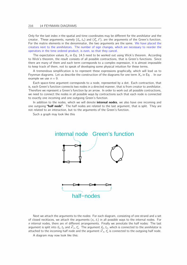
216 14 FEYNMAN DIAGRAMS
Only for the last index n the spatial and time coordinates may be different for the annihilator and thecreator. These arguments, namely (~xn, tn) and (~x ′n, t
′), are the arguments of the Green’s function.For the matrix elements in the denominator, the two arguments are the same. We have placed thecreators next to the annihilators. The number of sign changes, which are necessary to reorder theoperators in the time ordered product, is even, so that they cancel.
The expectation values Xn in Eq. 14.5 need to be worked out using Wick’s theorem. Accordingto Wick’s theorem, the result consists of all possible contractions, that is Green’s functions. Sincethere are many of them and each term corresponds to a complex expression, it is almost impossibleto keep track of them, not to speak of developing some physical intuition for these terms.
A tremendous simplification is to represent these expressions graphically, which will lead us toFeynman diagrams. Let us describe the construction of the diagrams for one term Xn in Eq. . In ourexample we use n = 9.
Each space-time argument corresponds to a node, represented by a dot. Each contraction, thatis, each Green’s function connects two nodes in a directed manner, that is from creator to annihilator.Therefore we represent a Green’s function by an arrow. In order to work out all possible contractions,we need to connect the nodes in all possible ways by contractions such that each node is connectedto exactly one incoming and one outgoing Green’s function.
In addition to the nodes, which we will denote internal nodes, we also have one incoming andone outgoing “half node” . The half nodes are related to the last argument, that is split. They arenot related to an interaction, but to the arguments of the Green’s function.
Such a graph may look like this
half−nodes
internal node Green’s function
Next we attach the arguments to the nodes: For each diagram, consisting of one strand and a setof closed necklaces, we attach the arguments (xi , ti) in all possible ways to the internal nodes. Forn internal nodes, there are n! different arrangements. Finally we annotate the half nodes: The lastargument is split into ~xn, tn and ~x ′n, t ′n. The argument ~xn, tn, which is connected to the annihilator isattached to the incoming half node and the argument ~x ′n, t ′n is connected to the outgoing half node.
A diagram may now look like this:
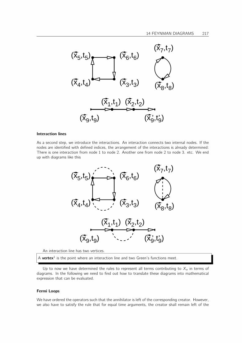
14 FEYNMAN DIAGRAMS 217
(x4,t4) (x3,t3)
(x5,t5) (x6,t6)(x7,t7)
(x8,t8)
(x1,t1) (x2,t2)
(x9,t9) (x9,t9)’’
Interaction lines
As a second step, we introduce the interactions. An interaction connects two internal nodes. If thenodes are identified with defined indices, the arrangement of the interactions is already determined:There is one interaction from node 1 to node 2. Another one from node 2 to node 3. etc. We endup with diagrams like this
(x4,t4) (x3,t3)
(x5,t5) (x6,t6)(x7,t7)
(x8,t8)
(x1,t1) (x2,t2)
(x9,t9) (x9,t9)’’
An interaction line has two vertices.
A vertex1 is the point where an interaction line and two Green’s functions meet.
Up to now we have determined the rules to represent all terms contributing to Xn in terms ofdiagrams. In the following we need to find out how to translate these diagrams into mathematicalexpression that can be evaluated.
Fermi Loops
We have ordered the operators such that the annihilator is left of the corresponding creator. However,we also have to satisfy the rule that for equal time arguments, the creator shall remain left of the
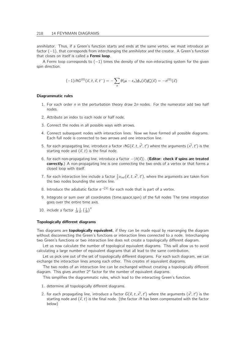
218 14 FEYNMAN DIAGRAMS
annihilator. Thus, if a Green’s function starts and ends at the same vertex, we must introduce anfactor (−1), that corresponds from interchanging the annihilator and the creator. A Green’s functionthat closes on itself is called a Fermi loop.
A Fermi loop corresponds to (−1) times the density of the non-interacting system for the givenspin direction.
(−1)i~G(0)(~x, t, ~x, t−) = −∑
n
θ(µ− ǫn)φn(~x)φ∗n(~x) = −n(0)(~x)
Diagrammatic rules
1. For each order n in the perturbation theory draw 2n nodes. For the numerator add two halfnodes.
2. Attribute an index to each node or half node.
3. Connect the nodes in all possible ways with arrows.
4. Connect subsequent nodes with interaction lines. Now we have formed all possible diagrams.Each full node is connected to two arrows and one interaction line.
5. for each propagating line, introduce a factor i~G(~x, t, ~x ′, t ′) where the arguments (~x ′, t ′) is thestarting node and (~x, t) is the final node.
6. for each non-propagating line, introduce a factor −〈n(~x)〉. (Editor: check if spins are treatedcorrectly.) A non-propagating line is one connecting the two ends of a vertex or that forms aclosed loop with itself.
7. for each interaction line include a factor 12vint(~x, t, ~x′, t ′), where the arguments are taken from
the two nodes bounding the vertex line.
8. Introduce the adiabatic factor e−ζ|t| for each node that is part of a vertex.
9. Integrate or sum over all coordinates (time,space,spin) of the full nodes The time integrationgoes over the entire time axis.
10. include a factor 1i~1n!
(1i~
)n
Topologically different diagrams
Two diagrams are topologically equivalent, if they can be made equal by rearranging the diagramwithout disconnecting the Green’s functions or interaction lines connected to a node. Interchangingtwo Green’s functions or two interaction line does not create a topologically different diagram.
Let us now calculate the number of topological equivalent diagrams. This will allow us to avoidcalculating a large number of equivalent diagrams that all lead to the same contribution.
Let us pick one out of the set of topologically different diagrams. For each such diagram, we canexchange the interaction lines among each other. This creates n! equivalent diagrams.
The two nodes of an interaction line can be exchanged without creating a topologically differentdiagram. This gives another 2n factor for the number of equivalent diagrams.
This simplifies the diagrammatic rules, which lead to the interacting Green’s function.
1. determine all topologically different diagrams.
2. for each propagating line, introduce a factor G(~x, t, ~x ′, t ′) where the arguments (~x ′, t ′) is thestarting node and (~x, t) is the final node. (the factor i~ has been compensated with the factorbelow)
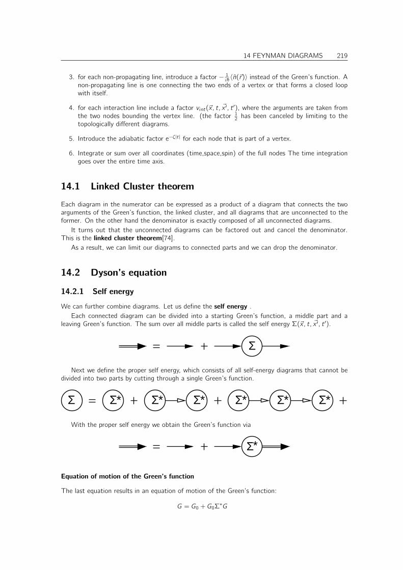
14 FEYNMAN DIAGRAMS 219
3. for each non-propagating line, introduce a factor − 1i~ 〈n(~r)〉 instead of the Green’s function. Anon-propagating line is one connecting the two ends of a vertex or that forms a closed loopwith itself.
4. for each interaction line include a factor vint(~x, t, ~x ′, t ′), where the arguments are taken fromthe two nodes bounding the vertex line. (the factor 12 has been canceled by limiting to thetopologically different diagrams.
5. Introduce the adiabatic factor e−ζ|t| for each node that is part of a vertex.
6. Integrate or sum over all coordinates (time,space,spin) of the full nodes The time integrationgoes over the entire time axis.
14.1 Linked Cluster theorem
Each diagram in the numerator can be expressed as a product of a diagram that connects the twoarguments of the Green’s function, the linked cluster, and all diagrams that are unconnected to theformer. On the other hand the denominator is exactly composed of all unconnected diagrams.
It turns out that the unconnected diagrams can be factored out and cancel the denominator.This is the linked cluster theorem[74].
As a result, we can limit our diagrams to connected parts and we can drop the denominator.
14.2 Dyson’s equation
14.2.1 Self energy
We can further combine diagrams. Let us define the self energy .Each connected diagram can be divided into a starting Green’s function, a middle part and a
leaving Green’s function. The sum over all middle parts is called the self energy Σ(~x, t, ~x ′, t ′).
Σ
Next we define the proper self energy, which consists of all self-energy diagrams that cannot bedivided into two parts by cutting through a single Green’s function.
ΣΣ Σ Σ ΣΣΣ ******
With the proper self energy we obtain the Green’s function via
Σ*
Equation of motion of the Green’s function
The last equation results in an equation of motion of the Green’s function:
G = G0 + G0Σ∗G
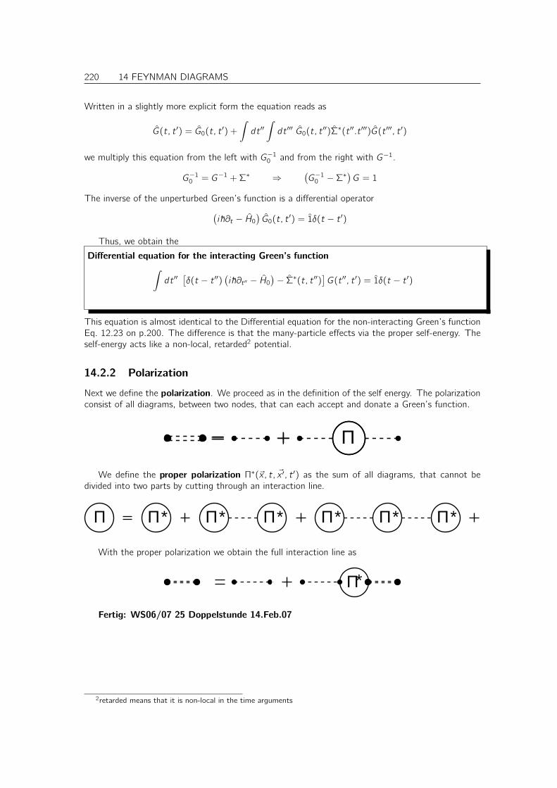
220 14 FEYNMAN DIAGRAMS
Written in a slightly more explicit form the equation reads as
G(t, t ′) = G0(t, t′) +
∫
dt ′′∫
dt ′′′ G0(t, t′′)Σ∗(t ′′.t ′′′)G(t ′′′, t ′)
we multiply this equation from the left with G−10 and from the right with G−1.
G−10 = G−1 +Σ∗ ⇒
(G−10 −Σ∗
)G = 1
The inverse of the unperturbed Green’s function is a differential operator(i~∂t − H0
)G0(t, t
′) = 1δ(t − t ′)
Thus, we obtain the
Differential equation for the interacting Green’s function
∫
dt ′′[δ(t − t ′′)
(i~∂t ′′ − H0
)− Σ∗(t, t ′′)
]G(t ′′, t ′) = 1δ(t − t ′)
This equation is almost identical to the Differential equation for the non-interacting Green’s functionEq. 12.23 on p.200. The difference is that the many-particle effects via the proper self-energy. Theself-energy acts like a non-local, retarded2 potential.
14.2.2 Polarization
Next we define the polarization. We proceed as in the definition of the self energy. The polarizationconsist of all diagrams, between two nodes, that can each accept and donate a Green’s function.
Π
We define the proper polarization Π∗(~x, t, ~x ′, t ′) as the sum of all diagrams, that cannot bedivided into two parts by cutting through an interaction line.
******Π Π Π Π Π Π Π
With the proper polarization we obtain the full interaction line as
*Π
Fertig: WS06/07 25 Doppelstunde 14.Feb.07
2retarded means that it is non-local in the time arguments
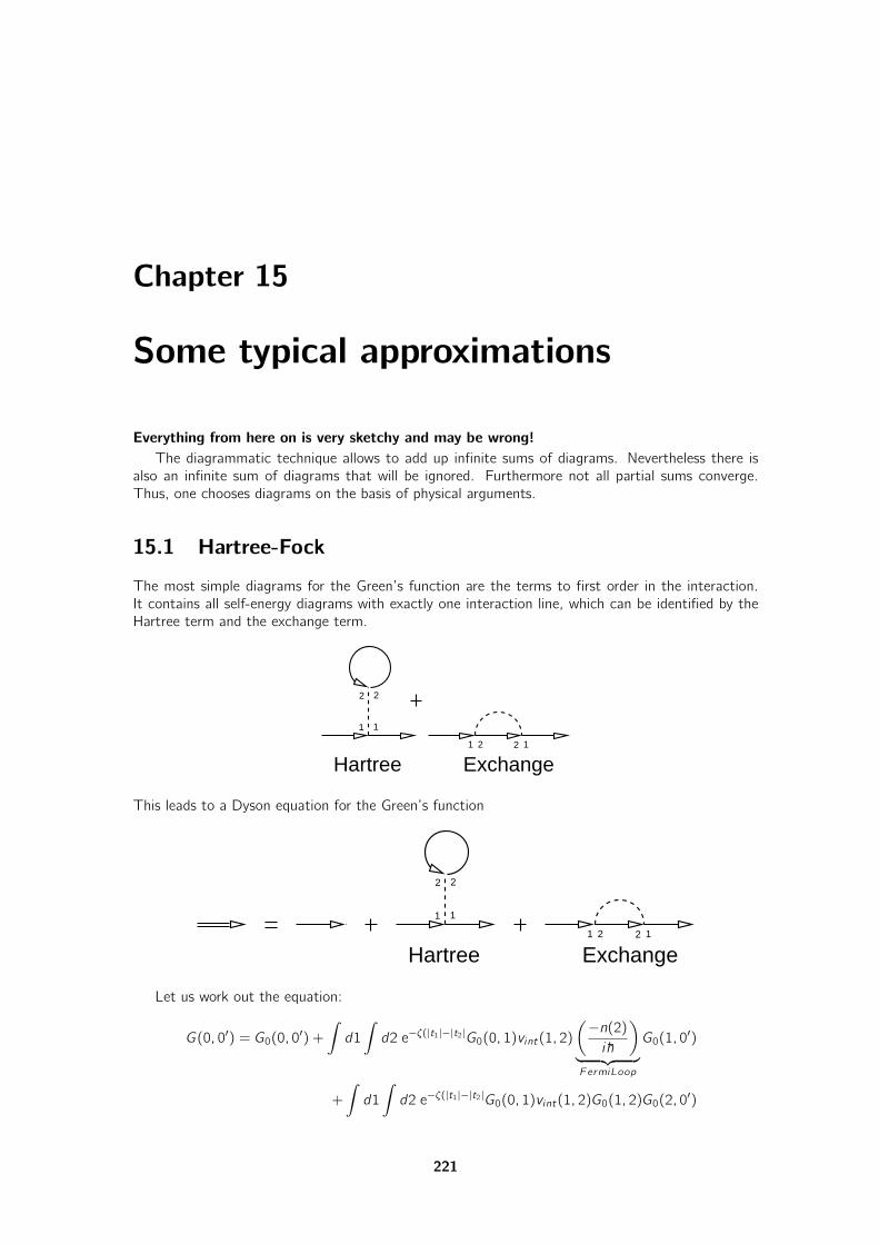
Chapter 15
Some typical approximations
Everything from here on is very sketchy and may be wrong!
The diagrammatic technique allows to add up infinite sums of diagrams. Nevertheless there isalso an infinite sum of diagrams that will be ignored. Furthermore not all partial sums converge.Thus, one chooses diagrams on the basis of physical arguments.
15.1 Hartree-Fock
The most simple diagrams for the Green’s function are the terms to first order in the interaction.It contains all self-energy diagrams with exactly one interaction line, which can be identified by theHartree term and the exchange term.
Hartree Exchange1
1 1
22
2 2 1
This leads to a Dyson equation for the Green’s function
Exchange1 2 2 1
Hartree
1 1
22
Let us work out the equation:
G(0, 0′) = G0(0, 0′) +
∫
d1
∫
d2 e−ζ(|t1|−|t2|G0(0, 1)vint(1, 2)
(−n(2)i~
)
︸ ︷︷ ︸
FermiLoop
G0(1, 0′)
+
∫
d1
∫
d2 e−ζ(|t1|−|t2|G0(0, 1)vint(1, 2)G0(1, 2)G0(2, 0′)
221
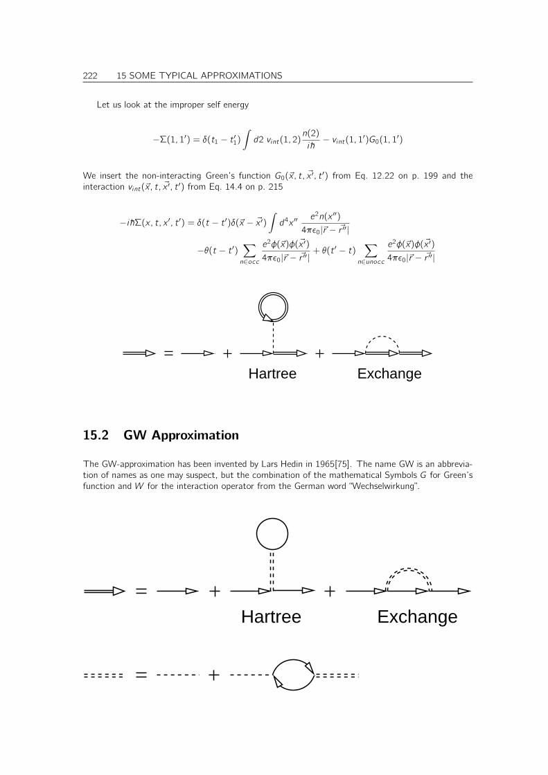
222 15 SOME TYPICAL APPROXIMATIONS
Let us look at the improper self energy
−Σ(1, 1′) = δ(t1 − t ′1)∫
d2 vint(1, 2)n(2)
i~− vint(1, 1′)G0(1, 1′)
We insert the non-interacting Green’s function G0(~x, t, ~x ′, t ′) from Eq. 12.22 on p. 199 and theinteraction vint(~x, t, ~x ′, t ′) from Eq. 14.4 on p. 215
−i~Σ(x, t, x ′, t ′) = δ(t − t ′)δ(~x − ~x ′)∫
d4x ′′e2n(x ′′)
4πǫ0|~r − ~r ′′|
−θ(t − t ′)∑
n∈occ
e2φ(~x)φ(~x ′)
4πǫ0|~r − ~r ′′|+ θ(t ′ − t)
∑
n∈unocc
e2φ(~x)φ(~x ′)
4πǫ0|~r − ~r ′′|
Hartree Exchange
15.2 GW Approximation
The GW-approximation has been invented by Lars Hedin in 1965[75]. The name GW is an abbrevia-tion of names as one may suspect, but the combination of the mathematical Symbols G for Green’sfunction and W for the interaction operator from the German word “Wechselwirkung”.
Hartree Exchange
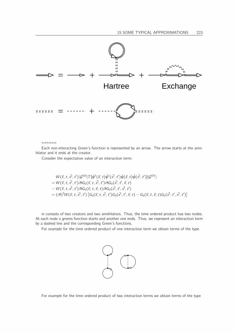
15 SOME TYPICAL APPROXIMATIONS 223
Hartree Exchange
======Each non-interacting Green’s function is represented by an arrow. The arrow starts at the anni-
hilator and it ends at the creator.Consider the expectation value of an interaction term:
W (~x, t, ~x ′, t ′)〈G(0)|T [ψ†(~x, t)ψ†(~x ′, t ′)ψ(~x, t)ψ(~x ′, t ′)]|G(0)〉= W (~x, t, ~x ′, t ′)i~G0(~x, t, ~x ′, t
′)i~G0(~x ′, t′, ~x, t)
− W (~x, t, ~x ′, t ′)i~G0(~x, t, ~x, t)i~G0(~x ′, t ′, ~x ′, t ′)= (i~)2W (~x, t, ~x ′, t ′)
[G0(~x, t, ~x ′, t
′)G0(~x ′, t′, ~x, t)− G0(~x, t, ~x, t)G0(~x ′, t ′, ~x ′, t ′)
]
in consists of two creators and two annihilators. Thus, the time ordered product has two nodes.At each node a greens function starts and another one ends. Thus, we represent an interaction termby a dashed line and the corresponding Green’s functions.
For example for the time ordered product of one interaction term we obtain terms of the type
For example for the time ordered product of two interaction terms we obtain terms of the type
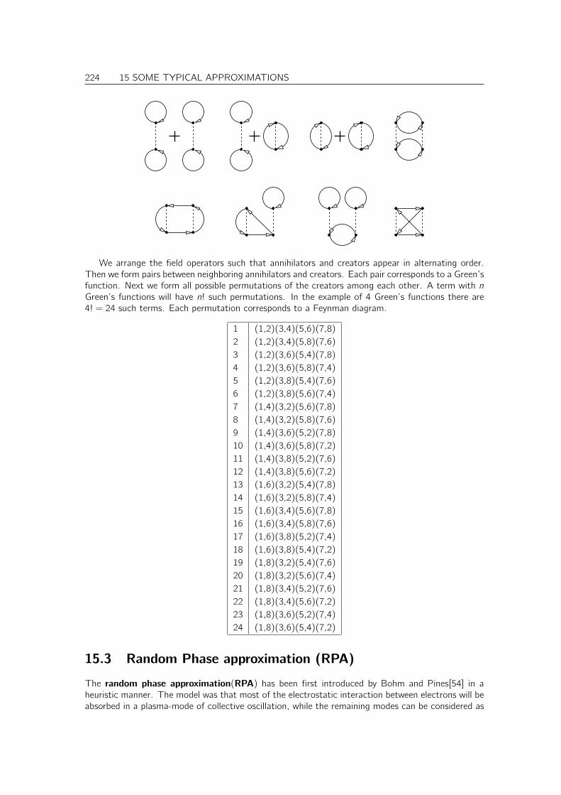
224 15 SOME TYPICAL APPROXIMATIONS
We arrange the field operators such that annihilators and creators appear in alternating order.Then we form pairs between neighboring annihilators and creators. Each pair corresponds to a Green’sfunction. Next we form all possible permutations of the creators among each other. A term with nGreen’s functions will have n! such permutations. In the example of 4 Green’s functions there are4! = 24 such terms. Each permutation corresponds to a Feynman diagram.
1 (1,2)(3,4)(5,6)(7,8)2 (1,2)(3,4)(5,8)(7,6)3 (1,2)(3,6)(5,4)(7,8)4 (1,2)(3,6)(5,8)(7,4)5 (1,2)(3,8)(5,4)(7,6)6 (1,2)(3,8)(5,6)(7,4)7 (1,4)(3,2)(5,6)(7,8)8 (1,4)(3,2)(5,8)(7,6)9 (1,4)(3,6)(5,2)(7,8)10 (1,4)(3,6)(5,8)(7,2)11 (1,4)(3,8)(5,2)(7,6)12 (1,4)(3,8)(5,6)(7,2)13 (1,6)(3,2)(5,4)(7,8)14 (1,6)(3,2)(5,8)(7,4)15 (1,6)(3,4)(5,6)(7,8)16 (1,6)(3,4)(5,8)(7,6)17 (1,6)(3,8)(5,2)(7,4)18 (1,6)(3,8)(5,4)(7,2)19 (1,8)(3,2)(5,4)(7,6)20 (1,8)(3,2)(5,6)(7,4)21 (1,8)(3,4)(5,2)(7,6)22 (1,8)(3,4)(5,6)(7,2)23 (1,8)(3,6)(5,2)(7,4)24 (1,8)(3,6)(5,4)(7,2)
15.3 Random Phase approximation (RPA)
The random phase approximation(RPA) has been first introduced by Bohm and Pines[54] in aheuristic manner. The model was that most of the electrostatic interaction between electrons will beabsorbed in a plasma-mode of collective oscillation, while the remaining modes can be considered as

15 SOME TYPICAL APPROXIMATIONS 225
weakly interacting electrons with a screened interaction potential. Gell-Mann and Brueckner derivedthe random phase approximation by summing leading order chain Feynman diagrams[76]. A moresystematic treatment that that of Bohm and Pines has been given by Nozieres and Pines[? ](see[77]).

226 15 SOME TYPICAL APPROXIMATIONS
Chapter 16
Models in many-particle theory
16.1 Dominant interactions
WEq. 8.9=1
2
∑
i ,j,k,l
Wa,b,c,d c†a c†b cd cc
Wa,b,c,dEq. 8.3=
∫
d4x
∫
d4x ′ φ∗a(~x)φ∗b(~x′)
e2
4π|~r − ~r ′|φd(~x)φc(~x ′)
We choose spin orbitals, which are eigenstates of sz , i.e.
〈~r , σ|φna,σa〉 = δσ,σaφn(~r)
This already limits the number of non-vanishing matrix elements
WEq. 8.9=1
2
∑
i ,j,k,l
Wa,b,c,d c†a c†b cd cc
Wa,b,c,dEq. 8.3= δσa,σd δσb,σc
∫
d3r
∫
d3r ′ φ∗na(~r)φnd (~r)e2
4π|~r − ~r ′|φ∗nb(
~r ′)φnc (~r ′)
Now we pick out only the dominant matrix elements. These are the Coulomb integrals Ki ,j andthe exchange integrals Ji ,j . (Note that chemists use the symbols in the opposite way.)
Ki ,j =1
2
∫
d3r
∫
d3r ′ φ∗i (~r)φi(~r)e2
4π|~r − ~r ′|φ∗j (~r
′)φj(~r ′)
Ji ,j =1
2
∫
d3r
∫
d3r ′ φ∗i (~r)φj(~r)e2
4π|~r − ~r ′|φ∗j (~r
′)φi(~r ′)
The rationale for the selection is that the matrix element is the Coulomb interaction of two densities.If the orbitals |φ(~r)〉 are orthonormal, each of the density is charge neutral unless the two orbitals areidentical. Thus, the dominant contribution is Ki ,j where the densities are not neutral. The Matrixelements Ki ,j are long-ranged, but can be approximated as
Ki ,j|Ri−Rj |→∞→ e2
4π|~Ri − ~Rj |
where Ri and ~Rj are centers of the respective orbitals.The exchange matrix elements Ji ,j describe the electrostatic interaction of neutral densities. Thus,
they contribute effectively only if the two densities overlap. Considering local orbitals it makes sense
227
228 16 MODELS IN MANY-PARTICLE THEORY
to consider only the interaction of identical pairs. Note, however, that this limitation becomes invalidas we take more and more orbitals.
If we limit the interaction matrix elements only to those terms, we obtain
Wa,b,c,d = δσa,σd δσb,σc
(
δna,nd δnb,ncKna,nb + δna,nc δnb,nd (1− δna,nb)Jna,nb)
The factor (1− δna,nb) takes into account that Ki ,i = Ji ,i , in order to avoid double counting.Thus, the dominant part of the interaction has the form1
W =1
2
∑
σ,σ′
∑
i ,j
Ki ,j c†i ,σ c
†j,σ′ cj,σ′ ci ,σ +
1
2
∑
σ,σ′
∑
i 6=jJi ,j c
†i ,σ c
†j,σ′ ci ,σ′ cj,σ
=1
2
∑
σ,σ′
∑
i ,j
Ki ,j c†i ,σ ci ,σ c
†j,σ′ cj,σ′ −
1
2
∑
σ,σ′
∑
i 6=jJi ,j c
†i ,σ ci ,σ′ c
†j,σ′ cj,σ
− 12
∑
σ
∑
i
Ki ,i c†i ,σ ci ,σ
=1
2
∑
σ,σ′
∑
i 6=jKi ,j c
†i ,σ ci ,σ c
†j,σ′ cj,σ′ −
1
2
∑
σ,σ′
∑
i 6=jJi ,j c
†i ,σ ci ,σ′ c
†j,σ′ cj,σ
+∑
i
Ki ,i c†i ,↑ci ,↑c
†i ,↓ci ,↓
The parameter Ki ,i is the so-called U-parameter
Udef= Ki ,i
It will be helpful to replace the creation and annihilation operators by orbital occupation and spinoperators.
ni = c†i ,↑ci ,↑ + c
†i ,↓ci ,↓
~Si =~
2
(
c†i ,↑c†i ,↓
)
~σ
(
c†i ,↑c†i ,↓
)
Si ,x =~
2
(
c†i ,↑ci ,↓ + c†i ,↓ci ,↑
)
Si ,y = −i~
2
(
c†i ,↑ci ,↓ − c†i ,↓ci ,↑
)
Si ,z =~
2
(
c†i ,↑ci ,↑ − c†i ,↓ci ,↓
)
Si ,+ = Si ,x + i Si ,y = ~c†i ,↑ci ,↓
Si ,− = Si ,x − i Si ,y = ~c†i ,↓ci ,↑
1
c†i ,σ c
†j,σ′ cj,σ′ ci ,σ = −c
†i ,σ c
†j,σ′ ci ,σ cj,σ′ = −δi ,jδσ,σ′ c
†i ,σ cj,σ′ + c
†i ,σ ci ,σ c
†j,σ′ cj,σ′
c†i ,σ c
†j,σ′ ci ,σ′ cj,σ = c
†i ,σδi ,j cj,σ c
†i ,σ ci ,σ′ c
†j,σ′ cj,σ
16 MODELS IN MANY-PARTICLE THEORY 229
Thus, we obtain
∑
σ,σ′
c†i ,σ ci ,σ′ c†j,σ′ cj,σ =
(1
2ni +
1
~Si ,z
)(1
2nj +
1
~Sj,z
)
+1
~2Si ,+Sj,− +
1
~2Si ,−Sj,+ +
(1
2ni −
1
~Si ,z
)(1
2nj −
1
~Sj,z
)
=1
2ni nj +
1
~2
(Si ,x + i Si ,y
) (Sj,x − i Sj,y
)+1
~2
(Si ,x − i Si ,y
) (Sj,x + i Sj,y
)− 2~2Si ,z Sj,z
=1
2ni nj +
2
~2Si ,x Sj,x +
2
~2Si ,y Sj,y +
2
~2Si ,z Sj,z
=1
2ni nj +
2
~2~Si ~Sj
Thus, we obtain
W =1
2
∑
i 6=jKi ,j ni nj −
1
2
∑
i 6=jJi ,j
(1
2ni nj +
2
~2~Si ~Sj
)
+∑
i
Ki ,i c†i ,↑ci ,↑c
†i ,↓ci ,↓
=1
2
∑
i 6=j
(
Ki ,j − Ji ,j)
ni nj −1
~2
∑
i 6=jJi ,j ~Si ~Sj +
∑
i
Ki ,i c†i ,↑ci ,↑c
†i ,↓ci ,↓
The last term is the Hubbard interaction
HUBBARD INTERACTION
WHubbarddef=∑
i
Ki ,i c†i ,↑ci ,↑c
†i ,↓ci ,↓
The Hubbard interaction describes the Coulomb repulsion of two electrons in the same spatial orbital.
HUND COUPLING
The interaction term proportional to the exchange integrals J is called Hund coupling.
WHunddef= −1
2
∑
i 6=jJi ,j ni nj −
1
~2
∑
i 6=jJi ,j ~Si ~Sj
Hund’s coupling causes spins to align parallel.
16.2 Hubbard model
The original Hubbard model was suggested in 1963 independently by Hubbard[? ], Kanamori andGutzwiller[78]. It describes a lattice of atoms with a single orbital on each atom, which has a largeCoulomb repulsion on each site.
H = −t∑
i
∑
σ
(
c†i ,σ ci+1,σ c†i+1,σ ci+1,σ
)
+ U∑
i
ni ,↑ni ,↓ + V∑
i
nini ,i+1
t is the hopping integral and U is the Coulomb parameter. V is the Coulomb repulsion of electronson two neighboring sites.
The one-dimensional Hubbard model has been solved by Lieb and Wu[79]. For half-filling theHubbard model describes a Mott insulator.
230 16 MODELS IN MANY-PARTICLE THEORY
16.3 t-J model
http://www-public.tu-bs.de:8080/~honecker/rgp/q-mod/
Nehmen wir an dass die Hubbard Wechselwirkung so gross ist, dass Zustaende mit einer Dop-pelbesetzung eines Gitterplatzes nicht mehr beitragen, dann erhält man aus dem Allgemeinen Modelldas t-J Modell.
H = −tP∑
i
∑
σ
(
c†i ,σ ci+1,σ c†i+1,σ ci+1,σ
)
P + J∑
i
~Si ~Si+1
where P projects out doubly occupied sites.
• For half filling the t-J model reduces to the heisenberg model
• The hubbard model for U»t is equivalent to the t-J model. In second order perturbation theoryone finds J = 4t2
U
16.4 Heisenberg model
H = J∑
i
~Si ~Si+1
16.5 Anderson impurity model
The Anderson model[80], named after its inventor P.W. Anderson2, describes an impurity of largeCoulomb repulsion in a normal metal. This model explains the formation of a local magnetic momenton the impurity atom.
The Anderson Hamiltonian has the form
H =∑
~k,σ
ǫk n~k,σ +∑
σ
ǫd nd,σ − ∆∑
~k
(
c†k,σdσ + d†σ ck,σ
)
+ Und,↑nd,↓
We used the creation and annihilation operators d†σ and dσ in the localized impurity level and itsnumber operator nd,σ = d†σdσ. The creation and annihilation operators in the Bloch states of thenormal metal are c†~k,σ and c~k,σ, and the corresponding number operator is n~k,σ := c
†~k,σc~k,σ. The index
σ denotes the spin quantum number, which can have values ↑ or ↓.The first term describes the one-particle energies of the normal metal and the second describes
the one-particle levels of the localized impurity. The third term describes the coupling between theimpurity and the band states. So far all terms are simple one-electron terms. The many-particleproblem enters with the last term that describes the Coulomb repulsion of the electrons in thelocalized orbital.
We could as well write the Hamiltonian as
H =∑
i ,σ
ǫi c†i ,σ ci ,σ +
∑
i ,j,σ
ti ,j
(
c†i ,σ cj,σ + ci ,σ c†j,σ
)
+∑
σ
ǫd d†σdσ
−∆∑
i ,σ
(
c†i ,σdσ + d†σ ci ,σ
)
+ Und,↑nd,↓
Here, we consider the Wannier functions localized on the sites of the normal metal, which make upthe Bloch states. The creation and annihilation operators are denoted by c†i ,σ and ci ,σ.
The Anderson model includes normal metal states also at the site of the impurity. This makessense because also a transition metal has s- and p-electrons, that however lie at different energies.
2P.W. Anderson, American physicist born 1923. Obtained the Nobel price in physics 1977. Anderson localizationdescribes how electron states become localized in an disordered material. more...
16 MODELS IN MANY-PARTICLE THEORY 231
16.5.1 The interaction energy
The U-parameter is defined as[80]
U =e2
4πǫ0
∫
d3r
∫
d3r ′φ∗d(~r)φd(~r)φ
∗d(~r ′)φd(~r ′)
|~r − ~r ′|
where φd(~r) is the wave function of a localized orbital.According to Eq. 8.9 the interaction energy has the form
W =1
2
∑
i ,j,k,l
Wi ,j,k,l c†i c†j cl ck
where Wi ,j,k,l is given,according to Eq. 8.3, by
Wi ,j,k,l =e2
4πǫ0
∫
d4x
∫
d4x ′φ∗i (~x)φ
∗j (~x ′)φk(~x)φ∗l (~x
′)
|~r − ~r ′|
In our case we just have two states, one for the spin up and one for spin down electron. Thus,the orbital indices can assume two values i =↑ and i =↓. The spinor wave functions are
φσ(~r , σ′) = φd(~r)δσ,σ′
where φd(~r) is simply the spatial part of the orbital. The product of two spinors, that are spin-eigenstates, is only non-zero, when both wave functions have the same spin.
Wσ1,σ2,σ3,σ4 =e2
4πǫ0
∑
σ,σ′
∫
d4r
∫
d4r ′
φ∗σ1 (~x)︷ ︸︸ ︷
φ∗d(~r)δ(σ1, σ)
φ∗σ2 (~x ′)
︷ ︸︸ ︷
φ∗d(~r′)δ(σ2, σ
′)
φσ3 (~x)︷ ︸︸ ︷
φd(~r)δ(σ3, σ)
φσ4 (~x ′)
︷ ︸︸ ︷
φ∗l (~r′)δ(σ4, σ
′)
|~r − ~r ′|
=e2
4πǫ0
∑
σ,σ′
δ(σ1, σ)δ(σ2, σ′)δ(σ3, σ)δ(σ4, σ
′)
∫
d4r
∫
d4r ′φ∗d(~r)φ
∗d(~r ′)φd(~r)φ∗l (~r
′)
|~r − ~r ′|= Uδ(σ1, σ3)δ(σ2, σ4)
W =U
2
∑
σ,σ′
d†σd†σ′ dσ′ dσ =
U
2
∑
σ,σ′
[
−d†σδσ′,σdσ′ + d†σdσd†σ′ dσ′]
= −U2(nd,↑ + nd,↓) +
U
2
∑
σ,σ′
nd,σnd,σ′
= −U2(nd,↑ + nd,↓) +
U
2
(n2d,↑ + nd,↑nd,↓ + nd,↓nd,↑ + n
2d,↓)
= Und,↓nd,↑
We used that n2d,σ = nd,σ and that nd,↑nd,↓ = nd,↓nd,↑.
16.5.2 Mean field approximation
Editor: Not ready yet
We can develop a mean field solution by replacing
nd,σ = 〈nd,σ〉+ (nd,σ − 〈nd,σ〉)

232 16 MODELS IN MANY-PARTICLE THEORY
Chapter 17
Zoo of Concepts from Solid StatePhysics
This is nothing than a collection of material for myself.
• Bloch electron (<-> Fermi liquid?), hole
• phonon
• photon,
• magnon, spin wave, Bloch[81]
• polaron, Zener polaron (phonon+electron)
• Polariton (light-phonon, light-plasmon)
• Soliton
• plasmon
• exciton (electron-hole)
• First order/second order phase transition
• Jahn-Teller effect
• Peierls distortion
• Nesting
• Orbital ordering
• Fermi liquid
• Luttinger liquid
• Mott insulator/ Band insulator
• Heavy Fermion
• Superconductivity
• Kondo Effect
• Stoner Magnetism
233

234 17 ZOO OF CONCEPTS FROM SOLID STATE PHYSICS
• Super exchange
• Double exchange
• Multiferroics (See article by Khomskii[82])
• Pseudogap
• Crystal Field splitting, 10Dt (M. Lezaic, in Electronic Oxides. Lecture notes of the 41th IFFSpring school 2010, Stefan Blüegel et al, Eds., Schriften des Forschungszentrums Jülich)
• Topological insulator
• Anderson Localization
• Conductance quantization
• Quantum Hall effect
• Pomeranchuk instability
• van Hove Singularity
• quantum critical phase: Popular introduction
Models
• Ising model
• t-J-model
• Heisenberg model
• Hubbard model
Methods
• Mean Field approximation
• saddle point approximation
• DCA
• Coherent Potential approximation
• Virtual Potential approximation
• Lanczos method, exact diagonalization
• NRG
• Dynamical matrix renormalization theory (DMRG): [83]. See also K.H. Marti and M. Reiher,in Progress in Physical Chemistry Vol. 3, Modern and Universal First-principles Methods for
Many-electron Systems in Chemistry and Physics, (Oldenburg Verlag, p293)
• Dynamical mean-field theory (DMFT)
• reduced-density-matrix functional theory (rDMFT)
• Quantum Monte Carlo
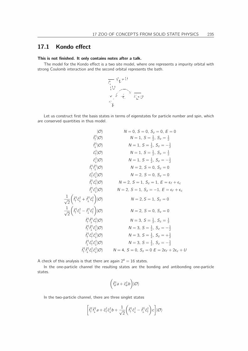
17 ZOO OF CONCEPTS FROM SOLID STATE PHYSICS 235
17.1 Kondo effect
This is not finished. It only contains notes after a talk.
The model for the Kondo effect is a two site model, where one represents a impurity orbital withstrong Coulomb interaction and the second orbital represents the bath.
Let us construct first the basis states in terms of eigenstates for particle number and spin, whichare conserved quantities in thus model.
|O〉 N = 0, S = 0, Sz = 0, E = 0
f †↑ |O〉 N = 1, S = 12 , Sz =
12
f †↓ |O〉 N = 1, S = 12 , Sz = − 12
c†↑ |O〉 N = 1, S = 12 , Sz =
12
c†↓ |O〉 N = 1, S = 12 , Sz = − 12
f †↑ f†↓ |O〉 N = 2, S = 0, Sz = 0
c†↑ c†↓ |O〉 N = 2, S = 0, Sz = 0
f †↑ c†↑ |O〉 N = 2, S = 1, Sz = 1, E = ǫf + ǫc
f †↓ c†↓ |O〉 N = 2, S = 1, Sz = −1, E = ǫf + ǫc
1√2
(
f †↑ c†↓ + f
†↓ c†↑
)
|O〉 N = 2, S = 1, Sz = 0
1√2
(
f †↑ c†↓ − f
†↓ c†↑
)
|O〉 N = 2, S = 0, Sz = 0
f †↑ f†↓ c†↑ |O〉 N = 3, S = 1
2 , Sz =12
f †↑ f†↓ c†↓ |O〉 N = 3, S = 1
2 , Sz = − 12f †↑ c†↑ c†↓ |O〉 N = 3, S = 1
2 , Sz = +12
f †↓ c†↑ c†↓ |O〉 N = 3, S = 1
2 , Sz = − 12f †↑ f†↓ c†↑ c†↓ |O〉 N = 4, S = 0, Sz = 0 E = 2ǫf + 2ǫc + U
A check of this analysis is that there are again 24 = 16 states.In the one-particle channel the resulting states are the bonding and antibonding one-particle
states.
(
f †σ a + c†σb
)
|O〉
In the two-particle channel, there are three singlet states
[
f †↑ f†↓ a + c
†↑ c†↓b +
1√2
(
f †↑ c†↓ − f
†↓ c†↑
)
c
]
|O〉
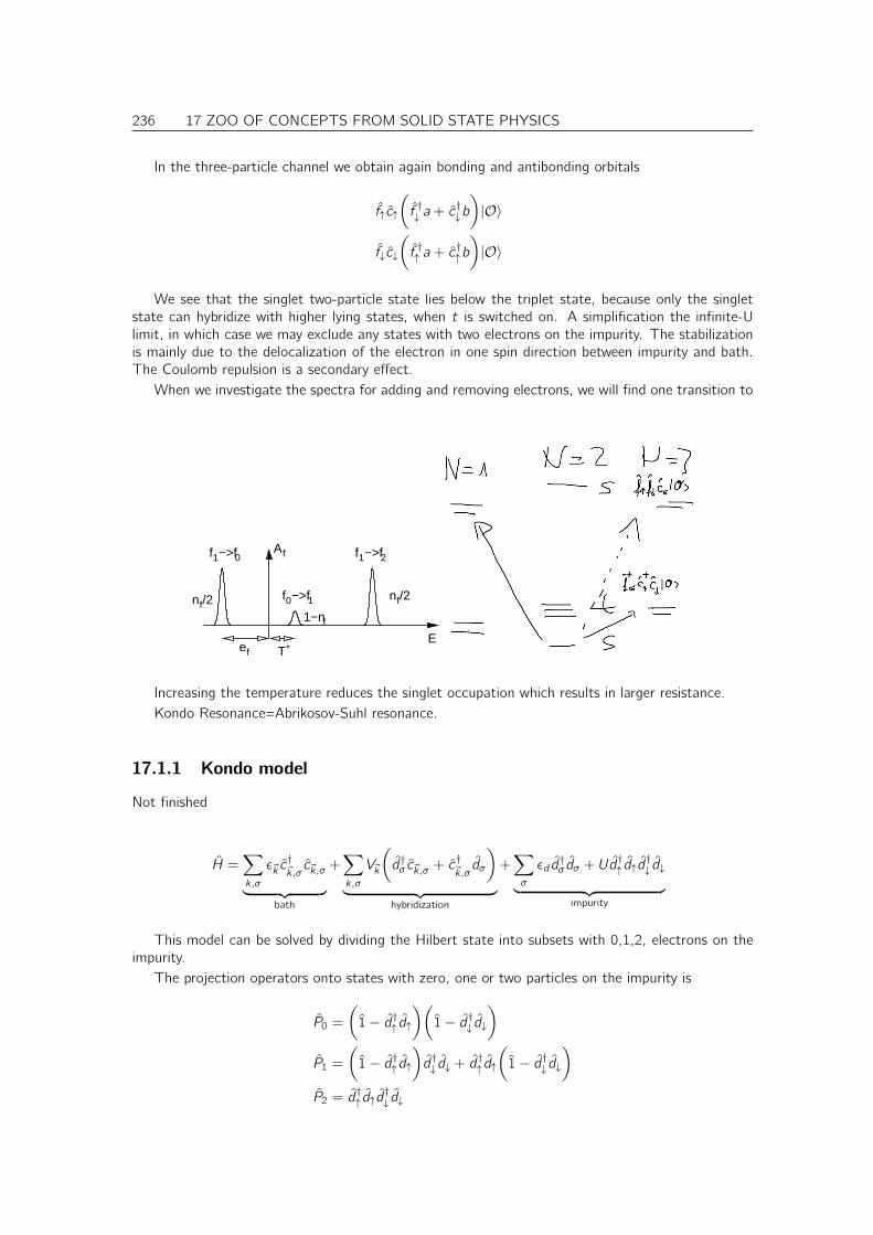
236 17 ZOO OF CONCEPTS FROM SOLID STATE PHYSICS
In the three-particle channel we obtain again bonding and antibonding orbitals
f↑c↑
(
f †↓ a + c†↓b
)
|O〉
f↓c↓
(
f †↑ a + c†↑b
)
|O〉
We see that the singlet two-particle state lies below the triplet state, because only the singletstate can hybridize with higher lying states, when t is switched on. A simplification the infinite-Ulimit, in which case we may exclude any states with two electrons on the impurity. The stabilizationis mainly due to the delocalization of the electron in one spin direction between impurity and bath.The Coulomb repulsion is a secondary effect.
When we investigate the spectra for adding and removing electrons, we will find one transition to
E*
f1−>f0 f1−>f2
f0−>f1nf/2nf/2
f1−n
fA
ef T
Increasing the temperature reduces the singlet occupation which results in larger resistance.Kondo Resonance=Abrikosov-Suhl resonance.
17.1.1 Kondo model
Not finished
H =∑
k,σ
ǫ~k c†~k,σc~k,σ
︸ ︷︷ ︸
bath
+∑
k,σ
V~k
(
d†σ c~k,σ + c†~k,σdσ
)
︸ ︷︷ ︸
hybridization
+∑
σ
ǫd d†σdσ + Ud
†↑ d↑d
†↓ d↓
︸ ︷︷ ︸
impurity
This model can be solved by dividing the Hilbert state into subsets with 0,1,2, electrons on theimpurity.
The projection operators onto states with zero, one or two particles on the impurity is
P0 =
(
1− d†↑ d↑)(
1− d†↓ d↓)
P1 =
(
1− d†↑ d↑)
d†↓ d↓ + d†↑ d↑
(
1− d†↓ d↓)
P2 = d†↑ d↑d
†↓ d↓
17 ZOO OF CONCEPTS FROM SOLID STATE PHYSICS 237
The projection operators can be rewritten in the form
P0 = 1−∑
σ
d†σdσ + P2
P1 =∑
σ
d†σdσ − 2P2
P2 = d†↑ d↑d
†↓ d↓
One can easily show that the three projection operators add up to the unity operator.
2∑
j=0
Pj = 1
This allows us to decompose the Hamiltonian according to
H =
2∑
i ,j=0
Pi HPj︸ ︷︷ ︸
Hi ,j
=
2∑
i ,j=0
Hi ,j
The individual blocks are
H00 =∑
k,σ
ǫ~k c†~k,σc~k,σP0 = HbathP0
H11 =
(∑
k,σ
ǫ~k c†~k,σc~k,σ + ǫd
)
P1 = (Hbath + ǫd)P1
H22 =
(∑
k,σ
ǫ~k c†~k,σc~k,σ + 2ǫd + U
)
P2 = (Hbath + 2ǫd + U)P2
H01 =∑
~k
V~k c†~k,σdσP1
H12 =∑
~k
V~k c†~k,σdσP2
H02 = 0
The annihilation operator dσ in H01 is needed to specify the spin of the electron to be deleted andbecause it may induce a sign change.
All energy contributions except the hybridization term conserve the number of electrons on theimpurity. Therefore these terms are diagonal in a representation with fixed number of electrons onthe impurity. The hybridization term is then the coupling between states with different numbers ofimpurity electrons.
Formally Eliminate the zero and two-particle contribution from the Schrödinger equation
Next we determine the wave function, which may contain zero, one and two electrons on the impurityas
|Ψ〉 = |Ψ0〉+ |Ψ1〉+ |Ψ2〉
(H00 − E)|Ψ0〉+ H01|Ψ1〉 = 0H10|Ψ0〉+ (H11 − E)|Ψ1〉+ H12|Ψ2〉 = 0
H21|Ψ1〉+ (H22 − E)|Ψ2〉 = 0
238 17 ZOO OF CONCEPTS FROM SOLID STATE PHYSICS
The first and the last equations relate the contribution with zero and two particles on the impurityto that with one particle on the impurity
|Ψ0〉 = −(H00 − E)−1H01|Ψ1〉|Ψ2〉 = −(H22 − E)−1H21|Ψ1〉
Insertion into the middle equation yields
(
H11 − E − H10(H00 − E)−1H01 − H12(H22 − E)−1H21)
|Ψ1〉 = 0
Note that |Ψ1〉 is only part of the state and therefore it is not normalized.
Substitute the Hamiltonian
Let us evaluate
(
E − H22)(
P0 + P1 + P2
)
︸ ︷︷ ︸
1
= EP0 + EP1 +
(
E − Hbath − 2ǫd − U)
P2
(
H22 − E)−1
=1
EP0 +
1
EP1 +
(
E − Hbath − 2ǫd − U)−1
P2
H12
(
H22 − E)−1
H21 =∑
~k,σ
V ∗~k P1c†~k,σdσP2
(
E − Hbath − 2ǫd − U)−1
P2∑
~k ′,σ′
V~k ′ d†σ′ c~k ′,σ′ P1
=∑
~k,σ
∑
~k ′,σ′
V ∗~k V~k ′ P1c†~k,σdσP2
(
E − Hbath − 2ǫd − U)−1
P2d†σ′ c~k ′,σ′ P1
=∑
~k,σ
∑
~k ′,σ′
V ∗~k V~k ′ c†~k,σ
(
E − Hbath − 2ǫd − U)−1
c~k ′,σ′ P1dσP2P2d†σ′ P1
All bath operators c†~k,σ, c~k,σ anticommutate with the impurity operators. The projection operatorsand the bath Hamiltonian contain even products of creation and annihilation operators and thereforecommutate with the creation operators of bath and impurity respectively. When we shift the impurityoperators to the right we experience two sign changes, which do not have a net effect.
P1dσP2P2d†σ′ P1 =
(∑
σ′′
d†σ′′ dσ′′ − 2P2)
dσP2d†σ′
(∑
σ′′′
d†σ′′ dσ′′′ − 2P2)
=
(∑
σ′′
d†σ′′ dσ′′
)
dσ
(
d†↑ d↑d†↓ d↓
)
d†σ′
(∑
σ′′′
d†σ′′′ dσ′′′
)
=
(
d†−σd−σ
)
dσ
(
d†↑ d↑d†↓ d↓
)
d†σ′
(
d†−σ′ d−σ′
)
= dσ
(
d†−σd−σ
)(
d†↑ d↑d†↓ d↓
)(
d†−σ′ d−σ′
)
d†σ′
= dσ
(
d†↑ d↑d†↓ d↓
)
d†σ′
17 ZOO OF CONCEPTS FROM SOLID STATE PHYSICS 239
d↑
(
d†↑ d↑d†↓ d↓
)
d†↑ =
(
1− d†↑ d↑)
d↑d†↓ d↓d
†↑ = −d
†↑ d↑d
†↓ d↓
d↑
(
d†↑ d↑d†↓ d↓
)
d†↓ =
(
1− d†↑ d↑)
d↑d†↓
(
1− d†↓ d↓)
= d↑d†↓
d↓
(
d†↑ d↑d†↓ d↓
)
d†↑ = d↓
(
d†↓ d↓d†↑ d↑
)
d†↑ = d↓d†↑
Thus, we obtain
dσ
(
d†↑ d↑d†↓ d↓
)
d†σ′ = −δσ,σ′ P2 − δσ,−σ′ d†−σdσ
Because the term will be applied to a state with exactly one electron on the impurity, the firstterm can be ignored and we obtain
H12
(
E − H22)−1
H21 = −∑
~k,~k ′,σ
V ∗~k V~k ′ c†~k,σ
(
E − Hbath − 2ǫd − U)−1
c~k ′,σd†↑ d↑d
†↓ d↓
−∑
~k,~k ′,σ
V ∗~k V~k ′ c†~k,σ
(
E − Hbath − 2ǫd − U)−1
c~k ′,−σd†−σdσ
We observe here that the mixing with the states with two particles on the impurity introduces a termin the effective Hamiltonian, that flips the spin on the impurity and in the bath.

240 17 ZOO OF CONCEPTS FROM SOLID STATE PHYSICS
Appendix A
Notation
A.1 Fermions and Bosons
Many expressions for Fermions and for Bosons are similar but differ by a sign. We indicate this signby the symbol ζ. It is the sign of the wave function under particle permutation, that is ψ(~x1, ~x2) =ζψ(~x2, ~x1). The commutator or anticommutator relation then read
[
ψ†(~x), ψ(~x ′)]
−ζ= δ(~x − ~x ′)
Similarly the Fermi or Bose distribution functions are
fT,µ(ǫ) =1
eβ(ǫ−µ) − ζ
A.2 Vectors, matrices, operators, functions, etc.
The Heaviside step function is θ(x).Dirac’s Delta function is δ(x). For vectorial arguments it is the product of the one-dimensional
delta functions for the cartesian coordinates.Operators are indicated by a hat such as A.Vectors are indicated by a vector arrow such as ~x . Matrices are made bold face such as A. I have
purposely combined two different notation, because this makes the difference optically more evident.I also used the psychological analogy of using a arrow for a one-dimensionally extended object, and“fat symbol” for a two-dimensionally extended object. On the blackboard I use two underscores formatrices.
Functionals are indicated by an argument in brackets such as F [y ], where y(x) is the functionin the argument. If function arguments are mixed with normal arguments they are combined as inF ([y ], x).
Commutators and anticommutators are indicated by brackets. The commutator has no a minussign as subscript or no subscript. An anticommutator always carries a plus sign as subscript.
A.3 Comparison with Fetter Walecka
The Green’s function GFW in the Book of Fetter Walecka is related to our definition by
G =1
~GFW
see Eq. FW-7.1.
241

242 A NOTATION
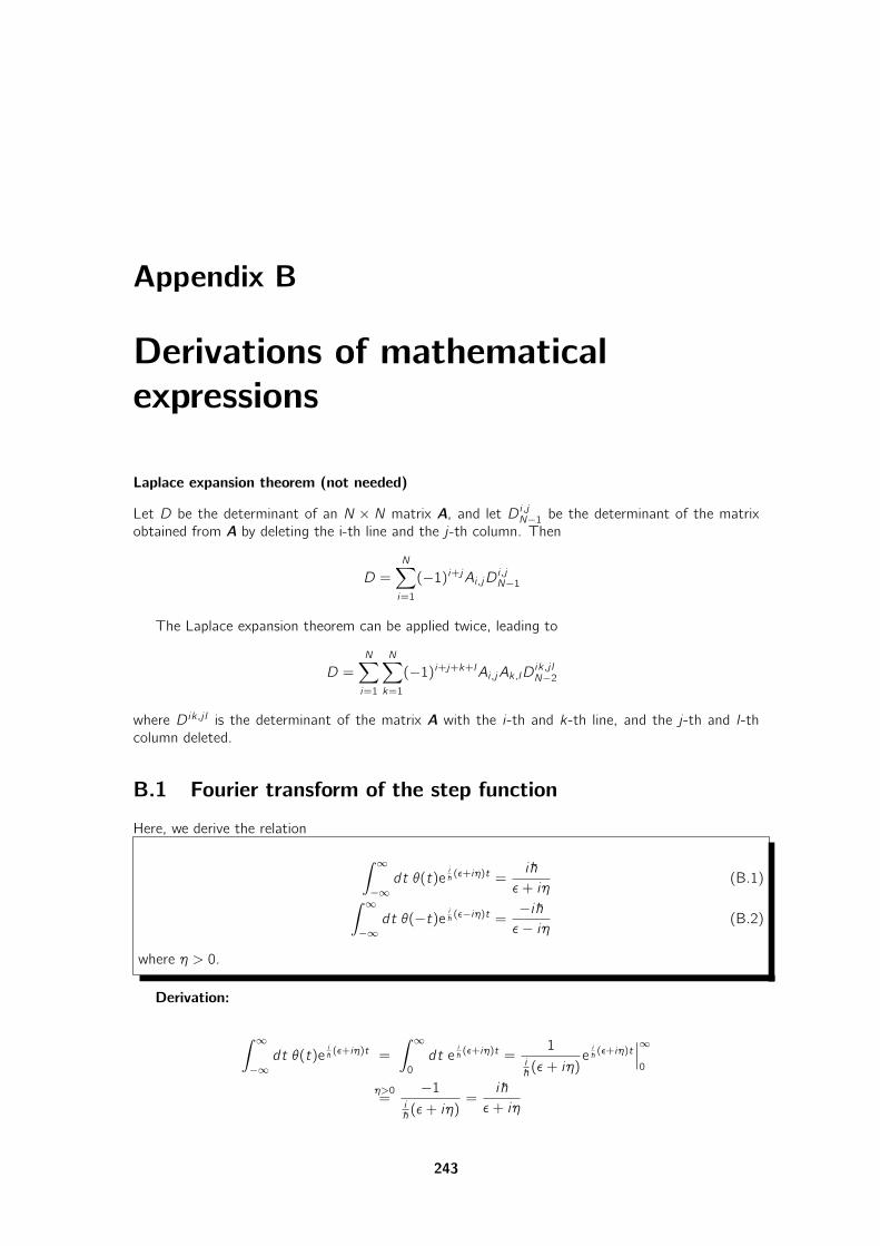
Appendix B
Derivations of mathematicalexpressions
Laplace expansion theorem (not needed)
Let D be the determinant of an N × N matrix A, and let Di ,jN−1 be the determinant of the matrixobtained from A by deleting the i-th line and the j-th column. Then
D =
N∑
i=1
(−1)i+jAi ,jDi ,jN−1
The Laplace expansion theorem can be applied twice, leading to
D =
N∑
i=1
N∑
k=1
(−1)i+j+k+lAi ,jAk,lDik,j lN−2
where Dik,j l is the determinant of the matrix A with the i-th and k-th line, and the j-th and l-thcolumn deleted.
B.1 Fourier transform of the step function
Here, we derive the relation
∫ ∞
−∞dt θ(t)e
i~(ǫ+iη)t =
i~
ǫ+ iη(B.1)
∫ ∞
−∞dt θ(−t)e i~ (ǫ−iη)t = −i~
ǫ− iη (B.2)
where η > 0.
Derivation:
∫ ∞
−∞dt θ(t)e
i~(ǫ+iη)t =
∫ ∞
0
dt ei~(ǫ+iη)t =
1i~(ǫ+ iη)
ei~(ǫ+iη)t
∣∣∣
∞
0
η>0=
−1i~(ǫ+ iη)
=i~
ǫ+ iη
243
244 B DERIVATIONS OF MATHEMATICAL EXPRESSIONS
∫ 0
−∞dt θ(−t)e i~ (ǫ−iη)t =
∫ 0
−∞dt e
i~(ǫ−iη)t =
1i~(ǫ− iη)
ei~(ǫ−iη)t
∣∣∣
0
−∞
η>0=
1i~(ǫ− iη)
=−i~ǫ− iη
The function is a simple pole at ǫ = −iη or ǫ = +iη respectively.
Appendix C
Adiabatic decoupling in theBorn-Oppenheimer approximation
C.1 Justification for the Born-Oppenheimer approximation
In the following, I will present an argument, that I believe is close to the original proof of Born andOppenheimer. We will investigate an artificial model that we can solve exactly and compare theresults of the Born-Oppenheimer approximation with the exact result.
Imagine a Hamiltonian in which all interactions are harmonic instead of Coulombic. Secondly,consider only a one-dimensional electron and a one-dimensional nucleus. The electron coordinate isdenoted by x and the nuclear coordinate by R. The corresponding momenta are pel for the electroncoordinate and Pnuc for the nuclear coordinate. Thus, the full Hamiltonian is
H =P 2nuc2M
+p2el2m+1
2ax2 + bxR +
1
2cR2
=m
M
P 2nuc2m+p2el2m+1
2ax2 + bxR +
1
2cR2 (C.1)
Exact solution of the model system
From the description of the multidimensional harmonic oscillator (see ΦSX:Quantum Physics andΦSX:Klassische Mechanik), we know that we need to know only the two classical eigenfrequenciesω+ and ω− to specify the spectrum of the two-dimensional quantum mechanical harmonic oscillator.
Ej,n = ~ω+
(
n +1
2
)
+ ~ω−
(
j +1
2
)
(C.2)
In order to obtain the classical frequencies ω±, let us consider the classical harmonic oscillator,which has the Hamilton function
H(Pnuc , pel , R, x)Eq. C.1=
P 2nuc2M
+p2el2m+1
2ax2 + bxR +
1
2cR2
Hamilton’s second equation yield( .pel.P nuc
)
=
(
m..x
M..R
)
= −(
a b
b c
)(
x
R
)
=
(
Fel
Fnuc
)
By diagonalizing the dynamical matrix D
D =1
m
(
a√
mM b√
mM b
mM c
)
245
246 C ADIABATIC DECOUPLING IN THE BORN-OPPENHEIMER APPROXIMATION
we obtain the eigenvalues ω2 of the dynamical matrix
mω2 =a + m
M c
2±
√(a − m
M c
2
)2
+m
Mb2
Let us investigate first two terms in an expansion in orders of mM .
mω2+ = a +m
M
b2
a+O
(m
M
)2
mω2− =m
M
(
c − b2
a
)
−(m
M
)2(
c2
2a+a
2
(2b2 − ac2a2
)2)
+O(m
M
)4
The higher frequency ω+ can be attributed to electronic excitation energies ∆E = ~ω+. Thus, ~ω+is similar size as excitation energies, that is typically in the range of few eV. The lower frequencyω− can be attributed to the atomic motion. The energy ~ω− is comparable to vibrational excitationenergies, that is in the range of about 10 meV.
Thus, the eigenvalue spectrum is
Ej,nEq. C.2= ~
√√√√√c − b2
a − mM
[
2c2
a +a2
(2b2−ac2a2
)2]
M
(
j +1
2
)
+ ~
√
a + mMb2
a
m
(
n +1
2
)
+O
((m
M
)2)
(C.3)
Born-Oppenheimer solution of the model system
We can now apply the Born-Oppenheimer approximation in order to see how it deviates from theexact result:
HBO =p2el2m+1
2ax2 + bRx +
1
2cR2
=p2el2m+1
2a(x +
b
aR)2 +
1
2
(
c − b2
a
)
R2
The force constant for the electrons is a, so that we obtain a frequency ωBO+ =√
am . Knowing that
the energy eigenvalues of the harmonic oscillator are ~ωBO+ (n+12) we can immediately determine the
Born-Oppenheimer energy surfaces.
EBOn (R) =1
2
(
c − b2
a
)
R2 + ~
√a
m
(
n +1
2
)
Now we can determine the eigenvalues of the nuclear Hamiltonian
Hnuc =P 2nuc2M
+ EBOn (R)
which has eigenvalues
Ej,n = ~
√
c − b2
a
M
(
j +1
2
)
+ ~
√a
m
(
n +1
2
)
(C.4)
We see that the spectrum obtained from the Born-Oppenheimer approximation Eq. C.4 provides thecorrect result, Eq. C.3, if m
M vanishes.
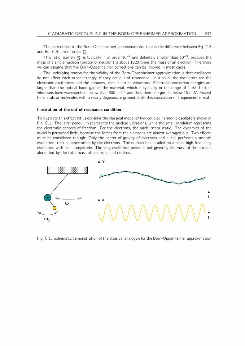
C ADIABATIC DECOUPLING IN THE BORN-OPPENHEIMER APPROXIMATION 247
The corrections to the Born-Oppenheimer approximations, that is the difference between Eq. C.3and Eq. C.4, are of order m
M .This ratio, namely m
M , is typically in of order 10−4 and definitely smaller than 10−3, because themass of a single nucleon (proton or neutron) is about 1823 times the mass of an electron. Thereforewe can assume that the Born-Oppenheimer corrections can be ignored in most cases.
The underlying reason for the validity of the Born-Oppenheimer approximation is that oscillatorsdo not affect each other strongly, if they are out of resonance. In a solid, the oscillators are theelectronic excitations and the phonons, that is lattice vibrations. Electronic excitation energies arelarger than the optical band gap of the material, which is typically in the range of 1 eV. Latticevibrations have wavenumbers below than 800 cm−1 and thus their energies lie below 10 meV. Exceptfor metals or molecules with a nearly degenerate ground state this separation of frequencies is real.
Illustration of the out-of-resonance condition
To illustrate this effect let us consider the classical model of two coupled harmonic oscillators shown inFig. C.1. The large pendulum represents the nuclear vibrations, while the small pendulum representsthe electronic degrees of freedom. For the electrons, the nuclei seem static. The dynamics of thenuclei is perturbed little, because the forces from the electrons are almost averaged out. Two effectsmust be considered though: Only the center of gravity of electrons and nuclei performs a smoothoscillation, that is unperturbed by the electrons. The nucleus has in addition a small high-frequencyoscillation with small amplitude. The long oscillation period is not given by the mass of the nucleusalone, but by the total mass of electrons and nucleus.
ω+
ω−
x
Y
t
t
Fig. C.1: Schematic demonstration of the classical analogon for the Born-Oppenheimer approximation

248 C ADIABATIC DECOUPLING IN THE BORN-OPPENHEIMER APPROXIMATION
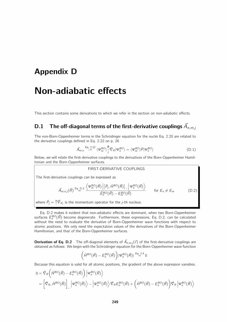
Appendix D
Non-adiabatic effects
This section contains some derivations to which we refer in the section on non-adiabatic effects.
D.1 The off-diagonal terms of the first-derivative couplings ~An,m,j
The non-Born-Oppenheimer terms in the Schrödinger equation for the nuclei Eq. 2.20 are related tothe derivative couplings defined in Eq. 2.22 on p. 26
~Am,nEq. 2.22:= 〈ΨBOm |
~
i~∇R|ΨBOn 〉 = 〈ΨBOm |P |ΨBOn 〉 (D.1)
Below, we will relate the first-derivative couplings to the derivatives of the Born-Oppenheimer Hamil-tonian and the Born-Oppenheimer surfaces.
FIRST-DERIVATIVE COUPLINGS
The first-derivative couplings can be expressed as
~Am,n,j(~R)Eq. D.3=
⟨
ΨBOm (~R)∣∣∣
[Pj , H
BO(~R)]
−
∣∣∣ΨBOn (~R)
⟩
EBOn (~R)− EBOm (~R)for En 6= Em (D.2)
where Pj = ~
i~∇Rj is the momentum operator for the j-th nucleus.
Eq. D.2 makes it evident that non-adiabatic effects are dominant, when two Born-Oppenheimersurfaces EBOn (~R) become degenerate. Furthermore, these expressions, Eq. D.2, can be calculatedwithout the need to evaluate the derivative of Born-Oppenheimer wave functions with respect toatomic positions. We only need the expectation values of the derivatives of the Born-OppenheimerHamiltonian, and that of the Born-Oppenheimer surfaces.
Derivation of Eq. D.2 The off-diagonal elements of ~An,m,j(~r) of the first-derivative couplings areobtained as follows: We begin with the Schrödinger equation for the Born-Oppenheimer wave function
(
HBO(~R)− EBOn (~R))
|ΨBOn (~R)〉Eq. 2.4= 0
Because this equation is valid for all atomic positions, the gradient of the above expression vanishes.
0 = ~∇R(
HBO(~R)− EBOn (~R)) ∣∣∣ΨBOn (~R)
⟩
=
[
~∇R, HBO(~R)]
−
∣∣∣ΨBOn (~R)
⟩
−∣∣∣ΨBOn (~R)
⟩
~∇REBOn (~R) +(
HBO(~R)− EBOn (~R))
~∇R∣∣∣ΨBOn (~R)
⟩
249
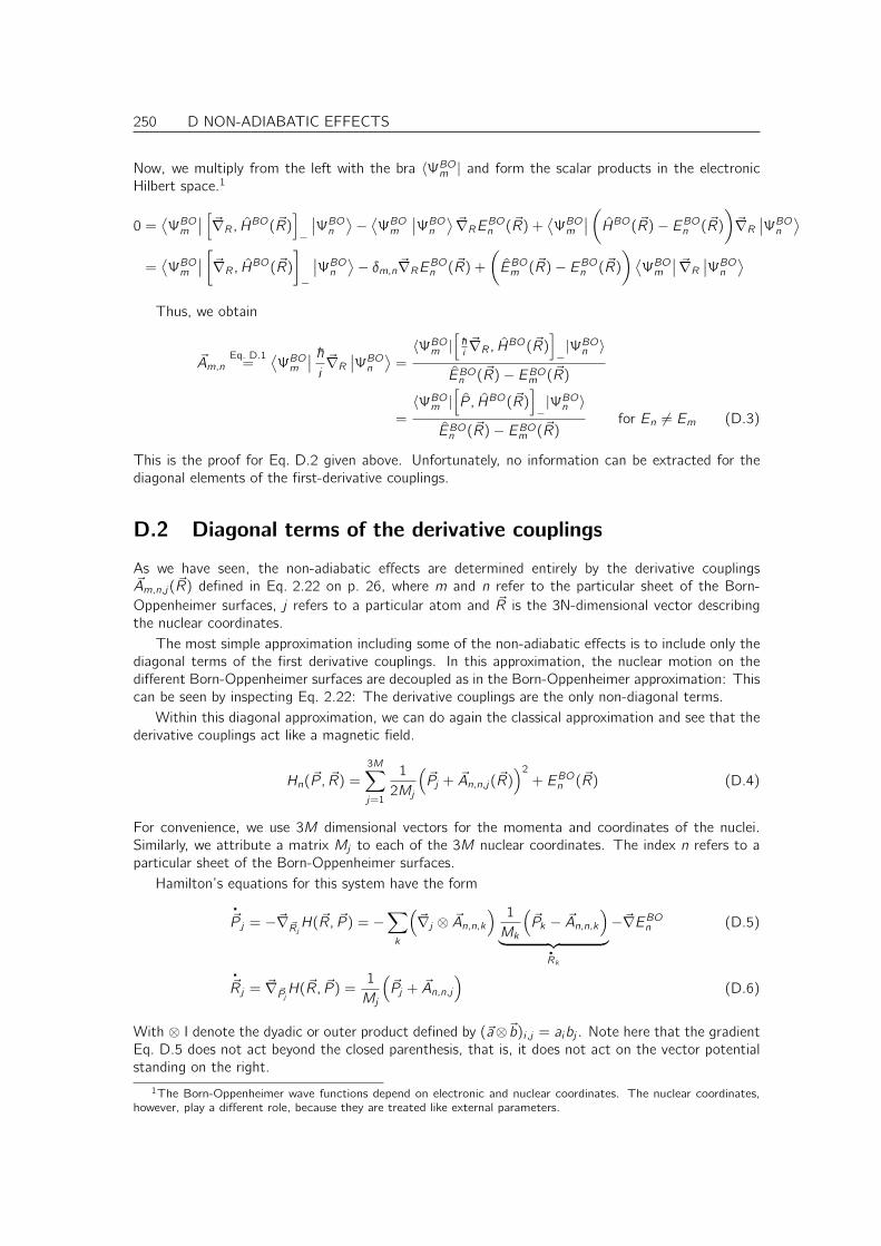
250 D NON-ADIABATIC EFFECTS
Now, we multiply from the left with the bra 〈ΨBOm | and form the scalar products in the electronicHilbert space.1
0 =⟨ΨBOm
∣∣
[
~∇R, HBO(~R)]
−
∣∣ΨBOn
⟩−⟨ΨBOm
∣∣ΨBOn
⟩~∇REBOn (~R) +
⟨ΨBOm
∣∣
(
HBO(~R)− EBOn (~R))
~∇R∣∣ΨBOn
⟩
=⟨ΨBOm
∣∣
[
~∇R, HBO(~R)]
−
∣∣ΨBOn
⟩− δm,n~∇REBOn (~R) +
(
EBOm (~R)− EBOn (~R))⟨ΨBOm
∣∣ ~∇R
∣∣ΨBOn
⟩
Thus, we obtain
~Am,nEq. D.1=
⟨ΨBOm
∣∣~
i~∇R∣∣ΨBOn
⟩=〈ΨBOm |
[~
i~∇R, HBO(~R)
]
−|ΨBOn 〉
EBOn (~R)− EBOm (~R)
=〈ΨBOm |
[
P , HBO(~R)]
−|ΨBOn 〉
EBOn (~R)− EBOm (~R)for En 6= Em (D.3)
This is the proof for Eq. D.2 given above. Unfortunately, no information can be extracted for thediagonal elements of the first-derivative couplings.
D.2 Diagonal terms of the derivative couplings
As we have seen, the non-adiabatic effects are determined entirely by the derivative couplings~Am,n,j(~R) defined in Eq. 2.22 on p. 26, where m and n refer to the particular sheet of the Born-Oppenheimer surfaces, j refers to a particular atom and ~R is the 3N-dimensional vector describingthe nuclear coordinates.
The most simple approximation including some of the non-adiabatic effects is to include only thediagonal terms of the first derivative couplings. In this approximation, the nuclear motion on thedifferent Born-Oppenheimer surfaces are decoupled as in the Born-Oppenheimer approximation: Thiscan be seen by inspecting Eq. 2.22: The derivative couplings are the only non-diagonal terms.
Within this diagonal approximation, we can do again the classical approximation and see that thederivative couplings act like a magnetic field.
Hn(~P , ~R) =
3M∑
j=1
1
2Mj
(
~Pj + ~An,n,j(~R))2
+ EBOn (~R) (D.4)
For convenience, we use 3M dimensional vectors for the momenta and coordinates of the nuclei.Similarly, we attribute a matrix Mj to each of the 3M nuclear coordinates. The index n refers to aparticular sheet of the Born-Oppenheimer surfaces.
Hamilton’s equations for this system have the form
.~P j = −~∇~Rj
H(~R, ~P ) = −∑
k
(
~∇j ⊗ ~An,n,k
) 1
Mk
(
~Pk − ~An,n,k
)
︸ ︷︷ ︸.Rk
−~∇EBOn (D.5)
.~Rj = ~∇~Pj
H(~R, ~P ) =1
Mj
(
~Pj + ~An,n,j
)
(D.6)
With ⊗ I denote the dyadic or outer product defined by (~a⊗~b)i ,j = aibj . Note here that the gradientEq. D.5 does not act beyond the closed parenthesis, that is, it does not act on the vector potentialstanding on the right.
1The Born-Oppenheimer wave functions depend on electronic and nuclear coordinates. The nuclear coordinates,however, play a different role, because they are treated like external parameters.
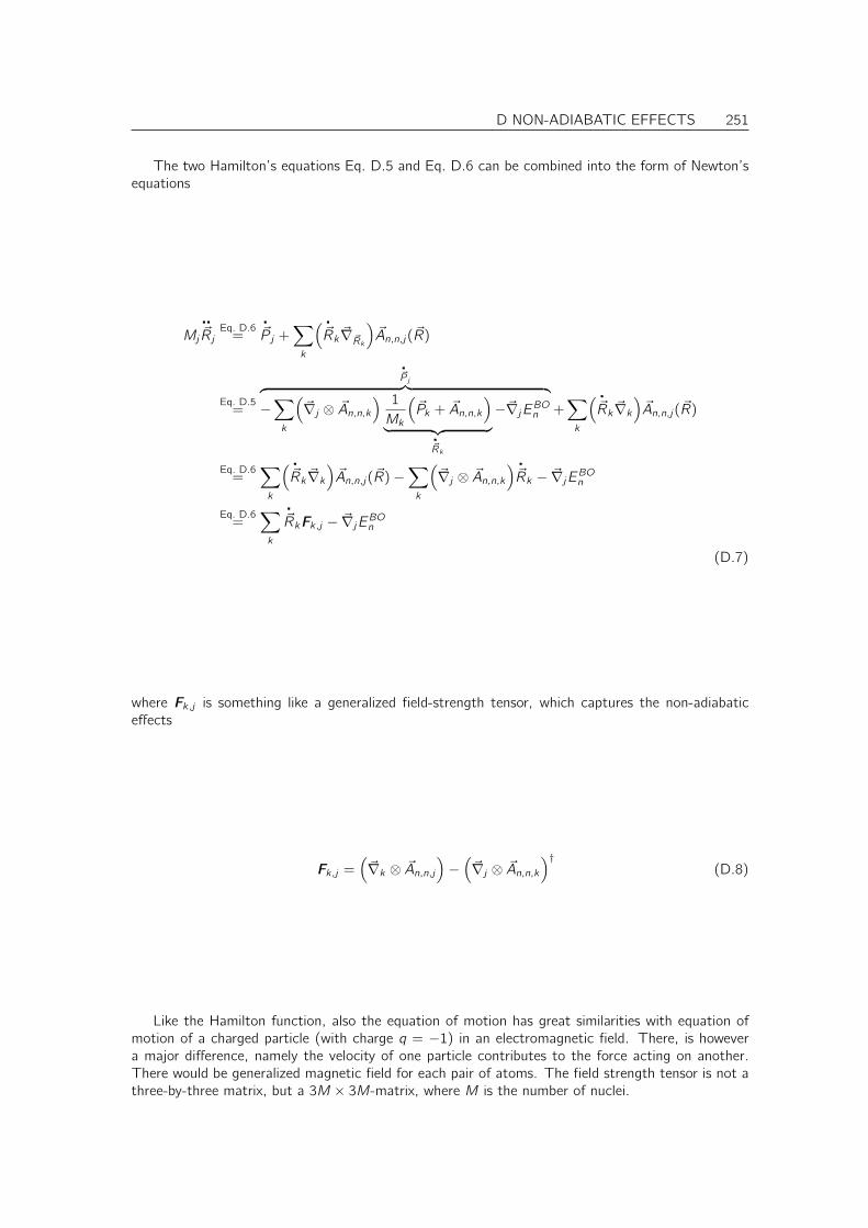
D NON-ADIABATIC EFFECTS 251
The two Hamilton’s equations Eq. D.5 and Eq. D.6 can be combined into the form of Newton’sequations
Mj
..~Rj
Eq. D.6=
.~P j +
∑
k
( .~Rk ~∇~Rk
)
~An,n,j(~R)
Eq. D.5=
.~P j
︷ ︸︸ ︷
−∑
k
(
~∇j ⊗ ~An,n,k
) 1
Mk
(
~Pk + ~An,n,k
)
︸ ︷︷ ︸.~Rk
−~∇jEBOn +∑
k
( .~Rk ~∇k
)
~An,n,j(~R)
Eq. D.6=
∑
k
( .~Rk ~∇k
)
~An,n,j(~R)−∑
k
(
~∇j ⊗ ~An,n,k
) .~Rk − ~∇jEBOn
Eq. D.6=
∑
k
.~RkFk,j − ~∇jEBOn
(D.7)
where Fk,j is something like a generalized field-strength tensor, which captures the non-adiabaticeffects
Fk,j =(
~∇k ⊗ ~An,n,j
)
−(
~∇j ⊗ ~An,n,k
)†(D.8)
Like the Hamilton function, also the equation of motion has great similarities with equation ofmotion of a charged particle (with charge q = −1) in an electromagnetic field. There, is howevera major difference, namely the velocity of one particle contributes to the force acting on another.There would be generalized magnetic field for each pair of atoms. The field strength tensor is not athree-by-three matrix, but a 3M × 3M-matrix, where M is the number of nuclei.
252 D NON-ADIABATIC EFFECTS
Reminder of electrodynamics The equation of motion of a charged particle in a magnetic field is
Mj
..~Rj = q
(
~E(~R) +.~R × ~B(~R)
)
= q(
~E +.~RF)
(D.9)
The magnetic field ~B and the electric field ~E are connected to the vector potential ~A and the electricpotential φ by
~B = ~∇× ~A
~E = −~∇Φ−.~A (D.10)
The electric field-strength tensor F is
F =(
~∇⊗ ~A)
−(
~∇⊗ ~A)†=
0 Bz −ByBy 0 Bx
By −By 0
(D.11)
The components the field-strength tensor are
Fi ,j = ∂iAj − ∂jAi (D.12)
and those of the magnetic field are
Bi =∑
j,k
ǫi ,j,k∂jAk (D.13)
where ǫi ,j,k is the Levi-Civita symbol or fully antisymmetric tensor. The Lorentz force can be writtenin terms of the Field strength tensor using
.~RF =
.~R × ~B (D.14)
We can work out the analogue of the field-strength tensor using the notation with 3M dimensionalvectors that combine cartesian coordinate with the particle index.
∂iAn,n,j − ∂jAn,n,i = ∂Ri 〈ΨBOn |~
i∂Rj |ΨBOn 〉 − ∂Rj 〈ΨBOn |
~
i∂Ri |ΨBOn 〉
=~
i
(
〈∂RiΨBOn |∂RjΨBOn 〉 − 〈∂RjΨBOn |∂RiΨBOn 〉)
= 2~ Im
(
〈∂RiΨBOn |∂RjΨBOn 〉)
Using again the vector-matrix notation for cartesian coordinates and indices for the atoms, we obtain
Fk,j = 2~ Im⟨~∇kΨBOn
∣∣⊗∣∣~∇jΨBOn
⟩(D.15)
This result seems to indicate that the non-adiabatic effects can be made to vanish, if the Born-Oppenheimer wave functions are chosen to be real. This is, however, not so: While real wave functionscan be chosen in the absence of magnetic fields as a consequence of time-inversion symmetry2, thereare cases where such a choice unavoidable produces a step in the wave function. This is related tothe existence of a geometrical phase. Key words related to the geometrical phase is the Jahn-Tellereffect and the Berry phase.
D.3 The diabatic picture
Editor: This section is not yet completed. It may be used alongside Baer’s paper.
2See appendix L
D NON-ADIABATIC EFFECTS 253
When the Born-Oppenheimer surfaces approach each other, the derivative couplings diverge.Therefore not only the Born-Oppenheimer approximation fails in those regions of configuration space,the formulation becomes including the non-adiabatic corrections becomes untractable. In order toavoid this problem, the diabatic representation of the nuclear wave functions has been developed,which avoids these problems. Unfortunately, the construction of the diabatic states is non-trivial andit is a non-local operation. The diabatic representation has been described well in the paper by Baer[84], which we follow here:
We start from the nuclear Hamiltonian in the adiabatic picture, which we have derived earlier
i~∂tφadiam (~R, t)
Eq. 2.20=
∑
n
[ M∑
j=1
1
2Mj
∑
k
(
δm,k~
i~∇Rj + ~Am,k,j(~R)
)(
δk,n~
i~∇Rj + ~Ak,n,j(~R)
)
+δm,nEBOm (~R)
]
φadian (~R, t) (D.16)
Now we introduce a position-dependent, unitary transformation of the nuclear wave function S(~R)that depends on the atomic positions.
φadian (~R, t) =∑
m
φdiam (~R, t)Sm,n(~R)
We want to insert it into Eq. D.16. Therefore, we first investigate the action of the kinetic energyterm on the transformation. We obtain
∑
m
(
δn,m ~Pj + ~An,m,j
)
Sm,o(~R) =~
i~∇jSn,o(~R) +
∑
m
Sn,m(~R)δm,o ~Pj +∑
m
~An,m,jSm,o(~R)
=∑
m
Sn,m(~R)δm,o ~Pj , (D.17)
if we can find a transformation Sn,m so that
~
i~∇jSn,o(~R) +
∑
m
~An,m,jSm,o(~R) = 0 (D.18)
Now we insert this transformation into Eq. D.16
i~∂t∑
n
Sm,nφdian (~R, t) =
∑
n,o
[ M∑
j=1
1
2Mj
∑
k
(
δm,k~
i~∇Rj + ~Am,k,j(~R)
)(
δk,n~
i~∇Rj + ~Ak,n,j(~R)
)
+δm,nEBOm (~R)
]
Sn,o(~R)φdiao (~R, t)
=∑
n,o
Sm,n(~R)
[ M∑
j=1
1
2Mj
∑
k
(
δn,k~
i~∇Rj)(
δk,o~
i~∇Rj)
+∑
k
S†n,k(~R)EBOk (~R)Sk,o(~R)
]
φdiao (~R, t)
i~∂tφdian (~R, t) =
∑
o
[ M∑
j=1
1
2Mjδn,o ~P
2j +
∑
k
S†n,k(~R)EBOk (~R)Sk,o(~R)
]
φdiao (~R, t) (D.19)
That is, in the diabatic picture the nuclear Schrödinger equation Eq. 2.20 has the simple form
i~∂tφdian (~R, t) =
[ M∑
j=1
−~22Mj
~∇2Rj + EBOn (~R)
]
φn(~R, t) +∑
m
Wn,m(~R)φm(~R, t) (D.20)
where Wn,m(~R) =∑
k
S†n,k(~R)EBOk (~R)Sk,o(~R)− EBOn (~R)δn,o (D.21)
254 D NON-ADIABATIC EFFECTS
Instead of a vector potential, the non-adiabatic effects are capture in a shifts of the total energysurfaces and coupling terms between them.
The adiabatic-to-diabatic transformation can be obtained
Sm,n(~R) =∑
o
exp
− i~
M∑
j=1
∫ ~R
~R0
d ~R′j ~Aj(~R)
m,o
So,n(~R0) (D.22)
if the integral is independent of the path taken. The integral is performed along a path conecting ~R0and ~R.
The requirement that the integral in Eq. D.22 is independent of the path is violated at coni-cal intersections. Thus, in the presence of a conical intersection the transformation to a diabaticrepresentation can only be approximated.
From here on, I recommend to follow the paper by Baer [84], and for references to newer devel-opments the review by Worth and Robb[9].
Appendix E
Non-crossing rule
Here we provide the proof of the non-crossing rule discussed in section 2.3.2 on p. 2.3.2.
NON-CROSSING RULE
Consider a Hamiltonian H(Q1, . . . , Qm) which depends on m parameters Q1, . . . , Qm. For eachaccidental crossing of two eigenvalues, there is a three-dimensional subspace of the parameter spacein which the degeneracy is lifted except for a single point.If the hamiltonian is real for all parameters, the subspace where the degeneracy is lifted has twodimensions.
The non-crossing rule has been derived by von Neumann and Wigner[15].
E.1 Proof of the non-crossing rule
Consider a Hamiltonian H(~Q), which depends on a set of coordinates ~Q. Let us explore the changesof the Hamiltonian in the neighborhood of ~Q0.
H(~Q) = H(~Q0) +(
~Q− ~Q0
)
~∇~Q
∣∣~Q0H +O
(
|~Q− ~Q0|2)
(E.1)
1. A gradient of a scalar function of ~Q defines a single direction in the coordinate space. Anydisplacement perpendicular to this direction will leave the scalar function unchanged to firstorder.
2. For a double valued function, the gradients of the first and the second component span atwo-dimensional space.
3. The number of free parameters of an object determines the maximum dimension of the spacein which it can be varied without affecting its defining properties.
This argument is generalized to a Hamiltonian, once with a doubly degenerate state and oncewith the degeneracy split into two non-degenerate states. Below, we will see that the space spannedwithout the degeneracy has a higher dimension than that with the degeneracy. The number ofadditional dimensions is 2 for real hamiltonians and 3 for complex hamiltonians. Thus, there are two,respectively three directions, along which the degeneracy is lifted. Displacements orthogonal to thesetwo or three distortions leave the degeneracy intact.
Thus, one can identify a two-dimensional, respectively three-dimensional space of displacementsthat are relevant for the intersection. Within this subspace, the intersection is zero-dimensional, thatis, a point. This is why one calls this intersection a conical intersection. Orthogonal to this two,respectively three-dimensional subspace, are the “irrelevant” directions, which may affect the positionor value of the conical intersection, but they do not lift the degeneracy.
255
256 E NON-CROSSING RULE
Free parameters of a hamiltonian with a specified multiplett structure: What is left, is todetermine the number of independent parameters that change a hamiltonian with a given multipletstructure without, however, lifting any degeneracies.
Every Hamiltonian can be constructed from its eigenvalues Ek and eigenvectors. The eigenvectorsform the unitary matrix U
Hi ,j =∑
k
U†i ,kEkUk,j (E.2)
Below, we will determine the number κ(n) of free parameters for a unitary matrix of dimension n.Note that κ(n) differs for real and complex unitary matrices.
Let us assume that the eigenvalues form ℓ multiplets with degeneracies gj for j = 1, . . . , ℓ.If we sum the number ℓ of free parameters for the energies Ek and the number κ(n) of parameters
of a unitary transformation U, we overcount the number of free parameters, because a number ofunitary matrices U do not affect the Hamiltonian at all.
The overcounting can be quantified as the number of independent unitary transformations thatleave the Hamiltonian invariant. These are the unitary transformations V with
∑
k
V †m,iHi ,jVj,n = Hi ,j . (E.3)
Thus, thus the desired unitary matrices V commutate with the Hamiltonian, i.e.
[H, V ]− = 0 . (E.4)
This requirement can be transformed into
0 = [H, V ]− =[UHU
†,UV U†]
− =[E, V ′′′
]
− (E.5)
where (E)i ,jdef= Eiδi ,j and V ′′′
def= UV U†.
Any unitary transformation that transforms only states within the same multiplet leaves thematrix E invariant.1 Any unitary transformation between different multipletts mixes energies andthus changes the matrix E. Hence, the overcounting corresponds to the free parameters of allunitary transformations that act only within the multiplets. Thus we need to subtract
∑ℓj=1 κ(gj).
Thus, the number of free parameters of a Hamiltonian with ℓ multiplets with degeneracies gj is
D(g1, . . . , gℓ) = κ
ℓ∑
j=1
gj
︸ ︷︷ ︸n
+ ℓ−ℓ∑
j=1
κ(gj) (E.6)
Degrees of freedom for a real unitary matrix Let me now work out the number κ(n) of a realunitary matrix with dimension n.
1. a general real matrix of dimension n has n2 matrix elements and thus n2 degrees of freedom.
2. the requirement of orthonormal vectors accounts for n(n−1)2 real-valued conditions∑
k U∗k,iUk,j =
0 with j > k . This corresponds to 12n(n− 1) degrees of freedom. Thus the number of degreesof freedom is reduced to n2 − 12n(n − 1).
3. the normalization of the vectors, i.e.∑
k U∗k,iUk,i = 1 with i = 1, . . . , n, contributes n real-
valued conditions. This reduces the number of degrees of freedom further to n2− 12n(n−1)−n =12n(n − 1).
1Consider one multiplett. The energies for all states in the multiplett are the same, that is E = E111, where E is theenergy of the multiplett. U†EU = EU†U = E111 = E.
E NON-CROSSING RULE 257
Thus, the number of degrees of freedom to fix a general unitary matrix is
κreal(n) =n(n − 1)2
(E.7)
Degrees of freedom for a complex unitary matrix Let me now work out the number κcomplex(n)of a compex unitary matrix with dimension n.
1. a general complex matrix of dimension n has n2 complex matrix elements and thus 2n2 realdegrees of freedom.
2. the requirement of orthonormal vectors accounts for n(n−1)2 complex-valued conditions∑
k U∗k,iUk,j =
0 with j > k . This corresponds to n(n − 1) degrees of freedom. Thus the number of degreesof freedom is reduced to 2n2 − n(n − 1).
3. the normalization of the vectors, i.e.∑
k U∗k,iUk,i = 1 with i = 1, . . . , n, contributes n real-
valued conditions. This reduces the number of degrees of freedom further to 2n2−n(n−1)−n =n2.
Thus, the number of degrees of freedom to fix a general unitary matrix is
κcomplex(n) = n2 (E.8)
Compare parameters with and without degeneracy: Now we need to understand how the numberof free parameters changes when a double degenerate states splits into two nondegenerate levels.In the presence of the double degeneracy, there shall be p muliplets plus one doublet. When thedegeneracy is lifted, the doublet splits into two singlets. The dimension of both hamiltonians isn = 2 +
∑pj=1 gj .
D(g1, . . . , gp, 1, 1)−D(g1, . . . , gp, 2)Eq. E.6=
[
κ(n) + (p + 2)−p∑
j=1
κ(gj)− 2κ(1)]
︸ ︷︷ ︸
split
−[
κ(n) + (p + 1)−p∑
j=1
κ(gj)− κ(2)]
︸ ︷︷ ︸
degenerate
= 1− 2κ(1) + κ(2)Eqs. E.7, E.8=
2 for a real hamiltonian
3 for a complex hamiltonian(E.9)

258 E NON-CROSSING RULE
Appendix F
Landau-Zener Formula
not finished!!!
The transition between two adiabatic total-energy surfaces has been analyzed by Landau andZener1 [86? , 85]. for a one-dimensional model. Here, we follow the analysis of Wittig[85].
The model of Landau and Zener considers two crossing Born-Oppenheimer surfaces in only onedimension X.
HBO(X) =
(
−F1X 0
0 −F2X
)
The Born-Oppenheimer surfaces are assumed to depend linearly on the atomic coordinate X.The non-adiabatic effects are approximated by non-diagonal elements of the Hamiltonian, that
are considered independent of the atomic position. Thus, the full Hamiltonian has the form
H(X) =
(
−F1X H12
H∗12 −F2X
)
The nuclear dynamics is considered classical, and with a constant velocity ∂tX(t) = V , thatis X(t) = V t. This turns the position-dependent Hamiltonian into an effectively time-dependentHamiltonian.
H(t) =
(
−F1V t H12
H∗12 −F2V t
)
The time dependent electronic Hamiltonian is described by the following Ansatz(
Φ1
Φ2
)
=
(
A(t)e−i~
∫dt EBO1 (X(t))
B(t)e−i~
∫dt EBO2 (X(t))
)
=
(
A(t)e+i~
∫dt F1V t
B(t)e+i~
∫dt F2V t
)
=
(
A(t)e+i~
F1V
2t2
B(t)e+i~
F2V
2t2
)
The lower bound of the time integral has been ignored because they are a multiplicative factor, thatcan be absorbed in the initial conditions.
Insertion into the time dependent Schrödinger equation yield
i~∂t
(
A(t)eiF1V t2/(2~)
B(t)eiF2V t2/(2~)
)
=
(
−F1V t H12
H∗12 −F2V t
)(
A(t)eiF1V t2/(2~)
B(t)eiF2V t2/(2~)
)
(
∂tA(t)
∂tB(t)
)
=
(
− i~H12B(t)e
i(F2−F1)V t2/(2~)
− i~H∗12A(t)e
−i(F2−F1)V t2/(2~)
)
1According to Wittig[85] the result of Landau[? ] has an error of 2π
259
260 F LANDAU-ZENER FORMULA
thus
∂tA(t) = −i
~H12B(t)e
i(F2−F1)V t2/(2~)
∂tB(t) = −i
~H∗12A(t)e
−i(F2−F1)V t2/(2~) ⇒ A(t) = −~i
H12|H12|2︸ ︷︷ ︸
1/H∗12
ei(F2−F1)V t2/(2~)∂tB(t)
Insertion of the second equation into the first yields a differential equation for B(t).
∂t
(
−~i
H12|H12|2
ei(F2−F1)V t2/(2~)∂tB(t)
)
︸ ︷︷ ︸
A(t)
= − i~H12B(t)e
i(F2−F1)V t2/(2~)
− H12|H12|2
(F2 − F1)V tei(F2−F1)V t2/(2~)∂tB(t) +
(
−~i
H12|H12|2
ei(F2−F1)V t2/(2~)∂2tB(t)
)
= − i~H12B(t)e
i(F2−F1)V2~
t2
− 1
|H12|2(F2 − F1)V t∂tB(t) +
(
−~i
1
|H12|2∂2tB(t)
)
= − i~B(t)
i
~(F2 − F1)V t ∂tB(t) + ∂2tB(t) = −
1
~2|H12|2B(t)
∂2tB(t) +i
~(F2 − F1)V t ∂tB(t) +
1
~2|H12|2B(t) = 0
Thus, we have a differential equation for the probability amplitude on the second sheet. We now lookfor a solution of this differential equation, respectively its value B(t = +∞) with the initial conditionB(−∞) = ∂tB(−∞) = 0.
This is a differential equation of the form..x + iαt
.x + βx = 0
So far, the derivation is standard. Wittig showed a solution to the problem using contour integrals.
1
t
..x
x+ iα
.x
x+β
t= 0
iα
∫ tf
ti
dt ∂t ln[x(t)] = −β∫ tf
ti
dt1
t−∫ tf
ti
dt1
t
..x
x
iα ln[xfxi] = −β
∫ ∞
−∞dt1
t−∫ ∞
−∞dt1
t
..x
x
The integral of the first term on the right hand side yields∫ ∞
−∞dt1
t= ±iπ
depending on whether the integration is performed in the upper or lower half plane.Thus, we obtain
ln[xf ] = ln[xi ]∓ πβ
α+i
α
∫ ∞
−∞dt1
t
..x
x
xf = xie∓πβ/α exp
(i
α
∫ ∞
−∞dt1
t
..x
x
)
If the transition probability is small, that is xf − xi << 1, we can ignore the last term and obtainthe estimate
xf ≈ xie∓πβ/α
F LANDAU-ZENER FORMULA 261
When we insert the parameters α = (F2−F1)V/~ and β = |H12|2/~2 we obtain the Landau-Zenerestimate.
LANDAU ZENER ESTIMATE FOR THE TRANSITION PROBABILITY AT A BAND CROSSING
The transition probability is (Eq. 16 of Wittig)
P = exp
2π
|H12|~
︸ ︷︷ ︸
Rabi frequency
|H12|V |F1 − F2|︸ ︷︷ ︸
τ
τ is of order of the time it takes to cross the region where the Born-Oppenheimer surfaces are closerthan the avoided crossing surface.
================================The result of their analysis is the Landau-Zener formula, which gives the probability for a
transition for a one-dimensional model
P = e−2πω12τ with ω12 =H12~
and τ =|H12|
v |F1 − F2|(F.1)
where v is the velocity and H12 is the coupling between the two crossing total-energy surfaces. ω12is the Rabi frequency at the crossing point and τ is a measure for the duration of the interactionbetween the surfaces. The model hamiltonian underlying the Landau-Zener formula has the form

262 F LANDAU-ZENER FORMULA

Appendix G
Supplementary material for theJahn-Teller model
This appendix extends the description of the Jahn-Teller model described in section 2.3.4 on p. 31.The stationary wave functions of the Jahn-Teller problem have been given in Eq. 2.62 on p. 40
|Φj,m〉Eq. 2.62=
∫
dX
∫
dZ1
2
(
|a,X,Z〉[
(eiα + 1)R+,j,m(R) + i(eiα − 1)R−,j,m(R)]
+ |b,X,Z〉[
−i(eiα − 1)R+,j,m(R) + (eiα + 1)R−,j,m(R)])
eimα
(G.1)
where the radial nuclear wave functions obey the one-dimensional, two-component radial Schrödingerequation Eq. 2.63 for the generalized nuclear coordinates (X,Z) of the Jahn-Teller model,
0Eq. 2.63=
−~2(R2∂2R + R∂R −m2
)
2MR2111
︸ ︷︷ ︸
−~2 ~∇2/(2M)
+ gRσz + wR2111
︸ ︷︷ ︸
EBO
+~2(m + 12
)
2MR2(111− σx)
︸ ︷︷ ︸
nonBO
−Ej,m111(
iR+,j,m(R)R−,j,m(R)
)
(G.2)
G.1 Relation of stationary wave functions for m and −m − 1In Eq. 2.64 and Eq. 2.65 on p. 41 we mentioned that the electron-nuclear wave functionsΦj,m(~x,X,Z)and Φj,−m−1(~x,X,Z) are complex conjugates of each other.1
Φj,−m−1(~x,X,Z) = Φ∗j,m(~x,X,Z) (G.3)
and that the same holds for the radial functions
(
R±,j,−m−1(R))∗= R±,j,m(R) ⇔
R−,j,−m−1(R) = −R−,j,m(R)R+,j,−m−1(R) = +R+,j,m(R)
(G.4)
Here, we provide the detailed derivation.
1More precisely, they can be chosen to be complex conjugates of each other.
263
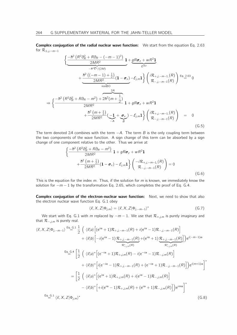
264 G SUPPLEMENTARY MATERIAL FOR THE JAHN-TELLER MODEL
Complex conjugation of the radial nuclear wave function: We start from the equation Eq. 2.63for R±,j,−m−1
−~2(R2∂2R + R∂R − (−m − 1)2
)
2MR2111
︸ ︷︷ ︸
−~2 ~∇2/(2M)
+ gRσz + wR2111
︸ ︷︷ ︸
EBO
+~2((−m − 1) + 12
)
2MR2(111− σx)
︸ ︷︷ ︸
nonBO
−Ej,m111(
iR+,j,−m−1,(R)R−,j,−m−1(R)
)
Eq. 2.63= 0
⇒−~2
(R2∂2R + R∂R −m2
)+
2A︷ ︸︸ ︷
2~2(m +1
2)
2MR2111 + gRσz + wR
2111
+~2(m + 12
)
2MR2(−111︸︷︷︸
−A
+ σx︸︷︷︸
B
)− Ej,m111(
iR+,j,−m−1,(R)R−,j,−m−1(R)
)
= 0
(G.5)
The term denoted 2A combines with the term −A. The term B is the only coupling term betweenthe two components of the wave function. A sign change of this term can be absorbed by a signchange of one component relative to the other. Thus we arrive at
−~2(R2∂2R + R∂R −m2
)
2MR2111 + gRσz + wR
2111
+~2(m + 12
)
2MR2(111− σx)− Ej,m111
(−iR+,j,−m−1,(R)R−,j,−m−1(R)
)
= 0
(G.6)
This is the equation for the index m. Thus, if the solution for m is known, we immediately know thesolution for −m − 1 by the transformation Eq. 2.65, which completes the proof of Eq. G.4.
Complex conjugation of the electron-nuclear wave function: Next, we need to show that alsothe electron nuclear wave function Eq. G.1 obey
〈~x,X,Z|Φj,m〉 = 〈~x,X,Z|Φj,−m−1〉∗ (G.7)
We start with Eq. G.1 with m replaced by −m − 1. We use that R+,j,m is purely imaginary andthat R−,j,m is purely real.
〈~x,X,Z|Φj,−m−1〉Eq. G.1=
1
2
(
〈~x |a〉[
(eiα + 1)R+,j,−m−1(R) + i(eiα − 1)R−,j,−m−1(R)]
+ 〈~x |b〉[
−i(eiα − 1)R+,j,−m−1(R)︸ ︷︷ ︸
R∗+,j,m(R)
+(eiα + 1)R+,j,−m−1(R)︸ ︷︷ ︸
R∗+,j,m(R)
])
ei(−m−1)α
Eq. G.4=
[1
2
(
〈~x |a〉∗[
(e−iα + 1)R+,j,m(R)− i(e−iα − 1)R−,j,m(R)]
+ 〈~x |b〉∗[
i(e−iα − 1)R+,j,−m−1(R) + (e−iα + 1)R−,j,−m−1(R)])
ei(m+1)α]∗
=
[1
2
(
〈~x |a〉∗[
(eiα + 1)R+,j,m(R) + i(eiα − 1)R−,j,m(R)]
− 〈~x |b〉∗[
+i(eiα − 1)R+,j,m(R) + (eiα + 1)R−,j,m(R)])
eimα]∗
Eq. G.1= 〈~x,X,Z|Φj,m〉∗ (G.8)
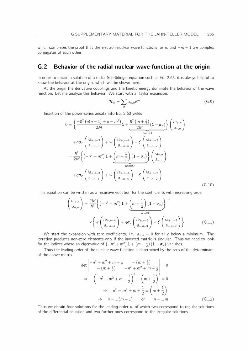
G SUPPLEMENTARY MATERIAL FOR THE JAHN-TELLER MODEL 265
which completes the proof that the electron-nuclear wave functions for m and −m − 1 are complexconjugates of each other.
G.2 Behavior of the radial nuclear wave function at the origin
In order to obtain a solution of a radial Schrödinger equation such as Eq. 2.63, it is always helpful toknow the behavior at the origin, which will be shown here.
At the origin the derivative couplings and the kinetic energy dominate the behavior of the wavefunction. Let me analyze this behavior. We start with a Taylor expansion:
R± =∑
n
a±,nRn (G.9)
Insertion of the power-series ansatz into Eq. 2.63 yields
0 =
−~2(n(n − 1) + n −m2
)
2M111 +~2(m + 12
)
2M(111− σx)
︸ ︷︷ ︸
nonBO
(
ia+,n
a−,n
)
+gσz
(
ia+,n−3a−,n−3
)
+ w
(
ia+,n−4a−,n−4
)
− E(
ia+,n−2a−,n−2
)
=~2
2M
(−n2 +m2
)111 +
(
m +1
2
)
(111− σx)︸ ︷︷ ︸
nonBO
(
ia+,n
a−,n
)
+gσz
(
ia+,n−3a−,n−3
)
+ w
(
ia+,n−4a−,n−4
)
− E(
ia+,n−2a−,n−2
)
(G.10)
This equation can be written as a recursive equation for the coefficients with increasing order(
ia+,n
a−,n
)
=2M
~2
(−n2 +m2
)111 +
(
m +1
2
)
(111− σx)︸ ︷︷ ︸
nonBO
−1
×
w
(
ia+,n−4a−,n−4
)
+ gσz
(
ia+,n−3a−,n−3
)
− E(
ia+,n−2a−,n−2
)
(G.11)
We start the expansion with zero coefficients, i.e. a±,n = 0 for all n below a minimum. Theiteration produces non-zero elements only if the inverted matrix is singular. Thus we need to lookfor the indices where an eigenvalue of
(−n2 +m2
)111 +
(m + 12
)(111− σx) vanishes.
Thus the leading order of the nuclear wave function is determined by the zero of the determinantof the above matrix.
det
∣∣∣∣∣
−n2 +m2 +m + 12 −(m + 12
)
−(m + 12
)−n2 +m2 +m + 12
∣∣∣∣∣= 0
⇒(
−n2 +m2 +m + 12
)2
−(
m +1
2
)2
= 0
⇒ n2 = m2 +m +1
2±(
m +1
2
)
⇒ n = ±(m + 1) or n = ±m (G.12)
Thus we obtain four solutions for the leading order n, of which two correspond to regular solutionsof the differential equation and two further ones correspond to the irregular solutions.
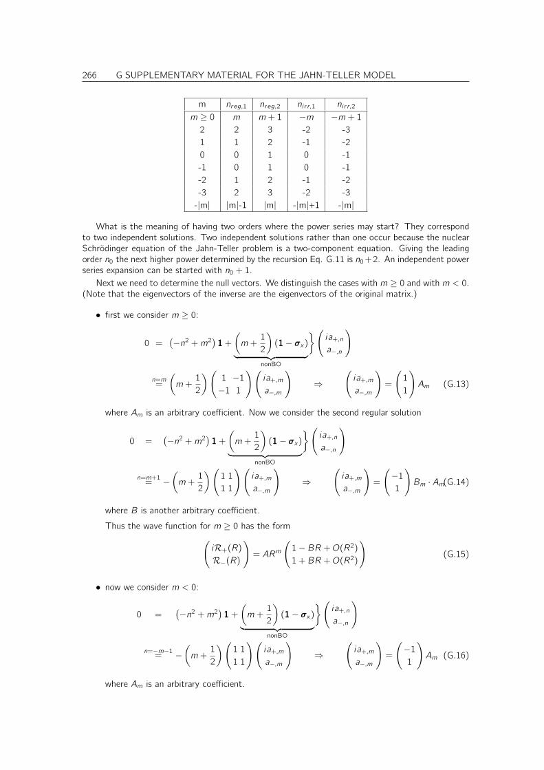
266 G SUPPLEMENTARY MATERIAL FOR THE JAHN-TELLER MODEL
m nreg,1 nreg,2 ni r r,1 ni r r,2
m ≥ 0 m m + 1 −m −m + 12 2 3 -2 -31 1 2 -1 -20 0 1 0 -1-1 0 1 0 -1-2 1 2 -1 -2-3 2 3 -2 -3
-|m| |m|-1 |m| -|m|+1 -|m|
What is the meaning of having two orders where the power series may start? They correspondto two independent solutions. Two independent solutions rather than one occur because the nuclearSchrödinger equation of the Jahn-Teller problem is a two-component equation. Giving the leadingorder n0 the next higher power determined by the recursion Eq. G.11 is n0+2. An independent powerseries expansion can be started with n0 + 1.
Next we need to determine the null vectors. We distinguish the cases with m ≥ 0 and with m < 0.(Note that the eigenvectors of the inverse are the eigenvectors of the original matrix.)
• first we consider m ≥ 0:
0 =(−n2 +m2
)111 +
(
m +1
2
)
(111− σx)︸ ︷︷ ︸
nonBO
(
ia+,n
a−,n
)
n=m=
(
m +1
2
)(
1 −1−1 1
)(
ia+,m
a−,m
)
⇒(
ia+,m
a−,m
)
=
(
1
1
)
Am (G.13)
where Am is an arbitrary coefficient. Now we consider the second regular solution
0 =(−n2 +m2
)111 +
(
m +1
2
)
(111− σx)︸ ︷︷ ︸
nonBO
(
ia+,n
a−,n
)
n=m+1= −
(
m +1
2
)(
1 1
1 1
)(
ia+,m
a−,m
)
⇒(
ia+,m
a−,m
)
=
(
−11
)
Bm · Am(G.14)
where B is another arbitrary coefficient.
Thus the wave function for m ≥ 0 has the form(
iR+(R)R−(R)
)
= ARm
(
1− BR +O(R2)1 + BR +O(R2)
)
(G.15)
• now we consider m < 0:
0 =(−n2 +m2
)111 +
(
m +1
2
)
(111− σx)︸ ︷︷ ︸
nonBO
(
ia+,n
a−,n
)
n=−m−1= −
(
m +1
2
)(
1 1
1 1
)(
ia+,m
a−,m
)
⇒(
ia+,m
a−,m
)
=
(
−11
)
Am (G.16)
where Am is an arbitrary coefficient.
G SUPPLEMENTARY MATERIAL FOR THE JAHN-TELLER MODEL 267
0 =(−n2 +m2
)111 +
(
m +1
2
)
(111− σx)︸ ︷︷ ︸
nonBO
(
ia+,n
a−,n
)
n=−m=
(
m +1
2
)(
1 −11 −1
)(
ia+,m
a−,m
)
⇒(
ia+,m
a−,m
)
=
(
1
1
)
Bm · Am (G.17)
where Bm is another arbitrary coefficient.
Thus the wave function for m ≥ 0 has the form(
iR+(R)R−(R)
)
= AmRm
(
−1 + BmR +O(R2)1 + BmR +O(R
2)
)
(G.18)
We observe that we can choose the coefficients Am, Bm such that the first terms of the powerseries expansion for m and −m − 1 are complex conjugates of each other. We will see below insection G.1 that this is a general property of the solutions.
Another observation is that the nuclear wave function is not differentiable in all orders at theorigin. Rather the m = solution exhibits a kink at the origin.
G.3 Optimization of the radial wave functions
There are different ways to solve the nuclear radial Schrödinger equation numerically, which arediscussed in the following two sections.
The one described here exploits Ritz’ variational principle. It starts from an expression for thetotal energy as functional of a nuclear wave function. By minimizing this energy we obtain the groundstate. Minimizing the same functional again again, but with the restriction that it is orthogonal tothe ground state, will yield the first excited state. Similarly, we can successively build up all radialwave functions.
We write down the total energy of an ensemble of electron and nuclear states. The states canbe expressed entirely by the nuclear radial functions. The occupations, which are denoted as Pm,j .The are Boltzmann weights.
In order to deal with real functions we introduce(
f+
f−
)
def=
(
iR+R−
)
(G.19)
The total energy functional to be minimized is obtained from the differential equation. Here weinclude all excited states, but give them probabilities Pm,j . The probabilities can be chosen fairlyarbitrarily. While they are inspired by the expressions for a thermal ensemble, they are used here onlyas a numerical tool. Without proof let me state the following: (1) If all probabilities differ from eachother, the resulting wave functions are eigenstates of the stationary Schrödinger equation. (2) Thestates are ordered such that the energies for states with higher probability are lower.
E[~fj,m(R)] =∑
m,j
Pm,j
∫ ∞
0
dR (2πR)︸ ︷︷ ︸
ang. integr.
×
~f ∗j,m(R)
[−~2(R2∂2R + R∂R −m2
)
2MR2111 + gRσz + wR
2111 +~2(m + 12)
2MR2(111 + σx)
]
~fj,m(R)
+∑
m
∑
j,j ′
Λm,j ′,j
[∫ ∞
0
dR (2πR)︸ ︷︷ ︸
ang. integr.
~f ∗j,m~fj ′,m
]
− δj,j ′
(G.20)
268 G SUPPLEMENTARY MATERIAL FOR THE JAHN-TELLER MODEL
This expression acts as potential energy in a fictitious Lagrangian
L[~fj,m(R),.~f j,m(R)] =
∑
m,j
Pm,j
∫
drmf
.~f j,m(R)
.~f j,m(R)− E[~fjm(R)] (G.21)
and derive an equation of motion for the radial wave function in the spirit of the Car-Parrinellomethod[87]. The time defining the “velocity of ~fm,j ”, is not a real time but simply a coordinatedescribing dynamics of the wave functions during the optimization process.
The first variation of the total energy with respect to the radial functions is
dE =∑
m,j
Pm,j
∫ ∞
0
dR (2πR) d~f ∗j,m~yj,m + c.c. (G.22)
which yields an effective gradient of the functional
~yj,m =
[−~2(R2∂2R + R∂R −m2
)
2MR2111 + gRσz + wR
2111 +~2(m + 12)
2MR2(111 + σx)
]
~fj,m(R)
+∑
j ′
~fj ′,mΛm,j ′,j
(G.23)
The Euler Lagrange equations for the Lagrangian Eq. G.21 produce an equation of motion
mf
..~f m,j(R) = −~yj,m(R) (G.24)
We did not consider here the constraint term, because we will enforce this constraint separately. Thisequation of motion is augmented by a friction term and discretized using the Verlet algorithm[88].
In the Verlet algorithm[88] a differential equation is discretized by replacing the first and secondderivatives by the differential quotients
.x → x(t + ∆)− x(t − ∆)
2∆..x → x(t + ∆)− 2x(t) + x(t − ∆)
∆2(G.25)
This allows to iteratively obtain the solution of a differential equation m..x = F (x)−γ .x for x(j∆).
x(t + ∆) = x(t)2
1 + a− x(t − ∆)1− a
1 + a+ F
∆2
m(1 + a)(G.26)
with a = γ∆2m .
We start from an arbitrary wave function ~fj,m(R) for each m and j . The wave function is firstorthogonalized to all functions with lower j , and then it is normalized. Starting from this initial wavefunction we perform a Car-Parrinello like optimization in the space orthogonal to the lower-lyingstates.
1. calculate the gradient ~yj,m(R)
~yj,m =
[−~2(R2∂2R + R∂R −m2
)
2MR2111 + gRσz + wR
2111 +~2(m + 12)
2MR2(111 + σx)
]
~fj,m(R)
(G.27)
2. orthogonalize ~yj,m(R) to all lower-lying functions
~yj,m ← ~yj,m −j−1∑
j ′=1
~fj ′,m
(∫ ∞
0
dR R ~f ∗j ′,m(R)~yj,m(R) (G.28)
G SUPPLEMENTARY MATERIAL FOR THE JAHN-TELLER MODEL 269
3. propagate with the Verlet algorithm
~f = ~f (t)2
1 + a− ~f (t − ∆)1− a
1 + a− ~y ∆2
2mf (1 + a)(G.29)
4. normalize
~f (t + ∆) = ~f + ~f (t)λ
1!= 2π
∫ ∞
0
dR R ~f ∗(+)~f (+)
=(
2π
∫ ∞
0
dR R ~f ∗ ~f (+))
− 1︸ ︷︷ ︸
C
+2λRe(
2π
∫ ∞
0
dR R ~f ∗~f (0))
︸ ︷︷ ︸
B
+λ2 2π
∫ ∞
0
dR R ~f ∗(0)~f (0)︸ ︷︷ ︸
A
λ = −BA
[
1−√
1− A2C
B2
]
(G.30)
Since the function is known for the next time step, we can begin again with the first point of theiteration sequence.
G.4 Integration of the Schrödinger equation for the radial nu-
clear wave functions
Editor: This is not finished!
0 =
− ~2
2M∂2R −
~2
2MR∂R +
~2[m(m + 1) + 12
]
2MR2± g|~R|+ w ~R2 − Em,j
R±,m,j ±i~2(m + 12)
2MR2R∓,m,j
0 =
−R2∂2R − R∂R +[
m(m + 1) +1
2
]
+2M
~2
[
−Em,jR2 ± gR3 + wR4]
R±,m,j ± i(
m +1
2
)
R∓,m,j
Now we introduce an exponential Ansatz R(x) = ex
R±,m,j(ex) = f±,m,j(x) (G.31)
R(x) = ex ⇒ dR
dx= ex = R ⇒ dx
dR= 1/R
R∂R = ∂x
R2∂2R = R2∂R1
RR∂R = R
2∂R1
R∂x = R
2(
− 1R2+1
R2R∂R
)
∂x = −∂x + ∂2xR2∂2R + R∂R = ∂
2x (G.32)
This yields
0 =
−∂2x +[
m(m − 1) + 12
]
+2M
~2
[
−Em,jR2 ± gR3 + wR4]
f±,m,j(x)∓ i(
m +1
2
)
f∓,m,j(x)
We solve this equation numerically on a grid using the Verlet algorithm[88], which replaces thesecond derivative with the differential quotient
∂2x f =f (+)− 2f (0) + f (−)
α2(G.33)
270 G SUPPLEMENTARY MATERIAL FOR THE JAHN-TELLER MODEL
where α is the grid spacing.An important aspect is that one needs to integrate from the outside inward. The reason is that in
the outer region, there is one solution that falls of towards the outside and one solution that increasesexponentially. We are interested in the solution falling off.
When we integrate outward, any little numerical error will admix a fraction of the exponentiallyincreasing solution. This small fraction will now be exponentially amplified, leading to a poor solution.On the other hand, when we integrate inward, every error will admix a partial solution that falls offin the inward direction, so that any error heals immediately.
Therefore we choose the strategy to integrate from the outside inward and match the solutionsin the center.
For a given energy, we calculate the Schrödinger equation outward from the inside with two
distinct boundary conditions and obtain(
f(i)1,1(x), f
(i)2,1(x)
)
and(
f(i)1,2(x), f
(i)2,2(x)
)
. At the same time
I evaluate the energy derivatives yielding(.f(i)
1,1(x),.f(i)
2,1(x))
and(.f(i)
1,2(x),.f(i)
2,2(x))
. The boundary
conditions are(
f(i)1,1(x), f
(i)2,1(x)
)
= (1, 0) and(
f(i)1,2(x), f
(i)2,2(x)
)
= (0, 1) at the first grid point. The
derivatives are set to zero. For the energy derivative functions value and derivative at the first gridpoints are set to zero.
The condition that the two functions match with value and derivative can be approximated bythe condition that the two functions match on two subsequent points xk on the grid.
2∑
α=1
(
f(i)i ,α (xk) + (ǫ− ǫ0)
.f(i)
i ,α(xk)
)
cα =
2∑
α=1
(
f(o)i ,α (xk) + (ǫ− ǫ0)
.f(o)
i ,α (xk)
)
cα+2 (G.34)
This value must be fulfilled for k = 1, 2 and i = 1, 2. This is an eigenvalue equation
f(i)1,1(xa) f
(i)1,2(xa) −f
(o)1,1 (xa) −f
(o)1,2 (xa)
f(i)2,1(xa) f
(i)2,2(xa) −f
(o)2,1 (xa) −f
(o)2,2 (xa)
f(i)1,1(xb) f
(i)1,2(xb) −f
(o)1,1 (xb) −f
(o)1,2 (xb)
f(i)2,1(xb) f
(i)2,2(xb) −f
(o)2,1 (xb) −f
(o)2,2 (xb)
+ (ǫ− ǫ0)
.f(i)
1,1(xa).f(i)
1,2(xa) −.f(o)
1,1(xa) −.f(o)
1,2(xa).f(i)
2,1(xa).f(i)
2,2(xa) −.f(o)
2,1(xa) −.f(o)
2,2(xa).f(i)
1,1(xb).f(i)
1,2(xb) −.f(o)
1,1(xb) −.f(o)
1,2(xb).f(i)
2,1(xb).f(i)
2,2(xb) −.f(o)
2,1(xb) −.f(o)
2,2(xb)
= 0
(G.35)
We define the matrix
Adef=
.f(i)
1,1(xa).f(i)
1,2(xa) −.f(o)
1,1(xa) −.f(o)
1,2(xa).f(i)
2,1(xa).f(i)
2,2(xa) −.f(o)
2,1(xa) −.f(o)
2,2(xa).f(i)
1,1(xb).f(i)
1,2(xb) −.f(o)
1,1(xb) −.f(o)
1,2(xb).f(i)
2,1(xb).f(i)
2,2(xb) −.f(o)
2,1(xb) −.f(o)
2,2(xb)
−1
f(i)1,1(xa) f
(i)1,2(xa) −f
(o)1,1 (xa) −f
(o)1,2 (xa)
f(i)2,1(xa) f
(i)2,2(xa) −f
(o)2,1 (xa) −f
(o)2,2 (xa)
f(i)1,1(xb) f
(i)1,2(xb) −f
(o)1,1 (xb) −f
(o)1,2 (xb)
f(i)2,1(xb) f
(i)2,2(xb) −f
(o)2,1 (xb) −f
(o)2,2 (xb)
(G.36)
and diagonalize it using the LAPACK routine ZGEEV. The eigenvalues are an estimate for the nextenergy eigenvalue. The eigenvalues are ǫ − ǫ0. Using the eigenvalues only one can zoom into thecorrect energy. That is, ǫ0 is adjusted to the new estimate for the energy eigenvalue until ǫ − ǫ0nearly vanishes for the chosen eigenvector.
Finally, one can evaluate the right-hand eigenvector, which provides the coefficients of the innerand outer partial solutions.
The final solution is then constructed
~f (x) =(
~f(i)1 + (ǫ− ǫ0)
.~f(i)
1
)
c1 +(
~f(i)2 + (ǫ− ǫ0)
.~f(i)
2
)
c2
~f (x) =(
~f(o)1 + (ǫ− ǫ0)
.~f(o)
1
)
c3 +(
~f(o)2 + (ǫ− ǫ0)
.~f(o)
2
)
c4 (G.37)
G SUPPLEMENTARY MATERIAL FOR THE JAHN-TELLER MODEL 271
Depending on the value of x , either the equation with the inner or the outer partial solutions is used.The solution is then normalized so that
2π
∫
dR R · R2m(
f ∗+,m,j(x(R))f+,m,j(x(R)) + f∗−,m,j(x(R))f−,m,j(x(R))
)
= 1
2π
∫ ∞
−∞dx
dR
dxR · R2m
(
f ∗+,m,j(x(R))f+,m,j(x(R)) + f∗−,m,j(x(R))f−,m,j(x(R))
)
= 1
2π
∫ ∞
−∞dx e(2m+2)x
(
f ∗+,m,j(x)f+,m,j(x) + f∗−,m,j(x)f−,m,j(x)
)
= 1
2πα∑
xi
e(2m+2)xi(
f ∗+,m,j(xi)f+,m,j(xi) + f∗−,m,j(xi)f−,m,j(xi)
)
= 1 (G.38)
The factor 2πr results from the angular integration. Please check!

272 G SUPPLEMENTARY MATERIAL FOR THE JAHN-TELLER MODEL
Appendix H
Notation for spin indices
We use a notation that combines the continuous spatial indices ~r with the discrete spin indices into afour dimensional vector ~x . This shortcut notation has a more rigorous basis[61], which we will showhere.
We introduce an artificial spin coordinate q. This is not a spatial coordinate, but it is a coordinatein some other abstract one-dimensional space. On this space, we assume that there is a complete1
and orthonormal basis with only two functions, namely α(q) and β(q). They obey∫
dq α∗(q)α(q) = 1∫
dq β∗(q)β(q) = 1∫
dq α∗(q)β(q) = 0
A wave function may now depend on a spatial coordinate and this fictitious spin variable q. Theyform together a four dimensional vector
~xdef=(~r , q)
An electronic wave function depends on all these variables:
〈~x |ψ〉 = 〈~r , q|ψ〉 = ψ(~r , q)
We can now decompose this vector into its components
ψ(~r , ↑) def=
∫
dq α∗(q)ψ(~r , q)
ψ(~r , ↓) def=
∫
dq β∗(q)ψ(~r , q)
1This is where the argument is weak: a complete set of functions on a finite interval is always infinite. Probablyone needs Grassman variables
273

274 H NOTATION FOR SPIN INDICES
Appendix I
Some group theory for symmetries
Symmetry operators are important to break down a Hamiltonian into a block diagonal matrix, whichgreatly simplifies the construction of the Hamilton eigenvalues. For this purpose we need to deter-mine distinct sets of states which are eigenstates with respect to the symmetry operators of theHamiltonian.
The following follows closely the Chemwikihttp://chemwiki.ucdavis.edu/Theoretical_Chemistry/Symmetry/Group_Theory%3A_Theory
I.0.1 Definitin of a group
The symmetry operators form a group.A group consists of a set of elements and an operation. In our case the elements are the symmetry
operations and the operations is the operator multiplication. To be a group the following propertiesneed to be fulfilled.
• Closure: For any two members A and B of the group, their product C = AB is a member ofthe group.
• Associativity: The order in which the multiplications are performed does not affect the result.
∀A,B,C∈G (AB)C = A(BC) (I.1)
• Identity: There is one element 1 in the group, called identity, which leaves all elements in thegroup unchanged when operated on it from the left or from the right.
∃1∈G∀A∈G 1A = A1 (I.2)
• Inverse: For each element A in the group, there is one element in the group, called the inverseA−1 of A, which produces the identity when operated on A.
∀A∈G∃A−1∈GA−1A = AA−1 = 1 (I.3)
I.0.2 Symmetry class
A similarity transform1 with an invertible operator X transforms an operator A into an operator Bby
X−1AX = B (I.4)
1Source: https://en.wikipedia.org/wiki/Matrix_similarity,http://mathworld.wolfram.com/SimilarityTransformation.html.
275
276 I SOME GROUP THEORY FOR SYMMETRIES
To construct the symmetry class CA containing operator A, calculate all operators obtained by asymilarity transfrom with any of the operators in the group.
CA = X−1AX∀X∈G (I.5)
If B is in the symmetry class CA containing A, then A is member of the symmetry class CB.Proof: If B is member of CA, then there is one group operation X so that B = X−1AX. Thus
also A = XBX−1. Because also the inverse X−1 is member of the group, A is member of the classCB containing B.
The classes produced by two operators in the same class are identical.
B ∈ CA ⇒ CB = CA (I.6)
Appendix J
Downfolding
Often, a Schroedinger equation can be divided into an important and an unimportant portion ofHilbert space. This could be a dividion into an impurity, which is important, and which is embeddedinto an “unimportant” bath, which is spatially separated.
It could also be that we need to focus onto certain bands in a band structure of non-interactingelectrons in a periodic potential, which the “unimportant” states shall not be completely ignored.
Another application is that of a many-particle problem, where few Slater-determinants are impor-tant. They constitute what chemists call “static correlation”, while other Slater determinants are ofsecondary importance. Their contribution is termed “dynamic correlation” in the context of quantumchemistry.1
Let us consider a Hilbert (or Fock-) space, which is divided into an important subspace A =|χAj 〉
with states |χAj 〉 and an unimportant subspace B =|χBj 〉
with states |χAj 〉. The matrix elements
of the hamiltonian H are
HAA,i,j = 〈χAi |H|〉χAj 〉HAB,i,j = 〈χAi |H|〉χBj 〉HBA,i,j = 〈χBi |H|〉χAj 〉HBB,i,j = 〈χBi |H|〉χBj 〉 (J.1)
The stationary Schrödinger equation has the form
(
HAA − ǫ111AA HAB
HBA HBB − ǫ111BB
)(
~cA
~cB
)
= 0 (J.2)
with the norm
~c2A + ~c2B = 1 (J.3)
We use the symbols 111AA and 111BB for the unit matrices in the subspaces A and B, respectively.From the second line of the Schrödinger equation Eq. J.2, we obtain
HBA~cA + (HBB − ǫ111BB)~cB = 0⇒ ~cB = −(HBB − ǫ111BB)−1HBA~cA (J.4)
1In the context of solid state physics and Green’s functions the notion of static and dynamic correlation is entirelydifferent: Here a static correlation is attributed to a self energy that is frequency independent, while dynamic correlationsare related with a frequency dependency of the self energy.
277
278 J DOWNFOLDING
The result Eq. J.4 is inserted into the first line of the Schrödinger equation Eq. J.2
(HAA − ǫ111AA)~cA +HAB~cB = 0Eq. J.4⇒
[
HAA −HAB(HBB − ǫ111BB)−1HBA︸ ︷︷ ︸
M(ǫ)
−ǫ111AA]
~cA = 0 (J.5)
Let us introduce a new symbol, namely
M(ǫ)def= HAA −HAB(HBB − ǫ111BB)−1HBA (J.6)
Eq. J.5 is an equation that acts only in A, the subspace of the important degrees of freedom. Thisis good. The price to pay is that the equation is now non-linear in the energy. We will come to thatlater.
We still need to translate the norm condition:
~c2A + ~c2B = 1
Eq. J.4⇒ ~cA
[
111AA +HAB︸︷︷︸
H†BA
(HBB − ǫ111BB)−2HBA]
~cA = 1 (J.7)
Let us introduce another new symbol, namely
O(ǫ)def= 111AA +HAB(HBB − ǫ111BB)−2HBA (J.8)
The matrix O(ǫ) is a matrix in the subspace A can be considered an “overlap operator”. It accountsfor the fact that the complete wave function has also a contribution in subspace B, and thereforethe probability weight inside A is less than one.
It turns out that the overlap operator O can be expressed as a derivative of the matrix M.
O(ǫ) = 111AA − ∂ǫM(ǫ) (J.9)
An eigenstate |ψ〉 of the full Hamiltonian can be expressed now in the form
|ψ〉 =∑
j∈A|χA,j 〉cA,j +
∑
k∈B|χB,k〉cB,k
Eq. J.4=
∑
j∈A|χA,j 〉cA,j −
∑
k,l ,m∈B
∑
j∈A|χB,k〉(HBB − ǫ111BB)−1l ,mHBA,m,jcA,j
=∑
j∈A
(
|χA,j 〉 −∑
k,l ,m∈B|χB,k〉(HBB − ǫ111BB)−1l ,mHBA,m,j
)
cA,j (J.10)
Thus, we arrived at a definition of energy-dependent basis states
|χA,j(ǫ)〉 = |χA,j 〉 −∑
k,l ,m∈B|χB,k〉(HBB − ǫ111BB)−1l ,mHBA,m,j (J.11)
The “unimportant” contribtion from subspace B have been downfolded into the states connected tosubsystem A.
The nonlinear matrix equation is recovered as
M(ǫ)− 111 = 〈χA,j |H − ǫ111|χA,k(ǫ)〉 = 〈χA,j(ǫ)|H − ǫ111|χA,k(ǫ)〉 = 0 (J.12)
J DOWNFOLDING 279
J.1 Downfolding with Green’s functions
The Green’s function is defined as(
ǫ111−H)
G(ǫ) = 111 (J.13)
Note, that there are different conventions for the Green’s function, that differ in the sign.
(
ǫ111AA −HAA −HAB−HBA ǫ111BB −HBB
)(
GAA(ǫ) GAB(ǫ)
GBA(ǫ) GBB(ǫ)
)
=
(
111AA 000AB
000BA 111BB
)
(J.14)
From the lower left submatrix of the above equation we obtain
−HBAGAA(ǫ) + (ǫ111BB −HBB)GBA(ǫ) = 000⇒ GBA(ǫ) = (ǫ111BB −HBB)−1HBAGAA(ǫ) (J.15)
This result we insert into the upper left submatrix(
ǫ111AA −HAA)
GAA(ǫ)−HABGBA(ǫ) = 111AA
⇒[
ǫ111AA −HAA −HAB(
ǫ111BB −HBB)−1HBA
]
GAA(ǫ) = 111AA (J.16)
This allows one to calculate the sub-block for the Green’s function for subsystem A directly
⇒ GAA(ǫ) =
[
ǫ111AA −HAA −HAB(
ǫ111BB −HBB)−1HBA
]−1(J.17)
This method is uses for example to describe non-interacting electrons near interfaces: It allowsto remove part of the system and replace it by another one.
J.2 Taylor expansion in the energy
In order to solve the equation
[M(ǫ)− 111ǫ] ~c = 0 (J.18)
we need to follow the eigenvalues of M(ǫ) − ǫ111 and determine those energies where one or moreeigenvalues become zero. This can be done by computing the determinant of M(ǫ)− 111ǫ as functionof energy and determine the zeros. The corresponding eigenvectors with zero eigenvalue are thesolutions that occur at the specific energies.
This process is much more complicated that the diagonalization of an anergy-independent Hamil-tonian. Therefore one usually searches for approximate solutions.
The most simple approach is the linearization about some energy ǫν[M(ǫν) + (ǫ− ǫν) ∂ǫ|ǫν M − 111ǫ
]~c = 0
[(
M(ǫν)− ǫν ∂ǫ|ǫν M)
−(
111− ∂ǫ|ǫν M)
ǫ]
~c = 0[(
M(ǫν) + ǫν [O(ǫν)− 111])
−O(ǫν)ǫ]
~c = 0 (J.19)
Thus, for each energy ǫν we have a linear Schrödinger equation. Those eigenstates that lie closeto the expansion energy will be accurate.
The Taylor expansion however has one important caveat: Every Taylor expansion has a con-vergence radius beyond which the Taylor expansion does no more converge tp the correct solution.Usually the convergence radius is given by the distance of the next pole or discontinuity from theexpansion point. In the present case the eigenstates of HBB, eigenstates of the isolated subsystemB introduce a singularity. Thus, at these energies the Taylor expansion will become unreliable.

280 J DOWNFOLDING
Appendix K
Sum rules related to the f-sum rule
Source: W. Thomas, “Über die Zahl der Dispersionselectronen, die einem stationären Zustandezugeordnet sind. Vorläufige Mitteilung”, Naturwiss. 13, 627 (1925); W. Kuhn, “Über die Gesamtstrkeder von einem Zustande ausgehenden Absorptionslinien”, Z. Phys. 33, 408-412 (1925); F. Reicheand W. Thomas, “Über die Zahl der Dispersionselektronen, die einem stationären Zustand zugeordnetsind”, ibid. 34, 510-525 (1925)
K.1 General derivation by Wang
I follow here the very general derivation given by Wang[89], from which a numberof other sum rulescan be derived in a straightforward manner.
For a general operator A we obtain
∑
n
(En − E0)∣∣〈0|A|n〉
∣∣2=∑
n
(En − E0)〈0|A|n〉〈n|A†|0〉
=∑
n
(
−〈0|HA|n〉+ 〈0|AH|n〉)
〈n|A†|0〉
=∑
n
〈0|[A, H]−|n〉〈n|A†|0〉
= 〈0|[A, H]−A†|0〉 (K.1)
We proceed completely analogously but for the commutator with the second matrix element
∑
n
(En − E0)∣∣〈0|A†|n〉
∣∣2=∑
n
(En − E0)〈0|A†|n〉〈n|A|0〉
=∑
n
〈0|A†|n〉(
〈n|HA|0〉 − 〈n|AH|0〉)
= −∑
n
〈0|A†|n〉〈n|[A, H]|0〉
= −〈0|A†[A, H]|0〉 (K.2)
Adding the two results, Eq. K.1 and Eq. K.2, yields
281
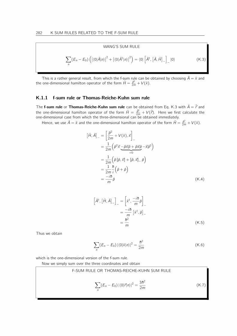
282 K SUM RULES RELATED TO THE F-SUM RULE
WANG’S SUM RULE
∑
n
(En − E0)(∣∣〈0|A|n〉
∣∣2+∣∣〈0|A†|n〉
∣∣2)
= 〈0|[
A†,[A, H
]
−
]
−|0〉 (K.3)
This is a rather general result, from which the f-sum rule can be obtained by choosing A = x andthe one-dimensional hamilton operator of the form H = p2
2m + V (x).
K.1.1 f-sum rule or Thomas-Reiche-Kuhn sum rule
The f-sum rule or Thomas-Reiche-Kuhn sum rule can be obtained from Eq. K.3 with A = ~r andthe one-dimensional hamilton operator of the form H = ~p2
2m + V (~r). Here we first calculate theone-dimensional case from which the three-dimensional can be obtained immediately.
Hence, we use A = x and the one-dimensional hamilton operator of the form H = p2
2m + V (x).
[H, A
]
− =
[p2
2m+ V (x), ~x
]
−
=1
2m
(
p2~x −p~xp + p~xp︸ ︷︷ ︸
=0
−~xp2)
=1
2m
(
p [p, ~x ] + [p, ~x ]− p)
=1
2m
~
i
(
p + p)
=−i~mp (K.4)
[
A†,[H, A
]
−
]
−=
[
x†,−i~mp
]
−
=−i~m
[x†, p
]
−
=~2
m(K.5)
Thus we obtain
∑
n
(En − E0) |〈0|x |n〉|2 =~2
2m(K.6)
which is the one-dimensional version of the f-sum rule.Now we simply sum over the three coordinates and obtain
F-SUM RULE OR THOMAS-REICHE-KUHN SUM RULE
∑
n
(En − E0) |〈0|~r |n〉|2 =3~2
2m(K.7)
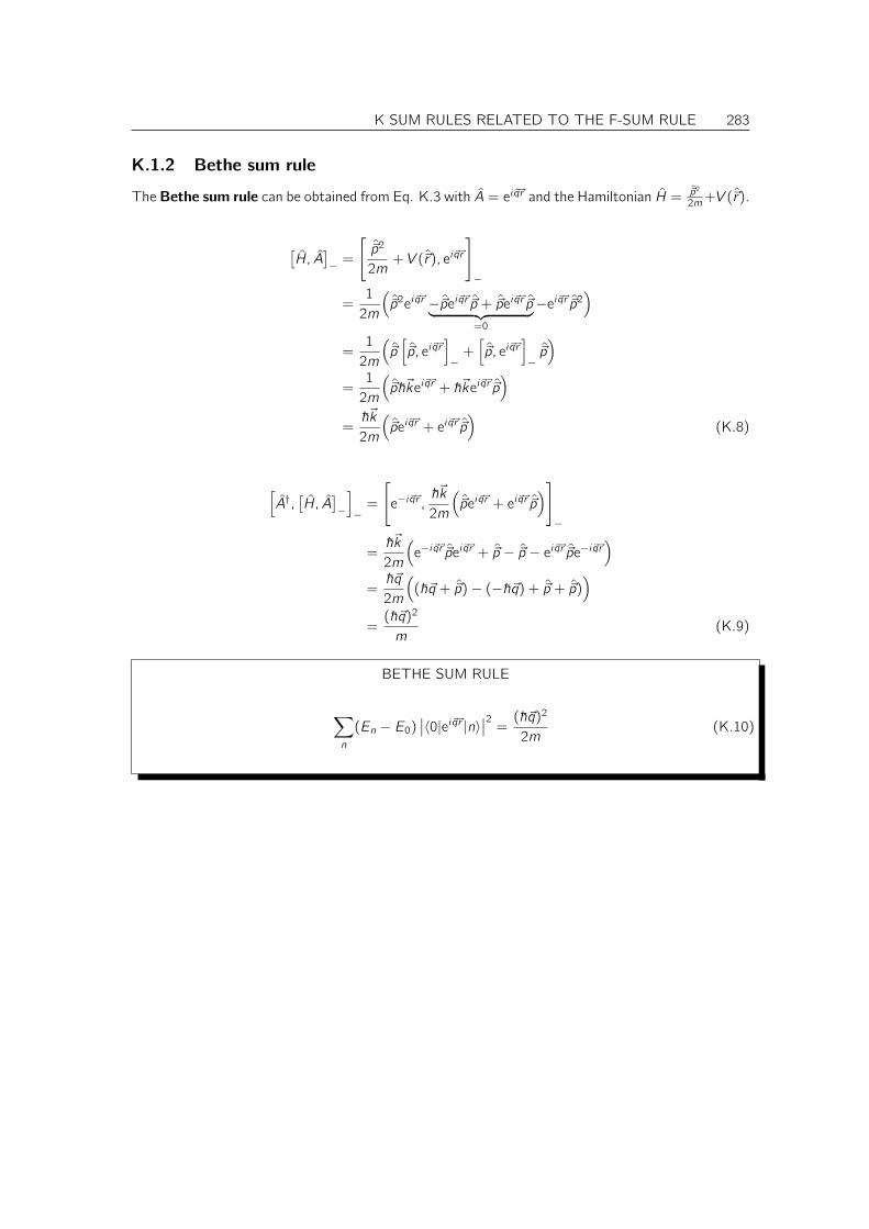
K SUM RULES RELATED TO THE F-SUM RULE 283
K.1.2 Bethe sum rule
The Bethe sum rule can be obtained from Eq. K.3 with A = ei ~q~r and the Hamiltonian H = ~p2
2m+V (~r).
[H, A
]
− =
[
~p2
2m+ V (~r), ei ~q~r
]
−
=1
2m
(
~p2ei ~q~r −~pei ~q~r ~p + ~pei ~q~r ~p︸ ︷︷ ︸
=0
−ei ~q~r ~p2)
=1
2m
(
~p[
~p, ei ~q~r]
−+[
~p, ei ~q~r]
−~p)
=1
2m
(
~p~~kei ~q~r + ~~kei ~q~r ~p)
=~~k
2m
(
~pei ~q~r + ei ~q~r ~p)
(K.8)
[
A†,[H, A
]
−
]
−=
[
e−i ~q~r ,~~k
2m
(
~pei ~q~r + ei ~q~r ~p)]
−
=~~k
2m
(
e−i ~q~r ~pei ~q~r + ~p − ~p − ei ~q~r ~pe−i ~q~r)
=~~q
2m
(
(~~q + ~p)− (−~~q) + ~p + ~p))
=(~~q)2
m(K.9)
BETHE SUM RULE
∑
n
(En − E0)∣∣〈0|ei ~q~r |n〉
∣∣2=(~~q)2
2m(K.10)

284 K SUM RULES RELATED TO THE F-SUM RULE
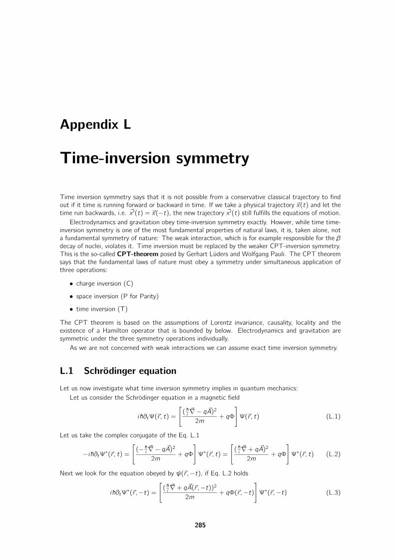
Appendix L
Time-inversion symmetry
Time inversion symmetry says that it is not possible from a conservative classical trajectory to findout if it time is running forward or backward in time. If we take a physical trajectory ~x(t) and let thetime run backwards, i.e. ~x ′(t) = ~x(−t), the new trajectory ~x ′(t) still fulfills the equations of motion.
Electrodynamics and gravitation obey time-inversion symmetry exactly. Howver, while time time-inversion symmetry is one of the most fundamental properties of natural laws, it is, taken alone, nota fundamental symmetry of nature: The weak interaction, which is for example responsible for the βdecay of nuclei, violates it. Time inversion must be replaced by the weaker CPT-inversion symmetry.This is the so-called CPT-theorem posed by Gerhart Lüders and Wolfgang Pauli. The CPT theoremsays that the fundamental laws of nature must obey a symmetry under simultaneous application ofthree operations:
• charge inversion (C)
• space inversion (P for Parity)
• time inversion (T)
The CPT theorem is based on the assumptions of Lorentz invariance, causality, locality and theexistence of a Hamilton operator that is bounded by below. Electrodynamics and gravitation aresymmetric under the three symmetry operations individually.
As we are not concerned with weak interactions we can assume exact time inversion symmetry.
L.1 Schrödinger equation
Let us now investigate what time inversion symmetry implies in quantum mechanics:Let us consider the Schrödinger equation in a magnetic field
i~∂tΨ(~r , t) =
[
( ~i~∇− q ~A)22m
+ qΦ
]
Ψ(~r , t) (L.1)
Let us take the complex conjugate of the Eq. L.1
−i~∂tΨ∗(~r , t) =[
(− ~i ~∇− q ~A)22m
+ qΦ
]
Ψ∗(~r , t) =
[
( ~i~∇+ q ~A)22m
+ qΦ
]
Ψ∗(~r , t) (L.2)
Next we look for the equation obeyed by ψ(~r ,−t), if Eq. L.2 holds
i~∂tΨ∗(~r ,−t) =
[
( ~i~∇+ q ~A(~r ,−t))2
2m+ qΦ(~r ,−t)
]
Ψ∗(~r ,−t) (L.3)
285
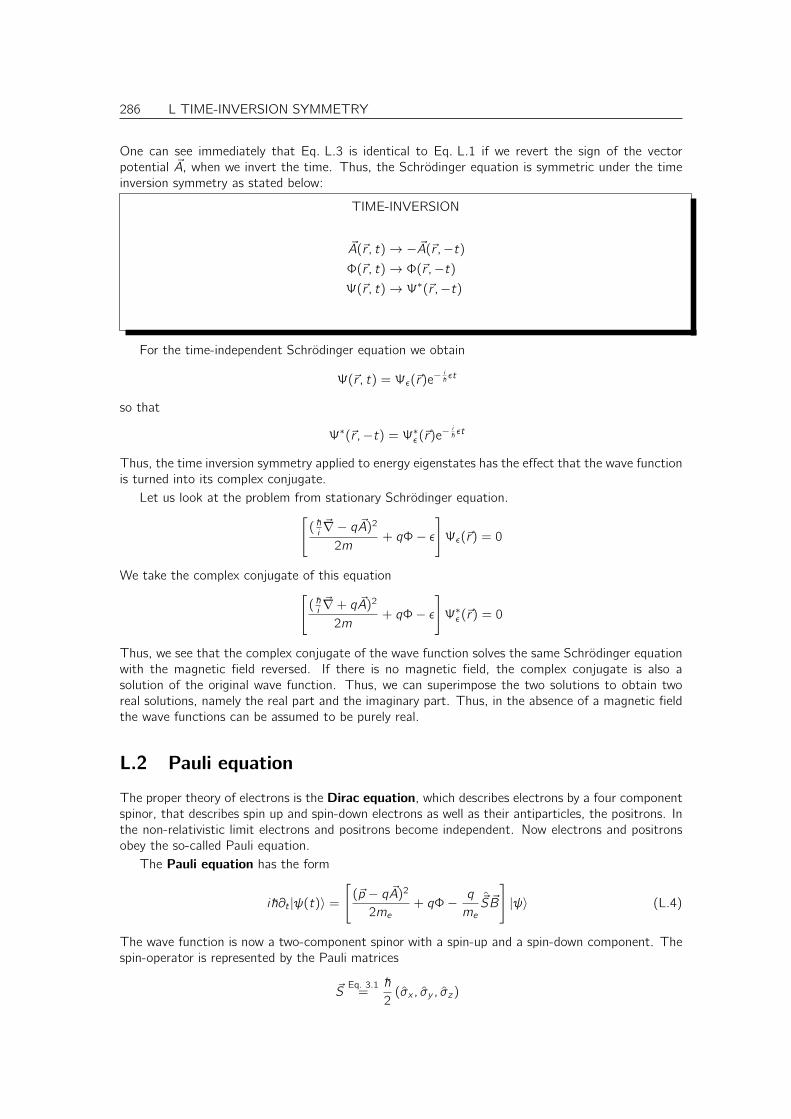
286 L TIME-INVERSION SYMMETRY
One can see immediately that Eq. L.3 is identical to Eq. L.1 if we revert the sign of the vectorpotential ~A, when we invert the time. Thus, the Schrödinger equation is symmetric under the timeinversion symmetry as stated below:
TIME-INVERSION
~A(~r , t)→ −~A(~r ,−t)Φ(~r , t)→ Φ(~r ,−t)Ψ(~r , t)→ Ψ∗(~r ,−t)
For the time-independent Schrödinger equation we obtain
Ψ(~r , t) = Ψǫ(~r)e− i~ǫt
so that
Ψ∗(~r ,−t) = Ψ∗ǫ(~r)e−i~ǫt
Thus, the time inversion symmetry applied to energy eigenstates has the effect that the wave functionis turned into its complex conjugate.
Let us look at the problem from stationary Schrödinger equation.[
( ~i~∇− q ~A)22m
+ qΦ− ǫ]
Ψǫ(~r) = 0
We take the complex conjugate of this equation[
( ~i~∇+ q ~A)22m
+ qΦ− ǫ]
Ψ∗ǫ(~r) = 0
Thus, we see that the complex conjugate of the wave function solves the same Schrödinger equationwith the magnetic field reversed. If there is no magnetic field, the complex conjugate is also asolution of the original wave function. Thus, we can superimpose the two solutions to obtain tworeal solutions, namely the real part and the imaginary part. Thus, in the absence of a magnetic fieldthe wave functions can be assumed to be purely real.
L.2 Pauli equation
The proper theory of electrons is the Dirac equation, which describes electrons by a four componentspinor, that describes spin up and spin-down electrons as well as their antiparticles, the positrons. Inthe non-relativistic limit electrons and positrons become independent. Now electrons and positronsobey the so-called Pauli equation.
The Pauli equation has the form
i~∂t |ψ(t)〉 =[
(~p − q ~A)22me
+ qΦ− q
me~S ~B
]
|ψ〉 (L.4)
The wave function is now a two-component spinor with a spin-up and a spin-down component. Thespin-operator is represented by the Pauli matrices
~SEq. 3.1=~
2(σx , σy , σz)
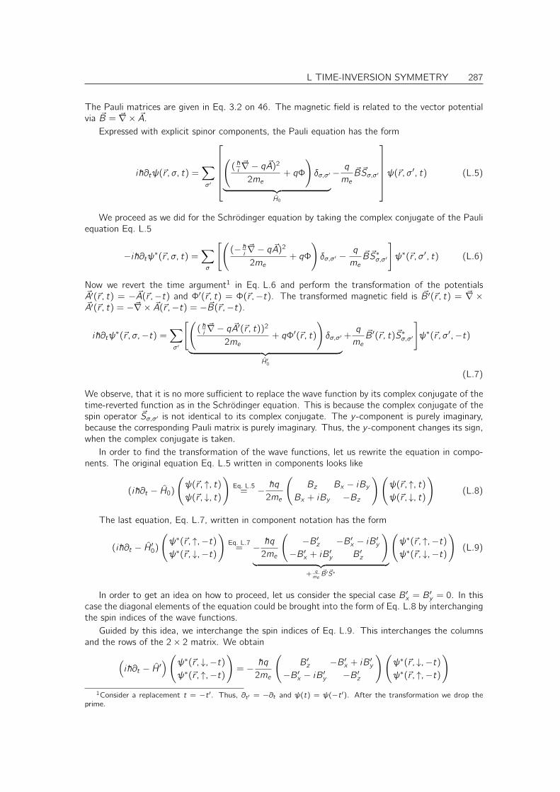
L TIME-INVERSION SYMMETRY 287
The Pauli matrices are given in Eq. 3.2 on 46. The magnetic field is related to the vector potentialvia ~B = ~∇× ~A.
Expressed with explicit spinor components, the Pauli equation has the form
i~∂tψ(~r , σ, t) =∑
σ′
(
( ~i~∇− q ~A)22me
+ qΦ
)
δσ,σ′
︸ ︷︷ ︸
H0
− q
me~B~Sσ,σ′
ψ(~r , σ′, t) (L.5)
We proceed as we did for the Schrödinger equation by taking the complex conjugate of the Pauliequation Eq. L.5
−i~∂tψ∗(~r , σ, t) =∑
σ
[(
(− ~i ~∇− q ~A)22me
+ qΦ
)
δσ,σ′ −q
me~B~S∗σ,σ′
]
ψ∗(~r , σ′, t) (L.6)
Now we revert the time argument1 in Eq. L.6 and perform the transformation of the potentials~A′(~r , t) = −~A(~r ,−t) and Φ′(~r , t) = Φ(~r ,−t). The transformed magnetic field is ~B′(~r , t) = ~∇ ×~A′(~r , t) = −~∇× ~A(~r ,−t) = −~B(~r ,−t).
i~∂tψ∗(~r , σ,−t) =
∑
σ′
[(
( ~i~∇− q ~A′(~r , t))22me
+ qΦ′(~r , t)
)
δσ,σ′
︸ ︷︷ ︸
H′0
+q
me~B′(~r , t)~S∗σ,σ′
]
ψ∗(~r , σ′,−t)
(L.7)
We observe, that it is no more sufficient to replace the wave function by its complex conjugate of thetime-reverted function as in the Schrödinger equation. This is because the complex conjugate of thespin operator ~Sσ,σ′ is not identical to its complex conjugate. The y -component is purely imaginary,because the corresponding Pauli matrix is purely imaginary. Thus, the y -component changes its sign,when the complex conjugate is taken.
In order to find the transformation of the wave functions, let us rewrite the equation in compo-nents. The original equation Eq. L.5 written in components looks like
(i~∂t − H0)(
ψ(~r , ↑, t)ψ(~r , ↓, t)
)
Eq. L.5= − ~q
2me
(
Bz Bx − iByBx + iBy −Bz
)(
ψ(~r , ↑, t)ψ(~r , ↓, t)
)
(L.8)
The last equation, Eq. L.7, written in component notation has the form
(i~∂t − H′0)(
ψ∗(~r , ↑,−t)ψ∗(~r , ↓,−t)
)
Eq. L.7= − ~q
2me
(
−B′z −B′x − iB′y−B′x + iB′y B′z
)
︸ ︷︷ ︸
+ qme~B′ ~S∗
(
ψ∗(~r , ↑,−t)ψ∗(~r , ↓,−t)
)
(L.9)
In order to get an idea on how to proceed, let us consider the special case B′x = B′y = 0. In this
case the diagonal elements of the equation could be brought into the form of Eq. L.8 by interchangingthe spin indices of the wave functions.
Guided by this idea, we interchange the spin indices of Eq. L.9. This interchanges the columnsand the rows of the 2× 2 matrix. We obtain
(
i~∂t − H′)(
ψ∗(~r , ↓,−t)ψ∗(~r , ↑,−t)
)
= − ~q2me
(
B′z −B′x + iB′y−B′x − iB′y −B′z
)(
ψ∗(~r , ↓,−t)ψ∗(~r , ↑,−t)
)
1Consider a replacement t = −t ′. Thus, ∂t ′ = −∂t and ψ(t) = ψ(−t ′). After the transformation we drop theprime.
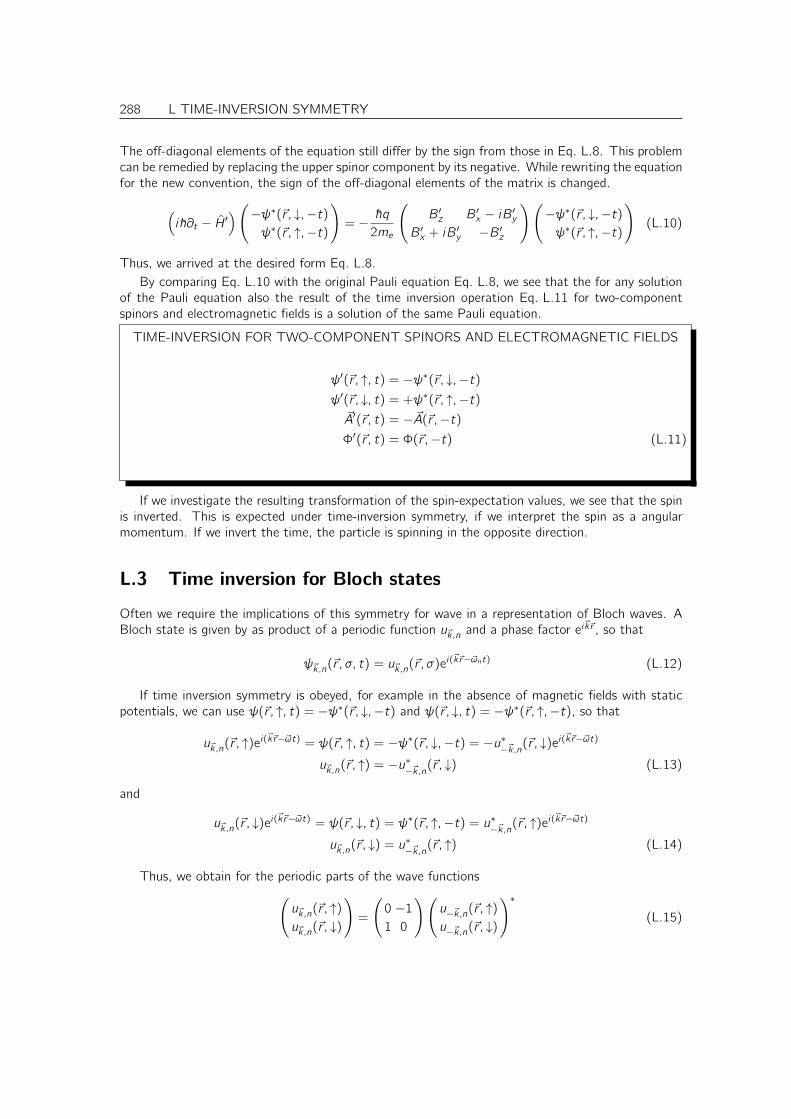
288 L TIME-INVERSION SYMMETRY
The off-diagonal elements of the equation still differ by the sign from those in Eq. L.8. This problemcan be remedied by replacing the upper spinor component by its negative. While rewriting the equationfor the new convention, the sign of the off-diagonal elements of the matrix is changed.
(
i~∂t − H′)(
−ψ∗(~r , ↓,−t)ψ∗(~r , ↑,−t)
)
= − ~q2me
(
B′z B′x − iB′yB′x + iB
′y −B′z
)(
−ψ∗(~r , ↓,−t)ψ∗(~r , ↑,−t)
)
(L.10)
Thus, we arrived at the desired form Eq. L.8.By comparing Eq. L.10 with the original Pauli equation Eq. L.8, we see that the for any solution
of the Pauli equation also the result of the time inversion operation Eq. L.11 for two-componentspinors and electromagnetic fields is a solution of the same Pauli equation.
TIME-INVERSION FOR TWO-COMPONENT SPINORS AND ELECTROMAGNETIC FIELDS
ψ′(~r , ↑, t) = −ψ∗(~r , ↓,−t)ψ′(~r , ↓, t) = +ψ∗(~r , ↑,−t)~A′(~r , t) = −~A(~r ,−t)Φ′(~r , t) = Φ(~r ,−t) (L.11)
If we investigate the resulting transformation of the spin-expectation values, we see that the spinis inverted. This is expected under time-inversion symmetry, if we interpret the spin as a angularmomentum. If we invert the time, the particle is spinning in the opposite direction.
L.3 Time inversion for Bloch states
Often we require the implications of this symmetry for wave in a representation of Bloch waves. ABloch state is given by as product of a periodic function u~k,n and a phase factor ei~k~r , so that
ψ~k,n(~r , σ, t) = u~k,n(~r , σ)ei(~k~r−~ωnt) (L.12)
If time inversion symmetry is obeyed, for example in the absence of magnetic fields with staticpotentials, we can use ψ(~r , ↑, t) = −ψ∗(~r , ↓,−t) and ψ(~r , ↓, t) = −ψ∗(~r , ↑,−t), so that
u~k,n(~r , ↑)ei(~k~r−~ωt) = ψ(~r , ↑, t) = −ψ∗(~r , ↓,−t) = −u∗−~k,n(~r , ↓)e
i(~k~r−~ωt)
u~k,n(~r , ↑) = −u∗−~k,n(~r , ↓) (L.13)
and
u~k,n(~r , ↓)ei(~k~r−~ωt) = ψ(~r , ↓, t) = ψ∗(~r , ↑,−t) = u∗−~k,n(~r , ↑)e
i(~k~r−~ωt)
u~k,n(~r , ↓) = u∗−~k,n(~r , ↑) (L.14)
Thus, we obtain for the periodic parts of the wave functions(
u~k,n(~r , ↑)u~k,n(~r , ↓)
)
=
(
0 −11 0
)(
u−~k,n(~r , ↑)u−~k,n(~r , ↓)
)∗
(L.15)
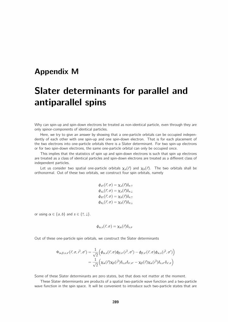
Appendix M
Slater determinants for parallel andantiparallel spins
Why can spin-up and spin-down electrons be treated as non-identical particle, even through they areonly spinor-components of identical particles.
Here, we try to give an answer by showing that a one-particle orbitals can be occupied indepen-dently of each other with one spin-up and one spin-down electron. That is for each placement ofthe two electrons into one-particle orbitals there is a Slater determinant. For two spin-up electronsor for two spin-down electrons, the same one-particle orbital can only be occupied once.
This implies that the statistics of spin up and spin-down electrons is such that spin up electronsare treated as a class of identical particles and spin-down electrons are treated as a different class ofindependent particles.
Let us consider two spatial one-particle orbitals χa(~r) and χb(~r). The two orbitals shall beorthonormal. Out of these two orbitals, we construct four spin orbitals, namely
φa↑(~r , σ) = χa(~r)δσ,↑
φa↓(~r , σ) = χa(~r)δσ,↓
φb↑(~r , σ) = χb(~r)δσ,↑
φb↓(~r , σ) = χb(~r)δσ,↓
or using α ∈ a, b and s ∈ ↑, ↓.
φα,s(~r , σ) = χα(~r)δs,σ
Out of these one-particle spin orbitals, we construct the Slater determinants
Φα,β,s,s ′(~r , σ, ~r ′, σ′) =
1√2
(
φα,s(~r , σ)φβ,s ′(~r ′, σ′)− φβ,s ′(~r , σ)φα,s(~r ′, σ′)
)
=1√2
(
χα(~r)χβ(~r ′)δs,σδs ′,σ′ − χβ(~r)χα(~r ′)δs,σ′δs ′,σ)
Some of these Slater determinants are zero states, but that does not matter at the moment.These Slater determinants are products of a spatial two-particle wave function and a two-particle
wave function in the spin space. It will be convenient to introduce such two-particle states that are
289
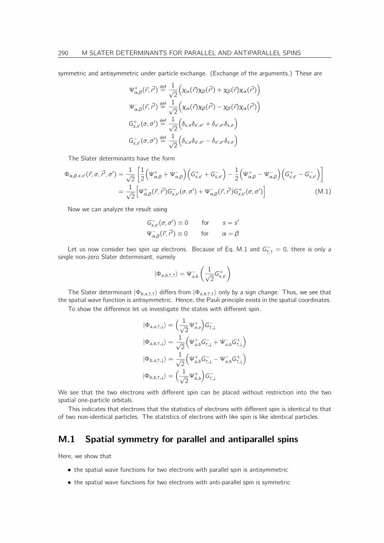
290 M SLATER DETERMINANTS FOR PARALLEL AND ANTIPARALLEL SPINS
symmetric and antisymmetric under particle exchange. (Exchange of the arguments.) These are
Ψ+α,β(~r ,~r ′)
def=1√2
(
χα(~r)χβ(~r ′) + χβ(~r)χα(~r ′))
Ψ−α,β(~r , ~r′)
def=1√2
(
χα(~r)χβ(~r ′)− χβ(~r)χα(~r ′))
G+s,s ′(σ, σ′)
def=1√2
(
δs,σδs ′,σ′ + δs ′,σ′δs,σ
)
G−s,s ′(σ, σ′)
def=1√2
(
δs,σδs ′,σ′ − δs ′,σ′δs,σ)
The Slater determinants have the form
Φα,β,s,s ′(~r , σ, ~r ′, σ′) =
1√2
[1
2
(
Ψ+α,β +Ψ−α,β
)(
G+s,s ′ + G−s,s ′
)
− 12
(
Ψ+α,β −Ψ−α,β)(
G+s,s ′ − G−s,s ′)]
=1√2
[
Ψ+α,β(~r ,~r ′)G−s,s ′(σ, σ
′) + Ψ−α,β(~r , ~r′)G+s,s ′(σ, σ
′)]
(M.1)
Now we can analyze the result using
G−s,s ′(σ, σ′) ≡ 0 for s = s ′
Ψ−α,β(~r , ~r′) ≡ 0 for α = β
Let us now consider two spin up electrons. Because of Eq. M.1 and G−↑,↑ = 0, there is only asingle non-zero Slater determinant, namely
|Φa,b,↑,↑〉 = Ψ−a,b(1√2G+s,s ′
)
The Slater determinant |Φb,a,↑,↑〉 differs from |Φa,b,↑,↑〉 only by a sign change. Thus, we see thatthe spatial wave function is antisymmetric. Hence, the Pauli principle exists in the spatial coordinates.
To show the difference let us investigate the states with different spin.
|Φa,a,↑,↓〉 =( 1√2Ψ+a,a
)
G−↑,↓
|Φa,b,↑,↓〉 =1√2
(
Ψ+a,bG−↑,↓ +Ψ
−a,bG
+↑,↓
)
|Φb,a,↑,↓〉 =1√2
(
Ψ+a,bG−↑,↓ −Ψ−a,bG+↑,↓
)
|Φb,b,↑,↓〉 =( 1√2Ψ+b,b
)
G−↑,↓
We see that the two electrons with different spin can be placed without restriction into the twospatial one-particle orbitals.
This indicates that electrons that the statistics of electrons with different spin is identical to thatof two non-identical particles. The statistics of electrons with like spin is like identical particles.
M.1 Spatial symmetry for parallel and antiparallel spins
Here, we show that
• the spatial wave functions for two electrons with parallel spin is antisymmetric
• the spatial wave functions for two electrons with anti-parallel spin is symmetric
M SLATER DETERMINANTS FOR PARALLEL AND ANTIPARALLEL SPINS 291
under exchange of the coordinates.A common misconception is that the Slater determinant of two one-particle spin-orbitals with
opposite spin describes two electrons with anti-parallel spin. For such a state the z-component ofthe spin vanishes, but it is a superposition of a two states with Sz = 0, namely one with antiparallelspin and the other with parallel spin with a total spin lying in the xy-plane.
In order to determine states with parallel and antiparallel spin, we need to determine the spin
eigenstates and eigenvalues. If the eigenvalue for S2tot = ( ~S1 + ~S2)2 vanishes, the wave function has
antiparallel spin. If the eigenvalue is 2~2 the spins are parallel.Using the ladder operators S± we write the total spin as
S2tot = ( ~S1 + ~S2)2
= ~S21 + ~S22 + 2 ~S1 ~S2
= ~S21 + ~S22 + 2
[1
2S1,+S2,− +
1
2S1,−S2,+ + S1,z S2,z
]
= ~S21 + ~S22 + S1,+S2,− + S1,−S2,+ + 2S1,z S2,z
]
The ladder operators are defined as
S+ = Sx + i Sy
S− = Sx − i Syand obey
S−| ↑〉 = | ↓〉~ and S−| ↓〉 = |∅〉S+| ↑〉 = |∅〉 and S+| ↓〉 = | ↑〉~
Thus(
S1+S2− + S1−S2+)
|G±↑,↓〉 =(
S1+S2− + S1−S2+) 1√2
(
| ↑, ↓〉 ± | ↓, ↑〉)
=1√2
(
| ↓, ↑〉 ± | ↑, ↓〉)
~2
= |G±↑,↓〉(
±~2)
(
S1+S2− + S1−S2+)
|G±↑,↑〉 = |∅〉(
S1+S2− + S1−S2+)
|G±↓,↓〉 = |∅〉
S1,z S2,z |G±↑,↓〉 = |G±↑,↓〉(
−~2
4)
S1,z S2,z |G±↑,↑〉 = |G±↑,↑〉(
+~2
4)
S1,z S2,z |G±↓,↓〉 = |G±↓,↓〉(
+~2
4)
~S2i |G±s,s ′〉 = |G±s,s ′〉3~2
4
S2tot |G±↑,↓〉 = |G±↑,↓〉[3~2
4+3~2
4± ~2 − ~
2
2
]
= |G±↑,↓〉(1± 1)~2
S2tot |G±↑,↑〉 = |G±↑,↑〉[3~2
4+3~2
4+~2
2
]
= |G±↑,↑〉2~2
S2tot |G±↓,↓〉 = |G±↓,↓〉[3~2
4+3~2
4+~2
2
]
= |G±↓,↓〉2~2
292 M SLATER DETERMINANTS FOR PARALLEL AND ANTIPARALLEL SPINS
Thus, we see that |G+↑,↓〉, |G+↑,↑〉 and |G+↓,↓〉 describe two electrons with parallel spin. Note that|G−s,s ′〉 vanishes for parallel spin.
The only solution with antiparallel spin is |G−↑,↓〉.From Eq. M.1 we know that the antisymmetric spin wave function is always combined with the
symmetric spatial orbital and vice versa. Hence, the wave functions describing two electrons withanti-parallel spin are symmetric in their spatial coordinates, while the ones with parallel spin have anantisymmetric spatial wave function.
M.2 An intuitive analogy for particle with spin
Consider balls that are painted on the one side green and on the other side red.If we place two such balls on a table with the green side up, turn around and look at them again,
we cannot tell if the two balls habe been interchanged.No we place them with opposite colors up. If we only allow that the positions of the two balls are
interchanged, but exclude that they are turned around, we can tell the two spheres apart from theirorientation. Hence, we can treat them as non-identical spheres.
However, if we consider exchanges of position and orientation, we are again unable to tell, whetherthe spheres have been interchanged or not.
Thus, if we can exclude that the spins of the particles –or the orientation of our spheres– change,we can divide electrons into two classes of particles, namely spin-up and spin-down electrons. Particleswithin each class are indistinguishable, but spin-up and spin-down electrons can be distinguished.When the spin is preserved, the Hamiltonian is invariant with respect to spin-rotation, and spin is agood quantum number.
However, if there is a magnetic field, which can cause a rotation of the spin direction, the divisioninto spin-up and spin-down particles is no more a useful concept. In our model, if the orientation ofthe spheres can change with time, we cannot use it as distinguishing feature.
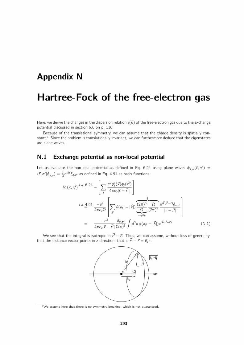
Appendix N
Hartree-Fock of the free-electron gas
Here, we derive the changes in the dispersion relation ǫ(~k) of the free-electron gas due to the exchangepotential discussed in section 6.6 on p. 110.
Because of the translational symmetry, we can assume that the charge density is spatially con-stant.1 Since the problem is translationally invariant, we can furthermore deduce that the eigenstatesare plane waves.
N.1 Exchange potential as non-local potential
Let us evaluate the non-local potential as defined in Eq. 6.24 using plane waves φ~k,σ(~r , σ′) =
〈~r , σ′|φ~k,σ〉 = 1Ωe
i~k~rδσ,σ′ as defined in Eq. 4.91 as basis functions.
Vx(~x, ~x ′)Eq. 6.24= −
∑
j
e2φ∗j (~x)φj(~x′)
4πǫ0|~r − ~r ′|
Eq. 4.91=
−e24πǫ0Ω
∑
~k
θ(kF − |~k |)
1︷ ︸︸ ︷
(2π)3
Ω︸ ︷︷ ︸
→d3k
Ω
(2π)3ei~k(~r ′−~r)δσ,σ′
|~r − ~r ′|
=−e2
4πǫ0|~r − ~r ′|δσ,σ′
(2π)3
∫
d3k θ(kF − |~k |)ei~k(~r′−~r) (N.1)
We see that the integral is isotropic in ~r ′ − ~r . Thus, we can assume, without loss of generality,that the distance vector points in z-direction, that is ~r ′ − ~r = ~ezs.
kF
kz
kF2 −kz
2
1We assume here that there is no symmetry breaking, which is not guaranteed.
293
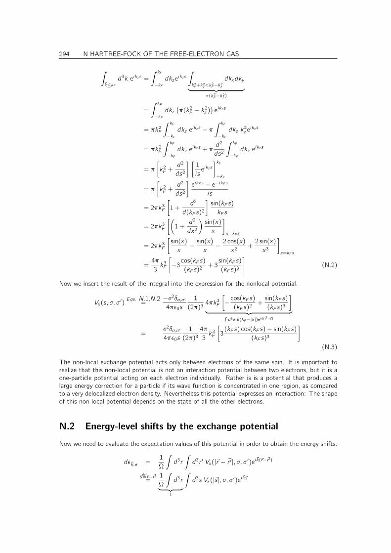
294 N HARTREE-FOCK OF THE FREE-ELECTRON GAS
∫
~k≤kFd3k eikz s =
∫ kF
−kFdkze
ikz s
∫
k2x+k2y<k
2F−k2z
dkxdky
︸ ︷︷ ︸
π(k2F−k2z )
=
∫ kF
−kFdkz
(π(k2F − k2z )
)eikz s
= πk2F
∫ kF
−kFdkz e
ikz s − π∫ kF
−kFdkz k
2z eikz s
= πk2F
∫ kF
−kFdkz e
ikz s + πd2
ds2
∫ kF
−kFdkz e
ikz s
= π
[
k2F +d2
ds2
] [1
i seikz s
]kF
−kF
= π
[
k2F +d2
ds2
]eikF s − e−ikF s
i s
= 2πk3F
[
1 +d2
d(kF s)2
]sin(kF s)
kF s
= 2πk3F
[(
1 +d2
dx2
)sin(x)
x
]
x=kF s
= 2πk3F
[sin(x)
x− sin(x)
x− 2 cos(x)
x2+2 sin(x)
x3
]
x=kF s
=4π
3k3F
[
−3cos(kF s)(kF s)2
+ 3sin(kF s)
(kF s)3
]
(N.2)
Now we insert the result of the integral into the expression for the nonlocal potential.
Vx(s, σ, σ′)Eqs. N.1,N.2
=−e2δσ,σ′4πǫ0s
1
(2π)34πk3F
[
−cos(kF s)(kF s)2
+sin(kF s)
(kF s)3
]
︸ ︷︷ ︸∫d3k θ(kF−|~k|)ei~k(~r ′−~r)
=e2δσ,σ′
4πǫ0s
1
(2π)34π
3k3F
[
3(kF s) cos(kF s)− sin(kF s)
(kF s)3
]
(N.3)
The non-local exchange potential acts only between electrons of the same spin. It is important torealize that this non-local potential is not an interaction potential between two electrons, but it is aone-particle potential acting on each electron individually. Rather is is a potential that produces alarge energy correction for a particle if its wave function is concentrated in one region, as comparedto a very delocalized electron density. Nevertheless this potential expresses an interaction: The shapeof this non-local potential depends on the state of all the other electrons.
N.2 Energy-level shifts by the exchange potential
Now we need to evaluate the expectation values of this potential in order to obtain the energy shifts:
dǫ~k,σ =1
Ω
∫
d3r
∫
d3r ′ Vx(|~r − ~r ′|, σ, σ′)ei~k(~r−~r′)
~sdef=~r−~r ′=
1
Ω
∫
d3r
︸ ︷︷ ︸
1
∫
d3s Vx(|~s |, σ, σ′)ei~k~s
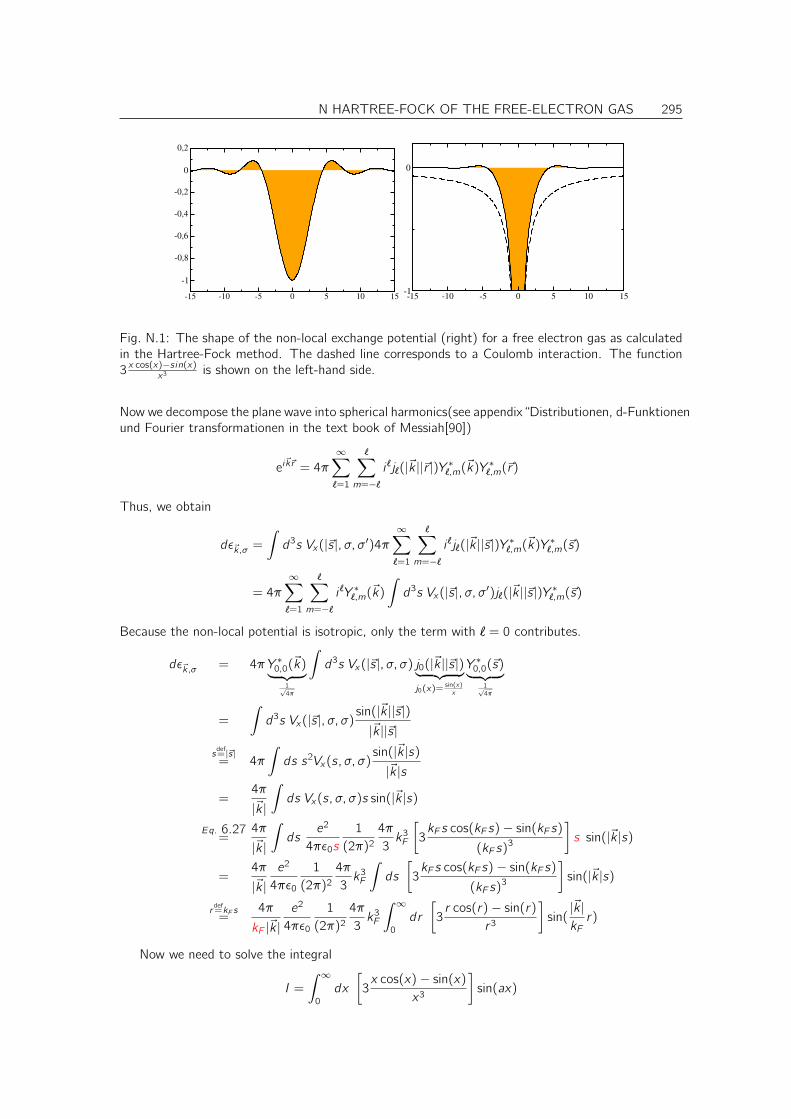
N HARTREE-FOCK OF THE FREE-ELECTRON GAS 295
-15 -10 -5 0 5 10 15
-1
-0,8
-0,6
-0,4
-0,2
0
0,2
-15 -10 -5 0 5 10 15-1
0
Fig. N.1: The shape of the non-local exchange potential (right) for a free electron gas as calculatedin the Hartree-Fock method. The dashed line corresponds to a Coulomb interaction. The function3 x cos(x)−sin(x)x3 is shown on the left-hand side.
Now we decompose the plane wave into spherical harmonics(see appendix “Distributionen, d-Funktionenund Fourier transformationen in the text book of Messiah[90])
ei~k~r = 4π
∞∑
ℓ=1
ℓ∑
m=−ℓi ℓjℓ(|~k ||~r |)Y ∗ℓ,m(~k)Y ∗ℓ,m(~r)
Thus, we obtain
dǫ~k,σ =
∫
d3s Vx(|~s |, σ, σ′)4π∞∑
ℓ=1
ℓ∑
m=−ℓi ℓjℓ(|~k ||~s |)Y ∗ℓ,m(~k)Y ∗ℓ,m(~s)
= 4π
∞∑
ℓ=1
ℓ∑
m=−ℓi ℓY ∗ℓ,m(~k)
∫
d3s Vx(|~s |, σ, σ′)jℓ(|~k ||~s |)Y ∗ℓ,m(~s)
Because the non-local potential is isotropic, only the term with ℓ = 0 contributes.
dǫ~k,σ = 4π Y ∗0,0(~k)︸ ︷︷ ︸
1√4π
∫
d3s Vx(|~s |, σ, σ) j0(|~k ||~s |)︸ ︷︷ ︸
j0(x)=sin(x)x
Y ∗0,0(~s)︸ ︷︷ ︸
1√4π
=
∫
d3s Vx(|~s |, σ, σ)sin(|~k ||~s |)|~k ||~s |
sdef=|~s|= 4π
∫
ds s2Vx(s, σ, σ)sin(|~k |s)|~k |s
=4π
|~k |
∫
ds Vx(s, σ, σ)s sin(|~k |s)
Eq. 6.27=
4π
|~k |
∫
dse2
4πǫ0s
1
(2π)24π
3k3F
[
3kF s cos(kF s)− sin(kF s)
(kF s)3
]
s sin(|~k |s)
=4π
|~k |e2
4πǫ0
1
(2π)24π
3k3F
∫
ds
[
3kF s cos(kF s)− sin(kF s)
(kF s)3
]
sin(|~k |s)
rdef=kF s=
4π
kF |~k |e2
4πǫ0
1
(2π)24π
3k3F
∫ ∞
0
dr
[
3r cos(r)− sin(r)
r3
]
sin(|~k |kFr)
Now we need to solve the integral
I =
∫ ∞
0
dx
[
3x cos(x)− sin(x)
x3
]
sin(ax)
296 N HARTREE-FOCK OF THE FREE-ELECTRON GAS
where a = |~k |/kF . The difficulty with this integral is that we cannot take the two terms apart,because the individual parts of the integrand diverge at the origin. Thus, during the derivation, wehave to deal with divergent expressions.
∂xsin(x)
xn−1= −(n − 1)sin(x)
xn+cos(x)
xn−1
⇒ sin(x)xn
=1
(n − 1)
[cos(x)
xn−1− ∂x
sin(x)
xn−1
]
(N.4)
Eq. N.4⇒∫ ∞
0
dxsin(x)
x3sin(ax) =
1
2
∫ ∞
0
dxcos(x)
x2sin(ax)− 1
2
∫ ∞
0
dx sin(ax)∂xsin(x)
x2
=1
2
∫ ∞
0
dxcos(x)
x2sin(ax)
−12
[
sin(ax)sin(x)
x2
]∞
0
+a
2
∫ ∞
0
dxsin(x)
x2cos(ax)
=a
2+1
2
∫ ∞
0
dxcos(x) sin(ax) + a sin(x) cos(ax)
x2(N.5)
Eq. N.4⇒∫ ∞
0
dxsin(x)
x2cos(ax) =
∫ ∞
0
dxcos(x)
xcos(ax)−
∫ ∞
0
dx cos(ax)∂xsin(x)
x
=
∫ ∞
0
dxcos(x)
xcos(ax)
−[
cos(ax)sin(x)
x
]∞
0
− a∫ ∞
0
dxsin(x)
xsin(ax)
= 1 +
∫ ∞
0
dxcos(x) cos(ax)− a sin(x) sin(ax)
x(N.6)
N HARTREE-FOCK OF THE FREE-ELECTRON GAS 297
Thus, we obtain
I = 3
∫ ∞
0
dxx cos(x)− sin(x)
x3sin(ax)
= 3
∫ ∞
0
dxcos(x) sin(ax)
x2− 3
∫ ∞
0
dxsin(x) sin(ax)
x3
Eq. N.5= 3
∫ ∞
0
dxcos(x) sin(ax)
x2− 3a2− 32
∫ ∞
0
dxcos(x) sin(ax) + a sin(x) cos(ax)
x2
= −3a2+3
2
∫ ∞
0
dxcos(x) sin(ax)
x2− 3a2
∫ ∞
0
dxsin(x) cos(ax)
x2
= −3a2+3a
2
∫ ∞
0
dycos( 1a y) sin(y)
y2− 3a2
∫ ∞
0
dxsin(x) cos(ax)
x2
Eq. N.6= −3a
2+3a
2
[
1 +
∫ ∞
0
dycos( 1ay) cos(y)− 1a sin( 1a y) sin(y)
y
]
−3a2
[
1 +
∫ ∞
0
dxcos(ax) cos(x)− a sin(ax) sin(x)
x
]
= −3a2+3a
2
[∫ ∞
0
dxcos(x) cos(ax)− 1a sin(x) sin(ax)
x
]
−3a2
[∫ ∞
0
dxcos(ax) cos(x)− a sin(ax) sin(x)
x
]
= −3a2+3a
2(−1a+ a)
[∫ ∞
0
dxsin(x) sin(ax)
x
]
= −3a2+3
2(a2 − 1)
[∫ ∞
0
dxsin(x) sin(ax)
x
]
We recognize that the integral is the fourier transform of sin(x)x . From the Fourier transform tablesof Bronstein[91] we take
√
2
π
∫ ∞
0
dx sin(xy)sin(ax)
x
Bronstein=
1√2πln
∣∣∣∣
y + a
y − a
∣∣∣∣
a→1;y→a⇒∫ ∞
0
dx sin(ax)sin(x)
x=
1
2ln
∣∣∣∣
a + 1
a − 1
∣∣∣∣=1
2ln
∣∣∣∣
1 + a
1− a
∣∣∣∣
Thus, we obtain
I = −3a2+3
4(a2 − 1) ln
∣∣∣∣
1 + a
1− a
∣∣∣∣
Now we are done with the Integral. We need to insert the result in the correction for the energyeigenvalues
dǫ~k,σ =4π
kF |~k |e2
4πǫ0
1
(2π)24π
3k3F
[
−3a2+3(a2 − 1)4
ln
∣∣∣∣
a + 1
a − 1
∣∣∣∣
]
=4π
k2F
e2
4πǫ0
1
(2π)24π
3k3F
[
−32+3(a2 − 1)4a
ln
∣∣∣∣
a + 1
a − 1
∣∣∣∣
]
= − e2
4πǫ0
2kFπ
[1
2+1− a24a
ln
∣∣∣∣
1 + a
1− a
∣∣∣∣
]
The function in parenthesis is shown in Fig. N.2 and the resulting dispersion relation is discussed insection 6.6 on p. 110.
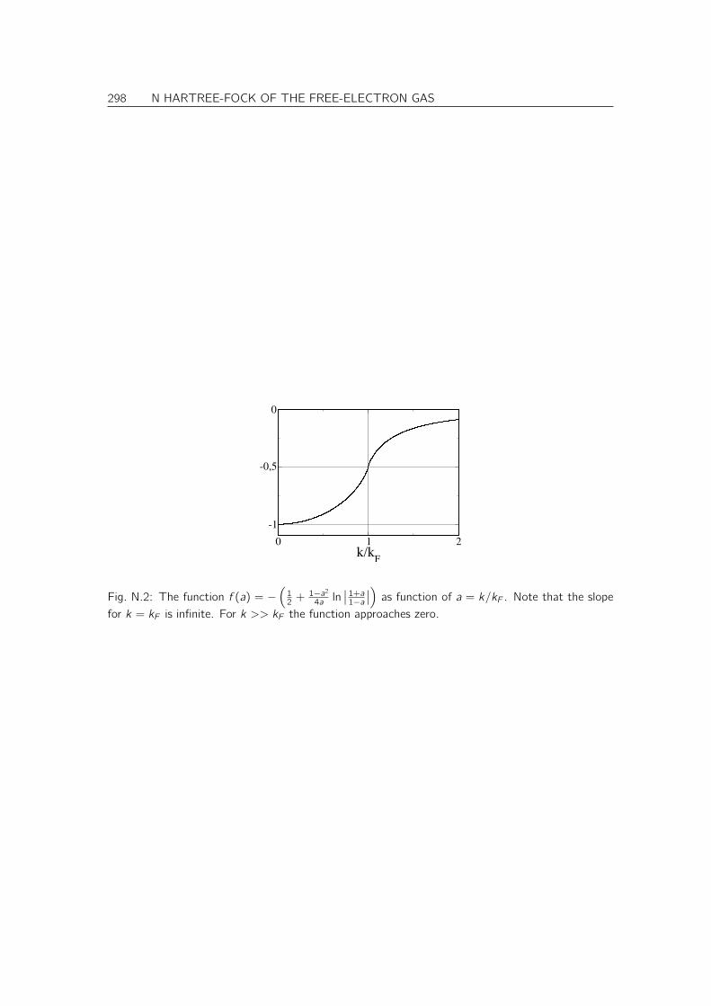
298 N HARTREE-FOCK OF THE FREE-ELECTRON GAS
0 1 2
k/kF
-1
-0,5
0
Fig. N.2: The function f (a) = −(12 +
1−a24a ln
∣∣ 1+a1−a∣∣
)
as function of a = k/kF . Note that the slope
for k = kF is infinite. For k >> kF the function approaches zero.
Appendix O
Derivation of Slater-Condon rules
In this section we derive the Slater-Condon rules spelled out in section 8.5. on p. 160.We assume that the Slater determinants are in maximum coincidence spelled out on p 160 The
principle of maximum coincidence can be used to place the one-particle orbitals that differ betweenthe two Slater determinants to the front. The other one-particle orbitals, which are identical in bothSlater determinants are placed in the identical position of both determinants.
O.1 Identical Slater determinants
The result has already been obtained when we worked out the equations for the Hartree-Fock method,where we obtained Eq. 6.6 and Eq. 6.13 on p. 101ff. They are identical to the first Slater-Condonrule Eq. 8.4 given above.
O.2 One-particle operator with one different orbital
First, we consider Slater determinants
〈~x1, . . . , ~xN |Ψ〉 =1√N!
N∑
i1,...,iN=1
ǫi1,...,iN 〈~x1|ψi1〉 · · · 〈~xN |ψiN 〉 (O.1)
〈~x1, . . . , ~xN |Φ〉 =1√N!
N∑
j1,...,jN=1
ǫj1,...,jN 〈~x1|φj1〉 · · · 〈~xN |φjN 〉 (O.2)
that differ by exactly one one-particle orbital. Due to the form of maximum coincidence defined insection 8.5, we can place these two orbitals in the first position. Hence, |ψ1〉 6= |φ1〉, but |ψi 〉 = |φi 〉for i 6= 1. Thus, 〈ψi |φj 〉 = δi ,j(1− δi ,1).
〈Ψ|A1|Φ〉 =1
N!
N∑
i1,...,iN=1
N∑
j1,...,jN=1
ǫi1,i2,...,iN ǫj1,j2,...,jN
·〈ψi1 |A|φj1〉 〈ψi2 |φj2〉︸ ︷︷ ︸
δi2 ,j2 (1−δi2 ,1)
. . . 〈ψiN |φjN 〉︸ ︷︷ ︸
δiN ,jN (1−δiN ,1)
=1
N!
N∑
i1,...,iN=1
N∑
j1=1
ǫi1,i2,...,iN ǫj1,i2,...,iN
·〈ψi1 |A|φj1〉(1− δi2,1) . . . (1− δiN ,1) (O.3)
299
300 O DERIVATION OF SLATER-CONDON RULES
Because the Levi-Civita symbol is only non-zero if all indices differ, the product of the two Levi-Civitasymbols can only be non-zero if their first index is identical.
〈Ψ|A1|Φ〉 =1
N!
N∑
i1,...,iN=1
(ǫi1,i2,...,iN )2 〈ψi1 |A|φi1〉(1− δi2,1) . . . (1− δiN ,1)
Furthermore the there is a contribution only if the first index i1 has the value 1. If that is not thecase there is a term (1− δi ,1) that vanishes.
〈Ψ|A1|Φ〉 =1
N!
N∑
i2...,iN=1
(ǫ1,i2,...,iN )2 〈ψ1|A|φ1〉 (O.4)
The Levi-Civita symbols contribute, if all indices are different, This happens (N − 1)! times, whichcorresponds to the number of permutations of the indices 2, . . . , N. Thus, we obtain
〈Ψ|A1|Φ〉 =1
N〈ψ1|A|φ1〉 (O.5)
Since the operator has the form A =∑N
i=1 Ai , and since all operators Ai contribute the sameresult, we obtain
〈Ψ|A|Φ〉 = 〈ψ1|A|φ1〉 (O.6)
which corresponds to the first line in the second Slater-Condon rule Eq. 8.5.
O.3 Two-particle operator with one different orbital
We consider the matrix element between two Slater determinants
〈~x1, . . . , ~xN |Ψ〉 =1√N!
N∑
i1,...,iN=1
ǫi1,...,iN 〈~x1|ψi1〉 · · · 〈~xN |ψiN 〉 (O.7)
〈~x1, . . . , ~xN |Φ〉 =1√N!
N∑
j1,...,jN=1
ǫj1,...,jN 〈~x1|φj1〉 · · · 〈~xN |φjN 〉 (O.8)
with all one-particle orbitals pairwise equal, except for the two first orbitals, that is
〈ψi |φj 〉 =
δi ,j for i , j ∈ 2, . . . , N0 for i = 1 and/or j = 1
= δi ,j(1− δi ,1) (O.9)
Note, that the Slater determinants are chosen in maximum coincidence, defined in section 8.5:the two orbitals that are present in only one of the two Slater determinants stand at the sameposition, namely the first. The orbitals which are identical for both Slater determinants are in thesame position.
Now, we can work out the matrix element of the interaction operator W1,2 that acts exclusively onthe first two particle coordinates. If the interaction would act onto any other orbital, at least one ofthe orbitals in the first position would be connected with another one by an overlap matrix element.This overlap matrix element vanishes because the orbitals in the first position are orthogonal to allother orbitals involved.
Later, we will see that the result is the same for each pair of coordinates, so that the sum over
O DERIVATION OF SLATER-CONDON RULES 301
pairs is done easily at the end of the calculation.
〈Ψ|W1,2|Φ〉 =1
N!
N∑
i1,...,iN=1
N∑
j1,...,jN=1
ǫi1,i2,...,iN ǫj1,j2,...,jN
·〈ψi1ψi2 |W1,2|φj1φj2〉 〈ψi3 |φj3〉︸ ︷︷ ︸
δi3 ,j3 (1−δi3 ,1)
. . . 〈ψiN |φjN 〉︸ ︷︷ ︸
δiN ,jN (1−δiN ,1)
=1
N!
N∑
i1,...,iN=1
N∑
j1,j2=1
ǫi1,i2,i3,...,iN ǫj1,j2,i3,...,iN
·〈ψi1ψi2 |W |φj1φj2〉(1− δi3,1) . . . (1− δiN ,1)Now we can work out the sum over the indices j1, j2. Because the antisymmetric tensor vanishes,whenever two indices are equal, the indices j1, j2 must be both in the set i1, i2. Furthermore thetwo indices j1, j2 must differ, again to avoid that the antisymmetric tensor vanishes. Hence, only twoterms from the second sum survive, namely the one with (j1, j2) = (i1, i2) and the one where the twoindices are interchanged (j1, j2) = (i2, i1).
〈Ψ|W1,2|Φ〉 =1
N!
N∑
i1,...,iN=1
[
(ǫi1,i2,...,iN )2 〈ψi1ψi2 |W1,2|φi1φi2〉
+ǫi1,i2,i3,...,iN ǫi2,i1,i3,...,iN 〈ψi1ψi2 |W1,2|φi2φi1〉]
·(1− δi3,1) . . . (1− δiN ,1)
=1
N!
N∑
i1,...,iN=1
(ǫi1,i2,...,iN )2(
〈ψi1ψi2 |W1,2|φi1φi2〉 − 〈ψi1ψi2 |W1,2|φi2φi1〉)
·(1− δi3,1) . . . (1− δiN ,1)Furthermore, there is a contribution only if one of the first two indices i1, i2 has the value 1. If thatis not the case, there is a term (1− δi ,1) that vanishes.
〈Ψ|W1,2|Φ〉 =1
N!
N∑
i2,i3,...,iN=1
(ǫ1,i2,...,iN )2(
〈ψ1ψi2 |W1,2|φ1φi2〉 − 〈ψ1ψi2 |W1,2|φi2φ1〉)
+1
N!
N∑
i1,i3,...,iN=1
(ǫi1,1,,i3...,iN )2(
〈ψi1ψ1|W1,2|φi1φ1〉 − 〈ψi1ψ1|W1,2|φ1φi1〉)
=2
N!
N∑
n=2
(
〈ψ1ψn|W1,2|φ1φn〉 − 〈ψ1ψn|W1,2|φnφ1〉) N∑
i3,...,iN=1
(ǫ1,n,...,iN )2
︸ ︷︷ ︸
(N−2)!
=2(N − 2)!
N!︸ ︷︷ ︸
2N(N−1)
N∑
n=2
(
〈ψ1ψn|W1,2|φ1φn〉 − 〈ψ1ψn|W1,2|φnφ1〉)
Since the operator has the form W = 12
∑Ni 6=j Wi ,j . Each pair contributes the same result. As there
are N(N − 1) distinct pairs in the double-sum, we obtain
〈Ψ|W |Φ〉 =N∑
n=1
(〈ψ1ψn|W1,2|φ1φn〉 − 〈ψ1ψn|W1,2|φnφ1〉
)
This result corresponds to the second line in the second Slater-Condon rule Eq. 8.5. The sum runsnow over all terms because the element with n = 1 cancels anyway.
302 O DERIVATION OF SLATER-CONDON RULES
O.4 One-particle operator with two different orbitals
〈Ψ|A1|Φ〉 =1
N!
N∑
i1,...,iN=1
N∑
j1,...,jN=1
ǫi1,i2,...,iN ǫj1,j2,...,jN
·〈ψi1 |A|φj1〉 〈ψi2 |φj2〉︸ ︷︷ ︸
δi2 ,j2 (1−δi2 ,1)(1−δi2 ,2)
. . . 〈ψiN |φjN 〉︸ ︷︷ ︸
δiN ,jN (1−δiN ,1)(1−δiN ,2)
It is evident that this matrix element vanishes, because in each term there is at least one scalarproduct between to orbitals that differ in the two slater determinants.
This result corresponds to the first line in the third Slater-Condon rule Eq. 8.6.
O.5 Two-particle operator with two different orbitals
〈Ψ|Wx1,x2 |Φ〉 =1
N!
∑
i1,...,iN
∑
j1,...,jN
ǫi1,i2,...,iN ǫj1,j2,...,jN
·〈ψi1ψi2 |W |φj1φj2〉 〈ψi3 |φj3〉︸ ︷︷ ︸
δi3 ,j3 (1−δi3 ,1)(1−δi3 ,2)
. . . 〈ψiN |φjN 〉︸ ︷︷ ︸
δiN ,jN (1−δiN ,1)(1−δiN ,2)
=1
N!
2∑
i1,i2=1
2∑
j1,j2=1
〈ψi1ψi2 |W |φj1φj2〉∑
i3,...,iN
ǫi1,i2,i3...,iN ǫj1,j2,i3...,iN
=1
N!
2∑
i1,i2=1
2∑
j1,j2=1
〈ψi1ψi2 |W |φj1φj2〉(N − 2)! (δi1,j1δi2,j2 − δi1,j2δi2,j1)
=2
N(N − 1)(〈ψ1ψ2|W |φ1φ2〉 − 〈ψ1ψ2|W |φ2φ1〉
)
With the interaction W = 12
∑Ni 6=j Wi ,j we obtain with 〈Ψ|Wi ,j |Φ〉 = 〈Ψ|W1,2|Φ〉
〈Ψ|W |Φ〉 = 〈ψ1ψ2|W |φ1φ2〉 − 〈ψ1ψ2|W |φ2φ1〉
This result corresponds to the second line in the third Slater-Condon rule Eq. 8.6.
O.6 More than two different one-particle orbitals
The result vanishes. The argument is analogous to that about in Section O.4
Appendix P
One- and two-particle operatorsexpressed by field operators
Here, we will explicitly derive the form of one- and two-particle operators by field operators as givenby Eqs. 8.8 and 8.9 on p. 162.
OPERATORS EXPRESSED BY ANNIHILATION AND CREATION OPERATORS
A one-particle operator has the form
A =∑
i ,j
Ai ,j c†i cj (P.1)
and a two-particle operator has the form
W =1
2
∑
i ,j,k,l
Wi ,j,k,l c†i c†j c l ck (P.2)
Note the reversed order of the annihilators relative to the indices!
Our approach will be to work out the matrix elements of a product of creation and annihilationoperators between Slater determinants Then the result will be compared with the Slater-Condon rulesEqs. 8.4 -8.6 on p. 161.
Our argument is restricted to Slater determinants constructed from the zero state by aproduct of creation operators in a unique basis of one-particle orbitals. basis. Thus, thesestates are eigenstates of the occupation-number operator
nk = c†k ck
P.1 Matrix elements between identical Slater determinants
One-particle operator
Let us determine the matrix element of a one-particle operator between two identical Slater deter-minants |Φ〉.
In the first step we used that 〈Φ|c†i cj |Φ〉 = 0 for i 6= j : Applied to a Slater determinant c†i ciproduces a different Slater determinant that is orthogonal to the original one. Thus, only the diagonal
303
304 P ONE- AND TWO-PARTICLE OPERATORS EXPRESSED BY FIELD OPERATORS
terms contribute.
〈Φ|c†i cj |Φ〉 = δi ,j〈Φ| ni︸︷︷︸c†i ci
|Φ〉 = δi ,jni
⇒ 〈Φ|∑
i ,j
Ai ,j c†i cj |Φ〉 =
∑
i
niAi ,i (P.3)
Eq. P.3 is identical to the first Slater-Condon rule Eq. 8.4 for one-particle operators on p.161. InEq. P.3 we sum over all one-particle basis functions and the occupation numbers ni select those thatare present in the Slater determinant. In Eq. 8.4 the sum goes directly over the one-orbitals in thedeterminant.
Two-particle operator
To work out the expressions for a two-particle operator, we use a similar argument. Unless theoperator c†i c
†j ck cl creates all orbitals that it has destroyed, the resulting Slater determinant will differ
from and be orthogonal to the original Slater determinant. There are just two possibilities, namely
• case 1: i = k and j = l .
c†i c†j ci cj
[c†i ,cj ]+=δi ,j= c†i δi ,j cj − c
†i ci c
†j cj = δi ,j ni − ni nj
• case 2: i = l and j = k
c†i c†j cj ci
[cj ,cj ]+=0= −c†i c
†j ci cj
[c†i ,cj ]+=δi ,j= −c†i δi ,j cj + c
†i ci c
†j cj = −δi ,j ni + ni nj
• All other cases vanish because the creators and annihilators do not match.
Thus, we obtain
〈Φ|c†i c†j ck cl |Φ〉 = δi ,kδj,l
(
δi ,jni − ninj)
+ δi ,lδj,k
(
−δi ,jni + ninj)
= δi ,kδj,lδi ,jni︸ ︷︷ ︸
a
− δi ,kδj,lninj︸ ︷︷ ︸
b
− δi ,lδj,kδi ,jni︸ ︷︷ ︸
c
+ δi ,lδj,kninj︸ ︷︷ ︸
d
a=c= δi ,lδj,kninj︸ ︷︷ ︸
d
− δi ,kδj,lninj︸ ︷︷ ︸
b
which yields
⇒ 〈Φ|∑
i ,j,k,l
Wi ,j,k,l c†i c†j c l ck |Φ〉 =
∑
i ,j
ninj [Wi ,j,i ,j −Wi ,j,j,i ]
Note, that we interchanged the two annihilators which changes the sign of the expression.Let us compare this result again with that of the first Slater-Condon rule Eq. 8.4 on p. 161.
P.2 Matrix elements between Slater determinants differing by
one orbital
We can construct such pairs of N-particle Slater determinants from a common (N−1)-particle Slaterdeterminant |Φ〉 by creating two different one-particle orbitals (one for each). We obtain c†a |Φ〉 andc†b |Φ〉. They differ by exactly one one-particle orbital since a 6= b and they are automatically inmaximum coincidence. Remember, that the bra related to c†a |Φ〉 is 〈c†aΦ| = 〈Φ|ca.
P ONE- AND TWO-PARTICLE OPERATORS EXPRESSED BY FIELD OPERATORS 305
Now we construct the matrix element of a one-particle operator
〈Φ|cac†i cj c†b |Φ〉 = δa,i(1− ni)δj,b(1− nb)
⇒ 〈Φ|ca
∑
i ,j
Ai ,j c†i cj
c†b |Φ〉 = Aa,b(1− na)(1− nb)
This result can be compared to the Slater-Condon rule Eq. 8.5 on p. 161. The role of the terms(1− na) and (1− nb) is to test if the corresponding one-particle orbital is already present in |Φ〉. If itis present that creator, c†a or c†b, would turn this state into a zero state, for which the matrix elementvanishes.
For the two-particle operator we have to connect all annihilators with creators of the same orbital.
〈Φ|cac†i c†j ck cl c
†b |Φ〉 = δa,iδk,jδl ,b〈Φ|cac
†i c†j ck cl c
†b |Φ〉
+ δa,iδk,bδl ,j〈Φ|cac†i c†j ck cl c
†b |Φ〉
+ δa,jδk,iδl ,b〈Φ|cac†i c†j ck cl c
†b |Φ〉
+ δa,jδk,bδl ,i〈Φ|cac†i c†j ck cl c
†b |Φ〉
+ δa,b︸︷︷︸
=0
δk,iδl ,j〈Φ|cac†i c†j ck cl c
†b |Φ〉
+ δa,b︸︷︷︸
=0
δk,jδl ,i〈Φ|cac†i c†j ck cl c
†b |Φ〉
The last tow terms vanish because we required the two orbitals |φa〉 and |φb〉 to differ. Hence, a 6= b.With the help of the delta functions, we can reduce the number if differing indices in the products
of creation and annihilation operators. This yields
〈Φ|cac†i c†j ck cl c
†b |Φ〉
a 6=b= δa,iδk,jδl ,b〈Φ|cac†a c†j cj cbc
†b |Φ〉
+ δa,iδk,bδl ,j〈Φ|cac†a c†j cbcj c†b |Φ〉
+ δa,jδk,iδl ,b〈Φ|cac†i c†a ci cbc†b |Φ〉
+ δa,jδk,bδl ,i〈Φ|cac†i c†a cbci c†b |Φ〉
Now we interchange the operators so that every pair having the same index stands next to eachother. We only need to interchange annihilation with annihilation operators and creation with creationoperators. Due to the anticommutator relations, each interchange causes a sign change.
〈Φ|cac†i c†j ck cl c
†b |Φ〉 = δa,iδk,jδl ,b〈Φ|cac†a c
†j cj cbc
†b |Φ〉
− δa,iδk,bδl ,j〈Φ|cac†a c†j cj cbc†b |Φ〉
− δa,jδk,iδl ,b〈Φ|cac†a c†i ci cbc†b |Φ〉
+ δa,jδk,bδl ,i〈Φ|cac†a c†i ci cbc†b |Φ〉
Finally exploit that our Slater determinant |Φ〉 is an eigenstate of the occupation-number operators
c†i ci |Φ〉 = |Φ〉nici c†i |Φ〉 = |Φ〉(1− ni)
where ni are the eigenvalues, which are the occupations of the orbital in |Φ〉.
〈Φ|cac†i c†j ck cl c
†b |Φ〉 = δa,iδk,jδl ,b(1− nb)nj(1− na)
− δa,iδk,bδl ,j(1− nb)nj(1− na)− δa,jδk,iδl ,b(1− nb)ni(1− na)+ δa,jδk,bδl ,i(1− nb)ni(1− na)
306 P ONE- AND TWO-PARTICLE OPERATORS EXPRESSED BY FIELD OPERATORS
Thus, we obtain
〈Φ|caW c†b |Φ〉 = 〈Φ|ca
1
2
∑
i ,j,k,l
Wi ,j,k,l c†i c†j cl ck
c†b |Φ〉
= −12
∑
i ,j,k,l
Wi ,j,k,l〈Φ|cac†i c†j ck cl c
†b |Φ〉
= −12
∑
j
(
Wa,j,j,b(1− na)nj(1− nb)−Wa,j,b,j(1− na)nj(1− nb)
−Wj,a,j,b(1− na)nj(1− nb) +Wj,a,b,j(1− na)nj(1− nb))
= −(1− na)(1− nb)1
2
∑
j
nj
(
Wa,j,j,b −Wa,j,b,j −Wj,a,j,b +Wj,a,b,j
)
Let us have a look at the definition Eq. 8.3 of the matrix elements from p. 161.
Wi ,j,k,l
Eq. 8.3def=
∫
d4x
∫
d4x ′ φ∗i (~x)φ∗j (~x′)W (~x, ~x ′)φk(~x)φl(~x ′)
We see that we can interchange simultaneously the first two and the last two indices, if W (~x, ~x ′) =W (~x ′, ~x). For the interaction this is indeed the case due to “actio=reactio”. Thus, Wa,j,j,b = Wj,a,b,j
and Wa,j,b,j = Wj,a,j,b and
〈Φ|caW c†b |Φ〉 = −(1− na)(1− nb)1
2
∑
j
nj
(
Wa,j,j,b −Wa,j,b,j
)
= (1− na)(1− nb)1
2
∞∑
j=1
nj
(
Wa,j,b,j −Wa,j,j,b
)
The first term ensures, that the Result vanishes, if |Φ〉 already contains the orbital |φa〉 or the orbital|φb〉.
Eq. P.4 is the result of the second Slater-Condon rule Eq. 8.5 on p. 161.
P.3 Matrix elements between Slater determinants differing by
two orbitals
The procedure is analogous to the above case. We construct the N-electron Slater determinantsc†a c
†b |Φ〉 and c†c c
†d |Φ〉 from the same N − 2 electron Slater determinant |Φ〉. Then we select those
terms where all creators are paired with an annihilator of the same orbital. All other terms vanish.
Note that the bra related to c†a c†b |Φ〉 is 〈Φ|cbca, because
(
c†a c†b
)†= cbca.
For the one-particle operator, the matrix element vanishes consistent with the third Slater-Condonrule Eq. 8.6, because the one-particle operator can only match one annihilator.
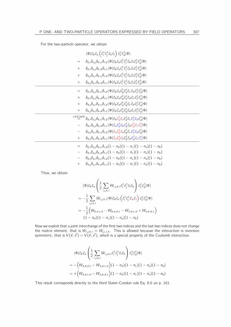
P ONE- AND TWO-PARTICLE OPERATORS EXPRESSED BY FIELD OPERATORS 307
For the two-particle operator, we obtain
〈Φ|cbca(
c†i c†j ck cl
)
c†c c†d |Φ〉
= δb,iδa,jδk,cδl ,d〈Φ|cbcac†i c†j ck cl c
†c c†d |Φ〉
+ δb,iδa,jδk,dδl ,c〈Φ|cbcac†i c†j ck cl c
†c c†d |Φ〉
+ δb,jδa,iδk,cδl ,d〈Φ|cbcac†i c†j ck cl c
†c c†d |Φ〉
+ δb,jδa,iδk,dδl ,c〈Φ|cbcac†i c†j ck cl c
†c c†d |Φ〉
= δb,iδa,jδk,cδl ,d〈Φ|cbcac†b c†a cc cd c†c c†d |Φ〉
+ δb,iδa,jδk,dδl ,c〈Φ|cbcac†b c†a cd cc c†c c†d |Φ〉
+ δb,jδa,iδk,cδl ,d〈Φ|cbcac†a c†b cc cd c†c c†d |Φ〉
+ δb,jδa,iδk,dδl ,c〈Φ|cbcac†a c†b cd cc c†c c†d |Φ〉
c 6=d ;a 6=b= δb,iδa,jδk,cδl ,d〈Φ|cbc†b cac†a cc c†c cd c
†d |Φ〉
− δb,iδa,jδk,dδl ,c〈Φ|cac†a cbc†b cd c†d cc c
†c |Φ〉
− δb,jδa,iδk,cδl ,d〈Φ|cac†a cbc†b cc c†c cd c†d |Φ〉
+ δb,jδa,iδk,dδl ,c〈Φ|cac†a cbc†b cd c†d cc c
†c |Φ〉
= δb,iδa,jδk,cδl ,d(1− nd)(1− nc)(1− na)(1− nb)− δb,iδa,jδk,dδl ,c(1− nd)(1− nc)(1− na)(1− nb)− δb,jδa,iδk,cδl ,d(1− nd)(1− nc)(1− na)(1− nb)+ δb,jδa,iδk,dδl ,c(1− nd)(1− nc)(1− na)(1− nb)
Thus, we obtain
〈Φ|cbca
1
2
∑
i ,j,k,l
Wi ,j,k,l c†i c†j cl ck
c†c c†d |Φ〉
= −12
∑
i ,j,k,l
Wi ,j,k,l〈Φ|cbca(
c†i c†j ck c l
)
c†c c†d |Φ〉
= −12
(
Wb,a,c,d −Wb,a,d,c −Wa,b,c,d +Wa,b,d,c
)
·(1− nd)(1− nc)(1− na)(1− nb)
Now we exploit that a joint interchange of the first two indices and the last two indices does not changethe matrix element, that is Wi ,j,k,l = Wj,i ,l .k . This is allowed because the interaction is inversionsymmetric, that is V (~x, ~x ′) = V (~x, ~x ′), which is a special property of the Coulomb interaction.
〈Φ|cbca
1
2
∑
i ,j,k,l
Wi ,j,k,l c†i c†j cl ck
c†c c†d |Φ〉
= −(
Wa,b,d,c −Wa,b,c,d
)
(1− nd)(1− nc)(1− na)(1− nb)
= +(
Wa,b,c,d −Wa,b,d,c
)
(1− nd)(1− nc)(1− na)(1− nb)
This result corresponds directly to the third Slater-Condon rule Eq. 8.6 on p. 161.
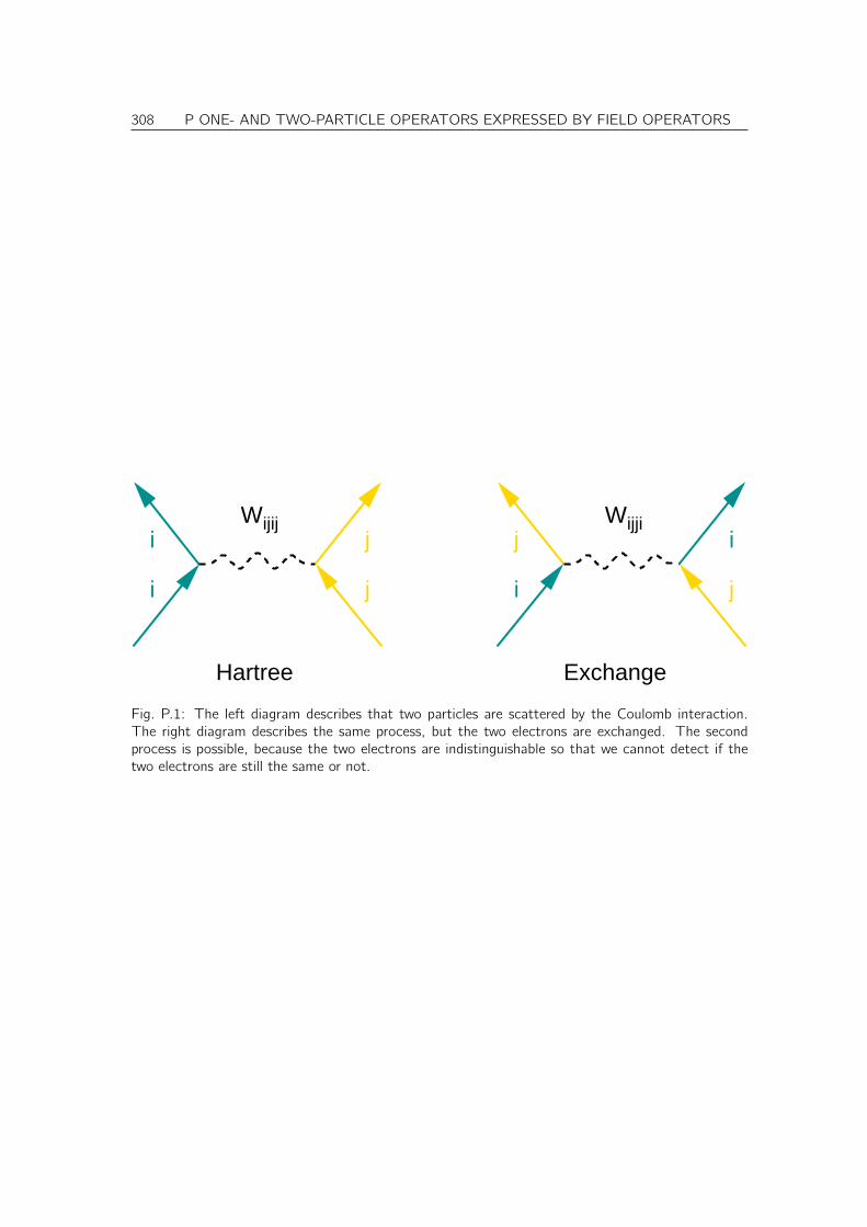
308 P ONE- AND TWO-PARTICLE OPERATORS EXPRESSED BY FIELD OPERATORS
Hartree Exchange
Wijij Wijji
i
i
j
j
j
j
i
i
Fig. P.1: The left diagram describes that two particles are scattered by the Coulomb interaction.The right diagram describes the same process, but the two electrons are exchanged. The secondprocess is possible, because the two electrons are indistinguishable so that we cannot detect if thetwo electrons are still the same or not.
Appendix Q
Green’s function and division ofsystems
Before we return to quantum field theory I would like to show one important application of Green’sfunctions in the one-particle theory. Green’s function are important whenever we couple to quantummechanical systems.
Let us partition a system in two subsystems. Consider for example a defect atom in a host crystal.The defect atom would be described by a Hamiltonian H11 and the host crystal by a HamiltonianH22. More precisely we divide Hilbert space up into two subspaces. The subspace of the impurityconsists of the wave functions |ψi 〉 and the Hilbert space of the host consists of the wave functions|φi 〉. Then the matrix H11 is defined by
(H11)i ,j = 〈ψi |H|ψj 〉
First we show how the Green’s function is determined(
G11(ǫ) G12(ǫ)
G21(ǫ) G22(ǫ)
)(
H11 − ǫ H12
H21 H22 − ǫ
)
=
(
1 0
0 1
)
We obtain four equations
G11(ǫ) (H11 − ǫ) + G12(ǫ)H21 = 1 (Q.1)
G21(ǫ) (H11 − ǫ) + G22(ǫ)H21 = 0 (Q.2)
G11(ǫ)H12 + G12(ǫ) (H22 − ǫ) = 0 (Q.3)
G21(ǫ)H12 + G22(ǫ) (H22 − ǫ) = 1 (Q.4)
We first determine the matrices G12(ǫ) and G21(ǫ) as function of the diagonal elements
G21(ǫ) = −G22(ǫ)H21 (H11 − ǫ)−1 (Q.5)
G12(ǫ) = −G11(ǫ)H12 (H22 − ǫ)−1 (Q.6)
and insert the result into the other two equations.
G11(ǫ) (H11 − ǫ)− G11(ǫ)H12 (H22 − ǫ)−1H21 = 1 (Q.7)
+G22(ǫ) (H22 − ǫ)− G22(ǫ)H21 (H11 − ǫ)−1H12 = 1 (Q.8)
which can be written as
G11(ǫ) =[
H11 − ǫ−H12 (H22 − ǫ)−1H21]−1
(Q.9)
G22(ǫ) =[
H22 − ǫ−H21 (H11 − ǫ)−1H12]−1
(Q.10)
309
310 Q GREEN’S FUNCTION AND DIVISION OF SYSTEMS
The uncoupled Green’s functions G011 and G022, that is the Green’s functions of the separated systems,are
G011(ǫ) = [H11 − ǫ]−1 (Q.11)
G022(ǫ) = [H22 − ǫ]−1 (Q.12)
which allows us to rewrite the result for the full Green’s function as
G11(ǫ) =[(G011(ǫ)
)−1 −H12G022(ǫ)H21]−1
(Q.13)
G22(ǫ) =[(G022(ǫ)
)−1 −H21G011(ǫ)H12]−1
(Q.14)
These equations provide us in a straightforward fashion to couple for example different impuritiesinto a host crystal. We need to know the Green’s functions for the separate systems. Then we needto set up an energy grid and perform a number of matrix inversions for each energy.
Q.1 Relation to a Schrödinger equation
The Green’s function itself allows to extract a wealth of useful information. However to get a betterinsight it may be instructive to derive an effective Schrödinger equation for the defect atom alone,which however also includes the effect of the host crystal accurately. In the following we introducethe Green’s function G22 of the host crystal which is not to be confused with the 22 element of thetotal Green’s function.
(
H11 − ǫ λH12
λH21 H22 − ǫ
)(
~c1
~c2
)
= 0 (Q.15)
We use the second line an resolve it for ~c2
λH21~c1 + (H22 − ǫ)~c2 = 0 ⇒ ~c2 = − (H22 − ǫ)−1︸ ︷︷ ︸
G22
H21~c1
and insert the result in the first line of Eq. Q.15.
(H11 − ǫ)~c1 +H12~c2 = 0[(H11 − ǫ)−H12(H − ǫ)−1H21
]~c1 = 0
[H11 −H12G22(ǫ)H21 − ǫ] ~c1 = 0 (Q.16)
This equation already looks like a Schrödinger equation in which the environment acts on the firstsystem with an energy-dependent potential H12G22(ǫ)H21.
Before we continue, note however that Eq. Q.16 can also be written as
G−111 (ǫ)~c1 = 0
Thus, we can find the eigenstates by looking for the poles of the full Green’s function. The Green’sfunction has an eigenvalue of zero at the energies where it has poles. The corresponding eigenvaluesare the vectors ~c1, which only need to be normalized.
However we still need to consider the normalization condition for ~c1.
~c∗1~c1 + ~c∗2~c2 = 1
~c∗1~c1 + ~c∗1H†21G
†22(ǫ)
︸ ︷︷ ︸
~c∗2
G22(ǫ)H21~c1︸ ︷︷ ︸
~c2
= 1
~c∗1(1 +H12G
222(ǫ)H21
)~c1 = 1
Q GREEN’S FUNCTION AND DIVISION OF SYSTEMS 311
The operator in the middle plays a role of an overlap operator.We can combine the equation Eq. Q.16 with the normalization condition to an energy-dependent
Schrödinger-like equation.[H11 −H12G22(ǫ)H21 +H12ǫG222(ǫ)H21 − ǫ
(1 +H12G
222(ǫ)H21
)]~c1 = 0
H11−H12
(G22(ǫ)− ǫG222(ǫ)
)H21
︸ ︷︷ ︸
V emb11
−ǫ(1 +H12G
222(ǫ)H21
)
︸ ︷︷ ︸
Oef f11
~c1 = 0
(Q.17)
We may now interpret this equation as a Schrödinger equation(H11 + V
emb11 − ǫOef f11
)~c1 = 0
of system 1 with an energy dependent overlap matrix
Oef f11 = 1 +H12G222(ǫ)H21
and an energy dependent embedding potential V emb
V emb11 = −H12(G22(ǫ)− ǫG222(ǫ)
)H21
Q.1.1 Another derivation of the effective Schrödinger equation
The same equation can also be obtained by linearizing the equation Eq. Q.16[H11 −H12G022(ǫ)H21 − ǫ
]~c1 = 0
[
H11 −H12G022(ǫ0)H21 −H12dG022dǫ
∣∣∣∣ǫ0
H21(ǫ− ǫ0)− ǫ]
~c1 = 0
H11 −H12[
G022(ǫ0)− ǫ0dG022dǫ
∣∣∣∣ǫ0
]
H21
︸ ︷︷ ︸
Hef f11
−ǫ[
1 +H12dG022dǫ
∣∣∣∣ǫ0
H21
]
︸ ︷︷ ︸
Oef f11
~c1 = 0
(Q.18)
It can be shown that the overlap matrix can directly be obtained from the energy derivative ofG−111 (ǫ) or equivalently the differential operator in Eq. Q.16. Precisely,
Oef f11 (ǫ) = −dG−111 (ǫ)
dǫ
Let us first determine the energy derivative of the decoupled Green’s function G(0)22 (ǫ). We beginwith the defining equation
(H22 − (ǫ+ dǫ))G(0)22 (ǫ+ dǫ) = 1
(H22 − ǫ− dǫ)(
G(0)22 (ǫ) +
G(0)22
dǫ
)
= 1 +O(dǫ2)
(H22 − ǫ))G(0)22 (ǫ) + dǫ[
G(0)22 (ǫ) + (H22 − ǫ)
G(0)22
dǫ
]
= 1 +O(dǫ2)
[
G(0)22 (ǫ) + (H22 − ǫ)
G(0)22
dǫ
]
= O(dǫ)
G(0)22
dǫ= − (H22 − ǫ)−1
︸ ︷︷ ︸
G(0)22 (ǫ)
G(0)22 (ǫ) = −
(
G(0)22 (ǫ)
)2
312 Q GREEN’S FUNCTION AND DIVISION OF SYSTEMS
Now we can work out the energy derivative of the full Green’s function
∂ǫG−111 (ǫ) = ∂ǫ [H11 −H12G22H21 − ǫ]
= −H12dG(0)22
dǫH21 − 1
= −[
1 +H12
(
G(0)22
)2
H21
]
= −Oef f11
which is what we wanted to show. With this result it is easy to show the equivalence of Eq. Q.18and Eq. Q.17.
Further information about one-particle Green’s functions can be found in the Book by Economou[92].
Appendix R
Time-ordered exponential,Propagators etc.
R.1 Time-ordered exponential
Often we encounter equations of the form of the time-dependent Schrödinger equation with a time-dependent Hamiltonian.
TIME-ORDERED EXPONENTIAL
The solution of a Schrödinger equation with a time-dependent Hamiltonian
i~∂t |ψ(t)〉 = H(t)|ψ(t)〉 (R.1)
can be solved in the form (Eq. 31 of[93])
|ψ(t)〉 =(
TDe−i~
∫ t
0 dt′ H(t ′)
)
|ψ(0)〉 (R.2)
Here, TD is Dyson’s time ordering operatora or P-product (Eq. 29 of [93]) which reorders thetime dependent operators in ascending order from right to left, that is
TDA(t)B(t ′) =
A(t)B(t ′) for t ≥ t ′B(t ′)A(t) for t ′ > t
(R.3)
aDyson’s time ordering operator must not be confused with Wick’s time ordering operator[73], which changes thesign for each permutation of two fermionic operators. If the Hamiltonian is particle number conserving, i.e. if creationand annihilation operators occur in even-numbered products, the action of Dyson’s time ordering operator on theHamiltonian is identical to Wick’s time ordering operator acting on individual creation and annihilation operators.
In a first step we convert the differential equation Eq. R.1 into an integral equation
|ψ(t)〉 = |ψ(0)〉 − i
~
∫ t
0
dt ′ H(t ′)|ψ(t)〉 (R.4)
313
314 R TIME-ORDERED EXPONENTIAL, PROPAGATORS ETC.
When we repeatedly insert the left hand side of Eq. R.4 on the right-hand side, we obtain
|ψ(t)〉 = |ψ(0)〉 − i
~
∫ t
0
dt ′ H(t ′)|ψ(t)〉
= |ψ(0)〉+ 1i~
∫ t
0
dt ′ H(t ′)|ψ(0)〉+(1
i~
)2 ∫ t
0
dt ′ H(t ′)
∫ t ′
0
dt ′′ H(t ′′)|ψ(t)〉
=
[ ∞∑
n=0
(1
i~
)n ∫ t
0
dt1 . . .
∫ tn−1
0
dtn H(t1) · · · H(tn)]
|ψ(0)〉 (R.5)
This result is only valid if the series converges. Convergence of the series is a non-trivial issue.Using Dyson’s time ordering operator we can rewrite Eq. R.5 with integrals that all have the same
bounds, namely 0 and t.
|ψ(t)〉 =[ ∞∑
n=0
TD1
n!
(1
i~
)n ∫ t
0
dt1 . . .
∫ t
0
dtn H(t1) · · · H(tn)]
|ψ(0)〉
= TD[ ∞∑
n=0
1
n!
(1
i~
∫ t
0
dt ′ H(t ′)
)n]
|ψ(0)〉 (R.6)
In the form used previously, in Eq. R.5, the Hamilton operators are in a specific order, namelyascending from right to left. Here, in Eq. R.6 on on the other hand, all orderings are allowed, buteach term is then ordered by the time-ordering operator. However, now we have,instead of one,n! terms according to the n! possible arrangement of the time arguments. This overcounting iscorrected by the factor 1/n!.
We recognize the similarity of this expression Eq. R.6 with the Taylor expansion of the exponentialfunction ex =
∑∞n=0
1n!x
n, which allows us to write
|ψ(t)〉 =[
TDe−i~
∫ t
0 dt′ H(t ′)
]
|ψ(0)〉 (R.7)
which proves Eq. R.2.
R.2 Wick’s time ordering operator
In his seminal paper[73] Wick laying the foundation for the diagrammatic expansion of the Green’sfunction, he introduced his time ordering operator, which we denote by TW or, without subscript asT . Like for Dyson’s time ordering operator, we do not add a hat above the symbol, because thisoperator differs from the operators that act on states. The time ordering operators are fundamentallydifferent: They are merely a prescription on how to rearrange regular operators.
R.3 Propagator in real time
R.3.1 Propagator in the Schrödinger picture
As shown above in section R.1, the solution of a Schrödinger equation
i~∂t |ψ(t)〉 = H(t)|ψ(t)〉can be expressed by the propagator U(t, 0) to the initial state
|ψ(t)〉 = U(t, t ′)|Ψ(t ′)〉 (R.8)
where
U(t2, t1)Eq. R.2= TD e−
i~
∫ t2t1dt ′ H(t ′) (R.9)
R TIME-ORDERED EXPONENTIAL, PROPAGATORS ETC. 315
Propagator in the interaction picture
If the Hamilton operator can be split into a time-independent term H0 and a time-dependent termW , we usually use the interaction picture: A state |ψI(t)〉 in the interaction picture is related to astate |ψS(t)〉 in the Schrödinger picture as
|ψI(t)〉 = ei~H0t |ψS(t)〉
This transforms the Schrödinger equation into
i~∂t |ψI(t)〉 = −H0|ψI(t)〉+ ei~H0t i~∂t |ψS(t)〉
= −H0|ψI(t)〉+ ei~H0t(H0 + W (t))|ψS(t)〉
=
[
−e i~ H0tH0e−i~H0t + e
i~H0t(
H0 + W (t))
e−i~H0t
]
|ψI(t)〉
= ei~H0tW (t)e−
i~H0t |ψI(t)〉
= WI(t)|ψI(t)〉
where WI(t) is the interaction operator in the interaction picture
WI(t) = ei~H0tWS(t)e
− i~H0t
Now we can use the expression for the time-ordered exponential to obtain a solution for thepropagator in the interaction picture, that is
|ΨI(t2)〉 = TD[
e− i~
∫ t2t1dt ′ WI(t
′)]
|ΨI(t1)〉
|ΨS(t2)〉 = e−i~H0t2TD
[
e− i~
∫ t2t1dt ′ WI(t
′)]
ei~H0t1 |ΨS(t1)〉
Thus, the propagator for Schrödinger states can be written in two forms, namely as
PROPAGATOR IN REAL TIME
U(t2, t1) = TD[
e− i~
∫ t2t1dt ′(
H0+WS(t′)
)]
(R.10)
= e−i~H0t2TD
[
e− i~
∫ t2t1dt ′ WI(t
′)]
ei~H0t1 (R.11)
R.4 Propagator in imaginary time
For a brief historical overview see Abeś article.[94]. The use of Feynman diagrams in statistical physicsgoes back to Matsubara[95]. The original proof of Wick’s theorem in the imaginary time formalismis due to Bloch and de Dominicis[96]. Abe says that this proof is complicated and a simpler one hasbeen given later by Gaudin[97] in 1960.
R.4.1 Imaginary-time propagator in the Schrödinger picture
In the finite temperature formulation of quantum mechanics Matsubara generalized time to a complexquantity.
τ = −i t
316 R TIME-ORDERED EXPONENTIAL, PROPAGATORS ETC.
In imaginary time, we can write down an equation analogous to the Schrödinger equation, whichthen obtains the form of a diffusion equation.
−~∂τ |ψ(τ)〉 = (H − µN)|ψ(τ)〉
This equation has the propagator U(τ, τ ′) which links the wave function between two different times.
|ψ(τ)〉 = U(τ, τ ′)|ψ(τ ′)〉 (R.12)
Because the Hamiltonian is independent of time, which is assumed to be the case, the propagatorhas the form
U(τ, τ ′) = e−(H−µN)(τ−τ′)/~ (R.13)
τ = 0 corresponds to the high temperature limit.The expectation of an operator A in a finite temperature ensemble has the simple form
⟨
A⟩
T,µ=
1∑
n e−βEn
∑
n
〈ψn|A|ψn〉e−βEn =∑
n〈Ψn|Ae−β(H−µN)|Ψn〉∑
n〈Ψn|e−β(H−µN)|Ψn〉=T r [AU(β~, 0)]
T r [U(β~, 0)]
The partition sum Z is the denominator, which is linked to the grand potential Ω via Z = e−βΩ.Thus, the grand potential is directly linked to the propagator in imaginary time
Ω(T, µ) = −kBT ln[Z(T, µ)] = −kBT ln(
T r [Uµ(β~, 0)])
Propagator in the interaction picture
For the sake of obtaining a diagrammatic expansion analogous to that in real time, one introducesan interaction picture in the imaginary-time formalism.
Again, the Hamilton operator is split into a non-interacting H0 and an interaction W .A state |ψI(τ)〉 in the interaction picture is related to a state |ψS(τ)〉 in the imaginary-time
Schrödinger picture is
|ψI(τ)〉 = e(H0−µN)τ/~|ψS(τ)〉
This transforms the Schrödinger equation into
−~∂τ |ψI(τ)〉 = −(H0 − µN)|ψI(τ)〉+ e(H0−µN)τ/~(−~∂τ )|ψS(τ)〉= −(H0 − µN)|ψI(τ)〉+ e(H0−µN)τ/~(H0 + W − µN)|ψS(τ)〉
=
[
−e(H0−µN)τ/~(H0 − µN)e−(H0−µN)τ/~ + e(H0−µN)τ/~(
H0 + W − µN)
e−(H0−µN)τ/~]
|ψI(τ)〉
= e(H0−µN)τ/~W e−(H0−µN)τ/~|ψI(τ)〉= WI(τ)|ψI(τ)〉
where WI(τ) is the interaction operator in the interaction picture
WI(τ) = e(H0−µN)τ/~WSe
−(H0−µN)τ/~
Now we can use the expression for the time ordered exponential to obtain a solution for thepropagator in the interaction picture, that is
|ΨI(τ2)〉 = TD[
e−∫ τ2τ1dτ ′ WI(τ
′)]
|ΨI(τ1)〉
|ΨS(τ2)〉 = e−(H0−µN)τ2/~TD[
e− 1~
∫ τ2τ1dτ ′ WI(τ
′)]
e(H0−µN)τ1/~|ΨS(τ1)〉
R TIME-ORDERED EXPONENTIAL, PROPAGATORS ETC. 317
Thus, the propagator for Schrödinger states can be written in two forms, namely as
PROPAGATOR IN IMAGINARY TIME
U(β~, 0) = e−β(
H0+WS−µN)
= e−β(H0−µN)TD[
e−1~
∫ β~
0 dτ ′ WI(τ′)
]
(R.14)
= e−β(H0−µN)TD[
exp
(
−1~
∫ β~
0
dτ e(H0−µN)τ/~WSe−(H0−µN)τ/~
)]
(R.15)

318 R TIME-ORDERED EXPONENTIAL, PROPAGATORS ETC.
Appendix S
Field operators in the interactionpicture
FIELD OPERATORS IN THE INTERACTION PICTURE
If the non-interacting Hamiltonian is is H0 =∑
α,β hα,β c†αcβ, the field operators in the interaction
picture can be written in the form
cα,I(t)Eq. S.5=
∑
β
(
e−i~ht
)
α,β
cβ (S.1)
c†n,I(t) =∑
β
(
e+i~ht
)
α,β
c†β (S.2)
If the non-interacting Hamiltonian H0 is expressed in its diagonal form, that is H0 =∑
n ǫnc†n cn, the
field operators in the interaction picture can be written in the form
cn,I(t) = e− i~ǫnt cn (S.3)
c†n,I(t) = e+ i~ǫnt c†n (S.4)
Proof for the annihilator using the Baker-Hausdorff Theorem
We start with the operator
cζ,I = ei~H0t cζ,Se
− i~H0t
with H0 =∑
α,β hα,β c†αcβ. where cζ,I is the annihilator in the interaction picture, and cζ,S = cζ is
the same operator in the Schrödinger picture.With the help of the Baker-Hausdorff theorem Eq. T.3 we can rewrite this expression as
ei~H0t cζe
− i~H0t =
∞∑
n=0
(i
~t
)n
Xn with Xn =1
n + 1[H0, Xn]− and X0 = cζ
319
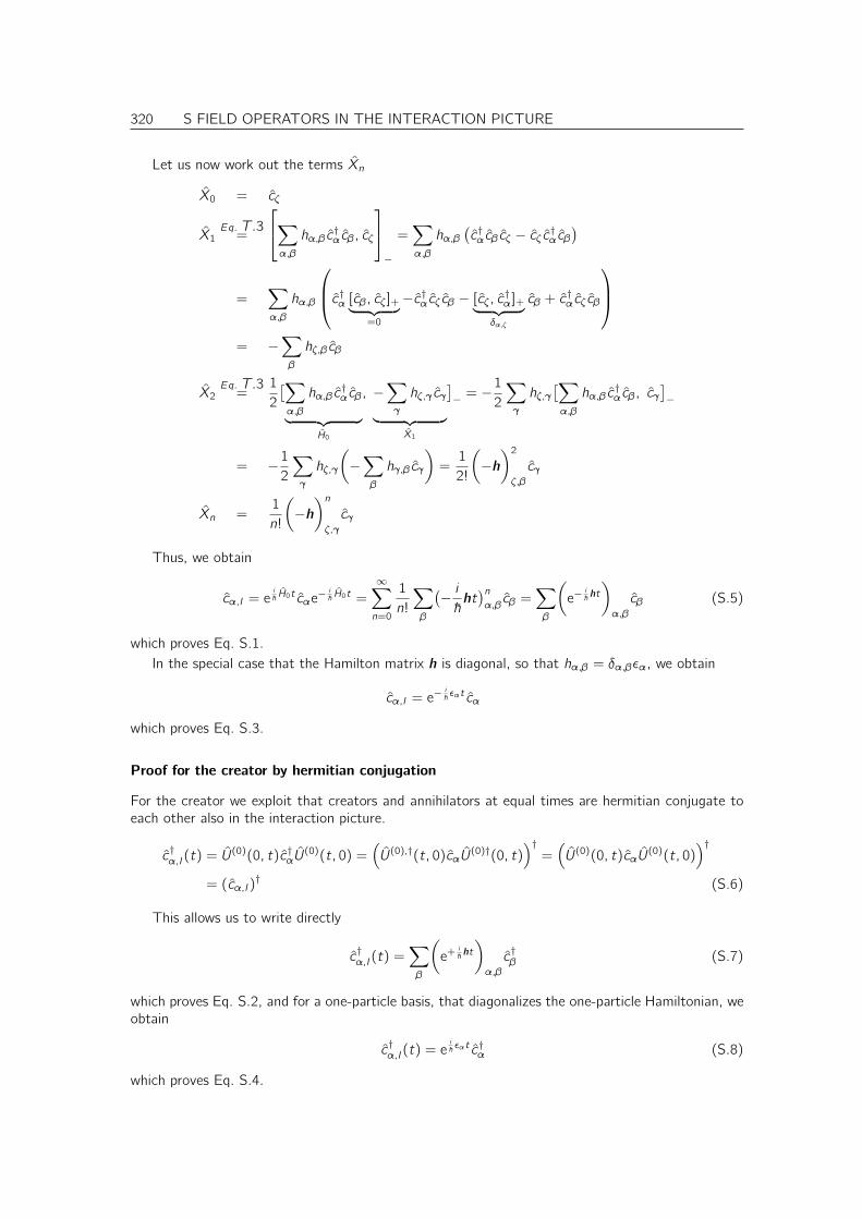
320 S FIELD OPERATORS IN THE INTERACTION PICTURE
Let us now work out the terms Xn
X0 = cζ
X1Eq. T.3=
∑
α,β
hα,β c†αcβ, cζ
−
=∑
α,β
hα,β(c†αcβ cζ − cζ c†αcβ
)
=∑
α,β
hα,β
c†α [cβ, cζ]+︸ ︷︷ ︸
=0
−c†αcζ cβ − [cζ, c†α]+︸ ︷︷ ︸
δα,ζ
cβ + c†αcζ cβ
= −∑
β
hζ,β cβ
X2Eq. T.3=
1
2
[∑
α,β
hα,β c†αcβ
︸ ︷︷ ︸
H0
, −∑
γ
hζ,γ cγ
︸ ︷︷ ︸
X1
]
− = −1
2
∑
γ
hζ,γ[∑
α,β
hα,β c†αcβ, cγ
]
−
= −12
∑
γ
hζ,γ
(
−∑
β
hγ,β cγ
)
=1
2!
(
−h)2
ζ,β
cγ
Xn =1
n!
(
−h)n
ζ,γ
cγ
Thus, we obtain
cα,I = ei~H0t cαe
− i~H0t =
∞∑
n=0
1
n!
∑
β
(− i~ht)n
α,βcβ =
∑
β
(
e−i~ht
)
α,β
cβ (S.5)
which proves Eq. S.1.In the special case that the Hamilton matrix h is diagonal, so that hα,β = δα,βǫα, we obtain
cα,I = e− i~ǫαt cα
which proves Eq. S.3.
Proof for the creator by hermitian conjugation
For the creator we exploit that creators and annihilators at equal times are hermitian conjugate toeach other also in the interaction picture.
c†α,I(t) = U(0)(0, t)c†αU
(0)(t, 0) =(
U(0),†(t, 0)cαU(0)†(0, t)
)†=(
U(0)(0, t)cαU(0)(t, 0)
)†
= (cα,I)† (S.6)
This allows us to write directly
c†α,I(t) =∑
β
(
e+i~ht
)
α,β
c†β (S.7)
which proves Eq. S.2, and for a one-particle basis, that diagonalizes the one-particle Hamiltonian, weobtain
c†α,I(t) = ei~ǫαt c†α (S.8)
which proves Eq. S.4.
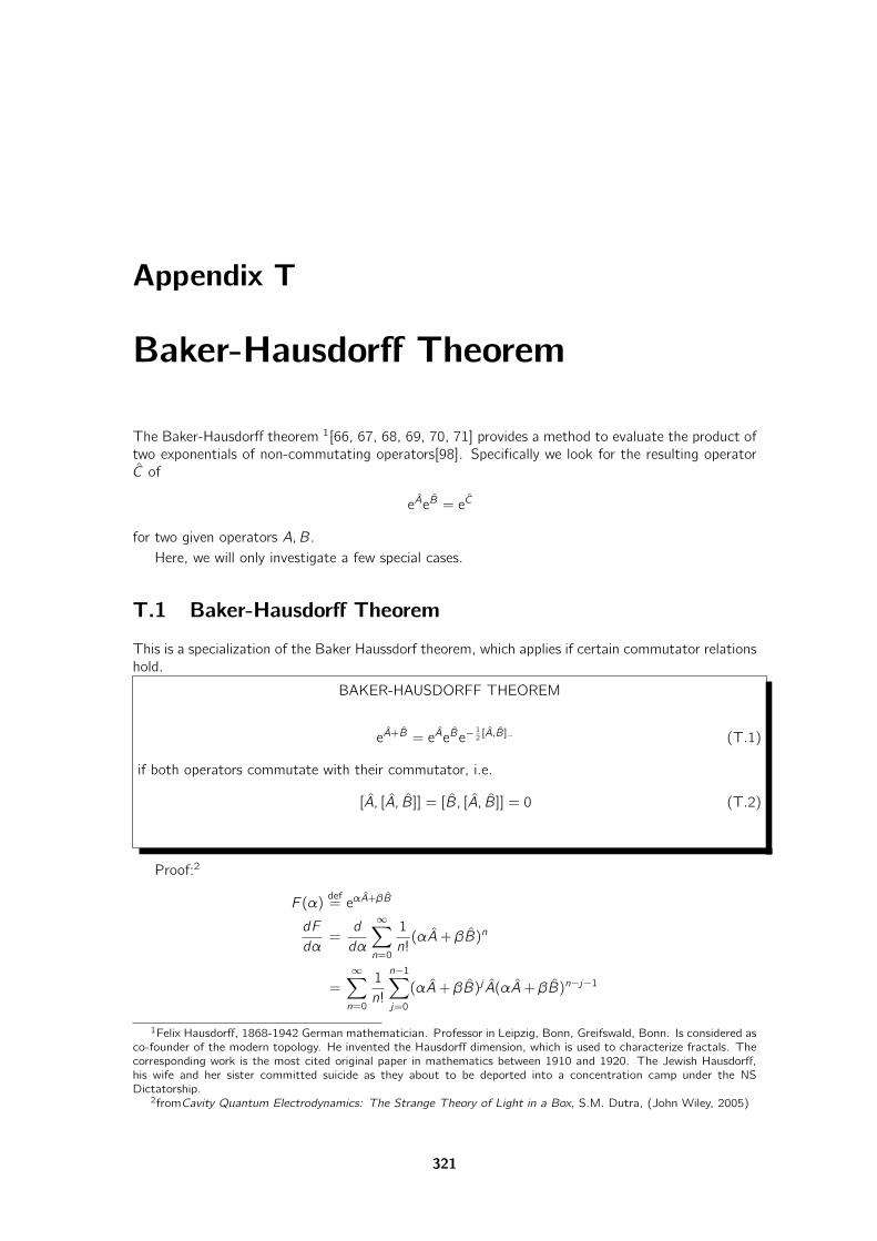
Appendix T
Baker-Hausdorff Theorem
The Baker-Hausdorff theorem 1[66, 67, 68, 69, 70, 71] provides a method to evaluate the product oftwo exponentials of non-commutating operators[98]. Specifically we look for the resulting operatorC of
eAeB = eC
for two given operators A,B.Here, we will only investigate a few special cases.
T.1 Baker-Hausdorff Theorem
This is a specialization of the Baker Haussdorf theorem, which applies if certain commutator relationshold.
BAKER-HAUSDORFF THEOREM
eA+B = eAeBe−12[A,B]− (T.1)
if both operators commutate with their commutator, i.e.
[A, [A, B]] = [B, [A, B]] = 0 (T.2)
Proof:2
F (α)def= eαA+βB
dF
dα=
d
dα
∞∑
n=0
1
n!(αA+ βB)n
=
∞∑
n=0
1
n!
n−1∑
j=0
(αA+ βB)j A(αA+ βB)n−j−1
1Felix Hausdorff, 1868-1942 German mathematician. Professor in Leipzig, Bonn, Greifswald, Bonn. Is considered asco-founder of the modern topology. He invented the Hausdorff dimension, which is used to characterize fractals. Thecorresponding work is the most cited original paper in mathematics between 1910 and 1920. The Jewish Hausdorff,his wife and her sister committed suicide as they about to be deported into a concentration camp under the NSDictatorship.
2fromCavity Quantum Electrodynamics: The Strange Theory of Light in a Box, S.M. Dutra, (John Wiley, 2005)
321
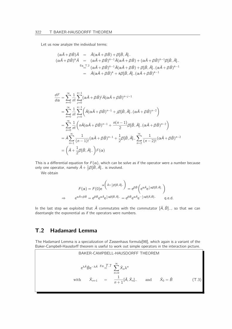
322 T BAKER-HAUSDORFF THEOREM
Let us now analyze the individual terms:
(αA+ βB)A = A(αA+ βB) + β[B, A]−
(αA+ βB)k A = (αA+ βB)k−1A(αA+ βB) + (αA+ βB)k−1β[B, A]−Eq. T.2= (αA+ βB)k−1A(αA+ βB) + β[B, A]−(αA+ βB)
k−1
= A(αA+ βB)k + kβ[B, A]−(αA+ βB)k−1
dF
dα=
∞∑
n=0
1
n!
n−1∑
j=0
(αA+ βB)j A(αA+ βB)n−j−1
=
∞∑
n=0
1
n!
n−1∑
j=0
(
A(αA+ βB)n−1 + jβ[B, A]−(αA+ βB)n−2)
=
∞∑
n=0
1
n!
(
nA(αA+ βB)n−1 +n(n − 1)2
β[B, A]−(αA+ βB)n−2)
= A
∞∑
n=1
1
(n − 1)!(αA+ βB)n−1 +
1
2β[B, A]−
∞∑
n=2
1
(n − 2)!(αA+ βB)n−2
=
(
A+1
2β[B, A]−
)
F (α)
This is a differential equation for F (α), which can be solve as if the operator were a number becauseonly one operator, namely A+ 12β[B, A]− is involved.
We obtain
F (α) = F (0)eα
(
A+ 12β[B,A]−
)
= eβB(
eαAe12αβ[B,A]−
)
⇒ eαA+βB = eβBeαAe12αβ[B,A]− = eβBeαAe−
12αβ[A,B]− q.e.d.
In the last step we exploited that A commutates with the commutator [A, B]−, so that we candisentangle the exponential as if the operators were numbers.
T.2 Hadamard Lemma
The Hadamard Lemma is a specialization of Zassenhaus formula[98], which again is a variant of theBaker-Campbell-Hausdorff theorem is useful to work out simple operators in the interaction picture.
BAKER-CAMPBELL-HAUSDORFF THEOREM
eλABe−λAEq. T.7=
∞∑
n=0
Xnλn
with Xn+1 =1
n + 1[A, Xn]− and X0 = B (T.3)
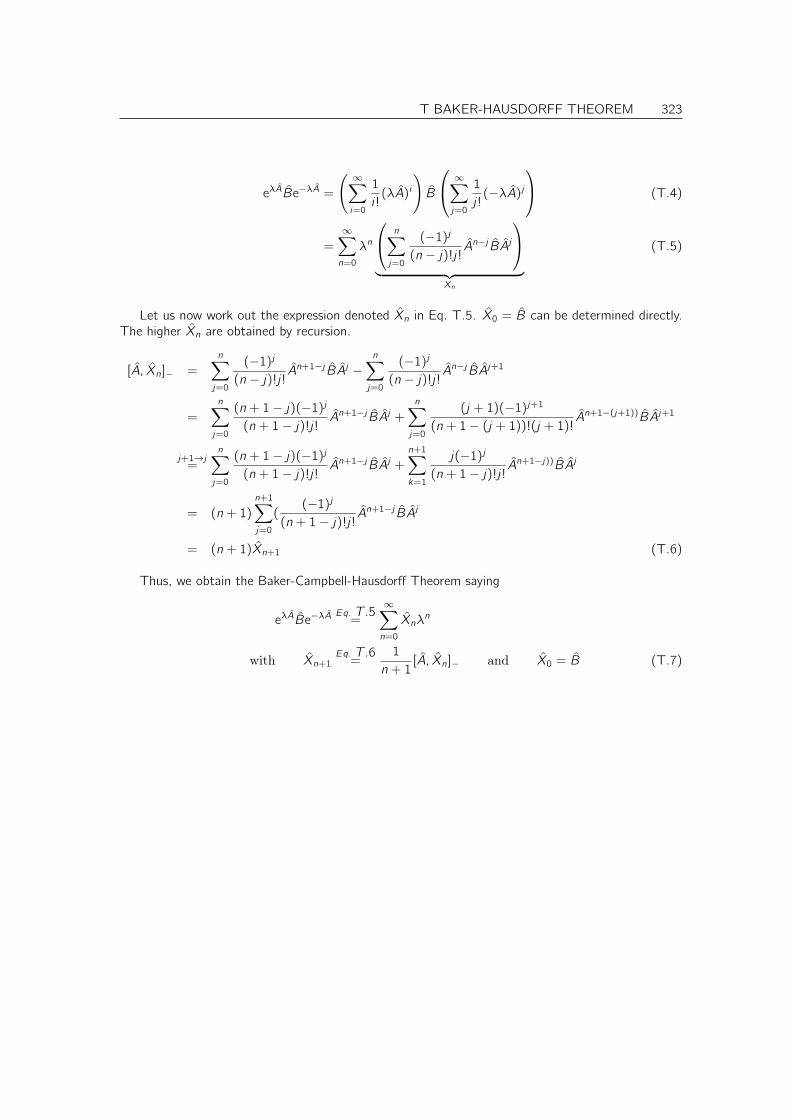
T BAKER-HAUSDORFF THEOREM 323
eλABe−λA =
( ∞∑
i=0
1
i !(λA)i
)
B
∞∑
j=0
1
j!(−λA)j
(T.4)
=
∞∑
n=0
λn
n∑
j=0
(−1)j(n − j)!j! A
n−j BAj
︸ ︷︷ ︸
Xn
(T.5)
Let us now work out the expression denoted Xn in Eq. T.5. X0 = B can be determined directly.The higher Xn are obtained by recursion.
[A, Xn]− =
n∑
j=0
(−1)j(n − j)!j! A
n+1−j BAj −n∑
j=0
(−1)j(n − j)!j! A
n−j BAj+1
=
n∑
j=0
(n + 1− j)(−1)j(n + 1− j)!j! An+1−j BAj +
n∑
j=0
(j + 1)(−1)j+1(n + 1− (j + 1))!(j + 1)! A
n+1−(j+1))BAj+1
j+1→j=
n∑
j=0
(n + 1− j)(−1)j(n + 1− j)!j! An+1−j BAj +
n+1∑
k=1
j(−1)j(n + 1− j)!j! A
n+1−j))BAj
= (n + 1)
n+1∑
j=0
((−1)j
(n + 1− j)!j! An+1−j BAj
= (n + 1)Xn+1 (T.6)
Thus, we obtain the Baker-Campbell-Hausdorff Theorem saying
eλABe−λAEq. T.5=
∞∑
n=0
Xnλn
with Xn+1Eq. T.6=
1
n + 1[A, Xn]− and X0 = B (T.7)

324 T BAKER-HAUSDORFF THEOREM
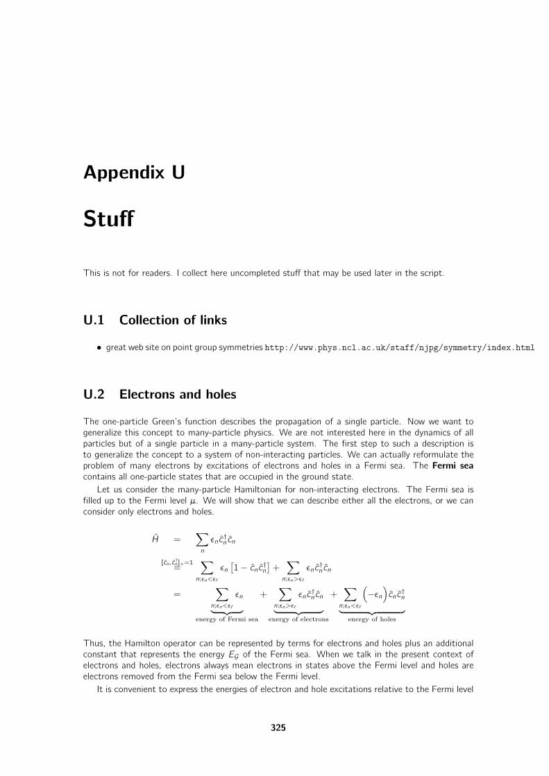
Appendix U
Stuff
This is not for readers. I collect here uncompleted stuff that may be used later in the script.
U.1 Collection of links
• great web site on point group symmetries http://www.phys.ncl.ac.uk/staff/njpg/symmetry/index.html
U.2 Electrons and holes
The one-particle Green’s function describes the propagation of a single particle. Now we want togeneralize this concept to many-particle physics. We are not interested here in the dynamics of allparticles but of a single particle in a many-particle system. The first step to such a description isto generalize the concept to a system of non-interacting particles. We can actually reformulate theproblem of many electrons by excitations of electrons and holes in a Fermi sea. The Fermi seacontains all one-particle states that are occupied in the ground state.
Let us consider the many-particle Hamiltonian for non-interacting electrons. The Fermi sea isfilled up to the Fermi level µ. We will show that we can describe either all the electrons, or we canconsider only electrons and holes.
H =∑
n
ǫnc†n cn
[cn,c†n ]+=1=
∑
n;ǫn<ǫf
ǫn[1− cnc†n
]+∑
n;ǫn>ǫf
ǫnc†n cn
=∑
n;ǫn<ǫf
ǫn
︸ ︷︷ ︸
energy of Fermi sea
+∑
n;ǫn>ǫf
ǫnc†n cn
︸ ︷︷ ︸
energy of electrons
+∑
n;ǫn<ǫf
(
−ǫn)
cnc†n
︸ ︷︷ ︸
energy of holes
Thus, the Hamilton operator can be represented by terms for electrons and holes plus an additionalconstant that represents the energy EG of the Fermi sea. When we talk in the present context ofelectrons and holes, electrons always mean electrons in states above the Fermi level and holes areelectrons removed from the Fermi sea below the Fermi level.
It is convenient to express the energies of electron and hole excitations relative to the Fermi level
325
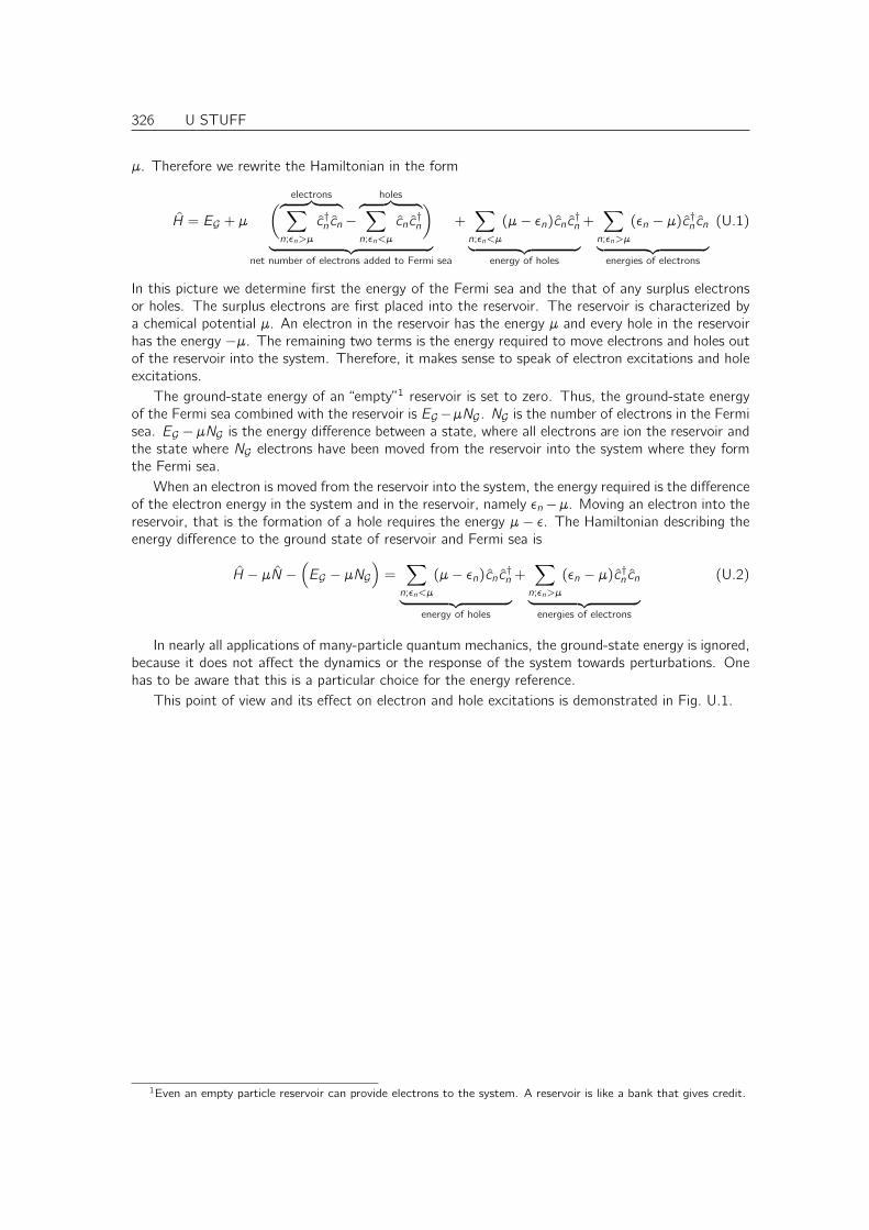
326 U STUFF
µ. Therefore we rewrite the Hamiltonian in the form
H = EG + µ
(electrons︷ ︸︸ ︷∑
n;ǫn>µ
c†n cn−
holes︷ ︸︸ ︷∑
n;ǫn<µ
cnc†n
)
︸ ︷︷ ︸
net number of electrons added to Fermi sea
+∑
n;ǫn<µ
(µ− ǫn)cnc†n︸ ︷︷ ︸
energy of holes
+∑
n;ǫn>µ
(ǫn − µ)c†n cn︸ ︷︷ ︸
energies of electrons
(U.1)
In this picture we determine first the energy of the Fermi sea and the that of any surplus electronsor holes. The surplus electrons are first placed into the reservoir. The reservoir is characterized bya chemical potential µ. An electron in the reservoir has the energy µ and every hole in the reservoirhas the energy −µ. The remaining two terms is the energy required to move electrons and holes outof the reservoir into the system. Therefore, it makes sense to speak of electron excitations and holeexcitations.
The ground-state energy of an “empty”1 reservoir is set to zero. Thus, the ground-state energyof the Fermi sea combined with the reservoir is EG−µNG . NG is the number of electrons in the Fermisea. EG −µNG is the energy difference between a state, where all electrons are ion the reservoir andthe state where NG electrons have been moved from the reservoir into the system where they formthe Fermi sea.
When an electron is moved from the reservoir into the system, the energy required is the differenceof the electron energy in the system and in the reservoir, namely ǫn−µ. Moving an electron into thereservoir, that is the formation of a hole requires the energy µ− ǫ. The Hamiltonian describing theenergy difference to the ground state of reservoir and Fermi sea is
H − µN −(
EG − µNG)
=∑
n;ǫn<µ
(µ− ǫn)cnc†n︸ ︷︷ ︸
energy of holes
+∑
n;ǫn>µ
(ǫn − µ)c†n cn︸ ︷︷ ︸
energies of electrons
(U.2)
In nearly all applications of many-particle quantum mechanics, the ground-state energy is ignored,because it does not affect the dynamics or the response of the system towards perturbations. Onehas to be aware that this is a particular choice for the energy reference.
This point of view and its effect on electron and hole excitations is demonstrated in Fig. U.1.
1Even an empty particle reservoir can provide electrons to the system. A reservoir is like a bank that gives credit.
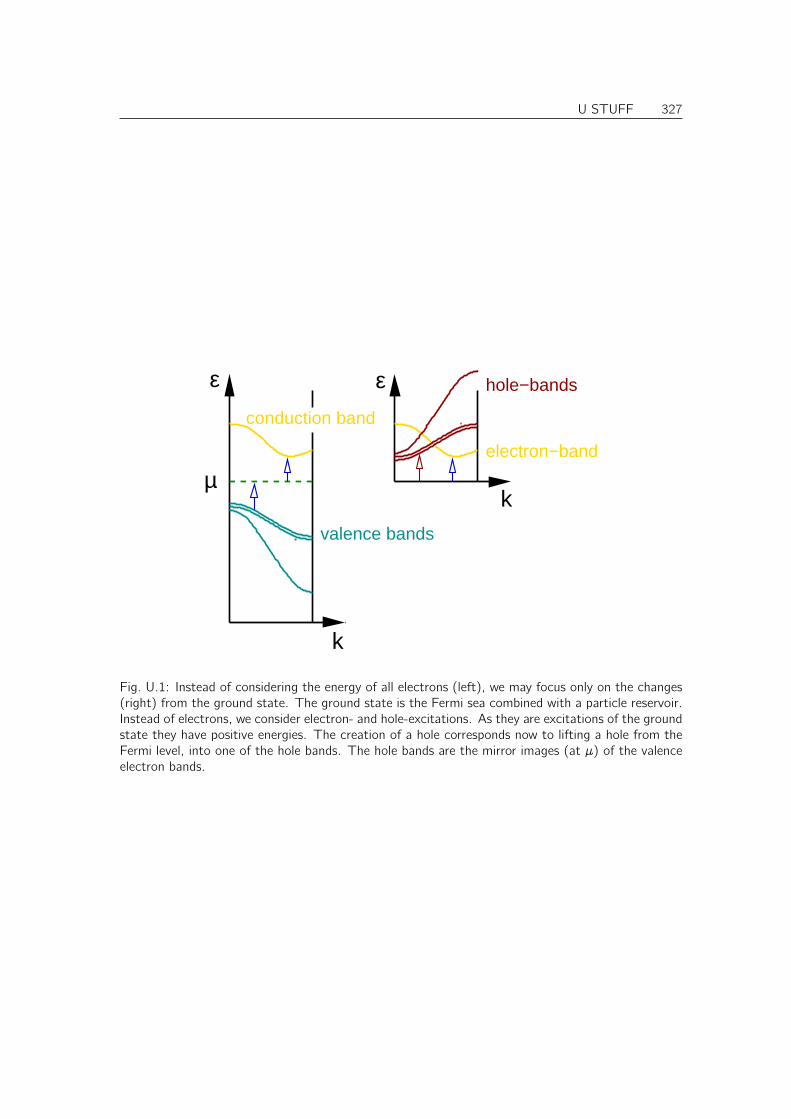
U STUFF 327
εε
µelectron−band
conduction band
valence bands
hole−bands
k
k
Fig. U.1: Instead of considering the energy of all electrons (left), we may focus only on the changes(right) from the ground state. The ground state is the Fermi sea combined with a particle reservoir.Instead of electrons, we consider electron- and hole-excitations. As they are excitations of the groundstate they have positive energies. The creation of a hole corresponds now to lifting a hole from theFermi level, into one of the hole bands. The hole bands are the mirror images (at µ) of the valenceelectron bands.

328 U STUFF
Appendix V
Dictionary
caveat Vorbehaltcoincidence Übereinstimmungconvolution Faltungcross section Wirkungsquerschnittesthetics Ästetikfactorial Fakultät (mathematische Operation)faculty Fakultät (akademische Verwaltungseinheit)for the sake of ... um ... willen (gen)formidable gewaltig, eindrucksvollpropagator Zeitentwicklungsoperatorcommutate kommutierenrank Rangscattering amplitude Streuamplitudewithout loss of generality ohne Beschränkung der Allgemeinheitwlog oBdA (ohne Beschränkung der Allgemeinheit)
V.1 Explanations
• caveat: Latin, a modifying or cautionary detail to be considered
V.2 Symbols
• ∀ “for all”.
• [A,B]− = [A,B] = AB−BA commutator of A and B. A and B may be matrices or operators.
• [A,B]+ = AB + BA anti-commutator of A and B. A and B may be matrices or operators.
• ~a × ~b vector product between two three dimensional vectors ~a and ~b.
~a × ~b =
aybz − azbyazbx − axbzaxby − aybx
(V.1)
329
330 V DICTIONARY
• ~a ⊗ ~b outer product or dydadic product of two vectors ~a and ~b.(
~a ⊗ ~b)
i ,j= aibj (V.2)
• det |A| determinant of matrix A
• perm|A| permanent of matrix A. The permanent is computed like the determinant with theexceptions that all terms are summed up without the sign changes for permutations.
• δi ,j Kronecker delta
δi ,j =
1 for i = j
0 else(V.3)
• δ(~x) Dirac’s delta function defined by
∀f (x)∫
dx f (x)δ(x) = f (0) (V.4)
which holds for all differentiable functions f (x). The delta function of a vector is the productof the delta functions of its components.
• ǫi1,...,iN Levy-Civita Symbol or fully antisymmetric tensor
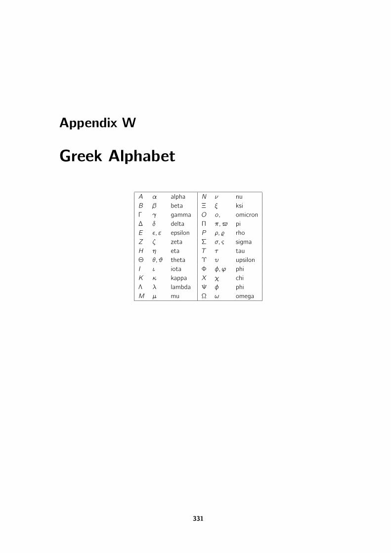
Appendix W
Greek Alphabet
A α alpha N ν nuB β beta Ξ ξ ksiΓ γ gamma O o, omicron∆ δ delta Π π, piE ǫ, ε epsilon P ρ, rhoZ ζ zeta Σ σ, ς sigmaH η eta T τ tauΘ θ, ϑ theta Υ υ upsilonI ι iota Φ φ,ϕ phiK κ kappa X χ chiΛ λ lambda Ψ φ phiM µ mu Ω ω omega
331

332 W GREEK ALPHABET
Appendix X
Philosophy of the ΦSX Series
In the ΦSX series, I tried to implement what I learned from the feedback given by the students whichattended the courses and that relied on these books as background material.
The course should be self-contained. There should not be any statements “as shown easily...” if,this is not true. The reader should not need to rely on the author, but he should be able to convincehimself, if what is said is true. I am trying to be as complete as possible in covering all materialthat is required. The basis is the mathematical knowledge. With few exceptions, the material is alsodeveloped in a sequence so that the material covered can be understood entirely from the knowledgecovered earlier.
The derivations shall be explicit. The novice should be able to step through every single step ofthe derivation with reasonable effort. An advanced reader should be able to follow every step of thederivations even without paper and pencil.
All units are explicit. That is, formulas contain all fundamental variables, which can be inserted inany desirable unit system. Expressions are consistent with the SI system, even though I am quotingsome final results in units, that are common in the field.
The equations that enter a specific step of a derivation are noted ontop of the equation sign.The experience is that the novice does not immediately memorize all the material covered and thathe is struggling with the math, so that he spends a lot of time finding the rationale behind a certainstep. This time is saved by being explicit about it. The danger that the student gets dependent onthese indications, is probably minor, as it requires some effort for the advanced reader to look up theassumptions, an effort he can save by memorizing the relevant material.
Important results and equations are highlighted by including them in boxes. This should facilitatethe preparations for examinations.
Portraits of the key researchers and short biographical notes provide independent associationsto the material. A student may not memorize a certain formula directly, but a portrait. Fromthe portrait, he may associate the correct formula. The historical context provides furthermore anindependent structure to organize the material.
The two first books are in german (That is the intended native language) in order to not addcomplications to the novice. After these first books, all material is in English. It is mandatory that thestudent masters this language. Most of the scientific literature is available only in English. Englishis currently the language of science, and science is absolutely dependent on international contacts.
I tried to include many graphs and figures. The student shall become used to use all his sensesin particular the visual sense.
I have slightly modified the selection of the material commonly tought in most courses. Sometopics, which I consider of mostly historical relevance I have removed. Others such as the Noethertheorem, I have added. Some, like Chaos, Stochastic processes, etc. I have not added yet.
333

334 X PHILOSOPHY OF THE ΦSX SERIES
Appendix Y
About the Author
Prof. Dr. rer. nat Peter E. Blöchl studied physics at Karlsruhe University of Technology in Germany.Subsequently he joined the Max Planck Institutes for Materials Research and for Solid state Researchin Stuttgart, where he worked on development of electronic-structure methods related to the LMTOmethod and on first-principles investigations of interfaces. He received his doctoral degree in 1989from the University of Stuttgart.
Following his graduation, he joined the renowned T.J. Watson Research Center in YorktownHeights, NY in the US on a World Trade Fellowship. In 1990 he accepted an offer from the IBMZurich Research Laboratory in Ruschlikon, Switzerland, which had just received two Nobel prices inPhysics (For the Scanning Tunneling Microscope in 1986 and for the High-Temperature Supercon-ductivity in 1987). He spent the summer term 1995 as visiting professor at the Vienna Universityof Technology in Austria, from where was awarded the habilitation in 1997. In 2000 he left theIBM Research Laboratory after a 10-year period and accepted an offer to be professor for theoreticalphysics at Clausthal University of Technology in Germany. Since 2003, Prof. Blöchl is member ofthe Braunschweigische Wissenschaftliche Gesellschaft (Academy of Sciences).
The main thrust of Prof. Blöchl’s research is related to ab-initio simulations, that is, parameter-free simulation of materials processes and molecular reactions based on quantum mechanics. Hedeveloped the Projector Augmented Wave (PAW) method, one of the most widely used electronicstructure methods to date. This work has been cited over 15,000 times. It is among the 100 mostcited scientific papers of all times and disciplines, and is among the 10 most-cited papers out of morethan 500,000 published in the 120-year history of Physical Review. Next to the research related tosimulation methodology, his research covers a wide area from biochemistry, solid state chemistry tosolid state physics and materials science. Prof. Bloechl contributed to 8 Patents and published about100 research publications, among others in well-known Journals such as “Nature”. The work of Prof.Blöchl has been cited over 23,000 times, and he has an H-index of 41.
335

336 Y ABOUT THE AUTHOR
Bibliography
[1] W.-D. Schöne, C. Timm, and W.-D. Schotte. Theoretische festkörperphysik, teil 1.http://kolxo3.tiera.ru/_Papers/TU%20Wien%20Scripta/Physik/Festkoerperphysik/Theoretische_Festkoerperphysik_I_001(de)(189s).p
2001.
[2] A.L. Fetter and J.D. Walecka. Quantum Theory of Many-ParticleSystems. McGraw-Hill, New York, 1971. ISBN 978-0-07-020653-3. URLhttp://store.doverpublications.com/0486428273.html.
[3] W. Nolting. Grundkurs Theoretische Physik 7: Viel-Teilchen Theorie. Springer, 2002.
[4] R.D. Mattuck. A Guide to Feynman Diagrams in the Many-Body Problem. McGraw-Hill, 1967.
[5] H. Eschrig. The Fundamentals of Density Functional Theory. Edition am Gutenbergplatz,Leipzig, 2003.
[6] J.W. Negele and H. Orland. Quantum Many-Particle Physics. Westview Press, 1988.
[7] M. Born and R. Oppenheimer. Zur quantentheorie der molekeln. Ann. Phys., 84:457, 1927.
[8] M. Born and K. Huang. Dynamical Theory of Crystal Lattices. Oxford University Press, Oxford,1954.
[9] G.A. Worth and M.A. Robb. Applying direct molecular dynamics to non-adiabatic systems. Adv.Chem. Phys., 124:355, 2002.
[10] Felix T. Smith. Diabatic and adiabatic representations for atomic collision prob-lems. Phys. Rev., 179:111–123, Mar 1969. doi: 10.1103/PhysRev.179.111. URLhttp://link.aps.org/doi/10.1103/PhysRev.179.111.
[11] F. Dufey. Störungsreihen für die nichtadiabatische Kopplung mit durchschneidendenPotentialflächen. PhD thesis, Technische Universität München, 2002.
[12] M. Baer, Á. Vibok, G. J. Halaśz, and D. J. Kouri. The electronic non-adiabatic coupling terms:On the connection between molecular physics and field theory. Adv. Quantum Chem., 44:103,2003.
[13] Y. Aharonov and D. Bohm. Significance of electromagnetic potentials in the quantumtheory. Phys. Rev., 115:485–491, Aug 1959. doi: 10.1103/PhysRev.115.485. URLhttp://link.aps.org/doi/10.1103/PhysRev.115.485.
[14] C. N. Yang and R. L. Mills. Conservation of isotopic spin and isotopic gauge in-variance. Phys. Rev., 96:191–195, Oct 1954. doi: 10.1103/PhysRev.96.191. URLhttp://link.aps.org/doi/10.1103/PhysRev.96.191.
[15] J. v. Neumann and E.P. Wigner. über das verhalten von eigenwerten bei adiabatischen prozessen.Phys. Z, 30:467, 1929.
[16] D.R. Yarkony. Diabolical conical intersections. Rev. Mod. Phys., 68:985, 1996.
337
338 BIBLIOGRAPHY
[17] J. H. Van Vleck. The jahnteller effect and crystalline stark splitting for clusters of the form xy6.J. Chem. Phys., 7:72, 1939.
[18] L. Butler. Chemical reaction dynamics beyond the born-oppenheimer approximation. Annu. Rev.Phys. Chem, 49:124, 1998.
[19] M. Baer and G.D. Billing, editors. The role of degenerate states in chemistry, volume 124 ofAdv. Chem. Phys. John Wiley and Sons, 2002.
[20] M.S. Child. Early perspectives on geometric phase. Adv. Chem. Phys., 124:1, 2002.
[21] Michael Baer. Beyond Born-Oppenheimer: Conical Intersections and Electronic NonadiabaticCoupling Terms. John Wiley, 2006.
[22] G.A. Worth and L.S. Cederbaum. Beyond born-oppenheimer: molecular dynamics througha conical intersection. Annu. Rev. Phys. Chem, 55:127, 2004. doi: doi:10.1146/annurev.physchem.55.091602.094335.
[23] G. Herzberg and H. C. Longuet-Higgins. Intersection of potential energy surfaces in poly-atomic molecules. Discuss. Faraday Soc., 35:77–82, 1963. doi: 10.1039/DF9633500077. URLhttp://dx.doi.org/10.1039/DF9633500077.
[24] M.V. Berry. Quantal phase factors accompanying adiabatic changes. Proc. Roy. Soc. A, 392:45, 1984.
[25] David C. Clary. Geometric phase in chemical reactions. Science, 309:1195, 2005.
[26] Carl D. Anderson. The positive electron. Phys. Rev., 43:491, 1933.
[27] P. E. Blöchl. ΦSX: Theoretical Physics III, Quantum Theory. Blöchl, 2015. URLhttp://www2.pt.tu-clausthal.de/atp/phisx.html.
[28] J.C. Slater. The theory of complex spectra. Phys. Rev., 34:1293, 1929.
[29] J.C. Slater. Cohesion in monovalent metals. Phys. Rev., 35:509, 1930.
[30] P. E. Blöchl. ΦSX: Quantum Mechanics of the Chemical Bond. Blöchl, 2015. URLhttp://www2.pt.tu-clausthal.de/atp/phisx.html.
[31] P. E. Blöchl. ΦSX: Theoretical Physics IV, Statistical Physics. Blöchl, 2015. URLhttp://www2.pt.tu-clausthal.de/atp/phisx.html.
[32] John P. Perdew, Kieron Burke, and Matthias Ernzerhof. Generalized gradient approximationmade simple. Phys. Rev. Lett, 77:3865, 1996.
[33] V. Fock. Näherungsmethode zur lösung des quantenmechanischen mehrkörperproblems.Zeitschr. Phys., 61:126, 1930.
[34] V. Fock. "selfconsistent field" mit austausch für natrium. Zeitschr. Phys., 62:795, 1930.
[35] D.R. Hartree. The wave mechanics of an atom with a non-coulomb central field. part i-theoryand methods. Proc. Cam. Phil. Soc., 24:89, 1928. Hartree approximation.
[36] D.R. Hartree. The wave mechanics of an atom with a non-coulomb central field. part ii–someresults and discussion. Proc. Cam. Phil. Soc., 24:111, 1928. Hartree approximation part two.
[37] J.P. Perdew and A. Zunger. Self interaction correction to density-functional approximations formany-electron systems. Phys. Rev. B, 23:5048, 1981.
[38] W. Kolos and C.C. Roothaan. Correlated orbitals for the ground state of the hydrogen molecule.Rev. Mod. Phys., 32:205, 1960.
BIBLIOGRAPHY 339
[39] Pierre Hohenberg and Walter Kohn. Inhomogeneous electron gas.Phys. Rev., 136:B864, 1964. doi: 10.1103/PhysRev.136.B864. URLhttp://link.aps.org/doi/10.1103/PhysRev.136.B864.
[40] Walter Kohn and Lu J. Sham. Self-consistent equations including exchange and corre-lation effects. Phys. Rev., 140:A1133, 1965. doi: 10.1103/PhysRev.140.A1133. URLhttp://link.aps.org/doi/10.1103/PhysRev.140.A1133.
[41] R. McWeeny. Some recent advances in density matrix theory. Rev. Mod. Phys., 32:334, 1960.
[42] A. Puzder, M.Y. Chou, and R.Q. Hood. Exchange and correlation in the si atom: A quantummonte carlo study. Phys. Rev. A, 64:22501, 2001.
[43] Mark S. Hybertsen and Steven G. Louie. Electron correlation in semiconductors and insulators:Band gaps and quasiparticle energies. Phys. Rev. B, 34:5390, 1986.
[44] Pierre Hohenberg and Walter Kohn. Inhomogeneous electron gas.Phys. Rev., 136:B864, 1964. doi: 10.1103/PhysRev.136.B864. URLhttp://link.aps.org/doi/10.1103/PhysRev.136.B864.
[45] Mel Levy. Universal variational functionals of electron densities, first order density matrixes andnatural spin-orbitals and solution of the v-representability problem. Proc. Nat’l Acad. Sci. USA,76:6062, 1979. URL http://www.pnas.org/content/76/12/6062.abstract.
[46] M. Levy. Electron densities in search of hamiltonians. Phys. Rev. A, 26:1200, 1982.
[47] Elliott H. Lieb. Density functionals for coulomb systems. Int. J. Quantum Chem.,24(3):243–277, 1983. ISSN 1097-461X. doi: 10.1002/qua.560240302. URLhttp://dx.doi.org/10.1002/qua.560240302.
[48] J. Harris and R.O. Jones. The surface energy of a bounded electron gas. J. Phys. F: Met.Phys., 4:1170, 1974.
[49] David C. Langreth and John P. Perdew. The exchange-correlation energy of a metallic surface.Sol. St. Commun., 17:1425, 1975.
[50] Olle Gunnarsson and Bengt I. Lundquist. Exchange and correlation in atoms, molecules, andsolids by the spin-density-functional formalism. Phys. Rev. B, 13:4274, 1976.
[51] K. Schwarz. Optimization of the statistical exchange parameter α for the free atoms h throughnb. Phys. Rev. B, 5:2466, 1971.
[52] I. Lindgren and K. Schwarz. Analysis of the electronic exchange in atoms. Phys. Rev. A, 5:542,1972.
[53] D.M. Ceperley and B.J. Alder. Ground state of the electron gas by a stochastic method. Phys.Rev. Lett., 45:566, 1980.
[54] David Bohm and David Pines. A collective description of electron interactions: Iii. coulombinteractions in a degenerate electron gas. Phys. Rev., 92:609, 1953.
[55] Robert O. Jones and Olle Gunnarsson. The density functional formalism, its applications andprospects. Rev. Mod. Phys., 61:689, 1989.
[56] A. D. Becke. Density-functional exchange energy with correct asymptotic behavior. Phys. Rev.A, 38:3098, 1988.
[57] John P. Perdew, Robert G. Parr, Mel Levy, and Jose L. Balduz. Density-functional the-ory for fractional particle number: Derivative discontinuities of the energy. Phys. Rev.Lett., 49:1691–1694, Dec 1982. doi: http://dx.doi.org/10.1103/PhysRevLett.49.1691. URLhttp://link.aps.org/doi/10.1103/PhysRevLett.49.1691.
340 BIBLIOGRAPHY
[58] A. Klamt, V. Jonas, T. Bürger, and J.W. Lohrenz. Refinement and paerameterization of cosmo-rs. J. Phys. Chem. A, 102:5074, 1998.
[59] M. Dion, H. Rydberg, E. Schröder, D. C. Langreth, and B. I. Lundqvist. Van der waals densityfunctional for general geometries. Phys. Rev. Lett, 92:246401, 2004.
[60] E.U. Condon. The theory of complex spectra. Phys. Rev., 36:1121, 1930.
[61] Attila Szabo and Neil S. Ostlund. Modern Quantum Chemistry. McGraw-Hill, New York, 1989.ISBN 9780070627390. URL http://store.doverpublications.com/0486691861.html.
[62] G.D. Mahan. Many Particle Physics. Kluwer academic Publishers, 2000.
[63] R.P. Feynman. The theory of positrons. Phys. Rev., 76:749, 1949.
[64] R.P. Feynman. Space time approach to quantum electrodynamics. Phys. Rev., 76:769, 1949.
[65] A. A. Abrikosow, L. P. Gorkov, and I. E. Dzyaloshinski. Methods of Quantum Field Theory inStatistical Physics. Prentice-Hall, Englewood Cliffs, NJ, 1964.
[66] J. Campbell. Proc. Lond. Math. Soc., 1897.
[67] J. Campbell. Proc. Lond. Math. Soc., 1898.
[68] H. Baker. Proc.Lond. Math. Soc, 34, 1902. Baker-Campbell-Hausdorff theorem.
[69] H. Baker. Proc.Lond. Math. Soc, 35, 1903. Baker-Campbell-Hausdorff theorem.
[70] H. Baker. Proc.Lond. Math. Soc (Ser.2), 3:24, 1905. Baker-Campbell-Hausdorff theorem.
[71] F. Hausdorff. Ber.Verh. Sächs. Akad. Wiss. Leipzig, 58:19, 1909.
[72] L. G. Molinari. Another proof of gell-mann and low’s theorem. J. Math. Phys., 48:52113, 2007.
[73] G.C. Wick. The evaluation of the collision matrix. Phys. Rev., 80:268, 1950.
[74] J. Goldstone. Derivation of the brueckner many-body theory. Proc. Roy.Soc. (London), A239:267, 1957. doi: doi:10.1098/rspa.1957.0037. URLhttp://rspa.royalsocietypublishing.org/content/239/1217/267.
[75] Lars Hedin. New method for calculating the one-particle green’s function with application tothe electron-gas problem. Phys. Rev., 139:A796–A823, Aug 1965. doi: 10.1103/PhysRev.139.A796. URL http://link.aps.org/doi/10.1103/PhysRev.139.A796.
[76] M. Gell-Mann and K.Brueckner. Correlation energy of an electron gas at high density. Phys.Rev., 106:364, 1957.
[77] S. Doniach and E.H. Sondheimer. Green’s Functions for Solid State Physicists. The Ben-jamin/Cummings Publishing Company, INC, Reading, Massachusetts. Reprinted 1998 by Impe-rial college press, 1974.
[78] Martin C. Gutzwiller. Effect of correlation on the ferromagnetism of transition metals. Phys.Rev. Lett., 10(5):159, 1963. doi: 10.1103/PhysRevLett.10.159.
[79] E.H. Lieb and F.Y. Wu. Absence of mott transition in an exact solution of the short-range,one-band model in one dimension. Phys. Rev. Lett, 20:1445, 1968.
[80] P.W. Anderson. Localized magnetic states in metals. Phys. Rev., 124:41, 1961.
[81] F. Bloch. Zur theorie des ferromagnetismus. Z. Phys., 61:206, 1930.
[82] D. Khomskii. Classifying multiferroics: Mechanisms and effects. Physics, 2:20, 2009.
BIBLIOGRAPHY 341
[83] U. Schollwoeck. The density-matrix renormalization group: a short introduction. Phil. Trans.R. Soc. A, 369:2643, 2011.
[84] M. Baer. Topological effects in molecular systems: an attempt towards a complete theory.Chem. Phys., 259:123, 2000.
[85] C. Wittig. The landau-zener formula. J. Phys. Chem., 109:8428, 2005.
[86] C. Zener. Non-adiabatic crossing of energy levels. Proc. Roy. Soc. A, 137:696, 1932.
[87] Roberto Car and Michele Parrinello. Unified approach for molecular dynamics and density-functional theory. Phys. Rev. Lett, 55:2471, 1985. doi: 10.1103/PhysRevLett.55.2471. URLhttp://link.aps.org/doi/10.1103/PhysRevLett.55.2471.
[88] L. Verlet. Computer "experiments" on classical fluids i. thermodynamical properties of lennard-jones molecules. Phys. Rev., 159:98, 1967.
[89] Sanwu Wang. Generalization of the thomas-reiche-kuhn and the bethe sum rules.Phys. Rev. A, 60:262–266, Jul 1999. doi: 10.1103/PhysRevA.60.262. URLhttp://link.aps.org/doi/10.1103/PhysRevA.60.262.
[90] A. Messiah. Quantum Mechanics. Dover, 2000.
[91] I.N. Bronstein and K.A. Semendjajew. Taschenbuch der Mathematik. BSB B.G. eubner Ver-lagsgesellschaft, Leipzig, 1983.
[92] E.N. Economou. Green’s Functions in Quantum Mechanics. Springer, 1979.
[93] F.J Dyson. The radiation theories of tomonaga, schwinger and feynman. Phys. Rev., 75:486,1949.
[94] Ryuzo Abe. Diagrammatic expansion in condensed matter physics. Prog. Theor. Phys., 8:19,1984.
[95] T. Matsubara. A new approach to quantum-statistical physics. Prog. Theor. Phys., 14:351,1955.
[96] Claude Bloch and Cyrano de Dominicis. Un développement du potentiel de gibbs d’un systémequantique composié d’un grand nombre de particules. Nucl. Phys., 7:459, 1958.
[97] M. Gaudin. Une démonstration simplifiié du théoréme de wick en mécanique statistique. Nucl.Phys., 15:89, 1960.
[98] W. Magnus. On the exponential solution of differential equations for a linear operator. Comm.Pure Appl. Math., 7:649, 1954.
Index
adiabatic connection, 137Aharonov-Bohm effect, 28antisymmetric tensor, 52avoided crossing, 30
Baker-Haussdorf theorem, 321, 322band structure, 57, 82Berry phase, 43Berry phase, 252Besselfunction
half-integer order, 122spherical, 122
Bethe sum rule, 283Bloch vector, 65Bloch’s theorem, 66Bohr magneton, 48Boltzmann constant, 76Born-Huang expansion, 22Born-Oppenheimer Approximation, 27Born-Oppenheimer approximation, 21Born-Oppenheimer surface, 27Born-Oppenheimer surfaces, 22Born-Oppenheimer wave functions, 21, 22Boson, 52Brillouin zone, 68Brillouin-zone integral, 86bulk modulus, 80
chemical potential, 76commutator, 329conical intersection, 30, 34, 255conical intersection, 30, 31contraction, 116correspondence principle, 61crystallographic space groups, 62
delta function, 241, 330density matrix
N-particle, 116density of states, 77, 174density operator, 116derivative coupling, 24determinant, 330dimensional bottle-neck, 19Dirac equation, 49
Dirac equation, 286Dirac sea, 59Dirac’s delta function, 330dispersion relation, 57dispersion relation, 82dyadic product, 330Dyson equation, 196
electron-gas parameter, 87exchange and correlation energy, 133exchange energy, 105exchange interaction, 130, 144exchange-correlation hole function, 125exciton, 168extended zone scheme, 67
f-sum rule, 282Fermi loop, 218Fermi momentum, 86Fermi sea, 325Fermi-distribution function, 77Fermion, 52ferromagnetism, 106Feynman diagrams, 180Fock Operator, 109Fock space, 131force, 59Franck-Condon principle, 23free electron gas, 82fully antisymmetric tensor, 52, 330fundamental relation, 74
Generalized gradient approximations, 148geometrical phase, 252GGA, 148grand canonical ensemble, 76grand potential, 76Green’s function
DGL for, 220advanced, 201greater, 201lesser, 201many-particle, 193retarded, 201
group, 275
INDEX 343
GW approximation, 139
Hamilton function, 58Hamilton’s equations, 58Hartree method, 97Hartree Energy, 104Hartree energy, 104Hartree-Fock method, 97Hartree-Fock equations, 107Heat, 74Heaviside function, 241Heisenberg operator, 190Heisenberg picture, 189Hellmann-Feyman theorem, 138hole, 60Hubbard interaction, 229Hund’s rule, 106, 128hybrid functionals, 140
interaction picture, 182
Jacob’s ladder, 142Jahn-Teller effect, 252Jahn-Teller model, 31jellium model, 82jellium oxide, 91jelly-O, 91
Kronecker delta, 330
Legendre transform, 134Lehmann representation, 198Levi-Civita symbol, 52Levy-Civita Symbol, 330Linked-cluster theorem, 219local operator, 109local potential, 109
magnetic anisotropy, 18mass, 59mass
effective, 60maximum coincidence, 160maximum coincidence, 299, 300maximum entropy principle, 75Migdal-Galitskii-Koltun sum rule, 200minimizer, 167minimum energy principle, 75molecular dynamics, 28molecular dynamics
ab-initio, 28
non-crossing rule, 29, 255non-local potential, 108number representation, 76, 154
oblate, 32occupation numbers, 76one-particle operator, 98one-particle reduced density matrix, 117one-particle wave function, 53outer product, 330
P-product, 313pair-correlation function, 124Pauli matrix, 46Pauli equation, 49, 286Pauli principle, 18periodic boundary conditions, 85periodic zone scheme, 67permanent, 330permutation operator, 51, 53phase
geometrical, 43point-group symmetry, 62polarization, 220polarization
proper, 220polaron, 32positions
relative, 62positron, 49product wave function, 53prolate, 32
quantum numbers, 51quasiparticles, 58
Rabi frequency, 261random phase approximation, 224random-phase approximation, 144rank, 53Reciprocal lattice vectors, 63reduced zone scheme, 67RPA, 144, 224
S-matrix, 205Schrödinger picture, 189Seitz radius, 87self energy, 193self energy, 196, 219self interaction, 105self-interaction energy, 105simple oxides, 91Slater determinant, 55Slater determinant, 75Slater rules, 160Slater-Condon rules, 160spectrum
one-particle, 77
344 INDEX
spin-orbitals, 45spinor, 45standard model, 17step function, 241stray fields, 19strong correlations, 57symmetry, 49, 50
tensorfully antisymmetric, 52
tensorfully antisymmetric, 330
thermodynamic beta, 76Thomas-Reiche-Kuhn sum rule, 282time ordering operator, Dyson’s, 313time ordering operator, Wick’s, 313time-inversion symmetry, 286
for spinors, 288time-ordered product, 184time-ordered product
fermion operators, 193transformation operator, 49two-particle density, 120two-particle operator, 98
U-parameter, 228unit cell
primitive, 62universal density functional, 131
vacuum state, 157vacuum state, 153, 154vector product, 329velocity, 58velocity
group velocity, 61Verlet algorithm, 268vertex, 217vertical process, 60
Wick’s time-ordering operator, 193Wick’s thoerem, 211Wigner Seitz cell, 68Wirtinger derivatives, 107Work, 74
Yang-Mills fields, 28


![A Scalable Runtime Platform for Multiagent-Based Simulationwinf.in.tu-clausthal.de/winf/publications/2014/Ahlbrecht+... · 2014. 11. 19. · see[11]. OurevaluationoftheATSim platformusingamid-sizedscenario(rushhour](https://img.pdfslide.us/doc/110x75/6016bc4f480dad023564aaa2/a-scalable-runtime-platform-for-multiagent-based-2014-11-19-see11.jpg)


![i-Dvm-webserver.ub.tu-clausthal.de/CALVOER/KATALOG/W.pdf · Wak - Wal 729 Wake, William: 2 an C 214 : 2 Des Ertz-Bischoffs von Cantelberg [William Wake] an den Chur-Pfaltzischerl](https://img.pdfslide.us/doc/110x75/5e1b786c72db15699742c527/i-dvm-wak-wal-729-wake-william-2-an-c-214-2-des-ertz-bischoffs-von-cantelberg.jpg)


![PhiSX: Statistical Physicsorion.pt.tu-clausthal.de/atp/downloads/scripts/sm.pdfThe roots of the theory of probability lie in the theory of games of chance.[1] In the French Society](https://img.pdfslide.us/doc/110x75/5eaea811e1c6880d583b1a29/phisx-statistical-the-roots-of-the-theory-of-probability-lie-in-the-theory-of-games.jpg)
