Embed Size (px)
Citation preview

don’t p
anic!
Quantum Mechanicsof the Chemical Bond
Peter E. Blöchl
Caution! This is an unfinished draft versionErrors are unavoidable!
Institute of Theoretical Physics; Clausthal University of Technology;D-38678 Clausthal Zellerfeld; Germany;http://www.pt.tu-clausthal.de/atp/
2
© Peter Blöchl, 2000-March 3, 2019Source: http://www2.pt.tu-clausthal.de/atp/phisx.html
Permission to make digital or hard copies of this work or portions thereof for personal or classroomuse is granted provided that copies are not made or distributed for profit or commercial advantage andthat copies bear this notice and the full citation. To copy otherwise requires prior specific permissionby the author.
1
1To the title page: What is the meaning of ΦSX? Firstly, it sounds like “Physics”. Secondly, the symbols stand forthe three main pillars of theoretical physics: “X” is the symbol for the coordinate of a particle and represents ClassicalMechanics. “Φ” is the symbol for the wave function and represents Quantum Mechanics and “S” is the symbol for theEntropy and represents Statistical Physics.
Foreword and outlook
This book shall provide some chemical insight for physicist and material scientists. This book isdevoted to simple concepts that only require back-on-the-envelope calculations. The emphasis is onqualitative considerations instead of accurate predictions. The book attempts to provide a structureinto the thinking about materials properties and reactive processes.
The for this course was born out the the experience with students venturing into ab-initio simu-lations. What I found necessary is first a good education in basic theoretical physics and secondly anintuitive feel for materials. These book addresses the second aspect.
There have been many attempts to condense quantum mechanics into simple concepts that allowone to understand materials without difficult mathematics and computer simulations. The mostimportant contribution is probably due to Linus Pauling’s book “The Nature of the Chemical Bond”,which was written already in 1939. His concepts are still large part of a lecture on structural chemistry.Later contributions are due to Walter Harrison, O.K. Andersen and Roald Hoffman and many more.
Simple qualitative arguments are important for a computer scientist to ask the right questions,and to analyze the results in a way that practitioners can understand. They are also useful to cross-check the results of computer simulations. Calculations are never perfect. Problems, even ones astrivial as setting up the incorrect starting structure, tend to plague the practitioner. Having an ideaof what is likely to happen allows one to detect and correct problems.
The experimentalist in the lab has very similar problems. He has to interpret his results, understandside effects, and detect if he has made an important observation, that brings him the Nobel price, orsimply a bad experiment.
The second goal of this book is to promote the understanding among experimentalist and The-oreticians on the one hand and Physicists, Chemists, Biochemists and Material scientists on theother.
Books[? ]
3

4

Contents
5

6 CONTENTS

Chapter 1
Brief review of quantum mechanics
1.1 Classical mechanics
In classical mechanics the state of a particle is described by its position ~r and its momentum ~p. Thetotal energy of a particle is described by its Hamilton function H(~p,~r). In many cases the Hamiltonfunction has the form
H(~p,~r) =p2
2m+ V (~r) (1.1)
The Hamiltonian must be expressed by positions and momenta and not by positions and velocities!The equations of motion are governed by the Hamilton’s equations
.pi = −
∂H
∂xi;
.x i =
∂H
∂pi(1.2)
Hamilton’s equations contain the same information as Newton’s equation, which can be demon-strated for the Hamilton function given above in Eq. 1.1.
..~rEq. 1.2
=d
dt
~p
m
Eq. 1.2= −
1
m~∇V
~F=−~∇V=
1
m~F
1.2 Quantum Mechanics
Electrons in a solid must be described quantum mechanically. Quantum mechanics cannot predictpositions and momenta with absolute precision. It only allows to predict probabilities for positions andmomenta. The information about a quantum state is no more captured by positions and momentabut by the wave function Ψ(~r). The meaning of the wave function is that its absolute square is theprobability that a particle is at a given position.
1.2.1 Hamilton operator and observables
Observables, i.e. observable quantities, such as energy, position, momenta etc are represented byoperators that act on wave functions. The position operator is simply ~r . The momentum operatoris
p =~i~∇
All observables can be represented in classical mechanics as functions of positions and momenta. Thecorresponding quantum mechanical operator is obtained by replacing the positions and momenta by
7
8 1 BRIEF REVIEW OF QUANTUM MECHANICS
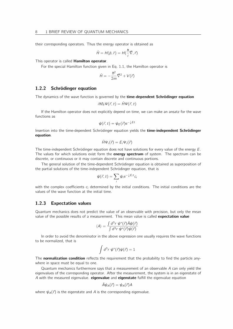
their corresponding operators. Thus the energy operator is obtained as
H = H(p, r) = H(~i~∇, ~r)
This operator is called Hamilton operator.For the special Hamilton function given in Eq. 1.1, the Hamilton operator is
H = −~2
2m~∇2 + V (~r)
1.2.2 Schrödinger equation
The dynamics of the wave function is governed by the time-dependent Schrödinger equation
i~∂tΨ(~r , t) = HΨ(~r , t)
If the Hamilton operator does not explicitly depend on time, we can make an ansatz for the wavefunctions as
ψ(~r , t) = ψE(~r)e−i~Et
Insertion into the time-dependent Schrödinger equation yields the time-independent Schrödingerequation.
HΨi(~r) = EiΨi(~r)
The time-independent Schrödinger equation does not have solutions for every value of the energy E.The values for which solutions exist form the energy spectrum of system. The spectrum can bediscrete, or continuous or it may contain discrete and continuous portions.
The general solution of the time-dependent Schrödinger equation is obtained as superposition ofthe partial solutions of the time-independent Schrödinger equation, that is
ψ(~r , t) =∑i
ψie− i~Ei tci
with the complex coefficients ci determined by the initial conditions. The initial conditions are thevalues of the wave function at the initial time.
1.2.3 Expectation values
Quantum mechanics does not predict the value of an observable with precision, but only the meanvalue of the possible results of a measurement. This mean value is called expectation value
〈A〉 =
∫d3r ψ∗(~r)Aψ(~r)∫d3r ψ∗(~r)ψ(~r)
In order to avoid the denominator in the above expression one usually requires the wave functionsto be normalized, that is ∫
d3r ψ∗(~r)ψ(~r) = 1
The normalization condition reflects the requirement that the probability to find the particle any-where in space must be equal to one.
Quantum mechanics furthermore says that a measurement of an observable A can only yield theeigenvalues of the corresponding operator. After the measurement, the system is in an eigenstate ofA with the measured eigenvalue. eigenvalue and eigenstate fulfill the eigenvalue equation
AψA(~r) = ψA(~r)A
where ψA(~r) is the eigenstate and A is the corresponding eigenvalue.

1 BRIEF REVIEW OF QUANTUM MECHANICS 9
1.2.4 Bracket notation
In quantum mechanics a compact and flexible notation has been developed, namely Dirac’s bracketnotation. A wave function Ψ(~r) is described by a ket |ψ〉. The complex conjugate wave function isdescribed by a bra 〈ψ|.
The scalar product between a bra 〈ψ| and a ket |φ〉 is defined as
〈ψ|φ〉 =
∫d3r ψ∗(~r)φ(~r) (1.3)
A scalar product is a complex number. Forming scalar products is the only way to extract numbersfrom the abstract notation. The scalar product has the general property
〈φ|ψ〉 = 〈ψ|φ〉∗
The expectation value of an operator is
〈ψ|A|ψ〉 =
∫d3r ψ∗(~r)Aψ(~r)
In order to make contact with the real-space representation described in the beginning, we intro-duce states
|~r〉
The wave function in real space is obtained from a ket by
ψ(~r) = 〈~r |ψ〉
The complex wave function is then
ψ∗(~r) = 〈ψ|~r〉
The scalar products have, per definition, the form
〈~r |~r ′〉 = δ(~r − ~r ′)
where δ(~r) is Dirac’s delta function in three dimensions. The delta function is defined by∫d3r f (~r)δ(~r − ~r0) = f (~r0)
which must hold for any continuous function f (~r).The unit operator 1 is the operator that reproduces any state, to which it is applied without
change. It can be expressed as
1 =
∫d3r |~r〉〈~r |
The position operator has the form
~r =
∫d3r |~r〉~r〈~r |
The momentum operator has the form
~p =
∫d3r |~r〉
~i~∇〈~r |
and the Hamilton operator for the Hamilton function H = ~p2/2m + V (~r) has the form
H = H(~p, ~r) =
∫d3r |~r〉
(−~2
2m~∇2 + V (~r)
)〈~r |
10 1 BRIEF REVIEW OF QUANTUM MECHANICS
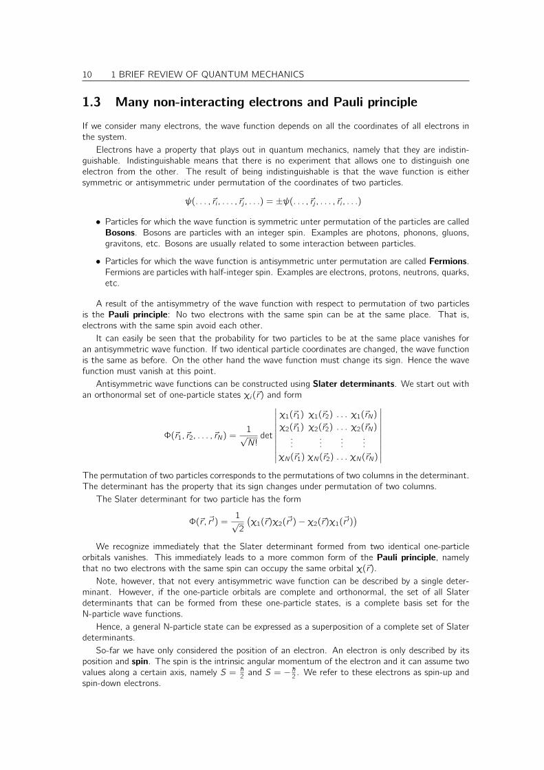
1.3 Many non-interacting electrons and Pauli principle
If we consider many electrons, the wave function depends on all the coordinates of all electrons inthe system.
Electrons have a property that plays out in quantum mechanics, namely that they are indistin-guishable. Indistinguishable means that there is no experiment that allows one to distinguish oneelectron from the other. The result of being indistinguishable is that the wave function is eithersymmetric or antisymmetric under permutation of the coordinates of two particles.
ψ(. . . , ~ri , . . . , ~rj , . . .) = ±ψ(. . . , ~rj , . . . , ~ri , . . .)
• Particles for which the wave function is symmetric unter permutation of the particles are calledBosons. Bosons are particles with an integer spin. Examples are photons, phonons, gluons,gravitons, etc. Bosons are usually related to some interaction between particles.
• Particles for which the wave function is antisymmetric unter permutation are called Fermions.Fermions are particles with half-integer spin. Examples are electrons, protons, neutrons, quarks,etc.
A result of the antisymmetry of the wave function with respect to permutation of two particlesis the Pauli principle: No two electrons with the same spin can be at the same place. That is,electrons with the same spin avoid each other.
It can easily be seen that the probability for two particles to be at the same place vanishes foran antisymmetric wave function. If two identical particle coordinates are changed, the wave functionis the same as before. On the other hand the wave function must change its sign. Hence the wavefunction must vanish at this point.
Antisymmetric wave functions can be constructed using Slater determinants. We start out withan orthonormal set of one-particle states χi(~r) and form
Φ(~r1, ~r2, . . . , ~rN) =1√N!
det
∣∣∣∣∣∣∣∣∣∣χ1(~r1) χ1(~r2) . . . χ1(~rN)
χ2(~r1) χ2(~r2) . . . χ2(~rN)...
......
...χN(~r1) χN(~r2) . . . χN(~rN)
∣∣∣∣∣∣∣∣∣∣The permutation of two particles corresponds to the permutations of two columns in the determinant.The determinant has the property that its sign changes under permutation of two columns.
The Slater determinant for two particle has the form
Φ(~r , ~r ′) =1√2
(χ1(~r)χ2(~r ′)− χ2(~r)χ1(~r ′)
)We recognize immediately that the Slater determinant formed from two identical one-particle
orbitals vanishes. This immediately leads to a more common form of the Pauli principle, namelythat no two electrons with the same spin can occupy the same orbital χ(~r).
Note, however, that not every antisymmetric wave function can be described by a single deter-minant. However, if the one-particle orbitals are complete and orthonormal, the set of all Slaterdeterminants that can be formed from these one-particle states, is a complete basis set for theN-particle wave functions.
Hence, a general N-particle state can be expressed as a superposition of a complete set of Slaterdeterminants.
So-far we have only considered the position of an electron. An electron is only described by itsposition and spin. The spin is the intrinsic angular momentum of the electron and it can assume twovalues along a certain axis, namely S = ~
2 and S = − ~2 . We refer to these electrons as spin-up andspin-down electrons.
Chapter 2
The covalent bond
2.1 Linear combination of atomic orbitals (LCAO)
The LCAO method has been proposed first by Bloch[? ]. Slater and Koster[? ] showed how thematrix elements can be evaluated from a small number of parameters.
Already the states of electrons in most molecules cannot be solved exactly. The problem is relatedto the interaction. One approximation is to assume that the electrons are not interacting. A soundtheoretical justification for this approximation is given by density functional theory (DFT), whichmaps the interacting electrons onto non-interacting electrons in an effective potential. However,density functional theory introduces additional terms in the total energy that we will not consider atthis point.
We still need to determine the electronic wave functions for a complicated potential. That is weneed to solve the Schrödinger equation[
−~2
2me~∇2 + v(~r)− εn
]ψn(~r) = 0
which, in bra-ket notation has the form[p2
2me+ v − εn
]|ψn〉 = 0 (2.1)
with v =∫d3r |~r〉v(~r)〈~r |. One way to tackle this problem is to define a basis set so that we can
write the one-particle wave functions |ψn〉 as superposition of basis functions |χR,`,m,σ,i 〉. Let usat the moment consider the wave functions of the isolated atoms as basis functions. The index Rdenotes a given atomic site, ` is the angular momentum quantum number, m the magnetic quantumnumber and σ is the spin quantum number. i is the principal quantum number of the atom. In thefollowing we will use a shorthand for the indices so that α = (R, `,m, σ, i). Thus we represent theone-particle wave functions as
|ψn〉 =∑α
|χα〉cα,n (2.2)
We insert the ansatz Eq. 2.2 into the Schrödinger equation Eq. 2.1, and multiply the equationfrom the left with 〈χβ |. This leads to a generalized eigenvalue problem1 for matrices∑
α
(Hβ,α − εnOβ,α) cα,n = 0 (2.3)
1An eigenvalue problem is called generalized if it has an overlap matrix that differs from the unity matrix
11
12 2 THE COVALENT BOND
where the Hamilton matrix Hα,β and the overlap matrix Oα,β are defined by
Hα,β = 〈χα|p2
2me+ v |χβ〉
Oα,β = 〈χα|χβ〉
A generalized eigenvalue problem, can be solved numerically using the LAPACK library[? ].The generalized eigenvalue problem yields the eigenvalues εn and the eigenvectors ~cn with elementscα,n.
The generalized eigenvalue problem does not yet determine the norm of the eigenvectors. Thenormalization condition is
〈ψn|ψm〉 =∑α,β
c∗α,nOα,βcβ,m = δn,m
2.2 From non-orthonormal to orthonormal basis functions
We consider here only one orbital on each atom as, for example, in the hydrogen molecule. We willsee that the concept can be generalized to most chemical bonds. The resulting eigenvalue equationis
2∑β=1
Hα,βcβ,n =
2∑β=1
Oα,βcβ,nεn
where H is the Hamilton matrix and O is called the overlap matrix. The diagonal elements areapproximated by the atomic eigenvalues ε1 and ε2 of the two atoms and the diagonal elements of theoverlap matrix are unity, if we start form normalized eigenvalues. We rename H12 = t and O12 = ∆so that
H =
(ε1 t
t∗ ε2
)and O =
(1 ∆
∆∗ 1
)(2.4)
The parameter t is called hopping matrix element.2
Approximate orthonormalization
Below, we will work with orthonormal basissets, even though the overlap is not negligible. For anon-orthonormal basis set the first step is an orthonormalization.
The Schrödinger equation (H − εnO)~cn = 0 can be rewritten by multiplication from the left withO−
12 .
(H − εnO)~cn = 0
⇒ O−12 (H − εnO)O−
12O
12︸ ︷︷ ︸
=111
~cn = 0
⇒(O−
12HO−
12︸ ︷︷ ︸
H′′′
−εn)O
12 ~cn︸ ︷︷ ︸~c ′
= 0
A function of an operator, such as the inverse square root, is defined via its Taylor expansion.The Taylor expansion of f (x) = (1 + x)−
12 is f (x) = 1− 1
2x +O(x2). Thus the inverse square roort
2The name results from the picture of an electron hopping from site to site. This transport is larger if the hoppingmatrix element is larger. It is often used in the context of orthonormal orbitals. The picture of and electron performingdiscrete hops from site to site is, however, misleading.
2 THE COVALENT BOND 13
of the overlap operator is (1 ∆
∆∗ 1
)− 12
=
(1 − 1
2 ∆
− 12 ∆∗ 1
)+O(|∆|)2
This gives us the transformed Hamiltonian in the form
H′′′ =
(ε1 − Re[∆∗t] t − ∆ ε1+ε2
2
t∗ − ∆∗ ε1+ε2
2 ε2 − Re[∆∗t]
)+O(|∆|2) (2.5)
Normally the hopping matrix element t is negative and the overlap matrix element ∆ is positive.We then observe that the diagonal elements are shifted upwards in energy. This effect is called Paulirepulsion: If two atoms come close, their atomic orbitals overlap. When orthogonality is restored, theenergy levels shift up. A simple argument goes as follows: As two atoms overlap, the electrons repelleach other due to the Pauli principle. The atoms become effectively compressed. As a consequence,via Heisenberg’s uncertainty principle3, the kinetic energy is increased and energy is shifted up.
Wolfsberg-Helmholtz Formula
We may use a simple empirical relation for the hopping matrix elements, namely the Wolfsberg-Helmholtz formula[? ], which says
t = kε1 + ε2
2∆ (2.6)
where k ≈ 1.75 is an empirical constant. Values for k depend somewhat on the type of the bondand vary between 1.6 and 2.0. For a motivation of the Wolfsberg formula see App. ?? on p. ??.
One can now orthonormalize the orbitals. Using the Wolfsberg-Helmholtz formula Eq. 2.6 weobtain a Hamiltonian Eq. 2.5 to first order in ∆, which has the form
H′ =
(ε1 (k − 1) ε1+ε2
2 ∆
(k − 1) ε1+ε2
2 ∆∗ ε2
)and O′ =
(1 0
0 1
)
The derivation is given in App. ??.The main difference from a general Hamilton matrix given in Eq. 2.4 is the renormalization of the
hopping matrix element from t to t ′ = (k − 1) ε1+ε2
2 ∆.The change of the diagonal elements amounts to a upward shift of both energy levels by the same
amount. The shift is (usually) upward, because the atomic energy levels are (usually) negative.
Complete neglect of overlap (CNO)
Since we want to approach the problem in small steps, we go back to Eq. 2.4 and ignore the off-diagonal elements of the overlap matrix. Thus, in the following we consider instead
H =
(ε1 t
t∗ ε2
)and O =
(1 0
0 1
)(2.7)
For our discussion it is important that t < 0, which is usually fulfilled. This approximation is calledComplete Neglect of Overlap (CNO).
3Heisenberg’s uncertainty principle says that the variation of position and momentum is equal or larger than 12~,
that is ∆x∆p ≥ 12~. This suggests that the momentum of a confined particle should be larger than about p > ~
2∆x.
Hence the energy would be about Ekin > ~2
m(2∆x)2 . This says that the kinetic energy rises with confinement.

14 2 THE COVALENT BOND
2.3 The two-center bond
. We consider now the simple case of a system with two orbitals. The typical example is a hydrogenmolecule. However the findings will be more general and will be applicable in most cases where twoatoms form a bond.
The model Hamiltonian, we investigate, is
H =
(ε1 t
t∗ ε2
)and O = 1 =
(1 0
0 1
)
Eigenvalues
We diagonalize the Hamiltonian by finding the zeros of the determinant of H − ε1.4 The zero’s ofthe characteristic polynomial determine the eigenvalues
0 = (ε1 − ε)(ε2 − ε)− |t|2
EIGENVALUES OF THE TWO-CENTER BOND
ε± =ε1 + ε2
2±
√(ε1 − ε2
2
)2
+ |t|2 (2.8)
1
ε
ε
−
ε+
t
ε
ε2
ε2
ε1
ε
ε
−ε
+
Fig. 2.1: Left: Energy levels of the two-center bond as function of the hopping parameter t. Right:energy levels as functiuon of some parameter, which tunes the diagonal elements of the Hamiltonianat a fixed hopping parameter t.
The result of Eq. 2.8 is shown in Fig. 2.1. If the hopping parameter t vanishes, the eigenvaluesare, naturally, just the diagonal elements of the Hamiltonian, the “atomic energy levels” ε1 and ε2.With increasing hopping parameter the splitting of the energy levels grows. It never becomes smaller!
• for a large hopping parameter t, i.e. for |t| >> |ε2 − ε1|, we obtain approximately
ε± ≈ε1 + ε2
2± |t| (2.9)
If the hopping parameter becomes much larger than the initial energy level splitting ε2− ε1, theenergy levels deviate approximately linearly with t from the mean value (ε1 + ε2)/2.
4The condition that the determinant vanishes, that is det[H − εO] = 0 determines the eigenvalues of the system.We need to determine the zeroes of a polynomial of the energy. This polynomial is called the characteristic polynomial
2 THE COVALENT BOND 15
• for a small hopping parameter t, i.e. for |t| << |ε2 − ε1|, we obtain approximately
ε− ≈ ε1 −|t|2
|ε2 − ε1|(2.10)
ε+ ≈ ε2 +|t|2
|ε2 − ε1|(2.11)
For small t the energy levels ε± deviate approximately quadratically with t from the “atomicenergy levels” ε1/2. The level shift is larger if the energy levels lie close initially.
Diagonalization conserves the trace
The mean value of the eigenvalues remains always the same, if basisset is orthonormal. This is aconsequence of the fact that the trace of a matrix is invariant under a unitary transformation.
The normalized eigenvectors ~cn of a hermitean matrix H form a unitary matrix U with Uα,n = cα,n.Thus, the eigenvalue equation has the form
HU = Uh
where h is a diagonal matrix with the eigenvalues εn on the main diagonal and U is unitary, that isUU† = 111. When we exploit that the trace of a product of matrices or operators is invariant undercyclic permitations of the individual terms, we can show∑
α
Hα,α = Tr[H] = Tr[HUU†] = Tr[UhU†] = Tr[U†Uh] = Tr[h] =∑n
εn
which prooves that the sum of eigenvalues is identical to the sum of diagonal elements of theHamiltonian. Hence, the sum of energy levels is equal to the sum of “atomic” energy levels.
This statement says that the stabilizing effect of a bond is exactly canceled by the destabilizingeffect of the corresponding antibond. It is, however, only true for an orthonormal basis set. If theoverlap matrix is not unity, there is the Pauli repulsion shifting the orbitals upward.
Eigenvectors
The two eigenvectors ~cn with n ∈ +,− are obtained from (H − εn111)~cn = 0, that is alternativelyfrom the equation
(ε1 − ε±)c1,± + tc2,± = 0 (2.12)
or from
t∗c1,± + (ε2 − ε±)c2,± = 0 (2.13)
Both equations lead to the same result.In our two-dimensional case, we can solve the equations simply by looking for an orthogonal vector
to the coefficients5 and to normalize it. Because the results will have a more transparent form, wechoose the second equation Eq. 2.13 for the lower, bonding eigenstate
c1,− =ε2 − ε−√
(ε2 − ε−)2 + |t|2and c2,− =
−t∗√(ε2 − ε−)2 + |t|2
(2.14)
and the first equation Eq. 2.12 for the higher, antibonding state
c1,+ =t√
(ε1 − ε+)2 + |t|2and c2,+ =
−(ε1 − ε+)√(ε1 − ε+)2 + |t|2
(2.15)
5A complex 2-dimensional vector ~b orthogonal to a vector ~a can be found simply as b1 = a2 and b2 = −a1

16 2 THE COVALENT BOND
Both results can be combined into
EIGENVECTORS OF THE TWO-CENTER BOND
~c− =
(1−t∗ε2−ε−
)(1 +
|t|2
(ε2 − ε−)2
)− 12
and ~c+ =
(t
ε+−ε1
1
)(1 +
|t|2
(ε+ − ε1)2
)− 12
(2.16)
The eigenvalues ε± are given in Eq. 2.8.
In order to to make the qualitatively relevant results more evident, we distinguish the degeneratelimit, i.e. (ε2 − ε1) << |t| from the non-degenerate case (ε2 − ε1) >> |t|.
Degenerate case
In the degenerate limit the two “atomic levels” are identical, i.e. ε1 = ε2 =: ε. The degenerate casedescribes the bonding of two symmetric orbitals, such as the orbitals of a hydrogen molecule.
From Eq. 2.8 we can directly determine the energy eigenvalues as
EIGENVALUES OF THE DEGENERATE TWO-CENTER BOND
ε± = ε± |t| (2.17)
The lower wave function with energy ε− is is the bonding state and the upper wave function withenergy ε+ is called the anti-bonding state.
|t|
|t|
−
ψ
ψ
+
Let us consider the binding between two atoms with one electron each. Before the bond isformed, the atoms are far apart and the hopping matrix element t vanishes. Once the bond hasformed, both electrons can move into the lower, bonding orbital. The energy gained is 2|t|. If thereare two electrons in each orbital or if there are no electrons the sum of occupied energy eigenvaluesremains identical. Occupying the anti-bonding orbital (at ε+ |t|) costs energy.
We can look up the eigenvectors from Eq. 2.16, but they are easily obtained directly6:(ε− ε± t
t∗ ε− ε±
)(c1,±
c2,±
)=
(∓|t| t
t∗ ∓|t|
)(c1,±
c2,±
)= 0 ⇒ c2,± = ±
t
|t|c1,±
6Personally, I prefer the direct calculation, because the steps are easier to memorize than a formula
2 THE COVALENT BOND 17
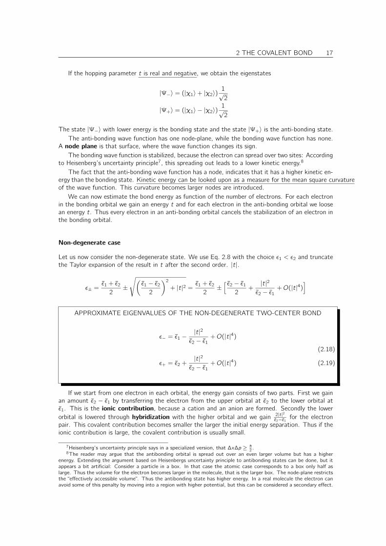
If the hopping parameter t is real and negative, we obtain the eigenstates
|Ψ−〉 = (|χ1〉+ |χ2〉)1√2
|Ψ+〉 = (|χ1〉 − |χ2〉)1√2
The state |Ψ−〉 with lower energy is the bonding state and the state |Ψ+〉 is the anti-bonding state.The anti-bonding wave function has one node-plane, while the bonding wave function has none.
A node plane is that surface, where the wave function changes its sign.The bonding wave function is stabilized, because the electron can spread over two sites: According
to Heisenberg’s uncertainty principle7, this spreading out leads to a lower kinetic energy.8
The fact that the anti-bonding wave function has a node, indicates that it has a higher kinetic en-ergy than the bonding state. Kinetic energy can be looked upon as a measure for the mean square curvatureof the wave function. This curvature becomes larger nodes are introduced.
We can now estimate the bond energy as function of the number of electrons. For each electronin the bonding orbital we gain an energy t and for each electron in the anti-bonding orbital we loosean energy t. Thus every electron in an anti-bonding orbital cancels the stabilization of an electron inthe bonding orbital.
Non-degenerate case
Let us now consider the non-degenerate state. We use Eq. 2.8 with the choice ε1 < ε2 and truncatethe Taylor expansion of the result in t after the second order. |t|.
ε± =ε1 + ε2
2±
√(ε1 − ε2
2
)2
+ |t|2 =ε1 + ε2
2±[ ε2 − ε1
2+|t|2
ε2 − ε1+O(|t|4)
]
APPROXIMATE EIGENVALUES OF THE NON-DEGENERATE TWO-CENTER BOND
ε− = ε1 −|t|2
ε2 − ε1+O(|t|4)
(2.18)
ε+ = ε2 +|t|2
ε2 − ε1+O(|t|4) (2.19)
If we start from one electron in each orbital, the energy gain consists of two parts. First we gainan amount ε2 − ε1 by transferring the electron from the upper orbital at ε2 to the lower orbital atε1. This is the ionic contribution, because a cation and an anion are formed. Secondly the lowerorbital is lowered through hybridization with the higher orbital and we gain 2|t|2
ε2−ε1for the electron
pair. This covalent contribution becomes smaller the larger the initial energy separation. Thus if theionic contribution is large, the covalent contribution is usually small.
7Heisenberg’s uncertainty principle says in a specialized version, that ∆x∆p ≥ ~2.
8The reader may argue that the antibonding orbital is spread out over an even larger volume but has a higherenergy. Extending the argument based on Heisenbergs uncertainty principle to antibonding states can be done, but itappears a bit artificial: Consider a particle in a box. In that case the atomic case corresponds to a box only half aslarge. Thus the volume for the electron becomes larger in the molecule, that is the larger box. The node-plane restrictsthe “effectively accessible volume”. Thus the antibonding state has higher energy. In a real molecule the electron canavoid some of this penalty by moving into a region with higher potential, but this can be considered a secondary effect.
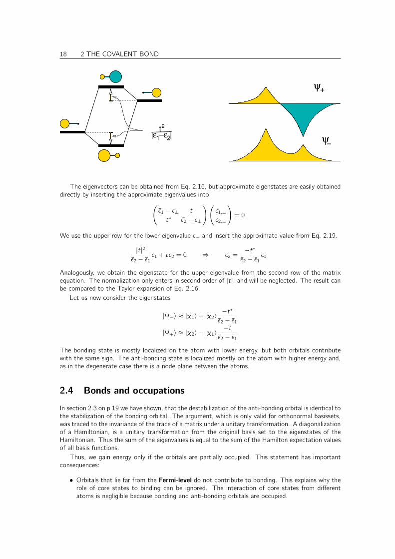
18 2 THE COVALENT BOND
−ε |1 2
2t
|εψ
−
ψ+
The eigenvectors can be obtained from Eq. 2.16, but approximate eigenstates are easily obtaineddirectly by inserting the approximate eigenvalues into(
ε1 − ε± t
t∗ ε2 − ε±
)(c1,±
c2,±
)= 0
We use the upper row for the lower eigenvalue ε− and insert the approximate value from Eq. 2.19.
|t|2
ε2 − ε1c1 + tc2 = 0 ⇒ c2 =
−t∗
ε2 − ε1c1
Analogously, we obtain the eigenstate for the upper eigenvalue from the second row of the matrixequation. The normalization only enters in second order of |t|, and will be neglected. The result canbe compared to the Taylor expansion of Eq. 2.16.
Let us now consider the eigenstates
|Ψ−〉 ≈ |χ1〉+ |χ2〉−t∗
ε2 − ε1
|Ψ+〉 ≈ |χ2〉 − |χ1〉−t
ε2 − ε1
The bonding state is mostly localized on the atom with lower energy, but both orbitals contributewith the same sign. The anti-bonding state is localized mostly on the atom with higher energy and,as in the degenerate case there is a node plane between the atoms.
2.4 Bonds and occupations
In section 2.3 on p 19 we have shown, that the destabilization of the anti-bonding orbital is identical tothe stabilization of the bonding orbital. The argument, which is only valid for orthonormal basissets,was traced to the invariance of the trace of a matrix under a unitary transformation. A diagonalizationof a Hamiltonian, is a unitary transformation from the original basis set to the eigenstates of theHamiltonian. Thus the sum of the eigenvalues is equal to the sum of the Hamilton expectation valuesof all basis functions.
Thus, we gain energy only if the orbitals are partially occupied. This statement has importantconsequences:
• Orbitals that lie far from the Fermi-level do not contribute to bonding. This explains why therole of core states to binding can be ignored. The interaction of core states from differentatoms is negligible because bonding and anti-bonding orbitals are occupied.
2 THE COVALENT BOND 19
1 2|ε −ε |
t2
No Bond
E=−2∆
No Bond
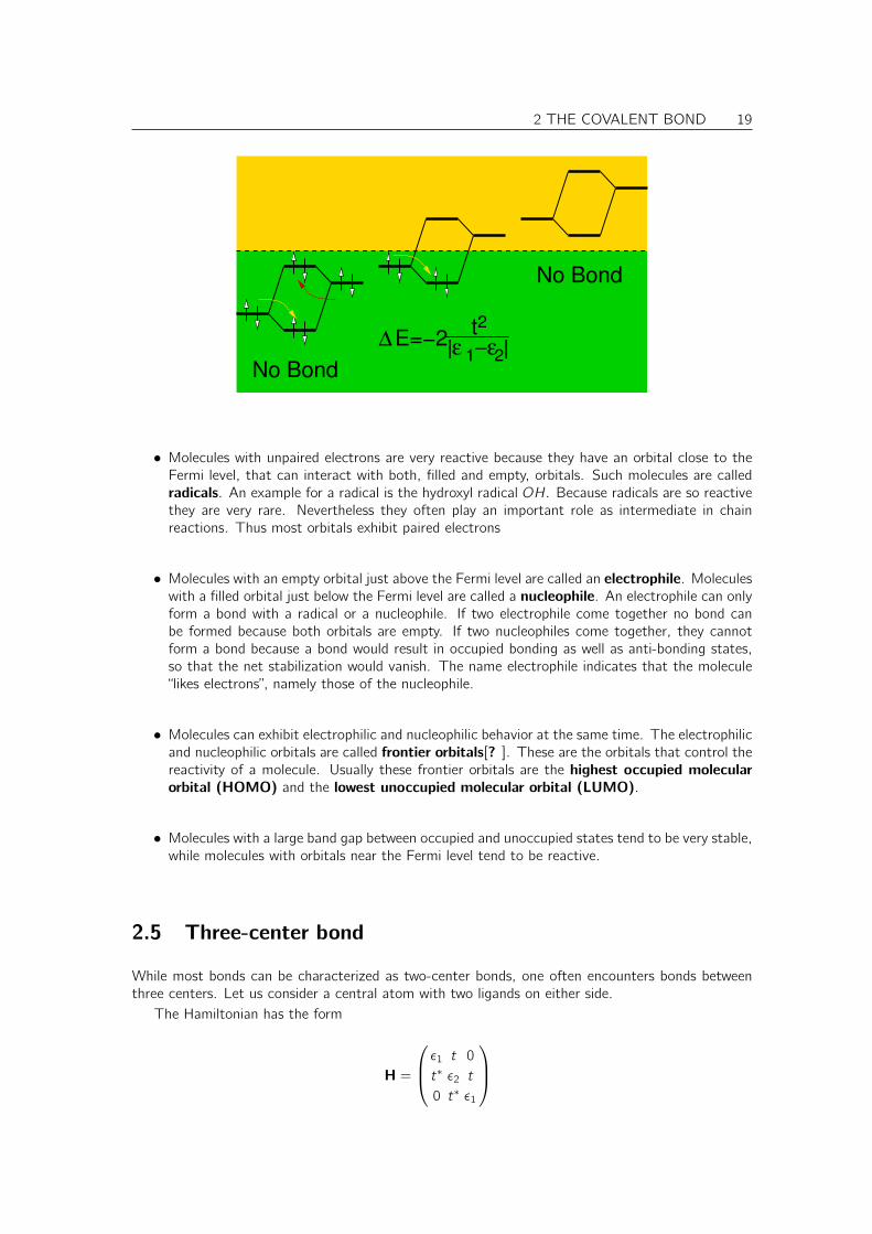
• Molecules with unpaired electrons are very reactive because they have an orbital close to theFermi level, that can interact with both, filled and empty, orbitals. Such molecules are calledradicals. An example for a radical is the hydroxyl radical OH. Because radicals are so reactivethey are very rare. Nevertheless they often play an important role as intermediate in chainreactions. Thus most orbitals exhibit paired electrons
• Molecules with an empty orbital just above the Fermi level are called an electrophile. Moleculeswith a filled orbital just below the Fermi level are called a nucleophile. An electrophile can onlyform a bond with a radical or a nucleophile. If two electrophile come together no bond canbe formed because both orbitals are empty. If two nucleophiles come together, they cannotform a bond because a bond would result in occupied bonding as well as anti-bonding states,so that the net stabilization would vanish. The name electrophile indicates that the molecule“likes electrons”, namely those of the nucleophile.
• Molecules can exhibit electrophilic and nucleophilic behavior at the same time. The electrophilicand nucleophilic orbitals are called frontier orbitals[? ]. These are the orbitals that control thereactivity of a molecule. Usually these frontier orbitals are the highest occupied molecularorbital (HOMO) and the lowest unoccupied molecular orbital (LUMO).
• Molecules with a large band gap between occupied and unoccupied states tend to be very stable,while molecules with orbitals near the Fermi level tend to be reactive.
2.5 Three-center bond
While most bonds can be characterized as two-center bonds, one often encounters bonds betweenthree centers. Let us consider a central atom with two ligands on either side.
The Hamiltonian has the form
H =
ε1 t 0
t∗ ε2 t
0 t∗ ε1
20 2 THE COVALENT BOND
2
2
21|−ε|ε
2ε
1
ε
t
The characteristic equation det[H− ε1] = 0 is
(ε1 − ε)[(ε2 − ε)(ε1 − ε)− |t|2
]− t2(ε1 − ε) = 0
(ε1 − ε)[(ε2 − ε)(ε1 − ε)− 2|t|2
]= 0
ε =
ε1+ε2
2 − |ε1−ε2|2
√1 +
(2√
2tε1−ε2
)2
≈ ε1 − 2t2
|ε1−ε2|
ε1
ε1+ε2
2 − |ε1−ε2|2
√1 +
(2√
2tε1−ε2
)2
≈ ε2 + 2t2
|ε1−ε2|
We can see that there are three states: a bonding state, a non-bonding state and an anti-bondingstate. Due to symmetry, the non-bonding state cannot interact with the orbital on the central atom.
Characteristic for a three center bond is that it maintains its full bond strength for two, three andfour electrons, because the electrons enter into the non-bonding orbital, which does not contributeto the bond-strength.
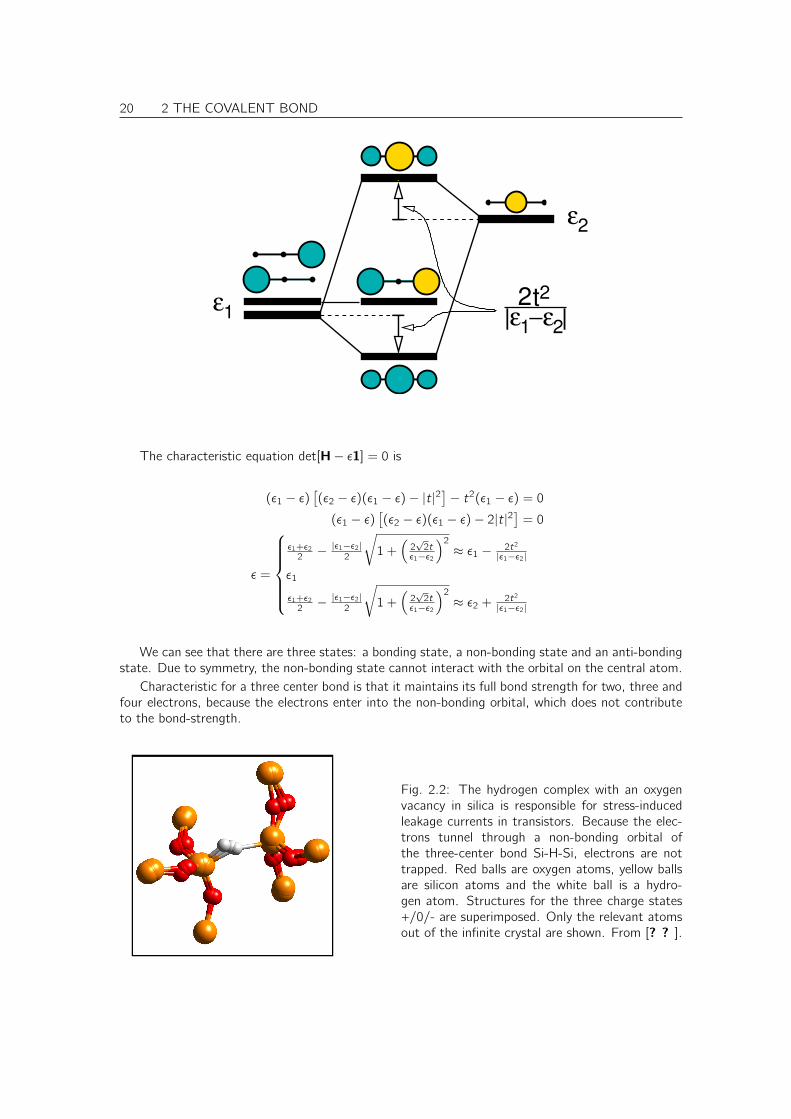
Fig. 2.2: The hydrogen complex with an oxygenvacancy in silica is responsible for stress-inducedleakage currents in transistors. Because the elec-trons tunnel through a non-bonding orbital ofthe three-center bond Si-H-Si, electrons are nottrapped. Red balls are oxygen atoms, yellow ballsare silicon atoms and the white ball is a hydro-gen atom. Structures for the three charge states+/0/- are superimposed. Only the relevant atomsout of the infinite crystal are shown. From [? ? ].
2 THE COVALENT BOND 21
2.6 Chains and rings
Let us now extend our description from a three-center bond to a chain and ring structures of manyatoms.
A chain is a model for a polymer, such as polyacetylene9 It is also a model for a finite cluster. Itis also a model for a state in a semiconductor heterojunction, which is within the conduction of onematerial, but in the band gap of the two neighboring materials.
A ring is a model for example for aromatic molecules such as benzene.Chains and rings will later be important for the description of solids. For the description we will use
periodic boundary conditions, two describe an infinite crystal. In one dimension, this constructioncorresponds directly to a ring structure. Similarly, the chain is a one-dimensional model for a solidwith surfaces.
2.6.1 Chains
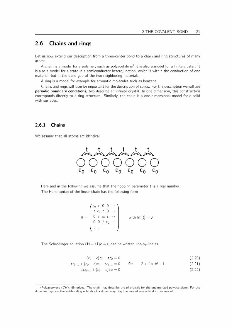
We assume that all atoms are identical.
t t t t
0ε 0ε 0ε 0ε 0ε 0ε 0ε
t t
Here and in the following we assume that the hopping parameter t is a real numberThe Hamiltonian of the linear chain has the following form
H =
ε0 t 0 0 · · ·t ε0 t 0 · · ·0 t ε0 t · · ·0 0 t ε0 · · ·...
...
with Im[t] = 0
The Schrödinger equation (H− ε1)~c = 0 can be written line-by-line as
(ε0 − ε)c1 + tc2 = 0 (2.20)
tci−1 + (ε0 − ε)ci + tci+1 = 0 for 2 < i < N − 1 (2.21)
tcN−1 + (ε0 − ε)cN = 0 (2.22)
9Polyacetylene (CH)n dimerizes. The chain may describe the pi orbitals for the undimerized polyacetylene. For thedimerized system the antibonding orbitals of a dimer may play the role of one orbital in our model

22 2 THE COVALENT BOND
Let us make a little detour, before we continue: Eq. 2.21 has similarities with a differential equation.Introducing a small spacing ∆, it can be written in the form
t∆2 ci−1 − 2ci + ci+1
∆2︸ ︷︷ ︸≈∂2
x f (x)
+(ε0 + 2t)ci − εci = 0
If we consider a function f (x) with values f (j∆) = cj , we can look at the above equation as adiscretized version of the following differential equation for f (x)[
t∆2∂2x + (ε0 + 2t)− ε
]f (x) = 0
This equation is analogous to the one-dimensional Schrödinger equation for a constant potential.The solutions of this problem are plane waves, which we can exploit to find a solution for the originalproblem.
Dispersion relation
After this intermezzo let us continue with the equation for the orbital coefficients. The translationalsymmetry suggests that we use an exponential ansatz for Eq. 2.21.
cj = eik∆j (2.23)
We have inserted here the spacing ∆ between the sites, so that the parameter k has the usual meaningand units of a wave vector.
Insertion of this ansatz into Eq. 2.21 yields
te−ik∆ + (ε0 − ε) + teik∆ Eqs. 2.21,2.23= 0
⇒ 2t cos(k∆) + (ε0 − ε) = 0
⇒ ε(k) = ε0 + 2t cos(k∆) (2.24)
This is the dispersion relation ε(k) for the linear chain, shown in Fig. 2.3.
For small molecules one can investigate the energy levels individually. However, for complex moleculesor crystals, the energy levels are positioned so close in energy that such a representation is no moreuseful. Therefore one chooses a different representation, namely the Density of States. As thename says the density of states is the density of energy levels as function of energy. For s moleculewith discrete energies, the density of states would be a sum of δ-functions, one for each energy level.For our chain, we will see below that the allowed k-values are equi-spaced on the k-axis. Using thedispersion relation ε(k), we can determine the spacing of energy levels on the energy axis.
∆ε =dε
dk︸︷︷︸vg
∆k︸︷︷︸π
(N+1)a
which gives us the density of states as
D(ε) =1
∆ε=
(dε
dk
)−11
∆k
Thus the density of states of a one-dimensional system is proportional to the inverse slope of thedispersion relation. The shape of the density of states shown in Fig. 2.3 is characteristic for a one-dimensional problem. For two or three dimensional problems the density of states would not divergeat the band edges, but start with a step in two dimensions or like the square root of the energyrelative to the band edge in three dimensions.

2 THE COVALENT BOND 23
)εD(E
ne
rgy le
ve
ls
ε ε
4
π∆
ε( )k
ε0| |t
k
0
Fig. 2.3: Dispersion relation of the linear chain. The green points correspond to the energy levels of achain with 11 atoms. In the middle figure we show the energy levels, and on the right the schematicdensity of states D(ε) for the infinite chain.
Boundary conditions
We still need to enforce the boundary conditions Eqs. 2.20 and 2.22. We can bring the boundaryconditions into the form of the central condition Eq. 2.21.
(ε0 − ε)c1 + tc2Eq. 2.20
= 0⇒
tci−1 + (ε0 − ε)ci + tci+1 = 0 for i = 1
and c0 = 0(2.25)
tcN−1 + (ε0 − ε)cNEq. 2.22
= 0⇒
tci−1 + (ε0 − ε)ci + tci+1 = 0 for i = N
and cN = 0(2.26)
Thus, the middle equation is now extended also to the end points i = 1 and i = N, which were notcovered by Eq. 2.21. Two additional sites with i = 0 and i = N+ 1 have been introduced in addition.
The boundary conditions, on the other hand obtain the particularly simple form
c0 = 0 and cN+1 = 0 (2.27)
I like this form, because it is now analogous to the well known particle-in-a-box problem. The onlydifference is the disrete nature of the problem, namely the discrete set of orbitals as opposed to acontinuous range of a spatial coordinate.
For a given energy we obtain two linear independent solutions, which we superimpose to form ageneral ansatz.
cj = Aeik∆j + Be−ik∆j (2.28)
The boundary conditions, now in the form c0 = cN+1 = 0, determine the allowed values for k andBA .
• The first boundary condition, c0 = 0
0 = c0Eq. 2.28
= A+ B ⇒ B = −A
24 2 THE COVALENT BOND
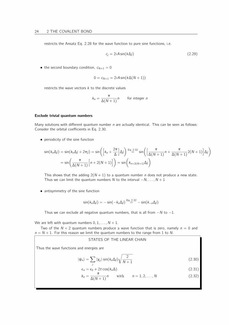
restricts the Ansatz Eq. 2.28 for the wave function to pure sine functions, i.e.
cj = 2iA sin(k∆j) (2.29)
• the second boundary condition, cN+1 = 0
0 = cN+1 = 2iA sin(k∆(N + 1))
restricts the wave vectors k to the discrete values
kn =π
∆(N + 1)n for integer n
Exclude trivial quantum numbers
Many solutions with different quantum number n are actually identical. This can be seen as follows:Consider the orbital coefficients in Eq. 2.30.
• periodicity of the sine function
sin(kn∆j) = sin(kn∆j + 2πj) = sin
([kn +
2π
∆
]∆j
)Eq. 2.32
= sin
([ π
∆(N + 1)n +
π
∆(N + 1)2(N + 1)
]∆j
)= sin
(π
∆(N + 1)
[n + 2(N + 1)
])= sin
(kn+2(N+1)∆j
)
This shows that the adding 2(N + 1) to a quantum number n does not produce a new state.Thus we can limit the quantum numbers N to the interval −N, . . . , N + 1
• antisymmetry of the sine function
sin(kn∆j) = − sin(−kn∆j)Eq. 2.32
= − sin(k−n∆j)
Thus we can exclude all negative quantum numbers, that is all from −N to −1.
We are left with quantum numbers 0, 1, . . . , N + 1.Two of the N + 2 quantum numbers produce a wave function that is zero, namely n = 0 and
n = N + 1. For this reason we limit the quantum numbers to the range from 1 to N.
STATES OF THE LINEAR CHAIN
Thus the wave functions and energies are
|ψn〉 =∑j
|χj〉 sin(kn∆j)
√2
N + 1(2.30)
εn = ε0 + 2t cos(kn∆) (2.31)
kn =π
∆(N + 1)n with n = 1, 2, . . . , N (2.32)

2 THE COVALENT BOND 25
0 1 2 3 N N+1N+1
1
N+1N
20 3
Note that the envelope of the wave function corresponds directly to the states of a particle in abox. This is a direct consequence of the analogy of Eq. 2.21 with a particle in a constant potentialdiscussed before.
Note that the three center bond is a simple example for a linear chain. It is instructive to comparethe general results obtained here for chains with those obtained previously for the three-center bond.
2.6.2 Rings
The Hamiltonian looks very similar to that of a linear chain. The only difference is that the firstatom in the ring is connected to the last one. Thus there is an addition hopping parameter in theupper right and the lower left corner of the matrix.
H =
ε0 t 0 0 · · · tt ε0 t 0 · · · 0
0 t ε0 t · · · 0
0 0 t ε0 · · · 0...
...t 0 · · · 0 t ε0
Boundary conditions
In contrast to the linear chain, the ring has full translational symmetry, which is not even destroyed bythe boundaries. The boundary conditions can again be expressed by the first and the last line of theSchrödinger equation. However, we can also treat the ring as an infinite chain with the requirement,that the wave function is periodic, that is cN+1 = c1. We use the ansatz
cj = eik∆j

26 2 THE COVALENT BOND
The boundary condition cN+1 = c1 requires that
cN+1 = eik∆(N+1) = c1 = eik∆ ⇒ eik∆N = 1 ⇒ kn∆N = 2πn
⇒ kn =2π
N∆n (2.33)
Exclude trivial quantum numbers
Two wave functions for two quantum numbers n and n′ are identical, if
eikn∆j = eikn′∆j for all integer j
⇒ ei(kn−kn′ )∆j = 1 for all integer j
⇒ kn′ = kn +2π
∆q with integer q
⇒ n′ = n + qN
States with quantum numbers that differ by N are identical. Therefore we limit wave vectors kn tothe interval ]− π
2 ,π2 ]. Only one of the values at the boundaries may be included.
STATES OF A RING
Thus we obtain the wave functions and the energy eigenvalues as
|ψn〉 =∑j
|χj〉eikn∆j 1√N
εn = ε0 + 2t cos(kn∆)
kn =2π
N∆n with n = −
N
2+ 1, . . . ,
N
2
The resulting k-values lie in the interval ] π∆ ,π∆ ].
The spacing in k-space is approximately twice as large as in the linear chain with the same numberof beads, but values with positive and negative kn are allowed.
Each pair of degenerate wave functions can be transformed into a pair of real wave functions, ofwhich one is a sinus and the other is a cosinus.
Geometrical construction of the eigenstates
There is an interesting and easy way to memorize construction for the energy levels of a ring. Theconstruction is demonstrated in Fig. 2.5. If one inscribes an equilateral polygon corresponding to thering structure into a sphere, one can easily obtain the energy levels of the ring structure as verticalposition of the corners.
The construction follows directly from the quantization condition
kn =2π
N∆n for n = 0, 1, 2, . . . , N
and the dispersion relation
ε(k) = ε0 + 2t cos(k∆)
Let us interpret φ := k∆ as an angle. The allowed values of the angle are φn = 2πN n and the allowed
energy values are
εn = ε0 + 2t cos(φn)
2 THE COVALENT BOND 27
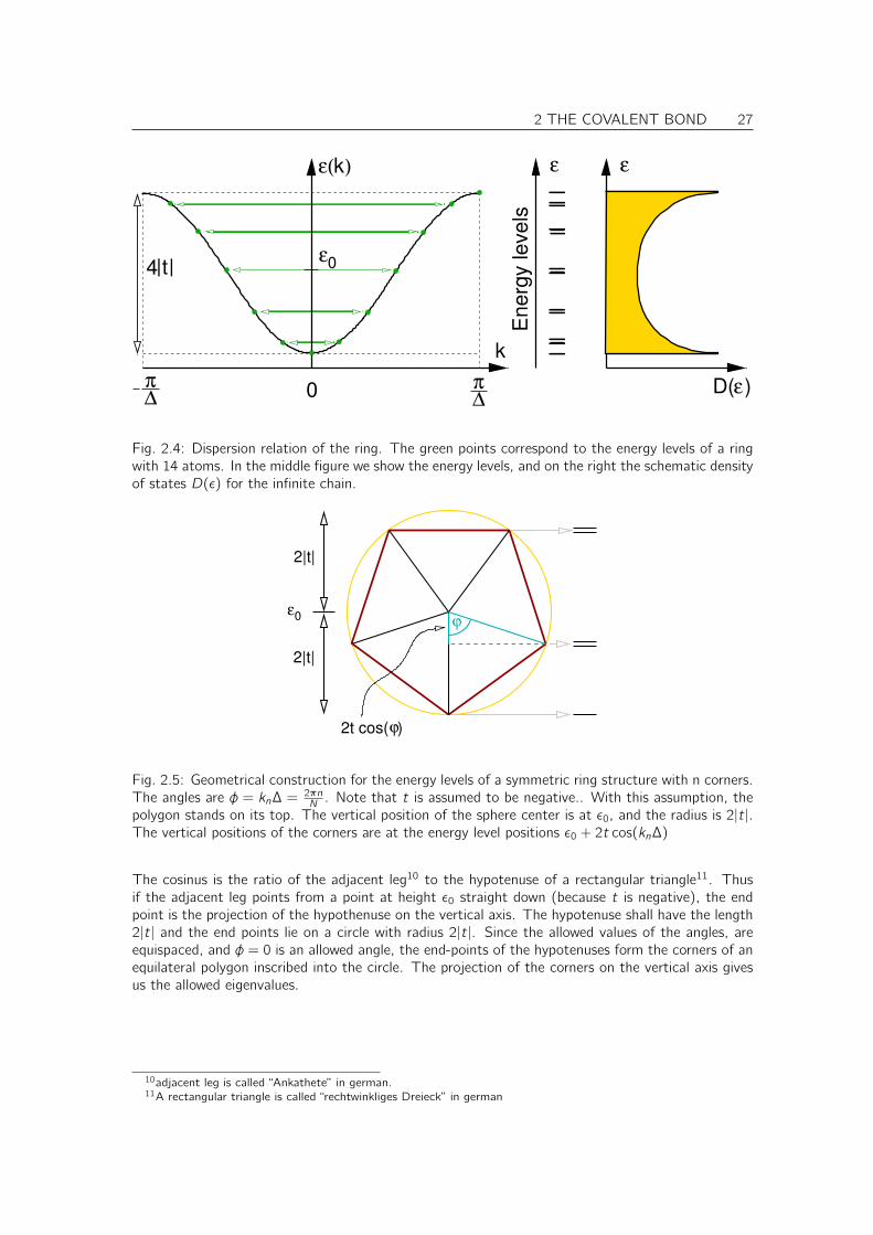
Energ
y levels
D( )ε
ε ε
0
π∆
π∆
ε( )k
| |t4ε
k
0
Fig. 2.4: Dispersion relation of the ring. The green points correspond to the energy levels of a ringwith 14 atoms. In the middle figure we show the energy levels, and on the right the schematic densityof states D(ε) for the infinite chain.
ε0
2t cos( )ϕ
2|t|
2|t|
ϕ
Fig. 2.5: Geometrical construction for the energy levels of a symmetric ring structure with n corners.The angles are φ = kn∆ = 2πn
N . Note that t is assumed to be negative.. With this assumption, thepolygon stands on its top. The vertical position of the sphere center is at ε0, and the radius is 2|t|.The vertical positions of the corners are at the energy level positions ε0 + 2t cos(kn∆)
The cosinus is the ratio of the adjacent leg10 to the hypotenuse of a rectangular triangle11. Thusif the adjacent leg points from a point at height ε0 straight down (because t is negative), the endpoint is the projection of the hypothenuse on the vertical axis. The hypotenuse shall have the length2|t| and the end points lie on a circle with radius 2|t|. Since the allowed values of the angles, areequispaced, and φ = 0 is an allowed angle, the end-points of the hypotenuses form the corners of anequilateral polygon inscribed into the circle. The projection of the corners on the vertical axis givesus the allowed eigenvalues.
10adjacent leg is called “Ankathete” in german.11A rectangular triangle is called “rechtwinkliges Dreieck” in german

28 2 THE COVALENT BOND

Chapter 3
The use of symmetry
3.1 Introduction
Exploiting the symmetry allows one to break down a large eigenvalue problem into many smallerones. The complexity of a matrix diagonlization grows with the third power of the matrix dimension.Therefore, it is much easier to diagonalize many smaller matrices than one big one, that is composedof the smaller ones. If one manages to break down the problem into ones with only one, two or threeorbitals, we may use the techniques from the previous chapter to diagonalize the Hamiltonian. Thisoften allows one to obtain an educated guess of the wave functions without much computation.
As shown below, the eigenstates of the Hamiltonian are also eigenstates of the symmetry opera-tor, if the Hamiltonian has a certain symmetry. (For degenerate states this is not automatically so,but a transformation can bring them into the desired form.) Furthermore, we will show the followingstatement, which will be central to this section:
BLOCK DIAGONALIZATION BY SYMMETRY
The Hamilton matrix elements between eigenstates of a symmetry operator with different eigenvaluesvanish.
In other words:In a basis of symmetry eigenstates, the Hamiltonian is block diagonal. All states in a given blockagree in all symmetry eigenvalues.
s
s1
s3
3
s
s
2
0 0
0
00
0
s21
Fig. 3.1: Block form of a Hamiltonian by using symmetry eigenstates with symmetry eigenvaluess1, s2, s3.
29
30 3 THE USE OF SYMMETRY
3.2 Symmetry and quantum mechanics
Here, I will revisit the main symmetry arguments discussed in chapter 9 of ΦSX:Quantum Physics.This is a series of arguments that is good to keep in mind.
1. Definition of a transformation operator. An operator S can be called a transformation, if itconserves the norm for every state.
∀|ψ〉 〈ψ|ψ〉 |φ〉=S|ψ〉= 〈φ|φ〉 (3.1)
2. Every transformation operator is unitary, that is S†S = 1
∀|ψ〉 〈ψ|S†S|ψ〉 = 〈ψ|ψ〉 ⇒ S†S = 1 (3.2)
3. Definition of a symmetry: A system is symmetric under the transformation S, if, for anysolution |Ψ〉 of the Schrödinger equation describing that system, also S|Ψ〉 is a solution of thesame Schrödinger equation. That is, if(
i~∂t |Ψ〉 = H|Ψ〉) |Φ〉:=S|Ψ〉⇒
(i~∂t |Φ〉 = H|Φ〉
)(3.3)
4. A unitary operator S is a symmetry operator of the system, if
[H, S]− = 0 (3.4)
Proof: Let |Ψ〉 be a solution of the Schrödinger equation and let |Φ〉 = S|Ψ〉 be the result ofa symmetry transformation.
i~∂t |Φ〉 = H|Φ〉|Φ:=S|Ψ〉⇒ i~∂t S|Ψ〉 = HS|Ψ〉
∂t S=0⇒ i~∂t |Ψ〉 = S−1HS|Ψ〉i~∂t |Ψ〉=H|Ψ〉⇒ H|Ψ〉 = S−1HS|Ψ〉(HS − SH
)|Ψ〉︸ ︷︷ ︸
[H,S]−
= 0
Because this equation holds for any solution of the Schrödinger equation, it holds for any wavefunction, because any function can be written as superposition of solutions of the Schrödingerequation. (The latter form a complete set of functions.) Therefore
[H, S]− = 0
Thus, one usually identifies a symmetry by working out the commutator with the Hamiltonian.
5. The matrix elements of the Hamilton operator between two eigenstates of the symmetry op-erator with different eigenvalues vanish. That is(
S|Ψs〉 = |Ψs〉s ∧ S|Ψs ′〉 = |Ψs ′〉s ′ ∧ s 6= s ′)⇒ 〈Ψs |H|Ψs ′〉 = 0 (3.5)
Proof: In the following we will need an expression for 〈ψs |S, which we will work out first:
• We start showing that the absolute value of an eigenvalue of a unitary operator is equalto one, that is s = eiφ where φ is real. With an eigenstate |ψs〉 of S with eigenvalue s,we obtain
s∗〈ψs |ψs〉sS|ψs 〉=|ψs 〉s
= 〈Sψs |Sψs〉 = 〈ψs | S†S︸︷︷︸1
|ψs〉 = 〈ψs |ψs〉
⇒ |s| = 1 (3.6)

3 THE USE OF SYMMETRY 31
• Next we show that the eigenvalues of the hermitian conjugate operator S† of a unitaryoperator S are the complex conjugates of the eigenvalues of S.
S†|ψ〉 S†S=1= S−1|ψs〉
S|ψs 〉=|ψs 〉s= |ψs〉s−1 = |ψs〉
s∗
ss∗|s|=1
= |ψs〉s∗ (3.7)
• Now, we are ready to show that the matrix elements of the Hamilton operator betweentwo eigenstates of the symmetry operator with different eigenvalues vanish.
We will use
〈ψs |S = s〈ψs | (3.8)
which directly follows from Eq. 3.7.
0[H,S]−=0
= 〈Ψs |[H, S]−|Ψs ′〉 = 〈Ψs |HS|Ψs ′〉 − 〈Ψs |SH|Ψs ′〉S|Ψs 〉=|Ψs 〉s,Eq. 3.8
= 〈Ψs |H|Ψs ′〉s ′ − s〈Ψs |H|Ψs ′〉 = 〈Ψs |H|Ψs ′〉(s ′ − s)
s 6=s ′⇒ 〈Ψs |H|Ψs ′〉 = 0 (3.9)
6. .CONSTRUCTION OF SYMMETRY EIGENSTATES
Eigenstates of a symmetry operator with a finite symmetry group, that is SN = 1 for a giveneigenvalue sα can be constructed from an arbitrary state |χ〉 by superposition.
|Ψα〉 =
N−1∑n=0
Sn|χ〉s−nα (3.10)
The eigenvalues sα of the symmetry operator S are
sα = ei2πNα , (3.11)
which follows from |sα| = 1 (Eq. 3.6) and sNα = 1. The operation in Eq. 3.10 acts like a filter,that projects out all contributions from eigenvalues other than the chosen one. Therefore, theresult may vanish.
Proof:
S|Ψα〉 = S
N−1∑n=0
Sn|χ〉s−nα =
[N−1∑n=0
Sn+1|χ〉s−(n+1)α
]sα
SN=1;sNα =1=
[N−1∑n=0
Sn|χ〉s−nα
]sα = |Ψα〉sα
With what has been discussed above, we have shown that the Hamilton operator is block diagonalin a representation of eigenstates of its symmetry operators. The eigenstates of the Hamilton operatorcan be obtained for each block individually. For us, it is more important that a wave function thatstarts out as an eigenstate of a symmetry operator to a given eigenvalue, will always remain aneigenstate to the same eigenvalue. In other words, the eigenvalue of the symmetry operator is aconserved quantity. (Note, that symmetry operators usually have complex eigenvalues)
The eigenvalues of the symmetry operators are the quantum numbers.

32 3 THE USE OF SYMMETRY
3.3 Symmetry eigenstates of the hydrogen molecule
Let us consider the hydrogen molecule and let us only consider the two s-orbitals. The hydrogenmolecule is symmetric with respect to a mirror plane in the bond center.
We orient the hydrogen molecule in z-direction and place the bond-center into the origin. Themirror operation S about the bond center has the form
Sψ(x, y , z) = ψ(x, y ,−z)
or in bra-ket notation
〈x, y , z |S|ψ〉 = 〈x, y ,−z |ψ〉
If we apply the mirror operation twice, we obtain the original result. Therefore, S2 = 1 is theidentity. For an eigenstate
S|ψ〉 = |ψ〉s
we obtain
S2|ψ〉 = |ψ〉s2 S2=1= |ψ〉1
Hence we obtain s2 = 1, which has two solutions, namely s = 1 and s = −1.We can now construct symmetrized orbitals out of our basis functions:
• for the eigenvalue s = +1 we obtain the symmetric state, namely
|χ′1〉 =1√2
(|χ1〉+ |χ2〉)
• for the eigenvalue s = −1 we obtain the anti-symmetric state, namely
|χ′2〉 =1√2
(|χ1〉 − |χ2〉)
The factor 1√2has been added to ensure that also the new orbitals are orthonormal.
In matrix-vector notation we may write1(|χ′1〉|χ′2〉
)=
(|χ1〉|χ2〉
)1√2
(1 1
1 −1
)
Now we can transform the Hamiltonian into the new basis set. In terms of the atomic orbitalsthe Hamilton matrix is
H =
(ε t
t ε
)The Hamiltonian in the basis of the new orbitals is
H′ =
(〈χ′1|H|χ′1〉 〈χ′1|H|χ′2〉〈χ′2|H|χ′1〉 〈χ′2|H|χ′2〉
)= U†HU =
(ε+ t 0
0 ε− t
)In this case we have already diagonalized the matrix. By introducing a basisset made of symmetrizedorbitals the Hamiltonian became block diagonal with two 1× 1 blocks.
1In the following expression one usually write the matrix to the left and the vector to the right. I use the conventionthat, in an expression that is a ket-vector, the ket stands always on the left side and the matrix, on the right side.From one notation to the other, it is necessary to transpose the matrix accordingly. For bra-expression the bra-vectorstands on the right side, and the matrix on the left. My notation has the advantage that the order of the individualterms remains unchanged, when a bra and a ket is combined to a matrix element (bra-ket).
3 THE USE OF SYMMETRY 33
3.4 Symmetry eigenstates of a main group dimer
Let us now consider the dimeric main group dimers. In addition to the two s-orbitals used forhydrogen, we need to include also the p orbitals in the basis. The main group dimer is, in a way, theprototype for a bond between two main group atoms.
As for the hydrogen molecule we will follow a sequence of steps:
1. choose a basisset
2. determine the symmetry of the molecule
3. select a subset of symmetry operations. Preferably, one selects operations that commutatewith each other. In that case they can be treated as independent.
4. For each set of eigenvalues of the symmetry operators, form the corresponding symmtrizedorbitals from the basis orbitals.
This procedure produces groups of orbitals, that block diagonalize the Hamiltonien. This is all one cando with symmetry operations. What remains to be done is to diagonalize the remaining sub-blocksof the Hamiltonian. This can be done in several ways, short of doing an ab-initio calculation.
• One can set up a parameterized Hamiltonian for the subblocks and diagonalize them. If the subgroups only contain less than three orbitals, they can be diagonalized directly. If more orbitalsare involved, one better uses the computer.
• One can do the first steps of an iterative diagonalization by hand. This gives only approximateanswers, but often provides most insight.
Choose a basis
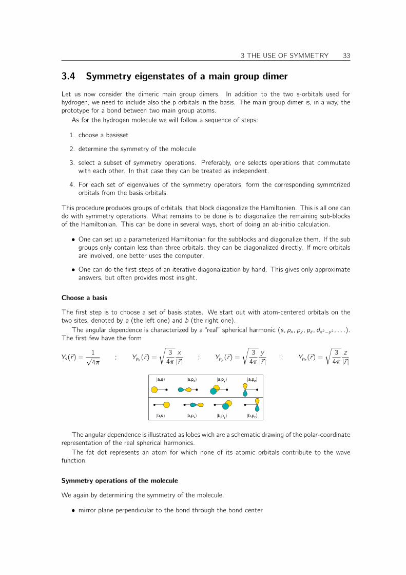
The first step is to choose a set of basis states. We start out with atom-centered orbitals on thetwo sites, denoted by a (the left one) and b (the right one).
The angular dependence is characterized by a “real” spherical harmonic (s, px , py , pz , dx2−y2 , . . .).The first few have the form
Ys(~r) =1√4π
; Ypx (~r) =
√3
4π
x
|~r | ; Ypy (~r) =
√3
4π
y
|~r | ; Ypz (~r) =
√3
4π
z
|~r |
b,px b,py b,pz
a,px a,py a,pz
b,s
a,s
The angular dependence is illustrated as lobes wich are a schematic drawing of the polar-coordinaterepresentation of the real spherical harmonics.
The fat dot represents an atom for which none of its atomic orbitals contribute to the wavefunction.
Symmetry operations of the molecule
We again by determining the symmetry of the molecule.
• mirror plane perpendicular to the bond through the bond center

34 3 THE USE OF SYMMETRY
• mirror planes with the bond in the mirror plane
• continuous rotational symmetry about the bond
• two fold rotational symmetry about any axis perpendicular to the bond, with the axis passingthrough the bond center
• point inversion about the bond center
We only need to pick out a few.2
Since we are already familiar with mirror operations, let us pick the three mirror planes.
C
B
A
One should select a subset of symmetry operations that commutate with each other. Symmetryoperations commutate, if the order, in which they are performed, does not affect result.
Example for non-commutating operations
An example for two operations that do not commutate is given in Fig. 3.2 on p. 38.
0 −1 0
1 0 0
0 0 1
︸ ︷︷ ︸
Rz (90)
1 0 0
0 0 −1
0 1 0
︸ ︷︷ ︸
Rx (90)
=
0 0 1
1 0 0
0 1 0
︸ ︷︷ ︸R(111)(90)
Rx (90)︷ ︸︸ ︷1 0 0
0 0 −1
0 1 0
Rz (90)︷ ︸︸ ︷0 −1 0
1 0 0
0 0 1
=
R(111)(90)︷ ︸︸ ︷0 −1 0
0 0 −1
1 0 0
Fig. 3.2: Demonstration of two non-commutative rotations. The result(top) of a 90 rotation about the z-axis (vertical) followed by a 90 aboutthe x-axis (horizontal, in the paperplane) differs from the result (bot-tom) obtained when the same oper-ations are performed in reversed or-der. R(111)(90) denotes a 90 rota-tion about the diagonal pointing along(1, 1, 1). R(111)(90) denotes a 90
rotation about the (1,−1, 1) axis
2The result does not become wrong, if we do not exploit all symmetries. If we miss out some, the blocks of theresulting Hamiltonian may be larger, which makes the diagonalization more cumbersome.

3 THE USE OF SYMMETRY 35
Eigenstates of the symmetry operators
Our basis orbitals are an s-orbital on each atom and three p-orbitals on each atom. We group themaccording to the eigenvalues for the three mirror planes A,B, C.
We begin by grouping them according to the eigenvalues of B and C, because the orbitals we havechosen are already eigenstates of these operations. The B+ indicates the states that are symmetricwith respect to the mirror plane B and B− indicates the states that are antisymmetric with respectto the mirror plane B. We use the analogous notation for the mirror planes A and C. On the righthand side, we list those orbitals that have the corresponding behavior with respect to the two mirrorplanes.
B+ C+
B+ C−
C+
C−
B−
B−
b,pyb,py
b,pza,pz
b,sa,s a,px a,px
Now we form the symmetrized states with respect to A using Eq. 3.10 from p. 35. Note that weneed not consider any mixing between states from sets with different symmetry eigenvalues.
|Ψα〉Eq. 3.10
=
N−1∑n=1
Sn|χ〉s−nα (3.12)
We start with |a, s〉 and form SA|a, s〉+ |b, s〉. Thus the symmetric state with respect to the mirrorplane A is 1√
2
(|a, s〉 = |b, s〉
)and the antisymmetric state is 1√
2
(|a, s〉 − |b, s〉
). Starting from
|b, s〉 gives the same states. The state |a, px 〉 transforms into SA|a, px 〉 = −|b, px 〉. Therefore thesymmetric state is 1√
2
(|a, px 〉 − |b, px 〉
)and the antisymmetric state is 1√
2
(|a, px 〉 + |b, px 〉
). Note,
that a state with a positive sign is not automatically a symmetric state. No new states are obtainedstarting from |b, px 〉.
An important cross check is to verify that the number of orbitals in each group is the same beforeand after symetrization.

36 3 THE USE OF SYMMETRY
A−
C+B−A+
B− C+
A− B−
C+B+
A+
C−
C+B+
A−
B+ C−A+
A+ B− C−
B+ C−A−
2
+ )(21
(1 − )
(21 + )
− )(21
(21 )−
(21 + )
(21 + )
(21 − )
a,s
by,pa ,p
b,pxa,px
a,py b,py
b,s
a,px b,px
a,pz b,pz
a,pz b,pz
a,s ,sb
y
Instead of solving a 8-dimensional eigenvalue problem, we only need to determine two 2-dimensionaleigenvalue problems, a tremendous simplification.
The two-dimensional problem can be estimated graphically. They correspond to the non-degenerateproblem of the two-center bond, discussed in section 2.3.
3.4.1 Approximate diagonalization
Up to now we have done all that can be done for the main-group dimer using symmetry alone. Nowwe need to diagonalize the remaining sub-blocks of the symmetry eigenstates. Here, I will show howone can get an idea of the eigenstates graphically, that is without any calculation. The results will beapproximate. Later we will see how to set up a parameterized Hamiltonian, and do the calculationfor a simple tight-binding model.
There are two problems to be solved:
• diagonalize the remaining sub-blocks containing more than one orbital
• determine the relative position of the orbitals
3.4.2 σ bonds and antibonds
The terms σ and π bond will be explained below. The σ bonds and antibonds result from the 2× 2blocks with orbitals that have cylinder symmetry.
Let us consider once the s orbitals on both atoms. As known from the section on the two-centerboind, they form a bonding and an antibonding orbital. The bonding orbital is symmetric with respectto mirror operation at the bond-center plane, and the antibonding orbital is antisymmetric. This is

3 THE USE OF SYMMETRY 37
Fig. 3.3: Schematic drawing of the hybridization of the σ states of a dimeric molecule. The verticalaxis corresponds to the energy of the orbitals
the information we know also from the symmetry consideration, but now we also know that theenergy levels are centered at the “atomic s orbital energy”.
Similarly we form the bonding and antibonding p-orbitals, that again form a symmetric (bonding)and an antisymmetric (antibonding) state.
From our symmetry considerations we know that only the bonding orbitals interact with eachother and the two antibonding orbitals interact with each other. This is indicated by the red arrowsin figure ??. Because they belong to different symmetry eigenvalues, the bonding orbitals do notinteract with the antibonding orbitals.
The hybridization of the two bonding orbitals is analogous to the two-center bond in the non-degenerate case. Note that the model of a two center bond gave us a general recipy on diagonalizing2× 2 Hamiltonians.
The two states of that model need not be orbitals on the two bonding partners as in section 2.3,but they can be any pair of orbitals that have a Hamilton matrix element between them.
The lower bonding level will have mostly s-character and it will lie even below the energy the pures-type orbital. The bonding p-orbital mixes into the s-type bond orbital so as to enhance the orbitalweight in the center of the bond, and to attenuate the wave function in the back bond. (pointingaway from the neighbor). This mixing of s and p-orbital forms so-called hybrid orbitals that willl bediscussed later.
The higher bonding orbital will lie above the p-type bonding orbital, and it will have predominantlyp-type character. However the s-type bonding orbital mixes in, but now in the opposite comparedto the bond orbital discussed above. Now the orbital in the middle of the bond is attenuated andenhanced in the back bond. This weakening of the bond explains that the p-type bond orbital shiftsup in energy.
Similarly we can analyze the interaction between the two antibonding orbitals. Only here thes-type antibond is weakened, so that it shifts towards lower energy and the p-type antibond is madestronger, shifting it further up in energy.
3.4.3 π bonds and antibonds
The 1 × 1 blocks form the π bonds and antibonds shown in Fig. ??. Using what we learned fromthe symmetric two-center bond, we know that bonding and antibonding orbitals are centered around

38 3 THE USE OF SYMMETRY
the “atomic p-level”. From the rotational symmetry of the bond, we can infer that the two bondingorbitals are degenerate and that the two antibonding orbitals are degenerate, too.
Fig. 3.4: Schematic drawing of the hybridization of the π-states of a dimeric molecule. The verticalaxis corresponds to the energy of the orbitals
Finally we can place the orbitals into one diagram shown in Fig.??. The center of the π orbitalswill lie below the two upper σ bonds, because the latter have been shifted up by the hybridizationwith the s orbitals.
The splitting between the π orbitals will be smaller than that of the σ orbitals, because the latterpoint towards each other and therefore have a larger overlap and Hamilton matrix element.
The order of the orbitals is not completely unique and,in particular, the σ-p-bond and π-bond caninterchange as one goes through a period in the periodic table.
π
σ
σ
σ
σ
π
∗
∗
∗
Fig. 3.5: Schematic energy level diagram of a main group dimer

3 THE USE OF SYMMETRY 39
3.5 Parameterized Hamiltonian of the main group dimer
In the following, I will demonstrate the the steps discussed so far for a parameterized Hamiltonian.In its symmetrized form, such a parameterized Hamiltonian allows us to diagonalize the remainingblocks of the Hamiltonian.
3.5.1 Notion of σ, π, δ-states
The states of a dimer are classified as to σ and π states. This notation is analogous to the classifi-cation of atomic orbitals according to their angular momentum as s, p, d, f -states. For systems witha single rotation axis, we classify the states according to their angular momentum about the bondaxis as σ, π, δ-states.
• A state that is rotationally symmetric is called a σ-state. A sigma state has the angularmomentum quantum number is m = 0 for rotation about the bond axis.
• A state that changes its sign twice when moving in a circle about the bond axis is a π state.A π-state has the angular momentum quantum number is m = 1 for rotation about the bondaxis.
• A state that changes its sign four times when moving in a circle about the bond axis, is aδ-state. A δ-state has the angular momentum quantum number is m = 2 for rotation aboutthe bond axis.
The notation carries a meaning beyond that of symmetry. σ bonds and anti-bonds are typicallythe strongest. The π-bonds are weaker and the δ-bonds are nearly negligible.
Antibonding orbitals are distinguished from the bond-orbitals by a star such as σ∗, pronounced“sigma-star” . The best is to inspect figure ??.
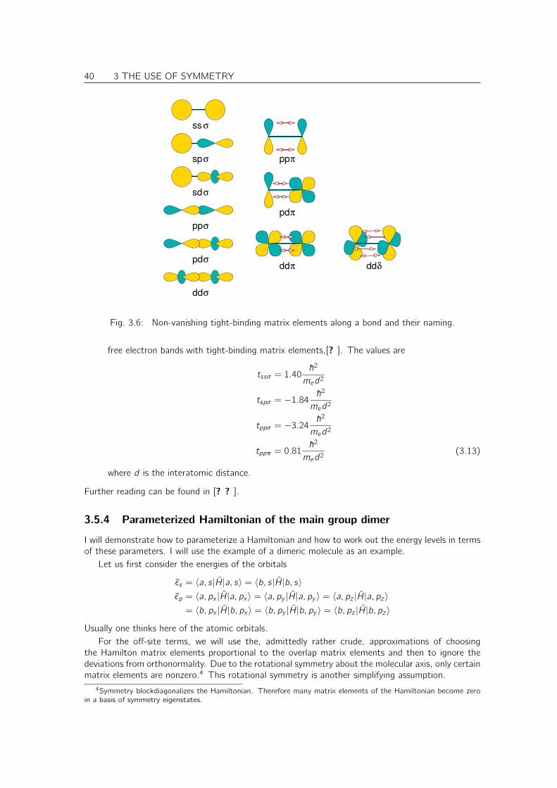
3.5.2 Slater-Koster tables
Slater and Koster[? ] have formed the basis of today’s empirical tight-binding methods3. Theyshowed that the Hamiltonian and overlap matrix can be built up easily using their Slater-Kostertables[? ], if one knows the matrix elements of Hamilton and overlap matrix for certain symmetriccombinations along a bond. These symmetric combinations are sketched in Fig. ??.
If the matrix elements are furthermore known as function of distance one can also investigate thechanges of the electronic structure, respectively estimate the forces.
3.5.3 Hopping matrix elements of Harrison
Harrison (“The physics of solid state chemistry” , Walter A. Harrison, Advances in Solid state Physics17, p135)[? ] has shown that the matrix elements can be reasonably fit by simple expressions.
• Harrison chose the orbital energies equal to the atomic energy levels obtained with the HartreeFock approximation.
• The parameters tssσ, tspσ, tppσ, tppπ for the hopping parameters can be derived by fitting the
3The kind of empirical models, where only nearest neighbor matrix elements of Hamiltonian are considered, andoverlap is set to unity is called tight binding models. However the definition is not clear cut and there are many variantsand extensions that run with the same name.
40 3 THE USE OF SYMMETRY
ddδddπ
ddσ
ss σ
spσ
sdσ
ppσ
pdσ
pdπ
ppπ
Fig. 3.6: Non-vanishing tight-binding matrix elements along a bond and their naming.
free electron bands with tight-binding matrix elements,[? ]. The values are
tssσ = 1.40~2
med2
tspσ = −1.84~2
med2
tppσ = −3.24~2
med2
tppπ = 0.81~2
med2(3.13)
where d is the interatomic distance.
Further reading can be found in [? ? ].
3.5.4 Parameterized Hamiltonian of the main group dimer
I will demonstrate how to parameterize a Hamiltonian and how to work out the energy levels in termsof these parameters. I will use the example of a dimeric molecule as an example.
Let us first consider the energies of the orbitals
εs = 〈a, s|H|a, s〉 = 〈b, s|H|b, s〉εp = 〈a, px |H|a, px 〉 = 〈a, py |H|a, py 〉 = 〈a, pz |H|a, pz 〉
= 〈b, px |H|b, px 〉 = 〈b, py |H|b, py 〉 = 〈b, pz |H|b, pz 〉
Usually one thinks here of the atomic orbitals.For the off-site terms, we will use the, admittedly rather crude, approximations of choosing
the Hamilton matrix elements proportional to the overlap matrix elements and then to ignore thedeviations from orthonormality. Due to the rotational symmetry about the molecular axis, only certainmatrix elements are nonzero.4 This rotational symmetry is another simplifying assumption.
4Symmetry blockdiagonalizes the Hamiltonian. Therefore many matrix elements of the Hamiltonian become zeroin a basis of symmetry eigenstates.
3 THE USE OF SYMMETRY 41
tssσ = 〈a, s|H|b, s〉tspσ = 〈a, s|H|b, px 〉tppσ = 〈a, px |H|b, px 〉tppπ = 〈a, py |H|b, py 〉 = 〈a, pz |H|b, pz 〉
If we describe the states as a vector with basisstates in the order (|a, s〉, |a, px 〉, |a, py 〉, |a, pz 〉,|b, s〉, |b, px 〉, |b, py 〉, |b, pz 〉), the Hamilton matrix has the form
H=
εs 0 0 0 tssσ tspσ 0 0
0 εp 0 0 −tspσ tppσ 0 0
0 0 εp 0 0 0 tppπ 0
0 0 0 εp 0 0 0 tppπ
tssσ −tspσ 0 0 εs 0 0 0
tspσ tppσ 0 0 0 εp 0 0
0 0 tppπ 0 0 0 εp 0
0 0 0 tppπ 0 0 0 εp
(3.14)
Symmetrized orbitals
We work out the Hamiltonian in the basis of eigenstates of the three symmetry planes, that we havedetermined in the beginning of section 3.4. These are
|φ1〉|φ2〉|φ3〉|φ4〉|φ5〉|φ6〉|φ7〉|φ8〉
=
1√2
(|a, s〉+ |b, s〉)1√2
(|a, px 〉 − |b, px 〉)1√2
(|a, s〉 − |b, s〉)1√2
(|a, px 〉+ |b, px 〉)1√2
(|a, pz 〉+ |b, pz 〉)1√2
(|a, pz 〉 − |b, pz 〉)1√2
(|a, py 〉+ |b, py 〉)1√2
(|a, py 〉 − |b, py 〉)
(3.15)
This can be done in two ways, which I demonstrate for one example, namely the matrix elementbetween 〈φ1| := 1√
2(〈a, s|+ 〈b, s|) and |φ2〉 := 1√
2(|a, px 〉 − |b, px 〉)
• We can represent the bra by a vector ~c1 = (1, 0, 0, 0, 1, 0, 0, 0) 1√2and the ket by the vector
~c2 = (0, 1, 0, 0, 0,−1, 0, 0) 1√2, so that
〈φ1| =
8∑i=1
〈φ1|χi 〉〈χi | =
8∑i=1
c∗i ,1〈χi |
|φ2〉 =
8∑i=1
|χi 〉〈χi |φ2〉 =
8∑i=1
|χi 〉ci ,2
Now, we multiply the Hamilton matrix from Eq. ??, which has elements 〈χi |H|χj〉, with ~c∗1from the left and with ~c2 from the right, which yields
〈φ1|H|φ2〉 =1
2(−tspσ − tspσ) = −tspσ

42 3 THE USE OF SYMMETRY
• As an alternative we can also directly decompose the matrix elements of the symmetrized statesinto those of the original (not symmetrized) basis orbitals.[
1√2
(〈a, s|+ 〈b, s|)]H
[1√2
(|a, px 〉 − |b, px 〉)]
=1
2
〈a, s|H|a, px 〉︸ ︷︷ ︸0
−〈a, s|H|b, px 〉︸ ︷︷ ︸tspσ
+ 〈b, s|H|a, px 〉︸ ︷︷ ︸−tspσ
−〈b, s |H|b, px 〉︸ ︷︷ ︸0
= −tspσ
In the basis of symmetry eigenstates from Eq. ??, the Hamiltonian obtains its block-diagonal formwith two 2× 2 blocks and and six eigenstates. The elements of this Hamilton matrix are 〈φi |H|φj〉.
H=
εs + tssσ −tspσ 0 0 0 0 0 0
−tspσ εp + tppσ 0 0 0 0 0 0
0 0 εs − tssσ tspσ 0 0 0 0
0 0 tspσ εp − tppσ 0 0 0 0
0 0 0 0 εp + tppπ 0 0 0
0 0 0 0 0 εp − tppπ 0 0
0 0 0 0 0 0 εp + tppπ 0
0 0 0 0 0 0 0 εp − tppπ
Note that the Hamilton matrix here differs from the one given previously, because its is representedin a different basis, namely the symmetrized orbitals |φj 〉 as opposed to the original basis states |χα〉.The basis set plays the role of a coordinate system in Hilbert space. Like the components of a vector,also the matrix elements of a tensor depend on the choice of the coordinate system.
3.5.5 Diagonalize the sub-blocks
The subblocks can be diagonalized. We use the approximate expression Eq. 2.19 for the non-degeratetwo-center bond with |t| < |ε1 − ε2|. The modifications of the orbitals are demonstrated in Fig. ??on p. ??.
• For the first block containing the ssσ and ppσ bonding orbitals we obtain the energies
ε− ≈ εs + tssσ −|tspσ|2
εp − εs + tppσ − tssσ
ε+ ≈ εp + tppσ +|tspσ|2
εp − εs + tppσ − tssσ
– The lower of the two states will have a character of a ssσ bond, however with a contri-bution from the ppσ bond mixed in such that the electrons are further localized in thebond.
– The higher lying state will have a character of a ppσ bond, bit now the ssσ orbital ismixed in such that the electron density in the bond is depleted.
• For the second block containing the ssσ and ppσ antibonding orbitals we obtain the energies
ε− ≈ εs − tssσ −|tspσ|2
εp − εs + tppσ − tssσ
ε+ ≈ εp − tppσ +|tspσ|2
εp − εs + tppσ − tssσ

3 THE USE OF SYMMETRY 43
– The lower of the two states will have a character of a ssσ antibond, however with acontribution from the ppσ antibond mixed in such that the electrons are less localized inthe bond. The state becomes less antibonding, which lowers its energy.
– The higher lying state will have a character of a ppσ antibond, bit the ssσ orbital ismixed in such that the electron density in the bond is enhanced, making the state moreantibonding, which shifts it up in energy.
The π type orbitals are already eigenstates, namely the bonding and antibonding states shown inFig. ??.
3.6 Stability of main group dimers
From the qualitative arguments we would not be able to say if the σ-state in the middle is below orabove the π states. From the node counting, we would expect the σ-state to lie above the pi states,because the latter have only one node plane, while the σ state has two. I believe that the reason isthat a small perturbation such as an electric field perpendicular to the bond axis would deform theorbitals such that the two node planes would join and form one connected node plane.
The little diagram tells us already a lot about stability.
1. for alkali metal dimers such as Li2, Na2 etc. we expect a reasonably strong bond. The bondingis analogous to that in the hydrogen molecule.
2. On the other hand we expect Be2 Mg2 to be marginally stable, because there is one σ-bondand one σ∗-anti-bond, which largely cancel their effect. There will be some bonding though,because the σ-p orbitals mix into the lowest two states and thus stabilize them.
3. For the dimers B2, Al2, there will again be a net σ bond. Thus we expect its bonds to be clearlystronger than that of the dimers of the di-valent atoms.
4. Then we arrive at C2 and Si2 where the four lowest orbitals are occupied. Since we have twopartially occupied degenerate orbitals, we need to be careful about spin-polarization. C2 is adifficult molecule, because the ordering of π bonds and σ bond depends on the distance. Whenthe σ bond is occupied, the system will have a net magnetic moment, because the two electronscan align their spins according to Hund’s rule. When the σ orbital is unoccupied, the systemwill have a π double bond.
5. Now we come to the most stable ions such as N2. Dinitrogen actually forms a triple bond. Itconsists of the two degenerate bonding π orbitals one one net σ bond. Dinitrogen is so non-reactive that it is often used to package food to avoid oxidation. Even though the atmosphereconsists of 70% of nitrogen molecules, we need to supply nitrogen compounds in the form offertilizer, to allow the excessive plant growth required for agriculture. Only some bacteria areable to transform dinitrogen to a form that can be metabolized.
6. Now we come to the chalcogenides5 such as O2 and S2. Oxygen has two electrons in the π∗
orbitals. Thus its net bonding corresponds to a double bond. However, it is stabilized by Hund’srule. The two electrons in the π∗ states are spin paired. Thus O2 has a net magnetic momentand a triplet spin splitting.That is if we apply a magnetic field, we will see three absorptionlines.
7. The halogen dimers are again only weakly bond. They have a net σ bond, but all the gain fromπ bonding is compensated by the π∗ anti-bonds.
8. The Nobel gases do not bind, because all bonding orbitals are compensated with anti-bondingorbitals.
5chalcogenide is spelled with a hard “ch” such as in “chemistry”. Chalcogenides are oxides, sulfides, selenides,tellurides, that is compounds of the oxygen group. Oxides alone are not named chalcogenides unless grouped togetherwith one of the heavier elements.

44 3 THE USE OF SYMMETRY
3.7 Bond types
• σ-bond. The wave function of a sigma bond is approximately axially symmetric. An example isthe bond in the H2 molecule.
• π-bond. A π bond has a node plane parallel to the bond axis. An example are two p orbitalswhich stand perpendicular to the bond axis. It is weaker than a σ bond because the orbitalsdo not point towards each other resulting in smaller matrix elements. An example is the planarmolecule ethene (C2H2), where two p-orbitals on the carbon atom combine in a π bond inaddition to the σ-bond
• Double bond is typically a π bond combined with a σ bond. The example is again ethene.
• A triple bond is two π-bonds combined with a single bond. An example is N2.
• Three-center bond involves three orbitals in a row. A simple example is the hypothetical linearH3 molecule. It forms a fully bonding orbital, a non-bonding orbital, to which the center atomdoes not contribute, and a fully anti-bonding orbital. The three center bond plays a role forfive-valent atoms such as P . Such atoms form trigonal bi-pyramids. There are three equatorialsp2 orbitals and a three-center bond along the z-axis.
• The best example for an aromatic bond is benzene (germ.:Benzol nicht Benzin!). It has theformula unit C6H6. The carbon form a six-fold ring. After we formed the sigma bonds thereare six electrons available to form three double bonds. There are however not three doublebonds and three single bonds but all the bond lengths are symmetric.
The wave function is best constructed from symmetry arguments
|Ψn〉 =∑j
|χj 〉e−2πi nj6
√1
6
where the χi are the pz orbitals on the individual carbon atoms. The Hamilton matrix has theform Hi ,i = ε and Hi ,i+1 = Hi−1,i = −t.
The energies are εn = ε+ t(e2πin/6 + e−2πin/6) = εn = ε−2t cos 2πn/6. Thus there is the fullysymmetric ground state at ε − 2t. Then there are two degenerate occupied states at ε − t,two degenerate unoccupied states at ε+ t and a fully anti-bonding state at ε+ t
3.8 Worked example: orbitals of the ethene
The molecule ethene, also called ethylene, has the formula unit C2H4 and forms a planar structure,where each carbon atom has two bonds to hydrogen and one to the other carbon atom with a bondangle of approximately 120.
Select Basisset
First we decide which orbitals we wish to include in the basis. We use the relevant orbitals, whichare the four hydrogen s-orbitals, and the s- and p-orbitals on carbon. That is we work with twelvebasis functions.

3 THE USE OF SYMMETRY 45
Determine symmetry operations
AB
C
H
HH
H
C C
We begin determining the symmetry operators of methane.
• A mirror plane in the molecular plane. (C)
• A mirror plane perpendicular to the C-C bond (A)
• a mirror plane containing the bond but perpendicular to the molecular plane (B)
• a two fold rotation about the bond axis
Determine symmetrized orbitals
• We start with the symmetry plane (A), perpendicular to the bond and determine the symmetricand antisymmetric orbitals.
A+
A−
A+B+
A+B−
A−B−
A−B+
46 3 THE USE OF SYMMETRY
A+B+C+
A+B+C−
A+B−C+
A−B+C+
A−B−C+
A−B−C−
Form bond orbitals
We ended up with two 1 × 1 blocks, two 2 × 2 blocks and two 3 × 3 blocks of the Hamiltonian.Because the 3× 3 blocks are difficult to handle, we form bonding and antibonding orbitals betweenthe hydrogen orbitals and the carbon-p-orbitals, which are energetically in a similar position.
A+B+C+
A+B+C−
A+B−C+
A−B+C+
A−B−C+
A−B−C−
Now we can align the orbitals on an energy axis. Without a proper diagonalization this step canbe nothing more than an educated guess. However it usually is sufficient to determine which orbitalsare occupied and which are empty. Furthermore we can usually guess, which are the highest occupiedand the lowest unoccupied orbitals, which is important for chemical considerations. We order theorbitals according to the bonding character. We place the s-orbitals on carbon lowest. Then we place
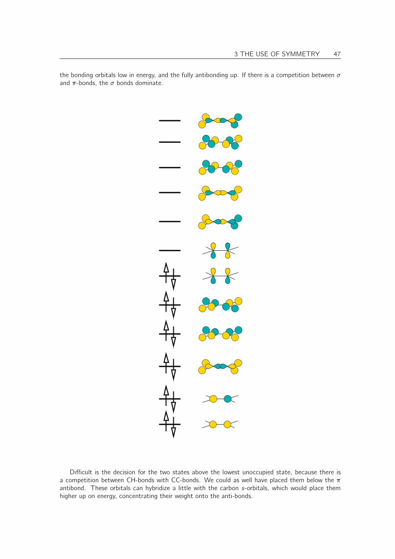
3 THE USE OF SYMMETRY 47
the bonding orbitals low in energy, and the fully antibonding up. If there is a competition between σand π-bonds, the σ bonds dominate.
Difficult is the decision for the two states above the lowest unoccupied state, because there isa competition between CH-bonds with CC-bonds. We could as well have placed them below the πantibond. These orbitals can hybridize a little with the carbon s-orbitals, which would place themhigher up on energy, concentrating their weight onto the anti-bonds.
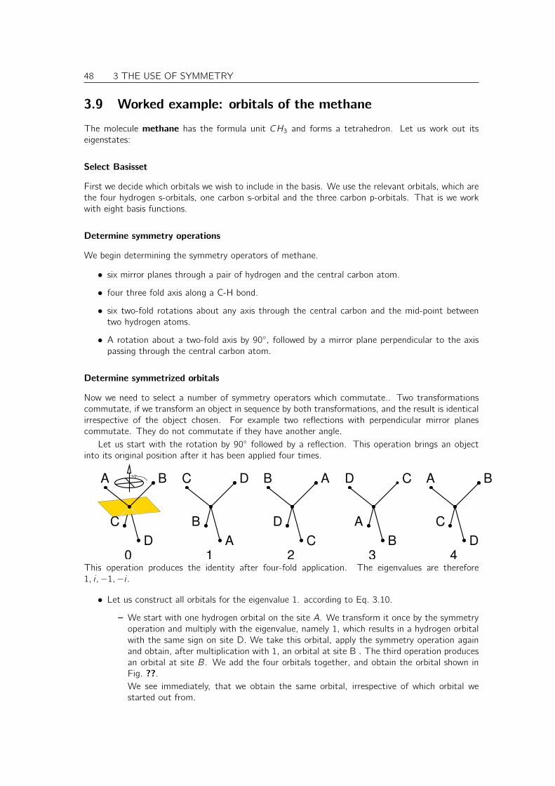
48 3 THE USE OF SYMMETRY
3.9 Worked example: orbitals of the methane
The molecule methane has the formula unit CH3 and forms a tetrahedron. Let us work out itseigenstates:
Select Basisset
First we decide which orbitals we wish to include in the basis. We use the relevant orbitals, which arethe four hydrogen s-orbitals, one carbon s-orbital and the three carbon p-orbitals. That is we workwith eight basis functions.
Determine symmetry operations
We begin determining the symmetry operators of methane.
• six mirror planes through a pair of hydrogen and the central carbon atom.
• four three fold axis along a C-H bond.
• six two-fold rotations about any axis through the central carbon and the mid-point betweentwo hydrogen atoms.
• A rotation about a two-fold axis by 90, followed by a mirror plane perpendicular to the axispassing through the central carbon atom.
Determine symmetrized orbitals
Now we need to select a number of symmetry operators which commutate.. Two transformationscommutate, if we transform an object in sequence by both transformations, and the result is identicalirrespective of the object chosen. For example two reflections with perpendicular mirror planescommutate. They do not commutate if they have another angle.
Let us start with the rotation by 90 followed by a reflection. This operation brings an objectinto its original position after it has been applied four times.
C
0 1 2 3 4
A B
D
CB
A
DC
D
C
B A CD
B
A
A B
D
This operation produces the identity after four-fold application. The eigenvalues are therefore1, i ,−1,−i .
• Let us construct all orbitals for the eigenvalue 1. according to Eq. 3.10.
– We start with one hydrogen orbital on the site A. We transform it once by the symmetryoperation and multiply with the eigenvalue, namely 1, which results in a hydrogen orbitalwith the same sign on site D. We take this orbital, apply the symmetry operation againand obtain, after multiplication with 1, an orbital at site B . The third operation producesan orbital at site B. We add the four orbitals together, and obtain the orbital shown inFig. ??.We see immediately, that we obtain the same orbital, irrespective of which orbital westarted out from.

3 THE USE OF SYMMETRY 49
– Now we proceed with the s-orbital on the carbon atom. This orbital falls on itself aftereach transformation. Since its copies are multiplied with 1, the orbital remains unchanged.
– Next we proceed to the p-orbitals. Because the pz orbital changes its sign after eachtransformation, its copies add to zero. The px and py orbitals change their sign afterevery two operations and therefore also cancel out.
In total we obtain exactly two symmetrized orbital with eigenvalue 1 of the symmetry operation.
• We proceed to eigenvalue −1.
– We begin again with a hydrogen orbital. After each transformation we need to multiplythe orbital with −1. Thus the orbital enters with a positive sign on sites A and B andwith negative sign on sites C and D. After adding up we obtain the symmetrized orbitalshown in Fig. ?? in the box with eigenvalue −1.
– the carbon s orbital does not produce a symmetrized orbital in this class, because its copyadd up to zero after multiplication with the factors 1 and −1.
– The pz orbital is a symmetry orbital in this class, because the symmetry operation simplyreverts its sign. After multiplication with the eigenvalue, namely −1, we obtain the originalorbital.
– the px and py orbitals are rotated by 90 in each operation. That is, after two operations,they revert their sign. After two operations we need to multiply with the square of theeigenvalue. Thus the copies of the orbitals cancel each other, and do not contribute tothis symmetry class.
Also in this class we obtain exactly two orbitals.
• Now we proceed to the complex valued eigenvalue i .
– We start with an s orbital and obtain two real-valued orbitals with opposite sign on theupper two atoms, and two imaginary-valued orbitals with opposite sign on the lower twohydrogen atoms. Thus the symmetrized orbital is complex valued.
– the s-orbital on carbon cancels out, because it falls on itself unter the operation andi + i2 + i3 + i4 = i − 1− i + 1 = 0.
– Also the pz orbital cancels out, because it changes it sign and i − i2 + i3 − i4 = 0.
– the px and py orbitals are transformed into each other by the symmetry operation. Frompx we obtain a symmetrized orbital 1√
2(|px 〉+ i |py 〉). The py orbital produces the same
symmetrized orbital with an additional factor i . Note, that this orbital is en eigenstate toLz with eigenvalue m = 1.
• for the eigenvalue −i , we obtain the same symmetrized orbitals as for the eigenvalue i , onlythat the orbitals are complex conjugate.
Thus we have divided the 8× 8 Hamiltonian in four 2× 2 blocks.
Form bond and antibonding orbitals
Next we diagonalize the 2× 2 blocks of the Hamiltonian expressed by symmetrized orbitals and thusobtain bonding and antibonding orbitals.
In order to align the orbitals on an energy axis we need to know the energies and hopping matrixelements. Because the carbon s-orbital lies energetically below the carbon p-orbital, we can concludethat the average value of the bonding and antibonding orbitals that contain the carbon s-orbital liesbelow that of the p-orbitals. Furthermore we recognize that the type and number of interactionsfor all bonding orbitals containing the carbon p-orbital is the same. Thus we conclude that they aredegenerate. The same holds true for the corresponding antibonding orbitals. This leads us to theschematic assignment of the electron states of methane shown in Fig. ??.
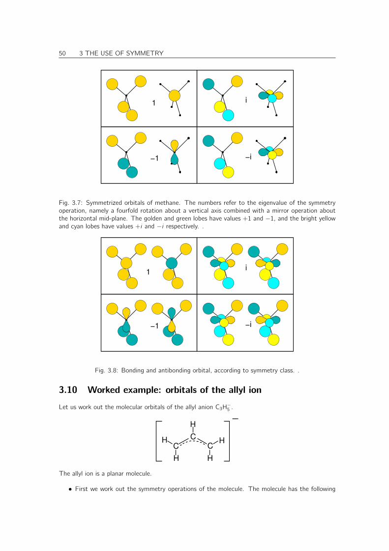
50 3 THE USE OF SYMMETRY
i1
−1 −i
Fig. 3.7: Symmetrized orbitals of methane. The numbers refer to the eigenvalue of the symmetryoperation, namely a fourfold rotation about a vertical axis combined with a mirror operation aboutthe horizontal mid-plane. The golden and green lobes have values +1 and −1, and the bright yellowand cyan lobes have values +i and −i respectively. .
−1
i1
−i
Fig. 3.8: Bonding and antibonding orbital, according to symmetry class. .
3.10 Worked example: orbitals of the allyl ion
Let us work out the molecular orbitals of the allyl anion C3H−5 .
C C
CH
HH
H
H
The allyl ion is a planar molecule.
• First we work out the symmetry operations of the molecule. The molecule has the following

3 THE USE OF SYMMETRY 51
Fig. 3.9: Symmetry eigenstates and energy level ordering of methane. The blue and bright-yellowlobes correspond to the imaginary part of the wave function. The imaginary part can be avoided bya suitable superposition of the two wave functions that are complex conjugate of each other. Whilethe resulting states are still eigenstates of the Hamilton operator, they are no more eigenstates ofthe symmetry operators. .
symmetry operations.
– a mirror plane in the plane of the molecule
– a mirror plane perpendicular to the molecular plane, containing the central C-H bond.
– a two-fold rotation about an axis through the central C-H bond.
• Now we work out the symmetrized orbitals. We start with every “atomic” orbital and constructthe symmetrized orbital according to Eq. 3.10 by adding the orbitals obtained from the firstby applying the symmetry operation repeatedly and multiplication with the eigenvalue of thesymmetry operation to the corresponding power.
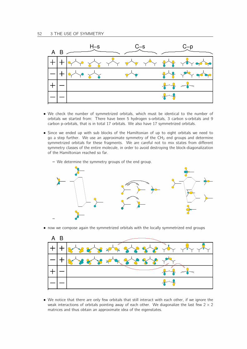
52 3 THE USE OF SYMMETRY
A BH−s C−s C−p
• We check the number of symmetrized orbitals, which must be identical to the number oforbitals we started from: There have been 5 hydrogen s-orbitals, 3 carbon s-orbitals and 9carbon p-orbitals, that is in total 17 orbitals. We also have 17 symmetrized orbitals.
• Since we ended up with sub blocks of the Hamiltonian of up to eight orbitals we need togo a step further. We use an approximate symmetry of the CH2 end groups and determinesymmetrized orbitals for these fragments. We are careful not to mix states from differentsymmetry classes of the entire molecule, in order to avoid destroying the block-diagonalizationof the Hamiltonian reached so far.
– We determine the symmetry groups of the end group.
–
• now we compose again the symmetrized orbitals with the locally symmetrized end groups
A B
• We notice that there are only few orbitals that still interact with each other, if we ignore theweak interactions of orbitals pointing away of each other. We diagonalize the last few 2 × 2matrices and thus obtain an approximate idea of the eigenstates.

3 THE USE OF SYMMETRY 53
A B
• We divide the orbitals into bonding and antibonding orbitals. This is not necessarily as straight-forward as in this case. Then we count the number of valence electrons, which is 18, resultingin 9 filled orbitals.We fill up the bonding orbitals first, proceeding to the non-bonding orbitals.We find that the non-bonding π orbital is the highest occupied orbital.
A B
The wave functions calculated from first principles are shown below in figure ??. We recognizegood agreement for some of the wave functions and poor agreement for others. We have been ableto identify the highest occupied orbital. We also recognize that the main character of the states issimilar in our estimated orbitals and the ab-initio wave functions.
The main error is that states lying in a similar energy region are hybridized incorrectly: That isa superposition of those states from our estimate would allow us to construct the true eigenstates.The limitations of the above procedure are not untypical. Like in this case, however, they usually donot strongly affect stability considerations. The reason behind this is that a unitary transformation ofcompletely filled or of completely empty states does not affect the energy. If the intermixing betweenfilled and occupied orbitals would be equally undetermined, the results would not be reliable, and oneshould resort to ab-initio calculations.
3.11 Worked example: orbitals of closo-B6H2−6
Boron can form B2−6 octahedra, which can arrange to crystals in a simple cubic lattice to form
hexaborides. In the form of B6H2−6 the boron cluster exists as anion in salts.
The discussion of bonding starts from tangential and radial orbitals. The radial orbitals are the sp-hybrids6 pointing inward and outward of the cage. The tangential orbitals are p-orbitals perpendicularto the direction to the cage-center.
The symmetry -adapted orbitals of the hexaboride cage are shown in figure ??. The symmetryoperations considered are the mirror reflections on the three planes, which cut through the centerand four opposite corners of the octahedron.
6Hybrid orbitals are discussed in te next chapter.
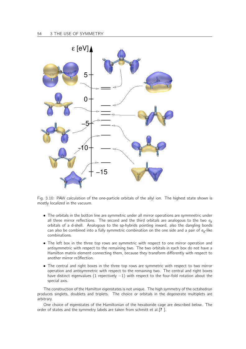
54 3 THE USE OF SYMMETRY
[eV]ε
−15
−10
−5
5
0
Fig. 3.10: PAW calculation of the one-particle orbitals of the allyl ion. The highest state shown ismostly localized in the vacuum.
• The orbitals in the botton line are symmetric under all mirror operations are symmnetric underall three mirror reflections. The second and the third orbitals are analogous to the two egorbitals of a d-shell. Analogous to the sp-hybrids pointing inward, also the dangling bondscan also be combined into a fully symmetric combination on the one side and a pair of eg-likecombinations.
• The left box in the three top rows are symmetric with respect to one mirror operation andantisymmetric with respect to the remaining two. The two orbitals in each box do not have aHamilton matrix element connecting them, because they transform differently with respect toanother mirror re3flection.
• The central and right boxes in the three top rows are symmetric with respect to two mirroroperation and antisymmetric with respect to the remaining two. The central and right boxeshave distinct eigenvalues (1 repectively −1) with respect to the four-fold rotation about thespecial axis.
The construction of the Hamilton eigenstates is not unique. The high symmetry of the octahedronproduces singlets, doublets and triplets. The choice or orbitals in the degenerate multiplets arearbitrary.
One choice of eigenstates of the Hamiltonian of the hexaboride cage are described below. Theorder of states and the symmetry labels are taken from schmitt et al.[? ].
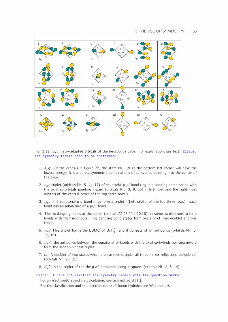
3 THE USE OF SYMMETRY 55
24
a1geg
eg
t2g
t2g
t2g
t1u tt1u
t1u
t1ut1u
t1u
1 2 3 4 5 6
7 8 9 10 11 12
14 15 16 17 18
19 20 21 22 23
Fig. 3.11: Symmetry-adapted orbitals of the hexaboride cage. For explanation, see text. Editor:The symmetry labels need to be confirmed.
1. a1g: Of the orbitals in figure ??, the state Nr. 19 at the bottom left corner will have thelowest energy. It is a purely symmetric combinations of sp-hybrids pointing into the center ofthe cage.
2. t1u: triplet (orbitals Nr. 5, 11, 17) of equatorial p-pi-bond-ring in a bonding combination withthe axial sp-orbitals pointing inward (orbitals Nr. 3, 9, 15). (left-most and the right-mostorbitals of the central boxes of the top three rows.)
3. t2g: The equatorial p-σ-bond-rings form a triplet. (Left orbital of the top three rows). Eachbond has an admixture of a p-pi bond.
4. The six dangling bonds at the corner (orbitals 22,23,24,4,10,16) consume six electrons to formbonds with their neighbors. The dangling bond states form one singlet, one doublet and onetriplet.
5. t2u? This triplet forms the LUMO of B6H2−6 and it consists of π∗ antibonds (orbitals Nr. 6,
12, 18).
6. t1g?: the antibonds between the equatorial pi-bonds with the axial sp-hybrids pointing inwardform the second-highest triplet.
7. eg: A doublet of two states which are symmetric under all three mirror reflections considered.(orbitals Nr. 20, 21).
8. t ′1u?: is the triplet of the the p-σ∗ antibonds along a square. (orbitals Nr. 2, 8, 14).
Editor: I have not verified the symmetry labels with the question marks.For an electroni9c structure calculation, see Schmitt et al.[? ].For the classification and the electron count of boron hydrides see Wade’s rules.

56 3 THE USE OF SYMMETRY
3.12 Exercise: sketch orbitals
• sketch wave functions and energy level diagram for a water molecule. The water molecule H2Ohas a bond angle of about 104. The hydrogen orbitals are located slightly above the oxygenp orbitals.
• The cyclopentadienyl ion has the formula [C5H5]−. It is a five-membered ring. Work out firstthe orbitals for one bead and use then the knowledge about eigenstates for ring systems.
• sketch the wave functions of ethene (ethylene) C2H4.
Chapter 4
Hybrid orbitals
Sofar we have used only two orbitals at a time that form a bond. In molecules there are many moreelectrons. In order to arrive even approximately at a description of a bond by two orbitals, we needto design so-called hybrid orbitals. Hybrid orbitals are constructed from atomic orbitals in such a waythat they point optimally towards the neighbors.1
4.1 Spherical and cubic harmonics
The spherical symmetry of the atom implies conservation of the angular momentum. Thus it is nosurprise that the eigenstates of the angular momentum are important to describe the atomic wavefunctions.
The eigenstates of the angular momentum are the spherical harmonics. Because the differentcomponents of the angular momentum operator ~L = ~r × ~p do not commutate, the two relevanteigenvalue equations are those for the total angular momentum or better for ~L2 and one componentthat usually is chosen as the z-component Lz .
The eigenvalue equations for the spherical harmonics are
~L2|Y`,m〉 = |Y`,m〉~2`(`+ 1) with ` = 0, 1, 2, . . .
Lz |Y`,m〉 = |Y`,m〉~m with m = −`,−`+ 1, . . . , `− 1, `
` is called the angular-momentum quantum number. The atomic orbitals are usually referred toas s, p, d, f -orbitals, if they have the angular momentum quantum number ` = 0, 1, 2, 3, respectively.m is themagnetic quantum number , because the m-degeneracy can be lifted by applying a magneticfield.
Spherical harmonics Y`,m(~r) only depend on the direction of ~r and are independent of the radius|~r |. This is the reason for expressing them in polar coordinates as function of the angular coordinatesθ and φ.
The definition of spherical harmonics is not unique. They differ in the so-called Condon-Shortleyphase (−1)m and the definition of the normalization.
We use the normalization
1
r2c
∮|~r |=rcdA Y ∗`,m(~r)Y`′,m′(~r) = δ`,`′δm,m′ (4.1)
1Here we consider only hybrid orbitals for s- and p orbitals. There are similar constructions including d-orbitals. Thelatter are less useful, since the d-like valence electrons behave so different from the s- and p orbitals, that combiningthem into hybrids is rarely useful.
57
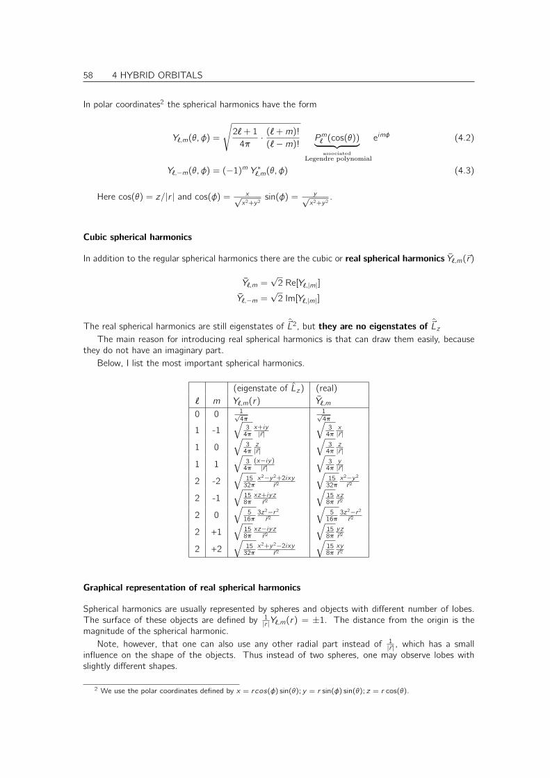
58 4 HYBRID ORBITALS
In polar coordinates2 the spherical harmonics have the form
Y`,m(θ, φ) =
√2`+ 1
4π·
(`+m)!
(`−m)!Pm` (cos(θ))︸ ︷︷ ︸
associatedLegendre polynomial
eimφ (4.2)
Y`,−m(θ, φ) = (−1)m Y ∗`,m(θ, φ) (4.3)
Here cos(θ) = z/|r | and cos(φ) = x√x2+y2
sin(φ) = y√x2+y2
.
Cubic spherical harmonics
In addition to the regular spherical harmonics there are the cubic or real spherical harmonics Y`,m(~r)
Y`,m =√
2 Re[Y`,|m|]
Y`,−m =√
2 Im[Y`,|m|]
The real spherical harmonics are still eigenstates of ~L2, but they are no eigenstates of ~LzThe main reason for introducing real spherical harmonics is that can draw them easily, because
they do not have an imaginary part.Below, I list the most important spherical harmonics.
(eigenstate of Lz) (real)` m Y`,m(r) Y`,m
0 0 1√4π
1√4π
1 -1√
34π
x+iy|~r |
√3
4πx|~r |
1 0√
34π
z|~r |
√3
4πz|~r |
1 1√
34π
(x−iy)|~r |
√3
4πy|~r |
2 -2√
1532π
x2−y2+2ixy~r2
√15
32πx2−y2
~r2
2 -1√
158π
xz+iyz~r2
√158π
xz~r2
2 0√
516π
3z2−r2
~r2
√5
16π3z2−r2
~r2
2 +1√
158π
xz−iyz~r2
√158π
yz~r2
2 +2√
1532π
x2+y2−2ixy~r2
√158π
xy~r2
Graphical representation of real spherical harmonics
Spherical harmonics are usually represented by spheres and objects with different number of lobes.The surface of these objects are defined by 1
|r |Y`,m(r) = ±1. The distance from the origin is themagnitude of the spherical harmonic.
Note, however, that one can also use any other radial part instead of 1|~r | , which has a small
influence on the shape of the objects. Thus instead of two spheres, one may observe lobes withslightly different shapes.
2 We use the polar coordinates defined by x = rcos(φ) sin(θ); y = r sin(φ) sin(θ); z = r cos(θ).

4 HYBRID ORBITALS 59
spx py pz
dxy dxz dyzdx2y2 dz2
Fig. 4.1: Real spherical harmonics: the representation is a surface defined by | 1|r | Y`,m(~r)| = 1. For a
given direction, the distance of the surface from the origin is the absolute value of the cubic sphericalharmonics. The different values of grey reflect to the signs of the function.
|Y l,m( )
|ϕ
ϕ
x
y
Fig. 4.2: Construction of the graph of a real spherical harmonics (cos(ϕ)) in polar coordinates . Notethat real and imaginary part need to be represented individually.
4.2 Rotation of p-orbitals
If we superimpose different p-orbitals we obtain other p-orbitals. A p-orbital has the form
χpx (~r) = Rp(|~r |)√
3
4π
x
|~r |
χpy (~r) = Rp(|~r |)√
3
4π
y
|~r |
χpy (~r) = Rp(|~r |)√
3
4π
z
|~r |
where Rp(r) is the radial part of the orbital and Ypx , Ypy and Ypz are the real spherical harmonics for` = 1.

60 4 HYBRID ORBITALS
Thus if we wish to construct a p orbital that looks into the direction ~e, where ~e is any normalizedvector, we simply need to superimpose the three p-orbitals according to
P-ORBITAL WITH SPECIFIED ORIENTATION
For a normalized direction vector ~e, a p−type orbital pointing in the direction of ~e is obtained bysuperposing the px , py , pz orbtials as follows:
χp,~e(~r) =
3∑i=1
eiχp,i(~r) = Rp(|~r |)√
3
4π
~e~r
|~r |
|p~e〉 = |px 〉ex + |py 〉ey + |pz 〉ez (4.4)
where R(r) is the radial part of the orbial χ(r).
*1
2*1
2+ =
Fig. 4.3: Schematic representation of mixing p-orbitals among each other. The result is a rotatedp-orbital
Thus, the shape of p orbitals does not change if we superimpose them, but only their direction.
4.3 Superposition of s- and p-orbitals: Hybrid orbitals
Similarly to the superposition of p-orbitals, we may investigate superpositions of s and p-orbitals.
χspx ,φ(~r) = χs(~r) cos(φ) + χpx (~r) sin(φ)
The angle φ is not an angle in the common sense: I have chosen the factors cos(φ) and sin(φ) onlyto ensure that the resulting orbital is again normalized.3
The resulting orbital has the form
χspx ,φ(~r) = Rs(|~r |)√
1
4πcos(φ) + Rp(|~r |)
√3
4π
x
|~r | cos(φ)
As we increase φ from zero to 90 the s-orbital is converted into a p-orbital.
Fig. 4.4: Schematic representation of mixing s and p-orbitals. The series begins on the left with apure s-orbital. As we proceed towards the right, an increasing amount of p-character is included, untilone arrives at a pure p-orbital on the very right. The orbitals between the extremes are s-p hybrids.
The concept of hybrid functionals is very useful for hybrid orbitals between s− and p−orbitals,because their wave functions have a very similar radial dependence. Often the concept is extended
3Normalization of the new orbital follows from sin2(φ) + cos2(φ) = 1 and the orthogonality of the s- and p-orbitals.
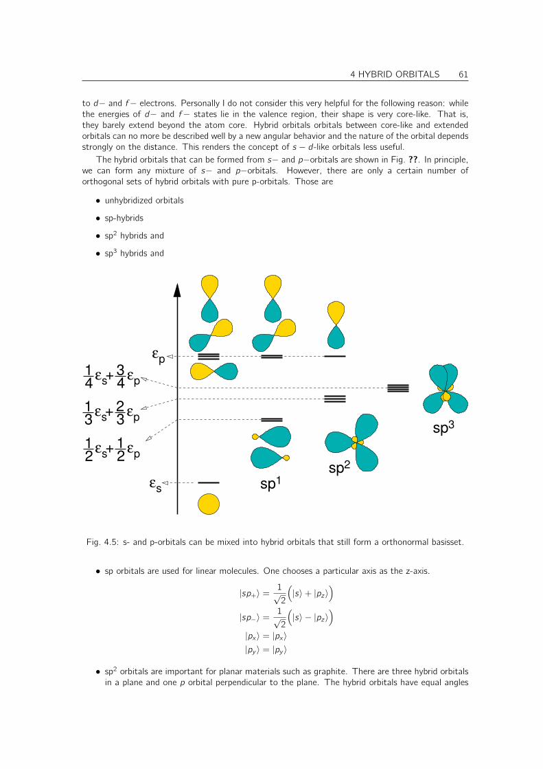
4 HYBRID ORBITALS 61
to d− and f− electrons. Personally I do not consider this very helpful for the following reason: whilethe energies of d− and f− states lie in the valence region, their shape is very core-like. That is,they barely extend beyond the atom core. Hybrid orbitals orbitals between core-like and extendedorbitals can no more be described well by a new angular behavior and the nature of the orbital dependsstrongly on the distance. This renders the concept of s − d-like orbitals less useful.
The hybrid orbitals that can be formed from s− and p−orbitals are shown in Fig. ??. In principle,we can form any mixture of s− and p−orbitals. However, there are only a certain number oforthogonal sets of hybrid orbitals with pure p-orbitals. Those are
• unhybridized orbitals
• sp-hybrids
• sp2 hybrids and
• sp3 hybrids and
εs
εp
12
εs12
εp+
εs εp+13
23
εs εp+14
34
sp1
sp3
sp2
Fig. 4.5: s- and p-orbitals can be mixed into hybrid orbitals that still form a orthonormal basisset.
• sp orbitals are used for linear molecules. One chooses a particular axis as the z-axis.
|sp+〉 =1√2
(|s〉+ |pz 〉
)|sp−〉 =
1√2
(|s〉 − |pz 〉
)|px 〉 = |px 〉|py 〉 = |py 〉
• sp2 orbitals are important for planar materials such as graphite. There are three hybrid orbitalsin a plane and one p orbital perpendicular to the plane. The hybrid orbitals have equal angles

62 4 HYBRID ORBITALS
(120o) among each other and have the same Hamilton matrix element ε = 13εs + 2
3εp.
|sp21〉 = |s〉
√1
3+ |px 〉
√2
3
|sp22〉 = |s〉
√1
3− |px 〉
√1
6+ |py 〉
√1
2
|sp23〉 = |s〉
√1
3− |px 〉
√1
6− |py 〉
√1
2
|pz 〉 = |pz 〉
• sp3 orbitals are the structural motif of most organic materials and of solids such as diamond.There are four hybrid orbitals pointing into the corners of a tetrahedron. All have the sameHamilton matrix element ε = 1
4εs + 34εp.
|sp31〉 =
1
2
(|s〉+ |px 〉+ |py 〉+ |px 〉
)|sp3
2〉 =1
2
(|s〉 − |px 〉 − |py 〉+ |px 〉
)|sp3
3〉 =1
2
(|s〉+ |px 〉 − |py 〉 − |px 〉
)|sp3
4〉 =1
2
(|s〉 − |px 〉+ |py 〉 − |px 〉
)It may be of interest to compare the hybrid orbitals if they point into the same direction.
|s〉 = |s〉1√1
+ |pz 〉√
0
1= |s〉 cos(0) + |pz 〉 sin(0)
|sp1〉 = |s〉1√2
+ |pz 〉√
1
2= |s〉 cos(45) + |pz 〉 sin(45)
|sp2〉 = |s〉1√3
+ |pz 〉√
2
3= |s〉 cos(54.73) + |pz 〉 sin(54.73)
|sp3〉 = |s〉1√4
+ |pz 〉√
3
4= |s〉 cos(60) + |pz 〉 sin(60)
|pz 〉 = |s〉1
∞ + |pz 〉√∞− 1
∞ = |s〉 cos(90) + |pz 〉 sin(90)
HYBRID ORBITALS BETWEEN S AND P STATES
Thus the building principle is
|spn〉 = |s〉1√n + 1
+ |pz 〉√
n
n + 1(4.5)
so that a pure s-orbital corresponds to a sp0 hybrid and a pure p-orbital corresponds to a sp∞ hybrid.
The building principle also allows us to point a hybrid orbital into an arbitrary direction, since wehave already learned in Eq. ?? how to direct a p-orbital.
4.4 Hybrid orbitals and structure
Hybridization is an important factor determining the structure of an atom in a molecular or crystallineenvironment.

4 HYBRID ORBITALS 63
There are two main factors determining the structure around an atom.
1. Depending on the number of electrons, the formation of hybrid orbitals usually costs energy.This energy is called promotion energy and is shown in Tab. ??. The promotion energydepends on the number of electrons on the system.
2. The second factor is that an admixture of s-orbitals into the p-orbitals concentrates the orbitalmore on the bond, and thus leads to a stronger bond.
3. An atom can increase the number of bonds by introducing three-center bonds involving purep-orbitals. This limits the maximum hybridization.
We will discuss these effects individually, before extracting general rules that allow us to estimatethe local structure around an atom.
Promotion energy The promotion energy must be offset by bond formation. One can see thatempty dangling bonds are preferably pure p orbitals, while filled dangling bonds, so-called lone pairsprefer to be in a hybrid orbital. This explains for example, why H2O is not linear: it has two lonepairs on the oxygen atom, and therefore prefers sp3 hybrids with a tetrahedral angle. In contrast,MgH2, haveing two empty dangling bonds, prefers a linear configuration.
Bond-strengthNow we can determine the binding energy as function of the number of bonds. In order to arrive
at a general statement, let us consider each bonding partner as a hydrogen atom. Instead of ahydrogen atom, we could also think of hybrid orbitals from potential bonding partners. Consideringonly a single type of bonding partners allows us to concentrate on the general characteristics.
The hopping integral of a central s-orbital with a hydrogen atom shall be tssσ and that of a properlydirected central p-orbital with a hydrogen shall be −tspσ. From these parameters we can derive thehopping integrals between the hybrid orbitals with the bonding partner using Eq. ?? for the sp-hybridorbitals on the central atom. In order to compare the strength between different bond, we need anestimate for the relative strength of the hopping integrals tssσ = 1.4 ~2
md2 and tspσ = −1.84 ~2
md2 , whichwe adopt from Eq. ??. Here d is the bond length.
〈Cs |H|Hs〉 = 〈Cs |H|Hs〉 = tssσ ≈ 1.4~2
md2
〈Csp1 |H|Hs〉 =1√2〈Cs |H|Hs〉+
1√2〈Cp|H|Hs〉 =
1√2tssσ −
1√2tspσ ≈ 2.29
~2
md2
〈Csp2 |H|Hs〉 =1√3〈Cs |H|Hs〉+
√2
3〈Cp|H|Hs〉 =
1√3tssσ −
√2
3tspσ ≈ 2.31
~2
md2
〈Csp3 |H|Hs〉 =1√4〈Cs |H|Hs〉+
√3
4〈Cp|H|Hs〉 =
1√4tssσ −
√3
4tspσ ≈ 2.29
~2
md2
〈Cp|H|Hs〉 = 〈Cp|H|Hs〉 = −tspσ ≈ 1.84~2
md2
0 1 2 3 4 5 6 7 8s,p3 0 0 0 0 0 0 0 0 0
sp,p2 0 12 1 1
2 0 0 0 0 0
sp2,p 0 23
43 1 2
313 0 0 0
sp3 0 34
32
54 1 3
412
14 0
Table 4.1: Promotion energy for different sets of hybrid orbitals in units of εp − εs for differentnumbers of electrons.

64 4 HYBRID ORBITALS
p sε −ε
eprom
sp1
sp2
sp3
s,p
sp1
s,p
sp1
s,p
sp1
sp2 sp2
sp3
1 2 3 4 5 6 7 8
s,p
s,p
Fig. 4.6: Promotion energy for the various hybridizations as function of the number of electrons asderived in table ??. The number of electrons is obtained by counting all electron pairs involved withchemical bonds with the central to the central orbital. Below the horizontal axis the hybridizationswith lowest energies are indicated.
It is apparent that the bond involving sp−hybrids are stronger than those with either s orbitals orp-orbitals. This is because the hybrids are concentrated in the bond direction, while s and p-orbitalspoint equally in both directions. Figure ?? shows the energy difference for bond formation relativeto that of the unhybridized orbitals.
Three-center bondsIn addition to the simple two-center bonds, we consider also three-center bonds. At the central
atom of a three center bond, there is usually a pure s−type orbital or a pure p−type orbital, becausethose can form equally strong bonds in two opposite directions.
In a three-center bond, the binding energy per partner is about 3/2 that of two individual bonds.4
Thus adding another bonding partner to an existing bond to form a three-center bond is like forminga bond that is half as strong as a regular bond.
Rules for the coordinationThis allows us to deduce an approximate rule for the coordination.
4In a two-center bond, the bonding orbital is stabilized by t2/|ε2−ε1|, while for a three-center bond the stabilizationis√
2t2/|ε2 − ε1|. Thus we can attribute a bond-strength of (√
(2) − 1)t2/|ε2 − ε1| to the second bond. Thus thisadditional bond is about one-half as strong as the first bond.

4 HYBRID ORBITALS 65
sp3
sp1
sp2
1 2 3 4 5 6
Number of bonds
Fig. 4.7: Bond energy relative to the unhybridized situation for different hybridizations as function ofthe number of bonds.
RULES FOR SP-BONDED ATOMS
• We attribute the electron pairs from the bonds to the central atom. The number of electronsexcludes certain hybridizations as shown in Fig. ??
• From the set of allowed hybridizations we determine the largest bond energy compatible withthe number of bonds from diagram Fig. ??
4.4.1 Hydrides of main group atoms
We will apply these rules to the hydrides of the main group elements. The s-orbital of a hydrogenatom is a representatives of a general dangling bond of a neighboring atom.
Let us consider the case with eight electrons, for which the promotion energy does not excludeany hybridization. Because the bonds with sp-hybrids are strongest, we form first sp3-hybrids5 Thisleads to the series HF, H2O (water), NH3(ammonia) and CH4(methane). As shown in table ??, allthese molecule have bond-angles close to the tetrahedral bond angle, namely 109.5. For the heavierelements though, the angle becomes smaller and approaches 90. This effect can be attributed toan admixture of unoccupied d-orbitals as it is demonstrated in fig. ??. The effect clearly sets in withthe 3rd period, because this is the first valence shell containing d-electrons with the same principalquantum number.
In order to see how the rule works one may consider the systems with the same number of bondsbut different electron number, namely BH3 and NH4. BH3 has 6 electrons. Hence the argument ofminimizing the promotion energy excludes the sp3 hybridization. Since one of the orbitals remainsempty it is best to have one orbital lying as high as possible. Note, that the sum of the orbitals
5According to our estimate the sp2 orbitals would be more favorable. However, the real structures indicate that sp3
orbitals are stronger.
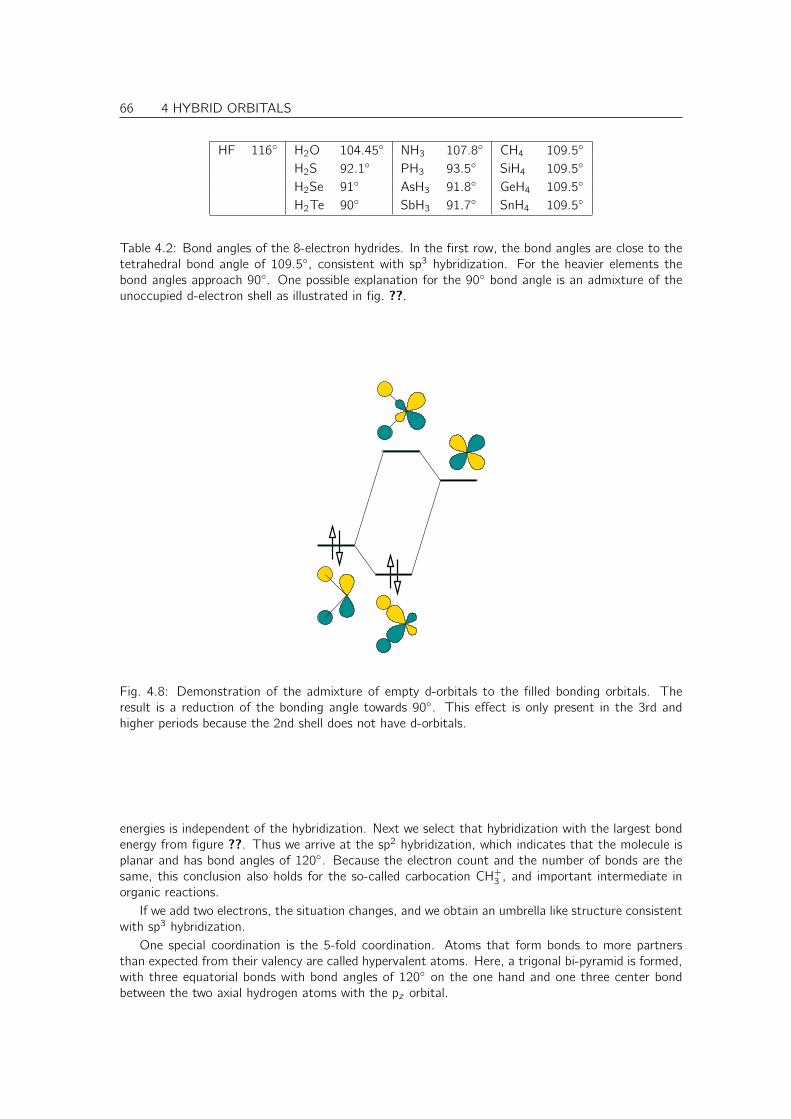
66 4 HYBRID ORBITALS
HF 116 H2O 104.45 NH3 107.8 CH4 109.5
H2S 92.1 PH3 93.5 SiH4 109.5
H2Se 91 AsH3 91.8 GeH4 109.5
H2Te 90 SbH3 91.7 SnH4 109.5
Table 4.2: Bond angles of the 8-electron hydrides. In the first row, the bond angles are close to thetetrahedral bond angle of 109.5, consistent with sp3 hybridization. For the heavier elements thebond angles approach 90. One possible explanation for the 90 bond angle is an admixture of theunoccupied d-electron shell as illustrated in fig. ??.
Fig. 4.8: Demonstration of the admixture of empty d-orbitals to the filled bonding orbitals. Theresult is a reduction of the bonding angle towards 90. This effect is only present in the 3rd andhigher periods because the 2nd shell does not have d-orbitals.
energies is independent of the hybridization. Next we select that hybridization with the largest bondenergy from figure ??. Thus we arrive at the sp2 hybridization, which indicates that the molecule isplanar and has bond angles of 120. Because the electron count and the number of bonds are thesame, this conclusion also holds for the so-called carbocation CH+
3 , and important intermediate inorganic reactions.
If we add two electrons, the situation changes, and we obtain an umbrella like structure consistentwith sp3 hybridization.
One special coordination is the 5-fold coordination. Atoms that form bonds to more partnersthan expected from their valency are called hypervalent atoms. Here, a trigonal bi-pyramid is formed,with three equatorial bonds with bond angles of 120 on the one hand and one three center bondbetween the two axial hydrogen atoms with the pz orbital.

4 HYBRID ORBITALS 67
electrons bonds binding0 0 s2 0 s, like helium2 1 ssσ bond2 2 s-type three-center bond4 0 s4 1 sp1 bond and sp1-type lone pair as back bond4 2 two sp1 bonds, linear molecule6 0 sp1
6 1-3 sp2 bonds, bond angle 120
8 0 sp2, like noble gases8 1-4 sp3, tetrahedral bond angle8 5 three equatorial sp2 bonds and one axial three-center bond8 6 three orthogonal three-center bonds, octahedron10 5 three equatorial sp2 bonds and one axial three-center bond10 6 three orthogonal three-center bonds and one filled non-bond12 6 three orthogonal three-center bonds and two filled non-bonds14 6 three orthogonal three-center bonds and three filled non-bonds
Table 4.3: Preferred hybridization of an anion as function of number of electons and bonds. Theelectron pair of a bond is added to the electron count. For the cases with zero bonds, we consider theconfiguration favorable for a slightly positive charge, given that the attempt to form a bond with ananion is likely to remove electrons. Filled non-bonds refer to the non-bonding orbital of a three-centerbond.
compound Ne Hybrid coordinationLiH 2 s,p linearBeH2 4 sp1 linearBH3 6 sp2 trigonalCH+
3 6 sp2 trigonalCH4 8 sp3 tetrahedralNH+
4 8 sp3 tetrahedralNH3 8 sp3 umbrellaH3O+ 8 sp3 umbrellaH2O 8 sp3 bentHF 8 sp3 linearCH−5 10 sp2 trigonal bipyramidalPH5 10 sp2 trigonal bipyramidal
Note that the hybrid orbitals allow us to estimate the atomic structure. However, they do nottell us about the atomic orbitals. In order to obtain the eigenstates, we need to form symmetrizedorbitals from the bonding and anti-bonding orbitals with the hybrid orbitals. The transformation intoeigenstates, however, does not change the energy of the system, because only occupied orbitals aretransformed into each other and unoccupied orbitals mix with each other.
The notation of hybrid orbitals thus shortcuts the complete diagonalization of the Hamiltonian,which is sufficient to estimate total energies and structures.
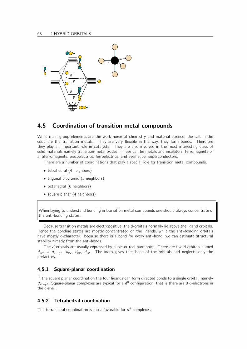
68 4 HYBRID ORBITALS
4.5 Coordination of transition metal compounds
While main group elements are the work horse of chemistry and material science, the salt in thesoup are the transition metals. They are very flexible in the way, they form bonds. Thereforethey play an important role in catalysts. They are also involved in the most interesting class ofsolid materials namely transition-metal oxides. These can be metals and insulators, ferromagnets orantiferromagnets, piezoelectrics, ferroelectrics, and even super superconductors.
There are a number of coordinations that play a special role for transition metal compounds.
• tetrahedral (4 neighbors)
• trigonal bipyramid (5 neighbors)
• octahedral (6 neighbors)
• square planar (4 neighbors)
When trying to understand bonding in transition metal compounds one should always concentrate onthe anti-bonding states.
Because transition metals are electropositive, the d-orbitals normally lie above the ligand orbitals.Hence the bonding states are mostly concentrated on the ligands, while the anti-bonding orbitalshave mostly d-character. because there is a bond for every anti-bond, we can estimate structuralstability already from the anti-bonds.
The d-orbitals are usually expressed by cubic or real harmonics. There are five d-orbitals namedd3z2−r2 dx2−y2 , dxy , dxz , dyz . The index gives the shape of the orbitals and neglects only theprefactors.
4.5.1 Square-planar coordination
In the square planar coordination the four ligands can form directed bonds to a single orbital, namelydx2−y2 . Square-planar complexes are typical for a d8 configuration, that is there are 8 d-electrons inthe d-shell.
4.5.2 Tetrahedral coordination
The tetrahedral coordination is most favorable for d4 complexes.
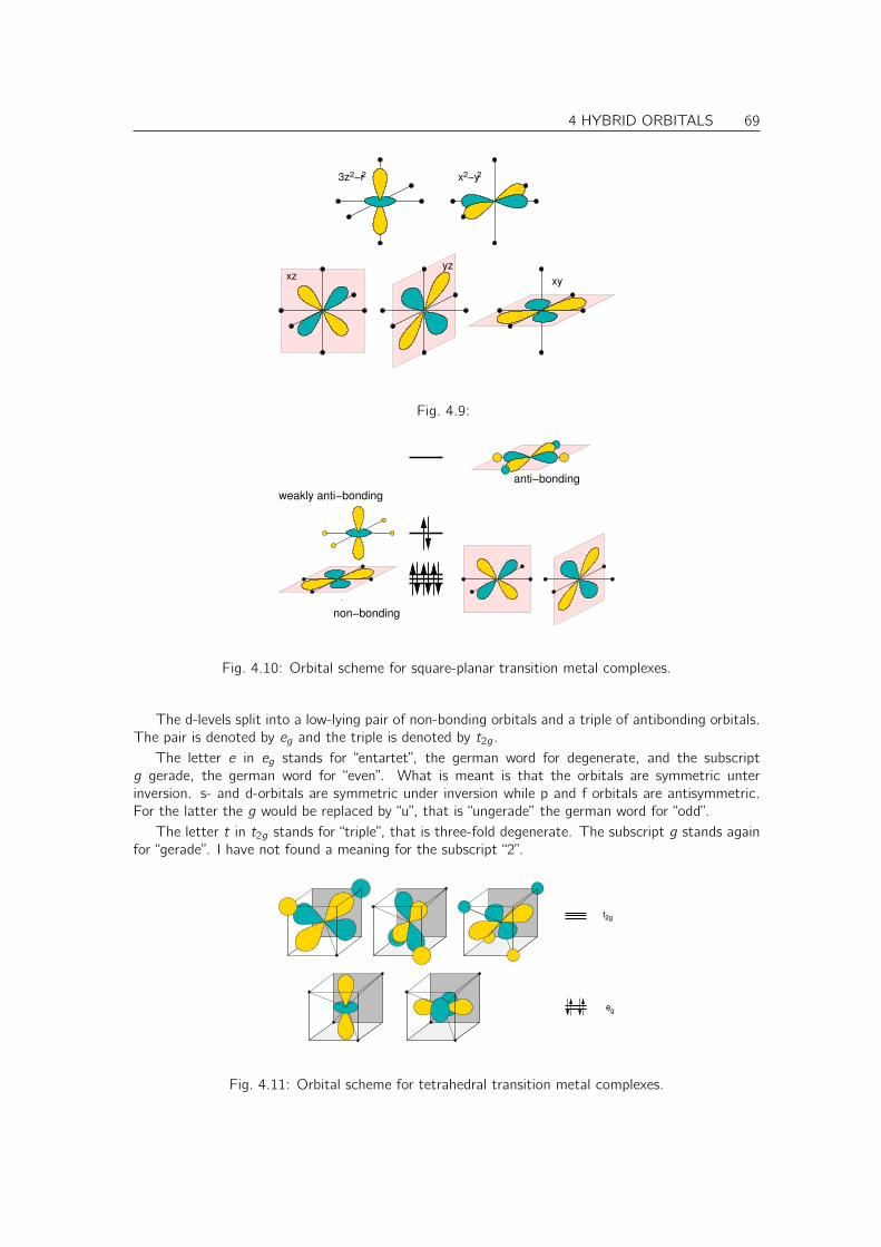
4 HYBRID ORBITALS 69
3z2−r2 x2−y2
xzyz
xy
Fig. 4.9:
non−bonding
anti−bonding
weakly anti−bonding
Fig. 4.10: Orbital scheme for square-planar transition metal complexes.
The d-levels split into a low-lying pair of non-bonding orbitals and a triple of antibonding orbitals.The pair is denoted by eg and the triple is denoted by t2g.
The letter e in eg stands for “entartet”, the german word for degenerate, and the subscriptg gerade, the german word for “even”. What is meant is that the orbitals are symmetric unterinversion. s- and d-orbitals are symmetric under inversion while p and f orbitals are antisymmetric.For the latter the g would be replaced by “u”, that is “ungerade” the german word for “odd”.
The letter t in t2g stands for “triple”, that is three-fold degenerate. The subscript g stands againfor “gerade”. I have not found a meaning for the subscript “2”.
eg
t2g
Fig. 4.11: Orbital scheme for tetrahedral transition metal complexes.
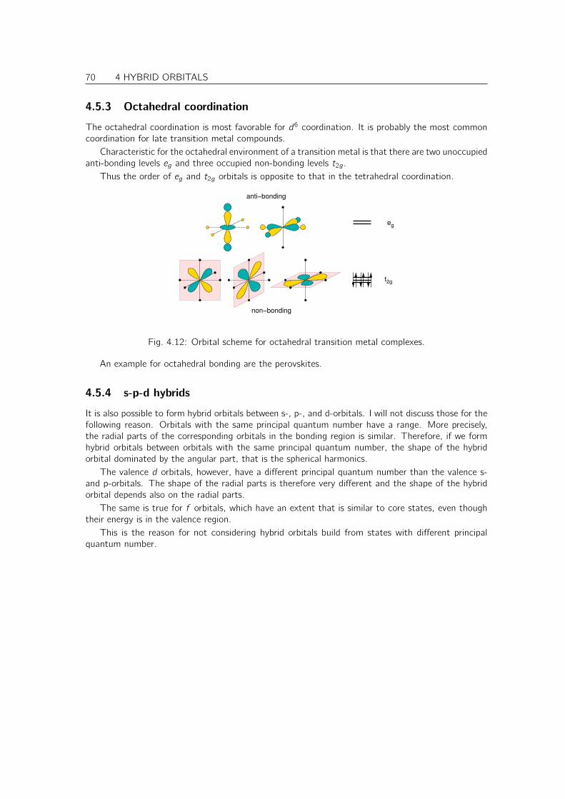
70 4 HYBRID ORBITALS
4.5.3 Octahedral coordination
The octahedral coordination is most favorable for d6 coordination. It is probably the most commoncoordination for late transition metal compounds.
Characteristic for the octahedral environment of a transition metal is that there are two unoccupiedanti-bonding levels eg and three occupied non-bonding levels t2g.
Thus the order of eg and t2g orbitals is opposite to that in the tetrahedral coordination.
eg
t2g
non−bonding
anti−bonding
Fig. 4.12: Orbital scheme for octahedral transition metal complexes.
An example for octahedral bonding are the perovskites.
4.5.4 s-p-d hybrids
It is also possible to form hybrid orbitals between s-, p-, and d-orbitals. I will not discuss those for thefollowing reason. Orbitals with the same principal quantum number have a range. More precisely,the radial parts of the corresponding orbitals in the bonding region is similar. Therefore, if we formhybrid orbitals between orbitals with the same principal quantum number, the shape of the hybridorbital dominated by the angular part, that is the spherical harmonics.
The valence d orbitals, however, have a different principal quantum number than the valence s-and p-orbitals. The shape of the radial parts is therefore very different and the shape of the hybridorbital depends also on the radial parts.
The same is true for f orbitals, which have an extent that is similar to core states, even thoughtheir energy is in the valence region.
This is the reason for not considering hybrid orbitals build from states with different principalquantum number.

Chapter 5
Frontier orbitals
Often we are interested in reactivity of a molecule or a material. We would like to find out thoseparts of the molecule that are most reactive, and we would like what kinds of reactions these “hotspots” can undergo. Frontier orbital theory is a simple tool that allows us to make exactly such ananalysis. Frontier orbital theory was invented by Kenichi Fukui who received in 1981 the Nobel pricein chemistry for this contribution[? ].
The frontier orbital concept, in its most simple form, says that the Highest Occupied MolecularOrbital (HOMO) and the Lowest Unoccupied Molecular Orbital (LUMO) are usually those that areresponsible for the reactivity.
The underlying idea is that only the hybridization of filled with empty orbitals leads to a stabi-lization of the system. Because the interaction is largest if the energetic separation between theparticipating orbitals is smallest, it is obvious that the orbitals near the Fermi level, contribute mostlyto the interaction.
1 2|ε −ε |
t2
No Bond
E=−2∆
No Bond
One differentiates nucleophilic and electrophilic sites at a molecule.
• an electrophile is characterized by a low-lying empty orbital, which can undergo an interactionwith an occupied orbital. “Electrophile” means electron-loving.
• a nucleophile is the opposite of an electrophile, and is characterized by a high-lying filledorbital. This orbital can undergo an interaction with an electrophile. “Nucleophile” meansnucleus-loving. Consider for example a proton, which is a nucleus. A proton has an emptyorbital, and thus interacts best with a filled orbital. Thus a filled orbital is nucleus-loving.
There are also sites that can be both, electrophilic and nucleophilic at the same time, if it has
71
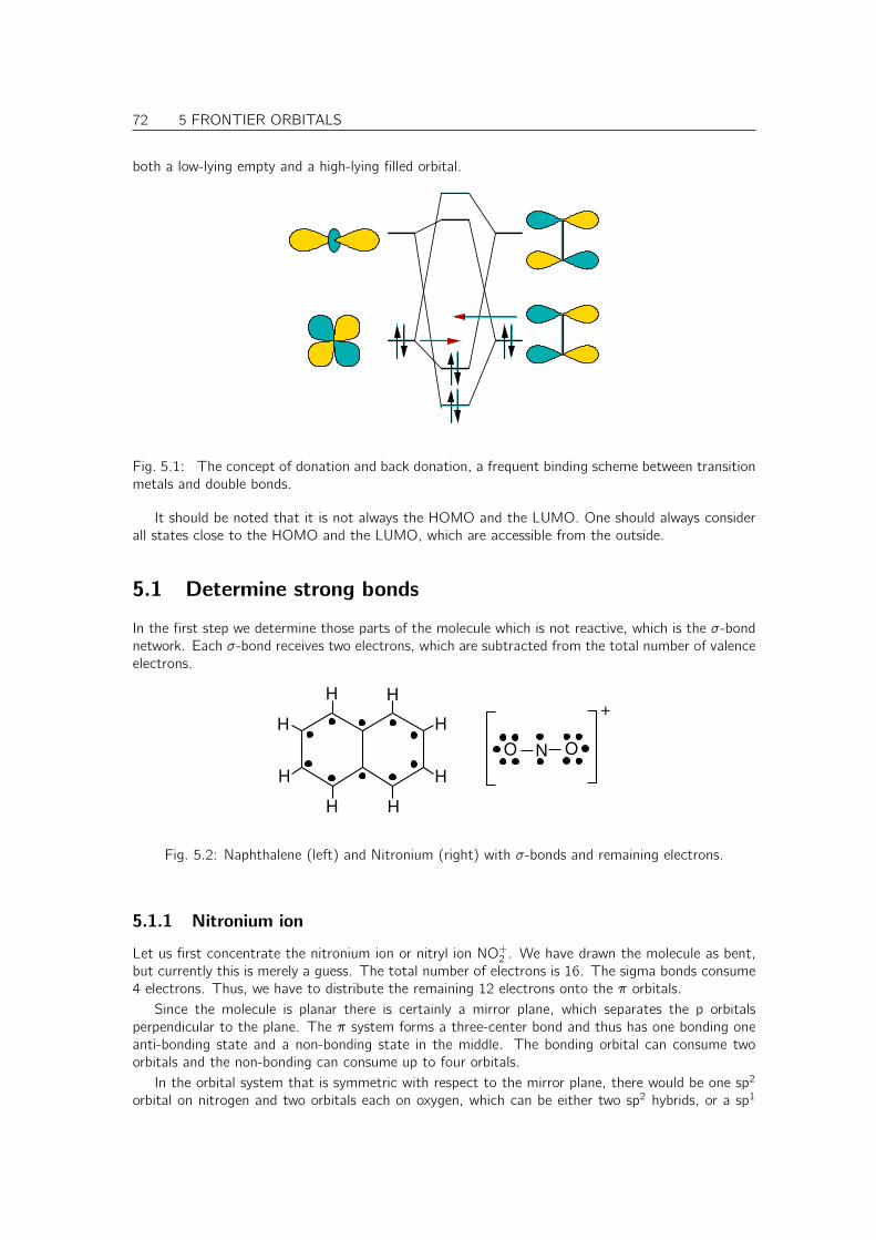
72 5 FRONTIER ORBITALS
both a low-lying empty and a high-lying filled orbital.
Fig. 5.1: The concept of donation and back donation, a frequent binding scheme between transitionmetals and double bonds.
It should be noted that it is not always the HOMO and the LUMO. One should always considerall states close to the HOMO and the LUMO, which are accessible from the outside.
5.1 Determine strong bonds
In the first step we determine those parts of the molecule which is not reactive, which is the σ-bondnetwork. Each σ-bond receives two electrons, which are subtracted from the total number of valenceelectrons.
O ON
+
HH
H
HH
H
H H
Fig. 5.2: Naphthalene (left) and Nitronium (right) with σ-bonds and remaining electrons.
5.1.1 Nitronium ion
Let us first concentrate the nitronium ion or nitryl ion NO+2 . We have drawn the molecule as bent,
but currently this is merely a guess. The total number of electrons is 16. The sigma bonds consume4 electrons. Thus, we have to distribute the remaining 12 electrons onto the π orbitals.
Since the molecule is planar there is certainly a mirror plane, which separates the p orbitalsperpendicular to the plane. The π system forms a three-center bond and thus has one bonding oneanti-bonding state and a non-bonding state in the middle. The bonding orbital can consume twoorbitals and the non-bonding can consume up to four orbitals.
In the orbital system that is symmetric with respect to the mirror plane, there would be one sp2
orbital on nitrogen and two orbitals each on oxygen, which can be either two sp2 hybrids, or a sp1
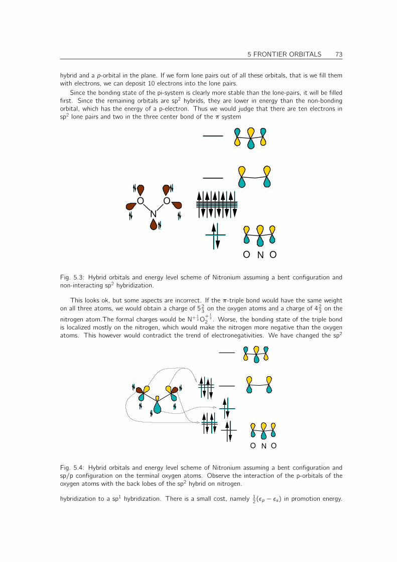
5 FRONTIER ORBITALS 73
hybrid and a p-orbital in the plane. If we form lone pairs out of all these orbitals, that is we fill themwith electrons, we can deposit 10 electrons into the lone pairs.
Since the bonding state of the pi-system is clearly more stable than the lone-pairs, it will be filledfirst. Since the remaining orbitals are sp2 hybrids, they are lower in energy than the non-bondingorbital, which has the energy of a p-electron. Thus we would judge that there are ten electrons insp2 lone pairs and two in the three center bond of the π system
O N O
N
OO
Fig. 5.3: Hybrid orbitals and energy level scheme of Nitronium assuming a bent configuration andnon-interacting sp2 hybridization.
This looks ok, but some aspects are incorrect. If the π-triple bond would have the same weighton all three atoms, we would obtain a charge of 5 2
3 on the oxygen atoms and a charge of 4 23 on the
nitrogen atom.The formal charges would be N+ 13 O
+ 13
2 . Worse, the bonding state of the triple bondis localized mostly on the nitrogen, which would make the nitrogen more negative than the oxygenatoms. This however would contradict the trend of electronegativities. We have changed the sp2
O N O
Fig. 5.4: Hybrid orbitals and energy level scheme of Nitronium assuming a bent configuration andsp/p configuration on the terminal oxygen atoms. Observe the interaction of the p-orbitals of theoxygen atoms with the back lobes of the sp2 hybrid on nitrogen.
hybridization to a sp1 hybridization. There is a small cost, namely 12 (εp − εs) in promotion energy.
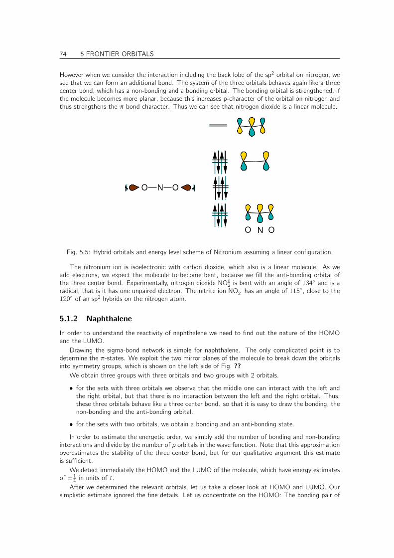
74 5 FRONTIER ORBITALS
However when we consider the interaction including the back lobe of the sp2 orbital on nitrogen, wesee that we can form an additional bond. The system of the three orbitals behaves again like a threecenter bond, which has a non-bonding and a bonding orbital. The bonding orbital is strengthened, ifthe molecule becomes more planar, because this increases p-character of the orbital on nitrogen andthus strengthens the π bond character. Thus we can see that nitrogen dioxide is a linear molecule.
O N O
O ON
Fig. 5.5: Hybrid orbitals and energy level scheme of Nitronium assuming a linear configuration.
The nitronium ion is isoelectronic with carbon dioxide, which also is a linear molecule. As weadd electrons, we expect the molecule to become bent, because we fill the anti-bonding orbital ofthe three center bond. Experimentally, nitrogen dioxide NO0
2 is bent with an angle of 134 and is aradical, that is it has one unpaired electron. The nitrite ion NO−2 has an angle of 115, close to the120 of an sp2 hybrids on the nitrogen atom.
5.1.2 Naphthalene
In order to understand the reactivity of naphthalene we need to find out the nature of the HOMOand the LUMO.
Drawing the sigma-bond network is simple for naphthalene. The only complicated point is todetermine the π-states. We exploit the two mirror planes of the molecule to break down the orbitalsinto symmetry groups, which is shown on the left side of Fig. ??
We obtain three groups with three orbitals and two groups with 2 orbitals.
• for the sets with three orbitals we observe that the middle one can interact with the left andthe right orbital, but that there is no interaction between the left and the right orbital. Thus,these three orbitals behave like a three center bond. so that it is easy to draw the bonding, thenon-bonding and the anti-bonding orbital.
• for the sets with two orbitals, we obtain a bonding and an anti-bonding state.
In order to estimate the energetic order, we simply add the number of bonding and non-bondinginteractions and divide by the number of p orbitals in the wave function. Note that this approximationoverestimates the stability of the three center bond, but for our qualitative argument this estimateis sufficient.
We detect immediately the HOMO and the LUMO of the molecule, which have energy estimatesof ± 1
4 in units of t.After we determined the relevant orbitals, let us take a closer look at HOMO and LUMO. Our
simplistic estimate ignored the fine details. Let us concentrate on the HOMO: The bonding pair of
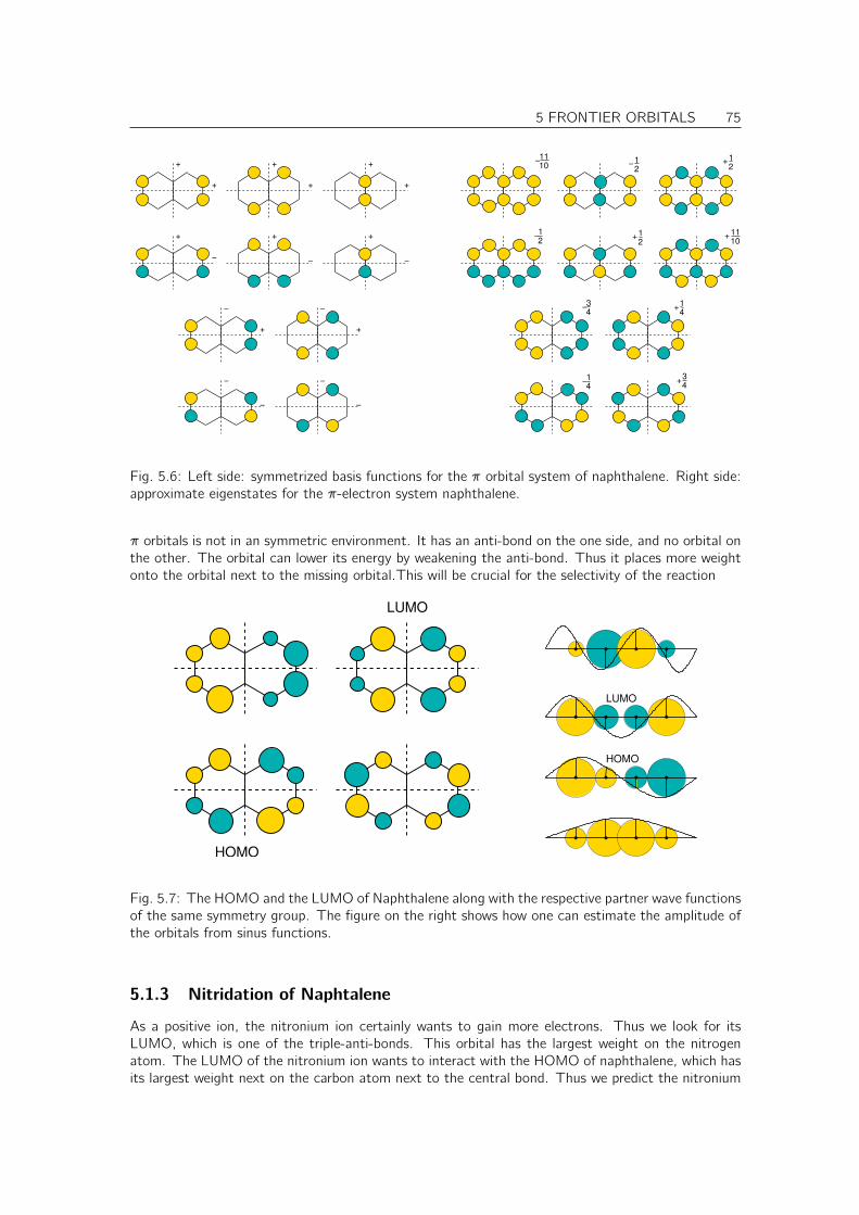
5 FRONTIER ORBITALS 75
10
11−
2
1−
10
11+
4
3−
4
1+
4
1−
4
3+
2
1+
2
1−
2
1+
+
+
++
+ +
+
++
+ +
− −
− −
−−
− −
−
Fig. 5.6: Left side: symmetrized basis functions for the π orbital system of naphthalene. Right side:approximate eigenstates for the π-electron system naphthalene.
π orbitals is not in an symmetric environment. It has an anti-bond on the one side, and no orbital onthe other. The orbital can lower its energy by weakening the anti-bond. Thus it places more weightonto the orbital next to the missing orbital.This will be crucial for the selectivity of the reaction
HOMO
LUMO
LUMO
HOMO
Fig. 5.7: The HOMO and the LUMO of Naphthalene along with the respective partner wave functionsof the same symmetry group. The figure on the right shows how one can estimate the amplitude ofthe orbitals from sinus functions.
5.1.3 Nitridation of Naphtalene
As a positive ion, the nitronium ion certainly wants to gain more electrons. Thus we look for itsLUMO, which is one of the triple-anti-bonds. This orbital has the largest weight on the nitrogenatom. The LUMO of the nitronium ion wants to interact with the HOMO of naphthalene, which hasits largest weight next on the carbon atom next to the central bond. Thus we predict the nitronium

76 5 FRONTIER ORBITALS
ion to attack preferentially this carbon atom.
H
LUMO
HOMO
OO N
N
OO
H
H
HH
H
H
HC
C
CC
C
CC
C
CC
Fig. 5.8: The electrophilic addition of nitronium to naphthalene. and final structure.

Chapter 6
From bonds to bands
So far we have employed a local picture of bonding. In solid state physics another viewpoint becamepopular, based on the concept of reciprocal space and band structures.
In order to approach the concepts in a simple way we again choose a simple model system, namelythe jellium model.
6.1 The Jellium model
For the electron gas the model system is the free electron gas or the jellium model. The jelliummodel consists of electrons and a spatially constant, positive charge background, which ensures thatthe overall system is neutral.
Because of translational symmetry, the potential is spatially constant. Thus the one-particlestates are simply plane waves.
φ~k,σ(~r , σ′) =1√Ω
ei~k~rδσ,σ′ (6.1)
We consider here states in a very large, but finite, volume Ω such as the universe. The states arenormalized to one within this volume.
This is an unusual notation for an ideally infinite system. Using this notation we avoid having todistinguish discrete and continuous sections of the spectrum and different normalization conditionsfor localized and extended states. A disadvantage is that extended states have a nearly vanishingamplitude, and that the spacing in k-space is extremely small. For a finite volume, only discrete valuesfor ~k are allowed. We will later see that in the final expression the factors Ω from the normalizationcan be translated into a volume element in k-space, so that the sums can be converted into integrals.
The dispersion relation of free electrons forms a parabola
ε~k,σ = V0 +(~k)2
2me
where V0 is the value of the potential.The jellium model approximates real metals surprisingly well, even though the potential of the
nuclei is far from being a constant. In a hand-waving manner we can say that the valence electrons areexpelled from the nuclear region by the Pauli repulsion of the core electrons, so that they move aroundin a region with fairly constant potential. The true story is a little more subtle though... In Fig. ??the band structure of free and non-interacting electron gas is shown in a unit cell corresponding toalumina and compared to the calculated band structure of alumina. We can see that the free electrongas already provides a fairly good description of some realistic systems.
77
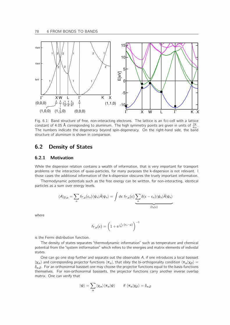
78 6 FROM BONDS TO BANDS
2
1
2
12
1( , , )
2
1(1, ,0)
5eV
10eV
15eV
Γ Γ K XX W L
(1,0,0)
(0,0,0) (1,1,0)
(0,0,0)
1 1 1
2
2
21 2 11
2 2
Γ X W L Γ K X
-10
-5
0
5
10
15
E[e
V]
Fig. 6.1: Band structure of free, non-interacting electrons. The lattice is an fcc-cell with a latticeconstant of 4.05 Å corresponding to aluminum. The high symmetry points are given in units of 2π
alat.
The numbers indicate the degeneracy beyond spin-degeneracy. On the right-hand side, the bandstructure of aluminum is shown in comparison.
6.2 Density of States
6.2.1 Motivation
While the dispersion relation contains a wealth of information, that is very important for transportproblems or the interaction of quasi-particles, for many purposes the k-dispersion is not relevant. Ithose cases the additional information of the k-dispersion obscures the truely important information.
Thermodynamic potentials such as the free energy can be written, for non-interacting, identicalparticles as a sum over energy levels.
〈A〉β,µ =∑n
fT,µ(εn)〈ψn|A|ψn〉 =
∫dε fT,µ(ε)
∑n
δ(ε− εn)〈ψn|A|ψn〉︸ ︷︷ ︸DA(ε)
where
fT,µ(ε) =
(1 + e
1kBT
(εn−µ)
)−1
is the Fermi distribution function.The density of states separates “thermodynamic information” such as temperature and chemical
potential from the “system intformation” which refers to the energies and matrix elements of individalstates.
One can go one step further and separate out the observable A, if one introduces a local basisset|χα〉 and corresponding projector functions 〈πα|, that obey the bi-orthogonality condition 〈πα|χβ〉 =δα,β. For an orthonormal basisset one may choose the projector functions equal to the basis-functionsthemselves. For non-orthonormal basissets, the projector functions carry another inverse overlapmatrix. One can verify that
|ψ〉 =∑α
|χα〉〈πα|ψ〉 if 〈πα|χβ〉 = δα,β
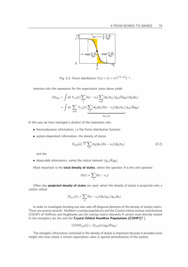
6 FROM BONDS TO BANDS 79
1
0
kBTε µ−
+
kBTε µ−
−
kBTε µ−
−
µ
f21
~1− exp( ) ~exp( )
ε
Fig. 6.2: Fermi distribution f (ε) = (1 + e1
kBT(ε−µ)
)−1.
Insertion into the expression for the expectation value above yields
〈A〉β,µ =
∫dε fT,µ(ε)
∑n
δ(ε− εn)∑α,β
〈ψn|πα〉〈χα|A|χβ〉〈πβ |ψn〉
=
∫dε∑α,β
fT,µ(ε)∑n
〈πβ |ψn〉δ(ε− εn)〈ψn|πα〉︸ ︷︷ ︸Dβ,α(ε)
〈χα|A|χβ〉
In this way we have managed a division of the expression into
• thermodynamic information, i.e the Fermi distribution function
• system-dependent information, the density of states
Dα,β(ε)def=∑n
〈πβ |ψn〉δ(ε− εn)〈ψn|πα〉 (6.2)
and the
• observable information, namly the matrix element 〈χα|A|χβ〉.
Most important is the total density of states, where the operator A is the unit operator.
D(ε) =∑n
δ(ε− εn)
Often also projected density of states are used, where the density of states is projected onto acertain orbital
Dα,α(ε) =∑n
δ(ε− εn)〈ψn|χα〉〈χα|ψn〉
In order to investigate bonding one also uses off-diagonal elements of the density of states matrix.There are several variants: Mulliken’s overlap populations and the Crystal orbital overlap contributions(COOP) of Hoffman and Hughbanks use the overlap matrix elements A variant more directly relatedto the energetics are the and the Crystal Orbital Hamilton Populations (COHP)[? ].
COHPα,β(ε) = Dα,β(ε)〈χβ |H|χα〉
The energetic information contained in the density of states is important because it provides someinsight into how robust a certain expectation value is against perturbations of the system.

80 6 FROM BONDS TO BANDS
6.2.2 Density of States for extended systems
For molecules, the total density of states is simply a series of Delta functions. For extended systemsthis is no more true, but the density of states becomes a continuous function.
The one-particle density of states can be obtained from the dispersion relation ε(p). Independentparticles in a constant potential have a conserved momentum ~p = ~~k . This implies that they can bedescribed by plane waves
Ψ(~r) =1√V
ei~k~r
Note that even electrons in a periodic potential, that is electrons ins a crystal, have a conservedmomentum. The wave function is not a plane wave, but a plane wave modulated by some periodic,p dependent function, as seen in the Bloch theorem. These dispersion relations are called bandstructure and can be calculated with first-principles calculations. Also lattice vibrations in a crystalcan be classified by their wave vector, resulting in a phonon band structure.
If we consider a system with periodic boundary conditions in a a box with side-lengths Lx , Ly , Lz ,the states are quantized, so that kiLi = 2πni where ni is an arbitrary integer. Thus there are onlystates with ~k = ( 2π
Lxi , 2πLyj, 2πLzk), where i , j, k are arbitrary integers. The volume V of the box is
V = LxLyLz .Thus the density of states is
D(ε) =∑i ,j,k
δ(ε(
2π~Lx
i︸ ︷︷ ︸px
,2π~Lx
j︸ ︷︷ ︸py
,2π~Lx
k︸ ︷︷ ︸pz
)− ε)
We can attribute to each state a volume in k-space, namely
∆Vk =2π
Lx
2π
Ly
2π
Lz=
(2π)3
V(6.3)
Using the relation ~p = ~~k we can convert this volume into a volume element in momentum space,namely
∆Vp =(2π~)3
V(6.4)
If the size of the box, that is Lx , Ly , Lz , is made very large, the volume element attributed to a singlestate in momentum space becomes very small. Thus we can replace the sum by an integral, where∆Vp is represented by d3p.
D(ε) =V
(2π~)3
∑i ,j,k
(2π~)3
V︸ ︷︷ ︸→d3p
δ(ε(~pi ,j,k)− ε
)Li→∞
=V
(2π~)3
∫d3p δ
(ε(~p)− ε
)(6.5)
It is intuitively clear that the expression for the density of states is related to a surface integralover a surface of constant energy. This will be shown in the following.
In order to transform the expression for the density of states into a surface integral in momentumspace, it is convenient to introduce the number of states N(ε).
The number of states is defined as the number of states that lie below the energy epsilon.
N(ε) =∑i ,j,k
θ(ε− ε(pi ,j,k))V→∞
=V
(2π~)3
∫d3p θ(ε− ε(~p)) (6.6)

6 FROM BONDS TO BANDS 81
where θ(x) is the Heaviside function θ(x), which vanishes for x < 0 and is equal to unity for x > 0.The Heaviside function is related to the δ-function via
θ(x) =
∫ x
−∞dx ′ δ(x ′) ⇔ ∂xθ(x) = δ(x) (6.7)
This allows us to relate the number of states to the density of states Thus we obtain
∂εN(ε)Eq. ??
=V
(2π~)3
∫d3p ∂εθ(ε− ε(~p))
Eq. ??=
V
(2π~)3
∫d3p δ(ε− ε(~p))
Eq. ??= D(ε) (6.8)
Here we show how the volume integral with the delta function can be converted into a surfaceintegral.
D(ε)Eq. ??
= ∂εN(ε) = lim∆→0
V
(2π~)3
∫d3p
θ(ε+ ∆− ε(p))− θ(ε− ε(p))
∆︸ ︷︷ ︸→δ(ε−ε(p))
py
e(p)>e+∆
nd
e(p)<e
px
The integral over the difference of the two Heaviside function corre-sponds to the volume of a volume sheet, which is enclosed by the sur-faces defined by ε(~p) = ε and ε(~p) = ε+ ∆.Let us calculate the distance of two points on the two surfaces. Letus pick one point ~p0 on the surface defined by ε(~p) = ε. The closestneighbor on the other surface ~p1 lies opposite to ~p0, that is ~p1 = ~p0+~n·d ,where d is the distance of the points and ~n = 1
|~∇pε|~∇pε is the normal
vector of the surface. ~p1 lies on the other surface and therefore fulfills
ε(~p1) = ε︸︷︷︸ε(~p0)
+∆
⇒ ε(~p0) + ∆ = ε(~p0 + ~n · d)Tay lor
= ε(~p0) + ~n · d ~∇pε+O(d2)
⇒ d =∆
~n~∇pε=
∆~∇pε|~∇pε|
~∇pε=
∆
|~∇pε|
Thus we obtain the thickness d of the sheet. Note that the thicknessdepends on the position on the sheet. The volume element of the sheetcan then be written as d3p = dA · dThus we can write the volume as
D(ε) =V
(2π~)3
∮d2Ap
1
|∇pε|
Thus we obtain the density of states from the dispersion relation as
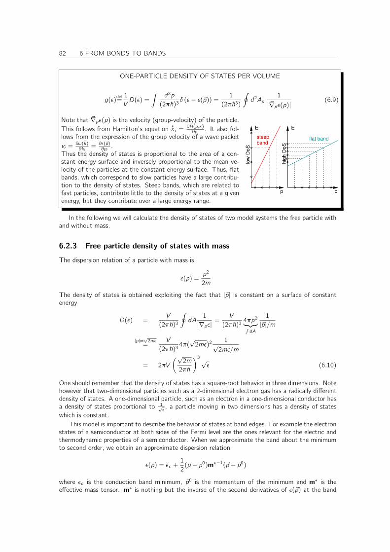
82 6 FROM BONDS TO BANDS
ONE-PARTICLE DENSITY OF STATES PER VOLUME
g(ε)def=
1
VD(ε) =
∫d3p
(2π~)3δ (ε− ε(~p)) =
1
(2π~3)
∮d2Ap
1
|~∇pε(p)|(6.9)
steepband
E
p p
E
flat band
hig
h D
oS
low
DoS
Note that ~∇pε(p) is the velocity (group-velocity) of the particle.This follows from Hamilton’s equation
.x i = ∂H(~p,~x)
∂pi. It also fol-
lows from the expression of the group velocity of a wave packetvi = ∂ω(~k)
∂ki= ∂ε(~p)
∂pi.
Thus the density of states is proportional to the area of a con-stant energy surface and inversely proportional to the mean ve-locity of the particles at the constant energy surface. Thus, flatbands, which correspond to slow particles have a large contribu-tion to the density of states. Steep bands, which are related tofast particles, contribute little to the density of states at a givenenergy, but they contribute over a large energy range.
In the following we will calculate the density of states of two model systems the free particle withand without mass.
6.2.3 Free particle density of states with mass
The dispersion relation of a particle with mass is
ε(p) =p2
2m
The density of states is obtained exploiting the fact that |~p| is constant on a surface of constantenergy
D(ε) =V
(2π~)3
∮dA
1
|∇pε|=
V
(2π~)34πp2︸ ︷︷ ︸∫dA
1
|~p|/m
|p|=√
2mε=
V
(2π~)34π(√
2mε)2 1√2mε/m
= 2πV
(√2m
2π~
)3√ε (6.10)
One should remember that the density of states has a square-root behavior in three dimensions. Notehowever that two-dimensional particles such as a 2-dimensional electron gas has a radically differentdensity of states. A one-dimensional particle, such as an electron in a one-dimensional conductor hasa density of states proportional to 1√
ε, a particle moving in two dimensions has a density of states
which is constant.This model is important to describe the behavior of states at band edges. For example the electron
states of a semiconductor at both sides of the Fermi level are the ones relevant for the electric andthermodynamic properties of a semiconductor. When we approximate the band about the minimumto second order, we obtain an approximate dispersion relation
ε(p) = εc +1
2(~p − ~p0)m∗−1(~p − ~p0)
where εc is the conduction band minimum, ~p0 is the momentum of the minimum and m∗ is theeffective mass tensor. m∗ is nothing but the inverse of the second derivatives of ε(~p) at the band
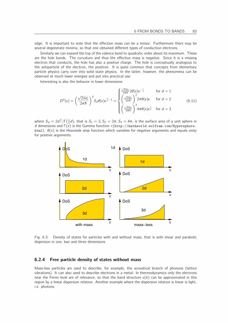
6 FROM BONDS TO BANDS 83
edge. It is important to note that the effective mass can be a tensor. Furthermore there may beseveral degenerate minima, so that one obtained different types of conduction electrons.
Similarly we can expand the top of the valence band to quadratic order about its maximum. Theseare the hole bands. The curvature and thus the effective mass is negative. Since it is a missingelectron that conducts, the hole has also a positive charge. The hole is conceptually analogous tothe antiparticle of the electron, the positron. It is quite common that concepts from elementaryparticle physics carry over into solid state physics. In the latter, however, the phenomena can beobserved at much lower energies and put into practical use.
Interesting is also the behavior in lower dimensions
Dd(ε) =
(√2mL
2π~
)dSdθ(ε)ε
d2−1 =
√2mL
2π~ 2θ(ε)ε−12 for d = 1(√
2mL2π~
)2
2πθ(ε)ε for d = 2(√2mL
2π~
)3
4πθ(ε)ε12 for d = 3
(6.11)
where Sd = 2dd2 /Γ( 1
2d), that is S1 = 2, S2 = 2π, S3 = 4π, is the surface area of a unit sphere ind dimensions and Γ(x) is the Gamma function <(http://mathworld.wolfram.com/Hypersphere.html). θ(x) is the Heaviside step function which vanishes for negative arguments and equals unityfor positive arguments.
ε
DoS
ε
DoS
ε
DoS
ε
DoS
ε
DoS
ε
DoS
1d
with mass mass−less
1d1d
2d
3d
2d
3d
Fig. 6.3: Density of states for particles with and without mass, that is with linear and parabolicdispersion in one, two and three dimensions
6.2.4 Free particle density of states without mass
Mass-less particles are used to describe, for example, the acoustical branch of phonons (latticevibrations). It can also used to describe electrons in a metal: In thermodynamics only the electronsnear the Fermi level are of relevance, so that the band structure ε(k) can be approximated in thisregion by a linear dispersion relation. Another example where the dispersion relation is linear is light,i.e. photons.
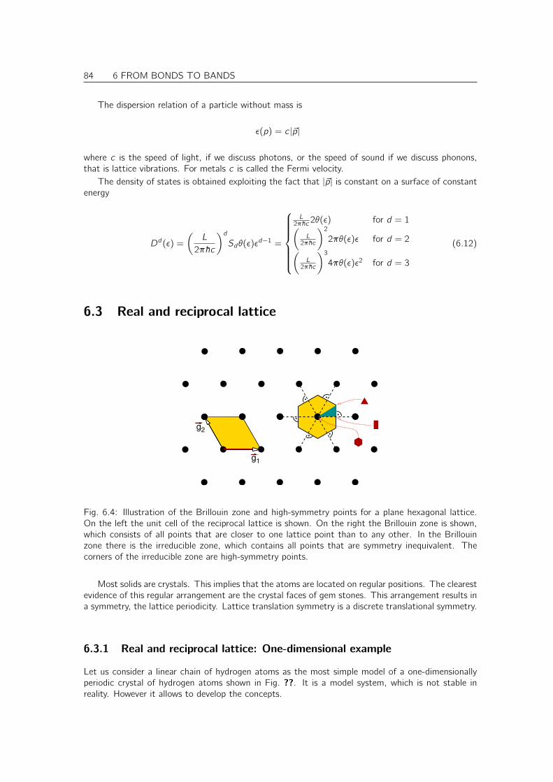
84 6 FROM BONDS TO BANDS
The dispersion relation of a particle without mass is
ε(p) = c |~p|
where c is the speed of light, if we discuss photons, or the speed of sound if we discuss phonons,that is lattice vibrations. For metals c is called the Fermi velocity.
The density of states is obtained exploiting the fact that |~p| is constant on a surface of constantenergy
Dd(ε) =
(L
2π~c
)dSdθ(ε)εd−1 =
L2π~c 2θ(ε) for d = 1(
L2π~c
)2
2πθ(ε)ε for d = 2(L
2π~c
)3
4πθ(ε)ε2 for d = 3
(6.12)
6.3 Real and reciprocal lattice
g1
g2
Fig. 6.4: Illustration of the Brillouin zone and high-symmetry points for a plane hexagonal lattice.On the left the unit cell of the reciprocal lattice is shown. On the right the Brillouin zone is shown,which consists of all points that are closer to one lattice point than to any other. In the Brillouinzone there is the irreducible zone, which contains all points that are symmetry inequivalent. Thecorners of the irreducible zone are high-symmetry points.
Most solids are crystals. This implies that the atoms are located on regular positions. The clearestevidence of this regular arrangement are the crystal faces of gem stones. This arrangement results ina symmetry, the lattice periodicity. Lattice translation symmetry is a discrete translational symmetry.
6.3.1 Real and reciprocal lattice: One-dimensional example
Let us consider a linear chain of hydrogen atoms as the most simple model of a one-dimensionallyperiodic crystal of hydrogen atoms shown in Fig. ??. It is a model system, which is not stable inreality. However it allows to develop the concepts.
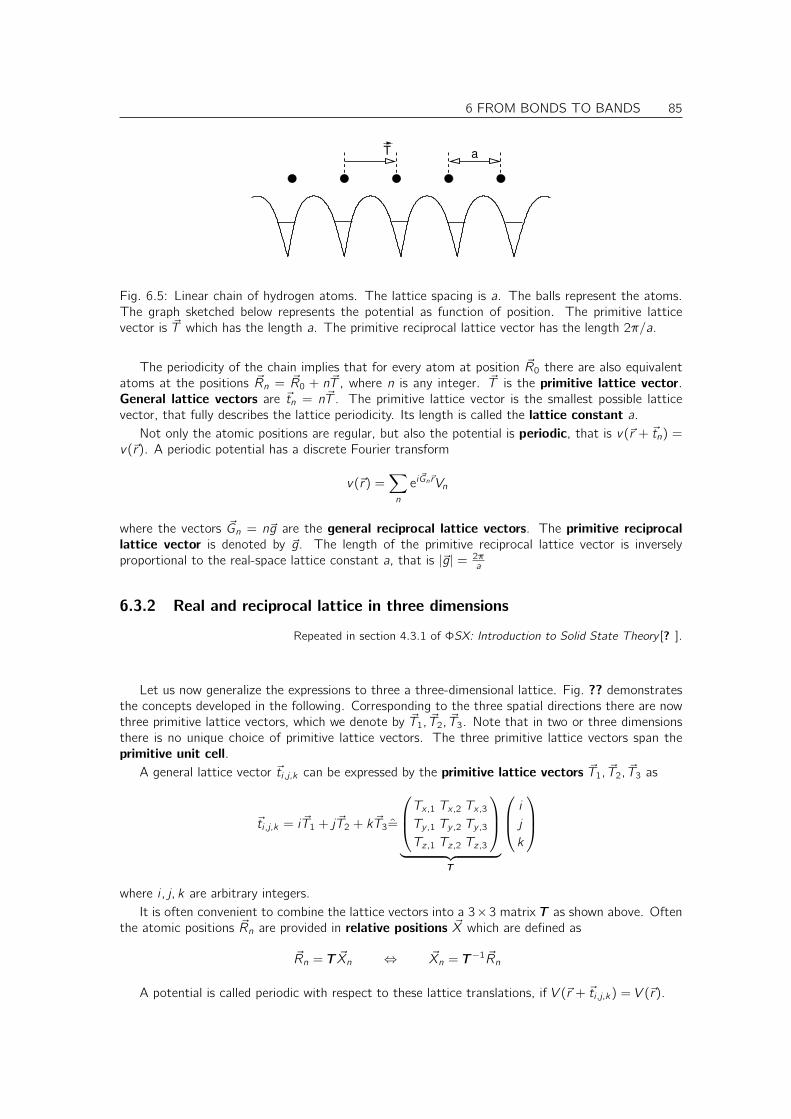
6 FROM BONDS TO BANDS 85
T a
Fig. 6.5: Linear chain of hydrogen atoms. The lattice spacing is a. The balls represent the atoms.The graph sketched below represents the potential as function of position. The primitive latticevector is ~T which has the length a. The primitive reciprocal lattice vector has the length 2π/a.
The periodicity of the chain implies that for every atom at position ~R0 there are also equivalentatoms at the positions ~Rn = ~R0 + n~T , where n is any integer. ~T is the primitive lattice vector.General lattice vectors are ~tn = n~T . The primitive lattice vector is the smallest possible latticevector, that fully describes the lattice periodicity. Its length is called the lattice constant a.
Not only the atomic positions are regular, but also the potential is periodic, that is v(~r + ~tn) =v(~r). A periodic potential has a discrete Fourier transform
v(~r) =∑n
ei~Gn~rVn
where the vectors ~Gn = n~g are the general reciprocal lattice vectors. The primitive reciprocallattice vector is denoted by ~g. The length of the primitive reciprocal lattice vector is inverselyproportional to the real-space lattice constant a, that is |~g| = 2π
a
6.3.2 Real and reciprocal lattice in three dimensions
Repeated in section 4.3.1 of ΦSX: Introduction to Solid State Theory [? ].
Let us now generalize the expressions to three a three-dimensional lattice. Fig. ?? demonstratesthe concepts developed in the following. Corresponding to the three spatial directions there are nowthree primitive lattice vectors, which we denote by ~T1, ~T2, ~T3. Note that in two or three dimensionsthere is no unique choice of primitive lattice vectors. The three primitive lattice vectors span theprimitive unit cell.
A general lattice vector ~ti ,j,k can be expressed by the primitive lattice vectors ~T1, ~T2, ~T3 as
~ti ,j,k = i ~T1 + j ~T2 + k ~T3=
Tx,1 Tx,2 Tx,3Ty,1 Ty,2 Ty,3
Tz,1 Tz,2 Tz,3
︸ ︷︷ ︸
T
i
j
k
where i , j, k are arbitrary integers.It is often convenient to combine the lattice vectors into a 3×3 matrix T as shown above. Often
the atomic positions ~Rn are provided in relative positions ~X which are defined as
~Rn = T ~Xn ⇔ ~Xn = T−1 ~Rn
A potential is called periodic with respect to these lattice translations, if V (~r + ~ti ,j,k) = V (~r).

86 6 FROM BONDS TO BANDS
RECIPROCAL LATTICE
The reciprocal lattice is given by those values of the wave vector ~G, for which the correspondingplane waves ei
~G~r have the same periodicity as the real-space lattice.The primitive reciprocal-lattice vectors ~gn for n = 1, 2, 3 are defined in three dimensions as
~gn~Tm = 2πδn,m (6.13)
Thus, in three dimensions the reciprocal lattice vectors can be obtained as
~g1 = 2π~T2 × ~T3
~T1
(~T2 × ~T3
) , ~g2 = 2π~T3 × ~T1
~T1
(~T2 × ~T3
) , ~g3 = 2π~T1 × ~T2
~T1
(~T2 × ~T3
)It is easily shown that these expressions fulfill the defining equation Eq. ?? for the reciprocal latticevectors. Note that the expressions for the second and third lattice vector are obtained from the firstby cyclic commutation of the indices.
Because the vector product is perpendicular to the two vectors forming it, every reciprocal latticevector is perpendicular to two real-space lattice vectors. This brings us to the physical meaning ofthe reciprocal lattice vectors: Two real space lattice vectors define a lattice plane. A plane can bedefined either by two linearly independent vectors in the plane or alternatively by the plane normal.The reciprocal lattice vectors apparently define lattice planes, because they are plane normals.
Let us now consider the distance ∆n of two neighboring lattice planes. It is obtained by projectingone vector pointing ~Tn from one plane to the other onto a normalized plane normal ~gn/|~gn|.
∆n = ~Tn~gn|~gn|
Eq. ??=
2π
|~gn|
⇒ |~gn| =2π
∆n
PHYSICAL MEANING OF RECIPROCAL LATTICE VECTORS
• The reciprocal lattice vectors are perpendicular to the lattice planes of the real-space lattice.
• The length of the primitive reciprocal lattice vectors is 2π divided by the distance of the latticeplanes.
We can form a 3× 3 matrix g from the three primitive reciprocal lattice vectors.
gdef=
gx,1 gx,2 gx,3gy,1 gy,2 gy,3
gz,1 gz,2 gz,3
The definition Eq. ?? of the reciprocal lattice vectors can be expressed in matrix form as
g>TEq. ??
= 2π111 (6.14)
Thus the matrix g is obtained as
gEq. ??
= 2π(T−1
)>(6.15)
The general reciprocal lattice vectors are
~Gi ,j,k = i~g1 + j~g2 + k~g3
6 FROM BONDS TO BANDS 87
Reciprocal lattice and Fourier transforms
The reciprocal lattice vectors play an important role in the Fourier transform of periodic functions.All plane waves that are periodic with the lattice vectors ~Tn are characterized by a reciprocal latticevector.
ei~G(~r+~Tn) = ei
~G~r
⇒ ~G(~r + ~Tn) = ~G~r + 2πmn
⇒ ~G~Tn = 2πmn
⇒ ~GT = 2π ~m
⇒ ~G = 2π ~mT−1 = 2π(T−1
)>~m
where mn are integers. The allowed values for ~G are exactly those of the reciprocal lattice. This wasthe motivation for the definition Eq. ??.

88 6 FROM BONDS TO BANDS
∆
1g
g2
2T
T1
C3 C6
t−2,3,0 ∆2
1
Fig. 6.6: Translational and rotational symmetry of a single graphite sheet and demonstration ofreciprocal lattice vectors. Graphite is a layered material, which consists of sheets as the one shown.The yellow balls indicate the carbon atoms and the blue sticks represent the bonds. In graphite thesetwo-dimensional sheets are stacked on top of each other, where every second sheet is shifted suchthat an atom falls vertically below the point indicated by C6. Here we only consider the symmetryof a single sheet. The elementary unit cell is indicated by the red parallelogram, which is spanned bythe elementary lattice vectors ~T1 and ~T2. The third lattice vector points perpendicular to the sheettowards you. An example for a general lattice vector is ~t3,−2,0 = 3~T1− 2~T2 + 0~T3. The lattice planesindicated by the dashed lines. The lattice planes are perpendicular to the sheet. The distance of thelattice planes are indicated by ∆1 and ∆2. The elementary reciprocal lattice vectors are ~g1 and ~g2.The third reciprocal lattice vector points perpendicular out of the plane towards you. Note that thereciprocal lattice vectors have the unit “inverse length”. Thus their length is considered irrelevant inthis real space figure. The axis through C3 standing perpendicular to the plane is a three-fold rotationaxis of the graphite crystal. The axis through C6 perpendicular to the plane is a 6-fold rotation axis ofthe graphite sheet, but only a three-fold rotation axis of the graphite crystal. (Note that a rotationaxis for the graphite crystal must be one for both sheets of the crystal). In addition there is a mirrorplane lying in the plane. Furthermore there are several mirror planes perpendicular to the plane: Onepassing through every atom with one of the three bonds lying in the plane and one perpendiculareach bond passing through the bond center.
6.4 Bloch Theorem
In order to make the description of an infinte crystal tractable, we exploit translational symmetry toblock-diagonalize the Hamiltonian. The theoretical basis is Bloch’s theorem.
6 FROM BONDS TO BANDS 89
BLOCH’S THEOREM
The eigenstates of the Hamiltonian with crystal symmetry S(~t), i.e. [H, S(~t)]− = 0, can be writtenas a product
ψ~k,n(~r) = ~u~k,n(~r)ei~k~r (6.16)
of a periodic function u~k,n(~r) with a plane wave ei~k~r . S(~t) is a translation operator for the real space
translation vector ~t....or...
The Hamiltonian of a crystal is block diagonal for Bloch states, that is
〈ψ~k |H|ψ~k ′〉 = 0 for ~k 6= ~k ′
when
ψk(~r) = ~uk(~r)ei~k~r where uk(~r + ~t) = uk(~r)
The underlying idea of Bloch’s theorem is to Block-diagonalize the Hamiltonian by finding theeigenstates of the translation operators.
Let S(~t) be the translation operator for a given lattice translation ~t = ~T1i + ~T2j + ~T3k .
S(~t) =
∫d3r |~r + ~t〉〈~r | (6.17)
Translation operator and canonical momentum
A general theorem is that any translation for an unbounded continuous variable can be expressed bythe canonical momentum.
S(~t) = e−i~ ~p~t (6.18)
This relation will be used for the Proof of Bloch’s theorem. It is discussed to some extend in chapter9 of ΦSX: Quantum Physics. Let us anyway go quickly over the proof.
Proof of Eq. ??:
1. First we define a basis of momentum eigenstates1
~p|~p〉 = |~p〉~p eigenvalue equation
〈~p|~p〉 = (2π~)3δ(~p − ~p′) orthonormality
1 =
∫d3p
(2π~)3|~p〉〈~p| completeness
The real space wave function of the momentum eigenstates are plane waves
〈~r |~p〉 = ei~ ~p~r real space representation
which provides a transformation between the momentum and position eigenstates.
2. Let us now work out a matrix element that we will need in the following:
〈~r |e−i~ ~p~t |~p〉 = 〈~r |~p〉︸︷︷︸
ei~ ~p~r
e−i~ ~p~t = e
i~ ~p(~r−~t) = 〈~r − ~t|~p〉
1There are various definitions for momentum eigenstates in the literature, that differ by their normalization.

90 6 FROM BONDS TO BANDS
3. Now we are ready to bring the operator defined by Eq. ?? into the form Eq. ??, which is thedefinition of the translation operator.
e−i~ ~p~t =
∫d3r |~r〉〈~r |︸ ︷︷ ︸
1
e−i~ ~p~t
∫d3p
(2π~)3|~p〉〈~p|︸ ︷︷ ︸
1
=
∫d3r |~r〉
∫d3p
(2π~)3
(〈~r |e−
i~ ~p~t |~p〉
)︸ ︷︷ ︸
〈~r−~t|~p〉
〈~p|
=
∫d3r |~r〉〈~r − ~t|
∫d3p
(2π~)3|~p〉〈~p|︸ ︷︷ ︸
1
=
∫d3r |~r + ~t〉〈~r | Eq. ??= S(t) q.e.d
Proof of Bloch’s theorem
Let us assume that |ψ〉 is an eigenstate of the lattice translation, i.e.
〈~r |S(~t)|ψ〉︸ ︷︷ ︸ψ(~r−~t)
Eq. ??= 〈~r |ψ〉︸ ︷︷ ︸
ψ(~r)
e−i~ ~p~t︸ ︷︷ ︸
e−i~k~t
Now we multiply this equation with e−i~k(~r−~t)
ψ(~r − ~t)e−i~k(~r−~t) = ψ(~r)e−i
~k~r
which says that the function u defined as
u(~r) = ψ(~r)e−i~k~r
is periodic. Thus the eigenstate of the lattice translation is a product of a periodic function u(~r) anda plane wave.
We have shown before that the eigenstates of a Hamiltonian can be expressed a superpositionof eigenstates of its symmetry operator. Thus also the eigenstates of the Hamiltonian with latticesymmetry can be written in the form of a Bloch wave, and the wave vector is a quantum number forthis system. This finishes the proof of Bloch’s theorem.
6.5 Reduced zone scheme
Here we will see that the band structure is periodic in reciprocal space, i.e.
εn(~k) = εn(~k + ~G)
and try to understand the implications.Let us consider an eigenstate of the Hamiltonian, which is written as a Bloch state with a periodic
part u~k,n(~r). We expand it by ei~G~r with a reciprocal lattice vector, which itself is periodic.
Ψ~k,n(~r) = u~k,n(~r)ei~k~r = u~k,n(~r)e−i
~G~rei(~k+~G)~r = u~k+~G,n(~r)ei(
~k+~G)~r = Ψ~k+~G,n(~r)
We have introduced
u~k+~G,n(~r)def= u~k,n(~r)e−i
~G~r
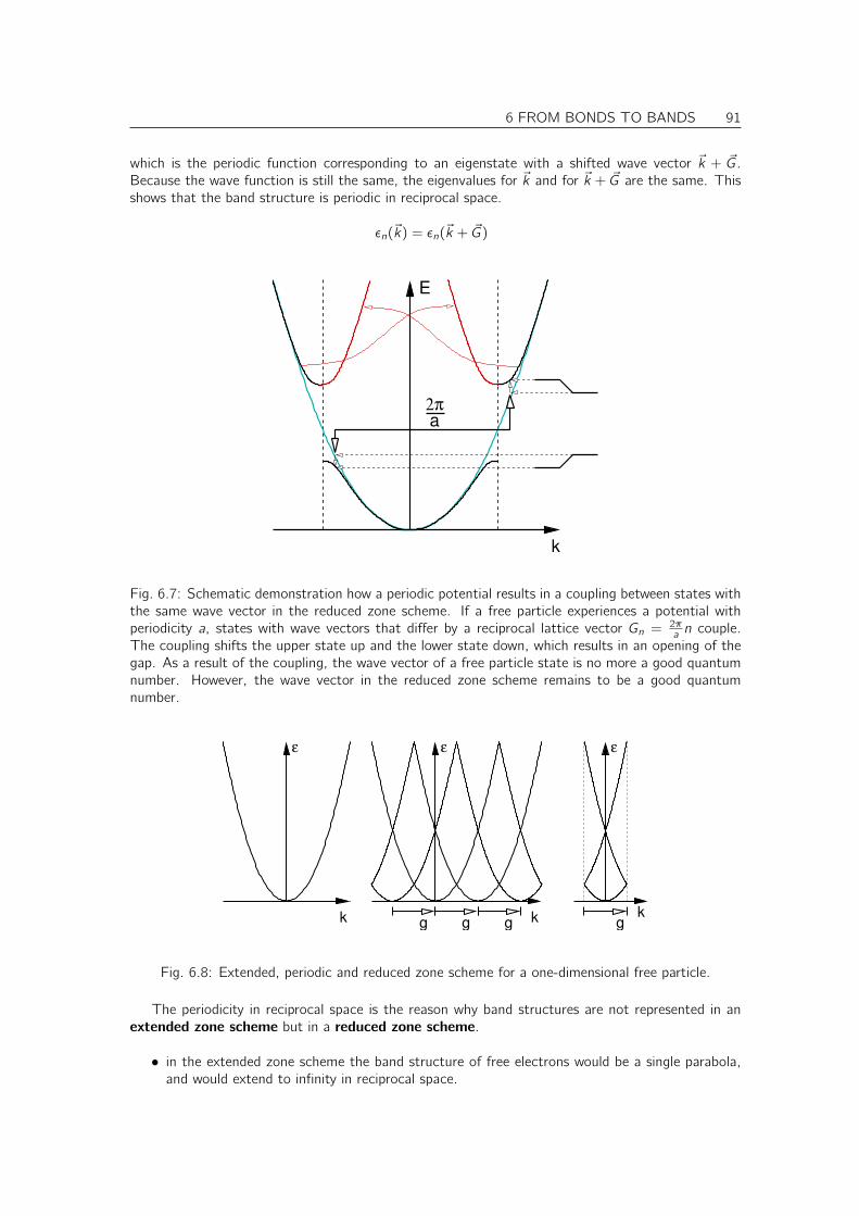
6 FROM BONDS TO BANDS 91
which is the periodic function corresponding to an eigenstate with a shifted wave vector ~k + ~G.Because the wave function is still the same, the eigenvalues for ~k and for ~k + ~G are the same. Thisshows that the band structure is periodic in reciprocal space.
εn(~k) = εn(~k + ~G)
2π
a
E
k
Fig. 6.7: Schematic demonstration how a periodic potential results in a coupling between states withthe same wave vector in the reduced zone scheme. If a free particle experiences a potential withperiodicity a, states with wave vectors that differ by a reciprocal lattice vector Gn = 2π
a n couple.The coupling shifts the upper state up and the lower state down, which results in an opening of thegap. As a result of the coupling, the wave vector of a free particle state is no more a good quantumnumber. However, the wave vector in the reduced zone scheme remains to be a good quantumnumber.
ggg g
ε εε
k k k
Fig. 6.8: Extended, periodic and reduced zone scheme for a one-dimensional free particle.
The periodicity in reciprocal space is the reason why band structures are not represented in anextended zone scheme but in a reduced zone scheme.
• in the extended zone scheme the band structure of free electrons would be a single parabola,and would extend to infinity in reciprocal space.
92 6 FROM BONDS TO BANDS
• in the periodic zone scheme, the free electron would consists of many parabola centered atthe reciprocal lattice points. Thus, the reciprocal zone scheme is periodic with the periodicityof the reciprocal lattice.
• in the reduced zone scheme, only the irreducible part of the periodic zone scheme is shown,that is one single repeat unit. The band structures shown in Fig. ?? are in a reduced zonescheme. There are several choices for the repeat units of the reciprocal lattice. One choice issimply the primitive unit cell of the reciprocal lattice. However, the shape of the unit cell doesnot have the point-group symmetry of the reciprocal lattice. Therefore one instead choosesthe Wigner Seitz cell2 of the reciprocal lattice, which is called the Brillouin zone.
Opening of gaps at the Brillouin zone boundary
See figure ??.
6.6 Bands and orbitals
Repeated in section 4.5 of ΦSX:Introduction to Solid-State Theory[? ]
So far we have discussed the band structures as a variation of the dispersion relation of the freeelectron bands. However this point of view obscures the relation to chemical binding and the localpicture of the wave functions.
The band structure can also be constructed starting from local orbitals. This is demonstratedhere for the two-dimensional square lattice with atoms having s- and p-orbitals in the plane.
In order to simplify the work, we restrict ourselves to the high symmetry points Γ, X and M ofthe two-dimensional reciprocal unit cell.
The real space lattice vectors are
~T1 =
(1
0
)a and ~T2 =
(0
1
)a
The corresponding reciprocal space lattice vectors are
~g1 =
(1
0
)2π
aand ~g2 =
(0
1
)2π
a
The high-symmetry points are
kΓ = 0 =
(0
0
)2π
a; kX =
1
2~g1 =
(1
0
)π
aand kM =
1
2(~g1 + ~g2) =
(1
1
)π
a
The first step is to construct Bloch waves out of the atomic orbitals, by multiplying them withei~k~t , where ~t is the lattice translation of the atom relative to the original unit cell. This is illustrated
in Fig. ?? on page ??.
• At the Γ, the phase factor for a lattice translation of the orbital is one. Thus we repeat theorbital from the central unit cell in all other unit cells.
2The Wigner Seitz cell of a lattice consists of all points that are closer to the origin than to any other lattice point.Thus, it is enclosed by planes perpendicular to the lattice vectors cutting the lattice vector in half.

6 FROM BONDS TO BANDS 93
MXΓ
ΓX
M
Γ X M Γ
g1
g2
εs
hppσ
hppπ
hppσ
hppπ
εp
ssσ2h
Fig. 6.9: Illustration of a band structure in real and reciprocal space for a planar square lattice.Bottom left: The reciprocal lattice is spanned by the reciprocal lattice vectors ~g1 and ~g2.The yellowsquare is the corresponding Brillouin zone. The green inset is the Brillouin zone, whose corners arethe high symmetry points Γ, X and M. On the top left the corresponding basis functions made fromone s-orbital and two p-orbitals in a Bloch-basis are shown. These states are also eigenstates ofthe Hamiltonian, because the coupling vanishes due to point group symmetry at the high-symmetrypoints. On the top left a schematic band structure is shown and compared to a free-electron band(red).
• At the X point, the phase factor for a lattice translation along the first lattice vector is ei~kX ~T1 =
eiπ = −1 and the phase factor for the lattice translation along the second lattice vector ~T2 isei~kX ~T2 = +1. Thus if we go to the right the sign of the orbital alternates, while in the vertical
direction the orbital remains the same.
• At the M point, the phase factor alternates in each lattice direction, resulting in a checkerboardpattern.
Next we need to set up the Hamilton matrix elements for each k-point, using the Slater-Kosterparameters. For a back-on-the envelope estimate the nearest neighbor matrix elements will be suffi-cient. The matrix elements are firstly εs and εp, the energies of the orbitals without any hybridization.Secondly we need the hopping matrix elements tssσ, tppσ, tppπ. In principle we would also need tspσ,but that matrix element will not be needed in our example.
In our simple example, the Bloch states are already eigenstates of the Hamiltonian so that weonly need to calculate their energy. We obtain
Γ X Mεp + tppσ − tppπ εp + tppσ + tppπ εp − tppσ + tppπ
εp + tppσ − tppπ εp − tppσ − tppπ εp − tppσ + tppπ
εs + 2tssσ εs εs + 2tssσ
94 6 FROM BONDS TO BANDS
If there is a band structure available, we can estimate the Hamilton matrix elements from that.Otherwise we just make an educated guess.
6.7 Calculating band structures in the tight-binding model
Repeated in section 4.6 of ΦSX:Introduction to Solid-State Theory[? ]
Now we wish to calculate the band structure. Let us begin with a tight-binding basisset with theusual assumption that the tight-binding orbitals shall be orthogonal. The tight-binding orbitals shallbe represented by kets |~t, α〉, where ~t denotes a discrete lattice-translation vector and α denotes thetype of the orbital such as an s, px , py , pz , . . . orbital on a specific site in the unit cell.
A Bloch wave can be represented as
|Ψ~k,n〉 =∑~t,α
|~t, α〉〈~t, α|Ψ~k,n〉
Eq. ??=
∑~t,α
|~t, α〉〈~t, α|∫d3r |~r〉ei~k~r 〈~r |u~k,n〉
=∑~t,α
|~t, α〉ei~k~t〈~t, α|∫d3r |~r〉ei~k(~r−~t)〈~r |u~k,n〉
u(~r)=u(~r−~t)=
∑~t,α
|~t, α〉ei~k~t〈~t, α|∫d3r |~r〉ei~k(~r−~t)〈~r − ~t|u~k,n〉
~r→~r+~t=
∑~t,α
|~t, α〉ei~k~t∫d3r 〈~t, α|~r + ~t〉︸ ︷︷ ︸
〈~0,α|~r〉
ei~k~r 〈~r |u~k,n〉︸ ︷︷ ︸〈~r |Ψ~k,n〉
=∑~t,α
|~t, α〉ei~k~t〈~0, α|ψ~k,n〉 (6.19)
This shows us how we can represent the entire wave function with a vector ~cn with elements cα,n =〈~0, α|Ψk,n〉, which has the dimension of the number of orbitals in the elementary unit cell.
Our next goal is to find an equation for this vector. We will use the matrix elements of theHamilton operator in the basis of tight-binding orbitals
〈~t, α|H|~t ′, β〉 = h~t,α,~t ′,β
Let us insert the ansatz Eq. ?? into the Schrödinger equation
H|Ψk,n〉 = |Ψk,n〉εk,nEq. ??⇒
∑~t,α
H|~t, α〉ei~k~t〈~0, α|Ψk,n〉 =∑~t,α
|~t, α〉ei~k~t〈~0, α|Ψk,n〉εk,n
〈~0,β|⇒∑~t,α
〈~0, β|H|~t, α〉︸ ︷︷ ︸h~0,β,~t,α
ei~k~t〈~0, α|Ψk,n〉 =
∑~t,α
〈~0, β|~t, α〉︸ ︷︷ ︸δ~0,~tδα,β
ei~k~t〈~0, α|Ψk,n〉εk,n
⇒
∑~t,α
h~0,β,~t,αei~k~t
︸ ︷︷ ︸
hα,β(~k)
〈~0, α|Ψk,n〉︸ ︷︷ ︸cα,n(~k)
= 〈~0, β|Ψk,n〉︸ ︷︷ ︸cβ,n(~k)
εk,n
⇒ h(~k)~cn(~k) = ~cn(~k)εn(~k)
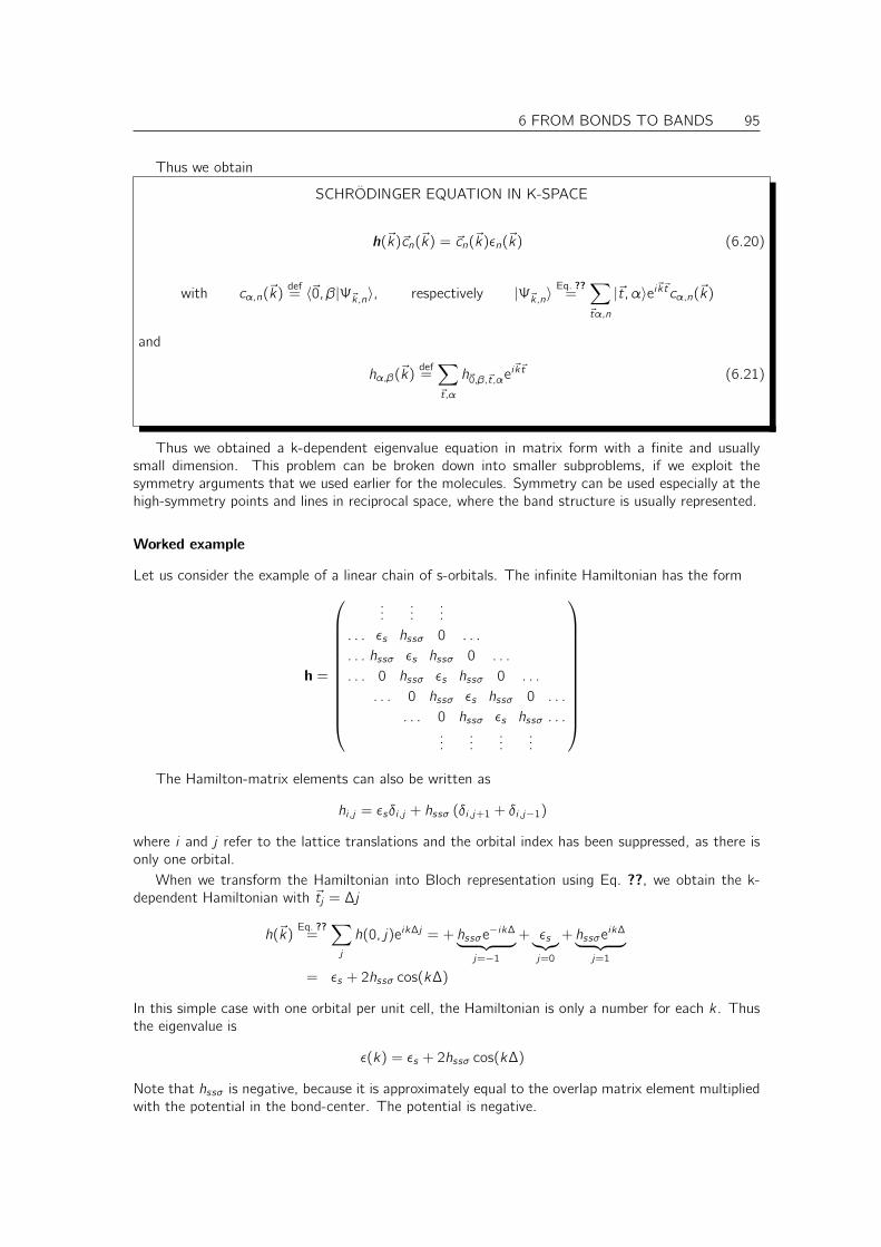
6 FROM BONDS TO BANDS 95
Thus we obtain
SCHRÖDINGER EQUATION IN K-SPACE
h(~k)~cn(~k) = ~cn(~k)εn(~k) (6.20)
with cα,n(~k)def= 〈~0, β|Ψ~k,n〉, respectively |Ψ~k,n〉
Eq. ??=
∑~tα,n
|~t, α〉ei~k~tcα,n(~k)
and
hα,β(~k)def=∑~t,α
h~0,β,~t,αei~k~t (6.21)
Thus we obtained a k-dependent eigenvalue equation in matrix form with a finite and usuallysmall dimension. This problem can be broken down into smaller subproblems, if we exploit thesymmetry arguments that we used earlier for the molecules. Symmetry can be used especially at thehigh-symmetry points and lines in reciprocal space, where the band structure is usually represented.
Worked example
Let us consider the example of a linear chain of s-orbitals. The infinite Hamiltonian has the form
h =
......
.... . . εs hssσ 0 . . .
. . . hssσ εs hssσ 0 . . .
. . . 0 hssσ εs hssσ 0 . . .
. . . 0 hssσ εs hssσ 0 . . .
. . . 0 hssσ εs hssσ . . ....
......
...
The Hamilton-matrix elements can also be written as
hi ,j = εsδi ,j + hssσ (δi ,j+1 + δi ,j−1)
where i and j refer to the lattice translations and the orbital index has been suppressed, as there isonly one orbital.
When we transform the Hamiltonian into Bloch representation using Eq. ??, we obtain the k-dependent Hamiltonian with ~tj = ∆j
h(~k)Eq. ??
=∑j
h(0, j)eik∆j = + hssσe−ik∆︸ ︷︷ ︸j=−1
+ εs︸︷︷︸j=0
+ hssσeik∆︸ ︷︷ ︸j=1
= εs + 2hssσ cos(k∆)
In this simple case with one orbital per unit cell, the Hamiltonian is only a number for each k . Thusthe eigenvalue is
ε(k) = εs + 2hssσ cos(k∆)
Note that hssσ is negative, because it is approximately equal to the overlap matrix element multipliedwith the potential in the bond-center. The potential is negative.
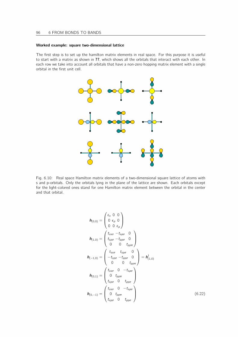
96 6 FROM BONDS TO BANDS
Worked example: square two-dimensional lattice
The first step is to set up the hamilton matrix elements in real space. For this purpose it is usefulto start with a matrix as shown in ??, which shows all the orbitals that interact with each other. Ineach row we take into account all orbitals that have a non-zero hopping matrix element with a singleorbital in the first unit cell.
Fig. 6.10: Real space Hamilton matrix elements of a two-dimensional square lattice of atoms withs and p-orbitals. Only the orbitals lying in the plane of the lattice are shown. Each orbitals exceptfor the light-colored ones stand for one Hamilton matrix element between the orbital in the centerand that orbital.
h(0,0) =
εs 0 0
0 εp 0
0 0 εp
h(1,0) =
tssσ −tspσ 0
tspσ −tppσ 0
0 0 tppπ
h(−1,0) =
tssσ tspσ 0
−tspσ −tppσ 0
0 0 tppπ
= h†(1,0)
h(0,1) =
tssσ 0 −tspσ0 tppπ
tspσ 0 tppσ
h(0,−1) =
tssσ 0 −tspσ0 tppπ
tspσ 0 tppσ
(6.22)
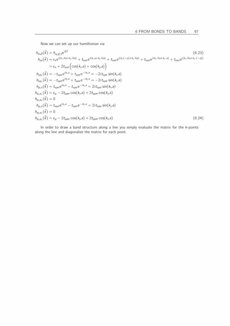
6 FROM BONDS TO BANDS 97
Now we can set up our hamiltonian via
hα,β(~k) = hα,β,~tei~k~t (6.23)
hss(~k) = εsei(kx ·0a+ky ·0a) + tssσei(kxa+ky ·0a) + tssσei(kx (−a)+ky ·0a) + tssσei(kx ·0a+ky ·a) + tssσei(kx ·0a+ky ·(−a))
= εs + 2tssσ
(cos(kxa) + cos(kya)
)hspx (~k) = −tspσeikxa + tspσe−ikxa = −2i tspσ sin(kxa)
hspy (~k) = −tspσeikya + tspσe−ikya = −2i tspσ sin(kya)
hpx s(~k) = tspσeikxa − tspσe−ikxa = 2i tspσ sin(kxa)
hpxpx (~k) = εp − 2tppσ cos(kxa) + 2tppπ cos(kya)
hpxpy (~k) = 0
hpy s(~k) = tspσeikya − tspσe−ikya = 2i tspσ sin(kya)
hpypx (~k) = 0
hpypy (~k) = εp − 2tppσ cos(kya) + 2tppπ cos(kxa) (6.24)
In order to draw a band structure along a line you simply evaluate the matrix for the k-pointsalong the line and diagonalize the matrix for each point.

98 6 FROM BONDS TO BANDS
Chapter 7
From atoms to solids
In this chapter I want to describe how one can construct an approximate density of states for materials.The density of states in turn already provides insight into many of the electronic properties of amaterial. A rough density of states can already be constructed without the knowledge of the atomicstructure of a material. Much of it depends only on the composition.
7.1 The Atom
7.1.1 The generalized hydrogen atom
When we think of an atom the first thought is the generalized hydrogen atom. A generalized hydrogenatom is an atom with non-interacting electrons and a nuclear charge +eZ. The Schrödingerequation of the generalized hydrogen atom can be solved analytically.
The energy levels of a generalized hydrogen atom are
εn,`,m,s = −mee
4
(4πε0~)2
Z2
2n2
The states are characterized by the quantum numbers
• the principal quantum number n
• the angular momentum quantum number ` ∈ 0, . . . , n − 1. The main angular momenta areals indicated by the letters s, p, d, f for ` = 0, 1, 2, 3.
• the magnetic quantum number m ∈ −`, . . . , `
• the spin quantum number s ∈ ↑, ↓.
Many of these quantum numbers are degenerate.
• The degeneracy of different angular momentum quantum numbers ` is a consequence of theZ/r potential, which has a dynamical symmetry that conserves the so-called Laplace-Runge-Lenz vector1. This degeneracy is lifted as soon as the potential obtains a shape different fromthe 1/r shape.
• The degeneracy of the magnetic quantum number is a consequence of the spherical symmetryof the atom.
1See ΦSX: Quantum mechanics, Appendix V “` degeneracy of the hydrogen atom”.
99
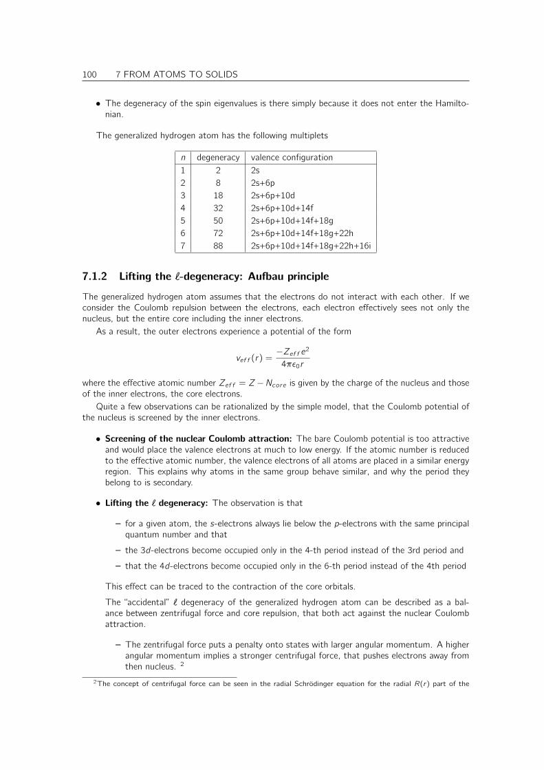
100 7 FROM ATOMS TO SOLIDS
• The degeneracy of the spin eigenvalues is there simply because it does not enter the Hamilto-nian.
The generalized hydrogen atom has the following multiplets
n degeneracy valence configuration1 2 2s2 8 2s+6p3 18 2s+6p+10d4 32 2s+6p+10d+14f5 50 2s+6p+10d+14f+18g6 72 2s+6p+10d+14f+18g+22h7 88 2s+6p+10d+14f+18g+22h+16i
7.1.2 Lifting the `-degeneracy: Aufbau principle
The generalized hydrogen atom assumes that the electrons do not interact with each other. If weconsider the Coulomb repulsion between the electrons, each electron effectively sees not only thenucleus, but the entire core including the inner electrons.
As a result, the outer electrons experience a potential of the form
vef f (r) =−Zef f e2
4πε0r
where the effective atomic number Zef f = Z−Ncore is given by the charge of the nucleus and thoseof the inner electrons, the core electrons.
Quite a few observations can be rationalized by the simple model, that the Coulomb potential ofthe nucleus is screened by the inner electrons.
• Screening of the nuclear Coulomb attraction: The bare Coulomb potential is too attractiveand would place the valence electrons at much to low energy. If the atomic number is reducedto the effective atomic number, the valence electrons of all atoms are placed in a similar energyregion. This explains why atoms in the same group behave similar, and why the period theybelong to is secondary.
• Lifting the ` degeneracy: The observation is that
– for a given atom, the s-electrons always lie below the p-electrons with the same principalquantum number and that
– the 3d-electrons become occupied only in the 4-th period instead of the 3rd period and
– that the 4d-electrons become occupied only in the 6-th period instead of the 4th period
This effect can be traced to the contraction of the core orbitals.
The “accidental” ` degeneracy of the generalized hydrogen atom can be described as a bal-ance between zentrifugal force and core repulsion, that both act against the nuclear Coulombattraction.
– The zentrifugal force puts a penalty onto states with larger angular momentum. A higherangular momentum implies a stronger centrifugal force, that pushes electrons away fromthen nucleus. 2
2The concept of centrifugal force can be seen in the radial Schrödinger equation for the radial R(r) part of the
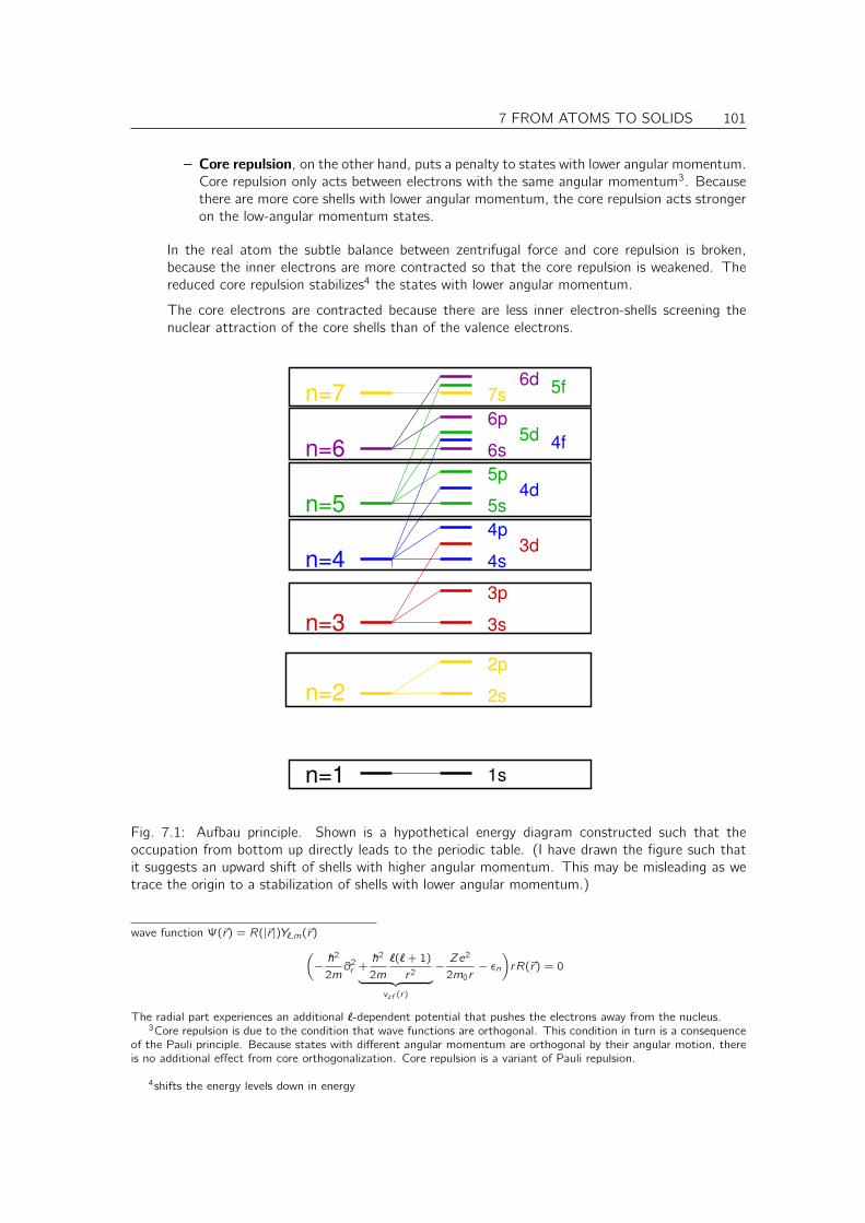
7 FROM ATOMS TO SOLIDS 101
– Core repulsion, on the other hand, puts a penalty to states with lower angular momentum.Core repulsion only acts between electrons with the same angular momentum3. Becausethere are more core shells with lower angular momentum, the core repulsion acts strongeron the low-angular momentum states.
In the real atom the subtle balance between zentrifugal force and core repulsion is broken,because the inner electrons are more contracted so that the core repulsion is weakened. Thereduced core repulsion stabilizes4 the states with lower angular momentum.
The core electrons are contracted because there are less inner electron-shells screening thenuclear attraction of the core shells than of the valence electrons.
n=1 1s
3s
3p
3d
n=3
n=5 5s
5p
5d
5f6d
6p
6sn=6
n=7 7s
2p
2s
4f
n=4 4s
4p
4d
n=2
Fig. 7.1: Aufbau principle. Shown is a hypothetical energy diagram constructed such that theoccupation from bottom up directly leads to the periodic table. (I have drawn the figure such thatit suggests an upward shift of shells with higher angular momentum. This may be misleading as wetrace the origin to a stabilization of shells with lower angular momentum.)
wave function Ψ(~r) = R(|~r |)Y`,m(~r)(−~2
2m∂2r +~2
2m
`(`+ 1)
r2︸ ︷︷ ︸vzf (r)
−Ze2
2m0r− εn
)rR(~r) = 0
The radial part experiences an additional `-dependent potential that pushes the electrons away from the nucleus.3Core repulsion is due to the condition that wave functions are orthogonal. This condition in turn is a consequence
of the Pauli principle. Because states with different angular momentum are orthogonal by their angular motion, thereis no additional effect from core orthogonalization. Core repulsion is a variant of Pauli repulsion.
4shifts the energy levels down in energy

102 7 FROM ATOMS TO SOLIDS
Radial extent is determined by principal qantum number
The radial extent of the orbitals is, surprisingly, rather similar for orbitals with the same principalquantum number n. A consequence is that the 4s and 4p orbitals in a transition metal behave almostlike free electrons, while the 3d-orbitals are core-like and interact only weakly with neighboring atoms.
This explains that the d-electrons of transition metal elements form weak bonds that can bebroken easily. This makes them ideal for catalytic behavior. A catalyst must form a bond with thetransition state of a reaction, thus lowering the reaction barrier, but this bond must also be able tobreak again, so that the catalyst can return into its original form. The f-electrons behave like truecore electrons, with the exception that the f-shell is only partially filled.
The crossing of 3d and 4s orbitals for increasing atomic number is evident from the periodictable. However, in compounds it is much less evident. In a compound, transition metals normallyloose their s-electrons. Because the s-electrons are located far from the nucleus, they experiencethe Pauli repulsion from the electrons of any neighboring atoms. This shifts their electron levels up,so that the s-electrons are transferred into the d-shell. We could say that the Pauli repulsion by thecore electrons is compensated by that of the neighboring atoms.
Even when the metals are in their elemental form, these metals can be considered cations immersedinto a free electron gas formed by the s-electrons.
7.2 From atoms to ions
7.2.1 Ionization potential and electron affinity
Even before atoms are brought together, they may already exchange electrons. This is the onsetfor the formation of an ionic bond. My experience is that this should be the first step to rationalizechemical bonding in compounds made from different atoms.
0Na +Na Cl −Cl 0
s
s
p
ioniz
ation p
ote
ntial
ele
ctr
on a
ffin
ity
vacuum level
I
0
A
Na
The energy to move an electron to the vacuum level is the ionization potential. The energy tomove an electron from the vacuum level to an atom is called the electron affinity.
Thus the energy gained by transferring electrons is the difference between the ionization potentialand the electron affinity.
∆E1 = A− I
7 FROM ATOMS TO SOLIDS 103
Once the ions are formed, they attract each other electrically, and additional energy
∆E2 =Q1Q2
4πε0|~R1 − ~R2|
is gained by bringing them closer together.The third effect playing a role is the onsite Coulomb repulsion of the electrons. Adding a second
electron to an atom is more difficult than adding the first, because the two additional electrons repelleach other. Therefore, the electron gain for transferring electrons becomes weaker with each electronalready transferred.
The direction of the charge transfer can be read from the electronegativities. Mulliken’s elec-tronegativity[? ] is proporational to the mean value of electron affinity and ionization potential.Electrons are transferred from the electropositive (less electronegative) atoms to the more elec-tronegative atoms. Therefore the first step that we consider when bringing atoms into a material,is to transfer electrons, so that the electropositive atoms give electrons to electronegative atoms.Electropositive atoms are predominantly to the left of the periodic table and electronegative atomsare on the right.
The limit for the electron transfer is reached when an electron shell is completely full or empty.
7.2.2 Oxidation states and electron count
In my experience, the best way to rationalize the electronic structure of a solid material is to use thefully ionic model as starting point.
This electron transfer is not always unique. If it is not obvious how the electrons are transferred,one can consider both choices or select one of them. If it is not obvious how to choose, it is also notimportant.
Let us do some examples. Use the periodic table to identify the number and type of availablevalence electrons.
• NaCl→ Na+Cl−
• MgO→ Mg2+O2−
• SiO2 → Si4+O2−2
• SrTiO3→ Sr2+Ti4+O2−3
• LaAlO3→ La3+Al3+O2−3
• CaMnO3→ Ca2+Mn4+O2−3 . The Mn atom keeps three some of its seven d-electrons. The
number of d-electrons left on Mn is determined by the number of electrons that can be passedto the oxygen atoms
• CO2 → C4+O2−2
• GaAs → Ga3+As3−. GaAs is a III − V compound. It belongs to the same structural classas silicon, but instead of four-valent electrons its consists of atoms with three and with fivevalence electrons.
Interesting is the case at surfaces or interfaces. Take as an example the interface between SrTiO3
and LaAlO3. SrTiO3 is a perovskite which consists of alternating planes of TiO2 and SrO. LaAlO3
has the same structure wit planes of AlO2 and LaO. A the interface a 2-dimensional electron gas isformed because the charges at the interface cannot becompensated.
Another case is the polar (111) surface of an oxide such as Al2O3. The oxide has alternatinglayers of Al and O. At the oxygen terminated surface there is a net charge. This charge has to enter
104 7 FROM ATOMS TO SOLIDS
the Al-states, which is unfavorable. In humid air, it can also react with water so that the oxygenatoms are converted into hydroxyl groups having less net charge.
A common misconception is that the ionic construction reflects the real charge distribution. Thereare various definitions of the charge of an atom. Here we use the concept of an oxidation stateWhatwe use here are the oxidation states. The oxidation state an extremely valuable tool to predict theposition of band gaps and of the stability of a material.
The oxidation state is a hypothetical charge that an atom would have if all bonds would be fullyionic. (See IUPAC definition on p. ??)
The oxidation state is based on the convention that an electron is fully attributed to the moreelectron acceptor. In reality, however, this orbital is a superposition of orbitals of electron donor andelectron acceptor. Therefore some of the charge distribution remains at the electron donor. Thisexplains the seeming contradiction between charge distribution and formal charges.
Even for an ionic compound, the charge density does not deviate much from that of overlappingatomic charge densities. The formation of an ionic bond does not lead to a large rearrangementof the charge distribution because of the following: The electrons of an electropositive atom areloosely bound and therefore located at large distance from the nucleus. In a compound, the nearestneighbors are located at the same distance, so that little charge rearrangement is required to transferan electron.
OXIDATION STATE
“A measure of the degree of oxidation of an atom in a substance. It is defined as the charge an atommight be imagined to have when electrons are counted according to an agreed-upon set of rules:
1. the oxidation state of a free element (uncombined element) is zero;
2. for a simple (monatomic) ion, the oxidation state is equal to the net charge on the ion;
3. hydrogen has an oxidation state of 1 and oxygen has an oxidation state of -2 when they arepresent in most compounds. (Exceptions to this are that hydrogen has an oxidation state of-1 in hydrides of active metals, e.g. LiH, and oxygen has an oxidation state of -1 in peroxides,e.g. H2O2;
4. the algebraic sum of oxidation states of all atoms in a neutral molecule must be zero, while inions the algebraic sum of the oxidation states of the constituent atoms must be equal to thecharge on the ion. For example, the oxidation states of sulfur in H2S, S8 (elementary sulfur),SO2, SO3, and H2SO4 are, respectively: -2, 0, +4, +6 and +6. The higher the oxidation stateof a given atom, the greater is its degree of oxidation; the lower the oxidation state, the greateris its degree of reduction.”
Source IUPAC. Compendium of Chemical Terminology, 2nd ed. (the "Gold Book"). Compiled byA. D. McNaught and A. Wilkinson. Blackwell Scientific Publications, Oxford (1997). XML on-linecorrected version: http://goldbook.iupac.org (2006-) created by M. Nic, J. Jirat, B. Kosata; updatescompiled by A. Jenkins. ISBN 0-9678550-9-8. doi:10.1351/goldbook.

Chapter 8
Instabilities
We already have seen that if an occupied and an unoccupied state is brought together, a bond isformed. As a result the occupied state is lowered and the unoccupied state is raised in energy. Thusa gap opens up. This effect can lead to symmetry-breaking distortions. We are used that nature sortof likes symmetries. Therefore it is important to see when symmetry is broken.
Let us consider the Hamiltonian with two states
H =
(ε1 t
t ε2
)
The eigenvalues are according to Eq. 2.8
ε± =ε1 + ε2
2±√
(ε1 − ε2
2)2 + t2 (8.1)
Let us make a model where the energy is given by the sum of one-particle energies and anadditional term, that describes a symmetry lowering coordinate, that is coupled to the parameter t.
To make things simpler we consider two electrons. Our total energy for the model is
E = 2ε1 + ε2
2− 2
√(ε1 − ε2
2)2 + t2 +
1
2ct2
If the two energies ε1 and ε2 are non-degenerate the total energy has the approximate form
E(t) = 2ε1 − 2t2
|ε2 − ε1|+
1
2ct2 +O(t4)
Thus the system is stable if c > 4|ε2−ε1| and unstable otherwise. It is clear that the system is likely to
develop an instability of the two energies are close together.For degenerate energies the situation changes drastically. In that case our energy has the form
E(t) = 2ε1 − |t|+1
2ct2 +O(t4)
Thus an instability is bound to develop for degenerate levels, no matter how strong the force-constantc is.
What is needed is a symmetry, so that the energy of the non-electronic degrees of freedom form aminimum with a zero derivative at the symmetry center. Secondly we need states that are degeneratein the symmetry center. Thirdly we need an occupation so that a degenerate multiplet is only partiallyoccupied.
105
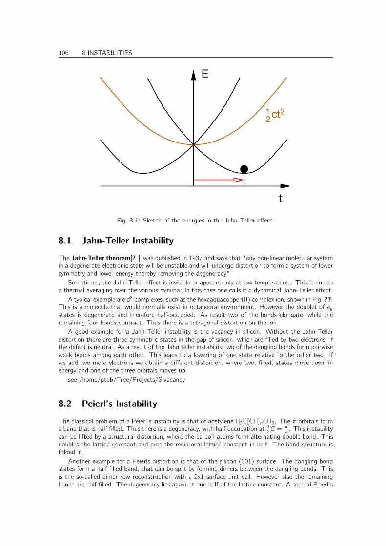
106 8 INSTABILITIES
ct212
E
t
Fig. 8.1: Sketch of the energies in the Jahn-Teller effect.
8.1 Jahn-Teller Instability
The Jahn-Teller theorem[? ] was published in 1937 and says that "any non-linear molecular systemin a degenerate electronic state will be unstable and will undergo distortion to form a system of lowersymmetry and lower energy thereby removing the degeneracy"
Sometimes, the Jahn-Teller effect is invisible or appears only at low temperatures. This is due toa thermal averaging over the various minima. In this case one calls it a dynamical Jahn-Teller effect.
A typical example are d8 complexes, such as the hexaaquacopper(II) complex ion, shown in Fig. ??.This is a molecule that would normally exist in octahedral environment. However the doublet of egstates is degenerate and therefore half-occupied. As result two of the bonds elongate, while theremaining four bonds contract. Thus there is a tetragonal distortion on the ion.
A good example for a Jahn-Teller instability is the vacancy in silicon. Without the Jahn-Tellerdistortion there are three symmetric states in the gap of silicon, which are filled by two electrons, ifthe defect is neutral. As a result of the Jahn teller instability two of the dangling bonds form pairwiseweak bonds among each other. This leads to a lowering of one state relative to the other two. Ifwe add two more electrons we obtain a different distortion, where two, filled, states move down inenergy and one of the three orbitals moves up.
see /home/ptpb/Tree/Projects/Sivacancy
8.2 Peierl’s Instability
The classical problem of a Peierl’s instability is that of acetylene H2C[CH]nCH2. The π orbitals forma band that is half filled. Thus there is a degeneracy, with half occupation at 1
2G = πa . This instability
can be lifted by a structural distortion, where the carbon atoms form alternating double bond. Thisdoubles the lattice constant and cuts the reciprocal lattice constant in half. The band structure isfolded in.
Another example for a Peierls distortion is that of the silicon (001) surface. The dangling bondstates form a half filled band, that can be split by forming dimers between the dangling bonds. Thisis the so-called dimer row reconstruction with a 2x1 surface unit cell. However also the remainingbands are half filled. The degeneracy lies again at one-half of the lattice constant. A second Peierl’s

8 INSTABILITIES 107
Fig. 8.2: The Jahn-Teller effect is responsible for the tetragonal distortion of the hexaaquacopper(II)complex ion, [Cu(OH2)6]2+, which might otherwise possess octahedral geometry. The two axialCu-O distances are 238 pm, whereas the four equatorial Cu¡ÝO distances are 195 pm.
distortion leads to the buckled dimer reconstruction, where the electron from one dangling bond isshifted to the other partner of the dimer bond. This occurs in an alternating manner, so that theresulting unit cell is (2x2).

108 8 INSTABILITIES
H H H
HHHH
H
HHHH
H H H H
Eg
H
H
H
H
H
H
H
H H
H
H
H
H
H
H
H
H H
2aπ
ε
k
Fig. 8.3: Acetylene in the symmetric (top) and the broken symmetry state(bottom)
Fig. 8.4: Two subsequent Peierls distortions lead to the buckled dimer reconstruction of the Si(001)surface
8.3 Nesting
8.4 Other instabilities
The structural instabilities are not the only ones that are possible. Instead of distorting the structureits is possible to develop a spin-polarization, that is to form a ferromagnet or an antiferromagnet, orit is possible to form a charge density wave, or even a pairing of electron pairs into Cooper pairs toform a superconductor.
Important is that a large density of states at the Fermi level is always an indication that thesystem would like to undergo a symmetry breaking transition. Such systems tend to exhibit interestingproperties, which can be put into technological use. Which kind of transition actually occurs, however,depends a lot on the system.
Chapter 9
Ionic compounds
Besides the covalent bond the ionic bond is among the strongest. The differences between thecovalent and ionic bond have been discussed by Pauling[? ].
9.1 Oxidation states and charges
The concept of oxidation state has been introduced by the American chemist Wendell Latimer in1938 in his book "The Oxidation States of the Elements and Their Potentials in Aqueous Solution".The term oxidation state is simply another word for charge state1. The term is only very indirectlyrelated to oxygen or the process of oxidation.
A common misunderstanding is that charge states or oxidation states has something to do withthe charge distribution. In fact the charge distribution is surprisingly little affected by the oxidationstate. The reason is that the atomic electron of electropositive elements are located in a regionwhere in a compound the anions would be located. If the anion is charged, its orbitals expand so thatthe net change in the charge distribution is minute. The charge transfer is simply screened away.[?] Thus the electron density at the cation is little affected by the anions.
The oxidation states are tremendously helpful in understanding the electron levels. Thus if onewants to understand the stability of compounds or if one wants to understand the energetic positionof the energy levels the concept of formal oxidation states is extremely valuable.
9.2 Electronegativity, hardness and softness
Once the atoms are compressed, we can allow charge transfer, which is one mechanism to minimizethe energy. The total energy of an atom depends not only on the radius but also its total charge.
We can expand the energy of an isolated atom in a box in a Taylor expansion in the number N ofexcess electrons about the neutral state. We obtain
E(N) = E0 + ε0N +1
2UN2 for Nmin ≤ N ≤ Nmax (9.1)
Here ε is the highest occupied atomic orbital and U is the Coulomb interaction parameter of thatorbital. This equation is only valid as long as the same multiplet of energy levels is occupied2. Forexample, for an oxygen atom the number ∆N of excess electrons may vary from −4 to 2.
1For a definition see http://goldbook.iupac.org/O04365.html.2In reality the total energy consists of straight line segments between integer occupations. The above form is an
smooth interpolation, which may mimic broadening of the levels in an environment. Current density functionals producea similar as in Eq. ??
109
110 9 IONIC COMPOUNDS
The Coulomb interaction parameter U is also identified with hardness[? ] η. The hardness ofneutral atoms lies in the range between 2 eV and 7 eV.[? ].
The connection of the energy derivative with respect to charge and the energy of the highestoccupied electron level is not immediately apparent. It follows from Janak’s theorem[? ] withinDensity functional theory, which says
εn =∂E
∂fn
where εn is an one-particle level as obtained from density functional theory, E is the density functionaltotal energy and fn is the occupation of the level εn.
Let us consider a small model system of two atoms, that each have an energy of the form givenin Eq. ??. In addition we consider the Coulomb interaction between the two ions in case of chargetransfer. To simplify the model, we assume that the densities of the two atoms do not overlap, sothat we can calculation the Coulomb interaction from a point charge model.
At sufficient large separation d , the total energy of the two atoms A and B is
Etot(NA, NB) = EA,0 + εA,0NA +1
2UAN
2A︸ ︷︷ ︸
EA(NA)
+EB,0 + εB,0∆NC +1
2UBN
2B︸ ︷︷ ︸
EB(NB)
+e2NANB
4πε0d(9.2)
ε0 is a dielectric constant. While this minimum model is extremely crude, we will explore the chemicaltrends that can be deduced from it.
Let us determine charge transfer and binding energy, while requiring overall charge neutrality, thatis NA + NB = 0. The equilibrium condition,
∂Etot∂NA︸ ︷︷ ︸µA(NA)
+∂Etot∂NC︸ ︷︷ ︸µB(NB)
dNBdNA︸ ︷︷ ︸−1
= 0
implies that the chemical potentials µA and µB of the two atoms are identical. The chemicalpotential is defined as derivative of the total energy with respect to particle number
µ =∂E(N)
∂N
The minimum total energy 3 is
3Thus we obtain the minimum of the total energy Eq. ?? as
µA − µB = εA − εB +
[UA + UB −
e2
4πε0d
]NA = 0
NA =εB − εA
UA + UB − e2
4πε0d
∆E = −1
2
(εB − εA)2
UA + UB − e2
4πε0d
If the minimum or maximum charge transfer is reached, the binding energy is
∆E = (εA − εB)NX +1
2(UA + UB)N2
x

9 IONIC COMPOUNDS 111
The binding energy of two ions at large distance d is
∆E = −1
2
(εB − εA)2
UA + UB − e2
4πε0d
with NA = −NB =εB − εA
UA + UB − e2
4πε0d
(9.3)
for partial charge transfer and
∆E = (εA − εB)NX +1
2(UA + UB)N2
x with NA = −NB = NX (9.4)
for maximum charge transfer within one multiplet. The maximum of the two energies ∆E is thephysical one.
This model shows already that the charge transfer is driven by the difference of the energies ofthe highest atomic orbitals. This is obvious because the system can lower its energy by placing someof the electrons into a lower level.
9.2.1 The concept of electronegativity
The concept of electronegativity is directly related to the position of the highest occupied electronlevel. Electronegativity is considered as the tendency of an atom or a molecule to attract electrons.There are different definitions of electronegativity:
Paulings electronegativities
The original definition goes back to Linus Pauling[? ], who determined the electronegativity differenceof two species to
χA − χB = ±
√(Ed(AB)−
Ed(AA) + Ed(BB)
2
)1
eV
where Ed are the bond dissociation energies. The Pauling electronegativities cover the range from0.7 to 4.0.
Using our simple model, we would obtain
χA − χB ≈
√1
2
(εB − εA)2
UA + UD
1
eV
Mulliken’s electronegativities
Mulliken introduced the concept of “absolute electronegativity”[? ] related to the mean value ofelectron affinity A and ionization potential I. Mulliken scaled the result in order to minimize thedeviation to Pauling’s electronegativity, and this posed the definition of the absolute or Mullikenelectronegativity to
χ =0.187
eV
I + A
2

112 9 IONIC COMPOUNDS
A
vacuum level
I
The ionization potential I is the energy required to remove an electron from a given atom orelectron. Thus the ionization potential is
I = E[N − 1]− E[N]
where N is the number of electrons. If N is the number of electrons for the neutral system, I iscalled the first ionization potential. If N is the number of electrons in the system with one positivecharge it is called the second ionization potential. For a solid, the first ionization potential is calledthe work function. If we remove the electron , it is placed far away from the atom. The potentialthere is the so-called vacuum level, which is assumed to be the zero of the energy scale.4
The electron affinity is the energy gained, when an atom or molecule captures an additionalelectron.
A = E[N]− E[N + 1]
Let us now return to our simple model for an atom Eq. ?? and determine the electro-negativity.We obtain
I = −ε0 +1
2U
A = −ε0 −1
2U
I + A
2= −ε0 = −
dE
dN
Thus we see that the electronegativity is directly related to the position of the highest occupiedorbital.
9.2.2 The concept of hardness
The second parameter in our model which determines the charge transfer in out model is the param-eter U, which is what chemists call hardness η. Hardness is defined as
η = I − A
Note that the definition of hardness often carries an additional factor 12 .
Related to hardness is the softness which is the inverse of hardness.If we determine the hardness in our model we obtain
η = U =d2E
dN
4Note that the vacuum level is not a well defined quantity, if the system is infinite. The dipole of a material cancause the vacuum level to assume different values over different surfaces of an extended material.

9 IONIC COMPOUNDS 113
9.2.3 Hard-Soft Acid-Base (HSAB) principle
In 1963 Pearson introduced the HSAB principle[? ].
HSAB PRINCIPLE
All other factors being equal (namely the strength of acids and bases), hard acids prefer to bind tohard bases and soft acids prefer to bind to soft bases.
A theoretical basis for the HSAB principle has been given by Parr et al.[? ].The principle is based on the following exchange reaction between a hard acid Ah, a hard base
Bh, a soft acid As and a soft base Bs .
AhBs + AsBh ⇒ AhBh + AsBs
It says that if the electronegativities of acids are equal and that of the bases are equal, the followingrelation holds.
∆EAhBh + ∆EAsBs − ∆EAhBs + ∆EAsBh < 0
Following Ayers et al.[? ], we may use our model Eq. ?? for the binding energy. The HSABprinciple says that, if the electronegativities are equal, i.e.
εAh = εAs and εBh = εBs ,
the following identity holds
0 > ∆EAhBh + ∆EAsBs − ∆EAhBs + ∆EAsBh
= −1
2
(εAh − εBh)2
UAh + UBh−
1
2
(εAs − εBs )2
UAs + UBs+
1
2
(εAs − εBh)2
UAs + UBh+
1
2
(εAh − εBs )2
UAh + UBs
= −(εA − εB)2
2
(+
1
UAh + UBh+
1
UAs + UBs−
1
UAs + UBh−
1
UAh + UBs
)= −
(εA − εB)2
2
(UAs + UBs + UAh + UBh(UAh + UBh)(UAs + UBs )
−UAs + UBh + UAh + UBs(UAs + UBh)(UAh + UBs )
)= −
(εA − εB)2
2(UAs + UBs + UAh + UBh)
(1
(UAh + UBh)(UAs + UBs )−
1
(UAs + UBh)(UAh + UBs )
)= −
(εA − εB)2
2(UAs + UBs + UAh + UBh)
((UAs + UBh)(UAh + UBs )− (UAh + UBh)(UAs + UBs )
(UAh + UBh)(UAs + UBs )(UAs + UBh)(UAh + UBs )
)= −
(εA − εB)2
2
UAs + UBs + UAh + UBh(UAh + UBh)(UAs + UBs )(UAs + UBh)(UAh + UBs )
×(
[UAsUAh + UAsUBs + UBhUAh + UBhUBs ]− [UAhUAs + UAhUBs + UBhUAs + UBhUBs ]
)= −
(εA − εB)2
2
UAs + UBs + UAh + UBh(UAh + UBh)(UAs + UBs )(UAs + UBh)(UAh + UBs )
×(
+UAsUBs + UBhUAh − UAhUBs − UBhUAs)
= −(εA − εB)2
2
UAs + UBs + UAh + UBh(UAh + UBh)(UAs + UBs )(UAs + UBh)(UAh + UBs )
((UAh − UAs )(UBh − UBs )
)︸ ︷︷ ︸
>0
q.e.d.
9.3 Van Arkel Ketelaar triangle
The Van Arkel-Ketelaar triangle allows to classify solids according to the electronegativities of theirconstituents. There are two main axes:
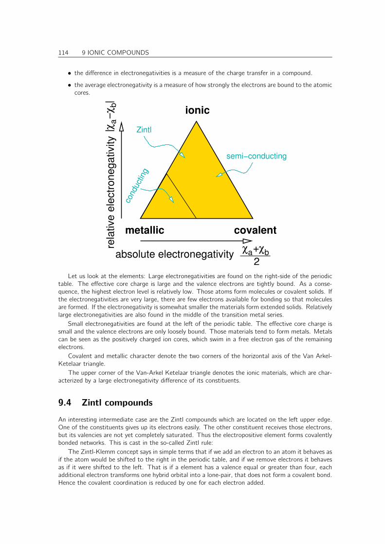
114 9 IONIC COMPOUNDS
• the difference in electronegativities is a measure of the charge transfer in a compound.
• the average electronegativity is a measure of how strongly the electrons are bound to the atomiccores.
χ χa b+
2
|χχ
ab
−|
absolute electronegativity
rela
tive
ele
ctr
on
eg
ativity
ionic
covalentmetallic
semi−conducting
Zintlco
nduct
ing
Let us look at the elements: Large electronegativities are found on the right-side of the periodictable. The effective core charge is large and the valence electrons are tightly bound. As a conse-quence, the highest electron level is relatively low. Those atoms form molecules or covalent solids. Ifthe electronegativities are very large, there are few electrons available for bonding so that moleculesare formed. If the electronegativity is somewhat smaller the materials form extended solids. Relativelylarge electronegativities are also found in the middle of the transition metal series.
Small electronegativities are found at the left of the periodic table. The effective core charge issmall and the valence electrons are only loosely bound. Those materials tend to form metals. Metalscan be seen as the positively charged ion cores, which swim in a free electron gas of the remainingelectrons.
Covalent and metallic character denote the two corners of the horizontal axis of the Van Arkel-Ketelaar triangle.
The upper corner of the Van-Arkel Ketelaar triangle denotes the ionic materials, which are char-acterized by a large electronegativity difference of its constituents.
9.4 Zintl compounds
An interesting intermediate case are the Zintl compounds which are located on the left upper edge.One of the constituents gives up its electrons easily. The other constituent receives those electrons,but its valencies are not yet completely saturated. Thus the electropositive element forms covalentlybonded networks. This is cast in the so-called Zintl rule:
The Zintl-Klemm concept says in simple terms that if we add an electron to an atom it behaves asif the atom would be shifted to the right in the periodic table, and if we remove electrons it behavesas if it were shifted to the left. That is if a element has a valence equal or greater than four, eachadditional electron transforms one hybrid orbital into a lone-pair, that does not form a covalent bond.Hence the covalent coordination is reduced by one for each electron added.

9 IONIC COMPOUNDS 115
This rule simply reflects the observation motivated earlier that the coordination of main groupelements is largely given by the number of valence electrons.
A good example for Zintl compounds are the Sr-silicides.
Fig. 9.1: Sr silicides: top SrSi2; bottom left SrSi; bottom left Sr5Si3.
Silicon is a four valent element and crystallizes in the diamond structure,where each atom istetrahedrally, that is four-fold, coordinated. If we form a silicide each strontium atom donates twoelectrons to the silicon network. Depending on the amount of Sr atoms, the silicon network receivesa certain number of electrons. It becomes iso-electronic to phosphorus, sulfur, chlorine or argon.
• In SrSi2 each silicon receives one additional electron. Hence it behaves similar to a phosphorusatom, that likes to form the bonds. Indeed the silicon network of SrSi2 is a three fold coordinatednetwork.
• In SrSi. each electron receives two electrons, and behaves like sulfur. That is it forms chainsof two-fold coordinated silicon atoms.
• In Sr5Si3, ten electrons are distributed over three silicon atoms. This is sufficient to form twoSi3− ions and one Si4− ion. The Si3− ions have one half occupied orbital left and combine toform dimers, while the remaining Si4− is isoelectronic to argon and forms an isolated ion.
The Zintl-Klemm concept is fairly general. Most of the concepts of covalent bonding where basedon the number of electrons available, and on the special role of d-electrons, (f-electrons play again aspecial role.) When we move vertically in the periodic table the electron count remains unchanged if
116 9 IONIC COMPOUNDS
we move horizontally, while keeping the number of electrons unchanged, the main difference is thatwe add a charge to the nucleus. This charge shifts the electron levels up and down, but does notaffect the nature of these electron levels. The effect is a change in the electronegativity, that is theability of hold on to its own electrons, respectively to attract further electrons.
We observe a similar effect in molecules. For example the ammonium ion NH+4 , the borohydride
ion5 BH−4 are iso-electronic to methane CH4 and hence form a tetrahedral structure.The carbocation CH+3 is iso-electronic to BH3 and forms the same structure, namely a trigo-
nal planar structure6. On the other hand H3C− ion and ammonium NH3 form an umbrella like atetrahedron with a missing corner.
9.5 Madelung constants
The electrostatic energy can be approximated by a point charge model. The evaluation is non-trivial,because the lattice sums over the pairwise interactions converges poorly due to the long-rangednature of the Coulomb interaction.
Ewald[? ] proposed the Ewald sum technique, which divides the electrostatic energy into twoparts: One is the electrostatic interaction of atom-centered spherical densities of Gaussian shape andis evaluated by a sum in reciprocal space. The other is the difference of the electrostatic interactionbetween point charges and these Gaussians. This results in a short ranged pair potential that can bedetermined by a real space sum.
For binary compounds, the electrostatic energy per ion can be expressed by aMadelung constantA
Emad =1
2∑
i
∑i ,j
QiQj
4πε|~Ri − ~Rj |=A
n
Q1Q2
4πε0d(9.5)
where n is the number of ions in the unit cell, A is the Madelung constant Q1 and Q2 are the chargesfor cations and anions and d is the smallest distance between cations and anions. Clearly this equationis restricted to binary systems.
We see that the Madelung constants per ion are fairly similar. This is not a result that can begeneralized to arbitrary structure. Probably it is an expression of the fact that ionic crystals formstructures with a large Madelung energy, because that makes them more stable. On the other hand,even for a diatomic molecule made out of two dimers the value of A/n is 1
2 , not too far form theother values.
For NaCl, with a nearest neighbor distance of 2.814 Åwe obtain an electrostatic energy of 3.6 eV.
9.6 Born-Mayer Equation
If one includes the Pauli- or Born repulsion between the ions, one obtains an estimate for thecomplete energy of a ionic crystal. One can use an exponential ansatz for the Pauli repulsion, namely
Erep = be−dρ
where ρ = 0.345 Å is a approximate constant determined empirically.The constant b can be determined from the lattice constant. The total energy is
E(d) = be−dρ +
A
n
Q1Q2
4πε0d(9.6)
5see sodium borohydrate NaBH46borane dimerizes to form B2H6.and exists in its molecular form only in the gas phase.

9 IONIC COMPOUNDS 117
A n An
sodium chloride 1.74756 2 0.8878cesium chloride 1.76267 2 0.881335fluorite 2.5194 3 0.8398corundum 4.1719 5 0.83438wurtzite 1.64132 2 0.82065zincblende 1.63805 2 0.81925sphalerite 1.6381 2 0.81905rutile 2.408 3 0.802667cuprite 2.0577 3 0.6859anatase 2.400 3 0.8CdI2 2.35 3 0.78333β-quartz 2.2197 3 0.7399dimer 1 2 0.5
Table 9.1: Madelung constants for binary ionic solids[? ]. E = A QAQB4πε0|d | where d is the smallest
anion-cation distance. (Not all values have been taken from Pauling’s book)
At the equilibrium distance the force must vanish, that is
dE
dd
∣∣∣∣d0
= −b
ρe−
d0ρ −
A
n
Q1Q2
4πε0d20
= 0
b = −A
n
Q1Q2
4πε0d20
ρe+d0ρ
Now we insert b into Eq. ?? and obtain
E =A
n
Q1Q2
4πε0d0
(1−
ρ
d0
)(9.7)
This is the so-called Born-Mayer equation.For NaCl, the shortest distance d0 between ions is 2.82 Å, which leads to a reduction of the total
energy relative to the electrostatic energy by about 12 %.
9.7 Kapustinskii Equation
Kapustinskii[? ] recognized that the Madelung constant divided by the number of ions in the unitcell leads to nearly the same value for a variety of structures. The resulting value increases withcoordination number. However since also the distance increases with coordination the result balancesout. That is he postulates that
A
n
is a constant. A is the Madelung constant, n the number of ions in the unit cell and rA + rB is thesum of the ionic radii.
Kapustinskii estimates the minimum distance from the ionic radii and replaces the Madelungconstant by that of the NaCl structure (A/n=0.8878). The result is the Kapustinskii equation
E
n= 0.8878
QAQB4πε0(rA + rB)
(1−
ρ
rA + rB
)(9.8)

118 9 IONIC COMPOUNDS
which allows one to estimate the lattice energy even without knowing the structure! Thaw agreementwith the lattice energy for ionic materials is typically smaller than 5 %.
9.8 Born-Haber Cycle
The Born Haber cycle allows one to estimate the energy of reaction, when an ionic solid is formedfrom two elemental substances. Parts of the Born-Haber cycle can also be used to estimate thecohesive energy of an ionic substance.
21Na(s) 2+ Cl (g)
Na+(g) Cl−(g)
Ediss=122 kJ/molEsubl=108 kJ/mol
Elatt=−788 kJ/mol
Hf=474 kJ/mol∆
Na(g) Cl(g)
EA=−349 kJ/mol
+
IP=496 kJ/mol
NaCl(s)
Fig. 9.2: Born-Haber cycle of NaCl.
In the following we will use the energy unit kJ/mol. The conversion is 1 eV=96.485309 kJ/mol.For simple estimates one simply uses the factor 1 eV≈ 100 kJ/mol. Part of the calculation will bedone in Hartree atomic units, defined by ~ = e = me = 4πε0 = 1. The unit of energy in the Hartreeatomic unit system is the Hartree: 1 H=27.211396 eV=2625.5 kJ/mol. The unit of length in theHartree atomic unit system is the Bohr radius 1 a0=0.5291772 Å=0.5291772× 10⁻¹⁰ m.
Let us consider a simple example:
1. We start out from metallic sodium and gaseous chlorine. First we need to decompose theelemental materials into its atoms. In the case of chlorine this is heat of dissociation, whichis 122 kJ/mole for Cl2. For the metal it is the sublimation energy 108 kJ/mol. Per formulaunit we need to supply 1
2 · 122 + 108 kJ/mol=169 kJ/mol, in order to form isolated atoms.
2. The next step is to convert the atoms into the respective ions. The energy to remove anelectron from an atom and place it at infinity is the first ionization potential. For Na it has thevalue of 496 kJ/mol. The energy to add an electron to an atom is the electron affinity. ForCl it has the value of -349 kJ/mol. Thus we need to supply 147 kJ/mol to convert the atomsinto ions.
3. Finally we need to bring the ions together to form the ionic solid. The lattice energy of NaCLis −788 kJ/mol .
4. If we add the three energy contributions together we obtain the heat of formation of sodiumchloride, namely 474 kJ/mol.

9 IONIC COMPOUNDS 119
Let us investigate the lattice energy.
• Using only the Madelung energy of sodium chloride,we obtain
Elatt = nA
n×Q1Q24πε0d = 0.3279H = 861kJ/mol.
The madelung constant for sodium chloride structure is A = 1.74756. The number of ions performula unit is n = 2. The interatomic distance is dNa−Cl = 2.82 Å=5.329 a0.In atomic unitse = 4πε0 = 1. Thus we obtain in Hartree atomic units an energy of Elatt = 0.3279 H.(Hstands for Hartree, the energy unit of the Hartree atomic unit system. 1H=2625.5 kJ/mol.)
• Using the Born-Mayer equation Eq. ?? we obtain Elatt = 756 kJ/mol. The error is 30 kJ/mol,that is about 0.3 eV.
9.9 Pauling bonding rules
Another approach to think about coordination has been given by Pauling7 Pauling set up a numberof rules that hold pretty well for ionic compounds[? ]. The rationale behind is that ions would like topack together as much as possible, in order to maximize the electrostatic attraction of opposite ions.However, each ion has a natural radius at which the wave functions overlap so much that they repeleach other appreciably. Thus, the structure according to this model is given by a balance betweenPauli repulsion of the electronic shells and the Coulomb attraction on the other. The stronger thecovalent contribution, the less reliable are these rules.
• Pauling’s first rule: “A coordinated polyhedron of anions is formed about each cation,the cation-anion distance being determined by the radius sum, and the ligancy of thecation by the radius ratio.” (See [? ], p544.)
The rationale is that if the anions are too large, the Pauli repulsion between the anions wouldprevent them to come close to the cation.
The ratio of the radii in Tab. ?? is calculated assuming the ions as hard spheres. The opti-mum structures have touching cation-anion distances so that the electrostatic interaction ismaximized. On the other hand the anions must not overlap due to their Pauli repulsion.
– trigonal planar: The centers of the anions form an equilateral triangle which has anglesof 60.
rArC + rA
= cos(30) =1
2
√3 ;
rCrA
=2√3− 1
– tetrahedral: the rectangle is a diagonal place through the cube. The base has a lengthof√
2a = 2rA. Cation and anion are connected by a main diagonal through the cube.Therefore rA + rC = 1
2
√3a.
rA + rCrA
=12
√3a
12
√2a
=
√3
2;
rCrA
=
√3
2− 1
– octahedral or square planar:
rA + rCrA
=12
√2a
12a
=√
2 ;rCrA
=√
2− 1
– square anti prism. The square antiprism is like a cube with the top face rotated by 45
about the vertical axis. Because the anions move closer together the space for the cationis smaller than in the cube.
7Apparently[? ], the radius ratio’s, which are part of the rules go back to the Austrian chemist G.F. Hüttig[? ].
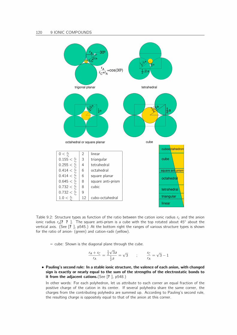
120 9 IONIC COMPOUNDS
a3
a12
3
a12 2
12
a
r +r AC
rA 30o
rA
rC+rA=cos(30o)
cube
2a12
1a
2
21 a2
1
octahedral or square planar
trigonal planar tetrahedral
0 < rcra
2 linear0.155 < rc
ra3 triangular
0.255 < rcra
4 tetrahedral0.414 < rc
ra6 octahedral
0.414 < rcra
6 square planar0.645 < rc
ra8 square anti-prism
0.732 < rcra
8 cubic0.732 < rc
ra9
1.0 < rcra
12 cubo-octahedral
square anti prism
triangular
tetrahedral
linear
octahedral
cubooctahedron
cube
Table 9.2: Structure types as function of the ratio between the cation ionic radius rc and the anionionic radius ra[? ? ]. The square anti-prism is a cube with the top rotated about 45 about thevertical axis. (See [? ], p545.) At the bottom right the ranges of various structure types is shownfor the ratio of anion- (green) and cation-radii (yellow).
– cube: Shown is the diagonal plane through the cube.
rA + rCrA
=12
√3a
12a
=√
3 ;rCrA
=√
3− 1
• Pauling’s second rule: In a stable ionic structure, the valence of each anion, with changedsign is exactly or nearly equal to the sum of the strengths of the electrostatic bonds toit from the adjacent cations.(See [? ], p548.)
In other words: For each polyhedron, let us attribute to each corner an equal fraction of thepositive charge of the cation in its center. If several polyhedra share the same corner, thecharges from the contributing polyhedra are summed up. According to Pauling’s second rule,the resulting charge is oppositely equal to that of the anion at this corner.

9 IONIC COMPOUNDS 121
Pauling calls this rule the “electrostatic valence rule”. This rule corresponds to the requirementof local charge neutrality.
• Pauling’s third rule: The presence of shared edges and especially shared faces in acoordinated structure decreases its stability; this effect is large for cations with largevalence and small ligancy.” (See [? ], p559.) In other words, Corner-joined polyhedra aremore favorable than edge sharing polyhedra, which, in turn, are more favorable than face-sharingpolyhedra.
This rule is justified because the ions of same character, say the cations in the center of thepolyhedra, would like to stay as far away from each other as possible in order to minimize theirelectrostatic repulsion.
• Pauling’s fourth rule: “In a crystal containing different cations, those with large valenceand small coordination number tend not to share polyhedron elements with each other”(See [? ], p561.)
• Pauling’s fifth rule: Structures will form from only few component elements.
The rationale behind this weakest rule of Pauling is that for a material with many componentsit is likely that there is a phase separation, which withdraws one element from the mixture.
I did not find this rule in the Book by Pauling. It is mentioned however in [? ]

122 9 IONIC COMPOUNDS
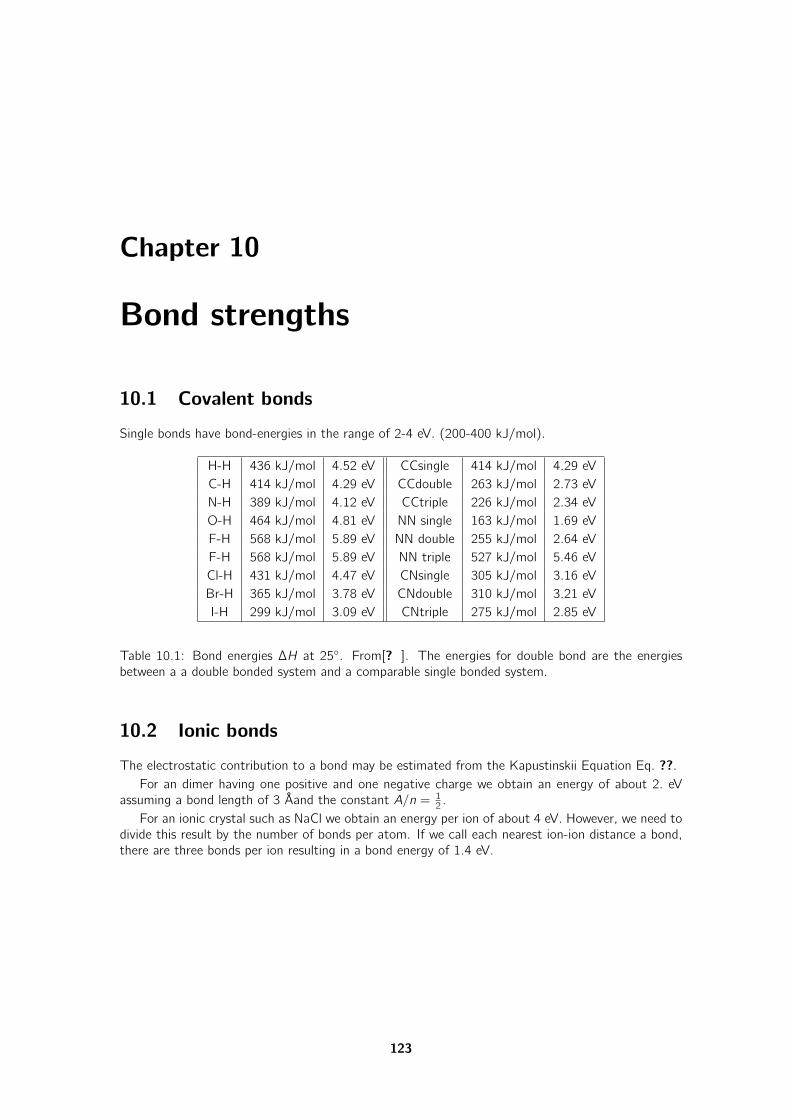
Chapter 10
Bond strengths
10.1 Covalent bonds
Single bonds have bond-energies in the range of 2-4 eV. (200-400 kJ/mol).
H-H 436 kJ/mol 4.52 eV CCsingle 414 kJ/mol 4.29 eVC-H 414 kJ/mol 4.29 eV CCdouble 263 kJ/mol 2.73 eVN-H 389 kJ/mol 4.12 eV CCtriple 226 kJ/mol 2.34 eVO-H 464 kJ/mol 4.81 eV NN single 163 kJ/mol 1.69 eVF-H 568 kJ/mol 5.89 eV NN double 255 kJ/mol 2.64 eVF-H 568 kJ/mol 5.89 eV NN triple 527 kJ/mol 5.46 eVCl-H 431 kJ/mol 4.47 eV CNsingle 305 kJ/mol 3.16 eVBr-H 365 kJ/mol 3.78 eV CNdouble 310 kJ/mol 3.21 eVI-H 299 kJ/mol 3.09 eV CNtriple 275 kJ/mol 2.85 eV
Table 10.1: Bond energies ∆H at 25. From[? ]. The energies for double bond are the energiesbetween a a double bonded system and a comparable single bonded system.
10.2 Ionic bonds
The electrostatic contribution to a bond may be estimated from the Kapustinskii Equation Eq. ??.For an dimer having one positive and one negative charge we obtain an energy of about 2. eV
assuming a bond length of 3 Åand the constant A/n = 12 .
For an ionic crystal such as NaCl we obtain an energy per ion of about 4 eV. However, we need todivide this result by the number of bonds per atom. If we call each nearest ion-ion distance a bond,there are three bonds per ion resulting in a bond energy of 1.4 eV.
123

124 10 BOND STRENGTHS
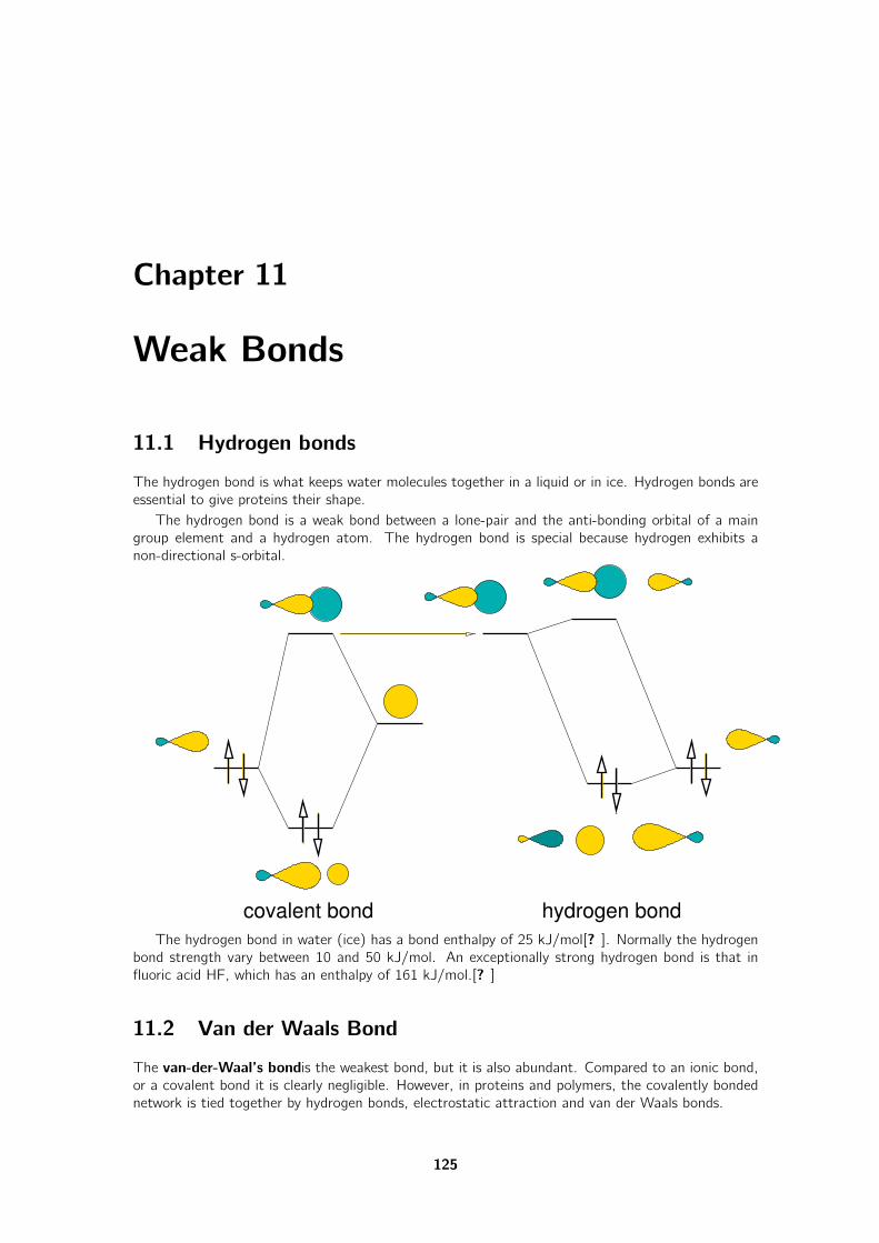
Chapter 11
Weak Bonds
11.1 Hydrogen bonds
The hydrogen bond is what keeps water molecules together in a liquid or in ice. Hydrogen bonds areessential to give proteins their shape.
The hydrogen bond is a weak bond between a lone-pair and the anti-bonding orbital of a maingroup element and a hydrogen atom. The hydrogen bond is special because hydrogen exhibits anon-directional s-orbital.
covalent bond hydrogen bond
The hydrogen bond in water (ice) has a bond enthalpy of 25 kJ/mol[? ]. Normally the hydrogenbond strength vary between 10 and 50 kJ/mol. An exceptionally strong hydrogen bond is that influoric acid HF, which has an enthalpy of 161 kJ/mol.[? ]
11.2 Van der Waals Bond
The van-der-Waal’s bondis the weakest bond, but it is also abundant. Compared to an ionic bond,or a covalent bond it is clearly negligible. However, in proteins and polymers, the covalently bondednetwork is tied together by hydrogen bonds, electrostatic attraction and van der Waals bonds.
125
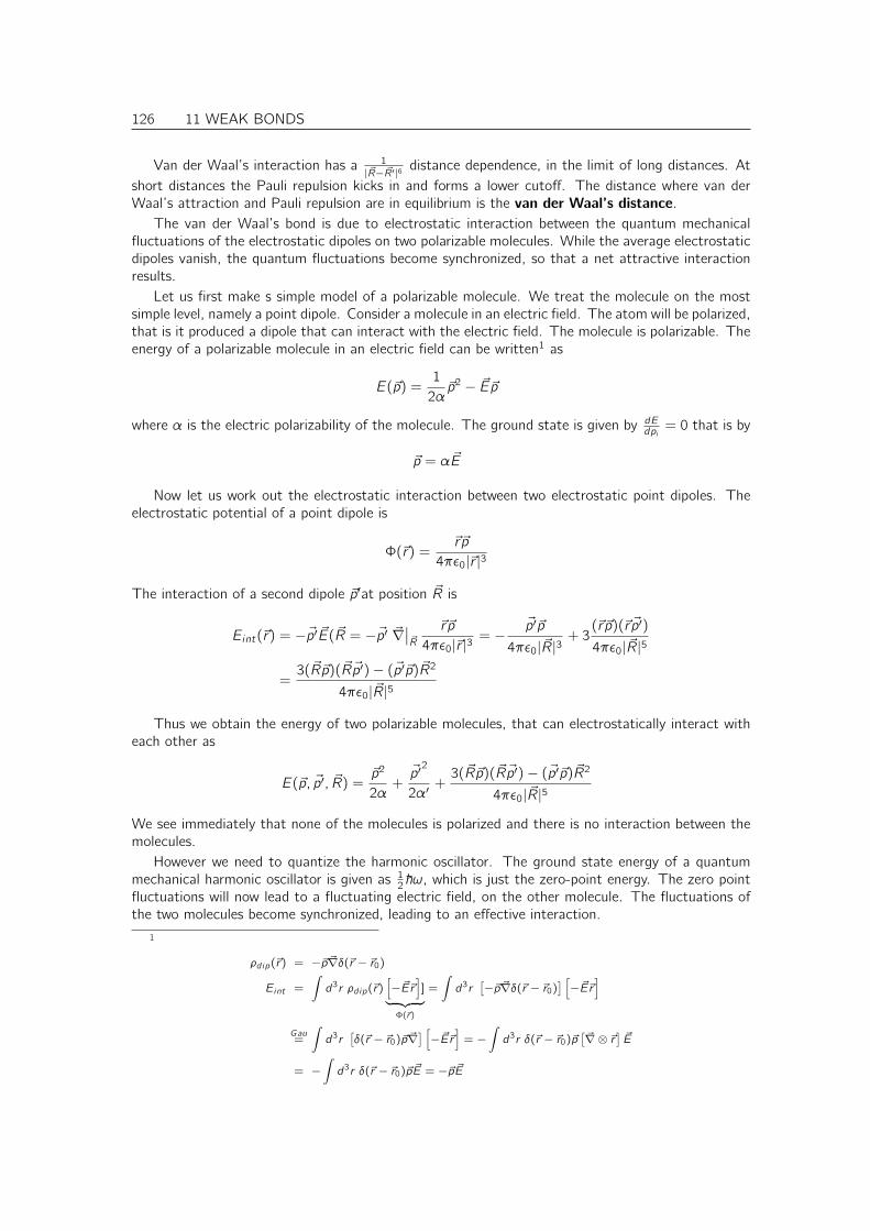
126 11 WEAK BONDS
Van der Waal’s interaction has a 1
|~R− ~R′|6 distance dependence, in the limit of long distances. Atshort distances the Pauli repulsion kicks in and forms a lower cutoff. The distance where van derWaal’s attraction and Pauli repulsion are in equilibrium is the van der Waal’s distance.
The van der Waal’s bond is due to electrostatic interaction between the quantum mechanicalfluctuations of the electrostatic dipoles on two polarizable molecules. While the average electrostaticdipoles vanish, the quantum fluctuations become synchronized, so that a net attractive interactionresults.
Let us first make s simple model of a polarizable molecule. We treat the molecule on the mostsimple level, namely a point dipole. Consider a molecule in an electric field. The atom will be polarized,that is it produced a dipole that can interact with the electric field. The molecule is polarizable. Theenergy of a polarizable molecule in an electric field can be written1 as
E(~p) =1
2α~p2 − ~E~p
where α is the electric polarizability of the molecule. The ground state is given by dEdpi
= 0 that is by
~p = α~E
Now let us work out the electrostatic interaction between two electrostatic point dipoles. Theelectrostatic potential of a point dipole is
Φ(~r) =~r ~p
4πε0|~r |3
The interaction of a second dipole ~p′at position ~R is
Eint(~r) = −~p′ ~E(~R = −~p′ ~∇∣∣~R
~r ~p
4πε0|~r |3= −
~p′~p
4πε0|~R|3+ 3
(~r ~p)(~r ~p′)
4πε0|~R|5
=3(~R~p)(~R~p′)− (~p′~p)~R2
4πε0|~R|5
Thus we obtain the energy of two polarizable molecules, that can electrostatically interact witheach other as
E(~p, ~p′, ~R) =~p2
2α+~p′
2
2α′+
3(~R~p)(~R~p′)− (~p′~p)~R2
4πε0|~R|5
We see immediately that none of the molecules is polarized and there is no interaction between themolecules.
However we need to quantize the harmonic oscillator. The ground state energy of a quantummechanical harmonic oscillator is given as 1
2~ω, which is just the zero-point energy. The zero pointfluctuations will now lead to a fluctuating electric field, on the other molecule. The fluctuations ofthe two molecules become synchronized, leading to an effective interaction.
1
ρdip(~r) = −~p~∇δ(~r − ~r0)
Eint =
∫d3r ρdip(~r)
[−~E~r
]]︸ ︷︷ ︸
Φ(~r)
=
∫d3r
[−~p~∇δ(~r − ~r0)
] [−~E~r
]
Gau=
∫d3r
[δ(~r − ~r0)~p~∇
] [−~E~r
]= −
∫d3r δ(~r − ~r0)~p
[~∇⊗ ~r
]~E
= −∫d3r δ(~r − ~r0)~p ~E = −~p ~E
11 WEAK BONDS 127
We need to derive the frequencies of the system of two dipoles. This can be done classically. Letus decompose the energy into its eigenmodes. We can use symmetry to decompose the eigenvectorsof the Hessian matrix d2E
dpidpj.
5
3
1 2
4
6
E1(x) =1
αx2 +
2x2
4πε0|~R|3with ~p = x~ex ; ~p′ = x~ex
E2(x) =1
αx2 −
2x2
4πε0|~R|3with ~p = −x~ex ; ~p′ = x~ex
E3(x) =1
αα2 −
x2
4πε0|~R|3with ~p = x~ez ; ~p′ = x~ez
E4(x) =1
αα2 +
x2
4πε0|~R|3with ~p = −x~ez ; ~p′ = x~ez
E5(x) =1
αα2 −
x2
4πε0|~R|3with ~p = x~ey ; ~p′ = x~ey
E6(x) =1
αα2 +
x2
4πε0|~R|3with ~p = −x~ey ; ~p′ = x~ey
These equations give us right away the force constants for all six modes. if we assume an isotropicmass m for the dipole dynamics, we obtain the zero-point energy as
E =
6∑i=1
~ωi =∑i=16
~√cim
=~√αm
[√1 +
2α
4πε0|~R|3+
√1−
2α
4πε0|~R|3+ 2
√1 +
α
4πε0|~R|3+ 2
√1−
α
4πε0|~R|3
)
For long distances |R| we can consider α
4πε|~R|3 as small quantity and restrict ourselves to the
leading order term in the Taylor expansion. The Taylor expansion of the square root is√
1 + ∆ =1 + 1
2 ∆− 18 ∆2 +O(∆3). We obtain
E(~R) =~√αm
[6−
3
4
(α
4πε|~R|3
)2
+O(1
|R|9 )
]The constant is irrelevant and the distance dependent term is the Van der Waals interaction
EV dW (|~R|) = −~√αm
3
4
(α
4πε0|~R|3
)2
= −3~α 3
2
4(4πε0)2√m
1
|~R|6

128 11 WEAK BONDS
In this formula the mass has no physical significance other that ω =√
cm is the frequency of the
dipole oscillation. The dipole oscillation frequency can be related to the optical excitation frequencyof the isolated molecule, respectively the band gap. Thus we find the approximate relation
~√c
m= Eg
The force constant is that of the isolated molecule, that is 1α , which yields
√m =
~Eg√α
This leads to the final expression for the Van der Waal’s energy
EV dW (|~R|) = −3Egα
2
4(4πε0)2
1
|~R|6
Chapter 12
Crystal structures
The zoo of crystal structures can be very confusing. At first sight the atoms seem to be able toorganize in any possible arrangement. However there are some characteristics, that allows us to bringsome order into the chaos.
As with the electronic states there is a long-ranged view and a short ranged view. The long-ranged view of crystals are the symmetry groups and lattice types. The short ranged view discussescoordination polyhedra, bond numbers etc.
Here we will first provide the general principles, and then we will discuss the crystal structures inthe light of these patterns.
A useful online resource on crystal structures is the AFLOW library of Crystallographic proto-types[? ? ] http://aflowlib.org/CrystalDatabase/prototype_index.html.
12.1 Bravais lattices
There are 14 different lattice types in three dimensions. They are called Bravais lattices afterAuguste Bravais1
In a crystal the point groups symmetry is limited by the requirement of discrete translationalsymmetry. For example it is not possible to form a crystal with a five-fold symmetry axis. This doesnot imply that it is not possible to form materials with a five fold symmetry, but they cannot bedescribed by three translational lattice vectors. Such materials are called quasi crystals.
There are 14 Bravais lattices, which can be attributed to 7 crystal systems. For a given crystalsystem, there is always a primitive lattice, that is a lattice point at each corner of the unit cell, andvariants such as face-centered, body centered and base centered lattices.
• the cubic system has four three-fold rotation axes
• the hexagonal system has one six-fold rotation axes
• the trigonal (or rhombohedral) system has one three-fold rotation axes
• the tetragonal system has one four-fold rotation axis
• the orthorhombic system requires either three twofold axes of rotation or one twofold axis ofrotation and two mirror planes.
• the monoclinic system requires either one twofold axis of rotation or one mirror plane.
• the triclinic system contains no other symmetry than the translational symmetry, except theinversion.
1Auguste Bravais, 1811-1863. French Physicist
129
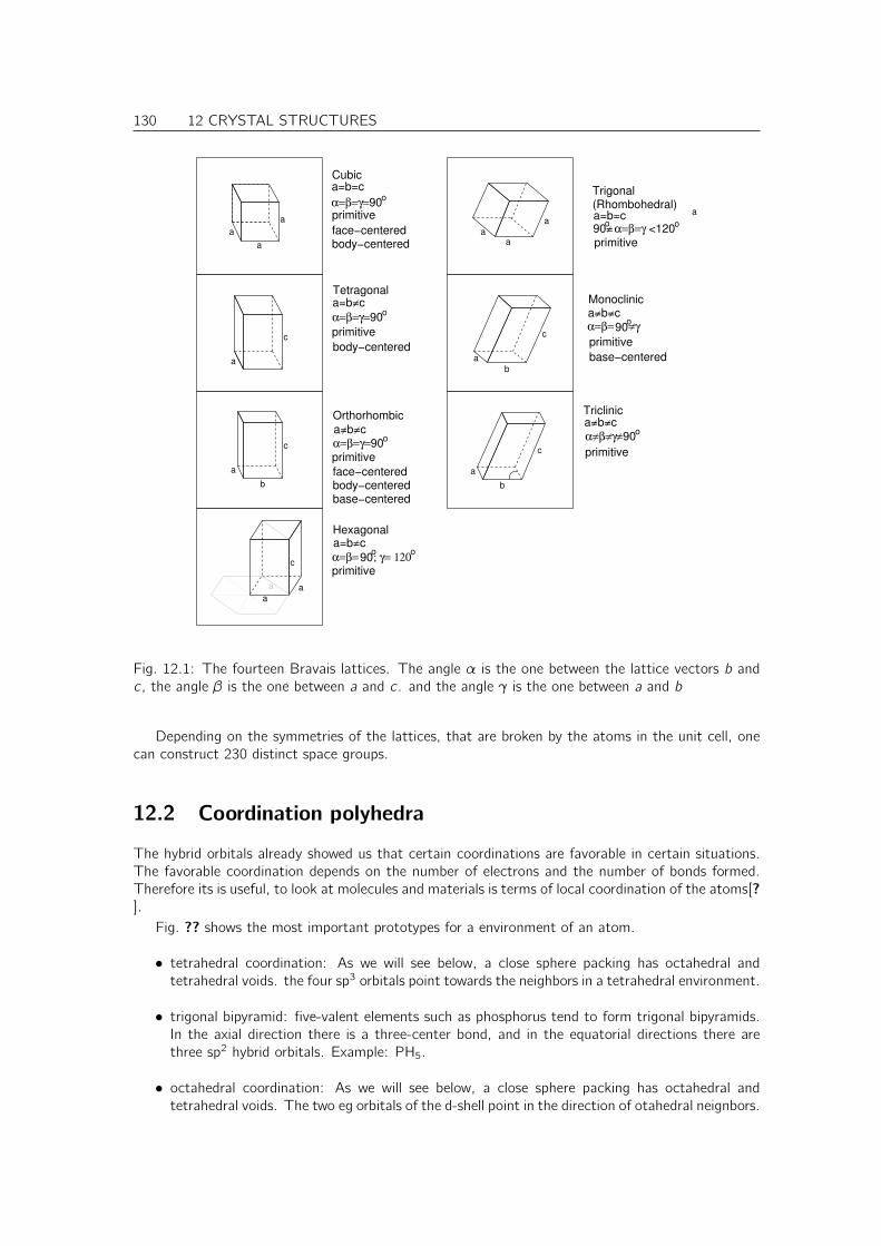
130 12 CRYSTAL STRUCTURES
Cubic
Orthorhombic
α=β= 120 ; γ=
Hexagonal
Monoclinic
α=β=γ 90= <120
Trigonal(Rhombohedral)
Triclinic
Tetragonal
face−centeredbody−centered
body−centered
primitive
primitive
primitive
primitive
face−centeredbody−centered
primitive
primitive
base−centered
primitive
base−centered
α=β=γ=90o
a=b=c
α=β=γ=90o
a=b=c
a=b=cα=β=γ=90
o
a=b=coo
90
a=b=c
90α=β= =γo
ooa=b=c
a=b=cα=β=γ=90
o
c
aa
a
a
a
a
a
c
a
c
b
aa
a
a
b
c
b
c
a
a
Fig. 12.1: The fourteen Bravais lattices. The angle α is the one between the lattice vectors b andc , the angle β is the one between a and c . and the angle γ is the one between a and b
Depending on the symmetries of the lattices, that are broken by the atoms in the unit cell, onecan construct 230 distinct space groups.
12.2 Coordination polyhedra
The hybrid orbitals already showed us that certain coordinations are favorable in certain situations.The favorable coordination depends on the number of electrons and the number of bonds formed.Therefore its is useful, to look at molecules and materials is terms of local coordination of the atoms[?].
Fig. ?? shows the most important prototypes for a environment of an atom.
• tetrahedral coordination: As we will see below, a close sphere packing has octahedral andtetrahedral voids. the four sp3 orbitals point towards the neighbors in a tetrahedral environment.
• trigonal bipyramid: five-valent elements such as phosphorus tend to form trigonal bipyramids.In the axial direction there is a three-center bond, and in the equatorial directions there arethree sp2 hybrid orbitals. Example: PH5.
• octahedral coordination: As we will see below, a close sphere packing has octahedral andtetrahedral voids. The two eg orbitals of the d-shell point in the direction of otahedral neignbors.

12 CRYSTAL STRUCTURES 131
cube8
3 trigonal planar 4 square planarlinear1
twinned cubo−octahedron12
trigonal bipyramid5 octahedrontetrahedron4 6
icosahedron12cubo−octahedron12
Fig. 12.2: Coordination polyhedra. The cubo-octahedron can be seen as an octahedron with thecorners chopped off.
• cubo-octahedron: the cubo-octahedron is the coordination of a face-centered cubic lattice, onetype of close sphere packing.
• twinned cubo-octahedron: the twinned cubo-octahedron is the coordination of a hexagonallyclose packed lattice, one type of close sphere packing.
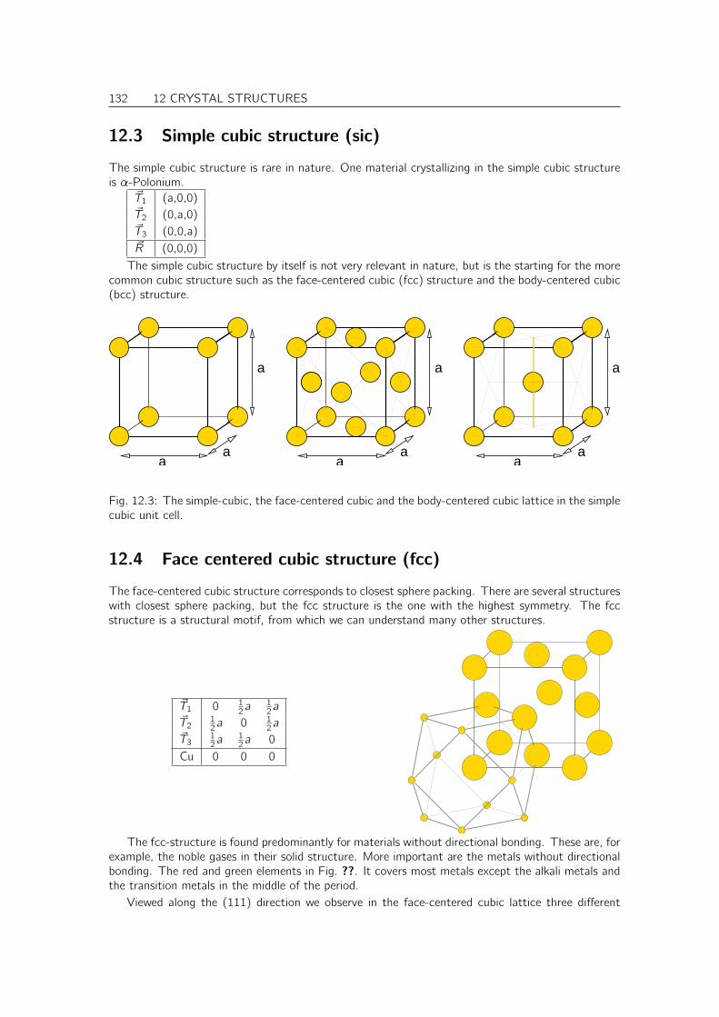
132 12 CRYSTAL STRUCTURES
12.3 Simple cubic structure (sic)
The simple cubic structure is rare in nature. One material crystallizing in the simple cubic structureis α-Polonium.
~T1 (a,0,0)~T2 (0,a,0)~T3 (0,0,a)~R (0,0,0)
The simple cubic structure by itself is not very relevant in nature, but is the starting for the morecommon cubic structure such as the face-centered cubic (fcc) structure and the body-centered cubic(bcc) structure.
aa
a
aa
a
aa
a
Fig. 12.3: The simple-cubic, the face-centered cubic and the body-centered cubic lattice in the simplecubic unit cell.
12.4 Face centered cubic structure (fcc)
The face-centered cubic structure corresponds to closest sphere packing. There are several structureswith closest sphere packing, but the fcc structure is the one with the highest symmetry. The fccstructure is a structural motif, from which we can understand many other structures.
~T1 0 12a
12a
~T212a 0 1
2a~T3
12a
12a 0
Cu 0 0 0
The fcc-structure is found predominantly for materials without directional bonding. These are, forexample, the noble gases in their solid structure. More important are the metals without directionalbonding. The red and green elements in Fig. ??. It covers most metals except the alkali metals andthe transition metals in the middle of the period.
Viewed along the (111) direction we observe in the face-centered cubic lattice three different
12 CRYSTAL STRUCTURES 133
H He
Be
Sc
Mg
Ti
CB ON F Ne
Ar
Rn
Kr
Xe
ClSPSiAl
Ca
Fr Ra
Ge
Sn
Tl
Ga
Pb
In
Se
PoBi
Sb
As
Te
At
I
Br
Hg
Cd
Zn
Au
Ag
CuMn Co Ni
Y ZrSr
Hf
Ac
La
Tc
Re Os Ir Pt
Ru PdRh
Li
Na
K
Rb
CsBa Ta W
MoNb
V Cr Fe
Fig. 12.4: Elements with fcc(red), hcp(green) and bcc(blue) structures.
layers, that can be denoted . . . ABCA . . .. Each layer consists of equilateral triangles. They differ intheir lateral position. The second most important close packing of equally sized spheres is the thehcp structure, where the layering is . . . ABAB . . ..
Most ionic materials such as oxides exhibit a face-centered cubic arrangement of anions. Theanions are much larger than most cations, so that they try to pack as closely as possible. Theanions distributed themselves over the interstitial places. The fcc structure contains tetrahedral andoctahedral interstitial places. Per fcc site there are two tetrahedral and one octahedral interstitialplace. They are located at the positions denoted by O for octahedral and T for tetrahedral in thefollowing table.
~T1 1 0 0~T1 0 1 0~T1 0 0 1atomic site 0 0 0atomic site 0 1
212
atomic site 12 0 1
2
atomic site 12
12 0
tetrahedral interstitial 14
14
14
tetrahedral interstitial 34
14
14
tetrahedral interstitial 14
34
14
tetrahedral interstitial 34
34
14
tetrahedral interstitial 14
14
34
tetrahedral interstitial 34
14
34
tetrahedral interstitial 14
34
34
tetrahedral interstitial 34
34
34
octahedral interstitial 12 0 0
octahedral interstitial 0 12 0
octahedral interstitial 0 0 12
octahedral interstitial 12
12
12
The coordination of each atom in the fcc structure is the cubo-octahedron and that of the hcpatom is the twinned cubo-octahedron shown in Fig. ??. Each atom has 12 nearest neighbors.
Elements that crystallize in the fcc structure[? ]: Al, Ni, Pd, Ir, Pb,Ca, Cu, Ag, Au, Yb.
134 12 CRYSTAL STRUCTURES
AB
C
AB
CA A
B BC C
Fig. 12.5: Sphere packing of face-centered cubic (fcc) and hexagonally closed-packed (hcp) struc-tures. The fcc structure, shown, occupies the sites in the sequence ABCABC, while the hexagonallyclosed packed structure occupies the sites with ABABAB
Fig. 12.6: Voids in the fcc structure. The filles circles denote the spheres of the loer layer and theempty circles are the spheres in the upper layer. The red star denotes an octahedral void enclosedby six spheres. The green triangle is a tetrahedral void enclosed by four spheres.
12.5 Structures derived from the fcc structure
12.5.1 Zinc-blende structure (ZnS)
If we start from the fcc structure and fill the one-half of the tetrahedral voids with the atoms of adifferent type we arrive at the zinc-blende structure.
12 CRYSTAL STRUCTURES 135
Fig. 12.7: Cation (gold) arrangement of a (111) plane of close-packed anions in octahedral voids.From left to right: Rocksalt structure (NaCl,MgO), corundum structure (Al2O3), rutile structure(TiO2), perovskite (CaTiO3) Calcium ions are drawn in pink. Editor: Rutile must be checked.Relation to anatase?
~T1 0 12a
12a
~T212a 0 1
2a~T3
12a
12a 0
Zn1 0 0 0S2
14a
14a
14a
Each atom in the zinc-blende structure is tetrahedrally coordinated by its four nearest neighbors.Thus it is ideal for ions with an average valence of four. Most compound semiconductors relevantfor semiconductor industry crystallize in this structure. Compound semiconductors are denoted asIV-IV, III-V, II-VI compounds according to the valency of their constituents.
IV-IV III-V II-VI I-VIIβ-SiC GaSb CuClSiGe GaAs
AlAs
The zinc-blende structure has large voids, namely in the center of the cube and in the middle ofits edges. These are the tetrahedral voids of the fcc structure that have not been filled yet.
The sublattices of both atom types again form two interwoven fcc lattices.The zincblende structure is identical to the diamond structure, with the only difference that
the two atoms are inequivalent. Each atom is tetrahedrally coordinated. Inside the structure largetetrahedral voids are present.
The zinc-blende structure can be seen as an fcc-lattice with one-half of the tetrahedral interstitialsites occupied by cations.
12.5.2 Diamond structure
A simpler variant of the zinc-blende structure is the diamond structure. The only difference to thezinc-blende structure is that all atoms are identical in the diamond structure.

136 12 CRYSTAL STRUCTURES
~T1 0 12a
12a
~T212a 0 1
2a~T3
12a
12a 0
C1 0 0 0C2
14a
14a
14a
Each atom is tetrahedrally coordinated. Inside the structure large tetrahedral voids are present,namely just the remaining tetrahedral voids of the fcc structure that has not been filled. tetrahedralvoids occupied.
Note the zig-zag chains running along the (110) directions.Both carbon and silicon crystallize in the diamond structure.
12.5.3 Fluorite structure (CaF2)
If we fill all the tetrahedral voids of the fcc structure with ions of a different type, we arrive at thefluorite structure. The formula unit for the fluorite structure is AB2.
Each fluorine is tetrahedrally coordinated with Ca atoms. Each calcium atom is centered in acube of eight fluorine atoms.Thus the calcium is has the same environment as an atom in the bccstructure. The fluorine ions form a simple-cubic structure among each other, with every secondcenter occupied by a calcium atom. Thus the fluorite structure is related to the CsCl structure suchthat only half of the cation positions of the CsCl structure are occupied.
~T1 0 12a
12a
~T212a 0 1
2a~T3
12a
12a 0
Ca1 0 0 0F1
14a
14a
14a
F214a
14a − 1
4a
Cubic unit cell (4 formula units)
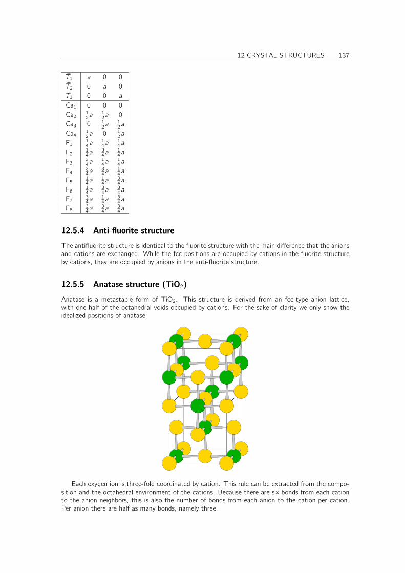
12 CRYSTAL STRUCTURES 137
~T1 a 0 0~T2 0 a 0~T3 0 0 a
Ca1 0 0 0Ca2
12a
12a 0
Ca3 0 12a
12a
Ca412a 0 1
2a
F114a
14a
14a
F214a
34a
14a
F334a
14a
14a
F434a
34a
14a
F514a
14a
34a
F614a
34a
34a
F734a
14a
34a
F834a
34a
34a
12.5.4 Anti-fluorite structure
The antifluorite structure is identical to the fluorite structure with the main difference that the anionsand cations are exchanged. While the fcc positions are occupied by cations in the fluorite structureby cations, they are occupied by anions in the anti-fluorite structure.
12.5.5 Anatase structure (TiO2)
Anatase is a metastable form of TiO2. This structure is derived from an fcc-type anion lattice,with one-half of the octahedral voids occupied by cations. For the sake of clarity we only show theidealized positions of anatase
Each oxygen ion is three-fold coordinated by cation. This rule can be extracted from the compo-sition and the octahedral environment of the cations. Because there are six bonds from each cationto the anion neighbors, this is also the number of bonds from each anion to the cation per cation.Per anion there are half as many bonds, namely three.

138 12 CRYSTAL STRUCTURES
The ideal structure shown above undergoes relaxations, which distorts the octahedra and makesthe angles on the three-fold coordinated oxygen ions more equal.
Anatase is the fcc-type variant of the rutile structure, which is based on an hcp-type anion lattice.
12.5.6 Bixbyite structure (Mn2O3)
The bixbyite structure is a variant of the fluorite structure with a quarter of oxygen atoms removed.The distribution of the oxygen vacancies is similar to sudoku game. In each of the three cartesiandirections there shall be three oxygen atoms in a row. separated by a vacancy. The pattern of oxygenvacancies is shown in the following figure.
Only the oxygen sublattice is shown.Each Mn atom is in the center of a cube of oxygen atoms of which two are removed. Thus there
are 6 neighbors. This environment PROBABLY arranges itself into the shape of an octahedron. Theprocess of this rearrangement is shown here.
First two of the corners are removed. Then the four remaining equatorial atoms are shifted into theirnew positions.
The following table provides the prototypical bixbyite structure expressed by the ideal lattice pointsof the fluorite lattice. This lattice undergoes severe rearrangements until the true bixbyite structureis reached.
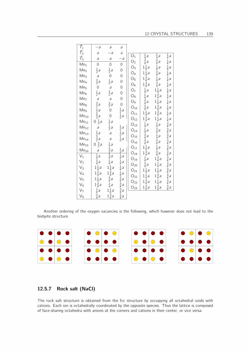
12 CRYSTAL STRUCTURES 139
~T1 −a a a~T2 a −a a~T3 a a −aMn1 0 0 0Mn2
12a
12a 0
Mn3 a 0 0Mn4
32a
12a 0
Mn5 0 a 0Mn6
12a
32a 0
Mn7 a a 0Mn8
32a
32a 0
Mn912a 0 1
2a
Mn1032a 0 1
2a
Mn11 0 12a
12a
Mn12 a 12a
12a
Mn1312a a 1
2a
Mn1432a a 1
2a
Mn15 0 32a
12a
Mn16 a 32a
12a
V114a
34a
14a
V234a
14a
14a
V3 1 14a 1 1
4a14a
V4 1 34a 1 3
4a14a
V5 1 14a
34a
34a
V6 1 34a
14a
34a
V714a 1 1
4a34a
V834a 1 3
4a34a
O114a
14a
14a
O234a
34a
14a
O3 1 14a
14a
14a
O4 1 14a
34a
14a
O5 1 34a
14a
14a
O6 1 34a
34a
14a
O714a 1 1
4a14a
O814a 1 3
4a14a
O934a 1 1
4a14a
O1034a 1 3
4a14a
O11 1 14a 1 3
4a14a
O12 1 34a 1 1
4a14a
O1314a
14a
34a
O1414a
34a
34a
O1534a
14a
34a
O1634a
34a
34a
O17 1 14a
14a
34a
O18 1 34a
34a
34a
O1914a 1 3
4a34a
O2034a 1 1
4a34a
O21 1 14a 1 1
4a34a
O22 1 14a 1 3
4a34a
O23 1 34a 1 1
4a34a
O24 1 34a 1 3
4a34a
Another ordering of the oxygen vacancies is the following, which however does not lead to thebixbyite structure.
12.5.7 Rock salt (NaCl)
The rock salt structure is obtained from the fcc structure by occupying all octahedral voids withcations. Each ion is octahedrally coordinated by the opposite species. Thus the lattice is composedof face-sharing octahedra with anions at the corners and cations in their center, or vice versa.
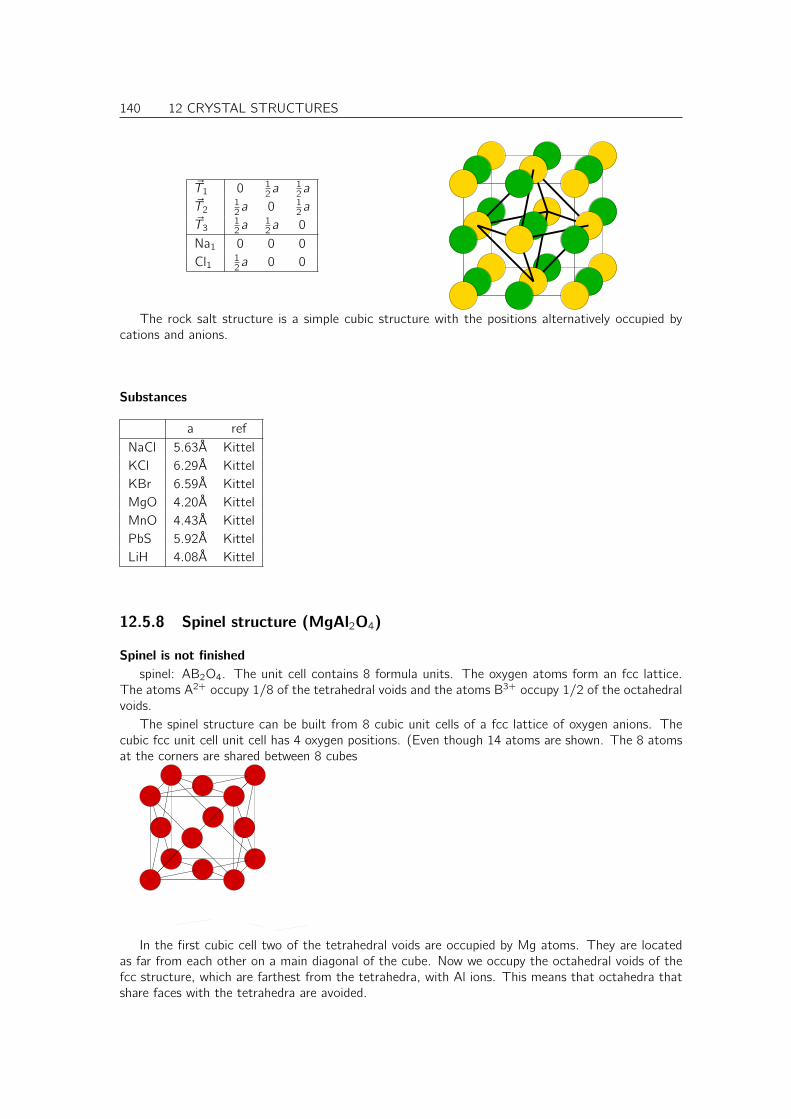
140 12 CRYSTAL STRUCTURES
~T1 0 12a
12a
~T212a 0 1
2a~T3
12a
12a 0
Na1 0 0 0Cl1 1
2a 0 0
The rock salt structure is a simple cubic structure with the positions alternatively occupied bycations and anions.
Substances
a refNaCl 5.63Å KittelKCl 6.29Å KittelKBr 6.59Å KittelMgO 4.20Å KittelMnO 4.43Å KittelPbS 5.92Å KittelLiH 4.08Å Kittel
12.5.8 Spinel structure (MgAl2O4)
Spinel is not finishedspinel: AB2O4. The unit cell contains 8 formula units. The oxygen atoms form an fcc lattice.
The atoms A2+ occupy 1/8 of the tetrahedral voids and the atoms B3+ occupy 1/2 of the octahedralvoids.
The spinel structure can be built from 8 cubic unit cells of a fcc lattice of oxygen anions. Thecubic fcc unit cell unit cell has 4 oxygen positions. (Even though 14 atoms are shown. The 8 atomsat the corners are shared between 8 cubes
In the first cubic cell two of the tetrahedral voids are occupied by Mg atoms. They are locatedas far from each other on a main diagonal of the cube. Now we occupy the octahedral voids of thefcc structure, which are farthest from the tetrahedra, with Al ions. This means that octahedra thatshare faces with the tetrahedra are avoided.
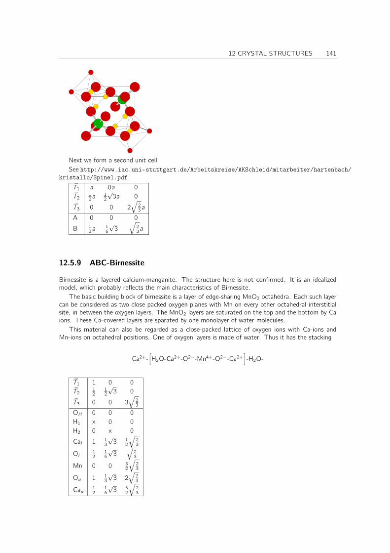
12 CRYSTAL STRUCTURES 141
Next we form a second unit cellSee http://www.iac.uni-stuttgart.de/Arbeitskreise/AKSchleid/mitarbeiter/hartenbach/
kristallo/Spinel.pdf~T1 a 0a 0~T2
12a
12
√3a 0
~T3 0 0 2√
23a
A 0 0 0
B 12a
16
√3
√23a
12.5.9 ABC-Birnessite
Birnessite is a layered calcium-manganite. The structure here is not confirmed. It is an idealizedmodel, which probably reflects the main characteristics of Birnessite.
The basic building block of birnessite is a layer of edge-sharing MnO2 octahedra. Each such layercan be considered as two close packed oxygen planes with Mn on every other octahedral interstitialsite, in between the oxygen layers. The MnO2 layers are saturated on the top and the bottom by Caions. These Ca-covered layers are sparated by one monolayer of water molecules.
This material can also be regarded as a close-packed lattice of oxygen ions with Ca-ions andMn-ions on octahedral positions. One of oxygen layers is made of water. Thus it has the stacking
Ca2+-[H2O-Ca2+-O2−-Mn4+-O2−-Ca2+
]-H2O-
~T1 1 0 0~T2
12
12
√3 0
~T3 0 0 3√
23
OH 0 0 0H1 x 0 0H2 0 x 0
Cal 1 13
√3 1
2
√23
Ol 12
16
√3
√23
Mn 0 0 32
√23
Ou 1 13
√3 2
√23
Cau 12
16
√3 5
2
√23
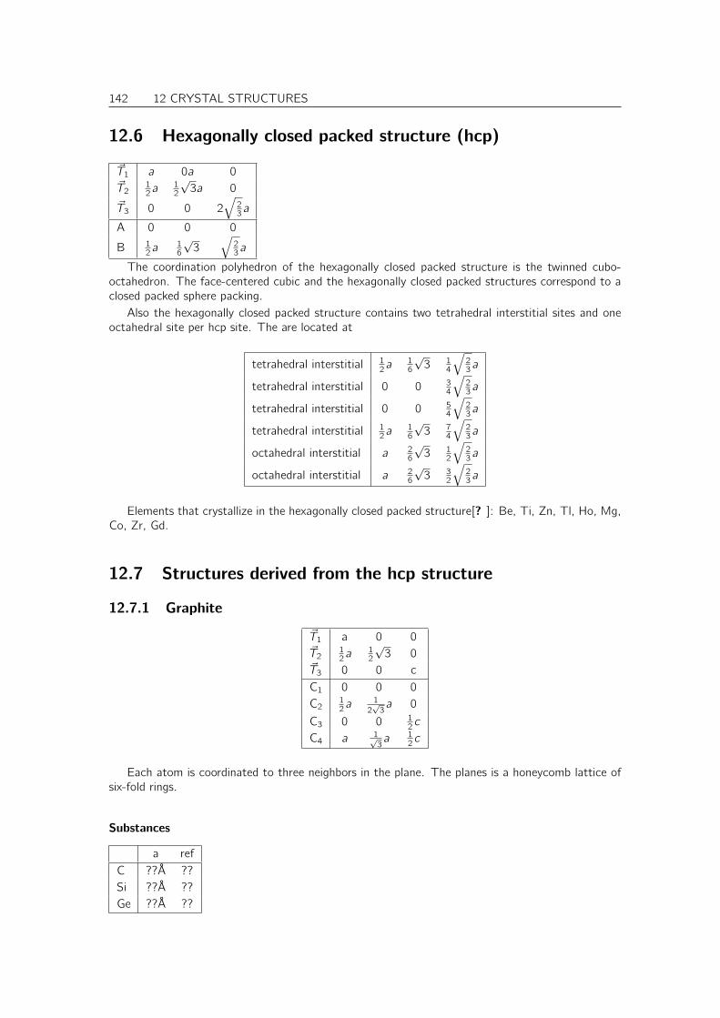
142 12 CRYSTAL STRUCTURES
12.6 Hexagonally closed packed structure (hcp)
~T1 a 0a 0~T2
12a
12
√3a 0
~T3 0 0 2√
23a
A 0 0 0
B 12a
16
√3
√23a
The coordination polyhedron of the hexagonally closed packed structure is the twinned cubo-octahedron. The face-centered cubic and the hexagonally closed packed structures correspond to aclosed packed sphere packing.
Also the hexagonally closed packed structure contains two tetrahedral interstitial sites and oneoctahedral site per hcp site. The are located at
tetrahedral interstitial 12a
16
√3 1
4
√23a
tetrahedral interstitial 0 0 34
√23a
tetrahedral interstitial 0 0 54
√23a
tetrahedral interstitial 12a
16
√3 7
4
√23a
octahedral interstitial a 26
√3 1
2
√23a
octahedral interstitial a 26
√3 3
2
√23a
Elements that crystallize in the hexagonally closed packed structure[? ]: Be, Ti, Zn, Tl, Ho, Mg,Co, Zr, Gd.
12.7 Structures derived from the hcp structure
12.7.1 Graphite
~T1 a 0 0~T2
12a
12
√3 0
~T3 0 0 cC1 0 0 0C2
12a
12√
3a 0
C3 0 0 12c
C4 a 1√3a 1
2c
Each atom is coordinated to three neighbors in the plane. The planes is a honeycomb lattice ofsix-fold rings.
Substances
a refC ??Å ??Si ??Å ??Ge ??Å ??

12 CRYSTAL STRUCTURES 143
12.7.2 NiAs structure (B8-type)
The NiAs structure can be considered the hexagonal variant of the rock-salt structure. Here theanions (As) form a hexagonally closed packed lattice, and all octahedral voids are filled by nickelions.2
The nickel sublattice consists of a closed-packed layer that is stacked ontop of each other in anAAA-stacking.
~T1 a 0 0~T2
12a
12
√3 0
~T3 0 0 cNi1 0 0 0Ni2 0 0 1
2c
As112a
12√
3a 1
4c
As2 a 1√3a 3
4c
a c refNiAs 3.618Å 5.034 Å ??
12.7.3 α-Corundum
The corundum structure can be seen as a distorted hcp lattice of oxygen atoms with cations fillingtwo-thirds of the octahedral interstitial sites. The cations fill in each row within the plane twopositions and then leave one vacant. The arrangement of Al cations and vacant octahedral sites issuch that the Al atoms form condensed six-fold rings similar to the graphite structure, where eachring encloses a vacant octahedral site.
Fig. 12.8: Arrangement of Al ions in the α-corundum structure. Aluminium atoms are shown in gold,and the octahedral interstices as black squares. The oxygen atoms in the layer below in red.
2In contrast, the anions (Cl) in the rocksalt (NaCl) structure form an cubic closed packed lattice (fcc) and whilethe cations (Na) fill all octahedral voids.
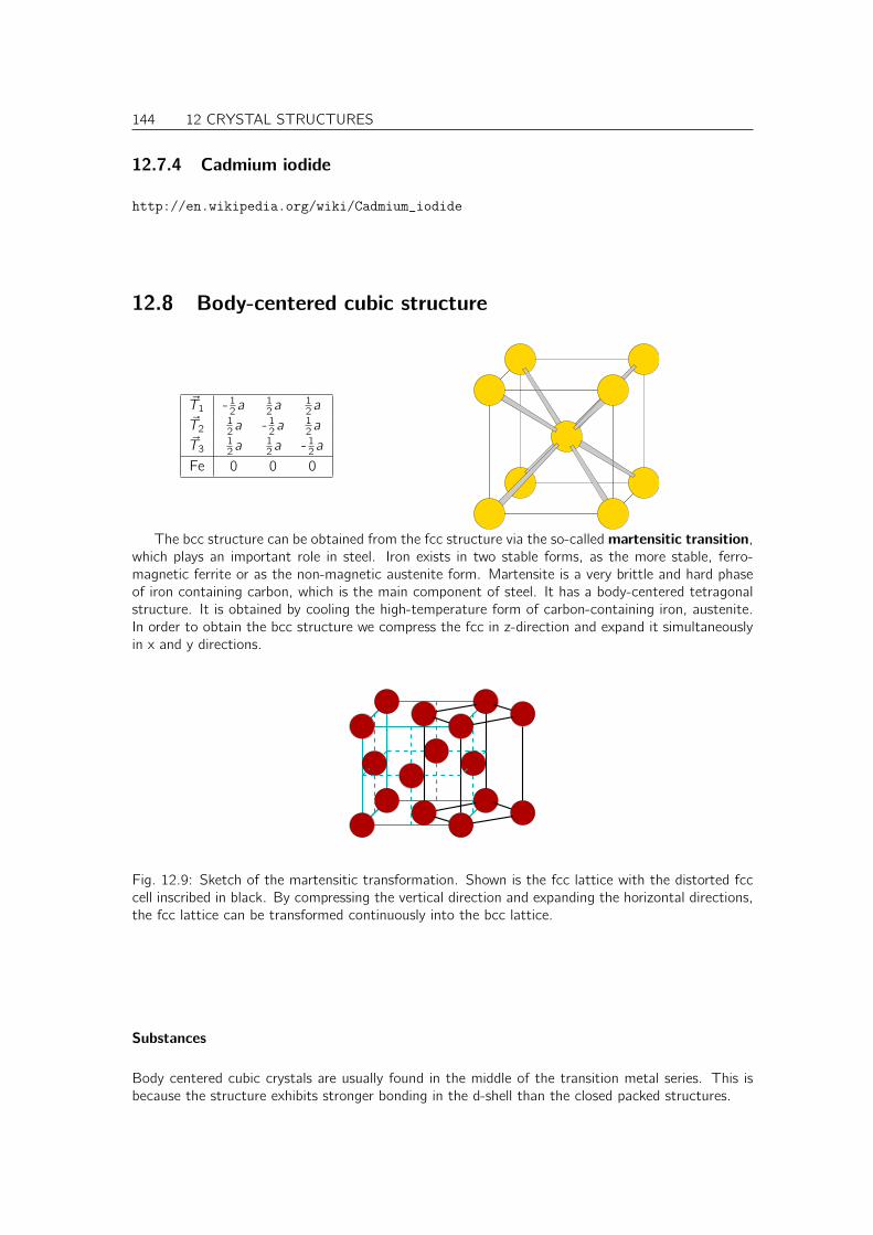
144 12 CRYSTAL STRUCTURES
12.7.4 Cadmium iodide
http://en.wikipedia.org/wiki/Cadmium_iodide
12.8 Body-centered cubic structure
~T1 - 12a
12a
12a
~T212a - 1
2a12a
~T312a
12a - 1
2a
Fe 0 0 0
The bcc structure can be obtained from the fcc structure via the so-calledmartensitic transition,which plays an important role in steel. Iron exists in two stable forms, as the more stable, ferro-magnetic ferrite or as the non-magnetic austenite form. Martensite is a very brittle and hard phaseof iron containing carbon, which is the main component of steel. It has a body-centered tetragonalstructure. It is obtained by cooling the high-temperature form of carbon-containing iron, austenite.In order to obtain the bcc structure we compress the fcc in z-direction and expand it simultaneouslyin x and y directions.
Fig. 12.9: Sketch of the martensitic transformation. Shown is the fcc lattice with the distorted fcccell inscribed in black. By compressing the vertical direction and expanding the horizontal directions,the fcc lattice can be transformed continuously into the bcc lattice.
Substances
Body centered cubic crystals are usually found in the middle of the transition metal series. This isbecause the structure exhibits stronger bonding in the d-shell than the closed packed structures.

12 CRYSTAL STRUCTURES 145
a refLi 3.491Å KittelNa 4.225Å KittelK 5.225Å KittelRb 5.585Å KittelCs 6.045Å KittelFe 2.87Å KittelCr 2.88Å KittelV 3.03Å KittelNb 3.30Å KittelMo 3.15Å KittelTa 3.30Å KittelW 3.16Å Kittel
12.9 Structures derived from the bcc structure
12.9.1 Caesium chloride structure (CsCl)
~T1 a 0 0~T2 0 a 0~T3 0 0 a
Cs1 0 0 0Cl1 1
2a12a
12a
The structure is a body-centered cubic structure with the positions alternatively occupied bycations and anions.
Substances
a refCsCl ??Å ??
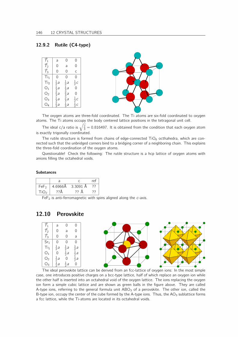
146 12 CRYSTAL STRUCTURES
12.9.2 Rutile (C4-type)
~T1 a 0 0~T2 0 a 0~T3 0 0 cTi1 0 0 0Ti2 1
2a12a
12c
O113a
13a 0
O223a
23a 0
O313a
23a
12c
O423a
13a
12c
The oxygen atoms are three-fold coordinated. The Ti atoms are six-fold coordinated to oxygenatoms. The Ti atoms occupy the body centered lattice positions in the tetragonal unit cell.
The ideal c/a ratio is√
23 = 0.816497. It is obtained from the condition that each oxygen atom
is exactly trigonally coordinated.The rutile structure is formed from chains of edge-connected TiO6 octhahedra, which are con-
nected such that the unbridged corners bind to a bridging corner of a neighboring chain. This explainsthe three-fold coordination of the oxygen atoms.
Questionable! Check the following: The rutile structure is a hcp lattice of oxygen atoms withanions filling the octahedral voids.
Substances
a c refFeF2 4.6966Å 3.3091 Å ??TiO2 ??Å ?? Å ??FeF2 is anti-ferromagnetic with spins aligned along the c-axis.
12.10 Perovskite
~T1 a 0 0~T2 0 a 0~T3 0 0 aSr1 0 0 0Ti1 1
2a12a
12a
O1 0 12a
12a
O212a 0 1
2a
O312a
12a 0
The ideal perovskite lattice can be derived from an fcc-lattice of oxygen ions: In the most simplecase, one introduces positive charges on a bcc-type lattice, half of which replace an oxygen ion whilethe other half is inserted into an octahedral void of the oxygen lattice. The ions replacing the oxygenion form a simple cubic lattice and are shown as green balls in the figure above. They are calledA-type ions, referring to the general formula unit ABO3 of a perovskite. The other ion, called theB-type ion, occupy the center of the cube formed by the A-type ions. Thus, the AO3 sublattice formsa fcc lattice, while the Ti-atoms are located in its octahedral voids.
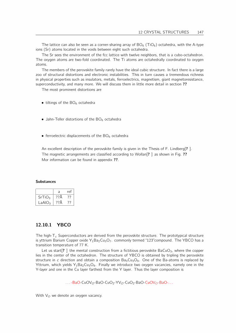
12 CRYSTAL STRUCTURES 147
The lattice can also be seen as a corner-sharing array of BO6 (TiO6) octahedra, with the A-typeions (Sr) atoms located in the voids between eight such octahedra.
The Sr sees the environment of the fcc lattice with twelve neighbors, that is a cubo-octahedron.The oxygen atoms are two-fold coordinated. The Ti atoms are octahedrally coordinated to oxygenatoms.
The members of the perovskite family rarely have the ideal cubic structure. In fact there is a largezoo of structural distortions and electronic instabilities. This in turn causes a tremendous richnessin physical properties such as insulators, metals, ferroelectrics, magnetism, giant magnetoresistance,superconductivity, and many more. We will discuss them in little more detail in section ??
The most prominent distortions are
• tiltings of the BO6 octahedra
• Jahn-Teller distortions of the BO6 octahedra
• ferroelectric displacements of the BO6 octahedra
An excellent description of the perovskite family is given in the Thesis of F. Lindberg[? ].The magnetic arrangements are classified according to Wollan[? ] as shown in Fig. ??Mor information can be found in appendix ??.
Substances
a refSrTiO3 ??Å ??LaAlO3 ??Å ??
12.10.1 YBCO
The high-Tc Superconductors are derived from the perovskite structure. The prototypical structureis yttrium Barium Copper oxide Y1Ba2Cu3O7. commonly termed “123”compound. The YBCO has atransition temperature of 77 K.
Let us start[? ] the mental construction from a fictitious perovskite BaCuO3, where the copperlies in the center of the octahedron. The structure of YBCO is obtained by tripling the perovskitestructure in c direction and obtain a composition Ba3Cu3O9. One of the Ba-atoms is replaced byYttrium, which yields Y1Ba2Cu3O9. Finally we introduce two oxygen vacancies, namely one in theY-layer and one in the Cu layer farthest from the Y layer. Thus the layer composition is
. . . -BaO-CuOVO-BaO-CuO2-YVO-CuO2-BaO-CuOVO-BaO-. . .
With VO we denote an oxygen vacancy.

148 12 CRYSTAL STRUCTURES
h!
A−type
B−type
C−type
D−type
E−type
F−type
G−type
Fig. 12.10: Classification of magnetic orderings of perovskites according to Wollan[? ]. One octantof the magnetic unit cell, that is all the inequivalent octahedra, is shown. The gold and blue octahedrarepresent central atoms with up and down spin arrangement.
~T1 a 0 0~T2 0 a 0~T3 0 0 3aCu1
12a
12a 0
O112a 0 0
Ba1 0 0 12a
O212a
12a
12a
Cu212a
12a a
O312a 0 a
O4 0 12a a
Y1 0 0 32a
Cu312a
12a 2a
O512a 0 2a
O6 0 12a 2a
Ba2 0 0 52a
O712a
12a
52a
CuO
CuO
CuO
BaO
CuO
Y
BaO
2
2
The important structural element of the YBCO structure are the Cu atoms in the square planarenvironment of oxygen ligands. The CuO2 layers form square networks of Cu atoms with O-atomson the connecting lines. The CuO planes with the oxygen on-top and below are corner sharingCuO4-squares.
The charge distribution of the layers is such that we can assume that the Cu atoms are formallyin the +2 charge state, but there is one hole h+ per unit cell, because the trivalent Y3+ cannotcompensate the charge of 4− from the neighboring CuO2 layers.
12.10.2 CaCuO2
The CaCuO2 structure is the prototype structure containing the square CuO2 lattice present in thehigh-Tc superconductors.
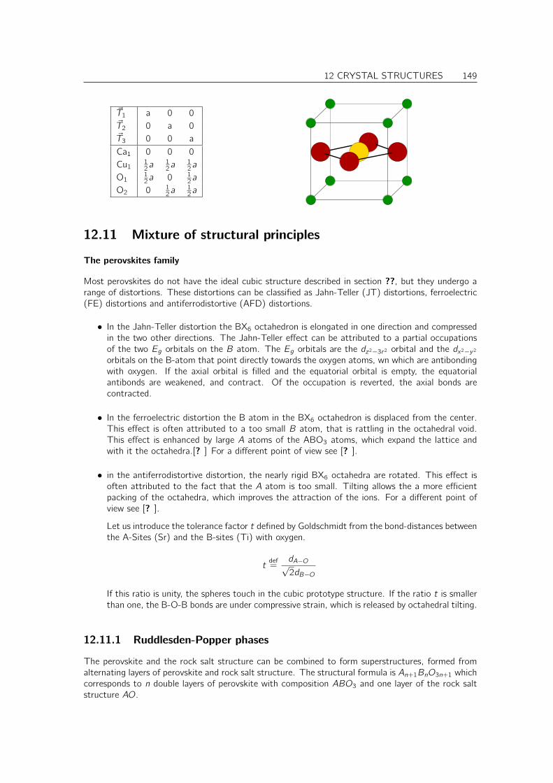
12 CRYSTAL STRUCTURES 149
~T1 a 0 0~T2 0 a 0~T3 0 0 aCa1 0 0 0Cu1
12a
12a
12a
O112a 0 1
2a
O2 0 12a
12a
12.11 Mixture of structural principles
The perovskites family
Most perovskites do not have the ideal cubic structure described in section ??, but they undergo arange of distortions. These distortions can be classified as Jahn-Teller (JT) distortions, ferroelectric(FE) distortions and antiferrodistortive (AFD) distortions.
• In the Jahn-Teller distortion the BX6 octahedron is elongated in one direction and compressedin the two other directions. The Jahn-Teller effect can be attributed to a partial occupationsof the two Eg orbitals on the B atom. The Eg orbitals are the dz2−3r2 orbital and the dx2−y2
orbitals on the B-atom that point directly towards the oxygen atoms, wn which are antibondingwith oxygen. If the axial orbital is filled and the equatorial orbital is empty, the equatorialantibonds are weakened, and contract. Of the occupation is reverted, the axial bonds arecontracted.
• In the ferroelectric distortion the B atom in the BX6 octahedron is displaced from the center.This effect is often attributed to a too small B atom, that is rattling in the octahedral void.This effect is enhanced by large A atoms of the ABO3 atoms, which expand the lattice andwith it the octahedra.[? ] For a different point of view see [? ].
• in the antiferrodistortive distortion, the nearly rigid BX6 octahedra are rotated. This effect isoften attributed to the fact that the A atom is too small. Tilting allows the a more efficientpacking of the octahedra, which improves the attraction of the ions. For a different point ofview see [? ].
Let us introduce the tolerance factor t defined by Goldschmidt from the bond-distances betweenthe A-Sites (Sr) and the B-sites (Ti) with oxygen.
tdef=
dA−O√2dB−O
If this ratio is unity, the spheres touch in the cubic prototype structure. If the ratio t is smallerthan one, the B-O-B bonds are under compressive strain, which is released by octahedral tilting.
12.11.1 Ruddlesden-Popper phases
The perovskite and the rock salt structure can be combined to form superstructures, formed fromalternating layers of perovskite and rock salt structure. The structural formula is An+1BnO3n+1 whichcorresponds to n double layers of perovskite with composition ABO3 and one layer of the rock saltstructure AO.
150 12 CRYSTAL STRUCTURES
12.11.2 Magnéli phases
Magneli phases are layers of rutile and corundum type structures: However, the structure is disputed.(http://arxiv.org/pdf/cond-mat/0309483)
MnO2n−1=M2O3+(n-2)VO2
about oxides see http://ruby.chemie.uni-freiburg.de/Vorlesung/oxide_0.html
12.11.3 Intermetallics
Intermetallics are compounds formed from several metal atoms, that, unlike alloys, form orderedstructures.
Stichworte
• Laves Phasen
• Heusler Phasen
• Zintl phasen
• Hume Rothery phasen
L10 is a fcc lattice with alternating planes of A and B atoms. An example is TiAl.
~T112a
12a 0
~T212a − 1
2a 0~T3 0 0 a
Ti 0 0 0Al 1
2a 0 0
L12 is an fcc-lattice with one atom type on the cube faces and the other at the cube corners.The parent compound is Ni3Al.
B2 is a bcc-lattice with one type of atom in the cube center and the other at the cube corners.A compound is NiAl. The B2 structure is essentially the CsCl struycture.
C1 is simply the fluorite structure or the antifluorite structure respectively. Examples are Mg2Si,Co2Si, Ni2Si, Mg2Ge.
The D03 structure with composition A3B can bee seen as a supercell of eight bcc-unit cells, ofwhich the body centers of four cubes are of B-type. examples are Fe3Al.
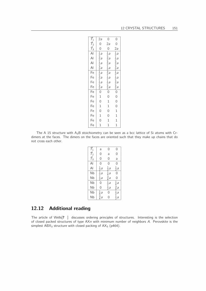
12 CRYSTAL STRUCTURES 151
~T1 2a 0 0~T2 0 2a 0~T3 0 0 2a
Al 12a
12a
12a
Al 32a
32a
12a
Al 12a
32a
32a
Al 32a
12a
32a
Fe 12a
32a
12a
Fe 32a
12a
12a
Fe 12a
12a
32a
Fe 32a
32a
32a
Fe 0 0 0Fe 1 0 0Fe 0 1 0Fe 1 1 0Fe 0 0 1Fe 1 0 1Fe 0 1 1Fe 1 1 1
The A 15 structure with A3B stoichiometry can be seen as a bcc lattice of Si atoms with Cr-dimers at the faces. The dimers on the faces are oriented such that they make up chains that donot cross each other.
~T1 a 0 0~T2 0 a 0~T3 0 0 aAl 0 0 0Al 1
2a12a
12a
Nb 12a
14a 0
Nb 12a
34a 0
Nb 0 12a
14a
Nb 0 12a
34a
Nb 14a 0 1
2a
Nb 34a 0 1
2a
12.12 Additional reading
The article of Wells[? ] discusses ordering principles of structures. Interesting is the selectionof closed packed structures of type AXn with minimum number of neighbors A. Perovskite is thesimplest ABX3 structure with closed packing of AX3 (p464).

152 12 CRYSTAL STRUCTURES

Chapter 13
Crystal-Orbital HamiltonianPopulations
One very useful way to analyze local chemical bonding in solids and complex molecules are the pro-jected density of states, Crystal Orbital Overlap (COOP) contributions or Crystal Orbital HamiltonianPopulations.
13.1 Definition of the density of states
These quantities are meant to analyze the band structure energy
EB =∑n
fnεn
which is the sum of orbital energies weighted by their occupations.The Band structure energy can be rewritten with the help of the total density of states as
EB =
∫ ∞−∞
dε f (ε− µ)ε∑n
δ(ε− εn)︸ ︷︷ ︸D(ε)
=
∫ ∞−∞
dε D(ε)εf (ε− µ)
The total density of states D(ε) can can now be expressed by a local basisset. Let us consider anon-orthogonal basis set |χi 〉. In order to decompose our wave functions into these local orbitals weintroduce projector functions.
|ψn〉 =∑i
|χi 〉〈pi |ψn〉 (13.1)
One requirement for this identity to hold is that the basis functions are complete and secondly that
〈pi |χj〉 = δi ,j (13.2)
which follows, when we insert the basis function instead of the wave functions in Eq. ??The projector functions can be constructed from a support basis 〈fi | such from
〈pi | =∑j
QI,j 〈fj | with∑k
Qi ,k〈fk |χj〉 = δi ,j
The reader can easily convince himself that the projector functions defined in this way fulfill thebiorthogonality condition Eq. ??. While nothing forbids to use 〈fi | = 〈χi |, the above formulation issubstantially more flexible and more convenient in practice.
153
154 13 CRYSTAL-ORBITAL HAMILTONIAN POPULATIONS
The Density of states has the form
D(ε) =∑n
δ(ε− εn)〈ψn|ψn〉 =∑i ,j
∑n
δ(ε− εn)〈ψn|pi 〉〈χi |χj〉〈pj |ψn〉︸ ︷︷ ︸Dj,i 〈χj |χi 〉
Similarly we can directly multiply the density of states with the energy
D(ε) =∑n
δ(ε− εn)〈ψn|ψn〉 =∑i ,j
∑n
δ(ε− εn)〈ψn|pi 〉〈χi |H|χj 〉〈pj |ψn〉︸ ︷︷ ︸Dj,i 〈χi |H|χj 〉
This defines the density of states in the basis of our basisset as
Di ,j(ε) =∑n
〈pi |ψn〉δ(ε− εn)〈ψn|pj〉
With the density of states, we obtain the band structure energy as
EB =∑i ,j
∫dε f (ε)Di ,j(ε)〈χi |H|χj〉
=∑i ,j
∫dε f (ε)Di ,j(ε)ε〈χi |χj〉
Thus the density of states yields the complete information about the energy levels, in an energyresolved, spatially resolved and angular momentum resolved manner.
The diagonal elements ofDi ,j(ε)〈χj |χi 〉 are called the projected density of states. The off-diagonalelements are called Crystal orbital overlap populations (COOP’s). When the Overlap is replaced bythe Hamiltonian we obtain the crystal orbital Hamilton population (COHP), Di ,j 〈χj |H|χi 〉 whichdirectly yields energetic information.
13.2 Example: Formaldehyde
Let us have a look at a very simple example namely formaldehyde H2co. In Fig. ?? the total densityof states and COOPs. are shown. The total density of states in this case shows lines for each energylevel of the molecule. In order to analyze the CO bond, we determine the COOP between the twomentioned orbitals. Two of the calculated states contribute to bonding. The others are in differentsymmetry classes. We see that the lower of the two peaks contributes a large negative contribution,indicating a bonding interaction between the two orbitals. That is the two orbitals contribute to thisstate with the same sign.
The second state has a positive contribution, indicating an anti-bonding interaction. The integral,however shows, that this state does not compensate the bond completely, but about half of thebonding weight is left. This indicates that at higher energy there will be another state with anti-bonding character.
The last two figures show the projection on the p-orbitals of carbon and oxygen respectively. Weobserve that the bonding state has most of its weight on the carbon atom, while the higher statehas almost zero weight on the carbon atom. This state is mostly localized on the oxygen atom.
The results can now be rationalized as follows:
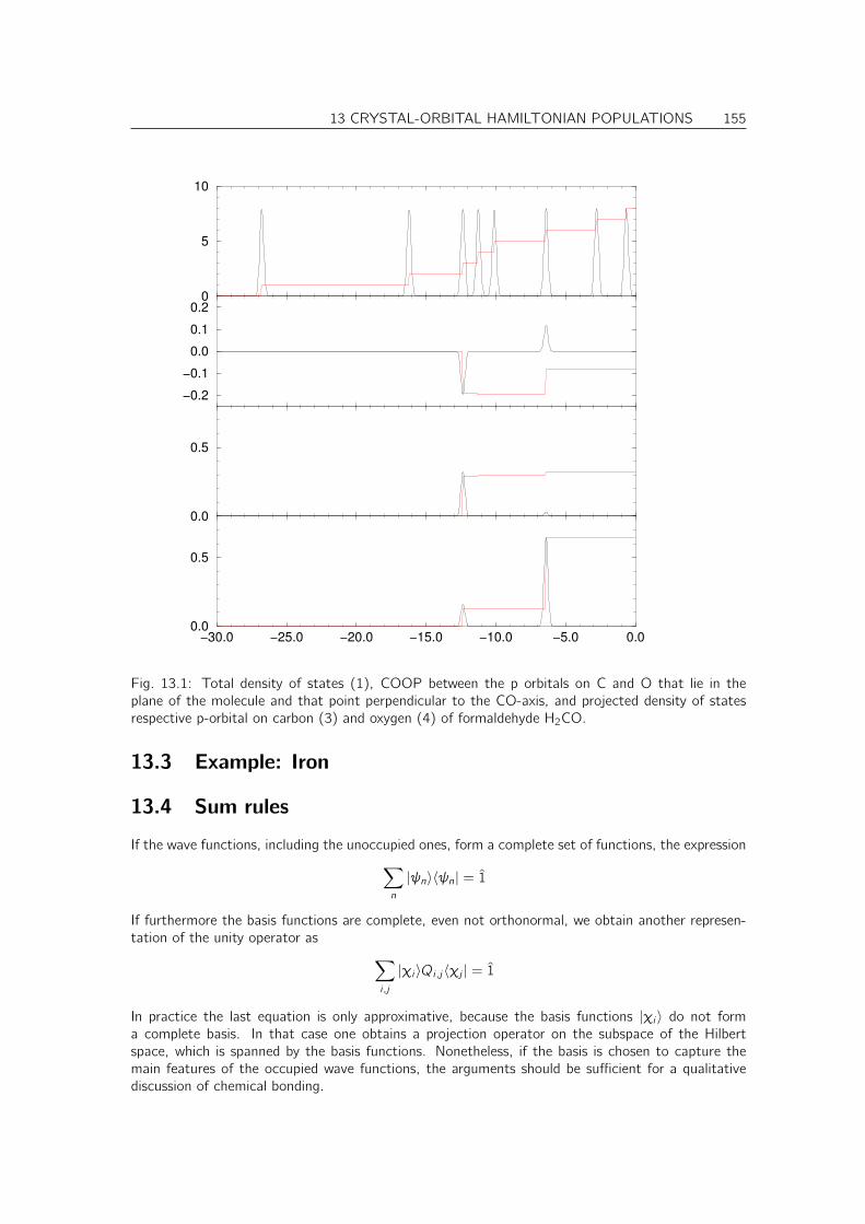
13 CRYSTAL-ORBITAL HAMILTONIAN POPULATIONS 155
−30.0 −25.0 −20.0 −15.0 −10.0 −5.0 0.00.0
0.5
0.0
0.5
−0.2
−0.1
0.0
0.1
0.20
5
10
Fig. 13.1: Total density of states (1), COOP between the p orbitals on C and O that lie in theplane of the molecule and that point perpendicular to the CO-axis, and projected density of statesrespective p-orbital on carbon (3) and oxygen (4) of formaldehyde H2CO.
13.3 Example: Iron
13.4 Sum rules
If the wave functions, including the unoccupied ones, form a complete set of functions, the expression∑n
|ψn〉〈ψn| = 1
If furthermore the basis functions are complete, even not orthonormal, we obtain another represen-tation of the unity operator as ∑
i ,j
|χi 〉Qi ,j 〈χj | = 1
In practice the last equation is only approximative, because the basis functions |χi 〉 do not forma complete basis. In that case one obtains a projection operator on the subspace of the Hilbertspace, which is spanned by the basis functions. Nonetheless, if the basis is chosen to capture themain features of the occupied wave functions, the arguments should be sufficient for a qualitativediscussion of chemical bonding.
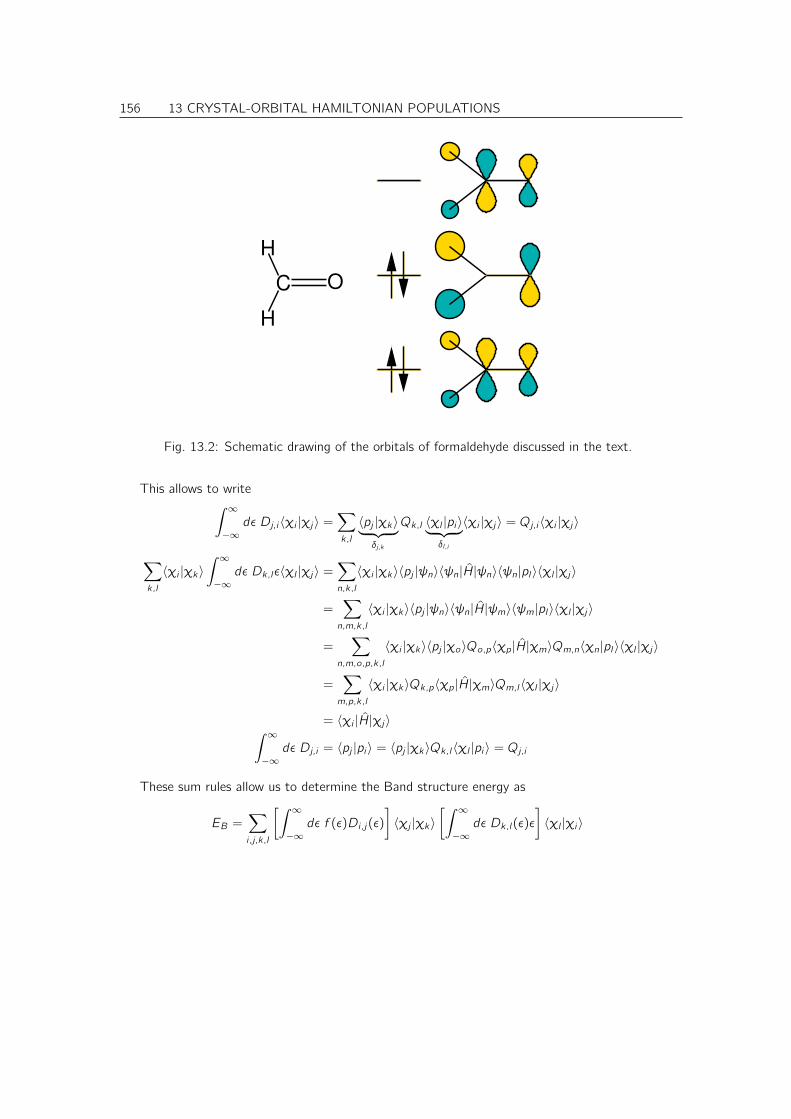
156 13 CRYSTAL-ORBITAL HAMILTONIAN POPULATIONS
C O
H
H
Fig. 13.2: Schematic drawing of the orbitals of formaldehyde discussed in the text.
This allows to write∫ ∞−∞
dε Dj,i 〈χi |χj〉 =∑k,l
〈pj |χk〉︸ ︷︷ ︸δj,k
Qk,l 〈χl |pi 〉︸ ︷︷ ︸δl ,i
〈χi |χj 〉 = Qj,i 〈χi |χj〉
∑k,l
〈χi |χk〉∫ ∞−∞
dε Dk,lε〈χl |χj〉 =∑n,k,l
〈χi |χk〉〈pj |ψn〉〈ψn|H|ψn〉〈ψn|pl〉〈χl |χj〉
=∑n,m,k,l
〈χi |χk〉〈pj |ψn〉〈ψn|H|ψm〉〈ψm|pl〉〈χl |χj〉
=∑
n,m,o,p,k,l
〈χi |χk〉〈pj |χo〉Qo,p〈χp|H|χm〉Qm,n〈χn|pl〉〈χl |χj〉
=∑m,p,k,l
〈χi |χk〉Qk,p〈χp|H|χm〉Qm,l 〈χl |χj〉
= 〈χi |H|χj〉∫ ∞−∞
dε Dj,i = 〈pj |pi 〉 = 〈pj |χk〉Qk,l〈χl |pi 〉 = Qj,i
These sum rules allow us to determine the Band structure energy as
EB =∑i ,j,k,l
[∫ ∞−∞
dε f (ε)Di ,j(ε)
]〈χj |χk〉
[∫ ∞−∞
dε Dk,l(ε)ε
]〈χl |χi 〉
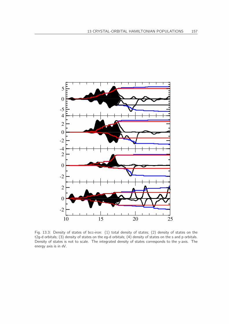
13 CRYSTAL-ORBITAL HAMILTONIAN POPULATIONS 157
-5
0
5
-4
-2
0
2
4
-2
0
2
10 15 20 25
-2
0
2
Fig. 13.3: Density of states of bcc-iron: (1) total density of states; (2) density of states on thet2g-d orbitals; (3) density of states on the eg-d orbitals; (4) density of states on the s and p orbitals.Density of states is not to scale. The integrated density of states corresponds to the y-axis. Theenergy axis is in eV.

158 13 CRYSTAL-ORBITAL HAMILTONIAN POPULATIONS
Chapter 14
Magnetism
14.1 Quick and Dirty
14.1.1 Driving force for a parallel (ferromagnetic) alignment of spins
The origin of magnetic behavior of materials has, surprisingly, nothing to do with magnetic momentsthat align due their magnetic fields.
The origin is instead the Pauli principle and the electrostatic interaction between electrons: Elec-trons with like spin stay apart from each other, while electrons with opposite spin also come closetogether. Thus, the electrostatic energy due to the Coulomb repulsion between electrons is larger forelectrons with opposite spin than for electrons with like spin. Thus, in order to reduce their energy,the electrons tend to align their spins in a parallel orientation.
This a natural tendency of electrons to align with parallel spins is the origin of Hund’s rule. Aselectrons fill the shells of an atom, they first orient their spins parallel. Thus the total spins of theatoms is such maximized for each angular momentum shell
Li Be B C N O F Ne12~ 0 1
2~ ~ 32~ ~ 1
2~ 0
Let us now dig a little deeper: Imagine a homogeneous electron gas with a given density. Nowconsider the density of the remaining electrons as seen by one of the electrons at a specified position.If the material has N electrons our specified electron only sees N − 1 electrons. Thus it sees thetotal density with a “hole” around himself. The hole corresponds to exactly the one missing electron.
The Coulomb energy of electrons can be written as
Ee−e =1
2
∫d3r
∫d3r ′
e2n(~r)n(~r ′)
4πε0|~r − ~r ′|+
∫d3r en(~r)
1
2
∫d3r ′
eh(~r , ~r ′)
4πε0|~r − ~r ′|
where eh(~r , ~r ′) is the positive density of the exchange hole of an electron located at ~r . If wecompare systems with the same density the first term, called Hartree energy, is identical. Thus,the difference of the Coulomb energy of two systems with the same density can be traced to theattractive interaction of the electrons with their exchange-correlation hole.
If we compare electrostatic energy of a non-magnetic and a ferromagnetic electron gas, thedifference is the interaction of the electron with its own exchange-hole. This energy is larger in theferromagnetic case, because the hole is closer to the specified electron, where the Coulomb interactionis strongest. Thus the electrostatic repulsion between electrons is weaker in the ferromagnetic case.
159

160 14 MAGNETISM
n
x x
nonmagnetic ferromagnet
Fig. 14.1: The exchange energy for a magnetic electron gas is favorable compared to a nonmagneticelectron gas. The reason is that the exchange correlation hole of the magnetic electron gas is morecompact. The Coulomb attraction of electron and its exchange correlation hole is therefore larger.
14.1.2 Driving force for antiparallel alignment of spins
The story is however not yet complete: Not all materials are magnetic. Even free-electron like metalssuch as sodium and aluminium are nonmagnetic. The orbitals of molecules are occupied such thatelectron pair with antiparallel spins, which seems to completely disagree with the above argument.
What is missing is the effect of the kinetic energy. Depending on whether the kinetic energy orthe Coulomb energy wins, the material will be nonmagnetic or magnetic.
Let us return to the free electron gas. As we fill the electrons into the orbitals, we note that weneed to occupy orbitals with higher energy, if we can only fill one electron into each orbital as in theferromagnetic case. In the nonmagnetic case we fill the orbitals with an electron pair and less orbitalsneed to be filled. Thus, from the point of view of one-particle energies, it is always more efficient tofill the lowest orbitals with a singlet pair of two electrons.
x
nonmagnetic
E
ferromagnet
Fig. 14.2: Schematic drawing of the energy levels in a box with non-magnetic and magnetic occupa-tions of the levels. The particle in a box serves as model for a free electron gas.
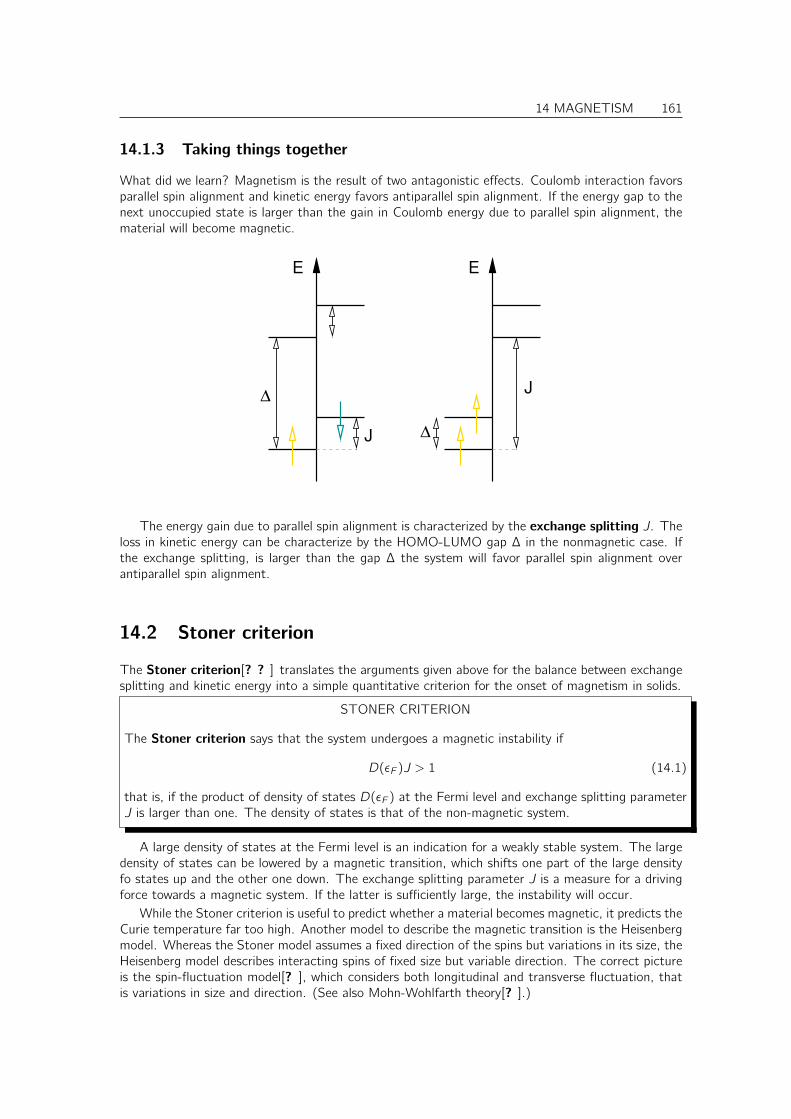
14 MAGNETISM 161
14.1.3 Taking things together
What did we learn? Magnetism is the result of two antagonistic effects. Coulomb interaction favorsparallel spin alignment and kinetic energy favors antiparallel spin alignment. If the energy gap to thenext unoccupied state is larger than the gain in Coulomb energy due to parallel spin alignment, thematerial will become magnetic.
J∆
J ∆
E E
The energy gain due to parallel spin alignment is characterized by the exchange splitting J. Theloss in kinetic energy can be characterize by the HOMO-LUMO gap ∆ in the nonmagnetic case. Ifthe exchange splitting, is larger than the gap ∆ the system will favor parallel spin alignment overantiparallel spin alignment.
14.2 Stoner criterion
The Stoner criterion[? ? ] translates the arguments given above for the balance between exchangesplitting and kinetic energy into a simple quantitative criterion for the onset of magnetism in solids.
STONER CRITERION
The Stoner criterion says that the system undergoes a magnetic instability if
D(εF )J > 1 (14.1)
that is, if the product of density of states D(εF ) at the Fermi level and exchange splitting parameterJ is larger than one. The density of states is that of the non-magnetic system.
A large density of states at the Fermi level is an indication for a weakly stable system. The largedensity of states can be lowered by a magnetic transition, which shifts one part of the large densityfo states up and the other one down. The exchange splitting parameter J is a measure for a drivingforce towards a magnetic system. If the latter is sufficiently large, the instability will occur.
While the Stoner criterion is useful to predict whether a material becomes magnetic, it predicts theCurie temperature far too high. Another model to describe the magnetic transition is the Heisenbergmodel. Whereas the Stoner model assumes a fixed direction of the spins but variations in its size, theHeisenberg model describes interacting spins of fixed size but variable direction. The correct pictureis the spin-fluctuation model[? ], which considers both longitudinal and transverse fluctuation, thatis variations in size and direction. (See also Mohn-Wohlfarth theory[? ].)
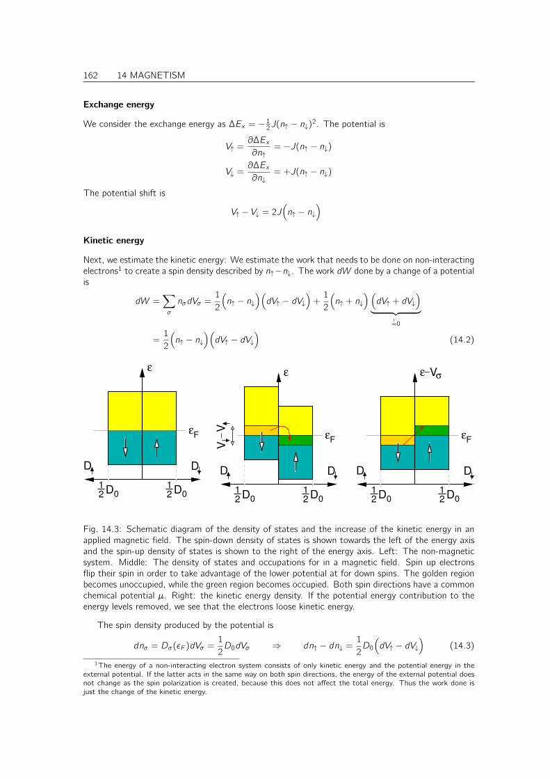
162 14 MAGNETISM
Exchange energy
We consider the exchange energy as ∆Ex = − 12J(n↑ − n↓)2. The potential is
V↑ =∂∆Ex∂n↑
= −J(n↑ − n↓)
V↓ =∂∆Ex∂n↓
= +J(n↑ − n↓)
The potential shift is
V↑ − V↓ = 2J(n↑ − n↓
)Kinetic energy
Next, we estimate the kinetic energy: We estimate the work that needs to be done on non-interactingelectrons1 to create a spin density described by n↑−n↓. The work dW done by a change of a potentialis
dW =∑σ
nσdVσ =1
2
(n↑ − n↓
)(dV↑ − dV↓
)+
1
2
(n↑ + n↓
)(dV↑ + dV↓
)︸ ︷︷ ︸
!=0
=1
2
(n↑ − n↓
)(dV↑ − dV↓
)(14.2)
D
εF
D0
1
2D
0
1
2
D D
εF
D0
1
2D
0
1
2
D D
εF
ε
VV
ε Vσ
D0
1
2D
0
1
2
D
ε
Fig. 14.3: Schematic diagram of the density of states and the increase of the kinetic energy in anapplied magnetic field. The spin-down density of states is shown towards the left of the energy axisand the spin-up density of states is shown to the right of the energy axis. Left: The non-magneticsystem. Middle: The density of states and occupations for in a magnetic field. Spin up electronsflip their spin in order to take advantage of the lower potential at for down spins. The golden regionbecomes unoccupied, while the green region becomes occupied. Both spin directions have a commonchemical potential µ. Right: the kinetic energy density. If the potential energy contribution to theenergy levels removed, we see that the electrons loose kinetic energy.
The spin density produced by the potential is
dnσ = Dσ(εF )dVσ =1
2D0dVσ ⇒ dn↑ − dn↓ =
1
2D0
(dV↑ − dV↓
)(14.3)
1The energy of a non-interacting electron system consists of only kinetic energy and the potential energy in theexternal potential. If the latter acts in the same way on both spin directions, the energy of the external potential doesnot change as the spin polarization is created, because this does not affect the total energy. Thus the work done isjust the change of the kinetic energy.
14 MAGNETISM 163
Here, we approximated the density of states Dσ(ε) by one-half of the total density of states D0 ofthe non-spinpolarized system at the Fermi level.
Taken together, we obtain for the work done by polarizing the non-interacting system
dW =1
2
(n↑ − n↓
)·
2
D0
(dn↑ − dn↓
)⇒
∫ n↑−n↓
0
dW =1
2D0
(n↑ − n↓
)2
(14.4)
Stability of the interacting system
In order to obtain the energy required to polarize the interacting system of electrons, we need to addthe exchange splitting.∫ n↑−n↓
0
dW =1
2D0
(n↑ − n↓
)2
−1
2J(n↑ − n↓
)2
=1
2J(n↑ − n↓
)2( 1
D0J− 1)
(14.5)
Thus we see that a spin polarization is favorable, if
D0J > 1 (14.6)
which is the Stoner criterion Eq. ??
14.3 ????
Magnetism is observed most frequently in 3d transition metals and elements with a partially filledf-shell. The atomic orbitals with d- and f-character are strongly bound to the atom core and hardlyobverlap. Therefore they form only very flat bands.
Wave functions with d- and f-like angular momentum character are strongly bound to the coreThe radial extent of orbitals is closely related to the principal quantum number. The 3-d valence
electrons coexist with 4s and 4p valence electrons, but have a radial extent close to the core-like3s and 3p orbitals. This effect is even stronger for the lanthanides and actinides with a partiallyfilled f-shell: The 4-f electrons in the lanthanides coexist with 6s-, 6p- and 5d- valence electrons.As a consequence the s- and p-electrons either form strong covalent bonds or they even get lost.In a metal they form free electron-like bands with a large band width. This large band width winsover the Coulomb interaction. This is why metals with s- and p-electrons, such as Na dna Al, donot form magnetic metals. Because d and f-electrons are located closer to the nucleus, the formnarrow, almost atom-like bands. The loss in kinetic energy for parallel spin-alignment is small. On theother hand the Coulomb interaction is large because the d- and f-electrons are confined into a smallspatial region. As a consequence the atomic Hund’s rule behavior often survives for transition metalsand f-electron materials,leading to magnetic transition metals, and rare earth metals. Consequentlylanthanides and actinides are part of the materials used as strong magnets.
14.4 Exchange splitting
The interaction between spins in the Ising model is not of magnetic nature as one might naivelyexpect. The magnetic interaction is long ranged and much smaller than the exchange interactionsthat play a role in the Ising model.
Let us demonstrate this by exploring the exchange interaction for the minimum Ising model, theIsing dimer, which is also a model for a hydrogen molecule. Consider two sites with one electron oneach site. The basis set is built up of a single spatial orbital on each site, φ and ψ. Each orbital is atwo component spinor, where the upper component corresponds to the spin-up contribution and the

164 14 MAGNETISM
lower component is the spin-down contribution so that we can build four one-particle orbitals fromtwo spatial wave functions.
| ↑, 0〉 =
(φ(r)
0
)= φ(r)α
| ↓, 0〉 =
(0
φ(r)
)= φ(r)β
|0, ↑〉 =
(ψ(r)
0
)= ψ(r)α
|0, ↓〉 =
(0
ψ(r)
)= ψ(r)β
where α = (1, 0) and β = (0, 1).Out of the one-particle wave functions, we build two-particle Slater determinants of the type
| ↑, ↓〉 = 1√2
(| ↑, 0〉 × |0, ↓〉 − |0, ↓〉 × | ↑, 0〉). Out of the 16 product states that can be build from
the four one-particle states, 6 are excluded because they differ only by a sign change from others,and 4 additional ones are excluded because they involve two identical one-particle states, which isprohibited due to Pauli principle. We are left with 6 states:
| ↑↓, 0〉 = φ(r1)φ(r2)α1β2 − β1α2√
2
| ↑, ↑〉, =1√2
(φ(r1)ψ(r2)− ψ(r1)φ(r2)
)α1α2
| ↑, ↓〉, =1√2
(φ(r1)ψ(r2)α1β2 − ψ(r1)φ(r2)β1α2
)| ↓, ↑〉, =
1√2
(φ(r1)ψ(r2)β1α2 − ψ(r1)φ(r2)α1β2
)| ↓, ↓〉, =
1√2
(φ(r1)ψ(r2)− ψ(r1)φ(r2)
)β1β2
|0, ↑↓〉 = ψ(r1)ψ(r2)α1β2 − β1α2√
2
Two states, namely | ↑↓, 0〉 and |0, ↑↓〉, correspond to charge transfer states, where one electronhas been transferred from one site to another. We exclude them with the argument that the Coulombrepulsion makes these states very unfavorable. This is a model assumption that serves our purposebut is not valid in general.
We evaluate the expectation value of the Hamiltonian.
E =∑σ1,σ2
∫d3r1
∫d3r2 Ψ∗(~r1, σ1, ~r2, σ2)
×[ 2∑i=1
(−~2
2m∇2i + V (ri)
)+
e2
4πε0
1
|r1 − r2|
]ψ(~r1, σ,~r2, σ) (14.7)
Let us now consider only Slater determinants, which implies that we make the so-called Hartree-Fock approximation
Ψ(~r1, σ1, ~r2, σ2) =1√2
(χa(~r1, σ1)χb(~r2, σ2)− χb(~r1, σ1)χa(~r2, σ2)
)(14.8)
where χa and χb are orthonormal spin orbitals. With Slater determinants the total energy has the
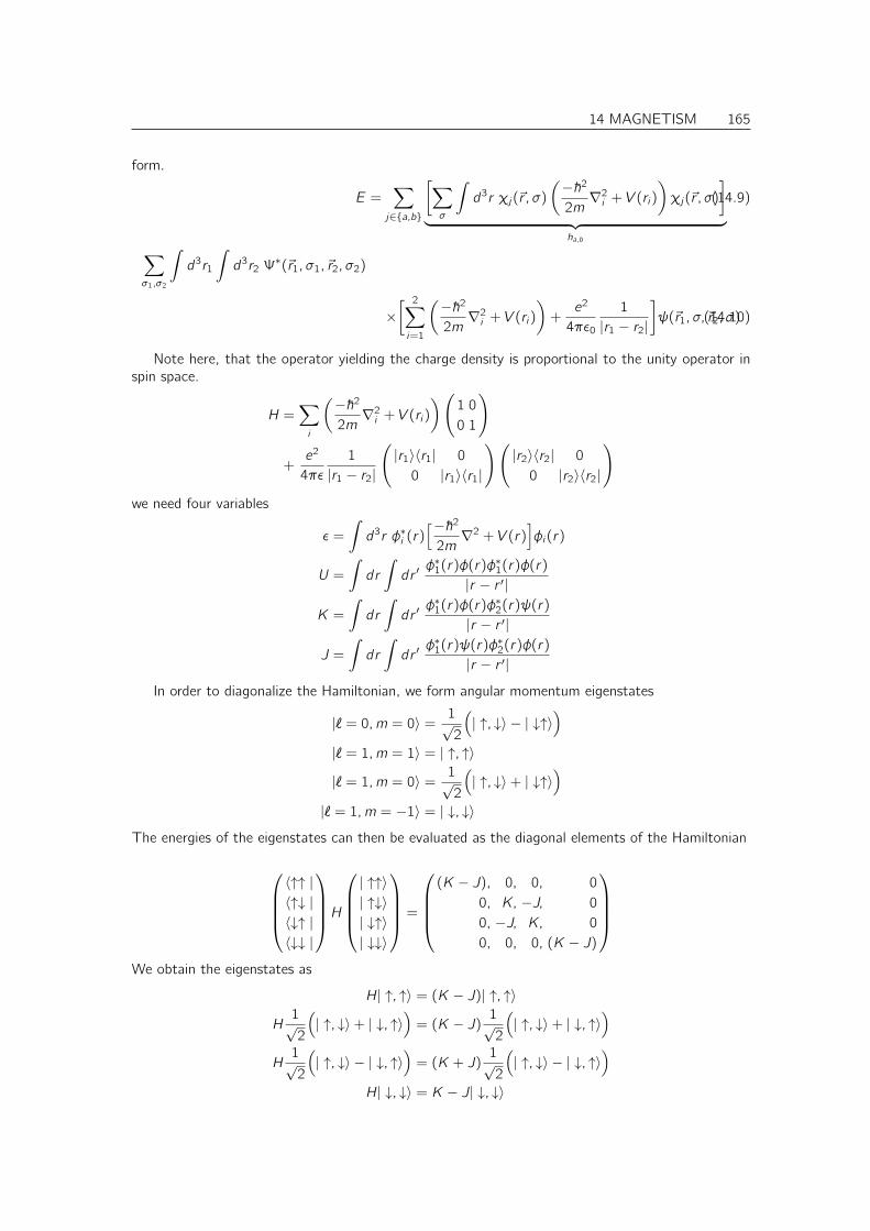
14 MAGNETISM 165
form.
E =∑j∈a,b
[∑σ
∫d3r χj(~r , σ)
(−~2
2m∇2i + V (ri)
)χj(~r , σ)
]︸ ︷︷ ︸
ha,b
(14.9)
∑σ1,σ2
∫d3r1
∫d3r2 Ψ∗(~r1, σ1, ~r2, σ2)
×[ 2∑i=1
(−~2
2m∇2i + V (ri)
)+
e2
4πε0
1
|r1 − r2|
]ψ(~r1, σ,~r2, σ)(14.10)
Note here, that the operator yielding the charge density is proportional to the unity operator inspin space.
H =∑i
(−~2
2m∇2i + V (ri)
)(1 0
0 1
)
+e2
4πε
1
|r1 − r2|
(|r1〉〈r1| 0
0 |r1〉〈r1|
)(|r2〉〈r2| 0
0 |r2〉〈r2|
)we need four variables
ε =
∫d3r φ∗i (r)
[−~2
2m∇2 + V (r)
]φi(r)
U =
∫dr
∫dr ′
φ∗1(r)φ(r)φ∗1(r)φ(r)
|r − r ′|
K =
∫dr
∫dr ′
φ∗1(r)φ(r)φ∗2(r)ψ(r)
|r − r ′|
J =
∫dr
∫dr ′
φ∗1(r)ψ(r)φ∗2(r)φ(r)
|r − r ′|
In order to diagonalize the Hamiltonian, we form angular momentum eigenstates
|` = 0, m = 0〉 =1√2
(| ↑, ↓〉 − | ↓↑〉
)|` = 1, m = 1〉 = | ↑, ↑〉
|` = 1, m = 0〉 =1√2
(| ↑, ↓〉+ | ↓↑〉
)|` = 1, m = −1〉 = | ↓, ↓〉
The energies of the eigenstates can then be evaluated as the diagonal elements of the Hamiltonian
〈↑↑ |〈↑↓ |〈↓↑ |〈↓↓ |
H| ↑↑〉| ↑↓〉| ↓↑〉| ↓↓〉
=
(K − J), 0, 0, 0
0, K, −J, 0
0, −J, K, 0
0, 0, 0, (K − J)
We obtain the eigenstates as
H| ↑, ↑〉 = (K − J)| ↑, ↑〉
H1√2
(| ↑, ↓〉+ | ↓, ↑〉
)= (K − J)
1√2
(| ↑, ↓〉+ | ↓, ↑〉
)H
1√2
(| ↑, ↓〉 − | ↓, ↑〉
)= (K + J)
1√2
(| ↑, ↓〉 − | ↓, ↑〉
)H| ↓, ↓〉 = K − J| ↓, ↓〉
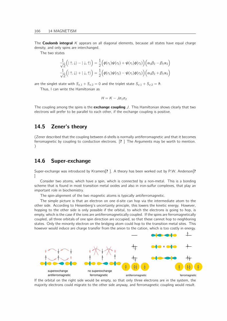
166 14 MAGNETISM
The Coulomb integral K appears on all diagonal elements, because all states have equal chargedensity, and only spins are interchanged.
The two states
1√2
(| ↑, ↓〉 − | ↓, ↑〉
)=
1
2
(φ(r1)ψ(r2) + ψ(r1)φ(r2)
)(α1β2 − β1α2
)1√2
(| ↑, ↓〉+ | ↓, ↑〉
)=
1
2
(φ(r1)ψ(r2)− ψ(r1)φ(r2)
)(α1β2 + β1α2
)are the singlet state with Sz,1 + Sz,2 = 0 and the triplet state Sz,1 + Sz,2 = ~.
Thus, I can write the Hamiltonian as
H = K − Jσ1σ2
The coupling among the spins is the exchange coupling J. This Hamiltonian shows clearly that twoelectrons will prefer to be parallel to each other, if the exchange coupling is positive.
14.5 Zener’s theory
(Zener described that the coupling between d-shells is normally antiferromagnetic and that it becomesferromagnetic by coupling to conduction electrons. [? ] The Arguments may be worth to mention.)
14.6 Super-exchange
Super-exchange was introduced by Kramers[? ]. A theory has been worked out by P.W. Anderson[?]
Consider two atoms, which have a spin, which is connected by a non-metal. This is a bondingscheme that is found in most transition metal oxides and also in iron-sulfur complexes, that play animportant role in biochemistry.
The spin-alignment of the two magnetic atoms is typically antiferromagnetic.The simple picture is that an electron on one d-site can hop via the intermediate atom to the
other side. According to Heisenberg’s uncertainty principle, this lowers the kinetic energy. However,hopping to the other side is only possible if the orbital, to which the electrons is going to hop, isempty, which is the case if the ions are antiferromagnetically coupled. If the spins are ferromagneticallycoupled, all three orbitals of one spin direction are occupied, so that these cannot hop to neighboringstates. Only the minority electron on the bridging atom could hop to the transition metal sites. Thishowever would induce are charge transfer from the anion to the cation, which is too costly in energy.
antiferromagnetic ferromagnetic
no superexchangesuperexchange
ferromagneticantiferromagnetic
If the orbital on the right side would be empty, so that only three electrons are in the system, themajority electrons could migrate to the other side anyway, and ferromagnetic coupling would result.
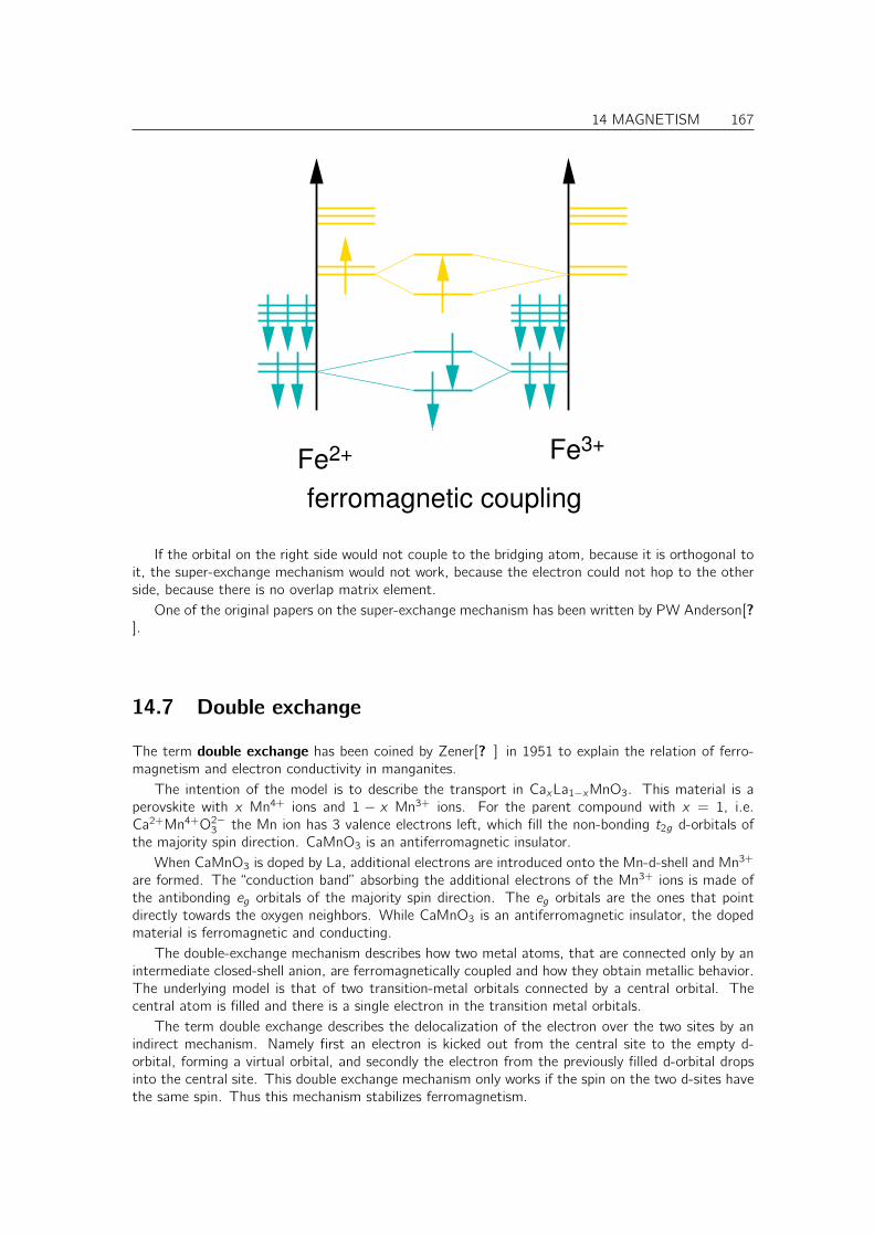
14 MAGNETISM 167
Fe2+ Fe3+
ferromagnetic coupling
If the orbital on the right side would not couple to the bridging atom, because it is orthogonal toit, the super-exchange mechanism would not work, because the electron could not hop to the otherside, because there is no overlap matrix element.
One of the original papers on the super-exchange mechanism has been written by PW Anderson[?].
14.7 Double exchange
The term double exchange has been coined by Zener[? ] in 1951 to explain the relation of ferro-magnetism and electron conductivity in manganites.
The intention of the model is to describe the transport in CaxLa1−xMnO3. This material is aperovskite with x Mn4+ ions and 1 − x Mn3+ ions. For the parent compound with x = 1, i.e.Ca2+Mn4+O2−
3 the Mn ion has 3 valence electrons left, which fill the non-bonding t2g d-orbitals ofthe majority spin direction. CaMnO3 is an antiferromagnetic insulator.
When CaMnO3 is doped by La, additional electrons are introduced onto the Mn-d-shell and Mn3+
are formed. The “conduction band” absorbing the additional electrons of the Mn3+ ions is made ofthe antibonding eg orbitals of the majority spin direction. The eg orbitals are the ones that pointdirectly towards the oxygen neighbors. While CaMnO3 is an antiferromagnetic insulator, the dopedmaterial is ferromagnetic and conducting.
The double-exchange mechanism describes how two metal atoms, that are connected only by anintermediate closed-shell anion, are ferromagnetically coupled and how they obtain metallic behavior.The underlying model is that of two transition-metal orbitals connected by a central orbital. Thecentral atom is filled and there is a single electron in the transition metal orbitals.
The term double exchange describes the delocalization of the electron over the two sites by anindirect mechanism. Namely first an electron is kicked out from the central site to the empty d-orbital, forming a virtual orbital, and secondly the electron from the previously filled d-orbital dropsinto the central site. This double exchange mechanism only works if the spin on the two d-sites havethe same spin. Thus this mechanism stabilizes ferromagnetism.

168 14 MAGNETISM
E
antiferro ferroferro
n
antiferro ferro
Fig. 14.4: Scheme to demonstrate the competition between ferromagnetism and antiferromag-netism. If there are two electrons on the sytem they can be accomodated in bonding orbitals onlywhen the two atoms are antiferromagnetic. No covalen binding survives if the two atoms are ferro-magnetically aligned. If, on the other hand, there is only one orbital in the bonding or the antibondingorbital, that is n = 1 and n = 3, the ferromagnetic coupling is more favorate, because the hybridiza-tion is stronger if the atomic levels are closer together. Bottom: schematic binding energy as functionof number of electrons.
The ground state will be a superposition of the four relevant three-particle states
|χ1〉 = d†1,↑c†↑ c†↓ |0〉
|χ2〉 = d†2,↑c†↑ c†↓ |0〉
|χ3〉 = d†1,↓c†↑ c†↓ |0〉
|χ4〉 = d†1,↓c†↑ c†↓ |0〉
The operators c†σ create an electron on the central oxygen atom, while d†1,σ creates an electron onthe left transition metal atom, while d†2,σ creates an electron on the right transition metal atom.
Because the Hamiltonian has rotational symmetry regarding the spin, the Hamiltonian does notcouple states with different total spin. That is the Hamiltonian is block diagonal with one blockdescribing states with S = + ~2 and the other block containing states with S = − ~2 . The problemfurthermore has parity symmetry, which blocks the states into mirror symmetric and antisymmetric

14 MAGNETISM 169
states. Thus the eigenstates will have the form
|ψ1〉 =1√2
(d†1,↑ + d†2,↑
)c†↑ c
†↓ |0〉
|ψ2〉 =1√2
(d†1,↑ − d
†2,↑
)c†↑ c
†↓ |0〉
|ψ3〉 =1√2
(d†1,↓ + d†2,↓
)c†↑ c
†↓ |0〉
|ψ4〉 =1√2
(d†1,↓ − d
†2,↓
)c†↑ c
†↓ |0〉
However, there are no direct Hamilton matrix elements among the basis states |χ1〉, . . . , |χ4〉.The presence of a coupling term is important to drive delocalization of the d-electron between thetwo sites. An effective coupling, however, comes about by including virtual states, for which one ofthe electrons is kicked out from the central atom and placed into an empty d-orbital.
tt t t
Fig. 14.5: Scheme describing the Slater determinants obtained by hopping from one of the realstates. We have excluded states with double occupation on a peripheral site. This neglect has onlyquantitative consequences. Note that the hopping into an antiferromagnetic virtual orbital does notallow a coupling between two real configuration. It only renormalizes the energy.
Consider a Hamiltonian between two real and a virtual orbital
H =
d†1,↑c†↑ c†↓ |O〉
d†2,↑c†↑ c†↓ |O〉
d†1,↑d†2,↑c
†↓ |O〉
2ε0 + εd 0 t
0 2ε0 + εd t
t t ε0 + 2εd
〈O|c↓c↑d1,↑
〈O|c↓c↑d2,↑
〈O|c↓d2,↑d1,↑
This is the same Hamiltonian as that for the three-center bond. The difference is that here it is amany-particle Hamiltonian. The ground state can therefore be written easily as
|Ψ〉 =1√2
(d†1 + d†2
)c†↑ c
†↓ |O〉 cos(α) + d†1↑d
†2↑c†↓ |O〉 sin(α)
where α is a small parameter that is still to be determined.
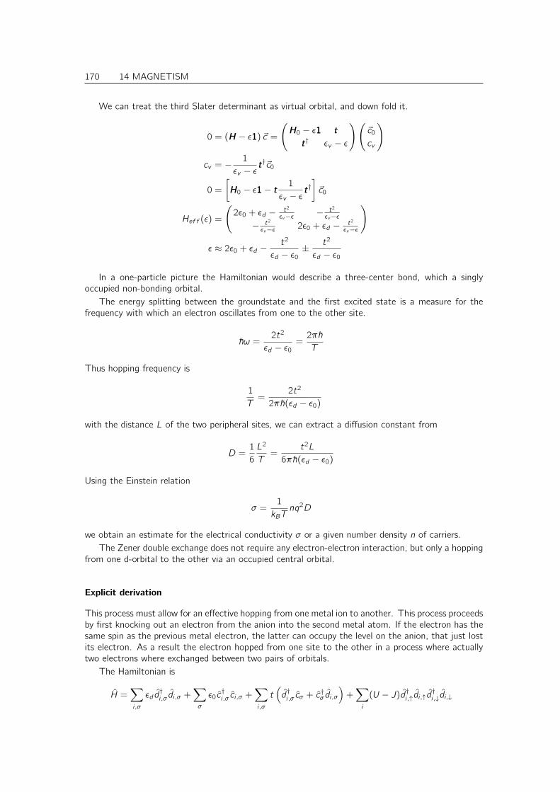
170 14 MAGNETISM
We can treat the third Slater determinant as virtual orbital, and down fold it.
0 = (H − ε111) ~c =
(H0 − ε111 t
t† εv − ε
)(~c0
cv
)
cv = −1
εv − εt†~c0
0 =
[H0 − ε111− t
1
εv − εt†]~c0
Hef f (ε) =
(2ε0 + εd − t2
εv−ε − t2
εv−ε− t2
εv−ε 2ε0 + εd − t2
εv−ε
)
ε ≈ 2ε0 + εd −t2
εd − ε0±
t2
εd − ε0
In a one-particle picture the Hamiltonian would describe a three-center bond, which a singlyoccupied non-bonding orbital.
The energy splitting between the groundstate and the first excited state is a measure for thefrequency with which an electron oscillates from one to the other site.
~ω =2t2
εd − ε0=
2π~T
Thus hopping frequency is
1
T=
2t2
2π~(εd − ε0)
with the distance L of the two peripheral sites, we can extract a diffusion constant from
D =1
6
L2
T=
t2L
6π~(εd − ε0)
Using the Einstein relation
σ =1
kBTnq2D
we obtain an estimate for the electrical conductivity σ or a given number density n of carriers.The Zener double exchange does not require any electron-electron interaction, but only a hopping
from one d-orbital to the other via an occupied central orbital.
Explicit derivation
This process must allow for an effective hopping from one metal ion to another. This process proceedsby first knocking out an electron from the anion into the second metal atom. If the electron has thesame spin as the previous metal electron, the latter can occupy the level on the anion, that just lostits electron. As a result the electron hopped from one site to the other in a process where actuallytwo electrons where exchanged between two pairs of orbitals.
The Hamiltonian is
H =∑i ,σ
εd d†i ,σdi ,σ +
∑σ
ε0c†i ,σ ci ,σ +
∑i ,σ
t(d†i ,σ cσ + c†σdi ,σ
)+∑i
(U − J)d†i ,↑di ,↑d†i ,↓di ,↓
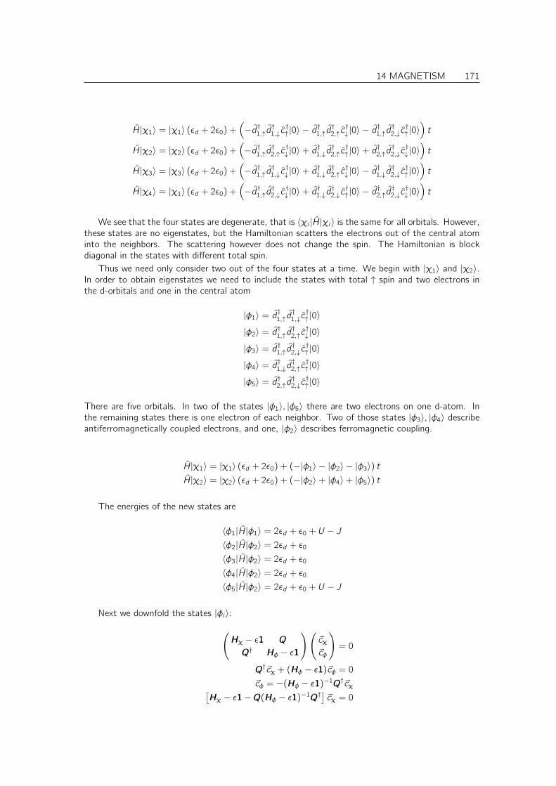
14 MAGNETISM 171
H|χ1〉 = |χ1〉 (εd + 2ε0) +(−d†1,↑d
†1,↓c
†↑ |0〉 − d
†1,↑d
†2,↑c
†↓ |0〉 − d
†1,↑d
†2,↓c
†↑ |0〉
)t
H|χ2〉 = |χ2〉 (εd + 2ε0) +(−d†1,↑d
†2,↑c
†↓ |0〉+ d†1,↓d
†2,↑c
†↑ |0〉+ d†2,↑d
†2,↓c
†↓ |0〉
)t
H|χ3〉 = |χ3〉 (εd + 2ε0) +(−d†1,↑d
†1,↓c
†↓ |0〉+ d†1,↓d
†2,↑c
†↓ |0〉 − d
†1,↓d
†2,↓c
†↑ |0〉
)t
H|χ4〉 = |χ1〉 (εd + 2ε0) +(−d†1,↑d
†2,↓c
†↓ |0〉+ d†1,↓d
†2,↓c
†↑ |0〉 − d
†2,↑d
†2,↓c
†↓ |0〉
)t
We see that the four states are degenerate, that is 〈χi |H|χi 〉 is the same for all orbitals. However,these states are no eigenstates, but the Hamiltonian scatters the electrons out of the central atominto the neighbors. The scattering however does not change the spin. The Hamiltonian is blockdiagonal in the states with different total spin.
Thus we need only consider two out of the four states at a time. We begin with |χ1〉 and |χ2〉.In order to obtain eigenstates we need to include the states with total ↑ spin and two electrons inthe d-orbitals and one in the central atom
|φ1〉 = d†1,↑d†1,↓c
†↑ |0〉
|φ2〉 = d†1,↑d†2,↑c
†↓ |0〉
|φ3〉 = d†1,↑d†2,↓c
†↑ |0〉
|φ4〉 = d†1,↓d†2,↑c
†↑ |0〉
|φ5〉 = d†2,↑d†2,↓c
†↑ |0〉
There are five orbitals. In two of the states |φ1〉, |φ5〉 there are two electrons on one d-atom. Inthe remaining states there is one electron of each neighbor. Two of those states |φ3〉, |φ4〉 describeantiferromagnetically coupled electrons, and one, |φ2〉 describes ferromagnetic coupling.
H|χ1〉 = |χ1〉 (εd + 2ε0) + (−|φ1〉 − |φ2〉 − |φ3〉) tH|χ2〉 = |χ2〉 (εd + 2ε0) + (−|φ2〉+ |φ4〉+ |φ5〉) t
The energies of the new states are
〈φ1|H|φ1〉 = 2εd + ε0 + U − J〈φ2|H|φ2〉 = 2εd + ε0
〈φ3|H|φ2〉 = 2εd + ε0
〈φ4|H|φ2〉 = 2εd + ε0
〈φ5|H|φ2〉 = 2εd + ε0 + U − J
Next we downfold the states |φi 〉:(Hχ − ε111 Q
Q† Hφ − ε111
)(~cχ
~cφ
)= 0
Q†~cχ + (Hφ − ε111)~cφ = 0
~cφ = −(Hφ − ε111)−1Q†~cχ[Hχ − ε111−Q(Hφ − ε111)−1Q†
]~cχ = 0
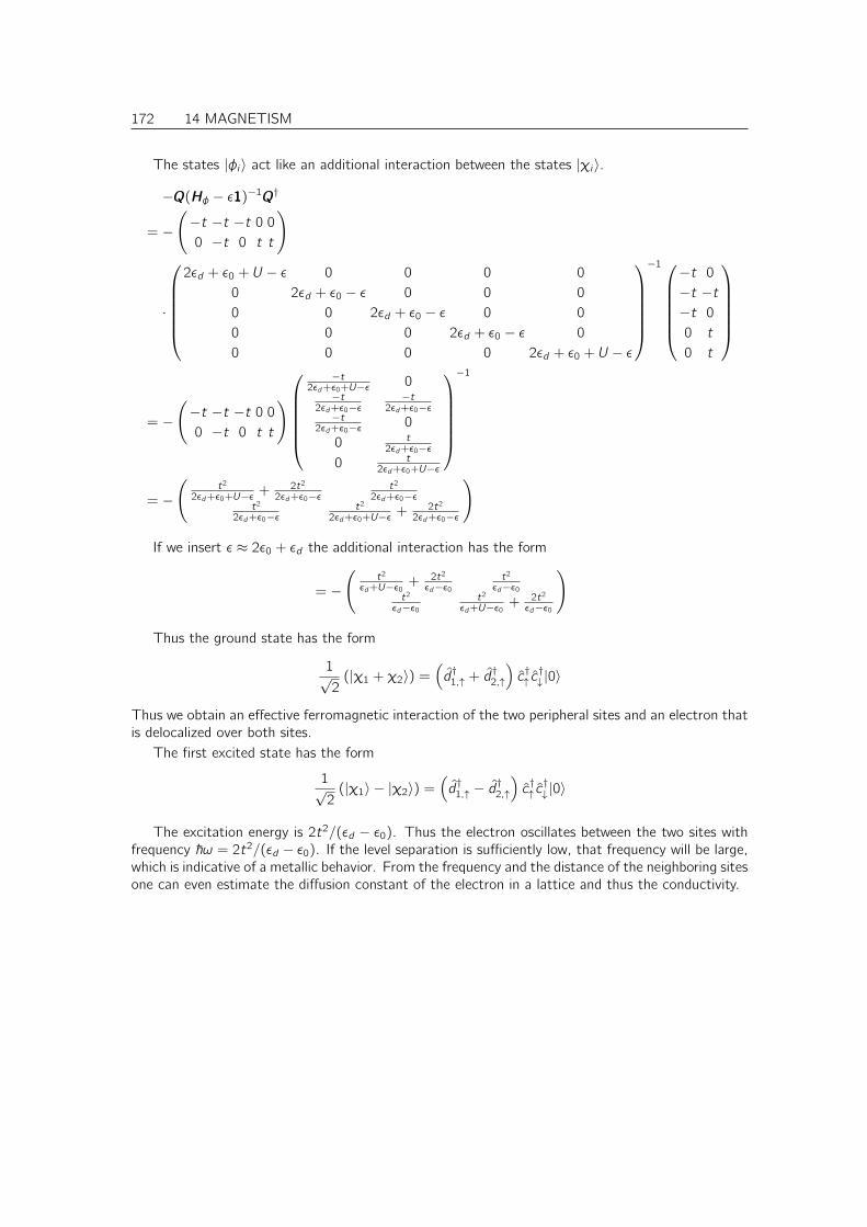
172 14 MAGNETISM
The states |φi 〉 act like an additional interaction between the states |χi 〉.
−Q(Hφ − ε111)−1Q†
= −
(−t −t −t 0 0
0 −t 0 t t
)
·
2εd + ε0 + U − ε 0 0 0 0
0 2εd + ε0 − ε 0 0 0
0 0 2εd + ε0 − ε 0 0
0 0 0 2εd + ε0 − ε 0
0 0 0 0 2εd + ε0 + U − ε
−1−t 0
−t −t−t 0
0 t
0 t
= −
(−t −t −t 0 0
0 −t 0 t t
)−t
2εd+ε0+U−ε 0−t
2εd+ε0−ε−t
2εd+ε0−ε−t
2εd+ε0−ε 0
0 t2εd+ε0−ε
0 t2εd+ε0+U−ε
−1
= −
(t2
2εd+ε0+U−ε + 2t2
2εd+ε0−εt2
2εd+ε0−εt2
2εd+ε0−εt2
2εd+ε0+U−ε + 2t2
2εd+ε0−ε
)
If we insert ε ≈ 2ε0 + εd the additional interaction has the form
= −
(t2
εd+U−ε0+ 2t2
εd−ε0
t2
εd−ε0t2
εd−ε0
t2
εd+U−ε0+ 2t2
εd−ε0
)
Thus the ground state has the form
1√2
(|χ1 + χ2〉) =(d†1,↑ + d†2,↑
)c†↑ c
†↓ |0〉
Thus we obtain an effective ferromagnetic interaction of the two peripheral sites and an electron thatis delocalized over both sites.
The first excited state has the form
1√2
(|χ1〉 − |χ2〉) =(d†1,↑ − d
†2,↑
)c†↑ c
†↓ |0〉
The excitation energy is 2t2/(εd − ε0). Thus the electron oscillates between the two sites withfrequency ~ω = 2t2/(εd − ε0). If the level separation is sufficiently low, that frequency will be large,which is indicative of a metallic behavior. From the frequency and the distance of the neighboring sitesone can even estimate the diffusion constant of the electron in a lattice and thus the conductivity.

Appendices
173


Appendix A
Polyhedra in paper
Fig. A.1: Pattern for constructing a tetrahedron
175
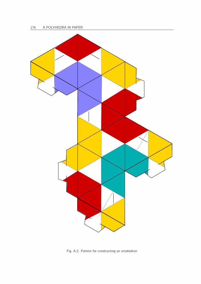
176 A POLYHEDRA IN PAPER
Fig. A.2: Pattern for constructing an octahedron

Appendix B
Justification of the Wolfsbergformula
Using the empirical Wolfsberg formula Eq. 2.6
t = kε1 + ε2
2∆
we can map the Schrödinger equation with a Hamiltonian and Overlap matrix given by Eq. 2.4
H =
(ε1 t
t ε2
)and O =
(1 ∆
∆ 1
)(B.1)
to first order in ∆ onto one with orthogonal Basis functions.
B.1 Approximate orthonormalization
The overlap operator can be made equal to unity by a transformation of the basis orbitals(|χ′1〉|χ′2〉
)=
(|χ1〉|χ2〉
)O
12
Let us first form the square root of the overlap matrix to first order in ∆. We start with an ansatzfor the overlap matrix
O12 = 1 + ∆A +O(∆2)
which defines the matrix A.The matrix A has to obey the equation
O = (1 + ∆A)(1 + ∆A) +O(∆2) = 1 + 2∆A +O(∆2)
⇒ 1 + ∆A =
(1 1
2 ∆12 ∆ 1
)
Using the Taylor expansion of 11+x = 1− x +O(x2), we can now form the inverse of O
12 ≈ 1 + ∆A.
Thus
O−12 =
(1 − 1
2 ∆
− 12 ∆ 1
)+O(∆2)
177
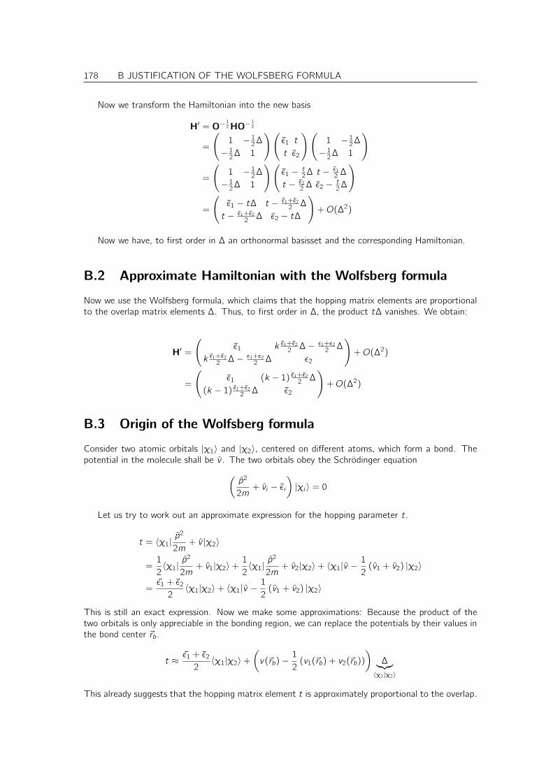
178 B JUSTIFICATION OF THE WOLFSBERG FORMULA
Now we transform the Hamiltonian into the new basis
H′ = O−12 HO−
12
=
(1 − 1
2 ∆
− 12 ∆ 1
)(ε1 t
t ε2
)(1 − 1
2 ∆
− 12 ∆ 1
)
=
(1 − 1
2 ∆
− 12 ∆ 1
)(ε1 − t
2 ∆ t − ε1
2 ∆
t − ε2
2 ∆ ε2 − t2 ∆
)
=
(ε1 − t∆ t − ε1+ε2
2 ∆
t − ε1+ε2
2 ∆ ε2 − t∆
)+O(∆2)
Now we have, to first order in ∆ an orthonormal basisset and the corresponding Hamiltonian.
B.2 Approximate Hamiltonian with the Wolfsberg formula
Now we use the Wolfsberg formula, which claims that the hopping matrix elements are proportionalto the overlap matrix elements ∆. Thus, to first order in ∆, the product t∆ vanishes. We obtain:
H′ =
(ε1 k ε1+ε2
2 ∆− ε1+ε2
2 ∆
k ε1+ε2
2 ∆− ε1+ε2
2 ∆ ε2
)+O(∆2)
=
(ε1 (k − 1) ε1+ε2
2 ∆
(k − 1) ε1+ε2
2 ∆ ε2
)+O(∆2)
B.3 Origin of the Wolfsberg formula
Consider two atomic orbitals |χ1〉 and |χ2〉, centered on different atoms, which form a bond. Thepotential in the molecule shall be v . The two orbitals obey the Schrödinger equation(
p2
2m+ vi − εi
)|χi 〉 = 0
Let us try to work out an approximate expression for the hopping parameter t.
t = 〈χ1|p2
2m+ v |χ2〉
=1
2〈χ1|
p2
2m+ v1|χ2〉+
1
2〈χ1|
p2
2m+ v2|χ2〉+ 〈χ1|v −
1
2(v1 + v2) |χ2〉
=ε1 + ε2
2〈χ1|χ2〉+ 〈χ1|v −
1
2(v1 + v2) |χ2〉
This is still an exact expression. Now we make some approximations: Because the product of thetwo orbitals is only appreciable in the bonding region, we can replace the potentials by their values inthe bond center ~rb.
t ≈ε1 + ε2
2〈χ1|χ2〉+
(v(~rb)−
1
2(v1(~rb) + v2(~rb))
)∆︸︷︷︸
〈χ1|χ2〉
This already suggests that the hopping matrix element t is approximately proportional to the overlap.

B JUSTIFICATION OF THE WOLFSBERG FORMULA 179
The second approximation is to assume that the potentials are approximately proportional to theenergies, that is
v(~rb)−1
2(v1(~rb) + v2(~rb))︸ ︷︷ ︸<0
∼ε1 + ε2
2
I have not found a convincing justification for this latter approximation, but that is what it is.

180 B JUSTIFICATION OF THE WOLFSBERG FORMULA
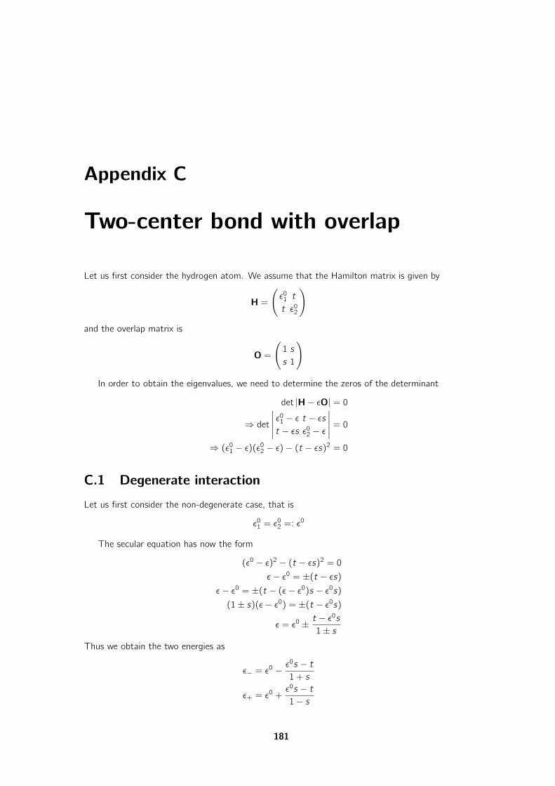
Appendix C
Two-center bond with overlap
Let us first consider the hydrogen atom. We assume that the Hamilton matrix is given by
H =
(ε0
1 t
t ε02
)and the overlap matrix is
O =
(1 s
s 1
)
In order to obtain the eigenvalues, we need to determine the zeros of the determinant
det |H− εO| = 0
⇒ det
∣∣∣∣∣ ε01 − ε t − εst − εs ε0
2 − ε
∣∣∣∣∣ = 0
⇒ (ε01 − ε)(ε0
2 − ε)− (t − εs)2 = 0
C.1 Degenerate interaction
Let us first consider the non-degenerate case, that is
ε01 = ε0
2 =: ε0
The secular equation has now the form
(ε0 − ε)2 − (t − εs)2 = 0
ε− ε0 = ±(t − εs)
ε− ε0 = ±(t − (ε− ε0)s − ε0s)
(1± s)(ε− ε0) = ±(t − ε0s)
ε = ε0 ±t − ε0s
1± sThus we obtain the two energies as
ε− = ε0 −ε0s − t1 + s
ε+ = ε0 +ε0s − t1− s
181
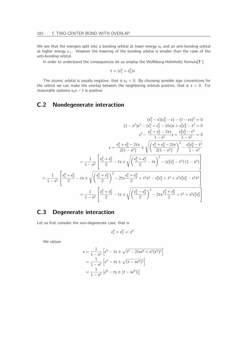
182 C TWO-CENTER BOND WITH OVERLAP
We see that the energies split into a bonding orbital at lower energy ε0 and an anti-bonding orbitalat higher energy ε+. However the lowering of the bonding orbital is smaller than the raise of theanti-bonding orbital.
In order to understand the consequences let us employ the Wolfsberg-Helmholtz formula[? ]
t = (ε01 + ε0
2)s
The atomic orbital is usually negative, that is ε0 < 0. By choosing sensible sign conventions forthe orbital we can make the overlap between the neighboring orbitals positive, that is s > 0. Forreasonable systems ε0s − t is positive.
C.2 Nondegenerate interaction
(ε01 − ε)(ε0
2 − ε)− (t − εs)2 = 0
(1− s2)ε2 − (ε01 + ε0
2 − 2ts)ε+ ε01ε
02 − t2 = 0
ε2 −ε0
1 + ε02 − 2ts
1− s2ε+
ε01ε
02 − t2
1− s2= 0
ε =ε0
1 + ε02 − 2ts
2(1− s2)±
√(ε0
1 + ε02 − 2ts
2(1− s2)
)2
−ε0
1ε02 − t2
1− s2
=1
1− s2
ε01 + ε0
2
2− ts ±
√(ε0
1 + ε02
2− ts
)2
− (ε01ε
02 − t2) (1− s2)
=
1
1− s2
ε01 + ε0
2
2− ts ±
√(ε0
1 + ε02
2
)2
− 2tsε0
1 + ε02
2+ t2s2 − ε0
1ε02 + t2 + s2ε0
1ε02 − s2t2
=
1
1− s2
ε01 + ε0
2
2− ts ±
√(ε0
1 − ε02
2
)2
− 2tsε0
1 + ε02
2+ t2 + s2ε0
1ε02
C.3 Degenerate interaction
Let us first consider the non-degenerate case, that is
ε01 = ε0
2 =: ε0
We obtain
ε =1
1− s2
[ε0 − ts ±
√t2 − 2tsε0 + s2(ε0)2
]=
1
1− s2
[ε0 − ts ±
√(t − sε0)2
]=
1
1− s2
[ε0 − ts ±
∣∣t − sε0)∣∣]
Appendix D
Covalent bonds to second order
This section shows a simple method to estimate the net covalent bonding energy.Consider a Hamiltonian H(0) and a perturbation H(1). We have in mind that the unperturbed
Hamiltonian H(0) is diagonal in a basisset of tight-binding orbitals and that H(1) contains the hop-ping matrix elements, between tight-binding orbitals. The unperturbed Hamiltonian has orthonormaleigenstates |ψ(0)
n 〉 with energies ε(0)n .
The first-order change of the wave function due to a perturbation H(1) is obtained from thefirst-order terms of the Schrödinger equation as follows:(
H(0) − ε(0)n
)|ψ(1)n 〉+
(H(1) − ε(1)
n
)|ψ(0)n 〉 = 0
⇒ |ψ(1)n 〉 =
(ε(0) − H(0)
)−1(H(1) − ε(1)
n
)|ψ(0)n 〉
=∑m
|ψ(0)m 〉〈ψ(0)
m |(ε(0)n − H(0)
)−1(H(1) − ε(1)
n
)|ψ(0)n 〉
=∑m
|ψ(0)m 〉
H(1)m,n − ε(1)
n 〈ψ(0)m |ψ(0)
n 〉ε
(0)n − ε(0)
m
=∑m 6=n|ψ(0)m 〉
H(1)m,n
ε(0)n − ε(0)
m
(D.1)
In the last step we imposed that the norm of the wave function remains conserved, so that 〈ψ(0)m |ψ(1)
n 〉 =0.
Furthermore, we will exploit that the states shall be orthonormal to any order, which implies that
〈ψ(0)m + ψ(1)
m + ψ(2)m + . . . |ψ(0)
n + ψ(1)n + ψ(2)
n + . . .〉 = δm,n (D.2)
in every order or the perturbation. This implies in the first order
〈ψ(1)n |ψ(0)
m 〉+ 〈ψ(0)n |ψ(1)
m 〉 = 0 ⇒ Re〈ψ(0)n |ψ(1)
n 〉 = 0 (D.3)
and in the second order
〈ψ(2)n |ψ(0)
m 〉+ 〈ψ(1)n |ψ(1)
m 〉+ 〈ψ(0)n |ψ(2)
m 〉 = 0⇒ 〈ψ(2)n |ψ(0)
n 〉+ 〈ψ(0)n |ψ(2)
n 〉 = −〈ψ(1)n |ψ(1)
n 〉 (D.4)
With the assumption that the occupations do not change, the energy to second order is obtained
183
184 D COVALENT BONDS TO SECOND ORDER
as
E =∑n
fn〈ψ(0)n + ψ(1)
n + ψ(2)n + . . . |H(0) + H(1)|ψ(0)
n + ψ(1)n + ψ(2)
n + . . .〉
=∑n
fn 〈ψ(0)n |H(0)|ψ(0)
n 〉︸ ︷︷ ︸ε
(0)n
+∑n
fn
(〈ψ(1)
n |H(0)|ψ(0)n 〉+ 〈ψ(0)
n |H(0)|ψ(1)n 〉︸ ︷︷ ︸
〈ψ(1)n |ψ(0)
n 〉ε(0)n +ε
(0)n 〈ψ(0)
n |ψ(1)n 〉=0 (see Eq. ??)
+〈ψ(0)n |H(1)|ψ(0)
n 〉)
+∑n
fn
(〈ψ(2)
n |H(0)|ψ(0)n 〉+ 〈ψ(0)
n |H(0)|ψ(2)n 〉︸ ︷︷ ︸
−ε(0)n 〈ψ(1)
n |ψ(1)n 〉 (see Eq. ??)
+〈ψ(1)n |H(1)|ψ(0)
n 〉+ 〈ψ(0)n |H(1)|ψ(1)
n 〉+ 〈ψ(1)n |H(0)|ψ(1)
n 〉). . .
=∑n
fn
(ε(0)n + 〈ψ(0)
n |H(1)|ψ(0)n 〉)
+∑n
fn
(〈ψ(1)
n |H(1)|ψ(0)n 〉+ 〈ψ(0)
n |H(1)|ψ(1)n 〉+ 〈ψ(1)
n |H(0) − ε(0)n |ψ(1)
n 〉)
+ . . .
=∑n
fn
(ε(0)n + 〈ψ(0)
n |H(1)|ψ(0)n 〉)
+∑n
fn∑m;m 6=n
( H(1)n,m
ε(0)n − ε(0)
m
〈ψ(0)m |H(1)|ψ(0)
n 〉+ 〈ψ(0)n |H(1)|ψ(0)
m 〉H
(1)m,n
ε(0)n − ε(0)
m
+H
(1)n,m
ε(0)n − ε(0)
m
〈ψ(0)m |H(0) − ε(0)
n |ψ(0)m 〉︸ ︷︷ ︸
ε(0)m −ε(0)
n
H(1)m,n
ε(0)n − ε(0)
m
)+ . . .
=∑n
fn
(εn + 〈ψ(0)
n |H(1)|ψ(0)n 〉)
+∑n
fn
( ∑m;m 6=n
∣∣∣H(1)n,m
∣∣∣2ε
(0)n − ε(0)
m
)+ . . .
(D.5)
Thus we obtain to second order the energy change
SECOND ORDER BONDING
For an already insulating system, for which the occupations remain unchanged, the energy gain dueto the hopping matrix elements to second order are obtained as
∆E =∑n
fn
(εn + ∆εn
)(D.6)
with the level shifts
∆εn = H(1)n,n +
∑m;m 6=n
∣∣∣H(1)m,n
∣∣∣2ε
(0)m − ε(0)
n
(D.7)
The matrix elements are defined as
H(1)m,n = 〈ψ(0)
m |H(1)|ψ(0)n 〉 (D.8)
Thus the shift of the energy levels are obtained by summing up all level repulsions.The second-order expression is valid when the perturbation between occupied and unoccupied levelsis small compared to the already existing band gap. It breaks down when |H(1)
n,m| > |εm − εn|. If theunperturbed energy levels are separated by a band gap, however, the total energy is only sensitive tolevel repulsions between filled and empty states. The requirement is then reduced to the limitationthat the hopping matrix elements between filled and empty states must be smaller than the bandgap.
This derivation suggests to first optimize the system using all onsite interactions, and to redis-
D COVALENT BONDS TO SECOND ORDER 185
tribute the electrons to form ions. If this system produces a band gap separating the filled and emptystates, and if the hopping matrix elements accross the band gap are smaller than the band gap, theremaining bonding contribution can be obtained by perturbation theory. In this case the diagonalelements of the Hamiltonian form the zero’th order term H0, while the off-diagonal elements of theHamiltonian, the hopping matrix elements, are treated as perturbation.
The Hamiltonian would have the form
H =∑α
|χα〉εα〈χα| −∑
α,β;α 6=β|χα〉tα,β〈χβ | (D.9)
where |χα〉 are the tight-binding orbitals, εα their energies, and tα,β is the hopping matrix elementbetween orbitals |χα〉 and |χβ〉.
Because, in this case, the perturbation vanishes on the diagonal, the first order term vanishes,and the change of the total energy is entirely fiven by the hopping matrix elements, which enter tosecond order.
APPROXIMATE COVALENT ENERGY AT FIXED OCCUPATIONS
In this special second order approximation, we obtain the total energy due to level shifts, i.e. for fixedoccupations, in the form
∆Ecov ≈ −∑
m,n;fα>fβ
|tα,β |2fn − fmε
(0)m − ε(0)
n
. (D.10)
The Hamiltonian is of the form Eq. ??.
In this manner we can add up the approximate binding energy in a bond-by-bond manner.The following is not worked out! This procedure works for ionic systems. One way to access
covalent systems, where the preconditions of the above derivation are violated, is to start from afictitious system with a negative on-site Coulomb interaction. This stabilized ionic systems. Thenthe hopping energy can be evaluated using the formula above. Finally one needs to correct again forthe negative Coulomb interaction. This requires however the onsite occupations to be evaluated tosecond order.

186 D COVALENT BONDS TO SECOND ORDER
Appendix E
Reading
• Walter A Harrison has written a series of books describing the properties of materials on thebasis of the tight-binding theory. “Electronic Structure and the Properties of Solids: ThePhysics of the Chemical Bond” ”Elementary Electronic Structure”
• a magnificent resource is the book “Orbital interactions in Chemistry” by Albright, Burdett andWhangbo. It provides a good feel for orbitals and how they relate to atomic structures. Mostlyfor organic and organometallic chemistry.
• An easy to read introduction to simple molecular orbital theory of solids and surfaces is the book“Solids and Surfaces: A chemist’s View of Bonding in extended Structures” by R. Hoffmann.[?] The book covers basically the material of the article[? ].
• The book “Computational Chjemistry of Solid state Materials” by R. Dronskowski[? ] providesa critical overview over simple empirical rules of Inorganic chemistry. In addition it contains adescription of computational simulation techniques, which is complemented with own applica-tions.
• Chemogenesis webbook: http://www.meta-synthesis.com/webbook.html
187

188 E READING

Appendix F
Dictionary
principal quantum number Hauptquantenzahl
189

190 F DICTIONARY

Appendix G
Greek Alphabet
A α alpha N ν nuB β beta Ξ ξ ksiΓ γ gamma O o, omicron∆ δ delta Π π,$ piE ε, ε epsilon P ρ, % rhoZ ζ zeta Σ σ, ς sigmaH η eta T τ tauΘ θ, ϑ theta Υ υ upsilonI ι iota Φ φ,ϕ phiK κ kappa X χ chiΛ λ lambda Ψ φ phiM µ mu Ω ω omega
191

192 G GREEK ALPHABET

Appendix H
Philosophy of the ΦSX Series
In the ΦSX series, I tried to implement what I learned from the feedback given by the students whichattended the courses and that relied on these books as background material.
The course should be self-contained. There should not be any statements “as shown easily...” if,this is not true. The reader should not need to rely on the author, but he should be able to convincehimself, if what is said is true. I am trying to be as complete as possible in covering all materialthat is required. The basis is the mathematical knowledge. With few exceptions, the material is alsodeveloped in a sequence so that the material covered can be understood entirely from the knowledgecovered earlier.
The derivations shall be explicit. The novice should be able to step through every single step ofthe derivation with reasonable effort. An advanced reader should be able to follow every step of thederivations even without paper and pencil.
All units are explicit. That is, formulas contain all fundamental variables, which can be inserted inany desirable unit system. Expressions are consistent with the SI system, even though I am quotingsome final results in units, that are common in the field.
The equations that enter a specific step of a derivation are noted ontop of the equation sign.The experience is that the novice does not immediately memorize all the material covered and thathe is struggling with the math, so that he spends a lot of time finding the rationale behind a certainstep. This time is saved by being explicit about it. The danger that the student gets dependent onthese indications, is probably minor, as it requires some effort for the advanced reader to look up theassumptions, an effort he can save by memorizing the relevant material.
Important results and equations are highlighted by including them in boxes. This should facilitatethe preparations for examinations.
Portraits of the key researchers and short biographical notes provide independent associationsto the material. A student may not memorize a certain formula directly, but a portrait. Fromthe portrait, he may associate the correct formula. The historical context provides furthermore anindependent structure to organize the material.
The two first books are in german (That is the intended native language) in order to not addcomplications to the novice. After these first books, all material is in English. It is mandatory that thestudent masters this language. Most of the scientific literature is available only in English. Englishis currently the language of science, and science is absolutely dependent on international contacts.
I tried to include many graphs and figures. The student shall become used to use all his sensesin particular the visual sense.
I have slightly modified the selection of the material commonly tought in most courses. Sometopics, which I consider of mostly historical relevance I have removed. Others such as the Noethertheorem, I have added. Some, like Chaos, Stochastic processes, etc. I have not added yet.
193

194 H PHILOSOPHY OF THE ΦSX SERIES
Appendix I
About the Author
Prof. Dr. rer. nat Peter E. Blöchl studied physics at Karlsruhe University of Technology in Germany.Subsequently he joined the Max Planck Institutes for Materials Research and for Solid state Researchin Stuttgart, where he developed of electronic-structure methods related to the LMTO method andperformed first-principles investigations of interfaces. He received his doctoral degree in 1989 fromthe University of Stuttgart.
Following his graduation, he joined the renowned T.J. Watson Research Center in YorktownHeights, NY in the US on a World-Trade Fellowship. In 1990 he accepted an offer from the IBMZurich Research Laboratory in Ruschlikon, Switzerland, which had just received two Nobel prices inPhysics (For the Scanning Tunneling Microscope in 1986 and for the High-Temperature Supercon-ductivity in 1987). He spent the summer term 1995 as visiting professor at the Vienna University ofTechnology in Austria, from where was later awarded the habilitation in 1997. In 2000, he left theIBM Research Laboratory after a 10-year period and accepted an offer to be professor for theoreticalphysics at Clausthal University of Technology in Germany. Since 2003, Prof. Blöchl is member ofthe Braunschweigische Wissenschaftliche Gesellschaft (Academy of Sciences).
The main thrust of Prof. Blöchl’s research is related to ab-initio simulations, that is, parameter-free simulation of materials processes and molecular reactions based on quantum mechanics. Hedeveloped the Projector Augmented Wave (PAW) method, one of the most widely used electronicstructure methods to date. This work has been cited over 25,000 times.1 It is among the 100 mostcited scientific papers of all times and disciplines2 , and it is among the 10 most-cited papers outof more than 500,000 published in the 120-year history of Physical Review. 3 Next to the researchrelated to simulation methodology, his research covers a wide area from biochemistry, solid statechemistry to solid state physics and materials science. Prof. Blöchl contributed to 8 Patents andpublished about 100 research publications, among others in well-known Journals such as “Nature”.The work of Prof. Blöchl has been cited over 35,000 times, and he has an H-index of 42.4
1Researcher ID: B-3448-20122R. van Noorden, B. Maher and R. Nuzzo, Nature 514, 550 (2014)3Oct. 15, 2014, search in the Physical Review Online Archive with criteria “a-z”.4Researcher ID: B-3448-2012
195

196 I ABOUT THE AUTHOR

Bibliography
[] T.A. Albright, J.K. Burdett, and M.-H. Whangbo. Orbital interactions in Chemistry. John Wileyand Sons, New York, 1985.
[] F. Bloch. über die quantenmechanik der elektronen in kristallgittern. Zeitschr. Phys., 52:555,1929.
[] J.C. Slater and G.F. Koster. Simplified lcao method for the periodic potential problem. Phys.Rev., 94:1498, 1954.
[] M. Wolfsberg and L. Helmholtz. J. Chem. Phys, 20:837, 1952.
[] K. Fukui. Nobel Lectures Chemistry, 1981-1990, chapter The role of frontier orbitals in chemicalreactions. World Scientific, Singapore, 1982.
[] P.E. Blöchl and J.H. Stathis. Hydrogen electrochemistry and stress-induced leakage current insilica. Phys. Rev. Lett, 83:372, 1999.
[] P.E. Blöchl. First-principles calculations of defects in oxygen-deficient silica exposed to hydrogen.Phys. Rev. B, 62:6158, 2000.
[] W. Harrison. The physics of solid state chemistry. Advances in Solid State Physics, 17:135,1977.
[] S. Froyen and W.A. Harrison. Elementary prediction of linear combination of atomic orbitalmatrix elements. Phys. Rev. B, 20:2420, 1979.
[] W.A. Harrison. Theory of the two-center bond. Phys. Rev. B, 27:3592, 1983.
[] M. van Schilfgaarde and W.A. Harrison. Theory of the multicenter bond. Phys. Rev. B, 33:2653, 1986.
[] Konny Schmitt, Claudia Stückl, Herbert Ripplinger, and Barbara Albert. Crystal and electronicstructure of bab6 in comparison with cab6 and molecular [B6H6]2−. Solid State Sciences, 3(3):321 – 327, 2001. ISSN 1293-2558. doi: https://doi.org/10.1016/S1293-2558(00)01091-8.URL http://www.sciencedirect.com/science/article/pii/S1293255800010918.
[] R. Dronskowski and P.E. Blöchl. Crystal orbital hamilton populations (cohp). energy-resolvedvisualization of chemical bonding in solids based on density-functional calculations. J. Phys.Chem., 97:8617, 1993.
[] P. E. Blöchl. ΦSX: Introduction to Solid State Theory. Blöchl, 2017. URL http://www2.pt.tu-clausthal.de/atp/phisx.html.
[] R.S. Mulliken. A new electroaffinity scale; together with data on valence states and on valenceionization potentials and electron affinities. J. Chem. Phys., 2:782, 1934.
[] H. A. Jahn and E. Teller. Stability of polyatomic molecules in degenerate electronic states. i.orbital degeneracy. Proc. R. Soc. London A, 1937.
197

198 BIBLIOGRAPHY
[] Linus Pauling. The nature of the chemical bond. iii. the transition from one extreme bond typeto another. J. Am. Chem. Soc., 54:988, 1932.
[] H. Räbiger, S. Lany, and A. Zunger. Charge self-regulation upon changing the oxidation stateof transition metals in insulators. Nature, 453:763, 2008.
[] R.G. Parr and R.G. Pearson. Absolute hardness: Companion parameter to absolute electroneg-ativity. J. Am. Chem. Soc., 105:7512, 1983.
[] J.F. Janak. Proof that ∂e/∂ni = εi in density functional theory. Phys. Rev. B, 18:7165, 1978.
[] Linus Pauling. The nature of the chemical bond. iv. the energy of single bonds and the relativeelectronegativity of atoms. J. Am. Chem. Soc., 54:3570, 1932.
[] R.G. Pearson. Hard and soft acids and bases. J. Am. Chem. Soc., 85:3533, 1963.
[] P.K. Chattaraj, H. Lee, and R.G. Parr. Hsab principle. J. Am. Chem. Soc., 113:1855, 1991.
[] P.W. Ayers, R.G. Parr, and R.G. Pearson. Elucidating the hard/soft acid/base principle: Aperspective based on half-reactions. J. Chem. Phys., 124:194107, 2006.
[] P.P. Ewald. Ann. Phys., 64:253, 1921.
[] The nature of the chemical bond and the structure of molecules and crystals. Cornell UniversityPress, 1960.
[] A.F. Kapustinskii. Q. Rev. Chem. Soc, 10:203, 1956.
[] W.B. Jensen. The origin of the ionic-radius ratio rules. J. Chem. Educ., 87:587, 2010.
[] G.F. Huettig. Notiz zur geometrie der koordinationszahl. Z. anorg. Chem., 114:24, 1920.
[] J.I. Gersten and F.W. Smith. The Physics and Chemistry of Materials. John Wiley and Sons,Inc., 2001.
[] S.H.Pine. Organic Chemistry. McGraw Hill, 1987.
[] J. Huheey, E.A. Keiter, and R.L. Keiter. Inorganic Chemistry: Principles of Structure andReactivity. Harper Collins, New York, 1993.
[] Fredrik Lindberg. Studies of Oxygen Deficient Complex Cobaltates with Perovskite RelatedStructures. PhD thesis, Physicsl, Inorganic and Structural Chemistry, Stockholm University,2006.
[] E.O. Wollan and W.C. Koehler. Neutron diffraction study of the magnetic properties of theseries of perovskite-type compounds [(1-x)la, xca]mno3. Phys. Rev., 100:545, 1955.
[] J.C. Slater. The lorentz correction in barium titanate. Phys. Rev., 78:748, 1950.
[] R.E. Cohen. Origin of ferroelectricity in perovskite oxides. Nature, 358:136, 1992.
[] A.F. Wells. The structuresof crystals. Solid State Physics, 7:425, 1958.
[] K.K. Murata and S. Doniach. Theory of magnetif fluctuations in itinerant ferromagnets. Phys.Rev. Lett., 29:285, 1972.
[] Peter Mohn and E.P. Wohlfarth. The curie temperature of the ferromagnetic transition metalsand their compounds. J. Phys. F: Met. Phys., 17:2421, 1987.
[] C. Zener. Interaction between the d shells in the transition metals. Phys. Rev., 81:440, 1951.

BIBLIOGRAPHY 199
[] H.A. Kramers. L’interaction entre les atomes magnetogenes dans un cristal paramagnetique.Physica, 1:191, 1934.
[] P.W Anderson. New approach to the theory of superexchange interactions. Phys. Rev., 115:2,1959.
[] C. Zener. Interaction between the d-shells in the transition metals. ii. ferromagnetic compoundsof manganese with perovskite structure. Phys. Rev., 82:403, 1951.
[] R. Hoffmann. Solids and Surfaces: A Chemist’s View of Bonding in Extended Structures.Wiley-VCH, 1988.
[] R. Hoffmann. A chemical and theoretical way to look at bonding on surfaces. Rev. Mod. Phys.,60:601, 1988.
[] R. Dronskowski. Computational Chemistry of Solid State Materials: A Guide for MaterialScientists, Chemists, Physicists and others. Wiley VCH, 2005.

Index
angular-momentum quantum number, 61anti-bonding state, 20
band structure, 84Bloch theorem, 84block diagonal, 33bond
ionic, 21bonding state, 20Born repulsion, 120Born-Mayer equation, 121Boson, 14bra, 13bracket notation, 13Bravais lattice, 133Brillouin zone, 96
characteristic polynomial, 18chemical potential, 114COHP, 83commutating operations, 52complete neglect of overlap, 17COOP, 83core repulsion, 105Coulomb integral, 170Crystal Orbital Hamilton Population, 83Crystal Orbital Overlap Population, 83
delta function, 13density of states
total, 83density functional theory, 15density of states
projected, 83Density of States, 26Density of states
per volume, 86Dirac’s bracket notation, 13Dirac’s delta function, 13dispersion relation
linear chain, 26double bond, 48double exchange, 171
eg, 73eigenstate, 12
eigenvalue, 12eigenvectors, 16electron affinity, 106, 116electronegativity, 107, 115electronegativity
absolute, 115Mulliken, 115
electronegativityPauling, 115
electrophile, 23, 75energy spectrum, 12entartet, 73ethene, 48Ewald sum, 120exchange coupling, 170exchange splitting, 165expectation value, 12expectation value
in bracket notation, 13extended zone scheme, 95
Fermi-level, 22Fermion, 14free electron gas, 81Frontier orbitals, 75
Hamilton function, 11Hamilton operator, 12
bracket notation, 13Hamilton’s equations, 11hardness, 114, 116Hartree-Fock approximation, 168heat of dissociation, 122HOMO, 23hopping matrix element, 16HSAB principle, 117Hund’s rule, 163hybridization, 21
ionic bond, 21ionization potential, 106, 116
Jahn-Teller theoem, 110Janack’s theorem, 114jellium model, 81
INDEX 201
Kapustinskii equation, 121ket, 13
LAPACK, 16Laplace-Runge-Lenz vector, 103lattice constant, 89lattice vector
general, 89primitive, 89reciprocal, 89
LUMO, 23
Madelung constant, 120magnetic quantum number, 61martensitic transition, 148methane, 52momentum operator, 11momentum operator
in bracket notation, 13
node plane, 21normalization condition, 12nucleophile, 23, 75number of states, 84
Observable, 11oxidation state, 108, 113
Pauli principle, 14periodic, 89periodic boundary condition, 25periodic zone scheme, 96position operator, 13positions
relative, 89promotion energy, 67
quantum numbers, 35quasi crystal, 133
radical, 23Reciprocal lattice vectors, 90reduced zone scheme, 95
scalar product, 13in bracket notation, 13
Schrödinger equationtime dependent, 12time independent, 12
Slater determinant, 14Slater-Koster tables, 43softness, 116spherical harmonics, 61spherical harmonics
real, 62
spherical harmonicscubic, 62
spin, 14star, 43Stoner criterion, 165symmetry, 34
t2g, 73three-center bond, 48tight-binding method, 43tight-binding model, 40transformation operator, 34triple, 73triple bond, 48
unit cellprimitive, 89
vacuum level, 116Van Arkel-Ketelaar triangle, 117van der Waal’s distance, 130van-der-Waal’s bond, 129
Wigner Seitz cell, 96Wolfsberg-Helmholtz formula, 17work function, 116


![PhiSX: Statistical Physicsorion.pt.tu-clausthal.de/atp/downloads/scripts/sm.pdfThe roots of the theory of probability lie in the theory of games of chance.[1] In the French Society](https://img.pdfslide.us/doc/110x75/5eaea811e1c6880d583b1a29/phisx-statistical-the-roots-of-the-theory-of-probability-lie-in-the-theory-of-games.jpg)