PhD Thesis - Automated Recognition of 3D CAD Model Objects in

Automated Recognition

of 3D CAD Model Objects

in Dense Laser Range Point

Clouds

by

Frederic N. Bosche

A thesis

presented to the University of Waterloo

in fulfillment of the

thesis requirement for the degree of

Doctor of Philosophy

in

Civil Engineering

Waterloo, Ontario, Canada, 2008

� Frederic N. Bosche 2008

I hereby declare that I am the sole author of this thesis. This is a true copy of the

thesis, including any required final revisions, as accepted by my examiners.

I understand that my thesis may be made electronically available to the public.

ii

Abstract

There is shift in the Architectural / Engineering / Construction and Facility

Management (AEC&FM) industry toward performance-driven projects. Assur-

ing good performance requires efficient and reliable performance control processes.

However, the current state of the AEC&FM industry is that control processes are

inefficient because they generally rely on manually intensive, inefficient, and often

inaccurate data collection techniques.

Critical performance control processes include progress tracking and dimen-

sional quality control. These particularly rely on the accurate and efficient col-

lection of the as-built 3D status of project objects. However, currently available

techniques for as-built 3D data collection are extremely inefficient, and provide

partial and often inaccurate information. These limitations have a negative impact

on the quality of decisions made by project managers and consequently on project

success.

This thesis presents an innovative approach for Automated 3D Data Collec-

tion (A3dDC). This approach takes advantage of Laser Detection and Ranging

(LADAR), 3D Computer-Aided-Design (CAD) modeling and registration technolo-

gies. The performance of this approach is investigated with a first set of exper-

imental results obtained with real-life data. A second set of experiments then

analyzes the feasibility of implementing, based on the developed approach, auto-

mated project performance control (APPC) applications such as automated project

progress tracking and automated dimensional quality control. Finally, other appli-

cations are identified including planning for scanning and strategic scanning.

iii

Acknowledgements

First of all, I would like to truly thank my supervisor, Dr. Carl T. Haas, for his

dedicated supervision and mentoring, and honest friendship. I would also like to

thank the members of my Ph.D. committee, as well as Dr. Vanheeghe who deserved

to be part of it, for their help in my PhD research and thesis writing endeavors.

Then, I would like to thank all my family, starting with my parents, Nicole and

Jean-Pierre, for their psychological and also financial support. All this would not

have been possible without their support, that started almost thirty years ago. I

thank my sister, Valerie, and brothers, Nicolas and Aurelien, for they have played a

key role in the happy life that I have lived up to now. Also, I have had the chance to

have the presence, support and wisdom of my grand-parents during all this time. I

would like to thank them for this, in particular my grand-mother, Louise, to whom

this thesis is dedicated.

Next, I would like to thank all my friends, from all over the world, who have

never complained about my research worries and who know what it takes to be

friends.

Final and nonetheless very special thanks go to Catherine.

iv

Dedication

This thesis is dedicated to my grand-mother, Louise Bourhis, nee Rouat.

v

Contents

1 Introduction 1

1.1 Background And Motivation . . . . . . . . . . . . . . . . . . . . . . 1

1.2 Objectives . . . . . . . . . . . . . . . . . . . . . . . . . . . . . . . . 2

1.3 Scope . . . . . . . . . . . . . . . . . . . . . . . . . . . . . . . . . . 3

1.4 Methodology . . . . . . . . . . . . . . . . . . . . . . . . . . . . . . 3

1.5 Structure of the Thesis . . . . . . . . . . . . . . . . . . . . . . . . . 4

2 Literature Review 5

2.1 Performance-driven Projects and Control Processes in the AEC&FM

industry . . . . . . . . . . . . . . . . . . . . . . . . . . . . . . . . . 5

2.2 Feedback 3D Information Flows . . . . . . . . . . . . . . . . . . . . 6

2.3 Leveraging New Reality-Capture Sensors . . . . . . . . . . . . . . . 7

2.3.1 Laser Scanning . . . . . . . . . . . . . . . . . . . . . . . . . 8

2.4 Performance Expectations for 3D Object Recognition in Construction 9

2.5 Automated 3D Object Recognition in Range Images . . . . . . . . . 11

2.6 A Priori Information Available in the AEC&FM Context . . . . . . 15

2.6.1 3D CAD Modeling . . . . . . . . . . . . . . . . . . . . . . . 16

2.6.2 3D Registration . . . . . . . . . . . . . . . . . . . . . . . . . 17

2.7 Conclusion on Using Existing 3D Object Recognition Techniques . . 19

3 New Approach 21

3.1 Overview . . . . . . . . . . . . . . . . . . . . . . . . . . . . . . . . . 21

3.2 Step 1 - Project 3D Model Format Conversion . . . . . . . . . . . . 22

3.3 Step 2 - 3D Registration . . . . . . . . . . . . . . . . . . . . . . . . 24

vi

3.4 Step 3 - Calculation of the As-planned Range Point Cloud . . . . . 26

3.4.1 The Ray Shooting Problem . . . . . . . . . . . . . . . . . . 27

3.4.2 Developed Approach . . . . . . . . . . . . . . . . . . . . . . 32

3.5 Step 4 - Range Points Recognition . . . . . . . . . . . . . . . . . . . 34

3.5.1 Automated Estimation of Δρmax . . . . . . . . . . . . . . . 35

3.6 Step 5 - Objects Recognition . . . . . . . . . . . . . . . . . . . . . . 38

3.6.1 Sort Points . . . . . . . . . . . . . . . . . . . . . . . . . . . 38

3.6.2 Recognize Objects . . . . . . . . . . . . . . . . . . . . . . . 39

3.6.3 Automated Estimation of Surfmin . . . . . . . . . . . . . . 41

3.7 Sensitivity Analyses . . . . . . . . . . . . . . . . . . . . . . . . . . . 44

4 Experimental Analysis of the Approach’s Performance 45

4.1 Level of Automation . . . . . . . . . . . . . . . . . . . . . . . . . . 45

4.2 Experimental Data . . . . . . . . . . . . . . . . . . . . . . . . . . . 46

4.3 Accuracy . . . . . . . . . . . . . . . . . . . . . . . . . . . . . . . . . 47

4.3.1 Accuracy Performance Metrics . . . . . . . . . . . . . . . . . 48

4.3.2 Experimental Results . . . . . . . . . . . . . . . . . . . . . . 49

4.3.3 Automated Estimation of Δρmax . . . . . . . . . . . . . . . 53

4.3.4 Automated Estimation of Surfmin . . . . . . . . . . . . . . 54

4.4 Robustness . . . . . . . . . . . . . . . . . . . . . . . . . . . . . . . 58

4.4.1 Planned Internal Occlusion Rate . . . . . . . . . . . . . . . 58

4.4.2 Total Occlusion Rate (TOR) . . . . . . . . . . . . . . . . . . 59

4.5 Efficiency . . . . . . . . . . . . . . . . . . . . . . . . . . . . . . . . 60

4.5.1 Overall Computational Performance . . . . . . . . . . . . . . 61

4.5.2 Performance of The Developed Technique for Calculating As-

planned Range Point Clouds . . . . . . . . . . . . . . . . . . 62

4.6 Conclusion . . . . . . . . . . . . . . . . . . . . . . . . . . . . . . . . 65

5 Enabled Applications: Feasibility Analysis and Experiments 67

5.1 Experimental Data . . . . . . . . . . . . . . . . . . . . . . . . . . . 67

5.2 APPC: Automated Construction Progress Tracking . . . . . . . . . 68

vii

5.2.1 Progress Calculation Method . . . . . . . . . . . . . . . . . 68

5.2.2 Experimental Results . . . . . . . . . . . . . . . . . . . . . . 69

5.2.3 Discussion . . . . . . . . . . . . . . . . . . . . . . . . . . . . 72

5.3 APPC: Automated Dimensional QA/QC . . . . . . . . . . . . . . . 75

5.4 APPC: Automated Dimensional Health Monitoring . . . . . . . . . 76

5.5 Planning For Scanning . . . . . . . . . . . . . . . . . . . . . . . . . 76

5.5.1 Experiment . . . . . . . . . . . . . . . . . . . . . . . . . . . 78

5.6 Strategic Scanning . . . . . . . . . . . . . . . . . . . . . . . . . . . 80

6 Conclusions and Recommendations 81

6.1 Contribution . . . . . . . . . . . . . . . . . . . . . . . . . . . . . . . 81

6.2 Limitations . . . . . . . . . . . . . . . . . . . . . . . . . . . . . . . 82

6.3 Suggestions for Future Research . . . . . . . . . . . . . . . . . . . . 83

Appendices 85

A Description of the STL Format 85

B The Spherical Coordinate Frame 88

B.1 The Spherical Coordinate Frame . . . . . . . . . . . . . . . . . . . . 88

B.2 Coordinate Frame Conversions . . . . . . . . . . . . . . . . . . . . . 89

B.2.1 Spherical to Cartesian . . . . . . . . . . . . . . . . . . . . . 89

B.2.2 Cartesian to Spherical . . . . . . . . . . . . . . . . . . . . . 89

C Calculation of the Minimum Spherical Angular Bounding Volumes

(MSABVs) of STL Entities 92

C.1 MSABV of a STL Facet . . . . . . . . . . . . . . . . . . . . . . . . 93

C.1.1 Bounding Pan Angles: ϕmin and ϕmax . . . . . . . . . . . . 95

C.1.2 Bounding Tilt Angles: θmin and θmax . . . . . . . . . . . . . 100

C.2 MSABV of a STL Object . . . . . . . . . . . . . . . . . . . . . . . 100

viii

D Construction of the Bounding Volume Hierarchy (BVH) of a pro-

ject 3D Model 105

D.1 Back-Facing Facet Culling . . . . . . . . . . . . . . . . . . . . . . . 105

D.2 Scan’s Viewing Frustum Culling . . . . . . . . . . . . . . . . . . . . 107

D.2.1 Calculation of a Scan’s Viewing Frustum . . . . . . . . . . . 107

D.2.2 Does a STL Entity Intersect a Scan’s Viewing Frustum? . . 108

D.3 Calculation of the BVH . . . . . . . . . . . . . . . . . . . . . . . . 111

E Containment of a Ray in a Minimum Spherical Angular Bounding

Volume (MSABV). 113

F Calculation of the Range of the Intersection Point of a Ray and a

STL Facet 117

F.1 Is Projected Point Inside Facet? . . . . . . . . . . . . . . . . . . . . 118

G Object Recognition Results of Experiment 3 122

G.1 Input Data . . . . . . . . . . . . . . . . . . . . . . . . . . . . . . . 122

G.2 Recognition Process Results . . . . . . . . . . . . . . . . . . . . . . 124

G.2.1 Step 1 - Convert 3D model . . . . . . . . . . . . . . . . . . . 124

G.2.2 Step 2 - 3D model Scan-Referencing . . . . . . . . . . . . . . 125

G.2.3 Step 3 - Calculate As-planned Range Point Cloud . . . . . . 126

G.2.4 Step 4 - Recognize Points . . . . . . . . . . . . . . . . . . . 127

G.2.5 Step 5 - Recognize Objects . . . . . . . . . . . . . . . . . . . 128

G.2.6 Recognition Statistics . . . . . . . . . . . . . . . . . . . . . . 130

H Notation 142

References 146

ix

List of Tables

4.1 Level of automation and frequency of each of the five steps consti-

tuting the developed object recognition approach. . . . . . . . . . . 46

4.2 Characteristics of the TrimbleTM GX 3D scanner. . . . . . . . . . . 47

4.3 Day, Number, ID, number of scanned points, resolution and mean

registration error (εReg with respect to the 3D model) for the five

scans. . . . . . . . . . . . . . . . . . . . . . . . . . . . . . . . . . . 48

4.4 Number of visually identified objects in the investigated five scans. . 49

4.5 Automatically estimated Δρmax and Surfmin thresholds for the five

experiments. . . . . . . . . . . . . . . . . . . . . . . . . . . . . . . . 50

4.6 Object recognition results for the five scans (the values in third and

fourth columns are numbers of objects). . . . . . . . . . . . . . . . 51

4.7 Object recognition results for the five scans (the values in third and

fourth columns are as-planned (expected) covered surfaces in m2). . 52

4.8 Computational times (in seconds) of the steps 2 to 5 of the recogni-

tion process for the five scans. . . . . . . . . . . . . . . . . . . . . . 61

4.9 Comparison of the computational performances of the developed ob-

ject recognition technique using a MSABV-based BVH (Experiment

5 ) and of the common technique using a sphere-based BVH (Exper-

iment 5’ ). . . . . . . . . . . . . . . . . . . . . . . . . . . . . . . . . 63

5.1 Recognition results for the day d1 (values in columns 3 and 4 are

numbers of objects). . . . . . . . . . . . . . . . . . . . . . . . . . . 69

5.2 Recognition results for the day d2 (values in columns 3 and 4 are

numbers of objects). . . . . . . . . . . . . . . . . . . . . . . . . . . 70

5.3 Progress recognition results for the periods d0–d1 and d1–d2 where

recognized progress is calculated using the method in Section Progress

Calculation Method (values in columns 3 and 4 are numbers of objects). 71

x

5.4 Progress recognition results for the periods d0–d1 and d1–d2 using the

relaxed method for the calculation of the recognized progress (values

in columns 3 and 4 are numbers of objects). . . . . . . . . . . . . . 72

5.5 Planned vs. scanned objects for the five scans (the values in third

and fourth columns are numbers of objects). . . . . . . . . . . . . . 79

5.6 Planned vs. scanned objects for the five scans (the values in third and

fourth columns are the sums of objects’ as-planned covered surfaces

in m2). . . . . . . . . . . . . . . . . . . . . . . . . . . . . . . . . . . 80

G.1 Recognition Statistics for Scan 3. . . . . . . . . . . . . . . . . . . . 131

H.1 Mathematical notations. . . . . . . . . . . . . . . . . . . . . . . . . 142

H.2 Notations of the variables used in the algorithms. . . . . . . . . . . 143

xi

List of Figures

2.1 Illustration of control processes in the AEC&FM industry. . . . . . 6

2.2 Total terrestrial laser scanning market (hardware, software and ser-

vices) [53] (with permission from Spar Point Research LLC). . . . . 9

2.3 A typical construction laser scan of a scene with clutter, occlusions,

similarly shaped objects, symmetrical objects, and non search objects. 11

3.1 Illustration of the MSABV (minimum spherical angular bounding

volume) of a STL facet in the scan’s spherical coordinate frame. . . 33

3.2 Illustration of the structure of the chosen BVH for project 3D model

where bounding volumes are MSABVs. . . . . . . . . . . . . . . . . 34

3.3 Impact of the reflection angle on the range measurement uncertainty. 37

3.4 Illustration of the as-planned covered surfaces of as-planned range

points. . . . . . . . . . . . . . . . . . . . . . . . . . . . . . . . . . . 41

3.5 Illustration of αϕ and αθ, the pan and tilt components of the reflec-

tion angle, α, of an as-planned point. . . . . . . . . . . . . . . . . . 42

4.1 (a) Photo, (b) 3D CAD model and (c) laser scan of the steel structure

of the investigated PEC project building. . . . . . . . . . . . . . . . 47

4.2 Mean registration error εReg, Automatically calculated Δρmax and

performances for different values of Δρmax. . . . . . . . . . . . . . . 56

4.3 Performance for different values of Surfmin, and automatically esti-

mated value of Surfmin. . . . . . . . . . . . . . . . . . . . . . . . . 57

4.4 Recall rates for different levels of planned internal occlusions. . . . . 59

4.5 Recall rates for different levels of occlusions. . . . . . . . . . . . . . 60

5.1 Illustration of automated construction of a Project 4D Information

Model (p4dIM). . . . . . . . . . . . . . . . . . . . . . . . . . . . . . 68

xii

5.2 Example of a model and recognized as-built range point cloud of a

structure. The results are detailed for one column with a cylindrical

shape from a structure. . . . . . . . . . . . . . . . . . . . . . . . . . 77

A.1 Example of 3D STL-formatted object [122]. The STL format faith-

fully approximate the surface of any 3D object with a tesselation of

oriented triangular facets. . . . . . . . . . . . . . . . . . . . . . . . 86

A.2 Illustration of one STL triangular facet. . . . . . . . . . . . . . . . . 86

A.3 ASCII format of a .STLfile . . . . . . . . . . . . . . . . . . . . . . . 87

B.1 Spherical coordinate frame. . . . . . . . . . . . . . . . . . . . . . . 89

B.2 The five different cases that must be distinguished in the calculation

of the pan angle from Cartesian coordinates. . . . . . . . . . . . . . 90

C.1 Illustration of the MSABV of a STL facet. . . . . . . . . . . . . . . 93

C.2 Spherical coordinates of the three vertices of a STL facet. . . . . . . 94

C.3 Illustration of the MSABV of a STL facet for the situation where

the facet has Regular bounding pan angles, ϕmin and ϕmax. . . . . . 95

C.4 Illustration of the MSABV of a STL facet for the two situations

where the facet has Inverted bounding pan angles. . . . . . . . . . . 96

C.5 Illustration of the MSABV of a STL facet for the situations where

the facet is Above or Below the scanner. . . . . . . . . . . . . . . . 97

C.6 Example of a case where θmin is not the tilt angle of one of the three

STL triangle vertices. . . . . . . . . . . . . . . . . . . . . . . . . . . 101

C.7 Illustration of the proposed strategy for estimaing of the bounding

tilt angles of an edge of a STL facet. . . . . . . . . . . . . . . . . . 101

D.1 Illustration of the facing property (front-facing or back-facing) of

a STL facet given its location with respect to the scanner’s origin.

This figure considers that facet normal vectors are oriented toward

the outside of the volumes they describe. . . . . . . . . . . . . . . . 107

D.2 Illustration of the intersection of a MSABV with a scan’s viewing

frustum. . . . . . . . . . . . . . . . . . . . . . . . . . . . . . . . . . 109

E.1 Illustration of a MSABV in the Regular category. . . . . . . . . . . 114

E.2 Illustration of the case where a MSABV has Inverted bounding pan

angles. . . . . . . . . . . . . . . . . . . . . . . . . . . . . . . . . . . 114

xiii

E.3 Illustration of the case where a MSABV is Above (a) or Below (b)

the scanner. . . . . . . . . . . . . . . . . . . . . . . . . . . . . . . . 115

F.1 Illustration of the calculation of the intersection of the scanning di-

rection of an as-planned range point with a STL facet. . . . . . . . 118

F.2 Illustration of the calculation of whether a point on the plane defined

by a STL facet is inside the facet. . . . . . . . . . . . . . . . . . . . 120

G.1 3D CAD model. . . . . . . . . . . . . . . . . . . . . . . . . . . . . . 123

G.2 As-built 3D laser scanned point cloud. . . . . . . . . . . . . . . . . 123

G.3 STL-formatted 3D model. . . . . . . . . . . . . . . . . . . . . . . . 124

G.4 3D model referenced in the scan’s spherical coordinate frame. . . . . 125

G.5 As-planned range point cloud corresponding to Scan 3. . . . . . . . 126

G.6 Points recognized in Scan 3. . . . . . . . . . . . . . . . . . . . . . . 127

G.7 The 3D model object recognition results obtained with Scan 3. . . . 130

xiv

Chapter 1

Introduction

1.1 Background And Motivation

The performance of the delivery process of Architectural/Engineering/Construction

and Facility Management (AEC&FM) projects is measured in terms of construc-

tion safety, time, quality and cost. Assuring good performance requires efficient and

reliable performance control processes. This is true for projects managed in a tradi-

tional manner, particularly for projects using the Lean Construction management

approach [60, 87]. Control processes include [87]:

1. A forward information flow that drives the process behavior. In the AEC&FM

industry, the forward information flow corresponds to the flow of information

resulting from design, planning and management activities.

2. A feedback information flow for monitoring purposes. The feedback flow

is typically used to adjust the forward information flow and management

processes in order to meet the overall expected project performance. In the

construction industry, for instance, the feedback flow results from construction

monitoring activities.

The current state of the AEC&FM industry is that control processes are ineffi-

cient, mainly because they still rely heavily on manual, partial and often inaccurate

data collection and processing [80, 85, 87, 102].

The lack of interoperability has been identified as one major reason for these

inefficient control processes [35, 43]. To respond to this situation, research efforts

are directed toward the development of database systems that aim at rationalizing,

streamlining and relating the data pertaining to a given project in order to extract

valuable information for efficient, and potentially automated, project control [39,

1

Introduction 2

112, 113]. These systems are often referred to as Building Product Models or

Building Information Models (BIMs) [24, 40]. In this thesis, they are referred to as

Project Information Models (PIMs) in order to consider any AEC&FM project —

not only buildings, but also infrastructure and industrial facilities.

Currently, PIMs can however only partially improve project process flows. While

they could significantly impact forward process flows, they remain constrained by

the inefficiency and unreliability of currently achieved performance feedback infor-

mation flows [80, 85, 102]. Research efforts are thus also being conducted, driven by

new technologies, with the aim of developing efficient and reliable Automated Data

Collection (ADC) systems for efficient project performance control, and ultimately

Automated Project Performance Control (APPC) [87].

Current efforts address the automated collection and processing of different

data types, such as resource locations [9, 26, 100, 109] and material properties

[36, 50, 79, 69, 116]. However, efficient, accurate and comprehensive project three-

dimensional (3D) as-built status monitoring systems are only emerging. They are

being based on broadly accepted and rapidly growing commercial 3D imaging tech-

nologies, in particular terrestrial LAser Detection And Ranging (LADAR) technolo-

gies, also referred to as laser scanning or range imaging technologies. However,

commercial systems either only allow data visualization [41, 68, 75, 110] or require

time-consuming and skillful manual data analysis to segment the original data at

the object level and perform measurements — even with current top-of-the-line

point cloud management software such as Trimble� RealWorks�[119] or Leica�

CloudWorx�[77]. The AEC&FM industry could thus better benefit from range

imaging technologies if laser scanned data could be analyzed more efficiently and

potentially automatically in order to be organized at the object level [30, 108].

1.2 Objectives

The overall objective is therefore to develop an accurate, robust, efficient

and automated system for extracting from a site laser scan the as-built

point cloud of each scanned project 3D object.

By conducting many scans during the entire construction, and later operation,

of a project, and using such a system to extract from them as-built 3D information

about the project 3D objects, a Project 4D Information Model (P4dIM),

storing the 3D as-built status of each project 3D element over time, could be auto-

matically built. This model, which can be seen as a portion of the entire PIM, would

then support multiple APPC applications identified earlier such as automated 3D

progress tracking, automated dimensional QA/QC and automated structural health

monitoring.

Introduction 3

Sub-objectives are focused on the object recognition method that is developed

here as well as the applications of the method that are explored:

3D Object Recognition Method:

� Develop an approach for accurate, efficient, robust and as automated as pos-

sible recognition of project 3D objects in site laser scans.

� Analyze the performance of the developed approach with real-life data, and

conclude with respect to its limitations and identify aspects in which it could

be improved.

Applications:

� Demonstrate how the developed 3D object recognition approach enables the

automated construction of a P4dIM.

� Investigate the possibility and analyze the performance of using a P4dIM con-

structed with the developed approach to support APPC applications such as

automated 3D project progress tracking and automated dimensional QA/QC.

In summary, the hypothesis that this thesis is testing is that a method exists by

which particular 3D objects may be reliably recognized in 3D construction images.

1.3 Scope

The scope of this thesis is on industrial construction sites with expansion to other

sectors of construction to follow in subsequent research. It is focused on developing

a basic approach for object recognition in 3D construction images and only begins

to explore the potential applications.

1.4 Methodology

The new method presented in this thesis was based on an iterative process of

literature review, algorithm and software development, laboratory experimentation,

and eventually full scale field deployment and experimentation. This explains the

distribution of the literature review and references to related work throughout the

thesis document.

Introduction 4

1.5 Structure of the Thesis

This thesis presents the results of the research that has been conducted toward

achieving these objectives.

Chapter 2 first presents the context of construction project management ob-

jectives and their relationship to emerging automated data acquisition paradigms.

Performance metrics and objectives are established for 3D object recognition sys-

tems within this context. 3D range imaging technologies and their potential impact

on industry practices are presented. The limitations of current systems for 3D im-

age processing in the AEC&FM industry lead to the review of existing approaches

for automated 3D object recognition. 3D CAD modeling and registration tech-

nologies available to the AEC&FM industry are then introduced resulting in the

reformulation of the classic 3D object recognition problem in this specific context.

The expected performance of existing automated 3D object recognition solutions

to this new problem is finally reviewed.

Chapter 3 presents a novel approach for 3D object recognition in 3D images

that is developed specifically for taking better advantage of the 3D modeling and

registration technologies available in the AEC&FM industry context.

Chapter 4 presents experimental results demonstrating the performance of the

proposed approach in terms of accuracy, efficiency, robustness and level of automa-

tion.

Finally, Chapter 5 presents experimental results that demonstrate how the de-

veloped approach can be used to automatically construct a P4dIM enabling multi-

ple APPC applications, in particular automated construction 3D progress control

and automated dimensional QA/QC. Two other interesting applications are also

presented including: planning for scanning and strategic scanning.

Chapter 6 summarizes the contribution of this research. The limitations of the

developed approach and of its use for constructing of P4dIMs are reviewed, and

areas of future research suggested.

Chapter 2

Literature Review

This chapter presents literature related to the context of developing a new ap-

proach to 3D object recognition in construction 3D images. The context of con-

struction project management objectives and their relationship to emerging control

and automated data acquisition paradigms is presented (Sections 2.1 and 2.2). The

emerging 3D imaging industry and its relationship to the industrial construction

sector is described (Section 2.3). Performance metrics and qualitative objectives

for a new automated 3D object recognition method within this context are estab-

lished (Section 2.4). The general object recognition problem is explored with the

intent of identifying an existing solution to the problem in our context (Section

2.5). Specificities of the AEC&FM industry context, namely the prevalence of 3D

design models and the existence of 3D positioning technologies, are then explored

leading to a reformulation of the classic 3D object recognition problem reflecting

the opportunities provided by these technologies within the scope of this research

(Section 2.6). Finally, the performance of the existing automated 3D object recog-

nition techniques within this new framework is reviewed, and opportunities for

better-performing solutions are identified (Section 2.7).

2.1 Performance-driven Projects and Control

Processes in the AEC&FM industry

The performance of the delivery process of Architectural/Engineering/Construction

and Facility Management (AEC&FM) projects is measured in terms of construction

safety, time, quality and cost. Assuring good performance requires efficient and re-

liable performance control processes (see Figure 2.1). This is true for projects man-

aged in a traditional manner, particularly for projects using the Lean Construction

management approach [60, 87]. Control processes include [87]:

5

Literature Review 6

1. A forward information flow that drives the process behavior. In the AEC&FM

industry, the forward information flow corresponds to the flow of information

resulting from design, planning and management activities.

2. A feedback information flow for monitoring purposes. The feedback flow

is typically used to adjust the forward information flow and management

processes in order to meet the overall expected project performance. In the

construction industry, for instance, the feedback flow results from construction

monitoring activities.

Figure 2.1: Illustration of control processes in the AEC&FM industry.

2.2 Feedback 3D Information Flows

Progress tracking and dimensional quality assessment and quality control (QA/QC)

are two of the most important feedback information collection activities performed

on construction projects. Decision making performance, and consequently project

success, undeniably depend on accurate and efficient progress tracking [10, 50, 85]

and dimensional QA/QC [8, 30, 50, 51].

Dimensional QA/QC relies entirely on the collection of information about the

as-built 3D shape and pose of project 3D elements. Progress tracking requires col-

lecting information about the as-built construction status of project elements, in

particular 3D elements [30]. For 3D elements, the as-built construction status —

i.e. not-built, partially built or entirely built — can actually be deduced from infor-

mation about their as-built 3D shapes and poses. As a result, the accurate and

efficient tracking of the as-built 3D shape and pose of project 3D objects

over time would enable not only more efficient dimensional QA/QC, but

also progress tracking [30], and in fact other critical AEC&FM life cy-

cle monitoring applications such as displacement analysis for structural

health monitoring [29, 91].

However, current AEC&FM systems for tracking the as-built 3D shape and

pose of project 3D objects only provide partial information, and this information

Literature Review 7

is also often inaccurate. Not only do they provide incomplete and unreliable in-

formation, but they also rely on manually intensive and inefficient data collection

[84, 97, 100, 102]. As an example, current tools available for 3D shape and pose

measurement include measurement tapes, levels or, sometimes, total stations. Fur-

thermore, it is estimated in [30] that, only a decade ago, “approximately 2% of

all construction work had to be devoted to manually intensive quality control and

tracking of work package completion”, and very little improvements have been no-

ticed since [102]. As a result, it can be concluded that, on a typical construction

project, significant amounts of labor, time and money are spent on collecting in-

complete and unreliable 3D information. This is particularly unacceptable when

considering that the construction industry has no margin for wasting money. Con-

struction contractors claim an average small net profit of 2% to 5% [115, 65], and,

correspondingly, the construction industry typically presents higher business failure

rates than other industries. For instance, in 2007, 1, 095 of the roughly 260, 000

firms in the Canadian construction industry filed bankruptcy, representing 16% of

all business bankruptcies in Canada that year [111].

In conclusion, the AEC&FM industry could greatly benefit from sys-

tems enabling more accurate, efficient and comprehensive collection of

information about the 3D shape and pose of project 3D objects [8, 30].

2.3 Leveraging New Reality-Capture Sensors

New reality-capture sensors can be leveraged for more efficient, accurate and com-

prehensive project as-built 3D status monitoring [8, 52, 71, 85]. They include:

global positioning technologies (e.g. Global Navigation Satellite Systems (GNSSs)),

Radio Frequency IDentification (RFID) systems, digital cameras, and laser scan-

ners, also referred to LAser Detection And Ranging (LADAR).

GNSS and RFID technologies are being investigated to track 3D information,

typically resource locations [26, 28, 78, 95, 109, 124]. They are however clearly un-

adapted to the sensing of accurate 3D shape and pose information for the intended

applications.

Digital cameras are used to record project as-built status and research is being

conducted to develop algorithms for automated recognition of project 3D objects

in digital pictures [21, 22]. However, performance results reported to date relate

to highly structured and relatively small experimental data sets, and are focused

on only large objects or surfaces. Even under these conditions, recall rates are

low. Under the realistic field conditions considered in this thesis the recall rates

would be even lower and of no practical utility. In the work reported by Kim and

Kano in [68], which uses the author’s approach of using 3D CAD perspective as a

Literature Review 8

priori information [19], results improve but are still handicapped by the limitations

presented by 2D image data. Overall, research efforts which attempt to leverage

digital cameras for 3D object recognition face the inherent difficulty of extracting

3D information from 2D images.

2.3.1 Laser Scanning

In contrast, laser scanners enable the remote acquisition of very accurate and

comprehensive project 3D as-built information in the form of dense range point

clouds, also referred to as range images, or simply laser scans.

Laser scanners used in the AEC&FM industry are based on two different tech-

nologies: time-of-flight (also referred to as pulsed) or phase-based technology [63].

With both technologies, each range point is acquired in the equipment’s spherical

coordinate frame by using a laser mounted on a pan-and-tilt unit. The pan-and-tilt

unit provides the spherical angular coordinates of the point. The range is however

calculated using different principles. Time-of-flight scanners send a laser pulse in a

narrow beam toward the object and deduce the range by calculating the time taken

by the pulse to be reflected off the target and back to the scanner. Phase-based

scanners measure phase shift in a continuously emitted and returned sinusoidal

wave, the distance to the measured surface being calculated based on the magni-

tude of the phase shift [63]. While phase-based and pulsed laser scanners typically

achieve similar point measurement accuracies (1.5 mm to 15 mm depending on

the range), they differ in scanning speed and maximum scanning range. Pulsed

scanners can typically acquire points at distances of up to a kilometer, while phase-

based scanners are currently limited to a maximum distance of 50 meters. However,

phase-based scanners present scanning speeds of up to 500, 000 points per second,

while pulsed scanners currently achieve speeds of a maximum of 10, 000 points per

second [63].

Whatever the range measurement principle, laser scanning is arguably the

technology that is currently the best adapted for accurately and effi-

ciently sensing the 3D status of projects [7, 31, 44] for application to

progress tracking and dimensional quality control.

In fact, as illustrated in Figure 2.2, the terrestrial laser scanning hardware, soft-

ware and services market has experienced an exponential growth in revenues in

the last decade, with the AEC&FM industry as one of its major customers. This

indicates that owners and contractors clearly see the potential of using this technol-

ogy for reliably and comprehensively sensing the 3D as-built status of construction

projects.

Despite this industry-wide agreement that laser scanners can have a significant

Literature Review 9

Figure 2.2: Total terrestrial laser scanning market (hardware, software and services)

[53] (with permission from Spar Point Research LLC).

impact on the industry’s practices in project 3D as-built status sensing, it is noticed

that laser scans are currently used only to (1) extract a few dimensions, or (2)

capture existing 3D conditions for designing new additional structures. Most of

the 3D information contained in laser scans is discarded, and laser scans are not

used to their full potential. A reason for this situation is that, as described in

Section 2.2, it is necessary, in order to efficiently support control processes such as

3D progress tracking and dimensional QA/QC, that 3D as-built data be organized

(segmented) at the object level. However, no significant advances have yet

been reported in the accurate and efficient extraction from site laser

scans of as-built 3D information accurately organized at the object level.

Commercial systems either only allow data visualization [41, 68, 75, 110] or require

time-consuming and skillful manual data analysis to segment the original data at

the object level and perform measurements — even by using current top-of-the-line

point cloud management software such as Trimble� RealWorks�[119] or Leica�

CloudWorx�[77].

2.4 Performance Expectations for 3D Object Re-

cognition in Construction

Since a reliable, automated 3D object recognition system in construction does not

currently exist, the literature has no directly adoptable metrics. In fact, for such

a system, no performance target or expectations in terms of accuracy, robustness,

efficiency and level of automation have ever been estimated and reported. The

Literature Review 10

author attempts here to estimate, mostly qualitatively, such performance expec-

tations. These are used in the rest of this thesis for assessing the performance of

automated 3D object recognition systems within the investigated context.

Accuracy: Accuracy refers to the performance of the system to correctly extract

from a given scan all the as-built point clouds corresponding to project 3D

objects, and to correctly assign each extracted range point to the right object.

Such performance can be measured using fundamental recall rate, specificity

rate, etc. While perfect recall rates could be expected, the recognition of the

as-built point cloud of certain project 3D objects could also be considered

more critical than of other ones. For instance, when considering a scan of

a steel structure, it can be argued that it is more critical, both for dimen-

sional quality control and progress tracking, to be able to correctly extract

the as-built point clouds of all beams and columns than of panel braces. In

the investigated context, it is thus difficult to quantitatively set targets for

performance measures such as recall rate, and a qualitative analysis of object

recognition results may be preferred. Nonetheless, these fundamental mea-

sures are used in this thesis with the goal of setting benchmarks that can be

used for comparison with future research results.

Robustness: Robustness refers to the performance of the system to correctly ex-

tract 3D objects’ point clouds in laser scans with different levels of clutter

and, more critically, occlusions. This is very important since, as is shown in

Figure 2.3, objects are often scanned with partial and sometimes significant

occlusion. In the investigated context, an object recognition system should

be able to recognize objects with high levels of occlusions.

Note that occlusions can be categorized in two types: (1) internal occlu-

sions are due due to other project 3D objects (e.g. columns and walls); and

(2) external occlusions are due to non-project objects (e.g. equipment and

temporarily stored materials). A good system should be robust with both

types of occlusions.

Efficiency: Efficiency refers to the speed of the 3D object recognition system. Such

a system is intended to support many applications such as progress track-

ing and dimensional QA/QC that provide key information to design-making

processes. Thus, having real-time project 3D status information would be

preferable. However, as discussed previously, currently available systems for

progress control provide information on a daily basis at best, and, as is re-

ported by Navon and Sacks [87], construction managers do not (yet) seem

to have a strong desire for information updates at a higher frequency than

daily. Since the time needed to conduct a site laser scan is in the order of


minutes (at most one hour), it can be concluded that it would be appropriate

if a system for extracting from a scan all the clouds corresponding to project

3D objects took no more than a few hours.

Level of automation: Having a fully automated system is preferable since it

would not be subject to human error and would probably be more efficient.

However, as described in Section 2.2, current approaches for recording the 3D

as-built information are manually intensive. Therefore, a system with some

level of automation, and consequently less manually intensive than current

approaches, while providing information at least as accurate would be an

improvement.

Figure 2.3: A typical construction laser scan of a scene with clutter, occlusions,

similarly shaped objects, symmetrical objects, and non search objects.

It should be emphasized that no approach based on 2D images to date comes

close to these performance objectives [21, 22]. This is why the industry is adopting

3D imaging as a basis for field applications. This thesis is the first effort to ex-

tract object 3D status information automatically from construction range images

and thus it will establish a benchmark for performance that subsequent work will

improve on.

In the next section, classic approaches for 3D object recognition from the

robotics and machine vision literature are summarized though not extensively re-

viewed.

2.5 Automated 3D Object Recognition in Range

Images

The problem of automatically recognizing construction projects’ 3D objects in site

sensed 3D data is a model-based 3D object recognition problem. Model-based 3D


object recognition problems are a sub-set of pattern matching problems [13].

The literature on model-based 3D object recognition is extensive. Solutions

are designed based on the constraints characterizing the problem in its specific

context. In the specific problem investigated here, it can be assumed at this point

that: (1) search objects may have any arbitrary shape; (2) they can be viewed

from any location, meaning that their pose in the sensed data is a priori unknown;

(3) the relative pose of two objects in the sensed data is also a priori unknown;

and (4) they can be partially or fully occluded.

Object recognition systems rely on the choice of data representations into which

the sensed data and the search object models can be obtained (possibly after con-

version) and from which both data can be described using similar features (or

descriptors) [13]. The choice of the data representation determines the recogni-

tion strategy and thus has a significant impact on the efficiency and robustness of

the recognition system. An adequate representation is unambiguous, unique, not

sensitive, and convenient to use [13]. However, the performance required by the

application generally lead to the choice of representations that compromise some

of these characteristics for the benefit of others. In the case of the problem investi-

gated here, a data representation should be unambiguous and unique, because this

would ensure that each object can only be represented in one distinctive way [27].

The choice of a data representation must be accompanied by robust techniques for

extracting compatible features from both object models and input range image.

Model-based object recognition systems that can be found in the literature use

data representations with different levels of complexity. 3D data representations

that have been used in the literature include parametric forms, algebraic implicit

surfaces, superquadrics, generalized cylinders and polygonal meshes [13]. Polygonal

meshes are very popular for at least three reasons: (1) meshes can faithfully approx-

imate objects with complex shapes (e.g. free-forms) to any desired accuracy (given

sufficient storage space); (2) 3D points, such as range points, can easily be trian-

gulated into meshes; and (3) a variety of techniques exists for generating polygonal

mesh approximations from other 3D data respresentations such as implicit surfaces

[89] or parametric surfaces [73]. Triangles are the most commonly used polygons

in polygonal meshes.

In the case of the problem investigated here, search objects are construction

project 3D objects. The specificity of construction project 3D objects is that they

are often designed in 3D using Computer-Aided Design (CAD) modeling software,

and the object 3D models are generally parametric forms. 3D design is now par-

ticularly standard in industrial projects which are the specific type of projects

identified within the scope of this research. Parametric forms could thus be used

as the search object data representation for the object recognition problem inves-


tigated here. However, as noted by Besl [42], parametric forms are more generally

used for their completeness which makes them useful as a source of an initial ob-

ject specification, from which other representations can be generated, in particular

polygonal meshes that can be more easily used in object recognition applications.

Additionally, in the case of the problem investigated here, as-built construction 3D

objects often have deformed parametric shapes which can be considered as arbitrary

shapes, more commonly referred to free-forms.

Significant research efforts are conducted in the field of surface matching for

solving free-form 3D object recognition problems. An excellent survey of free-form

object representation and recognition techniques can be found in [27]. Data features

that have been investigated include spherical representations [55], generalized cones

[88], deformable quadratics [94], global surface curvatures [118] (although these are

admittedly impractical), and different local (point) surface or shape descriptors such

as local curvatures [18, 38], polyhedral meshes [93, 96], surface patches [114, 12],

point signatures [32], spin images [64], harmonic shape images [126], and more

recently 3D tensors [81].

Several of these techniques, typically those based on global shape representation

[94, 118], cannot be used for object recognition in complex scenes with occlusions.

Additionally, techniques based on spherical representations require the modeled ob-

jects to have a topology similar to the one of the sphere [55]. However, construction

objects often have topologies that are different from the one of the sphere.

Among the other techniques, only a few report performances in complex scenes,

in particular scenes with occlusions. Those that claim and demonstrate such ro-

bustness all use the polygonal (triangular) mesh as the data representation of both

the sensed data and the search object models. Additionally, they are all based

on local surface or shape descriptors. They include the spin image approach [64],

the harmonic shape image approach [126], and the 3D-tensor approach [81]. These

three techniques are described below.

Johnson and Hebert [64] propose a recognition algorithm based on the spin im-

age, a 2D surface feature describing the local surface around each mesh point. A

spin image is more exactly a 2D histogram in which each bin accumulates neighbor-

ing mesh points having similar parameters with respect to the investigated mesh

point. For each neighboring point, these parameters are the radial coordinate and

the elevation coordinate in the cylindrical coordinate system defined by the ori-

ented mesh point of interest. Recognition is then performed by matching sensed

data spin images with the spin images of all search objects. This technique shows

strengths including robustness with occlusions. In experiments presented in [64],

objects up to 68% occluded were systematically recognized. However, it remains

limited in three ways: (1) the recognition performance is sensitive to the resolution


(bin size) and sampling (size of the spin image) of spin images; (2) spin images have

a low discriminating capability because they map a 3D surface to a 2D histogram,

which may lead to ambiguous matches; and (3) although a technique is presented

in [64] for accelerating the matching process, matching is done one-to-one so that

the recognition time grows rapidly with the sizes of the model library and of the

sensed data. Then, Zhang and Herbert [126] present a technique that uses another

local (point) surface descriptor, the harmonic shape image. A harmonic shape im-

age is constructed by mapping a local 3D surface patch with disc topology to a 2D

domain. Then, the shape information of the surface (curvature) is encoded into the

2D image. Harmonic shape images conserve surface continuity information, while

spin images do not, so that they should be more discriminative. Additionally, while

the calculation of harmonic shape images requires the estimation of the size of each

image, it does not require the estimation of any bin size. The recognition process is

then similar to the one use in the spin image approach [64]. The results reported on

the performance of this technique with respect to occlusions are limited. In particu-

lar, the expected improved performance compared to the spin image approach is not

demonstrated. Additionally, similarly to the spin image approach, this technique

has two main limitations: (1) harmonic shape images have a limited discriminating

capability because they map a 3D surface to a 2D image; and (2) matching is done

one-to-one so that the recognition time of this technique grows rapidly with the

sizes of the model library and of the sensed data.

Finally, Mian et al. [82, 81] have recently presented a technique based on another

local shape descriptor: the 3D tensor. A 3D tensor is calculated as follows. A

pair of mesh vertices sufficiently far from each other and with sufficiently different

orientations is randomly selected. Then a 3D grid is intersected with the meshed

data. The pose of the grid is calculated based on the paired vertices and their

normals. Each tensor element is then calculated as the surface area of intersection

of the mesh with each bin of the grid. The sizes of the grid and of its bins are

automatically calculated. They respectively determine the degree of locality of the

representation and the level of granularity at which the surface is represented. The

recognition is performed by simultaneously matching all the tensors from the sensed

data with tensors from the 3D models. Once an object is identified, its sensed range

points are segmented from the original data and the process is repeated until no

more objects are recognized in the scene. The main advantage of this technique is

that 3D tensors are local 3D descriptors, so that they are more discriminative than

spin images or harmonic shape images. Experiments were performed and an overall

recognition rate of 95% is achieved, and the approach can effectively handle up to

82% occlusion. Experimental comparison with the spin image approach also reveal

that this approach is superior in terms of both accuracy, efficiency and robustness.

However, similarly to the previous ones, this technique has one main limitation:


the recognition time of this technique grows rapidly with the sizes of the model

library and the sensed data.

Besl [42] reviewed the difficulties in matching free-form objects in range data

using local features (point, curve, and surface features). In particular, as seen

with the three techniques above, the computational complexity of such matching

procedures can quickly become prohibitive. For example, brute-force matching of

3D point sets was shown to have exponential computational complexity. Because

of this, all the works using local features have developed techniques to reduce

the amount of computation required in their feature matching step. For example,

Johnson and Hebert [64] use Principal Component Analysis (PCA) to more rapidly

identify positive spin image matches. Similarly, Mian et Al. [81] use a 4D hash

table. Nonetheless, these techniques remain limited in the case of large model

libraries and range images.

The result of this review of 3D object recognition techniques is that techniques

based on local shape descriptors are expected to perform better in the context of

the problem investigated here. Furthermore, the recent work by Mian et al. [81]

seems to demonstrate the best performance with such problems.

However, the problem investigated here presents two additional conditions that,

with the current assumptions, none of the above techniques can overcome:

� Construction models generally contain many objects that have the same shape

and typically the same orientation (e.g. columns, beams), so that they cannot

be unambiguously recognized, by the methods described above.

� Many construction 3D objects present symmetries so that their pose cannot

be determined unambiguously.

In the next section, some sources of a priori information available within the

AEC&FM context are however presented that can be leveraged to remove those

constraints.

2.6 A Priori Information Available in the

AEC&FM Context

Within the context of the AEC&FM industry, two sources of a priori information

can be leveraged, that are typically not available in other contexts: project 3D

CAD models and 3D registration technologies.


2.6.1 3D CAD Modeling

In recent decades, the increase in computing power has enabled the development of

3D design with 3D CAD engines. In 3D CAD design, the construction project (e.g.

building, infrastructure), and consequently all the 3D objects it is constituted of

(e.g. beams, columns), are modeled entirely in 3D. A project 3D CAD model thus

constitutes a list, or database, of CAD representations of all the 3D objects which

can be used by the techniques presented in the previous section for automatically

recognizing project 3D objects in construction range images.

Furthermore, it has been shown that, despite the use of different methods for

improving the efficiency of their matching steps, the efficiency of effective techniques

such as the three ones identified at the end of Section 2.5 remains poor. The reason

is that recognition is based on matching hundreds of data features one-on-one, and

is due to the third of the project assumptions presented in page 12: the relative pose

of two objects in the sensed data is also a priori unknown. However, one important

characteristics of project 3D CAD models is that they provide a spatially organized,

or 3D-organized, list of CAD representations of the project 3D objects. In a 3D

CAD model, the relative pose of each pair of objects has a meaning, and this relative

pose is expected to be the same as in reality once the project is built. Thus, within

the context of the problem investigated here, the third assumption of the general

object recognition problem can be reversed. This implies that, as soon as one 3D

object is fully recognized (shape and pose) in a site laser scan, then it is known

where all the other project 3D objects are to be recognized. This characteristic

could be leveraged by techniques such as the three ones identified at the end in

Section 2.5 to significantly reduce the complexity of their feature matching process.

Furthermore, it can be noted that, from a given 3D view point, occlusions of

project objects due to other project objects, referred to as internal occlusions, are

expected to be the same in reality and in the 3D model. This is another interesting

characteristic, because, despite some demonstrated robustness, the recognition rate

of the techniques presented at the end of the previous section generally rapidly

decrease passed a certain level of occlusions. Even the 3D tensor -based technique

[81] performs well with occlusions only to a certain level (≈ 80%). However, it

can be noted that the data descriptors used by the techniques above are object-

centered, so that they cannot describe internal occlusions and consequently take

them into account in the matching strategy.

In conclusion, by using AEC&FM project 3D CAD models, the problem inves-

tigated here can be significantly simplified. In particular, by using project 3D CAD

models with recognition techniques such as the 3D tensor -based one proposed by

Mian et a. [81], the complexity of their matching step can be significantly reduced.

The recognition (shape and pose) of a single object would enable targeting the


recognition of all the remaining objects. However, these techniques would not be

able to take advantage of another interesting characteristic of 3D CAD models,

namely that, from a given view point, the project 3D CAD model and the range

image are expected to present the same internal occlusions.

2.6.2 3D Registration

Project 3D models are generally geo-referenced or at least project-referenced. Field

data, such as laser scans, can also be geo-referenced or project-referenced by using

some 3D registration techniques that are available specifically within the AEC&FM

context.

Registering the project 3D CAD model and range image in a com-

mon coordinate frame would enable further reducing the complexity of

the investigated problem. Indeed, if the 3D CAD model and range image are

registered in a common coordinate system, then they are aligned in 3D, and, conse-

quently, the second of the project assumptions presented in page 12 can be reversed:

it can now be assumed that the pose of all project 3D objects in the sensed data is

a priori known. So, compared to using the 3D CAD model only, combining both

3D CAD model and registration information, it is known a priori where all project

3D objects are to be recognized (searched) in the range image. In this context, the

efficiency of techniques such as the three ones described at the end of section 2.5

could be further improved.

Techniques for 3D registration of sensed 3D data are generally categorized in

two groups based on the positioning tracking system they use [106]:

Dead Reckoning (DR) positioning uses angular and linear accelerometers to

track changes in motion. Using the motion sensed information, the current

pose of the object on which the sensing system is installed is deduced from

its previous pose in time.

One main limitation of these systems is that they can only provide positions

in a local object-centered coordinate frame. In order to provide positions in

a global non-object centered coordinate system, in our case a geo-referenced

or project-referenced coordinate system, it is necessary that the initial pose

be known in that coordinate system, which can only be achieved by using

a global positioning technique. Additionally, the accuracy of dead reckoning

systems rapidly decreases over time.

Global positioning uses natural or man-made landmarks, the position of which

is known in the global coordinate frame of interest. Using different machine


vision techniques, the current position with respect to these landmarks, and

consequently the global position, can be calculated.

The advantage of this technique is that the global position is known at any

time with an accuracy that is independent from the previous measurement.

The limitation of this technique is that landmarks must be available any time

that the position must be estimated, which may require the knowledge of a

large amount of landmarks.

In practice, particularly in automated or assisted navigation applications, these

two registration techniques are often implemented complementarily since their ad-

vantages are complementary [106].

In the research conducted here, it is expected that scans be performed in a

static manner. As a result, it is not possible to use DR positioning techniques to

geo-reference or project-reference them. Thus, only global positioning techniques

can be used. In the AEC&FM context, two types of global positioning systems are

available:

Global Navigation Satellite Systems (GNSSs) enable the positioning (regis-

tration) of 3D data into the geocentric coordinate system. Currently existing

GNSSs include the NAVSTAR system (often referred to the Global Position-

ing System (GPS)), the GLONASS system, and soon the Galileo and other

systems [57]. GNSSs achieve different levels of accuracies depending on the

system itself and whether differential GPS (DGPS) and/or post-processing

techniques are applied. In the case of Real-Time Kinematic (RTK) GPS, a

DGPS technique, positioning accuracies can be as high as: ±1 cm for hori-

zontal location and ±2 cm for vertical location. Higher accuracies may even

be achieved by combining additional post-processing techniques [25, 99, 92].

In the AEC&FM industry, GNSS technologies are already investigated to

track the pose of important resources for applications as diverse as productiv-

ity tracking, supply chain management [95] and lay-down yard management

[26].

Benchmark-based registration: The AEC&FM industry uses local reference

points, referred to as benchmarks or facility tie points, as means to perform

project registration in surveying activities. Benchmarks are defined on-site

(at least three are necessary), and define a project 3D coordinate frame. The

project 3D CAD model is then designed (e.g. project 3D model) with refer-

ence to this coordinate frame. When acquiring site 3D data, like laser scans,

the obtained data is referenced in the equipment’s coordinate frame. How-

ever, by sensing the location of at least three benchmarks in the coordinate


frame of the equipment, the sensed data can be registered in the project coor-

dinate frame. This registration approach enables sub-centimeter registration

accuracy.

While both GPS or benchmark-based registration could theoretically be used

to register site laser scans in project coordinate systems, the benchmark-based

technique is preferred for three reasons:

1. Since benchmarks are already present on site for surveying activities, register-

ing laser scans by using these benchmarks would enable an accurate registra-

tion without the need for additional infrastructure. In the case of GPS-based

registration, in order to obtain the same level of registration accuracy, a GPS

receiver unit would have to be exactly installed on the scanner (note that

some laser scanner providers now start designing laser scanners with embed-

ded GPS receivers), a base station would have to be installed for achieving

DGPS accuracies, and post-processing techniques would probably also have

to be implemented.

2. Using at least three benchmarks a laser scan can be fully registered (the

location and orientation of the scanner are known). In contrast, using a

single GPS signal, a laser scan cannot be fully registered. Indeed, a single

GPS signal (even with DGPS) enables the estimation of the location of an

object but not of its orientation. As a result, in GPS-based registration,

complete pose estimation would require either (1) mounting multiple GPS

receivers (at least three) on the scanner, (2) or using heading, pitch and roll

sensors. In both cases, however, the accuracy in the estimation of the scan’s

orientation would be less accurate than in benchmark-based registration.

3. Finally, since the construction of the project is performed using the site bench-

marks as reference points, it seems most appropriate, when having in mind

quality control applications, that the registration of site laser scans be per-

formed using these same benchmarks.

2.7 Conclusion on Using Existing 3D Object Re-

cognition Techniques

By using the project 3D CAD model as a 3D-organized list of the search 3D ob-

jects and benchmark-based registration for registering the 3D CAD model and the

investigated laser scan in a common coordinate frame, the problem of recognizing

project 3D objects in site laser scans can be significantly simplified. To reflect these


simplifications, it is reformulated as developing an approach for accurate, ef-

ficient, robust and as automated as possible recognition of project 3D

CAD model objects in site laser scans, where the project 3D CAD model

and the scans are registered in a common project 3D coordinate frame.

With this new problem, one significant constraint of the object recognition

problem addressed by the techniques described in Section 2.5 is removed: the pose

(location and orientation) of each search object is now known a priori. The removal

of this constraint could be leveraged to significantly reduce the complexity of 3D

object recognition techniques.

However, as identified at the end of Section 2.6.1, all these techniques, includ-

ing the spin image approach [64], the harmonic shape image approach [126] and

the 3D-tensor approach [82, 81], use shape descriptors that cannot take 3D CAD

model internal occlusions into account. The reason is that the shape descriptors

are calculated in object-centered coordinate systems.

Shape descriptors calculated in object-centered coordinate systems are generally

preferred to shape descriptors calculated in viewer-centered coordinate systems for

one main reason: the objects do not have to be aligned to the view prior to calculate

the descriptors. The result is that object descriptions do not change with the view,

and, consequently, objects with unknown pose [64] can be more effectively and

efficiently recognized. Since, in the AEC&FMindustry, 3D CAD model and 3D

registration technologies can be leveraged to remove this constraint of the unknown

pose of search objects, shape descriptors calculated in viewer-centered coordinate

frames could be investigated. Such descriptors should enable accurate and efficient

object recognition in scenes including very high levels of occlusion. The literature

on 3D object recognition techniques based on using viewer-centered data descriptors

is very sparse, if not inexistent, so that no such data descriptor has been identified.

In Chapter 3, an approach is introduced that uses a viewer-centered data rep-

resentation, the range point cloud. This data representation is calculated from the

scanning location and in the coordinate frame of the investigated range image. Its

main advantage is that it enables using data descriptors that can take 3D model

internal occlusions into account the same way as they are expected to occur in the

range image. Ultimately, this enables the recognition of objects with very high lev-

els of occlusions (see performance analysis in Chapter 4), and consequently multiple

APPC applications (see Chapter 5). Furthermore, as will be shown in Chapter 5,

the approach enables other applications than project 3D object recognition in site

laser scans with benefit to the AEC&FM industry.

Chapter 3

New Approach

3.1 Overview

A novel approach is proposed to solve the investigated problem, restated here:

Investigated Problem: Develop an accurate, robust, computationally

efficient and as automated as possible system for recognizing project 3D

CAD model objects in site laser scans, where the model and the scans

are registered in a common project 3D coordinate frame.

The approach uses the range point cloud (or range image) as the 3D object data

representation, and simultaneously shape descriptor, for model matching, which

enables model internal occlusions be taken into account. Five steps constitute this

approach:

1 - 3D CAD Model Conversion: In order to have access to the 3D information

contained in project 3D CAD models that are generally in proprietary for-

mats, an open-source 3D format is identified, the STereoLithography (STL)

format. This format is chosen because it (1) faithfully retains 3D information

from the original 3D CAD model; and (2) enables simple calculations in Step

3.

2 - Scan-Referencing: The project 3D model and laser scan registration infor-

mation is used to register (or reference) the model in the scan’s spherical

coordinate frame. This step is a prerequisite to the calculation of the as-

planned range point cloud conducted in Step 3.

3 - As-planned Range Point Cloud Calculation: For each range point (or as-

built range point) of the investigated range point cloud, a corresponding vir-

tual range point (or as-planned range point) is calculated by using the scan-

referenced project 3D model as the virtually scanned world. Each point in

21

New Approach 22

the as-planned range point cloud corresponds to exactly one point in the as-

built range point cloud. They have the same scanning direction. In the virtual

scan, however, it is known from which 3D model object each as-planned range

point is obtained.

4 - Point Recognition: For each pair of as-built and as-planned range points,

these are matched by comparing their ranges. If the ranges are similar, the

as-planned range point is considered recognized.

5 - Object Recognition: The as-planned points, and consequently their corre-

sponding as-built range points, can be sorted by 3D model object. As a

result, for each object, its recognition can be inferred from the recognition of

its as-planned range points.

An algorithmic implementation of this object recognition approach is given in

Algorithm 1. Note that it includes additional procedures, CalculateScanFrustum

and CalculateVerticesNormals, the need for which is explained later in this chapter.

The five steps of this approach are now successively detailed in Sections 3.2 to

3.6. The mathematical notations and variable names used in the description of this

approach are described in Appendix H. Section 3.7 then rapidly discusses the need

for sensitivity analyses with respect to the object recognition performance of this

approach.

3.2 Step 1 - Project 3D Model Format Conver-

sion

The 3D information contained in project 3D CAD models must be fully accessible

to practically use this approach. Project 3D CAD models generally present the

project 3D designed data in protected proprietary 3D CAD engine format (e.g.

DXF, DWG, DGN, etc). An open-source format must thus be identified into which

the 3D CAD model can be converted. This conversion must retain as much of the

3D information originally contained in the 3D CAD model as possible. Additionally,

since the project 3D model is used to calculate the as-planned range point cloud

(see Step 3 described in Section 3.4), the chosen open-source format must enable

this calculation to be as efficient as possible.

Several open-source 3D data formats exist, including the Virtual Reality Mod-

eling Language (VRML) format (now the X3D format), the STandard for the Ex-

change of Product data (STEP) format (and consequently the Industry Foundation

Classes (IFC) format), the Initial Graphics Exchange Specification (IGES) format,

New Approach 23

Data: Model, Scan

Result: Model.{Object.IsRecognized}CalculateScanFrustum(Scan) // see Algorithm 20 in Appendix D

Step 1 - Convert Model into STL format.

STLconvert(Model)

CalculateVerticesNormals(Model) // see Algorithm 27 in Appendix F

Step 2 - Reference Model in the coordinate frame of the scan.

ReferenceInScan(Model, T , R) // see Algorithm 2

Step 3 - Calculate As-planned range point cloud.

CalculateAsPlannedCloud(Scan.{PB}, Model, Scan.Frustum) // see Algorithm 3

Step 4 - Recognize points.

for each Scan.PP doRecognizePoint(Scan.PP , Scan.PB) // see Algorithm 5

end

Step 5 - Recognize objects.

SortPoints(Model, Scan.{(PP , PB)}) // see Algorithm 6

for each Model.Object doRecognizeObject( Model.Object.{(PP , PB)}) // see Algorithm 7

end

Algorithm 1: Overall program Recognize-3D-Model recognizing the 3D CAD

model objects in the 3D laser scanned data.

and the STereoLithography (STL) format. These vector graphics markup languages

may describe 3D data with only one or a combination of elementary data repre-

sentations that: (1) approximate object surfaces with facet tessellations, or (2)

approximate object volumes with simple 3D parametric forms (e.g. 3D primitives).

For the purpose of simplification, only formats that use only one elementary

data representation were investigated, and among these, representations based on

facet approximations were preferred for three reasons:

1. They can faithfully represent the surface of 3D objects with any shape, thus

retaining almost all the 3D information from original 3D CAD models.

2. They enable a simple calculation of the as-planned range point cloud (Step

3). The underlying reason for this is that polyhedra’s facets are flat (2D)

bounded surfaces.

Finally, among these 3D formats based on facet approximation, the STere-

oLithography (STL) format is chosen. The reason for this choice is that the STL

format approximates the surfaces of 3D objects with a tessellation of triangles, and

this approximation particularly enables a simple and efficient calculation of the as-

planned range points (Step 3). See Appendix A for a detailed description of the

STL format.

New Approach 24

3.3 Step 2 - 3D Registration

As discussed in Section 2.6.2, the project 3D model and 3D laser scans can be

most effectively and efficiently registered in a common coordinate system by using

benchmark-based project registration.

This type of registration consists in identifying points (or benchmarks) in one

data set and pairing them with their corresponding points in the second data set

and then automatically calculate the transformation parameters (translations and

rotations) to register the two data sets in the same coordinate system. This problem

is generally referred to as the rigid registration between two sets of 3D points with

known correspondence problem [58]. It defers from the general rigid registration

between two sets of 3D points problem for which no point correspondence is a

priori known [107].

When matching corresponding benchmark, it is unlikely that the points match

exactly. As a result, the rigid registration between two sets of 3D points with known

correspondence problem must be approached as an optimization problem. A good

reference to this problem can be found in [58].

This problem is generally mathematically stated as: automatically identifying

the rotation matrix (R), translation matrix (T ) and scaling factor (k) that minimize

a cost function that measures the closeness between the two point sets with n

corresponding points (n ≥ 3). The cost function is generally the mean squared

error, εReg, of the Euclidean distances between each point in one set, xi and its

corresponding point in the other set, yi, registered in the same coordinate frame,

calculated as:

εReg (k,R, T ) =1

n

n∑i=1

‖yi − (kRxi + T )‖2 (3.1)

Solutions to this problem are presented in [14] and [58], and a more robust refined

one is presented in [120]. Iterative and noniterative algorithms for finding the

solution are proposed in [61] and [59] respectively.

In the case of the benchmark-based registration problem, it can however be

noticed that there is no scaling issue, in which case k = 1. The problem is thus

redefined here as identifying the rotation matrix (R) and translation matrix (T )

that minimize mean squared error, εReg calculated as:

εReg (R, T ) =1

n

n∑i=1

‖yi − (Rxi + T )‖2 (3.2)

The Step 3 of the proposed 3D object recognition approach, presented in Sec-

tion 3.4, requires the 3D model be registered in the scan’s spherical coordinate

New Approach 25

frame. Therefore, first of all, the matrices R and T calculated during the regis-

tration process are used to register each vertex of the STL-formatted 3D model

into the laser scan’s Cartesian coordinate frame, and then the coordinates of each

vertex are recalculated in the scan’s spherical coordinate frame. The algorithmic

implementation of this process is presented in Algorithm 2. Appendix B details

the spherical coordinate frame used here, as well as the transformation formulas

between the Cartesian and this spherical coordinate frames.

Data: Model, T , R

for each Model.Object dofor each Model.Object.Facet as F do

for each F.Vertex doF.Vertex.[XY Z]Scan ← R (F.Vertex.[XY Z]Model) + TF.Vertex.−→n ← R (F.Vertex.−→n )F.Vertex.[PTR]Scan ← CartesianToSpherical(F.Vertex.[XY Z]Scan)

// see Algorithm 11 in Appendix B

endF.−→n ← R (F.−→n )

endend

Algorithm 2: Procedure ReferenceInScan referencing the STL-formatted

project 3D model in the scan’s spherical coordinate frame.

The optimal (minimal) value of εReg provides some information about the overall

quality of the registration optimization process. This value is thus used in Step 4

as a priori information about the expected matching quality between each pair of

as-built and as-planned points. In the rest of this thesis, this optimal value of εReg

is referred to as the registration error or referencing error, and is also noted εReg.

Finally, it is remined that the overall procedure for performing the rigid regis-

tration of two sets of 3D points consists in: (1) manually associate at least three

benchmark points in the range point cloud to their corresponding benchmark points

in the 3D model, and (2) run the registration algorithm to obtain the matrices Rand T minimizing εReg and register the two point sets in the same coordinate frame.

As a result, although this registration procedure is generally not time consuming,

it is not fully automated.

New Approach 26

3.4 Step 3 - Calculation of the As-planned Range

Point Cloud

The 3D model scan-referencing (Step 2 ) enables the virtual world defined by the

project 3D model to be viewed from the viewpoint of the scanner, in a similar

manner to virtual or augmented reality [104, 17]. From this viewpoint, it is then

possible to calculate a virtual range point cloud (or as-planned range point cloud)

corresponding to the investigated real range point cloud (or as-built range point

cloud), using the 3D model as the virtually scanned world. For each as-built range

point, a corresponding as-planned range point having the same scanning direction

can be calculated in the virtual world, as summarized in Algorithm 3. Note that,

Algorithm 3 includes the function CalculateBVH calculating a bounding volume

hierarchy of the 3D model, BV H . The need for calculating this bounding vol-

ume hierarchy will be addressed in Section 3.4.2, and its calculation is detailed in

Appendix D.

Data: Scan.{PB}, Model, Scan.Frustum

Result: Scan.{PP }

BVH ← CalculateBVH(Model, Scan.Frustum) // see Algorithm 23 in Appendix D

for each Scan.PB doScan.PP ← CalculateAsPlannedPoint(Scan.PB,BVH) // see Algorithm 4

end

Algorithm 3: Procedure CalculateAsPlannedPointCloud calculating the as-

planned range point cloud corresponding to an as-built range point cloud.

The calculation of each as-planned range point is performed as follows. Consider

one as-built range point, PB. It is defined in spherical coordinates by its pan angle,

tilt angle and range, (ϕ, θ, ρ). Its corresponding as-planned range point, PP , is

first assigned the same pan and tilt angles, ϕ and θ. Then, its range is calculated

by performing the virtual scan in the scanning direction, or ray, defined by these

two angles and using the scan-referenced 3D model as the virtually scanned world.

Since the project 3D model is STL-formatted, its range is thus the distance between

the scanner’s origin and the closest intersection point of the ray with a STL facet

of a 3D model object.

Once the closest intersected STL facet is identified, the as-planned point is not

only assigned a range value, but it is also assigned, as an IDobject feature, the name

or ID of the object to which the intersected STL facet belongs. So, contrary to the

real scan, it is known in the virtual scan from which object each as-planned range

point is obtained. A point that does not intersect any STL facet of any object is

assigned an infinite range and a null IDobject feature value.

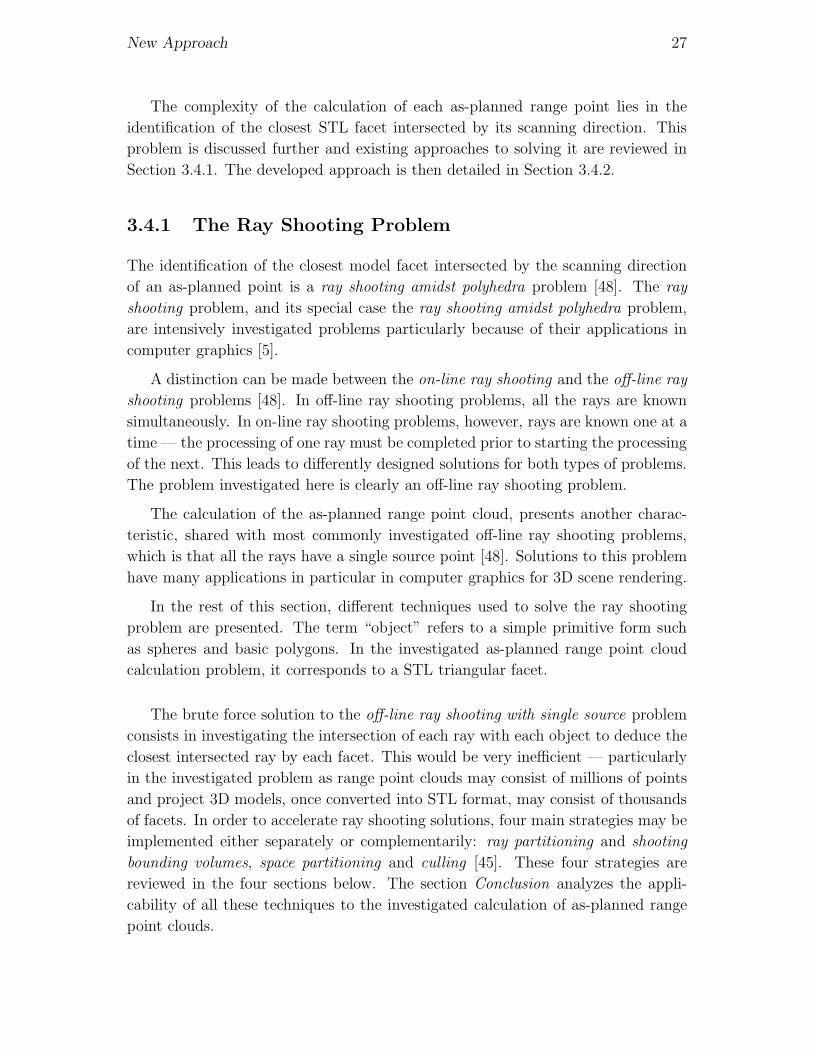
New Approach 27

The complexity of the calculation of each as-planned range point lies in the

identification of the closest STL facet intersected by its scanning direction. This

problem is discussed further and existing approaches to solving it are reviewed in

Section 3.4.1. The developed approach is then detailed in Section 3.4.2.

3.4.1 The Ray Shooting Problem

The identification of the closest model facet intersected by the scanning direction

of an as-planned point is a ray shooting amidst polyhedra problem [48]. The ray

shooting problem, and its special case the ray shooting amidst polyhedra problem,

are intensively investigated problems particularly because of their applications in

computer graphics [5].

A distinction can be made between the on-line ray shooting and the off-line ray

shooting problems [48]. In off-line ray shooting problems, all the rays are known

simultaneously. In on-line ray shooting problems, however, rays are known one at a

time — the processing of one ray must be completed prior to starting the processing

of the next. This leads to differently designed solutions for both types of problems.

The problem investigated here is clearly an off-line ray shooting problem.

The calculation of the as-planned range point cloud, presents another charac-

teristic, shared with most commonly investigated off-line ray shooting problems,

which is that all the rays have a single source point [48]. Solutions to this problem

have many applications in particular in computer graphics for 3D scene rendering.

In the rest of this section, different techniques used to solve the ray shooting

problem are presented. The term “object” refers to a simple primitive form such

as spheres and basic polygons. In the investigated as-planned range point cloud

calculation problem, it corresponds to a STL triangular facet.

The brute force solution to the off-line ray shooting with single source problem

consists in investigating the intersection of each ray with each object to deduce the

closest intersected ray by each facet. This would be very inefficient — particularly

in the investigated problem as range point clouds may consist of millions of points

and project 3D models, once converted into STL format, may consist of thousands

of facets. In order to accelerate ray shooting solutions, four main strategies may be

implemented either separately or complementarily: ray partitioning and shooting

bounding volumes, space partitioning and culling [45]. These four strategies are

reviewed in the four sections below. The section Conclusion analyzes the appli-

cability of all these techniques to the investigated calculation of as-planned range

point clouds.

New Approach 28

Rays Partitioning

Ray partitioning aims at exploiting the coherence between spatially adjacent rays.

Indeed, rays with the same source and almost the same direction are likely to

intersect the same object with a similar intersection point. Different strategies

have thus been developed to group rays into beams [15, 56, 98], cones [11] pencils

[105] or ray bounds [90].

Assarsson and Moller [16] particularly apply viewing frustum culling techniques

(see description in Section Culling Techniques) to beams of rays in order to rapidly

reduce the number of objects that may be intersected by any of the rays consti-

tuting the beam. This technique presents some limitations noted by Reshetov et

al. [98] who present an improved version. In essence, these two techniques aim

at identifying lower entry nodes in space partitioning trees (see section below) for

entire groups of rays, thus reducing the overall complexity. Note that these two

techniques perform their technique of “beam frustum culling” using axis-aligned

bounding boxes (see Section Shooting Bounding Volumes).

Shooting Bounding Volumes

Bounding Volumes (BVs) are often used to rapidly test whether a ray may intersect

a given object. Indeed, an object cannot be intersected by a ray if a volume

bounding it is not itself intersected by the ray. Strategies are thus implemented

that aim at computing for each search object a simple bounding volume so that, for

the calculation of each ray, a sub-set of objects that may potentially be intersected

by the ray can be identified rapidly.

Spheres and axis-aligned bounding boxes and oriented bounding boxes are com-

monly used bounding volumes [125]. But, more complex bounding volumes have

also been analyzed, for instance by Kay and Kajiya [66]. In general, the choice of a

bounding volume is the result of a trade-off between the ease of intersection testing

and the reduction in the number of intersection testing it enables (or “tightness”),

and thus results on specificities of the given problem [125]. Weghorst et al. [125]

studied this trade-off for different types of bounding volumes.

Space Partitioning And Bounding Volume Hierarchies

Space partitioning aims at dividing the space into regions, sub-regions and so on

until each leaf region contains only a small number of objects. Then, for the cal-

culation of each ray, the resulting partition tree is walked in a top-down manner

and only the objects contained in the leaf regions that are intersected by the ray

New Approach 29

are tested for intersection with the ray. In order to significantly improve the per-

formance of the calculations for each ray, it is important that the calculation for

testing whether the ray intersects a region be very simple.

Space partitioning data structures, that have been investigated and successfully

applied include uniform grids, octrees, binary space partitioning (BSP) trees, kd-

trees, and bounding volume hierarchies (BVHs) [45].

As presented in the two sub-sections below, space partitioning data structures

may be constructed in different manners and present different properties. However,

for the calculation of all the rays at run-time, they are walked in a similar top-

down manner [103]. At each node of the space partition tree, starting at its root, a

simple test is conducted with the parameters of the ray and of the regions defined

by the first partition so that it can be determined whether the ray intersects one

or more of the sub-regions defined by this partition. Similar tests are recursively

conducted with the intersected regions and so on until the regions are all leafs of

tree. The result is that only the objects contained in the intersected leaf regions are

investigated for potential intersection with the ray. The closest intersected object

is the solution to the ray shooting problem for this one ray. The process is then

repeated with all remaining rays — note that ray partitioning techniques presented

in the previous section actually aim at not repeating for all rays the entire process

from the root of the tree.

Uniform grids, Octrees, BSP trees and kd-trees:

Uniform grids, octrees, BSP trees and kd-trees partition the space by subdividing

it, and have the specificity that the resulting regions do not overlap (only at edges).

Although these four structures are built by dividing the space in different ways,

their construction typically follows the same procedure. The entire space is first

considered. Then, a first partition is identified that divides the entire space in

two or more regions. Each of these regions contains a certain number of objects.

Objects intersecting two or more regions may either be considered as part of all

of them, or be split so that each resulting object is inside one region only. The

process is repeated with each sub-region until a termination criterion is reached —

typically if the number of objects contained the region is less than a pre-defined

number.

Uniform grids are built by subdividing the entire space in a uniform grid of

cubes. Octrees are built by subdividing each space, or region, into eight cubes.

BSP trees are built by subdividing each space, or region, using planes (hyperplanes)

that can be oriented in any direction. Finally, kd-trees are a special case of BSP

trees where the splitting planes are perpendicular to the coordinate system axes.

New Approach 30

One main application of of these data structures (as well as BVHs) is in accel-

erating ray tracing algorithms for CAD rendering applications. For example, Knoll

et al. [72] and Bronnimann and Glisse [23] present ray tracing algorithms using

octrees, Wald et al. [123] an algorithm using a BSP tree, and Reshetov et al. [98]

and Havran and Bittner [54] algorithms using kd-trees.

A particularly interesting work is presented by Keeler et al. [67] who construct

a true spherical visibility map of scenes made of triangular facets. This spherical

visibility map is stored in a BSP tree which can thus be used for speeding up

ray shooting solutions. Additionally, this technique simultaneously achieves the

culling of hidden surfaces, another accelerating technique described in more detail

in the section Culling Techniques below. Note, however, that contrary to the other

space partitioning data structures presented above, this spherical visibility map

partitions the space based on the viewer’s location, or ray source. As a result, it

must be recomputed for every ray source. In contrast, uniform grids, octrees, BSP

trees and kd-trees are all viewer-independent and thus only have to be computed

once.

Bounding Volume Hierarchies (BVHs):

Bounding Volume Hierarchies (BVHs) are an extension of using Bounding Volumes

(BVs) presented in Section Shooting Bounding Volumes above. BVHs partition

the space and are constructed from the bottom up and have the specificity that

bounding volumes may overlap [47].

BVHs are constructed as follows: (1) the BVs of all objects are calculated and

considered as the leafs of the hierarchy; and then (2) the BVs are aggregated using

a pre-defined closeness criterion, and the process typically stops until all the BVs

are aggregated in a single BV, which consequently bounds all the objects in the

scene [47].

As described in Section Shooting Bounding Volumes above, spheres and axis-

aligned bounding boxes and oriented bounding boxes are commonly used BVs [125].

In a BVH, each parent node may have any number of children nodes. BVHs

may thus be more convenient in some situations than uniform grids, octrees, BSP

trees or kd-trees that can only split a space in a pre-defined number of regions.

Additionally, BVHs can be rapidly updated in the case of dynamic scenes. They

are thus very popular for implementing collision detection applications, such as in

video games [121].

The effectiveness of BVHs in the searching process is dependent on the trade-

off achieved by the BVs between (1) ease of intersection testing and (2) reduction

in the number of intersection testing (tightness) they enable [125]. Therefore, the

New Approach 31

effectiveness of a BVH is very dependent on the characteristics of the investigated

problem.

Examples of ray shooting algorithms using BVHs can be found in [33, 47, 121,

125].

Culling Techniques

While space partitioning data structures enable faster identification of the closest

facet intersected by a ray, other techniques, referred to as culling techniques, can

be used complementarily to reduce the number of objects that actually need to be

including in them, and consequently reduce the time necessary to walk them for

the calculation of each ray. These techniques mainly include [6]:

Viewing frustum culling: The viewing frustum is a geometric representation of

the volume in which facets may potentially be intersected by the rays. Facets

outside this volume cannot be intersected by any ray, so they are discarded.

If an object lies over a border, it is either kept entirely or spliy along this

boundary in a process called clipping, and the pieces that lie outside the

frustum are discarded.

Back-face culling: Rays cannot intersect a back-facing object, so all back-facing

objects can be discarded from space data structures. Back-facing objects can

easily be identified in the case where objects are oriented polygons.

Occlusion culling: Objects may lie entirely behind other objects, in which case

they are said to be occluded. Since the closest intersection of a ray with an

object is necessarily with a non-occluding object, occluded objects can be

discarded from space data structures.

The problem of occlusion culling has been intensely studied, and is more

generally referred to as the hidden surface removal problem. Many hidden

surface removal techniques have been developed [37, 49, 70, 83], but they are

either efficient, but so intricate that no attempt to implement them has yet

been reported, or practical, but not robust enough for practical reliable appli-

cation [67]. However, Keeler et al. [67] recently presented a new technique for

efficiently and reliably constructing spherical visibility maps of scenes made

of triangular facets. A spherical visibility map is organized in a BSP tree and

the authors demonstrate its applicability to the rendering problem with only

primary rays (no reflections or refractions are considered).

New Approach 32

Conclusion

This section provided a general overview of techniques for solving the off-line ray

shooting with single source problem. Many of these techniques would be applicable

to the investigated calculation of as-planned range point clouds.

Space partitioning techniques could be applied to reduce the number of STL

facets that would need to be investigated to identify the closest one intersected by

the scanning direction (ray) of each as-planned point. Ray partitioning techniques,

in particular beam tracing techniques, could be applied for further reducing the

complexity. Finally, culling technique could certainly be applied, in particular

back-face culling since STL facets are oriented.

In the next section, an approach is thus presented that efficiently and accurately

calculates as-planned range point clouds. It uses a 3D model’s BVH as well as back-

facing and viewing frustum culling techniques. This approach enables accurate

calculation of the range of any as-planned point in any scene. It will be shown

in Chapter 4 that the performance, in particular efficiency, of the overall object

recognition approach is mainly due to the performance of this as-planned range

point cloud calculation technique.

3.4.2 Developed Approach

The proposed approach to calculate as-planned range point clouds uses a Bounding

Volume Hierarchy (BVH) to efficiently organize the 3D model data. The par-

ticularity here is that the hierarchy uses a novel bounding volume referred to as

the Minimum Spherical Angular Bounding volume, or MSABV. The MSABV, il-

lustrated for one facet in Figure 3.1, is defined by the four pan and tilt angles

bounding a facet, or group of facets, in the scan’s spherical coordinate frame. It is

however open (no limit in range). The detailed calculation of the MSABV of STL

entities (facets and objects) is presented in Appendix C.

The MSABV of a group of facets is the union of the MSABVs of these facets.

Therefore, MSABVs can be aggregated in a BVH. The proposed BVH is constructed

by aggregating the MSABVs of all the facets of each STL object into one MSABV

for each object, and finally by aggregating the MSABVs of all the objects of the

project 3D model into one MSABV for the entire project 3D model. The proposed

BVH thus has three levels as illustrated in Figure 3.2. The detailed calculation

of the BVH of the project 3D model is presented in Appendix D. Appendix D

particularly describes how the size of the BVH can be significantly reduced by

performing scan’s viewing frustum culling and back-facing culling.

New Approach 33

(a) 3D View.

(b) Top View. (c) Side View: Projection of the facet andMSABV by rotation around the z axison one quadrant of the (Y Z) plane.

Figure 3.1: Illustration of the MSABV (minimum spherical angular bounding vol-

ume) of a STL facet in the scan’s spherical coordinate frame.

Then, as expected for any bounding volumes, a ray may intersect a STL facet

(respectively object or model) only if it is itself contained inside the MSABV of

the facet (respectively object or model). The calculations to test whether the

scanning direction of an as-planned point is contained inside a MSABV are detailed

in Appendix E.

This test is simpler to implement than the intersection test between a ray and

a bounding box, but not necessarily simpler than with spheres. However, it will be

shown in Chapter 4 that MSABVs are a tighter bounding volumes than spheres,

enabling faster as-planned point cloud calculation for large point clouds.

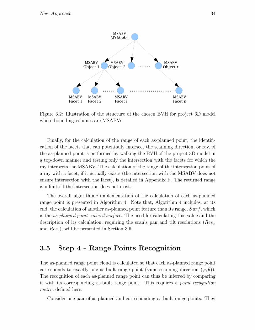
New Approach 34

Figure 3.2: Illustration of the structure of the chosen BVH for project 3D model

where bounding volumes are MSABVs.

Finally, for the calculation of the range of each as-planned point, the identifi-

cation of the facets that can potentially intersect the scanning direction, or ray, of

the as-planned point is performed by walking the BVH of the project 3D model in

a top-down manner and testing only the intersection with the facets for which the

ray intersects the MSABV. The calculation of the range of the intersection point of

a ray with a facet, if it actually exists (the intersection with the MSABV does not

ensure intersection with the facet), is detailed in Appendix F. The returned range

is infinite if the intersection does not exist.

The overall algorithmic implementation of the calculation of each as-planned

range point is presented in Algorithm 4. Note that, Algorithm 4 includes, at its

end, the calculation of another as-planned point feature than its range, Surf , which

is the as-planned point covered surface. The need for calculating this value and the

description of its calculation, requiring the scan’s pan and tilt resolutions (Resϕ

and Resθ), will be presented in Section 3.6.

3.5 Step 4 - Range Points Recognition

The as-planned range point cloud is calculated so that each as-planned range point

corresponds to exactly one as-built range point (same scanning direction (ϕ, θ)).

The recognition of each as-planned range point can thus be inferred by comparing

it with its corresponding as-built range point. This requires a point recognition

metric defined here.

Consider one pair of as-planned and corresponding as-built range points. They

New Approach 35

Data: PB, BVH

Result: PP

Assign values to PP.ϕ and PP .θ.

PP .ϕ ← PB .ϕPP .θ ← PB.θ

Calculate PP.ρ and other properties of PP .

PP .ρ ← ∞PP .IDobj ← NaN

for each BVH.Object doif IsRayInMSABV(PP , BVH.Object.MSABV) = True then

// see Algorithm 24 in Appendix E

for each BVH.Object.Facet doif IsRayInMSABV(PP , BVH.Object.Facet.MSABV) = True then

// see Algorithm 24 in Appendix E ρ’ ←CalculateIntersectionPointRange(BVH.Object.Facet, PB)

// see Algorithm 25 in Appendix F

if ρ’ < PP .ρ thenPP .ρ ← ρ’

PP .IDobj ← BVH.Object.IDend

endend

endendPP .(x, y, z) ← SphericalToCartesian(PP (ϕ, θ, ρ)) // see Algorithm 10

PP .Surf ← CalculateCoveredSurface(PP , Scan.Resϕ, Scan.Resθ) // see Algorithm 9

Algorithm 4: Function CalculateAsPlannedPoint calculating the as-planned

range point corresponding to an as-built range point.

have the same pan and tilt angles. The point recognition metric can thus only

consider their ranges. (Note that, if other point features, such as color or texture,

are available for both points, they can certainly be incorporated in the metric). A

simple point recognition metric is the comparison of the difference between their

ranges, Δρ, with a pre-defined threshold, Δρmax. If |Δρ| is smaller than or equal

to Δρmax, then the as-planned range point is considered recognized; it is not rec-

ognized otherwise. The algorithmic implementation of this calculation is presented

in Algorithm 5.

3.5.1 Automated Estimation of Δρmax

In order for the recognition of each point to be robust and performed automati-

cally, Δρmax must be adequately calculated automatically. An adequate value may

depend on many characteristics such as:

New Approach 36

Data: Scan.(PB, PP ), Δρmax

Δρ ← Scan.PP .ρ− Scan.PB.ρ

if |Δρ| ≤ Δρmax thenScan.PP .IsRecognized ← True

elseScan.PP .IsRecognized ← False

end

Algorithm 5: Procedure RecognizePoint matching an as-planned range point

to its corresponding as-built range point.

Point range measurement uncertainty: Range measurement uncertainty due

to technology limitations is normally provided by laser scanner providers,

though in very specific conditions (material reflectivity, with scanning direc-

tions perpendicular to the scanned surface, etc). Range measurement un-

certainty generally increases with the measured range. For instance, in the

case of the scanner used in this research, the provided range measurement

uncertainty are: 1.5mm at 50m and 7mm at 50m for 100% reflective tar-

gets positioned perpendicularly to the scanning direction. It would therefore

be appropriate to customize the threshold Δρmax with the range of each as-

planned point, PP .ρ, in order to take this uncertainty into account:

Δρmax = f1 (PP .ρ)

Point pan and tilt angles uncertainties: Pan and tilt angle measurement un-

certainties result from imperfections of the pan&tilt unit embedded in the

laser scanner. They are independent from the scanned point, and are gener-

ally provided by laser scanner providers. For instance, in the case of the scan-

ner used in this research, pan and tilt uncertainties are respectively 60μrad

and 70μrad (0◦0′12′′ and 0◦0′14′′). These respectively translate into 0.6mm

and 0.7mm precision at 10m, or 6mm and 7mm precision at 100m. The im-

pact of pan and tilt uncertainties on the as-planned point range measurement

is that the as-planned point range may be assigned to an incorrect direc-

tion. Methods using point neighborhood analysis can be used for dealing

with such uncertainties. The calculation of the threshold Δρmax could thus

be further customized with the pan and tilt uncertainties, uϕ and uθ, and

each as-planned range point scanning direction defined by PP .ϕ and PP .θ:

Δρmax = f1 (PP . (ρ, ϕ, θ) , (uϕ, uθ))

Point reflection angle: Uncertainty in range acquisition also increases with the

reflection angle between the scanning direction and the scanned surface nor-

mal vector (see illustration in Figure 3.3). If the as-planned reflection angle,

New Approach 37

α, of each as-planned range point, PP can be estimated when calculating its

range, it could then be used to further customize the Δρmax threshold:

Δρmax = f1 (PP . (ρ, ϕ, θ, α) , (uϕ, uθ))

Figure 3.3: Impact of the reflection angle on the range measurement uncertainty.

Scanned Surface reflectivity: Range measurement uncertainty also decreases

with the reflectivity of the surface it is acquired from. Thus, similarly as

above, if the surface reflectivity, λ, can be obtained when calculating each

as-planned range point, PP , the threshold Δρmax could then be further cus-

tomized:

Δρmax = f1 (PP . (ρ, ϕ, θ, α, λ) , (uϕ, uθ))

Registration error: Errors in scan registration lead to errors in model-to-scan

referencing and thus may significantly affect object recognition results. Here,

registration is performed using tie points (at least three non-aligned points),

and it has been shown in Section 3.3 that it is possible to automatically obtain

some registration error information, such as the mean registration error, εReg,

at the end of the registration process. The mean registration error, εReg, could

be used to adjust Δρmax, as larger Δρmax values should be used with larger

εReg values:

Δρmax = f1 (PP . (ρ, ϕ, θ, α, λ) , (uϕ, uθ) , εReg)

New Approach 38

Construction error: During construction, crews do their best to build elements

at their intended location. However, there is always some location error that

may thus impact the matching of as-built and as-planned range points. An

upper for such errors, εConst, could thus be used to adjust Δρmax:

Δρmax = f1 (PP . (ρ, ϕ, θ, α, λ) , (uϕ, uθ) , εReg, εConst)

By taking all these scan and point characteristics into account, it would be

possible to automatically estimate an adequate value of Δρmax for each as-planned

range point. However, this would require the estimation of the relations between

Δρmax and the different parameters mentioned above (PP . (ρ, ϕ, θ, α, λ), (uϕ, uθ),

εReg, and εConst), in other words of the function f1 (), a priori. For this, multiple ex-

periments with complex setups would have to be conducted, which was completely

out of the scope of this research. Thus, a simpler Δρmax threshold estimation is

used at this point. Only two criteria are retained for setting this value: for each

scan, Δρmax is set equal to the sum of the mean registration error εReg and an

upper bound for construction error εConst which must thus be defined a priori —

and a value of 50mm is chosen because it is larger than generally acceptable (spec-

ified) construction location errors, but small enough to avoid false positive point

recognitions. In fact, after conducting multiple experiments, these two errors have

appeared as probably the most critical sources of error to the proposed approach.

The following formula for automatically estimating Δρmax is thus used:

Δρmax = εReg + εConst (3.3)

It will be shown in Chapter 4 that this simple automated estimation of Δρmax

leads to good object recognition accuracy performance.

3.6 Step 5 - Objects Recognition

3.6.1 Sort Points

When calculated, each as-planned range point is assigned, as an IDobj feature,

the ID of the object from which it is obtained. The as-planned range points can

thus be sorted by IDobj, so that each model object is assigned an as-planned

point cloud. The as-built range points corresponding to as-planned range points

with a NaN IDobj value (they also have infinite ranges) are discarded or can be

grouped in a new object, non-model object. Then, since each as-planned range point

corresponds to exactly one as-built range point, each model object is also assigned

a corresponding as-built point cloud (regardless of the point recognition results).

The algorithmic implementation of this step is presented in Algorithm 6

New Approach 39

Data: Scan,Model

Result: Model,NonModel

for each Scan.PP doif Scan.PP .IDobj = NaN then

ObjectHandle ← GetObjectHandle(Scan.PP .IDobj)

ObjectHandle.({(PP , PB)}) ← Add(ObjectHandle.({(PP , PB)}),(Scan.PP , Scan.PB))

elseNonModel ← Add(NonModel, Scan.PB)

endend

Algorithm 6: function SortPoints sorting the as-planned and corresponding

recognized points by model object.

3.6.2 Recognize Objects

At this point, each model object is assigned an as-planned range point cloud and its

corresponding as-built range point cloud. Note that these can be empty, in which

case the object is clearly not recognized. In the case these are not empty, an object

recognition metric must be used.

A basic object recognition metric might consider the number of recognized

points and compare it to a pre-defined threshold. The problem with such a metric

is the automated estimation of the threshold. Indeed, the further from the scanner

an object is, the less points may be obtained from it, so that, with a given scan’s

angular resolution and a pre-defined threshold, it is possible that an object far

enough from the scanner cannot be recognized. This could be avoided by choosing

a low threshold value. However, this would result in a higher probability of Type I

object recognition errors.

Another approach, that would somewhat avoid this problem, is to infer object

recognition based on the as-planned range point cloud recognition rate. Indeed,

the number of as-planned range points would vary with the scanner-object distance

similarly to the number of recognized points, so that the recognition rate would

be invariant with the distance between the scanner and the object and the scan’s

angular resolution. However, this metric presents a limitation, that the first metric

did not have. It is not robust with respect to occlusions due to non-model objects

(external occlusions). Indeed, an object occluded by other non-model objects would

have a low as-planned point cloud recognition rate, potentially lower than a pre-

defined threshold, despite possibly many recognized points.

A third metric is preferred. It infers object recognition by calculating the object

recognized surface, SurfR, and comparing it to a threshold, Surfmin. If SurfR is

New Approach 40

larger than or equal to Surfmin, then the object is considered recognized; it is

not otherwise. The algorithmic implementation of this object recognition metric is

given in Algorithm 7.

Data: Model, Surfmin

for each Model.Object doModel.Object.SurfR ← CalculateRecognizedSurface(Model.Object) // see

Algorithm 8

if Model.Object.SurfR ≥ Surfmin thenModel.Object.IsRecognized ← True

elseModel.Object.IsRecognized ← False

endend

Algorithm 7: Procedure RecognizeObject from as-built and as-planned range

point clouds.

For each object, the recognized surface, SurfR, is calculated as the weighted

sum of its recognized as-planned points, where each point’s weight is its as-planned

covered surface. The algorithmic implementation of this calculation is given in

Algorithm 8.

Data: Object

Result: SurfR

SurfR ← 0for each Object.PB do

if Object.PB .IsRecognized = True thenSurfR ← SurfR + Object.PP .Surf

endend

Algorithm 8: Function CalculateRecognizedSurface calculating the recognized

surface of a model object.

The covered surface of an as-planned point, PP .Surf , is illustrated in Figure

3.4. It can be roughly defined as the area delimited by the equidistant boundaries

between it and its immediate neighboring points, and is calculated as:

PP .Surf =Surfunit

cos (PP .αϕ) cos (PP .αθ)(PP .ρ)2 (3.4)

New Approach 41

where: α is the as-planned point reflection angle. It is the angle be-

tween the point scanning direction and the normal to the

STL facet from which it is obtained, and can be decomposed

into its pan and tilt components, αϕ and αθ, as illustrated in

Figure 3.5.

Surfunit is the surface (expressed in m2), covered by a point with

range 1 m, perpendicular to the point’s scanning direction,

given the scan angular resolution, defined by Resϕ and Resθ.

It is calculated with the following equation:

Surfunit = tan(Resϕ) tan(Resθ) (3.5)

Figure 3.4: Illustration of the as-planned covered surfaces of as-planned range

points.

The algorithmic implementation of the calculation of the covered surface of an

as-planned range point is presented in Algorithm 9, with notations similar to those

used in Figure 3.5. Note that the calculation of the covered surface of an as-planned

range point can be performed at the same time as the calculation of its range. For

this reason, Algorithm 9 is called by Algorithm 4.

3.6.3 Automated Estimation of Surfmin

In order to automate this object recognition process, an adequate value of Surfmin

must be defined automatically. A large value of Surfmin would likely increase

specificity rates (smaller Type I error rates), but would also decrease recall rates

(larger Type II error rates). In contrast, a low value of Surfmin would likely increase

recall rates, but at the expense of smaller specificity rates.

New Approach 42

Figure 3.5: Illustration of αϕ and αθ, the pan and tilt components of the reflection

angle, α, of an as-planned point.

Data: PP , Resϕ, Resθ

Result: Surf

−→u ← [PP .x, PP .y, PP .z]−→u ← 1

‖−→u ‖−→u

−→v ← −→Z × −→u−→v ← 1

‖−→v ‖−→v

−→w ← −→u × −→v

Facet ← GetFacetHandle(PP .IDfacet)

Facet.−→nw ← Facet.−→n - (Facet.−→n · −→w )−→wFacet.−→nw ← 1

‖Facet.−→nw‖ Facet.−→nw

PP .αϕ ← arccos(-Facet.−→nw · −→u )

Facet.−→nv ← Facet.−→n - (Facet.−→n · −→v )−→vFacet.−→nv ← 1

‖Facet.−→nv‖ Facet.−→nv

PP .αθ ← arccos(-Facet.−→nv · −→u )

Surf ← tan(Resϕ ) tan(Resθ )

cos(PP .αϕ ) cos(PP .αθ )(PP .ρ)2

Algorithm 9: Function CalculateCoveredSurface calculating the covered sur-

face of an as-planned range point.

New Approach 43

Furthermore, the calculation of the object recognized surface, SurfR, is invari-

ant with the scan angular resolution. So, in order for the object recognition metric

to remain invariant with this factor, Surfmin (expressed in m2) must be automati-

cally adjusted with it, as transcribed with the formula:

Surfmin = A (Surfunit)

where: A is constant factor.

This formula can be interpreted as: at a distance of 1m from the scanner,

at least A points of an object as-planned as-planned range point cloud must be

recognized in order for this object to be itself recognized. If A is set too low,

then the probability of false positive object recognition increases. Indeed, consider

A = 100. Then, for an object at distance of 10m from the scanner, only 1 point

would have to be recognized for its recognized surface, SurfR, to be larger than

Surfmin. However, if A is set too large, then the probability of type II recognition

error increases. Indeed, consider A = 1, 000, 000. Then, for an object at distance of

10m from the scanner, 10, 000 points would have to be recognized for its recognized

surface, SurfR, to be larger than Surfmin. This further implies that the recognition

of objects close to the scanner would be very sensitive to external occlusions (e.g.

equipment, temporary structures).

Surfmin is consequently calculated as follows. The largest distance of the 3D

model to the scanner, Model.ρmax, is calculated. It is the largest range of the

STL-formatted 3D model vertices. Then, the value of Surfmin is set so that, at the

range distance Model.ρmax and with the given scan angular resolution, at least n

as-planned range points must be recognized in order for their total covered surface

to be larger or equal to Surfmin. This is transcribed into the formula:

Surfmin = n (Model.ρmax)2 Surfunit (3.6)

Since no object has any part of it with a range larger than Model.ρmax, this

threshold achieves ensures that, for any object to be recognized, at least n of its as-

planned range points must be recognized for the object to be recognized. As a result,

this threshold simultaneously ensures that both a minimum surface and a minimum

number of point be recognized. The value of n must be defined a priori. A value of

5 points is chosen because it is expected to be sufficiently low for avoiding Type II

recognition errors (object failed to be recognized) due to external occlusions, but

sufficiently large for avoiding Type I recognition errors (object recognized although

not present). The performance of this automated estimation of Surfmin will be

demonstrated in Chapter 4.

New Approach 44

3.7 Sensitivity Analyses

Sensitivity analysis is addressed in chapter 4, with focus on the point and object

recognition metrics.

The optimality of the automatically calculated Δρmax and Surfmin thresholds

is thoroughly investigated. However, as discussed then, the sensitivity analysis re-

sults do not report on the optimality of the overall point recognition and object

recognition metrics — although a good accuracy performance is demonstrated for

the overall developed approach. For instance, the analyses do not cover the po-

tential impact of customizing the Δρmax threshold value for each individual point,

for instance based on its planned range and reflection angle. The impact of differ-

ent values of n, in the calculation of Surfmin, on the object recognition accuracy

performance is not investigated either. And, finally, no experimental results are

reported on the potential impact of using soft point recognition and object recogni-

tion metrics instead of the hard ones used at this point. These analyses are needed

and should be conducted in future work.

Other aspects of the performance of the developed approach are covered in

Chapter 4, but sometimes only partially. For instance, the quantitative estimation

of the impact of registration error on the accuracy (and robustness) performance

of the developed approach would be interesting but is not covered. Then, the

efficiency of the developed method for calculating as-planned range point clouds

is compared with a method using spheres as bounding volumes, but not with any

method using bounding boxes as bounding volumes (the comparison with spheres

as bounding volumes is covered), neither with the spherical visibility map method

described by Keeler et al. [67]. These comparisons are needed to better demonstrate

the efficiency of the developed approach.

Chapter 4

Experimental Analysis of the

Approach’s Performance

This chapter presents results of experiments conducted with the aim of investigat-

ing and demonstrating the performance of the developed approach for automated

recognition of 3D model objects in site laser scans, in terms of accuracy, robustness,

efficiency, and level of automation.

First of all, Section 4.1 rapidly qualitatively analyzes the level of automation of

the developed approach. Then, Section 4.2 presents the data sets used to conduct

the experiments demonstrating the accuracy, robustness and efficiency of the ap-

proach. Section 4.3 demonstrates the accuracy of the approach in terms of object

recognition performance. The performance of the automated estimation of the two

thresholds, Δρmax and Surfmin, is also demonstrated. Then, Section 4.4 analyzes

the robustness of the developed approach, particularly with respect to occlusions.

The efficiency of the approach, namely its computational complexity, is covered in

Section 4.5. Finally, Section 4.6 summarizes the observed performance and com-

pares this performance with the targets estimated in Section 2.4.

4.1 Level of Automation

The level of automation and frequency of each of the five steps constituting the

developed object recognition approach are summarized in Table 4.1.

Tbale 4.1 shows that the approach is almost fully automated. The only part

that has to be performed manually is the manual matching of the benchmarks in

both data sets (model and scan) in the registration step (Step 2 ) This manual

process is however fairly simple and can be achieved in a matter of minutes.

45

Experimental Analysis of the Approach’s Performance 46

Furthermore, Step 1 only has to be performed once for all scans and Step 2 only

has to be conducted once per scan’s location. This means that, in the case several

scans are conducted from a given location, Step 2 does not have to be repeated.

In fact, it could be envisioned that scanners be located permanently, or at least

for long periods of time, in fixed locations and scans be conducted regularly from

these locations. In which case, only Step 3, Step 4 and Step 5 would have to be

repeated for each of these scans, making the recognition process for all but the first

scan fully automated.

Table 4.1: Level of automation and frequency of each of the five steps constituting

the developed object recognition approach.

Approach’s Step Level of Automation Frequency

Step 1 - Convert Model to STL Fully automated One time only

format:

Step 2- Register model in scan: Partially automated Once per scanner’s

location

Step 3- Calculate as-planned scan: Fully automated Once per scan

Step 4- Recognize as-planned Fully automated Once per scan

points:

Step 5- Recognize objects: Fully automated Once per scan

4.2 Experimental Data

The remaining analysis of the performance of the developed object recognition ap-

proach is performed using real-life data obtained from the construction of a build-

ing that is part of a power plant project in downtown Toronto in Ontario, Canada.

The building is 60m long by 15m wide by 9.5m high. It has a steel structure, the

construction of which is the focus of the conducted experiments. The 3D model

contains 612 objects and, once converted into STL format, a total of 19, 478 facets.

The as-built data consists of five scans conducted on two different days and from

different locations. They were all obtained using the same scanner, a TrimbleTM

GX 3D scanner, that uses time-of-flight technology. Some of the main character-

istics of this scanner are presented in Table 4.2. Characteristics of the five scans

are provided in Table 4.3. Note that, in the rest of this chapter, the scans will be

referred to by their ID. Figure 4.1 presents a photo, the 3D CAD model, and one

colored 3D laser scan of the building steel structure.


(a) Photo (b) 3D CAD model

(c) Laser scan

Figure 4.1: (a) Photo, (b) 3D CAD model and (c) laser scan of the steel structure

of the investigated PEC project building.

Table 4.2: Characteristics of the TrimbleTM GX 3D scanner.

Laser Type Pulsed; 532nm; green

Distance Range 2 m to 200 m

Accuracy 1.5 mm @ 50 m; 7 mm @ 100 m

Angle Range Hor: 360◦; Vert: 60◦

Accuracy Hor: 60 μrad; Vert: 70 μrad

Maximum Resolution Hor: 31 μrad; Vert: 16 μrad

Acquisition Speed up to 5000 pts/s

4.3 Accuracy

In this section, the accuracy of the developed object recognition approach is in-

vestigated. Object recognition accuracy performance metrics are first described in


Table 4.3: Day, Number, ID, number of scanned points, resolution and mean reg-

istration error (εReg with respect to the 3D model) for the five scans.

Scan Number of Resolution (μrad) εReg (mm)

ID Day range points Hor Vert

1 1 691,906 582 582 36.86

2 1 723,523 582 582 45.49

3 2 810,399 582 582 29.57

4 2 650,941 582 582 16.26

5 2 134,263 300 300 19.54

Section 4.3.1. Experimental results demonstrating the overall recognition accuracy

are then presented in Section 4.3.2. Finally, Sections 4.3.3 and 4.3.4 analyze the

performance of the automated estimations of Δρmax and Surfmin.

4.3.1 Accuracy Performance Metrics

The problem investigated here is an object recognition problem [13]. Fundamental

robust metrics object recognition accuracy are the recall rate (or sensitivity rate

or true positive rate), the specificity rate (or true negative rate), the Type I error

rate (or false positive rate), the Type II error rate (or false negative rate), and

the precision rate. In the investigated problem, these are defined as follows. The

formula below use the notation n ({x}) for the cardinality of the set {x}:

Recall: Number of model objects that truly are in the investigated scan and are

recognized divided by the total number of model objects that truly are in the

investigated scan.

Recall Rate =n ({Object in scan} ∩ {Object recognized})

n ({Object in scan})

Type II error rate: Number of model objects that truly are in the investigated

scan but are not recognized divided by the total number of model objects

that truly are in the investigated scan. This is equal to one minus the recall

Type II Error Rate =n ({Object in scan} ∩ {Object not recognized})

n ({Object in scan})

Specificity (or true negative rate): Number of model objects that truly are

not in the investigated scan and are not recognized divided by the total num-

ber of model objects that truly are not in the investigated scan.

Specificity Rate =n ({Object not in scan} ∩ {Object not recognized})

n ({Object not in scan})


Type I error rate: Number of model objects that truly are not in the investi-

gated scan but are recognized divided by the total number of model objects

that truly are not in the investigated scan. This is equal to one minus the

specificity.

Type I Error Rate =n ({Object not in scan} ∩ {Object recognized})

n ({Object not in scan})

Precision: Number of objects that truly are in the investigated scan and are

recognized divided by the total number of objects that are recognized.

Precision Rate =n ({Object in scan} ∩ {Object recognized})

n ({Object recognized})

The accuracy performance analysis presented in the following two sections focuses

on the analysis of the recall, specificity and precision rates only (Type I and II error

rates directly relate to the first two).

It must be noted that the calculation of these accuracy performance metrics

requires the manual visual identification of which objects truly are present or not in

each investigated scan. This identification was conducted and might have resulted

in a few errors. Nonetheless, it has been performed conservatively, so that the

results are generally biased toward lower performance. Table 4.4 summarizes the

number of model objects manually identified in each of the five investigated scans.

Table 4.4: Number of visually identified objects in the investigated five scans.

Scan ID Number of objects

visually identified

1 321

2 286

3 302

4 271

5 38

4.3.2 Experimental Results

Five experiments, Experiment 1 to Experiment 5, are conducted with the scans Scan

1 to Scan 5 respectively (Table 4.5). For these experiments, the Δρmax and Surfmin

values are calculated automatically using the proposed formulae in Equations 3.3

and 3.6 in Chapter 3. For the calculation of Surfmin, a value of n = 5 is chosen.


As discussed in Section 3.6.3, this value is expected to be low enough to prevent

false negative recognitions (objects failed to be recognized because less than n of

their as-planned range points are recognized), and high enough to prevent false

positive recognitions (object recognized when only a couple of their as-planned

range points are recognized). The threshold values automatically estimated for the

five experiments are listed in Table 4.5. Note that the estimated values of Surfmin

are equal to about 0.01m2 which is the surface of a square of side 10cm. Therefore,

in these experiments, an object is recognized if the covered surface of its as-planned

range points that are recognized is at least as large as the surface of a square of

side 10 cm.

Table 4.5: Automatically estimated Δρmax and Surfmin thresholds for the five

experiments.

Experiment Scan ID Δρmax (mm) Surfmin (m2)

1 1 86.86 0.0104

2 2 95.49 0.0118

3 3 79.57 0.0109

4 4 66.26 0.0118

5 5 69.54 0.0031

Appendix G displays, for Experiment 3, the data at the different stages of the

recognition process, and provides detailed recognition statistics for each of the 612

model objects.

Table 4.6 summarizes the recognition results and performances obtained in the

five experiments. It appears that the approach achieves very high specificity and

precision rates. This indicates that it rarely recognizes model objects that are not

present in the scan. Lower recall rates are however obtained (in average 82%),

indicating that the approach fails to recognize some objects that truly are in the

scans.

First of all, a more detailed analysis of the results, such as those presented in

Figure G.7 and Table G.1 in Appendix G, shows that low recall rates are particularly

obtained for small objects such as wall panel braces, while high recall rates are

obtained for larger objects such as columns and beams. This is confirmed in Table

4.7.

Table 4.7 presents the same results as in Table 4.6, but with values obtained,

not be summing up objects (e.g. in Experiment 1, 273 objects that are in Scan 1

are recognized), but by summing up the planned covered surfaces of the objects

(e.g. in Experiment 1, the as-planned covered surfaces of the 273 objects recognized


in Scan 1 equals 252.71m2). The results in Table 4.7 thus indicate that the objects

that the recognition approach does not recognize but that truly are in the scans are

objects for which the covered surfaces of their as-planned range point clouds are

small. In fact, further analysis shows that, among the objects that are manually

identified but are not recognized in the five experiments, respectively 6 (out of 49),

8 (out of 49), 6 (out of 49), 8 (out of 30) and 2 (out of 8) have as-planned range

point clouds with covered surfaces lower than Surfmin. As a result, it is possible

that visible surfaces of those objects in the scan are lower than Surfmin, in which

case these objects maybe should not be counted as false negative recognition errors.

If they are not counted, the recall rates for each experiment increases further.

Table 4.6: Object recognition results for the five scans (the values in third and

fourth columns are numbers of objects).

Objects Objects

Experiment Recognized Scanned Recall Specificity Precision

No Yes

1 No 260 49 85% 90% 90%

Yes 30 273

2 No 298 49 83% 92% 90%

Yes 26 239

3 No 283 49 84% 91% 90%

Yes 27 253

4 No 327 60 78% 96% 94%

Yes 13 212

5 No 568 8 79% 99% 83%

Yes 6 30

all No 1,736 215 82% 94% 91%

Yes 102 1,007

There are different sources of errors that impact at different levels the accuracy

performance of the approach. They include:

3D registration error: A significant source of error for this approach is 3D reg-

istration error. While Δρmax partially takes this error into account in the

recognition of range points, this error may remain significant and still have a

considerable impact on the object recognition results.

3D registration error is in fact particularly significant in the data sets used

here. Indeed, as shown in Table 4.3, the average mean registration error for


Table 4.7: Object recognition results for the five scans (the values in third and

fourth columns are as-planned (expected) covered surfaces in m2).

Objects Objects

Experiment Recognized Scanned Recall Specificity Precision

No Yes

1 No 12.25 13.12 95% 59% 97%

Yes 8.65 252.71

2 No 21.13 7.49 97% 77% 97%

Yes 6.33 241.53

3 No 17.43 20.01 93% 66% 97%

Yes 9.02 256.78

4 No 30.51 20.97 91% 94% 99%

Yes 2.1 209.44

5 No 0.57 0.34 97% 64% 97%

Yes 0.31 11.23

all No 81.88 61.93 94% 76% 97%

Yes 26.42 971.7

the five scans with the 3D model is roughly equal to 30 mm. The reason

for these high mean registration error values is that facility tie points were

not acquired when these five scans were conducted. Instead, manual point

matching had to be used, which typically leads to lower registration quality

(and reliability). In the industry, tie-point -based scan registration error

specifications are very stringent with values of a few millimeters at most

[117]. With mean registration errors of a couple of millimeters, it is expected

that the recognition results presented here would demonstrate better accuracy

performance, starting with higher recall rates.

Construction error: The second most significant source of error is construction

error. Here as well, while Δρmax partially takes this error into account in the

recognition of range points, this error may remain significant and still have a

considerable impact on the object recognition results.

Thresholds values: Although the recognition results summarized in Tables 4.6

and 4.7 are fairly good, it could be argued, at this point, that these results

could have been better if the thresholds, Δρmax and Surfmin, had different

values. The performance of the methods proposed for the automated estima-

tions of these thresholds is actually analyzed in more detail in Sections 4.3.3

and 4.3.4, respectively.


Schedule Error: Another source of error that has not been mentioned yet is re-

ferred to as schedule error. Indeed, the performance of the proposed approach

is expected to be optimal when the 3D as-built facility is scanned in a state

similar to the matched 3D model, because internal occlusions most likely

match then. In the five experiments conducted here, the entire project 3D

model is used to perform the object recognition. Since the states in which the

project was scanned during the five scans included most of the model objects,

the negative impact of recognizing a full model in a scan of a partially built

project did not occur obviously. Indeed, in such a situation, the comparison of

the real scan and the as-planned scan may lead to inappropriate recognition

results and thus may impact the recognition accuracy. In particular, if the

3D model contains additional objects from those actually present, then the

presence of these objects prevents the recognition of the model objects they

occlude in the model but are present in the scan.

The solution to this problem is to use a project 4D model that better reflects

the actual status of the scanned facility at the time of the scan. A project

4D model is obtained by combining information from the project 3D model

and the project schedule. The use of project 4D models with the developed

approach is further discussed in Section 5.2.3. Furthermore, it is discussed

in Chapter 5 how the developed approach can be used to track progress and

thus update the project schedule, and consequently 4D model automatically.

4.3.3 Automated Estimation of Δρmax

In this section, we investigate the performance of the proposed method for the

automated estimation of the threshold Δρmax. It is proposed in Section 3.5.1 that

the value of Δρmax be automatically estimated using Equation 3.3. It has been

shown, in the analysis of the overall recognition accuracy, that the automated

estimations of Δρmax (and Surfmin) generally lead to good recognition results.

However, it is investigated here whether other values of Δρmax could have led to

even better recognition performances.

Figure 4.2 shows for each of the five experiments presented earlier, the scan

mean registration error εReg, the automatically estimated value of Δρmax and the

recognition performances for other Δρmax values. In these experiments, the results

are obtained with the automatically estimated values of Surfmin presented in Table

4.5 (it will be shown in the next section that values of Surfmin estimated with this

automated method are appropriate).

The results in Figure 4.2 show that, in any of the experiment, for values of Δρmax

lower than εReg, the recall rate is very low, although the precision and specificity


rates are very high. In contrast, for values of Δρmax higher than εReg, the recall rate

is much higher with not significantly lower precision and specificity rates. Therefore,

using εReg as a minimum for the Δρmax value appears appropriate. The value of

εConst of 50 mm also appears adequate in general, although a lower value might be

preferred depending on the user’s expectations in terms of construction error.

In conclusion, the proposed method for automatically estimating Δρmmax per-

forms well with good trade-offs between high recall rates on one side and high

sensitivity and precision rates on the other. Nonetheless, a more thorough sensitiv-

ity analysis could be conducted to better estimate optimal values for Δρmax. More

complex methods to automatically estimate Δρmax could also be investigated. For

instance, it would be interesting to investigate customizing the value of Δρmax for

each range point as a function of, for instance, its planned range and reflection

angle on the surface it is expected (as-planned) to be obtained from. Additionally,

a soft recognition decision criterion could be investigated instead of the hard one

used at this point.

4.3.4 Automated Estimation of Surfmin

In this section, we investigate the performance of the proposed method for the

automated estimation of the threshold Surfmin. It is proposed in Section 3.6.3 to

automatically set Surfmin using Equation 3.6 with a value of n equal to 5. It has

been shown in the analysis of the overall recognition accuracy that the automated

estimations of Surfmin (and Δρmax) generally lead to good recognition results.

However, it is investigated here whether other values of Surfmin could have led to

even better recognition performances.

Figure 4.3 shows for each of the five experiments presented above, the automat-

ically estimated Surfmin value and the object recognition performances for other

values of Surfmin (note the logarithmic scale of the x axis). In these experiments,

the results are obtained with the automatically estimated values of Δρmax pre-

sented in Table 4.5 (it has been shown in the previous section that values of Δρmax

estimated with this automated method are appropriate).

The results in Figure 4.3 show that, in any experiment, for values of Surfmin

higher than the automatically calculated one, the recall rate is very low, although

the precision and specificity rates are very high. In contrast, for values of Surfmin

lower than the automatically calculated one, the recall rate is much higher with not

significantly lower precision and specificity rates.

In conclusion, the proposed method for the automated estimation of Surfmin

performs well with good trade-offs between high recall rates on one side and high

sensitivity and precision rates on the other. Nonetheless, it would be of interest to


conduct a more detailed sensitivity analysis. In particular, the impact of different

values of n on the accuracy performance of the approach would be needed. Addi-

tionally, similarly to the Δρmax, it would be interesting to investigate the use of a

soft decision criterion for the recognition of objects, instead of the hard criterion

used at this point. Other methods to automatically estimate Surfmin could also

be explored.


(a) Experiment 1 (Scan 1) (b) Experiment 2 (Scan 2)

(c) Experiment 3 (Scan 3) (d) Experiment 4 (Scan 4)

(e) Experiment 5 (Scan 5)

Figure 4.2: Mean registration error εReg, Automatically calculated Δρmax and per-

formances for different values of Δρmax.


(a) Experiment 1 (Scan 1) (b) Experiment 2 (Scan 2)

(c) Experiment 3 (Scan 3) (d) Experiment 4 (Scan 4)

(e) Experiment 5 (Scan 5)

Figure 4.3: Performance for different values of Surfmin, and automatically esti-

mated value of Surfmin.


4.4 Robustness

In this section, the performance of the developed object recognition approach is

tested with respect to occlusions. This is done by analyzing the accuracy perfor-

mance presented in Section 4.3 for different object occlusion rates.

The difficulty of such an analysis lies in the estimation of the occlusion rate

of 3D model objects in a given scene. Results for two types of occlusion rates are

presented here. First, Section 4.4.1 analyzes the accuracy performance with respect

to the planned internal occlusion rate (PIOR). This rate is a lower bound of the true

total occlusion rate but can be reliably estimated. Then, Section 4.4.2 analyzes the

accuracy performance with a crude estimation of the total occlusion rates (TORs)

of objects.

4.4.1 Planned Internal Occlusion Rate

In the developed approach, it is possible to compute the planned internal occlusion

rate (PIOR) of an object, as the ratio of its as-planned covered surface, calculated

by summing the covered surfaces of its as-planned range points, and its visible

surface without occlusion, estimated by summing up the surfaces of its front-facing

STL facets:

PIOR = 1− As-planned Covered Surface

Visible Surface Without Occlusion

The PIOR is an estimated lower bound of the total occlusion rate since it consid-

ers planned internal occlusions, but not external ones. Additionally, visible facets

may sometimes occlude each other, so that the visible surface without occlusion

calculated by summing the surfaces of front-facing facets is an upper bound of the

true visible surface without occlusion. In any case, the analysis of the accuracy per-

formance for different PIORs should give an idea of the robustness of the developed

approach with occlusions.

Figure 4.4 shows the recall rates and numbers of recognized objects for different

object PIORs. It first appears that recall rates tend to decrease with the PIOR,

particularly for PIORs above 75%. This may be interpreted as a somewhat limited

robustness with occlusions. However, it can also be seen in Figure 4.4 that many

objects with internal occlusions rates of at least 85% are successfully recognized.

A little bit more that forty objects with occlusion rates of 95% and above are

even successfully recognized in the five experiments. This better demonstrates the

capacity of the approach to recognize highly occluded objects. Furthermore, it

must be reminded that PIORs are only lower bounds of total occlusion rates.


Figure 4.4: Recall rates for different levels of planned internal occlusions.

4.4.2 Total Occlusion Rate (TOR)

The total occlusion rate (TOR) of an object can be estimated as the ratio of the

recognized as-planned covered surface of an object, calculated by summing up the

covered surfaces of all its as-planned range points that are recognized, and the

visible surface of an object without occlusion, estimated by summing up the surfaces

of its front-facing STL facets:

TOR = 1− Recognized As-planned Covered Surface

Visible Surface Without Occlusion

This computation of the TOR is a crude estimation of the true TOR. Indeed,

the recognized as-planned covered surface does not only vary with the level of oc-

clusion, but also with the performance of the point recognition metric, so that a low

point recognition performance would artificially increase the estimation of the TOR

using the formula suggested here. Additionally, as explained in Section 4.4.1, the

visible surface without occlusion calculated by summing the surfaces of front-facing

facets is an upper bound of the true visible surface without occlusion. However,

since it has been demonstrated in Section 4.3 that the developed approach achieves

good accuracy performance, calculated recognized as-planned covered surfaces are

probably good estimations of the true recognized surfaces, and this computation of

the TOR can be assumed as an acceptable estimation of the true TOR.

Figure 4.5 shows the recall rates and numbers of recognized objects for different

TORs estimated as suggested above. Compared to the results in Figure 4.4, both


the histogram and curve appear shifted to the right which is consistent with the fact

the PIOR is a lower bound of the TOR. The results in Figure 4.5 first show that the

recall rates are very high (about 100%) for TORs up to 85% but then significantly

decrease. This shows that the developed approach handles occlusions well. The

results even appear better than with the 3D-tensor -based approach developed by

Mian et al. [82, 81] that is the 3D object recognition technique that has reported

the best performance with occlusion to date (objects up to 85% were successfully

recognized). Indeed, with the developed approach, the recall rate also decreases

after 85% but not as significantly — this is just a crude comparison of the two

approaches since the results were obtained with different data sets. In addition,

It can be seen in Figure 4.4 that many objects with internal occlusions rates of at

least 95% are successfully recognized. This further demonstrates the capacity of

the developed approach to recognize highly occluded objects.

Figure 4.5: Recall rates for different levels of occlusions.

4.5 Efficiency

The efficiency of the developed approach is measured by the computational time

necessary to recognize project 3D model objects in site laser scans. In Section 4.5.1,

the overall computational time is analyzed with the five experiments described at

the beginning of Section 4.3.2. Then, Section 4.5.2 investigates in more detail the

efficiency of the developed approach for calculating as-planned range point clouds

by comparing its performance with the one of another commonly implemented

technique.


4.5.1 Overall Computational Performance

First of all, as discussed in Section 4.1 and summarized in Table 4.1, Step 1 of the

developed object recognition approach, namely the conversion of 3D model into STL

format, only needs to be performed once for all the scans. The complexity of this

step is thus not critical, so that it is discarded in this analysis — for information,

it took only about five seconds to convert into STL format the 3D model used the

five experiments presented in this chapter.

Table 4.8 summarizes the computational times of Step 2, Step 3, and Step 4 and

Step 5 combined, for the five experiments described in Section 4.3.2. These times

were obtained by running the VB.NET developed program on a computer having

a 2.41 GHz processor and 2 GB RAM memory.

It first appears that it takes overall, for instance for Experiment 3 — where Scan

3 contains a little bit more than 810, 000 scanned points and the 3D model contains

612 objects —, only about 3.5 minutes to recognize and extract the as-built range

point clouds corresponding to all the 3D model objects present in the scan.

Then, it can also be concluded from Table 4.8 that Step 3 seems to be the most

critical one in terms of computational time. Its computational time is directly

related to the efficiency of the developed technique for calculating as-planned range

point clouds. As a result, it is of interest to compare the efficiency of this technique

with the efficiency of other potential ones. This analysis is conducted in Section

4.5.2.

Table 4.8: Computational times (in seconds) of the steps 2 to 5 of the recognition

process for the five scans.

Experiment:

1 2 3 4 5

Process Step Times:

Step 2 - Register model in scan 0.6 0.6 0.6 0.6 0.6

Step 3 - Calculate as-planned scan 174.3 156.2 186.4 157.2 70.4

Steps 4+5 - Recognize as-planned points 11.2 8.5 10.0 8.4 2.5

and objects

Total (2+3+4+5) 186.1 165.3 197.0 166.1 73.5


4.5.2 Performance of The Developed Technique for Calcu-

lating As-planned Range Point Clouds

In this section, the efficiency of the developed technique for calculating as-planned

range point clouds is assessed.

The efficiency of the chosen technique for this calculation impacts the compu-

tational times of Step 3, but also Step 2. Indeed, typical viewer-independent space

partitioning data structures only need that the the location of the viewer (the ray

source) be registered in the Cartesian coordinate system of the 3D model, which

is a simple operation. In contrast, in the developed technique, the space partition-

ing data structure (a Bounding Volume Hierarchy (BVH)), and more exactly the

type of bounding volumes it uses, the minimum spherical angular bounding volume

(MSABV), is viewer-dependent and is thus computed in the scan’s spherical coor-

dinate frame, which implies the registration (rotation, translation and coordinate

conversion) of a large number of vertices. It is thus important to consider the com-

putational time of Step 2 in this efficiency analysis (although it will be shown that

is has a negligible impact).

In order to analyze the efficiency of the developed approach for calculating as-

planned range point clouds, it is proposed to compare the computational times of

Step 2 and Step 3 obtained using this technique with those obtained using another

common ray shooting technique.

This second technique is similar to the developed one in the sense that it uses

the BVH as a spatial partitioning data structure. However, it uses spheres as

bounding volumes. Spheres are observer-independent bounding volumes. Thus,

the sphere-based technique differs from the developed one as the BVH can be

calculated off-line, as soon the 3D model is converted in the STL format. The

chosen sphere-based BVH has the same three-level structure as the MSABV-based

BVH used in the developed approach (see Figure 3.2 in Section 3.4.2).

The calculation of the bounding spheres of a set of n 3D points has been a very

intensively investigated problem. In the experiment conducted here, the approach

presented in [46] is used for the calculation of the bounding sphere of each STL

object. Note that this approach does not calculate the exact minimum bounding

sphere, but is a computationally efficient approach to accurately estimate it. The

calculation of the minimum bounding sphere of a STL facet is a special case of the

problem solved in [46], and for which the solution can be obtained using a simple

deterministic method.

The same culling techniques are also implemented, namely scan’s viewing frus-

tum culling and back-face culling.


The sphere-based technique used here is very popular since it is very efficient

for dealing with real-time applications with dynamic scenes, such as in first-person

shooter computer games. The reasons for this efficiency are that (1) sphere-based

BVH are observer-independent, and (2) it is very simple to calculate whether a ray

intersects a sphere.

In order to compare both techniques, a new experiment, Experiment 5’, is con-

ducted with the same data as in Experiment 5 but using the sphere-based technique

instead of the MSABV-based one. Both techniques lead to the same performance in

terms of accuracy, level of automation and robustness, but with very different com-

putational complexities. Table 4.9 summarizes the computational times recorded

for Experiment 5 and Experiment 5’. The computational time for Step 3 is also

detailed for better analysis. It clearly appears that the MSABV-based technique is

significantly more computationally efficient. This may first be surprising since the

MSABV-based technique requires the computation of the BVH as part of the Step

3. However, spheres are not as “tight” bounding volumes as MSABVs. Therefore,

with spheres, more ray-facet intersections are tested in average for the calculation of

an as-planned point. And, since as-planned range point clouds typically contain at

least several thousands of points, the time necessary to calculate the MSABV-based

BVH is rapidly made up by the shorter average time to calculate each as-planned

point. Note also that the impact of the developed technique on the computational

complexity of Step 2 is insignificant compared to the complexity of Step 3.

Table 4.9: Comparison of the computational performances of the developed ob-

ject recognition technique using a MSABV-based BVH (Experiment 5 ) and of the

common technique using a sphere-based BVH (Experiment 5’ ).

Computational times of Steps 2 and 3: Experiment Experiment

5 5’

Step 2 - Register model in scan: 0.6 ≈0

Step 3 - Calculate as-planned range point cloud: 70.4 454.6

Step 3.1 - Calculate BVH: 55.3 NaN

Step 3.2 - Calculate cloud: 15.1 454.6

Total (2+3) 71.0 454.6

This experiment demonstrates that the developed approach achieves in prac-

tice efficient computational times to calculate as-planned range point clouds. It

can however be noted that AEC&FM project 3D objects often have cubic forms

in which case it would probably be more interesting to compare the efficiency of

the developed approach with one using axis-aligned or oriented bounding boxes as


bounding volumes. The efficiency of the developed approach could also be compared

with the efficiency of the technique by Keeler et al. [67] based on the calculation of

spherical visibility maps and described in Section 3.4.1 (sub-section Uniform grids,

Octrees, BSP trees and kd-trees). None of these comparisons have however been

conducted at this point, and future work could focus on such investigations.

Furthermore, it should be noted that the computational time for the calculation

of the MSABV-based BVH (Step 3.1 ) is strongly correlated with the value of the

parameter Incr used to calculate the bounding tilt angles of each STL facet’s

MSABV (see Appendix C). In the experiments conducted here, this parameter is

set to 10 mm which is very small. The advantage with such a small value is that

it ensures reliable results in all situations. With the data sets used here, however,

the same experiments conducted with a value of Incr of 100 mm lead to the same

recognition results but with a computational time of Step 2 an order of magnitude

lower. The reason is that, in these experiments, the distance between the scanner

and the 3D model, and more exactly each facet of the model, is fairly large so

that the phenomenon illustrated in Figure C.6 of Appendix C has an insignificant

impact here. This indicates that the value of Incr should be adjusted to different

situations. In fact, Incr should probably be automatically estimated for each facet

as a function of the bounding pan angles of the facet’s spherical bounding volume,

the minimum distance of the facet to the scanner, and the scan angular resolution.

This automated estimation of Incr has not been investigated, and the small value

of 10 mm is systematically used.

Then, it must be noted that, while the number of points in each of the scans

used here is large enough to provide reliable results with respect to the overall

computational performance of the developed approach, it is expected that, in real

life applications, scanned point clouds contain even more points. In fact, laser

scanners of new generation enable the acquisition of scans with angular resolutions

down to 150μrad [76], which is four to ten times denser by area than the scans

here. As a result, it is expected that, in practice, the computational complexity of

calculating MSABV-based BVHs will be insignificant compared to the reduction in

the complexity of calculating as-planned range point clouds that they enable.

Furthermore, as already mentioned in Section 4.1, if it is decided to locate at a

given spot a laser scanner for long periods or even the entire duration of a project,

and conduct many scans from that spot, then the 3D model BVH is the same for

all these scans and thus only has to be calculated once, which would reduce even

further its impact on the overall computational complexity.


4.6 Conclusion

This chapter has investigated the performance of the developed approach in terms

of level of automation, accuracy, robustness and efficiency.

It has first been shown that the developed approach is almost fully automated.

The only manual part is the matching of corresponding benchmarks in the project

3D model and laser scan for the registration step (Step 2 ). Compared to currently

used manually-intensive techniques for tracking the status of 3D objects on site,

this approach thus constitutes a ground-breaking improvement in terms of level of

automation.

With respect to accuracy, the results obtained with real-life data show that the

developed approach enables the recognition of project 3D objects in laser scans with

high recall, sensitivity and precision rates. It has been shown that the observed

object recognition failures occurred with small objects, which is expected to have

only small effects on applications such as automated 3D progress tracking. It has

also been shown that the data used in the experiments conducted here had the

particularity of having poor registration quality, which had a significant impact on

the reported recognition results. With registration quality constraints such as those

already used in the AEC&FM industry, the accuracy of the developed approach

would likely further improve. Finally, other recognition failures were also due to

errors in the 3D model. As a result, the developed approach has the potential

to achieve the levels of object recognition accuracies qualitatively estimated in

Section 2.4. It should also be noted that previous studies in civil engineering have

only attempted to recognize a type of design 3D objects a 2D image and not a

particular object.

In parallel, it has been shown that the developed approach is very robust with

occlusions. It performs at least as well as, and possibly even better than, the best

techniques reported in the literature, such as the recent one proposed by Mian et

al. [82, 81].

Using the approach described in this thesis, object recognition can be achieved

in small computational times. For instance, the as-built range point clouds of the

612 objects constituting a project 3D model were recognized in laser scans of close

to a million range points in less than five minutes. Such computational times are

significantly lower than the maximum of a few hours set as a performance objective

in Section 2.4.

In conclusion, the developed approach demonstrates high performance for prac-

tical 3D object recognition in site laser scans. Further work could nonetheless

be conducted with the aim of further improving this performance. For instance,


(1) the methods for the automated estimations of Δρmax and Surfmin could be

refined; (2) soft recognition metrics could be explored; and (3) other techniques for

the calculation of as-planned range point clouds could be investigated.

Given the demonstrated performance of the developed approach for project

3D CAD object recognition in construction site laser scans, it is now possible to

investigate the use of the results that it can provide for important applications such

as automated 3D progress tracking and automated dimensional quality control.

The investigation of such applications is the focus of Chapter 5 that also shows the

possibility to use the developed approach for other applications such as planning

for scanning and strategic scanning.

Chapter 5

Enabled Applications: Feasibility

Analysis and Experiments

The developed approach enables Automated 3D Data Collection (A3dDC). Further,

as illustrated in Figure 5.1, if it is used with 3D laser scans acquired during the

entire life of a project, it then enables the automated acquisition of the evolution

of the 3D as-built status of the model 3D objects over time, that can be stored in

a Project 4D Information Model (P4dIM). Note that the P4dIM can be integrated

as a part of the entire Project Information Model (PIM).

The P4dIM enables multiple applications related to the management of con-

struction projects’ life cycle 3D data. Sections 5.2 to 5.4 present results of ex-

periments demonstrating three Automated Project Performance Control (APPC)

applications: Automated construction progress (and productivity) tracking, Auto-

mated dimensional QA/QC, and similarly Automated dimensional health monitor-

ing. Then, Sections 5.5 and 5.6 present two other enabled applications with poten-

tial benefit to laser scanning in the AEC&FM context: Planning for scanning and

Strategic scanning.

5.1 Experimental Data

The experimental results presented in this chapter are obtained with the same

data sets as the ones used in Chapter 4. These include the 3D CAD model of the

steel structure of a building and five laser scans obtained on two different days

of its construction and from different locations. For more information about this

experimental data, please refer to Section 4.2.

67

Enabled Applications: Feasibility Analysis and Experiments 68

Figure 5.1: Illustration of automated construction of a Project 4D Information

Model (p4dIM).

5.2 APPC: Automated Construction Progress

Tracking

By analyzing the object recognition information contained in the P4dIM for two

different days, it should be possible to automatically infer the construction progress

between these two days — and productivity information can be inferred directly

from progress.

Previously investigated Automated Data Collection (ADC) systems for progress

tracking use indirect progress measurement methods, typically by tracking the

location and activity of construction resources such as workers and equipment

[86, 101, 124]. The developed approach, however, directly recognizes quantities

put in place (even partial objects like partially built brick walls). The P4dIM can

thus be used to measure progress directly.

5.2.1 Progress Calculation Method

As an example, consider a project with its 3D model. Scans may be conducted at

different days but also during a same day from different locations and in different

directions. Consider {S}di and {S}di+1, the sets of scans conducted at respectively


day di and di+1. Then, construction progress between the days di and di+1 can be

estimated by identifying in the P4dIM the objects that are recognized in {S}di+1 but

not in {S}di.

5.2.2 Experimental Results

An experiment is conducted that uses the data presented in Section 5.1, and that

aims at investigating the performance of using the P4dIM and the progress calcu-

lation method above for construction project tracking.

Combining Daily Scans

First, it can be noted in the results presented in Tables 5.1 to 5.2 that combining the

recognition results of different scans acquired on a same day increases, sometimes

significantly, the overall object recognition accuracy performance for that day, in

particular the recall rate. This is particularly true if the scans are obtained from

very different locations.

Table 5.1: Recognition results for the day d1 (values in columns 3 and 4 are numbers

of objects).

Objects Objects

Scan ID Recognized Scanned Recall Specificity Precision

No Yes

1 No 260 49 85% 90% 90%

Yes 30 273

2 No 298 49 83% 92% 90%

Yes 26 239

d1 No 194 58 85% 83% 89%

Yes 39 321

Progress Inference

The performance of inferring construction progress for the periods d0–d1 and d1–d2

is now investigated based on the recognition results obtained for d1 and d2. d0 is

the day 0 of the construction, when no project element is built yet.

Table 5.3 summarizes the progress recognition accuracy performance obtained

for the sets of scans {S}d1 and {S}d2 using the information contained in the P4dIM


Table 5.2: Recognition results for the day d2 (values in columns 3 and 4 are numbers

of objects).

Objects Objects

Scan ID Recognized Scanned Recall Specificity Precision

No Yes

3 No 283 49 84% 91% 90%

Yes 27 253

4 No 327 60 78% 96% 94%

Yes 13 212

5 No 568 8 79% 99% 83%

Yes 6 30

d2 No 212 48 87% 86% 90%

Yes 34 318

automatically constructed with the developed approach and the progress calculation

method presented in Section Progress Calculation Method. In this table actual

progress for a period di–di+1 is calculated as the set of objects that are visually

identified in at least one scan of di+1 but not visually identified in any scan of di.

The results are quite disappointing, particularly for the period d1–d2. For in-

stance, only 3 of the 9 objects that are part of the actual progress are properly

recognized.

The problem is that the proposed approach to estimate the recognized progress

is very sensitive to the accuracy of the object recognition results obtained for each

day. For a period di–di+1, errors in both the object recognition results for di and

di+1 impact the estimation of progress. For instance, a failure to recognize an object

in the scans of di may result, if it is recognized in at least one scan of di+1, in the

wrong conclusion that it is part of the progress. Similarly, a failure to recognize

an object in the scans of di+1 may result, if it was not in any scan of di, in the

wrong conclusion that it is not built yet. The reason why the results reported for

the period d0–d1 are much better than for those of the period d1–d2 is that there is

obviously no error in the object recognition results for day d0 (nothing is built), so

that only object recognition errors with the scans of day d1 impact the accuracy of

the recognized progress.

As discussed in Section 4.3.2, the object recognition results obtained with the

available experimental data are not very good, due to several reasons, but mainly

the poor registration quality. With regard to the the discussion in the previous

paragraph, this likely explains the poor progress recognition results presented in

Table 5.3.


Table 5.3: Progress recognition results for the periods d0–d1 and d1–d2 where rec-

ognized progress is calculated using the method in Section Progress Calculation

Method (values in columns 3 and 4 are numbers of objects).

Objects in Objects in

Period Recognized Scanned Recall Specificity Precision

Progress Progress

No Yes

d0 – d1 No 194 58 85% 83% 89%

Yes 39 321

d1 – d2 No 587 6 33% 97% 16%

Yes 16 3

In order to be able to better assess the feasibility of using information contained

in the P4dIM to automatically track progress, the following change in the calcu-

lation of the recognized progress is suggested: the recognized progress for a period

di–di+1 is the set of objects that are recognized (using the developed approach) in at

least one scan of day di+1 and that are not visually identified in any scan of day

di.. In essence, progress calculation method is a relaxed version of the normally

more appropriate (because fully automated) method presented in Section Progress

Calculation Method. In this relaxed method, progress is calculated by simulating

perfect recognition information for the scans of day di, so that it is only sensitive

to the object recognition errors with the scans of di+1.

Table 5.4 summarizes the progress recognition accuracy performance obtained

for the same data as in Table 5.3 but using this relaxed progress calculation method.

The results show that progress is quite successfully automatically recognized.

For the period d0–d1, the results are the same as in Table 5.3, because the objects

recognized at day d0 are the same as the ones actually built: none. For the pe-

riod d1–d2, much better results than in Table 5.3 are reported. First, 100% of the

scanned progress over that period (9 objects) is automatically recognized. Then,

most of the scanned non-progress (objects not part of the progress) is also auto-

matically recognized (specificity rate of 95%). However, the precision rate appears

to be very low (23%). Indeed, 31 objects are recognized as part of the scanned

progress during the period d1–d2 although they are not (Type I error). This means

that these 31 objects are recognized in at least one of the scans of {S}d2, and are

not visually identified in any scan of {S}d1. This is actually to be related to the

object recognition results reported with the scans of d2, {S}d2. Indeed, as can be

seen in Table 5.2, 34 objects are recognized in at least one scan of {S}d2 although


they are not in any of these scans. The reasons for these Type I errors, identified

in Section 4.3, are:

1. The small sizes of these objects. (Note that this implies that they are probably

not critical in terms of progress tracking); and

2. The poor 3D registration quality, which particularly impacts the recognition

of small objects.

Table 5.4: Progress recognition results for the periods d0–d1 and d1–d2 using the

relaxed method for the calculation of the recognized progress (values in columns 3

and 4 are numbers of objects).

Objects in Objects in

Period Recognized Scanned Recall Specificity Precision

Progress Progress

No Yes

d0 – d1 No 194 58 85% 83% 89%

Yes 39 321

d1 – d2 No 572 0 100% 95% 23%

Yes 31 9

Overall, the results in Table 5.4 demonstrate that, if 3D high-quality 3D regis-

tration can be ensured, P4dIMs built with the developed approach could potentially

be used to automatically track construction progress (and consequently productiv-

ity). Nonetheless, it is acknowledged that the experiments presented here do not

suffice to fully prove the feasibility of implementing this P4dIM-based APPC ap-

plication. More comprehensive data sets with, in particular, better registration

quality, would need to be obtained to strengthen this analysis.

The results presented in this section are further discussed below. In particular,

means to improve them are suggested.

5.2.3 Discussion

Using 4D Models for Supporting Progress Tracking

The experimental results presented in Section 5.2.2, in particular the results re-

ported in Table 5.3, illustrate the sensitivity of progress tracking calculation results

to object recognition errors.


One way to improve these results is to take advantage of construction projects’

4D models. A project 4D model is the result of the fusion of the project 3D model

and the project Construction Project Management (CPM) schedule. With the 4D

model, the physically derived precedence relationships from the CPM schedule can

be used to extract the as-planned 3D model of each day. This as-planned 3D model

only contains the project 3D objects that are planned to be built at that date, and

should improve automated progress monitoring results in two ways:

1. The as-planned 3D model of day di should provide a good estimate of the

objects that are already built at day di, so that the progress at day di+1 can

be automatically inferred with the proposed method.

From current practice, it is clear that most projects proceed only in the most

general form with respect to their schedules and most individual activities are

generally offset by days and weeks from their original schedule dates. CPM

schedules may thus be argued to provide poor information with respect to the

as-built status of a project at a given date. However, by using the developed

laser scanning -based object recognition approach to recognize progress from

day d0, the progress recognized at the end of each day, di, can be used to

automatically update and recompute the CPM schedule (and consequently

the 4D model), so that the schedule is automatically maintained up-to-date.

2. An automatically updated CPM schedule, and consequently 4D model, also

provides an up-to-date estimation of the expected as-planned 3D model for

day di+1, which should optimize the object recognition accuracy performance

for scans conducted on day di+1 — as-built and as-planned range point clouds

would better match —, and consequently ensure higher progress recognition

accuracy performance for the period di–di+1.

Scanned Progress vs. True Progress

With the developed approach, only the scanned progress can be recognized. There-

fore, if the scanned progress significantly differs from the true progress, the recog-

nized progress will be misleading. It is thus important to ensure that the scanned

progress actually reflects the true progress. This can be done by conducting many

scans from many locations and in many directions.

It could be argued that this would result in the need to analyze many scans

with a lot of redundant information. In that regard, Section 5.5 will discuss the

possibility to use the developed approach to plan in advance and thus optimize the

number and locations of scans to be conducted to ensure the acquisition of data

from all (critical) objects.


Furthermore, despite multiple scans during one day, it is still likely that no range

data is ever obtained for some objects, because they are systematically occluded

by either internal occlusions or external occlusions.

Internal occlusions, partial or total, are taken into account by the developed

object recognition approach and do not impact its accuracy performance, (it is

only calculated based on the objects present in the scans). However, total internal

occlusions may impact progress recognition accuracy similarly to object recognition

errors. For instance, an object actually built at a day di may be fully occluded from

all the scan locations of that day, but recognized in a scan of day di+1. This would

result in the wrong conclusion that the object is part of the progress during the

period di–di+1 (Type I error). Similarly, an object actually built at day di+1 may

be fully occluded from all the scan locations of that day. This would result in

the wrong conclusion that the object is not part of the progress during the period

di–di+1 (Type II error).

External occlusions cannot be taken into account a priori, although they are

very common on construction sites. For instance, as can be seen in Figure G.2

(page 122) with Scan 3, portable toilets as well as a large container are present

on the side of the scanned structure. Their presence results in full occlusions of

some structural elements. Similarly to internal occlusions, neither partial nor full

external occlusions impact the accuracy performance of the developed object recog-

nition approach. However, total external occlusions may similarly impact the object

recognition accuracy.

Two techniques can be implemented to reduce and mitigate the impact of total

occlusions of built 3D model objects on the accuracy of the proposed approach for

automated progress monitoring:

Reducing external occlusions: Scanned scenes should always be cleared as much

as possible of non-model objects prior to conducting scanning operations.

Such good practice would reduce the number of external occlusions, thus re-

ducing their negative impact on the accuracy performance of the proposed

approach for automated progress recognition.

Leveraging precedence relationships from CPM schedules: The physically

derived precedence relationships from the CPM schedule can also be used to

recognize with reasonable confidence objects which are not recognized in a

day’s fused scans and yet can be inferred to exist due to the recognition of

successor elements. Implementing this could help significantly reduce the im-

pact of all types of occlusions on the accuracy performance of the proposed

approach for automated progress recognition.


Progress vs. 3D Progress

Finally, it must be noted that not all construction activities can be monitored in

terms of progress and productivity by collecting 3D information only (e.g. painting

activities). Reliable and efficient ADC systems for complete project progress and

productivity tracking should thus consider fusing data and information from several

monitoring systems such as those described in [86], [101] or [124].

5.3 APPC: Automated Dimensional QA/QC

The P4dIM obtained with the developed approach could be used to perform auto-

mated dimensional Quality Assessment / Quality Control (QA/QC).

The P4dIM stores detailed life-cycle range point clouds for each project object

(as long as it has been scanned and recognized). Then, it can be observed that many

AEC&FM project 3D objects are designed with parametric forms or combinations

of parametric forms (e.g. cubic floors, cylindrical columns, H-beam). Approaches

fitting parametric forms to point clouds, such as those presented in [74], could thus

be used to fit to each object as-built point cloud the same type of 3D parametric

form as the one it is designed with. Then, the main form parameters (e.g. length,

width and height) of the designed and fitted 3D parametric forms can be compared

to each other to infer dimensional quality information.

The advantage of such a comparison is that it is fully compatible with typical

dimensional tolerances, that generally refer to the parameters of the 3D parametric

form(s) used to design the objects. In fact, Boukamp and Akinci [20] present an

approach for automatically extracting and processing construction specifications,

including dimensional tolerances, from project documentations for each project

object, or object type. Such an approach could be combined with the proposed

method for automated dimensional monitoring to create a system for fully auto-

mated dimensional QA/QC.

As an illustrative example, consider a structural concrete column with a cylin-

drical shape, for which a recognized dense and sufficiently large range point cloud

is stored in the P4dIM (see example in Figure 5.2). A cylinder fitting algorithm

can be used to fit a cylinder to the scanned data, and the fitting results can be used

to perform automated dimensional quality control, such as:

Horizontal location: The horizontal location of the as-built column can be con-

trolled by investigating whether the horizontal location of the center point of

the fitted cylinder is the same, within tolerances, as the horizontal location

of the column in the scan-referenced 3D model.


Verticality: The verticality of the as-built column can be controlled by investi-

gating whether the direction of the main axis of the fitted cylinder is vertical,

within tolerances.

Diameter and Length: The diameter and length of the as-built column can be

controlled by investigating whether the diameter and length of the fitted

cylinder are the same, within tolerances, as those of the same column in the

scan-referenced 3D model.

Note that information about the quality of the fit can also be used to estimate the

reliability of the dimensional quality control results.

5.4 APPC: Automated Dimensional Health Mon-

itoring

The structural health of a structure is often related to its dimensional integrity.

Since 3D as-built point clouds of each project object are stored in the P4dIM over

time, using methods such as the one presented in the previous section, could be used

to monitor objects as-built dimensions over time. And, since 3D laser scans can

be conducted remotely (from tens of metres), this would enable safe dimensional

monitoring operations.

It must be noted that dimensional health monitoring often involve the analysis

of the deformation of elements. Fitting the exact same hard parametric form as

the one used in the 3D model is likely not appropriate to recognize deformations,

and algorithms fitting deformable parametric forms should be preferred. Examples

of algorithms to fit deformable forms, including deformable parametric forms, can

be found in [34, 62].

5.5 Planning For Scanning

Further than enabling APPC applications, the developed approach would enable

three additional important applications: planning for scanning and strategic scan-

ning. The first one is presented in this section, and the next one in Section 5.6.

For each scan, the developed approach conducts, from the same position, a vir-

tual (as-planned) scan using the scan-referenced project 3D model as the virtually

scanned world. The assumption is that, if the building is built where it is intended

to be, the project elements should be positioned in the exact same way in the two


(a) Design of the structure. (b) Design of one of the structure’scolumns.

(c) Recognized points from the structure inthe as-built scan.

(d) Recognized points from the column.Points colors are set to Δρ.

Figure 5.2: Example of a model and recognized as-built range point cloud of a

structure. The results are detailed for one column with a cylindrical shape from a

structure.

scans. The analysis of the performance of the developed approach presented in

Chapter 4 confirms that this assumption is generally correct.

However, what this performance analysis does not clearly emphasize is that an

as-planned point cloud can be used to test a scanning position prior to conducting

the scan in reality, and investigate whether it would enable the acquisition of 3D

information of objects considered of interest.


For instance, in the case of project progress monitoring, it can be determined

a priori the recognition of which objects is critical to infer the expected progress.

Then, the analysis of the as-planned range point cloud from a given location can

provide information about which objects are expected to be recognized in the real

scan from this location — and even the quantity of information (surface) that is

expected to be recognized for each of them. If no (or not enough) information

about a critical object is expected to be obtained from this location, another scan

location can be investigated.

This idea can be pushed further. The developed approach could be used, before

the construction of a project is even started, to plan the project life cycle scanning

operations. It would enable the optimization of the number of scans and their

locations that would need to be performed during a project in order to ensure

the acquisition of 3D information a priori identified as critical to specific APPC

applications.

This approach can be seen as part of the more general paradigm of construction

inspection planning. Preliminary work investigating a formalism for construction

inspection planning has been reported by Gordon et al. [51].

Note that such an approach for planning for scanning would perform well only if

the virtually scanned scenes faithfully represent the scenes expected to be scanned

in reality. As discussed in Section 5.2.3, using the project 4D model would be very

beneficial to that end. Also, as mentioned in Section 5.2.3, external occlusions (e.g.

equipment and temporary structures) are very common on construction sites and

constitute an additional source of recognition error. So, using the developed ap-

proach for planning for scanning would result in the necessity to ensure that scanned

scenes be cleared as much as possible of non-model objects prior to conducting real

scanning operations.

5.5.1 Experiment

An experiment is conducted to test the feasibility of using the developed approach

for planning for scanning.

Table 5.5 summarizes the planned vs scanned (visually identified) object recog-

nition results and performance obtained for the same five experiments as in Section

4.3 and in terms of number of objects. Table 5.6 summarizes the same results but

in terms of as-planned covered surface.

It first appears in Table 5.5 that the developed approach achieves very good

results in terms of recall, meaning that most of the scanned objects are also planned.


Table 5.6 confirms this result by showing that objects, that are planned but are not

scanned, actually have as-planned range point clouds with small covered surfaces.

They are thus probably not critical in terms of progress tracking.

It can, however, be argued from the results presented in Table 5.5 (and simi-

larly in Table 5.6), that the approach achieves poor specificity and precision per-

formances. However, these values are misleading. Indeed, they are to be related

to the fact that these experiments are conducting using the entire 3D model of

the project to calculate the as-planned point clouds. So, many objects may be

in the as-planned point clouds but may not be built yet at the time of the scans.

For instance, it can be seen in the 3D model displayed in Figure G.1 (page 123),

that there is a small structure inside the main building frame that is in the 3D

model and contains many objects (exactly 131), but that is not present in any of

the five scans. These objects significantly impact, directly or indirectly (as internal

occluders), the specificity and precision performances presented here.

Table 5.5: Planned vs. scanned objects for the five scans (the values in third and

fourth columns are numbers of objects).

Objects Objects

Experiment Planned Scanned Recall Specificity Precision

No Yes

1 No 156 6 98% 54% 70%

Yes 134 316

2 No 114 8 97% 35% 57%

Yes 210 280

3 No 140 6 98% 45% 64%

Yes 170 296

4 No 119 8 97% 35% 54%

Yes 221 264

5 No 556 2 95% 97% 67%

Yes 18 36

all No 1,085 30 98% 59% 61%

Yes 753 1,192

In conclusion, as-planned range point clouds can be used to effectively predict

the content, in terms of objects and covered surfaces, of actual laser scans. It thus

possible to used as-planned range point clouds to perform planning for scanning.


Table 5.6: Planned vs. scanned objects for the five scans (the values in third and

fourth columns are the sums of objects’ as-planned covered surfaces in m2).

Objects Objects

Experiment Planned Scanned Recall Specificity Precision

No Yes

1 No 0.22 0.01 100% 1% 93%

Yes 20.67 265.82

2 No 0.16 0.05 100% 1% 90%

Yes 27.29 248.97

3 No 0.24 0 100% 1% 91%

Yes 26.21 276.79

4 No 0.19 0.01 100% 1% 88%

Yes 32.42 230.4

5 No 0 0 100% 0% 93%

Yes 0.88 11.57

all No 0.81 0.08 100% 1% 91%

Yes 107.48 1033.55

5.6 Strategic Scanning

Further than planning for scanning, the developed approach could be used to per-

form strategic scanning.

As mentioned above, as-planned scans can be conducted prior to real scans to

predict their expected 3D information content. Since, in an as-planned scan, it

is known from which object each range point is obtained, it would be possible,

when conducting the real scan from the exact same position, to control the scanner

so that only range points that are expected to provide 3D information about the

objects of interests are acquired.

This is of great interest to the AEC&FM industry. Indeed, project managers,

who are currently dedicating resources to conduct project 3D scanning, face the

situation that they must save enormous amounts of scanned data, from which only

a small portion is actually useful to their control processes. With the proposed

approach, only useful 3D scanned data would be acquired, thus reducing the overall

amount of data being stored and processed during the life of a project.

Chapter 6

Conclusions and

Recommendations

It is concluded that a method exists, which has been presented in this thesis, by

which particular 3D objects may be reliably recognized in 3D construction images

when a priori3D design information is available.

6.1 Contribution

This thesis presented a novel approach for accurate, robust, efficient and (almost)

fully automated recognition of project 3D objects in site laser scans. It leverages

the opportunities that project 3D CAD models and 3D registration technologies

provide in the AEC&FM context.

A detailed analysis of the performance of this approach with respect to accuracy,

robustness, efficiency and level of automation has been presented based on real-life

data. The developed approach demonstrates high performances in all these areas,

both by comparison with existing techniques for 3D object recognition in range

images, and with respect to targets qualitatively estimated a priori, specific to this

specific AEC&FM context, related to previous 2D image work, and based on the

personal expertise of the author as well as feedback from an industry practitioner

(the project manager of the project where all the experiments were conducted).

This approach is in fact the first reported work for automated 3D object recog-

nition in site range images. Its performance demonstrates a potential for use in

practice.

Performances, in particular accuracy, efficiency and robustness, are also reported

with quantitative measures, so that this approach can be used as a benchmark for

comparison with future research.

81

Conclusions and Recommendations 82

Experiments described in Chapter 5, show how the developed approach can be

used to automatically construct a P4dIM recording the 3D status of each project

3D object over time. The P4dIM could then enable multiple APPC applications

such as Automated project progress control, Automated dimensional QA/QC and

Automated dimensional health monitoring. While only frameworks for the imple-

mentation of the two latter applications have been investigated, more detailed and

conclusive experimental results with real-life data are reported on the feasibility of

implementing automated project progress control.

Finally, experimental results with real-life data have shown how the developed

approach can be used for implementing automated planning for scanning for opti-

mizing scanning activities on site. Further optimizing of the scanning activities on

site could be achieved by implementing strategic scanning, for which an implemen-

tation framework has simply been laid down.

6.2 Limitations

Despite the reported high performance of this work, some limitations of the de-

veloped approach and of its applicability to support APPC applications exist and

must be emphasized.

In terms of accuracy, the achieved performance does not show perfect recall,

sensitivity and precision rates. A major reason for the “not so high” reported ac-

curacy performance results is the fact that the conducted experiments had poor

registration quality. Additionally, the use of the complete 3D model to recognize

objects in scans of scenes of a partially built project further impacted the accu-

racy results. In order to further demonstrate the performance of this approach, it

would thus be of major interest to conduct a new set of experiments with higher

registration quality and using 4D models.

The chosen recognition metrics may also be questioned. A more detailed sensi-

tivity analysis of the accuracy performance with different estimations of the thresh-

olds Δρmax and Surfmin may indicate that the chosen estimations are not optimal.

Soft recognition criteria instead of the hard ones defined at this point may also

result in improved object recognition performance.

In terms of efficiency, the developed approach shows a performance higher than

qualitatively expected. Nonetheless, some areas of potential improvement have been

identified. For instance, other ray shooting techniques for calculating as-planned

range point clouds may lead to more efficient results: Ray partitioning could be

implemented to complement the proposed technique, and more efficient methods


for calculating the bounding tilt angles of the MSABVs of STL facets could be

investigated. Alternative techniques using viewer-independent bounding volumes

(e.g. bounding boxes) could also be explored.

With respect to the APPC applications enabled by using P4dIMs constructed

with the developed object recognition approach, the reported results are limited as

well.

Although experimental results have been presented with respect to the accuracy

performance of implementing automated progress tracking using P4dIMs built using

the developed approach, the results are not quite conclusive. These are probably

due to the poor quality of the experimental data at hand. Additionally, precedence

information contained in CPM schedules has not been leveraged at this point.

Similar comments can be made with respect to the reported results on the

planning for scanning application.

Finally, in the case of automated dimensional QA/QC, dimensional health mon-

itoring and strategic scanning applications, no experimental results demonstrating

their feasibility have been reported.

Furthermore, it must be noted that many APPC applications do not only rely

on 3D information, but also other types of information (e.g. material availability,

shipping information). It is suggested in this thesis to fuse different sources and

types of information (e.g. resource location information obtained with RFID-based

sensing systems) for increasing the completeness of such APPC applications. How-

ever, no experimental results are reported to support this.

6.3 Suggestions for Future Research

The previous section already listed some areas of potential improvement to the de-

veloped approach as well as to the use of P4dIMs constructed with it for supporting

APPC applications.

Overall, it appears that the developed approach already performs very well with

respect to efficiency and level of automation. In contrast, the accuracy performance

of the approach has only been demonstrated to some level. The author believes that

its true performance is much higher, with significant impact on APPC applications

such as automated project progress tracking. A new set of more comprehensive and

precise experiments is therefore needed. These experiments should demonstrate the

possibility to achieve higher object recognition accuracy (e.g. 95−100% recall rates)

and robustness (e.g. higher recall rates for objects as much as 95% occluded). In


particular, the impact of higher registration quality on object recognition accuracy

and robustness performance should be better demonstrated.

Additionally, these experiments should better demonstrate the performance

of applications such as automated progress tracking and automated dimensional

QA/QC using P4dIMs built using the developed approach.

If all these experiments show conclusive results, there is then little doubt that

the AEC&FM industry will show interest in adopting this approach as a stan-

dard practice for project control (particularly for industrial projects) as well as a

benchmark for comparing future solutions.

Appendix A

Description of the STL Format

The STereoLithography (STL) file format is known as the Rapid Prototyping indus-

try’s standard data transmission format. It was originally created by the company

3D Systems Inc., and most of today’s CAD systems are capable of producing STL

files. The STL format approximates the surfaces of a solid 3D surface with a tes-

sellation of triangles, as illustrated with one example in Figure A.1. This appendix

provides a detailed description of this format. Comprehensive detailed information

about it can be found in [4].

A .STL file can be either in ASCII or binary format. The binary format does

not allow the distinction between solids within the file, so that one file equals one

solid, while the ASCII format allows this distinction, which is more adequate to

the investigated problem.

As shown in Figure A.3, an ASCII formatted .STL file does not include any

header and it successively describes each of the 3D objects included in the file,

referred to as solids. Each solid is described by a series of triangles, referred to

as facets. Each facet is described by (1) the [x, y, z] coordinates in floating point

numbers of its three vertices and (2) the [x, y, z] coordinates of its unit normal

vector (see Figure A.2). The direction of the normal vector is always related to

the order in which the three vertices are described using the right hand rule, as

illustrated in Figure A.2. It is therefore possible to ignore in the STL file the

description information of the normal and infer it from the vertices.

In any given file, all the facet vertices are recorded so that all the facet normal

vectors point either outwards or inwards with respect to the overall solid volume.

The choice of the direction must be made by the user (outwards being generally

the default choice).

85

Appendix A 86

Figure A.1: Example of 3D STL-formatted object [122]. The STL format faithfully

approximate the surface of any 3D object with a tesselation of oriented triangular

facets.

Figure A.2: Illustration of one STL triangular facet.

Appendix A 87

solid name

facet normal nx ny nz

outer loop

vertex V1x V1y V1z

vertex V2x V2y V2z

vertex V3x V3y V3z

endloop

endfacet

facet...

...

endfacet

endsolid

solid...

...

endsolid

Figure A.3: ASCII format of a .STL file

Appendix B

The Spherical Coordinate Frame

This appendix describes the spherical coordinate frame used in this research. It

also presents the transformation formula and corresponding algorithmic implemen-

tations for converting spherical coordinates into Cartesian coordinates, and vice

versa.

B.1 The Spherical Coordinate Frame

Spherical coordinates can be expressed using different sets of three coordinates.

The spherical coordinate system used here is illustrated in Figure B.1. Its three

coordinates are:

Azimuth or Pan angle: Angle, ϕ, from the positive X-axis to the vector defined

by the frame origin and the point projected on the (X-Y) plane. This angle

is defined on the [0; 2π[ interval.

Zenith or Tilt angle: Angle, θ, from the positive Z-axis to the vector defined by

the frame origin and the point. This angle is defined on the [0; π[ interval.

Radial Distance or Range. Euclidean distance, ρ, from the origin to the point.

This distance is defined on the [0;∞[ interval.

In this thesis, these coordinates are generally referred to as Pan, Tilt and Range

(PTR) coordinates.

88

Appendix B 89

Figure B.1: Spherical coordinate frame.

B.2 Coordinate Frame Conversions

B.2.1 Spherical to Cartesian

The conversion of spherical coordinates, as defined here, into Cartesian coordinates

is simple. The following formula can be used to calculate this conversion. Its

algorithmic implementation is presented in Algorithm 10:

⎧⎨⎩

x = ρ sin (θ) cos (ϕ)

y = ρ sin (θ) cos (ϕ)

z = ρ cos (θ)

Data: [ϕ, θ, ρ]Result: [x, y, z]

x ← ρ sin(θ) cos(ϕ)

y ← ρ sin(θ) cos(ϕ)

z ← ρ cos(θ)

Algorithm 10: Function SphericalToCartesian converting spherical coordi-

nates as defined here (pan, tilt, range) into Cartesian coordinates.

B.2.2 Cartesian to Spherical

The conversion of Cartesian coordinates into spherical coordinates, as defined here,

is however more complicated. In particular, the calculation of the pan angle ϕ,

that must be defined on the segment [0; 2Π), must distinguish five different cases.

Appendix B 90

Figure B.2 illustrates these different cases. The following formula can be used to

calculate this conversion. Its algorithmic implementation is presented in Algorithm

11:

⎧⎪⎪⎪⎪⎪⎪⎪⎪⎪⎪⎪⎪⎨⎪⎪⎪⎪⎪⎪⎪⎪⎪⎪⎪⎪⎩

ρ =√

x2 + y2 + z2

θ = arccos (z/ρ)

ϕ =

⎧⎪⎪⎪⎪⎪⎪⎪⎨⎪⎪⎪⎪⎪⎪⎪⎩

π/4 if x = 0 and y ≥ 0 (case 1)

3π/4 if x = 0 and y < 0 (case 2)

arctan (y/x) if x > 0 and y ≥ 0 (case 3)

2Π + arctan (y/x) if x > 0 and y < 0 (case 4)

Π + arctan (y/x) if x < 0 (case 5)

Figure B.2: The five different cases that must be distinguished in the calculation

of the pan angle from Cartesian coordinates.

Appendix B 91

Data: [x, y, z]Result: [ϕ, θ, ρ]

ρ ←√

x2 + y2 + z2

θ ← acos(z/ρ)

if x = 0 thenif y ≥ 0 then // Case 1

ϕ ← π/4else// Case 2

ϕ ← 3π/4end

else if x > 0 thenif y ≥ 0 then // Case 3

ϕ ← atan(y/x)

else// Case 4ϕ ← 2Π + atan(y/x)

endelse // Case 5

ϕ ← Π + atan(y/x)

Algorithm 11: Function CartesianToSpherical converting Cartesian coordi-

nates into spherical coordinates as defined here (pan, tilt, range).

Appendix C

Calculation of the Minimum

Spherical Angular Bounding

Volumes (MSABVs) of STL

Entities

This appendix describes the calculation of the Minimum Spherical Angular Bound-

ing Volume (MSABV) of a STL facet and of a STL object.

Figure C.1 illustrates the MSABV of a STL facet. A MSABV is described by

a set of four spherical angles, two pan angles (ϕmin and ϕmax) and two tilt angles

(θmin and θmax) that bound a definite set of points, here the vertices of the STL

entity (facet or object). These four spherical bounding angles are defined as:

ϕmin: The smallest of the two pan angles that bound the facet (or object).

ϕmax: The largest of the two pan angles that bound the facet (or object).

θmin: The smallest of the two tilt angles that bound the facet (or object).

θmax: The largest of the two tilt angles that bound the facet (or object).

These definitions may appear odd at this point but are very important. The

analysis conducted in this appendix will explain the reason for them.

The calculation of the bounding pan and tilt angles of mesh surfaces in a spher-

ical coordinate frame is not trivial, mainly due to the fact that the ranges of defi-

nition of spherical pan and tilt angles are bounded. A simple method is presented

here that takes advantage of the fact that (1) STL facets only contain three vertices;

and (2) the MSABV of a STL object can be easily calculated based on the MSABVs

92

Appendix C 93

(a) 3D View.

(b) Top View. (c) Side View: Projection of the facet andMSABV by rotation around the z axison one quadrant of the (Y Z) plane.

Figure C.1: Illustration of the MSABV of a STL facet.

of its STL facets. The calculation of the MSABV of a STL facet is presented in

Section C.1, and the calculation of the MSABV of a STL object is presented in

Section C.2.

C.1 MSABV of a STL Facet

Figure C.2 displays a STL facet and the coordinates of its three vertices in the

spherical coordinate frame of an investigated scan. It can be easily shown that the

bounding pan and tilt angles of a STL facet are the pan and tilt angles of points

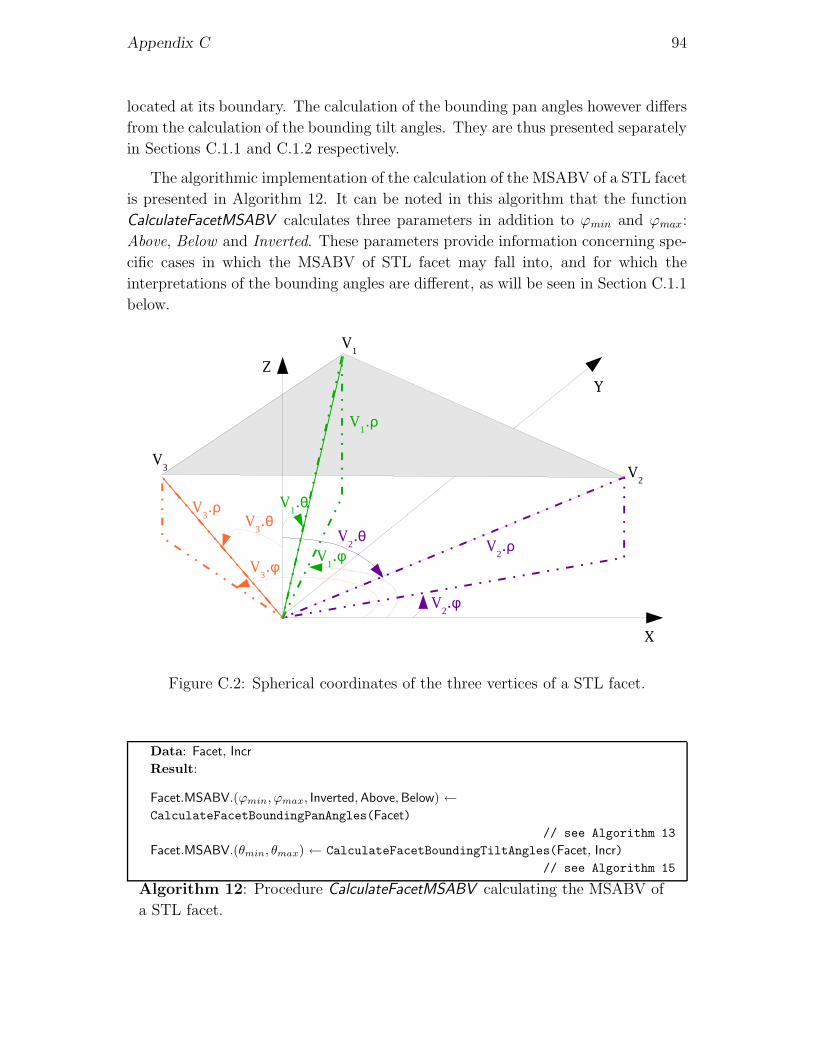
Appendix C 94

located at its boundary. The calculation of the bounding pan angles however differs

from the calculation of the bounding tilt angles. They are thus presented separately

in Sections C.1.1 and C.1.2 respectively.

The algorithmic implementation of the calculation of the MSABV of a STL facet

is presented in Algorithm 12. It can be noted in this algorithm that the function

CalculateFacetMSABV calculates three parameters in addition to ϕmin and ϕmax:

Above, Below and Inverted. These parameters provide information concerning spe-

cific cases in which the MSABV of STL facet may fall into, and for which the

interpretations of the bounding angles are different, as will be seen in Section C.1.1

below.

Figure C.2: Spherical coordinates of the three vertices of a STL facet.

Data: Facet, Incr

Result:

Facet.MSABV.(ϕmin, ϕmax, Inverted, Above, Below) ←CalculateFacetBoundingPanAngles(Facet)

// see Algorithm 13

Facet.MSABV.(θmin, θmax) ← CalculateFacetBoundingTiltAngles(Facet, Incr)

// see Algorithm 15

Algorithm 12: Procedure CalculateFacetMSABV calculating the MSABV of

a STL facet.

Appendix C 95

C.1.1 Bounding Pan Angles: ϕmin and ϕmax

Figure C.3 shows a scene with a STL facet viewed from the top of the scanner. It

can be shown, as illustrated in Figure C.3, that the bounding pan angles of a STL

facet, ϕmin and ϕmax, are always the pan angles of two of its vertices. Additionally,

at least in the case illustrated here, which is referred to the Regular case, ϕmin is

the smallest and ϕmax the largest of the pan angles of the three vertices. Therefore,

they can be calculated as:

ϕmin = min (V1.ϕ, V2.ϕ, V3.ϕ)

ϕmax = max (V1.ϕ, V2.ϕ, V3.ϕ)

where: V1, V2 and V3 are the three vertices of the STL facet.

Figure C.3: Illustration of the MSABV of a STL facet for the situation where the

facet has Regular bounding pan angles, ϕmin and ϕmax.

However, as shown in the two examples in Figure C.4, they are some cases for

which ϕmin and ϕmax are not respectively the smallest and largest of the pan angles

of the three vertices. In the example in Figure C.4(a), ϕmax is truly the largest

of the pan angles of the three vertices, but ϕmin is not the smallest. And, in the

example in Figure C.4(b), ϕmin is truly the smallest of the pan angles of the three

vertices, but ϕmax is not the largest. Such cases are due to the fact that pan angles

are only defined in the interval [0; 2π[, and they occur when “the facet intersects

the positive x axis when viewed from the top”. These cases are referred to as facets

with Inverted bounding pan angles.

As shown in the example in Figure C.5, two additional cases must be distin-

guished, when the facet is Above or Below the scanner, which occurs when the z

Appendix C 96

axis intersects the facet. In these two cases, values of ϕmin and ϕmax calculated with

the three vertices would be misleading and must be set to 0 and 2π respectively.

In conclusion, STL facets must be classified into four groups, Regular, Inverted,

Above and Below, so that their bounding pan angles, ϕmin and ϕmax can be in-

terpreted adequately. As will be seen in Appendix E, it is actually important to

distinguish facets Above from facets Below the scanner.

Algorithm 13 presents the algorithmic implementation of the calculation of the

bounding pan angles of a STL facet. The strategy is to: (1) sort the values of

the pan angles of the three vertices into ϕmintemp, ϕmidtemp, ϕmaxtemp; and then (2)

analyze those values to deduce which case the STL facet falls into and calculate the

values of ϕmin and ϕmax accordingly. The calculation of the values ϕmin nor ϕmax

according to the different cases is presented in Algorithm 14.

(a) Type I Inverted. (b) Type II Inverted.

Figure C.4: Illustration of the MSABV of a STL facet for the two situations where

the facet has Inverted bounding pan angles.

Appendix C 97

Figure C.5: Illustration of the MSABV of a STL facet for the situations where the

facet is Above or Below the scanner.

In Algorithm 14, Facet.−→n is the unit vector normal to the STL facet as defined

in the STL format (see Appendix A). Also, It can be noted in this algorithm that

the distinction between a facet Above and a facet Below the scanner considers only

the case when the facet is front-facing (with respect to the scanner’s location).

This is appropriate since, as will be discussed in Appendix D, no as-planned range

point can be obtained from an back-facing facet, so that all the back-facing facets

are discarded. The calculation of whether a STL facet is back-facing is presented

in Appendix D.

Appendix C 98

Data: Facet

Result: ϕmin, ϕmax, Inverted, Above, Below

ϕmaxtemp ← Facet.V1.ϕ

if Facet.V2.ϕ > ϕmaxtemp thenϕmidtemp ← ϕmaxtemp

ϕmaxtemp ← Facet.V2.ϕelse

ϕmidtemp ← Facet.V2.ϕend

if Facet.V3.ϕ > ϕmaxtemp thenϕmintemp ← ϕmidtemp

ϕmidtemp ← ϕmaxtemp

ϕmaxtemp ← Facet.V3.ϕelse if Facet.V3.ϕ > ϕmidtemp then

ϕmintemp ← ϕmidtemp

ϕmidtemp ← Facet.V3.ϕelse

ϕmintemp ← Facet.V3.ϕend

(ϕmin, ϕmax, Inverted, Above, Below) ← CalculateFacetBoundingPanAngles2(ϕmintemp,ϕmidtemp, ϕmaxtemp, Facet.−→n ) // see Algorithm 14

Algorithm 13: Function CalculateFacetBoundingPanAngles calculating the

bounding pan angles of a STL facet.

Appendix C 99

Data: ϕmintemp, ϕmidtemp, ϕmaxtemp, −→nResult: ϕmin, ϕmax, Inverted, Above, Below

Above ← False

Below ← False

Inverted ← False

if ϕmaxtemp − ϕmintemp > π thenif ϕmidtemp − ϕmintemp ≤ π then

if ϕmaxtemp − ϕmidtemp ≤ π thenif −→n · −→Z < 0 then //

−→Z : vertical axis of the scan’s coordinate

frameAbove ← True

elseBelow ← True

endϕmin ← 0ϕmax ← 2π

elseInverted ← True

ϕmin ← ϕmidtemp

ϕmax ← ϕmaxtemp

endelse

Inverted ← True

ϕmin ← ϕmintemp

ϕmax ← ϕmidtemp

endelse

ϕmin ← ϕmintemp

ϕmax ← ϕmaxtemp

end

Algorithm 14: Function CalculateFacetBoundingPanAngles2 calculating

whether a STL facet falls into any of the three special cases (Inverted, Above,

Below), and calculating the values of its bounding pan angles, ϕmin and ϕmax,

accordingly.

Appendix C 100

C.1.2 Bounding Tilt Angles: θmin and θmax

The calculation of the bounding tilt angles is simpler in the sense that it does not

require distinguishing between different cases. However, it is more complicated be-

cause, as tentatively illustrated with one example in Figure C.6, while the bounding

tilt angles of a STL facet are also the tilt angles of points located at its boundary,

they are not necessarily those of two of its vertices. The calculation of the exact

bounding tilt angles, θmin and θmax, of a STL facet thus requires calculating the

smallest and largest tilt angles of its three edges and then deduce θmin and θmax

from the set composed of these three edges.

The exact calculation of the bounding tilt angles of an edge of a STL facet, i.e. a

segment, is however quite complicated, as it would require determining the equation

of the edge in spherical coordinates. Such a function is not only non-linear, but is

also piecewise continuous.

A simpler but approximative approach is used here. As illustrated in Figure

C.7, the strategy is to calculate the tilt angles of a finite number of evenly spread

points on each edge. The bounding tilt angles of the edge are then estimated as

the bounding tilt angles of the set composed of all these points. The algorithmic

implementation of this calculation is presented in Algorithm 15.

This approach requires setting the incremental distance used to pick the points

along the edge, Incr. If Incr is small, the resulting estimated bounding tilt angles

will be a good approximation of the true bounding tilt angles, but this will be

achieved at the expense of a longer calculation time. In the experiments presented

in this thesis, a value of Incr of 10mm is used for ensuring a good estimation of

the facets’ bounding tilt angles, despite its computational impact.

A method for the selection of Incr based on some properties of each STL facet

(bounding pan angles and distance to the scanner) is discussed in Chapter 4, but has

not been implemented. Such a method would enable reducing the computational

complexity of this calculation.

Another, certainly better, method would be to calculate the bounding tilt angles

of each section of the edge, i.e. sub-segment, for which the equation in spherical

coordinates is fully continuous, and then infer the bounding tilt angles of the edge

as the bounding tilt angles of the set of sections constituting the edge. Such a

method has not been investigated either.

C.2 MSABV of a STL Object

The MSABV of a STL object can be deduced from the MSABV of all its facets.

More exactly, it is the union of the MSABV of its facets. The algorithmic implemen-

Appendix C 101

Figure C.6: Example of a case where θmin is not the tilt angle of one of the three

STL triangle vertices.

Figure C.7: Illustration of the proposed strategy for estimaing of the bounding tilt

angles of an edge of a STL facet.

tation of this calculation is presented in Algorithm 16, that calls the Algorithms 17

and 18 for the calculations of the bounding pan and tilt angles respectively. It can

be seen that, similarly to the STL facets, the interpretation of the bounding pan

Appendix C 102

Data: Facet, Incr

Result: θmin and θmax

θmin ← π

θmax ← 0

for each Facet.Edge as E do

E.Length ←∥∥∥−−−−−−−−−−−−−−−−−−−−→E.Vb. [x, y, z]− E.Va. [x, y, z]

∥∥∥E.−→u ←

−−−−−−−→E.Vb−E.Va

E.Length

TempPoint.[x, y, z] ← E.Va.[x, y, z]

while∥∥∥−−−−−−−−−−−−−−−−−−−−−−−−−→TempPoint. [x, y, z]− E.Va. [x, y, z]

∥∥∥ ≤ E.Length doTempPoint.θ ← CalculateTiltAngle(TempPoint.[x, y, z])if TempPoint.θ < θmin then θmin ← TempPoint.θif TempPoint.θ > θmax then θmax ← TempPoint.θTempPoint.[x, y, z] ← TempPoint.[x, y, z] + Incr (E.−→u )

endendif Facet.Above = True then θmin ← 0

if Facet.Below = True then θmax ← π

Algorithm 15: Function CalculateFacetBoundingTiltAngles estimating the

bounding tilt angles of a STL triangle.

angles must distinguish between four cases: Regular, Above, Below and Inverted. A

STL object falls in one of the last three cases if at least one of its facets falls into

that same case.

Data: Object

Result: ϕmin, ϕmax, θmin, θmax, Inverted, Above, Below

Object.MSABV.(ϕmin, ϕmax, Above, Below, Inverted) ←CalculateObjectBoundingPanAngles(Object.{Facet}) // see Algorithm 17

Object.MSABV.(θmin, θmax) ← CalculateObjectBoundingTiltAngles(Object.{Facet})// see Algorithm 18

Algorithm 16: Function CalculateObjectMSABV calculating the MSABV of

a STL object.

Appendix C 103

Data: {Facet}Result: ϕmin, ϕmax, Above, Below, Inverted

Above ← False

Below ← False

Inverted ← False

for each Facet doif Facet.Above = True then Above ← True

if Facet.Below = True then Below ← True

if Facet.Inverted = True then Inverted ← Trueend

ϕmin ← 2 π

ϕmax ← 0if Above = True or Below = True then

ϕmin ← 0ϕmax ← 2 π

else if Inverted = True thenfor each Facet do

if Facet.Inverted = True thenif Facet.ϕmin > ϕmin then ϕmin ← Facet.ϕmin

if Facet.ϕmax < ϕmax then ϕmax ← Facet.ϕmax

elseif Facet.ϕmin > π then

if Facet.ϕmin < ϕmax then ϕmax ← Facet.ϕmin

elseif Facet.ϕmax > ϕmin then ϕmin ← Facet.ϕmax

endend

endelse

for each Facet doif Facet.ϕmin < ϕmin then ϕmin ← Facet.ϕmin

if Facet.ϕmax > ϕmax then ϕmax ← Facet.ϕmax

endend

Algorithm 17: Function CalculateObjectBoundingPanAngles calculating

whether a STL object fall into one of the four cases (Regular, Above, Below,

Inverted) and calculating its bounding pan angles, ϕmin and ϕmax, accordingly.

Appendix C 104

Data: {Facet}Result: θmin, θmax

θmin ← π

θmax ← 0

for each Facet doif Facet.θmin < θmin then θmin ← Facet.θmin

if Facet.θmax > θmax then θmax ← Facet.θmax

end

Algorithm 18: Function CalculateObjectBoundingTiltAngles estimating the

bounding tilt angles of a STL object.

Appendix D

Construction of the Bounding

Volume Hierarchy (BVH) of a

project 3D Model

This appendix describes the calculation of the proposed Bounding Volume Hierar-

chy (BVH) of a STL-formatted 3D model, where the bounding volumes are Min-

imum Spherical Angular Bounding Volumes (MSABVs). The calculations of the

MSABV of STL entities (facets and objects) is presented in Appendix C.

It is particularly shown here that the size of the BVH can be significantly

and easily reduced (or pruned), without impacting the resulting as-planned point

calculation, by using scan’s viewing frustum culling and back-facing facet culling

techniques, leading to a significant reduction in the computational complexity of of

the BVH for the calculation of each as-planned range point.

The back-facing facet culling and scan’s viewing frustum culling techniques used

here are described in Sections D.1 and D.2 respectively. The resulting calculation

of the pruned BVH is presented in Section D.3.

D.1 Back-Facing Facet Culling

An as-planned range point can only be obtained from a front-facing facet, with

respect to the scanner’s location. The reason is that, in the problem investigated

here, facets are part of closed tessellated volumes, so that, from any view point,

any back-facing facet is always hidden behind other front-facing facets.

Then, as presented in Appendix A, all the facet normal vectors of a STL-

formated model are oriented toward the outside of objects (or all of them toward

105

Appendix D 106

the inside; this is chosen a priori), so that it is simple, given a STL facet’s normal

vector, to identify whether it is back-facing (or front-facing) from the scanner’s

location (see illustration in Figure D.1).

This back-facing property must not be confused with the visibility property. In

the case of closed tessellated volumes, back-facing facet are always hidden, front-

facing facet are not necessarily all visible, so that the set of hidden facets is smaller

than the set of back-facing ones. As a result, performing facet visibility culling gen-

erally achieves a more effective facet culling than back-facing facet culling. However,

it is more complicated to calculate whether a facet is hidden rather than simply

back-facing, so that back-facing facet culling can be implemented more efficiently.

Back-facing facet culling is preferred here.

As illustrated in Figure D.1, the facing property (front-facing or back-facing)

of a STL facet can easily be calculated by comparing the direction of its normal

vector with its location with respect to the scanner’s origin. For this, the scalar

product between any vector from the scan’s origin to any point on the STL facet

(for instance the coordinate vector of its first vertex V1) and the vector normal to

the facet −→n is calculated. If the scalar product is strictly negative, then the facet

is front-facing; it is back-facing otherwise. The algorithmic implementation of this

calculation is presented in Algorithm 19. It assumes that the normal vector to the

facet points outside the object’s volume. This can be ensured for all facets when

converting the 3D model into STL format (see Appendix A).

The number of back-facing facets in a scan-referenced 3D model is typically

roughly equal to half of all the model facets — mainly because most AEC&FM 3D

objects present vertical and horizontal symmetries. Therefore, by implementing

back-facing facet culling, the size of the BVH of the 3D model can be significantly

reduced, leading a significant improvement in the computational complexity of the

calculation of each as-planned range point.

Data: Facet

Result:

if Facet.−→V1 · Facet.−→n < 0 then

Facet.IsFrontFacing ← True

elseFacet.IsFrontFacing ← False

end

Algorithm 19: Procedure CalculateFacetIsFrontFacing calculating whether

the facet is front-facing from the scanner’s origin.

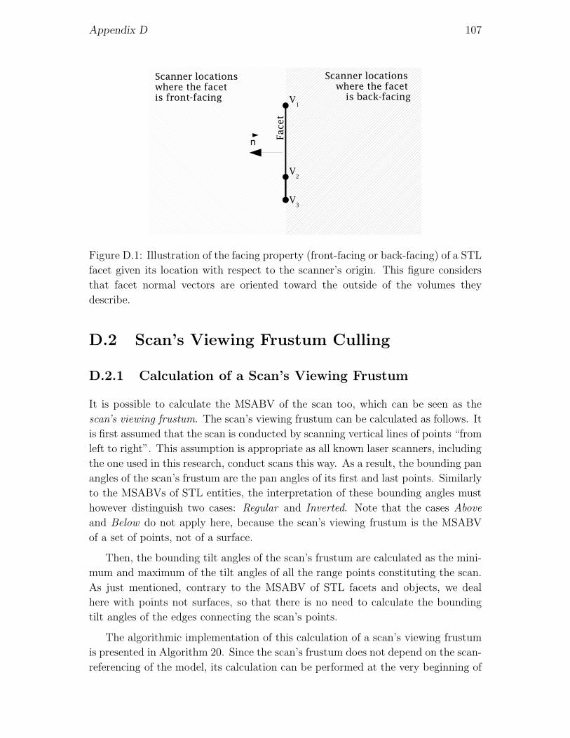
Appendix D 107

Figure D.1: Illustration of the facing property (front-facing or back-facing) of a STL

facet given its location with respect to the scanner’s origin. This figure considers

that facet normal vectors are oriented toward the outside of the volumes they

describe.

D.2 Scan’s Viewing Frustum Culling

D.2.1 Calculation of a Scan’s Viewing Frustum

It is possible to calculate the MSABV of the scan too, which can be seen as the

scan’s viewing frustum. The scan’s viewing frustum can be calculated as follows. It

is first assumed that the scan is conducted by scanning vertical lines of points “from

left to right”. This assumption is appropriate as all known laser scanners, including

the one used in this research, conduct scans this way. As a result, the bounding pan

angles of the scan’s frustum are the pan angles of its first and last points. Similarly

to the MSABVs of STL entities, the interpretation of these bounding angles must

however distinguish two cases: Regular and Inverted. Note that the cases Above

and Below do not apply here, because the scan’s viewing frustum is the MSABV

of a set of points, not of a surface.

Then, the bounding tilt angles of the scan’s frustum are calculated as the mini-

mum and maximum of the tilt angles of all the range points constituting the scan.

As just mentioned, contrary to the MSABV of STL facets and objects, we deal

here with points not surfaces, so that there is no need to calculate the bounding

tilt angles of the edges connecting the scan’s points.

The algorithmic implementation of this calculation of a scan’s viewing frustum

is presented in Algorithm 20. Since the scan’s frustum does not depend on the scan-

referencing of the model, its calculation can be performed at the very beginning of

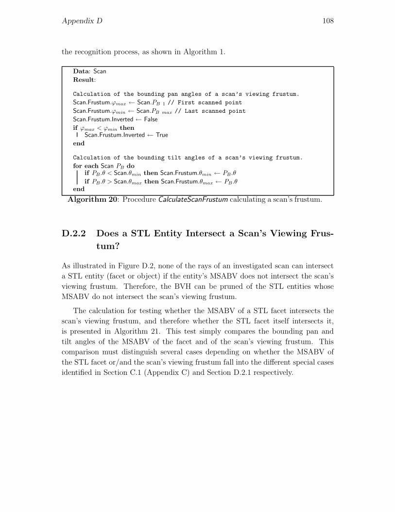
Appendix D 108

the recognition process, as shown in Algorithm 1.

Data: Scan

Result:

Calculation of the bounding pan angles of a scan’s viewing frustum.

Scan.Frustum.ϕmax ← Scan.PB 1 // First scanned point

Scan.Frustum.ϕmin ← Scan.PB max // Last scanned point

Scan.Frustum.Inverted ← False

if ϕmax < ϕmin thenScan.Frustum.Inverted ← True

end

Calculation of the bounding tilt angles of a scan’s viewing frustum.

for each Scan PB doif PB.θ < Scan.θmin then Scan.Frustum.θmin ← PB.θif PB.θ > Scan.θmax then Scan.Frustum.θmax ← PB.θ

end

Algorithm 20: Procedure CalculateScanFrustum calculating a scan’s frustum.

D.2.2 Does a STL Entity Intersect a Scan’s Viewing Frus-

tum?

As illustrated in Figure D.2, none of the rays of an investigated scan can intersect

a STL entity (facet or object) if the entity’s MSABV does not intersect the scan’s

viewing frustum. Therefore, the BVH can be pruned of the STL entities whose

MSABV do not intersect the scan’s viewing frustum.

The calculation for testing whether the MSABV of a STL facet intersects the

scan’s viewing frustum, and therefore whether the STL facet itself intersects it,

is presented in Algorithm 21. This test simply compares the bounding pan and

tilt angles of the MSABV of the facet and of the scan’s viewing frustum. This

comparison must distinguish several cases depending on whether the MSABV of

the STL facet or/and the scan’s viewing frustum fall into the different special cases

identified in Section C.1 (Appendix C) and Section D.2.1 respectively.

Appendix D 109

(a) MSABV not intersecting a scan’s viewingfrustum

(b) MSABV intersecting a scan’s viewingfrustum

Figure D.2: Illustration of the intersection of a MSABV with a scan’s viewing

frustum.

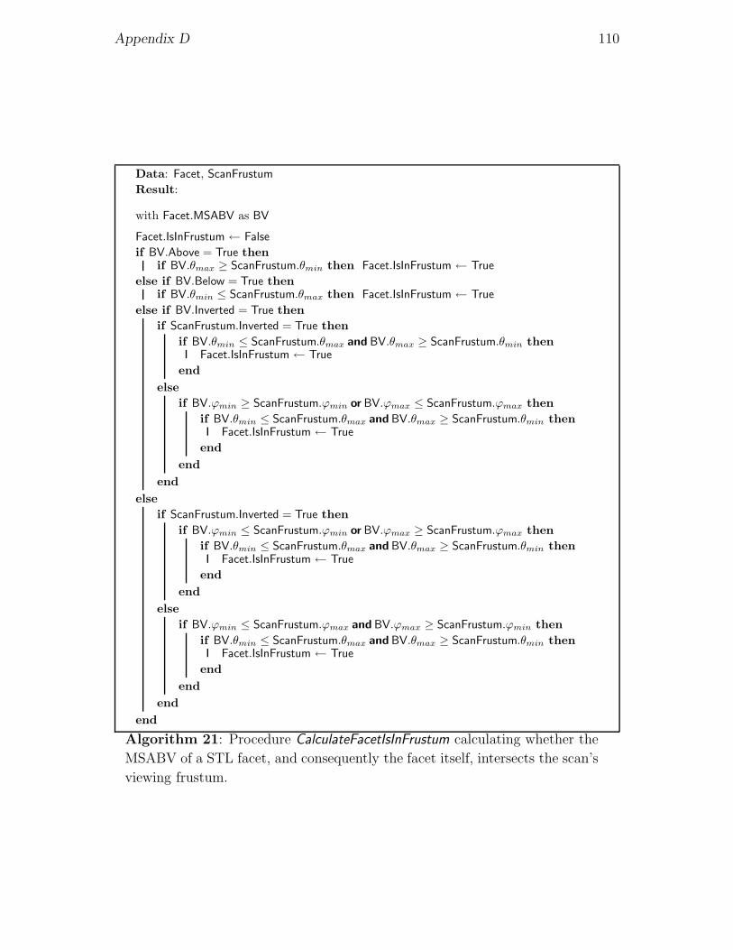
Appendix D 110

Data: Facet, ScanFrustum

Result:

with Facet.MSABV as BV

Facet.IsInFrustum ← False

if BV.Above = True thenif BV.θmax ≥ ScanFrustum.θmin then Facet.IsInFrustum ← True

else if BV.Below = True thenif BV.θmin ≤ ScanFrustum.θmax then Facet.IsInFrustum ← True

else if BV.Inverted = True thenif ScanFrustum.Inverted = True then

if BV.θmin ≤ ScanFrustum.θmax and BV.θmax ≥ ScanFrustum.θmin thenFacet.IsInFrustum ← True

endelse

if BV.ϕmin ≥ ScanFrustum.ϕmin or BV.ϕmax ≤ ScanFrustum.ϕmax thenif BV.θmin ≤ ScanFrustum.θmax and BV.θmax ≥ ScanFrustum.θmin then

Facet.IsInFrustum ← True

endend

endelse

if ScanFrustum.Inverted = True thenif BV.ϕmin ≤ ScanFrustum.ϕmin or BV.ϕmax ≥ ScanFrustum.ϕmax then


endend

elseif BV.ϕmin ≤ ScanFrustum.ϕmax and BV.ϕmax ≥ ScanFrustum.ϕmin then


endend

endend

Algorithm 21: Procedure CalculateFacetIsInFrustum calculating whether the

MSABV of a STL facet, and consequently the facet itself, intersects the scan’s

viewing frustum.

Appendix D 111

It can be noted that a STL object intersects a scan’s viewing frustum if at least

one of its facets intersects it. The calculation of whether a STL object intersects

a scan’s viewing frustum can thus be simply performed after the calculations for

all its facets have been performed. Its algorithmic implementation is presented in

Algorithm 22.

Data: Object

Result:

Object.IsInFrustum ← False

for each Object.Facet doif Object.Facet.IsInFrustum = True then

Object.IsInFrustum ← False

endend

Algorithm 22: Procedure CalculateObjectIsInFrustum calculating whether a

STL object intersects the scan’s frustum.

D.3 Calculation of the BVH

The resulting algorithmic implementation of the calculation of the pruned BVH is

presented in Algorithm 23. This calculation only depends on the scan-referenced

3D model and the scan’s frustum. As a result, it can be performed prior to the

calculation of the as-planned range point cloud, as shown in Algorithm 3.

It can be noted that Algorithm 12, calculating the MSABV of a facet and called

by Algorithm 23, requires the parameter Incr as input. The need for this parameter

and its estimation are described in Appendix C.

Appendix D 112

Data: Model, ScanFrustum

Result: BVH

DEFINE Incr

Calculate the MSABV and culling properties of STL facets and objects:

for each Model.Object dofor each Model.Object.Facet do

CalculateFacetisFrontFacing(Model.Object.Facet) // see Algorithm 19

CalculateFacetMSABV(Model.Object.Facet, Incr)

// see Algorithm 12 in Appendix C

CalculateFacetIsInFrustum(Model.Object.Facet, ScanFrustum) // see

Algorithm 21

endCalculateObjectMSABV(Model.Object) // see Algorithm 16 in Appendix C

CalculateObjectIsInFrustum(Model.Object) // see Algorithm 22

end

Calculate the BVH of the 3D model:

for each Model.Object doif Model.Object.IsInFrustum = True then

AddObjectNodeToBVH (BVH,Model.Object)for each Model.Object.Facet do

if Model.Object.Facet.IsFrontFacing = True thenif Model.Object.Facet.IsInFrustum = True then

AddFacetNodeToBVHObject (BVH.Object, Model.Object.Facet)end

endend

endend

Algorithm 23: Function CalculateBVH calculating the pruned BVH of the

STL-formatted 3D model.

Appendix E

Containment of a Ray in a

Minimum Spherical Angular

Bounding Volume (MSABV).

This Appendix describes the calculation to test whether a ray corresponding to the

scanning direction of an as-planned range point is contained in a minimum spherical

angular bounding volume (MSABV) (of a STL facet or object). The calculation

differs when the MSABV falls into one of the different cases identified in Appendix

C: Regular, Above, Below, Inverted.

In the case a MSABV falls in the Regular case, as illustrated in Figure E.1, the

scanning direction of an as-planned range point, PP , is contained in this MSABV

if, and only if:

1. The pan angle of the point scanning direction, PP .ϕ, verifies:

PP .ϕ ≥MSABV.ϕmin and PP .ϕ ≤MSABV.ϕmax

2. And, the tilt angle of the point scanning direction, PP .θ, verifies:

PP .θ ≥ MSABV.θmin and PP .θ ≤MSABV.θmax

Similarly, in the case a MSABV falls into the Inverted case, as illustrated in

Figure E.2, the scanning direction of an as-planned range point, PP , is contained

in this MSABV if, and only if:

(PP .ϕ ≤MSABV.ϕmin or PP .ϕ ≥MSABV.ϕmax) and

(PP .θ ≥ MSABV.θmin and PP .θ ≤ MSABV.θmax)

113

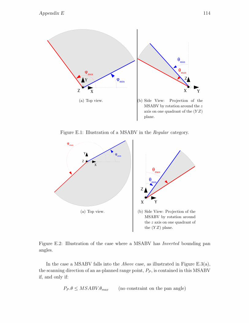
Appendix E 114

(a) Top view. (b) Side View: Projection of theMSABV by rotation around the z

axis on one quadrant of the (Y Z)plane.

Figure E.1: Illustration of a MSABV in the Regular category.

(a) Top view. (b) Side View: Projection of theMSABV by rotation aroundthe z axis on one quadrant ofthe (Y Z) plane.

Figure E.2: Illustration of the case where a MSABV has Inverted bounding pan

angles.

In the case a MSABV falls into the Above case, as illustrated in Figure E.3(a),

the scanning direction of an as-planned range point, PP , is contained in this MSABV

if, and only if:

PP .θ ≤MSABV.θmax (no constraint on the pan angle)

Appendix E 115

Finally, in the case a MSABV falls into the Below case, as illustrated in Figure

E.3(b), the scanning direction of an as-planned range point, PP , is contained in this

MSABV if, and only if:

PP .θ ≥MSABV.θmin (no constraint on the pan angle)

(a) Above case. Side View: Projection of theMSABV by rotation around the z axis onthe (Y Z) plane.

(b) Below case. Side View: Projection of theMSABV by rotation around the z axis onthe (Y Z) plane.

Figure E.3: Illustration of the case where a MSABV is Above (a) or Below (b) the

scanner.

The overall algorithmic implementation of the calculation to test whether the

scanning direction of an as-planned range point is contained in a MSABV is pro-

vided in Algorithm 24.

Appendix E 116

Data: PP , MSABV

Result: IsSurrounded

IsSurrounded← False

if MSABV.Above = True thenif PP .θ ≤ MSABV.θmax then

IsSurrounded← True

endelse if MSABV.Below = True then

if PP .θ ≥ MSABV.θmin thenIsSurrounded← True

endelse if MSABV.Inverted = True then

if PP .ϕ ≥ MSABV.ϕmax or PP .ϕ ≤ MSABV.ϕmin thenif PP .θ ≥ MSABV.θmin and PP .θ ≤ MSABV.θmax then

IsSurrounded← True

endend

elseif PP .ϕ ≥ MSABV.ϕmin and PP .ϕ ≤ MSABV.ϕmax then

if PP .θ ≥ MSABV.θmin and PP .θ ≤ MSABV.θmax thenIsSurrounded← True

endend

end

Algorithm 24: Function IsRayInMSABV calculating whether the scanning

direction of as-planned range point is contained in a MSABV.

Appendix F

Calculation of the Range of the

Intersection Point of a Ray and a

STL Facet

In this appendix, we describe the calculation of the range, ρ′, of the intersection

point of the scanning direction of an as-planned range point with a STL facet. The

intersection point may not necessarily exist.

This problem can be seen as a constrained version of the linear projection of a

point (here the scan’s origin) on the plane defined by the STL facet in a given direc-

tion (here the scanning direction of the as-planned range point). The constraint is

that the sub-ensemble on which the point is projected, the STL facet, is bounded.

Figure F.1 illustrates this problem.

This problem can be solved using the following two-step process for which the

algorithmic implementation is presented in Algorithm 25:

Projection. Project the scan’s origin as PProj on the 2D plane defined by the

STL facet along the scanning direction of the investigated as-planned range

point. This is a simple projection problem that won’t be described here. Its

algorithmic implementation is simply included in Algorithm 25.

Constraint. Assess whether the projected point, PProj, is within the boundaries of

the STL facet. If the point is within the boundaries, its range, ρ′ is calculated.

If it is not, it is assigned an infinite range. A method for identifying whether

the projected point is within the boundaries of the STL facet is presented in

the following section.

117

Appendix F 118

Figure F.1: Illustration of the calculation of the intersection of the scanning direc-

tion of an as-planned range point with a STL facet.

Data: Facet, PB

Result: ρ′

−→uP ← 1∥∥∥−→PB

∥∥∥−→PB

α ← −−→uP · Facet.−→n

PProj . [x, y, z] ← PB . [x, y, z] +

(−−−−−−−−−−−−→PB−Facet.Vertex1·Facet.−→n

)

cos α−→uP

if IsPointInsideFacet(Facet, PProj) = True then // see Algorithm 26

ρ′ ←√

(PProj .x)2 + (PProj .y)2 + (PProj .z)2

elseρ′ ← ∞

end

Algorithm 25: Function CalculateIntersectionPointRange calculating whether

a point projected on a 2D surface is inside the STL triangle defining that

surface.

F.1 Is Projected Point Inside Facet?

One simple approach to assess whether the projected point, PProj, is within the

boundaries of the STL facet is the following. It uses the fact that each facet edge is

a section of the line that is the intersection of the plane defined by the facet and a

Appendix F 119

second plane perpendicular to the first one. Figure F.2 illustrates the three planes,

perpendicular to the plane defined by a STL facet, that define the three edges of the

facet. Each of these three planes is simply defined by a point, P lane.P t, that can be

set to one of the facet’s vertices, and a normal vector, P lane.−→n , that can easily be

computed based on the facet’s vertices and normal vector. For instance, P lane1.P t

and P lane1.−→n of the plane P lane1 defining the edge between the vertices Facet.V1

and Facet.V2 of a STL facet, are calculated as:

P lane1.P t = Facet.V1

P lane1.−→n = (Facet.V2 − Facet.V1)× Facet.−→n

The formula used for P lane1.−→n assumes that the normal vector to the STL

facet points toward the outside of the object, which is consistent with the previous

assumptions on the matter. Again, this can be ensured during the conversion of

the 3D model into STL format (see Appendix A).

Then, the projected point, PProj, is inside the facet if, and only if:

(PProj − Facet.V1) · P lane1.−→n ≤ 0 and

(PProj − Facet.V2) · P lane2.−→n ≤ 0 and

(PProj − Facet.V3) · P lane3.−→n ≤ 0

The algorithmic implementation of this calculation is presented in Algorithm

26.

Data: Facet, PProj

Result: IsInside

IsInside ← False

if (PProj − Facet.Vertex1.XY Z) · Facet.Vertex1.−→n ≤ 0 then



IsInside ← True

endend

end

Algorithm 26: Function IsPointInsideFacet calculating whether a point pro-

jected on a 2D surface is inside the STL triangle defining that surface.

Note that the vectors normal to the planes P lane1, P lane2 and P lane3 can

be calculated as soon as the 3D model is converted into STL format, and then

Appendix F 120

(a) Perspective view.

(b) Topview.

Figure F.2: Illustration of the calculation of whether a point on the plane defined

by a STL facet is inside the facet.

scan-referenced with the rest of the model during Step 2 of the developed object

recognition process. The algorithmic implementation of the calculation of the vec-

tors normal to the planes P lane1, P lane2 and P lane3 of a STL facet is presented in

Algorithm 27, and this algorithm is called in Algorithm 1 as soon as the 3D model

has been converted into STL format. Note that the normal vector of the plane i is

simply assigned to the vertex i. The scan-referencing of the vectors normal to the

planes P lane1, P lane2 and P lane3 of each facet in the scan’s coordinate frame is

Appendix F 121

included in Algorithm 2.

Data: Model

Result:

for each Model.Object dofor each Model.Object.Facet As F do

for i = 1 to 3 doj ← i + 1if j = 4 then j ← 1F.Vertex i.−→n ← (F.Vertexj − F.Vertexi)× F.−→n

endend

end

Algorithm 27: Procedure CalculateVerticesNormals calculating the normals

of the planes perpendicular to the plane of a STL facet and defining its three

edges.

Appendix G

Object Recognition Results of

Experiment 3

This Appendix presents the different data sets (model and scan) at the different

steps of the recognition process obtained in Experiment 3 described in Chapter 4.

A table with the detailed object recognition statistics for each of the 612 objects of

the 3D model is also provided at the end of this appendix.

G.1 Input Data

The experiment’s input data consists of the 3D CAD model of the building’s struc-

ture and the laser scan Scan 3 presented in Chapter 4. The 3D CAD model is

presented in Figure G.1. It contains 612 objects including large objects, such as

columns and beams, and small objects, such wall panel braces or hand rail tubes.

Scan 3 is presented in Figure G.2. It contains 810, 399 range points and has a scan

angular resolution of 582 μrad in pan and 582 μrad in tilt.

122

Appendix G 123

Figure G.1: 3D CAD model.

Figure G.2: As-built 3D laser scanned point cloud.

Appendix G 124

G.2 Recognition Process Results

G.2.1 Step 1 - Convert 3D model

The first step of the recognition process is to convert the 3D CAD model into STL

format. Figure G.3 presents the STL-formatted model that contains 19, 478 facets

— an average of about 32 facets per object. It can be seen that the 3D CAD model

is faithfully converted.

Figure G.3: STL-formatted 3D model.

Appendix G 125

G.2.2 Step 2 - 3D model Scan-Referencing

The second step of the recognition process uses the 3D model and scan registration

information to reference the STL-formatted 3D model in the scan’s spherical coor-

dinate frame. Figure G.4 shows the 3D model and Scan 3 in the scan’s spherical

coordinate frame.

Figure G.4: 3D model referenced in the scan’s spherical coordinate frame.

Appendix G 126

G.2.3 Step 3 - Calculate As-planned Range Point Cloud

The third and main step of the recognition process is the calculation of the as-

planned range point cloud. Figure G.5 presents the calculated as-planned point

cloud corresponding to Scan 3.

Figure G.5: As-planned range point cloud corresponding to Scan 3.

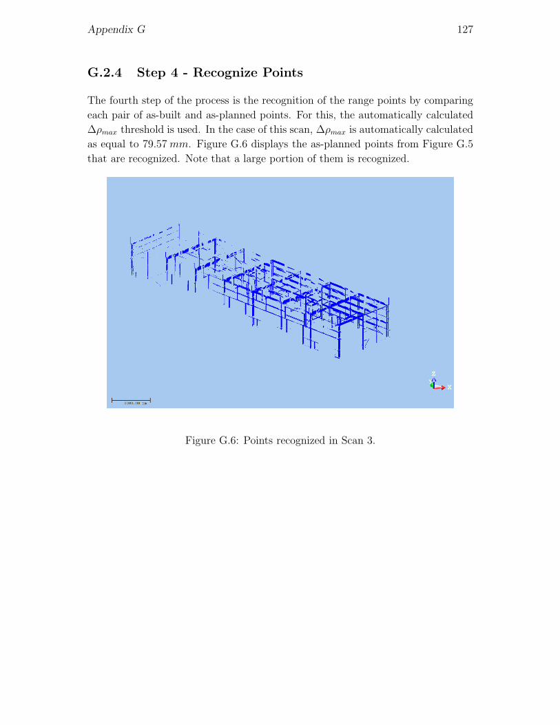
Appendix G 127

G.2.4 Step 4 - Recognize Points

The fourth step of the process is the recognition of the range points by comparing

each pair of as-built and as-planned points. For this, the automatically calculated

Δρmax threshold is used. In the case of this scan, Δρmax is automatically calculated

as equal to 79.57 mm. Figure G.6 displays the as-planned points from Figure G.5

that are recognized. Note that a large portion of them is recognized.

Figure G.6: Points recognized in Scan 3.

Appendix G 128

G.2.5 Step 5 - Recognize Objects

The fifth and last step of the process is the recognition of the model objects by

comparing, for each object, the covered surface of its recognized as-planned points

with the automatically calculated threshold Surfmin. Here, Surfmin is automat-

ically calculated as equal to 0.0109 m2. Figure G.7 displays the objects from the

3D model that are recognized in the scan. The colors used in Figure G.7 have the

following meaning:

Gray: The object is not expected (planned) to be recognized in this scan — be-

cause the covered surface of its as-planned points does not exceed Surfmin.

Green: The object is expected to be recognized and is recognized in the scan.

Red: The object is expected to be recognized but is not recognized in the scan.

This must, however, not lead to the conclusion that the object is not built.

Several situations must in fact be distinguished.

The object is in the scan. It is then colored in red because it is built, but

at the wrong location.

The object is not in the scan. This may occur in three different situa-

tions:

� The construction is behind schedule.

� Inadequate 3D model: the search 3D model does not adequately

represent the project in the state it is expected to be found.

� External occlusions: the object is occluded by another object that

is not part of the 3D model (e.g. piece of equipment).

Since, an object colored in red may mean different things, it must be in-

terpreted as a warning saying that this particular object requires further

analysis. Note that, the last two of the four situations identified above can

be somewhat avoided using good practice. First, an adequate as-planned 3D

model can be used for the object recognition by using a project 4D model

instead of the 3D model (see Section 5.2.3). Then, external occlusions (oc-

clusions to non-model objects) can be avoided by cleaning the scanned scene

prior to conduct any scan as well as locating the scanner so that external

occlusions that cannot be removed are minimized (see Section 5.2.3). If these

best practices are implemented, an object colored in red will then indicate

either that it is built at the wrong location, or that construction is behind

schedule, the first case being easily identifiable by investigating the scan man-

ually.

Appendix G 129

It can be seen in Figure G.7 that most of the 3D model objects (exactly 466

objects) are expected to be recognized in the investigated scan. Out of these, a

majority of them (exactly 280 objects) is actually recognized in the scan. While it

can be noted that the main structural elements are well recognized, 186 elements

still are not recognized (colored in red). As mentioned above, these objects may

not be recognized for several reasons. For instance, the 131 objects constituting

the small inner structure at the back of the building (see Figure G.1) should not

have been included in the 3D model considering the current level of progress.

Then, the small elements around two of the door frames in the front long wall

are not recognized because they were occluded by other non-model objects such as

a set of portable toilets (external occlusions).

Next, the three door frames colored in red in the front long side (6 objects) are

not recognized but are in the scan (see Figure G.2). It can thus be concluded that

they are likely built at the wrong location, or design change orders have not been

reported to the 3D model.

Finally, many of the objects the furthest from the scanner are not recognized

although they are present in the scan. These objects include 5 fairly large beams

and the column in the middle of the back side of the building. An important reason

why they are not recognized is that, from the scanner’s location, they are highly

occluded by other model objects, so that only small parts of their total surfaces were

actually expected to be recognized in the scan, and their recognized surfaces often

simply fell short of the Surfmin threshold. It is also likely that poor registration

quality negatively impacted their recognition.

Detailed statistics about the recognition of each 3D model object are provided

in the next section.

Appendix G 130

��

��

Scanner

Figure G.7: The 3D model object recognition results obtained with Scan 3.

G.2.6 Recognition Statistics

Table G.1 summarizes the recognition statistics obtained for each of the 612 objects

composing the original 3D CAD model. In this table, the column values are:

Column 1: ID of the object.

Column 2: Number of points in the object’s as-planned range point cloud.

Column 3: Number of points in the object’s as-planned range point cloud that

are recognized.

Column 4: Covered Surface of the points in the object’s as-planned range point

cloud.

Column 5: Covered Surface of the points in the object’s as-planned range point

cloud that are recognized.

Column 6: Whether the object is considered planned (1) or not (0). It is consid-

ered planned if the covered Surface of the points in the object’s as-planned

range point cloud (column 4) is larger than Surfmin.

Appendix G 131

Column 7: Whether the object is recognized (1) or not (0). Note that an object

can be recognized only if it is planned (the covered surface of the recognized as-

planned range points cannot exceed the covered surface of all the as-planned

range points).

Column 8: Whether the object is manually visually identified (1) or not (0) in

the scan.

Table G.1: Recognition Statistics for Scan 3.

Object Planned Recog. Planned Recog. Planned Recog. ActualID Points Points Surface Surface

(m2) (m2)1 5071 281 1.31 0.06 1 1 1

2 2240 514 1.89 0.3 1 1 1

3 4477 60 1.23 0.02 1 1 1

4 4868 29 1.35 0.01 1 0 1

5 4324 0 1.09 0 1 0 1

6 6456 48 1.21 0.01 1 0 1

7 1737 1401 0.49 0.39 1 1 1

8 1765 1314 0.52 0.36 1 1 1

9 215 33 0.1 0.02 1 1 0

10 500 498 0.12 0.12 1 1 1

11 457 40 0.1 0.01 1 0 1

12 67 6 0.02 0 1 0 1

13 260 42 0.04 0.01 1 0 1

14 81 7 0.04 0.01 1 0 1

15 28 2 0.02 0 1 0 0

16 41 0 0.04 0 1 0 0

17 12 0 0.01 0 1 0 0

18 8 2 0.01 0 1 0 0

19 6 2 0.01 0 1 0 0

20 2411 12 1.35 0.01 1 0 1

21 1940 0 1.19 0 1 0 1

22 1657 1022 1.21 0.7 1 1 1

23 1484 797 1.47 0.65 1 1 1

24 1199 0 1.15 0 1 0 1

25 1091 0 1.21 0 1 0 1

26 739 506 0.56 0.31 1 1 1

27 717 575 0.61 0.46 1 1 1

28 298 0 0.37 0 1 0 0

29 329 0 0.36 0 1 0 0

30 109 38 0.21 0.07 1 1 1

31 218 80 0.8 0.15 1 1 1

32 5 0 0.07 0 1 0 0

33 860 420 1.62 0.86 1 1 1

34 768 356 1.09 0.5 1 1 1

35 88 0 0.91 0 1 0 0

36 31 0 0.2 0 1 0 0

37 54 4 0.11 0.01 1 0 0

38 61 0 0.23 0 1 0 0

39 19 0 0.1 0 1 0 0

40 80 0 0.19 0 1 0 0

41 192 0 0.23 0 1 0 0

42 326 30 0.2 0.02 1 1 0

43 53 0 0.2 0 1 0 0

44 161 6 0.19 0.01 1 0 1

Continued on next page...

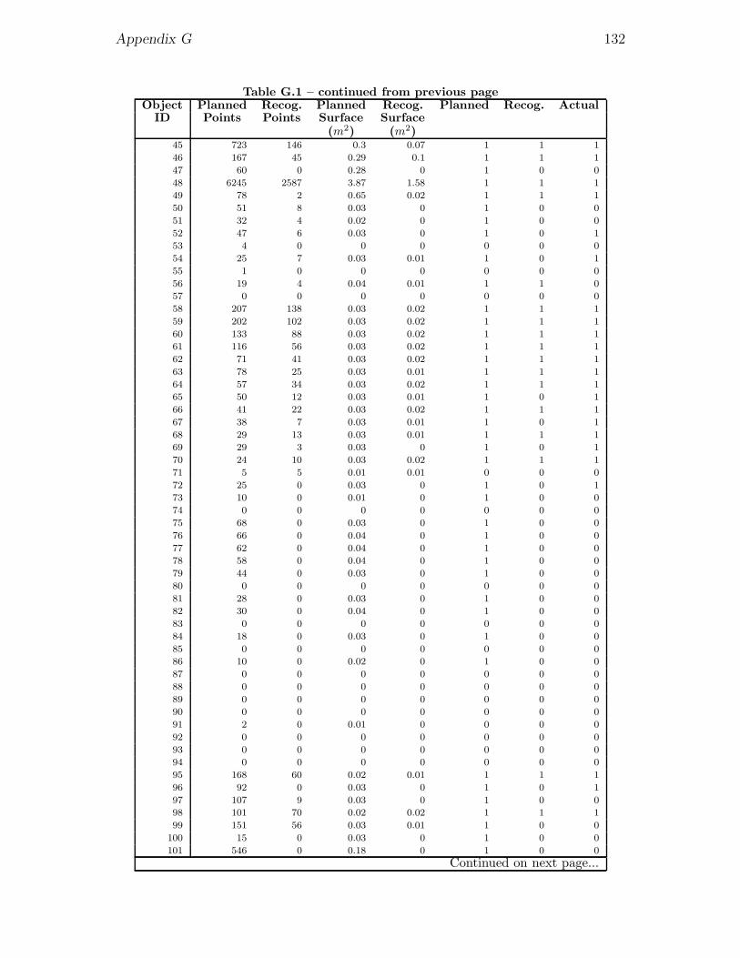
Appendix G 132

Table G.1 – continued from previous pageObject Planned Recog. Planned Recog. Planned Recog. Actual

ID Points Points Surface Surface(m2) (m2)

45 723 146 0.3 0.07 1 1 1

46 167 45 0.29 0.1 1 1 1

47 60 0 0.28 0 1 0 0

48 6245 2587 3.87 1.58 1 1 1

49 78 2 0.65 0.02 1 1 1

50 51 8 0.03 0 1 0 0

51 32 4 0.02 0 1 0 0

52 47 6 0.03 0 1 0 1

53 4 0 0 0 0 0 0

54 25 7 0.03 0.01 1 0 1

55 1 0 0 0 0 0 0

56 19 4 0.04 0.01 1 1 0

57 0 0 0 0 0 0 0

58 207 138 0.03 0.02 1 1 1

59 202 102 0.03 0.02 1 1 1

60 133 88 0.03 0.02 1 1 1

61 116 56 0.03 0.02 1 1 1

62 71 41 0.03 0.02 1 1 1

63 78 25 0.03 0.01 1 1 1

64 57 34 0.03 0.02 1 1 1

65 50 12 0.03 0.01 1 0 1

66 41 22 0.03 0.02 1 1 1

67 38 7 0.03 0.01 1 0 1

68 29 13 0.03 0.01 1 1 1

69 29 3 0.03 0 1 0 1

70 24 10 0.03 0.02 1 1 1

71 5 5 0.01 0.01 0 0 0

72 25 0 0.03 0 1 0 1

73 10 0 0.01 0 1 0 0

74 0 0 0 0 0 0 0

75 68 0 0.03 0 1 0 0

76 66 0 0.04 0 1 0 0

77 62 0 0.04 0 1 0 0

78 58 0 0.04 0 1 0 0

79 44 0 0.03 0 1 0 0

80 0 0 0 0 0 0 0

81 28 0 0.03 0 1 0 0

82 30 0 0.04 0 1 0 0

83 0 0 0 0 0 0 0

84 18 0 0.03 0 1 0 0

85 0 0 0 0 0 0 0

86 10 0 0.02 0 1 0 0

87 0 0 0 0 0 0 0

88 0 0 0 0 0 0 0

89 0 0 0 0 0 0 0

90 0 0 0 0 0 0 0

91 2 0 0.01 0 0 0 0

92 0 0 0 0 0 0 0

93 0 0 0 0 0 0 0

94 0 0 0 0 0 0 0

95 168 60 0.02 0.01 1 1 1

96 92 0 0.03 0 1 0 1

97 107 9 0.03 0 1 0 0

98 101 70 0.02 0.02 1 1 1

99 151 56 0.03 0.01 1 0 0

100 15 0 0.03 0 1 0 0

101 546 0 0.18 0 1 0 0


Appendix G 133



102 528 255 0.24 0.11 1 1 1

103 448 254 0.22 0.11 1 1 1

104 0 0 0 0 0 0 0

105 7 0 0.03 0 1 0 0

106 3 0 0.01 0 0 0 0

107 17 0 0.03 0 1 0 0

108 0 0 0 0 0 0 0

109 0 0 0 0 0 0 0

110 0 0 0 0 0 0 0

111 37 0 0.06 0 1 0 0

112 0 0 0 0 0 0 0

113 42 0 0.04 0 1 0 0

114 132 0 0.11 0 1 0 0

115 63 0 0.05 0 1 0 0

116 172 0 0.11 0 1 0 0

117 212 0 0.12 0 1 0 0

118 0 0 0 0 0 0 0

119 49 0 0.07 0 1 0 0

120 6678 3081 1.75 0.78 1 1 1

121 6644 175 8.86 0.17 1 1 1

122 101 0 0.2 0 1 0 0

123 95 0 0.04 0 1 0 1

124 192 0 0.06 0 1 0 1

125 688 0 0.46 0 1 0 1

126 36 20 0.11 0.04 1 1 1

127 2 0 0 0 0 0 0

128 0 0 0 0 0 0 0

129 38 29 0.07 0.06 1 1 1

130 64 4 0.12 0.01 1 0 0

131 46 7 0.21 0.02 1 1 0

132 91 67 0.14 0.1 1 1 1

133 43 8 0.13 0.01 1 0 0

134 110 75 0.2 0.09 1 1 1

135 55 9 0.11 0.01 1 1 0

136 192 160 0.21 0.16 1 1 1

137 75 16 0.09 0.03 1 1 0

138 245 204 0.19 0.14 1 1 1

139 110 26 0.08 0.02 1 1 0

140 419 345 0.24 0.2 1 1 1

141 182 28 0.09 0.02 1 1 0

142 723 502 0.29 0.19 1 1 1

143 279 50 0.08 0.02 1 1 0

144 1290 1007 0.27 0.21 1 1 1

145 1345 942 0.27 0.18 1 1 1

146 817 727 0.25 0.22 1 1 1

147 1 0 0 0 0 0 0

148 0 0 0 0 0 0 0

149 93 32 0.04 0.01 1 1 0

150 171 72 0.04 0.02 1 1 0

151 207 145 0.05 0.04 1 1 1

152 342 219 0.04 0.03 1 1 1

153 124 83 0.05 0.03 1 1 1

154 78 51 0.05 0.03 1 1 1

155 45 33 0.04 0.03 1 1 1

156 30 19 0.04 0.02 1 1 1

157 29 10 0.04 0.01 1 1 1

158 5 5 0.01 0.01 0 0 0


Appendix G 134



159 31 14 0.02 0.01 1 0 0

160 35 10 0.02 0 1 0 0

161 27 10 0.02 0.01 1 0 0

162 9 0 0.01 0 0 0 0

163 12 4 0.01 0 1 0 0

164 6 2 0.01 0 0 0 0

165 12 3 0.02 0 1 0 0

166 0 0 0 0 0 0 0

167 7396 335 1.75 0.06 1 1 1

168 162 72 0.03 0.01 1 1 0

169 301 142 0.03 0.02 1 1 0

170 91 21 0.03 0.01 1 0 0

171 65 17 0.03 0.01 1 0 0

172 44 7 0.03 0 1 0 0

173 33 5 0.03 0.01 1 0 0

174 12 1 0.02 0 1 0 0

175 2 1 0 0 0 0 0

176 43 20 0.02 0.01 1 0 0

177 46 15 0.01 0 1 0 0

178 32 12 0.02 0.01 1 0 0

179 5 0 0 0 0 0 0

180 20 9 0.02 0.01 1 0 0

181 5 4 0.01 0.01 0 0 0

182 14 4 0.02 0.01 1 0 0

183 0 0 0 0 0 0 0

184 174 95 0.36 0.2 1 1 1

185 8165 817 2.6 0.08 1 1 1

186 1907 276 1.43 0.2 1 1 1

187 1715 1421 2.33 2.1 1 1 1

188 933 889 2.21 2.1 1 1 1

189 554 107 2.1 0.14 1 1 1

190 352 8 1.96 0.05 1 1 1

191 274 18 2.32 0.21 1 1 1

192 5353 4055 2.25 1.8 1 1 1

193 2532 2142 1.82 1.64 1 1 1

194 811 533 0.91 0.63 1 1 1

195 834 811 1.45 1.41 1 1 1

196 225 119 0.58 0.32 1 1 1

197 135 73 0.48 0.29 1 1 1

198 93 4 0.4 0.01 1 0 1

199 3297 2382 1.41 1.03 1 1 1

200 1753 1241 1.23 0.9 1 1 1

201 368 204 0.38 0.2 1 1 1

202 521 472 0.9 0.83 1 1 1

203 55 38 0.14 0.1 1 1 1

204 0 0 0 0 0 0 1

205 11254 8752 2.32 1.93 1 1 1

206 6666 481 2.45 0.09 1 1 1

207 414 305 0.83 0.61 1 1 1

208 343 124 0.74 0.26 1 1 1

209 21820 16715 4.23 3.14 1 1 1

210 10453 7216 3.83 2.12 1 1 1

211 4466 2918 2.88 1.91 1 1 1

212 3669 3214 3.54 3.11 1 1 1

213 1802 1070 2.82 1.7 1 1 1

214 1410 957 2.32 1.33 1 1 1

215 1083 647 2.65 1.74 1 1 1


Appendix G 135



216 1037 671 2.77 1.54 1 1 1

217 87 3 0.19 0.01 1 0 1

218 372 90 1.15 0.27 1 1 1

219 1451 1014 3.42 2.46 1 1 1

220 1480 531 2.69 1.1 1 1 1

221 2607 932 3.84 1.78 1 1 1

222 3254 556 3.69 0.81 1 1 1

223 4433 2031 3.67 1.85 1 1 1

224 14000 7013 4.1 1.94 1 1 1

225 18918 11754 6.7 4.12 1 1 1

226 8723 6692 4.17 3.34 1 1 1

227 5283 4525 3.56 3.01 1 1 1

228 3816 3176 3.49 2.89 1 1 1

229 3535 2972 4.22 3.55 1 1 1

230 2768 2248 4.25 3.47 1 1 1

231 5043 4368 2.09 1.86 1 1 1

232 3640 3328 2.48 2.32 1 1 1

233 1408 1036 1.7 1.33 1 1 1

234 1048 858 1.76 1.48 1 1 1

235 296 138 0.83 0.37 1 1 1

236 604 45 2.3 0.11 1 1 1

237 95 78 0.16 0.13 1 1 1

238 45 9 0.06 0.01 1 1 1

239 86 3 0.09 0 1 0 1

240 296 55 0.25 0.05 1 1 1

241 371 145 0.24 0.09 1 1 1

242 474 88 0.24 0.04 1 1 1

243 3213 112 1.15 0.05 1 1 1

244 143 0 0.22 0 1 0 1

245 0 0 0 0 0 0 0

246 216 51 0.2 0.05 1 1 1

247 19 0 0.01 0 1 0 1

248 479 0 0.28 0 1 0 1

249 573 50 0.28 0.02 1 1 1

250 1920 986 1.06 0.55 1 1 1

251 440 5 0.46 0.01 1 0 1

252 425 185 0.89 0.28 1 1 1

253 446 2 0.72 0 1 0 1

254 798 325 1.36 0.55 1 1 1

255 7 0 0.02 0 1 0 0

256 953 47 1.49 0.07 1 1 0

257 827 317 1.26 0.48 1 1 1

258 2625 115 0.75 0.05 1 1 1

259 2701 266 0.87 0.07 1 1 1

260 70 2 0.15 0 1 0 1

261 88 2 0.19 0 1 0 1

262 1441 1095 1.47 1.08 1 1 1

263 1369 977 1.42 1.01 1 1 1

264 664 435 0.77 0.5 1 1 1

265 193 35 0.2 0.03 1 1 1

266 0 0 0 0 0 0 0

267 3246 2569 1.86 1.44 1 1 1

268 61 0 0.04 0 1 0 1

269 2030 1550 1.44 1.09 1 1 1

270 2866 59 1.48 0.03 1 1 0

271 526 5 0.25 0 1 0 0

272 7424 6048 2.49 2.2 1 1 1


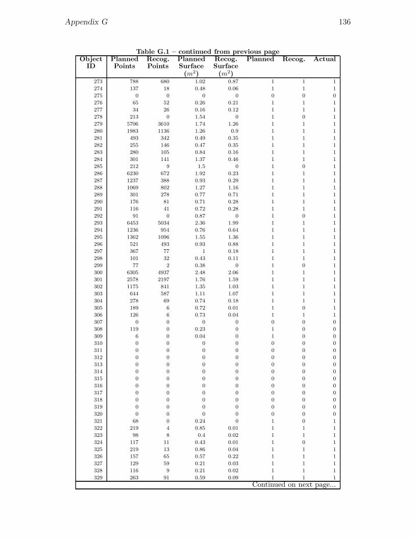
Appendix G 136



273 788 680 1.02 0.87 1 1 1

274 137 18 0.48 0.06 1 1 1

275 0 0 0 0 0 0 0

276 65 52 0.26 0.21 1 1 1

277 34 26 0.16 0.12 1 1 1

278 213 0 1.54 0 1 0 1

279 5706 3610 1.74 1.26 1 1 1

280 1983 1136 1.26 0.9 1 1 1

281 493 342 0.49 0.35 1 1 1

282 255 146 0.47 0.35 1 1 1

283 280 105 0.84 0.16 1 1 1

284 301 141 1.37 0.46 1 1 1

285 212 9 1.5 0 1 0 1

286 6230 672 1.92 0.23 1 1 1

287 1237 388 0.93 0.29 1 1 1

288 1069 802 1.27 1.16 1 1 1

289 301 278 0.77 0.71 1 1 1

290 176 81 0.71 0.28 1 1 1

291 116 41 0.72 0.28 1 1 1

292 91 0 0.87 0 1 0 1

293 6453 5034 2.36 1.99 1 1 1

294 1236 954 0.76 0.64 1 1 1

295 1362 1096 1.55 1.36 1 1 1

296 521 493 0.93 0.88 1 1 1

297 367 77 1 0.18 1 1 1

298 101 32 0.43 0.11 1 1 1

299 77 2 0.38 0 1 0 1

300 6305 4937 2.48 2.06 1 1 1

301 2578 2197 1.76 1.59 1 1 1

302 1175 841 1.35 1.03 1 1 1

303 644 587 1.11 1.07 1 1 1

304 278 69 0.74 0.18 1 1 1

305 189 6 0.72 0.01 1 0 1

306 126 6 0.73 0.04 1 1 1

307 0 0 0 0 0 0 0

308 119 0 0.23 0 1 0 0

309 6 0 0.04 0 1 0 0

310 0 0 0 0 0 0 0

311 0 0 0 0 0 0 0

312 0 0 0 0 0 0 0

313 0 0 0 0 0 0 0

314 0 0 0 0 0 0 0

315 0 0 0 0 0 0 0

316 0 0 0 0 0 0 0

317 0 0 0 0 0 0 0

318 0 0 0 0 0 0 0

319 0 0 0 0 0 0 0

320 0 0 0 0 0 0 0

321 68 0 0.24 0 1 0 1

322 219 4 0.85 0.01 1 1 1

323 98 8 0.4 0.02 1 1 1

324 117 11 0.43 0.01 1 0 1

325 219 13 0.86 0.04 1 1 1

326 157 65 0.57 0.22 1 1 1

327 129 59 0.21 0.03 1 1 1

328 116 9 0.21 0.02 1 1 1

329 263 91 0.59 0.09 1 1 1


Appendix G 137



330 697 93 0.37 0.05 1 1 1

331 1251 48 0.75 0.03 1 1 1

332 234 148 0.35 0.23 1 1 1

333 0 0 0 0 0 0 0

334 44 11 0.2 0.02 1 1 1

335 0 0 0 0 0 0 0

336 111 89 0.2 0.16 1 1 1

337 98 78 0.21 0.17 1 1 1

338 478 320 0.43 0.3 1 1 1

339 155 115 0.11 0.08 1 1 1

340 159 109 0.32 0.24 1 1 1

341 181 153 0.11 0.1 1 1 1

342 98 59 0.07 0.05 1 1 1

343 338 294 0.28 0.27 1 1 1

344 989 628 0.48 0.32 1 1 1

345 1438 1191 0.6 0.5 1 1 1

346 686 577 0.47 0.41 1 1 1

347 294 45 0.29 0.04 1 1 1

348 395 20 0.41 0.02 1 1 1

349 218 7 0.35 0.01 1 1 1

350 287 14 0.49 0.02 1 1 1

351 8001 4539 3.46 1.73 1 1 1

352 5952 3228 3.55 1.89 1 1 1

353 165 0 1.46 0 1 0 1

354 141 42 0.28 0.08 1 1 1

355 57 0 0.3 0 1 0 0

356 18 0 0.04 0 1 0 1

357 2008 1310 4.9 2.09 1 1 1

358 4407 404 1.22 0.1 1 1 1

359 1000 526 0.66 0.43 1 1 1

360 1 0 0 0 0 0 0

361 0 0 0 0 0 0 0

362 0 0 0 0 0 0 0

363 0 0 0 0 0 0 0

364 0 0 0 0 0 0 0

365 0 0 0 0 0 0 0

366 118 100 0.2 0.17 1 1 1

367 114 98 0.25 0.17 1 1 1

368 181 149 0.44 0.26 1 1 1

369 109 18 0.19 0.03 1 1 1

370 157 147 0.21 0.19 1 1 1

371 128 123 0.17 0.16 1 1 1

372 225 180 0.4 0.35 1 1 1

373 226 221 0.4 0.4 1 1 1

374 316 316 0.23 0.23 1 1 1

375 324 321 0.3 0.3 1 1 1

376 439 438 0.37 0.37 1 1 1

377 455 453 0.39 0.39 1 1 1

378 1204 59 0.32 0.02 1 1 0

379 1202 93 0.31 0.03 1 1 0

380 1299 0 0.3 0 1 0 0

381 838 0 0.19 0 1 0 0

382 1316 0 0.3 0 1 0 0

383 826 658 0.29 0.23 1 1 1

384 1486 1093 0.52 0.36 1 1 1

385 945 574 0.33 0.19 1 1 1

386 1194 2 0.28 0 1 0 0


Appendix G 138



387 897 559 0.32 0.19 1 1 1

388 2073 994 2.44 1.12 1 1 1

389 2640 1310 3 1.5 1 1 1

390 377 82 0.22 0.04 1 1 1

391 349 50 0.2 0.02 1 1 1

392 434 60 0.24 0.03 1 1 1

393 571 164 0.32 0.09 1 1 1

394 325 75 0.23 0.06 1 1 1

395 384 105 0.27 0.07 1 1 1

396 467 79 0.32 0.05 1 1 1

397 420 104 0.29 0.07 1 1 1

398 0 0 0 0 0 0 0

399 0 0 0 0 0 0 0

400 0 0 0 0 0 0 0

401 0 0 0 0 0 0 0

402 164 42 0.17 0.04 1 1 1

403 205 49 0.22 0.05 1 1 1

404 277 62 0.3 0.06 1 1 1

405 234 88 0.26 0.09 1 1 1

406 0 0 0 0 0 0 1

407 0 0 0 0 0 0 1

408 0 0 0 0 0 0 1

409 0 0 0 0 0 0 1

410 0 0 0 0 0 0 0

411 0 0 0 0 0 0 0

412 0 0 0 0 0 0 0

413 0 0 0 0 0 0 0

414 59 44 0.12 0.09 1 1 1

415 66 63 0.14 0.13 1 1 1

416 109 83 0.24 0.17 1 1 1

417 122 0 0.35 0 1 0 1

418 806 72 0.52 0.05 1 1 1

419 0 0 0 0 0 0 0

420 1009 460 0.47 0.22 1 1 1

421 0 0 0 0 0 0 1

422 0 0 0 0 0 0 0

423 161 47 0.74 0.19 1 1 1

424 419 253 0.44 0.25 1 1 1

425 0 0 0 0 0 0 0

426 1027 796 0.92 0.73 1 1 1

427 299 214 0.59 0.41 1 1 1

428 11 2 0.02 0 1 0 0

429 149 0 0.32 0 1 0 0

430 2 0 0 0 0 0 0

431 105 0 0.23 0 1 0 0

432 14 0 0.03 0 1 0 0

433 243 166 0.44 0.2 1 1 1

434 21 0 0.03 0 1 0 0

435 149 149 0.18 0.18 1 1 1

436 200 189 0.2 0.19 1 1 1

437 0 0 0 0 0 0 0

438 160 114 0.14 0.1 1 1 1

439 223 198 0.29 0.24 1 1 1

440 192 169 0.17 0.15 1 1 1

441 464 399 0.55 0.42 1 1 1

442 341 270 0.38 0.29 1 1 1

443 203 150 0.15 0.12 1 1 1


Appendix G 139



444 539 508 0.58 0.55 1 1 1

445 552 498 0.51 0.43 1 1 1

446 323 255 0.2 0.17 1 1 1

447 729 31 0.61 0.02 1 1 0

448 713 39 0.57 0.03 1 1 0

449 471 0 0.24 0 1 0 0

450 186 155 0.09 0.07 1 1 1

451 617 346 0.48 0.23 1 1 1

452 522 344 0.22 0.16 1 1 1

453 1353 760 0.6 0.29 1 1 1

454 1293 729 0.61 0.3 1 1 1

455 949 839 0.29 0.29 1 1 1

456 2050 1454 0.63 0.43 1 1 1

457 1840 1629 0.61 0.55 1 1 1

458 946 857 0.22 0.22 1 1 1

459 2914 2425 0.62 0.56 1 1 1

460 1463 1269 0.5 0.47 1 1 1

461 1175 998 0.43 0.39 1 1 1

462 168 120 0.34 0.25 1 1 1

463 14 0 0.03 0 1 0 0

464 0 0 0 0 0 0 0

465 107 0 0.19 0 1 0 0

466 196 0 0.4 0 1 0 0

467 138 0 0.55 0 1 0 0

468 0 0 0 0 0 0 0

469 13 0 0.04 0 1 0 0

470 175 0 0.49 0 1 0 0

471 135 0 0.51 0 1 0 0

472 1 0 0 0 0 0 0

473 52 0 0.31 0 1 0 0

474 147 0 0.46 0 1 0 0

475 184 0 0.29 0 1 0 0

476 203 0 0.4 0 1 0 0

477 90 0 0.18 0 1 0 0

478 145 0 0.29 0 1 0 0

479 14 0 0.03 0 1 0 0

480 8 0 0.02 0 1 0 0

481 3 0 0.02 0 1 0 0

482 2 0 0 0 0 0 0

483 3 0 0.01 0 1 0 0

484 16 0 0.03 0 1 0 0

485 28 0 0.05 0 1 0 0

486 13 0 0.02 0 1 0 0

487 16 0 0.03 0 1 0 0

488 252 0 0.4 0 1 0 0

489 233 0 0.39 0 1 0 0

490 2 0 0.01 0 0 0 0

491 7 0 0.02 0 1 0 0

492 44 0 0.36 0 1 0 0

493 86 0 0.58 0 1 0 0

494 22 0 0.04 0 1 0 0

495 14 0 0.02 0 1 0 0

496 2 0 0 0 0 0 0

497 5 0 0.03 0 1 0 0

498 13 0 0.02 0 1 0 0

499 15 0 0.03 0 1 0 0

500 35 0 0.06 0 1 0 0


Appendix G 140



501 15 0 0.02 0 1 0 0

502 7 0 0.03 0 1 0 0

503 3 0 0.01 0 0 0 0

504 11 0 0.02 0 1 0 0

505 20 0 0.03 0 1 0 0

506 0 0 0 0 0 0 0

507 0 0 0 0 0 0 0

508 0 0 0 0 0 0 0

509 4 0 0.01 0 1 0 0

510 0 0 0 0 0 0 0

511 0 0 0 0 0 0 0

512 19 0 0.04 0 1 0 0

513 29 0 0.06 0 1 0 0

514 21 0 0.08 0 1 0 0

515 20 0 0.07 0 1 0 0

516 5 0 0.01 0 0 0 0

517 34 0 0.06 0 1 0 0

518 21 0 0.03 0 1 0 0

519 0 0 0 0 0 0 0

520 11 0 0.03 0 1 0 0

521 0 0 0 0 0 0 0

522 0 0 0 0 0 0 0

523 32 0 0.1 0 1 0 0

524 30 0 0.11 0 1 0 0

525 0 0 0 0 0 0 0

526 0 0 0 0 0 0 0

527 14 0 0.04 0 1 0 0

528 0 0 0 0 0 0 0

529 40 0 0.06 0 1 0 0

530 22 0 0.03 0 1 0 0

531 6 0 0.01 0 1 0 0

532 0 0 0 0 0 0 0

533 0 0 0 0 0 0 0

534 0 0 0 0 0 0 0

535 49 0 0.06 0 1 0 0

536 38 0 0.05 0 1 0 0

537 174 0 0.28 0 1 0 0

538 0 0 0 0 0 0 0

539 3 0 0.01 0 0 0 0

540 0 0 0 0 0 0 0

541 0 0 0 0 0 0 0

542 5 0 0.02 0 1 0 0

543 4 0 0.02 0 1 0 0

544 1 0 0 0 0 0 0

545 2 0 0.01 0 0 0 0

546 0 0 0 0 0 0 0

547 0 0 0 0 0 0 0

548 5 0 0.01 0 0 0 0

549 4 0 0.01 0 0 0 0

550 0 0 0 0 0 0 0

551 0 0 0 0 0 0 0

552 3 0 0.01 0 0 0 0

553 0 0 0 0 0 0 0

554 0 0 0 0 0 0 0

555 2 0 0 0 0 0 0

556 6 0 0.01 0 0 0 0

557 0 0 0 0 0 0 0


Appendix G 141



558 3 0 0.01 0 0 0 0

559 0 0 0 0 0 0 0

560 0 0 0 0 0 0 0

561 12 0 0.07 0 1 0 0

562 6 0 0.01 0 0 0 0

563 3 0 0 0 0 0 0

564 2 0 0 0 0 0 0

565 5 0 0.01 0 0 0 0

566 0 0 0 0 0 0 0

567 0 0 0 0 0 0 0

568 2 0 0.01 0 0 0 0

569 1 0 0 0 0 0 0

570 3 0 0 0 0 0 0

571 3 0 0 0 0 0 0

572 1 0 0 0 0 0 0

573 0 0 0 0 0 0 0

574 0 0 0 0 0 0 0

575 2 0 0.01 0 1 0 0

576 1 0 0 0 0 0 0

577 32 0 0.1 0 1 0 0

578 23 0 0.04 0 1 0 0

579 0 0 0 0 0 0 0

580 9 0 0.04 0 1 0 0

581 1 0 0 0 0 0 0

582 0 0 0 0 0 0 0

583 0 0 0 0 0 0 0

584 34 0 0.26 0 1 0 0

585 10 0 0.03 0 1 0 0

586 16 0 0.06 0 1 0 0

587 0 0 0 0 0 0 0

588 0 0 0 0 0 0 0

589 0 0 0 0 0 0 0

590 0 0 0 0 0 0 0

591 0 0 0 0 0 0 0

592 3 0 0.01 0 0 0 0

593 0 0 0 0 0 0 0

594 3124 2063 1.37 0.84 1 1 1

595 2685 2274 0.99 0.84 1 1 1

596 1925 1662 0.86 0.68 1 1 1

597 3925 3857 1.43 1.41 1 1 1

598 1246 275 0.41 0.18 1 1 1

599 559 33 0.48 0.02 1 1 0

600 345 0 0.25 0 1 0 0

601 637 69 0.4 0.04 1 1 0

602 858 52 0.45 0.03 1 1 0

603 769 34 0.33 0.01 1 0 0

604 17 0 0.02 0 1 0 0

605 799 52 0.48 0.04 1 1 0

606 96 0 0.07 0 1 0 0

607 362 38 0.28 0.03 1 1 0

608 301 27 0.22 0.02 1 1 0

609 0 0 0 0 0 0 0

610 726 68 0.46 0.04 1 1 0

611 452 41 0.3 0.03 1 1 0

612 918 51 0.21 0.01 1 0 0

Appendix H

Notation

This appendix presents the mathematical notations and variables used in this thesis.

They are listed Tables H.1 and H.2, respectively.

Table H.1: Mathematical notations.

Notation Description� x Angle x (note: if the angle is noted with a Greek letter,

the notation � is discarded).

x← y Assignment of the value of y to x.

x y x multiplied by y.xy

or x/y x divided by y.√x Square root of x.

xn x to the power of n.

x.y Property y of x.

{x} Set of elements of type x.

n ({x}) Cardinality of the set of elements of type x.

(a, b, . . . , z) Set of elements of different types.

[a, b, . . . , z] Coordinate vector

[x, y, z] Cartesian 3D coordinates

[x, y, z] =

⎡⎣

x

y

z

⎤⎦

[ϕ, θ, ρ] Spherical coordinates (ϕ:pan, θ:tilt and ρ:range) as defined

in Appendix B.−→x Vector x.−→x · −→y Scalar product of vectors −→x and −→y .−→x ×−→y Cross product of vectors −→x and −→y .


142

Appendix H 143

Table H.1 – continued from previous page

Notation Description

‖−→x ‖ Euclidean distance (norm) of vector −→x .

|x| Absolute value of x.

Tx (x) Translation along the x axis of amount x:

Tx (x) =

⎡⎣

x

0

0

⎤⎦

Ty (y) Translation along the y axis of amount y:

Ty (y) =

⎡⎣

0

y

0

⎤⎦

Tz (z) Translation along the z axis of amount z:

Tz (z) =

⎡⎣

0

0

z

⎤⎦

Rx ( � x) Rotation around the x axis of angle � x:

Rx ( � x) =

⎡⎣

1 0 0

0 cos (� x) sin ( � x)

0 − sin ( � x) cos ( � x)

⎤⎦

Ry ( � y) Rotation around the y axis of angle � y:

Ry ( � y) =

⎡⎣

cos ( � y) 0 − sin ( � y)

0 1 0

sin ( � y) 0 cos (� y)

⎤⎦

Rz ( � z) Rotation around the z axis of angle � z:

Rz ( � z) =

⎡⎣

cos ( � z) sin ( � z) 0

− sin ( � z) cos ( � z) 0

0 0 1

⎤⎦

Table H.2: Notations of the variables used in the algo-

rithms.

Variable Description

Data Data.

Representation A data representation.

Feature A data feature.

Mesh A mesh of data points.

SpinImage A spin image as described in [64].


Appendix H 144



Model The project 3D model.

Object A STL object contained in the project 3D model.

ID A unique identifier.

IDobj An identifier specifying the ID of a STL object.

Facet A facet of a STL object.

Edge An edge of a STL facet.

V ertex (or V ) A vertex of a STL facet (or any other type of mesh).

Scan The investigated as-built range point cloud.

(Resϕ, Resθ) The pan and tilt resolutions of a scan.

Frustum Viewing frustum of a scan, defined as the minimum spher-

ical angular bounding volume of the scan’s range points.

PB An as-built range point.

PP An as-planned range point.

Tree The hierarchical tree of extents of the project 3D model

(extents being here minimum spherical angular bounding

volumes).

MSABV A minimum spherical angular bounding volume

(MSABV).

ϕmin, ϕmax Minimum and maximum bounding pan angles of a mini-

mum spherical angular bounding volume.

θmin, θmax Minimum and maximum bounding tilt angles of a mini-

mum spherical angular bounding volume.

Above Property whether a STL entity (facet of object) is above

the scanner.

Below Property whether a STL entity (facet of object) is below

the scanner.

Inverted Property whether a STL entity (facet of object) has in-

verted bounding pan angles.

α Reflection angle of an as-planned range point scanning di-

rection with an intersected STL facet.

(αϕ, αθ) Decomposition of the reflection angle, α, in its pan and

tilt components.

Δρ Difference between the range of an as-planned point and

its the the range of its corresponding as-built point:

(PP .ρ− PB.ρ).

Δρmax Point recognition threshold.


Appendix H 145



Surfunit Surface covered by a point at a range of 1 m perpendicu-

larly to the direction defined by the origin and the point

(scanning direction).

Surf Covered surface of a as-planned range point.

SurfR Covered surface of the recognized points of a STL object’s

as-planned range point cloud.

Surfmin Object surface recognition threshold.

IsFrontFacing Property of a STL facet specifying whether it is front-

facing with respect to the scanner’s location.

IsInFrustum Property of a STL entity specifying whether it intersects

the frustum of a scan.

IsRecognized Property of a point or STL object specifying whether it is

recognized in a scan.

References

[1] ASCE Construction Research Congress (CRC), San Diego, CA, USA, April

5-7 2005. 150, 152

[2] EG-ICE: 13th EG-ICE Workshop - Intelligent Computing in Engineering and

Architecture, Ascona, Switzerland, June 25-30 2006. 149, 155

[3] ASCE Construction Research Congress (CRC) ”A Global Community”,

Grand Bahama Island, The Bahamas, May 6-8 2007. 149, 155

[4] 3D Systems Inc. Stereolithography interface specification. Technical Report

50065-S01-00, 3D Systems Inc., 1989. 85

[5] P. K. Agarwal and J. Matousek. Ray shooting and parametric search. SIAM

Journal on Computing, 22(4):794–806, 1993. 27

[6] T. Akenine-Moller, E. Haines, and N. Hoffman. Real-Time Rendering, 2nd

edition. A.K. Peters Ltd., 2002. 31

[7] B. Akinci. Using sensor systems and standard project models to capture and

model project history for building commissioning and facility management.

In Proceeding of the Facility Area Network Workshop, University of Illinois,

Urbana-Champaign, IL, USA, February 26-27 2004. 8

[8] B. Akinci, F. Boukamp, C. Gordon, D. Huber, C. Lyons, and K. Park. A

formalism for utilization of sensor systems and integrated project models for

active construction quality control. Automation in Construction, 15(2):124–

138, 2006. 6, 7

[9] B. Akinci, E. Ergen, C. T. Haas, C. H. Caldas, J. Song, C.R. Wood, and

J. Wadephul. Field trials of RFID technology for tracking fabricated pipe.

Fiatech smart chips report, FIATECH, Austin, TX, 2004. 2

[10] B. Akinci, S. Kiziltas, E. Ergen, I. Z. Karaesmen, and F. Keceli. Modeling and

analyzing the impact of technology on data capture and transfer processes at

construction sites: A case study. Journal of Construction Engineering and

Management, 132(11):1148–1157, 2006. 6

146

Appendix H 147

[11] J. Amanatides. Ray tracing with cones. Computer Graphics (SIGGRAPH

04), 18(3):129–135, 1984. 28

[12] F. Arman and J. K. Aggarwal. Object recognition in dense range images

using a CAD system as a model base. In Proceedings of the IEEE International

Conference on Robotics and Automation (ICRA), volume 3, pages 1858–1863,

Cincinnati, OH, USA, 13-18 May 1990. 13

[13] F. Arman and J.K. Aggarwal. Model-based object recognition in dense-range

images: a review. Computing Surveys (CSUR), 25(1):5–43, 1993. 12, 48

[14] K. S. Arun, T. S. Huang, and S. D. Blostein. Least-squares fitting of two 3-d

point sets. IEEE Transactions on Pattern Analysis and Machine Intelligence,

9(5):698–700, 1987. 24

[15] J. Arvo and D. Kirk. Fast ray tracing by ray classification. Computer Graph-

ics, 21(4):55–64, 1987. 28

[16] U. Assarsson and T. Moller. Optimized view frustum culling algorithms for

bounding boxes. Journal of Graphics Tools, 5:9–22, 2000. 28

[17] A. H. Behzadan and V. R. Kamat. Georeferenced registration of construction

graphics in mobile outdoor augmented reality. Journal of Computing in Civil

Engineering, 21(4):247–258, 2007. 26

[18] P. J. Besl and N. D. McKay. A method for registration of 3-D shapes. IEEE

Transactions on Pattern Analysis and Machine Intelligence, 14(2):239–256,

1992. 13

[19] F. Bosche, J. Teizer, C. T. Haas, and C. H. Caldas. Integrating data

from 3D CAD and 3D cameras for real-time modeling. In Proceeding of

the ISCCBE/ASCE Joint International Conference on Computing and Deci-

sion Making in Civil and Building Engineering, pages 37–46, Montreal, QC,

Canada, July 12-15 2006. 8

[20] F. Boukamp and B. Akinci. Automated reasoning about construction speci-

fications to support inspection and quality control. Automation in Construc-

tion, 17(1):90–106, 2007. 75

[21] I. K. Brilakis and L. Soibelman. Multimodal image retrieval from construction

databases and model-based systems. Journal of Construction Engineering

and Management, 132(7):777–785, July 2006. 7, 11

[22] I. K. Brilakis and L. Soibelman. Shape-based retrieval of construction site

photographs. Journal of Computing in Civil Engineering, 22(1):14–20, 2008.

7, 11

Appendix H 148

[23] H. Bronnimann and M. Glisse. Octrees with near optimal cost for ray-

shooting. Computational Geometry, 34(3):182–194, 2006. 30

[24] B. A. Brucker and S. D. Nachtigall. Initiating the building information model

from owner and operator criteria and requirements. In Proceeding of the

ASCE International Conference on Computing in Civil Engineering, Cancun,

Mexico, July 12-15 2005. 2

[25] R. Buick. RTK base station networks driving adoption of GPS +/- 1 inch

automated steering among crop growers. Trimble Navigation Ltd., 2006. 18

[26] C. Caldas, D. Grau, and L. Soibelman. Using global positioning systems

to improve materials locating processes on industrial projects. Journal of

Construction Engineering and Management, 132(7):741–749, 2006. 2, 7, 18

[27] R. J. Campbell and P. J. Flynn. A survey of free-form object representa-

tion and recognition techniques. Computer Vision and Image Understanding,

81(2):166–210, 2001. 12, 13

[28] F. Caron, S. Razavi, J. Song, P. Vanheeghe, E. Duflos, C. H. Caldas, and

C. T. Haas. Locating sensor nodes on construction projects. Autonomous

Robots, 22(3):255–263, April 2007. 7

[29] P. C. Chang, A. Flatau, and S. C. Liu. Review paper: Health monitoring of

civil infrastructure. Structural Health Monitoring, 2(3):257–267, 2003. 6

[30] G. S. Cheok and W. C. Stone. Non-intrusive scanning technology for con-

struction management. In Proceedings of the 16th International Symposium

on Automation and Robotics in Construction (ISARC), pages 645–650, Uni-

versidad Carlos III de Madrid, Madrid, Spain, September 22-24 1999. 2, 6,

7

[31] G. S. Cheok, W. C. Stone, R. R. Lipman, and C. Witzgall. LADARs for

construction assessment and update. Automation in Construction, 9(5):463–

477, 2000. 8

[32] C. S. Chua and R. Jarvis. Point signatures: A new representation for 3D

object recognition. International Journal of Computer Vision, 25(1):63–85,

1997. 13

[33] D. Cline, K. Steele, and P. Egbert. Lightweight bounding volumes for ray

tracing. Journal of graphics tools, 11(4):61–71, 2006. 31

[34] L. D. Cohen. Deformable surfaces and parametric models to fit and track 3D

data. In IEEE International Conference on Systems, Man, and Cybernetics,

volume 4, pages 2451–2456, Beijing, China, 14-17 October 1996. 76

Appendix H 149

[35] G. S. Coleman and J. W. Jun. Interoperability and the construction process:

A white paper for building owners and project decision-makers. Technical

report, American Institute of Steel Construction, Inc., 2004. 1

[36] V. A. Collins. Evaluation and Comparison of Commercially Available Matu-

rity Measurement Systems. PhD thesis, Carnegie Mellon Department of Civil

and Environmental Engineering, Pittsburgh, PA, USA, 2004. 2

[37] M. de Berg, D. Halperin, M. H. Overmars, J. Snoeyink, and M. J. van Kreveld.

Efficient ray shooting and hidden surface removal. Algorithmica, 12(1):30–53,

1994. 31

[38] C. Dorai and A. K. Jain. COSMOS - a representation scheme for 3D free-form

objects. IEEE Transactions on Pattern Analysis and Machine Intelligence,

19(10):1115–1130, 1997. 13

[39] C. Eastman. New opportunities for IT research in construction. In Proceeding

of the 13th EG-ICE Workshop - Intelligent Computing in Engineering and

Architecture [2], pages 163–174. 2

[40] C. Eastman, F. Wang, S.-J. You, and D. Yang. Deployment of an AEC

industry sector product model. Computer-Aided Design, 37(12):1214–1228,

2005. 2

[41] M. G. Fard and F. Pena-Mora. Semi-automated visualization of construc-

tion progress monitoring. In Proceeding of the ASCE Construction Research

Congress (CRC) “A Global Community” [3]. 2, 9

[42] H. Freeman, editor. Machine Vision for Three-Dimensional Scenes, chap-

ter The free-form surface matching problem (by P. J. Besl), pages 25–71.

Academic Press, 1990. 13, 15

[43] M. P. Gallaher, A. C. O’Connor, J. L. Jr. Dettbarn, and L. T. Gilday. Cost

analysis of inadequate interoperability in the U.S. capital facilities industry.

Technical report, National Institute of Standards and Technology (NIST),

2004. 1

[44] J. H. Jr Garrett, B. Akinci, and S. Matthews. Sensor data driven proactive

management of infrastructure systems. In Proceeding of the 13th EG-ICE

Workshop - Intelligent Computing in Engineering and Architecture [2], pages

262–284. 8

[45] A. S. Glassner, editor. An Introduction to Ray Tracing, chapter A Survey of

Ray tracing Acceleration Techniques (by J. Arvo and D. Kirk), pages 201–

262. Academic Press Ltd., 1989. 27, 29

Appendix H 150

[46] A. S. Glassner, editor. Graphics Gems, chapter An efficient bounding sphere

(by J. Ritter), pages 301–303. Academic Press Professional, Inc., San Diego,

CA, USA, 1990. 62

[47] J. Goldsmith and J. J. Salmon. Automatic creation of object hierarchies for

ray tracing. IEEE Computer Graphics and Applications, 7(5):14–20, 1987.

30, 31

[48] J. E. Goodman and J. O’Rourke, editors. Handbook of discrete and computa-

tional geometry, chapter Ray shooting and lines in space (by M. Pellegrini),

pages 599–614. CRC Press, Inc., Boca Raton, FL, USA, 1997. 27

[49] M. T. Goodrich. A polygonal approach to hidden-line and hidden-surface

elimination. CVGIP: Graph Models Image Process, 54(1):1–12, 1992. 31

[50] C. Gordon and B. Akinci. Technology and process assessment of using

LADAR and embedded sensing for construction quality control. In Proceed-

ing of the ASCE Construction Research Congress (CRC) [1], pages 557–561.

2, 6

[51] C. Gordon, B. Akinci, and J. H. Jr. Garrett. Formalism for construction in-

spection planning: Requirements and process concept. Journal of Computing

in Civil Engineering, 21(1):29–38, January/February 2007. 6, 78

[52] C. Gordon, F. Boukamp, D. Huber, E. Latimer, K. Park, and B. Akinci.

Combining reality capture technologies for construction defect detection: a

case study. In Proceeding of the 9th EuropIA International Conference(EIA9):

E-Activities and Intelligent Support in Design and the Built Environment,

pages 99–108, Istanbul, Turkey, October 8-10 2003. 7

[53] T. Greaves and B. Jenkins. 3D laser scanning market red hot: 2006 industry

revenues �253 million, 43% growth. SparView, 5(7), 2007. xii, 9

[54] V. Havran and J. R. Bittner. On improving kd-trees for ray shooting. In

The 10th International Conference in Central Europe on Computer Graph-

ics, Visualization and Computer Vision (WSCG), pages 209–216, University

of West Bohemia, Campus Bory, Plzen-Bory, Czech Republic, February 4-8

2002. 30

[55] M. Hebert, K. Ikeuchi, and H. Delingette. A spherical representation for

recognition of free-form surfaces. IEEE Transactions on Pattern Analysis

and Machine Intelligence, 17(7):681–690, 1995. 13

[56] P. S. Heckbert and P. Hanrahan. Beam tracing polygonal objects. Computer

Graphics, 18(3):119–127, 1984. 28

Appendix H 151

[57] B. Hofmann-Wellenhof, H. Lichtenegger, and E. Wasle. GNSS Global Naviga-

tion Satellite Systems: GPS, GLONASS, Galileo, and more. Springer, 2007.

18

[58] B. K. P. Horn. Closed-form solution of absolute orientation using orthonormal

matrices. Journal of the Optical Society of America - A, 5(7):1127–1135, 1987.

24

[59] B. K. P. Horn. Closed form solution of absolute orientation using unit quater-

nions. Journal of the Optical Society of America - A, 4(4):629–642, 1987. 24

[60] G. A. Howell. What is lean construction? In Proceedings of the 7th Annual

Conference of the International Group for Lean Construction, IGLC-7, pages

1–10, University of California, Berkeley, CA, USA, July 26-28 1999. 1, 5

[61] T. S. Huang, S. D. Blostein, and E. A. Margerum. Least-squares estimation

of motion parameters from 3-D point correspondences. In IEEE Conference

on Computer Vision and Pattern Recognition, pages 24–26, Miami Beach,

FL, USA, 1986. 24

[62] S. Ilic and P. Fua. Using Dirichlet free form deformation to fit deformable

models to noisy 3-D data. Computer Vision - ECCV 2002 (Lecture Notes in

Computer Science), 2351:831–832, 2002. 76

[63] G. Jacobs. 3D scanning: Using multiple laser scanners on projects. Profes-

sional Surveyor Magazine, 28(4), 2008. 8

[64] A. E. Johnson and M. Hebert. Using spin images for efficient object recog-

nition in cluttered 3D scenes. IEEE Transactions on Pattern Analysis and

Machine Intelligence, 21(5):433–449, 1999. 13, 14, 15, 20, 143

[65] P.-E. Josephson, B. Larsson, and H. Li. Illustrative benchmarking rework

and rework costs in Swedish construction industry. Journal of Management

in Engineering, 18(2):76–83, April 2002. 7

[66] T. L. Kay and J. T. Kajiya. Ray tracing complex scenes. Computer Graphics,

20(4):269–278, 1986. 28

[67] T. Keeler, J. Fedorkiw, and S. Ghali. The spherical visibility map. Computer-

Aided Design, 39(1):17–26, January 2007. 30, 31, 44, 64

[68] H. Kim and N. Kano. Comparison of construction photograph and VR image

in construction progress. Automation in Construction, 17(2):137–143, 2008.

2, 7, 9

Appendix H 152

[69] S. Kim, S. Pakzad, D. Culler, J. Demmel, G. Fenves, S. Glaser, and M. Turon.

Health monitoring of civil infrastructures using wireless sensor networks. In

6th International Symposium on Information Processing in Sensor Networks,

pages 254–263, Cambridge, MA, USA, 25-27 April 2003. 2

[70] N. Kitsios and A. Tsakalidis. Space reduction and an extension for a hidden

line elimination algorithm. Computational Geometry, 6:397–404, 1996. 31

[71] S. Kiziltas and B. Akinci. The need for prompt schedule update by utiliz-

ing reality capture technologies: a case study. In Proceeding of the ASCE

Construction Research Congress (CRC) [1], pages 163–167. 7

[72] I. Knoll, A. andWald, S. G. Parker, and C. D. Hansen. Interactive isosurface

ray tracing of large octree volumes. In IEEE Symposium on Interactive Ray

Tracing, pages 115–124, Salt Lake City, UT, USA, 18-20 September 2006. 30

[73] V. Krishnamurthy and M. Levoy. Fitting smooth surfaces to dense polygon

meshes. In 23rd International Conference on Computer Graphics and Interac-

tive Techniques (SIGGRAPH), pages 313–324, New Orleans, Louisiana, USA,

4-9 August 1996. 12

[74] S.-W. Kwon, F. Bosche, C. Kim, C. T. Haas, and K. A. Liapi. Fitting range

data to primitives for rapid local 3D modeling using sparse point range clouds.

Automation in Construction, 13(1):67–81, 2004. 75

[75] S. Lee and F. Pena-Mora. Visualisation of construction progress monitoring.

In Proceeding of the ASCE Construction Research Congress (CRC) [1], pages

2527–2533. 2, 9

[76] Leica Geosystems. Leica HDS6000 - Datasheet. Leica Geosystems, 2008. 64

[77] Leica Geosystems AG. Leica CloudWorx 3.3 for AutoCAD. Leica Geosystems

AG, 2007. 2, 9

[78] M. Lu, W. Chen, X. Shen, H.-C. Lam, and J. Liu. Positioning and tracking

construction vehicles in highly dense urban areas and building construction

sites. Automation in Construction, 16(5):647–656, 2008. 7

[79] J. P. Lynch, A. Partridge, K. H. Law, T. W. Kenny, A. S. Kiremidjian, and

E. Carryer. Design of piezoresistive MEMS-based accelerometer for integra-

tion with wireless sensing unit for structural monitoring. Journal of Aerospace

Engineering, 16(3):108–114, 2003. 2

[80] B. McCullouch. Automating field data collection in construction organiza-

tions. In ASCE Construction Congress V, pages 957–963, Minneapolis, MN,

USA, October 5-7 1997. 1, 2

Appendix H 153

[81] A. S. Mian, M. Bennamoun, and R. Owens. Three-dimensional model-based

object recognition and segmentation in cluttered scenes. IEEE Transactions

on Pattern Analysis and Machine Intelligence, 28(10):1584–1601, 2006. 13,

14, 15, 16, 20, 60, 65

[82] A. S. Mian, M. Bennamoun, and R.A. Owens. A novel representation and

feature matching algorithm for automatic pairwise registration of range im-

ages. International Journal of Computer Vision, 66(1):19–40, 2006. 14, 20,

60, 65

[83] K. Mulmuley. An efficient algorithm for hidden surface removal. Computer

Graphics (SIGGRAPH’89), 23(3):379–88, 1989. 31

[84] R. Navon. Automated project performance control of construction projects.

Automation in Construction, 14(4):467–476, 2005. 7

[85] R. Navon. Research in automated measurement of project performance indi-

cators. Automation in Construction, 16(2):176–188, 2007. 1, 2, 6, 7

[86] R. Navon and E. Goldschmidt. Monitoring labor inputs: automated-data-

collection model and enabling technologies. Automation in Construction,

12(2):185–199, 2002. 68, 75

[87] R. Navon and R. Sacks. Assessing research issues in automated project per-

formance. Automation in Construction, 16(4):474–484, 2007. 1, 2, 5, 10

[88] R. Nevatia and T. O. Binford. Description and recognition of curved objects.

Artificial Intelligence, 8:69–76, 1977. 13

[89] P. Ning and J. Bloomenthal. An evaluation of implicit surface tilers. Computer

Graphics and Applications, 13(6):33–41, 1993. 12

[90] M. Ohta and M. Maekawa. Ray-bound tracing for perfect and efficient anti-

aliasing. The Visual Computer: International Journal of Computer Graphic,

6(3):125–133, 1990. 28

[91] H. S. Park, H. M. Lee, H. Adeli, and I. Lee. A new approach for health

monitoring of structures: terrestrial laser scanning. Computer-Aided Civil

and Infrastructure Engineering, 22(1):19–30, 2007. 6

[92] F. Peyret, D. Betaille, and G. Hintzy. High-precision application of GPS in

the field of real-time equipment positioning. Automation in Construction,

9(3):299–314, 2000. 18

Appendix H 154

[93] F. Pipitone and W. Adams. Rapid recognition of freeform objects in noisy

range images using tripod operators. In IEEE International Conference on

Computer Vision and Pattern Recognition, pages 715–716, New York, NY,

USA, 15-17 June 1993. 13

[94] N. S. Raja and A. K. Jain. Recognizing geons from superquadrics fitted to

range data. Image Vision Comput., 10(3):179–190, 1992. 13

[95] S. N. Razavi, D. Young, H. Nasir, C. T. Haas, C. H. Caldas, P. Goodrum,

and P. Murray. Field trial of automated material tracking in construction. In

CSCE Annual Conference, Quebec, QC, Canada, 10-13 June 2008. 7, 18

[96] I. D. Reid and J. M. Brady. Recognition of object classes from range data.

Artificial Intelligence Journal, 78(1-2):289–326, 1995. 13

[97] J. Reinhardt, B. Akinci, and J. H. Jr. Garrett. Navigational models for

computer supported project management tasks on construction sites. Journal

of Computing in Civil Engineering, 18(4):281–290, 2004. 7

[98] A. Reshetov, A. Soupikov, and J. Hurley. Multi-level ray tracing algorithm.

ACM Transactions on Graphics, 24(3):1176–1185, 2005. 28, 30

[99] C. Rizos. Network RTK research and implementation - a geodetic perspective.

Journal of Global Positioning Systems, 1(2):144–150, 2002. 18

[100] R. Sacks, R. Navon, I. Brodetskaia, and A. Shapira. Feasibility of automated

monitoring of lifting equipment in support of project control. Journal of

Construction Engineering and Management, 131(5):604–614, 2005. 2, 7

[101] R. Sacks, R. Navon, A. Shapira, and I. Brodetsky. Monitoring construction

equipment for automated project performance control. In Proceedings of the

19th International Symposium on Automation and Robotics in Construction

(ISARC), pages 161–166, National Institute of Standards and Technology

(NIST), Gaithersburg, MD, USA, September 23-25 2002. 68, 75

[102] K. Saidi, A. Lytle, and C. W. Stone. Report of the NIST workshop on

data exchange standards at the construction job site. In Proceedings of the

20th International Symposium on Automation and Robotics in Construction

(ISARC), pages 612–622, Eidhoven, The Netherlands, September 21-25 2003.

1, 2, 7

[103] I. K. Scherson and E. Caspary. Data structures and the time complexity of

ray tracing. The Visual Computer, 3(4):201–213, 1987. 29

Appendix H 155

[104] L. M. Sheppard. Virtual building for construction projects. Computer Graph-

ics and Applications, 24(1):6–12, 2004. 26

[105] M. Shinnya, T. Takahashi, and S. Naito. Principles and applications of pencil

tracing. Computer Graphics (Proceedings of ACM SIGGRAPH 87), 21(4):45–

54, 1987. 28

[106] R. Siegwart and I. R. Nourbakhsh. Introduction to Autonomous Mobile

Robots. The MIT Press, 2004. 17, 18

[107] O. Skrinjar. Point-based registration with known correspondence: Closed

form optimal solutions and properties. Lecture Notes in Computer Science

(Biomedical Image Registration), 4057:315–321, 2006. 24

[108] L. Soibelman, J. Wu, C. H. Caldas, I. K. Brilakis, and K.-Y. Lin. Data

analysis on complicated construction data sources: Vision, research, and re-

cent developments. In Proceeding of the 13th EG-ICE Workshop - Intelligent

Computing in Engineering and Architecture [2], pages 637–652. 2

[109] J. Song, C. T. Haas, and C. H. Caldas. Tracking the location of materials on

construction job sites. Journal of Construction Engineering and Management,

132(9):911–918, 2006. 2, 7

[110] L. Song. Project progress measurement using CAD-based vision system. In

Proceeding of the ASCE Construction Research Congress (CRC) “A Global

Community” [3]. 2, 9

[111] Statistics Canada CANSIM. Bankruptcies, by industry, by province and

territory - Table 177-0006, 2007. 7

[112] S. Staub-French and M. Fischer. Industrial case study of electronic design,

cost and schedule integration. Technical report, Center for Integrated Facility

Engineering (CIFE), Stanford University, 2001. 2

[113] S. Staub-French and A. Khanzode. 3D and 4D modeling for design and

construction coordination: issues and lessons learned. Journal of Information

Technology in Construction (ITCon), 12:381–407, 2007. 2

[114] F. Stein and G. Medioni. Structural indexing: Efficient 3-D object recog-

nition. IEEE Transactions on Pattern Analysis and Machine Intelligence,

14(2):125–145, 1992. 13

[115] M. Stevens. Overhead costing. http://www.contractorsblog.com/

archives/2006/01/dual_overhead_r.html#more, 2006. 7

http://www.contractorsblog.com/archives/2006/01/dual_overhead_r.html#more

http://www.contractorsblog.com/archives/2006/01/dual_overhead_r.html#more

Appendix H 156

[116] N. A. Tanner, J. R. Wait, C. R. Farrar, and H. Sohn. Structural health

monitoring using modular wireless sensors. Journal of Intelligent Materials

Systems and Structures, 14(1):43–56, 2003. 2

[117] The National 3D-4D-BIM Program. GSA Building Information Modeling

Guide Series: 03 - GSA BIM Guide for 3D Imaging. General Service Ad-

ministration (GSA), May 2007. 52

[118] J.-P. Thirion. The extremal mesh and the understanding of 3D surfaces.

International Journal of Computer Vision, 19(2):115–128, 1996. 13

[119] Trimble. Realworks Survey 6.1 - Technical Notes. Trimble. 2, 9

[120] S. Umeyama. Least-squares estimation of transformation parameters between

two point patterns. IEEE Transactions on Pattern Analysis and Machine

Intelligence, 13(4):376–380, 1991. 24

[121] G. Van den Bergen. Efficient collision detection of complex deformable models

using AABB trees. Journal of Graphics Tools, 2(4):1–13, 1997. 30, 31

[122] W. H. Wah. Introduction to STL format. http://rpdrc.ic.polyu.edu.hk/

content/stl/stl_introduction.htm#specs, 2006. xiii, 86

[123] I. Wald, P. Slusallek, C. Benthin, and M Wagner. Interactive rendering with

coherent ray tracing. Computer Graphics Forum, 20(3):153–165, 2001. 30

[124] L.-C. Wang. Enhancing construction quality inspection and management

using RFID technology. Automation in Construction, 17(4):467–479, 2008.

7, 68, 75

[125] H. Weghorst, G. Hooper, and D. Donald Greenberg. Improved computational

methods for ray tracing. ACM Transactions on Graphics, 3(1):52–69, 1984.

28, 30, 31

[126] D. Zhang and M. Hebert. Harmonic shape images: a representation for 3D

free-form surfaces based on energy minimization. Lecture Notes in Computer

Science (EMMCVPR’99), 1654:30–43, 1999. 13, 14, 20

http://rpdrc.ic.polyu.edu.hk/content/stl/stl_introduction.htm#specs

http://rpdrc.ic.polyu.edu.hk/content/stl/stl_introduction.htm#specs

Documents

PhD Thesis - Automated Recognition of 3D CAD Model Objects in