Embed Size (px)
Citation preview

APPROVED: JungHwan Oh, Major Professor Bill Buckles, Committee Member Yan Huang, Committee Member Song Fu, Committee Member Barrett Bryant, Chair of the Department of
Computer Science and Engineering Costas Tsatsoulis, Dean of the College of
Engineering Mark Wardell, Dean of the Toulouse
Graduate School
AUTOMATED REAL-TIME OBJECTS DETECTION IN COLONOSCOPY
VIDEOS FOR QUALITY MEASUREMENTS
Muthukudage Jayantha Kumara
Dissertation Prepared for the Degree of
DOCTOR OF PHILOSOPHY
UNIVERSITY OF NORTH TEXAS
August 2013

Kumara, Muthukudage Jayantha. Automated Real-time Objects Detection in
Colonoscopy Videos for Quality Measurements. Doctor of Philosophy (Computer Science and
Engineering), August 2013, 80 pp., 13 tables, 21 figures, bibliography, 75 titles.
The effectiveness of colonoscopy depends on the quality of the inspection of the colon.
There was no automated measurement method to evaluate the quality of the inspection. This
thesis addresses this issue by investigating an automated post-procedure quality measurement
technique and proposing a novel approach automatically deciding a percentage of stool areas in
images of digitized colonoscopy video files. It involves the classification of image pixels based
on their color features using a new method of planes on RGB (red, green and blue) color space.
The limitation of post-procedure quality measurement is that quality measurements are
available long after the procedure was done and the patient was released. A better approach is
to inform any sub-optimal inspection immediately so that the endoscopist can improve the
quality in real-time during the procedure. This thesis also proposes an extension to post-
procedure method to detect stool, bite-block, and blood regions in real-time using color
features in HSV color space. These three objects play a major role in quality measurements in
colonoscopy. The proposed method partitions very large positive examples of each of these
objects into a number of groups. These groups are formed by taking intersection of positive
examples with a hyper plane. This hyper plane is named as ‘positive plane’. ‘Convex hulls’ are
used to model positive planes. Comparisons with traditional classifiers such as K-nearest
neighbor (K-NN) and support vector machines (SVM) proves the soundness of the proposed
method in terms of accuracy and speed that are critical in the targeted real-time quality
measurement system.

Copyright 2013
by
Muthukudage Jayantha Kumara
ii

ACKNOWLEDGEMENTS
My first debt of gratitude must go to my advisor, Dr. JungHwan Oh. He patiently
provided the vision, encouragement, and advice necessary for me to move forward through the
doctoral program and complete my dissertation. He has been a strong and supportive adviser
to me throughout my graduate school career. Completing my PhD degree is probably the most
challenging activity of life. It has been a great opportunity to spend several years in the
Department of Computer Science and Engineering, University of North Texas, and I am always
glad to have a good relationship with the members of the department.
Special thanks to my committee, Dr. Bill P. Buckles, Dr. Yan Huang, and Dr. Song Fu for
their support, guidance and helpful suggestions. Their guidance has served me well and I owe
them my heartfelt appreciation. Members of Multimedia Information System Lab (MigLab) also
deserve my sincerest thanks, their friendship and assistance has meant more to me than I could
ever express. I should also mention the help of Dr. Wallapak Tavanapong and Dr. Peit C. De
Greon rendered towards my dissertation. They provided me guidance, feedbacks, support in
completing required work in timely manner.
I wish to thank my parents, Wimalasena Muthukudag, Jayawathi Muthukudage and my
father-in-law, mother-in-law, my brother, and sisters. Their love provided my inspiration and
was my driving force. I owe them everything and wish I could show them just how much I love
and appreciate them. My wife, Nirosha Sumanasinghe, whose love and encouragement allowed
me to finish this journey. She already has my heart so I will just give her a heartfelt “thanks.”
Finally, I would like to give my heartfelt thanks to all the people who helped me in any how in
completing my journey through pre-school to Ph.D.
iii

TABLE OF CONTENTS
Page ACKNOWLEDGEMENTS ................................................................................................................... iii
LIST OF TABLES ................................................................................................................................ vi
LIST OF FIGURES ............................................................................................................................. vii
CHAPTER 1 INTRODUCTION ............................................................................................................ 1
CHAPTER 2 BACKGROUND AND RELATED LITERATURE .................................................................. 6
2.1 Color Spaces .................................................................................................................. 9
2.2 Equation of a Plane ..................................................................................................... 10
2.3 Classification Models .................................................................................................. 12
CHAPTER 3 METHODOLOGY ......................................................................................................... 17
3.1 Data Acquisition .......................................................................................................... 18
3.2 Training the Models .................................................................................................... 19
3.3 Boston Bowel Preparation Scale (BBPS) Generation .................................................. 36
3.4 Integration of Methodology in Real Time Software Development Kit ....................... 39
3.5 Performance Gain through Massive Parallelism ........................................................ 42
3.6 Blood Based Anomaly (Erythema) Detection ............................................................. 45
CHAPTER 4 EXPERIMENTAL SETUP & RESULTS ............................................................................. 50
4.1 Block Division Model ................................................................................................... 50
4.2 Convex Hull Model ...................................................................................................... 53
4.3 BBPS score ................................................................................................................... 62
4.4 Performance Gain through Massive Parallelism ........................................................ 63
iv

4.5 Erythema Detection .................................................................................................... 64
CHAPTER 5 CONCLUSION .............................................................................................................. 65
Future Directions ............................................................................................................. 66
BIBLIOGRAPHY .............................................................................................................................. 67
v

LIST OF TABLES
Page Table 3.1 Relationship between the quality term and the quality points. ................................... 37
Table 3.2 Stool percentage in a frame and the assigned score value .......................................... 39
Table 4.1 Number of examples (pixels) used in the training stage .............................................. 51
Table 4.2 Performance comparison with the previous work ....................................................... 51
Table 4.3 Average time taken for KNN and the proposed method .............................................. 52
Table 4.4 Number of positive examples used in the training sets for each case ........................ 54
Table 4.5 Number of examples (pixels) used in test bed for each case ....................................... 54
Table 4.6 Accuracy metric ............................................................................................................. 55
Table 4.7 Accuracy comparison between RGB and HSV color spaces .......................................... 60
Table 4.8 Accuracy of the proposed method with all three initial axes ....................................... 61
Table 4.9 Comparison of calculated BBPS scores with ground truth BBPS scores ....................... 63
Table 4.10 Time performance of the blurry detection module in CPU and GPU ......................... 64
Table 4.11 Statistical measures for healthy and erythema frames .............................................. 64
vi
LIST OF FIGURES
Page
Figure 1.1 Six parts of colon ............................................................................................................ 2
Figure 1.2 Examples of green bite-block, blood, and stool frames ................................................ 3
Figure 2.1 Support vector machine hyper plane and its maximum margin ................................. 13
Figure 2.2 k-NN classification based on majority voting in a neighborhood ................................ 15
Figure 3.1 RGB color cube, pixels locatins, and plane placement. ............................................... 20
Figure 3.2 Block division methodology ......................................................................................... 22
Figure 3.3 Basic steps of convex hull generation ......................................................................... 26
Figure 3.4 Convex hull methodology in RGB color space ............................................................. 28
Figure 3.5 Positive plane selection for bite-block in RGB space. .................................................. 29
Figure 3.6 Positive plane selection for blood in RGB color space. ............................................... 30
Figure 3.7 Positive plane selction for stool in RGB color space. ................................................... 31
Figure 3.8 Convex hull modelling in HSV color space. .................................................................. 34
Figure 3.9 Positive plane selection in HSV color space. ............................................................... 35
Figure 3.10 Two phases in colonoscopy video ............................................................................. 38
Figure 3.11 SAPPHIRE middle ware architecture .......................................................................... 40
Figure 3.12 Application of proposed method ............................................................................... 42
Figure 3. 13 OpenCL memory model ............................................................................................ 44
Figure 4.1 Sample results from the block division method .......................................................... 53
Figure 4. 2 Accuracy comparisons of proposed method .............................................................. 56
Figure 4.3 Speed comparisons of proposed method .................................................................... 58
Figure 4.4 Sample results of the convex hull method .................................................................. 62
vii

CHAPTER 1
INTRODUCTION
Advances in video technology are being incorporated into today’s healthcare practices.
Various types of endoscopes are used for colonoscopy, upper gastrointestinal endoscopy,
enteroscopy, bronchoscopy, cystoscopy, laparoscopy, wireless capsule endoscopy, and
minimally invasive surgeries (i.e., video endoscopic neurosurgery). These endoscopes come in
various sizes, but all have a tiny video camera at the tip of the endoscope. During an endoscopic
procedure, this tiny video camera generates a video signal of an existing or created space inside
the human body, which is displayed on a monitor for real-time analysis by the physician.
Colonoscopy is an important screening tool for colorectal cancer. In the US, colorectal
cancer is the second leading cause of all cancer deaths behind lung cancer [1]. As the name
implies, colorectal cancers are malignant tumors that develop in the colon and rectum. The
survival rate is higher if the cancer is found and treated early before metastasis to lymph nodes
or other organs occurs. Colonoscopy has contributed to a marked decline in the number of
colorectal cancer related deaths. However, recent data suggest that there is a significant (4-
12%) miss-rate for the detection of even large polyps and cancers [2]-[4]. The miss-rate may be
related to the experience of the endoscopist and the location of the lesion in the colon, but no
prospective studies related to this have been done thus far.
A normal colon consists of six parts: cecum with appendix, ascending colon, transverse
colon, descending colon, sigmoid and rectum as shown in the Fig 1.2. Colonoscopy allows for
inspection of the entire colon and provides the ability to perform a number of therapeutic
operations such as polyp removal during a single procedure. The effectiveness of colonoscopy
8

in prevention of colorectal cancers depends on the quality of the inspection of the colon, which
generally can be evaluated in terms of the withdrawal time (time spent during the withdrawal
phase) and the thoroughness of the inspection of the colon mucosa. Current American Society
for Gastrointestinal Endoscopy (ASGE) guidelines suggest that (1) on average the withdrawal
phase during a screening colonoscopy should last a minimum of 6 minutes and (2) the
visualization of cecum anatomical landmarks such as the appendiceal orifice and the ileocecal
valve should be documented [5].
Fig. 1.1 Six parts of colon: 1 - cecum, 2 - ascending colon, 3 - transverse colon, 4 - descending
colon, 5 -sigmoid and 6 - rectum
There was no automated measurement method to evaluate the endoscopist's skill and
the quality of colonoscopic procedure. To address this critical need, we have been investigating
automated post-procedure quality measurement system by adapting some algorithms and
software [6][7], which automatically records colonoscopic procedures on a hard disk in MPEG-2
format [8]. This system has been placed at Mayo Clinic Rochester since the beginning of
9

February 2003 to capture de-identified colonoscopic procedures performed by de Groen (co-
author) and colleagues. The limitation of post-processing quality measurement is that quality
measurements are available long after the procedure was done and the patient was released.
The endoscopist can only improve the quality of the next colonoscopy procedures. However, a
better approach is to inform any sub-optimal inspection immediately so that the endoscopist
can improve the quality during the procedure. This new system has been placed at Mayo Clinic
Rochester since the beginning of 2011. The goal of new system proposed in this dissertation is
to achieve real-time analysis and feedback to aid the endoscopist towards optimal inspection to
improve overall quality of colonoscopy during the procedure.
Color-based object detection is necessary for both post-processing and real-time quality
measurements. Some of those objects are bite-block, blood, and stool shown in the Fig. 1.3. All
these objects do not pose any other distinguishable characteristics (i.e., shape or texture)
rather than color.
Fig. 1.2 Examples of (a) green bite-block areas, (b) blood, and (c) stool areas marked with blue
lines
Upper GI (gastroenterology) endoscopy and colonoscopy procedures are performed in
the same room at different times. It is necessary to distinguish the type of procedure prior to
(a) (b) (c)
10

execute any quality measurement to evaluate the procedure. Stool detection, for instance, is
generating useful information only on colonoscopy procedures and does not make any useful
information on upper GI procedures. We need develop a method that detects the procedure
type at the beginning of the procedure so that only colonoscopy related modules can run on
the procedure. In upper GI endoscopy, a bite-block is inserted for patient protection. By
detecting this bite-block, we can distinguish colonoscopy from upper GI endoscopy procedures.
Blood detection plays several important roles in various endoscopies, for example,
blood detection in wireless capsule endoscopy aims to find abnormal regions in the small
bowel. On the other hand blood detection in colonoscopy has two applications such as
abnormal region detection and estimation of whether biopsies of polypectomies are performed
during the procedure. I propose a method to detect blood regions in colonoscopy procedures.
The diagnostic accuracy of colonoscopy depends on the quality of bowel preparation
[9]. Inadequate cleansing can result in missed lesions. The quality of bowel cleansing is
generally assessed by the quantity of solid or liquid stool in the lumen. Despite a large body of
published data on methods that could optimize cleansing, a substantial level of inadequate
cleansing occurs in 10% to 75% of patients in randomized controlled trials [10]. Poor bowel
preparation has been associated with patient characteristics such as inpatient status, history of
constipation, use of antidepressants, and noncompliance with cleansing instructions. To assess
the quality of bowel preparation, I propose a method to compute the amount of mucosa
covered by stool. And then, have been used them in a standard quality measurement practice
called Boston Bowel Preparation Scale (BBPS).
11

Poor bowel preparation has been associated with patient characteristics, such as
inpatient status, history of constipation, use of antidepressants, and noncompliance with
cleansing instructions. The American Society for Gastrointestinal Endoscopy (ASGE) and
American College of Gastroenterology (ACG) Taskforce on Quality in Endoscopy suggested that
every colonoscopy report should include an assessment of the quality of bowel preparation.
They proposed the use of terms such as “excellent,” “good,” “fair,” and “poor,” but admitted
that these terms lack standardized definitions [11]. BBPS was first introduced by the authors of
[11] in which the terms “excellent,” “good,” “fair,” and “poor,” were replaced by a four-point
scoring system applied to each of the three broad regions of the colon: the right colon
(including the cecum and ascending colon), the transverse colon (including the hepatic and
splenic flexures), and the left colon (including the descending colon, sigmoid colon, and
rectum).
In this thesis, I propose a method to detect the above objects (bite-block, blood, and
stool). Its main idea is to subdivide very large positive examples into subsets based on a
concept called positive planes, and model each positive plane as a separate classifier for that
subset of positive examples. For the modeling of each plane, two methodologies have been
developed in which data partitioning was needed to achieve required detection speed.
12

CHAPTER 2
BACKGROUND AND RELATED LITERATURE
Color based classification plays a major role in the field of medical image analysis. A
significant number of publications based on color features can be found in the literature.
I proposed a method [12] of classifying stool images in colonoscopy videos using a
support vector machine (SVM) classifier. The video frame is down-sampled into blocks in order
to reduce the size of the feature vector. Features to the SVM classifier are, in fact, the average
value for each block. Then, a stool mask is made for each video frame using the trained SVM
classifier, and post processing methods are applied to improve the detection accuracy. The post
processing methods include a majority filter and a binary area opening filter. Finally, the frames
having more than 5% of stool area are classified as stool frames. A deficiency of these SVM
methods that it lacks the ability to learn new data instances when available. The novel method
presented in [13] is to detect stool regions with a higher accuracy yet requiring less
computation. In this method, a block division approach is used to represent the positive class
examples and reduces the number of comparisons considerably. This method has been
developed for stool detection in post processing environment. In [14], a methodology was
proposed aimed at the detection of bleeding patterns in wireless capsule endoscopy (WCE)
frames. In this study the features used are the hue, saturation, and value histograms [15], and
co-occurrence matrix only considering the dominant colors. These features are then used with a
SVM ensemble to detect bleeding patterns in WCE videos. Another method to detect bleeding
and other blood-based abnormalities in WCE images was presented in [16]. This work was
based on a previously published method in [17]. In this, segmentation is carried out on
13
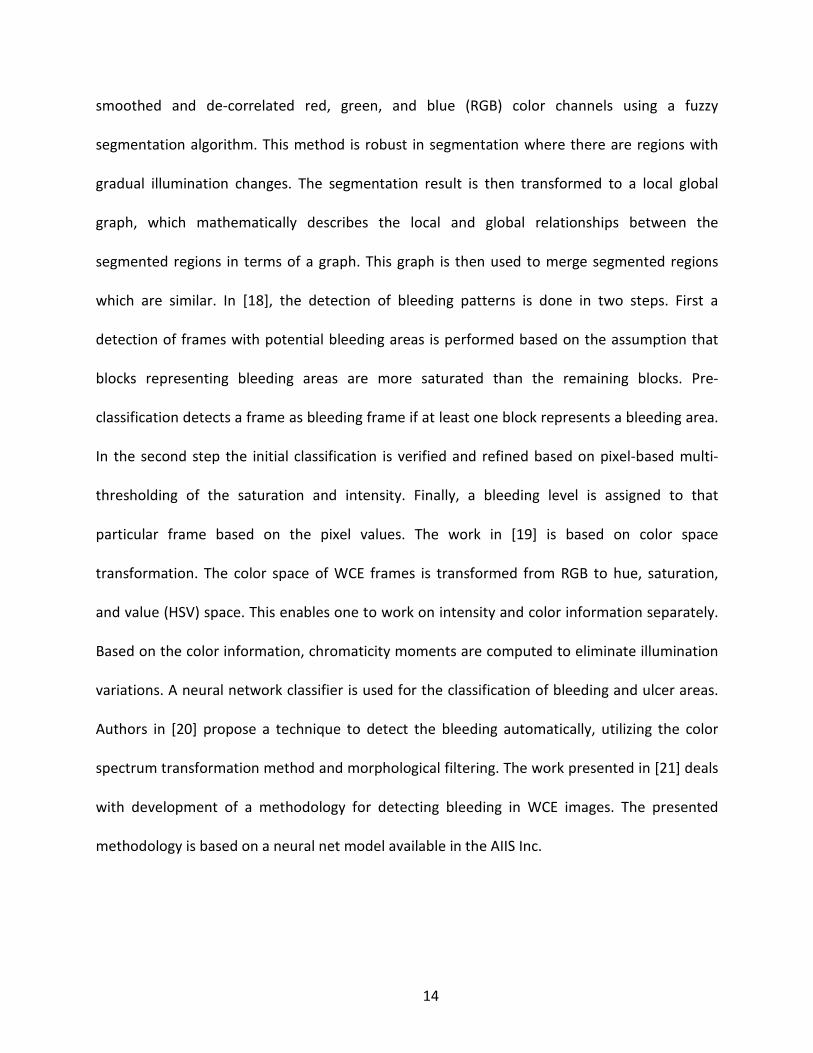
smoothed and de-correlated red, green, and blue (RGB) color channels using a fuzzy
segmentation algorithm. This method is robust in segmentation where there are regions with
gradual illumination changes. The segmentation result is then transformed to a local global
graph, which mathematically describes the local and global relationships between the
segmented regions in terms of a graph. This graph is then used to merge segmented regions
which are similar. In [18], the detection of bleeding patterns is done in two steps. First a
detection of frames with potential bleeding areas is performed based on the assumption that
blocks representing bleeding areas are more saturated than the remaining blocks. Pre-
classification detects a frame as bleeding frame if at least one block represents a bleeding area.
In the second step the initial classification is verified and refined based on pixel-based multi-
thresholding of the saturation and intensity. Finally, a bleeding level is assigned to that
particular frame based on the pixel values. The work in [19] is based on color space
transformation. The color space of WCE frames is transformed from RGB to hue, saturation,
and value (HSV) space. This enables one to work on intensity and color information separately.
Based on the color information, chromaticity moments are computed to eliminate illumination
variations. A neural network classifier is used for the classification of bleeding and ulcer areas.
Authors in [20] propose a technique to detect the bleeding automatically, utilizing the color
spectrum transformation method and morphological filtering. The work presented in [21] deals
with development of a methodology for detecting bleeding in WCE images. The presented
methodology is based on a neural net model available in the AIIS Inc.
14

Besides this work, there are several studies on selecting a color space for a particular
application. Authors in [22] build a random forest to learn the similarity function of pairs of
person images using color features from 6 kinds of popular color spaces (RGB, normalized RGB
(NRGB), HSV, YCbCr, CIE XYZ and CIE Lab). The authors carried out experiments on the
challenging dataset VIPeR to show the performances of different color spaces and their
combination. Authors reported that the combination of NRGB, HSV, YCbCr and CIE Lab color
spaces achieves the best performance. Work presented in [23] assesses the impact of color
spaces on skin detection based on color features. In this study, authors trying to prove that for
every color space there exists an optimum skin detector scheme such that the performance of
all these skin detectors schemes is the same. Work in [24] presents a comprehensive and
systematic approach for skin detection based on color. In this study, each component of several
color models has been evaluated, and then they selected a suitable color model for skin
detection. After listing the top components, authors exemplify that a mixture of color
components can discriminate very well skin in both indoor and outdoor scenes. A new
approach for dealing with color space issues is carried out in [25]. Authors in this study are
proposing an opponent color space with low cross contamination of color attributes (i.e.
lightness, chroma, and hue). And also they compose a list of properties a color space should
have in order to operate effectively.
There is no methodology for the detection of bite-block in the literature to the best of
our knowledge. In the proposed method, we achieve a very high accuracy with fast enough
speed for real-time processing. And it inherits a characteristic that enables the classifier to train
the system on subset of training data. This is achieved by considering only one hyper plane at a
15

time. Each hyper plane intersects only a subset of the whole training dataset. More details are
given in Chapter 3.
2.1 Color Spaces
Imaging instrumentation used in the endoscopy procedures generates RGB color
information by default. RGB color channel are strongly correlated and hence, they do not
exhibits a good discrimination power. A color space conversion is needed and at the same time,
it is required to ensure a better discrimination power. In this study, there are two color spaces
used. Every color space used has its own advantage over the other. A brief description of each
color space used and their advantages in real time environment is presented in the following
paragraphs.
2.1.1 RGB Color Space
An RGB color space is any additive color space based on the RGB color model [26]. The
complete specification of an RGB color space also requires a white point chromaticity and a
gamma correction curve. RGB is a convenient color model for computer graphics because the
human visual system works in a way that is similar, though not quite identical. RGB color space
is directly available from the imaging instrumentation and hence, there is no need of color
space transformation. RGB color space is represented as 3D Cartesian coordinate system. It
should be noted that, RGB color space is used at the cost of accuracy to gain the real time
performance.
16

2.1.2 HSV Color Space
HSV is an angular representation of points in an RGB color model. This representation
rearranges the geometry of RGB in an attempt to be more intuitive and perceptually relevant
than the Cartesian (cube) representation. Developed in the 1970s for computer graphics
applications, HSV is used today in image analysis and computer vision [26]. HSV color space
inhibits a greater discriminative power when compare against the RGB color space. This color
space, in this study, gives a better accuracy while it is suffering from speed requirement in real
time environment where detection speed plays a critical role. The main disadvantage of using
HSV color space is that it is not directly accessible from the imaging instrumentation. And hence
need a color space transformation.
2.2 Equation of a Plane
A plane is a two-dimensional surface. A plane can be defined in three-dimensional
space. A plane can be represented using a point on the surface and a normal vector to the
plane. Let 𝑟0 be the position vector of some known point 𝑃0 in the plane, and let 𝑛 be a nonzero
vector normal to the plane. The idea is that a point 𝑃 with position vector 𝑟 is in the plane if
and only if the vector drawn from 𝑃0 to P is perpendicular to 𝑛. Two vectors are perpendicular if
and only if their dot product is zero, it follows that the desired plane can be expressed as the
set of all points r such that
𝑛 . (𝑟 − 𝑟0) = 0 (2.1)
Expanding the equation 2.1 gives
𝑛𝑥(𝑥 − 𝑥0) + 𝑛𝑦(𝑦 − 𝑦0) + 𝑛𝑧(𝑧 − 𝑧0) = 0 (2.2)
17

2.2.1 Defining a Plane through Three Points
Let p1=(x1, y1, z1), p2=(x2, y2, z2), and p3=(x3, y3, z3) be non-collinear points. Then the plane can be
represented as a scalar equation as 𝑎𝑥 + 𝑏𝑦 + 𝑐𝑧 = 𝑑. This will generate a system of equations
as follows,
𝑎𝑥1 + 𝑏𝑦1 + 𝑐𝑧1 + 𝑑 = 0
𝑎𝑥2 + 𝑏𝑦2 + 𝑐𝑧2 + 𝑑 = 0
𝑎𝑥3 + 𝑏𝑦3 + 𝑐𝑧3 + 𝑑 = 0
This system of equations can be solved using Cramer’s Rule and matrix manipulations.
Let 𝐷 = 𝑥1 𝑦1 𝑧1𝑥2 𝑦2 𝑧2𝑥3 𝑦3 𝑧3
If 𝐷 is non-zero (a plane that does not go through the origin) the values for a, b, and c can be
calculated as
𝑎 = 𝑥1 𝑦1 𝑧1 −𝑑𝐷
𝑥2 𝑦2 𝑧2 𝑥3 𝑦3 𝑧3
𝑏 = 𝑥1 𝑦1 𝑧1 −𝑑𝐷
𝑥2 𝑦2 𝑧2 𝑥3 𝑦3 𝑧3
𝑐 = 𝑥1 𝑦1 𝑧1 −𝑑𝐷
𝑥2 𝑦2 𝑧2 𝑥3 𝑦3 𝑧3
18

These equations are parametric on d. setting d to a non-zero value and substitute it into these
equations will yield one solution set.
2.3 Classification Models
2.3.1 Support Vector Machine
Support vector machine (SVM) is a supervised learning model for classification
and regression analysis. From a given set of labels and corresponding training data, SVM build
support vectors, which are point in space. A SVM model is a representation of the examples as
points in space, mapped so that the examples of the separate categories are divided by a clear
margin that is as wide as possible.
Given a training data set D, which is a set of points, n of the form given in the equation
2.3, where yi is either 1 or -1, representing the class of xi. Each point is a p-dimensional vector.
The aim is to find a hyper plan that clearly separates two classes into two regions while
maximizing the margin between two classes. Any hyper plane can be written as set of point x
satisfying the equation given in the equation 2.4.
𝐷 = �(𝑥𝑖 ,𝑦𝑖)�𝑥𝑖 ∈ 𝑅𝑝,𝑦𝑖 ∈ {−1,1}�𝑖=1𝑛
(2.3)
𝑤. 𝑥 − 𝑏 = 0 (2.4)
Where, w is the normal vector of the hyper plane, w.x is the dot product of the x and w.
The offset of the hyper plane relative to the origin along the normal vector is 𝑏‖𝑤‖
. Then, if the
data set is linearly separable, the two hyper planes that form the margin between two classes
19

can be written as given in equations 2.5 and 2.6. The distance between these two hyper planes
is 2‖𝑤‖
. By minimizing the ||w||, one can maximize the margin between two hyper planes [27].
This concept is shown in the Fig. 2.1.
𝑤. 𝑥 − 𝑏 = 1 (2.5)
𝑤. 𝑥 − 𝑏 = −1 (2.6)
If the data set is not linearly separable, then we need to introduce a kernel function to
the SVM so that the data set is mapped into high dimensional data space so that the data set is
linearly separable in the high dimensional data space. For instance, Radial Basis Function.
Which is the kernel function is been used in this study.
Fig. 2.1 Support vector machine hyper plane and its maximum margin
20
There are many number of SVM implementations available in the literature. These
implementations can be divided into two main sub categories based on their approach:
Decomposition-based methods and Variant-based methods. Decomposition methods,
especially sequential minimal optimization (SMO) type algorithms, are sometimes very slow for
linear kernel SVM. Decomposition methods consider only a small subset of variables in each
iteration. The idea is: the variables are split into two parts, the set of free variables called
working set, and the set of fixed variables. Free variables are those which can be updated in
current iteration, whereas fixed variables are temporarily fixed at a particular value. The
advantage of decomposition method is that its memory requirement is linear in the number of
training examples. [28]-[44]. Decomposition methods tackle the lack-of-memory issue by
splitting problem into a series of smaller ones. But they are time consuming especially for large-
scale problems. So researchers consider various approximate versions of standard SVM at the
price of accuracy for speedup, and make great progress in this direction. Variant-based
methods are reported in [45]-[53].
2.3.2 K-Nearest Neighbor
K-NN (k-nearest-neighbor) [54] has been widely used for classification problems. It is
based on a distance function that measures the difference or similarity between two instances.
The standard Euclidean distance d(x, y) between two instances x and y is often used as the
distance function as defined in Equation 2.7.
𝑑(𝑥,𝑦) = �∑ (𝑎𝑖(𝑥) − 𝑎𝑖(𝑦))2𝑛𝑖=1
2 (2.7)
Where 𝑎𝑖(𝑥) is the value of ith attribute of 𝑥, and 𝑎𝑖(𝑦) is the value of ith attribute of 𝑦.
21

Given an instance x, K-NN assigns the most common class of x’s k nearest neighbors to x,
as shown in Equation 2.8. We use C and c to denote the class variable and its value respectively.
The class of the instance x is denoted by c(x).
𝑐(𝑥) = 𝑎𝑟𝑔𝑚𝑎𝑥𝑐∈𝐶
∑ 𝛿(𝑐, 𝑐(𝑦𝑖))𝑘𝑖=1 (2.8)
where y1, y2, · · ·, yk are the k nearest neighbors of x, k is the number of the neighbors,
and δ(c, c(yi)) = 1 if c = c(yi), and δ(c, c(yi)) = 0 otherwise. This concept is shown in Fig. 2.2.
Fig. 2.2 KNN classification based on majority voting in a neighborhood
There are approaches for improving KNN’s classification accuracy. Three major
categories can be found in the literature: 1) Use more accurate distance functions instead of
the standard Euclidean distance; 2) Introducing an optimum neighborhood sizes search to
replace parameter k; 3) Replace the sample voting scheme with a probabilistic function.
22

In KNN, the standard Euclidean distance is used. Thus, the distance between instances is
calculated based on all attributes of the instance. However, when many numbers of irrelevant
attributes are included, the predicted example would be wrong with a high probability. One
way out of this problem is to eliminate irrelevant attributes when calculating the distance
named as feature selection [55]-[61]. KNN accuracy depends on the parameter k. Then an
automated algorithm to select the best k value would give a better accuracy with KNN. The
simplest method is to try several k values and choose the best one. Besides that, there are
various other methods to select an optimum value for k has been proposed [62]–[66]. KNN uses
a simple voting to produce class estimation. All the neighborhood instances are treated equally.
In [67], it is been trying to estimate class probabilities with varying weight assignments.
The classifiers described in the previous two sub sections perform well in terms of the
accuracy in the domain of color based object detection. But both techniques fail to perform
classification in real time as the time taken is considerably high. In this thesis, I proposed a data
partitioning technique along with a data modeling method to overcome the computational
complexity barrier of two techniques mentioned above.
23

CHAPTER 3
METHODOLOGY
In this section, it is presented the data acquisition method, modeling of the training data
with two techniques, usage of RGB and HSV color spaces in each technique, generation of
Boston Bowel Preparation Scale (BBPS), integration of the proposed method with a real-time
SDK, performance gain through a massive parallelism, a real world application of the proposed
method, and a variation of blood based anomaly (Erythema) detection.
A frame in a colonoscopy video consists of a number of pixels as a digitized image
typically does. Each pixel has three number values representing Red (R), Green (G), and Blue
(B), so each pixel can be projected into 3-dimensional (3-D) RGB color space. A set of pixels,
which are from a region such as stool, can form arbitrary shape(s) of volume(s) in 3-D RGB color
space. This volume, if modeled mathematically, can be used to detect pixels from a stool
region. Colonoscope instruments generate signals in the RGB color space hence RGB is the
directly accessible color space. We develop the proposed methodology in RGB color space.
Next, we transform the RGB color space to HSV color space and do exactly the same procedure.
RGB color space is favorable in real time environment as it is directly accessible. HSV is
favorable in terms of discrimination power of color information. RGB color space is favorable
over HSV since the conversion needs extra computational time. For the mathematical
representation, we propose to use a set of planes in which each plane consists of a subset of
positive class examples, and behaves as an individual classifier for that subset of positive
examples. More information is discussed in the training and the detecting stages. The training
stage has three steps: All positive class pixel projection, Positive class plane selection, and
24
positive class plane modeling using either block division method or convex hull model. As a
result, the training stage generates a classification model which is used in the detecting stage.
The remaining of this section is as follow: Section 3.1 describes the data acquisition
procedure. Section 3.2 explains the training process in two techniques and for RGB and HSV
color spaces separately. Section 3.3 present the BBPS score generation based on stool scores.
Section 3.4 provides the description of integration into real-time SDK. And Section 3.5 provides
information on how to gain performance through massive parallelism. Finally section 3.6
provides a methodology to differentiate erythema video frames from a normal frame.
3.1 Data Acquisition
The main source of data for this study is coming from colonoscopy videos. These videos
are recorded during a colonoscopy screening procedure. At the time of recording, patient
information is reported along with the video itself. For this study, I used only videos that are
anonymous and do not carry any patient information. All the patient information is striped off
by the doctors, before deliver to be used in this study. In this manner, patient’s identity is
protected and not revealed to any person who is relevant to this study
The basic unit of information is a video frame extracted from a given colonoscopy video.
This unit is in two different versions, testing units and training units. Testing units are basically
for evaluation of the developed methodology and the ground truth units are for the
development of the methodology. Both these categories contain ground truth information. All
these video frames are annotated by the doctors. This information is then used in the training
of stage and the detection stage of the proposed methodology. Testing units are used in the
cross validation process.
25

3.2 Training the Models
3.2.1 Block Division Model
3.2.1.1 Training Stage of the Block Division Method
First, I project all stool pixels extracted from stool frames into RGB color cube. Each
unique pixel has a unique location in the RGB color cube as three coordinates R, G, B as
illustrated in Fig. 3.1(a). For convenience, RGB is mapping to XYZ coordinate system as shown.
In the second step, we put 256 planes into the RGB cube along with R (X) axis so that each
integer location of R axis has a plane parallel to GB plane as seen in Fig. 3.1 (b). It is possible to
put planes along G axis or B axis in which there is no difference among them in terms of
modeling. Then, we assign a number (from 0 to 255) to each plane (i.e., Plane#0, Plane#1 …
Plane#255). Among these 256 planes, we select only planes with stool pixels projected on it.
Each selected plane is called a positive plane.
Each positive plane is treated as a 2D model at the relevant location. For instance,
Plane#0 at the location (0, 0, 0) is treated as a classifier for positive class examples (stool pixels
in our case) that has a R (X) value of zero (0). This method inherits fast classification as it already
possesses the property of eliminating non-relevant class examples (i.e., non-stool pixels in our
case) in the training process.
26

(a)
(b)
Fig. 3.1 (a) RGB cube and corresponding locations of stool pixels, and mapping of RGB axis to
XYZ axis (within brackets), and (b) several planes inserted into the RGB cube of (a)
27

If we pick a positive plane, it can be seen in Fig. 3.2(a). In the positive plane modeling,
we model the areas of positive class examples. First, a positive plane is divided into four blocks.
The block is a square since each plane is a square (256 x 256), and each may contain all stool
pixels, all non-stool pixels, or mixture of non-stool and stool pixels. For all four blocks, we check
the following three conditions. If all (or more than 95%) of pixels in a block are positive class
examples (stool pixels), the block becomes a positive block, and the procedure for this block is
done. If all pixels in a block are non-positive class examples (non-stool pixels), then the block
becomes a negative block, and the procedure for this block is done. If some (less than 95%) of
pixels in a block are positive class examples (stool pixels), and the block has more than or equal
to the MNP (minimum number of pixels –in this study, MNP = 16), the block is divided into four
smaller blocks, and we check the above three conditions for all four smaller blocks. The
minimum block size is 4 x 4. When the iteration reaches the minimum block size, a block
becomes a positive block if it has more positive class examples (stool pixels). Otherwise, it
becomes negative block. This procedure is recursive, and the blocks become smaller in the next
iteration (Each block is iteratively divided by four). In case the block has less than the MNP, if it
has more positive class examples (stool pixels), then it becomes a positive block. Otherwise, it
becomes a negative block. All levels of blocks have their own unique number values in the way
shown in Fig. 3.2(c). It is very convenient and non-ambiguous way for the numbering. Among
these numbers, a set of numbers for positive blocks can form a vector for a positive plane, and
a set of vectors from all positive planes can form a classification model for the detecting stage.
This model possesses incremental learning property. Its incremental learning is performed as
follows. When there is a new positive pixel to be inserted into the model, we can find a
28

corresponding minimum size (4 x 4) block which is a negative block. The block can become a
positive block if it gets more positive class examples (stool pixels) by adding this new positive
pixel. In this way, we do not have to run the entire training process from beginning when we
need to add additional positive examples.
(a) (b)
(c) (d)
Fig. 3.2 (a) selected plane (b) positive class examples (stool pixels) projected on a positive plane
(plane#175) as looking into the RGB cube from right side in (a), (c) minimum coverage area of
the positive classes examples (stool pixels), and (d) unique numbering of blocks for fast access
(not all shown for clarity)
29
3.2.1.2 Detecting Stage of Block Division Method
Detection of the positive pixel is performed by evaluating a candidate pixel on the
classification model generated in Section 3.2.1. Once there is pixel to be detected, the R (X)
value of the pixel is obtained and used as the index to pick the corresponding positive plane.
For example, if the R (X) value is 5, then Plane#5 is selected and examined. This will dramatically
reduce the number of comparisons so that the searching time is significantly reduced. In other
words, the detecting time of the proposed technique is not dependent on the number of
positive planes, but on how many positive blocks there are in the corresponding plane, which is
comparatively very small. By comparing the GB (YZ) values of the pixel with the vector
obtained from the third step of the training stage, in other words, if the GB (YZ) values of the
pixel can be found in the corresponding vector, it can be classified as a positive class pixel.
Otherwise, it is classified as negative class pixel. After all pixels of a frame are evaluated, we can
calculate a percentage of stool area for each frame such that the number of all stool pixels is
divided by the number of total pixels.
3.2.2 Convex Hull Model
3.2.2.1 Training the Model with RGB Color Space
Digital color images modeled in RGB color space (cube) represent each color channel
with 8-bitinteger ranging from 0 to 255, giving us a total of 2563 potential colors. Fig. 1.2 shows
an example of frames that can be found in colonoscopy and upper endoscopy videos. We
project all positive class pixels in ground truth frames into RGB color cube as the first step. To
discriminate positive class pixels from negative ones we use the fact that each color pixel has a
30

unique location in the RGB color cube as three coordinates R, G, B as illustrated in Fig. 3.1(a),
3.3(a), and 3.5(a). For convenience, RGB is mapped to the XYZ coordinate system as shown. In
the second step (positive class plane selection), we put 256 planes into the RGB cube along with
R (X) axis so that each integer location of R axis has a plane parallel to GB plane as seen in Fig.
3.1 (b), 3.3(b), and 3.5(b). Only a limited number of positive planes are shown. One can select
either G axis or B axis as the initial axis since there is no specific reason to select one particular
axis. In our study we select R axis to put planes along with. Then, we assign a number (from 0 to
255) to each plane (i.e., Plane#0, Plane#1, … Plane#255). Among these 256 planes, we select
only planes with positive class pixels. Each selected plane is called a ‘Positive plane’.
Each positive plane contains a projection of positive pixels at the corresponding
location, and is treated as a 2D model at the relevant location. For instance, Plane#0 at the
location (0, 0, 0) is treated as a model for positive class examples that has a R (X) value of zero
(0). This method inherits fast classification as it already possesses the property of eliminating
non-relevant class examples in the training process. Finally, we model each positive plane using
convex hulls. A brief introduction to convex hull is given next.
3.2.2.1.1 Convex Hull Modeling
Algebraically, the convex hull of dataset X can be characterized as the set of all of
convex combinations of finite subsets of points from X: that is, the set of points of the form
∑ ∝𝑖𝑛𝑗=1 𝑥𝑗 , where n is an arbitrary non-zero positive integer, the numbers ∝𝑖 are non-negative
and sum to 1, and the points xj are in X. So, the convex hull Hconvex(X) of set X is given in
Equation 1, where the αi is a fraction between 0 and 1.
31

𝐻𝑐𝑜𝑛𝑣𝑒𝑥(𝑋) = �∑ ∝𝑖 𝑥𝑖𝑘𝑖=1 �𝑥𝑖 ∈ 𝑋,∝𝑖∈ ℝ,∝𝑖 ≥ 0,∑ ∝𝑖= 1,𝑘 = 1,2, … .𝑘
𝑖=1 � (3.1)
To generate the convex hull points that adhere to the constraints given in equation 3.1,
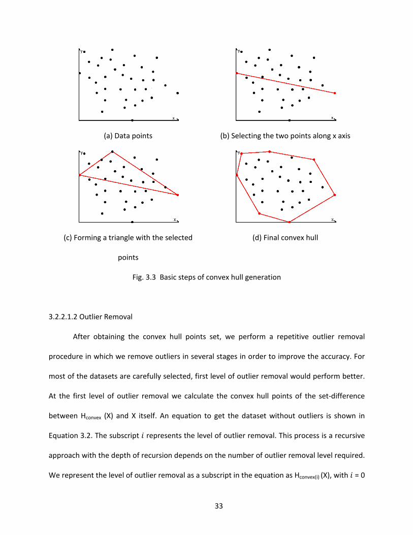
we use the quick hull algorithm introduced in [68]. The basic steps of the quick hull algorithm
are given below and a graphical representation is given in the Fig. 3.3.
1. Find the furthest and the closest points along the x axis; these two points will be
included in the convex hull points set.
2. Divide the data set into two haves using the line drawn between two points selected
in step 1.
3. Select a point on one side of the line drawn that is the furthest point from the line.
This point along with two points selected in the step 1 will create a triangle.
4. The points lying inside of that triangle will be discarded as they cannot be part of the
convex hull.
5. Repeat the steps 3 and 4 on the two lines formed by the triangle (Two new lines
formed).
6. Iterate until no more points are left.
32
(a) Data points (b) Selecting the two points along x axis
(c) Forming a triangle with the selected
points
(d) Final convex hull
Fig. 3.3 Basic steps of convex hull generation
3.2.2.1.2 Outlier Removal
After obtaining the convex hull points set, we perform a repetitive outlier removal
procedure in which we remove outliers in several stages in order to improve the accuracy. For
most of the datasets are carefully selected, first level of outlier removal would perform better.
At the first level of outlier removal we calculate the convex hull points of the set-difference
between Hconvex (X) and X itself. An equation to get the dataset without outliers is shown in
Equation 3.2. The subscript 𝑖 represents the level of outlier removal. This process is a recursive
approach with the depth of recursion depends on the number of outlier removal level required.
We represent the level of outlier removal as a subscript in the equation as Hconvex(i) (X), with 𝑖 = 0
33

representing the convex hull with no outlier removal and 𝑖 = 1 with one level of outlier removal
and so on.
𝐻𝐶𝑜𝑛𝑣𝑒𝑥(𝑖)(𝑋) = 𝐻𝐶𝑜𝑛𝑣𝑒𝑥(𝑋 − ⋃ 𝐻𝑐𝑜𝑛𝑣𝑒𝑥(𝑛)𝑖−1𝑛=0 (𝑋)) (3.2)
After performing the optimal number of levels of outlier removal, we record the plane
number along with the set of hull points of that particular plane. This optimal number of levels
can be decided experimentally. The training model is built out of planes along with their hull
points. This procedure is done for all the positive class planes.
3.2.2.1.3 Training the Model with Bite-block, Blood, and Stool Video Frames
The pixel values of green bite-block, blood, and stool examples are projected into RGB
color space and obtain the subset of data that intersect with each hyper plane at each integer
position of Red (X) axis. If the number of data in a subset is non-zero, then the corresponding
plane is a green bite-block, blood, or stool positive plane. The selection of positive planes is
depicted in Fig. 3.4(a) and 3.4(b). Only a limited number of positive planes are shown to
illustrate the technique.
34

(a) (b)
Fig. 3.4 (a) RGB cube and corresponding locations of pixels for each object, and mapping of RGB
axis to XYZ axis (within brackets), and (b) several planes inserted into the RGB cube of (a)
35

An example of a positive plane from green bite-block, blood, and stool datasets can be
seen in Fig. 3.5 (a), Fig. 3.6 (a), and Fig. 3.7 (a), respectively. Then I model each positive plane
with a convex hull which is shown in Fig. 3.5(c), Fig. 3.6(c), Fig. 3.7(c), respectively. Fig. 3.5(d),
Fig. 3.5(d), and Fig. 3.5(d) show first level of noise removal on dataset shown in Fig 3.5(a), Fig
3.6(a), and Fig 3.7(a), respectively.
(a) (b)
(c) (d)
Fig. 3.5 (b) Positive class examples (green bite-block pixels) projected on a positive plane
(plane#20) as looking into the RGB cube from right side in (b), (c) convex hull of the positive
class examples, and (d) convex hull (in green) after first level outlier removal
36

(a) (b)
(c) (d)
Fig. 3.6 (a) Positive class examples (blood pixels) projected on a positive plane (plane#150) as
looking into the RGB cube from right side in Fig. 4(b),(b) convex hull of the positive class
examples , and (c) convex hull (in green) after first level outlier removal
37
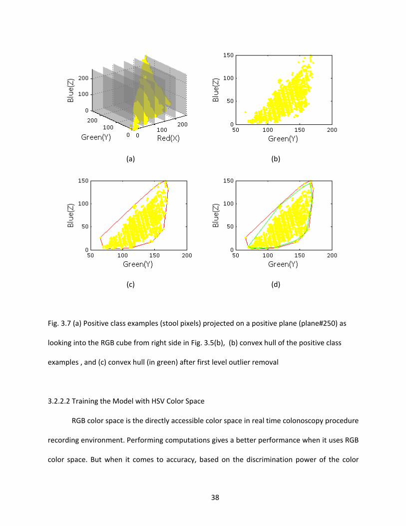
(a) (b)
(c) (d)
Fig. 3.7 (a) Positive class examples (stool pixels) projected on a positive plane (plane#250) as
looking into the RGB cube from right side in Fig. 3.5(b), (b) convex hull of the positive class
examples , and (c) convex hull (in green) after first level outlier removal
3.2.2.2 Training the Model with HSV Color Space
RGB color space is the directly accessible color space in real time colonoscopy procedure
recording environment. Performing computations gives a better performance when it uses RGB
color space. But when it comes to accuracy, based on the discrimination power of the color
38

spaces, HSV color space out performs RGB color space. Therefore, using HSV color space is a
necessity to achieve a better accuracy. First, I transform RGB color space information into HSV
color space information using the transformation given in the equation 3.3. And then follow the
same methodology as per the RGB color space.
𝐶𝑚𝑎𝑥 = max(𝑅,𝐺,𝐵)
𝐶𝑚𝑖𝑛 = min (𝑅,𝐺,𝐵)
∆ = 𝐶𝑚𝑎𝑥 − 𝐶𝑚𝑖𝑛
𝐻 =
⎩⎪⎨
⎪⎧600 × �𝐺−𝐵
∆� ,𝐶𝑚𝑎𝑥 = 𝑅
600 × �𝐵−𝑅∆� ,𝐶𝑚𝑎𝑥 = 𝐺
600 × �𝑅−𝐺∆� ,𝐶𝑚𝑎𝑥 = 𝐵
𝑆 = �0 , ∆ = 0∆
𝐶𝑚𝑎𝑥 ,∆ <> 0
𝑉 = 𝐶𝑚𝑎𝑥 (3.3)
Each positive class plane contains a projection of positive pixels at the corresponding
location, and is treated as a 2D model at the relevant location. For instance, Plane#0 at the
location (0, 0, 0) is treated as a model for positive class examples that has a V (Z) value of zero
(0). This method inherits fast classification as it already possesses the property of eliminating
non-relevant class examples in the training process. Finally, we model each positive plane using
convex hulls.
39

3.2.2.2.1 Training the Model with Bite-block, Blood, and Stool Video Frames
The pixel values of green bite-block, blood, and stool examples are projected into HSV
color space and we obtain the subset of data that intersect with each hyper plane at each
integer position of Value (Z) axis. If the number of data in a subset is non-zero, then the
corresponding plane is a green bite-block, blood, or stool positive plane, respectively. The
selection of positive planes is depicted in Fig. 3.8(a) and 3.8(b). Only a limited number of
positive planes are shown to illustrate the technique.
40

(a) (b)
Fig. 3.8 (a) HSV cube and corresponding locations of example pixels in the HSV color cube, and
mapping of HSV axis to XYZ axis (within brackets), and (b) several planes inserted into the HSV
cube of (a). First row: green bite block, second row: blood and third row: stool
41
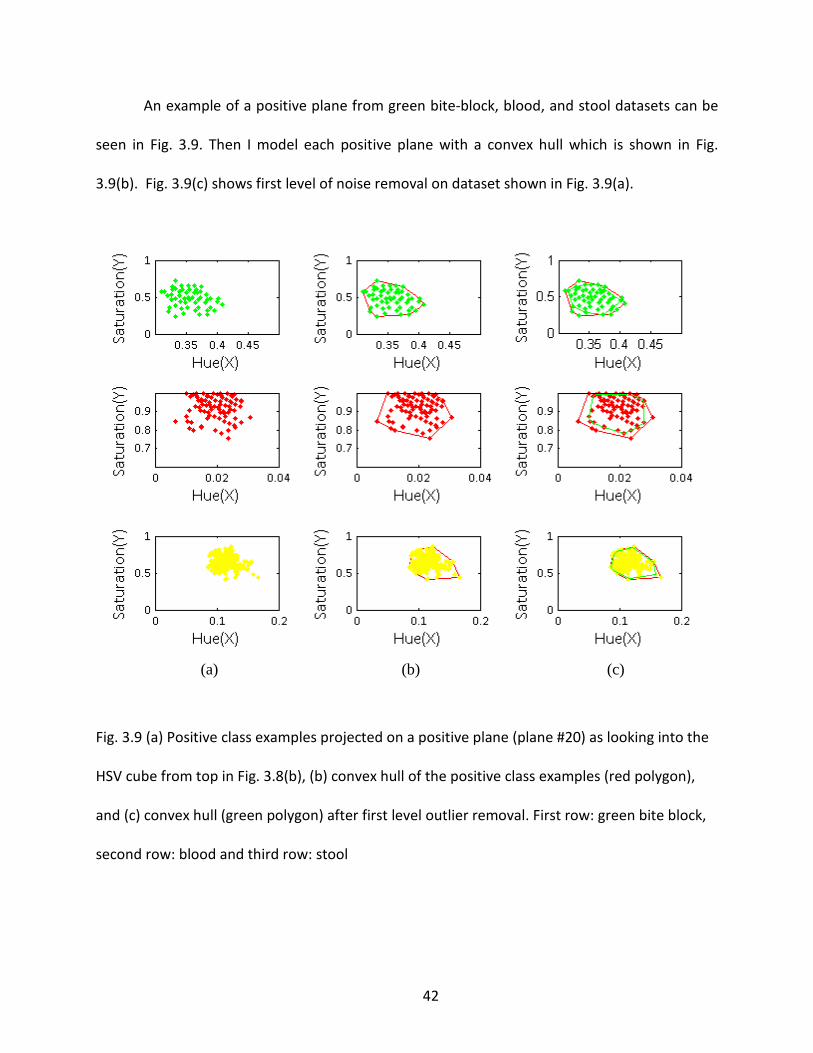
An example of a positive plane from green bite-block, blood, and stool datasets can be
seen in Fig. 3.9. Then I model each positive plane with a convex hull which is shown in Fig.
3.9(b). Fig. 3.9(c) shows first level of noise removal on dataset shown in Fig. 3.9(a).
(a) (b) (c)
Fig. 3.9 (a) Positive class examples projected on a positive plane (plane #20) as looking into the
HSV cube from top in Fig. 3.8(b), (b) convex hull of the positive class examples (red polygon),
and (c) convex hull (green polygon) after first level outlier removal. First row: green bite block,
second row: blood and third row: stool
42

3.2.2.2.2 Detection Stage for Convex Hull Model
In this stage, a video frame that is unseen and need to classify into one of three cases
(bite-block, blood, and stool) is processed one pixel at a time. Determination of the label of a
pixel is performed by evaluating it against the classification model generated in Section 3.2.2.
In the case of HSV color space, an unseen video frame is transformed into HSV color space first.
Once there is a pixel to be classified, the R (V value in the HSV model) value of the pixel is
obtained and used as the index to pick the corresponding positive plane. For example, if the R
value of a pixel to be classified is 5, then Plane#5 is selected and examined if it is a positive class
plane. This will dramatically reduce the number of comparisons so that the searching time is
significantly reduced. In other words, the detecting time of the proposed technique is
dependent on neither the number of positive planes nor how many positive examples in the
corresponding plane. For the labeling of the pixel, it is evaluated against to the convex polygon
of the corresponding positive plane. Pixels that are either on or inside the convex polygon are
labeled as positive class examples. There is a separate model generated for each, green bite-
block, blood, and stool pixels detections. Each model is generated based on the positive class
training examples of each case (green bite-block, blood, and stool)
3.3 Boston Bowel Preparation Scale (BBPS) Generation
In this section, I will discuss a method of automatically computing BBPS score based on
the percentages of stool areas obtained using the methodology proposed. the authors in [11]
proposed ‘Boston Bowel Preparation Scale’ (BBPS) in which the terms “excellent,” “good,”
“fair,” and “poor,” were replaced by a four-point scoring system applied to each of the three
43
broad regions of the colon: the right colon (including the cecum and ascending colon), the
transverse colon (including the hepatic and splenic flexures), and the left colon (including the
descending colon, sigmoid colon, and rectum). These six parts of colon can be seen in Fig. 1.1,
and the relationships between the terms and the points can also be seen in Table 3.1.
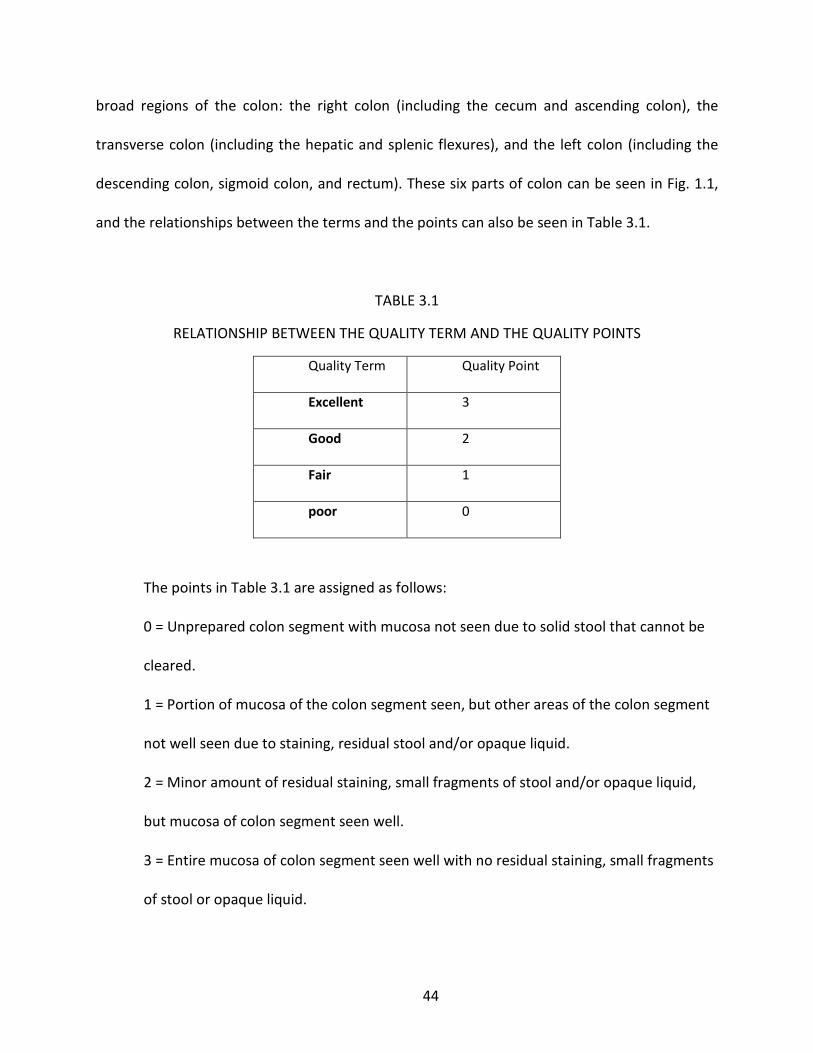
TABLE 3.1
RELATIONSHIP BETWEEN THE QUALITY TERM AND THE QUALITY POINTS
Quality Term Quality Point
Excellent 3
Good 2
Fair 1
poor 0
The points in Table 3.1 are assigned as follows:
0 = Unprepared colon segment with mucosa not seen due to solid stool that cannot be
cleared.
1 = Portion of mucosa of the colon segment seen, but other areas of the colon segment
not well seen due to staining, residual stool and/or opaque liquid.
2 = Minor amount of residual staining, small fragments of stool and/or opaque liquid,
but mucosa of colon segment seen well.
3 = Entire mucosa of colon segment seen well with no residual staining, small fragments
of stool or opaque liquid.
44
Each region of the colon receives a “segment score” from 0 to 3 and these segment
scores are summed for a total BBPS score ranging from 0 to 9. Therefore, the maximum BBPS
score for a perfectly clean colon without any residual liquid is 9, and the minimum BBPS score
for an unprepared colon is 0.
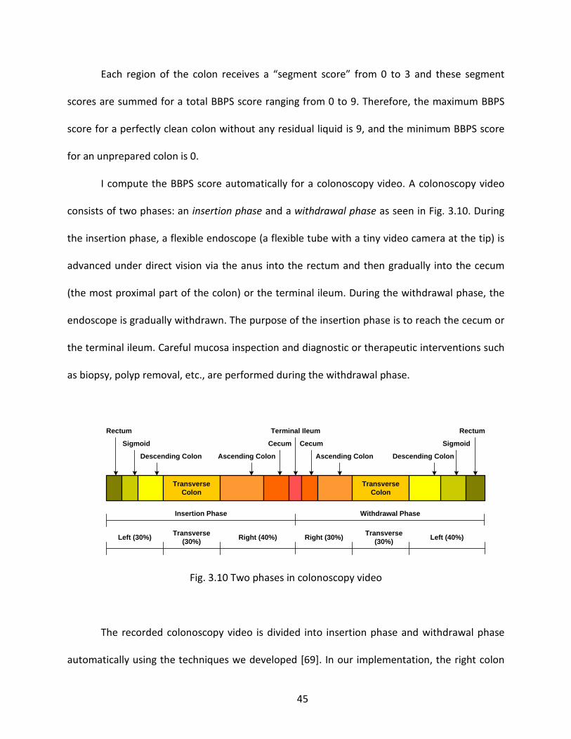
I compute the BBPS score automatically for a colonoscopy video. A colonoscopy video
consists of two phases: an insertion phase and a withdrawal phase as seen in Fig. 3.10. During
the insertion phase, a flexible endoscope (a flexible tube with a tiny video camera at the tip) is
advanced under direct vision via the anus into the rectum and then gradually into the cecum
(the most proximal part of the colon) or the terminal ileum. During the withdrawal phase, the
endoscope is gradually withdrawn. The purpose of the insertion phase is to reach the cecum or
the terminal ileum. Careful mucosa inspection and diagnostic or therapeutic interventions such
as biopsy, polyp removal, etc., are performed during the withdrawal phase.
Sigmoid
Descending Colon
Cecum
Rectum
Transverse Colon
Terminal Ileum
Ascending Colon
Cecum
Ascending Colon
Transverse Colon
Rectum
Sigmoid
Descending Colon
Insertion Phase Withdrawal Phase
Left (30%) Transverse (30%) Right (40%) Right (30%) Transverse
(30%) Left (40%)
Fig. 3.10 Two phases in colonoscopy video
The recorded colonoscopy video is divided into insertion phase and withdrawal phase
automatically using the techniques we developed [69]. In our implementation, the right colon
45

has the last 40% of insertion phase plus the first 30% of withdrawal phase. The transverse colon
has the middle 30% of insertion phase plus the middle 30% of withdrawal phase. The left colon
has the first 30% of insertion phase plus the last 40% of withdrawal phase. These numbers are
based on our experiments and the opinion of the domain expert. We calculate these score
values mathematically based on the stool percentage values obtained above for each frame.
We assign a score value for each frame based on the stool pixel percentage present in the
frame, and calculate the numerical average for each colon segment (right colon, transverse
colon, and left colon) for the final score value. The stool percentage values and the
corresponding score values are shown in the table 3.2.
TABLE 3.2
STOOL PERCENTAGE IN A FRAME AND THE ASSIGNED SCORE VALUE
Stool percentage % Score value assigned
0 – 10 3
11- 25 2
26 – 50 1
51 – 100 0
3.4 Integration of Methodology in Real Time Software Development Kit
SAPPHIRE middleware is a framework to process real time video streams. This
framework is specially built aiming at endoscopy video processing. SAPPHIRE is a configurable
multi module system so that modules performing literally different tasks, from object detection
46

to motion to camera motion estimation, can be integrated. There is one critical requirement
that every module must satisfy in order to be integrated into SAPPHIRE without performance
degradation. That is any module should finish its processing within 33ms. The method proposed
in this dissertation is capable of producing a better result while adhere to the requirements of
SAPPHIRE. The general architecture of the SAPPHIRE is given in the Fig. 3.11. In order to be the
SAPPHIRE middle ware, any module needs to follow a set of programming rules called
SAPPHIRE Application Programming Interface (API). SAPPHIRE middle ware communicates with
the modules using the API provided by the SDK. Structure of the SAPPHIRE middleware is given
below.
Fig. 3.11 SAPPHIRE middle ware architecture. This thesis work marked with red circles
47

The proposed method is being applied in the real world applications successfully. The
case study, stool detection, has being implemented and tested in a clinical setting. This
implementation estimates the amount of stool debris available in the colon when a
colonoscopy procedure is performed. Determination of amount of stool debris available in the
colon plays a critical role as explained in the introduction section. The implemented
methodology has been integrated into the real time video processing framework, SAPPHIRE.
This framework is built to accept video signals from the Colonoscope and process information
in each video frame. Then, this information is being display on a head up display to give doctors
a feedback of their work. A sample snapshot of the proposed method in work is depicted in Fig.
3.12. In addition to stool detection, green bite-block detection is also in use. This module
determines the type of the procedure, upper endoscopy or colonoscopy, at the very beginning
of the procedure.
48
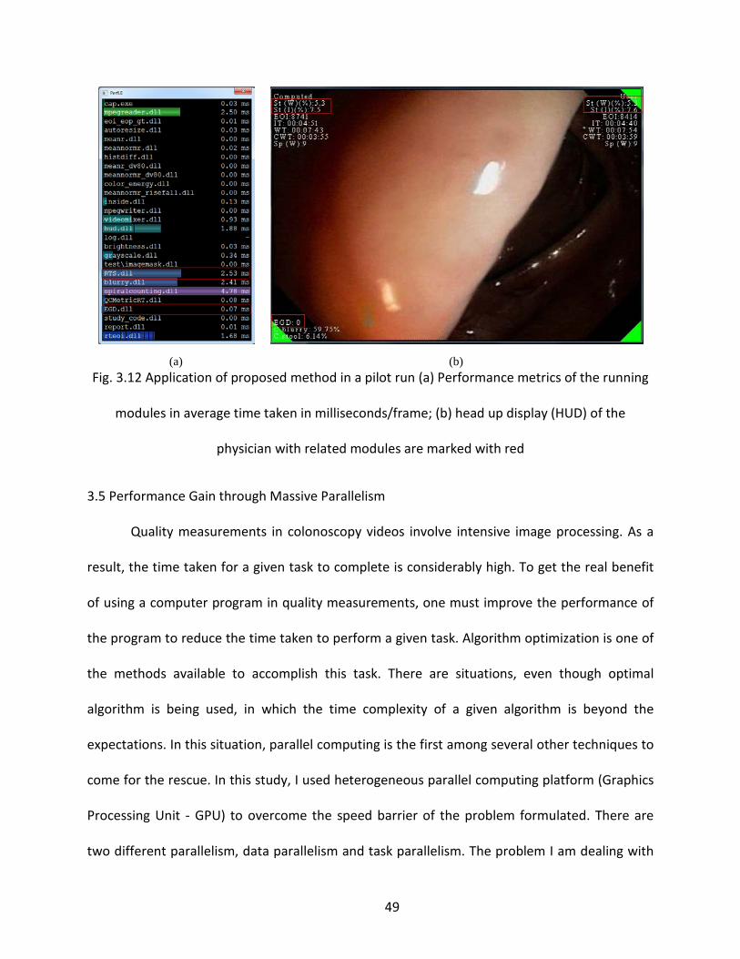
(a) (b) Fig. 3.12 Application of proposed method in a pilot run (a) Performance metrics of the running
modules in average time taken in milliseconds/frame; (b) head up display (HUD) of the
physician with related modules are marked with red
3.5 Performance Gain through Massive Parallelism
Quality measurements in colonoscopy videos involve intensive image processing. As a
result, the time taken for a given task to complete is considerably high. To get the real benefit
of using a computer program in quality measurements, one must improve the performance of
the program to reduce the time taken to perform a given task. Algorithm optimization is one of
the methods available to accomplish this task. There are situations, even though optimal
algorithm is being used, in which the time complexity of a given algorithm is beyond the
expectations. In this situation, parallel computing is the first among several other techniques to
come for the rescue. In this study, I used heterogeneous parallel computing platform (Graphics
Processing Unit - GPU) to overcome the speed barrier of the problem formulated. There are
two different parallelism, data parallelism and task parallelism. The problem I am dealing with
49

is inherently data parallel. Hence, I am using data parallelism in this study. In this scenario, the
problem data set is sub divided into many number of partitions and perform the algorithm on
each of them in parallel. The number of data partitions is basically defends on the capability of
the GPU device available in the system. With a modern day computer, this number can go up to
thousands without any performance degradation.
NVIDIA GTX460 GPU with CUDA programming and OpenCL API were used to achieve a
better acceleration with which the proposed methodology can perform in real time with a
reduced burden to the underlying computer system. OpenCL architecture and the proposed
implementation are discussed in brief next.
3.5.1 OpenCL
OpenCL (open computing language) is a cross platform parallel computing API extension
to C language for heterogeneous computing devices [70]. OpenCL code is portable across
various devices with correctness guaranteed. There is no guarantee for a consistent
performance gain across different target devices. Performance gain is achieved through the
massive parallelism. When it comes to the fast computation, the memory model plays a major
role. OpenCL memory model is given in the Fig. 3.13.
50

Fig. 3.13 OpenCL memory model
3.5.2 OpenCL Execution Model
OpenCL execution model is a combination of host and device programs written in C.
Inherently serial or modestly parallel parts of the execution model are included in the host code
while highly parallel parts are included in the device code. An OpenCL kernel (piece of program
run on GPU device) is executed by an array of work items. All these work items run the same
code as single program multiple data (SPMD). OpenCL host code mostly triggers device
execution and memory allocation.
Compute Device
Compute Device Memory
Global Memory
Global/Constant Memory Data Cache
Local Memory
Compute Unit 1
Private Memory
Work-Item 1
Private Memory
Work-Item M
Compute Unit N
Private Memory
Work-Item 1
Private Memory
Work-Item M
Local Memory
51

3.5.3 Proposed OpenCL Implementation
Amongst the very time consuming modules, the blurry detection module comes first.
The blurry detection module has several steps and need to implement the most time
consuming part in GPU. The basic block diagram of the algorithm is given in the Fig. 3.14.
Fig. 3.14 Block diagram of the blurry detection module
The Edge detection (Sobel edge) detection part of the algorithm is implemented in the GPU as it
inherits massive parallelism. The video frame is read from the video stream and converts it to
gray scale. The gray scaled image is then transferred into the GPU and stores it in the global
memory. Additionally, Sobel masks are transferred into the constant memory of the GPU. Host
code triggers the execution of Sobel convolution in the GPU. Finally, edge map result is
transferred from the GPU device to host for further processing.
3.6 Blood based Anomaly (erythema) Detection
Erythema is a blood based anomaly seen on human skin or on internal organs’ walls
such as colon wall. The main characteristic of erythema condition is the redness. As the first
Read image
Convert to Gray scale
Edge detection
Enhance connectivity
Block sum generation
Apply threshold
52
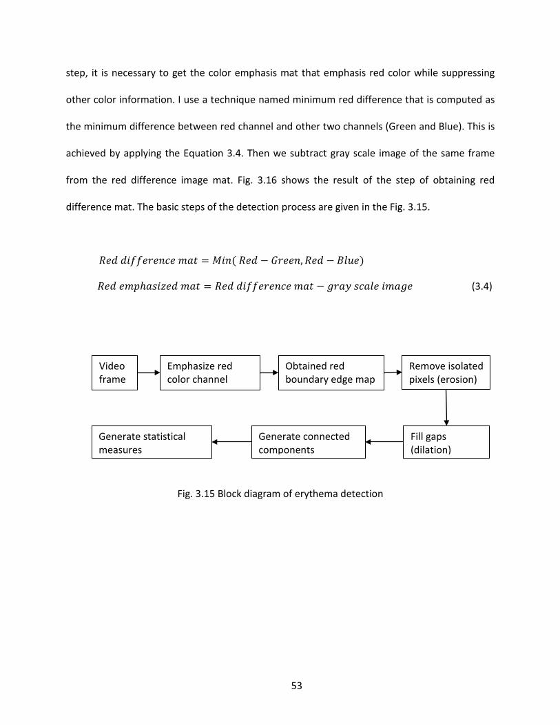
step, it is necessary to get the color emphasis mat that emphasis red color while suppressing
other color information. I use a technique named minimum red difference that is computed as
the minimum difference between red channel and other two channels (Green and Blue). This is
achieved by applying the Equation 3.4. Then we subtract gray scale image of the same frame
from the red difference image mat. Fig. 3.16 shows the result of the step of obtaining red
difference mat. The basic steps of the detection process are given in the Fig. 3.15.
𝑅𝑒𝑑 𝑑𝑖𝑓𝑓𝑒𝑟𝑒𝑛𝑐𝑒 𝑚𝑎𝑡 = 𝑀𝑖𝑛( 𝑅𝑒𝑑 − 𝐺𝑟𝑒𝑒𝑛,𝑅𝑒𝑑 − 𝐵𝑙𝑢𝑒)
𝑅𝑒𝑑 𝑒𝑚𝑝ℎ𝑎𝑠𝑖𝑧𝑒𝑑 𝑚𝑎𝑡 = 𝑅𝑒𝑑 𝑑𝑖𝑓𝑓𝑒𝑟𝑒𝑛𝑐𝑒 𝑚𝑎𝑡 − 𝑔𝑟𝑎𝑦 𝑠𝑐𝑎𝑙𝑒 𝑖𝑚𝑎𝑔𝑒 (3.4)
Fig. 3.15 Block diagram of erythema detection
Video frame
Emphasize red color channel
Obtained red boundary edge map
Remove isolated pixels (erosion)
Fill gaps (dilation)
Generate connected components
Generate statistical measures
53

(a) (b)
Fig. 3.16 Red difference mat of (a) healthy and (b) erythema video frames
Minimum red difference mat contains both red boundary and non-red boundary
regions. In our application domain, this includes redness regions and blood vessels. The main
approach is to distinguish erythema by edge characteristics of red boundary edge map. The
canny edge detector [71] is used to obtain the edge map of both red and non-red boundary
regions. To obtain the boundary pixels that are resulted only from red boundary pixels, I
perform pixel wise AND operation between canny edge result and red emphasized mat. This is
shown in Eq. 3.5. Result is shown in Fig. 3.17.
Red boundary pixels map = (Canny edge result) ∩ (Red emphasized mat) (3.5)
54
(a) (b)
(c) (d)
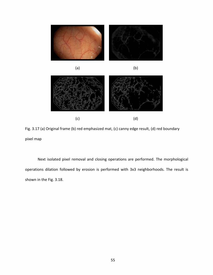
Fig. 3.17 (a) Original frame (b) red emphasized mat, (c) canny edge result, (d) red boundary
pixel map
Next isolated pixel removal and closing operations are performed. The morphological
operations dilation followed by erosion is performed with 3x3 neighborhoods. The result is
shown in the Fig. 3.18.
55

(a) (b)
Fig. 3.18 (a) Red boundary pixel map, (b) after performing morphological operations for row1:
healthy and row 2: erythema condition
The next step is to distinguish frames with healthy blood vessels from frames that have
erythema conditions. In this step, we obtain the 8 neighborhood connected components of the
Red boundary pixel map. Connected component labeling is done using the algorithm outlined in
[72], the basic steps of the algorithm are 1. Search for the unlabelled pixel p in the binary
image. 2. Use a flood-fill algorithm to label all the pixels in the connected component
containing p. 3. Repeat steps 1 and 2 until all the pixels are labeled. After obtaining the
connected components, we use statistical measures such as number of connected components,
number of elements in each component, and the variance of the number of elements in each
component. These measures are greatly differing for healthy frames that have healthy blood
vessels and unhealthy frames with erythema condition.
56

CHAPTER 4
EXPERIMENTAL SETUP AND RESULTS
In this section, accuracy and performance data are presented in two sub sections, one
for block division method and the other for convex hull method. BBPS calculation evaluation,
performance gain through massively parallel implementation, sample results of the proposed
method, and results of erythema detection are also provided.
4.1 Block Division Model
In this section, results of the proposed method and comparison of block division method
are presented. For the comparison, I used support vector machine and KNN classifier. Based on
the results, it is clearly seen that the proposed method out performs both classifiers mentioned
before in terms of speed. That makes the proposed method well suited in the domain of
colonoscopy video analysis. All the computations in our experiments were performed on a PC-
compatible workstation with an Intel Pentium D CPU, 1GB RAM, and Windows XP operating
system.
4.1.1 Data Set
For our experiments, 58 videos recorded from Fujinon colonoscope were used. The
average length of the videos is around 20 minutes, and their frame size is 720 x 480 pixels. We
extracted 1,000 frames from all 58 colonoscopy videos, in which each frame has at least one
stool region. The domain experts marked and confirmed the positive regions in these frames.
From half (500) of these frames, we filtered out duplicate examples (pixels), and obtained only
unique positive examples for the training. Table 4.1 shows the positive pixels used for the
57

training. In the case of stool detection, using 31,858 stool pixels, we followed all the steps in
Section 3.2.1. Then, we used all the pixels in the remaining half (500) of the frames for the
detecting discussed in Section 3.2.1. We assess the effectiveness of our proposed algorithm at
the pixel level by determining the performance metrics Sensitivity and Specificity. For a
comparison purpose, we implemented the method in our previous work [12] using the same
dataset mentioned above. Table 4.2 shows this comparison.
TABLE 4.1
NUMBER OF EXAMPLES (PIXELS) USED IN THE TRAINING STAGE
Stool Dataset
Positive (stool) 31,858
TABLE 4.2
PERFORMANCE COMPARISON WITH THE PREVIOUS WORK
Sensitivity Specificity
New Old New Old
92.9 (%) 90.6 95.0 93.8
Also, we implemented the well-known KNN (K-Nearest Neighbor, K=1 in our study)
classifier using the same dataset mentioned above to see how fast the proposed method can
perform. Table 4.3 presents the speed comparison for KNN classifier with our proposed
method. It takes more than 420 seconds (7 minutes) to evaluate a frame (720 x 480 pixels) in
the KNN. On average, it takes 0.00127 seconds to evaluate one pixel. However, it takes around
58

11 seconds to evaluate a frame (720 x 480 pixels) in the proposed method. If we consider only
the detection, it takes less than one second to evaluate one frame. This is a significant
achievement. As mentioned in Chapter 1, we need to process 3,600 frames to generate a
colonoscopy report for 20 minute colonoscopy video. It is not practical to use KNN classifier
even though it can provide 98% of sensitivity and specificity on average.
TABLE 4.3
AVERAGE TIME TAKEN FOR KNN AND THE PROPOSED METHOD
KNN (trainging +detection) Proposed method
(Detection)
Proposed Method
(Training )
4,37.5 (seconds) 0.9 10.0
Fig. 4.1 lists some results obtained using the proposed method. The numbers (1, 2 and
3) on each frame represent the regions semi-automatically segmented for the determination of
ground truth. For instance, region 2 in Fig. 4.1(a), region 1 in Fig. 4.1(b), and region 1 in Fig.
4.1(c) were labeled as stool by the domain experts. The first row consists of the original frames
with the ground truth marked, and the second row contains the results from our method for
the first row (stool regions are marked with blue).
59

(a)
(b)
(c)
Fig. 4.1 Sample results from the block division methodology
4.2 Convex Hull Model
In this section, I evaluate the proposed convex hull method in terms of accuracy and
computation speed. For the evaluation, I compare the proposed method with the K-NN and
SVM classifiers for both accuracy and speed. In addition, I provide a comparison of accuracies
obtained from the proposed method with HSV and RGB color spaces. Finally, I present an
accuracy comparison of the proposed method for different axes as the initial axis (i.e. accuracy
of the proposed method when placing the planes along Hue, Saturation, and Value axes).
For our experiments, I used a set of 68 real colonoscopy and upper endoscopy
videos. This video set contains 20 videos recorded from Fujinon scope, and 48 videos recorded
from Olympus scope to make it scope-independent. From this video set, we extract total 2,000
video frames showing positive regions of each object as seen in Table 4.4. The ground truths
from these frames have been extracted and confirmed by our domain expert. For bite-block,
currently only Olympus video frames are available. The average length of the videos is around
20 minutes, and their frame size is 720 x 480 pixels. These frames have a black boundary
60

around edge of frame as seen in Fig. 1.3. I ignore all black boundaries. From these frames, we
obtained only unique positive examples of total 290,000 pixels for this experiment as seen in
Table 4.5.
TABLE 4.4
NUMBER OF FRAMES USED FOR THE EXPERIMENT
Object Type Fujinon Olympus Total Frames Bite-block 0 700 700
Blood 100 400 500
Stool 300 500 800
Total 400 1,600 2,000
TABLE 4.5
NUMBER OF EXAMPLES (PIXELS) USED FOR THE EXPERIMENT
Object Type Positive
Examples
Negative
Examples
Total
Examples
Bite-block 140,000 760,000 900,000
Blood 44,000 856,000 900,000
Stool 106,000 794,000 900,000
All the computations in our experiments were performed on a PC-compatible
workstation with an Intel Core i7 quad core CPU, 8GB RAM, and Windows 7 operating system.
61

4.2.1 Accuracy Evaluation
In this section, I compare the proposed method with the K-NN and SVM classifiers for
accuracy. I present our results using commonly used performance metric accuracy. As seen in
Table 4.6, Actual Class is the class that a particular example belongs (positive or negative), and
the Predicted Class is the result from the classifier, where, TP –True Positive, TN – True
Negative, FP – False Positive, and FN – False Negative. Accuracy is defined as
(TP+TN)/(TP+FP+FN+TN), and it represents the number of correctly classified instances.
TABLE 4.6
ACCURACY METRIC
Predicted Class
Actual Class
Positive Negative
Positive TP FN
Negative FP TN
First, I partition the testing dataset of pixels (shown in Table 4.5) into nine sub-data sets
each having 100,000 data points by adding appropriate numbers of negative pixels. Then, I
incrementally add subsets to evaluate and compare two classifiers with our proposed method.
After incrementing the size of the data set, a testing is carried out as a 10-fold cross validation
[73] to achieve a better estimation. Accuracy comparisons for three object detections are given
in Fig. 8. The proposed method’s accuracy is very close to the accuracy of SVM, and far better
than KNN in the bite-block detection (Fig. 4.2(a)) and the blood detection (Fig. 4.2(b)). For the
stool detection, the proposed method’s accuracy is better than both classifiers (Fig. 4.2(c)). This
62

is due to the fact that the hue range in stool examples is much larger than bite-block and blood
examples, and the proposed method is more robust than SVM and KNN in handling variations
in our applications. The effect of hue range is getting larger when more data points are
considered, and causes the accuracies of SVM and KNN to get lower with the increasing size of
data set as shown in Fig. 4.2(c).
4.2.1.1 Detection Accuracy for Bite-block, Blood, and Stool
In this section, we present accuracy comparison of three algorithms, SVM, K-NN, and proposed
method for green bite block, blood, and stool detection. It is clearly seen from the graphs that
the proposed method outperforms SVM in two instances and get closer to SVM in one instance.
Proposed method is getting its best performance with the increasing size of the dataset. And it
can keep consistency in all three case studies where other two methods failed to be consistent.
(a)
63

(b)
(c)
Fig. 4.2 Accuracy comparisons of proposed method (Hull), SVM, and K-NN for (a) bite-block, (b)
blood, and (c) stool detections
4.2.2 Performance Evaluation
We evaluate the proposed algorithm against SVM and K-NN classifiers for speed
performance. We represent speed performance as time taken to process large number of data
points and incrementally add data points to make it larger at each evaluation. And the Fig. 4.3
shows gradual degradation of speed performance of each algorithm with the increasing
number of data points. We, in our domain, are aiming at frame level object detection. Hence,
we expect the proposed method to perform well with a number of data points equal to
720x480 = 345,600 that is the resolution of a colonoscopy video frame. This test was performed
64

with the gradually increasing sample size to demonstrate the applicability of each technique in
the domain of large data set processing.
4.2.2.1 Detection Speed for Bite-block, Blood, and Stool
Proposed method shows promising applicability in this context. Specially, the proposed
method is well suited to be used in the context of real-time processing. The other two well
known methods, SVM and K-NN, perform closely to proposed method in terms of accuracy. But
they are very inefficient in the context of real-time processing.
(a)
(b)
65

(c)
Fig. 4.3 Speed comparisons of proposed method (Hull), SVM, and K-NN for (a) bite-block, (b)
blood, and (c) stool detections
4.2.3 Accuracy Comparison of the Proposed Method in RGB and HSV Color Spaces
This subsection provides an accuracy comparison of the proposed method in RGB and
HSV color spaces. For the RGB color space, the red axis was used as the initial axis. And the
value axis was used as the initial axis in HSV color space. The accuracy calculation was done as
the same way in Section 4.2.1. Table 4.7 shows that the HSV color space outperforms the RGB
color space in all three object detections.
66

TABLE 4.7
ACCURACY COMPARISON BETWEEN RGB AND HSV COLOR SPACES
Number of Data Points (* 100K)
Bite-block Blood Stool RGB HSV RGB HSV RGB HSV
1 0.97 0.99 0.99 0.99 0.99 0.99 2 0.98 0.99 0.96 0.99 0.99 0.99 3 0.98 0.99 0.96 0.99 0.99 0.99 4 0.98 0.99 0.96 0.99 0.98 0.99 5 0.98 0.99 0.95 0.99 0.98 0.99 6 0.98 0.99 0.95 0.99 0.98 0.99 7 0.98 0.99 0.95 0.99 0.98 0.99 8 0.98 0.99 0.96 0.99 0.98 0.99 9 0.98 0.99 0.96 0.99 0.98 0.99 Average 0.98 0.99 0.96 0.99 0.98 0.99
4.2.4 Accuracy Comparison of the Proposed Method with Different Initial Axes
This section provides an accuracy comparison of the proposed method with different
initial axes (selecting Hue or Saturation axis instead of Value axis). The results are shown in
Table 4.8 in which three columns for each object; Hue, Saturation (Sat), and Value (Val). Testing
was carried out as the same way in Section 4.2.1. As seen in the table, when the initial axis is
value, the accuracies for all three objects are better. To achieve a better accuracy, the initial
axis should be value axis.
67

TABLE 4.8
ACCURACY OF THE PROPOSED METHOD WITH ALL THREE INITIAL AXES
Data points (*100k)
Green bite-block Blood Stool
Hue Sat Val Hue Sat Val Hue Sat Val 1 0.99 0.99 0.99 0.71 0.88 0.99 0.99 0.99 0.99
2 0.99 0.99 0.99 0.76 0.85 0.99 0.99 0.99 0.99
3 0.99 0.99 0.99 0.83 0.86 0.99 0.96 0.98 0.99
4 0.99 0.99 0.99 0.86 0.87 0.99 0.93 0.95 0.99
5 0.99 0.99 0.99 0.89 0.87 0.99 0.91 0.94 0.99
6 0.99 0.99 0.99 0.91 0.88 0.99 0.9 0.93 0.99
7 0.99 0.99 0.99 0.92 0.89 0.99 0.9 0.93 0.99
8 0.98 0.98 0.99 0.93 0.91 0.99 0.92 0.94 0.99
9 0.97 0.97 0.99 0.94 0.92 0.99 0.92 0.94 0.99
Average 0.99 0.99 0.99 0.86 0.88 0.99 0.94 0.95 0.99
4.2.5 Evaluation Examples
Fig. 4.4 shows examples of results obtained using the proposed method. The first row of
Fig. 4.4 consists of the original frames with the ground truth marked for stool, green bite bock
and blood. The second row contains the results from our proposed method for each frame
listed in first row. For these three examples, three training models are used. Blue colored pixels
represent the pixels that our proposed method detected as positive class pixels in each
application.
68

(a)
(b)
(c)
(d)
(e)
(f)
Fig. 4.4 (a) Frame with a stool region, (b) frame with a green bite block region, (c) frame with a
blood region, (d) result of our proposed method for frame in (a) using stool model, (e) result of
the method for the frame in (b) using green bite block model, and (f) result of our method for
the frame in (c) using blood model
4.3 BBPS Score
We generated BBPS scores for all 58 videos and list randomly selected 5 results in Table
4.9 having a comparison with the ground truth scores suggested by domain experts. The
column ‘Ground truth BBPS’ in Table 4.9 is the average score values from three different
experts. It is rarely found a video with all three experts come closer in terms of the scores.
Therefore, it is hard to find the definite score for a given video. We took the average of three
BBPS ground truths as our target value to be reached. As seen in the table, the calculated
values are very close to the ground truths.
69

TABLE 4.9
COMPARISON OF CALCULATED BBPS SCORES WITH GROUND TRUTH BBPS SCORES
Video ID Calculated BBPS Ground Truth BBPS
1 7 6
5 4 3
9 6 6
10 6 7
13 6 5
4.4 Performance Gain through Massive parallelism
In this section, performance gain by using the GPU with OpenCL is presented. It is clearly
seen that with the use of GPU with OpenCL, the targeted module can process a video frame
within the given time slot bounded by the real time processing requirement. That is the 33ms
time constraint. Any module to process 30 frames per second in real time systems; it should
finish its work for a frame within 33ms. I measure the time performance at three points in the
algorithm; 1) Image reading and gray scale conversion; 2) Sobel edge detection; 3) Enhance
connectivity, block sum generation, and thresholding. Time performance for above mentioned
sections is shown in the Table 4.10.
70

TABLE 4.10
TIME PERFORMANCE OF THE BLURRY DETECTION MODULE IN THE CPU AND GPU
Check Point 1 2 3 Total
GPU with OpenCL (Sec/Frame)
0.102 0.015 0.1 0.209
CPU (sec/Frame)
0.102 0.176 0.1 0.378
4.5 Erythema Detection
In this section, the results of the Erythema detection are provided. As can be seen in the
Table 4.11, there is a clear cut between healthy video frames and Erythema video frames in
terms of statistical measures generated. These statistical measures can be used to separate
healthy frames from Erythema frames.
TABLE 4.11
STATISTICAL MEASURES FOR HEALTHY AND ERYTHEMA CONDITION
Statistical Measure Healthy video frame Erythema video frames
Average Connected components 314.11 609.28
Average number of elements
in a component
46.90 42.59
Standard Deviation
of number of elements
53.69 43.13
71

CHAPTER 5
CONCLUSION
Medical video analysis for quality assessment is a key subject area in the medical
domain. Specifically, endoscopy procedures are subjected to quality assessments. Quality
assessment will improve the procedures’ productivity and the increase the patient survival rate.
Colonoscopy video, one of endoscopy procedures, analysis inherently involved with huge
amount of data. With 20 minutes of video at a rate of 29.97 frames per second, there are about
36,000 frames to analyze. To provide quality measurements in real time with this many frames
is a challenging task. State of the art methods are failing at very large data sets and hence a
novel approach was needed.
In this dissertation, a novel method of object detection has been proposed. This novel
method was developed to detect three classes of objects found in the colonoscopy procedures.
The proposed method can perform the object detection with a great accuracy by adhering to
the real time processing requirements very well.
The proposed method is capable of learning from a sub set of training data. And it is
capable of building a complete training model by dividing the whole data set into many sub
data sets and generating a sub model for each sub set of data. For the modeling of each sub
data set, a convex hull is used. This concept can eliminate the lazy learning problems associated
with the models such as k-NN classifier. It can learn incrementally and hence does not need to
keep the whole dataset for re-training as per the SVM.
72

Further, there are four application of the proposed method have been provided in this
dissertation; green bite-block detection, blood detection, and stool detection. In addition,
blood detection has been used to detect Erythema condition in the colon wall and stool
detection has been used to estimate the BBPS score value for a colonoscopy procedure.
The proposed method is currently in a pilot run in a clinical setting and performing
successfully with the satisfied expectations.
5.1 Future Directions
The current method represents a sub set of data using a convex hull. This would in some
instances generate soft modeling of the data set. The one solution for this problem is to model
the data set using a concave hull. This approach would approximate the distribution of the data
set very closely. And also, investigation of the other domain problems where the proposed
method can be adopted is another future work.
73

BIBLIOGRAPHY
[1] American Cancer Society. “Colorectal Cancer Facts and Figures,” American Cancer Society Special Edition 2005, pp. 1–20, 2005.
[2] Johnson C.D., Fletcher J.G., MacCarty R.L., et al. “Effect of slice thickness and primary 2D
versus 3D virtual dissection on colorectal lesion detection at CT colonography in 452 asymptomatic adults,” AJR American Journal of Roentgenology, vol. 189(3), pp. 672-80, 2007
[3] Pabby A., Schoen R.E., Weissfeld J.L., Burt R., Kikendall J.W., Lance P., et al. “Analysis of
colorectal cancer occurrence during surveillance colonoscopy in the dietary prevention trial,” Gastrointestinal Endoscopy, vol. 61(3), pp. 385-391, 2005.
[4] Rex D.K., Bond J.H., Winawer S., Levin T.R., Burt R.W., et al. “Quality in the technical
performance of colonoscopy and the continuous quality improvement process for colonoscopy: recommendations of the U.S. multi-society task force on colorectal cancer,” American Journal Gastroenterol, vol. 97(6), pp. 1296-1308, 2002.
[5] Douglas K.R., John L.P., Todd H.B., Amitabh C., Jonathan C., Stephen E.D., et al. “Quality
Indicators for Colonoscopy,” In: American Journal of Gastroenterology, vol. 101, pp. 873–885, 2006.
[6] Oh J., Hwang S., Cao Y., Tavanapong W., Liu D., Wong J., et al. “Measuring Objective
Quality of Colonoscopy,” IEEE Transactions on Biomedical Engineering. Vol. 56(9), pp. 2190-2196, 2009.
[7] Hwang S., Oh J., Lee J., de Groen P.C., Cao Y., Tavanapong W., et al. “Automatic
Measurement of Quality Metrics for Colonoscopy Videos,” Proc. of ACM Multimedia 2005, pp. 912-921, 2005.
[8] Stanek S., Tavanapong W., Wong J., Oh J., and de Groen P. C., “Automatic Real-Time
Capture and Segmentation of Endoscopy Video. PACS and Imaging Informatics,” In: SPIE Medical Imaging. Vol. 6919, pp. 69190X-69190X-10, 2008.
[9] Cappel, M.S., Friedel D., “The Role of Sigmoidoscopy and Colonoscopy in the Diagnosis
and Management of Lower Gastrointestinal Disorders: Endoscopic Findings, Therapy, and Complications,” In: Medical Clinics of North America, vol. 86, pp. 1253–1288, 2002.
[10] Ness R.M., Manam R., Hoen H.J., Chalasani N., “Predictors of Inadequate Bowel
Preparation for Colonoscopy,” In: American Journal of Gastroenterology, vol. 96, pp. 1797–1802, 2001.
74

[11] Lai E.J., Calderwood A.H., Doros G., et al. “The Boston Bowel Preparation Scale: a valid and reliable instrument for colonoscopy-oriented research,” In: Gastrointestinal Endoscopy Clinics of North America, vol. 69, pp. 620-625, 2009.
[12] Hwang S., Oh J., Tavanapong W., Wong, J., and de Groen P.C., “Stool Detection in
Colonoscopy Videos,” In: Proc. of International Conference of the IEEE Engineering in Medicine and Biology Society (EMBC), Vancouver, British Columbia, Canada, pp. 3004-3007, 2008.
[13] Muthukudage J., Oh J., Tavanapong W., Wong J., de Groen P.C., “Color Based Stool
Region Detection in Colonoscopy Videos for Quality Measurements,” In: Lecture Notes in Computer Science, vol. 7087, pp. 61-72, 2011.
[14] Giritharan B., Yuan X., Liu J., Buckles B., Oh J., Tang S.J., “Bleeding detection from
capsule endoscopy videos,” in: Proceedings of the 30th Annual International Conference of the IEEE Engineering in Medicine and Biology Society, 2008 (EMBS’ 08), Vancouver, British Columbia, Canada, pp. 4780–4783, 2008.
[15] Manjunath B.S., Ohm J., Vasudevan VV., Yamada A., “Color and texture descriptors,”
IEEE Transactions on Circuits and Systems for Video Technology, 11 (6), pp. 703–715, 2001.
[16] Karargyris A., Bourbakis N., “A methodology for detecting blood-based abnormalities in
wireless capsule endoscopy videos,” in: Proceedings of the 8th IEEE International Conference on BioInformatics and BioEngineering, 2008 (BIBE’08), Athens, Greece, pp. 1–6, 2008.
[17] Bourbakis N., “Detecting abnormal patterns in WCE images,” in: Proceedings of the 5th
IEEE Symposium on Bioinformatics and Bioengineering, 2005 (BIBE’05), Minneapolis, Minnesota, USA, pp. 232–238, 2005.
[18] Lau P.Y., Correia P., “Detection of bleeding patterns in WCE video using Multiple
features,” in: Proceedings of the 29th Annual International Conference of the IEEE Engineering in Medicine and Biology Society, 2007, (EMBS’07), Vancouver, British Columbia, Canada, pp. 5601–5604, 2007.
[19] Li B., Meng M.Q., “Computer-based detection of bleeding and ulcer in wireless capsule
endoscopy images by chromaticity moments,” Computers in Biology and Medicine, vol. 39 (2), pp. 141–147, 2009.
[20] Jung Y.S., Kim Y.H., Lee D.H., Kim J.H., "Active Blood Detection in a High Resolution
Capsule Endoscopy using Color Spectrum Transformation," Biomedical Engineering and Informatics, BMEI 2008, vol. 1, pp. 859-862, 2008.
75

[21] Bourbakis N., Makrogiannis S., Kavraki D., "A neural network-based detection of
bleeding in sequences of WCE images," Bioinformatics and Bioengineering, 2005. BIBE 2005, pp. 324-327, 2005.
[22] Du Y., Ai H., Lao S., "Evaluation of color spaces for person re-identification," Pattern
Recognition (ICPR), pp. 1371-1374, 2012.
[23] Albiol A., Torres L., and Delp E.J., "Optimum Color Spaces for Skin Detection," ICIP 2001 Vol. 1, pp. 122-124, 2001.
[24] Gomiiez G., Sanclhez M., and Suicar L.E., "On Selecting an Appropriate Color Space for
Skin Detection," Proc. of 2nd Mexican Int. Conf on Artificial Intelligence. pp. 69-78, 2002.
[25] Lissner, I., Urban, P., "Toward a Unified Color Space for Perception-Based Image Processing," IEEE Transactions on Image Processing, vol. 21(3), pp.1153-1168, 2012.
[26] Tkalcic M., Tasic J.F., "Colour spaces: perceptual, historical and applicational
background," EUROCON 2003. Computer as a Tool. The IEEE Region 8 , vol.1, pp.
304-308, 2003
[27] Cortes, Corinna, Vapnik, Vladimir N., "Support-Vector Networks," Machine Learning,
vol. 20(3), pp. 273 – 297, 1995.
[28] Saunders C., Stitson M.O., Weston J., Bottou L., Schdieolkopf B., Smola A., “Support vector machine reference manual,” Royal Holloway, University of London, Egham, UK, Tech. Rep. CSD-TR-98-03, 1998.
[29] Joachims T., “Making large-scale support vector machine learning practical,” In
Advances in Kernel Methods: Support Vector Machines, 1999, pp. 169-184.
[30] Lin C.J., “On the convergence of the decomposition method for support vector machines,” IEEE Transactions on Neural Networks, vol. 12(6), pp. 1288-1298, 2001.
[31] Palagi L., Sciandrone M., “On the convergence of a modified version of SVMlight
algorithm,” Optimization Methods and Software, vol. 20(2-3), pp. 315-332, 2005.
[32] Platt J., “Fast training of SVMs using sequential minimal optimization,” In B. Schdieolkopf, C.Burges and A.Smola (ed.), Advances in Kernel Methods: Support Vector Learning, MIT Press, Cambridge, MA, 1999, pp. 185-208.
[33] S.S.Keerthi, S.Shevade, C.Bhattacharyya and K.Murthy, “Improvements to Platt's SMO
algorithm for SVM classifier design,” Dept. of CSA, Bangalore, India, Tech. Rep., 1999.
76

[34] S.S.Keerthi, S.Shevade, C.Bhattacharyya and K.Murthy, “Improvements to SMO
algorithm for SVM regression,” IEEE Transactions on Neural Networks, vol. 11(5), pp. 1188-1193, 2000.
[35] G.Flake, S.Lawrence, “Efficient SVM regression training with SMO,” Machine Learning,
vol. 46(1-3), pp. 271-290, 2002.
[36] S.S.Keerthi and E.G.Gilbert, “Convergence of a generalized SMO algorithm for SVM classifier design,” Machine Learning, vol. 46, pp. 351-360. 2002.
[37] C.J.Lin, “Asymptotic convergence of an SMO algorithm without any assumptions,” IEEE
Transaction on Neural Networks, vol. 13(1), pp. 248-250, 2002.
[38] P.H.Chen, R.E.Fan and C.J.Lin, “A study on SMO-Type decomposition method for support vector machines,” Department of Computer Science, National Taiwan University Tech. Rep., 2005.
[39] R.E.Fan, P.H.Chen, and C.J.Lin, “Working set selection using the second order information for training SVM,” Journal of Machine Learning Research, vol. 6, pp. 1889-1918, 2005.
[40] D. DeCoste and K. Wagstaff, “Alpha seeding for support vector machines,” In
Proceedings of International Conference on Knowledge Discovery and Data Mining (KDD-2000), 2000.
[41] C.W.Hsu and C.J.Lin, “A simple decomposition method for support vector machines,”
Machine Learning, vol. 46, pp. 291-314, 2002.
[42] O.L.Mangasarian and D.R.Musicant, “Successive over-relaxation for support vector machines,” IEEE Transactions on Neural Networks, vol. 10(5), pp. 1032-1037. 1999.
[43] C.C.Chang and C.J.Lin, “LIBSVM,” Software available at http://www.csie.ntu.
edu.tw/̃cjlin/libsvm.
[44] S.S.Keerthi and C.-J. Lin, “Asymptotic behaviors of support vector machines with Gaussian kernel,” Neural Computation, vol. 15, pp. 1667-1689, 2003.
[45] J.Suykens and J.Vandewalle, “Least squares support vector machine classifiers,” Neural
Processing Letters, pp. 293-300, 1999.
[46] J.Suykens. L.Lukas, P.Van Dooren, B.De Moor and J.Vandewalle, “Least squares support vector machine classifiers: a large scale algorithm,” in Proc. of the European Conference on Circuit Theory and Design, Stresa, Italy, pp. 893-842, 1999.
77

[47] B.Hamers, J.Suykens and B.De Moor, “A comparison of iterative methods for least
squares support vector machine classifiers,” ESAT-SISTA, K.U.Leuven (Leuven, Belgium), Internal Report 01-110, 2001.
[48] W.Chu, C. J. Ong and S. S. Keerthi, “An improved conjugate gradient scheme to the
solution of least squares SVM,” IEEE Transactions on Neural Networks, vol. 16(2), pp. 498-501, 2005.
[49] S.S.Keerthi and S.K.Shevade, “SMO algorithm for least squares svm formulations,”
Neural Computation, vol. 15(2), pp. 487-507, 2003.
[50] O.L.Mangasarian and D.R.Musicant, “Lagrangian support vector machines,” Journal of Machine Learning Research, vol. 1, pp. 161-177, 2001.
[51] Glenn Fung and L.Mangasarian, “Proximal support vector machine classifiers,”
Proceedings of the 7th ACM conference on knowledge discovery and data mining, ACM, pp. 77-86, 2001.
[52] Y.J.Lee and O.L.Mangasarian, “RSVM: Reduced support vector machines,” In
Proceedings of the First SIAM International Conference on Data Mining, 2001.
[53] Kuan-Ming Lin and Chih-Jen Lin, “A study on reduced support vector machines,” IEEE Transaction on Neural Networks, vol. 14(6), pp. 1449-1459, 2003.
[54] D. W. Aha, D. Kibler, and M. K. Albert. “Instance-based learning algorithms,” Machine
Learning, vol. 6, pp. 37–66, 1991.
[55] Han K.K., “text categorization using weight adjusted k-nearest neighbor classification,”
Dept. of CS, University of Minnesota, Tech. Rep., 1999.
[56] Huang Z., “A fast clustering algorithm to cluster very large categorical data sets in data mining,” In Proc. SIGMOD Workshop on Research Issues on Data Mining and Knowledge Discovery, 1997.
[57] Jiang L., Zhang H., Cai Z., and Su J., “Evolutional naïve bayes,” In Proceedings of the 1st
International Symposium on Intelligent Computation and its Applications, pp. 344–350. , 2005.
[58] Kohavi R., John G., “Wrappers for feature subset selection,” Artificial Intelligence, vol.
97, pp. 273–324, 1997.
78
[59] Langley P., Sage S., “Induction of selective bayesian classifiers,” In Proceedings of Uncertainty in Artificial Intelligence, Morgan Kaufmann, pp. 400–406, 1994.
[60] Stanfill C., Waltz D., “Toward memory-based reasoning,” Communications of the ACM,
vol. 29, pp. 1213–1228, 1986.
[61] Wilson D.R., Martinez T.R., “Improved heterogeneous distance functions,” Artificial Intelligence Research, vol. 6, pp. 1–34, 1997.
[62] Jiang J., Zhang H., Cai Z., “Dynamic k-nearest-neighbor naive bayes with attribute
weighted,” In Proceedings of the 3rd International Conference on Fuzzy Systems and Knowledge Discovery, pp. 365–368, 2006.
[63] Kohavi R., “Scaling up the accuracy of naive-bayes classifiers: A decision-tree hybrid,” In
Proceedings of the Second International Conference on Knowledge Discovery and Data Mining, pp. 202–207, 1996.
[64] Langley P., Iba W., Thomas K., “An analysis of Bayesian classifiers,” In Proceedings of the
Tenth National Conference of Artificial Intelligence, pp. 223–228, 1992.
[65] Webb Z. Z. G.I., “Lazy learning of Bayesian rules,” Machine Learning, vol. 41, pp. 53–84, 2000.
[66] Xie Z.,Hsu W., Liu Z., Lee M., “SNNB: A selective neighborhood based naive bayes for
lazy learning,” In Proceedings of the Sixth Pacific-Asia Conference on KDD, pp. 104–114, 2002.
[67] Frank E., Hall M., Pfahringer B., “Locally weighted naive bayes,” In Proceedings of the
Conference on Uncertainty in Artificial Intelligence, Morgan Kaufmann, pp. 249–256. 2003.
[68] Barber C.B., Dobkin D.P., Huhdanpaa H., “The quickhull algorithm for convex hulls,” ACM
Transactions on Mathematical Software (TOMS), vol. 22(4), pp. 469-483, 1996.
[69] Oh, J., Rajbal, M.A., Muthukudage, J.K., Tavanapong, W., Wong, J., and de Groen. P.C., “Real-Time Phase Boundary Detection in Colonoscopy Videos,” In: Proc. of 6th International Symposium on Image and Signal Processing and Analysis (ISPA 2009), Salzburg, Austria, pp. 724-729, 2009.
[70] Slo-Li Chu; Chih-Chieh Hsiao, "OpenCL: Make Ubiquitous Supercomputing Possible," 2010 12th IEEE International Conference on High Performance Computing and Communications (HPCC), pp. 556-561, 2010.
79

[71] Canny, John, "A Computational Approach to Edge Detection," IEEE Transactions on
Pattern Analysis and Machine Intelligence, vol. PAMI-8(6), pp.679-698, 1986.
[72] Eves, Howard, “A Survey of Geometry,” I, Boston: Allyn and Bacon, Inc., 1963.
[73] Rodriguez, J.D., Perez, A., Lozano, J.A., "Sensitivity Analysis of k-Fold Cross Validation in Prediction Error Estimation," IEEE Transactions on Pattern Analysis and Machine Intelligence, vol. 32(3), pp.569-575, 2010.
[74] Gonzalez R.C., and Woods R.E., “Digital Image Processing,” 3rd ed., Prentice Hall, Upper
Saddle River, New Jersey, USA, pp. 394 – 456, 2008.
[75] Duda R.O., Hart P.E., and Stork D.G., “Pattern Classification,” John Wiley and Sons, New York, USA, pp 517-581, 2001.
80