Embed Size (px)
Citation preview

Phase Transitions
Proseminar in Theoretical Physics
Institut fur theoretische Physik
ETH Zurich
SS07

typeset & compilation by H. G. Katzgraber (with help from F. Hassler)

Table of Contents
1 Symmetry and ergodicity breaking, mean-field study of the
Ising model 1
1.1 Introduction . . . . . . . . . . . . . . . . . . . . . . . . . . . . . . 1
1.2 Formalism . . . . . . . . . . . . . . . . . . . . . . . . . . . . . . . 2
1.3 The model system: Ising model . . . . . . . . . . . . . . . . . . . 4
1.4 Solutions in one and more dimensions . . . . . . . . . . . . . . . . 8
1.5 Symmetry and ergodicity breaking . . . . . . . . . . . . . . . . . 14
1.6 Concluding remarks . . . . . . . . . . . . . . . . . . . . . . . . . . 17
2 Critical Phenomena in Fluids 21
2.1 Repetition of the needed Thermodynamics . . . . . . . . . . . . . 21
2.2 Two-phase Coexistence . . . . . . . . . . . . . . . . . . . . . . . . 23
2.3 Van der Waals equation . . . . . . . . . . . . . . . . . . . . . . . 26
2.4 Spatial correlations . . . . . . . . . . . . . . . . . . . . . . . . . . 30
2.5 Determination of the critical point/ difficulties in measurement . . 32
3 Landau Theory, Fluctuations and Breakdown of Landau The-
ory 37
3.1 Introduction . . . . . . . . . . . . . . . . . . . . . . . . . . . . . . 37
3.2 Landau Theory . . . . . . . . . . . . . . . . . . . . . . . . . . . . 40
3.3 Fluctuations . . . . . . . . . . . . . . . . . . . . . . . . . . . . . . 44
3.4 Conclusive Words . . . . . . . . . . . . . . . . . . . . . . . . . . . 49
4 Scaling theory 53
4.1 Critical exponents . . . . . . . . . . . . . . . . . . . . . . . . . . . 53
4.2 Scaling hypothesis . . . . . . . . . . . . . . . . . . . . . . . . . . 54
4.3 Deriving the Homogeneous forms . . . . . . . . . . . . . . . . . . 58
4.4 Universality classes . . . . . . . . . . . . . . . . . . . . . . . . . . 61
4.5 Polymer statistics . . . . . . . . . . . . . . . . . . . . . . . . . . . 62
4.6 Conclusions . . . . . . . . . . . . . . . . . . . . . . . . . . . . . . 68
iii

TABLE OF CONTENTS
5 The Renormalization Group 71
5.1 Introduction . . . . . . . . . . . . . . . . . . . . . . . . . . . . . . 71
5.2 Classical lattice spin systems . . . . . . . . . . . . . . . . . . . . . 72
5.3 Scaling limit . . . . . . . . . . . . . . . . . . . . . . . . . . . . . . 73
5.4 Renormalization group transformations . . . . . . . . . . . . . . . 76
5.5 Example: The Gaussian fixed point . . . . . . . . . . . . . . . . . 83
6 Critical slowing down and cluster updates in Monte Carlo
simulations 89
6.1 Introduction . . . . . . . . . . . . . . . . . . . . . . . . . . . . . . 89
6.2 Critical slowing down . . . . . . . . . . . . . . . . . . . . . . . . . 92
6.3 Cluster updates . . . . . . . . . . . . . . . . . . . . . . . . . . . . 95
6.4 Concluding remarks . . . . . . . . . . . . . . . . . . . . . . . . . . 101
7 Finite-Size Scaling 105
7.1 Introduction . . . . . . . . . . . . . . . . . . . . . . . . . . . . . . 105
7.2 Scaling Function Hypothesis . . . . . . . . . . . . . . . . . . . . . 106
7.3 Critical Temperature Tc . . . . . . . . . . . . . . . . . . . . . . . 109
7.4 Distinguishing between 1st and 2nd Order Phase Transitions . . . 113
7.5 Concluding remarks . . . . . . . . . . . . . . . . . . . . . . . . . . 114
8 Berezinskii-Kosterlitz-Thouless Transition 117
8.1 Introduction . . . . . . . . . . . . . . . . . . . . . . . . . . . . . . 117
8.2 Vortices . . . . . . . . . . . . . . . . . . . . . . . . . . . . . . . . 119
8.3 Villain and Coulomb gas models . . . . . . . . . . . . . . . . . . . 121
8.4 Effective interaction . . . . . . . . . . . . . . . . . . . . . . . . . . 128
8.5 Kosterlitz-Thouless Transition . . . . . . . . . . . . . . . . . . . . 131
9 O(N) Model and 1/N Expansion 137
9.1 Introduction . . . . . . . . . . . . . . . . . . . . . . . . . . . . . . 137
9.2 The Model . . . . . . . . . . . . . . . . . . . . . . . . . . . . . . . 138
9.3 Mathematical Background . . . . . . . . . . . . . . . . . . . . . . 139
9.4 Spontaneous Symmetry Breaking . . . . . . . . . . . . . . . . . . 142
9.5 1/N expansion . . . . . . . . . . . . . . . . . . . . . . . . . . . . . 149
9.6 Renormalization and critical exponents . . . . . . . . . . . . . . . 152
9.7 Concluding remarks . . . . . . . . . . . . . . . . . . . . . . . . . . 154
10 Quantum Phase Transitions and the Bose-Hubbard Model 157
10.1 What is a Quantum Phase Transition? . . . . . . . . . . . . . . . 157
10.2 The Bose-Hubbard Model . . . . . . . . . . . . . . . . . . . . . . 160
iv

TABLE OF CONTENTS
10.3 Ultra-cold bosonic Gas in an optical Lattice Potential . . . . . . . 169
11 Quantum Field Theory and the Deconfinement Transition 175
11.1 Introduction . . . . . . . . . . . . . . . . . . . . . . . . . . . . . . 175
11.2 Gauge Field Theories . . . . . . . . . . . . . . . . . . . . . . . . . 176
11.3 Wilson Loop and Static qq-Potential . . . . . . . . . . . . . . . . 177
11.4 Quantum Field Theories at Finite Temperature . . . . . . . . . . 180
11.5 The Wilson Line or Polyakov Loop . . . . . . . . . . . . . . . . . 183
11.6 The Deconfinement Phase Transition . . . . . . . . . . . . . . . . 184
11.7 Deconfinement in the SU(3) Gauge Theory . . . . . . . . . . . . . 188
12 The Phases of Quantum Chromodynamics 193
12.1 Introduction . . . . . . . . . . . . . . . . . . . . . . . . . . . . . . 193
12.2 The QCD Phase Diagram . . . . . . . . . . . . . . . . . . . . . . 203
12.3 Colour superconductivity and colour
flavour locking . . . . . . . . . . . . . . . . . . . . . . . . . . . . . 211
12.4 Relativistic Heavy-Ion Collisions . . . . . . . . . . . . . . . . . . . 215
13 BCS theory of superconductivity 221
13.1 Introduction . . . . . . . . . . . . . . . . . . . . . . . . . . . . . . 221
13.2 Cooper Pairs . . . . . . . . . . . . . . . . . . . . . . . . . . . . . 222
13.3 BCS Theory . . . . . . . . . . . . . . . . . . . . . . . . . . . . . . 224
13.4 Finite Temperatures . . . . . . . . . . . . . . . . . . . . . . . . . 228
13.5 Type II Superconductors and the Vortex State . . . . . . . . . . . 233
14 Bose Einstein Condensation 239
14.1 Introduction . . . . . . . . . . . . . . . . . . . . . . . . . . . . . . 239
14.2 The non-interacting Bose gas . . . . . . . . . . . . . . . . . . . . 240
14.3 The Bose Gas with Hard Cores in the Mean Field Limit . . . . . 243
14.4 The weakly interacting Bose Gas in the Critical Regime . . . . . . 245
14.5 Spontaneous Symmetry Breaking in the Bose Gas . . . . . . . . . 247
15 Superfluidity and Supersolidity 251
15.1 Superfluid Helium . . . . . . . . . . . . . . . . . . . . . . . . . . . 251
15.2 Supersolid Helium . . . . . . . . . . . . . . . . . . . . . . . . . . . 260
v

TABLE OF CONTENTS
vi

Chapter 1
Symmetry and ergodicity
breaking, mean-field study of
the Ising model
Rafael Mottlsupervisor: Dr. Ingo Kirsch
We describe a ferromagnetic domain in a magnetic material by
the Ising model using the language of statistical mechanics. By
heuristic arguments we show that there is no spontaneous magne-
tization for the nearest-neighbour Ising model in one dimension
and that there is spontaneous magnetization in two and three
dimensions. Three solutions are presented: the transfer matrix
method in one dimension and non-zero external magnetic field,
some ideas of the Onsager solution for the two-dimensional case
with zero external magnetic field and the mean-field theory for
arbitrary dimension and non-zero external magnetic field. Sym-
metry and ergodicity breaking are introduced and applied to the
Ising model. The restricted ensemble is used to describe the sys-
tem with broken ergodicity.
1.1 Introduction
We describe a ferromagnetic domain with spontaneous magnetization. In a cor-
related state of spontaneous magnetization we have an ordered system whereas
above some critical temperature we observe an unordered state: a phase transi-
tion occurs at the critical temperature TC .
1

1.2 Formalism
This phase transition is described by an order parameter which is zero above the
critical temperature (zero order) and non-zero below the critical temperature: a
measure of order which is in our case of a magnetic material the magnetization
M of the material.
From a general Hamiltonian with all possible spin-interaction terms we make a
couple of assumptions to get to the Ising model. This model was introduced by
the German physicist Ernst Ising (1900 - 1998).
1.2 Formalism
The analysis of the Ising model makes use of the statistical mechanical descrip-
tion of the system. We remember the reader of the statistical mechanical basics
to introduce afterwards the definitions of phases, phase transition and critical
exponents.
1.2.1 Statistical mechanical basics
We describe a certain sample region Ω of volume V (Ω) which contains a number
of particles N(Ω). The analysis is based on the canonical ensemble description.
The corresponding partition function is given by:
ZΩ[Kn] = Tr exp −βHΩ(Kn,Θn), (1.1)
β =1
kBT, (1.2)
where the trace operator is the sum over all possible states in phase space Γ. The
Hamiltonian defined on the phase space depends on the degrees of freedom Θn of
the system (in our case: spin variables) and certain coupling constants Kn (e.g.
external magnetic field).
From the partition function we can calculate the free energy
FΩ[Kn] = FΩ[K] = −kBT logZΩ[K]. (1.3)
By taking the thermodynamical limit we get the bulk free energy per site
fb[K] = limN(Ω)→∞
FΩ[K]
N(Ω). (1.4)
As we will see below, phase boundaries are defined as the regions of non-analyticity
of the bulk free energy per site. We need the thermodynamic limit in order to
2

Symmetry and ergodicity breaking, mean-field study of the Isingmodel
describe phase transitions. As the bulk free energy per site is just a finite sum
over exponential terms having non-singular exponents it would be analytic every-
where. Thus phase transitions are only observed in the thermodynamical limit.
By applying partial derivatives to the bulk free energy we obtain the well-known
thermodynamical properties: internal energy, heat capacity, magnetization and
magnetic susceptibility:
ǫin[K] =∂
∂β(βfb[K]), (1.5)
C[K] =∂ǫin[K]
∂T, (1.6)
M [K] = −∂fb[K]
∂H, (1.7)
χT [K] =∂M [K]
∂H. (1.8)
1.2.2 Phases, phase transitions and critical exponents
A phase is a region of analyticity of the bulk free energy per site. Different phases
are separated by phase boundaries which are singular loci of the bulk free energy
per site of dimension d - 1. We distinguish between two different kinds of phase
transitions:
1. first-order phase transition: one (or more) of the first partial derivatives of
the bulk free energy per site is discontinuous
2. continuous phase transition: all first derivatives of the bulk free energy per
site are continuous.
For a continuous phase transition we can introduce the critical exponents which
describe the behaviour of the thermodynamical properties near the phase transi-
tion:
1. heat capacity C ∼|t|−α
2. order parameter M ∼|t|β
3. susceptibility χ ∼|t|−γ
3

1.3 The model system: Ising model
4. equation of state M ∼ H1/δ.
The first three critical exponents are defined for zero external magnetic field and
t describes the deviation of the temperature from the critical temperature:
t =T − TCTC
. (1.9)
The notation ∼ means that the described value has a singular part proportional
to the given value.
1.2.3 Correlation function, correlation length and
their critical exponents
The definition of the correlation function looks as follows:
G(r) :=⟨
(S(r) − 〈S(r)〉) (S(0) − 〈S(0)〉)⟩, (1.10)
where r is the location of the spin variable S(r). The correlation function mea-
sures the correlation between the fluctuations of the spin variables S(r) and S(0).
Near the critical temperature TC we assume that the correlation function has the
so called Ornstein-Zernike form
G(r) ≃ r−pe−r/ξ. (1.11)
ξ is the correlation length, i.e. the “length scale over which the fluctuations of the
microscopic degrees of freedom are significantly correlated with each other” [1].
Cooling the system down near the critical temperature, we observe the divergence
of the correlation length. Finally, the critical exponents ν and η for the correlation
function are defined as
ξ ∼|t|−ν , p = d− 2 + η. (1.12)
1.3 The model system: Ising model
We introduce the Ising model and want to discuss the possibility of observing
spontaneous magnetization in different dimensions.
4

Symmetry and ergodicity breaking, mean-field study of the Isingmodel
1.3.1 Characterization of the Ising model
The properties of the general spin system are the follwing:
1. periodic lattice Ω in d dimensions
2. lattice contains N(Ω) fixed points called lattice sites
3. for each site: classical spin variable Si = ±1, i = 1, . . . , N, in a definite
direction (degrees of freedom)
4. most general Hamiltonian
−HΩ =∑
i∈Ω
HiSi +∑
i,j
JijSiSj +∑
i,j,k
KijkSiSjSk + . . . (1.13)
In order to be able to solve the problem of calculating the partition function we
have to make some assumptions:
1. Kijk = 0, . . ., we constrain the exchange interactions to two-spin interac-
tions,
2. Hi ≡ H, we assume that the external magnetic field is constant over the
lattice,
3.∑
i,j → ∑<ij>, we assume that the two-spin interactions are very short-
ranged by considering only nearest-neighbour interactions,
4. Jij ≡ J , the exchange interactions should be spatially isotropic,
5. we descibe a hypercubic lattice for which each lattice site has z = 2d nearest
neighbours,
6. by choosing J > 0, we want to describe a ferromagnetic material, whereas
assuming J < 0 would describe an antiferromagnetic material (without
changing anything in the following description and calculus).
With these six assumptions we end up with the following nearest-neighbour Ising
model Hamiltonian:
−HΩ = H∑
i∈Ω
Si + J∑
<i,j>
SiSj. (1.14)
5

1.3 The model system: Ising model
The number of possible configurations is 2N(Ω) and the trace operator in the
partition function ZΩ looks as:
Tr ≡∑
S1=±1
∑
S2=±1
· · ·∑
SN(Ω)=±1
≡∑
Si=±1. (1.15)
1.3.2 Arguments for/against phase transition in one,
two dimensions
By a simple argument we can show that in the nearest-neighbour Ising model
there is no phase transition in one dimension for non-zero temperature . A
phase transition in two dimensions is however possible. Since we are looking for
spontaneous magnetization, we set the external magnetic field to zero. The free
energy can be calculated if we know the internal energy and the entropy:
FΩ[K] = Ein,Ω[K] − TSΩ[K] = −J∑
<i,j>
SiSj − TkB log (♯(states)). (1.16)
The internal energy Ein,Ω is just equal to the Hamiltonian and the entropy SΩ
equals Boltzmann’s constant times the logarithm of the number of possible real-
izations of a certain state.
One dimension
We describe two different states:
1. phase A: all spins up
2. phase B: a domain wall separates a region with spins up and a region with
spins down.
The number of possibilities of setting the domain wall is N−1, placing it at some
of the N − 1 bonds between the N spin variables. We get:
state internal energy entropy free energy
state A −NJ 0 −NJstate B −NJ + 2J kB log (N − 1) −NJ + 2J − kBT log (N − 1)
The difference in free energy is
6

Symmetry and ergodicity breaking, mean-field study of the Isingmodel
FN,B − FN,A = 2J − kBT log (N − 1). (1.17)
This implies that for the limit N → ∞ the energy difference goes to minus infinity
which means that the building of a domain wall is energetically more favourable.
More and more domain walls are built and we will not observe a state with all
spins up (or down). Thus there is on phase transition in one dimension (for
T 6= 0).
Two dimensions
Again we describe two different states:
1. phase A: all spins up
2. phase B: a domain wall separates a region with spins up and a region with
spins down where we suppose that the domain wall contains n bonds.
We use an upper bound for the number of possibilities of setting the domain wall:
coming from a bond between two lattice sites there are 3 possibilities of choosing
the next bond (the one where we are coming from is forbidden). As we assumed
that the number of bonds is n, the number of possible domain walls is 3n. In this
case we get:
state internal energy entropy free energy
state A E0 0 E0
state B E0 + 2Jn ∼ kBn log 3 E0 + 2Jn− kBTn log 3
The difference in the free energy is
FN,B − FN,A = [2J − kBT log 3]n, (1.18)
which now depends in the limit n→ ∞ on the factor standing in front of the n.
There are two cases:
1. T > TC = 2JkB log 3
: the free energy difference goes to minus infinity and the
system is unstable towards the formation of domains: we do not observe
spontaneous magnetization.
2. T < TC : state A is energetically favourable and we will observe long range
order leading to spontaneous magnetization.
So in two dimensions we observe a phase transition at some critical temperature.
7

1.4 Solutions in one and more dimensions
1.3.3 Short and long range order
We want to discuss the question if the impossibility of a phase transition in one
dimension is generally true or if it is just a consequence of the assumptions of the
nearest-neighbour Ising model. Consider a general interaction term between two
spins located at ~ri and ~rj of the form
Jij =J
|ri − rj|σ, (1.19)
then one can show that we observe three different behaviour dependent on the
value σ:
σ < 1 thermodynamic limit does not exist,
1 6 σ 6 2 short-range order persists for 0 < T < TC ,
2 < σ short-range interaction: no ferromagnetic state for T > 0.
So for the interaction (1.19) with 1 6 σ 6 2 there exists a phase transition even
in one dimension.
1.4 Solutions in one and more dimensions
There are several approaches to solve the nearest-neighbour Ising model:
d = 1 H = 0 ad hoc methods, recursion method
H 6= 0 transfer matrix method (Kramers, Wannier 1941)
d = 2 H = 0 low temperature expansion, Onsager solution (1944)
d = 1,2,3 H 6= 0 mean-field theory (Weiss)
In the following we give an introduction to the transfer matrix method, the
Onsager solution and the mean-field theory.
1.4.1 Transfer matrix method
We discuss the solution of a one-dimensional system with non-zero external mag-
netic field (H 6= 0). The idea of the transfer matrix method is to reduce the
problem of calculating the partition function to the problem of finding the eigen-
values of a matrix.
Bulk free energy per site
With
8
Symmetry and ergodicity breaking, mean-field study of the Isingmodel
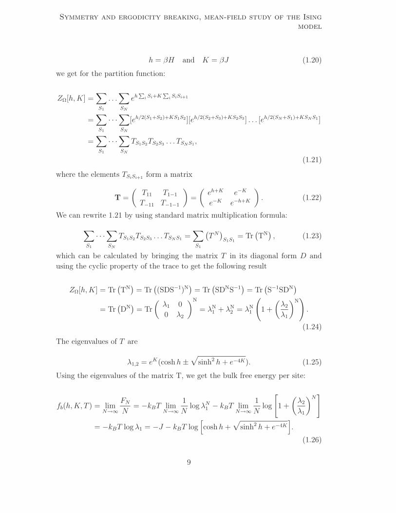
h = βH and K = βJ (1.20)
we get for the partition function:
ZΩ[h,K] =∑
S1
. . .∑
SN
ehP
i Si+KP
i SiSi+1
=∑
S1
· · ·∑
SN
[eh/2(S1+S2)+KS1S2 ][eh/2(S2+S3)+KS2S3 ] . . . [eh/2(SN+S1)+KSNS1 ]
=∑
S1
· · ·∑
SN
TS1S2TS2S3 . . . TSNS1 ,
(1.21)
where the elements TSiSi+1form a matrix
T =
(T11 T1−1
T−11 T−1−1
)=
(eh+K e−K
e−K e−h+K
). (1.22)
We can rewrite 1.21 by using standard matrix multiplication formula:
∑
S1
· · ·∑
SN
TS1S2TS2S3 . . . TSNS1 =∑
S1
(TN)S1S1
= Tr(TN), (1.23)
which can be calculated by bringing the matrix T in its diagonal form D and
using the cyclic property of the trace to get the following result
ZΩ[h,K] = Tr(TN)
= Tr((SDS−1)N
)= Tr
(SDNS−1
)= Tr
(S−1SDN
)
= Tr(DN)
= Tr
(λ1 0
0 λ2
)N
= λN1 + λN
2 = λN1
(1 +
(λ2
λ1
)N).
(1.24)
The eigenvalues of T are
λ1,2 = eK(coshh±√
sinh2 h+ e−4K). (1.25)
Using the eigenvalues of the matrix T, we get the bulk free energy per site:
fb(h,K, T ) = limN→∞
FNN
= −kBT limN→∞
1
Nlog λN1 − kBT lim
N→∞
1
Nlog
[1 +
(λ2
λ1
)N]
= −kBT log λ1 = −J − kBT log[coshh+
√sinh2 h+ e−4K
].
(1.26)
9
1.4 Solutions in one and more dimensions
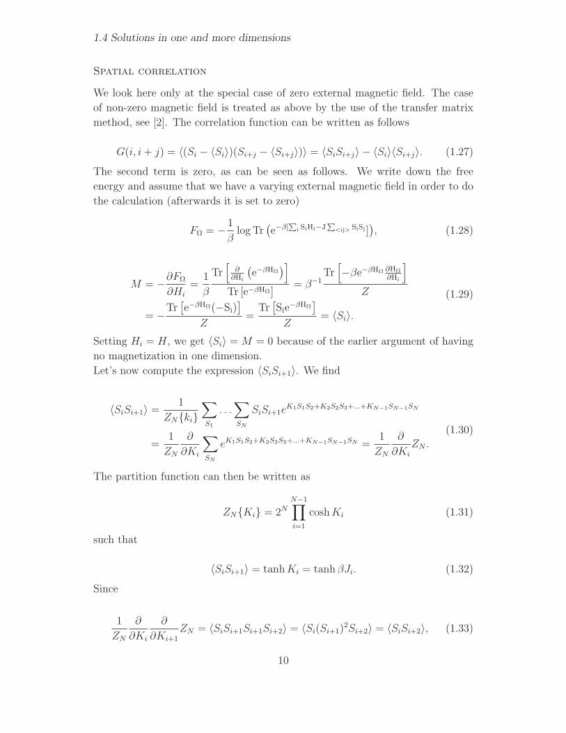
Spatial correlation
We look here only at the special case of zero external magnetic field. The case
of non-zero magnetic field is treated as above by the use of the transfer matrix
method, see [2]. The correlation function can be written as follows
G(i, i+ j) = 〈(Si − 〈Si〉)(Si+j − 〈Si+j〉)〉 = 〈SiSi+j〉 − 〈Si〉〈Si+j〉. (1.27)
The second term is zero, as can be seen as follows. We write down the free
energy and assume that we have a varying external magnetic field in order to do
the calculation (afterwards it is set to zero)
FΩ = − 1
βlog Tr
(e−β[
P
i SiHi−JP
<ij> SiSj ]), (1.28)
M = −∂FΩ
∂Hi
=1
β
Tr[
∂∂Hi
(e−βHΩ
)]
Tr [e−βHΩ ]= β−1
Tr[−βe−βHΩ ∂HΩ
∂Hi
]
Z
= −Tr[e−βHΩ(−Si)
]
Z=
Tr[Sie
−βHΩ]
Z= 〈Si〉.
(1.29)
Setting Hi = H, we get 〈Si〉 = M = 0 because of the earlier argument of having
no magnetization in one dimension.
Let’s now compute the expression 〈SiSi+1〉. We find
〈SiSi+1〉 =1
ZNki∑
S1
. . .∑
SN
SiSi+1eK1S1S2+K2S2S3+...+KN−1SN−1SN
=1
ZN
∂
∂Ki
∑
SN
eK1S1S2+K2S2S3+...+KN−1SN−1SN =1
ZN
∂
∂Ki
ZN .
(1.30)
The partition function can then be written as
ZNKi = 2NN−1∏
i=1
coshKi (1.31)
such that
〈SiSi+1〉 = tanhKi = tanhβJi. (1.32)
Since
1
ZN
∂
∂Ki
∂
∂Ki+1
ZN = 〈SiSi+1Si+1Si+2〉 = 〈Si(Si+1)2Si+2〉 = 〈SiSi+2〉, (1.33)
10

Symmetry and ergodicity breaking, mean-field study of the Isingmodel
where we have used S2i = 1, we can proceed by induction and obtain
G(i, i+ j) = 〈SiSi+j〉 =1
ZN
∂
∂Ki
∂
∂Ki+1
. . .∂
∂Ki+j−1
ZNKi
= tanhKi tanhKi+1 . . . tanhKi+j−1.
(1.34)
Setting all the Ki = K, we finally get the result:
G(i, i+ j) = (tanhK)j = e−j log (cothK). (1.35)
When - as we assumed - the Ki do not depend on i we obtain a translationally
invariant correlation function. For zero temperature the correlation function
equals one - a perfectly correlated state. By this result we also get an expression
for the correlation length which we expand for small T :
ξ =1
log (cothK)=
(log
eK + e−K
eK − e−K
)−1
=(log[1 + 2e−2K +O(e−4K)
])−1 ∼= 1/2 eJ/(kBT ).
(1.36)
This expression diverges for T → 0, as we expected from 1.12.
1.4.2 Onsager solution
One can apply the ideas of the transfer matrix method to the two-dimensional
case. As this procedure includes a rather tedious and long calculation we present
here only some ideas. The full calculation can be found in [3].
We describe a square lattice in two dimensions and write for the spin variables
in the α’s row
µα = s1, s2, . . . , snαth row. (1.37)
We suppose periodic boundary conditions:
sn+1 = s1 , µn+1 = µ1. (1.38)
We separate the energy terms belonging to the spin interactions in a row and
those belonging to row-row interactions as
E(µ) = −ǫn∑
k=1
sksk+1 (1.39)
11

1.4 Solutions in one and more dimensions
and
E(µ, µ′) = −ǫn∑
k=1
sks′k. (1.40)
The second one is only defined for nearest rows (nearest-neighbour interactions).
The partition function then reads
ZΩ[H = 0, T ] =∑
µie−β
Pnα=1[E(µα,µα+1)+E(µα)]
=∑
µi
n∏
α=1
e−β[E(µα,µα+1)+E(µα)] =∑
µi
n∏
α=1
〈µα|P |µα+1〉.(1.41)
Similarly to the transfer matrix method, we may think of P as some 2n × 2n
matrix. As before we can show by similar arguments that the knowledge of the
largest eigenvalue of P is enough for calculating the partition function:
ZΩ[H = 0, T ] =∑
µi〈µ1|P |µ2〉〈µ2|P |µ3〉 . . . 〈µn|P |µ1〉
=∑
µi〈µ1|P n|µ1〉 = TrP n =
2n∑
α=1
(λα)n.
(1.42)
For detailson the calculation of the eigenvalues λα see [3]. It is possible to show
that at large N ZΩ depends only on the largest eigenvalue λmax, i.e.
limN→∞
1
NlogZΩ = lim
n→∞
1
nlog λmax, (1.43)
where N = n2 is the number of sites. Then, the bulk free energy per site turns
out to be [3]
βfb[0, T ] = − log (2 cosh 2βǫ) − 1
2π
∫ π
0
dφ log
[1
2
(1 +
√1 − κ2 sin2 φ
)], (1.44)
where
κ = 2[cosh 2φ coth 2φ]−1 , kBTC = (2.269185)ǫ. (1.45)
For the specific heat near the transition temperature T ≃ TC one gets
12

Symmetry and ergodicity breaking, mean-field study of the Isingmodel
1
kBC[O, T ] ≈ 2
π
(2ǫ
kBTC
)2 [− log
∣∣∣∣1 − T
TC
∣∣∣∣+ log
(kBTC
2ǫ
)−(1 +
π
4
)], (1.46)
which fulfills no power-law, but just exhibits a logarithmical behaviour as |T −TC | → 0. The specific heat is continuous, the phase transition does not involve
latent heat.
The computation of the spontaneous magnetization is again rather complicated
and can be found in a paper by Yang [4]:
M [H = 0, T ] =
0 , T > TC1 − [sinh 2βǫ]−4 1
8 , T < TC(1.47)
1.4.3 Mean-field theory
Having discussed two exact solutions we now present an approximation method
which can be used to make model predictions in an arbitrary dimension for non-
zero external magnetic field.
Bulk free energy per site and spontaneous magnetization
Our starting point is again the Hamiltonian given by equation (1.14). The idea
of mean-field theory is to approximate the interactions between the spins by the
introduction of a mean-field due to neighbouring spins.
J∑
j n.n.
Sj = J∑
j n.n.
〈Sj〉 + J∑
j n.n.
(Sj − 〈Sj〉) ∼= J∑
j n.n.
〈Sj〉 = 2dJM, (1.48)
where the first term after the first equality sign describes the mean-field and the
second one describes the fluctuations in the mean-field which will be neglected.
In the following we introduce an effective external magnetic field Heff and can
easily calculate the partition function, the bulk free energy per site and the
magnetization:
ZΩ[H,T ] = (2 cosh βHeff )N = (2 cosh β[H + 2dJM ])N , (1.49)
fb[H,T ] = −kBT log (2 coshβ[H + 2dJM ]), (1.50)
M [H,T ] = −∂fb[H,T ]
∂H= tanh
H + 2dJM
kBT. (1.51)
13

1.5 Symmetry and ergodicity breaking
Therefore we got a formula determining M . As we look for spontaneous magne-
tization we want to solve the equation (setting H = 0)
M = tanh2dJM
kBT. (1.52)
If the slope of the tangens hyperbolicus at the point zero is greater than one, the
above equation has three possible solutions else only one possible solution. This
condition defines the critical temperature
TC =2dJ
kB. (1.53)
For T > TC the only solution is M = 0. However if T < TC the equation allows
two other non-zero solutions which describe spontaneous magnetization.
Critical exponents
For the calculation of the critical exponents one expands the formula (1.51) for
small H, M and uses the definition
τ =TCT. (1.54)
This leads to the formula
H
kBT= M(1 − τ) +M3(τ − τ 2 +
τ 3
3+ . . .) + . . . . (1.55)
From this we can easily get the desired critical exponents:
defining property critical exponent
H = 0 M ∼√
T−TC
TC∼ tβ β = 1
2
τ = 1 M ∼ H1/3 ∼ H1/δ δ = 3
M = 0 χ ∼ (T − TC)−1 ∼ t−γ γ = 1
1.5 Symmetry and ergodicity breaking
Having discussed some solution methods of the nearest-neighbour Ising model
we now analyse the model from some more general perception by looking at two
things: symmetry breaking in the Ising model and broken ergodicity. We will see
that broken symmetry is a special case of broken ergodicity.
14

Symmetry and ergodicity breaking, mean-field study of the Isingmodel
1.5.1 Broken symmetry
From the form of our Hamiltonian (1.14) it is obvious that for H = 0 (zero
magnetic field) the Hamiltonian has the symmetry
HΩ(−Si) = HΩ(Si), (1.56)
the time-reversal symmetry. It is broken in the thermodynamical limit as one
recognizes in the expression for the spontaneous magnetization:
M = 〈Si〉 6= 0. (1.57)
1.5.2 Broken ergodicity
The ergodic hypothesis predicts that the following two expressions are equal: the
time average of some quantity A
〈A〉ta := limt→∞
1
t
∫ t
0
dt′A(ηi(t′)), (1.58)
and its expectation value calculated with the Boltzmann distribution
〈A〉eqm := Tr [PΩ(ηi)A(ηi))]. (1.59)
Thus the ergodic hypothesis states
〈A〉ta = 〈A〉eqm. (1.60)
This means that for infinitely long time the system comes arbitrarily close to
every possible configuration described by the Boltzmann distribution.
Is the ergodic hypothesis fulfilled for our model? Let’s assume that the Boltzmann
factor describes the probability distribution in the thermodynamical limit. Then
one gets
M = 〈Si〉 = Tr[PΩ(Si)Si] = Tr[exp (−βHΩ(Si))
ZΩ[K]Si] = 0. (1.61)
This is because we sum over a symmetric and an antisymmetric summand. This
result contradicts to the calculated solutions with M 6= 0 (e.g. Onsager solution).
What went wrong? The reason is that the Boltzmann distribution is not valid
anymore in the thermodynamic limit. In order to keep the idea of the ergodic
hypothesis we need a new probability distribution in the thermodynamic limit as
it is done by the restricted ensemble presented in the next section.
15

1.5 Symmetry and ergodicity breaking
The restricted ensemble
The idea is to separate the phase space in components
Γ =⋃
α
Γα =⋃
α(Kn)Γα. (1.62)
We state to assumptions on this composition of the phase space:
1. Confinement: there is a cumulative probability for escape from some com-
ponent Γα : Pα.
2. If the system is confined to a component we can apply internal ergodicity
to it to get any expectation value of some quantities.
So we separate our phase space of the spin variables in our magnetic model system
in the following two components
Γ = Si ∈ Γ : M(Si) > 0 ∪ Si ∈ Γ : M(Si) < 0. (1.63)
A calculation in [2] shows that a measure for the transition probability is
(Pα)′ ∼ exp(−βN (d−1)/d
), (1.64)
which leads in the thermodynamic limit to
limN→∞
(Pα)′(N) =
6= 0 , for d = 1
0 , for d > 1.(1.65)
This shows that in the one-dimensional case the transition probability is non-zero:
we have to sum over all possible states (not the restricted states) and therefore get
by the argument 1.61 no spontaneous magnetization. For the other dimensions
the transition probability is zero and we can use the restricted ensemble to get
the prediction of spontaneous magnetization.
1.5.3 What is special about a broken symmetry?
Symmetry breaking implies ergodicity breaking. Ergodicity breaking does not
imply symmetry breaking. So broken symmetry is a special case of broken ergod-
icity. There are two properties which are only observed when broken ergodicity
is due to broken symmetry:
16

Symmetry and ergodicity breaking, mean-field study of the Isingmodel
1. Different components are mapped on each other by the symmetry mapping
which is broken: the time-reversal mapping (Si → −Si) maps states
of positive magnetization in one component to states of negative magneti-
zation in the other component.
2. We can introduce an order parameterM with three properties: |M | contains
the information of the amount of order, M/|M | = ±1, the “direction” of
the order parameter identifies the components and |M | → 0 for T ր TC ,
as it also observes in our analytical solutions.
1.6 Concluding remarks
Let us now compare the calculated critical exponents with experimental values.
1.6.1 Critical exponents in two dimensions
crit.exp. mean-field Onsager Rb2CoF∗4 Rb2MnF ∗
4
α 0(disc.) 0(log) ≃ 0.8 4.7 × 10⁻³
β 0.5 0.125 0.122 ± 0.008 0.17 ± 0.03
∗ values from [5]. Therefore two-dimensional magnetic system are realized in
nature.
1.6.2 Critical exponents in three dimensions
crit. exp. mean-field Monte Carlo∗∗ CrBr∗3 RbMnF ∗3
β 0.5 0.3258 ± 0.0044 0.368 ± 0.005 0.316 ± 0.008
δ 3 4.8030 ± 0.0558 4.28 ± 0.1
∗ from [5] and ∗∗ from [6]. The Monte-Carlo simulation gives the best theoretical
predictions for the critical exponents.
1.6.3 Concepts to remember
Phase transitions occur in the thermodynamical limit where we have to adapt
the Boltzmann distribution by the introduction of the restricted ensemble. The
broken symmetry in the Ising model is the time-reversal symmetry.
17

1.6 Concluding remarks
18

Bibliography
[1] J. Cardy, Scaling and Renormalization in Statistical Physics (Cambridge Uni-
versity Press, Cambridge, 1996).
[2] N. Goldenfeld, Lectures on phase transitions and the renormalization group
(Westview Press, Boulder, Colorado, 1992).
[3] K. Huang, Statistical Mechanics (John Wiley & Sons, New York, 1987).
[4] C. Yang, The spontaneous magnetization of a two-dimensional ising model,
Phys. Rev. 85, 808 (1952).
[5] L. J. De Jongh and A. R. Miedema, Experiments on simple magnetic model
systems, Adv.Phys. 23, 1 (1974).
[6] A. Ferrenberg and D. Landau, Critical behaviour of the three-dimensional
ising model: A high-resolution monte carlo study, Phys.Rev. B 44, 5081
(1991).
19

BIBLIOGRAPHY
20

Chapter 2
Critical Phenomena in Fluids
Severin Zimmermannsupervisor: Davide Batic
In this chapter, we discuss the critical phenomena at the liquid-
gas transition, with particular emphasis on the description given
by the Van der Waals equation. Furthermore we will calculate
some critical exponents and look at difficulties of measurements
near the critical point.
2.1 Repetition of the needed Thermodynam-
ics
2.1.1 Thermodynamic Potentials and their differen-
tials
The energy
E = E(S, V,N)
dE = TdS − pdV + µdN
The Helmholtz free energy
F = F (T, V,N) = E − TS
dF = −SdT − pdV + µdN
The Gibbs free energy
G = G(T, p,N) = F + pV = µN
21

2.1 Repetition of the needed Thermodynamics
dG = −SdT − V dp+ µdN
All these relations follow from the First Law of Thermodynamics, from them we
can read off thermodynamic identities and Maxwell-Relations.
2.1.2 Phase diagram
Phase diagram in the p-V plane
In this chapter we will only look at first order transitions, such as melting, va-
porizing etc.
From the extremal principle for the Gibbs free energy we know that the realized
phase is always the one with the lowest G. Therefore the coexistence line between
two phases indicates that GI = GII i.e. µI = µII .
Consider now the coexistence line between liquid and solid in the p - T plane:
Gl(T, p,N) = Gs(T, p,N)
Now we move along the line: T → T + δT , p → p + δp and expand G to first
order:
Gl,s(T + δT, p+ δp,N) = Gl,s|T,p +∂Gl,s
∂T
∣∣∣∣T,p
δT +∂Gl,s
∂p
∣∣∣∣T,p
δp
22

Critical Phenomena in Fluids
Using thermo-dynamical identities given by the differentials above we come to an
important consequence: the Clausius-Clapeyron relation.
dp
dT
∣∣∣∣transition
=Sl − SsVl − Vs
Normally ∂p∂T
> 0, because Vl > Vs and Sl < Ss. However there are exceptions
like H2O (Vl < Vs) due to hydrogen bonds and 3He (Sl > Ss) due to spin disorder
present in the solid phase.
From the Clausius-Clapeyron relation we also see that if Sl 6= Ss latent heat
will be released in this first order transition which corresponds to the chemical
enthalpie. If we get close to a critical point the latent heat will become vanishingly
small.
2.1.3 Landau’s Symmetry Principle
We saw in the phase diagram that two phases of matter must be separated by
a line of (first order) transitions due to the the fact that one can’t continuously
change symmetry. A symmetry is either present or absent.
The existence of the critical point on liquid gas transition line tells you that there
is no symmetry difference between those two phases.
2.2 Two-phase Coexistence
2.2.1 Fluid at constant pressure
If we keep the pressure in a fluid constant and apply heat, the liquid will start
expanding and at a certain temperature it will start boiling. During the boiling
the temperature remains constant while the volume increases. When all the
matter has become gaseous further heating will cause the gas to expand.
The whole process corresponds to moving along a horizontal line in the figure
below. During the entire time that the liquid is turned into gas the system remains
at the intersection point of the horizontal and the transition line, afterwards the
system will move again horizontally.
23

2.2 Two-phase Coexistence
Figure 2.2: Coexistence curve in the p - T plane
2.2.2 Fluid at Constant Temperature
If we look at isotherms in figure 2.3 we see that at T > Tc the isotherms are
well approximated by the ideal gas law (and small corrections). As T → T+c the
isotherms become flatter until they have a horizontal tangent at the top of the
two-phase region. At T < Tc as we move to the left (meaning: decreasing V and
increasing p) we will reach point A where we have equilibrium vapor pressure and
equilibrium volume vg(T ). Under further compression the gas starts condensing
at constant pressure. Eventually we reach point B where all gas is liquefied, then
the pressure will rise again.
24

Critical Phenomena in Fluids
Figure 2.3: Isotherms above and below the critical temperature
2.2.3 Maxwell’s Equal Area Rule
Figure 2.4: Maxwell’s equal area construction
Although model equations of state (like due to Van der Waals) are analytic
through the two-phase coexistence region. However isotherms exhibit a non-
analytic behavior at the boundaries of the two-phase region. This reflects that
the model equations of state can’t ensure that at the equilibrium state the Gibbs
free energy is globally minimized.
25

2.3 Van der Waals equation
So in the two-phase coexistence region the Gibbs free energy is the same for both
phases. An equivalent statement to this is that the chemical potentials are equal.
In addition to thermal equilibrium we also need mechanical equilibrium (which
implies that the pressure in the liquid phase is equal to the pressure in gas phase).
Hence the isotherm must be horizontal in the two-phase coexistence region.
dG = µdN +Ndµ
dµ =1
NdG− µ
NdN =
1
N(−SdT + V dp+ µdN) − µ
NdN
= − S
NdT +
V
Ndp
We can drop the dT because we are looking at isotherms, so dT = 0.
µl − µg =
∫ liq
gas
dµ =
∫ liq
gas
V
Ndp = 0
The geometrical interpretation of this is that the horizontal must be drawn such
that the two bounded areas sum to zero.
2.3 Van der Waals equation
If we look at an ideal gas we have the following equation:
pV = NkBT
Van der Waals made two significant changes to that equation. He introduced the
parameter a due to the attractive interaction between the atom and he introduced
the parameter b to take care of the hard-core potentials of atoms (atoms have a
non-zero radius). Van der Waals proposed the following equation:
p =NkBT
V −Nb− N2a
V
The parameter a and b can be determinated by fitting the equation to experi-
mental data (e.g. a = 3.45 kPa · dm6/mol2, b = 0.0237 dm3/mol for Helium)
2.3.1 Determination of the Critical Point
We can rewrite the Van der Waals equation to obtain a cubic polynomial for the
volume.
V 3 −(Nb+
NkBT
p
)V 2 +
N2a
pV − N3ab
p= 0
26

Critical Phenomena in Fluids
Solving this equation we get 2 imaginary and 1 real solution for T > Tc and 3
real solutions at T < Tc. Hence at T = Tc the three solutions merge and we get:
(V − Vc)3 = 0
By comparing the coefficients of these two cubic polynomials we get:
3Vc = Nb =NkBTcpc
; 3V 2c =
N2a
pc; V 3
c =N3ab
pc
this leads to
Vc = 3Nb; pc =a
27b2; kBTc =
8a
27b
Using a high temperature fit for a and b you can predict Tc, pc and Tc and get
quite good results, this theory also predicts an universal number.
pcVcNkBTc
=3
8
2.3.2 Law of Corresponding States
We can rescale the Van der Waals equation defining reduced pressure, volume
and temperature.
π =p
pc; ν =
V
Vc; τ =
T
Tc
This rescaling leads to: (π +
3
ν2
)(3ν − 1) = 8τ
This equation is called law of corresponding states. It is the same for all fluids
with no other parameter involved, so all properties which follow from this equa-
tion are universal.
Experimentally it’s also well-satisfied even for fluids which don’t obey the Van
der Waals equation.
2.3.3 Vicinity of the critical point/ critical exponents
Now we want to calculate some critical exponents of important quantities like
the specific heat CV ∝ |T − Tc|−α
the width of the two-phase coexistence region Vg − Vl ∝ |Tc − T |β
the compressibility kT = - 1V
(∂V∂p
)T∝ |T − Tc|−γ
and the shape of the critical isotherm |p− pc| ∝ |V − Vc|δ To calculate
27

2.3 Van der Waals equation
the exponent α we need the Helmholtz free energy due to the Van der Waals
equation:
p =∂F
∂V
F =
∫pdV =
∫ (NkBT
V −Nb− aN2
V 2
)dV
F = NkBT log(V −Nb) +aN2
V+ f(T )
CV = T∂S
∂T= T
∂2F
∂T 2
Now if we look at the free energy we see that CV depends just on the constant
of integration. Therefore it’s the same as for an ideal gas (a = 0, b = 0).
For an ideal gas we know that U = 32
NkBT due to Boltzmann, then the heat
capacity CV is given by:
CV dWV = Cideal
V =
(∂U
∂T
)
V
=3
2NkB
We see that CV does not diverge at the critical point and α = 0.
To calculate the exponent β we start with the law of corresponding states and
rewrite it using:
t ≡ τ − 1T − TcT
, φ ≡ ν − 1 =V − VcV
this leads to
π =8(1 + t)
3(1 + φ) − 1− 3
(1 + φ)2
Now we expand this equation using a Taylor series around the critical point (π
= τ = ν = 1).
π|t,φ=0+dπ
dt
∣∣∣∣t,φ=0
·t+ dπ
dφ
∣∣∣∣t,φ=0
·φ+d2π
dtdφ
∣∣∣∣t,φ=0
·tφ+1
2
d2π
dt2
∣∣∣∣t,φ=0
·t2+ 1
2
d2π
dφ2
∣∣∣∣t,φ=0
·φ2+...
Note that π ∝ t so all higher derivatives in t are zero and the first derivative in
φ is zero as well. Therefore we get:
1 + 4t− 6tφ− 3
2φ3 +O(tφ2, φ4)
We want to find the coexistence volumes Vl(p), Vg(p) or their corresponding
values φl and φg. Therefore we use Maxwell’s construction for a fixed t < 0 (T
< Tc) ∮V
Ndp = 0
28

Critical Phenomena in Fluids
and make a substitution due to π = ppc
dp = pc · dπ = pc
[−6t− 9
2φ2
]dφ
this leads to ∫ φg
φl
φ(−6t− 9
2φ2)dφ = 0
The function in the integral is odd in φ. Hence we conclude that φg = −φl,because the integral has to be zero for all values of t.
By going back to our expansion of the law of corresponding states we get
π = 1 − 4t− 6tφg −3
2φ3g
π = 1 − 4t− 6tφl −3
2φ3l = 1 − 4t+ 6tφg +
3
2φ3g
Now we subtract and get
φg = 2√−t
|φg − φl| = |2φg| ∝(Tc − T
Tc
) 12
⇒ β =1
2To calculate the critical exponent γ of the compressibility kT we start with the
definition and switch the derivatives.
kT = − 1
V
∂V
∂p= − 1
V
(∂p
∂V
)−1
Then we use the Van der Waals equation to get p(V) and calculate the derivative.
kT =1
V
(NkBT
(V −Nb)2− 2aN2
V 3
)−1
=V 2(V −Nb)2
NkBTV 3 − 2aN2(V −Nb)2
We want to look at the critical point so we use V = Vc = 3Nb
kT =36N4b4
27N4b3kBT − 8aN4b2=
36b2
27bkBT − 8a
=36b2/27bkB
T − 8a
27bkB︸ ︷︷ ︸Tc
29

2.4 Spatial correlations
Now we see that kT ∝ (T − Tc)−1, so γ = 1
As a result we know that the compressibility diverges at T → Tc which means
that the system becomes extremely sensitive to an applied pressure at the critical
point. As we approach the critical temperature the system is thermodynamically
unstable towards phase separation.
We can determine the shape of the critical isotherm by doing the same as for
the exponent β, but now we set t = 0 (T = Tc)
π = 1 − 3
2φ3
π − 1 =p− pcpc
= −3
2
(V − VcVc
)3
∝ (V − Vc)3 ⇒ δ = 3
2.4 Spatial correlations
In fluid the two point correlation function describes the statistical fluctuations in
the density.
We consider a volume of space V embedded in a bigger volume Ω. Then particles
of a fluid in Ω will wander through V and cause a number fluctuation in the
volume V. The mean Number of particles in V is given by:
〈N〉 = kBT∂logΞ
∂µ
∣∣∣∣T,V
= kBT1
Ξ
∂Ξ
∂µ
∣∣∣∣T,V
where Ξ is the trace of the grand partition function
Ξ = Tr(e−β(H−µN)
Similarly we define
⟨N2⟩≡ Tr
(N2e−β(H−µN)
Tr (e−β(H−µN)= kBT
1
Ξ
∂2Ξ
∂µ2
Now we can relate this to 〈N〉
1
β2
∂2logΞ
∂µ2=
1
β2
∂
∂µ
(1
Ξ
∂Ξ
∂µ
)=
1
β2
(− 1
Ξ2
(∂Ξ
∂µ
)2
+1
Ξ
∂2Ξ
∂µ2
)
=1
β2
1
Ξ
∂2Ξ
∂µ2− 〈N〉2
30

Critical Phenomena in Fluids
The fluctuation of N is given by
∆N2 =⟨N2⟩− 〈N〉2 =
1
β2
∂2logΞ
∂µ2
∣∣∣∣T,V
=1
β
∂
∂µ〈N〉
∣∣∣∣T,V
=kBT(∂µ∂N
)T,V
(∂µ∂N
)T,V
is not very useful so we try to express it in measurable quantities. We
do this by using Jacobians:
∂(u, v)
∂(x, y)= det
(∂u∂x
∂u∂y
∂v∂x
∂v∂y
)
∂µ
∂N
∣∣∣∣V,T
=∂(µ, V )
∂(N, V )=∂(µ, V )
∂(N, p)· ∂(N, p)
∂(N, V )=
(∂µ
∂N
∣∣∣∣p,T
∂V
∂p
∣∣∣∣N,T
− ∂µ
∂p
∣∣∣∣N,T
∂V
∂N
∣∣∣∣p,T
)(∂V
∂p
∣∣∣∣N,T
)−1
The first bracket can be simplified by using ∂µ∂N
∣∣p,T
= 0 for the first term and
the Maxwell-Relation ∂µ∂p
∣∣∣N,T
= ∂V∂N
∣∣T,p
for the second term. Whereas the second
bracket is related to the compressibility.
Finally we get:
∆N2 = kBTρ2V kT
2.4.1 Number fluctuations and the correlation func-
tion
The dimensionless two-point correlation function is given as
G(r − r′) =1
ρ2
(〈ρ(r), ρ(r′)〉 − ρ2
)
Here we expect two widely separated points to be uncorrelated (G(r − r′) → 0
as |r − r′| → ∞ )
We perform an integration to write
∫ddrddr′G(r − r′) =
1
ρ2
(⟨N2⟩− 〈N〉2
)
= kBTV kT
On the other hand we have translational invariance for our two-point correlation
function which implies
∫ddrddr′G(r − r′) = V
∫ddrG(r)
31
2.5 Determination of the critical point/ difficulties in measurement
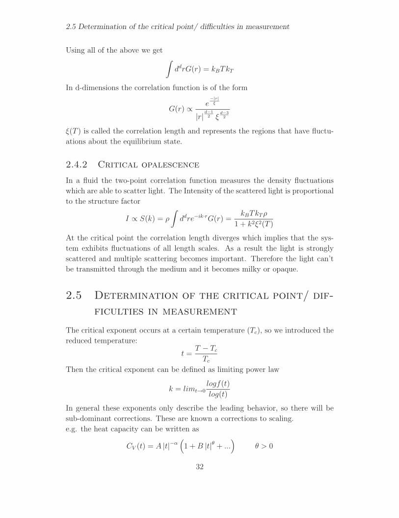
Using all of the above we get∫ddrG(r) = kBTkT
In d-dimensions the correlation function is of the form
G(r) ∝ e−|r|
ξ
|r| d−12 ξ
d−32
ξ(T ) is called the correlation length and represents the regions that have fluctu-
ations about the equilibrium state.
2.4.2 Critical opalescence
In a fluid the two-point correlation function measures the density fluctuations
which are able to scatter light. The Intensity of the scattered light is proportional
to the structure factor
I ∝ S(k) = ρ
∫ddre−ik·rG(r) =
kBTkTρ
1 + k2ξ2(T )
At the critical point the correlation length diverges which implies that the sys-
tem exhibits fluctuations of all length scales. As a result the light is strongly
scattered and multiple scattering becomes important. Therefore the light can’t
be transmitted through the medium and it becomes milky or opaque.
2.5 Determination of the critical point/ dif-
ficulties in measurement
The critical exponent occurs at a certain temperature (Tc), so we introduced the
reduced temperature:
t =T − TcTc
Then the critical exponent can be defined as limiting power law
k = limt→0logf(t)
log(t)
In general these exponents only describe the leading behavior, so there will be
sub-dominant corrections. These are known a corrections to scaling.
e.g. the heat capacity can be written as
CV (t) = A |t|−α(1 +B |t|θ + ...
)θ > 0
32

Critical Phenomena in Fluids
These corrections vanish at the critical point, but they can make a significant
difference for |t| > 0. If we want reliable values for the actual critical exponents
in practise those corrections can’t be neglected.
There are also other constants of proportionality
CV (t) =At−α t > 0A′(−t)−α′
t < 0
A, A’ are called critical amplitudes and α, α′ are called critical exponents. The
exponents are the same above and beneath the critical temperature (α = α′), but
the amplitudes are different for both sides. However the ratio AA′ is universal.
2.5.1 Measurement
It’s actually quite difficult to measure critical exponents for various reasons.
Suppose we want to measure CV (T ) to read off α. Theoretically it can be plotted
versus the reduced temperature t to read off α, practically CV is measured by
putting ∆E into the system and measuring the change ∆T. This works rather
fine in areas which aren’t too close to the critical temperature. |t| >> δTTc
(where
δT is the limiting sensitivity), so we require very high resolution thermometry if
we want to go close to the critical temperature. Today one uses paramagnetic
salt (e.g. GdCl3) or alloys (e.g. Pd(Mn)) because they have a sub-nanokelvin res-
olution. Another problem is the background, in addition to the critical behavior
there is normally a slightly varying background which has no singular behavior
at Tc. So we need to subtract it to determine the critical exponent, this requires
curve fitting.
Other problems are impurity effects or the finite size of the system which causes
a rounding of the divergence.
The last big problem is called critical slowing down. As T → Tc it takes longer
and longer for the system to equilibrate. At the critical point the correlation
length diverges, so the regions, which show fluctuations about the equilibrium
state get bigger and bigger. Therefore the system takes longer to relax (the
relaxation time diverges).
33

2.5 Determination of the critical point/ difficulties in measurement
34
Bibliography
[1] N. Goldenfeld, Lectures on Phase Transitions and the Renormalization Group
(Westview Press, New York, 1992).
[2] H. E. Stanley, Introduction to Phase Transitions and Critical Phenomena
(Clarendon Press, Oxford, 1971).
35

BIBLIOGRAPHY
36

Chapter 3
Landau Theory, Fluctuations
and Breakdown of Landau
Theory
Raphael Honeggersupervisor: Dr. Andrey Lebedev
Describing phase transitions of second order with an order param-
eter, that is zero for the phase of higher symmetry and growing
continuously in the other phase, one could expand the free energy
about the critical point in a power series in this order parame-
ter. This somehow doesn’t seem to make much sense, because we
know, that at the critical point, we don’t find analytic behavior,
which is the requirement for such an expansion. However, we will
show, that assuming the existence of such a power series, makes
us able to qualitatively calculate the behavior of thermodynamic
quantities near the critical point.
3.1 Introduction
3.1.1 Second Order Phase Transitions
Because of their different behavior in the change of symmetry, we distinguish
between different types of phase transitions. First order phase transitions are the
ones, we encounter every day, as for example when boiling or freezing water. The
important property of such phase transitions is, that the transition occurs as an
abrupt change in symmetry.
37

3.1 Introduction
On the other hand, second order phase transitions have the property, that the
symmetry is changed in a continuous way. As example, we could think of a
body center cubic lattice, where at a certain critical temperature, the centered
particle starts to move towards one of the corners. As soon as this particle isn’t
placed anymore in the middle of the cube, the body center cubic symmetry is
broken and the lattice has to be described by another symmetry. While in this
case, the displacement of the centered particle is a continuous function of the
temperature, there can’t be found such a continuous parameter when melting ice
or boiling water (or any other substance).[1]
3.1.2 Order Parameter
As described before, a second order phase transition is connected with a con-
tinuous change of symmetry. Besides the change of the relative positions in a
lattice, this could also be the probability of finding one kind of atom at a given
lattice position or the magnetization in a ferromagnet or something else. It then
is sensible to introduce a parameter η, called the order parameter, that describes
this continuous change of symmetry in the following way:
• η is zero for the phase of higher symmetry,
• η takes non-zero values (positive or negative) for the “asymmetric” phase,
• for second order phase transitions, η is a continuous function of tempera-
ture.
3.1.3 Bragg-Williams Theory
Before we get to the concept of Landau Theory, we discuss a simplified version of
the Ising model, that somehow might give us an idea of why expanding the free
energy in a power series in the order parameter makes sense.
In the Ising Model, the internal Energy U = 〈H〉 is assumed to be of the form
U = 〈H〉 =∑
i
HiSi −∑
i,j
JijSiSj −∑
i,j,k
KijkSiSjSk − ... (3.1)
where Si = ±1 represents the spin at lattice site i and Hi, Jij, Hijk, ... are the
spin interaction constants. In Bragg-Williams Theory we assume, that all the
spin interaction constants besides the Jij are zero. Furthermore, we assume that
only nearest neighbor sites interact with each other and this in the same way. As
additional simplification, we replace the Si by their position independent average
38

Landau Theory, Fluctuations and Breakdown of Landau Theory
m = 〈S〉 =: η, which will be the order parameter. Then we can write the internal
energy as
U = −J∑
〈i,j〉η2 = −J Nzη
2
2(3.2)
denoting with 〈i, j〉 the sum over nearest neighbors and therefore with z the
number of nearest neighbor sites.
The entropy for a given η = m is the logarithm of the number of configurations
with a given number N↑ of sites with spin up and N↓ of sites with spin down
S = ln
(N
N↑
)= ln
(N !
(N(1 + η)/2)!(N(1 − η)/2)!
)(3.3)
where we used that η = (N↑ − N↓)/N and N↓ = N − N↑. Using Sterling’s
Approximation for large N
ln(N !) ≈ N(ln(N) − 1) (3.4)
wo obtain
S ≈ N
(ln(2) − 1 + η
2ln (1 + η) − 1 − η
2ln (1 − η)
)(3.5)
For small η, we expand in powers of η, to get
S
N≈ ln(2) − 1
2η2 − 1
12η4 − ... (3.6)
Now, we are ready to write down the Bragg-Williams free energy density per site
F (T, η)
N=
U − TS
N= −T ln(2) +
1
2(T − Tc) η
2 +1
12Tη4 + ... (3.7)
Here we set zJ =: Tc, the transition temperature. The reason why we did this is,
that minimizing F (T, η)/N with respect to η leads exactly to the conditions for
the order parameter described above, if we take Tc as critical temperature. That
means, for T > Tc, we have a minimum at η = 0, which corresponds to the phase
of higher symmetry. For T < Tc however, we get a maximum at η = 0 and two
equivalent minima at η 6= 0, which corresponds to the low symmetry phase.
Looking at the Bragg-Williams free energy, generalizing the idea of expanding
the free energy in a power series in η doesn’t look so strange anymore and that’s
exactly what’s done in Landau Theory.[2]
39
3.2 Landau Theory
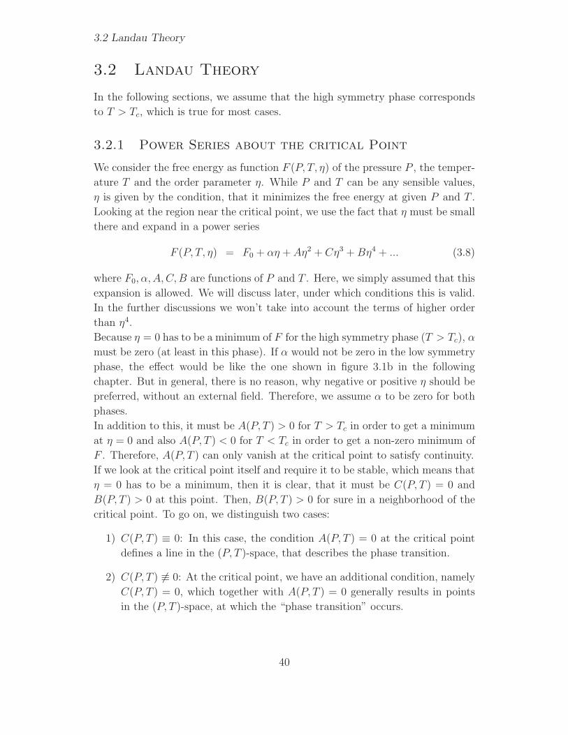
3.2 Landau Theory
In the following sections, we assume that the high symmetry phase corresponds
to T > Tc, which is true for most cases.
3.2.1 Power Series about the critical Point
We consider the free energy as function F (P, T, η) of the pressure P , the temper-
ature T and the order parameter η. While P and T can be any sensible values,
η is given by the condition, that it minimizes the free energy at given P and T .
Looking at the region near the critical point, we use the fact that η must be small
there and expand in a power series
F (P, T, η) = F0 + αη + Aη2 + Cη3 +Bη4 + ... (3.8)
where F0, α, A,C,B are functions of P and T . Here, we simply assumed that this
expansion is allowed. We will discuss later, under which conditions this is valid.
In the further discussions we won’t take into account the terms of higher order
than η4.
Because η = 0 has to be a minimum of F for the high symmetry phase (T > Tc), α
must be zero (at least in this phase). If α would not be zero in the low symmetry
phase, the effect would be like the one shown in figure 3.1b in the following
chapter. But in general, there is no reason, why negative or positive η should be
preferred, without an external field. Therefore, we assume α to be zero for both
phases.
In addition to this, it must be A(P, T ) > 0 for T > Tc in order to get a minimum
at η = 0 and also A(P, T ) < 0 for T < Tc in order to get a non-zero minimum of
F . Therefore, A(P, T ) can only vanish at the critical point to satisfy continuity.
If we look at the critical point itself and require it to be stable, which means that
η = 0 has to be a minimum, then it is clear, that it must be C(P, T ) = 0 and
B(P, T ) > 0 at this point. Then, B(P, T ) > 0 for sure in a neighborhood of the
critical point. To go on, we distinguish two cases:
1) C(P, T ) ≡ 0: In this case, the condition A(P, T ) = 0 at the critical point
defines a line in the (P, T )-space, that describes the phase transition.
2) C(P, T ) 6≡ 0: At the critical point, we have an additional condition, namely
C(P, T ) = 0, which together with A(P, T ) = 0 generally results in points
in the (P, T )-space, at which the “phase transition” occurs.
40

Landau Theory, Fluctuations and Breakdown of Landau Theory
It is only the first case, we’re interested in. That’s why we assume C(P, T ) ≡ 0
and therefore write the free energy as
F (P, T, η) = F0(P, T ) + A(P, T )η2 +B(P, T )η4 (3.9)
If A(P, T ) has no singularity at the transition point, we can expand it in terms
of (T − Tc), at least in a region of the critical point Tc = Tc(P ). Near the critical
point, we can then write
F (P, T, η) = F0(P, T ) + a(P )(T − Tc)η2 +B(P )η4 (3.10)
where we assumed, that we can write B(P, T ) ∼ B(P, Tc) = B(P ).
This is the form of the free energy, with which we can predict qualitatively the
behavior of thermodynamic quantities near the critical point. But first we want
to describe what happens, if we apply an external field.[1]
3.2.2 External Field
If we apply a small external field h, which could be a magnetic field for a ferro-
magnet, we have to apply in first order approximation a term of the form −ηhVin equation (3.10). That is
Fh(P, T, η) = F0(P, T ) + a(P )tη2 +B(P )η4 − ηhV (3.11)
where we replaced t := (T − Tc(P )). Even if the field h is small, but non-zero,
the Minimum in η will be non-zero, to minimize F .[1]
3.2.3 The Minima
Lets go one step further and explicitly discuss the minima of the free energy
without (3.10) and with an external field (3.11).
For T ≥ Tc, by definition, the free energy (3.10) has a single minimum at η = 0.
As soon as T gets smaller than Tc, η = 0 will be a maximum and the two
equivalent minima can be obtained by requiring the derivative to be zero
∂F (P, T, η)
∂η= (2a(P )t+ 4B(P )η2)η = 0 (3.12)
So, we have two minima at
η = ±√
a
2B(Tc − T ) (3.13)
41
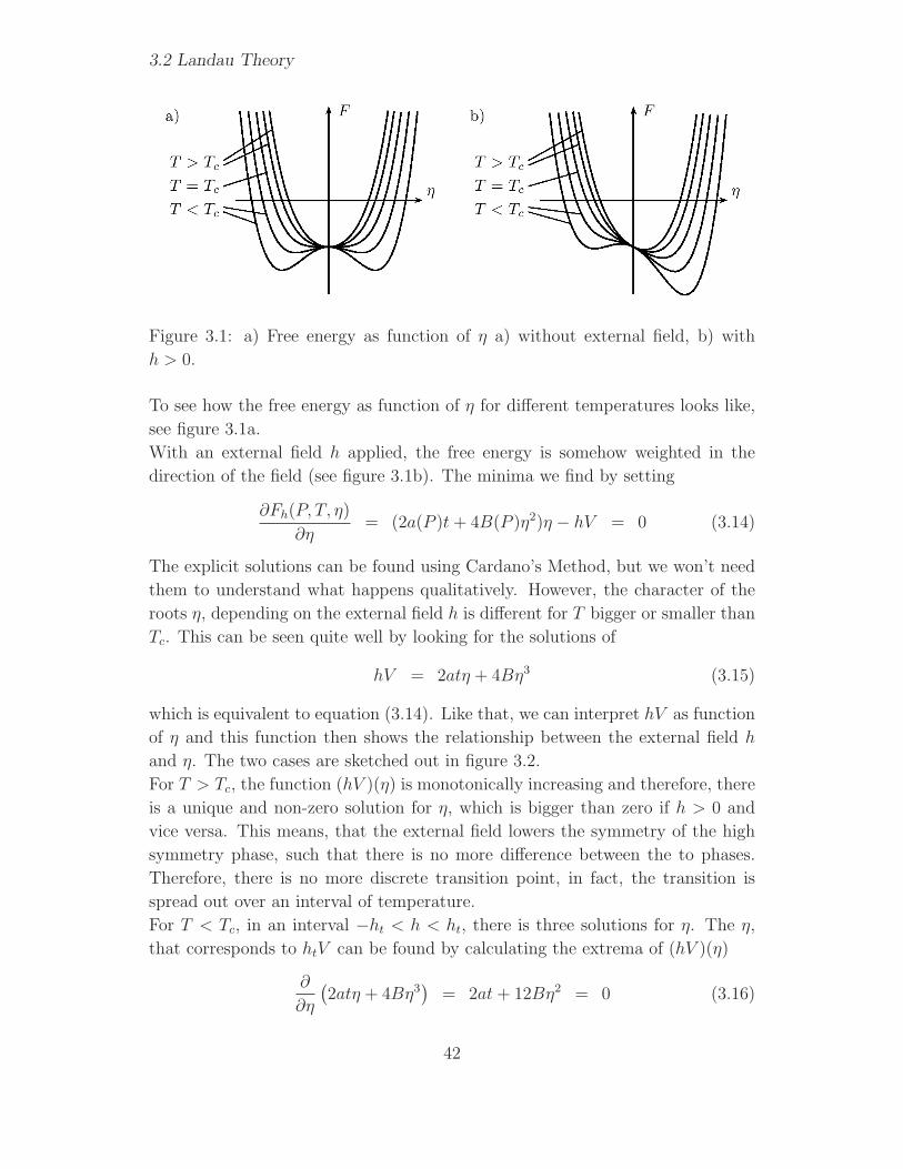
3.2 Landau Theory
Figure 3.1: a) Free energy as function of η a) without external field, b) with
h > 0.
To see how the free energy as function of η for different temperatures looks like,
see figure 3.1a.
With an external field h applied, the free energy is somehow weighted in the
direction of the field (see figure 3.1b). The minima we find by setting
∂Fh(P, T, η)
∂η= (2a(P )t+ 4B(P )η2)η − hV = 0 (3.14)
The explicit solutions can be found using Cardano’s Method, but we won’t need
them to understand what happens qualitatively. However, the character of the
roots η, depending on the external field h is different for T bigger or smaller than
Tc. This can be seen quite well by looking for the solutions of
hV = 2atη + 4Bη3 (3.15)
which is equivalent to equation (3.14). Like that, we can interpret hV as function
of η and this function then shows the relationship between the external field h
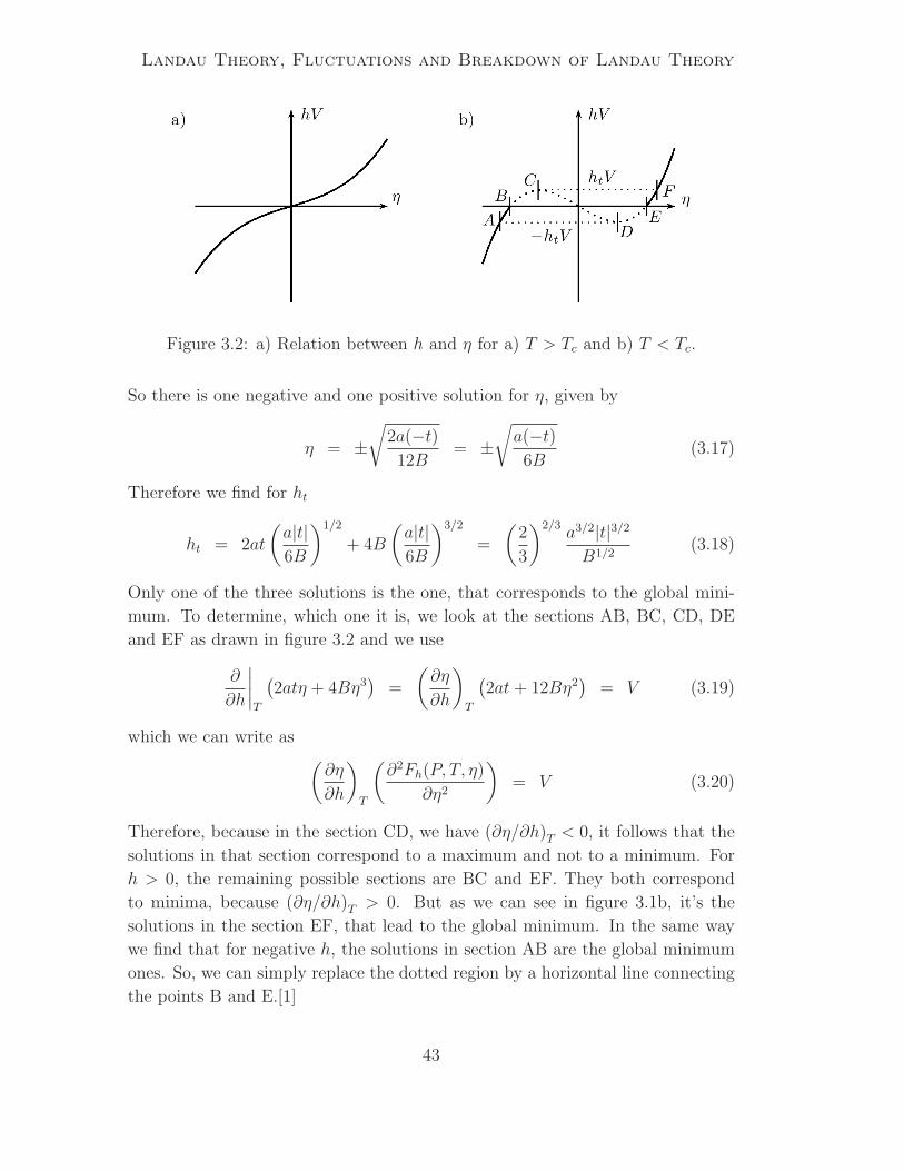
and η. The two cases are sketched out in figure 3.2.
For T > Tc, the function (hV )(η) is monotonically increasing and therefore, there
is a unique and non-zero solution for η, which is bigger than zero if h > 0 and
vice versa. This means, that the external field lowers the symmetry of the high
symmetry phase, such that there is no more difference between the to phases.
Therefore, there is no more discrete transition point, in fact, the transition is
spread out over an interval of temperature.
For T < Tc, in an interval −ht < h < ht, there is three solutions for η. The η,
that corresponds to htV can be found by calculating the extrema of (hV )(η)
∂
∂η
(2atη + 4Bη3
)= 2at+ 12Bη2 = 0 (3.16)
42
Landau Theory, Fluctuations and Breakdown of Landau Theory
Figure 3.2: a) Relation between h and η for a) T > Tc and b) T < Tc.
So there is one negative and one positive solution for η, given by
η = ±√
2a(−t)12B
= ±√a(−t)6B
(3.17)
Therefore we find for ht
ht = 2at
(a|t|6B
)1/2
+ 4B
(a|t|6B
)3/2
=
(2
3
)2/3a3/2|t|3/2B1/2
(3.18)
Only one of the three solutions is the one, that corresponds to the global mini-
mum. To determine, which one it is, we look at the sections AB, BC, CD, DE
and EF as drawn in figure 3.2 and we use
∂
∂h
∣∣∣∣T
(2atη + 4Bη3
)=
(∂η
∂h
)
T
(2at+ 12Bη2
)= V (3.19)
which we can write as(∂η
∂h
)
T
(∂2Fh(P, T, η)
∂η2
)= V (3.20)
Therefore, because in the section CD, we have (∂η/∂h)T < 0, it follows that the
solutions in that section correspond to a maximum and not to a minimum. For
h > 0, the remaining possible sections are BC and EF. They both correspond
to minima, because (∂η/∂h)T > 0. But as we can see in figure 3.1b, it’s the
solutions in the section EF, that lead to the global minimum. In the same way
we find that for negative h, the solutions in section AB are the global minimum
ones. So, we can simply replace the dotted region by a horizontal line connecting
the points B and E.[1]
43

3.3 Fluctuations
3.2.4 Critical Behavior
The Entropy near the critical point is given by
S = −∂F (P, T, η)
∂T= S0 −
∂A(P, T )
∂Tη2 (3.21)
where we used that in equilibrium, ∂F∂η
= 0. Using (3.13), we get
S =
S0 + a2
2B(T − Tc), T < Tc
S0, T > Tc(3.22)
We can see that the entropy is a continuous function. Using Maxwell’s relations,
we can now calculate the specific heat for constant pressure
CP = T
(∂S
∂T
)
P
=
CP0 + a2
2BT, T < Tc
CP0, T > Tc(3.23)
So Landau Theory predicts a discontinuity in CP at T = Tc, namely a negative
jump of (a2Tc/2B). Similar results we can find for quantities like the heat capacity
at constant volume V , the coefficient of thermal expansion or the compressibility.
And in fact, such discontinuities have been measured in nature.
With equation (3.19), we find for the susceptibility
χ :=
(∂η
∂h
)
T ;h→0
= limh→0
V
2at+ 12Bη2(3.24)
Using limh→0 η2 = 0 for T > Tc and equation (3.13), we get
χ =
V
2a(T−Tc), T > Tc
V4a(Tc−T )
, T < Tc(3.25)
This result can be explained by looking at figure 3.1a. The minima of the free
energy curve get very flat, the closer we get to the critical temperature. A small
perturbation of the equilibrium then results in a big change in η.[1]
3.3 Fluctuations
3.3.1 Fluctuations in the Order Parameter
So far, we assumed the order parameter to be spatially uniform, that is indepen-
dent of the position r. More realistic is the case, in which we allow at least small
deviations from the equilibrium value η. The work, which is needed to bring
44

Landau Theory, Fluctuations and Breakdown of Landau Theory
a system out of equilibrium at given pressure P and temperature T is just the
change of the free energy ∆F . Therefore, the probability ω for a fluctuation for
constant P and T is given with the Gibbs distribution
ω ∼ e− ∆F
kBT (3.26)
For small deviations from the equilibrium value η, we use that (∂F/∂η)η=η = 0
and write
∆F =1
2(η − η)2
(∂2F
∂η2
)
P,T
(3.27)
Using the definition of the susceptibility (3.24) and equation (3.20), we get for
temperatures T ∼ Tc
ω ∼ e− (η−η)2V
2χkBTc ⇒⟨(∆η)2
⟩=
kBTcχ
V(3.28)
which is a Gaussian distribution with the mean square fluctuation 〈(∆η)2〉. From
(3.25) we see that χ goes like 1/t as T → Tc, so 〈(∆η)2〉 also goes like 1/t for
T → Tc, which means that the fluctuations grow anomaly much near the critical
point. So, the actual critical behavior of the free energy potential at the critical
point is due to the already discussed flat minima of F .[1]
For an inhomogeneous body, we have to introduce the free energy density F ,
where F =∫Fdr. We use the expansion (3.11) as for F , just with the coefficients
divided by the volume V and add the spacial derivatives, such that changes in the
free energy due to deviations from the equilibrium value are considered. Assuming
that we have only fluctuations with long wave length, it is enough to add terms
up to second derivatives, that is terms proportional to
∂η
∂xi, η
∂η
∂xi, η
∂2η
∂xi∂xk,
∂η
∂xi
∂η
∂xk(3.29)
By integrating over the volume, the first two terms transform to surface effects,
which we’re not interested in and the third term reduces to the form of the fourth
term, just by integrating by parts. Therefore, we can write the additional terms
in the form
gik(P, T )∂η
∂xi
∂η
∂xk(3.30)
In the following, we will use the simplification gik = gδik. Finally, we write the
free energy density as
F(P, T, η) = F0(P, T ) + αtη2 + bη4 + g
(∂η
∂r
)2
− ηh (3.31)
45

3.3 Fluctuations
where η ≡ η(r) and α = a/V , b = B/V with the coefficients a,B from expansion
(3.11). The coefficient g must be bigger than zero in order to make sure that the
non-fluctuating case is the energetically most favorable.[1]
3.3.2 The Correlation Radius
We have to use some concepts of Statistical Mechanics. We use that the Helmholz
free energy is given by
A = −kBT ln [Z(h(r))] (3.32)
where Z(h(r)) is the partition function, given by
Z(h(r)) = Tr exp
[− 1
kBT
(H(η(r)) −
∫ddrh(r)η(r)
)](3.33)
whereH(η(r)) is the part of the Hamiltonian, that doesn’t depend on the external
field h(r) and d is the dimension of the system. The expectation value of η(r)
then can be obtained by the functional derivative
〈η(r)〉 = − δA
δh(r′)= lim
ε→0
A(h(r) + εδ(r − r′)) − F (h(r))
ε(3.34)
We then define the generalized isothermal susceptibility
χT (r, r′) =δ 〈η(r)〉δh(r′)
(3.35)
To find the relation
χT (r, r′) = − δ2A
δh(r)δh(r′)
= kBT
(1
Z
δ2Z
δh(r)δh(r′)− 1
Z
δZ
δh(r)· 1
Z
δZ
δh(r′)
)
=1
kBT(〈η(r)η(r′)〉 − 〈η(r)〉 〈η(r′)〉)
=1
kBTG(r, r′) (3.36)
where G(r, r′) is the correlation function. Now we take the functional derivative
of the Landau free energy and require it to be zero, that means, we require it to
be stationary
δF
δη(r)= 2αtη(r) + 4bη3(r) + 2g∇2η(r) − h(r) = 0 (3.37)
46

Landau Theory, Fluctuations and Breakdown of Landau Theory
This differential equation has to be satisfied by the expectation value 〈η(r)〉,because the Trace, with which the expectation value is calculated, is nothing else
than the functional integral over all possible η(r) that satisfy equation (3.37).
If we now substitute η(r) in equation (3.37) with this expectation value 〈η(r)〉and use the definition of the generalized isothermal susceptibility χT (3.35), we
obtain
(2αt+ 12bη2(r) − 2g∇2
)χT (r, r′) − δ(r − r′) = 0 (3.38)
With equation (3.36) we then find for the correlation function
1
kBT
(2αt+ 12bη2(r) − 2g∇2
)G(r − r′) = δ(r − r′) (3.39)
where we assumed that we have a translationally invariant system and therefore
wrote G(r, r′) = G(r − r′). With equation (3.39), we see that G(r − r′) actually
is a Green’s Function. To calculate it, we go back to the case where we have a
spatially uniform η and use the equilibrium values for h = 0, we calculated in the
last chapter (that is η2 = 0 for t > 0 and η2 = −at/2b for t < 0). This leads to
the new equation
(1
ξ2(t)−∇2
)G(r − r′) =
kBT
2gδ(r − r′) (3.40)
where we introduced the temperature dependent quantity
ξ(t) =
(gαt
)1/2T > Tc(
g2α(−t)
)1/2
T < Tc(3.41)
To resolve this, we use the Fourier Transform which makes us able to write
G(k) =kBT
2g
1
k2 + ξ−2(3.42)
That is simply the Fourier Transform of the Yukawa Potential, multiplied by
kBT/8πg. It follows directly
G(r) =kBT
8πg
e−rξ
r(3.43)
This is why we call ξ(t) the correlation length. It gives the order of magnitude,
at which the fluctuations fall off.[3]
47

3.3 Fluctuations
3.3.3 The Ginzburg Criterion
The criterion for Landau Theory to be valid is that the mean square fluctuation
of the order parameter, averaged over the correlation volume ξ3, is small with
respect to the characteristic value given by (3.13). That is
kBTcχ
ξ3≪ α|t|
2b(3.44)
Using the calculation for χ (3.25) and the correlation radius ξ (3.39), wo obtain
the Ginzburg Criterion
α|t| ≫ kBT2c b
2
g3(3.45)
While we built up our theory, we assumed that we can expand in terms of t. So
we require t to be small with respect to Tc as well. If we apply this property to
(3.45), we get the validity condition
k2BTcb
2
αg3≪ 1 (3.46)
Only if (3.46) is valid, there exists a temperature interval at which Landau Theory
can be applied. From (3.45) we see, that the theory, that was built up for
temperatures near the critical temperature Tc, so for small |t|, is not valid for
small |t|! We expect the right-hand side of (3.45) to be small, such that Landau
Theory can be applied for small |t|, but not for very small |t|. There is always a
region near the critical temperature, the fluctuation region, at which the theory
is not valid.[1]
3.3.4 Landau Theory in higher Dimensions
As we derived the correlation length ξ(t) for any dimension d, we can also refor-
mulate the Ginzburg criterion for this dimension. We take
Tcχ
ξ3≪ α|t|
2b→ Tcχ
ξd≪ α|t|
2b(3.47)
which, replacing χ and ξ as before, leads to
b
gd/2kBTc (α|t|)d/2−2 ≪ 1 (3.48)
This condition is always satisfied for temperatures near the critical point, if d >
4 and it can be satisfied for d = 4. In fact, the case d = 4 can be used to
approximate real systems of dimension d = 3.[4]
48

Landau Theory, Fluctuations and Breakdown of Landau Theory
3.4 Conclusive Words
We started with Bragg-Williams Theory, a very simplified version of the Ising
Model, to make an example of a case, where it makes sense to expand the free
energy in a potential series in the order parameter. We then generalized this idea
and derived the Landau free energy, applying phenomenological properties. Only
by leaving mean field theory and considering fluctuations in the order parameter,
we could find a criterion for Landau theory to be valid, the Ginzburg criterion.
We found that due to the flatness of the free energy near the critical point, the
fluctuations grow up to infinity. That’s why Landau theory, at least in 3 dimen-
sions, can’t be valid for temperatures very close to the critical point. Because of
this effect, Landau theory makes quantitatively wrong predictions, like for exam-
ple for the critical indices, but it describes the phase transitions very well in a
phenomenological way.
49

3.4 Conclusive Words
50

Bibliography
[1] L. D. Landau and E. M. Lifschitz, Lehrbuch der theoretischen Physik, Statis-
tische Physik (Akademie-Verlag Berlin, Berlin, Leipziger Strasse 3-4, 1979).
[2] P. M. Chaikin and T. C. Lubensky, Principles of Condensed Matter Physics
(Cambridge University Press, 2000).
[3] N. D. Goldenfeld, Lectures on Phase Transitions and the Renormalisation
Group (Addison-Wesley, 1992).
[4] T. Fließbach, Statistische Physik, Lehrbuch zur Theoretischen Physik IV
(Spektrum Akademischer Verlag, Heidelberg, 2007).
51

BIBLIOGRAPHY
52

Chapter 4
Scaling theory
Roger Herrigelsupervisor: Helmut Katzgraber
Near the critical temperature of a continuous phase transition the
singularity of the thermodynamic quantities, such as the specific
heat or the magnetization are controlled by critical exponents.
These exponents are not independent of each other. In this chap-
ter we show, that only two critical exponents are independent and
the rest can be derived from scaling relations. Furthermore, we
study polymer statistics and see that the above exponents also
describe the behavior of the spatial extent of a chain-molecule.
4.1 Critical exponents
We define the reduced temperature t and the reduced external magnetic field h,
which are dimensionless quantities via:
t =T − TcTc
h =H
kBTc. (4.1)
The critical exponent λ of a function f(t) is defined as
λ = limt→0
ln f(t)
ln t(4.2)
Thus the function f(t) near the critical temperature TC is dominated by tλ. For
a magnetic system the critical exponents are listed in Table 4.1.
In principle, we should consider two different exponents α for t > 0 and α′ for
t < 0. Likewise for the exponents γ and ν. But we show that α = α′ and we
53

4.2 Scaling hypothesis
Exponent Definition Description
α CH ∼ |t|−α specific heat at H = 0
β M ∼ |t|β magnetization at H = 0, t < 0
γ χ ∼ |t|−γ isothermal susceptibility at H = 0
δ M ∼ h1δ critical isotherm
ν ξ ∼ |t|−ν correlation length
η G (r) ∼ |r|−(d−2+η) correlation function
Table 4.1: Critical exponents of a magnetic system
will therefore not distinguish between them. The amplitudes, however, are not
necessarily the same, in general if cH ∼ A|t|α then A 6= A′.
There are exponent inequalities which follow from fundamental thermodynamic
considerations. One example is the Rushbrooke inequality [1]:
α+ 2β + γ ≥ 2. (4.3)
Using the scaling hypothesis in the next section we show that these inequalities
are in fact equalities.
4.2 Scaling hypothesis
4.2.1 Definition of a homogeneous function
A function f(r) is homogeneous if for all values of λ
f(λr) = g(λ)f(r) (4.4)
g(λ) is called the scaling function which must be of the form g(λ) = λp.
In n dimensions the variables may scale with different factors. Therefore we
define the generalized homogeneous function by the condition
λf(x, y) = f(λax, λby) ⇔ λcf(x, y) = f(λax, λby). (4.5)
4.2.2 Scaling hypothesis
The scaling hypothesis states that the singular part of the free energy density
f(t, h) is a homogeneous function near a second-order phase transition. Further-
more, the reduced temperature t and the order parameter h rescale by different
factors:
54

Scaling theory
f(t, h) = b−df(bytt, byhh). (4.6)
A short calculation shows that if f(t, h) is a generalized homogeneous function
then the Legendre transform is also a homogeneous function. If follows that in
the vicinity of a second-order phase transition all thermodynamic potentials are
generalized homogeneous functions.
4.2.3 Derivation of the scaling relations
If we choose b = |t|1yt Equation (4.6) of the free energy density becomes
f(t, h) = |t|dyt f(±1, |t|−
yhyt h). (4.7)
The function f on the right-hand-side is now a function of only one variable and
we write it as
f(t, h) = |t|dyt φ(|t|−
yhyt h). (4.8)
In fact, there are two different scaling functions φ+ for t > 0 and φ− for t < 0.
From Equation (4.8) the critical exponent can be easily derived.
1. Magnetization M ∼ |t|β at H = 0
M =1
kBT
∂f
∂h
∣∣∣∣h=0
=1
kBT|t|
d−yhyt φ′
∣∣∣∣h=0
∼ |t|d−yh
yt ⇒ β =d− yhyt
(4.9)
2. Heat capacity C ∼ |t|−α at H = 0
C =∂2f
∂t2
∣∣∣∣h=0
∼ |t|dyt
−2 ⇒ α =d
yt− 2 (4.10)
In principle, for the different exponents α and α′ we must use different
scaling functions φ+ and φ−. We see that this has no effect on the scaling
an therefore α = α′.
3. Magnetic susceptibility χ ∼ |t|γ at H = 0
χ =1
kBT
∂M
∂h
∣∣∣∣h=0
=1
(kBT )2
∂2f
∂h2
∣∣∣∣h=0
∼ |t|d−2yh
yt ⇒ γ =d− 2yhyt
(4.11)
55

4.2 Scaling hypothesis
Tc
~tβ
~h1/δ
T
H
m
Figure 4.1: Shape of the magnetization and the critical isotherm
4. Critical isotherm M ∼ h1δ
We have
M =1
kBT
∂f
∂h= |t|
d−yhyt φ′(|t|−
yhyt h). (4.12)
But M should remain finite as t → 0. Therefor φ′(x) must scale like
φ′ (x) ∼ xd
yh−1
such that
M ∼ |t|d−yh
yth
d−yhyh
|t|yh(d−yh)
yhyt
= hd−yh
yh . (4.13)
The t dependence cancels out and it follows that
δ =yh
d− yh. (4.14)
The shape of the magnetization and the critical isotherm are shown in Figure
4.1.
4.2.4 Hyperscaling
The correlation function G has also a homogeneous form which is given by
G(r) = b−2(d−yh)G(r
b, bytt). (4.15)
56

Scaling theory
Using the same technique as for the free energy we can rewrite Equation (4.15)
to obtain:
G(r) = |t|2(d−yh)
yt Φ
(r
|t|−1yt
). (4.16)
1. Correlation length ξ ∼ |t|−νWe know that the correlation function has the form G ∼ e
rξ for all t, also
for t 6= 0. The only r/ξ dependence can be found in the argument of Φ and
thus
ξ ∼ |t|−1yt ⇒ ν =
1
yt. (4.17)
2. Correlation function G ∼ |r|−(d−2−η)
We start form Equation (4.15) were we choose b = r and t = 0 to obtain
G (r) ∼ r−2(d−yh) ⇒ η = d+ 2 − 2yh (4.18)
4.2.5 Scaling Relations
From the eight equations of the exponents α, β, γ, δ, ν,η, yt, and yh one obtains
the following identities:
α+ 2β + γ = 2 Rushbrook’s Identity
δ − 1 = γβ
Widom’s Identity
2 − α = dν Josephson’s Identity
γ = ν (2 − η)
The scaling relations which involve the spatial dimension d of a system are also
called hyperscaling relations. It follows that given two independent exponents all
other can be obtained using the four scaling relations above.
4.2.6 Ising model
Every theory should be validated by experimental data. For the two-dimensional
Ising Hamiltonian [2] the exact values from the Onsager solution α = 0, β = 1/8,
γ = 7/4, δ = 15, ν = 1, η = 1/4 solves our set of equation. Thus the Onsager
solution fulfills the scaling relations.
57

4.3 Deriving the Homogeneous forms
4.3 Deriving the Homogeneous forms
Kadanoff presented in 1966 a heuristic argument that provides intuitive support
for the scaling hypothesis [1]. His work also was the beginning of the renormal-
ization group theory.
4.3.1 Scaling of the free energy
Consider an Ising model [3] of N spin si = ±1 situated on an d-dimensional
hypercubic lattice. We consider only nearest neighbor interactions. The lattice
constant is a. The Hamiltonian is given by
HΩ = −JN∑
〈ij〉sisj −H
N∑
i
si. (4.19)
We partition the lattice into cells of length ba. Thus there are N/bd blocks each
containing bd sites. Figure 4.2 shows such a partition with b = 3 in a two-
dimensional system.
Figure 4.2: Block spin transformation
We now want to define a block spin s for each cell. We do this by setting s to
the direction of the majority of the original spins in the cell. Alternatively it is
also possible to set the block spin equal to the spin in the middle of the cell or
equal to the spin in the left upper corner of the cell. Important is, that all block
spins have the same magnitude.
The original spins interacting only with their nearest neighbors and the external
field. We make the assumption that the block spin also interacts only with
nearest-neighbor block spins and an effective external field. Thus we define new
coupling constants J and H and the Hamiltonian for the block spin is given by
HΩ = −JNb−d∑
〈ij〉sisj − H
Nb−d∑
i
si. (4.20)
58

Scaling theory
Since the Hamiltonian has the same structure for both the block spins and the
original spins, we may expect that also the thermodynamic functions are similar,
but with different parameters. For the free energy density f it follows
f(t, h) = b−df(t, h). (4.21)
The new parameters t and h depend on t and h as well as the scaling parameter
b. This means we have that h = h (h, b) and t = t (t, b). From Equation (4.21)
we conclude that h ∝ h and t ∝ t. For the dependence of b Kadanoff assumed
that
h = byhh t = bytt, (4.22)
which leads to
f(t, h) = b−df(bytt, byhh). (4.23)
Equation (4.23) is identical to Equation (4.5) and thus we obtained the homo-
geneity of the free energy density f .
4.3.2 Scaling for the correlation function
For a given partition function Z = Tre−βHΩ where β = 1/kBT the free energy is
given by F = −β−1 lnZ.
If we consider a system with a non-uniform magnetic field
βHΩ = βHΩ0 −∑
r
h(r)s(r), (4.24)
we obtain the 2-point correlation function by taking the derivative of βF with
respect to h(r)
G(r1 − r2, HΩ) = 〈s(r1)s(r2)〉 − 〈s(r1)〉 〈s(r2)〉 (4.25)
=∂2
∂h(r1)∂h(r2)lnZ
∣∣∣∣h(r)=0
. (4.26)
We demand that h(r) does not vary significantly over a distance ba of a block.
Thus we can assume it transforms in the same manner as a uniform field h = h(r).
Setting r = r/b we obtain
59

4.3 Deriving the Homogeneous forms
βHΩ(s) = βHΩ0(s) −∑
r
h(r)s(r). (4.27)
The free energy of the original and the block spin systems are the same. Thus
we obtain
∂2
∂h(r1)∂h(r2)ln Z(h) =
∂2
∂h(r1)∂h(r2)lnZ(h). (4.28)
The left-hand-side is the correlation function of the the block spin system G(r1−r2, HΩ). From h(r) = byhh(r) we obtain the infinitesimal change δh(r) = byhδh(r).
It is crucial that a change in h(r) correspond to all fields h(ri) with ri in the block
of r. Thus we obtain for the right-hand-side:
b−2yh
⟨(s(1)1 + ...+ s
(1)
bd
)(s(2)1 + ...+ s
(2)
bd
)⟩= b−2yh
bd∑
i
bd∑
j
⟨s(1)i s
(2)j
⟩. (4.29)
Figure 4.3: Correlation between spins of two distant blocks
The spins of the block 1 corresponding to r1 are labeled by s(1)i while the spins
of block 2 corresponding to r2 are labeled by s(2)i . If r = |r1 − r2| ≫ ba the term
under the sum, as can be seen in Figure 4.3, is almost the same for all i and j
and we obtain
G(r
b, HΩ) = b2d−2yhG(r,HΩ) (4.30)
Taking b2d−2yh to the other side of the equation and using the relation (4.22) we
see that this is exactly the same homogeneous Equation as (4.15).
60

Scaling theory
4.4 Universality classes
Universality is a prediction of the renormalization group theory. There we have
some renormalization group fixed point and two systems are in the same uni-
versality class if they flow into the same renormalization group fixed point [3].
Systems in the same Universality class have the same critical exponents but can
have different transition temperatures. According to renormalization group two
systems require only a few common features to be in the same universality classes.
They must have the same
• spatial dimension
• symmetries of the order parameter
• range and symmetries of Hamiltonian
The details of the form and magnitude of interactions is irrelevant. Therefore, if
the above properties of a system are the same of an other (well known) system,
we already known its critical exponents!
4.4.1 Finite size scaling
Experiments on real systems and numerical calculations like Monte Carlo sim-
ulations [4] use finite systems. By observing how the quantities C, M , χ vary
for different lattices sizes it its possible to calculate the values for the critical
exponents. For example, we have for the specific heat C that
CL = Lαν C(L
1ν t), (4.31)
where C is independent of the lattice size while Tc, α and ν depends on it. If
these three parameters are chosen correctly and CLL−α/ν is plotted against L
1ν t
the curve of different lattice sizes will collapse onto a universal curve.
4.4.2 Random systems
A real system will inevitably contain impurities. We will now study there influ-
ence on the critical behavior. Since random inhomogeneities tend to disorder a
system, it is possible that the ordered phase is completely eliminated. But it is
also possible that systems remain ordered and only the universality class may be
modified.
61

4.5 Polymer statistics
The Harris criterion [5], [3] says that the critical behavior of a quenched disordered
system does not differ from that of the pure systems if
dν > 2. (4.32)
This is equivalent to α < 0. The exponent of Equation (4.32) are thus of the
pure fixed point. For most three-dimensional systems the criterion is satisfied,
and therefore a weak randomness has no effect on the critical exponents.
4.5 Polymer statistics
A polymer is a chain of monomers. A large class of natural and synthetic materials
are polymers. Examples are plastic such as PVC PE and PET but also our RNA
DNA and proteins are polymers.
4.5.1 Random walk
A flexible polymer chain can be idealized by a random walk on a periodic lattice.
We consider random walks on a hypercubic grid. This means the distance from
one point to the next is a constant, the direction from one point to the next is
chosen at random and no direction is more probable than another. Figure 4.4
shows a random and a self-avoiding random walk for a two-dimensional system.
Figure 4.4: A random and a self-avoiding random walk
Let cN (~r) be the number of distinct walks from 0 to ~r in N steps. The end-to-end
vector is the sum of n jump vectors:
~r =∑
n
~an. (4.33)
62
Scaling theory
The average square distance is then given by
⟨r2⟩
=∑
n=m
〈~an~am〉 +∑
n6=m〈~an~am〉
︸ ︷︷ ︸=0
= Na2. (4.34)
Since two pieces of the polymer cannot be at the same place, a more accurate
description is given by the self-avoiding random walk. The goal of the following
sections is to find a scaling behavior for the average square distance of a self-
avoiding random walk.
4.5.2 O(n) vector model
We consider the n vector model. This model describes a hypercubic lattice of
dimension d where each site i of the lattice caries a spin ~Si with n components
S1i , S
2i , .., S
ni . We chose the following normalization
∑
α
(~Sα)2
= n. (4.35)
We consider only nearest-neighbor interaction. Thus the Hamiltonian of the
system is
HΩ = −K∑
〈ij〉,αSαi S
αj . (4.36)
We want to expand the exponential of the Hamiltonian in a power series
exp(−βHΩ) = exp(−βK∑
〈ij〉,αSαi S
αj ) =
∏
〈ij〉exp(−βK
∑
α
Sαi Sαj ) (4.37)
=∏
〈ij〉(1 − βK
∑
〈ij〉,αSαi S
αj +
1
2(βK)2(
∑
〈ij〉,αSαi S
αj )2 − ...).
The trace of this term is the partition function form which we construct a link
to the self-avoiding random walk.
4.5.3 Moment Theorem
We denote by 〈...〉0 the average of all possible orientation of the n-dimensional
spin space. If we choose the normalization Equation (4.35) and take the limit
63
4.5 Polymer statistics
n → 0 only one of these averages is nonvanishing while all other momentum are
0, i.e.,
⟨Sαi S
βi
⟩0
= δαβ (4.38)
Proof: We start with n ∈ N\0. The spins are normalized like in Equation
(4.33). The characteristic function f(~k) of Sα is given by
f(~k) =⟨exp(i~k~S)
⟩0. (4.39)
It follows that the moments are calculated in the following manner
⟨SαSβSγ
⟩0
=
(−i ∂∂kα
)(−i ∂∂kβ
)(−i ∂∂kγ
)f(~k)|k = 0. (4.40)
Let k = |~k|. If we use our normalization condition (4.35) we obtain
∇2f = −∑
α
⟨(Sα)2 exp
(i~k)~S⟩
0= −fn. (4.41)
Using the chain rule ∂f∂kα
= fα
kdfdk
we can write the Laplacian as
∇2f =∑
α
∂2f
∂k2α
=n− 1
k
df
dk+d2f
dk2. (4.42)
From Equation (4.41) and Equation (4.42) we obtain the differential equation
n− 1
k
df
dk+d2f
dk2= −nf. (4.43)
The solution of this differential equation for n = 0 is f(k) = a+ bk2. Considering
the boundary conditions from Equation (4.39), f(0) = 1 and df/dk(0) = 0, we
obtain
f(k) = 1 − 1
2k2. (4.44)
This implies that all moment except of 〈Sαi Sαi 〉0 = 1 vanish.
64

Scaling theory
4.5.4 mapping to n→ 0 model of a magnetic system
Using Equation (4.38) the partition function at a zero external field has the form
Z = Tr exp (−βHΩ) (4.45)
= Ω
⟨∏
〈ij〉
1 − βK
∑
α
Sαi Sαj +
1
2(βK)2
(∑
α
Sαi Sαj
)2⟩
0
.
Note that the trace and the average 〈...〉0 differ only by a factor Ω =∏
i
∫dΩi.
All higher terms of the power series are zero due to the moment theorem. Now we
can expand the product over 〈ij〉. This gives us 3B terms. Each of this terms is
represented by a diagram on the lattice. To obtain a certain term of the expansion
we have to choose for each factor either 1, βK∑
α Sαi S
αj or (βK)2 (∑
α Sαi S
αj
)2.
If we choose βK∑
α Sαi S
αj we draw a line form i to j in our lattice, if we choose
1 we do nothing. The term (βK)2 (∑α S
αi S
αj
)2will correspond to a closed loop
from the lattice site i and j and back. We thus obtain 3B diagrams of the form
shown in Figure 4.5.
Figure 4.5: Diagram of a typical term in the expansion.
On taking the average any vertex with more than two lines running into it, is
associated to a power grater than two of that spin variable and will according
the moment theorem vanish. Vertices with only one line also vanish because the
average is invariant under the parity transformation ~Si → −~Si.We are left with diagrams consisting of closed, mutually self-avoiding loops like
in Figure 4.6. If we take the average around such a loop we force the spin index
to be the same
65
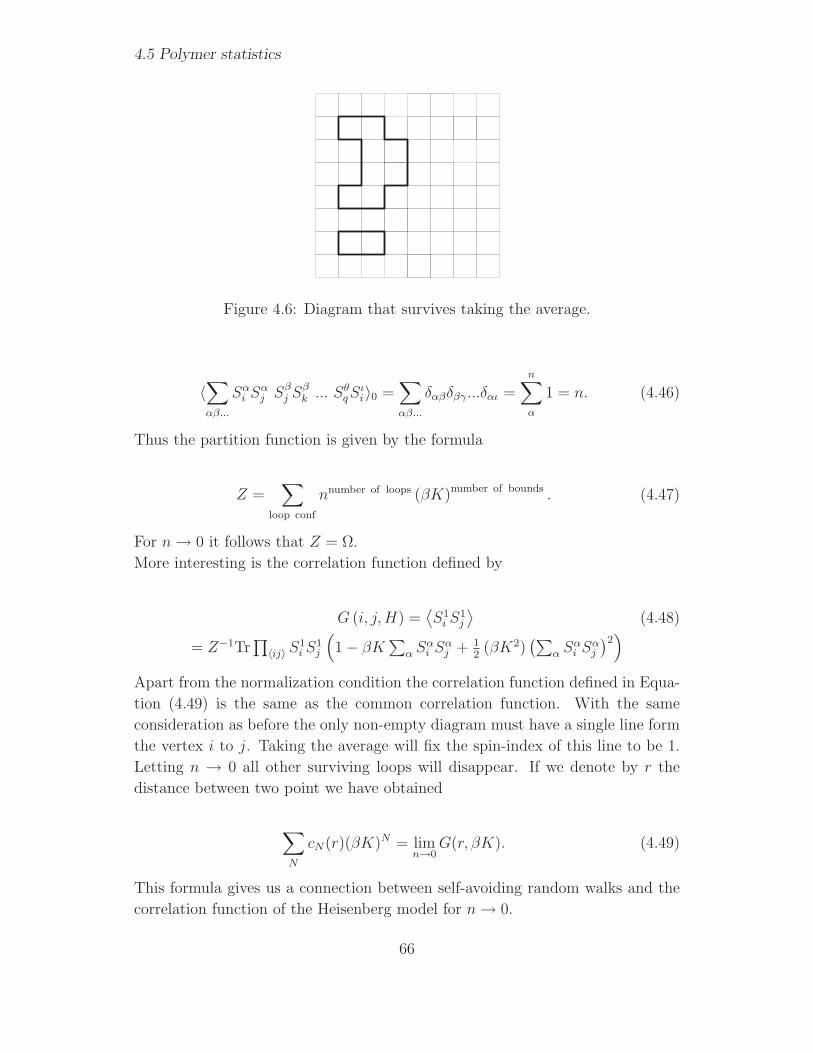
4.5 Polymer statistics
Figure 4.6: Diagram that survives taking the average.
〈∑
αβ...
Sαi Sαj S
βj S
βk ... S
θqS
ιi〉0 =
∑
αβ...
δαβδβγ...δαι =n∑
α
1 = n. (4.46)
Thus the partition function is given by the formula
Z =∑
loop conf
nnumber of loops (βK)number of bounds . (4.47)
For n→ 0 it follows that Z = Ω.
More interesting is the correlation function defined by
G (i, j,H) =⟨S1i S
1j
⟩(4.48)
= Z−1Tr∏
〈ij〉 S1i S
1j
(1 − βK
∑α S
αi S
αj + 1
2(βK2)
(∑α S
αi S
αj
)2)
Apart from the normalization condition the correlation function defined in Equa-
tion (4.49) is the same as the common correlation function. With the same
consideration as before the only non-empty diagram must have a single line form
the vertex i to j. Taking the average will fix the spin-index of this line to be 1.
Letting n → 0 all other surviving loops will disappear. If we denote by r the
distance between two point we have obtained
∑
N
cN(r)(βK)N = limn→0
G(r, βK). (4.49)
This formula gives us a connection between self-avoiding random walks and the
correlation function of the Heisenberg model for n→ 0.
66

Scaling theory
4.5.5 Critical behavior
We denote x = βK = KkBT
and xc = KkBTc
. The total number of self-avoiding
walks of N steps is
cN =∑
r
cN (r) . (4.50)
From Equation (4.49) it follows that
∑
N
cNxN =
∑
N
∑
r
cN(r)xN = limn→0
∑
r
G(r, x) = χ ∼ |x− xc|−γ. (4.51)
The series on the left-hand-side should (according to the right-hand-side) diverge
as x reaches the critical value xc. This suggests the following value for cN :
cN = const · x−Nc Nγ−1 (4.52)
such that
∑
N
cNxN =
∫ ∞
0
dNNγ−1
(x
xc
)N(4.53)
= const(γ) ln
(x
xc
)−γ∼ |x− xc|−γ
where we used the approximation ln(xxc
)= ln
(1 + (x−xc)
xc
)≈ x−xc
xcfor x−xc ≪ 1.
We are also interested in the scaling behavior of 〈r2〉. We have
⟨r2⟩
=∑
~R
r2 cN(r)
cN(4.54)
∑
~r
r2G (r, x) =∑
~r
∑
N
cN (r)xNr2 (4.55)
=∑
N
(∑
~r
cN (r)R2
)xN =
∑
N
aNxN ,
where we defined aN =∑
~r cN (r) r2 which scales like
67

4.6 Conclusions
∑
~r
r2G (r, x) ∼∫
Rd
r2rd−1r−(d−2+η) exp
(r
ξ
)drdΩ (4.56)
=
∫ ∞
0
r3−η exp
(r
ξ
)dr
∫
Ω
dΩ
∼ ξ4−ηΓ (d− η) ∼ |xc − x|γ−2ν .
Here we used that G (r, x) = r−(d−2+η) exp(− rξ
). Like above we have that
∑
N
aNxN ∼ |xc − x|γ−2ν ⇒ aN ∼ x−Nc Nγ−2ν−1. (4.57)
We conclude that
⟨r2⟩∼ aNcN
=x−NC N2ν+γ−1
x−NC Nγ−1∼ N2ν . (4.58)
Summarizing we have found that for a simple random walk 〈r2〉 ∼ N and for a
self-avoiding random walk 〈r2〉 ∼ N2ν . In three dimension γ = 7/6 and ν = 3/5.
4.6 Conclusions
Near the critical point of a second-order phase transition the thermodynamic
potentials are assumed to be homogeneous functions. It follows that only two of
the six critical exponents are independent of each other and the other four can
be derived from the scaling relations.
Furthermore we can group systems into universality classes. All system in the
same universality class have the same critical exponents. Impurities can de-
stroy the ordered phase. The Harris criterion says that the critical behavior of
a quenched disordered system does not differ form that of the pure systems if
dν > 2.
Finally we found that spatial extent of a random and self-avoiding random walk
can be scaled with the critical exponents of the O(n) n → 0 model. We have
that for a simple random walk 〈r2〉 ∼ N and for a self-avoiding random walk
〈r2〉 ∼ N2ν , where N is the number of steps.
68

Bibliography
[1] H. E. Stanley, Introduction to Phase Transitions and Critical Phenomena
(Oxford University Press, 1971).
[2] K. Huang, Statistical Mechanics (John Wiley, 1987).
[3] N. Goldenfeld, Lectures on Phase Transitions and the Renormalization Group
(Addison-Wesley, 1992).
[4] D. P. Laundau, A Guide to Monte Carlo Simulations in Statistical Physics
(Cambridge University Press, 2005).
[5] J. Cardy, Scaling and Renormalization in Statistical Physics (Cambridge Uni-
versity Press, Cambridge, 1996).
[6] P. G. de Gennes, Scaling Concepts in Polymer Physics (Cornell University
Press, 1979).
69

BIBLIOGRAPHY
70

Chapter 5
The Renormalization Group
Thomas Coutandinsupervisors: Dr. Ch. Iniotakis, Dr. M. Matsumoto
5.1 Introduction
Given a macroscopic physical system near a critical point. A renormalization
group (RG) for our system is a set of symmetry transformations which are de-
fined to act on an appropriate space of states of our system. These symmetry
transformations are called RG transformations. The idea of symmetry trans-
formations is here in principle the same as the one we know from atomic physics,
for example. But there are some differences: first the whole system will not be
simply invariant under an RG transformation, second it is not so easy to find
an RG and third the RG is not a group. Besides that recall that carrying out
a symmetry transformation does not mean the same as solving a particular model.
Our job: Find an RG for our system (there may be many). The idea: Study
the behavior of our system under a change of scale. What do we get from
RG theory? First we get a connection to QFT. Second the critical exponents
appear as symmetry properties of the RG transformations: (a) as a direct
consequence of having found an RG for our system we get the scaling relations
corresponding to our system; (b) there is a way to calculate critical exponents.
In this text the RG will be treated in the framework of Classical Statistical
Mechanics restricted to lattice spin systems, having applications in condensed
matter physics in mind1.
1This text is mainly based on a paper of J. Frohlich and T. Spencer [1].
71

5.2 Classical lattice spin systems
It should be emphasized that RG methods are not restricted to statistical me-
chanics; far from it, the idea underlying the RG has many applications in other
parts of physics. Definitely included is for example astrophysics and Quantum
Field Theory.
5.2 Classical lattice spin systems
In the following we will only look at the simplest, classical spin systems, namely
lattice ones. For the treatment below we should justify the following: (i) the use
of classical spin systems, (ii) considering infinitely large lattice systems and
(iii) considering only the (hyper-) cubic lattice.
As physical systems we will only consider classical spin systems with a mathe-
matical structure described by four properties defining 1. the lattice, 2. the spin,
3. the energy and 4. the equilibrium state of the lattice system.
Classical spin system (summarized2): lattice: Zd; classical spin: ϕ(j) ∈
RN(j) ≃ R
N , j ∈ Zd (N : dimension of spin space); spin configuration on
Λ ⊂ Zd: ϕΛ := ϕ(j) : j ∈ Λ ∈ KΛ :=
∏j∈Λ R
N(j); a priori distribution of
the spin ϕ(j): probability measure dλ(ϕ(j)). For a finite sublattice Λ ⊂ Zd:
a priori distribution of a spin configuration on Λ: probability measure∏j∈Λ dλ(ϕ(j)); energy/hamilton function on Λ: HΛ(ϕΛ) (continuous); for
Λn ր Zd, n→ ∞ (Λn: finite), there exist the interaction energy between Λ and
Λc, WΛ,Λc ≡ limn→∞WΛ,Λn\Λ ≡ limn→∞ HΛn − (HΛ +HΛn\Λ), and the free en-
ergy, f(β, λ), per unit volume defined by βf(β, λ) ≡ limn→∞ − 1|Λn| logZβ(Λn),
where Zβ(Λn) ≡∫KΛn
exp[−βHΛn(ϕΛn)]∏
j∈Λndλ(ϕ(j)), for all β ≥ 0.
An equilibrium state at inverse temperature β of the infinite lattice spin
system is given by a probability measure, dµβ,λ(ϕ), on KZd with the following
defining property : for every bounded measurable function A on KΛ, where Λ is
an arbitrary finite sublattice, the following holds:
〈A〉β,λ ≡∫
K∞
A(ϕΛ)dµβ,λ(ϕ) =
∫
KΛc
dρ(ϕΛc)
∫
KΛ
e−β(WΛ,Λc (ϕ) + HΛ(ϕΛ))A(ϕΛ)∏
j∈Λ
dλ(ϕ(j)) ,
(5.1)
where dρ(ϕΛc) is a finite measure on KΛc . These are the so called Dobrushin-
Lanford-Ruelle equations. Note: For simplicity we will consider a one-
component spin field ϕ : Zd → R in the following, i.e. N = 1.
2For more details see [1] or a more detailed version available from me.
72

The Renormalization Group
Correlation function (“correlating” the spins of a finite number of lattice sites
x1, . . . , xn):
〈ϕ(x1) · · · ϕ(xn) 〉β ≡⟨
n∏
k=1
ϕ(xk)
⟩
β
=
∫
K∞
n∏
k=1
ϕ(xk) dµβ(ϕ) . (5.2)
Inverse correlation length (mass): m(β) := − lim|x|→∞1|x| log 〈ϕ(0)ϕ(x)〉cβ,
measures the exponential decay rate of 〈ϕ(0)ϕ(x)〉cβ ; susceptibility: χ(β) :=∑x∈Zd
〈ϕ(0)ϕ(x)〉cβ, where 〈ϕ(0)ϕ(x)〉cβ := 〈ϕ(0)ϕ(x)〉β − 〈ϕ(0)〉2β.In the following we will only consider phase transitions at a critical point. β = βcis defined to be a critical point if m(β) ց 0 as β ր βc, or β ց βc. Scaling
laws: m(t) ∼ tν and χ(t) ∼ t−γ as t → 0, where m(t) := m(β) , χ(t) := χ(β) ,
t := βc−ββc
and a(t) ∼ b(t) , t → 0 :⇔ limt→0+log a(t)log b(t)
= 1. The exponents ν and
γ, occurring in the scaling laws, are called critical exponents.
5.3 Scaling limit
5.3.1 Scaled lattice systems, renorm. condition
For the following we consider the case in which β < βc. In order to simplify
the discussion we make some other assumptions (equilibrium state, inverse
correlation length):
• The equilibrium state dµβ(ϕ) is invariant under lattice translations , i.e.
∀x ∈ Zd : dµβ(ϕx) = dµβ(ϕ) ,with ϕx(j) = ϕ(j + x) , x, j ∈ Z
d . (5.3)
• Furthermore for β < βc, the equilibrium state dµβ is extremal (w.r.t. trans-
lation invariance), i.e. ergodic under the action of lattice translations. Phys-
ically this means that dµβ is a “macrostate”; see [4].
• The inverse correlation length m(β) is positive, i.e. 〈ϕ(x)ϕ(y)〉β tends to
0 exponentially fast, as |x − y| → ∞ (with decay rate m(β): by a trivial
re-definition of ϕ it is always possible to assume that 〈ϕ(x)〉β = 0 ).
• Furthermore β 7→ m(β) is continuous and m(β) ց 0, as β ր βc.
Due to the divergence of the correlation length, ξ ≡ m(β)−1, at a critical point
we are interested in the large scale behavior of the correlation functions
〈ϕ(z1) · · ·ϕ(zn)〉β , β near to βc (zi ∈ Zd, 1 ≤ i ≤ n) ; (5.4)
73

5.3 Scaling limit
more precisely we are interested in the long distance limit of (5.4), in which
|zi − zj| → ∞ , whenever i 6= j . (5.5)
In order to realize such a limit we consider a scale transformation
Zd → Z
dϑ−1 := y ∈ R
d : ϑy ∈ Zd , z 7→ ϑ−1z (5.6)
where ϑ ∈ [1,∞[ is called a scale parameter. Then, for given points xk ∈ Zd ⊂
Rd, 1 ≤ k ≤ n, we choose for every ϑ ∈ [1,∞[ functions ϑ 7→ xi(ϑ) ∈ Z
dϑ−1 ⊂ R
d,
1 ≤ i ≤ n, in such a way that
xi(ϑ) = xi +O(ϑ−1) , (ϑ→ ∞) . (5.7)
In particular we get |xi(ϑ)−xj(ϑ)| = |xi−xj|+O(ϑ−1) , (ϑ→ ∞). Then in the
scaling limit, in which ϑ→ ∞ the corresponding points zi = zi(ϑ) := ϑxi(ϑ) ∈Zd satisfy (5.5). The scaling limit is also called continuum limit. One reason is
certainly that the lattice spacing of Zdϑ−1 , namely ϑ−1, vanishes in the scaling limit.
The general strategy is now to construct from our real lattice system in some
way, including the above scale transformation with scale parameter ϑ, an “effec-
tive” one. The first step in doing this is the construction of a scaled lattice
system, “naturally” determined by the scale transformation (5.6). The second
step is the construction of an effective lattice system of Zd. The transformation
mapping the original state of our real system to the effective state is then an RG
transformation. Crucial is the construction of the RG transformation itself,
i.e. that the transformation is actually realized as a symmetry transformation.
Note that this (scaled) “effective” lattice system will only be a construction; the
motivation for doing this is only to extract the effective large scale behavior of
the correlation functions from our physical lattice system Zd.
In order to specify this new scaled lattice system we have to make clear in partic-
ular what we mean by a spin in this new system. So we define the scaled spin,
ϕ(ϑ), on Zdϑ−1 as
ϕ(ϑ) : Zdϑ−1 → R
d , y 7→ ϕ(ϑ)(y) := α(ϑ) ϕ(ϑy) , (5.8)
where α(ϑ) is a positive rescaling factor. Similarly, one has to bring in scaled
parameters (w.r.t. Zdϑ−1), dependent on the scale parameter ϑ, corresponding to
just these (thermodynamic) parameters, which determine the equilibrium state
(defined by the DLR-equations (5.1)) of our real lattice system Zd. One such
parameter is the inverse temperature β.
74

The Renormalization Group
Since we want the transformation, mapping the real lattice system to a scaled
“effective” one, to be realized as an RG transformation and think of the latter
being a symmetry transformation, it would be rather disadvantageous to allow
any (“non-natural”) “symmetry breaking”. Therefore we require, due to β < βc,
the “scaled inverse temperature”, β(ϑ), to satisfy β(ϑ) < βc , ∀ϑ ∈ [1,∞[ .
Intuitively expecting but also motivated by the fact that (free) energy has scale
dimension 0 (see [3]) we set (with obvious notation):
H(ϑ)
ϑ−1Λ(ϕ(ϑ)) := HΛ(ϕ) , dλ(ϑ)(ϕ(ϑ)(ϑ−1j)
):= dλ(ϕ(j)) , j ∈ Z
d . (5.9)
This enables us to define the scaled equilibrium state of Zdϑ−1 , denoted by
dµ(ϑ)β(ϑ), to be the probability measure which solves the DLR-equations (5.1),
wherein all expressions are replaced by their scaled counterparts. The corre-
sponding (expectation value) functional on the set of observables is denoted by
〈·〉(ϑ)β(ϑ). Note that due to (5.9) dµ
(ϑ)β(ϑ) differs from dµβ only in respect thereof
that the scaled parameters have to be brought in, instead of the unscaled ones.
Therefore
dµ(ϑ)β(ϑ)(ϕ
(ϑ)) = dµβ(ϑ)(ϕ) . (5.10)
Define the scaled correlations for points yi ∈ Zdϑ−1 (1 ≤ i ≤ n, ϑ ∈ [1,∞[) :
Gϑ(y1, . . . , yn) :=⟨ϕ(ϑ)(y1) · · ·ϕ(ϑ)(yn)
⟩(ϑ)
β(ϑ)
(5.8)=
(5.10)α(ϑ)n 〈ϕ(ϑy1) · · ·ϕ(ϑyn)〉β(ϑ)
(5.11)
(also called rescaled correlation function). This finally enables us to state
the renormalization condition:
For x1, . . . , xn ∈ Zd: 0 < |xi − xj| <∞ , n ≥ 2
⇒ 0 < G∗(x1, . . . , xn) := limϑ→∞
Gϑ (x1(ϑ), . . . , xn(ϑ)) <∞ , (5.12)
where xi(ϑ) satisfies (5.7), 1 ≤ i ≤ n. G∗(x1, . . . , xn) is called limiting correla-
tion function.
Now it has to be emphasized that the condition (5.12) is only the renormaliza-
tion condition for an RG transformation which ends up with the “scaled” state
dµβ(ϑ) (see (5.10)) as effective state of Zd. In general, where the RG transforma-
tion ends up with just any effective state of Zd, the general renormalization
condition is obtained by considering the scaling limit of the correlation function
with respect to the effective state.
5.3.2 Consequences of the renormalization condition
The renormalization condition yields a connection to QFT. The statement is:
the limiting correlation functions of a classical lattice spin system may
75

5.4 Renormalization group transformations
be the Euclidean Green’s functions of a relativistic quantum field the-
ory satisfying the Wightman axioms. For more information, see [1] and
references given there.
The renormalization condition implies non-trivial scaling relations between
critical exponents (see below). From (5.11), (5.12), m(β) ց 0 as β ր βc and the
definition of the inverse correlation length it follows that
β(ϑ) ր βc , as ϑ→ ∞ . (5.13)
In order to get a scaling relation between the critical exponents η, ν and γ, it
suffices to show a second “renormalization condition” (in addition to (5.12)):
ϑm(β(ϑ)) → m∗ > 0 , as ϑ→ ∞ . (5.14)
Together with the definitions of the critical exponents, (5.14) implies
βc − β(ϑ) ∼ ϑ− 1ν , ϑ→ ∞ . (5.15)
as well as the scaling relation between the critical exponents η, ν and γ (to see
this use3 in particular (5.11), the definition of the susceptibility and (5.13)):
(2 − η)ν − γ = 0 . (5.16)
(Determination of critical exponents) An explicit construction of the renor-
malization condition, i.e. having found a choice for the functions α(ϑ) and β(ϑ),
determines, in principle, the critical exponents ν, γ and η: (i) α(ϑ) determines η
via equation (5.31) and (ii) β(ϑ) determines ν by (5.15).
5.4 Renormalization group transformations
Here we only study the static (time-averaged) case but there exists an RG theory
for dynamics as well. The ultimate ambition of RG theory is the construction
of a non-trivial limiting correlation function, i.e. the accomplishment of a renor-
malization condition.
As it was already stated in 5.3.1 an RG transformation is a combination of a
scale transformation and some coarse graining process, leading finally to an
effective state. Now we will consider a typical example of RG transformations,
namely the RG block spin transformations.
3Fact: From (5.12) and (5.14) it follows that the quantity χϑ :=
∑y ∈ Zd
ϑ−1
ϑ−d Gϑ(0, y) has
the property that 0 < limϑ→∞ χϑ < ∞.
76

The Renormalization Group
5.4.1 Kadanoff (RG) block spin transformations
An RG block spin transformation consists of two transformations: a scale trans-
formation and a block spin transformation. As stated above, a scale transforma-
tion is somehow incorporated in every RG transformation.
Starting point: our lattice system as described in the preliminaries + assump-
tions from last section.
First we let act a scale transformation on our lattice (system) Zd. Since we
are interested in the large scale behavior of our lattice system, we choose a scale
transformation
Zd → Z
dϑ−1 , z 7→ ϑ−1z (5.17)
where ϑ ∈ [1,∞[. (intuitively speaking: zooming out).
As a consequence of scaling the lattice, all the quantities which can be associated
with our lattice get rescaled in some way (see last section). In particular we ex-
pect that the spin as well as all the thermodynamic parameters which determine
the equilibrium state (especially the inverse temperature) become non-trivially
rescaled. For the spin we therefore introduced the rescaling factor α(ϑ) (see
(5.8)); the scaled inverse temperature we denote by β(ϑ).
Second we will do a block spin transformation, which is a (linear) transfor-
mation in spin (configuration) space KZd . The construction is described below.
Characteristic to any block spin transformation is a number
L ∈ N : L > 1 , (5.18)
called block size. For the following we fix it. The main idea is now to “divide”
the scaled lattice Zdϑ−1 , ϑ ∈ [1,∞[ , into (hyper-) cubic blocks with side length
ǫ := ϑ−1L, then to take an average of all the spins contained in a block – this
average one might call block spin – and identifying each block with a site in Zd;
with this site is then associated the block spin.
Depending on how big ϑ was chosen in the scale transformation one might want
to average over a bigger block with side length ǫ := ϑ−1Lm. The question which
then automatically arises is: How big do we want to have ǫ ? Since we want to
identify each block with a site in Zd, a good answer is certainly ǫ ≈ 1. Therefore
define
m ≡ m(ϑ) := min j ∈ N : ϑ ≤ Lj (5.19)
and set the scaled “block” size to be
ǫ := ϑ−1Lm(ϑ) . (5.20)
77
5.4 Renormalization group transformations
Hence 1 ≤ ǫ < L. Note that therefore
ϑ→ ∞ ⇔ m→ ∞ . (5.21)
When we use the latter as scaling limit we write ϑm instead of ϑ in order to
remind of (5.21).
Now we want to understand how we can construct from the scaled lattice (system)
Zdϑ−1 a new effective lattice (system) Z
d; effective in the sense that we extract
only relevant information from Zdϑ−1 .
• First we specify how we want to divide the lattice Zdϑ−1 into ǫ-blocks (blocks
with side length ǫ): we want to do it in that way that the ǫ-blocks are cen-
tered in exactly these points which are contained in C := y ∈ Zdϑ−1 | ∃x ∈
Zd : y = ǫx.
• Realizing that Zd is naturally contained in Z
dL−m we do the following “iden-
tification map”
Zdϑ−1 → Z
dL−m , y 7→ ǫ−1y , (5.22)
which maps any ǫ-block centered in y := ǫx ∈ C ⊂ Zdϑ−1 , x ∈ Z
d, to an
1-block centered in x ∈ Zd ⊂ Z
dL−m .
• Then we associate with each site x ∈ Zd ⊂ Z
dL−m a block spin (r(ϑ)ϕ)(x),
which is the average of all spins that are “contained” in the ǫ-block cen-
tered in ǫx ∈ Zdϑ−1 . It follows the ultimate block spin transformation,
a linear transformation in spin configuration space KZd , transforming the
measure µβ(ϑ) into a measure R(ϑ)µβ(ϑ), which means intuitively establish-
ing the block spin as a “real” spin on Zd. To what extent the measure
R(ϑ)µβ(ϑ) really describes an (“effective”) equilibrium state on Zd will then
be discussed.
• Note that after having constructed the block spin we “forget” the points
contained in ZdL−m \ Z
d. What we regard as relevant information has been
absorbed into the block spin.
In order to introduce the notions of block spin and block correlation function we
define a function κ ≡ κǫ : Zdϑ−1 → R as follows:
κǫ(y) :=
ǫ−d ‖ǫ−1y‖∞ ≤ 1
2
0 otherwise(5.23)
78

The Renormalization Group
So this function, where ǫ is defined by (5.20), assigns to exactly those points in
Zdϑ−1 a non-vanishing value, which are after being subject to a “scale transforma-
tion” (“identification map” !) Zdϑ−1 → R
dǫ−1ϑ−1 = Z
dL−m , y 7→ ǫ−1y , contained in
a closed box in ZdL−m centered in 0 with edge length 1. And the non-vanishing
value is just the inverse volume of the unscaled box. Next define:
κǫx(y) := κǫ(y − ǫx) =
ǫ−d ‖ǫ−1y − x‖∞ ≤ 1
2
0 otherwise, x ∈ Z
d . (5.24)
Compared to the original function, here the role of 0 (center of the “scaled box”)
is played by the point x ∈ Zd understood as a point in Z
dL−m .
Now define the block spin, (r(ϑ)ϕ)(x), at site x ∈ Zd to be
(r(ϑ)ϕ)(x) := ϑ−d∑
y ∈ Zdϑ−1
κǫx(y) ϕϑ(y) (5.25a)
(5.24)=
1
(Lm)d
∑
y ∈ Zdϑ−1
‖ǫ−1y−x‖∞≤ 12
ϕϑ(y) (5.25b)
(5.8)=
1
(Lm)d
∑
y ∈ Zdϑ−1
‖ǫ−1y−x‖∞≤ 12
α(ϑ) ϕ(ϑy) (5.25c)
=↑
z:=ϑy
α(ϑ)1
(Lm)d
∑
z ∈ Zd
‖L−mz−x‖∞≤ 12
ϕ(z) . (5.25d)
The average is taken in dividing by (Lm)d = (ϑǫ)d instead of ǫd. We do this
because we get then the right average in the trivial case, where ϑ = 1.
At this point we recall why we want to construct an RG (block spin) transfor-
mation: we hope to accomplish the renormalization condition ! Therefore the
following definition becomes important:
For xi ∈ Zd , 1 ≤ i ≤ n, define the block correlation function, Gϑ(κx1 , . . . , κxn),
to be
Gϑ(κx1 , . . . , κxn) :=∑
y1,...,yn ∈ Zdϑ−1
n∏
k=1
(ϑ−d κǫxk
(yk))Gϑ(y1, . . . , yn) (5.26a)
(5.24)=
(1
(Lm)d
)n ∑
y1,...,yn ∈ Zdϑ−1
‖ǫ−1yi−xi‖∞≤ 12, 1≤i≤n
Gϑ(y1, . . . , yn) (5.26b)
79

5.4 Renormalization group transformations
(5.11)=
(1
(Lm)d
)n ∑
y1,...,yn ∈ Zdϑ−1
‖ǫ−1yi−xi‖∞≤ 12, 1≤i≤n
α(ϑ)n 〈ϕ(ϑy1) · · ·ϕ(ϑyn)〉β(ϑ) (5.26c)
=↑
zi:=ϑyi
α(ϑ)n(
1
(Lm)d
)n ∑
y1,...,yn ∈ Zdϑ−1
‖L−mzi−xi‖∞≤ 12, 1≤i≤n
〈ϕ(z1) · · ·ϕ(zn)〉β(ϑ) . (5.26d)
Gϑ(κx1 , . . . , κxn) describes the average correlation between ǫ-blocks, centered in
points ǫxi ∈ C ⊂ Zdϑ−1 , 1 ≤ i ≤ n, with respect to the scaled equilibrium state.
Then:
Gϑ(κx1 , . . . , κxn)(5.26b)
=
(1
(Lm)d
)n ∑
y1,...,yn ∈ Zdϑ−1
‖ǫ−1yi−xi‖∞≤ 12, 1≤i≤n
Gϑ(y1, . . . , yn)
(5.11)=
(1
(Lm)d
)n ∑
y1,...,yn ∈ Zdϑ−1
‖ǫ−1yi−xi‖∞≤ 12, 1≤i≤n
α(ϑ)n 〈ϕ(ϑy1) · · ·ϕ(ϑyn)〉β(ϑ)
(5.25c)=
⟨(r(ϑ)ϕ)(x1) · · · (r(ϑ)ϕ)(xn)
⟩β(ϑ)
(5.27)
=
∫
KZd
n∏
k=1
(r(ϑ)ϕ)(xk) dµβ(ϑ)(ϕ) (5.28)
Intuitively (5.27) says that the average correlation between the spins contained
in ǫ-blocks, centered in points ǫxi ∈ C ⊂ Zdϑ−1 , xi ∈ Z
d, with respect to the
scaled equilibrium state is just the correlation between the block spins in xi ∈ Zd,
1 ≤ i ≤ n, with respect to the state dµβ(ϑ) on Zd.
Since dµβ(ϑ) is a translation-invariant (finite) probability measure on KZd there
is a unique (finite) probability measure R(ϑ)µβ(ϑ) on KZd such that:
∫
KZd
n∏
k=1
(r(ϑ)ϕ)(xk) dµβ(ϑ)(ϕ) =
∫
KZd
n∏
k=1
ϕ(xk) d(R(ϑ)µβ(ϑ))(ϕ) , (5.29)
for all xi ∈ Zd, (1 ≤ i ≤ n), and n ∈ N \ 0.
Having defined the measure R(ϑ)µβ(ϑ), we have to check if
1. there is a lattice system (described by the four properties stated in 5.2)
with an equilibrium state given by our new measure R(ϑ)µβ(ϑ).
2. R(ϑ)µβ(ϑ) satisfies the assumptions stated in 5.3.1 .
80

The Renormalization Group
Important points: R(ϑ)µβ(ϑ) is
• invariant under lattice translations ? Yes!
• extremal invariant ? Yes!
• a Gibbs measure (i.e. a measure which satisfies the DLR-equations (5.1) for
some Hamilton function H) ? Unfortunately, this is not true in general ! See
[4]. The proceeding is now to choose an appropriate space of Gibbs states
which is closed under the action of any RG block spin transformation.
Finally from (5.28) and (5.29) we get
G∗(κx1 , . . . , κxn) := limϑ→∞
Gϑ(κx1 , . . . , κxn) = limϑ→∞
∫
KZd
n∏
k=1
ϕ(xk) d(R(ϑ)µβ(ϑ))(ϕ) ,
(5.30)
provided the limit exists.
In order to arrive at an interesting concept we now assume that α(ϑ) is “propor-
tional” to some power of ϑ, or, consistent with α(1) = 1, that
α(ϑ)2 = ϑd−2+η , ϑ→ ∞ , (5.31)
for some η (this includes the definition of η). Then define
(rϕ)(x) := L(η−d−2)/2∑
z ∈ Zd
‖L−1z−x‖∞≤ 12
ϕ(z) . (5.32)
Then
(r(ϑ)ϕ)(x) = α(ǫ−1) (rm(ϑ)ϕ)(x) . (5.33)
Analogous to (5.29) define Rµβ(ϑ) to be the unique measure on KZd such that:
∫
KZd
n∏
k=1
(rϕ)(xk) dµβ(ϑ)(ϕ) =
∫
KZd
n∏
k=1
ϕ(xk) d(Rµβ(ϑ))(ϕ) , (5.34)
for all xi ∈ Zd, (1 ≤ i ≤ n), and n ∈ N \ 0. Then
∫
KZd
n∏
k=1
(r(ϑ)ϕ)(xk) dµβ(ϑ)(ϕ) =
∫
KZd
n∏
k=1
ϕ(xk) d(Rm(ϑ)µβ(ϑ))(α(ǫ)ϕ) . (5.35)
81

5.4 Renormalization group transformations
Due to uniqueness we get
d(R(ϑ)µβ(ϑ))(ϕ) = d(Rm(ϑ)µβ(ϑ))(α(ǫ)ϕ) . (5.36)
So we can write (5.30) alternatively
G∗(κx1 , . . . , κxn) := limm→∞
Gϑm(κx1 , . . . , κxn) = limm→∞
∫
KZd
n∏
k=1
ϕ(xk) d(Rmµβ(ϑm))(α(ǫ)ϕ) .
(5.37)
Note that by (5.31), (5.32) and (5.34) the transformation R ≡ Rη depends on
the exponent η.
5.4.2 Fixed points, critical exponents
Definitions
Let M be some appropriately chosen cone of finite measures, µ, on the space,
KZd , of spin configurations and Rη be an RG block spin transformation, defined
by (5.31), (5.32) and (5.34), acting on M (Rη : M → M). Furthermore we as-
sume that the action of Rη on M is smooth. Then, a fixed point of Rη is a point
µ∗ ∈M which is invariant under the action of Rη, i.e. Rη µ∗ = µ∗. Obviously, if
the scaling limit of a state dµ, dµ∗(ϕ) := d(limm→∞Rmµ)(ϕ), exists, then dµ∗ is
a fixed point.
General strategy: For the following we assume that we already know η, corre-
sponding to a specific class of spin systems; this means that we already made a
choice of α(ϑ). In particular we assume the existence of a fixed point of Rη.
Then the strategy is to find all fixed points of Rη. Having a specific spin system
in mind, the state of this system (assumed to be contained in M) will be driven
to one of those fixed points (this has to be checked!).
Having found one (some or all) fixed point(s) of Rη we calculate the critical expo-
nents, corresponding to this (these) fixed point(s), as it is described below. The
idea here is to study how Rη behaves in the vicinity of a fixed point. This is done
in considering the linearization of Rη.
When we know ν then we know how to choose β(ϑ) (see (5.15)) and the RG
transformation is constructed (we assumed to know α(ϑ) already).
Now we choose a fixed point, µ∗, of Rη. We define Mf.p. ≡ Mf.p.(Rη, µ∗) to
be the manifold of all fixed points of Rη passing through µ∗. Under suitable
82

The Renormalization Group
conditions on M and Rη one can decompose M in the vicinity of µ∗ into a sta-
ble manifold, Ms(µ∗), and an unstable manifold, Mu(µ
∗), defined as follows:
states on Ms(µ∗) are driven towards µ∗ and states on Mu(µ
∗) are driven away
from µ∗. Finally we introduce the following tangent spaces (C, I, R, M) at the
point µ∗:
tangent space
at µ∗ (to)
called space of vector space spanned by eigen-
vectors of DRη(µ∗) correspond-
ing to eigenvalues of modulus
C Mf.p.(Rη, µ∗)
I Ms(µ∗) “irrelevant perturb.” < 1
R Mu(µ∗) “relevant perturbations” > 1
M “marginal perturb.” 1
Determination of the critical exponents ν and γ
The important statement is: The critical exponents ν and γ are determined
by the spectrum of DRη(µ∗), more precisely by the relevant eigenvalues
(which have modulus > 1) of DRη(µ∗).
Assumption: The tangent space at µ∗ splits into a one-dimensional space of
relevant perturbations and a co-dimension-one space of irrelevant perturbations,
which means in particular that there are no further marginal perturbations.
Since the space of relevant perturbations is 1-dimensional there exists exactly
one simple relevant eigenvalue λ = λ(L). One can proof4 that
ν =logL
log λ(L)(5.38)
This holds for every choice of L > 1. The critical exponent γ is then determined
by η and ν via the scaling relation (5.16).
5.5 Example: The Gaussian fixed point
Primary aim of this (very brief) example is to point out the connection of the
theory stated above towards a formalism often found in literature.
One big difference lies in the treatment of the thermodynamic limit. Regard-
ing the RG transformation this point is basically ignored, one just considers a
4For a sketch of the proof see [1] or a more detailed version available from me.
83

5.5 Example: The Gaussian fixed point
“macroscopic” but finite sublattice of Zd. Furthermore spins are no longer con-
fined to the discrete lattice sites but defined to be continuously distributed over
the subset of Rd “filling up” this macroscopic sublattice.
Let us consider a Hamilton function which has the Ginzburg-Landau form, i.e.
K := βH[ϕ] :=1
2
∫(rϕ2 +
1
4uϕ4 + c(∇ϕ)2) ddx . (5.39)
The above Hamilton function can be described by a point in a parameter space,
defined with respect to the parameters r, u and c: µ := (r, u, c)T .
The Gaussian model is obtained by setting u = 0 in the above expression
(5.39) for the Hamilton function. Equation (5.39) can be expressed in Fourier-
transformed space (ϕk: Fourier components of ϕ; u = 0) as
K|u=0 =1
2
∑
|k|<2π
(r + ck2) |ϕk|2 . (5.40)
The cutoff-parameter corresponds to the distinguished minimal distance, namely
the lattice constant (here 1 cutoff-parameter: 2πlattice constant
= 2π1
).
Above we have defined an RG transformation to transform equilibrium states.
This corresponds in principle to a transformation between parameters which de-
termine the equilibrium state (or to a transformation between Hamilton func-
tions). The link between these two formulations are the DLR-equations: to every
equilibrium state corresponds a(n) (equivalence class of) Hamilton function(s)
(DLR) and the latter one can be described by a point in parameter space.
The RG-transformed “Hamilton function” K′, defined to include no additive con-
stant, is obtained from K by
const. e−K′
=
∫e−K
∏
2πϑ−1 ≤ |q| < 2π
dϕq
ϕk = ϑ1−
η2 ϕ′
ϑk
. (5.41)
The [. . . ]-term can be interpreted as a block spin transformation (w.r.t. a block
size ϑ ≡ Lm). Here all the degrees of freedom in a block with side length ϑ are
integrated out. Due to the simple form of K|u=0, see (5.40), this step becomes
trivial in the case u = 0. The next and last step of our RG transformation –
essentially an RG block spin transformation, only carried out in k-space – is to
express [. . . ] in terms of the scaled quantities (w.r.t. ϑ again as in the integration
process before).
84

The Renormalization Group
Carrying out the RG transformation in the Gaussian model gives immediately:
K′|u=0 =1
2
∑
|k| < 2πϑ−1
(r + ck2) |ϕk|2
=1
2
∑
|k| < 2πϑ−1
(r + ck2) ϑ2−η |ϕ′ϑk|2
=↑
k′:=ϑk
1
2
∑
|k′| < 2π
(ϑ2−ηr + ϑ−ηck′2) |ϕ′k′|2 . (5.42)
We notice that K′|u=0 has the same form as K, i.e. K′|u=0 can be represented by
a point in the parameter space defined above, namely:
R(ϑ)µ|u=0 ≡ (ϑ2−ηr, 0, ϑ−ηc)T (5.43)
(R(ϑ): RG transformation on the parameter space).
Now we can discover fixed points of R(ϑ): for η = 0 we find the fixed point
µ∗0 := (0, 0, c)T , and for η = 2 we obtain another fixed point (r, 0, 0)T . µ∗
0 is
called the Gaussian fixed point and corresponds to the “hamilton function”
K∗ := 12
∑|k|<2π
ck2 |ϕk|2 . The next question arising is how R(ϑ) behaves in the
vicinity of a Gaussian fixed point. For the case u = 0 we have already found
out (see (5.43)). If one wants to study the vicinity of µ∗0 more detailed one in-
cludes the parameter u. Then it is advantageous to consider only the linearized
R(ϑ), denoted by RL(ϑ). This means that we linearize K′ with respect to K − K∗;
K′L := linearization of K′. One finds5 that K′L has the same form as K and can
be represented by the following point in parameter space:
RL(ϑ)µ ≡
ϑ2 ∗ 0
0 ϑ4−d 0
0 0 1
r
u
c
(5.44)
Note that only the second row of the matrix above gives new information. ϑ2 is
the relevant eigenvalue, ϑ4−d has to be the irrelevant and 1 is the marginal one.
The new information is essentially that µ∗0 is only stable whenever d > 4. From
the relevant eigenvalue we get, setting ϑ := L and using (5.38):
ν =log(L)
log(L2)=
1
2. (5.45)
Summary: The Gaussian fixed point is stable only for d > 4 and the critical
exponents corresponding to the Gaussian fixed point are η = 0 and ν = 12,
(γ = 1, . . .).
5See [3], p. 169-175; the * in (5.44) denotes a term which is irrelevant for our discussion.
85

5.5 Example: The Gaussian fixed point
86

Bibliography
[1] J. Frohlich and T. Spencer, Some recent rigorous results in the theory of phase
transitions and critical phenomena, Seminaire BOURBAKI (1981/82).
[2] J. Frohlich, ed., Scaling and Self-Similarity in Physics: Renormalization in
Statistical Mechanics and Dynamics (Birkhauser, 1983).
[3] S. Ma, Modern Theory of Critical Phenomena (Benjamin, 1976).
[4] A. van Enter, R. Fernandez, and A. Sokal, Regularity Properties and Patholo-
gies of Position-Space Renormalization-Group Transformations: Scope and
Limitations of Gibbsian Theory, Journal of Statistical Physics 72 (1993).
[5] D. Ruelle, Statistical mechanics: Rigorous Results (Imperial College Press,
1999).
[6] K. Wilson and J. Kogut, Phys. Rep. 12C, 75 (1974).
[7] C. Domb and M. Green, eds., Phase Transitions and Critical Phenomena,
vol. 6 (1976).
[8] R. Israel, Convexity in the Theory of Lattice Gases (Princeton University
Press, 1979).
[9] P. Pfeuty and G. Toulouse, Introduction to the Renormalization Group and
to Critical Phenomena (John Wiley, 1977).
87

BIBLIOGRAPHY
88

Chapter 6
Critical slowing down and
cluster updates in Monte
Carlo simulations
Ruben Andristsupervisor: Dr. Munehisa Matsumoto
As a critical temperature Tc is approached, a (nearest neighbor
correlated) Ising system develops large spatial correlations which
have long temporal correlations associated with them. Hence
the characteristic time scale diverges at Tc. This chapter seeks to
give an introduction to critical slowing down as observed in the
2-dimensional Ising model and to explain how this divergence
in time scale can be counteracted in simulations using cluster
update schemes.
6.1 Introduction
6.1.1 Motivation
Mean-field theory often gives a qualitatively correct picture of a given model’s
phase diagram. And for certain problems such as the Ising Model in one or two
dimensions, exact solutions have been found[1]. However, a close comparison
of the aforementioned shows some inaccuracy, which gives rise to the need for
accurate predictions both for problems being discussed and such that remain
unsolved.
89

6.1 Introduction
Monte Carlo simulations provide means of acquiring numerical predictions for
the behavior of a given model. Through extensive use of random numbers, these
simulations seek to probe phase space in a stochastic manner to determine the
equilibrium state of the underlying system. This is done by constructing a Markov
Chain of states, where every new state of the system is generated from the pre-
vious one. The generation itself is non deterministic, as one of the possible new
states is picked randomly on every step.
If the choosing of the new state can be implemented in a way to ensure a tendency
towards the equilibrium state of the system, then relaxation to this equilibrium
state is guaranteed if the system is left untouched for some time.
6.1.2 Historical notes
Estimations making use of random numbers have been known as far back as
the 19th century. For instance, Laplace was able to estimate the number π by
throwing a set of needles randomly onto a board with lines.
The first work on Monte Carlo simulations was published in 1949 by N. Metropolis
et al.[2]. Ever since, the simulations have not only grown along with the computer
industry but have also enabled a whole new field of research by providing reference
data and investigating new models numerically.
One model which has been of particular interest is the Ising model in two dimen-
sions. We shall also use it in this context to outline and discuss the application
of a Monte Carlo simulation.
6.1.3 Ising model in two dimensions
This Ising model consists of spins with only two states (σ ∈ ±1) arranged in a
plane. For simplification we will only look at nearest neighbor interactions. This
results in the following Hamiltonian[3]:
H = −J∑
NN
σiσj −H∑
i
σi,
where J is some interaction constant and H represents the magnetic field. Also,
theory predicts the critical temperature to be Tc = 2.269 and the following power
law relation for the correlation length ξ:
ξ ∝ ε−ν ,
where ν is termed critical exponent and ε = |1−T/Tc| is the reduced temperature.
90

Critical slowing down and cluster updates in Monte Carlosimulations
6.1.4 Conditions for validity
To ensure the validity of the simulation data, we must show that the simulation
really does converge to the equilibrium state. Sufficient conditions for convergence
are given by Ergodicity and the Detailed Balance relation.
Ergodicity
Ergodicity means that every point in phase space must be reachable. This is a
requirement, as the system may otherwise be trapped in a non-equilibrium state.
We write the probability for the system to be in state i as:
Pi(t+ 1) = Pi(t) −∑
j 6=iwi→j +
∑
i6=jwj→i, (6.1)
where wi→j is the probability of getting from state i to state j. We can rewrite
this equation in matrix form by defining the following:
Lij = wj→i (for i 6= j)
Lii = 1 −∑
j 6=iwi→j
Equation 6.1 then translates to:
Pi(t+ 1) =∑
j
LijPi(t) (6.2)
And we want to show that Pi(t) converges to some equilibrium distribution Pi(∞).
This can be done by looking at the properties of the probability matrix L. Sup-
pose ergodicity is given, then any state can be reached within a finite number of
steps. By choosing n to be the number of steps required to be able to reach any
state we can assure that (Ln)ij > 0 ∀i, j.The theorem by Perron and Frobenius states that any matrix with strictly positive
elements has a non degenerate largest eigenvalue. Since we are dealing with a
probability matrix, the largest possible eigenvalue is 1. Therefore, if we can show
that a stable distribution exists, then we know that it is unique.
Supposing such a unique state with non degenerate, largest eigenvalue 1 exists,
we can show convergence by taking the limit
lims→∞
(Ln)sPi(t) −→ Pi(∞)
Taking this limit results in all distributions with an eigenvalue below 1 to vanish,
whereas the equilibrium distribution with eigenvalue remains.
91

6.2 Critical slowing down
Detailed Balance
In order for the above argument to hold, we must show that an equilibrium
distribution exists. Such an equilibrium distribution should satisfy the Balance
Relation: ∑
j 6=iP eqj wj→i
!=∑
j 6=iP eqi wi→j (6.3)
One way to satisfy this is by requiring detailed balance:
P eqj wj→i
!= P eq
i wi→j (6.4)
6.2 Critical slowing down
6.2.1 Metropolis algorithm
The algorithm introduced by N. Metropolis et al.[4] incorporates so-called local
updates, which flip only a single spin according to a certain probability, which
depends only on the nearest neighbors. Several such updates form a Markov chain
where successive states differ only in at most one single site that was potentially
updated.
The flipping probability proposed with was:
wb→a =
e−∆E/kBT ∆E > 0
1 ∆E < 0, (6.5)
where ∆E = Eafter − Ebefore, kB is the Boltzmann constant and T is the tem-
perature. Note that for a negative ∆E, the probability for flipping the spin is 1
(always flipped), since there is a gain in energy associated with this transition.
When implementing the Metropolis Algorithm, the sites can be chosen either in
a specific order or randomly.
Ergodicity
If we choose the sites for the local updates randomly, then ergodicity can be
shown very easily: To get from a given state to any other state, we simply need
to update all the sites which differ between these states. Since there is a non-
vanishing probability for all of the attempted flips, there is also a non-vanishing
probability to construct a Markov chain to the other state. As this holds for any
two states, ergodicity is given.
92

Critical slowing down and cluster updates in Monte Carlosimulations
Detailed balance
It is instructive to verify that the detailed balance relation (Eq. 6.4) holds. To
do this, we compare the probability of flipping one site back and forth:
Pbwb→a!= Pawa→b (6.6)
W.l.o.g. the energy difference is ∆E = Ea − Eb > 0. Therefore, the transition
probability to the state of lower energy Eb becomes 1. Hence we get the relation
e−Eb/kBT · e−(Ea−Eb)/kBT != e−Ea/kBT · 1 (6.7)
And from this we get the relation −Eb − Ea + Eb = −Ea.
6.2.2 Measured properties
The fact that only very small changes occur in each step suggests the interpre-
tation that the simulation time is somehow related to real time. Thus not only
can the Metropolis Algorithm be used to find the equilibrium state, it also gives
some insight in the evolution of the system over time. For numerical comparison,
the magnetization M is a good choice, as it is also the order parameter of a 2D
Ising ferromagnet. The n-th measurement is taken by calculating the average
magnetization per site:
Mn =1
S
S∑
i=1
σi,
where S is the total number of spins in the system and the sum is taken over all
of these. To reduce the impact of random noise, this property is then averaged
over time:
〈M〉 =1
N
N∑
n=1
Mn,
where N is the number of states considered in the measurement. To reduce the
impact of the set of random numbers, the simulation ought to be repeated several
times using different sets of random numbers.
When visualizing the system during the simulation, several observations can be
made: While at high temperatures, the system is mainly dominated by noise,
one can clearly see the formation of domains at low temperatures. Introducing a
magnetic field favors one state over the other, which results in (nearly) all spins
aligning at low temperatures. By sweeping this magnetic field H (i.e. from a
negative to a positive value), one can clearly observe a phase transition. The fact
93

6.2 Critical slowing down
that this transition exhibits a metastable state – the orientation of the magneti-
zation does not immediately follow a change in the orientation of the magnetic
Field – suggests this transition to be first order.
The other interesting change happens as we continuously cool down from the high
temperature state (with small correlated domains). As we approach a certain
point Tc, we start to see all sizes of clusters emerge. Further cooling gradually
creates percolating clusters growing to a completely ordered state.
6.2.3 Divergence of time scale
In order for the simulation to yield numerical results for the equilibrium state, we
must allow time for the system to relax to this equilibrium state. This means we
have to omit the first N0 configurations obtained during the simulation, where
N0 must be chose sufficiently large to ensure relaxation.
However, the relaxation time of the system depends on T , and at the critical
temperature Tc it diverges. The fact that this is a physical effect, which is not
only seen in simulations, suggests that the Metropolis dynamics do in fact nicely
capture the properties of the physical system.
This slow relaxation is termed “Critical Slowing Down” and the divergence is
associated with a long correlation length. As the correlation of the spins is
not local any more, the local updates of the Metropolis algorithm become very
ineffective. This can be shown by measuring the magnetization against time M/t
at different temperatures T .
Relaxation from high energy state
When starting from a high energy state (Fig. 6.1), i.e. checkerboard pattern,
we can see that for low temperatures, there is a relaxation to a fixed average
magnetization per site, which is close to 1 (most spins are aligned). At high tem-
peratures some random noise prevails and the system shows next to no alignment
of the spins. For a simulation at Tc, the results are, however, inconclusive as the
system is unable to relax to the equilibrium state within the given time span of
the measurements.
Relaxation from low energy state
A very similar picture is obtained when doing the same measurements starting
from a low energy state (Fig. 6.2), i.e. when all spins are aligned: While the
simulations at low temperatures maintain the high magnetization, those at high
94

Critical slowing down and cluster updates in Monte Carlosimulations
temperatures drop to a state dominated by noise which exhibits next to no total
magnetization. The results for Tc show, once again, no signs of relaxation.
This long relaxation time results in most of the gathered data being discarded
as N0 must be larger than the steps required for the system to relax. This is
very ineffective and makes it difficult to acquire reliable data around the critical
temperature Tc. Therefore some other methods must be sought to probe the
system around the critical temperature.
6.3 Cluster updates
The basic idea of cluster updates is to flip several spins in a common domain
at once rather than attempting to do single flips. This allows for changes which
correspond in scale to the current correlation length of the system and therefore do
not become ineffective as T approaches Tc (and the correlation length diverges).
First steps in this were taken by Kasteleyn and Fortuin,[5] who showed that the
ferromagnetic two state Potts model could be mapped to a percolation problem.
This is done by mapping the “bonds” of the Ising model onto a corresponding
lattice, where there is a non zero probability for aligned nearest neighbors to be in
the same cluster. Therefore, domains of aligned spins are grouped into clusters.
The importance of this discovery lies in the fact that, even though the Potts
model suffers from critical slowing down, the percolation problem does not.
The cluster probability suggested by Swendson and Wang[6] was:
p = 1 − e− 2J
kBTδσiσj , (6.8)
where J is some interaction constant, kB and T are the Boltzmann constant
and temperature respectively. Note that the delta function results in a non-zero
probability only in the case of aligned spins.
The method suggested with this cluster probability was to
1. Iterate through all bonds and try placing them
2. Identify all clusters created in step 1
3. Randomly assign a new value to the clusters
Thus each newly generated state differs substantially from the previous one. The
method introduced by Wolff[7] proceeds to build clusters sequentially by starting
from a random site and growing them recursively. Contrary to the Swendson-
Wang method, all grown clusters are flipped, which is a slight improvement.
95

6.3 Cluster updates
Monte Carlo Time0
0.2
0.4
0.6
0.8
1M
agne
tisat
ion
per S
ite
T = 1.0T = 2.0T = 2.27T = 2.5T = 4.0
Metropolis Simulation on a 100x100 Grid
Figure 6.1: Relaxation from high energy state under metropolis dynamics
Monte Carlo Time0
0.2
0.4
0.6
0.8
1
Mag
netis
atio
n pe
r Site
T = 1.0T = 2.0T = 2.27T = 2.5T = 4.0
Metropolis Simulation on a 100x100 Grid
Figure 6.2: Relaxation from low energy state under metropolis dynamics
96

Critical slowing down and cluster updates in Monte Carlosimulations
Ergodicity
Ergodicity can be seen immediately since there is always a non vanishing proba-
bility of building a single site cluster. Such single site updates correspond to the
Metropolis update scheme, which was already shown to be ergodic.
Detailed balance
To show detailed balance we look at a specific cluster and show that the proba-
bilities of flipping it back and forth are equal.
The probability of constructing a certain cluster is given by the probability to
place the inner bonds and the probability not to place the outer ones. Since when
constructing the very same cluster in two situations, the inner part will be the
same, we only need to look at the non-placed bonds outlining the cluster.
Suppose we have a cluster with n (m) spins aligned (not aligned) on the border
(respectively). In the cluster grown before the flip (state b), we must not include
n spins which would be aligned with the cluster. Likewise in the state a, when
looking at the inverse transition, we must not include m such spins:
Pb(1 − p)n!= Pa(1 − p)m (6.9)
From this, we get the following relation
e−Eb/kBT e− 2n
kBT = e−Ea/kBT e− 2m
kBT ,
Which requires −Eb− 2n = −Ea− 2m to hold. Since all the difference in energy
between the states originates from the change on the border of the cluster, we
can also use n and m to calculate the difference in energy:
∆E = Eb − Ea = (m− n) − (n−m) = 2m− 2n,
which clearly satisfies the requirement.
6.3.1 Measured properties
Again a visualization shows some interesting properties of the simulation. At
high temperatures, the picture corresponds to the one observed with Metropolis
dynamics. At low temperatures, however, the system starts to oscillate wildly.
This can easily be understood since at low temperatures, there is a good chance
of building a percolating cluster (or even one that fills the whole system) every
time. The oscillation allows the system to populate both states of lowest energy
97
6.3 Cluster updates
in phase space, whereas in Metropolis dynamics, the system would be trapped in
one of the two degenerate states.
As the temperature is swept though Tc, we see a (remarkably quick) change in
size of the clusters. In particular, at Tc all sizes of clusters emerge. Similarly as
for the Metropolis method, we can obtain a visual picture of the relaxation by
plotting the magnetization per site against time.
Both simulations starting from a high energy state (Fig. 6.3) as well as from a
low energy state (Fig. 6.4) exhibit fast relaxation to the equilibrium state for all
temperatures. This initial relaxation is followed by random oscillations around
that state. Even though this oscillation is stronger around Tc, averaging over
time allows for accurate results even at the critical temperature.
6.3.2 Relaxation compared to local updates
The advantage of the cluster updates over Metropolis dynamics become very
obvious when comparing the evolution of a system under each of the two sim-
ulation methods (Fig. 6.5). The local update scheme converges only gradually
to the equilibrium state, whereas the cluster update scheme exhibits very fast
relaxation. The fact that the two methods do find the same equilibrium state
nicely outlines that the cluster updates really do catch the main properties of the
relaxing system.
At the critical temperature (Fig. 6.6), the difference is even more dramatic: The
local updates do not show a tendency to converge, whereas the cluster update
scheme quickly finds the equilibrium state and proceeds by oscillating there.
Hence, this allows us to gather reliable data.
6.3.3 Drawbacks of cluster updates
However, the cluster update scheme also has drawbacks: At temperatures away
from Tc, performance can be worse than for local updates, since extensive effort
is put into constructing clusters which do not greatly affect the evolution of the
system.
Another major drawback is the fact that the cluster update scheme does not
include ways to handle a magnetic field. This is due to the fact that the dynamics
are dictated by the cluster probability which does not depend on a magnetic field.
One could try to implement the cluster flipping such that it is influenced by the
magnetic field similarly as for local updates. However, this results in freezing at
the critical temperature because the probability for a successful flip becomes very
small.
98

Critical slowing down and cluster updates in Monte Carlosimulations
Monte Carlo Time0
0.2
0.4
0.6
0.8
1M
agne
tisat
ion
per S
iteT = 1.0T = 2.0T = 2.27T = 2.5T = 4.0
Metropolis Simulation on a 100x100 Grid
Figure 6.3: Relaxation from high energy state using cluster updates
Monte Carlo Time0
0.2
0.4
0.6
0.8
1
Mag
netis
atio
n pe
r Site
T = 1.0T = 2.0T = 2.27T = 2.5T = 4.0
Cluster Update Simulation on a 100x100 Grid
Figure 6.4: Relaxation from high energy state using cluster updates
99

6.3 Cluster updates
Monte Carlo Time0
0.2
0.4
0.6
0.8
1M
agne
tisat
ion
per S
ite
Cluster UpdateMetropolis
Simulations on a 100x100 Grid at T=2.0
Figure 6.5: Comparison of local and cluster updates at T = 2.0
Monte Carlo Time0
0.2
0.4
0.6
0.8
1
Mag
netis
atio
n pe
r Site
Cluster UpdateMetropolis
Simulations on a 100x100 Grid at T=2.27
Figure 6.6: Comparison of local and cluster updates at T = Tc
100

Critical slowing down and cluster updates in Monte Carlosimulations
What is more, the fast relaxation was achieved by giving up the close modeling
of the physical system present in the local update scheme. Therefore, cluster
updates should not be used to investigate the dynamics of the system, but only
to probe the equilibrium state.
6.4 Concluding remarks
The results of the simulations show that good predictions can be achieved using
Monte Carlo methods. In particular, it was shown that cluster updates provide a
means to overcome the difficulties around the critical temperature Tc. However,
this cluster update scheme has drawbacks as well, which gives rise to the need for
other methods to simulate specific properties of a system that cannot be handled
by such cluster updates.
101

6.4 Concluding remarks
102

Bibliography
[1] L. Onsager, Phys. Rev. 65, 117 (1944).
[2] N. Metropolis and S. Ulam, Journal of the American Statistical Association
44, 335 (1949).
[3] D. P. Landau and K. Binder, A Guide to Monte Carlo Simulations in Statis-
tical Physics (Cambridge University Press, 2000).
[4] N. Metropolis, A. W. Rosenbluth, M. N. Rosenbluth, A. H. Teller, and
E. Teller, J. of Chem. Phys. 21, 1087 (1953).
[5] P. W. Kasteleyn and C. M. Fortuin, Journal of the Physical Society of Japan
Supplement 26s, 11 (1969).
[6] R. H. Swendsen and J.-S. Wang, Phys. Rev. Lett. 58, 86 (1987).
[7] U. Wolff, Phys. Rev. Lett. 62, 361 (1989).
103

BIBLIOGRAPHY
104

Chapter 7
Finite-Size Scaling
Darko Pilavsupervisor: Munehisa Matsumoto
We discuss - by looking at the Ising Model - how one can use
finite-size scaling in order to extract crucial information of an in-
finite system out of a finite system. We also see different possible
ways of distinguishing between 1st and 2nd order phase transi-
tions.
7.1 Introduction
There are two options to get the right behaviour of certain quantities of a ther-
modynamic system. Either by exact analysis or by simulations of the system.
Both ways have their drawbacks. The downside of exact analysis is evidently the
inability to solve complicated systems, so solutions are available only for very lim-
ited cases. On the other hand, if we look at simulations, certain difficulties arise
there as well. We can not simulate the infinite system due to finite processing
time and finite memory. This is why we need to look at finite systems. But finite
systems behave differently than infinite ones. So if we manage to extract the size
dependence of our quantities, we can deduce the behaviour of the thermodynamic
system.
Let us look at the difference in behaviour between finite and infinite systems.
Taking the Ising model as an example we have the following Hamiltonian
H = −J∑
〈i,j〉σiσj σn ∈ ±1. (7.1)
105

7.2 Scaling Function Hypothesis
As you can see, we neglect the three and more site interactions and since we want
to look at the 2nd order phase transition we also have no magnetic field (See Fig.
7.1).
TC T
H
2nd Order
1st Order
Figure 7.1: Phase diagram of the Ising model (D ≥ 2)
Consider the magnetisation, the order parameter of the system. By definition the
order parameter vanishes in one phase and is finite in the other. If we however
consider the finite system, the absolute value of the magnetisation will never
completely disappear and the transition will be smeared out (See Fig. 7.2). The
reason why we look at the absolute value of the magnetisation in finite systems
is that the system is able to flip the whole magnetisation and the positive and
negative contributions will cancel out.
Figure 7.2: Left: Magnetisation in the thermodynamic limit. Right: Magnetisa-
tion in a finite size system with different system sizes.
7.2 Scaling Function Hypothesis
Our goal is to know how we can extract the correct values for the interesting
quantities of the infinite system out of the finite system. It is reasonable to
106

Finite-Size Scaling
introduce a scaling function and merge it with the theoretical scaling behaviour
of the infinite system. Of course we can do this for any thermodynamic quantity,
in this chapter however we will be using the example of magnetic susceptibility.
Now we should talk about how this scaling function should look like. But first
a few facts should be mentioned. The magnetic susceptibility can be defined by
the fluctuation of magnetisation as follows
kbTχM =∑
〈i,j〉〈σiσj〉 − 〈σi〉〈σj〉. (7.2)
This definition can be understood quite intuitively after a short hand waving
argument. The right hand side is the fluctuation of the magnetisation. If the
fluctuations are high the system must be limp and a small magnetic field results
in an large magnetisation of the system, therefore the magnetic susceptibility is
high. On the other hand a system with low fluctuations is stiff and even a large
magnetic field will have only little impact.
Another important fact is that when we approach the critical temperature, the
correlation length ξ will diverge as |t|−ν and the magnetic susceptibility will
saturate when ξ ∼ L since all the sites of the lattice will be correlated.
Including this into the scaling theory gives us
χ(L, T ) = |t|−γg(
L
ξ(t)
), (7.3)
where t = (T − Tc)/Tc [1]. The scaling function g(x) should also satisfy
• g(x) −→ const. as x −→ ∞,
• g(x) ∝ xγ/ν as x −→ 0.
The first of these two constraints ensures correct power law behaviour in the ther-
modynamic limit. The other ensures, that the magnetic susceptibility becomes
independent of the temperature if ξ ≫ L since
χ(L, T ) = |t|−γg(
L
ξ(t)
)
ξ≫L∝ |t|−γ(
L
ξ(t)
)γ/ν
∝ |t|−γ(L|t|ν)γ/ν
∝ Lγ/ν . (7.4)
107

7.2 Scaling Function Hypothesis
The side product of this calculation is that the maximum of our thermo dynamical
quantity grows as Lγ/ν .
There are different consistent ways of parametrising the scaling function. When
using numerical analysis one mostly uses the following
TD limit FS system
M ∝ |t|−β M = L−β/νgM(tL1/ν),
χ ∝ |t|γ χ = Lγ/νgχ(tL1/ν),
C ∝ |t|α C = Lα/νgC(tL1/ν).
These two notations are equivalent, since
χ(L, T ) = |t|−γg(
L
ξ(t)
)
∝ ξγ/νg(Ltν)
∝ Lγ/νg′(L1/νt).
The proportionality constant can be plugged into g′ and so we will get the new
scaling function. All we need to know for this calculus is that near Tc the cor-
relation length diverges like |t|−ν and the measured correlation length behaves
like L. Therefore this approach is only valid for temperatures close enough to
the critical temperature Tc and for sufficient large system sizes L. The reason
behind the system size dependence is, that the distance between two lattice sites
compared to the system size itself gets too large for small systems.
Now that we know on what our universal scaling function depends, we can plot
the measured quantities so that the measured data collapses if we plug in the
correct exponents. Thus if we measure and plot χ(L, T )L−γ/ν versus tL1/ν for
different system sizes, we can apply numerical data fitting algorithms in order to
extract the correct parameters γ and ν. In the plot the data curves for different
System sizes should collapse on a single curve - the universal scaling function
(See Fig. 7.3).
Of course the same can be done for other thermodynamic quantities like the heat
capacity (See Fig. 7.4). The important thing is to collect all the parameters at
once, since e.g. ν is the same for all thermodynamic quantities and in this way
the error resulting from the numerical fitting can be reduced.
108

Finite-Size Scaling
-10 -8 -6 -4 -2 0 2 4 6 8 10
t L1/ν
0.01
0.02
0.03
0.04
0.05
0.06
χ/L
γ/ν
L = 4L = 6L = 8L = 10L = 12
Fitted Magnetic Susceptibility3D Ising Model
Figure 7.3: Fitted Magnetic Susceptibility. If we go away from Tc or go to small
system sizes, the data collapse does not work too well anymore.
-10 -8 -6 -4 -2 0 2 4 6 8 10
t L1/ν
0.5
1
1.5
C/L
α/ν
L = 4L = 6L = 8L = 10L = 12
Fitted Heat Capacity3D Ising Model
Figure 7.4: Fitted Heat Capacity. If we go away from Tc or go to small system
sizes, the data collapse does not work too well anymore.
7.3 Critical Temperature Tc
The extraction of the critical temperature Tc should be emphasised since knowing
where the phase transition exactly is enables making more samples around the
critical point and getting more reliable data.
As mentioned before, the problem of getting the critical temperature lies in the
smeared out transition due to finite size (See Fig. 7.2). Another contribution to
this problem is the lack of divergence of correlation length or any thermodynamic
109
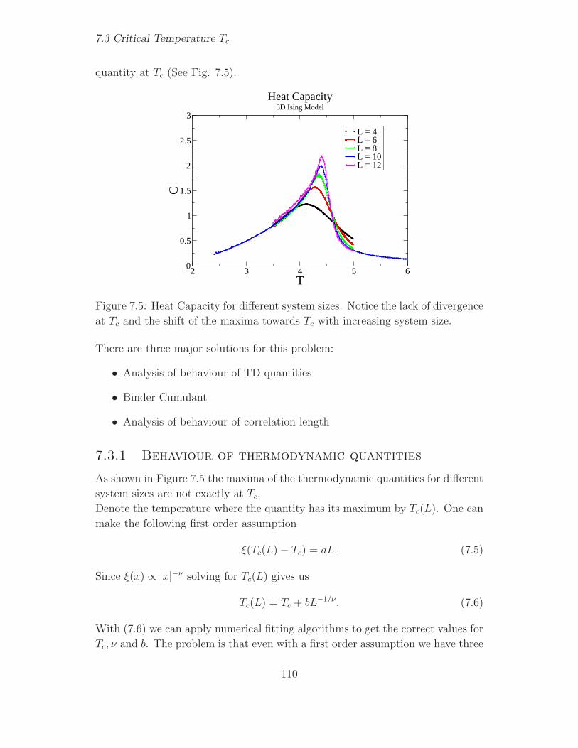
7.3 Critical Temperature Tc
quantity at Tc (See Fig. 7.5).
2 3 4 5 6T
0
0.5
1
1.5
2
2.5
3
C
L = 4L = 6L = 8L = 10L = 12
Heat Capacity3D Ising Model
Figure 7.5: Heat Capacity for different system sizes. Notice the lack of divergence
at Tc and the shift of the maxima towards Tc with increasing system size.
There are three major solutions for this problem:
• Analysis of behaviour of TD quantities
• Binder Cumulant
• Analysis of behaviour of correlation length
7.3.1 Behaviour of thermodynamic quantities
As shown in Figure 7.5 the maxima of the thermodynamic quantities for different
system sizes are not exactly at Tc.
Denote the temperature where the quantity has its maximum by Tc(L). One can
make the following first order assumption
ξ(Tc(L) − Tc) = aL. (7.5)
Since ξ(x) ∝ |x|−ν solving for Tc(L) gives us
Tc(L) = Tc + bL−1/ν . (7.6)
With (7.6) we can apply numerical fitting algorithms to get the correct values for
Tc, ν and b. The problem is that even with a first order assumption we have three
110
Finite-Size Scaling
tunable parameters. If we use higher order assumptions instead of (7.5) there
will be even more. This requires very good statistical accuracy of the data. For
this method, it is important to use measurements of different quantities, since all
have the same Tc and ν [2].
7.3.2 Binder Cumulant
Another possibility of extracting the critical temperature out of a finite system
is the very often used Binder Cumulant
UL := 1 − 〈M4〉L〈M2〉2L
. (7.7)
The crucial property of the Binder Cumulant is that it does not depend on the
lattice size at the critical temperature as can easily be seen in (7.8).
〈M4〉L〈M2〉2L
=L−4β/νgM4(tL1/ν)
(L−2β/νgM2(tL1/ν))2
= gc(tL1/ν) (7.8)
The distribution of the magnetisation is a Gaussian around zero for T > Tc and a
sum of two Gaussians for T < Tc. With this knowledge it is possible to calculate
the following two limits
UL = 1 − 〈M4〉L〈M2〉2L
L→∞−→
23
for T < Tc0 for T > Tc
. (7.9)
The transition from 2/3 to 0 will happen faster for larger systems and at the
critical temperature all lines should intersect at Tc since there the Binder Cumu-
lant does not depend on L (See Fig. 7.6). Due to finite size effects, numerical
roundoff errors etc., this intersection will not be exactly in one point.
If the Finite Size Scaling approach is applied on the Binder Cumulant it is possible
to get a good value for ν. Since the β is cancelled out (As seen in (7.8)), the only
tunable parameter is ν.
7.3.3 Behaviour of correlation length
Very similarly to the Binder Cumulant method we can derive Tc with the corre-
lation length ξ. The scaling ansatz for the correlation length is
ξL = Lgξ(tL1/ν). (7.10)
111

7.3 Critical Temperature Tc
3.5 4 4.5 5 5.5T
0
0.1
0.2
0.3
0.4
0.5
0.6
UL
L = 4L = 8L = 16
Binder Parameter3D Ising Model
Figure 7.6: The Binder Cumulants for different system sizes intersect at Tc.
-10 -5 0 5 10
(T - TC)
L1/ν
0
0.1
0.2
0.3
0.4
0.5
0.6
UL
L = 4L = 8L = 16
Fitted Binder Parameter3D Ising Model
Figure 7.7: Finite Size Scaling applied on the Binder Cumulant gives us ν.
If we go to critical temperature (7.10) can be written as
ξL/L = gξ(0). (7.11)
So here too, the ξ/L curves for different system sizes should intersect at nearly
the same point.
Naturally Finite Size Scaling can be applied on ξ too and again the only tunable
parameter will be ν.
112

Finite-Size Scaling
3 3.5 4 4.5 5 5.5 6T
0.12
0.14
0.16
ξL = 4L = 8L = 16
Correlation Length3D Ising Model
Figure 7.8: The intersection point gives the critical temperature Tc.
7.4 Distinguishing between 1st and 2nd Or-
der Phase Transitions
In this chapter we will see why it is difficult to distinguish between 1st and 2nd
order phase transitions and what we can do to overcome this problem. We will
consider three ways of distinguishing these two types of transitions
• Failure of Finite Size Scaling,
• Lack of Merging of Histogram Peaks,
• Behaviour of thermodynamic Maxima at Tc
7.4.1 Failure of Finite Size Scaling
If we apply the Finite Size Scaling, as we have seen in this chapter, on a 1st order
phase transition we will not be able to get good values for critical exponents and
the data will not collapse.
The Binder Cumulant as well as the Correlation Length divided by system size
ξ/L will not intersect in a single point, even if system size is increased.
Such a behaviour is a good indicator of an 1st order phase transition.
113

7.5 Concluding remarks
7.4.2 Behaviour of Histogram Peaks
Another way of distinguishing between the different types of phase transitions is
to look at the histogram of the order parameter.
If there are two peaks that merge with increasing system size, we know that it
is a 2nd order transition. If, however, the peaks stay in the same place after
increasing system size, we know that it is a 1st order transition.
7.4.3 Behaviour of thermodynamic Maxima at Tc
The third approach that will be discusses in this chapter is nothing else than
applying a Finite Size Scaling approach that is designed for 1st order phase
transitions on the measured data. If it gives reasonable results, we will know,
that it is a 1st order transition.
All one has to do is to look at the maxima of thermodynamic quantities at Tc.
Scaling as we have seen in (7.4) indicates a 2nd order transition, whereas scaling
of the maximum as Ld, where d is the dimension of the lattice, indicates a 1st
order transition.
7.4.4 Problem of Weak 1st Order Phase Transitions
A weak 1st order transition is a major problem, since all the approaches we
discussed beforehand might fail. For example the Finite Size Scaling as we have
seen in section 7.4.3 might work quite well for a weak first order transition. It
will yield completely wrong exponents, but the data will collapse fairly nice.
The problem is the correlation length ξ. In a first order transition it will not
diverge, but if it gets larger than the system size we can not be sure if it diverges
or not. So if ξ gets very large near Tc the system will behave as if it were a second
order transition unless the system size exceeds the correlation length.
7.5 Concluding remarks
With the Finite Size Scaling, it is possible to gather correct values for the critical
exponents of a thermodynamic system and to differentiate between first and
second order phase transitions. Nevertheless weak first order phase transitions
are and will stay a problem that can only be handled with simulations of large
enough systems. But with invention of clever techniques and faster algorithms,
one can overcome this problem as well.
114

Bibliography
[1] M. Plischke and B. Bergersen, Equilibrium Statistical Physics (World Scien-
tific, Singapore, 1994).
[2] D. P. Landau and K. Binder, A Guide to Monte Carlo Simulations in Statis-
tical Physics (Cambridge University Press, 2000).
115

BIBLIOGRAPHY
116

Chapter 8
Berezinskii-Kosterlitz-
Thouless Transition
Roland Bauerschmidtsupervisor: Dr. Andrey Lebedev
The two-dimensional XY model is introduced and the phe-
nomenological features are outlined. Then, the relation to the
Villain model is established and equivalence to a two-dimensional
gas of point defects, interacting via a Coulomb potential, is
shown. Finally, the Kosterlitz-Thouless renormalization group
equations are motivated and the critical features analyzed.
8.1 Introduction
The XY model refers to a d-dimensional lattice with two-component (classical)
unit vectors Sx at each site of the lattice (referred to as spin or rotor). Exhibiting
O(2) symmetry, it is a special case of the general O(n) model. We consider the
two-dimensional XY model a the quadratical two-dimensional lattice (a0Z)2. The
interaction between neighboring spins is given by the potential
V (Sx,Sy) := −J Sx · Sy = −J cos(θx − θy) =: V (θx − θy). (8.1)
Dimensions one and two are distinguished by the fact that long-range order is
impossible (Mermin-Wagner theorem). Nonetheless there is a transition of vortex
unbinding, whose explaination is due to Kosterlitz and Thouless.
To second order, the interaction reduces to J2(θx−θy)2 (neglecting a constant con-
tribution); the corresponding model is sometimes also referred to as the spin-wave
117

8.1 Introduction
theory. However, the feature of periodicity that is responsible for the formation
of vortices, and thus ultimately for the Kosterlitz-Thouless transition, is lost in
this approximation.
8.1.1 Absence of long-range order in two dimensions
Before explaining the Kosterlitz-Thouless transition, however, we recall a result
from Landau theory (chapter 3): Long-range order is destroyed by fluctuations
in dimensions less than or equal to two. The treatment roughly follows lecture
notes from Simons[1].
Unlike in the following sections, we assume the quadratic approximation of the
O(n) model here and consider a lattice of arbitrary dimension d (the non-linear
σ-model, a special case of the Ginzburg-Landau Hamiltonian),
H =J
2
∑
xy
(Sx − Sy)2 (8.2)
Assuming without loss of generality that the axis of the order parameter is S0 =
(0, . . . , 0, 1), we consider deviations from this direction,
S0 = (Π1, . . . ,Πn−1,√
1 − Π2), (8.3)
where the ground state corresponds to Π = 0. The Πi are Goldstone modes (or
spin-waves). If we consider only Gaussian order, the Hamiltonian becomes
H =J
2
∑
xy
(Πx − Πy)2 +
(√1 − Π2
x −√
1 − Π2y
)2
(8.4)
≈ J
2
∑
xy
(Πx − Πy)2 =
J
2
∑
xy
Πx(−)Πy (8.5)
where is the lattice Laplacian. Recall that the correlation function 〈Π(x)Π(y)〉of a Gaussian ensemble is given by the Green’s function (of the lattice Laplacian
in this case), which goes approximately like log(x − y) in two-dimensions and
like |x − y|d−2 in more than two dimensions. In the two-dimensional case, the
correlation function diverges for |x| → ∞, whereas it is finite in dimensions
greater than two. (The Green’s function of the lattice Laplacian will be discussed
in more detail later.)
In fact, this is a general result, the Mermin-Wagner-Hohenberg theorem: There
is no phase with spontaneous breaking of a continuous symmetry for T > 0, in
d ≤ 2 dimensions. The Kosterlitz-Thouless transition, however, is an example
that the absence of spontaneous symmetry breaking does not forbid the existence
of criticality. In particular, the Kosterlitz-Thouless transition cannot be described
within the Landau model, for there is no order parameter!
118

Berezinskii-Kosterlitz-Thouless Transition
8.2 Vortices
We begin with a field of spins Sx on the lattice Λ ⊂ Z2. The angle between
two neighboring spins Sx and Sy is ψxy = arccos (Sx · Sy) ∈ [0, 2π). We can now
consider arbitrary paths on the lattice. Adding the angles between neighboring
spins around a closed loop γ ⊂ Z2, the sum
ψγ =∑
xy∈γψxy = 2πk, (8.6)
must be an integer multiple of 2π, where xy denotes the bond between two nearest
neighbors x and y in γ. This is a consequence of the fact that a sum of angles is
only meaningful up to the addition of a multiple of 2πk1, and that the angle of
a spin with itself must obviously vanish. A vortex with vorticity (or topological
charge) k is a square (or plaquette) p ⊂ Z2 of the lattice such that the closed
loop around the boundary of the square ∂p has a sum of angles ψ∂p = 2πk.
8.2.1 Continuum extension
We can now extend the field of spins (initially only defined on Z2) to R
2, con-
tinuously everywhere except within vortex squares p ⊂ Z2, which is necessary
to simulate the “topological” properties of the lattice model in the continuum
version. We require the curve integral around a vortex to be an integer multiple
of 2π, meaning that the resulting space is not simply connected. Besides that, we
do not go into detail on how the continuum continuation should look in detail; in
fact, the explicit form is insignificant because only the values on the lattice are
of physical significance when working with the lattice model.
If γxy : [0, 1] → R2 is a curve connecting a curve connecting nearest neighbors x
and y (meaning that γ(0) = x and γ(1) = y), the angle can be expressed as
ψxy =
∫ 1
0
dtd
dtθ(γxy(t)), (8.7)
where θ(x) is a local choice of angle (with respect to some fixed axis) associated
with x such that t 7→ θ(γ(t)) is differentiable (and in particular, continuous).
1Angles can be thought of a as equivalence classes, where a ∼ b iff a = b + 2πk, k ∈ Z.
Only this identification of angles makes the sum is a well-defined operation, sending two angles
to a another angle.
Our notation corresponds to local coordinates of S1 as a manifold, where all smooth 2π-
periodic functions on R are smooth with respect to the differentiable structure of S1 if identified
in the obvious way, meaning in particular that cos is smooth at every angle. However, it is
important to note that two charts are required to cover S1, which is the reason that vortices
can appear.
119

8.2 Vortices
Note, however, that if we make a global choice of such an angle for all x, θ(γ(t))
cannot be continuous for every curve γ because 0 and 2π have to be identified.2
Remark. There are other physical models that can be modeled after the XY
model; however, many of the models consider a field of spins on a continuum
rather than a lattice. The introduction of a lattice of finite spacing can be seen
as a mathematical regularization of those models. For simplicity, this discussion
is restricted to the lattice model.
8.2.2 Free Energy argument
The most simple realization of a vortex of charge k is given by the spin field
φ(x, y) = k arctan(yx
). (8.8)
The field is singular at r = |x2+y2| = 0. In fact, vorticity is a homotopy invariant,
hence the domain must be homotopically non-trivial.
In the continuum approximation of the Gaussian model, the sum over the nearest
neighbor interactions∑
〈x,y〉(φx−φy)2 is replaced by the integral
∫Λ(∇φ(x))2 d2x
over the continuum extension of the spin field; here Λ ⊂ Λ ⊂ R2 denotes the
lattice, take away subsets of diameter of the order of the lattice spacing centered
at each vortex. This is necessary because at a vortex, the angle rotates very
rapidly, making the continuum approximation of the energy very bad; due to the
discrete nature of the lattice, the cores do not contribute at all in the original
model. We furthermore have to assume that the continuum extension of the spin
field is chosen so that both terms agree reasonably well far away from the vortex
center, as mentioned before. For the circular field defined above this condition
seems to be well satisfied.
In this approximation, the energy of the above vortex is given by
J
2
∫
SL\Sa
(∇φ)2 d2x =J
2
∫ 2π
0
dφ
∫ L
a
(1
r
)2
r dr = Jπ log
(L
a
), (8.9)
in the approximation that the region of the lattice is spherical.
In this approximation for the energy of an isolated vortex, the phase transition
can already be predicted: We assume that we add a single vortex to a given con-
figuration of spins. The number of sites the vortex can occupy is approximately
2This corresponds to a U(1)-principal bundle which can only be covered with more than
one chart. For two neighboring spins (on the lattice), we require that there is always a chart
covering both, though.
120

Berezinskii-Kosterlitz-Thouless Transition
(a) (b)
Figure 8.1: Simple configurations with vortices: (a) One vortex of charge +1,
(b) Two vortices with charges ±1
(La
)2, hence the entropy can be estimated to be S = −2 log
(La
)(units such that
k = 1) and the Helmholtz free energy is
F = U − TS = log
(L
a
)(Jπ − 2T ). (8.10)
Thus, for T > Jπ2
(or with β = T−1 and K = βJ , K < 2π), the formation of
vortices seems favorable.
8.3 Villain and Coulomb gas models
We will now establish a better picture of how vortices arise in the model, meaning
that the approximations seem natural from first principles. In the first step of
the analysis, we will replace the rotor model by the so-called Villain model,
whose qualitative features are the same. Subsequently, it will be shown that
the partition function of the Villain model decouples exactly into a part for a
two-dimensional Coulomb gas and a part for spin-waves.
8.3.1 Villain model
Following Jose et al.[2], we can perform a duality transformation of an arbitrary
potential by doing Fourier transformations in the angle variable. In particular,
we are obviously interested in the interaction between two spins, given by
V (θ − θ′) = −K(1 − cos(θ − θ′)), (8.11)
where the irrelevent constant term −K is introducted for later convenience. Note
that we now denote with V (θ) what was −βV (θ) in (8.1), where K = βJ in order
to keep the notation simple. This will lead to the Villain model.
121

8.3 Villain and Coulomb gas models
Clearly, V (θ) is a 2π-periodic function and so is eV (θ). It can therefore be ex-
panded as a Fourier series,
eV (θ) =∞∑
s=−∞eV (s) eisθ =:
∞∑
s=−∞f(s), (8.12)
where the Fourier coefficient is written as eV (s). Now the sum over all integers
S(t) =∞∑
s=−∞f(t+ sT ) (8.13)
of any function f (that is regular enough) is obviously T -periodic and can thus
be written as a Fourier sum,
S(t) =∞∑
m=−∞fme
im 2πTt, (8.14)
where the Fourier coefficient fm can be expressed in terms of the Fourier transform
f of f as fm = 1Tf(2π
Tm) which can be verified by a straight-forward calculation.
The Fourier transform of the potential is a special case of this with t = 0 and
T = 0, therefore eim2πTt = 1 and (8.12) is equal to
eV (θ) =∞∑
m=−∞f(2πm), f(ω) =
∫ ∞
−∞dt eV (t)+it(θ−ω). (8.15)
Writing
eV0(θ) =
∫ ∞
−∞dt eV (t)+itθ, (8.16)
this becomes
eV (θ) =∞∑
m=−∞eV0(θ+2πm). (8.17)
Note that if we modify V0 and define eV (θ) by the last equation, it will still be
periodic automatically. A good approximation of the rotor model is given by
V0(θ) := −1
2Kθ2, (8.18)
which is the expansion of the original potential V up to second order (see figure
8.2). Compared to the ordinary expansion, however, the Villain model is periodic
which we have seen to be the crucial feature in the formation of vortices. In fact,
it has been shown that result of this approximation is actually the same as for
the original cos-potential model[3].
122

Berezinskii-Kosterlitz-Thouless Transition
−2.50.0
0.5
x
5.02.5−5.0
0.25
0.75
0.0
Figure 8.2: (Reduced) Boltzmann factor for (1) the rotor model ecos(θ)−1, (2) the
Villain model V0(θ) = −12θ2, and (3) the spin-wave approximation e−
12θ2 . In the
vicinity of the origin, all of the potentials are very similar. However, unlike the
Gaussian approximation, the original rotor and the Villain model are periodic.
8.3.2 Coulomb gas model
In this section, the equivalence of the Villain model obtained in the previous
section and the model of a gas of point defects, interacting via a two-dimensional
Coulomb potential shall be established, following a treatment by Frohlich and
Spencer[3] that emphasizes the analogies with exterior calculus.
Figure 8.3: Continuous extension of a loop in Z2 to R
2. The field of spins
is considered continuous everywhere except within plaquettes, which are greyly
shaded.
We assume an extension of the spin field to R2 as described before. The sum
of angles around a closed loop is then (by construction) the same as the curve
integral around that loop, where two points are connected by an arbitary curve
(due to homotopy invariance):
∑
xy∈γψxy = 2πnγ (8.19)
The vorticity nγ is a property of the curve γ. Using Stokes’ theorem, it can be
decomposed as the sum of vorticities due to the enclosed vortices, where each of
123

8.3 Villain and Coulomb gas models
them corresponds to a lattice square p,
nγ =∑
p∈S,γ=∂Snp, (8.20)
and
2πnp =∑
xy∈∂pψxy. (8.21)
Here, ψxy refers to the angle between the two sites the bond xy connects.
Digression: Discrete Exterior Calculus
We can now use discrete analogues of the standard notions of exterior calcu-
lus, such as k-forms or exterior derivatives, which allows to rewrite the problem
conveniently. An extensive treatment can be found in [4], for example.
Let the lattice be denoted by Λ.
An oriented k-cell can be thought of as the lattice version of an oriented k-
dimensional unit volume. It is defined as follows: A 0-cell is a single lattice
site x with a choice of orientation, a 1-cell is an oriented bond xy between two
neighboring lattice sites, and a 2-cell is an oriented plaquette (square) p. With
each k-cell ck, we associate a set of k − 1 cells ∂ck, the boundary of ck and the
cell of reversed orientation c−1k . We denote the set of k-cells by Ck.
The boundary of a 0-cell is empty and the orientation is defined intrinsically. The
boundary of a 1-cell is defined by ∂xy = x, y−1, where x and y are the sites
connected by the bond, and for a 2-cell by ∂p = x1x2, x2x3, x3x4, x4x1, where
the xi are the sites at the corner of the square and the xixj the bonds between
neighboring corners. Oriention means a choice of the order of the elements in
the boundary. Orientation reserval of ck is defined by requiring that ∂c−1k =⋃
s∈∂ck s−1.
A k-chain is a function ω : Ck → R such that ω(c−1k ) = −ω(ck), where c−1
k
denotes orientation reversal of the k-cell ck. It can be thought of as the integral
of a k-form over a volume corresponding to ck. We denote the set of k-chains by
Ωk.
Analogues of the exterior derivative d : Ωk → Ωk+1 and the codifferential δ :
Ωk → Ωk−1 can be defined as follows:
(dω)(ck+1) =∑
ck∈∂ck+1
ω(ck). (8.22)
(δω)(ck−1) =∑
ck: ck−1∈∂ck
ω(ck), (8.23)
124

Berezinskii-Kosterlitz-Thouless Transition
Note that the definition of the exterior derivative defines the analogue of Stoke’s
theorem. It is easily verfied that with respect to the scalar product (·, ·) : Ωk ×Ωk → R defined by
(ω, φ) :=1
2
∑
ck⊂Z2
ω(ck)φ(ck), (8.24)
δ and d are actually adjoints of each other, meaning that (ω, dφ) = (δω, φ).
The Laplacian on k-chains can be defined as
− := δd + dδ, (8.25)
which is analoguous to the definition of the Laplacian of differential k-forms3.
Similar properties as for the differential versions of the notions hold:
d2 = 0, δ2 = 0, (8.27)
and if α is a k-chain such that dα = 0, there is (k− 1)-chain β such that α = dβ
(and similarly for δ), which corresponds to Poincare’s Lemma [Verify!].
Going back to the model, we can use the definition (8.22) of the lattice exterior
derivative d to rewrite the constraint equation (8.21) as
2πnp =∑
xy∈∂pψxy = dψp. (8.28)
This implies that
dn = d2ψ = 0. (8.29)
By Poincare’s Lemma, there is a 1-chain (function on bonds) mb, such that
np = dmp, (8.30)
which allows us to rewrite (8.28) as
2πdmp = dψp, (8.31)
3Note that in the case of a 0-form (function) f in the differential case or 0-chain f in the
discrete case, the Laplacian reduces to −δd because δf = 0. Observing that ∂xy = x, y−1,this means
−(f,f) = (df,df) =∑
xy⊂Λ
(dfxy)2 =∑
xy⊂Λ
∑
z⊂∂xy
fz
2
=∑
xy⊂Λ
(fx − fy)2, (8.26)
which agrees with what one would expect for the discrete Laplacian of a function.
125

8.3 Villain and Coulomb gas models
meaning that d(2πm−ψ)p = 0, and thus there is a 0-chain (function on sites) θxsuch that
2πmb − ψb = −dθb or ψb = dθb + 2πmb. (8.32)
However, θ and m are not unique; there is still a freedom of gauge. We will
consider two possible choices:
1. Writing ψb = dθb + 2πmb, we require θx ∈ (−π, π], and consider all integer
valued 1-chains m (that is, mb ∈ Z for all bonds b). This way, we obtain
all configurations compatible with the constraint (8.21).
2. Writing ψb = dθR
b + 2πmR
b , we do not impose restrictions on θR
x ∈ R,
requiring that mR
b = −(δ−1n)b, with the discrete Laplacian’s Green’s
function −1 and suitable boundary conditions.4
With these preparations, it will now turn out that the canonical ensemble de-
scribed by the Hamiltonian
H(ψ) = −J (ψ, ψ) = −J2
∑
xy⊂Λ
ψ2xy, (8.33)
is equivalent to the Villain model using choice (1) ψb = dθb+2πmb, while it is also
equivalent to a two-dimensional Coulomb gas model choice (2) ψb = dθR
b + 2πmR
b
is used, establishing the equivalence of the two models.
We consider the canonical ensemble with inverse temperature β
dµβ(ψ) = Z−1β e−βH(ψ)
∏
p⊂Λ
δ(dψp − 2πnp)∏
xy⊂Λ
dλ(ψxy), (8.34)
where the Kronecker-δ(dψp−2πnp) enforces the constraint (8.21), and dλ(ψxy) is
the usual Lebesque measure with variable ψxy. Only in this section, the Lebesque
measure is denoted explicitly to avoid confusion with the exterior derivative. The
partition function Zβ is defined as usual.
4Actually, the Green’s function is (Gy)x, satisfying (xGy)x = δxy, meaning that (f)x =
ρx is solved by fx =∑
y∈Z2(Gy)xρy, for
(f)x =
x
∑
y∈Z2
(Gy)xρy
x
=
∑
y∈Z2
δxyρy
x
= ρx.
However, we write (−1ρ)x =∑
y∈Z2(Gy)xρy.
126

Berezinskii-Kosterlitz-Thouless Transition
Using choice (1), we obtain the partition function (with K := βJ)
ZK =∑
m⊂Λ: mxy∈Z
∫ π
−π. . .
∫ π
−π
∏
x∈Λ
dλ(θx) e−K
2
P
xy⊂Λ(dθxy+2πmxy)2 (8.35)
=∑
m⊂Λ: mxy∈Z
∫ π
−π. . .
∫ π
−π
∏
x∈Λ
dλ(θx)∏
xy⊂Λ
e−K2
(dθxy+2πmxy)2 . (8.36)
Because dθxy = θx − θy and for every combination of x and y, mxy assumes all
possible integers5, the partition sum can be rewritten as
ZK =
∫ π
−π. . .
∫ π
−π
∏
x∈Λ
dλ(θx)∏
xy⊂Λ
g(θx − θy), (8.37)
where
g(θ) =∞∑
m=−∞e−
K2
(θ+2πm)2 . (8.38)
But we know this expression: It is the partition function for the Villian model!
On the other hand, we might as well use choice (2) to rewrite the partition
function as
ZK =
∫ ∞
−∞. . .
∫ ∞
−∞
∏
x∈Λ
dλ(θx) e−K
2(dθR+2πmR,dθR+2πmR) (8.39)
=
∫ ∞
−∞. . .
∫ ∞
−∞
∏
x∈Λ
dλ(θx) e−K
2(dθR,dθR)+(2πmR,2πmR) (8.40)
because δ2 = 0 implies that
(mR, dθR) = (δmR, θR) = (δ(−δ−1n), θR) = 0. (8.41)
This means, however, that the partition function decouples into a spin-wave and
a vortex part,
ZK =
(∫ ∞
−∞. . .
∫ ∞
−∞
∏
x∈Λ
dλ(θx) e−K
2(dθR,dθR)
)
︸ ︷︷ ︸ZSW
K
∑
n⊂Λ: np∈Z
e−K2
(2πmR,2πmR)
︸ ︷︷ ︸ZV
K
,
(8.42)
while due to
(mR,mR) = (−(δ−1n),−(δ−1n)) = (n,−1n) =∑
p⊂Λ
np(−1n)p, (8.43)
5Note that actually, it assumes all possible integers many times. But since the number of
times is equal for all terms, we can assume that it is unity.
127

8.4 Effective interaction
the vortex part is equivalent to a two-dimensional lattice Coulomb gas:
ZVK =
∑
n⊂Λ: np∈Z
e2π2K
P
p⊂Λ np(−1n)p . (8.44)
Figure 8.4: The dual lattice (Z2)∗ (dotted) is the lattice of squares of the original
lattice Z2 (solid). Sites are identified with squares, and bonds with bonds. The
dual identification corresponds to the Hodge operation.
Note that n is defined on lattice squares (plaquettes) which we can consider a
dual lattice (Z2)∗. However, we can identify squares with sites of the lattice, as
indicated in figure 8.4. We shall furthermore identify bonds of the dual lattice
with the corresponding perpendicular bonds on the real lattice: xy ∼= x∗y∗. Re-
calling the constraint (8.21) dn = 0, one observes that n = dδn. With these
considerations, we obtain
(n,n) = (δn, δn) =∑
xy⊂Λ
(∑
p: xy∈∂pnp
)2
=∑
x∗y∗⊂Λ∗
(nx∗ − ny∗)2 , (8.45)
meaning that the Laplacian of a 2-chain does indeed look like the Laplacian of a
function (0-chain) on the dual lattice.
8.4 Effective interaction
We have thus seen that the rotor model is equivalent to a two-dimensional lattice
gas of point defects, interacting via a Coulomb potential. In order to understand
the critical properties of the rotor model, we therefore need to understand the
criticial properties of the Coulomb gas. The qualitative picture is that at low
temperatures, particles of opposite charge form closely bound pairs, while at
higher temperatures the pairs unbind and a transition to a plasma takes place.
Under assumption of the Villain model, all of the previous calculations were exact.
In this section, we will state a number of approximations and further assumptions
that we will then use in the renormalization group analysis of the criticial features
128

Berezinskii-Kosterlitz-Thouless Transition
in the next section. Note that the results can as well be established in a rigorous
way as shown by Frohlich and Spencer[3, 5], which we shall not consider here,
however.
8.4.1 Generalized Villain model
In order to construct a (perturbative) renormalization group procedure for the
Villain model (or Coulomb gas) in the next section, it is necessary to modify
the partition function by introducing an energy cost for the creation of vortices,
corresponding to a chemical potential. Hence, in the generalized Villain model,
the vortex part of the partition function is modified by substituting e−βE with
e−β(E+N ·Ec) =: yN0 e−βE, where y0 is called the fugacity. N ≡ N(n) is a measure
for the number of vortices of the vortex configuration n. We can choose
N(n) =∑
p⊂Λ
n2p. (8.46)
The exact form is insignificant, however. The generalized partition function is
ZVK =
∑
n⊂Λ: np∈Z
yN(n)0 e2π
2KP
p⊂Λ np(−1n)p . (8.47)
The fugacity y0 controls the fluctuations: A small value of y0 corresponds to a
large energy associated with a vortex, making the creation of vortices unfavorable.
In the limit y0 → 0, the energy associated with a vortex becomes infinite such
that vortices disappear and the system is described only by the spin-wave part
of the partition function.
The original Villain model is obtained for y0 = 1.
8.4.2 Approximation of the Green’s function
In the following, we will generally approximate the Green’s function of the lattice
Laplacian by the normal Laplacian’s Green’s function
−1xy ≈ C(x− y) := log
( |x− y|a0
), (8.48)
which makes sense for large |x− y|.
8.4.3 Dielectric constant
An effective description corresponding of the Coulomb gas can be obtained in a
perturbative way. This section follows the heuristic derivation given by Kardar[6].
129

8.4 Effective interaction
We assume the approximation that the dominant contribution to the partition
function is given by the configurations n with none or two charges of opposite
sign:
ZVK =
∑
n
y0
P
p⊂Λ n2p e2π
2KP
p⊂Λ np(−1n)p = 1 + y02∑
y,y′
e−2π2K−1
yy′ +O(y04) (8.49)
We have excluded the possiblity of charge configurations where the total charge
is odd, for we have seen before that the energy of an isolated charge diverges.
The additional reduced energy (βH) if two additional (external) charges are
added to a given configuration n (internal charges) is
E(x, x′;n) = 2πK(+1)C(x− x′)(−1) + 2πKD(x, x′;n) (8.50)
where
D(x, x′;n) =∑
y
(+1)C(x− y)ny +∑
y
(−1)C(x′ − y)ny (8.51)
is the interaction term between the external and the internal charges.
The Boltzmann factor of the effective interaction between the two further charges
x and x′ is now assumed to be the ensemble average
e−βV (x−x′) = 〈e−E(x,x′;n)〉 (8.52)
of the Boltzmann factor corresponding to the additional energy of the two external
charges with the system.
Making use of1 + u
1 + v= 1 + u− v + O((u+ v)2), (8.53)
this can be approximated to order y20 by
e−βV (x−x′) = e−2π2KC(x−x′)·[1 + y2
0 e−2π2KC(y−y′)
(e2π
2KP
y,y′ D(x,x′;n(2)) − 1)]
+ O(y40). (8.54)
In center of mass coordinates R = (y + y′)/2 and r = y′ − y, and under the
assumption that r is small, meaning that the dipoles are tightly bound, we obtain
Dxx′;yy′ = −r · ∇RC(x−R) + r · ∇RC(x′ −R) + O(r3) (8.55)
We can further use the approximation
e2π2KDxx′;yy′ − 1 = 2π2KDxx′;yy′ + 4π4K2D2
xx′;yy′ + O((x+ y)3) (8.56)
in this order.
130

Berezinskii-Kosterlitz-Thouless Transition
Approximating sums by integrals, and putting everything together, the effective
potential can now be evaluated to obtain
e−βVxx′ = e−2π2KC(x−x′)[1 + 4π5K2y0
2C(x− x′)
∫ ∞
a
dr r3e−2πK log(r/a)
]+O(y0
4),
(8.57)
or
e−βVxx′ = e−2π2KeffC(x−x′), (8.58)
with
Keff = K − 2π3K2y02a2πK
∫ ∞
a
dr r3−2πK + O(y04). (8.59)
The term a2πK may be combined with y0 to define a new fugacity y.
Remark. Note that this heuristic derivation only suggests the renormalization of
the coupling constant in the Coulomb gas part of the partition function. However,
as can be seen by a more careful argument by Jose et al.[2], which considers the
spin-spin correlation function instead of the partition function, the same renor-
malization should be carried out in the spin-wave part of the partition function
as well.
8.5 Kosterlitz-Thouless Transition
We have thus motivated an effective coupling constant for a the two-dimensional
Coulomb gas. In this section, we shall apply the method of the renormalization
group to this result to determine the critical features of the model.
8.5.1 Recursion relations
The effective coupling constant Keff that suggested by a perturbative analysis is
Keff = K − 4π3K2y2
∫ ∞
a
dr r3−2πK . (8.60)
Unfortunately, the integral on the right hand side diverges for K < 2π, that is
T > πJ2
, which is exactly the temperature where the contribution of vortices
becomes favorable in the Free Energy (see section 8.2.2). However, it can still
be made sense of by the means of renormalization using a procedure described
by Jose et al.[2]. Absorbing a finite part of the integral into a new bare coupling
constant K ′,
K ′ := K − 4π3K2y2
∫ a(1+l)
a
dr r3−2πK , (8.61)
131

8.5 Kosterlitz-Thouless Transition
and rescaling the divergent part of the integral,∫ ∞
a(1+l)
dr r3−2πK = (1 + l)4−2πK
∫ ∞
a
dr r3−2πK , (8.62)
equation (8.60) can be restarted as
Keff = K ′ − 4π3K ′2y′2∫ ∞
a
dr r3−2πK′
, (8.63)
when the rescaled fugacity is defined by
y′ := y(1 + l)2−πK . (8.64)
We have also made a further replacement of K with K ′ which is valid in the same
order of y0 as the original equation. In the limit l → 0, the iteratation of this
transformation is described by the differential equations,
dK
dl= −4π3K2y2 + O(y4) (8.65)
dy
dl= (2 − πK)y + O(y3), (8.66)
known as Kosterlitz renormalization group (RG) equations or recursion relations.
8.5.2 Renormalization group flow
It is readily observed that (Kc, yc) = ( 2π, 0) is a fixed point (in this order), which
we shall later identify as the critical point. For the subsequent discussion, we
adapt rescaled and shited variables
X :=1
4(2 − πK) (8.67)
Y := π2y (8.68)
L := 2l, (8.69)
such that the recursion relations simplify to
dX
dL= 2Y 2 + O((X + Y )4) (8.70)
dY
dL= 2XY + O((X + Y )3) (8.71)
in the vicinity of the fixed point (X,Y ) = (0, 0).
Note that −X ∼ K ∼ T−1, meaning that low temperatures correspond to low
X and vice versa, and that dX/dL ≥ 0; hence X is a relevant scaling field (in
132

Berezinskii-Kosterlitz-Thouless Transition
I
II
III
X
Y
II
X(L_0) X(L)
Figure 8.5: Renormalization group flow in the vinicity of the critical point
(X,Y ) = (0, 0). The separatices Y = |X| divide the parameter space into three
regions I, II, and III.
the sense of renormalization), as is Y for high temperatures X > 0. For low
temperatures X < 0, however, Y is irrelevant.
The hyperbolae hα : L 7→ (X(L), Y (L)), α ∈ R implicitly defined by
X(L)2 − Y (L)2 = α (8.72)
solve the recursion relations (8.70, 8.71).
As can be seen in figure 8.5, parameter space in divided into three regions which
are separated by the critical trajectory, corresponding to the degenerate hyper-
bola with α = 0.
In region I (low temperatures), the flows terminate on the fixed line Y = 0
and X < 0. This can be interpreted as follows: The points in region I are
effectively described by the renormalized values of the parameters, given by the
points on the flow passing through the initial point. All flows terminate at Y = 0;
recalling the interpretation y0 = e−βEc , this means that the energy associated to
the creation of a vortex diverges and vortices disappear. Hence region I describes
a (renormalized) spin-wave theory with a finite values forX orKeff . In the picture
of charges, the dielectric constant ε = Keff/K corresponds to an insulating phase.
In region II (high temperatures), in contrast, flows do not terminate on fixed
points, and X and Y proceed to infinity — this is where perburbation theory
breaks down. However, the points are clearly described by non-zero Y , meaning
that the formation of vortices becomes likely. This is a phase of free vortices,
which we can also think of as a metallic phase.
133

8.5 Kosterlitz-Thouless Transition
We can now think of physical changes of a system as trajectories in parameter
space. The previous considerations suggest that the effective partition function
is not analytic as a function in parameter space when the separatix is crossed.
We will thus associate the separatix with the critical temperature.
Screening length
Recall that the renormalization group transformation corresponds to an infinit-
simal change of length scale from a to a(1 + l), meaning that ddla(l) = a(l), thus
a(l) = a exp(l). (8.73)
For parameters with X(L) ≈ 1, that is high temperature, we assume that there
is an abundance of vortices, suggesting that the screening length is only of the
order of the lattice spacing. In the original variables this means λ(l) ∼ a. We
further assume that the screening length scales as follows (refer to a textbook for
motivation)λ(l0)
a=λ(l)
a(l)i.e. λ(l0) ∼ a exp(l), (8.74)
where (X(L0), Y (L0)) is a point in parameter space describing the actual lattice
spacing a.
In region II, the solution of the recursion relations (8.72) can be used to integrate
them and obtain
L− L0 =1
2√
|α|
[arctan
(X(L)√
|α|
)− arctan
(X(L0)√
|α|
)]. (8.75)
The parameter α parameterizing the hyperbolae is negative for the vortex phase
(region II) and vanishes at the critical temperature (separatix). Approaching the
critical temperature from below, we thus approximate α linearly by
α = −b2(TC − T ), b > 0. (8.76)
Close to the critical temperature, we can now consider X(L) ≈ 1 and X(L0) < 0
to obtain (refer to figure 8.5 for visualization of the points):
L ≈ π
2√|α|
≈ π
2b√T − TC
(8.77)
Hence we can estimate the screening length to be
λ ∼ a exp(l) ≈ a exp
(π
4b√T − TC
). (8.78)
Note the remarkable feature that it has an essential singularity at T = TC (i.e.
(TC − T )nλ→ ∞ as T → TC for any n ∈ N).
134

Bibliography
[1] B. Simons, Phase Transitions and Collective Phenomena, Lecture Notes, Uni-
versity of Cambridge, 1997.
[2] J. V. Jose, L. P. Kadanoff, S. Kirkpatrick, and D. R. Nelson, Renormalization,
vortices, and symmetry-breaking perturbations in the two-dimensional planar
model, Phys. Rev. B 16, 1217 (1977).
[3] J. Frohlich and T. Spencer, The Kosterlitz-Thouless Transition in Two-
Dimensional Abelian Spin System and the Coulomb Gas, Commun. Math.
Phys. 81 (1981).
[4] M. Desbrun, A. N. Hirani, M. Leok, and J. E.
Marsden, Discrete Exterior Calculus (2005), URL
http://www.citebase.org/abstract?id=oai:arXiv.org:math/0508341.
[5] J. Frohlich and T. Spencer, The Berezinskii-Kostelritz-Thouless Transition.
(Energy-Entropy Arguments and Renormalization in Defect Gases) (1984), in
Frohlich, J. ( Ed.): Scaling and Self-similarity In Physics, 29-138.
[6] J. Kardar, Statistical Mechanics II: Statistical Mechanics of Fields, Lecture
Notes, MIT, Spring 2004.
135

BIBLIOGRAPHY
136

Chapter 9
O(N) Model and 1/N Expansion
Michael Kaysupervisor: Ingo Kirsch
We introduce the Ginzburg-Landau-Wilson O(N) model which
describes N-dimensional self-interacting spins on a lattice of ar-
bitrary dimension d. We also develop the 1/N expansion of the
partition function, analyze the existence of spontaneous symme-
try breaking (for d = 1, 2, 3, 4) and calculate critical exponents
by applying a general Renormalization Group procedure.
9.1 Introduction
The O(N) model is a field theoretical model used to describe a hypothetical sys-
tem of N-dimensional spins in a lattice of arbitrary dimension. In particular
O(N) refers to the invariance of the Hamiltonian of the system under isometries
of the N-dimensional spin space. The peculiarity of this theory is that as N goes
to infinity it becomes simpler and in fact exactly solvable. In the large N limit
the magnitude of the spin vectors self averages thus giving rise to an effective
average spin field with fluctuations of order 1/N [1]. This behavior motivates an
expansion of all physical quantities of interest in powers of 1/N, away from the
exact theory.
The ultimate goal of the 1/N expansion is that of obtaining physical quantities
for N = 3. This turned out to be a very hard task and indeed is still a hot topic
today.
The aim of this chapter is not that of presenting detailed calculations in the
1/N-expansion approximation, because it would only result in a strenuous math-
ematical effort, but that of discussing some important aspects of this theory.
137

9.2 The Model
After a brief description of the model, the mathematical background will be
given with particular emphasis on the steepest descent method. Next we will
investigate the existence of spontaneous symmetry breaking for space (lattice)
dimensions d = 1, 2, 3, 4 at leading order in 1/N. We will then present a general
renormalization group scheme that is applicable to any order in 1/N. The calcu-
lation of critical exponents will be outlined for leading order in 1/N, and results
for next-to-leading order will also be given.
9.2 The Model
In order to define the system we need first to introduce a Hamiltonian expressed
in terms of the spin configurations. Let us consider the spins to be located at
discrete lattice sites. We can neglect the microscopic details of the system and
thus let the lattice constant a vanish. Each spin configuration will be interpolated
by a real smooth spin density field φ, which can be thought of as a (Fourier)
superposition of waves. Divergences in the thermodynamic quantities resulting
from the continuum limit, can be avoided by setting an upper bound Λ to the
wavenumber of the order Λ ∼ 1/a. This eliminates the unphysical spin density
fluctuations within one lattice spacing. This simple idea is closely related to the
(less intuitive) renormalization techniques that will be described in Sec. 9.4.
We require the Hamiltonian to be O(N) invariant. The Hamiltonian density
corresponding to the simplest non-trivial O(N) model in a space of dimension d
is the so-called Ginzburg-Landau-Wilson model. This is of the form
H(φa, ∂µφa) ≡ 1
2(∂µφ
a)2 +1
2µ2
0φaφa +
λ0
8N(φaφa)2, (9.1)
where a = 1, ..., N runs over the spin components, µ = 1, ..., d and each φa =
φ(xµ) is a scalar field. In the field theoretical framework the first term in the
r.h.s of Eq. (9.1) corresponds to the relativistic kinetic term for bosons (Klein-
Gordon), the second term is a mass term and the last term to corresponds to the
first non-trivial O(N)-symmetric interaction. µ0 and λ0 are the bare mass and
bare coupling constant, respectively. By ”bare” we mean free parameters that do
not coincide with the physical quantities yet to be defined. We stress that λ0 > 0,
otherwise the energy would be unbounded from below. Higher order interaction
terms are neglected because they would lead to an unrenormalizable theory for
d 6 4 [2].
We consider the system described by the Hamiltonian (9.1) subject to a constant
external magnetic field ~J at fixed temperature. The partition function, that is
the sum of the probabilities that each configuration φ is realized under these
138

O(N) Model and 1/N Expansion
macroscopic conditions, is
Z[β, Ja] = N∫
Dφa exp
(−∫
[H− Ja(x)φa(x)] ddx
), (9.2)
where β is the inverse temperature and N a normalization constant.
It is now useful to introduce the functional W ,
W [β, ~J ] = lnZ[β, ~J ], (9.3)
which corresponds to the definition of the negative Gibbs free energy. All ther-
modynamic quantities can be derived from either of these two functionals.
Note that Z is the generating functional of the n-point correlation functions of
φa, which in turn can be represented as the sum of all the Feynman diagrams of
the theory with n external lines. On the other hand, W is the generating func-
tional of the connected n-point correlation functions G(n), which in turn can be
represented as the sum of all the connected Feynman diagrams of the theory with
n external lines. For details on the computation on n-point correlation functions
see Ref. [2].
9.3 Mathematical Background
An exact solution of the functional integral (9.2) can be obtained only if the
Hamiltonian is a quadratic form, that is if the interaction term in Eq. (9.1)
is neglected. In this section we will outline two perturbative methods for the
approximation of the partition function: the weak-coupling expansion (see e.g.
[3]) and the steepest descent method [4]. It is important to stress that our aim
is to obtain an expansion of Z in 1/N.
9.3.1 Weak Coupling Expansion
We assume that the interaction term of the Hamiltonian density (9.1) is a weak
perturbation. After integrating by parts, the Hamiltonian is split into a free part
∫ddxH0[φ
a(x)] ≡ 1
2
∫ddxddx′φa(x)(−∇2 + µ2
0)φa(x′) (9.4)
and an interaction term∫ddxV [φa(x)] ≡
∫ddx
λ0
8N(φaφa)2. (9.5)
139
9.3 Mathematical Background
We then use the fact that Ja and φa are conjugate fields, that is
δWδJa(x)
=1
ZδZ
δJa(x)= 〈φa(x)〉 ~J , (9.6)
where 〈〉 ~J denotes the ensemble average in the presence of an external field ~J .
This allows us to write the partition function in the form
Z[β, Ja] = exp
[−∫ddxV
(δ
δJa(x)
)]Z0[β, J
a], (9.7)
where Z0 is the partition function for non-interacting φa fields.
Next we perform the integration over φa in Z0 to obtain
Z = C exp
[−∫ddxV
(δ
δJa(x)
)]exp
[1
2
∫ddxddyJa(x)∆(x− y)Ja(y)
],
(9.8)
where C is a normalization constant and ∆(x − y) is the free propagator of the
φa fields, defined through the relation
[−∇2 + µ20]∆(x− y) = δ(x− y). (9.9)
The final step is to expand the exponential of the interaction term in (9.8) in a
functional Taylor series, and retain the higher order terms in 1/N. Although the
expansion parameter contains a λ0/N term, it also contains a factor of order N
due to the presence of N φa fields. The number of terms at leading order in 1/N
is in fact infinite. Therefore this method is inappropriate for the construction of
a 1/N expansion. It is however the most commonly used procedure in the case
of one scalar field.
9.3.2 The Steepest Descent Method
We can always assume that for finite N, the magnitude squared of the N-dimen-
sional spin field and that of the external magnetic field are of order N. As a
consequence the Hamiltonian density H is of order N and H − Jaφa becomes a
functional of the general form A/κ with κ = 1/N . This leads to the following
form for the partition function:
Z[κ] =
∫Dφa exp
[−∫ddxA(φa(x))/κ
]. (9.10)
For simplicity we set A ≡ A(x) where x ∈ R and A(x) is a real valued analytic
function in the interval [a, b]. Accordingly Z ≡ I(κ) where
I(κ) =
∫ b
a
dx exp (−A(x)/κ) . (9.11)
140
O(N) Model and 1/N Expansion
We now want to approximate I for κ → 0+, Using the steepest descent method
Ref. [4].
The dominant contribution to (9.11) corresponds to the minimum of A(x). Let
the absolute minimum be at xc ∈ (a, b). Then the integral can be approximated
by limiting the integration interval to a small neighborhood of xc, [xc− ε, xc+ ε].
The maximum error E is then
E = (b− a) exp(−A′′(xc)ε2/2κ
)(9.12)
which suggests a suitable change of variables
x 7→ y ≡ (x− xc)/√κ. (9.13)
We can now expand A/κ around the minimum as
A/κ = A(xc)/κ+1
2A′′(xc)y2 +
1
6
√κA′′′(xc)y3 +
1
24κA(4)(xc)y4 +O(κ3/2). (9.14)
At leading order in κ, I(κ) becomes
I(κ) ≈ √κ exp (−A(xc)/κ)
∫ ε/√κ
−ε/√κdy exp
(−A′′(xc)y2/2
). (9.15)
Since κ is small, we can extend the interval of integration to the whole real axis.
The fact that A′′(xc) > 0 ensures that the contribution of the integrand at infinity
is negligible. Thus (9.15) reduces simply to
I(κ) ≈√
2πκ/A′′(xc) exp (−A(xc)/κ) . (9.16)
An extension to higher orders is obtained by expanding the exponential of the
higher order terms in a Taylor series. This will result in a sum of terms of
increasing order in√κ. Odd powers of
√κ vanish under integration, thus leading
to a sum over powers of κ with coefficients corresponding to expectation values
of a Gaussian distribution:
I(κ) ≈√
2πκ/A′′(xc) exp (−A(xc)/κ) J(κ), (9.17)
where
J(κ) = 1 +∞∑
l=1
Jlκl. (9.18)
This series is asymptotic, that is there is no disk around κ = 0 in the complex
plane where it converges, because it diverges for κ < 0. However for small enough
κ, the partial L-sums approximate J(κ) within an error proportional to L!κL.
In conclusion, the steepest descent method is the appropriate technique to expand
the partition function Z[κ] (κ =1/N) in 1/N. The procedure presented in this
section will be extended to functional integrals in Sec. 9.4 and Sec. 9.5.
141

9.4 Spontaneous Symmetry Breaking
9.4 Spontaneous Symmetry Breaking
The aim of this section is to establish whether spontaneous symmetry breaking
occurs in the Ginzburg-Landau-Wilson model for dimension d=1,2,3,4 at leading
order in 1/N. For this, we will calculate the ensemble average of the spin field
〈φa〉 ~J in the thermodynamic limit as the external magnetic field ~J → 0 and to
verify whether a non-vanishing solution exists.
In our particular case when symmetry breaking occurs the state of thermody-
namic equilibrium (or ground state) is no more invariant under a reflection in spin
space about the space perpendicular to the direction of magnetization. There-
fore, only the O(N-1) subgroup of the O(N) invariance group of the Hamiltonian
is preserved by the ground state. At first one might argue that such an asymmet-
ric state is not stable, because a priori the direction of magnetization is totally
arbitrary. However stability is supported by the following consideration: once a
specific direction is chosen, the probability that the magnetization reorients itself
corresponds to the probability that all spins at all lattice sites reorient simulta-
neously. This would require a time of the order of a Poincare cycle [5].
Instead of computing 〈φa〉 ~J directly from the partition function and taking the
limit ~J → 0 it is much more convenient to introduce the effective action Γ which
is essentially the negative Helmholtz free energy. We can exploit its property of
being maximal at equilibrium for any mechanically isolated system at constant
temperature. Before introducing Γ, it is convenient to rename 〈φa〉 ~J ≡ φac where
the subscript c stands for classical field, and 〈φa〉 ~J→0 ≡ 〈φa〉.
9.4.1 The effective action
The effective action Γ[φac ] is the negative Legendre transform of W [Ja]:
Γ[φac ] ≡ W[Ja] −∫ddxJa(x)φac(x) (9.19)
which follows directly from (9.6). From the properties of Z and W mentioned in
Sec. 9.2, Γ turns out to be the generating functional of the one-particle irreducible
(1PI) n-point correlation functions Γ(n)[2]. Correspondingly, the 1PI Feynman
diagrams are those connected diagrams which remain connected after any of the
lines joining two points is deleted.
From (9.19) it immediately follows
δΓ[φac ]
δφbc(x)= −J b(x). (9.20)
142

O(N) Model and 1/N Expansion
Therefore the ensemble average of the spin field 〈φa〉 extremalizes Γ, that is
δΓ[φac ]
δφbc(x)
∣∣∣∣〈φb〉
= 0. (9.21)
Since Γ is essentially the negative Helmholtz free energy, we can assert that, if the
extremum is an absolute maximum, 〈φa〉 corresponds to a state of thermodynamic
equilibrium and that otherwise it is not an absolute extremum. Indeed, if this
were the case thermodynamic equilibrium would not exist and the energy would
be unbounded from below. Thus our task is to determine the nature of the
extremum.
In order to simplify this analysis we demand that the classical field is a constant
function of the space coordinates. Therefore we require the spins to be distributed
uniformly throughout space. In this case the effective action reduces to a real
valued function of N real variables. It is customary to introduce the effective
potential V (φac) which is defined through the relation
Γ(φc) = −ΩV (φc), (9.22)
where Ω is the volume of space (lattice) and goes to infinity as the thermody-
namic limit is reached. The analysis of the extremum then reduces to that of the
Hessian of V . In order to understand what the Hessian of V corresponds to, we
consider the Taylor expansion of Γ as a functional of one scalar field φc, around
〈φ〉. We define the shifted field ϕ = φc − 〈φ〉 and write
Γ[ϕ] ≡∞∑
n=0
1
n!
∫ddx1...d
dxnΓ(n)(x1, ..., xn)ϕ(x1)...ϕ(xn). (9.23)
In Fourier representation, (9.23) becomes
Γ[ϕ] =∞∑
n=0
1
n!
∫ddp1...d
dpnδd(p1 + ...+ pn)Γ
(n)(p1, ..., pn)ϕ(p1)...ϕ(pn). (9.24)
Note that we have used the same notation for the n-point correlation functions
and their respective Fourier transforms. This convention will be adopted through-
out the text and will not lead to any confusion.
For a constant field φc we can then write V (ϕ) in the form
V (ϕ) = −∞∑
n=0
1
n!ϕnΓ(n)(pi = 0) (9.25)
and deriveδ2V
δφ2c
∣∣∣∣〈φ〉
= −Γ(2)(0) =(G(2)(0)
)−1. (9.26)
143

9.4 Spontaneous Symmetry Breaking
For the case of N scalar fields Eq. (9.26) becomes
δ2V
δφacδφbc
∣∣∣∣〈φa〉
= −Γ(2)ab (0) =
(G
(2)ab (0)
)−1
≡M2ab, (9.27)
where M2ab is the physical square mass tensor that corresponds to the inverse
susceptibility tensor (χab)−1 in statistical mechanics.
If M2ab is positive semi-definite, the extremum of V is a plausible ground state
(state of thermodynamic equilibrium). Otherwise tachyons appear, that is parti-
cles with imaginary mass, hence they are faster than the speed of light (as their
name suggests). The appearance of these particles is symptomatic for an insta-
bility.
Therefore the first and crucial step in the investigation of the existence of sym-
metry breaking in our model is to compute the effective potential at leading order
in 1/N. We follow Ref. [6].
We choose the external magnetic field ~J such that Ja = 0 for all 1 < a 6 N and
J1 = J . The partition function (9.2) then takes the form
Z[J ] = N∫
Dφa exp
(−∫ddx
1
2φa(−∇2 + µ2
0)φa +
λ0
8N(φaφa)2 − Jφ1
).
(9.28)
The calculation can be simplified by using the Hubbard-Stratanovich transfor-
mation:
exp
(− λ0
8N
∫ddx(φaφa)2
)∝∫
DΨ exp
(∫ddx
[N
Ψ2
2− Ψ
2(φaφa)
√λ0
]).
(9.29)
We now apply the steepest descent method. For this, we bring the partition
function to the form of (9.11). This is readily achieved by rewriting the partition
function as
Z[J ] = N∫
DΨDφa exp
(−N
∫ddx
[1
2Nφa(−∇2 + µ2
0 −√λ0Ψ)φa − Ψ2
2
]).
(9.30)
Integration over the φa fields with 1 < a 6 N reduces Z to the form
Z[J ] = N∫
Dφ1DΨ det(−∇2 + µ20 −
√λ0Ψ)(N−1)/2×
exp
(−∫ddx
[1
2φ1(−∇2 + µ2
0)φ1 +
N
2Ψ2 + Jφ1
]). (9.31)
We now set (φ1)2 = φaφa. From the matrix identity
ln det(A) = Tr ln(A), (9.32)
144

O(N) Model and 1/N Expansion
the effective potential for ~J = 0 at leading order in 1/N is given by
V (φa, χ) =1
2µ2
0φ2 +
N
2Ψ2 +
1
2N
∫ddk
(2π)dln(k2 + µ2
0 −√λ0Ψ), (9.33)
where for convenience we have renamed φac ≡ φa, φacφac ≡ φ2.
Defining χ ≡ µ20 −
√λ0Ψ, we obtain the expression given in [7]:
V (φa, χ) = − N
2λ0
χ2 +1
2χφ2 +
Nµ20
λ0
χ+1
2N
∫ddk
(2π)d[ln(k2 + χ)
]. (9.34)
The stationary point of V is determined by the following two equations
∂V
∂χ= 0 (9.35)
and∂V
∂φa= 0. (9.36)
Eq. (9.35) can be expressed as
φ2 =2N
λ0
χ− 2Nµ20
λ0
−N
∫ddk
(2π)2
1
k2 + χ. (9.37)
This shows that V = V (φ2, χ(φ2)), and thus
dV
dφ2=∂V
∂φ2+∂V
∂χ
∂χ
∂φ2=
1
2χ. (9.38)
Eq. (9.36) can now be written as
dV
dφ2φa = χφa = 0 (9.39)
showing that the extremum of V can be either symmetric (φa = 0 for all a), or
asymmetric (χ = 0). The important consequence of this result is that in our
model symmetry breaking occurs only if there is a positive solution of φ2 with
χ = 0.
We now proceed to analyze Eq. (9.37) for each space dimension d separately.
Note that the integral in V (φa, χ) is divergent and the renormalization procedure
depends on the dimension of space. For the cases d = 1, 2, 3 we follow Ref. [7]
and Ref. [8] for d = 4.
145

9.4 Spontaneous Symmetry Breaking
9.4.2 Dimension d = 1
For dimension d = 1 the theory is already finite so that we do not need to
renormalize either the mass or the coupling constant, hence µ2 = µ20 and λ = λ0.
From (9.37), the squared magnetization density φ2 is simply given by
φ2 =2N
λχ− 2Nµ2
λ− N
2√χ
. (9.40)
Clearly there is no positive value of φ2 for χ = 0. Whatever the value of µ2,
at χ = 0 φ2 = −∞, hence, the theory to leading order in 1/N does not exhibit
symmetry breaking. We note that, as χ increases φ2 increases and therefore also
the derivative of V increases with φ2. V is therefore a monotonically increasing
and convex function of φ2 which ensures that its minimum is at the origin as
expected.
9.4.3 Dimension d = 2
For dimension d = 2 the integral in Eq. (9.37) diverges logarithmically. In order
to remove this divergence we must add a logarithmically divergent counterterm.
For example, we leave λ ≡ λ0 and define the renormalized quantity µ2/λ as
µ2
λ≡ µ2
0
λ0
+1
2
∫d2k
(2π)2
1
k2 +M2, (9.41)
where M2 is a regularization parameter with dimensions of mass squared. The
introduction of this mass term is completely analogous to setting an upper bound
Λ to the momentum (see Sec. 9.2). No further renormalization is needed. From
Eq. (9.37) we derive
φ2 =2N
λχ− 2Nµ2
λ+N
4πln(χ/M2). (9.42)
We recognize that Eq. (9.42) has the same features as Eq. (9.40). In particular, for
any positive value ofM2 there is no φ2 > 0 for χ = 0, so that we can conclude that
in two dimensions there is no spontaneous symmetry breaking at leading order
in 1/N. These results for d = 1 and 2 are consistent with the Mermin-Wagner
theorem.
9.4.4 Dimension d = 3
In three dimensions the theory contains an ultraviolet divergence which is fully
absorbed in the renormalized parameter µ2/λ defined as
µ2
λ≡ µ2
0
λ0
+1
2
∫d3k
(2π)3
1
k2, (9.43)
146

O(N) Model and 1/N Expansion
leaving λ ≡ λ0. From Eq. (9.37) we set
φ2 =2N
λχ− 2Nµ2
λ+N
4π
√χ. (9.44)
This case is no longer trivial as for the lower dimensions. We remark that λ =
λ0 > 0 to ensure the existence of a ground state (see Sec. 9.2). Two cases must
be considered:
i) µ2 > 0 which implies that there is no φ2 > 0 for χ = 0 and that the
minimum is at the origin (φ2 = 0).
ii) µ2 < 0 which admits the existence of an asymmetric minimum located at
〈φ〉2 = −2Nµ2
λ. (9.45)
To the right of the minimum the effective potential is monotonically in-
creasing and convex since its derivative is monotonically increasing. To the
left of the minimum we enter an unphysical region, because from Eq. (9.44),
Im(χ) 6= 0. This implies that the derivative of V w.r.t. φ2 is complex and
therefore also V .
In conclusion, at leading order in 1/N symmetry breaking does occur in three
dimensions.
9.4.5 Dimension d = 4
The investigation of symmetry breaking in four dimensions is more subtle. Indeed
a puzzle emerged from the conclusions drawn in Ref. [7]. On the one hand, by
applying the method adopted for lower dimensions, the authors predicted the
existence of an asymmetric minimum and argued that symmetry breaking exists
for d = 4 at leading order in 1/N. On the other hand, when analyzing the poles
of the 1PI 2-point correlation functions around that minimum (see Sec. 9.4.1),
tachyons appeared. It was then speculated that there was a sickness in the theory
at leading order in 1/N. However there was a subtlety in the analysis of [7] which
was pointed out and resolved in Ref. [8] without having to invoke a different
method. Here we follow the treatment in Ref. [8].
As for the lower dimensions, the first step consists of eliminating the divergences
in the saddle point equation (9.37) by introducing the following renormalized
mass and coupling constant
µ2
λ≡ µ2
0
λ0
+1
2
∫d4k
(2π)4
1
k2(9.46)
147

9.4 Spontaneous Symmetry Breaking
and1
λ≡ 1
λ0
+1
2
∫d4k
(2π)4
1
k2(k2 +M2). (9.47)
Next we rewrite the saddle point equation in terms of the renormalized parameters
χ = µ2 +λ
2
(φ2
N
)+
λ
32π2χ ln(χ/M2). (9.48)
At this point it is worthwhile rewriting (9.48) in terms of renormalization in-
variant quantities. In this way we eliminate the complication of dealing with
arbitrary M . One such renormalization invariant quantity is certainly µ2/λ (see
Eq. (9.46)). Another is
χ0 ≡M2 exp(32π2/λ), (9.49)
which is obtained from the condition that1
λ0
(M) =1
λ0
(M ′) for all M and M ′.
In order to further simplify our analysis we introduce the quantity ρ through the
relation
χ ≡ χ0ρ. (9.50)
The saddle-point equation now takes the renormalization invariant form
ρ ln ρ = −32π2
χ0
(µ2
λ
)− 16π2
χ0
(φ2
N
), (9.51)
from which one realizes that ∃ φ2b such that for any value φ2 > φ2
b and for any
value of µ2/λ, Im(ρ ln ρ) and therefore Im(ρ) is different from zero. This is due
to the fact that ρ ln ρ has a finite minimum value for real positive ρ, which also
defines φ2b through the relation
ρ ln ρ(φ2b) = min
ρ>0ρ ln ρ. (9.52)
Since ρ is proportional to the derivative of V w.r.t. φ2 (see Eqs. (9.38), (9.50)),
for φ2 > φ2b V (φ2) is complex and therefore unphysical.
For 0 6 φ2 < φ2b , V (φ2) is a real double valued function. This results directly
from the fact that ρ is a double valued function of ρ ln ρ. Futher analysis shows
that for any value of µ2/λ, one of the two branches (branch I ) of V is symmetric
i.e. its minimum is at φ2 = 0, while the other (branch II ) is asymmetric for
µ2/λ < 0 (see Fig. 9.1).
This result is very important, because depending on whether branch II is more
energetically favorable than branch I, symmetry breaking may or may not occur.
Indeed the authors of Ref. [7] had only realized the existence of branch II which
led them to the conclusion that symmetry breaking occurs in four dimensions.
148

O(N) Model and 1/N Expansion
Figure 9.1: ReV (φ2) vs. φ2 for µ2/λ < 0. The solid line indicates the do-
main for which the effective potential is real, while the dashed line indicates that
ImV (φ2) 6= 0 (from Ref. [8]). Note that g ≡ λ
However a simple calculation shows that branch I is always lower than branch II,
whatever the value of µ2/λ and there are no tachyons (see Ref. [8]). This means
that there is (surprisingly) no spontaneous symmetry breaking at leading order
in 1/N in four dimensions.
9.5 1/N expansion
In this section we will outline the most important steps and give sample calcu-
lations for the construction of the 1/N expansion in a three-dimensional space,
referring almost exclusively to Ref. [9] and using the steepest descent method out-
lined in Sec. 9.3.2. We will obtain three important formulas at next-to-leading
order in 1/N: i) the so-called constraint equation relating the inverse suscepti-
bility (renormalized square mass, see Sec. 9.4.1) to the reduced temperature; ii)
the expression of the 2-point 1PI correlation function Γ(2) and iii) that of the
4-point 1PI correlation function Γ(4). These three formulas will be crucial for the
construction of a Renormalization Group (RG) scheme in the subsequent section.
We start by reconsidering the Hamiltonian introduced in (9.1). From now on
we will refer to the bare squared mass µ20 as the mean-field reduced temperature
t0 as motivated in Landau theory. We now bring the partition function (9.2)
to the form (9.11) which corresponds to the first step in the steepest descent
method. This is achieved through a transformation similar to the one adopted
for the calculation of the effective potential at leading order in 1/N (see (9.30)).
Here we integrate over the N φa fields and obtain an expression of the partition
149

9.5 1/N expansion
function in terms of only one field, i.e. the auxiliary field Ψ:
Z[Ψ] = N∫
DΨ exp
[−NHeff +
1
2
∫d3rd3r′Ja(~r)∆(~r, ~r′; Ψ)Ja(~r′)
], (9.53)
where the effective Hamiltonian Heff is defined by
Heff =
∫d3r
1
λ0
Ψ2(~r) − Tr ln ∆(~r, ~r′; Ψ), (9.54)
and the φ-propagator ∆(~r, ~r′; Ψ) is defined through the relation
[−∇2 + t0 + iΨ(~r)]∆(~r, ~r′; Ψ) = δ(~r − ~r′). (9.55)
Next we need to calculate correlation functions in the absence of an external
magnetic field. The connected 2-point correlation functions Gab(x, x′) are given
by
Gab(~r, ~r′) = δabG(2)(~r − ~r′), (9.56)
where
G(2)(~r − ~r′) = 〈∆(~r, ~r′,Ψ)〉, (9.57)
and the 4-point connected function is written as
G(4)(~r1, ~r2;~r3, ~r4) = 〈∆(~r1, ~r2,Ψ)∆(~r3, ~r4,Ψ)〉. (9.58)
In order to calculate ensemble averages we need to follow the next step in the
steepest descent method, that is we expand Heff in N−1/2. For the particular
case of the connected correlation functions (9.57) and (9.58), we will also need to
find an approximate expression for the φ-propagator.
For the approximation of the effective Hamiltonian, we will only outline the most
critical steps. We expand Heff around 〈Ψ〉 which turns out to be a much more
efficient procedure than the most common expansion around the saddle point. It
is useful to introduce the inverse susceptibility t0 defined through the relation
t0 ≡ Γ(2)(0) = G(2)(0). (9.59)
Now we can implement the change of variables (see 9.13)
Ψ 7−→ ψ ≡ N1/2(Ψ − 〈Ψ〉), (9.60)
where 〈Ψ〉 is given by
〈Ψ〉 = −i(t0 − t0 −
1
Nδ
), (9.61)
150

O(N) Model and 1/N Expansion
where δ is of order zero in 1/N and is defined through the condition 〈ψ〉 = 0.
Eq. (9.61) is obtained by first showing that
∆(~r, ~r′, 〈Ψ〉) ≈ 〈∆(~r, ~r′,Ψ)〉 ≡ ∆(~r − ~r′) =
∫d3p
(2π)3
ei~p~r
(p2 + t0). (9.62)
In carrying out the expansion of Heff one realizes that an analogous one must
be developed for ∆(~r, ~r′,Ψ) about 〈Ψ〉.We consider Eq. (9.55) and rewrite it using the change variables (Ψ 7−→ ψ):
[−∇2 + t0 −N−1/2(N−1/2δ − iψ(~r))]∆(~r, ~r′; Ψ) = δ(~r − ~r′). (9.63)
It is useful to express Eq. (9.63) in terms of matrix operators and define
−∇2 + t0 7→ A; N−1/2(N−1/2δ − iψ(~r)) 7→ Ξ and ∆ 7→ B. (9.64)
Eq. (9.63) takes the form
[A− Ξ]B = 1. (9.65)
We note that Ξ is of the form Ξij = ξiδij. For sufficiently small ξi, B reduces to
Bil =((A− Ξ)−1
)il
=((1 − A−1Ξ)A−1
)il
(9.66)
=
( ∞∑
k=0
(A−1Ξ
)kA−1
)
il
(9.67)
=∞∑
k=0
∑
j1,..,jk
A−1ij1ξj1 ...ξjkA
−1jkl
. (9.68)
For our case the sums over the indices are simply replaced by integrals over the
reals. At this point calculating the correlation functions (9.57) and (9.58) is a
simple exercise and amounts to retaining the correct orders in 1/N.
By retaining only the 1PI parts of the connected correlation functions, one obtains
(see [9]) the expressions for the n-point 1PI correlation functions Γ(n). The results
at next-to-leading order are
Γ(2)(p) = p2 + t0 +N−1[Σ(p; t0, λ0) − Σ(0; t0, λ0)] (9.69)
and
Γ(4)(0) = N−1D(0) +O(N−2), (9.70)
where
Σ(p; t0, λ0) =1
2
∫d3k
(2π)3∆(k + p)D(k) (9.71)
151

9.6 Renormalization and critical exponents
and
A(t0, λ0) =
∫d3k
(2π)3
d3k′
(2π)3∆(k)2∆(k’)D(k + k’). (9.72)
D is the propagator of the ψ field in Fourier space and its value at ~k = 0 is
D(0) = (λ0 + at−1/20 ) where a = 1/(16π).
Furthermore from the condition 〈ψ〉 = 0 (see Eq. (9.60)), we obtain the so-called
constraint equation
t0 = t0 −λ0
2
∫d3k
(2π)3∆(k) +N−1
[λ0
8A(t0, λ0) − λ0Σ(0; t0, λ0)D(0)−1
]+O(N−2)
(9.73)
which yields a relation between the inverse susceptibility t0 and the mean field
reduced temperature t0.
9.6 Renormalization and critical exponents
In this section we will outline a renormalization group procedure (see [9]) for the
calculation of critical exponents at leading order in 1/N.
At leading order the constraint Eq. (9.73) reads
t0 = t0 −λ0
2
∫d3k
(2π)3∆(k). (9.74)
This expression contains a divergent integral. By using exactly the same pro-
cedure as the one adopted in the investigation of symmetry breaking in three
dimensions (see Sec. 9.4.4), this divergence can be absorbed by subtracting from
the mean-field reduced temperature t0 its fluctuation correction t0c . This yields
t0 − t0c = t0 + 2aλ0t1/20 , (9.75)
where
t0c = −λ0
2
∫d3k
(2π)3
1
k2. (9.76)
From the equation above it clearly follows that t0c plays the role of the critical
temperature, since as the critical point is approached, i.e. as t0 → 0, t0 → t0c .
From Eq. (9.75) one could immediately extract critical exponents, however in
general this is not recommended and we observe that an exact power law behav-
ior exists only in the limit λ0 → ∞. This suggests to introduce a renormalization
scheme which ensures that the exact power law behavior occurs at finite normal-
ized λ.
The renormalization scheme used here is very general and can be extended to
152

O(N) Model and 1/N Expansion
higher orders in the 1/N expansion. We start by introducing renormalized vari-
ables as follows
λ0 = mZλ(λ)λ, (9.77)
t0 − t0c = m2Zt(λ)t, (9.78)
t0 = m2t, (9.79)
where m is a scale parameter with dimensions of mass multiplying the dimension-
less renormalized quantities. We call the Z functions renormalization functions.
In order to determine them, we need to impose the usual renormalization condi-
tions
Γ(2)(p2 = 0, t = 1) = m2 (9.80)
limN→∞
NΓ(4)(pi = 0, t = 1) = mλ, (9.81)
which give
Zλ(λ) = (1 − aλ)−1 =z + a
z, (9.82)
Zt(λ) =1 + aλ
1 − aλ=z + 2a
z. (9.83)
A scaling field z ≡ λ−1 − a was introduced in order to simplify the calculations
in what follows.
Now that the renormalization functions are known we are ready to write down
the appropriate RG equation. In particular let us consider the equation relating
the unrenormalized reduced temperature to the renormalized one:
t0 − t0c = m2
(1 +
2a
z
)t. (9.84)
the l.h.s. of this equation is renormalization invariant, namely it does not depend
on the choice of m. Therefore the so called RG equation reads[z∂
∂z− 2t
∂
∂t+ 2 − 2a
z + 2a
]t(z, t) = 0 (9.85)
which is obtained by setting to zero the derivative with respect to m of the r.h.s.
of equation 9.84. By solving the RG equation we obtain the scaling relations.
This is done with the method of characteristics (see [10]). The characteristic
equations of 9.85 are
z(l) = zl; (9.86)
t(l) = tl−2; (9.87)
t(z(l), t(l)) = l
(zl + 2a
z + 2a
). (9.88)
153

9.7 Concluding remarks
We can choose any parametrization we want for the renormalized parameters.
Thus we might as well take l to satisfy t(l) = 1 from which the scaling relations
follow
t(l) ∼ tl−2−η = tl−2; (9.89)
t(l) ∼ tl1/ν = tl. (9.90)
Finally the critical exponents at leading order in 1/N are
η = 0; ν = 1; γ = (2 − η)ν = 2. (9.91)
For higher orders in 1/N the RG procedure stays the same apart from the fact
that the two point correlation function needs to be renormalized and therefore
t0. The complication lies in computing the renormalization functions. However
this is only a technical matter and no additional concepts must be introduced.
At next-to-leading order in 1/N, the critical exponents are
η = 8(3π2N)−1 +O(N−2), (9.92)
ν = 1 − 32(3π2N)−1 +O(N−2), (9.93)
γ = 2(1 − 12(π2N)−1) +O(N−2). (9.94)
It is hard to say whether the critical exponents at next-to-leading order are at all
meaningful for physical N. Indeed it appears that as the order in 1/N increases,
the values of the critical exponents suffer abrupt changes.
9.7 Concluding remarks
In this chapter we have introduced the Ginzburg-Landau-Wilson O(N) model,
for which we have investigated the existence of spontaneous symmetry breaking
for space dimensions 1 through 4, developed the 1/N expansion and presented a
general RG procedure for the calculation of critical exponents. This has required
in particular an outline of the so called steepest descent method and its advan-
tage in the present context. Moreover we reviewed fundamental methods used
for the investigation of symmetry breaking. We found that at leading order in
1/N spontaneous symmetry breaking exists only in three dimensions.
The O(N) model and 1/N expansion constitute one of the most frequently used
theoretical approaches in the preliminary investigation of critical behavior in con-
densed matter systems. Two important examples are the ferromagnetic transition
and superconductivity.
154

Bibliography
[1] S. K. Ma, The 1/n Expansion, in Phase transitions and critical phenomena,
edited by C. Domb and M. S. Green (Academic Press, London, 1976), vol. 6.
[2] L. H. Ryder, Quantum Field Theory (Cambridge University Press, Cam-
bridge, 2005).
[3] D. J. Wallace, The ε-Expansion for Exponents and the Equation of State in
Isotropic Systems, in Phase transitions and critical phenomena, edited by
C. Domb and M. S. Green (Academic Press, London, 1976), vol. 6.
[4] J. Zinn-Justin, Path Integrals in Quantum Mechanics (Oxford University
Press, Oxford, 2005).
[5] K. Huang, Statistical Mechanics (John Wiley & Sons, New York, 1987).
[6] J. Zinn-Justin, Quantum Field Theory and Critical Phenomena (Oxford Uni-
versity Press, Oxford, 1989).
[7] S. Coleman, R. Jackiw, and H. D. Politzer, Spontaneous symmetry breaking
in the O(N) model for large N, Phys. Rev. D 10, 2491 (1974).
[8] L. F. Abbott, J. S. Kang, and H. J. Schnitzer, Bound states, tachyons, and
restoration of symmetry in the 1/N expansion, Phys. Rev. D 13, 2212 (1976).
[9] I. D. Lawrie and D. J. Lee, Renormalization group and 1/N expansion for the
three-dimensional Ginzburg- Landau-Wilson model, Phys. Rev. B 64, 184505
(2001).
[10] N. Goldenfeld, Lectures on Phase Transitions and the Renormalization
Group, Frontiers in Physics (Westview Press, 1992).
155

BIBLIOGRAPHY
156

Chapter 10
Quantum Phase Transitions and
the Bose-Hubbard Model
Eric Marcel Fehrsupervisor: Fabricio Albuquerque
In the first section the general concepts of quantum phase tran-
sitions are introduced. The study of the Bose-Hubbard model
then allows to have closer look at the crucial concept of compe-
tition between different terms in the Hamiltonian. In the case
of the Bose-Hubbard model these are the hopping term, which
is related to superfluidity, and the on-site repulsion term, cor-
responding to a Mott insulating state. This is followed by a
mean-field approach, from which one can easily obtain the phase
diagram, which is then discussed in detail. At the end we will
present the work of Greiner et.al. as they were able to realize the
Bose-Hubbard model in the system of an ultra-cold bosonic gas
in an optical lattice potential.
10.1 What is a Quantum Phase Transition?
As the temperature approaches zero a system would be in its ground state and
classically, as thermal fluctuations will die out in the limit of zero temperature,
no change of this is possible. But if we consider a quantum system, quantum
fluctuations due to Heisenberg’s uncertainty relation would always be present,
even at T = 0. Hence it is possible that these fluctuations can drive a change in
the ground state. Consider a Hamiltonian, H(g), whose degrees of freedom reside
on the sites of a lattice and which varies as a function of a dimensionless coupling
157

10.1 What is a Quantum Phase Transition?
g. The ground state energy of H(g) would, for a finite lattice, generically be a
smooth, analytic function of g. The main possibility of an exception comes from
the case when g couples only to a conserved quantity:
H(g) = H0 + gH1 , (10.1)
where H0 and H1 commute. Therefore H0 and H1 can be simultaneously diago-
nalized and so, even though the eigenvalues vary with g, the eigenfunctions are
independent of g. This means that there can be a level-crossing where an excited
level becomes the ground state at g = gc, creating a point of non-analyticity of the
ground state energy as a function of g.1 So we can look at these non-analyticities
in the ground state energy of the infinite lattice system as the quantum critical
points.
For the two limits g ≫ gc and g ≪ gc it is clear that the system would be in
one of the two ground states. But for g approaching gc the two terms would
start to compete each other, hence we will call them the competing terms in the
Hamiltonian, and the system would undergo a phase transition.
Figure 10.1: Sketch of a level-crossing where an excited state becomes the new
ground state.
We will now only consider second order quantum phase transitions. Loosely
speaking these are transitions at which the characteristic energy scale of fluctu-
ations above the ground state (∆), we will call it energy gap if it is nonzero,
vanishes as g approaches gc, meaning that we get a real level-crossing as sketched
in figure 10.1. In most cases ∆ vanishes as a power law
1It is possible to treat avoided level-crossings in a similar way.
158

Quantum Phase Transitions and the Bose-Hubbard Model
∆ ∼ J |g − gc|zν , (10.2)
where J is the energy scale of a characteristic microscopic coupling and zν is a
critical exponent (its value is universal and independent of microscopic details of
the Hamiltonian H(g)). This behavior of (10.2) holds both for g > gc and for
g < gc with the same value of zν but different constants of proportionality.
Today one knows of some materials which show such quantum critical behavior,
for example:
LiHoF4 : The low-lying magnetic excitations of this insulator consist of fluc-
tuations of the Ho ions between two spin states that are aligned parallel
and anti-parallel to a particular crystalline axis. One can think of a two-
state ”Ising” spin sitting on each Ho ion. At T = 0 all these spins would
be aligned parallel and hence it would be a ferromagnet. If this material
is placed in a magnetic field transverse to the magnetic axis there would
be quantum tunneling induced between the two states of the Ho ions. For
sufficiently strong tunneling rate the long range order would be destroyed
and a quantum paramagnet is formed.
CeCu6−xAux : This heavy fermion material has a magnetically ordered ground
state, with the magnetic moments on the Ce ions arranged in a spin density
wave with an incommensurate period (this simply means that the expecta-
tion value of the spin operator oscillates in a wave-like manner with a period
that is not a rational number times a period of the crystalline lattice). This
order is present at large values of the doping x. By decreasing the value
of x or by applying pressure on the crystal it is possible to destroy the
magnetic order and in a second order quantum phase transition the ground
state becomes a Fermi liquid.
Two-dimensional electron gas in semiconductor heterostructures :
This has a very rich phase diagram with a large number of quantum phase
transitions. Imagine bringing two ferromagnetic layers close to each other.
For larger layer spacing the two would stay in their ferromagnetic order
aligned in the same direction (that one of an applied field!). But for smaller
spacings there turns out to be a anti-ferromagnetic exchange between the
two layers, such that the ground state becomes a spin singlet.
Ultra-cold bosonic gas in an optical lattice potential : This would show
a transition of second order from a superfluid to a Mott-insulator as one
increases the depth of the optical lattice potential. We will see that this
behavior is well described by the Bose-Hubbard model discussed below.
159

10.2 The Bose-Hubbard Model
10.2 The Bose-Hubbard Model
We will now study these general concepts of quantum phase transitions discussed
above in more detail in the Bose-Hubbard model. The Bose-Hubbard Hamilto-
nian (10.3) was first studied by Fisher et.al [1] in 1989 and reads:
HB = −w∑
〈i,j〉
(b†i bj + b†j bi
)− µ
∑
i
ni +U
2
∑
i
ni(ni − 1) . (10.3)
Here b†i and bi are creation and annihilation operators for bosons at site i, ni = b†i bibeing the occupation number operator at the same site. The creation and anni-
hilation operators act as follows on the eigenstates of the single-site occupation
number operator
b†i |ni〉 =√ni + 1 |ni + 1〉 bi |ni〉 =
√ni |ni − 1〉 (10.4)
and fulfill the commutation relations,
[bi, b
†j
]= δij and
[bi, bj
]=[b†i , b
†j
]= 0 ∀i, j . (10.5)
We can easily verify that the Hamiltonian HB shown in Eq. (10.3) is invariant
under a global U(1) phase transformation under which bi → bieıφ. The first term
is called the hopping term and describes the hopping of the particles from one
site to its nearest-neighbor sites (〈i, j〉 denotes that we sum up only over pairs of
nearest neighbors) hence accounting for the delocalization of particles in the lat-
tice. Therefore this term can be seen as the kinetic part of the Hamiltonian. The
last term is the on-site repulsion denoting the repulsion between two particles
at the same site. The term with the chemical potential µ allows to control the
total density of particles in the system. Comparing the hopping and the on-site
repulsion we can see that, while the former favors states in which the particles
are delocalized throughout the lattice, the latter makes multiple occupied sites
energetically expensive and favors states in which the particles are well localized.
We can expect that both terms will compete in the intermediate coupling regime,
when µ is small enough, and, following the arguments presented in the Introduc-
tion, we can expect a quantum phase transition. However, before going into a
mean-field analysis of HB, which will allow us to verify that this is indeed the
case, it is instructive to analyze the two limits wU
→ 0 (where on-site repulsion
dominates) and wU→ ∞ (where hopping dominates).
160

Quantum Phase Transitions and the Bose-Hubbard Model
10.2.1 Limit of zero Hopping
In the limit of wU→ 0 the Hamiltonian reduces to (10.6)
Hon-site = −µ∑
i
ni +U
2
∑
i
ni(ni − 1) (10.6)
This Hamiltonian is just a sum of single-site Hamiltonians and therefore the
ground state is just the tensor product of well defined single-site eigenstates. We
can therefore look at a single site. There we know, we must have integer filling.
Considering a state with n0 particles at this site, we get an energy contribution
of this site like
E(n)ss =
U
2n0(n0 − 1) − µn0 . (10.7)
This would be minimal for n0 = 12+ µU
but casted to an integer value, meaning that
the value of n0 changes only for integer values of µU. As this result is independent
of the lattice site, we know that we have a commensurate filling of the lattice
and the total density would be pinned at an integer value for a whole range of
the chemical potential. This means that the ground state is incompressible, as
the compressibility is defined as κ = dρdµ
, where ρ is the density.
As we will be interested in the particle correlations in momentum space, when,
later on, analyzing the experimental results for quantum atomic gases, we now
want to examine the distribution of particles in momentum space. Hence we have
to derive the expectation value for the number of particles at a certain momentum
p in the ground state of (10.6). We therefore introduce b†q and bq as the creation
and annihilation operators for particles at momentum q, which are given by the
Fourier transform of the corresponding real space operators as
b†q =1√M
M∑
i=1
b†i e−ıqri and bq =
1√M
M∑
i=1
bi eıqri , (10.8)
where M denotes the total number of sites. The expectation value of nq = b†q bqthen can be written as
〈b†q bq〉gs =1
M〈M∑
i,j=1
b†i bj e−ıq(ri−rj)〉gs . (10.9)
The sum and also the phase factor can be taken out of the expectation brackets,
such that we get the sum over the expectation values 〈b†i bj〉gs but this would be
zero for i 6= j , as the ground state is a product of single-site wave functions.
Hence it follows
161

10.2 The Bose-Hubbard Model
〈b†q bq〉gs =1
M
M∑
i,j=1
n δij e−ıq(ri−rj) =
1
M
M∑
i=1
n = n , (10.10)
and n has no index as we have commensurate filling of the lattice. We see that this
expectation value is independent of q (featureless) and hence every momentum is
covered with the same weight, which denotes the total delocalization in Fourier
space and therefore the strict localization in real space. In particular, in this limit,
there will not be any phase coherence and a momentum space pattern won’t show
any substructure such as interference fringes. Also the energy spectrum of this
state has a well defined gap ∆ = 2Un − µ from the ground state to its lowest
excitations. A material having this properties is termed a Mott insulator (MI).
10.2.2 Limit of dominant Hopping
In this case the Hamiltonian (10.3) reduces to
Hhopp = −w∑
〈i,j〉
(b†i bj + b†j bi
). (10.11)
We will first rewrite this Hamiltonian in Fourier space. For that we need the
Fourier-back-expansion
b†i =1√M
∑
q
b†q eıqri and bi =
1√M
∑
q
bq e−ıqri . (10.12)
Rewritten in Fourier space this would give us
H ′hopp = − w
M
∑
〈i,j〉
∑
q,k
(b†q bk e
ı(qri−krj) + h.c.). (10.13)
As we consider only nearest neighbors, we can write rj = ri + a , where a is a
unitary vector connecting nearest-neighbor sites. The summation over i would
then give us M × δqk and the left phase factor with a just can be expressed as a
cosine.
H ′hopp = −w
∑
q,k,a
b†q bk δ(q − k)(e−ıka + eıka
)= −2w
∑
q,a
nq cos(qa) (10.14)
A system of free bosonic particles will, at T = 0, form a perfect condesate and
hence all particles would occupy the state with lowest available energy. As w is
positive the ground state of this Hamiltonian would be at q = 0 and therefore
162

Quantum Phase Transitions and the Bose-Hubbard Model
the particles occupying the ground state would have zero momentum (〈b†q bq〉gs =
δ~q,~0 , only one momentum contributes) and hence they are well localized at one
particular point in momentum space. This means, the particles in this state are
spread out over the whole lattice in real space and they have a constant phase
equal ∀i (phase coherence). Important to note: Fixing such a constant phase
is clearly a sign that this state is no longer invariant under a global U(1) phase
transformation. This denotes that the U(1)-symmetry of the Hamiltonian HB,
and hence of H ′hopp, is broken.
Using a terminology widely used in literature we will refer to this state as a
superfluid (SF). However, we should have in mind that, although everybody
expects all bose-condensed systems to display superfluid behavior, there is no
proof and this cannot always be tested experimentally.
10.2.3 Mean-Field Approach and Spontaneous Symme-
try Breaking
Following the original work of Fisher [1, 2] we introduce a mean-field approxi-
mation of the Bose-Hubbard model. Within this approach, we can decouple the
original Hamiltonian and write it as a sum of single-site operators
HMF =∑
i
(−µni +
U
2ni(ni − 1) − Ψ∗
B bi − ΨB b†i
). (10.15)
It treats the interactions exactly, as it has the same on-site terms as HB, and
approximates the kinetic energy (hopping) by adding a ’field’ ΨB representing the
averaged influence of neighboring sites. The complex field ΨB is just a variational
parameter and has to be self-consistently determined such that the ground state
energy EMF of HMF is minimized.
The ground state wave function of HMF for an arbitrary ΨB will simply be a
product of single-site wave functions, because HMF is just a sum of single-site
Hamiltonians. Next we want to evaluate the expectation value of HB in this wave
function. By adding and subtracting HMF from HB, we can write the mean-field
value E0 of the ground state energy of HB, eq. (10.3), in the form
E0
M=EMF (ΨB)
M− Zw〈b†〉〈b〉 + 〈b〉Ψ∗
B + 〈b†〉ΨB , (10.16)
where EMF (ΨB) is the ground state energy of HMF , M is the number of sites of
the lattice, Z is the number of nearest neighbors around each lattice point and
the expectation values are evaluated in the ground state of HMF . This can be
done as the mean-field ground state wave function applies to each site separately
163

10.2 The Bose-Hubbard Model
and the expectation value is the same for each site. Further this treatment is
valid for arbitrary dimensions2.
Notice that the additional term with the fields ΨB in HMF breaks the U(1)
symmetry we had for the HamiltonianHB and does not conserve the total number
of particles. Therefore the Hamiltonian is U(1)-symmetric whenever ΨB = 0,
which should correspond to MI phases as seen in the limit of zero hopping (see
section 10.2.1). On the other hand for ΨB 6= 0 this symmetry is broken and we
have a superfluid (compare section 10.2.2). Therefore |ΨB| can be seen as the
order parameter of our phase transition and we will see later that ΨB ∝ 〈b〉.3As one can see by numerical analysis of the system, the phase transition between
the Mott insulator and the superfluid would be of second order, meaning that
the order parameter ΨB rises continuously as one crosses into the ordered phase
(superfluid phase). Therefore we can write down the Landau theory argument
for the ground state energy as follows
E0 = E00 + r |ΨB|2 + s |ΨB|4 , (10.17)
assuming s to be positive in order to have a minimum. For r > 0 there is a
unique ground state at ΨB = 0 (see fig. 10.3), which would be the case of the
Mott insulating phase, and for r < 0, where the before unique ground state gets
unstable, there are an infinite number of minima of the energy at a nonzero value
of ΨB (see fig. 10.2) meaning that the symmetry is spontaneously broken and
the system chooses a particular value of the phase (constant global phase) as it
is the case in the superfluid phase. Hence the phase boundary must be at r = 0.
When a continuous symmetry is spontaneously broken it gives rise to long range
order along a chosen direction in order parameter space (longitudinal), and the
correlations along orthogonal directions (in order parameter space) transverse to
the ordered one exhibit power law decay all over this ordered phase. The trans-
verse correlation functions would just diverge at k = 0 (k being the momentum).
As we have a complex, and hence two dimensional, scalar field ΨB as an order
parameter there is just one transverse direction in order parameter space namely
the angular direction of ΨB in polar coordinates (or the imaginary part), as we
can always do a U(1) phase transformation such that the ordering of the system
is along the real or radial part of ΨB.
2Nevertheless one has to be careful since the results obtained from such a treatment are
poorer for lower dimensions.3Another important assumption underlying (10.15) is that the ground state does not spon-
taneously break a translational symmetry of the lattice, as the mean-field Hamiltonian is the
same on every site. However, in Quantum Monte Carlo simulations one has seen that such
phases breaking translational symmetry do not exist in the model we consider.
164
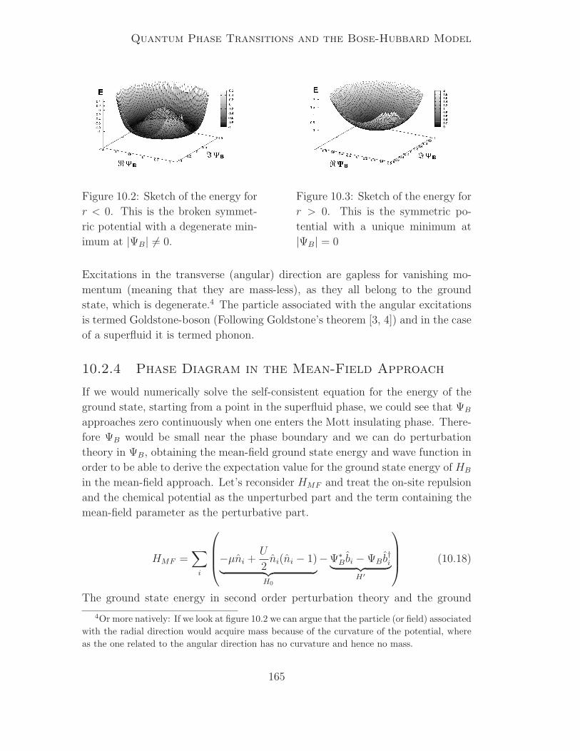
Quantum Phase Transitions and the Bose-Hubbard Model
Figure 10.2: Sketch of the energy for
r < 0. This is the broken symmet-
ric potential with a degenerate min-
imum at |ΨB| 6= 0.
Figure 10.3: Sketch of the energy for
r > 0. This is the symmetric po-
tential with a unique minimum at
|ΨB| = 0
Excitations in the transverse (angular) direction are gapless for vanishing mo-
mentum (meaning that they are mass-less), as they all belong to the ground
state, which is degenerate.4 The particle associated with the angular excitations
is termed Goldstone-boson (Following Goldstone’s theorem [3, 4]) and in the case
of a superfluid it is termed phonon.
10.2.4 Phase Diagram in the Mean-Field Approach
If we would numerically solve the self-consistent equation for the energy of the
ground state, starting from a point in the superfluid phase, we could see that ΨB
approaches zero continuously when one enters the Mott insulating phase. There-
fore ΨB would be small near the phase boundary and we can do perturbation
theory in ΨB, obtaining the mean-field ground state energy and wave function in
order to be able to derive the expectation value for the ground state energy of HB
in the mean-field approach. Let’s reconsider HMF and treat the on-site repulsion
and the chemical potential as the unperturbed part and the term containing the
mean-field parameter as the perturbative part.
HMF =∑
i
−µni +
U
2ni(ni − 1)
︸ ︷︷ ︸H0
−Ψ∗B bi − ΨB b
†i︸ ︷︷ ︸
H′
(10.18)
The ground state energy in second order perturbation theory and the ground
4Or more natively: If we look at figure 10.2 we can argue that the particle (or field) associated
with the radial direction would acquire mass because of the curvature of the potential, where
as the one related to the angular direction has no curvature and hence no mass.
165

10.2 The Bose-Hubbard Model
state wave function in first order can be written in general like
En = E(0)n + 〈n|H ′|n〉 +
∑
k 6=n
|〈k|H ′|n〉|2
E(0)n − E
(0)k
+O(|ΨB|3)
|n〉 = |n0〉 +∑
k 6=n|k〉 〈k|H ′|n〉
E(0)n − E
(0)k
+O(|ΨB|2)
We will calculate all the terms separately and, without loss of generality, we
will look only at a single-site as it would be the same for each site. Note that
〈n|H ′|n〉 = 0 as H ′ contains linear terms in b and b†. Therefore
E(0)n =
U
2n(n− 1) − µn H ′
kn = 〈k|H ′|n〉
a) |k〉 = |n+ 1〉 H ′kn = 〈n+ 1|(−ΨB b
† − Ψ∗B b)|n〉 = −ΨB
√n+ 1
⇒ |H ′kn|2 = |ΨB|2(n+ 1) E(0)
n − E(0)k = −Un+ µ
b) |k〉 = |n− 1〉 H ′kn = 〈n− 1|(−ΨB b
† − Ψ∗B b)|n〉 = −Ψ∗
B
√n
⇒ |H ′kn|2 = |ΨB|2n E(0)
n − E(0)k = U(n− 1) − µ
Collecting these results in the expression of En = EMF0 and the mean-field ground
state
EMF0
M= E(0)
n + |ΨB|2(
n+ 1
µ− Un+
n
U(n− 1) − µ
)= E(0)
n − |ΨB|2χ0 +O(|ΨB|3)
|n〉 = |n〉 − ΨB
√n+ 1
µ− Un|n+ 1〉 − Ψ∗
B
√n
U(n− 1) − µ|n− 1〉 +O(|ΨB|2) ,
where we define χ0 = n+1Un−µ + n
µ−U(n−1). From this the expectation values follow
as
〈b〉 = 〈n|b|n〉 = −ΨB
(n+ 1
µ− Un+
n
U(n− 1) − µ
)= ΨBχ0
〈b†〉 = 〈n|b†|n〉 = −Ψ∗B
(n+ 1
µ− Un+
n
U(n− 1) − µ
)= Ψ∗
Bχ0 ,
which are the relations we would have to use to determine ΨB self-consistently.
Using eq. (10.16) we get the mean-field approximation of the ground state energy
of the Bose-Hubbard Hamiltonian
166

Quantum Phase Transitions and the Bose-Hubbard Model
E0
M= E(0)
n + |ΨB|2[χ0 − Zwχ2
0
]. (10.19)
Therefore r (compare eq. (10.17)) is the coefficient of |ΨB|2 and from r = 0 we
will get the phase boundary as discussed in the previous section. If we minimize
eq. (10.19) with respect to χ0 we can see that χ0 must be positive, as Zw is
positive. Therefore the sign change in r can only come from 1−Zwχ0, hence the
phase boundary is given by
Zw =(n− µ
U)( µU− n+ 1)
n(n− µU) + (n+ 1)( µ
U− n+ 1)
. (10.20)
Equation (10.20) describes the phase boundary for given n (integer density of
particles). Therefore we can obtain the phase diagram by simply plotting this
function in the ZwU
- µU-plane, as is done in figure 10.4.
Figure 10.4: Phase diagram of HB obtained through mean-field approach.
The limit of w = 0 corresponds to the Mott insulating state, as seen above,
provided that µU
is not equal to a positive integer. We know already that both
the hopping term and the on-site term commute with the total number operator
NB =∑
i ni, such that both conserve the total number of bosons. Therefore,
for w = 0 and µU
at non-integer values (case of integer values would be discussed
later), we have a well defined energy gap and the ground state is an eigen-state of
NB (is incompressible). As one turns on a small nonzero w the ground state will
move adiabatically without undergoing any level-crossing with any other state.
The perturbation arising from a nonzero w commutes with NB. Consequently
the ground state will remain an eigen-state of NB with precisely the same eigen-
value (rests incompressible) even for small nonzero w. Assuming translational
167

10.2 The Bose-Hubbard Model
invariance we get quantized values of the density (pinned at integer values). This
argument also shows that the energy gap will survive everywhere within the lobe
and hence we have a Mott insulating state inside the lobes. [2]
In [1] there is a nice argument how one can understand the lobe like shapes of
the phase boundaries which we will recall here. Choose an arbitrary point on the
µ-w plane inside one of the lobes (in the MI-phase) and start to increase µ while
keeping w fixed. Eventually one will reach a point where the chemical potential
together with the kinetic energy gained by adding an extra particle, free to hop
through the lattice, would balance the associated potential energy cost (this is
the level-crossing shown in fig. 10.1). Therefore, since any nonzero numbers of
particles free to hop without energy cost will, at zero temperature, immediately
Bose-condense and build a superfluid, such a point of energy balance defines the
phase boundary for a transition between the Mott insulating and the superfluid
phase. The same is true, for holes instead of particles, when one lowers µ. Now,
the kinetic energy, which is account for by the hopping term, increases with w
such that the balance is found earlier, meaning that the width within µ of the
MI-phase would decrease. And this leads to the lobe like shapes shown in figure
10.4.
Note that the superfluid phase extends all the way down to w = 0 at integer
values of µU, where we have a degeneracy. This degeneracy clearly denotes that
occupying the state with n bosons is energetically identical to occupying it with
n + 1. Therefore we are free to add additional particles even at arbitrary low,
but nonzero, w without energy cost, which leads to superfluidity as the additional
number of bosons is free to hop through the lattice and will hence Bose-condense.5
It is instructive to consider the contours of constant density in the phase diagram;
the lines of integer density are hereby of particular interest. For non-integer densi-
ties the constant density contours lie entirely within the superfluid phase, skirting
the Mott insulating phases and terminating on the µ axis at the special point of
integer value of µU. But the integer density contours meet the phase boundary
right at the tip of the lobes (points of maximum w on the phase boundary).
If this were not the case we would simply get a negative compressibility (κ = dρdµ
)
in the vicinity of the tips, which is a physical impossibility. That the contours
for densities just slightly greater or smaller than n lie just slightly above or below
the MI-phase with constant density n, is consistent with the assertion that the
MI-SF transition at a generic point on the phase boundary is driven by the
addition or subtraction of small numbers of particles to the incompressible MI-
phase. Therefore the density changes continuously from its fixed integer value n
5These points of integer values of µU
are in fact tri-critical points as they are facing the
superfluid phase as well as two Mott insulating phases with different densities.
168
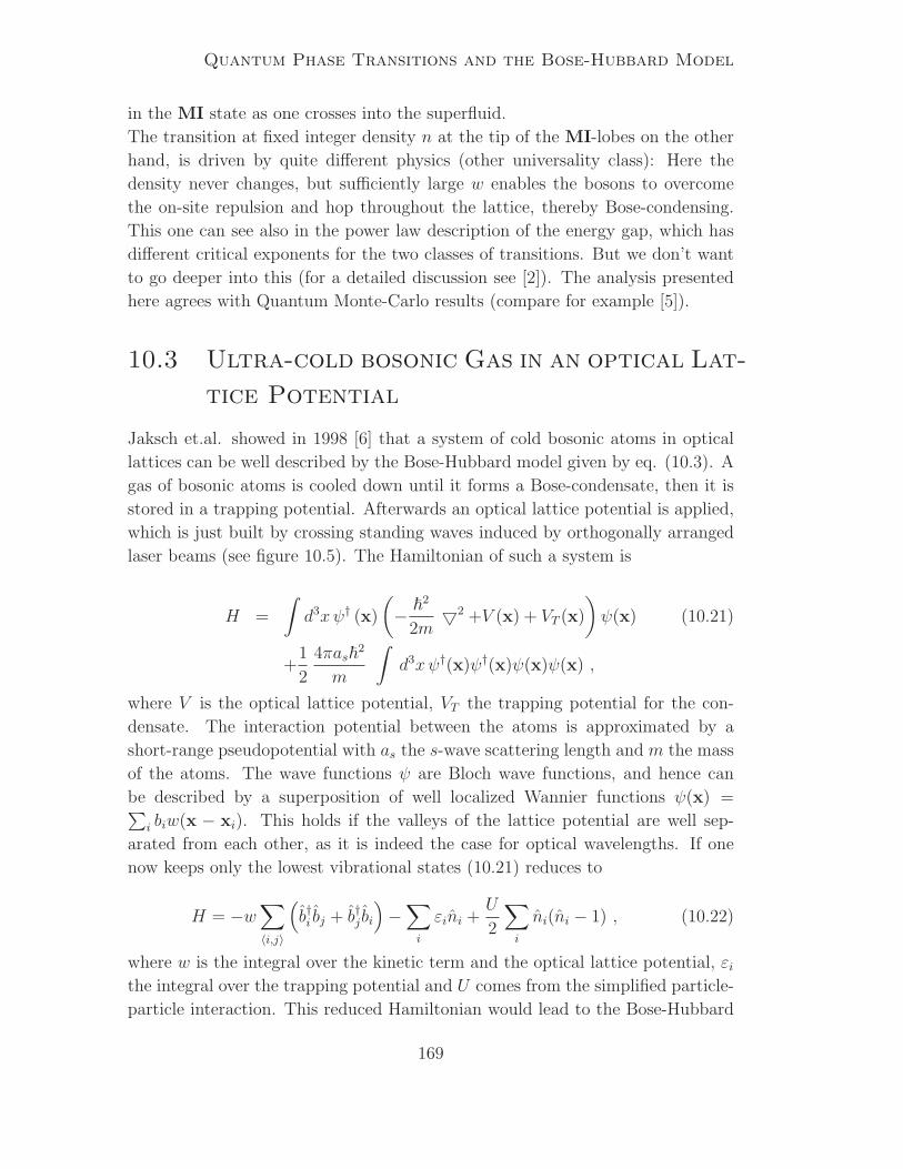
Quantum Phase Transitions and the Bose-Hubbard Model
in the MI state as one crosses into the superfluid.
The transition at fixed integer density n at the tip of the MI-lobes on the other
hand, is driven by quite different physics (other universality class): Here the
density never changes, but sufficiently large w enables the bosons to overcome
the on-site repulsion and hop throughout the lattice, thereby Bose-condensing.
This one can see also in the power law description of the energy gap, which has
different critical exponents for the two classes of transitions. But we don’t want
to go deeper into this (for a detailed discussion see [2]). The analysis presented
here agrees with Quantum Monte-Carlo results (compare for example [5]).
10.3 Ultra-cold bosonic Gas in an optical Lat-
tice Potential
Jaksch et.al. showed in 1998 [6] that a system of cold bosonic atoms in optical
lattices can be well described by the Bose-Hubbard model given by eq. (10.3). A
gas of bosonic atoms is cooled down until it forms a Bose-condensate, then it is
stored in a trapping potential. Afterwards an optical lattice potential is applied,
which is just built by crossing standing waves induced by orthogonally arranged
laser beams (see figure 10.5). The Hamiltonian of such a system is
H =
∫d3xψ† (x)
(− ~
2
2m2 +V (x) + VT (x)
)ψ(x) (10.21)
+1
2
4πas~2
m
∫d3xψ†(x)ψ†(x)ψ(x)ψ(x) ,
where V is the optical lattice potential, VT the trapping potential for the con-
densate. The interaction potential between the atoms is approximated by a
short-range pseudopotential with as the s-wave scattering length and m the mass
of the atoms. The wave functions ψ are Bloch wave functions, and hence can
be described by a superposition of well localized Wannier functions ψ(x) =∑i biw(x − xi). This holds if the valleys of the lattice potential are well sep-
arated from each other, as it is indeed the case for optical wavelengths. If one
now keeps only the lowest vibrational states (10.21) reduces to
H = −w∑
〈i,j〉
(b†i bj + b†j bi
)−∑
i
εini +U
2
∑
i
ni(ni − 1) , (10.22)
where w is the integral over the kinetic term and the optical lattice potential, εithe integral over the trapping potential and U comes from the simplified particle-
particle interaction. This reduced Hamiltonian would lead to the Bose-Hubbard
169

10.3 Ultra-cold bosonic Gas in an optical Lattice Potential
Hamiltonian if we assume the trapping potential to be flat in the region observed,
such that we can assume the εi to be independent of the lattice sites and hence
take them out of the sum.
Figure 10.5: Sketch of an optical lattice built by
crossing standing waves.
Figure 10.6: Schematic ex-
perimental apparatus, 3D in-
terference pattern with mea-
sured absorption images, ob-
tained after ballistic expansion
from a lattice with potential
depth of V0 = 10Er and a time
of flight of 15 ms.
Such an ultra-cold bosonic gas in an optical lattice potential, as proposed by
Jaksch et. al. [6], was realized in the lab by Greiner et.al. in 2002 [7]. They
controlled the hopping rate w by tuning the intensity of the laser beams (changing
the depth of the optical potential, measured in terms of recoil energy Er) and
studied the effect of the depth of the optical lattice potential on the coherence of
the state. They measured coherence just by ramping up the optical potential to
the desired depth and suddenly releasing the particles from the combined trap and
lattice potential, such that the wave functions could expand freely and interfere
with each other. They made absorption images along two orthogonal directions
of these interference pattern (see figure 10.6).
In the superfluid regime they obtained interference pattern with sharp maxima.
Increasing the potential depth further (meaning decreasing the hopping rate w)
also higher order interference maxima appeared as effects due to the presence of
the lattice. However, at a potential depth of 13 Er the interference maxima no
longer increased. Instead an incoherent background of atoms gained more and
more strength until at a potential depth of 22 Er, no interference pattern was
visible at all (compare with figure 10.7). This is just what we have seen in section
10.2.1 and 10.2.2.
A remarkable feature they observed during the evolution from the coherent to
170

Quantum Phase Transitions and the Bose-Hubbard Model
Figure 10.7: Absorption images of multiple matter wave interference patterns.
These were obtained after suddenly releasing the atoms from an optical lattice
potential with different potential depths V0 after a time of flight of 15 ms. Values
of V0 were: a, 0 Er; b, 3 Er; c, 7 Er; d, 10 Er; e, 13 Er; f, 14 Er; g, 16 Er; h, 22
Er.
the incoherent state was that when the interference pattern was still visible no
broadening of the interference peaks could be detected until they completely van-
ished in the incoherent background. This behavior can be explained on the basis
of the superfluid-Mott insulator phase diagram. In fact the trapping potential is
not that flat as we have assumed6 and therefore the system, after it has crossed
the quantum critical point, will evolve into alternating regions of incoherent Mott
insulator domains and coherent superfluid domains (compare with [6]), where the
superfluid fraction continuously decreases for increasing ratios U/w.
We have to mention that Greiner et.al. were also able to restore coherence after
being in the Mott insulator state when they lowered the potential depth, here
they also did measurements on the energy gap and discovered that it vanished at
the same potential depth were the interference pattern reappeared.
At the end one can conclude that theory and experiment are in good agreement
with each other. Nevertheless their realization of the Bose-Hubbard model with
an atomic gas now allows the study of strongly correlated many-body quantum
mechanics with unprecedent control of parameters.
6The system is hence in-homogeneous.
171

10.3 Ultra-cold bosonic Gas in an optical Lattice Potential
172

Bibliography
[1] M. P. A. Fisher, P. B. Weichman, G. Grinstein, and D. S. Fisher, Boson local-
ization and the superfluid-insulator transition, Phys. Rev. B 40, 546 (1989).
[2] S. Sachdev, Quantum Phase Transitions (Cambridge University Press, Cam-
bridge, 1999).
[3] J. Goldstone, , Nuovo cimento 19, 154 (1961).
[4] J. Goldstone, A. Salam, and S. Weinberg, Broken Symmetries, Phys. Rev.
127, 965 (1962).
[5] G. G. Batrouni, R. T. Scalettar, and G. T. Zimanyi, Quantum Critical Phe-
nomena in One-Dimensional Bose Systems, Phys. Rev. Lett. 65, 1765 (1990).
[6] D. Jaksch, C. Bruder, J. I. Cirac, C. W. Gardiner, and P. Zoller, Cold Bosonic
Atoms in Optical Lattices, Phys. Rev. Lett. 81, 3108 (1998).
[7] M. Greiner, O. Mandel, T. Esslinger, T. W. Hansch, and I. Bloch, Quantum
phase transition from a superfluid to a Mott insulator in a gas of ultracold
atoms, Nature 415, 39 (2002).
173

BIBLIOGRAPHY
174

Chapter 11
Quantum Field Theory and the
Deconfinement Transition
Yves Barmazsupervisor: Urs Wenger
Several gauge field theories show a phase transition between a
low temperature confining phase and a high temperature decon-
fining phase. We introduce the lattice formalism for studying the
behavior of pure gauge theories, in particular the interaction of
static quarks. We show some criterion for confinement. We an-
alyze how the so-called center symmetry is related to the phase
transition, and how one can use this relation to make predictions
about the critical behavior of the gauge theory.
11.1 Introduction
Some gauge field theories present a phase transition between a confining phase
and an non-confining one, the most important example being the quantum chro-
modynamics (QCD), which describes the strong interaction of the Standard
Model. We will try to study this phenomenon here, with the restriction to pure
gauge theories. The introduction of dynamical fermions would involve different
symmetries between the phases, and consequently different symmetry breaking
mechanisms. We will begin with a recall of a few notions of field theories, at both
zero and finite temperature, mostly taken from [1].
175

11.2 Gauge Field Theories
11.2 Gauge Field Theories
Quantum field theories usually lead to divergent quantities, due to the infinite
number of degrees of freedom. One way to regularize these quantities is to intro-
duce a space-time lattice. The continuum version of the action, S =∫d4xL, is
replaced by a sum over lattice elements (e.g. sites or plaquettes, which are ele-
mentary loops of the lattice). While the scalar fields and Dirac fields are assigned
to the lattice points, vector fields (such as gauge fields) live on the links between
the sites.
In a gauge field theory, one can show that the local gauge invariance can be
implemented via the introduction of link variables Uµ(n) related to the gauge
potential as
Uµ(n) ≡ Un,n+µ = eieaAµ(n). (11.1)
Gauge transformations are described by an element G(n) of a gauge group as-
signed to each lattice site. To ensure gauge invariance, the link variables trans-
form as follows under a local gauge transformation:
Uµ(n) → G(n)Uµ(n)G−1(n+ µ) = eieaAGµ (n), (11.2)
where AGµ (n) is a discretized version of Aµ(x) − 1e∂µΛ(x), and µ is a unit vector
in the µ-direction.
In a pure gauge theory, the only term in the action is the kinetic term of the
gauge field. For simplicity we consider the case where the gauge group is U(1).
The corresponding Lagrangian density is given by
L(x) = Fµν(x)Fµν(x) (11.3)
where a summation over repeated indices is understood, and Fµν describes the
field-strength tensor. Here we work with the Euclidean time version of the action,
and the indices µ, ν are taken in 1, 2, 3, 4.To get a lattice version of this kinetic term, from the structure FµνFµν it is clear
we can consider the smallest loops, e.g. a plaquette in the µ-ν-plane:
Uµν(n) := Uµ(n)Uν(n+ µ)U †µ(n+ ν)U †
ν(n). (11.4)
The link variables are path-ordered. This will become important when we will
consider non-Abelian theories. Inserting (11.1), one finds
Uµν(n) = eiea2Fµν(n), (11.5)
where Fµν(n) = 1a[(Aν(n+ µ) − Aν(n)) − (Aµ(n+ ν) − Aµ(n))] is the discretized
version of the field-strength tensor. For a small lattice constant a, one can show
176

Quantum Field Theory and the Deconfinement Transition
that1
e2
∑
n
∑
µ<ν
[1 − 1
2
(Uµν(n) + U †
µν(n))]
≈ 1
4
∑
n,µ,ν
a4Fµν(n)Fµν(n).
Thus the lattice action for the gauge potential is given by
SG [U ] =1
e2
∑
P
[1 − 1
2
(UP + U †
P
)](11.6)
where UP (plaquette variable) stands for the product of link variables around the
boundary of a plaquette ”P” taken in the counterclockwise direction.
Our formula for the pure gauge action can be generalized for SU(N) gauge the-
ories,
S(SU(N))G [U ] = β
∑
P
[1 − 1
NRe TrUP
], β =
2N
g20
, (11.7)
where the sum extends over all distinct plaquettes, and UP stands for the path-
ordered product of link variables along the boundary of the plaquette. This action
is invariant under the gauge transformation on the lattice described above.
At this point we should mention that the gauge action contains highly non-
trivial interaction terms, due to the non-Abelian character of the theory. This
self-coupling of the gauge potentials is believed to be responsible for quark con-
finement.
Knowing the lattice expression for the SU(N) gauge action, we can now compute
correlation functions:
〈U cdµ1
(n1) . . . 〉 =
∫DU U cd
µ1(n1) . . . e
−SG
∫DU e−SG
. (11.8)
Here the integration measure DU will be a product over the lattice links of Haar
measures of SU(N), which are gauge invariant. This choice hence guarantees that
quantum fluctuations will not break the gauge invariance of the whole theory.
11.3 Wilson Loop and Static qq-Potential
As we will see, the Wilson loops allow to describe the potential of two interacting
static quarks. In particular, their counterpart in finite temperature field theories
will provide a criterion to decide whether quarks are confined or not.
We consider a heavy quark (Q) and an antiquark (Q) introduced in the ground
state of a quantum system described by the Abelian gauge action (11.6). We
want to study the energy of this (infinitely) heavy pair. We consider the gauge
invariant state
|φαβ(x,y)〉 = Ψ(Q)
α (x, 0)U(x, 0;y, 0)Ψ(Q)β (y, 0)|Ω〉, (11.9)
177

11.3 Wilson Loop and Static qq-Potential
with |Ω〉 describing the ground state and
U(x, t;y, t) = P exp
(ie
∫ y
x
dziAi(z, t)
), (11.10)
where the integration is performed along a straight line joining x and y. The P in
front of the exponential stands for the path-ordering operation. This is of course
irrelevant if we consider an Abelian gauge theory. Ψ(Q) is a Dirac field operator
describing the heavy quarks, with its Dirac indices denoted by α or β. The vector
fields Ai are taken in the Lie algebra of the gauge group (up to multiplication by
ie dzi). |φαβ〉 is not an eigenstate of the Hamiltonian, but it serves as a trial state
to find the lowest energy of states with non-vanishing projection onto it. We will
study the propagation of |φαβ〉 to extract this energy. The evolution of this state
is described by the Green function
Gα′β′,αβ (x′,y′;x,y; t) =
〈Ω|T(Ψ
(Q)
β′ (y′, t)U(y′, t;x′, t)Ψ(Q)α′ (x′, t)Ψ
(Q)
α (x, 0)U(x, 0;y, 0)Ψ(Q)β (y, 0)
)|Ω〉
(11.11)
In the limit of infinite quark masses, the positions are frozen, and in the contin-
uation to imaginary times, t→ −iT , with the limit T → ∞, the contributions of
states with energy higher than the one of the ground state vanish exponentially,
so we expect
Gα′β′,αβ (x′,y′;x,y;−iT ) → δ(3)(x−x′)δ(3)(y−y′)Cα′β′,αβ(x,y)e−E(R)T , (11.12)
where Cα′β′,αβ is a function describing the overlap of the trial state (11.9) with the
ground state(s) of the Hamiltonian in the presence of the static pair, and E(R)
is the ground state energy of the static pair separated by a distance R = |x−y|,which includes the self-energy. To compute this energy, we need a path integral
representation of the Green function (11.11), which is given by
1
Z
∫DADψ(Q)Dψ(Q)
(ψ
(Q)
β′ (y′, t) . . . ψ(Q)β (y, 0)
)eiS, (11.13)
where
S = SG [A] + SQ
[ψ(Q), ψ
(Q), A]
SQ
[ψ(Q), ψ
(Q), A]
=∫d4xψ
(Q)(x) (iγµDµ −MQ)ψ(Q)(x).
(11.14)
The last term SQ represents the gauge-invariant Dirac action for the heavy quarks.
Notice that the path-integral involves here in the continuum formulation the
gauge fields Aµ instead of the link variables Uµ(n) in the lattice formulation.
178
Quantum Field Theory and the Deconfinement Transition
We now set x = (x, 0), x′ = (x′, t), y = (y, 0) and y′ = (y′, t). Since we are in
the static case, dropping the spatial derivatives in the action still gives a good
approximation. After some calculation, one gets
limMQ→∞
Gα′β′,αβ = δ(x−x′)δ(y−y′) (P+)αα′ (P−)ββ′ e−2iMQt〈exp
(ie
∮dzµAµ(z)
)〉,
(11.15)
where the integral is to be performed along the boundary of a rectangle with
corners at x, x′, y and y′, 〈·〉 denotes the ground state expectation value in the
absence of the static quark-antiquark source, and the matrices P± are defined by
P± = (1 ± γ0). Once again we make the continuation to imaginary times, and
we get
limMQ→∞
[Gα′β′,αβ]t→iT = δ(x − x′)δ(y − y′) (P+)αα′ (P−)ββ′ e−2MQt〈WC [A]〉eucl,
(11.16)
where the Wilson loop is defined by
WC [A] = exp
(ie
∮
C
dzµAµ(z)
), (11.17)
the integration being performed along a rectangular contour in the Euclidean
space-time with corners given by (x, 0), (x, T ), (y, 0) and (y, T ), and its Euclidean
expectation value by
〈WC [A]〉eucl =
∫DAWC [A] e−S∫
DAe−S . (11.18)
To get the static qq-potential, it suffices to study the behavior for large T of
W (R, T ) ≡ 〈WC [A]〉eucl:
limT→∞
W (R, T ) = F (R)e−E(R)T . (11.19)
F (R) reflects the overlap between the ground state(s) and our trial state. The
interaction energy follows simply as
E(R) = − limT→∞
1
Tln〈WC [A]〉eucl. (11.20)
So far we have used the continuum formulation, which has only a formal mean-
ing. To define it, and in order to be able to compute this energy, we need the
lattice formulation. The Wilson loop can simply be replaced by a product of link
variables
WC [U ] =∏
l∈CUl, (11.21)
179
11.4 Quantum Field Theories at Finite Temperature
taken along a temporal rectangular contour C on the lattice, with ground state
expectation value
W (R, T ) ≡ 〈WC [U ]〉 =
∫DU WC [U ] e−S∫
DU e−S . (11.22)
Calculations show that the inter-quark potential rises linearly with separation of
the quarks in QCD, which indicates confinement at zero temperature, while QED
leads to a Coulomb potential.
11.4 Quantum Field Theories at Finite Tem-
perature
To study the thermodynamic properties of quantum field theories, the path inte-
gral formalism allows to express partition functions and other expectation values
of thermodynamic observables in an elegant and simple way. Phase transitions
taking place of course at finite temperatures, we will need this formalism, that
we are briefly introducing here.
11.4.1 Path Integral Representation of the Partition
Function in Quantum Mechanics
Before turning our attention to complicated systems of fields, it is easier to begin
with the simple case of statistical quantum mechanics. The partition function is
given there by
Z = Tr e−βH , (11.23)
where β = 1kBT
as usual and H stands for the Hamiltonian of the system. We set
kB = 1. Let n be the number of degrees of freedom. In the following, we describe
with
|q〉 = |q1, . . . , qn〉 (11.24)
the simultaneous eigenstates of the coordinate operators Qi with eigenvalues qi.
The partition function then reads
Z =
∫ n∏
α=1
dqα〈q|e−βH |q〉. (11.25)
We notice a certain similarity of the integrand with the Euclidean time propagator
〈q′|e−H(τ ′−τ)|q〉 ≈∫
DqDp eip(l)α
“
q(l+1)α −q(l)α
”
e−ǫH(q(l),p(l)), (11.26)
180
Quantum Field Theory and the Deconfinement Transition
where DqDp =∏n
β=1
∏N−1l=1 dq
(l)β
∏N−1l=0
dp(l)β
2π, q(0) = q and q(N) = q′, and where
the equality is reached in the limit N → ∞. To get the partition function from
this propagator, it suffices to replace the Euclidean time interval τ ′ − τ with the
inverse temperature β, identify the coordinates at ”time” τ = 0 with the ones at
τ = β, and perform the integration over q (= q(0) in the following). Our partition
function then gets the form
Z = limN→∞ǫ→0Nǫ=β
∫DqDp eiφ[q,p]e−
PN−1l=0 ǫH(q(l),p(l))|q(N)=q(0) , (11.27)
where DqDp =∏N−1
l=0
∏αdq
(l)α dp
(l)α
2πand φ [q, p] =
∑N−1l=0
∑α p
(l)α
(q(l+1)α − q
(l)α
), as
well as a (formal) continuum version
Z =
∫
per
Dq∫
Dp e−R β0 dτ[
P
α ipα(τ)qα(τ)−H(q(τ),p(τ))], (11.28)
where ”per” (for periodic) reminds the reader that coordinates at ”time” τ = 0
and τ = β are to be identified. We now have a path integral representation for
the partition function, and we remark that three features make a distinction from
the classical partition function:
1. The phase-space measure involves coordinates and momentum variables
associated with every Euclidean time support on the discretized interval
[0, β] (and not only at one fixed time)
2. The Boltzmann factor is replaced by
exp(−βH
),
where H = 1N
∑N−1l=0 H
(q(l), p(l)
)is the ”time” averaged Hamiltonian de-
fined at discrete time supports.
3. The phase-space measure multiplied by the phase factor depends on coor-
dinates and momenta, and couples coordinates at neighboring lattice sites
on the time (temperature) axis.
We notice that the integrand in the partition function (11.27) involves the phase
eiφ[q,p], and hence this is not a probability distribution in the phase space.
If the Hamiltonian has the form H = 12
∑nα=1 p
2α + V (q), then performing the
Gauss integration on momenta, one finds that∫
per
[dq] e−R β0 dτ LE(q,q), (11.29)
181

11.4 Quantum Field Theories at Finite Temperature
where[dq] =∏N−1
l=0
∏nα=1
dq(l)α√2πǫ
, LE(q(l), q(l)) =∑
α12q(l)2α + V (q(l)), with q = q(0).
We can conclude that within the path integral framework, temperature is in-
troduced by restricting the Euclidean time to the compact interval [0, β] and
imposing periodic boundary conditions on the coordinate degrees of freedom.
11.4.2 Scalar Bosons
Following the prescription we just found to introduce temperature into a system,
we describe now the formalism of the finite temperature field theories with the
example of the scalar field. Although we will not use this kind of field later, this
remains the simplest kind of field, and hence gives rise to the simplest partition
function. To find this partition function, we simply start from the quantum
mechanics version, and we replace the coordinates qα(τ) by fields φx(τ) := φ(x, τ).
With the Lagrangian
LE[φ, φ] =∫d3xLE(φ, ∂µφ),
LE = 12∂µφ∂µφ+ 1
2M2φ2,
(11.30)
we find the path integral representation of the partition function
Z0 = N∫
per
Dφ e−R β0 dτ
R
d3xLE[φ,φ]. (11.31)
The scalar field has to satisfy periodic boundary conditions φ(x, 0) = φ(x, β).
The partition function can thus be interpreted as a weighted sum over all field
configurations living on a Euclidean space-time surface compactified along the
time-direction.
11.4.3 Non-Perturbative SU(N) Gauge Theory at Fi-
nite Temperature
We want to study the behavior of hadronic matter at finite temperature as de-
scribed by a pure SU(N) theory, which corresponds to a QCD without dynamic
quarks. In particular, we would like to know if this model predicts a phase transi-
tion from a low temperature confining phase to a high temperature where quarks
and gluons are deconfined, and if this is the case, we would like to find the criti-
cal temperature and the order of the transition. The non-perturbative framework
provided by the lattice form of QCD should give answers to these questions.
To compute thermodynamical observables, we need a non-perturbative formula-
tion of the partition function. From the above discussion, we guess that
Z =
∫DU eS[U ]. (11.32)
182

Quantum Field Theory and the Deconfinement Transition
The action now takes the form
S =∑
n
Re
βt∑
i
Tr (U4i(n)) + βs∑
i<j
Tr (Uij(n))
(11.33)
where Uµ(n) are link variables subjected to periodic boundary conditions, and
Uµν(n) the corresponding path-ordered products around plaquettes starting at
the lattice site n following the two directions µ and ν. The sum over n is meant
over all lattice sites, and over roman indices i and j from 1 to 3. βt and βs are
independent couplings for ”time-like” and ”space-like” plaquettes, which depend
on the temperature and the conventional bare coupling 2g2
, explicitly
2g2
= a3−d√βsβt,T =
√βs/βt
Nta,
(11.34)
where a is the space-like lattice spacing, (NtT )−1 the time-like spacing, and d
the spatial dimension. Notice that for d = 3, the coupling constant becomes
dimensionless.
11.5 The Wilson Line or Polyakov Loop
Since the lattice is periodic in time, in addition to the topologically trivial Wilson
loops defined above (which may be shrunk to a point), there exist topologically
non-trivial loops which wind around the lattice along the time direction. For
example, the ”Wilson line” or ”Polyakov loop” L(x) at some spatial location x
is defined by
L(x) = Tr
β∏
n=1
U4(x + nt). (11.35)
Its expectation in the ensemble (11.32) determines the free energy of a single
static quark relative to the vacuum,
e−Fq/T = 〈L(x)〉 (11.36)
and the correlation function of two Wilson lines yields the static quark-antiquark
free energy
e−Fqq(x−y)/T = 〈L(x)L†(y)〉, (11.37)
as one could guess from the similarity with the Wilson loop in the case of zero
temperature. Static quarks will be confined if this correlation function vanishes
when |x − y| → ∞. Provided cluster decomposition holds, that is
lim|x−y|→∞
〈L(x)L†(y)〉 = |〈L〉|2, (11.38)
183

11.6 The Deconfinement Phase Transition
this condition is equivalent to L(x) = 0, which shows that inserting a single static
quark requires infinite energy. On the other hand, if 〈L〉 6= 0, the free energy will
go to a constant as the quarks are separated, which indicates that there is no
confinement. Accordingly, the expectation value of the Wilson line evaluated in
a pure gluonic medium serves as an order parameter for distinguishing a confined
phase from a deconfined one in the pure SU(3) gauge theory. Following [2], we
can now use this order parameter to study the deconfinement transition.
11.6 Spontaneous Breakdown of the Center
Symmetry and the Deconfinement Phase
Transition
11.6.1 The Center Symmetry
In statistical mechanics, phase transitions are usually associated with the break-
down of a global symmetry. This is also expected in the SU(3) gauge theory. The
lattice action (11.33) is not only invariant under periodic gauge transformation,
but also possesses a further symmetry which is not shared with the Wilson line.
Recall that the center C of a group G is the subgroup
C =z ∈ G|zgz−1 = g ∀g ∈ G
. (11.39)
For example, the center of SU(3) is
Z3 =e
2πil3 ∈ C|l = 0, 1, 2
. (11.40)
We assume now that the center is not trivial. If we multiply all time-like oriented
link variables U4 between two neighboring spatial sections of the lattice by an
element of the center,
U4(n, n4) → z U4(n, n4), n4 fixed, z ∈ C fixed ∀n ∈ Z, (11.41)
our action is kept invariant. But the Wilson line is not invariant, since it contains
exactly one element that does not transform trivially:
L(x) → zL(x). (11.42)
If the ground state of the quantum system respects the symmetry of the classical
action, then link configurations related with the center symmetry will occur with
the same probability, therefore the same numbers of configurations will yield
184

Quantum Field Theory and the Deconfinement Transition
the values Ll = e2πil/3L, (l = 0, 1, 2) for the Wilson line. Consequently, its
expectation value will vanish, but this was interpreted as a signal for confinement.
Thus we expect that the center symmetry is realized in the low temperature,
confining phase of the pure SU(3) gauge theory. On the other hand, if 〈L〉 6= 0,
then the center symmetry is broken. So we expect further that the deconfinement
transition is accompanied by a breakdown of the center symmetry, and that the
phases of the Polyakov loops cluster around one of the Z3 roots.
These considerations are valid for the pure gauge sector, or equivalently, in the
infinite quark mass limit, which is of course unphysical. However the study of
the pure SU(3) gauge theory provides us with important information on the role
played by the non-Abelian gauge fields for quark confinement.
11.6.2 High Temperatures
In the action (11.33), the couplings obey βt ∼ T and βs ∼ 1/T . Thus in the limit
of high temperatures the contribution of any configuration with non-zero electric
flux (Un,4i 6= 1) becomes arbitrarily small compared to the configurations with
vanishing electric flux (remember that the trace of a unitary matrix is maximal
for the unit matrix). Therefore for high temperatures the partition function is
highly peaked about configurations in which the spatial link variables are static
up to a gauge transformation,
Ui(n) = U4(n)Ui(n + t)U4(n + i)†. (11.43)
Moreover periodicity in the time direction requires Ui(n) = Ui(n + Ntt). These
two conditions imply that the twists
Ωx =
β∏
n=1
U4(x + nt) (11.44)
must satisfy the condition
Ωx = Ui(x)Ωx+iUi(x)†. (11.45)
For almost all configurations of spatial link variables, this relation requires the
twists to equal a constant element of the center, Ωx = z, z ∈ C. Consequently,
the Wilson lines being the traces of twists, we have that 〈L(x)L†(y)〉 6= 0 in the
limit |x − y| → ∞.
Similarly, small symmetry-breaking perturbations (such as a ”magnetic field”
term h∑
x ReTr Ωx) will cause the only significant contributions to come from a
neighborhood of configurations for which Ωx = 1.
185
11.6 The Deconfinement Phase Transition
Therefore at sufficiently high temperatures we have 〈L(x)〉 6= 0 and we are in a
non-confining phase of the theory.
Nevertheless we should notice that this result of symmetry breaking is valid only
in the infinite volume limit. In finite volumes, finite potential barriers do not
prevent tunneling between the ground states, the symmetry is then reestablished,
and the expectation value of the Wilson line vanishes, 〈L(x)〉 = 0. In practice
one then consider the expectation value of the modulus of the Wilson line, 〈|L|〉(small in the symmetric phase, large in the phase of broken symmetry), or the
distribution of phases of the Wilson lines in numerical simulations.
11.6.3 Phase Transitions
If now the zero-temperature theory is in a confining phase, then there must be at
least one phase transition to separate this phase from the high temperature non
confining phase. L(x) will be an order parameter for this phase transition where
the global center symmetry is spontaneously broken.
If the transition is continuous, then the critical behavior will be due to long-range
fluctuations in the Wilson line L(x). Specifically, integrating out the spatial gauge
fields should produce only short-range interactions in the resulting effective field
theory for L(x).
The dynamics of spatial gauge fields are qualitatively the same at high and low
temperatures. In particular spatial Wilson loops obey an area-law behavior at
all temperatures, and both high and low temperature limits of the theory can
be shown to predict short range interactions. It is consistent to expect a similar
behavior for all temperatures, and we will assume this is the case. Integrating
out all degrees of freedom except the Wilson lines (whose behavior is temperature
dependent) should thus produce an effective theory with short range interactions
which is invariant under the center symmetry,
L(x) → zL(x), z ∈ C. (11.46)
The corresponding partition function was calculated [3] as
Z =
∫DL exp [−Seff ] (11.47)
with the effective action
Seff(L) = βeff
∑
x,i
|L(x) − L(x + i)|2
+∑
x
−1
2ln[27 − 18|L(x)|2 + 8ReL(x)3 − |L(x)|4
]− 6βeff |L(x)|2
(11.48)
186

Quantum Field Theory and the Deconfinement Transition
If, as a function of T , this theory has a continuous transition, then one could in
principle locate the renormalization group fixed point which governs the critical
behavior. And if, in the space of d-dimensional theories with short-range interac-
tions invariant under the center symmetry, there exists only a singe fixed point,
then the critical behavior of the original (d + 1)-dimensional finite temperature
gauge theory will be the same as that of simple d-dimensional spin models in-
variant under the same global symmetry. As a matter of fact, in many cases
only one single fixed point in a given class of theories is known, so that one can
use the critical behavior of spin models to predict the critical behavior in finite
temperature gauge theories. [2]
We emphasize that these predictions depend on the assumption of a continuous
transition. It is in general difficult to rule out the possibility of a first order
transition occurring before.
11.6.4 Predictions
We are now equipped to make predictions about phase diagrams (g2, T ), g2 being
the coupling, T the temperature, and phase transitions of finite temperature
gauge theories.
At T = 0, the confining phase extends from ∞ to some critical coupling g2cr,
which may vanish (this happens for asymptotically free theories), depending on
the dimension of the theory and the gauge group.
• In the confining phase, where the center symmetry is unbroken, Wilson line
correlation function takes the form
Γ(x) ≡ 〈L(0)L†(x)〉 ∼ exp [−σ|x|/T ] , as |x| → ∞, (11.49)
which corresponds to a linear static quark-antiquark potential, Fqq ∼ σ|x|,where the string tension σ depends on gcr and T .
• In the high-temperature phase, the center symmetry is broken, and two
cases are to be considered.
– If the center C is continuous, like for an Abelian group, this phase
must contain massless Goldstone bosons, and the correlation function
of Wilson lines
Γ(x) ∼M2
(1 +
e2
T |x|d−2
), as |x| → ∞ (11.50)
corresponds to a static Coulomb potential, Fqq ∼ −e2/|x|d−2 with
renormalized charge e2.
187

11.7 Deconfinement in the SU(3) Gauge Theory
– If the center is discrete, this phase can have a non-zero mass gap,
whence
Γ(x) ∼M2(1 + O
(e−µ|x|
)), as |x| → ∞. (11.51)
In this case, the short-range static potential Fqq ∼ O(e−µ|x|
)is similar
to the Debye screening of an electric plasma.
The strong coupling limit of any of the gauge theories we consider may be shown
to reduce exactly to an equivalent spin-system with nearest neighbor ferromag-
netic couplings invariant under the center symmetry. The low temperature phase
(11.49) corresponds to the disordered phase of the spin system while the high
temperature phase (11.50-11.51) is analogous to the ordered phase. This is an
example of inverse symmetry breaking, where the symmetry is broken in the
high temperature phase. Note that the correlation length ξ in the disordered
spin model yields the string tension in the gauge theory via σ = (ξT )−1.
11.6.5 Examples
In (3 + 1) dimensions, the SU(2) gauge theory with its center group Z2 is ex-
pected to show the same critical behavior as the 3d Ising model, while the phase
transitions of the SU(N) gauge theories for N ≥ 3 are first order.
In (2 + 1) dimensions, the transition of the SU(2) gauge theory now corresponds
to the one of the 2d Ising model, and the SU(3) theory to the 2d, q = 3 Potts
model. It is not clear whether the SU(4) theory has a second order or a very
weak first order phase transition. For N = 5, and presumably for all N > 5,
the phase transitions of the SU(N) theories are first order. Finally the expected
critical behavior of the U(1) gauge theory is the one of the 2-dimensional XY
model, with its Berezinsky-Kosterlitz-Thouless transition.
11.7 Discussion of the Deconfinement Phase
Transition in the Pure SU(3) Gauge The-
ory
Here we will discuss some results of numerical simulations, without going into
deep explanations on the methods used. These simulations aim at determining
characteristics of the phase transitions such as the critical temperature, the nature
of the transition, or critical exponents if they exist.
188

Quantum Field Theory and the Deconfinement Transition
Numerical simulations are performed on a small lattice, but large enough to avoid
finite volume effects.
The deconfinement transition in the pure SU(3) gauge theory is supposed to be
associated with the breakdown of the Z3 center symmetry, and predicted to be
first order. The order parameter that distinguishes the two phases is the ex-
pectation value of the Wilson line. In the infinite volume limit, the first order
deconfining phase transition would appear as a discontinuity in the Wilson line
or in the energy density. However, on a finite lattice this discontinuity will be
smoothed out, but a rapid variation should be seen, and is indeed seen. Neverthe-
less, such a variation does not exclude the possibility that the transition is second
order. To reach a definitive result, one can then consider a few characteristics of
a first order transition, for example the coexistence of phases at the critical tem-
peratures: In Monte Carlo simulations, this should manifest itself in the more or
less frequent flip of the system between the ”ordered” and ”disordered” phases.
To determine the critical temperature, if the transition is first order, as it is the
case here, and spatial lattice volume large enough, then localizing the disconti-
nuity should suffice. Alternatively, one may test the Z3 symmetry directly by
looking at the distribution of real and imaginary parts of Polyakov loops, mea-
sured on a large number of link configurations, as a function of the temperature.
• In the Z3 symmetric phase, configurations related by Z3 symmetry opera-
tions occur with equal probability.
• In the Z3-broken phase the system will spend a substantial simulation time
in one of the three vacua, before tunnelling between the vacua will restore
the Z3 symmetry.
We conclude this section with some orders of magnitude. The critical temper-
ature for QCD is in the range of 1012 K, or 270 MeV, a temperature that the
universe reached some 10−6 s after the Big Bang. Once more we should empha-
size that these results are valid only for pure Yang-Mills theories. The presence
of dynamical quarks would break the center symmetry. This would weaken the
transition, which would then be only a cross-over. This happens for example in
the QCD of the Standard Model, where a cross-over takes place at 170 MeV.
189

11.7 Deconfinement in the SU(3) Gauge Theory
190
Bibliography
[1] H. J. Rothe, Lattice gauge theories : an introduction (World Scientific, New
Jersey, 2005).
[2] B. Svetitsky and L. G. Yaffe, Critical behavior at finite-temperature confine-
ment transitions, Nucl. Phys. B 210, 423 (1982).
[3] A. D. Kennedy, J. Kuti, S. Meyer, and B. J. Pendleton, Where is the contin-
uum in lattice quantum chromodynamics?, Phys. Rev. Lett. 54, 87 (1985).
191

BIBLIOGRAPHY
192

Chapter 12
The Phases of Quantum
Chromodynamics
Bela Bauersupervisor: Dr. Urs Wenger, Dr. Philippe de Forcrand
The purpose of this work is to explore the phase diagram of mat-
ter as described by Quantum Chromodynamics. Interest in these
phases is caused by the wish to understand the high-temperature
universe fractions of a second after the Big Bang, and by the de-
sire to understand high-density matter, which can be found in
the core of neutron stars.
The various phase transitions that occur in the T -µ-plane are
described. Exotic high density phases, such as the colour flavour
locking phase, are discussed in more detail. Finally, a short in-
troduction to relativistic heavy ion collisions (RHIC), which is
an experimental tool to explore these phases, is given.
12.1 Introduction
In the first section of this report, some necessary foundations of QCD are in-
troduced, where it is assumed that the reader is at least in very general terms
familiar with the concept of a field theory. Special emphasis is put on the chi-
ral symmetry (breaking) in QCD and the physical consequences of spontaneous
symmetry breaking, as seen in the Goldstone theorem and the Higgs mechanism.
In the second part, the phase transitions in the T -µ-plane are described. In the
third section, an exotic phase that occurs in high-density matter, colour super-
conductivity, will be described. In the last section, relativistic heavy ion collisions
193

12.1 Introduction
will be introduced very quickly.
12.1.1 QFT and thermodynamics
Partition function in QFT
In order to make the connection between quantum field theory and statistical
mechanics, we consider the partition function of a statistical system, which, for
the canonical ensemble, is given as
Z =∑
all states
e−βE, (12.1)
where β = 1/T . We will now try to connect this expression to quantum field
theory. For a quantum system, we can rewrite the above using
e−βE → 〈α|e−βH |α〉 (12.2)
for some state |α〉 with energy expectation value E. From the path integral
representation of quantum field theory we know that the transition amplitude
between two field configurations φa and φb is given by
〈φb(x)|e−iHt|φa(x)〉 =
∫
φ(x,0)=φa(x),φ(x,t)=φb(x)
Dφ exp
[i
∫ t
0
d4xL]
(12.3)
where L = 12(∂µφ)2 − V (φ). We now switch to imaginary time (Euclidian
time/action) with τ = it, yielding∫ t0d4xL → i
∫ τ0d4xLE in the exponent. We
then find our final result
Z =
∫
φ(0)=φ(β)
Dφ exp
[−∫ β
0
d4xLE]. (12.4)
Here, the sum over all states was incorporated into the functional integral. We
only consider diagonal matrix elements, i.e. 〈φ|e−iHt|φ〉, and replace iHt by
βH, therefore the boundary condition on the integral in (12.3) becomes φa(x) =
φb(x) = φ(x, 0) = φ(x, β).
Chemical potential and the grand canonical ensemble
In the canonical ensemble used above the total particle number is kept constant.
In a relativistic field theory, particle number conservation is not a useful concept
anymore:
194

The Phases of Quantum Chromodynamics
• The theory is no longer formulated in terms of particles, but in terms of
fields. Particle number is not an obvious property of these fields. However,
a particle number operator counting the number of particles can be applied.
• The creation of particle-antiparticle pairs can occur. Therefore, a conserved
quantity can only be defined through the number of particles minus the
number of antiparticles.
A more convenient way is to choose an ensemble where the particle number is
allowed to fluctuate and then introduce a weight factor in a similar fashion to the
Gibbs factor above. This will also prove to be useful later in the discussion.
This ensemble is called the grand canonical ensemble. The partition function is
given as
Z =∑
all states α
e−βEαeβµNα . (12.5)
The quantity µ is called the chemical potential associated with the total charge
N . It causes a shift in the energy of each energy level which is proportional to a
charge N .
Closely related to this is the grand (canonical) potential (also referred to as
Helmholtz free energy), which, if the partition function is chosen as a starting
point, can be defined to be
Ω(T, µ) = −T lnZ. (12.6)
It can be shown that this potential has the following properties:
Ω = E − TS − µN (12.7)
= −pV. (12.8)
In equilibrium, this potential will be minimized.
Chemical potential in path integrals and the U(1)B symmetry
Now, the concept of a chemical potential will be incorporated into the path
integral formalism. Two arguments will be demonstrated, which yield the same
result. First, the chemical potential will be considered as a change in the energy
of a given state. A global time-dependent phase factor to the field,
ψ → ψeiµt, (12.9)
which changes the Lagrangian only through the time derivative, has an effect
equivalent to changing the frequency of the phase rotation of the field, which is
195

12.1 Introduction
equivalent to a change in the energy, since |α(t)〉 = e−iEt|α(0)〉. This can be used
to account for the chemical potential in the Lagrangian by using a replacement
∂
∂tψ →
(∂
∂t+ iµ
)ψ (12.10)
which is equivalent to the aforementioned phase factor. This leads to the following
Lagrangian (not Euclidian time!), which is invariant under (12.9):
L = −ψ [iγµ(∂µ + δ0µiµ) −m]ψ (12.11)
= −ψ [iγµ∂µ −m]ψ + µψγ0ψ. (12.12)
The other argument is that the chemical potential should couple to the baryon
density. Since ψγ0ψ represents the charge density in the Lagrangian, it can be
seen that the last term couples this density to the chemical potential in the desired
way. The symmetry (12.9) is a global, continuous symmetry referred to as U(1)Band due to Noether’s theorem, it is connected to the conserved baryon number.
Variables of the phase diagram
When talking about a phase diagram, one needs to define what the parameters
of the phase diagrams, i.e. the variables along its axes, are. Generally, one would
like to choose variables that, in equilibrium, are constant throughout the system
— even in different phases — and that are intensive, i.e. independent of the
system size. In the phase diagram we want to consider for QCD, the obvious
variables would be the temperature and the density. The second, however, does
not fulfill the above properties, since, in a regime of phase coexistence at a first
order phase transition, it is not constant throughout the system. From basic
thermodynamics, however, it is known that in such a phase coexistence region,
the chemical potential is constant across the phase boundaries. Therefore, it is
chosen as the second parameter of the phase diagram along with the temperature.
12.1.2 Example: Partition function for fermions
Instead of using the path integral formulation, a simpler approach can be used
in the case of fermions without interaction. It will be used as a quick way to
calculate the particle density as a function of the chemical potential for low
temperatures. Take, as an example, a system with two momentum states that, if
occupied by a particle, have an energy contribution ω~p − µ =√~p2 +m2 − µ and
ω~p + µ if occupied by an anti-particle. Each state is degenerate due to spin-up
196

The Phases of Quantum Chromodynamics
and spin-down particles. We therefore have
Z =∑
all states
e−E/T (12.13)
= e−E(|0,0〉)/T + e−E(|↑,0〉)/T + e−E(|0,↑〉)/T + ... (12.14)
= 1 + e−(ω ~p0−µ)/T + e−(ω ~p1
+µ)/T + ... (12.15)
=∏
~p
(1 + e−(ω~p−µ)/T )2(1 + e−(ω~p+µ)/T )2 (12.16)
We can now find the particle density (using q(~p) = (1+e−(ω~p−µ)/T )2(1+e−(ω~p+µ)/T )2)
N = −∂Ω
∂µ= −∂Z
∂µ
∂Ω
∂Z= −T
Z
∂Z
∂µ(12.17)
= −TZ
∑
~p
∏
~p′ 6=~p
q(~p)
∂
∂µq(~p) (12.18)
= −T∑
~p
(1
q(~p)
)(1 + e−(ω~p+µ)/T )22(1 + e−(ω~p−µ)/T )e−(ω~p−µ)/T (− 1
T) + ...
(12.19)
= 2∑
~p
1
e(ω~p−µ)/T + 1− 1
e(ω~p+µ)/T + 1
. (12.20)
The two terms in (12.20) show the well-known Fermi distribution for particles and
antiparticles, which has the appearance of a step function for low temperatures.
The Fermi momentum, i.e. the momentum up to which all states are occupied
in the ground state, is
pF =√µ2 −m2. (12.21)
Replacing the sum over ~p by an integral over phase space for the infinite volume
where ~p becomes continuous and and assuming that the temperature is low and
the occupied states form a Fermi sphere with volume 4π3p3F in momentum space,
we find for the density of charge
n =N
V=
8π
3(µ2 −m2)3/2. (12.22)
It can be seen that for µ < m, there will be no occupied states. The function n
is therefore not analytic at µ = m. It can be used as order parameter for a phase
transition at this point. This is closely analogous to the situation in QCD for low
temperatures.
197

12.1 Introduction
12.1.3 QCD and symmetries
Chiral symmetry
Consider a simple fermionic field described by the Dirac equation
(iγµ∂µ −m)ψ(x) = −i∂µψγµ −mψ = 0. (12.23)
In the following, we will use the Weyl representation where
γ5 =
( −1 0
0 1
), ψ(x) =
(ψL(x)
′
ψR(x)′
)(12.24)
ψL(x) =1 − γ5
2ψ(x) (12.25)
ψR(x) =1 + γ5
2ψ(x). (12.26)
ψ′L and ψ′
R are 2-component Weyl spinors and represent left-handed and right-
handed components of the field and therefore eigenstates of the helicity operator
with eigenvalue ±1. Now consider the following currents corresponding to the
symmetry transformations U(1)B : ψ(x) → eiαψ(x) and ψ(x) → eiαγ5ψ(x),
jµ(x) = ψ(x)γµψ(x) and jµ5(x) = ψ(x)γµγ5ψ(x), (12.27)
and their divergences
∂µjµ = (∂µψ)γµψ + ψγµ∂µψ (12.28)
= (imψ)ψ + ψ(−imψ) (12.29)
= 0 (12.30)
∂µjµ5 = (∂µψ)γµγ5ψ(x) + ψγµγ5∂µψ (12.31)
= (imψ)γ5ψ − ψγ5(−imψ) (12.32)
= 2imψγ5ψ, (12.33)
where we have used the anticommutation relation γ5, γµ = 0. It can be seen
that for m = 0, the axial vector current jµ5 is conserved. We can now define
left-handed and right-handed currents as
jµL = ψLγµψL = ψ†1 − γ5
2γ0γµ
1 − γ5
2ψ, (12.34)
jµR = ψRγµψR = ψ†1 + γ5
2γ0γµ
1 + γ5
2ψ. (12.35)
198

The Phases of Quantum Chromodynamics
We then find that (using the anticommutation and γ5γ5 = I)
jµL + jµR = jµ, (12.36)
∂µjµL = ∂µj
µR = 0. (12.37)
This shows that (for zero quark masses) the currents for left-handed and right-
handed quark fields are separately conserved.
Chiral symmetry breaking in QCD and dynamical quark masses
In the case of QCD with two massless quark flavours, we denote by Q the doublet
of light quarks,
Q =
(u
d
)= QL +QR, (12.38)
where, just as above,
QL =1 − γ5
2
(u
d
), QR =
1 + γ5
2
(u
d
)(12.39)
These transform as
QL → ULQL, QR → URQR, (12.40)
where UL and UR are transformations realizing the isospin symmetry separately
for left-handed and right-handed quarks, hence
UL, UR ∈ SU(2). (12.41)
The chiral flavour symmetries of QCD would therefore be SU(2)L × SU(2)R. In
a theory with more massless quark flavours, this symmetry becomes SU(Nf )L ×SU(Nf )R, where Nf is the number of quark flavours. With the additional colour
(gauge) symmetry SU(3)C and the symmetry that, due to Noether’s theorem,
induces baryon number conservation, the full symmetry group of QCD with Nf
massless quark flavours is
SU(3)C × SU(Nf )L × SU(Nf )R × U(1)B. (12.42)
It is known for QCD that the coupling between quarks and antiquarks becomes
very strong at large distances, while, in our theory of massless quarks, the creation
of a quark-antiquark-pair is connected to only a very small energy cost. Hence
we can expect the vacuum to be populated by such pairs. Since, however, the
overall momentum and angular momentum, i.e. spin, of the vacuum needs to be
0, they carry net helicity charge. Considering that the creator of a left-handed
199

12.1 Introduction
quark is the annihilator of a right-handed antiquark (and vice versa), we find a
vacuum with the non-vanishing expectation value for QQ
〈0|QQ|0〉 = 〈0|QLQL +QRQR +QLQR +QRQL|0〉 (12.43)
= 〈0|QLQR +QRQL|0〉 (12.44)
6= 0. (12.45)
If we now apply the symmetry transformations of (12.41) and require the vacuum
to be unaffected, we find the condition
〈0|QLQR +QRQL|0〉 = 〈0|QLU†LURQR +QRU
†RULQL|0〉 (12.46)
which can only be fulfilled if UL = UR. Therefore, it appears that the dynamic
creation of quark-antiquark pairs in the vacuum that mixes left-handed and right-
handed quarks breaks the full symmetry down to SU(2)V !
The Goldstone theorem and the Higgs mechanism
In 1961, it was shown by Goldstone ([1], [2, Ch. 11.1]) that in the absence of
long-range interactions, the spontaneous breaking of a continuous symmetry is
always associated with the appearance of a massless particle, called a Goldstone
boson. By a spontaneous symmetry breaking, we denote a situation where the
Lagrangian of the field theory has a symmetry which is not realized in the ground
state. A short proof for classical scalar field theories will be given here. Consider
a theory with several fields φa(x) with a Lagrangian
L = Dφ− V (φ) (12.47)
where D is some differential operator on φ(x). If the potential V is minimized
by a field φa0(x) such that (∂
∂φaV
)(φa0) = 0, (12.48)
we can expand the potential about this field up to second order, finding
V (φ) = V (φ0) +1
2(φ− φ0)
a(φ− φ0)b
(∂2
∂φa∂φbV
)(φ0) (12.49)
The coefficient of the quadratic term is a symmetric matrix whose eigenvalues,
due to formal analogy with ordinary mass terms, can be identified with the masses
of the fields. A massless particle would therefore correspond to a vanishing eigen-
value of this matrix. Assuming that the Lagrangian has a continuous symmetry,
which takes the form
φa → φa + α∆a(φ), (12.50)
200

The Phases of Quantum Chromodynamics
and assuming that the fields are constant such that Dφ = 0, we find that the
potential must realize the symmetry:
V (φa) = V (φa + α∆a(φ)) = V (φa) + α∆a(φ)∂
∂φaV (φ) (12.51)
Differentiating this with respect to a second field φb, we find at φ = φ0
0 =
(∂∆a
∂φb
)(φ0)
(∂V
∂φa
)(φ0) + ∆a(φ0)
(∂2
∂φa∂φbV
)(φ0). (12.52)
The first term vanishes due to (12.48). In the second term, we recognize the
coefficient matrix of (12.49). Since we assumed that the ground state does not
respect the symmetry, i.e. ∆a(φ0) 6= 0, we see that
∆a(φ0)
(∂2
∂φa∂φbV
)(φ0) = ∆a(φ0) · 0, (12.53)
hence ∆a(φ0) is an eigenvector of the coefficient matrix with eigenvalue 0. This
proves Goldstone’s theorem.
It can be shown that this extends to general field theories, i.e. beyond the classical
scalar case shown above. If, however, spontaneous symmetry breaking occurs
in a gauge theory, where the local gauge symmetry has led to the occurrence
of gauge vector bosons, by a mechanism called Higgs mechanism these vector
bosons acquire mass. This will be demonstrated for the case of a complex scalar
field with the Lagrangian
L = −1
4(Fµν)
2 + |Dµφ|2 − V (φ), Dµ = ∂µ + ieAµ (12.54)
which couples the field to itself and an electromagnetic field. This is invariant
under a local U(1) transformation,
φ→ eiα(x)φ(x), Aµ(x) → Aµ(x) −1
e∂µα(x) (12.55)
We now choose the potential in such a way that the ground state acquires a
non-vanishing expectation value and expand the Lagrangian about that vacuum
state φ0 using φ(x) = φ0(x) + 1√2(φ1(x) + iφ2(x)). We find for the kinetic term
(cutting off cubic and quartic terms)
|Dµφ|2 =1
2(∂µφ1)
2 +1
2(∂µφ2)
2 +√
2eφ0Aµ∂µφ2 + e2φ2
0AµAµ. (12.56)
The last term can be written as
∆L =1
2m2AAµA
µ (12.57)
201

12.1 Introduction
and obviously assigns a mass to the gauge bosons given by the gauge fields Aµ.
This calculation can be extended to non-Abelian gauge theories, where the same
effect is observed. The Goldstone boson that is associated with the symmetry
breaking does not appear as a physical particle. In a certain sense, however, it
can be understood as giving the gauge vector bosons a longitudinal component,
which does not appear as linearly independent component for the massless vector
bosons of the theory with full symmetry in the ground state.
12.1.4 Simplifications of QCD
Throughout this report, we will mainly consider a stripped-down version of QCD,
which is supposed to make the considerations a lot easier. The simplifications
made to standard QCD are:
• The electroweak interactions are not taken into consideration.
• We will consider the two lightest quarks, u and d, as massless, and there
will be no other quarks. The action then takes on a global SU(2)L ×SU(2)R × U(1)B symmetry which is broken down to SU(2)V × U(1)B for
low temperatures, as seen above.
In the following, the term QCD will mostly be used synonymously for QCDLite.
The full theory of QCD will be referred to as QCD+.
In the path integral formalism introduced above, this theory can be written with
a grand canonical partition function
Z = eΩ(T,µ)/T =
∫DA Dψ Dψ e−SE (12.58)
with the Euclidian action
SE =
∫ 1/T
0
dx0
∫d3x
1
2g2Tr(FµνFµν) −
Nf∑
f=1
ψf
(/∂ + ig /A+
µ
Nc
γ0
)ψf
(12.59)
Here, Nf = 2 is the number of quark flavours and Nc = 3 is the number of
colours.
12.1.5 The MIT Bag Model
Currently, the dynamics of QCD are far from being solved even in the simplest
cases. A simplified treatment of nucleons, based on the concepts of confinement
and asymptotic freedom, is the so-called Bag Model ([3]). Here, the quarks are
202
The Phases of Quantum Chromodynamics
assumed to be massless and move non-interactingly in a spherical “bag” of radius
R, which has a constant energy density 3B ≈ 3 · 175MeV fm−3, which can be
found by fitting results of the model to observed data for nucleons. This constant
energy causes an inwards-acting pressure that confines the quarks to the “bag”.
Due to the asymptotic freedom inside the bag, the condensate which breaks chiral
symmetry is not present and therefore, chiral symmetry is restored.
12.2 The QCD Phase Diagram
Current research interest is directed towards two regions in the phase diagram:
the region of low temperatures and high densities, and the region of high temper-
atures and low densities. In the case of high densities, research is motivated by
the occurence of exotic phases and the relevance for astrophysics (neutron stars).
The method used is mainly that of analytic calculations, since lattice simulations
become very difficult for large fermion numbers due to the sign problem. In the
region of high temperatures, the quark-gluon plasma is being studied very care-
fully. For theoretical investigations, lattice simulations are the primary tool here,
since little analytic results can be found. Experimentally, the QGP can be stud-
ied through heavy-ion collisions. The third region of the phase diagram, where
both T and µ are finite and large, is very difficult to study both theoretically and
experimentally and therefore less research activity is directed towards this. An
overview over the phase diagram is given in figure 12.1.
12.2.1 Low temperature and finite density
The ground state T = 0 First, the case of T = 0, i.e. the ground state, will
be considered. It will be found that there are various phase transitions along the
axis of finite chemical potential in the phase diagram. Considering the partition
function again,
Z =∑
all states α
exp
(−Eα − µNα
T
), (12.60)
it is obvious that for T = 0 the state which minimizes Eα − µNα dominates the
sum. For µ = 0, this is the vacuum with N = E = 0, where the baryon number
n(µ) = 0. If we increase µ, this remains true as long as Eα − µNα > 0 for all
excited states α. When Eα − µNα = 0, the vacuum is no longer the dominating
state. Therefore, at µ = µ0, where
µ0 := minα
(EαNα
), (12.61)
203

12.2 The QCD Phase Diagram
µ
T
µ0 = 923MeV µ1
〈nB〉 = 0 〈nB〉 > 0
exotic phases,
e.g. colour
superconductivity:
CFL
chiral symm.
broken:
〈ψψ〉 > 0
chiral symmetry
restored (for mu,d,s = 0):
〈ψψ〉 ≈ 0Tc =
166MeV
Crossover region
for finite quarkmasses
2nd order
P.T. for zeroquark masses
1st order
P.T.
Figure 12.1: Phase diagram of QCD
we expect the transition to a phase where n(µ) > 0. This behaviour was seen
before in (12.20) for the case of free fermions. In both cases, n(µ) can be used
as order parameter which is not analytical at µ = µ0. In the case of the free
fermions, this transition is at µ0 = m. In the case of QCD, it is somewhat more
difficult to estimate the value of µ0. Using
E
N= mN − NmN − E
N, (12.62)
where mN is the nucleon mass, it becomes obvious that the state which minimizes
E/N is the state that maximizes the second term ǫ = NmN−EN
, which is the binding
energy per nucleus. Using empirical data on the binding energy in atomic nuclei
and the Weizsacker formula (neglecting electromagnetic terms), it is found that
for a nucleus with an infinite number of nucleons, which is a situation similar to
what we have here, this energy saturates to (see [4, p. 213]) ǫ ≈ 16 MeV. We
therefore conclude that for the reduced QCD we are using there is a first-order
phase transition at
µ0 ≈ mN − 16 MeV ≈ 923 MeV (12.63)
This phase can be characterized as a nuclear liquid with a density of about n0 ≈0.16 fm−3. In a full theory including Coulomb forces, the situation is changed:
the proposed nucleus with an infinite number of nucleons becomes unstable due
204

The Phases of Quantum Chromodynamics
to Coulomb repulsion. Since iron nuclei have the highest binding energy, they
are energetically favoured; adding electrons to ensure electric neutrality, a phase
transition at µ0 ≈ mN−8 MeV ≈ 931 MeV to the density of iron solid is expected.
At sufficient chemical potential corresponding to very high pressures, neutron
matter becomes stable (i.e. gravitational compression in a neutron star). The
phases along this axis of the phase diagram therefore correspond to the phases
occuring in a neutron star.
For values of µ in the region of µ0 < µ < 200MeV + µ0, very little is known
about the phases. Speculations are that there might be crystallization of nuclear
matter, superconducting phases, kaon condensation and strange-quark matter,
but this is not very well-understood.
If µ becomes large on a QCD scale, i.e. µ≫ µ0 +200MeV, the increasing density
of particles forces these to occupy high momentum states due to Fermi statistics1.
A high density of quarks causes a screening of the interaction forces and they are
asymptotically free for high momenta. Hence, one can expect the quark-antiquark
condensate of the ground state which breaks the chiral symmetry to vanish.
Therefore, we expect a phase transition at µ = µ1 where the chiral symmetry
is restored! However, there are speculations that this naive approach does not
describe the true phase diagram. Exotic phases, where the chiral symmetry is
again broken by some completely different mechanism, have been proposed and
will be treated in section 12.3.
The situation for low temperatures Generally, it can be assumed that
the phase transition at T = 0, µ = µ1 extends as a line of phase transitions
into the T -µ-plane, since the argument of asymptotic freedom persists. Since
this phase transition is not very well understood, the properties of such a line of
phase transitions are also largely unknown. More discussion of this will be found
in sect. 12.2.3.
The situation at µ = µ0 is much easier. Since, for T > 0, the baryon density
1As a matter of fact, this argument is not entirely correct but just a heuristic way to make
the transition more plausible. As was said in the beginning, compactification of the time com-
ponent imposes periodic boundary conditions in the time direction, which become antiperiodic
boundary conditions for fermions. If one now applies a spectral decomposition of the fields
with regard to the time direction, one finds a discrete spectrum (Matsubara frequencies), i.e.
a discrete spectrum in momentum space. Antiperiodicity however requires those frequencies to
be odd multiples of πT , i.e. a ground state momentum p = 0 cannot be occupied. Increasing
chemical potential drives the lowest Matsubara frequency to even higher values, so that even-
tually all momentum states are asymptotically free. Therefore, the Fermi sphere argument is
not valid in the sense that the Fermi sphere is in fact not filled, but rather a “Fermi shell”.
Nevertheless, the argument will be used in the following for its intuitive clarity
205

12.2 The QCD Phase Diagram
n(µ) > 0 even for µ < µ0, this cannot be used as an order parameter to predict
a phase transition at µ = µ0 in this situation. For first order phase transitions,
however, it can be argued from thermodynamics that such a transition does not
appear as a point, but rather as a line of first-order phase transitions. Therefore
we expect a first-order phase transition to be a point in a line of phase transitions,
generally terminated by a critical point. The slope of this line is described by the
Clausius-Clapeyron equation, which in this case reads
dT
dµ= −∆n
∆s. (12.64)
Using this, we can use the analogy to a normal liquid-gas transition to find
properties of this line of phase transitions.
• Due to the third law of thermodynamics (Nernst theorem), the entropy
should be minimal for T → 0. Therefore, at T = 0, there can be no change
in the entropy, ∆s = 0, and therefore the slope is infinite at that point.
• We expect the phase corresponding to a gas, i.e. that of higher temperature,
to have a lower particle density than the “liquid” phase, ∆n < 0. Since the
system absorbs latent heat at a first order phase transition, δQ < 0, and
thereby ∆s < 0. Therefore, with ∆n∆s
> 0, we find that dTdµ< 0.
• A line of first-order phase transitions can be expected to end in a point
where the two phases merge and cannot be distinguished, a critical point.
There are estimates that the critical point is found at a temperature similar
to the binding energy in the nuclear matter phase, i.e. at T0 ≈ 16 MeV.
If the phase transition at µ = µ1 is of first order, a similar argument would apply
there.
12.2.2 Quark-gluon-plasma at high temperatures
In this section, the phases of QCD will be considered as the temperature is raised
while the chemical potential remains at µ = 0. The transition here is between a
phase in which the pions — as lightest mesons — dominate the hadronic matter,
and a phase where quarks and gluons form a high-energy plasma. For both
phases, we make the approximation that interactions between particles can be
neglected; we also assume that no other hadrons except pions are formed in the
low-temperature phase. In fact, lattice simulations show that this is not a good
approximation, but it will lead to a rough estimate for the transition temperature.
206

The Phases of Quantum Chromodynamics
It is well-known that the radiation pressure of a field is given by P = 13ǫ, where
ǫ is the energy density. The energy density of a bosonic free field is given by
ǫ = 3P = nfπ2
30T 4 (12.65)
where nf is the number of degrees of freedom in the field. For the case of pions,
nf = 3 since there are three types of pions, π+, π−, π0. For the quark gluon
plasma, we have
• Gluons:
– One octet, carrying colour and anti-colour
– Two spin states
• Quarks:
– Three colours,
– two spins,
– two flavours,
– particles and anti-particles for the quarks, and a factor of 74
for the
different (Fermi) statistics in the calculation of the energy density.
Hence, we have
Phadronic = 3 · π2
90T 4 (12.66)
PQGP = 37 · π2
90T 4 −B. (12.67)
Here, B is the bag constant defined in sect. 12.1.5 and accounts for the change in
pressure due to the energy density in quark matter, which is assumed to coincide
with that inside a nucleon. It describes in a simple way the interactions between
the quarks, which, in the hadronic phase, are encapsulated into the pions. We
know from thermodynamic considerations that p = − ∂Ω∂V
= −ΩV
(Ω is extensive)
and therefore
Ω = −pV. (12.68)
Since the system, in equilibrium, chooses the state that minimizes this potential,
we can conclude that at constant volume, the state with the highest pressure will
be realized. The above expressions for the pressure in the different phases hence
tells us that the phase transition occurs when Phadronic = PQGP, which leads to
Tc =
(45
17π2
)1/4
B1/4 ≈ 150MeV (12.69)
207

12.2 The QCD Phase Diagram
Using the above, we can also find the energy density of the plasma phase:
ǫQGP ≈ 850MeV
fm3 (12.70)
The order of the phase transition from hadronic matter to the quark-gluon plasma
has recently been a topic of discussion. While originally, it was expected to be of
strong first order (the above argument even allows to estimate the latent heat),
this behaviour was not seen experimentally. Currently, the most accepted view
is the following:
• In the case of zero quark masses, the transition is of second order.
• In the case of non-zero quark masses, the chiral symmetry is never an
exact symmetry, hence there is no symmetry breaking connected to the
transition. Therefore, the expectation is that there is no phase transition
at all but instead a crossover region.
Debye screening in QGP An important effect in the QGP is Debye screen-
ing of the quark interactions. Debye screening is an effect that QGP has in
common with classical (nuclear matter) plasmas, where electric field screening
occurs. In order to heuristically derive the Debye screening ([5]) for the case
of QGP, consider an external colour potential φa (i.e. in a hypothetical colour
capacitor). If the space is filled with mobile colour charges of (constant) density
ρa, the system is described up to first order by the Poisson equation
∆φa = −gρa, (12.71)
where g is the effective coupling. The external potential induces a non-vanishing
colour density, which can be calculated to be
ρa(φ) ≈ −m2Dφ
a. (12.72)
Here, mD denotes the Debye screening mass, which is gT for gluons and gT/√
6
for each quark flavour. If we now consider a test charge at the origin, of colour
charge taδ(r), we find the system to be described by the screened Poisson equation[∆ − gm2
D
]φa = −gtaδ(r). (12.73)
Generally, a screened Poisson equation [∆ − λ2]u(r) = −f(r) has the solution
u(r) =∫d3r′ e
−λ|r−r′|
4π|r−r′“|f(r′). In our case, we therefore find
φa(r) = tag
4πre−gmDr (12.74)
Hence, the colour potential seen by a single colour charge decreases exponentially.
The Debye mass mD obviously defines a length scale, the Debye screening length
λD, as a significant length scale for the potential.
208

The Phases of Quantum Chromodynamics
12.2.3 High temperature and chemical potential
As discussed above, there are two lines of first order phase transitions along the
axis of zero temperature and finite chemical potential, and a phase transition of
second order in the case of zero quark masses or a crossover for finite quark masses
along the axis of low densities and high temperatures. In the high-temperature
QGP and the high-density phase, the quark-antiquark condensate 〈QQ〉, which
was used as order parameter for the phase transition between phases with and
without chiral symmetry, vanishes (despite the fact that chiral symmetry might
be broken again in CFL, as discussed below). It can therefore be expected that
in the case of zero quark masses, where the transition from hadronic matter to
QGP is connected to the breaking of an exact symmetry, the regions of 〈QQ〉 = 0
and of 〈QQ〉 6= 0 are separated by one single line of phase transitions, i.e. that
the line of second order phase transitions at high temperatures and the line of
first order phase transitions at high densities merge. The point where the two
lines meet is a tricritical point.
If the quark masses are not exactly zero, the chiral symmetry is never exactly re-
stored and the line of second order phase transitions to QGP becomes a crossover
region. In this case, the aforementioned tricritical point does not exist and is re-
placed by a (bi-)critical point.
Properties of the tricritical point A tricritical point is a point where
three disctinct phases merge into one, i.e. where a line of three-phase coexistence
phase transitions merges into a second order phase transition where no coex-
istence is possible. Such points exist in other physical systems and have been
studied there, so that some properties of this tricritical point can be deduced
from universality.
In order to understand the tricritical point in this case, an additional parameter
has to be introduced into the phase diagram. The quark mass m can be used for
this. The sign of the quark mass can be chosen arbitrarily, since it corresponds
to the multiplication of the fields by γ5. Accordingly, opposite signs of the quark
mass m lead to opposite signs of the chiral condensate 〈QQ〉. Phase transitions
along the axis of the quark mass occur because finite quark masses explicitly
break the chiral symmetry.
The line of first-order transitions starting at µ = µ1, which distinguishes a high-
density and a low-density phase, can now be extended to finite m to form surfaces
of first order phase transitions, i.e. surfaces of coexistence of the high- and
low-density phases. The regions of low density and temperature under each
such surface are separated at the m = 0 plane by opposite signs of the chiral
209
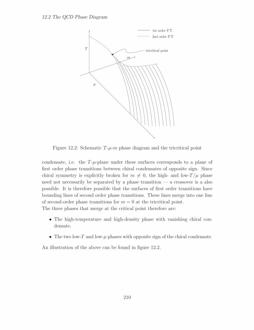
12.2 The QCD Phase Diagram
m
T
µ
1st order P.T.
2nd order P.T.
tricritical point
Figure 12.2: Schematic T -µ-m phase diagram and the tricritical point
condensate, i.e. the T -µ-plane under these surfaces corresponds to a plane of
first order phase transitions between chiral condensates of opposite sign. Since
chiral symmetry is explicitly broken for m 6= 0, the high- and low-T/µ phase
need not necessarily be separated by a phase transition — a crossover is a also
possible. It is therefore possible that the surfaces of first order transitions have
bounding lines of second order phase transitions. These lines merge into one line
of second-order phase transitions for m = 0 at the tricritical point.
The three phases that merge at the critical point therefore are:
• The high-temperature and high-density phase with vanishing chiral con-
densate.
• The two low-T and low-µ phases with opposite sign of the chiral condensate.
An illustration of the above can be found in figure 12.2.
210

The Phases of Quantum Chromodynamics
12.3 Colour superconductivity and colour
flavour locking
For low temperatures and high chemical potentials, a mechanism called colour
superconductivity has been proposed. A variety of phases can be predicted using
this mechanism; the two most important ones are:
Two-flavour colour superconductivity This phase, also referred to as 2SC,
appears under the assumption of only two quark flavours whose masses are
very small on the energy scales of the problem and can therefore be ignored.
Colour flavour locking If the theory of 2SC is extended to three quark flavours,
one finds CFL. Interest in this phase is particularly strong due to the fact
that it breaks the chiral symmetry, but by a completely different mechanism
than by which it is broken in QCD for low densities.
The only currently known way to create such densities is by gravitational collapse,
which takes place in neutron stars. Hence, at least some of these phases, especially
CFL, are expected to play an important role in the physics of neutron stars. For
example, the specific heat capacity of quark matter, which is linked to the cooling
rate of neutron stars, is affected by colour superconductivity effects. Currently,
however, there are plans to build collision experiments to explore these phases in
more detail.
Throughout this discussion, it will be assumed that the coupling between quarks
is weak. Since, as was mentioned before, the high chemical potential in dense
matter forces the quarks to occupy high-momentum states, i.e. the Fermi mo-
mentum is increased as µ increases. Since the quarks at the Fermi surface are the
relevant degrees of freedom for dynamic processes, it can be assumed that those
are asymptotically free. As a consequence, perturbative calculations provide valid
results in the high-density regime.
12.3.1 Symmetry breaking due to colour superconduc-
tivity
CFL
In the case of a theory with three quarks, (u, d, s), a phase commonly referred to
as colour flavour locking appears. The attractive force that causes the formation
of a condensate of quark pairs is provided by the single gluon exchange, which, at
weak coupling, dominates the quark interaction. Knowing this, it can be deduced
211

12.3 Colour superconductivity and colourflavour locking
([6, 7]) that the ground state has nonvanishing condensates
〈ψaαiL (~p)ψbβjL(−~p)ǫab〉 = −〈ψaαiR (~p)ψbβjR(−~p)ǫab〉 ∝ ǫαβAǫijA. (12.75)
Here, indices (α, β) refer to colour, (i, j) to flavour and (a, b) to spin; for A,
summation convention applies. Using the identity
ǫαβAǫijA = δαi δβj − δαj δ
βi (12.76)
we see that in the condensate (12.75), colour and flavour indices are linked;
the condensate is therefore not symmetric under separate rotations of colour or
flavour, but only under rotations that simultaneously modify colour and flavour
indices.
The full symmetry group of QCD with 3 massless quarks (12.42) was SU(3)c ×SU(3)L×SU(3)R×U(1)B. With the above condensates, the SU(3)L and SU(3)Rchiral symmetries become locked to the colour symmetry SU(3)c. Hence, the full
symmetry group of the CFL phase is reduced to
SU(3)color,L,R × Z2. (12.77)
Though the condensates do not mix right-handed and left-handed fermions, as
it is the case in low-density, low-temperature QCD, the chiral symmetry is effec-
tively broken due to CFL! The baryon number U(1)B symmetry is also broken:
the condensate of quark pairs in the ground state, 〈QQ′〉, is not invariant under
a U(1)B transformation Q→ eiαQ, since 〈QQ′〉 6= e2iα〈QQ′〉 except for eiα = −1,
which corresponds to Z2. This, however, does not imply that baryon number
is not conserved. A physical interpretation of the reduced symmetry would be
that the quantum number to which it refers (baryon number in this case, electric
charge in the case of ordinary superconductivity) can easily be transported within
the sample, which directly relates to superconductivity.
In general, a gauge-invariant order parameter is difficult to find for the case
of a broken gauge symmetry. For example, in the electroweak theory, such a
parameter cannot be found. In the case of CFL, however, order parameters can
be found for the breaking of the global symmetries, i.e. the breaking of the chiral
SU(3)L × SU(3)R and the U(1)B baryon number symmetry.
2SC
If the three massless quarks of CFL are replaced by just two, a state called 2SC
can be found. Again, an attractive force leading to a BCS instability is provided
212

The Phases of Quantum Chromodynamics
by the single gluon exchange. However, in this case, the resulting condensate is
of a different structure. It is found to be
〈ǫαβ3ǫijψαi ψ
βj 〉 6= 0. (12.78)
Again, (α, β) are colour and (i, j) are flavour indices. It can be seen that one
colour is distinguished from the others (in this case 3 or blue). This breaks the
local SU(3)C gauge symmetry down to a SU(2)C symmetry. The ground state
condensate also doesn’t mix left-handed and right-handed fermions, therefore the
chiral SU(2)L × SU(2)R symmetry is not broken in the 2SC phase. Since U(1)Bis also unbroken, no global symmetries are broken. Hence, a symmetry breaking
distinguishes the 2SC phase from the phase of low densities and temperatures,
where chiral symmetry is dynamically broken. It has been shown that the tran-
sition is of first order.
12.3.2 Energy gap in the excitation spectrum
In an ordinary solid, the electron gas description, i.e. the description as an ideal,
non-interacting Fermi gas, becomes more and more valid as temperature is de-
creased since the phonon-electron scattering becomes less and less important. In
some materials, however, there is a critical temperature Tc at which the existence
of a weak, interacting force leads to the formation of electron bound states, which
condensate as so-called Cooper pairs. This is one of the central predictions of
the BCS theory of type I superconductivity. For the case of an ordinary super-
conductor, this attractive interaction is mediated by a dynamical deformation of
the ion lattice.
In the case of very dense quark matter, where high-momentum states up to
some Fermi momentum pF are occupied leading to weak coupling in the limit of
asymptotic freedom, one might intuitively think (and it was generally accepted
for a long time) that the system can be described as a Fermi gas, too. As in the
case of the electron gas, there is a screening mechanism, which for the case of
QCD has been described in sect. 12.2.2 when referring to the high-temperature
QGP. Yet again there are attractive interactions between the quarks, which lead
to formation of Cooper pairs.
In the case of colour superconductivity, the well-known effects of superconduc-
tivity (of colour charge) and the Meissner-Ochsenfeld effect, i.e. the expulsion of
(colour) fields, do apply but have no observable consequences. The most relevant
physical aspect therefore is the fact that for a binding energy of E in such a quark
pair, the quark energy spectrum has a gap between the ground state and the first
213

12.3 Colour superconductivity and colourflavour locking
excited state which is equal to ∆ = −E2. This affects thermodynamics properties
of such high-density quark matter.
The central question therefore would be to calculate this energy gap. For a long
time, it was thought that the binding energy is very low around 1 MeV ([8]). In
the late 1990s, non-perturbative effects have been proposed ([9]) leading to much
higher energy gaps on the order of 100 MeV.
12.3.3 Physical consequences of CFL
Pseudo-Goldstone bosons We saw that in the case of CFL, SU(3)c ×SU(3)L × SU(3)R is reduced to SU(3)c,L,R. From sect. 12.1.3, we know that
for each broken global continuous symmetry, a massless Goldstone boson occurs
and for each broken gauge symmetry, the gauge vector boson acquires a finite
mass. Due to the breaking of the colour symmetry, which is the gauge group, we
expect the gauge bosons, i.e. the gluons, to acquire mass.
Of the Goldstone bosons due to broken chiral symmetry, an octet appears as
oscillations of the diquark condensates (12.75), which can be described by an
effective Lagrangian. If the masses of the light quarks are assumed to take non-
zero values, the symmetry is not exact any more, so that pseudo-Goldstone bosons
are created which, as opposed to normal Goldstone bosons, have a finite mass.
In the case of the CFL bosons, they can be considered as physical mesons and
masses can be calculated, giving, for example
m2π± =
2c
f 2π
ms(mu +md), m2K± =
2c
f 2π
md(mu +ms), (12.79)
where c, fπ are coefficients of the effective Lagrangian. Due to the weak coupling
at asymptotically high densities in CFL, analytic calculations for these coefficients
are possible and give estimates of the mass of, for example, the kaons, in the range
of mK± ≈ 5 . . . 20MeV for µ = 400MeV.
Additionally, the breaking of U(1)B to Z2 is associated with the appearance of a
singlet Goldstone boson, which is responsible for the superconductive transport
of colour charge.
Neutron star cooling A neutron star is the result of a supernova created
by a star with a mass between 1.44 and 3 times the mass of the sun. For such
stars, the supernova collapses after it is ”dead“, but the mass is not high enough
to create a black hole. Neutron stars are objects of extraordinary density, which
is around 1012 kg/cm3 in the core. Their radius is about 10 km.
One of the observable properties of a neutron star is its cooling, which, at least
during some parts of its life cycle, is dominated by neutrino emission and the heat
214

The Phases of Quantum Chromodynamics
capacity of the star. Since the heat capacity is affected by the physical situation
at the Fermi surface, colour superconductivity will have some effect on the cooling
rate. In the CFL phase, all quarks have a gap in the excitation spectrum with
∆ ≫ T , hence their thermal excitation is very low, ∝ exp(−∆/T ).
Hence, there is no contribution to the specific heat from the quarks; the bulk of
the specific heat is due to the electrons, with some contributions by the pseudo-
Goldstone-bosons discussed in the last paragraph. The core is therefore only
cooled by contact to the outer, hadronic-matter-shell of the neutron star.
12.4 Relativistic Heavy-Ion Collisions
The way to experimentally study the quark-gluon plasma, i.e. QCD at high
temperatures and low, yet finite chemical potentials, is through relativistic heavy-
ion collisions ([4, Ch. 8.5], [10, Ch. 4]). In these collisions, particle accelerators
are used to collide heavy nuclei such as sulphur, lead or gold with very high
energies. The first experiments, for example SPS at CERN, had center of mass
(CM) energies in the range 2A . . . 18A GeV, where A is the number of nucleons
in the nucleus. Current experiments, such as the RHIC collider in Brookhaven,
NY, reach energies of 200A GeV. At the LHC in CERN, expected CM energies
are 5500A GeV. There are plans to build collider experiments that could explore
the region of high densities at low temperatures, using even heavier nuclei such
as uranium, but using lower collision energies. One facility where this is planned
is CBM/FAIR at GSI, Darmstadt.
12.4.1 Stages of a RHI collision
Relativistic heavy ion collisions are usually described in four phases (see also fig.
12.3), where the exact distinction between phases differs between authors. This
roughly follows [5], with additional input from [4].
• In the first phase, the ultra-relativistic nuclei, which are deformed in the
center-of-mass system due to relativistic length contraction, approach each
other and partons initially scatter from each other. Phase-space density is
very high and the system can be approximated by classical fields. Interac-
tions at this stage occur at a very short timescale, tint ≈ 0.1 − 0.3 fm/c.
In this step, according to current calculations, energy densities of up to 20
GeV fm−3 occur.
• The equilibration or thermalization of the system takes place through mul-
tiple parton scattering. Thermalization times are estimated to be around
215
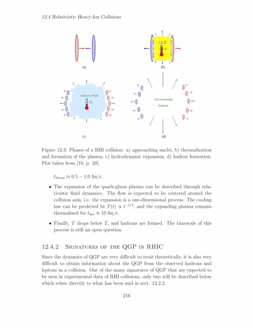
12.4 Relativistic Heavy-Ion Collisions
Figure 12.3: Phases of a RHI collision: a) approaching nuclei, b) thermalization
and formation of the plasma, c) hydrodynamic expansion, d) hadron formation.
Plot taken from [10, p. 20].
ttherm ≈ 0.5 − 1.0 fm/c.
• The expansion of the quark-gluon plasma can be described through rela-
tivistic fluid dynamics. The flow is expected to be centered around the
collision axis, i.e. the expansion is a one-dimensional process. The cooling
law can be predicted be T (t) ∝ t−1/3, and the expanding plasma remains
thermalized for tdec ≈ 10 fm/c.
• Finally, T drops below Tc and hadrons are formed. The timescale of this
process is still an open question.
12.4.2 Signatures of the QGP in RHIC
Since the dynamics of QGP are very difficult to treat theoretically, it is also very
difficult to obtain information about the QGP from the observed hadrons and
leptons in a collision. Out of the many signatures of QGP that are expected to
be seen in experimental data of RHI collisions, only two will be described below
which relate directly to what has been said in sect. 12.2.2.
216

The Phases of Quantum Chromodynamics
J/Ψ suppression
One physical signature of QGP creation that was hoped to be observable in RHI
collisions is the suppression of J/Ψ (cc) production. The relatively long decay
time of the J/Ψ, which is the reason for the appearance of a sharp and high
resonance peak in non-QGP collisions, i.e. pp, is caused by two facts:
• Due to confinement, i.e. the linearly increasing potential between the two
constituents of the meson, these constituents are not free to pair with other
particles.
• Since the mass of the J/Ψ, 3096.9 MeV, is lower than that of two mesons
containing a charm and a light quark, e.g. the various types of D (mass
≈ 1870 MeV), a process in which it is broken up into two such mesons
with continuous quark lines is not possible. It therefore has to decay via
quark-antiquark annihilation and production of gluons, which is suppressed.
In 1986, it was proposed ([11]) that the creation of the J/Ψ is suppressed by
the creation of QGP. The reason for this was thought to be the effect of decon-
finement in a high-temperature plasma and the screening of the attractive forces
as described in sect. 12.2.2 ([10, 12, 4]). If the screening length λD falls below
the radius of the J/Ψ, the pair can dissociate and the isolated heavy quarks can
create mesons with light quarks as well. This should in principle extend to other
heavy mesons.
The effect of heavy meson suppression has been measured experimentally, as
seen in fig. 12.4.2. Recently, however, lattice simulations have shown that heavy
mesons are more stable than expected — this is still an area of open discussion.
217
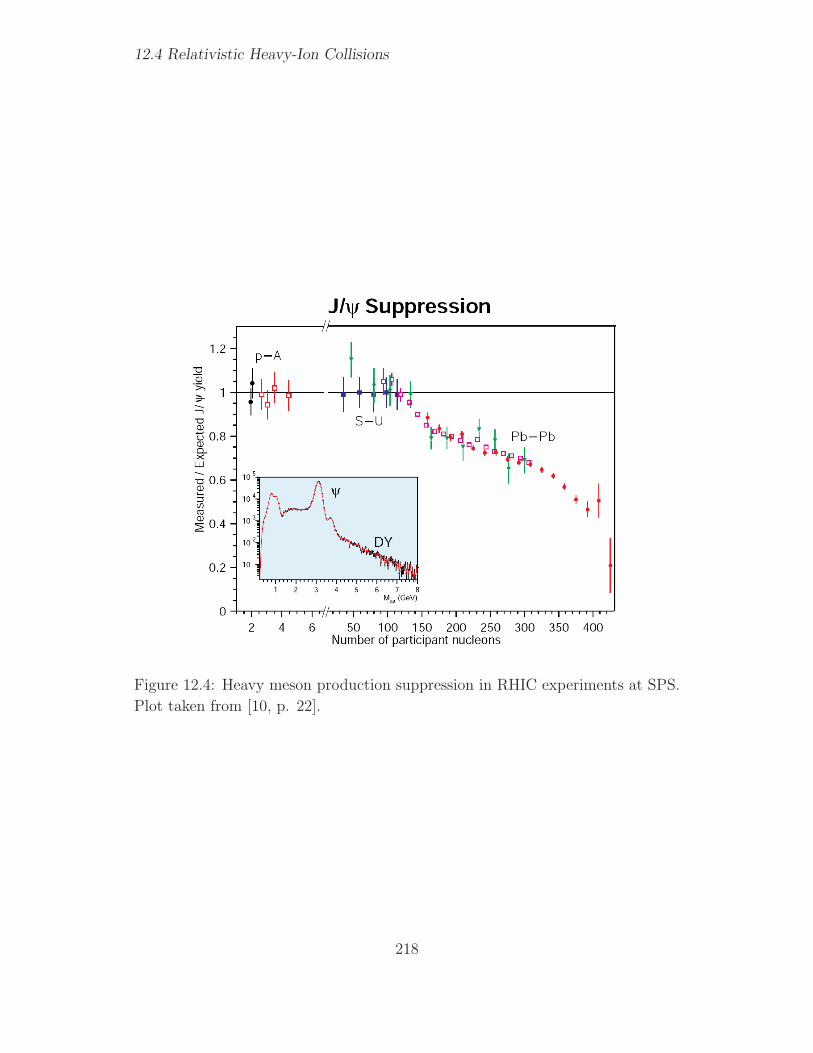
12.4 Relativistic Heavy-Ion Collisions
Figure 12.4: Heavy meson production suppression in RHIC experiments at SPS.
Plot taken from [10, p. 22].
218

Bibliography
[1] J. Goldstone, A. Salam, and S. Weinberg, Phys. Rev. 127, 965 (1962).
[2] M. Peskin and D. Schroeder, An Introduction to Quantum Field Theory
(Addison-Wesley, 1995).
[3] A. Chodos, Phys. Rev. D 9, 3471 (1974).
[4] J. Kogut and M. Stephanov, The Phases of Quantum Chromodynamics
(Cambridge University Press, 2004).
[5] B. Muller, Large Hadron Phenomenology (Taylor & Francis, 2004), Scottish
Graduate Series.
[6] K. Rajagopal and F. Wilczek (2000), hep-ph/0011333.
[7] M. Alford and F. Wilczek, Color-flavor locking and chiral symmetry breaking
in high density qcd, Phys. Lett. B 537, 443 (1999), hep-ph/9804403.
[8] D. Bailin and A. Love, Phys. Rep. 81, 325 (1984).
[9] R. Rapp, T. Schafer, E. Shuryak, and M. Velkovsky, Phys. Rev. Lett. 81, 53
(1998).
[10] S. Hands, The phase diagram of qcd, Contemp. Phys. 42, 209 (2001).
[11] T. Matsui and H. Satz, Phys. Lett. B 178, 416 (1986).
[12] F. Karsch, Deconfinement and quarkonium suppression, Eur. Phys. J. C 43,
35 (2005), hep-lat/0502014.
219

BIBLIOGRAPHY
220
Chapter 13
BCS theory of
superconductivity
Thomas Burgenersupervisor: Dr. Christian Iniotakis
In this chapter BCS theory for conventional superconductors will
be presented. Starting with a discussion of the Cooper problem
I continue by introducing a model hamiltonian and solving it
with a Bogoliubov-Valatin transformation. After having found
a solution of the hamiltionian I’m going to calculate the critical
temperature, the temperature dependence of the order param-
eter and some thermodynamic quantities. At the end I briefly
introduce the difference between type I and type II superconduc-
tors.
13.1 Introduction
In 1957 John Bardeen, Leon N. Cooper and John R. Schrieffer [1] published their
work about superconductivity. For this work they received the Nobel prize in
1972. The theory is today called the BCS theory, coming from the first letters
of the names of its inventors. The theory is formulated in terms of a mean-field
theory and was the first “working” microscopic theory for superconductors. In
its original form the theory was only applied to conventional superconductors.
In this chapter I’d like to present the main features of the BCS theory. Most of
the things I show here are from the book of Tinkham [2].
221
13.2 Cooper Pairs
13.2 Cooper Pairs
The basic concept for understanding superconductivity within the context of BCS
theory is the formation of Cooper pairs. I will first discuss how these bound pairs
of electrons are formed and then explain how an attractive interaction between
two electrons can occur.
13.2.1 Bound Pairs of Electrons
The basic idea that even a weak attraction can bind pairs of electrons into a
bound state goes back to Cooper [3]. He showed that the Fermi sea of electrons
is unstable against the formation of at least one bound pair, regardless of how
weak the interaction is, so long as it is attractive. This result is a consequence of
the Fermi statistic and of the existence of the Fermi sea background.
To show how the binding comes about, we consider a simple model of two elec-
trons added to a filled Fermi sea at T = 0, with the assumption, that the extra
electrons interact with each other but not with the electrons in the sea, except
via the exclusion principle. Therefore we are looking for a two-particle wavefunc-
tion. We expect the lowest-energy state to have zero momentum. Including the
antisymmetric singlet spin function suggests building up a wavefunction of the
sort
Ψ0(r1, r2) =∑
k
(gke
ik·r1e−ik·r2)(|↑↓〉 − |↓↑〉) . (13.1)
Taking into account the antisymmetry of the total wavefunction with respect to
exchange of the two electrons leads to the condition
gk!= g−k
for the coefficients in the wavefunction. By inserting (13.1) into the Schrodinger
equation of the problem, one can show that the weighting coefficients gk and the
energy eigenvalue E are to be determined by solving
(E − 2ǫk)gk =∑
k>kf
Vkk′gk′ . (13.2)
In this expression, the ǫk are unperturbed plane-wave energies and the Vkk′ are
the matrix elements of the interaction potential
Vkk′ =1
Ω
∫V (r)ei(k
′−k)·rdr, (13.3)
222

BCS theory of superconductivity
where r = r1 − r2 and Ω is the normalization volume. If a set of gk satisfying
(13.2) with E < 2EF can be found, then a bound pair state exists.
Since it is hard to analyze this situation for general Vkk′ , Cooper introduced the
very serviceable approximation of the interaction potential as a step function
Vkk′ =
−V , EF < ǫk, ǫk′ < EF + ~ωc0 , otherwise
, (13.4)
where EF is the Fermi energy and ~ωc is a cutoff energy. Then from (13.2) we
get
gk = V
∑gk′
2ǫk − E. (13.5)
Summing up both sides and canceling∑gk gives
1
V=∑
k>kF
1
2ǫk − E. (13.6)
When we replace the summation by an integration, with N(0) denoting the den-
sity of states at the Fermi level for electrons of one spin orientation, this becomes
1
V= N(0)
∫ EF +~ωc
EF
dǫ
2ǫ− E=
1
2N(0) ln
2EF − E + 2~ωc2EF − E
. (13.7)
In most classic superconducters, it is found that N(0)V < 0.3 and this allows use
of the so-called weak-coupling approximation, valid for N(0)V ≪ 1, in which the
solution to the preceding equation can be written as
E ≈ 2EF − 2~ωce− 2
N(0)V . (13.8)
Thus, there is a bound state with negative energy with respect to the Fermi
surface made up entirely of electrons with k > kF . The contribution of the
attractive potential leads to binding regardless how small V is. Note that the
form of the binding energy is not analytic at V = 0; i.e. it cannot be expanded
in powers of V . As a result, it cannot be obtained by perturbation theory, a fact
that greatly delayed the genesis of the theory.
13.2.2 Origin of the Attractive Interaction
We now have to understand the origin of the negative Vkk′ needed for supercon-
ductivity.
223

13.3 BCS Theory
To get a negative Vkk′ we have to take the electron-lattice interactions into ac-
count. The physical idea is that the first electron polarizes the medium by attract-
ing positive ions; these excess positive ions in turn attract the second electron,
resulting in an effective attractive interaction between the electrons. If this at-
traction is strong enough to override the screened Coulomb interaction, it gives
rise to a net attractive interaction, and superconductivity results. Historically,
the importance of the electron-lattice interaction in explaining superconductivity
was first suggested by Frohlich [4] in 1950. This suggestion was confirmed exper-
imentally by the discovery [5], [6] of the isotope effect, i.e. the proportionality
of the critical temperature Tc and the critical magnetic field Hc to M−1/2 for
isotopes with mass M of the same element.1
Obviously, these lattice deformations are correlated to the characteristic phonon
frequencies of the material. From momentum conservation, we can see that if an
electron is scattered from k to k′, the relevant phonon must carry the momentum
q = k− k′, and the characteristic frequency must then be the phonon frequency
ωq. It is plausible that the phonon contribution to the screening function is
proportional to (ω2 − ω2q)
−1. This resonance denominator gives a negative sign
if ω < ωq, corresponding to the physical argument above; for higher frequencies,
i.e. electron energy difference larger than ~ωq, the interaction becomes repulsive.
Thus, the cutoff energy ~ωc of Cooper’s attractive matrix element −V is expected
to be of the order of the Debye energy ~ωD = kΘD, which characterizes the cutoff
of the phonon spectrum.
13.3 BCS Theory
I’d like to present now the BCS theory for conventional superconductors. I start
with introducing the model hamiltonian, which will be solved using a Bogoliubov-
Valatin-Transformation. At the end of the section I will calculate the conden-
sation energy and show, that the superconducting state is energetically more
favorable.
13.3.1 The Model Hamiltonian
We have seen that the Fermi sea is unstable against the formation of a bound
Cooper pair when the net interaction is attractive. Clearly we must then expect
1The critical temperature and the critical field will be introduced and discussed later in the
chapter.
224

BCS theory of superconductivity
pairs to condense until an equilibrium state is reached. Because we work now
with a system of many electrons, we have to find a smart way to handle the
many-body wavefunction. This can be done by using second quantisation: Let’s
introduce the creation operator c†kσ, which creates an electron of momentum k
and spin σ, and the correspondig annihilation operator ckσ. These operators obey
the standard anticommutation relations for fermions:
ckσ, c†k′σ′ ≡ ckσc†k′σ′ + c†k′σ′ckσ = δkk′δσσ′ (13.9)
ckσ, ck′σ′ = 0 = c†kσ, c†k′σ′. (13.10)
Additionally the particle number operator nkσ is defined by
nkσ ≡ c†kσckσ. (13.11)
With these operatos we can write down our pairing hamiltonion:
H =∑
kσ
ǫknkσ +∑
kl
Vklc†k↑c
†−k↓c−l↓cl↑. (13.12)
The first sum corresponds to the kinetic part for (single/unpaired) electrons and
the second sum describes the annihilation of a Cooper pair c−l↓cl↑ and the cre-
ation of another one c†k↑c†−k↓. Clearly this hamiltonian omits many other terms
which involve electrons not paired as (k ↑,−k ↓). Such terms have zero expecta-
tion value in the BCS ground-state wavefunction but may be important in other
applications. To regulate the mean number of particles N , we add a term −µN ,
where µ is the chemical potential and N is the particle-number. Mathematically
this is equivalent to taking the zero of kinetic energy to be at µ (or EF ). The
hamiltonian then reads as
H− µN =∑
kσ
ξknkσ +∑
kl
Vklc†k↑c
†−k↓c−l↓cl↑. (13.13)
We now apply mean-field theory to this hamiltonian. We first note that because
of coherence, operators such as c−k↓ck↑ can have nonzero expectation values bkin the superconducting state, rather than averaging to zero as in a normal metal,
where all phases are random. Moreover, because of the large numbers of particles
involved, the fluctuation about these expectation values should be small. This
suggests that it will be useful to express such a product of operators formally as
c−k↓ck↑ = bk + (c−k↓ck↑ − bk) (13.14)
and subsequently neglect quantities which are bilinear in the presumably small
fluctuation term in parantheses. By inserting (13.14) in our pairing hamiltonion
225

13.3 BCS Theory
(13.13), we obtain the so-called model hamiltonian
HM − µN =∑
kσ
ξkc†kσckσ +
∑
kl
Vkl(c†k↑c
†−k↓bl + b∗kc−l↓cl↑ − b∗kbl), (13.15)
where the bk are to be determined self-consistently, so that
bk ≡ 〈c−k↓ck↑〉 . (13.16)
We define further
∆k = −∑
l
Vklbl = −∑
l
Vkl 〈c−l↓cl↑〉 , (13.17)
which will turn out to be the order parameter. In terms of ∆k, the model hamil-
tonian becomes
HM − µN =∑
kσ
ξkc†kσckσ −
∑
k
(∆kc†k↑c
†−k↓ + ∆∗
kc−k↓ck↑ − ∆kb∗k), (13.18)
which now only consists of terms with products of two operators.
13.3.2 Bogoliubov-Valatin-Transformations
We now have to diagonalize the hamiltonian (13.18). This can be done by apply-
ing a suitable linear transformation to define new Fermi operators γk. As shown
independently by Bogoliubov [7] and by Valatin [8], the appropriate transforma-
tion is specified by
ck↑ = u∗kγk↑ + vkγ†−k↓ (13.19a)
c†−k↓ = −v∗kγk↑ + ukγ†−k↓, (13.19b)
where the numerical coefficients uk and vk are complex numbers and satisfy |uk|2+|vk|2 = 1. Substituting these new operators into the model hamiltonian (13.18),
and carrying out the indicated products taking into account the noncommutivity
of the operators, we obtain
HM − µN =∑
k
ξk
((|uk|2 − |vk|2)(γ†k↑γk↑ + γ†−k↓γ−k↓)
+2|vk|2 + 2u∗kv∗kγ−k↓γk↑ + 2ukvkγ
†k↑γ
†−k↓
)
+∑
k
((∆kukv
∗k + ∆∗
ku∗kvk)(γ
†k↑γk↑ + γ†−k↓γ−k↓ − 1)
+(∆kv∗k
2 − ∆∗ku
∗k
2)γ−k↓γk↑
+(∆∗kv
2k − ∆ku
2k)γ
†k↑γ
†−k↓ + ∆kb
∗k
). (13.20)
226

BCS theory of superconductivity
Now, if we choose uk and vk so that the coefficients of γ−k↓γk↑ and γ†k↑γ†−k↓
vanish, the hamiltonian is diagonalized; e.g. it is carried into a form containing
only constants plus terms proportional to the occupation numbers γ†k↑γk↑. The
coefficients of both undesired terms are zero if
2ξkukvk + ∆∗kv
2k − ∆ku
2k = 0
∣∣∣∣·∆∗
k
u2k
⇒(
∆∗kvkuk
)2
+ 2ξk
(∆∗
kvkuk
)− |∆k|2 = 0
⇒ ∆∗kvkuk
=√ξ2k + |∆k|2
︸ ︷︷ ︸≡Ek
−ξk ≡ Ek − ξk (13.21)
Using the normalization condition |uk|2+|vk|2 = 1 we can solve for the coefficients
and find
|vk|2 = 1 − |uk|2 =1
2
(1 − ξk
Ek
). (13.22)
The phases of uk, vk and ∆k are related by (13.21) since ∆∗kvk/uk is real. That
is, the phase of vk relative to uk must be the phase of ∆k. There is no loss in
generality in choosing all the uk to be real and positive. If we do so, vk and ∆k
must have the same phase.
13.3.3 Calculation of the Condensation Energy
Next we like to calculate the condensation energy. Therefore we need the ground
state wavefunction of the superconducting state. BCS took an ansatz for the
ground state of the following form
|ΨG〉 =∏
k
(uk + vkc†k↑c
†−k↓) |0〉 (13.23)
where |uk|2 + |vk|2 = 1. This form implies that the probability of the pair
(k ↑,−k ↓) being occupied is |vk|2, whereas the probability that it is unoccupied
is |uk|2 = 1− |vk|2. It is important to note, that first |ΨG〉 does not conserve the
particle number2, and second it is the vacuum state for the γ operators, e.g.
γk↑ |ΨG〉 = 0 = γ−k↓ |ΨG〉 . (13.24)
2However, the actual particle number is very sharply peaked about an averaged value N .
For details see section 3.3 of [2]
227

13.4 Finite Temperatures
We first calculate the energy of the ground state in the superconducting phase
to be
〈ΨG|H − µN |ΨG〉 = 2∑
k
ξkv2k +
∑
kl
Vklukvkulvl
=∑
k
(ξk − ξ2
k
Ek
)− ∆2
V(13.25)
where we again used the approximativ potential introduced in 13.2. The normal
state at T = 0 corresponds to the BCS state with ∆ = 0, in which case Ek = |ξk|.Thus the energy of the normal state is given by
〈Ψn|H − µN |Ψn〉 =∑
|k|<kF
2ξk. (13.26)
By taking the difference of these two energies we get an expression for the con-
densation energy to be
〈E〉s − 〈E〉n =∑
|k|>kF
(ξk − ξ2
k
Ek
)+∑
|k|<kF
(−ξk − ξ2
k
Ek
)− ∆2
V
= 2∑
|k|>kF
(ξk − ξ2
k
Ek
)− ∆2
V
=
(∆2
V− 1
2N(0)∆2
)− ∆2
V= −1
2N(0)∆2. (13.27)
This shows us that the superconducting state has lower energy than the normal
state.
13.4 Finite Temperatures
So far we looked only at the ground state properties of our superconductor. In this
section I’d like to discuss finite temperature effects, including the interpretation
of ∆k as an energy gap in the excitation spectrum, the determination of the
critical temperature Tc and the calculation of some thermodynamic quantities.
13.4.1 Excitations and the Energy Gap
If we insert (13.22)) in the model hamiltonian (13.18) we get
HM − µN =∑
k
(ξk − Ek + ∆kb∗k) +
∑
k
Ek(γ†k↑γk↑ + γ†−k↓γ−k↓). (13.28)
228

BCS theory of superconductivity
0
1
2
3
4
-3 -2 -1 0 1 2 3
Ek/
∆
ξk/∆
EksEkn
Figure 13.1: Energies of elementary excitations in the normal and superconduct-
ing states as functions of ξk.
The first sum is simply a constant and the second sum gives the increase in energy
above the ground state in term of the number operators γ†kσγkσ. Thus, the γ†kσoperators describe the elementary quasi-particle excitations of the system3. The
energies of these excitations are given by
Ek =√ξ2k + |∆k|2. (13.29)
A plot of the excitation spectrum is given in Figure 13.1. This also shows us that
∆k plays the role of an energy gap or minimum excitation energy since even at
the Fermi surface, where ξk = 0, Ek = |∆k| > 0.
We can compute the energy gap ∆k by rewriting (13.17) in terms of the γ oper-
ators:
∆k = −∑
l
Vkl 〈c−l↓cl↑〉
= −∑
l
Vklu∗l vl
⟨1 − γ†l↑γl↑ − γ†−l↓γ−l↓
⟩
= −∑
l
Vklu∗l vl(1 − 2f(El))
= −∑
l
Vkl
∆l
2El
tanhβEl
2. (13.30)
3Such quasi-particles are coherent particle-hole excitations: With (13.19) the γ†kσ operators
always consist of an electron creation and annihilation operator, and coherence comes from
condition (13.21).
229

13.4 Finite Temperatures
At the third equality we used that the γ operators describe fermions and therefore
we can replace the expectation values of the number operators by the Fermi
function f . Using again our approximated potential we find
1
V=
1
2
∑
k
tanh(βEk/2)
Ek
. (13.31)
From this formula we can determine Tc and the temperature dependence of ∆(T ).
13.4.2 Determination of Tc and ∆(0)
The critical temperature Tc is the temperature at which ∆(T ) → 0. In this case,
Ek → |ξk|, and the excitation spectrum becomes the same as in the normal state.
Thus, Tc is found by replacing Ek with |ξk| in (13.31) and solving. After changing
the sum to an integral, taking advantage of the symmetry of |ξk| about the Fermi
level, and changing to a dimensionless variable of integration, we find that this
condition becomes
1
N(0)V=
∫ βc~ωc/2
0
tanhx
xdx = ln
(2eγ
πβc~ωc
), (13.32)
where γ = 0.577... is the Euler constant. Consequently,
kTc = β−1c ≈ 1.13~ωce
−1/N(0)V . (13.33)
For small temperatures (13.31) can be rewritten as
1
N(0)V=
∫~ωc
0
dξ
(ξ2 + ∆2)1/2(13.34)
⇒ ∆(T = 0) =~ωc
sinh(1/N(0)V )≈ 2~ωce
−1/N(0)V , (13.35)
which gives us a relation of Tc and ∆(0):
∆(0)
kTc≈ 2
1.13≈ 1.764. (13.36)
13.4.3 Temperature Dependence of the Gap
We can also determine the temperature dependence of the energy gap from
(13.31). By inserting the expression for Ek and rewriting the sum as an inte-
gral we get1
N(0)V=
∫~ωc
0
tanh 12β(ξ2 + ∆2)1/2
(ξ2 + ∆2)1/2dξ. (13.37)
230

BCS theory of superconductivity
Figure 13.2: Temperature dependence of the energy gap compared with experi-
mental data [9].
This formula has to be evaluated numerically. A plot of the results together with
some experimental data is shown in Figure 13.2. We see that the theoretical
value fits the experimental one quite good. The reason why mean-field theory
gives that good result here is, that the effective number of nearest neighbors of a
Cooper pair is big.
Near Tc we can find approximately
∆(T )
∆(0)≈ 1.74
(1 − T
Tc
)1/2
, T ≈ Tc, (13.38)
which shows the square-root dependence of the order parameter, which is typical
for a mean-field theory.
13.4.4 Thermodynamic Quantities
With ∆(T ) determined, the temperature dependent set of fermion excitation
energies Ek =√ξ2k + ∆(T )2 is fixed. These energies determine the quasi-particle
occupation numbers fk = (1 + eβEk)−1, which in turn determine the electronic
entropy in the usual way for a fermion gas, namely,
Ses = −2k∑
k
((1 − fk) ln(1 − fk) + fk ln fk). (13.39)
A plot of this formula for the normal and superconducting state is shown in Fig-
ure 13.3.
231

13.4 Finite Temperatures
Figure 13.3: Electronic entropy in the normal and superconducting state.
Given Ses(T ), the specific heat can be written as
Ces = TdSesdT
= −βdSesdβ
= 2βk∑
k
− ∂fk∂Ek
(E2
k +1
2βd∆2
dβ
). (13.40)
The first term is the usual one coming from the redistribution of quasi-particles
among the various energy states as the temperature changes. The second term
is more unusual and describes the effect of the temperature dependent gap in
changing the energy levels themselves.
For the normal state the electronic specific heat is given by
Cen = γT =2π2
3N(0)k2T. (13.41)
It is important to note, that at Tc we will observe a jump in C(T ) because the
derivative d∆2
dβis finite below Tc and 0 above. This jump can be calculated and
gives
∆C = (Ces − Cen)|Tc= N(0)kβ2
∫ ∞
−∞
(− ∂f
∂|ξ|
)
= N(0)
(−d∆
2
dT
)∣∣∣∣Tc
≈ 9.4N(0)k2Tc (13.42)
A plot together with experimental results is shown in Figure 13.4. Again BCS
theory gives very good predictions.
232
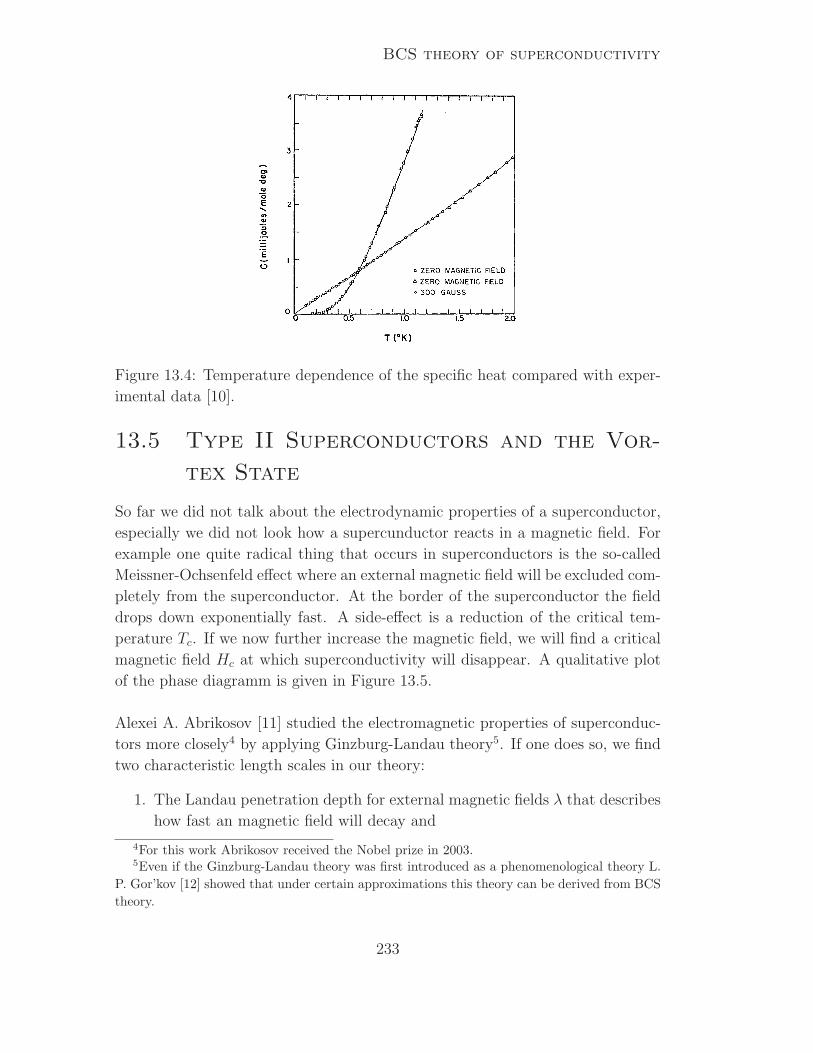
BCS theory of superconductivity
Figure 13.4: Temperature dependence of the specific heat compared with exper-
imental data [10].
13.5 Type II Superconductors and the Vor-
tex State
So far we did not talk about the electrodynamic properties of a superconductor,
especially we did not look how a supercunductor reacts in a magnetic field. For
example one quite radical thing that occurs in superconductors is the so-called
Meissner-Ochsenfeld effect where an external magnetic field will be excluded com-
pletely from the superconductor. At the border of the superconductor the field
drops down exponentially fast. A side-effect is a reduction of the critical tem-
perature Tc. If we now further increase the magnetic field, we will find a critical
magnetic field Hc at which superconductivity will disappear. A qualitative plot
of the phase diagramm is given in Figure 13.5.
Alexei A. Abrikosov [11] studied the electromagnetic properties of superconduc-
tors more closely4 by applying Ginzburg-Landau theory5. If one does so, we find
two characteristic length scales in our theory:
1. The Landau penetration depth for external magnetic fields λ that describes
how fast an magnetic field will decay and
4For this work Abrikosov received the Nobel prize in 2003.5Even if the Ginzburg-Landau theory was first introduced as a phenomenological theory L.
P. Gor’kov [12] showed that under certain approximations this theory can be derived from BCS
theory.
233

13.5 Type II Superconductors and the Vortex State
0
0.2
0.4
0.6
0.8
1
0 0.2 0.4 0.6 0.8 1
H/H
c(0)
T/Tc
normal state
Meissner-Ochsenfeld state
Hc
Figure 13.5: Phase diagram of a type I superconductor.
2. the Ginzburg-Landau coherence length ξ, which characterizes the distance
over which the order parameter ψ can typically vary.
With these two length scales we are able to define the Ginzburg-Landau param-
eter κ as
κ ≡ λ
ξ. (13.43)
For a lot of superconductors κ is small. Abrikosov now asked what would happen
if κ becomes large? By linearizing the GL equations near Tc he found a threshold
for κ and introduced the differentiation of Type I and Type II superconductors:
• κ < 1√2: Type I superconductor
• κ > 1√2: Type II superconductor.
Type I superconductors now have the electromagnetic property of expelling the
external magnetic field completely as discussed above. But in type II supercon-
ductors we have to introduce two new critical magnetic fields different from Hc.
The upper critical field Hc2 > Hc separates the normal and the superconducting
state. The second critical field Hc1 < Hc < Hc2 divides the superconducting
phase in two diffentent states. For external fields smaller than Hc1 we will again
observe a Meissner-Ochsenfeld state. For fields between Hc1 and Hc2 we will
find vortices in our superconductor where superconductivity is locally destroyed.
Therefore the external magnetic field can penetrate the superconductor and the
total flux is quantized in units of the magnetic flux quantum
Φ0 =hc
2e= 2.07 × 10⁻⁷ G/cm2. (13.44)
The phase diagram for type II superconductors is shown in Figure 13.6.
234

BCS theory of superconductivity
0 0.2 0.4 0.6 0.8 1H
T/Tc
normal state
vortex state
Meissner-Ochsenfeld state
Hc1Hc2
Figure 13.6: Phase diagram of a type II superconductor.
An important feature of the vortices is, that they reject each other. Therefore
it’s somehow clear, that they will arange themselves in a certain way and form
a vortex lattice. There are different solutions of Ginzburg-Landau theory repre-
senting different symmetries of the vortex lattice. One family of solutions can be
written as [13]
Ψ(x, y) =1
N∞∑
n=−∞exp
(π(ixy − y2)
ω1ℑω2
+ iπn
+iπ(2n+ 1)
ω1
(x+ iy) + iπω2
ω1
n(n+ 1)
)
with
N =
(ω1
2ℑω2
exp
(πℑω2
ω1
))1/4
.
By choosing the parameters ω1 and ω2 in an adequate way we get the solutions
for the square and a triangular lattice symmetry. Some plots are shown in Figure
13.7. In a perfect superconductor the triangular symmetry is energetically more
favorable but the difference between the two states is quite small6. Therefore one
can observe both symmetries in nature. The reason for that can be found in the
symmetry of the ion lattice or in the specific shape of the real Fermi surface.
6In his original work Abrikosov made a numerical mistake and identified the square lattice
as the lowest energy solution.
235

13.5 Type II Superconductors and the Vortex State
-2 -1 0 1 2-2
-1
0
1
2
-2 -1 0 1 2-2
-1
0
1
2
Figure 13.7: Square and triangular symmetry of the vortex lattice in type II
superconductors.
236

Bibliography
[1] J. Bardeen, L. N. Cooper, and J. R. Schrieffer, Theory of Superconductivity,
Phys. Rev. 108, 1175 (1957).
[2] M. Tinkham, Introduction to Superconductivity, Second Edition (Dover, New
York, 1996).
[3] L. N. Cooper, Bound Electron Pairs in a Degenerate Fermi Gas, Phys. Rev.
104, 1189 (1956).
[4] H. Frohlich, Theory of the Superconducting State. I. The Ground State at
the Absolute Zero of Temperature, Phys. Rev. 79, 845 (1950).
[5] E. Maxwell, Isotope Effect in the Superconductivity of Mercury, Phys. Rev.
78, 477 (1950).
[6] C. A. Reynolds, B. Serin, W. H. Wright, and L. B. Nesbitt, Superconductivity
of Isotopes of Mercury, Phys. Rev. 78, 487 (1950).
[7] N. N. Bogoliubov, Nuovo Cimento 7, 794 (1958).
[8] J. G. Valatin, Nuovo Cimento 7, 843 (1958).
[9] I. Giaever and K. Megerle, Study of Superconductors by Electron Tunneling,
Phys. Rev. 122, 1101 (1961).
[10] N. E. Phillips, Heat Capacity of Aluminum between 0.1K and 4.0K, Phys.
Rev. 114, 676 (1959).
[11] A. A. Abrikosov, Zh. Eksp. Teor. Fiz. 32, 1442 (1957).
[12] L. P. Gor’kov, Zh. Eksp. Teor. Fiz. 36, 1918 (1959).
[13] T. Dahm, S. Graser, C. Iniotakis, and N. Schopohl, Spectrum of low-energy
excitations in the vortex state: Comparison of the Doppler-shift method to a
quasiclassical approach, Phys. Rev. B 66, 144515 (2002).
237

BIBLIOGRAPHY
238

Chapter 14
Bose Einstein Condensation
Volker Schluesupervisor: Fabricio Albuquerque
The phenomenon of Bose-Einstein-Condensation in dilute gases
is exposed in its historical context as well as studied with view
on more recent experiments with trapped atomic clouds. The
Gross-Pitaevskii Equation is discussed.
14.1 Introduction
In 1924 D. Bose gave a deduction of Planck’s Law of Black Body Radiation,
relying on no classical concepts whatsoever [1]. Up to this point, the prefactor of
the formula
ρ(ν, T ) =8πν2
c3hν
ehνkT − 1
resulted from an electromagnetic treatment. The new method divides the phase
space of a light quantum into “cells” of size h3, and counts the number of ways
(W) a certain occupation state can be realized. The occupation numbers of each
cell, however, should be as such, that this number maximizes the entropy of the
macroscopic system, related by Boltzmann’s law :
S ∝ log(W )
From this all thermodynamic properties can be deduced. A. Einstein expected
the analogy between gases of quanta and gases of molecules to be complete.
Consequently, he developed the quantum theory of the one-atomic ideal gas [2],
239
14.2 The non-interacting Bose gas
wherein not only the occupation density, i.e. the Bose distribution function, is
given explicitly,
n =1
eα+E/kT − 1,
but it is also found that the new equations of state allow only for a maximal
number of particles for given volume and temperature; or, for fixed particle num-
ber and temperature the volume may not be reduced arbitrarily. In practice,
however, the density of particles may always be increased, and it is immediately
suggested, that the over-counting particles “condense” in the lowest quantum
state, that of zero kinetic energy, (the particles therefore condense in momentum
space). It is shown that the condensate is in thermodynamic equilibrium with
the gas.
The papers of Bose and Einstein employed a method of counting, in which
the quanta could not be thought of as statistically independent anymore. Today
this “mutual influence” is understood in terms of correlation functions (cf. sec-
tion 14.4), which could also be used to establish a criterion for condensation in
interacting systems; it reads1
lim|~r−~r′|→∞
ρ(~r, ~r′) =〈N0〉V
,
where 〈N0〉 denotes the expectation value of the occupation number of the zero-
momentum state, and ρ(~r, ~r′) = 〈ψ†(~r′)ψ(~r)〉 denotes the one-particle density
matrix.
In the following we will limit ourselves to Bose-Einstein condensation in dilute
gases [3]. Experimental breakthroughs in the last decade, namely the trapping of
atoms using laser cooling, enable the investigation of Bose-Einstein condensation
as a macroscopic quantum phenomenon, e.g. through the measurement of the
density distribution, n(~r) = N |φ0(~r)|2 , reflecting the shape of the single-particle
ground state wave function (of the trap), provided all atoms are condensed, and
are non-interacting.
14.2 The non-interacting Bose gas
For an ideal gas of non-interacting bosons in thermodynamic equilibrium [4], the
thermodynamic potential Ων of all particles occupying a given quantum state |ν〉with energy εν is given by
1In a homogeneous Bose gas the density matrix and the correlation function are proportional
for distances large compared to the de Broglie scale.
240
Bose Einstein Condensation
Ων = −kBT log∞∑
nν=0
enν(µ−εν)/kBT .
To ensure convergence, we must have µ < 0; then the distribution function is
obtained as follows:
nν = −∂Ων
∂µ=
1
eεν−µkBT − 1
. (14.1)
For N =∑
ν(e(εν−µ)/kBT − 1)−1 here the chemical potential µ is a function of the
(fixed) particle number N and the temperature T. If we exclude from the above
sum the term ν corresponding to the lowest energy level εν we obtain the number
of excited particles Nex – the transition temperature TC will then be the lowest
temperature allowing for all particles to be in excited states, at µ = 0:
N = Nex(TC , µ = 0) . (14.2)
We shall now calculate this temperature in the case of a harmonic trap [3]. The
gas will then be subject to the potential
V (~r) =3∑
i=1
1
2mω2
i r2i (14.3)
and the energy levels are εν = ε(n1, n2, n3) =∑3
i=1(ni + 1/2)~ωi. For large
particle numbers and temperatures, that is N1/3 ≫ 1, T ≫ ~ωi/kB, it is common
to treat the energy spectrum as a continuum, hence replacing sums by integrals
in the calculation of Nex. For large energies, that is ǫ ≫ ~ωi, we may further
neglect the zero point energy, to find that there are approximately
1∏3
i=1 ~ωi
∫ ε
0
dε′∫ ε−ε′
0
dε′′∫ ε−ε′−ε′′
0
dε′′′ 1 =1
6
ε3
∏3i=1 ~ωi
states with energies less or equal to ε, yielding a density of states given by
(2∏3
i=1 ~ωi)−1ε2 = cε2. Consequently,
Nex(TC , µ = 0) ≈∫ ∞
0
dε cε2 1
eε/kBTC − 1= c(kBTC)3Γ(3)ζ(3) (14.4)
resulting in, by means of (14.2),
TC ≈ ~ωN1/3
kBζ(3)1/3; (14.5)
241

14.2 The non-interacting Bose gas
where ω = (ω1ω2ω3)1/3 and ζ(3)−1/3 ≈ 0.94. From equations (14.4), (14.5) we
easily obtain the number of particles in the condensate,
N0 = N −Nex(T, µ = 0) ≈ N(1 − (T
TC)3) . (14.6)
This dependence is characteristic for thermally driven phase transitions, and we
will now study the specific heat of the gas, near TC , in order to determine that
it is a second order phase transition2, with a discontinuously changing quantity
near the critical point. First, the energy for T < TC(µ = 0), is given by
E ≈∫ ∞
0
dε cε2 ε
eε/kBT − 1= cΓ(4)ζ(4)(kBT )4 ,
(only the particles in the excited states contribute), therefore Cv ≈ 4E/T .
Expressed in terms of the number of particles N and the transition temperature
TC , we have, using (14.5),
E ≈ 3ζ(4)
ζ(3)NkB
T 4
TC3
and Cv ≈ 12(ζ(4)/ζ(3))NkB( TTC
)3.
Secondly, for T > TC(µ 6= 0), we simply note the more general expressions
N ≈∫ ∞
0
dε cε2 1
e(ε−µ)/kBT − 1(14.7)
E ≈∫ ∞
0
dε cε3 1
e(ε−µ)/kBT − 1. (14.8)
Thirdly, a discontinuity of the specific heat at T = TC , can be seem as follows:dEdT
= (∂E∂T
)µ + (∂E∂µ
)T∂µ∂T
. Since we assume µ = ∂µ/∂T |T=TC(T − TC) (T & TC)
the second term is non-vanishing and causes a discontinuity,
∆C|T=TC= (
∂E
∂µ)T∂µ
∂T|T=TC
.
The equations (14.8) imply on one hand
(∂E
∂µ)T
p.I.= 3N ,
while ( ∂µ∂T
)N = −(∂N∂T
)µ(∂N∂µ
)−1T , so that on the other,
(∂N
∂T)µ
p.I.=
∫ ∞
0
dε2cε ε−µ
T+ cε2 1
T
eε−µkBT − 1
(T→TC ,µ→0)−→ 3N
TC
2In fact this–Bose-Einstein Condensation in three dimensions–is the only phase transition
that can take place in a non-interacting system.[5]
242

Bose Einstein Condensation
and
(∂N
∂µ)T
p.I.=
∫ ∞
0
dε2cε
eε−µkBT − 1
(T→TC ,µ→0)−→∫ ∞
0
dε2cε
eε
kBTC − 1=
2cΓ(1)ζ(2)(kBTC)3
kBTC
(14.5)=
ζ(2)
ζ(3)
N
kBTC.
Therefore
∆C|T=TC= −9N
ζ(3)
ζ(2)kB ≈ −6.58NkB .
It is to be remarked that the above results hold only for a density of states ∝ ε2
corresponding to the harmonic trap. If the quadratic dependence is replaced by
a more general exponent α − 1, the analogous calculation yields ∆C ∝ ζ(α)ζ(α−1)
so that ∆C −→ 0 as α ց 2 ; α = 3/2 is the case of the free, homogeneous
Bose gas. However, it can be shown [4], that the derivative of the specific heat,
w.r.t. temperature remains discontinuous at T = TC , the jump being ∆(∂C∂T
)v ∼=−3.66 N
TC.
14.3 The Bose Gas with Hard Cores in the
Mean Field Limit
We expect a dilute interacting Bose Gas to be effectively described by the Hamil-
tonian
H =∑
i
[~p2i
2m+ V (~ri)
]+ U0
∑
i<j
δ(~ri − ~rj) . (14.9)
For a zero temperature calculation we adopt the Hartree approximation, consist-
ing of finding the single particle wave function φ which minimizes the energy
expectation value of (14.9) in the state
Ψ(~r1, . . . , ~rN) =N∏
i=1
φ(~ri) , (14.10)
under the constraint that φ remains normalized. Hence we must have
δF [φ]!= 0 , (14.11)
where F [φ] = 〈Ψ|H|Ψ〉 − µN〈φ|φ〉. The calculation of F gives
F [φ] = N
∫d~r φ∗(~r)
(~p2
2m+ V (~r) +
1
2U0(N − 1)|φ(~r)|2 − µ
)φ(~r)
243

14.3 The Bose Gas with Hard Cores in the Mean Field Limit
so that for the variation we obtain
δF [φ] = N
∫d~r
(δ(φ∗)
~p2
2mφ(~r) + φ∗(~r)
~r2
2mδ(φ) + · · · − µφ∗(~r)δ(φ)
).
In the case δφ = 0, (14.11) can only be satisfied if
~p2
2mφ(~r) + V (~r)φ(~r) + U0(N − 1)|φ(~r)|2φ(~r) − µφ(~r) = 0 .
Replacing φ by Ψ =√Nφ, the wave function of the condensed state, and noting
N − 1 ≈ N we arrive at the Gross-Pitaevskii equation
− ~2
2mψ + V ψ + U0|ψ|2ψ = µψ ; (14.12)
the Lagrange multiplier µ in F may therefore be interpreted as the chemical
potential.
For a slowly varying external potential (as the harmonic trap) the Bose Gas
should locally be uniform, and excited particles, which are not in the zero kinetic
energy state, may be neglected in the sense that the first term in (14.12) can
be dropped in the determination of the groundstate wave function. Noting that
|ψ(~r)|2 = n(~r) is the particle density of the gas, we immediately get
n(~r)U0 + V (~r) = µ , (14.13)
expressing that the condensed particles distribute such that the energy to add a
new particle is the same at each point. Due to the analogy to the theory of Fermi
Gases and atoms, one refers to the above as the Thomas-Fermi approximation.
We now consider a few properties of the harmonic trap (14.3) [3]. As we see from
(14.13) the boundary of the cloud is given by V (~r) = µ , in this case an ellipsoid
with semi-axes Ri =√
2µ/mω2i . Using (14.13) and (14.3) we have
N =
∫
V (~r)≤µd~r n(~r) =
8π
15
(2µ
mω2
) 32 µ
U0
which establishes a relationship between the chemical potential and the number
of particles, namely µ ∝ N25 ; in particular, since ∂E/∂N = µ, the energy per
particle isE
N=
5
7µ .
It should be remarked, both interaction and finite temperatures will in fact de-
plete the zero-momentum state, thus making the ansatz (14.10) invalid. The
wave function taking care of these excitations is rather
244

Bose Einstein Condensation
Ψ =N1! · · ·Nk!
N !
∑
[π]∈Sn
N1∏
i1=1
φε1(~rπ−1(i1)) · · ·N1+···+Nk∏
ik=N1+···+Nk−1+1
φεk(~rπ−1(ik))
where φεjis the (excited) state of energy εj occupied Nj times. A treatment
starting from this wave function corresponds to a Hartree-Fock-approximation.
Therein the reduction of the transition temperature in the presence of interactions
was investigated.
14.4 The weakly interacting Bose Gas in the
Critical Regime
In an interacting system the concept of Bose-Einstein Condensation retains: it
is the macroscopic occupation of a single-particle state, (which is not necessarily
the zero-momentum state). The transition temperature experiences a change,
but even the determination of the sign of the shift is non-trivial: in fact, for
repulsive interactions it increases linearly with the s-wave scattering length [6].
We shall now be interested in correlations, in particular the correlation length, in
the gas, as its behavior near the critical point determines the critical exponent ν.3
Correlations are expressed by the off-diagonal elements of the one-body density
matrix 〈Ψ†(~r)Ψ(~r′)〉, while it is assumed, that in thermodynamic equilibrium,
this is only a function of the distance s = |~r − ~r′|,
n(s) = 〈Ψ†(~r)Ψ(~r′)〉 .
Then in the presence of a condensate (here at ~p ≈ 0), where in momentum space
n(~p) = N0δ(~p) + n(~p) we have
n(s) =1
V
∫d~p n(~p)ei~p·s~e/~
s→∞−→ N0
V
since in normal systems n is smooth. Thus typically n(s) falls off to zero quickly
for T > TC , while it approaches a plateau for T < TC .
From an experimental point of view, the correlation function is essentially de-
termined by evaluating the interference pattern of two matter waves originating
from spatially separated regions of a trapped gas [7]. Rubidium atoms can be
prepared in the hyperfine ground state |J = 1,mJ = −1〉 in a magneto-optical
trap, and further cooled to the desired temperature by radio-frequency induced
3In fact only ν and α have been determined experimentally, because the order parameter is
not directly accessible.
245

14.4 The weakly interacting Bose Gas in the Critical Regime
evaporation. A virtual double slit is created using a radio-wave field with two
frequency components, inducing spin-flip transitions into the magnetically un-
trapped atomic state |J = 2,mJ = 0〉. The emitted atoms are accelerated down-
wards, as subjected to gravity, and overlap outside the trap. From the visibility
of the interference pattern the spatial coherence is deduced. The correlation func-
tion thus quantifies the phase coherence of the atoms, on which the formation of
the interference pattern depends. The order parameter is the condensate wave
function itself.
Closely above TC the decay of n(s) is characterized by the correlation length ξ,
〈Ψ†(~r)Ψ(~r′)〉 ∝ 1
sexp(−s
ξ)|s=|~r−~r′|
for a homogeneous Bose Gas (and s > λdB =√
2π~2/mkBT ).
The theory of critical phenomena predicts a singularity of ξ as a function of T
near the critical point (see also Fig.14.1)of the form
ξ ∝ | TCT − TC
|ν .
More recent measurements in this regime [8], using the same method as referred
to above, found this to be satisfied, if ν = 0.67± 0.13. This directly supports the
classification of Bose-Einstein-Condensation in weakly interacting gas to the same
universality class as the 3D XY-Model. The correlation length reflects the scale
of regions of equal phase, its divergence corresponds to the governing of long-
range fluctuations of the system, already indicating the onset of the condensed
phase.
From the theoretical point of view it is precisely this generation of a large scale
(the scale set by the correlation length), at which the properties of the system
become independent of the details of the microscopic structure, which allowed
for the renormalization group idea: the generation of a scale-dependent effec-
tive hamiltonian.4 In this context—the renormalization group analysis of a field
theory—the above critical exponent can be predicted [9]. Since the order parame-
ter of the system is, as we have seen, the condensate wave function, which is given
by its modulus and its phase, the critical phenomena should be encaptured by the
2-vector model, which is a (φ2)2 field theory with an effective (O(2)-invariant-)
hamiltonian of the form
H(φ) =
∫ (1
2(∂µφ)2 +
1
2(rC + t)φ2 +
1
4!gΛε(φ2)2
)ddx (14.14)
4Universality then relies upon the existence of IR fixed points in hamiltonian space.
246

Bose Einstein Condensation
where φ is a 2-vector (t is the reduced temperature, g is a function of temperature
which plays the role of a coupling constant, Λ has to be thought of as a large
momentum cutoff, rC is a critical value). Universal quantities are calculated
by the method of ε-Expansion, which is a formal dimensional continuation to a
critical theory in d = 4 − ε dimensions where infrared divergences appear, for
a critical field theory does not exist for a dimension smaller than four. The
Renormalization Group Equations then determine the critical behavior of the
corresponding correlation functions, and allow for a systematic determination of
the critical exponents. For the case of interest to us, ε = 1, the summed expansion
yields
ν = 0.671 ± 0.005
in good agreement with experiment, which is also a confirmation of RG ideas,
and the concept of universality.
14.5 Spontaneous Symmetry Breaking in the
Bose Gas
The condensation of atoms into the lowest quantum state locks their phase5, as all
condensed atoms are described by the same wavefunction. Since the interactions
in alkali gases (as considered in 14.4) are short range, there is then an infinite
wavelength zero-momentum excitation, which changes the overall phase. The
situation is comparable to a ferromagnet, in which all spins line up at T = 0,
and only interact via the short-range exchange interaction: the corresponding
excitation is a spin wave carrying no energy. Both is a consequence of Goldstone’s
theorem, which may be stated as follows [10]: If a continuous symmetry of the
Lagrangian is spontaneously broken, and if there are no long-range forces, then
there exist zero-frequency excitations at zero momentum. These are also called
Goldstone bosons.
5The continuous O(2)-symmetry of (14.14) is broken.
247

14.5 Spontaneous Symmetry Breaking in the Bose Gas
Figure 14.1: Schematics of the correlation function and the correlation length
close to the phase transition temperature. Source: [8]
248

Bibliography
[1] D. Bose, Plancks Gesetz und Lichtquantenhypothese, Zeitschrift fur Physik
26 (1924).
[2] A. Einstein, Quantentheorie des einatomigen idealen Gases. Erste und
zweite Abhandlung, Sitzungsberichte der preussischen Akademie der Wis-
senschaften: physikalisch-mathematische Klasse (1924).
[3] C. Pethick and H. Smith, Bose-Einstein Condensation in Dilute Gases
(Cambridge University Press, 2002).
[4] L. Landau and E. Lifshitz, Statistical Physics, Part 1 (Pergamon, Oxford,
1980).
[5] I. Herbut, A modern Approach to Critical Phenomena (Oxford University
Press, 2007).
[6] G. Baym, J.-P. Blaizot, M. Holzmann, F. Laloe, and D. Vautherin, The
transition Temperature of the Dilute Interacting Bose Gas, Physical Review
Letters 83, 9 (1999).
[7] I. Bloch, T. Hansch, and T. Esslinger, Measurement of the spatial coherence
of a trapped Bose gas at the phase transition, Nature 403, 166 (2000).
[8] T. Donner, S. Ritter, T. Bourdel, A. Ottl, M. Kohl, and T. Esslinger, Critical
Behavior of a Trapped Interacting Bose Gas, Science 315, 1556 (2007).
[9] J. Zinn-Justin, Quantum Field Theory and Critical Phenomena (The Inter-
national Series of Monographs on Physics, Oxford, 1993).
[10] J. Kapusta and C. Gale, Finite-Temperature Field Theory: Principles and
Applications (Cambridge University Press, 2006).
249

BIBLIOGRAPHY
250

Chapter 15
Superfluidity and Supersolidity
Lars Bonnessupervisor: Lode Pollet
The first part of this report covers the superfluid behavior of4He, the Two-fluid model, Bose-Einstein condensation (BEC)
and quantized vortices. The second part will discuss the phe-
nomenon of superflow in crystalline Helium by reviewing the im-
portant experiments (Kim-Chan etc.) and the theoretical ap-
proaches of zero-point vacancies and crystalline disorder.
15.1 Superfluid Helium
15.1.1 Motivation
Helium is the lightest noble gas. Its stable isotopes are 3He (0, 000137 % natural
concentration) and 4He (99, 999863 % natural concentration) which obeys Bose
statistics.
Experiments carried out with 4He in 1938 observed a drop in the viscosity of liquid
Helium (a decrease of at least a factor of 1500) below a certain temperature, later
known as “lambda temperature” Tλ at approximately 2.17K. For this nonviscous
fluid the term “superfluidity” was introduced and the new phase of Helium is
named “He II” besides the normal phase is referred to as “He I”. The phase
diagram is drawn in Fig. 15.1.
An ideal Bose-Einstein gas of 4He will condensate below Tc = 3.3K. Although
the assumptions of an ideal Bose-Einstein gas are very rough Tc and Tλ are similar
and the question was if superfluidity is related to condensation.
251
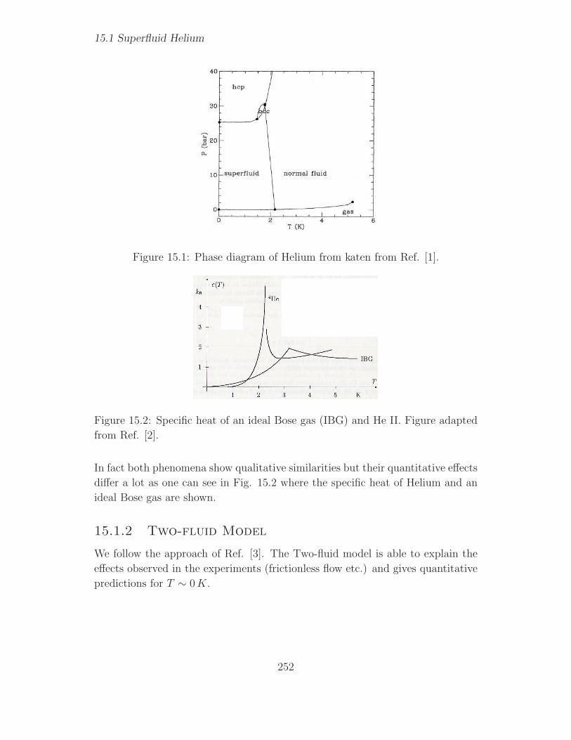
15.1 Superfluid Helium
Figure 15.1: Phase diagram of Helium from katen from Ref. [1].
Figure 15.2: Specific heat of an ideal Bose gas (IBG) and He II. Figure adapted
from Ref. [2].
In fact both phenomena show qualitative similarities but their quantitative effects
differ a lot as one can see in Fig. 15.2 where the specific heat of Helium and an
ideal Bose gas are shown.
15.1.2 Two-fluid Model
We follow the approach of Ref. [3]. The Two-fluid model is able to explain the
effects observed in the experiments (frictionless flow etc.) and gives quantitative
predictions for T ∼ 0K.
252

Superfluidity and Supersolidity
Ansatz
Assume liquid 4He of mass density ρ flowing through a capillary with a velocity
v (parallel to the walls) at a certain time t0 and assume furtherly T = 0. Its
energy density in the laboratory frame is E = ρv2
2. By a Galilean transformation
to the rest frame of the Helium the walls move with −v relative to the liquid.
Excitations (i.e., phonons etc.) will occur in the liquid in the case of friction.
Assume one elementary excitation with momentum ~p and an energy ǫ(~p) where
ǫ is an arbitrary relation of dispersion. The energy is given by
E = ǫ(~p) + ~p~v︸ ︷︷ ︸∆E
+ρv2
2. (15.1)
This formula can be derived by applying a Galilean transformation S = e−iG
with G = m~~v∑
j ~rj to the Hamiltonian with translation invariant potential.1 If
energy dissipates from the Helium, then ∆E < 0 is required and thus
v >ǫ(~p)
p(15.2)
if ~v and ~p are assumed to be antiparallel. This is a necessary condition for the
appearance of friction induced elementary excitations.
If, in particular, Eq. (15.2) can not be fullfilled for a given v the flow is frictionless.
For a finite temperature close to T = 0 the liquid already contains thermal
excitations2. They are assumed to form a gas of quasi particles distributed via the
function n(ǫ) (particle density function) and moving with a velocity ~v′ relatively
to the liquid. The distribution function in the rest frame of the gas is displaced
by −~p~v′ (n(ǫ− ~p~v′)).
The momentum per unit volume of the gas of quasi particles is calculated via
~P =
∫dτ ~pn(ǫ− ~p~v′) (15.3)
with the measure dτ = d3p(2π~)3
. Since ~p~v′ is small3 one Taylor expands n(ǫ − ~p~v′)
to first order in ~p~v′. By averaging over the three spatial dimensions ~p~v′ ≈ 13pp~v′
1e−iGHeiG = H − i[G,H] − 1
2[G, [G,H]] + .... By explicit calculation one finds [G,H] =
−~~v∑
j Pj where Pj is the operator of momentum, [G, [G,H]] = −M~v2 and that higher terms
vanish in this expansion.2The concept of a gas of quasi-particles representing elementary excitations does not hold
for large temperatures near Tλ.3In the low temperature regime we are dealing with, the momenta of the excitations are
small. Since the COM movement of this gas of quasi particles will vanish when taking the
average over all times its variation resulting from interaction with the thermal radiation field
v′ is small aswel.
253

15.1 Superfluid Helium
where p is the unit vector parallel to ~p, one obtains directly
~P = ~v′∫dτ
1
3p2
(−dn(ǫ)
dǫ
)
︸ ︷︷ ︸ρn
. (15.4)
This flow carries mass and by comparison with the form ~P = ~v′ ρn one determines
the mass density to
ρn =
∫dτ
1
3p2
(−dn(ǫ)
dǫ
). (15.5)
The particles in this excitation gas may scatter inelastically with the capillary
walls and thus induce friction into our system even if the velocity v of the liquid
Helium does not fulfill Eq. (15.2).
The result of the calculations above is that the fraction ρn
ρof the total liquid will
have friction with the walls and so one makes the ansatz of dividing the total
mass density into a normal part (ρn) that behaves like a normal liquid (He I) and
a superfluid part (ρs) that has no friction with
ρ = ρn + ρs. (15.6)
Hence the current is given by
~j = ρn~vn + ρs~vs. (15.7)
The normal and the superfluid part interpenetrate without interaction. This
model was firstly introduced by Tisza and Landau.
Quantitative Description
The spectrum of liquid Helium is shown in Fig. 15.3. For small momenta it is
parameterized as ǫ(p) = cp where c is the speed of sound and the quasi particles
in this regime are called phonons. For larger p the linearity does not hold but in
the regime of the local minimum it is parameterized as ǫ(p) = ∆ + (p−p0)2
2m′ . One
refers to the quasi particles in this regime as rotons.
With knowledge of the spectrum one can derive the densities for the normal and
superfluid part via Eq. (15.5) and (15.6).
The phonons are distributed by the Bose distribution n(p) = [e(ǫ(p)T −1)]−1. Since
the energy gap ∆ = 8.7K of the roton excitation is large4 one can approximate
their distribution by Boltzmann law n(p) = e−ǫ(p)T .
4The calculations in the previous part were made under the assumption that we were close
to zero temperature. Close to lambda temperature the concentration of quasi particles becomes
that large that its concept breaks down.
254

Superfluidity and Supersolidity
Figure 15.3: Spectrum of liquid Helium.[3]
We now calculate the normal and superfluid density component using the results
from the two-fluid model.
Phonon part: Substitute dndǫ
= 1cdndp
in Eq. (15.5) and perform a partial inte-
gration. The energy off all phonons can be calculated analogously to the
black body radiation but with a factor 13
because of only one polarization
direction to EPh ∝ T 4. The result is
(ρn)ph =4Eph3c2
T 4 (15.8)
Roton part: Use dndǫ
= − nT
and use the approximations that the main contribu-
tion of rotons has a momentum p = p0 since the energy gap is large and only
rotons with the lowest momentum will be excited. The number of rotons
can be derived by minimizing the free energy F = −NT ln[eVN
∫dτe−
ǫ(p)T
]
with respect to the particle number N. Finally, with Nrot ∝√Te−
∆T ,
(ρn)rot =p2
3T
Nrot
V
1√Te−
∆T . (15.9)
15.1.3 General BEC
The superfluid phase of Helium is characterized by “generalized BEC”[4]. This
is defined as one can find at any time a complete orthonormal basis set of single
particle wave functions such that one and only one is occupied with a number
of atoms of order5 N whereas the occupation numbers of all others is of order 1.
This will be illustrated in a simple basis set.
5N is a macroscopic large number of particles of Helium in the order of 1023.
255

15.1 Superfluid Helium
As an expamle how to derive long range order in a condensed system, the boson
field operator is written in a basis of plane waves
Ψ(t, ~r) =1√V
∑
~p
apei~
»
~p~r− p2
2mt
–
(15.10)
and the condensation takes place at p = 0. The occupation of this state is
a†a = N0 where N0 ∼ N and thus consistent with the concept of generalized
BEC.
As N ≫ 1 the commutator [a0, a†0] = a0a
†0 − N = (N + 1) − N ≈ N − N = 0
can be approximated to be zero and since the operators commute one can treat
them like classical numbers. In a physical sense one can argue that if a particle is
added to the macroscopically occupied ground state the state will not be altered.
Define Ξ = a0√V
. For full mathematical rigour the assumptions only hold in the
thermodynamic limit
limN→∞
< m,N |Ξ|m,N + 1 >= Ξ (15.11)
limN→∞
< m,N + 1|Ξ†|m,N >= Ξ∗, (15.12)
with NV
= const where N is the occupation number of the ground state and m
denotes such other quantum number as the occupation numbers of the other
levels.
So the Boson field operator can be separated by
Ψ = Ξ︸︷︷︸condensate
+ Φ︸︷︷︸uncondensed
, (15.13)
whereas the uncondensed operator in the thermodynamic limit vanishes since
limN→∞
< m,N |Φ|m,N + 1 >= 0 (15.14)
limN→∞
< m,N + 1|Φ†|m,N >= 0. (15.15)
The density matrixNρ(t;~r1, ~r2) =< m,N |Ψ†(t, ~r2)Ψ(t, ~r1)|m,N > can be written
with use of Eq. (15.13)
Nρ(~r1, ~r2) = n0 +Nρ′(~r1, ~r2). (15.16)
With help of Eq. (15.10) one sees
ρ′(~r1, ~r2) =∑
p 6=0
a†papei~~p(~r2−~r1) →
∫
p 6=0
dτn~pei~~p(~r2−~r1) (15.17)
256

Superfluidity and Supersolidity
for V → ∞ and thus ρ′(~r1, ~r2) → 0, |~r1 − ~r2| → ∞.
Since ρ is finite and non zero in the limit of |~r1 − ~r2| → ∞ the liquid will have
long range ordering.
It is very important to note that the condensate density mn0 and the superfluid
density ρs do not correspond. For superfluid Helium at T = 0 one finds n0
n∼ 10%
whereas ρs
ρ= 1 because of Galilean invariance.
15.1.4 Phase Transition
As seen before Helium undergoes condensation into a single particle wave function
below Tλ. Thus the phase relation between the particles in the condensate is fixed
and by choosing a phase for the condensate wave function the U(1) symmetry of
the system is spontaneously broken in the phase transition.
When having superfluid flow the BEC can not be claimed to be in the p = 0 wave
function. So Ξ will now become a function of space and time and can be written
as
Ξ(t, r) =√n0(t, r)e
iφ(t,r) (15.18)
and can be considered as a wave function for the condensate. Since Ξ(t, r) ≡ 0
for T > Tλ this quantity is the ordering parameter6. It goes to zero continuously
hence the phase transition will be of second order.
The ordering parameter is complex and the phase transition is of in λ-transition
universality class as the three dimensional XY model.
The critical exponent describing the behavior of the specific heat in the vicinity of
the phase transition α (Cv ∝ (T − Tλ)−α) for this phase transition is ought to be
best measured by a space shuttle experiment [5] to α = −0.01285±0.00038, which
is very close to theoretical predictions by perturbation theory [6] that calculate
it to α = −0.01294 ± 0.00060, i.e. the specific heat remains finite at Tλ.
15.1.5 Superfluid Velocity
The mass current ~jcon can be calculated via
~j =i~
2m(Ξ∗∇Ξ − Ξ∇Ξ∗) = n0
~
m∇φ. (15.19)
With Eq. (15.18) one defines the superfluid velocity to be proportional to this
current thus
~vs :=~
m∇φ. (15.20)
6Both its real and imaginary part are ordering parameters.
257

15.1 Superfluid Helium
The potential of the velocity is the phase of the condensate wave function thus
it is an irrotational flow (∇ × ~vs = 0). The amplitude of the condensate wave
function (the amount of particles that undergo BEC) is not important for the
effect of superfluidity.
The superfluidity itself is not an observable but the current ~j = ~vρ = ~vsρs +~vnρnis.
The superflow in Helium is a response to the phase of the condensate and, in three
spatial dimension, both phenomena go hand in hand. There are Bose-Einstein
condensates that do not show a superfluid response and, in the two dimensional
case, superfluidity occurs without condensation.
Onsanger-Feynman quantization
Calculating the flux∮~vsd~l = ~
m∆φ and taking into account that the phase of
the wave function is just defined modulus 2πn, n ∈ Z, one derives the Onsanger-
Feynman quantization ∮~vsd~l = n
h
m. (15.21)
For a simply connected region it follows that n = 0.
In a normal fluid the vorticity as defined in Eq. (15.21) can take any value
whereas its value in the superfluid case has to be multiples of hm
. This has
important consequences.
Vortices
The case n 6= 0 in Eq. (15.21) can only be realized only in a not simply connected
area. One introduces vortices (either closed loops or ending at the surfaces)
where the velocity field has a divergence (vs ∝ 1r
where r is the distance to
the vortex [3]) but the wave function is vanishing so this divergence does not
cause any problems thus we define vs in every point outside the vortex. From a
macroscopical viewpoint the vortex is infinitely small.
Consider a rotating cylinder with radius R with liquid Helium inside rotating at
~ω = (0, 0, ω) parallel to the symmetry axis. The energy in the rest frame of the
Helium is given by
Erot = E −Mω. (15.22)
The goal is to find a ωc such that for ω > ωc the appearance of vortices is
favored. Because of the symmetry of the system the vortex has to be parallel to
the symmetry axis. The energy difference in the presence of a vortex is given by
258
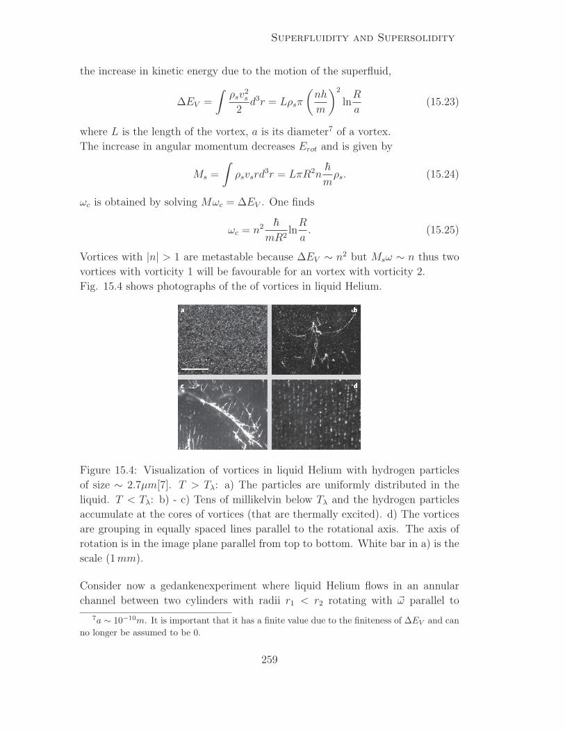
Superfluidity and Supersolidity
the increase in kinetic energy due to the motion of the superfluid,
∆EV =
∫ρsv
2s
2d3r = Lρsπ
(nh
m
)2
lnR
a(15.23)
where L is the length of the vortex, a is its diameter7 of a vortex.
The increase in angular momentum decreases Erot and is given by
Ms =
∫ρsvsrd
3r = LπR2n~
mρs. (15.24)
ωc is obtained by solving Mωc = ∆EV . One finds
ωc = n2 ~
mR2lnR
a. (15.25)
Vortices with |n| > 1 are metastable because ∆EV ∼ n2 but Msω ∼ n thus two
vortices with vorticity 1 will be favourable for an vortex with vorticity 2.
Fig. 15.4 shows photographs of the of vortices in liquid Helium.
Figure 15.4: Visualization of vortices in liquid Helium with hydrogen particles
of size ∼ 2.7µm[7]. T > Tλ: a) The particles are uniformly distributed in the
liquid. T < Tλ: b) - c) Tens of millikelvin below Tλ and the hydrogen particles
accumulate at the cores of vortices (that are thermally excited). d) The vortices
are grouping in equally spaced lines parallel to the rotational axis. The axis of
rotation is in the image plane parallel from top to bottom. White bar in a) is the
scale (1mm).
Consider now a gedankenexperiment where liquid Helium flows in an annular
channel between two cylinders with radii r1 < r2 rotating with ~ω parallel to
7a ∼ 10−10m. It is important that it has a finite value due to the finiteness of ∆EV and can
no longer be assumed to be 0.
259

15.2 Supersolid Helium
its symmetry axis. The scalar velocities in the following are the circumferential
components of the vectors.
For T > Tλ the liquid behaves like a classical one with a velocity field vn(r) = ωr
where the velocity of the liquid at the boundary equals the boundaries velocity
vn(r2) = vwall. The moment of intertia is Iclω.
Consider cooling down below Tλ. The region is not simply connected thus n 6= 0
is possible even if there are no vortices present. i.e. ω < ωc.
The angular velocity of the superfluid is measured in units of ω′ = ~
mR2 (n = 1
in Eq. (15.21).). Since the quantization of the circulation in Eq. (15.21) the
superfluid velocity can not build a velocity field similar the the normal component.
It is found that the angular velocity of the superfluid Helium will be given by
ωs = nω′ where n is determined as the integer closest to ωω′ . The angular velocity
of the superfluid can even exceed the one of the cylinders, e.g. if ω = 0.75ω′[4].
The total angular of momentum when cooling below the critical temperature is
reduced by ρn(T )ρ
. Hence, one can tune the angular momentum of the configuration
by varying T .
This effect is known as the “Hess-Fairbank” effect.
15.2 Supersolid Helium
At pressures above ∼ 26 bar Helium can form a crystal, as shown in Fig. 15.1.
In the following the hcp (hexagonal close packing) phase will be discussed. The
hcp structure is drawn schematically in Fig. 15.5.
Figure 15.5: Schematic drawing of the hcp structure.
15.2.1 Observations / Experiments
Kim-Chan Experiment
In analogy to the Andronikashvili experiments (disks rotating in superfluid He-
lium) the response of solid Helium to a rotation is observed. E. Kim and E. W.
260
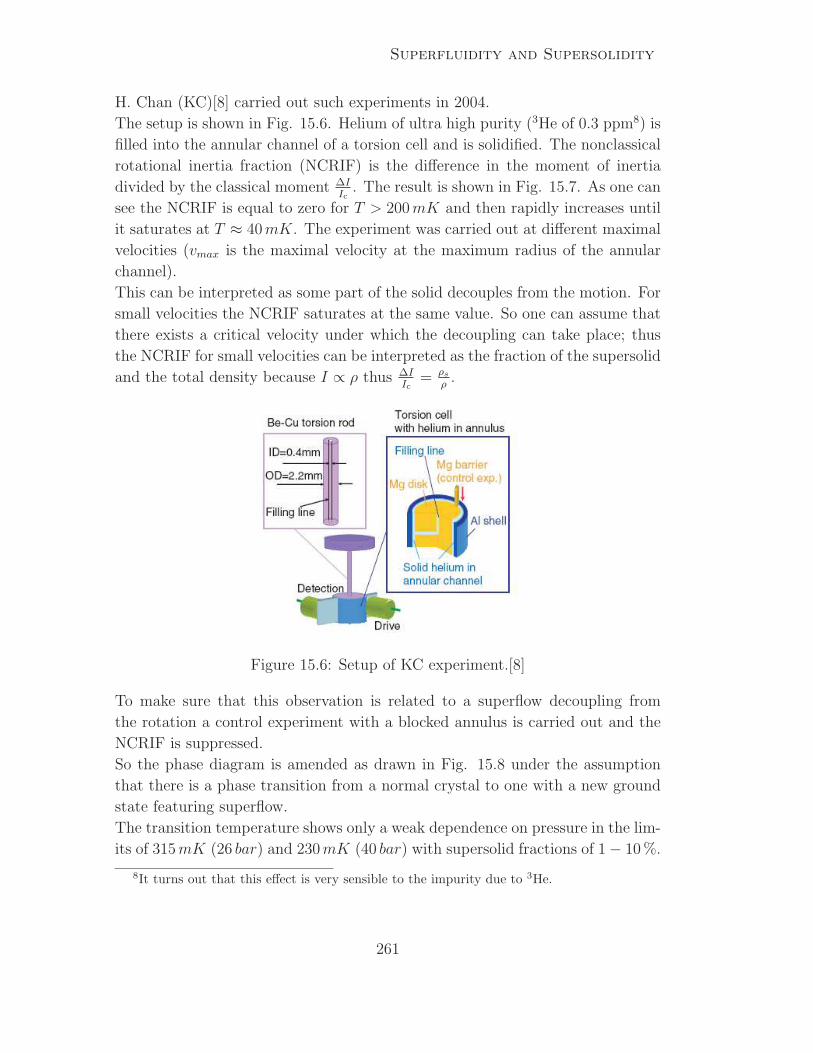
Superfluidity and Supersolidity
H. Chan (KC)[8] carried out such experiments in 2004.
The setup is shown in Fig. 15.6. Helium of ultra high purity (3He of 0.3 ppm8) is
filled into the annular channel of a torsion cell and is solidified. The nonclassical
rotational inertia fraction (NCRIF) is the difference in the moment of inertia
divided by the classical moment ∆IIc
. The result is shown in Fig. 15.7. As one can
see the NCRIF is equal to zero for T > 200mK and then rapidly increases until
it saturates at T ≈ 40mK. The experiment was carried out at different maximal
velocities (vmax is the maximal velocity at the maximum radius of the annular
channel).
This can be interpreted as some part of the solid decouples from the motion. For
small velocities the NCRIF saturates at the same value. So one can assume that
there exists a critical velocity under which the decoupling can take place; thus
the NCRIF for small velocities can be interpreted as the fraction of the supersolid
and the total density because I ∝ ρ thus ∆IIc
= ρs
ρ.
Figure 15.6: Setup of KC experiment.[8]
To make sure that this observation is related to a superflow decoupling from
the rotation a control experiment with a blocked annulus is carried out and the
NCRIF is suppressed.
So the phase diagram is amended as drawn in Fig. 15.8 under the assumption
that there is a phase transition from a normal crystal to one with a new ground
state featuring superflow.
The transition temperature shows only a weak dependence on pressure in the lim-
its of 315mK (26 bar) and 230mK (40 bar) with supersolid fractions of 1 − 10 %.
8It turns out that this effect is very sensible to the impurity due to 3He.
261

15.2 Supersolid Helium
Figure 15.7: A-C: Measurement of NCRIF of Kim and Chan as a function of
temperature. The different lines correspond to different maximal velocities. D:
Measurement of NCRIF as function of maximal velocity vmax[8]
Quality of the Crystal
The KC experiment was repeated by other experimentalists. It was observed
that the appearance of NCRIF was related to the quality of the crystal. If it
was annealed (melted, refrozen, etc.) the supersolid behavior was weakened and
vanished for a fully annealed crystal[9].
This leads to the conjecture that supersolidity is not an universal property but
that one can create samples of solid Helium that do not show non-classical be-
havior in torsional experiments.
Communicating Vessels
Further investigation on the depedence of the quality of the crystal are carried
out by relaxation of a crystal with different hights. The experimental setup[10]
consists of a certain volume with a tube in it. In this volume and the tube solid
Helium is in equilibrium with its liquid phase but the levels in the tube and the
rest of the volume differ (h(t)) as drawn in Fig. 15.9; the top of the tube is closed.
If mass is able to flow frictionless the levels will relax.
One observes the following (at temperatures comparable to those of the Kim-
Chang experiments):
• Crystals of good quality (few grain boundaries, defects, etc.) show no mass
flow. The upper bound of the velocity (due to errors) differs from the
expectation by Kim-Chan by a factor of 300.
262

Superfluidity and Supersolidity
Figure 15.8: Phase diagram by Kim and Chan.[8]
• In some samples one observed cusps in this sample and relaxation took
place as long as the cusps disappeared.
• If a relaxation takes place, h(t) = const. A viscous fluid would have shown
an exponential decay wheres a constant flow indicates a superflow at its
critical velocity.
• The more cusps the faster the relaxation.
15.2.2 Models
Zero Point Vacancies
The classic model of a crystal proposes an integer number of atoms per unit cell
- the crystal is commensurate and thus insulating because it does not feature off-
diagonal long range order as it is discussed below. If one drops this assumption
the ground state can have vacancies (empty lattice points in the crystal) if their
activation energy is not positive (gapless vacancies)[11].
Only zero-point vacancies or interstitials can make an ideal crystal supersolid.
This is necessary because one must have (restricting to single-particle effects)
off-diagonal long range order (ODLRO) that is defined as∫n(~r, ~r′)d3r → ∞ (15.26)
in the thermodynamic limit[11] where n(~r, ~r′) =∏N
i≥2
∫d3riΨG(~r, ~ri)ΨG(~r′, ~ri) is
the single-particle density matrix with N denoting the total number of particles
and ΨG the wave function of the ground state.
263

15.2 Supersolid Helium
Figure 15.9: Left: Experimental setup of a crystall grown to a different height in
a tube, Right: Photo of solid Helium at 1.3 K. L = liquid, S = solid phase.[10]
By using path-integral Monte Carlo simulations [11] [1] in complex time (τ = it)
one investigates the behavior of the density matrix and the time dependent zero-
momentum Greens function G that is the two-point correlation function n in the
zero-time limit via n(~r) = G(~r, τ → 0−).
G(~r, τ) = 〈Φ(~r, τ)|Φ(0, 0)〉 (15.27)
thus G(k, τ) is the Fourier transform of G(~r, τ). The zero-momentum value is
just the integral over all positions since G(k, τ) ∼∫d3r G(~r, τ)e−i
~kr hence
G(k = 0, τ) ∼∫d3rG(~r, τ). (15.28)
Numerical results from such simulations are shown in Fig. 15.10. Both quantities
decay exponentially and the activation energy for an interstitial or a vacancy is
very large (∼ 23K for an interstitial and ∼ 13K for a vacancy) compared to the
temperature of T = 0.2K where the simulation is performed. The energy gap for
creating an interstitial ∆I or a vacancy ∆V is calculated by fitting G(k = 0, τ) ∝e−∆V/I|τ | to the numerical data.
The possibility for the true ground state to consist of a larger number of vacan-
cies is not ruled out by these observations but further Monte Carlo simulations in
which a certain number of vacancies were forced in the crystal show a strong at-
traction between these vacancies so they phase separate from the bulk crystal[11].
The result of these simulations is that the true ground state of an ideal 4He-crystal
is the insulating and commensurate hcp-phase.
264
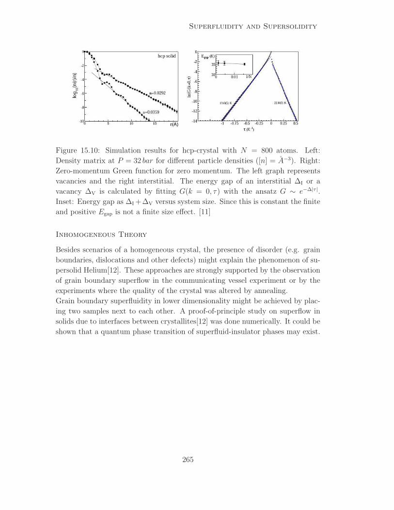
Superfluidity and Supersolidity
Figure 15.10: Simulation results for hcp-crystal with N = 800 atoms. Left:
Density matrix at P = 32 bar for different particle densities ([n] = A−3). Right:
Zero-momentum Green function for zero momentum. The left graph represents
vacancies and the right interstitial. The energy gap of an interstitial ∆I or a
vacancy ∆V is calculated by fitting G(k = 0, τ) with the ansatz G ∼ e−∆|τ |.
Inset: Energy gap as ∆I +∆V versus system size. Since this is constant the finite
and positive Egap is not a finite size effect. [11]
Inhomogeneous Theory
Besides scenarios of a homogeneous crystal, the presence of disorder (e.g. grain
boundaries, dislocations and other defects) might explain the phenomenon of su-
persolid Helium[12]. These approaches are strongly supported by the observation
of grain boundary superflow in the communicating vessel experiment or by the
experiments where the quality of the crystal was altered by annealing.
Grain boundary superfluidity in lower dimensionality might be achieved by plac-
ing two samples next to each other. A proof-of-principle study on superflow in
solids due to interfaces between crystallites[12] was done numerically. It could be
shown that a quantum phase transition of superfluid-insulator phases may exist.
265

15.2 Supersolid Helium
266

Bibliography
[1] Ceperley, D.M. , Path integrals in the theory of condensed helium, Rev. Mod.
Phys. 67, 279 (1995).
[2] T. Fliessbach, Statistische Physik, Lehrbuch zur theoretischen Physik IV
(Spektrum Akademischer Verlag, Heidelberg, Berlin, Oxford, 1995).
[3] Lifschitz, E.M. and Pitajewski, L.P. , Lehrbuch der statistischen Physik IX,
Statistische Physik, Teil 2 (Akademie-Verlag Berlin, Berlin, 1989).
[4] Leggett, A. J. , Superfluidity, Rev. Mod. Phys. 71, 318 (1999).
[5] Lipa, J. A. , Swanson, D. R., Nissen, J.A., Chui, T. C. P. and Israelsson,
U. E. , Heat capacity and thermal relaxation of bulk helium very near the
lambda point, Phys. Rev. Lett. 76, 944 (1996).
[6] Kleinert, H., Critical exponents from seven-loop strong-coupling φ4-theory in
three dimensions, Phys. Rev. D 60, 085001 (1999).
[7] Bewley, G. P., Lathrop, D. P. and Sreenivasan, K. R. , Visualaziation of
quantized vortices, Nature 441, 588 (2006).
[8] Kim, E. and Chan, M. H. W., Observation of superflow in solid helium,
Science 305, 1941 (2004).
[9] Rittner, A. S. C., Reppy, J. D. , Observation of Classical Rotational Inertia
and Nonclassical Supersolid Signals in Solid 4He below 250mK, Phys. Rev.
Lett. 97, 165301 (2006).
[10] Sasaki, S., Ishiguro, R., Caupin, F. , Maris, H. J. and Balibar, S. , Su-
perfluidity of grain boundaries and supersolid behavior, Science 313, 1098
(2006).
[11] Prokof’ev, N.V., What makes a crystal supersolid? (2006), (cond-
mat/0612499).
267

BIBLIOGRAPHY
[12] Prokof’ev, N.V. and Svistunov, B.V. , On the supersolid state of matter
(2004), (cond-mat/0409472).
268