PHASE PLANE METHOD APPLIED TO OPTIMAL CONTROL IN NONLINEAR ...facta.junis.ni.ac.rs/macar/macar2007s/macar2007s06.pdf · PHASE PLANE METHOD APPLIED TO OPTIMAL CONTROL IN NONLINEAR

FACTA UNIVERSITATIS Series: Mechanics, Automatic Control and Robotics Vol. 6, Special Issue, 2007, pp. 71 - 98

PHASE PLANE METHOD APPLIED TO OPTIMAL CONTROL IN NONLINEAR DYNAMICAL SYSTEMS WITH TROGGER

OF COUPLED SINGULARITIES UDC 531.3(045)=111

Katica R. (Stevanović) Hedrih

Faculty od Mechanical Engineering University of Niš, Mathematical Institute SANU Belgrade

18 000 - Niš, ul. Vojvode Tankosića 3/22, Serbia Telefax: 381 18 42 41 663 / Mobile 063 8 75 75 99

e-mail: [email protected] * e-mail(home): [email protected]

Abstract. Short Main idea of the phase plane method applied to the optimal control in nonlinear dynamical systems with triggers of a coupled singularities, and with one degree of freedom, is reconsidered. Paper presents a short review of the author's previous published results containing series of the special cases of the optimal control in nonlinear dynamical systems with trigger of coupled singularities important for engineering applications. This paper analyses the controllability of motion of conservative or nonconservative nonlinear dynamical systems in which triggers of coupled singularities exist or appear. It is shown that the phase plane method is useful for the analysis of nonlinear dynamics of conservative and nonconservative systems with one degree of freedom of control strategies and also shows the way it can be used for controlling the relative motion in rheonomic systems having equivalent scleronomic conservative or nonconservative system. For the system with one generalized coordinate described by nonlinear differential equation of nonlinear dynamics with triggers of coupled singularities, the functions of system potential energy and conservative force must satisfy some conditions defined by a Theorem on the existence of a trigger of coupled singularities and the separatrix in the form of number eight. Task of the defined dynamical conservative system optimal control is: by using controlling force acting to the system, transfer initial state of the nonlinear dynamics of the system into the final terminate state of the nonlinear dynamics in the minimal time for that optimal control task. Some research results of fascinating nonlinear dynamics of a heavy material particle along circles with coupled rotations with many different properties of nonlinear dynamics and optimal control of this dynamics are presented. A visualizations of nonlinear dynamical processes in such rheonomic systems were made.

Key words: phase plane method, optimal control, nonlinear dynamics, conservative system, nonconservative system, phase plane portrait, triggers of coupled singularities, theorem, coupled rotation, material particle, homoclinic points, homoclinic orbit, bifurcation, separatrice layering, separatrice in the form of number eight.

Received February 6, 2008

72 K.R. (STEVANOVIĆ) HEDRIH

I. INTRODUCTION

The controllability of motion of dynamical systems in which exist or appear triggers of coupled singularities is in the focus of our attention. It is shown that the phase plane method is useful for the analysis of nonlinear dynamics of systems with one degree of freedom control strategies.

The differential equation of the nonlinear dynamics of a system with possibilities of the trigger of the coupled singularities existence is in the basic and general form of:

0)()](,[ =+ xfxFkgx&& where x is generalized coordinate and in the special cases in same time relative coordinate. For that case when in the system existed a trigger of the coupled singularities, than the functions f (x), F (x) and g[k, F(x)] must satisfy some conditions defined by a Theorem on the existence of a trigger of the coupled singularities and the separatrix in the form of number eight.

Task of the defined dynamical system optimal control is: By using controlling force )(~ tu acting to the system, transfer initial kinetic state of the nonlinear dynamics of the

system defined by x1(0) = α and x2(0) = β into the final or terminate kinetic state of the nonlinear dynamics defined by x1(T) = γ and x2(T) = χ, where T is minimal time for that optimal control task.

In an engineering system [5], [7], [8], [10], [11], [16], [17], [18] with mass deviation properties to the axes of rotation, in the gravitation field, where complex coupled rotation motion exists, in the case of some kinetic parameter values, the phenomenon of bifurca-tion equilibrium position (see Ref. [1], [2], [3], [6], [9], [12]) or appearance of two new relative dynamic stable equilibrium positions in relation to precession rotation motion are nonlinear properties of such system.

In such systems with the change of some kinetic parameters of the system, the proc-ess of losing stability of one static equilibrium position is followed with appearing two close stable dynamical equilibrium positions (see Ref. [1], [2], [3], [4], [6], [9], [12]). Also, these two new appeared singularities with the previous stable position, which lost its stability, make a trigger of coupled singularities.

Trigger of coupled singularities, with corresponding choice of kinetic parameters of the system dynamics, which degenerates into one threefold (triple) singular point, corre-sponds to stable equilibrium position. Coupled singularities existence is coupled with existence of two types of homoclinic orbits–separatrix trajectories: new appeared, second homoclinic orbit in the form of number eight, which appear with bifurcation of equilib-rium position, inside of previous homoclinic orbit, whose shape is deformed in the form of one pair of symmetric "waves".

Homoclinic orbit coupled with trigger of coupled singularities is in the form of number "eight". Such trigger of coupled singularities is a characteristic nonlinear phenomenon of dynamical systems, which is the source of sensitive dependence of the system dynamics behavior with respect to a small change of initial conditions in the vicinity of these coupled singularities. In such system, under the action of the pure periodic excitation, behavior of system dynamics with stochastic-like and chaotic-like processes appears.

In one of classical monographs [1] by A. A. Andronov, A. A. Witt and S. E. Hajkin, which has a great number of editions, some classical examples of nonlinear systems with one degree of freedom of oscillatory motion and their phase portraits except general the-ory of nonlinear oscillations are presented, and such examples can also be found in books by J. J. Stoker [23] as well as by D.P. Rašković [22]. Especially in monograph by Guckenheimer, J. and Holmes, Ph. [3], results of research on nonlinear systems and

Phase Plane Method Applied to Optimal Control in Nonlinear Dynamical Systems... 73

properties of various kinds of bifurcations are pointed out. A series of monographs by Mitropolyskiy, Yu. A [21] deals with theory, methods and problems of asymptotic theory of non-steady nonlinear oscillations of nonlinear systems and trigger of coupled singularities in the resonant range.

Control of dynamics in such system is very important for engineering applications. This paper analyses the controllability of motion of dynamical systems in which exist or appear triggers of coupled singularities. S series of the separate tasks earlier published is presented (see Refs. [7], [13], [14], [15]). It is shown that the phase plane method is useful for the analysis of nonlinear dynamics of systems with one degree of freedom control strategies and also shoes the way it can be used for controlling the relative motion in rheonomic sys-tems having equivalent scleronomic conservative or nonconservative system.

In monographs (see [25]) V. Vujičić gave a modification of the analytical mechanics of rheonomic systems, with the aim to include the influence of nonstationary constraints into the laws of motion. In his approach, rheonomic coordinate is chosen as a function derived from rheonomic constraints. On this basis, an extended system of Lagrangian equations was formulated with an additional equation corresponding to rheonomic coordinate. In the paper by Vujičić and Hedrih [26] the rheonomic constraints general-ized force in the extension of the Lagrange's system of differential equations of motion of the first and the second kind is introduced. In the paper by K. S. Hedrih [19] the power of the rheonomic constraints change is introduced.

A series of papers [4-19], by author of this paper, presents results of original research on nonlinear dynamics of mechanical systems with properties of periodic exchanges, which have application in engineering systems. In the papers [9, 10] some results and new knowledge about rheonomic nonlinear systems, which have equivalent holonomic scleronomic conservative nonlinear system are presented. Paper [9] considered a class of nonlinear systems with coupled rotation motions into system with two degrees of mobil-ity, but with one degree of freedom of motion defines one generalized coordinate, and one degree of motility that is defined by rheonomic coordinate linearly depending on time. For such special class of rheonomic nonlinear systems, an equivalent holonomic scleronomic conservative nonlinear system and equivalent kinetic and potential energy are defined. Theorem of existence of relative equilibrium positions in such a class of rheonomic conservative systems by using equivalent holonomic conservative system is defined, as well as proven [4, 6]. Theorem of existence of homoclinic orbits in the form of number eight and trigger of coupled singularities in the phase portrait of nonlinear dynamics of relative motions in the class rheonomic system is defined and proven.

Like basic properties of linear oscillatory system with one and more degrees of oscillatory freedom are the own frequencies of discreet material particle system who have linear oscillatory motion, also for nonlinear system with one degree of oscillatory free-dom we may consider phase portrait with singularity structure, which gives nonlinear dynamic's properties of system in phase plane. Therefore for nonlinear dynamic systems and their subsystems it's important to study a structure of phase portraits, their stability as well as their transformations and transformations of phase trajectories which we obtained changing any parameters of systems. Author defines a trigger of coupled singularities theorem and existence of homoclinic orbits and their transformation shaped by number eight, as well as their application on systems relevant for technical practice in hers article [4, 6]. Also she constructs phase portraits and particularly considers phenomena of homo-clinic orbits transformations and their disintegration, appearance and disappearance homoclinic orbits shaped by number eight, like a trigger of coupled singularities.


II. THEOREM ON THE EXISTENCE OF A TRIGGER OF THE COUPLED SINGULARITIES AND THE SEPARATRIX IN THE FORM OF NUMBER EIGHT IN THE CONSERVATIVE SYSTEM

By using nonlinear dynamic analysis of systems with described nonlinear phenome-non of the trigger of coupled singularities and corresponding families of phase portraits and potential energies (see Refs. [1], [4], [6]) as well as the corresponding experimental investigations of such nonlinear dynamics in mechanical engineering systems with cou-pled rotation motions ([5], [13]) it was easy to define and to prove the theorem of the existence of a trigger of coupled singularities in nonlinear dynamical systems with periodical structure, previous published in the Reference [4].

Theorem 1*: In the system whose dynamics can be described with the use of non-linear differential equation in the form:

0)()](,[ =+ xfxFkgx&& (1)

and whose potential energy is in the form:

( )∫ ==x

xFkmdxxfxFkgm0

)](,[)](,[ GE (2)

in which the functions f (x) and g (x) are:

∫=x

dxxfxF0

)()( and ∫=x

dxxkgxkG0

),(),( (3)

and satisfy the following conditions: )()( xfxf −− ),(),( 0 xkgnTxkg =+

)()( 0 xfnTxf =+ ),(),( xkgxkg =− ( ) 00 =f )....,(),(,0)](,[ 3221 kkkkkforxFkg r ∪∈= (4)

0)( =sxf , 0sTxs = , ,...4,3,2,1=s 00 rTxxr ±±= , ,...4,3,2,1,0=r20

0Tx <

)....,(),(,0)](,[ 3221 kkkkkforxFkg ∪∉≠ and both functions f (x) and g (x) have one maximum or minimum in the interval between two zero roots:

a* for parameters values )...,,(),( 3221 kkkkk ∪∉ outside of the intervals ),,(),( 3221 kkkk ∪ the trigger of singularities in the local area does not exist.

b* for parameters values )...,,(),( 3221 kkkkk ∪∈ inside of the intervals ),,(),( 3221 kkkk ∪ the series of triggers of coupled singularities in the local domains exist.

The proof of defined theorem and details are published in the References [4] and [6]. Then, the trigger of coupled singularities exists in the phase portrait in the intervals

defined by: ⎟⎠

⎞⎜⎝

⎛ ++−∈ sTTsTTx2

,2

00 ,...4,3,2,1,0=s

Integral energy of the system described by (1) is:

consttxFkGxxFkGx =+=+ ))]((,[2)](,[2 020

2 && (5)


Equation of homoclinic orbit in the form number "eight" trough homoclinic point (0,0) is: consthFkGxFkGx hc ===+ 0

2 )]0(,[2)](,[2& (6)

for ).....,(),(,0)](,[ 3221 kkkkkforxFkg r ∪∈= in which the functions F(x) and G(k,x) are in the form (3) and satisfy the conditions (4).

Equation of homoclinic orbit other form in the continuous closed form trough homoklinic point (xs,0) is:

consthxFkGxFkGx scs ==±=+ 02 )](,[2)](,[2& (7)

III. LINEARIZED APPROXIMATION

Now, let us consider special cases of the dynamics described by defined nonlinear differential equation (1) in the vicinity of the equilibrium positions. For beginning we consider small oscillations around stable and also unstable equilibrium positions correspond to the stable and unstable saddle type singularities coupled in ones set with trigger of three coupled singularities.

By use the cases considered in the previous theorem of the trigger of the existence of the coupled singularities in the set of the trigger of the coupled singularities, we can start with this nonlinear differential equation (1) in the case when one stable singular point center type exists in the phase plane and correspond to stable equilibrium position. a* for parameters values )...,,(),( 3221 kkkkk ∪∉ outside of the intervals )...,,(),( 3221 kkkk ∪ the trigger of singularities in the local area does not exist. Only a singular point center type exists. Then for small vibrations in the vicinity of this singular point it is easy to obtain right and acceptable linearized differential equation in the form:

02 =ω+ xx&& (8) where own (eigen) circular frequency of the small oscillations is expressed in the following form:

( ) 0)()](,[][)(

)](,[

0

22 >⎭⎬⎫

⎩⎨⎧

′+∂

∂=ω

=x

xfxFkgxfxF

xFkg (9)

and taking into account properties of the functions considered in the previous theorem we can write simplest expression: 0)}0()]0(,[{2 >′=ω fFkg .This is condition for no existence of the trigger of coupled singularities.

b* for parameters values )...,,(),( 3221 kkkkk ∪∈ inside of the intervals )...,,(),( 3221 kkkk ∪ the series of triggers of coupled singularities in the local domains exist. This trigger of coupled singularities contains one unstable singular point saddle type and two stable points center types.

Then, for small perturbations in the vicinity of this unstable singular saddle point it is easy to obtain an unacceptable linearized differential equation for long time period of the motion. In the vicinity of the unstable saddle point corresponding to unstable equilibrium position linearized equation takes the following form:


02 =− xkx&& (10) where 0)}0()]0(,[{2 >′−= fFkgk (11)

In the vicinity of the two corresponding stable singular points of centre type, corresponding to stable equilibrium positions, linearized equation is in the form (8) where

0)()](,[)]([)(

)](,[ 22 >⎭⎬⎫

⎩⎨⎧

′+∂

∂=ω

±= rxxr xfxFkgxf

xFxFkg (12)

and taking into account properties of the functions considered in the previous theorem 1* for the case of the trigger of coupled singularities existence, we can write simplest expression:

0))](([)(

)](,[ 22 >⎭⎬⎫

⎩⎨⎧

±∂

±∂=ω r

rr xf

xFxFkg (13)

for the own (eigen) circular frequencies of the small oscillations of the two stable equilibrium positions.

IV. OPTIMAL CONTROL OF NONLINEAR DYNAMICS IN THE CONSERVATIVE SYSTEM

For optimal control of the nonlinear dynamics of this considered system defined by nonlinear differential equation (1) we can introduce two phase coordinate in the space state x1 and x2, and by the differential equation second order (1), we can introduce two nonlinear differential equations first order in the following form:

21 xx =& )()](,[ 112 xfxFkgx −=& (14)

with initial conditions x1(0) = α and x2(0) = β. Task of the defined dynamical system optimal control is: By using controlling force )(~ tu

acting to the system, transfer initial state of the nonlinear dynamics of the system defined by x1(0) = α and x2(0) = β into the final terminate state of the nonlinear dynamics defined by x1(T) = γ and x2(T) = χ, where T is minimal time for that optimal control task. Than, we can write two new nonlinear differential equations of the first order for optimal control task in the following form: 21 xx =& )(~)()](,[ 112 tuxfxFkgx ±−=& (15)

with initial conditions state in the form

α=)0(1x and β=)0(2x . (16)

and with final terminate conditions in the form

γ=)(1 Tx and χ=)(2 Tx , (17)

where T is time necessary for this motion.


Pontrijagin's maximum principle (see Refs. [25] and [14]) is used. For minimization of the time T to the previous system dynamics defined by nonlinear differential equations (15), we add to these equations the following functional

∫ ⋅=T

dt0

1I (18)

as a criterion of the optimality – time minimization, or "criterion of quality" of the motion control, with addition in the form of the controlling force )(~ tu constraints in the form:

00~)(~~ utuu +≤≤− . (19)

The concept of controllability of motion (or system dynamics) implies the possibility that the mechanical system motion (or dynamics) is realized according to a given pro-gram under the excitation of special generalized forces. Motion or dynamics controlling force )(~ tu is here considered as generalized force of controllability corresponding to generalized coordinate of the system. The phrase "system motion or system dynamics control" implies the process of realizing a given or programming motion or dynamics. Programs can be of a great variety. This study includes the program of the pathways and the program of velocities. For the motion upon the derived manifolds it is also necessary to know and take into consideration the relations of their generation.

Formulation of the Theorem 2* (see Ref. [25]) gives the following explanation: "The mechanical system motion or dynamics is controllable according to the program given in advance if there are such controlling forces of such magnitude, depending upon the program parameters, which are by their absolute value greater than other respective active forces if the controlling force direct the motion opposite to the motion direction under the influence of the other forces".

Concept of optimal motion of system dynamics implies here motion or dynamics of the mechanical systems whose particular attributes have extreme values with respect to some dynamics parameters.

Now, let's determine the controlling force )(~ tu that can control the dynamics of the system of accordance with defined control tasks (15)-(19).

The problem of optimal controllable dynamics is to find dynamic parameters that is, those forces that translate a controllable mechanical system dynamics described by system differential equation (1) from initial state [x1(0) = α, x2(0) = β] to final terminate state of the nonlinear dynamics defined by [x1(T) = γ, x2(T) = χ], where T is minimal time, so that functional (18) achieve its extreme value.

It is possible criterion of the optimal control of dynamics to write in the following way:

∫ −−Η=T

dtxpxp0

2211 ][~&&I (20)

or in the forms:

∫ ±−−−=T

dtuxfxFkgtpxtpupp,xx0

11212121 }~)()](,[){()(]~,,,[~ HI (20.a)

This previous functional (20.a) is for the case with unspecific interval of time. As the one of the boundary of time interval is in the integral of functional, then it is necessary to take into account noisochroous variations of the functional.


On this basis we can to write:

0

][][~

0

2

1

2

1

0221102211

=⎥⎥⎦

⎤

⎢⎢⎣

⎡δ

∂Η∂

+δ⎟⎟⎠

⎞⎜⎜⎝

⎛−

∂Η∂

+δ⎟⎟⎠

⎞⎜⎜⎝

⎛+

∂Η∂

+

+Δ−−Η+δ−δ−=Δ

∫ ∑∑=

=

=

=

T i

iii

i

i

iii

i

TT

dtuu

pxp

xpx

txpxpxpxp

&&

&&I (21)

Optimal dynamics is defined by solving the following system of differential equations with corresponding additional conditions of the optimal control of motion:

i

i px

∂Η∂

=& ; i

i xp

∂Η∂

−=& ; 0=∂Η∂u

; 00 )( utuu ≤≤− ; 0=Η=Tt

.2,1=i (22)

By using theory presented in Ref. [25], as well as previous obtained conditions of the optimal control of motions, we can write the following Hamilton functional in the form:

}~)()](,[){()(1]~,,,[ 112212121 uxfxFkgtpxtpupp,xx ±−++=H (23)

Second pair of the canonical differential equations is:

)()(

)()](,[)]([)(

)](,[)()(

12

2

112

11

12

11

tpx

tp

xfxFkgxfxF

xFkgtpx

tp

−=∂∂

−=

⎭⎬⎫

⎩⎨⎧

′+∂

∂=

∂∂

−=

H

H

&

&

(24)

or

)()(

0)()](,[)]([)(

)](,[)()(

21

112

11

122

tptp

xfxFkgxfxF

xFkgtptp

&

&&

−=

=⎭⎬⎫

⎩⎨⎧

′+∂

∂+

(24*)

and

)()(

0)(~

21

2

tptp

tpu

&

m

−=

==∂∂H

00 )( utuu ≤≤−

0}~)()](,[){()(1]~,,,[ 112212121 =±−++=== TtTt

uxfxFkgtpxtpupp,xxH

[ ] 0)}(~))(())((,){()()(1

]~,,,[

11221

2121

=±−++=

==

TuTxfTxFkgTpTxTp

upp,xxTt

H (25)

First integral of the system of optimal control of the system dynamics

0)()](,[ 0 =±+ uxfxFkgx&& (26)

we can obtain by following form:

0)(~)](,[)](,[22 000

20

2

=−±−+− xxumxFkmxFkmxmxm GG&&

(27)


Taking into account expression (2) for the system potential energy and corresponding initial condition: t = 0 x(0) = x0 0)0( xx && = , it is possible to write the previous integral (27) of energy in the following form

0)( 00 =−±−+− xxFpp 0k0k EEEE (28)

Then, we have a set of two phase trajectories with different initial points, first through the initial condition point x1(0) = α and x2(0) = β, and second through final terminate condition point x1(T) = γ and x2(T) = χ corresponding to the final and terminate dynamic state of the system and with force with alternative directions:

0)( 00 =−+−+− xxFpp 0k0k EEEE (29)

0)(0 =−−−+− TpTpT xxFEEEE kk (30) or 0)(~2)](,[2)](,[2 000

20

2 =−+−+− xxuxFkxFkxx GG&& (29.a)

0)(~2)](,[2)](,[2 022 =−−−+− TTT xxuxFkxFkxx GG&& (30.a)

Previous defined trajectories by equations (29.a)-(20a) must be with last one common point – cross section representative point ),(1 CC xxN & in the phase plane of dynamical state as a cross section of the previous trajectories, first through the initial condition point x1(0) = α and x2(0) = β, and second through final terminate condition point x1(T) = γ and x2(T) = χ correspond to the final terminate dynamic state of the system and with force with alternative directions: If this cross section is real, control of the motion is possible and system is controllable, if this cross section does not exist, control of this motion is not possible. As the trajectories are in the case if the conservative mechanical system are curves of the constant energy then for optimal control of motion with respect to the time period minimization, then optimal control is with constant energy. We must find con-stant energy curve - trajectory passing through the initial phase state of system dynamics and canal phase state of the system dynamics.

We have case of control by using a force with constant value by with change of the direction (bing-bang solution). In this system, the control force occurs linearly and in accordance with maximum principle, attains its upper and/or lowed bounds in the general case. Solution of the task is by solving basic system of differential equations and corresponding particular solutions which contain the state of the defined dynamics in the initial moment and in the final terminate moment of time T. At moment tC we must change the control force direction.

In the considered case the dynamics of the system is described by nonlinear differential equations, but it is possible to solve the problem in analytical form.

Now, for obtaining phase coordinate of the cross section between phase trajectories ),,( CC xxC & we use two phase trajectories through this point and for different direction of

the control force by which we can find moment of time in which it is necessary to change controlling force direction. For that reason we can write that both phase trajectories contain this phase dynamical state point:


0)(~2)](,[2)](,[2 00020

2 =−−+− xxuxFkxFkxx CCC m&& GG (31)

0)(~2)](,[2)](,[2 022 =−±−+− TCTCTC xxuxFkxFkxx GG&& (32)

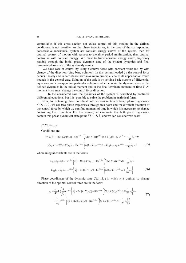
Phase coordinates of the dynamic state ),( CC xxC & in which it is optimal to change direction of the optimal control force are in the form:

)]}(,[2)](,[2{~41)(

21

020

2

00 xFkxFkxx

uxxx TTTC GG −+−+= &&m

)(~2)](,[2)](,[2 02

TCTCTC xxuxFkxFkxx −+−±= m&& GG (33)

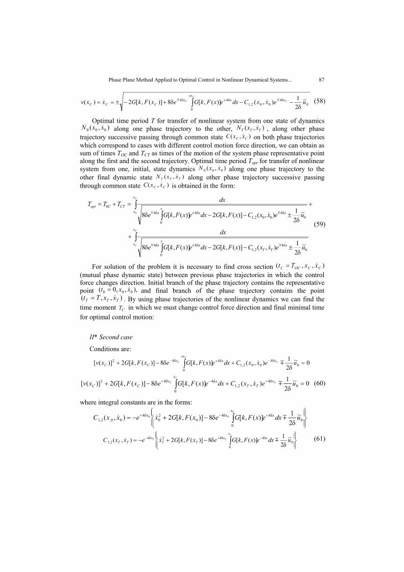
Optimal time period T for transfer nonlinear system from one state dynamics ),( 00 xxC & along one phase trajectory to the other ),( TT xxC & along other phase trajectory

successive passing through common state ),( CC xxC & on the both phase trajectories which correspond to cases with different control motion force direction, we can obtain as sum of the times TOC and TCT as times of the motion of the system phase representative point along one first and second trajectory.

∫−+−±

==−=Cx

xCCC

xxuxFkxFkx

dxtttT0 )(2)](,[2)](,[2 000

20

00m& GG

(34)

∫−±+−±

=−=T

C

x

x TTT

CTCTxxuxFkxFkx

dxtfT)(2)](,[2)](,[2 0

2 GG& (35)

Optimal time period Topt for transfer nonlinear system from one state dynamics ),( 000 xxN & along one phase trajectory to the other ),( TTT xxN & along other phase trajectory

successive passing through common state ),( CC xxC & is

∫

∫

−±+−+

+−+−

=

=+=

T

C

C

x

x TTT

x

x

CTCopt

xxuxFkxFkx

dx

xxuxFkxFkx

dx

TTT

)(2)](,[2)](,[2

)(2)](,[2)](,[2

02

00020

0

0

GG

GG

&

m&

(36)

c3 x( ) 0.8 x 0+( )⋅

3 cos 2 0⋅( ) cos 2 x⋅( )−( )⋅ cos 0( ) cos x( )−( )−[ ]2

+:=Lambda

34

:=

c4 x( ) 0.8 x 0+( )⋅3 cos 2 0⋅( ) cos 2 x⋅( )−( )⋅ cos 0( ) cos x( )−( )−[ ]

2+−:=

ca3 x( ) 0.8− x 2.58−( )⋅3 cos 2 2.58⋅( ) cos 2 x⋅( )−( )⋅ cos 2.58( ) cos x( )−( )−[ ]

2+:=

Lambda34

:=

ca4 x( ) 0.8− x 2.58−( )⋅3 cos 2 2.58⋅( ) cos 2 x⋅( )−( )⋅ cos 2.58( ) cos x( )−( )−[ ]

2+−:=


a*

20 15 10 5 0 5 10 15 20

2

1

1

2

3

44

2−

f x( )

f1 x( )

f2 x( )

2020− x

ϕ

PE

b*

4 3 2 1 0 1 2 3 4

4

3

2

1

1

2

3

44

4−

c3 x( )

c4 x( )

ca3 x( )

ca4 x( )

44− x

ϕ&

ϕ

( )TTT xxTt &,,=

( )CCCC xxTt &,,= ( )000 ,,0 xxt &=

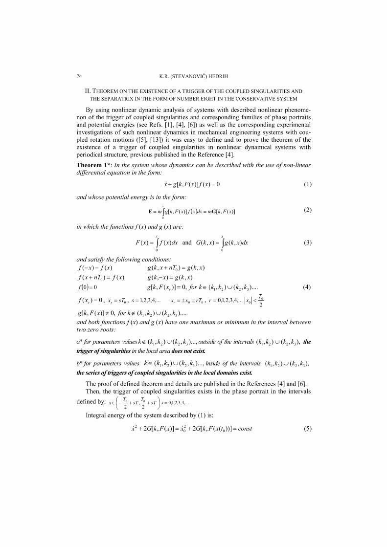
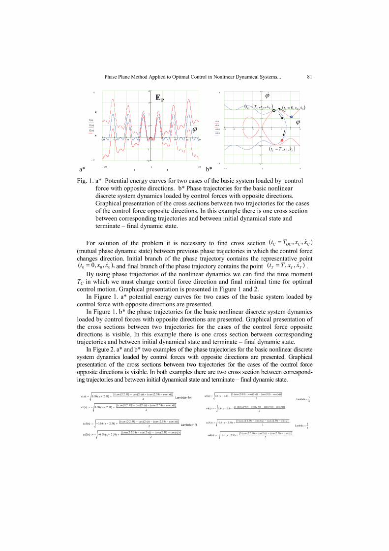
Fig. 1. a* Potential energy curves for two cases of the basic system loaded by control force with opposite directions. b* Phase trajectories for the basic nonlinear discrete system dynamics loaded by control forces with opposite directions. Graphical presentation of the cross sections between two trajectories for the cases of the control force opposite directions. In this example there is one cross section between corresponding trajectories and between initial dynamical state and terminate – final dynamic state.

For solution of the problem it is necessary to find cross section ),,( CCOCC xxTt &= (mutual phase dynamic state) between previous phase trajectories in which the control force changes direction. Initial branch of the phase trajectory contains the representative point

),,,0( 000 xxt &= and final branch of the phase trajectory contains the point ),,( TTT xxTt &= . By using phase trajectories of the nonlinear dynamics we can find the time moment

TC in which we must change control force direction and final minimal time for optimal control motion. Graphical presentation is presented in Figure 1 and 2.

In Figure 1. a* potential energy curves for two cases of the basic system loaded by control force with opposite directions are presented.

In Figure 1. b* the phase trajectories for the basic nonlinear discrete system dynamics loaded by control forces with opposite directions are presented. Graphical presentation of the cross sections between two trajectories for the cases of the control force opposite directions is visible. In this example there is one cross section between corresponding trajectories and between initial dynamical state and terminate – final dynamic state.

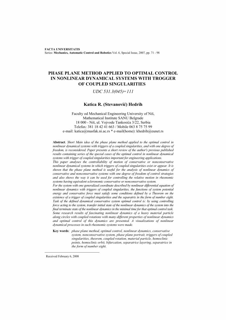
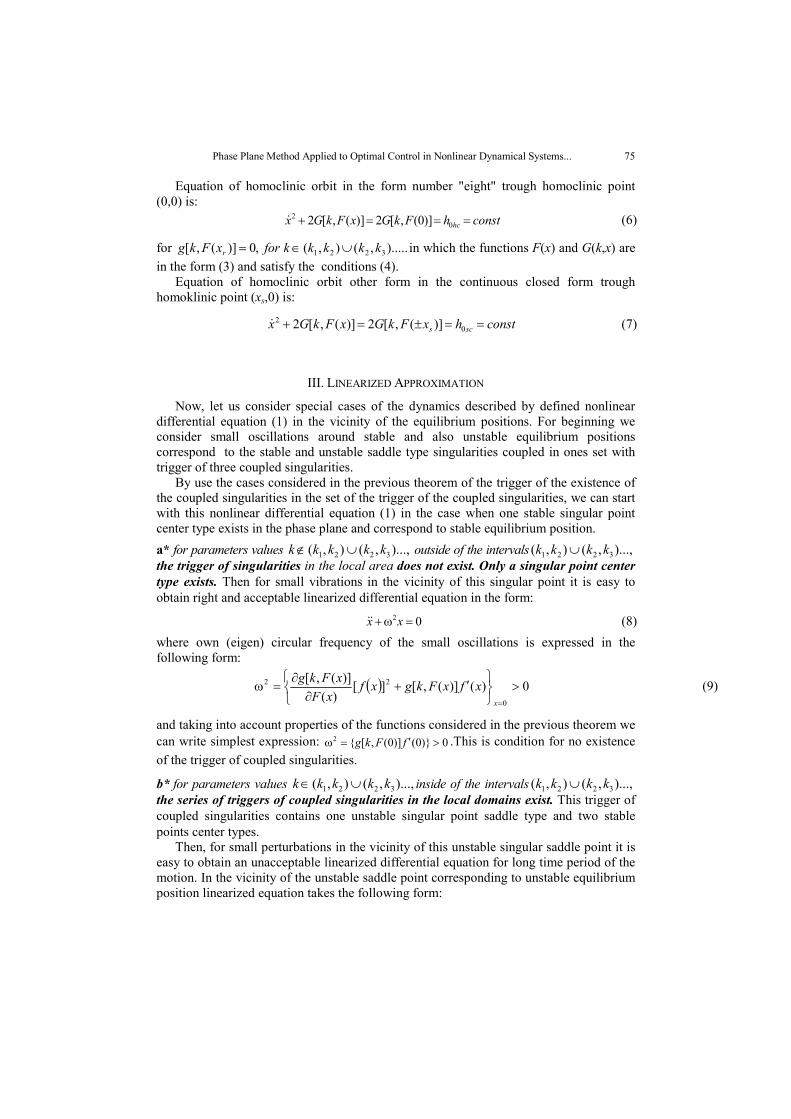
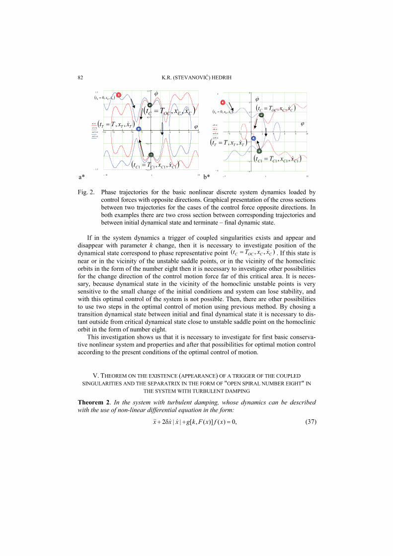
In Figure 2. a* and b* two examples of the phase trajectories for the basic nonlinear discrete system dynamics loaded by control forces with opposite directions are presented. Graphical presentation of the cross sections between two trajectories for the cases of the control force opposite directions is visible. In both examples there are two cross section between correspond-ing trajectories and between initial dynamical state and terminate – final dynamic state.

a x( ) 0.08 x 2.58+( )⋅

cos 2 2.58⋅( ) cos 2 x⋅( )−( ) cos 2.58( ) cos x( )−( )−[ ]2

+:= Lambda=1/4

a1 x( ) 0.08 x 2.58+( )⋅cos 2 2.58⋅( ) cos 2 x⋅( )−( ) cos 2.58( ) cos x( )−( )−[ ]

2+−:=

aa1 x( ) 0.08− x 2.58−( )⋅cos 2 2.58⋅( ) cos 2 x⋅( )−( ) cos 2.58( ) cos x( )−( )−[ ]

2+:= Lambda=1/4

aa2 x( ) 0.08− x 2.58−( )⋅cos 2 2.58⋅( ) cos 2 x⋅( )−( ) cos 2.58( ) cos x( )−( )−[ ]

2+−:=

a3 x( ) 0.8 x 0.8+( )⋅3 cos 2 0.8⋅( ) cos 2 x⋅( )−( )⋅ cos 0.8( ) cos x( )−( )−[ ]

2+:=

Lambda34

:=

a4 x( ) 0.8 x 0.8+( )⋅3 cos 2 0.8⋅( ) cos 2 x⋅( )−( )⋅ cos 0.8( ) cos x( )−( )−[ ]

2+−:=

aa3 x( ) 0.8− x 2.58−( )⋅3 cos 2 2.58⋅( ) cos 2 x⋅( )−( )⋅ cos 2.58( ) cos x( )−( )−[ ]

2+:=

Lambda34

:=

aa4 x( ) 0.8− x 2.58−( )⋅3 cos 2 2.58⋅( ) cos 2 x⋅( )−( )⋅ cos 2.58( ) cos x( )−( )−[ ]

2+−:=


a*

10 8 6 4 2 0 2 4 6 8 10

1.5

1

0.5

0.5

1

1.51.5

1.5−

a x( )

a1 x( )

aa1 x( )

aa2 x( )

1010− x

( )TTT xxTt &,,=

( )000 ,,0 xxt &=

( )1111 ,, CCCC xxTt &=

( )CCOCC xxTt &,,=

ϕ

ϕ&

b*

4 2 0 2 4 6 8 10

4

3

2

1

1

2

3

44

4−

a3 x( )

a4 x( )

aa3 x( )

aa4 x( )

105− x

( )000 ,,0 xxt &=

( )TTT xxTt &,,=

ϕ&

ϕ

( )CCOCC xxTt &,,=

( )1111 ,, CCCC xxTt &=

Fig. 2. Phase trajectories for the basic nonlinear discrete system dynamics loaded by control forces with opposite directions. Graphical presentation of the cross sections between two trajectories for the cases of the control force opposite directions. In both examples there are two cross section between corresponding trajectories and between initial dynamical state and terminate – final dynamic state.

If in the system dynamics a trigger of coupled singularities exists and appear and

disappear with parameter k change, then it is necessary to investigate position of the dynamical state correspond to phase representative point ),,( CCOCC xxTt &= . If this state is near or in the vicinity of the unstable saddle points, or in the vicinity of the homoclinic orbits in the form of the number eight then it is necessary to investigate other possibilities for the change direction of the control motion force far of this critical area. It is neces-sary, because dynamical state in the vicinity of the homoclinic unstable points is very sensitive to the small change of the initial conditions and system can lose stability, and with this optimal control of the system is not possible. Then, there are other possibilities to use two steps in the optimal control of motion using previous method. By chosing a transition dynamical state between initial and final dynamical state it is necessary to dis-tant outside from critical dynamical state close to unstable saddle point on the homoclinic orbit in the form of number eight.

This investigation shows us that it is necessary to investigate for first basic conserva-tive nonlinear system and properties and after that possibilities for optimal motion control according to the present conditions of the optimal control of motion.

V. THEOREM ON THE EXISTENCE (APPEARANCE) OF A TRIGGER OF THE COUPLED SINGULARITIES AND THE SEPARATRIX IN THE FORM OF "OPEN SPIRAL NUMBER EIGHT" IN

THE SYSTEM WITH TURBULENT DAMPING

Theorem 2. In the system with turbulent damping, whose dynamics can be described with the use of non-linear differential equation in the form:

,0)()](,[||2 =+δ+ xfxFkgxxx &&&& (37)


and whose potential energy is in the form (2) in which the functions f (x) and g (x) are in the form (3) and satisfy the conditions (4) and both functions f (x) and g (x) have one maximum or minimum in the interval between two zero roots: a* for parameters values )...,,(),( 3221 kkkkk ∪∉ outside of the intervals (k1,k2) ∪ (k2,k3)..., the trigger of coupled singularities in the local area does not exist. b* for parameters values )...,,(),( 3221 kkkkk ∪∈ inside of the intervals (k1,k2) ∪ (k2,k3)..., the series of triggers of coupled singularities in the local domains exist, as well as corresponding homoclinic orbit - the separatrix in the form of "open spiral number eight".

The proof of defined theorem 2 and details are published in the References [4] and [6].

For the system with turbulent damping [23], whose dynamics can be described with the use of non-linear differential equation in the form (37), we can solve phase trajectories by integrating previous equation by introducing following notation: vx =& :

)()](,[24 22

xfxFkgvdxdv

−=δ± (38)

and after integration we obtain:

0)](,[8)](,[2 42,1

4

0

42 =+−+ δδ±δ ∫ xxx

x eCdxexFkGexFkGv mm (39)

where integral constant is in the following form:

⎪⎭

⎪⎬⎫

⎪⎩

⎪⎨⎧

−+−= δ±δδ± ∫ dxexFkGetxFkGxeC xx

xx 4

0

40

20

42,1

0

00 )](,[8))]((,[2 m& (40)

depending on initial condition of motions. Equation of homoclinic orbit in the form "open spiral number eight" trough homoclinic

point (0,0) is:

0)]0(,[2)](,[8)](,[2 44

0

42 =−−+ δδ±δ ∫ xxx

x eFkGdxexFkGexFkGv mm (41)

where constant of integration is:

)}0(,[2{2,1 FkGC −= for )....,(),(,0)](,[ 3221 kkkkkforxFkg r ∪∈= (42)

Equation of homoclinic orbit other form in the continuous closed form trough homoklinic point )0,( sx is:

0)](,[8)](,[2 42,1

4

0

42 =+−+ δδ±δ ∫ xxx

x eCdxexFkGexFkGv mm (43)

where is:

⎪⎭

⎪⎬⎫

⎪⎩

⎪⎨⎧

−−= δ±δδ± ∫ dxexFkGexFkGeC xx

xs

xs

ss 4

0

442,1 )](,[8)](,[2 m (44)


VI. OPTIMAL CONTROL OF NONLINEAR DYNAMICS IN THE NO CONSERVATIVE SYSTEM

For optimal control of the nonlinear dynamics of this considered no conservative system defined by nonlinear differential equation (37), we can introduce two phase coordinate in the space dynamic state x1 and x2, and by the differential equation second order, we can introduce two nonlinear differential equations first order in the following form (for details see Ref. [15]): 21 xx =& )()](,[||2 11222 xfxFkgxxx −δ−=& (45)

with initial conditions x1(0) = α and x2(0) = β. Task of the defined dynamical system optimal control is: By using controlling force )(~ tu acting to the system, transfer initial state of the nonlinear dynamics of the system

defined by x1(0) = α and x2(0) = β into the final state of the nonlinear dynamics defined by x1(T) = γ and x2(T) = χ, where T is minimal time for that optimal control task. Than we can write two new nonlinear differential equations first order for optimal control task in the following form: 21 xx =& )(~)()](,[||2 11222 tuxfxFkgxxx ±−δ−=& (46)

with initial conditions state in the form (16) and with final conditions in the form (17), where T is time necessary for this motion.

Pontrijagin's maximum principle (see Ref. [15]) is used. For minimization of the time T to the previous system dynamics defined by nonlinear differential equations (37) we add to these equations the following functional in the form (18)as a criterion of the optimality – time minimization, or "criterion of quality" of the moticontrol, with addition in the form of the controlling force )(~ tu constraints in the form (19): 00

~)(~~ utuu +≤≤− . It is possible to write the criterion of the optimal control of dynamics in the previous

used formulation (20):

∫ ±−δ−−−=T

dttuxfxFkgxxtpxtpupp,xx0

1122212121 )}(~)()](,[||2){()(]~,,,[~ HI (47)

This previous functional (47) is for the case with unspecific interval of time. As the one of the boundary of time interval is in the integral of functional, then it is necessary to take into account noisochroous variations of the functional.

On this basic we can to write:

0

][][~

0

2

1

2

1

0221102211

=⎥⎥⎦

⎤

⎢⎢⎣

⎡δ

∂Η∂

+δ⎟⎟⎠

⎞⎜⎜⎝

⎛−

∂Η∂

+δ⎟⎟⎠

⎞⎜⎜⎝

⎛+

∂Η∂

+

+Δ−−Η+δ−δ−=Δ

∫ ∑∑=

=

=

=

T i

iii

i

i

iii

i

TT

dtuu

pxp

xpx

txpxpxpxp

&&

&&I

(48)

In this case optimal control dynamics is defined by solving the corresponding system of differential equations with corresponding additional conditions of the optimal control of motion as in previous considered case defined by system (22).


By using theory from Ref. [25] and [15], as well as previous obtained conditions (22) of the optimal control of motions, we can write the following Hamilton functional in the form:

{ })(~)()](,[||2)()(1]~,,,[ 11222212121 tuxfxFkgxxtpxtpupp,xx ±−δ−++=H (49)

Second pair of the canonical differential equations from system of equations (22) is:

⎭⎬⎫

⎩⎨⎧

′+∂

∂=

∂∂

−= )()](,[)]([)(

)](,[)()( 112

11

12

11 xfxFkgxf

xFxFkgtp

xtp H

&

)(2)()( 2212

2 tpxtpx

tp δ±−=∂∂

−=H

& (50)

and

)(2)()(

0)(~

2212

2

tpxtptp

tpu

δ±−=

==∂∂

&

mH

00 )( utuu ≤≤−

{ } 0~)()](,[||2)()(1

]~,,,[

1122221

2121

=±−δ−++=

=

=

=

Tt

Tt

uxfxFkgxxtpxtp

upp,xxH (51)

0)}(~))(())]((,[)()(2){(

)()(1]~,,,[

11222

212121

=±−δ−+

++==

TuTxfTxFkgTxTxTp

TxTpupp,xxTt

H

For the system with turbulent damping loaded by control force, whose dynamics can be described with the use system of non-linear differential equations in the form (46), equations of the phase trajectories by integrating previous system of differential equations by introducing following notation: vx =& . Then, we obtain:

02

2~2)()](,[24 uxfxFkgv

dxdv

±−=δ± (52)

and after integration we obtain the following equations of the phase trajectories:

( ) ( ) 0~21],[8],[2 0

42,1

4

0

42 =δ

+δ−+ δδ±δ ∫ ueCdxexFkGexFkGv xxx

x mmm (53)

where constant of integration is:

⎪⎭

⎪⎬⎫

⎪⎩

⎪⎨⎧

δδ−+−= δ±δδ± ∫ 0

4

0

40

20

42,1

~21)](,[8))]((,[2

0

00 udxexFkGetxFkGxeC xx

xx m& m (54)

depending on initial condition of motions. Previous defined trajectories must be with last one common point – cross section

representative point ),(1 CC xxN & in the phase plane of dynamical state as a cross section of the previous trajectories. First through the initial condition point x1(0) = α and x2(0) = β, and second through final condition point x1(T) = γ and x2(T) = χ correspond to the final dynamic state of the system and for the force with alternative directions. If this cross section is real, defined optimal control of the motion is possible and system is


controllable, if this cross section not exists control of this motion, in the defined conditions, is not possible. As the phase trajectories, in the case of the corresponding conservative mechanical system are constant energy curves of the system, then for optimal control of motion with respect to the time period minimization, then optimal control is with constant energy. We must to fined constant energy curve, trajectory passing through the initial phase dynamic state of the system dynamics and final terminate phase state of the system dynamics.

We have case of control by using a control force with constant value but by with change of the direction (bing-bang solution). In this system loaded by the control force occurs linearly and in accordance with maximum principle, attains its upper and/or lowed bounds in the general case. Solution of the task is by solving basic system of differential equations and corresponding particular solutions which contain the dynamic state of the defined dynamics in the initial moment and in the final terminate moment of time T. At moment tC we must change the control force direction.

In the considered case the dynamics of the system is described by nonlinear differential equations, but it is possible to solve the problem in analytical form.

Now, for obtaining phase coordinate of the cross section between phase trajectories ),( CC xxC & , we use two phase trajectories through this point and for different direction of

the control force by which we can find moment of time in which it is necessary to change controlling force direction. For that reason, we can write that both phase trajectories contain this phase dynamical state point ),( CC xxC & , and we can consider two cases.

I* First case

Conditions are:

0~21),()](,[8)](,[2)]([ 0

4002,1

4

0

42 =δ

++δ−+ δδ±δ ∫ uexxCdxexFkGexFkGxv C

C

C xxxx

xCC

mm &

0~21),()](,[8)](,[2)]([ 0

42,1

4

0

42 =δ

−+δ−+ δδ±δ ∫ uexxCdxexFkGexFkGxv C

C

C xTT

xx

xCC

mm & (55)

where integral constants are in the forms:

⎪⎭

⎪⎬⎫

⎪⎩

⎪⎨⎧

δδ−+−= δ±δδ± ∫ 0

4

0

40

20

400,2,1

~21)](,[8)](,[2),(

0

00 udxexFkGexFkGxexxC xx

xx m&& m

⎪⎭

⎪⎬⎫

⎪⎩

⎪⎨⎧

δ−+−= δ±δδ± ∫ 0

4

0

4242,1

~21)](,[8)](,[2),( udxexFkGexFkGxexxC x

xx

TTx

TT

T

TT m&& m (56)

Phase coordinates of the dynamic state ),( CC xxC & in which it is optimal to change direction of the optimal control force are in the form:

⎪⎭

⎪⎬⎫

⎪⎩

⎪⎨⎧

δδ−+

δ−

−⎪⎭

⎪⎬⎫

⎪⎩

⎪⎨⎧

δδ−+

δδ

±=

δ±δδ±

δ±δδ±

∫

∫

04

0

424

0

04

0

40

20

4

0

~21)](,[8)](,[2~

~21)](,[8)](,[2~ln

41 0

00

udxexFkGexFkGxeu

udxexFkGexFkGxeu

x

xx

xTT

x

xx

xxC

T

TT m&

m&

m

m

(57)


04

002,14

0

4 ~21),()](,[8)](,[2)( uexxCdxexFkGexFkGxxv C

C

C xxxx

xCCC δ

−−δ+−±== δδ±δ ∫ mm && (58)

Optimal time period T for transfer of nonlinear system from one state of dynamics ),( 000 xxN & along one phase trajectory to the other, ),( TTT xxN & , along other phase

trajectory successive passing through common state ),( CC xxC & on both phase trajectories which correspond to cases with different control motion force direction, we can obtain as sum of times TOC and TCT as times of the motion of the system phase representative point along the first and the second trajectory. Optimal time period Topt for transfer of nonlinear system from one, initial, state dynamics ),( 000 xxN & along one phase trajectory to the other final dynamic state ),( TTT xxN & along other phase trajectory successive passing through common state ),( CC xxC & is obtained in the form:

∫∫

∫∫

δ±−−δ

+

+

δ±−−δ

=+=

δδ±δ

δδ±δ

T

C

C

x

x xTT

xx

x

x

x xxx

xCTCopt

uexxCxFkGdxexFkGe

dx

uexxCxFkGdxexFkGe

dxTTT

04

2,14

0

4

04

002,14

0

40

~21),()](,[2)](,[8

~21),()](,[2)](,[80

mm

mm

&

&

(59)

For solution of the problem it is necessary to find cross section ),,( CCOCC xxTt &= (mutual phase dynamic state) between previous phase trajectories in which the control force changes direction. Initial branch of the phase trajectory contains the representative point ),,,0( 000 xxt &= and final branch of the phase trajectory contains the point

),,( TTT xxTt &= . By using phase trajectories of the nonlinear dynamics we can find the time moment CT in which we must change control force direction and final minimal time for optimal control motion:

II* Second case

Conditions are:

0~21),()](,[8)](,[2)]([ 0

4002,1

4

0

42 =δ

+δ−+ δ−δ+δ− ∫ uexxCdxexFkGexFkGxv C

C

C xxxx

xCC m&

0~21),()](,[8)](,[2)]([ 0

42,1

4

0

42 =δ

+δ−+ δ+δ−δ+ ∫ uexxCdxexFkGexFkGxv C

C

C xTT

xx

xCC m& (60)

where integral constants are in the forms:

⎪⎭

⎪⎬⎫

⎪⎩

⎪⎨⎧

δδ−+−= δ+δ−δ+ ∫ 0

4

0

40

20

400,2,1

~21)](,[8)](,[2),(

0

00 udxexFkGexFkGxexxC xx

xx m&&

⎪⎭

⎪⎬⎫

⎪⎩

⎪⎨⎧

δδ−+−= δ−δ+δ− ∫ 0

4

0

4242,1

~21)](,[8)](,[2),( udxexFkGexFkGxexxC x

xx

TTx

TT

T

TT m&& (61)


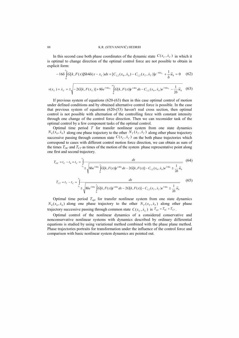
In this second case both phase coordinates of the dynamic state ),( CC xxC & in which it is optimal to change direction of the optimal control force are not possible to obtain in explicit form:

0~1)],(),([)(4)](,[16 04

2,1002,10

=δ

+−+−δδ− δ−∫ uexxCxxCdxxxShxFkG C

Cx

TTC

x

&& (62)

0

4002,1

4

0

4 ~21),()](,[8)](,[2)( uexxCdxexFkGexFkGxxv C

C

C xxxx

xCCC δ

−−δ+−±== δδ±δ ∫ mm && (63)

If previous system of equations (620-(63) then in this case optimal control of motion under defined conditions and by obtained alternative control force is possible. In the case that previous system of equations (620-(53) haven't real cross section, then optimal control is not possible with alternation of the controlling force with constant intensity through one change of the control force direction. Then we can reconsider task of the optimal control by a few component tasks of the optimal control.

Optimal time period T for transfer nonlinear system from one state dynamics ),( 000 xxN & along one phase trajectory to the other ),( TTT xxN & along other phase trajectory

successive passing through common state ),( CC xxC & on the both phase trajectories which correspond to cases with different control motion force direction, we can obtain as sum of the times TOC and TCT as times of the motion of the system phase representative point along one first and second trajectory.

∫∫ δ

±−−δ±

==−=δδ±δ

Cx

x xxx

x

CCOC

uexxCxFkGdxexFkGe

dxtttT0

04

002,14

0

4

0

~21),()](,[2)](,[8 mm &

(64)

∫∫ δ

±−−δ±

=−=δδ±δ

T

C

x

x xTT

xx

x

CTCT

uexxCxFkGdxexFkGe

dxttT

04

2,14

0

4 ~21),()](,[2)](,[8 mm &

(65)

Optimal time period Topt for transfer nonlinear system from one state dynamics ),( 000 xxN & along one phase trajectory to the other ),( TTT xxN & along other phase

trajectory successive passing through common state ),( CC xxC & is CTCopt TTT += 0 . Optimal control of the nonlinear dynamics of a considered conservative and

nonconservative nonlinear systems with dynamics described by ordinary differential equations is studied by using variational method combined with the phase plane method. Phase trajectories portraits for transformation under the influence of the control force and comparison with basic nonlinear system dynamics are pointed out.


VII. NONLINEAR DYNAMICS OF A HEAVY MATERIAL PARTICLE ALONG CIRCLE WHICH ROTATES AND OPTIMAL CONTROL

VII.1. Motion of the heavy material particle along circles

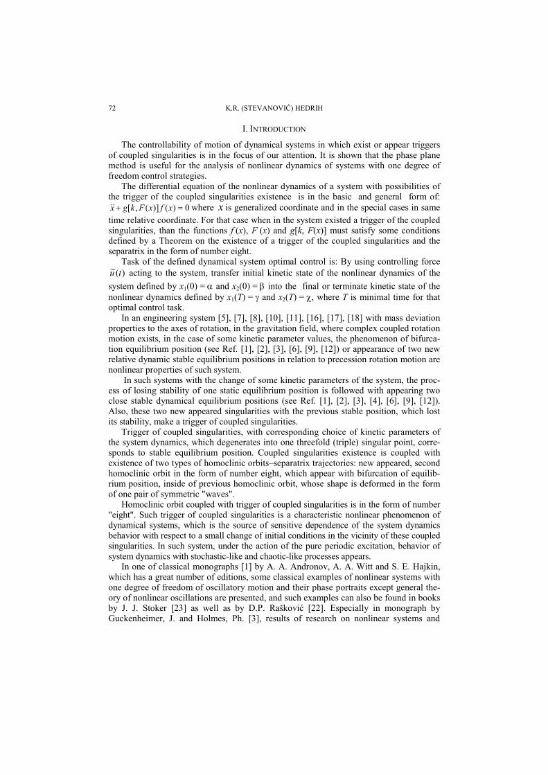
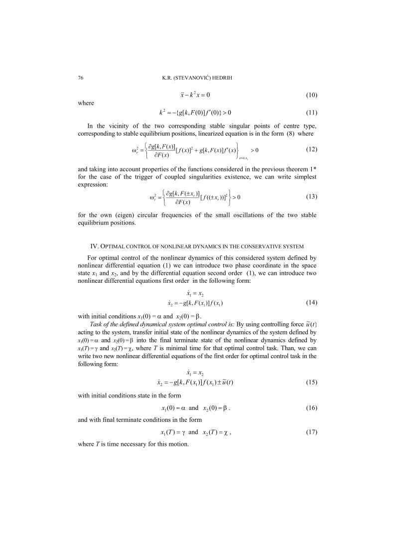
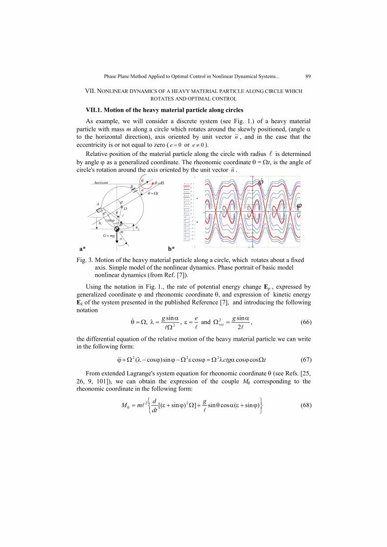
As example, we will consider a discrete system (see Fig. 1.) of a heavy material particle with mass m along a circle which rotates around the skewly positioned, (angle α to the horizontal direction), axis oriented by unit vector n

r , and in the case that the eccentricity is or not equal to zero ( 0=e or 0≠e ).

Relative position of the material particle along the circle with radius l is determined by angle ϕ as a generalized coordinate. The rheonomic coordinate θ = Ωt, is the angle of circle's rotation around the axis oriented by the unit vector n

r .

a*

rhph

lϕsinl

ϕ

α

α

θ

A

B

O

nrhorizont

mgG =m

tΩ=θ

Ω=θ&

e

e

b*

12 8 4 0 4 8 12

2

1.2

0.4

0.4

1.2

22

2−

f1 x e1,( )

f2 x e1,( )

f3 x e1,( )

f4 x e1,( )

f5 x e1,( )

f6 x e1,( )

f7 x e1,( )

f8 x e1,( )

f9 x e1,( )

f10 x e1,( )

f11 x e1,( )

f12 x e1,( )

f13 x e1,( )

f14 x e1,( )

f15 x e1,( )

f16 x e1,( )

ϕ&

ϕ

Fig. 3. Motion of the heavy material particle along a circle, which rotates about a fixed axis. Simple model of the nonlinear dynamics. Phase portrait of basic model nonlinear dynamics (from Ref. [7]).

Using the notation in Fig. 1., the rate of potential energy change Ep , expressed by generalized coordinate ϕ and rheonomic coordinate θ, and expression of kinetic energy Ek of the system presented in the published Reference [7], and introducing the following notation

,2sin and ,sin , 2

2 lll& α

=Ω=εΩ

α=λΩ=θ

gegrez (66)

the differential equation of the relative motion of the heavy material particle we can write in the following form:

tctg ΩϕαλΩ=ϕεΩ−ϕϕ−λΩ+ϕ coscoscossin)cos( 222&& (67)

From extended Lagrange's system equation for rheonomic coordinate θ (see Refs. [25, 26, 9, 101]), we can obtain the expression of the couple Mθ corresponding to the rheonomic coordinate in the following form:

⎭⎬⎫

⎩⎨⎧ ϕ+εαθ+Ωϕ+ε=θ )sin(cossin])sin[( 22

ll

gdtdmM (68)


VII.2. Linearized Approximation

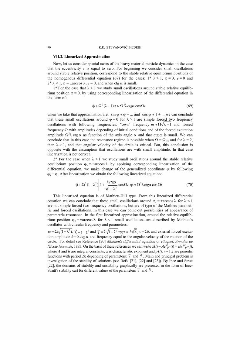
Now, let us consider special cases of the heavy material particle dynamics in the case that the eccentricity e is equal to zero. For beginning we consider small oscillations around stable relative position, correspond to the stable relative equilibrium positions of the homogenous differential equation (67) for the cases: 1* λ > 1, ϕ = 0, e = 0 and 2* λ < 1, ϕ = ±arccos λ, e = 0, and when ctg α is small.

1* For the case that λ > 1 we study small oscillations around stable relative equilib-rium position ϕ = 0, by using corresponding linearization of the differential equation in the form of:

tctg ΩαλΩ≈ϕ−λΩ+ϕ cos)1( 22&& (69)

when we take that approximation are: sin ϕ ≈ ϕ + ... and cos ϕ ≈ 1 + ... we can conclude that these small oscillations around ϕ = 0 for λ > 1 are simple forced two frequency oscillations with following frequencies: "own" frequency 1−λΩ≈ω and forced frequency Ω with amplitudes depending of initial conditions and of the forced excitation amplitude Ω2λ ctg α as function of the axis angle α and that ctg α is small. We can conclude that in this case the resonance regime is possible when Ω = Ωrez and for λ = 2, then λ > 1, and that angular velocity of the circle is critical. But, this conclusion is opposite with the assumption that oscillations are with small amplitude. In that case linearization is not correct.

2* For the case when λ < 1 we study small oscillations around the stable relative equilibrium position ϕs = ±arccos λ by applying corresponding linearization of the differential equation, we make change of the generalized coordinate ϕ by following ϕs + ϕ. After linearization we obtain the following linearized equation:

tctgtctg

ΩαλΩ≈ϕ⎥⎥⎦

⎤

⎢⎢⎣

⎡Ω

λ−

αλ+λ−Ω+ϕ coscos

11)1( 2

2

22&& (70)

This linearized equation is of Mathieu-Hill type. From this linearized differential equation we can conclude that these small oscillations around ϕs = ±arccos λ for λ < 1 are not simple forced two frequency oscillations, but are of type of the Mathieu paramet-ric and forced oscillations. In this case we can point out possibilities of appearance of parametric resonance. In the first linearized approximation, around the relative equilib-rium position ϕs = ±arccos λ for λ < 1 small oscillations are described by Mathieu's oscillator

with circular frequency and parameters:

,)1( 2λ−Ω=ω 21~λ−=λ and ,~1~ 2 λ=αλ−λ=γ hctg τ = Ωt, and external forced excita-

tion amplitude h = λ ctg α and frequency equal to the angular velocity of the rotation of the circle. For detail see Reference [20] Mathieu's differential equation or Floquet, Annales de l'Ecole Normale, 1883. On the basis of these references we can write ϕ(t) = Aeμtp1(t) + Be−μtp2(t), where A and B are integral constants; μ is characteristic exponent and pi(t), i = 1,2 are periodic functions with period 2π depending of parameters: λ

~ and γ~ . Main and principal problem is investigation of the stability of solutions (see Refs. [21], [22] and [23]). By Ince and Strutt [22], the domains of stability and unstability graphically are presented in the form of Ince-Strutt's stability cart for different values of the parameters λ

~ and γ~ .


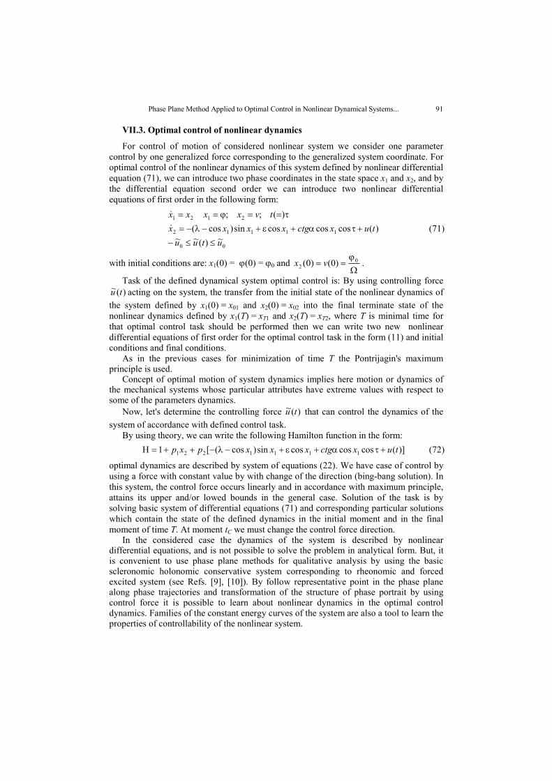
VII.3. Optimal control of nonlinear dynamics

For control of motion of considered nonlinear system we consider one parameter control by one generalized force corresponding to the generalized system coordinate. For optimal control of the nonlinear dynamics of this system defined by nonlinear differential equation (71), we can introduce two phase coordinates in the state space x1 and x2, and by the differential equation second order we can introduce two nonlinear differential equations of first order in the following form:

00

11112

2121

~)(~~)(coscoscossin)cos(

)( ; ;

utuutuxctgxxxx

tvxxxx

≤≤−+τα+ε+−λ−=

τ==ϕ==&

&

(71)

with initial conditions are: x1(0) = ϕ(0) = ϕ0 and Ωϕ

== 02 )0()0( vx .

Task of the defined dynamical system optimal control is: By using controlling force )(~ tu acting on the system, the transfer from the initial state of the nonlinear dynamics of

the system defined by x1(0) = x01 and x2(0) = x02 into the final terminate state of the nonlinear dynamics defined by x1(T) = xT1 and x2(T) = xT2, where T is minimal time for that optimal control task should be performed then we can write two new nonlinear differential equations of first order for the optimal control task in the form (11) and initial conditions and final conditions.

As in the previous cases for minimization of time T the Pontrijagin's maximum principle is used.

Concept of optimal motion of system dynamics implies here motion or dynamics of the mechanical systems whose particular attributes have extreme values with respect to some of the parameters dynamics.

Now, let's determine the controlling force )(~ tu that can control the dynamics of the system of accordance with defined control task.

By using theory, we can write the following Hamilton function in the form: )](coscoscossin)cos([1 1111221 tuxctgxxxpxp +τα+ε+−λ−++=Η (72)

optimal dynamics are described by system of equations (22). We have case of control by using a force with constant value by with change of the direction (bing-bang solution). In this system, the control force occurs linearly and in accordance with maximum principle, attains its upper and/or lowed bounds in the general case. Solution of the task is by solving basic system of differential equations (71) and corresponding particular solutions which contain the state of the defined dynamics in the initial moment and in the final moment of time T. At moment tC we must change the control force direction.

In the considered case the dynamics of the system is described by nonlinear differential equations, and is not possible to solve the problem in analytical form. But, it is convenient to use phase plane methods for qualitative analysis by using the basic scleronomic holonomic conservative system corresponding to rheonomic and forced excited system (see Refs. [9], [10]). By follow representative point in the phase plane along phase trajectories and transformation of the structure of phase portrait by using control force it is possible to learn about nonlinear dynamics in the optimal control dynamics. Families of the constant energy curves of the system are also a tool to learn the properties of controllability of the nonlinear system.


a* c*

10 8 6 4 2 0 2 4 6 8 10

4

2

2

4

6

8

1010

4−

f x( )

l x( )

g x( )

h x( )

m x( )

1010− x

30 20 10 0 10 20 30

4

3

2

1

1

2

3

44

4−

a x( )

a1 x( )

a3 x( )

a4 x( )

a5 x( )

a6 x( )

a7 x( )

a8 x( )

a9 x( )

a10 x( )

a11 x( )

a12 x( )

a13 x( )

a14 x( )

3030− x

10 8 6 4 2 0 2 4 6 8 10

4

3

2

1

1

2

3

44

4−

a x( )

a1 x( )

a3 x( )

a4 x( )

a5 x( )

a6 x( )

a7 x( )

a8 x( )

a9 x( )

a10 x( )

a11 x( )

a12 x( )

a13 x( )

a14 x( )

1010− x 3 2 1 0 1 2 3

10

5

0

5

108.736

7.427−

S2 2⟨ ⟩( )i

2.7022.449− S2 1⟨ ⟩( )i

PE

ϕ

ϕ

ϕ

ϕ&

ϕ&

ϕ&

ϕ

b* d*

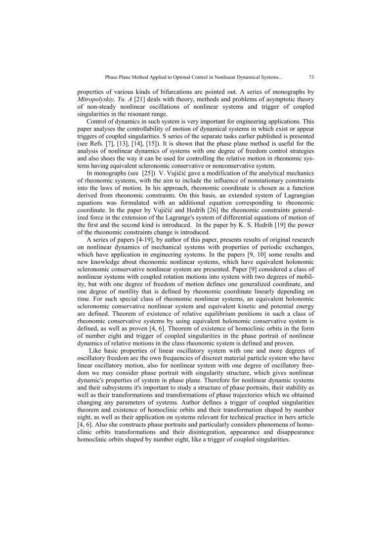
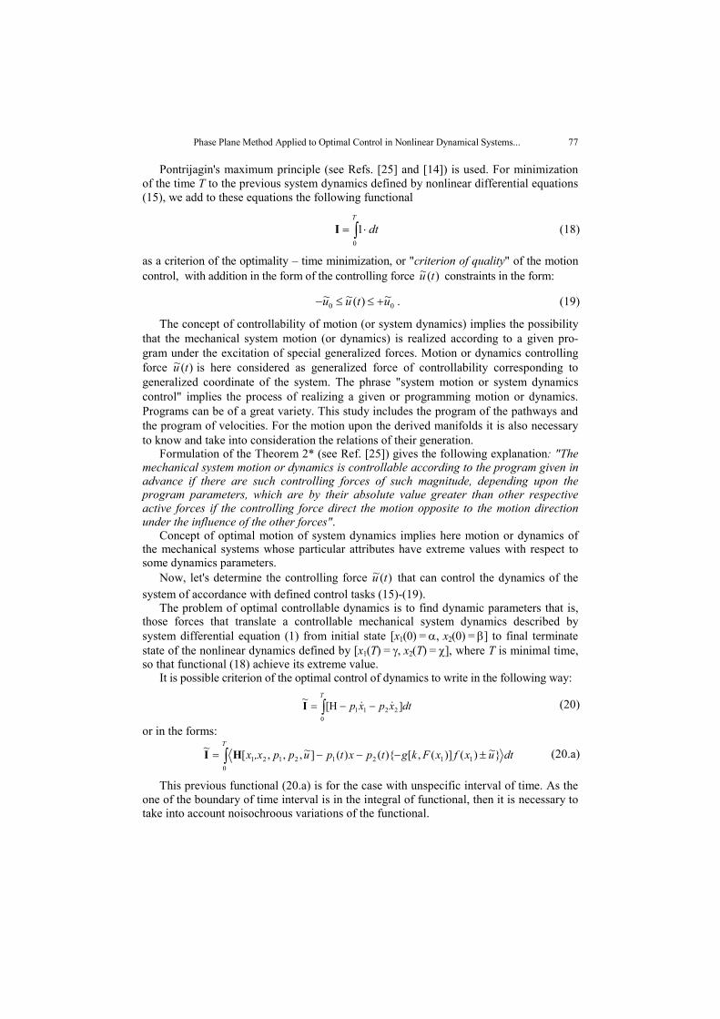
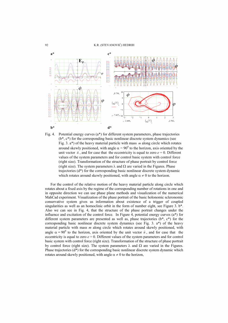
Fig. 4. Potential energy curves (a*) for different system parameters, phase trajectories (b*, c*) for the corresponding basic nonlinear discrete system dynamics (see Fig. 3. a*) of the heavy material particle with mass m along circle which rotates around skewly positioned, with angle α = 900 to the horizon, axis oriented by the unit vector n

r , and for case that the eccentricity is equal to zero e = 0. Different values of the system parameters and for control basic system with control force (right size). Transformation of the structure of phase portrait by control force (right size). The system parameters λ and Ω are varied in the Figures. Phase trajectories (d*) for the corresponding basic nonlinear discrete system dynamic which rotates around skewly positioned, with angle α ≠ 0 to the horizon.

For the control of the relative motion of the heavy material particle along circle which rotates about a fixed axis by the regime of the corresponding number of rotations in one and in opposite direction we can use phase plane methods and visualization of the numerical MahCad experiment. Visualization of the phase portrait of the basic holonomic scleronomic conservative system gives us information about existence of a trigger of coupled singularities as well as an homoclinic orbit in the form of number eight, see Figure 3. b*. Also we can see in Fig. 4, that the structure of the phase portrait changes under the influence and excitation of the control force. In Figure 4, potential energy curves (a*) for different system parameters are presented as well as, phase trajectories (b*, c*) for the corresponding basic nonlinear discrete system dynamics (see Fig. 3. a*) of the heavy material particle with mass m along circle which rotates around skewly positioned, with angle α = 900 to the horizon, axis oriented by the unit vector n

r , and for case that the eccentricity is equal to zero e = 0. Different values of the system parameters and for control basic system with control force (right size). Transformation of the structure of phase portrait by control force (right size). The system parameters λ and Ω are varied in the Figures. Phase trajectories (d*) for the corresponding basic nonlinear discrete system dynamic which rotates around skewly positioned, with angle α ≠ 0 to the horizon,


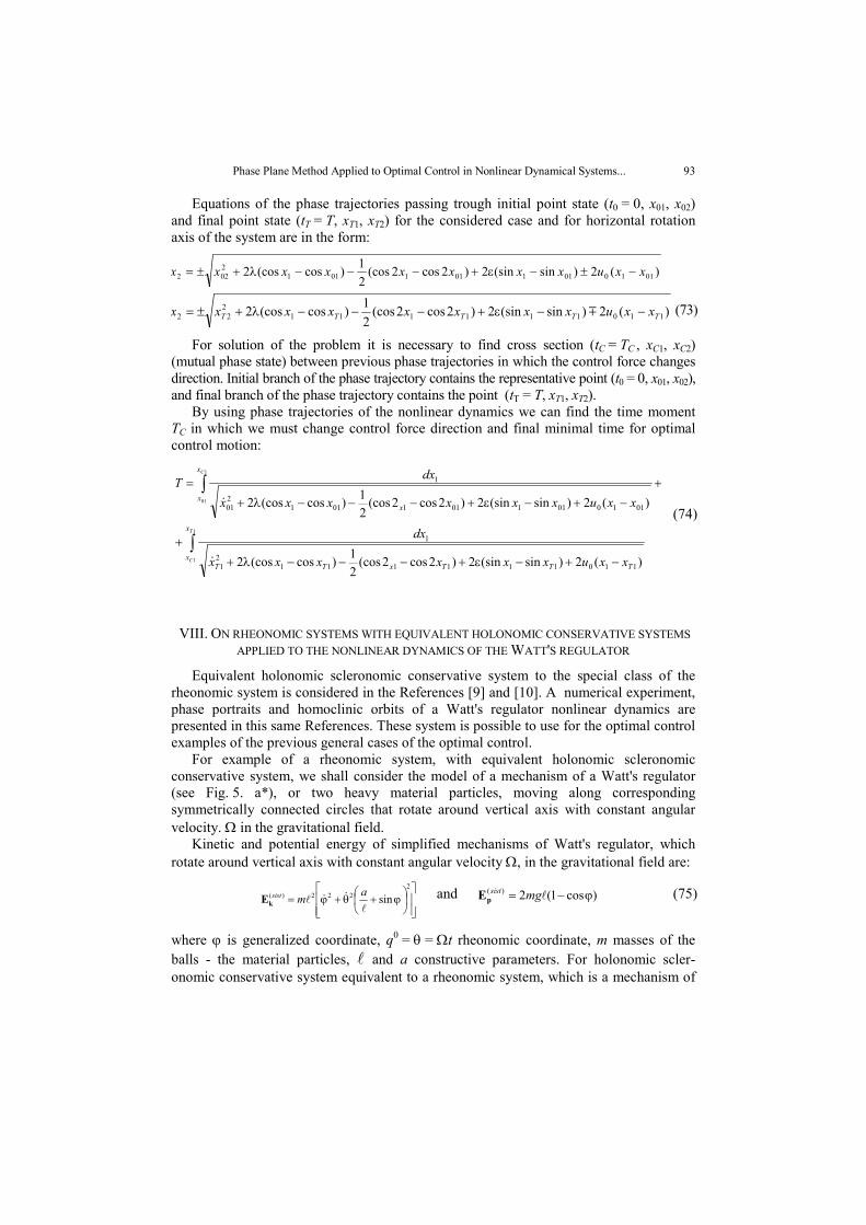
Equations of the phase trajectories passing trough initial point state (t0 = 0, x01, x02) and final point state (tT = T, xT1, xT2) for the considered case and for horizontal rotation axis of the system are in the form:

)(2)sin(sin2)2cos2(cos21)cos(cos2 0110011011011

2022 xxuxxxxxxxx −±−ε+−−−λ+±=

)(2)sin(sin2)2cos2(cos21)cos(cos2 110111111

222 TTTTT xxuxxxxxxxx −−ε+−−−λ+±= m (73)

For solution of the problem it is necessary to find cross section (tC = TC , xC1, xC2) (mutual phase state) between previous phase trajectories in which the control force changes direction. Initial branch of the phase trajectory contains the representative point (t0 = 0, x01, x02), and final branch of the phase trajectory contains the point (tT = T, xT1, xT2).

By using phase trajectories of the nonlinear dynamics we can find the time moment TC in which we must change control force direction and final minimal time for optimal control motion:

∫

∫

−+−ε+−−−λ++

+−+−ε+−−−λ+

=

1

1

1

01

)(2)sin(sin2)2cos2(cos21)cos(cos2

)(2)sin(sin2)2cos2(cos21)cos(cos2

11011111121

1

0110011011011201

1

T

C

C

x

xTTTxTT

x

xx

xxuxxxxxx

dx

xxuxxxxxx

dxT

&

& (74)

VIII. ON RHEONOMIC SYSTEMS WITH EQUIVALENT HOLONOMIC CONSERVATIVE SYSTEMS APPLIED TO THE NONLINEAR DYNAMICS OF THE WATT'S REGULATOR

Equivalent holonomic scleronomic conservative system to the special class of the rheonomic system is considered in the References [9] and [10]. A numerical experiment, phase portraits and homoclinic orbits of a Watt's regulator nonlinear dynamics are presented in this same References. These system is possible to use for the optimal control examples of the previous general cases of the optimal control.

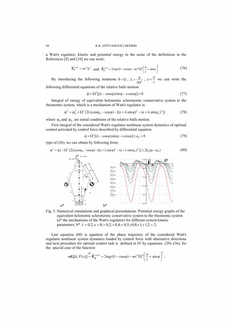
For example of a rheonomic system, with equivalent holonomic scleronomic conservative system, we shall consider the model of a mechanism of a Watt's regulator (see Fig. 5. a*), or two heavy material particles, moving along corresponding symmetrically connected circles that rotate around vertical axis with constant angular velocity. Ω in the gravitational field.

Kinetic and potential energy of simplified mechanisms of Watt's regulator, which rotate around vertical axis with constant angular velocity Ω, in the gravitational field are:

⎥⎥⎦

⎤

⎢⎢⎣

⎡⎟⎠⎞

⎜⎝⎛ ϕ+θ+ϕ=

2222)( sinl

&&lamsist

kE and )cos1(2)( ϕ−= lmgsistpE (75)

where ϕ is generalized coordinate, q0 = θ = Ωt rheonomic coordinate, m masses of the balls - the material particles, l and a constructive parameters. For holonomic scler-onomic conservative system equivalent to a rheonomic system, which is a mechanism of


a Watt's regulator, kinetic and potential energy in the sense of the definitions in the References [9] and [10] we can write:

22)(~ϕ= &lmsist

kE and 2

22)( sin)cos1(2~⎟⎠⎞

⎜⎝⎛ ϕ+Ω−ϕ−=l

llammgsist

pE (76)

By introducing the following notations Ω=θ& , 2Ω

=λl

g , l

a=ε we can write the

following differential equations of the relative balls motion:

0]cossin)cos[(2 =ϕε−ϕϕ−λΩ+ϕ&& (77)

Integral of energy of equivalent holonomic scleronomic conservative system to the rheonomic system, which is a mechanism of Watt's regulator is:

]})sin()sin[()cos(cos2{ 20

20

220

2 ϕλ+ε−ϕλ+ε−ϕ−ϕλΩ+ϕ=ϕ && (78)

where 0ϕ and 0ϕ& are initial conditions of the relative balls motion. First integral of the considered Watt's regulator nonlinear system dynamics of optimal

control activated by control force described by differential equation

0]cossin)cos[( 02 =±ϕε−ϕϕ−λΩ+ϕ u&& (79)

type of (26), we can obtain by following form:

)(~2]})sin()sin[()cos(cos2{ 002

02

022

02 ϕ−ϕ±ϕλ+ε−ϕλ+ε−ϕ−ϕλΩ+ϕ=ϕ u&& (80)

a*

A B

M N

O P

K L

m2

m1 m1 2a

2a

ll 2l/3

m3

m2

ϕ

tΩ=θΩ=θ&

γ

b*

8 6 4 2 0 2 4 6 8

4.5

3.5

2.5

1.5

0.5

0.5

EP1 x( )

EP2 x( )

EP3 x( )

EP4 x( )

EP5 x( )

EP6 x( )

EP7 x( )

EP8 x( )

ϕ pE~

Fig. 5. Numerical simulations and graphical presentations. Potential energy graphs of the

equivalent holonomic scleronomic conservative system to the rheonomic system (a* the mechanisms of the Watt's regulator) for different system kinetic parameters: b* ;2;2,1;1;8,0;5,0;4,0;2,0;0;2,0 +++++++=ε=λ

Last equation (80) is equation of the phase trajectory of the considered Watt's

regulator nonlinear system dynamics loaded by control force with alternative directions and next procedure for optimal control task is defined in IV by equations (29)–(36), for the special case of the function

222)( sin)cos1(2~)](,[ ⎟

⎠⎞

⎜⎝⎛ ϕ+Ω−ϕ−==l

llammgxFkm sist

def

pEG .


IX. CONCLUDING REMARKS

We can conclude that it is very suitable for investigations of nonlinear properties of the motion of the special class of rheonomic systems with rheonomic coordinate linearly dependent of the time in the form q0 = Ωt to use corresponding equivalent holonomic, scleronomic conservative system and corresponding phase portraits of this system for optimal control. By using example of mechanisms of Watt's regulator published in Refer-ences [9] and [10], we show that is possible to apply phase portraits for optimal control in the nonlinear systems with nonlinear motion properties and different forms of homoclinic orbits, as well as the bifurcations of the relative rest positions in the considered class of the rheonomic systems and the transformation of the homoclinic orbits. We investigate existence and nonexistence of homoclinic orbits in the shape of the number eight for differ-ent values of the system kinetic parameters: eccentricity ε and velocity of the support rotation Ω(λ) and optimal control in the systems with trigger of coupled singularities.

For such special class of rheonomic nonlinear systems, the equivalent holonomic conserva-tive nonlinear system and equivalent kinetic and potential energies are on the form (76).

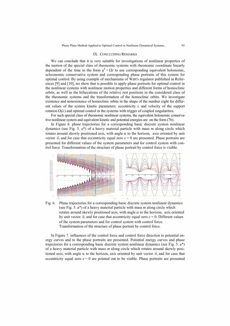
In Figure 6. phase trajectories for a corresponding basic discrete system nonlinear dynamics (see Fig. 5. a*) of a heavy material particle with mass m along circle which rotates around skewly positioned axis, with angle α to the horizon, axis oriented by unit vector ,n

rand for case that eccentricity equal zero e = 0 are presented. Phase portraits are

presented for different values of the system parameters and for control system with con-trol force. Transformation of the structure of phase portrait by control force is visible.

100 80 60 40 20 0 20 40

4

3

2

1

1

2

3

44

4−

a x( )

a1 x( )

a3 x( )

a4 x( )

a5 x( )

a6 x( )

a7 x( )

a8 x( )

a9 x( )

a10 x( )

a11 x( )

a12 x( )

a13 x( )

a14 x( )

50100− x

20 18 16 14 12 10 8 6 4

4

3

2

1

1

2

3

44

4−

a x( )

a1 x( )

a3 x( )

a4 x( )

a5 x( )

a6 x( )

a7 x( )

a8 x( )

a9 x( )

a10 x( )

a11 x( )

a12 x( )

a13 x( )

a14 x( )

3−20− x Fig. 6. Phase trajectories for a corresponding basic discrete system nonlinear dynamics

(see Fig. 5. a*) of a heavy material particle with mass m along circle which rotates around skewly positioned axis, with angle α to the horizon, axis oriented by unit vector ,n

rand for case that eccentricity equal zero e = 0. Different values

of the system parameters and for control system with control force. Transformation of the structure of phase portrait by control force.

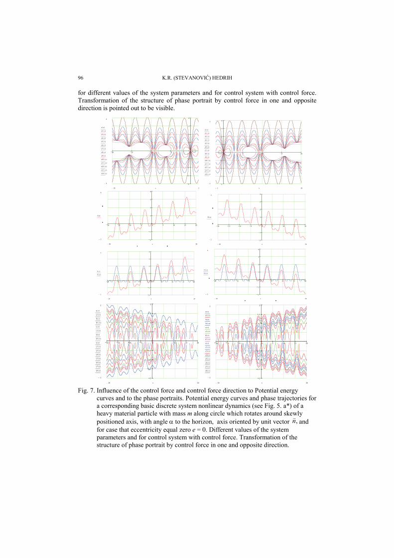
In Figure 7. influences of the control force and control force direction to potential en-ergy curves and to the phase portraits are presented. Potential energy curves and phase trajectories for a corresponding basic discrete system nonlinear dynamics (see Fig. 5. a*) of a heavy material particle with mass m along circle which rotates around skewly posi-tioned axis, with angle α to the horizon, axis oriented by unit vector ,n

rand for case that

eccentricity equal zero e = 0 are pointed out to be visible. Phase portraits are presented


for different values of the system parameters and for control system with control force. Transformation of the structure of phase portrait by control force in one and opposite direction is pointed out to be visible.

20 15 10 5 0

4

3

2

1

1

2

3

44

4−

a x( )

a1 x( )

a3 x( )

a4 x( )

a5 x( )

a6 x( )

a7 x( )

a8 x( )

a9 x( )

a10 x( )

a11 x( )

a12 x( )

a13 x( )

a14 x( )

220− x

0 5 10 15 20

4

3

2

1

1

2

3

44

4−

a x( )

a1 x( )

a3 x( )

a4 x( )

a5 x( )

a6 x( )

a7 x( )

a8 x( )

a9 x( )

a10 x( )

a11 x( )

a12 x( )

a13 x( )

a14 x( )

202− x

20 15 10 5 0 5 10 15 20

2

1

1

2

3

44

2−

f x( )

2020− x

20 15 10 5 0 5 10 15 20

2

1

1

2

3

44

2−

f2 x( )

2020− x

20 15 10 5 0 5 10 15 20

2

1

1

2

3

44

2−

f x( )

f1 x( )

2020− x

20 15 10 5 0 5 10 15 20

2

1

1

2

3

44

2−

f1 x( )

f2 x( )

2020− x

20 15 10 5 0 5 10 15 20

2

1.5

1

0.5

0.5

1

1.5

22

2−

a x( )

a1 x( )

b x( )

b1 x( )

c x( )

c1 x( )

d x( )

d1 x( )

e x( )

e1 x( )

e3 x( )

e4 x( )

e5 x( )

e6 x( )

e7 x( )

e8 x( )

2020− x

20 15 10 5 0 5 10 15 20

2

1.5

1

0.5

0.5

1

1.5

22

2−

a x( )

a1 x( )

b x( )

b1 x( )

c x( )

c1 x( )

d x( )

d1 x( )

e x( )

e1 x( )

e3 x( )

e4 x( )

e5 x( )

e6 x( )

e7 x( )

e8 x( )

2020− x Fig. 7. Influence of the control force and control force direction to Potential energy

curves and to the phase portraits. Potential energy curves and phase trajectories for a corresponding basic discrete system nonlinear dynamics (see Fig. 5. a*) of a heavy material particle with mass m along circle which rotates around skewly positioned axis, with angle α to the horizon, axis oriented by unit vector ,n

rand

for case that eccentricity equal zero e = 0. Different values of the system parameters and for control system with control force. Transformation of the structure of phase portrait by control force in one and opposite direction.


Acknowledgements. Parts of this research were supported by the Ministry of Sciences and Environmental Protection of Republic of Serbia through Mathematical Institute SANU Belgrade Grant ON144002 "Theoretical and Applied Mechanics of Rigid and Solid Body. Mechanics of Materials" and Faculty of Mechanical Engineering University of Niš.

REFERENCES 1. Andronov, A.A., Vitt, A.A., Haykin, S.E., (1981), Teoriya kolebaniy, Nauka, Moskva., pp. 568 2. Gerard I. and Daniel J., Elementary Stability and BIfurcation Theory, Springer Verlag, 1980. 3. Guckenheimer, J. and Holmes, Ph., (1983), Nonlinear Oscillations, Dynamical Systems, and Bifurcations

of Fields , Springer-Verlag, pp. 461. 4. Hedrih (Stevanović), K., Trigger of Coupled Singularities (invited plenary lecture) , Dynamical Systems-

Theory and Applications, Edited By J. Awrejcewicz and all, Lodz 2001, pp. 51-78. 5. Hedrih (Stevanović), K., Nonlinear Dynamics of a Gyrorotor, and Sensitive Dependence on initial

Conditions of a Heav Gyrorotor Forced Vibration/Rotation Motion, Semi-Plenary Invited Lecture, Proceednings: COC 2000, Edited by F.L. Chernousko and A.I. Fradkov, IEEE, CSS, IUTAM, SPICS, St. Petersburg, Inst. for Problems of Mech. Eng. of RAS, 2000., Vol. 2 of 3, pp. 259-266.

6. Hedrih (Stevanović) K., A Trigger of Coupled Singularities, MECCANICA, Vol.39, No. 3, 2004., pp. 295-314. , DOI: 10.1023/B:MECC.0000022994.81090.5f,

7. Hedrih (Stevanović) K., (2005), Nonlinear Dynamics of a Heavy Material Particle Along Circle which Rotates and Optimal Control, Chaotic Dynamics and Control of Systems and Processes in Mechanics (Eds: G. Rega, and F. Vestroni), p. 37-45. IUTAM Book, in Series Solid Mechanics and Its Applications, Editerd by G.M.L. Gladwell, Springer,. 2005, XXVI, 504 p., ISBN: 1-4020-3267-6.

8. Hedrih (Stevanović) K., (2005), Homoclinic Orbits Layering in the Coupled Rotor Nonlinear Dynamics and Chaotic Clock Models, SM17 – Multibody Dynamics (M. Geraldin and F. Pfeiffer), p. Lxiii – CD - SM10624, Mechanics of the 21st Century (21st ICTAM, Warsaw 2004) - CD ROM INCLUDED, edited by Witold Gutkowski and Tomasz A. Kowalewski, IUTAM, Springer 2005, ISBN 1-4020-3456-3, Hardcover., p. 421+CD. ISBN-13 978-1-4020-3456-5 (HB), ISBN-10 1-4020-3559-4(e-book), ISBN-13-978-1-4020-3559-3

9. Hedrih (Stevanović), K., On Rheonomic Systems with Equaivalent Holonomic Conservative System, Int. Conf. ICNM-IV, 2002, Edited by W. Chien and all. Shanghai, T. Nonlinear dynamics. pp. 1046-1054.

10. Hedrih (Stevanović) K., (2004), On Rheonomic Systems with Equivalent Holonomic Conservative Systems Applied to the Nonlinear Dynamics of the Watt's Regulator, Proceedings, Volume 2, The eleventh world congress in Mechanism and machine sciences, IFToMM, China Machine press, Tianjin, China, April 1-4, 2004, pp. 1475-1479. ISBN 7-111-14073-7/TH-1438.

11. Hedrih (Stevanović), K., The Vector Method of the Heavy Rotor Kinetic Parameter Analysis and Nonlinear Dynamics , Monograph, University of Niš, 2001, pp. 252., YU ISBN 86-7181-046-1.

12. Hedrih (Stevanović) K., A Trigger of Coupled Singularities, MECCANICA, Vol.39, No. 3, 2004., pp. 295-314. International Journal of the Italian Association of Theoretical and Applied Мechanics, Meccanica, Publisher: Springer Science+Business Media B.V., Formerly Kluwer Academic Publishers B.V., ISSN: 0025-6455 (Paper) 1572-9648 (Online) DOI: 10.1023/B:MECC.0000022994.81090.5f, Issue: Volume 39, Number 3, Date: June 2004 Pages: 295 - 314 http://www.springerlink.com/app/home/contribution.asp?wasp=ddefdd004a224ad7bd78087cafbb21c2&referrer=parent&backto=issue,6,12;journal,5,47;linkingpublicationresults,1:102958,1

13. Hedrih (Stevanović), K., (2007), The Control in Nonlinear Dynamical Systems with Triggers of a Coupled Singularities, Invited Participation, The 14th International Workshop on Dynamics & Control to be held on May 28–June 2, 2007, in Zvenigorod – Moscow, Russoa, Abstracts, 2007, p. 40. Institute for Problems in Mechanics of the the Russian Academy of Sciences.and Steklov Mathematical Institute of the Russian Academy of Sciences.

14. Hedrih (Stevanović K., The optimal control in nonlinear mechanical systems with trigger of the coupled singularities, in the book: Advances in Mechanics : Dynamics and Control : Proceedings of the 14th International Workshop on Dynamics and Control / [ed. by F.L. Chernousko, G.V. Kostin, V.V. Saurin] : A.Yu. Ishlinsky Institute for Problems in Mechanics RAS. – Moscow : Nauka, 2008. pp. 174-182, ISBN 978-5-02-036667-1.

15. Katica (Stevanović) Hedrih , Optimal Control of Dissipative Nonlinear Dynamical Systems with Triggers of Coupled Singularities, Journal of Physics: Conference Series, 96 (2008) 012220doi:10.1088/1742-6596/96/1/012220, IOP Publishing http://www.iop.org/EJ/main/-list=current/

16. Katica (Stevanović) Hedrih and Ljiljana Veljović, Nonlinear dynamics of the heavy gyro-rotor with two skew rotating axes, Journal of Physics: Conference Series, 96 (2008) 012221doi:10.1088/1742-6596/96/1/012221, IOP Publishing http://www.iop.org/EJ/main/-list=current/


17. Hedrih (Stevanović K., For optimal time of study: vector and tensor methods in classical mechanics., Proceedings Nonlinear Dynamics, Dedicated to the 150th Anniversary of A.M. Lyapunov, Polytechnic Kharkov, 2008. pp. 98-107.

18. Hedrih (Stevanović K., Dynamics of coupled systems, Nonlinear Analysis: Hybrid Systems, Volume 2, Issue 2, June 2008, Pages 310-334

19. Hedrih (Stevanović), K., (1994), Snaga Promene Reonomnih Veza, (The Power Of The Rheonomic Constraints Change), Zbornik Radova Jugoslovenskog Dru{Tva Za Mehaniku, Simpozijum Iz Opšte Mehanike, Novi Sad, 1994, Pp. 177-184.

20. Mathieu, E., Cours de Physique Mathématique, Paris, 1873.; 21. Mitropolyskiy, Yu.A, (1964), Problemi asimptoticheskoy teorii nestashionarnih kolebaniy, Nauka Moskva,

pp. 431. 22. Rašković, D. Teoirija oscilacija (Theory of Oscillations) Naučna knjiga, Beograd, 1965., pp. 504. 23. Stoker, J. J., (1950), Nonlinear Vibrations, Interscience Publishers, New Yor, pp.273. 24. Strutt, M.J. O.: Lamésche, Mathieusche und verwandle Funktionen in Physik und Technik, Berlin,1932. 25. Vujičić, V. A., Preprinciples of Mehanics, Mathematical Institute SANU, Beograd, 1999, p. 223. 26. Vujičić, V., Hedrih (Stevanović), K., (1993), The Rheonomic Constraints Force, Facta Universitatis, Series

Mechanics, Automatic Control and Robotics, Vol. 1, N3, 1993, Niš. pp. 313-322.

METODA FAZNE RAVNI U PRIMENI NA OPTIMALNO UPRAVLJANJE U NELINEARNIM DINAMIČKIM SISTEMIMA

SA TRIGEROM SPREGNUTIH SINGULARITETA

Katica R. (Stevanović) Hedrih

Glavna ideja metode fazne ravni u primeni na optimalno upravljanje u nelinearnim dinamičkim sistemima sa trigerom spregnutih singulariteta i sa jednim stepenom slobode kretanja je ponovo razmotrena. Članak sadrži objedinjen pregled autorovih ranije publikovanih rezultata serije specijalnih slučajeva optimalnog upravljanja u nelinearnim dinamičkim sistemima sa trigerom spregnutih singulariteta koji su značajni za inženjerske primene.

U radu se analizira upravljivost kretanjem konzervativnih, kao i nekonzervativnih nelinearnih dinamičkih sistema sa trigerim singulariteta u odgovarajućoj faznoj ravni. Pokazano je da je metoda fazne ravni upotrebljiva i prigodna za analizu upravljačkih strategija nelinearne dinamike i konzervativnih i nekonzervativnih sistema sa jednim stepenom slobode kretanja i sa trigerom spregnutih singulariteta, a takođe i kao put za upravljanje relativnim kretanjem u reonomnim sistemima koji imaju ekvivalentni scleronomni conzervativni ili nekonzervativni szstem.

Za sistem, koji je opisam sa jednom generalisanom koordinatom i nelinearnom diferencijalnom jednačinom sa trigerom spregnutih singulariteta fnkcija potencijalne energije i konzervativne sile moraju zadovoljavati određene uslove definisane teoremom o postojanju trigera spregnutih singulariteta i separatrise u obliku broja osam. Zadatak definisanog optimalnog upravljanja konzervativnim sistemom je sledeći: koristeći destvo sile upravljanja na nelinearni sistem, isti prevesti iz posmatranog stanja nelinearne dinamike u definisano stanje nelinearne dinamike kroz protek minimalnog vremena, kao kriterijum optimalnog upravljanja.

Neki istraživački rezultati "čudesne" nelinearne dinamike teške materijalne tačke duž krugova sa spregnutim rotacijama sa više različitih svojstava nelinearne dinamike kao i optimalno upravljanje tim dinamikama su takođe prikazani. Vizuelizacija nelinearnih dinamičkih procesa u takvim reonomnim sistemima su predstavljene.

Ključne reči: Metoda fazne ravni, optimalno upravljanje,nelinearna dinamika, konzervativni sistem, nekonzervativni system, fazni portret u ravni, trigger spregnutih singulariteta, teorema o trigeru spregnutih singulariteta, spregnute rotacije, teška materijalna tačka, homoklinička tačka, homoklinička orbita, bifurkacija, raslojavanje orbite, separatrisa u obliku broja osam

Documents

PHASE PLANE METHOD APPLIED TO OPTIMAL CONTROL IN NONLINEAR ...facta.junis.ni.ac.rs/macar/macar2007s/macar2007s06.pdf · PHASE PLANE METHOD APPLIED TO OPTIMAL CONTROL IN NONLINEAR