Embed Size (px)
Citation preview
Phase-Field Modeling of Technical Alloy Systems
Problems and Solutions
B. Böttger
ACCESS e.V., RWTH Aachen University, Germany
Thermo-Calc User Meeting, Sept 8-9 2011, Aachen
Outline
1. Introduction
2. Pragmatic Multi-Phase-Field Model
3. Coupling to Thermodynamic Data: Quasi-Equilibrium
4. Specific Problems and Solutions
a) Stoichiometric Phases
b) Composition Sets
c) Charged Species
5. Conclusion
Outline
1. Introduction
2. Pragmatic Multi-Phase-Field Model
3. Coupling to Thermodynamic Data: Quasi-Equilibrium
4. Specific Problems and Solutions
a) Stoichiometric Phases
b) Composition Sets
c) Charged Species
5. Conclusion
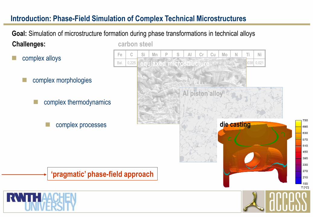
Fe C Si Mn P S Al Cr Cu Mo N Ti Ni
Bal. 0,225 0,078 1,66 0,012 0,0015 1,526 0,021 0,019 0,0053 0,0024 0,0038 0,021
Goal: Simulation of microstructure formation during phase transformations in technical alloys
Introduction: Phase-Field Simulation of Complex Technical Microstructures
complex alloys
complex morphologies
complex thermodynamics
complex processes
„pragmatic‟ phase-field approach
carbon steel
equiaxed microstructure
Al piston alloy
die casting
Challenges:
What is a „pragmatic‟ phase-field approach?
Introduction: Pragmatic Phase-Field Approach
multiphase-field model which allows simulation on µm scale
online-coupling to off-the-shelf thermodynamic and diffusion databases
advanced thermal coupling to external process conditions
robust multi-purpose code (no dedicated solutions)
pragmatic simulation strategy (calibration, simplifications)
MICRESS®: MICRostructure Evolution Simulation Software
Outline
1. Introduction
2. Pragmatic Multi-Phase-Field Model
3. Coupling to Thermodynamic Data: Quasi-Equilibrium
4. Specific Problems and Solutions
a) Stoichiometric Phases
b) Composition Sets
c) Charged Species
5. Conclusion
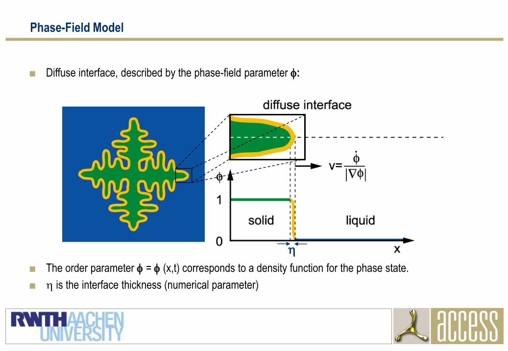
■ Diffuse interface, described by the phase-field parameter f:
■ The order parameter f = f (x,t) corresponds to a density function for the phase state.
■ h is the interface thickness (numerical parameter)
Phase-Field Model
h
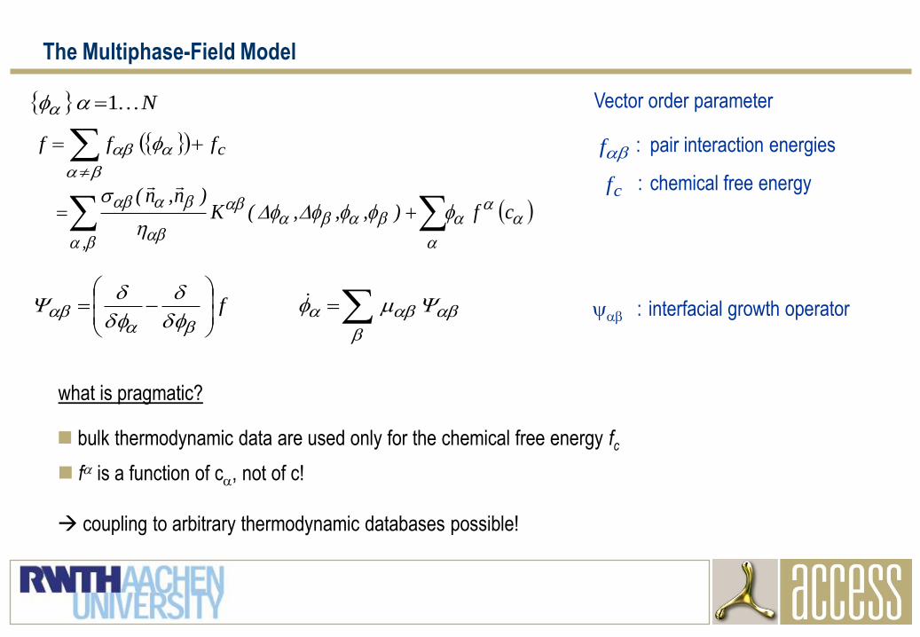
The Multiphase-Field Model
Vector order parameter N1f
what is pragmatic?
bulk thermodynamic data are used only for the chemical free energy fc
f is a function of c, not of c!
coupling to arbitrary thermodynamic databases possible!
fffffh
cf),,,(K
)n,n(
,
ff
f
f : interfacial growth operator
cfff
ff
cf
: pair interaction energies
: chemical free energy
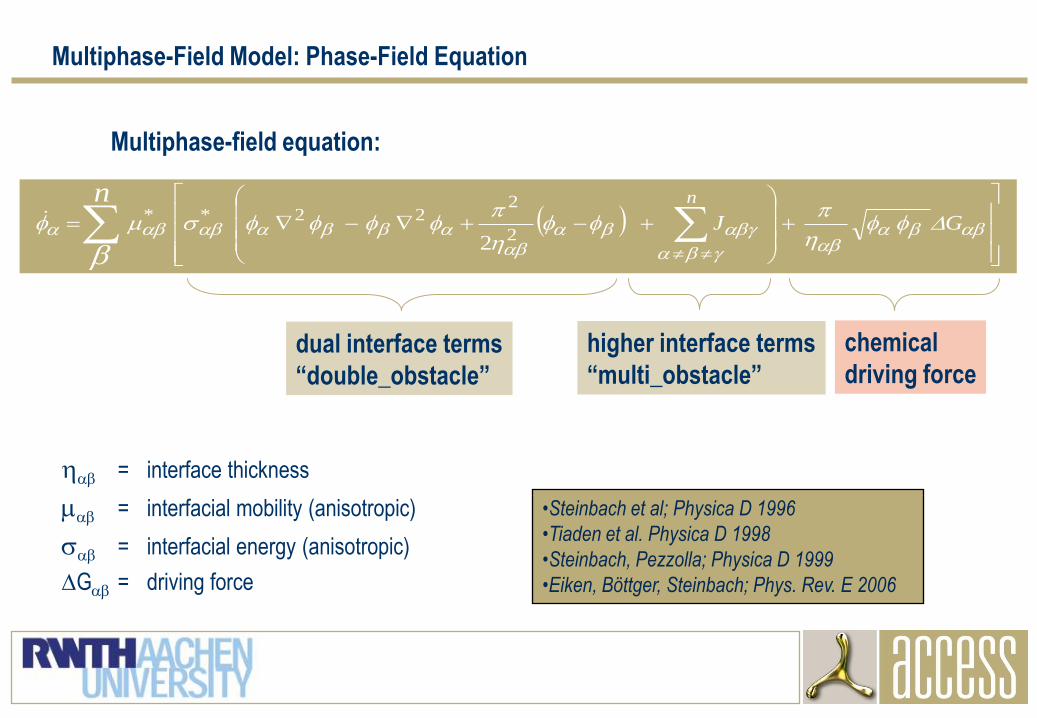
h = interface thickness
= interfacial mobility (anisotropic)
= interfacial energy (anisotropic)
G = driving force
ffh
ff
h
fffff
GJ
n**
n
2
222
2
•Steinbach et al; Physica D 1996
•Tiaden et al. Physica D 1998
•Steinbach, Pezzolla; Physica D 1999
•Eiken, Böttger, Steinbach; Phys. Rev. E 2006
Multiphase-field equation:
dual interface terms
“double_obstacle”
higher interface terms
“multi_obstacle”
chemical
driving force
Multiphase-Field Model: Phase-Field Equation
Outline
1. Introduction
2. Pragmatic Multi-Phase-Field Model
3. Coupling to Thermodynamic Data: Quasi-Equilibrium
4. Specific Problems and Solutions
a) Stoichiometric Phases
b) Composition Sets
c) Charged Species
5. Conclusion
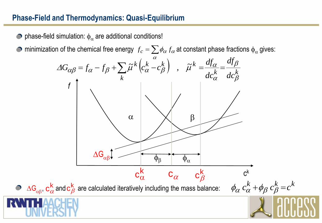
Phase-Field and Thermodynamics: Quasi-Equilibrium
G
, and are calculated iteratively including the mass balance:kckc
kkk ccc ff
kk
k
k
kkk
dc
df
dc
df~,cc~ffG
minimization of the chemical free energy at constant phase fractions f gives:
f ffc
kckc c
f
ff
ck
G
phase-field simulation: f are additional conditions!
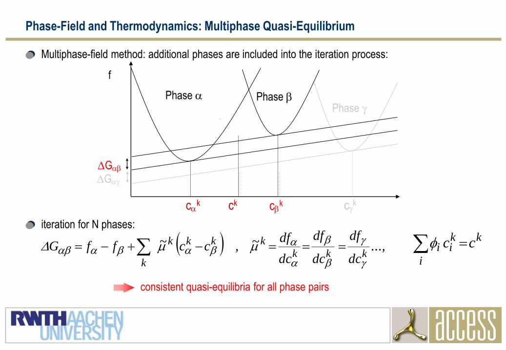
Phase-Field and Thermodynamics: Multiphase Quasi-Equilibrium
Multiphase-field method: additional phases are included into the iteration process:
consistent quasi-equilibria for all phase pairs
iteration for N phases:
,...dc
df
dc
df
dc
df~,cc~ffGkkk
kkkk
k
k
i
kii cc f
G
G
ck ck ck
Phase Phase Phase
ck
f
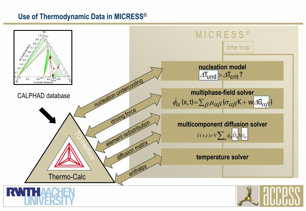
Use of Thermodynamic Data in MICRESS®
multicomponent diffusion solver
M I C R E S S ®
nucleation model
temperature solver
multiphase-field solver
time loop
Thermo-Calc
CALPHAD database f )GwK()t,x(
?TT critund
f cD)t,x(c

Outline
1. Introduction
2. Pragmatic Multi-Phase-Field Model
3. Coupling to Thermodynamic Data: Quasi-Equilibrium
4. Specific Problems and Solutions
a) Stoichiometric Phases
b) Composition Sets
c) Charged Species
5. Conclusion

Outline
1. Introduction
2. Pragmatic Multi-Phase-Field Model
3. Coupling to Thermodynamic Data: Quasi-Equilibrium
4. Specific Problems and Solutions
a) Stoichiometric Phases
b) Composition Sets
c) Charged Species
5. Conclusion
G α β
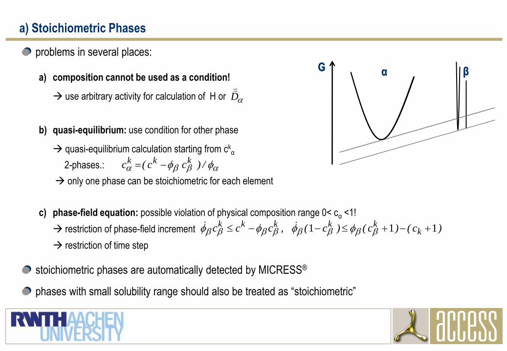
a) Stoichiometric Phases
stoichiometric phases are automatically detected by MICRESS®
G α β
phases with small solubility range should also be treated as “stoichiometric”
a) composition cannot be used as a condition!
use arbitrary activity for calculation of H or D
problems in several places:
c) phase-field equation: possible violation of physical composition range 0< cα <1!
restriction of phase-field increment
restriction of time step
)c()c()c(,ccc kkkkkk 111 ffff
b) quasi-equilibrium: use condition for other phase
quasi-equilibrium calculation starting from ckα
2-phases.:
only one phase can be stoichiometric for each element
ff /)cc(c kkk
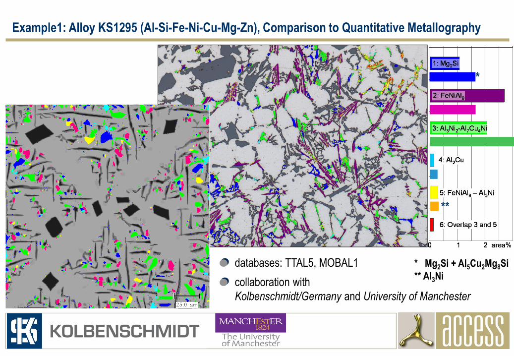
Example1: Alloy KS1295 (Al-Si-Fe-Ni-Cu-Mg-Zn), Comparison to Quantitative Metallography
*
* Mg2Si + Al5Cu2Mg8Si
** Al3Ni
**
databases: TTAL5, MOBAL1
collaboration with
Kolbenschmidt/Germany and University of Manchester
Outline
1. Introduction
2. Pragmatic Multi-Phase-Field Model
3. Coupling to Thermodynamic Data: Quasi-Equilibrium
4. Specific Problems and Solutions
a) Stoichiometric Phases
b) Composition Sets
c) Charged Species
5. Conclusion
LIQUID FCC_A1
#1: FCC
#3: Nb(C,N)#2: Ti(N,C)
G
composition
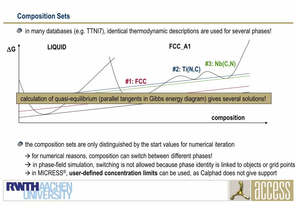
Composition Sets
calculation of quasi-equilibrium (parallel tangents in Gibbs energy diagram) gives several solutions!
for numerical reasons, composition can switch between different phases!
in phase-field simulation, switching is not allowed because phase identity is linked to objects or grid points
in MICRESS®, user-defined concentration limits can be used, as Calphad does not give support
in many databases (e.g. TTNI7), identical thermodynamic descriptions are used for several phases!
the composition sets are only distinguished by the start values for numerical iteration
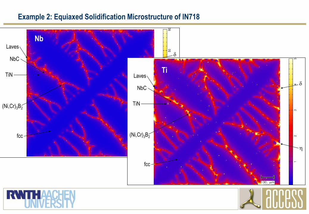
δ
Laves
TiN
NbC
(Ni,Cr)3B2
fcc
h
Nb
Example 2: Equiaxed Solidification Microstructure of IN718
h
Laves
TiN
NbC
(Ni,Cr)3B2
fcc
δ
Ti
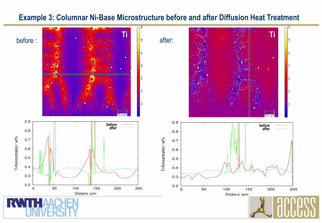
Example 3: Columnar Ni-Base Microstructure before and after Diffusion Heat Treatment
after:before :
beforeafter
beforeafter
TiTi

Outline
1. Introduction
2. Pragmatic Multi-Phase-Field Model
3. Coupling to Thermodynamic Data: Quasi-Equilibrium
4. Specific Problems and Solutions
a) Stoichiometric Phases
b) Composition Sets
c) Charged Species
5. Conclusion
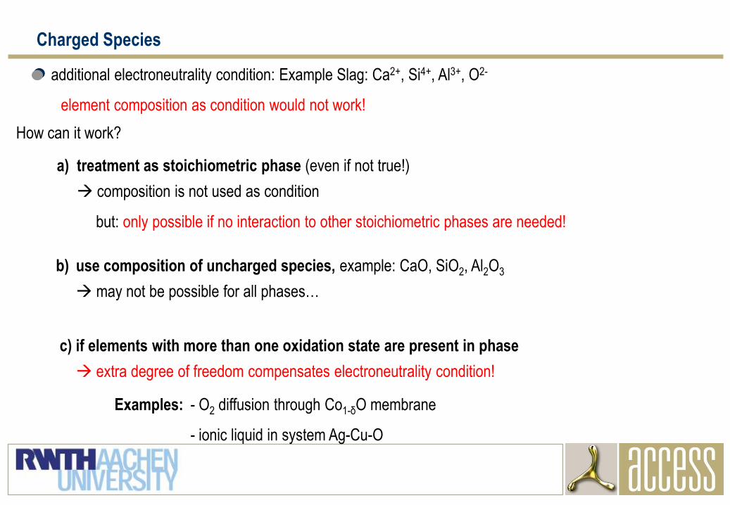
Charged Species
b) use composition of uncharged species, example: CaO, SiO2, Al2O3
may not be possible for all phases…
a) treatment as stoichiometric phase (even if not true!)
composition is not used as condition
but: only possible if no interaction to other stoichiometric phases are needed!
additional electroneutrality condition: Example Slag: Ca2+, Si4+, Al3+, O2-
element composition as condition would not work!
c) if elements with more than one oxidation state are present in phase
extra degree of freedom compensates electroneutrality condition!
How can it work?
Examples: - O2 diffusion through Co1-δO membrane
- ionic liquid in system Ag-Cu-O
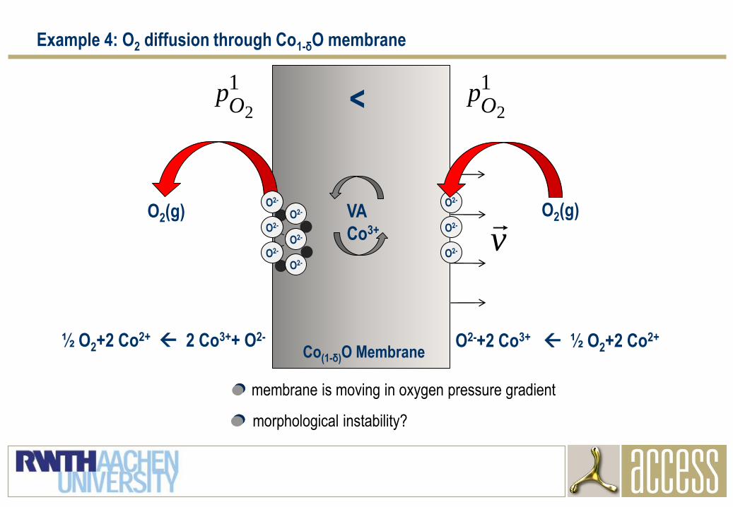
v
Example 4: O2 diffusion through Co1-δO membrane
<
membrane is moving in oxygen pressure gradient
morphological instability?
Co(1-δ)O Membrane½ O2+2 Co2+
2 Co3++ O2- O2-+2 Co3+ ½ O2+2 Co2+
1
2Op 1
2Op
O2(g)O2(g) VA
Co3+
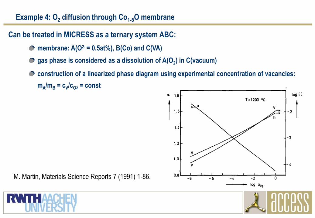
Example 4: O2 diffusion through Co1-δO membrane
M. Martin, Materials Science Reports 7 (1991) 1-86.
Can be treated in MICRESS as a ternary system ABC:
construction of a linearized phase diagram using experimental concentration of vacancies:
mA/mB = cV/cO2 = const
gas phase is considered as a dissolution of A(O2) in C(vacuum)
membrane: A(O2- = 0.5at%), B(Co) and C(VA)
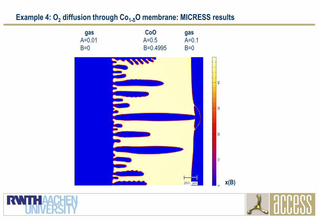
Example 4: O2 diffusion through Co1-δO membrane: MICRESS results
gas CoO gas
A=0.01 A=0.5 A=0.1
B=0 B=0.4995 B=0
x(B)
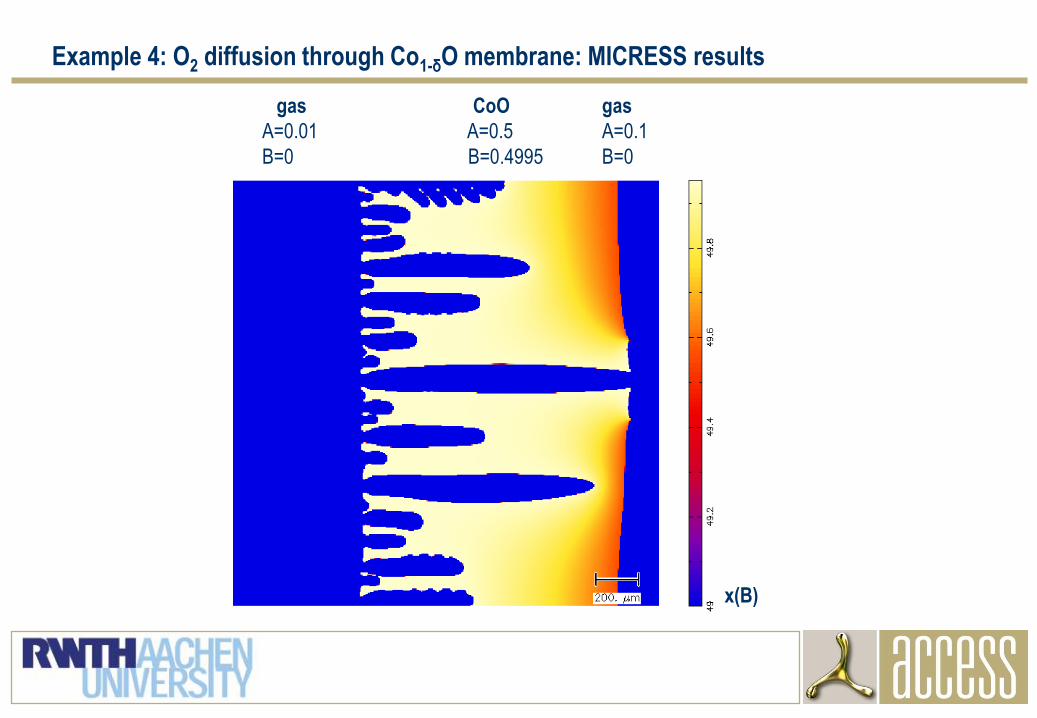
Example 4: O2 diffusion through Co1-δO membrane: MICRESS results
gas CoO gas
A=0.01 A=0.5 A=0.1
B=0 B=0.4995 B=0
x(B)
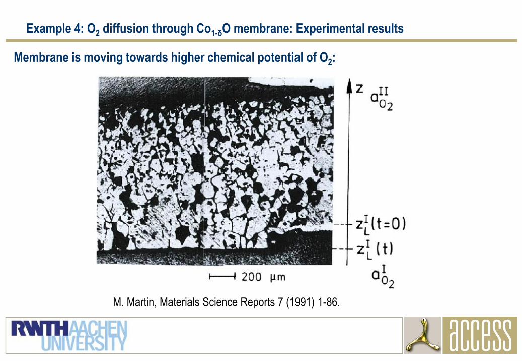
Example 4: O2 diffusion through Co1-δO membrane: Experimental results
Membrane is moving towards higher chemical potential of O2:
M. Martin, Materials Science Reports 7 (1991) 1-86.
Example 4: O2 diffusion through Co1-δO membrane: Experimental results
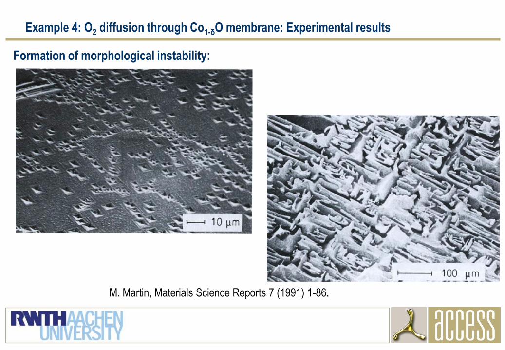
Formation of morphological instability:
M. Martin, Materials Science Reports 7 (1991) 1-86.
Example 4: O2 diffusion through Co1-δO membrane: Experimental results
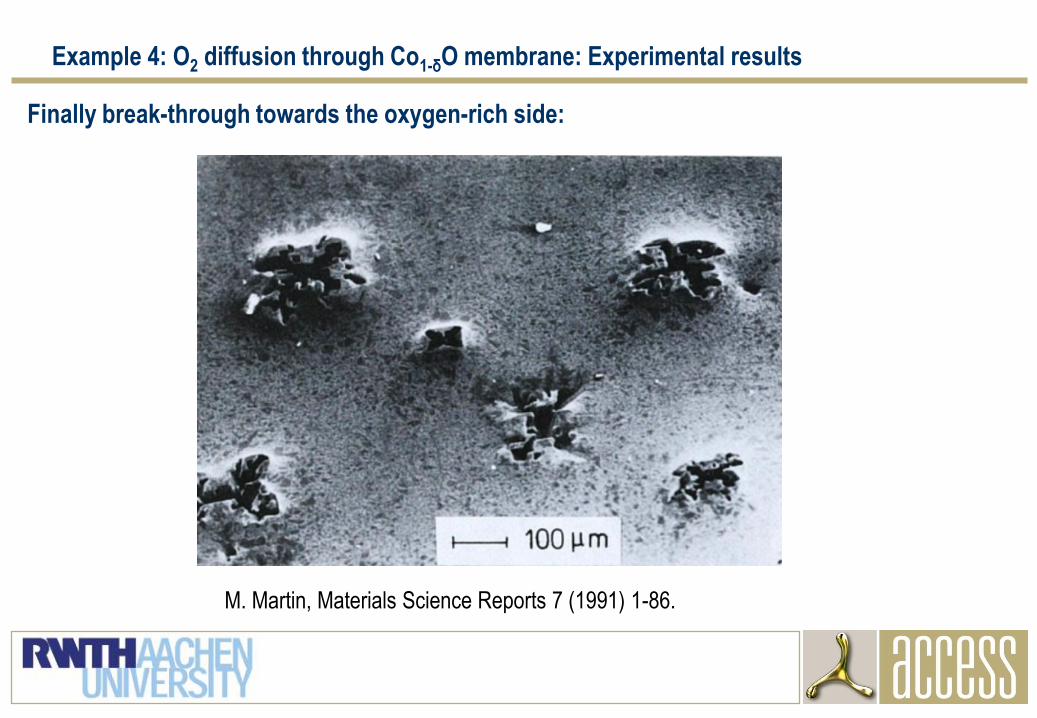
Finally break-through towards the oxygen-rich side:
M. Martin, Materials Science Reports 7 (1991) 1-86.
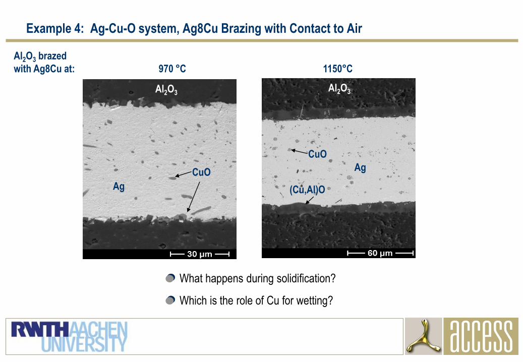
Example 4: Ag-Cu-O system, Ag8Cu Brazing with Contact to Air
Al2O3 brazed
with Ag8Cu at: 970 °C 1150°C
Al2O3
Ag
CuO
(Cu,Al)O
Al2O3
Ag
CuO
What happens during solidification?
Which is the role of Cu for wetting?
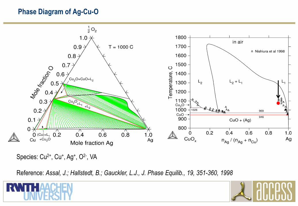
Phase Diagram of Ag-Cu-O
Reference: Assal, J.; Hallstedt, B.; Gauckler, L.J., J. Phase Equilib., 19, 351-360, 1998
Species: Cu2+, Cu+, Ag+, O2-, VA
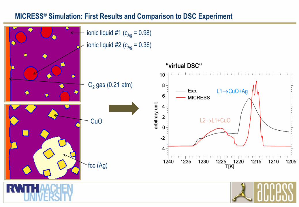
MICRESS® Simulation: First Results and Comparison to DSC Experiment
ionic liquid #1 (cAg = 0.98)
ionic liquid #2 (cAg = 0.36)
CuO
O2 gas (0.21 atm)
fcc (Ag)
“virtual DSC“
L2L1+CuO
L1CuO+Ag
Outline
1. Introduction
2. Pragmatic Multi-Phase-Field Model
3. Coupling to Thermodynamic Data: Quasi-Equilibrium
4. Specific Problems and Solutions
a) Stoichiometric Phases
b) Composition Sets
c) Charged Species
5. Conclusion
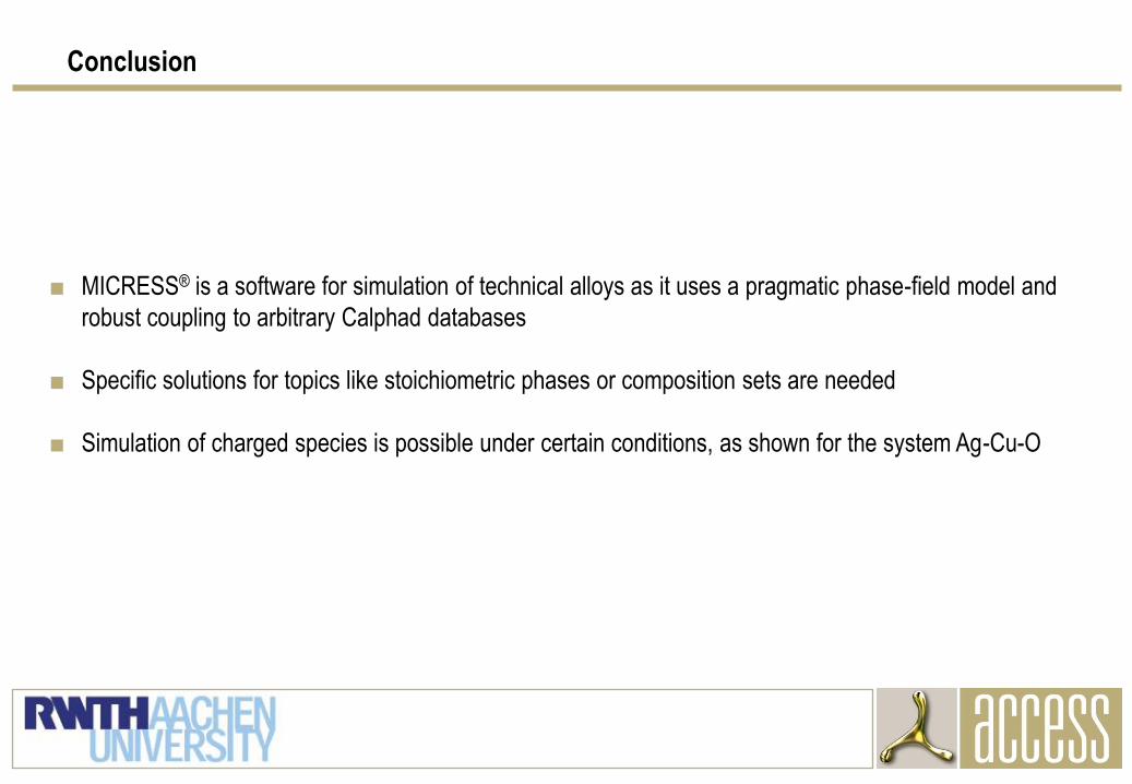
Conclusion
■ MICRESS® is a software for simulation of technical alloys as it uses a pragmatic phase-field model and
robust coupling to arbitrary Calphad databases
■ Specific solutions for topics like stoichiometric phases or composition sets are needed
■ Simulation of charged species is possible under certain conditions, as shown for the system Ag-Cu-O

Thank you for
your attention!