9HSTFMG*aefbie+

ISBN 978-952-60-4518-4 ISBN 978-952-60-4519-1 (pdf) ISSN-L 1799-4934 ISSN 1799-4934 ISSN 1799-4942 (pdf) Aalto University School of Chemical Technology Department of Biotechnology and Chemical Technology www.aalto.fi

BUSINESS + ECONOMY ART + DESIGN + ARCHITECTURE SCIENCE + TECHNOLOGY CROSSOVER DOCTORAL DISSERTATIONS

Aalto-D

D 2

0/2

012

The purpose of this research was to develop modelling of industrial processes by improving the thermodynamic representation of the equilibrium between phases. For this purpose an extensive experimental work was performed. Vapour liquid equilibrium of binary mixtures of butane + alcohols and of diethyl sulphide + C4 – hydrocarbons were studied. Absorption of carbon dioxide in alkanolamine solutions is the leading industrial technology for the removal of carbon dioxide. In recent years, this technology has gained importance also for carbon capture from large point sources. The scarcity of experimental data for some alkanolamine systems affected the accuracy of thermodynamic models. Several experimental techniques were developed in this work to supply new data for the solubility of carbon dioxide in aqueous solutions of diisopropanolamine (DIPA) and methyldiethanolamine (MDEA). The vapour-liquid equilibrium and the solid-liquid equilibrium of aqueous DIPA and MDEA were also studied and modelled.

Claudia D

ell'Era

Phase E

quilibrium M

easurements and M

odelling for Separation Process D

esign A

alto U

nive

rsity

Department of Biotechnology and Chemical Technology

Phase Equilibrium Measurements and Modelling for Separation Process Design

Claudia Dell'Era

DOCTORAL DISSERTATIONS

Aalto University publication series DOCTORAL DISSERTATIONS 20/2012

Phase Equilibrium Measurements and Modelling for Separation Process Design

Claudia Dell'Era

Doctoral dissertation for the degree of Doctor of Science in Technology to be presented with due permission of the School of Chemical Technology for public examination and debate in Auditorium KE2 (Komppa Auditorium) at Aalto University School of Chemical Technology (Espoo, Finland) on the 16th of March, 2012, at 12 noon.

Aalto University School of Chemical Technology Department of Biotechnology and Chemical Technology Research group of Chemical Engineering

Supervisor Professor Ville Alopaeus Instructor Dr. Juhani Aittamaa Preliminary examiners Associate Professor Kaj Thomsen. Technical University of Denmark, Denmark Prof. Dr. -Ing. Hans Hasse. University of Kaiserslautern, Germany Opponent Prof.dr.ir Cornelis J. (Cor) Peters. Petroleum Institute, United Arab Emirates

Aalto University publication series DOCTORAL DISSERTATIONS 20/2012 © Claudia Dell'Era ISBN 978-952-60-4518-4 (printed) ISBN 978-952-60-4519-1 (pdf) ISSN-L 1799-4934 ISSN 1799-4934 (printed) ISSN 1799-4942 (pdf) Unigrafia Oy Helsinki 2012 Finland The dissertation can be read at http://lib.tkk.fi/Diss/

Abstract Aalto University, P.O. Box 11000, FI-00076 Aalto www.aalto.fi

Author Claudia Dell'Era Name of the doctoral dissertation Phase Equilibrium Measurements and Modelling for Separation Process Design Publisher School of Chemical Technology Unit Department of Biotechnology and Chemical Technology

Series Aalto University publication series DOCTORAL DISSERTATIONS 20/2012

Field of research Chemical Engineering

Manuscript submitted 20 September 2011 Manuscript revised 13 December 2011

Date of the defence 16 March 2012 Language English

Monograph Article dissertation (summary + original articles)

Abstract The purpose of this research was to develop modelling of industrial processes by improving the thermodynamic representation of the equilibrium between phases. For this purpose an extensive experimental work was performed, comprising of vapour-liquid, gas-liquid and solid-liquid equilibrium measurements.

Vapour liquid equilibrium of binary mixtures of butane + alcohols was measured with a static total pressure apparatus due to the importance of hydrocarbon and alcohol mixtures in the production of biofuels. The same equipment was used to measure binary systems of diethyl sulphide + C4 – hydrocarbons of importance in refinery applications. The activity coefficients of these systems were modelled with activity coefficients models.

The absorption of carbon dioxide in alkanolamine solutions is the leading technology for the removal of carbon dioxide during refining of gas and oil. In recent years, this technology has gained importance also for carbon capture from large point sources. The scarcity of experimental data for some alkanolamine systems affected the accuracy of thermodynamic models. Several experimental techniques were developed to supply new experimental data for aqueous solutions of diisopropanolamine (DIPA) and methyldiethanolamine (MDEA). The solubility of carbon dioxide in solutions of these amines was measured with a static total pressure apparatus for gas solubility, and with a bubbling apparatus. The density of carbonated aqueous DIPA was also measured and modelled. The vapour-liquid equilibrium of water + DIPA and water + MDEA was measured with a static total pressure apparatus. The solid-liquid equilibrium of the same systems was measured with a visual method and a Differential Scanning Calorimeter. The activity coefficients of aqueous DIPA and MDEA solutions were modelled using NRTL, thus providing the first model of this sort for DIPA. A new model of the Henry’s law constant of carbon dioxide in binary and ternary aqueous solutions of alkanolamines was developed at temperatures up to 393 K.

Keywords vapour-liquid equilibrium, solid-liquid equilibrium, solubility, carbon dioxide, DIPA, MDEA, butane, diethyl sulphide, UNIFAC, COSMO, Henry’s law, miniplant

ISBN (printed) 978-952-60-4518-4 ISBN (pdf) 978-952-60-4519-1

ISSN-L 1799-4934 ISSN (printed) 1799-4934 ISSN (pdf) 1799-4942

Location of publisher Espoo Location of printing Helsinki Year 2012

Pages 128 The dissertation can be read at http://lib.tkk.fi/Diss/

I

PrefaceThe research work presented in this thesis was completed during the years 2004 -2007 and

2009-2011 at the Chemical Engineering research unit of Aalto University School of

Chemical Technology (operating as Helsinki University of Technology until 2009).

Fortum Foundation is acknowledged for their economic support, in the form of a 4 years

scholarship from 2004 to 2007.

My professor Ville Alopaeus and my former professor Juhani Aittamaa receive my gratitude

for their guidance and support during all these years. My thanks also go to Dr. Kari I.

Keskinen, who proposed the subject and supported me in obtaining funding for this research.

Warm thanks are due to my co-author, guide and friend Dr. Petri Uusi-Kyyny. He taught

me how experimental research is conducted, he helped me overcoming practical and

theoretical problems and he was always a valuable support, both technologically and

humanly. I will never forget the importance of his contribution to this research and to my

growth as a chemical engineer and scientist.

I wish to express my gratitude to all my co-authors; it was a great pleasure to work with

every one of you. In particular, I would like to acknowledge Dr. Juha-Pekka Pokki for his

help in addressing difficulties with thermodynamic modelling and Dr. Kaj Jakobsson for

supporting me with computation and programming. I wish also to separately thank Anne

Penttilä, with whom I worked intensely in the last two years.

The working environment within the Chemical Engineering research unit was always

creative, inspiring and friendly. Therefore, I would like to thank all my former colleagues for

their contributions and in particular my friends Anna Zaytseva, Erlin Sapei and Raisa

Vermasvuori. During these years as a researcher I also meet two of my best friends, Asta

Nurmela and Piia Haimi. I wish to thank them dearly for their unconditioned support, for the

liberating conversations and for all fun and laughter! With their love and patience, they

contributed to making Finland my new home.

From the personnel of the Chemical Engineering research unit, I would also like to thank

Sirpa Aaltonen and Lasse Westerlund who helped throughout the years in dealing with

practical issues and who always had a nice word for me.

II

My mum Lucia, my dad Angelo and my brother Enrico deserve my deepest gratitude. Even if

we live in different countries, they fight the distance to make me feel the warmth of their love

and support.

This thesis is dedicated to my husband Daniel and my son Robin, whom I deeply love. I wish

to thank them for bringing joy and meaning to my life.

Claudia Dell’Era Espoo, 22nd January 2012

III

List of publications

I. Penttilä, A., Dell’Era, C., Uusi-Kyyny, P.; Alopaeus, V. The Henry’s Law Constant of

N2O and CO2 in Aqueous Binary and Ternary Amine Solutions (MEA, DEA, DIPA,

MDEA, and AMP). Fluid Phase Equilibria 311 (2011) 59–66.

II. Dell’Era, C., Uusi-Kyyny, P.,Rautama, E.-L., Pakkanen, M., Alopaeus, V.

Thermodynamics of aqueous solutions of methyldiethanolamine and

diisopropanolamine. Fluid Phase Equilibria 299 (2010) 51–59.

III. Dell’Era, C., Uusi-Kyyny, P., Pokki, J.-P., Pakkanen, M., Alopaeus, V. Solubility of

carbon dioxide in aqueous solutions of diisopropanolamine and methyldiethanolamine.

Fluid Phase Equilibria 293 (2010) 101–109.

IV. Dell’Era, C., Pokki, J.-P., Uusi-Kyyny, P., Pakkanen, M., Alopaeus, V. Vapour-liquid

equilibrium for the systems diethyl sulphide + 1-butene, + cis-2-butene, + 2-

methylpropane, + 2-methylpropene, + n-butane, + trans-2-butene, Fluid Phase Equilib.

291 (2010) 180-187.

V. Dell’Era, C., Zaytseva, A., Uusi-Kyyny, P., Pokki, J.-P., Pakkanen, M., Aittamaa, J.

Vapour-liquid equilibrium for the systems butane + methanol, +2-propanol, +1-butanol,

+2-butanol, +2-methyl-2-propanol at 364.5 K, Fluid Phase Equilib., 254 (2007) 49-59.

VI. Ouni, T., Lievo, P., Uusi-Kyyny, P., Dell'Era, C., Jakobsson, K., Pyhälahti, A.,

Aittamaa, J. Practical Methodology for Distillation Design using Miniplant. Chem.

Eng. Tech. 29 (2006) 104-112.

IV

Statement of the author’s contribution to the appended publications

I. The author supervised the work, contributed to the development of the model, and

helped in writing the manuscript.

II. The author designed and set-up the experimental measurement systems with co-author

Uusi-Kyyny. The author conducted most of the experimental work, analysed the

results, modelled the systems and wrote the paper.

III. The author designed and set-up the experimental measurement systems with co-author

Uusi-Kyyny. The author conducted most of the experimental work, analysed the results

and wrote the paper.

IV. The author analysed the results, modelled the systems and wrote the paper.

V. The author analysed the results, modelled the systems and wrote the paper.

VI. The author developed the model of the column, and contributed to writing the

manuscript in relation to the column model.

V

Notations Symbols a attractive parameter of the Soave-Redlich-Kwong equation of state

ija interaction parameters of the NRTL model A fitted parameter of activity coefficient model

ijA parameter of the Henry’s law constant model for solvent components ij

ijkA parameter of the Henry’s law constant model for solvent components ijk b co-volume parameter of the Soave-Redlich-Kwong equation of state

ib co-volume parameter of the Soave-Redlich-Kwong equation of state for component i

ijb interaction parameters of the NRTL model

ijB parameter of the Henry’s law constant model for solvent components ij

ijkB parameter of the Henry’s law constant model for solvent components ijk

ijC parameter of the Henry’s law constant model for solvent components ij

ijkC parameter of the Henry’s law constant model for solvent components ijk

pc heat capacity

ijD parameter of the Henry’s law constant model for for solvent components ij f fugacity G Gibbs energy

ijg interaction parameters of the NRTL model

jiH , Henry’s law constant of solute i in solvent component j

jkiH , Henry’s law constant of solute i in a solution of j and k

jkmiH , Henry’s law constant of solute i in a solution of j, k and m H enthalpy

fusiH ,� enthalpy of fusion of component i

ijk interaction parameter of the Soave-Redlich-Kwong equation of state N number of components

PN number of experimental points P pressure

iP partial pressure of component i sat

iP vapour pressure of pure component i q calculated variable R ideal gas constant s measured variable T temperature u measured variable V volume

iV molar volume of component i

VI

iw weight fraction wt% weight percent x mole fraction Z compressibility factor

Greek letters � loading = moles of absorbed CO2 / moles of amine

SRK� parameter of the Soave-Redlich-Kwong equation of state

ij� non-randomness parameter of the NRTL and e-NRTL models � uncertainty � volume fraction � difference � fugacity coefficient � activity coefficient � density

ij interaction parameters of the NRTL model and e-NRTL models acentric factor (Soave-Redlich-Kwong equation of state

Superscripts � phase � phase EX excess L liquid S solid Sat saturated V vapour q partial property ( q)� infinite dilution � unsymmetric convention º pure component (standard state) ^ mixture - minimum value + maximum value

'q perturbed value (of q)

Subscripts calc calculated exp experimental fus fusion i component j component k component l experimental point

VII

m component S solvent tp triple point W water

Abbreviations

AMP 2-amino-2-methyl-1-propanol atm. atmospheric (pressure) DEA diethanolamine DES diethyl sulphide DGA 2-(2-aminoethoxy) ethanol DIPA diisopropanolamine DSC differential scanning calorimeter EOS equation of state FCC fluid catalytic cracking GLE gas-liquid equilibrium HETP height equivalent to a theoretical plate LPG liquefied petroleum gas MDEA methyldiethanolamine MEA monoethanolamine MTBE methyl tert-butyl ether (2-methoxy-2-methyl propane) PVT pressure-volume-temperature RK Redlich-Kwong equation of state SLE solid-liquid equilibrium SRK Soave-Redlich-Kwong equation of state TEA triethanolamine VLE vapour-liquid equilibrium

VIII

Table of contents

1 Introduction ....................................................................................................... 1

1.1 The miniplant concept .................................................................................. 2 1.2 Systems of interest ....................................................................................... 3

2 Thermodynamic principles ............................................................................... 9

2.1 Phase-equilibrium thermodynamic ............................................................... 9 2.1.1 Vapour-liquid equilibrium (VLE) ......................................................... 9 2.1.2 Gas- liquid equilibrium (GLE) ........................................................... 10 2.1.3 Solid-liquid equilibrium (SLE) ........................................................... 11

2.2 Fugacity coefficients .................................................................................. 13 2.3 Activity coefficients ................................................................................... 13

2.3.1 The NRTL model ............................................................................... 15 3 Experimental procedures ................................................................................ 17

3.1 Vapour-Liquid Equilibrium measurements ................................................. 17 3.1.1 Static total pressure apparatus for VLE measurements ........................ 17 3.1.2 Modifications of the static total pressure apparatus for VLE

measurements of aqueous alkanolamine systems ................................ 19 3.2 Gas Liquid Equilibrium (GLE) measurements............................................ 19

3.2.1 Static total pressure apparatus for GLE measurements ........................ 19 3.2.2 Bubbling apparatus............................................................................. 22

3.3 Solid-Liquid Equilibrium measurements .................................................... 24 3.3.1 Visual method .................................................................................... 24 3.3.2 Differential Scanning Calorimeter (DSC) ........................................... 25

3.4 Estimation of the experimental uncertainty ................................................ 26 4 Results .............................................................................................................. 29

4.1 The miniplant concept applied to distillation design ................................... 30 4.2 VLE of butane + alcohols .......................................................................... 31 4.3 VLE of diethyl sulphide + C4 - hydrocarbons ............................................. 36 4.4 Aqueous alkanolamine systems .................................................................. 37

4.4.1 Solubility data of CO2 in water + alkanolamine solvents .................... 39 4.4.2 Thermodynamics of water + alkanolamine systems ............................ 41 4.4.3 Henry’s law constant of CO2 in aqueous alkanolamine solutions ........ 47

5 Conclusions ...................................................................................................... 53

References.................................................................................................................... 55

Errata Corrige ............................................................................................................. 62

1

1 Introduction

Mathematical models are powerful tools in the development and design of chemical

units. Process design is usually performed by constructing a mathematical model of the

entire process. Various design options may then be evaluated quickly and inexpensively

at an early stage of the design process. Commonly, a pilot plant is built to provide design

and operating information before the construction of a large plant. Scale-up methods are

applied to extrapolate the pilot plant up to full scale. The construction of several plants of

intermediate size may be necessary if simple scale-up rules are applied, since they usually

do not allow large size extrapolation steps. The construction of pilot plants is costly and

time demanding. Strengthening model-based process design is the most efficient way of

reducing the need of pilot plants. Particularly in the case of separation units, an accurate

mathematical representation of the process phenomena might be sufficient to design full

scale chemical plants.

Various phenomena take place in chemical units, such as phase equilibrium, mass and

heat transfer, chemical reactions and hydraulics. An accurate description of these

phenomena can only be achieved with the aid of good quality experimental data. In

separation processes, the formation or co-existence of different phases is exploited in

order to separate the compounds of interest. A model of the thermodynamic equilibrium

between phases provides the basis for successfully designing these chemical units.

Thermodynamic is composed of mathematical equations derived from very few

fundamental postulates [1]. A general thermodynamic model is applied to a specific

process using physical properties at the operative conditions of interest. It was the aim of

this work to improve thermodynamic modelling of separation unit for chosen systems of

industrial interest. For these systems, phase equilibrium data were either scarce or

unavailable in the open literature. An extensive experimental work was performed to

supply vapour-liquid equilibrium (VLE), solid-liquid equilibrium (SLE) or gas solubility

(GLE) data. In addition, the systems studied were described either with traditional

thermodynamic models or with new expressions.

In absence of experimental data, phase equilibrium can also be predicted. The accuracy

of predictive models is often inadequate for modelling chemical units that are sensitive to

2

phase equilibrium, e.g. reactive distillation. In this work, the performances of some

predictive methods on selected systems of interest were investigated.

1.1 The miniplant concept

Model-based process design has the great advantage of being inexpensive and versatile.

On the other end, process design using pilot plants and scale-up is a robust way to

proceed. The greatest danger in model-based design is that some important factor may go

unnoticed during design. This rarely happens when pilot plants are used, since all aspects

of plant design and operation are encountered during the scale-up process.

The miniplant concept is a compromise solution between the two approaches. Design

using a miniplant is mostly achieved through model-based process design. A small scale

pilot plant, i.e. the miniplant, is then constructed, and the performances of the model are

tested against experimental runs. In comparison to a traditional pilot plant, a miniplant

has a smaller scale, thus reducing utility costs and risks related to operation safety.

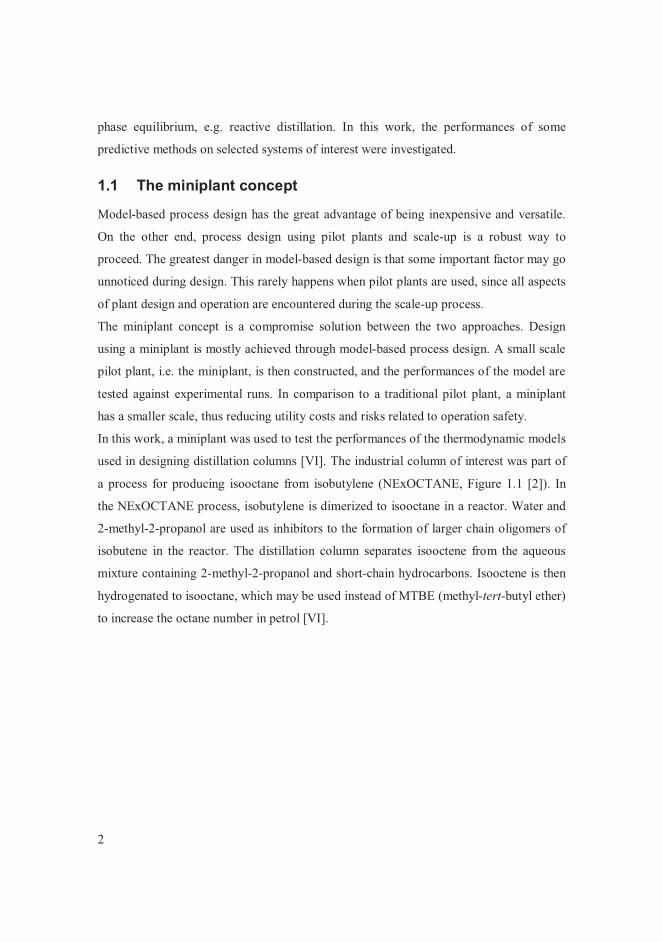
In this work, a miniplant was used to test the performances of the thermodynamic models

used in designing distillation columns [VI]. The industrial column of interest was part of

a process for producing isooctane from isobutylene (NExOCTANE, Figure 1.1 [2]). In

the NExOCTANE process, isobutylene is dimerized to isooctane in a reactor. Water and

2-methyl-2-propanol are used as inhibitors to the formation of larger chain oligomers of

isobutene in the reactor. The distillation column separates isooctene from the aqueous

mixture containing 2-methyl-2-propanol and short-chain hydrocarbons. Isooctene is then

hydrogenated to isooctane, which may be used instead of MTBE (methyl-tert-butyl ether)

to increase the octane number in petrol [VI].

3

Figure 1.1 Schematic representation of the NExOCTANE process.

1.2 Systems of interest

The vapour-liquid equilibrium of mixtures of alcohols and hydrocarbons is important for

process design and optimisation in the field of biofuels. Methanol, ethanol and butanol

are among the fuels produced by gasification of biomass, cracking or fermentation.

Alcohols are widely used also in the oil industry, e.g. as fuel additives and inhibitors [3].

In particular, the VLE of binary systems of 2-methyl-2-propanol + hydrocarbons is

needed in modelling the production of isooctane from isobutylene with the

NExOCTANE [2] process, in which 2-methyl-2-propanol is used as inhibitor.

The VLE of solutions of butane and methanol is of particular interest due to the azeotrope

formed by the combination of a polar and a non-polar compound. In addition, the

tendency to self-associate evidenced by the molecules of methanol makes the behaviour

of the mixture strongly non-ideal [4]. For these reasons several researcher groups

measured the vapour-liquid equilibrium of butane + methanol at various temperatures [4-

10]. A great amount of data is necessary to successfully model this complex system and

to determine the position of the azeotrope. Therefore, the VLE of butane + methanol was

measured in this work at 364.5 K [V]. At the same temperature were measured binary

VLE data for the systems of butane + 2-propanol, + 1-butanol, + 2-butanol, + 2-methyl-2-

propanol [V]. Our research group also measured binary VLE data of butane with

REACTORS

FEED

RECYCLE

ISOOCTENE

C4 RAFFINATE

DISTILLATIONCOLUMN

4

methanol, 2-propanol, 2-butanol and 2-methyl-2-propanol at 323 K [11]. Kretschmer and

Wiebe [5] published some equilibrium data points for the system of n-butane + 2-

propanol at temperatures lower than 364.5 K. The VLE of butane + 1-butanol was

measured by Deák et al. [12] at various temperatures. Isobaric VLE measurements of

butane + 2-butanol were found at 0.5 and 0.7 MPa in the temperature range from 320 to

440 K [13]. Melpolder [14] measured at various temperatures the VLE of butane + 2-

methyl-2-propanol.

Vapour-liquid equilibrium data of sulphur compounds in hydrocarbons are of great

interest for the oil industry. Sulphur compounds are present in raw oil or produced during

refining. Due to the detrimental environmental effect of many sulphur compounds, their

amount in fuels is strictly regulated. Refineries face the challenge of designing units

capable of removing sulphur compounds down to trace levels in order to comply with

regulations. The greatest amount of sulphur in fuels comes from petrol produced by fluid

catalytic cracking (FCC) mainly in the form of thiols, sulphides and thiophenes [15, 16].

Diethyl sulphide (DES) is formed in the FCC units through chemical reactions from

sulphur compounds present in the feedstock [16, 17]. The VLE of the systems of diethyl

sulphide in C4-hydrocarbons, i.e. 1-butene, cis-2-butene, 2-methylpropane, 2-

methylpropene, n-butane and trans-2-butene, was measured in this work [IV]. No VLE

data were found in the open literature for any of the measured systems. Extensive work

was conducted in our research group on the VLE of DES in hydrocarbons by Sapei et al.

[18-21].

Carbon dioxide is present in great quantity in gas streams, LPGs and crudes, alongside

sulphur compounds, which occur in widely varying amount depending on the crude.

Many sulphur compounds are removed from hydrocarbons by converting them into

hydrogen sulphide by reaction with hydrogen in presence of a catalyst. As a consequence,

the gas streams produced during refining contain a substantial amount of hydrogen

sulphide, an extremely poisonous and corrosive gas [22].

In the oil industry, chemical absorption of CO2 and H2S, both acidic gases in aqueous

solutions, is traditionally carried out in an absorber unit by means of a regenerable

solvent. Aqueous solutions of alkanolamines are used as solvents, being weak bases that

react reversibly with these contaminants [22]. In the absorber unit, the acid gas stream is

5

contacted counter-currently with the amine solution, and the acid impurities are absorbed

into the solvent. The amine solution is then regenerated by reversing the chemical

reactions with the help of lower pressure and higher temperature conditions. The

regenerated solvent solution is returned to the absorber [22, 23].

Recently, carbon dioxide has received great attention for its role as a greenhouse gas. The

capture and subsequent storage of carbon dioxide from large point sources is explored as

a possible technical solution in limiting the amount of carbon dioxide released to the

atmosphere. Renewed interest towards alkanolamines as CO2 absorbents has grown along

with the possibility of adapting traditional gas sweetening technologies to carbon capture.

Good knowledge of the behaviour of CO2 in aqueous alkanolamines solutions is essential

to adjust the traditional alkanolamine technology to this new function.

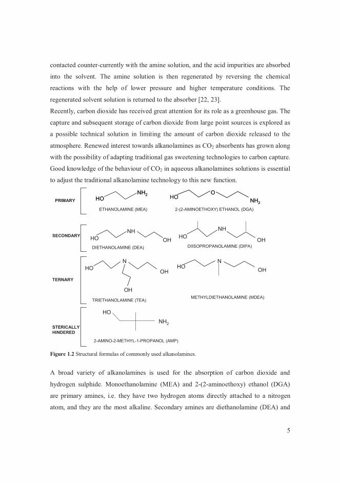
Figure 1.2 Structural formulas of commonly used alkanolamines.

A broad variety of alkanolamines is used for the absorption of carbon dioxide and

hydrogen sulphide. Monoethanolamine (MEA) and 2-(2-aminoethoxy) ethanol (DGA)

are primary amines, i.e. they have two hydrogen atoms directly attached to a nitrogen

atom, and they are the most alkaline. Secondary amines are diethanolamine (DEA) and

PRIMARY

SECONDARY

TERNARY

STERICALLYHINDERED

HONH2

HONH2 HO NH2

OHO NH2

O

ETHANOLAMINE (MEA) 2-(2-AMINOETHOXY) ETHANOL (DGA)

HO OHNH

HO OH

NH

DIETHANOLAMINE (DEA) DIISOPROPANOLAMINE (DIPA)

HO OH

N

OH

HONH2

2-AMINO-2-METHYL-1-PROPANOL (AMP)

TRIETHANOLAMINE (TEA)

HO OHN

METHYLDIETHANOLAMINE (MDEA)

6

diisopropanolamine (DIPA) and ternary amines are triethanolamine (TEA) and

methyldiethanolamine (MDEA) [23]. Sterically hindered amines are also employed in

gas sweetening, in particular 2-amino-2-methyl-1-propanol (AMP). MEA and DEA are

traditionally the most used amines. However, highly concentrated MEA solutions are

avoided in presence of CO2 due to their high aggressiveness towards materials. DEA

forms carbamates when reacting with CO2, therefore its absorption capabilities are

reduced [24]. MDEA is known as a high-capacity selective solvent for H2S in presence of

CO2. The use of amine blends, in particular blends of MDEA with primary amines such

as MEA or AMP, has improved the absorption of MDEA with respect to CO2 [23, 24].

DIPA is primarily utilised in Europe as the solvent amine in the Adip solution of the

Shell Adip process [23]. Even though DIPA has been used for a long time in gas

sweetening, there are relatively few experimental data on aqueous solutions of DIPA in

the open literature. This scarcity of data reflects on the quality of the thermodynamic

models of systems containing DIPA. Thus, among the amines, DIPA was the primary

interest of this research.

In this work, the solubility of CO2 in water + DIPA was measured with two experimental

techniques at various temperatures and compositions of the solvent [III]. Solubility data

of CO2 in water + DIPA were found in Isaacs et al. [25] and in ter Maat et al. [26]. Great

attention was also given to MDEA for its importance in new applications, such as carbon

capture units. The solubility of CO2 in water + MDEA was measured at various

temperatures and solvent compositions. The solubility of CO2 in water + MDEA was

investigated by many research groups at various conditions of temperature and

composition. For this reason, MDEA was also used for validating some of the

experimental techniques developed in this research. In [27-34] were found some data

point at similar experimental conditions than those studied in this work [III].

The thermodynamics of the solvent solutions, i.e. water + alkanolamine, strongly

influences the solubility of CO2, especially at low gas loadings. SLE data are the most

appropriate to calculate the activity coefficients of aqueous alkanolamine solutions at low

amine concentrations. For water + alkanolamine systems, VLE data are valuable mainly

at high temperature and at high amine concentrations [35].This limitation is caused by the

high difference in boiling point and vapour pressure of the system compounds. In this

7

work, the VLE and SLE of water + DIPA and water + MDEA were measured [II]. In

particular, the investigation of VLE data focused on the experimental conditions of

significance for water + alkanolamine systems. The activity coefficients of these

solutions were modelled using the NRTL [36] model, which is particularly suitable for

aqueous systems [37].

Neither VLE nor SLE data of water + DIPA were found in the literature. Only Long and

Yamin [38] published a model for the activity coefficients of this system in the journal of

their university. They fitted the empirical parameters of the NRTL model against their

own VLE measurements, but these data are not given in tabulated form in their article. In

this work, the activity coefficients of water + DIPA were modelled using the measured

VLE and SLE data [II], thus proposing the first model of this sort for water + DIPA.

VLE data points of water + MDEA were available from several sources at low amine

concentrations [39-43]. In this work, VLE measurements were mainly conducted at high

amine concentrations, where VLE data are sufficiently accurate for activity coefficients

modelling. With the exception of Kuwairi [39] and Xu et al. [42], who specifically

studied the vapour pressure of aqueous MDEA solutions, the other data points were the

solvent vapour pressures measured during gas solubility investigations. The SLE of water

+ MDEA was measured by Chang et al. [35]. After the publication of our work [II] also

Fosboel et al. [44] published SLE data for the system of water + MDEA. Several models

of the activity coefficients of water + MDEA were found in the literature, all of them

using the NRTL equations. The regressions of the model parameters were based either

solely on VLE data [45], on VLE and SLE data [35], or on VLE, SLE and excess

enthalpy data [46-48]. In this work, the activity coefficients of water + MDEA were

modelled using VLE, SLE and excess enthalpy data [II].

It was noticed that many literature models of the Henry’s law constant of CO2 in aqueous

solutions of alkanolamines deviated at high temperatures from the experimental

measurements. This is a source of error in describing the solubility of CO2 in these

solvents. Therefore, a model of the Henry’s law constant of CO2 in aqueous solutions of

alkanolamines, and alkanolamine blends was developed [I]. The performances and

strengths of this model were evidenced by comparison with similar models found in the

literature [49-55].

8

A comprehensive thermodynamic model of the solubility of CO2 in alkanolamine

solutions can be developed in the future, based on the achievements of this research

work. In fact, after the publication of [II] and [III] Zong et al. [56] used this work to

extend their CO2 solubility model to aqueous solutions of DIPA, thus confirming the

importance of these data in the development of thermodynamic modelling of

alkanolamine solutions.

9

2 Thermodynamic principles

2.1 Phase-equilibrium thermodynamic

Phase-equilibrium thermodynamic describes the equilibrium distribution of the

components among the phases present in the system [57]. Phase-equilibrium

thermodynamic is extensively treated in [1, 37, 57, 58]. A short summary is here

presented, with focus on the equations used in this work.

For any species i in a mixture, the condition of thermodynamic equilibrium between two

phases � and � can be written in terms of fugacities as in:

Eq. 2.1 �ii ff ˆˆ �

2.1.1 Vapour-liquid equilibrium (VLE)

In the case of VLE, Eq. 2.1 becomes:

Eq. 2.2 Li

Vi ff ˆˆ �

The fugacity of component i in vapour phase is expressed in terms of fugacity

coefficients Vi�̂ according to:

Eq. 2.3 Pxf Vi

Vi

Vi �̂ˆ �

Equivalently, the fugacity of a component i in liquid phase can be described as a function

of the liquid phase fugacity coefficient Li�̂ .

Eq. 2.4 Pxf Li

Li

L �̂ˆ �

When both the vapour and the liquid phase fugacities are calculated from the fugacity

coefficients (� -� approach), the basic VLE equation (Eq. 2.2) becomes:

Eq. 2.5 Li

Li

Vi

Vi xx �� ˆˆ �

An alternative procedure results when the liquid phase fugacities are eliminated in favour

of the activity coefficients, i.e. the � -� approach used in this work. The fugacity of

component i in the liquid phase is expressed as a function of the activity coefficient Li�̂

and of the standard state fugacity �,Lif , chosen as the fugacity of the pure liquid i at the

system temperature and pressure.

10

Eq. 2.6 �,ˆˆ Li

Li

Li

Li fxf ��

The standard state fugacity depends on the vapour pressure of pure component i at the

system temperature ( SatiP ), and on the saturated liquid fugacity coefficient of the pure

component i ( SatLi

,� ) at the system temperature. The effect on the liquid fugacity of the

difference between the system pressure and the vapour pressure is represented by the

exponential term in Eq. 2.7, i.e. the Poynting pressure correction. The basic VLE

equation given in Eq. 2.2 thus becomes:

Eq. 2.7 ��

�

�

��

�

�� �

P

P

Li

SatLi

Sati

Li

Li

Vi

Vi

Sati

VRT

PxPx 1expˆˆ ,���

The Poynting correction is calculated from the molar volume of component i in the liquid

phase. In this work, the molar volume was obtained from the Rackett equation of state

(EOS) [59].

2.1.2 Gas- liquid equilibrium (GLE)

Gas-liquid equilibrium (GLE, also called gas solubility) is a particular case of vapour-

liquid equilibrium, where at least one of the components is in supercritical state.

Equivalently to the case of VLE, the � -� approach can be used for GLE [1].

The equilibrium equation for the subcritical component i is given by Eq. 2.7, when the

standard state fugacity is chosen as the fugacity of the pure liquid i at the system

temperature and pressure. The GLE equation for the supercritical compound j is

Eq. 2.8 ���

���� �

P

P

LjSjj

Lj

Vj

Vj Sat

j

VRT

HxPx 1expˆˆ,

*��

The activity coefficient of species i is normally defined according to the symmetric

normalisation, i.e. 1ˆ �i� when 1�Lix or, in other words, the activity coefficient of i

approaches unity when i becomes pure. In this case the standard state fugacity may be

regarded as the normalising factor, according to Eq. 2.6.

Eq. 2.9 LjSj

idLj xHf ,

,ˆ �

Eq. 2.10 Sj

Lj

Lj

j Hxf

,

*ˆ

ˆ ��

11

For a solute j, whose ideal behaviour is described based on Henry’s law (Eq. 2.9), the

activity coefficient *ˆ j� is normalised using the Henry’s law constant SjH , , as shown in

Eq. 2.10. In this case, the activity coefficient is called unsymmetric, and it approaches

unity when species j becomes infinitely diluted, i.e. 1ˆ* �j� when 0�Ljx .

Unsymmetrically and symmetrically normalised activity coefficients are completely

interconvertible by means of the infinite dilution activity coefficient �i�̂ .

Eq. 2.11 ��i

ii �

��

ˆˆˆ*

The unsymmetrically normalised activity coefficients are normally used for solutes,

supercritical compounds, and ions in electrolyte systems.

The Henry’s law constant is specific for a solute in a certain solvent (S). For single

solvents, the Henry’s law constant is a function of temperature. For multicomponent

solvents, the Henry’s law constant may depend not only on temperature, but also on the

composition of the solvent.

2.1.3 Solid-liquid equilibrium (SLE)

In the case of SLE, Eq. 2.1 becomes:

Eq. 2.12 Li

Si ff ˆˆ �

The liquid phase fugacity is described by Eq. 2.6. The solid phase fugacity is a function

of the standard state fugacity �,Sif and of the solid phase activity coefficient S

i�̂ .

Eq. 2.13 �,ˆˆ Si

Si

Si

Si fxf ��

Eq. 2.12 thus becomes:

Eq. 2.14 �� ,, ˆˆ Li

Li

Li

Si

Si

Si fxfx �� �

In this work, Eq. 2.14 was simplified into Eq. 2.17 according to [37, 60]. In most systems

the pure solid crystallises out, thus the fugacity of the solid phase at equilibrium can be

replaced by the fugacity of the pure solid, i.e. 1ˆ �Si

Six � [60]. The ratio of the standard

state fugacities can be evaluated from the conditions at the triple point by applying Eq.

2.15 to each phase. These considerations transform Eq. 2.14 into Eq. 2.16, when the

volume difference V� is assumed independent of pressure.

12

Eq. 2.15 dPRT

VdTRT

Hfd ��

��� 2ln

Eq. 2.16 � �itpitpitpip

itp

itpL

i

Si PP

RTV

TT

TT

Rc

TTRH

ff

,,,,

,

,,

,

1ln11ln ��

����

����

���

���

��

����

��

��

�

�

Eq. 2.16 is considerably simplified when the following assumptions apply:

1. The triple point temperatures are substituted with the melting point temperatures.

Triple point temperatures are usually very nearly the same as atmospheric melting

points, and the latter are more often known [37].

2. The pressure correction is considered negligible, which is usually the case [37].

3. The heat-capacity correction is dropped since it is small in the vicinity of the

melting point [37, 60].

The activity coefficient of component i in liquid phase can therefore be directly

calculated from melting point data as follows:

Eq. 2.17 � � ���

����

��

���

ifus

ifusLi

Li T

TRTH

x,

, 1ˆln �

13

2.2 Fugacity coefficients

The evaluation of the fugacity coefficient of component i in vapour phase requires the

availability of a PVT EOS, i.e. an equation in the form � � 0,, �TVPf describing the

volumetric behaviour of i as a function of pressure and temperature. In fact, the fugacity

coefficient can be expressed according to Eq. 2.18 as a function of the compressibility

factor Z.

Eq. 2.18 � �� ��P

iVi P

dPZ0

1ˆln�

In this work, the virial equation of state was used in [III]; otherwise the Soave-Redlich-

Kwong (SRK) was the chosen EOS [II, IV, V]. The virial EOS [1] is either volume-

explicit (the virial equation in pressure) or pressure-explicit (the virial equation in

density). In this work, the density form of the virial equation was used.

The Soave-Redlich-Kwong (SRK) [37, 61] equation of state is the modification made by

Soave of the Redlich-Kwong (RK) [62] EOS. Soave improved the performances of the

RK EOS by developing the dependence on temperature of the attractive parameter a .

Soave multiplied the RK � �,Ta with a new temperature dependent parameter SRK� .

When the SRK EOS is applied to a mixture, mixing rules are used to calculate the EOS

parameters. In this work, linear mixing rules were used for the co-volume parameters b

(Eq. 2.19) and quadratic mixing rules for the attractive parameters a (Eq. 2.20 and Eq.

2.21). The binary interaction parameters ijk were set to zero.

Eq. 2.19 ��

�N

ii

Vi bxb

1

ˆ

Eq. 2.20 � ���� �

�N

i

N

jijSRK

Vj

ViSRK axxa

1 1

ˆˆ ��

Eq. 2.21 � � � � � � � � jSRKiSRKijijSRK aaka ��� �� 1

2.3 Activity coefficients

Activity coefficients are determined principally from phase-equilibrium measurements, in

particular from vapour-liquid and liquid-liquid equilibrium data [37]. Freezing point

14

depression data (SLE) are also used in special cases, such as the alkanolamine-water

systems, in which one of the components has very low vapour pressure [35].

There are many equations correlating activity coefficients with composition mostly using

mole fractions ix , but occasionally also volume fractions i� . Sometimes, activity

coefficients are also expressed as a function of temperature.

In design of chemical units, semi-empirical models with a small amount of parameters

are often preferred. Commonly used activity coefficients models are the Wilson [63], the

NRTL [36] and the UNIQUAC [64]. The superiority of one method over the others is not

always clear, and it often depends on the chemical system. Among these three semi-

empirical models, the Wilson model better describes the greatest amount of chemical

systems, while NRTL better describes aqueous systems [37].

If the experimental data for a specific system are scarce, the activity coefficients can be

calculated by means of predictive methods. The UNIFAC [65] and UNIFAC-Dortmund

[66] models are commonly used. They are based on the group contribution theory, which

states that many properties of complex molecules can be approximated assuming that a

smaller group of atoms within the molecule contributes to that property in a fixed way.

The group contributions are optimised using a large amount of experimental data. The

original UNIFAC and the UNIFAC-Dortmund differ in the values of the group

contributions. The group contributions for the UNIFAC models used in this work were

updated until the work by Wittig et al. [67], while in the case of the UNIFAC-Dortmund

until Gmehling et al. [68].

Another predictive approach is that of COSMO-RS [69] and COSMO-SAC [70].

COSMO-RS treats the molecules as a unity, in opposition to the group contribution

theory. The molecule surface is charged and the charge density is calculated via quantum

mechanical calculations. The interactions between surfaces are statistically estimated.

COSMO-SAC is a modification of COSMO-RS that predicts the intermolecular

interactions based on the molecular structure with the help of a few adjustable

parameters.

All of the above mentioned models were used at various extents, but the non-random

two-liquid model (NRTL) [36] model was especially important in this work. In fact,

NRTL is particularly suitable for describing aqueous systems [37], and it was

15

successfully applied by many research groups in modelling aqueous systems of

alkanolamines [35, 45-48]. For these reasons, the NRTL model was used in this work to

describe the activity coefficients of water +DIPA and water + MDEA.

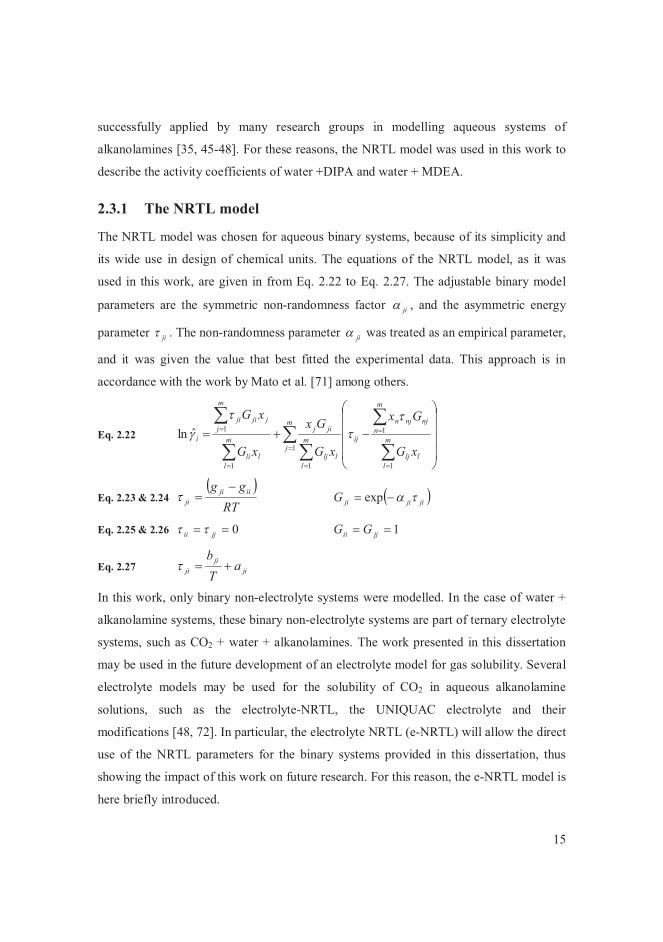
2.3.1 The NRTL model

The NRTL model was chosen for aqueous binary systems, because of its simplicity and

its wide use in design of chemical units. The equations of the NRTL model, as it was

used in this work, are given in from Eq. 2.22 to Eq. 2.27. The adjustable binary model

parameters are the symmetric non-randomness factor ji� , and the asymmetric energy

parameter ji . The non-randomness parameter ji� was treated as an empirical parameter,

and it was given the value that best fitted the experimental data. This approach is in

accordance with the work by Mato et al. [71] among others.

Eq. 2.22 ��

�

��

��

�

�

��

�

����

�

�

����

�

�

���m

jm

lllj

m

nnjnjn

ijm

lllj

jijm

llli

m

jjjiji

i

xG

Gx

xG

Gx

xG

xG

1

1

1

11

1ˆln

�

Eq. 2.23 & 2.24 � �

RTgg iiji

ji

�� � �jijijiG ��� exp

Eq. 2.25 & 2.26 0�� jjii 1�� jjii GG

Eq. 2.27 jiji

ji aTb

��

In this work, only binary non-electrolyte systems were modelled. In the case of water +

alkanolamine systems, these binary non-electrolyte systems are part of ternary electrolyte

systems, such as CO2 + water + alkanolamines. The work presented in this dissertation

may be used in the future development of an electrolyte model for gas solubility. Several

electrolyte models may be used for the solubility of CO2 in aqueous alkanolamine

solutions, such as the electrolyte-NRTL, the UNIQUAC electrolyte and their

modifications [48, 72]. In particular, the electrolyte NRTL (e-NRTL) will allow the direct

use of the NRTL parameters for the binary systems provided in this dissertation, thus

showing the impact of this work on future research. For this reason, the e-NRTL model is

here briefly introduced.

16

The e-NRTL [73-79]. has been extensively used for aqueous strong electrolytes and

aqueous organic electrolytes, for weak electrolytes, strong acids and mixes solvent

electrolytes. The e-NRTL was applied by many researchers to model the activity

coefficients of sour gases + water + alkanolamines systems (e.g. [34, 45, 54, 80]). The

original e-NRTL model is continuously revised and improved, when applied to sour gas

systems [48]).

In the case of mixed-solvent solutions, the electrolyte NRTL model describes the excess

Gibbs energy as the sum of three contributions. The short-range species interactions are

described using the non-random two-liquid approach [73], the Pitzer-Debye-Hückel [81]

formula is used to account for the long-range electrostatic interactions, and the Born

equation [82] is utilized to model the Gibbs free energy of transfer of the ionic species

from the infinite dilution state in a mixed solvent to the infinite dilution state in the

aqueous phase [79]. The short-range interaction model assumes that there are three types

of local composition interactions. The first type has a molecule as the central species

interacting with other molecular species, cationic species or anionic species. The other

two types of interactions have ether an anion or a cation as the central species. The

surrounding species are either molecules or oppositely charged ions [76]. The models

adjustable parameters are the same as in the NRTL model, i.e. the symmetric non-

randomness factor ji� , and the asymmetric energy parameter ji . The species i and j

derive from the model interactions leading to three types of binary parameters: molecule-

molecule, molecule-electrolyte and electrolyte-electrolyte parameters [76].

The activity coefficients of the binary sub-system of water + alkanolamine have a strong

influence on the predictions of the solubility of CO2 or H2S in alkanolamine solvents,

especially at low gas absorption levels. While modelling the solubility of sour gases in

alkanolamine solutions, the NRTL parameters of the binary system of water +

alkanolamine can be used in the e-NRTL models to describe the interaction between the

solvent molecules. In fact, the e-NRTL reduces to the standard NRTL model if applied to

non-electrolytic systems.

17

3 Experimental procedures

In this work, several experimental methods were employed to measure phase equilibria of

various systems. A static total pressure apparatus was used to measure the binary VLE of

butane in alcohols (methanol, 2-propanol, 1-butanol, 2-butanol and 2-methyl-2-propanol)

[V], and of diethyl sulphide in C4 -hydrocarbons (1-butene, cis-2-butene, 2-

methylpropane, 2-methylpropene, n-butane, trans-2-butene) [IV]. The same equipment

was then modified to measure the VLE of water + DIPA and water + MDEA at high

amine contents [II].

Another static total pressure apparatus, suitable for gas solubility measurements, was

constructed, and the solubility of carbon dioxide in water + DIPA was measured. The

same equipment also simultaneously measured the density of the carbonated aqueous

solvent. The solubility of CO2 in water + DIPA and water + MDEA was also measured at

atmospheric pressure with a bubbling apparatus developed and constructed in this work.

The solubility data obtained with the two techniques were compared against each other,

and against literature data [III].

The SLE of water + DIPA and water + MDEA was measured with two experimental

procedures, i.e. by means of a Differential Scanning Calorimeter (DSC), and with a

method based on the visual observation of the melting point (visual method). The DSC

was also used to measure the enthalpy of fusion of pure DIPA. The two experimental

techniques for SLE measurements were validated against literature data, and their

performances were compared with each other [II].

3.1 Vapour-Liquid Equilibrium measurements

3.1.1 Static total pressure apparatus for VLE measurements

The main feature of a static total pressure apparatus is that VLE data of binary systems

are measured without the analysis of the equilibrium composition of the two phases. The

equilibrium compositions of the liquid and vapour phase are calculated from the

measured temperatures, pressures, and initial compositions, in addition to the dimensions

of the equipment.

18

The experimental set-up and procedure used in this work were the same that were used

by Uusi-Kyyny et al. [83]. A schematic representation of the equipment is given in [IV]

and [V]. For the measurements of the systems of C4 -hydrocarbons + diethyl sulphide the

original equilibrium cell (AISI 316L) was substituted with a cell made of Hastelloy C-

276 to avoid corrosion. The cell was sealed with a gold plated pressurised stainless steel

o-ring.

For each binary system, the VLE curve was constructed by measuring the equilibrium

points starting from both ends of the composition range. In practice, a pre-calculated

amount of component 1 was injected to the equilibrium cell via a syringe pump.

Subsequent additions of component 2 were made with a second syringe pump until the

point of equimolarity was reached. The measurement then continued by repeating the

same procedure starting from component 2 with subsequent additions of component 1.

The coincidence of the two half-curves at equimolar composition was a clear indication

of the success of the measurement.

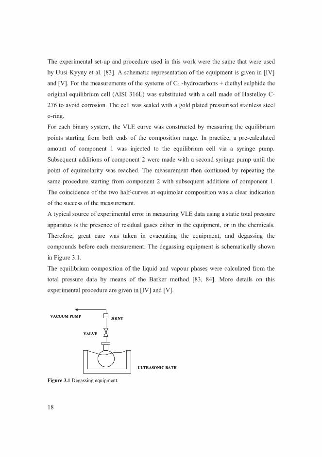
A typical source of experimental error in measuring VLE data using a static total pressure

apparatus is the presence of residual gases either in the equipment, or in the chemicals.

Therefore, great care was taken in evacuating the equipment, and degassing the

compounds before each measurement. The degassing equipment is schematically shown

in Figure 3.1.

The equilibrium composition of the liquid and vapour phases were calculated from the

total pressure data by means of the Barker method [83, 84]. More details on this

experimental procedure are given in [IV] and [V].

Figure 3.1 Degassing equipment.

ULTRASONIC BATH

VALVE

JOINTVACUUM PUMP

ULTRASONIC BATH

VALVE

JOINTVACUUM PUMP

19

3.1.2 Modifications of the static total pressure apparatus for VLE

measurements of aqueous alkanolamine systems

The same static total pressure apparatus described in 3.1.1 was used to measure water +

alkanolamine systems with some modifications in set-up and procedure. Total pressure

VLE of water + alkanolamine systems is accurate only at high amine concentrations, due

to the extremely low vapour pressure of alkanolamines [35]. For this reason, the

measurements did not cover the whole composition range, but they were conducted only

starting from pure alkanolamines and subsequently adding water. The pre-calculated

amount of alkanolamine, i.e. DIPA or MDEA, was manually fed to the equilibrium cell

with a syringe, which was accurately weighted before and after injection. The use of a

syringe pump was discouraged by the high viscosity of the amines. DIPA is a solid at

room temperature; therefore it was heated above its melting point, i.e. KT fus 8.315� ,

prior to feeding. The amines were degassed when in the equilibrium cell. Subsequent

injections of water were performed with a syringe pump, and the VLE curve was

constructed. Details on this experimental procedure are given in [II].

3.2 Gas Liquid Equilibrium (GLE) measurements

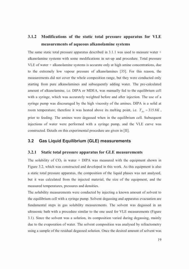
3.2.1 Static total pressure apparatus for GLE measurements

The solubility of CO2 in water + DIPA was measured with the equipment shown in

Figure 3.2, which was constructed and developed in this work. As this equipment is also

a static total pressure apparatus, the composition of the liquid phases was not analysed,

but it was calculated from the injected material, the size of the equipment, and the

measured temperatures, pressures and densities.

The solubility measurements were conducted by injecting a known amount of solvent to

the equilibrium cell with a syringe pump. Solvent degassing and apparatus evacuation are

fundamental steps in gas solubility measurements. The solvent was degassed in an

ultrasonic bath with a procedure similar to the one used for VLE measurements (Figure

3.1). Since the solvent was a solution, its composition varied during degassing, mainly

due to the evaporation of water. The solvent composition was analysed by refractometry

using a sample of the residual degassed solution. Once the desired amount of solvent was

20

in the cell, CO2 was added and the equilibrium point was measured, i.e. the equilibrium

temperature and pressure in the cell were measured. The amount of injected gas was

calculated from the pressure in the CO2 feed cylinder, which was measured before and

after the gas injection. The system was considered at equilibrium when the pressure in the

cell was constant for at least 1.5 h. Even under vigorous stirring, the system took about 4

h to reach equilibrium. The solubility curves were constructed at constant temperature by

subsequent gas additions. The experimental run was concluded at a total pressure of ca. 1

MPa, in order to comply with the range of the pressure transducer situated in the

equilibrium cell. More details on the experimental procedure and on the instrumentation

are given in [III].

Figure 3.2 Static total pressure apparatus: (1) 250 cm3 round bottom flask for amine solution feed to the syringe pump; (2) 260 cm3 syringe pump; (3) circular bath controlling the temperature of the syringe pump; (4) oven (bottom hole Ø= 10 cm, side hole Ø= 2.5 cm); (5) equilibrium cell; (6) CO2 feed cylinder; (7) density meter; (8) circular bath controlling the temperature of the density meter; � recirculation lines; —water lines; T1, T2, T3 and T4 temperature probes, P1 and P2 pressure transducers.

21

As it is customary in alkanolamine systems (e.g. [25, 26, 40] ), the solubility of CO2 in

the aqueous solvents was expressed as loading (�):

Eq. 3.1 � = moles of absorbed CO2 / moles of amine

In calculating this quantity from the measured variables, it was assumed that the amount

of moles of alkanolamine in the liquid phase was constant during the experimental run,

and it was equal to the amount of moles of amine in the degassed solvent. This

assumption is justified by the low vapour pressure of alkanolamines [23, 85]. The virial

equation of state [1] in density truncated to the third virial coefficient was used to

calculate the moles of CO2, as it is described in [III]. The mole fraction of CO2 in the

liquid phase was also estimated for comparison purposes.

The experimental method was validated by measuring the solubility of CO2 in water at

298.57 K. Our results were compared with literature data [86-92] in terms of Henry’s law

constant of CO2 in water ( WH ,1 ), and of mole fraction of CO2 in the liquid phase ( Lx1 ).

These quantities were calculated from the measured variables according to the � - �

model for the reduction and correlation of solubility data by Van Ness and Abbott [1] for

single solute / single solvent systems. In the approach by van Ness and Abbott [1], some

assumptions are suggested in order to simplify the basic GLE equation, i.e. Eq. 2.8, thus

facilitating the data reduction procedure. The Poynting correction and the activity

coefficient of the solvent were assumed equal to unity. The molar volume LV1 of the

solute was assumed constant, and equal to the infinite dilution molar volume �,1

LV ,

according to the Krichevsky-Kasarnovsky [93] correction. Eq. 2.8 thus becomes

Eq. 3.2 � �RT

PPVHxPxsatL

WLVV 1

,1

,1*1111 expˆ �

��

��

The unsymmetric activity coefficient of the solute was modelled according to Eq. 3.3, as

suggested by van Ness and Abbott [1].

Eq. 3.3 � � � �� �1ln 22

*1 �� LxA�

The Henry’s law constant of CO2 in water measured in this work was 5.9 MPa smaller

than that of Fonseca et al. [86], while it agreed with all the other sources [87-91] within

the experimental uncertainty. In terms of mole fraction, the maximum deviation between

22

our work and the data found in the literature [91, 92] was of 0.00012 with the work by

Carroll et al. [91]. The results of the validation are reported in [III].

3.2.2 Bubbling apparatus

The solubility of CO2 in aqueous solutions of water + DIPA and water + MDEA at

atmospheric pressure was measured at various temperatures and solvent compositions

with a bubbling apparatus. The apparatus and the associated analytic technique were

developed is this work, based on the volumetric calcimeter suggested by Loeppert and

Suarez [94], and on the bubbling cell described by Hovorka and Dohnal [95].

A schematic representation of the equipment is given in Figure 3.3. The bubbling cell

was composed of a presaturator and the equilibrium cell, also indicated as dilution cell.

The function of the presaturator, which was filled with distilled water, was to wet the gas

in order to keep constant the amount of solvent in the dilution cell. The measurements

with the bubbling apparatus were isobaric. An alkanolamine solution of known

composition was filled into the dilution cell, and the temperature was stabilised to the

desired value by means of a water bath that circulated water through the jacket of the

bubbling cell. CO2 was bubbled through the alkanolamine solution via the presaturator

until the solution reached saturation. It was found with preliminary tests that the time to

reach equilibrium with the bubbling equipment depended on the temperature and on the

composition of the solvent, and it could be up to 2 weeks. At saturation, the temperature

and pressure were recorded, and 3-4 samples of the saturated solution were taken for

analysis with the volumetric calcimeter (Figure 3.4). Another equilibrium point was then

measured by changing the temperature.

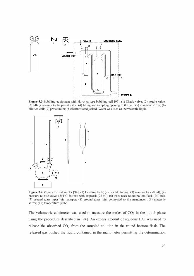
23

Figure 3.3 Bubbling equipment with Hovorka-type bubbling cell [95]. (1) Check valve; (2) needle valve; (3) filling opening to the presaturator; (4) filling and sampling opening to the cell; (5) magnetic stirrer; (6) dilution cell; (7) presaturator; (8) thermostated jacked. Water was used as thermostatic liquid.

Figure 3.4 Volumetric calcimeter [94]. (1) Leveling bulb; (2) flexible tubing; (3) manometer (50 ml); (4) pressure release valve; (5) HCl burette with stopcock (25 ml); (6) three-neck round-bottom flask (250 ml); (7) ground glass taper joint stopper; (8) ground glass joint connected to the manometer; (9) magnetic stirrer; (10) temperature probe.

The volumetric calcimeter was used to measure the moles of CO2 in the liquid phase

using the procedure described in [94]. An excess amount of aqueous HCl was used to

release the absorbed CO2 from the sampled solution in the round bottom flask. The

released gas pushed the liquid contained in the manometer permitting the determination

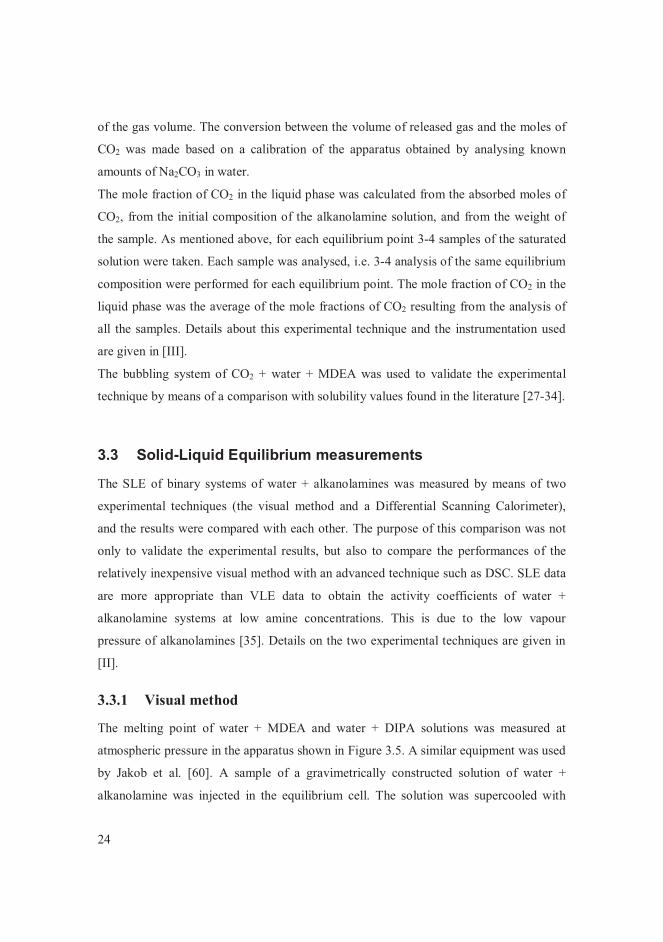
24

of the gas volume. The conversion between the volume of released gas and the moles of

CO2 was made based on a calibration of the apparatus obtained by analysing known

amounts of Na2CO3 in water.

The mole fraction of CO2 in the liquid phase was calculated from the absorbed moles of

CO2, from the initial composition of the alkanolamine solution, and from the weight of

the sample. As mentioned above, for each equilibrium point 3-4 samples of the saturated

solution were taken. Each sample was analysed, i.e. 3-4 analysis of the same equilibrium

composition were performed for each equilibrium point. The mole fraction of CO2 in the

liquid phase was the average of the mole fractions of CO2 resulting from the analysis of

all the samples. Details about this experimental technique and the instrumentation used

are given in [III].

The bubbling system of CO2 + water + MDEA was used to validate the experimental

technique by means of a comparison with solubility values found in the literature [27-34].

3.3 Solid-Liquid Equilibrium measurements

The SLE of binary systems of water + alkanolamines was measured by means of two

experimental techniques (the visual method and a Differential Scanning Calorimeter),

and the results were compared with each other. The purpose of this comparison was not

only to validate the experimental results, but also to compare the performances of the

relatively inexpensive visual method with an advanced technique such as DSC. SLE data

are more appropriate than VLE data to obtain the activity coefficients of water +

alkanolamine systems at low amine concentrations. This is due to the low vapour

pressure of alkanolamines [35]. Details on the two experimental techniques are given in

[II].

3.3.1 Visual method

The melting point of water + MDEA and water + DIPA solutions was measured at

atmospheric pressure in the apparatus shown in Figure 3.5. A similar equipment was used

by Jakob et al. [60]. A sample of a gravimetrically constructed solution of water +

alkanolamine was injected in the equilibrium cell. The solution was supercooled with

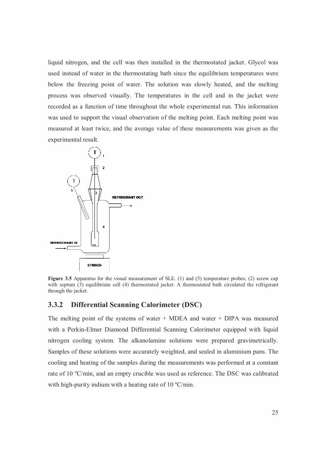
25

liquid nitrogen, and the cell was then installed in the thermostated jacket. Glycol was

used instead of water in the thermostating bath since the equilibrium temperatures were

below the freezing point of water. The solution was slowly heated, and the melting

process was observed visually. The temperatures in the cell and in the jacket were

recorded as a function of time throughout the whole experimental run. This information

was used to support the visual observation of the melting point. Each melting point was

measured at least twice, and the average value of these measurements was given as the

experimental result.

Figure 3.5 Apparatus for the visual measurement of SLE. (1) and (5) temperature probes; (2) screw cap with septum (3) equilibrium cell (4) thermostated jacket. A thermostated bath circulated the refrigerant through the jacket.

3.3.2 Differential Scanning Calorimeter (DSC)

The melting point of the systems of water + MDEA and water + DIPA was measured

with a Perkin-Elmer Diamond Differential Scanning Calorimeter equipped with liquid

nitrogen cooling system. The alkanolamine solutions were prepared gravimetrically.

Samples of these solutions were accurately weighted, and sealed in aluminium pans. The

cooling and heating of the samples during the measurements was performed at a constant

rate of 10 ºC/min, and an empty crucible was used as reference. The DSC was calibrated

with high-purity indium with a heating rate of 10 ºC/min.

26

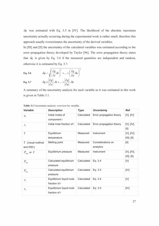
3.4 Estimation of the experimental uncertainty

No measurement, however carefully made, can be completely free of uncertainties. In

this work, great importance was given to the estimation of uncertainties, not only for

measured quantities, but also for the calculated variables that were derived from the

measured quantities.

When possible, the uncertainty of a measured variable was identified with the uncertainty

of the instrument that measured it. Not only the instrument resolution and accuracy, but

also its calibration contributed to the uncertainty of the instrument. This definition of

uncertainty applied to all the temperatures, pressures, densities and volumes measured

during VLE and GLE experiments. In some cases, a quantity is not directly measured

with an instrument, but it results from the interpretation of the response of an analytical

technique. This was the case of the mole fractions analysed with the volumetric

calcimeter, and of the melting points measured with the DSC and the visual method. The

uncertainty of these variables was estimated based on considerations that were specific to

the analytical technique.

Due to the characteristics of the experimental methods, the composition of the vapour and

of the liquid phase in VLE measurements, and the gas solubility in GLE measurements

were calculated quantities. In [V] the uncertainty q� of a derived variable ),....,( usqq �

was estimated by calculating 'q when all the measured variables ),....,( us assumed their

minimum ),....,( uuusss �� ���� �� or their maximum values

),....,( uuusss �� ���� �� . The uncertainty of the calculated variable was the

maximum deviation between q and 'q according to Eq. 3.4.

Eq. 3.4 � � � ����� ��� usqqusqqq ,....,;,....,max ''�

This method gives an estimate of q� , but it does not necessarily calculate the absolute

maximum uncertainty. The absolute maximum uncertainty was obtained when the matrix

of all the possible combinations of the values assumed by the measured variables was

constructed, i.e. q� was calculated according to Eq. 3.5.

Eq. 3.5 � � � � � � � �;...,....,;,....,;,....,;,....,max '''' �������� ����� usqqusqqusqqusqqq�

27

q� was estimated with Eq. 3.5 in [IV]. The likelihood of the absolute maximum

uncertainty actually occurring during the experimental work is rather small; therefore this

approach usually overestimates the uncertainty of the derived variables.

In [III] and [II] the uncertainty of the calculated variables was estimated according to the

error propagation theory developed by Taylor [96]. The error propagation theory states

that q� is given by Eq. 3.6 if the measured quantities are independent and random,

otherwise it is estimated by Eq. 3.7.

Eq. 3.6 22

... ���

���

��

�����

���

��

� uuqs

sqq ���

Eq. 3.7 uuqs

sqq ��� �

�����

��� ...

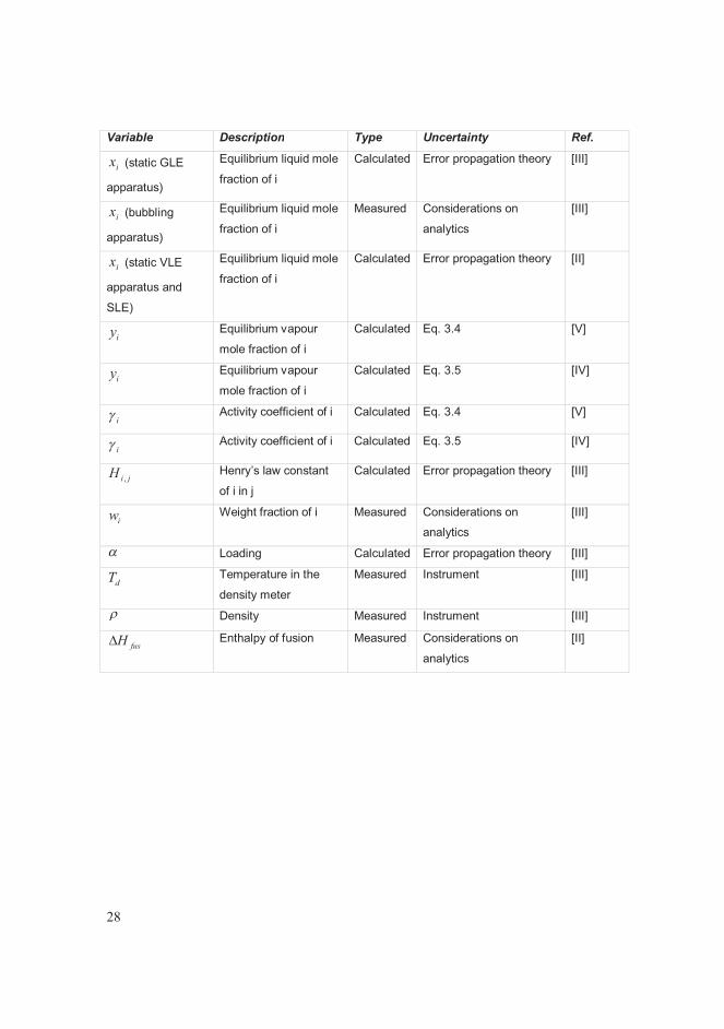
A summary of the uncertainty analysis for each variable as it was estimated in this work

is given in Table 3.1.

Table 3.1 Uncertainty analysis: overview by variable.

Variable Description Type Uncertainty Ref.

in Initial moles of

component i

Calculated Error propagation theory [V], [IV]

iz Initial mole fraction of i Calculated Error propagation theory [V], [IV],

[II]

T Equilibrium

temperature

Measured Instrument [V], [IV];

[III]; [II]

T (visual method

and DSC)

Melting point Measured Considerations on

analytics

[II]

expP or P Equilibrium pressure Measured Instrument [V], [IV],

[III], [II]

legP Calculated equilibrium

pressure

Calculated Eq. 3.4 [V]

legP Calculated equilibrium

pressure

Calculated Eq. 3.5 [IV]

ix Equilibrium liquid mole

fraction of i

Calculated Eq. 3.4 [V]

ix Equilibrium liquid mole

fraction of i

Calculated Eq. 3.5 [IV]

28

Variable Description Type Uncertainty Ref.

ix (static GLE

apparatus)

Equilibrium liquid mole

fraction of i

Calculated Error propagation theory [III]

ix (bubbling

apparatus)

Equilibrium liquid mole

fraction of i

Measured Considerations on

analytics

[III]

ix (static VLE

apparatus and

SLE)

Equilibrium liquid mole

fraction of i

Calculated Error propagation theory [II]

iy Equilibrium vapour

mole fraction of i

Calculated Eq. 3.4 [V]

iy Equilibrium vapour

mole fraction of i

Calculated Eq. 3.5 [IV]

i� Activity coefficient of i Calculated Eq. 3.4 [V]

i� Activity coefficient of i Calculated Eq. 3.5 [IV]

jiH ,Henry’s law constant

of i in j

Calculated Error propagation theory [III]

iw Weight fraction of i Measured Considerations on

analytics

[III]

� Loading Calculated Error propagation theory [III]

dT Temperature in the

density meter

Measured Instrument [III]

� Density Measured Instrument [III]

fusH� Enthalpy of fusion Measured Considerations on

analytics

[II]

29

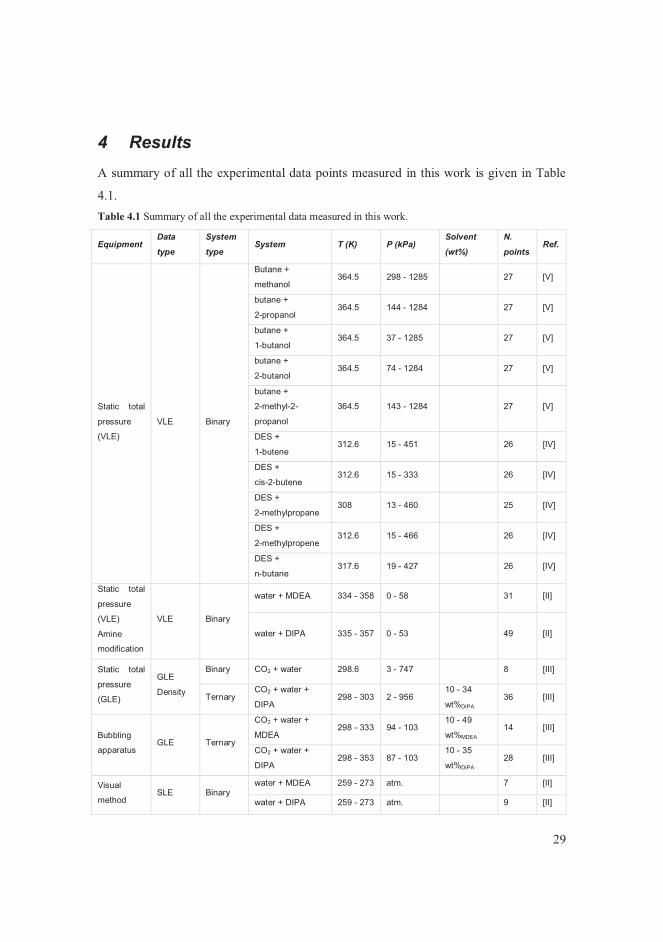
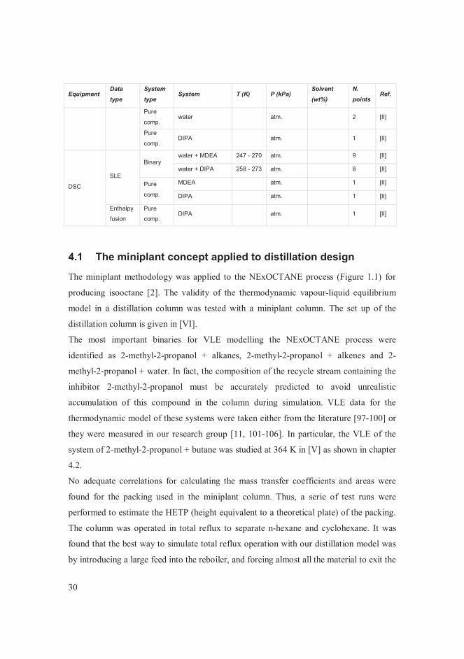
4 Results A summary of all the experimental data points measured in this work is given in Table

4.1.Table 4.1 Summary of all the experimental data measured in this work.

Equipment Data

type

System

type System T (K) P (kPa)

Solvent

(wt%)

N.

points Ref.

Static total

pressure

(VLE)

VLE Binary

Butane +

methanol 364.5 298 - 1285 27 [V]

butane +

2-propanol 364.5 144 - 1284 27 [V]

butane +

1-butanol 364.5 37 - 1285 27 [V]

butane +

2-butanol 364.5 74 - 1284 27 [V]

butane +

2-methyl-2-

propanol

364.5 143 - 1284 27 [V]

DES +

1-butene 312.6 15 - 451 26 [IV]

DES +

cis-2-butene 312.6 15 - 333 26 [IV]

DES +

2-methylpropane 308 13 - 460 25 [IV]

DES +

2-methylpropene 312.6 15 - 466 26 [IV]

DES +

n-butane 317.6 19 - 427 26 [IV]

Static total

pressure

(VLE)

Amine

modification

VLE Binary

water + MDEA 334 - 358 0 - 58 31 [II]

water + DIPA 335 - 357 0 - 53 49 [II]

Static total

pressure

(GLE)

GLE

Density

Binary CO2 + water 298.6 3 - 747 8 [III]

Ternary CO2 + water +

DIPA 298 - 303 2 - 956

10 - 34

wt%DIPA36 [III]

Bubbling

apparatus GLE Ternary

CO2 + water +

MDEA 298 - 333 94 - 103

10 - 49

wt%MDEA14 [III]

CO2 + water +

DIPA 298 - 353 87 - 103

10 - 35

wt%DIPA28 [III]

Visual

method SLE Binary

water + MDEA 259 - 273 atm. 7 [II]

water + DIPA 259 - 273 atm. 9 [II]

30

Equipment Data

type

System

type System T (K) P (kPa)

Solvent

(wt%)

N.

points Ref.

Pure

comp. water atm. 2 [II]

Pure

comp. DIPA atm. 1 [II]

DSC

SLE

Binary water + MDEA 247 - 270 atm. 9 [II]

water + DIPA 258 - 273 atm. 8 [II]

Pure

comp.

MDEA atm. 1 [II]

DIPA atm. 1 [II]

Enthalpy

fusion

Pure

comp. DIPA atm. 1 [II]

4.1 The miniplant concept applied to distillation design

The miniplant methodology was applied to the NExOCTANE process (Figure 1.1) for

producing isooctane [2]. The validity of the thermodynamic vapour-liquid equilibrium

model in a distillation column was tested with a miniplant column. The set up of the

distillation column is given in [VI].

The most important binaries for VLE modelling the NExOCTANE process were

identified as 2-methyl-2-propanol + alkanes, 2-methyl-2-propanol + alkenes and 2-

methyl-2-propanol + water. In fact, the composition of the recycle stream containing the

inhibitor 2-methyl-2-propanol must be accurately predicted to avoid unrealistic

accumulation of this compound in the column during simulation. VLE data for the

thermodynamic model of these systems were taken either from the literature [97-100] or

they were measured in our research group [11, 101-106]. In particular, the VLE of the

system of 2-methyl-2-propanol + butane was studied at 364 K in [V] as shown in chapter

4.2.

No adequate correlations for calculating the mass transfer coefficients and areas were

found for the packing used in the miniplant column. Thus, a serie of test runs were

performed to estimate the HETP (height equivalent to a theoretical plate) of the packing.

The column was operated in total reflux to separate n-hexane and cyclohexane. It was

found that the best way to simulate total reflux operation with our distillation model was

by introducing a large feed into the reboiler, and forcing almost all the material to exit the

31

column as bottom product. The simulated compositions were matched with the measured

compositions. Heat losses were important for simulating this small column. Thus, they

were estimated for the condenser, for the reboiler and for the column body. The HETP

was obtained by trial-and-error altering the number of theoretical stages to mach the

experimental compositions [VI].

Test runs for the actual feed to the distillation column of the NExOCTANE process were

performed. Thus, the VLE model of 2-methyl-2-propanol in hydrocarbons could be tested

against miniplant data. The calculated HETP values were used in the column simulations,

and both feed and stream locations were placed in accordance with the HETP

calculations. Focus was placed on the composition of the key components in the product

streams, i.e. isobutene, diisobutene and 2-methyl-2-propanol. The 2-methyl-2-propanol

content was well predicted both in the top product and in the side draw. Globally, the

VLE and the HETP models complemented each other to successfully represent the

behaviour of the column [VI].

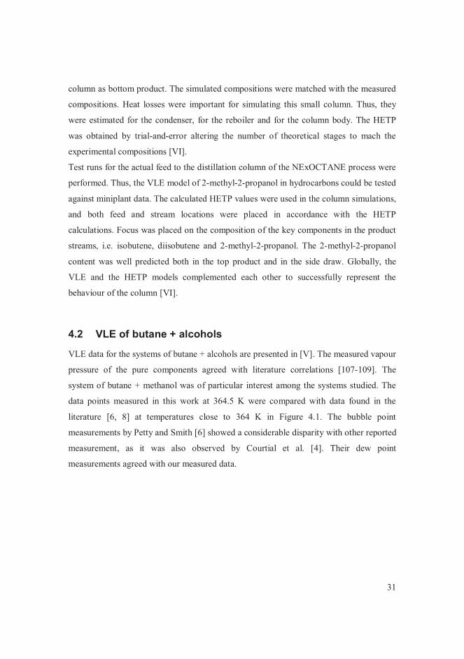
4.2 VLE of butane + alcohols

VLE data for the systems of butane + alcohols are presented in [V]. The measured vapour

pressure of the pure components agreed with literature correlations [107-109]. The

system of butane + methanol was of particular interest among the systems studied. The

data points measured in this work at 364.5 K were compared with data found in the

literature [6, 8] at temperatures close to 364 K in Figure 4.1. The bubble point

measurements by Petty and Smith [6] showed a considerable disparity with other reported

measurement, as it was also observed by Courtial et al. [4]. Their dew point

measurements agreed with our measured data.

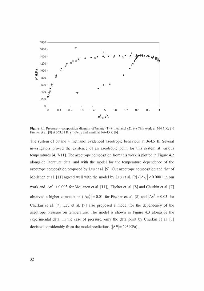
32

Figure 4.1 Pressure – composition diagram of butane (1) + methanol (2). (•) This work at 364.5 K; (×) Fischer et al. [8] at 363.31 K; (�) Petty and Smith at 366.45 K [6].

The system of butane + methanol evidenced azeotropic behaviour at 364.5 K. Several

investigators proved the existence of an azeotropic point for this system at various

temperatures [4, 7-11]. The azeotrope composition from this work is plotted in Figure 4.2

alongside literature data, and with the model for the temperature dependence of the

azeotrope composition proposed by Leu et al. [9]. Our azeotrope composition and that of

Moilanen et al. [11] agreed well with the model by Leu et al. [9] ( 0001.01 �� Lx in our

work and 003.01 �� Lx for Moilanen et al. [11]). Fischer et. al. [8] and Churkin et al. [7]

observed a higher composition ( 01.01 �� Lx for Fischer et. al. [8] and 03.01 �� Lx for

Churkin et al. [7]. Leu et al. [9] also proposed a model for the dependency of the

azeotrope pressure on temperature. The model is shown in Figure 4.3 alongside the

experimental data. In the case of pressure, only the data point by Churkin et al. [7]

deviated considerably from the model predictions ( 295��P KPa).

0

200

400

600

800

1000

1200

1400

1600

1800

0 0.1 0.2 0.3 0.4 0.5 0.6 0.7 0.8 0.9 1

xL1, xV

1

P/k

Pa

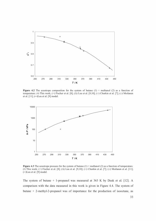
33

Figure 4.2 The azeotrope composition for the system of butane (1) + methanol (2) as a function of temperature. (•) This work; (×) Fischer et al. [8]; (�) Leu et al. [9,10]; (�) Churkin et al. [7]; (�) Moilanen et al. [11]; (�)Leu et al. [9] model.

Figure 4.3 The azeotrope pressure for the system of butane (1) + methanol (2) as a function of temperature. (•) This work; (×) Fischer et al. [8]; (�) Leu et al. [9,10]; (�) Churkin et al. [7]; (�) Moilanen et al. [11]; �)Leu et al. [9] model.

The system of butane + 1-propanol was measured at 363 K by Deak et al. [12]. A

comparison with the data measured in this work is given in Figure 4.4. The system of

butane + 2-methyl-2-propanol was of importance for the production of isooctane, as

0.6

0.7

0.8

0.9

1

250 270 290 310 330 350 370 390 410 430 450

T / K

xL 1

1

10

100

1000

10000

250 270 290 310 330 350 370 390 410 430 450

T / K

lnP

/kPa

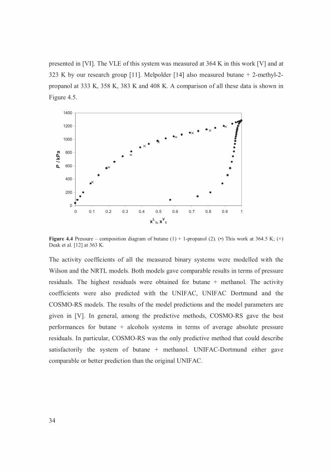
34

presented in [VI]. The VLE of this system was measured at 364 K in this work [V] and at

323 K by our research group [11]. Melpolder [14] also measured butane + 2-methyl-2-

propanol at 333 K, 358 K, 383 K and 408 K. A comparison of all these data is shown in

Figure 4.5.

Figure 4.4 Pressure – composition diagram of butane (1) + 1-propanol (2). (•) This work at 364.5 K; (×) Deak et al. [12] at 363 K.

The activity coefficients of all the measured binary systems were modelled with the

Wilson and the NRTL models. Both models gave comparable results in terms of pressure

residuals. The highest residuals were obtained for butane + methanol. The activity

coefficients were also predicted with the UNIFAC, UNIFAC Dortmund and the

COSMO-RS models. The results of the model predictions and the model parameters are

given in [V]. In general, among the predictive methods, COSMO-RS gave the best

performances for butane + alcohols systems in terms of average absolute pressure

residuals. In particular, COSMO-RS was the only predictive method that could describe

satisfactorily the system of butane + methanol. UNIFAC-Dortmund either gave

comparable or better prediction than the original UNIFAC.

0

200

400

600

800

1000

1200

1400

0 0.1 0.2 0.3 0.4 0.5 0.6 0.7 0.8 0.9 1

xL1, xV

1

P/k

Pa

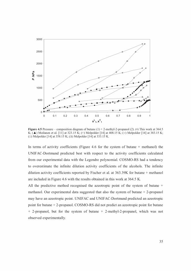
35

Figure 4.5 Pressure – composition diagram of butane (1) + 2-methyl-2-propanol (2). (•) This work at 364.5 K; () Moilanen et al. [11] at 323.15 K; (+) Melpolder [14] at 408.15 K; (�) Melpolder [14] at 383.15 K; �) Melpolder [14] at 358.15 K; (�) Melpolder [14] at 333.15 K.

In terms of activity coefficients (Figure 4.6 for the system of butane + methanol) the

UNIFAC-Dortmund predicted best with respect to the activity coefficients calculated

from our experimental data with the Legendre polynomial. COSMO-RS had a tendency

to overestimate the infinite dilution activity coefficients of the alcohols. The infinite

dilution activity coefficients reported by Fischer et al. at 363.39K for butane + methanol

are included in Figure 4.6 with the results obtained in this work at 364.5 K.

All the predictive method recognised the azeotropic point of the system of butane +

methanol. Our experimental data suggested that also the system of butane + 2-propanol

may have an azeotropic point. UNIFAC and UNIFAC-Dortmund predicted an azeotropic

point for butane + 2-propanol. COSMO-RS did not predict an azeotropic point for butane

+ 2-propanol, but for the system of butane + 2-methyl-2-propanol, which was not

observed experimentally.

0

500

1000

1500

2000

2500

3000

0 0.1 0.2 0.3 0.4 0.5 0.6 0.7 0.8 0.9 1

xL1, xV

1

P/k

Pa

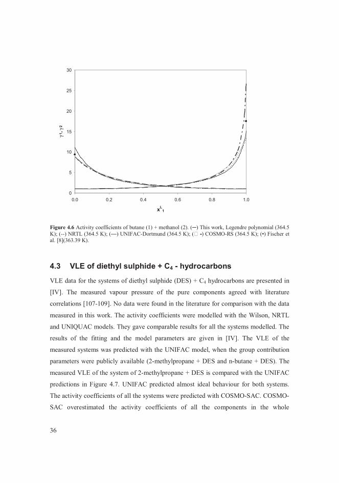
36

Figure 4.6 Activity coefficients of butane (1) + methanol (2). (�) This work, Legendre polynomial (364.5 K); (--) NRTL (364.5 K); (�) UNIFAC-Dortmund (364.5 K); (� -) COSMO-RS (364.5 K); (•) Fischer et al. [8](363.39 K).

4.3 VLE of diethyl sulphide + C4 - hydrocarbons

VLE data for the systems of diethyl sulphide (DES) + C4 hydrocarbons are presented in

[IV]. The measured vapour pressure of the pure components agreed with literature

correlations [107-109]. No data were found in the literature for comparison with the data

measured in this work. The activity coefficients were modelled with the Wilson, NRTL

and UNIQUAC models. They gave comparable results for all the systems modelled. The

results of the fitting and the model parameters are given in [IV]. The VLE of the

measured systems was predicted with the UNIFAC model, when the group contribution

parameters were publicly available (2-methylpropane + DES and n-butane + DES). The

measured VLE of the system of 2-methylpropane + DES is compared with the UNIFAC

predictions in Figure 4.7. UNIFAC predicted almost ideal behaviour for both systems.

The activity coefficients of all the systems were predicted with COSMO-SAC. COSMO-

SAC overestimated the activity coefficients of all the components in the whole

0

5

10

15

20

25

30

0.0 0.2 0.4 0.6 0.8 1.0

xL1

�1, �

2

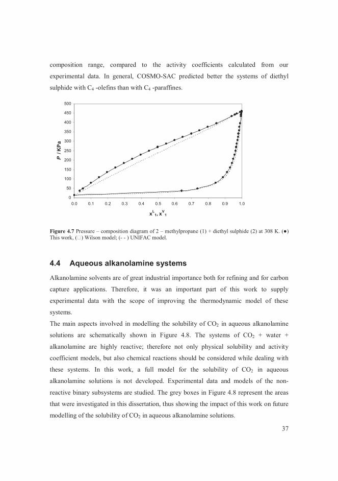
37

composition range, compared to the activity coefficients calculated from our

experimental data. In general, COSMO-SAC predicted better the systems of diethyl

sulphide with C4 -olefins than with C4 -paraffines.

Figure 4.7 Pressure – composition diagram of 2 – methylpropane (1) + diethyl sulphide (2) at 308 K. (�)This work, (�) Wilson model; (- - ) UNIFAC model.

4.4 Aqueous alkanolamine systems

Alkanolamine solvents are of great industrial importance both for refining and for carbon

capture applications. Therefore, it was an important part of this work to supply

experimental data with the scope of improving the thermodynamic model of these

systems.

The main aspects involved in modelling the solubility of CO2 in aqueous alkanolamine

solutions are schematically shown in Figure 4.8. The systems of CO2 + water +

alkanolamine are highly reactive; therefore not only physical solubility and activity

coefficient models, but also chemical reactions should be considered while dealing with

these systems. In this work, a full model for the solubility of CO2 in aqueous

alkanolamine solutions is not developed. Experimental data and models of the non-

reactive binary subsystems are studied. The grey boxes in Figure 4.8 represent the areas

that were investigated in this dissertation, thus showing the impact of this work on future

modelling of the solubility of CO2 in aqueous alkanolamine solutions.

0

50

100

150

200

250

300

350

400

450

500

0.0 0.1 0.2 0.3 0.4 0.5 0.6 0.7 0.8 0.9 1.0

xL1, x

V1

P/K

Pa

38

Figure 4.8 Modelling of the solubility of CO2 in aqueous alkanolamine solutions. In grey are evidenced the areas studied in this work.

The description of the activity coefficients relies on solubility data, and on the accurate

thermodynamic description of the mixed solvent. The activity coefficients of the solvent

species are obtained from phase equilibrium data of the solvent. In the specific case of

DIPA, scarcity of solubility data and absence of solvent phase equilibrium data limited

the development of a model for aqueous DIPA systems. In fact, no satisfactory

thermodynamic model for aqueous DIPA solvents was available in the open literature

before this work. Therefore, new phase equilibrium data were considered of great

importance for model development.

In addition, it was also noticed that many of the existing models for the Henry’s law

constant of CO2 in alkanolamine solutions deviated highly from the experimental data at

high temperatures, i.e. close to operative conditions in the alkanolamine solvent

regeneration column. Thus, a new model for the Henry’s law constant of CO2 in

alkanolamine solutions was developed, in which the Henry’s law constant depended on

Solubility of CO2in water + alkanolamine

Aqueous-phasechemical equilibrium

GLE of CO2in water + alkanolamine

Chemical reactionequilibrium data

Vapour phase fugacitycoefficient model (EOS)

Henry’s law constant of CO2 in water + alkanolamine model

Activity coefficient modelfor electrolyte systems(e-NRTL)

Solubility data of CO2in water + alkanolamine

Activity coefficient modelfor sub-system water + alkanolamine (NRTL)

Water + alkanolamine phase equilibrium data (VLE, SLE)

N2O – CO2 analogy. Solubility data of N2O in water + alkanolamine

39

the temperature, and on the composition of the solvent. Particular attention was given to

the model performances at high temperatures.

4.4.1 Solubility data of CO2 in water + alkanolamine solvents

A summary of all the measured solubility data of CO2 in water + MDEA and water +

DIPA with the two equipments (GLE static and bubbling apparatus) is given in Table 4.1,

and the data are presented in [III].

The solubility of CO2 in water + DIPA measured in this work with the GLE static

apparatus is plotted in Figure 4.9. A numerical comparison with literature data was not

possible since no data at the same experimental conditions were found. Some of the data

points by Isaacs et al. [25] and ter Maat [26] were included in Figure 4.9 for visual

comparison. With respect to amine concentrations, the data in Figure 4.9 behave

consistently, i.e. at the same temperature and partial pressure of CO2, the loading is

higher the lower is the amine concentration. Similarly, with respect to temperature, at the

same amine concentration and pressure the loading is higher the lower is the temperature.

Figure 4.9 . Loading � = [mole CO2/ mole amine] of CO2 (1) in solutions of water (2) and DIPA (3) as a function of the partial pressure P1 of CO2. (�) This work, GLE static apparatus, w3 = 10.1 % at 299.72 K ; �) this work, GLE static apparatus, w3 = 11.0 % at 298.22 K; (�) this work, GLE static apparatus, w3 = 33.9 % at 298.29 K; (×) Isaacs et al. w3 � 33 % at 313.15 K; (�) Isaacs et al. w3 � 33 % at 373.15 K; (�) ter Maat et al. w3 = 35 % at 298.15 K.

0.0

0.2

0.4

0.6

0.8

1.0

1.2

1.4

1 10 100 1000 10000

ln P 1 / kPa

�

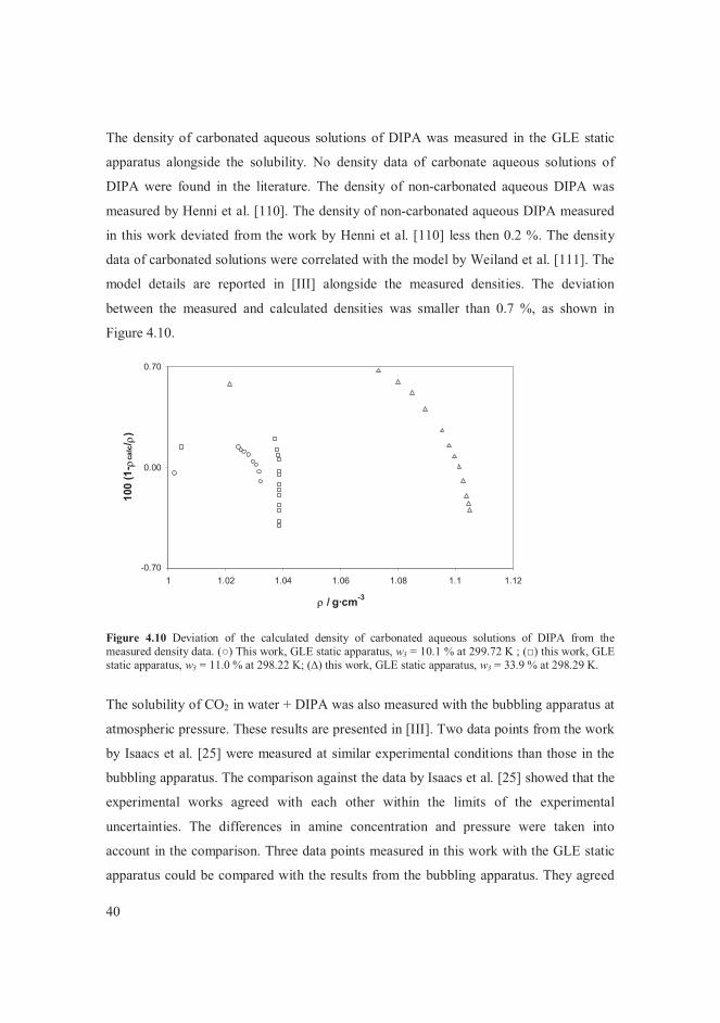
40

The density of carbonated aqueous solutions of DIPA was measured in the GLE static

apparatus alongside the solubility. No density data of carbonate aqueous solutions of

DIPA were found in the literature. The density of non-carbonated aqueous DIPA was

measured by Henni et al. [110]. The density of non-carbonated aqueous DIPA measured

in this work deviated from the work by Henni et al. [110] less then 0.2 %. The density

data of carbonated solutions were correlated with the model by Weiland et al. [111]. The

model details are reported in [III] alongside the measured densities. The deviation

between the measured and calculated densities was smaller than 0.7 %, as shown in

Figure 4.10.

Figure 4.10 Deviation of the calculated density of carbonated aqueous solutions of DIPA from the measured density data. (�) This work, GLE static apparatus, w3 = 10.1 % at 299.72 K ; (�) this work, GLE static apparatus, w3 = 11.0 % at 298.22 K; (�) this work, GLE static apparatus, w3 = 33.9 % at 298.29 K.

The solubility of CO2 in water + DIPA was also measured with the bubbling apparatus at

atmospheric pressure. These results are presented in [III]. Two data points from the work

by Isaacs et al. [25] were measured at similar experimental conditions than those in the

bubbling apparatus. The comparison against the data by Isaacs et al. [25] showed that the

experimental works agreed with each other within the limits of the experimental

uncertainties. The differences in amine concentration and pressure were taken into

account in the comparison. Three data points measured in this work with the GLE static

apparatus could be compared with the results from the bubbling apparatus. They agreed

-0.70

0.00

0.70

1 1.02 1.04 1.06 1.08 1.1 1.12

� / g�cm-3

100

(1- �

calc

/ �)

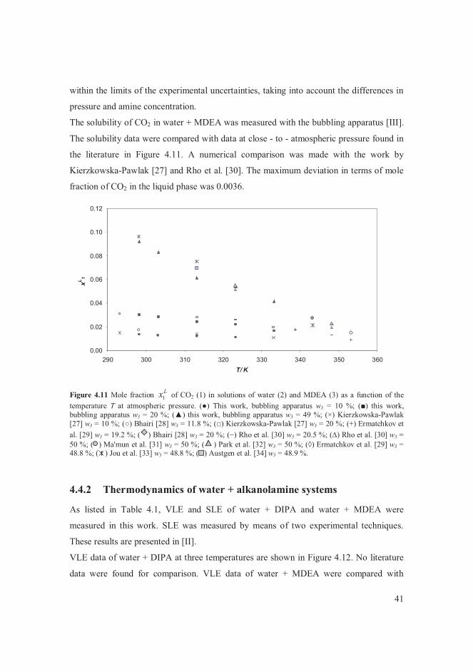
41

within the limits of the experimental uncertainties, taking into account the differences in

pressure and amine concentration.

The solubility of CO2 in water + MDEA was measured with the bubbling apparatus [III].

The solubility data were compared with data at close - to - atmospheric pressure found in

the literature in Figure 4.11. A numerical comparison was made with the work by

Kierzkowska-Pawlak [27] and Rho et al. [30]. The maximum deviation in terms of mole

fraction of CO2 in the liquid phase was 0.0036.

Figure 4.11 Mole fraction Lx1 of CO2 (1) in solutions of water (2) and MDEA (3) as a function of the temperature T at atmospheric pressure. (�) This work, bubbling apparatus w3 = 10 %; (�) this work, bubbling apparatus w3 = 20 %; () this work, bubbling apparatus w3 = 49 %; (×) Kierzkowska-Pawlak [27] w3 = 10 %; (�) Bhairi [28] w3 = 11.8 %; (�) Kierzkowska-Pawlak [27] w3 = 20 %; (+) Ermatchkov et al. [29] w3 = 19.2 %; ( ) Bhairi [28] w3 = 20 %; (�) Rho et al. [30] w3 = 20.5 %; (�) Rho et al. [30] w3 = 50 %; ( ) Ma'mun et al. [31] w3 = 50 %; ( ) Park et al. [32] w3 = 50 %; (�) Ermatchkov et al. [29] w3 = 48.8 %; ( ) Jou et al. [33] w3 = 48.8 %; ( ) Austgen et al. [34] w3 = 48.9 %.

4.4.2 Thermodynamics of water + alkanolamine systems

As listed in Table 4.1, VLE and SLE of water + DIPA and water + MDEA were

measured in this work. SLE was measured by means of two experimental techniques.

These results are presented in [II].

VLE data of water + DIPA at three temperatures are shown in Figure 4.12. No literature

data were found for comparison. VLE data of water + MDEA were compared with

0.00

0.02

0.04

0.06

0.08

0.10

0.12

290 300 310 320 330 340 350 360T/ K

xL 1

42

literature sources at similar conditions in [II]. The results of the numerical comparison

with the work by Xu et al. [42] showed agreement within the experimental uncertainties.

Kuwairi [39] developed two correlations for the vapour pressure of 1N and 2N aqueous

solutions of MDEA. These correlations predicted lower vapour pressures than those

measured in this work and by Sandall et al. [43].

Figure 4.12 Vapour-liquid equilibrium data of the system water (1) + DIPA (2). (�) This work, 357 K; (�)this work, 349 K; () this work, 335 K.

SLE of water + DIPA was measured at low amines concentrations with a DSC, and with

the visual method. The SLE measurements were possible only up to 08.02 �Lx . For

higher amines concentrations either the phase transition was indiscernible (visual

method), or the results were of difficult interpretation (DSC). The SLE data are shown in

[II]. No literature SLE data were found; therefore only the melting point of pure DIPA,

measured with both techniques, was compared with literature values [112-114]. The

values measured in this work, as well as the values in the literature, were scattered in a

range of 4 K. The value measured with the visual method agreed with [113], while the

value measured with the DSC agreed with [114].

The enthalpy of fusion of pure DIPA was measured with the DSC ( 74.22�� fusH

kJ/mol). No measured values of this quantity were found in the literature. For comparison

purposes, the enthalpy of fusion of pure DIPA was estimated with predicted methods, i.e.

the method of Marrero and Gani [115], the method of Bondi [116] (found in [85]), and

0

10

20

30

40

50

60

0 0.1 0.2 0.3 0.4 0.5 0.6 0.7 0.8 0.9 1

x L2

P/k

Pa

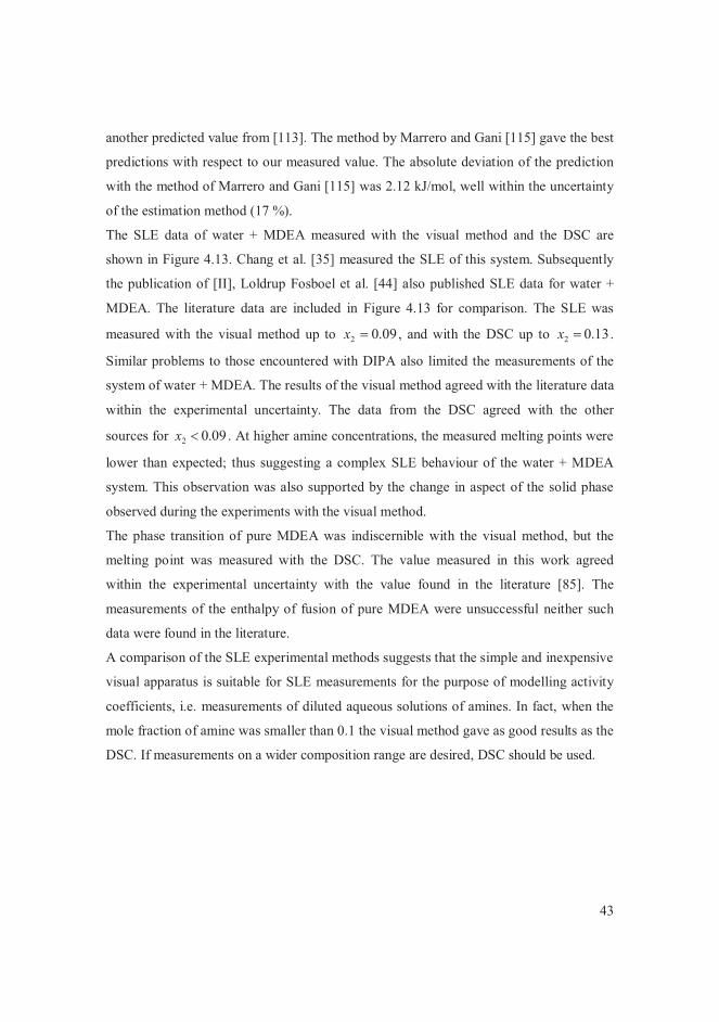
43

another predicted value from [113]. The method by Marrero and Gani [115] gave the best

predictions with respect to our measured value. The absolute deviation of the prediction

with the method of Marrero and Gani [115] was 2.12 kJ/mol, well within the uncertainty

of the estimation method (17 %).

The SLE data of water + MDEA measured with the visual method and the DSC are

shown in Figure 4.13. Chang et al. [35] measured the SLE of this system. Subsequently

the publication of [II], Loldrup Fosboel et al. [44] also published SLE data for water +

MDEA. The literature data are included in Figure 4.13 for comparison. The SLE was

measured with the visual method up to 09.02 �x , and with the DSC up to 13.02 �x .

Similar problems to those encountered with DIPA also limited the measurements of the

system of water + MDEA. The results of the visual method agreed with the literature data

within the experimental uncertainty. The data from the DSC agreed with the other

sources for 09.02 �x . At higher amine concentrations, the measured melting points were

lower than expected; thus suggesting a complex SLE behaviour of the water + MDEA

system. This observation was also supported by the change in aspect of the solid phase

observed during the experiments with the visual method.

The phase transition of pure MDEA was indiscernible with the visual method, but the

melting point was measured with the DSC. The value measured in this work agreed

within the experimental uncertainty with the value found in the literature [85]. The

measurements of the enthalpy of fusion of pure MDEA were unsuccessful neither such

data were found in the literature.

A comparison of the SLE experimental methods suggests that the simple and inexpensive

visual apparatus is suitable for SLE measurements for the purpose of modelling activity

coefficients, i.e. measurements of diluted aqueous solutions of amines. In fact, when the

mole fraction of amine was smaller than 0.1 the visual method gave as good results as the

DSC. If measurements on a wider composition range are desired, DSC should be used.

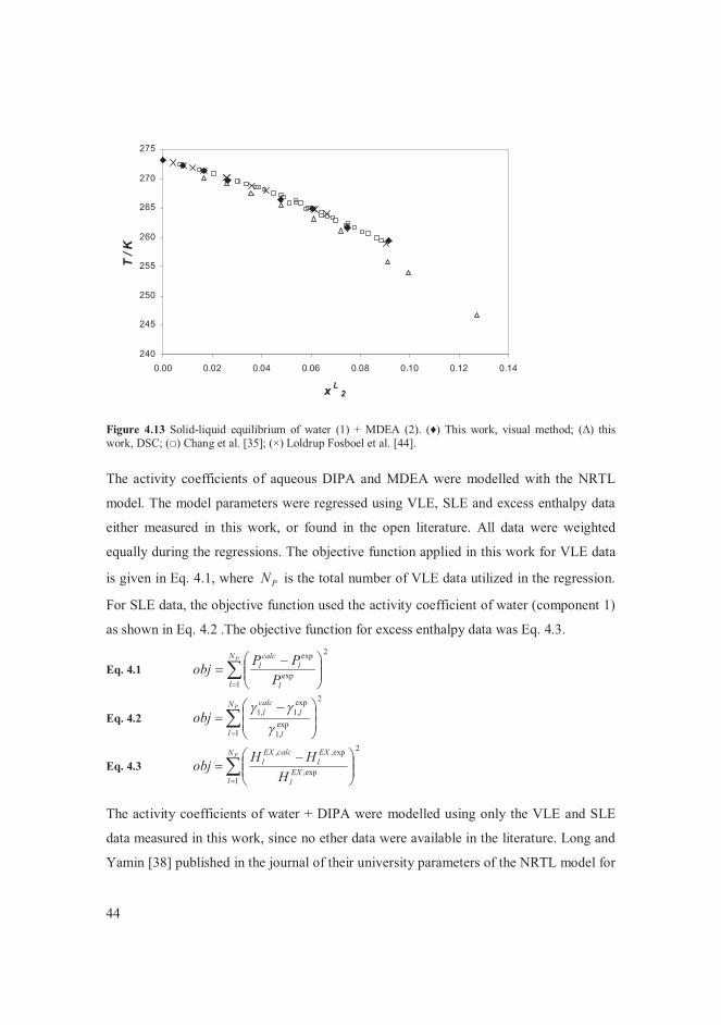
44

Figure 4.13 Solid-liquid equilibrium of water (1) + MDEA (2). (�) This work, visual method; (�) this work, DSC; (�) Chang et al. [35]; (×) Loldrup Fosboel et al. [44].

The activity coefficients of aqueous DIPA and MDEA were modelled with the NRTL

model. The model parameters were regressed using VLE, SLE and excess enthalpy data

either measured in this work, or found in the open literature. All data were weighted

equally during the regressions. The objective function applied in this work for VLE data

is given in Eq. 4.1, where PN is the total number of VLE data utilized in the regression.

For SLE data, the objective function used the activity coefficient of water (component 1)

as shown in Eq. 4.2 .The objective function for excess enthalpy data was Eq. 4.3.

Eq. 4.1 ��

���

����

� ��

PN

l l

lcalc

l

PPPobj

1

2

exp

exp

Eq. 4.2 ��

���

����

� ��

PN

l l

lcalclobj

1

2

exp,1

exp,1,1

���

Eq. 4.3 ��

���

����

� ��

PN

lEXl

EXl

calcEXl

HHHobj

1

2

exp,

exp,,

The activity coefficients of water + DIPA were modelled using only the VLE and SLE

data measured in this work, since no ether data were available in the literature. Long and

Yamin [38] published in the journal of their university parameters of the NRTL model for

240

245

250

255

260

265

270

275

0.00 0.02 0.04 0.06 0.08 0.10 0.12 0.14

x L2

T/K

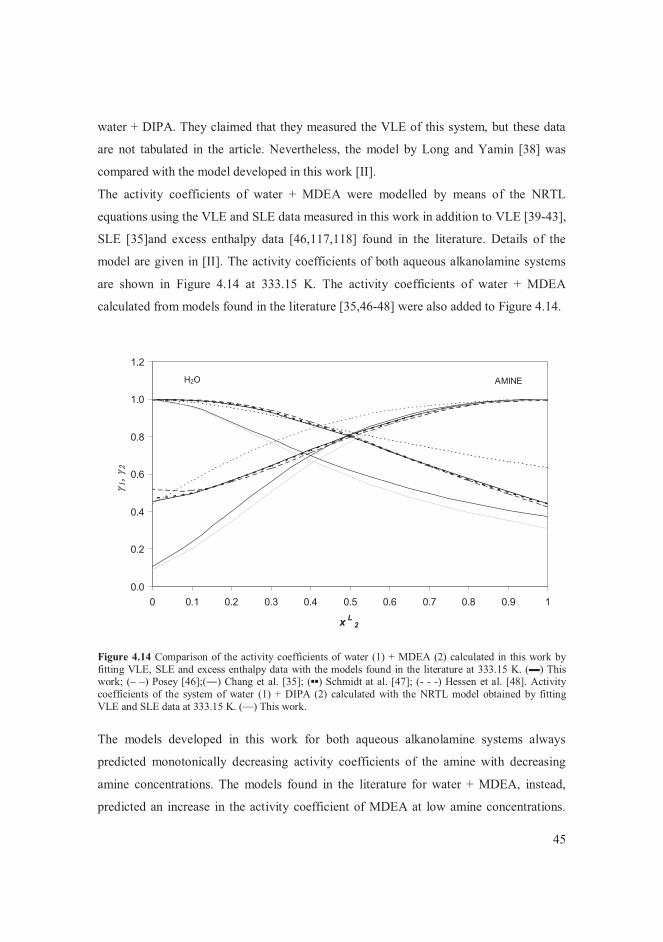
45

water + DIPA. They claimed that they measured the VLE of this system, but these data

are not tabulated in the article. Nevertheless, the model by Long and Yamin [38] was

compared with the model developed in this work [II].

The activity coefficients of water + MDEA were modelled by means of the NRTL

equations using the VLE and SLE data measured in this work in addition to VLE [39-43],

SLE [35]and excess enthalpy data [46,117,118] found in the literature. Details of the

model are given in [II]. The activity coefficients of both aqueous alkanolamine systems

are shown in Figure 4.14 at 333.15 K. The activity coefficients of water + MDEA

calculated from models found in the literature [35,46-48] were also added to Figure 4.14.

Figure 4.14 Comparison of the activity coefficients of water (1) + MDEA (2) calculated in this work by fitting VLE, SLE and excess enthalpy data with the models found in the literature at 333.15 K. (�) This work; (– –) Posey [46];(�) Chang et al. [35]; (��) Schmidt at al. [47]; (- - -) Hessen et al. [48]. Activity coefficients of the system of water (1) + DIPA (2) calculated with the NRTL model obtained by fitting VLE and SLE data at 333.15 K. (�) This work.

The models developed in this work for both aqueous alkanolamine systems always

predicted monotonically decreasing activity coefficients of the amine with decreasing

amine concentrations. The models found in the literature for water + MDEA, instead,

predicted an increase in the activity coefficient of MDEA at low amine concentrations.

0.0

0.2

0.4

0.6

0.8

1.0

1.2

0 0.1 0.2 0.3 0.4 0.5 0.6 0.7 0.8 0.9 1

x L2

� � !�

"

H2O AMINE

46

This phenomenon becomes more evident while increasing the temperature, as shown in

Figure 4.15 at 393.15 K. It should be noticed that this temperature is still within the range

of validity of the models parameters. The behaviour of the activity coefficient of MDEA

at low amine concentrations influences the shape of the Gibbs energy, as shown in Figure

4.16. Our model predicted the common parabolic shape of the Gibbs energy, while the

other models predicted more complex shapes.

Figure 4.15 Comparison of the activity coefficients of water (1) + MDEA (2) calculated in this work by fitting VLE, SLE and excess enthalpy data with the models found in the literature at 393.15 K. (�) This work; (– –) Posey [46];(�) Chang et al. [35]; (��) Schmidt et al. [47]; (- - -) Hessen et al. [48].

0.0

0.5

1.0

1.5

2.0

0 0.1 0.2 0.3 0.4 0.5 0.6 0.7 0.8 0.9 1

x L2

� "

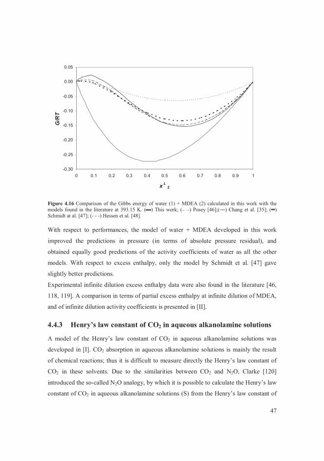
47

Figure 4.16 Comparison of the Gibbs energy of water (1) + MDEA (2) calculated in this work with the models found in the literature at 393.15 K. (�) This work; (– –) Posey [46];(�) Chang et al. [35]; (��)Schmidt at al. [47]; (- - -) Hessen et al. [48].

With respect to performances, the model of water + MDEA developed in this work

improved the predictions in pressure (in terms of absolute pressure residual), and

obtained equally good predictions of the activity coefficients of water as all the other

models. With respect to excess enthalpy, only the model by Schmidt et al. [47] gave

slightly better predictions.

Experimental infinite dilution excess enthalpy data were also found in the literature [46,

118, 119]. A comparison in terms of partial excess enthalpy at infinite dilution of MDEA,

and of infinite dilution activity coefficients is presented in [II].

4.4.3 Henry’s law constant of CO2 in aqueous alkanolamine solutions

A model of the Henry’s law constant of CO2 in aqueous alkanolamine solutions was

developed in [I]. CO2 absorption in aqueous alkanolamine solutions is mainly the result

of chemical reactions; thus it is difficult to measure directly the Henry’s law constant of

CO2 in these solvents. Due to the similarities between CO2 and N2O, Clarke [120]

introduced the so-called N2O analogy, by which it is possible to calculate the Henry’s law

constant of CO2 in aqueous alkanolamine solutions (S) from the Henry’s law constant of

-0.30

-0.25

-0.20

-0.15

-0.10

-0.05

0.00

0.05

0 0.1 0.2 0.3 0.4 0.5 0.6 0.7 0.8 0.9 1

x L2

G/R

T

48

N2O in the same solvent (Eq. 4.4). N2O does not react with alkanolamine solvents, so its

Henry’s constant can be directly measured. The problem of modelling the Henry’s law

constant of CO2 in aqueous alkanolamine solutions thus reduces to modelling the Henry’s

law constant of N2O in aqueous alkanolamine solutions.

Eq. 4.4 ���

����

��

WON

WCOSONSCO H

HHH

,

,,,

2

2

22

According to Eq. 4.4, expressions of the Henry’s law constant of CO2 and N2O in water

(W) are needed. The solubility of CO2 in water was modelled according to the work by

Carroll et al. [91], whose correlation also agreed with our solubility measurements, as

shown in [III]. The solubility of N2O in water was modelled using data from literature

sources, as described in [I].

The Henry’s law constant of a gas in a mixed solvent may be calculated, as a first

approximation, from the Henry’s law constant of the pure components by means of the

ideal solution mixing rule [1]. The ideal model can be improved by taking into account an

excess term for the Henry’s constant. A new expression of the excess Henry’s law

constant of N2O in aqueous binary and ternary alkanolamine solutions was developed in

this work as a function of temperature and solvent composition. The parameters of the

new expression were fitted using experimental Henry’s law constant data points up to

120 ºC, thus reaching industrial gas-sweetening operative temperatures (e.g. regeneration

in a MEA plant usually takes place at 100- 120ºC [121]). The binary solvents were

aqueous solutions of MEA, DEA, DIPA, MDEA and AMP, while the ternary solvents

were aqueous blends of MDEA + MEA, + DEA, + DIPA or + AMP, and AMP + MEA or

+ DEA. The model may be applied to any binary or ternary aqueous amine solvent, as

long as Henry’s constant binary solvent measurements are available for parameter

regression.

The expression of the Henry’s law constant of N2O in a binary alkanolamine solvent is

expressed in Eq. 4.5 as the sum of an ideal term and an excess term. The Henry’s law

constant of N2O in a ternary alkanolamine solvent is shown in Eq. 4.6. In the model

equations water is component 1, the amines are components 2 and 3. The liquid mole

fractions refer to the unloaded solvent.

49

Eq. 4.5 # $ # $LLL

i

LiiON

EXON

i

LiiONON xC

BTxxAxHHxHH 212

12

22112

2

1,12,

2

1,12, exp1

2222�%

&

'()

*����� ��

��

Eq. 4.6 � �2

32

32233

2123

123

23

21123

3

1,123, exp1

22 LL

LL

i

Li

i

Li

L

i

LiiONON

xxxxDxC

BTxxAxHH

��%

&

'()

*��

���

��%

&

'()

*�%

&

'()

*��

���

��� ���

���

The model empirical parameters are symmetrical. Parameters ijA , ijB and ijC were

regressed using 648 experimental Henry’s law constant points in binary solvents.

Parameters ijD were obtained from 316 Henry’s law constant measurement points in

ternary solvents. The ternary parameter ijkA , ijkB and ijkC were calculated using mixing

rules from the binary parameters. The detailed model equations and the experimental data

used in the regression of the parameters are given in [I]. A comparison between the

model prediction and the experimental data is shown in Figure 4.17 for the system of

N2O + water + DIPA. The average absolute residual of the Henry’s law constant for this

system was 3.4 %. The model predictions for N2O in water + DIPA + MDEA are shown

in Figure 4.18. The average absolute residual of the Henry’s law constant for this system

was 2.6%.

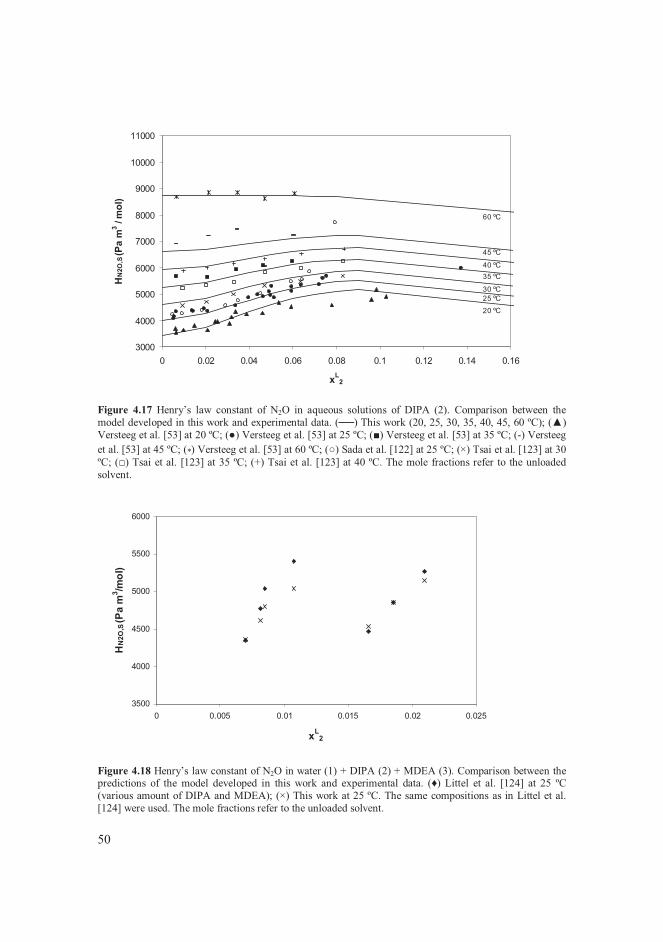
50

Figure 4.17 Henry’s law constant of N2O in aqueous solutions of DIPA (2). Comparison between the model developed in this work and experimental data. (��) This work (20, 25, 30, 35, 40, 45, 60 ºC); ()Versteeg et al. [53] at 20 ºC; (�) Versteeg et al. [53] at 25 ºC; (�) Versteeg et al. [53] at 35 ºC; (-) Versteeg et al. [53] at 45 ºC; (*) Versteeg et al. [53] at 60 ºC; (�) Sada et al. [122] at 25 ºC; (×) Tsai et al. [123] at 30 ºC; (�) Tsai et al. [123] at 35 ºC; (+) Tsai et al. [123] at 40 ºC. The mole fractions refer to the unloaded solvent.

Figure 4.18 Henry’s law constant of N2O in water (1) + DIPA (2) + MDEA (3). Comparison between the predictions of the model developed in this work and experimental data. (�) Littel et al. [124] at 25 ºC (various amount of DIPA and MDEA); (×) This work at 25 ºC. The same compositions as in Littel et al. [124] were used. The mole fractions refer to the unloaded solvent.

3000

4000

5000

6000

7000

8000

9000

10000

11000

0 0.02 0.04 0.06 0.08 0.1 0.12 0.14 0.16

xL2

HN

2O,S

(Pa

m3

/mol

)

20 ºC

45 ºC

40 ºC35 ºC

30 ºC25 ºC

60 ºC

3500

4000

4500

5000

5500

6000

0 0.005 0.01 0.015 0.02 0.025

xL2

HN

2O,S

(Pa

m3 /m

ol)

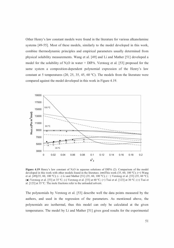
51

Other Henry’s law constant models were found in the literature for various alkanolamine

systems [49-55]. Most of these models, similarly to the model developed in this work,

combine thermodynamic principles and empirical parameters usually determined from

physical solubility measurements. Wang et al. [49] and Li and Mather [51] developed a

model for the solubility of N2O in water + DIPA. Versteeg et al. [53] proposed for the

same system a composition-dependent polynomial expression of the Henry’s law

constant at 5 temperatures (20, 25, 35, 45, 60 ºC). The models from the literature were

compared against the model developed in this work in Figure 4.19.

Figure 4.19 Henry’s law constant of N2O in aqueous solutions of DIPA (2). Comparison of the model developed in this work with other models found in the literature. (�)This work (35, 60, 100 ºC); (�) Wang et al. [49](35, 60, 100 ºC); (- -) Li and Mather [51] (35, 60, 100 ºC); (· · ·) Versteeg et al. [53] (35, 60 ºC); �) Versteeg et al. [53] at 35 ºC; (*) Versteeg et al. [53] at 60 ºC; (×) Tsai et al. [123] at 30 ºC; (�) Tsai et al. [123] at 35 ºC. The mole fractions refer to the unloaded solvent.

The polynomials by Versteeg et al. [53] describe well the data points measured by the

authors, and used in the regression of the parameters. As mentioned above, the

polynomials are isothermal, thus this model can only be calculated at the given

temperatures. The model by Li and Mather [51] gives good results for the experimental

3000

5000

7000

9000

11000

13000

15000

17000

19000

0 0.02 0.04 0.06 0.08 0.1 0.12 0.14 0.16 0.18 0.2

xL2

HN

2O,S

(Pa

m3 /m

ol)

35 ºC

100 ºC

60 ºC

52

data at 35 ºC, but underestimates the Henry’s law constant at 60 ºC. The authors were

uncertain about the reasons of the poor performances of their model at temperatures

above 45 ºC for aqueous solutions of DIPA. They suggested it may depend on the lack of

density data of water + DIPA solutions at high temperatures, which was true when their

model was published [51]. The model by Wang et al. [49] represents well the

experimental data at 35 and 60 ºC, but when extrapolated to higher temperatures (100 ºC)

it predicts a rather improbable behaviour of the Henry’s law constant. The model

developed in this work behaves consistently with the lower temperatures and with the

other amine systems even when extrapolated up to higher temperatures. The average

absolute residual of the Henry’s law constant calculated on 82 measured point was 3.4 %

for our model, 3.8 % for the model by Wang et al. [49], and 8.1 % for Li and Mather

[51]. Graphical and numerical comparisons among the models for all the systems studied

in this work are given in [I].

In general, this semiempirical model predicts the Henry’s law constant of N2O in binary

and ternary aqueous amine solvents either comparably or better than the literature

models. It is particularly successful in describing ternary solvent systems, improving the

performances of the literature models even when 23D is set equal to zero, i.e. the ternary

solvent is predicted based solely on binary solvent data. Additional features of the model

are mathematical simplicity and consistent behaviour on the whole composition, and

temperature range (i.e. up to 120 ºC) [I].

53

5 Conclusions An accurate representation of the phase separation may be sufficient to design full scale

separation plants, such as distillation columns. The aim of this research was to strengthen

modelling of separation processes of industrial interest by improving the thermodynamic

representation of the equilibrium between phases. This was successfully achieved in this

work through targeted experimental investigations and thermodynamic modelling of

chosen systems.

Several experimental methods were developed in this work to measure VLE, GLE and

SLE data. A total of 135 VLE data points were measured for binary systems of butane +

alcohol, which are important in the field of biofuels and in the production of gasoline

additives. Some of these systems also presented azeoptropic behaviour, and our data

contributed to the determination of the azeotropic point. Mixtures of sulphur compounds

and hydrocarbons are often encountered in refinery applications, but data in the open

literature are extremely scarce. This shortage negatively influenced the prediction of

sulphur compounds behaviour in refinery separation units. Therefore, phase equilibrium

data of sulphur compounds are greatly needed. This work supplied 129 VLE datapoints

of binary systems of diethyl sulphide in C4 – hydrocarbons. It was found that traditional

activity coefficients models satisfactorily predicted most of the systems studied. In

average, activity coefficient models with empirical parameters predicted the

thermodynamic behaviour of the system studied better than predictive model, thus

confirming the importance of experimental phase equilibrium data for thermodynamic

modelling.

In this work great attention was given to CO2 both for its role in industrial applications

and as a greenhouse gas. CO2 removal with alkanolamine solutions is a process of

industrial importance in refinery, and CO2 capture applications. A scarcity of

experimental data was noticed for some alkanolamine systems, and in particular for

aqueous solutions of DIPA. Before the publications of this work, neither a model for the

solubility of CO2 in DIPA solvents, nor a satisfactory thermodynamic model of aqueous

DIPA solutions was available. CO2 solubility in aqueous DIPA solvents, VLE and SLE

data of DIPA solutions were measured. The first activity coefficient model for aqueous

54

DIPA solution based on VLE and SLE data was developed in this work. Alongside

DIPA, also aqueous solutions of MDEA were modelled, due to their importance in

carbon capture applications. CO2 solubility in aqueous MDEA, VLE and SLE data of

MDEA solutions were measured. The activity coefficient model for aqueous MDEA

solutions developed in this work predicts better than the models found in the literature for

the same system.

It was noticed that many of the existing models of the Henry’s law constant of CO2 in

solutions of alkanolamines highly deviated from the experimental data at temperatures

closed to the industrial. This was recognised as an important source of error in modelling

the solubility of CO2 in solutions of alkanolamines. Therefore, a new model for the

Henry’s law constant of CO2 binary and ternary aqueous solutions of alkanolamines was

developed. The new model is mathematically simple and reliable up to high temperatures,

where most of the other models failed. In particular, this model was better than any other

model in predicting ternary aqueous solvent systems, even when predictions were solely

based on binary solvent data.

In future work, the large amount of experimental data and modelling work accomplished

in this research may be unified into a full thermodynamic model for the solubility of CO2

in aqueous alkanolamine solutions. Other researchers already used our published data in

developing their solubility model, thus confirming the importance of these measurements

in the field of alkanolamine technology. While developing the full solubility model of

CO2 in aqueous alkanolamine solutions, chemical reactions should also be addressed due

to the high reactivity of these systems. This strong thermodynamic framework will be the

base for successful modelling of absorption and regeneration units both in refinery

applications and in carbon capture.

55

References [1] H. C. Van Ness, M. M. Abbott, Classical thermodynamics of nonelectrolyte solutions

with applications to phase equilibria, McGraw-Hill, New York, 1982.

[2] R. A. Meyers, Handbook of Petroleum Refining Processes (3rd Edition), McGraw-

Hill, USA, 2004.

[3] T. M. Soria, F. A. Sanchez, S. Pereda, S. B. Bottini. Fluid Phase Equilib. 296 (2010)

116-124.

[4] X. Courtial, C. Soo, C. Coquelet, P. Paricaud, D. Ramjugernath, D. Richon. Fluid

Phase Equilib. 277 (2009) 152-161.

[5] C. B. Kretschmer, R. Wiebe. J. Am. Chem. Soc. 74 (1952) 1276-1277.

[6] L. B. Petty, J. M. Smith. Ind. Eng. Chem. 47 (1955) 1258-1265.

[7] V. N. Churkin, V. A. Gorshkov, S. Y. Pavlov, E. N. Levicheva, L. L. Karpacheva. Zh.

Fiz. Khim. 52 (1978) 488-489.

[8] K. Fischer, S. J. Park, J. Gmehling. ELDATA: Int. Electron. J. Phys. Chem. Data. 2

(1996) 135-148.

[9] A. D. Leu, D. B. Robinson, S. Y. K. Chung, C. J. Chen. Can. J. Chem. Eng. 70 (1992)

330-334.

[10] A. D. Leu, C. J. Chen, D. B. Robinson. AIChE Symp. Ser. 85 (1989) 11-16.

[11] P. Moilanen, P. Uusi-Kyyny, J. Pokki, M. Pakkanen, J. Aittamaa. J. Chem. Eng.

Data. 53 (2008) 83-88.

[12] A. Deak, A. I. Victorov, T. W. de Loos. Fluid Phase Equilib. 107 (1995) 277-301.

[13] T. Anyu, X. Xianjin, S. Yuguang. Chengdu Keji Daxue Xuebao. 4 (1992) 19-25.

[14] F. W. Melpolder. Fluid Phase Equilib. 26 (1986) 279-288.

[15] S. Brunet, D. Mey, G. Perot, C. Bouchy, F. Diehl. Appl. Catal., A. 278 (2005) 143-

172.

[16] P. O. Vistisen, P. Zeuthen. Ind. Eng. Chem. Res. 47 (2008) 8471-8477.

[17] W. H. Hoffert, K. Wendtner. J. Inst. Pet. 35 (1949) 171-192.

[18] E. Sapei, P. Uusi-Kyyny, K. I. Keskinen, J. Pokki, V. Alopaeus. Fluid Phase Equilib.

301 (2011) 200-205.

56

[19] E. Sapei, A. Zaytseva, P. Uusi-Kyyny, K. I. Keskinen, J. Aittamaa. Fluid Phase

Equilib. 252 (2007) 130-136.

[20] E. Sapei, A. Zaytseva, P. Uusi-Kyyny, K. I. Keskinen, J. Aittamaa. J. Chem. Eng.

Data. 52 (2007) 571-576.

[21] E. Sapei, A. Zaytseva, P. Uusi-Kyyny, K. I. Keskinen, J. Aittamaa. J. Chem. Eng.

Data. 52 (2007) 192-198.

[22] The petroleum handbook, 4th ed., Shell International Petroleum, London, 1959.

[23] A. L. Kohl, R. B. Nielsen, Gas Purification (5th Edition), Elsevier 1997.

[24] Z. Bensetiti, I. Iliuta, F. Larachi, B. P. A. Grandjean. Ind. Eng. Chem. Res. 38 (1999)

328-332.

[25] E. E. Isaacs, F. D. Otto, A. E. Mather. J. Chem. Eng. Data. 22 (1977) 71-73.

[26] H. ter Maat, S. Praveen, P. Ijben, D. Arslan, H. F. Wouters, P. J. G. Huttenhuis, J. A.

Hogendoorn, G. F. Versteeg, The determination of VLE data on CO2 and H2S in

MDEA and its blends with other amines. Research report 186, Gas Processor

Association, Tulsa, 2004.

[27] H. Kierzkowska-Pawlak. Sep. Sci. Technol. 42 (2007) 2723-2737.

[28] A. M. Bhairi, Experimental equilibrium between acid gas and ethanolamine

solutions. Ph.D. Thesis. Oklaoma State University, Stillwater, 1984.

[29] V. Ermatchkov, A. Perez-Salado Kamps, G. Maurer. Ind. Eng. Chem. Res. 45

(2006) 6081-6091.

[30] S. Rho, K. Yoo, J. S. Lee, S. C. Nam, J. E. Son, B. Min. J. Chem. Eng. Data. 42

(1997) 1161-1164.

[31] S. Ma'mun, R. Nilsen, H. F. Svendsen, O. Juliussen. J. Chem. Eng. Data. 50 (2005)

630-634.

[32] M. K. Park, O. C. Sandall. J. Chem. Eng. Data. 46 (2001) 166-168.

[33] F. Y. Jou, A. E. Mather, F. D. Otto. Ind. Eng. Chem. Process Des. Dev. 21 (1982)

539-544.

[34] D. M. Austgen, G. T. Rochelle, C. C. Chen. Ind. Eng. Chem. Res. 30 (1991) 543-

555.

[35] H. T. Chang, M. Posey, G. T. Rochelle. Ind. Eng. Chem. Res. 32 (1993) 2324-2335.

[36] H. Renon, J. M. Prausnitz. AIChE J. 14 (1968) 135-144.

57

[37] S. M. Walas, Phase equilibria in chemical engineering, Butterworths, Boston, MA,

1985.

[38] F. Long, Z. Yamin. J. Nanjing Univ. Chem. Technol. 2 (2001) 45-48.

[39] B. S. Kuwairi, Vapor pressure of selected pure materials and mixtures. Ph.D. Thesis.

Oklaoma State University, USA, 1983.

[40] R. Sidi-Boumedine, S. Horstmann, K. Fischer, E. Provost, W. Furst, J. Gmehling.

Fluid Phase Equilib. 218 (2004) 85-94.

[41] G. Kuranov, B. Rumpf, N. A. Smirnova, G. Maurer. Ind. Eng. Chem. Res. 35 (1996)

1959-1966.

[42] S. Xu, S. Qing, Z. Zhen, C. Zhang, J. J. Carroll. Fluid Phase Equilib. 67 (1991) 197-

201.

[43] O. C. Sandall, E. B. Rinker, S. Ashour, Acid Gas Treating by Aqueous

Alkanolamines. GRI Annual Report. (1993).

[44] P. L. Fosboel, M. G. Pedersen, K. Thomsen. J. Chem. Eng. Data. 56 (2011) 995-

1000.

[45] D. M. Austgen, A model for Vapor-Liquid Equilibria for acid gas-alkanolamine-

water systems. PhD. Thesis. University of Texas, Austin, USA, 1989.

[46] M. L. Posey, Thermodynamic model for acid gas loaded aqueous alkanolamine

solutions. PhD. Thesis. University of Texas, Austin, USA, 1996.

[47] K. A. G. Schmidt, Y. Maham, A. E. Mather. J. Therm. Anal. Calorim. 89 (2007) 61-

72.

[48] E. T. Hessen, T. Haug-Warberg, H. F. Svendsen. Chem. Eng. Sci. 65 (2010) 3638-

3648.

[49] Y. W. Wang, S. Xu, F. D. Otto, A. E. Mather. Chem. Eng. J. 48 (1992) 31-40.

[50] H. A. Al-Ghawas, D. P. Hagewiesche, G. Ruiz-Ibanez, O. C. Sandall. J. Chem. Eng.

Data. 34 (1989) 385-391.

[51] Y. Li, A. E. Mather. Fluid Phase Equilib. 96 (1994) 119-142.

[52] Y. Zhang, C. Chen. Ind. Eng. Chem. Res. 50 (2011) 163-175.

[53] G. F. Versteeg, W. P. M. Van Swaaij. J. Chem. Eng. Data. 33 (1988) 29-34.

[54] Y. Liu, L. Zhang, S. Watanasiri. Ind. Eng. Chem. Res. 38 (1999) 2080-2090.

58

[55] A. Jamal, Absorption and desorption of CO2 and CO in alkanolamine systems.

Ph.D. Thesis. The University of British Columbia, Canada., 2002.

[56] L. Zong, C. Chen. Fluid Phase Equilib. 306 (2011) 190-203.

[57] J. M. Prausnitz, R. N. Lichtenhaler, E. G. d. Azevedo, Molecular thermodynamics of

fluid-phase equilibria, 2nd ed., Prentice-Hall, Englewood Cliffs, NJ, 1986.

[58] S. I. Sandler, Chemical and engineering thermodynamics, 3rd ed., Wiley, New York,

1999.

[59] H. G. Rackett. J. Chem. Eng. Data. 15 (1970) 514-517.

[60] A. Jakob, R. Joh, C. Rose, J. Gmehling. Fluid Phase Equilib. 113 (1995) 117-126.

[61] G. Soave. Chem. Eng. Sci. 27 (1972) 1197-1203.

[62] O. Redlich, J. N. S. Kwong. Chem. Rev. 44 (1949) 233-244.

[63] G. M. Wilson. J. Am. Chem. Soc. 86 (1964) 127-130.

[64] D. S. Abrams, J. M. Prausnitz. AIChE J. 21 (1975) 116-128.

[65] A. Fredenslund, R. L. Jones, J. M. Prausnitz. AIChE J. 21 (1975) 1086-1099.

[66] U. Weidlich, J. Gmehling. Ind. Eng. Chem. Res. 26 (1987) 1372-1381.

[67] R. Wittig, J. Lohmann, J. Gmehling. Ind. Eng. Chem. Res. 42 (2003) 183-188.

[68] J. Gmehling, R. Wittig, J. Lohmann, R. Joh. Ind. Eng. Chem. Res. 41 (2002) 1678-

1688.

[69] A. Klamt, F. Eckert. Fluid Phase Equilib. 172 (2000) 43-72.

[70] S. Lin, S. I. Sandler. Ind. Eng. Chem. Res. 41 (2002) 899-913.

[71] F. A. Mato, R. B. Mato, F. Mato. Ind. Eng. Chem. Res. 28 (1989) 1441-1446.

[72] P. L. Fosboel, K. Thomsen, E. H. Stenby. Ind Eng Chem Res. 48 (2009) 4565-4578.

[73] C. C. Chen, H. I. Britt, J. F. Boston, L. B. Evans. AIChE J. 28 (1982) 588-596.

[74] C. C. Chen, L. B. Evans. AIChE J. 32 (1986) 444-454.

[75] B. Mock, L. B. Evans, C. C. Chen. AIChE J. 32 (1986) 1655-1664.

[76] C. Chen, Y. Song. AIChE J. 50 (2004) 1928-1941.

[77] C. Chen, Y. Song. Ind. Eng. Chem. Res. 43 (2004) 8354-8362.

[78] C. Chen, Y. Song. Ind. Eng. Chem. Res. 44 (2005) 8909-8921.

[79] G. M. Bollas, C. C. Chen, P. I. Barton. AIChE J. 54 (2008) 1608-1624.

[80] D. M. Austgen, G. T. Rochelle, X. Peng, C. C. Chen. Ind. Eng. Chem. Res. 28

(1989) 1060-1073.

59

[81] K. S. Pitzer. J. Am. Chem. Soc. 102 (1980) 2902-2906.

[82] A. A. Rashin, B. Honig. J. Phys. Chem. 89 (1985) 5588-5593.

[83] P. Uusi-Kyyny, J. Pokki, M. Laakkonen, J. Aittamaa, S. Liukkonen. Fluid Phase

Equilib. 201 (2002) 343-358.

[84] J. A. Barker. Aust. J. Chem. 6 (1953) 207-210.

[85] DIPPR, Project 801- Full version 2005/2008/2009. Design institute for physical

property data/AIChE.

[86] I. M. A. Fonseca, J. P. B. Almeida, H. C. Fachada. J. Chem. Thermodyn. 39 (2007)

1407-1411.

[87] M. A. Postigo, M. Katz. J. Solution Chem. 16 (1987) 1015-1024.

[88] P. Kruus, C. A. Hayes. Can. J. Chem. 63 (1985) 3403-3410.

[89] A. H. Harvey. AIChE J. 42 (1996) 1491-1494.

[90] R. Crovetto. J. Phys. Chem. Ref. Data. 20 (1991) 575-589.

[91] J. J. Carroll, J. D. Slupsky, A. E. Mather. J. Phys. Chem. Ref. Data. 20 (1991) 1201-

1209.

[92] E. Wilhelm, R. Battino, R. J. Wilcock. Chem. Rev. 77 (1977) 219-262.

[93] I. R. Krichevsky, J. S. Kasarnovsky. J. Am. Chem. Soc. 57 (1935) 2168-2171.

[94] R. H. Loeppert, V. Dohnal, Methods of Soil Analysis, Part 3. Chemical Method.

SSSA Book Series No. 5, in: Sparks DL (Ed.), Madison, WI, 1996.

[95] S. Hovorka, V. Dohnal. J. Chem. Eng. Data. 42 (1997) 924-933.

[96] J. R. Taylor, An introduction to error analysis: the study of uncertainties in physical

measurements, 2nd ed., University Science Books, Sausalito (CA), 1997.

[97] W. V. Wilding, N. F. Giles, L. C. Wilson. J. Chem. Eng. Data. 41 (1996) 1239-1251.

[98] N. A. Darwish, Z. A. Al-Anber. Fluid Phase Equilib. 131 (1997) 287-295.

[99] K. Fischer, J. Gmehling. J. Chem. Eng. Data. 39 (1994) 309-315.

[100] C. Christensen, J. Gmehling, P. Rasmussen, U. Weidlich, T. Holderbaum, Heats of

Mixing Data Collection. DECHEMA Chemistry Data Series, Volume III. Part 1,

Frankfurt/Main, 1984.

[101] P. Uusi-Kyyny, J. Pokki, J. Aittamaa, S. Liukkonen. J. Chem. Eng. Data. 46 (2001)

1244-1248.

60

[102] Y. Kim, J. Pokki, K. Rehak, J. Matous, J. Aittamaa. J. Chem. Eng. Data. 49 (2004)

246-250.

[103] T. Ouni, P. Uusi-Kyyny, J. Pokki, J. Aittamaa. J. Chem. Eng. Data. 49 (2004) 787-

794.

[104] J. Pokki, M. Laakkonen, P. Uusi-Kyyny, J. Aittamaa. Fluid Phase Equilib. 212

(2003) 129-141.

[105] A. Zaytseva, P. Uusi-Kyyny, J. Pokki, M. Pakkanen, J. Aittamaa. J. Chem. Eng.

Data. 49 (2004) 1168-1174.

[106] H. Laavi, P. Uusi-Kyyny, J. Pokki, M. Pakkanen, V. Alopaeus. J. Chem. Eng. Data.

53 (2008) 913-918.

[107] C. L. Yaws. Chemical Properties Handbook. McGraw-Hill, New York, 1999.

[108] R. H. Perry, D. W. Green, Perry's Chemical Engineers' Handbook. 7th ed.,

McGraw-Hill, New York, 1997.

[109] R. C. Reid, J. M. Prausnitz, B. E. Poling, The Properties of Gases and Liquids. 4th

ed., McGraw-Hill, New York, 1987.

[110] A. Henni, J. J. Hromek, P. Tontiwachwuthikul, A. Chakma. J. Chem. Eng. Data. 48

(2003) 1062-1067.

[111] R. H. Weiland, J. C. Dingman, D. B. Cronin, G. J. Browning. J. Chem. Eng. Data.

43 (1998) 378-382.

[112] Handbook of Fine Chemicals, Aldrich Chemical Co., Milwaukee, WI, 1988-1989.

[113] The Alkanolamines Handbook, Dow Chemical Company, Midland, Michigan,

1981.

[114] M. J. Astle, R. C. Weast, Handbook of Data on Organic Compounds, CRC Press

Inc., Boca Raton, FL., 1985.

[115] J. Marrero, R. Gani. Fluid Phase Equilib. 183-184 (2001) 183-208.

[116] A. Bondi. Chem. Rev. 67 (1967) 565-580.

[117] Y. Maham, A. E. Mather, C. Mathonat. J. Chem. Thermodyn. 32 (2000) 229-236.

[118] Y. Maham, A. E. Mather, L. G. Hepler. J. Chem. Eng. Data. 42 (1997) 988-992.

[119] J. H. Kim, C. Dobrogowska, L. G. Hepler. Can. J. Chem. 65 (1987) 1726-1728.

[120] J. K. A. Clarke. Ind. Eng. Chem. Fundam. 3 (1964) 239-245.

[121] M. S. Jassim, G. T. Rochelle. Ind. Eng. Chem. Res. 45 (2006) 2465-2472.

61

[122] E. Sada, H. Kumazawa, M. A. Butt. J. Chem. Eng. Data. 23 (1978) 161-163.

[123] T. Tsai, J. Ko, H. Wang, C. Lin, M. Li. J. Chem. Eng. Data. 45 (2000) 341-347.

[124] R. J. Littel, G. F. Versteeg, W. P. M. Van Swaaij. J. Chem. Eng. Data. 37 (1992)

49-55.

62

Errata Corrige

Publication III. Chapter 2.2.4 pg. 104.

The sentence: ”The Poynting correction of CO2 was calculated with the Krichevsky–

Kasarnovsky correction [10]” should be removed.

The Krichevsky–Kasarnovsky GLE equation was not used in this work, since the activity

coefficient of the solute CO2 was not assumed equal to unity. The activity coefficient and

the Poynting correction of water were assumed equal to unity.

9HSTFMG*aefbie+

ISBN 978-952-60-4518-4 ISBN 978-952-60-4519-1 (pdf) ISSN-L 1799-4934 ISSN 1799-4934 ISSN 1799-4942 (pdf) Aalto University School of Chemical Technology Department of Biotechnology and Chemical Technology www.aalto.fi

BUSINESS + ECONOMY ART + DESIGN + ARCHITECTURE SCIENCE + TECHNOLOGY CROSSOVER DOCTORAL DISSERTATIONS

Aalto-D

D 2

0/2

012

The purpose of this research was to develop modelling of industrial processes by improving the thermodynamic representation of the equilibrium between phases. For this purpose an extensive experimental work was performed. Vapour liquid equilibrium of binary mixtures of butane + alcohols and of diethyl sulphide + C4 – hydrocarbons were studied. Absorption of carbon dioxide in alkanolamine solutions is the leading industrial technology for the removal of carbon dioxide. In recent years, this technology has gained importance also for carbon capture from large point sources. The scarcity of experimental data for some alkanolamine systems affected the accuracy of thermodynamic models. Several experimental techniques were developed in this work to supply new data for the solubility of carbon dioxide in aqueous solutions of diisopropanolamine (DIPA) and methyldiethanolamine (MDEA). The vapour-liquid equilibrium and the solid-liquid equilibrium of aqueous DIPA and MDEA were also studied and modelled.

Claudia D

ell'Era

Phase E

quilibrium M

easurements and M

odelling for Separation Process D

esign A

alto U

nive

rsity

Department of Biotechnology and Chemical Technology

Phase Equilibrium Measurements and Modelling for Separation Process Design

Claudia Dell'Era

DOCTORAL DISSERTATIONS