INTRODUCTION TO APPLIED NUCLEAR PHYSICS

Paola CappellaroMassachusetts Institute of Technology

Introduction to Applied Nuclear Physics

Paola Cappellaro

Massachusetts Institute of Technology

This text is disseminated via the Open Education Resource (OER) LibreTexts Project (https://LibreTexts.org) and like thehundreds of other texts available within this powerful platform, it is freely available for reading, printing and"consuming." Most, but not all, pages in the library have licenses that may allow individuals to make changes, save, andprint this book. Carefully consult the applicable license(s) before pursuing such effects.

Instructors can adopt existing LibreTexts texts or Remix them to quickly build course-specific resources to meet the needsof their students. Unlike traditional textbooks, LibreTexts’ web based origins allow powerful integration of advancedfeatures and new technologies to support learning.

The LibreTexts mission is to unite students, faculty and scholars in a cooperative effort to develop an easy-to-use onlineplatform for the construction, customization, and dissemination of OER content to reduce the burdens of unreasonabletextbook costs to our students and society. The LibreTexts project is a multi-institutional collaborative venture to developthe next generation of open-access texts to improve postsecondary education at all levels of higher learning by developingan Open Access Resource environment. The project currently consists of 14 independently operating and interconnectedlibraries that are constantly being optimized by students, faculty, and outside experts to supplant conventional paper-basedbooks. These free textbook alternatives are organized within a central environment that is both vertically (from advance tobasic level) and horizontally (across different fields) integrated.

The LibreTexts libraries are Powered by MindTouch and are supported by the Department of Education Open TextbookPilot Project, the UC Davis Office of the Provost, the UC Davis Library, the California State University AffordableLearning Solutions Program, and Merlot. This material is based upon work supported by the National Science Foundationunder Grant No. 1246120, 1525057, and 1413739. Unless otherwise noted, LibreTexts content is licensed by CC BY-NC-SA 3.0.

Any opinions, findings, and conclusions or recommendations expressed in this material are those of the author(s) and donot necessarily reflect the views of the National Science Foundation nor the US Department of Education.

Have questions or comments? For information about adoptions or adaptions contact info@LibreTexts.org. Moreinformation on our activities can be found via Facebook (https://facebook.com/Libretexts), Twitter(https://twitter.com/libretexts), or our blog (http://Blog.Libretexts.org).

This text was compiled on 12/16/2021

®

1 12/16/2021

TABLE OF CONTENTSThis text covers basic concepts of nuclear physics with emphasis on nuclear structure and interactions of radiation with matter. Topicsinclude elementary quantum theory; nuclear forces; shell structure of the nucleus; alpha, beta and gamma radioactive decays;interactions of nuclear radiations (charged particles, gammas, and neutrons) with matter; nuclear reactions; fission and fusion.

1: INTRODUCTION TO NUCLEAR PHYSICS1.1: BASIC CONCEPTS1.2: BINDING ENERGY AND SEMI-EMPIRICAL MASS FORMULA1.3: RADIOACTIVE DECAY

2: INTRODUCTION TO QUANTUM MECHANICS2.1: LAWS OF QUANTUM MECHANICS2.2: STATES, OBSERVABLES AND EIGENVALUES2.3: MEASUREMENT AND PROBABILITY2.4: ENERGY EIGENVALUE PROBLEM2.5: OPERATORS, COMMUTATORS AND UNCERTAINTY PRINCIPLE

3: RADIOACTIVE DECAY I3.1: REVIEW - ENERGY EIGENVALUE PROBLEM3.2: UNBOUND PROBLEMS IN QUANTUM MECHANICS3.3: ALPHA DECAY

4: ENERGY LEVELS4.1: BOUND PROBLEMS4.2: QUANTUM MECHANICS IN 3D - ANGULAR MOMENTUM4.3: SOLUTIONS TO THE SCHRÖDINGER EQUATION IN 3D4.4: IDENTICAL PARTICLES

5: NUCLEAR STRUCTURE5.1: CHARACTERISTICS OF THE NUCLEAR FORCE5.2: THE DEUTERON5.3: NUCLEAR MODELS

6: TIME EVOLUTION IN QUANTUM MECHANICSUntil now we used quantum mechanics to predict properties of atoms and nuclei. Since we were interested mostly in the equilibriumstates of nuclei and in their energies, we only needed to look at a time-independent description of quantum-mechanical systems. Todescribe dynamical processes, such as radiation decays, scattering and nuclear reactions, we need to study how quantum mechanicalsystems evolve in time.

6.1: TIME-DEPENDENT SCHRÖDINGER EQUATION6.2: EVOLUTION OF WAVE-PACKETS6.3: EVOLUTION OF OPERATORS AND EXPECTATION VALUES6.4: FERMI’S GOLDEN RULE

7: RADIOACTIVE DECAY II7.1: GAMMA DECAY7.2: BETA DECAY

8: APPLICATIONS OF NUCLEAR SCIENCE8.1: INTERACTION OF RADIATION WITH MATTER

BACK MATTER

2 12/16/2021

INDEXGLOSSARY

1 12/16/2021

CHAPTER OVERVIEW1: INTRODUCTION TO NUCLEAR PHYSICS

1.1: BASIC CONCEPTSIn this chapter we review some notations and basic concepts in Nuclear Physics. The chapter is meant to setup a common languagefor the rest of the material we will cover as well as rising questions that we will answer later on.

1.2: BINDING ENERGY AND SEMI-EMPIRICAL MASS FORMULA1.3: RADIOACTIVE DECAYRadioactive decay is the process in which an unstable nucleus spontaneously loses energy by emitting ionizing particles and radiation.

Paola Cappellaro 1.1.1 11/18/2021 https://phys.libretexts.org/@go/page/25689

1.1: Basic ConceptsIn this chapter we review some notations and basic concepts in Nuclear Physics. The chapter is meant to setup a commonlanguage for the rest of the material we will cover as well as rising questions that we will answer later on.

TerminologyA given atom is specified by the number of

neutrons: Nprotons: Zelectrons: there are Z electron in neutral atoms

Atoms of the same element have same atomic number Z. They are not all equal, however. Isotopes of the same elementhave different # of neutrons N .

Isotopes are denoted by or more often by

where X is the chemical symbol and A = Z + N is the mass number. E.g.: , [the Z number is redundant, thus it isoften omitted].

When talking of different nuclei we can refer to them as

Nuclide: atom/nucleus with a specific N and Z.Isobar: nuclides with same mass # A ( Z, N).Isotone: nuclides with same N, Z.Isomer: same nuclide (but different energy state).

Units, dimensions and physical constants

Nuclear energies are measured in powers of the unit Electronvolt: . The electronvolt corresponds tothe kinetic energy gained by an electron accelerated through a potential difference of 1 volt. Nuclear energies are usually inthe range of MeV (mega-electronvolt, or 10 eV).

Nuclear masses are measured in terms of the atomic mass unit : 1 amu or . One amu is equivalent to1/12 of the mass of a neutral ground-state atom of C. Since electrons are much lighter than protons and neutrons (andprotons and neutrons have similar mass), one nucleon has mass of about 1 amu.

Because of the mass-energy equivalence, we will often express masses in terms of energy units. To convert between energy(in MeV) and mass (in amu) the conversion factor is of course the speed of light square (since E = mc ). In these units wehave: .

Proton mass: 938.280MeV/cNeutron mass: 938.573MeV/cElectron mass: 0.511MeV/c

Note: you can find most of these values in Krane (and online!)

Scales of magnitude for typical lengths are femtometer (1 fm=10 m) also called Fermi (F) and Angstrom 1˚ A = 10 m(for atomic properties) while typical time scales span a very broad range.

Physical constants that we will encounter include the speed of light, c = 299, 792, 458 m s , the electron charge, e =1.602176487 × 10 C, the Planck constant h = 6.62606896 × 10 J s and , Avogadro’s number N = 6.02214179 ×1023 mol , the permittivity of vacuum (F=Faraday) and many others. A goodreference (online) is NIST: http://physics.nist.gov/cuu/index.html

There you can also find a tool to convert energy in different units: http://physics.nist.gov/cuu/Constants/energy.html

AZ

XN

XA

Z

U23592

U238

≠

≠

1eV = 1.6 ×  J10−19

6

1u = 1.66 ×  kg10−27

12

2

= 931.502 MeV/uc2

2

2

2

−15 −10

−1

−19 −34 ℏ a−1 = 8.854187817 ×  Fϵ0 10−12 m−1

Paola Cappellaro 1.1.2 11/18/2021 https://phys.libretexts.org/@go/page/25689

Nuclear RadiusThe radius of a nucleus is not well defined, since we cannot describe a nucleus as a rigid sphere with a given radius.However, we can still have a practical definition for the range at which the density of the nucleons inside a nucleusapproximate our simple model of a sphere for many experimental situations (e.g. in scattering experiments). A simpleformula that links the nucleus radius to the number of nucleons is the empirical radius formula:

R = R0A1/3

Paola Cappellaro 1.2.1 12/4/2021 https://phys.libretexts.org/@go/page/25690

1.2: Binding energy and Semi-empirical mass formula

Binding Energy

Two important nuclear properties that we want to study are the nuclear binding energy and the mass of nuclides. You couldthink that since we know the masses of the proton and the neutron, we could simply find the masses of all nuclides withthe simple formula:

However, it is seen experimentally that this is not the case. From special relativity theory, we know that to each masscorresponds some energy, . Then if we just sum up the masses of all the constituents of a nucleus we would havehow much energy they represent. The mass of a nucleus is also related to its intrinsic energy. It thus makes sense that thisis not only the sum of its constituent energies, since we expect that some other energy is spent to keep the nucleus together.If the energy were equal, then it wouldn’t be favorable to have bound nuclei, and all the nuclei would be unstable,constantly changing from their bound state to a sum of protons and neutrons.

The binding energy of a nucleus is then given by the difference in mass energy between the nucleus and its constituents.For a nucleus the binding energy B is given by

However, we want to express this quantity in terms of experimentally accessible quantities. Thus we write the nuclearmass in terms of the atomic mass, that we can measure,

where is the atomic mass of the nucleus. We further neglect the electronic binding energy by setting

We finally obtain the expression for the nuclear binding energy:

Figure : Binding energy per nucleon n (B/A in MeV vs. A) of stables nuclides (Red) and unstable nuclides (Gray).(CC BY-NC-ND; Paola Cappellaro)

Quantities of interest are also the neutron and proton separation energies:

Z +N .mN =?

mp mn (1.2.1)

E =mc2

AZXN

B= [Z +N − ( X)]mp mn mNA c2

( X) = [ ( X)−Z ] +mNA c2 mA

A me c2 Be (1.2.2)

( X)mAA Be

( X) = [ ( X)−Z ] .mNA c2 mA

A me c2 (1.2.3)

B= {Z +N −[ ( X)−Z ]}mp mn mAA me c2

1.2.1

Sn

Sp

=B ( )−B ( )AZXN

A−1Z XN−1

=B ( )−B ( )AZXN

A−1Z−1XN

Paola Cappellaro 1.2.2 12/4/2021 https://phys.libretexts.org/@go/page/25690

which are the analogous of the ionization energies in atomic physics, reflecting the energies of the valence nucleons. Wewill see that these energies show signatures of the shell structure of nuclei.

Semi-empirical mass formulaThe binding energy is usually plotted as B/A or binding energy per nucleon. This illustrates that the binding energy isoverall simply proportional to A, since B/A is mostly constant.

There are however corrections to this trend. The dependence of B/A on A (and Z) is captured by the semi-empirical massformula. This formula is based on first principle considerations (a model for the nuclear force) and on experimentalevidence to find the exact parameters defining it. In this model, the so-called liquid-drop model, all nucleons areuniformly distributed inside a nucleus and are bound together by the nuclear force while the Coulomb interaction causesrepulsion among protons. Characteristics of the nuclear force (its short range) and of the Coulomb interaction explain partof the semi-empirical mass formula. However, other (smaller) corrections have been introduced to take into accountvariations in the binding energy that emerge because of its quantum-mechanical nature (and that give rise to the nuclearshell model).

The semi-empirical mass formula (SEMF) is

where the binding energy B(Z, A) is given by the following formula:

We will now study each term in the SEMF.

Volume term

The first term is the volume term a A that describes how the binding energy is mostly proportional to A. Why is that so?

Remember that the binding energy is a measure of the interaction among nucleons. Since nucleons are closely packed inthe nucleus and the nuclear force has a very short range, each nucleon ends up interacting only with a few neighbors. Thismeans that independently of the total number of nucleons, each one of them contribute in the same way. Thus the force isnot proportional to A(A − 1)/2 ∼ A (the total # of nucleons one nucleon can interact with) but it’s simply proportional toA. The constant of proportionality is a fitting parameter that is found experimentally to be a = 15.5MeV.

This value is smaller than the binding energy of the nucleons to their neighbors as determined by the strength of thenuclear (strong) interaction. It is found (and we will study more later) that the energy binding one nucleon to the othernucleons is on the order of 50 MeV. The total binding energy is instead the difference between the interaction of a nucleonto its neighbor and the kinetic energy of the nucleon itself. As for electrons in an atom, the nucleons are fermions, thusthey cannot all be in the same state with zero kinetic energy, but they will fill up all the kinetic energy levels according toPauli’s exclusion principle. This model, which takes into account the nuclear binding energy and the kinetic energy due tothe filling of shells, indeed gives an accurate estimate for a .

Surface term

The surface term, , also based on the strong force, is a correction to the volume term. We explained the volumeterm as arising from the fact that each nucleon interacts with a constant number of nucleons, independent of A. While thisis valid for nucleons deep within the nucleus, those nucleons on the surface of the nucleus have fewer nearest neighbors.This term is similar to surface forces that arise for example in droplets of liquids, a mechanism that creates surface tensionin liquids.

Since the volume force is proportional to B ∝ A, we expect a surface force to be ∼ (since the surface ). Also the term must be subtracted from the volume term and we expect the coefficient a to have a similar order

M(Z,A) =Zm ( H)+N −B(Z,A)/1 mn c2

v

2

v

v

−asA2/3

V ( )BV2/3

S ∼ V 2/3s

Paola Cappellaro 1.2.3 12/4/2021 https://phys.libretexts.org/@go/page/25690

of magnitude as a . In fact a = 13 − 18MeV.

Coulomb term

The third term derives from the Coulomb interaction among protons, and of course is proportional toZ. This term is subtracted from the volume term since the Coulomb repulsion makes a nucleus containing many protonsless favorable (more energetic).

To motivate the form of the term and estimate the coefficient a , the nucleus is modeled as a uniformly charged sphere. Thepotential energy of such a charge distribution is

since from the uniform distribution inside the sphere we have the charge and the potentialenergy is then:

Using the empirical radius formula and the total charge (reflecting the fact that this termwill appear only if Z > 1, i.e. if there are at least two protons) we have :

which gives the shape of the Coulomb term. Then the constant a can be estimated from , with R = 1.25 fm,to be a ≈ 0.691 MeV, not far from the experimental value.

Figure : SEMF for stable nuclides. We plot B(Z, A)/A vs. A. The various term contributions are added one by one toarrive at the final formula. (CC BY-NC-ND; Paola Cappellaro)

Symmetry term

The Coulomb term seems to indicated that it would be favorable to have less protons in a nucleus and more neutrons.However, this is not the case and we have to invoke something beyond the liquid-drop model in order to explain the factthat we have roughly the same number of neutrons and protons in stable nuclei. There is thus a correction term in theSEMF which tries to take into account the symmetry in protons and neutrons. This correction (and the following one) canonly be explained by a more complex model of the nucleus, the shell model, together with the quantum-mechanicalexclusion principle, that we will study later in the class. If we were to add more neutrons, they will have to be moreenergetic, thus increasing the total energy of the nucleus. This increase more than off-set the Coulomb repulsion, so that itis more favorable to have an approximately equal number of protons and neutrons. The shape of the symmetry term is

v s

− Z(Z−1)ac A−1/3

c

E =1

4πϵ0

3

5

Q2

R

q(r) = π ρ =Q43

r3 ( )r

R

3

E = ∫ dq( ) = ∫ ρ = dr4π ρ1

4πϵ0r  

q( )r  

| |r  

1

4πϵ0d3r  

q( )r  

| |r  

1

4πϵ0∫

R

0

r2q(r)

r

= (4π dr Q ) = dr =1

4πϵ0∫

R

0

3Q

4πR3r2 ( )

r

R

3 1

r

1

4πϵ0∫

R

0

3Q2r4

R6

1

4πϵ0

3

5

Q2

R

R=R0A1/3 = Z(Z−1)Q2 e2

=Q2

R

Z(Z−1)e2

R0A1/3

c ≈ac35

e2

4πϵ0R00

c

1.2.2

Paola Cappellaro 1.2.4 12/4/2021 https://phys.libretexts.org/@go/page/25690

. It can be more easily understood by considering the fact that this term goes to zero for A = 2Z and its effect issmaller for larger A (while for smaller nuclei the symmetry effect is more important). The coefficient is a = 23 MeV.

Pairing term

The final term is linked to the physical evidence that like-nucleons tend to pair off. Then it means that the binding energyis greater (δ > 0) if we have an even-even nucleus, where all the neutrons and all the protons are paired-off. If we have anucleus with both an odd number of neutrons and of protons, it is thus favorable to convert one of the protons into aneutrons or vice-versa (of course, taking into account the other constraints above). Thus, with all other factor constant, wehave to subtract (δ < 0) a term from the binding energy for odd-odd configurations. Finally, for even-odd configurations wedo not expect any influence from this pairing energy (δ = 0). The pairing term is then

with a ≈ 34MeV. [Sometimes the form ∝ A is also found].

Line of Stability in the Chart of nuclides

By taking the first derivative wrt Z we can calculate the optimal Z such that the mass is minimum. We obtain:

which gives at small A, but has a correction for larger A such that Z ≈ 0.41A for heavy nuclei. [ Note theapproximation and series expansion is taken because ]

If we plot vs. the nuclides lie between 1/2 and 0.41. There is a line of stability, following the stable isotopes (redin Figure and black in Figure ). The isotopes are then variously labeled, for example here by their lifetime.Interactive information is available at www.nndc.bnl.gov/chart/.

(A−2Z)2

A

sym

+δ =apA−3/4

⎧

⎩⎨⎪

⎪

+  even-even apA−3/4

0 even-odd 

−  odd-odd apA−3/4

p−1/2

Zmin =A

2

⎛

⎝

1+ 14A−1/3 ac

asym

1+ 14A2/3 ac

asym

⎞

⎠

≈A

2(1+ )

1

4A2/3 ac

asym

−1

≈ (1− )A

2

1

4A2/3 ac

asym

Z ≈ A

2

≪ac asym

Z/A A

1.2.4 1.2.3

Paola Cappellaro 1.2.5 12/4/2021 https://phys.libretexts.org/@go/page/25690

Figure : Chart of nuclides from www.nndc.bnl.gov/chart/ . Each nuclide is color-labeled by its half-life (black forstable nuclides) © Brookhaven National Laboratory. All rights reserved. This content is excluded from our CreativeCommons license. For more information, see http://ocw.mit.edu/fairuse.

Figure : Nuclide chart (obtained with the software Mathematica). Left: Z vs. A, Right: Z/A vs. A. In red, stablenuclides. The black line represents Z = A/2. (CC BY-NC-ND; Paola Cappellaro)

1.2.3

1.2.4

Paola Cappellaro 1.3.1 12/9/2021 https://phys.libretexts.org/@go/page/25691

1.3: Radioactive decayRadioactive decay is the process in which an unstable nucleus spontaneously loses energy by emitting ionizing particlesand radiation. This decay, or loss of energy, results in an atom of one type, called the parent nuclide, transforming to anatom of a different type, named the daughter nuclide.

The three principal modes of decay are called the alpha, beta and gamma decays. We will study their differences and exactmechanisms later in the class. However these decay modes share some common feature that we describe now. What theseradioactive decays describe are fundamentally quantum processes, i.e. transitions among two quantum states. Thus, theradioactive decay is statistical in nature, and we can only describe the evolution of the expectation values of quantities ofinterest, for example the number of atoms that decay per unit time. If we observe a single unstable nucleus, we cannotknow a priori when it will decay to its daughter nuclide. The time at which the decay happens is random, thus at eachinstant we can have the parent nuclide with some probability p and the daughter with probability 1 − p. This stochasticprocess can only be described in terms of the quantum mechanical evolution of the nucleus. However, if we look at anensemble of nuclei, we can predict at each instant the average number of parent an daughter nuclides.

If we call the number of radioactive nuclei N, the number of decaying atoms per unit time is dN/dt. It is found that this rateis constant in time and it is proportional to the number of nuclei themselves:

The constant of proportionality λ is called the decay constant. We can also rewrite the above equation as

where the RHS is the probability per unit time for one atom to decay. The fact that this probability is a constant is acharacteristic of all radioactive decay. It also leads to the exponential law of radioactive decay:

We can also define the mean lifetime

and the half-life

which is the time it takes for half of the atoms to decay, and the activity

Since can also be obtained as , the activity can be estimated from the number of decays ΔN during a small time δtsuch that .

A common situation occurs when the daughter nuclide is also radioactive. Then we have a chain of radioactive decays,each governed by their decay laws. For example, in a chain , the decay of N and N is given by:

Another common characteristic of radioactive decays is that they are a way for unstable nuclei to reach a moreenergetically favorable (hence stable) configuration. In α and β decays, a nucleus emits a α or β particle, trying to approachthe most stable nuclide, while in the γ decay an excited state decays toward the ground state without changing nuclearspecies.

= −λN(t)dN

dt

λ = −dN/dt

N

N(t) = N(0)e−λt

τ = 1/λ

= ln(2)/λt1/2

A(t) = λN(t)

A ∣∣dN

dt∣∣

δt ≪ t1/2

→ →N1 N2 N3 1 2

d = − dt, d = + dt− dtN1 λ1N1 N2 λ1N1 λ2N2

Paola Cappellaro 1.3.2 12/9/2021 https://phys.libretexts.org/@go/page/25691

Alpha decayIf we go back to the binding energy per mass number plot (B/A vs. A) we see that there is a bump (a peak) for A ∼ 60 −100. This means that there is a corresponding minimum (or energy optimum) around these numbers. Then the heaviernuclei will want to decay toward this lighter nuclides, by shedding some protons and neutrons. More specifically, thedecrease in binding energy at high A is due to Coulomb repulsion. Coulomb repulsion grows in fact as Z , much fasterthan the nuclear force which is ∝ A.

This could be thought as a similar process to what happens in the fission process: from a parent nuclide, two daughternuclides are created. In the α decay we have specifically:

where α is the nucleus of He-4: .

The α decay should be competing with other processes, such as the fission into equal daughter nuclides, or into pairsincluding C and O that have larger B/A then α. However α decay is usually favored. In order to understand this, westart by looking at the energetic of the decay, but we will need to study the quantum origin of the decay to arrive at a fullexplanation.

Figure : Alpha decay schematics. (CC BY-NC-ND; Paola Cappellaro)

Energetics

In analyzing a radioactive decay (or any nuclear reaction) an important quantity is Q, the net energy released in the decay: . This is also equal to the total kinetic energy of the fragments, here (here

assuming that the parent nuclide is at rest).

When Q > 0 energy is released in the nuclear reaction, while for Q < 0 we need to provide energy to make the reactionhappen. As in chemistry, we expect the first reaction to be a spontaneous reaction, while the second one does not happen innature without intervention. (The first reaction is exo-energetic the second endo-energetic). Notice that it’s no coincidencethat it’s called Q. In practice given some reagents and products, Q give the quality of the reaction, i.e. how energeticallyfavorable, hence probable, it is. For example in the alpha-decay , which is the Geiger-Nuttall rule (1928).

The alpha particle carries away most of the kinetic energy (since it is much lighter) and by measuring this kinetic energyexperimentally it is possible to know the masses of unstable nuclides. We can calculate Q using the SEMF. Then:

We can approximate the finite difference with the relevant gradient:

2

⟶ +αAZXN

A−4Z−2X

′N−2

42He2

12 16

1.3.1

Q = ( − − )mX mX ′ mα c2 Q = +TX ′ Tα

log( ) ∝t1/21

Qα√

= B ( )+B ( He)−B ( ) = B(A−4,Z−2) −B(A,Z) +B ( He)QαA−4Z−2 X

′N−2

4 AZXN

4

= [B(A−4,Z−2) −B(A,Z−2)] +[B(A,Z−2) −B(A,Z)] +B ( He) ≈= −4 −2 +B ( He)Qα4 ∂B

∂A∂B∂Z

4

= 28.3 −4 + +4 (1 − )( )−4av83asA

−1/3 acZ

3AZ

A1/3asym (1 − +3 )2Z

AapA

−7/4 2

Paola Cappellaro 1.3.3 12/9/2021 https://phys.libretexts.org/@go/page/25691

Since we are looking at heavy nuclei, we know that Z ≈ 0.41A (instead of Z ≈ A/2) and we obtain

where the second term comes from the surface contribution and the last term is the Coulomb term (we neglect the pairingterm, since a priori we do not know if a is zero or not).

Then, the Coulomb term, although small, makes Q increase at large A. We find that Q ≥ 0 for , and it is Q ≈6MeV for A = 200. Although Q > 0, we find experimentally that α decay only arise for A ≥ 200.

Further, take for example Francium-200 . If we calculate from the experimentally found mass differenceswe obtain (the product is At.) We can do the same calculation for the hypothetical decay into a C andremaining fragment :

Thus this second reaction seems to be more energetic, hence more favorable than the alpha-decay, yet it does not occur(some decays involving C-12 have been observed, but their branching ratios are much smaller).

Thus, looking only at the energetic of the decay does not explain some questions that surround the alpha decay:

Why there’s no C-decay? (or to some of this tightly bound nuclides, e.g O-16 etc.)Why there’s no spontaneous fission into equal daughters?Why there’s alpha decay only for A ≥ 200?What is the explanation of Geiger-Nuttall rule?

Beta decay

The beta decay is a radioactive decay in which a proton in a nucleus is converted into a neutron (or vice-versa). Thus A isconstant, but Z and N change by 1. In the process the nucleus emits a beta particle (either an electron or a positron) andquasi-massless particle, the neutrino

Figure : Beta decay schematics (CC BY-NC-ND; Paola Cappellaro)

There are 3 types of beta decay:

This is the decay (or negative beta decay). The underlying reaction is:

≈ −36.68 +44.9 +1.02 ,Qα A−1/3 A2/3

p

A ≳ 150

( )20087 Fr113 Qα

≈ 7.6MeVQα196 12

( )18881

Tl107

= [m ( )−m ( )−m ( C)] ≈ 28MeVQ C12 c2 AZXN

A−12Z−6

X ′N−6

12

12

log ∝t1/21

Qα√

1.3.2

→ + +AZXN

AZ+1

X ′N−1

e− ν

β−

n → p+ +e− ν

Paola Cappellaro 1.3.4 12/9/2021 https://phys.libretexts.org/@go/page/25691

that corresponds to the conversion of a proton into a neutron with the emission of an electron and an anti-neutrino. Thereare two other types of reactions, the reaction,

which sees the emission of a positron (the electron anti-particle) and a neutrino; and the electron capture:

a process that competes with, or substitutes, the positron emission.

Recall the mass of nuclide as given by the semi-empirical mass formula. If we keep A fixed, the SEMF gives the bindingenergy as a function of Z. The only term that depends explicitly on Z is the Coulomb term. By inspection we see that B ∝Z . Then from the SEMF we have that the masses of possible nuclides with the same mass number lie on a parabola.Nuclides lower in the parabola have smaller M and are thus more stable. In order to reach that minimum, unstable nuclidesundergo a decay process to transform excess protons in neutrons (and vice-versa).

Figure : Nuclear Mass Chain for A=125, (left) and A=128 (right). (CC BY-NC-ND; Paola Cappellaro)

The beta decay is the radioactive decay process that can convert protons into neutrons (and vice-versa). We will studymore in depth this mechanism, but here we want simply to point out how this process can be energetically favorable, andthus we can predict which transitions are likely to occur, based only on the SEMF.

For example, for A = 125 if Z < 52 we have a favorable n → p conversion (beta decay) while for Z > 52 we have p → n(or positron beta decay), so that the stable nuclide is Z = 52 (tellurium).

Conservation laws

As the neutrino is hard to detect, initially the beta decay seemed to violate energy conservation. Introducing an extraparticle in the process allows one to respect conservation of energy.

The Q value of a beta decay is given by the usual formula:

Using the atomic masses and neglecting the electron’s binding energies as usual we have

The kinetic energy (equal to the Q) is shared by the neutrino and the electron (we neglect any recoil of the massivenucleus). Then, the emerging electron (remember, the only particle that we can really observe) does not have a fixedenergy, as it was for example for the gamma photon. But it will exhibit a spectrum of energy (or the number of electron ata given energy) as well as a distribution of momenta. We will see how we can reproduce these plots by analyzing the QMtheory of beta decay.

Examples

β+

→ + +ν ⟺ p → n+ +νAZXN

AZ−1X

′N+1 e+ e+

+ → +ν ⟺ p+ → n+νAZXN e− A

Z−1X′N+1 e−

2

1.3.3

= [ ( X)− ( )− ] .Qβ− mNA mN

AZ+1X

′ me c2

= {[ ( X)−Z ]−[ ( )−(Z+1) ]− } = [ ( X)− ( )] .Qβ− mAA me mA

AZ+1X

′ me me c2 mAA mA

AZ+1X

′ c2

6429Cu

↗↘

Zn+ + ,6430 e− ν

Ni + +ν,6428 e+

= 0.57 MeVQβ

= 0.66 MeVQβ

Paola Cappellaro 1.3.5 12/9/2021 https://phys.libretexts.org/@go/page/25691

The neutrino and beta particle ( ) share the energy. Since the neutrinos are very difficult to detect (as we will see they arealmost massless and interact very weakly with matter), the electrons/positrons are the particles detected in beta-decay andthey present a characteristic energy spectrum (see Fig. ).

The difference between the spectrum of the particles is due to the Coulomb repulsion or attraction from the nucleus.

© Neil Spooner. All rights reserved. This content is excluded from our Creative Commons license. For more information,see http://ocw.mit.edu/fairuse.

Figure : Beta decay spectra: Distribution of momentum (top plots) and kinetic energy (bottom) for (left) and (right) decay.

Notice that the neutrinos also carry away angular momentum. They are spin-1/2 particles, with no charge (hence the name)and very small mass. For many years it was actually believed to have zero mass. However it has been confirmed that itdoes have a mass in 1998.

Other conserved quantities are:

Momentum: The momentum is also shared between the electron and the neutrino. Thus the observed electronmomentum ranges from zero to a maximum possible momentum transfer.Angular momentum (both the electron and the neutrino have spin 1/2)Parity? It turns out that parity is not conserved in this decay. This hints to the fact that the interaction responsibleviolates parity conservation (so it cannot be the same interactions we already studies, e.m. and strong interactions)Charge (thus the creation of a proton is for example always accompanied by the creation of an electron)Lepton number: we do not conserve the total number of particles (we create beta and neutrinos). However the numberof massive, heavy particles (or baryons, composed of 3 quarks) is conserved. Also the lepton number is conserved.Leptons are fundamental particles (including the electron, muon and tau, as well as the three types of neutrinosassociated with these 3). The lepton number is +1 for these particles and -1 for their antiparticles. Then an electron isalways accompanied by the creation of an antineutrino, e.g., to conserve the lepton number (initially zero).

Although the energy involved in the decay can predict whether a beta decay will occur (Q > 0), and which type of betadecay does occur, the decay rate can be quite different even for similar Q-values. Consider for example and .They both decay by decay:

Even if they have very close Q-values, there is a five order magnitude in the lifetime. Thus we need to look closer to thenuclear structure in order to understand these differences.

Gamma decayIn the gamma decay the nuclide is unchanged, but it goes from an excited to a lower energy state. These states are calledisomeric states. Usually the reaction is written as:

β±

1.3.4

β±

1.3.4 β− β+

Na22 Cl36

β

+ +ν, Q = 0.22MeV, = 2.6 years 2211Na11 →22

10 Ne12 β+ T 1

2

+ + Q = 0.25MeV, = 3 ×  years 3617

Cl19 →3618 Ar18 β− ν T 1

2

105

⟶ +γAZX

∗N

AZXN

Paola Cappellaro 1.3.6 12/9/2021 https://phys.libretexts.org/@go/page/25691

where the star indicate an excited state. We will study that the gamma energy depends on the energy difference betweenthese two states, but which decays can happen depend, once again, on the details of the nuclear structure and on quantum-mechanical selection rules associated with the nuclear angular momentum.

Spontaneous fissionSome nuclei can spontaneously undergo a fission, even outside the particular conditions found in a nuclear reactor. In theprocess a heavy nuclide splits into two lighter nuclei, of roughly the same mass.

Branching Ratios

Some nuclei only decay via a single process, but sometimes they can undergo many different radioactive processes, thatcompete one with the other. The relative intensities of the competing decays are called branching ratios.

Branching ratios are expressed as percentage or sometimes as partial half-lives. For example, if a nucleus can decay bybeta decay (and other modes) with a branching ration the partial half-life for the beta decay is .bβ = λλβ bβ

1 12/16/2021

CHAPTER OVERVIEW2: INTRODUCTION TO QUANTUM MECHANICS

2.1: LAWS OF QUANTUM MECHANICS2.2: STATES, OBSERVABLES AND EIGENVALUES2.3: MEASUREMENT AND PROBABILITY2.4: ENERGY EIGENVALUE PROBLEM2.5: OPERATORS, COMMUTATORS AND UNCERTAINTY PRINCIPLE

Paola Cappellaro 2.1.1 10/21/2021 https://phys.libretexts.org/@go/page/25696

2.1: Laws of Quantum MechanicsEvery physical theory is formulated in terms of mathematical objects. It is thus necessary to establish a set of rules to mapphysical concepts and objects into mathematical objects that we use to represent them. Sometimes this mapping is evident,as in classical mechanics, while for other theories, such as quantum mechanics, the mathematical objects are not intuitive.

In the same way as classical mechanics is founded on Newton’s laws or electrodynamics on the Maxwell-Boltzmannequations, quantum mechanics is also based on some fundamental laws, which are called the postulates or axioms ofquantum mechanics.

We want in particular to develop a mathematical model for the dynamics of closed quantum systems : therefore we areinterested in defining

states – observables – measurements – evolution

Some subtleties will arise since we are trying to define measurement in a closed system, when the measuring person isinstead outside the system itself. A more complete picture, that can explain some of the confusion arising from themeasurement process, is possible, but we will not study it in this course.

We are interested in giving a description of physical phenomena and in particular in how they emerge during anexperiment.

1 We define a closed system any system that is isolated, thus not exchanging any input or output and not interactingwith any other system. An open system instead interacts e.g., with an external environment.

the first step determines the possible outcomes of the experiment,while the measurement retrieves the value of the outcome.

In quantum mechanics (QM) the situation is slightly different:

the first step (preparation) determines the probabilities of the various possible outcomes,the second step (measurement) retrieve the value of a particular outcome, in a statistic manner.

This separation of the experiment in two steps is reflected into the two types of operators that we find in QM.

The first step corresponds to the concept of a state of the system,while the second step corresponds to observables.

In CM the state of a system is described by a set of properties. For example, if we consider a ball, we can define its state bygiving its position, momentum, energy, angular momentum (if for example the ball is spinning), its temperature etc. Wecan then perform a measurement on this ball, for example measuring its position. This will give us one value for onepossible observable (the position).

We can express this process in mathematical terms. The state of the system is defined by a set of values: . All of these values (and there might be of course more that I haven’t written down) are needed to

fully describe the state of the ball. Performing a measurement of the position, will retrieve the values (thesame values that describe the state).

If we now consider a nucleus, we can as well give a description of its state. In quantum mechanics, a complete descriptionof the state of a quantum object (or system) is given mathematically by the state vector (or wavefunction ) . Thesituation is however different than in classical mechanics.

The state vector is no longer a collection of values for different properties of the system. The state gives instead a completedescription of the set of probabilities for all the physical properties (or observables). All the information is contained in thestate, irrespectively on how I got the state, of its previous history.

1

Note

Experiments – A physical experiment can be divided into two steps: preparation and measurement. In classical mechanics(CM):

{ , , E, , T , …}r   p   L 

{ , , } =rx ry rz r  

|ψ⟩ ψ( )r  

☰

Paola Cappellaro 2.1.2 10/21/2021 https://phys.libretexts.org/@go/page/25696

On the other hand, the observables are all the physical properties that in principle can be measured, in the same way as itwas in classical mechanics. Since however the state only gives probabilities for all observables, the result of measurementwill be a statistical variable.

All of these considerations are made more formal in the axioms of quantum mechanics that also indicate the mathematicalformalism to be used.

1. The properties of a quantum system are completely defined by specification of its state vector . The state vector isan element of a complex Hilbert space H called the space of states.

2. With every physical property (energy, position, momentum, angular momentum, ...) there exists an associated linear,Hermitian operator A (usually called observable), which acts in the space of states H. The eigenvalues of the operatorare the possible values of the physical properties.

3. (a) If is the vector representing the state of a system and if represents another physical state, there exists aprobability of finding in state , which is given by the squared modulus of the inner product on

(Born Rule). (b) If A is an observable with eigenvalues and eigenvectors [such that the eigenvalue equation is

], given a system in the state , the probability of obtaining as the outcome of the measurement ofA is . After the measurement the system is left in the state projected on the subspace of theeigenvalue (Wave function collapse).

4. The evolution of a closed system is unitary (reversible). The evolution is given by the time-dependent Schrödingerequation

where is the Hamiltonian of the system (the energy operator) and is the reduced Planck constant /2 (with thePlanck constant, allowing conversion from energy to frequency units).

|ψ⟩

A

|ψ⟩ |φ⟩

p(|ψ⟩, |φ⟩) |ψ⟩ |φ⟩

H : p(|ψ⟩, |φ⟩) = |⟨ψ ∣ φ⟩|2

an |n⟩

A|n⟩ = |n⟩an |ψ⟩ an

p ( ) = |⟨n ∣ ψ⟩an |2

an

iℏ =H|ψ⟩∂|ψ⟩

∂t

H ℏ h π h

☰

Paola Cappellaro 2.2.1 12/2/2021 https://phys.libretexts.org/@go/page/25697

2.2: States, Observables and Eigenvalues

From the first postulate we see that the state of a quantum system is given by the state vector (or thewavefunction ). The state vector contains all possible information about the system. The state vector is a vectorin the Hilbert space. A Hilbert space H is a complex vector space that possess an inner product.

An example of Hilbert space is the usual Euclidean space of geometric vectors. This is a particularly simple case since thespace in this case is real. In general as we will see, Hilbert space vectors can be complex (that is, some of their componentscan be complex numbers). In the 3D Euclidean space we can define vectors, with a representation such as or :

This representation corresponds to choose a particular basis for the vector (in this case, the usual coordinates).We can also define the inner product between two vectors, and (which is just the usual scalar product):

Notice that we have taken the transpose of the vector in order to calculate the inner product. In general, in a Hilbertspace, we can define the dual of any vector. The Dirac notation makes this more clear.

The notation is called the Dirac notation and the symbol is called ket. This is useful in calculating inner products ofstate vectors using the bra which is the dual of the ket), for example . An inner product is then written as (this is a bracket, hence the names).

We will often describe states by their wavefunction instead of state vector. The wavefunction is just a particular way ofwriting down the state vector, where we express the state vector in a basis linked to the position of a particle itself (this iscalled the position representation). This particular case is however the one we are mostly interested in this course.Mathematically, the wavefunction is a complex function of space and time. In the position representation (that is, theposition basis) the state is expressed by the wavefunction via the inner product .

The properties of Hilbert spaces, kets and bras and of the wavefunction can be expressed in a more rigorous mathematicalway. In this course as said we are mostly interested in systems that are nicely described by the wavefunction. Thus we willjust use this mathematical tool, without delving into the mathematical details. We will see some more properties of thewavefunction once we have defined observables and measurement.

All physical observables (defined by the prescription of experiment or measurement ) are represented by a linearoperator that operates in the Hilbert space H (a linear, complex, inner product vector space).

In mathematics, an operator is a type of function that acts on functions to produce other functions. Formally, an operator isa mapping between two function spaces A : that assigns to each function a function

.

Examples of observables are what we already mentioned, e.g. position, momentum, energy, angular momentum. Theseoperators are associated to classical variables. To distinguish them from their classical variable counterpart, we will thusput a hat on the operator name. For example, the position operators will be . The momentum operators and the angular momentum operators . The energy operator is called Hamiltonian (this is also true in classicalmechanics) and is usually denoted by the symbol .

Definition: State vector

|ψ(t)⟩ψ( , t)x 

= { , , }v   vx vy vz

=v  ⎡

⎣⎢

vx

vy

vz

⎤

⎦⎥

{x, y, z}v   u 

⋅ = [ ] ⋅ = + +v   u  vx vy vz

⎡

⎣⎢

ux

uy

uz

⎤

⎦⎥ vxux vyux vzuz

,v   v  T

|ψ⟩ |⋅⟩⟨⋅| ⟨φ| ⟨φ ∣ ψ⟩

ψ(x) = ⟨x ∣ ψ⟩

Definition: Observable

2 g(I) → f(I) g ∈ g(I)f = A(g) ∈ f(I)

, ,x y z , ,px py pz

, ,Lx Ly Lz

H

Paola Cappellaro 2.2.2 12/2/2021 https://phys.libretexts.org/@go/page/25697

There are also some operators that do not have a classical counterpart (remember that quantum-mechanics is more generalthan classical mechanics). This is the case of the spin operator, an observable that is associated to each particle (electron,nucleon, atom etc.). For example, the spin of an electron is usually denoted by S; this is also a vector variable (i.e. we candefine \(S_{x}, S_{y}, S_{z})). I am omitting here the hat since there is no classical variable we can confuse the spin with.While the position, momentum etc. observable are continuous operator, the spin is a discrete operator.

The second postulate states that the possible values of the physical properties are given by the eigenvalues of the operators.

2 A function space is a collection of functions satisfying certain properties.

Eigenvalues and eigenfunctions of an operator are defined as the solutions of the eigenvalue problem:

where n = 1, 2, . . . indexes the possible solutions. The are the eigenvalues of A (they are scalars) and are theeigenfunctions.

The eigenvalue problem consists in finding the functions such that when the operator A is applied to them, the result is thefunction itself multiplied by a scalar. (Notice that we indicate the action of an operator on a function by ).

You should have seen the eigenvalue problem in linear algebra, where you studied eigenvectors and eigenvalues ofmatrices. Consider for example the spin operator for the electron S. The spin operator can be represented by the followingmatrices (this is called a matrix representation of the operator; it’s not unique and depends on the basis chosen):

We can calculate what are the eigenvalues and eigenvectors of this operators with some simple algebra. In class weconsidered the eigenvalue equations for and . The eigenvalue problem can be solved by setting the determinant ofthe matrix equal to zero. We find that the eigenvalues are for both operators. The eigenvectors are different:

We proved also that (that is, the eigenvectors are orthogonal) and that they form a complete basis (we can writeany other vector, describing the state of the electron spin, as a linear combination of either the eigenvectors of or of

).

The eigenvalue problem can be solved in a similar way for continuous operators. Consider for example the differentialoperator, . The eigenvalue equation for this operator reads:

where a is the eigenvalue and is the eigenfunction.

what is ? What are all the possible eigenvalues (and their corresponding eigenfunctions)?

Note

f(I)

Definition: Eigenvalues and eigenfunctions

A [ ( )] = ( )un x  anun x 

an ( )un x 

A[f(⋅)]

= ( ) , = ( ) , = ( )Sx

1

2

0

1

1

0Sy

1

2

0

i

−i

0Sz

1

2

1

0

0

−1

Sx Sz

−s1Sα ± 12

= [ ] , = [ ]vz11

0vz2

0

1

= [ ] , = [ ]vx11

2–

√

1

1vx2

1

2–

√

1

−1

⋅ = 0v1 v2

Sz

Sx

d[⋅]

dx

= af(x)df(x)

dx

f(x)

Question

f(x)

Paola Cappellaro 2.2.3 12/2/2021 https://phys.libretexts.org/@go/page/25697

The eigenvalue equation for the operator is is:

which is solved by , a = n.

The ”standard” Gaussian function is the eigenfunction of the Fourier transform. The Fourier transform is

an operation that transforms one complex-valued function of a real variable into another one (thus it is an operator):

Notice that sometimes different normalizations are used. With this definition, we also find that the inverse Fouriertransform is given by:

Let’s now turn to quantum mechanical operators.

The position operator for a single particle is simply given by the scalar . This means that the operator acting onthe wavefunction simply multiplies the wavefunction by . We can write

We can now consider the eigenvalue problem for the position operator. For example, for the x-component of this iswritten as:

where we used the definition of the position operator. Here is the eigenvalue and the eigenfunction. The solutionto this equation is not a proper function, but a distribution (a generalized function): the Dirac delta function:

Dirac Delta function is equal to zero everywhere except at where it is infinite. The Dirac Delta functionalso has the property that and of course (which corresponds to theeigenvalue problem above). We also have:

That is, the integral of any function multiplied by the delta function gives back the function itself evaluated at the point .[See any textbook (and recitations) for other properties.]

How many solutions are there to the eigenvalue problem defined above for the position operator? One per each possibleposition, that is an infinite number of solutions. Conversely, all possible positions are allowed values for the measurementof the position (a continuum of solutions in this case).

Examples

xd[⋅]

dx

x = af(x)df(x)

dx

f(x) = xn

12π√e− /2x2

: f(x) → (k),  with  (k) = [f(x)](k) = f(x) dxFx f~

f~

Fx

1

2π−−

√∫

∞

−∞e−ikx

: (k) → f(x), f(x) = (k) dkF−1k f

~ 1

2π−−

√∫

∞

−∞f~

eikx

Definition: Position operator

x ^ x  x ^

ψ( )x  x 

[ψ( )] = ψ( ).x ^ x  x  x 

x 

[ (x)] = (x) → x (x) = (x)x un xnun un xnun

xn (x)un

(x) = δ (x− )un xn

Definition: Dirac Delta function

δ (x− )x0 x0

δ(x)dx = 1∫ ∞−∞ xδ (x− ) = δ (x− )x0 x0 x0

∫ dxδ (x− )f(x) = f ( )x0 x0

x0

Paola Cappellaro 2.2.4 12/2/2021 https://phys.libretexts.org/@go/page/25697

The momentum operator is defined (in analogy with classical mechanics) as the generator of translations. This meansthat the momentum modifies the position of a particle from to . It is possible to show that this definitiongives the following form of the position operator (in the position representation, or position basis)

or in vector notation . Here is the reduced Planck constant (with the Planck constant) with value

Planck’s constant is introduced in order to make the values of quantum observables consistent with the correspondingclassical values.

Figure : Schematics of Dirac’s delta function. Left: the rectangular function of base and height becomes the delta-function (right) in the limit of . (CC BY-NC-ND; Paola Cappellaro)

We now study the momentum operator eigenvalue problem in 1D. The problem’s statement is

This is a differential equation that we can solve quite easily. We set and call the wavenumber (for reasons clearin a moment). The differential equation is then

which has as solution the complex function:

The momentum eigenfunctions and eigenvalues are thus and .

Now remember the meaning of the eigenvalues. By the second postulate, the eigenvalues of an operator are the possiblevalues that one can obtain in a measurement.

Obs. 1 There are no restrictions on the possible values obtained from a momentum measurements. All values arepossible.

Obs. 2 The eigenfunction corresponds to a wave traveling to the right with momentum . This was alsoexpressed by De Broglie when he postulated the existence of matter waves.

Louis de Broglie (1892-1987) was a French physicist. In his Ph.D thesis he postulated a relationship between themomentum of a particle and the wavelength of the wave associated with the particle (1922). In de Broglie’s equation a

Definition: Momentum operator

x  +dx  x 

= −iℏ , = −iℏ , = −iℏpx∂

∂xpy

∂

∂ypz

∂

∂z

= −iℏ∇p ℏ h/2π h

ℏ = 1.054 ×  J s.10−34

2.2.1 ϵ ϵϵ → 0

[ (x)] = (x) → −iℏ = (x)px un pnun∂ (x)un

∂xpnun

k = p/ℏ k

= i (x)∂ (x)un

∂xknun

(x) = A = Aun ei xkn ei xpn

h

= Aun ei xkn kn

p = ℏk

(x)un = ℏpn kn

Paola Cappellaro 2.2.5 12/2/2021 https://phys.libretexts.org/@go/page/25697

particle wavelength is the Planck’s constant divided by the particle momentum. We can see this behavior in the electroninterferometer video . For classical objects the momentum is very large (since the mass is large), then the wavelength isvery small and the object loose its wave behavior. De Broglie equation was experimentally confirmed in 1927 whenphysicists Lester Germer and Clinton Davisson fired electrons at a crystalline nickel target and the resulting diffractionpattern was found to match the predicted values.

3 A. Tonomura, J. Endo, T. Matsuda, T. Kawasaki and H. Ezawa, Am. J. of Phys. 57, 117 (1989)

Properties of eigenfunctionsFrom these examples we can notice two properties of eigenfunctions which are valid for any operator:

1. The eigenfunctions of an operator are orthogonal functions. We will as well assume that they are normalized. Considertwo eigenfunctions of an operator A and the inner product defined by . Then wehave

2. The set of eigenfunctions forms a complete basis. This means that any other function can be written in terms of the set of eigenfunctions of an operator A:

[Note that the last equality is valid iif the eigenfunctions are normalized, which is exactly the reason for normalizingthem]. If the eigenvalues are a continuous parameter, we have a continuum of eigenfunctions, and we will have to replace thesum over n with an integral.

Consider the two examples we saw. From the property of the Dirac Delta function we know that we can write any functionas:

We can interpret this equation as to say that any function can be written in terms of the position eigenfunction (notice that we are in the continuous case mentioned before, since the x-eigenvalue is a continuous function). In this casethe coefficient becomes also a continuous function

This is not surprising as we are already expressing everything in the position basis.

If we want instead to express the function using the basis given by the momentum operator eigenfunctions we have:(consider 1D case)

where again we need an integral since there is a continuum of possible eigenvalues. The coefficient can be calculatedfrom

We then have that is just the Fourier transform of the function (up to a multiplier).

3

Note

,un um ⟨f ∣ g⟩ = ∫ x (x)g(x)d3 f ∗

∫ x (x) (x) =d3 u∗m un δnm

{ (x)}un

f(x) = (x),  with  = ∫ x (x)f(x)∑n

cnun cn d3 u∗n

f(x) = ∫ d δ ( −x)f ( )x′ x′ x′

δ ( −x)x′

cn

→ c ( ) = ∫ dxδ (x− )f(x) = f ( ) .cn xn xn xn

f(x)

f(x) = ∫ dk (x)c(k) = ∫ dk c(k)uk eikx

c(k)

c(k) = ∫ dx (x)f(x) = ∫ dx f(x)u∗k e−ikx

c(k) f(x)

Paola Cappellaro 2.2.6 12/2/2021 https://phys.libretexts.org/@go/page/25697

The Fourier transform is an operation that transforms one complex-valued function of a real variable into another:

Notice that sometimes different normalizations are used. With this definition, we also find that the inverse Fouriertransform is given by:

Review of linear Algebra

This is a very concise review of concepts in linear algebra, reintroducing some of the ideas we saw in the previousparagraphs in a slightly more formal way.

Vectors and vector spaces

Quantum mechanics is a linear theory, thus it is well described by vectors and vector spaces. Vectors are mathematicalobjects (distinct from scalars) that can be added one to another and multiplied by a scalar. In QM we denote vectors by theDirac notation: . Then, these have the properties:

If and are vectors, then is also a vector.Given a scalar s, is also a vector.

A vector space is a collection of vectors. For example, for vectors of finite dimensions, we can define a vector space ofdimensions N over the complex numbers as the collection of all complex-valued N-dimensional vectors.

A familiar example of vectors and vector space are the Euclidean vectors and the real 3D space.

Another example of a vector space is the space of polynomials of order n. Its elements, the polynomials can be proved to be vectors since they can be summed to obtain another

polynomial and multiplied by a scalar. The dimension of this vector space is n + 1.

In general, functions can be considered vectors of a vector space with infinite dimension (of course, if we restrict theset of functions that belong to a given space, we must ensure that this is still a well-defined vector space. For example,the collection of all function bounded by is not a well defined vector-space, since (with sa scalar > 1) is not a vector in the space.

Inner product

We denote by the scalar product between the two vectors and . The inner product or scalar product is amapping from two vectors to a complex scalar, with the following properties:

It is linear in the second argument: .It has the property of complex conjugation: .It is positive-definite: .

For Euclidean vectors the inner product is the usual scalar product .

: f(x) → (k),  with  (k) = [f(x)](k) = f(x) dxFx f~

f~

Fx

1

2π−−

√∫

∞

−∞e−ikx

: (k) → f(x), f(x) = (k) dkF−1k

f~ 1

2π−−

√∫

∞

−∞f~

eikx

|ψ⟩, |φ⟩, …

| ⟩ψ1 | ⟩ψ2 | ⟩ = | ⟩+| ⟩ψ3 ψ1 ψ2

| ⟩ = s | ⟩ψ4 ψ1

Example A.1

Example A.2

= + x+ +⋯ +Pn a0 a1 a2x2 anx

n

Example A.3

f(x) 3[f(x) < 3, ∀x] sf(x)

⟨ψ ∣ φ⟩ |ψ⟩ |φ⟩

⟨ψ ∣ + ⟩ = ⟨ψ ∣ ⟩+ ⟨ψ ∣ ⟩a1φ1 a2φ2 a1 φ1 a2 φ2

⟨ψ ∣ φ⟩ = ⟨φ ∣ ψ⟩∗

⟨ψ ∣ ψ⟩ = 0 ⇔ |ψ⟩ = 0

Example B.1

⋅ = | | | | cosϑv  1 v  2 v  1 v  2

Paola Cappellaro 2.2.7 12/2/2021 https://phys.libretexts.org/@go/page/25697

For functions, the inner product is defined as:

Linearly independent vectors (and functions)

We can define linear combinations of vectors as . If a vector cannot be expressed as a linearsuperposition of a set of vectors, than it is said to be linearly independent from these vectors. In mathematical terms, if

then is linearly independent of the vectors .

Basis

A basis is a linearly independent set of vectors that spans the space. The number of vectors in the basis is the vector spacedimension. Any other vector can be expressed as a linear combination of the basis vectors. The basis is not unique, and wewill usually choose an orthonormal basis.

For the Polynomial vector space, a basis are the monomials . For Euclidean vectors the vectorsalong the 3 coordinate axes form a basis.

We have seen in class that eigenvectors of operators form a basis.

Unitary and Hermitian operators

An important class of operators are self adjoint or Hermitian operators, as observables are described by them. We need firstto define the adjoint of an operator A. This is denoted A and it is defined by the relation:

This condition can also be written (by using the second property of the inner product) as:

If the operator is represented by a matrix, the adjoint of an operator is the conjugate transpose of that operator: .

A self adjoint operator is an operator such that A† = A, or more precisely

For matrix operators, .

An important properties of Hermitian operators is that their eigenvalues are always real (even if the operators are definedon the complex numbers). Then, all the observables must be represented by hermitian operators, since we want theireigenvalues to be real, as the eigenvalues are nothing else than possible outcomes of experiments (and we wouldn’t wantthe position of a particle, for example, to be a complex number).

Then, for example, the Hamiltonian of any system is an hermitian operator. For a particle in a potential, it’s easy to checkthat the operator is real, thus it is also hermitian.

Example B.2

⟨f ∣ g⟩ = f(x g(x)dx∫∞

−∞)∗

|ψ⟩ = | ⟩+ | ⟩+…a1 φ1 a2 φ2

|ξ⟩ ≠ | ⟩ , ∀∑i

ai φi ai

|ξ⟩ {| ⟩}φi

Example D.1

{ } , k = 0, … ,nxk

†

⟨( ψ) ∣ φ⟩ = ⟨ϕ ∣ (Aψ)⟩ ∀{|ψ⟩, |φ⟩}A†

⟨ψ φ⟩ = ⟨φ|A|ψ∣∣A†∣∣ ⟩∗

= ⟨k j⟩ = ⟨j|A|k =A†k,j

∣∣A†∣∣ ⟩∗ A∗

j,k

Definition: Self-adjoint

⟨ψ|A|φ⟩ = ⟨φ|A|ψ⟩∗

=Aki A∗ik

Paola Cappellaro 2.2.8 12/2/2021 https://phys.libretexts.org/@go/page/25697

U are such that their inverse is equal to their adjoint: , or

We will see that the evolution of a system is given by a unitary operator, which implies that the evolution is time-reversible.

Definition: Unitary operators

=U−1 U †

U = U = 1.U † U †

Paola Cappellaro 2.3.1 10/28/2021 https://phys.libretexts.org/@go/page/25698

2.3: Measurement and ProbabilityFrom the second postulate we have seen that the possible outcomes of a measurement are the eigenvalues of the operatorcorresponding to the measured observable. The question of which one of the eigenvalue we will obtain is still open. Thisquestion is resolved by the third postulate, which gives a recipe on how to predict which outcome will be observed.However, this mathematical recipe does not tell us (in general) with absolute certainty which one of the eigenvalue will bethe outcome. It only provides us with the probability of obtaining each eigenvalue.

In postulate 3.b we consider an observable and a system in the state . The eigenvalue equation for the operator A(corresponding to ) can be expressed as

where are the eigenvalues and the eigenvectors . The postulate states that the probability of obtaining as theoutcome of the measurement of A is .

We want to re-express the postulate in terms of the wavefunction . To do so, we need to define the inner product inthe Hilbert space of the wavefunctions. Given two wave functions and , the inner product is given by:

(where ∗ indicates the complex conjugate).

We first rewrite the eigenvalue problem for the operator A in terms of the eigenfunctions and the associatedeigenvalues :

Then, we have seen that any function can be expressed in terms of the eigenfunctions . We can as well express thewavefunction in terms of these eigenfunctions:

Finally, according to postulate 3.b the probability of obtaining the outcome if the system is in the state is given bythe inner product :

where the last equality follows from the orthogonality of the eigenfunctions , for . Since is a probability, the coefficients of the wavefunction expansion are called probability amplitudes. We

now confirm that the wavefunction contain all information about the state of the system, since given the wavefunction wecan calculate all the probabilities of each outcome for each possible observable with the following procedure:

1. Find the eigenfunctions of the observable’s operator. E.g., given an operator O, we will calculate its eigenfunctions , such that .

2. Find the probability amplitude of the wavefunction with respect to the eigenfunction of the desired eigenvalueoutcome. E.g., if the outcome is , such that we will calculate .

3. The probability of obtaining the given eigenvalue in the measurement is the probability amplitude modulus square. E.g..

Wavefunction collapseThe third postulate states also that after the measurement the system is left in the eigenstate corresponding to theeigenvalue found (more generally, if more than one eigenstate is associated to the same eigenvalue, the state is projectedon the subspace of the eigenvalue , that is, the subspace spanned by all the eigenstates associated with ).

A |ψ⟩

A

A|n⟩ = |n⟩an

an |n⟩ an

p ( ) = |⟨n ∣ ψ⟩an |2

ψ( )x 

ψ( )x  φ( )x  ⟨φ ∣ ψ⟩

⟨φ ∣ ψ⟩ = ∫ φ(x ψ(x)d3x  )∗

( )un x 

an

A [ ( )] = ( )un x  anun x 

( )un x 

ψ( ) = ( ),  with  = ∫ ( )ψ( )x  ∑n

cnun x  cn d3x u∗n x  x 

an ψ( )x 

p ( ) = =an ∫ ( )ψ( )∣∣∣ d3x u∗

n x  x ∣∣∣2

| |cn2

∫ ( ) ( ) = 0d3x u∗n x um x  m ≠ n

= p ( )| |cn2 an cn

(x)wn O [ (x)] = (x)wn onwn

om O [ (x)] = (x)wm omwm = ∫ ( )ψ( )cm d3x w∗m x  x 

p ( ) =om | |cm2

an an

Paola Cappellaro 2.3.2 10/28/2021 https://phys.libretexts.org/@go/page/25698

This is the wavefunction collapse, a concept that is usually quite puzzling in quantum mechanics. We can make thisstatement at least a bit less puzzling by taking into account the following two considerations.

The wavefunction collapse is puzzling because it predicts an instantaneous evolution of the system from its pre-measurement state to its post-measurement state (when we measure ). This type of evolution is verydifferent than the usual evolution predicted by the fourth postulate (that we will see in a later lecture). However, this weirdbehavior arises from considering the measurement apparatus (and hence the measurement) as a classical system, outsidethe realm of quantum mechanics. Although this view gives most of the time a correct answer – and thus we will use it inthis class – it is a quite imprecise description. More rigorous descriptions of the measurement process, invoking forexample decoherence , can give a better picture of what actually happens (e.g. the wave-function collapse can take a finitetime and be measured experimentally in some cases).

More pragmatically, the wavefunction collapse is needed in order to make experiment consistent. What the collapse entailsis that if I make a measurement and I obtain as an outcome the eigenvalue , I can check that result again, by repeatingthe measurement just after the first one (with no time for any change in the system between the two measurement). If Icould not make this second check, I could never be able to be confident that I got the correct answer the first time (e.g. mydetector could be wrong) and so I could never gain any knowledge at all on my system.

Obs.: I want to clarify the meaning of “subspace of the eigenvalue ”. If there is a set of eigenstates associated with theeigenvalue , then the state is projected onto a superposition of these eigenstates .

4 Decoherence is the phenomenon by which an open quantum system, interacting with the environment, undergoes anirreversible evolution that often leaves it in a state best described by the rules of classical mechanics.

Position measurementWe have already calculated the eigenvalues and eigenfunctions of the position operator. The eigenfunctions were

with eigenvalues . We also calculated the expansion of a function in terms of the positioneigenfunctions. Repeating the calculation for the wavefunction we find:

from which we obtain that the probability of finding a particle in the position is given by:

More generally, since is continuous, we can drop the subscript , as any value of is an eigenvalue. Then, generalizingto the 3D case, we can say that the probability of finding a particle described by the wavefunction at the position isgiven by the modulus square of the wavefunction itself:

We can also say that the wavefunction is the probability amplitude for the position measurement. More precisely, weshould say that the probability of finding a particle between and is while is aprobability density (per unit length). In 3D, is the probability density per unit volume and the probability is givenby .

Given this interpretation of the wavefunction, it becomes natural to require that the wavefunction be normalized. Werequire that integrating the probability of a particular position over all possible position we obtain 1 (i.e. certainty, theparticle has to be somewhere!). Then

From being a very abstract notion, the wavefunction has thus assumed a very physical meaning. We can still say that thewavefunction describes the state of a system and contains all the information about this system. In addition, and more

ψ(x) (x)un an

4

an

an, | ⟩an nj |ψ⟩ |ψ⟩ → |n⟩ = | ⟩∑j cj nj

Note

(x) = δ (x− )un xn xn

c ( ) = ∫ dxδ (x− )ψ(x) = ψ ( ) ,xn xn xn

xn

p ( ) =xn |ψ ( )|xn2

x n x

ψ( )x  x 

p( ) = |ψ( )x  x  |2

x x+dx p(x)dx = |ψ(x) dx|2 |ψ(x)|2

|ψ( )x  |2

|ψ( ) xx  |2d3

∫ p( ) = 1 → ∫ |ψ( ) = 1d3x  x  d3x  x  |2

Paola Cappellaro 2.3.3 10/28/2021 https://phys.libretexts.org/@go/page/25698

concretely, the absolute value of the wavefunction tells us where it is more probable to find the system.

Momentum measurementWe calculated the eigenvalues and eigenfunctions of the momentum operator to be

(Notice that we could have labeled the wave-numbers as —and the momentum — to have the eigenvalue equation: , but we omitted the subscript since momentum is a continuous variable; then we also simply label the

eigenfunctions by instead of ).

As usual, we would like the eigenfunctions to be normalized. However notice that , sowe cannot fix such that the result is normalized as usual. For convention we set (we

are considering the 1D case). Now we can calculate the probability amplitude for the momentum measurement, bycalculating the coefficients of the expansion of the wavefunction in terms of the momentum eigenfunctions basis. Here werename the coefficients of the expansion . This is given by:

Notice that this last equation is simply stating that the probability amplitude for the momentum measurement is the Fouriertransform of the wavefunction, . Then

is the probability of finding that the particle has a momentum between and when measuring the momentum.

Flux of particles

The choice of the coefficient implies that:

which is not the usual normalization for the wavefunction.

Why is it not possible to normalize the momentum eigenstates?

We saw that for the wavefunction, the normalization was related to its interpretation as the probability amplitude for theposition. If a wavefunction is in a momentum eigenstate , then we cannot really talk about a particle, butrather the system is better described by a wave. In fact, the probability of finding the system at any position is constantand equal to . Thus the coefficient can be better linked to a flux of particles rather than a particle density.

We can set where is the velocity and correspond to a flux of particle, as described by the plane

wave . Then fixes the value of to .

Expectation valuesWe have just seen that the outcome of a measurement is a random quantity (although it is of course limited to a given set ofvalues –the eigenvalues– from which we can choose from). In order to know more about the state of a system we need thento repeat the measurement several times, in order to build a statistics of the observable.

For example, we could be interested in knowing what is the average of the measurements of a particular observable. Thisquantity is usually called in QM the expectation value of an observable.

How do we usually calculate the average of a given quantity? Consider for example the average number obtained bythrowing a dice. In an experiment, I would have to repeatedly throw the dice, record the number that comes out (say )and then calculate the sum: . Equivalently, I could count the number of times that each number appears and calculate the average number from the frequencies . In the limit of N → ∞, the

p = ℏk  and  (x) = Υuk eikx

kn pn=pun pnun n

k n

∫ (x) (x)dx = ∫ |Υ dx = ∞u∗k uk |

2

Υ Υ = − : (x) = −12π√

uk12π√eikx

c(k) φ(k)

c(k) ≡ φ(k) = ∫ (x ψ(x) → φ(k) = ∫ ψ(x)uk )∗ 1

2π−−

√e−ikx

φ(k) =F [ψ(x)]

p(k → k+dk) = |φ(k) dk|2

ℏk ℏ(k+dk)

Υ

∫ (x) (x)dx = δ (k− )u∗k uk′ k′

ψ(x) = (x)ukx

Υ Υ

v|ψ = Γ|2

v= =p

mℏkm Γ

eikx |Υ = Γℏkm

|2 Υ Υ = mΓℏk

−−−√

ni

⟨n⟩ = 1N∑N

i=1 ni tn n

= /N : ⟨n⟩ = nνn tn ∑6n=1 νn

Paola Cappellaro 2.3.4 10/28/2021 https://phys.libretexts.org/@go/page/25698

frequencies approach the probabilities . Then for the dice we have and the average is justcalculates from the sum .

The procedure for calculating the average (or expectation value) of a quantity is very general. We have for discrete andcontinuous probability distribution functions respectively

In QM we just need to replace the probability p by its value as given by the third postulate. For example, the expectationvalue of the position can be expressed in terms of the probability density function given by the modulus square of thewavefunction:

How can we in practice obtain this expectation value? (that is, by performing real experiments). If we make a firstmeasurement on a single particle and then repeat the measurement over and over again this is not what we measure. Infact, in that case we know (from the postulates) that after the first measurement we expect always to get the same result. Infact, these repeated successive measurement are only a way to check that yes, we got the first answer correct. (otherwisewe could never be certain of anything, since we would not even know that our experimental apparatus works).

Instead what we can do is adopt one of two strategies. Either we can repeat the same experiment (not measurement) manytimes on the same system. This implies first preparing the system in a given state with a reproducible procedure and thenperforming a measurement. The second option is to make the experiment on a set (an ensemble ) of identical systems. Inorder to obtain the exact expectation value we would need an infinite number (of repetitions or systems), however a largeenough sample is usually practically enough.

Obs.: Notice that we can rewrite the expression above for the expectation value of the position as

This last form is a more general one that is valid for any operator.

The expectation value of an observable is

where we first used the Dirac notation to express the expectation value, which is an even more general expression.

The expectation value for the momentum operator is given by:

νn →νn pn = 1/6(∀n)pn(1 +2 +… 6) = 3.51

6

⟨x⟩ = ⟨x⟩ = ∫ dxp(x)x∑i

pixi

⟨x⟩ = x|ψ(x, t) dx∫∞

−∞|2

⟨x⟩ = ψ(x, t xψ(x, t)dx = ψ(x, t [ψ(x, t)]dx∫∞

−∞)∗ ∫

∞

−∞)∗x

Definition: Expectation value

O

⟨ ⟩ = ⟨ψ| |ψ⟩ = ψ(x, t [ψ(x, t)]dxO O ∫∞

−∞)∗O

Example

ψ(x, t [ψ(x, t)]dx = ψ(x, t (−iℏ ) dx∫∞

−∞)∗p ∫

∞

−∞)∗ ∂ψ(x, t)

∂x

Paola Cappellaro 2.4.1 11/25/2021 https://phys.libretexts.org/@go/page/25699

2.4: Energy Eigenvalue ProblemThe energy operator is called Hamiltonian. The first postulate stated that the time dependence of the wavefunction isdictated by the Schrödinger equation:

If we assume that is the product of a time-dependent part T(t) and a time-independent one , we can attempt tosolve the equation by separation of variables. From , we can rewrite the Schrödinger equation (usingthe fact that does not change T(t)):

and we rearrange terms based on their dependence on t or

Each side has to be equal to a constant, in order for the equality to hold. Then the time-independent wavefunction obeysthe time-independent Schrödinger equation:

where E is identified as the energy of the system. If the wavefunction is given by just its time-independent part, , the state is stationary. Thus, the time-independent Schrödinger equation allows us to find stationary states

of the system, given a certain Hamiltonian.

Notice that the time-independent Schrödinger equation is nothing else than the eigenvalue equation for the Hamiltonianoperator. It is thus particularly interesting to study eigenvalues and eigenfunctions of this operator (which, as said,correspond to the energies and stationary states of the system) .

In general, the wavefunction describing the state of a quantum system is not.

The energy of a particle has contributions from the kinetic energy as well as the potential energy:

In quantum mechanics we can find the equivalent operator by substituting the quantum operators for the position andmomentum in the above expression:

or more explicitly:

and in a compact form

(Notice that V (x, y, z) is just a multiplicative operator, in the same way as the position is).

iℏ =Hψ( , t)∂ψ( , t)x 

∂tx 

ψ( , t)x  φ( )x 

ψ( , t) = T (t)φ( )x  x 

H

iℏ =H[T (t)φ( , t)] → φ( ) ⋅ iℏ = T (t) ⋅H[φ( , t)]∂T (t)φ( )x 

∂tx  x 

∂T (t)

∂tx 

x 

iℏ = H[φ( , t)]1

T (t)

∂T (t)

∂t

1

φ( )x x 

Hφ( ) = Eφ( )x  x 

ψ( , t) = φ( )x  x 

5

E = ( + + )+V (x, y, z)1

2mp2

x p2y p2

z

H = ( + + )+V ( , , )1

2mp2

x p2y p2

z x y z

H = − ( + + )+V (x, y, z)ℏ2

2m

∂2

∂x2

∂2

∂y2

∂2

∂z2

H = − +V (x, y, z)ℏ2

2m∇2

Paola Cappellaro 2.4.2 11/25/2021 https://phys.libretexts.org/@go/page/25699

5 I want to clarify the distinction between eigenfunctions and wavefunctions. In this class we are interested in both.The eigenfunctions are related to a given operator, and they are the solutions to the eigenvalue equation for thatoperator. They are important since they form a basis and they allow us to calculate the probability of obtaining a givenmeasurement outcome. The wavefunction describes the state of the quantum system. In general, it is not aneigenfunction. However, if we are considering a stationary state, the wavefunction that represents it must be aneigenfunction of the Hamiltonian (energy) operator. Thus in that particular case only (which is a quite common case!)the wavefunction is also an eigenfunction.

Free particleIn 1D, for a free particle there is no potential energy, but only kinetic energy that we can rewrite as:

The eigenvalue problem is then the differential equation

we rewrite it as:

where we used the identity

between the kinetic energy eigenvalue and the wavenumber ( and the momentum ).

For a free particle there is no restriction on the possible energies, can be any positive number. The solution to theeigenvalue problem is then the eigenfunction:

We see that there are two independent functions for each eigenvalue . Also there are two distinct momentumeigenvalues for each energy eigenvalue, which correspond to two different directions of propagation of the wavefunction .

Note

H = = −1

2mp2 ℏ2

2m

∂2

∂x2

H (x) = (x)wn Enwn

H (x) = (x) → − = (x)wn Enwn

ℏ2

2m

(x)∂2wn

∂x2Enwn

+ = 0 → + = 0(x)∂2wn

∂x2

2mEn

ℏ2wn

(x)∂2wn

∂x2k2

nwn

=ℏ2k2

n

2mEn

En kn = ℏpn kn

En

(x) = A sin( x) +B cos( x) = +wn kn kn A′ei xkn B′e−i xkn

En

±kn

e±i xkn

Paola Cappellaro 2.5.1 12/9/2021 https://phys.libretexts.org/@go/page/25700

2.5: Operators, Commutators and Uncertainty Principle

Commutator

The Commutator of two operators A, B is the operator C = [A, B] such that C = AB − BA.

If the operators A and B are scalar operators (such as the position operators) then AB = BA and the commutator isalways zero.

If the operators A and B are matrices, then in general . Consider for example:

Then

Then [A, B] = 2AB.

A is Turn to your right. B is Take 3 steps to your left.

Do these two operators commute?

Figure : Two rotations A, B along the x-axis. Left: we apply AB (first the 3 /4 rotation), right we apply BA.Since the two operators commute, the result is the same. (CC BY-NC-ND; Paola Cappellaro)

Let A and B be two rotations. First assume that A is a /4 rotation around the x direction and B a 3 /4 rotation in thesame direction. Now assume that the vector to be rotated is initially around z. Then, if we apply AB (that means, first a3 /4 rotation around x and then a /4 rotation), the vector ends up in the negative z direction. The same happen if weapply BA (first A and then B).

Definition: Commutator

Example 2.5.1

Example 2.5.2

AB ≠ BA

A = ( ) , B = ( )1

2

0

1

1

0

1

2

1

0

0

−1

AB = ( ) , BA = ( )1

2

0

1

−1

0

1

2

0

−1

1

0

Example 2.5.3

Question

2.5.1 π

Example 2.5.4

π π

π π

Paola Cappellaro 2.5.2 12/9/2021 https://phys.libretexts.org/@go/page/25700

Figure : Two rotations A, B along the x- and z-axis. Left: we apply AB (first the /2 rotation along z), right: weapply BA. Since the two operators do not commute, the result is not the same. (CC BY-NC-ND; Paola Cappellaro)

Now assume that A is a /2 rotation around the x direction and B around the z direction. When we apply AB, thevector ends up (from the z direction) along the y-axis (since the first rotation does not do anything to it), if instead weapply BA the vector is aligned along the x direction. In this case the two rotations along different axes do notcommute.

These examples show that commutators are not specific of quantum mechanics but can be found in everyday life. We nowwant an example for QM operators.

The most famous commutation relationship is between the position and momentum operators. Consider first the 1D case.We want to know what is (I’ll omit the subscript on the momentum). We said this is an operator, so in order toknow what it is, we apply it to a function (a wavefunction). Let’s call this operator .

From which is valid for all we can write

Considering now the 3D case, we write the position components as . Then we have the commutatorrelationships:

that is, vector components in different directions commute (the commutator is zero).

Properties of commutatorsAny operator commutes with scalars [A, BC] = [A, B]C + B[A, C] and [AB, C] = A[B, C] + [A, C]BAny operator commutes with itself [A, A] = 0, with any power of itself [A, A ] = 0 and with any function of itself

(from previous property and with power expansion of any function).

From these properties, we have that the Hamiltonian of the free particle commutes with the momentum: sincefor the free particle . Also, .

We now prove an important theorem that will have consequences on how we can describe states of a systems, bymeasuring different observables, as well as how much information we can extract about the expectation values of differentobservables.

2.5.2 π

π

[ , ]x px, = [ , ]Cxp Cxp x px

[ , ]ψ(x) = [ψ(x)] = [ [ψ(x)]] − [ [ψ(x)]] = −iℏ(x − x)ψ(x)x p Cxp x p p xd

dx

d

dx

−iℏ(x − (xψ(x))) = −iℏ(x −ψ(x) −x ) = iℏψ(x)dψ(x)

dx

d

dx

dψ(x)

dx

dψ(x)

dx

[ , ]ψ(x) = iℏψ(x)x p ψ(x)

[ , ] = iℏx p

{ , }rx ryrz

[ , ] = iℏra pb δa,b

[A, a] = 0

n

[A, f(A)] = 0

[p,H] = 0

H = /2mp2 [x, ] = [x, p]p+p[x, p] = 2iℏpp2

Paola Cappellaro 2.5.3 12/9/2021 https://phys.libretexts.org/@go/page/25700

If A and B commute, then they have a set of non-trivial common eigenfunctions.

Proof

Let be an eigenfunction of A with eigenvalue a:

Then

But since [A, B] = 0 we have BA = AB. Let’s substitute in the LHS:

This means that ( ) is also an eigenfunction of A with the same eigenvalue a. If is the only linearlyindependent eigenfunction of A for the eigenvalue a, then is equal to at most up to a multiplicativeconstant: .

That is, we can write

But this equation is nothing else than an eigenvalue equation for B. Then is also an eigenfunction of B witheigenvalue . We thus proved that is a common eigenfunction for the two operators A and B. ☐

We have just seen that the momentum operator commutes with the Hamiltonian of a free particle. Then the twooperators should share common eigenfunctions.

This is indeed the case, as we can verify. Consider the eigenfunctions for the momentum operator:

What is the Hamiltonian applied to ?

thus we found that is also a solution of the eigenvalue equation for the Hamiltonian, which is to say that it is alsoan eigenfunction for the Hamiltonian.

Commuting observables

Degeneracy

In the proof of the theorem about commuting observables and common eigenfunctions we took a special case, in which weassume that the eigenvalue was non-degenerate. That is, we stated that was the only linearly independenteigenfunction of A for the eigenvalue (functions such as don’t count, since they are not linearly independentfrom ).

In general, an eigenvalue is degenerate if there is more than one eigenfunction that has the same eigenvalue. Thedegeneracy of an eigenvalue is the number of eigenfunctions that share that eigenvalue.

Theorem 2.5.1

φa

A = aφa φa

BA = aBφa φa

A (B ) = a (B )φa φa

Bφa φa

Bφa φa

B ∝φa φa

B =φa baφa

φa

ba φa

Example 2.5.5

[ ] = ℏk → −iℏ = ℏk → = Ap ψk ψk

dψk

dxψk ψk e−ikx

ψk

H [ ] = − = A =ψk

ℏ2

2m

(A )d2 e−ikx

dx2

ℏ2k2

2me−ikx Ekψk

ψk

a φa

a 4 ,αφa φa

φa

Definition: Degeneracy

Paola Cappellaro 2.5.4 12/9/2021 https://phys.libretexts.org/@go/page/25700

For example is -degenerate if there are eigenfunction , such that .

What happens if we relax the assumption that the eigenvalue is not degenerate in the theorem above? Consider forexample that there are two eigenfunctions associated with the same eigenvalue:

then any linear combination is also an eigenfunction with the same eigenvalue (there’s an infinity ofsuch eigenfunctions). From the equality we can still state that ( ) is an eigenfunction of A but wedon’t know which one. Most generally, there exist and such that

but in general , or is not an eigenfunction of B too.

Consider again the energy eigenfunctions of the free particle. To each energy are associated two linearly-independent eigenfunctions (the eigenvalue is doubly degenerate). We can choose for example and

. Notice that these are also eigenfunctions of the momentum operator (with eigenvalues ±k). If we hadchosen instead as the eigenfunctions cos(kx) and sin(kx) these are not eigenfunctions of .

In general, it is always possible to choose a set of (linearly independent) eigenfunctions of A for the eigenvalue suchthat they are also eigenfunctions of B.

For the momentum/Hamiltonian for example we have to choose the exponential functions instead of the trigonometricfunctions. Also, if the eigenvalue of A is degenerate, it is possible to label its corresponding eigenfunctions by theeigenvalue of B, thus lifting the degeneracy. For example, there are two eigenfunctions associated with the energy E:

. We can distinguish between them by labeling them with their momentum eigenvalue : and .

Proof

Assume now we have an eigenvalue with an -fold degeneracy such that there exists independenteigenfunctions , k = 1, . . . , n. Any linear combination of these functions is also an eigenfunction

. For any of these eigenfunctions (let’s take the one) we can write:

so that is an eigenfunction of A with eigenvalue a. Then this function can be written in terms of the :

This notation makes it clear that is a tensor (an n × n matrix) operating a transformation from a set ofeigenfunctions of A (chosen arbitrarily) to another set of eigenfunctions. We can write an eigenvalue equation alsofor this tensor,

where the eigenvectors are vectors of length .

If we now define the functions , we have that are of course eigenfunctions of A with eigenvaluea. Also

a n n { } , j= 1, 2, … ,nφaj A = aφa

j φaj

a

A = a  and  A = aφa1 φa

1 φa2 φa

2

= +φa c1φa1 c2φ

a2

A (B ) = a (B )φa φa Bφa

c~1 c~2

B = +φa1 c~1φ

a1 c~2φ

a2

B α φa1 φa

1 φa1

Example 2.5.6

E = ℏ2k2

2m

=φE eikx

=φE e−ikx

p

Theorem 2.5.2

a

=φE e±ikx ±k =φE,+k eikx

=φE,−k e−ikx

a n n

φak

=φ~a ∑nk=1 c

~kφa

khth

B [A [ ]] = A [B [ ]] = aB [ ]φah φa

h φah

= B [ ]φah φa

h

{ }φak

B [ ] = =φah

φah ∑

k

ch,kφak

ch,k

= → =cvj bjvj ∑h

ch,kvj

h bjvj

vj n

=ψaj ∑h v

j

hφah ψa

j

Paola Cappellaro 2.5.5 12/9/2021 https://phys.libretexts.org/@go/page/25700

We have thus proved that are eigenfunctions of B with eigenvalues . The are simultaneous eigenfunctionsof both A and B.

Consider the set of functions . From the point of view of A they are not distinguishable, they all have the same

eigenvalue so they are degenerate. Taking into account a second operator B, we can lift their degeneracy by labeling themwith the index j corresponding to the eigenvalue of B ( ).

Assume that we choose and as the degenerate eigenfunctions of with the sameeigenvalue . We now want to find with this method the common eigenfunctions of . We first need to findthe matrix (here a 2×2 matrix), by applying to the eigenfunctions.

and . Then the matrix is:

with eigenvalues , and eigenvectors (not normalized)

We then write the eigenfunctions:

Complete set of commuting observables

We have seen that if an eigenvalue is degenerate, more than one eigenfunction is associated with it. Then, if we measurethe observable A obtaining we still do not know what the state of the system after the measurement is. If we take anotherobservable B that commutes with A we can measure it and obtain . We have thus acquired some extra information aboutthe state, since we know that it is now in a common eigenstate of both A and B with the eigenvalues and . Still, thiscould be not enough to fully define the state, if there is more than one state . We can then look for another observableC, that commutes with both A and B and so on, until we find a set of observables such that upon measuring them andobtaining the eigenvalues a, b, c, d, . . . the function is uniquely defined. Then the set of operators {A, B, C, D, . . .} is called a complete set of commuting observables. The eigenvalues a, b, c, d, . . . that specify the state are called goodquantum numbers and the state is written in Dirac notation as .

Obs. The set of commuting observable is not unique.

Uncertainty principle

Uncertainty for waves

The uncertainty principle, which you probably already heard of, is not found just in QM. Consider for example thepropagation of a wave. If you shake a rope rhythmically, you generate a stationary wave, which is not localized (where isthe wave??) but it has a well defined wavelength (and thus a momentum).

B [ ]= B [ ] =ψaj ∑

h

vj

h φah ∑

h

vj

h∑k=1

n

ch,kφak

= = = =∑k

φak∑h

ch,kvj

h∑k

φakbjvj

kbj∑

k

vjkφak

bjψaj

ψaj bj ψa

j

{ }ψaj

bj

Example 2.5.7

= sin(kx)φ1 = cos(kx)φ2 H

=Ekℏ2k2

2mp

c p

= −iℏ = iℏk cos(kx) = −iℏkpφ1dφ1

dxφ2

= iℏkpφ2 φ1 c

=( )c0

−iℏk

iℏk

0

= [ ] , = [ ]v1 −i

1v2 i

1

ψ

= + = −i sin(kx) +cos(kx) ∝ , = + = i sin(kx) +cos(kx) ∝ψ1 v11φ1 v1

2φ2 e−ikx ψ2 v21φ1 v2

2φ2 eikx

a

b

a b

φab

φabcd…

|abcd…⟩

Paola Cappellaro 2.5.6 12/9/2021 https://phys.libretexts.org/@go/page/25700

Figure : A wave with a well defined wavelength but no well-defined position (CC BY-NC-ND; Paola Cappellaro)

If instead you give a sudden jerk, you create a well localized wavepacket. Now however the wavelength is not well defined(since we have a superposition of waves with many wavelengths). The position and wavelength cannot thus be welldefined at the same time. In QM we express this fact with an inequality involving position and momentum . Thenwe have . We are now going to express these ideas in a more rigorous way.

Figure : A wave packet with a well defined position but no well-defined wavelength. (From Griffith) (CC BY-NC-ND; Paola Cappellaro)

Repeated measurements

Recall that the third postulate states that after a measurement the wavefunction collapses to the eigenfunction of theeigenvalue observed.

Let us assume that I make two measurements of the same operator A one after the other (no evolution, or time to modifythe system in between measurements). In the first measurement I obtain the outcome (an eigenvalue of A). Then forQM to be consistent, it must hold that the second measurement also gives me the same answer . How is this possible?We know that if the system is in the state , with the eigenfunction corresponding to the eigenvalue (assume no degeneracy for simplicity), the probability of obtaining is . If I want to impose that , I mustset the wavefunction after the measurement to be (as all the other are zero). This is the so-calledcollapse of the wavefunction. It is not a mysterious accident, but it is a prescription that ensures that QM (and experimentaloutcomes) are consistent (thus it’s included in one of the postulates).

Now consider the case in which we make two successive measurements of two different operators, A and B. First wemeasure A and obtain . We now know that the state of the system after the measurement must be . We now have twopossibilities.

If [A, B] = 0 (the two operator commute, and again for simplicity we assume no degeneracy) then is also aneigenfunction of B. Then, when we measure B we obtain the outcome with certainty. There is no uncertainty in themeasurement. If I measure A again, I would still obtain . If I inverted the order of the measurements, I would haveobtained the same kind of results (the first measurement outcome is always unknown, unless the system is already in aneigenstate of the operators).

This is not so surprising if we consider the classical point of view, where measurements are not probabilistic in nature.

The second scenario is if . Then, is not an eigenfunction of B but instead can be written in terms ofeigenfunctions of B, (where are eigenfunctions of B with eigenvalue ). A measurement of B doesnot have a certain outcome. We would obtain with probability .

2.5.3

p = 2πℏλ

≥σxσpℏ2

2.5.4

akak

ψ = ∑k ckφk φk ak

ak | |ck2

= 1| |ck2

ψ = φk ,h ≠ kch

ak φk

φk

bkak

[A,B] ≠ 0 φk

=φk ∑h ckhψh ψh bh

bh ∣∣ckh∣∣2

Paola Cappellaro 2.5.7 12/9/2021 https://phys.libretexts.org/@go/page/25700

There is then an intrinsic uncertainty in the successive measurement of two non-commuting observables. Also, the resultsof successive measurements of A, B and A again, are different if I change the order B, A and B.

It means that if I try to know with certainty the outcome of the first observable (e.g. by preparing it in an eigenfunction) Ihave an uncertainty in the other observable. We saw that this uncertainty is linked to the commutator of the twoobservables. This statement can be made more precise.

Define C = [A, B] and ΔA and ΔB the uncertainty in the measurement outcomes of A and B: ,where is the expectation value of the operator (that is, the average over the possible outcomes, for a given state:

).

Then:

This is Heisenberg Uncertainty Principle.

The most important example is the uncertainty relation between position and momentum. We know that these twooperators do not commute and their commutator is . Then

Theorem 2.5.3

Δ = ⟨ ⟩ − ⟨AA2 A2 ⟩2

⟨ ⟩O O

⟨ ⟩ = ⟨ψ| |ψ⟩ =O O ∑k Ok| |ck2

ΔAΔB ≥ |⟨C⟩|1

2

Example 2.5.8

[ , ] = iℏx p

Δ Δ ≥x pℏ

2

1 12/16/2021

CHAPTER OVERVIEW3: RADIOACTIVE DECAY I

3.1: REVIEW - ENERGY EIGENVALUE PROBLEM3.2: UNBOUND PROBLEMS IN QUANTUM MECHANICS3.3: ALPHA DECAY

Paola Cappellaro 3.1.1 11/25/2021 https://phys.libretexts.org/@go/page/25703

3.1: Review - Energy Eigenvalue ProblemThe time-independent wavefunction obeys the time-independent Schrödinger equation:

where E is identified as the energy of the system. If the wavefunction is given by just its time-independent part, , the state is stationary. Thus, the time-independent Schrödinger equation allows us to find stationary states

of the system, given a certain Hamiltonian.

Notice that the time-independent Schrödinger equation is nothing else than the eigenvalue equation for the Hamiltonianoperator.

The energy of a particle has contributions from the kinetic energy as well as the potential energy:

or more explicitly:

which can be written in a compact form as

(Notice that V (x, y, z) is just a multiplicative operator, in the same way as the position is).

In 1D, for a free particle there is no potential energy, but only kinetic energy that we can rewrite as:

The eigenvalue problem is then the differential equation

For a free particle there is no restriction on the possible energies, E can be any positive number. The solution to theeigenvalue problem is then the eigenfunction:

which represents two waves traveling in opposite directions.

We see that there are two independent functions for each eigenvalue E . Also there are two distinct momentum eigenvalues for each energy eigenvalue, which correspond to two different directions of propagation of the wave function .

Hφ( ) = Eφ( )x  x 

ψ( , t) = φ( )x  x 

H = ( + + )+V ( , , )1

2mp2

x p2y p2

z x y z

H = − ( + + )+V (x, y, z)ℏ2

2m

∂2

∂x2

∂2

∂y2

∂2

∂z2

H = − +V (x, y, z)ℏ2

2m∇2

H = = −1

2mp2 ℏ2

2m

∂2

∂x2

H (x) = (x)wn Enwn

H (x) = (x) → − = (x)wn Enwn

ℏ2

2m

(x)∂2wn

∂x2Enwn

n

(x) = A sin( x) +B cos( x) = +wn kn kn A′ei xkn B′e−i xkn

n±kn e±i xkn

Paola Cappellaro 3.2.1 12/9/2021 https://phys.libretexts.org/@go/page/25704

3.2: Unbound Problems in Quantum MechanicsWe will then solve the time-independent Schrödinger equation in some interesting 1D cases that relate to scatteringproblems.

Infinite BarrierWe first consider a potential as in Figure . We consider two cases:

Case A. The system (a particle) has a total energy larger than the potential barrier .Case B. The energy is smaller than the potential barrier, .

Figure : Potential function and total energy of the particle. (CC BY-NC-ND; Paola Cappellaro)

Let’s first consider the classical problem. The system is a rigid ball with total energy E given by the sum of the kinetic andpotential energy. If we keep the total energy fixed, the kinetic energies are different in the two regions:

If E > V , the kinetic energy in region two is , yielding simply a reduced velocity for the particle. IfE < V instead, we would obtain a negative T kinetic energy. This is not an allowed solution, but it means that theparticle cannot travel into Region II and it’s instead confined in Region I: The particle bounces off the potential barrier.

In quantum mechanics we need to solve the Schrödinger equation in order to find the wavefunction describing the particleat any position. The time-independent Schrödinger equation is

The two cases differ because in Region II the energy difference is either positive or negative.

Positive energy

Let’s first consider the case in which . In both regions the particle behaves as a free particle withenergy E = E and E = E − V . We have already seen the solutions to such differential equation. These are:

where and .

We already interpreted the function as a wave traveling from left to right and as a wave traveling from right toleft. We then consider a case similar to the classical case, in which a ball was sent toward a barrier. Then the particle isinitially described as a wave traveling from left to right in Region I. At the potential barrier the particle can either bereflected, giving rise to a wave traveling from right to left in Region I, or be transmitted, yielding a wave traveling from

3.2.1

E > VHE < VH

3.2.1

= E = E−TI TII VH

H = = E−TIIp2

2mVH

H II

Hψ(x) = − ψ(x) +V (x)ψ(x) = Eψ(x) →ℏ2d2

2mdx2

⎧

⎩⎨⎪

⎪

− = Eψ(x) in Region I ℏ2

2m

ψ(x)d2

dx2

− = (E− )ψ(x) in Region II ℏ2

2m

ψ(x)d2

dx2VH

ΔE = E−VH

ΔE = E− > 0VH

I II H

(x) = A +BψI eikx e−ikx

(x) = C +DψII ei xk′

e−i xk′

= Eℏ2k2

2m= E−ℏ2k′2

2mVH

eikx e−ikx

Paola Cappellaro 3.2.2 12/9/2021 https://phys.libretexts.org/@go/page/25704

left to right in Region II. This solution is described by the equations above if we set D = 0, implying that there is no waveoriginating from the far right.

Since the wavefunction should describe a physical situation, we want it to be a continuous function and with continuousderivative. Thus we have to match the solution values and their derivatives at the boundary x = 0. This will give equationsfor the coefficients, allowing us to find the exact solution of the Schrödinger equation. This is a boundary conditionsproblem.

From

and D = 0 we obtain the conditions:

with solutions

We can further find A by interpreting the wavefunction in terms of a flux of particles. We thus fix the incoming wave flux

to be which sets (we can consider A to be a real, positive number for simplicity). Then we have:

We can also verify the following identity

which follows from:

Let us multiply it by :

Recall the interpretation of as a wave giving a flux of particles . This relationshipsimilarly holds for the flux in region II as well as for the reflected flux. Then we can interpret the equality above as anequality of particle flux:

The incoming flux is equal to the sum of the reflected and transmitted fluxes.The particle flux is conserved. We can then define the reflection and transmission coefficients as:

where

(0) = (0)  and  (0) = (0)ψI ψII ψ′I ψ′

II

A+B = C, ik(A−B) = i Ck′

B = A, C = Ak−k′

k+k′

2k

k+k′

Γ |A| = mΓℏk

−−−√

B = , C =k−k′

k+k′

mΓ

ℏk

− −−−√

2k

k+k′

mΓ

ℏk

− −−−√

k|A = k|B + |C|2

|2

k′ |2

k|B + |C|2

k′ |2

= [k + (2k ]|A|2

(k+ )k′ 2(k− )k′ 2

k′ )2

= k|A|2+4 k(k− )k′ 2 k′

(k+ )k′ 2

ℏ/m =

|A = |B + |Cℏk

m|2

ℏk

m|2

ℏk′

m|2

ψ(x) = Aeikx |ψ(x) v= |A|2 |2 ℏkm

Γ = |Aℏkm

|2 = |BΓRℏkm

|2 = |CΓTℏkm

|2

Γ = + = RΓ +TΓΓR ΓT

Paola Cappellaro 3.2.3 12/9/2021 https://phys.libretexts.org/@go/page/25704

It’s then easy to see that and we can interpret the reflection and transmission coefficients as the reflection andtransmission probability, respectively.

In line with the probabilistic nature of quantum mechanics, we see that the solution of the Schrödinger equation does notgive us a precise location for the particle. Instead it describes the probability of finding the particle at any point in space.Given the wavefunction found above we can then calculate various quantity of interest, such as the probability of theparticle having a given momentum, position and energy.

Negative Energy

Now we turn to the case where E < V , so that . In the classical case we saw that this implied the impossibilityfor the ball to be in region II. In quantum mechanics we cannot simply guess a solution based on our intuition, but we needagain to solve the Schrödinger equation. The only difference is that now in region II we have .

As quantum mechanics is defined in a complex space, this does not pose any problem (we can have negative kineticenergies even if the total energy is positive) and we can solve for simply finding an imaginary number ,

(with real).

The solutions to the eigenvalue problem are similar to what already seen:

where we took D = 0 as before.

Quantum mechanics allows the particle to enter the classical forbidden region, but the wavefunction becomes a vanishingexponential function. This means that even if the particle can indeed enter the forbidden region, it cannot go very far, theprobability of finding the particle far away from the potential barrier (given by becomes smaller and smaller.

Again we match the function and its derivatives at the boundary to find the coefficients:

with solutions

The situation in terms of flux is instead quite different. We now have the equality: :

In terms of flux, we can write this relationship as , which implies R = 1 and T = 0. Thus we have no transmission,just perfect reflection, although there is a penetration of the probability in the forbidden region. This can be called an

R

T

=k|B|2

k|A|2

= ,( )k−k′

k+k′

2

=|Ck′ |2

k|A|2

=( )2k

k+k′

2k′

k

T +R = 1

H ΔE < 0.

= E− < 02ℏ2k′′

2mVH

k′′ = iκk′′

κ = ( −E)2m

ℏ2 VH− −−−−−−−−−

√ κ

(x) = A +BψI eikx e−ikx

(x) = C = C ,ψII ei xk′′

e−κx

P (x > 0) = = |C| (x)|ψII2

|2e−2κx

(0) = (0) → A+B = CψI ψII

(0) = (0) → ik(A−B) = −κCψ′I ψ′

II

B = A, C = Ak− iκ

k+ iκ

2k

k+ iκ

k|B = k|A|2 |2

k|B = k = k = k|2 ∣

∣∣k− iκ

k+ iκ

∣

∣∣2 +k2 κ2

+k2 κ2

Γ = ΓR

Paola Cappellaro 3.2.4 12/9/2021 https://phys.libretexts.org/@go/page/25704

evanescent transmitted wave.

Finite barrierWe now consider a different potential which creates a finite barrier of height V between x = 0 and L. As depicted inFigure this potential divides the space in 3 regions. Again we consider two cases, where the total energy of theparticle is greater or smaller than V . Classically, we consider a ball initially in Region I. Then in the case where

Figure : Finite barrier potential (CC BY-NC-ND; Paola Cappellaro)

E > V the ball can travel everywhere, in all the three regions, while for E < V it is going to be confined in Region I, andwe have perfect reflection. We will consider now the quantum mechanical case.

Positive kinetic energy

First we consider the case where . The kinetic energies in the three regions are

And the wavefunction is

(again we put the term for physical reasons, in analogy with the classical case studied). The coefficients canbe calculated by considering the boundary conditions.

In particular, we are interested in the probability of transmission of the beam through the barrier and into region III. Thetransmission coefficient is then the ratio of the outgoing flux in Region III to the incoming flux in Region I (both of thesefluxes travel to the Right, so we label them by R):

while the reflection coefficient is the ratio of the reflected (from right to left, labeled L) and incoming (from left to right,labeled R) flux in Region I:

We can solve explicitly the boundary conditions:

H3.2.2

H

3.2.2

H H

ΔE = E− > 0VH

   Region I   Region II   Region III 

T = = E T = = E− T = = Eℏ2k2

2m

ℏ2k′2

2mVH

ℏ2k2

2m

 Region I 

A +Beikx e−ikx

 Region II 

C +Dei xk′e−i xk′

 Region III 

Eeikx

F = 0e−ikx

T = = =k∣∣ψR

III∣∣2

k∣∣ψRI

∣∣2

k|E|2

k|A|2|E|2

|A|2

R = = =k∣∣ψL

I∣∣2

k∣∣ψRI

∣∣2

k|B|2

k|A|2

|B|2

|A|2

(0) = (0) (L) = (L)ψI ψII ψII ψIII

(0) = (0) (L) = (L)ψ′I ψ′

II ψ′II ψ′

III

Paola Cappellaro 3.2.5 12/9/2021 https://phys.libretexts.org/@go/page/25704

and find the coefficients B, C, D, E (A is determined from the flux intensity . From the full solution we can verify that T+ R = 1, as it should be physically.

Obs. Notice that we could also have found a different solution, e.g. in which we set and A = 0, corresponding to aparticle originating from the right.

Negative Energy

In the case where , in region II we expect as before an imaginary momentum. In fact we find

And the wavefunction is

The difference here is that a finite transmission through the barrier is possible and the transmission coefficient is not zero.Indeed, from the full solution of the boundary condition problem, we can find as in the previous case the coefficients T andR and we have T + R = 1.

There is thus a probability that the particle tunnels through the finite barrier and appears in Region III, then continuing to x→ ∞.

Obs. Although we have been describing the situation in terms of wave traveling in one direction or the other, what we aredescribing here is not a time-dependent problem. There is no time-dependence at all in this problem (all the solutions areonly a function of x, not of time). This is the same situation as stationary waves for example in a rope. The state of thesystem is not evolving. It is always (at any time) described by the same waves and thus at any time we will have the sameoutcomes and probability outcomes for any measurement.

Estimates and Scaling

Instead of solving exactly the problem for the second case, we try to make some estimates in the case there is a very smalltunneling probability. In this case we have the following approximations for the coefficients A, B, C and D.

Assuming T ≪ 1 we expect D ≈ 0 since if there is a very small probability for the particle to be in region III, theprobability of coming back from it through the barrier must be even smaller (in other words, if we would havean increasing probability to have a wave coming out of the barrier).Also, T ≪ 1 implies R ≈ 1. This means that B/A ≈ 1 or B ≈ A.Matching the wavefunction at x = 0, we have C = A + B ≈ 2A.Finally matching the wavefunction at x = L we obtain:

We can then calculate the transmission probability T from , with these assumptions. We obtain

Thus the transmission probability depends on the length of the potential barrier (the longer the barrier the less transmissionwe have, as it is intuitive) and on the coefficient . Notice that depends on the difference between the particle energyand the potential strength: If the particle energy is near the edge of the potential barrier (that is, ΔE ≈ 0) then ≈ 0 andthere’s a high probability of tunneling. This case is however against our first assumptions of small tunneling (that’s whywe obtain the unphysical result that T ≈ 4!!). The case we are considering is instead where the particle energy is smallcompared to the potential, so that is large, and the particle has a very low probability of tunneling through.

Γ

F ≠ 0

ΔE = E− < 0VH

 Region I 

k = 2mE

ℏ2

− −−−√

 Region II 

= iκ,κ =k′ 2m( −E)VH

ℏ2

− −−−−−−√

 Region III 

k = 2mE

ℏ2

− −−−√

 Region I 

A +Beikx e−ikx

 Region II 

C +De−κx eκx Region III 

Eeikx

D ≠ 0

ψ(L) = C = 2A = Ee−κL e−κL eikL

T =k∣∣ψ

RIII

∣∣2

k∣∣ψRI

∣∣2

T = = = → T = 4k|E|2

k|A|2|E|2

|A|24|A|2e−2κL

|A|2e−2κL

κ κ

κ

κ

Paola Cappellaro 3.3.1 12/2/2021 https://phys.libretexts.org/@go/page/25705

3.3: Alpha DecayIf we go back to the binding energy per mass number plot ( vs. ) we see that there is a bump (a peak) for

. This means that there is a corresponding minimum (or energy optimum) around these numbers. Then theheavier nuclei will want to decay toward this lighter nuclides, by shedding some protons and neutrons. More specifically,the decrease in binding energy at high is due to Coulomb repulsion. Coulomb repulsion grows in fact as , much fasterthan the nuclear force which is proportional to .

This could be thought as a similar process to what happens in the fission process: from a parent nuclide, two daughternuclides are created. In the decay we have specifically:

where is the nucleus of .

The decay should be competing with other processes, such as the fission into equal daughter nuclides, or into pairsincluding C or O that have larger B/A then . However decay is usually favored. In order to understand this, we startby looking at the energetic of the decay, but we will need to study the quantum origin of the decay to arrive at a fullexplanation.

Figure : Alpha decay schematics (CC BY-NC-ND; Paola Cappellaro)

Energetics

In analyzing a radioactive decay (or any nuclear reaction) an important quantity is , the net energy released in the decay: . This is also equal to the total kinetic energy of the fragments, here (here

assuming that the parent nuclide is at rest).

When > 0 energy is released in the nuclear reaction, while for < 0 we need to provide energy to make the reactionhappen. As in chemistry, we expect the first reaction to be a spontaneous reaction, while the second one does not happen innature without intervention. (The first reaction is exo-energetic the second endo-energetic). Notice that it’s no coincidencethat it’s called . In practice given some reagents and products, give the quality of the reaction, i.e. how energeticallyfavorable, hence probable, it is. For example in the alpha-decay , which is the Geiger-Nuttall rule (1928).

The alpha particle carries away most of the kinetic energy (since it is much lighter) and by measuring this kinetic energyexperimentally it is possible to know the masses of unstable nuclides.

We can calculate using the SEMF. Then:

We can approximate the finite difference with the relevant gradient:

B/A A

A ∼ 60 −100

A Z2

A

α

N⟶ +αXZA XN−2

′Z−2A−4

α He −4 : 42He2

α12 16 α α

3.3.1

Q

Q = ( − − )mX mX ′ mα c2 Q = +TX ′ Tα

Q Q

Q Q

log( ) ∝t1/21

Qα√

Q

= B( )+B ( He)−B ( ) = B(A−4,Z−2) −B(A,Z) +B ( He)Qα

A−4

Z−2X ′

N−24 A

ZXN4

Qα = [B(A−4,Z−2) −B(A,Z−2)] +[B(A,Z−2) −B(A,Z)] +B ( He)4

≈ −4 −2 +B ( He)∂B

∂A

∂B

∂Z4

= 28.3 −4 + +4 (1 − )( )−4av8

3asA

−1/3 acZ

3A

Z

A1/3asym (1 − +3 )

2Z

AapA

−7/42

(3.3.1)

(3.3.2)

(3.3.3)

Paola Cappellaro 3.3.2 12/2/2021 https://phys.libretexts.org/@go/page/25705

Since we are looking at heavy nuclei, we know that (instead of ) and we obtain

where the second term comes from the surface contribution and the last term is the Coulomb term (we neglect the pairingterm, since a priori we do not know if is zero or not).

Then, the Coulomb term, although small, makes increase at large A. We find that for , and it is ≈6MeV for A = 200. Although > 0, we find experimentally that decay only arise for .

Further, take for example Francium-200 ( ). If we calculate from the experimentally found mass differences weobtain (the product is At). We can do the same calculation for the hypothetical decay into a C andremaining fragment ( ):

Thus this second reaction seems to be more energetic, hence more favorable than the alpha-decay, yet it does not occur(some decays involving C-12 have been observed, but their branching ratios are much smaller).

Thus, looking only at the energetic of the decay does not explain some questions that surround the alpha decay:

Why there’s no C-decay? (or to some of this tightly bound nuclides, e.g O-16 etc.)Why there’s no spontaneous fission into equal daughters?Why there’s alpha decay only for ?What is the explanation of Geiger-Nuttall rule?

Quantum mechanics description of alpha decayWe will use a semi-classical model (that is, combining quantum mechanics with classical physics) to answer the questionsabove.

In order to study the quantum mechanical process underlying alpha decay, we consider the interaction between thedaughter nuclide and the alpha particle. Just prior to separation, we can consider this pair to be already present inside theparent nuclide, in a bound state. We will describe this pair of particles in their center of mass coordinate frames: thus weare interested in the relative motion (and kinetic energy) of the two particles. As often done in these situations, we candescribe the relative motion of two particles as the motion of a single particle of reduced mass (where m' isthe mass of the daughter nuclide).

Consider for example the reaction . What is the interaction between the Th and alpha particle in thebound state?

At short distance we have the nuclear force binding the U.At long distances, the coulomb interaction predominates

The nuclear force is a very strong, attractive force, while the Coulomb force among protons is repulsive and will tend toexpel the alpha particle.

Since the final state is known to have an energy , we will take this energy to be as well the initial energy ofthe two particles in the potential well (we assume that since is the kinetic energy while the potential energy iszero). The size of the potential well can be calculated as the sum of the daughter nuclide ( Th) and alpha radii:

On the other side, the Coulomb energy at this separation is (here Z' = Z − 2 ).Then, the particles are inside a well, with a high barrier (as ) but there is some probability of tunneling, since Q> 0 and the state is not stably bound.

Thus, if the parent nuclide, , was really composed of an alpha-particle and of the daughter nuclide, , then withsome probability the system would be in a bound state and with some probability in a decayed state, with the alpha particle

Z ≈ 0.41A Z ≈ A/2

≈ −36.68 +44.9 +1.02 ,Qα A−1/3 A2/3

ap

Q Q ≥ 0 A ≳ 150 Q

Q α A ≥ 200

20087 Fr113 Qα

≈ 7.6MeVQα196 12

18881 TI 107

C = [m( )−m( )−m ( C)] ≈ 28MeVQ12 c2 A

ZXN

A−12

Z−6X ′

N−612

12

A ≥ 200

log ∝t1/21

Qα√

μ =mαm

′

+mα m′

U → Th+α238 234

238

= 4.3 MeVQα

= EQα Q234

R = + = ((234 + ) = 9.3fmR′ Rα R0 )1/3 41/3

= /R = 28MeV ≫VCoul e2Z ′Zα Qα

≫ QVCoul 

U238 Th234

Paola Cappellaro 3.3.3 12/2/2021 https://phys.libretexts.org/@go/page/25705

outside the potential barrier. This last probability can be calculated from the tunneling probability P we studied in theprevious section, given by the amplitude square of the wavefunction outside the barrier, .

How do we relate this probability to the decay rate?

We need to multiply the probability of tunneling P by the frequency at which could actually be found as being intwo fragments (although still bound together inside the potential barrier). The decay rate is then given by

.

To estimate the frequency , we equate it with the frequency at which the compound particle in the center of mass frame isat the well boundary: , where is the velocity of the particles when they are inside the well (see cartoon inFigure ). We have , from which we have . Then the frequency is

.

Figure : Potential well for alpha decay tunneling. The inner radius is R while the intersection of with the potentialis R > (not to scale). (CC BY-NC-ND; Paola >Cappellaro>)

Figure : Positions of daughter and alpha particles in the nucleus, as seen in (left) the laboratory frame and (right) inthe center of mass frame. When the relative distance is zero, this correspond to a undivided (parent) nuclide. When therelative distance is R, it corresponds to a separate alpha and daughter nuclide inside the nucleus. (CC BY-NC-ND; PaolaCappellaro)

The probability of tunneling is given by the amplitude square of the wavefunction just outside the barrier, ,where R is the coordinate at which , such that the particle has again a positive kinetic energy:

Recall that in the case of a square barrier, we expressed the wavefunction inside a barrier (in the classically forbiddenregion) as a plane wave with imaginary momentum, hence a decaying exponential . What is the relevant

T

=PT |ψ ( )|Rout2

T f U238

Th+α234

= fλα PT

f

f = /Rvin vin3.3.3 m = + ≈ 40MeV1

2v2in Qα V0 ≈ 4 × fm/svin 1022

f ≈ 4.3 ×1021

3.3.2 Qα

c

3.3.3

=PT |ψ ( )|Rc2

c ( ) =VCoul  Rc Qα

= ≈ 63fmRc

e2ZαZ′

Qα

(r) ∼ψin e−κr

Paola Cappellaro 3.3.4 12/2/2021 https://phys.libretexts.org/@go/page/25705

momentum here? Since the potential is no longer a square barrier, we expect the momentum (and kinetic energy) to bea function of position.

The total energy is given by and is the sum of the potential (Coulomb) and kinetic energy. As we’ve seen that theCoulomb energy is higher than , we know that the kinetic energy is negative:

with µ the reduced mass

and ). This equation is valid at any position inside the barrier:

If we were to consider a small slice of the barrier, from to , then the probability to pass through this barrier wouldbe . If we divide then the total barrier range into small slices, the final probability is the product of theprobabilities of passing through all of the slices. Then and taking the continuous limit

.

Finally the probability of tunneling is given by , where G is calculated from the integral

We can solve the integral analytically, by letting , then

which yields

where to simplify the notation we used the function

Finally the decay rate is given by

where G is the so-called Gamow factor.

In order to get some insight on the behavior of we consider the approximation R ≪ R :

where E is the Gamow energy:

ℏκ

E = Qα

Q

= T + = +Qα VCoulℏ2k2

2μ

ZαZ′e2

r

μ =mαm

′

+mα m′

= − (with\(κ ∈ Rk2 κ2

κ(r) = =[ (r) − ]2μ

ℏ2VCoul Qα

− −−−−−−−−−−−−−−√ ( − )

2μ

ℏ2

ZαZ ′e2

rQα

− −−−−−−−−−−−−−−−

√

r r+dr

d (r) =PT e−2κ(r)dr

dP kT log( ) = log(d )PT ∑k P k

T

log( ) = log[d (r)] = −2 κ(r)drPT ∫ Rc

RPT ∫ Rc

R

=PT e−2G

G= drκ(r) = dr∫RC

R

∫RC

R

( − )2μ

ℏ2

ZαZ ′e2

rQα

− −−−−−−−−−−−−−−−

√

r = y = yRcZαZ

′e2

Qα

G= dyZαZ0e

2

ℏc

2μc2

Qα

− −−−−

√ ∫1

R/RC

−11

y

− −−−−

√

G= [arccos( )− ] = g( )ZαZ

′e2

ℏc

2μc2

Qα

− −−−−

√R

Rc

−−−

√R

Rc

−−−

√ 1 −R

Rc

− −−−−−

√ZαZ

′e2

ℏc

2μc2

Qα

− −−−−

√π

2

R

Rc

−−−

√

g(x) = (arccos(x) −x ) .2

π1 −x2− −−−−

√

=λαvin

Re−2G

G c

G= g( ) ≈ [1 − ]1

2

EG

Qα

− −−

√R

Rc

−−−

√1

2

EG

Qα

− −−

√4

π

R

Rc

−−−

√

G

=EG ( )2π ZZα e2

ℏc

2μc2

2

Paola Cappellaro 3.3.5 12/2/2021 https://phys.libretexts.org/@go/page/25705

For example for the decay studied E = 122, 000MeV (huge!) so that while .

The exponent is thus a large number, giving a very low tunneling probabily: . Then, or years, close to what observed.

These results finally give an answer to the questions we had regarding alpha decay. The decay probability has a very strongdependence on not only but also on Z Z (where Z are the number of protons in the two daughters). This leads to thefollowing observations:

Other types of decay are less likely, because the Coulomb energy would increase considerably, thus the barrier becomestoo high to be overcome.The same is true for spontaneous fission, despite the fact that is much higher (∼ 200MeV).We thus find that alpha decay is the optimal mechanism. Still, it can happen only for A ≥ 200 exactly becauseotherwise the tunneling probability is very small.The Geiger-Nuttall law is a direct consequence of the quantum tunneling theory. Also, the large variations of the decayrates with are a consequence of the exponential dependence on .

A final word of caution about the model: the semi-classical model used to describe the alpha decay gives quite accuratepredictions of the decay rates over many order of magnitudes. However it is not to be taken as an indication that the parentnucleus is really already containing an alpha particle and a daughter nucleus (only, it behaves as if it were, as long as wecalculate the alpha decay rates).

U238G = 171/EG Qα

− −−−−−√ g( ) ≈ 0.518R

Rc

−−√

= = 4 ×e−2G e−89 10−39

= 1.6 ×  sλα 10−17 = 4.5 ×t1/2 109

Qα 1 2 i

Q

Q Q

1 12/16/2021

CHAPTER OVERVIEW4: ENERGY LEVELS

4.1: BOUND PROBLEMSAlthough the potential determined the space-dependent wavefunction, there was no limitation imposed on the possible wavenumbersand energies involved. An infinite number of continuous energies were possible solutions to the time-independent Schrödingerequation. In this chapter, we want instead to describe systems which are best described as particles confined inside a potential.

4.2: QUANTUM MECHANICS IN 3D - ANGULAR MOMENTUM4.3: SOLUTIONS TO THE SCHRÖDINGER EQUATION IN 3D4.4: IDENTICAL PARTICLES

Paola Cappellaro 4.1.1 11/11/2021 https://phys.libretexts.org/@go/page/25710

4.1: Bound ProblemsIn the previous chapter we studied stationary problems in which the system is best described as a (time-independent) wave,“scattering” and “tunneling” (that is, showing variation on its intensity) because of obstacles given by changes in thepotential energy.

Although the potential determined the space-dependent wavefunction, there was no limitation imposed on the possiblewavenumbers and energies involved. An infinite number of continuous energies were possible solutions to the time-independent Schrödinger equation.

In this chapter, we want instead to describe systems which are best described as particles confined inside a potential. Thistype of system well describe atoms or nuclei whose constituents are bound by their mutual interactions. We shall see thatbecause of the particle confinement, the solutions to the energy eigenvalue equation (i.e. the time- independentSchrödinger equation) are now only a discrete set of possible values (a discrete set os energy levels). The energy istherefore quantized. Correspondingly, only a discrete set of eigenfunctions will be solutions, thus the system, if it’s in astationary state, can only be found in one of these allowed eigenstates.

We will start to describe simple examples. However, after learning the relevant concepts (and mathematical tricks) we willsee how these same concepts are used to predict and describe the energy of atoms and nuclei. This theory can predict forexample the discrete emission spectrum of atoms and the nuclear binding energy.

Energy in Square infinite well (particle in a box)The simplest system to be analyzed is a particle in a box: classically, in 3D, the particle is stuck inside the box and cannever leave. Another classical analogy would be a ball at the bottom of a well so deep that no matter how much kineticenergy the ball possess, it will never be able to exit the well.

We consider again a particle in a 1D space. However now the particle is no longer free to travel but is confined to bebetween the positions 0 and L. In order to confine the particle there must be an infinite force at these boundaries that repelsthe particle and forces it to stay only in the allowed space. Correspondingly there must be an infinite potential in theforbidden region.

Thus the potential function is as depicted in Figure : V(x) = ∞ for x < 0 and x > L; and V(x) = 0 for 0 ≤ x ≤ L. Thislast condition means that the particle behaves as a free particle inside the well (or box) created by the potential.

Figure : Potential of an infinite well (CC BY-NC-ND; Paola Cappellaro)

We can then write the energy eigenvalue problem inside the well:

Outside the well we cannot write a proper equation because of the infinities. We can still set the values of at theboundaries 0, L. Physically, we expect in the forbidden region. In fact, we know that in the forbiddenregion (since the particle has zero probability of being there) . Then if we write any in terms of the energyeigenfunctions, this has to be zero in the forbidden region, thus the have to be zero.

4.1.2

4.1.1

H [ ] = − = (x)wn

ℏ2

2m

(x)∂2wn

∂x2Enwn

(x)wn

(x) = 0wn ψ(x) = 06 ψ(x)

ψ(x) = (x)∑n cnwn ∀cn wn

Paola Cappellaro 4.1.2 11/11/2021 https://phys.libretexts.org/@go/page/25710

At the boundaries we can thus write the boundary conditions :

We can solve the eigenvalue problem inside the well as done for the free particle, obtaining the eigenfunctions

with eigenvalues .

It is easier to solve the boundary conditions by considering instead:

We have:

Thus from we have that B = 0. The second condition states that

The second condition thus does not set the value of A (that can be done by the normalization condition). In order to satisfythe condition, instead, we have to set

for integer n. This condition then in turns sets the allowed values for the energies:

where we set and n is called a quantum number (associated with the energy eigenvalue). From this, we seethat only some values of the energies are allowed. There are still an infinite number of energies, but now they are not acontinuous set. We say that the energies are quantized. The quantization of energies (first the photon energies in black-body radiation and photo-electric effect, then the electron energies in the atom) is what gave quantum mechanics its name.However, as we saw from the scattering problems in the previous chapter, the quantization of energies is not a generalproperty of quantum mechanical systems. Although this is common (and the rule any time that the particle is bound, orconfined in a region by a potential) the quantization is always a consequence of a particular characteristic of the potential.There exist potentials (as for the free particle, or in general for unbound particles) where the energies are not quantized anddo form a continuum (as in the classical case).

6 Note that this is true because the potential is infinite. The energy eigenvalue function (for the Hamiltonian operator)is always valid. The only way for the equation to be valid outside the well it is if .

7 Note that in this case we cannot require that the first derivative be continuous, since the potential becomes infirboundary. In the cases we examined to describe scattering, the potential had only discontinuity of the first kind.

7

(0) = (L) = 0wn wn

(x) = + ,w′n A′ei xkn B′e−i xkn

=Enℏ2k2

n

2m

(x) = A sin( x) +B cos( x)wn kn kn

(0) = A×0 +B×1 = B = 0wn

(0) = 0wn

(L) = A sin( L) = 0wn kn

L = nπ → =kn knnπ

L

= = ≡En

ℏ2k2n

2m

ℏ2π2

2mL2n2 E1n

2

=E1ℏ2π2

2mL2

Note

(x) = 0wn

Paola Cappellaro 4.1.3 11/11/2021 https://phys.libretexts.org/@go/page/25710

Figure : Quantized energy levels (E for n = 0 − 4) in red. Also, in green the position probability distribution (CC BY-NC-ND; Paola Cappellaro)

Finally we calculate the normalization of the energy eigenfunctions:

Notice that because the system is bound inside a well defined region of space, the normalization condition has now a veryclear physical meaning (and thus we must always apply it): if the system is represented by one of the eigenfunctions (and itis thus stationary) we know that it must be found somewhere between 0 and L. Thus the probability of finding the systemsomewhere in that region must be one. This corresponds to the condition or .

Finally, we have

Now assume that a particle is in an energy eigenstate, that is for some n: . We plot

in Figure some possible wavefunctions.

Figure : Energy eigenfunctions. Blue: n=1, Mauve n=2, Brown n=10, Green n=100 (CC BY-NC-ND; PaolaCappellaro)

Consider for example n = 1

What does an energy measurement yield? What is the probability of this measurement?

Answer

( with probability 1)

4.1.2 n| (x)|wn

2

dx = 1 → sin dx = = 1 → A =∫∞

−∞| |wn

2 ∫L

0A2 ( x)kn

2 L

2A2 2

L

−−√

p(x)dx = 1∫ L

0|ψ(x) dx = 1∫ L

0|2

(x) = sin x, = , =wn

2

L

−−√ kn kn

nπ

LEn

ℏ2π2

2mL2n2

ψ(x) = (x)wn ψ(x) = sin( )2L

−−√ nπx

L

4.1.3

4.1.3

Exercise 4.1.1

E = ℏ2π2

2m

Paola Cappellaro 4.1.4 11/11/2021 https://phys.libretexts.org/@go/page/25710

what does a postion measurement yield? What is the probability of finding the particle at 0 ≤ x ≤ L? and at x = 0, L?

What is the difference in energy between n and n + 1 when n → ∞? And what about the position probability atlarge n? What does that say about a possible classical limit?

Answer

In the limit of large quantum numbers or small deBroglie wavelength on average the quantum mechanicaldescription recovers the classical one (Bohr correspondence principle).

Finite Square WellWe now consider a potential which is very similar to the one studied for scattering (compare Figure 3.2.2 to Figure ),but that represents a completely different situation. The physical picture modeled by this potential is that of a boundparticle. Specifically if we consider the case where the total energy of the particle E < 0 is negative, then classically wewould expect the particle to be trapped inside the potential well. This is similar to what we already saw when studying theinfinite well. Here however the height of the well is finite, so that we will see that the quantum mechanical solution allowsfor a finite penetration of the wavefunction in the classically forbidden region.

What is the expect behavior of a classical particle? (consider for example a snowboarder in a half-pipe. If she does nothave enough speed she’s not going to be able to jump over the slope, and will be confined inside)

Figure : Potential of a finite well. The potential is non-zero and equal to −V in the region −a ≤ x ≤ a. (CC BY-NC-ND; Paola Cappellaro)

For a quantum mechanical particle we want instead to solve the Schrödinger equation. We consider two cases. In the firstcase, the kinetic energy is always positive:

so we expect to find a solution in terms of traveling waves. This is not so interesting, we only note that this describes thecase of an unbound particle. The solutions will be similar to scattering solutions (see mathematica demonstration). In thesecond case, the kinetic energy is greater than zero for and negative otherwise (since the total energy is negative).

Exercise 4.1.2

Exercise 4.1.3

| |wn2

λ ∝ 1/k

4.1.4

2

Exercise 4.1.4

4.1.4 H

Hψ(x) = − ψ(x) +V (x)ψ(x) = Eψ(x) →2d2

2mdx2

⎧

⎩

⎨

⎪⎪⎪⎪⎪

⎪⎪⎪⎪⎪

− = Eψ(x) in Region I ℏ2

2m

ψ(x)d2

dx2

− = (E+ )ψ(x) in Region II ℏ2

2m

ψ(x)d2

dx2 VH

− = Eψ(x) in Region III ℏ2

2m

ψ(x)d2

dx2

|x| ≤ a

Paola Cappellaro 4.1.5 11/11/2021 https://phys.libretexts.org/@go/page/25710

Notice that I set E to be a positive quantity, and the system’s energy is −E. We also assume that E < V . The equations arethus rewritten as:

Then we expect waves inside the well and an imaginary momentum (yielding exponentially decaying probability offinding the particle) in the outside regions. More precisely, in the 3 regions we find:

Figure : cot z (Red) and z cot z (Black) (CC BY-NC-ND; Paola Cappellaro)

And the wavefunction is

(Notice that in the first region I can write either or . The first notation makes it clear that we have anexponential decay). We now want to match the boundary conditions in order to find the coefficients. Also, we rememberfrom the infinite well that the boundary conditions gave us not the coefficient A, B but a condition on the allowed valuesof the energy. We expect something similar here, since the infinite case is just a limit of the present case.

First we note that the potential is an even function of x. The differential operator is also an even function of x. Then thesolution has to either be odd or even for the equation to hold. This means that A and B have to be chosen so that

is either even or odd. This is arranged by setting [even solution] or [odd solution]. Here I choose the odd solution, . That also sets and we

rewrite this constant as .

We then have:

Since we know that (odd solution) we can consider the boundary matching condition only at x = a.

The two equations are:

H

Hψ(x) = − ψ(x) +V (x)ψ(x) = Eψ(x) →2d2

2mdx2

⎧

⎩

⎨

⎪⎪⎪⎪⎪

⎪⎪⎪⎪⎪

− = −Eψ(x) in Region I ℏ2

2m

ψ(x)d2

dx2

− = ( −E)ψ(x) in Region II ℏ2

2m

ψ(x)d2ψ2

dx2 VH

− = −Eψ(x) in Region III ℏ2

2m

ψ(x)d2

dx2

 Region I 

= iκ,k′

κ = =−2mE2

ℏ2

− −−−−√ 2mE

ℏ2

− −−−√

 Region II 

k =2m( + )VH E2

ℏ2

− −−−−−−−√

=2m( −E)VH

ℏ2

− −−−−−−√

 Region III 

= iκk′

κ = 2mE

ℏ2

− −−−√

4.1.5

 Region I 

C ′e−κ|x|

 Region II 

+A′eikx B′e−ikx

 Region III 

D′e−κx

C ′e−κ|x| C ′eκx

ψ(x) = +A′eikx B′e−ikx ψ(x) = A cos(kx)ψ(x) = A sin(kx) ψ(−x) = −ψ(x) = −C ′ D′

− = = CC ′ D′

 Region I   Region II   Region III ψ(x) = −Ceκx

(x) = −κCψ′ eκxψ(x) = A sin(kx)

(x) = kA cos(kx)ψ′

ψ(x) = Ce−κx

(x) = −κCψ′ e−κx

ψ(−x) = −ψ(x)

{A sin(ka) = Ce−κa

Ak cos(ka) = −κCe−κa

Paola Cappellaro 4.1.6 11/11/2021 https://phys.libretexts.org/@go/page/25710

Substituting the first equation into the second we find: . Then we obtain an equation not forthe coefficient A (as it was the case for the infinite well) but a constraint on the eigenvalues and :

This is a condition on the eigenvalues that allows only a subset of solutions. This equation cannot be solved analytically,we thus search for a solution graphically (it could be done of course numerically!).

To do so, we first make a change of variable, multiplying both sides by a and setting . Notice that

and . Setting , we have or . Then we can

Figure : Graphic solution of the eigenvalue equation. Left: odd solutions; Right: even solutions. The red curves ofdifferent tone are the function (left) or (right) for different (increasing) values of . Crossings(solutions) are marked by a black dot. (CC BY-NC-ND; Paola Cappellaro)

Figure : Left: Odd solution for the finite barrier potential, for two potential depth. Ground state of the wavefunction.The wavefunction is a sinusoidal in Region II (Black) and an exponential decay in regions I and III (Blue). Notice that forthe shallower potential (dashed lines) the wavefunction just barely “fit” inside the well. Right: Odd solution, for larger vector (higher quantum number), allowing two oscillations. (CC BY-NC-ND; Paola Cappellaro)

rewrite the equation as , or:

This is a transcendental equation for (and hence E) as a function of , which gives the depth of the well (via V ). To

find solutions we plot both sides of the equation and look for crossings. That is, we plot , which

represent a quarter circle (as z is positive) of radius and .

The coefficient A (and thus C and D) can be found (once the eigenfunctions have been found numerically orgraphically) by imposing that the eigenfunction is normalized.

Ak cos(ka) = −κA sin(ka)k κ

κ = −k cot(ka)

ka = z,κa = z1

=z21

2mE

ℏ2 a2 =z2 2m( −E)VH

ℏ2 a2 =z20

2mVHa2

ℏ2 = −z21 z2

0 z2 κa = −z20 z2

− −−−−−√

4.1.6

− −z20 z2

− −−−−−√ −z2

0 z2− −−−−−

√ z0

4.1.7

k

κa = −ka cot(ka) → = −z cot(z)z1 = −z cot(z)−z20

z2− −−−−−

√

= −z cot(z)−z20 z2

− −−−−−√

z z0 H

(z) = −y1 −z20 z2

− −−−−−√

=z02mVHa2

ℏ2

− −−−−−√ (z) = z cot(z)y2

Observation 1

Paola Cappellaro 4.1.7 11/11/2021 https://phys.libretexts.org/@go/page/25710

Notice that the first red curve never crosses the blue curves. That means that there are no solutions. If thereare no solutions (That is, if the well is too shallow there are no bound solutions, the particle can escape). Only if

there’s a bound solution.

There’s a finite number of solutions, given a value of . For example, for there’s only onesolution, 2 for , etc.

Remember however that we only considered the odd solutions. A bound solution is always possible if we consider theeven solutions., since the equation to be solved is

Importantly, we found that for the odd solution there is a minimum size of the potential well (width and depth) thatsupports bound states. How can we estimate this size? A bound state requires a negative total energy, or a kinetic energysmaller than the potential: . This poses a constraint on the wavenumber k and thus the wavelength,

.

However, in order to satisfy the boundary conditions (that connect the oscillating wavefunction to the exponentially decayone) we need to fit at least half of a wavelength inside the width of the potential, . Then we obtain

Figure : Even solution for the finite barrier potential. The wavefunction is in Region II (Black) and anexponential decay in regions I and III (Blue). Left: any wavefunction can “fit” in the well and satisfy the boundarycondition (there’s no minimum well depth and width). Right, wavefunction with a higher quantum number, showing twooscillations a relationship between the minimum potential depth and width

Although we solved a 1D problem, the square well represents a 3D problem as well. Consider for example a spherical wellin 3D: The potential is zero inside a region of radius a and is V for r > a. Then we can rewrite the timeindependentSchrödinger equation in 3D for this potential in spherical coordinates and use separation of variables . Becauseof symmetry, the wavefunction is a constant in and , thus we will have to solve just a single differential equation forthe radial variable, very similar to what found here. We must then choose the odd-parity solution in order to obtain a finitewavefunction at r = 0. Thus in 3D, only the odd solutions are possible and we need a minimum potential well depth inorder to find a bound state. (CC BY-NC-ND; Paola Cappellaro)

Observation 2

< π/2z0

>VHℏ2

ma2π2

8

Observation 3

> π/2z0 π/2 ≤ ≤ 3π/2z0

3π/2 ≤ ≤ 5π/2z0

κa = ka tan(ka) = .−z20 z2

− −−−−−√

= <Ekinℏ2k2

2mVH

λ = 2πk

λ ≥2πℏ

2mVH− −−−−

√

2a λ ≤ 2a12

4.1.8 ∝ cos(kx)

≤ λ ≤ 4a → ≥2πℏ

2mVH− −−−−

√VH

ℏ2

ma2

π2

8

H({r,ϑ,φ})

ϑ φ

Paola Cappellaro 4.2.1 12/9/2021 https://phys.libretexts.org/@go/page/25711

4.2: Quantum Mechanics in 3D - Angular momentum

Schrödinger equation in spherical coordinates

We now go back to the time-independent Schrödinger equation

We have already studied some solutions to this equations – for specific potentials in one dimension. Now we want to solveQM problems in 3D. Specifically, we look at 3D problems where the potential is isotropic, that is, it only depends onthe distance from the origin. Then, instead of using cartesian coordinates , it is convenient to use sphericalcoordinates :

Figure : Spherical Coordinates (CC BY-NC-ND; Paola Cappellaro)

First, we express the Laplacian in spherical coordinates:

To look for solutions, we use again the separation of variable methods, writing :

We then divide by RY/r and rearrange the terms as

Each side is a function of r only and , so they must be independently equal to a constant C that we set (for reasons tobe seen later) equal to . We obtain two equations:

and

(− +V (x, y, z))ψ(x) = Eψ(x)ℏ2

2m∇2

V ( )x 

= {x, y, z}x 

= {r,ϑ,φ}x 

⇔

⎧

⎩⎨⎪⎪

⎪⎪

x = r sinϑ cosφ

y = r sinϑ sinφ

x = r cosϑ

⎧

⎩⎨⎪⎪

⎪⎪

r = + +x2 y2 z2− −−−−−−−−−√

ϑ = arctan(z/ )+x2 y2− −−−−−

√

φ = arctan(y/x)

4.2.1

∇2

= ( )+ (sinϑ )+∇2 1

r2

∂

∂rr2 ∂

∂r

1

sinϑr2

∂

∂ϑ

∂

∂ϑ

1

ϑr2 sin2

∂2

∂φ2

ψ( ) = ψ(r,ϑ,φ) = R(r)Y (ϑ,φ)x 

− [ ( )+ (sinϑ )+ ]+V (r)RY = ERYℏ2

2m

Y

r2

d

drr2 dR

dr

R

sinϑr2

∂

∂ϑ

∂Y

∂ϑ

R

ϑr2 sin2

Y∂2

∂φ2

2

− [ ( )]+ (V −E) = [ (sinϑ )+ ]ℏ2

2m

1

R

d

drr2 dR

drr2 ℏ2

2mY

1

sinϑ

∂

∂ϑ

∂Y

∂ϑ

1

ϑsin2

Y∂2

∂φ2

ϑ,φ

C = − l(l+1)ℏ2

2m

( )− (V −E) = l(l+1)1

R

d

drr2 dR

dr

2mr2

2

(sinϑ )+ = −l(l+1)Y1

sinϑ

∂

∂ϑ

∂Y

∂ϑ

1

ϑsin2

Y∂2

∂φ2

Paola Cappellaro 4.2.2 12/9/2021 https://phys.libretexts.org/@go/page/25711

This last equation is the angular equation. Notice that it can be considered an eigenvalue equation for an operator

. What is the meaning of this operator?

Angular momentum operator

We take one step back and look at the angular momentum operator. From its classical form we can define theQM operator:

In cartesian coordinates this reads

Some very important properties of this vector operator regard its commutator. Consider for example :

Now remember that and . Also . This simplifiesmatters a lot

By performing a cyclic permutation of the indexes, we can show that this holds in general:

Since the different components of the angular momentum do not commute, they do not possess common eigenvaluesand there is an uncertainty relation for them. If for example I know with absolute precision the angular momentumalong the z direction, I cannot have any knowledge of the components along x and y.

What is the uncertainty relation for the x and y components?

Assume we know with certainty the angular momentum along the z direction. What is the uncertainty in the angularmomentum in the x and y directions?

Answer

From the uncertainty relations, and , we have that if (perfectknowledge) then we have a complete uncertainty in and .

(sinϑ )+1sin ϑ

∂∂ϑ

∂∂ϑ

1ϑsin2

∂ 2

∂φ2

= ×L  r   p  

= × = −i ×L ^r  ^ p  ^ r  ^ ∇ ^

= − = −iℏ(y − z)Lx y pz py z∂∂z

∂∂y

= − = −iℏ(z − x)Ly z px pzx∂

∂x∂∂z

= − = −iℏ(z − y)Lz xpy px y∂∂y

∂∂x

[ , ]Lx Ly

[ , ]= [ − , − ] = [ , ] −[ , ] −[ , ] +[ , ]Lx Ly y pz py z z px pzx y pz z px py z z px y pz pzx py z pzx

[ , ] = [ , ] = 0xi xj pi pj [ , ] = ixi pj δij [AB,C] = A[B,C] + [A,C]B

[ , ]= [ , ] −\enclosehorizontalstrike[ , ] −\enclosehorizontalstrike[ , ]Lx Ly y pz z px py z z px y pz pzx

+ [ , ] = iℏ ( − ) = iℏpy z pz x xpy y px Lz

[ , ]= iℏLa Lb Lc

Obs

Exercise 4.2.1

Δ Δ ≥ |⟨ ⟩|Lx Ly

ℏ

2Lz

Exercise 4.2.2

Δ Δ ≥ |⟨ ⟩|Lx Lzℏ2

Ly Δ Δ ≥ |⟨ ⟩|Ly Lzℏ2

Lx Δ = 0Lz

Lx Ly

Paola Cappellaro 4.2.3 12/9/2021 https://phys.libretexts.org/@go/page/25711

Consider the squared length of the angular momentum vector . We can show that

(for ). Thus we can always know the length of the angular momentum plus one of its components.

For example, choosing the z-component, we can represent the angular momentum as a cone, of length , projectionon the z-axis and with complete uncertainty of its projection along x and y.

We now express the angular momentum using spherical coordinates. This simplifies particularly how the azimuthalangular momentum is expressed:

The form of should be familiar:

Figure : Graphical representation of the angular momentum, with fixed and L , but complete uncertainty in and . (CC BY-NC-ND; Paola Cappellaro)

as you should recognize the angular part of the 3D Schrödinger equation. We can then write the eigenvalue equations forthese two operators:

and

where we already used the fact that they share common eigenfunctions (then, we can label these eigenfunctions by and .

The allowed values for and are integers such that and . This result can beinferred from the commutation relationship. For interested students, the derivation is below.

Obs.

= + +L2

L2

x L2

y L2

z [ , ]= 0La L2

a = {x, y, z}

⟨L⟩

⟨ ⟩Lz

Lz

= iℏ(sinφ +cotϑ cosφ ) ,Lx

∂

∂ϑ

∂

∂φ

= −iℏ(cosφ −cotϑ sinφ ) ,Ly

∂

∂ϑ

∂

∂φ

= −iℏLz

∂

∂φ

L2

= − [ (sinϑ )+ ]L2

ℏ2 1

sinϑ

∂

∂ϑ

∂

∂ϑ

1

ϑsin2

∂2

∂φ2

4.2.2 Lz2 Lx

Ly

Φ(ϑ,φ) = l(l+1)Φ(ϑ,φ)L2

ℏ2

Φ(ϑ,φ) = ℏ Φ(ϑ,φ)Lz mz

l

: (ϑ,φ)mz Φl,mz

l mz l = 0, 1, 2, … = −l, … , l−1, lmz

Paola Cappellaro 4.2.4 12/9/2021 https://phys.libretexts.org/@go/page/25711

Derivation of the eigenvalues. Assume that the eigenvalues of L and are unknown, and call them and . Weintroduce two new operators, the raising and lowering operators and . The commutatorwith is (while they of course commute with L ). Now consider the function , where isan eigenfunction of L and :

and

Then is also an eigenfunction of L and . Furthermore, we can keep finding eigenfunctions of withhigher and higher eigenvalues , by applying the operator (or lower and lower with ), whilethe L eigenvalue is fixed. Of course there is a limit, since we want . Then there is a maximum eigenfunction suchthat and we set the corresponding eigenvalue to . Now notice that we can write L instead of by using by using :

Using this relationship on we find:

In the same way, there is also a minimum eigenvalue and eigenfunction s.t. and we can find . Since is always the same, we also have , with solution (the

other solution would have ). Finally we have found that the eigenvalues of are between and withinteger increases, so that giving = N/2: that is, is either an integer or an half-integer. We thus set

and . □

We can gather some intuition about the eigenvalues if we solve first the second equation, finding

where, because of the periodicity in can only take on integer values (positive and negative) so that .

If we solve the first equation, we would find for each eigenvalue there are many eigenfunctions. What is the degeneracyof the eigenvalue ? We know that given can take many values (between and ), in particular 2 + 1 values. This isthe degeneracy of .

What are the possible values of if = 7 and = 5?

We know that we can define quantum numbers such that they take integer numbers . Also,we have the relation among the expectation values:

so in general

Then here we have

2 Lz λ μ

= + iL+ Lx Ly = − iL− Lx Ly

Lz [ , ] = ±ℏLz L± L±2 = ff± L± f

2 Lz

= f = λf = λL2f± L±L2 L± f±

= [ , ] f + f = ±ℏ f + μf = (μ±ℏ)Lzf± Lz L± L±Lz L± L± f±

= ff± L±2 Lz Lz

= μ+ℏ +ℏ +…μ′ L+ L−2 ≤ λμ′

= 0L+fM ℏlM 2 Lx,y

L±

= + +ℏL2 L−L+ L2z Lz

fM

= λ → ( + +ℏ ) = [0 + +ℏ (ℏ )] → λ = ( +1)L2fm fm L−L+ L2z Lz fM ℏ2l2M lM fM ℏ2lM lM

lm = 0L−fmλ = ( −1)ℏ2lm lm λ ( −1) = ( +1)lm lm lM lM = −lm lM

>lm lM Lz +ℏl −ℏll = −l+N l l

λ = l(l+1)ℏ2 μ = ℏm,m = −l, −l+1, … , l

−iℏ = ℏ Φ(ϑ,φ), (ϑ,φ) = (ϑ)∂Φl,m

∂φmz Φl,m Θl ei φmz

φ,mz

(ϑ,φ+2π) = (ϑ,φ)Φlm Φlm

l

l l,mz −l l l

l

Exercise 4.2.3

Lx l mz

mx(y) = −l, … , l−1, lmx(y)

⟨ ⟩ = ⟨ + + ⟩ → l(l+1) = +⟨ + ⟩/L2

L2

x L2

y L2

z m2z L

2

x L2

y ℏ2

⟨ ⟩ ≤ [l(l+1) − ]L2x ℏ2 m2

z

⟨ ⟩ ≤ (56 −25) = 31L2

x ℏ2 ℏ2

Paola Cappellaro 4.2.5 12/9/2021 https://phys.libretexts.org/@go/page/25711

If could only take its maximum value (with probability one) we would have thus we

have (with 5 the closest integer to ). Often, because of symmetry, we have and,

thus restricting even further the maximum value of .

Spin angular momentum

The quantization of angular momentum gave the result that the angular momentum quantum number was defined byinteger values. There is another quantum operator that has the same commutation relationship as the angular momentum

but has no classical counterpart and can assume half-integer values. It is called the intrinsic spin angular momentum (orfor short, spin). Because it is not a classical properties, we cannot write spin in terms of position and momentum operator.The spin is defined in an abstract spin space (not the usual phase space). Every elementary particle has a specific and

immutable value of the intrinsic spin quantum number s (with s determining the eigenvalues of ), which wecall the spin of that particular species: pi mesons have spin 0; electrons have spin 1/2; photons have spin 1; gravitons havespin 2; and so on. By contrast, the orbital angular momentum quantum number of a particle can a priori take on any(integer) value, and will change when the system is perturbed.

The eigenvectors of the spin operators are not spherical harmonics. Actually, since the spin is not defined in terms ofposition and momentum, they are not a function of position and are not defined on the usual phase space. The eigenstatesare instead described by linear vectors, for example, two-dimensional vectors for the spin- . Thus the operators will be aswell represented by matrices.

We already saw the operators describing the spin- operators and we even calculated their eigenvalues and eigenvec tors(see section 2.2).

We can then also define the total angular momentum, which is the sum of the usual angular momentum (called the orbitalangular momentum) and the spin:

What is the meaning of the sum of two angular momentum operators and what are the eigenvalues and eigenfunctions ofthe resulting operators?

Addition of angular momentum

We have seen above that any elementary particle posses an intrinsic spin. Then, we can always define the total angularmomentum as the sum of the orbital angular momentum and the intrinsic spin. This is an example of addition of angularmomentum. Then of course we could also consider two distinct particles and ask what is the total orbital angularmomentum of the two particles (or of more particles). There are thus many cases of addition of angular momentum, forexample:

1.

2.

3.

4. 5. ...

Consider for example the second case. A possible state of the two particles can be described by theeigenvalues/eigenfunctions of each particle angular momentum. For example we could specify and as well as and

(I will from now on just write and etc.). Then a state could be for example written in Dirac’s notation as . This however does not tell us anything about the total system and its angular momentum. Sometime this

Lx ⟨ ⟩ = ∑ =L2

x PiL2x,i L2

x,max

≤ 5ℏLx,max 31−−

√ ⟨ ⟩ = ⟨ ⟩L2

x L2

y

⟨ ⟩ = [l(l+1) − ] /2L2x ℏ2 m2

z

Lx

S  ^

, s(s+1)S2

ℏ2

l

l

12

12

= +J  ^L ^

S  ^

= +J  ^L ^

S  ^

= +L ^L ^

1 L ^2

= + = + + +J  ^J  ^

1 J  ^2 L ^

1 S  ^1 L ^

2 S  ^2

= + +S  ^S  ^

1 S  ^2 S  ^

3

l1 m1z l2

m2z m1 m1

z

| , , , ⟩l1 m1 l2 m2

Paola Cappellaro 4.2.6 12/9/2021 https://phys.libretexts.org/@go/page/25711

quantity is more interesting (for example if the two particles are interacting, their total angular momentum is bound todetermine their energy, and not the state of each particle alone).

Coupled and uncoupled representations

The sum of angular momentum satisfy the general commutation rules, etc. We can then also

define the eigenvalues (and eigenfunctions) of the total angular momentum , for example (for L ) and m (for ).However, since we only have 2 quantum numbers, we expect the eigenfunctions to be degenerate and we still need to findtwo more quantum numbers. Equivalently, what we need to do is to find a complete set of commuting observables, suchthat an eigenfunction (common to all these observables) is well defined –no ambiguity in it– by the set of eigenvalues (orquantum numbers) of the observables.

The first question we can ask is : are these eigenfunctions going to be in common with the single particle operators? Todetermine this, we need to look at the commutation of the operators.

Now we know that , but what about ?

We first express L explicitly: . Then the commutator is:

Thus the two operators do not commute and do not share common eigenfunctions. What about ?

since . This means that there are common eigenfunctions of and . These operators are acomplete set of commuting observables. An eigenfunction is thus well defined by the set of eigenvalues and andwe can write the eigenstates as or .

There are then two possible representations of the combined system (two possible basis to represent a general state):

How do we go from one basis to the other? As usual this is done by expressing each vector in one basis as a linearcombination of vectors in the other basis:

Notice that since the total angular momentum in the direction must be , we limit the sum to terms s.t. .

What are the coefficients ?

Since the two representations are two orthogonal basis, we have that unless all theindexes are equal. Then the coefficient can be calculated (as usual!) from the inner product of and

:

These coefficients are called the Clebsch-Gordon coefficients.

Addition rules: Two particles

In describing the energy levels of atoms and nuclei it is very convenient to be able to find the allowed values of (l, m)

given the values of ( ) for two given particles (e.g. electrons, protons or neutrons). Indeed, we saw that the operator appears in the Hamiltonian of the system. Thus its eigenvalue will be important in determining the systemenergy.

[ , ] = 0, [ , ] = iL2 Lz Lx Ly Lz

L ^l 2 Lz

[ , ] = 0L21 Lz,1 [ , ]L2 Lz,1

2 = = + +2 ⋅L2 +∣∣∣L 

1^

L2^ ∣

∣∣

2

L21 L2

2 L ^1 L ^

2

[ , ] = [ + +2 ( + + ) , ]L2 Lz,1 L21 L2

2 Lx,1Lx,2 Ly,1Ly,2 L1zL

2z Lz,1

= [2 ( + ) , ] = 2i (( − ) ≠ 0Lx,1Lx,2 Ly,1Ly,2 Lz,1 Ly,1Lx,2 Lx,1Ly,2

L21

[ , ] = [ + +2 ( + + ) , ] = 0L2 L21 L2

1 L22 Lx,1Lx,2 Ly,1Ly,2 L1

zL2z L2

1

[ , ] = 0L21 La,1 , ,L2

1 L22 L2 Lz

l,m, l1 l2ψl,m, ,li l2 |l,m, , ⟩l1 l2

 Representation 

 Uncoupled 

 Coupled 

 Eigenstates 

| , , , ⟩ ,l1 m1 l2 m2

|l,m, , ⟩ ,l1 l2

 Complete set of commuting observables 

, ,  and L21 L2

2 L1,z L2,z

, ,  and L21 L2

2 L2 Lz

|l,m, , ⟩ = | , , , ⟩l1 l2 ∑,m1 m2

cl ,m1 m2 l1 m1 l2 m2

z m + = mm1 m2

cl ,m1 m2

⟨ , , , ∣ , , , ⟩ = 0l′1m′

1l′2m′

2l1 m1 l2 m2

| , , , ⟩l1 m1 l2 m2

|l,m, , ⟩l1 l2

= ⟨ , , , ∣ l,m, , ⟩cl ,m1 m2l1 m1 l2 m2 l1 l2

,l1 l2 L2

l(l+1)ℏ2

Paola Cappellaro 4.2.7 12/9/2021 https://phys.libretexts.org/@go/page/25711

Even if we cannot fix the value of if we only know and we can at least restrict the possible values of . Inorder to do so, one has to analyze the possible maximum length of the total angular momentum and the degeneracy of theeigenvalues.

1. Maximum : For two particles with quantum numbers and we know that in the coupled representation we cannotfix the values of and . However, we know that given and only some values of and are allowed (e.g.

. Then the maximum values of and are and . This also determinesthe maximum value of . But itself can only take values . Then the maximum value of is . Thus, what we just proved is that .

2. Minimum : To find the minimum value we need to look at the degeneracy of the state . Since this statecould be also written (in the uncoupled representation) as , the degeneracy of thestate must be the same. What are the two degeneracies? We know that for a given angular momentum operator with total angular momentum quantum number , there are 2+ 1 states with the same angular momentum . Then, considering the uncoupled representation we have possible states with and . In thecoupled representation instead we have to consider all the states that have an allowed . We

want these two quantities to be equal. Now remember that . Then , so that .

Using the degeneracy condition we thus proved that .

The addition rule states thus that

Consider two spins-1/2 particles (for example two electrons with zero orbital angular momentum). Since we choosespin- we have only 1 possible value s = and two values for . We can omit writing explicitly the squantum number (since it’s always , and we write and . A basis for theuncoupled representation is then given by:

Consider now the coupled representation. The possible values for s are 1 or 0. In the first case, we have 3 possiblevalues for = −1, 0, 1. While the second only has = 0. Again, since the values of and are fixed we do notwrite them:

In this particular example it is easy to calculate the Clebsch-Gordon coefficients and we find the relations between thetwo representations:

l , ,l1 m1 l2 m2 l

l l1 l2m1 m2 l1 l2 m1 m2

= − , − +1, … ,m1 l1 l1 l1 m1 m2 =m1 l1 =m2 l2m : = +mmax l1 l2 m m = −l, … , l−1, l

l =mmax lmax

l ≤ +l1 l2l l |l,m, , ⟩l1 l2

| , , , ⟩∑ + =mm1 m2cl ,m1 m2

l1 m1 l2 m2

L l l

l(l+1)ℏ2

D = (2 +1) (2 +1)l1 l2 l1 l2

l : D = (2l+1)∑ +l1 l2l=lmin

k =∑Kk=1

K(K+1)

2

(2l+1) = (1 + + −∑ +l1 l2l=lmin

l1 )l22 l2min = −(2 +1) (2 +1) =l2min (1 + + )l1 l2

2 l1 l2 ( − )l1 l22

l ≥ | − |l1 l2

The total angular momentum quantum number is bounded by  | − | ≤ l ≤ +l1 l2 l1 l2

Example 4.2.1

12

12

: = ±mz mz12

12

+ , + ⟩ = + ⟩∣∣12

12

∣∣12

+ , − ⟩ = − ⟩∣∣12

12

∣∣12

| , , , ⟩ =s1 m1 s2 m2

⎧

⎩

⎨

⎪⎪⎪⎪⎪

⎪⎪⎪⎪⎪

+ , + , + , + ⟩ = + , + ⟩∣∣12

12

12

12

∣∣12

12

+ , + , + , − ⟩ = + , − ⟩∣∣12

12

12

12

∣∣12

12

+ , − , + , + ⟩ = − , + ⟩∣∣12

12

12

12

∣∣12

12

+ , − , + , − ⟩ = − , − ⟩∣∣12

12

12

12

∣∣12

12

m m s1 s2

|s,m, , ⟩ =s1 s2

⎧

⎩

⎨

⎪⎪⎪⎪⎪

⎪⎪⎪⎪⎪

0, 0, , ⟩ = |0, 0⟩12

12

1, −1, , ⟩ = |1, −1⟩12

12

1, 0, , ⟩ = |1, 0⟩12

12

1, 1, , ⟩ = |1, 1⟩12

12

Paola Cappellaro 4.2.8 12/9/2021 https://phys.libretexts.org/@go/page/25711

Addition rules: many particles

The addition rules can be generalized to many particles, by just repetitively applying the two-particle rules. We then findfor N particles:

where is the largest of the .

|0, 0⟩ =

|1, −1⟩ =

|1, 0⟩ =

|1, 1⟩ =

+ ,− ⟩− − ,+ ⟩∣∣1

2

1

2∣∣

1

2

1

2

2√

− , − ⟩∣∣12

12

+ ,− ⟩+ − ,+ ⟩∣∣1

2

1

2∣∣

1

2

1

2

2√

+ , + ⟩∣∣12

12

=lmax ∑Nk=1 lk

= max {0, 2 − }lmin lN lmax

lN { }lk

Paola Cappellaro 4.3.1 12/9/2021 https://phys.libretexts.org/@go/page/25712

4.3: Solutions to the Schrödinger Equation in 3DWe now go back to the Schrödinger equation in spherical coordinates and we consider the angular and radial equationseparately to find the energy eigenvalues and eigenfunctions.

Angular Equation

The angular equation was found to be:

Notice that this equation does not depend at all on the potential, thus it will be common to all problems with an isotropicpotential.

We can solve the equation by using again separation of variables: . By multiplying both sides of theequation by we obtain:

As usual we separate the two equations in the different variables and introduce a constant C = m :

The first equation is easily solved to give with since we need to impose the periodicityof , such that .

The solutions to the second equations are associated Legendre Polynomials: , the first few of l whichare in table 1. Notice that, as previously found when solving for the eigenvalues of the angular momentum, we have that

, with = 0, 1, . . . .

Table : Legendre Polynomials

The normalized angular eigenfunctions are then Spherical Harmonic functions, given by the normalized Legendrepolynomial times the solution to the equation in (see also Table 2)

As we expect from eigenfunctions, the Spherical Harmonics are orthogonal:

The radial equation

We now turn to the radial equation:

(sinϑ )+ = −l(l+1) (ϑ,φ)1

sinϑ

∂

∂ϑ

∂ (ϑ,φ)Y ml

∂ϑ

1

ϑsin2

(ϑ,φ)∂2Y ml

∂φ2Y ml

Y (ϑ,φ) = Θ(ϑ)Φ(φ)(ϑ)/Y (ϑ,φ)sin2

[sinϑ (sinϑ )]+ l(l+1) ϑ = −1

Θ(ϑ)

d

dϑ

dΘ

dϑsin2 1

Φ(φ)

Φd2

dφ2

2

= − Φ(φ)Φd2

dφ2m2

sinϑ (sinϑ ) = [ − l(l+1) ϑ] Θ(ϑ)d

dϑ

dΘ

dϑm2 sin2

Φ(φ) = eimφ m = 0, ±1, ±2, …Φ Φ(φ+2π) = Φ(φ)

Θ(ϑ) = A (cosϑ)P ml

m = −l, −l+1, . . . , l l

4.3.1

φ

(ϑ,φ) = (cosϑ)Y ml

(2l+1)

4π

(l−m)!

(l+m)!

− −−−−−−−−−−−−−

√ P ml eimφ

dΩ (ϑ,φ) (ϑ,φ) =∫4π

Y ml

Y m′

l′δl,l′δm,m′

Paola Cappellaro 4.3.2 12/9/2021 https://phys.libretexts.org/@go/page/25712

alt

Table : Spherical Harmonics

To simplify the solution, we introduce a different function . Then the equation reduces to:

This equation is very similar to the Schrödinger equation in 1D if we define an effective potential

. The second term in this effective potential is called the centrifugal term.

Solutions can be found for some forms of the potential V ( ), by first calculating the equation solutions , thenfinding and finally the wavefunction

Notice that we need 3 quantum numbers (n, l, m) to define the eigenfunctions of the Hamiltonian in 3D.

For example we can have a simple spherical well: V ( ) = 0 for and otherwise. In the case of = 0, thisis the same equation as for the square well in 1D. Notice however that since the boundary conditions need to be such thatR( ) is finite for all , we need to impose that , hence only the odd solutions are acceptable (as we hadanticipated). For > 0 we can find solutions in terms of Bessel functions.

Two other important examples of potential are the harmonic oscillator potential (which is an

approximation for any potential close to its minimum) and the Coulomb potential , which describes theatomic potential and in particular the Hydrogen atom.

The Hydrogen atomWe want to solve the radial equation for the Coulomb potential, or at least find the eigenvalues of the equation. Notice we

are looking for bound states, thus the total energy is negative E < 0. Then we define the real quantity , and

the quantities :

and . The values of the two constants are and (thus is a dimensionless

parameter). The Bohr radius gives the distance at which the kinetic energy of an electron (classically) orbiting around thenucleus equals the Coulomb interaction: . In the semi-classical Bohr model, the angular momentum

is quantized, with lowest value , then by inserting in the equation above, we find . We will seethat the Rydberg energy gives instead the minimum energy for the hydrogen.

We further apply a change of variable , and we rewrite the radial equation as:

( )− (V −E) = l(l+1)R(r)d

drr2 dR(r)

dr

2mr2

ℏ2

4.3.2

u(r) = rR(r)

− +[V + ]u(r) = Eu(r)ℏ2

2m

ud2

dr2

ℏ2

2m

l(l+1)

r2

(r) = V (r) +V ′ ℏ2

2m

l(l+1)

r2

r (r)un,l

(r) = (r)/rRn,l un,l

(r,ϑ,φ) = (r) (ϑ,φ).Ψn,l,m Rn,l Y ml

r r < r0 V (r) = V0 l

r r u(r = 0) = 0l

V (r) = −V0r2

r20

V0

V (r) = − e2

4πϵ0

1r

κ = −2mE

ℏ2

− −−−−√

8

 Bohr radius:  = ,  Rydberg constant:  R =a04πϵ0ℏ2

mee2

ℏ2

2ma20

=λ2 R

|E|= 5.29 ×  ma0 10−11

R = 13.6eV λ

=12mev

2 14πϵ0

e2

r

L = vrme L = ℏ r = a0

ρ = 2κr

Paola Cappellaro 4.3.3 12/9/2021 https://phys.libretexts.org/@go/page/25712

There are two limiting cases:

For , the equation reduces to , with solution .

For we have , giving .

8 Note that the definition of the Bohr radius is slightly different if the Coulomb potential is not expressed in SI unitsbut in cgs units

A general solution can then be written as (with S to be determined). We then expand in seriesas and try to find the coefficients . By inserting in the equation wehave:

From which we obtain:

(where the terms in brackets correspond to the derivatives of ). This equation defines a recursive equation for thecoefficients :

If we want the function to be well defined, we must impose that for . This imposes a maximumvalue for , such that all the higher coefficients are zero.

Then we have that . But this is an equation for , which in turns determines the energy eigenvalue:

We then rename the parameter the principal quantum number since it is an integer (as j and l are integers). Then theenergy is given by and the allowed energies are given by the famous Bohr formula:

Note that the energy is only determined by the principal quantum number. What is the degeneracy of the quantumnumber? We know that the full eigenfunction is specified by knowing the angular momentum L and one of itscomponents (e.g. ). From the equation above, , we see that for each can vary from = 0 to =

− 1. Then we also have 2 + 1 values for each l (and 2 spin states for each m). Finally, the degeneracy is thengiven by

= [ − + ]u(ρ)ud2

dρ2

1

4

λ

ρ

l(l+1)

ρ2

ρ → 0 = uud2

dρ2

l(l+1)

ρ2 u(ρ) ∼ ρl+1

ρ → ∞ =ud2

dρ2

u(ρ)

4u(ρ) ∼ e−ρ/2

Note

u(ρ) = S(ρ)e−ρ/2ρl+1 S(ρ)S(ρ) = ∑∞

j=0 sjρj sj u(ρ) = e−ρ/2ρl+1 ∑∞

j=0 sjρj

[ρ +(2l+2 −ρ) −(l+1 −λ)]S(ρ) = 0d2

dρ2

d

dρ

[ρ{j(j+1) } +(2l+2 −ρ) {(j+1) } −(l+1 −λ) { }] = 0∑j

sj+1ρj−1 sj+1ρ

j sjρj

S(ρ)sj

=sj+1j+ l+1 −λ

j(j+1) +(2l+2)(j+1)sj

u(ρ) u(ρ) → 0 ρ → ∞j, jmax >sj jmax

+ l+1 −λ = 0jmax λ

λ = + l+1.jmax

λ n

E = − R

n2

= −En

1

n2

me

2ℏ2( )

e2

4πϵ0

2

Obs.

n2

Lz n = + l+1jmax n, l l l

n l m

2(2l+1) = 2∑l=0

n−1

n2

Paola Cappellaro 4.3.4 12/9/2021 https://phys.libretexts.org/@go/page/25712

Atomic periodic structureWe calculated the energy levels for the Hydrogen atom. This will give us spectroscopy information about the excited statesthat we can excite using, for example, laser light. How can we use this information to infer the structure of the atoms?

A neutral atom, of atomic number Z, consists of a heavy nucleus, with electric charge Ze, surrounded by Z electrons (mass and charge -e). The Hamiltonian for this system is

The first term is simply the kinetic energy of each electron in the atom. The second term is the potential energy of the jthelectron in the electric field created by the nucleus. Finally the last sum (which runs over all values of j and k except j = k)is the potential energy associated with the mutual repulsion of the electrons (the factor of 1/2 in front corrects for the factthat the summation counts each pair twice).

Given this Hamiltonian, we want to find the energy levels (and in particular the ground state, which will give us the stableatomic configuration). We then need to solve Schrödinger ’s equation. But what would an eigenstate of this equation nowbe?

Consider for example Helium, an atom with only two electrons. Neglecting for the moment spin, we can write thewavefunction as (and stationary wavefunctions, ), that is, we have a function of the spatialcoordinates of both electrons. The physical interpretation of the wavefunction is a simple extension of the one-particlewavefunction: is the probability of finding contemporaneously the two electrons at the positions and , respectively. The wavefunction must then be normalized as . The generalization tomany electrons (or more generally to many particles) is then evident.

To determine the ground state of an atom we will then have to solve the Schrödinger equation

This equation has not been solved (yet) except for the case Z=1 of the Hydrogen atom we saw earlier. What we can do is tomake a very crude approximation and ignore the Coulomb repulsion among electrons. Mathematically this simplifiestremendously the equation, since now we can simply use separation of variables to write many equations for eachindependent electron. Physically, this is often a good enough approximation because mutual repulsion of electron is not asstrong as the attraction from all the protons. Then the Schrödinger equation becomes:

and we can write

Then, we can solve for each electron separately, as we did for the Hydrogen atom equation, and find for each electron thesame level structure as for the Hydrogen, except that the since the potential energy is now the electron energy(Bohr’s formula) is now multiplied by Z. The solutions to the time-independent Schrödinger equations are then the sameeigenfunctions we found for the hydrogen atom, .

Thus if we ignore the mutual repulsion among electrons, the individual electrons occupy one-particle hydrogenic states (), called orbitals, in the Coulomb potential of a nucleus with charge Ze.

There are 2 hydrogenic wave functions (all with the same energy ) for a given value of . Looking at the PeriodicTable we see this periodicity, with two elements in the = 1 shell, 8 in the = 2 shell, 18 in the third shell. Higher shellshowever are more influenced by the electron-electron repulsion that we ignored, thus simple considerations from thismodel are no longer valid.

However, we would expect instead the electrons in the atoms to occupy the state with lowest energy. The ground statewould then be a situation were all the electron occupy their own ground state ( = 0, = 0, = 0). But is this correct? Thisis not what is observed in nature, otherwise all the atom would show the same chemical properties. So what happens?

m

H = [− − ]+∑j=1

Zℏ2

2m∇2

j

1

4πϵ0

Ze2

rj

1

2

1

4πϵ0∑j≠k

Ze2

| − |r  j r  k

Ψ( , , t)r  1 r  2 ψ ( , )r  1 r  2

|ψ ( , )|r  1 r  22d3r  1d

3r  2 r  1r  2 ∫ = 1|ψ ( , )|r  1 r  2

2d3r  1d

3r  2

Hψ ( , … , ) = Eψ ( , … , )r  1 r  Z r  1 r  Z

[− − ]ψ ( , … , ) = Eψ ( , … , )∑j=1

Zℏ2

2m∇2

j

1

4πϵ0

Ze2

rjr  1 r  Z r  1 r  Z

ψ ( , … , ) = ψ ( )ψ ( ) …ψ ( )r  1 r  Z r  1 r  2 r  Z

14πϵ0

Ze2

rj

ψ ( = (r,ϑ,φ)r  j ψlmn

n, l,m

n2 En n

n n

n l m

Paola Cappellaro 4.3.5 12/9/2021 https://phys.libretexts.org/@go/page/25712

To understand, we need to analyze the statistical properties of identical particles. But before that, we will intro duce thesolution for another central potential, the harmonic oscillator potential (which is an approximation for

any potential close to its minimum).

The Harmonic Oscillator Potential

The quantum h.o. is a model that describes systems with a characteristic energy spectrum, given by a ladder of evenlyspaced energy levels. The energy difference between two consecutive levels is . The number of levels is infinite, butthere must exist a minimum energy, since the energy must always be positive. Given this spectrum, we expect theHamiltonian will have the form

where each level in the ladder is identified by a number . The name of the model is due to the analogy withcharacteristics of classical h.o., which we will review first.

Classical harmonic oscillator and h.o. model

A classical h.o. is described by a potential energy (the radial potential considered above, ,

has this form). If the system has a finite energy E, the motion is bound by two values , such that . Theequation of motion is given by

and the kinetic energy is of course

The energy is constant since it is a conservative system, with no dissipation. Most of the time the particle is in the position since there the velocity is zero, while at x = 0 the velocity is maximum.

The h.o. oscillator in QM is an important model that describes many different physical situations. It describes e.g. theelectromagnetic field, vibrations of solid-state crystals and (a simplified model of) the nuclear potential. This is becauseany potential with a local minimum can be locally described by an h.o.. Provided that the energy is low enough (or x closeto ), any potential can in fact be expanded in series, giving: where .

It is easy to solve the equation of motion. Instead of just solving the usual equation, we follow a slightly different route.We define dimensionless variables,

where we defined a parameter with units of frequency: and we introduce a complex classical variable(following Roy J. Glauber –Phys. Rev. 131, 2766–2788 (1963))

The classical equations of motion for x and p define the evolution of the variable :

The evolution of is therefore just a rotation in its phase space: .

Since and and oscillate, as usual in the classical case:

V (r) = −V0r2

r20

V0

ΔE

H|n⟩ =(n+ ) ω|n⟩,1

2

n

V = k12

x2 V (r) = −V0r2

r20

V0

±x0 V ( ) = Ex0

→ m = −kx ,⎧

⎩⎨= ,dx

dt

p(t)

m

= −kxdp

dt

xd2

dx2

T = m = .1

2x2 p2

2m

x0

x0 V (x) ≈ V ( ) +b +…x0 (x− )x02

b = Vd2

dx2∣∣x0

P = , X = xp

mω−−−√

mω−−−√

ω = k/m− −−−

√

α = (X+ iP ).1

2–

√

α

→ = −iωα(t)⎧

⎩⎨= ,dx

dt

p(t)

m

= −kxdp

dt

dα

dt

α α(t) = α(0)e−iωt

X = Re(α)2–

√ P = operatornameIm(α),X2–

√ P

Paola Cappellaro 4.3.6 12/9/2021 https://phys.libretexts.org/@go/page/25712

The classical energy, given by , is constant at all time.

Oscillator Hamiltonian: Position and momentum operators

Using the operators associated with position and momentum, the Hamiltonian of the quantum h.o. is written as:

In terms of the dimensionless variables, P and X, the Hamiltonian is .

In analogy with the classical variable a(t) [and its complex conjugate a (t), which simplified the equation of motion, weintroduce two operators, a, a , hoping to simplify the eigenvalue equation (time-independent Schrödinger equation):

Also, we define the number operator as N = a a, with eigenvalues n and eigenfunctions . The Hamiltonian can bewritten in terms of these operators. We substitute a, a at the place of X and P, yielding

and the minimum energy is called the zero point energy.

The commutation properties are: and . Also we have:

□ Prove the commutation relationships of the raising and lowering operators.

So we also have .

□

From the commutation relationships we have:

that is, is also an eigenvector of the N operator, with eigenvalue (n − 1). Thus we confirm that this is the loweringoperator: . Similarly, is an eigenvector of N with eigenvalue n + 1:

We thus have and . What are the coefficients c , d ?

Since

and

we must have . Analogously, since , as seen from the commutation relationship:

X = ( + )12√α0e−iωt α∗

0eiωt

P = ( − )−i

2√α0e

−iωt α∗0e

iωt

ω/2 ( + ) = ωX2 P 2 α20

H = + = + m .p2

2m

kx2

2

p2

2m

1

2ω2x2

H = ( + )ω

2X2 P 2

∗

†

a = (X+ iP ) = ( x+ p)1

2ℏ√1

2ℏ√mω−−−

√i

mω√

= (X− iP ) = ( x− p) ,a† 12ℏ√

12ℏ√

mω−−−√

i

mω√

† |n⟩†

H = ℏω( a+ ) = ℏω(N + )a† 12

12

ω/2

[a, ] = 1a† [N , a] = −a, [N , ] =a† a†

x = ( +a)ℏ2mω

− −−−√ a†

p = i ( −a)mωℏ2

− −−−√ a†

[a, ] = [X+ iP ,X− iP ] = ([X, −iP ] + [iP ,X]) = − [X,P ] = − [x, p] = 1a† 1

2

1

2

i

ℏ

i

ℏ

a = [a, ] + a = 1 + a = 1 +Na† a† a† a†

[N , a] = [ a, a] = [ , a] a = −a  and  [N , ] = [ a, ] = [a, ] =a† a† a† a† a† a† a† a†

a|n⟩ = [a,N ]|n⟩ = an|n⟩−Na|n⟩ → N(a|n⟩) = (n−1)(a|n⟩),

a|n⟩

a|n⟩ = |n−1⟩cn |n⟩a†

|n⟩ = [N , ] |n⟩ = N |n⟩− n|n⟩ → N ( |n⟩) = (n+1)(a|n⟩).a† a† a† a† a†

a|n⟩ = |n−1⟩cn |n⟩ = |n+1⟩a† dn n n

⟨n|N |n⟩ = ⟨n a n⟩ = n∣∣a† ∣∣

⟨n a n⟩ = (⟨an|)(a|n⟩) = ⟨n−1 ∣ n−1⟩ ,∣∣a† ∣∣ c2

n

=cn n−−√ a = N +1a†

Paola Cappellaro 4.3.7 12/9/2021 https://phys.libretexts.org/@go/page/25712

So in the end we have :

All the n eigenvalues of N have to be non-negative since (this follows from theproperties of the inner product and the fact that is just a regular state vector). However, if we apply over andover the a (lowering) operator, we could arrive at negative numbers n: we therefore require that to truncate thisprocess. The action of the raising operator a can then produce any eigenstate, starting from the 0 eigenstate:

The matrix representation of these operator in the basis (with infinite-dimensional matrices) is particularly simple,since and :

Position representation

Figure : Left: Harmonic oscillator wavefunction. Right: corresponding probability distribution function for n = 2(blue) and n = 3 (Red, dotted). (Copyright; author via source)

We have now started from a (physical) description of the h.o. Hamiltonian and made a change of basis in order to arrive ata simple diagonal form of it. Now that we know its eigenkets, we would like to go back to a more intuitive picture ofposition and momentum. We thus want to express the eigenkets in terms of the position representation.

⟨n+1 ∣ n+1⟩ = ⟨ n ∣ n⟩ = ⟨n a n⟩ ⟨n|(N +1)|n⟩ = n+1d2n a† a† ∣∣ a†∣∣

a|n⟩ = |n−1⟩; |n⟩ = |n+1⟩.n−−√ a† n+1− −−−−√

n = ⟨n|N |n⟩ = ⟨ ∣ ⟩ ≥ 0ψn1 ψn1

| ⟩ = a|n⟩ψn1

a|0⟩ = 0†

|n⟩ = |0⟩.( )a† n

n!−−

√

|n⟩

⟨n|a| ⟩ =n′ δ ,n−1n′ n−−

√ ⟨n ⟩ =∣∣a†∣∣n′ δ ,n+1n′ n+1− −−−−

√

a = =⎡

⎣⎢

0

0

0

1–

√

0

0

0

2–

√

0

…

…

…

⎤

⎦⎥ a†

⎡

⎣⎢

0

1–

√

0

0

0

2–

√

0

0

0

…

…

…

⎤

⎦⎥

4.3.1

|n⟩

Paola Cappellaro 4.3.8 12/9/2021 https://phys.libretexts.org/@go/page/25712

Figure : Left: Harmonic oscillator wavefunction. Right: corresponding probability distribution function for n = 40. InRed, the classical probability. (Copyright; author via source)

The position representation corresponds to expressing a state vector in the position basis: (where is the eigenstate of the position operator that is a continuous variable,

hence the integral). This defines the wavefunction .

The wave function description in the x representation of the quantum h.o. can be found by starting with the ground state

wavefunction. Since we have . In the x representation, given

The other eigenstates are built using Hermite Polynomials , using the formula to derive differential

equations:

with solutions . The n = 2 and n = 3 wavefunctions are plotted in the following

figure, while the second figure displays the probability distribution function. Notice the different parity for even and oddnumber and the number of zeros of these functions. Classically, the probability that the oscillating particle is at a givenvalue of x is simply the fraction of time that it spends there, which is inversely proportional to its velocity

at that position. For large n, the probability distribution becomes close to the classical one (see Fig.

4.3.2).

9 For more details on Hermite Polynomials and their generator function, look on Cohen-Tannoudji. Online informationfrom: Eric W. Weisstein. Hermite Polynomial. From MathWorld–A Wolfram Web Resource.

4.3.2

|ψ⟩

|ψ⟩ = ∫ dx⟨x ∣ ψ⟩|x⟩ = ∫ dxψ(x)|x⟩ |x⟩

ψ(x) = ⟨x ∣ ψ⟩

a|0⟩ = 0 (X+ iP )|0⟩ = ( x+ ) |0⟩ = 01

2ℏ√1

2ℏ√mω−−−

√ip

mω√

(x) = ⟨x ∣ 0⟩ψ0

⟨x ( x+ ) 0⟩= 0 → (mωx+ ) (x) = 0 → (x) ∝1

2ℏ−−

√

∣

∣∣ mω−−−

√ip

mω−−−√

∣

∣∣

d

dxψ0 ψ0 e−mω /2x2

(x)Hn9 |n⟩ = |0⟩

( )a† n

n!√

(x) = ⟨x ∣ n⟩ = (x)ψn

1

n!−−

√ 2n[ x− ]mω−−−

√1

mω−−−√

d

dx

n

ψ0

(x) = ⟨x ∣ n⟩ = (x) (x)ψn1n!2n√Hn ψ0

v(x) = ωx0 1 − x2

x20

− −−−−√

Note

Paola Cappellaro 4.4.1 11/18/2021 https://phys.libretexts.org/@go/page/25713

4.4: Identical ParticlesWe start first with the simplest case of a two-particle system. The wavefunction is then: and if we assume thatthere is no interaction between the two particles, we will be able to describe the states using separation of variables:

where a and b label two different single-particle states. Implicit in this expression is the assumption that I can distinguishthe two particles by some mean, and link particle one to the position 1 and the state a. However, if we consider twoidentical particles (2 electrons, two photons, two neutrons) there is no physical mean to distinguish them. Even if we try tomeasure them in order to keep track of which one is which, we know that in the process we destroy the state (by thewavefunction collapse) so not even this is a possibility.

Bosons, fermions

In quantum mechanics identical particle are fundamentally indistinguishable. Then the expression above does not correctlydescribe the state anymore. In order to faithfully describe a state in which we cannot know if particle a or b is at r or r ,we can take a linear combination of these two possibilities: . Now,since the two possibilities have the same probability, we have . Then there are two possible

combinations:

These two combinations describe two types of particle. The combination with the plus sign describes bosons, particles thatare invariant under exchange of a particle pair. The combination with the minus sign describes fermions:

all particles with integer spin are bosonsall particles with half-integer spin are fermions

(This can be proved in relativistic QM).

Exchange operator

We can define an operator that interchanges the two particles:

Since of course , we have that . Then the eigenvalues of must be . [If is

an eigenfunction of with eigenvalue , we have , from which .] If two particles areidentical, then the Hamiltonian is invariant with respect to their exchange and . Then we can find energyeigenfunctions that are common eigenfunctions of the exchange operator, or . Then if the systemis initially in such a state, it will be always be in a state with the same exchange symmetry. For the considerations above,however, we have seen that the wavefunction is not only allowed, but it must be in a state with a definite symmetry:

Pauli exclusion principle

From the form of the allowed wavefunction for fermions, it follows that two fermions cannot occupy the same state.Assume that , then we always have that

This is the well-known Pauli exclusion principle. Notice that of course it applies to any fermions. For example, it applies toelectrons, and this is the reason why electrons do not pile up in the lowest energy level of the atomic structure, but form a

ψ ( , )r  1 r  2

ψ ( , ) = ( ) ( )r  1 r  2 ψa r  1 ψb r  2

1 2ψ ( , ) = ( ) ( ) + ( ) ( )r  1 r  2 A1ψa r  1 ψb r  2 A2ψb r  1 ψa r  2

| | = | | =A1 A212√

ψ ( , ) = [ ( ) ( ) ± ( ) ( )]r  1 r  21

2–

√ψa r  1 ψb r  2 ψb r  1 ψa r  2

P

[ψ ( , )] = ψ ( , )P r  1 r  2 r  2 r  1

[ [ψ ( , )]] = ψ ( , )P P r  1 r  2 r  1 r  2 = 1P2

P ±1 φn

P pn = =P2φn p2

nφn φn = 1p2n

[H, ] = 0P

ψ ( , ) = ±ψ ( , )r  1 r  2 r  2 r  1

ψ ( , ) = {r  1 r  2ψ ( , )r  2 r  1−ψ ( , )r  2 r  1

 bosons 

 fermions 

( ) = ( )ψa r   ψb r  

( , ) = [ ( ) ( ) − ( ) ( )] = 0.ψf r  1 r  21

2–

√ψa r  1 ψb r  2 ψb r  1 ψa r  2

Paola Cappellaro 4.4.2 11/18/2021 https://phys.libretexts.org/@go/page/25713

shell model. We will see that the same applies as well to protons and neutrons, giving rise to the shell model for nuclei.

1 12/16/2021

CHAPTER OVERVIEW5: NUCLEAR STRUCTURE

5.1: CHARACTERISTICS OF THE NUCLEAR FORCEIn order to study the nuclear structure we need to know the constituents of nuclei (the nucleons, that is, protons and neutrons) andtreat them as QM objects. From the point of view of QM as we studied until now, we want first to know what is the state of the system(at equilibrium). Thus we want to solve the time-independent Schrödinger equation. This will give us the energy levels of the nuclei.

5.2: THE DEUTERONWe start with the simplest problem, a nucleus formed by just one neutron and one proton: the deuteron. We will at first neglect thespins of these two particles and solve the energy eigenvalue problem (time-independent Schrödinger equation) for a bound p-nsystem.

5.3: NUCLEAR MODELSStarting from a microscopic description of the nucleus constituents, nuclear scientists developed some models describing the nucleus.These models need to yield results that agree with the already known nuclear properties and be able to predict new properties that canbe measured in experiments. We are now going to review some of these models.

Paola Cappellaro 5.1.1 12/2/2021 https://phys.libretexts.org/@go/page/25717

5.1: Characteristics of the Nuclear ForceIn this part of the course we want to study the structure of nuclei. This in turns will give us insight on the energies andforces that bound nuclei together and thus of the phenomena (that we’ll study later on) that can break them apart or createthem.

In order to study the nuclear structure we need to know the constituents of nuclei (the nucleons, that is, protons andneutrons) and treat them as QM objects. From the point of view of QM as we studied until now, we want first to knowwhat is the state of the system (at equilibrium). Thus we want to solve the time-independent Schrödinger equation. Thiswill give us the energy levels of the nuclei.

The exact nature of the forces that keep together the nucleus constituents are the study of quantum chromodynamics, thatdescribes and look for the source of the strong interaction, one of the four fundamental interactions, along with gravitation,the electromagnetic force and the weak interaction. This theory is well-beyond this course. Here we want only to point outsome of the properties of the nucleon-nucleon interaction:

At short distances is stronger than the Coulomb force: we know that nuclei comprise tightly packed protons, thus tokeep these protons together the nuclear force has to beat the Coulomb repulsion.The nuclear force is short range. This is supported by the fact that interactions among e.g. two nuclei in a molecule areonly dictated by the Coulomb force and no longer by the nuclear force.Not all the particles are subjected to the nuclear force (a notable exception are electrons)The nuclear force does not depend at all on the particle charge, e.g. it is the same for protons and neutrons.The nuclear force does depend on spin, as we will prove in the case of the deuteron.Experiments can reveal other properties, such as the fact that there is a repulsive term at very short distances and thatthere is a component that is angular-dependent (the force is then not central and angular momentum is not conserved,although we can neglect this to a first approximation).

We will first see how these characteristics are reflected into the Hamiltonian of the simplest (non-trivial) nucleus, thedeuteron. This is the only nucleus that we can attempt to solve analytically by forming a full model of the interactionbetween two nucleons. Comparing the model prediction with experimental results, we can verify if the characteristics ofthe nuclear force we described are correct. We will then later study how the nuclear force properties shape the nature andcomposition of stable and unstable nuclei.

Paola Cappellaro 5.2.1 11/25/2021 https://phys.libretexts.org/@go/page/25718

5.2: The Deuteron

Reduced Hamiltonian in the center-of-mass frame

We start with the simplest problem, a nucleus formed by just one neutron and one proton: the deuteron. We will at firstneglect the spins of these two particles and solve the energy eigenvalue problem (time-independent Schrödinger equation)for a bound p-n system. The Hamiltonian is then given by the kinetic energy of the proton and the neutron and by theirmutual interaction.

Here we stated that the interaction depends only on the distance between the two particles (and not for example theangle...)

We could try to solve the Schrödinger equation for the wavefunction . This is a wavefunction that treatsthe two particles as fundamentally independent (that is, described by independent variables). However, since the twoparticles are interacting, it might be better to consider them as one single system. Then we can use a different type ofvariables (position and momentum).

We can make the transformation from where describes the average position of the two particles (i.e.the position of the total system, to be accurately defined) and describes the relative position of one particle wrt the other:

We can also invert these equations and define and . Also, we can define the center of massmomentum and relative momentum (and velocity):

Then the (classical) Hamiltonian, using these variables, reads

where and is the reduced mass. Now we can just write the quantum version of this classicalHamiltonian, using

in the equation

Now, since the variables r and R are independent (same as and ) they commute. This is also true for and r (and

and R). Then, commutes with the whole Hamiltonian, . This implies that is a constant of the

motion. This is also true for , the energy of the center of mass. If we solve the problem in the center-of-mass frame, then we can set and this is not ever going to change. In general, it means that we can ignore the firstterm in the Hamiltonian and just solve

H = + + (| − |)1

2mn

p2n

1

2mp

p2p Vnuc xp xn

Ψ = Ψ( , , t)x p x n

{ , } → { , }x p x n R  r   R 

r  

{=R  +mpx  p mnx  n

+mp mn

= −r   x p x n

 center of mass 

 relative position 

= ( , )x p xp R  r   = ( , )x n xn R  r  

{= +p  cm p  p p  n

= ( − ) /Mp  r mnp  p mpp  n

H = + + (|r|)1

2Mp2cm

1

2μp2r Vnuc

M = +mp mn μ =mpmn

+mp mn

= −iℏ = −iℏpcm∂

∂R pr

∂

∂r  

H = + + (| |)1

2Mp2cm

1

2μp2r Vnuc r

rp rn pcm pr

pcm [ ,H] = 0p  ^cm p  ^

cm

=Ecm1

2Mp  ^2

cm

= 0Ecm

= − + (| |)HD

ℏ2

2μ∇2

r Vnuc r  

Paola Cappellaro 5.2.2 11/25/2021 https://phys.libretexts.org/@go/page/25718

In practice, this corresponds to having applied separation of variables to the original total Schrödinger equation. TheHamiltonian (the deuteron Hamiltonian) is now the Hamiltonian of a single-particle system, describing the motion of areduced mass particle in a central potential (a potential that only depends on the distance from the origin). This motion isthe motion of a neutron and a proton relative to each other. In order to proceed further we need to know the shape of thecentral potential.

Ground stateWhat are the most important characteristics of the nuclear potential? It is known to be very strong and short range. Theseare the only characteristics that are of interest now; also, if we limit ourselves to these characteristics and build a simple,fictitious potential based on those, we can hope to be able to solve exactly the problem.

If we looked at a more complex, albeit more realistic, potential, then most probably we cannot find an exact solution andwould have to simplify the problem. Thus, we just take a very simple potential, a nuclear square well of range

and of depth .

We need to write the Hamiltonian in spherical coordinates (for the reduced variables). The kinetic energy term is given by:

Figure : Nuclear potential (CC BY-NC-ND; Paola Cappellaro)

where we used the angular momentum operator (for the reduced particle) .

The Schrödinger equation then reads

We can now also check that . Then is a constant of the motion and it has common eigenfunctions with the

Hamiltonian.

We have already solved the eigenvalue problem for the angular momentum. We know that solutions are the sphericalharmonics :

Then we can solve the Hamiltonian above with the separation of variables methods, or more simply look for a solution :

and then we can eliminate to obtain:

HD

≈ 2.1fmR0 − = −35 MeVV0

− = − ( )− [ (sinϑ )+ ] = − ( )+ℏ2

2μ∇2

r

ℏ2

2μ

1

r2

∂

∂rr2 ∂

∂r

ℏ2

2μr2

1

sinϑ

∂

∂ϑ

∂

∂ϑ

1

ϑsin2

∂2

∂φ2

ℏ2

2μ

1

r2

∂

∂rr2 ∂

∂r

L2

2μr2

5.2.1

L2

[− ( )+ + (r)] (r,ϑ,φ) = (r,ϑ,φ)ℏ2

2μ

1

r2

∂

∂rr2 ∂

∂r

L2

2μr2Vnuc Ψn,l,m EnΨn,l,m

[ ,H] = 0L2

L2

(ϑ,φ)Y ml

(ϑ,φ) = l(l+1) (ϑ,φ)L2Y ml ℏ2 Y m

l

= (r) (ϑ,φ)Ψn,l,m ψn,l Y ml

− ( ) (ϑ,φ) + (r) = [ − (r)] (r) (ϑ,φ)ℏ2

2μ

1

r2

∂

∂rr2

∂ (r)ψn,l

∂rY ml

ψn,l

[ (ϑ,φ)]L2Y ml

2μr2En Vnuc ψn,l Y m

l

Y ml

Paola Cappellaro 5.2.3 11/25/2021 https://phys.libretexts.org/@go/page/25718

Now we write . Then the radial part of the Schrödinger equation becomes

with boundary conditions

This equation is just a 1D Schrödinger equation in which the potential is replaced by an effective potential

that presents the addition of a centrifugal potential (that causes an outward force).

Figure : Nuclear potential for . Left, nuclear potential and centrifugal potential. Right, the effective potential(CC BY-NC-ND; Paola Cappellaro)

Notice that if is large, the centrifugal potential is higher. The ground state is then found for = 0. In that case there is nocentrifugal potential and we only have a square well potential (that we already solved).

This gives the eigenfunctions

and

The allowed eigenfunctions (as determined by the boundary conditions) have eigenvalues found from the odd-paritysolutions to the equation

with

(with ).

− ( )+[ (r) + ] (r) = (r)ℏ2

2μ

1

r2

d

drr2

d (r)ψn,l

drVnuc

l(l+1)ℏ2

2μr2ψn,l Enψn,l

(r) = (r)/rψn,l un,l

− +[ (r) + ]u(r) = Eu(r)ℏ2

2μ

ud2

dr2Vnuc

ℏ2

2μ

l(l+1)

r2

(0) = 0 → ψ(0) is finite unl

(∞) = 0 →  bound state unl

V (r)

(r) = (r) +Veff Vnucl(l+1)ℏ2

2μr2

5.2.2 l ≠ 0

l l

[− + (r)] (r) = (r)ℏ2

2μ

1

r

∂2

∂rVnuc u0 E0u0

u(r) = A sin(kr) +B cos(kr), 0 < r < R0

u(r) = C +D , r >e−κr eκr R0

−κ = k cot(k )R0

= ( + ) = −k2 2μ

ℏ2E0 V0 κ2 2μ

ℏ2E0

< 0E0

Paola Cappellaro 5.2.4 11/25/2021 https://phys.libretexts.org/@go/page/25718

Recall that we found that there was a minimum well depth and range in order to have a bound state. To satisfy thecontinuity condition at we need or . Then .

In order to find a bound state, we need the potential energy to be higher than the kinetic energy . If we know we can use to find

We thus find that indeed a bound state is possible, but the binding energy is quite small. Solvingnumerically the trascendental equation for E we find that

Notice that in our procedure we started from a model of the potential that includes the range and the strength inorder to find the ground state energy (or binding energy). Experimentally instead we have to perform the inverse process.From scattering experiments it is possible to determine the binding energy (such that the neutron and proton get separated)and from that, based on our theoretical model, a value of can be inferred.

Deuteron excited stateAre bound excited states for the deuteron possible?

Consider first = 0. We saw that the binding energy for the ground state was already small. The next odd solution wouldhave . Then the kinetic energy is 9 times the ground state kinetic energy or

. The total energy thus becomes positive, the indication that the state is nolonger bound (in fact, we then have no longer a discrete set of solutions, but a continuum of solutions).

Consider then > 0. In this case the potential is increased by an amount (for = 1). The potential

thus becomes shallower (and narrower). Thus also in this case the state is no longer bound. The deuteron has only onebound state.

Spin dependence of nuclear force

Until now we neglected the fact that both neutron and proton possess a spin. The question remains how the spin influencesthe interaction between the two particles.

The total angular momentum for the deuteron (or in general for a nucleus) is usually denoted by I. Here it is given by

For the bound deuteron state = 0 and . A priori we can have or 1 (recall the rules for addition of

angular momentum, here ).

There are experimental signatures that the nuclear force depends on the spin. In fact the deuteron is only found with (meaning that this configuration has a lower energy).

The simplest form that a spin-dependent potential could assume is (since we want the potential to be ascalar). The coefficient of proportionality can have a spatial dependence. Then, we guess the form for the spin-

dependent potential to be . What is the potential for the two possible configurations of theneutron and proton spins?

The configuration are either or . Let us write in terms of the two spins:

The last term is the one we are looking for:

r = R0 λ/4 ≤ R0 k ≥ 2π =R014

π

2≥R0

π

2k

>V0 Ekin R0

k ≥ π

2R0

> = = = 23.1MeVV0ℏ2π2

2μ4R20

π2

8

ℏ2c2

μc2R20

π2

8

(191MeV fm)2

469MeV (2.1fm)2

= −E0 Ekin V0

0

= −2.2MeVE0

R0 V0

V0

l

k = = 33π2R0

k0

= 9 = 9 ×32.8MeV = 295.2MeV .E1kin E0

kin

l ≥ 18.75MeVl(l+1)ℏ2

2μR20

l

= + +I  ^L ^

S  ^p S  ^

n

l = + =I  ^S  ^p S  ^

n S  ^= 0S  ^

=S  ^p,n

12

= 1S  ^

∝ ⋅Vspin S  ^p S  ^

n

(r)/V1 ℏ2

= (r)/ ⋅Vspin V1 ℏ2S  ^p S  ^

n

= 1S  ^= 0S  ^

= ℏS(S+1)S  ^2

= + +2 ⋅S  ^2

S  ^2

p S  ^2

n S  ^p S  ^

n

Paola Cappellaro 5.2.5 11/25/2021 https://phys.libretexts.org/@go/page/25718

Because and commute, we can write an equation for the expectation values wrt eigenfunctions of theseoperators :

since , we obtain

If V (r) is an attractive potential (< 0), the total potential is for a triplet state, while itsstrength is reduced to for a singlet state. How large is V ?

We can compute V and V from knowing the binding energy of the triplet state and the energy of the unbound virtualstate of the singlet (since this is very close to zero, it can still be obtained experimentally). We have (asbefore, since this is the experimental data) and . Solving the eigenvalue problem for a square well, knowingthe binding energy E and setting E ≈ 0, we obtain V = −35MeV and V = −25MeV (Notice that of course V is equal tothe value we had previously set for the deuteron potential in order to find the correct binding energy of 2.2MeV, we just –wrongly– neglected the spin earlier on). From these values by solving a system of two equations in two variables:

we obtain V = −32.5MeV V = −10MeV. Thus the spin-dependent part of the potential is weaker, but not negligible.

10 Note that of course we use the coupled representation since the properties of the deuteron, and of its spin-dependentenergy, are set by the common state of proton and neutron

⋅ = ( − − )S  ^p S  ^

n

1

2S  ^2

S  ^2

p S  ^2

n

S2

,S  ^2

p S  ^2

n10

⟨ ⋅ ⟩ =⟨S, , , ⋅ S, , , ⟩ = (S(S+1) − ( +1) − ( +1))S  ^p S  ^

n Sp Sn Sz∣∣∣S  ^

p S  ^n∣∣∣ Sp Sn Sz

ℏ2

2Sp Sp Sn Sn

=Sp,n12

⟨ ⋅ ⟩ = (S(S+1) − ) =S  ^p S  ^

n

ℏ2

2

3

2

+ ℏ2

4

− 3ℏ2

4

 Triplet State,  S = 1, , ⟩∣∣12

12mz

 singlet State,  S = 0, , , 0⟩∣∣12

12

1 = = +|Vnuc S=1 VT V014V1

= = −|Vnuc S=0 VS V034V1 1

0 1= −2.2MeVET

= 77keVES

T S T S T

{+ =V0

14V1 VT

− =V034V1 VS

0 1

Note

Paola Cappellaro 5.3.1 12/16/2021 https://phys.libretexts.org/@go/page/25719

5.3: Nuclear ModelsIn the case of the simplest nucleus (the deuterium, with 1p-1n) we have been able to solve the time independentSchrödinger equation from first principles and find the wavefunction and energy levels of the system —of course withsome approximations, simplifying for example the potential. If we try to do the same for larger nuclei, we soon would findsome problems, as the number of variables describing position and momentum increases quickly and the math problemsbecome very complex.

Another difficulty stems from the fact that the exact nature of the nuclear force is not known, as there’s for example someevidence that there exist also 3-body interactions, which have no classical analog and are difficult to study via scatteringexperiments.

Then, instead of trying to solve the problem exactly, starting from a microscopic description of the nucleus constituents,nuclear scientists developed some models describing the nucleus. These models need to yield results that agree with thealready known nuclear properties and be able to predict new properties that can be measured in experiments. We are nowgoing to review some of these models.

Shell structure

The atomic shell model

You might already be familiar with the atomic shell model. In the atomic shell model, shells are defined based on theatomic quantum numbers that can be calculated from the atomic Coulomb potential (and ensuing the eigenvalue equation)as given by the nuclear’s protons.

Shells are filled by electrons in order of increasing energies, such that each orbital (level) can contain at most 2 electrons(by the Pauli exclusion principle). The properties of atoms are then mostly determined by electrons in a non-completelyfilled shell. This leads to a periodicity of atomic properties, such as the atomic radius and the ionization energy, that isreflected in the periodic table of the elements. We have seen when solving for the hydrogen

Figure : Atomic Radius vs Z. (CC BY-NC-ND; Paola Cappellaro)

atom that a quantum state is described by the quantum numbers: where is the principle quantum number(that in the hydrogen atom was giving the energy). is the angular momentum quantum number (or azimuthal quantumnumber ) and the magnetic quantum number. This last one is thus together with the spin quantumnumber, sets the degeneracy of each orbital (determined by and ) to be . Historically, the orbitalshave been called with the spectroscopic notation as follows:

5.3.1

|ψ = |n, l, m n

l

m m = −l, … , l −1, l

n l < n D(l) = 2(2l +1)

Paola Cappellaro 5.3.2 12/16/2021 https://phys.libretexts.org/@go/page/25719

The historical notations come from the description of the observed spectral lines:

Figure : Ionization energy vs Z. (CC BY-NC-ND; Paola Cappellaro)

Orbitals (or energy eigenfunctions) are then collected into groups of similar energies (and similar properties). Thedegeneracy of each orbital gives the following (cumulative) occupancy numbers for each one of the energy group:

Notice that these correspond to the well known groups in the periodic table.

There are some difficulties that arise when trying to adapt this model to the nucleus, in particular the fact that the potentialis not external to the particles, but created by themselves, and the fact that the size of the nucleons is much larger than theelectrons, so that it makes much less sense to speak of orbitals. Also, instead of having just one type of particle (theelectron) obeying Pauli’s exclusion principle, here matters are complicated because we need to fill shells with two types ofparticles, neutrons and protons.

In any case, there are some compelling experimental evidences that point in the direction of a shell model.

Evidence of nuclear shell structure: Two-nucleon separation energy

The two-nucleon separation energy (2p- or 2n-separation energy) is the equivalent of the ionization energy for atoms,where nucleons are taken out in pair to account for a term in the nuclear potential that favor the pairing of nucleons. Fromthis first set of data we can infer that there exist shells with occupation numbers

These are called Magic numbers in nuclear physics. Comparing to the size of the atomic shells, we can see that the atomicmagic numbers are quite different from the nuclear ones (as expected since there are two-types of particles and otherdifferences.) Only the guiding principle is the same. The atomic shells are determined by solving the energy eigenvalueequation. We can attempt to do the same for the nucleons.

s = sharp p =  principal  d =  diffuse  f =  fine 

5.3.2

2, 10, 18, 36, 54, 70, 86

8, 20, 28, 50, 82, 126

Paola Cappellaro 5.3.3 12/16/2021 https://phys.libretexts.org/@go/page/25719

Nucleons HamiltonianThe Hamiltonian for the nucleus is a complex many-body Hamiltonian. The potential is the combination of the nuclear andcoulomb interaction:

There is not an external potential as for the electrons (where the protons create a strong external central potential for eachelectron). We can still simplify this Hamiltonian by using mean field theory .

11 This is a concept that is relevant in many other physical situations

Figure : Top: Two-proton separation energies of isotones (constant N). Bottom: two-neutron separation energies ofisotopes (constant Z). On the x-axis: nucleon number. The sudden changes at the magic number are apparent. From Krane,fig 5.2

We can rewrite the Hamiltonian above by picking 1 nucleon, e.g. the neutron:

or the proton:

H= + (| − |) +∑i

p2i

2mi

∑j,i≤j

Vnuc x i x j ∑j,i≤j

e2

| − |x i x j

sum on protons only 

11

Note

5.3.3

jth

= + (| − |)Hnj

p2j

2mn

∑i≤j

Vnuc x i x j

kth

= + (| − |) +Hp

k

p2k

2mn

∑i≤k

Vnuc x i x k ∑i≤k

e2

| − |x i x k

sum on protons only 

Paola Cappellaro 5.3.4 12/16/2021 https://phys.libretexts.org/@go/page/25719

then the total Hamiltonian is just the sum over these one-particle Hamiltonians:

The Hamiltonians and describe a single nucleon subjected to a potential — or

for a proton. These potentials are the effect of all the other nucleons on the nucleonwe picked, and only their sum comes into play. The nucleon we focused on is then evolving in the mean field created by allthe other nucleons. Of course this is a simplification, because the field created by the other nucleons depends also on the

nucleon, since this nucleon influences (for example) the position of the other nucleons. This kind of back-action isignored in the mean-field approximation, and we considered the mean-field potential as fixed (that is, given by nucleonswith a fixed position).

We then want to adopt a model for the mean-field and . Let’s start with the nuclear potential. We modeled theinteraction between two nucleons by a square well, with depth −V and range R . The range of the nuclear well is relatedto the nuclear radius, which is known to depend on the nuclear mass number A, as . Then is thesum of many of these square wells, each with a different range (depending on the separation of the nucleons). The depth isinstead almost constant at V = 50MeV, when we consider large-A nuclei (this correspond to

Figure : Potential obtained from the sum of many rectangular potential wells. Black, the potential range increasesproportionally to the number of nucleons considered. Red, . Blue, harmonic potential, that approximates thedesired potential. (CC BY-NC-ND; Paola Cappellaro)

the average strength of the total nucleon potential). What is the sum of many square wells? The potential smooths out. Wecan approximate this with a parabolic potential. [Notice that for any continuous function, a minimum can always beapproximated by a parabolic function, since a minimum is such that the first derivative is zero]. This type of potential isuseful because we can find an analytical solution that will give us a classification of nuclear states. Of course, this is acrude approximation. This is the oscillator potential model:

Now we need to consider the Coulomb potential for protons. The potential is given by: for

, which is just the potential for a sphere of radius R containing a uniform charge . Then we can write aneffective (mean-field, in the parabolic approximation) potential as

We defined here a modified nuclear square well potential for protons, which is shallower than for

neutrons. Also, we defined the harmonic oscillator frequencies .

The proton well is thus slightly shallower and wider than the neutron well because of the Coulomb repulsion. Thispotential model has limitations but it does predict the lower magic numbers.

H= +∑j (neutrons) 

Hnj ∑

k( protons )

Hp

k

Hnj H

pj (| |)V j

nuc x j

(| |) = (| |) + (| |)V j x j Vj

nuc x j Vj

coul x j

jth

Vj

nuc Vj

coul

0 0

R ∼ 1.25 fmA1/3 V jnuc

0

5.3.4

R ∼ A1/3

≈ − (1 − )Vnuc V0r2

R20

= [ − ]Vcoul(Z−1)e2

R0

32

r2

2R20

r ≤ R0 0 (Z −1)e

=Veff ( − )r2 V0

R20

(Z −1)e2

2R30

≡ m1

2ω2r2

− +V03

2

(Z −1)e2

R0 ≡−V ′

0

=V ′0 V0

32

(Z−1)e2

R0

= ( − )ω2 2m

V0

R20

(Z−1)e2

2R30

Paola Cappellaro 5.3.5 12/16/2021 https://phys.libretexts.org/@go/page/25719

The eigenvalues of the potential are given by the sum of the harmonic potential in 3D (as seen in recitation) and the squarewell:

(where we take V ′ = V for the neutron).

Note that solving the equation for the harmonic oscillator potential is not equivalent to solve the full radial equation, wherethe centrifugal term must be taken into account. We could have solved that total equation and found the energyeigenvalues labeled by the radial and orbital quantum numbers. Comparing the two solutions, we find that the h.o.quantum number N can be expressed in terms of the radial and orbital quantum numbers as

Since we have the selection rule for as a function of (with ). Thedegeneracy of the E eigenvalues is then (ignoring spin) or

when including the spin.

We can now use these quantum numbers to fill the nuclear levels. Notice that we have separate levels for neutrons andprotons. Then we can build a table of the levels occupations numbers, which predicts the first 3 magic numbers.

For higher levels there are discrepancies thus we need a more precise model to obtain a more accurate prediction. Theother problem with the oscillator model is that it predicts only 4 levels to have lower energy than the 50MeV well potential(thus only 4 bound energy levels). The separation between oscillator levels is in fact

. Inserting the numerical values we find

. Then the separation between oscillator levels is on the order of 10-20MeV.

Spin orbit interaction

In order to predict the higher magic numbers, we need to take into account other interactions between the nucleons. Thefirst interaction we analyze is the spin-orbit coupling.

The associated potential can be written as

where and are spin and angular momentum operators for a single nucleon. This potential is to be added to the single-nucleon mean-field potential seen before. We have seen previously that in the interaction between two nucleons there wasa spin component. This type of interaction motivates the form of the potential above (which again is to be taken in a mean-field picture).

We can calculate the dot product with the same trick already used:

= ℏω(N + )− .EN

3

2V ′

0

0 0

ℏ2 l(l+1)

2mr2

N = 2(n −1) + l

l = 0, 1, … n −1 l N : l = N , N −2, … l ≥ 0

N (N) = (2l +1) = (N +1)(N +2)D′ ∑l=N ,N−2,…

12

D(N) = (N +1)(N +2)

N

0

1

2

3

4

l

0

1

0, 2

1, 3

0, 2, 4

 Spectroscopic 

 Notation 

1 s

1p

2 s, 1 d

2p, 1f

3 s, 2 d, 1 g

D(N)12

1

3

6

10

15

D(N)

2

6

12

20

30

 Cumulative 

 of nucle- 

 ons# 

2

8

20

40

70

ℏω = ≈−2ℏ2V0

mR20

(Z−1)e2

2R30

− −−−−−−−−−−−√ 2ℏ2c2V0

mc2R20

− −−−−√

ℏω = ≈ 51.52(200MeVfm ×50MeV)

2

938MeV(1.25fm )A1/32

− −−−−−−−−−−−−−−

√ A−1/3

(r) ⋅1

ℏ2Vso l  ^

s  ^

s  ^ l  ^

⟨ ⋅ ⟩= ( − − ) = [j(j+1) − l(l +1) − ]l  ^s  ^ 1

2j  ^2

l  ^2

s2 ℏ2

2

3

4

Paola Cappellaro 5.3.6 12/16/2021 https://phys.libretexts.org/@go/page/25719

where is the total angular momentum for the nucleon. Since the spin of the nucleon is , the possible values of are. Then , and we obtain

and the total potential is

Now recall that both V is negative and choose also V negative. Then:

when the spin is aligned with the angular momentum ( ) the potential becomes more negative, i.e. the well isdeeper and the state more tightly bound.when spin and angular momentum are anti-aligned the system’s energy is higher.

The energy levels are thus split by the spin-orbit coupling (see figure 5.3.5). This splitting is directly proportional to theangular momentum (is larger for higher ): . The two states in the same energy configuration but withthe spin aligned or anti-aligned are called a doublet.

Consider the N = 3 h.o. level. The level is pushed far down (because of the high ). Then its energy is sodifferent that it makes a shell on its own. We had found that the occupation number up to N = 2 was 20 (the 3rd magicnumber). Then if we take the degeneracy of , , we obtain the 4th magic number 28.

[Notice that since here already includes the spin, .]

Since the level now forms a shell on its own and it does not belong to the N = 3 shell anymore, the residualdegeneracy of N = 3 is just 12 instead of 20 as before. To this degeneracy, we might expect to have to add the lowestlevel of the N = 4 manifold. The highest possible for N = 4 is obtained with = 1 from the formula

(this would be 1g). Then the lowest level is for withdegeneracy D = 2(9/2 + 1) = 10. This new combined shell comprises then 12 + 10 levels. In turns this gives us themagic number 50.

Figure : The energy levels from the harmonic oscillator level (labeled by N) are first shifted by the angularmomentum potential (2p, 1f). Each l level is then split by the spin-orbit interaction, which pushes the energy up ordown, depending on the spin and angular momentum alignment (CC BY-NC-ND; Paola Cappellaro)

Using these same considerations, the splittings given by the spin-orbit coupling can account for all the magic numbersand even predict a new one at 184:

N = 4, and . Then we have 20 − 8 = 12 +D(9/2) = 10. From 28 we add another 22 to arrive at themagic number 50.N = 5, and . The shell thus combines the N = 4 levels not already included above, and the

levels obtained from the . The degeneracy of N = 4 was 30, from which we subtractthe 10 levels included in N = 3. Then we have . From 50 we add arrive at

j  ^s = 1

2j

j = l ± 12

j(j+1) − l(l +1) = (l ± ) (l ± +1)− l(l +1)12

12

⟨ ⋅ ⟩= {l  ^s  ^ l ℏ2

2

−(l +1) ℏ2

2

 for j = l + 12

 for j = l − 12

(r) = {Vnuc

+V0 Vsol

2

−V0 Vsot+1

2

 for j = 1 + 12

 for j = l − 12

0 so

j = l + 12

l l ΔE = (2l +1)ℏ2

2

Example 5.3.1

1f7/2 l

j D(j) = 2j+1

1f7/2

l n

N = 2(n −1) + l → l = 4 j = l +1/2 = 4 +1/2 = 9/2

5.3.5

1 g → 1g7/2 1g9/2

1 h → 1h9/2 1h11/2

D (1 ) = 12h11/2 N = 51h11/2

(30 −10) +D (1 ) = 20 +12 = 32h11/2

Paola Cappellaro 5.3.7 12/16/2021 https://phys.libretexts.org/@go/page/25719

the magic number 82.N = 6, and . The shell thus have levels (D(N) = (N + 1)(N + 2)). The predicted magic number is then 126.

is added to the N = 6 shell, to give , predicting a yet not-observed 184 magic number.

Figure : Shell Model prediction of the magic numbers. Level splittings due to h.o. levels, l-quantum number and spin-orbit coupling. Notice that further variations in the position of the levels are actually present (see Krane Fig. 5.6). Hereonly the shiftings leading to new shell groupings are shown. (CC BY-NC-ND; Paola Cappellaro)

These predictions do not depend on the exact shape of the square well potential, but only on the spin-orbit coupling and itsrelative strength to the nuclear interaction V as set in the harmonic oscillator potential (we had seen that the separationbetween oscillator levels was on the order of 10MeV.) In practice, if one studies in more detail the potential well, one findsthat the oscillator levels with higher are lowered with respect to the others, thus enhancing the gap created by the spin-orbit coupling.

The shell model that we have just presented is quite a simplified model. However it can make many predictions about thenuclide properties. For example it predicts the nuclear spin and parity, the magnetic dipole moment and electricquadrupolar moment, and it can even be used to calculate the probability of transitions from one state to another as a resultof radioactive decay or nuclear reactions.

1i → 1i11/2 1i13/2 D(N = 5) −D (1 )+D (1 ) = 42 −12 +14 = 44h11/2 i13/2

N = 7 → 1j15/2

D(N = 6) −D (1 )+D (1 ) = 56 −14 +16 = 58i13/2 j15/2

5.3.6

0

l

Paola Cappellaro 5.3.8 12/16/2021 https://phys.libretexts.org/@go/page/25719

Figure : Shell Model energy levels (from Krane Fig. 5.6). Left: Calculated energy levels based on potential. To theright of each level are its capacity and cumulative number of nucleons up to that level. The spin-orbit interaction splits thelevels with l > 0 into two new levels. Note that the shell effect is quite apparent, and magic numbers are reproducedexactly.

Spin pairing and valence nucleonsIn the extreme shell model (or extreme independent particle model), the assumption is that only the last unpaired nucleondictates the properties of the nucleus. A better approximation would be to consider all the nucleons above a filled shell ascontributing to the properties of a nucleus. These nucleons are called the valence nucleons.

Properties that can be predicted by the characteristics of the valence nucleons include the magnetic dipole moment, theelectric quadrupole moment, the excited states and the spin-parity (as we will see). The shell model can be then used notonly to predict excited states, but also to calculate the rate of transitions from one state to another due to radioactive decayor nuclear reactions.

As the proton and neutron levels are filled the nucleons of each type pair off, yielding a zero angular momentum for thepair. This pairing of nucleons implies the existence of a pairing force that lowers the energy of the system when thenucleons are paired-off.

Since the nucleons get paired-off, the total spin and parity of a nucleus is only given by the last unpaired nucleon(s) (whichreside(s) in the highest energy level). Specifically we can have either one neutron or one proton or a pair neutron-proton.

The parity for a single nucleon is , and the overall parity of a nucleus is the product of the single nucleon parity. (Theparity indicates if the wavefunction changes sign when changing the sign of the coordinates. This is of course dictated bythe angular part of the wavefunction – as in spherical coordinates Then if you look back at the angular wavefunction for acentral potential it is easy to see that the spherical harmonics change sign iff is odd).

5.3.7

(−1)l

l

Paola Cappellaro 5.3.9 12/16/2021 https://phys.libretexts.org/@go/page/25719

The shell model with pairing force predicts a nuclear spin I = 0 and parity = even (or ) for all even-evennuclides.

Odd-Even nuclei

Despite its crudeness, the shell model with the spin-orbit correction describes well the spin and parity of all odd-A nuclei.In particular, all odd-A nuclei will have half-integer spin (since the nucleons, being fermions, have half-integer spin).

and . (of course has spin zero and even parity because all the nucleons are paired). The first ({}_{8}^{15} \mathrm{O}_{7}\)) has an unpaired neutron in the shell, than = 1, = 1/2 and we would predict theisotope to have spin 1/2 and odd parity. The ground state of instead has the last unpaired neutron in the shell, with = 2 and = 5/2, thus implying a spin 5/2 with even parity. Both these predictions are confirmed byexperiments.

These are even-odd nuclides (i.e. with A odd).

has 1proton in .

has 1proton in .

has 1proton in .

has 1 neutron in .

has paired nucleons: .

There are some nuclides that seem to be exceptions:

has last proton in instead of (details in the potential could account for the inversionof the two level order)

has last proton in instead of .

has last neutron in instead of .

. Here we invert with . This seems to be wrong because the 1i level must be quite moreenergetic than the 3p one. However, when we move a neutron from the 3p to the 1i all the neutrons in the 1i level arenow paired, thus lowering the energy of this new configuration.

Odd-Odd nuclei

Only five stable nuclides contain both an odd number of protons and an odd number of neutrons: the first four odd-oddnuclides , and . These nuclides have two unpaired nucleons (or odd-odd nuclides), thus their spin is morecomplicated to calculate. The total angular momentum can then take values between and .

Two processes are at play:

1. the nuclei tends to have the smallest angular momentum, and

Obs.

Π =I Π 0+

Example 5.3.2

158 O7

178 O9 O16

p1/2 l s178 O9 d5/2

l s

Example 5.3.3

→ S12351

b72 1 :→   g7/272

+

→   S12351

b72 1 :→   g7/272

+

→   Cl3517 1 :→   d3/2

32

+

→   Si2914

2 :→   s1/212

+

→   Si2814 →  0+

Example 5.3.4

→   S12151

b70 2 d5/2 1 :→ g7/252

+

→ 14762 Sn85 2f7/2 1 :→   h9/2

72

−

→ 7935Br44 2p3/2 1 :→  f5/2

32

−

→ P20782 b125 1i13/2 3p1/2

→   N  1 ⟷ 2 → ( )6128 i33 f5/2 p3/2

32

−

→ A  1 ⟷ 3 → ( )19779

u118 f5/2 p3/232

+

H, Li,  B21

63

105  N14

7

| − |j1 j2 +j1 j2

Paola Cappellaro 5.3.10 12/16/2021 https://phys.libretexts.org/@go/page/25719

2. the nucleon spins tend to align (this was the same effect that we saw for example in the deuteron In any case, theresultant nuclear spin is going to be an integer number.

Nuclear Magnetic Resonance

The nuclear spin is important in chemical spectroscopy and medical imaging. The manipulation of nuclear spin byradiofrequency waves is at the basis of nuclear magnetic resonance and of magnetic resonance imaging. Then, the spinproperty of a particular isotope can be predicted when you know the number of neutrons and protons and the shell model.For example, it is easy to predict that hydrogen, which is present in most of the living cells, will have spin 1/2. We alreadysaw that deuteron instead has spin 1. What about Carbon, which is also commonly found in biomolecules? is of courseand even-even nucleus, so we expect it to have spin-0. instead has one unpaired neutron. Then has spin- .

Why can nuclear spin be manipulated by electromagnetic fields? To each spin there is an associated magnetic dipole, givenby:

where is called the gyromagnetic ratio, is the g-factor (that we are going to explain) and is the nuclear magneton (with the proton mass). The factor is derived from a combination of the angular

momentum g-factor and the spin g-factor. For protons , while it is for neutrons as they don’t have any charge.The spin g-factor can be calculated by solving the relativistic quantum mechanics equation, so it is a property of theparticles themselves (and a dimensionless number). For protons and neutrons we have: and .

In order to have an operational definition of the magnetic dipole associated to a given angular momentum, we define it tobe the expectation value of when the system is in the state with the maximum angular momentum:

Then under our assumptions (and of course and ) we have

How can we calculate ? There are two cases, either or . And notice that we want to find the

projection of in the state which is aligned with , so we want the expectation value of . By replacing the

operators with their expectation values (in the case where ), we obtain

for .

for .

(thus we have a small correction due to the fact that we are taking an expectation value with respect to a tilted state and notthe usual state aligned with . Remember that the state is well defined in the coupled representation, so the uncoupledrepresentation states are no longer good eigenstates).

Finally the dipole is

for and

otherwise. Notice that the exact g-factor or gyromagnetic ratio of an isotope is difficult to calculate: this is just anapproximation based on the last unpaired nucleon model, interactions among all nucleons should in general be taken intoaccount.

C126

136 C7 C13 1

2

μ = I = IgμN

ℏγN

γN g μN

= ≈ 3 × eV/TμNeℏ2m

10−8 m g

= 1gl = 0gl

= 5.59gs,p = −3.83gs,n

μ z

⟨μ⟩= ⟨ + ⟩= ⟨ +( − ) ⟩μN

ℏgllz gssz

μN

ℏgljz gs gl sz

= jℏjz = ℏlz mz = ℏsz ms

⟨μ⟩= ( jℏ +( − ) ⟨ ⟩)μN

ℏgl gs gl sz

sz j = l + 12

j = l − 12

S  ^J  ^ | ⋅ |S J J

|J |2

= jℏjz

⟨ ⟩= +szℏ2

j = l + 12

⟨ ⟩= −szℏ2

j

j+1j = l − 1

2

Sz

⟨μ⟩= [ (j− )+ ]μN gl

1

2

gs

2

j = l + 12

⟨μ⟩= [ − ]μN gl gl

j(j+ )32

j+1

gs

2

1

j+1

Paola Cappellaro 5.3.11 12/16/2021 https://phys.libretexts.org/@go/page/25719

More complex structures

Other characteristics of the nuclear structure can be explained by more complex interactions and models. For example alleven-even nuclides present an anomalous 2 excited state (Since all even-even nuclides are 0 we have to look at theexcited levels to learn more about the spin configuration.) This is a hint that the properties of all nucleons play a role intodefining the nuclear structure. This is exactly the terms in the nucleons Hamiltonian that we had decided to neglect in firstapproximation. A different model would then to consider all the nucleons (instead of a single nucleons in an externalpotential) and describe their property in a collective way. This is similar to a liquid drop model. Then important propertieswill be the vibrations and rotations of this model.

A different approach is for example to consider not only the effects of the last unpaired nucleon but also all the nucleonsoutside the last closed shell. For more details on these models, see Krane.

+ +

1 12/16/2021

CHAPTER OVERVIEW6: TIME EVOLUTION IN QUANTUM MECHANICSUntil now we used quantum mechanics to predict properties of atoms and nuclei. Since we were interested mostly in the equilibriumstates of nuclei and in their energies, we only needed to look at a time-independent description of quantum-mechanical systems. Todescribe dynamical processes, such as radiation decays, scattering and nuclear reactions, we need to study how quantum mechanicalsystems evolve in time.

6.1: TIME-DEPENDENT SCHRÖDINGER EQUATION6.2: EVOLUTION OF WAVE-PACKETS6.3: EVOLUTION OF OPERATORS AND EXPECTATION VALUESThe Schrödinger equation describes how the state of a system evolves. Since via experiments we have access to observables and theiroutcomes, it is interesting to find a differential equation that directly gives the evolution of expectation values.

6.4: FERMI’S GOLDEN RULE

Paola Cappellaro 6.1.1 12/2/2021 https://phys.libretexts.org/@go/page/25724

6.1: Time-dependent Schrödinger EquationWhen we first introduced quantum mechanics, we saw that the fourth postulate of QM states that: The evolution of aclosed system is unitary (reversible). The evolution is given by the time-dependent Schrödinger equation

where is the Hamiltonian of the system (the energy operator) and is the reduced Planck constant ( with the Planck constant, allowing conversion from energy to frequency units).

We will focus mainly on the Schrödinger equation to describe the evolution of a quantum-mechanical system. Thestatement that the evolution of a closed quantum system is unitary is however more general. It means that the state of asystem at a later time is given by , where is a unitary operator. An operator is unitary if its adjoint U (obtained bytaking the transpose and the complex conjugate of the operator, ) is equal to its inverse: and

.

Note that the expression is an integral equation relating the state at time zero with the state at time .For example, classically we could write that (where is the speed, for constant speed). We can as wellwrite a differential equation that provides the same information: the Schrödinger equation. Classically for example, (in theexample above) the equivalent differential equation would be (more generally we would have Newton’s equationlinking the acceleration to the force). In QM we have a differential equation that control the evolution of closed systems.This is the Schrödinger equation:

where is the system’s Hamiltonian. The solution to this partial differential equation gives the wavefunction atany later time, when is known.

Solutions to the Schrödinger equation

We first try to find a solution in the case where the Hamiltonian is such that the potential istime independent (we can then write ). In this case we can use separation of variables to look for solutions. That is,we look for solutions that are a product of a function of position only and a function of time only:

Then, when we take the partial derivatives we have that

The Schrödinger equation simplifies to

Dividing by we have:

Now the LHS is a function of time only, while the RHS is a function of position only. For the equation to hold, both sideshave then to be equal to a constant (separation constant):

The two equations we find are a simple equation in the time variable:

iℏ =H|ψ⟩∂|ψ⟩

∂t

H ℏ ℏ = h/2π h

t U(t) †

=U † ( )U ∗ T =U † U−1

U = 1U †

|ψ(t)⟩ = U(t)|ψ(0)⟩ t

x(t) = x(0) +vt v

= vdx

dt

iℏ =Hψ(x, t)∂ψ(x, t)

∂t

H ψ(x, t)

ψ(x, 0)

H = +V (x, t)p

2

2mV (x, t)

V (x)

ψ(x, t) = φ(x)f(t)

= φ(x), = f(t)  and   = f(t)∂ψ(x, t)

∂t

df(t)

dt

∂ψ(x, t)

∂x

dφ(x)

dx

ψ(x, t)∂2

∂x2

φ(x)d2

dx2

iℏ φ(x) = − f(t) +V (x)φ(x)f(t)df(t)

dt

ℏ2

2m

φ(x)d2

x2

ψ(x, t)

iℏ = − +V (x)df(t)

dt

1

f(t)

ℏ2

2m

φ(x)d2

x2

1

φ(x)

iℏ = E, − +V (x) = Edf(t)

dt

1

f(t)

ℏ2

2m

φ(x)d2

x2

1

φ(x)

Paola Cappellaro 6.1.2 12/2/2021 https://phys.libretexts.org/@go/page/25724

and

that we have already seen as the time-independent Schrödinger equation. We have extensively studied the solutions of thethis last equation, as they are the eigenfunctions of the energy-eigenvalue problem, giving the stationary (equilibrium)states of quantum systems. Note that for these stationary solutions we can still find the corresponding totalwavefunction, given as stated above by , which does describe also the time evolution of the system:

Does this mean that the states that up to now we called stationary are instead evolving in time?

The answer is yes, but with a caveat. Although the states themselves evolve as stated above, any measurable quantity (suchas the probability density or the expectation values of observable, are still time-independent. (Check it!)

Thus we were correct in calling these states stationary and neglecting in practice their time-evolution when studying theproperties of systems they describe.

Notice that the wavefunction built from one energy eigenfunction, , is only a particular solution of theSchrödinger equation, but many other are possible. These will be complicated functions of space and time, whose shapewill depend on the particular form of the potential . How can we describe these general solutions? We know that ingeneral we can write a basis given by the eigenfunction of the Hamiltonian. These are the functions (as definedabove by the time-independent Schrödinger equation). The eigenstate of the Hamiltonian do not evolve. However we canwrite any wavefunction as

This just corresponds to express the wavefunction in the basis given by the energy eigenfunctions. As usual, thecoefficients can be obtained at any instant in time by taking the inner product: .

What is the evolution of such a function? Substituting in the Schrödinger equation we have

that becomes

For each we then have the equation in the coefficients only

A general solution of the Schrödinger equation is then

= − Ef(t),   →  f(t) = f(0)df(t)

dt

i

ℏe−i Et

ℏ

− +V (x) = Eℏ2

2m

φ(x)d2

x2

1

φ(x)

φ(x)

ψ(x, t) = φ(x)f(t)

ψ(x, t) = φ(x)e−iEt

ℏ

|ψ(x, t)|2 ⟨A⟩ = ∫ ψ(x, t A[ψ(x, t)]))∗

ψ(x, t) = φ(x)f(t)

V (x)

{φ(x)}

ψ(x, t) = (t) (x)∑k

ck φk

(t)ck ⟨ ∣ ψ(x, t)⟩φk

iℏ = (t)H (x)∂ ( (t) (x))∑k ck φk

∂t∑k

ck φk

iℏ (x) = (t) (x)∑k

∂ ( (t))ck

∂tφk ∑

k

ck Ekφk

φk

iℏ = (t)  →   (t) = (0)dck

dtEkck ck ck e−i

tEk

ℏ

ψ(x, t) = (0) (x)∑k

ck e−itEk

ℏ φk

Paola Cappellaro 6.1.3 12/2/2021 https://phys.libretexts.org/@go/page/25724

We can define the eigen-frequencies from the eigen-energies. Thus we see that the wavefunction is asuperposition of waves propagating in time each with a different frequency .

The behavior of quantum systems –even particles– thus often is similar to the propagation of waves. One example isthe diffraction pattern for electrons (and even heavier objects) when scattering from a slit. We saw an example in theelectron diffraction video at the beginning of the class.

What is the probability of measuring a certain energy at a time ? It is given by the coefficient of the

eigenfunction, . This means that the probability for the given energy is constant,

does not change in time. Energy is then a so-called constant of the motion. This is true only for the energy eigenvalues,not for other observables‘.

Consider instead the probability of finding the system at a certain position, . This of course changesin time. For example, let , with (and

normalized energy eigenfunctions. Then at a later time we have . What is ?

The last term describes a wave interference between different components of the initial wavefunction.

The expressions found above for the time-dependent wavefunction are only valid if the potential is itself time-independent. If this is not the case, the solutions are even more difficult to obtain.

Unitary Evolution

We saw two equivalent formulation of the quantum mechanical evolution, the Schrödinger equation and the Heisenbergequation. We now present a third possible formulation: following the 4 postulate we express the evolution of a state interms of a unitary operator, called the propagator:

with . (Notice that a priori the unitary operator could also be a function of space). We can show that this isequivalent to the Schrödinger equation, by verifying that above is a solution:

where in the second step we used the fact that since the equation holds for any wavefunction it must hold for theoperator themselves. If the Hamiltonian is time independent, the second equation can be solved easily, obtaining:

where we set . Notice that as desired is unitary, .

Obs.

ℏ =ωk Ek

φk ωk

Obs.

Ek t φk

= =| (t)|ck2

(0)∣∣∣ck e−i

tEk

ℏ∣∣∣2

| (0)|ck2

Example 6.1.1

p(x) = |ψ(x, t)|2

ψ(x, 0) = (0) (x) + (0) (x)c1 φ1 c2 φ2 + = + = 1| (0)|c12

| (0)|c22

| |c12

| |c22

φ1,2

ψ(x, 0) = (0) (x) + (0) (x)c1 e−i tω1 φ1 c2 e−i tω2 φ2 p(x, t)

(0) (x) + (0) (x)∣∣c1 e−i tω1 φ1 c2 e−i tω2 φ2 ∣∣2

= + + +| (0)|c12| (x)|φ1

2 | (0)|c22| (x)|φ2

2 c∗1c2φ∗

1φ2e−i( − )tω2 ω1 c1c∗

2φ1φ∗

2ei( − )tω2 ω1

= + +2 Re[ ]| |c12 | |c2

2 c∗1c2φ∗

1φ2e−i( − )tω2 ω1

Obs.

th

ψ(x, t) = (t)ψ(x, 0)U

= 1U†U U

ψ(x, t)

iℏ =H ψ(x, 0) → iℏ =H∂ ψ(x, 0)U

∂tU

∂U

∂tU

ψ

iℏ =H → (t) =∂U

∂tU U e−iHt/ℏ

(t = 0) = 1U U = = 1U†U eiHt/ℏe−iHt/ℏ

Paola Cappellaro 6.2.1 12/9/2021 https://phys.libretexts.org/@go/page/25725

6.2: Evolution of Wave-packetsIn Section 6.1.1 we looked at the evolution of a general wavefunction under a time-independent Hamiltonian. The solutionto the Schrödinger equation was given in terms of a linear superposition of energy eigenfunctions, each acquiring a time-dependent phase factor. The solution was then the superposition of waves each with a different frequency.

Now we want to study the case where the eigenfunctions form a continuous basis, . More precisely, wewant to describe how a free particle evolves in time. We already found the eigenfunctions of the free particle Hamiltonian (

): they were given by the momentum eigenfunctions and describe more properly a traveling wave. Aparticle localized in space instead can be described by wavepacket initially well localized in x-space (for example,a Gaussian wavepacket).

How does this wave-function evolve in time? First, following Section 2.2.1, we express the wavefunction in terms ofmomentum (and energy) eigenfunctions:

We saw that this is equivalent to the Fourier transform of , then and are a Fourier pair (can be obtainedfrom each other via a Fourier transform).

Thus the function is obtained by Fourier transforming the wave-function at = 0. Notice again that the function is the continuous-variable equivalent of the coefficients .

The second step is to evolve in time the superposition. From the previous section we know that each energy eigenfunctionevolves by acquiring a phase , where is the energy eigenvalue. Then the time evolution of thewavefunction is

where

For the free particle we have . If the particle encounters instead a potential (such as in the potential barrier orpotential well problems we already saw) could have a more complex form. We will thus consider this more generalcase.

Now, if is strongly peaked around , it is a reasonable approximation to Taylor expand about . We canthen approximate by

and keeping terms up to second-order in , we obtain

where

{ } → {φ(k)}φk

H = /2mp2 eikx

ψ(x, 0)

ψ(x, 0) = (k) dk,1

2π−−

√∫

∞

−∞ψ eikx

(k)ψ ψ(x, 0) (k)ψ

(k)ψ t

(k)ψ (0)ck

e−iω(k)t ω(k) = /ℏEk

ψ(x, t) = (k) dk,∫∞

−∞ψ eiφ(k)

φ(k) = kx−ω(k)t.

=ωkℏk2

2m

ωk

(k)ψ k = k0 φ(k) k0

(k)ψ

(k) ≈ψ e−

(k− )k02

4(Δk)2

k−k0

ψ(x, t) ∝ exp[−ikx+i{ + (k− ) + }],∫∞

−∞e

−(k− )k0

2

4(Δk)2 φ0 φ′0 k0

1

2φ′′

0 (k− )k02

φ0

φ′0

φ′′0

= φ ( ) = x− t,k0 k0 ω0

= = x− t,dφ ( )k0

dkvg

= = −αt,φ ( )d2 k0

dk2

−ikx+i{ x− t+(x− t) (k− ) + }k0 ω0 vg k01

2φ′′

0 (k− )k02

Paola Cappellaro 6.2.2 12/9/2021 https://phys.libretexts.org/@go/page/25725

with

As usual, the variance of the initial wavefunction and of its Fourier transform are relates: , where isthe initial width of the wave-packet and the spread in the momentum. Changing the variable of integration to

, we get

where

The above expression can be rearranged to give

where and .

Again changing the variable of integration to , we get

The integral now just reduces to a number. Hence, we obtain

where

Note that even if we made an approximation earlier by Taylor expanding the phase factor about , the abovewave-function is still identical to our original wave-function at = 0.

The probability density of our particle as a function of times is written

Hence, the probability distribution is a Gaussian, of characteristic width (increasing in time), which peaks at . Now, the most likely position of our particle obviously coincides with the peak of the distribution function.

Thus, the particle’s most likely position is given by

It can be seen that the particle effectively moves at the uniform velocity

which is known as the group-velocity. In other words, a plane-wave travels at the phase-velocity, , whereas awave-packet travels at the group-velocity, . From the dispersion relation for particle waves thegroup velocity is

= ω ( ) , = , α = ,ω0 k0 vgdω ( )k0

dk

ω ( )d2 k0

dk2

Δk = 1/(2Δx) Δx

Δk

y = (k− ) /(2Δk)k0

ψ(x, t) ∝ dyei( x− t)k0 ω0 ∫∞

−∞ei y−(1+i )β1 β2 y2

β1

β2

= 2Δk (x− − t) ,x0 vg

= 2α(Δk t,)2

ψ(x, t) ∝ dy,ei( x− t)−(1+i ) /4k0 ω0 β2 β2

∫∞

−∞e−(1+i )β2 (y− )y0

2

= iβ/2y0 β = / (1 +i )β1 β2

z = (y− )(1 +i )β21/2 y0

ψ(x, t) ∝ dz.(1 +i )β2−1/2ei( x− t)−(1+i ) /4k0 ω0 β2 β2

∫∞

−∞e−z2

ψ(x, t) ∝ ,ei( x− t)k0 ω0 e

−[1−i2αΔ t](x− − t)x0 vg

2 k2

4σ(t)2

1 + i2α(Δk t)2− −−−−−−−−−−√

(t) = (Δx + .σ2 )2 α2t2

4(Δx)2

φ(k) k = k0

t

|ψ(x, t) ∝ (t) exp[− ].|2 σ−1(x− − t)x0 vg

2

2 (t)σ2

σ(t)x = + tx0 vg

x = + t.x0 vg

= ,vgdω

dk

= ω/kvp= dω/dt = dω/dtvg vg

Paola Cappellaro 6.2.3 12/9/2021 https://phys.libretexts.org/@go/page/25725

which is identical to the classical particle velocity. Hence, the dispersion relation turns out to be consistent with classicalphysics, after all, as soon as we realize that particles must be identified with wave-packets rather than plane-waves.

Note that the width of our wave-packet grows as time progresses: the characteristic time for a wave-packet of originalwidth to double in spatial extent is

So, if an electron is originally localized in a region of atomic scale (i.e., ) then the doubling time is onlyabout 10 s. Clearly, particle wave-packets (for freely moving particles) spread very rapidly.

The rate of spreading of a wave-packet is ultimately governed by the second derivative of with respect to , .This is why the relationship between and is generally known as a dispersion relation, because it governs how wave-packets disperse as time progresses.

If we consider light-waves, then is a linear function of and the second derivative of with respect to is zero. Thisimplies that there is no dispersion of wave-packets, wave-packets propagate without changing shape. This is of course truefor any other wave for which . Another property of linear dispersion relations is that the phase-velocity,

, and the group-velocity, are identical. Thus a light pulse propagates at the same speed of a planelight-wave; both propagate through a vacuum at the characteristic speed .

Of course, the dispersion relation for particle waves is not linear in (for example for free particles is quadratic). Hence,particle plane-waves and particle wave-packets propagate at different velocities, and particle wave-packets also graduallydisperse as time progresses.

= = = .vgd(ℏω)

d(ℏk)

dE

dp

p

m

ΔxΔx

∼ .t2m(Δx)2

ℏ

Δx ∼  m10−10

−16

ω(k) k ω∂ 2

∂k2

ω k

ω k ω k

ω(k) ∝ k

= ω/kvp = dω/dkvgc = 3 ×  m/s108

k

Paola Cappellaro 6.3.1 11/4/2021 https://phys.libretexts.org/@go/page/25726

6.3: Evolution of Operators and Expectation ValuesThe Schrödinger equation describes how the state of a system evolves. Since via experiments we have access toobservables and their outcomes, it is interesting to find a differential equation that directly gives the evolution ofexpectation values.

Heisenberg EquationWe start from the definition of expectation value and take its derivative wrt time

We then use the Schrödinger equation:

and the fact (since the Hamiltonian is hermitian ). With this, we have

We now rewrite as a commutator and the integrals as expectation values:

This is an equivalent formulation of the system’s evolution (equivalent to the Schrödinger equation).

Notice that if the observable itself is time independent, then the equation reduces to . Then if the

observable commutes with the Hamiltonian, we have no evolution at all of the expectation value. An observable thatcommutes with the Hamiltonian is a constant of the motion. For example, we see again why energy is a constant of themotion (as seen before).

Notice that since we can take the expectation value with respect to any wavefunction, the equation above must holdalso for the operators themselves. Then we have:

This is an equivalent formulation of the system’s evolution (equivalent to the Schrödinger equation).

Notice that if the operator is time independent and it commutes with the Hamiltonian then the operator isconserved, it is a constant of the motion (not only its expectation value).

Consider for example the angular momentum operator for a central potential system (i.e. with potential that only

depends on the distance, ). We have seen when solving the 3D time-independent equation that .

d⟨ ⟩A

dt= ∫ xψ(x, t [ψ(x, t)]

d

dtd3 )∗A

= ∫ x ψ(x, t) +∫ xψ(x, t ψ(x, t) +∫ xψ(x, td3∂ψ(x, t)∗

∂tA d3 )∗ ∂A

∂td3 )∗A

∂ψ(x, t)

∂t

= − Hψ(x, t), = (Hψ(x, t)∂ψ(x, t)

∂t

i

ℏ

∂ (x, t)ψ∗

∂t

i

ℏ)∗

(Hψ(x, t) = ψ(x, t = ψ(x, t H)∗ )∗H

∗ )∗ =HH∗

d⟨ ⟩A

dt= ∫ xψ(x, t H ψ(x, t) +∫ xψ(x, t ψ(x, t) − ∫ xψ(x, t Hψ(x, t)

i

ℏd3 )∗ A d3 )∗ ∂A

∂t

i

ℏd3 )∗A

= ∫ xψ(x, t [H − H]ψ(x, t) +∫ xψ(x, t ψ(x, t)i

ℏd3 )∗ A A d3 )∗ ∂A

∂t

[H − H] = [H, ]A A A

= ⟨[H, ]⟩+⟨ ⟩d⟨ ⟩A

dt

i

ℏA

∂A

∂t

Observation

= ⟨[H, ]⟩d⟨ ⟩A

dt

i

ℏA

A

= [H, ] +dA

dt

i

ℏA

∂A

∂t

Observation

A H

L2

V (r) [H, ]= 0L2

Paola Cappellaro 6.3.2 11/4/2021 https://phys.libretexts.org/@go/page/25726

Thus the angular momentum is a constant of the motion.

Ehrenfest’s Theorem

We now apply this result to calculate the evolution of the expectation values for position and momentum.

Now we know that and we already calculated . So we have:

Notice that this is the same equation that links the classical position with momentum (remember velocity). Nowwe turn to the equation for the momentum:

Here of course , so we only need to calculate . We substitute the explicit expression for the

momentum:

Then,

Notice that in both Equations and , canceled out. Moreover, both equations only involves real variables(as in classical mechanics).

Usually, the derivative of a potential function is a force, so we can write . If we could approximate , then both two Equations and are rewritten:

These are two equations in the expectation values only. Then we could just make the substitutions and (i.e. identify the expectation values of QM operators with the corresponding classical variables). We obtain in

this way the usual classical equation of motions. This is Ehrenfest’s theorem.

= ⟨[H, ]⟩ = ⟨[ +V (x), ]⟩d⟨ ⟩x

dt

i

ℏx

i

ℏ

p2

2mx

[V (x), ] = 0x [ , ]= −2iℏp2 x p

= ⟨ ⟩d⟨ ⟩x

dt

1

mp (6.3.1)

p/m = v

= ⟨[H, ]⟩ = ⟨[ +V (x), ]⟩d⟨ ⟩p

dt

i

ℏp

i

ℏ

p2

2mp

[ , ]= 0p

2

2mp [V (x), ]p

[V (x), ]f(x)p = V (x)[−iℏ ]−[−iℏ ]∂f(x)

∂x

∂(V (x)f(x))

∂x

= −V (x)iℏ + iℏ f(x) + iℏ V (x) = iℏ f(x)∂f(x)

∂x

∂V (x)

∂x

∂f(x)

∂x

∂V (x)

∂x

= −⟨ ⟩d⟨ ⟩p

dt

∂V (x)

∂x(6.3.2)

Observation

6.3.1 6.3.2 ℏ

Observation

− = F (x)∂V(x)

∂x

⟨F (x)⟩ ≈ F (⟨x⟩) 6.3.1 6.3.2

= ⟨ ⟩ = F (⟨x⟩)d⟨ ⟩x

dt

1

mp

d⟨ ⟩p

dt

⟨ ⟩ → pp

⟨ ⟩ → xx

Paola Cappellaro 6.3.3 11/4/2021 https://phys.libretexts.org/@go/page/25726

Figure : Localized (left) and spread-out (right) wavefunction. In the plot the absolute value square of thewavefunction is shown in blue (corresponding to the position probability density) for a system approaching theclassical limit (left) or showing more quantum behavior. The force acting on the system is shown in black (same in thetwo plots). The shaded areas indicate the region over which is non-negligible, thus giving an idea of the regionover which the force is averaged. The wavefunctions give the same average position . However, while for the leftone , for the right wavefunction (CC BY-NC-ND; Paola Cappellaro)

When is the approximation above valid? We want . This means that the wavefunction is localized

enough such that the width of the position probability distribution is small compared to the typical length scale over whichthe potential varies. When this condition is satisfied, then the expectation values of quantum-mechanical probabilityobservable will follow a classical trajectory.

Assume for example is an eigenstate of the position operator . Then and

If instead the wavefunction is a packet centered around but with a finite width (i.e. a Gaussian function) we no

longer have an equality but only an approximation if (or localized wavefunction).

6.3.1

|ψ(x)|2

⟨x⟩F (⟨x⟩) ≈ ⟨F (x)⟩ F (⟨x⟩) ≠ ⟨F (x)⟩

⟨ ⟩ ≈∂V(x)

∂x

∂V(⟨x⟩)

∂⟨x⟩

ψ(x) ψ(x) = δ(x− )x ⟨ ⟩ = ∫ dx xδ(x− =x x)2 x

⟨ ⟩ = ∫ δ(x− ⟨x⟩)dx =∂V (x)

∂x

∂V (x)

∂x

∂V (⟨x⟩)

∂⟨x⟩

⟨x⟩ Δx

Δx ≪ L = ∣∣

1V

∂V(x)

∂x∣∣−1

Paola Cappellaro 6.4.1 12/16/2021 https://phys.libretexts.org/@go/page/25727

6.4: Fermi’s Golden RuleWe consider now a system with an Hamiltonian , of which we know the eigenvalues and eigenfunctions:

Here I just expressed the energy eigenvalues in terms of the frequencies . Then, a general state will evolve as:

If the system is in its equilibrium state, we expect it to be stationary, thus the wavefunction will be one of theeigenfunctions of the Hamiltonian. For example, if we consider an atom or a nucleus, we usually expect to find it in itsground state (the state with the lowest energy). We consider this to be the initial state of the system:

where stands for initial ). Now we assume that a perturbation is applied to the system. For example, we could have alaser illuminating the atom, or a neutron scattering with the nucleus. This perturbation introduces an extra potential inthe system’s Hamiltonian (a priori can be a function of both position and time , but we will consider the simplercase of time-independent potential ). Now the hamiltonian reads:

What we should do, is to find the eigenvalues and eigenfunctions of this new Hamiltonian and express in this new basis and see how it evolves:

Most of the time however, the new Hamiltonian is a complex one, and we cannot calculate its eigenvalues andeigenfunctions. Then we follow another strategy.

Consider the examples above (atom+laser or nucleus+neutron): What we want to calculate is the probability of making atransition from an atom/nucleus energy level to another energy level, as induced by the interaction. Since is the originalHamiltonian describing the system, it makes sense to always describe the state in terms of its energy levels (i.e. in terms ofits eigenfunctions). Then, we guess a solution for the state of the form:

This is very similar to the expression for above, except that now the coefficient are time dependent. The time-dependency derives from the fact that we added an extra potential interaction to the Hamiltonian.

Let us now insert this guess into the Schrödinger equation, :

(where is the time derivative). Using the eigenvalue equation to simplify the RHS we find

Now let us take the inner product of each side with :

H0

(x) = (x) = ℏ (x)H0uk Ekuk ωkuk

= /ℏωk Ek

ψ(x, t) = (0) (x)∑k

ck e−i tωk uk

ψ(x, 0) = (x)ui

i

V

V (x, t)V

(x)V

H = + (x)H0 V

{ }Evh { (x)}vh

(x)ui

(x) = (0) → (x, t) = (0) (x).ui ∑h

dh vh ψ′ ∑h

dh e−i t/ℏE vh vh

H0

(x, t) = (t) (x)ψ′ ∑k

ck e−i tωk uk

ψ(x, t) ck

iℏ = +∂ψ′

∂tH0ψ

′ V ψ′

iℏ [ (t) (x) − iω (t) (x)] = (t) ( (x) + [ (x)])∑k

ck e−i tωk uk ck e−i tωk uk ∑k

ck e−i tωkH0uk V uk

c

[iℏ (t) (x) +ℏω (t) (x)] = [ (t) ℏ (x)+ (t) [ (x)]]∑k

ck e−i tωk uk ck e−i tωk uk ∑k

ck e−i tωk ωkuk ck e−i tωk V uk

iℏ (t) (x) = (t) [ (x)]∑k

ck e−i tωk uk ∑k

ck e−i tωk V uk

(x)uh

iℏ (t) (x) (x)dx = (t) (x) [ (x)] dx∑k

ck e−i tωk ∫∞

−∞

u∗h

uk ∑k

ck e−i tωk ∫∞

−∞

u∗h

V uk

Paola Cappellaro 6.4.2 12/16/2021 https://phys.libretexts.org/@go/page/25727

In the LHS we find that for and it is 1 for (the eigenfunctions are orthonormal).Then in the sum over the only term that survives is the one :

On the RHS we do not have any simplification. To shorten the notation however, we call the integral:

The equation then simplifies to:

This is a differential equation for the coefficients . We can express the same relation using an integral equation:

We now make an important approximation. We said at the beginning that the potential is a perturbation, thus weassume that its effects are small (or the changes happen slowly). Then we can approximate in the integral with itsvalue at time 0, :

[Notice: for a better approximation, an iterative procedure can be used which replaces with its first order solution,then second etc.].

Now let’s go back to the initial scenario, in which we assumed that the system was initially at rest, in a stationary state . This means that for all . The equation then reduces to:

or, by calling ,

What we are really interested in is the probability of making a transition from the initial state to another state . This transition is caused by the extra potential but we assume that both initial and final

states are eigenfunctions of the original Hamiltonian (notice however that the final state will be a superposition of allpossible states to which the system can transition to).

We obtain

The function is called a sinc function (see Figure ). Take . In the limit (i.e. assuming we are

describing the state of the system after the new potential has had a long time to change the state of the quantum system) thesinc function becomes very narrow, until when we can approximate it with a delta function. The exact limit of the functiongives us:

(x) (x)dx = 0∫ ∞

−∞u∗h uk h ≠ k h = k

k k = h

iℏ (t) (x) (x)dx = iℏ (t)∑k

ck e−i tωk ∫∞

−∞

u∗h

uk ch e−i tωh

Vhk

= (x) [ (x)] dxVhk ∫∞

−∞u∗h V uk

(t) = − (t)chi

ℏ∑k

ck ei( − )tωh ωk Vhk

(t)ch

(t) = − ( ) d + (0)chi

ℏ∑k

∫t

0

ck t′ ei( − )ωh ωk t′

Vhk t′ ch

V

( )ck t′

(t = 0)ck

(t) = − (0) d + (0)chi

ℏ∑k

ck ∫t

0

ei( − )ωh ωk t′

Vhk t′ ch

( )ck t′

ψ(x, 0) = (x)ui (0) = 0ck k ≠ i

(t) = − dchi

ℏ∫

t

0

ei( − )ωh ωi t′

Vhi t′

Δ = −ωh ωh ωi

(t) = − d = − (1 − )chi

ℏVhi ∫

t

0

eiΔωht′

t′ Vhi

ℏΔωh

eiΔ tωh

(x)ui

(x) : P (i → h) =uh | (t)|ch2

V

H0

P (i → h) = sin4| |Vhi

2

Δℏ2 ω2h

( )Δ tωh

2

2

sin zz

6.4.1sin(Δωt/2)

Δω/2t → ∞

P (i → h) = δ (Δ )2π t| |Vhi

2

ℏ2ωh

Paola Cappellaro 6.4.3 12/16/2021 https://phys.libretexts.org/@go/page/25727

We can then find the transition rate from as the probability of transition per unit time, :

This is the so-called Fermi’s Golden Rule, describing the transition rate between states.

This transition rate describes the transition from to a single level with a given energy . In many casesthe final state is an unbound state, which, as we saw, can take on a continuous of possible energy available. Then,instead of the point-like delta function, we consider the transition to a set of states with energies in a small interval

. The transition rate is then proportional to the number of states that can be found with this energy. Thenumber of state is given by , where is called the density of states (we will see how to calculatethis in a later lecture). Then, Fermi’s Golden rule is more generally expressed as:

[Note, before making the substitution we need to write . This is why in the final formulation for the Golden rule we

only have a factor and not its square.]

Figure : Sinc function . Left: Sinc function at short times. Right: Sinc function at longer times, the

function becoming narrower and closer to a Dirac delta function (CC BY-NC-ND; Paola Cappellaro)

i → h =WihdP(i→h)

dt

= δ (Δ )Wih

2π

ℏ2| |Vhi

2 ωh

Obs.

ui uh = ℏEh ωh

E → E+dE

dn = ρ(E)dE ρ(E)

=Wih ρ ( )2π

ℏ| |Vhi

2 Eh∣∣∣

=Eh Ei

δ(Δω) → ρ(E)

δ(Δω) = ℏδ(ℏΔω) = ℏδ ( − ) →Eh Ei ℏρ ( )|Eh =Eh Ei

ℏ

6.4.1sin(Δωt/2)

Δω/2

1 12/16/2021

CHAPTER OVERVIEW7: RADIOACTIVE DECAY II

Radioactive decay is the process in which an unstable nucleus spontaneously loses energy by emitting ionizing particles and radiation.This decay, or loss of energy, results in an atom of one type, called the parent nuclide, transforming to an atom of a different type,named the daughter nuclide.

The three principal modes of decay are called the alpha, beta and gamma decays. We already introduced the general principles ofradioactive decay in Section 1.3 and we studied more in depth alpha decay in Section 3.3. In this chapter we consider the other two typeof radioactive decay, beta and gamma decay, making use of our knowledge of quantum mechanics and nuclear structure.

7.1: GAMMA DECAYGamma decay is the third type of radioactive decay. Unlike the two other types of decay, it does not involve a change in the element.It is just a simple decay from an excited to a lower (ground) state. In the process of course some energy is released that is carried awayby a photon. Similar processes occur in atomic physics, however there the energy changes are usually much smaller, and photons thatemerge are in the visible spectrum or x-rays.

7.2: BETA DECAYThe beta decay is a radioactive decay in which a proton in a nucleus is converted into a neutron (or vice-versa). In the process thenucleus emits a beta particle (either an electron or a positron) and quasi-massless particle, the neutrino.

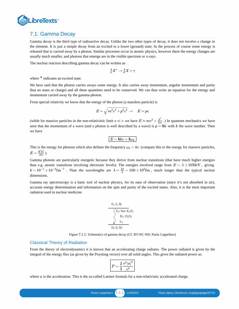
Paola Cappellaro 7.1.1 12/9/2021 https://phys.libretexts.org/@go/page/25731

7.1: Gamma DecayGamma decay is the third type of radioactive decay. Unlike the two other types of decay, it does not involve a change inthe element. It is just a simple decay from an excited to a lower (ground) state. In the process of course some energy isreleased that is carried away by a photon. Similar processes occur in atomic physics, however there the energy changes areusually much smaller, and photons that emerge are in the visible spectrum or x-rays.

The nuclear reaction describing gamma decay can be written as

where indicates an excited state.

We have said that the photon carries aways some energy. It also carries away momentum, angular momentum and parity(but no mass or charge) and all these quantities need to be conserved. We can thus write an equation for the energy andmomentum carried away by the gamma-photon.

From special relativity we know that the energy of the photon (a massless particle) is

(while for massive particles in the non-relativistic limit we have .) In quantum mechanics we haveseen that the momentum of a wave (and a photon is well described by a wave) is with the wave number. Thenwe have

This is the energy for photons which also defines the frequency (compare this to the energy for massive particles,).

Gamma photons are particularly energetic because they derive from nuclear transitions (that have much higher energiesthan e.g. atomic transitions involving electronic levels). The energies involved range from , giving

. Than the wavelengths are , much longer than the typical nucleardimensions.

Gamma ray spectroscopy is a basic tool of nuclear physics, for its ease of observation (since it’s not absorbed in air),accurate energy determination and information on the spin and parity of the excited states. Also, it is the most importantradiation used in nuclear medicine.

Figure : Schematics of gamma decay (CC BY-NC-ND; Paola Cappellaro)

Classical Theory of RadiationFrom the theory of electrodynamics it is known that an accelerating charge radiates. The power radiated is given by theintegral of the energy flux (as given by the Poynting vector) over all solid angles. This gives the radiated power as:

where is the acceleration. This is the so-called Larmor formula for a non-relativistic accelerated charge.

→ X+γAZX

∗ AZ

∗

E = → E = pc+m2c4 p2c2− −−−−−−−−−

√

v≪ c E ≈ m +c2 p2

2m

p = ℏk k

E = ℏkc = ℏωk

= kcωk

E = ℏ2k2

2m

E ∼ .1 ÷10MeV

k ∼ ÷10−1 10−3 fm−1 λ = ∼ 100 ÷ fm2πk

104

7.1.1

P =2

3

|ae2 |2

c3

a

Paola Cappellaro 7.1.2 12/9/2021 https://phys.libretexts.org/@go/page/25731

As an important example we consider an electric dipole. An electric dipole can be considered as an oscillating charge,over a range , such that the electric dipole is given by . Then the equation of motion is

and the acceleration

Averaged over a period , this is

Finally we obtain the radiative power for an electric dipole:

Electromagnetic Multipoles

In order to determine the classical e.m. radiation we need to evaluate the charge distribution that gives rise to it. Theelectrostatic potential of a charge distribution is given by the integral:

When treating radiation we are only interested in the potential outside the charge and we can assume the charge (e.g. aparticle!) to be well localized ( ). Then we can expand in power series. First, we express explicitly the norm

We set

and

This is a small quantity, given the assumption . Then we can expand:

Replacing with its expression we have:

Example 7.1.1

r0 d(t) = qr(t)

r(t) = cos(ωt)r0

a = = − cos(ωt)r r0ω2

T = 2π/ω

⟨ ⟩ = dta(t) =a2 ω

2π∫

T

0

1

2r2

0ω4

=PE11

3

e2ω4

c3| |r  0

2

(r)ρe

V ( ) =r  1

4πϵ0∫Vol′

( )ρe r′→

−∣∣∣r   r′

→∣∣∣

≪ rr′ 1

−∣∣r   r  ′∣∣

− = = r .∣∣r   r  ′∣∣ + −2r cosϑr2 r′2 r′− −−−−−−−−−−−−−−√ 1 + −2 cosϑ( )

r′

r

2 r′

r

− −−−−−−−−−−−−−−−−−

√

R =r′

r

ϵ = −2R cosϑ.R2

≪ rr′

= = (1 − ϵ+ − +…)1

−∣∣r   r  ′∣∣

1

r

1

1 + ϵ− −−−

√

1

r

1

2

3

8ϵ2 5

16ϵ3

ϵ

Paola Cappellaro 7.1.3 12/9/2021 https://phys.libretexts.org/@go/page/25731

We recognized in the coefficients to the powers of the Legendre Polynomials (with the power of , andnote that for powers > 3 we should have included higher terms in the original expansion):

With this result we can as well calculate the potential:

The various terms in the expansion are the multipoles. The few lowest ones are :

This type of expansion can be carried out as well for the magnetostatic potential and for the electromagnetic, time-dependent field.

At large distances, the lowest orders in this expansion are the only important ones. Thus, instead of considering the totalradiation from a charge distribution, we can approximate it by considering the radiation arising from the first fewmultipoles: i.e. radiation from the electric dipole, the magnetic dipole, the electric quadrupole etc.

Each of these radiation terms have a peculiar angular dependence. This will be reflected in the quantum mechanicaltreatment by a specific angular momentum value of the radiation field associated with the multipole. In turns, this will giverise to selection rules determined by the addition rules of angular momentum of the particles and radiation involved in theradiative process.

Quantum mechanical theoryIn quantum mechanics, gamma decay is expressed as a transition from an excited to a ground state of a nucleus. Then wecan study the transition rate of such a decay via Fermi’s Golden rule

There are two important ingredients in this formula, the density of states and the interaction potential .

Density of states

The density of states is defined as the number of available states per energy: , where is the number of

states. We have seen at various time the concept of degeneracy: as eigenvalues of an operator can be degenerate, theremight be more than one eigenfunction sharing the same eigenvalues. In the case of the Hamiltonian, when there aredegeneracies it means that more than one state share the same energy.

1

r

1

1 + ϵ− −−−

√= (1 − ( −2R cosϑ) + − +…)

1

r

1

2R2 3

8( −2R cosϑ)R2 2 5

16( −2R cosϑ)R2 3

= (1 +[− +R cosϑ]+[ − cosϑ+ ϑ]1

r

1

2R2 3

8R4 3

2R3 3

2R2 cos2

+[− + cos(ϑ) − (ϑ) + (ϑ)]+…)5R6

16

15

8R5 15

4R4 cos2 5

2R3 cos3

= (1 +R cosϑ+ ( − )+ ( − )+…)1

rR2 3 ϑcos2

2

1

2R3 5 (ϑ)cos3

2

3 cos(ϑ)

2

R (cosϑ)Pl l Rl

ϵ

= (cosϑ) = (cosϑ)1

r

1

1 + ϵ− −−−

√

1

r∑l=0

∞

RlPl

1

r∑l=0

∞

( )r′

r

l

Pl

V ( ) = ρ ( ) (cosϑ)dr  1

4πϵ0

1

r∫Vol′

r  ′1

r∑l=0

∞

( )r′

r

l

Pl r  ′

ρ ( )d =  Monopole 14πϵ0

1r ∫Vol′ r  ′ r′

→ Q

4π rϵ0

ρ ( ) (cosϑ)d = ρ ( ) cosϑd =  Dipole 14πϵ0

1r2 ∫Vol′ r  ′ r′P1 r′

→1

4πϵ0

1r2 ∫Vol′ r  ′ r′ r′

→⋅r d  

4πϵ0r2

ρ ( ) (cosϑ)d = ρ ( ) ( ϑ− )d  Quadrupole 14πϵ0

1r3

∫Vol′

r  ′ r′2P2 r′→

14πϵ0

1r3

∫Vol′

r  ′ r′2 32

cos2 12

r′→

W = ρ ( )2π

ℏ⟨ | | ⟩∣

∣ ψf V ψi∣∣2

Ef

ρ ( )Ef V

ρ ( ) =EfdNs

dEfNs

Paola Cappellaro 7.1.4 12/9/2021 https://phys.libretexts.org/@go/page/25731

By considering the nucleus+radiation to be enclosed in a cavity of volume L , we have for the emitted photon awavefunction represented by the solution of a particle in a 3D box that we saw in a Problem Set.

As for the 1D case, we have a quantization of the momentum (and hence of the wave-number ) in order to fit thewavefunction in the box. Here we just have a quantization in all 3 directions:

(with integers). Then, going to spherical coordinates, we can count the number of states in a spherical shell between and to be . Expressing this in terms of , we have . If we consider just a

small solid angle instead of we have then the number of state . Since , we

finally obtain the density of states:

Figure : Density of states: counting the states 2D (CC BY-NC-ND; Paola Cappellaro)

The vector potential

Next we consider the potential causing the transition. The interaction of a particle with the e.m. field can be expressed in

terms of the vector potential of the e.m. field as:

where is the particle’s momentum. The vector potential in QM is an operator that can create or annihilate photons,

where annihilates (creates) one photon of momentum . Also, is the polarization of the e.m. field. Since

gamma decay (and many other atomic and nuclear processes) is able to create photons (or absorb them) it makes sense thatthe operator describing the e.m. field would be able to describe the creation and annihilation of photons. The second

characteristic of this operator are the terms which describe a plane wave, as expected for e.m. waves, withmomentum and frequency .

Dipole transition for gamma decay

To calculate the transition rate from the Fermi’s Golden rule,

3

k

= , = , =kx2π

Lnx ky

2π

Lny kz

2π

Lnz

n n

n+dn d = 4π dnNs n2 k d = 4π dkNs k2 L3

(2π)3

dΩ 4π d = dkdΩNsL3

(2π)3 k2 E = ℏkc = ℏω

ρ(E) = = dΩ = dΩ = dΩdNs

dE

L3

(2π)3k2 dk

dE

L3

(2π)3

k2

ℏc

ω2

ℏc3

L3

(2π)3

7.1.2

A  ^

= ⋅Ve

mcA  ^

p  ^

p  ^ A  ^

= ( + )A  ^∑k

2πℏc2

V ωk

− −−−−−

√ akei ⋅k r   a†

ke−i ⋅k r   ϵ  k

( )ak a†k

k  ϵ  k

∝ e−i ⋅k r  

ℏk ck

W = ρ ( ) ,2π

ℏ⟨ | | ⟩∣

∣ ψf V ψi∣∣2

Ef

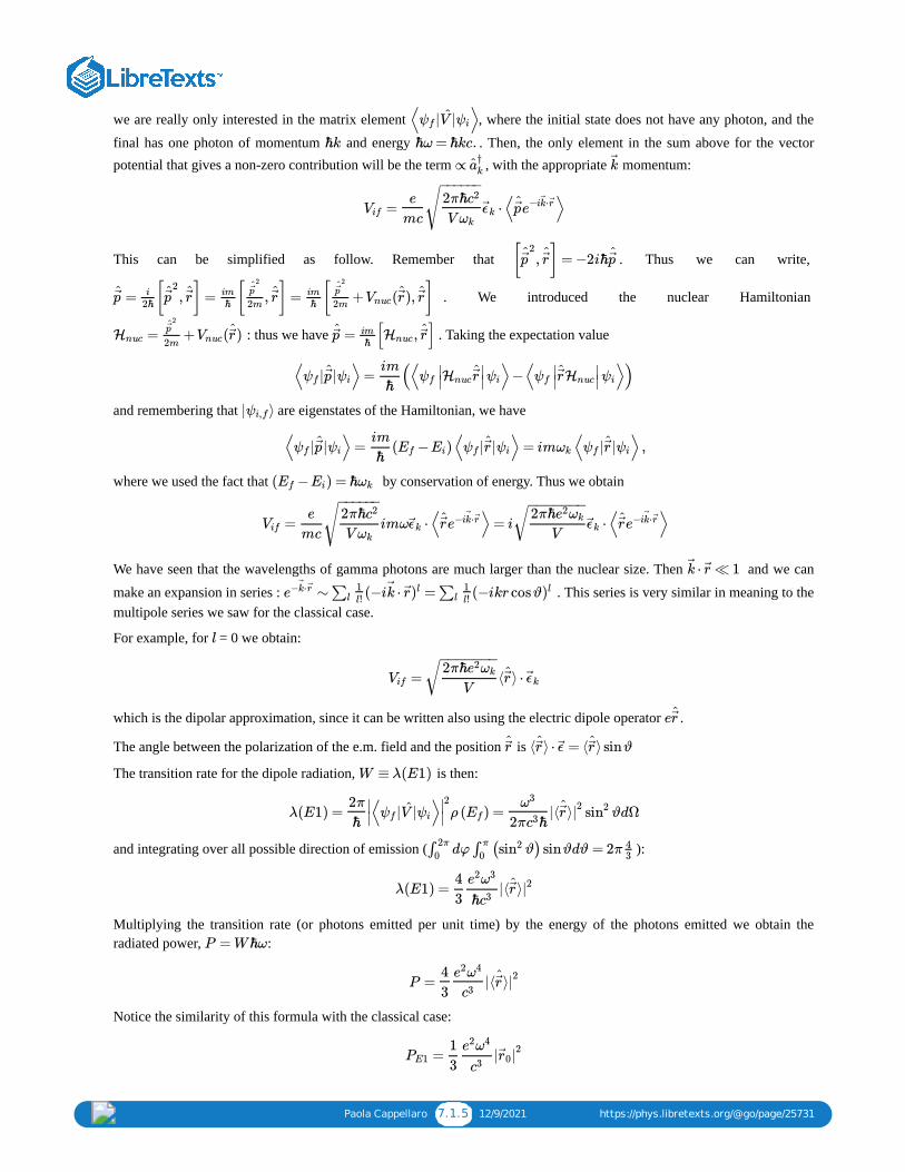
Paola Cappellaro 7.1.5 12/9/2021 https://phys.libretexts.org/@go/page/25731

we are really only interested in the matrix element , where the initial state does not have any photon, and the

final has one photon of momentum and energy . Then, the only element in the sum above for the vectorpotential that gives a non-zero contribution will be the term , with the appropriate momentum:

This can be simplified as follow. Remember that . Thus we can write,

. We introduced the nuclear Hamiltonian

: thus we have . Taking the expectation value

and remembering that are eigenstates of the Hamiltonian, we have

where we used the fact that by conservation of energy. Thus we obtain

We have seen that the wavelengths of gamma photons are much larger than the nuclear size. Then and we can

make an expansion in series : . This series is very similar in meaning to themultipole series we saw for the classical case.

For example, for = 0 we obtain:

which is the dipolar approximation, since it can be written also using the electric dipole operator .

The angle between the polarization of the e.m. field and the position is

The transition rate for the dipole radiation, is then:

and integrating over all possible direction of emission ( ):

Multiplying the transition rate (or photons emitted per unit time) by the energy of the photons emitted we obtain theradiated power, :

Notice the similarity of this formula with the classical case:

⟨ | | ⟩ψf V ψi

ℏk ℏω = ℏkc.

∝ a†k k 

= ⋅⟨ ⟩Vife

mc

2πℏc2

V ωk

− −−−−−

√ ϵ  k p  ^e−i ⋅k r  

[ , ] = −2iℏp  ^2r  ^ p  ^

= [ , ] = [ , ] = [ + ( ), ]p  ^ i

2ℏp  ^2

r  ^ im

ℏp  ^2

2mr  ^ im

ℏp  ^2

2mVnuc r  ^ r  ^

= + ( )Hnucp  ^2

2mVnuc r  ^ = [ , ]p  ^ im

ℏHnuc r  ^

⟨ | | ⟩ = (⟨ ⟩−⟨ ⟩)ψf p  ^ ψi

im

ℏψf

∣∣Hnucr  ^∣

∣ψi ψf∣∣r  ^Hnuc

∣∣ψi

| ⟩ψi,f

⟨ | | ⟩ = ( − )⟨ | | ⟩ = im ⟨ | | ⟩ ,ψf p  ^ ψi

im

ℏEf Ei ψf r  ^ ψi ωk ψf r  ^ ψi

( − ) = ℏEf Ei ωk

= imω ⋅⟨ ⟩ = i ⋅⟨ ⟩Vife

mc

2πℏc2

V ωk

− −−−−−

√ ϵ  k r  ^e−i ⋅k r   2πℏe2ωk

V

− −−−−−−√ ϵ  k r  ^e−i ⋅k r  

⋅ ≪ 1k  r  

∼ (−i ⋅ = (−ikr cosϑe− ⋅k r   ∑l1l!

k  r  )l ∑l1l!

)l

l

= ⟨ ⟩ ⋅Vif2πℏe2ωk

V

− −−−−−−√ r  ^ ϵ  k

er  ^

r  ^ ⟨ ⟩ ⋅ = ⟨ ⟩ sinϑr  ^ ϵ   r  ^

W ≡ λ(E1)

λ(E1) = ρ ( ) = |⟨ ⟩ ϑdΩ2π

ℏ⟨ | | ⟩∣

∣ ψf V ψi∣∣2

Ef

ω3

2π ℏc3r  ^ |

2sin2

dφ ( ϑ) sinϑdϑ = 2π∫ 2π0

∫ π

0sin2 4

3

λ(E1) = |⟨ ⟩4

3

e2ω3

ℏc3r  ^ |2

P = Wℏω

P = |⟨ ⟩4

3

e2ω4

c3r  ^ |

2

=PE11

3

e2ω4

c3| |r  0

2

Paola Cappellaro 7.1.6 12/9/2021 https://phys.libretexts.org/@go/page/25731

We can estimate the transition rate by using a typical energy for the photon emitted (equal to a typical energydifference between excited and ground state nuclear levels) and the expectation value for the dipole (

). Then, the transition rate is evaluated to be

(with E in MeV). For example, for A = 64 and E = 1MeV the rate is or (femtoseconds!) forE = 0.1MeV is on the order of picoseconds.

Because of the large energies involved, very fast processes are expected in the nuclear decay from excited states, inaccordance with Fermi’s Golden rule and the energy/time uncertainty relation.

Extension to MultipolesWe obtained above the transition rate for the electric dipole, i.e. when the interaction between the nucleus and the e.m.field is described by an electric dipole and the emitted radiation has the character of electric dipole radiation. This type ofradiation can only carry out of the nucleus one quantum of angular momentum (i.e. , between excited and groundstate). In general, excited levels differ by more than 1 , thus the radiation emitted need to be a higher multipole radiationin order to conserve angular momentum.

Electric Multipoles

We can go back to the expansion of the radiation interaction in multipoles:

Then the transition rate becomes:

Notice the strong dependence on the quantum number. Setting again we also have a strong dependence onthe mass number.

Thus, we have the following estimates for the rates of different electric multipoles:

Magnetic Multipoles

The e.m. potential can also contain magnetic interactions, leading to magnetic transitions. The transition rates can becalculated from a similar formula:

where is the magnetic moment of the proton (and its mass).

Estimates for the transition rates can be found by setting :

E = ℏω

|⟨ ⟩| ∼ ≈r  ^ Rnuc r0A1/3

λ(E1) = = 1.0 ×e2

ℏc

E3

(ℏc)3r2

0A2/3 1014A2/3E3

λ ≈ 1.6 ×1015s−1 τ = 10−15

τ

Obs.

Δl = ±1l

∼ (i ⋅V ∑l

1

l!k ^

r  ^)l

λ(El) = c⟨| |8π(l+1)

l[(2l+1)!!]2e2

ℏc( )

E

ℏc

2l+1

( )3

l+3

2

r  ^ ⟩2l

l |⟨ ⟩| ∼r  ^ r0A1/3

λ(E1) = 1.0 ×1014A2/3E3

λ(E2) = 7.3 ×107A4/3E5

λ(E3) = 34A2E7

λ(E4) = 1.1 ×10−5A8/3E9

λ(Ml) = c⟨| | [ ( − )]8π(l+1)

l[(2l+1)!!]2e2

ℏc

E2l+1

ℏc( )

3

l+3

2

r  ^ ⟩2l−2 ℏ

cmp

μp

1

l+1

μp mp

− ≈ 10μp1

l+1

λ(M1) = 5.6 ×1013E3

λ(M2) = 3.5 ×107A2/3E5

λ(M3) = 16A4/3E7

Paola Cappellaro 7.1.7 12/9/2021 https://phys.libretexts.org/@go/page/25731

Selection Rules

The angular momentum must be conserved during the decay. Thus the difference in angular momentum between the initial(excited) state and the final state is carried away by the photon emitted. Another conserved quantity is the total parity ofthe system.

Parity change

The parity of the gamma photon is determined by its character, either magnetic or electric multipole. We have

Then if we have a parity change from the initial to the final state this is accounted for by the emitted photon as:

This of course limits the type of multipole transitions that are allowed given an initial and final state.

Angular momentum

From the conservation of the angular momentum:

the allowed values for the angular momentum quantum number of the photon, , are restricted to

Once the allowed have been found from the above relationship, the character (magnetic or electric) of the multipole isfound by looking at the parity.

In general then, the most important transition will be the one with the lowest allowed , . Higher multipoles are alsopossible, but they are going to lead to much slower processes.

Table : Angular momentum and parity of the gamma multipoles (CC BY-NC-ND; Paola Cappellaro)

Dominant Decay Modes

In general we have the following predictions of which transitions will happen:

1. The lowest permitted multipole dominates2. Electric multipoles are more probable than the same magnetic multipole by a factor ∼ 10 (however, which one is

going to happen depends on the parity)

3. Emission from the multipole + 1 is 10 times less probable than the -multipole emission.

λ(M4) = 4.5 ×10−6A2E9

(El) = (−1  Electric multipole Πγ )l

(Ml) = (−1  Magnetic multipole Πγ )l−1

→Πi Πf

=Πγ ΠiΠf

ΔΠ = no →  Even Electric, Odd Magnetic 

ΔΠ =  yes  →  Odd Electric, Even Magnetic 

= +I  ^i I  ^

f L ^γ

l

= | − | , … , +lγ Ii If Ii If

l

l Π

7.1.1

2

≈λ(El)

λ(Ml)102

l −5 l

Paola Cappellaro 7.1.8 12/9/2021 https://phys.libretexts.org/@go/page/25731

4. Combining 2 and 3, we have:

Thus E2 competes with M1 while that’s not the case for M2 vs. E1

Internal conversion

What happen if no allowed transitions can be found? This is the case for even-even nuclides, where the decay from the 0excited state must happen without a change in angular momentum. However, the photon always carries some angularmomentum, thus gamma emission is impossible.

Then another process happens, called internal conversion:

where is a ionized state and is one of the atomic electrons.

Besides the case of even-even nuclei, internal conversion is in general a competing process of gamma decay (see Krane formore details).

≈ , ≈λ(E, l+1)

λ(El)10−5 λ(M , l+1)

λ(Ml)10−5

≈ , ≈λ(E, l+1)

λ(Ml)10−3 λ(M , l+1)

λ(El)10−7

+

X+ZA

X∗ →AZ e−

XAZ e−

Paola Cappellaro 7.2.1 12/2/2021 https://phys.libretexts.org/@go/page/25732

7.2: Beta DecayThe beta decay is a radioactive decay in which a proton in a nucleus is converted into a neutron (or vice-versa). In theprocess the nucleus emits a beta particle (either an electron or a positron) and quasi-massless particle, the neutrino.

Figure : Beta decay schematics (CC BY-NC-ND; Paola Cappellaro)

Recall the mass chain and Beta decay plots of Fig. 7. When studying the binding energy from the SEMF we saw that atfixed A there was a minimum in the nuclear mass for a particular value of Z. In order to reach that minimum, unstablenuclides undergo beta decay to transform excess protons in neutrons (and vice-versa).

Reactions and Phenomenology

The beta-decay reaction is written as:

This is the decay. (or negative beta decay) The underlying reaction is:

which converts a proton into a neutron with the emission of an electron and an anti-neutrino. There are two other types ofreactions, the reaction,

with this underlying reaction

which sees the emission of a positron (the electron anti-particle) and a neutrino; and the electron capture:

with this underlying reaction

a process that competes with, or substitutes, the positron emission.

7.2.1

⟶ + +XNZ

AX

N−1′

Z+1

A e− ν

β−

n → p+ +e− ν

β+

⟶ + +νXNZA

XN+

1

′Z−1

A e+

p⟶ n+ +νe+

+ → +νAZXN e− A

Z−1X′N+1

p+ → νe− n+

Paola Cappellaro 7.2.2 12/2/2021 https://phys.libretexts.org/@go/page/25732

The neutrino and beta particle ( ) share the energy.

Since the neutrinos are very difficult to detect (as we will see they are almost massless and interact very weakly withmatter), the electrons/positrons are the particles detected in beta-decay and they present a characteristic energy spectrum(see Fig. 45). The difference between the spectrum of the particles is due to the Coulomb repulsion or attraction fromthe nucleus. Notice that the neutrinos also carry away angular momentum. They are spin-1/2 particles, with no charge(hence the name) and very small mass. For many years it was actually believed to have zero mass. However it has beenconfirmed that it does have a mass in 1998.

Figure \(\PageIndex{2}\): : Beta decay spectra: Distribution of momentum (top plots) and kineticenergy (bottom) for (left) and (right) decay. © Neil Spooner. All rights reserved. Thiscontent is excluded from the Creative Commons license. For more information, seehttp://ocw.mit.edu/fairuse.

Conservation LawsAs the neutrino is hard to detect, initially the beta decay seemed to violate energy conservation. Introducing an extraparticle in the process allows one to respect conservation of energy. Besides energy, there are other conserved quantities:

Energy: The Q value of a beta decay is given by the usual formula:

Using the atomic masses and neglecting the electron’s binding energies as usual we have

The kinetic energy (equal to the ) is shared by the neutrino and the electron (we neglect any recoil of the massivenucleus). Then, the emerging electron (remember, the only particle that we can really observe) does not have a fixedenergy, as it was for example for the gamma photon. But it will exhibit a spectrum of energy (which is the number ofelectron at a given energy) as well as a distribution of momenta. We will see how we can reproduce these plots byanalyzing the QM theory of beta decay.

Momentum: The momentum is also shared between the electron and the neutrino. Thus the observed electronmomentum ranges from zero to a maximum possible momentum transfer.Angular momentum (both the electron and the neutrino have spin 1/2)

Example 7.2.1

Cu∖6429

↗ Zn+ + , = 0.57MeV64 e− ν Qβ

Ni + +ν, = 0.66MeV6428 e+ Qβ

β±

β±

β− β+

= [ ( X)− ( )− ] .Qβ− mNA mN

AZ+1

X ′ me c2

Qβ− = {[ ( X)−Z ] −[ ( )−(Z+1) ] − }mAA me mA

AZ+1X

′ me me c2

= [ ( X)− ( )] .mAA mA

AZ+1X

′ c2

Q

Paola Cappellaro 7.2.3 12/2/2021 https://phys.libretexts.org/@go/page/25732

Parity? It turns out that parity is not conserved in this decay. This hints to the fact that the interaction responsibleviolates parity conservation (so it cannot be the same interactions we already studies, e.m. and strong interactions)Charge (thus the creation of a proton is for example always accompanied by the creation of an electron)Lepton number: we do not conserve the total number of particles (we create beta and neutrinos). However the numberof massive, heavy particles (or baryons, composed of 3 quarks) is conserved. Also the lepton number is conserved.Leptons are fundamental particles (including the electron, muon and tau, as well as the three types of neutrinosassociated with these 3). The lepton number is +1 for these particles and -1 for their antiparticles. Then an electron isalways accompanied by the creation of an antineutrino, e.g., to conserve the lepton number (initially zero).

Fermi’s Theory of Beta DecayThe properties of beta decay can be understood by studying its quantum-mechanical description via Fermi’s Golden rule,as done for gamma decay.

In gamma decay process we have seen how the e.m. field is described as an operator that can create (or destroy) photons.Nobody objected to the fact that we can create this massless particles. After all, we are familiar with charged particles thatproduce (create) an e.m. field. However in QM photons are also particles, and by analogy we can have also creation ofother types of particles, such as the electron and the neutrino.

For the beta decay we need another type of interaction that is able to create massive particles (the electron and neutrino).The interaction cannot be given by the e.m. field; moreover, in the light of the possibilities of creating and annihilatingparticles, we also need to find a new description for the particles themselves that allows these processes. All of this isobtained by quantum field theory and the second quantization. Quantum field theory gives a unification of e.m. and weakforce (electro-weak interaction) with one coupling constant e. The interaction responsible for the creation of the electronand neutrino in the beta decay is called the weak interaction and its one of the four fundamental interactions (togetherwith gravitation, electromagnetism and the strong interaction that keeps nucleons and quarks together). One characteristicof this interaction is parity violation.

Matrix element

The weak interaction can be written in terms of the particle field wavefunctions:

where annihilates (creates) the particle a, and g is the coupling constant that determines how strong the

interaction is. Remember that the analogous operator for the e.m. field was (creating one photon of momentum k).

Then the matrix element

can be written as:

(Here since we have scalar operators).

To first approximation the electron and neutrino can be taken as plane waves:

and since we can approximate this with

W = ρ ( )2π

ℏ⟨ | | ⟩∣

∣ ψf V ψi∣∣2

Ef

= gVint Ψ†eΨ

†ν

( )Ψa Ψ†a

∝ a†k

= ⟨ | | ⟩Vif ψf Hint ψi

= g∫ ( ) [ ( ) ( )] ( )Vif d3x Ψ∗p x  Ψ∗

e x  Ψ∗ν x  Ψn x 

† → ∗

= g∫ ( ) ( )Vif d3x Ψ∗p x 

ei ⋅k e x  

V−−

√

ei ⋅k ν x  

V−−

√Ψn x 

kR ≪ 1

= ∫ ( ) ( )Vifg

Vd3x Ψ∗

p x  Ψn x 

Paola Cappellaro 7.2.4 12/2/2021 https://phys.libretexts.org/@go/page/25732

We then write this matrix element as

where is a very complicated function of the nuclear spin and angular momentum states. In addition, we will use in theFermi’s Golden Rule the expression

where the Fermi function accounts for the Coulomb interaction between the nucleus and the electron that wehad neglected in the previous expression (where we only considered the weak interaction).

Density of states

In studying the gamma decay we calculated the density of states, as required by the Fermi’s Golden Rule. Here we need todo the same, but the problem is complicated by the fact that there are two types of particles (electron and neutrino) asproducts of the reaction and both can be in a continuum of possible states. Then the number of states in a small energyvolume is the product of the electron and neutrino’s states:

The two particles share the energy:

For simplicity we assume that the mass of the neutrino is zero (it’s much smaller than the electron mass and of the kineticmass of the neutrino itself). Then we can take the relativistic expression

while for the electron

and we then write the kinetic energy of the neutrino as a function of the electron's,

The number of states for the electron can be calculated from the quantized momentum, under the assumption that the

electron state is a free particle in a region of volume

and the same for the neutrino,

where we used the relationship between momentum and wavenumber:

At a given momentum/energy value for the electron, we can write the density of states as

where we used : and

The density of states is then

=Vifg

VMnp

Mnp

→ F ( , )| |Mnp2 | |Mnp

2 Z0 Qβ

F ( , )Z0 Qβ

= d d .d2Ns Ne Nν

Q

= + .Qβ Te Tν

= c ,Tν pν

= + → E = +  with  = −E2 p2c2 m2c4 Te mec2 Te +p2

ec2 m2

ec4

− −−−−−−−−−√ mec

2

= − .Tν Qβ Te

(ψ ∼ )ei ⋅k r   V = :L3

d = 4π d = dNe ( )L

2π

3

k2e ke

4πV

(2πℏ)3p2e pe

d = dNν

4πV

(2πℏ)3p2ν pν

= ℏ .p   k 

ρ ( )d = d = 16 d = dpe pe Ne

dNν

dTνπ2 V 2

(2πℏ)6p2e pep2

ν

dpν

dTν

V 2

4π4ℏ6c3[Q− ]Te

2p2e pe

= cdTν

dpν= ( − ) /c.pν Qβ Te

ρ ( )d = d = dpe peV 2

4π4ℏ6c3[Q− ]Te

2p2e pe

V 2

4π4ℏ6c3[Q−( − )]+p2

ec2 m2

ec4

− −−−−−−−−−√ mec

22

p2e pe

Paola Cappellaro 7.2.5 12/2/2021 https://phys.libretexts.org/@go/page/25732

or rewriting this expression in terms of the electron kinetic energy:

Knowing the density of states, we can calculate how many electrons are emitted in the beta decay with a given energy.This will be proportional to the rate of emission calculated from the Fermi Golden Rule, times the density of states:

and

These distributions are nothing else than the spectrum of the emitted beta particles (electron or positron). In theseexpression we collected in the constant C various parameters deriving from the Fermi Golden Rule and density of statescalculations, since we want to highlight only the dependence on the energy and momentum. Also, we introduced a newfunction, F(Z, Q), called the Fermi function, that takes into account the shape of the nuclear wavefunction and in particularit describes the Coulomb attraction or repulsion of the electron or positron from the nucleus. Thus, F(Z, Q) is different,depending on the type of decay. These distributions were plotted in Fig. 45. Notice that these distributions (as well as thedecay rate below) are the product of three terms:

the Statistical factor (arising from the density of states calculation), the Fermi function (accounting for the Coulomb interaction), F(Z, Q)and the Transition amplitude from the Fermi Golden Rule,

These three terms reflect the three ingredients that determine the spectrum and decay rate of in beta decay processes.

Decay rate

The decay rate is obtained from Fermi’s Golden rule:

where ρ(E) is the total density of states. ρ(E) (and thus the decay rate) is obtained by summing over all possible states ofthe beta particle, as counted by the density of states. Thus, in practice, we need to integrate the density of states over allpossible momentum of the outgoing electron/positron. Upon integration over we obtain:

(where we took in the relativistic limit for high electron speed).

We can finally write the decay rate as:

where we introduced the constant

ρ ( ) = = ( + )TeV 2

4π4ℏ6c3[Q− ]Te

2p2e

dpe

dTe

V 2

4c6π4ℏ6[Q− ]Te

2+2T 2

e Temec2

− −−−−−−−−−−√ Te mec

2

( as  d = ( + )/ d )pe pe Te mec2 c2 Te

N(p) = CF (Z,Q) [Q−T = CF (Z,Q)| |Vfi2 p

2

c2]2 | |Vfi

2 p2

c2[Q−( − )]+p2

ec2 m2

ec4

− −−−−−−−−−√ mec

22

N ( ) = F (Z,Q) ( + )TeC

c5| |Vfi

2 [Q− ]Te2 +2T 2

e Temec2

− −−−−−−−−−−√ Te mec

2

[Q−Tp2

c2 ]2

| |Vfi2

W = ρ(E)2π

ℏ| |Vif

2

pe

ρ(E) = d ≈V 2

4π4ℏ6c3∫

pmaxe

0pe [Q− ]Te

2p2e

V 2

4π4ℏ6c3

(Q−m )c2 5

30c3

≈ pcTe

W = ρ(E) = F (Z, )2π

ℏ| |Vif

2 2π

ℏ

g

V

2| |Mnp

2 Qβ

V 2

4π4ℏ6c3

(Q−m )c2 5

30c3

= F (Z, )G2F | |Mnp

2Qβ

(Q−m )c2 5

60 ℏ(ℏcπ3 )6

=GF

1

2π3−−−

√

g cm2e

ℏ3

Paola Cappellaro 7.2.6 12/2/2021 https://phys.libretexts.org/@go/page/25732

which gives the strength of the weak interaction. Comparing to the strength of the electromagnetic interaction, as given bythe fine constant , the weak is interaction is much smaller, with a constant

We can also write the differential decay rate :

The square root of this quantity is then a linear function in the neutrino kinetic energy, :

This is the Fermi-Kurie relation. Usually, the Fermi-Kurie plot is used to infer by linear regression the maximum electronenergy (or Q) by finding the straight line intercept.

Figure : Example of Fermi-Kurie plot (see also Krane, Fig. 9.4, 9.5) (CC BY-NC-ND; Paola Cappellaro)

α = ∼e2

ℏc1

137∼ .10−6

dW

dpe

= ρ ( ) ∝ F (Z,Q)dW

dpe

2π

ℏ| |Vif

2 pe [Q− ]Te2p2

e

Q−Te

∝ Q−dW

dpe

1

F (Z,Q)p2e

− −−−−−−−−−−−

√ Te

7.2.3

Paola Cappellaro 8.1 12/16/2021 https://phys.libretexts.org/@go/page/25744

8: Applications of Nuclear ScienceWe have now a clearer picture of the nuclear structure and of the radioactive decays, as well as the formalism –based onquantum mechanics and quantum field theory– that describes their dynamics. We can turn to the study of someapplications of these ideas.

First, we will study how radiation interacts with matter. This is fundamental both in order to know what are the effects ofradiation emitted during nuclear processes on the materials around (and the people) and in order to devise detectors thatcan measure these radiations. At the same time the knowledge of how radiation interacts with matter leads to manyimportant applications in e.g. nuclear medicine, for imaging and therapy, in materials science, for imaging and diagnostic,in agriculture, archeology etc. Most of you might have already studied these applications in 22.01 and also analyzed theprocesses that give rise to the interactions. Thus we will be here only have a quick review, focusing mostly on the physicalprocesses.

Then we will study two nuclear reactions (fission and fusion) that can be used as sources of energy (or in the case offusion, that holds that promise).

8.1: Interaction of Radiation with Matter

Paola Cappellaro 8.1.1 11/18/2021 https://phys.libretexts.org/@go/page/25738

8.1: Interaction of Radiation with Matter

Cross Section

Classically, the cross section is the area on which a colliding projectile can impact. Thus for example the cross section of aspherical target of radius r is just given by . The cross section has then units of an area. Let’s consider for example anucleus with mass number A. The radius of the nucleus is then and the classical cross sectionwould be . For a typical heavy nucleus, such as gold, A = 197, we have

.

When scattering a particle off a target however, what becomes important is not the head-on collision (as between balls) butthe interaction between the particle and the target (e.g. Coulomb, nuclear interaction, weak interaction etc.). Formacroscopic objects the details of these interactions are lumped together and hidden. For single particles this is not thecase, and for example we can as well have a collision even if the distance between projectile and target is larger than thetarget radius. Thus the cross section takes on a different meaning and it is now defined as the effective area or moreprecisely as a measure of the probability of a collision. Even in the classical analogy, it is easy to see why the cross sectionhas this statistical meaning, since in a collision there is a certain (probabilistic) distribution of the impact distance. Thecross section also describes the probability of a given (nuclear) reaction to occur, a reaction that can be generally writtenas:

where is an heavy target and a a small projectile (such as a neutron, proton, alpha...) while and b are the reactionproducts (again with b being nucleons or light nucleus, or in some cases a gamma ray).

Then let be the current of incoming particles, hitting on an heavy (hence stationary) target. The heavy product willalso be almost stationary and only b will escape the material and be measured. Thus we will observe the productsarriving at a detector at a rate . If there are n target nuclei per unit area, the cross section can then be written as

This quantity do not always agree with the estimated cross section based on the nucleus radius. For example, protonscattering x-section can be higher than neutrons, because of the Coulomb interaction. Neutrinos x-section then will be evensmaller, because they only interact via the weak interaction.

Differential Cross Section

The outgoing particles ( ) are scattered in all directions. However most of the time the detector only occupies a smallregion of space. Thus we can only measure the rate at a particular location, identified by the angles . What we areactually measuring is the rate of scattered particles in the small solid angle , and the relevant cross section isthe differential cross section

From this quantity, the total cross section, defined above, can be calculated as

(Notice that having added the factor gives for constant ).

Doubly differential cross section

When one is also interested in the energy of the outgoing particles , because this can give information e.g. on thestructure of the target or on the characteristic of the projectile-target interaction, the quantity that is measured is the crosssection as a function of energy. This can be simply

πr2

R ≈ = 1.25 fmR0A1/3 A1/3

σ = π ≈ 5R20A

2/3 A2/3fm2

σ ≈ 100 = 1 barn  (  symbol b, 1b = = = 100fm2 10−28  m2 10−24  cm2 fm2

a+X → +b  or  X(a, b)X ′ X ′

X X ′

Ia X ′

b

Rb

σ =Rb

nIa

b

Rb ϑ,φ

dΩ, r(ϑ,φ)

=dσ

dΩ

r(ϑ,φ)

4π nIa

σ = dΩ = sinϑdϑ dφ∫4π

dσ

dΩ∫

π

0∫

2π

0

dσ

dΩ

4π σ = 4π dσ

dΩdσ

dΩ

Eb

Paola Cappellaro 8.1.2 11/18/2021 https://phys.libretexts.org/@go/page/25738

if the detector is energy-sensitive but collect particles in any direction, or the doubly differential cross section

Neutron Scattering and Absorption

When neutrons travel inside a material, they will undergo scattering (elastic and inelastic) as well as other reactions, whileinteracting with the nuclei via the strong, nuclear force. Given a beam of neutron with intensity , when traveling throughmatter it will interact with the nuclei with a probability given by the total cross section . At high energies, reactions suchas (n,p), are possible, but at lower energy usually what happens is the capture of the neutron with theemission of energy in the form of gamma rays. Then, when crossing a small region of space dx the beam is reduced by anamount proportional to the number of nuclei in that region:

This formula, however, is too simplistic: on one side the cross section depends on the neutron energy (the cross sectionincreases at lower velocity as and at higher energies, the cross section can present some resonances – some peaks) andneutrons will lose part of their energy while traveling, thus the actual cross section will depend on the position. On theother side, not all reactions are absorption reactions, many of them will ”produce” another neutron (i.e., they will onlychange the energy of the neutron or its direction, thus not attenuating the beam). We then need a better description of thefate of a neutron beam in matter. For example, when one neutron with energy enters the material, it is firstslowed down by elastic and inelastic collisions and it is then finally absorbed.

We then want to know how many collisions are necessary to slow down a neutron and to calculate that, we first need toknow how much energy does the neutron loose in one collision. Different materials can have different cross sections,however the energy exchange in collision is much higher the lightest the target. Consider an elastic collision with a nucleusof mass M. In the lab frame, the nucleus is initially at rest and the neutron has energy and momentum . After thescattering, the neutron energy is , speed at an angle with , while the nucleus recoil gives a momentum at anangle (I will use the notation for the

Figure : Cross section for the neutron-He3 reactions. The data and plot can be obtained online fromhttp://t2.lanl.gov/data/ndviewer.html. (CC BY-NC-ND; Paola Cappellaro)

dσ

dEb

σd2

dΩdEb

I0

σT(n,α) (n, γ)

dI = − ndx → I(x) =I0σT I0e− nxσT

1/v

∼ 1MeV

E0 mv0

E1 v  1 φ v  0 MV  

ψ w

8.1.1 σ(E)

Paola Cappellaro 8.1.3 11/18/2021 https://phys.libretexts.org/@go/page/25738

Figure : Cross section for the neutron-U235 reactions. Notice the dependence at higher energies andresonances at lower energies. (CC BY-NC-ND; Paola Cappellaro)

magnitude of a vector ). The collision is better analyzed in the center of mass frame, where the condition ofelastic scattering implies that the relative velocities only change their direction but not their magnitude.

The center of mass velocity is defined as . Relative velocities in the center of mass frame aredefined as . We can calculate the neutron (kinetic) energy after the collision from . Anexpression for is obtained from the CM speed:

where we defined as the scattering angle in the center of mass frame (see Figure ).

Figure : Neutron scattering from a nucleus. Left, lab frame. Right, center of mass frame (CC BY-NC-ND; PaolaCappellaro)

Given the assumption of elastic scattering, we have , but .

Finally, we can express everything in terms of :

We now simplify this expression by making the approximation , where A is the mass number of the nucleus.

In terms of the neutron energy, we finally have

8.1.2 σ(E) 1/v

,w = | |w  w 

= =v  CMm +Mv  0 V 0

m+M

m

m+Mv  0

= −u  v   v  CM = mE112

| |v  12

| |v  12

= = + +2 ⋅ = + +2 cosϑ| |v  12 | + |u 1 v  CM

2 | |u 12 | |v  CM

2 u 1 v  CM u21 v2

CMu1vCM

ϑ 8.1.3

8.1.3

| | = | | =u 1 u 0 u0 = − = (1 − ) =u0 v0 vCM v0m

m+M

M

m+Mv0

v0

= + +2 cosϑ =| |v  12 M 2

(m+M)2v2

0

m2

(m+M)2v2

0

M

(m+M)v0

m

(m+M)v0 v2

0

+ +2mM cosϑM 2 m2

(m+M)2

M/m ≈ A

Paola Cappellaro 8.1.4 11/18/2021 https://phys.libretexts.org/@go/page/25738

This means that the final energy can be equal to (the initial one) if – corresponding to no collision– and reaches

a minimum value of .

Notice that from this expression it is clear that the neutron loose more energy in the impact with lighter nuclei, in particularall the energy in the impact with proton:

If , that is, almost no energy is lost.

If , and for all the energy is lost.

For low energy, the cross section is independent of thus we have a flat distribution of the outgoing energies: theprobability to scatter in any direction is constant, thus . What is the probability of a given energy ?

Figure : Probability distribution of the outgoing energy in neutron scattering from a nucleus. (CC BY-NC-ND; PaolaCappellaro)

We have . Then, since , the probability of a given

scattering energy is constant, as expected, and equal to . Notice that the probability is different than zero

only for . The average scattering energy is then and the average energy lost in ascattering event is .

It still requires many collision to lose enough energy so that a final capture is probable. How many?

The average energy after one collision is . After two collision it can be approximated by

. Then, after n collision, we have . Thus, if we want to know

how many collisions are needed to reach an average thermal energy we need to calculate n:

However, this calculation is not very precise, since the approximation we made, that we can calculate the average energyafter the scattering considering only the average after the scattering is not a good one, since the energy

distribution is not peaked around its average (but is quite flat). Consider instead the quantity log and take the

average over the possible final energy (note that this is the same as calculating for the first collision):

= ,E1 E0+1 +2A cosϑA2

(A+1)2

E0 ϑ = 0

= = α  for ϑ = π (here α = )E1 E0(A−1)

2

(A+1)2 E0(A−1)

2

(A+1)2

A ≫ 1, ≈ ≈E1 E0+2A cos ϑA2

A2E0

A = 1, = = cosE1 E02+2 cos ϑ

4E0 ( )ϑ

2

2ϑ = π

ϑ

P (cosϑ) = 12

E1

8.1.4

P ( )d = −P (cosϑ)d(cosϑ) = − sinϑdϑE1 E112

= − sinϑdE

dϑ

2 AE0

(A+1)2

P ( ) =E1(A+1)2

4 AE0

α ≤ ≤E0 E1 E0 ⟨ ⟩ =E1 E01+α

2

⟨ ⟩ =Eloss E01−α

2

⟨ ⟩ =E1 E01+α

2⟨ ⟩ ≈E2

⟨ ⟩ =E11+α

2E0( )1+α

2

2

⟨ ⟩ ≈ =En E0( )1+α

2

n

E0( )⟨ ⟩E1

E0

n

= ⟨ ⟩Eth En

= ≈ → n log( ) = log( ) → n = log( )/ log( )Eth

E0

⟨ ⟩En

E0( )

⟨ ⟩E1

E0

n ⟨ ⟩E1

E0

Eth

E0

Eth

E0

⟨ ⟩E1

E0

nth ⟨ ⟩En (n−1)th

( )En−1

En

⟨log( )⟩ = log( )P ( )d = log( ) d = 1 + logEn−1

En

∫En−1

αEn−1

En−1

En

En En ∫En−1

αEn−1

En−1

En

(A+1)2

4AEn−1En

(A−1)2

2A

( )A−1

A+1

Paola Cappellaro 8.1.5 11/18/2021 https://phys.libretexts.org/@go/page/25738

The expression does not depend on the energy, but only on the moderating nucleus (it depends on A).

Then we have that , from which we can calculate the En

En number of collisions needed to arrive at a certain energy:

with the average logarithmic energy loss:

For protons and it takes 18 collision to moderate neutrons emitted in fission while 2200collisions are needed in .

Charged particle interaction

Charged particles (such as alpha particles and electrons/positrons) going through matter can interact both with the nuclei –via the nuclear interaction and the coulomb interaction– and with the electron cloud –via the Coulomb interaction.Although the effects of a collision with the light electron is going to affect the colliding particle much less than an impactwith the heavy nucleus, the probability of such a collision is much higher. This can be intuitively understood by analyzingthe effective size of the nucleus and the electronic cloud. While the nucleus have a radius of about 8fm, the atomic radius ison the order of angstroms Then the area offered to the incoming particle is on the order of

.

On the other side, the electronic cloud present an area of barns to the incoming particle. Although thecross section of the reaction (or the probability of interaction between particles) is not the same as the area (as it is forclassical particles) still these rough estimates give the correct order of magnitude for it.

Thus the interactions with the electrons in the atom dominate the overall charged particle/matter interaction. However thecollision with the nucleus gives rise to a peculiar angular distribution, which is what lead to the discovery of the nucleusitself. We will thus study both types of scattering for light charged projectiles such as alpha particles and protons.

Alpha particles collision with the electronic cloud

Let us consider first the slowing down of alpha particles in matter. We first analyze the collision of one alpha particle withone electron.

ξ = ⟨log( )⟩En−1

En

⟨log( )⟩ = ⟨log ⟩  or  ⟨log( )⟩ = log( ) −nξE0

En( )En−1

En

n

En E0

n ( → ) = log( )E0 Eth

1

ξ

Eth

E0

ξ

ξ = 1 + log( )(A−1)2

2A

A−1

A+1

( H) , ξ = 11 (E = 2MeV)

238U

 Material 

H

0H2

D

He

Be

C

U

A

1

1&16

2

4

9

12

238

α

0

−

0.111

0.360

0.640

0.716

0.983

ξ

1

0.920

0.725

0.425

0.207

0.158

0.0084

n

18.2

19.8

25.1

42.8

88.1

115

2172

 (or  fm)105

π(8fm ∼ 200f = 2 barns )2 m2

π ∼ π( fm)105 2108

Paola Cappellaro 8.1.6 11/18/2021 https://phys.libretexts.org/@go/page/25738

Figure : Left: Charged particles interact mostly with the electronic cloud. Right: Conservation of momentum andkinetic energy in the collision of a very heavy object with a very light one (CC BY-NC-ND; Paola Cappellaro)

If the collision is elastic, momentum and kinetic energy are conserved (here we consider a classical, non-relativisticcollision)

Solving for and we find:

Since , we can approximate the electron velocity by . Then the change in energy for the alphaparticle, given by the energy acquired by the electron, is

thus the alpha particle looses a tiny fraction of its original energy due to the collision with a single electron:

The small fractional energy loss yields the characteristics of alpha slowing down:

1. Thousands of events (collisions) are needed to effectively slow down and stop the alpha particle2. As the alpha particle momentum is barely perturbed by individual collisions, the particle travels in a straight line inside

matter.3. The collisions are due to Coulomb interaction, which is an infinite-range interaction. Then, the alpha particle interacts

simultaneously with many electrons, yielding a continuous slowing down until the particle is stopped and a certainstopping range.

4. [ The electrons which are the collision targets get ionized, thus they lead to a visible trail in the alpha particle path (e.g.in cloud chambers)

We calculated the energy lost by the alpha particle in the collision with one electron. A more important quantity is theaverage energy loss of the particle per unit path length, which is called the stopping power.

We consider an alpha particle traveling along the x direction and interacting with an electron at the origin of the x-axis andat a distance from it. It is natural to assume cylindrical coordinates for this problem.

8.1.5

= + , = +mαvα mαv′α meve mαv2

α mαv′2α mev2

e

v′a ve

= −2 , = 2v′α vα vα

me

+me mα

ve vαmα

+me mα

/ ≪ 1me mα ≈ 2ve vα

ΔE = = = 41

2mev2

e

1

2me(2 )vα

2 me

mα

Eα

∼ ≪ 1ΔEα

Eα

me

mα

Definition: Stopping power

b

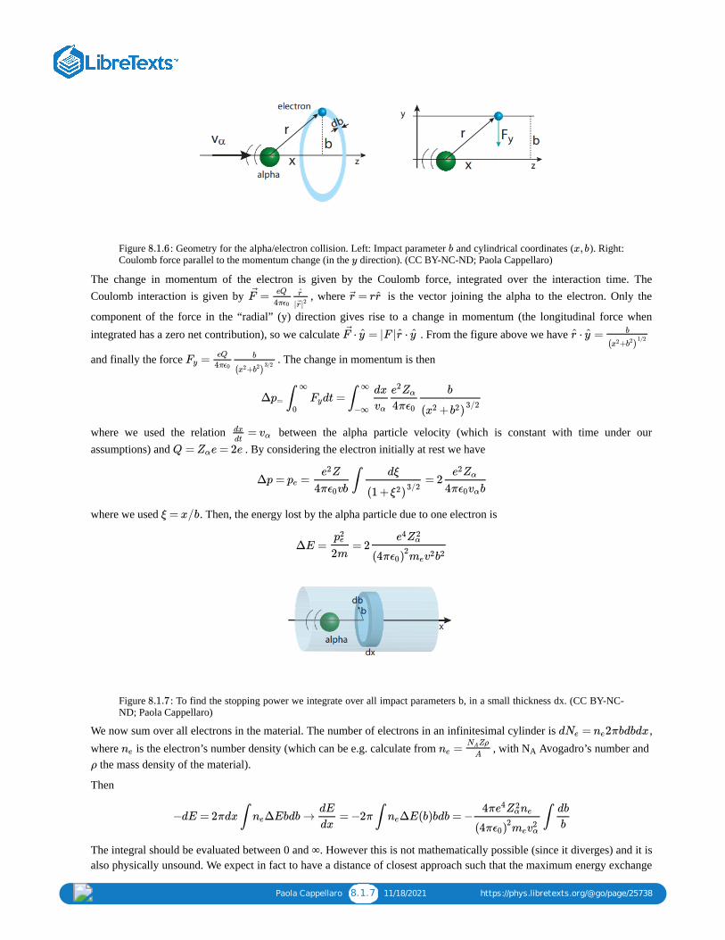
Paola Cappellaro 8.1.7 11/18/2021 https://phys.libretexts.org/@go/page/25738

Figure : Geometry for the alpha/electron collision. Left: Impact parameter and cylindrical coordinates ( ). Right:Coulomb force parallel to the momentum change (in the direction). (CC BY-NC-ND; Paola Cappellaro)

The change in momentum of the electron is given by the Coulomb force, integrated over the interaction time. TheCoulomb interaction is given by , where is the vector joining the alpha to the electron. Only the

component of the force in the “radial” (y) direction gives rise to a change in momentum (the longitudinal force whenintegrated has a zero net contribution), so we calculate . From the figure above we have

and finally the force . The change in momentum is then

where we used the relation between the alpha particle velocity (which is constant with time under ourassumptions) and . By considering the electron initially at rest we have

where we used . Then, the energy lost by the alpha particle due to one electron is

Figure : To find the stopping power we integrate over all impact parameters b, in a small thickness dx. (CC BY-NC-ND; Paola Cappellaro)

We now sum over all electrons in the material. The number of electrons in an infinitesimal cylinder is ,where is the electron’s number density (which can be e.g. calculate from , with N Avogadro’s number and

the mass density of the material).

Then

The integral should be evaluated between 0 and ∞. However this is not mathematically possible (since it diverges) and it isalso physically unsound. We expect in fact to have a distance of closest approach such that the maximum energy exchange

8.1.6 b x, by

=F   eQ

4πϵ0

r

|r  |2= rr   r

⋅ = |F | ⋅F   y r y ⋅ =r y b

( + )x2 b2 1/2

=FyeQ

4πϵ0

b

( + )x2 b2 3/2

Δ dt =p= ∫∞

0

Fy ∫∞

−∞

dx

vα

e2Zα

4πϵ0

b

( + )x2 b2 3/2

=dx

dtvα

Q = e = 2eZα

Δp = = ∫ = 2peZe2

4π vbϵ0

dξ

(1 + )ξ2 3/2

e2Zα

4π bϵ0vα

ξ = x/b

ΔE = = 2p2e

2m

e4Z2α

(4π )ϵ02mev2b2

8.1.7

d = 2πbdbdxNe ne

ne =neZρNA

A A

ρ

−dE = 2πdx ∫ ΔEbdb → = −2π ∫ ΔE(b)bdb = − ∫ne

dE

dxne

4πe4Z2αne

(4π )ϵ02mev

2α

db

b

Paola Cappellaro 8.1.8 11/18/2021 https://phys.libretexts.org/@go/page/25738

(as in the hard-on collision studied previously) is achieved. We had obtained . Then we set this energy equalto the electron’s Coulomb potential energy: from which we obtain

The maximum b is given by approximately the Bohr radius (or the atom’s radius). This can be calculated by setting where is the mean excitation energy of the atomic electrons. Then what we are stating is that

the maximum impact parameter is the one at which the minimum energy exchange happen, and this minimum energy is theminimum energy required to excite (knock off) an electron out of the atom. Although the mean excitation energy of theatomic electrons is a concept related to the ionization energy (which is on the order of 4 − 15eV) here is taken as anempirical parameter, which has been found to be well approximated by (with the atomic number of thetarget). Finally we have

and the stopping power is

with called the Coulomb logarithm.

Since the stopping power, or energy lost per unit length, is given by the energy lost in one collision (or ) times thenumber of collision (given by the number of electron per unit volume times the probability of one electron collision, givenby the cross section) we have the relation:

from which we can obtain the cross section itself. Since , we have

This can also be rewritten in terms of more general constants. We define the classical electron radius as

which is the distance at which the Coulomb energy is equal to the rest mass. Although this is not close to the real size of anelectron (as for example we would expect the electron radius –if it could be well defined– to be much smaller than thenucleus radius) it gives the correct order of magnitude of the effective area in the collision by charged particles. Also wewrite , so that

Since is usually quite small for alpha particles, the cross section can be quite large. For example for a typicalalpha energy of , and its rest mass , we have . The Coulomb logarithm ison the order of , while . Then the cross section is .

This is defined by

= 2Ee mev2α

≈Ee1

4πϵ0

e2

bmin

∼bmin1

4πϵ0

e2

2mev2α

∼14πϵ0

e2

bmaxEI EI

EI

∼ 10ZeVEI Z

=bmax

bmin

2mev2α

ZαEI

− = ln( ) = lnΛdE

dx

4πe4Z2αne

(4π )ϵ02mev2

α

bmax

bmin

4πe4Z2αne

(4π )ϵ02mev2

α

Λ

ΔE

− = ΔEdE

dxσcne

ΔE = 2mev2

= lnΛσc2πe4Z2

α

(4π )ϵ02m2

ev4α

= ∼ 2.8fm,re1

4πϵ0

e2

mec2

β = v

c

= 2π lnΛσc r2e

Z2α

β4

β

= 4MeVEα ∼ 4000MeVmαc2 ∼ 2 ×v2

c210−3

lnΛ ∼ 5 −15 2π ∼  barnr2e

12

∼ 4 ⋅ /4 ⋅ 10b = 5 × bσc12

106 106

Definition: Stopping length

1/ = − .lα1

E

dE

dx

Paola Cappellaro 8.1.9 11/18/2021 https://phys.libretexts.org/@go/page/25738

Then we can write an exponential decay for the energy as a function of distance traveled inside a material: . Thus the stopping length also gives the distance at which the energy has been reduced by

.

Figure : Stopping power for alpha particles (left) and protons (right) in graphite. x-axis: Energy in MeV. y-axis:Stopping power (MeV cm /g). The red curve is the total stopping power, given by the Coulomb stopping power fromcollision with the electrons (blue) and the Rutherford stopping power (black) from collision with the nuclei. The data istaken from NIST. (CC BY-NC-ND; Paola Cappellaro)

In terms of the cross section the stopping length is:

where , the atomic number density can be expressed in terms of the mass density and the Avogadro number, .

Stopping length for lead: or . The range of the particle in the material ishowever many stopping lengths (on the order of 10), thus the range in lead is around .

The range is more precisely defined as the distance a particle travels before coming to rest. Then, the range for aparticle of initial kinetic energy is defined as

Notice that these is a strong dependence of the stopping power on the mass density of the material (a lineardependence) such that heavier materials are better at stopping charged particles.

However, for alpha particles, it doesn’t take a lot to be stopped. For example, they are stopped in 5 mm of air.

The Bragg curve describes the Stopping power as a function of the distance traveled inside matter. As the stoppingpower (and the cross section) increase at lower energies, toward the end of the trajectory there is an increase in energylost per unit length. This gives rise to a characteristic Bragg peak in the curve. This feature is exploited for example forradiation therapy, since it allows a more precise spatial delivery of the dose at the desired location.

E(x) = exp(−x/ )E0 lα1/e(≈ 63%)

8.1.82

1/ = 4 Zn,lαm2

mα

σc

n n =ρ

ANA

Example 8.1.1

1/ = 4 ×lα 104  cm−1 = 2.5 ×  cmlα 10−5

2.5μm

Definition: Range

Eα

R ( ) = dx = − dEEα ∫r(E=0)

r( )Eα

∫Eα

0

( )dE

dx

−1

Definition: Bragg curve

Paola Cappellaro 8.1.10 11/18/2021 https://phys.libretexts.org/@go/page/25738

Figure : Bragg curve for protons (distance in mm) (CC BY-NC-ND; Paola Cappellaro)

B. Rutherford - Coulomb scattering

Elastic Coulomb scattering is called Rutherford scattering because of the experiments carried out in Rutherford lab in1911-1913 that lead to the discovery of the nucleus. The experiments involved scattering alpha particles off a thin layer ofgold and observing the scattering angle (as a function of the gold layer thickness).

The interaction is given as before by the Coulomb interaction, but this time between the alpha and the protons in thenucleus. Thus we have some difference with respect to the previous case. First, the interaction is repulsive (as both particlehave positive charges). Then more importantly, the projectile is now the smaller particle, thus loosing considerable energyand momentum in the interaction.

What we want to calculate in this interaction is the differential cross section . The differential (infinitesimal)cross section can be calculated (in a classical picture) by considering the impact parameter and the small annularregion between and :

Then the differential cross-section, calculated from the solid angle (given thesymmetry about ), is:

What we need is then a relationship between the impact parameter and the scattered angle ϑ (see figure).

8.1.9

dσ

dΩ

b

b b+db

dσ = 2πbdb

dΩ = dφ sinϑdϑ → 2π sinϑdϑ

φ

= =dσ

dΩ

2πbdb

2π sinϑdϑ

b

sinϑ

db

dϑ

Paola Cappellaro 8.1.11 11/18/2021 https://phys.libretexts.org/@go/page/25738

Figure : Rutherford scattering and momentum change (CC BY-NC-ND; Paola Cappellaro)

In order to find b(ϑ) we study the variation of energy, momentum and angular momentum. Conservation of energy statesthat:

which gives the minimum distance (or distance of closest approach) for zero impact parameter = 0, that happens whenthe particle stops and gets deflected back: .

The momentum changes due to the Coulomb force, as seen in the case of interaction with electrons. Here however thenucleus almost does not acquire any momentum at all, so that only the momentum direction is changed, but not its absolutevalue: initially the momentum is along the incoming (x) direction, and at the end of the interaction it is still

but along the ϑ direction. Then the change in momentum is (see Fig. above). Thismomentum difference is along the direction , which is at an angle with x. We then switch to a reference framewhere , with r the distance and the angle between the particle position and .

The momentum change is brought about by the force in that direction:

Notice that at t = 0, (as is almost aligned with x) and at t = ∞, (Fig). How does changes withtime?

The angular momentum conservation (which is always satisfied in central potential) provides the answer. At t = 0, theangular momentum is simply . At any later time, we have . In the coordinate system thevelocity has a radial and an angular component:

and only this last one contributes to the angular momentum (the other being parallel):

Figure : Momentum change and coordinate system ( ) for Rutherford scattering. (CC BY-NC-ND; PaolaCappellaro)

8.1.10

m = m +1

2v2

0

1

2v2 zZe2

4π rϵ0

b

m =12

v20

zZe2

4π dϵ0

= mp0 v0

mv0 Δp = 2 sin = 2m sinp0ϑ

2v0

ϑ

2

δp π−ϑ

2

= {r, γ}r   | |r   γ δp

Δp = ⋅ δ dt = dt = dt∫∞

0

F   pzZe2

4πϵ0∫

∞

0

⋅ δr p

| |r2

zZe2

4πϵ0∫

∞

0

cosγ

r2

γ = −π−ϑ

2r   γ =

π−ϑ

2γ

L = m bv0 L = m ×r   v   = {r, γ}r  

= +rv   r r γγ  

L = m → =r2 dγ

dt

1

r2

γ

bv0

8.1.11 {r,γ}

Paola Cappellaro 8.1.12 11/18/2021 https://phys.libretexts.org/@go/page/25738

Inserting into the integral we have :

By equating the two expressions for , we have the desired relationship between and ϑ:

Finally the cross section is:

(where is the incident –alpha– particle kinetic energy). In particular, the , and sin dependence are inexcellent agreement with the experiments. The last dependence is characteristic of single scattering events and observingparticles at large angles (although less probable) confirm the presence of a massive nucleus. Consider gold foil of thickness

and an incident beam of 8MeV alpha particles. The impact parameter that gives a scattering angle of 90 degreesor more is . Then the fraction of particles with that impact parameter is , thus we have

particles scattering at an angle (with the target density). Although this is a small number, itis quite large compared to the scattering from a uniformly dense target.

C. Electron stopping in matter

Electrons interact with matter mainly due to the Coulomb interaction. However, there are differences in the interactioneffects with respect to heavier particles. The differences between the alpha particle and electron behavior in matter is dueto their very different mass:

1. Electron-electron collisions change the momentum of the incoming electron, thus deflecting it. Then the path of theelectron is not straight anymore.

2. The stopping power is much less, so that e.g. the range is 1cm in lead. (remember that the ratio of the energy lost to theinitial energy for alpha particles was small, since it was proportional to the ratio of masses -electron to alpha. Here themasses ratio is 1, and we expect a large change in energy).

3. Electrons have more often a relativistic speed. For example, electrons emitted in the beta decay travel at relativisticspeed.

4. There is a second mechanism for deceleration. Since the electrons can undergo rapid changes of velocity due to thecollision, it is constantly accelerating (or decelerating) and thus it radiates. This radiation is called Bremsstrahlung, orbraking radiation (in German).

The stopping power due to the Coulomb interaction can be calculated in a very similar way to what done for the alphaparticle. We obtain:

Here is now a different ratio than the one obtained for the alpha particles, but with a similar meaning:

, where again we can recognize the ratio of the electron energy (determining the minimum

distance) and the mean excitation energy (which sets the maximum distance) as well as a correction due to relativisticeffects.

Δp = dt = dγ = 2 coszZe2

4πϵ0∫

∞

0

cosγγ

bv0

zZe2

4πϵ0∫

π+ϑ

2

π−ϑ

2

cosγ

bv0

zZe2

4π bϵ0v0

ϑ

2

Δp b

2m sin = 2 cos → b = cotv0ϑ

2

zZe2

4π bϵ0v0

ϑ

2

zZe2

4π mϵ0 v20

ϑ

2

= ( )dσ

dΩ( )zZe2

4πϵ0

2

(4 )Ta−2 sin−4 ϑ

2

= mTa12

v0 Z2 T −2 −4

ζ = 2μm

b ≤ = 14fmd

2∝ πb2

ζnπ ≈ 7.5 ×b2 10−5 ≥ 90∘ n

− = 4π lndE

dx( )

e2

4πϵ0

2ZρNA

A

1

mec2β2Λ′

Λ′

=Λ′ T

2mev2

− −−−√

(T+m )c2

EI

EI

Paola Cappellaro 8.1.13 11/18/2021 https://phys.libretexts.org/@go/page/25738

Figure : Stopping power for electrons in graphite (left) and Lead (right). x-axis: Energy in MeV. y-axis: Stoppingpower (MeV cm /g). The red curve is the total stopping power, given by the Coulomb stopping power (blue) and theradiative stopping power (black). Note the different contributions of the two types of processes for the two nuclides: theBremsstrahlung is much higher for heavier elements such as Lead. The data is taken from NIST. (CC BY-NC-ND; PaolaCappellaro)

A quantum mechanical calculation gives some corrections (for the alpha as well) that become important at relativisticenergies (see Krane):

To this stopping power, we must add the effects due to the “braking radiation”. Instead of calculating the exact contribution(see Krane), we just want to estimate the relative contribution of Bremsstrahlung to the Compton scattering. The ratiobetween the radiation stopping power and the coulomb stopping power is given by

where is a factor that takes into account relativistic corrections and remember . Then the radiationstopping power is important only if and for large Z. This expression is valid only for relativistic energies;below 1MeV the radiation losses are negligible. Then the total stopping power is given by the sum of the twocontributions:

Since the electron do not have a linear path in the materials (but a random path with many collisions) it becomes moredifficult to calculate ranges from first principles (in practice, we cannot just take as done in the calculations foralphas). The ranges are then calculated empirically from experiments in which the energy of monoenergetic electronbeams is varied to calculate . NIST provides databases of stopping power and ranges for electrons (as well as foralpha particles and protons, see the STAR database at http://www.nist.gov/pml/data/star/index.cfm. Since the variationwith the material characteristics (once normalized by the density) is not large, the range measured for one material can beused to estimate ranges for other materials.

8.1.122

− = 4π [ln + relativistic corrections ]dE

dx( )

e2

4πϵ0

2ZρNA

A

1

mec2β2Λ′

− / − = ≈dE

dx

∣

∣∣r

dE

dx

∣

∣∣c

e2

ℏc

Z

fc

T +mec2

mec2

T +mec2

mec2

Z

1600

∼ 10 −12fc ≈e2

ℏc1

137

T ≫ mec2

= +dE

dx

dE

dx

∣

∣∣c

dE

dx

∣

∣∣r

dt = dx/v

R(E)

Paola Cappellaro 8.1.14 11/18/2021 https://phys.libretexts.org/@go/page/25738

8.1.4 Electromagnetic radiationThe interaction of the electromagnetic radiation with matter depends on the energy (thus frequency) of the e.m. radiationitself. We studied the origin of the gamma radiation, since it derives from nuclear reactions. However, it is interesting toalso study the behavior of less energetic radiations in matter.

In order of increasing photon energy, the interaction of matter with e.m. radiation can be classified as:

Here is the ionization energy for the given target atom.

A classical picture is enough to give some scaling for the scattering cross section. We consider the effects of the interactionof the e.m. wave with an oscillating dipole (as created by an atomic electron).

The electron can be seen as being attached to the atom by a ”spring”, and oscillating around its rest position withfrequency . When the e.m. is incident on the electron, it exerts an additional force. The force acting on the electron is

, with the oscillating electric field. This oscillating driving force is in addition to theattraction of the electron to the atom , where (given by the Coulomb interaction strength and related to thebinding energy ) is linked to the electron’s oscillating frequency by . The equation of motion for theelectron is then

We seek a solution of the form , then we have the equation

We have already seen that an accelerated charge (or an oscillating dipole) radiates, with a power

where the accelaration is here , giving a mean square acceleration

The radiated power is then

EI

ω0

F = −eE(t) E(t) = sin(ωt)E0

∼ −kxe k

EI = k/ω20 me

= −k −eE(t) → + = − E(t)mexe xe xe ω20xe

e

me

(t) = A sin(ωt)xe

(− + )A = − → A =ω2 ω20

e

me

E01

−ω2 ω20

e

me

E0

P =2

3

e2

c3a2

a a = − A sin(ωt)ω2

⟨ ⟩ =a2 ( )ω2

−ω20 ω2

e

me

E0

21

2

P = c1

3( )

e2

mec2

2ω4

( − )ω20 ω2 2

E20

Paola Cappellaro 8.1.15 11/18/2021 https://phys.libretexts.org/@go/page/25738

Figure : Range for alpha particles (black) and electrons (red) in Lead (solid curves) and air (dashed). x-axis: Energyin MeV. y-axis: Range (g/cm ). Note the much longer range for electrons than for alpha particles. Only at very high energy,for lead, the range is shorter for electrons, thanks to the contribution from Bremsstrahlung. The data is taken fromNIST. (CC BY-NC-ND; Paola Cappellaro)

The radiation intensity is given by (recall that the e.m. energy density is given by and the intensity, orpower per unit area, is then ). Then we can express the radiated power as cross-section×radiation intensity:

This yields the cross section for the interaction of e.m. radiation with atoms :

or in SI units:

where we used the classical electron radius .

A. Rayleigh Scattering

We first consider the limit in which the e.m. radiation has very low energy: . In this limit the electron is initiallybound to the atom and the e.m. is not going to change that (and break the bound). We can simplify the frequency factor inthe scattering cross-section by , then we have:

8.1.132

=I0cE2

0

8πu = 1

2E2

I ∼ cu

P = σI0

σ =8π

3( )

e2

mec2

2

( )ω2

−ω20 ω2

2

σ = = 4π8π

3( )

e2

4πϵ0mec2

2

( )ω2

−ω20 ω2

2

r2e

2

3( )

ω2

−ω20 ω2

2

re

ω ≪ ω0

≈ω2

−ω20 ω2

ω2

ω20

Paola Cappellaro 8.1.16 11/18/2021 https://phys.libretexts.org/@go/page/25738

The Rayleigh scattering has a very strong dependence on the wavelength of the e.m. wave. This is what gives the bluecolor to the sky (and the red color to the sunsets).

B. Thomson Scattering

Thomson scattering is scattering of e.m. radiation that is energetic enough that the electron appears to be initially unboundfrom the atom (or a free electron) but not energetic enough to impart a relativistic speed to the electron. (If the electron is afree electron, the final frequency of the electron will be the e.m. frequency).

We are then considering the limit:

where the first inequalities tells us that the binding energy is much smaller than the e.m. energy (hence free electron) whilethe second tells us that the electron will not gain enough energy to become relativistic.

Then we can simplify the factor and the cross section is simply

with . Notice that contrasting with the Rayleigh scattering, Thomson scattering cross-section is completelyindependent of the frequency of the incident e.m. radiation (as long as this is in the given range). Both these two types ofscattering are elastic scattering, meaning that the atom is left in the same state as it was initially (so conservation of energyis satisfied without any additional energy coming from the internal atomic energy). Even in Thomson scattering we neglectthe recoil of the electron (as stated by the inequality ). This means that the electron is not changed by thisscattering event (the atom is not ionized) even if in its interaction with the e.m. field it behaves as a free electron.

Notice that the cross section is proportional to the classical electron radius square: .

C. Photoelectric Effect

At resonance the cross-section becomes (mathematically) infinite. The resonance condition means that the e.m.energy is equal to the ionization energy of the electron. Thus, what it really happens is that the electron gets ejectedfrom the atom. Then our simple model, from which we calculated the cross section, is no longer valid (hence the infinitecross section) and we need QM to fully calculate the cross-section. This is the photoelectric effect. Its cross section isstrongly dependent on the atomic number (as ).

D. Compton Scattering

Compton scattering is the scattering of highly energetic photons from electrons in atoms. In the process the electronacquire an energy high enough to become relativistic and escape the atom (that gets ionized). Thus the scattering is nowinelastic (compared to the previous two scattering) and the scattering is an effective way for e.m. radiation to lose energyin matter. At lower energies, we would have the photoelectric effect, in which the photon is absorbed by the atom. Theeffect is important because it demonstrates that light cannot be explained purely as a wave phenomenon.

=σR8π

3( )

e2

4πϵ0mec2

2ω4

ω40

ℏ ≪ ℏω ≪ω0 mec2

= ≈ −1ω2

−ω20 ω2

1

−1( /ω)ω02

=σT8π

3( )

e2

4πϵ0mec2

2

∼  barnσT23

ℏω ≪ mec2

=σT8π3r2e

ω ≈ ω0

EI

∝σpe Z5

Paola Cappellaro 8.1.17 11/18/2021 https://phys.libretexts.org/@go/page/25738

Figure : Photon/Electron collision in Compton scattering. (CC BY-NC-ND; Paola Cappellaro)

From conservation of energy and momentum, we can calculate the energy of the scattered photon.

From these equations we find and . Solving for

the change in the wavelength we find (with ):

or for the frequency:

The cross section needs to be calculated from a full QM theory. The result is that

thus Compton scattering decreases at larger energies.

E. Pair Production

Pair production is the creation of an electron and a positron pair when a high-energy photon interacts in the vicinity of anucleus. In order not to violate the conservation of momentum, the momentum of the initial photon must be absorbed bysomething. Thus, pair production cannot occur in empty space out of a single photon; the nucleus (or another photon) isneeded to conserve both momentum and energy .

Photon-nucleus pair production can only occur if the photons have an energy exceeding twice the rest mass ( ) of anelectron (1.022 MeV):

Pair production becomes important after the Compton scattering falls off (since its cross-section is \propto 1 / \omega\)).

8.1.14

+ = + → ℏω+ = ℏ +Eγ Ee E ′γ E ′

e mec2 ω′ |p +|2c2 m2c4

− −−−−−−−−−−√

ℏ = ℏ + → {k  k ′ p  ℏk = ℏ cosϑ+p cosφk′

ℏ sinϑ = p sinφk′

= [ℏ ( −ω) −2m ]p2 ( −ω)ω′

c2ω′ c2 cosφ = 1 − ϑ/ℏ2k′2 sin2 p2

− −−−−−−−−−−−−−−√

λ = 2πk

ω = kc

Δλ = (1 −cosϑ)2πℏ

cme

ℏ = ℏωω′ [1 + (1 −cosϑ)]ℏω

mec2

−1

≈σC σTmec

2

ℏω

mec2

ℏω = + + + ≥ 2 = 1.022MeVTe− me−c2 Te+ me+c2 mec2

Index

Aalpha decay

3.3: Alpha Decay

BBeta decay

1.3: Radioactive decay binding energy

1.2: Binding energy and Semi-empirical massformula

Ddaughter nuclide

1.3: Radioactive decay decoherence

2.3: Measurement and Probability deuteron

5.2: The Deuteron differential cross section

8.1: Interaction of Radiation with Matter dispersion relation

6.2: Evolution of Wave-packets doubly differential cross section

8.1: Interaction of Radiation with Matter

EEhrenfest’s theorem

6.3: Evolution of Operators and ExpectationValues evanescent transmitted wave

3.2: Unbound Problems in Quantum Mechanics expectation value

2.3: Measurement and Probability

FFermi’s Golden Rule

6.4: Fermi’s Golden Rule

GGamma decay

1.3: Radioactive decay gamma ray

7.1: Gamma Decay Gamow factor

3.3: Alpha Decay

HHamiltonian

2.4: Energy Eigenvalue Problem Heisenberg picture

6.3: Evolution of Operators and ExpectationValues

Iinternal conversion

7.1: Gamma Decay isotopes

1.1: Basic Concepts

Llepton number

7.2: Beta Decay

MMultipole Expansion

7.1: Gamma Decay Multipoles

7.1: Gamma Decay

Nneutrino

1.3: Radioactive decay 7.2: Beta Decay

neutron scattering8.1: Interaction of Radiation with Matter

nuclear force5.1: Characteristics of the Nuclear Force

Pparent nuclide

1.3: Radioactive decay Particle in Box

4.1: Bound Problems probability density

2.3: Measurement and Probability

Qquantum numbers

4.1: Bound Problems

Sshell model

1.2: Binding energy and Semi-empirical massformula sinc function

6.4: Fermi’s Golden Rule

Vvector potential

7.1: Gamma Decay

Wwavefunction collapse

2.3: Measurement and Probability

Glossary

Sample Word 1 | Sample Definition 1