Petar Marković* and Branko Urošević** · PDF file64 Economic Annals, Volume LVI, No. 188 / January – March 2011 (2004) develop important insights related to stress testing in

62

ECONOMIC ANNALS, Volume LVI, No. 188 / January – March 2011UDC: 3.33 ISSN: 0013-3264

* FREN, Belgrade. Email: [email protected].** Faculty of Economics, University of Belgrade, and National Bank of Serbia. The correponding

author. Email: [email protected]. The views expressed in this article are the authors’ alone and do not necessarily reflect views of FREN or National Bank of Serbia. Branko Urošević gratefully acknowledges financial support from the Ministry of Science and Technological Development of the Republic of Serbia, Grant No. OH 179005.

JEL CLASSIFICATION: G21, G24, G32

ABSTRACT: The paper develops a comprehensive framework for market risk stress testing in internationally active financial institutions. We begin by defining the scope and type of the stress test and explaining how to select risk factors and the stress time horizon. We then address challenges related to data gathering, followed by in-depth discussion of techniques for developing realistic shock scenarios. Next the process of shock application to a particular portfolio is described, followed by determination of

portfolio profit and loss. We conclude by briefly discussing the issue of assigning probability to stress scenarios. We illustrate the framework by considering the development of a ‘worst case’ scenario using global financial market data from Thomson Reuters Datastream.

KEY WORDS: stress testing, risk factors, scenario analysis, shock development, data gathering, stressing correlations, stressing interest rates, PnL calculation, stress scenario probability

DOI:10.2298/EKA1188062M

Petar Marković* and Branko Urošević**

MARKET RISK STRESS TESTING FOR INTERNATIONALLY ACTIVE FINANCIAL INSTITUTIONS

Scientific PaPerS

MARKET RISK STRESS TESTING

63

1. MARKET RISK STRESS TEST METhODOLOGY

The recent global financial crisis has clearly exposed the vulnerabilities of the global financial system. Global financial institutions, previously thought of as the bulwarks of stability of the global financial system, have effectively spread the crisis, which originated in the United States, throughout the world. In large part this has happened due to these institutions’ need to rebalance their large investment portfolios. Such rebalancing can (and did) cause a severe reduction in the value of the assets jointly held by most global players, and created spurious (yet very real) correlations among asset classes that are essentially entirely unrelated.1 As a result many institutions failed, while others had to be rescued by national governments in the US, UK, and continental Europe.

In order to ensure that large scale failures of financial institutions do not happen in the future (or, rather, to lower the probability and severity of such future events), regulators and companies themselves design ever more sophisticated stress tests.2 These tests are designed to probe the ability of a financial institution (or the whole financial sector) to endure a severe market downturn. These tests are important both in order to have a clear, structured framework within which to address important risks, as well as to make sure that institutions are setting aside sufficient capital buffers in order to protect public interest and prevent future meltdowns. Market risk stress testing is particularly important for internationally active financial institutions, since their investments in global capital markets are usually a very large portion of their on- as well as off-balance sheets.

In this paper we propose a comprehensive framework for market risk stress testing as applied to an internationally active financial institution.3 In addition to traditional market risk factors we address various important risk factors that influence market portfolios, such as credit and liquidity risks.

Despite the importance of stress tests for the wellbeing of the financial system and individual institutions, there is a relative dearth of publications dedicated to market risk stress test methodology. Quagliariello (2009) and Stulz and Apostolik

1 On the mechanisms of creating spurious correlations at times of massive portfolio adjustment see, for example, Bookstaber (2007).

2 Recent stress tests mandated by regulators showed a significant capital shortfall in the banking systems of development countries. For the reasons that led to such results see Haldane (2009).

3 While as a canonical example we have in mind a large international bank, the framework can be used by smaller banks or other types of financial institution such as insurance companies or pension or hedge funds, as long as they actively invest in global financial markets.

64

Economic Annals, Volume LVI, No. 188 / January – March 2011

(2004) develop important insights related to stress testing in banks. Fender et al (2001) present an international survey of stress testing methodologies and results. Jorion (2009) and Alexander and Sheedy (2004) provide methodological background related to market risk stress tests. Important guidelines related to market risk stress testing aimed at both practitioners and regulators can be found in Committee of European Banking Supervisors (2009), Basel Committee on Banking Supervision (2009), and Committee on the Global Financial System (2005), among others.

There is a fundamental tradeoff when facing the stress testing of a large internationally active financial institution. On one hand, in performing a stress test it is necessary to be as comprehensive as possible, i.e. to capture as many important risk factors as is feasible. A failure to do so may lead to understated risk assessment and, ultimately, to the downfall of an institution or the entire financial system. On the other hand simplifications are often necessary, especially for portfolios that are very large. This is, in part, due to limited human and computer resources.4 The need for an optimal trade-off between precision and allocation of resources becomes apparent when firms have a large number of different financial instruments in their portfolios. Ideally we would analyze each instrument individually, create a specific shock, and apply it to that instrument using a full re-pricing method (see below). For a modest size institution this is entirely feasible. For large institutions, however, this may be too costly in terms of human and computing time, and would be practically impossible for large companies holding millions of different instruments (as is often the case in global banks). Therefore the goal is to find a limited number of essential risk factors that influence the portfolio in question in a substantial way.

An important feature of stress testing is its reliance on historical market data to predict future market movements. This is true whether we use actual previous market moves to design potential future shocks or we simply use historical data to calibrate simulation models that will develop market shocks. In this paper we develop shock values of risk factors based on previous (historical) shocks and apply appropriate amplification factors (see below). While use of historical data is both natural and quite common it also presents an important methodological limitation: it is precisely what we do not know (or, rather, what has not happened yet and, thus, is not easily predictable) that can cause the most severe damage to our portfolio.5

4 This is more of an issue in large financial institutions, and less of an issue in small ones such as those in small emerging markets such as Serbia.

5 For an excellent discussion of this point see Taleb (2001) and Taleb (2007).


65

Since stress tests are repeated periodically it is necessary to recalibrate them. As market conditions change the aim is to include new information in the stress testing scenario analysis. The methods presented below have been developed to include dynamic calibration of shocks, updating the model to current market conditions. While part of the updating and recalibration process can be made automatically some issues require strategic considerations by risk management specialists and other experts.

In the paper we accompany the exposition of the framework with practical examples that elaborate how to develop a ‘worst case’ scenario test. In doing so it is assumed that the stress test is conducted by an internationally active financial institution that holds assets in both developed and emerging global financial markets.6

The rest of the paper is structured as follows. In section 2 we discuss the scope and type of stress tests. Section 3 discusses the severity of shocks. Section 4 comments on selection of asset classes that are targeted for stress testing, while Section 5 explains how the time horizon of a stress test is determined. Section 6 addresses risk factor selection, while Section 7 analyzes issues of data collection and preparation. Section 8 is the key section and presents development of shocks for stress testing purposes. Section 9 discusses how to apply shocks to an actual portfolio, while Section 10 concerns aggregate profit and loss calculations. Assigning probabilities to stress scenarios is briefly commented on in Section 11, while Section 12 concludes.

2. DEFINING ThE SCOpE AND TYpE OF ThE STRESS TEST

The first step in the development of a stress test is to determine its purpose, i.e. the type of test that needs to be performed.7 A sensitivity test focuses on a single risk factor at a given point in time and is usually used to figure out how well a portfolio is hedged against an adverse movement in a particular risk factor. A scenario test focuses on pre-defined changes in a set of risk factors, creating an

6 Since applying the shocks and Profit/Loss (PnL) calculations requires an actual portfolio and pricing methods for all securities, applying the shocks and calculation of PnL vectors will be omitted in this example. The same is true for the section where we discuss assigning probabilities to a stress test, and for stressing the correlation matrix.

7 The work of the Committee of European Banking Supervisors (2009), which contains the requirements of European regulators for bank stress testing, provides useful stress testing guidelines.

66


event or a scenario. This event can be anything – from a stock market crash to a sovereign debt crisis. The goal of scenario testing is to quantify the potential impact of such an event on the portfolio in question.

Creating scenario assumptions seems straightforward. In practice, however, it is not always easy to anticipate changes in market conditions that are relevant for the portfolio at hand. That is why it is essential for firms to conduct tests which cover a wide range of scenarios, including those that include severe market crashes. It is also possible to find a ‘worst case’ scenario, i.e. a scenario under which the portfolio would be most severely impacted. Creation of a worst case scenario requires analysis of moves in all relevant risk factors, which is, clearly, not an easy problem.

One way to create a comprehensive scenario is to fully replicate moves in the risk factors of a specific historical event. Such historical scenarios can cover various well-known adverse market events. In practice the most popular are: the oil crisis of 1973/74, the stock market crash on Black Monday 1987, the Asian currency crisis of 1997, the failure of LTCM (Long Term Capital Management) and the Russian default of 1998, and the latest world economic crisis triggered by the subprime mortgage crisis in 2008. A survey of common historical scenarios used in international financial institutions can be found in Fender et al (2001).

Another important decision is the choice of the test’s scope. In the simplest case it is possible to perform a stress test on a single sub-portfolio; for example, the UK equity market. If the goal is to stress test a business unit such as FICC (Fixed Income, Currency and Commodities unit), it takes more time and effort to develop the test. A firm-wide stress test is the most demanding, since it covers all marketable assets held by a firm and involves the close collaboration of different divisions. The benefit of a firm-wide test is that it provides the management (or regulators) with a comprehensive overview of risks taken by the firm. By aggregating the results of such a stress test a single value for expected losses if an adverse event occurs can be obtained. Just as importantly it also allows for a breakdown of profit/loss results across several important dimensions. In this way key areas of the firm’s vulnerability may be exposed.

One way to break down the results is by country or region. This would allow top management to better understand the vulnerabilities of each country or region, including risks related to political instability (e.g. exclusion from international trade, production halt), currency management (e.g. switching from fixed to


67

floating exchange rate and vice versa) or catastrophic events (e.g. wars and natural disasters).

In our example we explain how to perform the worst case scenario analysis. Therefore the test type is a scenario analysis. The scope of the test is firm-wide market risk. This means that the shocks will be applied to all marketable securities of the firm-wide portfolio, which includes all trading portfolios that the firm manages (as opposed to credit portfolios of the banking book). Since it is a scenario, multiple risk factors will be shocked at the same time to arrive at the stressed values of securities.

3. SEVERITY OF ShOCKS

The issue of how severe the shocks should be in order to adequately address relevant risks is usually addressed by the firm’s risk management experts, based on their subjective opinions and analysis of the historical data. An important guiding principle is that it is always better to be on the safe side, i.e. to assume a sufficiently severe market distress.

Decisions on severity often require risk managers to consult with several other professionals (traders, lawyers, etc). Let us assume, for example, that the goal of the stress test is to assess the risk of a country being placed under UN sanctions because of violation of the Nuclear Non-Proliferation Treaty. Securities originating from that country could be affected by changes in the ability of entities to raise capital, restrictions in capital mobility, and loss of investor confidence. Each of these issues would, ideally, be analyzed by an expert in the respective field. The task is made even harder if no such event has occurred previously in history, thus preventing the use of past data as a guide.

Since the global financial crisis in 2008 the regulators’ perspective on the problem of severity assessment has changed and they are increasingly active in providing guidelines on the severity issue.8 The general approach is to anticipate the most extreme event risks possible. One way to achieve that is to amplify the worst historically recorded market moves (see below).

8 See, for example, Basel Committee on Banking Supervision (2009)

68


In our example, in order to construct the worst case scenario, all shocks are based on the historically largest adverse movements in risk factors, suitably amplified to cover the expected increase in the size of the market stress.

4. SELECTION OF ASSET CLASSES

The next step in the stress testing analysis is to break down a portfolio into the appropriate asset classes which would be de-facto representatives of securities with similar risk factors. The breakdown depends on the type of portfolio being tested. If it contains only bonds, for example, it can be broken down by originating region, issuer’s credit rating, or by industrial sector of the issuers.

The common way to divide the trading portfolio of an internationally active financial institution is into Equity, Foreign Exchange or FX, Interest Rate Products, Credit Spreads, and Commodities. The choice corresponds to the typical division of markets (and corresponds to typical divisions in the largest global banks). It is important to note that each of the five groups can be broken down further into appropriate sub-portfolios. A survey which backs up this division is given in the paper produced by the working group of the Committee on the Global Financial System (2005).

In our example, with a firm-wide portfolio in mind, asset classes covered by this example will be broken down in the manner suggested above.

5. SELECTING ThE TIME pERIOD FOR ThE STRESS TEST

Since every stress test tells us how much loss or gain will be incurred on current positions for a certain period of time, all results depend very much on the time horizon of the test, also known as the stress window. The most important factors that help us decide on the appropriate stress window are the length of the scenario event and the liquidity of positions in the portfolio.9

Most of the destruction which takes place in a typical financial crisis usually takes place in the first several weeks of the crisis. These first weeks are the most

9 Obviously this time period is not to be confused with the length of the time series that are being analyzed. Time series are usually analyzed starting from 10, 20, or more years before the day of analysis, while the time period of the stress test is much shorter – commonly up to 3 months.


69

turbulent and usually are accompanied by the largest market movements. In the past this period has usually lasted between 10 - 90 days. For this reason the stress test window is usually selected within that interval.

It is important to notice that in performing the stress tests it is assumed as a rule that positions remain the same during the entire stress period. This is because it is hard to simulate changes in portfolio positions within the window period (see below).10

How quickly a firm can close out positions greatly influences the decision on the stress window period. Some positions may be quite liquid and easily convertible into cash, while for others it may be hard to predict the time necessary to unload the position. The level of market development plays a key role here, as more developed markets are more liquid in terms of volume of trade and tighter bid-ask spreads. They are also perceived as less risky by investors. As a result, even in the middle of the crisis investors are more likely to trade in developed than underdeveloped markets. That is why the stress window for developed markets is often shorter than that for emerging or underdeveloped markets.

There are also positions which are neither liquid nor transferable. These include non-traded contracts between the firm and other financial institutions, contracts under legal workout, and securities that cannot be sold to other market participants either on or off the market. Such securities have to be held until maturity: therefore they should be discarded when determining the stress window because they will stay in the portfolio even if their marked-to-model value falls dramatically.

Our example covers both developed and emerging markets. Since the usual time period for an emerging market stress test is roughly three months and the time period for developed markets can be assumed to be close to a month, as a stress window we selected two months, the middle of the two values. This means that all market movements will be analyzed on a 44 business day rolling period basis.

10 Another reason to assume a constant portfolio position is that during severe crises liquidity typically evaporates, making it difficult to perform trades.

70


6. RISK FACTOR SELECTION

One of the most difficult problems related to stress testing is to find the most appropriate risk factors, i.e. the set of variables that most impact the value of the portfolio. In selecting risk factors there is a trade-off between completeness and tractability/speed of the performance of the stress testing model. Selecting more risk factors will reduce the chance of omitting important risks. On the other hand introducing too many risk factors could cause stress tests to become over complex and impractical. Therefore it is paramount to select those risk factors that critically impact the value of portfolio, while limiting risk factors to a manageable number.

Determination of risk factors depends on the portfolio under consideration. For a bond portfolio the relevant risk factors could be benchmark interest rates or credit ratings. For equities, commodities, and FX products, returns on spot prices or indices are often used as risk factors. They are also a source of risk for derivative products.

Once the risk factors are selected their volatilities and correlations need to be forecasted.11 In the standard approach, volatility is determined based on a certain number of past trading days (say, 250), using equal weights for each observation. In more advanced methods such as EWMA or GARCH, newer market information is weighted differently (more) than stale market information. The benefit is that the new information is being used in the system as soon as it arrives. In times of financial stress the EWMA and GARCH methods provide better volatility forecasts than the standard approach. On the other hand after the crisis is over these methods may give too little credence to the past (more volatile) data, thus making risk managers overly confident in their risk assessment. For this reason it is advisable that different methodologies of forecasting volatility are compared on a regular basis. Yet another method that is frequently used is the method of implied volatilities (see Christoffersen (2003)).

In order to determine the credit spread, credit default swaps (CDSs) are often used. A credit spread, which is typically measured in basis points, is an indicator of the credit worthiness of a fixed income security or a group of securities.

Other interest rate product risk factors are interest rates and their volatilities for different tenors. The number of tenors used depends on the desired precision

11 See Christoffersen (2003).


71

of the stress test. It is customary to use several tenors of short-term rates, a few tenors of mid-term rates, and one long-term tenor. This is done since most changes occur in the prices of bonds that are close to maturity. The reason behind this is that investors know that interest rates are mean-reverting and expect them to return to that mean in the long term.

In our example each asset class is assigned risk factors which are directly observable in the market. In particular the following risk factors have been selected: equity returns and equity volatilities, FX returns (changes in the exchange rate) and FX volatilities, interest rate values, CDS spreads, and commodity returns. In addition commodities are broken down into: precious metals (represented by gold), industrial metals (represented by aluminum), energy (represented by WTI oil) and agricultural products (represented by S&P GSCI Agriculture). All other risks are related to these fundamental risk factors.

All risk factors are analyzed on the absolute change basis, except for equity returns, FX returns, and commodity returns, which will be analyzed on a relative basis (change in percentage).

7. DATA pREpARATION

Gathering valid data to construct shocks is an important but cumbersome process, which involves analyzing various time series from different data sources. The time series need to be matched by type, tenor, units, and frequency. There is often a serious problem of data consistency.

Marking to market is one of the crucial aspects of financial risk assessment. This is because market prices represent the most accurate representation of the value of securities, i.e. prices at which they can be purchased or sold in the free market. Even if the model price can sometimes be a better representative of the intrinsic value, a security will always be traded at the market price, not the model price. This is why, whenever possible, pricing data should be gathered directly from the market. In addition, market data is needed to calibrate any model, and thus calculate mark-to-model prices.

Marking to model is also necessary in a stress testing process since there are many securities which are not regularly traded on the market and therefore do not have a readily available market price. If a security is traded only occasionally it is better to use mark-to-model than state market prices. If the pricing model for

72


a security is well defined and represents a good approximation of the value of that security, then the results of the test will be valid. Faulty pricing models will lead to severe misjudgment of risk.

Model risk is therefore an important issue that a carefully designed stress test needs to address.12 Whenever possible modelled prices should be compared with market prices in order to properly calibrate the models. The goal is to make the contract correction - the difference between market and model price - as low as possible. If the contract correction is too high, the model should be discarded and a new one should be built. This process is similar to a backtesting procedure for VaR models. In backtesting, the number of VaR breaches is compared with the pre-defined confidence level.13

When an illiquid security is not traded at all, marking to model is the only way of pricing the security. Risk assessment for these securities relies on the quality of the model. Human judgment (and motives) can have a very serious impact on the quality of the models. For example, pricing and assessing the risk of a specific and unique currency-hedging instrument with a non-standard time to maturity and payment frequency can very much depend on human input. People providing inputs are usually either traders or controllers. There is a potentially serious moral hazard problem here, since traders have an incentive to skew risk officers’ perception of the value of the transaction in order to gain the most favorable view of themselves. In particular they may decide not to reveal certain risks if that could jeopardize their end-of-year bonus. Controllers, on the other hand, are put in place to oversee such actions and correct them, but they are not always able to identify this kind of behaviour (they may lack both appropriate skills and incentive to do so).

If some data are missing data gaps need to be filled in order for the rest of the stress testing mechanism to work. This is commonly done by linear interpolation or by assuming a particular type of stochastic process that risk factors follow (say, a random walk). Making linear interpolation reduces volatility of data, thus causing, potentially, a reduced perception of risk. Assuming a distribution such as a random walk allows for filling in the missing data while preserving

12 In the past couple of years accountants and financial regulators have worked to develop a joint approach that integrates standard international accounting practices with the need to properly measure and report risks within the Basel II and Basel III frameworks.

13 On backtesting of VaR models see Christoffersen (2003).


73

volatility. While both methods introduce a certain inaccuracy, the second model is potentially less inaccurate than the first.14

Another problem arises when there are no historical prices for a particular security, e.g. because the security does not yet exist on the market.15 In that case one solution would be to proxy the time series of the unavailable security with a similar security for which the information is available. This is commonly done for new financial instruments. The least biased replacement for time series of new stocks is to proxy them with appropriate market or sector indices. Bonds require more analysis, since a similar issuer in terms of yield and risk has to be identified so that the bonds of that issuer can be used to substitute the missing data.

Adapting the time series by concatenation is another solution. Proxy time series are used up to the date that the original time series begins, and the original values are used from that point on. It should be noted that this method should be used with caution since there can be unrealistically high changes at the points of data source switching, causing the shocks to appear excessively large.

Last but not least, when there is an abundance of data available, information from the market in which the security is most traded should be used.

In practice it may be useful to group data in the same asset class into different tiers, according to the assessment of their riskiness. Tiers are created in order to stratify the sample based on certain characteristics.

In our example, we group securities based on countries of origin into 2 tiers:

• Tier 1 - represents the most developed countries with stable financial markets and the lowest credit rating risk of AAA (from AAA+ to AAA-)

• Tier 2 - represents medium to high-risk countries with developing and emerging markets, but also developed markets which are currently less stable and under increasing risk.

In our case, we assume that roughly 50% of the firm-wide portfolio will be held in assets of the most developed countries (Tier 1), while the rest is in Tier 2. Representative countries are chosen for each tier based on market data availability.

14 Clearly, this hinges on the assumption that distribution used to complete the data corresponds well to the time series at hand.

15 Very short time series (say, shorter than one year) are usually treated in the same way as securities for which there are no prices at all.

74


Shocks are developed using only the time series of representative countries. Representative countries for the Tier 1 group are the USA and Switzerland, while for Tier 2 they are South Africa, South Korea, India, and Mexico.

Country grouping does not affect commodities which are being shocked the same way regardless of their origin. It is assumed that commodities do not vary in returns across countries.

8. CREATING MARKET ShOCKS

Once the risk factor values are available their changes are analyzed on the selected rolling time period basis. The fact that the time period T is rolling means that the changes in value of the risk factor will be observed from time tstart=0 to tend=T, then from tstart =1 to tend =T+1, and so on until tend reaches the last day of the time series.

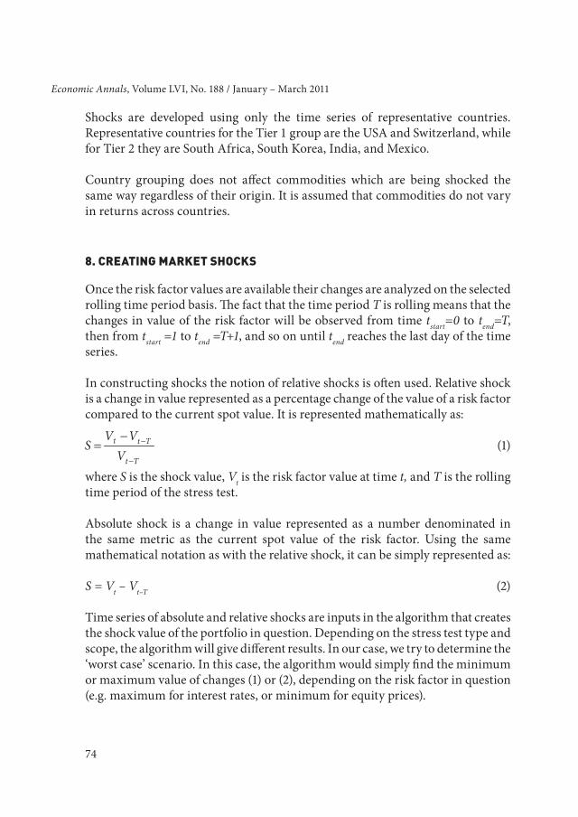
In constructing shocks the notion of relative shocks is often used. Relative shock is a change in value represented as a percentage change of the value of a risk factor compared to the current spot value. It is represented mathematically as:

(1)

where S is the shock value, Vt is the risk factor value at time t, and T is the rolling time period of the stress test.

Absolute shock is a change in value represented as a number denominated in the same metric as the current spot value of the risk factor. Using the same mathematical notation as with the relative shock, it can be simply represented as:

S = Vt – Vt–T (2)

Time series of absolute and relative shocks are inputs in the algorithm that creates the shock value of the portfolio in question. Depending on the stress test type and scope, the algorithm will give different results. In our case, we try to determine the ‘worst case’ scenario. In this case, the algorithm would simply find the minimum or maximum value of changes (1) or (2), depending on the risk factor in question (e.g. maximum for interest rates, or minimum for equity prices).


75

For a stress test executed on a diverse or firm-wide portfolio, different algorithms can exist for different risk factors. It is important that stress-testing algorithms are both theoretically and practically well founded. The methodology of shock development must also be convincing to traders, risk analysts, modellers, and top management, in order for the results of the test to be accepted as valid.

Once appropriate time series are collected (using the process explained at some detail in the previous section), time series of changes are created based on the type of stress test and the time period selected. Algorithms are then run on the time series of changes to obtain the shock values, which are then sent for approval to all parties involved. Once approved the final shock values are ready to be used in the stress test.

In the case where data is still missing and there is no good proxy for the time series, another approach – shock regression – can be used. Shock regression aims to establish dependencies between risk factors, which are, in practice, usually assumed to be linear.16 If the risk factor time series exists, but is not long enough to undergo the standard process of shock generation, regression is used to extrapolate the shock values. The process involves finding another, highly correlated risk factor, for which shock values can be developed. Once the second risk factor is identified the regression equation is used to arrive at the shock value for the risk factor with insufficient data.

For a brand new security there is no theoretically sound way to arrive at the dependencies between the two risk factors. A possible solution is to find a second risk factor that is related to the first one, and then to proxy dependency between a different pair of risk factors similarly related to the original risk facts. That dependency is then used instead of the original one. For example, let us suppose that the time series for gold mining industry stock price, gold price, and oil price are available, making their shock development successful under the standard process. If the oil refining industry stock price time series is completely unavailable for some reason (i.e. a country has just started to refine crude oil) but is necessary as a risk factor in a stress test, it can be determined through regression using proxy dependencies. The assumption is that the gold mining industry is dependent on gold prices in an approximately similar way as the oil refining industry is dependent on oil prices. The regression is then used to get the dependency of gold mining industry stock price shocks on gold price shocks. The resulting formula is taken as an approximation of the shock value dependency of the oil refining

16 Assumption of linearity may greatly understate true risks. See, for example, Božović et al (2009).

76


industry on oil prices. The shock values of oil prices are then used in the formula to get the final shock values for the oil refining industry. Notice that in this process no data on the oil refining industry is used, since none were available.

The benefit of these methods is that they include some information from the market, which improves the validity of the final shock value. On the other hand, they suffer from lack of automation and depend significantly on the judgment call of risk managers to find the right proxies.

When shock grouping is used there is a need to derive a single shock value for each risk factor within a group. This is done by assigning a weight to each shock on a group member level. Each shock is multiplied by its weight, and these values are summed up to get the shock value for the entire tier level. Two approaches are commonly used to calculate the weights for shocks – weighting by portfolio (money) exposure and weighting by risk exposure.

According to the first method, all assets related to the risk factor in the portfolio are expressed in terms of the same currency. These values are then divided by the total value of that portfolio in the same currency to get the weight of that group member’s contribution to the tier level risk factor shock. The main advantage of this approach is that it is very simple, and straightforward to implement. However, it gives unacceptable results when there are significant short positions in the portfolio. Short positions may distort the shock values and lead to counterfactual results, such as negative volatility. For this reason the portfolio money weighting method is not recommended for portfolios that contain significant short positions.

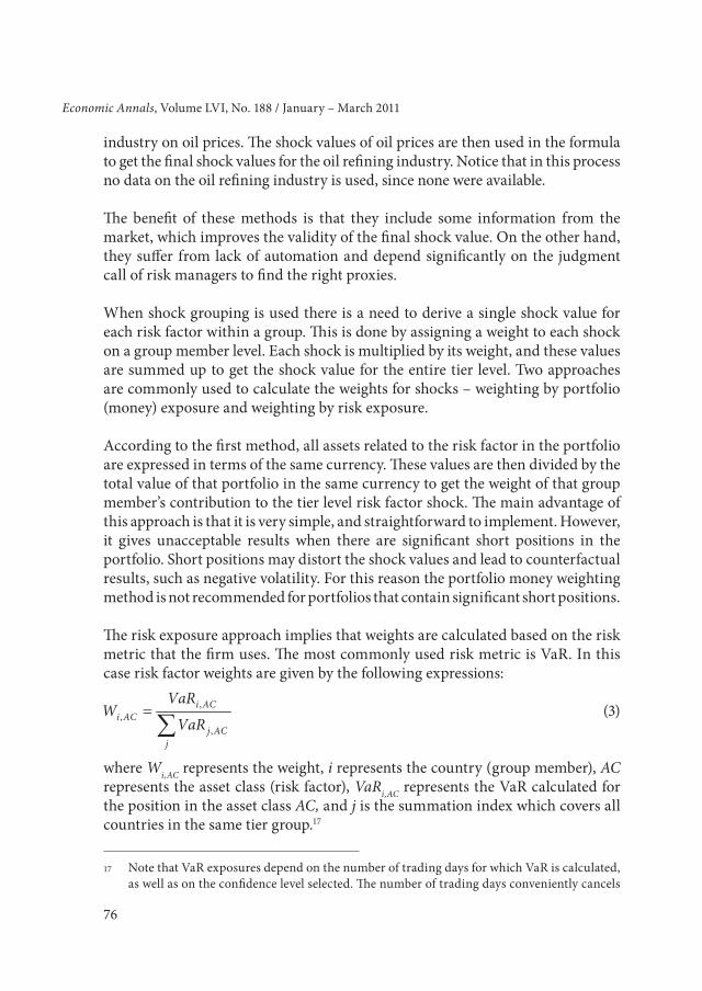
The risk exposure approach implies that weights are calculated based on the risk metric that the firm uses. The most commonly used risk metric is VaR. In this case risk factor weights are given by the following expressions:

(3)

where Wi,AC represents the weight, i represents the country (group member), AC represents the asset class (risk factor), VaRi,AC represents the VaR calculated for the position in the asset class AC, and j is the summation index which covers all countries in the same tier group.17

17 Note that VaR exposures depend on the number of trading days for which VaR is calculated, as well as on the confidence level selected. The number of trading days conveniently cancels


77

The benefit of the risk weighting approach is that there are no negative weights and the risk of each sub-portfolio is more accurately accounted for, and as a result the final weighted shocks reflect reality more closely. When calculating risk weights, rolling window average values can be used in order to smooth them. The rolling window should be sufficiently long to stabilize VaRs. In addition, the averaging can be augmented by exponential smoothing or some other method that makes recent VaRs more important in the total weighting scheme.

Since adverse moves in the future may surpass adverse moves realized in the past, it is reasonable to amplify historical shocks by a certain amplification factor. In order to determine a reasonable amplification shock the time series of the changes (shocks) of each risk factor can be analyzed. Suppose that for a particular risk factor we found the largest shock in the time series. This would be the benchmark shock. Next, we identify the second largest shock and compare it to the benchmark shock. In order to identify the second largest shock we want it to be distinguishable from the first (benchmark) shock. For this reason when attempting to locate the second largest shock we exclude one month’s worth of data before and after the benchmark shock from the time series under consideration. When both shocks are identified the amplification coefficient (a) may be defined as follows:

(4)

When the amplification coefficient is found for a particular risk factor the shock value is then multiplied by that coefficient. This amplified shock value represents the expected future adverse market move which incorporates the possibility of a progressively more severe crisis. Note that, according to this method, for each risk factor there is its own amplification factor. Moreover, the amplification factor is not determined in an ad hoc way.18

Another important issue is the correlation effect of market shocks. The correlation effect represents the change in correlations between different assets or

out the ratio calculation, provided that the standard square root scaling is used (on VaR calculations see, for example, Jorion (2009)). On the other hand, selecting different confidence levels for VaR leads to different weights. The confidence level that should be selected is the one that the firm believes is most appropriate for its needs.

18 Often it is customary to denominate shocks as multiples of the standard deviation of a risk factor. Note, however, that this implicitly assumes that the probability distribution of the risk factor has finite variance, which may not be a good assumption when very large market moves are discussed (see Taleb (2007)).

78


asset classes under adverse market conditions. Correlations rise sharply in times of crises, approaching unity. This may greatly impact portfolio valuation. For example, if a regression is used for pricing, a significant increase in correlations has the potential to significantly change not only risk but also pricing of assets. In addition, assuming a low correlation gives results that understate the actual risk, since low correlations will not hold under stress conditions.19

Correlations have to be shocked in a stress test in order to obtain a more realistic representation of what might occur under stressed market conditions. There are two main differences between changing the value of correlations and other risk factors. Correlations have a defined value range between -1 and 1, which makes both absolute and relative shocking impossible since both can breach the bounds. Correlations are interdependent in such a way that changing one correlation implies a change of several others. Since correlations are kept in matrices where each row and column represents an asset class or a risk factor, changing one correlation implies changing a subset of values in this matrix. These changes can be made by selecting a sub-matrix of affected values and adjusting it, so that the matrix can remain coherent as a symmetric positive definite.

A simple way to deal with the issue is to accept historical values for the entire distressed correlation matrix. This method can work well when utilizing historical scenarios, but implies some serious drawbacks. If the scenario covers an event that has happened in time predating some important innovations in the financial industry, the values could be seriously distorted compared to current conditions. Also, some of the present matrix elements may not have existed in the historical correlation matrix. The benefit of this solution is that it is very easy to implement and requires no complicated analysis.

Another important valuation input that needs to be stressed is the term structure of interest rates. The goal here is to develop an interest rate shock curve. One is created for each tier using the following steps: 1) Representative tenors are chosen; 2) Each tenor is processed to obtain the shock values; 3) Each shock is added as a

19 Bookstaber (2007) provides an interesting argument as to why financial distress may cause not only an increase in existing correlations but also the creation of spurious correlations (i.e. correlations that otherwise would not exist). Suppose a trader has two very large positions in entirely unrelated (and therefore uncorrelated) assets. Suppose, further, that in times of crisis the value of the first asset is significantly depressed. In order to cover losses from the first asset the trader may also be forced to sell out its second position, pushing its price down. As a result a significant positive correlation may be registered between two essentially unrelated assets.


79

point in the curve and represents the curve constraint; 4) The rest of the curve is generated with a chosen method by fitting it to the constraints.

It is common to select several points for representative tenors up to 10 years and only a few tenors after that point. This means that the shock curve is supposed to pass through these points, or be as close to them as possible in order to represent a good approximation. The goal of the fourth step is to create a shock curve which contains shock values for all tenors, not just the constraints. The shock curve will be added to the yield curve in the process of applying the shocks.

There are a number of methods used to construct the shock curve consistent with the given constraints. The simplest is a linear interpolation where the constraints are connected with straight lines. The values between two constraints are a weighted average of the constraints. Logarithmic interpolation is used when constraints are monotonically decreasing and naturally follow the shape of the logarithmic curve, but can give large deviation from the constraints if this condition is not met. Polynomial interpolation gives better results with non-monotonic constraints and provides a smoother curve, but requires a substantial number of data points. This may present a problem in an emerging market setting where the yield curve is sparse and usually of shorter-maturity. 20

Weights which are used to develop final shocks should not be sorted by tenors, but calculated based on the overall interest rate portfolio instead. If weights are calculated based on bucketed tenors, there will be misleading weighting. For example, if a regional portfolio holds only long-term bonds, shocking of short and mid-term interest rates will not be represented well in the tier shock, even though these rates implicitly change the price of long-term bonds. That is why it is better to allow this country’s weights to be non-zero for all tenors, so that the final shock constraints can be more representative of interest rate changes.

Let us now consider our example. All shocks for the available time series have been developed using functions provided in the Thomson-Reuters Datastream interface. The function called to get the maximum absolute change of a risk factor is: MAX(ACH(TS,44D),20Y), where TS is the instrument code of the time series being analyzed. This function calculates the maximum absolute change in the value of time series TS on a rolling period of 44 days (data points), in the 20 year length of the time series.

20 For a discussion on yield curve modelling in an emerging market setting see Drenovak and Urošević (2010).

80


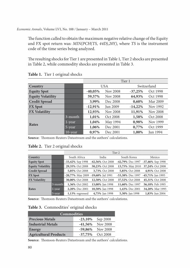
The function called to obtain the maximum negative relative change of the Equity and FX spot return was: MIN(PCH(TS, 44D),20Y), where TS is the instrument code of the time series being analyzed.

The resulting shocks for Tier 1 are presented in Table 1, Tier 2 shocks are presented in Table 2, while commodity shocks are presented in Table 3.

Table 1. Tier 1 original shocks Tier 1Country USA SwitzerlandEquity Spot -40,05% Nov 2008 -37,25% Oct 1998Equity Volatility 59,57% Nov 2008 64,93% Oct 1998Credit Spread 3,99% Dec 2008 0,60% Mar 2009FX Spot -12,91% Jun 2009 -14,22% Nov 1992FX Volatility 12,93% Nov 2008 11,91% Nov 2008

Rates

3-month 1,01% Oct 2008 1,58% Oct 20081-year 1,04% May 1994 0,98% Nov 19995-year 1,06% Dec 2001 0,77% Oct 199910-year 0,97% Dec 2001 1,00% Jun 1994

Source: Thomson-Reuters Datastream and the authors’ calculations.

Table 2. Tier 2 original shocks Tier 2Country South Africa India South Korea MexicoEquity Spot -33,42% Sep 1998 -42,56% Oct 2008 -42,79% Dec 1997 -37,46% Sep 1998Equity Volatility 29,35% Oct 2008 50,23% Oct 2008 13,75% May 2010 37,24% Oct 2008Credit Spread 5,05% Oct 2008 3,73% Oct 2008 5,85% Oct 2008 4,91% Oct 2008FX Spot -20,77% May 2009 -19,68% Jul 1991 -53,38% Dec 1997 -45,71% Jan 1995FX Volatility 30,00% Oct 2008 12,50% Oct 2008 37,52% Oct 2008 45,31% Oct 2008

Rates3-month 1,36% Oct 2002 13,00% Jan 1998 11,60% Dec 1997 56,10% Feb 19951-year 2,20% Dec 2001 10,50% Jan 1998 1,43% Dec 2001 34,20% Mar 19955-year 1,13% regressed 4,75% Jan 1998 5,30% Jan 1998 1,83% Jun 2004


Table 3. Commodities’ original shocksCommodities

Precious Metals -23,10% Sep 2008Industrial Metals -41,56% Nov 2008Energy -59,86% Nov 2008Agricultural Products -37,75% Oct 2008



81

Shocks for the two unavailable time series (South African 5-year and 10-year interest rates) have been approximated using the proxy regression analysis: we find a linear dependence (regression) of Indian 5-year and 10-year national interest rates to the Indian 1-year interest rate, and use this dependence as a proxy for the same tenor linear dependencies of South African interest rates.

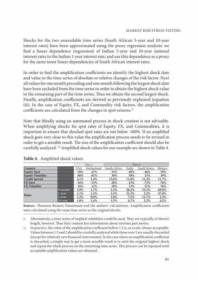
In order to find the amplification coefficients we identify the highest shock date and value in the time series of absolute or relative changes of the risk factor. Next all values for one month preceding and one month following the largest shock date have been excluded from the time series in order to obtain the highest shock value in the remaining part of the time series. Thus we obtain the second largest shock. Finally, amplification coefficients are derived as previously explained (equation (4)). In the case of Equity, FX, and Commodity risk factors, the amplification coefficients are calculated from the changes in spot returns.21

Note that blindly using an automated process in shock creation is not advisable. When amplifying shocks for spot rates of Equity, FX, and Commodities, it is important to ensure that shocked spot rates are not below -100%. If an amplified shock goes very close to this value the amplification process needs to be revised in order to get a sensible result. The size of the amplification coefficient should also be carefully analyzed. 22 Amplified shock values for our example are shown in Table 4.

Table 4. Amplified shock valuesTier 1 Tier 2

Country USA Switzerland South Africa India South Korea MexicoEquity Spot -58% -47% -35% -49% -46% -39%Equity Volatility 86% 81% 30% 58% 15% 39%Credit Spread 4,1% 1,4% 13,8% 11,8% 11,2% 11,7%FX Spot -16% -15% -26% -23% -73% -76%FX Volatility 16% 12% 38% 15% 51% 76%

Rates3-month 3,9% 1,7% 1,5% 28,2% 33,1% 69,9%1-year 1,1% 1,2% 2,5% 31,5% 2,2% 47,8%5-year 1,2% 0,8% 1,8% 7,5% 11,7% 2,3%10-year 1,0% 1,4% 1,5% 4,7% 2,3% 4,2%

Source: Thomson-Reuters Datastream and the authors’ calculations. Amplification coefficients were calculated using the same time series as the original shocks.

21 Alternatively, a time series of implied volatilities could be used. They are typically of shorter length, however. Thus they contain less information about extreme past moves.

22 In practice, the value of the amplification coefficient bellow 1.5 is, as a rule, always acceptable. Values between 1.5 and 2 should be carefully analyzed while those over 2 are usually discarded (except for relatively new financial instruments). In the case where an amplification coefficient is discarded, a simple way to get a more sensible result is to omit the original highest shock and repeat the whole process on the remaining time series. This process can be repeated until acceptable amplification values are obtained. .

82


Calculation of weights requires a testing portfolio, which we do not have. Therefore we use hypothetical weights in our example. We construct them using a hypothetical time series of VaR values over a certain time period for each asset class.

Weighted shocked values for each tier are then calculated using the following formula:

(5)

where FST,AC is the weighted (final) shock value of Tier T for the asset class AC, Sj,AC is the shock value for asset class AC of country j in Tier T, Wj,AC is the weight of that shock, and j is the summation index which covers all countries in Tier T.

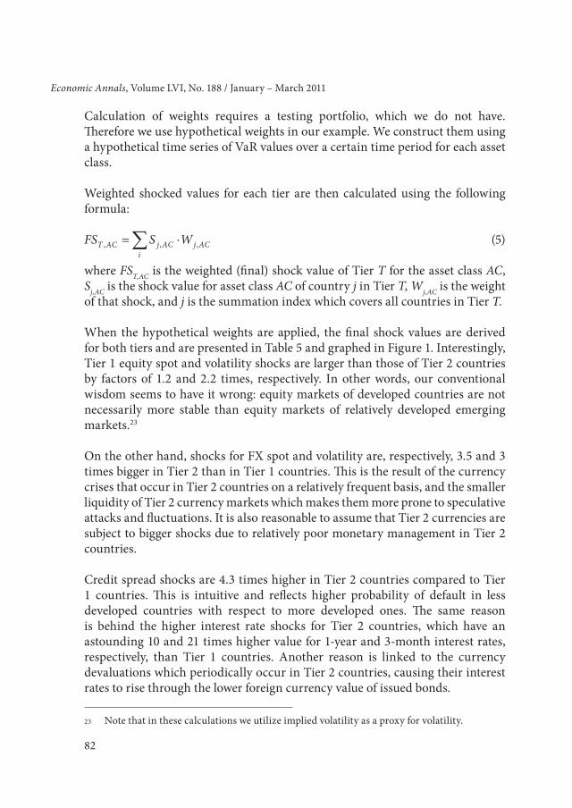
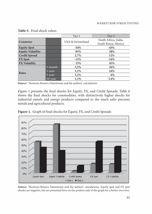
When the hypothetical weights are applied, the final shock values are derived for both tiers and are presented in Table 5 and graphed in Figure 1. Interestingly, Tier 1 equity spot and volatility shocks are larger than those of Tier 2 countries by factors of 1.2 and 2.2 times, respectively. In other words, our conventional wisdom seems to have it wrong: equity markets of developed countries are not necessarily more stable than equity markets of relatively developed emerging markets.23

On the other hand, shocks for FX spot and volatility are, respectively, 3.5 and 3 times bigger in Tier 2 than in Tier 1 countries. This is the result of the currency crises that occur in Tier 2 countries on a relatively frequent basis, and the smaller liquidity of Tier 2 currency markets which makes them more prone to speculative attacks and fluctuations. It is also reasonable to assume that Tier 2 currencies are subject to bigger shocks due to relatively poor monetary management in Tier 2 countries.

Credit spread shocks are 4.3 times higher in Tier 2 countries compared to Tier 1 countries. This is intuitive and reflects higher probability of default in less developed countries with respect to more developed ones. The same reason is behind the higher interest rate shocks for Tier 2 countries, which have an astounding 10 and 21 times higher value for 1-year and 3-month interest rates, respectively, than Tier 1 countries. Another reason is linked to the currency devaluations which periodically occur in Tier 2 countries, causing their interest rates to rise through the lower foreign currency value of issued bonds.

23 Note that in these calculations we utilize implied volatility as a proxy for volatility.


83

Table 5. Final shock valuesTier 1 Tier 2

Countries USA & Switzerland South Africa, India, South Korea, Mexico

Equity Spot -54% -43%Equity Volatility 85% 38%Credit Spread 2,7% 12%FX Spot -15% -54%FX Volatility 15% 45%

Rates

3-month 3,5% 36%1-year 1,1% 24%5-year 1,1% 6%10-year 1,1% 3,4%

Source: Thomson-Reuters Datastream and the authors’ calculations

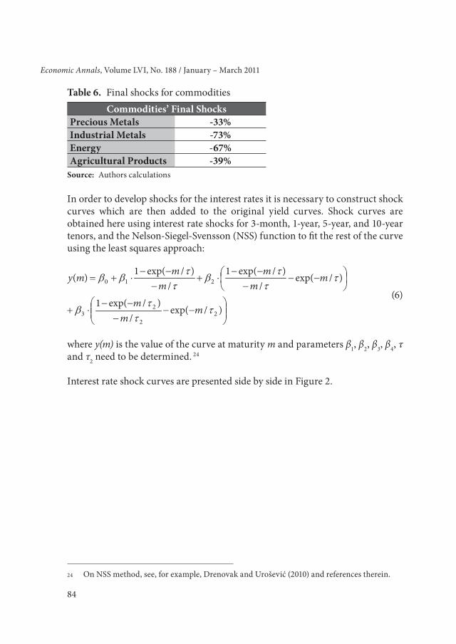
Figure 1 presents the final shocks for Equity, FX, and Credit Spreads. Table 6 shows the final shocks for commodities, with distinctively higher shocks for industrial metals and energy products compared to the much safer precious metals and agricultural products.

Figure 1. Graph of final shocks for Equity, FX, and Credit Spreads

Source: Thomson-Reuters Datastream and the authors’ calculations. Equity spot and FX spot shocks are negative, but are presented here on the positive side of the graph for a better overview.

84


Table 6. Final shocks for commoditiesCommodities’ Final Shocks

Precious Metals -33%Industrial Metals -73%Energy -67%Agricultural Products -39%

Source: Authors calculations

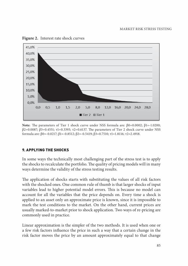
In order to develop shocks for the interest rates it is necessary to construct shock curves which are then added to the original yield curves. Shock curves are obtained here using interest rate shocks for 3-month, 1-year, 5-year, and 10-year tenors, and the Nelson-Siegel-Svensson (NSS) function to fit the rest of the curve using the least squares approach:

(6)

where y(m) is the value of the curve at maturity m and parameters β1, β2, β3, β4, τ and τ2 need to be determined. 24

Interest rate shock curves are presented side by side in Figure 2.

24 On NSS method, see, for example, Drenovak and Urošević (2010) and references therein.


85

Figure 2. Interest rate shock curves

Note: The parameters of Tier 1 shock curve under NSS formula are: β0=0.0002; β1=-1.0200; β2=0.0087; β3=0.4551; τ1=0.3393; τ2=0.6137. The parameters of Tier 2 shock curve under NSS formula are: β0=-0.0217; β1=-0.8512; β2=-0.5419; β3=0.7510; τ1=1.8116; τ2=2.4918.

9. AppLYING ThE ShOCKS

In some ways the technically most challenging part of the stress test is to apply the shocks to recalculate the portfolio. The quality of pricing models will in many ways determine the validity of the stress testing results.

The application of shocks starts with substituting the values of all risk factors with the shocked ones. One common rule of thumb is that larger shocks of input variables lead to higher potential model errors. This is because no model can account for all the variables that the price depends on. Every time a shock is applied to an asset only an approximate price is known, since it is impossible to mark the test conditions to the market. On the other hand, current prices are usually marked-to-market prior to shock application. Two ways of re-pricing are commonly used in practice.

Linear approximation is the simpler of the two methods. It is used when one or a few risk factors influence the price in such a way that a certain change in the risk factor moves the price by an amount approximately equal to that change

86


multiplied by a constant. This constant is a multiple of the correlation of the asset and the risk factor. The assumption of linearity makes the calculation of the shocked prices inexpensive in terms of computing time and decreases the overall cost of the stress test. The biggest disadvantage of this approach to full re-pricing is that it produces a potentially high level of errors.

Full re-pricing is much more accurate. It takes into account changes in all relevant input variables and recalculates the price based on the model formula. This is usually not a simple task because complex financial products require various other asset prices to be recalculated.25 The benefit is a better approximation of the stressed price. On the other hand, a serious drawback is the significant expense in terms of computing and modelling time.

There are also some intermediate solutions to re-pricing. Instead of using linear regressions prices can be regressed against risk factors with polynomial or some other type of non-linear dependency. This will increase the precision at the cost of more complex regression calculations and maintenance of new correlations. Some complex full re-pricing formulas can be simplified in order to avoid the most time-consuming calculations. The trade-off between precision and computing time is very important for stress tests.26

10. CALCULATING ThE pROFITS AND LOSSES OF ThE STRESSED pORTFOLIO

After the shocks have been applied to all assets covered under the stress test, the next step is calculating the profits and losses (PnL) of each position. This is done by subtracting the current value of each financial instrument from its shocked counterpart. As a result we obtain an absolute change in value, expressed in the currency used to denominate the instrument. Next, the change for one instrument is multiplied by the number of instruments currently in the portfolio, keeping in mind that all long positions will have a positive multiplier and all short positions will have a negative multiplier. This is how a PnL for a particular position/financial instrument is calculated. Individual PnLs are then aggregated

25 Until the financial crisis a large fraction of the portfolio of a typical internationally active financial institution consisted of highly complex mortgage-based securities. See Manola and Urošević (2010) for issues related to pricing MBSs.

26 Note that in the case of smaller financial institutions such as the ones operating in Serbia it may be perfectly feasible to carryout a full repricing of all assets, since the number and complexity of assets is not very high. The discussion in this section primarily pertains to large internationaly active institutions.


87

across different dimensions. In this way risk managers can identify weak sectors (markets, divisions) in a given stress scenario.

The cooperation between different risk management sectors can be very valuable here. The credit risk department can improve the process by revaluating the PnLs. One way to do this is to assign to each counterparty a probability of default (PD) and a loss given default (LGD) based on the appropriate credit risk measurement. LGD represents the fraction of value that is not paid out by the obligor if a default occurs. Exposure at default (ED) is known from the stressed value of the related security. The total expected value of the positive PnL position is then calculated as

(7)

where Sstressed and Scurrent are stressed and current asset prices, respectively. Using the expected PnLs will implicitly reduce all positive PnLs across all levels, giving the stress test more realistic results. That is why a credit risk stress test should be incorporated into the firm-wide stress test with market risk in order to obtain a more complete view of the outcome of the scenario.

Liquidity risk should also be incorporated into the analysis, since losses in some positions will cause a reduction in value of the posted collateral and create a need to deliver more securities to cover margin calls. This may drain the firm’s liquidity by increasing the need to close out some positions, and reduce their price further (see footnote 19). Also, the ability of the firm to raise funding can be impaired, because of the reduced portfolio value and consequent reduction in the firm’s credit rating. Therefore a better understanding of the interaction of risks is paramount for creating a realistic stress-testing framework for market risk.

11. ASSIGNING pROBABILITIES TO STRESS SCENARIOS

Thus far we have been concerned primarily with the issue of how bad things can get if an adverse market condition occurs. An interesting question that would supplement such information is: what is the likelihood of such an event occurring? An implicit assumption here is that even if a bad loss occurs we should not worry too much about it if the likelihood of such a loss is extremely remote. Note that this reasoning may be misleading and potentially even dangerous. As shown by Taleb (2007), if there is a chance that an institution will be wiped out due to an adverse market event (however unlikely), this possibility should not be neglected

88


simply because its calculated probability is small. Therefore if we still decide to quantify the likelihood of rare adverse events we need to do it with extreme care.

Extreme value theory (EVT) offers one possibility. It focuses on modelling the tails of the distribution of risk factors. This method has been proven to work well in the case of VaR calculations. However, such statistical methods have a significant drawback in the case of stress testing, as risk factors may not behave in the future as they did in the past. Since statistical methods assume that there is no structural change over the entire period, this issue raises the question of the credibility of assigned probability to a stress scenario. Another issue is the inability to backtest these probabilities, since no hypothetical scenario is going to be perfectly replicated in actual financial markets. Even so, probabilities should be calculated for the purpose of comparison between various scenarios.

12. CONCLUSION

Traditionally, stress testing provides important supplemental information aimed at addressing deficiencies of the standard risk metrics such as Value at Risk.27 For this reason stress testing is an integral part of the best practices framework of any respectable financial institution. In this paper we have presented a comprehensive framework for performing market risk stress testing for internationally active financial institutions. The framework can easily be adopted for smaller financial institutions active only in a single market.

The major drawback of stress testing remains the cost of its implementation. It requires not only technical resources such as expensive pricing models, but also the professional knowledge of various experts.

In the future it will be important to address the issue of dynamic changes in portfolio composition. This means removing the assumption of fixed portfolio composition for the entire stress time period. Clearly it is impossible to be certain how an investment portfolio will change in times of stress. However a firm may be able to make a reasonably educated guess by knowing its own trading strategies and investing rules, and using business intelligence to gather information on the behaviour of competitors.

27 See Jorion (2009), for example.


89

Another desirable improvement is to address the interaction of market, credit, liquidity, and operational risks much more carefully, and to include these interactions in a comprehensive stress testing framework.

While stress testing may not prevent future crises from happening, it may help financial institutions better understand what to expect when the crisis does occur. It may also help them avoid financial meltdown by taking preventive steps before the crisis is on the horizon.

REFERENCES

Alexander C. & Sheedy E. (2004). The Professional Risk Managers’ Handbook: A Comprehensive Guide to Current Theory and Best Practices. PRMIA

Basel Committee on Banking Supervision. (2009). Principles for sound stress testing practices and supervision. Bank for International Settlements

Bookstaber, R. (2007). Markets, Hedge Funds, and the Perils of Financial Innovation: a Demon of Our Own Design. John Wiley & Sons, New Jersey.

Božović, M., Urošević, B., and B. Živković (2009). On the Spillover of Exchange Rate Risk into Default Risk, Economic Annals, 183, 32-55.

Christoffersen, P. (2003). Elements of Financial Risk Management. Academic Press, San Diego, CA.

Committee of European Banking Supervisors. (2009). Guidelines on Stress Testing (CP32). European Banking Authority. Retrieved from: http://www.eba.europa.eu/documents/Publications/Consultation-papers/2009/CP32/CP32.aspx

Committee on the Global Financial System (2005). Stress testing at major financial institutions: survey results and practice. Bank for International Settlements

Drenovak, M. and B. Urošević (2010). Modeling the Benchmark Spot Curve for the Serbian Market. Economic Annals, 184, 29-57.

Fender I., Gibson M., Mosser P., (2001). An International Survey of Stress Tests. Current Issues in Economics and Finance, 7(10). Federal Reserve Bank of New York.

90


Haldane, A. (2009). Why Banks Failed the Stress Test. BIS Review. https://www.bankofengland.co.uk/publications/speeches/2009/speech374.pdf

Jorion P., (2009). Financial Risk Manager Handbook. Wiley Finance

Manola, A. and B. Urošević (2010). Option-Based Valuation of Mortgage-Backed Securities. Economic Annals, 186, 42-66.

Quagliariello M., (2009). Stress-testing the Banking System: Methodologies and Applications. Cambridge University Press

Stulz R. and Apostolik R. (2004). Readings for the Financial Risk Manager. Global Association of Risk Professionals. John Wiley & Sons, Inc.

Taleb, N. (2001). Fooled by Randomness: the Hidden Role of Chance in the Markets and in Life. Texere, London.

Taleb, N. (2007). The Black Swan. Random House, New York

Received: March 29, 2011Accepted: April 6, 2011

Documents

Petar Marković* and Branko Urošević** · PDF file64 Economic Annals, Volume LVI, No. 188 / January – March 2011 (2004) develop important insights related to stress testing in