Embed Size (px)
Citation preview

Perturbative topological field theory with Segal-likegluing
Pavel Mnev
Max Planck Institute for Mathematics, Bonn
ICMP, Santiago de Chile, July 27, 2015
Joint work with Alberto S. Cattaneo and Nikolai Reshetikhin

Introduction BV-BFV formalism, outline Examples
Plan
1 Introduction: calculating partition functions by cut/paste.
2 BV-BFV formalism for gauge theories on manifolds with boundary:an outline.
3 Abelian BF theory in BV-BFV formalism.
4 Further examples: Poisson sigma model, cellular models.

Introduction BV-BFV formalism, outline Examples
Plan
1 Introduction: calculating partition functions by cut/paste.
2 BV-BFV formalism for gauge theories on manifolds with boundary:an outline.
3 Abelian BF theory in BV-BFV formalism.
4 Further examples: Poisson sigma model, cellular models.
Introduction BV-BFV formalism, outline Examples
Plan
1 Introduction: calculating partition functions by cut/paste.
2 BV-BFV formalism for gauge theories on manifolds with boundary:an outline.
3 Abelian BF theory in BV-BFV formalism.
4 Further examples: Poisson sigma model, cellular models.
Introduction BV-BFV formalism, outline Examples
Plan
1 Introduction: calculating partition functions by cut/paste.
2 BV-BFV formalism for gauge theories on manifolds with boundary:an outline.
3 Abelian BF theory in BV-BFV formalism.
4 Further examples: Poisson sigma model, cellular models.
Introduction BV-BFV formalism, outline Examples
Cut/paste philosophy
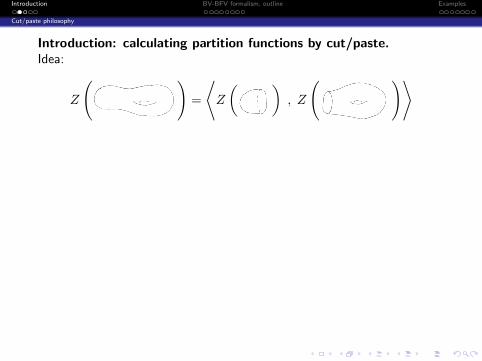
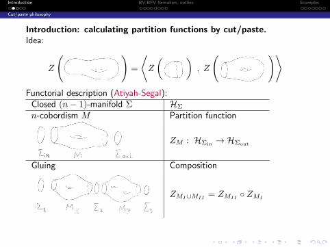
Introduction: calculating partition functions by cut/paste.Idea:
Z
( )=
⟨Z
( ), Z
( )⟩
Functorial description (Atiyah-Segal):Closed (n− 1)-manifold Σ HΣ
n-cobordism M Partition function
ZM : HΣin → HΣout
Gluing Composition
ZMI∪MII= ZMII
ZMI
Atiyah: TQFT is a functor of monoidal categories(Cobn,t)→ (VectC,⊗).
Introduction BV-BFV formalism, outline Examples
Cut/paste philosophy
Introduction: calculating partition functions by cut/paste.Idea:
Z
( )=
⟨Z
( ), Z
( )⟩Functorial description (Atiyah-Segal):
Closed (n− 1)-manifold Σ HΣ
n-cobordism M Partition function
ZM : HΣin → HΣout
Gluing Composition
ZMI∪MII= ZMII
ZMI
Atiyah: TQFT is a functor of monoidal categories(Cobn,t)→ (VectC,⊗).

Introduction BV-BFV formalism, outline Examples
Cut/paste philosophy
Example: 2D TQFT
Z
can be expressed in terms of building blocks:
1 Z
( ): C→ HS1
2 Z
( ): HS1 → C
3 Z
: HS1 ⊗HS1 → HS1
4 Z
: HS1 → HS1 ⊗HS1
– Universal local building blocks for 2D TQFT!

Introduction BV-BFV formalism, outline Examples
Corners
For n > 2 we want to glue along pieces of boundary/ glue-cut withcorners.Building blocks: balls with stratified boundary (cells)
Extension of Atiyah’s axioms to gluing with corners: extended TQFT(Baez-Dolan-Lurie).Example: Turaev-Viro 3D state-sum model.
building block - 3-simplex
q6j-symbol
gluing sum over spins on edges

Introduction BV-BFV formalism, outline Examples
Corners
For n > 2 we want to glue along pieces of boundary/ glue-cut withcorners.Building blocks: balls with stratified boundary (cells)
Extension of Atiyah’s axioms to gluing with corners: extended TQFT(Baez-Dolan-Lurie).
Example: Turaev-Viro 3D state-sum model.building block - 3-simplex
q6j-symbol
gluing sum over spins on edges

Introduction BV-BFV formalism, outline Examples
Corners
For n > 2 we want to glue along pieces of boundary/ glue-cut withcorners.Building blocks: balls with stratified boundary (cells)
Extension of Atiyah’s axioms to gluing with corners: extended TQFT(Baez-Dolan-Lurie).Example: Turaev-Viro 3D state-sum model.
building block - 3-simplex
q6j-symbol
gluing sum over spins on edges

Introduction BV-BFV formalism, outline Examples
Goal
Problems:
Very few examples!
Some natural examples do not fit into Atiyah axiomatics.
Goal:
Construct TQFT with corners and gluing out of perturbative pathintegrals for diffeomorphism-invariant action functionals.
Investigate interesting examples.

Introduction BV-BFV formalism, outline Examples
Classical BV-BFV theories
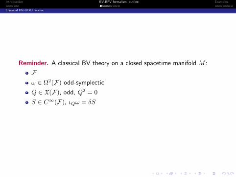
Reminder. A classical BV theory on a closed spacetime manifold M :
Fω ∈ Ω2(F) odd-symplectic
Q ∈ X(F), odd, Q2 = 0
S ∈ C∞(F), ιQω = δS

Introduction BV-BFV formalism, outline Examples
Classical BV-BFV theories
Reminder. A classical BV theory on a closed spacetime manifold M :
F
ω ∈ Ω2(F) odd-symplectic
Q ∈ X(F), odd, Q2 = 0
S ∈ C∞(F), ιQω = δS

Introduction BV-BFV formalism, outline Examples
Classical BV-BFV theories
Reminder. A classical BV theory on a closed spacetime manifold M :
Fω ∈ Ω2(F) odd-symplectic
Q ∈ X(F), odd, Q2 = 0
S ∈ C∞(F), ιQω = δS

Introduction BV-BFV formalism, outline Examples
Classical BV-BFV theories
Reminder. A classical BV theory on a closed spacetime manifold M :
Fω ∈ Ω2(F) odd-symplectic
Q ∈ X(F), odd, Q2 = 0
S ∈ C∞(F), ιQω = δS
Introduction BV-BFV formalism, outline Examples
Classical BV-BFV theories
Reminder. A classical BV theory on a closed spacetime manifold M :
Fω ∈ Ω2(F) odd-symplectic
Q ∈ X(F), odd, Q2 = 0
S ∈ C∞(F), ιQω = δS

Introduction BV-BFV formalism, outline Examples
Classical BV-BFV theories
Reminder. A classical BV theory on a closed spacetime manifold M :
Fω ∈ Ω2(F) odd-symplectic
Q ∈ X(F), odd, Q2 = 0
S ∈ C∞(F), ιQω = δS
Note: S, Sω = 0.

Introduction BV-BFV formalism, outline Examples
Classical BV-BFV theories
BV-BFV formalism for gauge theories on manifolds with boundaryReference: A. S. Cattaneo, P. Mnev, N. Reshetikhin, Classical BVtheories on manifolds with boundary, Comm. Math. Phys. 332 2 (2014)535–603.
For M with boundary:
M −−−−→ (F , ω, Q, S) – space of fieldsyπ yπ∗
∂M −−−−→ (F∂ , ω∂ = δα∂ , Q∂ , S∂) – phase space
Relations: Q2∂ = 0, ιQ∂ω∂ = δS∂ ; Q2 = 0, ιQω = δS + π∗α∂ .
⇒CME: 12 ιQιQω = π∗S∂
Gluing:MI ∪Σ MII → FMI
×FΣFMII
This picture extends to higher-codimension strata!

Introduction BV-BFV formalism, outline Examples
Classical BV-BFV theories
BV-BFV formalism for gauge theories on manifolds with boundaryReference: A. S. Cattaneo, P. Mnev, N. Reshetikhin, Classical BVtheories on manifolds with boundary, Comm. Math. Phys. 332 2 (2014)535–603.
For M with boundary:
M −−−−→ (F , ω−1, Q
1, S
0) – space of fieldsyπ yπ∗
∂M −−−−→ (F∂ , ω∂ = δα∂0
, Q∂1, S∂
1) – phase space
Subscripts =“ghost numbers”.
Relations: Q2∂ = 0, ιQ∂ω∂ = δS∂ ; Q2 = 0, ιQω = δS + π∗α∂ .
⇒CME: 12 ιQιQω = π∗S∂
Gluing:MI ∪Σ MII → FMI
×FΣ FMII
This picture extends to higher-codimension strata!

Introduction BV-BFV formalism, outline Examples
Classical BV-BFV theories
BV-BFV formalism for gauge theories on manifolds with boundaryReference: A. S. Cattaneo, P. Mnev, N. Reshetikhin, Classical BVtheories on manifolds with boundary, Comm. Math. Phys. 332 2 (2014)535–603.
For M with boundary:
M −−−−→ (F , ω, Q, S) – space of fieldsyπ yπ∗
∂M −−−−→ (F∂ , ω∂ = δα∂ , Q∂ , S∂) – phase space
Relations: Q2∂ = 0, ιQ∂ω∂ = δS∂ ; Q2 = 0, ιQω = δS + π∗α∂ .
⇒CME: 12 ιQιQω = π∗S∂
Gluing:MI ∪Σ MII → FMI
×FΣFMII
This picture extends to higher-codimension strata!

Introduction BV-BFV formalism, outline Examples
Classical BV-BFV theories
BV-BFV formalism for gauge theories on manifolds with boundaryReference: A. S. Cattaneo, P. Mnev, N. Reshetikhin, Classical BVtheories on manifolds with boundary, Comm. Math. Phys. 332 2 (2014)535–603.
For M with boundary:
M −−−−→ (F , ω, Q, S) – space of fieldsyπ yπ∗
∂M −−−−→ (F∂ , ω∂ = δα∂ , Q∂ , S∂) – phase space
Relations: Q2∂ = 0, ιQ∂ω∂ = δS∂ ; Q2 = 0, ιQω = δS + π∗α∂ .
⇒CME: 12 ιQιQω = π∗S∂
Gluing:MI ∪Σ MII → FMI
×FΣFMII
This picture extends to higher-codimension strata!

Introduction BV-BFV formalism, outline Examples
Classical BV-BFV theories
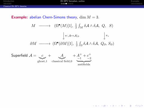
Example: abelian Chern-Simons theory, dimM = 3.
M −−−−→ (F , ω, Q, S)yπ yπ∗
∂M −−−−→ (F∂ , ω∂ = δα∂ , Q∂ , S∂)
Euler-Lagrange moduli spaces:
M −−−−→ H•(M)[1]
ι∗y
∂M −−−−→ H•(∂M)[1]

Introduction BV-BFV formalism, outline Examples
Classical BV-BFV theories
Example: abelian Chern-Simons theory, dimM = 3.
M −−−−→ (Ω•(M)[1], ω, Q, S)yπ:A7→A|∂yπ∗
∂M −−−−→ (Ω•(∂M)[1], ω∂ = δα∂ , Q∂ , S∂)
Superfield A = c︸︷︷︸ghost,1
+ A︸︷︷︸classical field,0
+A+
−1+ c+−2︸ ︷︷ ︸
antifields
Euler-Lagrange moduli spaces:
M −−−−→ H•(M)[1]
ι∗y
∂M −−−−→ H•(∂M)[1]
Introduction BV-BFV formalism, outline Examples
Classical BV-BFV theories
Example: abelian Chern-Simons theory, dimM = 3.
M −−−−→ (Ω•(M)[1], 12
∫MδA ∧ δA, Q, S)yπ:A7→A|∂
yπ∗
∂M −−−−→ (Ω•(∂M)[1], 12
∫∂δA ∧ δA, Q∂ , S∂)
Superfield A = c︸︷︷︸ghost,1
+ A︸︷︷︸classical field,0
+A+
−1+ c+−2︸ ︷︷ ︸
antifields
Euler-Lagrange moduli spaces:
M −−−−→ H•(M)[1]
ι∗y
∂M −−−−→ H•(∂M)[1]

Introduction BV-BFV formalism, outline Examples
Classical BV-BFV theories
Example: abelian Chern-Simons theory, dimM = 3.
M −−−−→ (Ω•(M)[1], 12
∫MδA ∧ δA,
∫MdA δ
δA , S)yπ:A7→A|∂yπ∗
∂M −−−−→ (Ω•(∂M)[1], 12
∫∂δA ∧ δA,
∫∂dA δ
δA , S∂)
Superfield A = c︸︷︷︸ghost,1
+ A︸︷︷︸classical field,0
+A+
−1+ c+−2︸ ︷︷ ︸
antifields
Euler-Lagrange moduli spaces:
M −−−−→ H•(M)[1]
ι∗y
∂M −−−−→ H•(∂M)[1]

Introduction BV-BFV formalism, outline Examples
Classical BV-BFV theories
Example: abelian Chern-Simons theory, dimM = 3.
M −−−−→ (Ω•(M)[1], 12
∫MδA ∧ δA,
∫MdA δ
δA ,12
∫MA ∧ dA)yπ:A7→A|∂
yπ∗
∂M −−−−→ (Ω•(∂M)[1], 12
∫∂δA ∧ δA,
∫∂dA δ
δA ,12
∫∂A ∧ dA)
Superfield A = c︸︷︷︸ghost,1
+ A︸︷︷︸classical field,0
+A+
−1+ c+−2︸ ︷︷ ︸
antifields
Euler-Lagrange moduli spaces:
M −−−−→ H•(M)[1]
ι∗y
∂M −−−−→ H•(∂M)[1]
Introduction BV-BFV formalism, outline Examples
Classical BV-BFV theories
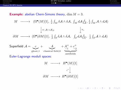
Example: abelian Chern-Simons theory, dimM = 3.
M −−−−→ (Ω•(M)[1], 12
∫MδA ∧ δA,
∫MdA δ
δA ,12
∫MA ∧ dA)yπ:A7→A|∂
yπ∗
∂M −−−−→ (Ω•(∂M)[1], 12
∫∂δA ∧ δA,
∫∂dA δ
δA ,12
∫∂A ∧ dA)
Superfield A = c︸︷︷︸ghost,1
+ A︸︷︷︸classical field,0
+A+
−1+ c+−2︸ ︷︷ ︸
antifields
Euler-Lagrange moduli spaces:
M −−−−→ H•(M)[1]
ι∗y
∂M −−−−→ H•(∂M)[1]

Introduction BV-BFV formalism, outline Examples
Quantum BV-BFV theories
Quantum BV-BFV formalism.
Σ closed, dim Σ = n− 1 7→ (H•Σ,ΩΣ)
M , dimM = n 7→(Fres, ωres)
ZM ∈ Dens12 (Fres)⊗H∂M satisfying mQME:(
i
~Ω∂M − i~∆res
)ZM = 0
Gauge-fixing ambiguity ⇒ ZM ∼ ZM +(i~Ω∂M − i~∆res
)(· · · ).
Gluing:
ZMI∪ΣMII= P∗(ZMI
∗Σ ZMII)
∗Σ — pairing of states in HΣ,P∗ — BV pushforward (fiber BV integral) for
FMIres ×FMII
resP−→ FMI∪ΣMII
res

Introduction BV-BFV formalism, outline Examples
Quantum BV-BFV theories
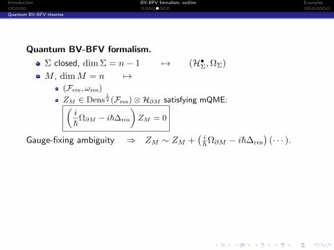
Quantum BV-BFV formalism.
Σ closed, dim Σ = n− 1 7→ (H•Σ,ΩΣ)
M , dimM = n 7→(Fres, ωres)
ZM ∈ Dens12 (Fres)⊗H∂M
satisfying mQME:(i
~Ω∂M − i~∆res
)ZM = 0
Gauge-fixing ambiguity ⇒ ZM ∼ ZM +(i~Ω∂M − i~∆res
)(· · · ).
Gluing:
ZMI∪ΣMII= P∗(ZMI
∗Σ ZMII)
∗Σ — pairing of states in HΣ,P∗ — BV pushforward (fiber BV integral) for
FMIres ×FMII
resP−→ FMI∪ΣMII
res

Introduction BV-BFV formalism, outline Examples
Quantum BV-BFV theories
Quantum BV-BFV formalism.
Σ closed, dim Σ = n− 1 7→ (H•Σ,ΩΣ)
M , dimM = n 7→(Fres, ωres)
ZM ∈ Dens12 (Fres)⊗H∂M satisfying mQME:(
i
~Ω∂M − i~∆res
)ZM = 0
Gauge-fixing ambiguity ⇒ ZM ∼ ZM +(i~Ω∂M − i~∆res
)(· · · ).
Gluing:
ZMI∪ΣMII= P∗(ZMI
∗Σ ZMII)
∗Σ — pairing of states in HΣ,P∗ — BV pushforward (fiber BV integral) for
FMIres ×FMII
resP−→ FMI∪ΣMII
res

Introduction BV-BFV formalism, outline Examples
Quantum BV-BFV theories
Quantum BV-BFV formalism.
Σ closed, dim Σ = n− 1 7→ (H•Σ,ΩΣ)
M , dimM = n 7→(Fres, ωres)
ZM ∈ Dens12 (Fres)⊗H∂M satisfying mQME:(
i
~Ω∂M − i~∆res
)ZM = 0
Gauge-fixing ambiguity ⇒ ZM ∼ ZM +(i~Ω∂M − i~∆res
)(· · · ).
Gluing:
ZMI∪ΣMII= P∗(ZMI
∗Σ ZMII)
∗Σ — pairing of states in HΣ,
P∗ — BV pushforward (fiber BV integral) for
FMIres ×FMII
resP−→ FMI∪ΣMII
res

Introduction BV-BFV formalism, outline Examples
Quantum BV-BFV theories
Quantum BV-BFV formalism.
Σ closed, dim Σ = n− 1 7→ (H•Σ,ΩΣ)
M , dimM = n 7→(Fres, ωres)
ZM ∈ Dens12 (Fres)⊗H∂M satisfying mQME:(
i
~Ω∂M − i~∆res
)ZM = 0
Gauge-fixing ambiguity ⇒ ZM ∼ ZM +(i~Ω∂M − i~∆res
)(· · · ).
Gluing:
ZMI∪ΣMII= P∗(ZMI
∗Σ ZMII)
∗Σ — pairing of states in HΣ,P∗ — BV pushforward (fiber BV integral) for
FMIres ×FMII
resP−→ FMI∪ΣMII
res

Introduction BV-BFV formalism, outline Examples
Quantization
QuantizationChoose p : F∂ → B Lagrangian fibration, α∂ |p−1(b) = 0.
H∂ = Dens12 (B) , Ω∂ = S∂ ∈ End(H∂)1.
F
π
yF∂p
yB

Introduction BV-BFV formalism, outline Examples
Quantization
QuantizationChoose p : F∂ → B Lagrangian fibration, α∂ |p−1(b) = 0.
H∂ = Dens12 (B) , Ω∂ = S∂ ∈ End(H∂)1.
F
π
yF∂p
yB

Introduction BV-BFV formalism, outline Examples
Quantization
QuantizationChoose p : F∂ → B Lagrangian fibration, α∂ |p−1(b) = 0.
H∂ = Dens12 (B) , Ω∂ = S∂ ∈ End(H∂)1.
F ⊃ Fb = π−1p−1b
π
yF∂p
yB 3 b boundary condition
Partition function:
ZM (b) =
∫L⊂Fb
ei~S , ZM ∈ Dens
12 (B)
L ⊂ Fb gauge-fixing Lagrangian.Problem: ZM may be ill-defined due to zero-modes.

Introduction BV-BFV formalism, outline Examples
Quantization
QuantizationChoose p : F∂ → B Lagrangian fibration, α∂ |p−1(b) = 0.
H∂ = Dens12 (B) , Ω∂ = S∂ ∈ End(H∂)1.
F ⊃ Fb = π−1p−1b
π
yF∂p
yB 3 b boundary condition
Solution: Split Fb = Fres × F 3 (φres, φ). Partition function:
ZM (b, φres) =
∫L⊂F
ei~S(b,φres,φ), ZM ∈ Dens
12 (B)⊗Dens
12 (Fres)
L ⊂ F gauge-fixing Lagrangian.
FresP−→ F ′res ⇒ Z ′M = P∗ZM

Introduction BV-BFV formalism, outline Examples
Abelian BF theory
Abelian BF theory: the continuum model.Input:
M a closed oriented n-manifold M .
E an SL(m)-local system.
Space of BV fields: F = Ω•(M,E)[1]⊕ Ω•(M,E∗)[n− 2] 3 (A,B)Action: S =
∫M〈B, dEA〉.
Reference: A. S. Schwarz, The partition function of degeneratequadratic functional and Ray-Singer invariants, Lett. Math. Phys. 2, 3(1978) 247–252.
A. S. Schwarz: For M closed and E acyclic, the partition function is theR-torsion τ(M,E) ∈ R.

Introduction BV-BFV formalism, outline Examples
Abelian BF theory
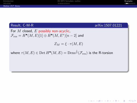
Result, C-M-R arXiv:1507.01221
For M closed, E possibly non-acyclic,Fres = H•(M,E)[1]⊕H•(M,E∗)[n− 2] and
ZM = ξ · τ(M,E)
where τ(M,E) ∈ DetH•(M,E) = Dens12 (Fres) is the R-torsion and
ξ = (2π~)∑nk=0(− 1
4− 1
2k(−1)k)·dim Hk(M,E)·(e−
πi2 ~)
∑nk=0( 1
4− 1
2k(−1)k)·dim Hk(M,E)
In particular ZM contains a mod16 phase e2πi16 s with
s =∑nk=0(−1 + 2k(−1)k) · dimHk(M,E).
Introduction BV-BFV formalism, outline Examples
Abelian BF theory
Result, C-M-R arXiv:1507.01221
For M closed, E possibly non-acyclic,Fres = H•(M,E)[1]⊕H•(M,E∗)[n− 2] and
ZM = ξ · τ(M,E)
where τ(M,E) ∈ DetH•(M,E) = Dens12 (Fres) is the R-torsion
and
ξ = (2π~)∑nk=0(− 1
4− 1
2k(−1)k)·dim Hk(M,E)·(e−
πi2 ~)
∑nk=0( 1
4− 1
2k(−1)k)·dim Hk(M,E)
In particular ZM contains a mod16 phase e2πi16 s with
s =∑nk=0(−1 + 2k(−1)k) · dimHk(M,E).
Introduction BV-BFV formalism, outline Examples
Abelian BF theory
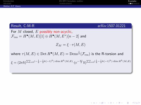
Result, C-M-R arXiv:1507.01221
For M closed, E possibly non-acyclic,Fres = H•(M,E)[1]⊕H•(M,E∗)[n− 2] and
ZM = ξ · τ(M,E)
where τ(M,E) ∈ DetH•(M,E) = Dens12 (Fres) is the R-torsion and
ξ = (2π~)∑nk=0(− 1
4− 1
2k(−1)k)·dim Hk(M,E)·(e−
πi2 ~)
∑nk=0( 1
4− 1
2k(−1)k)·dim Hk(M,E)
In particular ZM contains a mod16 phase e2πi16 s with
s =∑nk=0(−1 + 2k(−1)k) · dimHk(M,E).

Introduction BV-BFV formalism, outline Examples
Abelian BF theory
Result, C-M-R arXiv:1507.01221
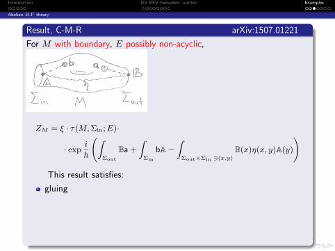
For M with boundary, E possibly non-acyclic,
ZM = ξ · τ(M,Σin;E)·
· expi
~
(∫Σout
Ba +
∫Σin
bA−∫
Σout×Σin 3(x,y)
B(x)η(x, y)A(y)
)
This result satisfies:
gluing
mQME
change of η shifts ZM by(i~Ω∂ − i~∆res
)-exact term.
BFV operator: Ω∂ = −i~(∫
ΣoutdEB δ
δB +∫
ΣindEA δ
δA
)

Introduction BV-BFV formalism, outline Examples
Abelian BF theory
Result, C-M-R arXiv:1507.01221
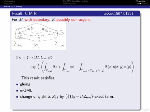
For M with boundary, E possibly non-acyclic,
ZM = ξ · τ(M,Σin;E)·
· expi
~
(∫Σout
Ba +
∫Σin
bA−∫
Σout×Σin 3(x,y)
B(x)η(x, y)A(y)
)
This result satisfies:
gluing
mQME
change of η shifts ZM by(i~Ω∂ − i~∆res
)-exact term.
BFV operator: Ω∂ = −i~(∫
ΣoutdEB δ
δB +∫
ΣindEA δ
δA
)

Introduction BV-BFV formalism, outline Examples
Abelian BF theory
Result, C-M-R arXiv:1507.01221
For M with boundary, E possibly non-acyclic,
ZM = ξ · τ(M,Σin;E)·
· expi
~
(∫Σout
Ba +
∫Σin
bA−∫
Σout×Σin 3(x,y)
B(x)η(x, y)A(y)
)
Where: Fres = H•(M,Σin;E)[1]⊕H•(M,Σout;E∗)[n− 2] 3 (a, b)
This result satisfies:
gluing
mQME
change of η shifts ZM by(i~Ω∂ − i~∆res
)-exact term.
BFV operator: Ω∂ = −i~(∫
ΣoutdEB δ
δB +∫
ΣindEA δ
δA
)

Introduction BV-BFV formalism, outline Examples
Abelian BF theory
Result, C-M-R arXiv:1507.01221
For M with boundary, E possibly non-acyclic,
ZM = ξ · τ(M,Σin;E)·
· expi
~
(∫Σout
Ba +
∫Σin
bA−∫
Σout×Σin 3(x,y)
B(x)η(x, y)A(y)
)
Where: B = Ω•(Σin)[1]⊕ Ω•(Σout)[n− 2] 3 (A,B)
This result satisfies:
gluing
mQME
change of η shifts ZM by(i~Ω∂ − i~∆res
)-exact term.
BFV operator: Ω∂ = −i~(∫
ΣoutdEB δ
δB +∫
ΣindEA δ
δA
)

Introduction BV-BFV formalism, outline Examples
Abelian BF theory
Result, C-M-R arXiv:1507.01221
For M with boundary, E possibly non-acyclic,
ZM = ξ · τ(M,Σin;E)·
· expi
~
(∫Σout
Ba +
∫Σin
bA−∫
Σout×Σin 3(x,y)
B(x)η(x, y)A(y)
)
Where: ξ as before (but for relative cohomology),
This result satisfies:
gluing
mQME
change of η shifts ZM by(i~Ω∂ − i~∆res
)-exact term.
BFV operator: Ω∂ = −i~(∫
ΣoutdEB δ
δB +∫
ΣindEA δ
δA
)

Introduction BV-BFV formalism, outline Examples
Abelian BF theory
Result, C-M-R arXiv:1507.01221
For M with boundary, E possibly non-acyclic,
ZM = ξ · τ(M,Σin;E)·
· expi
~
(∫Σout
Ba +
∫Σin
bA−∫
Σout×Σin 3(x,y)
B(x)η(x, y)A(y)
)
Where: τ - relative R-torsion,
This result satisfies:
gluing
mQME
change of η shifts ZM by(i~Ω∂ − i~∆res
)-exact term.
BFV operator: Ω∂ = −i~(∫
ΣoutdEB δ
δB +∫
ΣindEA δ
δA
)

Introduction BV-BFV formalism, outline Examples
Abelian BF theory
Result, C-M-R arXiv:1507.01221
For M with boundary, E possibly non-acyclic,
ZM = ξ · τ(M,Σin;E)·
· expi
~
(∫Σout
Ba +
∫Σin
bA−∫
Σout×Σin 3(x,y)
B(x)η(x, y)A(y)
)
Where: η ∈ Ωn−1(Conf2(M), E E∗) – propagator.
This result satisfies:
gluing
mQME
change of η shifts ZM by(i~Ω∂ − i~∆res
)-exact term.
BFV operator: Ω∂ = −i~(∫
ΣoutdEB δ
δB +∫
ΣindEA δ
δA
)
Introduction BV-BFV formalism, outline Examples
Abelian BF theory
Result, C-M-R arXiv:1507.01221
For M with boundary, E possibly non-acyclic,
ZM = ξ · τ(M,Σin;E)·
· expi
~
(∫Σout
Ba +
∫Σin
bA−∫
Σout×Σin 3(x,y)
B(x)η(x, y)A(y)
)
This result satisfies:
gluing
mQME
change of η shifts ZM by(i~Ω∂ − i~∆res
)-exact term.
BFV operator: Ω∂ = −i~(∫
ΣoutdEB δ
δB +∫
ΣindEA δ
δA
)

Introduction BV-BFV formalism, outline Examples
Gluing of propagators
Result, C-M-R arXiv:1507.01221
ηI , ηII – propagators on MI , MII .Assume H•(M,Σ1) = H•(MI ,Σ1)⊕H•(MII ,Σ2).Then the glued propagator on M is:
η(x, y) =
ηI(x, y) if x, y ∈MI
ηII(x, y) if x, y ∈MII
0 if x ∈MI , y ∈MII∫z∈Σ2
ηII(x, z)ηI(z, y) if x ∈MII , y ∈MI
Introduction BV-BFV formalism, outline Examples
Poisson sigma model
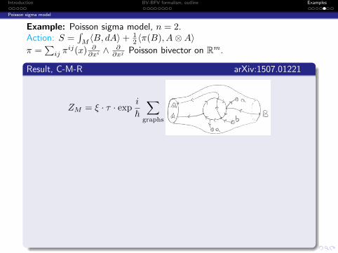
Example: Poisson sigma model, n = 2.Action: S =
∫M〈B, dA〉+ 1
2 〈π(B), A⊗A〉π =
∑ij π
ij(x) ∂∂xi ∧
∂∂xj Poisson bivector on Rm.
Result, C-M-R arXiv:1507.01221
ZM = ξ · τ · expi
~∑
graphs
ZM satisfies:
gluing
mQME
change of η shifts ZM by(i~Ω∂ − i~∆res
)-exact term.
Ω∂ = standard-ordering quantization (B 7→ −i~ δδA on Σin, A 7→ −i~ δ
δB
on Σout) of
∫∂
BidAi +1
2Πij(B)AiAj where Πij(x) = xi∗xj−xj∗xi
i~ is
Kontsevich’s deformation of π.

Introduction BV-BFV formalism, outline Examples
Poisson sigma model
Example: Poisson sigma model, n = 2.Action: S =
∫M〈B, dA〉+ 1
2 〈π(B), A⊗A〉π =
∑ij π
ij(x) ∂∂xi ∧
∂∂xj Poisson bivector on Rm.
Result, C-M-R arXiv:1507.01221
ZM = ξ · τ · expi
~∑
graphs
ZM satisfies:
gluing
mQME
change of η shifts ZM by(i~Ω∂ − i~∆res
)-exact term.
Ω∂ = standard-ordering quantization (B 7→ −i~ δδA on Σin, A 7→ −i~ δ
δB
on Σout) of
∫∂
BidAi +1
2Πij(B)AiAj where Πij(x) = xi∗xj−xj∗xi
i~ is
Kontsevich’s deformation of π.

Introduction BV-BFV formalism, outline Examples
Exact discretizations
Reference. Abelian and non-abelian BF :P. Mnev, Discrete BF theory, arXiv:0809.1160 (– for M closed),A. S. Cattaneo, P. Mnev, N. Reshetikhin, Cellular BV-BFV-BF theory.(– with gluing).1D Chern-Simons: A. Alekseev, P. Mnev, One-dimensional Chern-Simonstheory, Comm. Math. Phys. 307 1 (2011) 185–227.

Introduction BV-BFV formalism, outline Examples
Conclusion
1 → Corners.
2 Partition function for a “building block” (cell) in interestingexamples.
3 Compute cohomology of Ω∂ , e.g. in PSM.
4 More general polarizations, generalized Hitchin’s connection.
5 Observables supported on submanifolds.
Main references:
A. S. Cattaneo, P. Mnev, N. Reshetikhin, Classical BV theories onmanifolds with boundary, Comm. Math. Phys. 332 2 (2014)535–603.
A. S. Cattaneo, P. Mnev, N. Reshetikhin, Perturbative quantumgauge theories on manifolds with boundary, arXiv:1507.01221
![arxiv.org · arXiv:1010.5635v2 [math.AT] 12 May 2011 THE SEGAL CONJECTURE FOR TOPOLOGICAL HOCHSCHILD HOMOLOGY OF COMPLEX COBORDISM SVERRE LUNØE–NIELSEN …](https://img.pdfslide.us/doc/110x75/5f0beacb7e708231d432db05/arxivorg-arxiv10105635v2-mathat-12-may-2011-the-segal-conjecture-for-topological.jpg)


![STRING TOPOLOGY OF CLASSIFYING SPACES · Introduction Popularized by M. Atiyah and G. Segal [4, 61], topological quantum eld theo-ries, more generally quantum eld theories and their](https://img.pdfslide.us/doc/110x75/5f1f712ea5967340d14eeab7/string-topology-of-classifying-spaces-introduction-popularized-by-m-atiyah-and.jpg)