ip- pEw r/f 1., F.1,,

r;A~~l Lf~lt PROGRAMJULY 19S8 F EVALUATION

RESEARCH

TASK

/

SUMMARY REPORTPhase 1•v

6,,. , z /7. 2 . p SPECIAL PROJECTS OFFICEBUREAU OF NAVAL WEAPONSDEPARTMENT OF THE NAVY

.... WASHINGTON, D.C.

NATIONAL TECHNICALINFORMATION SERVICE

SwkvooKva 2215

PISULIMER NOTICE

THIS DOCUMENT IS BEST

QUALITY AVAILABLE. THE COPY

FURNISHED TO DTIC CONTAINED

A SIGNIFICANT NUMBER OF

PAGES WHICH DO NOT

REPRODUCE LEGIBLY.

PREFACE

This report summarizes the work and results of the first phase of Project PERT (program EvaluationResearch Task). The project began on 27 January 1958 with the purpose of studying the application ofstatistical and mathematical methods to the planning, evaluation, and control of the program of the NavySpecial Projects Office. The project team included people from theSpecial Projects Office, Booz. Allen &Hamilton. and Lockheed MJ-sile Systems Division.

The task objectives, specified at the outset, were as follows:

1. To develop methodology for providing the Director, Special Projects Office (SP) and the top SPmanagers with continuous program evaluation, i.e., the integrated evaluation of

(1) The progress to date and the progress outlook toward accomplishing the objectives of theFleet Ballistic Missile (FBM) program

(2) The changes in the validity of the established plans for accomplishing the program objectives.and

(3) The effect of changes proposed for established plans

2. To establish procedures for applying the methodology as designed and tested to the over-all FBMprogram

The first phase of the PERT project has been completed. A methodology has been devised, its feasi-bility and implications have been examined, and its theoretical potential has been assessed. The Directorof the Special Projects Office has approved the continuance of PERT into the second phase of activity-the systematic application of the methodology to selected subsystems of the Fleet Ballistic MissileProgram. The second phase "s now well under way.

TABLE OF CONTENTS

pageNumber

L INTRODUCTION TO PERT............................................I

H. THE PERT APPROACH............................................... 5

HI. FIELD ACTIVITY IN PHASE I .................................... 16

APPENDIXES

INDEX OF EXHIBITSpage

Number

A SYSTEM FLOW PLAN .......................................... 5

B ESTIMATING THE TIME DISTRIBUTION ................................. 6

C DETERMINING "EXPECTED" VALUE AND VARIANCE OF TIME INTERVALS ... 7

D LIST OF SEQUENCED EVENTS ................................... 8

E SAMPLE OUTPUT SHEET ........................................ 9

F DETERMINATION OF SLACK ..................................... 10

a DETERMINATION OF SLACK ..................................... 11

H SLACK - ACTUAL VS. EXPECTED ................................ 12

I ESTIMATE OF PROBABII'LTY OF MEETING SCHEDULED DATE T........... 13

J(1).(2) A RESCHEDULING PROCEDURE .................................. 14. 15

K SYSTEM FLOW PLAN-MISSILE ................................... 16

INDEX OF APPENDIXES

A THE STOCHASTIC MODEL AND ITS SPECIALIZATION TO THE FBM PROGRAM

B THE ANALYSIS OF ACTIVITY TIME ESTIMATES AND THE MATHEMATICAL COMPUTATIONS

C THE PRESENTLY EMPLOYED APPROXIMATE COMPUTATION

D A RESCHEDULING PROCEDURES. ..ST.'rT r ,C,* t

J DIST[;J...UTTO£ U :.;,i D I

I. INTRODUCTION TO PERT

This research project seeks to develop an The basic approach of PERT Is less novel thanimproved method for planning and evaluating prog- the execution of the approach. Grossly oversimpli-ress of a major research and development program- fied, the approach involvesin this case, the Fleet Ballistic Missile Program. (1) The selection of specific, identifiableThe objective is laudable but certainly not new. events which must occur along the way toImprovement in management methods Is continually successful conclusion of the project.sought. A few obvious comments on the nature of (2) The sequencing of these events and estab-the undertaking are in order if only to formally post lishing of interdependencies between eventsour appreciation of the broad nature of the problem, so that a project network is developed.

In its basic format the plan of a research and (3) The estimateof time required to achievedevelopment program is similar to the format of any these events together with a measurementother type of program. A series of tasks are sched- of the uncertainties involved.utled in a logical sequence building up to attain- (4) The design of an analysis or evaluationment of a final objective. Product performance Is procedure to process and manipulate thesespecified, resources are allocated, and time of data.achievement of each task as well as the final (5) The establishing of information channelsobjective Is presented. to bring actual achievement data and change

Three factors, however, set research and devel- data to the evaluation point.opment programming apart. First, we are attempting (6) The application of electronic data process-to schedule intellectual activity as well as the ing equipment to the analysis procedure.more easily measurable physical activity. Second, The end product is to be a periodic summaryby definition, research and development projects evaluation report across the top of the entire projectare of a pioneering nature. Therefore previous, par- backed by sub-summaries of the more detailed proj-allel experience upon which to base schedules of a ect areas. Where problems appear, alternatenew project is relatively unavailable. Third, the courses of action will be presented for consideration.unpredictability of specific research results inevita- There are qualifying factors to be consideredbly requires, frequent change in program detail., in any such method developed. These are clearlyThese points are acknowledged by all experienced understood. First, the system will still be basedresearch people. on human Judgment (events and times) at its very

Yet, even though it be ridiculous to conceive source. The system can integrate these judgmentsof scheduling research and development with the in an orderly, consistent and rapid manner-but thesplit-second precision of an auto assembly line, it quality of these judgments is a constraint upon theis clear that the farther reaching and more complex method. Second, the system should not add a signif-our projects become, the greater is the need for pro- icant load on research people whose job is to carrycedural tools to aid top managers to comprehend and on research and development-not to cater to ancontrol the project. At the very least, such a evaluation system. But technical people must domethod can improve over the random "how goes it" their forward planning, and such a system can be anexamination if only by providing element of this planning.

* Orderliness and consistency in planning and This last point introduces a most importantevaluating all areas of the project matter in research administration. The people most

* Automatic identification of all potential qualified to speak on what they have done, aretrouble spots arising in a complex project as doing, can do, and might do in a development projecta result of failure in one area are the development people themselves. To inter-

* Speed in integrating progress evaluation pose a substantial layer of evaluation organizationAnd throughout runs the requirement for faithful por- between top management and the development peopletrayal of the rapidly changing research endeavor. stretches the time of progress reporting, risks dis-

The fundamental problem is size and complex- tortlon of reports through successive interpretationity-and a means to handle this size and complexity on the way to the top, and generally adds to thein rapid evaluation andnecessary reprogramming, remoteness of top management to the tasks it isThis is the problem of PERT. managing.

A system should be a close coupling between Information Is received in the Management Cen-the laboratory and top management and should serve ter and charts updated once a week. These form theboth the planning and evaluation interests of both, basis of weekly briefings for the Director and otherseach at the proper level. This PERT seeks to do. with a. vital interest in the progress of the FBM

Since, in a very real sense, PERT is a major System. Progress and reporting evaluations asextension of the existing program evaluation sys- described in the course of the weekly meetings formtem-in philosophy If not in specific procedure-the the basis for executive action designed to remedycurrent project management pattern should be undesirable situations as they arise.briefly examined as background. The Management Center thus plays an important

role in the SP effort. It is an excellent device for1. CURRENT PROJECT MANAGEMENT OF THE giving a "bird's-eye" view of the magnitude of the

FBM SYSTEM SP activity. It presents a broad picture of progresscurrently being achieved as well as insights into

The Director of the Special Projects Office is anticipations. The system thus alms at the samecharged with the over-all management of the Fleet broad objectives posed in the opening discussion.Ballistic Missile System. This general cognizance However, the SP managers recognize that theoperates principally through two managerial divi- Management Center and its system, as presentlyelons-the Plans and Programs Division and the constituted, can be improved. Points of potentialTechnical Division. These two divisions are improvement include the following.charged with directing the activity of the FBM con-tractors toward the accomplishment of an over-allobjective-the operational capability for the FBM (1) The Milestones that Appear on the Management

System at a designated future point in time. Center Charts Frequently Represent Indefinite

The Technical Division oversees the FBM con- Accomplishmentstractors in the hardware developmental aspects of In order to be effectual, milestones should bethe system. The Plans and Programs Division is positive and tangible in nature so that they arecharged with management of resources, forward plan- definitely distinguishable as specific points in time.ning, and the evaluation of current progress as well If they cannot be so identified, scheduled datesas analysis of future ability to successfully accom- lose their meaning. Milestones now used make lib-plish the over-aNl objective. Both of these manage- eral use of terms such as "evaluate." 'test," orrial divisions have action prerogatives. It is their 'determination," which gives wide latitude in speci-responsibiliT to initiate and follow up on any reme- fying the time of actual accomplishment.dial steps that are necessary to ensure the timelyaccomplishment of the FBM System objective. (2) Milestones on thf Management Center Charts

The central repository of information depicting Frequently Have Different Meanings to SP ondover-all progress on the FBM System is the SP Man- to Contractorsagement Center. assigned organizationally to the Milestones should have commonly understoodPlans and Programs Division. Both managerial divi- meanings as well as being identifiable as a point insions transmit information to the Management Center time. In the absence of modifying statements, suchfor portrayal in an integrated progress report. milestones as "successful test" or "qualify by-"

allow for differing interpretations on the part of SP2 THE SP MANAGEMENT CENTER and its contractors.

The SP Management Center summarizes current (3) SP Contractors Do Not Consistently Measureand forecasted progress on the FBM System in an Progress against the Management Center

extensive graphical presentation. This presentation Milestones

covers the entire FBM program across the top and Effective communication and common under-extends in depth through the important subsystems standing of the total evaluation require that theand down to the level of principal components of the contractors measure their progress against sched-subsystems. This progress information is based uled milestones used by SP. This is not consist-upon a sequence of important milestones together ently the case. There need not be a complete Iden-with their scheduled dates for accomplishment. Indi- tity. but events of importance should be included incations of actual accomplishment, or slippage both systems in a common manner. It is. of course.(observed or forecast), are noted. The detail analy- of mutual advantage to have but a single milestonesis is then summarized in bar charts showing condi- system-with SP extracting from the contractors'tions as generally being in "good shape." with lists those milestones which are of summary impor-"minor we-kness." etc. tance for top executive action.

2

(4) The Method of Analyzing and Presenting Prog- the process of scheduling and sebsequent perform-ross in the Management Center Allows Some ance analysis is in order to get certain broad defini-Slippages to Occur Unnoticed tions in common understanding.

In summarizing progress, the Management Cen- Schedules and Schedulingter evaluation describes subsystem progress as (1) A plan is nothing more than an orderedbeing in *good shape," with "minor weakness," etc. sequence of events (or activities) necessaryThe qualitative nature of this summary evaluation to achieve a stated objective. To be com-can obscure impending trouble as no means exists plete, this ordered sequence of events mustfor highlighting the importance of an individual show all significant interrelationships thatmilestone to the over-all system. Thus, a subsys- exist among those events beyond simpletern may be shown in "good shape" because a sequence.slipped milestone of the subsystem is in itself rela- A plan should be definitive in that it istively insignificant. However, the slipped, minor developed in terms of the anticipated appli-event may be unrecognized evidence of the future cation of resources as well as the desiredslippage of a most important event. This lack of level of technical performance in the endrecognition of impending trouble can stem from the item. A change in the objectives, inabsence of a formalized network which shows the resources applied or performance desired.time interactions and sequences of all events in the will ordinarily changethe plan-the events,FBM System. their interrelationships, or their sequence.

(5) The Management Center Portrayal Does Not A schedule is the plan for action identi-

Give Sufficient Help to Technical Personnel in fled with calendar dates for planned accom-

Their Forward Planning Activity plishment of explicit objectives. Thisstated or 'plan" schedule becomes a formal

In a complex, accelerated research program, it benchmark for progress evaluation.is inevitable that schedule slippages will occur. (2) Actual day-to-day happenings never followWhen such a situation comes about, the Technical the stated or 'nominal" schedule exactly.Division must be in a position to evaluate the They should bear a reasonable identity,impact of the slippage on the whole program and but the "actudl" schedule will continuouslysuggest optional procedures if objectives are seri- change and fltex within the general limits ofously jeopardized. The timely evaluation of optional the nominal schedule.future coursesof action depends on a mechanism for It is important to note that the changingspeedily showing the consequences of such changes state of the 'actual" schedule does noton the entire program. The Management Center imply that the "nominal" schedule shouldanalysis deals with relatively few milestones _ similarly change. Only significant changesappraised in an 'ad hoc" process. The results can, in the anticipated 'actual" scheduletherefore, be inefficient and costly in terms of time should be reflected in the nominal sched-involved. The ability of the technical people to ule-otherwise we should never reach amake forward plans effectively suffers correspond- stable schedule for common use and prog-ingly. tess evaluation. The analysis procedure

These weaknesses in the present system- should aid technical people in arriving atadvanced as it is-have been pointed out by those conclusions as to when significant changeswho manage the system and those whose decisions in anticipations have occurred so that theare based on the output of the system. It is an aim nominal or stated schedule is changed.of PERT to correct these weaknesses. (3) At any point in time, an optimum 'actual"

The SP Management Center has as its raw schedule will exist. The existence of anmaterials--milestines, program plans, schedules, optimum means that some criterion has beenand their analysis. These basic features will have maximized or minimized. With a knowledgean important role in any modified methodology which of the appropriate criterion, it might be pos-builds on the foundation of the present system. The sible to specify an optimum schedule.PERT methodology seeks to exploit existing mate- However, the real problem in fixing an opti-rial and procedures to the greatest extent possible mum schedule lies in establishing a crite-as long as their use does not prejudice the ultimate rion that integrates time, resources, andusefulness of the new methods. technical performance meaningfully. No

such satisfactory common criterion for opti-3. THE SCHEDULING AND ANALYSIS PROCESS mization has been developed that could be

usefully brought into the PERT method dur-A quick identification of the main elements in ing Phase I.

3

(4) Since such a criterion is currently unavail- The PERT procedure is designed to fulfillable, an approach dealing with the time this most important requirement.variable is the only practical procedure at (4) An evaluation and analysis process for athis stage of development. Therefore, the research and development program should

PERT methodology has scheduled time (as reflect the inherent uncertainty of sched-a function of resource and performance) uled dates.with only incidental attempts to deal with Even should all future steps In a plan beoptimums. The proposed procedure is gen- firmly set, the uncertainties in estimatingeral in the sense that it can deal with a future dates require that recognition bevariety of different resource and perform- given to the random nature of the actualance combinations but only when these accomplishment times for each step. Ran-combinations are specifically designated by domness does not mean a lack of predicta-technical people. bility. It does mean thet there Is an indefi-

niteness to a prediction. A good evaluationprocess will take explicit account of the

The evaluation process must be capable of pro- magnitude of this indefiniteness. Engineersriding SP management with a validpicture of current in the FBM development have indicated.thatprogress at any point in time. To be effective, the the only realistic way of estimating R&Dprocess should also make for rapid, accurate analy- accomplishment is through the citing of aasis and be subject to ready interpretation. However. range of time in which it is predicted thata good analysis and evaluation process must do the accomplishment will take place.

more than merely fulfill these requirements. (5) When an existent schedule has been shown(1) The process should designate events in a to be infeasible, the analysis and evalua-

well-defined, positive sexse so that there tion process should be able to give aid incan be no question as to the time at which the formulation of a more appropriate ached-each event has been successfully accom- ule. In the PERT methodology, the analy-plished. asa process can provide this service

(2) Potential slippages must be discovered through itemizing new dates which have abefore the fact so that remedial action can high probability of being met.be Instituted. The PERT procedure fulfills (6) The development of the FBM incorporates athis requirement by citing probability state- tremendously complex system of eventments for the accomplishment of all future achievement. It is estimated that there mayevents In the schedule. be upwards of 5.000 events which should be

&mch knowledge of a potential slippage portrayed in the evaluation process. Theis Important before-the-fact Information. computations that must be undertaken forHowever, this knowledge alone is not each event as well as the interactionsenough. It is necessary for the managers between events require something more thanto know the significance of such a slippage unabetted human contemplation. For thisand its impact on other allied events. In reason, the PERT procedure has been laidsome cases, a schedule slippage is impor- out so as to be compatible with processing

tant systemwise. In other cases, the slip- on modern electronic computers.page of an event may have little effect onthe timely accomplishment of important 0

future events. The PERT method identifiesthe significance of actual and potential This chapter has considered in broad outline theslippages by showing the relative slack or background against which the PERT team approachedrigidity in key scheduled dates. its task. Having noted the broad objectives of the

(3) The utility of a good analysis and evalua- activity, the nature of specific requirements, and thetion process lies in the activity which it structure of the current systems foundations, it isgives rise to-not to the mere divulging of now possible to turn to a detailed examination of thefacts. A good evaluation process notes PERT approach. The following chapter will describepotential schedule disturbances and then the elements of the proposed procedure as it hasguides positive action In such a way as to been designed to accommodate the specifications ofobviate the disturbances it has identified, an efficient analysis and evaluation system.

4

II. THE PERr APPROACH

1. DATA STRUCTURE and time precedences. A flow plan is at least implic-itly associated with specified performance specifica-

The basic structure of the PERT approach tions and a given rate of resource application.rests on a flow plan and detailed elapsed-time Exhibit A presents an idealized version of aestimates. typical flow plan which will form the basis of subse-

quent analytical treatment. In Exhibit A the num-(1) The Flow Plan bered circles represent events in the development

It is assumed that an ordered sequence of events system. The arrows between events represent the(with associated resources and performance) can times necessary for accomplishing activities. Theconstitute a valid model of the FBM research and configuration of the event pattern is the result of adevelopment schedule. specified sequence of activities. Thus, event #50

The flow plan is a sequence of events that are might conceivably be the objective of the idealizednecessary to the accomplishment of the end objec- system. It must occur in time after events #51 andtive. The events themselves are distinguishable #54, i.e., event #50 is the culmination of two sepa-points in time that coincide with the beginning rate activities that start with events #51 and #54.and/or end of specific tasks in the R&D activity. It can be observed that some events depend only onThe flow plan identifies the events and casts them a single prior event while others can depend oninto a pattern which shows their interrelationships more. The activities (represented by the arrows)

SYSTEM FLOW PLAN

TIME OF

EXHIBIT A

S

cannot be initiated until the immediately preceding (3) The Time Distribution Estimateevent has been accomplished.

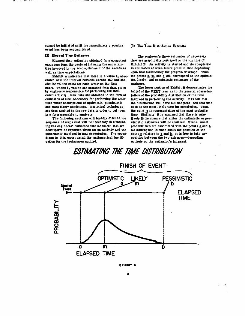
(2) Elapsed Time Estimates The engineer's three estimates of necessary

Elapsed-time estimates obtained from competent time are graphically portrayed on the top line ofengineers form the basis of inferring the uncertain- Exhibit B. An activity is started and its completionties involved in the accomplishment of the events as is estimated at some future point in time dependingwell as time expectations, upon how fortuitously the program develops. Thus

Exhibit A indicates that there is a value to asso- the points a. m., and b will correspond to the optimis-ciated with the interval between events #50 and #51. tic, likely, and pessimistic estimates of theSimilar values exist for each arrow on the flow engineer.chart. These to values are obtained from data given The lower portion of Exhibit B demonstrates theby engineers responsible for performing the indi- belief of the PERT team as to the general character-cated activity. Raw data are obtained in the form of istics of the probability distribution of the timeestimates of time necessary for performing the activ- involved in performing the activity. It is felt thatities under assumptions of optimistic, pessimistic, the distribution will have but one peak, and that thisand most likely conditions. Statistical techniques peak is the most likely time for completion. Thus,ate then applied to the raw data in order to put them the point m is representative of the most probablein a form amenable to analysis. time. Similarly, it is assumed that there is rela-

The following sections will broadly discuss the tively little chance that either the optimistic or pes-sequence of steps that will be necessary in translat- simistic estimates will be realized. Hence. smalling the engineers' estimates into measures that are probabilities are associated with the points a and b.descriptive of expected times for an activity and the No assumption is made about the position of theuncertainty involved in that expectation. The appen- point m relative to a and b. It is free to take anydixes to this report detail the mathematical justifi- position between the two extremes--dependingcation for the techniques applied, entirely on the estimator's judgment.

ESTIMATING THE TIME DI/,STPIT/ON

FINISH OF EVENT

OPTI ISTIC UKELY PESIMISTIC

. _T_ - ELAPSEDTIME

_-

0.

a m bELAPSED TIME

EXHIBIT B

6

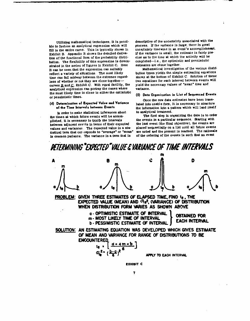
Utilizing mathematical techniques, it is possi- descriptive of the uncertainty associated with the

ble to fashion an analytical expression which will process. If the variance Is large, there is great

fill in the entire curve. This is typically shown in uncertainty timewise in an event's accomplishment.

Exhibit B. Appendix B shows the detailed deriva- If the variance is small, the estimate is fairly pre-

tion of the functional form of the probability distri- cise as to the time at which the activity will be

bution. The flexibility of this expression is demon- completed-i.e., the optimistic and pessimistic

strated in the series of figures in Exhibit C. Here estimates are close together.

it can be seen that the expression can suitably Mathematical investigation of the various distri-

reflect a variety of situations. The most likely bution types yields the simple estimating equations

time can fall midway between the extremes regard- shown at the bottom of Exhibit C. Solution of these

less of whether or not they are close together- two equations for each interval between events will

curves ILand.Q, Exhibit C. With equal facility, the yield the necessary values of 'mean' time and

analytical expression can portray the cases where variance.

the most likely time is close to either the optimistic (5) Data Organization in List of Sequenced Eventsor pessimistic times.

Once the raw data estimates have been trans-(4) Determination of Expected Value and Variance lated into usable form, it is necessary to structure

of the Time Intervals between Events the information into a pattern which will lend itself

In order to make statistical inferences about to analytical treatment.

the times at which future events will be accom- The first step in organizing the data is to order

pushed, it is necessary to typify the intervals the events in a particular sequence. Starting with

between adjacent events in terms of their expected the last event (the final objective), the events are

values and variances The expected value is a sta- placed-sequentially on a list until all future events

tistical term that cor,:csponds to "average" or "mean' are noted and the present is reached. The rationale

in common parlance. The variance is a term that is of the ordering of the events is such that no event

ffTE WI/N/NG 8E P(CTEP'VAL1E VA2IANCE OF TIME I7/TE4AVALSm

A BD

a*/T'\ 4 k a Ma Lt b oJ9 b 0 bat

PROBLEM: GIVEN THREE ESTIMATES OF ELAPSED TIME, FIND te, THEEXPECTED VALUE (MEAN) AND Ofet, (VARIANCE) OF DISTRIBUTIONWHEN DISTRIBUTION FORM W*RIES AS SHOWN ABOVE

a- OPTIMISTIC ESTIMATE OF INTERVAL OBTAINED FORm- MOST LIKELY TIME OF INTERVAL Tb- PESSIMISTIC ESTIMATE OF INTERVAL I EACH INTERVAL

SOLUTION: AN ESTIMATING EQUATION WAS DEVELOPED WHICH GIVES ESTIMATEOF MEAN AND VARIANCE FOR RANGE OF DISTRIBUTIONS T0 BEENCOUNTERED,.

,e " L ca44m-b]

(J 6 ~~ APIPLY TO EACH INTERVAL.

EXHIBIT C

WINNOWS"

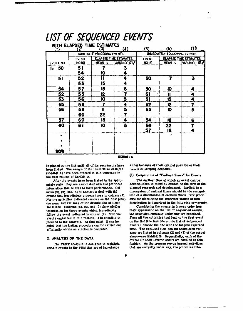
LIST OF SEQUENCED EVENTSWITH ELAPSED TIME ESTIMATES

(1) (2) (3) (4) (5) (6) (7)IMMEDIATE PRECEDING EVENTS IMMEDIATELY FOLLOWING EVENTS

EVENT ELAPSED TIME ESTIMATES EVENT ELAPSED TIME ESTIMATESEVENT NO NO.(S) MEAN to VARIANCE Mleg NO.(S) MEAN to V'RIANCE Oi.t

TO 50 51 7 354 10 4__ _ _ _ _ _

51 52 . . 4 50 7 353 15 4

54 57 18 6 50 10 452 55 12 7 51 1153 56 10 5 51 15 455 58 7 4 52 12 756 59 1I 5 53 10 5

60 22 757 60 is 4 54 18660 61 10 5 56 22 7

457 4

NOWEXHIBIT D

is placed on the list until all of Its successors have elthei because of their critical position or theirbeen listed. The events of the illustrative example . of slipping schedule.(Exhibit A) have been ordered in this sequence inthe first column of Exhibit D. (1) Computation of "Earliest Times* for Events

After the events have been listed An the appro- The earliest time at which an event can bepriate order, they are associated with the pe0rient accomplished Is found by examining the form of theInformation that relates to their performance. Colo planned research and development. Implicit in aumns (2), (3). and (4) of Exhibit D deal with thb discussion of earliest times should be the recogni-events that immediately precede those in column (1). tion of a distribution of earliest times. The proce-For the activities indicated (arrows on the flow plan), dure for identifying the important values of thisthe mean and variance of the distribution of times distribution is described in the following paqrapbsare listed. Columns (5). (6), and (7) show similar Considering the events in inverse order frominformation for those events which mlnedlately their appearance on the list of sequenced events,follow the event indicated in column (1). With the the activities currently under way are examined.events organized In this fashion, it is possible to Prom all the activities that lead to the first eventproceed to the analysis. At this point, it can be on the list (the last one on the list of sequencednoted that the listing procedure can be carried out events), choose the one with the longest expectedefficiently within an electronic computer. time. The expt.;ted time and its associated vari-

ance are listed in columns (2) and (3) of the outputsheet-see Exhibit E. Sequentially, each of the

2. ANALYSIS OF THE DATA events (in their Inverse order) are handled in thisThe PERT analysis is designed to highlight fashion. As the process moves beyond activities

certain events In the FBM that are of importance that are currently under way, the procedure lnte-

AMPLE OUTPUT .SEET(1) (2) (3) (4) (5) (6) (7) (8) (9) (10) (11) (12)

EARLIEST LATEST TIMESEVENT TIMES Toe - Tos PROS OF" LATEST

NO TEI7 TL I'PROS OF ORIGNAL MEETG TIMES NEW PROB OF

EXPECTED VARIANCE EXPECTED VARIANCE t" 'NO SLACKW SCHED SCHED Tosb9O SCHED 'NOSLK

50 92 38 92 0 0 .50 82 .05 90 90 .63

51 85 35 85 3 0 .50 77 .09 83 82 .70

54 74 29 82 4 8 .08 73 .42 80 77 .05

52 47 25 74 7 27 .004 70 1.00- 72 62 .00+"

53 70 31 70 7 0 .50 60 .04 68 67 .69

55 35 18 62 14 27 .004 55 1.00- 60 55 .09

56 60 26 60 12 0 .50 50 .02 58 58 .65

57 56 23 64 10 8 .08 55 .42 62 61 .35S 0. 0 0 6 6 0 0 0

X-l 0 0 • " 0 0 0 0

(TIME IS SHOWN IN WEEKS FROM X OR TIME "NOW")EXHIBIT E

grates means and variances previously considered. ing the variance for #53 to that for the activ-As an illustration of this process of integration, the ity between #51 and #53---or, 31 + 4 = 35.computation of event #51 will be described in detail.Exhibit E shows that event #51 is immediately (2) Computation of the 'Latest Times' for Events

preceded by events #52 and #53. The latest time at which an event can be ac-This exhibit also shows the activity between complished is found by fixing the objective event

events #51 and #52 has a mean estimated at some future date and working backwards throughtime of 11 weeks-while that between #51 the earlier events.and #53 has 15 weeks. The latest time for an event, like the earliest,

Adding the 11 weeks to the 47 weeks which is exists in the form of a distribution which is de-the earliest expected time for event #52 (see scribed in terms of its expectation (mean) and vari-Exhibit F, column (2)). yields an expected ance. Latest times are predicated upon a designa-earliest time for event #51 of 58 weeks-in- tion of some future date as being desirable (orsofar as event #51 depends on the activity satisfactory) for accomplishing the final objective.that was initiated with event #52. A similar The latest time for an interim event is located at acalculation is made for the earliest expected point such that. if the following events are accom-time for event #51 as constrained by the plished according to anticipations, the objectiveactivity starting with event #53. This calcu- will then be completed precisely on the desiredlation yields a mean (expectation) of 85 date.weeks. The procedure for arriving at the latest dates

Noting that the greater time span is required for events is performed in the same general fashion(on the average) by the activity starting with as that for the earliest times. However, the eventsevent #53, the choice of 85 weeks is made as are taken sequentially in the same order as theythe earliest time for event #51. The associ- appeared on the original listing-Exhibit D. Theated variance for event #51 is found by add- objective event is assigned a mean that corresponds

9

to its desirable date with zero variance. Then. (TE) for a small complex of events together with

utilizing the information in the last two columns of the time intervals between them (te). It can be seen

Exhibit D. earlier events are specified by subtract- that of the three paths that lead from event #8 to #6,

ing their activity times from the expected times of the longest expected time of event #6 is at the 65ththe succeeding events. For the illustrative example week.the results of the calculations are shown in columns If the 65th week is satisfactory for accomplish-(4) and (5) of Exhibit E. ing the performance of event #6, the system can be

anchored at this point and latest times computed in

(3) Computation of =Slack in the System backwards computation, discussed above. Exhibit

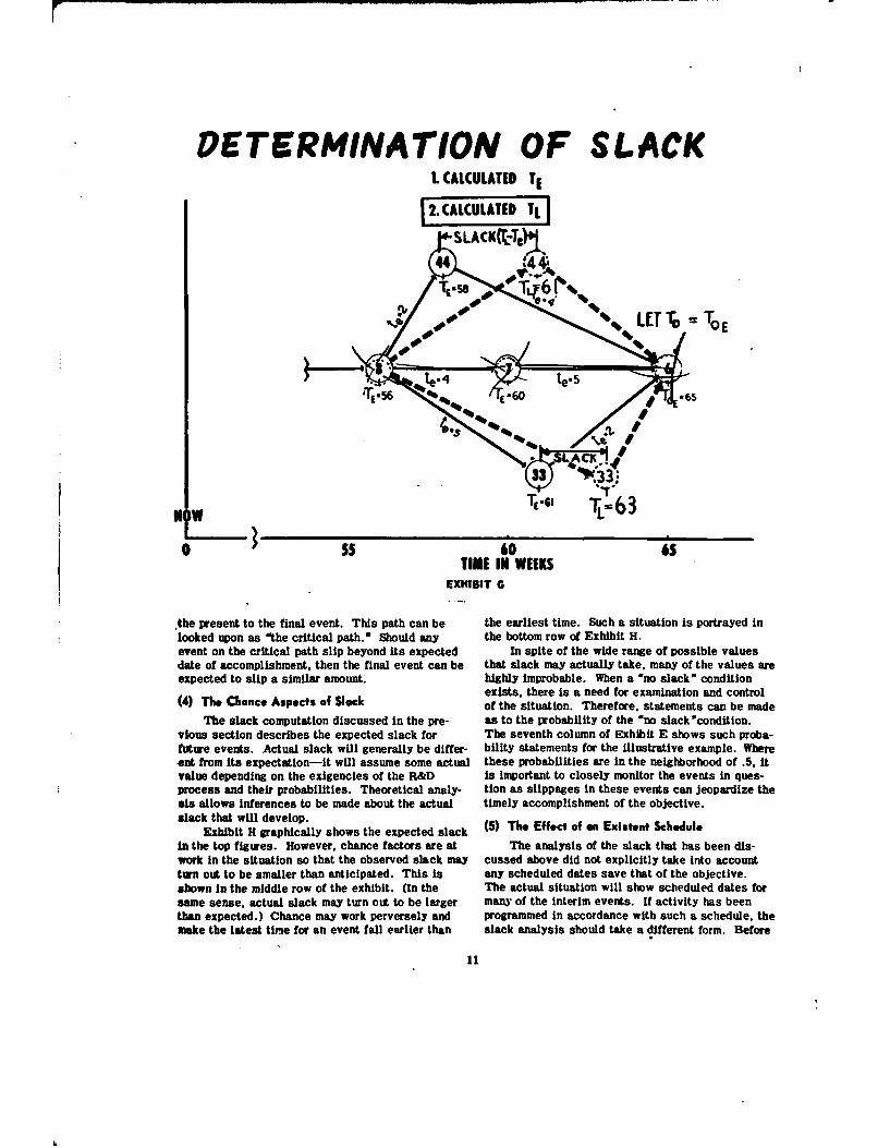
Examination of columns (2) and (4) in Exhibit G shows the time relationship of the earliest and

E shows that in some cases there are differences latest times for these events-the dashed circles

between the earliest and the latest times at which represent the latest times (TL). This comparisonan event will occur (i.e., their mean times). Slack illustrates that events #44 and #33 have slack, i.e.,can be taken as a measure of the scheduling flexi- events #44 and #33 could be scheduled anywherebility that is present in a flow plan. Thus, granting within their slack range and still not disturb the ex-

that the forward anchor point in the latest times pectation of timely accomplishment of the finalcomputation is a desirable one, then the slack period event at week 65.for an event represents the time interval in which it The slack for each event in the illustrativemight reasonably be scheduled. example appears in the sixth column of Exhibit E.

Mlack exists in a system as a consequence of It can be noted that for some of the events a zero

multiple path Junctures that arise when two or more slack condition exists. This indicates that the

activities contribute to a third. This condition is earliest and latest times for these events are

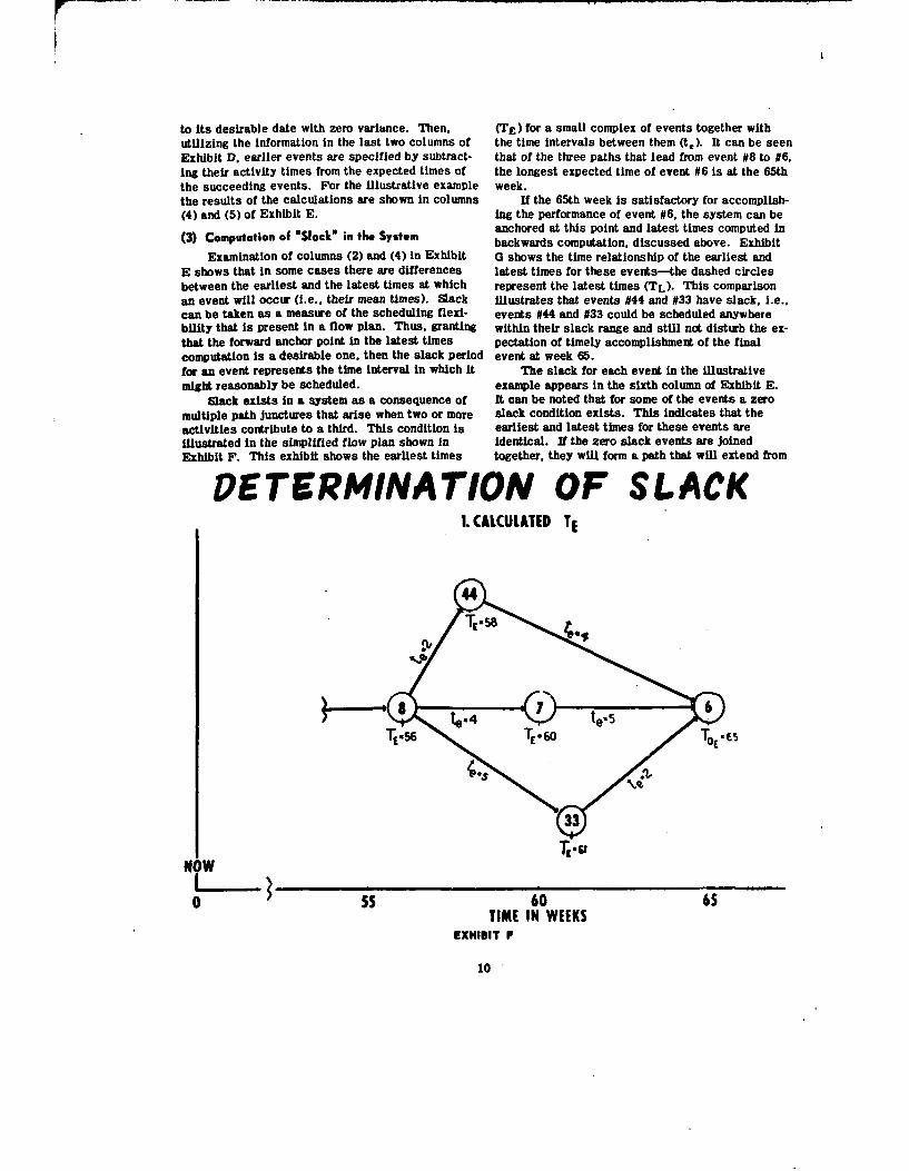
illustrated in the simplified flow plan shown In identical. If the zero slack events are joinedExhibit F. This exhibit shows the earliest times together, they will form a path that will extend from

DETERMINATION OF SLACK1. CALCULATED TE

NOW "60 65

TIME IN WEEKS

EXHIBIT F

10

DETERMINATION OF SLACKL CALCULATED TE

1-.CALULATED TL

SLACKC(.-TJ)"

TtTs---6 (4-

to ss %65E T O

TIE IN WEEK6 S

EXHIBIT G

.the present to the final event. This path can be the earliest time. Such a situation is portrayed inlooked upon as "the critical path." Should any the bottom row of Exhibit H.event on the critical path slip beyond its expected In spite of the wide range of possible valuesdate of accomplishment, then the final event can be that slack may actually take, many of the values areexpected to slip a similar amount, highly improbable. When a "no slack - condition

exists, there is a need for examination and control(4) The Chance Aspects of Stack of the situation. Therefore, statements can be made

The slack computation discussed in the pre- as to the probability of the "no slack "condition.vious section describes the expected slack for The seventh column of Exhibit E shows such proba-future events. Actual slack will generally be differ- bility statements for the illustrative example. Whereent from its expectation--it will assume some actual these probabilities are in the neighborhood of .5, itvalue depending on the exigencies of the R&D is important to closely monitor the events in ques-process and their probabilities. Theoretical analy- tion as slippages in these events can Jeopardize theala allows inferences to be made about the actual timely accomplishment of the objective.slack that will develop.

Exhibit H graphically shows the expected slack (5) The Effect of on Existent Schedule

in the top figures. However, chance factors are at The analysis of the slack that has been dis-work in the situation so that the observed slack may cussed above did not explicitly take into accountturn out to be smaller than anticipated. This is any scheduled dates save that of the objective.shown in the middle row of the exhibit. (In the The actual situation will show scheduled dates forsame sense, actual alack may turn out to be larger many of the interim events. If activity has beenthan expected.) Chance may work perversely and programmed in accordance with such a schedule, themaske the latest tiime for an event fall earlier than slack analysis should take a different form. Before

11

1.

SLACK - 4CT/AL IVS £CTEDEARLIEST TIME LATEST TIME

DISTRIBUTION DISTRIBUTION

VTHIS IS EXPECTED SLACK - BUT

TE f*-SLACK--.

BY CHANCE, THIS MAY OCCUR

SLACK

OR EVEN THIS-WITH A SCHEDULE

(NO SLACK, BUT RESTRICTION)

eEXHIBIT H

such an analysis is undertaken, an appraisal of the expected to occur at time T with variance, a TE'.feasibility of the existent schedule should be made. Statistical theory shows thatlhe probability distribu-

Decisions as to the feasibility of a scheduled tion of times for accomplishing an event can bedate for accomplishing an event rest ultimately on a closely approximated with the normal probabilitysubjective basis. As a guide for developing criteria density. It is, therefore, possible to calculate thefor making such decisions, it is possible to esti- probability that the event will have occurred by any

mate the probability of actually meeting scheduled future date. The probability that event #50 willdates. The uncertainties of the future prevent a have occurred by time T, is represented in Exhibitforecast of the precise time at which an event will I by the shaded area under the curve.be accomplished. However, there is knowledge of Similar calculations can be made for eachexpected times, and a procedure is also available scheduled date. A hypothetical list of dates isfor giving the probability of any given deviation shown in column (8) of Exhibit F. This series offrom that expectation. dates might represent an existent scheduled arrived

Exhibit I graphically illustrates the uncertain- at by any means. Column (9) of this exhibit showsties involved in predicting the precise time at which the probabilities of meeting each scheduled date Ifan event will occur. The exhibit shows the last few all activities are carried out as soon as they canevents in the illustrative example. Event #50 might be. Where the probabilities assume low values, it ishave been scheduled at time To$. However, an ear- reasonable to assume that the schedule is infeasi-liest time analysis could indicate that the event Is ble. High values indicate the opposite-that the

12

ESTIMATE OF PAOBABILITY OF MEETI/M MEMO P ITE-

SHADED AREA IS AN51 ESTIMATE OF THE CHANCES

50_50 I. DETERMINE Tos- ToE

0rTE5 2. USE NORMAL CURVE

TABLE FOR PROBABIUITY-P

Tos ToE

SCHEDULED EXPECTED(CURRENT) (FROM STUDY)

EXHIBIT I

schedule will be met with a high probability. Tech- tifying the location of the points ýLand dL innical managers can reappraise a given schedule In Exhibit J(l).the light of the probabilities here cited. If it is If the scheduled date of the objective event has beendecided that a scheduled date is infeasible, then changed, it is necessary to recompute the latestresources and/or performance must be altered or a times for all events. (Latest dates are based uponrescheduling must take place. If the first option Is the precise location of the objective event.) Columnchosen here, then competent technical advices will (10) on Exhibit E shows what a new set rf latestprovide a new plan and appropriate estimates will dates would be if the objective event was slippedbe acquired from the estimating sources. If the - from week 82 to week 90.decision is to reschedule, then a rational means of The earliest and latest times for an event arechanging the schedule should be found, then compared. Each event is categorized accord-

Ing to whether or not its latest time precedes its(6) A Method of Rescheduling t lrliest time. When the latest time falls before the

The procedure for obtaining an optimum sched- earliest, set the scheduled date at the latest time.ule Is both complicated and time consuming. An When the latest time does not fail before the earliest,optimum would have to define costs of slipping a then set the scheduled date for the event at thescheduled date and costs of scheduling before an point that maximizes the probability that it willactivity can be started, for all events individually actually be met and fall within the slack interval.and collectively. The problem appears to be insur- (See Exhibit J(2)). The techniques for making thismountable within the available time frame. An op- calculation are shown In Appendix D. The datestional procedure has been worked out. however, arrived at through the application of the procedurewhich provides a reasonable if sub-optimal approach to the illustrative example are shown in column (11)to the question of rescheduling. The procedure can of Exhibit E.be detailed in terms of the following steps: After obtaining the new schedule, it is appro-

0 If it is possible to extend the scheduled date priate to appraise again future possibilities by re-of the objective event, this should be done. computing the probabilities of "no slack" in the sys-Exhibit J(l) gives an indication of the range tem. If the probability of "no slack" is much inof dates that are suggested as appropriate if excess of .5. then serious consideration should bethey are satisfactory to the FBM management. brought to bear on the advisability of redeploymentAppendix D specifies the procedure for Iden- of resources and/or changes in performance. If the

13

L

A PESCHEDLULI/N6 PROCED1REI. SLIP LATEST SCHEDULED DATE

C Id

-~ITOE

TO A POINT BETWEEN cfd

AT c ; Pr [ACCOMPLISHMENT]= 25 (1 CHANCE IN 4)

AT d ; Pr [ACCOMPLISHMENT] = .50 (I CHANCE IN 2)

EXHIBIT J(1)

probability is approximately .5. then management should receive but routine checking. The probabili-

should closely monitor progress on the events. If ties for the illustrative example are shown in the

the probability of 'no slack* is much less than .5. last column of Exhibit E.

then progress on the activity leading to the event

2. RECOMPUTE ALL LATEST TIMES

3. FOR SCHEDULE OF INTERIM EVENTS-

WHERE TL < TE SET Ts = TL

TL 2 TE SET Ts TO MAXIMIZE

Prile Ts!-ZIxMISIT J(2)

114

III. FIELD ACTIVITY IN PHASE I

In the course of developing the methodology, sufficient consideration nor were they authenticatedthe PERT team visited at LMSD, Sunnyvale and by the contractor managements.Aerojet General, Sacramento. During the course ofthese visits, flow charts of the missile subsystemand the propulsion component were made. The 1. THE MISSILE SUBSYSTEMevents that appeared on these constructions were Exhibit K portrays the nature of the systemextracted from several sources. The SP Program flow chart for the missile. Time data were gatheredManagement Plans, and Lockheed Master Develop- in units of a month. Earliest and latest times werement Plan, and the Lockheed Master Test Plan all computed, as was the slack. The various compo-contributed to the itemization of the events. The nents of the subsystem were coded and the criticalsystem flow diagrams were constructed with some path indicated. The objective of this exercise washaste, but attempts were made to delete non-defini- to ascertain the availability of the basic data and totive and redundant milestones from the list. develop insights into the magnitudes of the numbers

Time estimates were gathered from engineers, involved.planners, and the various evaluation staffs. In some Exhibit K appears in censored form in order tocases, estimates were tendered conditionally with prevent disclosure of classified details. However.the understanding that they had not been subject to the complex form of the interactions of events can

$VST* fOW PtAN *1S6611W

l I LEGEND

- A- MISSILE SUBSYSTEM PLIGHTS AND TESTS-AMISSILE SUBLSYSTEM FLIGHTS AND TESTS

- PROPULSION COMPONENT A-ILAUNCHER SUSSYSTEM

- GUIDANCE COMPONENT- RE ENTRY BODY COMPONENT- WARHEAD DEVELOPMENT- CRITICAL. PATH (PROM METHODOLOGY)

EXHIIIIT K

15

be observed. In addition, it has been possible to others may be concerned with only the broader ele-color-code activities so as to highlight the sequence ments. All points of view can be accommodated byof activities that develop in any of the missile com- synthesizing the detailed findings and reportingponents. These are indicated in the legend on only those facts that will necessarily call for deci-Exhibit K. sion. Thus, many different outputs can be produced

according to the various requirements and interestsof the particular consumer.

An additional benefit arises from breaking the2. THE PROPULSION COMPONENT initial analysis into many detailed events. By

Whereas the events in the missile subsystem utilizing this procedure. it is possible to diminishwere gathered at a broad level with little detail, the the impact of existent schedules on the estimates.propulsion component was typified with 160 lower When estimates are elicited on the basis of detailedlevel events. The date of the exercise was 12 activities, the individual estimators are most apt toMarch; hence, this point marks the origin of the respond independent of schedules-as schedulestime scale. The form of the propulsion flow chart are generally published in fairly gross detail. Inwith the critical path (zero slack) indicated is given taking advantage of this independence, PERT hopesIn a separate appendix (classified). The detailed to obtain the most valid estimates possible.description of the events and the computed times At the presant time, the PERT team is activelyand standard deviations appear in the appendix. It engaged in obtaining authentic data for decisionmay be noted that according to the preliminary time purposes. In order to obtain both depth and breadthestimates as given in this appendix, the date of of outlook, analyses are being made of the missileevent #37 falls in the latter part of January, 1959. subsystem and three of its components. Thus. itThis outlook has undoubtedly changed since the will be possible to gain important insights into thedate of the study, as remedial action has been interactions among the missile components as wellundertaken by both the contractor and the SP staff. as the impact of the component's progress on the

In obtaining the system flow for the propulsion missile subsystem itself. Coincidental with thecomponent, recourse was made to what may be field activity, work is in progress on the program-called a principle of analysis and synthesis. The ming of the NORC computer to handle the calcula-process was analyzed into many events for pur- tions necessary for analysis and evaluation. A con-poses of providing detailed control in case such tinuing flow of information is to be provided by con-would be of interest at some point in time. This tractor personnel. Eventually, it Is planned thatdetailed Itemization of events should not be con- the entire FBM System can be integrated into astrued as implying that all events should be so laid single network so that total system evaluations canout for top management's attention. All of the successfully and automatically be made-ratherevents may hold interest for some individuals while than appraisals of isolated parts.

is

APPENDIX A

THE STOCHASTIC MODEL ANDITS SPECIALIZATION TO THE FBM PROGRAM

1. THE STOCHASTIC MODEL In this appendix the events will be interpretedas achievements or milestones in a process that

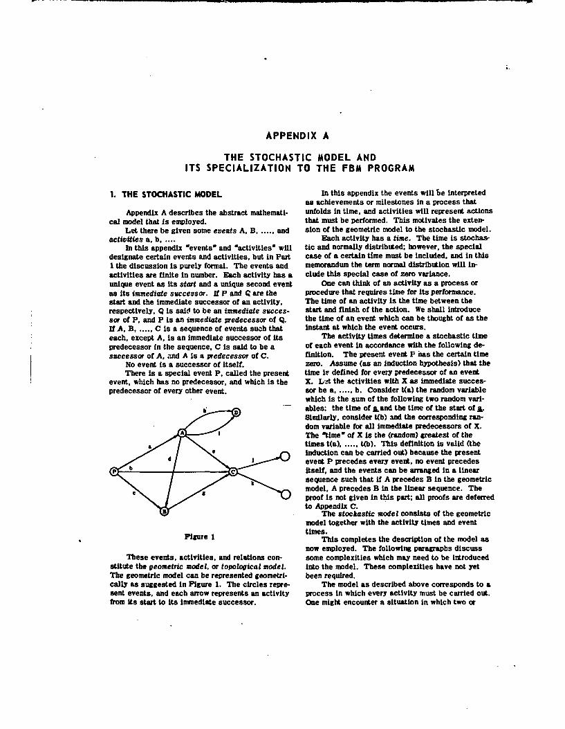
Appendix A describes the abstract mathemati- unfolds in time, and activities will represent actionscal model that is employed, that must be performed. This motivates the exten-

Let there be given some events A, B ...... and sion of the geometric model to the stochastic model.activities a. b .... Each activity has a time. The time is stochas-

In this appendix aeventso and eactivitieso will tic and normally distributed; however, the specialdesignate certain events and activities, but in Part case of a certain time must be included, and in thisI the discussion is purely formal. The events and memorandum the term normal distribution will in-activities are finite in number. Each activity has a clude this special case of zero variance.unique event as its start and a unique second event One can think of an activity as a process oras its immediate successor. If P and Q are the procedure that requires time for its performance.start and the immediate successor of an activity. The time of an activity is the time between therespectively, Q is said to be an immediate succes- start and finish of the action. We shall introducesor of P. and P Is an immediate predecessor of Q. the time of an event which can be thought of as theif A, B ...... C Is a sequence of events such that instant at which the event occurs.each, except A, is an immediate successor of its The activity times determine a stochastic timepredecessor in the sequence, C is said to be a of each event in accordance with the following de-successor of A. and A is a predecessor of C. finition. The present event P has the certain time

No event is a successor of itself, zero. Assume (as an Induction hypothesis) that theThere is a special event P, called the present time ia defined for every predecessor of an event

event, which has no predecessor, and which is the X. LAt the activities with X as immediate succes-predecessor of every other event. sor be a ...... b. Consider t(a) the random variable

which is the sum of the following two random vari-

D ~ables: the time of j~and the time of the start of jL.Similarly, consider t(b) and the corresponding ran-dom variable for all immediate predecessors of X.The atime' of X is the (random) greatest of thetimes t(a) ...... t(b). This definition is valid (theinduction can be carried out) because the presentevent P precedes every event, no event precedes

bc itself, and the events can be arranged in a linearsequence such that if A precedes B in the geometricmodel, A precedes B in the linear sequence. Theproof is not given in this part; all proofs are deferredto Appendix C.

The stockastic model consists of the geometricmodel together with the activity times and eventtimes.

Flgure 1 This completes the description of the model asnow employed. The following paragraphs discuss

These events, activities, and relations con- some complexities which may need to be inttoducedstitute the geometric model, or topological model. into the model. These complexities have not yetThe geometric model can be represented geometri- been required.cally as suggested in Figure 1. The circles repre- The model as described above corresponds to asent events, and each arrow represents an activity process in which every activity must be carried out.from its start to its immediate successor. One might encounter a situation in which two or

APPENDIX A(2)

more alternative activities are carried on in parallel that both activity a be completed before b Is startedwith the understanding that as soon as one activity and activity b be completed before a is started. Ifis completed, the parallel activities will be aban- one is merely sure that all prerequisites of activi-doned. Such a situation would involve the small ties are planned for completion before the activitiesadjustment of computing the shortest of two or more start, the plan is feasible.times rather than the longest. However, in spite of the logical redundancy of

It is conceivable that the time of an activity is activity times in the construction of a feasible plan.conditioned by the outcome of preceding activities, estimates of these times must be considered in mak-For example, in Figure 1 the activity g may be re- ing an intelligent plan. In the estimation of the timequired only if activity c 'fails." In this case the required to carry out an activity, it is often usefuldistribution of j would be constructed from the to break up the activity into portions or subactivi-probability of failure of c and the two conditional ties, to estimate for the subactivities, and to totaldistributions of j.that correspond to failure and the times for the parts. If an activity is to besuccess, respectively, of c. divided into parts, it is necessary to designate

accurately the points ef division. This means that,2. SPECIALIZATION OF THE MODEL TO THE when the activity is carried out, one must be able

FBM PROGRAM to recognize the instant at which ond subactivity

terminates and a succeeding one starts. The stateIn this part a realization of the stochastic of the process at this critical instant is an event.

model is extracted from the planned development of Another utility of events is found in the monitor-the FBM and the associated systems. ing of progress towards objectives. Events can

Many things must be done to achieve the pur- serve as milestones, and one can analyze progressposes with which SP is concerned. These things by checking off the events at the instants theyInclude decision making, research, development, occur.design, fabrication, production, testing, etc. Theactivities leading to the desired results must be The entire development of the FBM and its

planned. One reason for this is that the activities associated subsystems is an activity. But this

must be sequenced in some feasible manner. The over-all activity naturally breaks up into large sub-

sequences are optional to some extent. One might activities concerned with the missile, guidance,

develop a missile before thinking about a ship and ship, etc. Furthermore, these subactivities sub-

then adapt the ship to the missile characteristics, divide further until eventually one might have

Alternatively. one might conceivably set the ship _ thousands of subactivities. These subactivitles are

characteristics and accept resulting constraints on the activities .of the analysis.

the missile. Actually. under pressure of time it is In order to structure the thousands of activities

necessary to have numerous parallel developments into an orderly system, events are required. An

with coordination. evixt is a state or condition in future developmentThe present analysis assumes that the objec- which will be clearly recognized at the instant the

tives of SP have been planned. Necessarily, the state or condition occurs.

plan must designate what we call events. Indeed, Let us particularize these concepts by a fewif an activity is planned to commence after certain very simple, hypothetical examples. Suppose that aother accomplishments have been consummated, it second test program is to start as soon as a firstmust be necessary to recognize when the prerequi- test program is successful. We can consider thesite accomplishments have been realized. This first program as an activity I and the second programrequires some check point, or event in our termi- as an activity 11. A third activity c consists of thenology, which will trigger off the activity in ques- preparation of the facilities of the second testtion. Furthermore, usually action is desired Just program. If A designates the instant in time atas soon as the prerequisites are achieved; hence, which the second test program can start, the rela-an event occurs instantaneously-at the first in- tions among A and the activities can be representedstant when certain conditions prevail, as in Figure 2. In the situation of Figure 2. the

To construct a reasonable plan one would take completions of the activities a and b are not events.Into account the times required to carry out the vari- The event Arepresents the instant at which both aous activities. However. a feasible plan could be and b are completed. Hence, If Xand X are themade without such consideration. A feasible plan instants at which I and q are completed. respec-is one that could be carried out, and hence would tively, then A is the later of X. and X. The eventsbe void of inconsistencies such as a requirement X and .X could be introduced as In Figure 3. In this

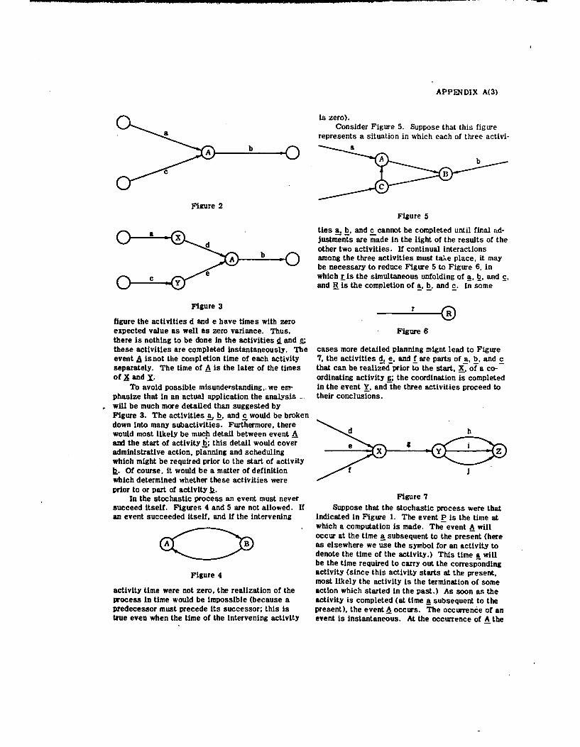
APPEINDIX A(3)

is zero).Consider Figure 5. Suppose that this figure

represents a situation in which each of three activi-ka

A b 0a A b

>Gý C

Figure 2Figure 5

a Q ties a, b, and c cannot be completed until final ad-aJustments are made in the light of the results of the

other two activities. If continual interactionsA b among the three activities must take place, it may

be necessary to reduce Figure 5 to Figure 6, inc e which ris the simultaneous unfolding of a. b, and c,

and R is the completion of a. b, and c. In some

Figure 3

figure the activities d and e have times with zeroexpected value as well as zero variance. Thus, Figure 6there Is nothing to be done in the activities d and Zthese activities are completed instantaneously. The cases more detailed planning might lead to Figureevent A is not the completion time of each activity 7, the activities d. e, and f are parts of a, b, and cseparately. The time of -A is the later of the times that can be realized prior to the start, X2 of a co-of X and Y. ordinating activity g; the coordination is completed

To avoid possible misunderstanding,. we em- in the event Y. and the three activities proceed tophasize that in an actual application the analysis - their conclusions.will be much more detailed than suggested byFigure 3. The activities a, b, and c would be brokendown into many subactivities. Furthermore, therewould most likely be much detail between event Aand the start of activity b; this detail would cover eadministrative action, planning and schedulingwhich might be required prior to the start of activity

k. Of course, it would be a matter of definition fwhich determined whether these activities wereprior to or part of activity b.

In the stochastic process an event must never Figure 7succeed itself. Figures 4 and 5 are not allowed. If Suppose that the stochastic process were thatan event succeeded itself, and if the intervening indicated in Figure 1. The event P is the time at

which a computation is made. The event A willoccur at the time a subsequent to the present (here> B as elsewhere we use the symbol for an activity todenote the time of the activity.) This time a willbe the time required to carry out the corresponding

Figure 4 activity (since this activity starts at the present,most likely the activity is the termination of some

activity time were not zero, the realization of the action which started in the past.) As soon a-s theprocess in time would be Impossible (because a activity is completed (at time a subsequent to thepredecessor must precede Its successor; this is present), the event A occurs. The occurrence of antrue even when the time of the intervening activity event is instantaneous. At the occurrence of A the

APPENDIX A(4)

activities d, e, h, and I are started. Similarly theactivity g starts at the time of the occurrence of B. BThe event C will occur as soon as e, b, and g arecompleted. Hence, the time of C subscquent to thepresent will be the greater of the three times a plus •e, b, and c plus g.

One can think of an event simply as the time ofthe completion of one set of activities and the time dof the commencement of another set. Thus, event C.is the time of the completion of activity e, b!, or j,

whichever is later, and C is also the time at which Figure 9activities j and k both commence.

An activity can involve simply waiting. Sup-pose that some project is to commence at time 5 some "schedule' has been set). Then Figure 8 mustfrom the present, and that it Is not necessary for be augmented as in Figure 9. The activityehasany action to take place prior to the start of the the expected time 2 with variance zero.project (except the decision, already made, to start Furthermore, it is necessary that the activity Ithe project at the specified time of 5 from the (of waiting) appear in the analysis. Without the con-present). If the event X is the start of the project, straint of % it is suggested that we could deter-there would be an activity between P andX desig- mine, at least roughly, some 'latest time" at whichnated by an arrow x., and the time x would have the C could occur without producing delay beyond thatexpected value 5 and variance zero. already inherent in the times of activities aand c.

The activity of waiting explains another aspect Then it is proposed that one could 'schedule" C

of the process which some people find paradoxical. between the earliest and latest times. Suppose that

Suppose we have the situation of Figure 8. In the we try to do this. In view of the expected value andstandard deviations of the times c and d (as indi-cated in Figure 8) it would seem fairly safe toschedule d to start 2 units of time subsequent to the

B occurrence of B. But there would be a very small

"-•. c probability that d will not be completed until after chas been completed. Hence, the expected time of

AD event D will be very slightly later than it would beif d were started immediately at the completion of b.In many cases it would be obvious that the delaywould be insignificant. However, in some cases onewould wish to delay the start of d as long as pos-sible, and the question would arise as to just what

Figure 8 risk of delaying D would result from various delaysIn the start of l. Such a question could be answeredif the activity e is introduced into the analysis as

figure we have indicated along with each activity indicated in Figure 9.

time the expected value and standard deviation of To repeat, if the analysis produced only earliest

the time. Someone will object that event _Q will not and latest times, and if scheduled times for events

occur as soon as activityb is completed for the were set In the light of earliest and latest times,

following reason. Event D cannot occur until the feasibility and implications of the schedule

roughly 10 units of time subsequent to .A (because would be determined by the analysis suggested in

i + F 10). If d starts as soon as b_ is completed, the case of Figure 9. This is due to the fact that

then d will be completed roughly 8 time units any constraint imposed by a 'schedule" would alter

before ý_ is completed. In many such cases there 'earliest* and Olatest' times.

will be administrative action which will delay the The stochastic process should include all

start of d. But if there is any such administrative constraints including all restrictions implied by

contraints on the stochastic process, they must aP- 'scheduling" or any other administrative action.

pear In the analysis. Suppose that in the present Then the times of the events are the times at which

case it has been decided that d will not start until they will occur, not earliest times at which they

two time units subsequent to _. (perhaps because could occur.

APPENDIX B

THE ANALYSIS OF ACTIVITY TIME ESTIMATESAND THE MATHEMATICAL COMPUTATIONS

The model of the FBM program consists of directly supervise the performance. These peopledesignated activities, events, relations of preced- are technicians in spirit, even if they have admin-ence and succession, and distributicns of activity Istrative responsibility.times. The analysis of the model involves two Since it will be difficult to get more than amajor items. Estimates of activity times must be single authoritative estimate, the problem of per-obtained. Then event times must be calculated. sonal bias is serious. These biases will dependThese two parts of the analysis are discussed in partly on the weight of company policies, schedules.this appendix, and commitments. In some cases it will be possible

to get supplementary estimates from technicians not1. THE ANALYSIS OF ACTIVITY TIME employed by the responsible contractor. For ex-

ESTIMATES ample, the estimates of an AeroJet employee canalso be made by some Lockheed technician who is

We have defined activities and we have stated intimately concerned with the activity and its re-that it is necessary to estimate the expected value suits; also, an estimate can be obtained within SP.and variance of each activity in the P'NM program. This leads to the question of the combinationThis part discusses the sources of these estimates of two or more estimates. This is discussed below.and the procedures for obtaining them. We turn then from the question of sources of

Activities are of diverse natures. They include time estimates to the parameters estimated. Theproduction, fabrication, testing, development. analy- estimates by a technician (or other person, if neces-sis, administration, research, and decision making. sary) should be made after careful explanations by aSpecific examples are the following: the fabrication highly qualified interviewer. After this first inter-which takes place between the delivery of a chain- view the estimates may be made and transmitted tober to Aerojet and the availability of the specific SP on forms.test vehicle for firing; the test program which takes We propose that the technical person be askedplace between the first development test and the to estimate the following for an activity. First, aqualifications of the A motor for firing. This last "likely" time which technically we shall interpretactivity can be broken down into subactivities as the mode of the activity time. Synonyms whichwhich would most likely include development, anal- can be offered are "most probable time," and "timeysis, administration, and decision making, you would expect." Even "expected time" makes an

The diversity of activities makes a general impression on persons who are not statisticians.discussion difficult. But we are at present facing but this term must be avoided when there is anythe generalities, possibility of confusion with the statistical mean-

First, let us consider appropriate sources of ing of this term.Information concerning the possible time that an Secondly, the technician is asked for an "opti-activity might take. In this matter it is essential mistic" time. There should be practically no hopenot to accept uncritically any times that appear in of completing the activity in less than the optimisticplans and contracts. Rather, one must probe to the time, but good luck might give a time close to thebases upon which the plans and contract schedules optimistic.

d•. are made. One reason is that schedules (other than Thirdly, we ask for a "pessimistic" time. Thisthe ones we shall set ) are not adequately responsive concept is not as sharp and clear as we would like.to changing conditions and prospects. Secondly, Although experience to date has not produced anypresent schedules di not estimate uncertainties, serious difficulty with this concept, we must handleand thirdly, they are made under pressures which the estimation with great care. This difficulty isInvolve matters other than the accurate estimate of the obvious one that in research or development ittimes; one such pressure is haste. is difficult to set a date within which an achieve-

Hence, preferably we should get information ment can be guaranteed.from people who are to perform the activities or to As a first description of the pessimistic time,

APPENDIX B(2)

we ask for a time which will not be exceeded, the activity times; from these we shall calculatebarring 'acts of God." but which might conceivably expected values and variances of event times.be approached. Hence, ourproblem is to estimate the expected value

An 'act of God' is an unexpected, unforeseen and variance of an activity time from the likely,event whose occurrence would not be anticipated in optimistic, and pessimistic times discussed above.any reasonable planning. Examples are wrecks Furthermore, we feel free to use a non-normal modeland unusual strikes. If all experts anticipate the of the distribution of activity times as a tool in thissuccess of a research project, and if the project estimation.fails, the failure is included as an 'act of God.' If. We recall that for unimodal frequency distribu-however, expert opinion is divided, failure is not an tions, the standard deviation can be estimated'act of God.0 and in setting a pessimistic estimate roughly as one-sixth of the range. Hence, it seemsthe estimator should allow for time to complete the reasonable to estimate the standard deviation of anactivity in case of failure and a fresh start. (An activity time as one-sixth of the difference be-alternative deserving serious consideration is a tween the pessimistic and optimistic time estimates.time estimate assuming success and an estimated The estimate of the expected value of an activ-probability of success.) ity time is more difficult. We do not accept the

The pessimistic estimate does not involve likely time as the expected value. We feel that ansimply a listing of foreseeable difficulties and an activity time will more often exceed than be lessestimate of the total time to overcome each. A tech- than an estimated likely time. Hence, if likelynical man might say that of ten possible but un- times were accepted as expected values, an unde-likely difficulties, it would be unreasonable to sirable bias would be introduced. Our apprehensionanticipate all ten; he might say that he is reason- of this bias is supported by estimates already oh-ably certain that it would be foolish to expect more tained. In many cases the likely time is nearer thethan three of the ten to materialize. Or the ian may optimistic than the pessimistic time. In such aknow from experience that delays are usually caused situation one feels that the expected time shouldby unforeseeable developments; this man might base exceed the likely time.his estimates more on intuition than analysis. We shall introduce an estimate of the expected

Perhaps we should say that a pessimistic esti- time which would seem to adjust at least crudelymate is a time which is longer than expected, but for the bias that would be present if likely timeswhich might be required in one out of a hundred were accepted as expected times. As a model ofsimilar activities. Furthermore, although one can- the distribution of an activity time, we introduce thenot set an absolute time limit which will never be beta distribution whose mode is at the likely time,exceeded, no normal person would hedge against a whose range is the interval between the optimistictime greater than the pessimistic time. and pessimistic times, and whose standard devia-

In case of a refusal by a technician to state a tion is one-sixth of the range. The probabilitypessimistic estimate, one would go to the person or density of this distribution isbody that decided to include the activity. This de-cision maker must justify some upper limit to the f(t) = (constant) (t - af (b - t)y (see Figure 10)accomplishment (the upper limit could include thetime to accomplish some substitute achievement, In which the optimistic and pessimistic time esti-and It might involve a prospect of foregoing the mates are respectively a and b (the left- and right-activity and of accepting some performance hand ends of the range); the -constant," a and y aredegradation). functions of a. b. and the likely time M (i.e., the

In Appendix A it was assumed that the activity modal time). To reduce this probability densitytimes are normally distributed. It will be clear that function to the standard form of the beta distribu-in many cases the times are not normal. However, tion, we introduce the random variable x as relatedwhen event times are calculated from activity times, to t. as follows:we compute sums of activity times. Hence. theevent times will be roughly normal even if the activ- t - aity times are not normal (because of the central X = - .

limit theorem). This will not be the case for im- b - a

mediate successors of the present event. Thesespecial cases can be handled directly, and we shall The probability density of 1 isnot discuss them here. For the general case weshall use only the expected values and variances of f"(x) = IB(a + 1. v + l) -xa(l - x)v

APPENDIX B(3)

B DISTRIBUTION

f (t)

fi(t) -K Qt- a)o( (b- t 1I"

a rn b

VALUES OF 0( a Y OBTAINED BY

I. SETTING M-m OF ESTIMATESb-a

2. SETTING a- (BETA DISTRIBUTION)=Figure 10

Since the modal value of t is _M, f _ denotes the as + (36r _ 36-r + 7r)a2 - 20rta - 2er = 0mode of x,

M - a We can now compute the parametersln f(t).b = - Given M, a and b, the above formulas enable us to

calculate in succession r, a. y, (using the relationIf E(z) and V(x) are respectively the expected value between r, a, and y. E(x). and finally E(t) (becauseand variance of x, straightforward computation the equation of transformation between t and zleads to Implies that E(t) - a + (b - a) E(z).

Let us study the relation between r and E(z).a - a Numerical calculation with use of the above formu-a + y las gives the first two columns of Table 1.

a + 1 Table 1a+y+2

r E(x) (4r + 11/6(a + 1) (y + 1) 0 .2053 .1667

V(x) (1/8 .2539 .2500(a + y + 2)2 (a + y + 3) 1/4 .3228 ..3333

.3/8 .4075 .4167Since the variance oft is (b - a)2/36, the variance 1/2 .5000 .5000of I is 1/36. We eliminate y from the equations for

I and V(x) after substituting 1/36 for V(x), and we If E(x) +s plotted as a function of r. it Is seen thatobtain the relation between these variables is approximately

Lb

APPENDIX B(4)

linear. A simple linear approximation, namely f*(x) vs. r

E(x) .(4r + I)/6 2.2 a

is given In the third column. We shall accept this •approximation because it is accurate enough for our 2.0purposes, and because the prior computation requiresamong other operations the solution of a cubic equa-tion. Prom the relations between E(x) and E(t) and .between r and _M, the linear approximation reducesto

E(t) = (a + 4M + b)/6.

This formula will be used in the FEM systemanalysis.

This result was derived under the assumption 1.4that the beta distribution is an adequate model of thedistribution of an activity time. The choice of thebeta distribution was dictatedby intuition because 1.2 *empirical evidence is lacking. Hence it will beappropriate to consider the reasonableness of theresult. 1.0

The result can be reduced to

I a+b)Em ) - (2" + 2-.

This means that E(t) is the weighted mean of M andthe mid-range (a + b)/2, with weights 2 and I re- .6spectively. In other words, E(t) is located one-thirdof the way from the likely time M to the mid-range. -

We can consider whether the weights 2 and 1 in .4 4the above formula seem appropriate. Perhaps itwould be intuitively better to move the likely timeonly one-fourth of the way towards the mid-range. 4

Perhaps one-half or one-tenth. Our own opinion is .2

that one-third seems reasonable. However. we In- S

tend to code into the computer routine this ratio asa parameter. Hence the weights can be changed if .0 0

authoritative judgment dictates. Furthermore, by • . .• .8 1.0making computer runs with various parameter valuesone can test the sensitivity of the computed result Figure 11

to this choice of weights.As experience with the development of the FBM that there Is enough probability above L = 1/2 to

accumulates, we can compare actual activity times bring the expected time up to .32. In.our opinionwith estimates of M, a. and b. This will enable us this graph is as reasonable as that obtained fromto reconsider the weights used. any other commonly occurring probability density

As further evidence of the appropriateness of function.the beta distribution model, we have presented thegraph of f*(x) for the case in which.r = 1/4 (Figure 2. THE MATHEMATICAL COMPUTATIONS11). This represents the case in which the likelytime is one-fourth of the way from the optimistic to This part discusses the calculation of the ex-the pessimistic time. This graph reveals that most pected values and variances of event times. A de-of the activity times will be symmetrically distrib- scription is given of the mathematical problems thatuted aboutr 1/4 between r = 0 and r = 1/2, but are presently unsolved.

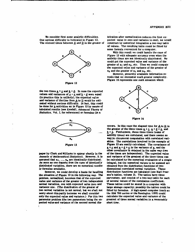
APPENDIX B(5)

We consider first some analytic difficulties. tribution after normalization reduces the first ex-One serious difficulty is indicated in Figure 12. pected value to zero and variance to one), we wouldThe elapsed times between A and D is the greater of construct by numerical integration a two-way table

of values. The resulting table could be fitted bysome formula convenient for a computer.

B With this result we could handle the case ofFigure 13 with adequate accuracy even when theactivity times are not identically distributed. Wecould get the expected value and variance of thegreater of al and a 2 , etc. Then we could computethe expected value and variance of the greater ofa3 and the greater of a, and a 2 , etc.

However, presently available information re-veals that we encounter much greater complexity.Figure 14 represents one such situation which

Figure 12

the two times A + c and b + d. In case the expected a evalues and variances of a - c and b - d were equal

(in practice this is unlikely), the expected valueand variance of the time from A to D would be esti-mated without serious difficulty. In fact, this could <be done for n activities as in Figure 13 by means of b •tabulated results (see Kendall, Advanced Theory o1Statistics, Vol. I, for references) or formulas (in a

Figure 14

Soccurs. In this case the elapsed time for AtoD is

the greater of the three times a +c. a+d+Le andb + e. Furthermore. these three times (sums ofactivity times) are correlated, and there seems no

a. wayto circumvent computation with correlated vari-ables. The correlations involved in the example of

Figure 13 Figure 13 are easily calculated. The covariance ofa+c and a + d + e is the variance of a, and theother covarlance is obtained in the same way (two

paper by Clark and Williams to appear shortly in the of the times are independent). The expected valueAasuals of Mathematical Statistics). However, it is and variance of the greatest of the three times canassumed that al .... a, are identically distributed, be calculated by the numerical evaluation of a singleAs soon as one departs from the case of identically integral, but the numerical values to be summed aredistributed variables, there are no numerical results obtained from the distribution functions of two-or formulas available, dimensional correlated normal variables. These

However, we could develop a basis for handling distribution functions are tabulated (see Karl Pear-the situation of Figure 12 in the following way. The son's tables, volume 2). The tables have threeproblem, normalized, becomes that of the expected para-meters. and consist of a two-way table for eachvalue and variance of the greater of two independent of several values of the correlation coefficient.normal variables, one with expected value zero and These tables could be stored in a computer withvariance one. (The distribution of the greater of large storage capacity; possibly the tables could betwo normal variables is not normal, but we shall not fitted by formulas. A high speed computer (such asworry about this partly because we shall consider the IBM 700 series or the Remington 1103) couldonly the expected value and variance.) For this two calculate the expected value and variance of theparameter problem (the two parameters being the ex- greatest of three normal variables in a reasonablypected value and variance of the second normal dis- short time.

APPENDIX B(6)

However, since even greater complexities are expect the computer to apply properly the rule ofencountered, and since we would like to use a thumb for combining correlations (however, givenmedium speed computer, we should investigate the two specific paths from the present to a specificpossibility of obtaining simple approximations. Let event, it would be easy to compute the correlationus discuss this prospect at some length. Consider of the two time constraints). The difficulty wouldfor the moment the problem of the greater of two cor- not be with the rule of thumb but with isolating therelated normal variables. This is a three parameter various paths and their interrelationships (whichproblem, the parameters being the difference of the determine the correlations).expected values, the ratio of the standard devia- It is likely that the best procedure with respecttions, and the coefficient of correlation. One could to the computer would be something like the follow-construct tables to handle this problem there would ing. When the computer calculates the expectedbe two-way tables for selected values of the corre- value and variance of an event time, the computerlation. Possibly the tables could be fitted by rela- must know the constraints on this time (there is atively simple analytic expressions, constraint for each path of activities from the

Consider the situation of Figure 14. If we re- present to the event in question, and the constraintstrict consideration to the two constraints a + c and of the path is the sum of the activity times along theb_ +e, we could determine the expected value and path). It might take the computer a relatively longvariance of the greater of these two times. Then we time to isolate all the paths to an event and to ac-could combine this constraint with that of the third curately compute the expected value and variancetime a + d + e, and this again Involves the greater of the event time. Hence, it may be desirable toof two time constraints. The difficulty is that one make a preliminary analysis off the computer. Forof these two constraints is Itself a complicated each event we would examine all the activity paths,computed result, and it is difficult to calcul;Ue the select the most important ones (rejecting thosecorrelation between a + d + e and the greater of the paths whose activity times are relatively small).other two times. We know the covariance of a + d + e and tell the computer how to compute (i.e., tell thewith each of a + c and b + e, but what relation is computer what constraints to consider, in what order,there between the two simpler correlations and the and with what simplifying approximations.)more complicated correlation involving the greater At best, it will be a non-trivial task to imple-of two times? The problem is not simple. However, ment the above analysis. Hence, we should con-It Is likely that study based upon numerical evalua- sider alternatives. The most obvious alternative istion of special cases would produce some rule of the one now employed. The time constraints of allthumb for estimating the desired correlation at least paths leading up to an event are considered, androughly. one assigns to the event the expected value and

With such a rule of thumb we could handle many variance of the greatest of these constraints.

complex situations in the following manner. Sup- This simplification gives biased estimates andpose that the time of some event were subject to the bias is such that the estimated expected timesseveral constraints (i.e., the time is the greatest of of events are too small. To get some idea of theseveral times). We would find the expected value bias, we can consider two independently distributedand variance of the greater of the first two times. normal variables with the same parameters p and o.Then using the rule of thumb, we would estimate the The expected value of the greater of the two iscorrelation between the time of the third constraint p + .56a (see Kendall. loc. cit.). Thus, if twoand the greater of the first two times. Then the parallel activities are each expected to take a yeartpbles mentioned above would permit us to estimate with a standard deviation of one month (which isthe expected value and variance of the greatest of roughly equivalent to a range from 9 to 15 months),the first three constraints. The fourth and succeed- the expected time to the completion of both activi-ing constraints would be introduced similarly, ties Is 12 + .56 (1) = 12 1/2 months roughly. In the

If this possibility should be realized, another presently used simplifications the half month isdifficulty would arise, namely that of arranging the lost. As a very rough guess, we might fear that theanalysis in a computer. The computer could deter- presently used simplification is biased to the extentmine all time constraints on each event (this of a couple of months.amounts to listing all paths along activity arrows However, the presently used simplification isfrom the present event to each event, and totaling appealing. For each event there is a longest time

the times and variances of the activities). This activity path from the present to the event. Thismight require too much time even on a high speed path can be called a "critical path.0 Of specialcomputer. Moreover, it might be unreasonable to interest Is the critical path to some future event 7

APPENDIX BC7)

of paramount Importance. Each activity time along and 1 respectively. Then if the expected time ofthis path contributes directly to the elapsed time the second activity changes from 1 to 2, there willfrom the present to Z. Slippages in the completion be practically no change in the expected time of thetimes of these activities cause slippages of equal second event B; but rigorously the expected elapsedamounts in Z. Furthermore, for events or activities time from A to B will be increased by a tiny frac- 4'0-not on the critical path, some delay can be tolerated tion of a second.without changing the expected time of Z. For each A precise notion of a latest time for events is"non-critical event (not on the critical path) one the following. Let Z be some event of paramountcan set a 'latest' expected time for the event such importance. Let some delay a in Z be selected.that if all expected times were condtrained to occur This delayD might be a week, or it could be a dayat this latest time (variances being unaltered), the or a month. Then for a given event X one couldexpected time of Z would be unchanged as computed compute the increase in the expected elapsed timeby the presextly used method. However, this con- from the present to X which would result in an in-cept introduces the biases of the present computa- crease of D in the expected elapsed time to Z. Thetions in a very severe form. But, ignoring the result would indicate how much the event X couldbiases, we have a way of designating critical events be slipped without a resulting serious delay.whose slippages are serious, and non-critical events The unfortunate aspecL of this definition is thateach with Its possible slippage. Such analysis is it seems computationally impossible. To show whyuseful in spite of the biases. is so, letXthenlay im e o s wfy

Let us next face the problem of some rigorous this Is so, let Xl be the latest time of X as definedanalysis of "latestO times at which events can occur in the last paragraph. To compute A'. it would seem

without jeopardizing the time of some event Z of necessary to make one or two runs of the analysisparamount Importance. Rigorously there seems *to with the constraints augmented by a single con-paaountgimpoatae.t Riges ouslyhtherents cstraint which would delay X (an artificial activitybe no rigid latest times at which events can occur, between X and XI .) A couple such trial runs wouldToeillussoratefsuane that Xe andtarer immediate a - enable one to interpolate for the delay in X whichpredecessorswould set back the expeted time of Z by theties are xandy respectively. Suppose that both _x amount D. The trouble is that this computationand y have the expected value it and variance a.ahn y have thme exp seted vagdlue and vari ance Y must be carried out for every event and activity ofThen if a time for Z is set rigidly, and if X a interest. The time required for such computationoccur at times 1 + .56a before Z (the term .56a is would seem to be excessive. However, It would beclarified above), then the expected time of Z will be woul se to be exc Howevertwdthe time rigidly set. One is inclined to accept the very easy to perform such analysis for selectedlatest times for X and Y as % + .56a prior to Z. But problems.note that if X precedes Z by p + to where t is say 4 As we maneuver from an intellectually soundor 5, and If Y precedes Z by only I. the expected definition of latest time to one that can be madetime of Z is still as set. This example reveals that operational, it seems necessary to introduce somethere is some freedom to adjust alatest times* ultimately illogical procedure. The most obviousamong two or more events, thing to do is to run time backwards. There are

Another logical difficulty is the following. If logical difficulties with this procedure. However,the expected time of any activity whatsoever is in- it seems rational to introduce the fiction of a re-creased, or If the expected time of any event is set verse development of the process which starts withat a later time, there is an increase in the expected some event Z and works backward in time to theelapsed time to each succeeding event. (Except in present. If such an analysis is made by the methodunusual situations involving activities with certain employed for the forward computation of the timestimes.) For example, suppose that there are two at which events will occur, then the expected timeactivities between events A and D. Suppose that of an event could be interpreted as a latest time forthe expected value and variance of the first activity the event. Such an analysis need not proceed merelytime is 10 and 1 month respectively, and the cor- from a fixed time for the final event, but could takeresponding parameters for the second event are I Into account the uncertainty of the final event.

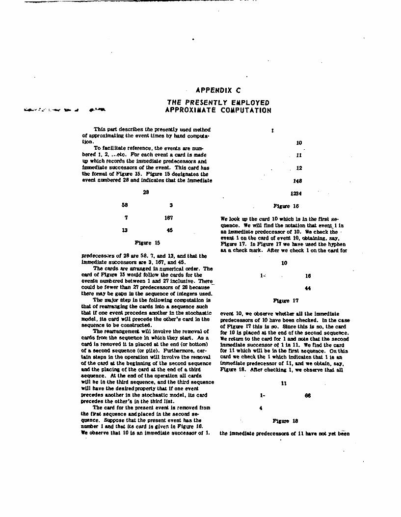
APPENDIX C

THE PRESENTLY EMPLOYED--.- :-- - . APPROXIMATE COMPUTATION

This part describes the presently used method 1of approximating the event times by hand computa-tion. 10

To facilitate reference, the events are num-bered 1. 2. ... etc. For each event a card is made U1up which records the immediate predecessors andImmediate successors of the event. This card has 12the format of Figure 15. Figure 15 designates theevent numbered 28 and Indicates that the immediate 148

28 1234

58 3 Flgure 16

7 167 We look up the card 10 which is In the first se-quence. We will find the notation that event I is

13 45 an immediate predecessor of 10. We check the -event 1 on the card of event 10, obtaining, say,

Figure 15 Figure 17. In Figure 17 we have used the hyphenas a check mark. After we check 1 on the card for

predecessors of 28 are 58. 7. and 13, and that theImmediate successors are 3. 167, and 45. 10

The cards are arranged In numerical order. Thecard of Figure 15 would follow the cards for the 1- 16events numbered between 1 and 27 inclusive. Therecould be fewer than 27 predecessors of 28 because 44there may be gaps In the sequence of integers used.

The major step in the following computation is Figure 17that of rearranging the cards into a sequence suchthat it one event precedes another in the stochastic event 10, we observe whether all the immediatemodel, Its card will precede the other's card In the predecessors of 10 have been checked. In the casesequence to be constructed. of Figure 17 this is so. Since this is so, the card

The rearrangement will Involve the removal of for 10 is placed at the end of the second sequence.cards from the sequence in which they start. As a We return to the card for 1 and note that the secondcard is removed it Is placed at the end (or bottom) Immediate successor of 1 Is 11. We find the cardof a second sequence (or pile). Furthermore. cer- for 11 which will be in the first sequence. On thistain steps In the operation will involve the removal card we check the I which indicates that I is anof the card at the beginning of the second sequence immediate predecessor of 11, and we obtain, say.and the placing of the card at the end of a third Figure 18. After checking 1, we observe that allsequence. At the end of the operation all cardswill be in the third sequence, and the third sequence 11will have the desired property that if one eventPrecedes another in the stochastic model. Its card 1- 66precedes the other's In the third list.

The card for the present event Is removed from 4the first sequence and placed in the second se-quence. Suppose that the present event has the Figure 18number I and that its card is given in Figure 16.We observe that 10 is an immediate successor of 1. the Immediate predecessors of 11 have not yet been

APPENDIX C(2)

checked. Hence. we leave the card for 11 in its sors of A. say B, which is still in sequence 1.place in sequence 1. (When at some later time in Choose an immediate predecessor or B, say C.the operation 4 is checked, the card for 11 will be which is still in sequence 1. This process can goplaced at the end of the second sequence of cards.) on forever, and an infinite sequence of events isWe continue until all the immediate successors of 1 generated. No event can appear twice in thishave been handled in the same way. Then the card infinite sequence because an event cannot be afor 1 is placed at the end of the third sequence predecessor of itself. But this is a contradiction;(actually, 1 will be the first card in sequence 3). we have an Infinite sequence with all different

The next step is to take the first card in se- terms, and the terms are selected from a finite setquence 2 and to handle it in the same way that 1 of events.was handled. Suppose that this first card in se- We shall now work with sequence 3. and com-quence 2 is 10 as given in Figure 17. Since Figure pute event times. The first event in sequence 3 is17 indicated that 16 is an immediate successor of the present event. Its time is zero with zero varn-10, we look for 16 in the first sequence. If we do ance. Next we consider the second event B in se-not find 16 (because it has been removed from the quence 3.first sequence), we take no action as regards 16. i Its sole predecessor is the present event. How-16 is still in sequence 1, we check on the card for16 the immediate predecessor 10. If, after 10 is ever, there might be two or more activities with Bchecked, we find that all the Immediate predecessors as immediate successor (each of these activitiesof 16 have been checked, we would place 16 at the would start with the present event). We select the

end of sequence 2. otherwise 16 is left In sequence activity with the greatest expected value; in caseend f squece . Oterwse 6 ileftin equnceof a tie, among the events with maximum expected1. We continue until all the immediate successors va wechoose one with maximum vaia ce.

of 10 have been handled. Then 10 is placed at the value we choosa vne with maximum variance. The

end of sequence 3. The first card in sequence 2 is expected value and variance of this most severe

processed, and the operation continues as indicated. viae of th time of the event.

We shall now prove that the process will con-

tinue until all the cards are In sequence 3, and that In general, suppose that expected values andsequence 3 will have the desired property, variances have been determined for all events that

In the first place we note that a card is not precede X in sequence ,3. Let the activities with Xplaced in sequence 2 until all its immediate prede- as immediate successor be a.....,z_. Let the startscessors are already in sequence 2 or 3. Hence, of these activities be the events A ...Z, respec-when a card is placed in sequence 3, all its prede- tlvely. We add the expected times and variances,cessors, immediate or not, are in sequence 3. respectively, of A and a. and we get a first con-Hence, the final sequence 3 will have the required straint on the expected time and variance of X. Inproperty. the same way we get an expected time and variance

Finally, we must show that during the opera- for each activity with X as its immediate successor.tion, sequence 2 will never be empty. Otherwise We choose the greatest of these expected times, orthe operation might come to a halt before all cards in case of a tie we choose the greatest of one of thewere in sequence 3. Suppose that we reach a point expected times with maximum variance. This ex-In the operation at which there is no card is se- pected time chosen is obtained from one of the activ-quence 2. but there are still cards in sequence 1. ites z... say y. We assigned to X as expectedEach event in sequence I has at least one imme- time and variance the sum of the expected times anddiate predecessor still in sequence 1 (otherwise the variances, respectively, of Y and y. This operationevent would have been removed from sequence 1 at is appropriate because in sequence 3, each event issome step). Select an arbitrary event &in se- preceded by all events which precede it in thequence 1. Choose one of the immediate predeces- stochastic model.

V

APPENDIX D

A RESCHEDULING PROCEDURE

1. FINAL EVENT (OBJECTIVE) (4) Assume that it is reasonable to have a finalscheduled date fall within this feasible interval.

(1) As a first criterion of schedule feasibility, Choose this date (a highly desirable one) asfollow the rule that the scheduled date of the week 90.final event must have a probability of accom- (5) Recompute all TL. based upon TL = 90.plishment in the range .25 to .50. (Note that if (6) Return and compute PR[e 2<S •11] for all eventsthe probability is .5, then in regard to the final based on the new values of tRe TL.event TE - TL = T ; if the probability is -T T T(7) The scheduled time of the final event has beengreater than .5, then the scheduled date for final changed to a date that is deemed feasible (bycompletion is later than its expected earliest the foregoing definition).value.) Some of the intervening events must be resched-

(2) If the probability of accomplishing the final uled in order to allow for proper dovetailing ofevent is below the stipulated minimum, the first the events in constructing the end product.step is to note the slippage necessary in the Interim events can be of a second kind. Whenfinal event to bring it within the range of mini- succeeding events are of a nature such thatmum interval cited above, they follow in a natural sequence regardless ofThe necessary schedule date of the final event scheduled date, there is no need to reschedulecan be computed as follows: (such events might be primarily of a progress61 = schedule date with approximately .25 measuring nature.)

probability of achievement However, a priori, there will probably not beK -- normal deviate exceeded with probabil- any designation which will automatically sepa-

ity, f rate the events (interim) into the categories 're-TE, - earliest expected time for final accom- schedulableI and Onot reschedulable. There-

plishment fore, all events should be rescheduled periodi-S1 1 , scheduled date with approximately .5 cally (nominally, at least). If the probabilities

probability of achievement of accomplishment are smaller than technical1. TE+ = ; X X = K 7 5 -67 personnel deem wise, then they can change the

I.=TK.75XK 7 - real scheduled dates as necessary.UTE (8) Methods for rescheduling an interim event are

2. TEo S outlined in this appendix under the title *'Proce-E.g., if TE -92 -6.2 dures for Scheduling.0

E 2 OTE 6(9) In appraising the new schedule, it should benoted that difficulties can arise in the face ofX , -. 67; X - (-.67) (6.2) - -4.15 either of two exigencies:1. The latest time, 1, can come before S2. The earliest time, 2. can come after S_

Taking the next larger integral value of X The probabilities of these two situations occur-ring are given respectively by:

1 ,T +X=+92+(4)88 1. P (no slack)2. P (restriction)S;1 - TEe - 92 If the probabilities are high that either of thesetwo situations will occur, then action or close

Therefore. the values of So in the interval 88 - observation is called for. In the example (Ex-92 will satisfy the criterion of number I above. hibit E), action would probably be called for in

(3) The interval 88 - 92 can be referred to as a the cases of events 69, 67, and 66. Close ob-"feasible* range. It should first be examined as servation should be devoted to 61, 60, 56. 53,to its propriety as a scheduled time for the final 51, and 50. The remainder of the events needevent. not be subjected to the same close scrutiny.

APPENDIX D(2)

(IO)Using the procedure indicated in (9) above, it is (3) It is noted that the foregoing designation of thepossible to designate three different classes of suggested schedule time does not explicitly takeevents-which are ordered in respect to their into account the costs associated with variousprobable relative criticalness. Such a list options.should only be suggestive. The technical per- When one sets a schedule by maximizing thesonnel upon review in the light of their full Joint probability, a premium is set 'n havingknowledge should make the actual designation C <, I and also on having the interval overlap theof real criticalness and provide for the neces- scheduled date. The particular premiums thatsary action and control, are set depend in some fashion on the variances

of the latest and earliest time distributions.2. INTERIM EVENTS The costs of not meeting the requirements are

not explicit and do not differentiate between the(1) An expected value exists for the earliest and case where S1 falls before I and the case where

latest times at which an event can occur-as S' falls after 1.does the variance for each of the two distrlbu- (4) Owing to the neglecting of cost functions, use oftions. this procedure will occasionally give values of

(2) Define E and v2 as mean and variance at ear- 81 that are larger than E when E > L. Such anRest times outcome appears illogical, thus this procedureL and v~as mean and variance at latest should only be used when E < L. When E > L,times the suggested value S' can be equated to L.S1 as the suggested time for scheduling This procedure will make 81 - L. and thus takethe event. advantage of fortuitous early completions at theS 1 , max [Pr (e _S s) Pr (1 a)] cost of occasionally scheduling an event at too

a early a time.

S. . . . I I "- I -