PERIODIC SOLUTIONS OF THE PLANAR N-CENTER … · PERIODIC SOLUTIONS TOPOLOGICAL CONSTRAINTS 3 Figure 1. First we will introduce some notations. Given an x ∈ H1(ST,X), we say it

arX

iv:1

507.

0288

3v2

[m

ath.

DS]

16

Sep

2015

PERIODIC SOLUTIONS OF THE PLANAR N-CENTER

PROBLEM WITH TOPOLOGICAL CONSTRAINTS

GUOWEI YU

Abstract. In the planar N-center problem, for a non-trivial free homotopyclass of the configuration space satisfying certain mild condition, we show thatthere is at least one collision free T -periodic solution for any positive T. We usethe direct method of calculus of variations and the main difficulty is to showthat minimizers under certain topological constraints are free of collision.

1. Introduction

In the study of the classic N -body problem, or the general singular Lagrangiansystems, one of the oldest ideas in finding periodic solution, at least goes back toPoincare, is by looking for minimizers of the action functional in certain admissibleclasses of loops.

Besides the usual coercive condition, comparing with regular systems, the extradifficulty is to show that the desired minimizer is free of singularity. Otherwise weget something called generalized solutions, see [2], [1].

If the singularities are caused by the strong force potentials (see Remark 1.1 forthe precise definition), then the extra difficulty is gone (again already known toPoincare). As in this case the action functional along any loop with singularitymust be infinite. All kinds of periodic solutions can be found using variationalmethods, for example see see [15], [1], [19] and [9].

However when the singularities are caused by the weak force potentials, includingthe Newtonian potential, then the action functional along a loop with singularitiesmay still be finite. In fact by the results of Gordon [16] and Venturelli [24], weknow in certain cases there are minimizers with singularities.

Started with the (re)-discovery of the Hip-Hop solution [11] in the NewtonianFour-body problem and the Figure-Eight solution [10] in the Newtonian three-bodyproblem. We have learned that one of the method to overcome the above problemis to impose certain symmetric constraints on the admissible class of loops. For thedetails please see [13], [3], [8], [6], [7], [14], [20] and the references within.

On the other hand very few results are available when topological constraintsare involved and it is still a difficult task to determine whether a minimizer is freeof collision in this case.

In order to clarify and overcome the difficulties related to the topological con-straints, in this paper we propose to study the simplified model, namely the planarN -center problem, with N ≥ 2. Since all the natural symmetries of the N -bodyproblem do not exist anymore, it will be a perfect test ground for various techniquesthat have been developed by many people in the past twenty years. The main resultof our paper is some simple criteria on the topological constraints that will ensure

1

http://arxiv.org/abs/1507.02883v2

2 GUOWEI YU

the existence of collision free minimizers (in the N -center problem the singularitiesare caused by collisions between the test particle and a center).

In forth coming papers we will show that some of the results proved in this papercan be generalized to the N -body problem.

In the planar N-center problem, a test particle is moving in the plane underthe gravitational field of N fixed point masses (centers). We use mj > 0 : j =1, . . . , N and C := cj ∈ C : j = 1, . . . , N ( cj 6= ck, if j 6= k) to denote the massesand positions of the N centers correspondingly.

If x : R → X , where X := C\C, is the position function of the test particle, thenx(t) should satisfy the following second order differential equation:

(1) x(t) = ∇V (x(t)) = −N∑

j=1

mj

|x(t) − cj |α+2(x(t) − cj),

for α > 0 and

V (x(t)) :=N∑

j=1

mj

α|x(t) − cj |α,

is the negative potential at x(t).

Remark 1.1. In general, α ≥ 2 correspond to the strong force potentials, 0 < α < 2correspond to the weak force potentials and in particular α = 1 corresponds theNewtonian potential. In this paper we will not discuss α ∈ (0, 1) and to distinguishwith the Newtonian case, by weak force potential, we will only mean α ∈ (1, 2).

Equation (1) has a natural variational formulation. It is the Euler-Lagrangeequation of the action functional

A(x) =

∫

L(x(t), x(t)) dt,

where the Lagrangian L has the form

L(x, x) :=1

2|x|2 + V (x).

For any T1 < T2, T > 0 and U ⊂ C, we let H1([T1, T2], U) be the space ofall Sobolev functions mapping [T1, T2] to U and H1(ST , U) be the space of allT -periodic Sobolev loops contained in U , where ST := [−T

2 ,T2 ]/−

T2 ,

T2 .

Given an x ∈ H1([T1, T2], U), define its action as

A([T1, T2];x) =

∫ T2

T1

L(x(t), x(t)) dt.

In particular if T = −T1 = T2 > 0, then we set

AT (x) := A([−T, T ];x).

For any nontrivial free homotopy class τ ∈ π1(X ) \ 0 and T > 0, let

Γ∗T (τ) := x ∈ H1(ST ,X ) : [x] = τ

and ΓT (τ) be the weak closure of Γ∗T (τ) in H1(ST ,C).

Our goal is to find some simple criteria on τ , such that the following infimimum

cT (τ) = infAT/2(x) : x ∈ ΓT (τ)

can be achieved at some collision free loop from Γ∗T (τ).

PERIODIC SOLUTIONS TOPOLOGICAL CONSTRAINTS 3

Figure 1.

First we will introduce some notations. Given an x ∈ H1(ST ,X ), we say it is ageneric T -periodic loop, if x is a smooth immersion in general position (for adefinition, see page 82, [18]). Such a loop only contains transverse self-intersectionsand we say it has excess self-intersection if it can be homotopic to anothergeneric loop with fewer self-intersection (see [17]).

If I ⊂ ST is a sub-interval with x identifies the end points of I, we say x|I is asub-loop of x. Such a sub-loop is called innermost, if it is also a Jordan curve. Asa result each innermost sub-loop separates the plane into two disjoint regions, onebounded and the other not. We say a center is enclosed by an innermost sub-loopif it is contained in the bounded region.

Definition 1.1. Given a τ ∈ π1(X ), choose an arbitrary generic loop x ∈ Γ∗T (τ)

without any excess self-intersection. We say τ is admissible, if any innermostsub-loop of x encloses at least two different centers.

Now we are ready to state the main results of our paper.

Theorem 1.1. When α ∈ (1, 2), for any admissible free homotopy class τ ∈ π1(X )and T > 0, there is a q ∈ Γ∗

T (τ) with AT/2(q) = cT (τ) and it is a T -periodicsolution of equation (1).

For the Newtonian potential, we get a slightly weaker result. To state our result,we consider the Hurewicz homomorphism: h : π1(X ) → H1(X ) ∼= ZN , which inour case is just the canonical abelianization map. Given an free homotopy class τ ,choose a generic x ∈ Γ∗

T (τ), we can define h(τ) = (h(τ)j)Nj=1 ∈ ZN as following

h(τ)j = ind(x, cj) =1

2πi

∫ T/2

−T/2

dx

x− cj, ∀j = 1, . . . , N,

where ind(x, cj) is the index of x with respect to cj . It is independent of the choiceof x, as long as [x] = τ.

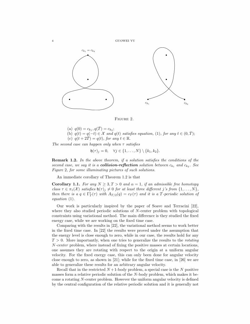
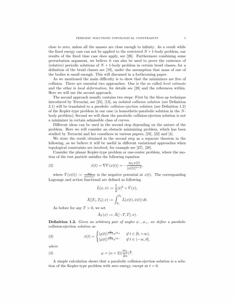
Theorem 1.2. When α = 1, for any admissible free homotopy class τ ∈ π1(X )and T > 0, there is a q ∈ ΓT (τ) with AT/2(q) = cT (τ). Furthermore one of thefollowing must be true:

(1) q ∈ Γ∗T (τ) and it satisfies equation (1);

(2) there are two centers ck1, ck2

∈ C (possibly ck1= ck2

), a T > 0 with T/2T ∈Z+ and q satisfies

4 GUOWEI YU

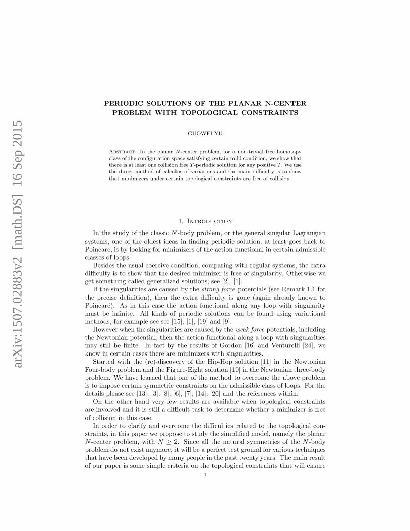
Figure 2.

(a) q(0) = ck1, q(T ) = ck2

;(b) q(t) = q(−t) ∈ X and q(t) satisfies equation, (1), for any t ∈ (0, T );(c) q(t+ 2T ) = q(t), for any t ∈ R.

The second case can happen only when τ satisfies

h(τ)j = 0, ∀j ∈ 1, . . . , N \ k1, k2.

Remark 1.2. In the above theorem, if a solution satisfies the conditions of thesecond case, we say it is a collision-reflection solution between ck1

and ck2. See

Figure 2, for some illuminating pictures of such solutions.

An immediate corollary of Theorem 1.2 is that

Corollary 1.1. For any N ≥ 3, T > 0 and α = 1, if an admissible free homotopyclass τ ∈ π1(X ) satisfies h(τ)j 6= 0 for at least three different j’s from 1, . . . , N,then there is a q ∈ Γ∗

T (τ) with AT/2(q) = cT (τ) and it is a T -periodic solution ofequation (1).

Our work is particularly inspired by the paper of Soave and Terracini [22],where they also studied periodic solutions of N -center problem with topologicalconstraints using variational method. The main difference is they studied the fixedenergy case, while we are working on the fixed time case.

Comparing with the results in [22], the variational method seems to work betterin the fixed time case. In [22] the results were proved under the assumption thatthe energy level is close enough to zero, while in our case, the results hold for anyT > 0. More importantly, when one tries to generalize the results to the rotatingN -center problem, where instead of fixing the positive masses at certain locations,one assumes they are rotating with respect to the origin at a uniform angularvelocity. For the fixed energy case, this can only been done for angular velocityclose enough to zero, as shown in [21]; while for the fixed time case, in [26] we areable to generalize these results for an arbitrary angular velocity.

Recall that in the restricted N+1-body problem, a special case is the N positivemasses form a relative periodic solution of the N -body problem, which makes it be-come a rotating N -center problem. However the uniform angular velocity is definedby the central configuration of the relative periodic solution and it is generally not


close to zero, unless all the masses are close enough to infinity. As a result whilethe fixed energy case can not be applied to the restricted N +1-body problem, ourresults of the fixed time case does apply, see [26]. Furthermore combining someperturbation argument, we believe it can also be used to prove the existence of(relative) periodic solutions of N + 1-body problem in certain braid classes, for adefinition of the braid classes see [19], under the assumption that mass of one ofthe bodies is small enough. This will discussed in a forthcoming paper.

As we mentioned the main difficulty is to show that the minimizers are free ofcollision. There are essential two approaches. One is the so called level estimateand the other is local deformation, for details see [28] and the references within.Here we will use the second approach.

The second approach usually contains two steps: First by the blow-up techniqueintroduced by Terracini, see [25], [13], an isolated collision solution (see Definition2.1) will be translated to a parabolic collision-ejection solution (see Definition 1.2)of the Kepler-type problem in our case (a homothetic-parabolic solution in the N -body problem); Second we will show the parabolic collision-ejection solution is nota minimizer in certain admissible class of curves.

Different ideas can be used in the second step depending on the nature of theproblem. Here we will consider an obstacle minimizing problem, which has beenstudied by Terracini and her coauthors in various papers, [23], [22] and [4].

We state the result obtained in the second step as a separate theorem in thefollowing, as we believe it will be useful in different variational approaches whentopological constraints are involved, for example see [27], [28].

Consider the planar Kepler-type problem or one-center problem, where the mo-tion of the test particle satisfies the following equation

(2) x(t) = ∇V (x(t)) = −m1x(t)

|x(t)|α+2,

where V (x(t)) := m1

α|x(t)|α is the negative potential at x(t). The corresponding

Lagrange and action functional are defined as following

L(x, x) :=1

2|x|2 + V (x),

A([T1, T2];x) :=

∫ T2

T1

L(x(t), x(t)) dt.

As before for any T > 0, we set

AT (x) := A([−T, T ];x).

Definition 1.2. Given an arbitrary pair of angles φ−, φ+, we define a paraboliccollision-ejection solution as

(3) x(t) =

(µ|t|)2

α+2 eiφ+ if t ∈ [0,+∞),

(µ|t|)2

α+2 eiφ− if t ∈ (−∞, 0],

where

(4) µ = (α+ 2)(m1

2α)

12 .

A simple calculation shows that a parabolic collision-ejection solution is a solu-tion of the Kepler-type problem with zero energy, except at t = 0.

6 GUOWEI YU

For any T > 0, define the following class of curves:

Γ∗T (x) := x ∈ H1([−T, T ],C \ 0) : x satisfies the following conditions .

(1) x(±T ) = x(±T );(2) Arg(x(±T )) = φ±.

Let ΓT (x) be the weak closure of Γ∗T (x) in H1([−T, T ],C) and

cT (x) := infAT (x) : x ∈ ΓT (x).

Theorem 1.3. For any T > 0 and |φ+ − φ−| ≤ 2π, there is a γ ∈ ΓT (x), withAT (γ) = cT (x).

(1) If α ∈ (1, 2), then γ ∈ Γ∗T (x) and AT (γ) < AT (x);

(2) If α = 1 and |φ+ − φ−| < 2π, then γ ∈ Γ∗T (x) and AT (γ) < AT (x).

Furthermore γ is a solution of the Kepler-type problem, if φ+ 6= φ−.

The proof of the above result will be given at the last section. They main ideaof the proof comes from [22]. For the case of α = 1, a different proof of the aboveresult can also found in [14].

Remark 1.3. By a classic result of Gordon in [16], we know that when α = 1 and|φ+ − φ−| = 2π the above result does not hold, so this is the best result we can getin the Newtonian case.

2. Asymptotic analysis

The asymptotic behavior of a solution as it approaching a collision, which willbe established in the section, is the base of any local deformation result. Most ofthe results in this section are not new, similar results in various settings have beenobtained before, see [13] and the references there. We include them here for theseek of completeness and also because the direct references of these results in ourparticular setting seems hard to locate.

Definition 2.1. Given a δ > 0 and time t0, we say y : [t0 − δ, t0 + δ] → C is anisolated collision solution, if it satisfies the following conditions

(1) y(t0) ∈ C;(2) y(t) ∈ X satisfies equation (1), if t 6= t0;(3) The energy constant is preserved through the collision, i.e., there is a h,

such that, if t 6= t0,

1

2|y(t)|2 − V (y(t)) = h

Furthermore we say y is a simple isolated collision solution, if it does not haveany transverse self-intersection.

Let y(t) be an isolated collision defined as above, to simplify notation, we willonly state and prove our results with t0 = 0 and y(t0) = c1, while the general casesare exactly the same. Furthermore for the rest of this paper, we assume c1 is alwayslocated at the origin: c1 = 0.

The main results of this section are Proposition 2.2 and 3.1. In this section wedo not require the isolated collision solution to a be minimizer.

Define the moment of inertia and angular momentum of y(t) with respectto the center c1 = 0 correspondingly as

I(t) := I(y(t)) := |y(t)|2;


J(t) := J(y(t)) := y(t)× y(t).

Set y(t) = ρ(t)eiθ(t) = u(t) + iv(t), with ρ(t), θ(t), u(t), v(t) ∈ R, then

J(t) = ρ2(t)θ(t) = u(t)v(t)− v(t)u(t).

Since y|[−δ,δ] only collides with c1, the negative potential with respect to theother N − 1 centers is a smooth function:

V ∗(y) := V (y)−m1

α|y|α=

N∑

j=2

mj

α|y − cj |α.

Now we will introduce two technical lemmas about I(t) and J(t) that will beuseful throughout the entire section.

The first lemma the well known Lagrange-Jacobi identity.

Lemma 2.1. There are continuous functions B1(t), B2(t) ∈ C0([−δ, δ],C), suchthat the following identities hold for all t ∈ [−δ, δ] \ 0

I(t) = (4− 2α)|y(t)|2

2+B1(t) = (4− 2α)[h+ V (y(t))] +B1(t)

= (4− 2α)m1

α|y(t)|α+B2(t)

Proof. By a straight forward computation

I = 2|y|2 −2m1

|y|α+ 2〈∇V ∗(y), y〉.

Using the energy identity

1

2|y|2 − V (y) =

1

2|y|2 −

m1

α|y|α− V ∗(y) = h,

we get

I = (4− 2α)|y|2

2− 2α(h+ V ∗(y)) + 2〈∇V ∗(y), y〉

:= (4− 2α)|y|2

2+B1.

It is not hard to see B1(t) ∈ C0([−δ, δ],C). The rest of the lemma can be shownsimilarly using the energy identity.

Remark 2.1. From the above proof, we can see B1(t) is well-defined for any t 6= 0and there is a positive constant C such that

|B1(t)| ≤ C|y(t)|, ∀t ∈ [−δ, δ] \ 0.

The second lemma is about the angular momentum J(t).

Lemma 2.2.

limt→0

J2(t) = 0.

8 GUOWEI YU

Proof. For any t ∈ [−δ, δ] \ 0,

J2 = (uv − vu)2 ≤ (u2 + v2)(u2 + v2)

= 2|y|2|y|2

2= 2|y|2[h+ V (y)]

= 2[m1

α|y|2−α + (h+ V1(y))|y|

2]

:= C|y|2−α +B(t)|y|2,

where C is a positive constant and B(t) ∈ C0([−δ, δ],C). The desired result followsfrom the facts that 2− α > 0 and limt→0 |y(t)| = 0

With the above two lemmas, we can get the following asymptotic estimates ofI(t) when y(t) is approaching to a collision.

Proposition 2.1. If y|[−δ,δ] is an isolated collision solution with y(0) = 0 and µdefined as in (4), then

(1) for t > 0,

I(t) ∼ (µt)4

2+α ; I(t) ∼4

2 + αµ(µt)

2−α2+α ; I(t) ∼ 4

2− α

(2 + α)2µ2(µt)

−2α2+α .

(2) for t < 0,

I(t) ∼ (−µt)4

2+α ; I(t) ∼ −4

2 + αµ(−µt)

2−α2+α ; I(t) ∼ 4

2− α

(2 + α)2µ2(−µt)

−2α2+α .

Furthermore1

2|y(t)|2 ∼ V (y(t)) ∼

1

4− 2αI(t) ∼

2

(2 + α)2µ2(µ|t|)

−2α2+α .

This type of asymptotic estimates has been proved by many authors in differentcircumstances. We refer the readers to [13] and the references there. We will onlyshow the proof for t ∈ (0, δ], while the other is similar. By quoting (6.2), page 323at [13], the above proposition follows immediately from the next lemma.

Lemma 2.3. For t > 0, the moment of inertia I(t) satisfies the following results:

(1) limt→0+ I(t) = 0;

(2) ∀t ∈ (0, δ], I(t) ≥ 0 and I(t) ≥ 0;

(3) There are constants a, b = 42−α > 2 and c such that I2 + a2 ≤ bII + cI;

(4) There is a constant d > 0, such that for any t ∈ (0, δ], I(t)Ib−2

b (t) ≥ d;

(5) There is a constant e > 0, such that for any t ∈ (0, δ], |d3I(t)dt3 | < eIγ(t),

with γ = 2b−3b−2 = 3

2 + 1α .

Proof. (1). Obvious.(2). The first inequality is obvious while the second follows from Lagrange-Jacobi

identity.(3). If y = u+ iv with u, v ∈ R, then simple calculation shows that

(5) (I

2)2 + J2 = (u2 + v2)(u2 + v2) = I|y|2.

By the Lagrange-Jacobi identity,

I(t) = (2− α)|y(t)|2 +B1(t).


Therefore

(6) |y(t)|2 =I(t)−B1(t)

2− α≤

I(t)

2− α+ C1.

Plug (6) into (5), we get

I2 + 4J2 ≤4

2− αII + 4C1I.

Then for b = 42−α and c = 4C1, we get

I2 ≤ I2 + 4J2 ≤ bII + cI.

(4). Again by the Lagrange-Jacobi identity, for any t ∈ [−δ, δ] \ 0,

(7) I ≥ (4− 2α)m1

α|y|α− C2.

Then for δ small enough,

IIb−2

b = I|y|α ≥(4− 2α)m1

α− C2|y|

α ≥ d > 0.

(5). For t 6= 0, after taking the derivatives of both sides of

I(t) = (4− 2α)[h+ V (y(t))] +B1(t),

we get

(8)d3I

dt3(t) = (4− 2α)

dV (y(t))

dt+ B1(t) = (4 − 2α)〈∇V (y(t)), y(t)〉+ B1(t).

Notice that

(9) |∇V (y)| ≤m1

|y|α+1+

N∑

j=2

mj

|y − cj |α+1≤ m1|y|

−(α+1) + C3,

and by (6), (7),

(10) |y| ≤ C4(I)12 + C5

(11) |y|−(α+1) ≤ C6Iα+1

α + C7.

Recall that by Remark 2.1,|B1(t)| ≤ C|y(t)|.

Combining the above estimates and the fact that I(t) → +∞, when t → 0, weget

|d3I

dt3| ≤ C10I

α+1

α I12 = C10I

32+ 1

α := eIγ .

Put y(t) in polar coordinates: y(t) = ρ(t)eiθ(t). We want to know how θ(t)behaves as y(t) goes to a collision.

Proposition 2.2. There are finite θ−, θ+, such that

limt→0−

θ(t) = θ−, limt→0+

θ(t) = θ+,

andlimt→0±

θ(t) = 0.

10 GUOWEI YU

Proof. By the definition of angular momentum

J =d

dt(y × y) = y × y.

On the other hand for any t ∈ (0, δ), y(t) is a solution of (1), so

y = −m1y

|y|α+2−

N∑

j=2

mi(y − cj)

|y − cj|α+2.

Therefore

J = y × y =

N∑

j=2

mjy × cj|y − cj |α+2

,

|J | = |y × y| ≤N∑

j=2

mj |cj | · |y|

|y − cj |α+2≤ C1|y| = C1I

12 .

By the first result of Proposition 2.1,

|J(t)| ≤ C1I12 (t) ≤ C2t

22+α .

Combining this with Lemma 2.2, we get

|J(t)| ≤

∫ t

0

|J(s)| ds ≤ C2t4+α2+α .

Hence

|J(t)| = ρ2(t)|θ(t)| = I(t)|θ(t)| ≤ C2t4+α2+α .

Again by Proposition 2.1, we have I(t) ∼ C3t4

2+α , so

|θ(t)| ≤ C4tα

2+α .

Therefore

(12) limt→0+

θ(t) = 0,

by this it is easy to see there must be a finite θ+ with

(13) limt→0+

θ(t) = θ+,

for some θ+ ∈ [0, 2π]. The remaining results can be proven similarly.

3. The Blow-up Technique

Throughout this section we fix an arbitrary simple isolated collision solutiony(t), t ∈ [t0,−δ, t0 + δ] as in Definition 2.1 and we will show that such a y cannotbe a minimizer of the fixed end problem under certain topological constraints.

The idea is to combining results of Theorem 1.3 and the blow-up technique firstintroduced by S. Terracini in the studying of the N -body problem, see [25], [13].We show that the same idea applies to the N -center problem as well.

Again to simplify notations, we assume t0 = 0 and y(0) = c1 = 0 for the restof the section. For any λ > 0, we introduce a new N -center problem, which is ablow-up or rescaling of the original one with respect to c1. To be precise, for eachλ, we replace the positions of the N centers at

cλj = λ− 22+α (cj − c1) = λ− 2

2+α cj , ∀j = 1 . . . , N,


here the blow-up is defined with respect to c1 and cλ1 is still at the origin as weassumed c1 = 0. A blow-up with respect to an arbitrary center ck can be definedsimilarly.

Under the gravitational field of the new N centers, the motion of a test particlesatisfies the following equation:

(14) x(t) = ∇Vλ(x(t)) = −N∑

j=1

mjx(t)

|x(t)− cλj |α+2

,

where Vλ(x(t)) :=∑N

j=1mj

α|x(t)−cλj |α .

The corresponding Lagrangian and action functional are denoted by

Lλ(x, x) =1

2|x|2 + Vλ(x),

Aλ([T1, T2];x) =

∫ T2

T1

Lλ(x(t), x(t)) dt,

AλT (x) = Aλ([−T, T ];x).

Definition 3.1. Given a λ > 0 and a curve x : [a, b] → C, we define its λ-rescale(with respect to c1) as:

xλ(t) := λ− 22+α [x(λt)− c1] + c1 = λ− 2

2+αx(λt), ∀t ∈ [a

λ,b

λ].

Lemma 3.1. Aλ([ aλ ,bλ ], xλ) = λ− 2

2+αA([a, b], x).

Proof. By straight forward calculation.

It is easy to see, yλ(t), t ∈ [− δλ ,

δλ ], the λ-rescale of y, is an isolated collision

solution for the rescaled N -center problem.When λ goes to 0, the rescaledN -center problem becomes more and more similar

to the Kepler-type problem, as all the centers except c1, were pushed further andfurther away and we will show that yλ converges a collision-ejection solution ofthe Kepler-type problem.

Under the polar coordinates y(t) = ρ(t)eiθ(t), recall that by Proposition 2.2

(15) limt→0±

θ(t) = θ±,

We define the following parabolic collision-ejection solution of the Kepler-typeproblem.

(16) y(t) =

(µ|t|)2

α+2 eiθ+ if t ∈ [0,+∞),

(µ|t|)2

α+2 eiθ− if t ∈ (−∞, 0],

where µ = (α + 2)(m1

2α )12 .

Proposition 3.1. For any T > 0, there is a sequence of positive numbers λn ց0, such that

(1) yλn(t) converges uniformly to y(t) on [−T, T ];

(2) yλn(t) converges uniformly to ˙y(t) on any compact subset of [−T, T ] \ 0.

12 GUOWEI YU

Proof. We fix an arbitrary T > 0 for the rest of the proof. First we will show thedesired convergences are pointwise.

Recall that yλ(t) = λ− 22+α y(λt) and y(λt) = ρ(λt)eiθ(λt), then for any t > 0

yλ(t) = λ− 22+α |y(λt)|

y(λt)

|y(λt)|= λ− 2

2+α |y(λt)|eiθ(λt)

= λ− 22+α

|y(λt)|

(µλt)2

2+α

(µλt)2

2+α eiθ(λt)

=|y(λt)|

(µλt)2

2+α

(µt)2

2+α eiθ(λt).

Since |y(λt)| = I12 (λt) ∼ (µλt)

22+α , and limt→0+ θ(t) = θ+, therefore for any

t ∈ (0, T ]

limλ→0

yλ(t) = (µt)2

2+α eiθ+ = y(t).

Similarly for any t ∈ [−T, 0)

limλ→0

yλ(t) = (µ|t|)2

2+α eiθ− = y(t).

At the same time yλ(0) ≡ 0 for any λ. Hence yλ converges to y point-wisely as λgoes to zero.

Now let’s try to estimate yλ(t). For any t > 0,

yλ(t) = λα

2+α y(λt) = λα

2+α [ρ(λt)eiθ(λt) + iρ(λt)θ(λt)eiθ(λt)]

= λα

2+α [1

2I(λt)I−

12 (λt) + iI

12 (λt)θ(λt)]eiθ(λt)

=[1

2

I(λt)I−12 (λt)

(µλt)−α

2+α

(µt)−α

2+α + iI

12 (λt)

(µλt)2

2+α

λ(µt)2

2+α θ(λt)]

eiθ(λt).

On the other hand, by Proposition 2.1

I(λt)I−12 (λt) ∼

4

2 + αµ(µλt)−

α2+α ,

I12 (λt) ∼ (µλt)

22+α .

Therefore for t > 0,

limλ→0

yλ(t) = limλ→0

[2

2 + αµ(µt)−

α2+α eθ(λt) + iλ(µt)

22+α θ(λt)eiθ(λt)]

=2µ

2 + α(µt)−

α2+α eiθ+ + lim

λ→0iλ(µt)

22+α θ(λt)eiθ(λt)

=2µ

2 + α(µt)−

α2+α eiθ+ = ˙y(t).

Notice that (12) and (13) imply

limλ→0

iλ(µt)2

2+α θ(λt)eiθ(λt) = 0.

Similarly if t < 0, we have

limλ→0

yλ(t) =2µ

2 + α(µ|t|)−

22+α eiθ− = ˙y(t).

Therefore yλ(t) converges point-wisely to ˙y(t) for any t 6= 0.


By the definition of yλ and Proposition 2.1, there is a λ∗ > 0, such that for anyλ ∈ (0, λ∗)

|yλ(t)| ≤ C1|t|2

2+α , ∀t ∈ [−T, T ],

|yλ(t)| ≤ C2|t|− α

2+α , ∀t ∈ [−T, T ] \ 0.

As a result∫ T

−T

|yλ(t)|2 dt ≤ C3T

6+α2+α ,

∫ T

−T

|yλ(t)|2 dt ≤ C4T

2−α2+α ,

which means ‖yλ‖H1 : λ ∈ (0, λ∗) has a finite upper bound. Hence there is asequence λn ց 0 such that yλn

converges uniformly to y on [−T, T ] as n goes toinfinity.

To show that there is a sequence yλn converges uniformly to ˙y on any compact

subset of [−T, T ] \ 0, using the above reasoning and the Cantor diagonalizationargument, it is enough to show that for any ε > 0 and λ∗ > 0 small enough, thereis a positive C(ε) > 0 such that

(17)

∫ −ε

−T

+

∫ T

ε

|yλ(t)|2 dt ≤ C(ε), ∀λ ∈ (0, λ∗).

By a straight forward computation

yλ(t) = λ2+2α2+α [ρ(λt)− ρ(λt)θ2(λt) + 2iρ(λt)θ(λt) + iρ(λt)θ(λt)]eiθ(λt).

Obviously ρ(t)θ2(t) → 0 as t → 0 and by the proof of Proposition 2.2

|J(λt)| = ρ(λt)|2ρ(λt)θ(λt) + ρ(λt)θ(λt)| ≤ C5ρ(λt).

Hence|yλ(t)| ≤ λ

2+2α2+α ρ(λt) + C6.

By Proposition 2.1, for λ, t small enough

ρ(λt) ≤ C7(λt)− 2+2α

2+α ,

and|yλ(t)| ≤ C7t

− 2+2α2+α + C6.

This obviously implies (17), for ep > 0 and λ∗ > 0 small enough.

Choose a r > 0 small enough, such that B(0, r)∩C = 0, where B(0, r) = z ∈C : |z| ≤ r, we further assume y([−δ, δ]) ⊂ B(0, r).

Without loss of generality, for θ± given in (15), we assume

θ− ∈ [0, 2π) and |θ+ − θ−| ≤ 2π.

As a result, there are two different choices of θ+:

θ+ ∈ [θ−, θ− + 2π] or θ+ ∈ [θ− − 2π, θ−].

Correspondingly we define the following two classes of admissible curves.

Definition 3.2. When θ+ ∈ [θ−, θ− + 2π], we define

Γ∗,+δ (y) = x ∈ H1([−δ, δ], B(0, r) \ 0) : x satisfies the following conditions

(1) x(±δ) = y(±δ);

14 GUOWEI YU

(2) Arg(x(±δ)) = Arg(y(±δ));

The weak closure of Γ∗,+δ (y) in H1([−δ, δ],C) will be denoted by Γ+

δ (y).

When θ+ ∈ [θ− − 2π, θ−], we define Γ∗,−δ (y) and Γ−

δ (y) similarly.

Proposition 3.2. If θ+ ∈ [θ−, θ− + 2π], there is a ξ ∈ Γ∗,+δ (y), such that

(1) Aδ(ξ) < Aδ(y), when α ∈ (1, 2).(2) Aδ(ξ) < Aδ(y), when α = 1 and |θ+ − θ−| < 2π.

If θ+ ∈ [θ− − 2π, θ−], similar results as above hold for some η ∈ Γ∗,−δ (y).

Proof. We will only give the detail for the existence of ξ, while the other is exactlythe same.

By Lemma 3.1, it is enough to show that for some λ > 0 small enough, there is

a ξλ ∈ H1([− δλ ,

δλ ], B(0, λ− 2

2+α r) \ 0) satisfies

ξλ(±δ

λ) = yλ(±

δ

λ); Arg(ξλ(±

δ

λ)) = Arg(yλ(±

δ

λ))

and

Aλδ/λ(ξλ) < Aλ

δ/λ(yλ).

As ξ(t) = λ2

2+α ξλ(tλ), t ∈ [−δ, δ] will satisfy all the desired requirements.

This will be demonstrated in two steps first we show this can done for the Kepler-type action functional A, then for the action functional Aλ as well.

Choose a T > 0, by Proposition 3.1 and the lower semicontinuity of A, we canfind a sequence of λn converging to 0, satisfying

(18) limn→+∞

AT (yλn) ≥ AT (y).

Again by Proposition 3.1, yλn(t) and yλn

(t) converges uniformly to y(t) and ˙y(t)correspondingly on the compact set [−T,− 1

2T ]∪ [ 12T, T ]. Hence there is a sequenceof positive numbers δn converging to 0, such that for n large enough

|yλn(t)− y(t)| ≤ δn and |yλn

(t)− ˙y(t)| ≤ δn, ∀t ∈ [−T,−1

2T ] ∪ [

1

2T, T ].

Now define a new sequence of curves zλn by

zλn(t) =

t−Tδn

[y(t)− yλn(t)] + yλn

(t), if t ∈ [T − δn, T ]

y(t), if t ∈ [−T + δn, T − δn]t+T+δn

δn[yλn

(t)− y(t)] + y(t), if t ∈ [−T,−T + δn].

As a result, for n large enough

zλn(±T ) = yλn

(±T ); Arg(zλn(±T )) = Arg(yλn

(±T )).

By a simple computation

|zλn(t)| ≤ C1, ∀t ∈ [−T,−T + δn] ∪ [T − δn, T ].

Therefore∫ T

T−δn

1

2|zλn

|2 +

∫ −T+δn

−T

1

2|zλn

|2 ≤ C2δn.

On the other hand it is easy to see,

V (zλn(t)) ≤ C3, ∀t ∈ [−T,−T + δn] ∪ [T − δn, T ]


Hence∫ −T+δn

−T

V (zλn) +

∫ T

T−δn

V (zλn) ≤ 2C3δn.

By the above argument,

(19) limn→+∞

AT (zλn) = AT (y).

At the same time, by Theorem 1.3, there is a γ ∈ H1([−T2 ,

T2 ],C \ 0) with

γ(±T2 ) = y(±T

2 ) and Arg(γ(±T2 )) = Arg(y(±T

2 )), such that

AT2(y)− AT

2(γ) = 3ε > 0,

for some ε > 0.As a result we can define a new sequence of curves ξλn

∈ H1([−T, T ],C \ 0)by

ξλn(t) =

zλn(t), if t ∈ [T2 , T ]

γ(t), if t ∈ [−T2 ,

T2 ]

zλn(t), if t ∈ [−T,−T

2 ].

Obviously

ξλn(±T ) = zλn

(±T ) = yλn(±T );

Arg(ξλn(±T )) = Arg(zλn

(±T )) = Arg(yλn(±T )),

and

AT (zλn)− AT (ξλn

) = 3ε.

Combining this with (18) and (19), for n large enough, we have

(20) AT (yλn)− AT (ξλn

) ≥ 2ε.

This finishes the first step.Now we will compare the values of the action functionals A and Aλ on yλn

.

Aλn

T (yλn) =

∫ T

−T

[1

2|yλn

|2 + Vλn(yλn

)]

=

∫ T

−T

[1

2|yλn

|2 +m1

α|yλn|α] +

∫ T+δn

−(T+δn)

N∑

j=2

mj

α|yλn− cλn

j |α.

≥ AT (yλn).

(21)

At the same time

Aλn

T (ξλn) =

∫ T

−T

[1

2|zλn

|2 + Vλn(ξλn

)]

=

∫ T

−T

[1

2|zλn

|2 +m1

α|ξλn|α] +

∫ T

−T

N∑

j=2

mj

α|ξλn− cλn

j |α

:= AT (ξλn) + Fn.

By the definition of ξλn, it is not hard to see, |ξλn

(t)|, t ∈ [−T, T ] have a uniform

upper bound for n large enough, and |cλn

j |, j > 1, goes to infinite as n goes toinfinity. This means limn→+∞ Fn = 0.

Therefore when n is large enough

(22) Aλn

T (ξλn) ≤ AT (ξλn

) + ε.

16 GUOWEI YU

By (20), (21) and (22), we have proved

Aλn

T (yλn)−Aλn

T (ξλn) ≥ ε,

for n large enough.

It is not hard to see for n large enough, we have T < δλn

and |ξλn(t)| ≤ λ

− 22+α

n r,

for any t ∈ [−T, T ]. Since ξλn(±T ) = yλn

(±T ), we can extend the domain of ξλnto

[− δλn

, δλn

] by simply attach yλn|[− T

λn,−T ] and yλn

|[T, Tλn

] to the corresponding ends

of ξλn|[−T,T ]. As a result, for n large enough

Aλn

−δ/λn(yλn

)−Aλn

δ/λn(ξλn

) ≥ Aλn

T (yλn)−Aλn

T (ξλn) ≥ ε > 0,

and ξλnobviously satisfies all the requirements posted at the begin of the proof

and we are done.

4. Proof of Theorem 1.1

This section will be devoted to the proof of Theorem 1.1. However except thelast proof, all the results in this section hold when α = 1 as well.

First we will briefly recall some results from [17].

Definition 4.1. Given a generic loop x ∈ Γ∗T (τ), we say it has a

(1) singular 1-gon , if there is a subinterval I ( ST such that x|I is a sub-loopcontained in the trivial free homotopy class;

(2) singular 2-gon , if there are two disjoint subintervals I1, I2 ( ST , suchthat x identifies the end points of I1 with I2 and the loop obtained by theidentification is contained in the trivial free homotopy class.

Then the following result was proved in Theorem 4.2, [17].

Theorem 4.1. If a generic loop x has excess self-intersection, then x has a singular1-gon or singular 2-gon.

Several Lemmas will be established before we can prove Theorem 1.1.

Lemma 4.1. Given an arbitrary non-trivial free homotopy class τ , for any T > 0,there is a q ∈ ΓT (τ), such that AT/2(q) = cT (τ).

Proof. For any x ∈ Γ∗T (τ), let ‖x‖∞ be the supremum norm and ‖x‖2 the L2 norm.

Since τ is non-trivial, there is at least one cj ∈ C such that ind(x, cj) 6= 0. It is easyto see

‖x‖∞ ≤ ‖x− cj‖∞ + |cj |.

Notice that for any s ∈ ST , there must be a s∗ ∈ ST , such that

|x(s)− cj | ≤ |x(s)− x(s∗)|.

At the same time

|x(s)− x(s∗)| ≤

∫

ST

|x(t)| dt ≤ T12 ‖x‖2.

The last inequality follows from the Cauchy-Schwarz inequality. By the aboveinequalities we get

‖x‖∞ ≤ ‖x− cj‖∞ + |cj | ≤ T12 ‖x‖2 + |cj |.


Hence

‖x‖2 ≤ T12 ‖x‖∞ ≤ T ‖x‖2 + T

12 |cj |.

As a result

‖x‖H1 ≤ C1‖x‖2 + C2.

The last inequality obviously implies the action functional AT/2 is coercive onΓ∗T (τ). As AT/2 is weakly lower semi-continuous, a standard argument in calculus of

variation shows that there is a minimizing sequence of loops qn ∈ Γ∗T (τ), which

converges weakly to a q ∈ ΓT (τ) with respect to the Sobolev norm (this is alsoimplies qn converges to q with respect to the supremum norm). Therefore

AT2(q) = lim inf

n→∞AT

2(qn) = cT (τ).

Given an x ∈ ΓT (τ), we say ∆(x) := t ∈ ST : x(t) ∈ C is the set of collisionmoments.

Lemma 4.2. If y ∈ ΓT (τ) satisfies AT2(y) = cT (τ), then ∆(y) is an isolated set

and for any t ∈ ST \∆(y), y(t) is a solution of equation (1) with constant energy

1

2|y(t)|2 − V (y(t)) = h,

for some h independent of t.

We omit the proof here as it is a simpler version of a similar result for the N-body problem as long as we have the Lagrange-Jacobi identity, Lemma 2.1, wherea detailed proof can be find in [8], [25] and [13]. The above lemma tells us, for aminimizer, its set of collision moments must be finite. The difficulty is to show thatit is actually empty.

For that we need to show it is possible to choose generic loops with no excessself-intersection as our minimizing sequence of loops and the following lemma willthe key to that.

Lemma 4.3. Given an x ∈ Γ∗T (τ) with a finite AT/2(x), for any ε∗ > 0, there is a

generic loop x ∈ Γ∗T (τ) with no excess self-intersection satisfying

AT/2(x) ≤ AT/2(x) + ε∗.

Proof. Recall that for the Lagrange assocated with our problem, it is well knownthat AT/2 ∈ C1(H1(ST ,X ),R), see [1] page 20.

Because C∞(ST ,X ) is a dense subset of H1(ST ,X ) (the smooth approximationtheorem, [12] page 252), the space of all smooth immersion T -periodic loops isdense in C∞(ST ,X ) (Theorem 2.2.12, [18] page 53), and the space of all smoothimmersion T -periodic loops in general position is dense in the space of all smoothimmersion T -periodic loops (Exercise 2, [18] page 82), for any ε > 0, we can find ageneric loop η ∈ Γ∗

T (τ) with AT/2(η) ≤ AT/2(x) + ε.If η does not have any excess self-intersection, let x = η. If it does, by Theorem

4.1, there must be a singular 1-gon or singular 2-gon.If there is a singular 1-gon, say [t1, t2] ⊂ ST with η(t1) = η(t2), we can just reverse

the time on η|[t1,t2]. Obviously the new loop is still in the same free homotopyclass. Afterwards η(t1) = η(t2) becomes a non-transverse intersection. Using theapproximation results given before we can find a generic loop from Γ∗

T (τ) in a small

18 GUOWEI YU

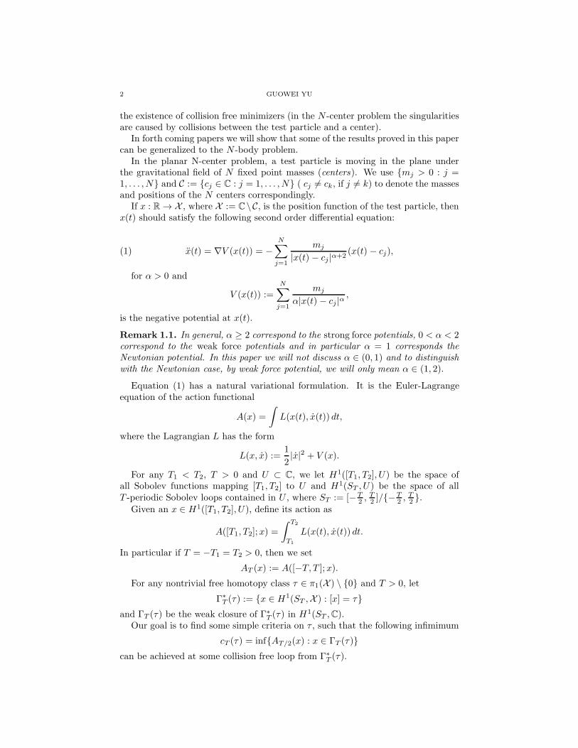
Figure 3.

Figure 4.

enough neighborhood of η, which eliminates the non-transverse self-intersectionwithout increasing the number of transverse self-intersection and at the same timethe action functional is increased by no more than ε.

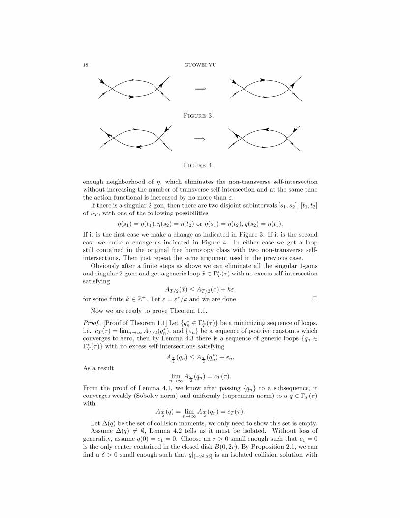
If there is a singular 2-gon, then there are two disjoint subintervals [s1, s2], [t1, t2]of ST , with one of the following possibilities

η(s1) = η(t1), η(s2) = η(t2) or η(s1) = η(t2), η(s2) = η(t1).

If it is the first case we make a change as indicated in Figure 3. If it is the secondcase we make a change as indicated in Figure 4. In either case we get a loopstill contained in the original free homotopy class with two non-transverse self-intersections. Then just repeat the same argument used in the previous case.

Obviously after a finite steps as above we can eliminate all the singular 1-gonsand singular 2-gons and get a generic loop x ∈ Γ∗

T (τ) with no excess self-intersectionsatisfying

AT/2(x) ≤ AT/2(x) + kε,

for some finite k ∈ Z+. Let ε = ε∗/k and we are done.

Now we are ready to prove Theorem 1.1.

Proof. [Proof of Theorem 1.1] Let q∗n ∈ Γ∗T (τ) be a minimizing sequence of loops,

i.e., cT (τ) = limn→∞ AT/2(q∗n), and εn be a sequence of positive constants which

converges to zero, then by Lemma 4.3 there is a sequence of generic loops qn ∈Γ∗T (τ) with no excess self-intersections satisfying

AT2(qn) ≤ AT

2(q∗n) + εn.

As a resultlimn→∞

AT2(qn) = cT (τ).

From the proof of Lemma 4.1, we know after passing qn to a subsequence, itconverges weakly (Sobolev norm) and uniformly (supremum norm) to a q ∈ ΓT (τ)with

AT2(q) = lim

n→∞AT

2(qn) = cT (τ).

Let ∆(q) be the set of collision moments, we only need to show this set is empty.Assume ∆(q) 6= ∅, Lemma 4.2 tells us it must be isolated. Without loss of

generality, assume q(0) = c1 = 0. Choose an r > 0 small enough such that c1 = 0is the only center contained in the closed disk B(0, 2r). By Proposition 2.1, we canfind a δ > 0 small enough such that q|[−2δ,2δ] is an isolated collision solution with


q([−2δ, 2δ]) ⊂ B(0, r). As qn converges uniformly to q, for n large enough we haveqn([−2δ, 2δ]) ⊂ B(0, 2r).

We claim for n large enough qn|[−2δ,2δ] does not have any self-intersection. If not,there must be a subinterval I ⊂ [−2δ, 2δ], such that qn|I is an innermost sub-loop.As qn(I) ⊂ B(0, 2r), at most one center, c1, can be enclosed by this innermostsub-loop, which is a contradiction to the fact that τ is an admissible class.

Since qn converges uniformly to q, q|[−2δ,2δ] can not have any transverse self-intersection as well. By Defintion 2.1, q|[−2δ,2δ] is a simple isolated collision solution.

Put q|[−2δ,2δ] in polar coordinates q(t) = ρ(t)eiθ(t), by Proposition 2.2, there aretwo finite angles θ−, θ+, such that, limt→0± θ(t) = θ±. Furthermore we may assume|θ+ − θ−| ≤ 2π, as we only define the polar coordinates on q|[−2δ,2δ] not the entireloop q|ST

.If θ+ ∈ [θ−, θ− + 2π] (resp. θ+ ∈ [θ− − 2π, θ−]), by Proposition 3.2, there is a

ξ+ ∈ Γ∗,+δ (q) (resp. ξ− ∈ Γ∗,−

δ (q)), where Γ∗,+δ (q) (resp. Γ∗,−

δ (q) ) is defined as inDefinition 3.2 (with y replace by q) satisfying

Aδ(ξ+) < Aδ(q)(resp. Aδ(ξ

−) < Aδ(q)).

According to Definition 3.2, ξ+ and ξ− have the same initial and end points asq|[−δ,δ], so we can define two new loops as

q+(t) =

ξ+(t), if t ∈ [−δ, δ]

q(t), if t ∈ ST \ [−δ, δ],

q−(t) =

ξ−(t), if t ∈ [−δ, δ]

q(t), if t ∈ ST \ [−δ, δ].

Obviously the actional functional of both loops, q+, q−, are strictly less than q.Therefore if we can show that one of them is contained in ΓT (τ), it will give us acontradiction and we are done.

Choose a 0 < δ∗ < δ, as q|[−2δ,−2δ+δ∗] (resp. q|[2δ−δ∗,2δ]) is a solution of equation(1) with a positive distance from any centers and qn converges uniformly to q asn goes to infinity, by the standard result of calculus of variation, when δ∗ is smallenough, for each n large enough, the action functional has a unique minimizer η−n(resp. η+n ) among all Sobolev curves defined on [−2δ,−2δ+ δ∗] (resp. [2δ− δ∗, 2δ])with the same initial point qn(−2δ) (resp. qn(2δ − δ∗)) and the same end pointq(−2δ+ δ∗) (resp. qn(2δ)). Obviously each η−n (resp. η+n ) is a solution of equation(1) and it converges to q|[−2δ,−2δ+δ∗] (resp. q|[2δ−δ∗,2δ]) with respect to the C1 normas n goes to infinity.

Now for each n (large enough), we can define a curve γ+n by

γ+n (t) =

η−n (t), if t ∈ [−2δ,−2δ+ δ∗]

q(t), if t ∈ [−2δ + δ∗,−δ]

ξ+(t), if t ∈ [−δ, δ]

q(t), if t ∈ [δ, 2δ − δ∗]

η+n (t), if t ∈ [2δ − δ∗, 2δ],

20 GUOWEI YU

and a curve γ−n just as above only with ξ+ replaced by ξ−. Using these curves we

further define two loops q+n , q−n ∈ H1(ST ,X ) by

q+n (t) =

γ+n (t), if t ∈ [−2δ, 2δ]

qn(t), if t ∈ ST \ [−2δ, 2δ],

q−n (t) =

γ−n (t), if t ∈ [−2δ, 2δ]

qn(t), if t ∈ ST \ [−2δ, 2δ].

We can do this beacuase γ+n and γ−

n both have the same initial and end pointsas qn|[−2δ,2δ]. Since q|[−2δ,2δ] does not have any transverse self-intersection and so

is each qn|[−2δ,2δ], when n is large enough, either γ+n or γ−

n must be homotopic to

qn|[−2δ,2δ] inside B(0, 2r) \ 0 with both end points fixed. This means either q+n or

q−n must be contained in ΓT (τ). Without loss of generality we may assume this istrue for a subsequence of q+n . By the way we define each q+n , it is not hard to seeit converges weakly to q+, which means q+ ∈ ΓT (τ) and this finishes our proof.

Remark 4.1. In the Newtonian case, α = 1, it is not hard to see the above con-tradictory argument fails only when we have

|θ+ − θ−| = 0(mod 2π).

This is due to the extra condition required in Proposition 3.2 (essentially in Theorem1.3), when α = 1.

5. Proof of Theorem 1.2

In this section, we always assume the potential is Newtonian, i.e., α = 1. Lety(t), t ∈ [t0 − δ, t0 + δ] be an isolated collision solution with y(t0) = ck ∈ C. Sety(t) − ck = ρ(t)eiθ(t), by Proposition 2.2, the following limits exist limt→t±

0

θ(t) =

θ±(t0). As explained in Remark 4.1, the key point is to understand what happenswhen

|θ+(t0)− θ−(t0)| = 0(mod 2π).

A similar situation was discussed in [22]. Following their idea we will perform alocal Levi-Civita regularization near the isolated collision and show that under theabove condition y must be a collision-reflection solution.

Definition 5.1. We say y is a collision-reflection solution, if the following istrue

y(t0 + t) = y(t0 − t), ∀t ∈ [0, δ].

Let’s recall the basics of a Levi-Civita transformation. We introduce a newcoordinates z with

z2(t) = y(t)− ck;

and a new time parameter s = s(t), t ∈ [t0 − δ, t0 + δ] with

ds = |y(t)− ck|−1dt.

To distinguish between the two time parameters, we set z′(s) = ddsz(s). By Propo-

sition 2.1, a simple estimate shows that∫ t0+δ

t0−δ

|y(t)− ck|−1dt < ∞.


As a result, we may assume s(t0) = 0 and there are two finite numbers S± > 0,such that

S+ = s(t0 + δ); S− = −s(t0 − δ).

Using the factor that the energy of y is a constant, i.e., there is a constant h, suchthat

(23)1

2|y(t)|2 − V (y(t)) = h, ∀t ∈ [t0 − δ, t0 + δ] \ t0.

A direct computation shows that z(s), s ∈ [−S−, S+] \ 0 is a solution of thefollowing equation

(24) 2z′′ = hz + zVk(z2 + ck) + |z|2z∇yVk(z

2 + ck)

where Vk(z2 + ck) = Vk(y) =

∑

j 6=kmj

|y−cj|. Obviously the singularity caused by the

collision with the center cj does not exist anymore in the above equation.

Lemma 5.1. Let y and z be defined as above, if |θ+(t0) − θ−(t0)| = 2π then thefollowing one-sided limits are well-defined and satisfying

lims→0−

z′(s) = − lims→0+

z′(s).

Proof. To simplify notation, we assume t0 = 0, ck = 0 and θ±(t0) = θ±. Put z(s)in polar coordinates: z(s) = r(s)eiφ(s), then

(25) z′(s) = [r′(s) + ir(s)φ′(s)]eiφ(s).

Since z2 = y = ρeiθ, we have

r(s) = ρ12 (t(s)), φ(s) =

1

2θ(t(s)).

Therefore by a direct computation

r′(s) =1

2ρ

12 (t(s))ρ(t(s)),

φ′(s) =1

2ρ(t(s))θ(t(s)).

By Proposition 2.1 and 2.2, we can get

ρ(t) ∼ (µt)23 , ρ(t) ∼

2

3µ(µt)−

13 ,

and

limt→0±

θ(t) = 0.

Recall the definition of the time parameter s, in particular s(0) = 0, we have

lims→0+

r′(s) = limt→0+

1

2ρ

12 (t)ρ(t) =

1

3µ,

lims→0+

φ′(s) = limt→0+

1

2ρ(t)θ(t) = 0.

At the same time

lims→0+

φ(s) = limt→0+

1

2θ(t) = θ+.

Plugging the above limits into (25)

lims→0+

z′(s) =1

3µei

θ+2 .

22 GUOWEI YU

A similar calculation will show

lims→0−

z′(s) =1

3µei

θ−2 .

Now the desired result immediately follows from |θ+ − θ−| = 2π.

Lemma 5.2. Under the same conditions of Lemma 5.1, y is a collision-reflectionsolution.

Proof. Again to simplify the notation, let’s assume t0 = 0 and y(0) = c1 = 0. Setz∗(s) = z(−s) for s > 0. Since (24) is independent of the time parameter s and thefirst derivative, z∗(s) also satisfies equation (24).

By Lemma 5.1,

lims→0+

(z∗)′(s) = lims→0+

−z′(−s) = lims→0−

−z′(s) = lims→0+

z′(s).

Since z∗(0) = z(0) = 0, the existence and uniqueness theorem of ordinary differ-ential equation tells us

z(s) = z∗(s) = z(−s), for s > 0.

As a result S− = S+ and

y(t) = y(−t), ∀t ∈ [0, δ].

Now we are ready to prove Theorem 1.2.

Proof. [Theorem 1.2] Following the notations introduced in Section 4, as we men-tioned most of the results from that section still hold for the Newtonian potential.Let qn (generic loop with no excess self-intersection) and q be the same loops ob-tained at the beginning of the proof of Theorem 1.1 with

AT2(q) = lim

n→∞AT

2(qn) = cT (τ).

If ∆(q) = ∅, then q is collision free solution of (1) and we are in the first case.If ∆(q) 6= ∅, for any t0 ∈ ∆(q) with q(t0) = ck1

, we can define a local polarcoordinates near q(t0) = ck1

q(t)− ck1= ρ(t)eiθ(t).

By Proposition 2.2, the following limits exist θ±(t0) = limt→t±0

θ(t). As explained

in Remark 4.1, such a collision can exist only when

(26) |θ+(t0)− θ−(t0)| = 0(mod 2π).

Because the polar coordinates are only defined locally, we may assume

θ+(t0)− θ−(t0) = 2π.

This is the condition required in Lemma 5.1 and 5.2. Now by Lemma 5.2, there isa δ > 0 such that

q(t0 + t) = q(t0 − t) ∀t ∈ [0, δ].

In fact the existence and uniqueness theorem of ordinary differential equation guar-antees above identity will hold until a moment t1 (set T = t1 − t0 > 0) when oneof the following two situations first appears

q(t1) = 0 or q(t1) = ck2∈ C.


If q(t1) = 0, then q(t1) is a break point (with zero velocity), so under thegravitational force the test particle has to come back to q(t0) following the samepath, i.e.

q(t1 + t) = q(t1 − t), ∀t ∈ [0, T ].

As a result t1+ T ∈ ∆(q) with q(t1+ T ) = ck1and the same condition as (26) must

hold at this moment as well. Therefore we can apply Lemma 5.2 again and get

q(t1 + T + t) = q(t1 + T − t), ∀t ∈ [0, T ].

By repeating the above arguments in both directions of the time, we find thatq must be a degenerating loop of period 2T , which goes back and forth betweenq(t0) = ck1

and q(t1) along the curve q|[t0, t1] without containing any other centers.Namely it is a collision-reflection solution between ck1

and q(t1). Which is absurd,as explained in the following.

Because τ is admissible, each innermost loop of qn encloses at least two differentcenters. If qn converges to a curve as above then it must contain at least twodifferent centers.

If q(t1) = ck2∈ C (it is possible that ck2

= ck1), then t1 ∈ ∆(q) with the same

condition as (26) holds again. By the same argument as above we once again canshow that q must be a collision-reflection solution between ck1

and ck2with period

2T .As a result, for each cj ∈ C \ ck1

, ck2, the index of q with respect to cj is well

defined and vanishes: Ind(q, cj) = 0.Obviously the same is also true for any qn with n large enough, which means for

the given free homotopy class τ , we must have

h(τ)j = 0, ∀j ∈ 1, . . . , N \ k1, k2.

This finishes the entire proof.

6. The Kepler-type Problem

This section will be devoted to the proof of Theorem 1.3. As we mentioned theidea is to consider an obstacle minimizing problem that have been studied in [23],[22] and [4]. In particular we will first following the approach given in [22] to geta result of the fixed energy problem, namely Theorem 6.3. The main difference isafterwards we will use this theorem to get a related result of the fixed time problem.

In order to relate the fixed energy problem and fixed time problem, we needto study curves defined on different time interval. Let x be a parabolic collision-ejection solution of the Kepler-type problem as defined in Definition 1.2. For anyS, T > 0, we set

Γ∗S(x;T ) := x ∈ H1([−S, S],C \ 0) : x satisfies the following conditions .

(1) x(±S) = x(±T );(2) Arg(x(−S)) = φ− and Arg(x(S)) = φ+.

Let ΓS(x;T ) be the weak closure of Γ∗S(x;T ) in H1([−S, S];C). We set

c(x;T ) = infAS(x) : x ∈ ΓS(x;T ) for any S > 0.

Remark 6.1. The readers should notice that

(1) Γ∗T (x;T ) = Γ∗

T (x) and ΓT (x;T ) = ΓT (x), if and only if S = T ,

24 GUOWEI YU

(2) c(x;T ) is different from cT (x) defined in the first section. In fact c(x;T ) ≤cT (x) and for most choices of T , the inequality is strict.

Instead of Theorem 1.3, we will first prove a slightly weaker result stated asfollowing.

Theorem 6.1. For any T > 0 and 0 < |φ+ − φ−| ≤ 2π, there is a S > 0 andη ∈ ΓS(x;T ), such that AS(η) = c(x;T ).

(1) If α ∈ (1, 2), then η ∈ Γ∗S(x;T ) is a classical solution of the Kepler-type

problem with zero energy and AS(η) < AT (x);(2) If α = 1 and |φ+ − φ−| < 2π, then η ∈ Γ∗

S(x;T ) is a classical solution ofthe Kepler-type problem with zero energy and AS(η) < AT (x);

Remark 6.2. Theorem 1.3 shows that x|[−T,T ] is not a minimizer of the fixed endproblem with the same time interval and Theorem 6.1 shows that x|[−T,T ] is not aminimizer of the fixed end problem with an arbitrary time interval. Therefore theresult obtained in Theorem 6.1 is weaker than in Theorem 1.3. However we willshow that Theorem 6.1 actually implies Theorem 1.3.

In Theorem 6.1, we need to show x is not a free-time minimizer in certainadmissible class of curves. As the time interval is not fixed, it is more natural tostudy the Maupertuis’ functional rather than the action functional.

For a given energy h, the associated Maupertuis’ functional of the Kepler-typeproblem is defined as

Mh([−T, T ];x) :=

∫ T

−T

1

2|x|2 dt

∫ T

−T

V (x(t)) + h dt, ∀x ∈ H1([−T, T ],C).

Theorem 6.2. For any a < b, If y ∈ H1([a, b],C \ 0) is a critical point of Mh

with Mh(y) > 0, then y(t) is a classical solution of

(27)

ω2(y)y(t) = ∇V (y(t)), t ∈ [a, b],12 |y(t)|

2 − V (y(t))ω2(y) = h

ω2(y) , t ∈ [a, b],

y(a) = q1, y(b) = q2,

where ω(y) is a positive number defined by

(28) ω2(y) :=

∫ b

a V (y(t)) + h dt∫ b

a12 |y(t)|

2 dt.

Furthermore x(t) := y(ω(y)t), t ∈ [ aω(y) ,

bω(y) ] is a classical solution of the Kepler-

type problem with energy h, i.e., for any t ∈ [a, b]

x(t) = ∇V (x(t)),12 |x(t)|

2 − V (x(t)) = h.

This is a standard result, whose proof can be found in [1].As a parabolic solution, x(t)’s energy is zero, we only need to study M0. To

simplify notation, set M := M0.Let

mT = infM([−T, T ];x) : x ∈ ΓT (x),

Where ΓT (x) is defined as in Section 1. We will prove the following result regardingthe Maupertuis’ functional and obtain Theorem 6.1 as its corollary.


Theorem 6.3. For any T > 0 and 0 < |φ+ − φ−| ≤ 2π, there is a y ∈ ΓT (x) suchthat M([−T, T ]; y) = mT > 0.

(1) If α ∈ (1, 2), then y ∈ Γ∗T (x) is a classical solution of the Kepler-type

problem with zero energy and M([−T, T ]; y) < M([−T, T ]; x);(2) If α = 1 and |φ+ − φ−| < 2π, then y ∈ Γ∗

T (x) is a classical solution of theKepler-type problem with zero energy and M([−T, T ]; y) < M([−T, T ]; x)and |y(t)| > 0 for any t ∈ [−T, T ] \ 0.

First we introduce some notations that will be needed in the proof.

Definition 6.1. For any ρ > ρ ≥ 0 small enough and T > 0, we set

ΓT (x; ρ) := x ∈ ΓT (x) : mint∈[−T,T ]

|x(t)| = ρ,

mT (ρ) := infM([−T, T ];x) : x ∈ ΓT (x; ρ),

MT (ρ) := x ∈ ΓT (x) : M([−T, T ];x) = mT (ρ);

ΓT (x; ρ, ρ) := x ∈ ΓT (x) : mint∈[−T,T ]

|x(t)| ∈ [ρ, ρ];

mT (ρ, ρ) := infM(x) : x ∈ ΓT (x; ρ, ρ);

MT (ρ, ρ) := x ∈ ΓT (x; ρ, ρ) : M(x) = m(ρ, ρ) and mint∈[−T,T ]

|x(t)| < ρ.

For the rest of this section, except in the proof of Theorem 1.3, which will givenat the very end, we will fix an arbitrary T > 0 and assume

(29) 0 < |φ+ − φ−| ≤ 2π,

To simplify notation, we omit the subindex T from all the notions introduced inDefinition 6.1 and the [−T, T ] from M([−T, T ];x).

Lemma 6.1. For any ρ ≥ 0, m(ρ) > 0 and M(ρ) 6= ∅.

Proof. Once we showed M(ρ) is nonempty, it is obvious that m(ρ) > 0.It is well known that M is weakly lower semicontinuous with respect to the H1

norm. By the standard argument in calculus of variations, it is enough to showthat M is coercive on Γ(x; ρ).

For any x ∈ Γ(x; ρ), we define

δ(x) := max|x(t0)− x(t1)| : t0, t1 ∈ [−T, T ].

Let φ = φ−+φ+

2 , then for any x ∈ Γ(x; ρ) there is a tφ ∈ (−T, T ], such that

Arg(x(tφ)) = φ or |x(tφ)| = 0.

Simply using the law of sines and (29), we find there is a ν ∈ (0, 2] independent ofx, such that

〈x(0), x(tφ)〉 ≤ (1− ν)|x(0)||x(tφ)|.

This is the so called noncentral condition introduced by Chen in [6]. In proposition2, [6], he also showed that once the noncentral condition is satisfied, then there isa constant C > 0, such that

(30) |x(t)| ≤ |x(−T )|+ δ(x) ≤ Cδ(x), ∀x ∈ Γ(x; ρ), t ∈ [−T, T ].

On the other hand by Cauchy-Schwarz inequality

(31) δ2(x) ≤ (

∫ T

−T

|x(t)| dt)2 ≤ 2T

∫ T

−T

|x(t)|2 dt.

26 GUOWEI YU

Therefore

‖x‖2H1 =

∫ T

−T

|x(t)|2 dt+

∫ T

−T

|x(t)|2 dt ≤ C1

∫ T

−T

|x(t)|2 dt.

By (30),

V (x(t)) =m1

α|x(t)|α≥ C2δ

−α(x),

combining this with (31), we get

∫ T

−T

V (x(t)) dt ≥ C3(

∫ T

−T

|x(t)|2 dt)−α2 .

Hence

M(x) =

∫ T

−T

1

2|x(t)|2 dt

∫ T

−T

V (x(t)) dt ≥ C4(

∫ T

−T

|x(t)|2 dt)2−α

2 ≥ C5‖x‖2−αH1 .

Therefore when α ∈ [1, 2), M is coercive on Γ(x; ρ).

Lemma 6.2. There is at least one x ∈ Γ(x; ρ, ρ) with M(x) = m(ρ, ρ) > 0.

The proof of the above lemma is exactly the same as Lemma 6.1. We will notrepeat it here. Notice that even with Lemma 6.2, M(ρ, ρ) may still be empty.

Lemma 6.3. x|[−T,T ] is the only minimizer of M in Γ(x; 0), i.e.,

M(0) = x|[−T,T ].

This lemma follows from a straight forward computation and a similar argumentused by Gordon in [16].

Lemma 6.4.

lim supρ→0+

m(ρ) ≤ m(0).

Proof. Without loss of generality let’s assume φ− = 0 and φ+ = φ. For any ρ > 0small enough, we define

xρ(t) =

x(t), if t ∈ Ω := [−T, T ] \ [−tρ, tρ],

ρeiωt, if t ∈ [−tρ, tρ],

where tρ = µ−1ρ2+α2 and ω = φµρ−

2+α2 . A straight forward computation shows

that

M(xρ)− M(x) =

∫

Ω

1

2| ˙x|2

∫ tρ

−tρ

[V (xρ)− V (x)] +

∫

Ω

V (x)

∫ tρ

−tρ

[1

2|xρ|

2 −1

2| ˙x|2]

+

∫ tρ

−tρ

1

2|xρ|

2

∫ tρ

−tρ

V (xρ)−

∫ tρ

−tρ

1

2|xρ|

2

∫ tρ

−tρ

V (x)

∼ O(ρ2−α

2 ).

This proves the lemma, because M(x) = m(0) according to Lemma 6.3.


The above lemmas guarantees the existence of the obstacle minimizers. In thefollowing we will get more information about these minimizers.

For any ρ ≥ 0 and x ∈ Γ(x; ρ), we set

Tρ(x) := t ∈ [−T, T ] : |x(t)| = ρ.

Lemma 6.5. If ρ > 0 and x ∈ M(ρ), the following results hold.

(1) For any (a, b) ⊂ [−T, T ] \ Tρ(x), x|(a,b) is C2 and a classic solution of thefollowing equation

(32) ω2x(t) = ∇V (x(t)), where ω2 =

∫ T

−TV (x(t) dt

∫ T

−T12 |x(t)|

2 dt.

(2) There exist t− ≤ t+, such that Tρ(x) = [t−, t+] and

|x(t)| > ρ, ∀t ∈ [−T, t−) ∪ (t+, T ],

|x(t)| = ρ, ∀t ∈ [t−, t+].

(3) The following energy identity holds for any t ∈ [−T, T ],

(33)1

2|x(t)|2 −

V (x(t))

ω2= 0.

(4) Set x(t) = r(t)eiθ(t) in polar coordinates, then one of the following threesituation must occur:(a) t− < t+ and x ∈ C1([−T, T ],C);(b) t− = t+ and x ∈ C1([−T, T ],C);(c) t− = t+ and x(t) doesn’t exist at t = t− = t+.

(5) If t− < t+ then θ|(t−,t+) is C2, strictly monotone and a classic solution ofthe following equation

θ(t) =1

ω2·1

ρ〈∇V (ρeiθ(t)), ieiθ(t)〉.

(6) r(t) > 0, if t ∈ (t+, T ] and r(t) < 0. if t ∈ [−T, t−).

Proof. The proof of (4) can be found in the proof of Proposition 2.6 in [5]. Theproofs of the rest results can be found in the proof of Lemma 4.30 in [22].

The last result, (6) is easy to see, once the reader notice that once other resultsare true. Then x(t), t ∈ [−T, t−) ∪ (t+, T ] is a parabolic solution (zero energy) ofthe following Kepler-type problem

x(t) = −m1x(t)

ω2|x(t)|α+2

with r(t±) = min|x(t)| : t ∈ [−T, T ].

In our proof we need the obstacle minimizers to have enough regularity, i.e., atleast C1. However the above lemma does not guarantees that. On the other handa minimizer contained in M(ρ, ρ) is C1.

Lemma 6.6. If x ∈ M(ρ, ρ), then x ∈ C1([−T, T ],C).

28 GUOWEI YU

Proof. First if x satisfies

min|x(t)| : for any t ∈ [−T, T ] > ρ,

then x is in the interior of the set Γ(x; ρ, ρ) and it is a classical solution of theKepler-type problem, so x(t) must be C1.

If

min|x(t)| : for any t ∈ [−T, T ] = ρ,

then x ∈ M(ρ) and it must satisfies all the properties in Lemma 6.5. Therefore weonly need to show the case (c) in Lemma 6.5 (4) will not happen.

Assume this is the case, let t0 ∈ (−T, T ) be the only moment that x does notexist, by a small perturbation of x near x(t0) in the direction away from the originwe can get a new with strictly smaller Maupertuis’ functional and still containedin Γ(ρ, ρ). A detailed argument can be found in the proof of Lemma 4.30 [22].

Lemma 6.7. For any 0 < |φ+ − φ−| ≤ 2π,

(1) if α ∈ (1, 2), then there is a ρ∗ > 0, small enough, such that M(ρ, ρ) = ∅,for any 0 < ρ < ρ ≤ ρ∗;

(2) if α = 1 and |φ+ − φ−| < 2π, then there is a ρ∗ > 0, small enough, suchthat M(ρ, ρ) = ∅ for any 0 < ρ < ρ ≤ ρ∗.

Let’s postpone the proof of Lemma 6.7 for a moment and see how we can use itto proof Theorem 6.3.

Proof. [Theorem 6.3] We will give the detailed proof for the case α ∈ (1, 2), whilethe other is similar.

First by the same argument as in the proof of Lemma 6.1, it is easy to see thereis a y ∈ Γ(x) with M(y) = m and m > 0.

Assume there is a t0 ∈ [−T, T ] with y(t0) = 0, then M(y) = m(0) and y ∈M(0) = m.

For any 0 < ρ < ρ < ρ∗, by Lemma 6.2, there is a xρ ∈ Γ(x; ρ, ρ) with M(xρ) =m(ρ, ρ). However by Lemma 6.7, xρ /∈ M(ρ, ρ). This means

min|x(t)| : t ∈ [−T, T ] = ρ,

so xρ ∈ Γ(x; ρ) and M(xρ) = m(ρ).Meanwhile by Lemma 6.1, there is a xρ ∈ Γ(x; ρ) with M(xρ) = m(ρ). Obviously

xρ ∈ Γ(x; ρ, ρ) and by Lemma 6.6

M(xρ) = m(ρ) > m(ρ, ρ) = m(ρ) = M(xρ).

The above argument implies m(ρ) is strictly decreasing with respect to ρ ∈ (0, ρ∗].Combining this with Lemma 6.4, we have

limt→0+

m(ρ) = lim supt→0+

m(ρ) ≤ m(0) = m.

Hence

m(ρ∗) < m,

which is absurd.

Now we are ready to prove Lemma 6.7.


Proof. [Lemma 6.7] An contradiction argument will be used here as well. Supposeour results are not true, then there are two sequences ρn and ρn with 0 < ρn <ρn, both converge to 0 as n goes to positive infinity. Furthermore for each n, thereis xn ∈ Γ(x; ρn), satisfying

M(xn) = mρn= mρn,ρn

.

Obviously each xn satisfies Lemma 6.5, so there are t−n ≤ t+n such that

Tρn(xn) := t ∈ [−T, T ] : xn(t) = ρn = [t−n , t

+n ].

Even though xn is a minimizer in Γ(x; ρn), by Lemma 6.5, it is possible that xn

is not C1 on [−T, T ]. However by exact the same arguments as in the proof of part(vi), Lemma 4.30 in [22], we know xn|[−T,T ] must be C1.

Write each xn(t) in polar coordinates: xn(t) = rn(t)eiθn(t).

First let us focus on the time interval Tρn(xn) = [t−n , t

+n ], then

xn(t) = ρneiθn(t), ∀t ∈ [t−n , t

+n ].

Hence by the energy identity, for any t ∈ (t−n , t+n ),

1

2|xn|

2 =1

2|ρniθne

iθn |2 =1

2ρ2nθ

2n =

V (xn)

ω2n

=1

ω2n

·m1

α|ρn|α.

Therefore

ρ2nθ2n =

2m1

ω2nα

ρ−αn .

By Lemma 6.5, θn is positive for t ∈ (t−n , t+n ), so

θn(t) =

√

2m1

ω2nα

ρ− 2+α

2n , ∀t ∈ (t−n , t

+n ).

Therefore

(34) θn(t+n )− θn(t

−n ) =

∫ t+n

t−n

θn(t) dt =

√

2m1

ω2nα

ρ− 2+α

2n (t+n − t−n ).

Meanwhile for t ∈ (t−n , t+n ), the angular momentum

(35) J(xn(t)) = ρ2nθn(t) =

√

2m1

ω2nα

ρ2−α2

n .

On the other hand, if t ∈ (−T, t−n ) (or t ∈ (t+n , T )), xn(t) is a solution of theKepler-type equation (32), so the angular momentum J(xn) is a constant, i.e.,

(36) J(xn(t)) = xn(t)× xn(t) = constant, ∀t ∈ (−T, t−n )( or t ∈ (t+n , T )).

Then we have the following result.

Lemma 6.8.

J(xn(t)) ≡2m1

ω2nα

ρ2−α

2n , ∀t ∈ (T, T ).

Proof. [Lemma 6.8] By (35) and (36), there are two constants c1, c2 such that

J(xn(t)) =

c1, when t ∈ (−T, t−n )

2m1

ω2nα

ρ2−α2

n , when t ∈ (t−n , t+n )

c2, when t ∈ (t+n , T )

30 GUOWEI YU

By Lemma 6.5, xn ∈ C1((−T, T ),C), therefore J(xn) = xn × xn ∈ C0((−T, T ),C),which means

J(xn(t−n )) = lim

t→(t−n )−J(xn(t)) = c1 = lim

t→(t−n )+J(xn(t)) =

2m1

ω2nα

ρ2−α2

n .

Similarly

J(xn(t+n )) = c2 =

2m1

ω2nα

ρ2−α2

n .

With Lemma 6.8, now we can compute the change of the angular variable θn(t)when t goes from t+n to T.

(37) θn(T )− θn(t+n ) =

∫ T

t+n

θn(t) dt =

∫ T

t+n

J(xn)

r2n(t)dt.

Since xn satisfies the energy identity (33),

1

2|xn|

2 =1

ω2n

·m1

α|xn|α.

Rewrite the above equation using polar coordinates

1

2|rne

iθn + irnθneiθn |2 =

1

2(r2n + r2nθ

2n) =

1

ω2n

·m1

αrαn,

r2n =2m1

ω2nα

·1

rαn− r2nθ

2n =

2m1

ω2nα

·1

|rn|α−

J2(xn)

r2n.

By (6), Lemma 6.5, rn(t) > 0, for t ∈ (t+n , T ]. Therefore

(38)drndt

= rn =

√

2m1

ω2nα

·1

rαn−

J2(xn)

r2n.

The negative square root was dropped because of the following lemma.By (38), we can change the integral variable in (37) from t to rn

θn(T )− θn(t+n ) =

∫ rn(T )

ρn

J(xn)

r2n

1√

2m1

ω2nα

· 1rαn

− J2(xn)r2n

drn

By Lemma 6.8, J(xn) =2m1

ω2nα

ρ2−α

2n plug it into the above equation we get

(39)

θn(T )− θn(t+n ) =

∫ rn(T )

ρn

1√

ρα−2n r4−α

n − r2n

drn =

∫ rn(T )

ρn

1

rn√

(ρn

rn)α−2 − 1

drn.

Notice that rn(T ) = |xn(T )| ≡ |x(T )| for any n, we set r∗ := |x(T )|. Set ξn = ρn

rn,

then drn = −ξ−2n ρn dξn. We can simplify (39) to

(40) θn(T )− θn(t+n ) = −

∫ρnr∗

1

1√

ξαn − ξ2ndξn =

∫ 1

ρnr∗

1√

ξαn − ξ2ndξn.

Furthermore if we set ξn = η2

2−αn , then dξn = 2

2−αηα

2−αn dηn. Plug this into (40)

(41) θn(T )− θn(t+n ) =

2

2− α

∫ 1

ρnr∗

1√

1− η2ndηn =

2

2− α(π

2− sin−1(

ρnr∗

)).


Similarly

(42) θn(t−n )− θn(−T ) =

2

2− α(π

2− sin−1(

ρnr∗

)).

By Lemma 6.5 says θn(t) is monotone increasing when t ∈ [t−n , t+n ], therefore

θn(T )− θn(−T ) ≥ θn(T )− θn(t+n ) + θn(t

−n )− θn(−T ) =

2

2− α(π − 2 sin−1(

ρnr∗

)).

Recall that ρn → 0, as n → +∞, so

limn→+∞

ρnr∗

= 0.

Therefore if α ∈ (1, 2), we have

limn→+∞

θn(T )− θn(−T ) ≥ limn→+∞

2

2− α(π − 2 sin−1(

ρnr∗

)) =2

2− απ > 2π.

Which is absurd, because for any n ∈ N,

θn(T )− θn(−T ) = φ+ − φ− ≤ 2π.

At the same time when α = 1 and φ+ − φ− < 2π, we get

φ+ − φ− = limn→+∞

θn(T )− θn(−T ) ≥ limn→+∞

2(π − 2 sin−1(ρnr∗

)) = 2π.

which is again a contradiction. This finishes our proof of Lemma 6.7.

Now we are ready to prove Theorem 6.1 and Theorem 1.3.

Proof. [Theorem 6.1] According to Lemma 3.1, [5], which says that there is a one-to-one correspondence between minimizers of A in ∪S>0ΓS(x;T ) and minimizersof M in ΓT (x), Theorem 6.1 is a direct corollary of Theorem 6.3.

Now let’s see how we can use Theorem 6.1 to prove Theorem 1.3.

Proof. [Theorem 1.3] We will only give the details for case α ∈ (1, 2), while theother is similar.

The result is trivial, when φ− = φ+, so we will assume 0 < |φ+ − φ−| ≤ 2π.Using the noncentral condition and same argument as in the proof of Lemma 6.1,it is easy to see AT is coercive in ΓT (x) and by the standard argument of calculusof variations, there is at least one γ ∈ ΓT (x) with AT (γ) = cT (x).

All we need to show is that γ is free of collision. By a classical result of Gordon[16], if γ contains a collision, then γ = x, because γ is a minimizer.

Therefore we are done, once we can find a collisionless curve y ∈ Γ∗T (x) with

AT (y) < AT (x).

By Theorem 6.1, there is a S > 0 and x ∈ ΓS(x;T ), such that AS(x) < AT (x)and |x(t)| 6= 0, for any t ∈ [−S, S].

Let ε = AT (x) − AS(x) > 0. We choose a T1 > maxS, T and define a newcurve

z(t) =

x(at+ b), if t ∈ [S, T1]

x(t), if t ∈ [−S, S]

x(at− b), if t ∈ [−T1,−S],

32 GUOWEI YU

where a = T1−TT1−S , b = T1

T−ST1−S . Then

AT1(x)− AT1

(z) = A([T, T1], x)− A([S, T1]; z) + A([−T1, T ]; x)− A([−T1, S]; z)

+ AT (x)− AS(x).

By the definition of x, it is obvious that

A([T, T1], x)− A([S, T1]; z) = A([−T1, T ]; x)− A([−T1, S]; z).

If we set

f(T1) := A([T, T1], x)− A([S, T1]; z),

then

(43) AT1(x)− AT1

(z) = 2f(T1) + ε.

A simple calculation shows

|f(T1)| = |(1 − a)

∫ T1

T

1

2| ˙x(t)|2 dt+ (1−

1

a)

∫ T1

T

m1

α|x(t)|αdt|

≤ |1− a|2

(2 + α)2µ

42+α

∫ T1

T

t−2α

2+α dt+ |1−1

a|m1

αµ− 2α

2+α

∫ T1

T

t−2α

2+α dt

= (C1|T − S|

T1 − S+ C2

|S − T |

T1 − T)(T

2−α2+α

1 − T2−α2+α )

Since α ∈ [1, 2), 0 < 2−α2+α < 1. Hence it is not hard to see

|f(T1)| → 0, as T1 → 0.

Therefore for T1 large enough

AT1(x)− AT1

(z) = 2f(T1) + ε > 0.

Set λ = T1

T and define

zλ(t) = λ− 22+α z(λt), t ∈ [−

T1

λ,T1

λ];

xλ(t) = λ− 22+α x(λt), t ∈ [−

T1

λ,T1

λ].

It is easy to see xλ(t) = x(t) and zλ ∈ Γ∗T (x). As in the proof of Lemma 3.1, a

straight forward calculation shows

AT (x)− AT (zλ) = λ− 22+α [AT1

(x)− AT1(zλ)] = λ− 2

2+α (2f(T1) + ε) > 0.

By the definition of zλ, |zλ(t)| 6= 0, for any t ∈ [−T, T ] and we are done.

Acknowledgements. The author wish to express his gratitude to Prof. Ke Zhangfor his continued support and encouragement.


References

[1] A. Ambrosetti and V. Coti Zelati. Periodic solutions of singular Lagrangian systems. Progressin Nonlinear Differential Equations and their Applications, 10. Birkhauser Boston, Inc.,Boston, MA, 1993.

[2] A. Bahri and P. H. Rabinowitz. A minimax method for a class of Hamiltonian systems withsingular potentials. J. Funct. Anal., 82(2):412–428, 1989.

[3] V. Barutello, D. L. Ferrario, and S. Terracini. Symmetry groups of the planar three-body prob-lem and action-minimizing trajectories. Arch. Ration. Mech. Anal., 190(2):189–226, 2008.

[4] V. Barutello, S. Terracini, and G. Verzini. Entire minimal parabolic trajectories: the planaranisotropic Kepler problem. Arch. Ration. Mech. Anal., 207(2):583–609, 2013.

[5] V. Barutello, S. Terracini, and G. Verzini. Entire parabolic trajectories as minimal phasetransitions. Calc. Var. Partial Differential Equations, 49(1-2):391–429, 2014.

[6] K.-C. Chen. Binary decompositions for planar N-body problems and symmetric periodicsolutions. Arch. Ration. Mech. Anal., 170(3):247–276, 2003.

[7] K.-C. Chen. Existence and minimizing properties of retrograde orbits to the three-body prob-lem with various choices of masses. Ann. of Math. (2), 167(2):325–348, 2008.

[8] A. Chenciner. Action minimizing solutions of the Newtonian n-body problem: from homol-ogy to symmetry. In Proceedings of the International Congress of Mathematicians, Vol. III(Beijing, 2002), pages 279–294. Higher Ed. Press, Beijing, 2002.

[9] A. Chenciner, J. Gerver, R. Montgomery, and C. Simo. Simple choreographic motions ofN bodies: a preliminary study. In Geometry, mechanics, and dynamics, pages 287–308.Springer, New York, 2002.

[10] A. Chenciner and R. Montgomery. A remarkable periodic solution of the three-body problemin the case of equal masses. Ann. of Math. (2), 152(3):881–901, 2000.

[11] A. Chenciner and A. Venturelli. Minima de l’integrale d’action du probleme newtonien de4 corps de masses egales dans R3: orbites “hip-hop”. Celestial Mech. Dynam. Astronom.,77(2):139–152 (2001), 2000.

[12] L. C. Evans. Partial differential equations, volume 19 of Graduate Studies in Mathematics.American Mathematical Society, Providence, RI, 1998.

[13] D. L. Ferrario and S. Terracini. On the existence of collisionless equivariant minimizers forthe classical n-body problem. Invent. Math., 155(2):305–362, 2004.

[14] G. Fusco, G. F. Gronchi, and P. Negrini. Platonic polyhedra, topological constraints andperiodic solutions of the classical N-body problem. Invent. Math., 185(2):283–332, 2011.

[15] W. B. Gordon. Conservative dynamical systems involving strong forces. Trans. Amer. Math.Soc., 204:113–135, 1975.

[16] W. B. Gordon. A minimizing property of Keplerian orbits. Amer. J. Math., 99(5):961–971,1977.

[17] J. Hass and P. Scott. Intersections of curves on surfaces. Israel J. Math., 51(1-2):90–120,1985.

[18] M. W. Hirsch. Differential topology. Springer-Verlag, New York-Heidelberg, 1976. GraduateTexts in Mathematics, No. 33.

[19] R. Montgomery. The N-body problem, the braid group, and action-minimizing periodic so-lutions. Nonlinearity, 11(2):363–376, 1998.

[20] M. Shibayama. Variational proof of the existence of the super-eight orbit in the four-bodyproblem. Arch. Ration. Mech. Anal., 214(1):77–98, 2014.

[21] N. Soave. Symbolic dynamics: from the N-centre to the (N+1)-body problem, a preliminarystudy. NoDEA Nonlinear Differential Equations Appl., 21(3):371–413, 2014.

[22] N. Soave and S. Terracini. Symbolic dynamics for the N-centre problem at negative energies.Discrete Contin. Dyn. Syst., 32(9):3245–3301, 2012.

[23] S. Terracini and A. Venturelli. Symmetric trajectories for the 2N-body problem with equalmasses. Arch. Ration. Mech. Anal., 184(3):465–493, 2007.

[24] A. Venturelli. Une caracterisation variationnelle des solutions de Lagrange du probleme plandes trois corps. C. R. Acad. Sci. Paris Ser. I Math., 332(7):641–644, 2001.

[25] A. Venturelli. ”Application de la Minimisation de L’action au Problme des N Corps dans leplan et dans L’espace,”. PhD thesis, Universit Denis Diderot in Paris, 2002.

[26] G. Yu. Periodic solutions of the rotating N-center and restricted N + 1-body problems withtopological constraints. 2015. Preprint.

34 GUOWEI YU

[27] G. Yu. Shape space figure 8 solutions of three body problem with two equalmasses, 2015,arXiv 1507.02892.

[28] G. Yu. Simple Choreography Solutions of Newtonian N-body Problem. 2015. Preprint.

Department of Mathematics, University of Toronto

Documents

PERIODIC SOLUTIONS OF THE PLANAR N-CENTER … · PERIODIC SOLUTIONS TOPOLOGICAL CONSTRAINTS 3 Figure 1. First we will introduce some notations. Given an x ∈ H1(ST,X), we say it