UNLV Theses, Dissertations, Professional Papers, and Capstones

5-1-2012

Periodic Solutions and Positive Solutions of Firstand Second Order Logistic Type ODEs withHarvestingCody Alan PalmerUniversity of Nevada, Las Vegas, palmerc8@unlv.nevada.edu

Follow this and additional works at: http://digitalscholarship.unlv.edu/thesesdissertations

Part of the Mathematics Commons, and the Ordinary Differential Equations and AppliedDynamics Commons

This Thesis is brought to you for free and open access by Digital Scholarship@UNLV. It has been accepted for inclusion in UNLV Theses, Dissertations,Professional Papers, and Capstones by an authorized administrator of Digital Scholarship@UNLV. For more information, please contactdigitalscholarship@unlv.edu.

Repository CitationPalmer, Cody Alan, "Periodic Solutions and Positive Solutions of First and Second Order Logistic Type ODEs with Harvesting"(2012). UNLV Theses, Dissertations, Professional Papers, and Capstones. 1606.http://digitalscholarship.unlv.edu/thesesdissertations/1606

PERIODIC SOLUTIONS AND POSITIVE SOLUTIONS OF FIRST AND

SECOND ORDER LOGISTIC TYPE ODES WITH HARVESTING

by

Cody Palmer

A thesis submitted in partial fulfillmentof the requirements for the

Masters of Science in Mathematical Sciences

Department of Mathematical SciencesCollege of Sciences

The Graduate College

University of Nevada Las VegasMay 2012

THE GRADUATE COLLEGE

We recommend the thesis prepared under our supervision by

Cody Palmer

entitled

Periodic Solutions and Positive Solutions of First and Second Order Logistic Type Odes with Harvesting

be accepted in partial fulfillment of the requirements for the degree of

Master of Science in Mathematical SciencesDepartment of Mathematical Sciences

David Costa, Committee Chair

Hossein Tehrani, Committee Member

Zhonghai Ding, Committee Member

Paul Schulte, Graduate College Representative

Ronald Smith, Ph. D., Vice President for Research and Graduate Studiesand Dean of the Graduate College

May 2012

ii

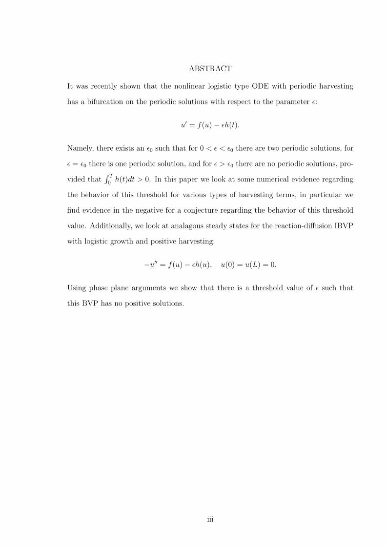
ABSTRACT

It was recently shown that the nonlinear logistic type ODE with periodic harvesting

has a bifurcation on the periodic solutions with respect to the parameter ε:

u′ = f(u)− εh(t).

Namely, there exists an ε0 such that for 0 < ε < ε0 there are two periodic solutions, for

ε = ε0 there is one periodic solution, and for ε > ε0 there are no periodic solutions, pro-

vided that∫ T0h(t)dt > 0. In this paper we look at some numerical evidence regarding

the behavior of this threshold for various types of harvesting terms, in particular we

find evidence in the negative for a conjecture regarding the behavior of this threshold

value. Additionally, we look at analagous steady states for the reaction-diffusion IBVP

with logistic growth and positive harvesting:

−u′′ = f(u)− εh(u), u(0) = u(L) = 0.

Using phase plane arguments we show that there is a threshold value of ε such that

this BVP has no positive solutions.

iii

ACKNOWLEDGEMENTS

I would like to thank my Advisor, Dr. David Costa, for all his encouragement and help

for the past year that I have worked on this. I would also like to thank Dr. Hossein

Tehrani, Dr. Zhonghai Ding, and Dr. Paul Schulte for their time and willingness to

oversee this project. I would also like to extend my appreciation to the regular attendees

of the UNLV PDE seminar for their patience and interest as I worked to understand

this material.

iv

TABLE OF CONTENTS

Page

ABSTRACT . . . . . . . . . . . . . . . . . . . . . . . . . . . . . . . . . . . . . iii

ACKNOWLEDGEMENTS . . . . . . . . . . . . . . . . . . . . . . . . . . . . . iv

TABLE OF CONTENTS . . . . . . . . . . . . . . . . . . . . . . . . . . . . . . v

LIST OF FIGURES . . . . . . . . . . . . . . . . . . . . . . . . . . . . . . . . . vi

1 Introduction . . . . . . . . . . . . . . . . . . . . . . . . . . . . . . . . . . . . 1

2 Preliminaries . . . . . . . . . . . . . . . . . . . . . . . . . . . . . . . . . . . 3

Crandall-Rabinowitz Saddle Node Bifurcation Theorem . . . . . . . . . 3

Basic Periodic Solutions Results . . . . . . . . . . . . . . . . . . . . . . 9

3 Existence and Multiplicity of Periodic Solutions . . . . . . . . . . . . . . . . 13

4 The Behavior of the Threshold . . . . . . . . . . . . . . . . . . . . . . . . . 17

5 Positive Solutions of the Second Order Logistic Type ODE . . . . . . . . . . 24

The Phase Plane . . . . . . . . . . . . . . . . . . . . . . . . . . . . . . 24

The Boundary Value Problem . . . . . . . . . . . . . . . . . . . . . . . 27

REFERENCES . . . . . . . . . . . . . . . . . . . . . . . . . . . . . . . . . . . . 30

VITA . . . . . . . . . . . . . . . . . . . . . . . . . . . . . . . . . . . . . . . . . 32

v

LIST OF FIGURES

Figure Page

4.1 Left: ε = .225 Right: ε = .226 . . . . . . . . . . . . . . . . . . . . . . . . 18

4.2 Left: ε = .186 Right ε = .187 . . . . . . . . . . . . . . . . . . . . . . . . 18

4.3 Left: ε = .153 Right ε = .154 . . . . . . . . . . . . . . . . . . . . . . . . 18

4.4 Left: ε = .129 Right ε = .13 . . . . . . . . . . . . . . . . . . . . . . . . . 19

4.5 Left: ε = .111 Right ε = .112 . . . . . . . . . . . . . . . . . . . . . . . . 19

4.6 Piecewise linear harvesting function g(t). . . . . . . . . . . . . . . . . . . . 20

4.7 Left: ε = 1.171. Right: ε = 1.172. . . . . . . . . . . . . . . . . . . . . . . 20

4.8 g 32(t) . . . . . . . . . . . . . . . . . . . . . . . . . . . . . . . . . . . . . . . 21

4.9 Left: ε = .84. Right: ε = .841. . . . . . . . . . . . . . . . . . . . . . . . . 22

4.10 Solutions for h(t) = .125 + .7 sin(πt2

). Left: ε = 1.09. Right: ε = 1.1. . . 22

4.11 g 32(t) and h(t) = .125 + 1.2 sin

(πt2

). . . . . . . . . . . . . . . . . . . . . . . 23

4.12 Solutions for h(t) = .125 + 1.2 sin(πt2

). Left: ε = .746. Right: ε = .747 . 23

5.1 Intersections of f(u) and εh(u). . . . . . . . . . . . . . . . . . . . . . . . . 25

5.2 Left:For ε > ε0. Right: For ε < ε0 . . . . . . . . . . . . . . . . . . . . . . . 27

5.3 The Phase Plane . . . . . . . . . . . . . . . . . . . . . . . . . . . . . . . . 28

vi

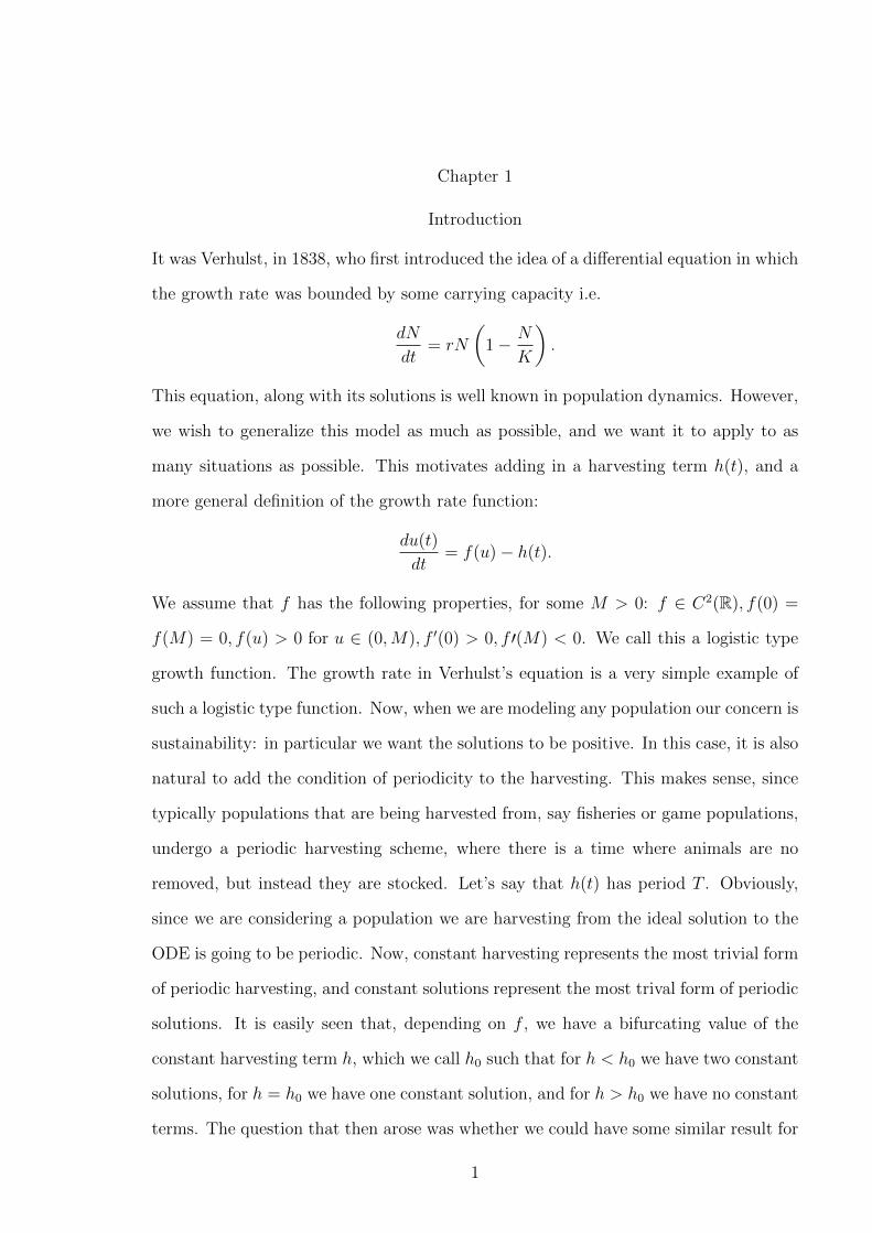
Chapter 1

Introduction

It was Verhulst, in 1838, who first introduced the idea of a differential equation in which

the growth rate was bounded by some carrying capacity i.e.

dN

dt= rN

(1− N

K

).

This equation, along with its solutions is well known in population dynamics. However,

we wish to generalize this model as much as possible, and we want it to apply to as

many situations as possible. This motivates adding in a harvesting term h(t), and a

more general definition of the growth rate function:

du(t)

dt= f(u)− h(t).

We assume that f has the following properties, for some M > 0: f ∈ C2(R), f(0) =

f(M) = 0, f(u) > 0 for u ∈ (0,M), f ′(0) > 0, f ′(M) < 0. We call this a logistic type

growth function. The growth rate in Verhulst’s equation is a very simple example of

such a logistic type function. Now, when we are modeling any population our concern is

sustainability: in particular we want the solutions to be positive. In this case, it is also

natural to add the condition of periodicity to the harvesting. This makes sense, since

typically populations that are being harvested from, say fisheries or game populations,

undergo a periodic harvesting scheme, where there is a time where animals are no

removed, but instead they are stocked. Let’s say that h(t) has period T . Obviously,

since we are considering a population we are harvesting from the ideal solution to the

ODE is going to be periodic. Now, constant harvesting represents the most trivial form

of periodic harvesting, and constant solutions represent the most trival form of periodic

solutions. It is easily seen that, depending on f , we have a bifurcating value of the

constant harvesting term h, which we call h0 such that for h < h0 we have two constant

solutions, for h = h0 we have one constant solution, and for h > h0 we have no constant

terms. The question that then arose was whether we could have some similar result for

1

nonconstant, periodic harvesting and periodic solutions. The answer, as shown in [9],

is yes. A scaling parameter is attached to the harvesting term and get the following

ODE:

du(t)

dt= f(u)− εh(t). (1.1)

It is shown in [9] that, provided that∫ T0h(t)dt > 0 then there is an ε0 such that

for ε > ε0 we have exactly two T -periodic solutions, for ε = ε0 we have exactly one

periodic solution, and for ε > ε0 we have no periodic solutions. Our goal in this thesis

is two-fold. First,we will be doing a review of the proof of this theorem with full details.

Additionally we will be looking at evidence on the behavior of this bifurcating value as

the harvesting term changes.

Second, we will be considering steady states of the following reaction-diffusion IBVP

ut = uxx + f(u)− εh(u), u(0, t) = u(L, t) = 0, u(x, 0) = u0(x)

where f is logistic and h > 0. Our motivation for looking at the steady states is again

sustainability: After a long time can the population reach apoint where it ceases to

change over time? So we set ut = 0, and since we are considering a time independant

solution, we can remove the initial condition as well. This leads to the BVP

−u′′ = f(u)− εh(u), u(0) = u(L) = 0

Using phase plane arguments we will consider the existence of positive solutions with

respect to ε and L.

2

Chapter 2

Preliminaries

In this section we will be going over some basic results that are foundational to my

work. We will be doing an extensive review of some basic theorems and how these are

applied, ultimately leading up to the main result of [9].

Crandall-Rabinowitz Saddle Node Bifurcation Theorem

Before we introduce the theorem, we will present some motivation. Consider F (λ, x) =

x2−λ. It is easy to see that for λ < 0 we have no solutions, for λ = 0 we have one, and

for λ > 0 we have two solutions. So, λ = 0 is a bifurcation value for the parameter in

the sense that there is a drastic change in the solution set of the equation. We can also

see that F (0, 0) = 0. We can ask, therefore, how do the solutions to F = 0 behave in

a neighborhood of (0, 0)? If we visualize this in three dimensions, it is easy to see that

they form a parabola with its vertex at the origin. Note that Fx(0, 0) = 0, and so if

we consider this derivative as a linear operator, then we have have that the null space

N(Fu(0, 0)) = R, and this has dimension 1. Also, the range of this linear operator is

just 0, and thus its codimension is 1 as well, and since Fλ(0, 0) = 1, then we see that

Fλ(0, 0) /∈ R(Fu(0, 0)).

This becomes a little less trivial if we consider an example in R2. Suppose that now

F (λ, x, y) = (F1(λ, x, y), F2(λ, x, y)) = (x2 − λ, y).

We see that F (0, 0, 0) = (0, 0). Now, we consider the Jacobian ∂(F1,F2)∂(x,y)

(λ, 0, 0) at λ = 0:

∂(F1(0, 0, 0), F2(0, 0, 0)

∂(x, y)=

0 0

0 1

We can see thatN(F(x,y)(0, 0, 0)) = {(x, 0) : x ∈ R} has dimension 1. Also, R(F(x,y)(0, 0, 0)) =

{(0, y) : y ∈ R} has a dimension of 1, and thus its codimension is 1 as well. Similarly,

we have Fλ(0, 0, 0) = (−1, 0) /∈ R(F(x,y)(0, 0, 0)). Simple algebra indicates that the

solutions to F (λ, x, y) = 0 in a neighborhood of the origin form a parabolic cylinder.

3

So we notice some patterns in the derivatives of functions that have this bifurcating

behavior. We can also talk about the stability of the solutions to F (λ, x, y) = 0. When

we have them, the two solutions are (±√λ, 0). We can determine stability by looking at

the eigenvalues of the Jacobian within a neighborhood of (0, 0, 0), and these are found

by looking at the roots of the characteristic equation

(2x− µ)(1− µ) = 0.

So our two solutions are µ = x2

and µ = 1. when x is positive, then we have two

positive eigenvalues which gives us a repelling node, while if x is negative then we have

two eigenvalues of different signs, which gives us a saddle. So among our solutions, one

of them is a saddle, and the other is a node. This motivates the name for the following

theorem, which generalizes to Banach Spaces the observations we have made.

We shall start by giving some preliminary information that will be useful for the

proof of the Saddle Node Bifurcation Theorem. First we give a common result regarding

linear transformations. Let X and Y be Banach spaces and recall that the kernel of a

linear transformation ϕ : X → Y is given as

ker(ϕ) = {x ∈ X : ϕ(x) = 0} .

Lemma 2.1. ϕ is injective if and only if ker(ϕ) = {0}.

The proof is elementary and is usually done in any undergraduate linear algebra

course. Also, for the remainder of this paper we will useN(ϕ) and ker(ϕ) interchangeably.

Proof. Assume ϕ is injective. Let ϕ(a) = 0 and ϕ(b) = 0. Then we have that ϕ(a) =

ϕ(b) and the injectivity of ϕ gives that a = b. So then the kernel of ϕ only has a single

element, and this element must be zero. Now assume that ker(ϕ) = {0}. If ϕ(a) = ϕ(b)

we then have that ϕ(a)− ϕ(b) = 0, hence ϕ(a− b) = 0, and since the kernel is trivial

we have that a− b = 0 and thus a = b which gives injectivity.

4

We shall be using the following version of the Implicit Function Theorem, which is

given in the appendix of [4] without proof, though they note that Theorem 10.2.1 of

[6] can be used as a proof .

Implicit Function Theorem. Let E, F and G be three Banach Spaces, f a continuous

mapping on an open subset A of E × F into G. Let the map y 7→ f(x, y) of

Ax = {y ∈ F : (x, y) ∈ A}

into G be differentiable in Ax for each x ∈ E such that Ax 6= ∅, and assume the

derivative of this map (denoted by fy) is continuous on A. Let (x0, y0) ∈ A be such that

f(x0, y0) = 0, and fy(x0, y0) is a linear homeomorphism of F onto G. Then there are

neighborhoods U of x0 and V of y0 in F such that:

(i) U × V ⊂ A

(ii) There is exactly one function u : U → V satisfying f(x, u(x)) = 0 for x ∈ U .

(iii) The mapping of U of (ii) is continuous.

If, moreover, the mapping f is k-times differentiable on A, then (iii) above may be

replaced by

(iv) u is k-times continuously differentiable.

The following two lemmas are given in [11]. The first is a corollary to the Open

Mapping Theorem, and the second is a version of the Hahn-Banach Theorem.

Lemma 2.2. Let X and Y be Banach Spaces, and let T be a bounded linear transfor-

mation between them. Then if T is bijective then T−1 is continuous.

Lemma 2.3. Let B be a closed linear subspace of a Banach space X,and let η ∈ X \B,

then there exists a linear transformation from X to R that vanishes on B but not on η.

We can now state and prove the Saddle Node Bifurcation Theorem of Crandall and

Rabinowitz [5]:

5

Theorem 2.1. Suppose that X and Y are Banach spaces. Let (λ0, u0) ∈ R×X and let

F be a continuously differentiable mapping of an open neighborhood V of (λ0, u0) into

Y . Suppose that:

(i) dimN(Fu(λ0, u0)) = dim(Y \R(Fu(λ0, u0))) = 1 and N(Fu(λ0, u0)) = span {w0}.

(ii) Fλ(λ0, u0) /∈ R(Fu(λ0, u0))

Then if Z is a complement of span{w0} in X then the solutions of F (λ, u) = F (λ0, u0)

near (λ0, u0) form a curve (λ(s), u(s)) = (λ(s), u0 + sw0 + z(s)) where s 7→ (λ(s), z(s))

is a continuously differentiable function near s = 0 and λ(0) = λ0, λ′(0) = 0 and

z(0) = z′(0) = 0.

If F is C2 then we have

λ′′(0) = −〈`, Fuu(λ0, u0)[w0, w0]〉〈`, Fλ(λ0, u0)〉

.

The proof given in [5] is only a few lines and leaves out many details. For the sake

of completeness we flesh out these details in the following proof, similar to what is

done in [12]. Also, one can note the contrast between this theorem and the Implicit

Function Theorem, which gives us a unique solution in a neighborhood when we solve

for one of the coordinates, while the Saddle Node Bifurcation theorem gives us a curve

of solutions for the coordinates in a neighborhood.

Proof. Define the following function G : R× R× Z → Y by

G(s, λ, z) = F (λ, u0 + sw0 + z)− F (λ0, u0).

Note now that G inherits the same continuity from F , and also that G(0, λ0, 0) =

F (λ0, u0)−F (λ0, u0) = 0. Now we also claim thatG(λ,z)(0, λ0, 0) is a linear homeomorphism.

Linearity follows from the linearity of the derivatives of F . Now, we can show that

G(λ,z)(0, λ0, 0) is injective using Lemma 2.1. Suppose we have a (τ, ψ) ∈ ker(G(λ,z)(0, λ, 0)),

this gives that

G(λ,z)(0, λ0, 0)[(τ, ψ)] = τFλ(λ0, u0) + Fu(λ0, u0)[ψ] = 0.

6

Now if τ 6= 0, then we have that Fλ(λ0, u0) = Fu(λ0, u0)[τ−1ψ] (since Fu(λ0, u0) is

linear) , which contradicts that Fλ(λ0, u0) /∈ R(Fu(λ0, u0), and hence we must have

that τ = 0, which gives

Fu(λ0, u0)[ψ] = 0.

Now this implies that ψ ∈ N(Fu(λ0, u0) = span(w0), but since ψ ∈ Z, and Z is a

complement of span(w0) we must have that ψ = 0 because span(w0) ∩ Z = {0}. So

this gives that

ker(G(λ,z)(0, λ, 0)) = {(0, 0)}.

Thus, by Lemma 2.1, this is an injective function. Now, as a consequence of Lemma

2.3, there is a linear functional ` : Y → R such that ker(`) = R(Fu(λ0, u0) and is

nonzero outside of R(Fu(λ0, u0). Now, we shall use this to show that G(λ,z)(0, λ0, 0) is

surjective. Let θ ∈ Y , and consider

G(λ0,z)(0, λ, 0)[(τ, ψ)] = τFλ(λ0, u0) + Fu(λ0, u0)[ψ] = θ.

Applying ` we get

τ`(Fλ(λ0, u0)) + `(Fu(λ0, u0))[ψ]) = `(θ).

Since ker(`) = R(Fu(λ0, u0)) we have that `(Fu(λ0, u0)[ψ] = 0 which gives τ`(Fλ(λ0, u0)) =

`(θ). Since Fλ(λ0, u0) /∈ R(Fu(λ0, u0) we have `(Fλ(λ0, u0)) 6= 0 which gives that

τ =`(θ)

`(Fλ(λ0, u0)),

that is to say that τ is uniquely determined by θ. It will be useful for us to note the

following: Since Z is a complement of span(w0), we have that Z + span(w0) = X, and

so for any element x ∈ X we have a z0 ∈ Z and a a ∈ R such that x = z0 + aw0. This

gives that

Fu(λ0, u0)[x] = Fu(λ0, u0)[z0 + aw0] = Fu(λ0, u0)[z0] + aFu(λ0, u0)[w0] = Fu(λ0, u0)[z0].

What this tells us is thatR(Fu(λ0, u0)|z) = R(Fu(λ0, u0)). Also, since Z is a complement

we have that Z ∩ N(Fu(λ0, u0)) = {0}, and so, as before, we have Fu(λ0, u0)|Z is

7

injective. This gives a well defined inverse of Fu(λ0, u0)|Z that has a domain of

R(Fu(λ0, u0)), we shall call this inverseK. Now since for any ψ ∈ Z we have Fu(λ0, u0)[ψ] =

θ − τFλ(λ0, u0), so then θ − τFλ(λ0, u0) is in the domain of K, and thus we have

ψ = K(θ − τFλ(λ0, u0))

and since τ is completly determined by θ, we see that ψ is also completely determined

by θ. This gives us surjectivity of G(λ,z)(0, λ0, 0). So since G(λ,z)(0, λ0, 0) is continuous

and bijective, then as a consequence Lemma 2.2, we get that (G(λ0,z)(0, λ, 0))−1 is also

continuous, and thus is a linear homeomorphism. So we have shown that G satisfies

the condition of the Implicit Function Theorem, where our three Banach spaces are

R, R × Z, and Y . So then we have functions λ(s) and u(s) where, in a neighborhood

of s = 0 we have that G(s, λ(s), u(s)) = 0 and (λ(s), u(s)) = (λ(s), u0 + sw0 + z(s)),

and the mapping s 7→ (λ(s), z(s)) is continuously differentiable, since F is continuously

differentiable. Now since G(0, λ(0), z(0)) = 0 = G(0, λ0, 0) we then have that λ(0) = λ0

and z(0) = 0. Additionally, note that

Gs(0, λ0, 0) =∂

∂s(F (λ, u0 + sw0 + z)− F (λ0, u0))

∣∣∣∣(0,λ0,0)

= Fu(λ0, u0)[w0] = 0.

On the other hand, since λ and z can depend on s we also have

Gs(0, λ0, 0) = G(λ,z)(0, λ0, 0)[λ′(0), z′(0)].

By the injectivity of G(λ,z)(0, λ, 0) we have that

λ′(0) = z′(0) = 0.

Now, taking the derivative with respect to s of F (λ(s), u(s)) gives

∂

∂sF (λ(s), u(s)) = Fλ(λ(s), u(s))λ′(s) + Fu(λ(s), u(s))u′(s) = 0.

Thus

∂2

∂s2F (λ(s), u(s)) = λ′′Fλ + (λ′(s))2 + 2λ′(s)Fλu[u

′(s)] +Fuu[u′(s), u′(s)] +Fu[u

′′(s)] = 0

8

Let s = 0 to get that

λ′′(0)Fλ(λ(0), u(0)) + Fu[u′′(0)] + Fuu(λ0, u0)([w0, w0] = 0,

since λ′(0) = u′(0) = 0 and u′ = w0, since u(s) = u0 + sw0 + z(s) and z′(0) = 0. Now

we apply the linear functional ` given by the Hahn Banach theorem to both sides to

get

λ′′(0)〈`, Fλ(λ0, u0)〉+ 〈`, Fuu(λ0, u0)[w0, w0]〉 = 0.

Solving gives that

λ′′(0) = −〈`, Fuu(λ0, u0)[w0, w0]〉〈`, Fλ(λ0, u0)〉

.

This completes the proof.

The following theorem will also be used, which is stated without proof, which can

be found in [8].

Theorem 2.2. Suppose F is C2, and F (λ0, u0) = 0 and F satisfies (i) from above, and

Fλ(λ0, u0) = 0. Suppose

H ≡

〈`, Fλλ(λ0, u0)〉 〈`, Fλu(λ0, u0)[w0]〉

〈`, Fλu(λ0, u0)[w0]〉 〈`, Fuu(λ0, u0)[w0, w0]〉

and that det(H) > 0, then the solution set of F (λ, u) = 0 near (λ, u) = (λ0, u0) is

{(λ0, u0)}.

Basic Periodic Solutions Results

The following results will be used as well. These are fairly elementary results on the

existence and multiplicity of periodic solutions to ODEs. The first one is a well known

result that can be found in [1].

Lemma 2.4. Consider

x′ = f(ε, t, x) (2.1)

9

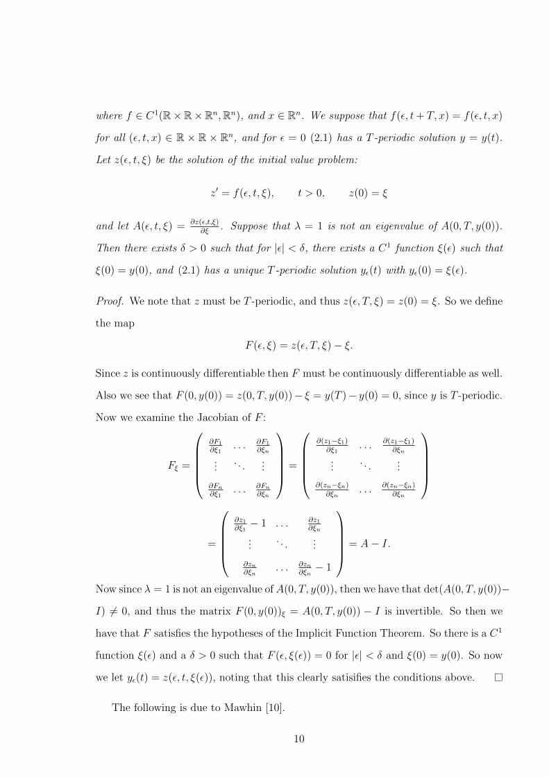
where f ∈ C1(R×R×Rn,Rn), and x ∈ Rn. We suppose that f(ε, t+ T, x) = f(ε, t, x)

for all (ε, t, x) ∈ R × R × Rn, and for ε = 0 (2.1) has a T -periodic solution y = y(t).

Let z(ε, t, ξ) be the solution of the initial value problem:

z′ = f(ε, t, ξ), t > 0, z(0) = ξ

and let A(ε, t, ξ) = ∂z(ε,t,ξ)∂ξ

. Suppose that λ = 1 is not an eigenvalue of A(0, T, y(0)).

Then there exists δ > 0 such that for |ε| < δ, there exists a C1 function ξ(ε) such that

ξ(0) = y(0), and (2.1) has a unique T -periodic solution yε(t) with yε(0) = ξ(ε).

Proof. We note that z must be T -periodic, and thus z(ε, T, ξ) = z(0) = ξ. So we define

the map

F (ε, ξ) = z(ε, T, ξ)− ξ.

Since z is continuously differentiable then F must be continuously differentiable as well.

Also we see that F (0, y(0)) = z(0, T, y(0))− ξ = y(T )− y(0) = 0, since y is T -periodic.

Now we examine the Jacobian of F :

Fξ =

∂F1

∂ξ1. . . ∂F1

∂ξn

.... . .

...

∂Fn

∂ξ1. . . ∂Fn

∂ξn

=

∂(z1−ξ1)∂ξ1

. . . ∂(z1−ξ1)∂ξn

.... . .

...

∂(zn−ξn)∂ξn

. . . ∂(zn−ξn)∂ξn

=

∂z1∂ξ1− 1 . . . ∂z1

∂ξn

.... . .

...

∂zn∂ξn

. . . ∂zn∂ξn− 1

= A− I.

Now since λ = 1 is not an eigenvalue ofA(0, T, y(0)), then we have that det(A(0, T, y(0))−

I) 6= 0, and thus the matrix F (0, y(0))ξ = A(0, T, y(0)) − I is invertible. So then we

have that F satisfies the hypotheses of the Implicit Function Theorem. So there is a C1

function ξ(ε) and a δ > 0 such that F (ε, ξ(ε)) = 0 for |ε| < δ and ξ(0) = y(0). So now

we let yε(t) = z(ε, t, ξ(ε)), noting that this clearly satisifies the conditions above.

The following is due to Mawhin [10].

10

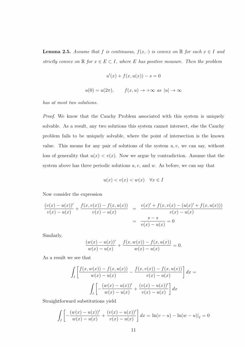
Lemma 2.5. Assume that f is continuous, f(x, ·) is convex on R for each x ∈ I and

strictly convex on R for x ∈ E ⊂ I, where E has positive measure. Then the problem

u′(x) + f(x, u(x))− s = 0

u(0) = u(2π), f(x, u)→ +∞ as |u| → ∞

has at most two solutions.

Proof. We know that the Cauchy Problem associated with this system is uniquely

solvable. As a result, any two solutions this system cannot intersect, else the Cauchy

problem fails to be uniquely solvable, where the point of intersection is the known

value. This means for any pair of solutions of the system u, v, we can say, without

loss of generality that u(x) < v(x). Now we argue by contradiction. Assume that the

system above has three periodic solutions u, v, and w. As before, we can say that

u(x) < v(x) < w(x) ∀x ∈ I

Now consider the expression

(v(x)− u(x))′

v(x)− u(x)+f(x, v(x))− f(x, u(x))

v(x)− u(x)=

v(x)′ + f(x, v(x)− (u(x)′ + f(x, u(x)))

v(x)− u(x)

=s− s

v(x)− u(x)= 0

Similarly,

(w(x)− u(x))′

w(x)− u(x)+f(x,w(x))− f(x, u(x))

w(x)− u(x)= 0.

As a result we see that∫I

[f(x,w(x))− f(x, u(x))

w(x)− u(x)− f(x, v(x))− f(x, u(x))

v(x)− u(x)

]dx =

∫I

[−(w(x)− u(x))′

w(x)− u(x)+

(v(x)− u(x))′

v(x)− u(x)

]dx

Straightforward substitutions yield∫I

[−(w(x)− u(x))′

w(x)− u(x)+

(v(x)− u(x))′

v(x)− u(x)

]dx = ln(v − u)− ln(w − u)|I = 0

11

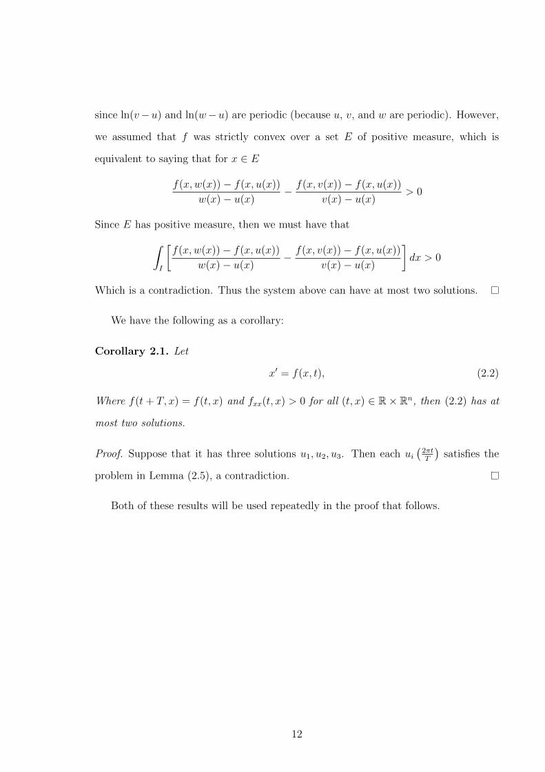
since ln(v−u) and ln(w−u) are periodic (because u, v, and w are periodic). However,

we assumed that f was strictly convex over a set E of positive measure, which is

equivalent to saying that for x ∈ E

f(x,w(x))− f(x, u(x))

w(x)− u(x)− f(x, v(x))− f(x, u(x))

v(x)− u(x)> 0

Since E has positive measure, then we must have that∫I

[f(x,w(x))− f(x, u(x))

w(x)− u(x)− f(x, v(x))− f(x, u(x))

v(x)− u(x)

]dx > 0

Which is a contradiction. Thus the system above can have at most two solutions.

We have the following as a corollary:

Corollary 2.1. Let

x′ = f(x, t), (2.2)

Where f(t+ T, x) = f(t, x) and fxx(t, x) > 0 for all (t, x) ∈ R× Rn, then (2.2) has at

most two solutions.

Proof. Suppose that it has three solutions u1, u2, u3. Then each ui(2πtT

)satisfies the

problem in Lemma (2.5), a contradiction.

Both of these results will be used repeatedly in the proof that follows.

12

Chapter 3

Existence and Multiplicity of Periodic Solutions

In this section we will establish the following:

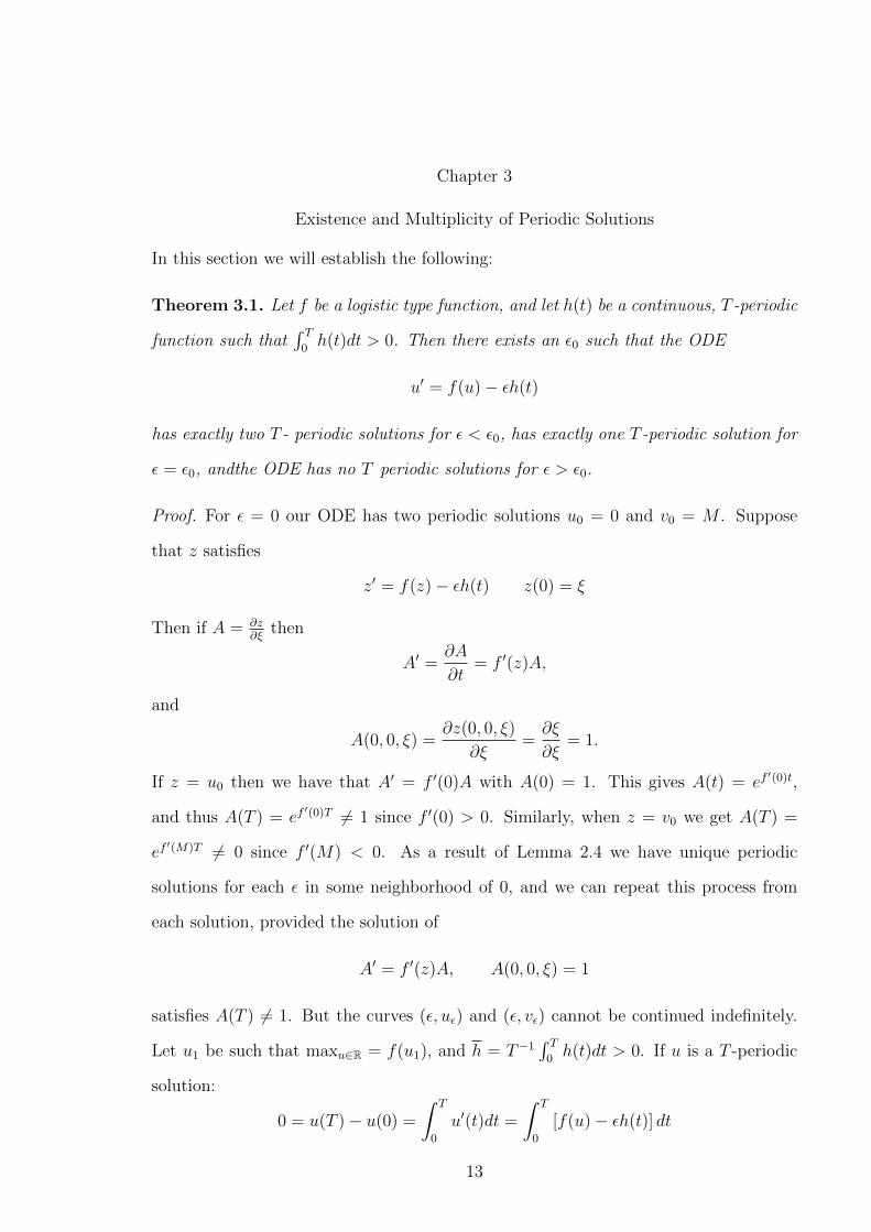
Theorem 3.1. Let f be a logistic type function, and let h(t) be a continuous, T -periodic

function such that∫ T0h(t)dt > 0. Then there exists an ε0 such that the ODE

u′ = f(u)− εh(t)

has exactly two T - periodic solutions for ε < ε0, has exactly one T -periodic solution for

ε = ε0, andthe ODE has no T periodic solutions for ε > ε0.

Proof. For ε = 0 our ODE has two periodic solutions u0 = 0 and v0 = M . Suppose

that z satisfies

z′ = f(z)− εh(t) z(0) = ξ

Then if A = ∂z∂ξ

then

A′ =∂A

∂t= f ′(z)A,

and

A(0, 0, ξ) =∂z(0, 0, ξ)

∂ξ=∂ξ

∂ξ= 1.

If z = u0 then we have that A′ = f ′(0)A with A(0) = 1. This gives A(t) = ef′(0)t,

and thus A(T ) = ef′(0)T 6= 1 since f ′(0) > 0. Similarly, when z = v0 we get A(T ) =

ef′(M)T 6= 0 since f ′(M) < 0. As a result of Lemma 2.4 we have unique periodic

solutions for each ε in some neighborhood of 0, and we can repeat this process from

each solution, provided the solution of

A′ = f ′(z)A, A(0, 0, ξ) = 1

satisfies A(T ) 6= 1. But the curves (ε, uε) and (ε, vε) cannot be continued indefinitely.

Let u1 be such that maxu∈R = f(u1), and h = T−1∫ T0h(t)dt > 0. If u is a T -periodic

solution:

0 = u(T )− u(0) =

∫ T

0

u′(t)dt =

∫ T

0

[f(u)− εh(t)] dt

13

=

∫ T

0

f(u)− f(u1)dt+

∫ T

0

f(u1)− εh(t)dt

=

∫ T

0

f(u)− f(u1)dt+ Tf(u1)− εh

If ε > f(u1)

hthen Tf(u1) − εh < 0, and by definition

∫ T0f(u) − f(u1)dt < 0. So then,

for ε > f(u1)

h, ∫ T

0

f(u)− f(u1)dt+ Tf(u1)− εh < 0,

a contradiction. So we must have a degenerate solution along the curve, and let (ε∗, u∗)

be the first degenerate solution along this curve. At this point we must have A(T ) = 1.

Define F (ε, u) = z(ε, T, u)− u, we see that

Fu(ε∗, u∗) = A(T )− 1 = 0.

So as a linear transformation, Fu(ε∗, u∗)[τ ] = 0 for all τ ∈ R, so the null space of

Fu(ε∗, u∗) = R, and thus has dimension 1, and the codimension of its range is 1. To use

the Saddle Node Bifurcation theorem, we need that Fε(ε∗, u∗) 6= 0. So we assume that

it is equal to 0 and derive a contradiction. If Fε(ε∗, u∗) = 0 then all the conditions of

Theorem 2.2 are satisfied, except the one about the matrixH. Note, since Fu(ε∗, u∗) = 0

then the ` is the identity mapping.

Now, if B(t) = Fε(ε∗, u∗) = ∂z(ε∗,T,u∗(0)∂ε

, then B satisfies

B′ = f ′(u∗(t))B − h(t), t > 0, B(0) = 0.

Solving this ODE gives that B(t) = A∫ t0A(s)−1h(s)ds. Differentiation confirms.

Let C(t) = Fξξ(ε∗, u∗), and this can be evaluated by solving

C ′ = f ′(u∗(t))c+ f ′′(u∗(t))A2, C(0) = 0.

The solution to this ODE is given by C(t) = f ′′(u∗(t))A(t)∫ t0A(s)ds, where

A(t) = exp

(∫ t

0

f ′(u∗(s))ds

).

14

Similarly if D(t) = Fεξ(ε∗, u∗), then we can use the above equation to get that

D′ = f ′(u∗(t))D + f ′′(u∗(t))AB, D(0) = 0.

Solving this ODE gives D(t) = f ′′(u∗(t))A(t)∫ t0B(s)ds.

For E(t) = Fεε(ε∗, u∗) then, as before, we have that:

E ′ = f ′(u∗(t))E + f ′′(u∗(t))B2, E(0) = 0

and the solution to this ODE is given by E(t) = f ′′(u∗(t))A(t)∫ t0A(s)−2b(s)2ds. Note

that this also gives that E(T ) < 0.

So we have that:

Fε(ε∗, u∗) = B(T ), Fξξ(ε∗, u∗) = C(T ),

Fεξ(ε∗, u∗) = D(T ), Fεε(ε∗, u∗) = E(T ).

So the matrix H in the above theorem takes the form

H = H(ε∗, u∗) =

E(T ) D(T )

D(T ) C(T )

det(H) = E(T )C(T )−D2(T ) =

(f ′′(u∗(T ))A(T ))2[∫ T

0

A(s)ds

∫ T

0

A(s)−1B(s)2ds

−(∫ T

0

B(s)ds

)2]> 0

by the Cauchy-Schwarz Inequality. By Theorem 2.2 this implies that the solution set of

F (ε, u) = 0 near (ε∗, u∗) is the singleton set {(ε∗, u∗)}. This contradicts that (ε∗, u∗) is

limit point of a curve of solutions of our ODE. Therefore Fε(ε∗, u∗) 6= 0 and the Saddle

Node bifurcation theorem applies.

So then we have a branch of solution extending from ε = 0 to ε = ε∗. At εast the saddle

node bifurcation theorem applies, and thus we have a curve of solutions (ε(s), u(s)),

such that ε(0) = ε∗ and ε′(0) = 0. Moreover we have that

ε′′(0) = −Fξξ(ε∗, u∗)Fε(ε∗, u∗)

15

From above we had that Fξξ(ε∗, u∗) = C(T ) < 0. Now if Fε(ε∗, u∗) = B(T ) > 0, then

we have that ε′′(0) > 0 and we see that ε(s) is a parabola like curve that open to the

right. But the point (ε∗, u∗) is a limit point to the curve from the left, and thus if the

bifurcation curve opens to the right, we have a problem. So we have that B(T ) < 0 and

thus ε′′(0) < 0, and hence we have a parabola-like curve that open to the left. The lower

branch of this parabola must match up with the curve leading up to (ε∗, u∗), else we

have a neighborhood of ε that has three periodic solutions, which is not possible. Now

we can continue the upper branch with decreasing ε from (ε∗, u∗). If we reach another

degenerate solution along this curve, then we can apply the same argument as we did

at our last degenerate solution. As a result, we could setup another bifurcating curve,

which would give us a neighborhood of ε with three periodic solutions, a contradiction.

Since we have no more degenerate solutions, we can extend this curve all the way until

ε = 0 to the constant solution u = M . So we have at least two periodic solutions in

(0, ε∗), and using Corollary 2.1, we have exactly two periodic solutions.

Now if for some ε > ε∗ we have a periodic solution, then using the same arguments

as above, we can extend a curve from this solution all the way back to ε = 0. But, since

we have at most 2 solutions, this curve will match up with the branches of the curve

we defined above. As a result this curve cannot extend beyond ε∗, since we have a limit

point there. So we cannot have a solution beyond ε∗. So all our periodic soutions lie

on this curve and the result is proved.

16

Chapter 4

The Behavior of the Threshold

In the proof of the Theorem 1.1 in [9] an upper bound is given for the threshold value

which is based on the average harvesting. In particular we had that

ε0 ≤T max f(u)∫ T

0h(t)dt

So when the total harvesting is the same, then we see that the upper bound for theis

threshold remains unchanged. For example we could consider the set of harvesting

functions ha(t) = 1 + a cos t. For each ha we have

ε0 ≤2πmax f(u)∫ 2π

0ha(t)dt

= 2πmax f(u)

We note that the difference between each ha is the total variation of the function.

One of the hypotheses was that∫ 2π

0h(t)dt > 0, meaning that we are going to be

harvesting more than we are stocking. However, if we increase the variation of the

harvesting we are going to be harvesting more from the population, and it will make it

more difficult for the population to recover, even though we are stocking more. So we

can intuitively conclude that if we increase the variation of the harvesting function, it

should lower the threshold value. This is conjectured at the end of [9]. In this section

we are going to look at classes of function that have the same average harvesting, but

have larger variation. It is easy to setup some of these classes, for example 1 + a cos t

or 2 + b sin t, but we will also be looking at some more complicated piecewise linear

harvesting functions. In order to determine the threshold value, we will be relying on

Mathematica to numerically solve these ODEs.

First we will consider the above example: the class of functions h(t) = 1 + a cos t.

To evaluate this threshold we made use of Mathematica’s NDSolve function. We used

a trial and error approach to deterimine the threshold value, and as figures 4.1 - 4.5

indicate, it behaves as conjectured.

17

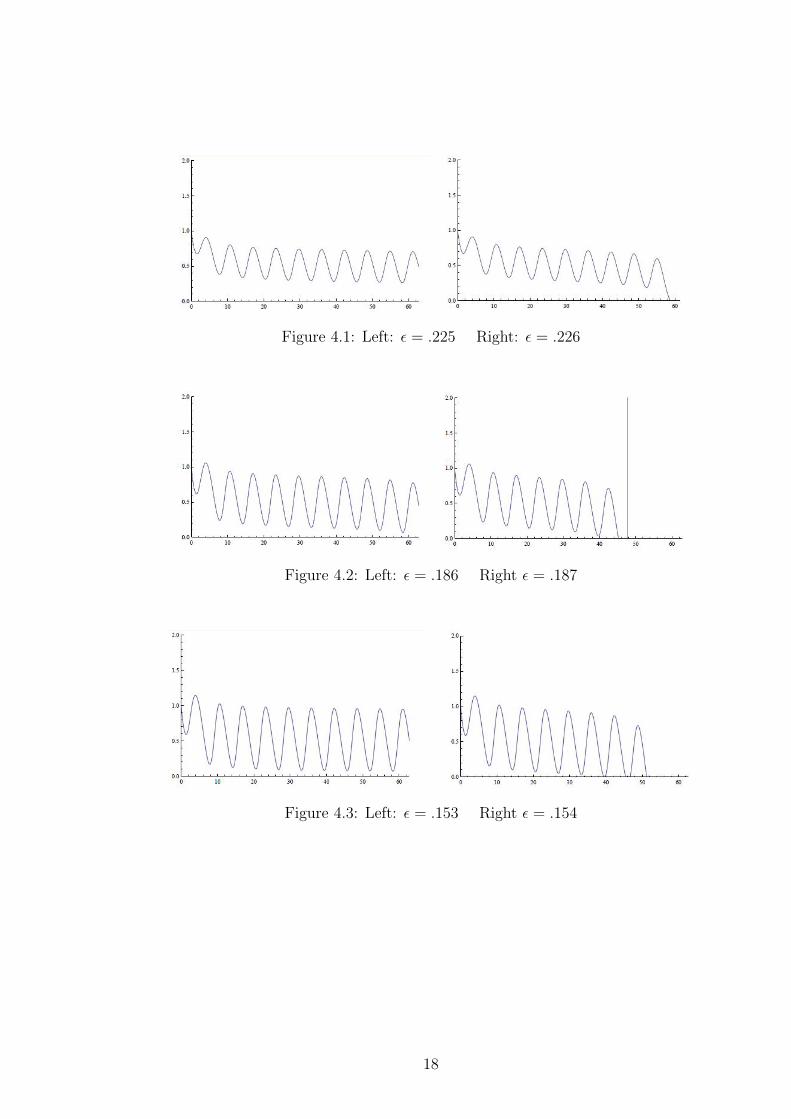
Figure 4.1: Left: ε = .225 Right: ε = .226

Figure 4.2: Left: ε = .186 Right ε = .187

Figure 4.3: Left: ε = .153 Right ε = .154

18

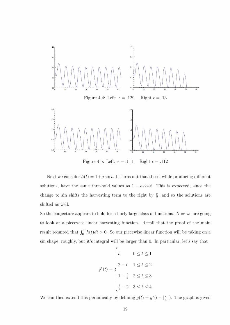
Figure 4.4: Left: ε = .129 Right ε = .13

Figure 4.5: Left: ε = .111 Right ε = .112

Next we consider h(t) = 1+a sin t. It turns out that these, while producing different

solutions, have the same threshold values as 1 + a cos t. This is expected, since the

change to sin shifts the harvesting term to the right by π2, and so the solutions are

shifted as well.

So the conjecture appears to hold for a fairly large class of functions. Now we are going

to look at a piecewise linear harvesting function. Recall that the proof of the main

result required that∫ T0h(t)dt > 0. So our piecewise linear function will be taking on a

sin shape, roughly, but it’s integral will be larger than 0. In particular, let’s say that

g∗(t) =

t 0 ≤ t ≤ 1

2− t 1 ≤ t ≤ 2

1− t2

2 ≤ t ≤ 3

t2− 2 3 ≤ t ≤ 4

We can then extend this periodically by defining g(t) = g∗(t−b t4c). The graph is given

19

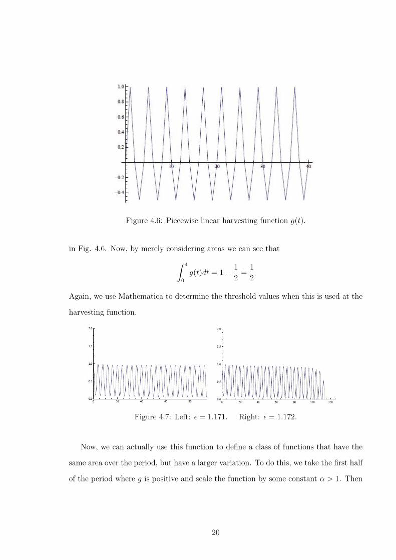
Figure 4.6: Piecewise linear harvesting function g(t).

in Fig. 4.6. Now, by merely considering areas we can see that∫ 4

0

g(t)dt = 1− 1

2=

1

2

Again, we use Mathematica to determine the threshold values when this is used at the

harvesting function.

Figure 4.7: Left: ε = 1.171. Right: ε = 1.172.

Now, we can actually use this function to define a class of functions that have the

same area over the period, but have a larger variation. To do this, we take the first half

of the period where g is positive and scale the function by some constant α > 1. Then

20

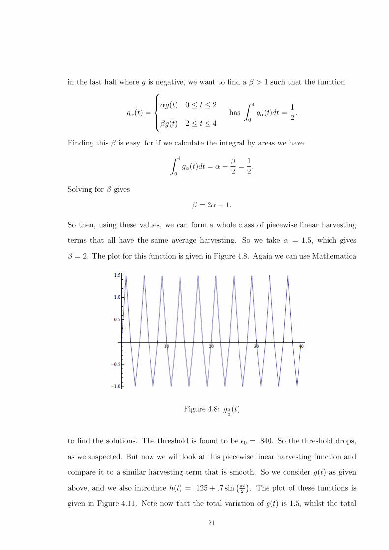
in the last half where g is negative, we want to find a β > 1 such that the function

gα(t) =

αg(t) 0 ≤ t ≤ 2

βg(t) 2 ≤ t ≤ 4

has

∫ 4

0

gα(t)dt =1

2.

Finding this β is easy, for if we calculate the integral by areas we have∫ 4

0

gα(t)dt = α− β

2=

1

2.

Solving for β gives

β = 2α− 1.

So then, using these values, we can form a whole class of piecewise linear harvesting

terms that all have the same average harvesting. So we take α = 1.5, which gives

β = 2. The plot for this function is given in Figure 4.8. Again we can use Mathematica

Figure 4.8: g 32(t)

to find the solutions. The threshold is found to be ε0 = .840. So the threshold drops,

as we suspected. But now we will look at this piecewise linear harvesting function and

compare it to a similar harvesting term that is smooth. So we consider g(t) as given

above, and we also introduce h(t) = .125 + .7 sin(πt2

). The plot of these functions is

given in Figure 4.11. Note now that the total variation of g(t) is 1.5, whilst the total

21

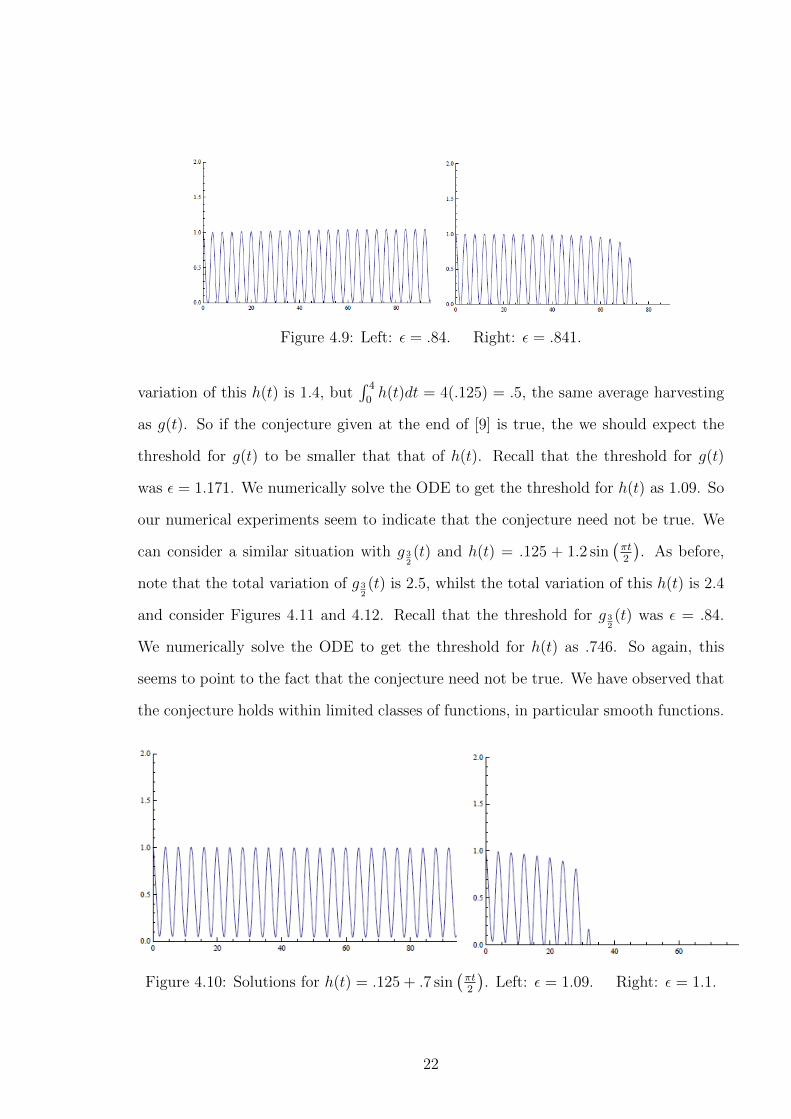
Figure 4.9: Left: ε = .84. Right: ε = .841.

variation of this h(t) is 1.4, but∫ 4

0h(t)dt = 4(.125) = .5, the same average harvesting

as g(t). So if the conjecture given at the end of [9] is true, the we should expect the

threshold for g(t) to be smaller that that of h(t). Recall that the threshold for g(t)

was ε = 1.171. We numerically solve the ODE to get the threshold for h(t) as 1.09. So

our numerical experiments seem to indicate that the conjecture need not be true. We

can consider a similar situation with g 32(t) and h(t) = .125 + 1.2 sin

(πt2

). As before,

note that the total variation of g 32(t) is 2.5, whilst the total variation of this h(t) is 2.4

and consider Figures 4.11 and 4.12. Recall that the threshold for g 32(t) was ε = .84.

We numerically solve the ODE to get the threshold for h(t) as .746. So again, this

seems to point to the fact that the conjecture need not be true. We have observed that

the conjecture holds within limited classes of functions, in particular smooth functions.

Figure 4.10: Solutions for h(t) = .125 + .7 sin(πt2

). Left: ε = 1.09. Right: ε = 1.1.

22

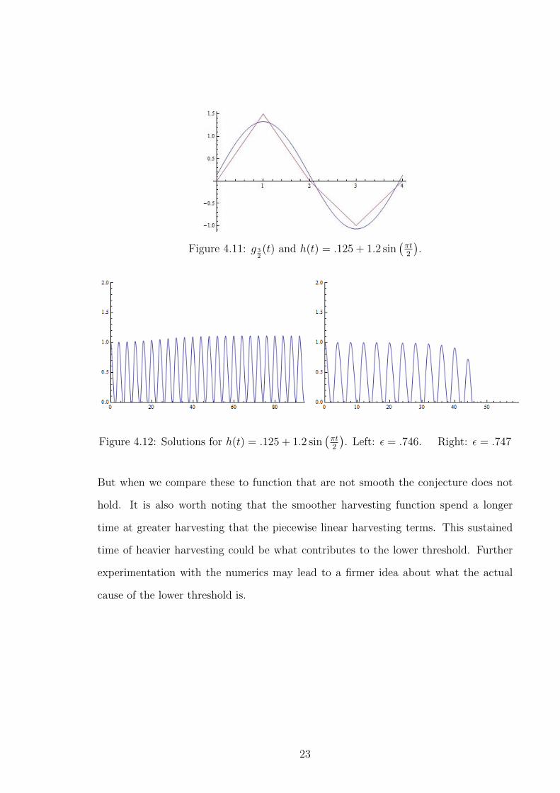
Figure 4.11: g 32(t) and h(t) = .125 + 1.2 sin

(πt2

).

Figure 4.12: Solutions for h(t) = .125 + 1.2 sin(πt2

). Left: ε = .746. Right: ε = .747

But when we compare these to function that are not smooth the conjecture does not

hold. It is also worth noting that the smoother harvesting function spend a longer

time at greater harvesting that the piecewise linear harvesting terms. This sustained

time of heavier harvesting could be what contributes to the lower threshold. Further

experimentation with the numerics may lead to a firmer idea about what the actual

cause of the lower threshold is.

23

Chapter 5

Positive Solutions of the Second Order Logistic Type ODE

Having now considered the case of harvesting over an entire population, it is natural

for us to move into more space conscious considerations. We will be considering the

well known reaction-diffusion equation with Dirichlet boundary conditions, a logistic

type growth term, and a positive, bounded, continuous harvesting term that depends

on the population (instead of time):

ut = uxx + f(u)− εh(u), u(0, t) = u(L, t) = 0, u(x, 0) = u0(x).

Since we are considering this in the context of an actual population we are going

to be interested primarily in steady state solutions (ut(x, t) = 0∀t > 0), for if we

are considering a biological model, then the steady state represents sustainability.

Obviously only positive solutions will make sense, as a negative population has no

physical meaning. So we have

0 = uxx + f(u)− εh(u), u(0) = u(L) = 0.

Naturally, this can be considered an ODE, and for convenience of notation we will

consider the variable as t instead of x:

−u′′ = f(u)− εh(u), u(0) = u(L) = 0. (5.1)

We wish to learn about the positive solutions as we change the value of the parameter

ε.

The Phase Plane

We will be using the phase plane to show our results in this section. Many undergraduate

ODE textbooks will contain a discussion on the use and construction of phase planes,

for example [7] or [2]. Along these lines, we will be constructing the phase plane for

the above ODE. First we can write it as a system of first order ODEs:

u′ = v, −v′ = f(u)− εh(u).

24

Figure 5.1: Intersections of f(u) and εh(u).

Now, this fits the definition of a conservative system, and thus the total energy in the

system remains constant. This gives

1

2v2 − F (u) + εH(u) = E (5.2)

where E is a constant, and F and H are the primitives of f and h repsectively. This

equation gives the level curves of the phase plane. Now we need to find the equilibrium

points, that is to say, the constant solutions of the ODE, and classify them. This

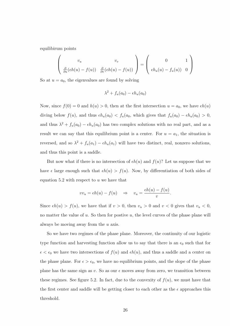
requires that f(u) − εh(u) = 0, which gives f(u) = εh(u). Now we can see that since

h(u) > 0, and since f(u) is bounded, then there is a sufficiently large ε such that there

are no equilibrium points. If there is a an equilibrium point, then the fact that f(0) = 0

and h(u) > 0 means that that at the first intersection we have that h(u) crosses f(u)

from above to below. Its qualitative behavior is similar to that of Figure 5.1. However,

due to the general nature of h(u), it need not only intersect f(u) at only one place,

but rather we can say that it will intersect at at least two places. This leads to at

least two equilibrium points on the phase plane, let us call these points u = a0 and

u = a1, noting that a0 ≤ a1. Now we want to classify these equilibrium points. We

will be using the method and theory of classification as given in chapter 2 of [7]. The

general idea to classify them is to consider the behavior of the phase plane in a small

neighborhood of the equilibrium points using a Taylor series expansion near that point.

This linearization leads us to consider the eigenvalues of the following matrix at the

25

equilibirum points vu vv

∂∂u

(εh(u)− f(u)) ∂∂v

(εh(u)− f(u))

=

0 1

εhu(u)− fu(u)) 0

So at u = a0, the eigenvalues are found by solving

λ2 + fu(a0)− εhu(a0)

Now, since f(0) = 0 and h(u) > 0, then at the first intersection u = a0, we have εh(u)

diving below f(u), and thus εhu(a0) < fu(a0, which gives that fu(a0) − εhu(a0) > 0,

and thus λ2 + fu(a0) − εhu(a0) has two complex solutions with no real part, and as a

result we can say that this equilibrium point is a center. For u = a1, the situation is

reversed, and so λ2 + fu(a1) − εhu(a1) will have two distinct, real, nonzero solutions,

and thus this point is a saddle.

But now what if there is no intersection of εh(u) and f(u)? Let us suppose that we

have ε large enough such that εh(u) > f(u). Now, by differentiation of both sides of

equation 5.2 with respect to u we have that

vvu = εh(u)− f(u) ⇒ vu =εh(u)− f(u)

v.

Since εh(u) > f(u), we have that if v > 0, then vu > 0 and v < 0 gives that vu < 0,

no matter the value of u. So then for postive u, the level curves of the phase plane will

always be moving away from the u axis.

So we have two regimes of the phase plane. Moreover, the continuity of our logistic

type function and harvesting function allow us to say that there is an ε0 such that for

ε < ε0 we have two intersections of f(u) and εh(u), and thus a saddle and a center on

the phase plane. For ε > ε0, we have no equilibrium points, and the slope of the phase

plane has the same sign as v. So as our ε moves away from zero, we transition between

these regimes. See figure 5.2. In fact, due to the convexity of f(u), we must have that

the first center and saddle will be getting closer to each other as the ε approaches this

threshold.

26

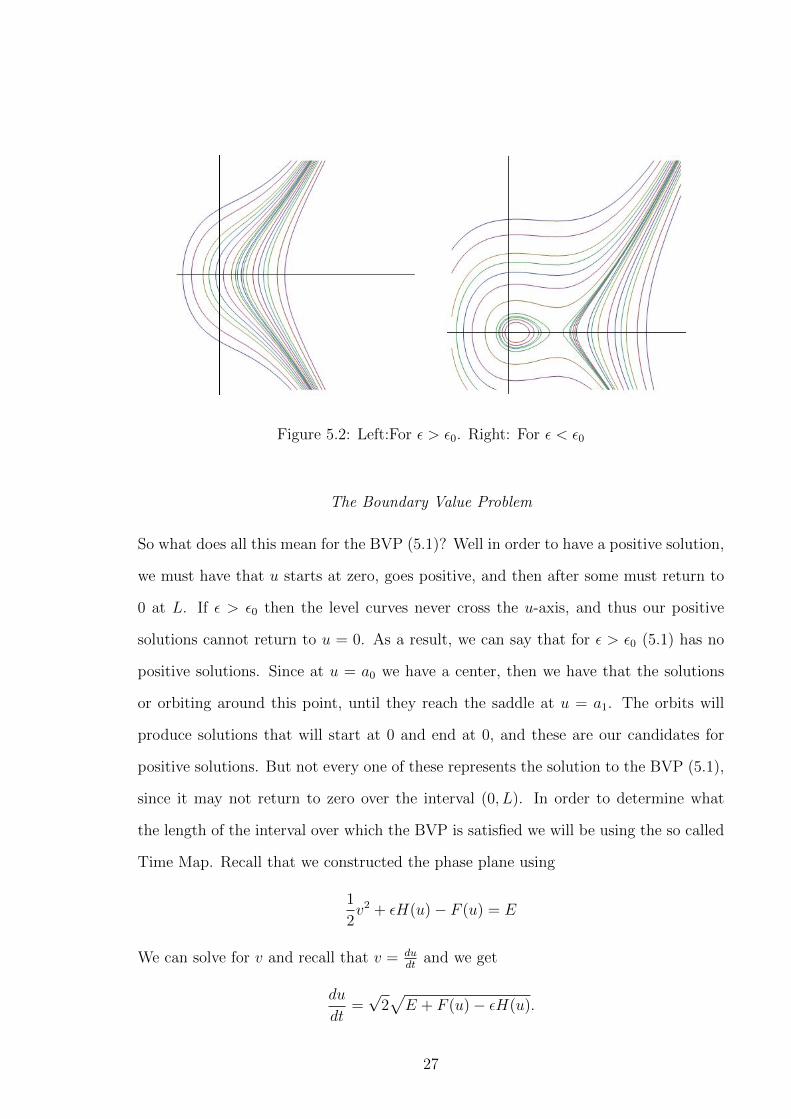
Figure 5.2: Left:For ε > ε0. Right: For ε < ε0

The Boundary Value Problem

So what does all this mean for the BVP (5.1)? Well in order to have a positive solution,

we must have that u starts at zero, goes positive, and then after some must return to

0 at L. If ε > ε0 then the level curves never cross the u-axis, and thus our positive

solutions cannot return to u = 0. As a result, we can say that for ε > ε0 (5.1) has no

positive solutions. Since at u = a0 we have a center, then we have that the solutions

or orbiting around this point, until they reach the saddle at u = a1. The orbits will

produce solutions that will start at 0 and end at 0, and these are our candidates for

positive solutions. But not every one of these represents the solution to the BVP (5.1),

since it may not return to zero over the interval (0, L). In order to determine what

the length of the interval over which the BVP is satisfied we will be using the so called

Time Map. Recall that we constructed the phase plane using

1

2v2 + εH(u)− F (u) = E

We can solve for v and recall that v = dudt

and we get

du

dt=√

2√E + F (u)− εH(u).

27

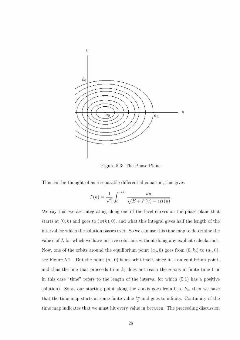
Figure 5.3: The Phase Plane

This can be thought of as a separable differential equation, this gives

T (k) =1√2

∫ w(k)

0

du√E + F (u)− εH(u)

.

We say that we are integrating along one of the level curves on the phase plane that

starts at (0, k) and goes to (w(k), 0), and what this integral gives half the length of the

interval for which the solution passes over. So we can use this time map to determine the

values of L for which we have postive solutions without doing any explicit calculations.

Now, one of the orbits around the equilibrium point (a0, 0) goes from (0, k0) to (a1, 0),

see Figure 5.2 . But the point (a1, 0) is an orbit itself, since it is an equilbrium point,

and thus the line that proceeds from k0 does not reach the u-axis in finite time ( or

in this case ”time” refers to the length of the interval for which (5.1) has a positive

solution). So as our starting point along the v-axis goes from 0 to k0, then we have

that the time map starts at some finite value L0

2and goes to infinity. Continuity of the

time map indicates that we must hit every value in between. The preceeding discussion

28

has yielded the following result:

Theorem 5.1. Given the BVP (5.1) there exists an ε0 such that for ε > ε0 there are

no positive solutions and for ε < ε0 there is an L0 such that for any L ≥ L0 the BVP

(5.1) has at least one positive solution.

Now when we consider the intersections of f(u) and εh(u), we see that they get

farther aprt as ε → 0, due to the convexity of f . This causes the time map to get

smaller. As a result, if our ε is small, the the space required to maintain the positive

solutions becomes small, that is, the length of our smallest interval for which there is a

positive solution gets smaller. Similarly, as ε approaches its threshold we see that the

smallest length of the interval is going to become larger, and thus more space is required

to have a postive solution, and thus have a steady state. This result is fairly unspecific

and only establishes existence. A more in-depth analysis of the time map could yield a

result on the multiplicity of the solutions as ε changes, see [3] as an example.

29

REFERENCES

[1] Antonio Ambrosetti and Giovanni Prodi. A Primer of Nonlinear Analysis, Cam-

bridge Studies in Advanced Mathematics, Vol. 34. Cambridge University Press,

Cambridge, 1995.

[2] David G. Costa. Multiplicidade de solucoes em equacoes diferenciais. Coleccao

Textos de Matematica, 16:137–154, 2002.

[3] David G. Costa and Hossein Terhani. Simple existence proofs for one-dimensional

semipositone problems. Proceedings of the Royal Society of Edinburgh,

136A:473–493, 2006.

[4] Michael G. Crandall and Paul H. Rabinowitz. Bifurcation from simple eigenvalues.

Journal of Functional Analysis, 8:321–340, 1971.

[5] Michael G. Crandall and Paul H. Rabinowitz. Bifurcation, perturbation of simple

eigenvalues, and linearized stability. Arch. Ration. Mech. Anal., 52:161–180, 1973.

[6] J. Dieudonne. Foundations of Modern Analysis. Academic Press, New York, 1960.

[7] D.W. Jordan and P. Smith. Nonlinear Ordinary Differential Equations. Oxford

Applied Mathematics and Computing Science Series. Oxford University Press, New

York, second edition, 1988.

[8] Ping Liu, Junping Shi, and Yuwen Wang. Imperfect transcritical and pitchfork

bifurcations. Journal of Functional Analysis, 251(2):573–600, 2007.

[9] Ping Liu, Junping Shi, and Yuwen Wang. Periodic solutions of a logistic type

population model with harvesting. Journal of Mathematical Analysis and Appli-

cations, 369:730–735, 2010.

30

[10] Jean Mawhin. First order differential equations with several periodic solutions. Z.

Agnew. Math. Phys., 38(2):257–265, 1987.

[11] Eric Schecter. Handbook of Analysis and its Foundations. Academic Press, 1996.

[12] Junping Shi. China lectures on solution set of semilinear elliptic equations (in

tokyo metropolitan university), 2005.

31

VITA

VITA

Graduate CollegeUniversity of Nevada, Las Vegas

Cody Palmer

Degrees:Bachelor of Science, 2009University of Nevada, Las Vegas

Thesis Title:Periodic and Positive Solutions of First and Second Order Logistic Type ODEs with

Harvesting.

Thesis Examination Committee:Chairperson, David G. Costa, Ph.D.Committee Member, Zhonghai Ding, Ph.D.Committee Member, Hossein Tehrani, Ph.D.Graduate Faculty Representative, Paul Schulte, Ph.D.

32