Embed Size (px)
Citation preview
Periodic Pattern Search on Time-Related Data Sets
Wan Gong
B.Sc., Mount Allison University, 1995
A THESIS SUBMITTED IN PARTIAL FULFILLMENT
O F THE REQUIREMENTS FOR THE DEGREE OF
MASTER OF SCIENCE
in the School
of
Computing Science
@ Wan Gong 1997
SIMON FRASER UNIVERSITY
November 1997
All rights reserved. This work may not be
reproduced in whole or in part, by photocopy
or other means, without the permission of the author.
National Library * I* 1 of Canada
B i b l m u e nationale du Canada
Acquisitions and Acquisitions et Bibliographic Services services bibliog raphiques
395 Weihngton Street 395, rue Wellington OnawaON KlAON4 Canada
The author has granted a non- exclusive licence allowing the National Library of Canada to rkproduce, loan, dstnbute or sell copies of this thesis in microform, paper or electronic formats.
I
The author retains ownership of the copyright in thls theGs. Neither the thesis nor substantial extracts from it may be printed or otherwise reproduced without the author's permission.
Your Ms V m rikrrwa
Our file Norre rekrmce
L'auteur a accorde une licence non exclusive permettant a la Bibliotheque nationale du Canada de reproduire, prster, lstribuer ou %
vendre des copies de cette these sous la forme de rnicrofiche/filrn, de ,
reproduction sur papier ou sur format electronique.
L'auteur conserve la propriete du droit d'auteur qui protkge cette these. Ni la these ni des extraits substantiels de celle-ci ne doivent itre imprimes ou autrement reproduits sans son autorisation. -
- APPROVAL
Name: Wan Gong
Degree: l l as te r of Science
Title of thesis: ' Periodic Pattern Search on Time-Related Data Sets
Examining Committee: Dr. Ramesh Iirishnamurti
Chair
Dr. .Jiawci Han
Senior Supervisor
Dr. Qiang l'anl,
Supervisor
Dr. l'eronica Dahl
Estcrnal Esarnincr
November 18, 1997 Date Approved:
Abstract
For many applications such as accounting, banking, business transaction processing
systems, geographical information systems, medical record book keeping, etc., the
changes made on their databases over time are a valuable source of information which
can direct the future operation of the enterprise. In this thesis, we will focus on rela-
tional databases with historical data or, in other words, time-related data, and try to
extract from them some useful knowledge about their periodic behavior. The discov-
ered knowledge could provide user some future guidance, to which end techniques in
knowledge discovery and data warehousing become important.
Knowledge discovery and data warehousing have been increasingly important in
handling and analyzing large databases efficiently and effectively. We can take ad-
vantage of existing on-line analytical processing techniques widely used in knowledge
discovery and data warehousing, and apply them on time-related data to solve peri-
odic pattern search problems.
The problems discussed in this presentation include two types. One is to find
periodic patterns of a time series with a given period, while the other is to find a
pattern with arbitrary length of period. The algorithms will be presented, along with
their experimental results.

Acknowledgments
I would like to thank my senior supervisor Dr. Jiawei Han for his invaluable guidance,
enthusiasm and financial support throughout the course of this work. I am also very
grateful to my supervisor Dr. Qiang Yang for his helpful comments and insightful
suggestions during the research and writing of this thesis. I would also like to thank
Dr. Veronica Dahl for taking the time to be my external examiner.
Many other people have helped and contributed their time to the research of this
thesis. My thanks to Ye Lu, Shan Cheng, and Bin Xia for their invaluable comments
and suggestions. I would also like to take this opportunity to express my gratitude
toward everyone in the Intelligent Database Laboratory of the School of Computing
Science at Simon Fraser University, especially Sonny Chee, Qing Chen, Shan Cheng,
Jenny Chiang, Micheline Kamber, Kris Koperski, Nebojsa Stefanovic, Bin Xia, Osmar
Zaiane, Shuhua Zhang, Hua Zhu, for their valuable suggestions and help in these two
years of study as well as their friendship. Thanks to all the other friends I have made
at Simon Fraser University for making my stay at SFU an enjoyable period of time.
Last but certainly not least, I will always be indebted to my family, especially my
parents Feili Gong and Wei Wang, my grandparents Yu Gong, Dejing Wang, Shiren
Wang, and Dezhi Li, and my sister Quan Gong. I would like to thank them for their
support and confidence in me. My gratitude goes to everyone at home and my two
aunts who generously supported my study. This thesis would not have been possible
without all their kindness and encouragement.

Dedication
To my parents and grandparents.
Contents
... . . . . . . . . . . . . . . . . . . . . . . . . . . . . . . . . . . . . . Abstract 111
. . . . . . . . . . . . . . . . . . . . . . . . . . . . . . . . Acknowledgments iv
Dedication . . . . . . . . . . . . . . . . . . . . . . . . . . . . . . . . . . . . v ... . . . . . . . . . . . . . . . . . . . . . . . . . . . . . . . . . . List of Tables viii
. . . . . . . . . . . . . . . . . . . . . . . . . . . . . . . . . . List of Figures ix
1 Introduction . . . . . . . . . . . . . . . . . . . . . . . . . . . . . . . . 1
1.1 Time-Related Databases . . . . . . . . . . . . . . . . . . . . . 1
1.2 The Role of OLAP in Databases and Data Warehousing . . . 3
1.3 Time-Related OLAP : Area of Applications . . . . . . . . . . 3
1.4 Periodic Pattern Discovery . . . . . . . . . . . . . . . . . . . . 5
. . . . . . . . . . . . . . . . . . . . . . 1.5 Organization of Thesis 6
. . . . . . . . . . . . . . . . . . . . . . . . . . . . . . . 2 Related Work 7
2.1 Data Warehousing and OLAP Techniques . . . . . . . . . . . 7
. . . . . . . . . . . . . . . . . . . . . . . . . 2.2 Pattern Discovery 11
. . . . . . . . . . . . . . . . . . 2.3 Trend and Cyclicity Analysis 14
. . . . . . . . . . . . . . . . . . . . . . . . . . . . 3 Problem Statement 16
. . . . . . . . . . . . . . . . . . . . . . . . . . . . . . . . 3.1 Time 16
. . . . . . . . . . . . . . . . . . . . . 3.2 Time-Related Attribute 18
. . . . . . . . . . . . . . . . . . . . . . . . . 3.3 Periodic Patterns 20
. . . . . . . . . . . . . . . . . . . . . 4 OLAP-Based Periodicity Search 24
. . . . . . . . . . . . . 4.1 OLAP-Based Partial Periodicity Search 25
. . . . . . . . . 4.1.1 Algorithm for Value-Based Approach 26
4.1.2 Generalization of the Working Cube . . . . . . . . . 46
. . . . . . . . . . . . . 4.1.3 Trend-Based Problem Solving 50
. . . . . . . . . . . 4.2 OLAP-Based Complete Periodicity Search 52
. . . . . . . . . . . . . . . . . . . . . 4.3 Discussion and Summary 54
. . . . . . . . . . . . . . . . . . . . . . . 5 Arbitrary Periodicity Search 56
. . . . . . . . . . . . . . . 5.1 Arbitrary Partial Periodicity Search 56
. . . . . . . . . . . . . . . . . . 5.1.1 Sequential Approach 59
. . . . . . 5.1.2 Optimizations of the Sequential Approach 61
. . . . . . . . . . . . . . . . . 5.1.3 Experimental Results 70
. . . . . . . . . . . . . . . . . . . . . . . . 5.1.4 Discussion 77
. . . . . . . . . . . . . 5.2 Arbitrary Complete Periodicity Search 78
. . . . . . . 5.2.1 Modification to the Previous Approaches 78
. . . . . . . . . . . . . . . . . . 5.2.2 Experimental Result 81
. . . . . . . . . . . . . . . . . . . . . . . . . . . . . 5.3 Summary 84
. . . . . . . . . . . . . . . . . . . . . 6 Conclusion and Future Research 86
. . . . . . . . . . . . . . . . . . . . . . . 6.1 Summary of Research 86
. . . . . . . . . . . . . . . . . . . . 6.2 Future Research Direction 88 . . . . . . . . . . . . . . . . . . . . . . . . . . . . . . . . . . Appendix: A 89
. . . . . . . . . . . . . . . . . . . . . . . . . . . . . . . . . . Bibliography 92
vii
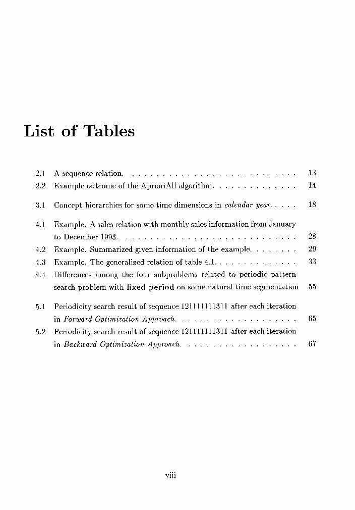
List of Tables
A sequence relation. . . . . . . . . . . . . . . . . . . . . . . . . . . . Example outcome of the AprioriAll algorithm. . . . . . . . . . . . . .
Concept hierarchies for some time dimensions in calendar year. . . . .
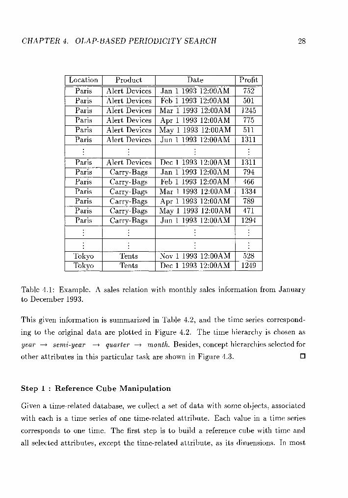
Example. A sales relation with monthly sales information from January
to December 1993. . . . . . . . . . . . . . . . . . . . . . . . . . . . . Example. Summarized given information of the example. . . . . . . . Example. The generalized relation of table 4.1. . . . . . . . . . . . . . Differences among the four subproblems related to periodic pattern
search problem with fixed period on some natural time segmentation
Periodicity search result of sequence 121 11 11 1131 1 after each iteration
in Forward Optimization Approach. . . . . . . . . . . . . . . . . . . . Periodicity search result of sequence 121 11 11 1131 1 after each iteration
in Backward Optimization Approach. . . . . . . . . . . . . . . . . . .
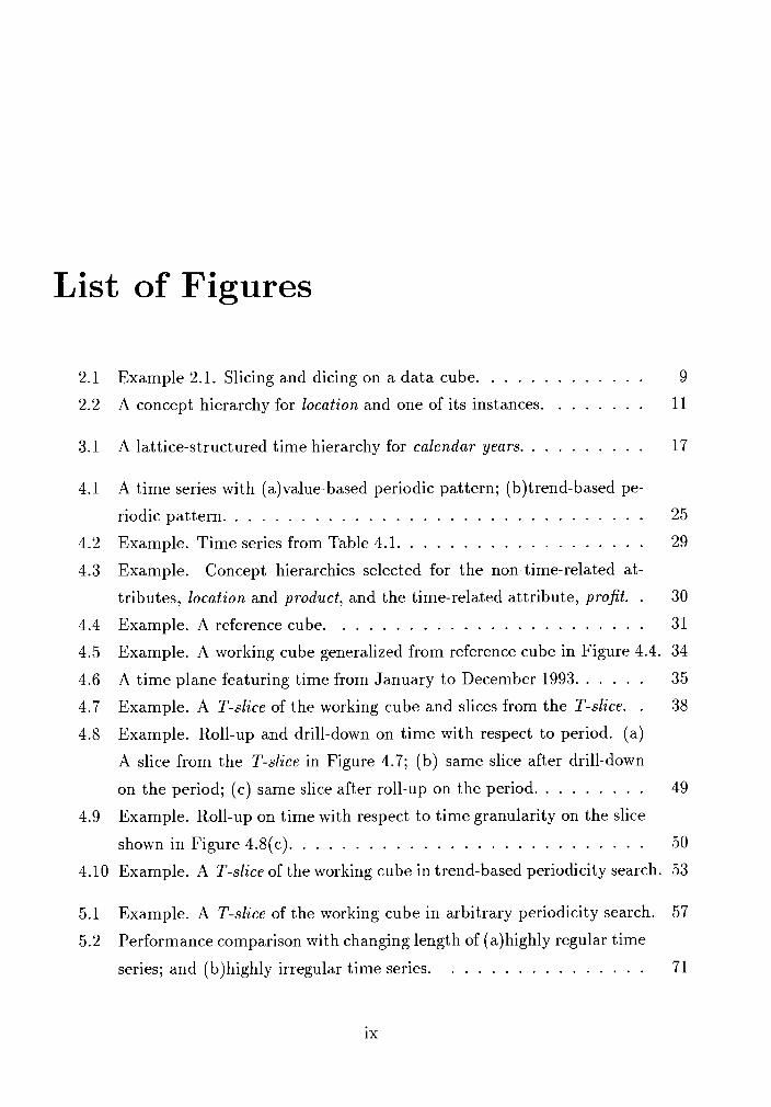
List of Figures
Example 2.1. Slicing and dicing on a data cube. . . . . . . . . . . . . 9
A concept hierarchy for location and one of its instances. . . . . . . . 11
A lattice-structured time hierarchy for calendar years. . . . . . . . . . 17
A time series with (a)value-based periodic pattern; (b)trend-based pe-
riodic pattern. . . . . . . . . . . . . . . . . . . . . . . . . . . . . . . . 25
Example. Time series from Table 4.1. . . . . . . . . . . . . . . . . . . 29
Example. Concept hierarchies selected for the non-time-related at-
tributes, location and product, and the time-related attribute, profit. . 30
Example. A reference cube. . . . . . . . . . . . . . . . . . . . . . . . 31
Example. A working cube generalized from reference cube in Figure 4.4. 34
A time plane featuring time from January to December 1993. . . . . . 35
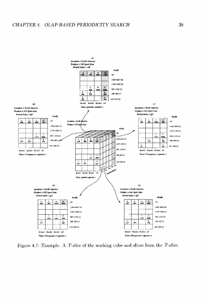
Example. A T-slice of the working cube and slices from the T-slice. . 38
Example. Roll-up and drill-down on time with respect to period. (a)
A slice from the T-slice in Figure 4.7; (b) same slice after drill-down
on the period; (c) same slice after roll-up on the period. . . . . . . . . 49
Example. Roll-up on time with respect to time granularity on the slice
shown in Figure 4.8(c). . . . . . . . . . . . . . . . . . . . . . . . . . . 50
Example. A T-slice of the working cube in trend-based periodicity search. 53
Example. A T-slice of the working cube in arbitrary periodicity search. 57
Performance comparison with changing length of (a) highly regular time
series; and (b)highly irregular time series. . . . . . . . . . . . . . . . 71
5.3 Performance comparison with changing positions of irregularity. . . . 74
5.4 Performance comparison with changing maximum pattern length on
(a)highly regular time series; and (b)highly irregular time series. . . 76
5.5 The experimental result of the three modified approaches with respect
to (a) location of irregularity occurrences in regular time series; (b)
varying lengths of regular time series; (c) varying lengths of irregu-
lar time series; (d) varying maximum pattern lengths on regular time
series; and (e) varying maximum pattern lengths on irregular time series. 82
Chapter 1
Introduction
Time is an important aspect of all real-world phenomena. Conventional databases
model an enterprise as it changes dynamically by a snapshot at a particular point
in time. As information is updated in a conventional database, its old, out-of-date
data is discarded forever, its changes over time are thus lost. But in many situations,
this snapshot-type of database is inadequate. They cannot handle queries related to
any historical data. For many applications such as accounting, banking, econometrics,
geographical information systems, medical record bookkeeping, etc., the changes made
on their databases over time are a valuable source of information which can direct their
future operation. Due to the importance of the time-varying data, efforts have been
made to design temporal databases which support some aspect of time. While lots
of theories have been published, temporal database design still remains in its infancy,
hindered by the plethora of temporal data models and the absence of real-time data
models [35] .
In this thesis, we mainly focus on relational databases with historical data or, in
other words, time-related data. We refer to such databases as time-related databases.
1.1 Time-Related Databases
There are numerous time concepts proposed to date for information preservation in
temporal databases. Some, such as valid t i m e [36] and logical t i m e [ll], denote the
C H A P T E R 1. INTRODUCTION 2
time a fact was true in reality [35]; opposed to them is the transaction time [36],
representing the time the information was entered into the database. Besides these
two concepts which are of general interest, there are also user-defined time, which
indicates the semantics of the time values which are known only to the user, and
decision time [ll], which is the time a decision occurred, etc. We can also describe a
time as absolute or relative. Moreover, the semantics of each of these time concepts
also depends on whether a relation models events or intervals.
A temporal database model may support one or more of the time concepts we men-
tioned. Our interest here lies on databases which model events. In these databases,
each tuple in a relation corresponds to an event at one point of time. For example, ev-
ery record in a sales registration relation refers to a transaction made by a customer
at this particular time. The event represented by this tuple is only valid in time
recorded in the tuple. Such a relation models events instead of intervals in which case
an event represented by a tuple remains valid until next time the tuple is updated.
To simplify the problem further, we also restrict our time-related databases to
support only one time concept of the time domain. We assume that this time concept
serves the purposes of both transaction time and valid time. Therefore, each event
denoted by a tuple in a relation is associated with one time-stamp.
To summarize, the time-related databases we focus on are, in fact, relational
databases with time-related data which model events. The time domain in our sim-
plified time-related database model has one time concept set on top of the assumption
that transaction time and valid time coincide.
We try to extract from time-related databases some useful knowledge that could
provide user some future guidance, to which end techniques in knowledge discovery
and data warehousing become important.
CHAPTER 1. INTRODUCTION 3
1.2 The Role of OLAP in Databases and Data Ware-
housing
Knowledge discovery and data warehousing have been increasingly important in han-
dling and analyzing large databases efficiently and effectively. Among all the tech-
niques applied in knowledge discovery and data warehousing, the most popularly used
tools are on-line analytical processing (OLAP) tools.
OLAP is a terminology for data generalization or abstraction. It is a technol-
ogy that uses a multidimensional view of aggregate data to provide quick access to
strategic information for further analysis [27]. The raw data in a database usually
represents information in its most primitive concept level. If knowledge is extracted
from and expressed using the raw data, it is often not meaningful enough for user
to comprehend. Therefore, using OLAP techniques, raw data from large databases
is generalized to higher levels in order to attain more meaningful and more useful
knowledge. The data generalization can be achieved through approaches such as data
cube [20, 25, 38, 411 and attribute-oriented induction [21, 231.
In this thesis, we will take advantage of the existing on-line analytical processing
techniques widely used in knowledge discovery and data warehousing, and apply them
on time-related data for useful knowledge which can lead towards solutions to some
interesting problems such as job dispatch, pattern discovering, similarity search, etc.
Time-Related OLAP : Area of Applications
Many enterprises such as bank, telephone company, hospital, stock market, etc. keep
the historical data as their essential source of information. Time-related OLAP is
undoubtedly a favorable solution to analyze such a large pool of data. There is much
valuable knowledge that we can discover from this rich source of data which can
sometimes be used to solve some very complicated problems.
Time-Related Job Dispatch
Job dispatch is one such complicated problem. Enterprises, such as bank, have
CHAPTER 1. INTRODUCTION
collected tremendous amount of data on service, customer, department, and em-
ployee information. A common problem that every manager of a bank branch
may face is job dispatch - how to allocate the resources available at a time for
high efficiency and high quality in serving the customers. We need a way to dig
from a large set of data the critical time periods for a particular branch, the
different types of services required at individual departments within these peri-
ods, the available resources and personnel with certain expertise to be allocated,
etc. Time-related OLAP can provide an effective way to locate the critical time
periods and summarize them in a generalized format that can reveal periodi-
cal patterns as well. The allocation of resources based on these critical periods
needs some scheduling techniques, but time-related OLAP can also provide some
guidance.
Regularities of Time-Related Data Change
Certain data need to be updated either because time has changed and it has
dominating influence over the data, or because some other data has changed due
to the change in time. For example, the increasing in number of tourists in a city
will result in an increase in revenue, while the number of tourists changes over
seasons. Such regularities of time-related data change can easily be detected by
finding the association among time and all time-related fields.
Trend Pattern Directed Search
Many time-related databases can also be characterized as time-series databases.
For such a database, associated with each time-related field is a set of sequences
of real values. These sequences constitute a set of curves over the time. The
patterns discovered from some of these databases mainly serve for the purpose of
indicating the trend or performance of objects contained in them, such as sales
databases. The patterns thus found are called trend patterns. Time-related
OLAP techniques can be used here to generalize the curves consisting of real
values to higher level concepts. From the generalized description of each curve,
we can further categorize and classify the curves into different patterns. For
example, we may find a pattern discribing the sales trend of certain product

CHAPTER 1. INTRODUCTION 5
during a period of time to be up-down-up. The patterns discovered will be used
for future reference on other curves to recognize their trend, performance, and
SO on.
Periodic Pattern Directed Search
Another type of time-series database contains data hidden in which are periodic
patterns. One example is the data collected in an electrocardiogram. We can
again apply OLAP techniques to find the periodic patterns for future reference.
As for the electrocardiogram application, a mismatch in the periodic pattern
discovered can mean a heart failure. The difference between this and the pre-
vious problem is that, in the periodic pattern directed search, the emphasis is
on repeating behaviors of a time series, while this periodicity concern is not an
element in the previous trend pattern directed search.
Similarity Analysis
Last, but not least, is the similarity analysis among sequences in time-series
databases. The purpose of this research topic is to find time sequences that are
similar to a given sequence or to be able to find all pairs of similar sequences
12, 3, 41.
Despite the great variety of problems related to the above-mentioned research
area, our interest in this thesis, however, is specifically devoted to the periodic pattern
discovery from time-related databases.
Periodic Pat tern Discovery
Problems related to periodicity search is stated as problems of finding patterns oc-
curring at regular intervals. Literally, the concept emphasizes on two aspects of the
problem, namely, pattern and interval. Thus, given a sequence of events, we would
like to find the patterns which repeat over time and their recurring intervals (period).
For instance, given a sales database which records sales information of a company over
a period of ten years, we may be asked to find out if there is a yearly sales pattern in
C H A P T E R 1. INTRODUCTION 6
these ten years, based on the monthly summarized data. After some analysis, we may
find that the revenue of certain products reaches their yearly maximum each July.
This is a periodic pattern. However, sometimes patterns do not repeat in a naturally
segmented time interval such as hourly, daily, monthly, etc. The electrocardiogram
is one such example. A person's heart does not often beat in a period describable
by intervals in minute, hour, or so. Therefore, another type of question one may ask
given the sales database is to find out the repeating patterns of a sequence as well as
the interval which corresponds to the pattern period.
Organization of Thesis
The rest of the thesis is organized as follows. Chapter 2 outlines some existing work
related to the thesis. The problem definition will be given in Chapter 3 along with
some properties associated with periodic time series. We will try to solve two peri-
odicity search problems. One is finding periodic behaviors with fixed period length,
and the other with arbitrary period length. The approaches towards solving these
two problems will be presented in Chapters 4 and 5 . The algorithms will be presented
and the experimental results will be analyzed in the two chapters. Some discussion
will conclude the thesis in Chapter 6.
Chapter 2
Related Work
The problem of finding periodic patterns in a time-related large database involves
two major concerns. In real-world applications, data mining tasks are applied to
data consisting of thousands or millions of tuples. When temporal components are
involved in a mining task, the size of the interested data could increase to an even
larger size. Consequently, efficiency in handling large databases is our first concern
to substantially reduce the computational complexity of this data intensive process.
Furthermore, we need a fast and effective algorithm to find periodic patterns in a
given time sequence. In this chapter, we will introduce some works related to these
two aspects.
2.1 Data Warehousing and OLAP Techniques
A data warehouse is a subject-oriented, integrated, time-variant, and nonvolatile col-
lection of data in support of management's decision-making process [28]. Since data
warehouses contain large volumes of consolidated data over long periods of time, its
content is more important than detailed, individual records as in conventional oper-
ational databases, and is hence targeted for decision support.
The construction of data warehouses [30], with data cleaning and data integra-
tion, can be viewed as an important preprocessing step for knowledge discovery tasks.
CHAPTER 2. RELATED WORK
Moreover, data warehouse provides OLAP(on-line analytical processing) tools for in-
teractive analysis of data from multiple dimensions with varied granularity, which
facilitates effective knowledge discovery as well. Thus, data warehousing and OLAP
techniques form a foundation for effective data mining. In [12], a detailed introduction
of data warehousing and OLAP technology is presented.
The data in a data warehouse are typically organized in a multidimensional model
which influences the query engines for OLAP. Such a multidimensional data model is
referred to as a data cube 1191.
In a data cube, there is a set of numeric measures that are the objects of analysis.
Each of these measures is uniquely determined by a set of dimensions that provide the
context of the measure. Each dimension is, in turn, described by a set of attributes
[la].
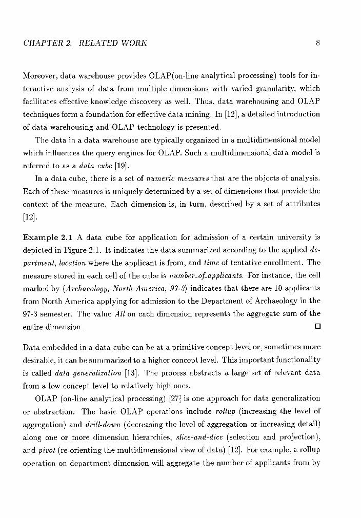
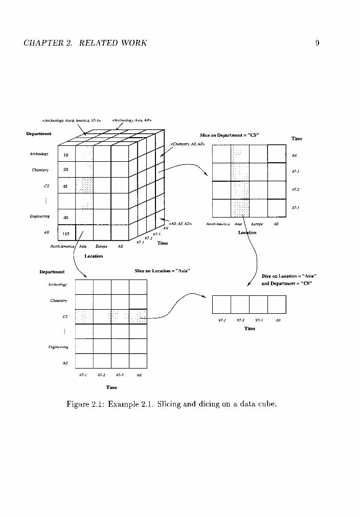
Example 2.1 A data cube for application for admission of a certain university is
depicted in Figure 2.1. It indicates the data summarized according to the applied de-
partment, location where the applicant is from, and time of tentative enrollment. The
measure stored in each cell of the cube is number-of-applicants. For instance, the cell
marked by (Archaeology, North America, 97-3) indicates that there are 10 applicants
from North America applying for admission to the Department of Archaeology in the
97-3 semester. The value All on each dimension represents the aggregate sum of the
entire dimension.
Data embedded in a data cube can be at a primitive concept level or, sometimes more
desirable, it can be summarized to a higher concept level. This important functionality
is called data generalization [13]. The process abstracts a large set of relevant data
from a low concept level to relatively high ones.
OLAP (on-line analytical processing) [27] is one approach for data generalization
or abstraction. The basic OLAP operations include rollup (increasing the level of
aggregation) and drill-down (decreasing the level of aggregation or increasing detail)
along one or more dimension hierarchies, slice-and-dice (selection and projection),
and pivot (re-orienting the multidimensional view of data) [12]. For example, a rollup
operation on department dimension will aggregate the number of applicants from by
CHAPTER 2. RELATED WORK
drcheolog): North America 97-3> <Archeology, Asto, All> \ /
Department Slice on Department = "CS"
hemrsn) AIL All>
Archeology
Chemrsny
cs
Engmeenng
All
N o
Time
A11
97-3
Location
Department Slice on Location = "Asia" Dice on Location = "Asia"
Archrology and Department = "CS"
Chemistry
CS Din 97-1 97-2 97-3 AN
Time
Engineering
All
97-1 97-2 97-3 AN
Time
Figure 2.1: Example 2.1. Slicing and dicing on a data cube.
CHAPTER 2. RELATED W O R K 10
department to by school. On the other hand, a drill-down on location dimension,
which specializes the aggregations on the number of applicants from by area to by
country, will give more detailed information on where the applications are from. The
difference between slicing and dicing is that slicing is selection on one dimension, while
dicing is on more than one dimension. Examples of slicing and dicing are shown in
Figure 2.1.
OLAP engines demand a fast processing on the large volume of data contained in
data warehouse, this requires highly efficient cube computation and query processing
techniques. Many methods have been proposed for efficient data warehouse implemen-
tation. Some powerful query optimization techniques are introduced to materialize
certain expensive computations frequently inquired and store the materialized sum-
mary data in the data warehouse. The selection of views to materialize must take
into account workload characteristics, the costs of incremental update, and upper
bounds on storage requirement [12]. [25] presents a greedy algorithm for selection of
the materialized views that was shown to have good performance. Several efficient
algorithms for both relational and multidimensional OLAP have also been developed
to compute the materialized views [l, 19, 421.
Another approach for data generalization is attribute-oriented induction. This
approach takes a data mining query expressed in an SQL-like data mining querying
language and collects the set of relevant data in a data set. Data generalization is
then performed on the set of relevant data by applying a set of data generalization
techniques [21, 23, 311 including attribute-removal, concept-tree climbing, attribute-
threshold control, propagation of counts and other aggregate function values, etc.
[21, 23, 131. The generalized data is expressed in the form of a generalized relation
on which many other operations or transformations can be performed to transform
generalized data in different kinds of knowledge or map them into different forms [23].
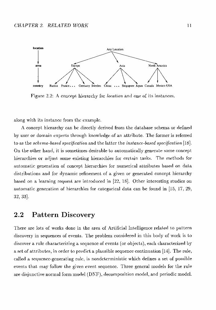
The essential background knowledge applied in data generalization is concept hi-
erarchy associated with each dimension [21]. A concept hierarchy is a tree or lattice
structure that organizes concepts in a database into a partial order such that those
in levels closer to the root are more general than those closer to the leaf nodes. A
concept hierarchy for attribute location in Example 2.1 is demonstrated in Figure 2.2
CHAPTER 2. RELATED WORK
location Any Location
I area , A A A
country Russia France. . . Germany Sweden China . . . Singapore Japan Canada Mexico USA
Figure 2.2: A concept hierarchy for location and one of its instances.
along with its instance from the example.
A concept hierarchy can be directly derived from the database schema or defined
by user or domain experts through knowledge of an attribute. The former is referred
to as the schema-based specification and the latter the instance-based specification 1181.
On the other hand, it is sometimes desirable to automatically generate some concept
hierarchies or adjust some existing hierarchies for certain tasks. The methods for
automatic generation of concept hierarchies for numerical attributes based on data
distributions and for dynamic refinement of a given or generated concept hierarchy
based on a learning request are introduced in [22, 181. Other interesting studies on
automatic generation of hierarchies for categorical data can be found in [15, 17, 29,
32, 331.
Pattern Discovery
There are lots of works done in the area of Artificial Intelligence related to pattern
discovery in sequences of events. The problem considered in this body of work is to
discover a rule characterizing a sequence of events (or objects), each characterized by
a set of attributes, in order to predict a plausible sequence continuation [14]. The rule,
called a sequence-generating rule, is nondeterministic which defines a set of possible
events that may follow the given event sequence. Three general models for the rule
are disjunctive normal form model (DNF), decomposition model, and periodic model.
CHAPTER 2. RELATED WORK
It apparently appears to be a more complex problem than the one we are handling.
For our work, the focus is solely on the periodic model. There is only one attribute
characterizing a given time sequence, the value or the shape of the sequence.
Another active research area is finding text subsequences that match a given reg-
ular expression, or finding text subsequences that approximately match a given string
[39, 41. This problem, however, does not take into account the periodic behavior of
a sequence, rather, the techniques used in this problem are oriented towards finding
matches for one pattern. In our problem, on the other hand, there is no given pat-
tern, instead, we have to find a way to search for the periodic pattern embedded in a
sequence.
In another type of pattern matching problem called similarity search [2, 4, 8, 161,
we try to compare two sequences to see if they are entirely [2, 41 or locally similar
[16]. The problem deals with comparing two sequences in parallel to discover the
commonalities within, while in the problem of periodicity search, we deal with finding
commonalities within all equal-period, consecutive, exclusive intervals with respect to
one sequence. A more detailed survey on the similarity search problem can be found
in [13].
Our problem is related to the problem of finding sequential patterns [6, 71. Given
a database of customer transactions, the problem of mining sequential patterns is to
find the maximal sequences among all sequences that have a certain user-specified
minimum support. Equivalently, we can consider this problem for more general cases.
For example, a sequence relation is shown in Table 2.1. If the minimum support
is set to 25%) i.e., a minimum support of 2 sequences in this case, the sequences
1234 and 15 are among those satisfying the support constraint since they occur in
that order in at least two of the customer sequences in Table 2.1. The two are
thus desired sequential patterns. We call a sequence satisfying the minimum support
constraint a large sequence. So besides the two sequential patterns, 1, 2, 34, etc.
are all large sequences even though they are not maximal. Moreover, a sequence is
called n-sequence if its length is n. While this problem takes into account neither the
periodic behavior of a sequence nor the pattern within one single sequence, some of
the techniques proposed in [7] are used in our research to deal with the OLAP-based
CHAPTER 2. RELATED WORK
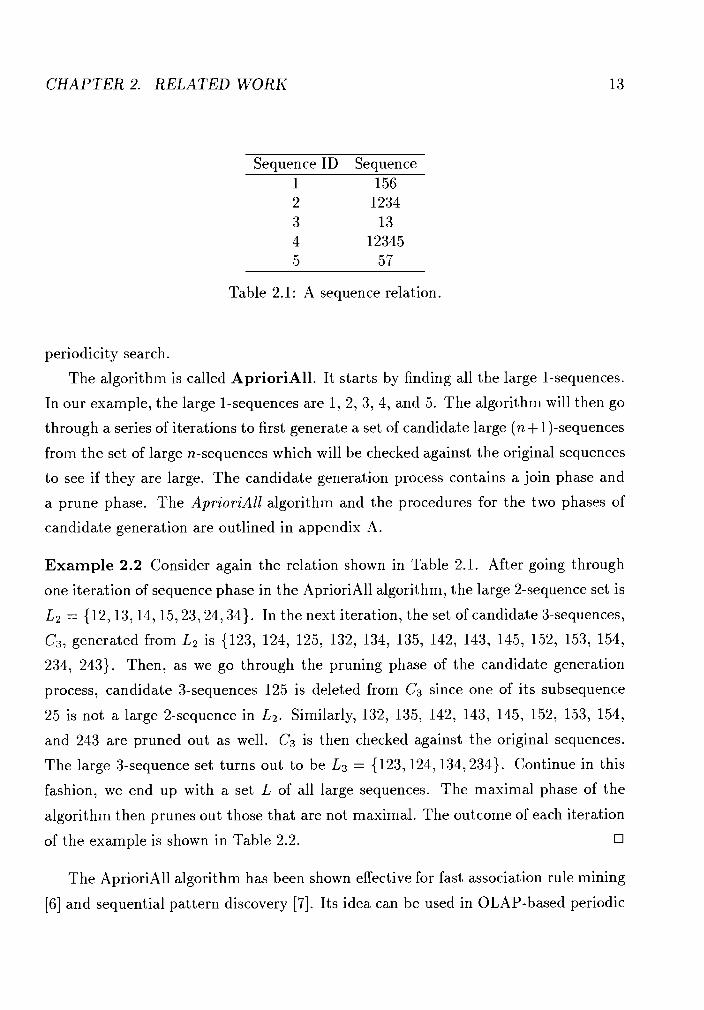
Sequence ID Sequence
Table 2.1: A sequence relation.
periodicity search.
The algorithm is called AprioriAll. It starts by finding all the large 1-sequences.
In our example, the large 1-sequences are 1, 2, 3, 4, and 5. The algorithm will then go
through a series of iterations to first generate a set of candidate large (n+ 1)-sequences
from the set of large n-sequences which will be checked against the original sequences
to see if they are large. The candidate generation process contains a join phase and
a prune phase. The AprioriAEl algorithm and the procedures for the two phases of
candidate generation are outlined in appendix A.
Example 2.2 Consider again the relation shown in Table 2.1. After going through
one iteration of sequence phase in the AprioriAll algorithm, the large 2-sequence set is
L2 = {12,13,14,15,23,24,34). In the next iteration, the set of candidate 3-sequences,
C3, generated from L2 is (123, 124, 125, 132, 134, 135, 142, 143, 145, 152, 153, 154,
234, 243). Then, as we go through the pruning phase of the candidate generation
process, candidate 3-sequences 125 is deleted from C3 since one of its subsequence
25 is not a large 2-sequence in L2. Similarly, 132, 135, 142, 143, 145, 152, 153, 154,
and 243 are pruned out as well. C3 is then checked against the original sequences.
The large 3-sequence set turns out to be L3 = (123,124,134,234). Continue in this
fashion, we end up with a set L of all large sequences. The maximal phase of the
algorithm then prunes out those that are not maximal. The outcome of each iteration
of the example is shown in Table 2.2. 0
The AprioriAll algorithm has been shown effective for fast association rule mining
[6] and sequential pattern discovery [7]. Its idea can be used in OLAP-based periodic
CHAPTER 2. RELATED WORK 14
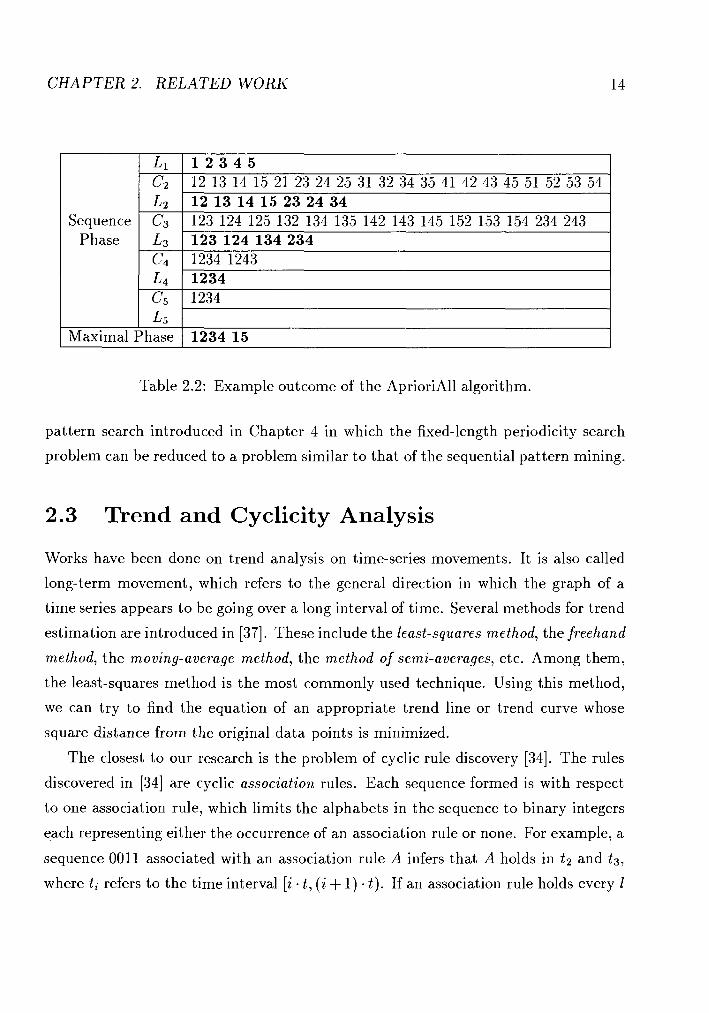
Sequence Phase
Table 2.2: Example outcome of the AprioriAll algorithm.
I L5
Maximal Phase
pattern search introduced in Chapter 4 in which the fixed-length periodicity search
problem can be reduced to a problem similar to that of the sequential pattern mining.
L1 C2 L2 C3 L3 C4 L4 Cs
1234 15
2.3 Trend and Cyclicity Analysis
1 2 3 4 5 12 13 14 15 21 23 24 25 31 32 34 35 41 42 43 45 51 52 53 54 12 13 14 15 23 24 34 123 124 125 132 134 135 142 143 145 152 153 154 234 243 123124134234 1234 1243 1234 1234
Works have been done on trend analysis on time-series movements. It is also called
long-term movement, which refers to the general direction in which the graph of a
time series appears to be going over a long interval of time. Several methods for trend
estimation are introduced in [37]. These include the least-squares method, the freehand
method, the moving-average method, the method of semi-averages, etc. Among them,
the least-squares method is the most commonly used technique. Using this method,
we can try to find the equation of an appropriate trend line or trend curve whose
square distance from the original data points is minimized.
The closest to our research is the problem of cyclic rule discovery [34]. The rules
discovered in [34] are cyclic association rules. Each sequence formed is with respect
to one association rule, which limits the alphabets in the sequence to binary integers
each representing either the occurrence of an association rule or none. For example, a
sequence 0011 associated with an association rule A infers that A holds in t2 and t3,
where ti refers to the time interval [i . t , (i + 1) - t ) . If an association rule holds every 1
CHAPTER 2. RELATED WORK 15
time units starting from ti, we say that the association rule has some cyclic behavior.
The cycle of this association rule is denoted by (I, i) .
In their study, Ozden et. al. revealed some properties of cyclic sequences, and
used these properties to discover rules that display regular cyclic variation over time
with respect to a given sequence. Some very useful properties are shown as follows.
Property 1. If an itemset X has a cycle (l,i), then any subset of X has the cycle
(17 i).
In this rule, an itemset refers to a set of items which are contained in a given sequence.
Suppose there are two items xl, x2, in X. If X has a cycle (4, O), i.e. if it repeats
every fourth time units starting from to, then this implies that xl and x2 will have
this cycle as well.
Property 2. For any cycle (1, i), its multiple (It, it), where 1 11'(11 is divisible by 1) and
i = i' mod 1, is also a cycle. Thus, only those cycles that are not multiples of other
cycles are interesting to us.
These rules are used as foundations of some techniques employed in cyclic as-
sociation rule mining. These techniques include cycle-pruning, cycle-skipping, and
cycle-elimination. The general idea of these optimization techniques is that we do
not have to check for cyclicity for each itemset, rather, we can use some rules (or
properties) of the cyclic sequences to reduce the search space. Some of these and the
other properties will be introduced later in more detail. They will be employed as
essential parts of our algorithms (see Chapter 5 ) . The periodicity search problem can
thus be considered as a superset of cyclic rule discovery problems.
Chapter 3
Problem Statement
Periodicity search is a problem of finding repeating patterns in some given sequences
of time-related data. Based on different interest, user may prefer to ask the question
concerning periodicity differently. Some are interested at the periodicity with respect
to a fixed period length, while others may simply want to know if a sequence has
any periodicity at all. These problems will be discussed further in the following
two chapters. But first, we give some definitions so that a clear description of the
periodicity search problem can be outlined.
3.1 Time
We introduced earlier some time concepts such as transaction time, valid time, deci-
sion time, etc. These are the time concepts in a macro view. Here, we narrow our
interest down to a much smaller time domain - one which regards the time in real
world and the database world as one concept. So the time attributes used in all the
examples of this thesis can be considered as representing both the valid time for the
records and the transaction time when these events are recorded.
The idea of a time hierarchy is to classify the time domain into different concepts
and organize them into hierarchical structures so that OLAP operations can be oper-
ated on time efficiently. Just like most other concept hierarchies, the representation
of time hierarchy may vary in different context. For example, time can be represented
C H A P T E R 3. PROBLEM STATEMENT
month
Year - quarter d a y h o u r m i n u t e second
wee,
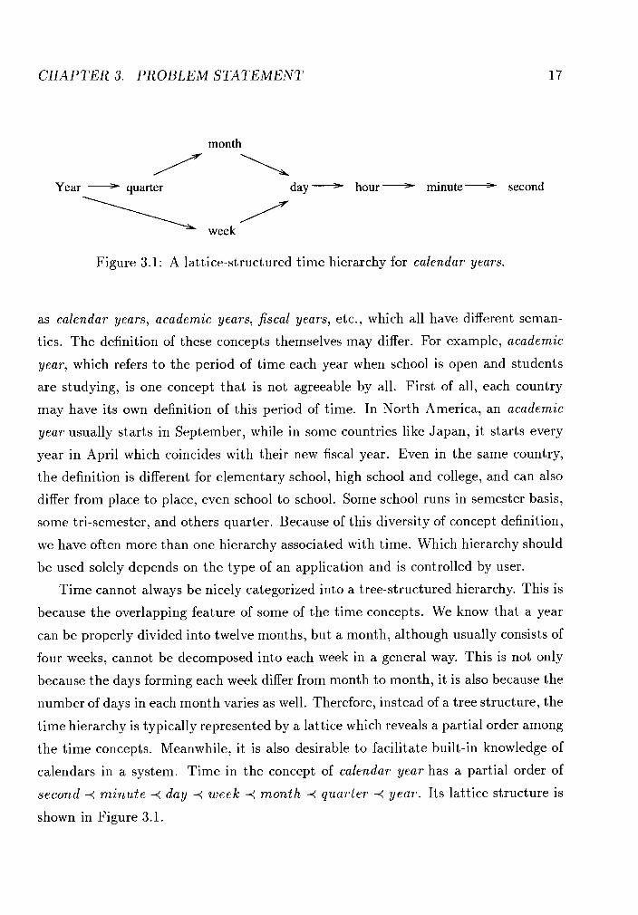
Figure 3.1: A lattice-structured time hierarchy for calendar years.
as calendar years, academic years, fiscal years, etc., which all have different seman-
tics. The definition of these concepts themselves may differ. For example, academic
year, which refers to the period of time each year when school is open and students
are studying, is one concept that is not agreeable by all. First of all, each country
may have its own definition of this period of time. In North America, an academic
year usually starts in September, while in some countries like Japan, it starts every
year in April which coincides with their new fiscal year. Even in the same country,
the definition is different for elementary school, high school and college, and can also
differ from place to place, even school to school. Some school runs in semester basis,
some tri-semester, and others quarter. Because of this diversity of concept definition,
we have often more than one hierarchy associated with time. Which hierarchy should
be used solely depends on the type of an application and is controlled by user.
Time cannot always be nicely categorized into a tree-structured hierarchy. This is
because the overlapping feature of some of the time concepts. We know that a year
can be properly divided into twelve months, but a month, although usually consists of
four weeks, cannot be decomposed into each week in a general way. This is not only
because the days forming each week differ from month to month, it is also because the
number of days in each month varies as well. Therefore, instead of a tree structure, the
time hierarchy is typically represented by a lattice which reveals a partial order among
the time concepts. Meanwhile, it is also desirable to facilitate built-in knowledge of
calendars in a system. Time in the concept of calendar year has a partial order of
second 4 minute 4 day 4 week 4 month 4 quarter 4 year. Its lattice structure is
shown in Figure 3.1.
CHAPTER 3. PROBLEM STATEMENT 18
Time Dimension
Year
Concept Hierarchies
year -+ quarter -+ month
month
I 1 week -+ day I
year -+ week month -+ half-month
week
I
day I day -+ {morning, afternoon) -+ hour
month + week week -+ {weekdays, weekend) -+ day
I day -+ {before-work, work hours, after-work) -+ hour
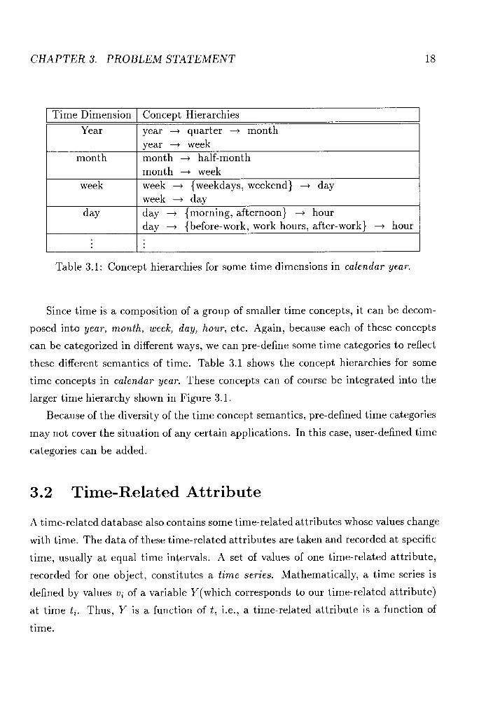
Table 3.1: Concept hierarchies for some time dimensions in calendar year.
Since time is a composition of a group of smaller time concepts, it can be decom-
posed into year, mon th , week, day, hour , etc. Again, because each of these concepts
can be categorized in different ways, we can pre-define some time categories to reflect
these different semantics of time. Table 3.1 shows the concept hierarchies for some
time concepts in calendar year. These concepts can of course be integrated into the
larger time hierarchy shown in Figure 3.1.
Because of the diversity of the time concept semantics, pre-defined time categories
may not cover the situation of any certain applications. In this case, user-defined time
categories can be added.
Time-Related Attribute
A time-related database also contains some time-related attributes whose values change
with time. The data of these time-related attributes are taken and recorded at specific
time, usually at equal time intervals. A set of values of one time-related attribute,
recorded for one object, constitutes a t i m e series. Mathematically, a time series is
defined by values v; of a variable Y(which corresponds to our time-related attribute)
at time ti. Thus, Y is a function of t, i.e., a time-related attribute is a function of
time.
CHAPTER 3. PROBLEM STATEMENT 19
When we plot the time series onto a graph with time vs. the time-related attribute,
we obtain a curve that indicates the trend of the time-related attribute with respect to
the selected object. We call such a time-series value-based. When we analyze value-
based time series, we usually emphasize on the absolute value of the time-related
attribute at different time or at the same time with different objects. Examples such
as "more revenue is generated in January than in February" and "more profit was
produced on product A than on product B in January" are answers to some questions
directed to value-based time series.
Sometimes, value-based time series do not necessarily give us clear information on
the performance or the trend of an object. Instead of analyzing time-related data at
a given time, we are more interested at the data over a range of time. In other words,
we would like to see the relative changes of data for a period of time interval, which
is indicated by the slope of the curve between two time unit. The time series thus
obtained is referred to as trend-based. Sample facts attained from such time series
include "the production increases faster in the first quarter than in the second quarter"
and "the daily temperature changes more dramatically in B.C than in Ontario during
summer".
Both value-based and trend-based time series mentioned above deal with actual
values(raw data) of the interested time-related attribute. This is necessary if we
want to use signal processing techniques to analyze very low level data for relatively
accurate result [9]. However, it is not always essential to achieve such high accuracy.
Users are often interested at only the rough shape of a time series. For example, the
salary difference between $80,000 and $90,000, though large, may mean little to some
people, who usually consider the two to be at the same salary level. Therefore, concept
hierarchy can be used to generalize the original data to correspond more closely to
user's interpretation of the data. Moreover, generalizing data to higher level concepts
also provides more meaningful versions to the data. When high accuracy is not an
indispensable requirement, or when a more expressive notion is desired for the values
of a time-related attribute, concept hierarchies can be used to significantly reduce the
processing time.
C H A P T E R 3. PROBLEM STATEMENT 2 0
Concept hierarchies, as mentioned in Chapter 2, can either be generated automat-
ically or defined by user. Once a concept hierarchy has been chosen for a time-related
attribute, the values in a time series can be mapped to their corresponding concept
indices in the hierarchy. The mapping produces a new index string which we refer to
as time sequence. The sequence is used in actual searching process.
Periodic Patterns
We talked about time and time-related attribute, two concepts most related to our
periodic pattern searching problem. The algorithms outlined in this thesis are all
based on the following assumptions.
Assumption 3.3.1 The input time series are all the same length with equal time
intervals.
Assumption 3.3.2 The time series are smoothed before periodicity analysis.
Assumption 3.3.3 Only rough periodicity matching is required.
Under these assumptions, no preprocessing is necessary to smooth the curves ob-
tained by plotting a time series, and we can use OLAP techniques on the time series,
with the help of concept hierarchies, to discover periodicities.
Given a time series, we denote the ith time as t i , i 20. The value of ti is ti = i . t , where t is the time unit referrring to the time granularity. We use Ti to denote the
i th time unit. That is, Ti is mapped to the time interval [ti, where i 20. For
any time series, the i th and the j th time units are called similar with respect to a
time-related attribute if the time-related attribute values at these two time units fall
into the same category according to the chosen concept hierarchy. A cycle is formed
if, thoughout the whole time series, there exist equally-spaced similar time units with
respect to some time-related attribute. Here is a formal definition for cycle.
Definition 3.3.1 For any given time series whose length is n, i f 31, o E Z, 0 5 1 < n
and 0 5 o < 1 where V s E Z,O 5 s 5 rill, the (I - s + o)th time units are all similar
CHAPTER 3. PROBLEM STATEMENT 2 1
with respect to the time series, we call this a cycle, denoted by C = (1, o, V ) , where
1 is the length of the cycle, o the oflset indicating the first time at which the cycle
occurs, and V the concept category of the values that form the cycle.
When the length of the cycle is known, the cycle can be denoted in a shorter term as
c = (0, V ) .
Example 3.1 Suppose we have a time series whose sequence, after mapping the
values into their corresponding categories, is 132113412341. We find that, starting
from time t l , every fourth bit in the sequence repeats the value at t l , which is 3. Thus
we have found a cycle with length 4 and offset l(corresponding to t l ) whose value
belongs to category 3, denoted by (4, 1, 3). The cycle sequence is represented as *3**.
Similarly, we also find cycles (4, 3, 1) and (6, 2, 2).
A periodic pattern is the union of a set of cycles. For example, the sequence given
in the previous example has pattern sequences *3*1 and **2***, where pattern *3*1
is the union of cycles (4, 1, 3) and (4, 3, 1).
Definition 3.3.2 For any given time series whose length is n, if for some l , m E 2,
0 5 1 < n and m > 0 , 3 m cycles C; of length I, 0 5 i < m, then what these m cycles
formed is a periodic pattern with length 1. The pattern is denoted by
P = (1, m, C), where C = { (o ; , x)IC; = ( I , o;, x) V 0 5 i < rn) If the number of cycles i n a pattern equals to the pattern length, we refer to such a
pattern as a complete periodic pattern which can be represented by the pattern
sequence itself. The general type of periodic pattern is consequently referred to as
partial periodic pattern.
The patterns *3*1 and **2*** in the previous example can thus be denoted by (4,
2, ((1, 3), (3, 1))) and (6, 1, ((2, 2))) respectively. Since not all time units in these
patterns have a cycle, they are partial periodic patterns. If, presumably, we find a
pattern (3, 3, ((0, I ) , (1, 2), (2, 3))), whose corresponding sequence string is 123,
then we call such a pattern a complete pattern.
CHAPTER 3. PROBLEM STATEMENT 22
Note that, if we have a cycle (2, 0, l), this implies (4, 0, I ) , (6, 0, 1)) etc. are all
cycles as well. In other words, if there is a cycle C1 = ( 1 , o, V ) , then C2 = ( I S , 0, V ) is also a cycle for any s > 0. We refer to C2 as a multiple of C1, which can be
derived from Cl without any searching through a time sequence. The discovery of
these cycles does not give us any further information about the time series. Similarly,
several periodic patterns merging together or one periodic pattern repeating multiple
times can produce new periodic patterns as well. All these derived patterns and cycles
are not of our concern.
Definition 3.3.3 Given a cycle C = ( 1 , o, V ) , and periodic patterns P = ( I , m, C),
Pl = (11 , ml , C1) and P2 = (12 , m2, C 2 ) their derivatives are the following.
1) A multiple of C is a cycle whose length is a multiple of that of C and whose oflset
and category are the same as in C , denoted by C t = C s = ( I - s , o, V ) .
2) A multiple of P is a periodic pattern whose corresponding pattern sequence can
be represented as the pattern sequence of P repeating multiple times. The multiple
pattern is denoted by P' = P . s = ( l . s , m - s , C f ) , where C' = { ( o ; + l . t , V,)l(o;, V , ) E C,
VO < i < m and 0 5 t < s ) .
3) The product of Pl and P2 is P' = Pl.P2 = ( lcm( l l , 1 2 ) , mt,C'), whereCf= {(oi+ll .
t ,V , ) I (o; ,K) E C I , VO < i < m and 0 < t < l ~ m ( 1 ~ , 1 ~ ) / 1 ~ ) U { ( o ; + l ~ ~ t , V , ) ~ ( o ; , V , ) E C2,
VO 5 i < m and 0 < t <lcm(ll , 12)/11), and m' is the cardinality of C'. CI
Example 3.2 Suppose the input time sequence is 121 113131 112. Obviously, there
exists cycles l * and I**. This implies that I*** and I***** are also cycles. The
latter two cycles are the multiples of the former. 1* and I** can also be regarded
as patterns with one cycle, whose multiples include 1*1*, 1**1**, 1*1*1*, etc. The
product of 1* and I**, in this case, is 1*111* which can be confirmed to be a pattern
as well.
Since the derived patterns are not of our concern, our searching effort will be focused
on cycles or periodic patterns that are large.
Definition 3.3.4 A large cycle is a cycle that is not a multiple of any other cycles.
A large periodic pattern is a pattern that is neither a multiple nor a product of
other periodic patterns. 0
C H A P T E R 3. PROBLEM STATEMENT 23
The periodic pattern searching problems we concentrate on in this thesis consist
of two types. The first deals with the situation when user is interested at only the
periodicity of a fixed period based on some natural segmentation of time such as
hourly, daily, monthly patterns. The other is a more general case, which is to detect
periodicity of arbitrary period length. The first problem will be discussed in Chapter
4, and the second one in Chapter 5 . In either case, we will consider approaches for
discovery of both partial periodic patterns and complete periodic patterns. Although
complete periodic pattern search is a special case of partial periodic pattern search,
it is very likely that users are often more interested at complete patterns, especially
since periodicity usually implies complete recurrence of a pattern. Thus, it is necessary
to single out this special case so that some optimization can be done on the general
approaches to ensure efficient processing in such situation.
Chapter 4
OLAP-Based Periodicity Search
The problem of periodicity search on natural time segmentation can be viewed as
a static periodicity search problem. What we try to find out is simply whether,
with respect to a given period, there exist periodic behaviors in the interested time
series, and, if so, what the patterns are like. Since we only care about rough periodic
patterns, and period is set as a natural time segmentation, we can easily use OLAP
techniques to approach such a problem.
The problem can be decomposed into some sub-categories. The most significant
difference among these subproblems lies on the pattern interpretation. The subprob-
lems we focus on in this thesis emphasize on the kind of interested patterns that
usually involve value-based and trend-based time series. These subproblems are con-
sequently referred to as value-based and trend-based periodicity searches for some
fixed period length, which deal with value-based and trend-based time series respec-
tively. The difference between the two problems is illustrated in Figure 4.1. On these
two curves, each point corresponds to one time unit on the time line. Thus the points
on each graph establish a time series. The given period length is 6. As can be seen
in Figure 4.l(a), the time series has a cycle occurring every six time units at value
2. The value-based pattern discovered in this time series is (6,1, {(0,2))) despite the
fact that there is no pattern matching at all with respect to the trend of the curve
presented in the figure. On the other hand, Figure 4.1 has an obvious trend-based
periodic pattern comprised of an up trend and a down trend every six time units. But
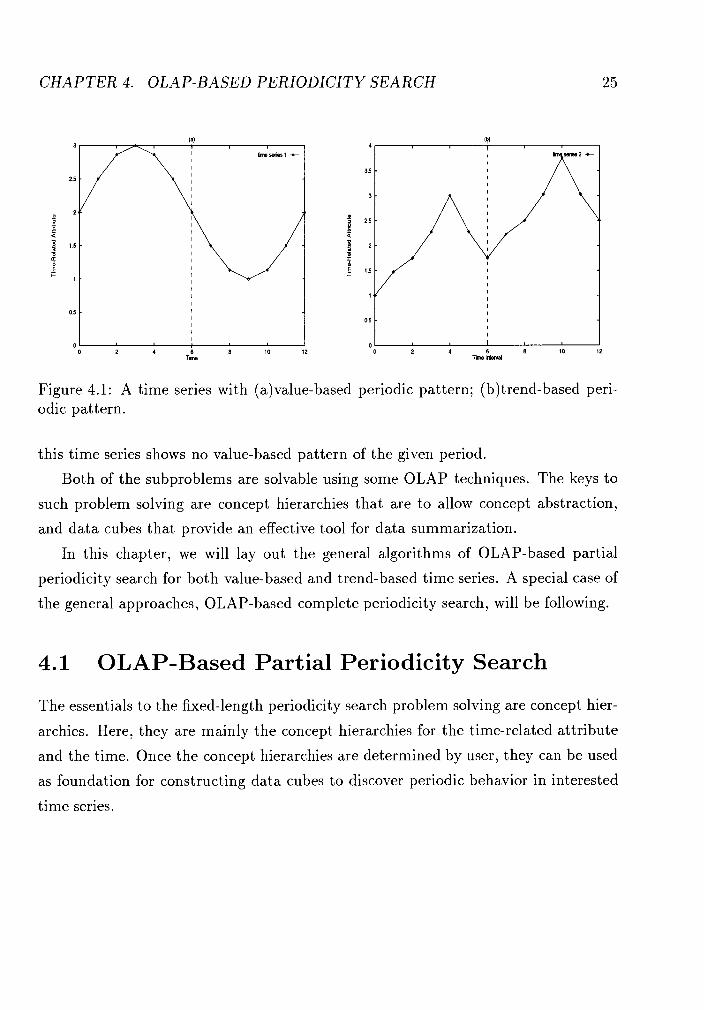
CHAPTER 4. OLAP-BASED PERIODICITY SEARCH
Figure 4.1: A time series with (a)value-based ~er iod ic pattern; (b)trend-based peri- odic pattern.
this time series shows no value-based pattern of the given period.
Both of the subproblems are solvable using some OLAP techniques. The keys to
such problem solving are concept hierarchies that are to allow concept abstraction,
and data cubes that provide an effective tool for data summarization.
In this chapter, we will lay out the general algorithms of OLAP-based partial
periodicity search for both value-based and trend-based time series. A special case of
the general approaches, OLAP-based complete periodicity search, will be following.
4.1 OLAP-Based Partial Periodicity Search
The essentials to the fixed-length periodicity search problem solving are concept hier-
archies. Here, they are mainly the concept hierarchies for the time-related attribute
and the time. Once the concept hierarchies are determined by user, they can be used
as foundation for constructing data cubes to discover periodic behavior in interested
time series.
CHAPTER 4. OLAP-BASED PERIODICITY SEARCH
4.1.1 Algorithm for Value-Based Approach
The purpose of this algorithm is to find periodic patterns of each task-relevant time
series based on their values. The algorithm is mainly composed of three steps. The
first two steps deal with data manipulation, and the third handles the actual pattern
search process. In the reference cube construction step, we collect the task-relevant
data into a minimally generalized data cube for fast indexing. The data are then
transferred into a generalized working cube in the next step in which each dimension
in the reference cube is rolled up to the interested concept level. In the next step,
we search the working cube for periodic patterns on these generalized levels using an
algorithm similar to that of sequential pattern mining by Agrawal et. al. [7]. The
main outline of the algorithm is as follows.
Algorithm 4.1.1 FindJatural-Segment Period(va1ue- based)
Input: 1) Non-time-related attributes A1, ..., A,; 2) time-related attribute AT; 3)
time attribute, T, bounded by a time interval; 4)time granularity, g, and a naturally
segmented period, p, where glp (P is a multiple of g); 5)a time hierarchy and concept
hierarchies associated with all task-relevant attributes; 6)confidence threshold, y.
Output: A set of periodic patterns associated with all periodic time series.
BEGIN
0 Step 1 : reference cube manipulation.
Select task-relevant data into a reference cube with dimensions for time, T, and
all other non-time-related attributes, All ..., A,. The average for the time-
related attribute, AT, is the measurement.
0 Step 2 : working cube manipulation.
Summarize data from the reference cube into a working cube with dimensions of
Al, . .., A, in the reference cube plus AT and two other dimensions referring to T,
one with respect to the period p, and the other with respect to the period indices.
The values on each dimension are generalized to a desired level according to their
corresponding concept hierarchies. The measurements are count, and average
of AT.
CHAPTER 4. OLAP-BASED PERIODICITY SEARCH
Step 3 : periodic pattern discovery.
For each time series, represented by a T-slice, do the following.
P1 = FindOneCyclePatterns()
FOR i := 2 TO p DO
CPi := FormCandidatePatternSet(i)
Pi := Check~attern~xistence(CP~)
IF Pi NOT empty THEN
FOR each i-cycle pattern P; in Pi DO
Delete the (i - 1)-cycle patterns that form P; in Pi-' END /* FOR */
END /* IF */ ELSE STOP /* Jump out of the loop */
END /* FOR */ RETURN Periodic pattern set P := UrZ1 Pi.
END
Each of the three steps in Algorithm 4.1.1 will be discussed in more detail in the
following sections. The confidence threshold introduced in the algorithm as an input
parameter is a control for the confidence of a periodic pattern found. So a periodic
pattern is confirmed only if it occurs in a portion of periods involved in the input
time series no less than the predefined confidence threshold, y. An example is used
to illustrate each step of the algorithm. This sample problem is stated as follows.
Example 4.1 Suppose we have a sales database which includes sales information of
a company from January 1993 to December 1993. Part of the database is shown in
Table 4.1. In this data set, location and product are the non-time-related attributes
and profit the time-related. The time granularity in this case is month since the profit
value associated with each tuple represents the monthly profit of the corresponding
product sold at the corresponding location, though the time recorded is specified to
minute. We would like to see if there exists some quarterly periodicity with respect
to the profit during this period of time. The confidence threshold is set as 75%.
CHAPTER 4. OLAP-BASED PERIODICITY SEARCH
Location
Paris Paris
I Paris I Alert Devices I Dec 1 1993 12:OOAM 1 1311
Paris Paris Paris Paris
Product
Alert Devices Alert Devices Alert Devices Alert Devices Alert Devices Alert Devices
Paris Paris Paris Paris Paris Paris
Table 4.1: Example. A sales relation with monthly sales information from January to December 1993.
Date
Jan 1 1993 12:OOAM Feb 1 1993 12:OOAM
Tokyo Tokyo
This given information is summarized in Table 4.2, and the time series correspond-
ing to the original data are plotted in Figure 4.2. The time hierarchy is chosen as
year -+ semi-year -, quarter --+ month. Besides, concept hierarchies selected for
other attributes in this particular task are shown in Figure 4.3.
Profit
752 501
Mar 1 1993 12:OOAM Apr 1 1993 12:OOAM May 1 1993 12:OOAM Jun 1 1993 12:OOAM
Carry-Bags Carry-Bags Carry-Bags Carry-Bags Carry-Bags Carry-Bags
Step 1 : Reference Cube Manipulation
1245 775 511 1311
Tents Tents
Given a time-related database, we collect a set of data with some objects, associated
with each is a time series of one time-related attribute. Each value in a time series
corresponds to one time. The first step is to build a reference cube with time and
all selected attributes, except the time-related attribute, as its dimensions. In most
Jan 1 1993 12:OOAM Feb 1 1993 12:OOAM Mar 1 1993 12:OOAM Apr 1 1993 12:OOAM May 1 1993 12:OOAM Jun 1 1993 12:OOAM
794 466 1334 789 471 1294
Nov 1 1993 12:OOAM Dec 1 1993 12:OOAM
528 1249
CHAPTER 4. OLAP-BASED PERIODICITY SEARCH
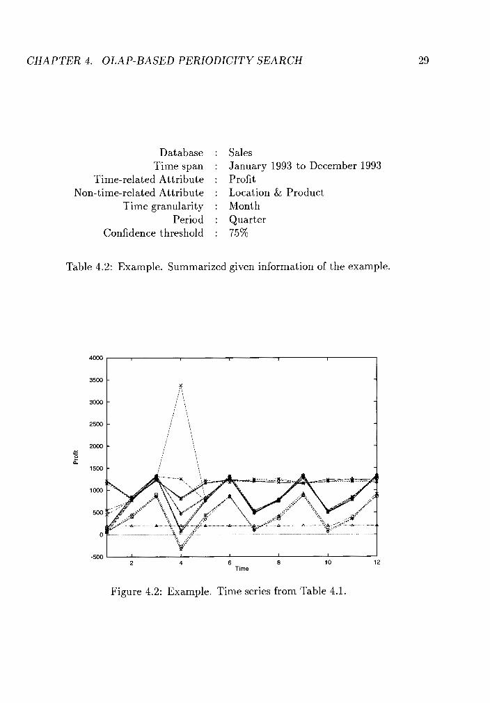
Database : Sales Time span : January 1993 to December 1993
Time-related Attribute : Profit Non-time-related Attribute : Location & Product
Time granularity : Month Period : Quarter
Confidence threshold : 75%
Table 4.2: Example. Summarized given information of the example.
- .- - 0 t
Time
Figure 4.2: Example. Time series from Table 4.1.
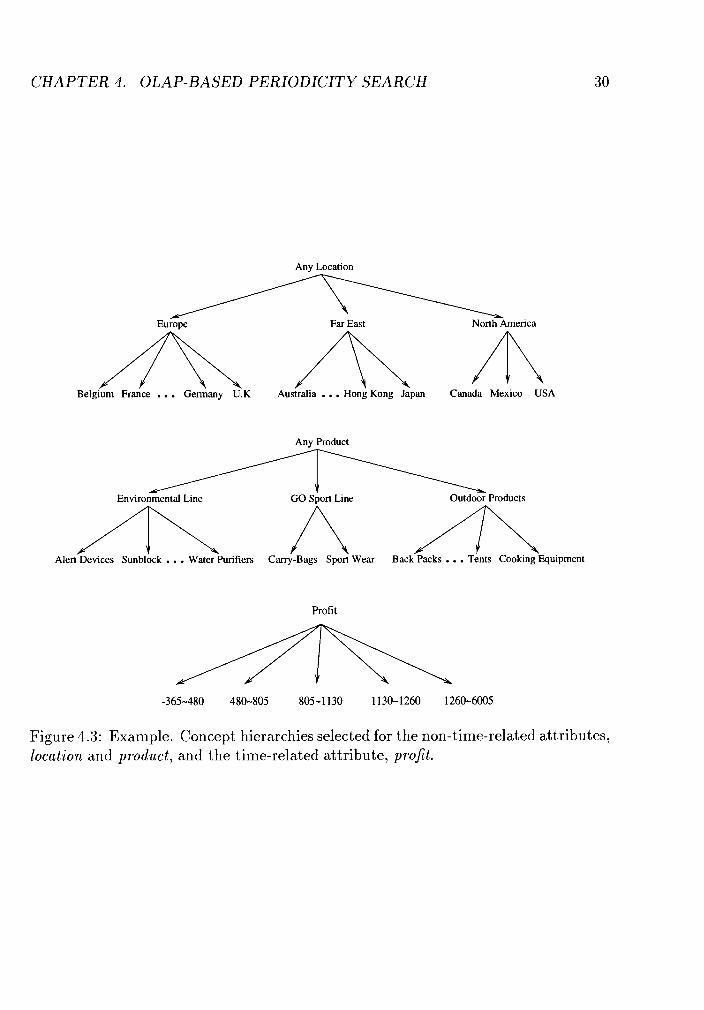
CHAPTER 4. OLAP-BASED PERIODICITY SEARCH
Any Location
A A A Belgium France . . . Germany U.K Australia . . . Hong Kong Japan Canada Mexico USA
Anv Product
A A A Alert Devices Sunblock . . . Water Purifiers Cany-Bags Sport Wear Back Packs . . . Tents Cooking Equipment
Profit
Figure 4.3: Example. Concept hierarchies selected for the non- time-related at tributes, location and product, and the time-related attribute, profit.
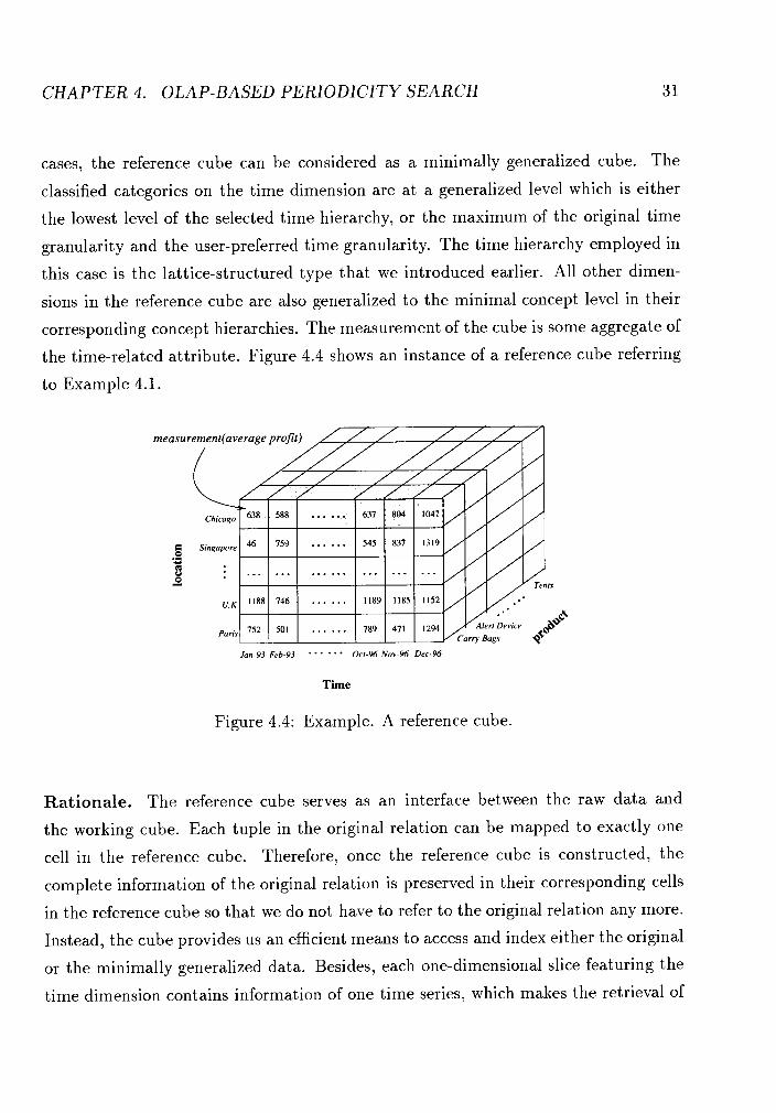
CHAPTER 4. OLAP-BASED PERIODICITY SEARCH 3 1
cases, the reference cube can be considered as a minimally generalized cube. The
classified categories on the time dimension are at a generalized level which is either
the lowest level of the selected time hierarchy, or the maximum of the original time
granularity and the user-preferred time granularity. The time hierarchy employed in
this case is the lattice-structured type that we introduced earlier. All other dimen-
sions in the reference cube are also generalized to the minimal concept level in their
corresponding concept hierarchies. The measurement of the cube is some aggregate of
the time-related attribute. Figure 4.4 shows an instance of a reference cube referring
to Example 4.1.
Jan-93 Feb-93 * . . * ' Ocr-% Now-% Dec-96
Time
Figure 4.4: Example. A reference cube.
Rationale. The reference cube serves as an interface between the raw data and
the working cube. Each tuple in the original relation can be mapped to exactly one
cell in the reference cube. Therefore, once the reference cube is constructed, the
complete information of the original relation is preserved in their corresponding cells
in the reference cube so that we do not have to refer to the original relation any more.
Instead, the cube provides us an efficient means to access and index either the original
or the minimally generalized data. Besides, each one-dimensional slice featuring the
time dimension contains information of one time series, which makes the retrieval of
CHAPTER 4. OLAP-BASED PERIODICITY SEARCH 3 2
one time series simple (e.g. the shaded slice shown in Figure 4.4 featuring the time
series with respect to (Chicago, Carry-Bags)).
Because each tuple in the task-relevant data set can be mapped to exactly one cell
in the reference cube, by the end of one complete scan through the original relation,
all task-relevant data are transferred into the reference cube. Thus, the complexity
of filling up the reference cube is linear in terms of number of tuples in the original
relation.
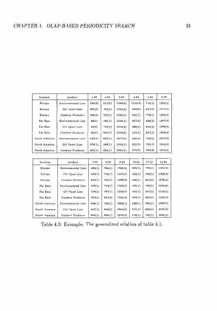
Step 2 : Working Cube Manipulation
A working cube is constructed on top of the reference cube and is a generalized version
of the original relation. The generalized version of the relation in Example 4.1 is shown
in Table 4.3. The numbers in brackets are the indices of each value corresponding to
the categories in the concept hierarchy of profit.
A working cube consists of dimensions of all non-time-related attributes in the ref-
erence cube (location, product) plus the time-related attribute (profit) and two other
dimensions referring to time. All non-time-related attribute and the time-related
attribute dimensions are generalized to their desired levels according to their corre-
sponding concept hierarchies. The levels are chosen based on the time granularity at
which level user would like to discover and view the periodic patterns. The measure-
ments in the working cube include count and average for the time-related attribute.
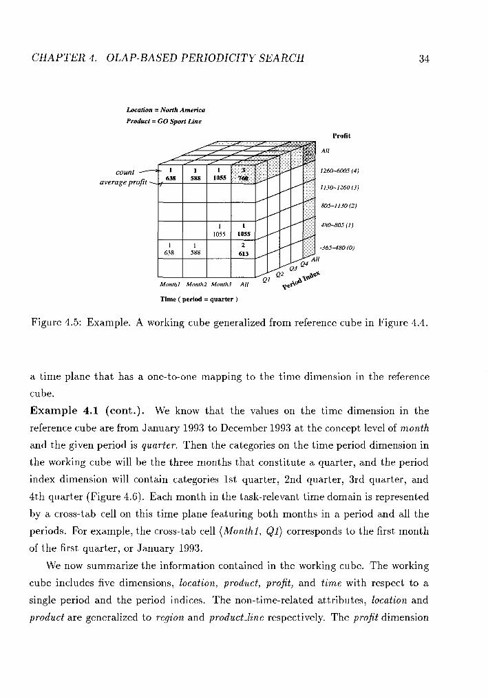
In Example 4.1, a slice of the working cube generalized from the reference cube in
Figure 4.4 is shown in Figure 4.5. The slice is taken on the location and the product
dimensions with values (North America, GO Sport Line).
As can be seen in Figure 4.5, the one-dimensional time dimension in the reference
cube is reshaped into a time plane with two time reference dimensions. One refers to
the given period which is usually set as a natural segmentation of time (e.g. hour,
day, month). The dimension domain is bounded by this natural segmentation. The
other serves as a dimension for period indices. Each category on this dimension refers
to a time period in the problem-related time domain, which is composed of all the
time units on the period dimension. In other words, the two dimensions establish
CHAPTER 4. OLAP-BASED PERIODICITY SEARCH
location
Europe
Europe
Europe
Far East
Far East
Far East
North America
North America
North America
location
Europe
Europe
Europe
Far East
Far East
Far East
North America
North America
North America
product
Environmental Line
GO Sport Line
Outdoor Products
Environmental Line
GO Sport Line
Outdoor Products
Environmental Line
GO Sport Line
Outdoor Products
product
Environmental Line
GO Sport Line
Outdoor Products
Environmental Line
GO Sport Line
Outdoor Products
Environmental Line
GO Sport Line
Outdoor Products
Table 4.3: Example. The generalized relation of table 4.1.
CHAPTER 4. OLAP-BASED PERIODICITY SEARCH
Location = North America
Product = GO Sport t i n e
Time ( period = quarter )
Figure 4.5: Example. A working cube generalized from reference cube in Figure 4.4.
a time plane that has a one-to-one mapping to the time dimension in the reference
cube.
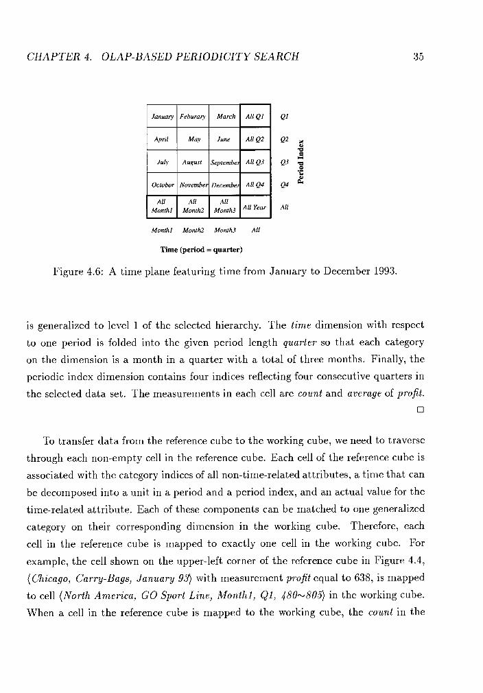
Example 4.1 (cont.). We know that the values on the time dimension in the
reference cube are from January 1993 to December 1993 at the concept level of month
and the given period is quarter. Then the categories on the time period dimension in
the working cube will be the three months that constitute a quarter, and the period
index dimension will contain categories 1st quarter, 2nd quarter, 3rd quarter, and
4th quarter (Figure 4.6). Each month in the task-relevant time domain is represented
by a cross-tab cell on this time plane featuring both months in a period and all the
periods. For example, the cross-tab cell (Monthl , Q1) corresponds to the first month
of the first quarter, or January 1993.
We now summarize the information contained in the working cube. The working
cube includes five dimensions, location, product, profit, and time with respect to a
single period and the period indices. The non-time-related attributes, location and
product are generalized to region and product-line respectively. The profit dimension
CHAPTER 4. OLAP-BASED PERIODICITY SEARCH
January Feburary I April May I& July August l--l- I Octobor I Novembe~
Monthl Month2 Month3 All
Ql
Q2 8 5 E
Q3 5 2
Q4
All
Time (period = quarter)
Figure 4.6: A time plane featuring time from January to December 1993.
is generalized to level 1 of the selected hierarchy. The time dimension with respect
to one period is folded into the given period length quarter so that each category
on the dimension is a month in a quarter with a total of three months. Finally, the
periodic index dimension contains four indices reflecting four consecutive quarters in
the selected data set. The measurements in each cell are count and average of profit.
0
To transfer data from the reference cube to the working cube, we need to traverse
through each non-empty cell in the reference cube. Each cell of the reference cube is
associated with the category indices of all non-time-related attributes, a time that can
be decomposed into a unit in a period and a period index, and an actual value for the
time-related attribute. Each of these components can be matched to one generalized
category on their corresponding dimension in the working cube. Therefore, each
cell in the reference cube is mapped to exactly one cell in the working cube. For
example, the cell shown on the upper-left corner of the reference cube in Figure 4.4,
(Chicago, Carry-Bags, January 93) with measurement profit equal to 638, is mapped
to cell (North America, GO Sport Line, Monthl, Q l , 480.-805) in the working cube.
When a cell in the reference cube is mapped to the working cube, the count in the
CHAPTER 4. OLAP-BASED PERIODICITY SEARCH 36
new working cell is incremented, and its average is recalculated for the time-related
attribute. By traversing through the reference cube, all information of the involved
time series is eventually transferred into the working cube.
A complete working cube contains dimensions for time (of one single period),
time period indices, one time-related attribute, and one or more non-time-related
attributes. A sliceldice from the cube including the complete time plane and the
entire domain of the time-related attribute dimension has a one-to-one mapping to
a time series. Let us refer to such a slice as a T-slice. It represents the time series
information of one object embedded in the working cube. The slice shown in Figure
4.5 is a T-slice.
Rationale. Generalizing a reference cube to a working cube can summarize the
information in the reference cube to a more abstract, meaningful level, and at the
same time reduce the amount of information to be processed. The actual values of
the time-related attribute originally stored in the reference cube as measurements are
now generalized to partitioned intervals of the time-related dimension in the working
cube. This way, we can discover, during each partitioned time period, which time-
related intervals are more crowded. These crowded intervals are likely to be parts of a
repeating periodic pattern. The representation of time is also altered from a dimension
in the reference cube to a plane in the working cube. The transformation enables us
to fold the entire task-relevant time line into a time segment that is corresponding
to the interested period. Therefore, we can find the behavior of each time series by
looking across the period index dimension. For example, by checking the time-related
attribute values across the period index dimension of Month1 in Figure 4.5, we are
actually examining the common behavior of the time series during the first month of
each quarter.
As mentioned earlier, every cell in the reference cube is mapped to exactly one cell
in the working cube. Hence, to transfer data from a reference cube to a working cube
requires exactly one scan through the entire reference cube. The complexity of this
data transformation is therefore linear as well, with respect to the number of cells in
the reference cube.
CHAPTER 4. OLAP-BASED PERIODICITY SEARCH
Step 3 : Periodic Pattern Discovery
Find 1 -Cycle Periodic Patterns
The periodic pattern discovery procedure is similar to that of sequential pattern
discovery [7 ] . The aggregation slice taken from a T-slice, which contains the entire
time and time-related attribute dimensions, and corresponds to the aggregation value
of the period index dimension (All), can be treated as one transaction from which
we want to find out if there exists a large cycle. The aggregation slice at the back
of the T-slice in Figure 4.5 is such a slice. If a certain portion of data points in this
slice (determined by a confidence threshold), or items as in a transaction, fall into one
concept category on the time-related attribute dimension, it means the time series at
this time unit forms a cycle whose length is the same as that of the chosen natural
time segmentation. The set of periodic patterns thus discovered containing one cycle
each is denoted by P1. An example can be seen from the aggregation slice shown
in Figure 4.7(a), which will be explained in more detail after the presentation of the
procedure FindOneCyclePatterns. The procedure is presented in pseudo-code as
follows.
PROCEDURE FindOneCyclePatterns()
BEGIN
num-cycles := 0
FOR t i m e i d := 0 TO (p/g - 1) DO
IF 3valueid < NumOfTimeRelatedValues such that the number of values
of current object at ttimeid fall into Vvalue-;d is no less than y THEN
Cnum-cycles := ( ~ 7 time-id, x a l u e - i d ) is a cycle
num-cycles := num-cycles + 1
END /* IF */ END /* FOR */ RETURN 1-cycle periodic pattern set P= {P;IP; = (p, 1, {(t;, x)l(p, ti, K) is a
cycle VO i < num-cycles)
END
CHAPTER 4. OLAP-BASED PERIODICITY SEARCH
(b)
Loconon = Nonh Ameruo
Produn = GO Spon D n e
P c d Index = Ql Prufit
12MCX05 (4)
Month1 Menth2 Month3 All
Time ( Frequency =quarter )
(.)
Localion =North America product = GO sport Line
Period lndex = AU
Momhl MonlhZ Monrh3 All
Timr (period = quarter )
/"
Profit
All
1260-6M5 NJ
1130-1260 (3)
805-1130 (2)
480-805 (1)
-365-480 (0)
(d
Localion = Nonh America
Prodnct = GO Spon Line
Period lndrx = Q2
Product =GO Spori Line
Period lndex = Q3 Pmnt
J
Monrhl Month2 Month3 AN
Time ( Frequency =quarter )
All
12M7-6W5141
1130-1260(31
m - I 1 3 0 (2)
480-805 (1)
-365-480 (0)
1260dW5 (4)
1130-1260(3)
IM2 805-ll30(2J
795 ~5 4813-805 111
22 1 365-480 (0)
Monrhl Month2 Monlh3 All
l i m e ( Frequency = quarter )
Period lndex = Q4
Time ( Frequency = quarter )
Profit
AN
1260-MOS (41
1130-1260 (31
805-1130 (2)
480-805 (1)
-365-480 (0)
Figure 4.7: Example. A T-slice of the working cube and slices from the T-slice.
CHAPTER 4. OLAP-BASED PERIODICITY SEARCH 3 9
Example 4.1 (cont.). Once the working cube is constructed, we start going through
each T-slice of the cube for periodic patterns. The cycles related to the object as-
sociated with T-slice in Figure 4.7 can be detected from the aggregation slice taken
from this T-slice by examining the nonempty cells of each month in the slice. This
aggregation slice is shown in Figure 4.7(a).
We examine each month sequentially according to the FOR loop in the procedure
layout. We first look at month 1 of each quarter. The second cell from bottom of
month 1 has a count 3 which, when compared with the number of periods (quarters),
4, contains exactly 75% of the total counts in this slice featuring month 1. It means
75% profit values of the first month each quarter belong to the same profit category
"480-805" and therefore forms a cycle. As we go through each month of the aggre-
gation slice, we conclude that cycles exist at all three months of each quarter for this
object. The profit categories these cycles fall into are "480--805" for months 1 and
2, and "805.-1130" for month 3. We denote these cycles as Co = (3, 0, l ) , C1 = (3,
1, I), and C2 = (3, 2, 2). The output from the procedure FindOneCyclePatterns() is
thus p1 = {P,f = (371, {(0,1))), P,2 = (371, { ( L l ) ) ) , Po3 = (371, {(2,2)))1. 0
Rationale. We look for all the 1-cycle patterns first instead of a whole periodic
pattern due to the accuracy concern with the employment of the confidence threshold.
For example, suppose we want to find periodic patterns of period length 3 in a time
series whose corresponding time sequence is 123123423144. The confidence threshold
is set as 75%. By going through each slice in a T-slice, we will discover sequentially
the 1-cycle patterns 1, 2, and 3. But this does not imply that 123 is a periodic
pattern, and, in fact, it is not. Therefore, this first procedure in the step forms a basis
for the later searching process. It prunes out those that do not meet the confidence
requirement and forms a set of patterns of a single cycle for further processing. 0
In the worst case scenario, for each time series, we need to go through each cell in
the aggregation slice of a T-slice to determine if cycles exists for each time interval
in a period. The maximum size of such a slice is that of the T-slice itself. Therefore,
the complexity of procedure FindOneCyclePatterns in each iteration is linear with
respect to the number of cells in a T-slice.
CHAPTER 4. OLAP-BASED PERIODICITY SEARCH
Form Candidate Patterns
We now combine every two 1-cycle patterns in P1 to form a set of candidate
periodic patterns containing two cycles, denoted by CP2, each of which will be tested
against the corresponding cells in the T-slice to see if it actually exists. The procedure
for the formation of candidate i-cycle patterns from (i - 1)-cycle patterns is shown in
procedure FormCandidatePatternSet.
PROCEDURE FormCandidatePatternSet (i)
BEGIN
/* Join Pi-' and Pi-' */ num-candidates := 0
FOR every pair of patterns P;-' = (p, i - l , C f l ) and pi-l = (p, i - 1 , ~ - l ) in
Pi-' DO
IF CF1[h] = c;-' [h]Vl < h 5 i - 2 AND c";' [i - 11 has a time index before
C?[i - 11 THEN i CPnum-candidates := (p, i7Ci) where Ci[h] = c;-'[h]Vl < h 5 i - 1 and
Ci [i] = Ci-' [i - 11
Insert CP~um-candidates into C P i num-candidates := num-candidates + 1
END /* IF */ END /* FOR */ /* Prune patterns that cannot exist */ FOR every candidate i-cycle pattern CPi DO
IF 3 some pattern Pi-' whose cycle set Ci-' is a subset of Ci of CPi such
that Ci-I is not in any pattern of Pi-' THEN
Delete CPi from C P
END /* IF */ END /* FOR */ RETURN i-cycle periodic pattern set CP"
END
The procedure contains two phases : a join phase and a prune phase [7]. The join
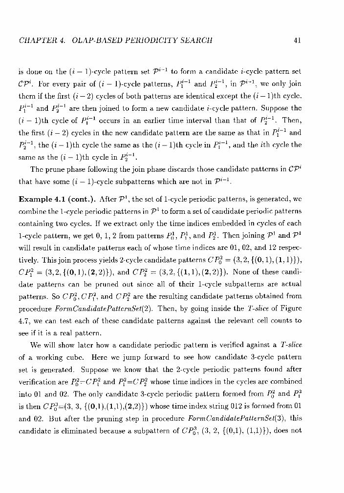
CHAPTER 4. OLAP-BASED PERIODICITY SEARCH 41
is done on the (i - 1)-cycle pattern set Pi-' to form a candidate i-cycle pattern set
CPi . For every pair of (i - 1)-cycle patterns, pi-' and pi-', in Pi-' , we only join
them if the first (i - 2) cycles of both patterns are identical except the (i - 1)th cycle.
pi-' and P;-' are then joined to form a new candidate i-cycle pattern. Suppose the
(i - 1)th cycle of pi-' occurs in an earlier time interval than that of pi-'. Then,
the first (i - 2) cycles in the new candidate pattern are the same as that in pi-' and
pi-', the (i - 1) th cycle the same as the (i - 1)th cycle in pi-', and the ith cycle the
same as the (i - 1)th cycle in pi-'. The prune phase following the join phase discards those candidate patterns in C P "
that have some (i - 1)-cycle subpatterns which are not in Pi-'.
Example 4.1 (cont.). After P', the set of 1-cycle periodic patterns, is generated, we
combine the 1-cycle periodic patterns in P1 to form a set of candidate periodic patterns
containing two cycles. If we extract only the time indices embedded in cycles of each
1-cycle pattern, we get 0, 1, 2 from patterns P,', P,' , and Pi. Then joining P' and P1
will result in candidate patterns each of whose time indices are 01, 02, and 12 respec-
tively. This join process yields 2-cycle candidate patterns C Po2 = (3,2, ((0, l), (1, I))) ,
CP," = (3,2, ((0, I ) , (2,2))) , and CP; = (3,2, ((1, l), (2,2))). None of these candi-
date patterns can be pruned out since all of their 1-cycle subpatterns are actual
patterns. So CP;, CP?, and CP; are the resulting candidate patterns obtained from
procedure FormCandidatePatternSet(2). Then, by going inside the T-slice of Figure
4.7, we can test each of these candidate patterns against the relevant cell counts to
see if it is a real pattern.
We will show later how a candidate periodic pattern is verified against a T-slice
of a working cube. Here we jump forward to see how candidate 3-cycle pattern
set is generated. Suppose we know that the 2-cycle periodic patterns found after
verification are P,2=CP,2 and P,"=CPi whose time indices in the cycles are combined
into 01 and 02. The only candidate 3-cycle periodic pattern formed from Pi and P,"
is then CP,3=(3, 3, {(0,1),(1,1),(2,2))) whose time index string 012 is formed from 01
and 02. But after the pruning step in procedure FormCandidatePatternSet(3), this
candidate is eliminated because a subpattern of CP:, (3, 2, {(0,1), (1,1))), does not
CHAPTER 4. OLAP-BASED PERIODICITY SEARCH 42
belong to the set of 2-cycle patterns.
Rationale. We sequentially construct sets of candidate patterns with increasing cycle
number because a pattern is periodic only if all its subpatterns are periodic. Therefore,
if some periodic patterns of length i are found, we only need to construct the candidate
(i + 1)-cycle patterns from these patterns. Any candidate formed otherwise will not be
periodic. The join phase ensures that we form sufficiently many candidate periodic
patterns with as little repetition as possible. We allow only one cycle mismatch
when joining two i-cycle periodic patterns. This is the only way we can generate
a candidate pattern of length (i + 1). For example, suppose there are two 2-cycle
periodic patterns represented by time sequences 12"" and **34. We can of course
form candidate patterns 123*, 12*4, etc. But these formations are meaningless if
there is no evidence of the existence of patterns 1*3*, 1**4, etc. Without these 2-
cycle patterns, 123* and 12*4 cannot exist. The choice of the indexing location of the
differed cycles in two patterns should not matter but it is necessary to be consistent
with this location for fewer repeating candidates. The prune phase, on the other
hand, is the supplementary of the join phase. The reason is the same. If a subpattern
of a candidate pattern is not periodic, then this candidate pattern will not be valid.
For each given number of cycles i , the number of candidate i-cycle patterns gen-
erated is at most ( z ) where n is the number of (i - 1)-cycle patterns found in the
previous call to the procedure. As a result, if the periodicity of a given time sequence
is very strong, it is possible that the total number of candidates generated during
the entire searching process is 2", where m is the length of the given period, leading
to a complexity of exponential. However, the actual performance of the algorithm
largely depends on the confidence threshold control and the nature of the input time
series. In [7], several alternatives to the AprioriAll algorithm have been discussed,
and results show that, in average, AprioriAll still outperforms the other proposals.
The worst case scenario is when an input time series has a complete periodicity. This
case will be handled separately in a later section.
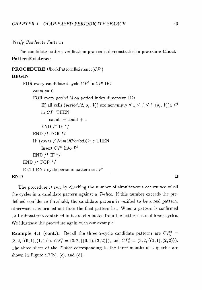
CHAPTER 4. OLAP-BASED PERIODICITY SEARCH
Verify Candidate Patterns
The candidate pattern verification process is demonstrated in procedure Check-
PatternExistence.
PROCEDURE CheckPat ternExistence(CP.)
BEGIN
FOR every candidate i-cycle C P i in CPi DO
count := 0
FOR every period-id on period index dimension DO
IF all cells (period-id, oj, V,) are nonempty V 1 5 j 5 i , (oj, V,)E Ci
in C P i THEN
count := count + 1
END /* IF */ END /* FOR */ IF (count / NumOfPeriods)> y THEN
Insert C P i into Pi
END /* IF */ END /* FOR */ RETURN i-cycle periodic pattern set PZ
END
The procedure is run by checking the number of simultaneous occurrence of all
the cycles in a candidate pattern against a T-slice. If this number exceeds the pre-
defined confidence threshold, the candidate pattern is verified to be a real pattern,
otherwise, it is pruned out from the final pattern list. When a pattern is confirmed
, all subpatterns contained in it are eliminated from the pattern lists of fewer cycles.
We illustrate the procedure again with our example.
Example 4.1 (cont.). Recall the three 2-cycle candidate patterns are CP; =
(372, ( ( 0 , 1 1 7 (1,1)))7 CP,2 = (372, {(0,1)7 (2 ,2)H, and CP,2 = (3,2, {(1,1)7 (2,2))) . The three slices of the T-slice corresponding to the three months of a quarter are
shown in Figure 4.7(b), (c), and (d).
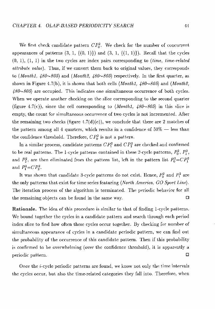
CHAPTER 4. OLAP-BASED PERIODICITY SEARCH
We first check candidate pattern CP;. We check for the number of concurrent
appearances of patterns (3, 1, ((0, 1))) and (3, 1, ((1, 1))) . Recall that the cycles
(0, I ) , (1, 1) in the two cycles are index pairs corresponding to (time, time-related
attribute value). Thus, if we convert them back to original values, they corresponds
to (Monthl, 480-805) and (Month2, 480-805) respectively. In the first quarter, as
shown in Figure 4.7(b), it is shown that both cells (Monthl, 480-805) and (Month2,
4 8 0 ~ 8 0 5 ) are occupied. This indicates one simultaneous occurrence of both cycles.
When we operate another checking on the slice corresponding to the second quarter
(figure 4.7(c)), since the cell corresponding to (Monthl, 480~805) in this slice is
empty, the count for simultaneous occurrence of two cycles is not incremented. After
the remaining two checks (figure 4.7(d)(e)), we conclude that there are 2 matches of
the pattern among all 4 quarters, which results in a confidence of 50% - less than
the confidence threshold. Therefore, CP; is not a pattern.
In a similar process, candidate patterns CP,2 and CP; are checked and confirmed
to be real patterns. The 1-cycle patterns contained in these 2-cycle patterns, P;, Pt,
and Pi, are then eliminated from the pattern list, left in the pattern list P,2=CP,2
and P,2=CP,2.
It was shown that candidate 3-cycle patterns do not exist. Hence, P; and Pf are
the only patterns that exist for time series featuring (North America, GO Sport Line).
The iteration process of the algorithm is terminated. The periodic behavior for all
the remaining objects can be found in the same way.
Rationale. The idea of this procedure is similar to that of finding 1-cycle patterns.
We bound together the cycles in a candidate pattern and search through each period
index slice to find how often these cycles occur together. By checking for number of
simultaneous appearance of cycles in a candidate periodic pattern, we can find out
the probability of the occurrence of this candidate pattern. Then if this probability
is confirmed to be overwhelming (over the confidence threshold), it is apparently a
periodic pattern.
Once the i-cycle periodic patterns are found, we know not only the time intervals
the cycles occur, but also the time-related categories they fall into. Therefore, when
CHAPTER 4. OLAP-BASED PERIODICITY SEARCH 45
a candidate (i + 1) pattern is constructed, all its cycles are specific. When we verify
this candidate pattern against the corresponding T-slice, we don't have to traverse
through each cell in the slice, but only those cells corresponding to the cycle values.
As a result, for each candidate i-cycle pattern, we need to verify it in m slices of a
T-slice, where m is the cardinality of the period index dimension; each verification
through a slice requires a check of i cells across the time dimension, . The verification
of each candidate pattern involves at most m . i checks. The maximum of m . i is
[TI, the cardinality of the entire task-relevant domain in the chosen time granularity.
Therefore, the complexity of this procedure is linear with respect to ITI.
Let us summarize the periodic pattern discovery process. Starting from 1-cycle
periodic pattern discovered by procedure FindOneCyclePat terns() , we construct
a candidate 2-cycle pattern set through a call to FormCandidatePatternSet(1).
After verifying these candidate patterns calling CheckPatternExistence(CP2), if
we find some 2-cycle pattern does exist, the 1-cycle patterns contained in this pattern
are eliminated from the pattern list. When all 2-cycle periodic patterns are found,
the same process will be applied to find periodic patterns containing three cycles.
The process will continue until the number of cycles in a discovered periodic pattern
reaches the length of the given period p, or until no more candidate periodic pattern
is available. The periodic patterns for this object in the resulting pattern list, F =
u:="=,', can be characterized by the non-time-related attribute values this T-slice
infers. In our example, the quarterly periodic patterns we found are those of time
series featuring the profit values of products in GO Sport Line sold in North America
from January 1993 to December 1993.
S u m m a r y of Algor i thm 4.1.1
Algorithm 4.1.1 is an approach of using concept hierarchies to solve problems with
value-based time series. Since our assumption is rough periodicity search, it processes
the time-related data as ranged categories. Then, once the original numerical values
are generalized into higher-level ranges, the algorithm requires a match of the time
series towards the discovered pattern with an accuracy no less than a predefined
CHAPTER 4. OLAP-BASED PERIODICITY SEARCH 46
confidence threshold, y. That is, if we claim a periodic pattern to exist with period p,
then what we are inferring is that the time series matches this pattern every p length
of the time for a percentage of the time series no less than y.
4.1.2 Generalization of the Working Cube
The key techniques in OLAP operations include roll-up and drill-down. As introduced
in Chapter 2, roll-up is an operation that increases the level of aggregation along some
dimension hierarchy, while drill-down is to decrease this level of aggregation along
some dimension hierarchy. How then can we accommodate these features into our
cube structure to allow pattern discovery across different abstraction levels of each
attribute?
For every non-time-related attribute, the roll-up and drill-down operations are
performed on the working cube the same as in usual practice. Taking the current
cube, the roll-up is done by merging the cells according to a group-by operation on
one or more of the dimensions. The drill-down is the converse operation of roll-
up. In the case of drill-down, because the working cube does not contain aggregate
information of lower-level concepts, the inner implementation of the operation is the
same as executing another roll-up operation on the attribute in the reference cube.
When the roll-up is done by a group-by on the time-related attribute dimension,
the operation undergoes the same procedure as for non-time-related attributes. But
if a drill-down operation is desired, the reconstruction of the working cube from the
reference cube is necessary to obtain the aggregation information of the time-related
attribute at the new specialized level.
The roll-up and drill-down on time in the working cube is more complicated.
It takes into account two situations, one on the time with respect to the naturally
segmented period, and the other with respect to the time granularity. Since time
in our working cube is actually a time plane featuring two time concepts, time of a
period and period indices, roll-up and drill-down operations executed on time require
reconciliation of both the time dimension and the period index dimension.
In some cases, user may like to do the roll-up or drill-down operations on the
CHAPTER 4. OLAP-BASED PERIODICITY SEARCH
naturally segmented period to discover periodic patterns of different period lengths
with natural time segmentation. Contrary to the situations discussed for other di-
mensions, both the roll-up and the drill-down operations on time with respect to
period can be executed exclusively from the working cube. Since each cell on the time
plane maps to exactly one time unit in the time line with the same time granular-
ity, the roll-up/drill-down operation executed on time is like a process of reshaping
the time plane. They are done by expanding or folding the time dimension further
into the generalized or specialized period, while adjusting the period index dimension
accordingly to reflect the change on the period. For example, suppose the original
time granularity is month, period is semi-year, and the time in the selected data set
spans through 4 consecutive semi-years (or two years). Then in the original working
cube, the time dimension with respect to period has six months as its categories, and
there are four indices on the period index dimension to index the four consecutive
semi-years. To roll-up the period to year, the time dimension is actually expanded
to include the twelve months in the first and the second halves of a year, and the
period index dimension is thus shrunk to two indices as pointers to the two years. On
the other hand, if we are to drill-down the period to quarter, the time dimension is
folded into quarter with three months and the period index dimension is expanded to
include 8 indices.
Example 4.1 (cont.). Suppose we want to drill-down on the time period. Accord-
ing to the time hierarchy we chose, the new specialized period is month. Although
the time granularity in our example is month which makes this drill-down operation
unnecessary, we do it anyway to show how it works.
Since a quarter is composed of three months, we can fold the time dimension
with respect to period into a narrower range (i.e. all three months of a quarter
can be folded into one single month), while the period index dimension is expanded
accordingly. Figure 4.8(b) illustrates the specialized version of the slice in (a) of the
same figure taken from the T-slice in Figure 4.7. The periodic patterns are then
searched in the same way as demonstrated before. Suppose we want to rollup the
time period to semi-year, then the process of reshaping the time plane in the working
CHAPTER 4. OLAP-BASED PERIODICITY SEARCH
cube is reverted from the previous case, resulted in a generalized slice shown in Figure
4.8(c).
Under another circumstance, user may like to roll-up or drill-down on the time
dimension with respect to the time granularity. In other words, user may like to
see the periodic patterns of the original period represented by a time unit that is
either a generalized or a specialized version from before. This calls for a method to
summarize a set of data points by one. We first consider a simple case for roll-up.
From the working cube, we slice out a time series (a T-slice). Since the average
aggregation values for the time-related attribute are stored as measurements, we can
group together the average and count of the time units which are to be generalized
into one new category and calculate a new average value which will be stored, along
with the total counts, in the cell corresponding to the generalized category in the new
working cube. Because drill-down is actually implemented as an operation of roll-up,
the basic operation is the same except that it has to be carried out from the reference
cube.
Example 4.1 (cont.). Suppose we would like to rollup the time dimension with
respect to time granularity so as to find semi-yearly periodic patterns based on the
average profit of each quarter. To do this, it is obviously not appropriate to merge
the cells of every three months in the working cube into one to represent data in a
quarter. If we then search for the periodic patterns in the same way as before, what
is found for each object in each quarter is the most frequent monthly profit range
of the quarter. This is apparently a different type of problem. In order to find the
semi-yearly periodic pattern based on the average profit of each quarter, we need to
summarize the monthly profit data retrieved from the reference cube into quarterly
information. This process before the construction of a new working cube can be
carried out on the fly. Figure 4.9 shows the same slice of the working cube in Figure
4.8(c) after roll-up on the time granularity from month to quarter. Once this is done,
the periodic pattern search process is executed as before.
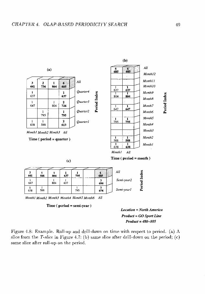
CHAPTER 4. OLAP-BASED PERIODICITY SEARCH
All
Quarter4 x 4 c C(
Quarter3 z .n
L
Quarter2 &
Monthl Month2 Month3 All
Time ( period = quarter )
All
Month12
Monthl l
Monthl 0
Month9
Month8
Monthl
Monthl All
Time ( period = month )
All 8 a G Y
Semi-year2 z .I
k
Semi-yearl &
Monthl Month2 Month3 Month4 Month5 Month6 All
Time ( period = semi-year ) Location = North America
Product = GO Sport Line Product = 480-805
Figure 4.8: Example. Roll-up and drill-down on time with respect to period. (a) A slice from the T-slice in Figure 4.7; (b) same slice after drill-down on the period; (c) same slice after roll-up on the period.
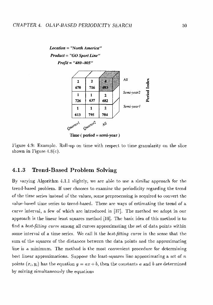
CHAPTER 4. OLAP-BASED PERIODICITY SEARCH
Location = "North America"
Product = "GO Sport Line"
Profit = "480-805"
All
Semi-year2
Semi-yearl
Time ( period = semi-year )
Figure 4.9: Example. Roll-up on time with respect to time granularity on the slice shown in Figure 4.8(c).
4.1.3 mend-Based Problem Solving
By varying Algorithm 4.1.1 slightly, we are able to use a similar approach for the
trend-based problem. If user chooses to examine the periodicity regarding the trend
of the time series instead of the values, some preprocessing is required to convert the
value-based time series to trend-based. There are ways of estimating the trend of a
curve interval, a few of which are introduced in [ 3 7 ] . The method we adopt in our
approach is the linear least squares method [lo]. The basic idea of this method is to
find a best-fitting curve among all curves approximating the set of data points within
some interval of a time series. We call it the best-fitting curve in the sense that the
sum of the squares of the distances between the data points and the approximating
line is a minimum. The method is the most convenient procedure for determining
best linear approximations. Suppose the least-squares line approximating a set of n
points (x;, y;) has the equation y = ax + b, then the constants a and b are determined
by solving simultaneously the equations
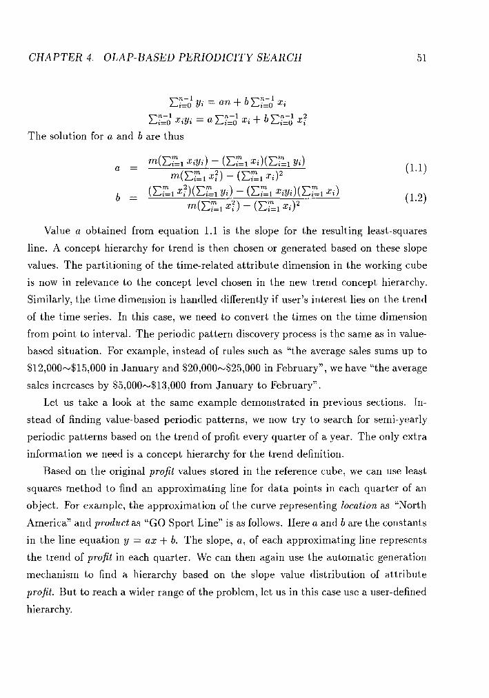
CHAPTER 4. OLAP-BASED PERIODICITY SEARCH
~ y : y; = an + b ~ y i : x; n-1 2 ~y:: x;y; = a ~15: x; + b Ci=, xi
The solution for a and b are thus
Value a obtained from equation 1.1 is the slope for the resulting least-squares
line. A concept hierarchy for trend is then chosen or generated based on these slope
values. The partitioning of the time-related attribute dimension in the working cube
is now in relevance to the concept level chosen in the new trend concept hierarchy.
Similarly, the time dimension is handled differently if user's interest lies on the trend
of the time series. In this case, we need to convert the times on the time dimension
from point to interval. The periodic pattern discovery process is the same as in value-
based situation. For example, instead of rules such as "the average sales sums up to
$12,000-$15,000 in January and $20,000-$25,000 in February", we have "the average
sales increases by $5,000-$13,000 from January to February".
Let us take a look at the same example demonstrated in previous sections. In-
stead of finding value-based periodic patterns, we now try to search for semi-yearly
periodic patterns based on the trend of profit every quarter of a year. The only extra
information we need is a concept hierarchy for the trend definition.
Based on the original profit values stored in the reference cube, we can use least
squares method to find an approximating line for data points in each quarter of an
object. For example, the approximation of the curve representing location as "North
America" and product as "GO Sport Line" is as follows. Here a and b are the constants
in the line equation y = ax + b. The slope, a , of each approximating line represents
the trend of profit in each quarter. We can then again use the automatic generation
mechanism to find a hierarchy based on the slope value distribution of attribute
profit. But to reach a wider range of the problem, let us in this case use a user-defined
hierarchy.
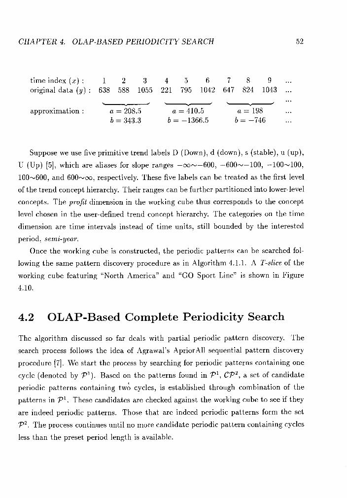
CHAPTER 4. OLAP-BASED PERIODICITY SEARCH
time index (x) : 1 2 3 4 5 6 original data (y) : 638 588 1055 221 795 1042 - - approximation : a = 208.5 a = 410.5
b = 343.3 b = -1366.5
Suppose we use five primitive trend labels D (Down), d (down), s (stable), u (up),
U (Up) [5], which are aliases for slope ranges -oo--600, -600--100, -100-100,
100-600, and 600-oo, respectively. These five labels can be treated as the first level
of the trend concept hierarchy. Their ranges can be further partitioned into lower-level
concepts. The profit dimension in the working cube thus corresponds to the concept
level chosen in the user-defined trend concept hierarchy. The categories on the time
dimension are time intervals instead of time units, still bounded by the interested
period, semi- year.
Once the working cube is constructed, the periodic patterns can be searched fol-
lowing the same pattern discovery procedure as in Algorithm 4.1 . l . A T-slice of the
working cube featuring "North America" and "GO Sport Line" is shown in Figure
4.10.
4.2 OLAP-Based Complete Periodicity Search
The algorithm discussed so far deals with partial periodic pattern discovery. The
search process follows the idea of Agrawal's ApriorAll sequential pattern discovery
procedure [7]. We start the process by searching for periodic patterns containing one
cycle (denoted by P1). Based on the patterns found in P1, CP2 , a set of candidate
periodic patterns containing tw6 cycles, is established through combination of the
patterns in P1. These candidates are checked against the working cube to see if they
are indeed periodic patterns. Those that are indeed periodic patterns form the set
P 2 . The process continues until no more candidate periodic pattern containing cycles
less than the preset period length is available.
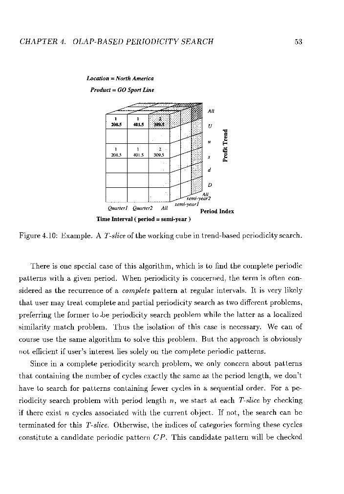
CHAPTER 4. OLAP-BASED PERIODICITY SEARCH
Location = North America
Product = GO Sport Line
Index Time Interval ( period = semi-year )
Figure 4.10: Example. A T-slice of the working cube in trend-based periodicity search.
There is one special case of this algorithm, which is to find the complete periodic
patterns with a given period. When periodicity is concerned, the term is often con-
sidered as the recurrence of a complete pattern at regular intervals. It is very likely
that user may treat complete and partial periodicity search as two different problems,
preferring the former to.&be periodicity search problem while the latter as a localized
similarity match problem. Thus the isolation of this case is necessary. We can of
course use the same algorithm to solve this problem. But the approach is obviously
not efficient if user's interest lies solely on the complete periodic patterns.
Since in a complete periodicity search problem, we only concern about patterns
that containing the number of cycles exactly the same as the period length, we don't
have to search for patterns containing fewer cycles in a sequential order. For a pe-
riodicity search problem with period length n, we start at each T-slice by checking
if there exist n cycles associated with the current object. If not, the search can be
terminated for this T-slice. Otherwise, the indices of categories forming these cycles
constitute a candidate periodic pattern CP. This candidate pattern will be checked
CHAPTER 4. OLAP-BASED PERIODICITY SEARCH 54
against the T-slice by calling the procedure CheckPatternExistence({CP)), as illus-
trated in partial periodicity search Algorithm 4.1.1, to see if it is indeed a complete
pattern. Apparently, skipping all the initial searching and checking procedures, and
jumping directly to the longest possible pattern saves much of the processing time. It
can potentially reduce the periodicity searching time to a magnitude of order n.
The periodic pattern discovery step in this problem involves one pass through
the aggregate slice of each T-slice for all candidate complete patterns, and another
through slices of the T-slice along the period index dimension for verification of these
candidate complete patterns. As analyzed in Section 4.1.1, the maximum number
of checks needed for each time series is 2 . ITI, where IT1 is the cardinality of the
task-relevant time domain of the chosen time granularity. The complexity for finding
complete periodic patterns of each time series in this approach is thus linear in terms
of the cardinality of the task-relevant time domain.
4.3 Discussion and Summary
In this chapter, we have presented some OL AP-based periodicity search algorithms for
fixed-length periodic pattern discovery problem. Some basic variations of the fixed-
length periodic pattern discovery problem are value-based, trend-based, partial pattern
search, and complete pattern search problems. The differences of these approaches
are listed in Table 4.3. The algorithms given are all OLAP-based, their performance
greatly relies on the manipulation of the data cube structure. In Chapter 5, the second
type of problem will be discussed in detail.
Note that, we can use the same reference cube for all these four subproblems. Thus,
when implemented into a system, we can easily give the option of choosing among the
four approaches, in which case all we need to reconstruct is the working cube, while
the reference cube can be left intact. This way, the execution effort required to switch
from one approach to another can be reduced considerably.
The algorithms presented handle time series of exactly one time-related attribute,
and the periodic patterns discovered are of only one fixed period length. This can be
easily extended to deal with multiple time-related attributes and periods. When more
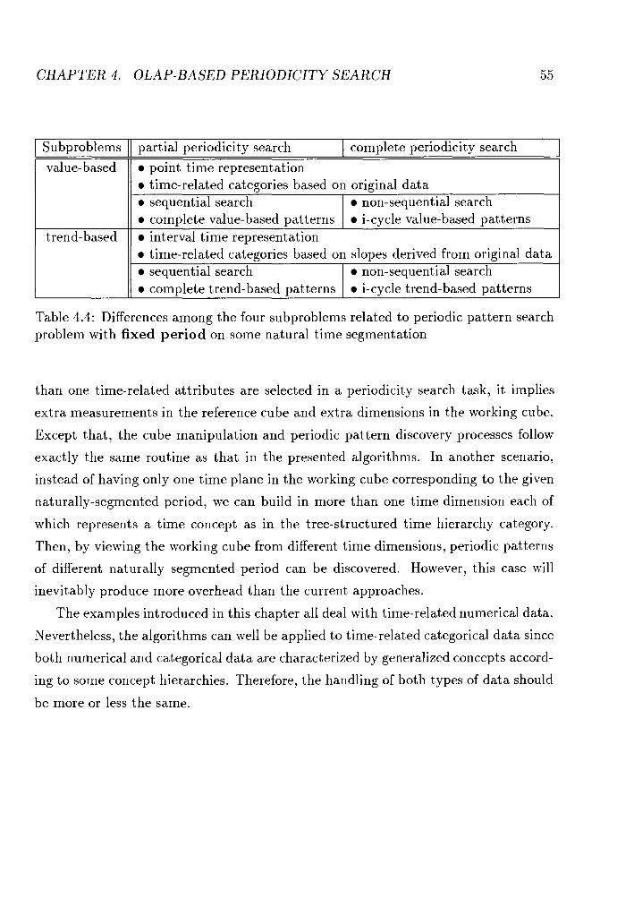
CHAPTER 4. OLAP-BASED PERIODICITY SEARCH 5 5
0 time-related categories based on original data 0 sequential search I non-sequential search
Subproblems
value- based
partial periodicity search I complete periodicity search
point time representation
0 time-related categories based on slopes derived from original data sequential search 1 non-sequential search
trend-based
I/ complete trend-based patterns I i-cycle trend-based patterns
0 complete value-based patterns I i-cycle value-based pat terns interval time represent ation
Table 4.4: Differences among the four subproblems related to periodic pattern search problem with fixed period on some natural time segmentation
than one time-related attributes are selected in a periodicity search task, it implies
extra measurements in the reference cube and extra dimensions in the working cube.
Except that, the cube manipulation and periodic pattern discovery processes follow
exactly the same routine as that in the presented algorithms. In another scenario,
instead of having only one time plane in the working cube corresponding to the given
naturally-segmented period, we can build in more than one time dimension each of
which represents a time concept as in the tree-structured time hierarchy category.
Then, by viewing the working cube from different time dimensions, periodic patterns
of different naturally segmented period can be discovered. However, this case will
inevitably produce more overhead than the current approaches.
The examples introduced in this chapter all deal with time-related numerical data.
Nevertheless, the algorithms can well be applied to time-related categorical data since
both numerical and categorical data are characterized by generalized concepts accord-
ing to some concept hierarchies. Therefore, the handling of both types of data should
be more or less the same.
Chapter 5
Arbitrary Periodicity Search
The problems discussed in the previous chapter deal with periodicity search with fixed
period. However, not all patterns have such nicely segmented period. Very often, we
recognize patterns with periods that cannot be described in a naturally segmented
time unit. For example, the algorithms from Chapter 4 cannot detect periodic patterns
that hold every 10 days, unless we explicitly specify this time segmentation. In this
chapter, we will discuss how to detect periodic patterns of arbitrary length.
5.1 Arbitrary Partial Periodicity Search
In this section, the three algorithms presented focus on general partial periodicity
detection, followed by some experimental results of these algorithms. The complete
periodicity search problem will be discussed in the next section.
The three algorithms presented here are sequential algorithm, forward optimization
algorithm, and backward optimization algorithm. The last two are the optimization
of the sequential algorithm. The difference among the three exists in the periodic
pattern discovery process, while all of the three algorithms share a common data
structure in data storage and retrieval.
The first step is data collection, which is the same as in Algorithm 4.1.1. We
collect all relevant time-related data and store them in a reference cube where we
can reference the data efficiently and effectively. The reference cube has the same
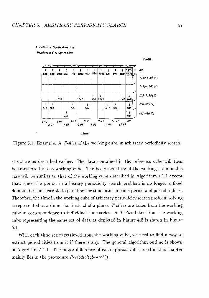
CHAPTER 5. ARBITRARY PERIODICITY SEARCH
Location = North America
Product = GO Sport Line
Profit
All
1260-6005 (4)
1130-1260 (3)
805-1130 (2)
480-805 (1)
-365-480 (0)
Time
Figure 5.1: Example. A T-slice of the working cube in arbitrary periodicity search.
structure as described earlier. The data contained in the reference cube will then
be transferred into a working cube. The basic structure of the working cube in this
case will be similar to that of the working cube described in Algorithm 4.1.1 except
that, since the period in arbitrary periodicity search problem is no longer a fixed
domain, it is not feasible to partition the time into time in a period and period indices.
Therefore, the time in the working cube of arbitrary periodicity search problem solving
is represented as a dimension instead of a plane. T-slices are taken from the working
cube in correspondence to individual time series. A T-slice taken from the working
cube representing the same set of data as depicted in Figure 4.5 is shown in Figure
5.1.
With each time series retrieved from the working cube, we need to find a way to
extract periodicities from it if there is any. The general algorithm outline is shown
in Algorithm 5.1.1. The major difference of each approach discussed in this chapter
mainly lies in the procedure PeriodicitySearch().
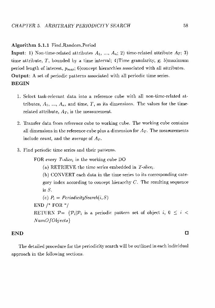
CHAPTER 5. ARBITRARY PERIODICITY SEARCH
Algorithm 5.1.1 Findl2andomPeriod
Input: 1) Non-time-related attributes Al, ..., A,; 2) time-related attribute AT; 3)
time attribute, T , bounded by a time interval; 4)Time granularity, g; 5)maximum
period length of interest, p,,,; 6)concept hierarchies associated with all attributes.
Output: A set of periodic patterns associated with all periodic time series.
BEGIN
1. Select task-relevant data into a reference cube with all non-time-related at-
tributes, All ..., A,, and time, T, as its dimensions. The values for the time-
related attribute, AT, is the measurement.
2. Transfer data from reference cube to working cube. The working cube contains
all dimensions in the reference cube plus a dimension for AT. The measurements
include count, and the average of AT.
3. Find periodic time series and their patterns.
FOR every T-slice; in the working cube DO
(a) RETRIEVE the time series embedded in T-slice;.
(b) CONVERT each data in the time series to its corresponding cate-
gory index according to concept hierarchy C. The resulting sequence
is S.
(c) P; = PeriodicitySearch(i, S )
END /* FOR */ RETURN P= {P;lP; is a periodic pattern set of object i , 0 5 i < NumO f Objects)
END
The detailed procedure for the periodicity search will be outlined in each individual
approach in the following sections.
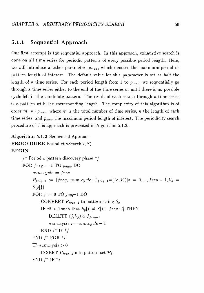
CHAPTER 5. ARBITRARY PERIODICITY SEARCH
5.1.1 Sequential Approach
Our first attempt is the sequential approach. In this approach, exhaustive search is
done on all time series for periodic patterns of every possible period length. Here,
we will introduce another parameter, p,,,, which denotes the maximum period or
pattern length of interest. The default value for this parameter is set as half the
length of a time series. For each period length from 1 to p,,,, we sequentially go
through a time series either to the end of the time series or until there is no possible
cycle left in the candidate pattern. The result of each search through a time series
is a pattern with the corresponding length. The complexity of this algorithm is of
order m . n . p,,,, where m is the total number of time series, n the length of each
time series, and p,,, the maximum period length of interest. The periodicity search
procedure of this approach is presented in Algorithm 5.1.2.
Algorithm 5.1.2 SequentialApproach
PROCEDURE PeriodicitySearch(i, S)
BEGIN
/* Periodic pattern discovery phase */ FOR freq := 1 TO p,,, DO
num-cycle := freq
Pfreq-1 := (freq, num-cycle, Cfre,-l={(o,V,)lo = 0 ,..., freq - l ,Vo =
S[oI > > FOR j := 0 TO freq-1 DO
CONVERT Pfr,q-l to pattern string S,
IF 3t > 0 such that S,[j] # S[j + freq . t ] THEN
DELETE (j, V,) € Cfreq-l
num-cycle := num-cycle - 1
END /* IF */ END /* FOR */ IF num-cycle > 0
INSERT Pf,,q-l into pattern set Pi END /* IF */
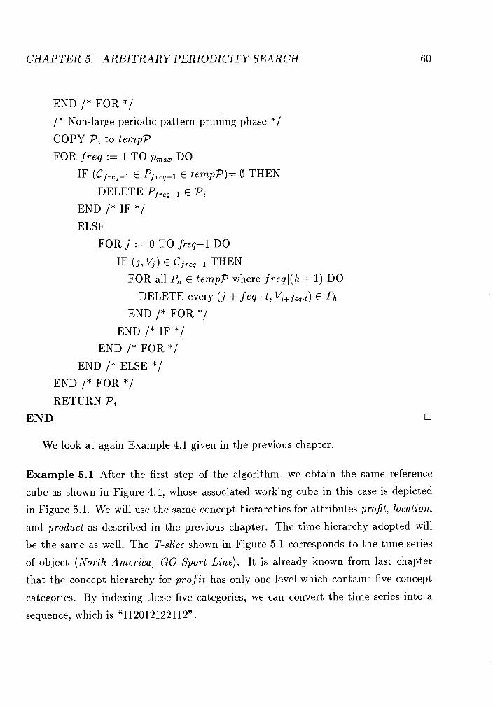
CHAPTER 5. A R B I T R A R Y PERlODlCITY SEARCH
END /* FOR * / /* Non-large periodic pattern pruning phase */ COPY Pi to temp?
FOR freq := 1 TO p,,, DO
IF (Cfreq-1 E Pfreq-1 E tempP)= 0 THEN
DELETE Pfreq-1 E P; END /* IF */ ELSE
FOR j := 0 TO freq-1 DO
IF ( j , V,) E Cfre,-I THEN
FOR all Ph E temp? where freql(h + 1) DO
DELETE every ( j + f eq . t , V,+ feq.t) E P h
END /* FOR */ END /* IF */
END /* FOR */ END /* ELSE */
END /* FOR */ RETURN P;
END
We look at again Example 4.1 given in the previous chapter
Example 5.1 After the first step of the algorithm, we obtain the same reference
cube as shown in Figure 4.4, whose associated working cube in this case is depicted
in Figure 5.1. We will use the same concept hierarchies for attributes profit, location,
and product as described in the previous chapter. The time hierarchy adopted will
be the same as well. The T-slice shown in Figure 5.1 corresponds to the time series
of object (North America, GO Sport Line). It is already known from last chapter
that the concept hierarchy for profit has only one level which contains five concept
categories. By indexing these five categories, we can convert the time series into a
sequence, which is "112012122112".
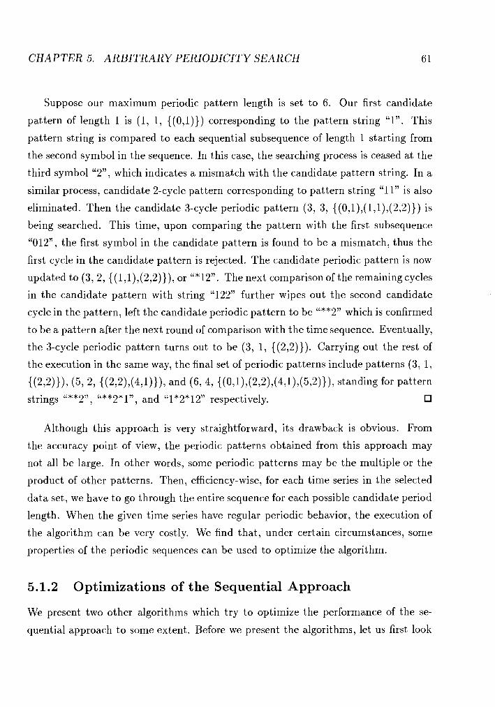
CHAPTER 5. ARBITRARY PERIODICITY SEARCH 6 1
Suppose our maximum periodic pattern length is set to 6. Our first candidate
pattern of length 1 is (1, 1, {(0,1))) corresponding to the pattern string "1". This
pattern string is compared to each sequential subsequence of length 1 starting from
the second symbol in the sequence. In this case, the searching process is ceased a t the
third symbol "2", which indicates a mismatch with the candidate pattern string. In a
similar process, candidate 2-cycle pattern corresponding to pattern string "11" is also
eliminated. Then the candidate 3-cycle periodic pattern (3, 3, {(0,1),(1,1),(2,2)}) is
being searched. This time, upon comparing the pattern with the first subsequence
"012", the first symbol in the candidate pattern is found to be a mismatch, thus the
first cycle in the candidate pattern is rejected. The candidate periodic pattern is now
updated to (3,2, {(1,1),(2,2)}), or "*12". The next comparison of the remaining cycles
in the candidate pattern with string "122" further wipes out the second candidate
cycle in the pattern, left the candidate periodic pattern to be "**2" which is confirmed
to be a pattern after the next round of comparison with the time sequence. Eventually,
the 3-cycle periodic pattern turns out to be (3, 1, {(2,2))). Carrying out the rest of
the execution in the same way, the final set of periodic patterns include patterns (3, 1,
{(212)>)1 (57 27 {(2,2),(4,1)>), and (67 47 {(0,1),(2,2),(4,1),(5,2))), standing for pattern
strings "**2" , "**2*1", and "1*2*12" respectively.
Although this approach is very straightforward, its drawback is obvious. From
the accuracy point of view, the periodic patterns obtained from this approach may
not all be large. In other words, some periodic patterns may be the multiple or the
product of other patterns. Then, efficiency-wise, for each time series in the selected
data set, we have to go through the entire sequence for each possible candidate period
length. When the given time series have regular periodic behavior, the execution of
the algorithm can be very costly. We find that, under certain circumstances, some
properties of the periodic sequences can be used to optimize the algorithm.
5.1.2 Optimizations of the Sequential Approach
We present two other algorithms which try to optimize the performance of the se-
quential approach to some extent. Before we present the algorithms, let us first look
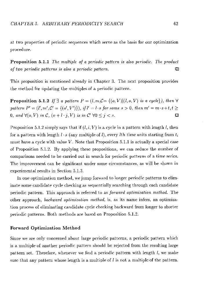
CHAPTER 5. ARBITRARY PERIODICITY SEARCH 62
at two properties of periodic sequences which serve as the basis for our optimization
procedure.
Proposition 5.1.1 The multiple of a periodic pattern is also periodic. The product
of two periodic patterns is also a periodic pattern.
This proposition is mentioned already in Chapter 3. The next proposition provides
the method for updating the multiples of a periodic pattern.
Proposition 5.1.2 If 3 a pattern P = (1, m,C= ((0, V)I(l, o, V) is a cycle)), then V
pattern P' = (I1, m', C' = {(or, V'))), if I' = 1. s for some s > 0, then rn' = me s + t , t 2 0, andV(o,V) inC, ( o + 1 - j , V ) is inCIVO 5 j < s .
Proposition 5.1.2 simply says that if (I, i , V) is a cycle in a pattern with length 1, then
for a pattern with length 1 . s (any multiple of I), every lth time units starting from ti
must have a cycle with value V. Note that Proposition 5.1.1 is actually a special case
of Proposition 5.1.2. By applying these propositions, we can reduce the number of
comparisons needed to be carried out in search for periodic patterns of a time series.
The improvement can be significant under some circumstances, as will be shown in
experimental results in Section 5.1.3.
In one optimization method, we jump forward to longer periodic patterns to elim-
inate some candidate cycle checking as sequentially searching through each candidate
periodic pattern. This approach is referred to as forward optimization method. The
other approach, backward optimization method, is, as its name infers, an optimiza-
tion process of eliminating candidate cycle checking backward from longer to shorter
periodic patterns. Both methods are based on Proposition 5.1.2.
Forward Optimization Met hod
Since we are only concerned about large periodic patterns, a periodic pattern which
is a multiple of another periodic pattern should be rejected from the resulting large
pattern set. Therefore, whenever we find a periodic pattern with length 1, we make
sure that any pattern whose length is a multiple of 1 is not a multiple of the pattern.
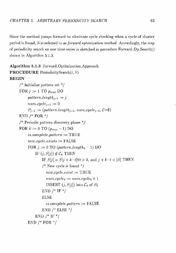
CHAPTER 5. ARBITRARY PERIODICITY SEARCH 63
Since the method jumps forward to eliminate cycle checking when a cycle of shorter
period is found, it is referred to as forward optimization method. Accordingly, the step
of periodicity search on one time series is sketched in procedure Forward-Op-Search()
shown in Algorithm 5.1.3.
Algorithm 5.1.3 Forward-Optimization Approach
PROCEDURE PeriodicitySearch(i, S )
BEGIN
/* Initialize pattern set */ FOR j := 1 TO p,,, DO
pattern-lengthj-l := j
n u m - ~ y c l e ~ - ~ := 0
Pj-1 := (pattern-lengthj-l, n u m - ~ y c l e ~ - ~ , C=0)
END /* FOR */ /* Periodic pattern discovery phase */ FOR k := 0 TO (p,,, - 1) DO
is-complete-pattern := TRUE
new-cycle-exists := FALSE
FOR j := 0 TO (pattern-lengthk - 1) DO
IF ( j , S[ j ] ) 4 Ck THEN IF S[j] = S[j + k.t]Vt > 0, and j + k . t < IS1 THEN
/* New cycle is found */ new-cycle-exist := TRUE
num-cyclek := num-cyclek + 1
INSERT ( j , S[ j ] ) into Ck of Pk
END /* IF */ ELSE
is-complete-pattern := FALSE
END /* ELSE */ END /* IF */
END /* FOR */
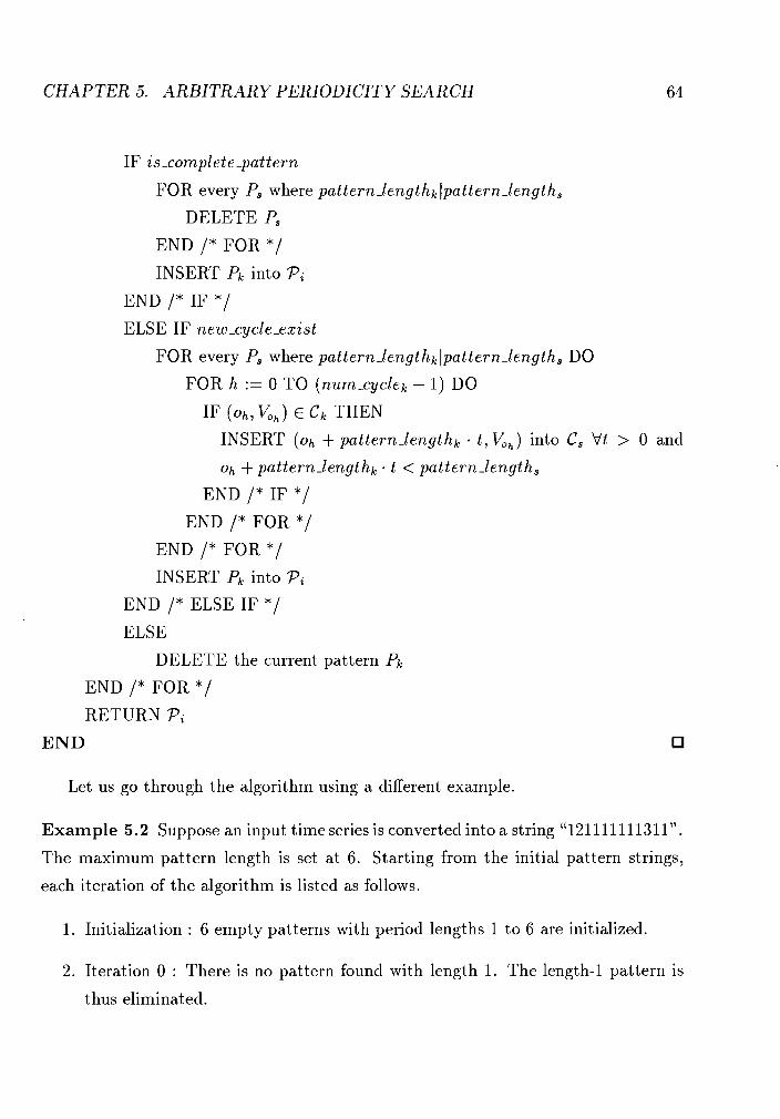
CHAPTER 5. ARBITRARY PERIODICITY SEARCH
IF is-complete-pattern
FOR every P, where pattern-lengthkIpattern-length,
DELETE P,
END /* FOR */ INSERT Pk into Pi
END /* IF */ ELSE IF new-cycle-exist
FOR every P, where pattern-lengthklpat temlength, DO
FOR h := 0 TO (num-cyclek - 1) DO
IF (oh, K,) E Ck THEN
INSERT (oh + pattern-lengthk - t , V,,) into C, V t > 0 and
oh + pattern-lengthk . t < pattern-length,
END /* IF */ END /* FOR */
END /* FOR */ INSERT Pk into Pi
END /* ELSE IF */ ELSE
DELETE the current pattern Pk
END /* FOR */ RETURN P;
END
Let us go through the algorithm using a different example.
Example 5.2 Suppose an input time series is converted into a string "121 11 11 1131 1".
The maximum pattern length is set at 6. Starting from the initial pattern strings,
each iteration of the algorithm is listed as follows.
1. Initialization : 6 empty patterns with period lengths 1 to 6 are initialized.
2. Iteration 0 : There is no pattern found with length 1. The length-1 pattern is
thus eliminated.
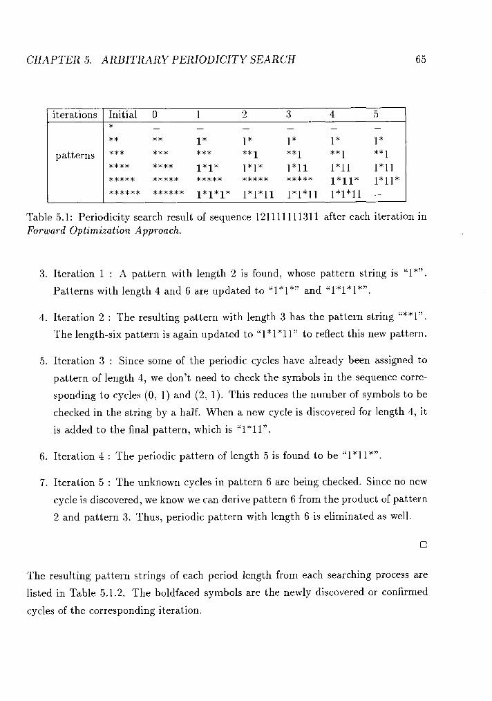
CHAPTER 5. ARBITRARY PERIODICITY SEARCH
I iterations I Initial 0 1 2 3 4 5
patterns
Table 5.1: Periodicity search result of sequence 121 111 11 131 1 after each iteration in Forward Optimization Approach.
3. Iteration 1 : A pattern with length 2 is found, whose pattern string is "l*".
Patterns with length 4 and 6 are updated to "1*1*" and "1*1*1*".
4. Iteration 2 : The resulting pattern with length 3 has the pattern string "**l".
The length-six pattern is again updated to "1*1*11" to reflect this new pattern.
5. Iteration 3 : Since some of the periodic cycles have already been assigned to
pattern of length 4, we don't need to check the symbols in the sequence corre-
sponding to cycles (0, 1) and (2, 1). This reduces the number of symbols to be
checked in the string by a half. When a new cycle is discovered for length 4, it
is added to the final pattern, which is " l* l ln .
6. Iteration 4 : The periodic pattern of length 5 is found to be "1*11*".
7. Iteration 5 : The unknown cycles in pattern 6 are being checked. Since no new
cycle is discovered, we know we can derive pattern 6 from the product of pattern
2 and pattern 3. Thus, periodic pattern with length 6 is eliminated as well.
The resulting pattern strings of each period length from each searching process are
listed in Table 5.1.2. The boldfaced symbols are the newly discovered or confirmed
cycles of the corresponding iteration.
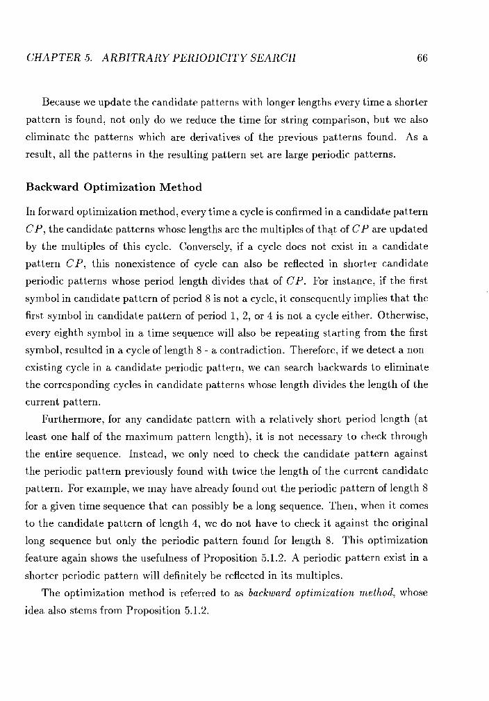
CHAPTER 5. ARBITRARY PERIODICITY SEARCH 66
Because we update the candidate patterns with longer lengths every time a shorter
pattern is found, not only do we reduce the time for string comparison, but we also
eliminate the patterns which are derivatives of the previous patterns found. As a
result, all the patterns in the resulting pattern set are large periodic patterns.
Backward Optimization Met hod
In forward optimization method, every time a cycle is confirmed in a candidate pattern
CP, the candidate patterns whose lengths are the multiples of that of CP are updated
by the multiples of this cycle. Conversely, if a cycle does not exist in a candidate
pattern CP, this nonexistence of cycle can also be reflected in shorter candidate
periodic patterns whose period length divides that of CP. For instance, if the first
symbol in candidate pattern of period 8 is not a cycle, it consequently implies that the
first symbol in candidate pattern of period 1, 2, or 4 is not a cycle either. Otherwise,
every eighth symbol in a time sequence will also be repeating starting from the first
symbol, resulted in a cycle of length 8 - a contradiction. Therefore, if we detect a non-
existing cycle in a candidate periodic pattern, we can search backwards to eliminate
the corresponding cycles in candidate patterns whose length divides the length of the
current pattern.
Furthermore, for any candidate pattern with a relatively short period length (at
least one half of the maximum pattern length), it is not necessary t o check through
the entire sequence. Instead, we only need to check the candidate pattern against
the periodic pattern previously found with twice the length of the current candidate
pattern. For example, we may have already found out the periodic pattern of length 8
for a given time sequence that can possibly be a long sequence. Then, when it comes
to the candidate pattern of length 4, we do not have to check it against the original
long sequence but only the periodic pattern found for length 8. This optimization
feature again shows the usefulness of Proposition 5.1.2. A periodic pattern exist in a
shorter periodic pattern will definitely be reflected in its multiples.
The optimization method is referred to as backward optimization method, whose
idea also stems from Proposition 5.1.2.
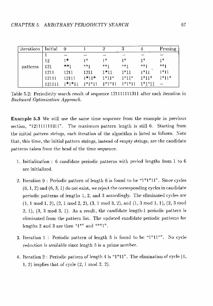
CHAPTER 5. ARBITRARY PERIODICITY SEARCH
iterations
pat terns
Initial 0 1 2 3 4 Pruning
Table 5.2: Periodicity search result of sequence 121 11 11 1131 1 after each iteration in Backward Opt imiza t ion Approach.
Example 5.3 We still use the same time sequence from the example in previous
section, "121111111311". The maximum pattern length is still 6. Starting from
the initial pattern strings, each iteration of the algorithm is listed as follows. Note
that, this time, the initial pattern strings, instead of empty strings, are the candidate
patterns taken from the head of the time sequence.
1. Initialization : 6 candidate periodic patterns with period lengths from 1 to 6
are initialized.
2. Iteration 0 : Periodic pattern of length 6 is found to be "1*1*11". Since cycles
(6 ,1 ,2) and (6 ,3 ,1) do not exist, we reject the corresponding cycles in candidate
periodic patterns of lengths 1, 2, and 3 accordingly. The eliminated cycles are
(1, 1 mod 1, 2), (2, 1 mod 2, 2), (3, 1 mod 3, 2), and (1, 3 mod 1, l), (2, 3 mod
2, I ) , (3, 3 mod 3, 1). As a result, the candidate length-1 periodic pattern is
eliminated from the pattern list. The updated candidate periodic patterns for
lengths 2 and 3 are then "1"" and "**ln.
3. Iteration 1 : Periodic pattern of length 5 is found to be "1*11*". No cycle
reduction is available since length 5 is a prime number.
4. Iteration 2 : Periodic pattern of length 4 is ''l*llV. The elimination of cycle (4,
1, 2) implies that of cycle (2, 1 mod 2, 2).
CHAPTER 5. ARBITRARY PERIODICITY SEARCH 68
5 . Iteration 3 : The candidate length-3 periodic pattern is "**lV, thus only the
substrings in the time sequence corresponding to the third symbol in the can-
didate pattern are checked; and it is checked against its double multiple 1*1*11
instead of the original time sequence. The length-3 periodic pattern turns out
to be """1".
6. Iteration 4 : The first symbol in the candidate 2-cycle periodic pattern "1"" is
checked against the length-4 pattern 1*11 and turns out to be an actual cycle.
7. Pruning : There is no pattern with length 1. The whole pattern list is checked
again to eliminate possible non-large patterns. In this case, the length-6 pattern
is pruned out since it is a product of the length-2 and the length-3 periodic
patterns.
The resulting pattern strings of each period length from each searching process
are listed in Table 5.3. The boldfaced asterisks are the newly eliminated cycles of the
corresponding it eration.
Contrary to the forward optimization approach, we update some patterns with
shorter lengths every time some cycles are eliminated from a longer length pattern.
Ideally, this approach will considerably reduce the number of string comparisons when
there is little regularity in the tested time sequence. However, the performance of the
backward optimization approach is not as satisfactory as one would expect. This is
mainly due to the large amount of overhead introduced in cycle elimination process.
Moreover, the approach relies on a complete check through the entire pattern list in
order to filter out the non-large patterns. This, too, is a tedious process.
One problem of the cycle elimination process is that it involves finding divisors
of an interger. The algorithm for finding divisors is very time consuming. Thus the
advantage of prepruning the cycles diminishes as the maximum period length gets
long. An obvious way to bypass the divisor finding is to leave the cycle elimination
step out of the opimization process. It may seem like a less efficient approach, but
because the overhead created by divisor finding no longer exists, the experimental
CHAPTER 5. ARBITRARY PERIODICITY SEARCH 69
performance result turned out to be improved. Therefore, our final algorithm for the
backward optimization approach contains only one optimization feature, which checks
the correctness of a pattern versus its nearest multiple instead of the entire sequence.
The final algorithm layout for the backward optimization approach is as follows.
Algorithm 5.1.4 Backward~OptimizationApproach
PROCEDURE PeriodicitySearch(i, S )
BEGIN
/* Initialize pattern set */ FOR j := 1 TO pmax DO
p a t t e ~ n - l e n g t h ~ _ ~ := j
n u m - ~ y c l e ~ - ~ := j
Pj-l := (pattern-lengthj-l, n ~ m - c y c l e ~ - ~ , C={(k, &)lk = 0, 1, ..., j - 1
and Vk = S[k]))
END /* FOR */ /* Periodic pattern discovery phase */ FOR k := (pma, - 1) DOWNTO 0 DO
IF k < pmax/2 AND P 2 . k + 1 @ Pi THEN
DELETE Pk
END /* IF */ ELSE
St := S
IF k < pmax/2 THEN
st := p2 .k+1
END /* IF */ FOR j := 0 TO (pattern-lengthk - 1) DO
IF ( j , V,) E Ck THEN
CONVERT Pk to pattern string Sp
IF 3t > 0 such that Sp[j] # S1[j + k t ] THEN
DELETE ( j , V,) E Ck
num-cycle := num-cycle - 1
CHAPTER 5. ARBITRARY PERIODICITY SEARCH
END /* IF */ END /* ELSE */
END /* FOR */ IF num-cycle > 0
INSERT Pk into pattern set Pi END /* IF */
END /* FOR */ END /* ELSE */
END /* FOR */ /* Non-large periodic pattern pruning phase same as that in algorithm 5.1.2.
Omitted. */ RETURN 7';
END
5.1.3 Experiment a1 Results
In this section, we will present the results of some experiments conducted to analyze
the performance of the three algorithms presented in this chapter with respect to
various factors such as data size, degree of pattern regularity, etc.
The experiments were conducted on a Pentium Pro 200 with 64 MB of memory
running Windows NT. Since the periodicity search of the time series is independent
of each other, we will run each experiment on only one time series but for 500 times.
Thus, the execution time shown on all the graphs in this chapter are the running time
of 500 repetitions.
Time Series Size Scale-up
First, the effects of varying size of time series on the two algorithms are examined.
Intuition tells us that, when a time series is irregular, i.e., does not have obvious
periodic behavior, both algorithms should be terminated quite soon. This is because
each iteration of searching process is stopped as soon as a mismatch is encountered.
Figure 5.2 shows the performance result of executing the three algorithms with
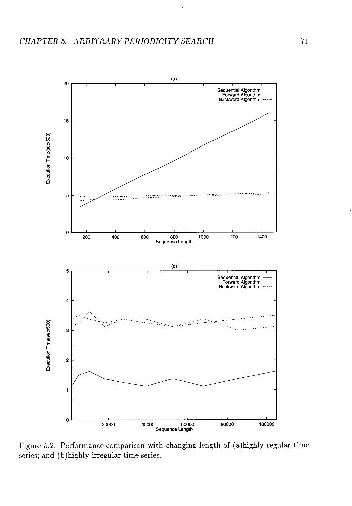
CHAPTER 5. ARBITRARY PERIODICITY SEARCH
Sequential Algorithm - Forward Algorithm - - - - -
Backword Algorithm -
I I I I I I I
200 400 600 800 1000 1200 1400 Sequence Length
(b) I I I I I
Sequential Algorithm - Forward Algorithm - - - - -
Backword Algorithm
20000 40000 60000 80000 100000 Sequence Length
Figure 5.2: Performance comparison with changing length of (a)highly regular time series; and (b)highly irregular time series.
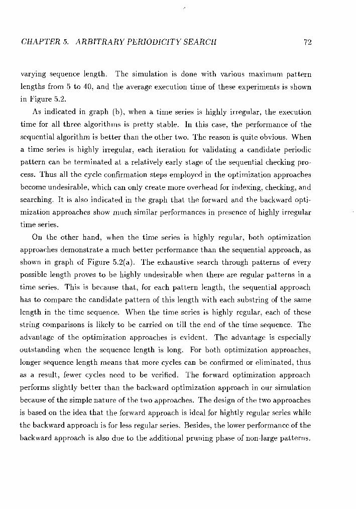
CHAPTER 5. ARBITRARY PERIODICITY SEARCH
varying sequence length. The simulation is done with various maximum pattern
lengths from 5 to 40, and the average execution time of these experiments is shown
in Figure 5.2.
As indicated in graph (b), when a time series is highly irregular, the execution
time for all three algorithms is pretty stable. In this case, the performance of the
sequential algorithm is better than the other two. The reason is quite obvious. When
a time series is highly irregular, each iteration for validating a candidate periodic
pattern can be terminated at a relatively early stage of the sequential checking pro-
cess. Thus all the cycle confirmation steps employed in the optimization approaches
become undesirable, which can only create more overhead for indexing, checking, and
searching. It is also indicated in the graph that the forward and the backward opti-
mization approaches show much similar performances in presence of highly irregular
time series.
On the other hand, when the time series is highly regular, both optimization
approaches demonstrate a much better performance than the sequential approach, as
shown in graph of Figure 5.2(a). The exhaustive search through patterns of every
possible length proves to be highly undesirable when there are regular patterns in a
time series. This is because that, for each pattern length, the sequential approach
has to compare the candidate pattern of this length with each substring of the same
length in the time sequence. When the time series is highly regular, each of these
string comparisons is likely to be carried on till the end of the time sequence. The
advantage of the optimization approaches is evident. The advantage is especially
outstanding when the sequence length is long. For both optimization approaches,
longer sequence length means that more cycles can be confirmed or eliminated, thus
as a result, fewer cycles need to be verified. The forward optimization approach
performs slightly better than the backward optimization approach in our simulation
because of the simple nature of the two approaches. The design of the two approaches
is based on the idea that the forward approach is ideal for hightly regular series while
the backward approach is for less regular series. Besides, the lower performance of the
backward approach is also due to the additional pruning phase of non-large patterns.
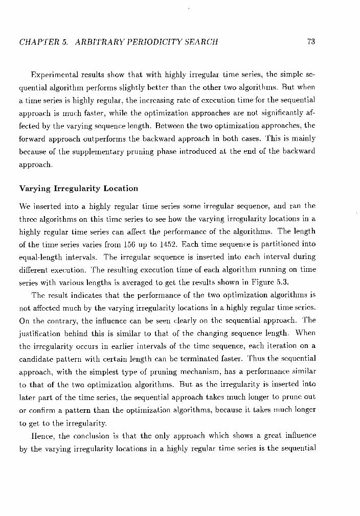
CHAPTER 5. ARBITRARY PERIODICITY SEARCH 73
Experimental results show that with highly irregular time series, the simple se-
quential algorithm performs slightly better than the other two algorithms. But when
a time series is highly regular, the increasing rate of execution time for the sequential
approach is much faster, while the optimization approaches are not significantly af-
fected by the varying sequence length. Between the two optimization approaches, the
forward approach outperforms the backward approach in both cases. This is mainly
because of the supplementary pruning phase introduced at the end of the backward
approach.
Varying Irregularity Locat ion
We inserted into a highly regular time series some irregular sequence, and ran the
three algorithms on this time series to see how the varying irregularity locations in a
highly regular time series can affect the performance of the algorithms. The length
of the time series varies from 156 up to 1452. Each time sequence is partitioned into
equal-length intervals. The irregular sequence is inserted into each interval during
different execution. The resulting execution time of each algorithm running on time
series with various lengths is averaged to get the results shown in Figure 5.3.
The result indicates that the performance of the two optimization algorithms is
not affected much by the varying irregularity locations in a highly regular time series.
On the contrary, the influence can be seen clearly on the sequential approach. The
justification behind this is similar to that of the changing sequence length. When
the irregularity occurs in earlier intervals of the time sequence, each iteration on a
candidate pattern with certain length can be terminated faster. Thus the sequential
approach, with the simplest type of pruning mechanism, has a performance similar
to that of the two optimization algorithms. But as the irregularity is inserted into
later part of the time series, the sequential approach takes much longer to prune out
or confirm a pattern than the optimization algorithms, because it takes much longer
to get to the irregularity.
Hence, the conclusion is that the only approach which shows a great influence
by the varying irregularity locations in a highly regular time series is the sequential
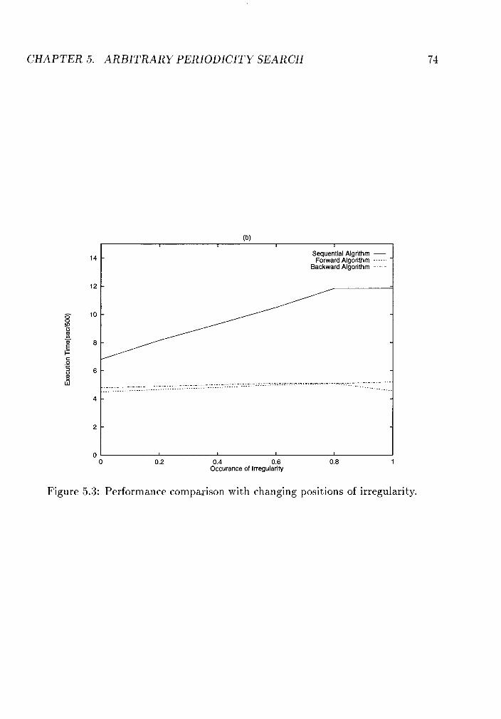
CHAPTER 5. ARBITRARY PERIODICITY SEARCH
I I
Sequential Algrithm - Forward Algorithm - - - - -
Backward Algorithm -
0 0.2 0.4 0.6 0.8 1 Occurance of Irregularity
Figure 5.3: Performance comparison with changing positions of irregularity.
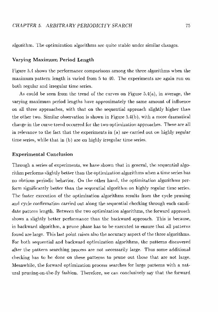
CHAPTER 5. ARBITRARY PERIODICITY SEARCH 75
algorithm. The optimization algorithms are quite stable under similar changes.
Varying Maximum Period Length
Figure 5.4 shows the performance comparisons among the three algorithms when the
maximum pattern length is varied from 5 to 40. The experiments are again run on
both regular and irregular time series.
As could be seen from the trend of the curves on Figure 5.4(a), in average, the
varying maximum period lengths have approximately the same amount of influence
on all three approaches, with that on the sequential approach slightly higher than
the other two. Similar observation is shown in Figure 5.4(b), with a more dramatical
change in the curve trend occurred for the two optimization approaches. These are all
in relevance to the fact that the experiments in (a) are carried out on highly regular
time series, while that in (b) are on highly irregular time series.
Experimental Conclusion
Through a series of experiments, we have shown that in general, the sequential algo-
rithm performs slightly better than the optimization algorithms when a time series has
no obvious periodic behavior. On the other hand, the optimization algorithms per-
form significantly better than the sequential algorithm on highly regular time series.
The faster execution of the optimization algorithms results from the cycle pruning
and cycle confirmation carried out along the sequential checking through each candi-
date pattern length. Between the two optimization algorithms, the forward approach
shows a slightly better performance than the backward approach. This is because,
in backward algorithm, a prune phase has to be executed to ensure that all patterns
found are large. This last point raises also the accuracy aspect of the three algorithms.
For both sequential and backward optimization algorithms, the patterns discovered
after the pattern searching process are not necessarily large. Thus some additional
checking has to be done on these patterns to prune out those that are not large.
Meanwhile, the forward optimization process searches for large patterns with a nat-
ural pruning-on-the-fly fashion. Therefore, we can conclusively say that the forward
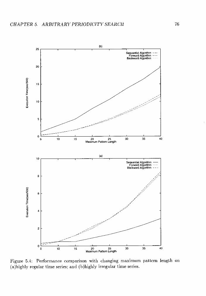
CHAPTER 5. ARBITRARY PERIODICITY SEARCH
(b) I I I I I I
Sequential Algorithm - Forward Algorithm - - - - -
Backward Algorithm - - - - -
Figure 5.4: Performance comparison with changing maximum pattern length on (a)highly regular time series; and (b)highly irregular time series.
CHAPTER 5. ARBITRARY PERIODICITY SEARCH 77
optimization algorithm provides a more efficient way of finding arbitrary patterns in
a time series.
5.1.4 Discussion
All three algorithms presented in previous sections deal with partial periodicity search
problem, in the sense that the number of cycles in a discovered periodic pattern may
be less than the length of the pattern. Since the worst case scenario for all three
algorithms occurs when a search has to go through the entire time sequence for each
candidate pattern length, the complexity for all three algorithms is O(m . n) where m
is the maximum pattern length and n the length of the input time sequence.
In the previous chapter when we discussed the fixed-length periodicity search
problem, we use a confidence threshold as a means of controlling the level of accuracy
of a pattern. This concept of confidence threshold is not employed in the arbitrary
periodicity search problem, because it is not trivial to verify the patterns when the
period length is arbitrary. We can of course apply the sequential algorithm with an
additional confidence threshold as a control parameter. So we can again use the same
strategy, for each period length, first find the 1-cycle patterns of each period length
inside a time series, then combine the 1-cycle patterns of the same period length to
form 2-cycle candidate patterns, etc. The drawback is obvious. This process has to be
executed for each time series at each period length. The processing will be extremely
expensive. Then shall we use optimization approaches similar to those presented
in previous sections to reduce the processing cost? Unfortunately this may not be
feasible either.
Consider the time sequence "11212111". If we set the confidence threshold to be
75% and the maximum pattern length to be 4, then, after the first iteration, we can
conclude that "1" is a periodic pattern with exactly 75% confidence. Then by our
forward optimization mechanism derived from properties 5.1.1 and 5.1.2, we should
be able to derive patterns "ll", "lll", and "llll", all of which are verified to be
false periodic patterns that do not meet the confidence threshold. Now if we try
the backward optimization approach, what we find is that the first pattern we find,
CHAPTER 5. ARBITRARY PERIODICITY SEARCH
LL* * 71 1 1 , will mean a mis-prune of the pattern "1" in a backward cycle pruning process.
So basically, no forward or backward optimization can be done to pre-prune or pre-
confirm any cycles that are not in the current pattern being checked. Every pattern
is detected sequentially through individual checking of an entire time sequence.
Accuracy relaxation is a missing piece in this arbitrary periodicity search approach.
It may be possible that OLAP techniques can be employed to overcome this weakness.
Further study is needed in this area.
Arbitrary Complete Periodicity Search
As mentioned in Chapter 4, users are sometimes specifically interested at periodic
patterns which show a complete match. In other words, every value in a discovered
pattern corresponds to a category which is repeated at the same time within every
period. This problem, again as mentioned, can be considered as a special case of the
partial periodicity search problem and is thus solvable by the previous approaches.
The major concern is still the efficiency and the possibility of optimization with a
narrowed search target.
5.2.1 Modification to the Previous Approaches
In this section, we will talk about ways of optimizing the previous three approaches to
handle explicitly the complete periodicity search problem. The optimized approaches
are referred to as "modified approaches" to avoid any possible confusion with the
forward and the backward optimization approaches discussed in the previous section.
Modified Sequential Approach
When complete periodic pattern matching is required, the search effort is consequently
reduced. In the general approach, when a mismatch occurs between a candidate
pattern and a substring of the time sequence, we prune out the corresponding cycle
in the candidate pattern and go on to verify the other cycles. But since in a complete
periodicity search, one mismatch of cycle already declares an incomplete periodic
CHAPTER 5 . ARBITRARY PERIODICITY SEARCH 79
pattern, the current search iteration can thus be terminated. The search goes on
for each possible period length, until either no more candidate periodic patterns are
available or a complete periodic pattern is found. The reason of the latter condition
will be shown in the following theorem.
Theorem 5.2.1 There exists at most one large complete periodic pattern in a given
sequence.
Proof.
Suppose there are more than one large, complete periodic patterns found in a given
sequence S. Among all these large, complete patterns, PI is one with the shortest
period length 11, and P2 is another with a period length 12.
Let 12= l I . s + t for somes 2 0 a n d 0 s t < 11.
If t = 0, then 11 112, which implies that P2 is a multiple of PI, a contradiction to
our assumption that P2 is a large periodic pattern.
Otherwise, if 0 < t < 11, then since PI and P2 are complete periodic patterns, for
all 0 5 j < t and n > 0, we have the following:
which suggests that there exists another complete pattern Pi whose period length is
t , 0 < t < 11. This again contradicts our assumption that PI is the periodic pattern
with the shortest period length.
Therefore, we conclude that there can be at most one large complete periodic
pattern in a given sequence. 0
Due to this theorem, the periodicity search on one given sequence can be termi-
nated upon the discovery of a large complete periodic pattern.
The faster termination of each sequential search proves to be very significant in
complete periodicity search. This will be shown later in experimental results.
CHAPTER 5. ARBITRARY PERIODICITY SEARCH
Modified Forward Opt imizat ion Approach
In the simplified version of the forward optimization approach for complete periodicity
search problem, we mainly keep the original routine except that the search process
will be ended once a large complete periodic pattern is found. Because the forward
approach is carried out from shorter period length to longer, the first complete pattern
we discover will definitely be a large pattern.
In forward optimization approach, in order to confirm the cycles exist in longer
periodic patterns, we have to first confirm the cycles in patterns with shorter period.
This requires all the unconfirmed substrings in the sequence to be searched even if the
pattern of the current period has already been identified as incomplete. Although this
approach does not take into account too much of the characteristics of the complete
periodicity search, its reduction of the searching space is a merit that could still be
significant in some cases.
Modified Backward Opt imizat ion Approach
There are more dramatic changes in the modified backward optimization approach
than the previous approach. In a backward approach, we discard cycles instead of
confirming cycles. Once a cycle is discarded from a candidate periodic pattern, the
pattern becomes incomplete, and can thus also be discarded. Therefore, for each
period length, we check through the time sequence to see if the candidate periodic
pattern of this length is complete, as soon as a mismatch is confirmed, this pattern,
along with all candidate patterns of lengths that divide the current period length, are
pruned out from the candidate list. Then if a complete periodic pattern is found, by
Theorem 5.2.1, all candidate patterns of lengths that divide the current period length
will be checked against the discovered pattern to see if any other complete periodic
pattern exists; if so, the one with the shortest period length will be the final large
complete pattern, otherwise, the current complete periodic pattern is proved to be
large and is the final solution.
Example 5.4 Suppose the input time sequence is 12121212121212121212, and the
maximum pattern length is set as 9. We start the searching process backwards from
CHAPTER 5. ARBITRARY PERIODICITY SEARCH 81
the maximum pattern length. In this case, the candidate length-9 periodic pattern
is 121212121. Upon checking with the first symbol in the next consecutive substring
of length 9, which is 2 (of "212121212"), the candidate pattern is pruned out from
the candidate list since it has been proved to be at least incomplete. Along with this
candidate pattern, we also prune out the candidate length-1 and length-3 patterns
whose length divides that of the length-9 pattern. Next, we check the candidate
length-8 periodic pattern 12121212 and finds it to be a complete periodic pattern. To
determine whether this is a large pattern or not, we search through the discovered
complete pattern 12121212 to see if there exist another complete pattern of length 2
or 4 (not length-1 since it is pruned out in the last iteration). As a result, the length-2
pattern 12 is the only large complete periodic pattern in this time sequence. [11
Although the original overhead problem persists in searching for divisors, the ap-
proach provides a more efficient means of pruning out incomplete periodic patterns.
Moreover, once a complete periodic pattern is discovered, though the process cannot
be terminated right away and we still have to go on to check if the pattern discovered
is large, it restricts the candidate patterns to be checked to only those that are po-
tentially the original large pattern from which the current pattern derives from. The
later experimental result proves the modified backward optimization approach to be
a more efficient version. Its performance is close to, if not better than, the modified
forward optimization approach.
5.2.2 Experimental Result
The experimental results of the three modified approaches are shown in Figure 5.5 .
The experiments are again conducted on a time series 1,000 times with respect to vary-
ing sequence lengths, varying maximum pat tern lengths, and the changing location
of irregularity occurrences within a highly regular sequence.
Graph (a) shows the average execution time of the three modified algorithms
running on a time series of various lengths with some irregularity inserted into different
locations in the time series. It is obvious from the graph that both the modified
sequential algorithm and the modified forward optimization algorithm are affected by
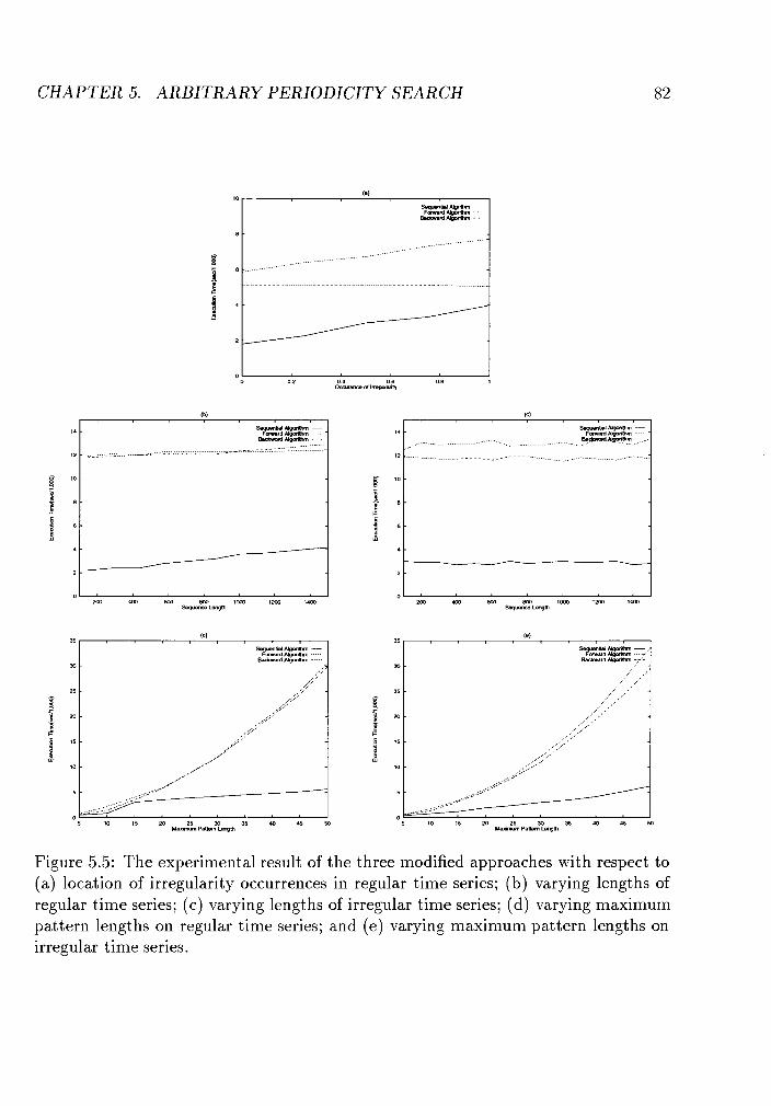
CHAPTER 5. ARBITRARY PERIODICITY SEARCH
Figure 5.5: The experimental result of the three modified approaches with respect to (a) location of irregularity occurrences in regular time series; (b) varying lengths of regular time series; (c) varying lengths of irregular time series; (d) varying maximum pattern lengths on regular time series; and (e) varying maximum pattern lengths on irregular time series.
CHAPTER 5. ARBITRARY PERIODICITY SEARCH 83
the changing irregularity location. The closer the irregularity is to the end of the
time sequence, the longer the execution takes for the two algorithms. This is due
to the longer duration time for the discovery of a periodic pattern mismatch when
the irregularity occurs at later part of a time sequence. Meanwhile, this influence
is not obvious with the modified backward algorithm. It could because that the
cycle pruning process in the backward approach is carried out regardless of when the
irregularity actually occurs. The discovery of one mismatch takes longer when the
irregularity occurs late in a sequence, but then once it is realized, a whole set of other
incomplete periodic patterns will be pruned out from the candidate periodic pattern
set.
The results shown in graphs (b) and (c) with respect to the varying length of
a time sequence are quite the contrary to what we saw in partial periodicity search
approaches. In the complete periodicity approaches, none of the three algorithms seem
to be affected by the sequence length except a little for the sequential algorithm. This
is because we hide the same complete periodic pattern inside all the time sequences
in this experiment, with varying lengths for all the sequences. Therefore, regardless
of the length of a time sequence, whenever the search process hits the actual pattern,
the algorithm is terminated by Theorem 5.2.1.
The last two graphs indicate a smooth change of execution time with the sequen-
tial algorithm and much more dramatic changes with the other two algorithms. The
influence of the varying maximum pattern length is overwhelming on the two opti-
mization algorithms because they insist on either examining the entire time sequence
even though a mismatch at earlier part of the sequence has already been confirmed,
or checking through the entire set of candidate patterns for those that are divisors
of the current pattern. The once tedious sequential pattern checking becomes more
favorable in this case when a early mismatch can declare the end of one candidate
pattern checking process and when the discovery of one complete periodic pattern
terminates the entire searching process.
From this series of experiments, it can be concluded that the relatively faster
termination of a checking through both a sequence and the entire set of candidate
periodic patterns favors the simple sequential algorithm more than the other two
CHAPTER 5. ARBITRARY PERIODICITY SEARCH 84
optimization algorithms. The overhead introduced in the two optimization algorithms
are more outstanding than in the general partial periodicity search process. Thus,
when a complete periodicity match is required, the sequential algorithm is a more
appropriate approach.
5.3 Summary
The problem of finding periodic patterns with arbitrary period lengths is discussed in
this chapter. The problem is discussed in two subproblems as was in the fixed-length
periodicity search. Three algorithms are introduced in partial periodicity search,
which are later on modified to apply in the complete periodicity search problem.
The three algorithms introduced in partial arbitrary periodicity search are sequen-
tial, forward optimization, and backward optimization approaches. Algorithm 5.1.2 is
the sequential approach. While the approach provides a straight-forward solution to
the problem, its efficiency may not be satisfactory when a candidate pattern cannot
be pruned out right away. According to some properties of periodic patterns, some
optimizations can be practiced on the first approach to improve both the efficiency
and accuracy. These optimizations are reflected in the forward and the backward
optimization approaches, illustrated in algorithms 5.1.3 and 5.1.4. The optimization
employed in the forward optimization approach emphasizes on the pre-confirmation
of cycles exist in longer periodic patterns, while that in the backward optimization
approach focus on the pre-pruning of the candidate cycles in shorter periodic patterns.
Both are based on the propositions 5.1.1 and 5.1.2. According to our simulation, we
have shown that the performance of two optimization approaches are not affected
by varying sequence length or irregularity location in a highly regular time series.
However, the varying maximum pattern length does have affect over the two meth-
ods. Besides, the forward optimization approach shows a better performance than the
backward optimization approach. The accuracy problem is also automatically elimi-
nated in the forward approach, while a post-pruning phase has to be executed after
pattern searching process in both sequential and backward optimization approaches.
In complete arbitrary periodicity search, the three algorithms are modified to
CHAPTER 5. ARBITRARY PERIODICITY SEARCH 8 5
reflect the complete restriction on the discovered periodic patterns. Each of them are
so modified that either a search through the sequence is terminated once the current
candidate pattern is proved to be incomplete, or the entire search process is terminated
once a complete periodic pattern is located (by Theorem 5.2.1). The improvement
of the performance is significant for all three modified algorithms, especially for the
sequential approach. Simulation results show that varying sequence length has little
influence on all three algorithms, while all are affected by the varying maximum
pattern length with a relatively small affect on the sequential approach. The backward
optimization approach stands out in experiments with respect to the varying locations
of irregularity occurrence with virtually no affect.
The accuracy relaxation is a missing piece in this study of arbitrary periodicity
search, which requires further study. The reasoning of this is already discussed in
Section 5.1.4. OLAP-based approaches such as illustrated in chapter 4 may be a pos-
sible solution for this problem, although it is not trivial concerning how to manipulate
different time planes to serve as the foundation for the discovery of periodic pattern
of varied lengths.
Chapter 6
Conclusion and Future Research
In this thesis, we have presented some algorithms for periodicity search problem.
There are two major subproblems of our concern: fixed-length periodicity search
and arbitrary periodicity search. In each of these subproblems, we discussed some
approaches for both partial and complete periodic pattern search. Some experimental
results were also given. In this chapter, we will conclude with a summary of this study
and propose some future research directions in the area.
6.1 Summary of Research
The goal of this study is to propose some possible solution to the problem of finding
periodic behaviors in large data sets. The research comprising this thesis has a number
of impacts including applying OLAP technology to discover periodicity across different
concept levels, finding patterns of partial periodicity, and using properties of periodic
time sequence to optimize the search process.
In fixed-length periodic pattern discovery problem, we proposed an OLAP-based
search algorithm which combined techniques of data cube and OLAP operations with
some sequential pattern search strategies to discover large periodic patterns of each
time series. The efficiency of this algorithm largely relies on the manipulation of data
cube that has been an active research topic for the past several years. The accuracy
of the algorithm has been shown in [7]. The use of OLAP techniques allows us to
C H A P T E R 6. CONCLUSION A N D FUTURE RESEARCH 8 7
explore periodicity across various concept levels and to find periodic patterns of our
interest as well.
In a mathematical context, periodicity usually refers to a complete pattern match
recurring in a regular interval. In this study, we extend this idea of periodicity to
allow partial pattern match. This is partly in correspondence to the seasonal variation
introduced in [37]. Thus, any regular behavior within a time series will be detected.
Periodic time series have certain properties as introduced in Chapter 5 . These
properties, when employed in arbitrary periodicity search, can substantially reduce
the search effort via cycle pre-confirming or cycle pre-pruning. The optimization
is implemented into the forward and the backward optimization algorithms, and is
tested to dramatically improve the performance in partial arbitrary periodicity search
problem.
Some simulation has been done on the arbitrary periodicity search problem with
respect to varying sequence length, varying maximum pattern length, and varying lo-
cation of irregularity occurrence. The results show that, in partial periodicity search
problem, the two optimization algorithms are far more efficient than the sequential
algorithm in most cases when a time series has even a slight indication of regular-
ity. The performance of the two optimization algorithms are very similar. On the
other hand, the simple, straight-forward sequential algorithm outperforms the two
optimization algorithms in complete periodicity search problem. This is due to the
fact that the restriction on a complete pattern match allows a faster termination in
each search through a time sequence and a complete termination of the entire search
process once a complete pattern is encountered(The0rem 5.2.1). However, there is
an indication showing a more dramatical increase of execution time of the sequen-
tial algorithm than that of the backward optimization algorithm with the change of
irregularity occurrence.
Hence we conclude that there is no single algorithm proposed that stands out in
all cases. Generally, the optimization approaches are suitable for detecting arbitrary
partial periodic behaviors among time sequences that have a strong indication of
periodicity, while the sequential approach has a faster response time in arbitrary
complete periodicity search, and in arbitrary paritial periodicity search when a time
CHAPTER 6. CONCLUSION AND FUTURE RESEARCH
sequence is not so regular.
6.2 Future Research Direction
We have proposed the algorithms for periodicity search in time-related data sets based
on Assumptions 3.3.1, 3.3.2 and 3.3.3. Among these three assumptions, the first two
can be relaxed to extend the scope of this research.
In real applications, very likely, time series of interest are not always input with
same time intervals. There may be pieces of information missing in some time series
or even different time granularity for different time series. This adds extra complexity
to the analysis of the time series. Some signal processing methods may be used to fill
in these gaps so that the time series can be normalized for periodicity detection. On
the other hand, periodicity detection may in turn provide some hint to these missing
data.
In most cases, such as stock data, time series obtained are rarely noise-free. Special
signal smoothing techniques need be applied to preprocessing these time series so that
the resulting time series we work on are relatively simple and smooth. A method
using wavelet transform technique to generalize an input signal is being studied in
[40], which may provide us with an efficient tool to handle this problem.
Another issue of concern is the accuracy relaxation aspect missing in the arbitrary
periodicity search problem. As stated in Section 5.1.4, accuracy relaxation problem
requires special handling of the input sequence that will with no doubt add extra
complexity into the problem of finding periodic patterns of arbitrary period length.
OLAP technology may be employed to overcome this weakness.
Furthermore, the approaches proposed in this thesis can also be extended to handle
a more complex situation such that certain conditions can be discovered under which
the periodic patterns occur. One obvious way to do this is to explicitly express the
interested conditions in the selective query to find periodic patterns associated with
these conditions. Another way is by using classication rule discovery techniques [26]
to describe the discovered patterns by other non-time-related attributes.
Appendix: A
AprioriAll Algorithm
Agrawal et. al. proposed an A~rioriAll algorithm for mining sequential patterns in
transaction databases[7]. The algorithm consists of two phases, a sequence phase for
discovery of all large sequences and a maximal phase for pruning out those patterns
that are not maximal. In the sequence phase, we need to go through iterations
of candidate large i-sequences generation and verification. The two procedures for
candidate generation are also outlined following the ApriorAll algorithm.
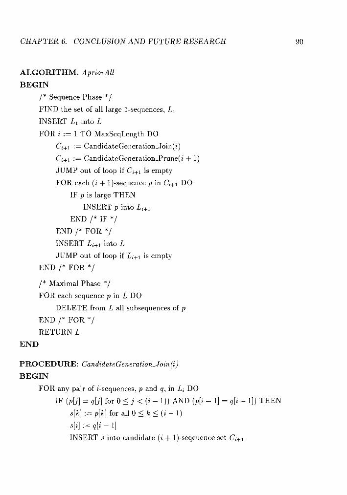
CHAPTER 6. CONCLUSION AND FUTURE RESEARCH
ALGORITHM. ApriorAll
BEGIN
/* Sequence Phase */ FIND the set of all large 1-sequences, L1
INSERT L1 into L
FOR i := 1 TO MaxSeqLength DO
C;+l := CandidateGeneration-Join(i)
C;+l := CandidateGeneration-Prune(i + 1)
JUMP out of loop if C;+l is empty
FOR each (i + 1)-sequence p in Ci+l DO
IF p is large THEN
INSERT p into L;+l
END /* IF */ END /* FOR */ INSERT L;+l into L
JUMP out of loop if L;+l is empty
END /* FOR */
/* Maximal Phase */ FOR each sequence p in L DO
DELETE from L all subsequences of p
END /* FOR */ RETURN L
END
PROCEDURE: CandidateGeneration-Join(i)
BEGIN
FOR any pair of i-sequences, p and q , in L; DO
IF (p[j] = q[j] for O 5 j < (i - 1)) AND (p[i - 11 = q[i - 11) 'THEN
s[k] := p[k] for all 0 5 k 5 (i - 1)
s[i] := q[i - 11
INSERT s into candidate (i + 1)-seqeuence set C;+l
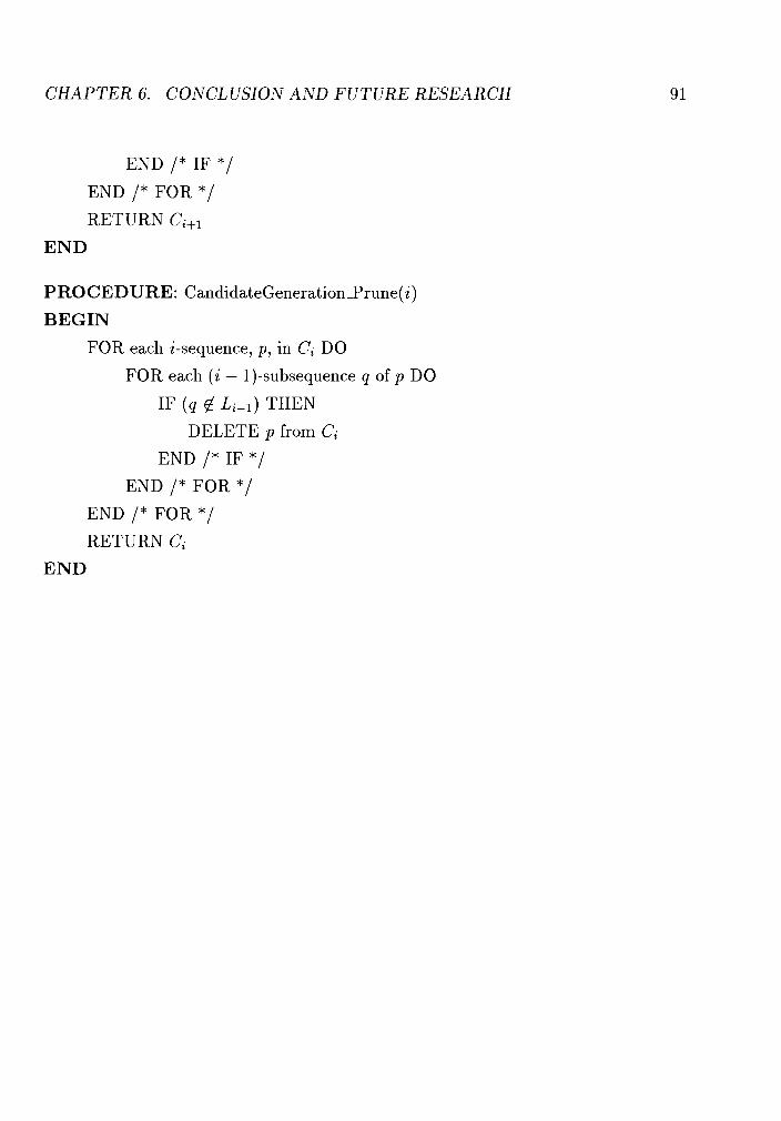
CHAPTER 6. CONCLUSION AND FUTURE RESEARCH
END /* IF */ END /* FOR */ RETURN Ci+l
END
PROCEDURE: CandidateGeneration-Prune(i)
BEGIN
FOR each i-sequence, p, in C; DO
FOR each (i - 1)-subsequence q of p DO
IF ( q @ L;-l) THEN
DELETE p from C;
END /* IF */ END /* FOR */
END /* FOR */ RETURN C;
END
Bibliography
[I] S. Agarwal, R. Agrawal, P. M. Deshpande, A. Gupta, J. F. Naughton, R. Ramakr-
ishnan, and S. Sarawagi. On the computation of multidimensional aggregates.
In Proc. 1996 Int. Conf. Very Large Data Bases, pages 506-521, Bombay, India,
Sept. 1996.
\ [2] R. Agrawal, C. Faloutsos, and A. Swami. Efficient similarity search in sequence
databases. In Proc. 4th Intl. Conf. on Foundations of Data Organization and
Algorithms, October 1993.
[3] R. Agrawal, T. Imielinski, and A. Swami. Mining association rules between sets of
items in large databases. In Proc. 1993 ACM-SIGMOD Int. Conf. Management
of Data, pages 207-216, Washington, D.C., May 1993.
\[4] R. Agrawal, K.-I. Lin, H.S. Sawhney, and K. Shim. Fast similarity search in
the presence of noise, scaling, and translation in time-series databases. In Proc.
21st Int. Conf. Very Large Data Bases, pages 490-501, Zurich, Switzerland, Sept.
1995.
[5] R. Agrawal, G. Psaila, E. L. Wimmers, and M. Zait. Querying shapes of his-
tories. In Proc. 21st Int. Conf. Very Large Data Bases, pages 502-514, Zurich,
Switzerland, Sept. 1995.
[6] R. Agrawal and R. Srikant. Fast algorithms for mining association rules. In
Proc. 1994 Int. Conf. Very Large Data Bases, pages 487-499, Santiago, Chile,
September 1994.
BIBLIOGRAPHY 93
[7] R. Agrawal and R. Srikant. Mining sequential patterns. In Proc. 1995 Int. Conf.
Data Engineering, pages 3-14, Taipei, Taiwan, March 1995.
[8] S. Altschul, W. Gish, W. Miller, E. Myers, and D. Lipman. A basic local align-
ment search tool. In Journal of Molecular Biology, 1990.
[9] P. Bloomfield Fourier Analysis of Time Series: An Introduction. John Wiley &
Sons, 1976.
[lo] R. Burden and J . Faires. Numerical Analysis, 5 ed. PWS Publishing Company,
1993.
[ll] S. Chakravarthy and S.-K. Kim. Resolution of time concepts in temporal
databases. In Information Sciences, volume 80 of 1, 1994.
[12] S. Chaudhuri and U. Dayal. An overview of data warehousing and OLAP tech-
nology. ACM SIGMOD Record, 26:65-74, 1997.
[13] M. S. Chen, J. Han, and P. S. Yu. Data mining: An overview from a database
perspective. IEEE Transactions on Knowledge and Data Engineering, $2366-883,
1996.
!, [14] T . G. Dietterich and R. S. Michalski. Discoverying patterns in sequences of
events. In Artijcial Intelligence, volume 25, 1985.
[15] G. Dunn and B. Everitt. An Introduction to Mathematical Taxonomy. Cambridge
Press, 1982.
\ [16] C. Faloutsos, M. Ranganathan, and Y. Manolopoulos. Fast subsequence matching
in time-series databases. In Proc. of the ACM SIGMOD Conference on Manage-
ment of Data, 1994.
[17] D. Fisher. Improving inference through conceptual clustering. In Proc. 1987
A AAI Conf., pages 461-465, Seattle, Washington, July 1987.
[18] Y. Fu. Discovery of multiple-level rules from large databases. In Ph. D. thesis,
Simon Fraser University, 1996.
BIBLIOGRAPHY 94
[19] J . Gray, S. Chaudhuri, A. Bosworth, A. Layman, D. Reichart, M. Venkatrao,
F. Pellow, and H. Pirahesh. Data cube: A relational aggregation operator gener-
alizing group-by, cross-tab and sub-totals. Data Mining and Ii'nowledge Discov-
ery, 1:29-54, 1997.
[20] A. Gupta, V. Harinarayan, and D. Quass. Aggregate-query processing in data
warehousing environment. In Proc. 21st Int. Conf. Very Large Data Bases, pages
358-369, Zurich, Switzerland, Sept. 1995.
[21] J . Han, Y. Cai, and N. Cercone. Data-driven discovery of quantitative rules in
relational databases. IEEE Trans. Knowledge and Data Engineering, 5:29-40,
1993.
[22] J. Han and Y. Fu. Dynamic generation and refinement of concept hierarchies for
knowledge discovery in databases. In Proc. AAA1794 Workshop on Knowledge
Discovery in Databases (IilDD '94), pages 157-168, Seattle, WA, July 1994.
[23] J. Han and Y. Fu. Exploration of the power of attribute-oriented induction in
data mining. In U.M. Fayyad, G. Piatetsky-Shapiro, P. Smyth, and R. Uthu-
rusamy, editors, Advances in Knowledge Discovery and Data Mining, pages 399-
421. AAAI/MIT Press, 1996.
1241 J. Han, Y. Fu, W. Wang, J . Chiang, W. Gong, K. Koperski, D. Li, Y. Lu,
A. Rajan, N. Stefanovic, B. Xia, and 0. R. Zaiane. DBMiner: A system for
mining knowledge in large relational databases. In Proc. 1996 Int 'I Conf. on Data
Mining and Ii'nowledge Discovery (IilDD'96), pages 250-255, Portland, Oregon,
August 1996.
[25] V. Harinarayan, A. Rajaraman, and J. D. Ullman. Implementing data cubes
efficiently. In Proc. 1996 ACM-SIGMOD Int. Conf. Management of Data, pages
205-216, Montreal, Canada, June 1996.
[26] M. Kamber, L. Winstone, W. Gong, S. Cheng, and J. Han. Generalization and
decision tree induction: Efficient classification in data mining. In Proc. of 1997
BIBLIOGRAPHY 95
Int. Workshop on Research Issues on Data Engineering (RIDEJ97), pages 111-
120, Birmingham, England, April 1997.
[27] http://www. olapcouncil. org.
[28] W. H. Inmon. Building the Data Warehouse. QED Technical Publishing Group,
Wellesley, Massachusetts, 1992.
[29] D. A. Keim, H.-P. Kriegel, and T. Seidl. Supporting data mining of large
databases by visual feedback queries. In Proc. 10th of Int. Conf. on Data Engi-
neering, pages 302-313, Houston, TX, Feb. 1994.
[30] R. Kimball. The Data Warehouse Toolkit. John Wiley & Sons, New York, 1996.
[31] R. S. Michalski. A theory and methodology of inductive learning. In Michalski
et al., editor, Machine Learning: An Artificial Intelligence Approach, Vol. 1,
pages 83-134. Morgan Kaufmann, 1983.
[32] R. S. Michalski and R. Stepp. Automated construction of classifications: Con-
ceptual clustering versus numerical taxonomy. IEEE Trans. Pattern Analysis
and Machine Intelligence, 5:396-410, 1983.
[33] R. Missaoui and R. Godin. An incremental concept formation approach for
learning from databases. In V.S. Alagar, L.V.S. Lakshmanan, and F. Sadri,
editors, Formal Methods in Databases and Software Engineering, pages 39-53.
Springer-Verlag, 1993.
\ [34] B. Ozden, S. Ramaswamy, and A. Silberschatz. Cyclic association rules. In
Appear in Proc. of 1998 Int. Conf. on Data Engineering (ICDE'98), 1998.
[35] G. Ozsoyoglu and R. T. Snodgrass. Temporal and real-time databases: A survey.
In IEEE Transactions on Knowledge an,d Data Engineering, volume 7 of 4, 1995.
[36] R. Snodgrass. Temporal databases. In Computer, volume 19, 1986.
[37] M. Spiegel. Schaum's outline series of theory and problems of statistics. In
McGraw Hill, 1996.
BIBLIOGRAPHY 96
[38] J. Widom. Research problems in data warehousing. In Proc. 4th Int. Conf. on
Information and Knowledge Management, pages 25-30, Baltimore, Maryland,
Nov. 1995.
[39] S. Wu and U. Manber. Fast text searching allowing errors. In Communications
of the ACM, volume 35 of 10, 1992.
[40] B. Xia. Similarity Search in Time Series Data Sets. In Master thesis, Simon
Fraser University, 1997.
[41] W. P. Yan and P. Larson. Eager aggregation and lazy aggregation. In Proc. 21st
Int. Conf. Very Large Data Bases, pages 345-357, Zurich, Switzerland, Sept.
1995.
[42] Y. Zhao, P. M. Deshpande, and J. F. Naughton. An array-based algorithm for
simultaneous multidimensional aggregates. In Proc. 1997 A CM-SIGMOD Int.
Conf. Management of Data, pages 159-170, Tucson, Arizona, May 1997.


![[Nebojsa Matic, Dragan Andric] PIC Mikrokontroleri(BookFi.org)](https://img.pdfslide.us/doc/110x75/55cf99e7550346d0339fb0ac/nebojsa-matic-dragan-andric-pic-mikrokontroleribookfiorg.jpg)