PERFORMANCE OPTIMIZATION OF A DIESEL ENGINE FOR DUAL …

The Pennsylvania State University

The Graduate School

College of Engineering

PERFORMANCE OPTIMIZATION OF A DIESEL ENGINE

FOR DUAL-FUEL COMBUSTION

A Thesis in

Industrial Engineering

by

Srinivas Jayaraman

© 2012 Srinivas Jayaraman

Submitted in Partial Fulfillment

of the Requirements

for the Degree of

Master of Science

August 2012

ii

The thesis of Srinivas Jayaraman was reviewed and approved* by the following:

André L. Boehman

Professor of Fuel Science, Material Science and Engineering and Mechanical

Engineering

Thesis Co-advisor

Jose Ventura

Professor of Industrial and Manufacturing Engineering

Thesis Co-advisor

Paul M. Griffin

Professor of Industrial and Manufacturing Engineering

Peter and Angela Dal Pezzo Department Head Chair

*Signatures are on file in the Graduate School

iii

ABSTRACT

With recent emphasis on clean fuel and environmental sustainability, it has

become increasingly important to look into methods of reducing fuel consumption and

emissions while simultaneously maintaining the level of engine performance. Through

this study an attempt has been made to observe the effects of using fumigated fuels and

an injection of diesel on the performance of an engine and subsequent emissions. The

performance of the engine will be judged primarily on brake specific fuel consumption

(BSFC), brake specific energy consumption (BSEC), brake thermal efficiency (BTE),

peak cylinder pressure and the apparent heat release rate, while total hydrocarbon content

(THC), nitrogen oxides (NOx), carbon dioxide (CO2) and carbon monoxide (CO) were

considered to analyze the emissions. The data collected was statistically analyzed to

determine which factors are most significant in determining the engine‘s performance.

Exhaust gas recirculation was also used to observe its effects on the above outcomes.

The engine used to conduct the tests is a DDC/VM-Motori 2.5L, 4 cylinder,

turbocharged, direct injection, light duty diesel engine. The fuels to be fumigated in the

cylinder are dimethyl ether (DME) and propane, and the injection is of ultra-low sulphur

diesel (ULSD). Previous studies have shown that DME, which has a low boiling point

and high cetane number, tends to advance the ignition point by increasing the low

temperature heat release. Methane has also been used in the past along with DME to

delay the heat release, provide for a more controlled reaction as well as reduce NOx

emissions. This study attempts to achieve the same effects using propane instead of

iv

methane along with DME. The concentrations of DME and propane in the fumigated fuel

were varied over a span of 0 to 60% energy equivalent of the total fuel requirement.

The experiments were conducted in two sets, the first set of experiments utilized

just DME as the fumigated fuel in the cylinder along with an injection of ULSD. In the

second set of experiments, propane was added to the DME to be fumigated in the

cylinder. Previous studies have shown favorable trends in the values of BSFC and BSEC

due to the addition of a fumigated fuel (usually natural gas) along with an injection of

diesel. Similar results were observed for the addition of DME and propane as the

fumigated fuels along with diesel along with an increase in BTE. It was observed that the

heat release was advanced with increasing energy substitution. There was also an

increase in the peak cylinder pressure with increasing fumigation as compared to baseline

diesel. Reduction in NOx emissions was observed which further reduced with EGR

introduction. THC emissions on the other hand increased with increasing substitution.

On completion of the experiments, a statistical analysis was performed to

determine the factors which had the most influence on the performance of the engine.

The tests were treated as a General Full Factorial Experimental Design and an analysis of

variance (ANOVA) was performed to determine the significant factors. Once, the

significant factors were determined, regression analysis was used to determine the effect

each factor has on the performance of the engine with interactions between the variables

also considered. Based on these conclusions, operating conditions were obtained for the

next set of tests. The engine was run at these conditions and the results were noted. It was

noticed that BTE increased with increasing substitution with DME and Propane along

with a corresponding decrease in BSEC and BSFC values. THC in the emissions

v

decreased with increasing DME but increased with propane. Total NOx, on the other hand

reduced with increasing DME and propane energy substitution.

vi

TABLE OF CONTENTS

LIST OF FIGURES ............................................................................................................ viii

LIST OF TABLES .............................................................................................................. xii

GLOSSARY ....................................................................................................................... xiii

ACKNOWLEDGEMENTS ................................................................................................ xv

Chapter 1 INTRODUCTION .............................................................................................. 1

1.1 Oil Depletion and Global Warming ...................................................................... 1 1.2 The Diesel Engine ................................................................................................ 3 1.3 The Diesel Engine Combustion Process ............................................................... 6 1.4 Differences between SI engines and CI Engines ................................................... 8 1.5 Thesis Overview .................................................................................................. 8

Chapter 2 Literature Review ............................................................................................... 10

2.1 Homogeneous Charge Compression Ignition (HCCI) Combustion........................ 10 2.1.1 Mixed Mode Combustion ........................................................................... 11 2.1.2 Premixed Charge Compression Ignition (PCCI) combustion ....................... 12

2.2 Reactivity Controlled Compression Ignition (RCCI) combustion .......................... 13 2.3 Fumigated Fuels .................................................................................................. 16

2.3.1 Dimethyl Ether (DME) ............................................................................... 16 2.3.2 Propane ...................................................................................................... 18 2.3.3 Advantages of Propane over Methane ......................................................... 21

Chapter 3 Experimental Setup ............................................................................................. 23

3.1 Engine Specifications ........................................................................................... 23 3.2 Load Generation and Dynamometer ..................................................................... 24 3.3 Engine Control ..................................................................................................... 25 3.4 Data Acquisition .................................................................................................. 25 3.5 Pressure Trace and Needle Lift Sensor ................................................................. 26 3.6 Mass of Air Flow (MAF) and Diesel Flow Rate ................................................... 26 3.7 Flowmeter Setup .................................................................................................. 27 3.8 Engine Emissions Measurement ........................................................................... 29

Chapter 4 Experiments and Analysis – Part 1 ...................................................................... 31

4.1 Experimental Runs ............................................................................................... 31 4.1.1 Multilevel Factorial Design ........................................................................ 32 4.1.2 Analysis of Variance (ANOVA) ................................................................. 34

4.2 Regression Analysis ............................................................................................. 35 4.2.1 Brake Thermal Efficiency (BTE) ................................................................ 37 4.2.2 Brake Specific Energy Consumption (BSEC) ............................................. 39

vii

4.2.3 Brake Specific Fuel Consumption (BSFC) .................................................. 40 4.2.4 Brake Specific Diesel Consumption ............................................................ 42 4.2.5 Heat Release Rate (HRR) ........................................................................... 43 4.2.6 Pressure Rise Rate (PRR) ........................................................................... 45 4.2.7 Obtaining a trade-off point.......................................................................... 47

Chapter 5 Experiments and Analysis – Part 2 ...................................................................... 50

5.1 Experimental Runs ............................................................................................... 50 5.2 DME and Propane fumigation without Exhaust Gas Recirculation ........................ 53

5.2.1 Brake Specific Energy Consumption (BSEC).............................................. 53 5.2.2 Brake Thermal Efficiency (BTE) ................................................................ 54 5.2.3 Brake Specific Fuel Consumption (BSFC) .................................................. 55 5.2.4 Heat Release Rate ....................................................................................... 55 5.2.4 Pressure Rise Rate (PRR) ........................................................................... 61 5.2.5 Total Hydrocarbon Emissions (THC) .......................................................... 66 5.2.6 Nitrogen Oxide emissions (NOx)................................................................. 67 5.2.7 Carbon Dioxide Emissions (CO2)................................................................ 69 5.2.8 Carbon Monoxide (CO) .............................................................................. 70

5.3 DME and Propane fumigation with Exhaust Gas Recirculation (EGR) ................. 71 5.3.1 Engine Performance parameters: ................................................................. 72 5.3.2 Engine Emissions ....................................................................................... 79

5.4 DME and Propane fumigation with exhaust gas recirculation (EGR) and split

injection ............................................................................................................... 84 5.4.1 Engine Performance Parameters .................................................................. 85

5.4.2 Engine Emissions ........................................................................................ 88

Chapter 6 Summary and Conclusions .................................................................................. 92

6.1 Summary ............................................................................................................. 92 6.2 Observations and Conclusions .............................................................................. 93 6.3 Suggestions for Future Work ................................................................................ 95

Bibliography ....................................................................................................................... 97

Appendix A Matheson Gas Flowmeter Calibration ..................................................... 102 A.1 Flowmeter 605 Calibration Chart: ........................................................................ 102 A.2 Flowmeter 603 Calibration Chart: ........................................................................ 103 A.3 Flowmeter 604 calibration chart: .......................................................................... 104 A.4 Flowmeter 605 Calibration Chart: ........................................................................ 105

Appendix B Interaction Plots ............................................................................................. 106

Appendix C Regression Analysis – Minitab Output ............................................................ 120

viii

LIST OF FIGURES

Figure 1.1: United States Oil Consumption [4] .................................................................... 2

Figure 1.2: The Diesel Cycle ............................................................................................... 4

Figure 1.3: Heat Release Profile of a Diesel Engine [9] ....................................................... 6

Figure 2.1: Rate of heat release for propane and DME at various equivalence ratios [46] ..... 19

Figure 3.1: Photograph of 2.5 L DDC/VM Motori Engine ................................................... 24

Figure 3.2: Matheson Gas 7410 series flow meter................................................................ 27

Figure 3.3: Block Diagram of DME, Propane flow and mixing into the engine .................... 28

Figure 3.4: AVL CEB II emissions bench............................................................................ 29

Figure 4.1: Brake Thermal Efficiency at varying DME and propane substitution levels ....... 38

Figure 4.2: Brake Specific Energy Consumption at varying DME and propane

substitution levels ........................................................................................................ 39

Figure 4.3: Brake Specific Fuel Consumption at varying DME and propane substitution levels ........................................................................................................................... 41

Figure 4.4: Brake Specific Diesel Consumption at varying DME and propane substitution

levels ........................................................................................................................... 42

Figure 4.5: Apparent Heat Release Rate at varying DME and propane substitution levels .... 44

Figure 4.6: Average Pressure Rise Rate at varying DME and propane substitution levels ..... 45

Figure 4.7: Visual representation of optimal points for the individual response variables ..... 46

Figure 4.8: Visual representation of the optimal point for obtaining a trade-off between BTE and PRR .............................................................................................................. 49


substitution levels without EGR ................................................................................... 53

Figure 5.2: Brake Thermal Efficiency at varying DME and propane substitution levels

without EGR ............................................................................................................... 54

Figure 5.3: Brake Specific Fuel Consumption at varying DME and Propane levels

without EGR ............................................................................................................... 55

ix

Figure 5.4: Heat Release Rate at varying DME and Propane levels without EGR ................. 56

Figure 5.5: Heat release rate v/s crank angle for 0% DME substitution and 0 – 40%

propane substitution without EGR ............................................................................... 57

Figure 5.6: Heat release rate v/s crank angle for 10% DME substitution and 0 – 30% propane substitution without EGR ............................................................................... 58




propane substitution and 40% DME substitution and 0% propane without EGR ........... 59

Figure 5.9: Heat release rate v/s crank angle for 10 - 40% DME substitution and 0% propane substitution without EGR ............................................................................... 60

Figure 5.10: Pressure rise rate in the cylinder at varying DME and propane levels ............... 61

Figure 5.11: Pressure rise rate v/s crank angle for 0% DME substitution and 0 – 40%




Figure 5.13: Pressure rise rate v/s crank angle for 20% DME substitution and 0 – 30% propane substitution without EGR ............................................................................... 63

Figure 5.14: Pressure rise rate v/s Crank Angle for 30% DME substitution and 0 – 30%

propane substitution and 40% DME substitution and 0% propane without EGR ........... 64

Figure 5.15: Pressure rise rate v/s crank angle for 0% propane substitution and 10 – 40%

DME substitution ........................................................................................................ 65

Figure 5.16: Total hydrocarbon emissions at varying DME and propane levels without

EGR ............................................................................................................................ 66

Figure 5.17: Nitrogen oxide (NOx) emissions at varying DME and propane levels

without EGR ............................................................................................................... 67

Figure 5.18: Nitric oxide (NO) emissions at varying DME and propane levels without EGR ............................................................................................................................ 68

Figure 5.19: Nitrogen Dioxide (NO2) emissions at varying DME and Propane levels

without EGR ............................................................................................................... 69

Figure 5.20: Carbon Dioxide emissions at varying DME and propane levels without EGR .. 70

Figure 5.21: Carbon Monoxide emissions at varying DME and propane levels without

EGR ............................................................................................................................ 71

x

Figure 5.22: Brake thermal efficiency (BTE) at varying DME and propane levels with

and without EGR ......................................................................................................... 72

Figure 5.23: Brake Specific Energy Consumption (BSEC) at varying DME and propane

levels with and without EGR ....................................................................................... 73

Figure 5.24: Average Heat Release Rate (HRR) at varying DME and Propane levels with

and without EGR ......................................................................................................... 74

Figure 5.25: Heat release rate v/s crank angle for 10% DME substitution and 0, 20 and 40% propane substitution with EGR ............................................................................ 74

Figure 5.26: Heat release rate v/s crank angle for 20 and 30% DME substitution and 0

and 20% propane substitution with EGR ...................................................................... 75

Figure 5.27: Heat release rate v/s crank angle for cases with and without EGR .................... 76

Figure 5.28: Average pressure rise rate (PRR) at varying DME and propane levels with

and without EGR ......................................................................................................... 77

Figure 5.29: Pressure rise rate v/s crank angle for 10% DME substitution and 0, 20 and 40% propane substitution with EGR ............................................................................ 77

Figure 5.30: Pressure rise rate v/s crank angle for 20 and 30% DME substitution and 0

and 20% propane substitution with EGR ...................................................................... 78

Figure 5.31: Pressure Rise v/s Crank Angle for cases with and without EGR ....................... 79

Figure 5.32: Total hydrocarbon emissions (THC) at varying DME and propane levels

with and without EGR ................................................................................................. 80

Figure 5.33: Nitrogen oxide emissions (NOx) at varying DME and propane levels with

and without EGR ......................................................................................................... 81

Figure 5.34: Nitric oxide emissions (NO) at varying DME and propane levels with and

without EGR ............................................................................................................... 82

Figure 5.35: Nitrogen dioxide emissions (NO2) at varying DME and propane levels with

and without EGR ......................................................................................................... 82

Figure 5.36: Carbon dioxide emissions (CO2) at varying DME and propane levels with and without EGR ......................................................................................................... 83

Figure 5.37: Carbon monoxide emissions (CO) at varying DME and propane levels with

and without EGR ......................................................................................................... 84

Figure 5.38: Brake Thermal Efficiency (BTE) at 20% DME, 20% propane, 16 deg BTDC pilot injection and varying main injection timing ......................................................... 85

xi

Figure 5.39: Brake Specific Energy Consumption (BSEC) at 20% DME, 20% Propane,

16 deg BTDC pilot injection and varying main injection timing with EGR ................... 86

Figure 5.40: Heat release rate (HRR) at 20% DME, 20% propane, 16 deg BTDC pilot

injection and varying main injection timing with EGR ................................................. 87

Figure 5.41: Pressure rise rate (PRR) at 20% DME, 20% propane, 16 deg BTDC pilot

injection and varying main injection timing with EGR ................................................. 88

Figure 5.42: Total Hydrocarbon emissions (THC) at 20% DME, 20% propane, 16 deg BTDC pilot injection and varying main injection timing with EGR .............................. 89

Figure 5.43: Total Nitrogen Oxide emissions (NOx) at 20% DME, 20% propane, 16 deg

BTDC pilot injection and varying main injection timing with EGR .............................. 89

Figure 5.44: Total Carbon dioxide emissions (CO2) at 20% DME, 20% Propane, 16 deg


Figure 5.45: Total Carbon dioxide emissions (CO) at 20% DME, 20% propane, 16 deg


Figure 6.1: Scatter plot of data points at which optimal values of response variables occur .. 95

Figure A.1: Calibration for Flowmeter tube 605 at 0 psig for Propane ................................. 102

Figure A.2: Calibration for Flowmeter tube 603 at 0 psig for Propane ................................. 103

Figure A.3: Calibration for Flowmeter tube 604 at 0 psig for DME ..................................... 104

Figure A.4: Calibration for Flowmeter tube 605 at 0 psig for DME ..................................... 105

Figure B.1: DME-Propane interaction plot for BTE ............................................................. 106

Figure B.2: DME-Propane interaction plot for BTE ............................................................. 106

Figure B.3: DME-Propane interaction plot for BSFC........................................................... 107

Figure B.4: DME-Propane interaction plot for BSDC .......................................................... 107

Figure B.5: DME-Propane interaction plot for PRR ............................................................. 108

Figure B.6: DME-Propane interaction plot for PRR ............................................................. 108

xii

LIST OF TABLES

Table 1.1: Differences between SI and CI Engines .............................................................. 8

Table 2.1: Physical Properties of Diesel, DME, Propane and Methane [35,36] ..................... 17

Table 3.1: 2.5 L DDC/VM-Motori Engine Specifications .................................................... 23

Table 4.1: Data collected from the preliminary experimental runs........................................ 33

Table 4.2: ANOVA significance table ................................................................................. 34

Table 4.3: Maximum and minimum values of Brake Thermal Efficiency and Pressure Rise Rate ..................................................................................................................... 48

Table 4.4: Trade-off point for optimizing BTE and PRR ..................................................... 48

Table 5.1: Test Matrix for DME and Propane fumigation with no EGR ............................... 51

Table 5.2: Test Matrix for DME and Propane fumigation with EGR .................................... 51

Table 5.3: Test Matrix for DME and Propane fumigation with EGR and split injection........ 51

Table C.1: Residuals and Fits table for Brake Thermal Efficiency ....................................... 110

Table C.2: Residuals and Fits table for Brake Specific Energy Consumption ....................... 112

Table C.3: Residuals and Fits table for Brake Specific Fuel Consumption ........................... 114

Table C.4: Residuals and Fits table for Brake Specific Diesel Consumption ........................ 116

Table C.5: Residuals and Fits table for Average Heat Release Rate ..................................... 118

Table C.6: Residuals and Fits table for Average Pressure Rise Rate ..................................... 120

xiii

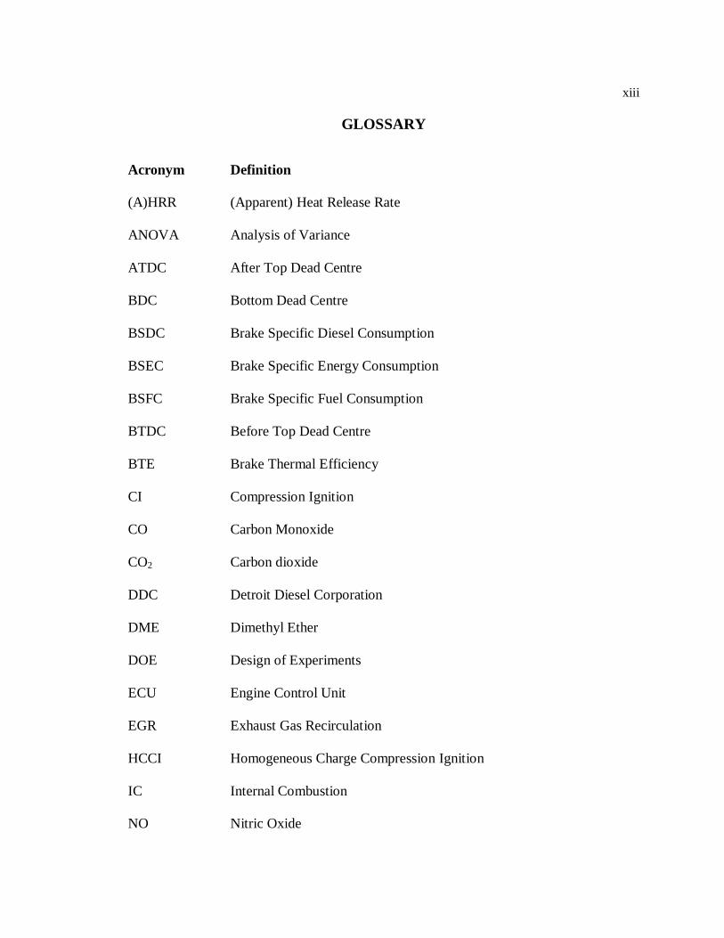
GLOSSARY

Acronym Definition

(A)HRR (Apparent) Heat Release Rate

ANOVA Analysis of Variance

ATDC After Top Dead Centre

BDC Bottom Dead Centre

BSDC Brake Specific Diesel Consumption

BSEC Brake Specific Energy Consumption

BSFC Brake Specific Fuel Consumption

BTDC Before Top Dead Centre

BTE Brake Thermal Efficiency

CI Compression Ignition

CO Carbon Monoxide

CO2 Carbon dioxide

DDC Detroit Diesel Corporation

DME Dimethyl Ether

DOE Design of Experiments

ECU Engine Control Unit

EGR Exhaust Gas Recirculation

HCCI Homogeneous Charge Compression Ignition

IC Internal Combustion

NO Nitric Oxide

xiv

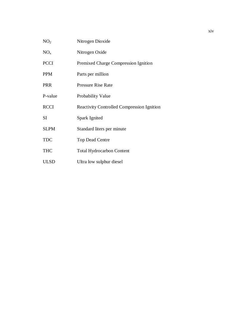
NO2 Nitrogen Dioxide

NOx Nitrogen Oxide

PCCI Premixed Charge Compression Ignition

PPM Parts per million

PRR Pressure Rise Rate

P-value Probability Value

RCCI Reactivity Controlled Compression Ignition

SI Spark Ignited

SLPM Standard liters per minute

TDC Top Dead Centre

THC Total Hydrocarbon Content

ULSD Ultra low sulphur diesel

xv

ACKNOWLEDGEMENTS

This thesis has given me the opportunity to study both the theoretical and the

experimental portion of improving the performance of a diesel engine, which is

something that has always fascinated me. I was able to observe and apply the concepts of

statistical analysis which are a very important component of my degree in Industrial

Engineering. I would firstly like to thank my advisor Dr. André Boehman for giving me

this opportunity and the guidance to work on my masters‘ thesis. It was through his

vision and motivation that I was able to complete the experiments achieving the desired

results in the process. I would also like to thank Dr. Jose Ventura and Dr. Paul Griffin for

their advice and time in reviewing my thesis.

This work was supported in part under US Department of Energy

through Contract: DE-EE0004232, as a subcontract from Volvo Group Truck

Technology. Thanks go to the Jerry Gibbs, Roland Gravel, Gurpreet Singh and

Ken Howden of the US DOE and Ralph Nine of the National Energy Technology

Laboratory. Thanks also go to Pascal Amar and Sam McLaughlin of Volvo Group for

their support and guidance.

I am extremely grateful to Bhaskar Prabhakar for helping me throughout the

experiments and the data analysis. It would have been impossible for me to conduct the

experiments without his knowledge and help on the setup and running of the engine. I

would also like to thank Vickey, Claire and Dongil for their time in helping me

understand the operation of the engine and the emissions bench.

xvi

Finally, a very special thanks to my parents K.S. Jayaraman and Padma

Jayaraman for their support through every stage of my life. My friends also deserve a

special mention in motivating me to complete my thesis so that we could all take the

graduation walk at the same time.

Chapter 1

INTRODUCTION

1.1 Oil Depletion and Global Warming

The conservation of the environment has been a topic of growing concern among

countries especially those with low-lying areas which are under the threat of being

submerged due to rising global temperatures. The Kyoto Protocol was one of the widely

agreed protocols whereby all the ratifying countries agreed to legally binding

commitments to cut down on emissions of global warming gases [1]. The lack of success

for this protocol was attributed to the fact that the United States rejected the treaty on the

basis that it placed too much pressure on the developed nations while exempting

developing countries like India and China [2]. The United States is among the highest

emitters of greenhouse gases and also has the highest per capita emissions [3]. Having

rejected the Kyoto Protocol, it is now essential for the United States to put in place steps

to independently reduce emissions. Exploring alternate blends of fuels capable of

reducing carbon dioxide, carbon monoxide and nitrogen oxide emissions is thus of

paramount importance.

Another growing environmental concern is the rapid depletion of oil reserves

worldwide. The United States of America has one of the largest automotive vehicle bases

in the world (254 million registered highway vehicles in 2009) Consequently, they are

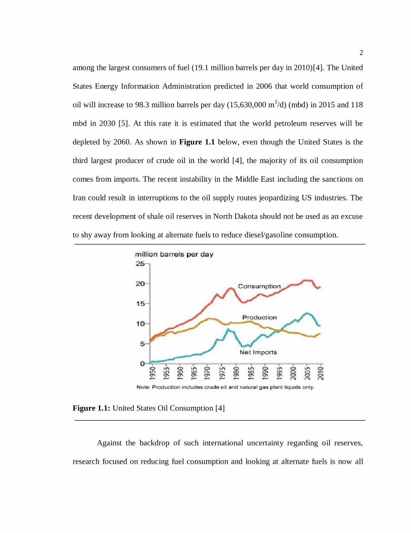
2

among the largest consumers of fuel (19.1 million barrels per day in 2010)[4]. The United

States Energy Information Administration predicted in 2006 that world consumption of

oil will increase to 98.3 million barrels per day (15,630,000 m3/d) (mbd) in 2015 and 118

mbd in 2030 [5]. At this rate it is estimated that the world petroleum reserves will be

depleted by 2060. As shown in Figure 1.1 below, even though the United States is the

third largest producer of crude oil in the world [4], the majority of its oil consumption

comes from imports. The recent instability in the Middle East including the sanctions on

Iran could result in interruptions to the oil supply routes jeopardizing US industries. The

recent development of shale oil reserves in North Dakota should not be used as an excuse

to shy away from looking at alternate fuels to reduce diesel/gasoline consumption.

Figure 1.1: United States Oil Consumption [4]

Against the backdrop of such international uncertainty regarding oil reserves,

research focused on reducing fuel consumption and looking at alternate fuels is now all

3

the more important. This study is part of the Volvo Group‘s ‗Super truck‘ project which

aims at achieving 55% BTE by gaseous fuel fumigation and other changes to the engine.

1.2 The Diesel Engine

As stated, the objective of this thesis is to look at ways to reduce fuel

consumption and emissions while at the same time maintaining if not improving the

performance of the diesel engine. In order to facilitate further understanding it would be

appropriate to begin with a brief introduction of the diesel engine and its operation.

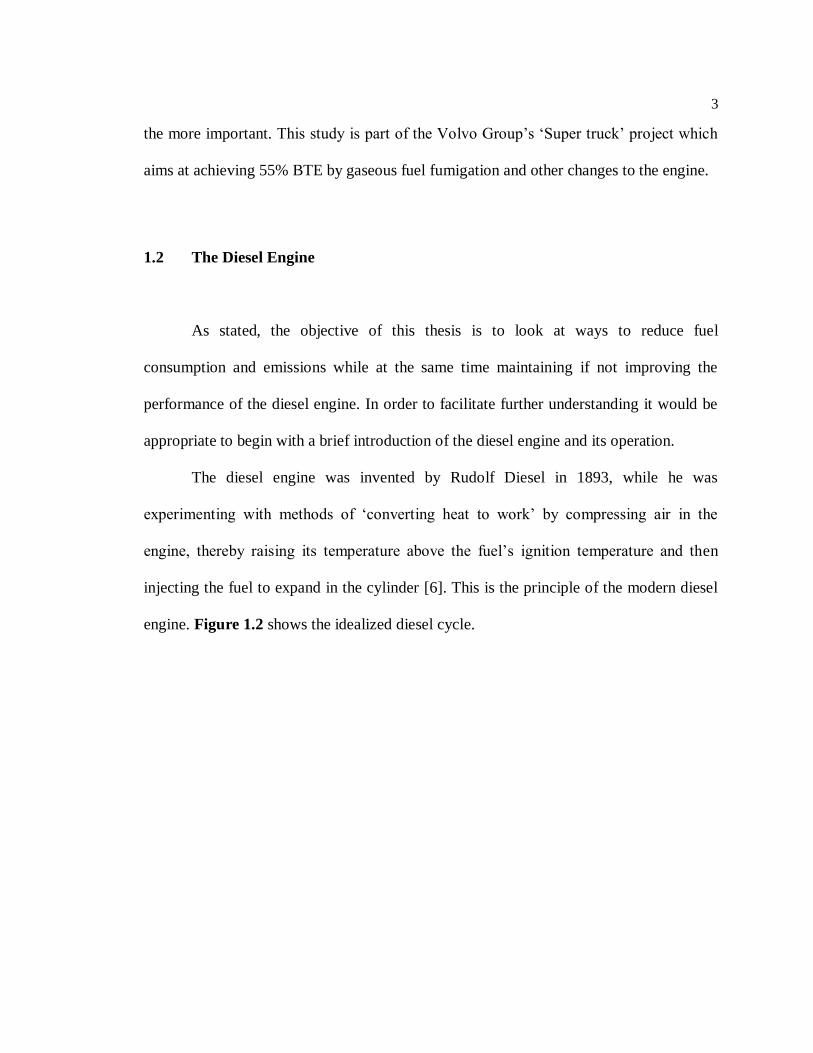
The diesel engine was invented by Rudolf Diesel in 1893, while he was

experimenting with methods of ‗converting heat to work‘ by compressing air in the

engine, thereby raising its temperature above the fuel‘s ignition temperature and then

injecting the fuel to expand in the cylinder [6]. This is the principle of the modern diesel

engine. Figure 1.2 shows the idealized diesel cycle.

4

Figure 1.2: The Diesel Cycle (Source: http:// hyperphysics.phy-astr.gsu.edu)

The diesel cycle differs from the Otto cycle for the petrol/gasoline engine in that

the fuel injection and the subsequent ignition takes place at constant pressure as opposed

to constant volume in the case of the Otto cycle [7]. Also, there is no spark to ignite the

fuel in the diesel engine unlike the gasoline or spark ignition (SI) engine. Ignition takes

place due to the compression of the intake air and consequently the injected fuel, thereby

the name ‗Compression-Ignition‘ (CI) engines. Figure 1.2 gives the diagram of an

idealized 4-stroke diesel engine.

1. Intake Stroke (e-a):

Atmospheric air after passing through the air filter gets inducted into the

engine through the intake valve while the exhaust valve remains closed. This

happens during the downward motion of the piston.

5

2. Compression Stroke (a-b):

Inducted air gets compressed adiabatically (without heat loss- under ideal

cycle) into the clearance volume as the piston moves upwards completing the

second stroke. This is also accompanied by a rise in temperature in the cylinder.

While this happens, both intake and exhaust valves remain closed.

3. Expansion Stroke (c-d):

Fuel is injected into the cylinder at this point (b). Injection occurs at

constant pressure and continues till point c. Injection stops at point c and at this

point, the temperature in the cylinder is greater than the fuel‘s auto-ignition

temperature. This causes the air-fuel mixture to expand (c-d) to the bottom dead

centre (BDC) adiabatically performing work. This is the stroke in which the

engine generates energy to perform work.

4. Exhaust Stroke (a-e):

The piston moves back to the TDC, pushing the exhaust gases created

during combustion out of the cylinder. Once, the exhaust stroke is complete, the

engine again goes through the four cycles.

6

1.3 The Diesel Engine Combustion Process

The combustion in a CI engine is generally considered as taking place in 4 stages

[6] as can be seen in Figure 1.3. The four stages are the ignition delay period, the period

of rapid combustion, the period of controlled combustion and the burnout or late-

combustion phase [8]

Figure 1.3: Heat Release Profile of a Diesel Engine [9]

1. Ignition Delay:

This is the preparatory phase between the injection of the fuel into the

cylinder and the actual ignition of the fuel. There is a period of inactivity between

when the first drop of fuel enters the cylinder to when the fuel undergoes actual

burning. The ignition delay period is extremely important in determining the

7

combustion rate and the knocking of the engine. For CI engines, the ignition delay

should be small to avoid knocking in the engine.

2. Period of Rapid Combustion:

At this stage, most of the fuel injected into the cylinder has evaporated

forming a combustible mixture with the air. This period is characterized by a

sharp rise in pressure, which continues until the peak cylinder pressure is reached

(for light to medium loads). In some cases, peak pressure is not reached in this

stage but in the next one. The heat-release rate is also usually at its maximum

during this period.

3. Period of Controlled Combustion:

Entering this stage, the temperature and pressure in the cylinder are

already quite high. Hence, any fuel injected into the cylinder burns quickly with a

reduced ignition delay. Further rises in the pressure and temperature are

dependent on the injection rate. As can be seen from the Figure 1.3, the heat

release during this period is over a larger crank-angle range.

4. After-burning period:

This is the final phase of combustion; where unburnt and partially burnt

fuel or fuel rich combustion products burn on coming in contact with oxygen. The

heat release is low during this stage and continues into the expansion stroke after

TDC.

8

1.4 Differences between SI engines and CI Engines

Table1.1: Differences between SI and CI Engines

Description SI engine CI engine

Ignition Spark induced due to high self-

ignition temperature of gasoline

Self-ignition induced by

compression of air and fuel

injection

Compression

Ratio

Lower compression ratios (6-10) Higher compression ratios

(16-20)

Thermal

Efficiency

Lower thermal efficiency due to lower

compression ratios

Higher thermal efficiency due

to greater compression ratios

Air-Fuel Ratio Usually close to stoichiometric ratio

over full range of load conditions

Varies based on engine load.

Low at full load to high at no

load

Power to

Weight ratio

Higher ratio due to lower weight Lower ratio due to increased

weight to withstand greater

peak pressures

Alternate fuels Ethanol can be used as an additive to

gasoline and also directly depending

on modifications to the engine.

Can be used directly instead

of diesel (e.g.: biodiesel)

depending on the engine and

fuel type

1.5 Thesis Overview

The objective of this thesis is to observe the effects of mixed-mode combustion

using a combination of fumigated fuels and diesel fuel on the performance of a CI engine.

This is also referred to as dual-fuel combustion. The fumigated fuels are dimethyl ether

(DME) and propane, while the injected fuel is ultra low sulphur diesel (ULSD). Previous

studies have been done along similar lines (Chapter 2) using DME and Methane. This

9

study attempts to achieve the same using propane which has a lower octane rating as

compared to methane.

An initial set of runs was made on the engine using DME and propane (Chapter

4). For these runs, the engine‘s emissions values were not noted. A regression analysis of

the data obtained was performed and the regression equation for each response variable

was used as the objective function for an optimization problem. The significance of each

factor in changing the response variables was also determined. The solution to the

optimization problem for each variable would be the energy substitution percentages at

which that variable would be at its optimum value. These solutions would comprise some

of the operating points to be run in the next set of experiments (Chapter 5). In the next

set of experiments, in addition to the engine performance parameters of BTE, BSEC,

BSFC, BSDC, HRR and PRR, engine emissions data was also measured which included

total hydrocarbon content (THC), carbon dioxide (CO2), carbon monoxide (CO) and

nitrogen oxides (NOx). The results obtained from Chapter 4 and Chapter 5 were tallied

and a set of conclusions were drawn (Chapter 6).

Chapter 2

Literature Review

2.1 Homogeneous Charge Compression Ignition (HCCI) Combustion

Recent research into reducing emissions and increasing thermal efficiency in

diesel engines has shown that homogeneous charge compression ignition (HCCI) is an

effective way of achieving these objectives. HCCI is a form of internal combustion in

which well-mixed fuel and air are compressed to the point of auto-ignition. In many

ways, HCCI incorporates the best features of both spark ignition (SI) combustion engines

and compression ignition (CI) combustion engines. As in an SI engine, the charge is

premixed while entering the cylinder and like the CI engine, the charge in the cylinder is

compression ignited [10]. HCCI combustion has gained popularity due to the fact that it

can operate at diesel engine-like compression ratios thus achieving greater efficiencies

than gasoline engines [11]. The homogeneous mixing of the fuel also results in cleaner

combustion and lower NOx emissions which are especially important considering the

current environmental scenario [12]. HCCI also has a large variety in terms of the fuels

that can be used [13].

While, the advantages of HCCI combustion have been well documented,

researchers have also found hindrances to successful application in engines [14-17].

11

Firstly, HCCI usage is limited by a sharp rise in peak cylinder pressure [14]. This can

cause significant damage to the engine if the engine is not designed capable of

withstanding these pressures. Secondly, previous studies have documented the difficulty

in controlling the auto-ignition point and thereby the heat release [15, 16]. This is due to

the fact that unlike SI or CI engines, the ignition is not controlled by the spark timing or

the fuel injection timing respectively. Though HCCI combustion engines have shown to

reduce NOx emissions levels, the levels of hydrocarbons (HC) and carbon monoxide

(CO) in the emissions have increased [17]. The operation of the engine in HCCI mode is

also limited in its range of operability over different speeds and loads as well as the

cylinder pressure levels [18].

Recent research has focused on overcoming the hindrances of HCCI using

different types of fuel mixing and preparation [19, 20]. This has resulted in the

development of mixed mode combustion and dual fuel combustion.

2.1.1 Mixed Mode Combustion

In mixed mode combustion, a gaseous fuel is fumigated into the intake air and a

conventional diesel injection is used with the intention of igniting the pre-mixed the

gaseous-fuel charge. This is similar in some respects to ‗dual fuel‘ combustion, where the

fuel is usually natural gas or bio-gas [14]. Karim states that there can be two categories of

‗dual fuel‘ operation [21]. The first is one where a small amount of diesel is injected

primarily to provide ignition to the gaseous fuel-air charge [21]. The second category is

one where the gaseous fuel is added to the air of a fully operational diesel engine [21].

12

As stated in the previous section, one of the hindrances to the usage of HCCI

combustion engines is the lack of control over point of ignition [15, 16]. HCCI

combustion takes place over two stages, first a low-temperature stage which is followed

by high temperature reactions for the main heat release [18]. Controlling the autoignition

in an HCCI combustion process is thus a function of controlling the low temperature heat

release reactions [15]. It is for this reason that ‗mixed mode combustion‘ is being

explored.

Musardo et al. have experimented with using traditional diesel injection along

with HCCI combustion to enable the engine to operate over a range of loads while

keeping in mind the objective of reducing NOx emissions [22].Their experiments also

attempt to bring greater control over the heat release rate for the HCCI combustion

process [22]. Some authors have also explored the combination of HCCI combustion

with spark ignition engines (SI) to achieve greater loads, [23-25]. These findings though

would not be applicable in this study as here the focus is mainly on diesel engines.

2.1.2 Premixed Charge Compression Ignition (PCCI) combustion

With a view to obtaining greater control over HCCI combustion another form of

combustion was envisaged which was a form of HCCI approximated by early fuel

injection and exhaust gas recirculation (EGR) [9]. PCCI is essentially injecting the fuel

into the intake port at variable timing during the intake cycle or the middle stage of the

compression stroke and allowing it sufficient time to mix with the injected air before

13

auto-ignition and subsequent premixed combustion [26]. EGR offers a method of

controlling the auto-ignition point for this type of combustion.

The main difference between HCCI and PCCI is in the homogeneity of the charge

injected into the cylinder. In HCCI, as the name indicates, the charge is homogeneous

when entering the cylinder after which it is compressed to the point of auto-ignition. In

PCCI on the other hand the fuel is injected early and then allowed time to mix with the

air and auto-ignite. The overall reduced temperatures in the cylinder result in reductions

in the NOx emission levels [26]. As the mixing in PCCI occurs in the cylinder, there is a

high possibility of incomplete combustion due to fuel sticking to the cylinder walls [9].

This consequently leads to greater HC and CO emissions.

Another limitation of PCCI as pointed out by Nakakita is the need for an injector

with a weak spray-tip and high diffusiveness for adequate diffusion and preventing fuel

adhesion to the cylinder walls [26]. This is contrary to the type of injector required for

normal combustion. Thus an engine intended to be operated in normal as well as PCCI

modes may need to have an injector with variable spray characteristics. In spite of the

difficulties in the practical use of PCCI, research into PCCI is ongoing as it offers a

practical route to approximate HCCI through injection timing and EGR control [9].

2.2 Reactivity Controlled Compression Ignition (RCCI) combustion

The present work deals with changing the concentrations of the gaseous pre-

mixed charge and observing its effects on the combustion process and consequently the

performance and emissions of the engine. Essentially, the changing fuel concentrations

14

are considered as a means of controlling the ignition point. This is very similar to the

concept of Reactivity Controlled Compression Ignition (RCCI) which is explained in this

section.

RCCI is a dual fuel engine combustion technology that was developed at the

University of Wisconsin-Madison Engine Research Center laboratories. RCCI is a variant

of Homogeneous Charge Compression Ignition (HCCI) that provides more control over

the combustion process and has the potential to dramatically lower fuel use and emissions

[27]. This is the combustion mode that closely resembles the conditions that are

attempted to be achieved during the experiments conducted in this study.

RCCI uses in-cylinder fuel blending with at least two fuels of different reactivity

and multiple injections to control in-cylinder fuel reactivity to optimize combustion

phasing, duration and magnitude. The process involves introduction of a low reactivity

fuel into the cylinder to create a well-mixed charge of low reactivity fuel, air and

recirculated exhaust gases. The high reactivity fuel is injected before ignition of the

premixed fuel occurs, using single or multiple injections directly into the combustion

chamber. Examples of fuel pairings for RCCI are gasoline and diesel mixtures, ethanol

and diesel, and gasoline and gasoline with small additions of a cetane-number booster

(di-tert-butyl peroxide (DTBP) [28].

RCCI allows optimization of HCCI and Premixed Controlled Compression

Ignition (PCCI) type combustion in diesel engines, reducing emissions and the need for

after-treatment methods [29]. By appropriately choosing the reactivities of the fuel

15

charges, their relative amounts, timing and combustion can be tailored to achieve optimal

power output (fuel efficiency), at controlled temperatures (controlling NOx) with

controlled equivalence ratios (controlling soot). Key benefits of the RCCI strategy

include:

Lowered NOx and PM emissions

Reduced heat transfer losses

Increased fuel efficiency

Eliminates need for costly after-treatment systems

Reitz et al. have demonstrated a net thermal efficiency of almost 56% using the

RCCI mode of combustion [27]. Hence, this is one of the combustion modes which are

being investigated in detail. Reitz et al. have run the engine at a maximum of 9 bar IMEP

which is lower than the 16 bar IMEP achieved by Bessonette et al. with HCCI

combustion [28, 30].

The various modes of combustion have been discussed in the previous sections

along with advantages and disadvantages of each mode. The following sections will

discuss the fuels considered for fumigation in the engine.

16

2.3 Fumigated Fuels

As stated in Chapter 1, this thesis will study the effect of mixed mode combustion

using dimethyl ether (DME) and propane as fumigated fuels along with a main injection

of diesel. The advantages and the reasons behind the selection of these fuels for

fumigation in the cylinder will be explained in this section.

2.3.1 Dimethyl Ether (DME)

The use of DME as a fuel in compression ignition engines has been considered

since the l990s. Fleisch et al. have shown in 1995 that DME can be used in a diesel

engine to obtain reductions in NOx emissions [31]. The main reason for the popularity of

DME is the fact that it has a high cetane number (higher than diesel) [32] and it can be

easily prepared from a variety of feedstock including bio-mass, coal and natural gas [33,

34]. Table 2.1 compares some of the properties of diesel and DME along with methane

and propane.

17

Table 2.1: Physical Properties of Diesel, DME, Propane and Methane [35,36]

Property Diesel DME Propane Methane

Chemical Formula C10.8H18.7 C2H6O C3H8 CH4

Mole Weight (g/mol) 148.6 46.07 44.11 16.04

Boiling point (°C) 71-193 -24.9 -42.1 -162

Autoignition temperature (°C) 250 235 470 650

Stoichiometric Air/Fuel Ratio 14.6 9 15.6 16.9

Liquid Viscosity (cP) 2-4 0.15 0.10 -

Lower Heating Value (MJ/kg) 42.5 28.8 46.4 49.9

Cetane Number 40-55 55-60 - -

Octane Number - - 97 120

As can be seen from Table 2.1, DME has a greater cetane number and a lower

autoignition temperature as compared to diesel. This means that DME when injected into

the cylinder can burn quicker than diesel with a smaller ignition delay. One of the reasons

attributed to the greater reactivity of DME in the combustion chamber is the lack of a

carbon-carbon bond [37]. Research on the oxidation of DME has demonstrated the

presence of OH, H and CH3 radicals during the propagation phase of the combustion

process [37]. The OH radical is then responsible for improving the ignition quality of the

fuel and shortening the ignition delay thus resulting in increased oxidation rates [38].

One of the primary disadvantages of DME is its low lubricity, which inhibits flow

in the flow tubes. However, Oguma and co-workers have recently found a method to

improve the lubricity of DME using fatty acid based lubricity improvers [56]. But, this

has also been stated as one of the biggest concerns of DME usage by researchers who

have presented evidence that DME leaks from the fuel injectors [39, 40]. The lower

boiling point of DME is another advantage for use as a fuel in cold weather conditions.

18

The flipside to this however is that for use under normal atmospheric conditions, DME

must be kept slightly pressurized as in the case of Liquefied Petroleum Gas (LPG). The

lower heating value of DME as compared to diesel also means that greater amount of fuel

has to be injected to provide the same combustion output. The main advantage of DME,

however, is in its ability to reduce particulate matter (PM) and NOx emissions [31].

The numerous advantages of DME as listed above had led to many researchers

experimenting with DME and DME blends in both SI and CI engines [14, 31, 33, 35, 38,

41]. The fuel blend of DME and methane is one of the commonly used by researchers

while experimenting with HCCI and mixed mode combustion [35, 38, 42]. Methane has

been popular for usage along with DME due to the fact that increasing the methane

concentration delays ignition and thereby the low temperature heat release event [35].

There is also a noticeable increase in the thermal efficiency and reduction in NOx

emissions due to the usage of mixtures with high methane and low DME proportions

[35]. Work has been done considering blends of DME with other fuels like propane and

butane [43, 44] as well a mixed mode combustion process using DME, methane and a

pilot injection of diesel. This study attempts to replicate the mixed mode combustion

process using DME and propane and a main injection of diesel.

2.3.2 Propane

Propane is produced as a by-product of two other processes, natural gas

processing and petroleum refining [45]. It accounts for about 2% of the energy used in

the United States. Uses include home and water heating, cooking and refrigerating food,

19

clothes drying, powering farm and industrial equipment and drying corn [45]. In addition

to these, the usage of propane as a gaseous fuel in automotive vehicles is gaining

popularity.

Like methane, propane has also been used as the gaseous fuel for the pre-mixed

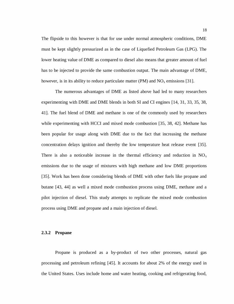
charge in HCCI combustion to varying results [46, 47]. Takatsuto et al. observed that the

combustion of propane has just a single heat release peak at higher temperatures unlike

the two peaks observed for DME combustion [46]. The reason for this could possibly be

attributed to the higher autoignition temperature of propane as compared to DME (Table

2.1). An increase in the fuel equivalence ratio also appeared to advance the high

temperature heat release as can be observed in Figure 2.1 below.

Figure 2.1: Rate of heat release for propane and DME at various equivalence ratios [46]

20

Aceves et al. have shown that in order that propane be used as an HCCI fuel in

diesel engines, high compression ratios (>18) and inlet heating (~140°C) are required

[48]. As propane alone when used as a fuel is intended to be a substitute for gasoline,

such conditions are not feasible in a HCCI engine. In order to overcome this barrier, Yap

et al. experimented with internal trapping of the exhaust gases to raise in-cylinder

temperatures [47]. They were able to run the engine at a compression ratio (CR) of 15

without any intake air heating system while observing reduced NOx emissions.

Propane is one of a series of n-alkanes used by researchers experimenting with

gaseous fuels for HCCI combustion [16, 49, 50]. As stated in Section 2.1, controlling the

auto ignition is one of the main difficulties in HCCI combustion. Propane when used as

the solitary gaseous fuel in an HCCI combustion process also faces the same problem due

to its high auto ignition temperature. For n-alkane HCCI combustion, researchers have

experimented with various controlling techniques like EGR recirculation [16], ozone

addition [49] or the use of additives to modify the cetane number of the fuel [50].

Mehresh et al. have attempted to achieve control over the auto ignition point by the use of

an ion sensor to determine the crank angle at 50% of the heat release [51].

But, propane when used in conjunction with another gaseous fuel along with an

injection of diesel can be used to control the ignition and heat release as has been

demonstrated in this study. The following section will identify the advantages for

selecting propane over methane as a fumigated fuel in addition to DME in the mixed

mode combustion process.

21

2.3.3 Advantages of Propane over Methane

As has been previously stated, the fuel blend of DME and methane has been used

by researchers experimenting with HCCI combustion [35, 38, 42]. In this study, we

attempt to replicate those experiments replacing methane with propane.

Chen et al. have shown through their experiments that methane when used alone

for HCCI combustion does not auto ignite due to its high auto ignition temperature

(650°C) [35]. On the other hand, propane when used alone does auto ignite albeit with

high compression ratios and possibly inlet air heating [48]. Propane having a lower auto

ignition temperature than methane (470°C) presents the possibility of observing an

increased amount of heat release at lower temperatures than would have been possible

with methane. This gives an increased amount control over the ignition in terms of the

range of crank angles over which ignition can occur. Similar to methane, a mixture have

a high proportion of propane and low in DME would result in delayed ignition which

could be controlled to occur at TDC. Chen et al. have shown that for a high methane and

low DME mixture, the high temperature heat release can occur as late as 12° after TDC

[35]

A comparison of the octane numbers of propane and methane shows that methane

has a higher octane number (120) as compared to propane (97) (Table 2.1). This implies

that propane has a higher cetane number than methane and thereby is more suitable for

compression ignition than methane. Both gases have similar lower heating values by

mass and stoichiometric air-fuel ratios.

22

In this chapter, previous research on HCCI, PCCI and RCCI combustion and

DME and DME blend fumigation has been reviewed. The following chapters will deal

with the setup for the experiments conducted and the results and conclusions derived

thereby.

23

Chapter 3

Experimental Setup

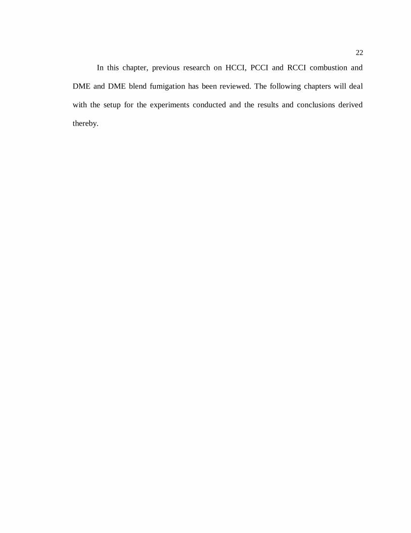
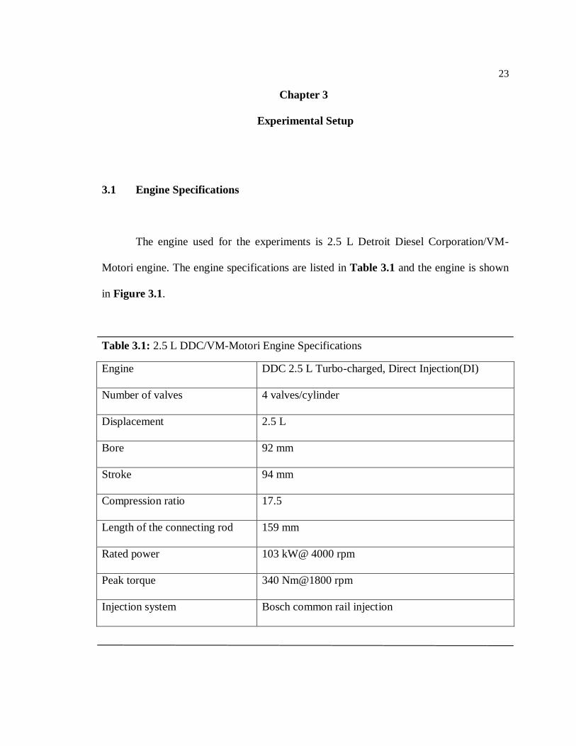
3.1 Engine Specifications

The engine used for the experiments is 2.5 L Detroit Diesel Corporation/VM-

Motori engine. The engine specifications are listed in Table 3.1 and the engine is shown

in Figure 3.1.

Table 3.1: 2.5 L DDC/VM-Motori Engine Specifications

Engine DDC 2.5 L Turbo-charged, Direct Injection(DI)

Number of valves 4 valves/cylinder

Displacement 2.5 L

Bore 92 mm

Stroke 94 mm

Compression ratio 17.5

Length of the connecting rod 159 mm

Rated power 103 kW@ 4000 rpm

Peak torque 340 Nm@1800 rpm

Injection system Bosch common rail injection

24

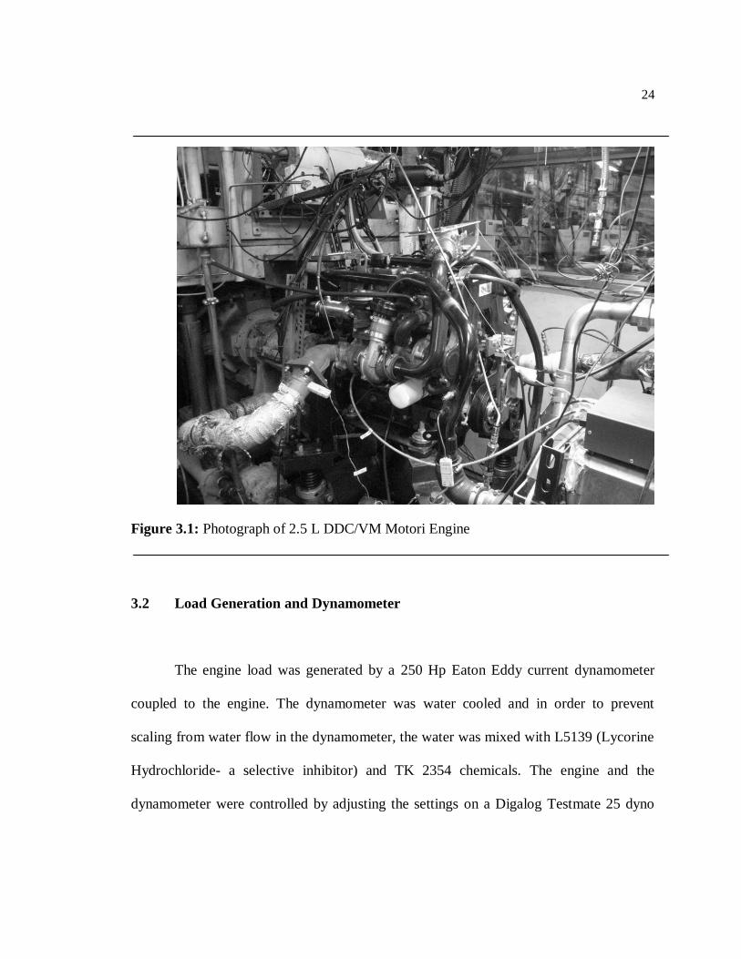
Figure 3.1: Photograph of 2.5 L DDC/VM Motori Engine

3.2 Load Generation and Dynamometer

The engine load was generated by a 250 Hp Eaton Eddy current dynamometer

coupled to the engine. The dynamometer was water cooled and in order to prevent

scaling from water flow in the dynamometer, the water was mixed with L5139 (Lycorine

Hydrochloride- a selective inhibitor) and TK 2354 chemicals. The engine and the

dynamometer were controlled by adjusting the settings on a Digalog Testmate 25 dyno

25

and throttle controller. Throughout the test, cooling water temperatures were monitored

to prevent overheating of the dynamometer.

3.3 Engine Control

The running conditions of the engine namely throttle opening, speed and load

were controlled by using an unlocked Electronic Control Unit (ECU). The ECU was

connected to an ETAS MAC 2 unit via an ETK connection. This was in turn connected to

a computer running INCA software, version 4.0. INCA is a measurement, calibration and

diagnostic software published by ETAS. All programming modifications to the engine

were performed using this interface. During the experiments, INCA was used to vary the

injection timing.

3.4 Data Acquisition

The engine data was collected real-time by means of a series of custom written

programs on National Instruments LabView, Version 7. This enables gathering of a

number of signals such as cylinder pressures and temperatures, air flow mass, fuel flow

rate etc. through a series of FieldPoint modules. This data can then be saved and viewed

in Microsoft Excel or Minitab and easily be processed and analyzed. Once all the

parameters reached steady state, a sampling interval of 2 seconds was used for a total

sampling time of 3-4 minutes.

26

3.5 Pressure Trace and Needle Lift Sensor

Cylinder pressure signals were measured using AVL GU12P pressure transducers.

The voltages from these transducers were amplified by a set of Kistler type 5010 dual

mode amplifiers. The signals were read by an AVL Indimodul 621 data acquisition

system. Needle lift data were obtained from a Wolff Controls Inc. Hall effect needle lift

sensor, which was placed on the injector of cylinder 1. This signal was read by the AVL

Indimodul, which was triggered by a crank angle signal from an AVL 365 C angle

encoder placed on the crank shaft. The Indicom interface recorded these signals over a

0.1 degree crank angle resolution and averaged them over 200 cycles.

3.6 Mass of Air Flow (MAF) and Diesel Flow Rate

The mass of air entering the engine at any given condition was calculated based

on the voltage reading on the MAF sensor. This sensor was calibrated using a laminar

flow element at room temperature, which was assumed to be 300 K.

The diesel fuel consumption was measured using a Sartorius electronic

microbalance. LabView was programmed to calculate the actual flow rate based on 100

measurements of the fuel tank mass, while it tracked small changes in mass over 60

seconds.

27

3.7 Flowmeter Setup

As the experiments required two gases (DME and Propane) to be mixed with the

air intake in specific proportions, it was important to setup the mixing process in a

manner that would be easy to control while at the same time ensuring a homogeneous

mixture. To this end, the flowmeter used was a Matheson Gas FM7410 series flowmeter

capable of flowing 4 gases. A picture of the flowmeter is given in Figure 3.2.

Figure 3.2: Matheson Gas 7410 series flow meter

The flowmeter consists of the following flow tubes numbered 605, 603, 604, 605

of which the tubes 605, 603 were used for propane while 604 and 605 were used for

DME. Each of the tubes was calibrated for the specific gases flowing through them at 0

28

psig. The calibration tables and equations can be found in Appendix A. The conversion

equation obtained was then corrected to the DME and propane cylinder pressure of 50 psi

in the LabView program. The flow obtained using the Matheson Gas flowmeter was

verified using a Hastings bubble flowmeter as well as an Omega FMA 1700/1800 digital

flowmeter. It was found that the Matheson Gas flowmeter was under-estimating the flow

by 25%. A factor of 1.25 was hence multiplied to the DME and propane flow rates

obtained using the Data Acquisition software to accurately reflect actual flow. A

schematic diagram of the liquefied gas flow into the engine is given in Figure 3.3.

Figure 3.3: Block Diagram of DME, Propane flow and mixing into the engine

29

3.8 Engine Emissions Measurement

Figure 3.4: AVL CEB II emissions bench (Source: www.avl.com)

Engine gaseous emissions were measured using an AVL CEB II combustion

emissions bench. A photograph of the bench is shown in Figure 3.4. The hot exhaust

from the engine was sampled through a series of head-line filters into an insulated heated

line which was maintained at 1900C. The gases were then filtered through smaller filters

to ensure particulate free exhaust entered the bench. Before data collection, the bench

was switched on at least 1-2 hrs in advance to let the analyzers warm up. Each day prior

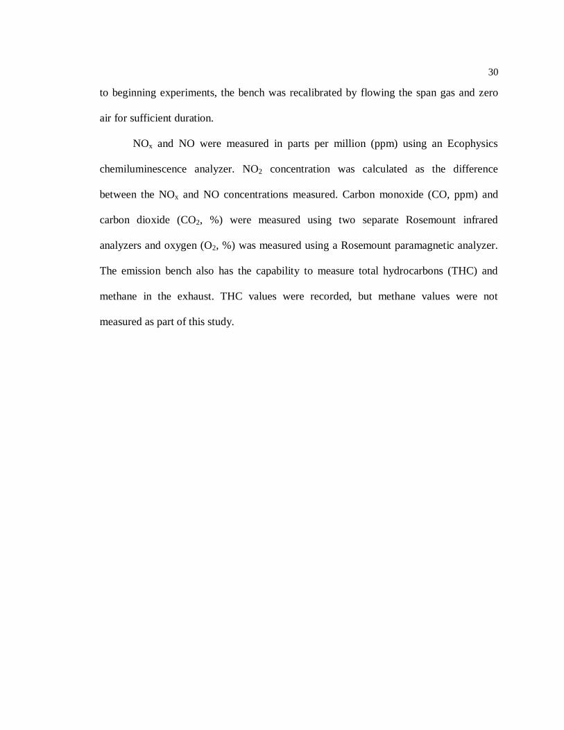
30

to beginning experiments, the bench was recalibrated by flowing the span gas and zero

air for sufficient duration.

NOx and NO were measured in parts per million (ppm) using an Ecophysics

chemiluminescence analyzer. NO2 concentration was calculated as the difference

between the NOx and NO concentrations measured. Carbon monoxide (CO, ppm) and

carbon dioxide (CO2, %) were measured using two separate Rosemount infrared

analyzers and oxygen (O2, %) was measured using a Rosemount paramagnetic analyzer.

The emission bench also has the capability to measure total hydrocarbons (THC) and

methane in the exhaust. THC values were recorded, but methane values were not

measured as part of this study.

Chapter 4

Experiments and Analysis – Part 1

Two sets of experiments were performed, the first set by Bhaskar Prabhakar in

August 2011. This was intended as a preliminary study on the effects of DME and

propane fumigation in a diesel engine. For these experiments, only the engine

performance parameters were noted while the effects on the engine‘s emissions were not

considered. Also, exhaust gas recirculation was not used while running the engine for

these experiments. The data from these experiments was analyzed to determine DME and

propane substitution proportions where the engine‘s performance could be optimized.

For these experiments, the engine speed and torque were held constant at 1800

rpm and 65 ft-lb (25% load) respectively. The diesel injection timing was held constant at

7 deg BTDC with no pilot injection introduced.

4.1 Experimental Runs

The experiment was setup as a full factorial experimental design on Minitab 16.

The two factors are DME and propane, while the responses are BSEC, BTE, BSFC,

BSDC, HRR and PRR.

32

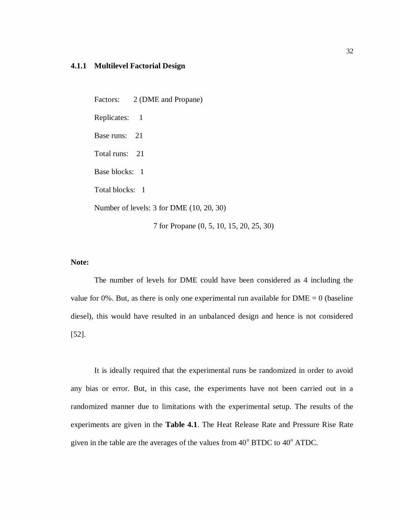
4.1.1 Multilevel Factorial Design

Factors: 2 (DME and Propane)

Replicates: 1

Base runs: 21

Total runs: 21

Base blocks: 1

Total blocks: 1

Number of levels: 3 for DME (10, 20, 30)

7 for Propane (0, 5, 10, 15, 20, 25, 30)

Note:

The number of levels for DME could have been considered as 4 including the

value for 0%. But, as there is only one experimental run available for DME = 0 (baseline

diesel), this would have resulted in an unbalanced design and hence is not considered

[52].

It is ideally required that the experimental runs be randomized in order to avoid

any bias or error. But, in this case, the experiments have not been carried out in a

randomized manner due to limitations with the experimental setup. The results of the

experiments are given in the Table 4.1. The Heat Release Rate and Pressure Rise Rate

given in the table are the averages of the values from 40o BTDC to 40

o ATDC.

33

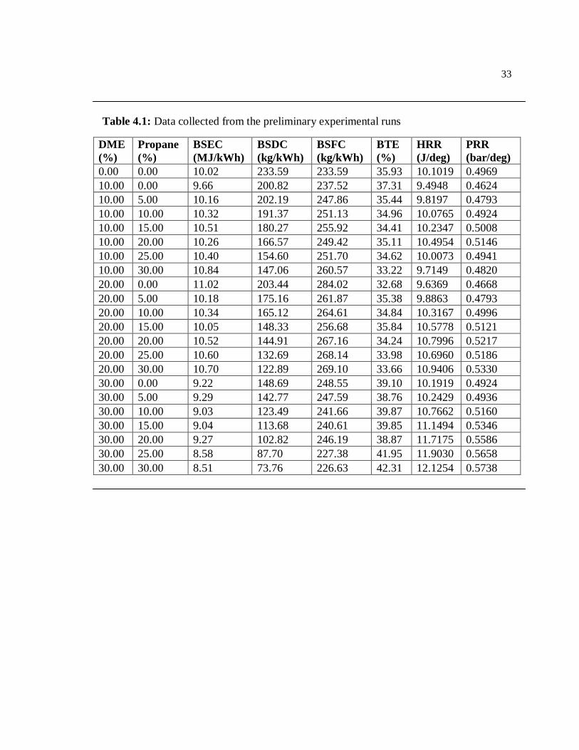
Table 4.1: Data collected from the preliminary experimental runs

DME

(%)

Propane

(%)

BSEC

(MJ/kWh)

BSDC

(kg/kWh)

BSFC

(kg/kWh)

BTE

(%)

HRR

(J/deg)

PRR

(bar/deg)

0.00 0.00 10.02 233.59 233.59 35.93 10.1019 0.4969

10.00 0.00 9.66 200.82 237.52 37.31 9.4948 0.4624

10.00 5.00 10.16 202.19 247.86 35.44 9.8197 0.4793

10.00 10.00 10.32 191.37 251.13 34.96 10.0765 0.4924

10.00 15.00 10.51 180.27 255.92 34.41 10.2347 0.5008

10.00 20.00 10.26 166.57 249.42 35.11 10.4954 0.5146

10.00 25.00 10.40 154.60 251.70 34.62 10.0073 0.4941

10.00 30.00 10.84 147.06 260.57 33.22 9.7149 0.4820

20.00 0.00 11.02 203.44 284.02 32.68 9.6369 0.4668

20.00 5.00 10.18 175.16 261.87 35.38 9.8863 0.4793

20.00 10.00 10.34 165.12 264.61 34.84 10.3167 0.4996

20.00 15.00 10.05 148.33 256.68 35.84 10.5778 0.5121

20.00 20.00 10.52 144.91 267.16 34.24 10.7996 0.5217

20.00 25.00 10.60 132.69 268.14 33.98 10.6960 0.5186

20.00 30.00 10.70 122.89 269.10 33.66 10.9406 0.5330

30.00 0.00 9.22 148.69 248.55 39.10 10.1919 0.4924

30.00 5.00 9.29 142.77 247.59 38.76 10.2429 0.4936

30.00 10.00 9.03 123.49 241.66 39.87 10.7662 0.5160

30.00 15.00 9.04 113.68 240.61 39.85 11.1494 0.5346

30.00 20.00 9.27 102.82 246.19 38.87 11.7175 0.5586

30.00 25.00 8.58 87.70 227.38 41.95 11.9030 0.5658

30.00 30.00 8.51 73.76 226.63 42.31 12.1254 0.5738

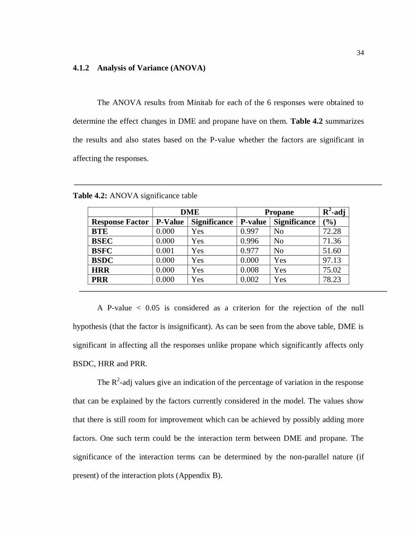
34

4.1.2 Analysis of Variance (ANOVA)

The ANOVA results from Minitab for each of the 6 responses were obtained to

determine the effect changes in DME and propane have on them. Table 4.2 summarizes

the results and also states based on the P-value whether the factors are significant in

affecting the responses.

Table 4.2: ANOVA significance table

DME Propane R2-adj

Response Factor P-Value Significance P-value Significance (%)

BTE 0.000 Yes 0.997 No 72.28

BSEC 0.000 Yes 0.996 No 71.36

BSFC 0.001 Yes 0.977 No 51.60

BSDC 0.000 Yes 0.000 Yes 97.13

HRR 0.000 Yes 0.008 Yes 75.02

PRR 0.000 Yes 0.002 Yes 78.23

A P-value < 0.05 is considered as a criterion for the rejection of the null

hypothesis (that the factor is insignificant). As can be seen from the above table, DME is

significant in affecting all the responses unlike propane which significantly affects only

BSDC, HRR and PRR.

The R2-adj values give an indication of the percentage of variation in the response

that can be explained by the factors currently considered in the model. The values show

that there is still room for improvement which can be achieved by possibly adding more

factors. One such term could be the interaction term between DME and propane. The

significance of the interaction terms can be determined by the non-parallel nature (if

present) of the interaction plots (Appendix B).

35

It is observed that with exception to BSDC, all the interaction plots have non-

parallel lines. This indicates the presence of a significant interaction between the factors

in determining the responses BTE, BSEC, BSFC, PRR and HRR. The interaction term

however cannot be included in the ANOVA due to insufficient degrees of freedom

available leading to the ‗Error‘ term in the analysis having zero degrees of freedom. This

stresses the need for replications in future runs of the experiment.

4.2 Regression Analysis

The previous section dealt with the significance of the factors, DME and Propane

in determining the responses, BTE, BSEC, BSFC, BSDC, HRR and PRR. It was also

noted that the DME-Propane interaction could potentially be significant in affecting the

values of the responses. This section will attempt to fit a regression model to describe the

relationship between each of the responses and the factors mathematically. This will be

followed by an optimality analysis to determine the operating point where the parameter

is at its optimal value. The relationship between the factors and the response need not

always be linear. To increase the accuracy of the model, it may be necessary to include

higher powers.

In the case of the regression analyses carried out in this study, it was noticed that

the data for some of the responses was following a decreasing trend initially and then an

increasing trend. This suggests the inclusion of a quadratic term in the variables DME

and Propane. On inclusion of further powers, it was observed that the correlation between

the variables was too high resulting in a reduction in the R2-adj value (whose significance

36

is explained below). It is for this reason that no powers beyond the squared term of the

variables were used.

The accuracy of the regression model will be based on the value of R2-adj – the

adjusted co-efficient of determination which is a measure of the percentage of variation

in the response explained by the regression model. A model with a R2-adj value of greater

than 80% is considered reasonably accurate [53]. In addition to the R2-adj values, the

residuals will also be considered while determining the feasibility of the model. Once an

appropriate model has been fitted, it will be checked to determine the validity of the

regression assumptions listed below,

1. The residuals are normally distributed

2. They have a variance which is constant.

Any of these assumptions not being met would lead to the need for

transformations in the model so that a regression model can be fitted.

The point (DME, Propane) = (0, 0), i.e., the readings for baseline diesel, has been

excluded from the dataset considered for regression. This is because the initial Minitab

iterations noted that the point (0, 0) had a lot of leverage over the regression line and was

resulting in reduced values of R2-adj. Also, the initial testing dataset given in Section 4.1

is incomplete in that the responses for when DME = 0% and propane is varied have not

been measured. While analyzing the regression results all terms with a P-value less than

0.05 will be considered significant. The Minitab output of the regression results are given

in Appendix C.

Once appropriate regression models have been fitted for the responses, it is

needed to obtain operating conditions to optimize the values of the responses. The

37

regression models obtained in the previous section will be used as objective functions for

each of the responses. Microsoft Excel solver was used as the optimization tool to solve

the problem.

The constraints for the optimization problem are given below.

10 ≤ DME ≤ 30

0 ≤ Propane ≤ 30

DME, Propane, BTE, BSEC, BSFC, BSDC, HRR, PRR ≥ 0

The following sections give the optimal desired values of the response variables

subject to the above constraints. The DME and propane substitution quantities to obtain

the optimal values are also given.

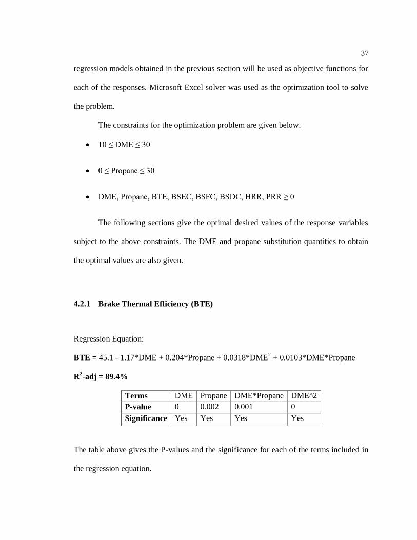
4.2.1 Brake Thermal Efficiency (BTE)

Regression Equation:

BTE = 45.1 - 1.17*DME + 0.204*Propane + 0.0318*DME2 + 0.0103*DME*Propane

R2-adj = 89.4%

Terms DME Propane DME*Propane DME^2

P-value 0 0.002 0.001 0

Significance Yes Yes Yes Yes

The table above gives the P-values and the significance for each of the terms included in

the regression equation.

38


In the X-axis of the graph (10, 0) = 10%DME and 0% propane

The bar graph of the actual data in Figure 4.1 shows an increasing trend in the

brake thermal efficiency with increasing energy substitution. This is corroborated by the

optimality analysis using Excel Solver.

Maximize BTE = 45.1 - 1.17*DME + 0.204*Propane + 0.0318*DME2 +

0.0103*DME*Propane

DME Propane BTE BSEC BSDC BSFC HRR PRR

30 30 41.77 8.668 78 228.71 12.052 0.5716

The point of maximum efficiency is found to be at 30% DME substitution and

30% propane substitution.

25.00

27.00

29.00

31.00

33.00

35.00

37.00

39.00

41.00

43.00

45.00

Bas

elin

e

10,0

10,5

10,1

0

10,1

5

10,2

0

10,2

5

10,3

0

20,0

20,5

20,1

0

20,1

5

20,2

0

20,2

5

20,3

0

30,0

30,5

30,1

0

30,1

5

30,2

0

30,2

5

30,3

0

BTE

(%

)

DME, Propane (% energy substitution)

39

4.2.2 Brake Specific Energy Consumption (BSEC)


BSEC = 7.69 + 0.308*DME + 0.0537*Propane - 0.0026*DME*Propane -

0.00837*DME2

R2-adj = 88.0%


P-value 0 0.003 0.002 0


The P-values and the significance for each of the terms included in the regression

equation are given in the table above. As can be seen all the terms included are

significant.


substitution levels

6.00

7.00

8.00

9.00

10.00

11.00

12.00

Bas

elin

e

10,

0

10,

5

10,

10

10,

15

10,

20

10,

25

10,

30

20,

0

20,

5

20,

10

20,

15

20,

20

20,

25

20,

30

30,

0

30,

5

30,

10

30,

15

30,

20

30,

25

30,

30

BSE

C (

MJ/

kWh

)


40

BSEC is observed to decrease in Figure 4.2 as the energy substitution is

increased. There is however, a slight increase when the DME substitution is 10% and the

amount of propane is increased from 0 to 30%. The optimality analysis supports this

trend with the point DME = 30% and propane = 30% estimated to have the lowest brake

specific energy consumption.

Minimize: BSEC = 7.69 + 0.308*DME + 0.0537*Propane - 0.0026*DME*Propane -

0.00837*DME2


30 30 41.77 8.668 78 228.71 12.052 0.5716

4.2.3 Brake Specific Fuel Consumption (BSFC)


BSFC = 173 + 9.28*DME + 1.13*Propane - 0.0631*DME*Propane - 0.222*DME2

R2-adj = 79.2%


P-value 0 0.008 0.002 0


It can be seen from the P-values in the above table that all the terms included are

significant.

41

Figure 4.3: Brake Specific Fuel Consumption at varying DME and propane substitution

levels

As seen in Figure 4.3, BSFC is also found to exhibit a similar trend as BSEC with

an initial increase around the 20% DME substitution mark followed by a later decrease.

The Excel Solver analysis puts the point of minimum brake specific fuel consumption at

30% DME and 30% propane which is an indication of reduced fuel consumption with

increasing energy substitution.

Minimize: BSFC = 173 + 9.28*DME + 1.13*Propane - 0.0631*DME*Propane -

0.222*DME2

DME Propane BTE BSEC BSFC BSDC HRR PRR

30 30 41.77 8.668 78 228.71 12.052 0.5716

150.00

170.00

190.00

210.00

230.00

250.00

270.00

290.00

310.00

Bas

elin

e

10,0

10,5

10,1

0

10,1

5

10,2

0

10,2

5

10,3

0

20,0

20,5

20,1

0

20,1

5

20,2

0

20,2

5

20,3

0

30,0

30,5

30,1

0

30,1

5

30,2

0

30,2

5

30,3

0

BSF

C (

kg/k

Wh

)


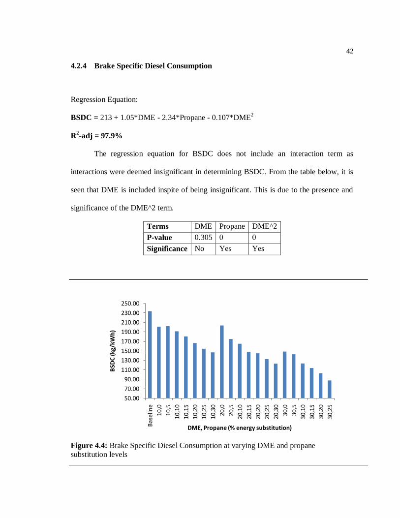
42

4.2.4 Brake Specific Diesel Consumption


BSDC = 213 + 1.05*DME - 2.34*Propane - 0.107*DME2

R2-adj = 97.9%

The regression equation for BSDC does not include an interaction term as

interactions were deemed insignificant in determining BSDC. From the table below, it is

seen that DME is included inspite of being insignificant. This is due to the presence and

significance of the DME^2 term.

Terms DME Propane DME^2

P-value 0.305 0 0

Significance No Yes Yes

Figure 4.4: Brake Specific Diesel Consumption at varying DME and propane

substitution levels

50.00

70.00

90.00

110.00

130.00

150.00

170.00

190.00

210.00

230.00

250.00

Bas

elin

e

10,

0

10,

5

10,1

0

10,1

5

10,2

0

10,2

5

10,3

0

20,

0

20,5

20,1

0

20,1

5

20,2

0

20,2

5

20,3

0

30,

0

30,

5

30,1

0

30,1

5

30,2

0

30,2

5

BSD

C (

kg/k

Wh

)


43

The bar plot in Figure 4.4 shows a steady decreasing trend in BSDC with

increasing energy substitution with the least diesel consumption occurring at the extreme

point of 30% DME and 30% propane substitution.

Minimize BSDC = 213 + 1.05*DME - 2.34*Propane - 0.107*DME2


30 30 41.77 8.668 78 228.71 12.052 0.5716

4.2.5 Heat Release Rate (HRR)


HRR = 9.97 - 0.0510*DME + 0.0271*Propane + 0.00308*DME*Propane +

0.00159*DME2 - 0.00156*Propane

2

R2-adj = 94.40%

Terms DME Propane DME*Propane DME^2 Propane^2

P-value 0.145 0.102 0 0.066 0.003

Significance No No Yes No Yes

From the above table, it is seen that the 3 of the 5 terms included are shown to be

insignificant. The DME and propane terms have to be included as the interaction term,

DME*Propane is significant. Exclusion of the DME2 terms results in a reduction in the

R2-adj value.

44

Figure 4.5: Apparent Heat Release Rate at varying DME and propane substitution levels

There is a steady increasing pattern visible with increasing energy substitution

reaching a peak at 30% each DME and propane substitution as observed in Figure 4.5.

The average values of the heat release rather than the peak heat release values were used

as the average values indicated a clear gradation between different runs which was not

observed with the peak values. The optimality analysis suggests that the minimum heat

release rate would be at 0% DME and 30% propane substitution.

Minimize HRR = 9.97 - 0.0510*DME + 0.0271*Propane + 0.00308*DME*Propane +

0.00159*DME2 - 0.00156*Propane

2


0 30 38.98 9.301 142.8 206.9 9.379 0.4753

6.0000

7.0000

8.0000

9.0000

10.0000

11.0000

12.0000

13.0000

Bas

elin

e

10,0

10,5

10,1

0

10,1

5

10,2

0

10,2

5

10,3

0

20,0

20,5

20,1

0

20,1

5

20,2

0

20,2

5

20,3

0

30,0

30,5

30,1

0

30,1

5

30,2

0

30,2

5

30,3

0

Ave

rage

HR

R (

J/d

eg)


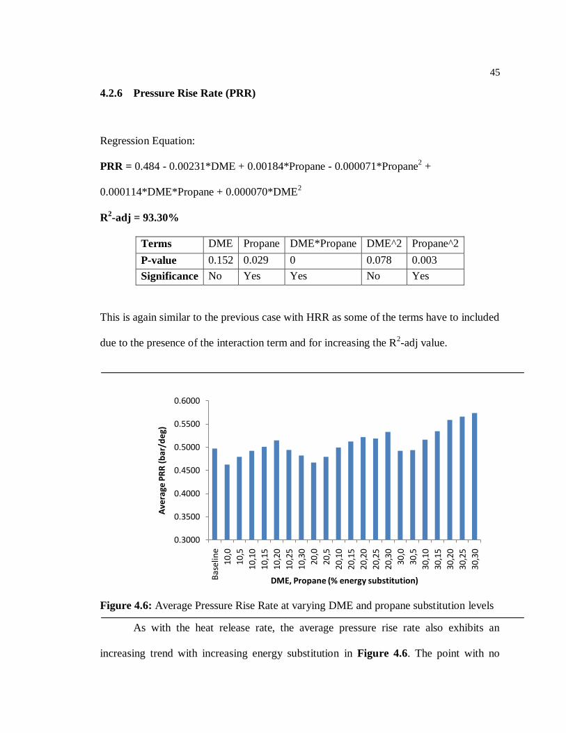
45

4.2.6 Pressure Rise Rate (PRR)


PRR = 0.484 - 0.00231*DME + 0.00184*Propane - 0.000071*Propane2 +

0.000114*DME*Propane + 0.000070*DME2

R2-adj = 93.30%

Terms DME Propane DME*Propane DME^2 Propane^2

P-value 0.152 0.029 0 0.078 0.003

Significance No Yes Yes No Yes

This is again similar to the previous case with HRR as some of the terms have to included

due to the presence of the interaction term and for increasing the R2-adj value.

Figure 4.6: Average Pressure Rise Rate at varying DME and propane substitution levels

As with the heat release rate, the average pressure rise rate also exhibits an

increasing trend with increasing energy substitution in Figure 4.6. The point with no

0.3000

0.3500

0.4000

0.4500

0.5000

0.5500

0.6000

Bas

elin

e

10,0

10,5

10,

10

10,

15

10,

20

10,

25

10,3

0

20,0

20,5

20,

10

20,

15

20,

20

20,

25

20,

30

30,0

30,5

30,

10

30,

15

30,

20

30,

25

30,

30

Ave

rage

PR

R (

bar

/deg

)


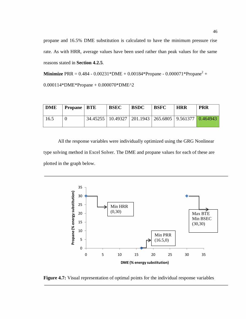
46

propane and 16.5% DME substitution is calculated to have the minimum pressure rise

rate. As with HRR, average values have been used rather than peak values for the same

reasons stated in Section 4.2.5.

Minimize PRR = 0.484 - 0.00231*DME + 0.00184*Propane - 0.000071*Propane2 +

0.000114*DME*Propane + 0.000070*DME^2


16.5 0 34.45255 10.49327 201.1943 265.6805 9.561377 0.464943

All the response variables were individually optimized using the GRG Nonlinear

type solving method in Excel Solver. The DME and propane values for each of these are

plotted in the graph below.

Figure 4.7: Visual representation of optimal points for the individual response variables

0

5

10

15

20

25

30

35

0 5 10 15 20 25 30 35

Pro

pan

e (%

en

ergy

su

bst

itu

tio

n)

DME (% energy substitution)

Max BTE Min BSEC

(30,30)

Min HRR

(0,30)

Min PRR

(16.5,0)

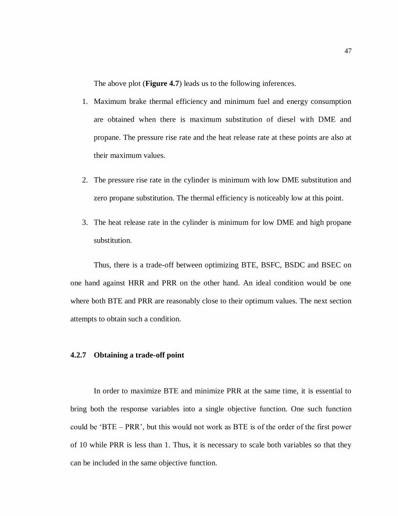
47

The above plot (Figure 4.7) leads us to the following inferences.

1. Maximum brake thermal efficiency and minimum fuel and energy consumption

are obtained when there is maximum substitution of diesel with DME and

propane. The pressure rise rate and the heat release rate at these points are also at

their maximum values.

2. The pressure rise rate in the cylinder is minimum with low DME substitution and

zero propane substitution. The thermal efficiency is noticeably low at this point.

3. The heat release rate in the cylinder is minimum for low DME and high propane

substitution.

Thus, there is a trade-off between optimizing BTE, BSFC, BSDC and BSEC on

one hand against HRR and PRR on the other hand. An ideal condition would be one

where both BTE and PRR are reasonably close to their optimum values. The next section

attempts to obtain such a condition.

4.2.7 Obtaining a trade-off point

In order to maximize BTE and minimize PRR at the same time, it is essential to

bring both the response variables into a single objective function. One such function

could be ‗BTE – PRR‘, but this would not work as BTE is of the order of the first power

of 10 while PRR is less than 1. Thus, it is necessary to scale both variables so that they

can be included in the same objective function.

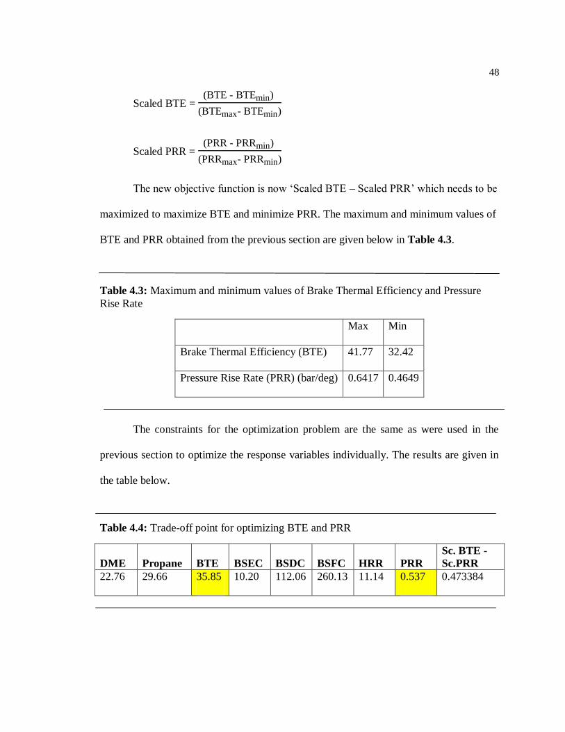
48

Scaled BTE = (BTE - BTEmin)

(BTEmax- BTEmin)

Scaled PRR = (PRR - PRRmin)

(PRRmax- PRRmin)

The new objective function is now ‗Scaled BTE – Scaled PRR‘ which needs to be

maximized to maximize BTE and minimize PRR. The maximum and minimum values of

BTE and PRR obtained from the previous section are given below in Table 4.3.

Table 4.3: Maximum and minimum values of Brake Thermal Efficiency and Pressure

Rise Rate

Max Min

Brake Thermal Efficiency (BTE) 41.77 32.42

Pressure Rise Rate (PRR) (bar/deg) 0.6417 0.4649

The constraints for the optimization problem are the same as were used in the

previous section to optimize the response variables individually. The results are given in

the table below.

Table 4.4: Trade-off point for optimizing BTE and PRR


Sc. BTE -

Sc.PRR

22.76 29.66 35.85 10.20 112.06 260.13 11.14 0.537 0.473384

49

Figure 4.8: Visual representation of the optimal point for obtaining a trade-off between

BTE and PRR

Figure 4.8 shows the condition obtained with respect to the points plotted from

the previous section. The BTE value obtained at 22.76% (~23%) DME substitution and

29.66% (~30%) propane (35.86%) is 14% lower than the maximum possible value of

41.77%. The PRR value of 0.537 bar/deg obtained at the same condition is 15% higher

than the minimum possible value of 0.4648 bar/deg. Thus, the point with 20% DME

substitution and 30% propane is the trade-off point for optimizing both BTE and PRR.

The results of the preliminary set of experiments along with the optimization

analysis were dealt with in this chapter without delving into the possible reasons behind

the trends observed. The following chapter deals with the next set of experiments wherein

it will be attempted to practically verify the analytically obtained results in this chapter in

addition to explaining the reasons behind the trends observed.

0

5

10

15

20

25

30

35

0 10 20 30 40

Pro

pan

e

DME

Max BTE

Min PRR

(22,30)

Chapter 5

Experiments and Analysis – Part 2

The previous chapter described the preliminary experiments conducted as part of

the study of DME and propane fumigation in a diesel engine. Based on the analysis of the

results of those experiments, the next set of experiments was formulated in order to verify

the results of the optimality analysis done in Chapter 4. In addition to the engine

performance parameters considered for the previous set of experiments, emission data

was also measured in this set of experiments.

5.1 Experimental Runs

The experiments were conducted for the following cases

1. DME and propane fumigation without exhaust gas recirculation (EGR)

2. DME and propane fumigation with EGR

3. DME and propane fumigation with EGR and split injection

The test matrices for each of these cases are given in Tables 5.1 – 5.3 respectively

based on the results of the regression analysis carried out in Section 4.2. The engine

speed and torque were held constant at 1800 rpm and 65 ft-lb (25% load) respectively as

in the previous set of experiments. The diesel injection timing was held constant for the

first two cases at 7 deg BTDC with no pilot injection introduced.

51

Table 5.1: Test Matrix for DME and Propane fumigation with no EGR

DME (%) Propane (%)

0 0 10 20 30 40

10 0 10 20 30 40

20 0 10 20 30

30 0 10 20 30

40 0

Table 5.2: Test Matrix for DME and Propane fumigation with EGR

DME (%) Propane (%)

0 0

10 0 20 40

20 0 20 40

30 0 20

Table 5.3: Test Matrix for DME and Propane fumigation with EGR and split injection

DME (%) Propane (%) Pilot Injection (deg) Main Injection (deg)

0 0 16 BTDC 3 ATDC

20 20 16 BTDC 3 ATDC



The measured values or responses are listed below

1. Brake Thermal Efficiency (BTE)

2. Brake Specific Energy Consumption (BSEC)

3. Brake Specific Fuel Consumption (BSFC)

4. Heat Release Rate (HRR)

5. Pressure Rise Rate (PRR)

6. Total Hydrocarbon Emissions (THC)

52

7. Nitrogen Oxide emissions (NOx)

8. Carbon dioxide emissions (CO2)

9. Carbon monoxide emissions (CO)

The Heat Release Rate and Pressure Rise Rate given in the table are the averages

of the values from 30o BTDC to 30

o ATDC as in the previous experiment.

53

5.2 DME and Propane fumigation without Exhaust Gas Recirculation

It was desired to initially observe the effects of DME and propane fumigation

alone on the engine‘s performance and emissions.

5.2.1 Brake Specific Energy Consumption (BSEC)

It can be seen from Figure 5.1 that the BSEC values appear to decrease towards

the right end of the graph with increasing DME substitution values. Overall, 20% less

energy is required when the engine is run with 60% of the diesel is substituted with 30%

DME and 30% propane as compared to baseline diesel. As obtained in the optimality

analysis (Section 4.2.2), it is seen that the lower BSFC values occur as the amount of

energy substitution with DME and propane increases.


substitution levels without EGR

4

5

6

7

8

9

10

11

0,0

0,1

0

0,2

0

0,3

0

0,4

0

10

,0

10,1

0

10,2

0

10,3

0

10,4

0

20,0

20,1

0

20,2

0

20,3

0

30

,0

30,1

0

30,2

0

30,3

0

40

,0

BSE

C (

MJ/

kWh

)

DME, propane (% energy substitution)

54

5.2.2 Brake Thermal Efficiency (BTE)

The general trend observed in Figure 5.2 indicates an increase in the BTE values

with increasing DME substitution. Chen et al. have documented this in their work on

DME and methane saying that mixtures with low DME and high methane content tend to

have higher brake thermal efficiencies [35]. It can be observed that the increases are

greater with increasing propane than with increasing DME. The maximum BTE was

observed at the case where DME substitution was 20% and propane substitution 30%.

The efficiency at this point was found to be 49.91% which is almost 25% greater than the

BTE for baseline diesel with no substitution. It was observed that the heat release peaks

were closer to the top dead centre (TDC) towards the right end of the graph which meant

less negative work to be done against the piston motion.


without EGR

20

25

30

35

40

45

50

55

60

0,0

0,1

0

0,2

0

0,3

0

0,4

0

10,

0

10,

10

10,

20

10,

30

10,

40

20,

0

20,

10

20,2

0

20,

30

30,

0

30,

10

30,

20

30,3

0

40,

0

BTE

(%

)

DME. propane (% energy substitution)

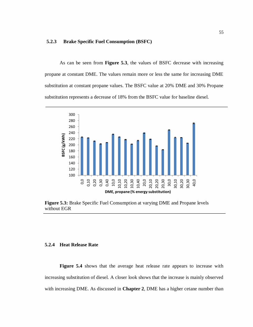
55

5.2.3 Brake Specific Fuel Consumption (BSFC)

As can be seen from Figure 5.3, the values of BSFC decrease with increasing

propane at constant DME. The values remain more or less the same for increasing DME

substitution at constant propane values. The BSFC value at 20% DME and 30% Propane

substitution represents a decrease of 18% from the BSFC value for baseline diesel.

Figure 5.3: Brake Specific Fuel Consumption at varying DME and Propane levels

without EGR

5.2.4 Heat Release Rate

Figure 5.4 shows that the average heat release rate appears to increase with

increasing substitution of diesel. A closer look shows that the increase is mainly observed

with increasing DME. As discussed in Chapter 2, DME has a higher cetane number than

100

120

140

160

180

200

220

240

260

280

300

0,0

0,10

0,20

0,30

0,40

10,0

10,1

0

10,2

0

10,3

0

10,4

0

20,0

20,1

0

20,2

0

20,3

0

30,0

30,1

0

30,2

0

30,3

0

40,0

BSF

C (

g/kW

h)


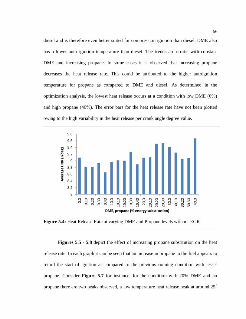
56

diesel and is therefore even better suited for compression ignition than diesel. DME also

has a lower auto ignition temperature than diesel. The trends are erratic with constant

DME and increasing propane. In some cases it is observed that increasing propane

decreases the heat release rate. This could be attributed to the higher autoignition

temperature for propane as compared to DME and diesel. As determined in the

optimization analysis, the lowest heat release occurs at a condition with low DME (0%)

and high propane (40%). The error bars for the heat release rate have not been plotted

owing to the high variability in the heat release per crank angle degree value.

Figure 5.4: Heat Release Rate at varying DME and Propane levels without EGR

Figures 5.5 - 5.8 depict the effect of increasing propane substitution on the heat

release rate. In each graph it can be seen that an increase in propane in the fuel appears to

retard the start of ignition as compared to the previous running condition with lesser

propane. Consider Figure 5.7 for instance, for the condition with 20% DME and no

propane there are two peaks observed, a low temperature heat release peak at around 25o

8

8.2

8.4

8.6

8.8

9

9.2

9.4

9.6

9.8

0,0

0,10

0,20

0,30

0,40

10,0

10,

10

10,

20

10,

30

10,4

0

20,0

20,

10

20,

20

20,

30

30,0

30,

10

30,

20

30,

30

40,0

Ave

rage

HR

R (

J/d

eg)


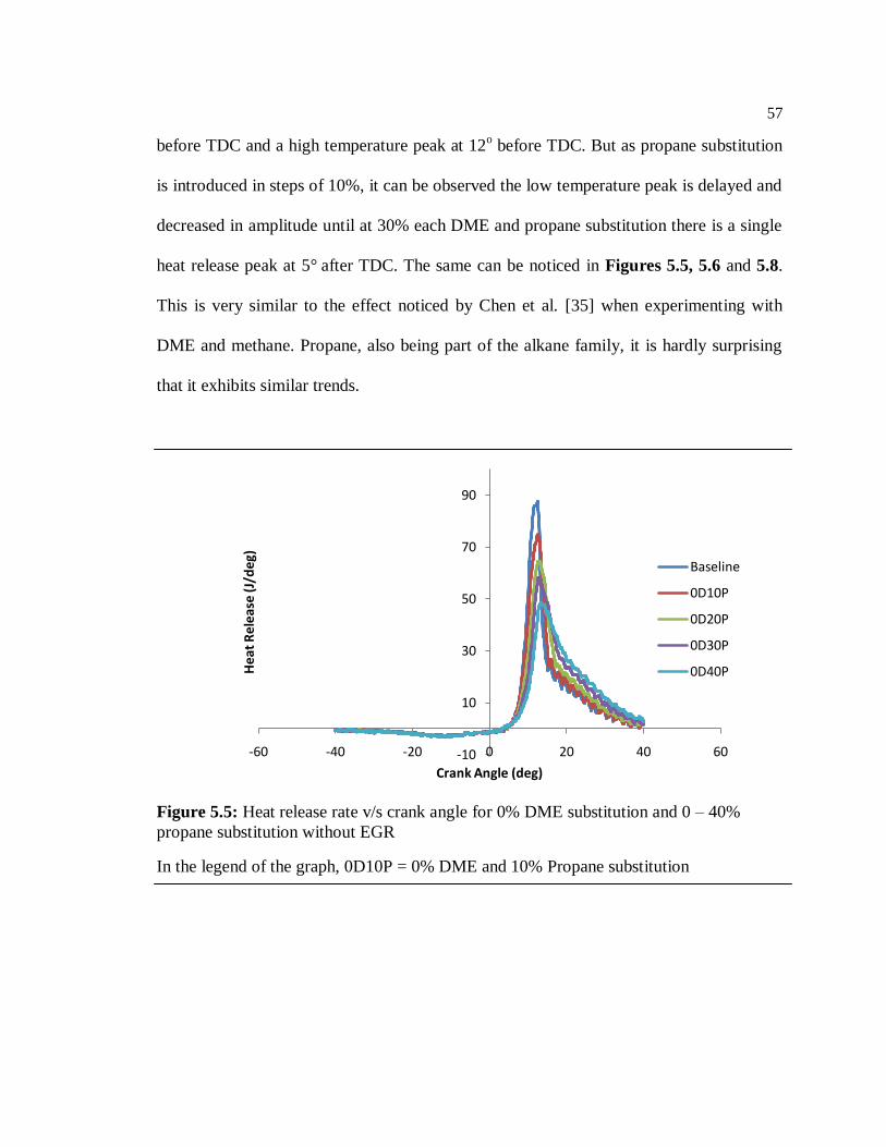
57

before TDC and a high temperature peak at 12o before TDC. But as propane substitution

is introduced in steps of 10%, it can be observed the low temperature peak is delayed and

decreased in amplitude until at 30% each DME and propane substitution there is a single

heat release peak at 5° after TDC. The same can be noticed in Figures 5.5, 5.6 and 5.8.

This is very similar to the effect noticed by Chen et al. [35] when experimenting with

DME and methane. Propane, also being part of the alkane family, it is hardly surprising

that it exhibits similar trends.


propane substitution without EGR

In the legend of the graph, 0D10P = 0% DME and 10% Propane substitution

-10

10

30

50

70

90

-60 -40 -20 0 20 40 60

Hea

t R

elea

se (

J/d

eg)

Crank Angle (deg)

Baseline

0D10P

0D20P

0D30P

0D40P

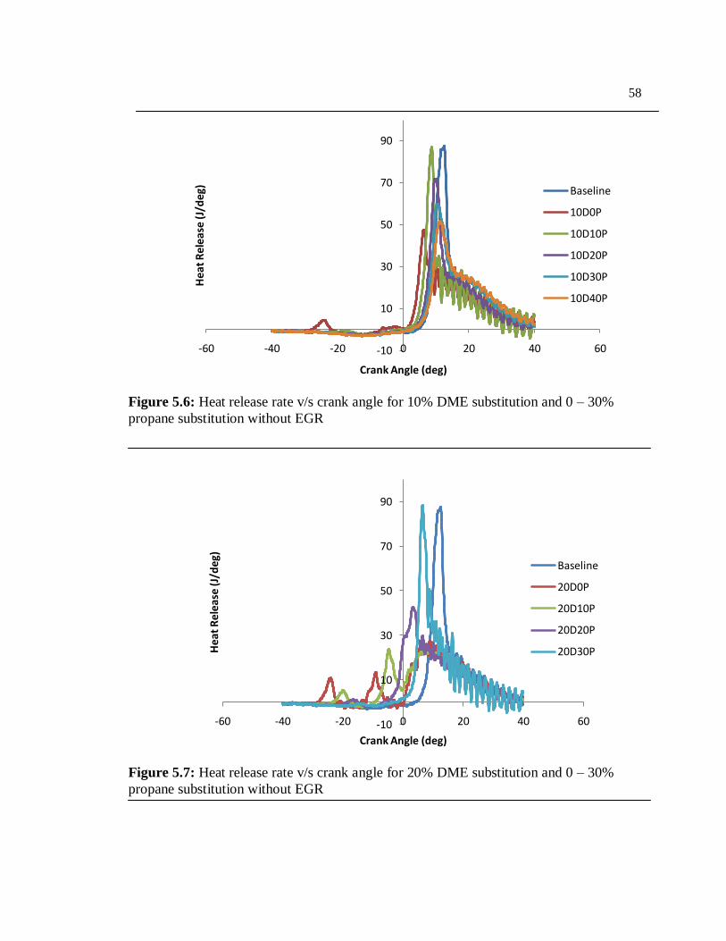
58





-10

10

30

50

70

90

-60 -40 -20 0 20 40 60

He

at R

ele

ase

(J/

de

g)

Crank Angle (deg)

Baseline

10D0P

10D10P

10D20P

10D30P

10D40P

-10

10

30

50

70

90

-60 -40 -20 0 20 40 60

Hea

t R

elea

se (

J/d

eg)

Crank Angle (deg)

Baseline

20D0P

20D10P

20D20P

20D30P

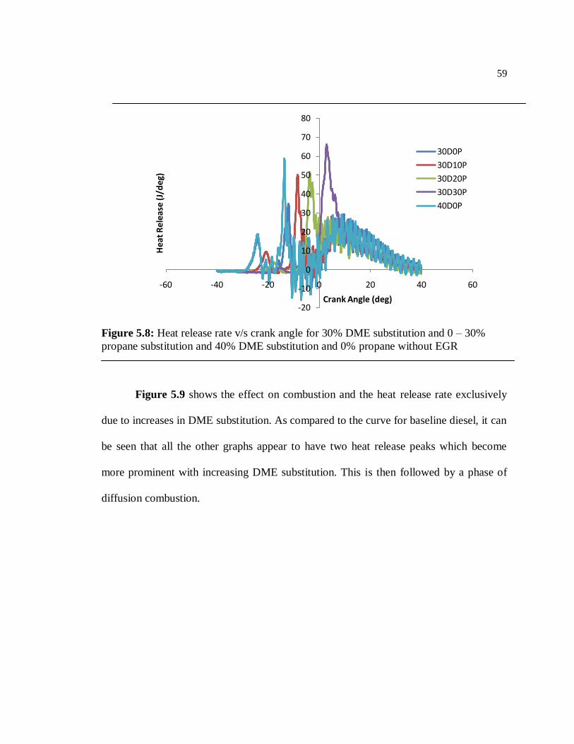
59


propane substitution and 40% DME substitution and 0% propane without EGR

Figure 5.9 shows the effect on combustion and the heat release rate exclusively

due to increases in DME substitution. As compared to the curve for baseline diesel, it can

be seen that all the other graphs appear to have two heat release peaks which become

more prominent with increasing DME substitution. This is then followed by a phase of

diffusion combustion.

-20

-10

0

10

20

30

40

50

60

70

80

-60 -40 -20 0 20 40 60

He

at R

ele

ase

(J/

de

g)

Crank Angle (deg)

30D0P

30D10P

30D20P

30D30P

40D0P

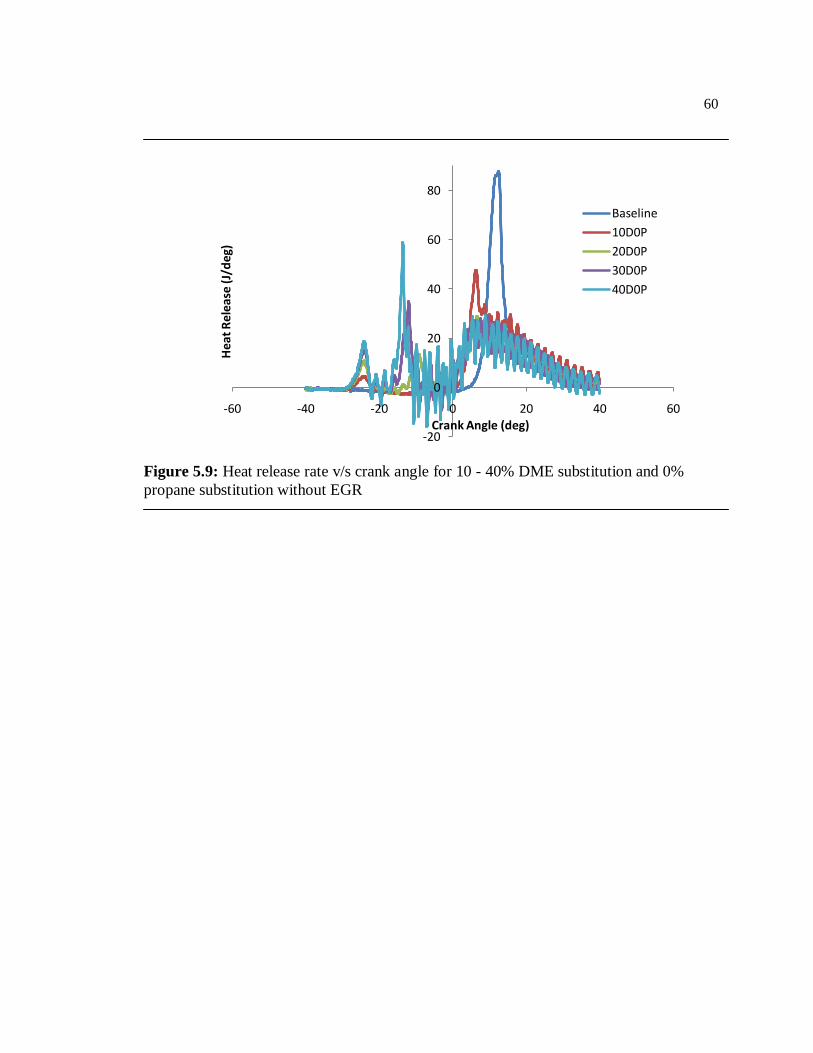
60

Figure 5.9: Heat release rate v/s crank angle for 10 - 40% DME substitution and 0%


-20

0

20

40

60

80

-60 -40 -20 0 20 40 60

He

at R

ele

ase

(J/

de

g)

Crank Angle (deg)

Baseline

10D0P

20D0P

30D0P

40D0P

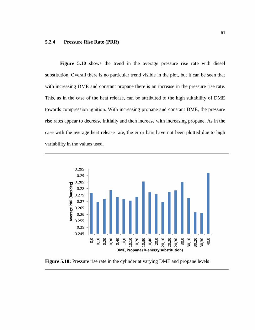
61

5.2.4 Pressure Rise Rate (PRR)

Figure 5.10 shows the trend in the average pressure rise rate with diesel

substitution. Overall there is no particular trend visible in the plot, but it can be seen that

with increasing DME and constant propane there is an increase in the pressure rise rate.

This, as in the case of the heat release, can be attributed to the high suitability of DME

towards compression ignition. With increasing propane and constant DME, the pressure

rise rates appear to decrease initially and then increase with increasing propane. As in the

case with the average heat release rate, the error bars have not been plotted due to high

variability in the values used.

Figure 5.10: Pressure rise rate in the cylinder at varying DME and propane levels

0.245

0.25

0.255

0.26

0.265

0.27

0.275

0.28

0.285

0.29

0.295

0,0

0,1

0

0,2

0

0,3

0

0,4

0

10

,0

10,1

0

10,2

0

10,3

0

10,4

0

20

,0

20,1

0

20,2

0

20,3

0

30,0

30,1

0

30,2

0

30,3

0

40,0

Ave

rage

PR

R (

bar

/deg

)


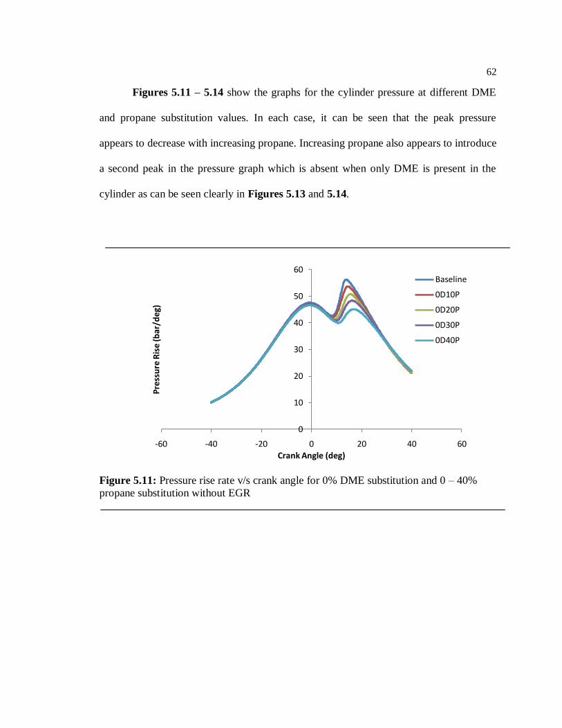
62

Figures 5.11 – 5.14 show the graphs for the cylinder pressure at different DME

and propane substitution values. In each case, it can be seen that the peak pressure

appears to decrease with increasing propane. Increasing propane also appears to introduce

a second peak in the pressure graph which is absent when only DME is present in the

cylinder as can be seen clearly in Figures 5.13 and 5.14.



0

10

20

30

40

50

60

-60 -40 -20 0 20 40 60

Pre

ssu

re R

ise

(bar

/deg

)

Crank Angle (deg)

Baseline

0D10P

0D20P

0D30P

0D40P

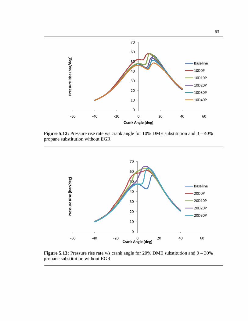
63





0

10

20

30

40

50

60

70

-60 -40 -20 0 20 40 60

Pre

ssu

re R

ise

(b

ar/d

eg)

Crank Angle (deg)

Baseline

10D0P

10D10P

10D20P

10D30P

10D40P

0

10

20

30

40

50

60

70

-60 -40 -20 0 20 40 60

Pre

ssu

re R

ise

(bar

/deg

)

Crank Angle (deg)

Baseline

20D0P

20D10P

20D20P

20D30P

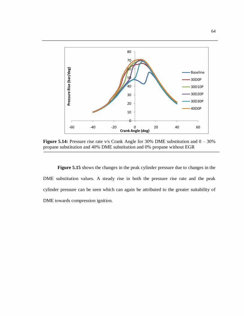
64

Figure 5.14: Pressure rise rate v/s Crank Angle for 30% DME substitution and 0 – 30%

propane substitution and 40% DME substitution and 0% propane without EGR

Figure 5.15 shows the changes in the peak cylinder pressure due to changes in the

DME substitution values. A steady rise in both the pressure rise rate and the peak

cylinder pressure can be seen which can again be attributed to the greater suitability of

DME towards compression ignition.

0

10

20

30

40

50

60

70

80

-60 -40 -20 0 20 40 60

Pre

ssu

re R

ise

(b

ar/d

eg)

Crank Angle (deg)

Baseline

30D0P

30D10P

30D20P

30D30P

40D0P

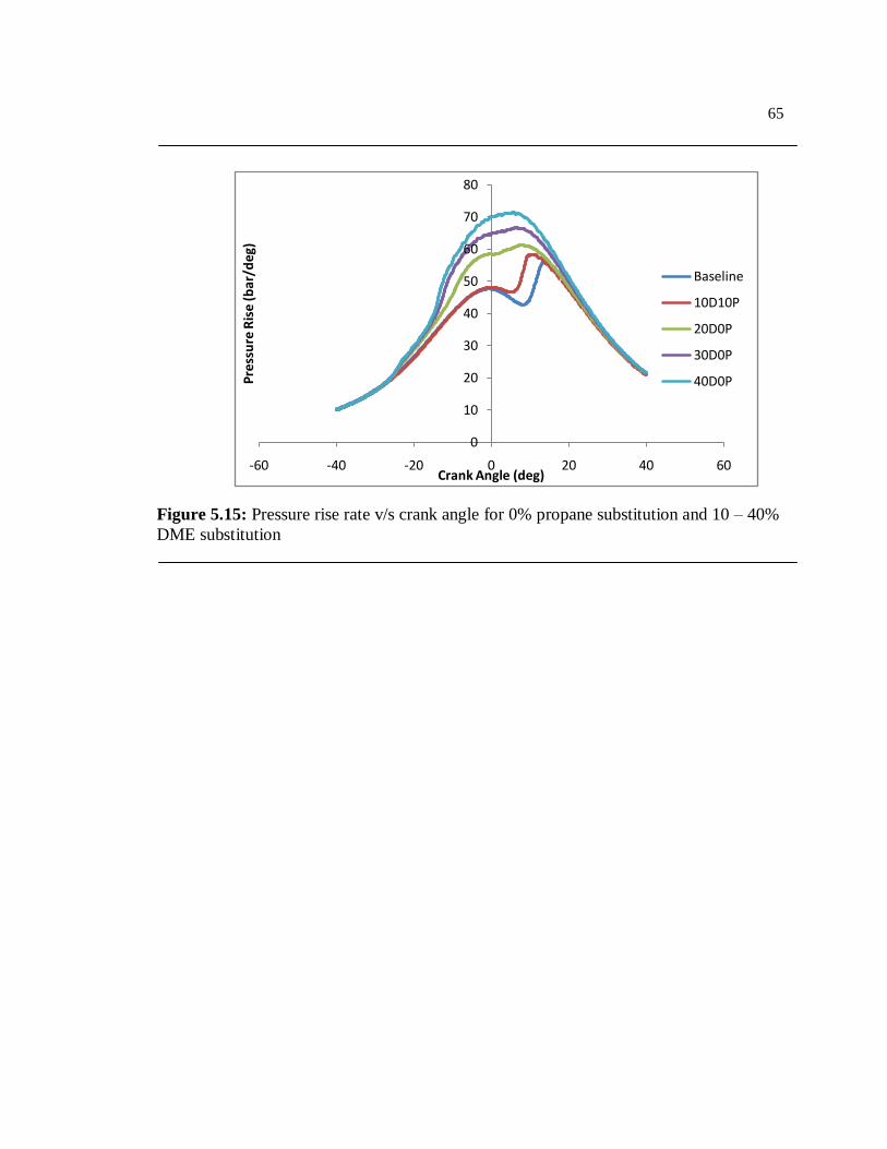
65

Figure 5.15: Pressure rise rate v/s crank angle for 0% propane substitution and 10 – 40%

DME substitution

0

10

20

30

40

50

60

70

80

-60 -40 -20 0 20 40 60

Pre

ssu

re R

ise

(b

ar/d

eg)

Crank Angle (deg)

Baseline

10D10P

20D0P

30D0P

40D0P

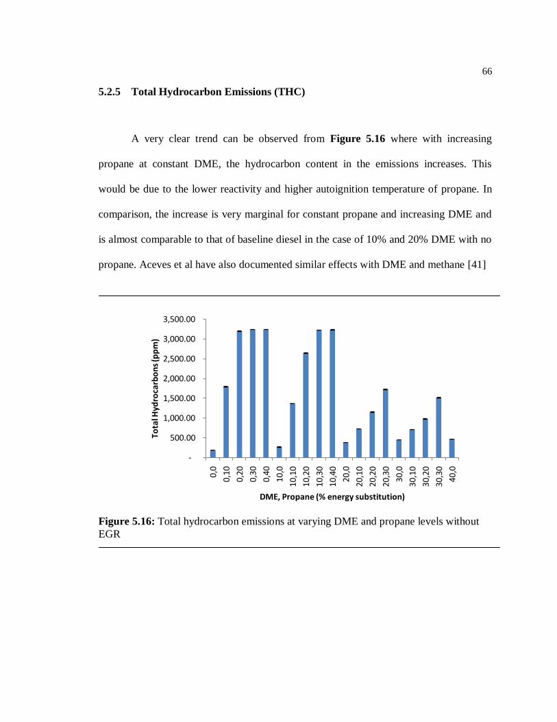
66

5.2.5 Total Hydrocarbon Emissions (THC)

A very clear trend can be observed from Figure 5.16 where with increasing

propane at constant DME, the hydrocarbon content in the emissions increases. This

would be due to the lower reactivity and higher autoignition temperature of propane. In

comparison, the increase is very marginal for constant propane and increasing DME and

is almost comparable to that of baseline diesel in the case of 10% and 20% DME with no

propane. Aceves et al have also documented similar effects with DME and methane [41]

Figure 5.16: Total hydrocarbon emissions at varying DME and propane levels without

EGR

-

500.00

1,000.00

1,500.00

2,000.00

2,500.00

3,000.00

3,500.00

0,0

0,1

0

0,2

0

0,3

0

0,4

0

10

,0

10,1

0

10,2

0

10,3

0

10,4

0

20

,0

20,1

0

20,2

0

20,3

0

30

,0

30,1

0

30,2

0

30,3

0

40

,0

Tota

l Hyd

roca

rbo

ns

(pp

m)


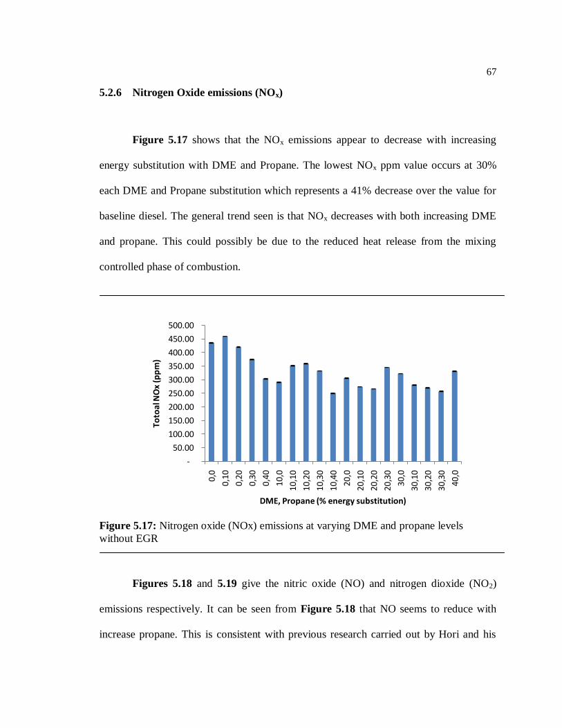
67

5.2.6 Nitrogen Oxide emissions (NOx)

Figure 5.17 shows that the NOx emissions appear to decrease with increasing

energy substitution with DME and Propane. The lowest NOx ppm value occurs at 30%

each DME and Propane substitution which represents a 41% decrease over the value for

baseline diesel. The general trend seen is that NOx decreases with both increasing DME

and propane. This could possibly be due to the reduced heat release from the mixing

controlled phase of combustion.

Figure 5.17: Nitrogen oxide (NOx) emissions at varying DME and propane levels

without EGR

Figures 5.18 and 5.19 give the nitric oxide (NO) and nitrogen dioxide (NO2)

emissions respectively. It can be seen from Figure 5.18 that NO seems to reduce with

increase propane. This is consistent with previous research carried out by Hori and his

-

50.00

100.00

150.00

200.00

250.00

300.00

350.00

400.00

450.00

500.00

0,0

0,1

0

0,2

0

0,3

0

0,4

0

10,0

10,

10

10,

20

10,

30

10,

40

20,0

20,

10

20,2

0

20,

30

30,0

30,

10

30,

20

30,

30

40,0

Toto

al N

Ox

(pp

m)


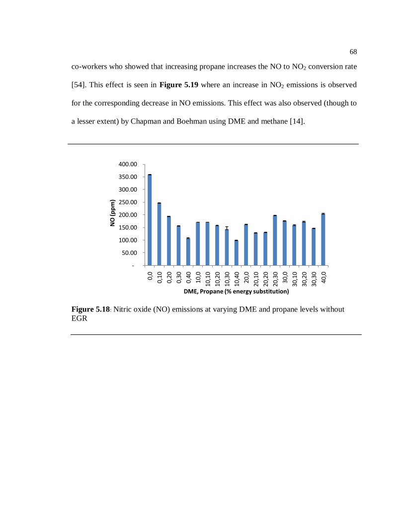
68

co-workers who showed that increasing propane increases the NO to NO2 conversion rate

[54]. This effect is seen in Figure 5.19 where an increase in NO2 emissions is observed

for the corresponding decrease in NO emissions. This effect was also observed (though to

a lesser extent) by Chapman and Boehman using DME and methane [14].

Figure 5.18: Nitric oxide (NO) emissions at varying DME and propane levels without

EGR

-

50.00

100.00

150.00

200.00

250.00

300.00

350.00

400.00

0,0

0,10

0,20

0,30

0,40

10,0

10,1

0

10,2

0

10,3

0

10,4

0

20,0

20,1

0

20,2

0

20,3

0

30,0

30,1

0

30,2

0

30,3

0

40,0

NO

(p

pm

)


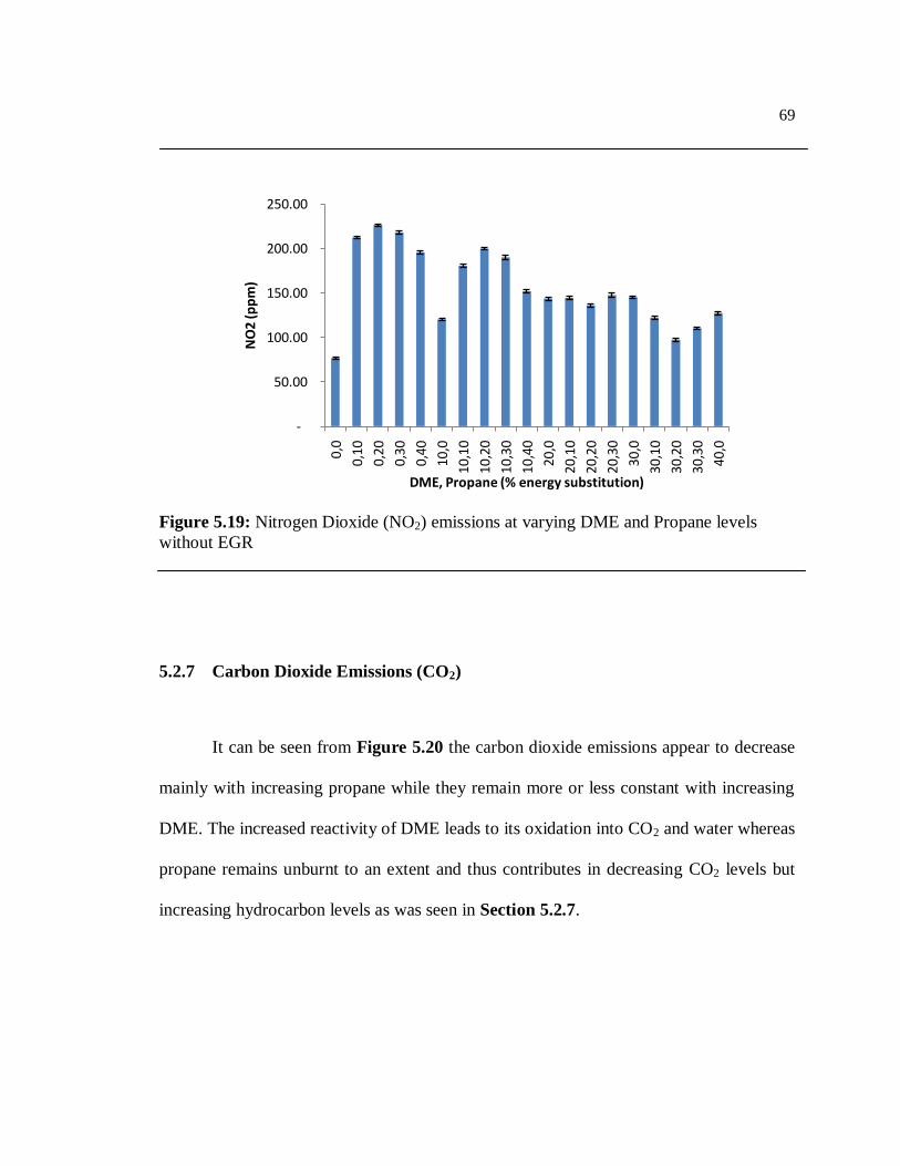
69

Figure 5.19: Nitrogen Dioxide (NO2) emissions at varying DME and Propane levels

without EGR

5.2.7 Carbon Dioxide Emissions (CO2)

It can be seen from Figure 5.20 the carbon dioxide emissions appear to decrease

mainly with increasing propane while they remain more or less constant with increasing

DME. The increased reactivity of DME leads to its oxidation into CO2 and water whereas

propane remains unburnt to an extent and thus contributes in decreasing CO2 levels but

increasing hydrocarbon levels as was seen in Section 5.2.7.

-

50.00

100.00

150.00

200.00

250.00

0,0

0,10

0,20

0,30

0,40

10,0

10,1

0

10,2

0

10,3

0

10,4

0

20,0

20,1

0

20,2

0

20,3

0

30,0

30,1

0

30,2

0

30,3

0

40,0

NO

2 (p

pm

)


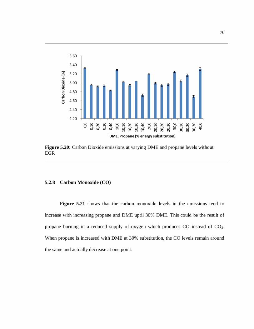
70

Figure 5.20: Carbon Dioxide emissions at varying DME and propane levels without

EGR

5.2.8 Carbon Monoxide (CO)

Figure 5.21 shows that the carbon monoxide levels in the emissions tend to

increase with increasing propane and DME uptil 30% DME. This could be the result of

propane burning in a reduced supply of oxygen which produces CO instead of CO2.

When propane is increased with DME at 30% substitution, the CO levels remain around

the same and actually decrease at one point.

4.20

4.40

4.60

4.80

5.00

5.20

5.40

5.60

0,0

0,10

0,20

0,30

0,40

10,0

10,1

0

10,2

0

10,3

0

10,4

0

20,0

20,1

0

20,2

0

20,3

0

30,0

30,1

0

30,2

0

30,3

0

40,0

Car

bo

n D

ioxi

de

(%

)


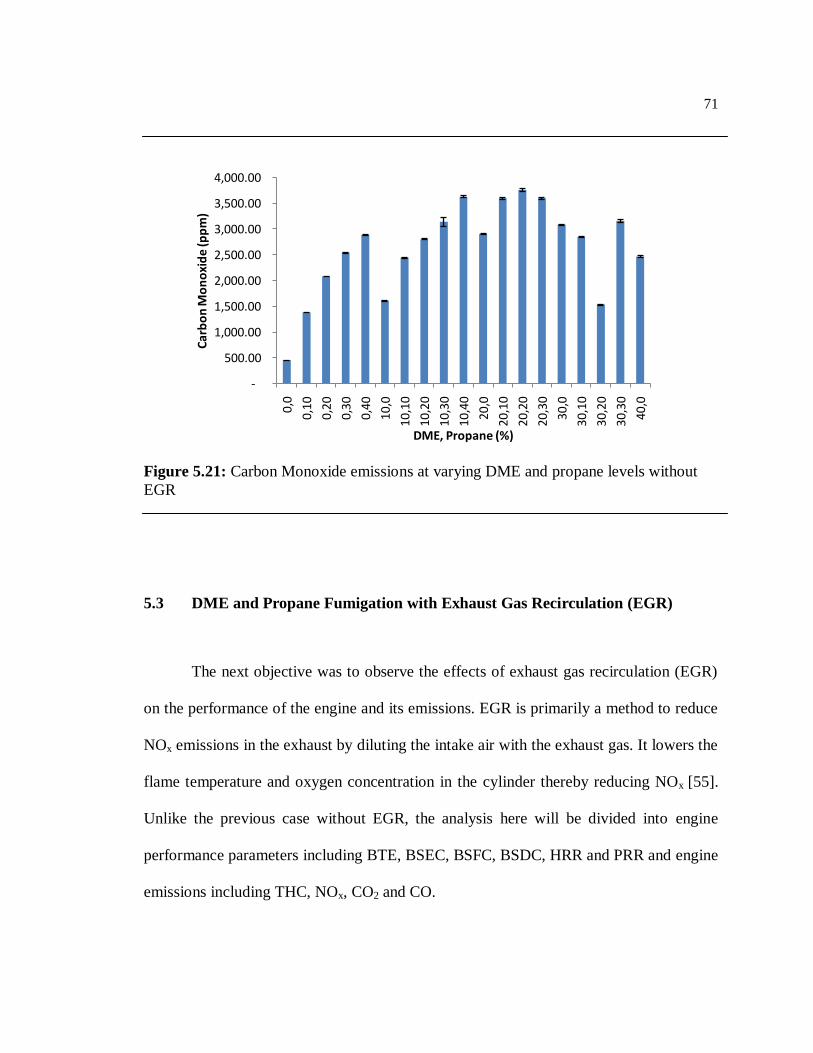
71

Figure 5.21: Carbon Monoxide emissions at varying DME and propane levels without

EGR

5.3 DME and Propane Fumigation with Exhaust Gas Recirculation (EGR)

The next objective was to observe the effects of exhaust gas recirculation (EGR)

on the performance of the engine and its emissions. EGR is primarily a method to reduce

NOx emissions in the exhaust by diluting the intake air with the exhaust gas. It lowers the

flame temperature and oxygen concentration in the cylinder thereby reducing NOx [55].

Unlike the previous case without EGR, the analysis here will be divided into engine

performance parameters including BTE, BSEC, BSFC, BSDC, HRR and PRR and engine

emissions including THC, NOx, CO2 and CO.

-

500.00

1,000.00

1,500.00

2,000.00

2,500.00

3,000.00

3,500.00

4,000.00

0,0

0,10

0,20

0,30

0,40

10,0

10,1

0

10,2

0

10,3

0

10,4

0

20,0

20,1

0

20,2

0

20,3

0

30,0

30,1

0

30,2

0

30,3

0

40,0

Car

bo

n M

on

oxi

de

(pp

m)

DME, Propane (%)

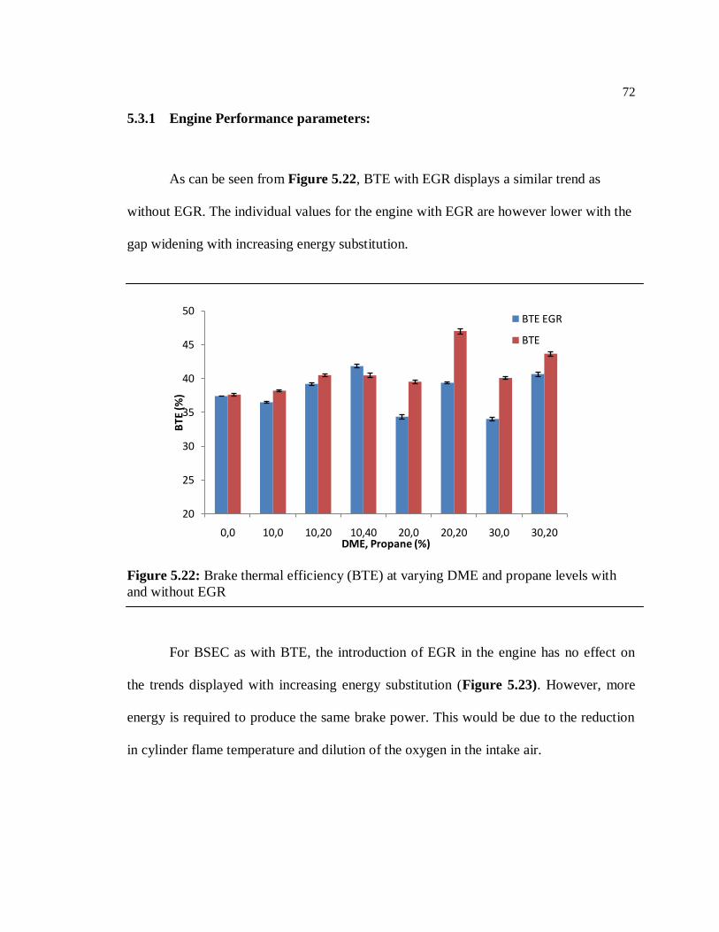
72

5.3.1 Engine Performance parameters:

As can be seen from Figure 5.22, BTE with EGR displays a similar trend as

without EGR. The individual values for the engine with EGR are however lower with the

gap widening with increasing energy substitution.

Figure 5.22: Brake thermal efficiency (BTE) at varying DME and propane levels with

and without EGR

For BSEC as with BTE, the introduction of EGR in the engine has no effect on

the trends displayed with increasing energy substitution (Figure 5.23). However, more

energy is required to produce the same brake power. This would be due to the reduction

in cylinder flame temperature and dilution of the oxygen in the intake air.

20

25

30

35

40

45

50

0,0 10,0 10,20 10,40 20,0 20,20 30,0 30,20

BTE

(%

)

DME, Propane (%)

BTE EGR

BTE

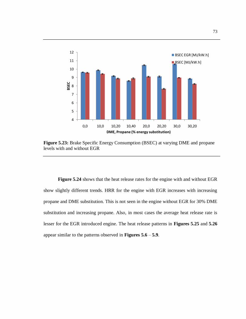
73

Figure 5.23: Brake Specific Energy Consumption (BSEC) at varying DME and propane

levels with and without EGR

Figure 5.24 shows that the heat release rates for the engine with and without EGR

show slightly different trends. HRR for the engine with EGR increases with increasing

propane and DME substitution. This is not seen in the engine without EGR for 30% DME

substitution and increasing propane. Also, in most cases the average heat release rate is

lesser for the EGR introduced engine. The heat release patterns in Figures 5.25 and 5.26

appear similar to the patterns observed in Figures 5.6 – 5.9.

4

5

6

7

8

9

10

11

12

0,0 10,0 10,20 10,40 20,0 20,20 30,0 30,20

BSE

C


BSEC EGR [MJ/kW.h]

BSEC [MJ/kW.h]

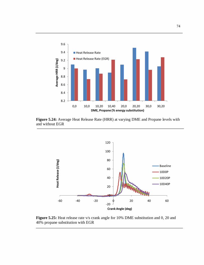
74

Figure 5.24: Average Heat Release Rate (HRR) at varying DME and Propane levels with

and without EGR

Figure 5.25: Heat release rate v/s crank angle for 10% DME substitution and 0, 20 and

40% propane substitution with EGR

8.2

8.4

8.6

8.8

9

9.2

9.4

9.6

0,0 10,0 10,20 10,40 20,0 20,20 30,0 30,20

Ave

rage

HR

R (

J/d

eg)


Heat Release Rate

Heat Release Rate (EGR)

-20

0

20

40

60

80

100

120

-60 -40 -20 0 20 40 60

Hea

t R

ele

ase

(J/

deg

)

Crank Angle (deg)

Baseline

10D0P

10D20P

10D40P

75

Figure 5.26: Heat release rate v/s crank angle for 20 and 30% DME substitution and 0

and 20% propane substitution with EGR

Figure 5.27 shows the heat release curve for two cases 30% DME and 20%

Propane and 10% DME and 0% Propane with and without the use of EGR. As can be

seen, for both sets of energy substitutions, the start of combustion and subsequent heat

release is delayed with the use of EGR.

-20

0

20

40

60

80

100

120

-60 -40 -20 0 20 40 60

He

at R

ele

ase

(J/

de

g)

Crank Angle (deg)

Baseline

20D0P

20D20P

30D0P

30D20P

76

Figure 5.27: Heat release rate v/s crank angle for cases with and without EGR

The average pressure rise rate in Figure 5.28 for EGR introduction increases with

DME and propane substitution as with the previous case but the values are considerably

lower. This could be attributed to the slower combustion owing to reduced cylinder

temperatures and slow pressure rises. The pressure rise graphs from Figures 5.29 and

5.30 are also similar to their counterparts from Section 5.2.6 except that the peak

pressures here are much lower.

-20

-10

0

10

20

30

40

50

60

70

80

-60 -40 -20 0 20 40 60

He

at R

ele

ase

(J/

de

g)

Crank Angle (deg)

30D20P

30D20P EGR

10D0P

10D0P EGR

77

Figure 5.28: Average pressure rise rate (PRR) at varying DME and propane levels with

and without EGR

Figure 5.29: Pressure rise rate v/s crank angle for 10% DME substitution and 0, 20 and

40% propane substitution with EGR

0.25

0.255

0.26

0.265

0.27

0.275

0.28

0.285

0.29

0,0 10,0 10,20 10,40 20,0 20,20 30,0 30,20

Ave

rage

PR

R (

bar

/de

g)


Pressure Rise Rate

Pressure Rise Rate (EGR)

0

10

20

30

40

50

60

-60 -40 -20 0 20 40 60

Pre

ssu

re (b

ar)

Crank Angle (deg)

Baseline

10D0P

10D20P

10D40P

78

Figure 5.30: Pressure rise rate v/s crank angle for 20 and 30% DME substitution and 0

and 20% propane substitution with EGR

Figure 5.31 shows the cylinder pressure trace for two conditions, 10% DME and

0% Propane and 30% DME and 20% Propane with and without EGR. Similar to the heat

release curve in Figure 5.27, the pressure rise is lower for the cases with EGR

introduction as compared to the corresponding ones without.

0

10

20

30

40

50

60

70

-60 -40 -20 0 20 40 60

Pre

ssu

re (b

ar)

Crank Angle (deg)

Baseline

20D0P

20D20P

30D0P

30D20P

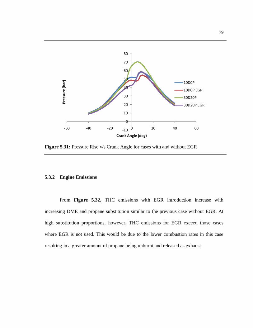
79

Figure 5.31: Pressure Rise v/s Crank Angle for cases with and without EGR

5.3.2 Engine Emissions

From Figure 5.32, THC emissions with EGR introduction increase with

increasing DME and propane substitution similar to the previous case without EGR. At

high substitution proportions, however, THC emissions for EGR exceed those cases

where EGR is not used. This would be due to the lower combustion rates in this case

resulting in a greater amount of propane being unburnt and released as exhaust.

-10

0

10

20

30

40

50

60

70

80

-60 -40 -20 0 20 40 60

Pre

ssu

re (b

ar)

Crank Angle (deg)

10D0P

10D0P EGR

30D20P

30D20P EGR

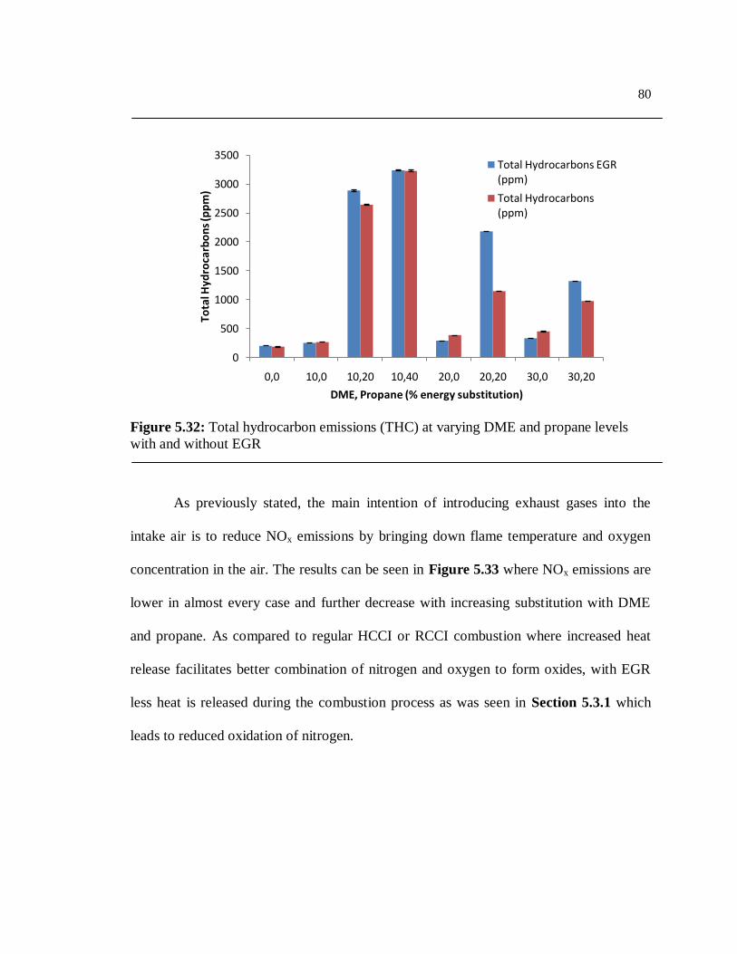
80

Figure 5.32: Total hydrocarbon emissions (THC) at varying DME and propane levels

with and without EGR

As previously stated, the main intention of introducing exhaust gases into the

intake air is to reduce NOx emissions by bringing down flame temperature and oxygen

concentration in the air. The results can be seen in Figure 5.33 where NOx emissions are

lower in almost every case and further decrease with increasing substitution with DME

and propane. As compared to regular HCCI or RCCI combustion where increased heat

release facilitates better combination of nitrogen and oxygen to form oxides, with EGR

less heat is released during the combustion process as was seen in Section 5.3.1 which

leads to reduced oxidation of nitrogen.

0

500

1000

1500

2000

2500

3000

3500

0,0 10,0 10,20 10,40 20,0 20,20 30,0 30,20

Tota

l Hyd

roca

rbo

ns

(pp

m)


Total Hydrocarbons EGR (ppm)

Total Hydrocarbons (ppm)

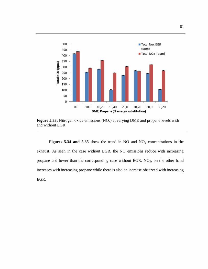
81

Figure 5.33: Nitrogen oxide emissions (NOx) at varying DME and propane levels with

and without EGR

Figures 5.34 and 5.35 show the trend in NO and NO2 concentrations in the

exhaust. As seen in the case without EGR, the NO emissions reduce with increasing

propane and lower than the corresponding case without EGR. NO2, on the other hand

increases with increasing propane while there is also an increase observed with increasing

EGR.

0

50

100

150

200

250

300

350

400

450

500

0,0 10,0 10,20 10,40 20,0 20,20 30,0 30,20

Tota

l NO

x (p

pm

)


Total Nox EGR (ppm)

Total NOx (ppm)

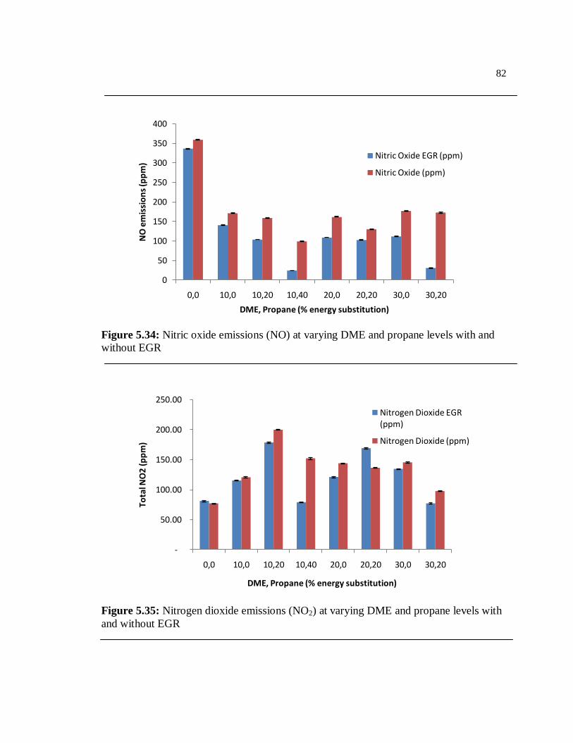
82

Figure 5.34: Nitric oxide emissions (NO) at varying DME and propane levels with and

without EGR

Figure 5.35: Nitrogen dioxide emissions (NO2) at varying DME and propane levels with

and without EGR

0

50

100

150

200

250

300

350

400

0,0 10,0 10,20 10,40 20,0 20,20 30,0 30,20

NO

em

issi

on

s (p

pm

)


Nitric Oxide EGR (ppm)

Nitric Oxide (ppm)

-

50.00

100.00

150.00

200.00

250.00

0,0 10,0 10,20 10,40 20,0 20,20 30,0 30,20

Tota

l NO

2 (p

pm

)


Nitrogen Dioxide EGR (ppm)

Nitrogen Dioxide (ppm)

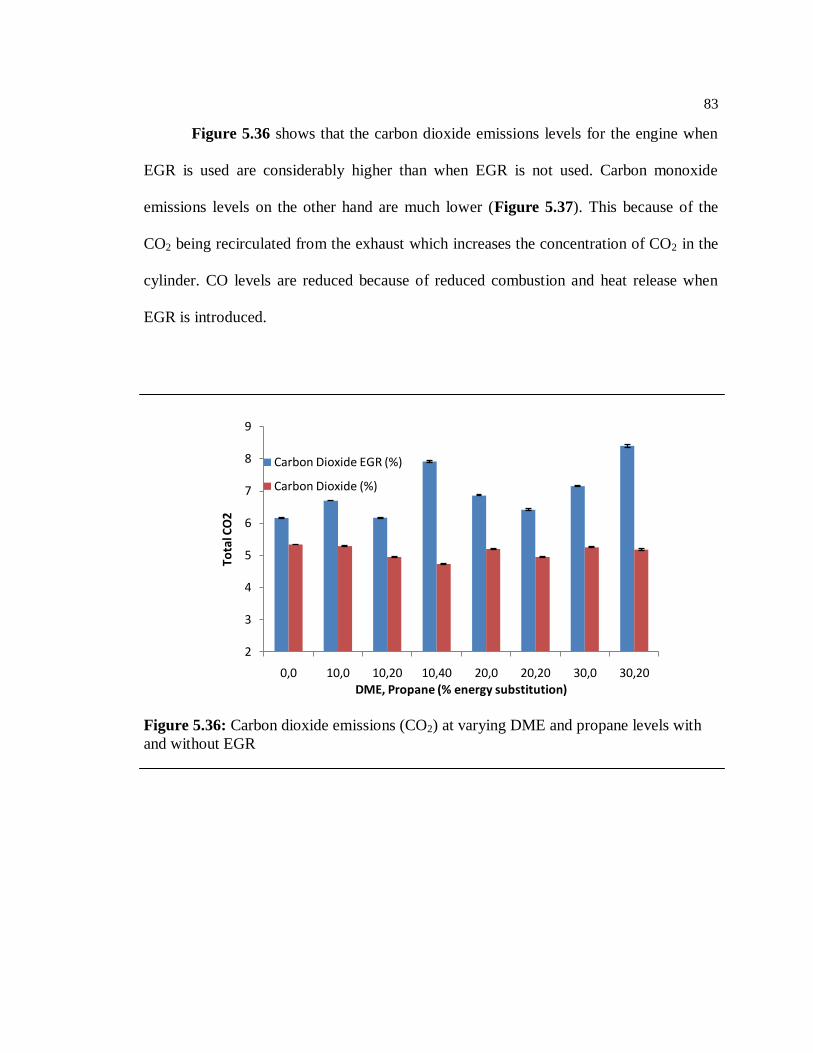
83

Figure 5.36 shows that the carbon dioxide emissions levels for the engine when

EGR is used are considerably higher than when EGR is not used. Carbon monoxide

emissions levels on the other hand are much lower (Figure 5.37). This because of the

CO2 being recirculated from the exhaust which increases the concentration of CO2 in the

cylinder. CO levels are reduced because of reduced combustion and heat release when

EGR is introduced.

Figure 5.36: Carbon dioxide emissions (CO2) at varying DME and propane levels with

and without EGR

2

3

4

5

6

7

8

9

0,0 10,0 10,20 10,40 20,0 20,20 30,0 30,20

Tota

l CO

2


Carbon Dioxide EGR (%)

Carbon Dioxide (%)

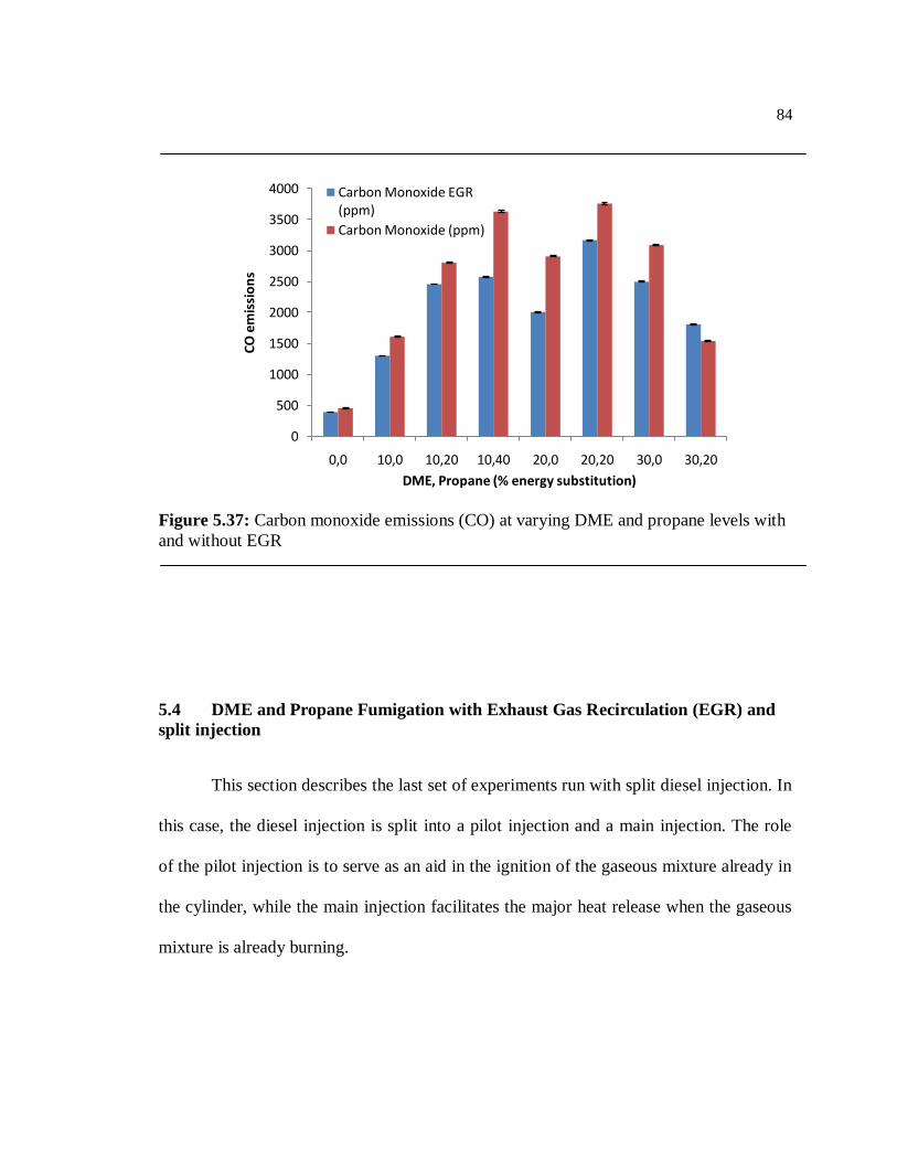
84

Figure 5.37: Carbon monoxide emissions (CO) at varying DME and propane levels with

and without EGR

5.4 DME and Propane Fumigation with Exhaust Gas Recirculation (EGR) and

split injection

This section describes the last set of experiments run with split diesel injection. In

this case, the diesel injection is split into a pilot injection and a main injection. The role

of the pilot injection is to serve as an aid in the ignition of the gaseous mixture already in

the cylinder, while the main injection facilitates the major heat release when the gaseous

mixture is already burning.

0

500

1000

1500

2000

2500

3000

3500

4000

0,0 10,0 10,20 10,40 20,0 20,20 30,0 30,20

CO

em

issi

on

s


Carbon Monoxide EGR (ppm)

Carbon Monoxide (ppm)

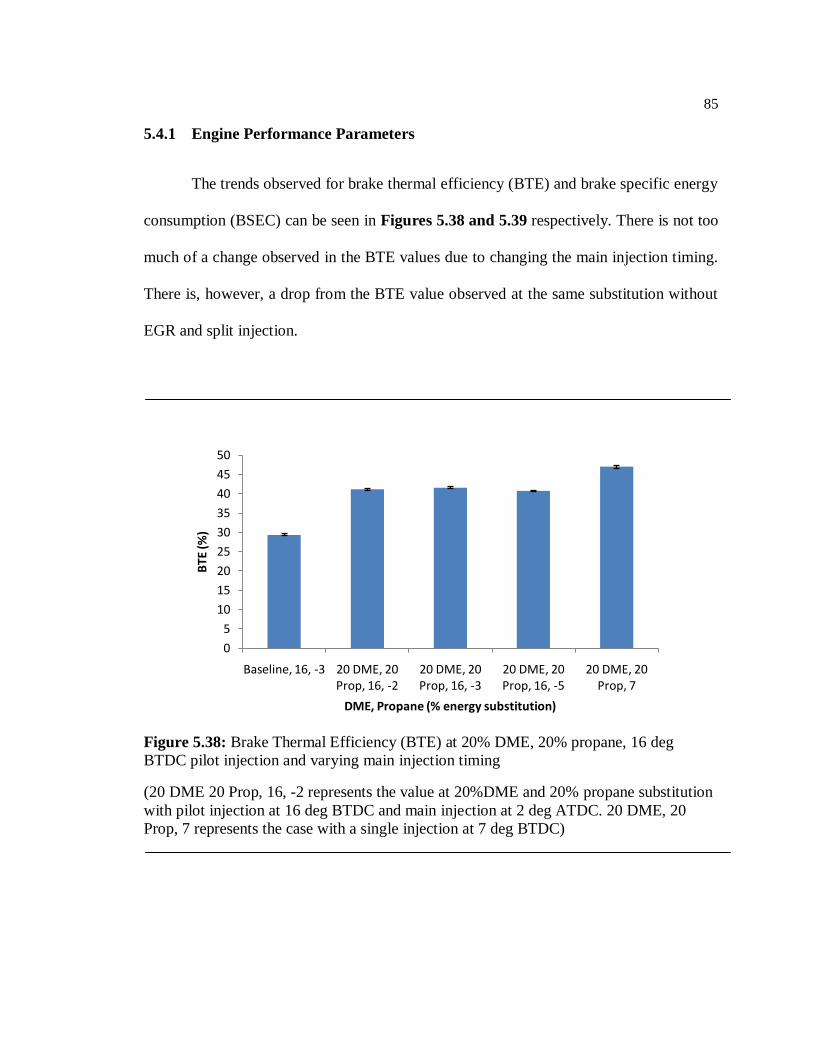
85

5.4.1 Engine Performance Parameters

The trends observed for brake thermal efficiency (BTE) and brake specific energy

consumption (BSEC) can be seen in Figures 5.38 and 5.39 respectively. There is not too

much of a change observed in the BTE values due to changing the main injection timing.

There is, however, a drop from the BTE value observed at the same substitution without

EGR and split injection.

Figure 5.38: Brake Thermal Efficiency (BTE) at 20% DME, 20% propane, 16 deg

BTDC pilot injection and varying main injection timing

(20 DME 20 Prop, 16, -2 represents the value at 20%DME and 20% propane substitution

with pilot injection at 16 deg BTDC and main injection at 2 deg ATDC. 20 DME, 20

Prop, 7 represents the case with a single injection at 7 deg BTDC)

0

5

10

15

20

25

30

35

40

45

50

Baseline, 16, -3 20 DME, 20 Prop, 16, -2

20 DME, 20 Prop, 16, -3

20 DME, 20 Prop, 16, -5

20 DME, 20 Prop, 7

BTE

(%

)


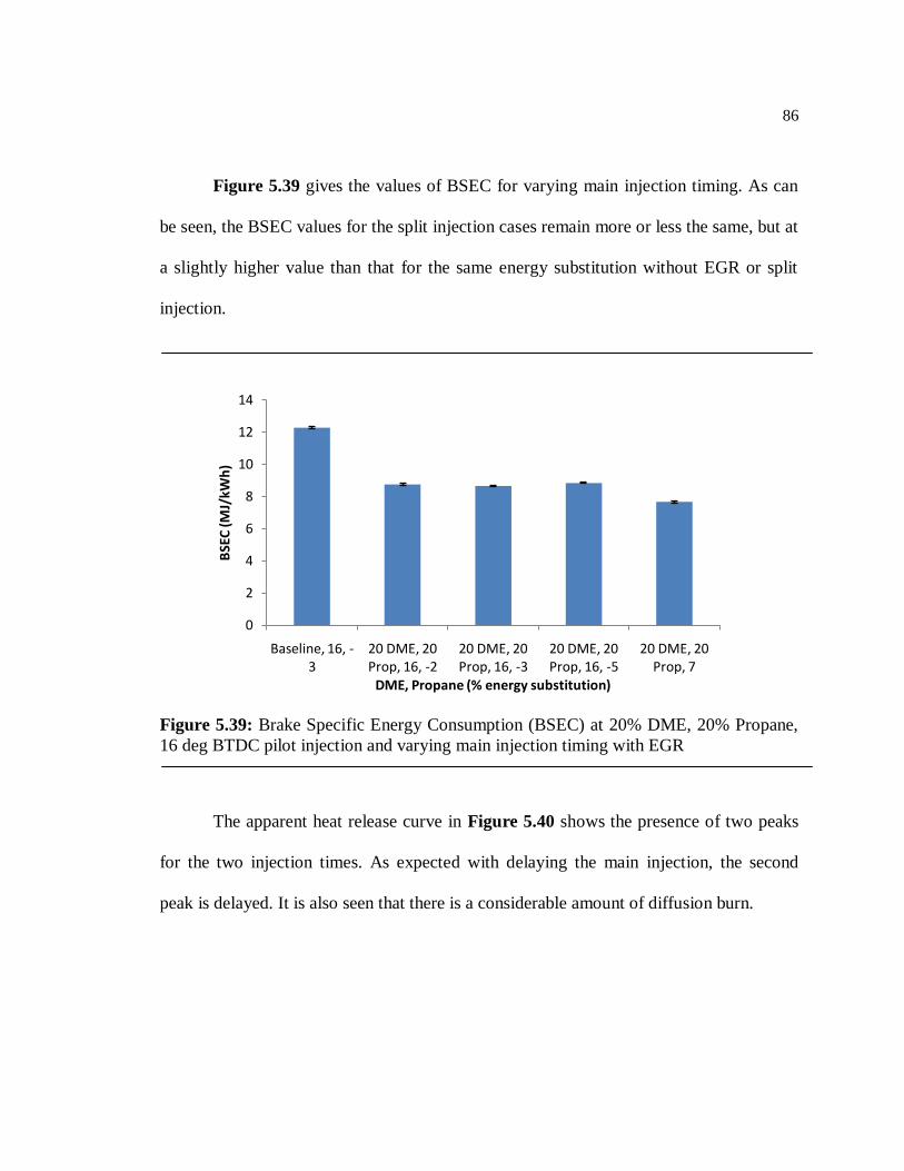
86

Figure 5.39 gives the values of BSEC for varying main injection timing. As can

be seen, the BSEC values for the split injection cases remain more or less the same, but at

a slightly higher value than that for the same energy substitution without EGR or split

injection.

Figure 5.39: Brake Specific Energy Consumption (BSEC) at 20% DME, 20% Propane,

16 deg BTDC pilot injection and varying main injection timing with EGR

The apparent heat release curve in Figure 5.40 shows the presence of two peaks

for the two injection times. As expected with delaying the main injection, the second

peak is delayed. It is also seen that there is a considerable amount of diffusion burn.

0

2

4

6

8

10

12

14

Baseline, 16, -3

20 DME, 20 Prop, 16, -2

20 DME, 20 Prop, 16, -3

20 DME, 20 Prop, 16, -5

20 DME, 20 Prop, 7

BSE

C (

MJ/

kWh

)


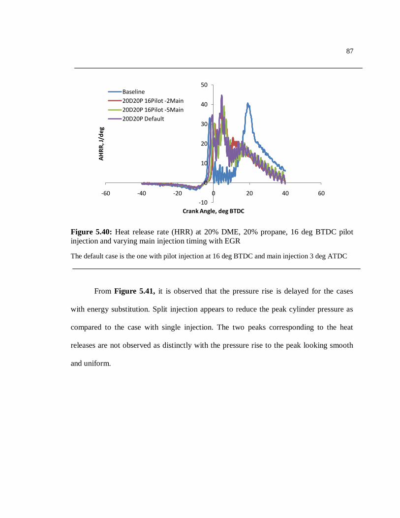
87

Figure 5.40: Heat release rate (HRR) at 20% DME, 20% propane, 16 deg BTDC pilot

injection and varying main injection timing with EGR

The default case is the one with pilot injection at 16 deg BTDC and main injection 3 deg ATDC

From Figure 5.41, it is observed that the pressure rise is delayed for the cases

with energy substitution. Split injection appears to reduce the peak cylinder pressure as

compared to the case with single injection. The two peaks corresponding to the heat

releases are not observed as distinctly with the pressure rise to the peak looking smooth

and uniform.

-10

0

10

20

30

40

50

-60 -40 -20 0 20 40 60

AH

RR

, J/d

eg

Crank Angle, deg BTDC

Baseline

20D20P 16Pilot -2Main


20D20P Default

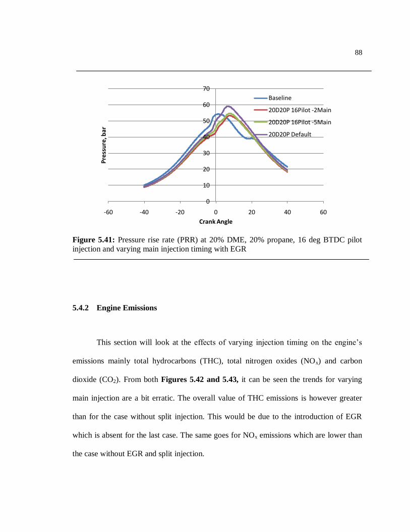
88

Figure 5.41: Pressure rise rate (PRR) at 20% DME, 20% propane, 16 deg BTDC pilot

injection and varying main injection timing with EGR

5.4.2 Engine Emissions

This section will look at the effects of varying injection timing on the engine‘s

emissions mainly total hydrocarbons (THC), total nitrogen oxides (NOx) and carbon

dioxide (CO2). From both Figures 5.42 and 5.43, it can be seen the trends for varying

main injection are a bit erratic. The overall value of THC emissions is however greater

than for the case without split injection. This would be due to the introduction of EGR

which is absent for the last case. The same goes for NOx emissions which are lower than

the case without EGR and split injection.

0

10

20

30

40

50

60

70

-60 -40 -20 0 20 40 60

Pre

ssu

re, b

ar

Crank Angle

Baseline



20D20P Default

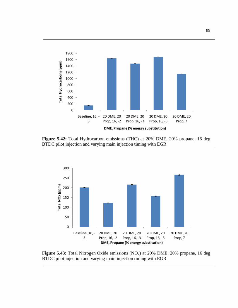
89

Figure 5.42: Total Hydrocarbon emissions (THC) at 20% DME, 20% propane, 16 deg

BTDC pilot injection and varying main injection timing with EGR

Figure 5.43: Total Nitrogen Oxide emissions (NOx) at 20% DME, 20% propane, 16 deg


0

200

400

600

800

1000

1200

1400

1600

1800

Baseline, 16, -3

20 DME, 20 Prop, 16, -2

20 DME, 20 Prop, 16, -3

20 DME, 20 Prop, 16, -5

20 DME, 20 Prop, 7

Tota

l Hyd

roca

rbo

ns

(pp

m)


0

50

100

150

200

250

300

Baseline, 16, -3

20 DME, 20 Prop, 16, -2

20 DME, 20 Prop, 16, -3

20 DME, 20 Prop, 16, -5

20 DME, 20 Prop, 7

Tota

l NO

x (p

pm

)


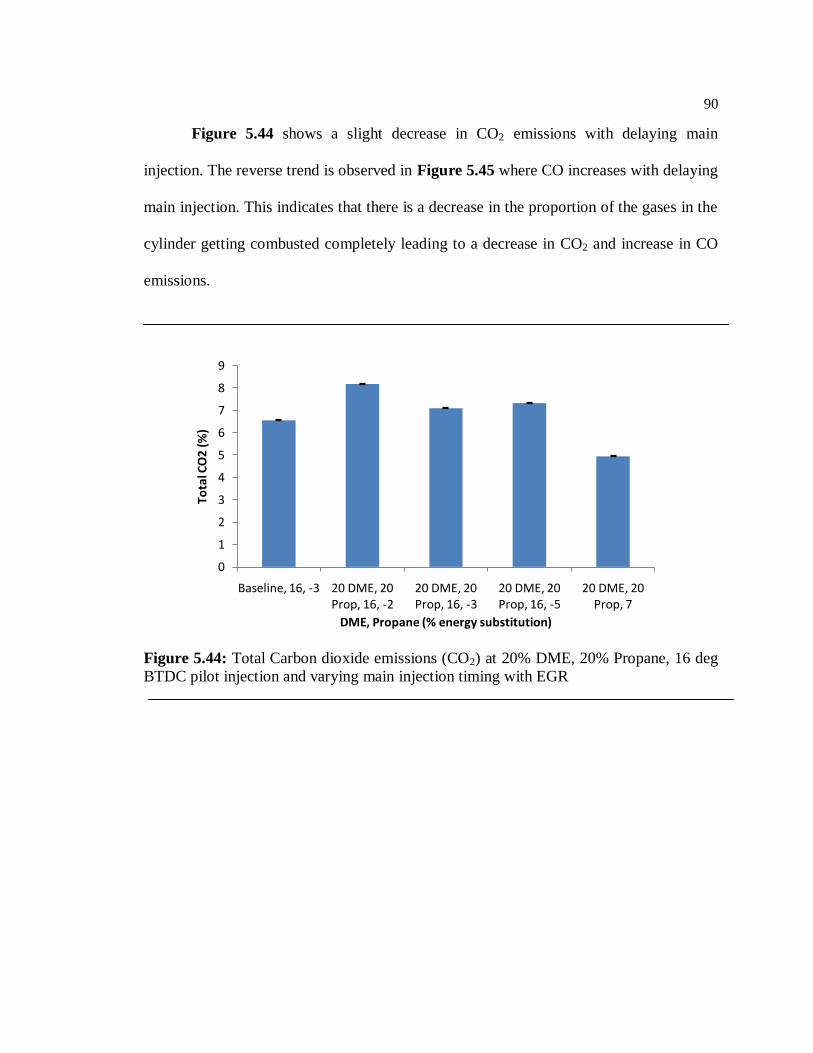
90

Figure 5.44 shows a slight decrease in CO2 emissions with delaying main

injection. The reverse trend is observed in Figure 5.45 where CO increases with delaying

main injection. This indicates that there is a decrease in the proportion of the gases in the

cylinder getting combusted completely leading to a decrease in CO2 and increase in CO

emissions.

Figure 5.44: Total Carbon dioxide emissions (CO2) at 20% DME, 20% Propane, 16 deg


0

1

2

3

4

5

6

7

8

9

Baseline, 16, -3 20 DME, 20 Prop, 16, -2

20 DME, 20 Prop, 16, -3

20 DME, 20 Prop, 16, -5

20 DME, 20 Prop, 7

Tota

l CO

2 (%

)


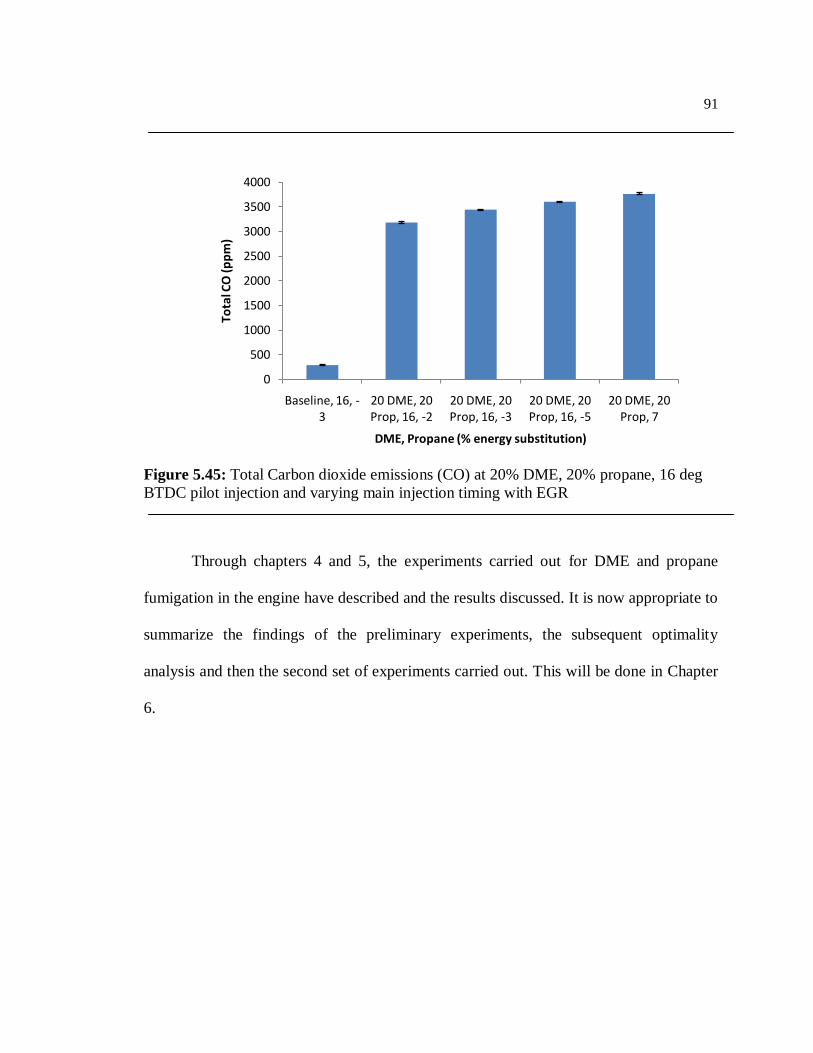
91

Figure 5.45: Total Carbon dioxide emissions (CO) at 20% DME, 20% propane, 16 deg


Through chapters 4 and 5, the experiments carried out for DME and propane

fumigation in the engine have described and the results discussed. It is now appropriate to

summarize the findings of the preliminary experiments, the subsequent optimality

analysis and then the second set of experiments carried out. This will be done in Chapter

6.

0

500

1000

1500

2000

2500

3000

3500

4000

Baseline, 16, -3

20 DME, 20 Prop, 16, -2

20 DME, 20 Prop, 16, -3

20 DME, 20 Prop, 16, -5

20 DME, 20 Prop, 7

Tota

l CO

(p

pm

)


Chapter 6

Summary and Conclusions

6.1 Summary

Before stating the conclusions derived from the experimental data, the motivation

and objectives of this study will be restated. The motivation for this research was to study

strategies that could be used to improve the brake thermal efficiency while reducing

emissions from compression ignition engines. This work is intended to support the

development of 55% thermal efficiency engines. Additional objectives were to minimize

the heat release rate and the pressure rise rate to prevent damage to the cylinders. The

following strategies were employed to this end:

1. Fumigating dimethyl ether and propane along with the intake air to modify the

cetane number of the fuel and gain better control over the combustion process.

2. Introduce exhaust gas recirculation along with DME and propane fumigation to

reduce flame temperature and oxygen concentration and thereby reduce NOx

emissions.

3. Use split pilot and main diesel injections to observe effects on heat release,

efficiency and emissions.

93

6.2 Observations and Conclusions

Preliminary experiments carried out were described in Chapter 4 and a regression

analysis was carried to determine patterns in the data and obtain optimal points for the

response factors. It was then attempted to verify these findings in the next set of

experiments in Chapter 5. The findings for each response factor are listed below.

1. Brake Thermal Efficiency (BTE) is at its maximum value for high DME and

propane energy substitution. This was observed during both the preliminary and

main set of experiments. Maximum efficiency of 49.91% was observed during the

second set of experiments at 20% DME and 30% Propane substitution.

Introduction of EGR tends to reduce BTE as it results in lower heat release rates.

2. Brake Specific Energy Consumption (BSEC), Brake Specific Fuel

Consumption (BSFC) and Brake Specific Diesel Consumption (BSDC) are at

their minimum values for high DME and propane substitutions. All the above

listed response factors were close to their observed minimum values at 30% each

DME and propane substitution.

3. The Apparent Heat Release Rate (HRR) was found to be minimum at low

DME and high propane substitution values. This is due to the high autoignition

temperature of propane which delays ignition and the subsequent heat release.

The preliminary experiments and the optimization analysis found HRR to be

minimum at 10% DME and 40% propane substitution, while the second set had

the minimum value at 0% DME and 40% propane substitution. Just as with the

other factors listed, EGR tends to decrease the average HRR value.

94

4. The Average Pressure Rise Rate (PRR) was found to be minimum at 30%

DME and 20% propane during the second set of experiments. This was contrary

to the preliminary set where PRR was minimum at 20% DME and 0% propane.

But, on the whole it was observed that both the pressure rise rate and the peak

cylinder pressure were maximum at high DME and propane substitution values

EGR introduction tended to decrease the pressure rise as well as the peak cylinder

pressure.

5. Total Hydrocarbon Emissions (THC) tended to increase with increased DME

and propane substitution. The increase was more substantial with propane than

with DME owing to propane‘s 3 carbon alkane structure and higher autoignition

temperature. THC emissions are low at low DME and propane substitution

values. At these values, THC emissions are further lowered with EGR

introduction. This is not the case however with high substitution values. The

minimum ppm value for THC emissions was observed at 10% DME and 0%

propane substitution.

6. Nitrogen Oxide Emissions (NOx) were observed to decrease with increasing

DME and propane. The ppm values were further reduced with EGR introduction.

The minimum NOx emissions value was obtained at 10% DME and 40% propane

substitution. This incidentally is the point in the preliminary set of experiments

where the heat release rate was minimum and which had low heat releases in the

main set as well. As stated in previous studies, the conversion from NO to NO2

increases with increased propane substitution.

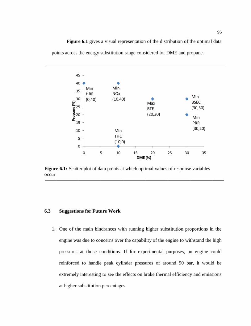
95

Figure 6.1 gives a visual representation of the distribution of the optimal data

points across the energy substitution range considered for DME and propane.

Figure 6.1: Scatter plot of data points at which optimal values of response variables

occur

6.3 Suggestions for Future Work

1. One of the main hindrances with running higher substitution proportions in the

engine was due to concerns over the capability of the engine to withstand the high

pressures at those conditions. If for experimental purposes, an engine could

reinforced to handle peak cylinder pressures of around 90 bar, it would be

extremely interesting to see the effects on brake thermal efficiency and emissions

at higher substitution percentages.

0

5

10

15

20

25

30

35

40

45

0 5 10 15 20 25 30 35

Pro

pan

e (%

)

DME (%)

Min HRR (0,40)

Max BTE (20,30)

Min NOx (10,40)

Min THC (10,0)

Min BSEC (30,30)

Min PRR (30,20)

96

2. The injection time during the course of these experiments was maintained at a

constant main injection of 7 deg BTDC for the first two sets while the last set with

split injection was not extensive. The effects of varying injection timing on the

performance of the engine could be observed by perhaps making a sweep across a

crank angle of around 10 deg.

3. The percentage of the exhaust gas recirculated into the engine was maintained at

around 25% for the experiments conducted. Varying the %EGR and observing its

effects on BTE and NOx emissions would make an interesting study.

Bibliography

[1] United Nations, 2009, ―Status of Ratification of the Kyoto Protocol,‖ United

Nations Framework Convention on Climate Change, http://unfccc.int/2860.php.

[2] Rahmstorf S., and Ganopolski A., 1999, ―Long-term global warming scenarios

computed with an efficient coupled climate model,‖ Climatic Change, 43(2), pp.

353–367.

[3] United Nations, 2011, "Environment Statistics Country Snapshot: United States",

United Nations Statistics Division,

http://unstats.un.org/unsd/environment/Questionnaires/country_snapshots.htm.

[4] United States Energy Information Administration, 2011, ―EIAs Energy in Brief:

How dependent are we on foreign oil?", United States Department of Energy,

http://www.eia.gov/energy_in_brief/foreign_oil_dependence.cfm

[5] Gruenspecht H., 2010, ―International Energy Outlook 2011,‖ Center for Strategic

and International Studies.

[6] Diesel R., 1895, ―DIESEL.‖, United States Patent No. 542,846

[7] Heywood J. B., 1988, "Internal combustion engine fundamentals", New York:

McGraw-Hill, Inc.

[8] Ganesan V., 1996, "Internal combustion engines", New York: McGraw-Hill, Inc.

[9] Lilik G. K., 2008, ―Hydrogen Assisted Diesel Combustion,‖ Master‘s Thesis,

Department of Energy and Mineral Engineering, the Pennsylvania State University.

[10] Crawley D. B., Lawrie L. K., Winkelmann F. C., Buhl W. F., Huang Y. J.,

Pedersen C. O., Strand R. K., Liesen R. J., Fisher D. E., Witte M. J., and others,

2001, ―EnergyPlus: creating a new-generation building energy simulation program,‖

Energy and Buildings, 33(4), pp. 319–331.

[11] Zhao F., Asmus T. W., Assanis D. N., Dec J. E., Eng J. A., and Najt P. M., 2003,

"Homogeneous charge compression ignition (HCCI) engines", SAE International.

[12] Warnatz J., Maas U., and Dibble R. W., 2006, "Combustion: Physical And

Chemical Fundamentals, Modeling And Simulation, Experiments, Pollutant

Formation", Springer, Berlin, p. 2.

98

[13] Epping K., Aceves S. M., Bechtold R. L., and Dec J., 2002, ―The potential of HCCI

combustion for high efficiency and low emissions", SAE Technical Paper 2002-01-

1923, 2002, doi:10.4271/2002-01-1923.

[14] Chapman E. M., and Boehman A. L., 2008, ―Pilot ignited premixed combustion of

dimethyl ether in a turbodiesel engine,‖ Fuel Processing Technology, 89(12), pp.

1262–1271.

[15] Milovanovic N., and Chen R., 2001, ―A review of experimental and simulation

studies on controlled auto-ignition combustion", SAE Technical Paper 2001-01-

1890, 2001, doi:10.4271/2001-01-1890.

[16] Christensen M., and Johansson B., 1998, ―Influence of mixture quality on

homogeneous charge compression ignition,‖ SAE transactions, 107, pp. 948–960.

[17] Ryan T., and Matheaus A., 2002, ―Fuel Requirements for HCCI Engine Operation,‖

SAE Technical Paper 2003-01-1813, 2003, doi:10.4271/2003-01-1813.

[18] Stanglmaier R. H., and Roberts C. E., 1999, ―Homogeneous Charge Compression

Ignition (HCCI): Benefits, Compromises, and Future Engine Applications,‖ SAE

Technical Paper Series, 1999-01-36(3682), pp. 1999–01–3682.

[19] Hardy W. L., and Reitz R. D., 2006, ―A study of the effects of high EGR, high

equivalence ratio, and mixing time on emissions levels in a heavy-duty diesel

engine for PCCI combustion" SAE Technical Paper 2006-01-0026, 2006,

doi:10.4271/2006-01-0026.

[20] Sun Y., and Reitz R. D., 2006, ―Modeling diesel engine NOx and soot reduction

with optimized two-stage combustion" SAE Technical Paper 2006-01-0027, 2006,

doi:10.4271/2006-01-0027.

[21] Karim G. A., 2003, ―Combustion in gas fueled compression: ignition engines of the

dual fuel type,‖ Journal of engineering for gas turbines and power, 125, p. 827.

[22] Musardo C., Staccia B., Midlam-Mohler S., Guezennec Y., and Rizzoni G., 2005,

―Supervisory control for nox reduction of an HEV with a mixed-mode HCCI/CIDI

engine,‖ American Control Conference, 2005. Proceedings of the 2005, pp. 3877–

3881.

[23] Roelle M. J., Shaver G. M., and Gerdes J. C., 2004, ―Tackling the transition: a

multi-mode combustion model of SI and HCCI for mode transition control,‖

Proceedings of the 2004 International Mechanical Engineering Conference and

Exposition, November 13-19 2004, Anaheim, California.

[24] Martinez-Frias J., Aceves S. M., Flowers D. L., Smith J., and Dibble R., 2001,

―Equivalence ratio-EGR control of HCCI engine operation and the potential for

99

transition to spark-ignited operation".Proceedings of the Society of Automotive

Engineers International Fall Fuels &Lubricants Meeting & Exposition, September

24-17, 2001, SanAntonio, Texas

[25] Koopmans L., Denbratt I., Strom H., Lundgren S., and Backlund O., 2003,

―Demonstrating a Si-Hcci-Si Mode Change on a Volvo 5- Cylinder Electronic

Valve Control Engine", SAE Technical Paper 2003-01-0753, 2003,

doi:10.4271/2003-01-0753.

[26] Nakakita K., 2002, ―P. 1 Research and Development Trends in Combustion and

Aftertreatment Systems for Next-Generation HSDI Diesel Engines,‖ Technical

Journal R&D Review, 37, p. 3.

[27] Kokjohn S. L., Hanson R. M., Splitter D. A., and Reitz R. D., 2011, ―Fuel reactivity

controlled compression ignition (RCCI): a pathway to controlled high-efficiency

clean combustion,‖ International Journal of Engine Research, 12(3), pp. 209–226.

[28] Splitter D., Reitz R., and Hanson R., 2010, ―High efficiency, low emissions RCCI

combustion by use of a fuel additive,‖ SAE International Journal of Fuels and

Lubricants, 3(2), pp. 742–756.

[29] Ashley S., 2010, ―Dual-fuel lab engines achieve high efficiencies, low emissions ",

Powertrain - Automotive Engineering International Online, Society of Automotive

Engineers

[30] Bessonette P. W., Schleyer C. H., Duffy K. P., Hardy W. L., and Liechty M. P.,

2007, ―Effects of fuel property changes on heavy-duty HCCI combustion,‖ SAE

paper, pp. 01–0191.

[31] Fleisch T., McCarthy C., Basu A., Udovich C., Charbonneau P., Slodowske W.,

Mikkelsen S. E., and McCandless J., 1995, "A new clean diesel technology:

demonstration of ULEV emissions on a Navistar diesel engine fueled with dimethyl

ether", Society of Automotive Engineers, 400 Commonwealth Dr, Warrendale, PA,

15096, USA,.

[32] Marchionna M., Patrini R., Snamprogetti S. P. A., and others, 2000, ―High cetane

ethers for the reformulation of diesel fuels,‖ Proceedings of the 16th World

Petroleum Congress, June 11 - 15, 2000, Calgary, Canada.

[33] Tijm P., Waller F., Toseland B., and Peng X., 1997, ―Liquid phase di-methyl ethere

a promising new diesel fuel,‖ Proceedings in Energy Frontiers International

Conference, Alaska.

[34] Hansen J. B., Voss B., Joensen F., and Siguroardottir I. D., 1995, ―Large scale

manufacture of dimethyl ether: A new alternative diesel fuel from natural gas,‖ SAE

transactions, 104(4), pp. 70–79.

100

[35] Chen Z., Konno M., Oguma M., and Yanai T., 2000, ―Experimental study of CI

natural gas/DME homogeneous charge engine", SAE Technical Paper 2000-01-

0329, 2000, doi:10.4271/2000-01-0329.

[36] Chapman E. M., 2008, ―NOx Reduction Strategies for Compression Ignition

Engines,‖ Doctoral Thesis, Department of Energy and Mineral Engineering, the

Pennsylvania State University.

[37] Nash J. J., and Joseph S., 1998, ―Unimolecular decomposition pathways of

dimethyl ether: an ab initio study,‖ The Journal of Physical Chemistry A, 102(1),

pp. 236–241.

[38] Chen Z., Qin X., Ju Y., Zhao Z., Chaos M., and Dryer F. L., 2007, ―High

temperature ignition and combustion enhancement by dimethyl ether addition to

methane–air mixtures,‖ Proceedings of the Combustion Institute, 31(1), pp. 1215–

1222.

[39] Ofner H., Gill D. W., Krotscheck C., and Engineers S. of A., 1998, ―Dimethyl ether

as fuel for CI engines-a new technology and its environmental potential" SAE

Technical Paper 981158, 1998, doi:10.4271/981158.

[40] Glensvig M., Sorenson S. C., and Abata D. L., 1997, ―An Investigation of the

Injection Characteristics of Dimethyl Ether,‖ Engine Combustion, Performance and

Emissions, ICE, 29, p. 3.

[41] Tsutsumi Y., Iijima A., Yoshida K., Shoji H., and Lee J. T., 2009, ―HCCI

combustion characteristics during operation on DME and methane fuels,‖

International Journal of Automotive Technology, 10(6), pp. 645–652.

[42] Lee S., Oh S., and Choi Y., 2009, ―Performance and emission characteristics of an

SI engine operated with DME blended LPG fuel,‖ Fuel, 88(6), pp. 1009–1015.

[43] Aceves S. M., Flowers D. L., Martinez-Frias J., Smith J. R., Westbrook C., Pitz W.,

Dibble R., Wright J. F., Akinyemi W. C., and Hessel R. P., 2000, "A sequential

fluid-mechanic chemical-kinetic model of propane HCCI combustion", Lawrence

Livermore National Lab., CA (US).

[44] Ogawa H., Miyamoto N., Kaneko N., and Ando H., 2003, ―Combustion control and

operating range expansion in an HCCl engine with selective use of fuels with

different low-temperature oxidation characteristics,‖ SAE transactions, 112(4), pp.

1203–1213.

[45] Alternative and Advanced Fuels, 2012, ―Alternative Fuels and Advanced Vehicles

Data Center: Propane Production", United States Department of Energy,

http://www.afdc.energy.gov/afdc/fuels/propane_production.html.

101

[46] Takatsuto R., Igarashi T., and Iida N., 1998, ―Auto ignition and combustion of DME

and n-butane/air mixtures in homogeneous charge compression ignition engine,‖

The Fourth International Symposium COMODIA ‗98 Proceedings, Japan, Koyoto.

[47] Yap D., Karlovsky J., Megaritis A., Wyszynski M. L., and Xu H., 2005, ―An

investigation into propane homogeneous charge compression ignition (HCCI)

engine operation with residual gas trapping,‖ Fuel, 84(18), pp. 2372–2379.

[48] Aceves S. M., Flowers D. L., Martinez-Frias J., Smith J. R., Dibble R., Au M., and

Girard J., 2001, ―HCCI combustion: analysis and experiments" Society of

Automotive Engineers Government/Industry Meeting, Washington, DC, May 14-16,

2001.

[49] Flynn P. F., Hunter G. L., ZurLoye A. O., Akinyemi O. C., Durrett R. P., Moore G.

A., Muntean G. G., Peters L. L., Pierz P. M., Wagner J. A., and others, 2001,

―Premixed charge compression ignition engine with optimal combustion control",

United States Patent No. 6,276,334.

[50] Stanglmaier R. H., Ryan T. W., and Souder J. S., 2001, ―HCCI Operation of a Dual-

Fuel Natural Gas Engine for Improved Fuel Efficiency and Ultra-Low NoDx

Emissions At Low-To-Moderate Engine Loads,‖ SAE TRANSACTIONS, 110(4),

pp. 1036–1042.

[51] Mehresh P., Souder J., Flowers D., Riedel U., and Dibble R. W., 2005,

―Combustion timing in HCCI engines determined by ion-sensor: experimental and

kinetic modeling,‖ Proceedings of the Combustion Institute, 30(2), pp. 2701–2709.

[52] Montgomery D. C., 2008, "Design and analysis of experiments", John Wiley &

Sons Inc.

[53] Kutner M. H., Nachtsheim C. J., and Neter J., 2004, ―Applied linear regression

models,‖ IRWIN, Chicago.

[54] Hori M., Matsunaga N., Marinov N., William P., and Charles W., 1998, ―An

experimental and kinetic calculation of the promotion effect of hydrocarbons on the

NO-NO2 conversion in a flow reactor,‖ Symposium (International) on Combustion,

pp. 389–396.

[55] Zheng M., Reader G. T., and Hawley J. G., 2004, ―Diesel engine exhaust gas

recirculation—-a review on advanced and novel concepts,‖ Energy Conversion and

Management, 45(6), pp. 883–900.

[56] Oguma M., Goto S., Yanai T., Mikita Y., "Methodology of Lubricity Evaluation for

DME based on HFRR", SAE Technical Paper 2011-32-0651, 2011, doi:

10.4271/2011-32-0651

102

Appendix A

Matheson Gas Flowmeter Calibration

A.1 Flowmeter 605 Calibration Chart:

Figure A.1 gives the flowmeter calibration chart for the 605 flowmeter tube for

propane at 0 psig. The readings are calibrated for reading the glass ball in the tube. It

could also have been calibrated for the steel ball in which case the equation would have

been different. The value obtained from the equation then has to be corrected for a flow

of 50 psig.

Figure A.1: Calibration for Flowmeter tube 605 at 0 psig for Propane

y = 0.000x2 + 0.081x + 0.041R² = 0.999

0.0000

5.0000

10.0000

15.0000

20.0000

25.0000

0.0 50.0 100.0 150.0 200.0

Flo

w R

ate

(sl

pm

)

Scale Reading

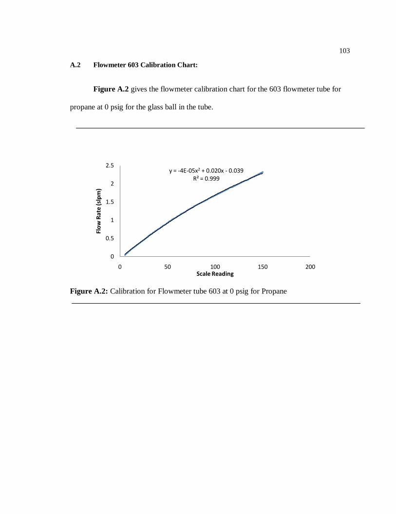
103



propane at 0 psig for the glass ball in the tube.

Figure A.2: Calibration for Flowmeter tube 603 at 0 psig for Propane

y = -4E-05x2 + 0.020x - 0.039R² = 0.999

0

0.5

1

1.5

2

2.5

0 50 100 150 200

Flo

w R

ate

(slp

m)

Scale Reading

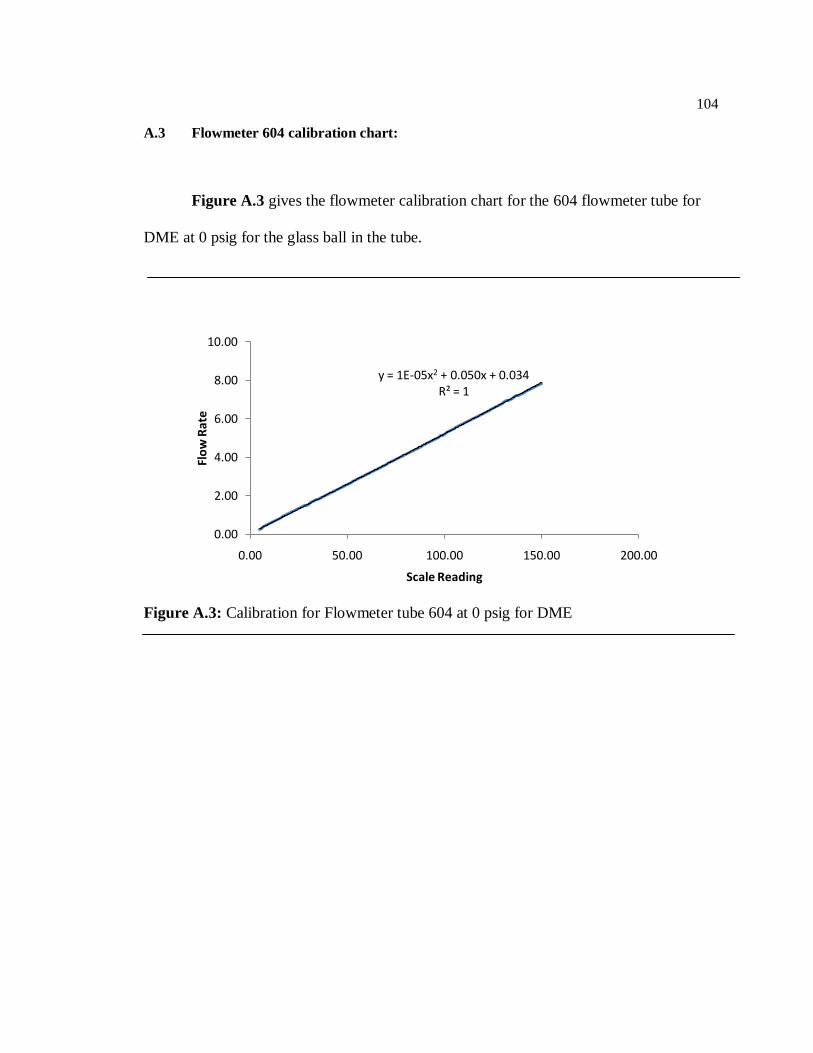
104

A.3 Flowmeter 604 calibration chart:


DME at 0 psig for the glass ball in the tube.

Figure A.3: Calibration for Flowmeter tube 604 at 0 psig for DME

y = 1E-05x2 + 0.050x + 0.034R² = 1

0.00

2.00

4.00

6.00

8.00

10.00

0.00 50.00 100.00 150.00 200.00

Flo

w R

ate

Scale Reading

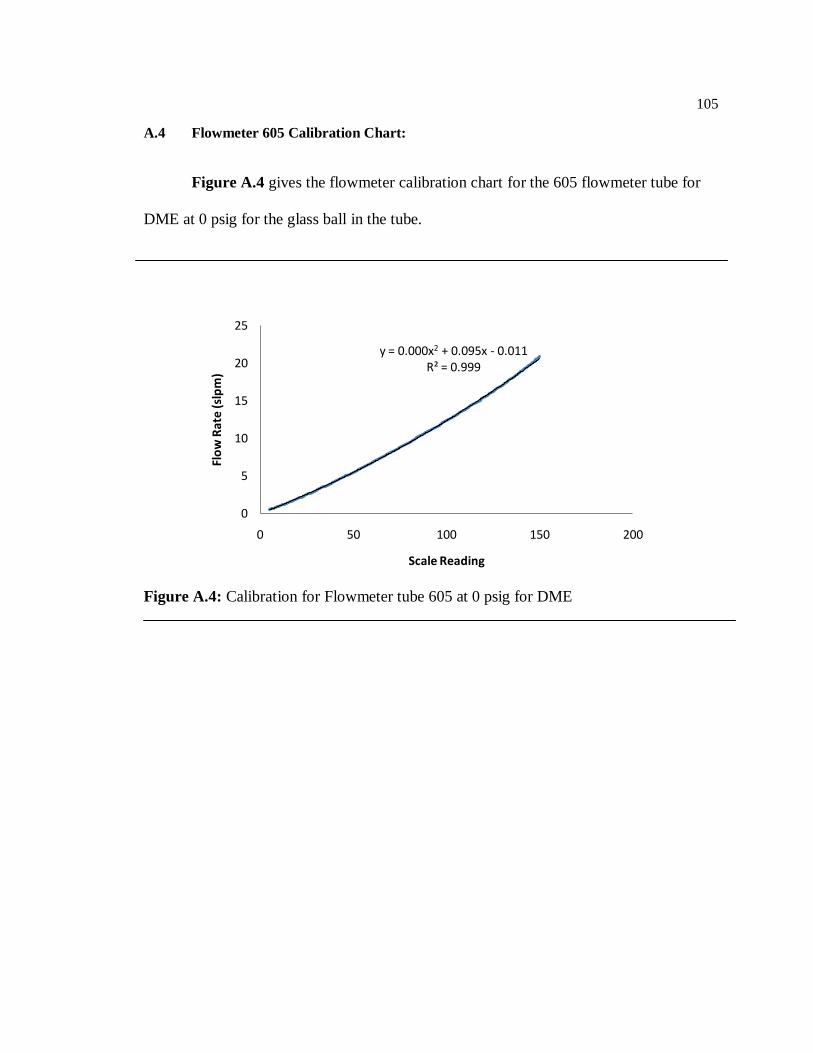
105



DME at 0 psig for the glass ball in the tube.

Figure A.4: Calibration for Flowmeter tube 605 at 0 psig for DME

y = 0.000x2 + 0.095x - 0.011R² = 0.999

0

5

10

15

20

25

0 50 100 150 200

Flo

w R

ate

(slp

m)

Scale Reading

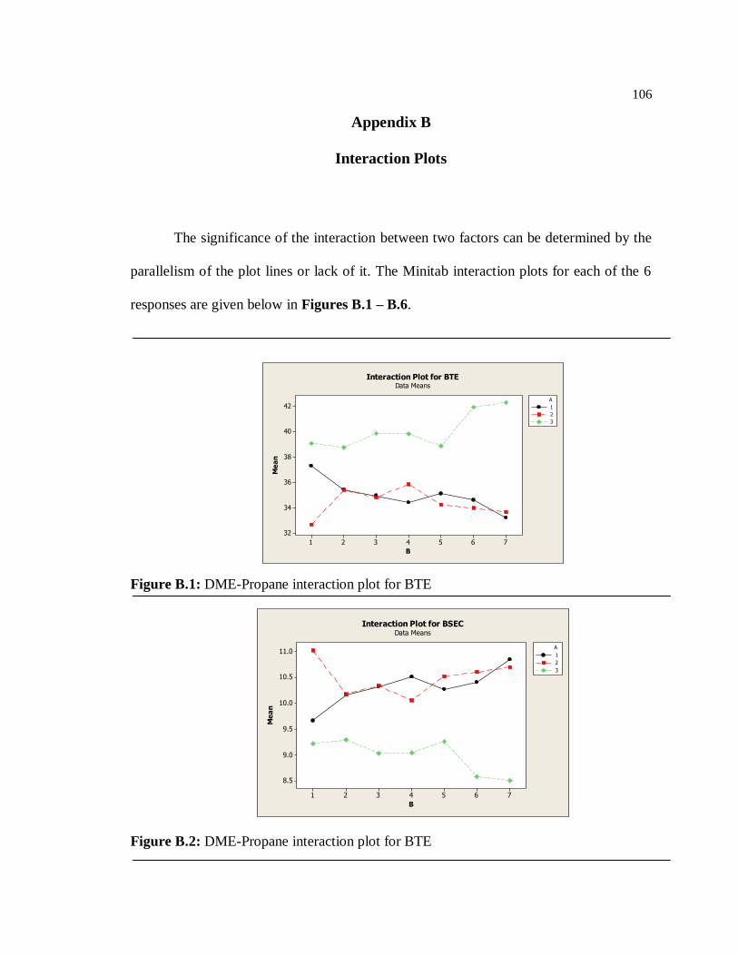
106

Appendix B

Interaction Plots

The significance of the interaction between two factors can be determined by the

parallelism of the plot lines or lack of it. The Minitab interaction plots for each of the 6

responses are given below in Figures B.1 – B.6.

7654321

42

40

38

36

34

32

B

Me

an

1

2

3

A

Interaction Plot for BTEData Means

Figure B.1: DME-Propane interaction plot for BTE

7654321

11.0

10.5

10.0

9.5

9.0

8.5

B

Me

an

1

2

3

A

Interaction Plot for BSECData Means

Figure B.2: DME-Propane interaction plot for BTE

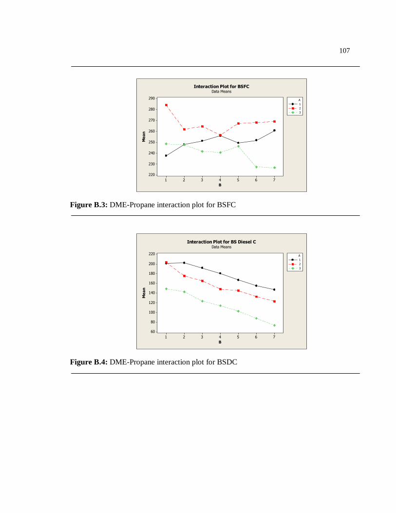
107

7654321

290

280

270

260

250

240

230

220

B

Me

an

1

2

3

A

Interaction Plot for BSFCData Means

Figure B.3: DME-Propane interaction plot for BSFC

7654321

220

200

180

160

140

120

100

80

60

B

Me

an

1

2

3

A

Interaction Plot for BS Diesel CData Means

Figure B.4: DME-Propane interaction plot for BSDC

108

7654321

0.575

0.550

0.525

0.500

0.475

0.450

B

Me

an

1

2

3

A

Interaction Plot for PRRData Means

Figure B.5: DME-Propane interaction plot for PRR

7654321

12.5

12.0

11.5

11.0

10.5

10.0

9.5

B

Me

an

1

2

3

A

Interaction Plot for HRRData Means

Figure B.6: DME-Propane interaction plot for PRR

Thus, as seen from the interaction plots, all the graphs except for the one with

Brake Specific Diesel Consumption display non-parallel behavior. This points to the

presence of an interaction term in the regression analysis which has been included.

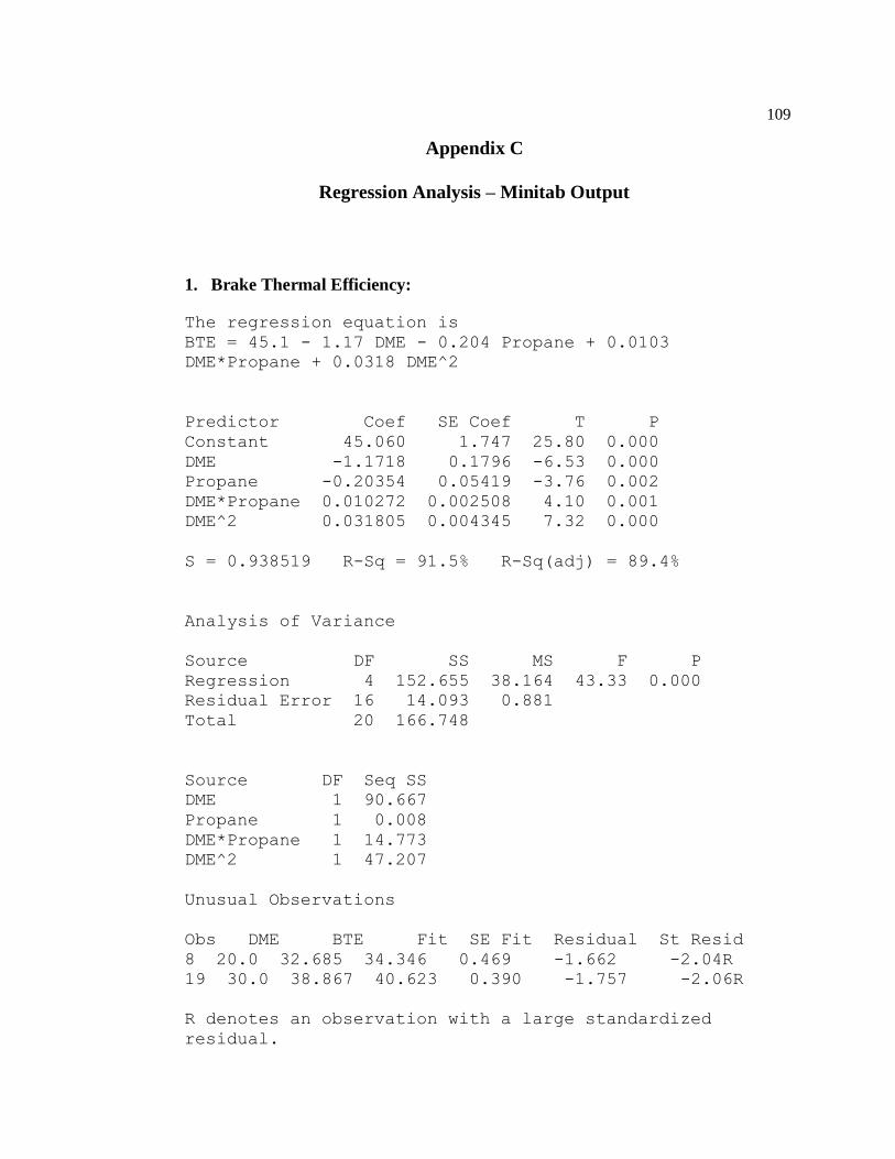
109

Appendix C

Regression Analysis – Minitab Output

1. Brake Thermal Efficiency:

The regression equation is

BTE = 45.1 - 1.17 DME - 0.204 Propane + 0.0103

DME*Propane + 0.0318 DME^2

Predictor Coef SE Coef T P

Constant 45.060 1.747 25.80 0.000

DME -1.1718 0.1796 -6.53 0.000

Propane -0.20354 0.05419 -3.76 0.002

DME*Propane 0.010272 0.002508 4.10 0.001

DME^2 0.031805 0.004345 7.32 0.000

S = 0.938519 R-Sq = 91.5% R-Sq(adj) = 89.4%

Analysis of Variance

Source DF SS MS F P

Regression 4 152.655 38.164 43.33 0.000

Residual Error 16 14.093 0.881

Total 20 166.748

Source DF Seq SS

DME 1 90.667

Propane 1 0.008

DME*Propane 1 14.773

DME^2 1 47.207

Unusual Observations

Obs DME BTE Fit SE Fit Residual St Resid

8 20.0 32.685 34.346 0.469 -1.662 -2.04R

19 30.0 38.867 40.623 0.390 -1.757 -2.06R

R denotes an observation with a large standardized

residual.

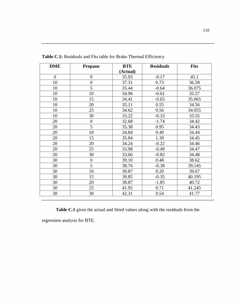
110

Table C.1: Residuals and Fits table for Brake Thermal Efficiency

DME Propane BTE

(Actual)

Residuals Fits

0 0 35.93 -9.17 45.1

10 0 37.31 0.73 36.58

10 5 35.44 -0.64 36.075

10 10 34.96 -0.61 35.57

10 15 34.41 -0.65 35.065

10 20 35.11 0.55 34.56

10 25 34.62 0.56 34.055

10 30 33.22 -0.33 33.55

20 0 32.68 -1.74 34.42

20 5 35.38 0.95 34.43

20 10 34.84 0.40 34.44

20 15 35.84 1.39 34.45

20 20 34.24 -0.22 34.46

20 25 33.98 -0.49 34.47

20 30 33.66 -0.82 34.48

30 0 39.10 0.48 38.62

30 5 38.76 -0.38 39.145

30 10 39.87 0.20 39.67

30 15 39.85 -0.35 40.195

30 20 38.87 -1.85 40.72

30 25 41.95 0.71 41.245

30 30 42.31 0.54 41.77

Table C.1 gives the actual and fitted values along with the residuals from the

regression analysis for BTE.

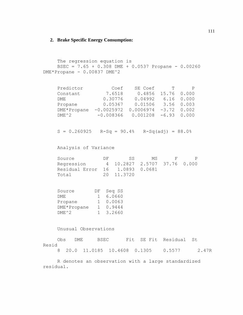
111

2. Brake Specific Energy Consumption:


BSEC = 7.65 + 0.308 DME + 0.0537 Propane - 0.00260

DME*Propane - 0.00837 DME^2


Constant 7.6518 0.4856 15.76 0.000

DME 0.30776 0.04992 6.16 0.000

Propane 0.05367 0.01506 3.56 0.003

DME*Propane -0.0025972 0.0006974 -3.72 0.002

DME^2 -0.008366 0.001208 -6.93 0.000

S = 0.260925 R-Sq = 90.4% R-Sq(adj) = 88.0%


Source DF SS MS F P

Regression 4 10.2827 2.5707 37.76 0.000


Total 20 11.3720

Source DF Seq SS

DME 1 6.0660

Propane 1 0.0063


DME^2 1 3.2660


Obs DME BSEC Fit SE Fit Residual St

Resid

8 20.0 11.0185 10.4608 0.1305 0.5577 2.47R


residual.

112

Table C.2: Residuals and Fits table for Brake Specific Energy Consumption

DME Propane BSEC (Actual) Residuals Fits

0 0 10.0200 2.33 7.69

10 0 9.6600 -0.27 9.933

10 5 10.1636 0.09 10.0715

10 10 10.3173 0.11 10.21

10 15 10.5103 0.16 10.3485

10 20 10.2644 -0.22 10.487

10 25 10.4032 -0.22 10.6255

10 30 10.8400 0.08 10.764

20 0 11.0185 0.52 10.502

20 5 10.1776 -0.33 10.5105

20 10 10.3375 -0.18 10.519

20 15 10.0549 -0.47 10.5275

20 20 10.5211 -0.01 10.536

20 25 10.5991 0.05 10.5445

20 30 10.6984 0.15 10.553

30 0 9.2177 -0.18 9.397

30 5 9.2906 0.02 9.2755

30 10 9.0345 -0.12 9.154

30 15 9.0420 0.01 9.0325

30 20 9.2655 0.35 8.911

30 25 8.5818 -0.21 8.7895

30 30 8.5113 -0.16 8.668


regression analysis for BSEC.

113

3. Brake Specific Fuel Consumption:


BSFC = 173 + 9.28 DME + 1.13 Propane - 0.0631 DME*Propane

- 0.222 DME^2

Predictor CoefSECoef T P

Constant 172.52 11.92 14.47 0.000

DME 9.278 1.226 7.57 0.000

Propane 1.1287 0.3699 3.05 0.008

DME*Propane -0.06312 0.01712 -3.69 0.002

DME^2 -0.22176 0.02965 -7.48 0.000

S = 6.40610 R-Sq = 83.4% R-Sq(adj) = 79.2%


Source DF SS MS F P

Regression 4 3297.62 824.41 20.09 0.000


Total 20 3954.23

Source DF Seq SS

DME 1 407.21

Propane 1 37.58


DME^2 1 2294.98


Obs DME BSFC Fit SE Fit Residual St Resid

8 20.0 284.02 269.38 3.20 14.64 2.64R


residual.

114

Table C.3: Residuals and Fits table for Brake Specific Fuel Consumption

DME Propane BSFC (Actual) Residuals Fits

0 0 233.590 60.59 173

10 0 237.520 -6.08 243.6

10 5 247.861 1.77 246.095

10 10 251.130 2.54 248.59

10 15 255.919 4.83 251.085

10 20 249.415 -4.16 253.58

10 25 251.698 -4.38 256.075

10 30 260.572 2.00 258.57

20 0 284.022 14.22 269.8

20 5 261.873 -7.27 269.14

20 10 264.611 -3.87 268.48

20 15 256.682 -11.14 267.82

20 20 267.164 0.00 267.16

20 25 268.144 1.64 266.5

20 30 269.099 3.26 265.84

30 0 248.546 -3.05 251.6

30 5 247.594 -0.19 247.785

30 10 241.658 -2.31 243.97

30 15 240.606 0.45 240.155

30 20 246.194 9.85 236.34

30 25 227.381 -5.14 232.525

30 30 226.633 -2.08 228.71


regression analysis for BSFC.

115

4. Brake Specific Diesel Consumption:


BS Diesel C = 213 + 1.05 DME - 2.34 Propane - 0.107

DME^2

Predictor CoefSECoef T P

Constant 212.834 8.934 23.82 0.000

DME 1.0514 0.9950 1.06 0.305

Propane -2.3421 0.1161 -20.18 0.000

DME^2 -0.10664 0.02462 -4.33 0.000

S = 5.31859 R-Sq = 98.2% R-Sq(adj) = 97.9%


Source DF SS MS F P

Regression 3 26511.9 8837.3 312.41 0.000


Total 20 26992.8

Source DF Seq SS

DME 1 14462.0

Propane 1 11519.2

DME^2 1 530.7


BS

ObsDME Diesel C Fit SE Fit Residual St Resid

1 10.0 200.82 212.68 2.66 -11.86 -2.58R

8 20.0 203.44 191.21 2.66 12.23 2.65R


residual.

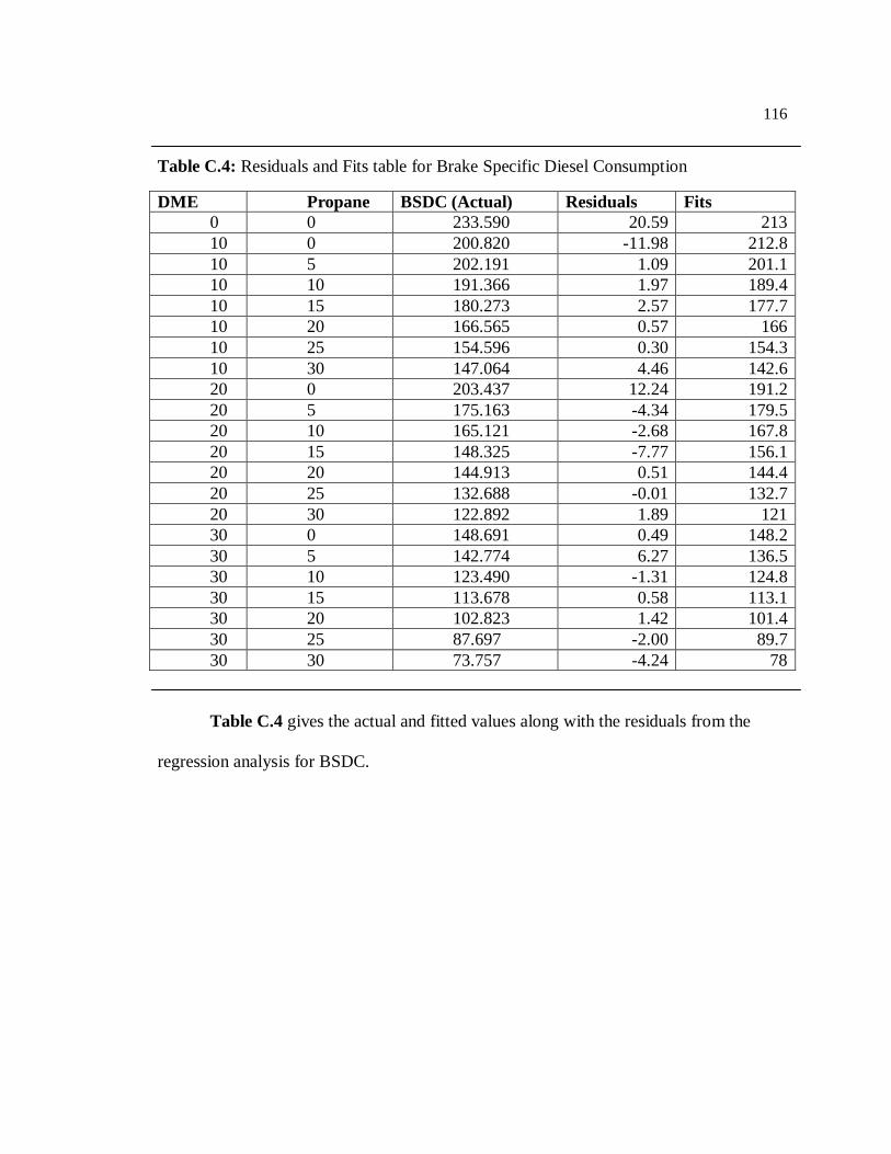
116

Table C.4: Residuals and Fits table for Brake Specific Diesel Consumption

DME Propane BSDC (Actual) Residuals Fits

0 0 233.590 20.59 213

10 0 200.820 -11.98 212.8

10 5 202.191 1.09 201.1

10 10 191.366 1.97 189.4

10 15 180.273 2.57 177.7

10 20 166.565 0.57 166

10 25 154.596 0.30 154.3

10 30 147.064 4.46 142.6

20 0 203.437 12.24 191.2

20 5 175.163 -4.34 179.5

20 10 165.121 -2.68 167.8

20 15 148.325 -7.77 156.1

20 20 144.913 0.51 144.4

20 25 132.688 -0.01 132.7

20 30 122.892 1.89 121

30 0 148.691 0.49 148.2

30 5 142.774 6.27 136.5

30 10 123.490 -1.31 124.8

30 15 113.678 0.58 113.1

30 20 102.823 1.42 101.4

30 25 87.697 -2.00 89.7

30 30 73.757 -4.24 78


regression analysis for BSDC.

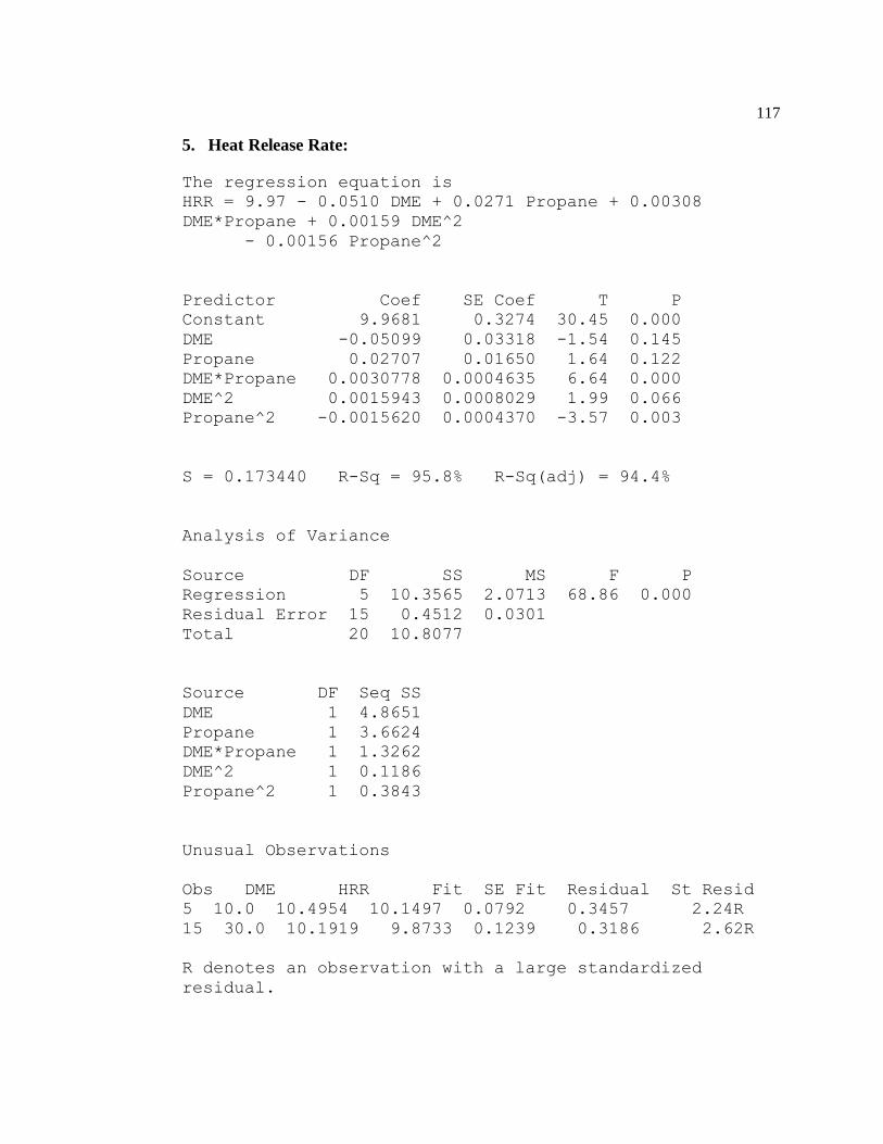
117

5. Heat Release Rate:


HRR = 9.97 - 0.0510 DME + 0.0271 Propane + 0.00308

DME*Propane + 0.00159 DME^2

- 0.00156 Propane^2


Constant 9.9681 0.3274 30.45 0.000

DME -0.05099 0.03318 -1.54 0.145

Propane 0.02707 0.01650 1.64 0.122

DME*Propane 0.0030778 0.0004635 6.64 0.000

DME^2 0.0015943 0.0008029 1.99 0.066

Propane^2 -0.0015620 0.0004370 -3.57 0.003

S = 0.173440 R-Sq = 95.8% R-Sq(adj) = 94.4%


Source DF SS MS F P

Regression 5 10.3565 2.0713 68.86 0.000


Total 20 10.8077

Source DF Seq SS

DME 1 4.8651

Propane 1 3.6624


DME^2 1 0.1186

Propane^2 1 0.3843


Obs DME HRR Fit SE Fit Residual St Resid

5 10.0 10.4954 10.1497 0.0792 0.3457 2.24R

15 30.0 10.1919 9.8733 0.1239 0.3186 2.62R


residual.

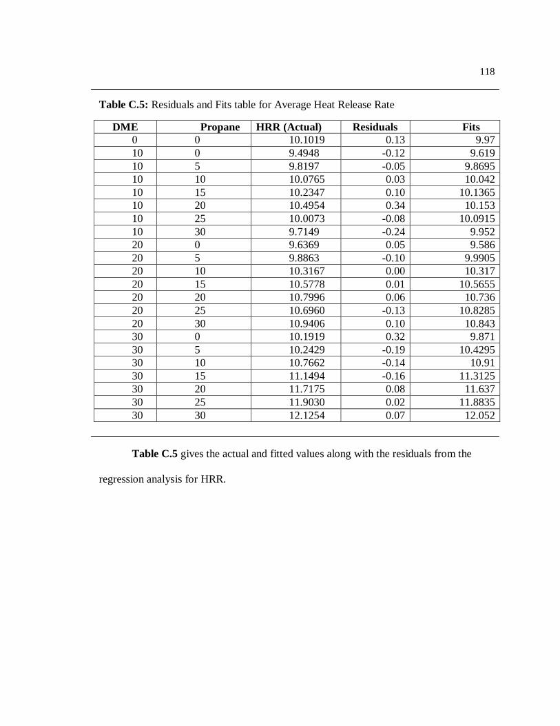
118

Table C.5: Residuals and Fits table for Average Heat Release Rate

DME Propane HRR (Actual) Residuals Fits

0 0 10.1019 0.13 9.97

10 0 9.4948 -0.12 9.619

10 5 9.8197 -0.05 9.8695

10 10 10.0765 0.03 10.042

10 15 10.2347 0.10 10.1365

10 20 10.4954 0.34 10.153

10 25 10.0073 -0.08 10.0915

10 30 9.7149 -0.24 9.952

20 0 9.6369 0.05 9.586

20 5 9.8863 -0.10 9.9905

20 10 10.3167 0.00 10.317

20 15 10.5778 0.01 10.5655

20 20 10.7996 0.06 10.736

20 25 10.6960 -0.13 10.8285

20 30 10.9406 0.10 10.843

30 0 10.1919 0.32 9.871

30 5 10.2429 -0.19 10.4295

30 10 10.7662 -0.14 10.91

30 15 11.1494 -0.16 11.3125

30 20 11.7175 0.08 11.637

30 25 11.9030 0.02 11.8835

30 30 12.1254 0.07 12.052


regression analysis for HRR.

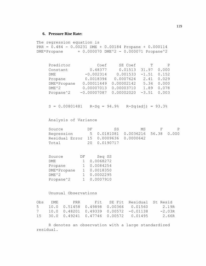
119

6. Pressure Rise Rate:


PRR = 0.484 - 0.00231 DME + 0.00184 Propane + 0.000114

DME*Propane + 0.000070 DME^2 - 0.000071 Propane^2


Constant 0.48377 0.01513 31.97 0.000

DME -0.002314 0.001533 -1.51 0.152

Propane 0.0018394 0.0007624 2.41 0.029

DME*Propane 0.00011449 0.00002142 5.34 0.000

DME^2 0.00007013 0.00003710 1.89 0.078

Propane^2 -0.00007087 0.00002020 -3.51 0.003

S = 0.00801481 R-Sq = 94.9% R-Sq(adj) = 93.3%


Source DF SS MS F P

Regression 5 0.0181081 0.0036216 56.38 0.000

Residual Error 15 0.0009636 0.0000642

Total 20 0.0190717

Source DF Seq SS

DME 1 0.0068272

Propane 1 0.0084254


DME^2 1 0.0002295

Propane^2 1 0.0007910


Obs DME PRR Fit SE Fit Residual St Resid

5 10.0 0.51458 0.49898 0.00366 0.01560 2.19R

7 10.0 0.48201 0.49339 0.00572 -0.01138 -2.03R

15 30.0 0.49241 0.47746 0.00572 0.01495 2.66R


residual.

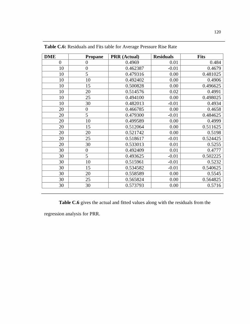
120

Table C.6: Residuals and Fits table for Average Pressure Rise Rate

DME Propane PRR (Actual) Residuals Fits

0 0 0.4969 0.01 0.484

10 0 0.462387 -0.01 0.4679

10 5 0.479316 0.00 0.481025

10 10 0.492402 0.00 0.4906

10 15 0.500828 0.00 0.496625

10 20 0.514576 0.02 0.4991

10 25 0.494100 0.00 0.498025

10 30 0.482013 -0.01 0.4934

20 0 0.466785 0.00 0.4658

20 5 0.479300 -0.01 0.484625

20 10 0.499589 0.00 0.4999

20 15 0.512064 0.00 0.511625

20 20 0.521742 0.00 0.5198

20 25 0.518617 -0.01 0.524425

20 30 0.533013 0.01 0.5255

30 0 0.492409 0.01 0.4777

30 5 0.493625 -0.01 0.502225

30 10 0.515961 -0.01 0.5232

30 15 0.534582 -0.01 0.540625

30 20 0.558589 0.00 0.5545

30 25 0.565824 0.00 0.564825

30 30 0.573793 0.00 0.5716


regression analysis for PRR.

Documents

PERFORMANCE OPTIMIZATION OF A DIESEL ENGINE FOR DUAL …