Embed Size (px)
Citation preview

Performance of Simple Delay-and-Sum Beamforming Without
Per-Stand Polarization Corrections for LWA Stations
Steve Ellingson∗
January 5, 2009
Contents
1 Introduction 2
1.1 Background . . . . . . . . . . . . . . . . . . . . . . . . . . . . . . . . . . . . . . . . . 21.2 This Memo . . . . . . . . . . . . . . . . . . . . . . . . . . . . . . . . . . . . . . . . . 2
2 Array Model 3
3 Optimal vs. “Simple” Beamforming 5
3.1 Optimal Beamforming . . . . . . . . . . . . . . . . . . . . . . . . . . . . . . . . . . . 53.2 Simple Beamforming . . . . . . . . . . . . . . . . . . . . . . . . . . . . . . . . . . . . 5
4 Results 6
4.1 Effect of Mutual Coupling on Collecting Area Generated by Optimal Beamforming . 64.2 Performance of Simple Beamforming Compared to Optimal Beamforming . . . . . . 6
A Array Geometry 12
∗Bradley Dept. of Electrical & Computer Engineering, 302 Whittemore Hall, Virginia Polytechnic Institute &State University, Blacksburg VA 24061 USA. E-mail: [email protected]
1

1 Introduction
It has been known since LWA Memo 67 [1] that the antennas within an LWA station are likely toexperience significant levels of mutual coupling. However, it is not yet clear if any special measuresare required or useful in the per-stand processing prior to “full RF” beamforming to account forthis. The station electronics can be much simpler if the differences in the responses of antennas canbe neglected; in particular, if the differences in polarization response as a function of frequency canbe neglected [2].
1.1 Background
LWA Memo 140 [3] considered the impact of mutual coupling on the ability to perform per-standcalibration prior to beamforming, using the scheme discussed in LWA Memos 106 [4], 107 [5], and138 [6]. It is found that for a stand near the center of the array, the requirements in terms of thelength of FIR filters is about the same, and that the mutual coupling does not seem to have mucheffect on the ability to convert the “raw” voltage signals provided from each dipole into standardleft- and right-circular polarizations. However, this is not the same as saying that mutual couplingdoes not significantly affect the polarization response; Memo 140 only shows that mutual couplingdoes not have much impact on the performance of this calibration. Furthermore, only one standnear the center of a 64-stand version of the array was considered. Thus, Memo 140 does not havemuch to say about the performance of a “full RF” beamforming scheme in which the differences inper-stand polarization response are neglected.
Memo 147 [7] showed some initial results from an attempt to characterize the stand-to-standvariations in the response of antennas in a full (256-stand) LWA station array. This study waslimited to one frequency, 38 MHz, using the old (100 m diameter circular, 4 m minimum inter-standseparation) station footprint. After some steps to demonstrate the efficacy/validity of the numericalanalysis, the H-plane patterns were examined. It was found that the H-plane co-pol patterns varydramatically from stand to stand, with gain differences ranging from +2 dB to −6 dB relative toa single stand isolated from the rest of the array. The cross-pol patterns were also seen to havesignificant variations.
1.2 This Memo
Having determined that mutual coupling does in fact significantly affect stand in situ responses,this memo attempts to follow up Memo 147 to answer the “bottom line” question of whether thesevariations matter in the sense that per-stand, frequency-dependent polarization and dispersion cor-rections are required to achieve acceptable beamforming performance. First, it should be noted thatan important difference between this memo and Memo 147 is that we now assume the new 110 m× 100 m elliptical station array footprint, with 5 m minimum inter-stand separation.1
It is found that despite the large stand-to-stand variations that exist over the entire frequencyrange of interest, simple beamforming – that is, delay-and-sum beamforming for each of the two“raw” polarizations neglecting stand-to-stand variations other than geometrical/propagation delay– is nearly optimal in terms of main lobe gain. The coupling-induced differences in stand responsesappear to “average out” with very low bias, such that near-optimum array gain can be achievedwithout per-stand corrections for polarization or antenna dispersion.
Although not quantified in this memo, it is important to note that these results do not implythat mutual coupling has negligible effect on array gain. Although the effect of coupling on mainbeam gain is very small for the two pointings considered in this memo, it is known from previous
1This new geometry was obtained by email from A. Cohen on Dec 18, 2008 and does not appear to be documentedanywhere at present. For this reason, the stand position data are included in this memo as Appendix A.
2
-60 -40 -20 0 20 40 60x (-W,+E) [m]
-60
-40
-20
0
20
40
60
y (
-S,+
N)
[m]
Figure 1: Array geometry. The exact locations of the stands are given in Appendix A.
work (Memo [8] and [9]) that the difference for some pointings can be on the order of 10’s ofpercent. Instead, the above findings indicate that simple delay-and-sum beamforming of the rawdipole polarizations is nearly optimal in the sense that it provides the maximum possible gain,whatever that gain may be. Furthermore, it should be noted that these results do not imply thatthe shape of the main lobe or the levels and positions of sidelobes are not significantly affectedby mutual coupling. To the contrary, the large variations in per-stand responses noted in thismemo and in Memo 147 mean that it is quite likely that mutual coupling has a significant effect onsidelobe levels and positions. The effect of mutual coupling on the main beam shape is probablyless significant – “small”, but difficult to characterize in a meaningful way without further study.2
Finally, it should be noted that the fence and shelter are not yet considered in the results presentedhere.
2 Array Model
The LWA station array consists of 256 stands, each consisting of two perpendicularly-arrangeddipoles, with irregular spacings within an ellipse with major and minor axes of diameter 110 maligned North-South and 100 m aligned East-West, respectively. This is shown in Figure 1. Theminimum spacing between stands is 5 m.
2Slide 6 of reference [9] gives an idea of what to expect; i.e., a very small difference in beamwidth but with anoffset in the direction of maximum gain as large as a degree or so.
3

The station array will be surrounded by a fence with 5 m minimum separation from the stands[10], and it is known from LWA Memo 129 [11] that the fence can have a significant impact onthe antenna patterns. It is also known from LWA Memo 141 [12] that the shelter can also have asignificant effect on the antenna patterns. However, the fence and the shelter are not included inthe model used to generate the results presented in this memo. Determining the effect of the fenceand shelter is left for future work.
Stand design is not completely determined at present. This is actually not of much consequencein this study since the proposed “tied fork” dipole design, when replicated 512 times, results in amodel with prohibitively-large computational burden and high potential for subtle numerical diffi-culties when analyzed using the moment method (e.g., NEC2 or NEC4). Therefore, a simple dipolemodel is used instead. In this model, each dipole is a perfectly-conducting cylinder 3.947 m longand 6 cm in diameter. This is roughly equivalent to a “blade”-type antenna having blade width of12 cm [13]. The center 15 cm is the feedpoint region, and is horizontal to the ground. The “arms”on either side bend downward at a 45 angle. In the coordinate system used in this memo, dipolesare aligned parallel to the x and y axes, with z pointing toward the zenith. The feedpoint heights ofx- and y-aligned dipoles is 2.019 m and 1.929 m respectively; that is, the entire dipole is shifted upor down slightly to prevent feedpoint wires from intersecting or becoming too close to be properlymodeled. The ground is assumed to be an infinite flat surface of perfectly-conducting material.
NEC2 is used to perform the analysis. The 15-cm-long feedpoint wire is divided into three seg-ments, and the center segment is loaded with a series impedance of 100 Ω, modeling the FEE input.Each dipole arm is divided into 10 segments, which is appropriate for frequencies up to 88 MHz.The design of the dipole and its segmentation were carefully reviewed with respect to known NECdesign guidelines and limitations, and the model was analyzed in a preliminary study to confirmit’s numerical stability over the frequency range 10–88 MHz. The model was further validated at38 MHz, as explained in LWA Memo 147 [7]. The complete array model (but not yet including theshelter and fence) uses about 12,000 segments and requires roughly one hour to run (on a 2007-vintage dual-core Centrino-based laptop, running Ubuntu Linux) for each frequency of interest.
A reasonable question to ask is “How well does this model describe arrays consisting of standsbased on the “tied fork” dipole concept, with each stand over a small ground screen?” The answer,unfortunately, is extremely difficult to answer in a satisfying way. Qualitatively, the behavior isexpected to be very similar with similar trends. Quantitatively, based on experience, the results areexpected to agree “sufficiently well” over most of the frequency range of interest, since the antennasare very similar from an electromagnetic perspective. The tied-fork dipole is likely to have somewhatbroader impedance bandwidth, so the greatest discrepancies in impedance are likely to occur at thehighest and lowest frequencies, and the greatest discrepancies in pattern will occur at the highestfrequencies. Regardless of all of these points, the issue is essentially moot as the tied-fork designwould require about 3 times as many segments, resulting in computational burden which is roughly33 = 27 times greater. Changing from an infinite perfectly-conducting ground screen to 256 separateground screens with intervening exposed earth makes the computation altogether intractable withoutextraordinary measures; e.g., moving to a large, high-performance computer cluster. An additionalissue favoring the use of the simple dipole + infinite ground model over a closer-to-true model is thatconventional tests for model “reasonableness” and numerical stability are correspondingly difficultto carry out for the latter. Thus, we are essentially trading off decreased model detail for both speedand increased confidence in the results.3
3A possible topic for future work be to identify a simple frequency-dependent model for the production standdesign. That is: For each frequency, these is a simple model model which best approximates the production standresponse. Then, in future analyses, the simple stand model would be varied with frequency in order to better predictthe performance of the actual stand.
4
3 Optimal vs. “Simple” Beamforming
In this memo we are concerned with the performance of “simple” beamforming; in particular, whatis lost with respect to “optimal” beamforming. Thus, we need to define these terms.
3.1 Optimal Beamforming
Optimal beamforming is defined as beamforming which results in maximum signal-to-noise ratio(SNR) in the specified pointing direction, subject to no other constraints (such as sidelobe lev-els/positions, etc.), and assuming spatially-white noise4. Assuming a single monochromatic planewave incident on the array, this is achieved by multiplying the signal measured at each dipole byit’s conjugate value. In the signal processing literature, this is commonly known as maximal ratio
combining (MRC). MRC has the effect of weighting dipoles producing signals with larger SNR moreheavily than dipoles producing signals with smaller SNR, and it can be shown that the result hasthe maximum possible SNR.
An informal proof of this is as follows: Consider a monochromatic plane wave incident on a dipolearray, and assume that the noise is spatially white. In this case, the power collected by each dipoleis equal to |I|2R, where I is the (complex-valued RMS) current at the dipole terminals, and R is theload across the dipole terminals. The maximum power that can be collected by the array is simplythe sum of the powers collected at the dipole terminals. In this case, we can interpret I as the dipolesignal and I∗R, where I∗ is the conjugate of I, as the associated beamforming coefficient. Scalingall the beamforming coefficients by the same amount does not change the SNR; therefore using I∗
as the beamforming coefficient yields output with the same SNR. Thus, I∗ is the (non-unique) MRCbeamforming coefficient for a dipole producing the output current I.
Optimal beamforming over a non-zero bandwidth requires frequency-dependent coefficients, wherethe coefficients for each frequency are determined using the same criteria. The inverse Fourier trans-form of these coefficients yields the impulse response of a filter which applies the correct coefficientto all frequencies simultaneously. If the polarization response of each stand (pair of orthogonaldipoles) varies from stand to stand, then the polarizations must be converted to a common pair oforthogonal polarizations (possibly, but not necessarily, left- and right-circular) before the coefficients(or filters) are calculated and applied, so that there is no loss due to imperfect correlation betweensimilarly-oriented dipoles.
3.2 Simple Beamforming
There are many technical challenges that must be overcome to implement optimal beamforming. Asmentioned in Section 1, it is desirable to avoid per-stand polarization corrections so as to simplify thedesign. In fact, it is desirable to avoid stand-specific processing for anything other than implementingthe propagation delays required for “delay-and-sum” beamforming. In this approach, we simply delaythe signal from each dipole according to the appropriate geometrical (propagation) delay, and sumthe results. Any variations in response between stands is ignored. Further, we wish to generate thetwo polarizations which are output from the beamformer by simply combining all similarly-orienteddipoles, regardless of any variations in polarization response from stand to stand. Henceforth, werefer to this approach as “simple” beamforming. Simple beamforming is optimal only if the standresponses are identical. In the presence of mutual coupling, simple beamforming cannot not beoptimal, since the coupling-induced variations in patterns between dipoles are ignored (i.e., it isnot MRC), as are variations in polarization response. However, if these variations are small, or ifthey large but “average out”, then simple beamforming may approach the performance of optimalbeamforming. We shall see in the next section that this is indeed the case, for the latter reason.
4Of course the noise is not spatially white for LWA, but the actual situation introduces complications which arenot relevant to the purpose of this study.
5
4 Results
In this memo, we consider the response of the array for two scenarios: (1) A single plane waveincident from the zenith (θ = 0), with a linearly-polarized electric field oriented in the x direction;and (2) A single plane wave incident from θ = φ = 45 (φ measured from the x axis toward the y
axis), with a linearly-polarized electric field oriented parallel to the ground.
4.1 Effect of Mutual Coupling on Collecting Area Generated by Optimal
Beamforming
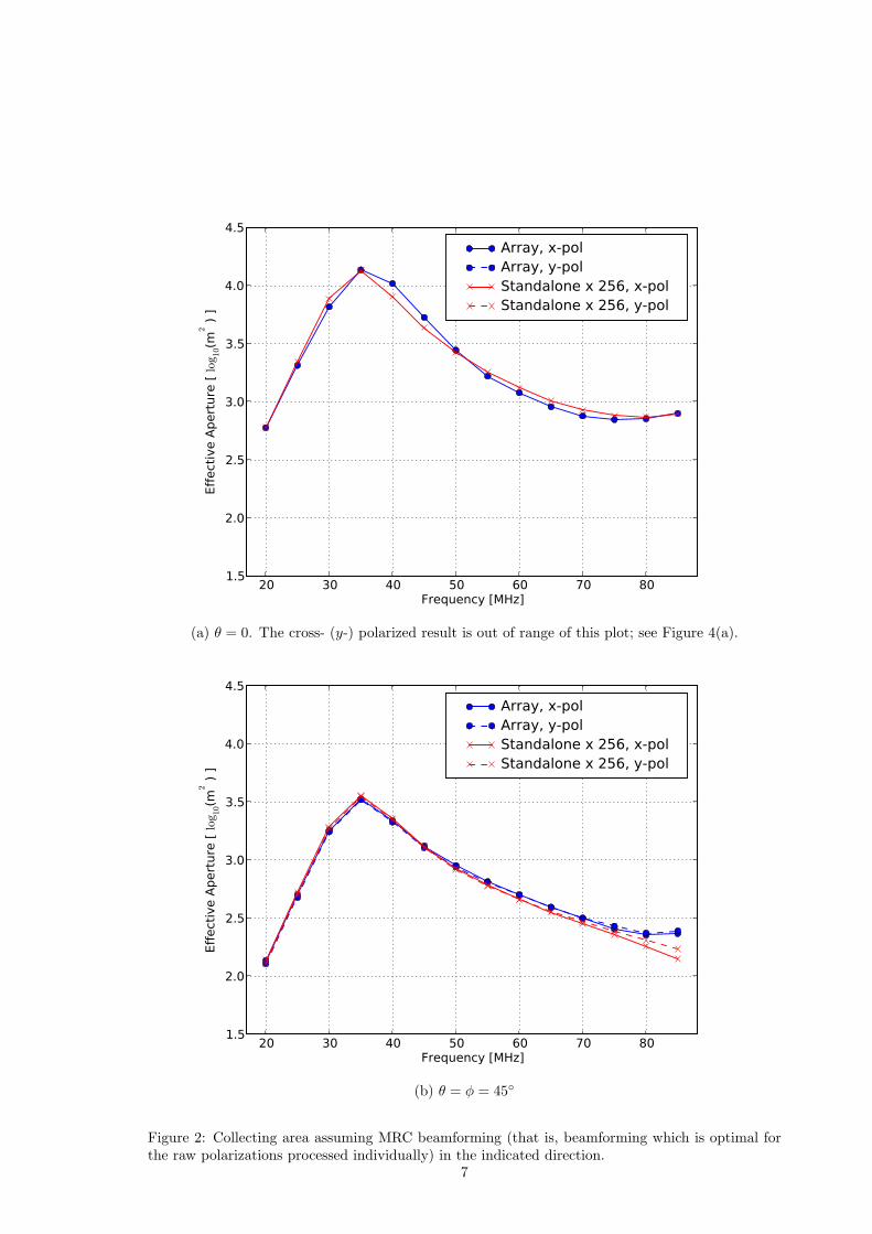
Figure 2 shows the collecting area of the array in each case, assuming MRC beamforming. Sincethere is only one incident plane wave and we assume the noise is spatially white, this result canbe determined by computing the collecting area for each dipole individually, and then summingthe results (as discussed in Section 3.1). The power collected by each dipole is simply the absolutevalue of the RMS current at the antenna terminals (determined by NEC) squared, times the loadimpedance (100Ω). The collecting area can then be obtained by dividing by the incident flux density,which is known since the incident electric field is known. The result is tallied separately for the x-and y-oriented dipoles; thus this is optimal only for the raw polarizations treated individually, andis not guaranteed to be optimal for any particular pair of orthogonal polarizations. Also shown isthe result for a single (“standalone”) dipole multiplied by 256, which can be compared to the aboveresult to assess the impact of mutual coupling. It is clear from Figure 2(a) and (b) that the impactis very small. Thus, mutual coupling has negligible effect on collecting area in these two scenarios,assuming the collecting area is obtained by optimal combining of the raw polarizations.
The above result is optimal for the raw polarizations individually, but not necessarily optimalfor fully-polarimetric beamforming, since per-stand polarization corrections were not performed.However, it is clear that per-stand polarization correction would not have made a significant dif-ference, since even when we ignore these corrections we get nearly the same result obtained in the“standalone × 256” case for which the stand polarization responses are identical. Thus, we shallhenceforth assume that MRC beamforming for the raw polarizations individually is essentially opti-mal even if the complete polarimetric response is of interest, and even though per-stand polarizationcorrections are not performed.
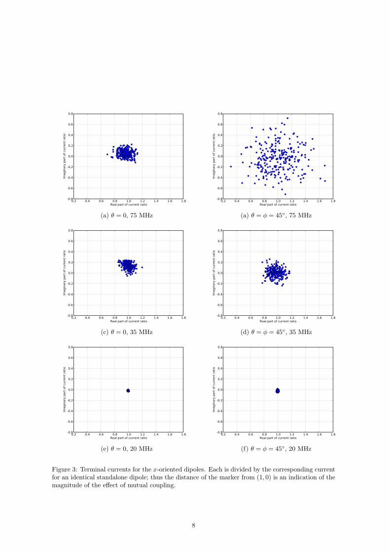
The above results are a bit surprising, since previous studies (see Section 1) make it clear thatthe individual element responses vary dramatically in response to mutual coupling. In fact, that isalso the case here, as demonstrated in Figure 3. In this figure, zero mutual coupling corresponds toall the markers being located exactly at (1, 0), whereas significant and disorderly mutual couplingmanifests as perturbation of the markers from that position. It is clear that the mutual couplingis in fact significant and disorderly for various combinations of frequencies and incident directions.However, the center of distribution always remains quite close to (1, 0), which probably explains theclose agreement in Figure 2. In other words, it appears that the mutual coupling-induced “errors”,although large, tend to average out leaving only a very small bias.
4.2 Performance of Simple Beamforming Compared to Optimal Beam-
forming
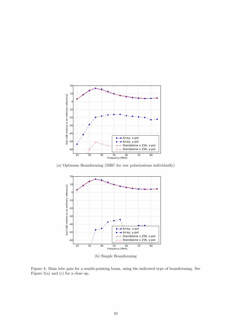
Next, we consider whether we can achieve results similar to those of Figure 2 using the “simple”beamforming scheme, as opposed to the optimal (MRC) beamforming scheme. A comparison isshown in Figure 4 for a zenith-pointing beam (another pointing is considered below). In this case,the results are expressed in terms of gain in dB relative to an arbitrary (but common) reference.5
Note that the results are nearly identical – i.e., that optimal and simple beamforming yield very
5This is a convenience that allows the coefficients for simple beamforming to have magnitude equal to one. Asexplained in Section 3.1, the SNR is not affected by a constant scaling in coefficients.
6
20 30 40 50 60 70 80Frequency [MHz]
1.5
2.0
2.5
3.0
3.5
4.0
4.5
Eff
ect
ive A
pert
ure
[ log10(m
2)
]
Array, x-polArray, y-polStandalone x 256, x-polStandalone x 256, y-pol
(a) θ = 0. The cross- (y-) polarized result is out of range of this plot; see Figure 4(a).
20 30 40 50 60 70 80Frequency [MHz]
1.5
2.0
2.5
3.0
3.5
4.0
4.5
Eff
ect
ive A
pert
ure
[ log10(m
2)
]
Array, x-polArray, y-polStandalone x 256, x-polStandalone x 256, y-pol
(b) θ = φ = 45
Figure 2: Collecting area assuming MRC beamforming (that is, beamforming which is optimal forthe raw polarizations processed individually) in the indicated direction.
7
0.2 0.4 0.6 0.8 1.0 1.2 1.4 1.6 1.8Real part of current ratio
-0.8
-0.6
-0.4
-0.2
0.0
0.2
0.4
0.6
0.8
Imagin
ary
part
of
curr
ent
rati
o
0.2 0.4 0.6 0.8 1.0 1.2 1.4 1.6 1.8Real part of current ratio
-0.8
-0.6
-0.4
-0.2
0.0
0.2
0.4
0.6
0.8
Imagin
ary
part
of
curr
ent
rati
o(a) θ = 0, 75 MHz (a) θ = φ = 45, 75 MHz
0.2 0.4 0.6 0.8 1.0 1.2 1.4 1.6 1.8Real part of current ratio
-0.8
-0.6
-0.4
-0.2
0.0
0.2
0.4
0.6
0.8
Imagin
ary
part
of
curr
ent
rati
o
0.2 0.4 0.6 0.8 1.0 1.2 1.4 1.6 1.8Real part of current ratio
-0.8
-0.6
-0.4
-0.2
0.0
0.2
0.4
0.6
0.8
Imagin
ary
part
of
curr
ent
rati
o
(c) θ = 0, 35 MHz (d) θ = φ = 45, 35 MHz
0.2 0.4 0.6 0.8 1.0 1.2 1.4 1.6 1.8Real part of current ratio
-0.8
-0.6
-0.4
-0.2
0.0
0.2
0.4
0.6
0.8
Imagin
ary
part
of
curr
ent
rati
o
0.2 0.4 0.6 0.8 1.0 1.2 1.4 1.6 1.8Real part of current ratio
-0.8
-0.6
-0.4
-0.2
0.0
0.2
0.4
0.6
0.8
Imagin
ary
part
of
curr
ent
rati
o
(e) θ = 0, 20 MHz (f) θ = φ = 45, 20 MHz
Figure 3: Terminal currents for the x-oriented dipoles. Each is divided by the corresponding currentfor an identical standalone dipole; thus the distance of the marker from (1, 0) is an indication of themagnitude of the effect of mutual coupling.
8
nearly the same gain – for the co-polarized dipoles. The reason for this appears to be the same asthe reason why the collecting area for optimal beamforming is not significantly affected by mutualcoupling; that is, because the differences in stand responses which are ignored by simple beamform-ing, although large, tend to average out leaving only a very small bias.
The cross- (y−) polarization results in Figure 4 are interesting. For optimal beamforming inthe absence of mutual coupling, we see that the cross-pol is negligible; in fact, this level mightnot even be numerically significant. In the presence of mutual coupling, however, the cross-polincreases to a level of about −25 dB relative to the co-polarized gain above about 50 MHz. Forsimple beamforming, the observed cross-pol in the presence of mutual coupling is much less. Apossible explanation for this is that since dipoles producing abnormally large outputs due to mutualcoupling are weighted more heavily in optimal beamforming, so is the coupling-enhanced cross-polcomponent. After all, there is no constraint in the MRC processing that cross-pol should be low.It is possible that the result would be better (lower cross-pol for optimal beamforming) if per-standpolarization calibration was implemented, but this hardly seems necessary since we prefer simplebeamforming for implementation reasons anyway.
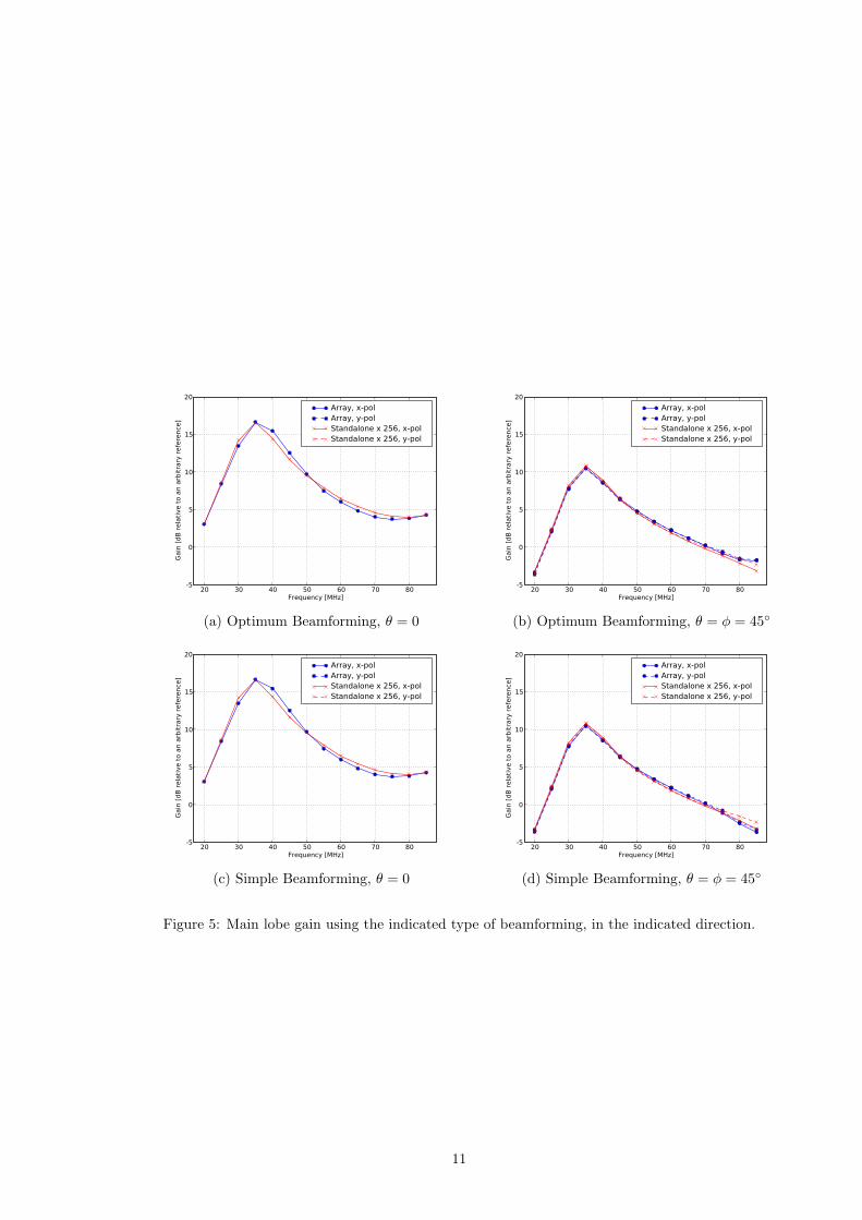
Figure 5 compares the results for the zenith-pointing and θ = φ = 45 beams, zooming in on thex-polarization. Once again we see that simple beamforming delivers gain which is very close to thatdelivered by optimal (now, MRC on raw polarizations) beamforming. Combined with the findingfrom Section 4.1 that per-stand polarization corrections are not required to achieve nearly-optimumcollecting area, this is pretty strong evidence that simple beamforming yields nearly-optimum gainand polarization characteristics, even in the presence of mutual coupling. However, the reader isonce again referred to the caveats given at the end of Section 1.2.
9
20 30 40 50 60 70 80Frequency [MHz]
-60
-50
-40
-30
-20
-10
0
10
20
Gain
[dB
rela
tive t
o a
n a
rbit
rary
refe
rence
]
Array, x-polArray, y-polStandalone x 256, x-polStandalone x 256, y-pol
(a) Optimum Beamforming (MRC for raw polarizations individually)
20 30 40 50 60 70 80Frequency [MHz]
-60
-50
-40
-30
-20
-10
0
10
20
Gain
[dB
rela
tive t
o a
n a
rbit
rary
refe
rence
]
Array, x-polArray, y-polStandalone x 256, x-polStandalone x 256, y-pol
(b) Simple Beamforming
Figure 4: Main lobe gain for a zenith-pointing beam, using the indicated type of beamforming. SeeFigure 5(a) and (c) for a close up.
10
20 30 40 50 60 70 80Frequency [MHz]
-5
0
5
10
15
20
Gain
[dB
rela
tive t
o a
n a
rbit
rary
refe
rence
]
Array, x-polArray, y-polStandalone x 256, x-polStandalone x 256, y-pol
20 30 40 50 60 70 80Frequency [MHz]
-5
0
5
10
15
20
Gain
[dB
rela
tive t
o a
n a
rbit
rary
refe
rence
]
Array, x-polArray, y-polStandalone x 256, x-polStandalone x 256, y-pol
(a) Optimum Beamforming, θ = 0 (b) Optimum Beamforming, θ = φ = 45
20 30 40 50 60 70 80Frequency [MHz]
-5
0
5
10
15
20
Gain
[dB
rela
tive t
o a
n a
rbit
rary
refe
rence
]
Array, x-polArray, y-polStandalone x 256, x-polStandalone x 256, y-pol
20 30 40 50 60 70 80Frequency [MHz]
-5
0
5
10
15
20
Gain
[dB
rela
tive t
o a
n a
rbit
rary
refe
rence
]
Array, x-polArray, y-polStandalone x 256, x-polStandalone x 256, y-pol
(c) Simple Beamforming, θ = 0 (d) Simple Beamforming, θ = φ = 45
Figure 5: Main lobe gain using the indicated type of beamforming, in the indicated direction.
11
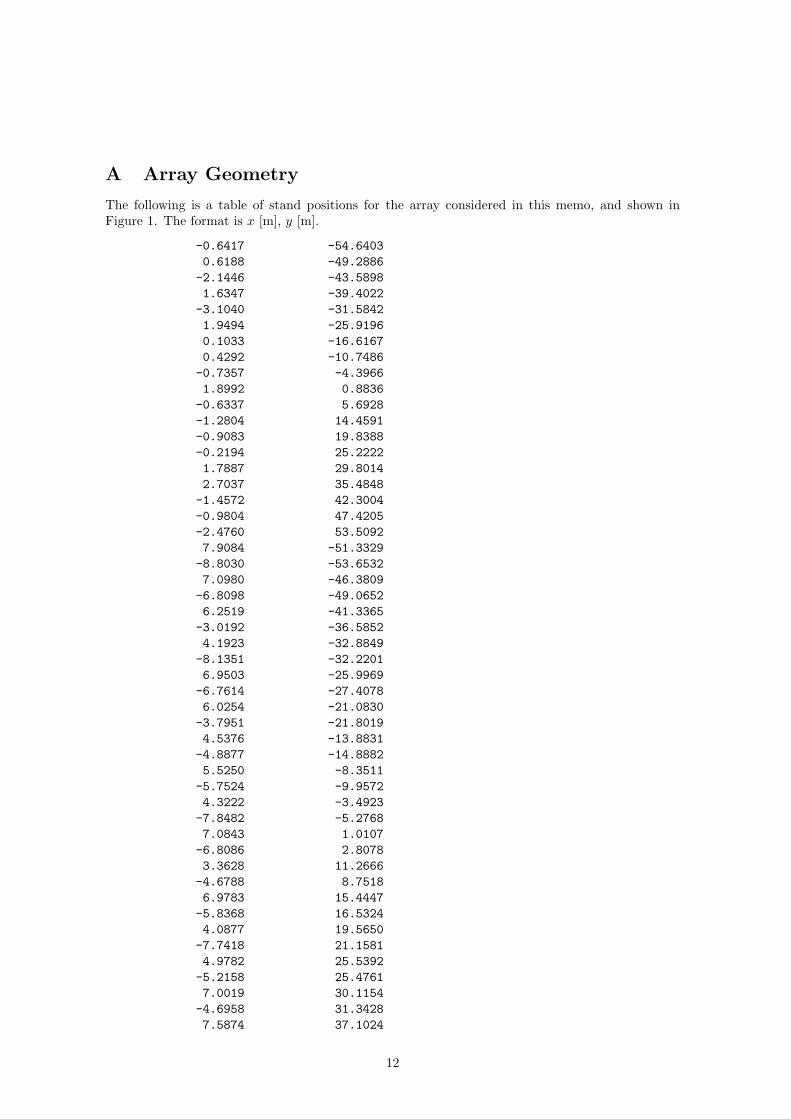
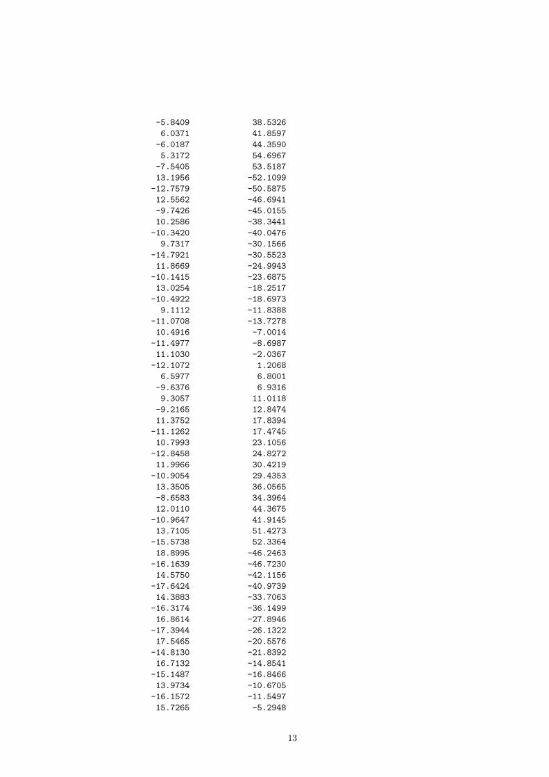
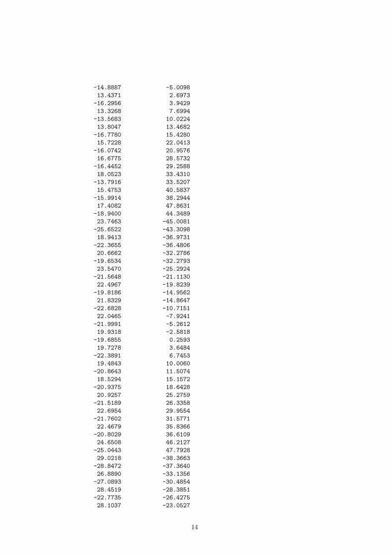
A Array Geometry
The following is a table of stand positions for the array considered in this memo, and shown inFigure 1. The format is x [m], y [m].
-0.6417 -54.6403
0.6188 -49.2886
-2.1446 -43.5898
1.6347 -39.4022
-3.1040 -31.5842
1.9494 -25.9196
0.1033 -16.6167
0.4292 -10.7486
-0.7357 -4.3966
1.8992 0.8836
-0.6337 5.6928
-1.2804 14.4591
-0.9083 19.8388
-0.2194 25.2222
1.7887 29.8014
2.7037 35.4848
-1.4572 42.3004
-0.9804 47.4205
-2.4760 53.5092
7.9084 -51.3329
-8.8030 -53.6532
7.0980 -46.3809
-6.8098 -49.0652
6.2519 -41.3365
-3.0192 -36.5852
4.1923 -32.8849
-8.1351 -32.2201
6.9503 -25.9969
-6.7614 -27.4078
6.0254 -21.0830
-3.7951 -21.8019
4.5376 -13.8831
-4.8877 -14.8882
5.5250 -8.3511
-5.7524 -9.9572
4.3222 -3.4923
-7.8482 -5.2768
7.0843 1.0107
-6.8086 2.8078
3.3628 11.2666
-4.6788 8.7518
6.9783 15.4447
-5.8368 16.5324
4.0877 19.5650
-7.7418 21.1581
4.9782 25.5392
-5.2158 25.4761
7.0019 30.1154
-4.6958 31.3428
7.5874 37.1024
12
-5.8409 38.5326
6.0371 41.8597
-6.0187 44.3590
5.3172 54.6967
-7.5405 53.5187
13.1956 -52.1099
-12.7579 -50.5875
12.5562 -46.6941
-9.7426 -45.0155
10.2586 -38.3441
-10.3420 -40.0476
9.7317 -30.1566
-14.7921 -30.5523
11.8669 -24.9943
-10.1415 -23.6875
13.0254 -18.2517
-10.4922 -18.6973
9.1112 -11.8388
-11.0708 -13.7278
10.4916 -7.0014
-11.4977 -8.6987
11.1030 -2.0367
-12.1072 1.2068
6.5977 6.8001
-9.6376 6.9316
9.3057 11.0118
-9.2165 12.8474
11.3752 17.8394
-11.1262 17.4745
10.7993 23.1056
-12.8458 24.8272
11.9966 30.4219
-10.9054 29.4353
13.3505 36.0565
-8.6583 34.3964
12.0110 44.3675
-10.9647 41.9145
13.7105 51.4273
-15.5738 52.3364
18.8995 -46.2463
-16.1639 -46.7230
14.5750 -42.1156
-17.6424 -40.9739
14.3883 -33.7063
-16.3174 -36.1499
16.8614 -27.8946
-17.3944 -26.1322
17.5465 -20.5576
-14.8130 -21.8392
16.7132 -14.8541
-15.1487 -16.8466
13.9734 -10.6705
-16.1572 -11.5497
15.7265 -5.2948
13
-14.8887 -5.0098
13.4371 2.6973
-16.2956 3.9429
13.3268 7.6994
-13.5683 10.0224
13.8047 13.4682
-16.7780 15.4280
15.7228 22.0413
-16.0742 20.9576
16.6775 28.5732
-16.4452 29.2588
18.0523 33.4310
-13.7916 33.5207
15.4753 40.5837
-15.9914 38.2944
17.4082 47.8631
-18.9400 44.3489
23.7463 -45.0081
-25.6522 -43.3098
18.9413 -36.9731
-22.3655 -36.4806
20.6662 -32.2786
-19.6534 -32.2793
23.5470 -25.2924
-21.5648 -21.1130
22.4967 -19.8239
-19.8186 -14.9562
21.8329 -14.8647
-22.6828 -10.7151
22.0465 -7.9241
-21.9991 -5.2612
19.9318 -2.5818
-19.6855 0.2593
19.7278 3.6484
-22.3891 6.7453
19.4843 10.0060
-20.8643 11.5074
18.5294 15.1572
-20.9375 18.6428
20.9257 25.2759
-21.5189 26.3358
22.6954 29.9554
-21.7602 31.5771
22.4679 35.8366
-20.8029 36.6109
24.6508 46.2127
-25.0443 47.7928
29.0218 -38.3663
-28.8472 -37.3640
26.8890 -33.1356
-27.0893 -30.4854
28.4519 -28.3851
-22.7735 -26.4275
28.1037 -23.0527
14
-26.4012 -22.9848
27.1227 -16.6874
-24.3916 -16.9852
25.5481 -11.5071
-26.5409 -7.4385
24.9300 -2.7158
-28.0636 -2.6715
25.4969 3.7717
-25.5579 2.7538
24.2924 8.6263
-26.0664 12.3274
25.1775 14.4677
-26.5543 17.3048
29.1182 22.2415
-25.2262 22.9725
26.9131 26.7292
-26.5026 28.2808
29.1861 31.1853
-27.7291 33.7202
29.3327 37.9612
-30.1810 40.3269
35.0420 -39.5341
-32.8441 -41.7774
34.2805 -32.0664
-33.8331 -32.3352
32.6059 -25.6007
-31.3849 -25.4098
32.0173 -17.7290
-29.3839 -17.6411
30.7056 -11.3911
-31.4897 -11.5853
29.1609 -5.3829
-34.9724 -6.9353
30.9098 -0.6914
-30.5879 1.6933
29.7352 6.4426
-29.1909 8.3535
30.8769 11.3155
-33.5187 12.9787
31.9913 16.1965
-32.5407 17.9274
33.0469 27.0970
-30.6914 25.5317
33.3625 34.9988
-32.5725 32.4500
33.9143 39.9699
-35.2642 39.3136
-36.6268 -36.4847
37.2981 -27.3307
-39.6483 -29.7389
35.8184 -20.9876
-35.5218 -22.5997
37.1341 -14.4744
-35.0808 -17.6007
15
36.1501 -8.3643
-37.2341 -12.5975
38.5491 -2.7244
-34.0486 -2.0158
36.5450 3.1454
-35.7834 3.6391
37.0096 9.9968
-36.8390 8.6736
38.6967 15.9076
-38.9928 14.0988
36.7558 20.5161
-35.6935 22.2359
37.3787 30.0275
-35.9543 28.3535
43.1045 -27.5871
-40.5514 -22.3927
40.9522 -22.7011
-41.5217 -17.3201
41.9859 -15.6864
-44.6673 -12.1776
40.8872 -10.1588
-40.8047 -8.0394
43.9657 -2.1493
-39.6399 0.1358
42.4244 3.4557
-41.9223 4.5853
41.8888 11.1213
-43.2501 10.8016
43.6038 16.9351
-40.6100 20.0608
41.5201 23.6954
-39.8577 25.0047
46.7343 -19.8940
-47.7129 -16.7461
47.3268 -12.4447
-49.1936 -7.1431
47.0654 -7.4021
-48.5481 -2.1663
49.3201 -0.3418
-48.2585 2.8298
48.5971 5.2913
-47.4207 13.5602
48.8035 11.1792
-47.1802 18.5544
16
References
[1] S. Ellingson, “Collecting Area of Planar Arrays of Thin Straight Dipoles,” Long Wavelength Ar-ray Memo Series No. 67, December 31, 2006. [online] http://www.phys.unm.edu/∼lwa/memos.
[2] L. D’Addario, “LWA Fine Delay Tracking,” Long Wavelength Array Memo Series No. 143,Nov 10, 2008. [online] http://www.phys.unm.edu/∼lwa/memos.
[3] S. Ellingson, “Polarimetric Response and Calibration of a Single Stand Embedded in an Arraywith Irregular Wavelength-Scale Spacings,” Long Wavelength Array Memo Series No. 140, Aug14, 2008. [online] http://www.phys.unm.edu/∼lwa/memos.
[4] S.W. Ellingson, “Polarization Processing for LWA Stations,” Long Wavelength Array MemoSeries No. 106, October 29, 2007. [online] http://www.phys.unm.edu/∼lwa/memos.
[5] S.W. Ellingson, “LWA Beamforming Design Concept,” Long Wavelength Array Memo SeriesNo. 107, October 30, 2007. [online] http://www.phys.unm.edu/∼lwa/memos.
[6] S. Ellingson, “Single-Stand Polarimetric Response and Calibration,” Long Wavelength ArrayMemo Series No. 138, June 15, 2008. [online] http://www.phys.unm.edu/∼lwa/memos.
[7] S. Ellingson, “Some Initial Results from an Electromagnetic Model of the LWA Sta-tion Array,” Long Wavelength Array Memo Series No. 147, Dec 15, 2008. [online]http://www.phys.unm.edu/∼lwa/memos.
[8] S. Ellingson, “Effective Aperture of a Large Pseudorandom Low-Frequency DipoleArray,” Long Wavelength Array Memo Series No. 73, Jan 13, 2007. [online]http://www.phys.unm.edu/∼lwa/memos.
[9] A. Kerkhoff, “Simulation of Mutual Coupling Effects in Large Aperiodic Phased Arrays,” March18, 2008. (Presentation at the LWA Pre-PDR Workshop; slides available on Basecamp.)
[10] Long Wavelength Array Project Office, “Station Configuration,” Engineering Change Notice(ECN) 3, Oct 22, 2008.
[11] S. Ellingson, “Interaction Between an Antenna and a Fence,” Long Wavelength Array MemoSeries No. 129, Mar 24, 2008. [online] http://www.phys.unm.edu/∼lwa/memos.
[12] S. Ellingson, “Interaction Between an Antenna and a Shelter,” Long Wavelength Array MemoSeries No. 141, Sep 25, 2008. [online] http://www.phys.unm.edu/∼lwa/memos.
[13] W.L. Stutzman and G.A. Thiele, Antenna Theory and Design, 2nd Ed., Wiley, 1998, p. 173.
17