Abstract— The ability to realize maximum returns from manufacturing equipment is affected by various interrelated business and technical factors that affect equipment performance. Among the key factors are operating and maintenance practices that significantly affect equipment performance. Understanding how these factors interact and impact manufacturing performance is essential in ensuring that the equipment is operated in a manner that provides desired performance and enables informed management decisions on performance prediction and improvement. However, performance analysis in practice is driven by past events (lagging indicators) and little has been done to model the various cause and effect relationships that determine performance (the leading indicators). There lacks therefore an approach of conducting predictive performance analysis for manufacturing systems. In this research, a performance modelling approach is developed that integrates process knowledge and corresponding dynamics that determine equipment performance. The approach consists of; first identification and quantification of the key interactions and factors (technical and operation factors) affecting manufacturing equipment performance. Secondly, a simulation model is developed (in ARENA software) to model the relationships and interactions among the various factors and their impact on performance. The approach is tested with an industrial case study in a processing plant and results are presented in the paper. The model is used in predictive performance analysis and screening of improvement scenarios for decision support.

Keywords—Performance, Manufacturing, Equipment, Reliability, Failure, Maintenance.

I. INTRODUCTION

Due to intense global competition and increasing demands from stakeholders, manufacturers are striving to improve and optimize their productivity in order to stay competitive. The increasing need to improve manufacturing performance demands adequate knowledge of performance measurement. It is evident that manufacturing equipment performance is dependent on several heterogeneous factors (both business and technical) interacting in context. Understanding how these factors interact and impact manufacturing performance is essential in ensuring that the equipment is operated in a

Peter Nganga Muchiri , School of Engineering, Kimathi University College of Technology

(KUCT),P.o.Box 657-10100 Nyeri, Kenya, Liliane Pintelon

Centre for Industrial Management, Katholieke Universiteit Leuven (KUL),Celestijnenlaan 300A, 3001 Heverlee, Belgium

Corresponding Author: ngangapet@yahoo.com; +254717877044

manner that provides desired performance and enables informed management decisions on performance prediction and improvement. Among the key factors are production (operation) and maintenance practices that significantly affect equipment performance. Though manufacturing equipment is designed to ensure successful operation through the anticipated service life, deterioration begins to take place as soon as it is commissioned. In addition to normal wear and deterioration, other failures may also occur, especially when the equipment is pushed beyond their design limits or due to operational errors. As a result, equipment down time, quality problems, slower production rate, safety hazards or environmental pollution becomes the obvious outcome. These outcomes have the potential to impact negatively the operating cost, profitability, demand satisfaction, and productivity among other important performance requirements. It has been asserted by some authors [1-3] that equipment maintenance and system reliability are important factors that affect the organization’s ability to provide quality and timely services to customers and be ahead of competition. Maintenance is therefore vital for sustainable performance of a manufacturing equipment [2, 4, 5]. While the relationship between production and maintenance is highly recognized, it is not well understood. The bulk of literature is mainly concerned with lagging performance. However, leading performance would yield a much greater added value but do require a much better understanding of the behaviour between production and maintenance as well as their mutual relationship. Moreover, recent research [6] has shown that little is known about the way in which production and maintenance interactions influence equipment performance and vice versa. Thus, the aim of this research is to gain insights of how equipment’s performance results from the interactions between production and maintenance by use of simulation modelling. The objective of performance modelling is to develop knowledge of manufacturing performance dynamics and an understanding of how manufacturing performance is realized. It is worth noting that the objective of this study is not performance optimization. Rather, the purpose of performance modelling is to develop insights and understanding of the system behaviour and the corresponding impact on performance. This, eventually, provides a basis for performance measurement and analysis and provides insights on performance improvement. In the next sections, the manufacturing performance modelling approach will be introduced. Further, the industrial case study

Performance Modelling of Manufacturing Equipment: Results from an Industrial Case Study

Peter Nganga Muchiri, Liliane Pintelon

will be presented. Finally, the results of the case study are tested with the developed model are discussed. 2. Maintenance interaction with Production

The scope of maintenance in a manufacturing environment is illustrated by its various definitions. The British Standards Institute defines maintenance as [7-9]:

“A combination of all technical and associated administrative activities required to keep equipment, installations and other physical assets in the desired operating condition or restore them to this condition.”

The Maintenance Engineering Society of Australia [10] gives a definition that indicates that maintenance is about achieving the required asset capabilities within an economic or business context. They define maintenance as:

“The engineering decisions and associated actions, necessary and sufficient for attainment of specified equipment ‘capability’.”

The “capability” in this definition is the ability to perform a specified function within a range of performance levels that may relate to capacity, rate, quality and responsiveness[11]. Effective and efficient maintenance is believed to effect asset performance enhancement by providing equipment reliability and improvement of service to customers whilst simultaneously reducing costs of production. Thus, many authors hold the view that maintenance is a vital part of manufacturing operation. Though some authors state that there is now a much clearer and more evident acknowledgement of maintenance’s potential of increasing the overall profit than ever before [12, 13], still a complex relationship between maintenance and production does exist [14-16]. In most organizations, there is a tendency to organize departments into functional specialism groups where, for example, the engineering deals with equipment design, production deals with equipment operation and maintenance deals with equipment care. Thus, the maintenance and the production function are pretty much separated in terms of the organizational unit they are embedded in and in terms of planning, control and performance in general. This strict separation is helpful in clarifying who is responsible for what and for a clear focus on the different technological specializations that are required in both types of functions. However, this separation may be less than optimal in situations in which the overall performance of organizations is the primary objective. Extensive research has been carried out over the years on production planning, maintenance modelling, and management of unreliable systems [17-21]. However, the tendency of separating maintenance and production is further propagated in theory where, the production planning models assume maximum equipment performance within a planning horizon while maintenance models disregard the impact on production capacity and performance [22]. Thus, additional effort is

required in order to see an integrated or the ‘whole picture’ of equipment performance.

Manufacturing System(Equipment)

Perf. Control(OEE, Output…)

Input Output

Operations Maintenance

Deterioration& Failure

Asset Utilization

Maint. RenewalEffect

Cooperation Opportunities

Fig. 1: The basic relationship/interaction between maintenance and

production.

In many situations, the production and maintenance functions cannot operate completely independently. Figure 1 shows the basic interdependence between the maintenance and the production function. Essentially, by utilizing Technical systems, i.e. physical assets, some kind of degradation occurs, which without maintenance intervention would lead to loss of function. Thus, the production function generates a demand for maintenance. The maintenance function, on the other hand, tries to remedy loss of function by a technical intervention. Both functions are in essence linked together by their requirement to access the assets for their respective purposes. Mostly, these requirements for access of an asset does require some coordination, since the production function and the maintenance function have different and sometimes conflicting requirements regarding the state of the asset for their purpose. E.g. a car cannot be used for driving when a tire replacement is carried out. On the other hand measuring oil pressure for condition based maintenance requires a running engine and may not conflict with the intention to drive the car. This type of interdependence necessitates a mutual coordination for access of assets and mutual performance analysis. 3.0 Performance modelling approach

To develop the performance model, the key interactions and factors (both business and technical factors) affecting manufacturing equipment’s performance are first identified. The technical factors considered in the model are related to equipment’s reliability, deterioration, failure and maintenance effects. The business factors are related with equipment utilization to meet it production targets based on production schedule and market demand. Once these factors are identified, their cause and effect relationship is analyzed on how they interact in the manufacturing process. The simulation model is used to mimic the operation of a

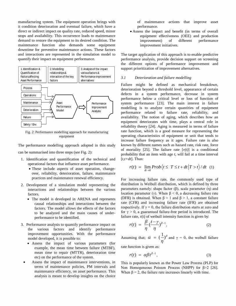
manufacturing system. The equipment operation brings with it condition deterioration and eventual failure, which have a direct or indirect impact on quality rate, reduced speed, minor stops and availability. This occurrence leads to maintenance demand to restore the equipment to its desired condition. The maintenance function also demands some equipment downtime for preventive maintenance actions. These factors and interactions are represented in the simulation model to quantify their impact on equipment performance.

Process

Operations

Maintenance

Deterioration

Failure

Safety / Env.

Asset PerformanceModel

Performance Improvement Analysis

1. Identification & Quantification of Factors affecting Asset Performance

2. Modelling relationships & interaction of the key factors

3. Analysis of the impact various factors & Performance improvement alternatives

Fig. 2: Performance modelling approach for manufacturing

equipment

The performance modelling approach adopted in this study

can be summarised into three steps (see Fig. 2):

1. Identification and quantification of the technical and operational factors that influence asset performance. These include aspects of asset operation, change-

over, reliability, deterioration, failure, maintenance practices and maintenance renewal efficiency.

2. Development of a simulation model representing the interactions and relationships between the various factors. The model is developed in ARENA and represents

causal relationships and interactions between the factors. The model allows the effects of the factors to be analyzed and the main causes of under-performance to be identified.

3. Performance analysis to quantify performance impact on the various factors and identify performance improvement opportunities. With the performance model developed, it is possible to: Assess the impact of various parameters (for

example, the mean time between failure (MTBF), mean time to repair (MTTR), deterioration time etc) on the performance of the system.

Assess the impact of maintenance interventions, in terms of maintenance policies, PM intervals and maintenance efficiency, on asset performance. This analysis is meant to develop insights on the choice

of maintenance actions that improve asset performance.

Assess the impact and benefit (in terms of overall equipment effectiveness (OEE) and production improvement) of different performance improvement initiatives.

The target application of this approach is to enable predictive performance analysis, provide decision support on screening the different options of performance improvement and support prioritization of improvement alternatives.

3.1 Deterioration and failure modelling

Failure might be defined as mechanical breakdown, deterioration beyond a threshold level, appearance of certain defects in a system performance, decrease in system performance below a critical level or loss of function of system performance [23]. The main interest in failure modelling is to analyze certain quantities of equipment performance related to failure rate, reliability, and availability. The notion of aging, which describes how an equipment deteriorates with time, plays a central role in reliability theory [24]. Aging is measured in terms of failure rate function, which is a good measure for representing the operating characteristics of equipment or unit that tends to increase failure frequency as it ages. Failure rate is also known by different names such as hazard rate, risk rate, force of mortality [25]. The failure rate [r(t)] is a conditional probability that an item with age t, will fail at a time interval [t,t+dt]. Thus:

0

( ) lim /dt

r t Prob t T t dt T t dt

(1)

For increasing failure rate, the commonly used type of distribution is Weibull distribution, which is defined by three parameters namely: shape factor (β), scale parameter (η) and location parameter (γ). When β < 0, a decreasing failure rate (DFR) is obtained. When β ≈ 1 and β > 1, a constant failure rate (CFR) and increasing failure rate (IFR) are obtained respectively. If γ = 0, the failure distribution starts at zero and for γ > 0, a guaranteed failure-free period is introduced. The failure rate, r(t) of weibull intensity function is given by:

1( ) ( )tr t

, (2)

Assuming that; 1 ( )

and γ = 0, the weibull failure

rate function is given as:

1( ) r t t , (3)

This is popularly known as the Power Law Process (PLP) for Non Homogeneous Poisson Process (NHPP) for β>2 [26]. When β = 2, the failure rate increases linearly with time.

Deterioration modelling concept is based on the PF-curve (potential (P) of failure-to failure (F)), which is derived from reliability centred maintenance (RCM) [27, 28]. The PF-curve represents a follow-up on equipment condition over time. It is based on the fact that most of the failure modes gives some sort of indication or warning that they are in the process of occurring or about to occur [27]. The PF-curve shows the time instance when the failure commences (potential (P) failure) to the point when the failure (F) actually occurs, and thus the name PF-curve. In this research, the PF concept is modified and then used to model the equipment condition, deterioration time and its effect, and failure. To determine the condition of the equipment and its impact on the system performance, the PF curve is defined as illustrated in Fig. 3.

Equi

pmen

t Con

ditio

n

Potential Failure

Failure occurs

Good condition CM Down time

Good condition

Deteriorating condition

PM time

Initiate PM

Deteriorating condition[Time to

defect (TTD)]

Time (t)

Fig. 3: The modified PF-Curve showing the state/condition of the

equipment

The condition of equipment is assumed to be in any of the following three states:

good condition, deteriorating condition or down - due to corrective maintenance (CM)

or due to preventive maintenance (PM).

The good condition period is the time it takes before a failure mode begins since the previous maintenance intervention. This is defined by a PF signal=0 in the simulation model. During this time, the machine runs at its designed speed and at a 100% quality rate. The arrival of failure mode causes the machine condition to start deteriorating and to run at a reduced speed and a lower quality rate, which are defined in the simulation experimental design. If PM action is not taken during deterioration condition state, the machine breaks down and CM action is taken to bring it back to good condition. If PM action is taken at deteriorating condition state, the equipment does not fail and returns to good condition state. The use of the modified PF curve concept also gives a window of opportunity in the investigation of predictive maintenance. Through equipment condition monitoring, it is possible to identify the development of failure modes, and thus support research on the use of condition-based maintenance. The use of condition-based maintenance is investigated together with the other maintenance policies.

3.2 Maintenance Modelling

It is assumed in this research that maintenance has a renewal effect on equipment failure rate and condition, which is defined as the improvement factor or the maintenance efficiency (ρ). We assume that the repair rejuvenates the equipment such that after the ith maintenance action, the equipment behaves as a new equipment, which would have worked a duration Ai, where Ai < t. Thus;

[Ai] – is a set of non-negative random variables, named effective age

[A0] = 0

The arithmetic reduction of age (ARA) model corresponds to a maintenance action that reduces the virtual age of the equipment of an amount proportional to its age just before repair [26]. This proportion is given by parameter ρ, which represents the maintenance efficiency. Thus the virtual age of equipment after repair is:

(1 )i i i iT T T T

A A A A (4)

The ARA model is defined by virtual age and the failure intensity is given as;

1

1( (1 ) )i

t

t Nt ii

Nt T

(5)

To model the effect of maintenance on manufacturing assets, the following three factors are integrated that are key to maintenance decision making:

How should maintenance be done? - This determines the degree of improvement or maintenance efficiency. In this case, three possible scenarios are assumed where maintenance leaves the equipment:

As bad as old (ABAO) i.e. ρ=0, As good as new (AGAN), i.e. ρ=1; and Imperfect maintenance, i.e. 0 < ρ < 1 (see

Fig. 4

t

t

Maint. actions

Fig. 4: The failure rate with imperfect maintenance

What maintenance needs to be done? - This determines the choice of the maintenance policies that trigger the maintenance actions. The maintenance policies considered here are: Failure based maintenance (FBM)- This it is a

purely reactive policy where corrective maintenance (CM) is done only when the equipment fails.

Time based or use based maintenance (TBM/UBM) – This is a preventive policy where maintenance is carried out at specified time intervals. For UBM, intervals are measured in working hours while in TBM intervals are in calendar days.

Condition based maintenance (CBM) - This is a predictive policy where PM is carried out whenever a given system parameter or condition approached or reaches a predetermined value or situation.

When should maintenance be done? - This determines the maintenance interval. The following maintenance timings are considered in the simulation model:

CM Time - Failure occurs at random times and thus cannot be predicted. Thus, corrective maintenance is done at random times.

PM time - This can be scheduled / planned maintenance activities and thus they are deterministic.

PM time can also be determined by the condition of the equipment according to the results of inspections and degradation or operation control. Thus random PM can be carried out based on condition monitoring.

PM timing can also be influenced by other factors like production schedules where PM is carried out during change-over.

CM time and PM time may be dependent if PM activity is done during CM action or due to the modification of the PM periodicity if too many failures are observed on the equipment.

Condition monitoring time is normally planned and therefore it is deterministic.

4.0 Industrial case study

The industrial case study approach was used to test the applicability of the developed approach and evaluate its actual relevance with respect to the realism. Further, the case study was used to help identify the limitations and difficulties in applying the performance modelling approach and provide direction for further research. The company was chosen due to availability of well documented asset performance data base due to their high interest in performance analysis and improvement programs. Due to the company’s request for confidentiality, the name of the company is not disclosed in this text. To conduct the case study, several meetings were held with the maintenance and production managers to discuss the production process, performance requirements, maintenance requirements, data analysis and results. In addition, plant visits were conducted to familiarize with the process and equipment involved. The data analysis and performance insights were carried out in collaboration with the plant’s management.

4.1 Process layout

The plant is made up of 6 production lines that are similar in process flow layout but different in production capacities and the product family they produce. The production is a continuous flow process that runs 24 hours per day and 7 days per week, unless the line is down due to operational or technical reasons. A simplification of the process layout based on the key equipment is shown in Fig. 5. The process is based on free radical reaction, where the compressed gas (1200–2000bars) is polymerized. The feed stock (gaseous form) is supplied at 40bars to the primary compressor, where it is compressed to 250bars. In the secondary compressor, the gas is compressed up to 1200-2000bars, which is the required pressure for polymerization in the reactor. The initiators trigger the polymerization reaction in the reactors, where the reactants are converted into solid product. Around 70% of the unconverted gas is separated from the product at the high pressure separator and the other 30% is removed at the low pressure separator. The unconverted gas is re-directed back to the process through the secondary and purge compressor and some coolers respectively. The polymer then undergoes the extrusion process after which the extruded material is cut into small pellets. The pellets are then transported through an air flow to the containers for shipment to the various customers.

Primary Compressor(2-Stage)

Purge Compressor(3-stage)

Secondary Compressor(2-stage)

Reactor(2000bar, 250 C)

HP Separator

LP Separator

Feed Stock40 bar-Gas

250bar ~ 2000bar

0.3 bar

40bar

250bar

ExtruderPelletizer

Coolers

Products

70%

65%

35%

30%

Fig. 5: The simplification of process layout

The quality and the property of the products are highly dependent on the molecular structure formed during polymerization. The molecular structure is also controlled by some modifiers, chemicals and additives that are added to enhance product performance and strengthen some properties for some product grades. The main setback for these modifiers and chemicals is that they are injected before the secondary compressor to avoid injection against very high pressure. (Injection of these chemicals to the reactor, where they are actually required, would demand a very high pressure pump). These chemical sometimes initiate polymerization in the compressor cylinders leading to high compressor failure. The risk of polymerization in the secondary compressor coupled with the critical working conditions, high pressure (1200-2000bar and high temperature (2500C), makes the secondary compressors the

most critical equipment in the process. However, it is worth noting that all the equipment in the process is critical since a functional failure of any equipment will result in a process shutdown. The other factors affecting the manufacturing system performance and the corresponding interactions were studied and quantified. Then, performance modelling of the case was carried out.

4.2 Data analysis

The case study involved analysis of diverse data of plant performance. The data analysis involved the identification and analysis of factors that cause the process not to operate at full capacity. The historical data was used in performance analysis. The data collected and analyzed from both production and maintenance departments included:

Causes and quantification of production losses (outages)

Production output OEE (overall equipment effectiveness) values Maintenance data - PM & CM interventions Failure data per equipment and per component Root cause analysis data (for failures)

Identification of the of lost manufacturing capacity was carried out within the OEE metric and involved losses due to process causes, mechanical reliability and quality failures which result into system slowdown and/or shutdowns. The initial data analysis was carried out in all the six production lines but more focus was given to line 3, due to special products grades it produces that have a higher impact on technical and production losses compared to other lines. Since line 3 is similar in design and capacity as both line 1 and 2, performance comparison was done between the three lines. For each production line and product grade, the plant has set a production benchmark (based on the maximum production ever attained by the plant for seven days consecutively). Using the benchmark production output per hour (tons/hr), it is possible to calculate the production loss for any type of outage.

Based on the loss analysis, mechanical availability, capacity availability and quality rate were calculated for each year. For example using the data for year 2005 (see Fig. 6 ), 6.4% of the total available time was lost due to mechanical downtime and 7.6% of time lost due to process related losses. From the total production output, 5.7% did not meet the quality requirements. Thus, the good quality production was 80.3% of the available capacity, which represents overall equipment effectiveness (OEE). The plant has set a target OEE of 90% - 95% and thus line 3 has an improvement potential of 10% to 15%.

Good quality production

80,3%

Quality Losses5,7%

Capacity Losses7,6%

Mech.Reliability Losses6,4%

Line 3 OEE Analysis (2005)

Fig. 6: OEE analysis showing the % of Production losses and

capacity realized

To investigate the performance dynamics that lead to OEE, further analysis on the root cause of production losses was carried out. First, Pareto analysis was carried out on the different causes of downtime and their frequency of occurrence as shown in Fig. 7. For the total recorded downtime of 624 hours in 2005, 53% of the downtime was caused by mechanical oriented problems. Capacity losses were attributed to downtime during change-over and due to process oriented losses. From the analysis, 25% of downtime was attributed to change-over while process problems account for 22% of downtime. It is worth noting that change-over time may not be termed as a loss since it is a planned downtime as per the different products demand. Further, it offers the maintenance management a window of opportunity for preventive maintenance. Thus mechanical problems were found to be the highest contributor of manufacturing downtime. From the analysis of 51 recorded outages in 2005, process problems had the highest frequency with 47%, while mechanical problems caused 43% of the outages. Changeovers have the least frequency of 10% (around 5 per year) but high downtime per change-over. The quality rate is mostly influenced by the process operating condition. Quality defects are also produced during slowdown and start-ups, which occur when the process has to be stopped due to maintenance actions or change-over. For a shutdown to occur, the process needs 4 hours of depressurizing and during this period, quality defects are produced.

0 10 20 30 40 50 60

Change-Overs

Process Losses

Mechanical downtime

Disruption Frequency & Downtime Analysis (2005)

Occurrence Rate (%) % Downtime Fig. 7: Pareto analysis of the causes and frequency of downtime

For mechanical failures, further analysis was carried out to determine the equipment responsible of the failures in the system. Using the 3 years failure data, failure rate and the subsequent downtime were analyzed per equipment as shown in Fig. 8. From the 3 years failure data, Pareto analysis was

carried out for 61 failures and around 800 hrs of downtime. Analysis was done for the average failure rate per year and per equipment and the time to repair per equipment. For the time to repair (TTR) analysis, triangular distribution was assumed due to high standard deviation with the mean values. Thus for each TTR, the low, average and high TTR values were identified.

0

5

10

15

20

25

30

Tim

e to

repa

ir (h

rs)

Time to Repair (hrs)

High

Av.

Low

0

2

4

6

8

10

12

14

16

Av. F

ailu

re R

ate/

yr

Av. Failure Rate per Year

Fig. 8: Average failure rate and time to repair per equipment

As shown in Fig. 8, the secondary compressor has the highest failure rate of 14 failures per year and takes an average of 18 hours to repair. The primary compressor has a lower failure rate of 2.6 failures per year. The pelletizer has an average failure rate of 3.33 failures per year but takes the least TTR with an average of 6 hours. The reactors on the other hand have low failure rate of 2.6 failures/year but high average down time of 24 hours per repair. These initial findings illustrated that secondary compressor is the least reliable equipment in the system. This high failure rate was initially attributed to the severe working condition with pressure of 2000 bar and temperature of 250oC.

To gain some insights in the secondary compressor failure mode, life data analysis was carried out using Weibull distribution [29]. The point of interest was to establish whether it has increasing failure rate or random rate and its possible characteristic life. As shown in Fig. 9, the beta value was found to be 1.57. This is an indication of near random failures and may qualify for an exponentially distributed failure rate. Though the beta value is slightly higher than one, it does not tell much about the increasing failure rate with respect to the operating time. It also indicates that the failures are not instigated by the life of the components but originates from other sources such as the operating context. Thus, the mean compressor life of 44 days may not indicate the equipment characteristic life, but just the Weibull mean for time to failure.

0,0

0,2

0,4

0,6

0,8

1,0

0 20 40 60 80 100 120failu

re &

surv

ival

Pro

babi

lity

Operation time (days)

Survival Graph for HP CompressorBeta Value=1.57; Char. Life (Alpha) = 44 days

Reliability Failure Probability

Fig. 9: Life data analysis of secondary compressor

Further, the failure rate of line 3 compressor was compared with the failure rate of the other compressors in the other lines. Much reliability interest was generated from the comparison between line 1, 2 and 3. These three lines are similar in design, manufacturer, capacity and age. Using a three year process disturbance data set, failures were sorted per compressor type and per line. As shown in Fig. 10, line 3 has the highest compressor failure compared with the other lines. The difference in reliability and performance can purely be attributed to the operating context. Further discussion with the process and maintenance engineers revealed that lines 1, 2 and 3 run different product grades, of which special grades are run in line 2 and 3. From a reliability and operability point of view, lines 2 and 3 are run outside their design operating envelopes due to the chemical composition of the products run. Line 3 operates outside the design operating envelope on a continuous basis, while line 2 operates outside the design operating envelope part of the time. Fit for service changes have been made over the last couple of years to improve their reliability. This includes changes of some components and piping from normal steel to stainless steel. In spite of these changes, the reliability differences between these lines (2 & 3) and line 1 are quite evident. For all lines however, the secondary compressor has the highest failures. This is attributed to higher vulnerability to gas leak due to high pressure (2000bars) and temp 250oC, which has an inherent reliability impact. The primary compressors are highly reliable in all the lines.

Line 1

Line 2

Line 3

Line 4

Line 5

Line 6

Sec. Comp. 15 31 56 21 18 13

Prim. Comp. 7 6 9 4 2 11

010203040506070

No.

of F

ailu

res

Compressor Failure Analysis / Line (3Yrs data)

Fig. 10: Comparison of compressor failures for process lines in

different operating context.

Finally, the compressor components failure of line 1 (that runs normal products grade) were compared with line 3 (that runs special grades) as shown in Fig. 11. It was found that the cylinders in line 3 have four times failure rate over line 1. Consequently, the valves in line 3 have three times failure rate over line 1. Line 3 also has other components failures that are not experienced by line 1. This finding supports the Engineers’ opinion that the operating context is responsible of approximate 80% of the failures. Thus, many failures that may appear as mechanically oriented may have their origin from the operating practices. Since these failures are process oriented, they can hardly be linked to the maintenance strategy like preventive maintenance. For most parts, the equipment strategy is based on random failures, so the most effective equipment strategy is condition monitoring to prevent major equipment damage.

The system performance analysis revealed important interactions between asset operation, asset maintenance and asset performance. However, no information was found on equipment’s deterioration, the duration it takes from the time a failure is identified to failure or effects of equipment deterioration of performance. The information on deterioration durations is an important input in condition based maintenance. Further, no information documented on the effects of maintenance on system reliability, failure rate or equipment performance after maintenance. This type of information can potentially support performance improvement analysis.

0 5 10 15 20 25 30

BearingCooling Hse.

FlexiblePipingProbe

ThermocoupleYokeQuill

ValvesCylinder

No. of Failures

Sec. Comp. Failures of Line 1 & 3 per Component

Line 3Line 1

Fig. 11: Comparison of components failures of line 1 versus line 3

5.0 System Performance Modelling

From the analysis of factors affecting system performance, it was found that a complex interaction exists between process factors and technical factors, which influence system performance. Modelling the interactions and relationships between these factors is an important step in analysing the process dynamics that determines the production system performance (OEE and production output). The purpose of the model is to support predictive performance analysis, analysis of improvement alternatives, set improvement targets and benchmarks.

5.1 Modelling approach

The model was developed in ARENA program [30] and simulated a simplified process layout on the basis of the key equipments as shown in Fig. 5. The system is a continuous process that runs for 24 hours/day unless there is a stoppage due to operational or technical reasons. Around 20% of the gas is converted at the reactor and the un-reacted gas is fed back to primary and secondary compressor through the low pressure and high pressure separators respectively. To simulate the production system, the benchmark production capacity was used. However, the production capacity is not revealed in the text due to confidentiality. To simulate the process disturbances, different sets of sub-models were developed for each equipment failure mode and repair rate, the process losses and change-over. The input of these outages was generated from the extensive data analysis. As shown in Table 1, the failure rate and the mean time to failure were established for each equipment. The time to failure was assumed to be exponentially distributed with the given mean due to the observed randomness of failure arrival. For the time to repair (TTR), a triangular distribution was assumed due to high variability in the observed TTR over the mean TTR. This is in exception to coolers and extruder, where a uniform distribution was used due low failure rate and thus little data on repair time. Also, planned maintenance was found at an average rate of 3 times per year. The time to planned maintenance was assumed to be exponentially distributed with a mean of 120 days. The downtime was assumed to be triangular distributed due to high range.

Table 1: The failure rate, downtime and process disturbance parameters used in simulation model.

Equipment or Process

Av. Failure or Rate/yr

Uptime /TTF (days)

Downtime /TTR (hrs)

1 HP Compressor 15 Expo [30] Tri [14,18,24]

2 MP Compressor 2.66 Expo [90] Tria [12,16,20]

3 Coolers 0.33 Expo [1200] Unif [10-12]

4 Reactors 2.5 Expo[120] Tria [18,24,30]

5 Pelletizer 3.33 Expo[70] Tria [6,8,12]

6 Extruder 0.33 Expo[1200] Unif [16-20]

7 Change-over 5 Const[75] Tia [20,24,30]

8 Reaction losses 21 Expo [15] Tria [8,10,12]

9 Planned Maint. 3 Expo[120] Tria [12,16,24]

To summarize, the simulation model developed to analyze the performance of this chemical system consist of the following sub-models: The production system sub-model mimicking the

production process. The process is always working unless there is a failure, planned maintenance, process disturbance or change-over.

The failure arrival sub-model for each equipment in the system. Each failure seizes the respective equipment and causes an outage to the whole production system until it is repaired.

The planned maintenance sub-models that seizes the whole system during maintenance time.

The process loss sub-model, which also seizes the production system until it is corrected.

The change-over sub-model, which stops the system until a change-over is complete.

The performance measurement sub-model that computes all the parameters and indicators necessary for evaluation system performance. These parameter are used in the computation of OEE and production output.

5.2 System Performance Analysis using Simulation Model

With the developed simulation model, a set of experiments were carried out to study the effect of disturbances on system performance, the effect of reliability improvements of some equipment, the effect of maintainability improvement and coordination of maintenance and operations logistics. Due to low failure rate of some equipment, each simulation was run for a period of 5 years (24 hrs/day and 365 days/yr). For each scenario, 50 replications were made and performance measurement obtained in terms of mechanical availability, capacity availability, quality rate, OEE and production output. Fifty replications were found to give a big sample size that minimizes the half width at 95% confidence interval and hence the variability of the obtained results is minimised. The following experiments for performance analysis were conducted.

5.2.1 Impact of disturbances on system performance

In the ideal situation, the model is configured to run on 100% availability, quality rate and OEE, and at the rate production capacity. This was the initial test to verify whether the model was imitating the Line 3 production system. Using the parameters derived from the data analysis, experiments were carried out to investigate the impact of both mechanical and process related failures. As shown in Fig. 12, the process disturbances were plotted in a box plot to visualize the magnitude and variability caused by each type. The mechanical reliability losses have a higher capacity impact with lower variability while process losses have low capacity impact but causes higher variability in performance. This is attributed to the high frequency of occurrence of the reaction losses. In this system therefore, both mechanical and process causes have a highly significant impact on OEE and production output.

0,75

0,8

0,85

0,9

0,95

1

Ideal Process

With Mech. Losses

With Prod. Losses

With All Losses

OEE

(%)

Impact of Process Disruption on OEE

1,80E+04

1,90E+04

2,00E+04

2,10E+04

2,20E+04

2,30E+04

2,40E+04

2,50E+04

Ideal Process

With Mech. Losses

With Prod. Losses

With All Losses

Out

put (

x-un

its)

Impact of Process Disruption on Production Output

Fig. 12: Impact of disturbances on system performance

5.2.2 Impact of compressors reliability improvement.

From the failure data analysis, secondary compressors were found to be the least reliable equipment responsible of highest failures and downtime in the system. For maintenance and asset management, secondary compressor would be the obvious target for failure root cause analysis and reliability improvement. Among the possible alternatives for compressor reliability improvement is: control polymerization in cylinder injecting acids and catalysts directly in the reactor and more process temperature control; design improvement to fit the current operating practices (product range); replacement with a more reliable compressor model based on reliability knowledge of the best performing models.

To plan for reliability improvement, it is important for management to know how much a certain percentage of an equipment reliability improvement would improve the whole system availability, OEE and production output. This is important information for decision support when performance targets are to be set or analysis of different improvement alternatives. With the use of the developed simulation model, experiments were carried out on the impact of both primary and secondary compressors reliability improvement on the whole system. As shown in Fig. 13, the secondary compressor

reliability improvement has a higher opportunity for the whole system OEE improvement up to 200% mean time to failure (MTTF) improvement. A 200% MTTF improvement on secondary compressor has an opportunity of around 4% increment on OEE. These insights derived from the model gives potential incentive for performance improvement. When its MTTF is improved beyond 200%, the secondary compressor becomes more reliable than other equipment in the system. Therefore, the additional improvement does not have a visible impact on the system performance. Likewise, reliability improvement on primary compressor (see Fig. 13), has a very minimal impact on system performance. This confirms the intuition that improvement efforts should be focused more on the least reliable equipment.

0,80,810,820,830,840,850,860,870,880,89

OEE

(%)

Effect of Prim. Comp. MTTF Increment on System OEE

0,80

0,81

0,82

0,83

0,84

0,85

0,86

0,87

0,88

OEE

(%)

Effect of Sec. Comp MTTF Increment on OEE

Fig. 13: Simulation analysis of the impact of compressors reliability

improvement.

5.2.3 Impact of maintainability improvement

Another option considered in OEE improvement is the reduction of down time during maintenance (MTTR), thus maintainability improvement. Among the alternatives considered for reduction of MTTR for secondary compressors are: reduction of diagnostic time through equipment condition monitoring and ready spare parts, tools and labour having complete repair modules for replacing the failed modules and repair them while the operation continues; implementation of redundant equipment. For compressors, it is almost impossible to have redundant standby equipment due to the cost involved. Repair modules and condition monitoring have been implemented in some lines with successful results. The use of repair modules has been implemented for some equipment like the pelletizer repairs causing significant reduction in downtime. Availability of ready tools and spares is another feasible alternative with a potential of downtime reduction for all equipment failures.

Among the experiments conducted with simulation model is to quantify effects of MTTR reduction of the secondary compressors and whole system on OEE. As shown in Fig. 14, reduction of secondary compressor MTTR from Exp 18 hrs to Exp 6 hrs (67% MTTR reduction) has a potential gain of 2% OEE. Comparing this to reliability improvement (Fig. 13), this is equivalent to 50% improvement on MTTF. This

predictive performance information can potentially support management in cost and benefit analysis of the different alternatives. Improvement of whole system MTTR, though not considered based on cost, has higher potential of OEE improvement. The ready tools and labour alternative have a potential of 30% TTR reduction and around 2% OEE improvement. During system maintenance (especially compressors and reactors), around 4hours are needed to de-compressurize the system for safety reasons. Therefore it is not possible to reduce TTR beyond 6 hours.

0,8

0,81

0,82

0,83

0,84

0,85

0,86

0,87

0,88

0,89

Current Scenario

Less 30% TTR

Less 60% TTR

Minimal TTR

OEE

Effect of Whole System MTTR Improvement on OEE

0,80

0,81

0,82

0,83

0,84

0,85

0,86

0,87

0,88

OEE

(%)

Effect of Sec. Comp MTTR Reduction on System OEE

Fig. 14: Simulation analysis of the impact of maintainability

improvement

5.2.3 Analysis of Potential Performance Improvement

alternatives

From the analysis of the possible improvement scenarios, three feasible improvement alternatives were considered for further analysis. They demonstrate the use of the developed predictive performance analysis in decision support. These scenarios are:

Acid pump installation – This improvement alternative was meant to prevent polymerization in the cylinders and valves. Polymerization in the compressor is attributed to injection of some acids and catalyst before the secondary compressor instead of injection in the reactor where they are actually required. With the installation of this pump, the line 3 compressor is expected to be as reliable as line 1 compressor. Thus, a possible 300% reliability improvement. The approximate maintenance cost for a cylinder replacement is $20,000 while the pump procurement and installation cost is $3 million (Plant Engineer’s estimate). With the developed model, simulation was carried out on potential performance impact on the whole system (see Table 2).

Redesigning Oil piping –Another reason that creates favourable condition for polymerization in the secondary compressor is inadequate temperature control. From the discussion with plant engineers, the reason why polymerization is higher in line 3

compared to line 2 (which sometimes runs the same special grades) is higher lubricating oil level in the cylinders. This is due to piping layout of the lubricant that allows oil to settle in the cylinder. This higher oil level is believed to retain much heat that facilitates polymerization. The re-piping of the lubricant line costs approximately $300,000 and has potential to improve compressor reliability as line 2 (approximately 50% reliability improvement). Likewise, simulation analysis showed the possible impact on performance improvement (see Table 2).

Tool box option – This option is aimed at reducing the time to repair (TTR) by ensuring that all the required tools and materials are in the plant to ready to use in case of a failure. Currently, some special tools are only available in workshop and time is lost travelling to the workshop during repair. The approximate cost of tool box option is $10,000 with a potential saving of 3hrs of repair time. The possible OEE and production improvement is shown in Table 2.

Table 2: Details of the improvements alternatives.

Improve.Alternative

Invest. cost ($)

FailureReduction /yr

Maint. Cost / Failure ($)

Maint. CostSavings ($) /yr

OEE IncreasePer Yr (%)

Output Increase (units)

1 Acid PumpInstallation

3 M 10 20,000 200,000 4.2 1000

2 Redesign Oil Piping

0.3M 6 20,000 120,000 2.1 500

3 Tool BoxOption

10,000 TTR saving / failure -3hrs

- - 2 480

Net present value (NPV) analysis [31, 32] was used to evaluate the economic potential and merit of the three improvement alternatives. The yearly cash flow (CF) was calculated as the sum of the yearly maintenance cost savings (from avoided failures) and incremental contribution from additional production output. The incremental contribution is calculated as the product of variable margin and production output increase. The contribution margin per ton was varied from $100 to $1000 to accommodate different products grades and due to confidentiality of cost information. For analysis purposes, it is assumed that price and the variable margin do not change in the projected duration. This may not be true in reality. The interest rate (i) was approximated as 8% (based on the banks rates of around 4% and additional risk factor of 4 %). The NPV was calculated (see equation below) for a time period (t) of 10 years and 20 years and results analyzed as shown in Fig. 15.

1

1- {( . ) }(1 )

t

tt

NPV Investment Maint Savings Additional production revenuei

-2,E+06

-1,E+06

0,E+00

1,E+06

2,E+06

3,E+06

4,E+06

5,E+06

6,E+06

0 200 400 600 800 1000Net

Pre

sent

Val

ue-N

PV($

)

Variable Margin ($)

Comparison of Alternatives' 10Yrs NPV for different Variable Margins (i=8%)

Alternative 2(0.3M$)Alternative 1(3M$)Alternative3 (Toolbox-0.01M$)

-2,E+06

0,E+00

2,E+06

4,E+06

6,E+06

8,E+06

1,E+07

0 200 400 600 800 1000

Net

Pre

sent

Val

ue-N

PV($

)

Variable Margin ($)

Comparison of Alternatives' 20Yrs NPV for different Variable Margins (i=8%)

Alternative 2(0.3M$)Alternative 1(3M$)Alternative3 (Toolbox-0.01M$)

Fig. 15: Investment analysis of the different improvement

alternatives

From investment analysis, we find that pump option has the least attractive NPV for lower contribution margin. This can be attributed to the high investment cost involved in pump installation. For higher contribution margin and longer time interval (t), the pump option has the most attractive NPV. However, the analysis does not include the reliability of the pump. If the pump would turn out to have a low reliability (owing to the high operating pressure-over 2500 bar), the additional OEE and production improvement cannot be realized and thus the NPV of this investment would be much lower than the given figures. Otherwise, a backup redundant pump needs to be installed. The ‘redesigning of oil piping’ alternative has the best NPV values for lower contribution margin and within shorter time interval. This is due to its potential in maintenance savings due to reliability improvement and thus additional production capacity. However, though the reduction of oil level in the compressor cylinders may help control temperature and prevent polymerization, other problems like wear and tear may be more prominent in the cylinders. Thus effective control of lubrication is important. The tool box alternative has the least attractive NPV for higher time interval and contribution margin. However, it is cheaper and easier to implement unlike the other alternatives where shutdown is required. It is also possible to implement this alternative in combination with other reliability improvement programs and realize significant overall system improvement. The tool box option also demonstrates the potential of the ‘small’ improvement initiatives and efforts, which eventually drives overall system continuous improvement. Finally, since the success of the proposed changes is based on the future outcome that is usually probabilistic, it is important to consider the probability of success of the three improvement alternatives. The probabilities may be subjective (based on previous

experience or intuition) or objective (based on data from a similar improvement initiative).

6.0 Conclusion

The industrial case study illustrated the need for identifying the most important factors in a production system and determining the limited set of variables to model a specific situation. Further, the case study demonstrated clearly how manufacturing performance is influenced by the interactions between operating practices (production) and maintenance practices. For example, it was found that different products have different impact on manufacturing assets in terms of reliability (and failure rate) and assets effectiveness. Understanding such important interactions and integrating them in performance modelling was shown to be important in performance knowledge development. It was found that both production and maintenance department keep separate databases that pertain to their specific interest of asset performance. Rarely had the different databases been simultaneously analyzed previously to get an integrated view of system performance. This study was the first attempt to combine the separate datasets, analyze the various factors affecting system performance, represent their interactions in a simulation model and show their integrated effect on system performance. With the developed simulation model, it was possible to demonstrate the effect of a change of one or more variables (for example the reliability of particular equipment in the system) to the whole system’s performance. According to the company management, the model enables them to link equipment strategy to overall system’s performance (reliability, availability, OEE and production output) and provide undisputed incentives for efforts or investments in performance improvement.

However, there are some challenges expected while implementing the performance modelling approach. Its success is dependent on availability of plant performance data that is accurate and well updated. This data base should encapsulate clear description of all events, when they occur, root cause, their duration, action taken among other factors. However, data collection and recording is a major challenge in many companies. In many cases, there is little or no data on manufacturing system performance. For development of the model, the main challenge is to analyze and simulate the relationship between the various factors affecting performance. While some factors, like failure, are easy to present in the model, other factors are more difficult to establish the relationships. For example the process conversion rate is affected by the atmospheric temperature and other conditions in the reaction, which are difficult to simulate. Also, data analysis indicates a relationship between operating practices and equipment failure process and reliability, which is challenging to simulate. The system quality rate is also affected by various technical and process factors that may be complex to model. In these cases, some assumptions are made on the system behaviour in the model to facilitate predictive performance analysis.

Finally, some key information on equipment condition and maintenance effect is rarely recorded, which would be of much value in asset performance modelling and decision support. This information is related to deterioration time interval from the commencement of failure mode to the actual failure and its effect on system performance. This information can potentially be used to model the effect of failure mode on system performance (e.g. quality rate and production rate). Also, the success of condition-based maintenance is dependent on the duration when the failure mode can be observed and monitored. This information can support the modelling of optimal condition monitoring interval. While maintenance is believed to renew the system condition, prevent failure occurrence, enhance performance and prolong system’s life, no information is available on the effect of maintenance on the system. The knowledge of maintenance effect on the system in the model can further support performance optimization by determining the optimal maintenance efforts and interval. References 1. Campbell, J.D., Uptime: Strategies for Excellence in Maintenance

Management. 1995, Portland, OR: Productivity Press. 2. Madu, C., Competing Through Maintenance Strategies. International

Journal of Quality & Reliability Management., 2000. Vol 17(No.9): p. pp937-948.

3. Madu, C., Reliability & Quality Interface. International Journal of Quality & Reliability Management., 1999. vol 16(No. 7): p. pp691-698.

4. Fleischer, J., U. Weismann, S., Niggeschmidt Calculation and Optimization Model for Costs and Effects of Availability Relevant Service Elements,. 13Th CIRP International Conference on Life Cycle Engineering; Proceedings of LCE2006, 2006.

5. Coetzee, L., Jasper, Maintenance. 1997, South Africa: Maintenance Publishers.

6. Muchiri P. N., Performance Modelling of Manufacturing Equipment with Focus on Maintenance, in Arenberg Doctoral School of Science, Engineering & Technology. 2010, Katholieke Universiteit Leuven: Leuven, Belgium. p. 188.

7. BSI, Glossary of maintenance terms in Terotechnology. British Standard Institution (BSI), London;, 1984. BS 3811

8. Pintelon, L., Gelders L., Puyvelde F.V,, Maintenance Management First Edition ed. 1997, Leuven, Belgium: Acco.

9. Pintelon, L., VanPuyvelde, F., , Maintenance decision making. 2006, Leuven, Belgium: Acco.

10. MESA, Maintenance Engineering Society of Australia Capability Assurance: A Generic Model of Maintenance. 1995, Maintenance Engineering Society of Australia (MESA): Australia.

11. Tsang, A.H.C., A strategic approach to managing maintenance performance. Journal of Quality in Maintenance Engineering, 1998. Volume 4(Number 2): p. pp. 87-94.

12. Al-Najjar, B., The lack of maintenance and not maintenance which costs: A model to describe and quantify the impact of vibration-based maintenance on company’s business. Internal Journal of Production Economics, 2007. 107(1): p. pp260-273.

13. Alsyouf, I., The Role of Maintenance in Improving Companies Productivity and Profitability. International Journal of Production Economics., 2007. Vol.105: p. pp.70 - 78.

14. Dunn, R., How much are you worthy? Plant Engineering. , 1998. Vol 52, (No.2).

15. McGrath, R., Maintenance: The missing link in supply chain strategy. Industrial Management., 1999. Jul/Aug.

16. Alsyouf, I., Cost effective maintenance for competitive advantage in School of Industrial Engineering. 2004, Vaxjo University: Sweden.

17. Das, T.K., Sarkar, S.,, Optimal preventive maintenance in a production Inventory system. IIE Transactions., 1999. 31: p. 537-551.

18. Dekker, R., Application of Maintenance Optimization Models: a Review and Analysis. Reliability Engineering and system safety, 1996. 51: p. 229 -240.

19. Chelbi, A., Rezg, N.,, Analysis of production/inventory system with randomly failing production units subjected to a minimum required availability level. International Journal of Production Economics., 2006. 99: p. 131-143.

20. Buzacott, J.A., Shanthikumar, J.G.,, Stochastic Models of Manufacturing Systems. 1993: Prentice-Hall,Englewood Cliffs, NJ.

21. Meller, R.D., Kim, D.S.,, The impact of preventive maintenance on system cost and buffer size. European Journal of Operation Research., 1996. 95: p. 577-591.

22. Aghezzaf, E.H., Jamali, M.A., Ait-Kadi, D.,, An integrated production and preventive maintenance model. European Journal of Operation Research., 2007. 181: p. 679-685.

23. Gertbakh, I., Reliability Theory with Application to Preventive Maintenance. 2000: Springer, New York.

24. Lai, C.D., Xie, M.,, Concepts and applications of stochastic aging in reliability. In: Pham H. (ed) Handbook of Reliability Engineering. Vol. pp165-180. 2003: Springer, London.

25. Badenius, D., Failure rate / MTBF. IEEE Transactions on Reliability., 1970. 19: p. pp.66-67.

26. Doyen, L., Gaudoin, O., Classes of imperfect models based on reduction of failure intensity or virtual age. Reliability Engineering and System Safety., 2004. 84: p. pp. 45-56.

27. Moubray, J., Reliability-Centred Maintenance. Second Edition. Butterworth-Heinemann, Oxford, 1997.

28. Pintelon, L., Gelders, L., Puyvelde, F.V,, Maintenance Management. Vol. 2nd Edition. 2000: Acco Publishers, Leuven, Belgium, 2nd Edition.

29. Wayne, N., Applied life data analysis, ed. W.s.i.p. Statistics. 2004: Hoboken (N.J.): John Wiley & Sons.

30. Kelton, W.D., Sadowski, R. P., Sturrock, D. T., Simulation with arena. McGraw-Hill series in industrial engineering and management science. 2007, Boston: McGraw-Hill, 4th Edition.

31. Blank, L., Tarquin, A.,, Engineering Economy. 2008: McGraw Hill, Boston, 6th Edition.

32. Riggs, J.L., Bedworth, D., Randhawa, S.U.,, Engineering Economics. 4Th Edition ed. 1996: McGraw-Hill, Boston, USA, 4th Edition.