Bachelor ﬁnal project - Modelling manufacturing systems

Bachelor final project - Modellingmanufacturing systems with SimPy

Department of Mechanical Engineering2020 - 2021

Case coordinator: dr.ir. A.A.J. Lefeber

D.J. van de Wiel 1023099

Eindhoven,

Contents1 Introduction 2

2 Installing Python and SimPy 32.1 Installation Python . . . . . . . . . . . . . . . . . . . . . . . . . . . . . . . . . . . . . 32.2 Installation SimPy . . . . . . . . . . . . . . . . . . . . . . . . . . . . . . . . . . . . . 3

3 SimPy in general 43.1 Introduction to Python . . . . . . . . . . . . . . . . . . . . . . . . . . . . . . . . . . 43.2 SimPy as a package . . . . . . . . . . . . . . . . . . . . . . . . . . . . . . . . . . . . 43.3 Environments . . . . . . . . . . . . . . . . . . . . . . . . . . . . . . . . . . . . . . . . 43.4 Processes . . . . . . . . . . . . . . . . . . . . . . . . . . . . . . . . . . . . . . . . . . 53.5 Events . . . . . . . . . . . . . . . . . . . . . . . . . . . . . . . . . . . . . . . . . . . . 63.6 Shared resources . . . . . . . . . . . . . . . . . . . . . . . . . . . . . . . . . . . . . . 6

4 Basic machine in SimPy 84.1 Set-up of a basic machine . . . . . . . . . . . . . . . . . . . . . . . . . . . . . . . . . 84.2 Environment . . . . . . . . . . . . . . . . . . . . . . . . . . . . . . . . . . . . . . . . 84.3 Source . . . . . . . . . . . . . . . . . . . . . . . . . . . . . . . . . . . . . . . . . . . . 94.4 Add a shared resource . . . . . . . . . . . . . . . . . . . . . . . . . . . . . . . . . . . 94.5 Exponential distributed source time and machine time . . . . . . . . . . . . . . . . . 10

5 More complex structures 125.1 Multiple machines in parallel or series . . . . . . . . . . . . . . . . . . . . . . . . . . 12

5.1.1 Machines in parallel . . . . . . . . . . . . . . . . . . . . . . . . . . . . . . . . 125.1.2 Machines in series . . . . . . . . . . . . . . . . . . . . . . . . . . . . . . . . . 13

5.2 Finite buffers . . . . . . . . . . . . . . . . . . . . . . . . . . . . . . . . . . . . . . . . 155.3 Priority resource . . . . . . . . . . . . . . . . . . . . . . . . . . . . . . . . . . . . . . 165.4 Sending products back . . . . . . . . . . . . . . . . . . . . . . . . . . . . . . . . . . . 175.5 Batching . . . . . . . . . . . . . . . . . . . . . . . . . . . . . . . . . . . . . . . . . . . 185.6 Large amount of resources . . . . . . . . . . . . . . . . . . . . . . . . . . . . . . . . . 19

6 Discussion 21

7 Conclusion 22

A Case study 24A.1 Generate vehicles and buffers . . . . . . . . . . . . . . . . . . . . . . . . . . . . . . . 24A.2 Source . . . . . . . . . . . . . . . . . . . . . . . . . . . . . . . . . . . . . . . . . . . . 24A.3 Vehicle and buffer function . . . . . . . . . . . . . . . . . . . . . . . . . . . . . . . . 25A.4 Lift . . . . . . . . . . . . . . . . . . . . . . . . . . . . . . . . . . . . . . . . . . . . . . 26A.5 Complete model . . . . . . . . . . . . . . . . . . . . . . . . . . . . . . . . . . . . . . 26

B Verification of models 28

1 | IntroductionIn the bachelor of Mechanical Engineering at the Technical University of Eindhoven, several coursesare given with help of the specification language Chi 3. One of the courses that use Chi 3 is Analysisof Production Systems (4DC10). However, Chi 3 is relatively hard to learn for students with lim-ited coding experience. Therefore it is decided to investigate the possibility of switching to anotherlanguage.

For the alternatives of Chi 3 two options have been looked at so far. These are MATLAB SimEventsand SimPy, a package for Python. In previous [1] research, it is concluded that either language wassuitable for building a small discrete event model, yet MATLAB SimEvents requires a lot of labourwhen scaled up to larger proportions. SimPy does not have this disadvantage and therefore, SimPyhas been presented as the most promising alternative for Chi 3. However, more research had to bedone to explore the possibilities with SimPy.

The continuation research and development of modules of SimPy for 4DC10 have been done in thepast few months. In this report, the findings of the continuation research are presented in the formof a tutorial for SimPy. This tutorial is built in such a way that students with no experience withSimPy so far can follow the instructions. However, a sufficient understanding of Python is necessary.Depending on the Python experience of the students it is advised to study a Python tutorial beforestarting with this tutorial.

This tutorial contains the following parts. First, a short installation guide is given. In the nextchapter, it is clarified which functionalities are most important to understand before starting withSimPy. Those functionalities are applied in chapter 4, where a basic set up of a production linewith one machine is modeled. This production line is built in a running example where the modelis expanded step by step. More complex variations of the basic production line are discussed inchapter 5. Finally in chapter 6 and 7 the discussion and conclusion are presented. In appendix A,the actual assignment of the course 4DC10 is build to show the potential of SimPy. In appendixB a section is dedicated to explain an option to verify obtained results in SimPy. At the end ofthe SimPy tutorial students should be able to complete the assignments that are part of the courseAnalysis of Production Systems.

Bachelor final project - Modelling manufacturing systems with SimPy 2

2 | Installing Python and SimPyIn this chapter a guide for the installation of Python and SimPy is given.

2.1 Installation PythonIf you are already familiar with Python and have it installed on your laptop you can skip this section.Python is an open source programming language, which means that everybody can use it for freeand the source code is available for everyone. That is one of the reasons why it is a very popularlanguage for programmers. However Python is not very user friendly without an IDE (integrateddevelopment environment). An IDE is a program which can run code and show the results in anorganized way. Anaconda Navigator is a platform which provides several options for IDE’s and isalso useful to install Python. Therefore, it is advised to use Anaconda Navigator. Examples of IDE’sare Spyder, Jupyter Notebook and Visual Studio Code. You can download Anaconda Navigator viathe following webpage:

https://www.anaconda.com/products/individual

If needed, documentation on how to install Anaconda Navigator on Windows can be found by click-ing on the next link:

https://docs.anaconda.com/anaconda/install/windows/

2.2 Installation SimPyWhen Python is installed you can open an IDE of your preference. In case Anaconda is installed,pip is also automatically installed. Pip is a program that is useful for installing packages like SimPy.To install SimPy you open an IDE and run the following line of code:

Listing 2.1: Installation SimPy1 pip install simpy

If this does not work you can also download SimPy manually via the following link:

https://pypi.org/project/simpy/


3 | SimPy in generalIn this chapter it is clarified what knowledge about Python is essential for following this tutorial.Furthermore, a topical guide is given for the most important functionalities of SimPy.

3.1 Introduction to PythonIn this tutorial everything is modelled in Python and more specifically in SimPy, a package thatcan be used in Python. Before the basics of SimPy are explained, it is necessary to understand thebasics of Python. Numerous tutorials are available online. The recommended tutorial can be foundin the link below:https://docs.python.org/3/tutorial/index.html

A good understanding of the following chapters is necessary: 2, 3, 4 (without 4.7) and 5.

The following subjects are important to understand:• variables and global variables• forloop• while- loop• if- statement• range() function• lists

– appending– popping

• functions– how to call a function– parameters and arguments– what is a generator function (understanding the difference between return and yield)

In order follow this tutorial properly it is recommended to try out and alter the examples. Thisgives a better understanding of all functionalities than only reading the tutorial. In the followingchapters it is assumed that basic knowledge of Python is achieved.

3.2 SimPy as a packageSimPy is a package for Python. A package adds extra functionalities that Python does not haveitself. These functionalities are implemented in Python, but it takes a lot of coding time and thesepackages do it all themselves. This means that functions from SimPy can be used without under-standing the source code that manages the functionalities. A downside of this principle is that whenthe package does not include functions that are required, the package has to be understood on adeeper level in order to make changes.

SimPy is a package that is used for discrete event simulation. In other words, it has functionalities toplan and execute events at certain time steps. SimPy keeps track of these time steps and makes sureeverything is executed at the planned time step. Simpy can be used to determine the throughput,flow time or utilization of manufacturing processes.

3.3 EnvironmentsSimPy manages everything using an environment object. The environment is initialized and ranand this starts the simulation. The environment schedules events and executes the events at thescheduled time and in the right order. The environment keeps track of the timeline. Simpy doesnot specify what the unit of the timeline is. This can be seconds, hours, days or any unit that is


suitable. In this tutorial it is referred to as seconds. The environment keeps simulating until thelast scheduled event is executed, or when the assigned running time is reached. Below it is shownhow the environment is initialized and ran.

Listing 3.1: Initialization of the Environment1 # Import SimPy to use functions like Environment , Resources , etc2 import simpy3

4 # Initialize the Environment object5 env = simpy. Environment ()6

7 # Run through the simulation until the last planned event is executed8 env.run ()9

10 # Run through the simulation and stop after 10 seconds11 env.run(until =10)

The script above initializes an environment and runs the environment. This is an example how toset up the environment. It does not simulate anything.

3.4 ProcessesA SimPy model is simulated with processes, and processes are managed by the environment. Pro-cesses in SimPy are described by a generator object. If it is unclear what a generator object is,section 9.9 of the recommended Python tutorial can be read. The environment communicates withthe process every time a yield statement is used. At that yield statement the process stops untilit complies with the requirements that is stated in the yield statement. An often used yield state-ment is an env.timeout. An env.timeout is just a delay. When it is yielded the generator functionstops and communicates the env.timeout and it’s value to the environment. After 10 seconds theenvironment sends a next to the generator function and the generator function continues where ithad stopped.

Each process has to be added to the environment. If a process is not added to the environment itis not part of the simulation. Below an example of a process can be found.

Listing 3.2: Example of a process1 import simpy2

3 # Define the generator function4 def example_function (env):5

6 # Add a delay in the process , in this case 10 seconds .7 yield env. timeout (10)8 print(’This is printed after ’, env.now , ’seconds .’)9

10 env = simpy. Environment ()11

12 # Initialize the process13 c = example_function (env)14

15 # Add the process to the environment16 env. process (c)17 env.run ()

In the example above first the generator function is defined. It is important that the generatorfunction has the environment as a parameter, otherwise it is not able to communicate with theenvironment. The generator function receives the parameters as arguments. The generator func-tion starts with a yield statement. It yields an env.timeout of 10 seconds. After 10 seconds theenvironment triggers the event and the process continues going through the generator function. A

5

print statement is used to check if the simulation works properly.

It is possible to add processes to the environment more efficiently. In listing 3.2 the process isinitialized and added to the environment on two separate lines of code (line 13 and 16). This canbe combined into one line of code:

Listing 3.3: Initialize process and add process to environment combined1 env. process ( example_function (env))

3.5 EventsThe environment manages the process with use of events. An event is generated by a process.At a yield statement the event is communicated to the environment. Events can be in one of thefollowing states. An event

• might happen, but is not triggered yet• is going to happen, because it is triggered• has happened and is processed

The environement manages when an event is triggered and processed.

Listing 3.4: Example of different event states1 import simpy2

3 def example_function (env):4 yield env. timeout (10)5


8 env. process ( example_function (env))9 env.run ()

In the example above all states of an event occur. First the example_function is read but nothinghappens, the event might happen. In line 8 example_function is called with a process. In line 9the environment is run. At the moment the environment queue begins with processing all processesand events. At this moment the environment timer starts to run the event is triggered. After 10seconds it is processed.

3.6 Shared resourcesA shared resource is a useful tool to simulate a machine with a limited capacity. For example, whenan oven can bake 10 cookies simultaneously, but there are 100 cookies ready to be baked. First 10cookies go into the oven and 90 cookies wait in the meantime. When the 10 cookies are ready, theycan leave the oven and 10 new cookies can enter the oven, while the remaining 80 cookies wait. Ashared resource does exactly this. In this tutorial the cookies are called products the shared resourceis called a machine. In a normal machine products do not have to enter the machine simultaneously.

A shared resource has to be initialized before it can be used. The capacity of the resource isdetermined in the initialization.

Listing 3.5: Initialization shared resource1 import simpy2


5 # Initialize the shared resource and determine the capacity6 machine = simpy. Resource (env , capacity = 10)

When the capacity is not defined in the initialization, it is set to 1 by default. It is important togive the environment as an argument of the resource. The environment manages the occupation of

TU/e 6

the resource and without the environment the resource does not do anything.

The resource is used in a generator function. In the generator function a with statement is used.The with statement automatically releases the resource when a product is finished. When a withstatement is not used the release has to be defined in a separate code line. An example of a generatorfunction is shown below.

Listing 3.6: Generator function with a shared resource1 import simpy2

3 def example_function (env):4 # Make a with statement for the request5 with machine . request () as req:6 # Request access to the machine7 yield req8 # Request accepted9

10 yield env. timeout (10)11 # After the 10 seconds time out the machine is automatically released12

13 env = simpy. Environment ()14 machine = simpy. Resource (env , capacity = 1)15 env. process ( example_function (env))16 env.run ()

The process calls the example_function and the shared resource example_resource is requestedin the with statement. The resource is only requested once since the process is called once. Infuture examples the process with the shared resource is called in a for loop repeatedly. In thatcase the shared resource can be occupied by a request from a previous process. When all events inthe generator function are processed the shared resource is released automatically because a withstatement is used. If a with statement is not used the release has to be stated on a separate line.This is shown below.

Listing 3.7: Shared resource with separate release1 import simpy2

3 def example_function (env):4 # Initialize the request5 req = machine . request ()6 yield req7 yield env. timout (10)8

9 # Release the request10 machine . release (req)11

12 env = simpy. Environment ()13 machine = simpy. Resource (env , capacity = 1)14 env. process ( example_function (env))15 env.run ()

TU/e 7

4 | Basic machine in SimPyIn this chapter a simple machine line is build, step by step. These are the basics which can beexpanded to build more complex models.

4.1 Set-up of a basic machineBefore anything is modelled, it is important to know what is modelled. Below a graphical repres-entation is shown with every part of a basic machine. This machine consists of a source, a bufferand a machine.

Source: The source generates products with a certain time interval between the generation ofeach product. This can be a constant time interval but there are also distributions possible like anexponential distribution.

Buffer: A buffer can store products while they are waiting for a machine to get available. Whenthe capacity of a machine is reached, the next product has to wait in the corresponding buffer ofthat machine until the previous product is finished and leaves the machine. A shared resource inSimPy has a queue where products wait until the request is accepted. This queue has an infinitecapacity. The buffer in this chapter also has an infinite capacity and therefore the queue of theshared resource works as a buffer. When the capacity of the buffer is limited the buffer has to bemodelled with a separate shared resource. This is done in section 5.2.

Machine: A machine receives products, does something with it, and then sends them to the nextstage. What the machine does exactly does not matter in this tutorial, it is modelled as a delaywith an env.timeout. The time a product is in a machine can be constant, but this can also beany kind of distribution. There are several options for modeling a machine. With the basic machinethat is modeled in this chapter there are limited options. To enlarge the possibilities with SimPyin chapter 5 different variations are modeled.

Source Infinite buffer Machine

In the following sections, the model is build step by step.

4.2 EnvironmentBefore SimPy can be used, an environment has to be initialized to manage the simulation. Thisis done as shown below. In the following sections the environment is used to manage the wholesimulation, it is referred to with env. Some constants that are used later on are also defined.Constants are always defined in capitals, so it is clear that they are constants.

Listing 4.1: Initialize the environment1 # Import SimPy to use functions like Environment , Resources , etc2 import simpy3

4 # Define constants5 AMOUNT_OF_PRODUCTS = 10 # Amount of products generated6 SOURCE_TIME = 1 # Time between each generated product7 MACHINE_TIME = 2 # Time it takes to go though the machine8

9 # Initialize the Environment object10 env = simpy. Environment ()


4.3 SourceWhen modeling a series of machines that work on products, the products have to be generated first.This is done in the source. The source is a generator function that is called by a process, with theenvironment env as an argument. In the source a for loop is made. The for loop iterates once forevery product that is generated. This is done by using the range function on AMOUNT_OF_PRODUCTS.The range function makes the following list:[0, 1, 2, ..., AMOUNT_OF_PRODUCTS]In the for loop an env.timeout is yielded. This env.timeout is the time it takes to generate oneproduct. Finally a print statement is used to print the resulted products and the correspondingarrival times. The arrival time is determined with the env.now function.

Listing 4.2: Example of a source1 import simpy2

3 AMOUNT_OF_PRODUCTS = 104 SOURCE_TIME = 15 MACHINE_TIME = 26

7 # Define the source that generates AMOUNT_OF_PRODUCTS amount of products in a forloop

8 def source (env):9 for i in range ( AMOUNT_OF_PRODUCTS ):

10 yield env. timeout ( SOURCE_TIME )11 print(’after ’, env.now , ’seconds ’, f’Product {i}’, ’was generated .’)12


15 # Initialize a process and add it to the environment16 env. process ( source (env))17

18 # Run the environment19 env.run ()

In the example above the generator function source is defined. It is called by the process later in thecode. The process gives it the following arguments: env, AMOUNT_OF_PRODUCTS and PRODUCTION_TIME.These arguments are listed in the functions parenthesis as parameters. The name of an argumentand parameter can be different as long as the order of the arguments and the parameters is thesame. So the first argument is received as the first parameter, the second argument is received asthe second parameter.

In the source a for loop is made. It iterates once for every product that is generated. The rangefunction is used to make a sequence of numbers from 0 to products (= 10) with steps of 1 (line9). In the for loop an env.timeout is yielded. A print statement is used to check if the simulationdoes what it is expected to do. A format string is used for the product name. This is explained insection 7.1 of the recommended Python tutorial.

4.4 Add a shared resourceIn the previous section the source is defined. In this section a shared resource is added to thesimulation.

First the source is expanded with a process. For every product that is generated, a new processis started which calls the generator function production. In production the generated productrequests a shared resource named machine. The shared resource machine is initialized on line 27.The request has to be initialized as well, this happens in the form of a with statement on line 19.

Listing 4.3: Example resource

TU/e 9

1 import simpy2


7 def source (env):8 for i in range ( AMOUNT_OF_PRODUCTS ):9 yield env. timeout ( SOURCE_TIME )

10 print(’after ’, env.now , ’seconds ’, f’Product {i}’, ’was generated .’)11 # Initialize the production process12 c = production (env , f’Product {i}’)13 # Add the production process to the environment14 env. process (c)15

16 # Define the generator function of the production with the machine as a sharedresource

17 def production (env , name):18 with machine . request () as req:19 yield req20 print(’at’, env.now , name , ’entered the machine ’)21 yield env. timeout ( MACHINE_TIME )22


25 # Initialize the machine26 machine = simpy. Resource (env , capacity = 1)27

28 env. process ( source (env))29 env.run ()

In the source the process production is initialized and added to the environment. The processgives the generator function the environment and product number as an argument. The productiongenerator function receives these parameters as env and name.

4.5 Exponential distributed source time and machine timeSo far the SOURCE_TIME and MACHINE_TIME are assumed to be constant. In this section they aremodeled as exponential distributed values. An exponential distribution is just an example, differentdistributions can be used. However, a negative value for SOURCE_TIME or MACHINE_TIME is notpossible. When a normal distribution is used there is small chance that a negative machine timeoccurs. Therefore, it is not logical to use a normal distribution.

Listing 4.4: Exponential distributed values1 import simpy2

3 # import random from numpy to use an exponential distributed value4 from numpy import random5

6 AMOUNT_OF_PRODUCTS = 107 SOURCE_TIME = 2 # The average source time8 MACHINE_TIME = 5 # The average machine time9

10 def source (env):11 for i in range ( AMOUNT_OF_PRODUCTS ):12

13 # Define the generating time for the product , this is different for eachproduct

14 t_source = random . exponential ( MACHINE_TIME )15 yield env. timeout ( t_source )16 print(’after ’, env.now , ’seconds ’, f’Product {i}’, ’was generated .’)17 c = production (env , f’Product {i}’)

TU/e 10

18 env. process (c)19

20

21 def production (env , name):22 with machine . request () as req:23 yield req24 print(’at’, env.now , name , ’entered the machine ’)25

26 # Define the production time for the machine , this is different for eachproduct

27 t_machine = random . exponential ( MACHINE_TIME )28 yield env. timeout ( t_machine )29

30

31 env = simpy. Environment ()32 machine = simpy. Resource (env , capacity = 1)33 env. process ( source (env))34 env.run ()

In the simulation above the results are different every time the code is run. However it is possibleto get the same results for the same simulation. This can be useful too see if changes in the codehave effect on the results. It is implemented by using the next two lines of code:

Listing 4.5: Implemented random seed1 RANDOM_SEED = 422 random .seed( RANDOM_SEED )

The number that is chosen for the random seed does not matter. For every number a differentsimulation can be ran.

TU/e 11

5 | More complex structuresIn the previous chapter it is shown step by step how to simulate a source and a machine withexponential distributed intervals. In this chapter more examples are shown with different optionsand functionalities.

5.1 Multiple machines in parallel or seriesIn this section it is shown how to model several machines in parallel or series.

5.1.1 Machines in parallelA simple way to simulate parallel machines is using a capacity that is 2 or higher. In default thecapacity is 1, but you can change the capacity of a resource by giving it as a parameter. In thiscase both machines share the same queue of the shared resource.

Source Infinite buffer

Machine 1

Machine 2

The capacity can be changed as shown below.

Listing 5.1: Example parallel machines 11 machine = simpy. Resource (env , capacity = 2)

In this case the machine can hold two products simultaneously while the third product has to waituntil one of the two products leaves the machine.

An other option is to initialize a shared resource for every machine. In the source it is determinedto which machine the product is send (line 12 and 15). This machine is given as an argument inthe process.

The machines are initialized the same as in the examples before. After initialization they are putin a list. A difference with the previous example is that the machines do not share a buffer. Anexample is shown below.

Source

Infinite buffer 1

Infinite buffer 2

Machine 1

Machine 2

Listing 5.2: Second option for parallel machines1 import simpy2 from numpy import random3

4 AMOUNT_OF_PRODUCTS = 10


5 SOURCE_TIME = 26 MACHINE_TIME = 57

8 def source (env , machines ):9 for i in range ( AMOUNT_OF_PRODUCTS ):

10

11 # Determine to which machine the product goes12 destination = random . randint (0, 1)13

14 # Pick one of the machines out of the list with machines15 machine = machines [ destination ]16 t_source = random . exponential ( SOURCE_TIME )17 yield env. timeout ( t_source )18 print(’after ’, env.now , ’seconds ’, f’Product {i}’, ’was generated .’)19 c = production (env , f’Product {i}’, machine , destination )20 env. process (c)21

22 # Define the generator function of the production with the machine as a sharedresource

23 def production (env , name , machine , destination ):24 with machine . request () as req:25 yield req26 print(’at’, env.now , name , ’entered machine ’, destination )27 t_machine = random . exponential ( MACHINE_TIME )28 yield env. timeout ( t_machine )29

30

31 env = simpy. Environment ()32 machine1 = simpy. Resource (env , capacity = 1)33 machine2 = simpy. Resource (env , capacity = 1)34

35 # Put all machines in a list36 machines = [machine1 , machine2 ]37 env. process ( source (env , machines ))38 env.run ()

5.1.2 Machines in seriesThe easiest way to model two machines in series is by putting a second machine in the same function.It is important that two different machines are made, otherwise the product would occupy the sameresource two times in a row. An example is shown below. In the example the source is not given,this is the same as the source from the basic machine.

Source Infinite buffer 1 Machine 1 Infinite buffer 2 Machine 2

Listing 5.3: Two machines in series 11 import simpy2

3 AMOUNT_OF_PRODUCTS = 104 SOURCE_TIME = 1.55 MACHINE_TIME1 = 26 MACHINE_TIME2 = 57

8 def source (env):9 ...

10

11 def production (env , name):12 with machine1 . request () as req1:

TU/e 13

13 yield req114 print(name , ’arrived at the first machine at ’, env.now)15 yield env. timeout ( PRODUCING_TIME1 )16 print(name , ’finished the first machine at ’, env.now)17

18 with machine2 . request () as req2:19 yield req220 print(name , ’arrived at the second machine at’, env.now)21 yield env. timeout ( PRODUCING_TIME2 )22 print(name , ’finished the second machine at’, env.now)23

24

25 env = simpy. Environment ()26 machine1 = simpy. Resource (env , capacity = 1)27 machine2 = simpy. Resource (env , capacity = 3)28 env. process ( source (env))29 env.run ()

Here req is changed to req1 and req2 to keep things clear. Furthermore the capacity of the resourcesare independent of each other. In this case there is an infinite large buffer between the two machines.

An other way to model machines in series is as follows:

Listing 5.4: Two machines in series 21 import simpy2

3 AMOUNT_OF_PRODUCTS = 104 SOURCE_TIME = 1.55 MACHINE_TIME1 = 26 MACHINE_TIME2 = 57

8 def source (env):9 ...

10

11 def production1 (env , name):12 with machine1 . request () as req1:13 yield req114 print(name , ’arrived at the first machine at ’, env.now)15 yield env. timeout ( PRODUCING_TIME1 )16

17 # Initialize the process for the second machine18 d = production2 (env , name)19 env. process (d)20 print(name , ’finished the first machine at ’, env.now)21

22 def production2 (env , name):23 with machine2 . request () as req2:24 yield req225 print(name , ’arrived at the second machine at’, env.now)26 yield env. timeout ( PRODUCING_TIME2 )27 print(name , ’finished the second machine at’, env.now)28

29 env = simpy. Environment ()30 machine1 = simpy. Resource (env , capacity = 1)31 machine2 = simpy. Resource (env , capacity = 3)32 env. process ( source (env))33 env.run ()

This way of modeling gives more flexibility. For instance when products are send to differentmachines over and over again. However both methods can be used.

TU/e 14

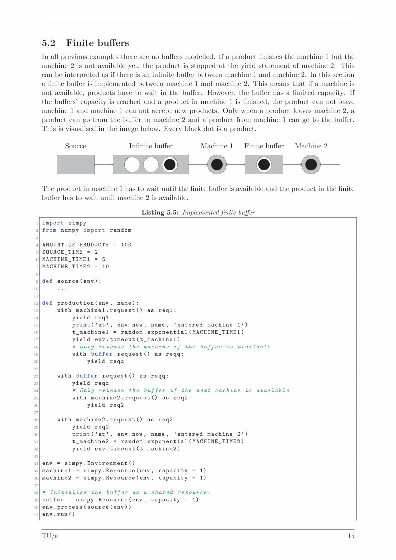
5.2 Finite buffersIn all previous examples there are no buffers modelled. If a product finishes the machine 1 but themachine 2 is not available yet, the product is stopped at the yield statement of machine 2. Thiscan be interpreted as if there is an infinite buffer between machine 1 and machine 2. In this sectiona finite buffer is implemented between machine 1 and machine 2. This means that if a machine isnot available, products have to wait in the buffer. However, the buffer has a limited capacity. Ifthe buffers’ capacity is reached and a product in machine 1 is finished, the product can not leavemachine 1 and machine 1 can not accept new products. Only when a product leaves machine 2, aproduct can go from the buffer to machine 2 and a product from machine 1 can go to the buffer.This is visualised in the image below. Every black dot is a product.

Source Infinite buffer Machine 1 Finite buffer Machine 2

The product in machine 1 has to wait until the finite buffer is available and the product in the finitebuffer has to wait until machine 2 is available.

Listing 5.5: Implemented finite buffer1 import simpy2 from numpy import random3

4 AMOUNT_OF_PRODUCTS = 1005 SOURCE_TIME = 26 MACHINE_TIME1 = 57 MACHINE_TIME2 = 108

9 def source (env):10 ...11

12 def production (env , name):13 with machine1 . request () as req1:14 yield req115 print(’at’, env.now , name , ’entered machine 1’)16 t_machine1 = random . exponential ( MACHINE_TIME1 )17 yield env. timeout ( t_machine1 )18 # Only release the machine if the buffer is available19 with buffer . request () as reqq:20 yield reqq21

22 with buffer . request () as reqq:23 yield reqq24 # Only release the buffer if the next machine is available25 with machine2 . request () as req2:26 yield req227

28 with machine2 . request () as req2:29 yield req230 print(’at’, env.now , name , ’entered machine 2’)31 t_machine2 = random . exponential ( MACHINE_TIME2 )32 yield env. timeout ( t_machine2 )33

34 env = simpy. Environment ()35 machine1 = simpy. Resource (env , capacity = 1)36 machine2 = simpy. Resource (env , capacity = 1)37

38 # Initialize the buffer as a shared resource .39 buffer = simpy. Resource (env , capacity = 1)40 env. process ( source (env))41 env.run ()

TU/e 15

Before machine1 is released, in line 20 it is checked if buffer is available. If buffer is not availablethe product stays in machine1. When buffer is released the product in machine1 can requestbuffer and machine1 is released. The capacity of buffer can be changed in the initialization.buffer is modeled with a shared resource.

5.3 Priority resourceUntil this point every queue of shared resource used the principle first come first serve. The productthat arrived first is accepted first. A priority resource has an extra functionality where differentproducts have different priorities. The priority is indicated with integers, the lower the number thehigher the priority. When a product arrives in a queue, it passes all products with a higher prioritynumber (and thus a lower priority). A priority resource does not kick a product out of the machinewhen a new product with a higher priority arrives in the queue.

Source Infinite buffer

0 1

Priority machine

A priority resource is initialized the same as a normal resource. It can also be used as a normalresource.

Listing 5.6: Initialize priority resource1 Example_priority_resource = simpy. PriorityResource (env , capacity = 1)

To make use of the priority functionality, it is important to give the priority as an argument whenthe process is initialized. This is shown in the example below.

Listing 5.7: Priority resource1 import simpy2 from numpy import random3



10 yield env. timeout ( SOURCE_TIME )11

12 # Give the product a random priority 0, 1 or 213 priority = random . randint (0, 3)14 print(’after ’, env.now , ’seconds ’, ’Product %2d’ % i, ’was generated with

priority ’, priority )15

16 # Initialize process and give priority as an extra argument17 c = production (env , ’Product %2d’ % i, priority )18 env. process (c)19

20 def production (env , name , priority ):21

22 # Create the with statement and define what exactly the integer for priority is23 with machine . request ( priority = priority ) as req:24 yield req25 print(’at’, env.now , name , ’entered the machine ’)26 yield env. timeout ( MACHINE_TIME )27

28 env = simpy. Environment ()

TU/e 16

29 machine = simpy. PriorityResource (env , capacity = 1)30 env. process ( source (env))31 env.run ()

In the example above the priority is a random integer from 0 to 2. In the parenthesis of the requestit is stated what defines the priority (line 23). Even if the priority is called priority it has to bestated in the parenthesis.

5.4 Sending products backIn this section a machine is modelled where products go from machine 1 to machine 2 and back tomachine 1. This is modeled by adding a process to the environment for every instance a productgoes from a machine to the next machine. Furthermore a priority resource is used to make sure aproduct that requests machine 1 for the second time has priority over the product that requests forthe first time. This priority is also used in an if statement to make sure products go only once tomachine 2.

Source Infinite buffer 1

Machine 1 Infinite buffer 2 Machine 2

Listing 5.8: Sending products back1 import simpy2

3 AMOUNT_OF_PRODUCTS = 104 SOURCE_TIME = 25 MACHINE_TIME1 = 26 MACHINE_TIME2 = 57


10 yield env. timeout ( SOURCE_TIME )11 print(’after ’, env.now , ’seconds ’, f’Product {i}’, ’was generated .’)12

13 # New products have a priority of 014 priority = 015 c = production1 (env , ’Product %2d’ % i, priority )16 env. process (c)17

18 def production1 (env , name , priority ):19 with machine1 . request () as req1:20 yield req121 print(’at’, env.now , name , ’entered machine 1’)22 yield env. timeout ( MACHINE_TIME1 )23

24 # Make an if statement to make sure that the product is only looped once25 if priority == 0:26 # Initialize a process for production 2 and add it to the environment27 env. process ( production2 (env , name , priority ))28

29 def production2 (env , name , priority ):30 with machine2 . request () as req2:31 yield req2

TU/e 17

32 yield env. timeout ( MACHINE_TIME2 )33

34 # Subtract 1 from priority to make sure it has priority in machine 135 priority -= 136 print(’at’, env.now , name , ’entered machine 2’)37

38 # Initialize a process for production 1 and add it to the environment39 env. process ( production1 (env , name , priority ))40


43 # Initialize two priority resources44 machine1 = simpy. PriorityResource (env , capacity = 1)45 machine2 = simpy. PriorityResource (env , capacity = 1)46 env. process ( source (env))47 env.run ()

5.5 BatchingIn this section a batching resource is modelled. Batching means that several products enter a batch-ing machine together at the same time and they have the same MACHINE_TIME. In this section abatching machine is modeled where the batching machine starts with a minimum batch size of 1.So the batch size can be different from one batch to another. Products can not enter the machineonce it has started.

SimPy does not have a functionility for a batching resource so a few changes have to be made tothe existing resource. This can be done with inheritance of a class. The original function can beseen below.

Listing 5.9: Original source code1 class Resource (base. BaseResource ):2 def _do_put (self , event):3 if len(self.users) < self. capacity :4 self.users . append (event)5 event. succeed ()

The class resource is already an inherited class from another class, BaseResource. The classResource contains multiple functions but _do_put is the only function that needs changes forthe batching resource. This function is called when a new product arrives at the resource or whena product leaves the resource. In both cases it checks if it is possible to accept a new product. In_do_put it is checked if the amount of users, len(self.users), is smaller than the capacity of theresource, self.capacity. If the amount of users is smaller than the capacity and there is a productin the queue, it accepts the next product in the queue.

For a batching resource the condition to accept a new product is changed. Products can only enterthe machine when it has not started yet. If self.users is zero, there are no current users and itcan accept a new product. If a product requests the machine at exactly the same moment as theprevious product is accepted, it can also enter the machine because it is in the same batch. This ischecked with self.loading_time. To make sure the capacity is not exceeded, self.loading_timeis set to -1 if the capacity is reached.

A non-batching machine checks if a product can enter the machine every time a product leaves themachine or if a product arrives in the queue. In a batching machine multiple products can enterthe machine at the same moment. Therefore if a product enters the machine it also checks if moreproducts can enter the machine. This is managed in the source code and it can be achieved with areturn True statement.

Listing 5.10: Batching resource

TU/e 18

1 # Make a new class an inherit all the properties of a normal resource2 class BatchingResource (simpy. Resource ):3

4 # Rewrite the _do_put function5 def _do_put (self , event: simpy. Resource . request ) -> None:6

7 # Make an if statement to determine the moment when the first productof a batch enters the machine

8 if len(self.users) == 0:9 self. loading_time = env.now

10

11 # Make an if statement to make sure the capacity is not exceeded .Return False

12 if len(self.users) >= self. capacity :13 self. loading_time = -114 return False15

16 # If the product request is at the same time as the request of thefirst product of the batch , it can enter the machine . Return True

17 elif self. loading_time == env.now:18 self.users. append (event )19 event. usage_since = self._env.now20 event. succeed ()21 return True

The batching resource can be used by initializing it like below:

Listing 5.11: Initializing batching resource1 batching_machine = Batchingresource (env , capacity = 3)

A capacity lower than 2 does not make sense since a batch of 1 is also possible with a normalresource.

5.6 Large amount of resourcesIn the previous sections the amount of resources was relatively small. In this section the resourcesare modelled in a way that the amount of resources is scalable easily.

A function is made where every resource is initialized. The resources are put in a list like insubsection 5.1.1. The list is returned and every resource can be requested by referring to thecorresponding list element.

Listing 5.12: Vehicle generator1 import simpy2

3 AMOUNT_OF_MACHINES = 104

5 # Make a function to generate resources6 def generate_machines (env , amount_of_machines ):7

8 # Make an empty list where all machines can be appended9 machines = []

10

11 # Make a for -loop that loops for every machine once12 for i in range ( amount_of_machines ):13

14 # Initialize a machine15 machine = simpy. Resource (env , capacity = 1)16

17 # Append the machine to the list18 machines . append ( machine )19 return ( machines )

TU/e 19

20

21


24 # Call the function to generate all resources25 machines = generate_machines (env , AMOUNT_OF_MACHINES )

In the list machines all vehicles can be found. The vehicles are all named machine and can bedistinguished by the position in the list.

With a list of resources the source and the production can be modelled.

Listing 5.13: Large amount of resources1 import simpy2 from numpy import random3

4 AMOUNT_OF_MACHINES = 105 AMOUNT_OF_PRODUCTS = 1006 SOURCE_TIME = 27 MACHINE_TIME = 108

9 ’’’ Define the source function . Determine in the source function to which machineit is send and call the production function . Give the machine and the number of

the machine as an argument . ’’’10 def source (env):11 for i in range ( AMOUNT_OF_PRODUCTS ):12 yield env. timeout ( SOURCE_TIME )13 destination_machine_number = random . randint (0, AMOUNT_OF_MACHINES )14 destination_machine = machines [ destination_machine_number ]15 c = production (env , ’Product %2d’ % i, destination_machine ,

destination_machine_number )16 env. process (c)17

18 # Define the production function19 def production (env , name , destination_machine , number ):20 with destination_machine . request () as req:21 yield req22 yield env. timeout ( MACHINE_TIME )23 print(name , ’finished machine ’, number )24

25 def generate_machines (env):26 machines = []27 for i in range ( AMOUNT_OF_MACHINES ):28 machine = simpy. Resource (env , capacity = 1)29 machines . append ( machine )30 return ( machines )31

32


35 machines = generate_machines (env)36

37 env. process ( source (env))38 env.run ()

TU/e 20

6 | DiscussionIn this chapter, it is discussed what the considerations in the tutorial were. It is also explainedwhat the limitations are and what can be concluded.

In this tutorial, only existing classes from SimPy are used. Classes could have also been used tomake multiple production lines for example. Classes are a useful tool when coding in Python. Nev-ertheless, classes require more understanding of Python than most functions that are used in thistutorial. It is an option to use classes in a very standardized way. In that case, the students donot have to design a class themselves but use the existing structure that is delivered. However, inthis tutorial, it is chosen to not make extra classes than the existing SimPy classes and keep it simple.

There are a lot of options in designing a production line with SimPy and this tutorial discussesonly a limited amount of possibilities. The discussed methods are considered suitable for the course4DC10 but there are likely similar or even more suitable variations possible. Since there is nota measurement tool to decide which design options are most suitable for the course it is partly amatter of opinion which options are preferred.


7 | ConclusionIn this report, a tutorial for SimPy is presented. With this tutorial, it is demonstrated that SimPyis a suitable substitute for Chi 3. First of all, it is shown that it is possible to model differentaspects that are necessary to simulate the assignment. When several examples of the tutorial arecombined the assignment can be executed. Second of all the code is kept fairly simple and neat.This makes learning the code and using the code a lot easier. However, there are a few side notesto this conclusion.

During the modeling of the different components that are used several findings have been done. It isimportant to have a basic understanding of Python before this tutorial is followed. A lot of aspectsof Python that are used are not explained. Without proper prior Python knowledge, people willhave a hard time following this tutorial.

There are examples available on the internet that present the possibilities with SimPy [2]. Allexamples show a different implementation, however, none of those examples are similar to theassignment of Analysis of production systems. It is concluded that SimPy is a good replacementfor Chi 3, but added explanations and examples like this tutorial are required.


Bibliography[1] Schenk, K.L., Lefeber, A.A.J. (2020). An orientation for discrete event simulation languages

for 4DC10. Retrieved in December 2020 from https://dc.wtb.tue.nl/lefeber/education/former-bsc-students/

[2] Topical guide SimPy. (n.d.). Simpy.Readthedocs.Io. Retrieved in December 2020 from https://simpy.readthedocs.io/en/latest/topical_guides/index.html

[3] Modeling and simulation of an autonomous vehicle storage and retrieval system (n.d.)


A | Case studyIn order to show what is possible with the given examples, a case study is done. This case studyconsists of the intermediate assignment of the course Analysis of production systems of 2020. Inthis chapter every part of the model is explained separately. In the end the different parts can bejoint to a full working model.

A.1 Generate vehicles and buffersIn the assignment totes are transported by vehicles and lifts. The vehicles and lifts can be modeledas a shared resource. Since the amount of vehicles is big it is chosen to model them with a for loop.When modeled with a for loop the amount of vehicles can be changed easily which saves a lot oflabour. Since there is a finite buffer with every vehicle it is logical to model them in the same forloop. There is a list for all vehicles and there is a list for all buffers. This can be seen below:

Listing A.1: Vehicles and buffers1 import simpy2

3 # The amount of floors determine the eventual amount of vehicles and buffers4 AMOUNT_OF_FLOORS = 105

6 def generate_vehicles_and_buffers (env , amount_of_floors ):7 # Make an empty list for vehicles and an empty list for buffers8 vehicles = []9 buffers = []

10

11 # Make a for loop to initialize every vehicle and buffer12 for i in range ( amount_of_floors ):13 vehicle = simpy. Resource (env , capacity = 1)14 vehicles . append ( vehicle )15 buffer = simpy. Resource (env , capacity = 1)16 buffers . append ( buffer )17

18 # Return the lists19 return (vehicles , buffers )20

21 env = simpy. Environment ()22 vehicles , buffers = generate_vehicles_and_buffers (env , AMOUNT_OF_FLOORS )

A.2 SourceIn the source the position of the new tote is determined. This is done with random integers.

Listing A.2: Source1 import simpy2 from numpy import random3

4 NEW_PRODUCTS = 105 SOURCE_TIME = 106 AMOUNT_OF_FLOORS = 37 AMOUNT_OF_COLUMNS = 128

9 def source (env , number , interval ):10 """ Source generates products with an exponential distribution """11 for i in range ( number ):12 # Determine the location of the product13 position = [ random . randint (0, AMOUNT_OF_FLOORS ), random . randint (0,

AMOUNT_OF_COLUMNS )]14

15 # Pick the corresponding vehicle and buffer from the lists16 vehicle , buffer = vehicles [ position [0]] , buffers [ position [0]]


17 t = random . exponential (scale= interval )18 yield env. timeout (t)19 c = go_through_vehicle (env , ’Product %2d’ % i, position , vehicle , buffer )20 env. process (c)21

22 env = simpy. Environment ()23 env. process ( source (env , NEW_PRODUCTS , SOURCE_TIME ))

A.3 Vehicle and buffer functionThe products are send to the correct vehicles with a process in the source.

Listing A.3: Vehicles function1 import simpy2

3 def go_through_vehicle (env , name , position , vehicle , buffer ):4 with vehicle . request () as req1:5 yield req16

7 # Add 1 to the corresponding column since the first column starts at 18 column = ( position [1] + 1)9

10 # Calculate the distance it takes the vehicle to accelerate to the maximumvelocity and decelerate to zero again

11 acceleration_distance_vehicle = ( MAXIMUM_VELOCITY_VEHICLE ** 2)/ACCELERATION_VEHICLE

12

13 # Multiply the columns with the clearance width14 vehicle_distance = ( column )* CLEARANCE_WIDTH15

16 # Make an if statement to calculate the transport time17 if vehicle_distance <= acceleration_distance_vehicle :18 movingtimevehicle = 2* math.sqrt( vehicle_distance / ACCELERATION_VEHICLE )19 else:20 movingtimevehicle = MAXIMUM_VELOCITY_VEHICLE / ACCELERATION_VEHICLE +

vehicle_distance / MAXIMUM_VELOCITY_VEHICLE21

22 # Make an env. timeout for transport to and from the tote and the loadingtime

23 yield env. timeout (2* movingtimevehicle + LOADING_TIME_VEHICLE )24

25 # Check if the corresponding buffer is available26 with buffer . request () as reqq:27 yield reqq28 yield env. timeout ( LOADING_TIME_VEHICLE )29

30 with buffer . request () as reqq:31 yield reqq32

33 # Check if the lift is available34 with lift. request () as reql:35 yield reql36

37 # Since the lift first has to move to the buffer , the buffer is notreleased immediately .

38

39 # Calculate the acceleration distance of the lift40 acceleration_distance_lift = ( MAXIMUM_VELOCITY_LIFT **2)/

ACCELERATION_LIFT41

42 # Add 1 to the the amount of floors because the floors start at 1, also multiply with the clearance height

43 lift_distance = ( position [0]+1) * CLEARANCE_HEIGHT44

TU/e 25

45 # Make a if statement to calculate the transport time46 if lift_distance <= acceleration_distance_lift :47 movingtimelift = 2* math.sqrt( lift_distance / ACCELERATION_LIFT )48 else:49 movingtimelift = MAXIMUM_VELOCITY_LIFT / ACCELERATION_LIFT +

lift_distance / MAXIMUM_VELOCITY_LIFT50 yield env. timeout ( movingtimelift + LOADING_TIME_LIFT )51

52 # Make process for lift53 l = lift(env , name , position , vehicle , buffer , movingtimelift )54 env. process (l)

A.4 LiftBelow the lift is modelled.

Listing A.4: Lift1 def lift(env , name , position , vehicle , buffer , movingtimelift ):2 with lift. request () as req:3 yield req4

5 # Make an env. timeout for unloading and transporting6 yield env. timeout ( LOADING_TIME_LIFT + movingtimelift )7 print(env.now , name , ’got to exit ’)8

9 lift = simpy. Resource (env)

A.5 Complete modelAll sections above can be combined into one model. The required constants have to be added tomake the simulation work. The result is shown below:

Listing A.5: Complete simulation of an autonomous vehicle storage1 from numpy import random2 import simpy3 import math4

5 AMOUNT_OF_PRODUCTS = 10 # Amount of products that arrive in this simulation6 AMOUNT_OF_FLOORS = 9 # The amount of floors that the storage has7 AMOUNT_OF_COLUMNS = 55 # The amount of columns the storage has8 LOADING_TIME_LIFT = 2 # Time it takes for (un) loading the lift9 LOADING_TIME_VEHICLE = 3 # Time it takes for (un) loading vehicle

10 CLEARANCE_WIDTH = 0.5 # Width between columns11 CLEARANCE_HEIGHT = 0.8 # Height between floors12 MAXIMUM_VELOCITY_VEHICLE = 1.5 # Maximum velocity of the vehicle13 ACCELERATION_VEHICLE = 1 # Acceleration of the vehicle14 MAXIMUM_VELOCITY_LIFT = 5 # Maximum velocity of the lift15 ACCELERATION_LIFT = 7 # Acceleration of the lift16 SOURCE_TIME = 7 # Average time interval between tote requests17

18 def generate_vehicles_and_buffers (env , amount_of_floors ):19 vehicles = []20 buffers = []21 for i in range ( amount_of_floors ):22 vehicle = simpy. Resource (env , capacity = 1)23 vehicles . append ( vehicle )24 buffer = simpy. Resource (env , capacity = 1)25 buffers . append ( buffer )26 return (vehicles , buffers )27

28 def source (env , number , interval ):29 for i in range ( number ):

TU/e 26

30 position = [ random . randint (0, AMOUNT_OF_FLOORS ), random . randint (0,AMOUNT_OF_COLUMNS )]

31 vehicle , buffer = vehicles [ position [0]] , buffers [ position [0]]32 t = random . exponential (scale= interval )33 yield env. timeout (t)34 c = vehicle_function (env , ’Product %2d’ % i, position , vehicle , buffer )35 env. process (c)36

37 def vehicle_function (env , name , position , vehicle , buffer ):38 with vehicle . request () as req1:39 yield req140 column = ( position [1] + 1)41 acceleration_distance_vehicle = ( MAXIMUM_VELOCITY_VEHICLE ** 2)/

ACCELERATION_VEHICLE42 vehicle_distance = ( column )* CLEARANCE_WIDTH43 if vehicle_distance <= acceleration_distance_vehicle :44 movingtimevehicle = 2* math.sqrt( vehicle_distance / ACCELERATION_VEHICLE )45 else:46 movingtimevehicle = MAXIMUM_VELOCITY_VEHICLE / ACCELERATION_VEHICLE +

vehicle_distance / MAXIMUM_VELOCITY_VEHICLE47 yield env. timeout (2* movingtimevehicle + LOADING_TIME_VEHICLE )48 with buffer . request () as reqq:49 yield reqq50 yield env. timeout ( LOADING_TIME_VEHICLE )51

52 with buffer . request () as reqq:53 yield reqq54 with lift. request () as reql:55 yield reql56 acceleration_distance_lift = ( MAXIMUM_VELOCITY_LIFT **2)/

ACCELERATION_LIFT57 lift_distance = ( position [0]+1) * CLEARANCE_HEIGHT58 if lift_distance <= acceleration_distance_lift :59 movingtimelift = 2* math.sqrt( lift_distance / ACCELERATION_LIFT )60 else:61 movingtimelift = MAXIMUM_VELOCITY_LIFT / ACCELERATION_LIFT +

lift_distance / MAXIMUM_VELOCITY_LIFT62 yield env. timeout ( movingtimelift + LOADING_TIME_LIFT )63 l = lift_function (env , name , position , vehicle , buffer , movingtimelift )64 env. process (l)65

66 def lift_function (env , name , position , vehicle , buffer , movingtimelift ):67 with lift. request () as req:68 yield req69 yield env. timeout ( LOADING_TIME_LIFT + movingtimelift )70 print(env.now , name , ’got to exit ’)71

72 env = simpy. Environment ()73 vehicles , buffers = generate_vehicles_and_buffers (env , AMOUNT_OF_FLOORS )74 lift = simpy. Resource (env)75 env. process ( source (env , AMOUNT_OF_PRODUCTS , SOURCE_TIME ))76 env.run ()

TU/e 27

B | Verification of modelsThe experience of coding has learned that the results are rarely correct in the first version. Thereforethe results have to be verified with queuing theory. In this chapter it is explained how to determinethe value of the average flow time of all products. This can be compared to the outcome of queuingtheory formulas.

The flow_time of a product is the time difference between the moment that it enters the systemand the moment that is leaves the system. Therefore the starting time is saved under the namestart_time and given as an argument to the next function. After the timeout of the last machineis processed the flow time is calculated. This is done by subtracting env.now by the start_time.Below there is an example of a simple model with a source and one machine with an exponentialdistributed MACHINE_TIME.

Listing B.1: Flow time1 import simpy2 from numpy import random3


8 def source (env , AMOUNT_OF_PRODUCTS , SOURCE_TIME ):9 for i in range ( AMOUNT_OF_PRODUCTS ):

10 t_source = random . exponential ( SOURCE_TIME )11 yield env. timeout ( t_source )12

13 # Save the time that the product entered the system and give it as anargument

14 start_time = env.now15 c = production (env , ’Product %2d’ % i, start_time )16 env. process (c)17

18 def production (env , name , start_time ):19 with machine . request () as req:20 yield req21 t_machine = random . exponential ( MACHINE_TIME )22 yield env. timeout ( t_machine )23

24 # Calculate the flow time and append it to the list of flow times25 flow_time = env.now - start_time26 flow_times . append( flow_time )27

28 # Make an empty list for the flow times29 flow_times = []30

31 env = simpy. Environment ()32 machine = simpy. Resource (env , capacity = 1)33 env. process ( source (env , AMOUNT_OF_PRODUCTS , SOURCE_TIME ))34 env.run ()35

36 # Calculate the average flow time37 average_flow_time = sum( flow_times )/len( flow_times )

In the script above the average flow time of a product is calculated. However the average flowtime of one simulation with 10 products is not very significant. To get a more significant averageflow time AMOUNT_OF_PRODUCTS has to be increased. An other important factor in the significanceof the flow time is the amount of simulations. When the model is run multiple times the averageof multiple simulations can be calculated. In other words, the average of the average flow time iscalculated. In the following sections this is called the overall_average_flow_time.


There are multiple ways of calculating the overall_average_flow_time. The most primitive op-tion is by running the script, noting down the average_flow_time and calculating theoverall_average_flow_time by hand. However this is not efficient, takes a lot of time and is notscalable. In the following part it is explained how to run multiple simulations in a for-loop toovercome this problem.

Listing B.2: Overall average flow time1 import simpy2 from numpy import random3

4 # Define the amount of simulations5 SIMULATIONS = 106 AMOUNT_OF_PRODUCTS = 107 SOURCE_TIME = 58 MACHINE_TIME = 59

10 # Make an empty list for the average flow times11 average_flow_times = []12

13 # Make a for -loop that runs SIMULATIONS amount of times14 for i in range( SIMULATIONS ):15

16 # A RANDOM_SEED is used to make every simulation reproducible17 RANDOM_SEED = i18

19 def source (env , AMOUNT_OF_PRODUCTS , SOURCE_TIME ):20 ...21

22 def production (env , name , start_time ):23 ...24

25 flow_times = []26 env = simpy. Environment ()27 machine = simpy. Resource (env , capacity = 1)28 env. process ( source (env , AMOUNT_OF_PRODUCTS , SOURCE_TIME ))29 env.run ()30

31 average_flow_time = sum( flow_times )/len( flow_times )32

33 # Append the average_flow_time to the average_flow_times list34 average_flow_times . append ( average_flow_time )35

36 # Calculate the overall_average_flow_time37 overall_average_flow_time = sum( average_flow_times )/len( average_flow_times )38

39 # Print the result and also state the amount of simulations and amount of productsper simulation

40 print( overall_average_flow_time , ’with ’, SIMULATIONS , ’simulations and ’,AMOUNT_OF_PRODUCTS , ’products per simulation ’)

With the overall_average_flow_time, SIMULATIONS and AMOUNT_OF_PRODUCTS the reliability ofthe model can be calculated. This can be done for example with a 95% confidence interval.

In the example above the amount of simulations and products per simulation is still relatively small.Bigger values give more significant results. The time it takes to run a lot of simulations with a lotof products is a down side. It can help to predict the time it takes to run the full code next timeby printing this after the results. This is done with the following lines of code at the beginning andend of your code.

Listing B.3: Calculate running time1 # import the time package

TU/e 29

2 import time3 # import other necessary packages4 ...5

6 # Define the starting time7 start_time = time.time ()8

9 # Put here your code10 ...11

12 # Print the running time13 print(’Running time is’, (time.time () - start_time ), ’seconds ’)

TU/e 30

Documents

Bachelor ﬁnal project - Modelling manufacturing systems