Embed Size (px)
Citation preview

Tivoli Performance Modeler for z/OS
User’s Guide
Version 2 Release 3
SC31-6385-07
���


Tivoli Performance Modeler for z/OS
User’s Guide
Version 2 Release 3
SC31-6385-07
���
Eighth Edition (September 2008)
This edition applies to IBM Tivoli® Performance Modeler for z/OS, Version 2 Release 3, Program Number 5698-A18
and to any subsequent releases until otherwise indicated in new editions. Make sure you are using the correct
edition for the level of the product.
More information about this and related products is available at
http://www-3.ibm.com/software/tivoli/products/perf-model-zos/
Order publications through your IBM representative or the IBM branch office serving your locality. Publications are
not stocked at the address below.
A form for reader’s comments is provided at the back of this publication. If the form has been removed, address
your comments to
IBM Corporation
H150/090
555 Bailey Avenue
San Jose, CA 95141-1003
U.S.A.
or fax your comments from within the U.S.A., to 800-426-7773, or, from outside the U.S.A., to 408-463-2629.
When you send information to IBM, you grant IBM a nonexclusive right to use or distribute the information in any
way it believes appropriate without incurring any obligation to you.
© Copyright International Business Machines Corporation 2002, 2008.
US Government Users Restricted Rights – Use, duplication or disclosure restricted by GSA ADP Schedule Contract
with IBM Corp.
Note!
Before using this information and the product it supports, be sure to read the general information under
“Notices” on page 135.
Contents
Figures . . . . . . . . . . . . . . . v
Chapter 1. Introduction and Overview . . 1
Using this manual . . . . . . . . . . . . 1
Introduction . . . . . . . . . . . . . . 1
Simulation versus analytic models . . . . . . . 2
Model input and output . . . . . . . . . . 3
Workload types and simulation . . . . . . . . 4
Simulation techniques . . . . . . . . . . . 5
Chapter 2. Performance Modeler
installation and system requirements . . 7
System requirements . . . . . . . . . . . . 7
Installation instructions . . . . . . . . . . . 7
Chapter 3. The Primary menu . . . . . 9
Chapter 4. Input screens . . . . . . . 13
The Configuration Definition screen . . . . . . 13
The Workload Definition screen . . . . . . . 15
The LPAR Definition screen . . . . . . . . . 17
Chapter 5. Running the simulator . . . 19
Run options . . . . . . . . . . . . . . 19
The Simulator Running screen . . . . . . . . 20
Graphing workload performance . . . . . . . 22
Print options . . . . . . . . . . . . . . 24
Chapter 6. Getting started -
performance modelling basics . . . . 27
Step 1 - Extract the RMF Reports and create the
LPAR.RPT and WGL.RPT files . . . . . . . . 27
Step 2 - Import the extracted reports into a
spreadsheet . . . . . . . . . . . . . . 32
Step 3 - Generate a chart showing utilization by
LPAR as well as total utilization for all LPARs . . . 34
Step 4 - Import the Workload Activity Report File
into the spreadsheet . . . . . . . . . . . 35
Step 5 - Graph the Workload Utilization . . . . . 37
Step 6 - Build a baseline model using the Build
function . . . . . . . . . . . . . . . 39
MIPS Discussion . . . . . . . . . . . . . 50
Capacity planning with Performance Modeler . . . 53
Service Level Agreements (SLAs) . . . . . . . 53
Capacity planning methodology . . . . . . . 54
Multi Image Run Wizard . . . . . . . . . . 62
Chapter 7. Modelling zAAP processors 71
zAAP overview . . . . . . . . . . . . . 71
Extracting zAAP information . . . . . . . . 74
zAAP processing options . . . . . . . . . . 77
New zAAP screens in performance modeler . . . 78
Building a model with zAAP CPs . . . . . . . 81
zAAP changes to the output reports . . . . . . 92
zAAP changes to Run Wizard . . . . . . . . 94
zAAP changes to Multi Image Run Wizard . . . . 95
Chapter 8. Modelling zIIP processors 101
zIIP overview . . . . . . . . . . . . . 101
Extracting zIIP information . . . . . . . . . 103
Graphing zIIP utilization . . . . . . . . 104
New zIIP screens in Performance Modeler . . . 104
Building a model with zIIP CPs . . . . . . . 107
Other changes due to modelling zIIP CPs . . . . 110
zIIP changes to the output reports . . . . . 110
Chapter 9. The Consolidate
spreadsheet function . . . . . . . . 113
Chapter 10. Monitoring IFL and ICF
processors . . . . . . . . . . . . 121
Extracting IFL and ICF information . . . . . . 121
Importing the extracted reports into a spreadsheet 121
Generating a chart showing ICF (or IFL) utilization 122
Appendix A. Workload Table
description . . . . . . . . . . . . 125
Appendix B. Defaults used in the
Build process . . . . . . . . . . . 129
Appendix C. Advanced modelling
topics . . . . . . . . . . . . . . . 131
Modelling TSO . . . . . . . . . . . . . 131
Modelling CICS and IMS . . . . . . . . . 131
Modelling workload growth . . . . . . . . 132
Latent demand in batch workloads . . . . . . 133
Notices . . . . . . . . . . . . . . 135
Trademarks . . . . . . . . . . . . . . 136
Index . . . . . . . . . . . . . . . 137
© Copyright IBM Corp. 2002, 2008 iii
| | | | | | | | |

iv Performance Modeler Ver 2 Rel 3 User’s Guide

Figures
1. The Primary menu and the Configuration
Definition screen . . . . . . . . . . . 9
2. The Workload Definition screen . . . . . . 15
3. The LPAR Definition screen . . . . . . . 17
4. The Simulator Running screen . . . . . . 20
5. The Graph Selection screen . . . . . . . 22
6. The Performance Tracking screen . . . . . 23
7. The Processor Utilization Tracking screen 24
8. The Print Option screen . . . . . . . . 25
9. LPAR Report Extract Screen . . . . . . . 28
10. LPAR Report Extract Screen . . . . . . . 30
11. Workload Report Extract Screen . . . . . . 31
12. Input Spreadsheet for CPFPM.123 . . . . . 33
13. LPAR Data Sheet . . . . . . . . . . . 34
14. LPAR Utilization Graph Sheet . . . . . . 35
15. Workload Data Sheet . . . . . . . . . 36
16. Workload Utilization Graph Sheet . . . . . 38
17. Model Build screen . . . . . . . . . . 40
18. Filled in Build Screen . . . . . . . . . 41
19. Select LPAR/Date/Time screen . . . . . . 42
20. Workload Selection Screen . . . . . . . 43
21. Workload Type Definition . . . . . . . . 45
22. Workloads Selected . . . . . . . . . . 46
23. LPAR Definition screen . . . . . . . . 47
24. Calibration screen . . . . . . . . . . 48
25. Workloads screen . . . . . . . . . . 49
26. Run Wizard screen . . . . . . . . . . 55
27. Updated Run Wizard screen . . . . . . . 56
28. Growth Rate screen . . . . . . . . . . 57
29. LPAR Definition screen . . . . . . . . 58
30. Print Option screen . . . . . . . . . . 59
31. SIM.NUM Results . . . . . . . . . . 60
32. Simulator Summary Table . . . . . . . . 61
33. Multi Image Run Wizard screen . . . . . . 64
34. CPU Selection screen . . . . . . . . . 65
35. Select LPARs screen . . . . . . . . . . 66
36. Select LPARs screen, Part 2 . . . . . . . 67
37. Wizard Growth screen . . . . . . . . . 68
38. Multi Image LPAR Definition screen . . . . 69
39. New Workload Activity fields . . . . . . 72
40. Sample LPAR Data Report with zAAP LPARs 74
41. Input spreadsheet zAAP buttons . . . . . 75
42. zAAP Utilization Chart . . . . . . . . 76
43. zAAP Workload Utilization chart . . . . . 77
44. ZAAP Configuration screen . . . . . . . 79
45. zAAP Workload screen . . . . . . . . . 80
46. ZAAP LPAR screen . . . . . . . . . . 81
47. ZAAP Build screen . . . . . . . . . . 82
48. ZAAP Option Selection screen . . . . . . 83
49. ZAAP Build screen after Step 5 . . . . . . 84
50. Workload Selection screen . . . . . . . . 85
51. General Purpose LPAR Definition screen 86
52. ZAAP LPAR Definition screen . . . . . . 87
53. Calibration screen for general purpose CPs 88
54. Calibration screen for zAAP CPs . . . . . 89
55. Simulator Running screen - general purpose
CPs . . . . . . . . . . . . . . . 90
56. Simulator Running screen - ZAAP CPs 91
57. SIMT.PRT for zAAP Modelling . . . . . . 92
58. SIM.PRT Results . . . . . . . . . . . 93
59. SIM.NUM Results . . . . . . . . . . 94
60. Run Wizard zAAP LPAR Definition Screen 95
61. Multi Image Run Wizard Screen with zAAP
CPs . . . . . . . . . . . . . . . 96
62. Special Purpose CPU Selection Form . . . . 97
63. Multi Image LPAR Definitions screen . . . . 98
64. Multi Image zAAP LPAR Definition screen 99
65. RMF Partition Data Report . . . . . . . 102
66. Workload Activity Report . . . . . . . 103
67. New steps on CPFPM spreadsheets . . . . 104
68. zIIP Configuration screen . . . . . . . 105
69. zIIP Workload screen . . . . . . . . . 106
70. zIIP LPAR screen . . . . . . . . . . 107
71. Model Build screen . . . . . . . . . 108
72. ZIIP Option Selection screen . . . . . . 109
73. Calibration screen for General Purpose CPs 110
74. Reporting of zIIP utilization . . . . . . . 111
75. MIPS consumption by LPAR chart . . . . 113
76. CPU Utilization by LPAR for 2064-1C7 114
77. CPU Utilization by LPAR for 2064-2C7 115
78. CPU Utilization by LPAR for 2064-210 115
79. Consolidate spreadsheet . . . . . . . . 116
80. Changing the LPARs . . . . . . . . . 118
81. The new MIPS Consumption by LPAR chart 119
82. IFL and ICF spreadsheet buttons . . . . . 121
83. ICF utilitization example . . . . . . . . 122
84. Chart of ICF utilitization . . . . . . . . 123
85. Workload Table . . . . . . . . . . . 125
© Copyright IBM Corp. 2002, 2008 v
| | | | | |

vi Performance Modeler Ver 2 Rel 3 User’s Guide

Chapter 1. Introduction and Overview
Using this manual
This chapter provides an overview and introduction to Performance Modeler.
Chapter 2, “Performance Modeler installation and system requirements,” on page 7
tells you what you need to get Performance Modeler working, and how to install
it.
The next three chapters, Chapter 3, “The Primary menu,” on page 9, Chapter 4,
“Input screens,” on page 13, and Chapter 5, “Running the simulator,” on page 19
provide a description of the various input screens and their content. They also
describe the different options on the Primary menu. These chapters are in the form
of a reference guide.
If you are familiar with these screens and are looking for a quick start tutorial, skip
to Chapter 6, “Getting started - performance modelling basics,” on page 27. This
chapter describes the recommended methodology for building a model and
conducting a capacity planning study. While there are lots of ways to conduct a
study, this chapter is a good place to learn the basic steps, and contains the
recommended sequence for building a capacity plan.
Chapter 7, “Modelling zAAP processors,” on page 71 describes the process for
modelling the zAAP processors.
Chapter 8, “Modelling zIIP processors,” on page 101 describes the process for
modelling the zIIP processors.
Chapter 9, “The Consolidate spreadsheet function,” on page 113 describes the
Consolidate sheet of the Lotus 123 and Excel spreadsheets. The function is
designed to help you size a processor when you are looking to move LPARs, or
consolidate LPARs from one or more existing CECs onto a single new CEC.
Chapter 10, “Monitoring IFL and ICF processors,” on page 121 describes a function
that has been added to allow monitoring of the Integrated Facility for Linux (IFL)
and Integrated Coupling Facility (ICF) assigned processors for z9, z10 and follow
on processor families.
Appendix A, “Workload Table description,” on page 125 describes each column of
the Workload table sheet of the Lotus 123 and Excel spreadsheets.
Appendix B, “Defaults used in the Build process,” on page 129 provides details of
the defaults used in the Build process.
Appendix C, “Advanced modelling topics,” on page 131 discusses some advanced
modelling topics.
Introduction
Performance Modeler is a performance modelling tool which runs under the
Windows® NT (or higher level) operating system on a personal computer.
© Copyright IBM Corp. 2002, 2008 1
||||

Performance Modeler can model performance characteristics at the individual
workload level for MVS™, OS/390®, or z/OS® based mainframes.
Performance Modeler is a Systems Management tool. It is designed to help
Information Technology shops manage their day to day performance as well as
their long term Capacity Planning functions. This manual is intended for the IT
professional who has experience with performance analysis and capacity planning.
Performance Modeler falls into the class of tools described as models. Models are
tools that are easy to use, yet can predict the output of complex systems. Models
are valuable because they let you examine a number of “what if” scenarios without
the expense of running the actual scenarios on the system being studied. In the
world of S/390® mainframes, predicting the impact of changing hardware or
software can be a difficult task.
Performance Modeler uses sophisticated simulation techniques to model the
performance of these systems with a high degree of accuracy. One of the
advantages of Performance Modeler is that it is a PC-based tool. That means it can
be run over and over without using mainframe resources. Plus, Performance
Modeler is a portable tool, and can be run wherever your PC or laptop is located.
This manual reflects several changes to Performance Modeler which have been
incorporated into Version 2 Release 3. These changes significantly enhance
Performance Modeler over the previous release (Version 2 Release 2). The key
enhancements in Release 3 are:
v The maximum number of LPARs has been increased from 15 to 30.
v LPAR Names are now included in the configuration file and are displayed in all
of the screen panels showing LPAR definitions.
v During simulation, the MIPS rating for the CP being modelled is dynamically
adjusted based on actual processor utilization. A reference point of 90% busy is
used as the baseline. When utilization is below 90%, the MIPS rating increases.
When utilization is greater than 90%, the MIPS rating decreases. This is done to
simulate the actual change in processor efficiency when utilization changes.
Since IBM LSPR ratios are based on a machine running at 90% busy, this value
(90%) is used as the baseline for the defined MIPS rating.
v A new Run option called Multi Image Run Wizard has been added. This option
combines the features of the Multi Image Run option with the Run Wizard
option. Now, multi image modelling scenarios can be defined on a single screen
panel. Once these scenarios are defined, the Wizard creates multiple
configuration files, calibrates each configuration file, and finally runs each model
with the results stored in the defined output file. While the Multi Image Run
option is still retained under the Run menu, most Multi Image modelling can
now be done using the new Multi Image Run Wizard option.
With Version 2 Release 3, Performance Modeler has been enhanced to support
modelling processors with zIIP CPs. In addition, the number of LPARs that can be
modelled has increased from 30 to 60.
Simulation versus analytic models
Modelling techniques generally fall into one of two categories, simulation or
analytic. In some cases, hybrid models have been developed which use
combinations of both techniques. The differences between these techniques are:
Introduction
2 Performance Modeler Ver 2 Rel 3 User’s Guide

v Analytic models consist of mathematical equations which describe the processes
being modelled. Analytic models are used when the processes being modelled
are well understood and can be described as mathematical expressions.
Simulation models rely on running the actual process being modelled, but in a
simplified form. Since these processes take place over time, simulation requires
running (simulating) these processes over and over in order to reach a steady
state that mimics the real process.
v Analytic models are by their nature fast to run and require less processing
power than simulation. Analytic models execute a number of mathematical
equations and can run in seconds or less.
Computer based simulators must execute lots of instructions in order to simulate
one point in time. And since simulators must model a period of time, lots of
iterations must take place before the results are meaningful. This means
simulators can run for an extended amount of real time, and use a larger
amount of computer resources compared to analytic models.
v Simulators are used today to predict complex processes where analytic equations
are not suitable. Some examples of these simulators are models which are used
to predict weather and models which predict the presence of oil deposits. These
models require large amounts of computer resources but produce results that are
not attainable with analytic techniques.
In the early days of mainframe computers, operating systems were simpler than
they are today. But over time, features have been added and operating system
complexity has grown. Older analytic models which were developed to predict
computer performance have found it difficult to keep up with the changing nature
and complexity of today’s systems.
Simulation models have a distinct advantage over analytic models when it comes
to staying current. Simulators can be easily reprogrammed to model changes in the
operating system as they occur.
These differences between analytic and simulation models are some of the reasons
why Performance Modeler was developed as a simulation model. Although
Performance Modeler uses simulation techniques, it is very efficient. This means
the time it takes to reach a set of meaningful results is quite fast. In fact, running
on modern PCs, Performance Modeler runs in less real time than the amount of
time actually being simulated.
Model input and output
Performance Modeler can model nearly every hardware and software change that
might be made. This makes Performance Modeler quite powerful in being able to
answer “what if” scenarios.
For example, Performance Modeler can model the effects of hardware
configuration changes such as the number of CPUs, the speed of the CPUs, Disk
I/O response times, and paging rates (auxiliary and Expanded Memory paging).
Performance Modeler can also model the effects of changing LPAR (Logical
Partitioning) parameters, including the number of logical CPUs per LPAR and their
Weighting Factors. You can also change the amount of work being run to model
the impact of increased or decreased workload volumes.
All of these inputs are specified on three easy-to-understand screens. These are the
Configuration screen, the Workload Activity screen, and the LPAR Definition
screen.
Simulation versus analytic models
Chapter 1. Introduction and Overview 3

When modelling configurations with the new zAAP processors, additional
information must be defined. This information can be viewed or changed on three
new screens that can be accessed from the primary menu when you select the
ZAAPs option. These screens are described in Chapter 7, “Modelling zAAP
processors,” on page 71. Similarly, when modelling configurations with zIIP
processors, additional information must be defined. This information can be
viewed by selecting the zIIPs option on the Primary menu bar. These screens are
described in Chapter 8, “Modelling zIIP processors,” on page 101.
The output from running Performance Modeler includes standard CPU utilization
reports for the entire processor, as well as a breakdown of utilization by individual
LPAR. But the most important output metric is the performance of each workload
being modelled. For online workloads, this is average response time (in seconds).
For batch workloads, this is average elapsed time factors (this is described in more
detail in Chapter 5, “Running the simulator,” on page 19.
The ability to model the performance of individual workloads makes Performance
Modeler a powerful tool for Performance Management and Capacity Planning.
Workload types and simulation
All workloads are defined to Performance Modeler as one of three different
workload types. These are single tasking workloads (Type=S), multi-tasking
workloads (Type=M), and batch workloads (Type=B).
Type S and Type M are both used for defining online (OLTP) workloads. Online
workloads have these attributes:
They are made up of transactions that enter the system in a random pattern
and require a relatively short burst of processing capacity.
Each transaction executes independently from other transactions.
CICS® regions and IMS™ message processing regions are examples of online
workloads, and so are TSO generated transactions.
Single tasking workloads are made up of transactions which run under a single
TCB (Task Control Block) or single task. These transactions can only run on one
CPU at a time. Multi-tasking workloads represent workloads whose transactions
can execute on multiple CPUs at the same time. A single CICS region is an
example of a workload that should be defined as single tasking. Multi-tasking
workloads can represent a number of TSO users, or they can represent a group of
workloads that are defined as one consolidated workload.
Multi-tasking workloads can also represent a single OLTP region which runs as
multiple TCBs or multiple threads. A CICS region which runs a large amount of
DB2 data base transactions might be represented as Type=M since it probably runs
multiple DB2 threads.
Two important fields are used to define online workloads. These are Average
Arrival Rate and Average Path Length. Average Arrival Rate is the average
transaction rate (transactions per second) and determines the rate at which new
transactions enter the system. The Average Path Length defines the average
number of instructions per transaction.
When these two parameters are multiplied, the result is the average MIPS
consumed by this workload. For example, [transactions per second] X [# of
instructions in Millions per transaction] = Millions of instructions per second or
Model input and output
4 Performance Modeler Ver 2 Rel 3 User’s Guide

MIPS consumed. This is a handy relationship to remember since it is an easy check
to see how much capacity each online workload tries to consume.
Batch workloads (Type=B) are handled and modelled differently from online
workloads. Batch jobs appear to the model as transactions that never end. Each
batch job executes a number of instructions, stops to perform an I/O operation,
then resumes executing again when the I/O completes. Unlike online workloads,
there is no Arrival Rate to define. Batch jobs are either executing, waiting to
execute, or performing I/O operations. For batch workloads, the Average Path
Length represents the average # of instructions that must execute before stopping
for a synchronous I/O operation. The ratio of Average Path Length to the time
required to perform an I/O operation determines whether the batch job is CPU
bound or I/O bound. This ratio is also one of the key factors in determining how
many MIPS are consumed by this workload. The more CPU bound the job, the
greater the MIPS the job tries to consume.
Simulation techniques
When the model runs, real time is divided into increments of simulated time. At
the beginning of each time interval, the model examines each workload. For online
workloads, the model determines if it is time to generate a new transaction. The
model generates new transactions based on the Average Arrival Rate. Batch jobs
are represented as never ending transactions so they are always present.
Both batch and online workloads may be suspended due to paging activity or
when higher priority workloads preempt their execution. More information on
how Performance Modeler simulates workload performance is included in
Chapter 6, “Getting started - performance modelling basics,” on page 27.
Workload types and simulation
Chapter 1. Introduction and Overview 5

6 Performance Modeler Ver 2 Rel 3 User’s Guide

Chapter 2. Performance Modeler installation and system
requirements
System requirements
Performance Modeler is a Microsoft® Windows-based program. Performance
Modeler runs on any PC capable of running Windows 2000 or Windows XP. Due
to the CPU intensive nature of simulation, a PC internal clock speed of 1.5 GHz or
greater is recommended. Performance Modeler supports different screen display
sizes, but 1024 by 768 is recommended for optimum viewing.
This program has been developed and tested in a Windows environment with
the locale set to English-United States (EN-US). The program, and the Lotus 123
and Excel scripts, use decimal notation with a period as the decimal symbol, for
example “123.4”. Make sure you have set the locale to EN-US or other
compatible locale.
Installation instructions
Here is how to install Performance Modeler:
1. Run Setupwin32.exe from the root directory on the distribution CD-ROM.
The Welcome screen is displayed.
2. Click Next to continue with the installation. Clicking Cancel cancels the
installation.
The Software License Agreement is displayed.
3. Please read the license agreement. Select “I accept the terms in the license
agreement” to continue with the installation. The Directory Name screen is
displayed.
If you select “I do not accept the terms in the license agreement”, then the
Decline License screen is displayed. If you press Yes, then the installation is
canceled, and if you press No, then the Software License Agreement is
displayed again.
4. If you wish to change the folder to which Performance Modeler is installed, do
so now.
To move to the next screen, press Next.
The confirmation screen is displayed.
5. Press Next to continue the installation.
The Installing screen is displayed, with a progress bar showing the state of the
installation.
6. A screen is displayed indicating the succes or failure of the installation process.
7. Next to continue.
The README file is displayed.
8. Press Finish to complete the process.
To launch Performance Modeler click Start > Programs > IBM Tivoli Performance
Modeler > IBM Tivoli Performance Modeler.
To uninstall Performance Modeler click Start > Programs > IBM Tivoli
Performance Modeler > Uninstall or the standard Start > Settings > Control
Panel > Add > Remove Programs method.
© Copyright IBM Corp. 2002, 2008 7

Following a successful installation, you should have these files in the folder you
selected for installation:
Filename Description
CPFPM.EXE Executable program
CPUMIPSZ.DAT Table of processor MIPS ratings
The latest CPUMIPSZ.DAT file with all current
processor performance information can be found at
http://www-3.ibm.com/software/sysmgmt/products/support/IBMTivoliPerformanceModelerforzOS.html
under Support Flashes.
DEFAULT.SIM Default model definition statements
CPFPMZ.HLP Help file
C31685n.PDF User’s Guide
CPFPM.123 123 spreadsheet
CPFPM.XLS EXCEL spreadsheet
README.TXT Readme file
You should also have the following subdirectories:
Subdirectory Description
_uninst Product uninstall information
license License text files in national languages
Installation instructions
8 Performance Modeler Ver 2 Rel 3 User’s Guide

Chapter 3. The Primary menu
The Primary menu is the launching point for all Performance Modeler operations.
The Primary menu provides options for entering model definition parameters as
well as running the simulator.
The first screen that appears when Performance Modeler starts is the Primary
menu (see Figure 1).
Here are the Primary Menu options.
Menu option Description
File The File menu lets you save the current model or load a previously
saved model. Save all models with the SIM file type. If no file type
is specified, the SIM type is automatically added to the file name.
Run The Run menu specifies the type of simulation to be performed.
Six types of simulations are possible. These are Single Run,
Multiple Run, Calibration Run, Run Wizard, Multi Image Run, and
Figure 1. The Primary menu and the Configuration Definition screen
© Copyright IBM Corp. 2002, 2008 9

Multi Image Run Wizard. These options are described more fully
in Chapter 5, “Running the simulator,” on page 19.
Configuration The Configuration option displays the Configuration Definition
screen. This is screen 1 of 3 input screens. The Configuration
Definition screen lets you choose the configuration to be modelled.
Detailed information on these input fields is shown in Chapter 4,
“Input screens,” on page 13.
Workloads The Workloads option displays the Workload Definition screen.
This is screen 2 of 3 input screens. This is where you define the
workloads to be modelled. Detailed information on these input
fields is shown in Chapter 4, “Input screens,” on page 13.
LPAR The LPAR option displays the LPAR Definition screen. This is
screen 3 of 3 input screens. The LPAR Definition Screen is where
you specify information about LPAR mode. Detailed information
on these input fields is shown in Chapter 4, “Input screens,” on
page 13.
ZAAPs The ZAAPs option lets you access the screens where you provide
information about the zAAP processors. These screens are similar
to the Configuration Screen, the Workloads Screen, and the LPAR
Screen described earlier. But these screens contain information that
is specific to the zAAP processors. The three screens are labelled
ZConfiguration, ZWorkloads, and ZLPARs. Detailed information
about these screens is shown in Chapter 7, “Modelling zAAP
processors,” on page 71.
ZIIPs The ZIIPS option lets you access the screens where you provide
information about the zIIP processors. These screens are similar to
the Configuration Screen, the Workloads Screen, and the LPAR
Screen described earlier. But these screens contain information that
is specific to the zIIP processors. The three screens are labelled
IConfiguration, IWorkloads, and ILPARs. Detailed information
about these screens is shown in Chapter 8, “Modelling zIIP
processors,” on page 101.
Edit The Edit option provides a simple way to move workload and
LPAR definitions. Individual Workload or LPAR definitions can be
cut, copied, and pasted within the same configuration file, or to
other configuration files. This provides a simple point and click
facility for moving work between different models. This capability
can be used when modelling the impact of moving work within a
SYSPLEX.
Extract The Extract option provides a data reduction program which reads
RMF™ reports and extracts key performance metrics. The extracted
data is stored in a format that can be easily imported into
spreadsheet programs. The extracted data is also used by the Build
option to automatically build a new model. The Extract option is
described in Chapter 6, “Getting started - performance modelling
basics,” on page 27.
Build The Build option provides the ability to automatically generate the
model input parameters. This function is described in Chapter 6,
“Getting started - performance modelling basics,” on page 27.
Merge The Merge option lets you combine several text files together into a
single text file. This may be used to combine several RMF/CMF
The Primary menu
10 Performance Modeler Ver 2 Rel 3 User’s Guide

report files into a single file. Later chapters show how to extract
reporting information from these report files.
View The View option lets you toggle on or off the Expanded Tab
Feature. This feature helps people with vision problems, or other
disabilities that stop them using a mouse. In Expanded Tab mode,
you can change the cursor position so that it points to labels and
other descriptive fields on a screen. In the default mode (Expanded
Tab disabled), pressing the tab key only moves the cursor to
editable input fields, or to command buttons.
Quit Exit Performance Modeler.
Help Display help for Performance Modeler screens and functions.
The Primary menu
Chapter 3. The Primary menu 11

The Primary menu
12 Performance Modeler Ver 2 Rel 3 User’s Guide

Chapter 4. Input screens
Input to Performance Modeler can be hand entered or it can be generated using an
automated BUILD function. The BUILD function is described in Chapter 6,
“Getting started - performance modelling basics,” on page 27.
This chapter describes the input fields contained in the three input screens.
Descriptions of the three new zAAP input screens can be found in Chapter 7,
“Modelling zAAP processors,” on page 71. Descriptions of the three new zIIP input
screens can be found in Chapter 8, “Modelling zIIP processors,” on page 101.
Techniques for determining these values are covered in later chapters.
The Configuration Definition screen
The Configuration Definition screen (Figure 1 on page 9) is the first screen to
appear when Performance Modeler is started. This screen contains information
about the processor and configuration being modelled. Here is a description of
each input field.
Field Name Field Description
Title For This Run
A description of this model (documentation only).
Total Run Time (sec)
The total amount of time in seconds that is simulated. A default of
400 seconds is suitable for most models.
Time Interval (sec)
The simulator breaks up real time into discrete intervals based on
this parameter. The smaller the interval, the more accurate the
simulation. But a smaller interval also increases the time required
to complete the simulation. The default interval of .01 seconds
means the simulator performs 100 simulation passes in each
second of simulated time.
# Of Seconds Per Report
The simulator updates the results in the Running screen after this
number of simulated seconds have elapsed. For example, a value
of 5 means the results are updated after every 5 seconds of
simulated Time. Default value is 10.
CPU Description
Description of CPU being modelled (documentation only).
CPU Speed (mips)
MIPS rating (Millions of Instructions Per Second) for the CPU
being modelled. This is the MIPS rating for each engine, not the
entire processor. For example, if the processor is a 5 way MP with
a total MIPS rating of 100 then the MIPS rating for a single engine
would be 20 MIPS. The MIPS rating is a measure of processor
capacity.
# Of CPUs (1-64)
The # of CPUs being modelled. For a 5 way MP, the # would be 5.
© Copyright IBM Corp. 2002, 2008 13

Page Pack Resp. Time (sec)
The average response time (seconds) to read a page (4K block)
from disk storage.
E-Stor Resp. Time (sec)
The average time to move a page (4K block of memory) between
Expanded Storage and Central Storage.
# Of Workloads (1-40)
The # of workloads that are modelled.
# Of LPARS (0-60)
The # of LPARS to be modelled. A value of 0 means no LPAR
Modelling.
HiperDispatching
For System z10 systems and follow on processors only. Improves
the way workload is dispatched across the server.
The Configuration Definition screen
14 Performance Modeler Ver 2 Rel 3 User’s Guide

The Workload Definition screen
Figure 2 is an example of the Workload Definition screen.
This screen contains information about each workload being modelled. Up to 40
workloads can be defined.
The D and R buttons to the left of each workload provide a fast way to delete (D)
or replicate (R) this workload definition.
The S button is used to select the workload for editing. Once selected, the
workload definition fields change color. You can now click on the Edit menu
function where you can perform a Cut, Copy, or Insert operation.
v The Copy operation copies the selected workload definitions to an internal
clipboard.
v The Cut operation is identical to Copy but also removes the selected workload
from the active model.
v The Insert operation pastes the contents from the internal clipboard immediately
after the selected workload.
These functions provide a simple way to move workloads from one model to
another without the need to reenter workload definitions. The S button is also
available on the LPAR Definition screen and allows you to move LPAR definitions
in a similar way.
Figure 2. The Workload Definition screen
The Workload Definition screen
Chapter 4. Input screens 15
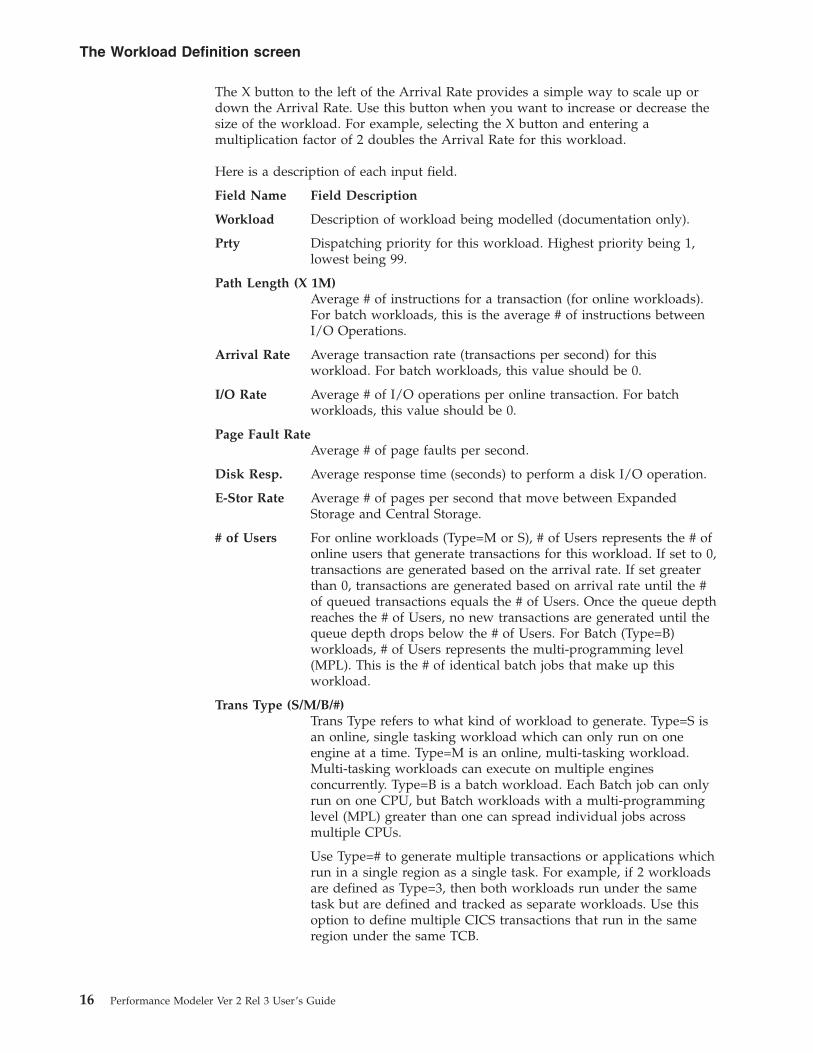
The X button to the left of the Arrival Rate provides a simple way to scale up or
down the Arrival Rate. Use this button when you want to increase or decrease the
size of the workload. For example, selecting the X button and entering a
multiplication factor of 2 doubles the Arrival Rate for this workload.
Here is a description of each input field.
Field Name Field Description
Workload Description of workload being modelled (documentation only).
Prty Dispatching priority for this workload. Highest priority being 1,
lowest being 99.
Path Length (X 1M)
Average # of instructions for a transaction (for online workloads).
For batch workloads, this is the average # of instructions between
I/O Operations.
Arrival Rate Average transaction rate (transactions per second) for this
workload. For batch workloads, this value should be 0.
I/O Rate Average # of I/O operations per online transaction. For batch
workloads, this value should be 0.
Page Fault Rate
Average # of page faults per second.
Disk Resp. Average response time (seconds) to perform a disk I/O operation.
E-Stor Rate Average # of pages per second that move between Expanded
Storage and Central Storage.
# of Users For online workloads (Type=M or S), # of Users represents the # of
online users that generate transactions for this workload. If set to 0,
transactions are generated based on the arrival rate. If set greater
than 0, transactions are generated based on arrival rate until the #
of queued transactions equals the # of Users. Once the queue depth
reaches the # of Users, no new transactions are generated until the
queue depth drops below the # of Users. For Batch (Type=B)
workloads, # of Users represents the multi-programming level
(MPL). This is the # of identical batch jobs that make up this
workload.
Trans Type (S/M/B/#)
Trans Type refers to what kind of workload to generate. Type=S is
an online, single tasking workload which can only run on one
engine at a time. Type=M is an online, multi-tasking workload.
Multi-tasking workloads can execute on multiple engines
concurrently. Type=B is a batch workload. Each Batch job can only
run on one CPU, but Batch workloads with a multi-programming
level (MPL) greater than one can spread individual jobs across
multiple CPUs.
Use Type=# to generate multiple transactions or applications which
run in a single region as a single task. For example, if 2 workloads
are defined as Type=3, then both workloads run under the same
task but are defined and tracked as separate workloads. Use this
option to define multiple CICS transactions that run in the same
region under the same TCB.
The Workload Definition screen
16 Performance Modeler Ver 2 Rel 3 User’s Guide
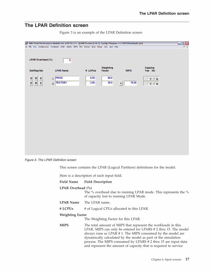
The LPAR Definition screen
Figure 3 is an example of the LPAR Definition screen.
This screen contains the LPAR (Logical Partition) definitions for the model.
Here is a description of each input field.
Field Name Field Description
LPAR Overhead (%)
The % overhead due to running LPAR mode. This represents the %
of capacity lost to running LPAR Mode.
LPAR Name The LPAR name.
# LCPUs # of Logical CPUs allocated to this LPAR.
Weighting Factor
The Weighting Factor for this LPAR.
MIPS The total amount of MIPS that represent the workloads in this
LPAR. MIPS can only be entered for LPARS # 2 thru 15. The model
always runs as LPAR # 1. The MIPS consumed by the model are
dynamically calculated by the model as part of the simulation
process. The MIPS consumed by LPARS # 2 thru 15 are input data
and represent the amount of capacity that is required to service
Figure 3. The LPAR Definition screen
The LPAR Definition screen
Chapter 4. Input screens 17

these LPARs. These are static values and represent a constant
amount of work running in LPARs # 2 thru 15.
Capping Yes No
Specifies whether LPAR Capping is to be enforced. When an LPAR
is Capped, it is limited to using a fraction of the total capacity of
the processor. The fraction it can use is determined by the
Weighting Factor. The fraction is calculated as Weight (this LPAR)
divided by the sum of the Weights for all LPARs.
Under normal operation (No Capping), LPAR weights are only
enforced when the processor utilization is at or near 100% busy.
But when Capping is turned on, the LPAR weight is always
enforced.
The LPAR Definition screen
18 Performance Modeler Ver 2 Rel 3 User’s Guide

Chapter 5. Running the simulator
Run options
The simulation process begins by selecting one of the five Run pull down menu
options from the Primary menu. These options include Single Run, Multiple Run,
Calibration Run, Run Wizard, and Multi Image Run. The following section
describes each of these options.
Run Option Description
Single Run Selecting Single Run starts the simulation process using the
currently loaded model.
Unless you stop the simulator by clicking the Stop button, the
model continues to run until is has simulated the Total Run Time
you selected. The Total Run Time is specified in the Configuration
Definition screen.
At the completion of the run, you can select one of these options:
Restart Restart the model from the beginning
Return Return to the Input screens
Print Print the results of the model
Multiple Run Multiple Run lets you run multiple models in a batch mode.
When you select Multiple Run, Performance Modeler displays a
screen that asks you to specify up to 25 model file names. These
are the names of the models which have been previously saved on
disk.
Save each model with the file type SIM. If the file name is entered
without an extension, a SIM extension is automatically added.
After each model completes its run, the results are written
according to your Print selection. The results can be printed
directly to the printer or written to disk.
Calibration Run
Calibration Run lets you calibrate the model.
This option is used to determine the correct Average Path Length
for all workloads. More information on this option is contained in
Chapter 6, “Getting started - performance modelling basics,” on
page 27.
Run Wizard The Run Wizard provides a simple way to create and run multiple
model configuration files (that is, SIM files).
Use this function after you create a baseline model and now want
to run multiple what if scenarios. More information on this option
is contained in Chapter 6, “Getting started - performance modelling
basics,” on page 27.
Multi Image Run
Use this option when you are trying to model multiple LPARs
running on the same processor. Normally, you only model the
performance of one LPAR. If there are two or more LPARs on the
processor, the first LPAR (LPAR #1) is the only LPAR that is
actually simulated. The other LPARs (LPAR #2 thru #15) are only
© Copyright IBM Corp. 2002, 2008 19

represented as a fixed amount of MIPS consumed. This works fine
when there is one dominant LPAR and multiple small additional
LPARs. But when there are two or more dominant LPARs, you
may want to model the performance of all of these LPARs. More
information on this option is contained in Chapter 6, “Getting
started - performance modelling basics,” on page 27.
Multi Image Run Wizard
This option combines the functions of the Multi Image Run with
the Run Wizard. You can define multiple scenarios for modelling
multiple images on the same processor. These scenarios can
involve modelling different growth rates over multiple intervals, as
well as multiple processors. After all of the scenarios are defined,
the Wizard creates all of the configuration files, calibrates them,
and finally runs each model with the results stored in the user
defined output file. The Multi Image Run Wizard option was
added in Version 2 Release 3. Since this option provides many of
the same functions provided in the older Multi Image Run option,
you do not need to use the Multi Image Run option.
The Simulator Running screen
The Simulator Running screen is displayed whenever the simulator is running.
Figure 4 shows an example of the Simulator Running screen.
This information is shown on the Simulator Running screen.
Figure 4. The Simulator Running screen
Run options
20 Performance Modeler Ver 2 Rel 3 User’s Guide

Field Description
Configuration The Configuration field shows the file name of the model currently
Running.
Simulation Time
Number of seconds that have been simulated to this point.
Real Time Used
Number of real seconds that have elapsed since the start of the
run.
Physical CPU Total CPU utilization (%) of the processor being modelled.
Model LCPU Model Logical CPU % busy. When running in LPAR mode, this is
the utilization of the LPAR being modelled (LPAR #1) from a
logical view. It represents the utilization of the logical
configuration, based on the number of logical CPUs defined to
LPAR #1. The calculation is CPU time used by LPAR #1 / (Total
Elapsed Time x # of Logical CPUs this LPAR).
Model PCPU Model Physical CPU % busy. This is the percent of the total
processor that is being used by the Model LPAR.
Workload Workload Name.
X Count Total # of transactions that have completed.
CPU (%) Single CPU % busy. Percent of a single CPU consumed by this
Workload.
Page Flts Page Faults. Total # of page faults that have occurred.
CPUR Real CPU Time. This is the average CPU time (seconds) per
Transaction.
NQ # of transactions currently on the input Queue. This is a snapshot
view of how many transactions are waiting to run at this point in
time.
AQLen Average Queue Length. The average # of transactions on the input
Queue measured over the total run time.
Resp Response Time. This value has two meanings depending on the
type of workload being modelled. For online workloads, this is the
average response time in seconds. For batch workloads this value
is called the Elongation Factor. Batch Elongation Factors represent a
measure of average elapsed time for each batch job running in this
workload.
The Elongation Factor is measured by the simulator and is the # of
real seconds that each batch job requires to execute 100 million
instructions. Since the total number of instructions executed by a
batch job is a constant value, the time required to run a batch job
can be calculated by the following formula:
Elapsed Time = Elongation factor x Total Number of Instructions /
100 Million.
In most cases, the Elongation Factor can be used by itself as a
baseline for average batch performance. For example, if the first
model shows an Elongation Factor of 25, and the second model
shows an Elongation Factor of 50, the following conclusion can be
drawn. The second model is predicting that average batch elapsed
The Simulator Running screen
Chapter 5. Running the simulator 21
times double compared to the first model. For most modelling
scenarios, the relative change in Elongation Factors is all that is
needed to predict the relative change in batch performance.
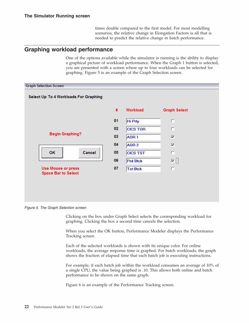
Graphing workload performance
One of the options available while the simulator is running is the ability to display
a graphical picture of workload performance. When the Graph 1 button is selected,
you are presented with a screen where up to four workloads can be selected for
graphing. Figure 5 is an example of the Graph Selection screen.
Clicking on the box under Graph Select selects the corresponding workload for
graphing. Clicking the box a second time cancels the selection.
When you select the OK button, Performance Modeler displays the Performance
Tracking screen.
Each of the selected workloads is shown with its unique color. For online
workloads, the average response time is graphed. For batch workloads, the graph
shows the fraction of elapsed time that each batch job is executing instructions.
For example, if each batch job within the workload consumes an average of 10% of
a single CPU, the value being graphed is .10. This allows both online and batch
performance to be shown on the same graph.
Figure 6 is an example of the Performance Tracking screen.
Figure 5. The Graph Selection screen
The Simulator Running screen
22 Performance Modeler Ver 2 Rel 3 User’s Guide
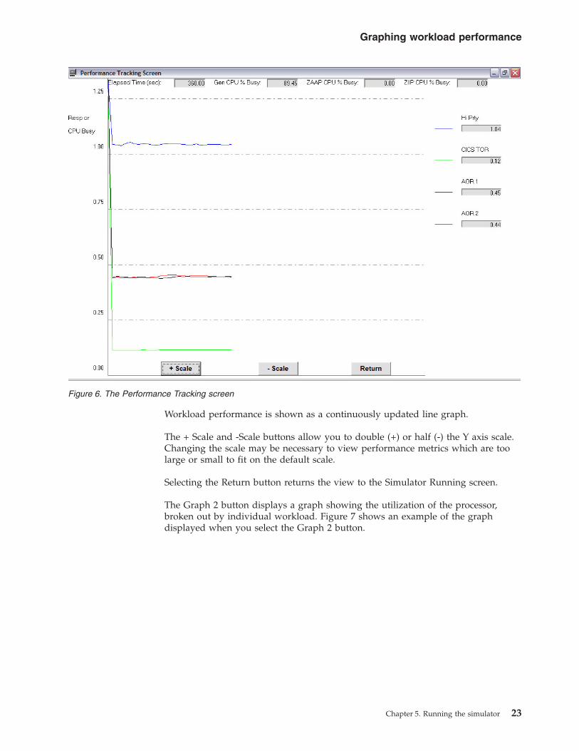
Workload performance is shown as a continuously updated line graph.
The + Scale and -Scale buttons allow you to double (+) or half (-) the Y axis scale.
Changing the scale may be necessary to view performance metrics which are too
large or small to fit on the default scale.
Selecting the Return button returns the view to the Simulator Running screen.
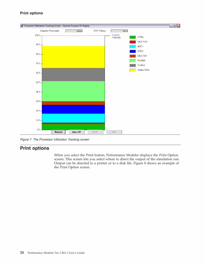
The Graph 2 button displays a graph showing the utilization of the processor,
broken out by individual workload. Figure 7 shows an example of the graph
displayed when you select the Graph 2 button.
Figure 6. The Performance Tracking screen
Graphing workload performance
Chapter 5. Running the simulator 23
Print options
When you select the Print button, Performance Modeler displays the Print Option
screen. This screen lets you select where to direct the output of the simulation run.
Output can be directed to a printer or to a disk file. Figure 8 shows an example of
the Print Option screen.
Figure 7. The Processor Utilization Tracking screen
Print options
24 Performance Modeler Ver 2 Rel 3 User’s Guide

Two Disk File options are available, text or numeric or both.
If you choose the text file, Performance Modeler writes a text image of the model
inputs and the results to disk.
If you choose the numeric option, Performance Modeler generates a disk file where
only the results are printed in CSV (Comma Separated Values) format. This file can
be imported into a spreadsheet as numeric data. Importing the simulation results
into a spreadsheet makes it easy to do additional data manipulation and create
customized graphs or tables of results.
The disk file name must be entered in the text box to the right of the option
selected. If the text & numeric option is selected, you must enter file names for
both types of output files.
Figure 8. The Print Option screen
Print options
Chapter 5. Running the simulator 25

26 Performance Modeler Ver 2 Rel 3 User’s Guide

Chapter 6. Getting started - performance modelling basics
Now that we’ve covered the basic operation and features of Performance Modeler,
it’s time to discuss how to actually build a model and produce a capacity plan.
While there are multiple ways to go about this, the beginner would be advised to
follow a straight forward process as described below. Once you get familiar with
this process and the different features of Performance Modeler, it will be much
easier to customize your use of this tool.
This chapter contains multiple scenarios which start with a simple case and
progresses to more complex scenarios. For each scenario, we follow a similar
methodology which progressively uses more features of Performance Modeler.
The first scenario begins with the simple case of modelling a system with one
dominant LPAR.
The following steps illustrate how to build a model for a 2064-105 running with
three active LPARs. After the model is built we illustrate the steps needed to
develop a capacity planning study.
Step 1 - Extract the RMF Reports and create the LPAR.RPT and
WGL.RPT files
The extracted .RPT files are used to build a model of the current system.
The input needed to build a model is provided in two kinds of RMF (or CMF)
reports. These are the CPU and the Workload Activity Reports.
The following control parms can be used when you run the RMF Post Processor
Report job to create these reports. If you need more information on how to
generate these reports, see the RMF Users Guide.
If the system runs in Compatibility Mode, use these RMF control parameters:
SYSID(XXXX)
REPORTS(CPU)
REPORTS(WKLD(PERIOD))
If the system runs in Goal Mode, use these control parameters:
REPORTS(CPU)
SYSRPTS(WLMGL(SCPER, RCLASS, SYSNAM(XXXX)))
These parms request both the CPU and Workload Reports. These reports are
generated from SMF records. You can choose to limit the size of these reports by
requesting reports that span a number of days and a specific time interval. A good
starting point is to choose five consecutive days for the peak hour of system
utilization. If you want to model a daytime as well as a night-time peak, you can
produce reports for multiple hours.
v The PERIOD parm in the Compatibility Mode list requests the workload report
at the Period within Performance Group level of detail.
v The SCPER parm in the Goal Mode list requests a Workload Report at the
Period within Service Class level of detail.
© Copyright IBM Corp. 2002, 2008 27
v The RCLASS parm requests that the report also include Reporting Class detail
information.
v The SYSID(XXXX) and SYSNAM(XXXX) parms request that the report only
include information for the system image with SMFID=XXXX. If the system is
part of a Parallel/Sysplex, the SYSNAM parm must be used. Using SYSNAM
ensures that the CPU time reported for each Service Class is only reported for
the system image you want to analyze.
These reports must be downloaded to your PC (as text files) and into a folder you
can access when you run the Extract Function. Finally, it is recommended that the
reporting interval be either 15 or 30 minutes in duration. That ensures the interval
is small enough to capture utilization spikes that might be hidden in a one hour or
longer report.
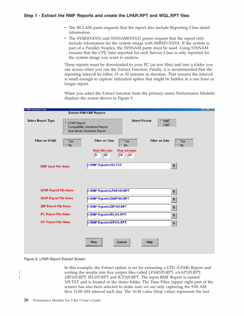
When you select the Extract function from the primary menu Performance Modeler
displays the screen shown in Figure 9.
In this example, the Extract option is set for extracting a CPU (LPAR) Report and
writing the results into five output files called LPAR105.RPT, zAAP105.RPT,
zIIP105.RPT, IFL105.RPT and ICF105.RPT. The input RMF Report is named
105.TXT and is located in the demo folder. The Time Filter (upper right part of the
screen) has also been selected to make sure we are only capturing the 9:00 AM
thru 11:00 AM interval each day. The 10:45 value (Stop value) represents the last
Figure 9. LPAR Report Extract Screen
Step 1 - Extract the RMF Reports and create the LPAR.RPT and WGL.RPT files
28 Performance Modeler Ver 2 Rel 3 User’s Guide
||
valid interval (10:45-11:00). The LPAR Report file (LPAR105.RPT) contains
information about LPAR utilization. The zAAP Report file contains similar
information about the utilization of LPARs that are sharing zAAP CPs. More
information on zAAP reports is contained in Chapter 7, “Modelling zAAP
processors,” on page 71. The zIIP Report file contains similar information about the
utilization of LPARs that are sharing zIIP CPs. More information on zIIP reports is
contained in Chapter 8, “Modelling zIIP processors,” on page 101. The IFL and ICF
Report files contain information about the utilisation of IFL and ICF assigned
processors. More information on the IFL and ICF reports is contained in
Chapter 10, “Monitoring IFL and ICF processors,” on page 121.
Clicking the S command button besides each input field displays a list of file
names in the current directory. Selecting (single left click) a file name in the display
list inserts that file name into the input field. This ensures that the file exists (for
input files) and is spelled correctly. The Filter on SYSID option can be used when
the RMF report contains several reports for different system images (SYSIDs). By
selecting Yes, you are asked to provide a four character SYSID. Only reports for the
selected SYSID are extracted. In this example, no SYSID filtering is necessary
because the RMF reports were only generated for the system running in the PROD
LPAR.
The LPAR Extract report can include information for all of the LPARs with shared
CPs, or it can be for a single LPAR with Dedicated CPs. If the Extract program
detects there are LPARs with Dedicated CPs it displays a list of the Active LPARs.
You are prompted to choose which LPAR is input to the Extraction program.
Choosing any LPAR with Shared CPs results in the extraction of data for all the
Shared LPARs. Choosing a Dedicated LPAR results in extraction for that LPAR
alone.
If you are modelling an image running in an LPAR with dedicated CPs, then the
RMF CPU Report must be generated by this image. In this case, the Extract
program uses the utilization information displayed in the CPU Activity Report,
not the Partition Data Report. The CPU Activity Report must be generated by
the same LPAR you are modelling.
During the Extract Process you may see error messages that indicate a problem
was detected. These messages typically begin with ″Couldn’t find ...″. This means
the input RMF or CMF report did not contain certain literals or data fields that the
extract program expected to find. If you encounter one of these errors, take a look
at the input report and make sure it was created correctly. If you cannot fix the
problem, write down the error message and report the problem to IBM. You may
also see an error message that says no records were found. That can happen when
you use the filter on SYSID or the Time Filter and no information matched the
filtering criteria. It can also mean there is a problem with the format of the RMF
report.
After the LPAR Report extract process is complete, Performance Modeler displays
the screen show in Figure 10. This screen displays the number of General Purpose,
zAAP, zIIP, IFL, and ICF processors found in the RMF/CMF report. The
information on the number of GP, zAAP and zIIP processors is used as input to
the Workload Extract function.
Step 1 - Extract the RMF Reports and create the LPAR.RPT and WGL.RPT files
Chapter 6. Getting started - performance modelling basics 29
||||
||

Next, select the Workload Extract function. Figure 11 shows the Extract Screen set
for the workload extract.
Figure 10. LPAR Report Extract Screen
Step 1 - Extract the RMF Reports and create the LPAR.RPT and WGL.RPT files
30 Performance Modeler Ver 2 Rel 3 User’s Guide

In this figure the Goal Mode Workload Extract option is chosen using the same
input file as the LPAR Extract (105.TXT). The two output files created by this step
are WGLPROD.RPT, which contains usage information for the Service Classes, and
RWGLPROD.RPT, which contains usage information for the Reporting Classes.
Since we are extracting information from an RMF Workload Activity Report for the
system running in the PROD LPAR, we have changed the names of the output files
to indicate these are for that LPAR. Over time you may create many WGL.RPT
files, so it is important to develop a naming convention that makes sense and helps
you keep track of these files.
At the bottom of the screen are fields labelled # of General CPUs, # of zAAP CPUs,
and # of zIIP CPUs. You must fill in the correct number of CPs that are in the
shared pool of CPs available to all of the LPARs on this processor. In this example,
the # of General CPUs is set to 5 because this is a 105. The # of zAAP CPUs is
explained in Chapter 7, “Modelling zAAP processors,” on page 71. The # of zIIP
CPUs is explained in Chapter 8, “Modelling zIIP processors,” on page 101.
If the processor contains a mix of shared and dedicated CPs you must use the
following procedure. When the LPAR extract program was run you were told there
was a mix of both dedicated and shared LPARs. You were also given the option to
select an LPAR with dedicated CPs, or an LPAR in the shared CP pool.
Figure 11. Workload Report Extract Screen
Step 1 - Extract the RMF Reports and create the LPAR.RPT and WGL.RPT files
Chapter 6. Getting started - performance modelling basics 31

v If you choose an LPAR in the shared pool then the physical processor should be
defined based on the number of shared CPs. For example, if the physical
processor is a 105, but two CPs are dedicated and three are shared, then the
underlying physical processor available to the shared LPARs must be defined as
a 103. That also means you should specify three CPUs as the Number of General
CPUs when you run the Workload Extract function.
v If you selected an LPAR with dedicated CPs, then you must treat the underlying
physical processor as having the number of dedicated CPs. In this example, if
you choose the LPAR with two dedicated CPs, then the underlying processor is
a 102, and the Number of General CPUs must be set to two.
Now that both the LPAR and Workload reports have been extracted we are ready
to import the extracted files into a spreadsheet for viewing and charting.
Step 2 - Import the extracted reports into a spreadsheet
Spreadsheets are excellent tools for manipulating numerical results. Once these
results are imported into a spreadsheet they can be converted into a table or chart
and used to build a presentation. Performance Modeler includes two spreadsheets
to help you customize and present your results. One is in EXCEL format, and
called CPFPM.XLS. The other is in Lotus 123 format, and called CPFPM.123. In the
following example we use the 123 version. Both spreadsheets look and work the
same.
Figure 12 shows a copy of the CPFPM.123 spreadsheet. There are several
individual sheets included with this file. The sheet labelled Input contains several
command buttons which automate many of the steps that follow. To the left of
each button is a light blue field. These are input fields that you can change before
you select the corresponding button.
Step 1 - Extract the RMF Reports and create the LPAR.RPT and WGL.RPT files
32 Performance Modeler Ver 2 Rel 3 User’s Guide

The first step in the spreadsheet lets you import the LPAR report file
(LPAR105.RPT) into the spreadsheet. The input fields have already been updated
to assign a name to the new sheet (LPAR105),which holds this report file. The
name of the report file (LPAR105.RPT) is specified in cell C4. When these fields are
filled in and you select the LPAR Data button, the new sheet in Figure 13 is
created.
Figure 12. Input Spreadsheet for CPFPM.123
Step 2 - Import the extracted reports into a spreadsheet
Chapter 6. Getting started - performance modelling basics 33

Starting in row 5 are the LPAR Names. From Row 7 down shows the utilization of
each LPAR plus Total utilization for the entire processor. Each row corresponds to
a different reporting interval. The header information in rows 1 thru 3 are used in
subsequent steps to control how charts are displayed.
Step 3 - Generate a chart showing utilization by LPAR as well as total
utilization for all LPARs
You can now create a chart showing utilization of this processor broken out by
LPAR. Step 2 in the Input sheet of the spreadsheet (Figure 12) has already been set
up to generate a new sheet with the name CPU105G. The G was added to the
previous sheet name to indicate it is a graph of the 105. The text in cells C9 and
C10 are titles you want to see in the new chart. When you select the LPAR Graph
button, the new sheet labelled CPU105G is created and shown in Figure 14.
Figure 13. LPAR Data Sheet
Step 2 - Import the extracted reports into a spreadsheet
34 Performance Modeler Ver 2 Rel 3 User’s Guide

This chart shows the utilization for each LPAR, and the total utilization for the
entire processor for each reporting interval. If you want to change the appearance
of this chart you can use the 123 (or EXCEL) commands, or you can change the
control information in rows 1-3 in the CPU105 sheet. For example, if you look at
cells F2 and F3 (Figure 18 on page 41), you can see where the X axis is designated
as column B. That column contains the date information. Cell F3 specifies that the
X axis label be displayed every 8 intervals. This was automatically set based on the
fact that the date changes every 8 intervals. If you want to use the Time values as
the X axis labels, and increment them every 2 intervals, change cell F2 to C, and
change cell F3 to 2. Then select the LPAR Graph button again to recreate the new
chart.
Step 4 - Import the Workload Activity Report File into the spreadsheet
Now you can import the workload activity report file (WGLPROD.RPT) into the
spreadsheet. As before, we have chosen a name for the new sheet (WGLPROD)
and specified the report file name. When we select the Workload Data button
(Figure 12) a new sheet is created and the workload report file is imported. This is
shown in Figure 15.
Figure 14. LPAR Utilization Graph Sheet
Step 3 - Generate a chart showing utilization by LPAR as well as total utilization for all
LPARs
Chapter 6. Getting started - performance modelling basics 35

In addition to importing the workload report file, the command button has also
sorted the data by Service Class Name, date/time, and by workload priority. That
was necessary so that we can properly graph this data in the next step. This is a
good place to explain how Performance Modeler assigns priority values to each
workload.
If the system runs in Compatibility Mode, the priority is based on the dispatching
priority defined in the system’s IEAIPSxx Parmlib member. In Compatibility Mode,
most workloads are assigned a static priority based on its Performance Group and
Period. That information is provided in the IEAIPSxx Parmlib member. If the
system runs in Goal Mode, the dispatching priority can vary and is controlled by
Workload Manager. But Performance Modeler must use a static value for
determining the relative importance of different workloads. That value is created
using the following logic.
Performance Modeler builds the workload priority by multiplying the workload
importance (usually 1 thru 5) by 100. Next, the Execution Velocity Goal assigned to
this workload is subtracted from 100 and added to the first value. For example, a
workload running with Importance=3, and having an Execution Velocity Goal of
30% would be assigned a priority of 370. Another workload running at the same
importance but with a goal=40% would have a priority of 360. With this scale, the
smaller the priority, the more important the workload when it is modelled by
Performance Modeler.
Figure 15. Workload Data Sheet
Step 4 - Import the Workload Activity Report File into the spreadsheet
36 Performance Modeler Ver 2 Rel 3 User’s Guide

Workloads assigned to a SYSTEM importance are assigned a priority of 0.
Workloads that have a response time goal instead of an execution velocity goal
have a 0 added to their initial priority. For example, a workload with
Importance=2 but with a response time goal have a priority of 200. That ensures it
is treated as more important than other importance 2 work having a velocity goal.
Workloads assigned a Discretionary importance have a priority of 600.
Next to the Workload Data button in the Input spreadsheet (Figure 12) is another
button labelled Graph Fixup. This button performs the same function as the
Workload Data button but with these important differences. In order to create a
chart showing Workload Utilization, the LPAR utilization data and the Workload
utilization data must cover the same reporting intervals. That means there must be
a one for one match between the data stored in the LPAR Data sheet and the
Workload Data sheet. In some situations, the RMF reports produce CPU and
Workload Activity reports that do not have the same reporting intervals. When this
happens, the Workload utilization chart are not created properly. Another factor
which causes the chart to be created improperly is if there has been a change in
workload importance or velocity goal during the time that the workload reports
were created.
The Graph Fixup button is designed to scan the CPU and Workload reports to spot
these events and correct them on the fly. If the button finds there are time interval
differences between the two reports, it either adds the missing interval to the
Workload Data sheet, or deletes the extra interval. If it finds there has been a
change in workload importance or velocity goal, it resets these values to the
original value. These steps are necessary in order to produce a proper chart
showing workload utilization. Since this logic is more complex than importing and
sorting the workload report, this button takes more time than executing the
Workload Data button.
A good practice is to always start by executing the Workload Data button first.
Then create the workload utilization chart (Step 4 in the spreadsheet). If the chart
looks wrong it probably means one of the two events described earlier has taken
place. That typically shows up as the workload bars do not add up to nor tracks
with the utilization for the entire LPAR. At this point you can select the Graph
Fixup button. That recreates the Workload Data sheet while it fixes the two
problems described above. At this point you should be able to successfully create a
Workload utilization chart as described next.
Step 5 - Graph the Workload Utilization
This step creates a workload utilization chart based on the workload activity data
we imported in the previous step. Once again, we have named the new sheet with
a similar name to the sheet containing the source data, but added a G to indicate
graph (WGLPRODG). We have also entered the two titles we want displayed on
the chart. This information has been provided in cells C18 thru C21 of the Input
sheet. When you select the WKLD Graph button you create the chart shown in
Figure 16.
Step 4 - Import the Workload Activity Report File into the spreadsheet
Chapter 6. Getting started - performance modelling basics 37

This figure shows the Total Utilization of the processor as the black line running
across the top of the chart. The red line indicates the utilization of this LPAR
(PROD). And below the red line are bars that show the actual utilization of each
workload that contributed to the LPAR utilization. A few explanations are in order
here.
First, the LPAR that is charted as the red line is actually selected by an input value
that you can change in the LPAR utilization sheet (CPU105). If you look at that
sheet (Figure 13), you can see that cell F1 contains the value D. This represents the
column of the LPAR that is selected for the red line. In this example, we did not
have to change anything because the default value (D) is already pointing to the
PROD LPAR. But if we want to produce another workload utilization chart for a
different LPAR, we have to change this value to point to the correct LPAR column.
You might also be wondering why there is that gap between the workload bars
and the red line. That gap is due to two effects. First, there is a certain amount of
LPAR utilization which is not associated with any workload. This is called
Uncaptured Time. Uncaptured Time makes up most of that gap. But we have also
chosen to graph only those workloads that are using a reasonable amount of the
processor. That minimum amount which determines whether we include a
workload in the graph is based on the value in cell C21 on the Input sheet (Figure
12). The default value of 2 means we will only include a workload in this chart if it
uses a minimum of 2% of the total processor in at least one reporting interval. You
can change this value to control how many workloads you want to include in the
workload utilization chart.
Figure 16. Workload Utilization Graph Sheet
Step 5 - Graph the Workload Utilization
38 Performance Modeler Ver 2 Rel 3 User’s Guide

Step 6 - Build a baseline model using the Build function
The charts created in Step 3 and Step 5 give you a good view of how this LPAR is
utilizing the processor. They also help you decide on which reporting interval to
use when building a baseline model.
The Build function allows you to build a model which corresponds to the actual
system during a specific reporting interval. Choosing the reporting interval is very
important since this model will probably serve as the baseline for comparing
different what if scenarios. A good practice is to pick an interval when utilization
is high, but not necessarily the highest peak of all peaks.
By inspecting the workload utilization chart shown in Figure 16, we can see the
total utilization averages in the mid 90% and occasionally hits 100%. For this
example, we choose the reporting interval of 10:30-10:45 on 3/27/03. During that
interval the total utilization was 98.59%. While this interval was chosen visually, it
represents the approximate 95th percentile of total utilization. That means 95% of
the time (for the 9-11 AM period), the total utilization was equal to or less than
this value. Choosing a 95th percentile interval ensures that we are not building a
baseline for a low usage period.
Keep in mind we are not trying to predict what the average performance will be,
but rather something close to the worst case performance. That represents the time
we will be out of capacity.
Selecting the Build function from the Performance Modeler Primary menu displays
the screen shown in Figure 17.
Step 6 - Build a baseline model using the Build function
Chapter 6. Getting started - performance modelling basics 39

This is the screen where you actually construct a baseline model. As shown in this
figure, there are six steps to building a model. These are described below.
Build Step Description
Step 1 Select Processor
This step asks you to define the CPU being modelled. The key
parameters are the MIPS rating and the number of CPUs. You can
manually change the processor description, MIPS rating, and
number of CPUs, or you can click on the S command button to
display the CPU table provided by Performance Modeler. When
you click on one of the processor models provided in this table, the
three fields are automatically updated.While you can use the
default MIPS rating supplied in this table, it is important to
understand how the MIPS ratings are developed. It is especially
important that you understand how to set the MIPS ratings for
future what if scenarios. This subject is covered in more detail in
the section titled MIPS Discussion.
Step 2 Select CPU Report File
In Step 2, you specify the name of the CPU report file. This is the
same file created during the Extract function described earlier. In
this example, the file is named LPAR105.RPT. Single clicking the
Step 2 Command Button displays a list of valid file names (*.RPT).
Selecting a file name in the display list inserts that file name into
the input field.
Figure 17. Model Build screen
Step 6 - Build a baseline model using the Build function
40 Performance Modeler Ver 2 Rel 3 User’s Guide

Step 3 Select ZAAP Options Select CPU Report File
In Step 3 you define the zAAP processors and provide other
information related to how zAAP processing is implemented. Since
this example does not use zAAP processors we skip this step. This
option is covered in Chapter 7, “Modelling zAAP processors,” on
page 71.
Step 4 Select ZIIP Options Select CPU Report File
In Step 4 you define the zIIP processors. Since this example does
not use zIIP processors we skip this step. This option is covered in
Chapter 8, “Modelling zIIP processors,” on page 101.
Step 5 Select Workload Report File
In Step 5, you specify the name of the extracted workload report
file created by the Workload Report Extract function. In this
example, the file is named WGLPROD.RPT.
At this point, the Build screen should look like Figure 18.
Continuing with the Build process.
Step 6 Select LPAR, Date and Time
Clicking on the Step 6 Command button displays the Date/Time
Selection screen which shows CPU utilization, by LPAR, for each
reported time interval. This is where you select the LPAR and the
Figure 18. Filled in Build Screen
Step 6 - Build a baseline model using the Build function
Chapter 6. Getting started - performance modelling basics 41

time interval which you want to model. This is done by clicking on
the cell containing the LPAR CPU utilization. In this example you
select the cell under the PROD LPAR column which corresponds to
the 10:30 AM interval on 3/27/06 as shown in Figure 19.
Step 7 Select Workloads for Modelling
Clicking the Step 7 Command button on the Build screen shows
you a table which shows processor and workload utilization
during the selected time interval for the selected LPAR (PROD).
This is called the Workload Selection Screen and is where you
actually pick the workloads you will model (Figure 20).
Figure 19. Select LPAR/Date/Time screen
Step 6 - Build a baseline model using the Build function
42 Performance Modeler Ver 2 Rel 3 User’s Guide

The Workload Selection Screen contains several columns of useful
information. A good practice is to select the Print option at the
bottom of the screen and print this table to disk. Once we have this
table on our PC disk, we can import it into our spreadsheet. In this
way we keep all the related information in a single file.
When you select the Print option, there are several print output
options. The default option for this screen is to write the table out
to a file named WKL.NUM. If you select this default you can
switch back to the spreadsheet and click on the Workload Table
button on the Input Sheet (Figure 12). That imports the table and
stores it in a new spreadsheet named WKLA. A description of all
the fields contained in the Workload Table can be found in
Appendix A, “Workload Table description,” on page 125.
This might also be a good time to consider saving the spreadsheet
file. A good practice is to leave the original copy of CPFPM.123 (or
CPFPM.XLS) unchanged. You can save the active copy of the
spreadsheet under a name that is recognizable for later retrieval. In
this example, a reasonable name might be Model-105-SEP06.123.
The name refers to the processor being studied as well as the date
when this file was created
Returning to the Workload Selection Screen (Figure 18), you are
now ready to select the individual workloads you want to model.
You select each workload by clicking on the row containing that
workload. Workloads are shown at the Period within Service Class
Figure 20. Workload Selection Screen
Step 6 - Build a baseline model using the Build function
Chapter 6. Getting started - performance modelling basics 43

(Goal Mode) level of detail, or at the Period within Performance
Group (Compatibility Mode). While there may be lots of individual
workloads shown, you do not have to select every workload when
you build a model. In fact, a good practice is to limit the selection
to between four and six workloads. That allows you to summarize
the modelling results in a single table that easily fits on a single
page. It also reduces the amount of data being analyzed. With
experience you can answer most of the questions regarding
capacity requirements by focusing on four to six key workloads.
A recommended approach to selecting workloads is to start at the
bottom of the Workload Selection Screen and work your way up.
Since the table is sorted by importance, you start your selection at
the least important workloads and working upwards.
When the system is constrained, it is usually the least important
workloads which feel the pain first and experience the worst
performance. Concentrating on these workloads ensures that you
see the impact of a constrained system. As you work your way up
the table you should look at the value of the Total (%) column.
That is the percent of the total processor that was used by that
workload in this reporting interval.
Workloads which show a high amount of processor utilization are
good candidates for modelling. But you might also want to select a
low importance workload that uses very little processing capacity.
That might make sense when it is a workload you care about, but
is currently constrained due to high processor utilization. In that
case, the Total (%) value may be small but you still want to see
what happens to this workload’s performance when you make
changes.
Another recommendation is you choose workloads that span the
range from high importance to low importance. That ensures you
see the impact of change on all kinds of work. You can expect the
lowest importance workloads to provide the biggest impact of a
processor upgrade, but you are probably focused on the
performance of your most important workloads as well. When you
select a workload you are presented with a screen asking you to
define the way Performance Modeler should treat this workload
(Figure 21).
Step 6 - Build a baseline model using the Build function
44 Performance Modeler Ver 2 Rel 3 User’s Guide

In this example we have selected the BATCHMD workload and we
must select one of three workload types. The first decision is
whether this is a batch workload or an OLTP workload. In this
example we know this is a batch workload so we select the B
option, then select OK. Next we select BATCHHI, then CICS, then
CICSHI. At this point we have selected four workloads and are
satisfied we have a range of meaningful workloads selected that
span the range from very important to low importance. You can
see the workloads you selected and their Type in Figure 22 (the X
means the workload was selected).
Figure 21. Workload Type Definition
Step 6 - Build a baseline model using the Build function
Chapter 6. Getting started - performance modelling basics 45

The two CICS workloads were selected with Type=M, for multi
tasking workloads. Since these are designated CICS, we are
confident these are OLTP workloads. The only decision then is
whether to designate them as S (single tasking) or M (multi
tasking). One clue to help you in this decision is to look at the
column labelled MPL. That is the Multi Programming Level. The
MPL is the average number of address spaces running in this
workload during the reporting interval. In this example, the MPL
for CICS was 9 and the MPL for CICSHI was 2. Since these
workloads clearly run across multiple address spaces, it is proper
to consider them as multi tasking workloads. If the MPL had been
1, you would have to consider other factors. For example, is this a
workload making heavy use of DB2 threads (CICS/DB2 region), or
is this using VSAM or a Data Base Manager which is limited to a
single TCB. In those situations, it might be appropriate to select S.
Now that we have all of our workloads selected we can click on
Build to begin the automatic build process. When Build is selected
you are presented with the following screen (Figure 23).
Figure 22. Workloads Selected
Step 6 - Build a baseline model using the Build function
46 Performance Modeler Ver 2 Rel 3 User’s Guide

This screen is asking you to provide information about the LPAR
definitions for the processor being modelled. Performance Modeler
needs to know how your LPARs are defined. The MIPS fields have
been filled in based on the actual utilization of each LPAR. But you
may need to update the other LPAR definitions to match your
actual values. In this example, the Number of Logical CPs and
Weights have been filled in based on the actual LPAR definitions
that were in effect during this time interval. If Performance
Modeler was not able to find these definitions, you would have to
manually enter the correct definitions.
After you update the LPAR definition screen and click OK, a
Calibration screen (Figure 24) is displayed. This is the final step in
the Build process.
Figure 23. LPAR Definition screen
Step 6 - Build a baseline model using the Build function
Chapter 6. Getting started - performance modelling basics 47

The Calibration step ensures that the Path Length values for each
workload are correct. Performance Modeler chooses an initial Path
Length for each workload. During the calibration step, the
simulator is invoked and the measured workload utilization is
compared back to the actual utilization. After each pass of the
simulator, the Path Lengths are adjusted and the process repeats.
The Calibration ends when all workloads are using, within a
specified tolerance, their actual utilization. Figure 24 shows the
actual utilization for each workload (Single CPU % Busy Target) as
well as the tolerance (usually within 1%-2% of the target). The
target is shown as the Single CPU % Busy. This is the actual
utilization as a percent of a single CP. This is also the Total % of
the processor used by this workload multiplied by the number of
physical CPs. The tolerance is scaled (usually 1% or 2%) depending
on how big or small the target is.
The Number of Simulated Seconds in the upper right corner
represents the number of seconds that are simulated before the
utilizations are compared and Path Lengths are adjusted. While
you can change many of the fields on this screen, you can use
these defaults for most cases. You should never change the Target
Utilizations since they are based on the actual utilizations for each
workload.
When the Calibration ends you should select the Return button to
go back to the Primary menu. At this point the model is
Figure 24. Calibration screen
Step 6 - Build a baseline model using the Build function
48 Performance Modeler Ver 2 Rel 3 User’s Guide

completely built and it would be a very good time to save the
current model. Click Select File > Save As to name this model. A
good name for this example might be 105B.SIM. That indicates the
processor and the fact this is a baseline model. You can verify this
model was built correctly by clicking Run > Single Run from the
Primary menu.
While the model runs, note the total processor utilization, the
model (first LPAR) physical utilization, and the utilization for each
workload. These should match very closely to the actual utilization
displayed in the WKL2 spreadsheet. Since Performance Modeler is
a simulator, the actual utilizations shown in the model are not
exactly the same as the utilizations shown in the RMF reports but
they should be very close.
If you select the Workloads screen option from the Primary Menu
the following (Figure 25) is displayed.
This figure shows each workload and how it is defined to
Performance Modeler. Since we only selected four workloads for
modelling we still have to account for the other work running in
this LPAR. That is accounted for in the Fill workloads. You may
also notice that the Path Lengths for the multi tasking (Type=M)
workloads vary from 2 to 8 million instructions. When the new
model was built, the average path length for these workloads was
assumed to be 2 million instructions per transaction. Based on that
Figure 25. Workloads screen
Step 6 - Build a baseline model using the Build function
Chapter 6. Getting started - performance modelling basics 49

assumption, the arrival rate was calculated so that the correct
utilization would be obtained. But Performance Modeler has a
restriction which limits the arrival rate for any workload.
The maximum allowable arrival rate is based on the modelling
time interval. The default time interval is set to .01 seconds. That
means Performance Modeler cycles 100 times thru the simulator
for every one second of elapsed time being modelled. Since each
workload is limited to one transaction being created per cycle, the
maximum number of transactions that can be generated with the
default time interval is 100 transactions per second.
In order to ensure transactions arrive in a random pattern,
Performance Modeler limits the maximum arrival rate to 85% of
the maximum, or in this case 85 transactions per second. In this
example, we needed to generate 238 CICS transactions per second.
Since we are limited to 85 per second, Performance Modeler
changed the path length from 2 to 8 million instructions per
transaction. That results in a lower transaction rate of only 60.23
transactions per second, well below the maximum of 85
transactions per second.
Modelling What If Scenarios
You are now ready to run what if scenarios. This is where you
model changes to your workloads or the configuration or both, and
compare the results back to your baseline model. This is also a
good place to take a step back and consider the methodology you
want to use.
In most studies you want to examine the impact of changes to the
workloads, the configuration, or both. A typical study might
involve modelling the impact of one years worth of workload
growth on the current processor, then modelling the impact of
upgrading the processor at that time. Performance Modeler is well
suited for that kind of analysis. One of the tools provided by the
spreadsheet included with Performance Modeler is the ability to
easily compare the changes from one run to another. This is
covered in more detail shortly. But before modelling what if
scenarios it is important to understand the way MIPS are
represented and used within Performance Modeler.
MIPS Discussion
In order to properly interpret and use the MIPS values provided in Performance
Modeler, consider the following:
Although capacity is often expressed as MIPS, no one, including IBM®, actually
measures MIPS. All mainframe vendors measure relative capacity. IBM publishes
their measurement results in a table of relative capacity called the LSPR (Large
Systems Performance Reference) results. These results show the relative capacity of
many IBM and PCM processors based on a set of workload specific benchmarks.
But LSPR results are often converted into MIPS. In the early days of mainframe
development, vendors and customers often measured the actual MIPS capacity for
various processor models. Over time, capacity measurements changed from
measuring MIPS to relative capacity. But the use of MIPS as a metric for processor
Step 6 - Build a baseline model using the Build function
50 Performance Modeler Ver 2 Rel 3 User’s Guide

capacity continues today. Converting LSPR results into MIPS requires that you
assign a MIPS rating to one processor, and extrapolate the MIPS ratings for the
other processors using the LSPR ratios.
For example, assume the LSPR rating for processor B is twice the capacity of
processor A. Then if we assign a MIPS rating of 100 MIPS to Processor A, we can
extrapolate the MIPS rating of processor B to be 200 MIPS. This is how the CPU
MIPS table available on the Configuration Definition screen was created.
From time to time, IBM has changed the actual workloads that make up the LSPR
benchmarks. They do that to keep the benchmarks relevant and ensure they
correctly match the kinds of work that customers actually run on their processors.
Sometimes new results are produced using a newer version of the operating
system, or reflect an architectural change, such as the change from 31 bit to 64 bit
addressing. New LSPR results often change the capacity ratios for existing
processor models. Plus, newer LSPR results may not include all of the processor
models included in the earlier tables, especially older models that were not
benchmarked with the latest workloads. This makes it difficult to produce a single
table of MIPs for all processors. In Version 2 Release 2 of Performance Modeler, the
following changes (compared to Version 2 Release 1) have been made to the MIPS
table.
First, the new IBM processor models announced on July 26, 2005 have been added
to the MIPS table. These include all the 2094 models, from the uniprocessor
2094-701 to the 54 way 2094-754. In addition, MIPS values are now based on the
latest IBM LSPR tables. These tables include several changes compared to the
earlier tables used in Version 2 Release 1. For example, the new LSPR tables are
derived using z/OS 1.6. Another change is the way the LSPR Default Mix
workload is derived. Previously, this workload was based on an equal weighting of
5 LSPR workloads called “LSPR Primitives”. The new Default Mix has dropped
one of these workloads (CB-S) and replaced it with a new workload called CB-J. If
you need an explanation of these workloads as well as the detail capacity ratios for
each workload, you can find this information at this IBM Web site:
http://www-1.ibm.com/servers/eserver/zseries/lspr/
The new LSPR results only included measurements for the z800, z900, z990, and
new z9 models. In order to update the MIPS table it was necessary to “bridge”
these new ratios back to the earlier ratios. That was done by choosing the 2064-1C1
as the bridge machine, and assigning it a MIPS rating of 252.8 MIPS (the same
rating used in Version 2 Release 1). Based on that rating, all of the other MIPS
ratings were calculated using the LSPR ratios for the Default Mix workload. One
result of this update is that many of the z800, z900, and z990 MIPS ratings have
changed slightly from Version 2 Release 1. Another change affecting the MIPS table
is the use of the Multi-Image LSPR ratios. IBM now produces two sets of LSPR
ratios, one for Single Image measurements, and a second set for Multi-Image
measurements. The Multi-Image LSPR ratios are based on running the LSPR
workloads in LPAR mode where a specific LPAR configuration is chosen for each
processor. Since most processors are run in LPAR mode today (Vs Single Image
mode), these measurements are designed to show the actual capacity delivered by
each processor while running in a predefined LPAR configuration. The actual
LPAR configuration is matched to the size of the processor. For example, the larger
the processor, the more complex is the LPAR configuration.
In Performance Modeler Version 2 Release 2, the MIPS table has also been updated
to include information related to zAAP processors. The z890, z990, and z9
Step 6 - Build a baseline model using the Build function
Chapter 6. Getting started - performance modelling basics 51

processors have been designated as being zAAP capable. That means these models
can be configured with zAAP CPs to assist the general purpose CPs.
In Performance Modeler Version 2 Release 3, the MIPS table has also been updated
to include information related to zIIP processors. The z9 processors have been
designated as being zIIP capable. That means these models can be configured with
zIIP CPs to assist the general purpose CPs.
One caution regarding the use of these MIPS ratings. The MIPS table included with
Performance Modeler is meant as a reference and starting point for determining
relative capacity. A single table of relative capacity cannot show the variations
based on different workload mixes or changes in operating systems. Plus, these
ratings do not consider the impact of LPAR overhead based on your actual LPAR
configuration.
When modelling the impact of changing processor models, it is important that the
relative capacity between the baseline model and the new processor model
accurately reflects the change in capacity. You may choose to use the MIPS rating
provided in the MIPS table for the baseline model, but you should be careful that
the ratio of the new processor MIPS to the baseline processor MIPS be as accurate
as possible. That is the only way to be sure you are properly modelling the change
in processors. That may require changing the MIPS rating for the new processor
from the value provided in the MIPS table.
One way to make sure you are using the correct ratio is to consult the actual LSPR
ratings provided at the IBM Web site. If the LPAR configuration changes between
the baseline and target models, you should consider adding a value to the LPAR
Overhead field in the LPAR Definition screen. You can also reflect the impact of
LPAR overhead by lowering the MIPS rating of the new processor. If you need
help determining the impact of LPAR changes, contact your IBM representative
and ask for his assistance.
Beginning in December/2005, IBM made their internal sizing tool, zPCR (zSeries
Processor Capacity Reference), available to customers at no charge. zPCR is a tool
that displays the IBM LSPR ratios for all current and older mainframe processors.
Using zPCR, you can define specific LPAR configurations and see how LPAR
changes can affect relative processor capacity. zPCR complements the use of zTPM.
It is strongly recommended that zPCR be used to derive MIPS ratings when
modelling new processors.
MIPS may be an abstract term but it is very useful for modelling and capacity
planning. For example, a single transaction is defined by the number of
instructions (path length) it needs to execute. Once the path length is known, you
can calculate the CPU time it takes to execute this transaction by this calculation:
CPU time = path length (in millions of instructions)
divided by the single CPU MIPS rating
To further illustrate, consider a transaction with a path length of 1 million
instructions. The CPU time it takes to execute this transaction on a CPU rated at 50
MIPS is 1/50 = .02 seconds. This calculation is used by the simulator, so the MIPS
rating and the average transaction path length are linked by this relationship.
Step 6 - Build a baseline model using the Build function
52 Performance Modeler Ver 2 Rel 3 User’s Guide

Capacity planning with Performance Modeler
Capacity Planning is one of several Systems Management disciplines. It includes
the collection of activities that enable IT shops to deliver acceptable service while
also managing their IT costs. Despite numerous books and papers on the subject,
Capacity Planning today is often given the least amount of attention compared to
other Systems Management functions. The reasons for this include 1-lack of trained
staff, and 2-lack of effective tools. The result of poor Capacity Planning can include
poor service delivery and the resulting dissatisfaction among the user community.
It can also result in sudden unplanned upgrades with the usual pressure on the IT
budget. These results create a climate where the IT organization appears to be in
react mode and unable to plan proactively for future upgrades.
Capacity Planning has many definitions. An appropriate one is “The activities that
ensure there is enough capacity to satisfy your end user’ service requirements.” For
online workloads, service is often measured as average response times. For batch
workloads, service can be defined as elapsed times for individual or groups of
related jobs. It may also be appropriate to measure service as the time it takes to
complete a nightly batch cycle. For example, many shops must complete a series of
batch jobs during third shift before online workloads are started in the morning.
But whatever the measure of service, each shop can describe a set of service level
objectives that define the line between acceptable and unacceptable service.
Service Level Agreements (SLAs)
IT shops that do a good job of Capacity Planning formalize their service level
requirements into a set of Service Level Agreements. SLAs are contracts where the
end user agrees with IT management on what are acceptable levels of service, as
well as the remedy if the service level is not met. But most important, SLAs can
form the basis of a Capacity Planning methodology. Manage capacity so that
Service Level Agreements are always being met. But this methodology requires
that Capacity Planners be able to predict how service delivery changes over time.
This includes predicting the impact of adding new workloads, or growth to
existing applications, or the impact of configuration changes. These requirements
point out the need for tools which can predict how performance changes due to
virtually any change that may occur.
The lack of effective performance prediction tools is one of the reasons Capacity
Planning is poorly executed in most shops. Without effective modelling tools, IT
shops rely on rules of thumb to predict when they are out of capacity. The most
common technique is to upgrade when processor utilization reaches a predefined
limit. This may work well for some shops some of the time. But the link between
processor utilization and workload performance is not clear cut. Certainly, the
performance of some workloads degrades when total utilization nears 100%, but
they are usually low priority work.
As workloads grow, and processor utilization nears 100%, this pattern develops:
v First, the lowest priority workloads begin to elongate, but higher priority work
seems unaffected.
v As workloads continue to grow, utilization stays at or near 100%, but now
medium priority work begins to suffer.
v Eventually the pain works its way up the priority chain till even the high
priority work slows down.
Capacity planning with Performance Modeler
Chapter 6. Getting started - performance modelling basics 53

This scenario points out the difficulty of equating high processor utilization with
an out of capacity situation. If we go back to our earlier definition for out of
capacity, we need to look at the performance of each class of work, and to compare
that against its service level requirement.
Another characteristic of performance is that it often follows an exponential curve.
That means, as workloads grow, performance stays relatively constant until it
reaches the point where it deteriorates suddenly and without much warning. This
is called the knee of the curve effect and reflects the point on the performance
graph when things go quickly from good to bad. If IT shops want to effectively
manage their capacity and service delivery, they must be able to predict where
they are on this curve, and especially, when they are approaching the knee of the
curve. And that requires a modelling tool like Performance Modeler. “Capacity
planning methodology” describes a methodology that uses Performance Modeler
for capacity planning.
Capacity planning methodology
All shops have SLAs. If they are written down or stored electronically, they are
explicit. But even when they are not formalized, IT shops and their users have an
implicit understanding of where the line is drawn between acceptable and
unacceptable performance. Sometimes the understanding is that performance for
important workloads cannot get any worse than the current level of service. This
certainly makes it hard to agree on when the line is crossed, but that won’t stop
the phone from ringing when service degrades. SLAs are workload dependent.
Important work usually has more stringent service requirements than lower
priority work. That makes it essential that IT shops develop a baseline knowledge
of current performance and that it be at the workload level.
The following example shows how Performance Modeler can be used to predict
how workload and configuration changes can impact workload performance. If
you have formalized SLAs, you can use these results and compare them back to
your SLAs. If you do not have formalized SLAs, you can compare the predicted
changes back to your baseline model. In this example we are using the baseline
model created earlier (105B.SIM) and examining the following scenario:
v Assume all workloads grow by an average of 15% to 20% per year.
v Predict the impact on one years worth of growth on the current processor (105)
v Predict the impact of upgrading to a 106.
There are two ways to model what if scenarios. The first way requires that you
create a separate configuration file (.SIM) for each scenario and save it on you disk
drive. After all the scenarios are built, you can click the Run > Multiple Run
option on the Primary Menu to run these models, one behind the other. After all
the runs are complete, you can examine the results. A second way to run multiple
scenarios is to use the Run Wizard feature. Run Wizard is also available under the
Run option on the Primary menu. Run Wizard allows you to enter all of the detail
for the different scenarios on a single screen. While this saves you the time it takes
to create and save separate configuration files, it has some restrictions. These are
explained as we go through a Run Wizard example. Figure 26 shows the Run
Wizard screen that appears when you click Run > Run Wizard.
Service Level Agreements (SLAs)
54 Performance Modeler Ver 2 Rel 3 User’s Guide

The Run Wizard screen allows you to select the baseline model, the interval for
future growth (3 months, 6 months, or yearly), up to 5 different growth rates, and
up to 8 different processors. In this example we update the screen until it looks
like the following (Figure 27).
Figure 26. Run Wizard screen
Capacity planning methodology
Chapter 6. Getting started - performance modelling basics 55

The updated screen indicates we want to look out one year across two different
processors (105 and 106) with two different growth rates. We also selected the
Display/Change Growth Rates button and defined the two growth rates to be 15%
and 20% as shown in Figure 28.
Figure 27. Updated Run Wizard screen
Capacity planning methodology
56 Performance Modeler Ver 2 Rel 3 User’s Guide

One of the restrictions of the Run Wizard is you can only apply a single growth
rate to all the workloads within an LPAR. If you wanted to use different growth
rates for different workloads you would have to use the first method for creating
multiple scenarios. But when a single growth rate is applied across all workloads,
Run Wizard can save you lots of keystrokes. In Figure 27 you can see we are
defining two growth rates. The first growth rate requests a 15% increase across all
workloads in all LPARs. The second growth rate is 20% applied across all LPARs.
Once the Run Wizard screen is completed you can click the Run button. An LPAR
Definition screen (Figure 29) for each processor selected is displayed.
Figure 28. Growth Rate screen
Capacity planning methodology
Chapter 6. Getting started - performance modelling basics 57

The LPAR Definition screen gives you the opportunity to change the LPAR settings
on the current as well as other processors. The zAAP CPs option in the upper right
corner of the screen allows you to specify that zAAP CPs are included with this
processor. This option is discussed in Chapter 7, “Modelling zAAP processors,” on
page 71. The zIIP CPs option allows you to include zIIP CPs and is discussed in
Chapter 8, “Modelling zIIP processors,” on page 101. When you finish updating
these screens, the Print Option Screen (Figure 30) is displayed.
Figure 29. LPAR Definition screen
Capacity planning methodology
58 Performance Modeler Ver 2 Rel 3 User’s Guide

Using the defaults create two output files on your disk after all the scenarios have
been run. The SIM.PRT file contains a text file showing the input values for each
modelling run, followed by the results. The SIM.NUM file contains a CSV (Comma
Separated Values) file which contains the modelling results from each run. You can
import these files into your spreadsheet using the buttons in the SIMT and SIMN
sheets. The Load SIM.PRT button in SIMT loads the text file and stores the results
starting at the row specified in cell B2. The Load SIM.NUM button in SIMN loads
the CSV formatted results file into that sheet. Figure 31 shows the SIMN sheet after
the Load SIM.NUM button was selected for this exercise.
Figure 30. Print Option screen
Capacity planning methodology
Chapter 6. Getting started - performance modelling basics 59

These results consist of five lines of results for each model run. The first row
contains the date and time the model was run. Row 3 shows the name of the
configuration file that was run. When using the Run Wizard, these are
automatically created and saved as temporary configuration files. At the end of the
runs you have the option of deleting these files or leaving them on your disk. The
actual model results are shown in row 5. These results include the following
information:
Run Title
Model Title. For models created by Run Wizard, this includes the name of
the baseline model and additional information which identifies the time
interval, processor, and growth rate.
Total MIPS
Total MIPS rating for the processor being modelled.
MIPS per CPU
MIPS rating for the individual CP.
Total CEC
Total average processor utilization for entire run.
Model CEC
Average processor utilization by LPAR #1 (the LPAR being modelled).
Other Columns
The remaining columns represent performance metrics. These include
average response times per transaction for OLTP workloads, and
Figure 31. SIM.NUM Results
Capacity planning methodology
60 Performance Modeler Ver 2 Rel 3 User’s Guide

Elongation Factors for the batch workloads. Since the Elongation Factor is
directly related to average batch job elapsed times, this is a measure of
batch job performance.
In this example we can see the first set of results represents the baseline model
showing how the system (105) is currently performing. The next set of results
show the 105 with 15% of growth to all workloads. Next are the results showing
the 105 with 20% growth. Next are the results for the 106 with the current
workload, followed by the 15% growth, and finally, the 106 with 20% growth.
These include six sets of results and represent all the combinations we asked Run
Wizard to perform. As you can see, if we activated all the options on Run Wizard
we could have run many combinations of what if scenarios.
While the table in the SIMN sheet contains all of the results we are investigating,
there is another sheet to the right called SIMSUM. The SIMSUM sheet provides a
command button designed to take the results in SIMN and format these results in
a more user friendly format. The Load Results Summary button reads the table
from SIMN and creates a new table in SIMSUM as shown in Figure 32.
This table summarizes the six modelling runs in the SIMN sheet while also adding
a % change row. The % change row shows the percent change in each result
compared to the baseline model. For example, the CICS entry on row 14 shows
that the average response time for CICS has grown from 0.25 seconds in the
baseline model to 5.80 seconds on the 105 with 15% growth. The % change in row
15 indicates that is a 2214% increase compared to the baseline run. The significance
Figure 32. Simulator Summary Table
Capacity planning methodology
Chapter 6. Getting started - performance modelling basics 61

of the % change value is it tells us how bad (or good) performance will get
compared back to how things are running today. If you have Service Level
Agreements (SLAs) in place, you can match them against the actual response times
produced by Performance Modeler. But in the absence of formal SLAs, you can use
the % change values to determine if things are going to be acceptable or not.
One characteristic of work running on processors is the knee of the curve effect.
That means there is a point where queueing delays build up exponentially and
performance degrades at an accelerated rate. In other words, at some point
performance can go from acceptable to unacceptable with little warning. One way
to determine if that is happening is to look at the % change value.
When the % change in workload performance increases sharply, you can be
reasonably confident that you are past the knee of the curve for that workload. For
example, look at the 15% growth results on the 105 above. While CICSHI response
times show a % change of only 4.89%, the CICS workload has a % change of
2214%. That indicates the CICSHI workload is probably operating to the left of the
knee of its performance curve, while CICS is past the knee of its curve. You can
also interpret those numbers to mean that CICSHI is probably still providing stable
performance while CICS is unstable and providing very large swings in response
times. In the absence of formal SLAs you could conclude that you are out of
capacity on this processor with 15% growth, provided you care about CICS
performance. Since the workloads are sorted in the table by priority (left to right),
you can see that as you move to the right, the % change gets worse. In each case
you need to ask yourself whether this workload has a service objective or is it
discretionary work. If there are no service objectives for a workload, then by
definition, you are not out of capacity when the % change value for that workload
is high.
This methodology works well when you do not have formal SLAs, but it can also
help you even when SLAs are in place. SLAs may be set incorrectly, or they may
be set to a value that only occurs when you are already past the knee of the curve.
Deciding what value of % change to use as the bar for acceptable or unacceptable
performance can be tricky. Certainly % change values over 100% indicate you are
past the knee of the curve, but less than 100% may require additional study. One
way to determine how volatile the workload is at a given point in time is to model
multiple increments of additional work. For example, if multiple small increases in
workload volume show an accelerated increase in response times, you can
conclude you are past the knee of the curve. With experience, you will be able to
correlate the results from Performance Modeler with your own criteria for
acceptable versus unacceptable performance.
Multi Image Run Wizard
This section discusses the Multi Image Run Wizard feature of Performance
Modeler. The Multi Image Run Wizard feature must be used when you want to
model the performance of multiple system images (LPARs) running on the same
processor. There are two situations where this occurs:
v When you have more than one dominant LPAR on the processor and you want
to see how changes impact all of these LPARs.
v When you are looking at consolidating multiple LPARs, currently running on
different processors, onto a single processor.
In earlier releases of Performance Modeler, the Multi Image run option was used to
create configuration files for multiple images running on the same processor. With
Capacity planning methodology
62 Performance Modeler Ver 2 Rel 3 User’s Guide

Version 2 Release 3, a new Run option called Multi Image Run Wizard has been
added. This new option provides the same base functions of the Multi Image Run
but with added Wizard-like functionality. With the availability of the Multi Image
Run Wizard there is no reason to use the Multi Image Run option. In order to
simplify the User Guide, and avoid confusion about which option to use, this
section describes only the new Multi Image Run Wizard option.
Before going through a Multi Image exercise, it is important to understand why
this feature is needed. Each simulation models the impact to performance within a
single LPAR, (LPAR #1). The work running in the other LPARs is not modelled but
the capacity used by these LPARs is defined by the MIPS field in the LPAR
definition screen. When we make a change to either the configuration or
workloads, we can only see the impact of those changes on the LPAR being
modelled. If we want to see the impact on more than one LPAR we need to run a
separate model for each LPAR. The problem with running these models is that the
MIPS consumed by LPAR #1 changes when you make a change to the model. And
those MIPS must be input into the other models as a MIPS value for LPARs #2.
The only way to know how those MIPS change is to run the first model, note the
MIPS used by LPAR #1, and save that value in the other models. But when we run
the other models, the MIPS used by each LPAR #1 can change again. The solution
to this problem is to automate a series of iterative runs. That is what the Multi
Image Run process does.
Once the process is started, each model is run, the MIPS consumed by LPAR #1 is
saved, then that value is used to update the MIPS field in the other models. After
all the models have been run, the utilizations by each image are compared to see if
they match. When they match (to within 1.25%), the runs stop and the process is
completed. If they do not match, the cycle continues and each model is run once
more. Each time we cycle through this process we have a more accurate set of
MIPS values. At the conclusion of this iterative process, a new set of configuration
files is built and saved on the PC.
The Wizard logic allows you to specify multiple scenarios, including different
processors and growth rates, just as you did using the Run Wizard. After
configuration files are built for each scenario, these new models are executed in the
proper order with all the results stored appropriately.
Figure 33 shows the first screen displayed when you select the Multi Image Run
Wizard.
Multi Image Run
Chapter 6. Getting started - performance modelling basics 63

In this example, there are two input images to be combined onto the same
processor. These are 110ESYSB.SIM and ZZ7DSYSB.SIM. Both of these
configuration files were created using the Build function as described earlier. In
Step 2, the Wizard is told to model the combined images with the current
workloads plus one year’s worth of growth, using a single growth rate. In Step 3
we specify we want to model these scenarios across two processors. Before we
select the Run button we must define these processor models. You do that by
selecting the Display/Change # of Gen CPs button. When you select that button,
the screen shown in Figure 34 is displayed.
Figure 33. Multi Image Run Wizard screen
Multi Image Run
64 Performance Modeler Ver 2 Rel 3 User’s Guide

This screen allows you to define the General Purpose CPs to be modelled. In this
example, the two processors are the 2084-308 and 2084-310. After selecting OK you
can also select zAAP or zIIP CPs to be included in the target configurations. If you
want to include zAAP CPs in the target configuration you must select the zAAP
option. On the next screen, select the Y option to indicate that zAAP CPs are to be
included, then choose the model and number of zAAP CPs. You can include zIIP
CPs using the same sequence.
After you select the Run button, you are asked if you want to include additional
LPARs in the final configuration. This is your chance to define additional LPARs
that are included in the target configuration. These LPARs are not being modelled
but must be represented as additional LPARs if they are to be included in the final
configuration. Be careful that you do not include the same LPAR more than once.
Also be sure you do not include an LPAR that is already defined as an input
image that is modelled. The logic used to produce these screens is as follows.
For each image being modelled, a screen showing the LPARs currently running in
the base model is displayed. This is your opportunity to specify whether you want
to include the other LPARs from the base model in the target configuration. In this
example, we have chosen to model two images, ESYS and DSYS. Since ESYS
currently runs on a 2064-110 with another LPAR called GSYS, the first screen looks
like Figure 35.
Figure 34. CPU Selection screen
Multi Image Run
Chapter 6. Getting started - performance modelling basics 65

If you accept the default as shown in Figure 34, the GSYS LPAR is included in the
target configuration file. Then a screen screen asking if you want to include
additional LPARs from the second image is displayed. The second image DSYS
currently runs on a ZZ7 along with an LPAR called TEST. Figure 36 shows this
screen.
Figure 35. Select LPARs screen
Multi Image Run
66 Performance Modeler Ver 2 Rel 3 User’s Guide

After all the LPARs are defined, a Wizard Growth Screen as shown in Figure 37 is
displayed. This is where you specify the growth rate for each LPAR.
Figure 36. Select LPARs screen, Part 2
Multi Image Run
Chapter 6. Getting started - performance modelling basics 67

In this example, a growth rate of 10% was chosen for each defined LPAR. If you
have elected to include zAAP or zIIP LPARs in the target configuration, Growth
screens are displayed, where you can specify growth rates for these LPARs.
Next, an LPAR definition screen (Figure 38) is shown which allows you to finalize
the LPAR definitions to be used for each target processor. This screen shows all of
the images being modelled followed by all of the additional LPARs you chose to
include in the final configuration. If you defined more than one processor, this
screen is repeated displayed, so you can define separate LPAR definitions for each
processor. If you selected zAAP or zIIP CPs, this screen is displayed again so you
can define LPAR definitions for the LPARs that are using these CPs.
Figure 37. Wizard Growth screen
Multi Image Run
68 Performance Modeler Ver 2 Rel 3 User’s Guide

In this example, we see the two LPARs we are modelling, ESYS and DSYS,
followed by the additional LPARs we have chosen to include, GSYS and TEST. The
last LPAR, Other, is there in case you want to add an additional amount of
capacity running in the target configuration. If you do not want to include this
work, simply leave the MIPS field set to 0. When all of the LPAR definitions are
complete, the Wizard begins running the different scenarios. This process involves
a series of iterative runs. These are required to calculate the actual capacity (MIPS)
used by each input image. After each run, the MIPS used by the modelled LPAR is
inserted into the other configuration files and the next run is made. When the
utilizations across all images are within 1.25% of each other, the iterations are
finished and the new configuration files are saved. These files are saved as
temporary files. This procedure is repeated for each scenario defined to the Wizard.
After all scenarios are finished, the saved configuration files are run in the proper
order with the results written out to the selected output option.
At the end of all of these runs, you have the option to delete the temporary
configuration files produced by the Wizard. It is important to note the order that is
used to produce these runs. The Wizard starts by running the baseline model for
each input image, followed by the different scenarios described to the Wizard for
each input image. In the example shown in Figure 33, that means the first input
image configuration file, 110ESYSB.SIM is run first on the 2064-110. This represents
the baseline run for this image and should be used as the base for comparing all
the other runs for this image. After all of the runs are made for the ESYS image,
the configuration files for the DSYS image are run.
Figure 38. Multi Image LPAR Definition screen
Multi Image Run
Chapter 6. Getting started - performance modelling basics 69

Following the completion of these runs, you can import the simulation results into
your spreadsheet using the SIMT and SIMN sheets. One word of caution. When
using the SIMSUM sheet to produce a summary table of results be careful you do
not mix the results from each image. For example, the results that are imported
into the SIMN sheet include the runs for both ESYS and DSYS. When using the
SIMSUM command button, you must specify the starting row and ending row
such that it only includes the results from one image. That means you must use
the SIMSUM command button twice, once to summarize the ESYS results, then a
second time to summarize the DSYS results.
Multi Image Run
70 Performance Modeler Ver 2 Rel 3 User’s Guide

Chapter 7. Modelling zAAP processors
One of the new features introduced in Performance Modeler V2R2 is the ability to
model zAAP (zSeries Application Assist Processor) usage.
This chapter starts with a short introduction to zAAP processing, followed by
several sections that explain how zAAP processing is modelled within Performance
Modeler. If you need more information on zAAP processors, contact your IBM
representative or consult the IBM web site (http://www.ibm.com/).
zAAP overview
zAAP processors are special purpose CPs that are designed to execute Java code
only. zAAP CPs are only available with certain processor models. These include
the z890, z990, and z9 family of mainframe processors. Since these CPs cannot run
z/OS they can only run when there is a general purpose CP already installed and
running z/OS. In fact, you cannot have more zAAP CPs than you have general
purpose CPs on the CEC. Similar to other special purpose CPs, zAAP CPs are
counted in the total number of CPs you can configure. Each zAAP CP reduces the
number of possible CPs by one. For example, adding a single zAAP CP to a z890
processor reduces the maximum number of general purpose CPs to three. That’s
because there is a limit of four CPs allowed on the z890 processors. If you add an
ICF (Integrated Coupling Facility) or IFL (Integrated Facility for Linux) CP, you
reduce that number further.
There are several benefits to running with zAAP CPs:
v zAAP CPs are sold at a lower price than are general purpose CPs.
v zAAP CPs are not counted by IBM when determining software charges. While
IBM cannot control how other ISV software vendors price their software, most
have agreed to follow the same policy. By offloading work to zAAP CPs, you
have the potential for reducing the amount of general purpose CPs that are
configured in your processor. That can translate to reduced software costs. This
provides a very strong incentive for utilizing zAAP CPs.
The degree to how much work can be offloaded to zAAP CPs depend on how
much Java code you run. You can estimate how much Java code you currently run
by downloading an estimation tool from the IBM web site. Or, if you are running
z/OS R1.6, that information is already captured and made available in the RMF
Workload Activity Reports.
Figure 39 shows an example of the new fields in the z/OS R1.6 RMF Workload
Activity Report which report on java code usage.
© Copyright IBM Corp. 2002, 2008 71

This is a snapshot from a z/OS R1.6 Workload Activity Report showing detail data
for a Service Class named BATIMP1. The new fields are found on the right side of
the report. These are the APPL% IFACP and the APPL% IFA fields. The APPL% CP
field above is the percent of time that this workload spent executing instructions.
You can think of this value as the percent of a single CPU used by this workload
during this reporting interval. If you divide this value by the number of general
purpose CPs that are available, you get the percent of the processor that was used
by this workload. In this example, the processor was a 2084-305 where all five CPs
were available. That means this workload used 22.76% (113.8/5) of the 305. Right
below APPL% CP is the new APPL% IFACP field. That represents the percent of
time that was spent executing Java code on the general purpose CPs. This is a
subset of the APPL% CP value.
In this example the value is very small. The next new field is APPL% IFA. This is
the percent of time spent executing instructions on the zAAP CPs. Dividing this
value by the number of available special purpose CPs gives you the percent of
utilization on those CPs.
One word of caution here. Unless a zAAP CP is dedicated to an LPAR, it is part of
a pool of shared CPs which can include ICF and IFL CPs. When a zAAP CP is
dispatched to process Java code, it can be dispatched on any CP in the shared pool
of special purpose CPs. That means there is no physical connection to the zAAP
CPs that were purchased and the actual CP that runs Java code.
For example, consider a processor with two IFLs, two ICFs, and two zAAP CPs.
Assuming all of these CPs are shared, the total size of the shared pool is six CPs.
While only two Logical zAAP CPs can be allocated to the z/OS LPAR, those two
CPs can be dispatched on any available CP in the pool of 6 shared CPs. That is an
important consideration when you measure the utilization of these CPs. In this
example, the actual utilization of the special purpose CPs by this workload is the
APPL% IFA value divided by the total number of shared CPs, or 7.5/6 = 1.25%.
That means this workload is running Java code that used 1.25% of the total
capacity of the shared pool of 6 special purpose CPs. From a capacity planning
Figure 39. New Workload Activity fields
zAAP overview
72 Performance Modeler Ver 2 Rel 3 User’s Guide

point of view, you can think of these CPs as an additional processor which must
be analyzed along with the general purpose CPs.
With the introduction of the z9 family of processors announced on July 26, 2005, a
change was made to the way special purpose CPs are managed. Instead of
allocating zAAP CPs from a shared pool of ICF, IFL, and zAAP CPs, the z9 models
implement the concept of private pools. That means zAAP CPs within z9 models
are managed as a private pool of zAAP only CPs. This distinction is important
when specifying the number of ZAAP CPs within Performance Modeler.
For example, when modelling z890 or z990 processors, the number of ZAAP CPs
refers to the total number of CPs in the shared pool and must include ICF and IFL
CPs as well as zAAP CPs. But when specifying this value for z9 processors, it is
the number of zAAP only CPs that are shared across all the LPARs. A recent
change to RMF has also changed the way Java code and zAAP usage is labelled. In
the most current version of RMF the field labelled IFACP (under APPL %) has
been changed to AAPCP while the field labelled IFA has been changed to AAP.
These changes represent a systemic re-labeling of zAAP fields from IFA to AAP.
Other than changing the field labels, these fields have the same meaning.
One way to identify the presence of zAAP CPs is to look at the RMF Partition Data
Report. LPAR definitions for the general purpose CPs are shown separately from
the special purpose LPAR definitions. Since zAAP CPs are made available to work
running in z/OS LPARs they must be assigned to the same LPAR name. When
same LPAR name appears in both the general and special purpose pool, you know
that LPAR has zAAP CPs assigned. ICF and IFL CPs are assigned to unique LPAR
names while zAAP CPs must be assigned to an existing z/OS LPAR. Another
characteristic of these LPARs is that depending on the processor model, the LPAR
definitions may be inherited from the general purpose LPAR definitions.
For example, with the z890 and z990 models, the LPAR Weights and Capping
definitions for the zAAP CPs are inherited from the general purpose CPs. If you
define a Weight of 75 for the general purpose CPs, you have the same Weight
assigned to the zAAP CPs for this LPAR. With the z9-109 models, these definitions
are not inherited and can be different. The sample Partition Data Report (Figure
40) illustrates how zAAP LPARs can be identified.
zAAP overview
Chapter 7. Modelling zAAP processors 73

This report shows two sets of LPAR definitions. The first set is for the z/OS
partitions and shows how the general purpose CPs are to be assigned. The second
set of LPAR definitions are for the special purpose CPs. Although the Processor
Type for all of these partitions are shown as ICF, you can identify the zAAP LPAR
by the name PROD1. Since that is the same name shown above for the general
purpose LPARs, this must be a zAAP LPAR. In the upper right hand corner there
are 11 total CPs, 5 general purpose, and 6 special purpose. Based on the allocation
of the special purpose CPs in the second set of LPAR definitions, it is reasonable to
conclude there are 4 zAAP CPs and 2 other CPs. These other CPs can be IFL or
ICF CPs. There is a second zAAP LPAR in the report called WAST. In this example,
both PROD1 and WAST are sharing the 4 zAAP CPs.
Extracting zAAP information
Performance Modeler has been enhanced to provide zAAP support in several
ways. First, the data extract functions have been modified to recognize and extract
zAAP specific information. For example, on the LPAR Extract screen there is a new
output file called ZAAP Report File. That file holds utilization information for the
LPARs that share the special purpose CPs. This file looks very much like the LPAR
Report File but is only written when a zAAP LPAR is found. This file can be
imported into your spreadsheet and used to build a utilization chart similar to the
utilization chart for general purpose CPs. The Input sheet in your spreadsheet (at
Step 8) shows the command button that imports the ZAAP Report File. In this
example (Figure 41), the file name is ZAAP306.RPT.
Figure 40. Sample LPAR Data Report with zAAP LPARs
zAAP overview
74 Performance Modeler Ver 2 Rel 3 User’s Guide

After you select the ZAAP Data button there is a new sheet created with the name
ZAAP306. That name was chosen because this report is for the six special purpose
CPs shown in the LPAR Data Report we looked at earlier. After importing the
ZAAP Report File we can select the ZAAP Graph button and produce the chart
shown below.
Figure 41. Input spreadsheet zAAP buttons
Extracting zAAP information
Chapter 7. Modelling zAAP processors 75

Figure 42 shows the utilization of the six special purpose CPs, broken out by
LPAR. Both the PROD1 and WAST LPARs run zAAP code using the four zAAP
CPs. But those CPs can be dispatched on any of the available six CPs in the shared
pool.
Another change to the Extract function is the recording of the new Workload
Activity Report fields. When you run the Workload Extract, two new columns of
data are recorded (when running z/OS R1.6 or later). These are the IFACPU (%)
and the IFA (%) fields. These new fields are described in detail in Appendix A,
“Workload Table description,” on page 125. The IFACPU (%) field contains the
APPL% IFACP value from the Workload Activity Report, but it is divided by the
number of general purpose CPs so it represents the percent utilization of all these
CPs. Similarly, the new IFA (%) field in the workload extract file contains the
APPL% IFA value from the Workload Activity Report, divided by the number of
special purpose CPs.
The number of special purpose CPs is an input value that you must provide on the
bottom of the Workload Extract screen. These new fields are used to create the
ZAAP Workload Utilization chart shown below in Figure 43. These fields are also
used when we build a new model. Selecting the ZWKLD Graph button in the
spreadsheet produces the zAAP Workload Utilization chart (Figure 43).
Figure 42. zAAP Utilization Chart
Extracting zAAP information
76 Performance Modeler Ver 2 Rel 3 User’s Guide

This chart shows the Total utilization of the CPs in the pool of special purpose
CPs. In this example that includes a total of six CPs. The red line labelled PROD1
shows how much was used by the PROD1 LPAR. The colored bars below the red
line indicate the percent used by each workload running in PROD1. This chart
shows there are two workloads running in the PROD1 LPAR which account for all
of the processing on the zAAP CPs.
zAAP processing options
Before discussing how zAAP models are built it is important to understand two
zAAP processing options. These are IFACrossover=Yes/No and
IFAHonorPriority=Yes/No. Both of these are installation choices and are specified
in the IEAOPTxx member of PARMLIB. IFACrossover=Yes/No specifies whether
zAAP eligible code is allowed to run on both the general purpose CPs as well as
the zAAP CPs. IFACrossover=Yes specifies the code can run on either kind of CP.
In the initial implementation of zAAP support, IFACrossover=No specified that
zAAP eligible code could only run on the zAAP CPs. But a recent change to zAAP
support in z/OS Rel 1.6 has changed the meaning of IFACrossover and
IFAHonorPriority. Current zAAP support now relies on three settings to determine
where and how zAAP eligible work is dispatched. These include the OPT settings
for IFACrossover and IFAHonorPriority. The third setting is dynamically calculated
by PR/SM and indicates whether the zAAP CPs need help. PR/SM uses Alternate
Wait Management to determine if there is zAAP work ready to run but there are
no available logical zAAP CPs. When that happens, a zAAP CPs need help
Figure 43. zAAP Workload Utilization chart
Extracting zAAP information
Chapter 7. Modelling zAAP processors 77

indicator is turned on. Depending on the combination of this indicator plus the
other two user settings, zAAP work may be dispatched on general purpose CPs.
The following table shows how these settings interact to determine where and how
zAAP eligible work is dispatched.
Table 1. Complex table example
XO HP IFA
NH
Description
Y Y Y Standard processors run both zAAP eligible and non zAAP
eligible work in priority order
Y Y N Standard processors run only non-zAAP eligible work in priority
order and run zAAP eligible work as if it has a priority less than
non zAAP eligible discretionary work
Y N Y Standard processors run non zAAP eligible work in priority order
and run zAAP eligible work as if it has a priority less than non
zAAP eligible discretionary work
Y N N Standard processors run non zAAP eligible work in priority order
and run zAAP eligible work as if it has a priority less than non
zAAP eligible discretionary work
N Y Y Standard processors run both zAAP eligible and non zAAP
eligible work in priority order
N N Y Standard processors do not run zAAP eligible workloads
N Y N Standard processors do not run zAAP eligible workloads
N N N Standard processors do not run zAAP eligible workloads
XO: Crossover
HP: HonorPriority
IFA NH: IFA Needs Help (determined by Alternate Wait State Management)
* zAAP Processors run all work in priority order.
Under the new zAAP support, zAAP eligible work may be dispatched on general
purpose CPs even when IFACrossover=NO is specified.
New zAAP screens in performance modeler
Now that you understand how zAAP CPs are assigned and workload usage data
is captured, let’s look at the new zAAP screens in Performance Modeler. Selecting
the zAAPs option from the Primary menu gives you access to the three new zAAP
definition screens. These are ZConfiguration, ZWorkloads, and ZLPARs. These
screens are similar to the three standard input screens available on the Primary
menu. Let’s take a look at each one. When you select the ZConfiguration option,
the following screen is displayed:
zAAP processing options
78 Performance Modeler Ver 2 Rel 3 User’s Guide

The ZAAP Configuration screen contains information about the CPs in the special
purpose CP pool. They can include IFL, ICF, and zAAP CPs. In this example they
are designated as a 2084-306 because there are six CPs in the pool. The bottom of
the screen shows that IFACrossover=NO and IFAHonorPriority=NO have been
selected. There are two LPARs defined. These represent the LPAR we are
modelling (LPAR #1) which in this case is PROD1, and LPAR #2, which represents
other LPARs sharing the special purpose CPs.
When you select the ZWorkloads option, the following screen is displayed:
Figure 44. ZAAP Configuration screen
New zAAP screens in performance modeler
Chapter 7. Modelling zAAP processors 79

This screen shows the same workloads that are defined in the standard Workloads
screen. The only field that is different and can be changed is the Path Length field.
That represents the average number of instructions that is zAAP eligible within
each transaction. For example, the Path Length for WASPROD is 6.291 million
instructions. That means each WASPROD transaction can execute 6.291 million
instructions on a zAAP CP. This is in addition to the other instructions each
transaction executes. All of the other fields are disabled because they are copied
from the Workloads screen and can only be changed on that screen. When the
simulator begins, Performance Modeler treats each transaction as consisting of
non-zAAP eligible code and zAAP eligible code. The amount of each is determined
by the Path Lengths defined in the Workloads and the ZWorkloads screens.
Workloads that have a 0 value for Path Lengths in the ZWorkloads screen do not
have any zAAP eligible work. Workloads can have zAAP eligible work defined
and still run on a processor with no zAAP CPs. If the ZConfiguration screen is set
to No zAAP CPs are available, the work still runs, but all of these instruction must
execute on the general purpose CPs. Conversely, you can have zAAP CPs
available, but if there is no zAAP eligible work, all instructions execute on the
general purpose CPs. When you select the ZLPARs option, the third zAAP input
screen, as shown in Figure 46, is displayed.
Figure 45. zAAP Workload screen
New zAAP screens in performance modeler
80 Performance Modeler Ver 2 Rel 3 User’s Guide

This screen looks very much like the standard LPAR screen, but it contains
information about the LPARs sharing the special purpose CPs. Since we are
modelling an LPAR which has zAAP eligible code, LPAR #1 represents the same
LPAR that was defined as LPAR #1 in the LPAR screen. A comparison of the two
screens shows they have the same LPAR definitions (Weight and Capping). Since
this is a z990 model, the LPAR definitions for LPAR #1 are inherited from the
general purpose LPAR definitions. The second LPAR, LPAR #2, represents other
LPARs that are sharing these special purpose CPs. These can be other zAAP LPARs
or they can be ICF or IFL LPARs. If you are modelling a z9-109 processor, the
special purpose CPs is isolated to zAAP CPs only. In that case you do not have to
define the LPARs that share ICF and IFL CPs.
Building a model with zAAP CPs
Building a model for a processor with zAAP CPs is very similar to building a
model with only general purpose CPs. The following example uses the same RMF
reports we used earlier to create the zAAP LPAR and Workload utilization charts.
The processor consists of five general purpose CPs and six special purpose CPs, all
shared across all LPARs. The actual number of zAAP CPs is four.
The first step to building a model is to run the LPAR and Workload extract
functions. Next, the files created by the extract are imported into the spreadsheet
and used to create the LPAR and Workload utilization charts. These steps were
covered earlier. The utilization charts were shown in Figure 42 on page 76 and
Figure 46. ZAAP LPAR screen
New zAAP screens in performance modeler
Chapter 7. Modelling zAAP processors 81

Figure 43 on page 77. As we did earlier, we use these charts to decide which
reporting interval to use to build the new model.
In this example, we use the 10:30 AM - 11:00 AM interval. Next we invoke the
Build Option from the Primary menu and begin filling in the required fields. After
executing Step 1 and Step 2, the Build screen looks like Figure 47.
Since this processor has zAAP CPs, we must execute Step 3 to select the zAAP
options. When you select the Step 3 command button, the screen shown in Figure
48 is displayed.
Figure 47. ZAAP Build screen
Building a model with zAAP CPs
82 Performance Modeler Ver 2 Rel 3 User’s Guide

The selections shown on this screen have already been filled in. For example, the
zAAP CPs are available option was changed to Yes. That means we do have zAAP
CPs active on this processor. Next we selected the Select zAAP Report File button
to display a list of .RPT files. From that list we selected the zAAP306.RPT file. This
is the file we created when we ran the LPAR extract. This file contains utilization
information for the LPARs which share the special purpose CPs. Since there are six
special purpose CPs, we named the file zAAP306.RPT. And finally, we set
IFACrossover=No to match the actual option set in the IEAOPTxx member of
PARMLIB. Now that this screen is filled in we selected OK to continue with the
Build screen. Since there are no zIIP CPs in this configuration we can skip Step 4.
After filling in Step 5 and Step 6, the Build screen looks like Figure 49.
Figure 48. ZAAP Option Selection screen
Building a model with zAAP CPs
Chapter 7. Modelling zAAP processors 83

We selected the Workload Report file as WGLPROD1.RPT and selected the
10:30-11:00 interval. The WGLPROD1.RPT file was created when we ran the
Workload extract. That report contains the new IFACPU (%) and the IFA (%) fields
which indicate how much zAAP eligible code was found in each workload. When
we select the Step 7 command button, the Workload Selection screen (Figure 50) is
displayed.
Figure 49. ZAAP Build screen after Step 5
Building a model with zAAP CPs
84 Performance Modeler Ver 2 Rel 3 User’s Guide

This screen shows us the workloads that are using the general purpose as well as
the zAAP CPs. The Total (%) column shows us that WASPROD used 4.94 % of the
five general purpose CPs. The IFA (%) column shows us that WASPROD also used
15.38 % of the six special purpose CPs. It also shows us there was little to no
zAAP eligible code which ran on the general purpose CPs (IFACPU (%) column).
That is consistent with the IFACrossover=No option. We have selected three
workloads for modelling. These are SYSSTC, WASPROD and ONLPROD.
When we select the Build command button we are presented with two LPAR
Definition screens. The first is the LPAR Definition Screen for the general purpose
CPs, Figure 51.
Figure 50. Workload Selection screen
Building a model with zAAP CPs
Chapter 7. Modelling zAAP processors 85

We have already updated the # LCPUs and the Weighting Factor to reflect the
actual LPAR definitions and were taken right out of the RMF LPAR Data Report.
They show that the LPARZAAP LPAR can access 2 logical CPs out of a total of five
general CPs in the shared pool and has a weight of 10 out of a total weight of 76.
When we select OK, the second LPAR Definition screen (Figure 52) is displayed.
This shows how the zAAP and other special purpose CPs are allocated.
Figure 51. General Purpose LPAR Definition screen
Building a model with zAAP CPs
86 Performance Modeler Ver 2 Rel 3 User’s Guide

These fields have also been changed to match the actual definitions in the LPAR
Data Report. They show that the LPARZAAP LPAR has four Logical CPs out of
the total of six special purpose CPs. These four CPs correspond to the four zAAP
CPs.
When we select OK we are shown a Calibration screen (Figure 53). This is for the
general purpose CPs and all of the fields have been defined to match the actual
target utilizations for these CPs.
Figure 52. ZAAP LPAR Definition screen
Building a model with zAAP CPs
Chapter 7. Modelling zAAP processors 87

If you select the zAAP button on the bottom of the screen, the second Calibration
screen (Figure 54) is displayed. This one shows the calibration settings for the
workloads executing on the zAAP CPs.
Figure 53. Calibration screen for general purpose CPs
Building a model with zAAP CPs
88 Performance Modeler Ver 2 Rel 3 User’s Guide

The Single CPU % Busy Target is different on this calibration screen because it
represents the utilization of the special purpose CPs. Do not change the % Busy
Target values. They represent the actual utilization of each workload.
Selecting the CP button on the previous screen lets you toggle back to the general
purpose CP Calibration screen.
When you select the OK button, the calibration begins. While the simulator runs,
the ZAAP button on the Simulator Running screen is enabled. Selecting the ZAAP
button changes the screen so it shows the utilization of the zAAP CPs. If you select
the Gen CP button, the screen reverts back to displaying general purpose CP
utilization. Figure 55 and Figure 56 show examples of these screen.
Figure 54. Calibration screen for zAAP CPs
Building a model with zAAP CPs
Chapter 7. Modelling zAAP processors 89

Figure 55. Simulator Running screen - general purpose CPs
Building a model with zAAP CPs
90 Performance Modeler Ver 2 Rel 3 User’s Guide

While these two screens look similar, there are some important differences. The
screen labelled General Purpose CP Display shows the utilization for the general
purpose CPs only. That includes the fields labelled Physical CPU, Model LCPU,
and Model PCPU at the top of the screen. The workload fields labelled CPU % and
CPUR are also unique to the utilization, or average CPU time, for work that
executes only on the general purpose CPs. When you toggle the display to the
screen labelled zAAP CP Display, these fields change to show the utilization of the
zAAP CPs.
All of the other fields on these screens stay unchanged. For example, the Resp time
field on the far right side of the screen remains unchanged. That field represents
the average response time for transactions running in each workload. The response
time includes the total elapsed time for a transaction, which includes time spent
running on the general purpose CPs, as well as time spent running on zAAP CPs.
The Calibration run ends when all workloads are running within their target %
busy. That includes both the targets for the general purpose as well as special
purpose CPs. Select Return to return to the Primary menu. This is also a good time
to save the current model.
Figure 56. Simulator Running screen - ZAAP CPs
Building a model with zAAP CPs
Chapter 7. Modelling zAAP processors 91

zAAP changes to the output reports
Running a model with zAAP CPs looks very similar to running with no zAAP
CPs. One difference is the enabled zAAP command button described above.
Another difference is the way output results are displayed. When running with
zAAP CPs, the SIM.PRT file includes both the zAAP CP input fields as well as
new zAAP utilization results. Figure 57 shows the additional information.
The new information in SIM.PRT includes a description of the special purpose CPs,
row 12 and 13. While these fields are labelled ZAAPs, they actually describe all of
the special purpose CPs in the shared pool. Each workload entry contains a new
field called ZAAP PATH LEN (rows 22-26). This is the average Path Length
defined as zAAP eligible work for each workload.
Figure 58 shows the remainder of the SIM.PRT file which includes the results of
this modelling run.
Figure 57. SIMT.PRT for zAAP Modelling
zAAP changes to the output reports
92 Performance Modeler Ver 2 Rel 3 User’s Guide

These results show the utilization of both the general purpose CPs and the special
purpose CPs. The remainder of this table is unchanged from a modelling run
without zAAP CPs.
There are similar changes to the SIM.NUM file when you run a model with zAAP
CPs. Figure 59 shows the SIM.NUM file from the same run used above.
Figure 58. SIM.PRT Results
zAAP changes to the output reports
Chapter 7. Modelling zAAP processors 93

This table shows the SIM.NUM results after they have been imported into our
spreadsheet.
The new fields in the SIM.NUM file include Total ZAAP and Model ZAAP
(columns F and G). Total ZAAP shows the utilization of all the special purpose
CPs. The Model ZAAP field shows the utilization of these CPs by the LPAR being
modelled (LPARZAAP). This table tells us the six special purpose CPs ran 36.35%
utilization. And the utilization that was due to the LPARZAAP LPAR was 19.93%.
Since the LPARZAAP LPAR can only use four of these six CPs, the actual
utilization of the four zAAP CPs can be calculated as 19/93 x 6/4 = 29.90%. This is
also the LPAR’s logical utilization since it represents the utilization of the four
logical CPs defined to this LPAR. Both numbers are important since performance
can be constrained by the total physical utilization (36.35%) or by its logical
utilization (29.90%). Whenever either of these numbers nears 100%, queueing
delays build and performance degrades.
zAAP changes to Run Wizard
Running a model with zAAP CPs changes the way the Run Wizard operates.
For every processor you ask Run Wizard to model, you have the option of
specifying whether to include zAAP CPs. You specify you want zAAP CPs
included the following way. When the Wizard displays the LPAR Definition screen
there are two new options in the upper right hand corner of the screen asking you
to specify whether there are zAAP or zIIP CPs available. If you specify Yes to
Figure 59. SIM.NUM Results
zAAP changes to the output reports
94 Performance Modeler Ver 2 Rel 3 User’s Guide

include zAAP CPs, a new screen is displayed after you fill in the LPAR definitions
for the general purpose CPs. The new screen is shown in Figure 60.
This screen allows you to define the LPAR definitions for the special purpose CPs.
This screen also asks you to specify the IFACrossover and IFAHonorPriority
settings for these runs. In this example, the upper right hand corner shows these
definitions apply to the first processor we want to model. That is a 2084-305. Since
this information was picked up from the previous screen, these fields cannot be
changed on this screen. The upper left hand corner of the screen shows
information about the special purpose CPs. These fields default to the definitions
in the base model (305B.SIM). In that model the special purpose CPs were defined
as six CPs so the default shows a 2084-306. If you want to change the special
purpose configuration you can change them on this screen. For example, if you
want to run with a pool of seven shared special purpose CPs, change the processor
to a 307. You can also change the LPAR definitions on this screen. These specify
how the special purpose CPs are to be shared across each LPAR.
zAAP changes to Multi Image Run Wizard
The Multi Image Run Wizard function has also been enhanced to support zAAP
CPs. Figure 61 shows the first screen displayed when you select the Multi Image
Run Wizard function from the Primary menu.
Figure 60. Run Wizard zAAP LPAR Definition Screen
zAAP changes to Run Wizard
Chapter 7. Modelling zAAP processors 95

In this example we specified two input models, 110ESYSB.SIM and
ZZ7DSYSB.SIM. When we select the Display/Change # of zAAP CPs button the
screen shown in Figure 62 is displayed. This is where we define our zAAP CPs
and the pool of special CPs where the zAAP CPs reside.
Figure 61. Multi Image Run Wizard Screen with zAAP CPs
zAAP changes to Multi Image Run Wizard
96 Performance Modeler Ver 2 Rel 3 User’s Guide

In this example we have specified there are 6 special purpose CPs (2084-306). The
zAAP CPs are allocated out of this pool of six shared CPs.
When we select Run we are asked if we want to include other images in the target
processor. We answered No to these questions, and the simulator runs for a short
period of time. This sequence was covered earlier and does not change from the
earlier description. The next screen Figure 63 is displayed.
Figure 62. Special Purpose CPU Selection Form
zAAP changes to Multi Image Run Wizard
Chapter 7. Modelling zAAP processors 97

This screen allows you to specify the LPAR definitions for the shared general
purpose CPs. After updating these fields we select OK. The following screen
(Figure 64) is displayed.
Figure 63. Multi Image LPAR Definitions screen
zAAP changes to Multi Image Run Wizard
98 Performance Modeler Ver 2 Rel 3 User’s Guide

This screen is only presented when you specify you have zAAP CPs in the target
processor. This screen allows you to specify how the special purpose CPs are to be
shared among the active LPARs. The screen initially shows one LPAR for each
input image specified in the first Multi Image Run Wizard screen. In this example,
two images were defined so these are represented as the first two LPARs. The next
LPAR is called the Other LPARs. This is your chance to specify any other z/OS
LPARs which are sharing the zAAP CPs. These are typically other LPARs that
share the zAAP CPs but are not being modelled.
Once you fill in this screen and select OK, the Multi Image Run Wizard continues
as described earlier. The Other LPARs is initially set with the number of Logical
CPUs equal to the number of special purpose CPs. If you do not intend to model
any other z/OS LPARs you can leave these fields alone. If you do have other z/OS
LPARs sharing the zAAP CPs you have to change these settings. First you must fill
in the MIPS field to indicate the zAAPs capacity used by these LPARs. Finally, you
must adjust Weight and the number of Logical CPUs to indicate how many special
purpose CPs can be allocated to this LPAR. Since we only have 4 zAAP CPs in this
example, this field should not be greater than 4.
This screen also allows you to specify the zAAP processing options for each z/OS
LPAR. These are the IFACrossover and IFAHonorPriority options discussed earlier.
Once these fields are updated and you select OK, the Multi Image Run Wizard
proceeds as described earlier.
Figure 64. Multi Image zAAP LPAR Definition screen
zAAP changes to Multi Image Run Wizard
Chapter 7. Modelling zAAP processors 99

100 Performance Modeler Ver 2 Rel 3 User’s Guide

Chapter 8. Modelling zIIP processors
With Tivoli Performance Modeler Version 2 Release 3, support for modelling zIIP
CPs is introduced. zIIP stands for “System z9 Integrated Information Processor”.
While zAAP CPs can execute Java code, zIIP CPs can execute a subset of DB2
code. Just as zAAP CPs offer the potential for offloading general purpose capacity
to special CPs, zIIP CPs offer the same potential for reducing software costs. If you
need additional information on zIIP CPs, contact your IBM representative or visit
the IBM web site.
The following section describes how Performance Modeler supports zIIP CPs.
zIIP overview
zIIP processors are special purpose CPs that are designed to execute DB2 code
only. zIIP CPs are only available with certain processor models. These include the
z9 family of mainframe processors. These are the models with the machine type
2094 and 2096. Since these CPs cannot run z/OS they can only run when there is a
general purpose CP already installed and running z/OS. The same rules regarding
the number of zAAP CPs you can configure that were discussed in the section on
zAAP CPs (Chapter 7, “Modelling zAAP processors,” on page 71) applies to zIIP
CPs. The same benefits regarding cost reductions discussed earlier for zAAPs
applies to zIIP CPs. But instead of offloading Java instructions, with zIIP CPs you
can now offload selected DB2 instructions.
zIIP CP support was announced with the introduction of the z9 family of IBM
processors and are not supported on earlier processor families such as the z900 or
z990 models. Another change in how special CPs are supported on z9 processors is
the way these special CPs are pooled and shared across LPARs. On z990
processors, all special CPs are managed from a single shared pool of CPs. These
include ICF, IFL, and zAAP CPs. On z9 series processors, these special CPs are
managed from separate pools according to their function. That means all zIIP CPs
are managed from a single pool that contain only zIIP CPs.
This change has several implications. First, RMF reports have been updated to
reflect the way these pools are managed. And second, performance analysis has
changed and becomes a little more complex. Instead of one pool of shared CPs to
analyse, there are now multiple pools. When analyzing capacity requirements on a
z9 processor, you must now look at each pool of CPs as a separate CEC, and
understand when each pool may become constrained. For example, when running
on a z9 model 704 (four general purpose CPs), configured with 2 zAAP CPs and 1
zIIP CP, you must treat the processor as consisting of three separate CECs. The first
CEC consisting of four general purpose CPs, the second CEC consisting of two
zAAP CPs, and the third CEC consisting of one zIIP CP.
Another change is the nomenclature used by RMF to report on special CPs. In
earlier releases of RMF, zAAP CP usage was captured in fields called IFA
(Integrated Facility for Applications). In the most current RMF release which now
supports reporting on zIIP CP usage, the IFA labels have changed to AAP. This
coincides with the introduction of IIP as the designation for zIIP CP usage. Along
with these new field labels, RMF now reports LPAR utilization in separate sections
depending on CP type. Figure 65 shows a new RMF Partition Data Report for a z9
© Copyright IBM Corp. 2002, 2008 101
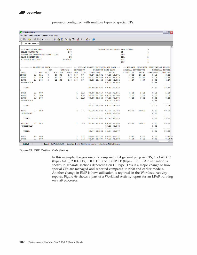
processor configured with multiple types of special CPs.
In this example, the processor is composed of 4 general purpose CPs, 1 zAAP CP
(type=AAP), 2 IFL CPs, 1 ICF CP, and 1 zIIP CP (type= IIP). LPAR utilization is
shown in separate sections depending on CP type. This is a major change to how
special CPs are managed and reported compared to z990 and earlier models.
Another change in RMF is how utilization is reported in the Workload Activity
reports. Figure 66 shows a part of a Workload Activity report for an LPAR running
on a z9 processor.
Figure 65. RMF Partition Data Report
zIIP overview
102 Performance Modeler Ver 2 Rel 3 User’s Guide

The major change to this report is that it now includes information on zIIP eligible
instructions. Under the APPL % column are two new fields, The IIPCP field reports
on the % of time that this workload executed zIIP eligible instructions on general
purpose CPs. The IIP field represents the % of time this workload executed zIIP
eligible instructions on zIIP CPs. The fields reporting on zAAP usage have been
changed from IFA to AAP. In order to capture and report zIIP eligible usage you
must be running z/OS 1.6 with the appropriate PTFs. These new fields contain the
information that is required by Performance Modeler in order to build a model
that supports zIIP CPs.
Extracting zIIP information
Much of the following discussion regarding zIIP support is the same as the
previous discussion on zAAP support. The procedure for running the Extract
function for zIIP utilization has already been covered in the previous section on the
zAAP extract. The only difference is the utilization of zIIP CPs is now stored in the
file labelled ZIIP Report File Name when you run the LPAR Extract function.
When you run a Workload Extract function, there is a new field called # of ZIIP
CPUs. This represents the number of zIIP CPs in the shared pool. After running
the LPAR and Workload Extract function, all of the information needed to build a
model with support for zIIP CPs has been captured. One word of caution; the
extracted data is only valid if the RMF report contains zIIP usage. Before running
these extracts you should examine the RMF reports to be sure they are properly
capturing the zIIP usage.
Figure 66. Workload Activity Report
zIIP overview
Chapter 8. Modelling zIIP processors 103
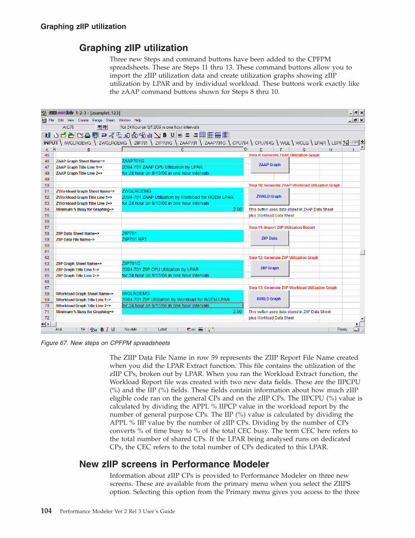
Graphing zIIP utilization
Three new Steps and command buttons have been added to the CPFPM
spreadsheets. These are Steps 11 thru 13. These command buttons allow you to
import the zIIP utilization data and create utilization graphs showing zIIP
utilization by LPAR and by individual workload. These buttons work exactly like
the zAAP command buttons shown for Steps 8 thru 10.
The ZIIP Data File Name in row 59 represents the ZIIP Report File Name created
when you did the LPAR Extract function. This file contains the utilization of the
zIIP CPs, broken out by LPAR. When you ran the Workload Extract function, the
Workload Report file was created with two new data fields. These are the IIPCPU
(%) and the IIP (%) fields. These fields contain information about how much zIIP
eligible code ran on the general CPs and on the zIIP CPs. The IIPCPU (%) value is
calculated by dividing the APPL % IIPCP value in the workload report by the
number of general purpose CPs. The IIP (%) value is calculated by dividing the
APPL % IIP value by the number of zIIP CPs. Dividing by the number of CPs
converts % of time busy to % of the total CEC busy. The term CEC here refers to
the total number of shared CPs. If the LPAR being analysed runs on dedicated
CPs, the CEC refers to the total number of CPs dedicated to this LPAR.
New zIIP screens in Performance Modeler
Information about zIIP CPs is provided to Performance Modeler on three new
screens. These are available from the primary menu when you select the ZIIPS
option. Selecting this option from the Primary menu gives you access to the three
Figure 67. New steps on CPFPM spreadsheets
Graphing zIIP utilization
104 Performance Modeler Ver 2 Rel 3 User’s Guide

new zIIP definition screens. These are IConfiguration, IWorkloads, and ILPARs.
These screens are similar to the three standard input screens available on the
Primary menu. Let’s take a look at each one. Selecting the IConfiguration option
displays the following screen.
The zIIP Configuration screen looks very similar to the zAAP Configuration screen
and contains information about the CPs in the zIIP CP pool. In this example they
are designated as a 2094-701. There are no user defined options such as Crossover
or HonorPriority for zIIP CPs so these options are not on this screen. The internal
setting for deciding where zIIP eligible instructions will run is equivalent to the
Crossover=NO and HonorPriority=YES settings for zAAP CPs. This means zIIP
eligible instructions may run on general purpose CPs whenever the system
determines that the zIIP CPs are running at high utilization and need help from
the general purpose CPs. When zIIP instructions run on the general purpose CPs,
they run at the same dispatching priority as the issuing task.
When you select the IWorkloads option, the following screen is displayed:
Figure 68. zIIP Configuration screen
New zIIP screens in Performance Modeler
Chapter 8. Modelling zIIP processors 105

This screen shows the same workloads that are defined in the standard Workloads
screen. The only field that is different and can be changed is the Path Length field.
That represents the average number of instructions that is zIIP eligible within each
transaction. For example, the Path Length for CISDDF (workload # 6) is 3.3561
million instructions. That means each transaction can execute 3.3561 million
instructions on a zIIP CP. This is in addition to the other instructions each
transaction executes. All of the other fields are disabled because they are copied
from the Workloads screen and can only be changed on that screen. When the
simulator begins, Performance Modeler treats each transaction as consisting of
three kinds of instructions, general purpose only instructions, zAAP eligible
instructions, and zIIP eligible instructions. General purpose instructions can only
execute on general purpose CPs. zAAP eligible instructions can execute on general
purpose CPs or on zAAP CPs. zIIP eligible instructions can execute on general
purpose CPs or on zIIP CPs.
Whether these instructions execute on general purpose CPs or on zIIP CPs
depends on several factors. If the configuration does not include zIIP CPs, then
these instructions must execute on the general purpose CPs. Even if you have zIIP
CPs, some of the zIIP eligible instructions may execute on the general purpose
CPs, depending on how busy the zIIP CPs run. Workloads that have a 0 value for
Path Lengths in the IWorkloads screen do not have any zIIP eligible work.
Figure 69. zIIP Workload screen
New zIIP screens in Performance Modeler
106 Performance Modeler Ver 2 Rel 3 User’s Guide

This screen looks very much like the standard LPAR screen, but it contains
information about the LPARs sharing the zIIP CPs. Since we are modelling an
LPAR which has zIIP eligible code, LPAR #1 (SOSP7) represents the same LPAR
that was defined as LPAR #1 in the LPAR screen. The second LPAR, Other,
represents other LPARs that are sharing the zIIP CPs.
Building a model with zIIP CPs
Building a model for a processor with zIIP CPs is very similar to building a model
with zAAP CPs. The Build function now contains one extra step where you can
specify whether you have zIIP CPs installed. Figure 71shows that Step 4 in the
Build function now provides you the opportunity to specify the zIIP configuration.
Figure 70. zIIP LPAR screen
New zIIP screens in Performance Modeler
Chapter 8. Modelling zIIP processors 107

When you select the Step 4 command button, the following screen is displayed:
Figure 71. Model Build screen
Building a model with zIIP CPs
108 Performance Modeler Ver 2 Rel 3 User’s Guide

The default setting is No zIIP CPs. If you are building a model for a processor
with zIIP CPs, you must do the following. First, select the Y option to indicate zIIP
CPs are available. Next, select the appropriate number of zIIP CPs by changing the
configuration to match the correct zIIP model. Since all zIIP CPs run at full speed,
you should not choose one of the sub capacity z9 models. For example, if you are
configuring 2 zIIP CPs on a z9 model 2094-706, then you should specify a 702 as
the zIIP model. Finally, select the zIIP Report File button so you can specify the
appropriate zIIP Extract file. This is the file containing the utilization of the zIIP
LPARs. This is the file you created when you ran the LPAR Extract function and
created the ZIIP Report File. After you select OK, the rest of the Build function
proceeds normally.
One of the differences is that as the Build function proceeds you are asked to
confirm or change the LPAR definitions for the LPARs using the zIIP CPs. Simply
confirm the definitions or make changes as appropriate. Finally, on the Calibration
screen, there are two buttons labelled ZAAP and ZIIP on the bottom of the screen
(see Figure 73 below). When you select the ZIIP button, the calibration screen
changes to show the target utilizations for each workload when they are executing
on the zIIP CPs. When you select the ZAAP button, the screen shows the
corresponding information for the zAAP CPs.
After the calibration step completes the new model is built and ready for saving.
Figure 72. ZIIP Option Selection screen
Building a model with zIIP CPs
Chapter 8. Modelling zIIP processors 109

Other changes due to modelling zIIP CPs
zIIP support has changed several other screens and added new screens. These are
similar to the changes introduced with zAAP support.
The changes are in the screens that support both the Run Wizard and the Multi
Image Run Wizard function. For example, when specifying the target
configurations in both wizards, you can now specify whether you have zIIP CPs.
As you proceed through the wizard there are screens that ask you to specify the
LPAR definitions for the LPARs allocating zIIP CPs. These new screens are
identical to the screens that were introduced when zAAP support was added.
For a description of these screens, read the section on zAAP support. You can
simply substitute zIIP for zAAP in the description to see how these new screens
work.
zIIP changes to the output reports
Running a model with zIIP CPs looks very similar to running with zAAP CPs. One
difference is the new two fields that show the utilization of the zIIP CPs. These
fields are shown in Figure 74.
Figure 73. Calibration screen for General Purpose CPs
Other changes due to modelling zIIP CPs
110 Performance Modeler Ver 2 Rel 3 User’s Guide

These new fields are Total ZIIP and Model ZIIP in columns H and I. Total ZIIP
represents the total utilization of the shared pool of zIIP CPs. Model ZIIP
represents the utilization of the zIIP CPs by the LPAR being modelled. This is a
good place to restate the key difference between modelling special CPs on a z990
processor compared to a z9 processor. First, z990 processors do not support zIIP
CPs, so you cannot model zIIP CPs on a z990. All of the special purpose CPs on a
z990 processor are dispatched from a single pool of shared CPs, which can be ICFs,
IFLs, or zAAP CPs. When you look at the modelling results for a z990 and you
look at the column labelled Total ZAAP in the SIMN sheet, you are looking at the
utilization of the entire pool of special purpose CPs. By contrast, all special
purpose CPs in a z9 processor run in their own shared pool. That means when
looking at the Total ZAAP column for a z9 processor, this represents the total
utilization of the pool of zAAP only CPs. And the Total ZIIP column represents the
total utilization of the pool of zIIP only CPs.
Figure 74. Reporting of zIIP utilization
zIIP changes to the output reports
Chapter 8. Modelling zIIP processors 111

112 Performance Modeler Ver 2 Rel 3 User’s Guide

Chapter 9. The Consolidate spreadsheet function
This section discusses a new feature introduced in TPM V2.3. The Consolidate
function is a new spreadsheet and set of Macros implemented in the CPFPM.123
and CPFPM.XLS files. This feature provides a simple point and click process for
sizing processors based on current utilization reports.
The function is designed to help you size a processor when you are looking to
move LPARs, or consolidate LPARs from one or more existing CECs onto a single
new CEC. While the modelling capability of TPM lets you see the impact of
change on workload performance, the Consolidate function lets you estimate the
correct processor model for a given mix of LPARs.
The output from the Consolidate function is a series of charts showing the actual
MIPS used for each reporting interval, mapped out against one or more target
processors. For example, Figure 75 shows an example of a chart created by the
Consolidate function, and is designed to size a processor capable of running
several LPARs. In this example, several LPARs are shown mapped out against a
2094-706 and a 2094-707. The chart shows that when you plot the actual MIPS used
by each LPAR for each reporting interval, the 706 looks to be a tight fit, while the
707 looks to be a better choice to host these LPARs. It should be pointed out that
these LPARs are currently spread over two 2064 generation processors.
Before you can use the Consolidate function, you must run the LPAR Extract
function for each CEC you want to analyse. The output of the Extract function is a
series of .RPT files that contain LPAR utilization data for various date and time
intervals. If the LPARs are spread over more than one CEC, you must run the
Figure 75. MIPS consumption by LPAR chart
© Copyright IBM Corp. 2002, 2008 113

Extract function and build an .RPT file for each of these CECs. You must also
ensure that the time span and reporting interval is the same for each .RPT file.
Once the extracts are complete, you should import these files into the CPFPM
spreadsheet and build the charts showing utilizations for each LPAR. This is the
same sequence described earlier in this manual (Step 1 and Step 2 in the Input
Sheet).
In the following example, we ran the LPAR extract for three CECs: a 2064-1C7, a
2064-2C7, and a 2064-210. The extracted data was used to build three spreadsheets
and they were named CPU1C7, CPU2C7, and CPU210 (Step 1 in the Input Sheet).
Next, a utilization chart was built for each CEC (Step 2 in the Input Sheet) and
they were named CPU1C7G, CPU2C7G, and CPU210G. Figures 76, 77, and 78
show these three charts. Notice that the reporting period and interval is the same
for each CEC.
Figure 76. CPU Utilization by LPAR for 2064-1C7
The Consolidate spreadsheet function
114 Performance Modeler Ver 2 Rel 3 User’s Guide

Once the LPAR utilization data has been imported into the spreadsheet we are
ready to use the Consolidate function. Let’s begin by describing the scenarios we
want to analyse. The first scenario is to consolidate all of the LPARs from the 1C7
Figure 77. CPU Utilization by LPAR for 2064-2C7
Figure 78. CPU Utilization by LPAR for 2064-210
The Consolidate spreadsheet function
Chapter 9. The Consolidate spreadsheet function 115

and 2C7 onto a single CEC. In this example we consider only the z9 EC models as
candidates for the target of this consolidation. Figure 79 shows the Consolidate
spreadsheet and the buttons that are present in this sheet.
The fields in blue are input fields.
The first step in this analysis is to normalize the utilization reports to MIPS being
used. You do this by multiplying the utilization data for each LPAR by the MIPS
rating of the CEC where that LPAR runs. In Figure 79 you can see that we have
listed the three existing spreadsheets which hold the utilization data for each of
our three CECs. In column C we have defined the MIPS rating for each of these
CECs.
When we click the MIPS Tables button under Step 1, the underlying code creates
three new sheets. Each new sheet contains the LPAR utilization data normalized to
MIPS actually being used. The new sheets are given the same name as the input
sheet containing utilization data, but with an M added to the end of the name. For
example, the utilization data in sheet CPU1C7 is normalized to MIPS and stored in
a new sheet named CPU1C7M. After Step 1 completes we have normalized the
utilization data to MIPS for each LPAR in each of the three CECs.
We are now ready to analyse the consolidation of the 1C7 and 2C7 onto a single z9
CEC. We do this by using one of the two buttons under Step 2.
Both of these buttons create a chart showing the total concurrent MIPS used by all
of the LPARs selected for consolidation, for each reporting interval. The difference
between the two buttons is that clicking the first button produces an Area chart
while clicking the second button produces a Stacked Bar chart.
Figure 79. Consolidate spreadsheet
The Consolidate spreadsheet function
116 Performance Modeler Ver 2 Rel 3 User’s Guide

When you have many reporting intervals it is probably easier to view the results in
an Area chart. This is probably the right choice when the reporting period spans 24
hours per day.
In this example we have a small set of reporting intervals, so we click the Bar
Graph button.
You must enter values in some input fields before you click one of these buttons:
v Under the column labelled Model enter the processors you want to examine as
candidates for consolidation. We have entered two processors here.
v To the right, under the column labelled MIPS, enter the MIPS rating for each
processor.
v At the bottom of the chart, enter the MIPS Chart Sheet Name. In this example
we have set the sheetname to 1C7and2C7. This is used as the name of the new
sheet.
v Beneath this line, enter the two lines that are inserted into the chart as titles.
When you click the Bar Graph button a message appears asking if you want to
include an LPAR into this consolidation analysis. There is one message for each
LPAR that appears in the Sheets defined under the Sheet Name column. This is
where you pick which LPARs are to be part of the analysis.
We have three sheets defined in this example, so there were three messages, one
for each LPAR currently running on these three CECs. In this scenario, we are only
interested in consolidating LPARs from the first two CECs (the 1C7 and 2C7), so
we reply yes to each of those LPARs and no to the LPARs currently running on the
210.
After all of the messages and replies are processed, a new chart is created in a new
sheet. Figure 75, shown earlier, is the chart produced from the example data.
One way to interpret these charts is to see if there are any intervals when the total
MIPS consumed today exceeds the capacity of the target processor. When that
happens, you can assume that one or more workloads will probably run worse
than it is currently running today. Whether that is acceptable or not is a different
question.
If you need to examine which workloads will run worse, and by how much, you
can build a model for this interval and model the impact on workload
performance.
In the previous example, we examined how much capacity would be required to
consolidate two CECs onto a single CEC. If we now want to change the
consolidation scenario we can do so with a few simple changes to the spreadsheet.
For example, suppose we want to examine consolidating the 2C7 and 210 onto a
single CEC. We can do that by changing the input fields as shown in Figure 80.
The Consolidate spreadsheet function
Chapter 9. The Consolidate spreadsheet function 117

The only thing we have changed is the MIPS Chart Sheet Name. Since we are now
looking to consolidate the 2C7 and the 210, we changed the name of the new sheet
to 2C7and210. Now when we click the Bar Graph button, and we are asked which
LPARs to include, we answer no to the LPARs running on the 1C7 and yes to the
LPARs running on the 2C7 and 210. After responding to all of the messages, the
new chart as shown in Figure 81 is displayed.
Figure 80. Changing the LPARs
The Consolidate spreadsheet function
118 Performance Modeler Ver 2 Rel 3 User’s Guide

If you want to make a change to the consolidation plan, select the Bar Graph
button again and select a different mix of LPARs. By answering yes or no, you can
choose to include or exclude LPARs from any of these CECs. This gives you a
powerful tool for looking at many different consolidation scenarios in a short
amount of time.
Once you have identified a list of potential candidates for consolidation, you can
use the modelling function in TPM to further examine the impact on workload
performance.
Figure 81. The new MIPS Consumption by LPAR chart
The Consolidate spreadsheet function
Chapter 9. The Consolidate spreadsheet function 119

120 Performance Modeler Ver 2 Rel 3 User’s Guide

Chapter 10. Monitoring IFL and ICF processors
For z9, z10 and follow on processor families a function has been added to allow
monitoring of the Integrated Facility for Linux (IFL) and Integrated Coupling
Facility (ICF) assigned processors. This function will show the utilization of these
specialty processors and for shared engines will allow monitoring of the need for
additional engines as they approach 100% utilization. Dedicated IFL and ICF
engines will always show 100% utilization.
Extracting IFL and ICF information
The information for utilization of the IFL and ICF engines is gathered as part of
the Extract RMF Reports LPAR Report process (“Step 1 - Extract the RMF Reports
and create the LPAR.RPT and WGL.RPT files” on page 27).
Importing the extracted reports into a spreadsheet
Four buttons have been added to the Input sheet of the Lotus 123 and Excel
spreadsheets, as shown in Figure 82.
This example looks at the ICF utilization. The input report file name is updated in
the C87, and the name of the output data sheet is updated in cell c86. When these
fields are filled in and you select the ICF Data button, the new sheet in Figure 83 is
created.
Figure 82. IFL and ICF spreadsheet buttons
© Copyright IBM Corp. 2002, 2008 121
|
|||
|
|
||||||
||
|||
||
|||
|||||

Starting in row 5 are the LPAR Names. From Row 7 down shows the ICF
utilization of each LPAR plus Total utilization for the entire processor. Each row
corresponds to a different reporting interval. The header information in rows 1
thru 3 are used in subsequent steps to control how charts are displayed.
Generating a chart showing ICF (or IFL) utilization
You can now create a chart showing ICF utilization of this broken out by LPAR if
the ICF is shared. Cell C91 in the Input sheet of the spreadsheet (Figure 82) has
already been set up to generate a new sheet with the name ICF726G. The G was
added to the previous sheet name to indicate it is a graph of the 726. The text in
cells C92 and C93 are titles you want to see in the new chart. When you select the
LPAR Graph button, the new sheet labelled ICF726G is created and shown in
Figure 84.
Figure 83. ICF utilitization example
Importing the extracted reports into a spreadsheet
122 Performance Modeler Ver 2 Rel 3 User’s Guide
|
|||||||
||
||||||||

This chart shows the utilization of the ICF for LPAR INTPRD12 for each reporting
interval and allows monitoring of the ICF as utilization increases.
Figure 84. Chart of ICF utilitization
Generating a chart showing ICF (or IFL) utilization
Chapter 10. Monitoring IFL and ICF processors 123
|
|||||

124 Performance Modeler Ver 2 Rel 3 User’s Guide

Appendix A. Workload Table description
Here is a description of each field in the Workload Table. Figure 85 shows a typical
Workload Table. This table is created during the Build process and imported into
the CPFPM spreadsheet using the command button labelled Workload Table.
Field Description
Workload
Workload name (defined in Workload Policy)
Serv Class
Service Class name
Period Period (for multi-period Service Classes)
Priority
A number that indicates the relative importance of this workload as seen
by Workload Manager. The number is created by TPM by multiplying the
Workload Importance (ie Importance=1) by 100. Next the Execution
Velocity Goal is subtracted from 100 and the result is added to the first
number. For example, a workload with importance=3 and execution
velocity goal of 30% would be assigned a priority of 370. The larger this
number, the less important it is. All workloads assigned to a SYSTEM Goal
are assigned a priority=0, and all Discretionary work is assigned a
priority=600.
CPU (%)
Percent of the time the workload is executing. This is also the APPL%
value in the Workload Activity Report and represents the Single CPU
Figure 85. Workload Table
© Copyright IBM Corp. 2002, 2008 125

Utilization. Dividing this number by the number of general purpose CPs
(versus zAAP CPs) that are available yields the Total (%) number below.
Total (%)
The percent of the total machine (available general purpose CPs) that is
being used by this workload.
AAPCPU (%)
This field is only shown if you are running z/OS V1R6 or later release of
z/OS. This field represents the percent of the general purpose CPs that
was used by this workload and was also capable of running on a zAAP
CP. This is a subset of the Total (%) field.
AAP (%)
This field is only shown if you are running z/OS V1R6 or later release of
z/OS. This field represents the percent of the special purpose CPs that was
used by this workload. This represents zAAP eligible code which executed
on a zAAP CP. Prior to the release of the z9 processors the zAAP CP can
be assigned to any available CP in the shared pool, and it is calculated as:
cpu time/(# of special purpose CPs x duration interval).
For example, if there are three ICFs and two zAAP CPs in the shared pool,
the number of special purpose CPs in the shared pool is five. This field
only has a value when there are zAAP CPs available.
When running on z9 or later processors, all special purpose CPs are
managed in separate pools. That means the # of special purpose CPs used
to calculate the AAP(%) value on a z9 will be the # of CPs in the zAAP
pool.
IIPCPU (%)
This field is only shown if you are running z/OS V1R6 or later release of
z/OS with the appropriate PTFs on a z9 processor. This field represents the
percent of the general purpose CPs that was used by this workload and
was also capable of running on a zIIP CP. This is a subset of the Total (%)
field.
IIP (%)
This field is only shown if you are running z/OS V1R6 or later release of
z/OS with the appropriate PTFs on a z9 processor. This field represents the
percent of the special purpose zIIP CPs that was used by this workload.
This represents zIIP eligible code which executed on a zIIP CP. This value
is calculated as:
cpu time/(# of zIIP CPs x duration interval).
The # of zIIP CPs is the total # of CPs in the shared pool of zIIP CPs.
Cumulative
The cumulative utilization for each workload. This is the CP utilization by
this workload, plus the sum of utilization from all workloads that run
higher priority within this LPAR. It is an indication of how busy the
system appears to each workload. This does not include the utilization by
other LPARs. The Cumulative column is only calculated for general
purpose CPs.
MPL The average number of Address Spaces that were active in this workload.
This is also called the Multi Programming Level.
Workload Table description
126 Performance Modeler Ver 2 Rel 3 User’s Guide

Xrate Transaction Rate (trans per second) for this workload. Generally this is
only meaningful for TSO and other workloads that capture transaction
statistics.
Velocity
The actual Execution Velocity measured for this workload. This is a
measure of the number of Address Spaces that were doing productive
work (ie executing or doing I/O) as a percent of the total number of
Address Spaces that were ready to do work.
PI Performance Index. A measure of how close the workload came to meeting
it’s workload Goal defined to Workload Manager. For workloads that have
an Execution Velocity Goal, the PI is calculated as Goal divided by actual
measured Velocity. A PI of 1 means the goal was achieved. Greater than 1
means it was missed, and less than 1 means it was exceeded.
Goal Goal assigned to this workload. This is the Execution Velocity Goal. If the
workload has a response time goal, it is displayed as a 0.
SSCHRT
Start SubChannel Rate. I/Os per second measured for this workload.
Resp Average Disk Response times (seconds) for this workload.
At the bottom of the Total (%) column are the following fields. If IFACPU and IFA
fields are shown in the workload table, there are two sets of results, one for the
general purpose CPs, and another for the CPs in the special purpose CP pool.
Total Sum of all the captured percent busy for all workloads.
Actual Actual percent busy for this LPAR.
Uncaptured
Uncaptured Time, the percent of LPAR busy that was not captured by
workload (Actual-Total).
C. R. (%)
Capture Ratio. The percent of LPAR busy that was captured by workloads
(Total/Actual x 100)
All LPARs
Total percent busy for the entire machine (includes other LPARs).
Rel IO
The Rel IO value represents the ratio of disk I/Os per second divided by
how many MSUs this image consumed. The Rel IO value is used to
determine which IBM LSPR (Large Systems Performance Ratio) benchmark
best represents this image. IBM recommends a rule of thumb that if the Rel
IO ratio is less than 30, then this image should be represented by the Lo IO
Mixed workload column in the LSPR table. The calculation of Rel IO uses
the MSU rating provided in row 26 of the Input sheet in the Lotus 123 and
Excel spreadsheets.
Workload Table description
Appendix A. Workload Table description 127

Workload Table description
128 Performance Modeler Ver 2 Rel 3 User’s Guide

Appendix B. Defaults used in the Build process
The Build process uses several defaults to build a model. These defaults should be
reviewed to see if they should be changed. For example, the I/O response times
are based on the average disk response times reported in the RMF Workload
Activity reports. Occasionally, these values may be skewed by a single disk drive
and may not make sense for inclusion in the model. An example would be a disk
response time which is exceptionally high such as greater than 1 second. When this
occurs, it probably makes sense to manually change it to a more realistic value. If
the average disk response time cannot be found in the workload reports, the Build
process uses a default of .010 seconds.
If the SSCHRT (Start Sub Channel Rate) is available, this is used to calculate the
I/Os per online transaction. If the SSCHRT is not available, Build uses a default of
50 disk I/Os per online transaction. If you know the actual number of I/Os per
transaction, you should change it to match the real value. Paging rates, for
auxiliary and Expanded storage defaults to 0. If you are experiencing significant
paging rates, change these values to match the actual paging rates.
Build also uses a default for the initial path length for OLTP workloads. The
default path length can vary between 2 million and 8 million instructions per
online transaction. Once the path length is set, Build calculates the average
transaction rate by using the following relationship. The MIPS consumed by each
OLTP workload is the product of average path length and the average transaction
rate. Once the MIPS consumed value is known, and the average path length is set
to the default value (2 to 8 million instructions per transaction), the transaction rate
is calculated as MIPS consumed divided by transaction rate. For example, if a
workload consumes 45 MIPS and the average path length is set to two million
instructions per transaction, the transaction rate must be 45/2 = 22.5 transactions
per second.
If you measure the actual CPU time used by an average transaction you may elect
to change this default. For example, assume the Build process generated these
model parms:
v An average path length of two million instructions per transaction
v An average transaction rate of 50 transactions per second
This means the workload consumes 100 MIPS. Now assume that actual
measurements show the average CPU time per transaction is .02 seconds, and
assume each CPU is rated at 120 MIPS per CPU. Then multiplying 120 MIPS by .02
seconds per transaction equals the actual path length of 2.4 million instructions per
transaction. If you change the default path length from 2.0 to 2.4 you must also
change the transaction rate. In order to keep the MIPS consumed the same, you
must change the average transaction rate by multiplying the original value by
2.0/2.4. That means the transaction rate must be changed from 50 to 50 x 2.0/2.4 =
41.67 transactions per second. The new path length multiplied by the new
transaction rate = 2.4 x 41.67 = 100 MIPS, so the MIPS consumed does not change.
© Copyright IBM Corp. 2002, 2008 129

130 Performance Modeler Ver 2 Rel 3 User’s Guide

Appendix C. Advanced modelling topics
This section discusses how to model some of the most common workload
environments. As with any tool, the value of Performance Modeler depends on
how you use it. Although most input parameters are straight forward and easy to
understand, some can be confusing or misunderstood. This section explains how to
translate real configurations into the correct input parameters.
Modelling TSO
TSO workloads should be modelled as multi tasking (Type=M) online workloads.
Each TSO transaction runs independently from another TSO transaction. Most
installations define multiple periods for TSO. As TSO transactions accumulate
service they move from one period to another. And as they move, their priority (or
Importance in Goal Mode) also changes. When you select a TSO workload, the
Build function assumes an average path length and uses that value to back into the
arrival rate. The calculation is based on the equation MIPS consumed = Path
Length x Arrival Rate. During the Build function, MIPS consumed is calculated as
Percent Busy x MIPS rating. You can use the default path length and calculated
arrival rate or you can change these values to more closely match their actual
values.
For example, assume you selected TSO Period 1 as one of the workloads you want
to model. Let’s also assume the MIPS consumed during the reporting interval was
20 MIPS. During the Build function the path length was assumed to be 2 million
instructions per second. Based on these values, the arrival rate was calculated as 10
transactions per second. The calculation was MIPS = Path Length x Arrival Rate
(20=2x10). But you can refine these values by changing the arrival rate to match
the actual arrival rate. The Workload Activity report shows the actual arrival rates
for TSO workloads. If you see that the actual transaction rate for TSO Period 1
work was 30 transactions per second, you can recalculate the path length using the
same equation. That results in New Path Length = MIPS/Arrival Rate. That gives
us New Path Length = 20/30 = .667 million instructions per transaction.
Modelling CICS and IMS
Online workloads such as CICS and IMS can be modelled in a number of ways. If
you want to model the performance of a single CICS or IMS region they can be
modelled as a single workload of Type=S (single tasking). But most CICS regions
do some degree of multi tasking. Although most of the execution takes place under
the single CICS main TCB (Task Control Block), some execution runs under
separate TCBs. VSAM file I/O, for example, creates multiple TCBs under heavy
load. And the Terminal I/O manager also runs under its own TCB. If we model all
the CICS workload as a single TCB (Type=S), we would have a very conservative
and possibly negative picture of what is really happening. The result could be a
model that shows a single CPU constraint when it really doesn’t exist. Single CPU
constraint occurs when a single tasking workload consumes near 100% of a single
CPU.
One way to consider that some amount of CICS is running under a separate TCB
is to break the workload into two copies. Each workload would be defined as
Type=S, but the amount of CPU consumption would be different. For example,
consider a single CICS region where we want to model 90% of the CPU running
© Copyright IBM Corp. 2002, 2008 131

under one TCB, and 10% under a second TCB. Let’s also assume this region is
consuming 50 MIPS capacity. One way to model this workload is to define two
workloads CICSB (CICS Big) and CICSL (CICS Little). If we assume the same
transaction rate for both workloads, we can control the MIPS consumed by
assigning 90% of the average path length to CICSB and 10% to CICSL. Once again,
a path length of 2 million instructions means we need a transaction rate of 25 trans
per second to consume 50 MIPS. Thus we can assign 25 trans per second to both
workloads but assign .9 x 2 = 1.8 million instructions as the path length to CICSB
and .1 x 2 = .2 million instructions to CICSL. This gives a net MIPS consumed of
50 but allocates 90% of that to CICSB and 10% to CICSL.
In this example, we assumed that 90% of the CICS work ran under a single TCB.
But if the CICS region uses DB2(R), the amount of multi tasking may be much
higher than 90/10. Since DB2 creates multiple TCBs, it may be appropriate to
model this CICS region as a Type=M workload. That depends on how much CPU
is consumed by DB2 versus the CPU running under the main TCB. This
information may be difficult to determine and is beyond the scope of this manual.
One rule of thumb for a DB2 intensive CICS region is to allocate half the MIPS to a
single tasking CICS workload and the other half to a multi tasking (Type=M) DB2
workload. In the example above, if the CICS region is DB2 intensive, we can
spread the workload over two workloads, CICS and DB2. The CICS workload
would be defined as Type=S, the average path length set to 2 million instructions
per second, and the transaction rate set to 12.5 transactions per second. This
workload would consume 50% of the 50 MIPS. The DB2 workload would be
defined as Type=M, with the same path length and transaction rate as CICS. This
would consume the other half of the 50 MIPS but would spread the work over
multiple TCBs.
Modelling workload growth
One of the common requirements for capacity planning is to model the impact of
workload growth. Workloads grow for several reasons. Over time, the volume of
work processed by existing applications tends to increase. This may reflect an
increase in the amount of data being fed into an application, or it may reflect end
users who are more efficient and faster at hitting the enter key. But experience has
show that most mainframe applications grow in their use of resources over time.
One of the more accurate ways to predict future growth is to look at historical
trends. This is often called navigating by looking at the wake. But growth also
occurs in sudden large increases as when a new application is installed or when a
major rewrite occurs. A typical exercise for the capacity planner is to project these
workload increases over time and model the impact on performance and capacity
requirements. Performance Modeler includes two features that make it easy to
model the impact of growth over a time interval. First, the Workload Definition
screen contains a button (X) next to each workload Average Arrival Rate field. This
is the multiplication button and provides you with a simple way to increase
workload volumes. When the multiplication button is selected, you are asked to
enter a multiplication factor. This factor is used to multiply the arrival rate. For
example, a multiplication factor of 1.50 increases the arrival rate by 50%. That
effectively increases the MIPS consumed by this workload by 50%. Using the
multiplication button makes it easy to increase the amount of online work being
modelled.
But batch workloads must be handled differently. The amount of work processed
by batch workloads can be increased by raising the # of Users parameter. For batch
workloads, this parameter controls the multi-programming level (MPL). For
example, a value of two tells the simulator to create two identical batch jobs. For
Modelling CICS and IMS
132 Performance Modeler Ver 2 Rel 3 User’s Guide

example, if the MPL for a batch workload is currently two, changing the MPL to
three is equivalent to a 50% increase in that workload. Changing the batch
workload MPL is preferable to changing other parameters, such as path length,
since it keeps the CPU to I/O ratio unchanged. The MPL can be a fraction
(non-integer) so you don’t have to worry about rounding the MPL up or down to
the nearest integer. When you use the X button for a batch workload the # of Users
value (MPL) is multiplied by the scaling factor. The large X button at the top of the
Workloads screen allows you to apply a single growth factor to every workload in
the model.
Latent demand in batch workloads
One of the most difficult exercises for the capacity planner is to estimate the
amount of latent demand in their system. This is the amount of work that is not
getting done because of resource constraints. Latent demand can be viewed as pent
up demand, waiting for additional capacity so it can break out. Understanding
latent demand is important since it determines how systems perform when new
capacity is added. Consider this scenario:
v The old system runs at 95% to 100% processor utilization during peak hour of
the day.
v The processor is replaced with a new processor rated as two times the capacity
of the current machine.
v The expectation was that processor utilization would drop to 50% to 60%. In
fact, processor utilization only drops to 80%.
The reason that utilization did not drop as low as expected is that a large amount
of work was not able to run on the old machine due to high utilization. When
capacity is added, this work is able to use the additional capacity and drive
utilization to higher than expected levels. This is a common scenario. Most
processors are not upgraded until they begin to run at high utilization. That means
there are probably workloads running at low priority that are being throttled or
held back. Since batch workloads are more likely to run at low priority (compared
to online workloads), these are the workloads which account for most examples of
latent demand. The following section discusses how Performance Modeler can be
used to measure and quantify the effect of batch latent demand.
Batch workloads differ from online workloads in the way they consume CPU
resources. The total MIPS consumed by an online workload can be calculated by
multiplying the transaction rate by the path length (transactions per second x
millions of instructions per transaction = millions of instructions per second or
MIPS). This relationship holds as long as there is sufficient capacity to allow the
online workload to run at the specified transaction rate. High priority online
workloads rarely demonstrate latent demand. But batch jobs consume as much
CPU capacity as they can. Batch jobs are only limited to the extent that they are
I/O bound and by how often they are preempted by higher priority jobs. Batch
jobs that run at low priority are often waiting while higher priority work use CPU
resources. The higher the processor utilization, the more time these jobs spend
waiting for a free CPU. The time waiting is called Queue time. Queue time is
directly affected by total processor utilization. But Queue time is also affected by
other constraints. For example, LPAR definitions may limit the capacity available
to batch jobs even when total utilization is below 90%. But these definitions and
their effects on batch performance can be modelled using Performance Modeler.
When additional capacity is modelled, the largest impact is usually seen by the
lowest priority workloads. When these are batch workloads, the result is a
Modelling workload growth
Appendix C. Advanced modelling topics 133

reduction in the modelled Elongation Factor for these workloads. Since Elongation
Factor is a direct measure of batch elapsed times, any reduction in Elongation
Factor is accompanied by an increase in processor utilization. In effect, batch
workloads are running faster and ending in less time by consuming more MIPS
while they run. The amount of increase in MIPS consumed depends on how
constrained were these workloads before capacity was added. This increase in
utilization can be defined as batch latent demand.
One word of caution on how to interpret these results. Batch workloads are
modelled as never ending tasks. That means each batch job continues to run for
the total duration of the model. If you model five batch jobs within a batch
workload (MPL=5), these five jobs keep running for the length of the model run.
When you model additional capacity, these five jobs run faster (lower Elongation
Factor), but the MPL is kept constant at five. In real life, when batch jobs end
sooner, the average MPL may actually go down. But the model assumes there is an
endless supply of batch work to maintain the same MPL, no matter how fast these
jobs run. That means the model depicts a worst case scenario regarding latent
demand. The latent demand shown by the model is probably on the high side. But
that depends on how much batch work is waiting to run. If you believe better
batch performance causes the average MPL to go down you can model that too.
For example, change the MPL from five to four, or whatever makes sense for your
installation. If you want a worst case view, or believe the batch MPL does not
change, leave it at five.
Latent demand in batch workloads
134 Performance Modeler Ver 2 Rel 3 User’s Guide

Notices
This information was developed for products and services offered in the U.S.A.
IBM may not offer the products, services, or features discussed in this document in
other countries. Consult your local IBM representative for information on the
products and services currently available in your area. Any reference to an IBM
product, program, or service is not intended to state or imply that only that IBM
product, program, or service may be used. Any functionally equivalent product,
program, or service that does not infringe any IBM intellectual property right may
be used instead. However, it is the user’s responsibility to evaluate and verify the
operation of any non-IBM product, program, or service.
IBM may have patents or pending patent applications covering subject matter
described in this document. The furnishing of this document does not give you
any license to these patents. You can send license inquiries, in writing, to:
IBM Director of Licensing
IBM Corporation
North Castle Drive
Armonk, NY 10504-1785
U.S.A.
Licensees of this program who wish to have information about it for the purpose
of enabling: (i) the exchange of information between independently created
programs and other programs (including this one) and (ii) the mutual use of the
information which has been exchanged, should contact:
IBM Corporation
Mail Station P300
522 South Road
Poughkeepsie New York 12601-5400
U.S.A.
Such information may be available, subject to appropriate terms and conditions,
including in some cases, payment of a fee.
The licensed program described in this document and all licensed material
available for it are provided by IBM under terms of the IBM Customer Agreement,
IBM International Program License Agreement or any equivalent agreement
between us.
For license inquiries regarding double-byte (DBCS) information, contact the IBM
Intellectual Property Department in your country or send inquiries, in writing, to:
IBM World Trade Asia Corporation
Licensing
2-31 Roppongi 3-chome, Minato-ku
Tokyo 106, Japan
The following paragraph does not apply to the United Kingdom or any other
country where such provisions are inconsistent with local law: INTERNATIONAL
BUSINESS MACHINES CORPORATION PROVIDES THIS PUBLICATION ″AS IS″
WITHOUT WARRANTY OF ANY KIND, EITHER EXPRESS OR IMPLIED,
INCLUDING, BUT NOT LIMITED TO, THE IMPLIED WARRANTIES OF
NON-INFRINGEMENT, MERCHANTABILITY OR FITNESS FOR A PARTICULAR
© Copyright IBM Corp. 2002, 2008 135

PURPOSE. Some states do not allow disclaimer of express or implied warranties in
certain transactions, therefore, this statement may not apply to you.
This information could include technical inaccuracies or typographical errors.
Changes are periodically made to the information herein; these changes will be
incorporated in new editions of the publication. IBM may make improvements
and/or changes in the product(s) and/or the program(s) described in this
publication at any time without notice.
Any references in this information to non-IBM Web sites are provided for
convenience only and do not in any manner serve as an endorsement of those Web
sites. The materials at those Web sites are not part of the materials for this IBM
product and use of those Web sites is at your own risk.
If you are viewing this information softcopy, the photographs and color
illustrations may not appear.
Trademarks
The following are trademarks of International Business Machines Corporation in
the United States, or other countries, or both:
1-2-3 CICS DB2
IBM IMS Lotus
MVS OS/390 RMF
S/390 Tivoli z/OS
Microsoft and Windows are trademarks of Microsoft Corporation in the United
States, other countries, or both.
Other company, product, and service names may be trademarks or service marks
of others.
Notices
136 Performance Modeler Ver 2 Rel 3 User’s Guide
Index
AAverage Arrival Rate 4
Average Path Length 4
average response timegraphed 22
Bbaseline model
build with Build function 39
batch workloads 4
modelling 5
Build functionbuild baseline model 39
Build option 10
build processdefaults 129
CCalibration Run option 19
Calibration screen 48
calibration screen for general purpose
CPs 88
calibration screen for special purpose
CPs 89
capacity planning 53
methodology 54
chartgenerating LPAR utilisation 34
CICS and IMSmodelling 131
Compatibility mode 27
Configuration Definition screen 9, 13
Configuration option 10
Consolidate function 113
Consolidate spreadsheet 116
CPFPM spreadsheetsnew steps 104
CPU Selection screen 65
DDB2 code
executed by zIIP processors 101
defaultsused in Build process 129
EEdit option 10
elapsed timegraphed 22
Extract option 10
extracted reportsimporting into spreadsheet 32
extracting zAAP information 74
FFile option 9
Filled in Build screen 41
GGeneral Purpose CPs
calibration screen 110
general purpose LPAR definition
screen 86
getting started 27
Goal mode 27
Graph Selection screen 22
graphing workload performance 22
Growth Rate screen 57
HHelp option 11
IICF processors
displayed in a chart 123
example data 122
extracting information 121
generating a chart 122
importing information into a
spreadsheet 121
monitoring 121
spreadsheet buttons 121
IFL processorsextracting information 121
generating a chart 122
importing information into a
spreadsheet 121
monitoring 121
spreadsheet buttons 121
inputspecifying 3
input screens 13
Input spreadsheetzAAP buttons 75
input spreadsheet for CPFPM.123 33
Llatent demand
in batch workloads 133
license inquiry 135
LPAR cappingenforcing 18
LPAR data report 74
LPAR data sheet 34
LPAR Definition screen 17, 47, 58
LPAR option 10
LPAR Report Extract screen 28
LPAR utilizationgenerating chart to show 34
LPAR utilization graph sheet 35
LPAR.RPTcreating 27
LPARsmodelling 62
MMerge option 10
MIPSdefining processor configuration 50
MIPS consumption by LPAR chart 113
modelbuilding with zIIP CPs 107
model build processmodel what if scenarios 50
select CPU report file 40
select processor 40
select workload report file 41
select workloads for modelling 42
select ZAAP options 41
select ZIIP options 41
model build screen 40
Model Build screen 108
model input 3
model output 3
model what if scenarios model build
step 50
modelling zAAP processors 71
modelsanalytical 2
building with zAAP CPs 81
general description 2
input 27
simulation 2
simulation vs analytical 2
Multi Image LPAR Definition screen 69
Multi Image LPAR Definitions screen 98
multi image runzAAP changes 95
Multi Image Run feature 62
Multi Image Run option 19
Multi Image Run Wizard option 20
Multi Image Run Wizard screen 64
Multi Image zAAP LPAR Definition
screen 99
multi-tasking workloads 4
Multiple Run option 19
Oonline workloads
modelling 4
outputdescribed 3
output reportschanges to cater for zAAP
processing 92
zIIP changes 110
© Copyright IBM Corp. 2002, 2008 137

PPerformance Modeler
installing 7
introduction 1
launching 7
purpose 2
uninstalling 7
performance modellingbasics 27
performance tracking 23
Performance Tracking screen 23
primary menu 9
Primary menu 9
Print option 19
Print Option screen 25, 59
print options 24
Process Utilization Tracking screen 24
Processing completed screen 30
processing optionszAAP 77
processorsizing 113
processor configurationMIPS discussed 50
QQuit option 11
RRestart option 19
Return option 19
RMF Partition Data Report 102
RMF reportscontrol parameters 27
extracting 27
Run option 9
run options 19
Run WizardzAAP changes 94
Run Wizard option 19
Run Wizard screen 55
Run Wizard zAAP LPAR Definition
Screen 95, 96
SSelect CPU Report File model build
step 40
Select CPU Report File options step 41
Select LPAR/Date/Time screen 42
Select LPARs screen 66
Select LPARs screen, Part 2 67
Select processor model build step 40
Select Workload Report File model build
step 41
Select Workloads for Modelling model
build step 42
Select ZAAP Options model build
step 41
Service Level Agreements 53
SIM.NUM results 60
SIMT.NUM Results report 94
SIMT.PRT for zAAP Modelling 92
SIMT.PRT Results report 93
simulationinformation displayed while
running 20
simulation models 2
simulation techniques 5
simulatorrunning 19
Simulator Running screen 20
Simulator Running screen - ZAAP
CPs 91
simulator summary table 61
Single Run option 19
single tasking workloads 4
Special Purpose CPU selection form 97
special purpose LPAR definition
screen 87
spreadsheetimporting extracted reports into 32
importing Workload Activity Report
File into 35
spreadsheet fileproducing with print option 25
system requirements 7
Ttext image 25
trademarks 136
TSOmodelling 131
VView option 11
WWGL.RPT
creating 27
Wizard Growth screen 68
Workload Activity fields 72
Workload Activity Report 103
Workload Activity Report Fileimporting into spreadsheet 35
workload data sheet 36
Workload Definition screen 15
workload growthmodelling 132
workload performance 23
graphing 22
Workload Report Extract screen 31
Workload Selection screen 43
workload tabledescription 125
Workload Table 125
Workload Type Definition screen 45
workload types 4
Workload Utilizationgraphing 37
workload utilization graph sheet 38
workloadsbatch 4
graphing 22
information 15
moving from model to model 15
workloads (continued)multi-tasking 4
onlinegraphing 22
single tasking 4
Workloads option 10
Workloads screen 49
Workloads Selected screen 46
ZzAAP
changes to output reports 92
ZAAP Build screen 82
after step 5 84
zAAP configuration screen 79
zAAP informationextracting 74
ZAAP LPAR screen 81
zAAP option selection screen 83
zAAP processing options 77
zAAP processorsmodelling 71
zAAP screens 78
zAAP utilization chart 76
zAAP workload screen 80
zAAP workload selection screen 85
zAAP workload utilization chart 77
ZAAPs option 10
zIIP Configuration screen 105
zIIP informationextracting 103
zIIP LPAR screen 107
ZIIP Option Selection screen 109
zIIP processorsmodelling 101
overview 101
zIIP screens 104
zIIP utilizationgraphing 104
reporting 111
zIIP Workload screen 106
ZIIPs option 10
138 Performance Modeler Ver 2 Rel 3 User’s Guide

Readers’ Comments — We’d Like to Hear from You
Tivoli Performance Modeler for z/OS
User’s Guide
Version 2 Release 3
Publication No. SC31-6385-07
We appreciate your comments about this publication. Please comment on specific errors or omissions, accuracy,
organization, subject matter, or completeness of this book. The comments you send should pertain to only the
information in this manual or product and the way in which the information is presented.
For technical questions and information about products and prices, please contact your IBM branch office, your
IBM business partner, or your authorized remarketer.
When you send comments to IBM, you grant IBM a nonexclusive right to use or distribute your comments in any
way it believes appropriate without incurring any obligation to you. IBM or any other organizations will only use
the personal information that you supply to contact you about the issues that you state on this form.
Comments:
Thank you for your support.
Submit your comments using one of these channels:
v Send your comments to the address on the reverse side of this form.
v Send a fax to the following number: 800-426-7773 (from within the U.S.) or 408-463-2629 (from outside the U.S.)
If you would like a response from IBM, please fill in the following information:
Name
Address
Company or Organization
Phone No. E-mail address

Readers’ Comments — We’d Like to Hear from You SC31-6385-07
SC31-6385-07
����
Cut or FoldAlong Line
Cut or FoldAlong Line
Fold and Tape Please do not staple Fold and Tape
Fold and Tape Please do not staple Fold and Tape
NO POSTAGENECESSARYIF MAILED IN THEUNITED STATES
BUSINESS REPLY MAIL FIRST-CLASS MAIL PERMIT NO. 40 ARMONK, NEW YORK
POSTAGE WILL BE PAID BY ADDRESSEE
IBM Corporation
H150/090
555 Bailey Avenue
San Jose, CA
U.S.A. 95141-9989
_ _ _ _ _ _ _ _ _ _ _ _ _ _ _ _ _ _ _ _ _ _ _ _ _ _ _ _ _ _ _ _ _ _ _ _ _ _ _ _ _ _ _ _ _ _ _ _ _ _ _ _ _ _ _ _ _ _ _ _ _ _ _ _ _ _ _ _ _ _ _ _ _ _ _ _ _ _ _ _ _ _ _ _ _ _ _ _ _
_ _ _ _ _ _ _ _ _ _ _ _ _ _ _ _ _ _ _ _ _ _ _ _ _ _ _ _ _ _ _ _ _ _ _ _ _ _ _ _ _ _ _ _ _ _ _ _ _ _ _ _ _ _ _ _ _ _ _ _ _ _ _ _ _ _ _ _ _ _ _ _ _ _ _ _ _ _ _ _ _ _ _ _ _ _ _ _ _
__
__
__
__
__
__
__
__
__
__
__
__
__
__
__
__
__
__
__
__
__
__
__
__
__
__
__
__
__
__
__
__
__
__
__
__
__
__
__
__
__
__
__
__
__
__
__
__
__
_


����
Program Number: 5698-A18
Printed in USA
SC31-6385-07