Performance Management Guide - Atossupport.bull.com/documentation/byproduct/servers/escala/software/aix/aix5.2/g/86Y232EF...Bull AIX 5L Performance Management Guide AIX Software September

Bull AIX 5L Performance Management Guide

AIX

86 A2 32EF 02ORDER REFERENCE

Bull AIX 5L Performance Management Guide

AIX

Software

September 2002

BULL CEDOC357 AVENUE PATTONB.P.2084549008 ANGERS CEDEX 01FRANCE


The following copyright notice protects this book under the Copyright laws of the United States of Americaand other countries which prohibit such actions as, but not limited to, copying, distributing, modifying, andmaking derivative works.

Copyright Bull S.A. 1992, 2002

Printed in France

Suggestions and criticisms concerning the form, content, and presentation ofthis book are invited. A form is provided at the end of this book for this purpose.

To order additional copies of this book or other Bull Technical Publications, youare invited to use the Ordering Form also provided at the end of this book.

Trademarks and Acknowledgements

We acknowledge the right of proprietors of trademarks mentioned in this book.

AIX� is a registered trademark of International Business Machines Corporation, and is being used underlicence.

UNIX is a registered trademark in the United States of America and other countries licensed exclusively throughthe Open Group.

The information in this document is subject to change without notice. Groupe Bull will not be liable for errorscontained herein, or for incidental or consequential damages in connection with the use of this material.

Contents

About This Book . . . . . . . . . . . . . . . . . . . . . . . . . . . . . . . . viiWho Should Use This Book . . . . . . . . . . . . . . . . . . . . . . . . . . . . . viiHighlighting . . . . . . . . . . . . . . . . . . . . . . . . . . . . . . . . . . . viiCase-Sensitivity in AIX. . . . . . . . . . . . . . . . . . . . . . . . . . . . . . . viiISO 9000 . . . . . . . . . . . . . . . . . . . . . . . . . . . . . . . . . . . viiRelated Publications . . . . . . . . . . . . . . . . . . . . . . . . . . . . . . . vii

Chapter 1. Tuning Enhancements for AIX 5.2 . . . . . . . . . . . . . . . . . . . . . . 1AIX Kernel Tuning Parameter Modifications . . . . . . . . . . . . . . . . . . . . . . . 1Modifications to vmtune and schedtune . . . . . . . . . . . . . . . . . . . . . . . . . 1Enhancements to no and nfso . . . . . . . . . . . . . . . . . . . . . . . . . . . . 2AIX 5.2 Migration Installation and Compatibility Mode. . . . . . . . . . . . . . . . . . . . 2System Recovery Procedures . . . . . . . . . . . . . . . . . . . . . . . . . . . . 3

Chapter 2. Performance Concepts . . . . . . . . . . . . . . . . . . . . . . . . . . 5How Fast is That Computer?. . . . . . . . . . . . . . . . . . . . . . . . . . . . . 5Understanding the Workload . . . . . . . . . . . . . . . . . . . . . . . . . . . . . 5Program Execution Dynamics . . . . . . . . . . . . . . . . . . . . . . . . . . . . 6System Dynamics . . . . . . . . . . . . . . . . . . . . . . . . . . . . . . . . 10Introducing the Performance-Tuning Process . . . . . . . . . . . . . . . . . . . . . . 11Performance Benchmarking. . . . . . . . . . . . . . . . . . . . . . . . . . . . . 15Related Information. . . . . . . . . . . . . . . . . . . . . . . . . . . . . . . . 16

Chapter 3. Resource Management Overview . . . . . . . . . . . . . . . . . . . . . 19Performance Overview of the processor Scheduler . . . . . . . . . . . . . . . . . . . . 19Performance Overview of the Virtual Memory Manager (VMM) . . . . . . . . . . . . . . . . 25Performance Overview of Fixed-Disk Storage Management . . . . . . . . . . . . . . . . . 33Support for Pinned Memory. . . . . . . . . . . . . . . . . . . . . . . . . . . . . 36Large Page Support . . . . . . . . . . . . . . . . . . . . . . . . . . . . . . . 37

Chapter 4. Introduction to Multiprocessing . . . . . . . . . . . . . . . . . . . . . . 39Symmetrical Multiprocessor (SMP) Concepts and Architecture . . . . . . . . . . . . . . . . 39SMP Performance Issues . . . . . . . . . . . . . . . . . . . . . . . . . . . . . 45SMP Workloads . . . . . . . . . . . . . . . . . . . . . . . . . . . . . . . . . 46SMP Thread Scheduling . . . . . . . . . . . . . . . . . . . . . . . . . . . . . . 49Thread Tuning . . . . . . . . . . . . . . . . . . . . . . . . . . . . . . . . . 51SMP Tools . . . . . . . . . . . . . . . . . . . . . . . . . . . . . . . . . . . 55

Chapter 5. Planning and Implementing for Performance . . . . . . . . . . . . . . . . . 63Identifying the Components of the Workload . . . . . . . . . . . . . . . . . . . . . . 63Documenting Performance Requirements . . . . . . . . . . . . . . . . . . . . . . . 64Estimating the Resource Requirements of the Workload . . . . . . . . . . . . . . . . . . 64Designing and Implementing Efficient Programs . . . . . . . . . . . . . . . . . . . . . 70Using Performance-Related Installation Guidelines . . . . . . . . . . . . . . . . . . . . 78

Chapter 6. System Monitoring and Initial Performance Diagnosis . . . . . . . . . . . . . 83The Case for Continuous Performance Monitoring . . . . . . . . . . . . . . . . . . . . 83Using the vmstat, iostat, netstat, and sar Commands . . . . . . . . . . . . . . . . . . . 83Using the topas Monitor . . . . . . . . . . . . . . . . . . . . . . . . . . . . . . 85Using the Performance Diagnostic Tool . . . . . . . . . . . . . . . . . . . . . . . . 88Using the Performance Toolbox . . . . . . . . . . . . . . . . . . . . . . . . . . . 88Determining the Kind of Performance Problem Reported . . . . . . . . . . . . . . . . . . 90Identifying the Performance-Limiting Resource . . . . . . . . . . . . . . . . . . . . . . 92

© Copyright IBM Corp. 1997, 2002 iii

Managing Workload . . . . . . . . . . . . . . . . . . . . . . . . . . . . . . . 97

Chapter 7. Monitoring and Tuning CPU Use . . . . . . . . . . . . . . . . . . . . . . 99Monitoring CPU Use . . . . . . . . . . . . . . . . . . . . . . . . . . . . . . . 99Using the time Command to Measure CPU Use. . . . . . . . . . . . . . . . . . . . . 106Identifying CPU-Intensive Programs . . . . . . . . . . . . . . . . . . . . . . . . . 108Using the tprof Program to Analyze Programs for CPU Use . . . . . . . . . . . . . . . . 110Using the pprof Command to Measure CPU usage of Kernel Threads. . . . . . . . . . . . . 117Detecting Instruction Emulation with the emstat Tool . . . . . . . . . . . . . . . . . . . 119Detecting Alignment Exceptions with the alstat Tool . . . . . . . . . . . . . . . . . . . 121Restructuring Executable Programs with the fdpr Program . . . . . . . . . . . . . . . . . 121Controlling Contention for the CPU . . . . . . . . . . . . . . . . . . . . . . . . . 123CPU-Efficient User ID Administration (The mkpasswd Command) . . . . . . . . . . . . . . 129

Chapter 8. Monitoring and Tuning Memory Use . . . . . . . . . . . . . . . . . . . . 131Determining How Much Memory Is Being Used . . . . . . . . . . . . . . . . . . . . . 131Finding Memory-Leaking Programs . . . . . . . . . . . . . . . . . . . . . . . . . 144Assessing Memory Requirements Through the rmss Command . . . . . . . . . . . . . . . 145Tuning VMM Memory Load Control with the schedtune Command . . . . . . . . . . . . . . 151Tuning VMM Page Replacement with the vmtune Command . . . . . . . . . . . . . . . . 155Tuning Paging-Space Thresholds . . . . . . . . . . . . . . . . . . . . . . . . . . 160Choosing a Page Space Allocation Method . . . . . . . . . . . . . . . . . . . . . . 161Using Shared Memory . . . . . . . . . . . . . . . . . . . . . . . . . . . . . . 162Using AIX Memory Affinity Support. . . . . . . . . . . . . . . . . . . . . . . . . . 163

Chapter 9. File System, Logical Volume, and Disk I/O Performance . . . . . . . . . . . . 165Monitoring Disk I/O . . . . . . . . . . . . . . . . . . . . . . . . . . . . . . . 165Guidelines for Tuning File Systems . . . . . . . . . . . . . . . . . . . . . . . . . 183Changing File System Attributes that Affect Performance . . . . . . . . . . . . . . . . . 190Changing Logical Volume Attributes That Affect Performance . . . . . . . . . . . . . . . . 192Physical Volume Considerations . . . . . . . . . . . . . . . . . . . . . . . . . . 195Volume Group Recommendations . . . . . . . . . . . . . . . . . . . . . . . . . . 195Reorganizing Logical Volumes . . . . . . . . . . . . . . . . . . . . . . . . . . . 196Reorganizing File Systems . . . . . . . . . . . . . . . . . . . . . . . . . . . . 197Reorganizing File System Log and Log Logical Volumes . . . . . . . . . . . . . . . . . 199Tuning with vmtune . . . . . . . . . . . . . . . . . . . . . . . . . . . . . . . 200Using Disk-I/O Pacing . . . . . . . . . . . . . . . . . . . . . . . . . . . . . . 204Tuning Logical Volume Striping . . . . . . . . . . . . . . . . . . . . . . . . . . . 206Tuning Asynchronous Disk I/O . . . . . . . . . . . . . . . . . . . . . . . . . . . 209Tuning Direct I/O . . . . . . . . . . . . . . . . . . . . . . . . . . . . . . . . 210Using Raw Disk I/O . . . . . . . . . . . . . . . . . . . . . . . . . . . . . . . 211Using sync/fsync Calls . . . . . . . . . . . . . . . . . . . . . . . . . . . . . . 212Setting SCSI-Adapter and Disk-Device Queue Limits . . . . . . . . . . . . . . . . . . . 212Expanding the Configuration . . . . . . . . . . . . . . . . . . . . . . . . . . . . 213Using RAID . . . . . . . . . . . . . . . . . . . . . . . . . . . . . . . . . . 213Using SSA . . . . . . . . . . . . . . . . . . . . . . . . . . . . . . . . . . 216Using Fast Write Cache . . . . . . . . . . . . . . . . . . . . . . . . . . . . . 217

Chapter 10. Monitoring and Tuning Communications I/O Use . . . . . . . . . . . . . . 219UDP and TCP/IP Performance Overview . . . . . . . . . . . . . . . . . . . . . . . 219Analyzing Network Performance . . . . . . . . . . . . . . . . . . . . . . . . . . 230Tuning TCP and UDP Performance . . . . . . . . . . . . . . . . . . . . . . . . . 256Tuning mbuf Pool Performance . . . . . . . . . . . . . . . . . . . . . . . . . . . 274Tuning Asynchronous Connections for High-Speed Transfers . . . . . . . . . . . . . . . . 276Tuning Name Resolution . . . . . . . . . . . . . . . . . . . . . . . . . . . . . 277Improving telnetd/rlogind Performance . . . . . . . . . . . . . . . . . . . . . . . . 278

iv Performance Management Guide

Tuning the SP Network . . . . . . . . . . . . . . . . . . . . . . . . . . . . . . 278

Chapter 11. Monitoring and Tuning NFS Use . . . . . . . . . . . . . . . . . . . . . 283NFS Overview . . . . . . . . . . . . . . . . . . . . . . . . . . . . . . . . . 283Analyzing NFS Performance . . . . . . . . . . . . . . . . . . . . . . . . . . . . 287Tuning for NFS Performance . . . . . . . . . . . . . . . . . . . . . . . . . . . . 294

Chapter 12. Monitoring and Tuning Java . . . . . . . . . . . . . . . . . . . . . . 309What is Java? . . . . . . . . . . . . . . . . . . . . . . . . . . . . . . . . . 309Why Java? . . . . . . . . . . . . . . . . . . . . . . . . . . . . . . . . . . 309Java Performance Guidelines . . . . . . . . . . . . . . . . . . . . . . . . . . . 309Monitoring Java . . . . . . . . . . . . . . . . . . . . . . . . . . . . . . . . 310Tuning Java . . . . . . . . . . . . . . . . . . . . . . . . . . . . . . . . . . 310

Chapter 13. Analyzing Performance with the Trace Facility . . . . . . . . . . . . . . . 313Understanding the Trace Facility . . . . . . . . . . . . . . . . . . . . . . . . . . 313Example of Trace Facility Use . . . . . . . . . . . . . . . . . . . . . . . . . . . 315Starting and Controlling Trace from the Command Line . . . . . . . . . . . . . . . . . . 317Starting and Controlling Trace from a Program . . . . . . . . . . . . . . . . . . . . . 318Using the trcrpt Command to Format a Report . . . . . . . . . . . . . . . . . . . . . 318Adding New Trace Events . . . . . . . . . . . . . . . . . . . . . . . . . . . . . 320

Chapter 14. Using Performance Diagnostic Tool (PDT) . . . . . . . . . . . . . . . . . 325Structure of PDT . . . . . . . . . . . . . . . . . . . . . . . . . . . . . . . . 325Scope of PDT Analysis . . . . . . . . . . . . . . . . . . . . . . . . . . . . . . 326Analyzing the PDT Report . . . . . . . . . . . . . . . . . . . . . . . . . . . . . 327Installing and Enabling PDT . . . . . . . . . . . . . . . . . . . . . . . . . . . . 330Customizing PDT . . . . . . . . . . . . . . . . . . . . . . . . . . . . . . . . 330Responding to PDT Report Messages . . . . . . . . . . . . . . . . . . . . . . . . 336

Chapter 15. Reporting Performance Problems . . . . . . . . . . . . . . . . . . . . 343Measuring the Baseline . . . . . . . . . . . . . . . . . . . . . . . . . . . . . . 343What is a Performance Problem . . . . . . . . . . . . . . . . . . . . . . . . . . 344Performance Problem Description . . . . . . . . . . . . . . . . . . . . . . . . . . 344Reporting a Performance Problem . . . . . . . . . . . . . . . . . . . . . . . . . . 344

Chapter 16. Application Tuning . . . . . . . . . . . . . . . . . . . . . . . . . . 347Profiling . . . . . . . . . . . . . . . . . . . . . . . . . . . . . . . . . . . 347Compiler Optimization Techniques . . . . . . . . . . . . . . . . . . . . . . . . . . 352Optimizing Preprocessors for FORTRAN and C . . . . . . . . . . . . . . . . . . . . . 359Code-Optimization Techniques . . . . . . . . . . . . . . . . . . . . . . . . . . . 360

Chapter 17. Using POWER4-based Systems . . . . . . . . . . . . . . . . . . . . . 363POWER4 Performance Enhancements . . . . . . . . . . . . . . . . . . . . . . . . 363Scalability Enhancements for POWER4-based Systems . . . . . . . . . . . . . . . . . . 36464-bit Kernel . . . . . . . . . . . . . . . . . . . . . . . . . . . . . . . . . . 365Enhanced Journaled File System (JFS2) . . . . . . . . . . . . . . . . . . . . . . . 365Related Information . . . . . . . . . . . . . . . . . . . . . . . . . . . . . . . 366

Chapter 18. Monitoring and Tuning Partitions . . . . . . . . . . . . . . . . . . . . 367Performance Considerations with Logical Partitioning . . . . . . . . . . . . . . . . . . . 367Workload Management . . . . . . . . . . . . . . . . . . . . . . . . . . . . . . 368LPAR Performance Impacts . . . . . . . . . . . . . . . . . . . . . . . . . . . . 369CPUs in a partition . . . . . . . . . . . . . . . . . . . . . . . . . . . . . . . 369Application Considerations. . . . . . . . . . . . . . . . . . . . . . . . . . . . . 370

Contents v

Appendix A. Monitoring and Tuning Commands and Subroutines. . . . . . . . . . . . . 373Performance Reporting and Analysis Commands . . . . . . . . . . . . . . . . . . . . 373Performance Tuning Commands . . . . . . . . . . . . . . . . . . . . . . . . . . 376Performance-Related Subroutines . . . . . . . . . . . . . . . . . . . . . . . . . . 377

Appendix B. Efficient Use of the ld Command . . . . . . . . . . . . . . . . . . . . 379Rebindable Executable Programs . . . . . . . . . . . . . . . . . . . . . . . . . . 379Prebound Subroutine Libraries . . . . . . . . . . . . . . . . . . . . . . . . . . . 379Examples . . . . . . . . . . . . . . . . . . . . . . . . . . . . . . . . . . . 379

Appendix C. Accessing the Processor Timer . . . . . . . . . . . . . . . . . . . . . 381POWER-based-Architecture-Unique Timer Access . . . . . . . . . . . . . . . . . . . . 382Accessing Timer Registers in PowerPC Systems . . . . . . . . . . . . . . . . . . . . 383Example of the second Subroutine. . . . . . . . . . . . . . . . . . . . . . . . . . 383

Appendix D. Determining CPU Speed . . . . . . . . . . . . . . . . . . . . . . . . 385

Appendix E. National Language Support: Locale versus Speed . . . . . . . . . . . . . 389Programming Considerations. . . . . . . . . . . . . . . . . . . . . . . . . . . . 389Some Simplifying Rules. . . . . . . . . . . . . . . . . . . . . . . . . . . . . . 390Setting the Locale . . . . . . . . . . . . . . . . . . . . . . . . . . . . . . . . 390

Appendix F. Summary of Tunable Parameters . . . . . . . . . . . . . . . . . . . . 391Environment Variables . . . . . . . . . . . . . . . . . . . . . . . . . . . . . . 391Kernel Tunable Parameters . . . . . . . . . . . . . . . . . . . . . . . . . . . . 401Network Tunable Parameters. . . . . . . . . . . . . . . . . . . . . . . . . . . . 407

Appendix G. Test Case Scenarios . . . . . . . . . . . . . . . . . . . . . . . . . 413Improve NFS Client Large File Writing Performance . . . . . . . . . . . . . . . . . . . 413Improve Tivoli Storage Manager (TSM) Backup Performance . . . . . . . . . . . . . . . . 414Streamline Security Subroutines with Password Indexing . . . . . . . . . . . . . . . . . 415

Appendix H. Notices . . . . . . . . . . . . . . . . . . . . . . . . . . . . . . 417Trademarks . . . . . . . . . . . . . . . . . . . . . . . . . . . . . . . . . . 418

Index . . . . . . . . . . . . . . . . . . . . . . . . . . . . . . . . . . . . 421

vi Performance Management Guide

About This Book

This book provides information on concepts, tools, and techniques for assessing and tuning theperformance of systems. Topics covered include efficient system and application design andimplementation, as well as post-implementation tuning of CPU use, memory use, disk I/O, andcommunications I/O. Most of the tuning recommendations were developed or validated on AIX Version 4.

Who Should Use This BookThis book is intended for application programmers, customer engineers, experienced end users, enterprisesystem administrators, experienced system administrators, system engineers, and system programmersconcerned with performance tuning of operating systems. You should be familiar with the operating systemenvironment. Introductory sections are included to assist those who are less experienced and to acquaintexperienced users with performance-tuning terminology.

HighlightingThe following highlighting conventions are used in this book:

Bold Identifies commands, subroutines, keywords, files, structures, directories, and other itemswhose names are predefined by the system. Also identifies graphical objects such as buttons,labels, and icons that the user selects.

Italics Identifies parameters whose actual names or values are to be supplied by the user.Monospace Identifies examples of specific data values, examples of text similar to what you might see

displayed, examples of portions of program code similar to what you might write as aprogrammer, messages from the system, or information you should actually type.

Case-Sensitivity in AIXEverything in the AIX operating system is case-sensitive, which means that it distinguishes betweenuppercase and lowercase letters. For example, you can use the ls command to list files. If you type LS, thesystem responds that the command is ″not found.″ Likewise, FILEA, FiLea, and filea are three distinct filenames, even if they reside in the same directory. To avoid causing undesirable actions to be performed,always ensure that you use the correct case.

ISO 9000ISO 9000 registered quality systems were used in the development and manufacturing of this product.

Related PublicationsThe following books contain information about or related to performance monitoring:

v AIX 5L Version 5.2 Commands Reference

v AIX 5L Version 5.2 Technical Reference

v AIX 5L Version 5.2 Files Reference

v AIX 5L Version 5.2 System User’s Guide: Operating System and Devices

v AIX 5L Version 5.2 System User’s Guide: Communications and Networks

v AIX 5L Version 5.2 System Management Guide: Operating System and Devices

v AIX 5L Version 5.2 System Management Guide: Communications and Networks

v AIX 5L Version 5.2 General Programming Concepts: Writing and Debugging Programs

v Performance Toolbox Version 2 and 3 for AIX: Guide and Reference

© Copyright IBM Corp. 1997, 2002 vii

v PCI Adapter Placement Reference, order number SA38-0538

viii Performance Management Guide

Chapter 1. Tuning Enhancements for AIX 5.2

There are a few performance tuning changes being introduced in AIX 5.2 that are discussed in thissection:

v AIX kernel tuning parameters

v Modifications to vmtune and schedtune

v Enhancements to no and nfso

v AIX 5.2 Migration Installation and Compatibility Mode

v System Recovery Procedures

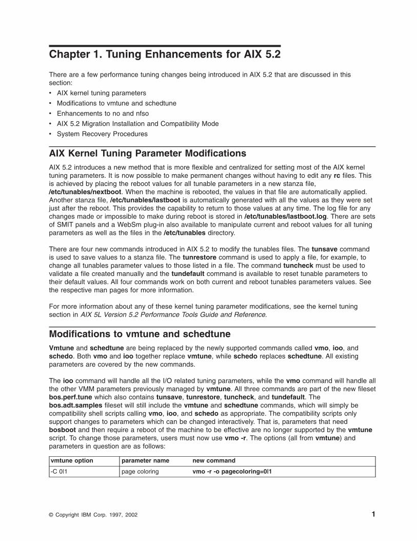
AIX Kernel Tuning Parameter ModificationsAIX 5.2 introduces a new method that is more flexible and centralized for setting most of the AIX kerneltuning parameters. It is now possible to make permanent changes without having to edit any rc files. Thisis achieved by placing the reboot values for all tunable parameters in a new stanza file,/etc/tunables/nextboot. When the machine is rebooted, the values in that file are automatically applied.Another stanza file, /etc/tunables/lastboot is automatically generated with all the values as they were setjust after the reboot. This provides the capability to return to those values at any time. The log file for anychanges made or impossible to make during reboot is stored in /etc/tunables/lastboot.log. There are setsof SMIT panels and a WebSm plug-in also available to manipulate current and reboot values for all tuningparameters as well as the files in the /etc/tunables directory.

There are four new commands introduced in AIX 5.2 to modify the tunables files. The tunsave commandis used to save values to a stanza file. The tunrestore command is used to apply a file, for example, tochange all tunables parameter values to those listed in a file. The command tuncheck must be used tovalidate a file created manually and the tundefault command is available to reset tunable parameters totheir default values. All four commands work on both current and reboot tunables parameters values. Seethe respective man pages for more information.

For more information about any of these kernel tuning parameter modifications, see the kernel tuningsection in AIX 5L Version 5.2 Performance Tools Guide and Reference.

Modifications to vmtune and schedtuneVmtune and schedtune are being replaced by the newly supported commands called vmo, ioo, andschedo. Both vmo and ioo together replace vmtune, while schedo replaces schedtune. All existingparameters are covered by the new commands.

The ioo command will handle all the I/O related tuning parameters, while the vmo command will handle allthe other VMM parameters previously managed by vmtune. All three commands are part of the new filesetbos.perf.tune which also contains tunsave, tunrestore, tuncheck, and tundefault. Thebos.adt.samples fileset will still include the vmtune and schedtune commands, which will simply becompatibility shell scripts calling vmo, ioo, and schedo as appropriate. The compatibility scripts onlysupport changes to parameters which can be changed interactively. That is, parameters that needbosboot and then require a reboot of the machine to be effective are no longer supported by the vmtunescript. To change those parameters, users must now use vmo -r. The options (all from vmtune) andparameters in question are as follows:

vmtune option parameter name new command

-C 0|1 page coloring vmo -r -o pagecoloring=0|1

© Copyright IBM Corp. 1997, 2002 1

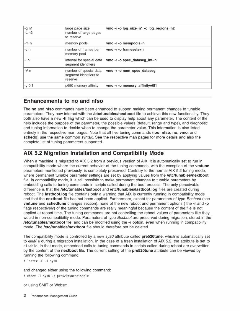
-g n1-L n2

large page sizenumber of large pagesto reserve

vmo -r -o lpg_size=n1 -o lpg_regions=n2

-m n memory pools vmo -r -o mempools=n

-v n number of frames permemory pool

vmo -r -o framesets=n

-i n interval for special datasegment identifiers

vmo -r -o spec_dataseg_int=n

-V n number of special datasegment identifiers toreserve

vmo -r -o num_spec_dataseg

-y 0|1 p690 memory affinity vmo -r -o memory_affinity=0|1

Enhancements to no and nfsoThe no and nfso commands have been enhanced to support making permanent changes to tunableparameters. They now interact with the /etc/tunables/nextboot file to achieve this new functionality. Theyboth also have a new -h flag which can be used to display help about any parameter. The content of thehelp includes the purpose of the parameter, the possible values (default, range and type), and diagnosticand tuning information to decide when to change the parameter value. This information is also listedentirely in the respective man pages. Note that all five tuning commands (ioo, nfso, no, vmo, andschedo) use the same common syntax. See the respective man pages for more details and also thecomplete list of tuning parameters supported.

AIX 5.2 Migration Installation and Compatibility ModeWhen a machine is migrated to AIX 5.2 from a previous version of AIX, it is automatically set to run incompatibility mode where the current behavior of the tuning commands, with the exception of the vmtuneparameters mentioned previously, is completely preserved. Contrary to the normal AIX 5.2 tuning mode,where permanent tunable parameter settings are set by applying values from the /etc/tunables/nextbootfile, in compatibility mode, it is still possible to make permanent changes to tunable parameters byembedding calls to tuning commands in scripts called during the boot process. The only perceivabledifference is that the /etc/tunables/lastboot and /etc/tunables/lastboot.log files are created duringreboot. The lastboot.log file contains only a warning that AIX is currently running in compatibility modeand that the nextboot file has not been applied. Furthermore, except for parameters of type Bosboot (seevmtune and schedtune changes section), none of the new reboot and permanent options ( the -r and -pflags respectively) of the tuning commands are really meaningful because the content of the file is notapplied at reboot time. The tuning commands are not controlling the reboot values of parameters like theywould in non-compatibility mode. Parameters of type Bosboot are preserved during migration, stored in the/etc/tunables/nextboot file, and can be modified using the -r option, even when running in compatibilitymode. The /etc/tunables/nextboot file should therefore not be deleted.

The compatibility mode is controlled by a new sys0 attribute called pre520tune, which is automatically setto enable during a migration installation. In the case of a fresh installation of AIX 5.2, the attribute is set todisable. In that mode, embedded calls to tuning commands in scripts called during reboot are overwrittenby the content of the nextboot file. The current setting of the pre520tune attribute can be viewed byrunning the following command:# lsattr -E -l sys0

and changed either using the following command:# chdev -l sys0 -a pre520tune=disable

or using SMIT or Websm.

2 Performance Management Guide

When the compatibility mode is disabled, the other visible change is that the following no parameters,which are all of type Reboot (they can only be changed during reboot), cannot be changed any morewithout using the new -r flag.:

v arptab_bsiz

v arptab_nb

v extendednetstats

v ifsize

v inet_stack_size

v ipqmaxlen

v nstrpush

v pseintrstack

Switching to the non-compatibility mode while preserving the current reboot settings can be done by firstchanging pre520tune, and then by running the following command:# tunrestore -r -f lastboot

which will copy the content of the lastboot file to the nextboot file. See AIX 5L Version 5.2 Kernel tuningin the AIX 5L Version 5.2 Performance Tools Guide and Reference for details about the new AIX 5.2tuning mode.

System Recovery ProceduresIf a machine is unstable after rebooting and pre520tune is set to enable, users should delete the offendingcalls to tuning commands from scripts called during reboot. To detect which parameters are set duringreboot, simply look at the /etc/tunables/lastboot file and search for parameters not marked with #DEFAULT VALUE. For more information on the content of tunable files, see the tunables File Formatsection in AIX 5L Version 5.2 Files Reference.

Alternatively, to reset all the tunable parameters to their default values, delete the /etc/tunables/nextbootfile, set pre520tune to disable, run the bosboot command, and reboot the machine.

Chapter 1. Tuning Enhancements for AIX 5.2 3


Chapter 2. Performance Concepts

Everyone who uses a computer has an opinion about its performance. Unfortunately, those opinions areoften based on oversimplified ideas about the dynamics of program execution. Uninformed intuition canlead to expensive and inaccurate guesses about the capacity of a system and the solutions to theperceived performance problems.

This chapter describes the dynamics of program execution and provides a conceptual framework forevaluating system performance. It contains the following major sections:

v How Fast is That Computer?

v Understanding the Workload

v Program Execution Dynamics

v System Dynamics

v Introducing the Performance-Tuning Process

v Performance Benchmarking

v Related Information

How Fast is That Computer?Using words like speed and fast to describe contemporary computers, while accepted by precedent, isextreme oversimplification. There was a time when a programmer could read a program, calculate the sumof the instruction times, and confidently predict how long it would take the computer to run that program.Thousands of programmers and engineers have spent the last 30 years making such straightforwardcalculations impossible, or at least meaningless.

Today’s computers are more powerful than their predecessors, not just because they use integratedcircuits instead of vacuum tubes and have far shorter cycle times, but because of innumerable hardwareand software architectural inventions. Each advance in integrated-circuit density brings an advance incomputer performance, not just because it allows the same logic to work in a smaller space with a fastersystem clock, but because it gives engineers more space in which to implement ideas. In short, computershave gained capacity by becoming more complex as well as quicker.

The complexity of modern computers and their operating systems is matched by the complexity of theenvironment in which they operate. In addition to running individual programs, today’s computer deals withvarying numbers of unpredictably timed interrupts from I/O and communications devices. To the extent thatthe engineers’ ideas were based on an assumption of a single program running in a standalone machine,they may be partly defeated by the randomness of the real world. To the extent that those ideas wereintended to deal with randomness, they may win back some of the loss. The wins and losses change fromprogram to program and from moment to moment.

The result of all these hardware and software wins and losses is the performance of the system. Thespeed of the system is the rate at which it can handle a specific sequence of demands. If the demandsmesh well with the system’s hardware and software architectures, we can say, ″The system runs thisworkload fast.″ We cannot say, ″The system is fast,″ or at least we should not.

Understanding the WorkloadAn accurate and complete definition of the system’s workload is critical to predicting or understanding itsperformance. A difference in workload can cause far more variation in the measured performance of asystem than differences in CPU clock speed or random access memory (RAM) size. The workloaddefinition must include not only the type and rate of requests to the system, but also the exact softwarepackages and in-house application programs to be executed.


Whenever possible, observe the current users of existing applications to get authentic, real-worldmeasurements of the rates at which users interact with their workstations or terminals.

Make sure that you include the work that your system is doing ″under the covers.″ For example, if yoursystem contains file systems that are NFS-mounted and frequently accessed by other systems, handlingthose accesses is probably a significant fraction of the overall workload, even though your system is notofficially a server.

Industry-Standard Benchmarks: A Risky ShortcutA benchmark is a workload that has been standardized to allow comparisons among dissimilar systems.Any benchmark that has been in existence long enough to become industry-standard has been studiedexhaustively by systems developers. Operating systems, compilers, and in some cases hardware, havebeen tuned to run the benchmark with lightning speed.

Unfortunately, few real workloads duplicate the exact algorithms and environment of a benchmark. Eventhose industry-standard benchmarks that were originally derived from real applications might have beensimplified and homogenized to make them portable to a wide variety of hardware platforms. Theenvironment in which they run has been constrained in the interests of reproducible measurements.

Any reasoning similar to ″System A is rated at 50 percent more MegaThings than System B, so System Ashould run my program 50 percent faster than System B″ might be a tempting shortcut, but may beinaccurate. There is no benchmark with such universal applicability. The only valid use forindustry-standard benchmarks is to narrow the field of candidate systems that will be subjected to aserious evaluation. There is no substitute for developing a clear understanding of your workload and itsperformance in systems under consideration.

Performance ObjectivesAfter defining the workload that the system will have to process, you can choose performance criteria andset performance objectives based on those criteria. The main overall performance criteria of computersystems are response time and throughput.

Response time is the elapsed time between when a request is submitted and when the response from thatrequest is returned. Examples include how long a database query takes, or how long it takes to echocharacters to the terminal, or how long it takes to access a Web page.

Throughput is a measure of the amount of work over a period of time. In other words, it is the number ofworkload operations that can be accomplished per unit of time. Examples include database transactionsper minute, kilobytes of a file transferred per second, kilobytes of a file read or written per second, or Webserver hits per minute.

The relationship between these metrics is complex. In some cases, you might have to trade off oneagainst the other. In other situations, a single change can improve both. Sometimes you can have higherthroughput at the cost of response time or better response time at the cost of throughput. Acceptableperformance is based on reasonable throughput combined with reasonable response time.

In planning for or tuning any system, make sure that you have clear objectives for both response time andthroughput when processing the specified workload. Otherwise, you risk spending analysis time andresource dollars improving an aspect of system performance that is of secondary importance.

Program Execution DynamicsNormally, an application programmer thinks of the running program as an uninterrupted sequence ofinstructions that perform a specified function. Great amounts of inventiveness and effort have beenexpended on the operating system and hardware to ensure that programmers are not distracted from thisidealized view by irrelevant space, speed, and multiprogramming or multiprocessing considerations. If the


programmer is seduced by this comfortable illusion, the resulting program might be unnecessarilyexpensive to run and might not meet its performance objectives.

To examine clearly the performance characteristics of a workload, a dynamic, rather than a static, model ofprogram execution is needed, as shown in the following figure.

To run, a program must make its way up both the hardware and operating-system hierarchies, more orless in parallel. Each element in the hardware hierarchy is scarcer and more expensive than the elementbelow it. Not only does the program have to contend with other programs for each resource, the transitionfrom one level to the next takes time. To understand the dynamics of program execution, you need a basicunderstanding of each of the levels in the hierarchy.

Hardware HierarchyUsually, the time required to move from one hardware level to another consists primarily of the latency ofthe lower level (the time from the issuing of a request to the receipt of the first data).

Fixed DisksThe slowest operation for a running program (other than waiting for a human keystroke) on a standalonesystem is obtaining code or data from a disk, for the following reasons:

v The disk controller must be directed to access the specified blocks (queuing delay).

v The disk arm must seek to the correct cylinder (seek latency).

v The read/write heads must wait until the correct block rotates under them (rotational latency).

v The data must be transmitted to the controller (transmission time) and then conveyed to the applicationprogram (interrupt-handling time).

Figure 1. Program Execution Hierarchy. The figure is a triangle on its base. The left side represents hardware entitiesthat are matched to the appropriate operating system entity on the right side. A program must go from the lowest levelof being stored on disk, to the highest level being the processor running program instructions. For instance, frombottom to top, the disk hardware entity holds executable programs; real memory holds waiting operating systemthreads and interrupt handlers; the translation lookaside buffer holds detachable threads; cache contains the currentlydispatched thread and the processor pipeline and registers contain the current instruction.

Chapter 2. Performance Concepts 7

Disk operations can have many causes besides explicit read or write requests in the program.System-tuning activities frequently prove to be hunts for unnecessary disk I/O.

Real MemoryReal Memory, often referred to as RAM, is fast compared to disk, but much more expensive per byte.Operating systems try to keep in RAM the code and data that are currently in use, spilling any excess ontodisk (or never bringing them into RAM in the first place).

RAM is not necessarily fast compared to the processor. Typically a RAM latency of dozens of processorcycles occurs between the time the hardware recognizes the need for a RAM access and the time thedata or instruction is available to the processor.

If the access is to a page of virtual memory that has been spilled to disk (or has not been brought in yet),a page fault occurs, and the execution of the program is suspended until the page has been read in fromdisk.

Translation Lookaside Buffer (TLB)One of the ways programmers are insulated from the physical limitations of the system is theimplementation of virtual memory. The programmer designs and codes the program as though the memorywere very large, and the system takes responsibility for translating the program’s virtual addresses forinstructions and data into the real addresses that are needed to get the instructions and data from RAM.Because this address-translation process can be time-consuming, the system keeps the real addresses ofrecently accessed virtual-memory pages in a cache called the translation lookaside buffer (TLB).

As long as the running program continues to access a small set of program and data pages, the fullvirtual-to-real page-address translation does not need to be redone for each RAM access. When theprogram tries to access a virtual-memory page that does not have a TLB entry (a TLB miss), dozens ofprocessor cycles (the TLB-miss latency) are usually required to perform the address translation.

CachesTo minimize the number of times the program has to experience the RAM latency, systems incorporatecaches for instructions and data. If the required instruction or data is already in the cache (a cache hit), itis available to the processor on the next cycle (that is, no delay occurs). Otherwise (a cache miss), theRAM latency occurs.

In some systems, there are two or three levels of cache, usually called L1, L2, and L3. If a particularstorage reference results in an L1 miss, then L2 is checked. If L2 generates a miss, then the referencegoes to the next level, either L3 if present or RAM.

Cache sizes and structures vary by model, but the principles of using them efficiently are identical.

Pipeline and RegistersA pipelined, superscalar architecture makes possible, under certain circumstances, the simultaneousprocessing of multiple instructions. Large sets of general-purpose registers and floating-point registersmake it possible to keep considerable amounts of the program’s data in registers, rather than continuallystoring and reloading.

The optimizing compilers are designed to take maximum advantage of these capabilities. The compilers’optimization functions should always be used when generating production programs, however small theprograms are. The Optimization and Tuning Guide for XL Fortran, XL C and XL C++ describes howprograms can be tuned for maximum performance.

Software HierarchyTo run, a program must also progress through a series of steps in the software hierarchy.


Executable ProgramsWhen a user requests a program to run, the operating system performs a number of operations totransform the executable program on disk to a running program. First, the directories in the user’s currentPATH environment variable must be scanned to find the correct copy of the program. Then, the systemloader (not to be confused with the ld command, which is the binder) must resolve any external referencesfrom the program to shared libraries.

To represent the user’s request, the operating system creates a process, which is a set of resources, suchas a private virtual address segment, required by any running program.

The operating system also automatically creates a single thread within that process. A thread is the currentexecution state of a single instance of a program. In AIX Version 4 and later, access to the processor andother resources is allocated on a thread basis, rather than a process basis. Multiple threads can becreated within a process by the application program. Those threads share the resources owned by theprocess within which they are running.

Finally, the system branches to the entry point of the program. If the program page that contains the entrypoint is not already in memory (as it might be if the program had been recently compiled, executed, orcopied), the resulting page-fault interrupt causes the page to be read from its backing storage.

Interrupt HandlersThe mechanism for notifying the operating system that an external event has taken place is to interrupt thecurrently running thread and transfer control to an interrupt handler. Before the interrupt handler can run,enough of the hardware state must be saved to ensure that the system can restore the context of thethread after interrupt handling is complete. Newly invoked interrupt handlers experience all of the delays ofmoving up the hardware hierarchy (except page faults). Unless the interrupt handler was run very recently(or the intervening programs were very economical), it is unlikely that any of its code or data remains inthe TLBs or the caches.

When the interrupted thread is dispatched again, its execution context (such as register contents) islogically restored, so that it functions correctly. However, the contents of the TLBs and caches must bereconstructed on the basis of the program’s subsequent demands. Thus, both the interrupt handler and theinterrupted thread can experience significant cache-miss and TLB-miss delays as a result of the interrupt.

Waiting ThreadsWhenever an executing program makes a request that cannot be satisfied immediately, such as asynchronous I/O operation (either explicit or as the result of a page fault), that thread is put in a wait stateuntil the request is complete. Normally, this results in another set of TLB and cache latencies, in additionto the time required for the request itself.

Dispatchable ThreadsWhen a thread is dispatchable, but not actually running, it is accomplishing nothing useful. Worse, otherthreads that are running may cause the thread’s cache lines to be reused and real memory pages to bereclaimed, resulting in even more delays when the thread is finally dispatched.

Currently Dispatched ThreadsThe scheduler chooses the thread that has the strongest claim to the use of the processor. Theconsiderations that affect that choice are discussed in Performance Overview of the CPU Scheduler. Whenthe thread is dispatched, the logical state of the processor is restored to the state that was in effect whenthe thread was interrupted.

Current InstructionsMost of the machine instructions are capable of executing in a single processor cycle, if no TLB or cachemiss occurs. In contrast, if a program branches rapidly to different areas of the program and accessesdata from a large number of different areas, causing high TLB and cache-miss rates, the average numberof processor cycles per instruction (CPI) executed might be much greater than one. The program is said toexhibit poor locality of reference. It might be using the minimum number of instructions necessary to do its


job, but consuming an unnecessarily large number of cycles. In part because of this poor correlationbetween number of instructions and number of cycles, reviewing a program listing to calculate path lengthno longer yields a time value directly. While a shorter path is usually faster than a longer path, the speedratio can be very different from the path-length ratio.

The compilers rearrange code in sophisticated ways to minimize the number of cycles required for theexecution of the program. The programmer seeking maximum performance must be primarily concernedwith ensuring that the compiler has all the information necessary to optimize effectively, rather than tryingto second-guess the compiler’s optimization techniques (see Effective Use of Preprocessors and theCompilers). The real measure of optimization effectiveness is the performance of an authentic workload.

System DynamicsIt is not enough to create the most efficient possible individual programs. In many cases, the actualprograms being run were created outside of the control of the person who is responsible for meeting theorganization’s performance objectives. Further, most of the levels of the hierarchy described in ProgramExecution Dynamics are managed by one or more parts of the operating system. In any case, after theapplication programs have been acquired, or implemented as efficiently as possible, further improvementin the overall performance of the system becomes a matter of system tuning. The main components thatare subject to system-level tuning are:

Communications I/ODepending on the type of workload and the type of communications link, it might be necessary totune one or more of the communications device drivers, TCP/IP, or NFS.

Fixed DiskThe Logical Volume Manager (LVM) controls the placement of file systems and paging spaces onthe disk, which can significantly affect the amount of seek latency the system experiences. Thedisk device drivers control the order in which I/O requests are acted on.

Real MemoryThe Virtual Memory Manager (VMM) controls the pool of free real-memory frames and determineswhen and from whom to steal frames to replenish the pool.

Running ThreadThe scheduler determines which dispatchable entity should next receive control. In AIX, thedispatchable entity is a thread. See Thread Support.

Classes of WorkloadWorkloads tend to fall naturally into a small number of classes. The types listed below are sometimesused to categorize systems. However, because a single system is often called upon to process multipleclasses, workload seems more apt in the context of performance.

MultiuserA workload that consists of a number of users submitting work through individual terminals.Typically, the performance objectives of such a workload are either to maximize system throughputwhile preserving a specified worst-case response time or to obtain the best possible response timefor a fairly constant workload.

ServerA workload that consists of requests from other systems. For example, a file-server workload ismostly disk read/write requests. In essence, it is the disk-I/O component of a multiuser workload(plus NFS or other I/O activity), so the same objective of maximum throughput within a givenresponse-time limit applies. Other server workloads consist of compute-intensive programs,database transactions, printer jobs, and so on.

WorkstationA workload that consists of a single user submitting work through the native keyboard and


receiving results on the native display of the system. Typically, the highest-priority performanceobjective of such a workload is minimum response time to the user’s requests.

When a single system is processing workloads of more than one type, a clear understanding must existbetween the users and the performance analyst as to the relative priorities of the possibly conflictingperformance objectives of the different workloads.

Introducing the Performance-Tuning ProcessPerformance tuning is primarily a matter of resource management and correct system-parameter setting.Tuning the workload and the system for efficient resource use consists of the following steps:

1. Identifying the workloads on the system

2. Setting objectives:

a. Determining how the results will be measured

b. Quantifying and prioritizing the objectives

3. Identifying the critical resources that limit the system’s performance

4. Minimizing the workload’s critical-resource requirements:

a. Using the most appropriate resource, if there is a choice

b. Reducing the critical-resource requirements of individual programs or system functions

c. Structuring for parallel resource use

5. Modifying the allocation of resources to reflect priorities

a. Changing the priority or resource limits of individual programs

b. Changing the settings of system resource-management parameters

6. Repeating steps 3 through 5 until objectives are met (or resources are saturated)

7. Applying additional resources, if necessary

There are appropriate tools for each phase of system performance management (see Appendix A.Monitoring and Tuning Commands and Subroutines). Some of the tools are available from IBM; others arethe products of third parties. The following figure illustrates the phases of performance management in asimple LAN environment.

Figure 2. Performance Phases. The figure uses five weighted circles to illustrate the steps of performance tuning asystem; plan, install, monitor, tune, and expand. Each circle represents the system in various states of performance;idle, unbalanced, balanced, and overloaded. Essentially, you expand a system that is overloaded, tune a system untilit is balanced, monitor an unbalanced system and install for more resources when an expansion is necessary.


Identifying the WorkloadsIt is essential that all of the work performed by the system be identified. Especially in LAN-connectedsystems, a complex set of cross-mounted file systems can easily develop with only informal agreementamong the users of the systems. These file systems must be identified and taken into account as part ofany tuning activity.

With multiuser workloads, the analyst must quantify both the typical and peak request rates. It is alsoimportant to be realistic about the proportion of the time that a user is actually interacting with the terminal.

An important element of this identification stage is determining whether the measurement and tuningactivity has to be done on the production system or can be accomplished on another system (or off-shift)with a simulated version of the actual workload. The analyst must weigh the greater authenticity of resultsfrom a production environment against the flexibility of the nonproduction environment, where the analystcan perform experiments that risk performance degradation or worse.

Setting ObjectivesAlthough you can set objectives in terms of measurable quantities, the actual desired result is oftensubjective, such as satisfactory response time. Further, the analyst must resist the temptation to tune whatis measurable rather than what is important. If no system-provided measurement corresponds to thedesired improvement, that measurement must be devised.

The most valuable aspect of quantifying the objectives is not selecting numbers to be achieved, butmaking a public decision about the relative importance of (usually) multiple objectives. Unless thesepriorities are set in advance, and understood by everyone concerned, the analyst cannot make trade-offdecisions without incessant consultation. The analyst is also apt to be surprised by the reaction of users ormanagement to aspects of performance that have been ignored. If the support and use of the systemcrosses organizational boundaries, you might need a written service-level agreement between theproviders and the users to ensure that there is a clear common understanding of the performanceobjectives and priorities.

Identifying Critical ResourcesIn general, the performance of a given workload is determined by the availability and speed of one or twocritical system resources. The analyst must identify those resources correctly or risk falling into an endlesstrial-and-error operation.

Systems have both real and logical resources. Critical real resources are generally easier to identify,because more system performance tools are available to assess the utilization of real resources. The realresources that most often affect performance are as follows:

v CPU cycles

v Memory

v I/O bus

v Various adapters

v Disk arms

v Disk space

v Network access

Logical resources are less readily identified. Logical resources are generally programming abstractions thatpartition real resources. The partitioning is done to share and manage the real resource.

Some examples of real resources and the logical resources built on them are as follows:

CPUv Processor time slice


Memoryv Page frames

v Stacks

v Buffers

v Queues

v Tables

v Locks and semaphores

Disk Spacev Logical volumes

v File systems

v Files

v Partitions

Network Accessv Sessions

v Packets

v Channels

It is important to be aware of logical resources as well as real resources. Threads can be blocked by alack of logical resources just as for a lack of real resources, and expanding the underlying real resourcedoes not necessarily ensure that additional logical resources will be created. For example, consider theNFS block I/O daemon (biod, see Tuning for NFS Performance). A biod daemon on the client is requiredto handle each pending NFS remote I/O request. The number of biod daemons therefore limits thenumber of NFS I/O operations that can be in progress simultaneously. When a shortage of biod daemonsexists, system instrumentation may indicate that the CPU and communications links are used only slightly.You may have the false impression that your system is underused (and slow), when in fact you have ashortage of biod daemons that is constraining the rest of the resources. A biod daemon uses processorcycles and memory, but you cannot fix this problem simply by adding real memory or converting to a fasterCPU. The solution is to create more of the logical resource (biod daemons).

Logical resources and bottlenecks can be created inadvertently during application development. A methodof passing data or controlling a device may, in effect, create a logical resource. When such resources arecreated by accident, there are generally no tools to monitor their use and no interface to control theirallocation. Their existence may not be appreciated until a specific performance problem highlights theirimportance.

Minimizing Critical-Resource RequirementsConsider minimizing the workload’s critical-resource requirements at three levels, as discussed below.

Using the Appropriate ResourceThe decision to use one resource over another should be done consciously and with specific goals inmind. An example of a resource choice during application development would be a trade-off of increasedmemory consumption for reduced CPU consumption. A common system configuration decision thatdemonstrates resource choice is whether to place files locally on an individual workstation or remotely ona server.

Reducing the Requirement for the Critical ResourceFor locally developed applications, the programs can be reviewed for ways to perform the same functionmore efficiently or to remove unnecessary function. At a system-management level, low-priority workloadsthat are contending for the critical resource can be moved to other systems, run at other times, orcontrolled with the Workload Manager.


Structuring for Parallel Use of ResourcesBecause workloads require multiple system resources to run, take advantage of the fact that the resourcesare separate and can be consumed in parallel. For example, the operating system read-ahead algorithmdetects the fact that a program is accessing a file sequentially and schedules additional sequential readsto be done in parallel with the application’s processing of the previous data. Parallelism applies to systemmanagement as well. For example, if an application accesses two or more files at the same time, addingan additional disk drive might improve the disk-I/O rate if the files that are accessed at the same time areplaced on different drives.

Reflecting Priorities in Resource AllocationThe operating system provides a number of ways to prioritize activities. Some, such as disk pacing, areset at the system level. Others, such as process priority, can be set by individual users to reflect theimportance they attach to a specific task.

Repeating the Tuning StepsA truism of performance analysis is that there is always a next bottleneck. Reducing the use of oneresource means that another resource limits throughput or response time. Suppose, for example, we havea system in which the utilization levels are as follows:

CPU: 90% Disk: 70% Memory 60%

This workload is CPU-bound. If we successfully tune the workload so that the CPU load is reduced from90 to 45 percent, we might expect a two-fold improvement in performance. Unfortunately, the workload isnow I/O-limited, with utilizations of approximately the following:

CPU: 45% Disk: 90% Memory 60%

The improved CPU utilization allows the programs to submit disk requests sooner, but then we hit the limitimposed by the disk drive’s capacity. The performance improvement is perhaps 30 percent instead of the100 percent we had envisioned.

There is always a new critical resource. The important question is whether we have met the performanceobjectives with the resources at hand.

Attention: Improper system tuning with vmtune, schedtune, and other tuning commands can result inunexpected system behavior like degraded system or application performance, or a system hang.Changes should only be applied when a bottleneck has been identified by performance analysis.

Note: There is no such thing as a general recommendation for performance dependent tuning settings.

Applying Additional ResourcesIf, after all of the preceding approaches have been exhausted, the performance of the system still does notmeet its objectives, the critical resource must be enhanced or expanded. If the critical resource is logicaland the underlying real resource is adequate, the logical resource can be expanded at no additional cost.If the critical resource is real, the analyst must investigate some additional questions:

v How much must the critical resource be enhanced or expanded so that it ceases to be a bottleneck?

v Will the performance of the system then meet its objectives, or will another resource become saturatedfirst?

v If there will be a succession of critical resources, is it more cost-effective to enhance or expand all ofthem, or to divide the current workload with another system?


Performance BenchmarkingWhen we attempt to compare the performance of a given piece of software in different environments, weare subject to a number of possible errors, some technical, some conceptual. This section contains mostlycautionary information. Other sections of this book discuss the various ways in which elapsed andprocess-specific times can be measured.

When we measure the elapsed (wall-clock) time required to process a system call, we get a number thatconsists of the following:

v The actual time during which the instructions to perform the service were executing

v Varying amounts of time during which the processor was stalled while waiting for instructions or datafrom memory (that is, the cost of cache and TLB misses)

v The time required to access the clock at the beginning and end of the call

v Time consumed by periodic events, such as system timer interrupts

v Time consumed by more or less random events, such as I/O interrupts

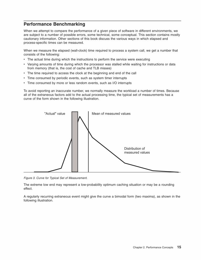
To avoid reporting an inaccurate number, we normally measure the workload a number of times. Becauseall of the extraneous factors add to the actual processing time, the typical set of measurements has acurve of the form shown in the following illustration.

The extreme low end may represent a low-probability optimum caching situation or may be a roundingeffect.

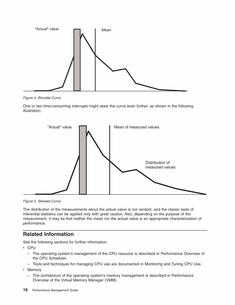
A regularly recurring extraneous event might give the curve a bimodal form (two maxima), as shown in thefollowing illustration.

Figure 3. Curve for Typical Set of Measurement.


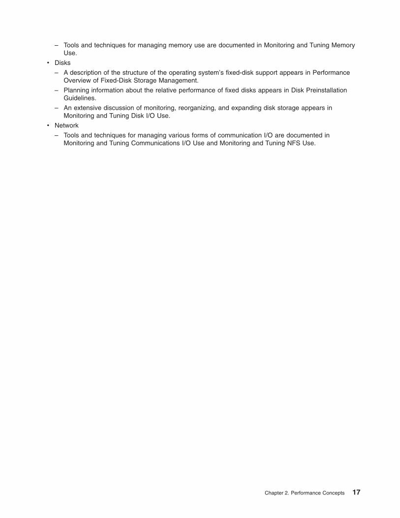
One or two time-consuming interrupts might skew the curve even further, as shown in the followingillustration:

The distribution of the measurements about the actual value is not random, and the classic tests ofinferential statistics can be applied only with great caution. Also, depending on the purpose of themeasurement, it may be that neither the mean nor the actual value is an appropriate characterization ofperformance.

Related InformationSee the following sections for further information:

v CPU

– The operating system’s management of the CPU resource is described in Performance Overview ofthe CPU Scheduler.

– Tools and techniques for managing CPU use are documented in Monitoring and Tuning CPU Use.

v Memory

– The architecture of the operating system’s memory management is described in PerformanceOverview of the Virtual Memory Manager (VMM).

"Actual" value Mean

Figure 4. Bimodal Curve

Figure 5. Skewed Curve


– Tools and techniques for managing memory use are documented in Monitoring and Tuning MemoryUse.

v Disks

– A description of the structure of the operating system’s fixed-disk support appears in PerformanceOverview of Fixed-Disk Storage Management.

– Planning information about the relative performance of fixed disks appears in Disk PreinstallationGuidelines.

– An extensive discussion of monitoring, reorganizing, and expanding disk storage appears inMonitoring and Tuning Disk I/O Use.

v Network

– Tools and techniques for managing various forms of communication I/O are documented inMonitoring and Tuning Communications I/O Use and Monitoring and Tuning NFS Use.



Chapter 3. Resource Management Overview

This chapter describes the components of the operating system that manage the resources that have themost effect on system performance, and the ways in which these components can be tuned. This chaptercontains the following major sections:

v Performance Overview of the CPU Scheduler.

v Performance Overview of the Virtual Memory Manager (VMM).

v Performance Overview of Fixed-Disk Storage Management.

Specific tuning recommendations appear in the following:

v Chapter 6. Monitoring and Tuning CPU Use.

v Chapter 7. Monitoring and Tuning Memory Use.

v Chapter 8. Monitoring and Tuning Disk I/O Use.

v Chapter 9. Monitoring and Tuning Communications I/O Use.

v Chapter 10. Monitoring and Tuning NFS Use.

Performance Overview of the processor SchedulerThis section discusses performance related topics for the processor Scheduler.

Thread SupportA thread can be thought of as a low-overhead process. It is a dispatchable entity that requires fewerresources to create than a process. The fundamental dispatchable entity of the AIX Version 4 scheduler isthe thread.

Processes are composed of one or more threads. In fact, workloads migrated directly from earlier releasesof the operating system continue to create and manage processes. Each new process is created with asingle thread that has its parent process priority and contends for the processor with the threads of otherprocesses. The process owns the resources used in execution; the thread owns only its current state.

When new or modified applications take advantage of the operating system’s thread support to createadditional threads, those threads are created within the context of the process. They share the process’sprivate segment and other resources.

A user thread within a process has a specified contention scope. If the contention scope is global, thethread contends for processor time with all other threads in the system. The thread that is created when aprocess is created has global contention scope. If the contention scope is local, the thread contends withthe other threads within the process to be the recipient of the process’s share of processor time.

The algorithm for determining which thread should be run next is called a scheduling policy.

Processes and ThreadsA process is an activity within the system that is started by a command, a shell program, or anotherprocess.

Process properties are as follows:

v pid

v pgid

v uid

v gid


v environment

v cwd

v file descriptors

v signal actions

v process statistics

v nice

These properties are defined in /usr/include/sys/proc.h.

Thread properties are as follows:

v stack

v scheduling policy

v scheduling priority

v pending signals

v blocked signals

v thread-specific data

These thread properties are defined in /usr/include/sys/thread.h.

Each process is made up of one or more threads. A thread is a single sequential flow of control. Multiplethreads of control allow an application to overlap operations, such as reading from a terminal and writingto a file.

Multiple threads of control also allow an application to service requests from multiple users at the sametime. Threads provide these capabilities without the added overhead of multiple processes such as thosecreated through the fork() system call.

AIX 4.3.1 introduced a fast fork routine called f_fork(). This routine is very useful for multithreadedapplications that will call the exec() subroutine immediately after they would have called the fork()subroutine. The fork() subroutine is slower because it has to call fork handlers to acquire all the librarylocks before actually forking and letting the child run all child handlers to initialize all the locks. Thef_fork() subroutine bypasses these handlers and calls the kfork() system call directly. Web servers are agood example of an application that can use the f_fork() subroutine.

Process and Thread PriorityThe priority management tools manipulate process priority. In AIX Version 4, process priority is simply aprecursor to thread priority. When the fork() subroutine is called, a process and a thread to run in it arecreated. The thread has the priority that would have been attributed to the process.

The kernel maintains a priority value (sometimes termed the scheduling priority) for each thread. Thepriority value is a positive integer and varies inversely with the importance of the associated thread. Thatis, a smaller priority value indicates a more important thread. When the scheduler is looking for a thread todispatch, it chooses the dispatchable thread with the smallest priority value.

A thread can be fixed-priority or nonfixed priority. The priority value of a fixed-priority thread is constant,while the priority value of a nonfixed-priority thread varies based on the minimum priority level for userthreads (a constant 40), the thread’s nice value (20 by default, optionally set by the nice or renicecommand), and its processor-usage penalty.

The priority of a thread can be fixed at a certain value, which can have a priority value less than 40, if theirpriority is set (fixed) through the setpri() subroutine. These threads are immune to the scheduler


recalculation algorithms. If their priority values are fixed to be less than 40, these threads will run andcomplete before any user threads can run. For example, a thread with a fixed value of 10 will run before athread with a fixed value of 15.

Users can apply the nice command to make a thread’s nonfixed priority less favorable. The systemmanager can apply a negative nice value to a thread, thus giving it a better priority.

The following illustration shows some of the ways in which the priority value can change.

The nice value of a thread is set when the thread is created and is constant over the life of the thread,unless explicitly changed by the user through the renice command or the setpri(), setpriority(),thread_setsched(), or nice() system calls.

The processor penalty is an integer that is calculated from the recent processor usage of a thread. Therecent processor usage increases by approximately 1 each time the thread is in control of the processor atthe end of a 10 ms clock tick, up to a maximum value of 120. The actual priority penalty per tick increaseswith the nice value. Once per second, the recent processor usage values for all threads are recalculated.

The result is the following:

v The priority of a nonfixed-priority thread becomes less favorable as its recent processor usageincreases and vice versa. This implies that, on average, the more time slices a thread has beenallocated recently, the less likely it is that the thread will be allocated the next time slice.

v The priority of a nonfixed-priority thread becomes less favorable as its nice value increases, and viceversa.

Note: With the use of multiple processor run queues and their load balancing mechanism, nice or renicevalues might not have the expected effect on thread priorities because less favored priorities mighthave equal or greater run time than favored priorities. Threads requiring the expected effects ofnice or renice should be placed on the global run queue.

You can use the ps command to display the priority value, nice value, and short-term processor-usagevalues for a process.

Figure 6. How the Priority Value is Determined. The illustration shows how the scheduling priority value of a threadcan change during execution or after applying the nice command. The smaller the priority value, the higher the threadpriority. At initiation, the nice value defaults to 20 and the base priority defaults to 40. After some execution and aprocessor penality, the nice value remains 20 and the base priority remains 40. After running the renice —5 commandand with the same processor usage as before, the nice value is now 15 and the base priority remains 40. After issuingthe setpri() subroutine with a value of 50, fixed priority is now 50 and the nice value and processor usage is irrelevant.

Chapter 3. Resource Management Overview 21

See Controlling Contention for the processor for a more detailed discussion on using the nice and renicecommands.

See Tuning the Thread-Priority-Value Calculation, for the details of the calculation of the processor penaltyand the decay of the recent processor usage values.

The priority mechanism is also used by AIX Workload Manager to enforce processor resourcemanagement. Because threads classified under the Workload Manager have their priorities managed bythe Workload Manager, they might have different priority behavior over threads not classified under theWorkload Manager.

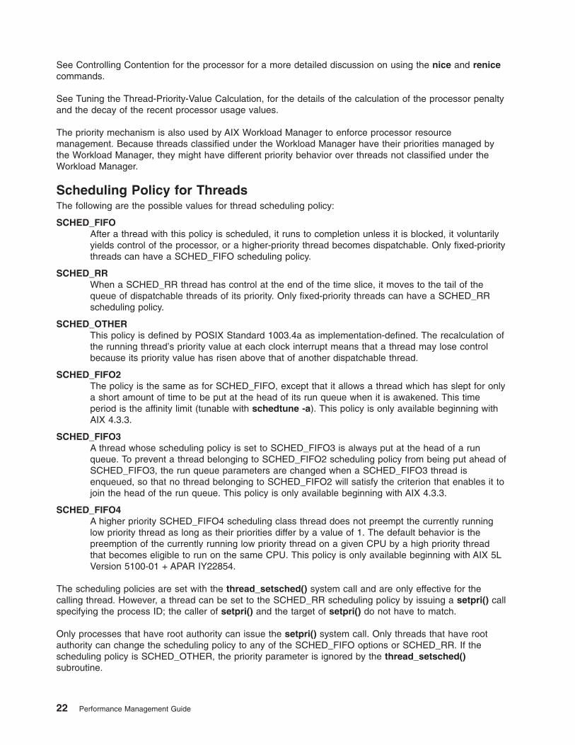
Scheduling Policy for ThreadsThe following are the possible values for thread scheduling policy:

SCHED_FIFOAfter a thread with this policy is scheduled, it runs to completion unless it is blocked, it voluntarilyyields control of the processor, or a higher-priority thread becomes dispatchable. Only fixed-prioritythreads can have a SCHED_FIFO scheduling policy.

SCHED_RRWhen a SCHED_RR thread has control at the end of the time slice, it moves to the tail of thequeue of dispatchable threads of its priority. Only fixed-priority threads can have a SCHED_RRscheduling policy.

SCHED_OTHERThis policy is defined by POSIX Standard 1003.4a as implementation-defined. The recalculation ofthe running thread’s priority value at each clock interrupt means that a thread may lose controlbecause its priority value has risen above that of another dispatchable thread.

SCHED_FIFO2The policy is the same as for SCHED_FIFO, except that it allows a thread which has slept for onlya short amount of time to be put at the head of its run queue when it is awakened. This timeperiod is the affinity limit (tunable with schedtune -a). This policy is only available beginning withAIX 4.3.3.

SCHED_FIFO3A thread whose scheduling policy is set to SCHED_FIFO3 is always put at the head of a runqueue. To prevent a thread belonging to SCHED_FIFO2 scheduling policy from being put ahead ofSCHED_FIFO3, the run queue parameters are changed when a SCHED_FIFO3 thread isenqueued, so that no thread belonging to SCHED_FIFO2 will satisfy the criterion that enables it tojoin the head of the run queue. This policy is only available beginning with AIX 4.3.3.

SCHED_FIFO4A higher priority SCHED_FIFO4 scheduling class thread does not preempt the currently runninglow priority thread as long as their priorities differ by a value of 1. The default behavior is thepreemption of the currently running low priority thread on a given CPU by a high priority threadthat becomes eligible to run on the same CPU. This policy is only available beginning with AIX 5LVersion 5100-01 + APAR IY22854.

The scheduling policies are set with the thread_setsched() system call and are only effective for thecalling thread. However, a thread can be set to the SCHED_RR scheduling policy by issuing a setpri() callspecifying the process ID; the caller of setpri() and the target of setpri() do not have to match.

Only processes that have root authority can issue the setpri() system call. Only threads that have rootauthority can change the scheduling policy to any of the SCHED_FIFO options or SCHED_RR. If thescheduling policy is SCHED_OTHER, the priority parameter is ignored by the thread_setsched()subroutine.


Threads are primarily of interest for applications that currently consist of several asynchronous processes.These applications might impose a lighter load on the system if converted to a multithreaded structure.

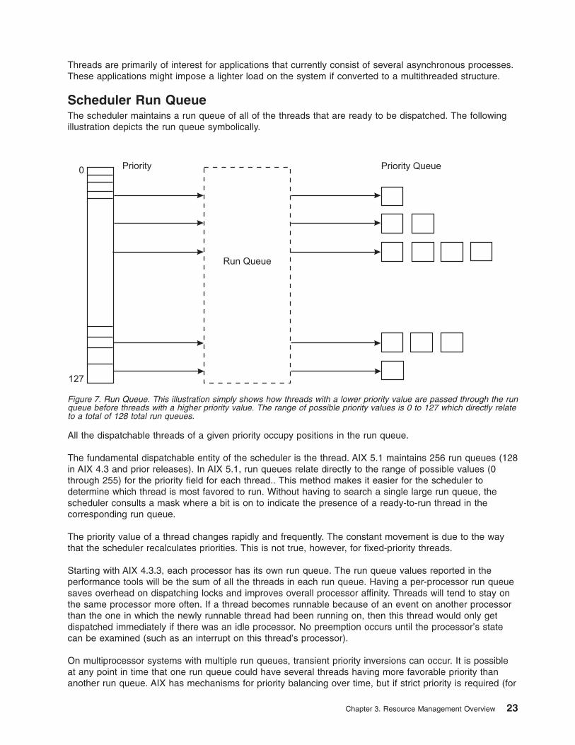
Scheduler Run QueueThe scheduler maintains a run queue of all of the threads that are ready to be dispatched. The followingillustration depicts the run queue symbolically.

All the dispatchable threads of a given priority occupy positions in the run queue.

The fundamental dispatchable entity of the scheduler is the thread. AIX 5.1 maintains 256 run queues (128in AIX 4.3 and prior releases). In AIX 5.1, run queues relate directly to the range of possible values (0through 255) for the priority field for each thread.. This method makes it easier for the scheduler todetermine which thread is most favored to run. Without having to search a single large run queue, thescheduler consults a mask where a bit is on to indicate the presence of a ready-to-run thread in thecorresponding run queue.

The priority value of a thread changes rapidly and frequently. The constant movement is due to the waythat the scheduler recalculates priorities. This is not true, however, for fixed-priority threads.

Starting with AIX 4.3.3, each processor has its own run queue. The run queue values reported in theperformance tools will be the sum of all the threads in each run queue. Having a per-processor run queuesaves overhead on dispatching locks and improves overall processor affinity. Threads will tend to stay onthe same processor more often. If a thread becomes runnable because of an event on another processorthan the one in which the newly runnable thread had been running on, then this thread would only getdispatched immediately if there was an idle processor. No preemption occurs until the processor’s statecan be examined (such as an interrupt on this thread’s processor).

On multiprocessor systems with multiple run queues, transient priority inversions can occur. It is possibleat any point in time that one run queue could have several threads having more favorable priority thananother run queue. AIX has mechanisms for priority balancing over time, but if strict priority is required (for

Figure 7. Run Queue. This illustration simply shows how threads with a lower priority value are passed through the runqueue before threads with a higher priority value. The range of possible priority values is 0 to 127 which directly relateto a total of 128 total run queues.


example, for real-time applications) an environment variable called RT_GRQ exists, that, if set to ON, willcause this thread to be on a global run queue. In that case, the global run queue is searched to see whichthread has the best priority. This can improve performance for threads that are interrupt driven. Threadsthat are running at fixed priority are placed on the global run queue if schedtune -F is set to 1.

The average number of threads in the run queue can be seen in the first column of the vmstat commandoutput. If you divide this number by the number of processors, the result is the average number of threadsthat can be run on each processor. If this value is greater than one, these threads must wait their turn forthe processor (the greater the number, the more likely it is that performance delays are noticed).

When a thread is moved to the end of the run queue (for example, when the thread has control at the endof a time slice), it is moved to a position after the last thread in the queue that has the same priority value.

Scheduler processor Time SliceThe processor time slice is the amount of time a SCHED_RR thread can absorb before the schedulerswitches to another thread at the same priority. You can use the -t option of the schedtune command toincrease the number of clock ticks in the time slice by 10 millisecond increments (see Modifying theScheduler Time Slice with the schedtune Command).

Note: The time slice is not a guaranteed amount of processor time. It is the longest time that a thread canbe in control before it faces the possibility of being replaced by another thread. There are manyways in which a thread can lose control of the processor before it has had control for a full timeslice.

Mode SwitchingA user process undergoes a mode switch when it needs access to system resources. This is implementedthrough the system call interface or by interrupts such as page faults. There are two modes:

v User mode

v Kernel mode

Processor time spent in user mode (application and shared libraries) is reflected as user time in the outputof commands such as the vmstat, iostat, and sar commands. Processor time spent in kernel mode isreflected as system time in the output of these commands.

User ModePrograms that execute in the user protection domain are user processes. Code that executes in thisprotection domain executes in user execution mode, and has the following access:

v Read/write access to user data in the process private region

v Read access to the user text and shared text regions

v Access to shared data regions using the shared memory functions

Programs executing in the user protection domain do not have access to the kernel or kernel datasegments, except indirectly through the use of system calls. A program in this protection domain can onlyaffect its own execution environment and executes in the process or unprivileged state.

Kernel ModePrograms that execute in the kernel protection domain include interrupt handlers, kernel processes, thebase kernel, and kernel extensions (device driver, system calls and file systems). This protection domainimplies that code executes in kernel execution mode, and has the following access:

v Read/write access to the global kernel address space

v Read/write access to the kernel data in the process region when executing within a process

Kernel services must be used to access user data within the process address space.


Programs executing in this protection domain can affect the execution environments of all programs,because they have the following characteristics:

v They can access global system data

v They can use kernel services

v They are exempt from all security restraints

v They execute in the processor privileged state.

Mode SwitchesThe use of a system call by a user-mode process allows a kernel function to be called from user mode.Access to functions that directly or indirectly invoke system calls is typically provided by programminglibraries, which provide access to operating system functions.

Mode switches should be differentiated from the context switches seen in the output of the vmstat (cscolumn) and sar (cswch/s) commands. A context switch occurs when the currently running thread isdifferent from the previously running thread on that processor.

The scheduler performs a context switch when any of the following occurs:

v A thread must wait for a resource (voluntarily), such as disk I/O, network I/O, sleep, or locks

v A higher priority thread wakes up (involuntarily)

v The thread has used up its time slice (usually 10 ms).

Context switch time, system calls, device interrupts, NFS I/O, and any other activity in the kernel isconsidered as system time.

Performance Overview of the Virtual Memory Manager (VMM)The virtual address space is partitioned into segments. A segment is a 256 MB, contiguous portion of thevirtual-memory address space into which a data object can be mapped.

Process addressability to data is managed at the segment (or object) level so that a segment can beshared between processes or maintained as private. For example, processes can share code segmentsyet have separate and private data segments.

Real-Memory ManagementVirtual-memory segments are partitioned into fixed-size units called pages. The default page size is 4096bytes. Some systems also support a larger page size, typically accessed only through the shmat systemcall.Each page in a segment can be in real memory (RAM), or stored on disk until it is needed. Similarly,real memory is divided into 4096-byte page frames. The role of the VMM is to manage the allocation ofreal-memory page frames and to resolve references by the program to virtual-memory pages that are notcurrently in real memory or do not yet exist (for example, when a process makes the first reference to apage of its data segment).

Because the amount of virtual memory that is in use at any given instant can be larger than real memory,the VMM must store the surplus on disk. From the performance standpoint, the VMM has two, somewhatopposed, objectives:

v Minimize the overall processor-time and disk-bandwidth cost of the use of virtual memory

v Minimize the response-time cost of page faults

In pursuit of these objectives, the VMM maintains a free list of page frames that are available to satisfy apage fault. The VMM uses a page-replacement algorithm to determine which virtual-memory pagescurrently in memory will have their page frames reassigned to the free list. The page-replacementalgorithm uses several mechanisms:

v Virtual-memory segments are classified into either persistent segments or working segments.


v Virtual-memory segments are classified as containing either computational or file memory.

v Virtual-memory pages whose access causes a page fault are tracked.

v Page faults are classified as new-page faults or as repage faults.

v Statistics are maintained on the rate of repage faults in each virtual-memory segment.

v User-tunable thresholds influence the page-replacement algorithm’s decisions.

The following sections describe the free list and the page-replacement mechanisms in more detail.

Free ListThe VMM maintains a logical list of free page frames that it uses to accommodate page faults. In mostenvironments, the VMM must occasionally add to the free list by reassigning some page frames owned byrunning processes. The virtual-memory pages whose page frames are to be reassigned are selected bythe VMM’s page-replacement algorithm. The VMM thresholds determine the number of frames reassigned.

Persistent versus Working SegmentsThe pages of a persistent segment have permanent storage locations on disk. Files containing data orexecutable programs are mapped to persistent segments. Because each page of a persistent segment hasa permanent disk storage location, the VMM writes the page back to that location when the page has beenchanged and can no longer be kept in real memory. If the page has not changed when selected forplacement on a free list, no I/O is required. If the page is referenced again later, a new copy is read infrom its permanent disk-storage location.

Working segments are transitory, exist only during their use by a process, and have no permanentdisk-storage location. Process stack and data regions are mapped to working segments, as are the kerneltext segment, the kernel-extension text segments, as well as the shared-library text and data segments.Pages of working segments must also have disk-storage locations to occupy when they cannot be kept inreal memory. The disk-paging space is used for this purpose.

The following illustration shows the relationship between some of the types of segments and the locationsof their pages on disk. It also shows the actual (arbitrary) locations of the pages when they are in realmemory.


Persistent-segment types are further classified. Client segments are used to map remote files (forexample, files that are being accessed through NFS), including remote executable programs. Pages fromclient segments are saved and restored over the network to their permanent file location, not on thelocal-disk paging space. Journaled and deferred segments are persistent segments that must beatomically updated. If a page from a journaled or deferred segment is selected to be removed from realmemory (paged out), it must be written to disk paging space unless it is in a state that allows it to becommitted (written to its permanent file location).

Computational versus File MemoryComputational memory, also known as computational pages, consists of the pages that belong toworking-storage segments or program text (executable files) segments.

File memory (or file pages) consists of the remaining pages. These are usually pages from permanentdata files in persistent storage.

Page ReplacementWhen the number of available real memory frames on the free list becomes low, a page stealer is invoked.A page stealer moves through the Page Frame Table (PFT), looking for pages to steal.

The PFT includes flags to signal which pages have been referenced and which have been modified. If thepage stealer encounters a page that has been referenced, it does not steal that page, but instead, resetsthe reference flag for that page. The next time the clock hand (page stealer) passes that page and thereference bit is still off, that page is stolen. A page that was not referenced in the first pass is immediatelystolen.

The modify flag indicates that the data on that page has been changed since it was brought into memory.When a page is to be stolen, if the modify flag is set, a pageout call is made before stealing the page.Pages that are part of working segments are written to paging space; persistent segments are written todisk.

Figure 8. Persistent and Working Storage Segments. This illustration shows the relationship between some of thetypes of segments and the locations of their pages on disk. It also shows the actual (arbitrary) locations of the pageswhen they are in real memory. Working segments are transitory, meaning they exist only during their use by a processand have no permanent disk-storage location. Process stack and data regions are mapped to working segments, asare the kernel text segment, the kernel-extension text segments, and the shared-library text and data segments.Pages of working segments must also have disk-storage locations to occupy when they cannot be kept in realmemory. The disk-paging space is used for this purpose.


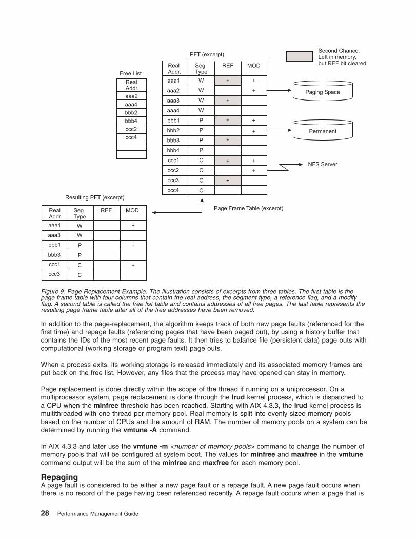
In addition to the page-replacement, the algorithm keeps track of both new page faults (referenced for thefirst time) and repage faults (referencing pages that have been paged out), by using a history buffer thatcontains the IDs of the most recent page faults. It then tries to balance file (persistent data) page outs withcomputational (working storage or program text) page outs.

When a process exits, its working storage is released immediately and its associated memory frames areput back on the free list. However, any files that the process may have opened can stay in memory.

Page replacement is done directly within the scope of the thread if running on a uniprocessor. On amultiprocessor system, page replacement is done through the lrud kernel process, which is dispatched toa CPU when the minfree threshold has been reached. Starting with AIX 4.3.3, the lrud kernel process ismultithreaded with one thread per memory pool. Real memory is split into evenly sized memory poolsbased on the number of CPUs and the amount of RAM. The number of memory pools on a system can bedetermined by running the vmtune -A command.

In AIX 4.3.3 and later use the vmtune -m <number of memory pools> command to change the number ofmemory pools that will be configured at system boot. The values for minfree and maxfree in the vmtunecommand output will be the sum of the minfree and maxfree for each memory pool.

RepagingA page fault is considered to be either a new page fault or a repage fault. A new page fault occurs whenthere is no record of the page having been referenced recently. A repage fault occurs when a page that is

Figure 9. Page Replacement Example. The illustration consists of excerpts from three tables. The first table is thepage frame table with four columns that contain the real address, the segment type, a reference flag, and a modifyflag. A second table is called the free list table and contains addresses of all free pages. The last table represents theresulting page frame table after all of the free addresses have been removed.


known to have been referenced recently is referenced again, and is not found in memory because thepage has been replaced (and perhaps written to disk) since it was last accessed.

A perfect page-replacement policy would eliminate repage faults entirely (assuming adequate real memory)by always stealing frames from pages that are not going to be referenced again. Thus, the number ofrepage faults is an inverse measure of the effectiveness of the page-replacement algorithm in keepingfrequently reused pages in memory, thereby reducing overall I/O demand and potentially improving systemperformance.

To classify a page fault as new or repage, the VMM maintains a repage history buffer that contains thepage IDs of the N most recent page faults, where N is the number of frames that the memory can hold.For example, 512 MB memory requires a 128 KB repage history buffer. At page-in, if the page’s ID isfound in the repage history buffer, it is counted as a repage. Also, the VMM estimates thecomputational-memory repaging rate and the file-memory repaging rate separately by maintaining countsof repage faults for each type of memory. The repaging rates are multiplied by 0.9 each time thepage-replacement algorithm runs, so that they reflect recent repaging activity more strongly than historicalrepaging activity.

VMM ThresholdsSeveral numerical thresholds define the objectives of the VMM. When one of these thresholds isbreached, the VMM takes appropriate action to bring the state of memory back within bounds. This sectiondiscusses the thresholds that the system administrator can alter through the vmtune command.

The number of page frames on the free list is controlled by the following parameters:

minfreeMinimum acceptable number of real-memory page frames in the free list. When the size of thefree list falls below this number, the VMM begins stealing pages. It continues stealing pages untilthe size of the free list reaches maxfree.

maxfreeMaximum size to which the free list will grow by VMM page-stealing. The size of the free list mayexceed this number as a result of processes terminating and freeing their working-segment pagesor the deletion of files that have pages in memory.

The VMM attempts to keep the size of the free list greater than or equal to minfree. When page faults orsystem demands cause the free list size to fall below minfree, the page-replacement algorithm runs. Thesize of the free list must be kept above a certain level (the default value of minfree) for several reasons.For example, the operating system’s sequential-prefetch algorithm requires several frames at a time foreach process that is doing sequential reads. Also, the VMM must avoid deadlocks within the operatingsystem itself, which could occur if there were not enough space to read in a page that was required to freea page frame.

The following thresholds are expressed as percentages. They represent the fraction of the total realmemory of the machine that is occupied by file pages (pages of noncomputational segments).

minpermIf the percentage of real memory occupied by file pages falls below this level, thepage-replacement algorithm steals both file and computational pages, regardless of repage rates.

maxpermIf the percentage of real memory occupied by file pages rises above this level, thepage-replacement algorithm steals only file pages.

maxclientIf the percentage of real memory occupied by file pages is above this level, the page-replacementalgorithm steals only client pages.


When the percentage of real memory occupied by file pages is between minperm and maxperm, theVMM normally steals only file pages, but if the repaging rate for file pages is higher than the repaging ratefor computational pages, computational pages are stolen as well.

The main intent of the page-replacement algorithm is to ensure that computational pages are given fairtreatment. For example, the sequential reading of a long data file into memory should not cause the lossof program text pages that are likely to be used again soon. The page-replacement algorithm’s use of thethresholds and repaging rates ensures that both types of pages get treated fairly, with a slight bias in favorof computational pages.

VMM Memory Load Control FacilityA process requires real-memory pages to execute. When a process references a virtual-memory page thatis on disk, because it either has been paged-out or has never been read, the referenced page must bepaged-in and, on average, one or more pages must be paged out (if replaced pages had been modified),creating I/O traffic and delaying the progress of the process.

The operating system attempts to steal real memory from pages that are unlikely to be referenced in thenear future, through the page-replacement algorithm. A successful page-replacement algorithm allows theoperating system to keep enough processes active in memory to keep the CPU busy. But at some level ofcompetition for memory, no pages are good candidates for paging out to disk because they will all bereused in the near future by the active set of processes. This situation depends on the following:

v Total amount of memory in the system

v The number of processes

v The time-varying memory requirements of each process

v The page-replacement algorithm

When this happens, continuous paging-in and paging-out occurs. This condition is called thrashing.Thrashing results in incessant I/O to the paging disk and causes each process to encounter a page faultalmost as soon as it is dispatched, with the result that none of the processes make any significantprogress.

The most destructive aspect of thrashing is that, although thrashing may have been triggered by a brief,random peak in workload (such as all of the users of a system happening to press Enter in the samesecond), the system might continue thrashing for an indefinitely long time.

The operating system has a memory load-control algorithm that detects when the system is starting tothrash and then suspends active processes and delays the initiation of new processes for a period of time.Five parameters set rates and bounds for the algorithm. The default values of these parameters havebeen chosen to be ″fail safe″ across a wide range of workloads. In AIX Version 4, memory load control isdisabled by default on systems that have available memory frames that add up to greater than or equal to128 MB.

Memory Load Control AlgorithmThe memory load control mechanism assesses, once per second, whether sufficient memory is availablefor the set of active processes. When a memory-overcommitment condition is detected, some processesare suspended, decreasing the number of active processes and thereby decreasing the level of memoryovercommitment.

When a process is suspended, all of its threads are suspended when they reach a suspendable state. Thepages of the suspended processes quickly become stale and are paged out by the page-replacementalgorithm, releasing enough page frames to allow the remaining active processes to progress. During theinterval in which existing processes are suspended, newly created processes are also suspended,preventing new work from entering the system. Suspended processes are not reactivated until asubsequent interval passes during which no potential thrashing condition exists. Once this safe intervalhas passed, the threads of the suspended processes are gradually reactivated.


Memory load-control parameters specify the following:

v The system memory overcommitment threshold (schedtune -h)

v The number of seconds required to make a safe interval (schedtune -w)

v The individual process memory overcommitment threshold by which an individual process is qualified asa suspension candidate (schedtune -p)

v The minimum number of active processes when processes are being suspended (schedtune -m)

v The minimum number of elapsed seconds of activity for a process after reactivation (schedtune -e)

For information on setting and tuning these parameters, see Tuning VMM Memory Load Control with theschedtune Command.

Once per second, the scheduler (process 0) examines the values of all the above measures that havebeen collected over the preceding one-second interval, and determines if processes are to be suspendedor activated. If processes are to be suspended, every process eligible for suspension by the -p and -eparameter test is marked for suspension. When that process next receives the CPU in user mode, it issuspended (unless doing so would reduce the number of active processes below the -m value). Theuser-mode criterion is applied so that a process is ineligible for suspension during critical system activitiesperformed on its behalf. If, during subsequent one-second intervals, the thrashing criterion is still beingmet, additional process candidates meeting the criteria set by -p and -e are marked for suspension. Whenthe scheduler subsequently determines that the safe-interval criterion has been met and processes are tobe reactivated, some number of suspended processes are put on the run queue (made active) everysecond.

Suspended processes are reactivated by:

1. Priority

2. The order in which they were suspended

The suspended processes are not all reactivated at once. A value for the number of processes reactivatedis selected by a formula that recognizes the number of then-active processes and reactivates eitherone-fifth of the number of then-active processes or a monotonically increasing lower bound, whichever isgreater. This cautious strategy results in increasing the degree of multiprogramming roughly 20 percent persecond. The intent of this strategy is to make the rate of reactivation relatively slow during the first secondafter the safe interval has expired, while steadily increasing the reintroduction rate in subsequent seconds.If the memory-overcommitment condition recurs during the course of reactivating processes, the followingoccur:

v Reactivation is halted

v The marked-to-be reactivated processes are again marked suspended

v Additional processes are suspended in accordance with the above rules

Allocation and Reclamation of Paging Space SlotsThe operating system supports three allocation methods for working storage, also referred to aspaging-space slots, as follows:

v Late allocation

v Early allocation

v Deferred allocation

Note: Paging-space slots are only released by process (not thread) termination or by the disclaim()system call. The slots are not released by the free() system call.


Late Allocation AlgorithmPrior to AIX 4.3.2 with the late allocation algorithm, a paging slot is allocated to a page of virtual memoryonly when that page is first touched. That is the first time that the page’s content is of interest to theexecuting program.

Many programs exploit late allocation by allocating virtual-memory address ranges for maximum-sizedstructures and then only using as much of the structure as the situation requires. The pages of thevirtual-memory address range that are never accessed never require real-memory frames or paging-spaceslots.

This technique does involve some degree of risk. If all of the programs running in a machine happened toencounter maximum-size situations simultaneously, paging space might be exhausted. Some programsmight not be able to continue to completion.

Early Allocation AlgorithmThe second operating system’s paging-space-slot-allocation method is intended for use in installationswhere this situation is likely, or where the cost of failure to complete is intolerably high. Aptly called earlyallocation, this algorithm causes the appropriate number of paging-space slots to be allocated at the timethe virtual-memory address range is allocated, for example, with the malloc() subroutine. If there are notenough paging-space slots to support the malloc() subroutine, an error code is set. The early-allocationalgorithm is invoked as follows:# export PSALLOC=early

This example causes all future programs to be executed in the environment to use early allocation. Thecurrently executing shell is not affected.

Early allocation is of interest to the performance analyst mainly because of its paging-space sizeimplications. If early allocation is turned on for those programs, paging-space requirements can increasemany times. Whereas the normal recommendation for paging-space size is at least twice the size of thesystem’s real memory, the recommendation for systems that use PSALLOC=early is at least four timesthe real memory size. Actually, this is just a starting point. Analyze the virtual storage requirements of yourworkload and allocate paging spaces to accommodate them. As an example, at one time, the AIXwindowsserver required 250 MB of paging space when run with early allocation.

When using PSALLOC=early, the user should set a handler for the following SIGSEGV signal bypre-allocating and setting the memory as a stack using the sigaltstack function. Even thoughPSALLOC=early is specified, when there is not enough paging space and a program attempts to expandthe stack, the program may receive the SIGSEGV signal.

Deferred Allocation AlgorithmThe third operating system’s paging-space-slot-allocation method is the default beginning with AIX 4.3.2Deferred Page Space Allocation (DPSA) policy delays allocation of paging space until it is necessary topage out the page, which results in no wasted paging space allocation. This method can save hugeamounts of paging space, which means disk space.

On some systems, paging space might not ever be needed even if all the pages accessed have beentouched. This situation is most common on systems with very large amount of RAM. However, this mayresult in overcommitment of paging space in cases where more virtual memory than available RAM isaccessed.

To disable DPSA and preserve the Late Page Space Allocation policy, run the following command:# /usr/samples/kernel/vmtune -d 0

To activate DPSA, run the following command:# /usr/samples/kernel/vmtune -d 1


In general, system performance can be improved by DPSA, because the overhead of allocating pagespace after page faults is avoided the. Paging space devices need less disk space if DPSA is used.

For further information, see Choosing a Page Space Allocation Method and Placement and Sizes ofPaging Spaces.

Performance Overview of Fixed-Disk Storage ManagementThe following illustration shows the hierarchy of structures used by the operating system to managefixed-disk storage. Each individual disk drive, called a physical volume (PV), has a name, such as/dev/hdisk0. If the physical volume is in use, it belongs to a volume group (VG). All of the physicalvolumes in a volume group are divided into physical partitions (PPs) of the same size (by default, 4 MB involume groups that include physical volumes smaller than 4 GB; 8 MB or more with bigger disks).

For space-allocation purposes, each physical volume is divided into five regions. See Position on PhysicalVolume for more information. The number of physical partitions in each region varies, depending on thetotal capacity of the disk drive.


Within each volume group, one or more logical volumes (LVs) are defined. Each logical volume consists ofone or more logical partitions. Each logical partition corresponds to at least one physical partition. Ifmirroring is specified for the logical volume, additional physical partitions are allocated to store theadditional copies of each logical partition. Although the logical partitions are numbered consecutively, theunderlying physical partitions are not necessarily consecutive or contiguous.

Logical volumes can serve a number of system purposes, such as paging, but each logical volume thatholds ordinary system data or user data or programs contains a single journaled file system (JFS orEnhanced JFS). Each JFS consists of a pool of page-size (4096-byte) blocks. When data is to be writtento a file, one or more additional blocks are allocated to that file. These blocks may or may not becontiguous with one another and with other blocks previously allocated to the file.

Figure 10. Organization of Fixed-Disk Data (Unmirrored). The illustration shows the hierarchy of a physical volume thatis partitioned into one or more logical volumes. These partitions or logical volumes contain file systems with directorystructures which contain individual files. Files are written to blocks contained in tracks on the storage media and theseblocks are usually not contiguous. Disk fragmenting occurs when data gets erased and new data files are written tothe empty blocks that are randomly scattered around multiple tracks on the media.


For purposes of illustration, the previous figure shows a bad (but not the worst possible) situation thatmight arise in a file system that had been in use for a long period without reorganization. The/op/filename file is physically recorded on a large number of blocks that are physically distant from oneanother. Reading the file sequentially would result in many time-consuming seek operations.

While an operating system’s file is conceptually a sequential and contiguous string of bytes, the physicalreality might be very different. Fragmentation may arise from multiple extensions to logical volumes as wellas allocation/release/reallocation activity within a file system. A file system is fragmented when its availablespace consists of large numbers of small chunks of space, making it impossible to write out a new file incontiguous blocks.

Access to files in a highly fragmented file system may result in a large number of seeks and longer I/Oresponse times (seek latency dominates I/O response time). For example, if the file is accessedsequentially, a file placement that consists of many, widely separated chunks requires more seeks than aplacement that consists of one or a few large contiguous chunks. If the file is accessed randomly, aplacement that is widely dispersed requires longer seeks than a placement in which the file’s blocks areclose together.

The effect of a file’s placement on I/O performance diminishes when the file is buffered in memory. Whena file is opened in the operating system, it is mapped to a persistent data segment in virtual memory. Thesegment represents a virtual buffer for the file; the file’s blocks map directly to segment pages. The VMMmanages the segment pages, reading file blocks into segment pages upon demand (as they areaccessed). There are several circumstances that cause the VMM to write a page back to its correspondingblock in the file on disk; but, in general, the VMM keeps a page in memory if it has been accessedrecently. Thus, frequently accessed pages tend to stay in memory longer, and logical file accesses to thecorresponding blocks can be satisfied without physical disk accesses.

At some point, the user or system administrator can choose to reorganize the placement of files withinlogical volumes and the placement of logical volumes within physical volumes to reduce fragmentation andto more evenly distribute the total I/O load. Chapter 8. Monitoring and Tuning Disk I/O Use contains furtherdetails about detecting and correcting disk placement and fragmentation problems.

Sequential-Access Read AheadThe VMM tries to anticipate the future need for pages of a sequential file by observing the pattern in whicha program is accessing the file. When the program accesses two successive pages of the file, the VMMassumes that the program will continue to access the file sequentially, and the VMM schedules additionalsequential reads of the file. These reads are overlapped with the program processing, and will make thedata available to the program sooner than if the VMM had waited for the program to access the next pagebefore initiating the I/O. The number of pages to be read ahead is determined by two VMM thresholds:

minpgaheadNumber of pages read ahead when the VMM first detects the sequential access pattern. If theprogram continues to access the file sequentially, the next read ahead will be for 2 timesminpgahead, the next for 4 times minpgahead, and so on until the number of pages reachesmaxpgahead.

maxpgaheadMaximum number of pages the VMM will read ahead in a sequential file.

The number of pages to read ahead on Enhanced JFS is determined by the two thresholds:j2_minPageReadAheadandj2_maxPageReadAhead.


Write BehindTo increase write performance, limit the number of dirty file pages in memory, reduce system overhead,and minimize disk fragmentation, the file system divides each file into 16 KB partitions. The pages of agiven partition are not written to disk until the program writes the first byte of the next 16 KB partition. Atthat point, the file system forces the four dirty pages of the first partition to be written to disk. The pages ofdata remain in memory until their frames are reused, at which point no additional I/O is required. If aprogram accesses any of the pages before their frames are reused, no I/O is required.

If a large number of dirty file pages remain in memory and do not get reused, the sync daemon writesthem to disk, which might result in abnormal disk utilization. To distribute the I/O activity more efficientlyacross the workload, write-behind can be turned on to tell the system how many pages to keep in memorybefore writing them to disk. The write-behind threshold is on a per-file basis, which causes pages to bewritten to disk before the sync daemon runs. The I/O is spread more evenly throughout the workload.

There are two types of write-behind: sequential and random. The size of the write-behind partitions andthe write-behind threshold can be changed with the vmtune command (see VMM Write-Behind).

Memory Mapped Files and Write BehindNormal files are automatically mapped to segments to provide mapped files. This means that normal fileaccess bypasses traditional kernel buffers and block I/O routines, allowing files to use more memory whenthe extra memory is available (file caching is not limited to the declared kernel buffer area).

Files can be mapped explicitly with the shmat() or mmap() subroutines, but this provides no additionalmemory space for their caching. Applications that use the shmat() or mmap() subroutines to map a fileexplicitly and access it by address rather than by the read() and write() subroutines may avoid some pathlength of the system-call overhead, but they lose the benefit of the system write-behind feature.

When applications do not use the write() subroutine, modified pages tend to accumulate in memory andbe written randomly when purged by the VMM page-replacement algorithm or the sync daemon. Thisresults in many small writes to the disk that cause inefficiencies in CPU and disk utilization, as well asfragmentation that might slow future reads of the file.

Disk-I/O PacingBecause most writes are asynchronous, FIFO I/O queues of several megabytes can build up, which cantake several seconds to complete. The performance of an interactive process is severely impacted if everydisk read spends several seconds working its way through the queue. In response to this problem, theVMM has an option called I/O pacing to control writes.

I/O pacing does not change the interface or processing logic of I/O. It simply limits the number of I/Os thatcan be outstanding against a file. When a process tries to exceed that limit, it is suspended until enoughoutstanding requests have been processed to reach a lower threshold. Using Disk-I/O Pacing describesI/O pacing in more detail.

Support for Pinned MemoryAIX 4.3.3 and AIX 5.1 enable memory pages to be maintained in real memory all the time. Thismechanism is called pinning memory. Pinning a memory region prohibits the pager from stealing pagesfrom the pages backing the pinned memory region. Memory regions defined in either system space oruser space may be pinned. After a memory region is pinned, accessing that region does not result in apage fault until the region is subsequently unpinned. While a portion of the kernel remains pinned, manyregions are pageable and are only pinned while being accessed.


The advantage of having portions of memory pinned is that, when accessing a page that is pinned, youcan retrieve the page without going through the page replacement algorithm. An adverse side effect ofhaving too many pinned memory pages is that it can increase paging activity for unpinned pages, whichwould degrade performance.

To tune pinned memory, use the vmtune command to dedicate a number of pages at boot time for pinnedmemory. The following flags affect how AIX manages pinned memory:

maxpinSpecifies the maximum percentage of real memory that can be pinned.

v_pinshmSetting the v_pinshm parameter to 1 (-S 1) causes pages in shared memory segments to bepinned by VMM, if the application, which does the shmget(), specifies SHM_PIN as part of theflags. The default value is 0. This option is available only in AIX 4.3.3 and later.

Large Page SupportIn addition to regular page sizes of 4 kilobytes, beginning with AIX 5.1, the operating system supportslarge, 16–MB pages. Applications can use large pages with the shmget and shmat system calls. For thesystem to be able to use large pages, the pages must be enabled by specifying the SHM_LGPAGE flagwith the shmget system call. Use this flag in conjunction with the SHM_PIN flag, and enable with thevmtune command.

To enable support for large pages, use the following flags with the vmtune command:

Table 1.

-gLargePageSize Specifies the size in bytes of the hardware-supported large pages used for theimplementation for the shmget system call with the SHM_LGPAGE flag. Largepages must be enabled with a non-zero value for the -L flag and the bosbootcommand must be run and the system restarted for this change to take effect.

-LLargePages Specifies the number of large pages to reserve for implementing the shmget systemcall with the SHM_LGPAGE flag. For this change to take effect, you must specify the-g flag, run the bosboot command, and restart the system.

Use the following flags with the shmget system call:

SHM_LGPAGECreates the region so it can be mapped through hardware-supported, large-page mechanisms, ifenabled. This flag must be used in conjunction with the SHM_PIN flag and enabled with thevmtune -L command, to reserve memory for the region (which requires a restart) and vmtune -Sto enable SHM_PIN. This has no effect on shared memory regions created with the EXTSHM=ONenvironment variable.

SHM_PINPins the shared memory region if enabled. This flag must be enabled with the vmtune command.This has no effect on shared memory regions created with EXTSHM=ON environment variable.



Chapter 4. Introduction to Multiprocessing

At any given time, a technological limit exists on the speed with which a single processor chip canoperate. If a system’s workload cannot be handled satisfactorily by a single processor, one response is toapply multiple processors to the problem.

The success of this response depends not only on the skill of the system designers, but also on whetherthe workload is amenable to multiprocessing. In terms of human tasks, adding people might be a goodidea if the task is answering calls to a toll-free number, but is dubious if the task is driving a car.

If improved performance is the objective of a proposed migration from a uniprocessor to a multiprocessorsystem, the following conditions must be true:

v The workload is processor-limited and has saturated its uniprocessor system.

v The workload contains multiple processor-intensive elements, such as transactions or complexcalculations, that can be performed simultaneously and independently.

v The existing uniprocessor cannot be upgraded or replaced with another uniprocessor of adequatepower.

Although unchanged single-thread applications normally function correctly in a multiprocessor environment,their performance often changes in unexpected ways. Migration to a multiprocessor can improve thethroughput of a system, and can improve the execution time of complex, multithreaded applications, butseldom improves the response time of individual, single-thread commands.

Getting the best possible performance from a multiprocessor system requires an understanding of theoperating-system and hardware-execution dynamics that are unique to the multiprocessor environment.

This chapter includes the following major sections:

v Symmetrical Multiprocessor (SMP) Concepts and Architecture

v SMP Performance Issues

v SMP Workloads

v SMP Thread Scheduling

v Thread Tuning

v SMP Tools

Symmetrical Multiprocessor (SMP) Concepts and ArchitectureAs with any change that increases the complexity of the system, the use of multiple processors generatesdesign considerations that must be addressed for satisfactory operation and performance. The additionalcomplexity gives more scope for hardware/software tradeoffs and requires closer hardware/softwaredesign coordination than in uniprocessor systems. The different combinations of design responses andtradeoffs give rise to a wide variety of multiprocessor system architectures.

This section describes the main design considerations of multiprocessor systems and the hardwareresponses to those considerations.

Types of MultiprocessingSeveral categories of multiprocessing (MP) systems exist, as described below:

Shared Nothing MP (pure cluster)Each processor is a complete stand-alone machine and runs a copy of the operating system. Theprocessors share nothing (each has its own memory, caches, and disks), but they are interconnected.


When LAN-connected, processors are loosely coupled. When connected by a switch, the processors aretightly coupled. Communication between processors is done through message-passing.

The advantages of such a system are very good scalability and high availability. The disadvantages ofsuch a system are an unfamiliar programming model (message passing).

Shared Disks MPProcessors have their own memory and cache. The processors run in parallel and share disks. Eachprocessor runs a copy of the operating system and the processors are loosely coupled (connected throughLAN). Communication between processors is done through message-passing.

The advantages of shared disks are that part of a familiar programming model is retained (disk data isaddressable and coherent, memory is not), and high availability is much easier than with shared-memorysystems. The disadvantages are limited scalability due to bottlenecks in physical and logical access toshared data.

Shared Memory Cluster (SMC)All of the processors in a shared memory cluster have their own resources (main memory, disks, I/O) andeach processor runs a copy of the operating system. Processors are tightly coupled (connected through aswitch). Communication between the processors is done through shared memory.

Shared Memory MPAll of the processors are tightly coupled inside the same box with a high-speed bus or a switch. Theprocessors share the same global memory, disks, and I/O devices. Only one copy of the operating systemruns across all of the processors, and the operating system must be designed to exploit this architecture(multithreaded operating system).

SMPs have several advantages:

v They are a cost-effective way to increase throughput.

v They offer a single system image since the Operating System is shared between all the processors(administration is easy).

v They apply multiple processors to a single problem (parallel programming).

v Load balancing is done by the operating system.

v The uniprocessor (UP) programming model can be used in an SMP.

v They are scalable for shared data.

v All data is addressable by all the processors and kept coherent by the hardware snooping logic.

v There is no need to use message-passing libraries to communicate between processors becausecommunication is done through the global shared memory.

v More power requirements can be solved by adding more processors to the system. However, you mustset realistic expectations about the increase in performance when adding more processors to an SMPsystem.

v More and more applications and tools are available today. Most UP applications can run on or areported to SMP architecture.

There are some limitations of SMP systems, as follows:

v There are limits on scalability due to cache coherency, locking mechanism, shared objects, and others.

v There is a need for new skills to exploit multiprocessors, such as threads programming and devicedrivers programming.

Parallelizing an ApplicationAn application can be parallelized on an SMP in two ways, as follows:

v The traditional way is to break the application into multiple processes. These processes communicateusing inter-process communication (IPC) such as pipes, semaphores or shared memory. The processes


must be able to block waiting for events such as messages from other processes, and they mustcoordinate access to shared objects with something like locks.

v Another way is to use the portable operating system interface for UNIX (POSIX) threads. Threads havesimilar coordination problems as processes and similar mechanisms to deal with them. Thus a singleprocess can have any number of its threads running simultaneously on different processors.Coordinating them and serializing access to shared data are the developer’s responsibility.

Consider the advantages of both threads and processes when you are determining which method to usefor parallelizing an application. Threads may be faster than processes and memory sharing is easier. Onanother hand, a process implementation will distribute more easily to multiple machines or clusters. If anapplication needs to create or delete new instances, then threads are faster (more overhead in forkingprocesses). For other functions, the overhead of threads is about the same as that of processes.

Data SerializationAny storage element that can be read or written by more than one thread may change while the programis running. This is generally true of multiprogramming environments as well as multiprocessingenvironments, but the advent of multiprocessors adds to the scope and importance of this consideration intwo ways:

v Multiprocessors and thread support make it attractive and easier to write applications that share dataamong threads.

v The kernel can no longer solve the serialization problem simply by disabling interrupts.

Note: To avoid serious problems, programs that share data must arrange to access that data serially,rather than in parallel. Before a program updates a shared data item, it must ensure that no otherprogram (including another copy of itself running on another thread) will change the item. Readscan usually be done in parallel.

The primary mechanism that is used to keep programs from interfering with one another is the lock. A lockis an abstraction that represents permission to access one or more data items. Lock and unlock requestsare atomic; that is, they are implemented in such a way that neither interrupts nor multiprocessor accessaffect the outcome. All programs that access a shared data item must obtain the lock that corresponds tothat data item before manipulating it. If the lock is already held by another program (or another threadrunning the same program), the requesting program must defer its access until the lock becomesavailable.

Besides the time spent waiting for the lock, serialization adds to the number of times a thread becomesnondispatchable. While the thread is nondispatchable, other threads are probably causing thenondispatchable thread’s cache lines to be replaced, which results in increased memory-latency costswhen the thread finally gets the lock and is dispatched.

The operating system’s kernel contains many shared data items, so it must perform serialization internally.Serialization delays can therefore occur even in an application program that does not share data with otherprograms, because the kernel services used by the program have to serialize shared kernel data.

Types of LocksThe Open Software Foundation/1 (OSF/1) 1.1 locking methodology was used as a model for the AIXmultiprocessor lock functions. However, because the system is preemptable and pageable, somecharacteristics have been added to the OSF/1 1.1 Locking Model. Simple locks and complex locks arepreemptable. Also, a thread may sleep when trying to acquire a busy simple lock if the owner of the lock isnot currently running. In addition, a simple lock becomes a sleep lock when a processor has been spinningon a simple lock for a certain amount of time (this amount of time is a systemwide variable).

Chapter 4. Introduction to Multiprocessing 41

AIX Version 4 Simple LocksA simple lock in operating system version 4 is a spin lock that will sleep under certain conditionspreventing a thread from spinning indefinitely. Simple locks are preemptable, meaning that a kernel threadcan be preempted by another higher priority kernel thread while it holds a simple lock. On a multiprocessorsystem, simple locks, which protect thread-interrupt critical sections, must be used in conjunction withinterrupt control in order to serialize execution both within the executing processor and between differentprocessors.

On a uniprocessor system, interrupt control is sufficient; there is no need to use locks. Simple locks areintended to protect thread-thread and thread-interrupt critical sections. Simple locks will spin until the lockbecomes available if in an interrupt handler. They have two states: locked or unlocked.

AIX Version 4 Complex LocksThe complex locks in AIX are read-write locks which protect thread-thread critical sections. These locksare preemptable. Complex locks are spin locks that will sleep under certain conditions. By default, they arenot recursive, but can become recursive through the lock_set_recursive() kernel service. They have threestates: exclusive-write, shared-read, or unlocked.

Lock GranularityA programmer working in a multiprocessor environment must decide how many separate locks must becreated for shared data. If there is a single lock to serialize the entire set of shared data items, lockcontention is comparatively likely. The existence of widely used locks places an upper limit on thethroughput of the system.

If each distinct data item has its own lock, the probability of two threads contending for that lock iscomparatively low. Each additional lock and unlock call costs processor time, however, and the existenceof multiple locks makes a deadlock possible. At its simplest, deadlock is the situation shown in thefollowing illustration, in which Thread 1 owns Lock A and is waiting for Lock B. Meanwhile, Thread 2 ownsLock B and is waiting for Lock A. Neither program will ever reach the unlock() call that would break thedeadlock. The usual preventive for deadlock is to establish a protocol by which all of the programs thatuse a given set of locks must always acquire them in exactly the same sequence.

According to queuing theory, the less idle a resource, the longer the average wait to get it. Therelationship is nonlinear; if the lock is doubled, the average wait time for that lock more than doubles.

Figure 11. Deadlock. Shown in the following illustration is a deadlock in which a column named Thread 1 owns Lock Aand is waiting for Lock B. Meanwhile, the column named Thread 2 owns Lock B and is waiting for Lock A. Neitherprogram thread will ever reach the unlock call that would break the deadlock.


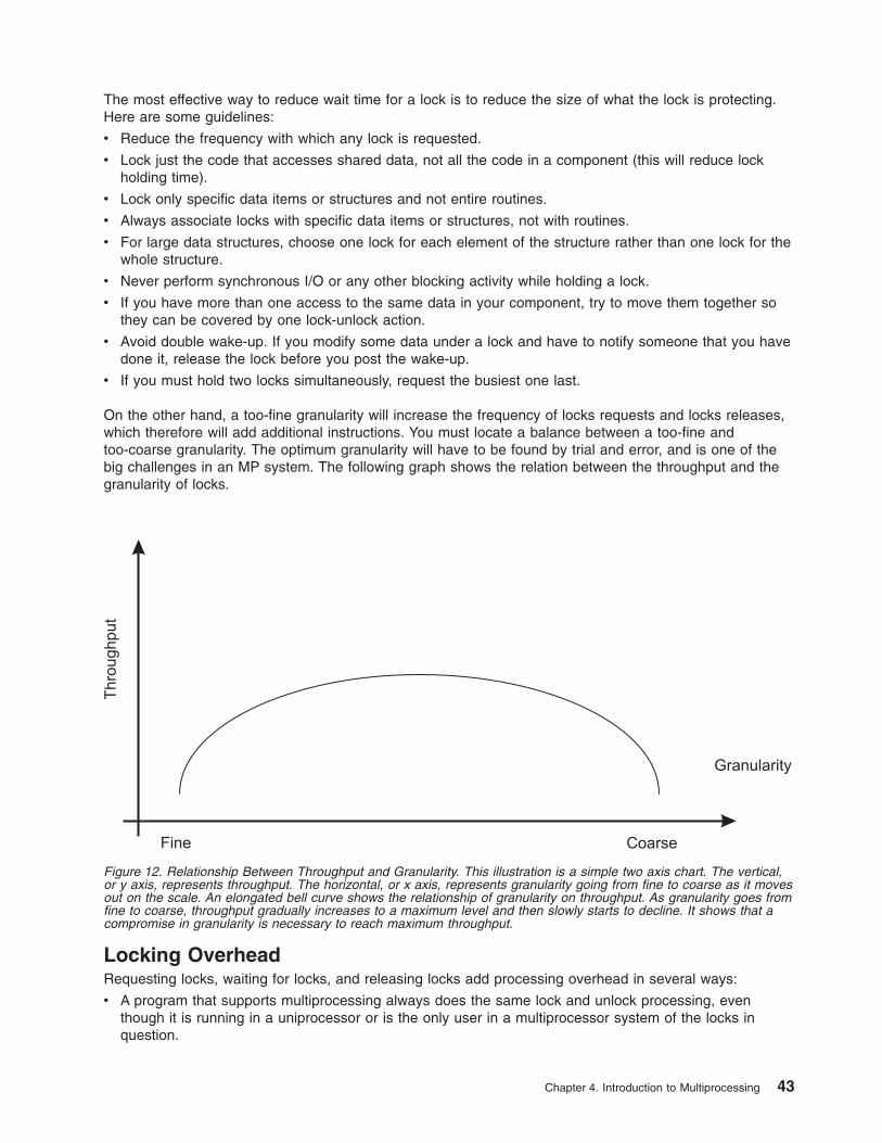
The most effective way to reduce wait time for a lock is to reduce the size of what the lock is protecting.Here are some guidelines:

v Reduce the frequency with which any lock is requested.

v Lock just the code that accesses shared data, not all the code in a component (this will reduce lockholding time).

v Lock only specific data items or structures and not entire routines.

v Always associate locks with specific data items or structures, not with routines.

v For large data structures, choose one lock for each element of the structure rather than one lock for thewhole structure.

v Never perform synchronous I/O or any other blocking activity while holding a lock.

v If you have more than one access to the same data in your component, try to move them together sothey can be covered by one lock-unlock action.

v Avoid double wake-up. If you modify some data under a lock and have to notify someone that you havedone it, release the lock before you post the wake-up.

v If you must hold two locks simultaneously, request the busiest one last.

On the other hand, a too-fine granularity will increase the frequency of locks requests and locks releases,which therefore will add additional instructions. You must locate a balance between a too-fine andtoo-coarse granularity. The optimum granularity will have to be found by trial and error, and is one of thebig challenges in an MP system. The following graph shows the relation between the throughput and thegranularity of locks.

Locking OverheadRequesting locks, waiting for locks, and releasing locks add processing overhead in several ways:

v A program that supports multiprocessing always does the same lock and unlock processing, eventhough it is running in a uniprocessor or is the only user in a multiprocessor system of the locks inquestion.

Figure 12. Relationship Between Throughput and Granularity. This illustration is a simple two axis chart. The vertical,or y axis, represents throughput. The horizontal, or x axis, represents granularity going from fine to coarse as it movesout on the scale. An elongated bell curve shows the relationship of granularity on throughput. As granularity goes fromfine to coarse, throughput gradually increases to a maximum level and then slowly starts to decline. It shows that acompromise in granularity is necessary to reach maximum throughput.


v When one thread requests a lock held by another thread, the requesting thread may spin for a while orbe put to sleep and, if possible, another thread dispatched. This consumes processor time.

v The existence of widely used locks places an upper bound on the throughput of the system. Forexample, if a given program spends 20 percent of its execution time holding a mutual-exclusion lock, atmost five instances of that program can run simultaneously, regardless of the number of processors inthe system. In fact, even five instances would probably never be so nicely synchronized as to avoidwaiting for one another (see Multiprocessor Throughput Scalability).

Waiting for LocksWhen a thread wants a lock already owned by another thread, the thread is blocked and must wait untilthe lock becomes free. There are two different ways of waiting:

v Spin locks are suitable for locks that are held only for very short times. It allows the waiting thread tokeep its processor, repeatedly checking the lock bit in a tight loop (spin) until the lock becomes free.Spinning results in increased CPU time (system time for kernel or kernel extension locks).

v Sleeping locks are suitable for locks that may be held for longer periods. The thread sleeps until thelock is free and is put back in the run queue when the lock becomes free. Sleeping results in more idletime.

Waiting always decreases system performance. If a spin lock is used, the processor is busy, but it is notdoing useful work (not contributing to throughput). If a sleeping lock is used, the overhead of contextswitching and dispatching as well as the consequent increase in cache misses is incurred.

Operating system developers can choose between two types of locks: mutually exclusive simple locks thatallow the process to spin and sleep while waiting for the lock to become available, and complex read-writelocks that can spin and block the process while waiting for the lock to become available.

Conventions govern the rules about using locks. Neither hardware nor software has an enforcement orchecking mechanism. Although using locks has made the AIX Version 4 ″MP Safe,″ developers areresponsible to define and implement an appropriate locking strategy to protect their own global data.

Cache CoherencyIn designing a multiprocessor, engineers give considerable attention to ensuring cache coherency. Theysucceed; but cache coherency has a performance cost. We need to understand the problem beingattacked:

If each processor has a cache that reflects the state of various parts of memory, it is possible that two ormore caches may have copies of the same line. It is also possible that a given line may contain more thanone lockable data item. If two threads make appropriately serialized changes to those data items, theresult could be that both caches end up with different, incorrect versions of the line of memory. In otherwords, the system’s state is no longer coherent because the system contains two different versions ofwhat is supposed to be the content of a specific area of memory.

The solutions to the cache coherency problem usually include invalidating all but one of the duplicate lineswhen the line is modified. Although the hardware uses snooping logic to invalidate, without any softwareintervention, any processor whose cache line has been invalidated will have a cache miss, with itsattendant delay, the next time that line is addressed.

Snooping is the logic used to resolve the problem of cache consistency. Snooping logic in the processorbroadcasts a message over the bus each time a word in its cache has been modified. The snooping logicalso snoops on the bus looking for such messages from other processors.

When a processor detects that another processor has changed a value at an address existing in its owncache, the snooping logic invalidates that entry in its cache. This is called cross invalidate. Crossinvalidate reminds the processor that the value in the cache is not valid, and it must look for the correct


value somewhere else (memory or other cache). Since cross invalidates increase cache misses and thesnooping protocol adds to the bus traffic, solving the cache consistency problem reduces the performanceand scalability of all SMPs.

Processor Affinity and BindingIf a thread is interrupted and later redispatched to the same processor, the processor’s cache might stillcontain lines that belong to the thread. If the thread is dispatched to a different processor, it will probablyexperience a series of cache misses until its cache working set has been retrieved from RAM or the otherprocessor’s cache. On the other hand, if a dispatchable thread has to wait until the processor that it waspreviously running on is available, the thread may experience an even longer delay.

Processor affinity is the probability of dispatching of a thread to the processor that was previouslyexecuting it. The degree of emphasis on processor affinity should vary directly with the size of the thread’scache working set and inversely with the length of time since it was last dispatched. The AIX Version 4dispatcher enforces affinity with the processors, so affinity is done implicitly by the operating system.

The highest possible degree of processor affinity is to bind a thread to a specific processor. Binding meansthat the thread will be dispatched to that processor only, regardless of the availability of other processors.The bindprocessor command and the bindprocessor() subroutine bind the thread (or threads) of aspecified process to a particular processor (see The bindprocessor Command). Explicit binding is inheritedthrough fork() and exec() system calls.

The binding can be useful for CPU-intensive programs that experience few interrupts. It can sometimes becounterproductive for ordinary programs, because it may delay the redispatch of a thread after an I/O untilthe processor to which the thread is bound becomes available. If the thread has been blocked for theduration of an I/O operation, it is unlikely that much of its processing context remains in the caches of theprocessor to which it is bound. The thread would probably be better served if it were dispatched to thenext available processor.

Memory and Bus ContentionIn a uniprocessor, contention for some internal resources, such as banks of memory and I/O or memorybuses, is usually a minor component using time. In a multiprocessor, these effects can become moresignificant, particularly if cache-coherency algorithms add to the number of accesses to RAM.

SMP Performance IssuesTo effectively use an SMP, take the following into account when you are attempting to enhanceperformance:

Workload ConcurrencyThe primary performance issue that is unique to SMP systems is workload concurrency, which can beexpressed as, ″Now that we have n processors, how do we keep them all usefully employed″? If only oneprocessor in a four-way multiprocessor system is doing useful work at any given time, it is no better than auniprocessor. It could possibly be worse, because of the extra code to avoid interprocessor interference.

Workload concurrency is the complement of serialization. To the extent that the system software or theapplication workload (or the interaction of the two) require serialization, workload concurrency suffers.

Workload concurrency may also be decreased, more desirably, by increased processor affinity. Theimproved cache efficiency gained from processor affinity may result in quicker completion of the program.Workload concurrency is reduced (unless there are more dispatchable threads available), but responsetime is improved.


A component of workload concurrency, process concurrency, is the degree to which a multithreadedprocess has multiple dispatchable threads at all times.

ThroughputThe throughput of an SMP system is mainly dependent on:

v A consistently high level of workload concurrency. More dispatchable threads than processors at certaintimes cannot compensate for idle processors at other times.

v The amount of lock contention.

v The degree of processor affinity.

Response TimeThe response time of a particular program in an SMP system is dependent on:

v The process-concurrency level of the program. If the program consistently has two or more dispatchablethreads, its response time will probably improve in an SMP environment. If the program consists of asingle thread, its response time will be, at best, comparable to that in a uniprocessor of the samespeed.

v The amount of lock contention of other instances of the program or with other programs that use thesame locks.

v The degree of processor affinity of the program. If each dispatch of the program is to a differentprocessor that has none of the program’s cache lines, the program may run more slowly than in acomparable uniprocessor.

SMP WorkloadsThe effect of additional processors on performance is dominated by certain characteristics of the specificworkload being handled. This section discusses those critical characteristics and their effects.

The following terms are used to describe the extent to which an existing program has been modified, or anew program designed, to operate in an SMP environment:

SMP safeAvoidance in a program of any action, such as unserialized access to shared data, that wouldcause functional problems in an SMP environment. This term, when used alone, usually refers to aprogram that has undergone only the minimum changes necessary for correct functioning in anSMP environment.

SMP efficientAvoidance in a program of any action that would cause functional or performance problems in anSMP environment. A program that is described as SMP-efficient is SMP-safe as well. AnSMP-efficient program has usually undergone additional changes to minimize incipient bottlenecks.

SMP exploitingAdding features to a program that are specifically intended to make effective use of an SMPenvironment, such as multithreading. A program that is described as SMP-exploiting is generallyassumed to be SMP-safe and SMP-efficient as well.

Workload MultiprocessingMultiprogramming operating systems running heavy workloads on fast computers give our human sensesthe impression that several things are happening simultaneously. In fact, many demanding workloads donot have large numbers of dispatchable threads at any given instant, even when running on asingle-processor system where serialization is less of a problem. Unless there are always at least as manydispatchable threads as there are processors, one or more processors will be idle part of the time.

The number of dispatchable threads is the total number of threads in the system


v Minus the number of threads that are waiting for I/O,

v Minus the number of threads that are waiting for a shared resource,

v Minus the number of threads that are waiting for the results of another thread,

v Minus the number of threads that are sleeping at their own request.

A workload can be said to be multiprocessable to the extent that it presents at all times as manydispatchable threads as there are processors in the system. Note that this does not mean simply anaverage number of dispatchable threads equal to the processor count. If the number of dispatchablethreads is zero half the time and twice the processor count the rest of the time, the average number ofdispatchable threads will equal the processor count, but any given processor in the system will be workingonly half the time.

Increasing the multiprocessability of a workload involves one or both of the following:

v Identifying and resolving any bottlenecks that cause threads to wait

v Increasing the total number of threads in the system

These solutions are not independent. If there is a single, major system bottleneck, increasing the numberof threads of the existing workload that pass through the bottleneck will simply increase the proportion ofthreads waiting. If there is not currently a bottleneck, increasing the number of threads may create one.

Multiprocessor Throughput ScalabilityReal workloads do not scale perfectly on an SMP system. Some factors that inhibit perfect scaling are asfollows:

v Bus/switch contention increases while the number of processors increases

v Memory contention increases (all the memory is shared by all the processors)

v Increased cost of cache misses as memory gets farther away

v Cache cross-invalidates and reads from another cache to maintain cache coherency

v Increased cache misses because of higher dispatching rates (more processes/threads need to bedispatched on the system)

v Increased cost of synchronization instructions

v Increased cache misses because of larger operating system and application data structures

v Increased operating system and application path lengths for lock-unlock

v Increased operating system and application path lengths waiting for locks

All of these factors contribute to what is called the scalability of a workload. Scalability is the degree towhich workload throughput benefits from the availability of additional processors. It is usually expressed asthe quotient of the throughput of the workload on a multiprocessor divided by the throughput on acomparable uniprocessor. For example, if a uniprocessor achieved 20 requests per second on a givenworkload and a four-processor system achieved 58 requests per second, the scaling factor would be 2.9.That workload is highly scalable. A workload that consisted exclusively of long-running, compute-intensiveprograms with negligible I/O or other kernel activity and no shared data might approach a scaling factor of3.2 to 3.9 on a 4-way system. However, most real-world workloads would not. Because scalability is verydifficult to estimate, scalability assumptions should be based on measurements of authentic workloads.

The following figure illustrates the problems of scaling. The workload consists of a series of hypotheticalcommands. Each command is about one-third normal processing, one-third I/O wait, and one-thirdprocessing with a lock held. On the uniprocessor, only one command can actually be processing at a time,regardless of whether the lock is held. In the time interval shown (five times the standalone execution timeof the command), the uniprocessor handles 7.67 of the commands.


On the multiprocessor, two processors handle program execution, but there is still only one lock. Forsimplicity, all of the lock contention is shown affecting processor B. In the period shown, the multiprocessorhandles 14 commands. The scaling factor is thus 1.83. We stop at two processors because more wouldnot change the situation. The lock is now in use 100 percent of the time. In a four-way multiprocessor, thescaling factor would be 1.83 or less.

Real programs are seldom as symmetrical as the commands in the illustration. In addition we have onlytaken into account one dimension of contention: locking. If we had included cache-coherency andprocessor-affinity effects, the scaling factor would almost certainly be lower.

This example illustrates that workloads often cannot be made to run faster simply by adding processors. Itis also necessary to identify and minimize the sources of contention among the threads.

Scaling is workload-dependent. Some published benchmark results imply that high levels of scalability areeasy to achieve. Most such benchmarks are constructed by running combinations of small, CPU-intensiveprograms that use almost no kernel services. These benchmark results represent an upper bound onscalability, not a realistic expectation.

Another interesting point to note for benchmarks is that in general, a one-way SMP will run slower (about5-15 percent) than the equivalent uniprocessor running the UP version of the operating system.

Multiprocessor Response TimeA multiprocessor can only improve the execution time of an individual program to the extent that theprogram can run in multithreaded mode. There are several ways to achieve parallel execution of parts of asingle program:

v Making explicit calls to libpthreads.a subroutines (or, in older programs, to the fork() subroutine) tocreate multiple threads that run simultaneously.

v Processing the program with a parallelizing compiler or preprocessor that detects sequences of codethat can be executed simultaneously and generates multiple threads to run them in parallel.

v Using a software package that is itself multithreaded.

Figure 13. Multiprocessor Scaling. This figure illustrates the problems of scaling. The workload consists of a series ofhypothetical commands. Each command is about one-third normal processing, one-third I/O wait, and one-thirdprocessing with a lock held. On the uniprocessor, only one command can actually be processing at a time, regardlessof whether the lock is held. In the same time interval, the uniprocessor handles 7.67 of the commands. In that sameperiod, the multiprocessor handles 14 commands for a scaling factor of 1.83..


Unless one or more of these techniques is used, the program will run no faster in a multiprocessor systemthan in a comparable uniprocessor. In fact, because it may experience more locking overhead and delaysdue to being dispatched to different processors at different times, it may be slower.

Even if all of the applicable techniques are exploited, the maximum improvement is limited by a rule thathas been called Amdahl’s Law:

v If a fraction x of a program’s uniprocessor execution time, t, can only be processed sequentially, theimprovement in execution time in an n-way multiprocessor over execution time in a comparableuniprocessor (the speed-up) is given by the equation:

As an example, if 50 percent of a program’s processing must be done sequentially, and 50 percent can bedone in parallel, the maximum response-time improvement is less than a factor of 2 (in an otherwise-idle4-way multiprocessor, it is at most 1.6).

SMP Thread SchedulingThread support divides program-execution control into two elements:

v A process is a collection of physical resources required to run the program, such as memory andaccess to files.

v A thread is the execution state of an instance of the program, such as the current contents of theinstruction-address register and the general-purpose registers. Each thread runs within the context of agiven process and uses that process’s resources. Multiple threads can run within a single process,sharing its resources.

In the SMP environment, the availability of thread support makes it easier and less expensive toimplement SMP-exploiting applications. Forking multiple processes to create multiple flows of control iscumbersome and expensive, because each process has its own set of memory resources and requiresconsiderable system processing to set up. Creating multiple threads within a single process requires lessprocessing and uses less memory.

Thread support exists at two levels:

v libpthreads.a support in the application program environment

v Kernel thread support

Although threads are normally a convenient and efficient mechanism to exploit multiprocessing, there arescalability limits associated with threads. Because threads share process resources and state, locking andserialization of these resources can sometimes limit scalability.

Figure 14. Amdahl’s Law. Amdahl’s Law says speed-up equals uniprocessor time divided by sequence time plusmultiprocessor time or 1 divided by x plus (x over n). Lim speed-up equals 1 divided by x and n equals infinity.


Default Scheduler Processing of Migrated WorkloadsThe division between processes and threads is invisible to existing programs. In fact, workloads migrateddirectly from earlier releases of the operating system create processes as they have always done. Eachnew process is created with a single thread (the initial thread) that contends for the CPU with the threadsof other processes.

The default attributes of the initial thread, in conjunction with the new scheduler algorithms, minimizechanges in system dynamics for unchanged workloads.

Priorities can be manipulated with the nice and renice commands and the setpri() and setpriority()system calls, as before. The scheduler allows a given thread to run for at most one time slice (normally 10ms) before forcing it to yield to the next dispatchable thread of the same or higher priority. See ControllingContention for the CPU for more detail.

Scheduling Algorithm VariablesSeveral variables affect the scheduling of threads. Some are unique to thread support; others areelaborations of process-scheduling considerations:

PriorityA thread’s priority value is the basic indicator of its precedence in the contention for processortime.

Scheduler run queue positionA thread’s position in the scheduler’s queue of dispatchable threads reflects a number ofpreceding conditions.

Scheduling policyThis thread attribute determines what happens to a running thread at the end of the time slice.

Contention scopeA thread’s contention scope determines whether it competes only with the other threads within itsprocess or with all threads in the system. A pthread created with process contention scope isscheduled by the library, while those created with system scope are scheduled by the kernel. Thelibrary scheduler utilizes a pool of kernels threads to schedule pthreads with process scope.Generally, create pthreads with system scope, if they are performing I/O. Process scope is useful,when there is a lot of intra-process synchronizations. Contention scope is a libpthreads.aconcept.

Processor affinityThe degree to which affinity is enforced affects performance.

The combinations of these considerations can seem complex, but you can choose from three distinctapproaches when you are managing a given process:

DefaultThe process has one thread, whose priority varies with CPU consumption and whose schedulingpolicy is SCHED_OTHER.

Process-level controlThe process can have one or more threads, but the scheduling policy of those threads is left asthe default SCHED_OTHER, which permits the use of the existing methods of controlling nicevalues and fixed priorities. All of these methods affect all of the threads in the process identically. Ifthe setpri() subroutine is used, the scheduling policy of all of the threads in the process is set toSCHED_RR.

Thread-level controlThe process can have one or more threads. The scheduling policy of these threads is set toSCHED_RR or SCHED_FIFOn, as appropriate. The priority of each thread is fixed and ismanipulated with thread-level subroutines.


The scheduling policies are described in Scheduling Policy for Threads.

Thread TuningUser threads provide independent flow of control within a process. If the user threads need to accesskernel services (such as system calls), the user threads will be serviced by associated kernel threads.User threads are provided in various software packages with the most notable being the pthreads sharedlibrary (libpthreads.a). With the libpthreads implementation, user threads sit on top of virtual processors(VP) which are themselves on top of kernel threads. A multithreaded user process can use one of twomodels, as follows:

1:1 Thread ModelThe 1:1 model indicates that each user thread will have exactly one kernel thread mapped to it.This is the default model on AIX 4.1, AIX 4.2, and AIX 4.3. In this model, each user thread isbound to a VP and linked to exactly one kernel thread. The VP is not necessarily bound to a realCPU (unless binding to a processor was done). A thread which is bound to a VP is said to havesystem scope because it is directly scheduled with all the other user threads by the kernelscheduler.

M:N Thread ModelThe M:N model was implemented in AIX 4.3.1 and is also now the default model. In this model,several user threads can share the same virtual processor or the same pool of VPs. Each VP canbe thought of as a virtual CPU available for executing user code and system calls. A thread whichis not bound to a VP is said to be a local or process scope because it is not directly scheduledwith all the other threads by the kernel scheduler. The pthreads library will handle the schedulingof user threads to the VP and then the kernel will schedule the associated kernel thread. As of AIX4.3.2, the default is to have one kernel thread mapped to eight user threads. This is tunable fromwithin the application or through an environment variable.

Thread Environment VariablesWithin the libpthreads.a framework, a series of tuning knobs have been provided that might impact theperformance of the application. If possible, the application developer should provide a front-end shell scriptto invoke the binary executable programs, in which the developer may specify new values to override thesystem defaults. These environment variables are as follows:

AIXTHREAD_COND_DEBUG (AIX 4.3.3 and subsequent versions)The AIXTHREAD_COND_DEBUG varible maintains a list of condition variables for use by the debugger. Ifthe program contains a large number of active condition variables and frequently creates and destroyscondition variables, this may create higher overhead for maintaining the list of condition variables. Settingthe variable to OFF will disable the list. Leaving this variable turned on makes debugging threadedapplications easier, but may impose some overhead.

AIXTHREAD_ENRUSGThis variable enables or disables the pthread resource collection. Turning it on allows for resourcecollection of all pthreads in a process, but will impose some overhead.

AIXTHREAD_GUARDPAGES=nFor AIX 4.3 and later:

* +-----------------------+* | pthread attr |* +-----------------------+ <--- pthread->pt_attr* | pthread struct |* +-----------------------+ <--- pthread->pt_stk.st_limit* | pthread stack |* | | |* | V |* +-----------------------+ <--- pthread->pt_stk.st_base* | RED ZONE |* +-----------------------+ <--- pthread->pt_guardaddr


* | pthread private data |* +-----------------------+ <--- pthread->pt_data

The RED ZONE on this illustration is called the Guardpage.

Starting with AIX 5.2, the pthread attr, pthread, and ctx represent the PTH_FIXED part of the memoryallocated for a pthread.

The approximate byte sizes in the diagram below are in [] for 32-bit. For 64-bit, expect the piecescomprising PTH_FIXED to be slightly larger and the key data to be 8 Kb, but otherwise the same.

* +-----------------------+* | page alignment 2 |* | [8K-4K+PTH_FIXED-a1] |* +-----------------------+* | pthread ctx [368] |* +-----------------------+<--- pthread->pt_attr* | pthread attr [112] |* +-----------------------+ <--- pthread->pt_attr* | pthread struct [960] |* +-----------------------+ <--- pthread* | pthread stack | pthread->pt_stk.st_limit* | |[96K+4K-PTH_FIXED] |* | V |* +-----------------------+ <--- pthread->pt_stk.st_base* | RED ZONE [4K] |* +-----------------------+ <--- pthread->pt_guardaddr* | pthread key data [4K] |* +-----------------------+ <--- pthread->pt_data* | page alignment 1 (a1) |* | [<4K] |* +-----------------------+

The RED ZONE on this illustration is called the Guardpage.

The decimal number of guard pages to add to the end of the pthread stack is n. It overrides the attributevalues that are specified at pthread creation time. If the application specifies its own stack, no guard pagesare created. The default is 0 and n must be a positive value.

The guardpage size in bytes is determined by multiplying n by the PAGESIZE. Pagesize is a systemdetermined size.

AIXTHREAD_MNRATIO (AIX 4.3 and later)AIXTHREAD_MNRATIO controls the scaling factor of the library. This ratio is used when creating andterminating pthreads. It ay be useful for applications with a very large number of threads. However, alwaystest a ratio of 1:1 because it may provide for better performance.

AIXTHREAD_MUTEX_DEBUG (AIX 4.3.3 and later)This variable maintains a list of active mutexes for use by the debugger. If the program contains a largenumber of active mutexes and frequently creates and destroys mutexes, this may create higher overheadfor maintaining the list of mutexes. Setting the variable to ON makes debugging threaded applicationseasier, but may impose the additional overhead. Leaving the variable off will disable the list.

AIXTHREAD_RWLOCK_DEBUG (AIX 4.3.3 and later)Maintains a list of read-write locks for use by the debugger. If the program contains a large number ofactive read-write locks and frequently creates and destroys read-write locks, this may create higheroverhead for maintaining the list of read-write locks. Setting the variable to OFF will disable the list.

AIXTHREAD_SCOPE={P|S} (AIX 4.3.1 and later)P signifies process-wide contention scope (M:N) and S signifies system-wide contention scope (1:1). EitherP or S should be specified and the current default is process-wide scope.


The use of this environment variable impacts only those threads created with the default attribute. Thedefault attribute is employed, when the attr parameter to the pthread_create() subroutine is NULL.

If a user thread is created with system-wide scope, it is bound to a kernel thread and it is scheduled bythe kernel. The underlying kernel thread is not shared with any other user thread.

If a user thread is created with process-wide scope, it is subject to the user scheduler. It does not have adedicated kernel thread; it sleeps in user mode; it is placed on the user run queue when it is waiting for aprocessor; and it is subjected to time slicing by the user scheduler.

Tests on AIX 4.3.2 have shown that certain applications can perform much better with the 1:1 model.

AIXTHREAD_SLPRATIO (AIX 4.3 and later)This thread tuning variable controls the number of kernel threads that should be held in reserve forsleeping threads. In general, fewer kernel threads are required to support sleeping pthreads because theyare generally woken one at a time. This conserves kernel resources.

AIXTHREAD_STK=n (AIX 4.3.3 ML 09 and AIX 5.1.1)The decimal number number of bytes that should be allocated for each pthread. This value may beoverridden by pthread_attr_setstacksize.

MALLOCBUCKETSMalloc buckets provides an optional buckets-based extension of the default allocator. It is intended toimprove malloc performance for applications that issue large numbers of small allocation requests. Whenmalloc buckets is enabled, allocation requests that fall within a predefined range of block sizes areprocessed by malloc buckets. All other requests are processed in the usual manner by the defaultallocator.

Malloc buckets is not enabled by default. It is enabled and configured prior to process startup by settingthe MALLOCTYPE and MALLOCBUCKETS environment variables.

For more information on mallos buckets, see General Programming Concepts: Writing and DebuggingPrograms.

MALLOCMULTIHEAP={considersize,heaps:n} (AIX 4.3.1 and later)Multiple heaps are required so that a threaded application can have more than one thread issuingmalloc(), free(), and realloc() subroutine calls. With a single heap, all threads trying to do a malloc(),free(), or realloc() call would be serialized (that is only one thread can do malloc/free/realloc at a time).The result is a serious impact on multi-processor machines. With multiple heaps, each thread gets its ownheap. If all heaps are being used then any new threads trying to malloc/free/realloc will have to wait (thatis serialize) until one or more of the heaps becomes available again. We still have serialization, but itslikelihood and impact are greatly reduced.

The thread-safe locking has been changed to handle this approach. Each heap has its own lock, and thelocking routine ″intelligently″ selects a heap to try to prevent serialization. If considersize is set in theMALLOCMULTIHEAP environment variable, then the selection will also try to select any available heapthat has enough free space to handle the request instead of just selecting the next unlocked heap.

More than one option can be specified (and in any order) as long as they are comma-separated, forexample, MALLOCMULTIHEAP=considersize,heaps:3. The options are:

heaps:nThe number of heaps used can be changed with this option. If n is not valid (that is, n<=0 orn>32), 32 is used.

considersizeUses a different heap-selection algorithm that tries to minimize the working set size of the process.The default is not to consider it and use the faster algorithm.


The default for MALLOCMULTIHEAP is NOT SET (only the first heap is used). If the environment variableMALLOCMULTIHEAP is set (for example, MALLOCMULTIHEAP=1) then the threaded application will beable to use all of the 32 heaps. Setting MALLOCMULTIHEAP=heaps:n will limit the number of heaps to ninstead of the 32 heaps.

For more information, see the Malloc Multiheap section in AIX 5L Version 5.2 General ProgrammingConcepts: Writing and Debugging Programs.

SPINLOOPTIME=nControls the number of times that the system will try to get a busy mutex or spin lock without taking asecondary action such as calling the kernel to yield the process. This control is intended for MP systems,where it is hoped that the lock being held by another actively running pthread will be released. Theparameter works only within libpthreads (user threads). The kernel parameter MAXSPIN affects spinning inthe kernel lock routines (see The schedtune -s Command). If locks are usually available within a shortamount of time, you may want to increase the spin time by setting this environment variable. The numberof times to retry a busy lock before yielding to another pthread is n. The default is 40 and n must be apositive value.

YIELDLOOPTIME=nControls the number of times that the system yields the processor when trying to acquire a busy mutex orspin lock before actually going to sleep on the lock. The processor is yielded to another kernel thread,assuming there is another runnable one with sufficient priority. This variable has been shown to beeffective in complex applications, where multiple locks are in use. The number of times to yield theprocessor before blocking on a busy lock is n. The default is 0 and n must be a positive value.

Variables for Process-Wide Contention ScopeThe following environment variables impact the scheduling of pthreads created with process-widecontention scope.

AIXTHREAD_MNRATIO=p:kwhere k is the number of kernel threads that should be employed to handle p runnable pthreads.This environment variable controls the scaling factor of the library. This ratio is used when creatingand terminating pthreads. The variable is only valid with process-wide scope; with system-widescope, this environment variable is ignored. The default setting is 8:1.

AIXTHREAD_SLPRATIO=k:pwhere k is the number of kernel threads that should be held in reserve for p sleeping pthreads.The sleep ratio is the number of kernel threads to keep on the side in support of sleepingpthreads. In general, fewer kernel threads are required to support sleeping pthreads, since theyare generally woken one at a time. This conserves kernel resources. Any positive integer valuemay be specified for p and k. If k>p, then the ratio is treated as 1:1. The default is 1:12.

AIXTHREAD_MINKTHREADS=nwhere n is the minimum number of kernel threads that should be used. The library scheduler willnot reclaim kernel threads below this figure. A kernel thread may be reclaimed at virtually anypoint. Generally, a kernel thread is targeted for reclaim as a result of a pthread terminating. Thedefault is 8.

Thread Debug OptionsThe pthreads library maintains a list of active mutexes, condition variables, and read-write locks for use bythe debugger.

When a lock is initialized, it is added to the list, assuming that it is not already on the list. The list is heldas a linked list, so determining that a new lock is not already on the list has a performance implicationwhen the list gets large. The problem is compounded by the fact that the list is protected by a lock(dbx__mutexes), which is held across the search of the list. In this case other calls to thepthread_mutex_init() subroutine are held while the search is done.


If the following environment variables are set to OFF, which is the default, then the appropriate debugginglist will be disabled completely. That means the dbx command (or any debugger using the pthread debuglibrary) will show no objects in existence.

v AIXTHREAD_MUTEX_DEBUG

v AIXTHREAD_COND_DEBUG

v AIXTHREAD_RWLOCK_DEBUG

To set any of these environment variables to ON, use the following command:# export variable_name=ON

Thread Tuning SummaryDepending on the type of application, the administrator can choose to use a different thread model. Testson AIX 4.3.2 have shown that certain applications can perform much better with the 1:1 model. This is animportant point because the default as of AIX 4.3.1 is M:N. By simply setting the environment variableAIXTHREAD_SCOPE=S for that process, we can set the thread model to 1:1 and then compare theperformance to its previous performance when the thread model was M:N.

If you see an application creating and deleting threads, it could be the kernel threads are being harvestedbecause of the 8:1 default ratio of user threads to kernel threads. This harvesting along with the overheadof the library scheduling can affect the performance. On the other hand, when thousands of user threadsexist, there may be less overhead to schedule them in user space in the library rather than managethousands of kernel threads. You should always try changing the scope if you encounter a performanceproblem when using pthreads; in many cases, the system scope can provide better performance.

If an application is running on an SMP system, then if a user thread cannot acquire a mutex, it will attemptto spin for up to 40 times. It could easily be the case that the mutex was available within a short amount oftime, so it may be worthwhile to spin for a longer period of time. As you add more CPUs, if theperformance goes down, this usually indicates a locking problem. You might want to increase the spin timeby setting the environment variable SPINLOOPTIME=n, where n is the number of spins. It is not unusualto set the value as high as in the thousands depending on the speed of the CPUs and the number ofCPUs. Once the spin count has been exhausted, the thread can go to sleep waiting for the mutex tobecome available or it can issue the yield() system call and simply give up the CPU but stay in a runnablestate rather than going to sleep. By default, it will go to sleep, but by setting the YIELDLOOPTIMEenvironment variable to a number, it will yield up to that many times before going to sleep. Each time itgets the CPU after it yields, it can try to acquire the mutex.

Certain multithreaded user processes that use the malloc subsystem heavily may obtain betterperformance by exporting the environment variable MALLOCMULTIHEAP=1 before starting theapplication. The potential performance improvement is particularly likely for multithreaded C++ programs,because these may make use of the malloc subsystem whenever a constructor or destructor is called. Anyavailable performance improvement will be most evident when the multithreaded user process is runningon an SMP system, and particularly when system scope threads are used (M:N ratio of 1:1). However, insome cases, improvement may also be evident under other conditions, and on uniprocessors.

SMP ToolsAll performance tools of the operating system support SMP machines. Some performance tools provideindividual processor utilization statistics. Other performance tools average out the utilization statistics for allprocessors and display only the averages.

This section describes the tools that are only supported on SMP. For details on all other performancetools, see the appropriate chapters.


The bindprocessor CommandUse the bindprocessor command to bind or unbind the kernel threads of a process to a processor. Rootauthority is necessary to bind or unbind threads in processes that you do not own.

Note: The bindprocessor command is meant for multiprocessor systems. Although it will also work onuniprocessor systems, binding has no effect on such systems.

To query the available processors, run the following:# bindprocessor -qThe available processors are: 0 1 2 3

The output shows the logical processor numbers for the available processors, which are used with thebindprocessor command as will be seen.

To bind a process whose PID is 14596 to processor 1, run the following:# bindprocessor 14596 1

No return message is given if the command was successful. To verify if a process is bound or unbound toa processor, use the ps -mo THREAD command as explained in Using the ps Command:# ps -mo THREADUSER PID PPID TID ST CP PRI SC WCHAN F TT BND COMMANDroot 3292 7130 - A 1 60 1 - 240001 pts/0 - -ksh

- - - 14309 S 1 60 1 - 400 - - -root 14596 3292 - A 73 100 1 - 200001 pts/0 1 /tmp/cpubound

- - - 15629 R 73 100 1 - 0 - 1 -root 15606 3292 - A 74 101 1 - 200001 pts/0 - /tmp/cpubound

- - - 16895 R 74 101 1 - 0 - - -root 16634 3292 - A 73 100 1 - 200001 pts/0 - /tmp/cpubound

- - - 15107 R 73 100 1 - 0 - - -root 18048 3292 - A 14 67 1 - 200001 pts/0 - ps -mo THREAD

- - - 17801 R 14 67 1 - 0 - - -

The column BND shows the number of the processor that the process is bound to or a dash (-) if theprocess is not bound at all.

To unbind a process whose PID is 14596, use the following command:# bindprocessor -u 14596# ps -mo THREADUSER PID PPID TID ST CP PRI SC WCHAN F TT BND COMMANDroot 3292 7130 - A 2 61 1 - 240001 pts/0 - -ksh

- - - 14309 S 2 61 1 - 400 - - -root 14596 3292 - A 120 124 1 - 200001 pts/0 - /tmp/cpubound



- - - 15107 R 120 124 0 - 0 - - -root 18052 3292 - A 12 66 1 - 200001 pts/0 - ps -mo THREAD

- - - 17805 R 12 66 1 - 0 - - -

When the bindprocessor command is used on a process, all of its threads will then be bound to oneprocessor and unbound from their former processor. Unbinding the process will also unbind all its threads.You cannot bind or unbind an individual thread using the bindprocessor command.

However, within a program, you can use the bindprocessor() function call to bind individual threads. If thebindprocessor() function is used within a piece of code to bind threads to processors, the threads remainwith these processors and cannot be unbound. If the bindprocessor command is used on that process,all of its threads will then be bound to one processor and unbound from their respective formerprocessors. An unbinding of the whole process will also unbind all the threads.


A process cannot be bound until it is started; that is, it must exist in order to be bound. When a processdoes not exist, the following error displays:# bindprocessor 7359 11730-002: Process 7359 does not match an existing process

When a processor does not exist, the following error displays:# bindprocessor 7358 41730-001: Processor 4 is not available

Note: Do not use the bindprocessor command on the wait processes kproc.

ConsiderationsBinding can be useful for CPU-intensive programs that experience few interrupts. It can sometimes becounterproductive for ordinary programs because it may delay the redispatch of a thread after an I/O untilthe processor to which the thread is bound becomes available. If the thread has been blocked for theduration of an I/O operation, it is unlikely that much of its processing context remains in the caches of theprocessor to which it is bound. The thread would probably be better served if it were dispatched to thenext available processor.

Binding does not prevent other processes from being dispatched on the processor on which you boundyour process. Binding is different from partitioning. Without Workload Manager (WLM), introduced in AIX4.3.3, it is not possible to dedicate a set of processors to a specific workload and another set ofprocessors to another workload. Therefore, a higher priority process might be dispatched on the processorwhere you bound your process. In this case, your process will not be dispatched on other processors, andtherefore, you will not always increase the performance of the bound process. Better results may beachieved if you increase the priority of the bound process.

If you bind a process on a heavily loaded system, you might decrease its performance because when aprocessor becomes idle, the process will not be able to run on the idle processor if it is not the processoron which the process is bound.

If the process is multithreaded, binding the process will bind all its threads to the same processor.Therefore, the process does not take advantage of the multiprocessing, and performance will not beimproved.

Note: Use process binding with care, because it disrupts the natural load balancing provided by AIXVersion 4, and the overall performance of the system could degrade. If the workload of the machinechanges from that which is monitored when making the initial binding, system performance cansuffer. If you use the bindprocessor command, take care to monitor the machine regularlybecause the environment might change, making the bound process adversely affect systemperformance.

The lockstat CommandThe lockstat command is only available in AIX Version 4.

As described earlier in this chapter, the use of locks and finding the right granularity is one of the bigchallenges in a MP operating system. You need to have a way to determine if locks are posing a problemon the system (for example, lock contention). The lockstat command displays lock-contention statistics foroperating system locks on SMP systems.

To determine whether the lockstat command is installed and available, run the following command:# lslpp -lI perfagent.tools

Before you use the lockstat command, create as root a new bosboot image with the -L option to enablelock instrumentation. Assume that the boot disk is hdisk0. Run the following:


# bosboot -a -d /dev/hdisk0 -L

After you run the command, reboot the machine to enable lock instrumentation. At this time, you can usethe lockstat command to look at the locking activity.

It is only possible to see which kernel locks are generated by the workload. Application locks cannot beseen directly with the lockstat command. However, they can be seen indirectly. In that case, check theapplication for bottlenecks, such as:

v One message queue with lots of processes writing and one reading (VMM)

v All processes yield (Dispatcher)

The lockstat command can be CPU-intensive because there is overhead involved with lockinstrumentation, which is why it is not turned on by default. The overhead of enabling lock instrumentationis typically 3-5 percent. Also note that trace buffers fill up much quicker when using this option becausethere are a lot of locks being used.

AIX Version 4 defines subsystems comprised of lock classes in /usr/include/sys/lockname.h. Each timean operating system developer needs to acquire a lock, they pick up or create a lock class which serves toidentify the lock.

The lockstat command generates a report for each kernel lock that meets all specified conditions. Whenno conditions are specified, the default values are used. The following are the parameters that can beused to filter the data collected:

-a Displays a supplementary list showing the most requested (or active) locks, regardless of theconditions defined by other flags.

-c LockCountSpecifies how many times a lock must be requested during an interval in order to be displayed. Alock request is a lock operation which in some cases cannot be satisfied immediately. All lockrequests are counted. The default is 200.

-b BlockRatioSpecifies a block ratio. When a lock request is not satisfied, it is said to be blocked. A lock musthave a block ratio that is higher than BlockRatio to appear in the list. The default of BlockRatio is5 percent.

-nCheckCountSpecifies the number of locks that are to be checked. The lockstat command sorts locksaccording to lock activity. This parameter determines how many of the most active locks will besubject to further checking. Limiting the number of locks that are checked maximizes systemperformance, particularly if the lockstat command is executed in intervals. The default value is 40.

-p LockRateSpecifies a percentage of the activity of the most-requested lock in the kernel. Only locks that aremore active than this percentage will be listed. The default value is 2, which means that the onlylocks listed are those requested at least 2 percent as often as the most active lock.

-t MaxLocksSpecifies the maximum number of locks to be displayed. The default is 10.

If the lockstat command is executed with no options, an output similar to the following is displayed:# lockstatSubsys Name Ocn Ref/s %Ref %Block %Sleep____________________________________________________________________

PFS IRDWR_LOCK_CLASS 259 75356 37.49 9.44 0.21PROC PROC_INT_CLASS 1 12842 6.39 17.75 0.00


The first column is the subsystem (Subsys) to which the lock belongs. Some common subsystems are asfollows:

PROC Scheduler, dispatcher or interrupt handlers

VMM Pages, segment and free list

TCP Sockets, NFS

PFS I-nodes, i-cache

Next, the symbolic name of the lock class is shown. Some common classes are as follows:

TOD_LOCK_CLASSAll interrupts that need the Time-of-Day (TOD) timer

PROC_INT_CLASSInterrupts for processes

U_TIMER_CLASSPer-process timer lock

VMM_LOCK_VMKERFree list

VMM_LOCK_PDTPaging device table

VMM_LOCK_LVPer paging space

ICACHE_LOCK_CLASSI-node cache

The other columns are as follows:

v The Ocn column provides the occurrence number of the lock in its class.

v The reference number (Ref/s) is the number of lock requests per second.

v The %Ref column is the reference rate expressed as a percentage of all lock requests.

v The last two columns present respectively the ratio of blocking lock requests to total lock requests(%Block) and the percentage of lock requests that cause the calling thread to sleep (%Sleep).

As a guideline, be concerned if a lock has a reference number (Ref/s) above 10000. In the example, bothclasses shown present a very high rate. In this case, you may want to use the vmstat command toinvestigate further. Refer to The vmstat Command for more information. If the output of the vmstatcommand shows a significant amount of CPU idle time when the system seems subjectively to be runningslowly, delays might be due to kernel lock contention, because lock requestors go into blocked mode. Lockcontentions cause wasted cycles because a thread may be spinning on a busy lock or sleeping until thelock is granted. Improper designs may even lead to deadlocks. The wasted cycles would degrade systemperformance.

The lockstat command output does not indicate exactly which application is causing a problem to thesystem. The lock-contentions problem can only be solved at the source-code level. For example, if yourapplication has a high number of processes that read and write a unique message queue, you might havelock contention for the inter-process communication (IPC) subsystem. Adding more message queues mayreduce the level of lock contention.

In this example, many instances of a process that opens the same file for read-only were runningsimultaneously on the system. In the operating system, every time a file is accessed, its i-node is updatedwith the last access time. That is the reason for the high reference number observed for the lock classIRDWR_LOCK_CLASS. Many threads were trying to update the i-node of the same file concurrently.


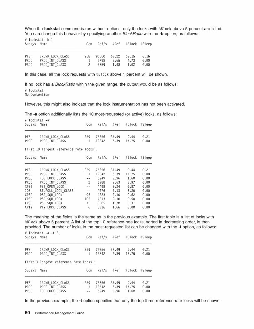
When the lockstat command is run without options, only the locks with %Block above 5 percent are listed.You can change this behavior by specifying another BlockRatio with the -b option, as follows:# lockstat -b 1Subsys Name Ocn Ref/s %Ref %Block %Sleep____________________________________________________________________

PFS IRDWR_LOCK_CLASS 258 95660 60.22 69.15 0.16PROC PROC_INT_CLASS 1 5798 3.65 4.73 0.00PROC PROC_INT_CLASS 2 2359 1.48 1.02 0.00

In this case, all the lock requests with %Block above 1 percent will be shown.

If no lock has a BlockRatio within the given range, the output would be as follows:# lockstatNo Contention

However, this might also indicate that the lock instrumentation has not been activated.

The -a option additionally lists the 10 most-requested (or active) locks, as follows:# lockstat -aSubsys Name Ocn Ref/s %Ref %Block %Sleep____________________________________________________________________


First 10 largest reference rate locks :

Subsys Name Ocn Ref/s %Ref %Block %Sleep____________________________________________________________________

PFS IRDWR_LOCK_CLASS 259 75356 37.49 9.44 0.21PROC PROC_INT_CLASS 1 12842 6.39 17.75 0.00PROC TOD_LOCK_CLASS -- 5949 2.96 1.68 0.00PROC PROC_INT_CLASS 2 5288 2.63 3.97 0.00XPSE PSE_OPEN_LOCK -- 4498 2.24 0.87 0.00IOS SELPOLL_LOCK_CLASS -- 4276 2.13 3.20 0.00XPSE PSE_SQH_LOCK 95 4223 2.10 0.62 0.00XPSE PSE_SQH_LOCK 105 4213 2.10 0.50 0.00XPSE PSE_SQH_LOCK 75 3585 1.78 0.31 0.00XPTY PTY_LOCK_CLASS 6 3336 1.66 0.00 0.00

The meaning of the fields is the same as in the previous example. The first table is a list of locks with%Block above 5 percent. A list of the top 10 reference-rate locks, sorted in decreasing order, is thenprovided. The number of locks in the most-requested list can be changed with the -t option, as follows:# lockstat -a -t 3Subsys Name Ocn Ref/s %Ref %Block %Sleep____________________________________________________________________




PFS IRDWR_LOCK_CLASS 259 75356 37.49 9.44 0.21PROC PROC_INT_CLASS 1 12842 6.39 17.75 0.00PROC TOD_LOCK_CLASS -- 5949 2.96 1.68 0.00

In the previous example, the -t option specifies that only the top three reference-rate locks will be shown.


If the output of the lockstat -a command looks similar to the following:No Contention



then an empty most-requested lock list means that the lock instrumentation has not been enabled. It canbe enabled by executing the bosboot command as explained at the beginning of this section.

The lockstat command can also be run in intervals, as follows:# lockstat 10 100

The first number passed in the command line specifies the amount of time (in seconds) between eachreport. Each report contains statistics collected during the interval since the previous report. If no interval isspecified, the system gives information covering an interval of one second and then exits. The secondnumber determines the number of reports generated. The second number can only be specified if aninterval is given.

Note: Under excessive lock contention on large SMPs, the lockstat command does not scale well andmight not return in the time period specified.

The schedtune -s CommandIf a thread wants to acquire a lock when another thread currently owns that lock and is running on anotherCPU, the thread that wants the lock will spin on the CPU until the owner thread releases the lock. Prior toAIX 4.3.1, this thread would spin indefinitely. In AIX 4.3.1, the thread spins up to a certain value asspecified by a tunable parameter called MAXSPIN.

The default value of MAXSPIN was previously 0xFFFFFFFF (the hexadecimal representation of a verylarge number in decimal form) on SMP systems and 1 on UP systems. In AIX 4.3.1, the default value ofMAXSPIN is 0x4000 (16384) for SMP systems and remains at 1 on UP systems. If you notice more idle orI/O wait time on a system that had not shown this previously, it could be that threads are going to sleepmore often. If this is causing a performance problem, then tune MAXSPIN such that it is a higher value orset to -1 which means to spin up to 0xFFFFFFFF times.

To revise the number of times to spin before going to sleep use the -s option of the schedtune command.To reduce CPU usage that might be caused by excessive spins, reduce the value of MAXSPIN as follows:# /usr/samples/kernel/schedtune -s 8192

You may observe an increase in context-switching. If context-switching becomes the bottleneck, increaseMAXSPIN.

To determine whether the schedtune command is installed and available, run the following command:# lslpp -lI bos.adt.samples

To change the value, you must be the root user.



Chapter 5. Planning and Implementing for Performance

A program that does not perform acceptably is not functional. Every program must satisfy a set of users,sometimes a large and diverse set. If the performance of the program is truly unacceptable to a significantnumber of those users, it will not be used. A program that is not being used is not performing its intendedfunction.

This situation is true of licensed software packages as well as user-written applications, although mostdevelopers of software packages are aware of the effects of poor performance and take pains to maketheir programs run as fast as possible. Unfortunately, they cannot anticipate all of the environments anduses that their programs will experience. Final responsibility for acceptable performance falls on the peoplewho select or write, plan for, and install software packages.

This chapter describes the stages by which a programmer or system administrator can ensure that anewly written or purchased program has acceptable performance. (Wherever the word programmerappears alone, the term includes system administrators and anyone else who is responsible for theultimate success of a program.)

To achieve acceptable performance in a program, identify and quantify acceptability at the start of theproject and never lose sight of the measures and resources needed to achieve it. Although this methodsounds elementary, some programming projects consciously reject it. They adopt a policy that might befairly described as design, code, debug, maybe document, and if we have time, fix the performance.

The only way that programs can predictably be made to function in time, not just in logic, is by integratingperformance considerations in the software planning and development process. Advance planning isperhaps more critical when existing software is being installed, because the installer has less freedom thanthe developer.

Although the detail of this process might seem burdensome for a small program, remember that we have asecond ″agenda.″ Not only must the new program have satisfactory performance, we must also ensurethat the addition of that program to an existing system does not degrade the performance of otherprograms run on that system.

This chapter includes the following major sections:

v Identifying the Components of the Workload

v Documenting Performance Requirements

v Estimating the Resource Requirements of the Workload

v Designing and Implementing Efficient Programs

v Using Performance-Related Installation Guidelines

Identifying the Components of the WorkloadWhether the program is new or purchased, small or large, the developers, the installers, and theprospective users have assumptions about the use of the program, such as:

v Who will be using the program

v Situations in which the program will be run

v How often those situations will arise and at what times of the hour, day, month, or year

v Whether those situations will also require additional uses of existing programs

v Which systems the program will run on

v How much data will be handled, and from where

v Whether data created by or for the program will be used in other ways


Unless these ideas are elicited as part of the design process, they will probably be vague, and theprogrammers will almost certainly have different assumptions than the prospective users. Even in theapparently trivial case in which the programmer is also the user, leaving the assumptions unarticulatedmakes it impossible to compare design to assumptions in any rigorous way. Worse, it is impossible toidentify performance requirements without a complete understanding of the work being performed.

Documenting Performance RequirementsIn identifying and quantifying performance requirements, it is important to identify the reasoning behind aparticular requirement. This is part of the general capacity planning process. Users might be basing theirstatements of requirements on assumptions about the logic of the program that do not match theprogrammer’s assumptions. At a minimum, a set of performance requirements should document thefollowing:

v The maximum satisfactory response time to be experienced most of the time for each distinct type ofuser-computer interaction, along with a definition of most of the time. Response time is measured fromthe time that the user performs the action that says ″Go″ until the user receives enough feedback fromthe computer to continue the task. It is the user’s subjective wait time. It is not from entry to asubroutine until the first write statement.

If the user denies interest in response time and indicates that only the result is of interest, you can askwhether ″ten times your current estimate of stand-alone execution time″ would be acceptable. If theanswer is ″yes,″ you can proceed to discuss throughput. Otherwise, you can continue the discussion ofresponse time with the user’s full attention.

v The response time that is minimally acceptable the rest of the time. A longer response time can causeusers to think the system is down. You also need to specify rest of the time; for example, the peakminute of a day, 1 percent of interactions. Response time degradations can be more costly or painful ata particular time of the day.

v The typical throughput required and the times it will be taking place. This is not a casual consideration.For example, the requirement for one program might be that it runs twice a day: at 10:00 a.m. and 3:15p.m. If this is a CPU-limited program that runs for 15 minutes and is planned to run on a multiusersystem, some negotiation is in order.

v The size and timing of maximum-throughput periods.

v The mix of requests expected and how the mix varies with time.

v The number of users per machine and total number of users, if this is a multiuser application. Thisdescription should include the times these users log on and off, as well as their assumed rates ofkeystrokes, completed requests, and think times. You may want to investigate whether think times varysystematically with the preceding and following request.

v Any assumptions that the user is making about the machines the workload will run on. If the user has aspecific existing machine in mind, make sure you know that early on. Similarly, if the user is assuming aparticular type, size, cost, location, interconnection, or any other variable that will constrain your abilityto satisfy the preceding requirements, that assumption also becomes part of the requirements.Satisfaction will probably not be assessed on the system where the program is developed, tested, orfirst installed.

Estimating the Resource Requirements of the WorkloadUnless you are purchasing a software package that comes with detailed resource-requirementdocumentation, estimating resources can be the most difficult task in the performance-planning process.The difficulty has several causes, as follows:

v There are several ways to do any task. You can write a C (or other high-level language) program, ashell script, a perl script, an awk script, a sed script, an AIXwindows dialog, and so on. Sometechniques that may seem particularly suitable for the algorithm and for programmer productivity areextraordinarily expensive from the performance perspective.


A useful guideline is that, the higher the level of abstraction, the more caution is needed to ensure thatone does not receive a performance surprise. Consider carefully the data volumes and number ofiterations implied by some apparently harmless constructs.

v The precise cost of a single process is difficult to define. This difficulty is not merely technical; it isphilosophical. If multiple instances of a given program run by multiple users are sharing pages ofprogram text, which process should be charged with those pages of memory? The operating systemleaves recently used file pages in memory to provide a caching effect for programs that reaccess thatdata. Should programs that reaccess data be charged for the space that was used to retain the data?The granularity of some measurements such as the system clock can cause variations in the CPU timeattributed to successive instances of the same program.

Two approaches deal with resource-report ambiguity and variability. The first is to ignore the ambiguityand to keep eliminating sources of variability until the measurements become acceptably consistent.The second approach is to try to make the measurements as realistic as possible and describe theresults statistically. Note that the latter yields results that have some correlation with productionsituations.

v Systems are rarely dedicated to running a single instance of a single program. There are almost alwaysdaemons running, there is frequently communications activity, and often workload from multiple users.These activities seldom add up linearly. For example, increasing the number of instances of a givenprogram may result in few new program text pages being used, because most of the program wasalready in memory. However, the additional processes may result in more contention for the processor’scaches, so that not only do the other processes have to share processor time with the newcomer, butall processes may experience more cycles per instruction. This is, in effect, a slowdown of theprocessor, as a result of more frequent cache misses.

Make your estimate as realistic as the specific situation allows, using the following guidelines:

v If the program exists, measure the existing installation that most closely resembles your ownrequirements. The best method is to use a capacity planning tool such as BEST/1.

v If no suitable installation is available, do a trial installation and measure a synthetic workload.

v If it is impractical to generate a synthetic workload that matches the requirements, measure individualinteractions and use the results as input to a simulation.

v If the program does not exist yet, find a comparable program that uses the same language and generalstructure, and measure it. Again, the more abstract the language, the more care is needed indetermining comparability.

v If no comparable program exists, develop a prototype of the main algorithms in the planned language,measure the prototype, and model the workload.

v Only if measurement of any kind is impossible or infeasible should you make an educated guess. If it isnecessary to guess at resource requirements during the planning stage, it is critical that the actualprogram be measured at the earliest possible stage of its development.

Keep in mind that independent software vendors (ISV) often have sizing guidelines for their applications.

In estimating resources, we are primarily interested in four dimensions (in no particular order):

CPU timeProcessor cost of the workload

Disk accessesRate at which the workload generates disk reads or writes

LAN trafficNumber of packets the workload generates and the number of bytes of data exchanged

Real memoryAmount of RAM the workload requires

The following sections discuss how to determine these values in various situations.

Chapter 5. Planning and Implementing for Performance 65

Measuring Workload ResourcesIf the real program, a comparable program, or a prototype is available for measurement, the choice oftechnique depends on the following:

v Whether the system is processing other work in addition to the workload we want to measure.

v Whether we have permission to use tools that may degrade performance (for example, is this system inproduction or is it dedicated to our use for the duration of the measurement?).

v The degree to which we can simulate or observe an authentic workload.

Measuring a Complete Workload on a Dedicated SystemUsing a dedicated system is the ideal situation because we can use measurements that include systemoverhead as well as the cost of individual processes.

To measure overall system performance for most of the system activity, use the vmstat command:# vmstat 5 >vmstat.output

This gives us a picture of the state of the system every 5 seconds during the measurement run. The firstset of vmstat output contains the cumulative data from the last boot to the start of the vmstat command.The remaining sets are the results for the preceding interval, in this case 5 seconds. A typical set ofvmstat output on a system looks similar to the following:kthr memory page faults cpu----- ----------- ------------------------ ------------ -----------r b avm fre re pi po fr sr cy in sy cs us sy id wa0 1 75186 192 0 0 0 0 1 0 344 1998 403 6 2 92 0

To measure CPU and disk activity, use the iostat command:# iostat 5 >iostat.output

This gives us a picture of the state of the system every 5 seconds during the measurement run. The firstset of iostat output contains the cumulative data from the last boot to the start of the iostat command.The remaining sets are the results for the preceding interval, in this case 5 seconds. A typical set of iostatoutput on a system looks similar to the following:tty: tin tout avg-cpu: % user % sys % idle % iowait

0.0 0.0 19.4 5.7 70.8 4.1

Disks: % tm_act Kbps tps Kb_read Kb_wrtnhdisk0 8.0 34.5 8.2 12 164hdisk1 0.0 0.0 0.0 0 0cd0 0.0 0.0 0.0 0 0

To measure memory, use the svmon command. The svmon -G command gives a picture of overallmemory use. The statistics are in terms of 4 KB pages (example from AIX 5.2):# svmon -G

size inuse free pin virtualmemory 65527 65406 121 5963 74711pg space 131072 37218

work pers clnt lpagepin 5972 0 0 0in use 54177 9023 2206 0

In this example, the machine’s 256 MB memory is fully used. About 83 percent of RAM is in use forworking segments, the read/write memory of running programs (the rest is for caching files). If there arelong-running processes in which we are interested, we can review their memory requirements in detail.The following example determines the memory used by a process of user hoetzel.


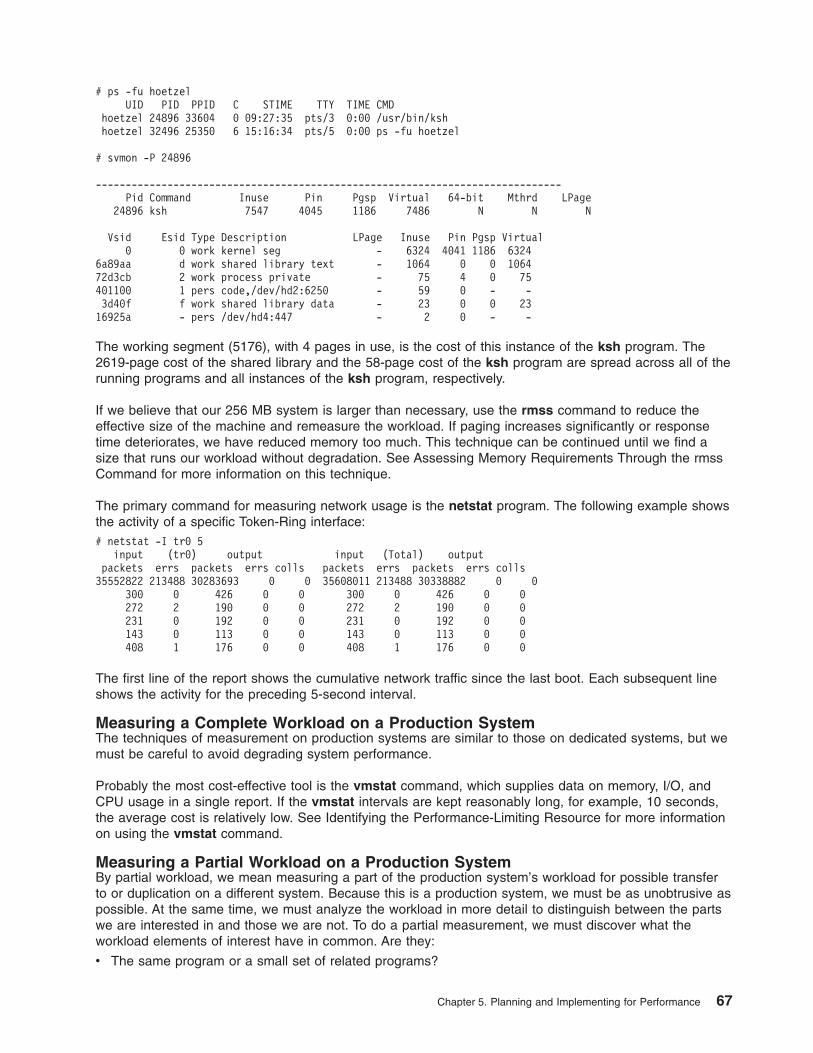
# ps -fu hoetzelUID PID PPID C STIME TTY TIME CMD

hoetzel 24896 33604 0 09:27:35 pts/3 0:00 /usr/bin/kshhoetzel 32496 25350 6 15:16:34 pts/5 0:00 ps -fu hoetzel

# svmon -P 24896

------------------------------------------------------------------------------Pid Command Inuse Pin Pgsp Virtual 64-bit Mthrd LPage

24896 ksh 7547 4045 1186 7486 N N N

Vsid Esid Type Description LPage Inuse Pin Pgsp Virtual0 0 work kernel seg - 6324 4041 1186 6324

6a89aa d work shared library text - 1064 0 0 106472d3cb 2 work process private - 75 4 0 75401100 1 pers code,/dev/hd2:6250 - 59 0 - -3d40f f work shared library data - 23 0 0 2316925a - pers /dev/hd4:447 - 2 0 - -

The working segment (5176), with 4 pages in use, is the cost of this instance of the ksh program. The2619-page cost of the shared library and the 58-page cost of the ksh program are spread across all of therunning programs and all instances of the ksh program, respectively.

If we believe that our 256 MB system is larger than necessary, use the rmss command to reduce theeffective size of the machine and remeasure the workload. If paging increases significantly or responsetime deteriorates, we have reduced memory too much. This technique can be continued until we find asize that runs our workload without degradation. See Assessing Memory Requirements Through the rmssCommand for more information on this technique.

The primary command for measuring network usage is the netstat program. The following example showsthe activity of a specific Token-Ring interface:# netstat -I tr0 5

input (tr0) output input (Total) outputpackets errs packets errs colls packets errs packets errs colls35552822 213488 30283693 0 0 35608011 213488 30338882 0 0

300 0 426 0 0 300 0 426 0 0272 2 190 0 0 272 2 190 0 0231 0 192 0 0 231 0 192 0 0143 0 113 0 0 143 0 113 0 0408 1 176 0 0 408 1 176 0 0

The first line of the report shows the cumulative network traffic since the last boot. Each subsequent lineshows the activity for the preceding 5-second interval.

Measuring a Complete Workload on a Production SystemThe techniques of measurement on production systems are similar to those on dedicated systems, but wemust be careful to avoid degrading system performance.

Probably the most cost-effective tool is the vmstat command, which supplies data on memory, I/O, andCPU usage in a single report. If the vmstat intervals are kept reasonably long, for example, 10 seconds,the average cost is relatively low. See Identifying the Performance-Limiting Resource for more informationon using the vmstat command.

Measuring a Partial Workload on a Production SystemBy partial workload, we mean measuring a part of the production system’s workload for possible transferto or duplication on a different system. Because this is a production system, we must be as unobtrusive aspossible. At the same time, we must analyze the workload in more detail to distinguish between the partswe are interested in and those we are not. To do a partial measurement, we must discover what theworkload elements of interest have in common. Are they:

v The same program or a small set of related programs?


v Work performed by one or more specific users of the system?

v Work that comes from one or more specific terminals?

Depending on the commonality, we could use one of the following# ps -ef | grep pgmname# ps -fuusername, . . .# ps -ftttyname, . . .

to identify the processes of interest and report the cumulative CPU time consumption of those processes.We can then use the svmon command (judiciously) to assess the memory use of the processes.

Measuring an Individual ProgramMany tools are available for measuring the resource consumption of individual programs. Some of theseprograms are capable of more comprehensive workload measurements as well, but are too intrusive foruse on production systems. Most of these tools are discussed in depth in the chapters that discuss tuningfor minimum consumption of specific resources. Some of the more prominent are:

svmonMeasures the real memory used by a process. Discussed in Determining How Much Memory IsBeing Used.

time Measures the elapsed execution time and CPU consumption of an individual program. Discussedin Using the time Command to Measure CPU Use.

tprof Measures the relative CPU consumption of programs, subroutine libraries, and the operatingsystem’s kernel. Discussed in Using the tprof Program to Analyze Programs for CPU Use.

vmstat -sMeasures the I/O load generated by a program. Discussed in Assessing Overall Disk I/O with thevmstat Command.

Estimating Resources Required by a New ProgramIt is impossible to make precise estimates of unwritten programs. The invention and redesign that takeplace during the coding phase defy prediction, but the following guidelines can help you to get a generalsense of the requirements. As a starting point, a minimal program would need the following:

v About 50 milliseconds of CPU time, mostly system time.

v Real Memory

– One page for program text

– About 15 pages (of which 2 are pinned) for the working (data) segment

– Access to libc.a. Normally this is shared with all other programs and is considered part of the basecost of the operating system.

v About 12 page-in Disk I/O operations, if the program has not been compiled, copied, or used recently.Otherwise, none required.

To the above, add the basic cost allowances for demands implied by the design (the units given are forexample purposes only):

v CPU time

– The CPU consumption of an ordinary program that does not contain high levels of iteration or costlysubroutine calls is almost unmeasurably small.

– If the proposed program contains a computationally expensive algorithm, develop a prototype andmeasure the algorithm.

– If the proposed program uses computationally expensive library subroutines, such as X or Motifconstructs or the printf() subroutine, measure their CPU consumption with otherwise trivialprograms.

v Real Memory


– Allow approximately 350 lines of code per page of program text, which is about 12 bytes per line.Keep in mind that coding style and compiler options can make a difference of a factor or two ineither direction. This allowance is for pages that are touched in your typical scenario. If your designplaces infrequently executed subroutines at the end of the executable program, those pages do notnormally consume real memory.

– References to shared libraries other than libc.a increase the memory requirement only to the extentthat those libraries are not shared with other programs or instances of the program being estimated.To measure the size of these libraries, write a trivial, long-running program that refers to them anduse the svmon -P command against the process.

– Estimate the amount of storage that will be required by the data structures identified in the design.Round up to the nearest page.

– In the short run, each disk I/O operation will use one page of memory. Assume that the page has tobe available already. Do not assume that the program will wait for another program’s page to befreed.

v Disk I/O

– For sequential I/O, each 4096 bytes read or written causes one I/O operation, unless the file hasbeen accessed recently enough that some of its pages are still in memory.

– For random I/O, each access, however small, to a different 4096-byte page causes one I/Ooperation, unless the file has been accessed recently enough that some of its pages are still inmemory.

– Each sequential read or write of a 4 KB page in a large file takes about 100 units. Each random reador write of a 4 KB page takes about 300 units. Remember that real files are not necessarily storedsequentially on disk, even though they are written and read sequentially by the program.Consequently, the typical CPU cost of an actual disk access will be closer to the random-access costthan to the sequential-access cost.

v Communications I/O

– If disk I/O is actually to Network File System (NFS) remote-mounted file systems, the disk I/O isperformed on the server, but the client experiences higher CPU and memory demands.

– RPCs of any kind contribute substantially to the CPU load. The proposed RPCs in the design shouldbe minimized, batched, prototyped, and measured in advance.

– Each sequential NFS read or write of an 4 KB page takes about 600 units on the client. Eachrandom NFS read or write of a 4 KB page takes about 1000 units on the client.

– Web browsing and Web serving implies considerable network I/O, with TCP connections openingand closing quite frequently.

Transforming Program-Level Estimates to Workload EstimatesThe best method for estimating peak and typical resource requirements is to use a queuing model such asBEST/1. Static models can be used, but you run the risk of overestimating or underestimating the peakresource. In either case, you need to understand how multiple programs in a workload interact from thestandpoint of resource requirements.

If you are building a static model, use a time interval that is the specified worst-acceptable response timefor the most frequent or demanding program (usually they are the same). Determine which programs willtypically be running during each interval, based on your projected number of users, their think time, theirkey entry rate, and the anticipated mix of operations.

Use the following guidelines:

v CPU time

– Add together the CPU requirements for the all of the programs that are running during the interval.Include the CPU requirements of the disk and communications I/O the programs will be doing.

– If this number is greater than 75 percent of the available CPU time during the interval, considerfewer users or more CPUs.


v Real Memory

– The operating system memory requirement scales with the amount of physical memory. Start with 6to 8 MB for the operating system itself. The lower figure is for a standalone system. The latter figureis for a system that is LAN-connected and uses TCP/IP and NFS.

– Add together the working segment requirements of all of the instances of the programs that will berunning during the interval, including the space estimated for the program’s data structures.

– Add to that total the memory requirement of the text segment of each distinct program that will berunning (one copy of the program text serves all instances of that program). Remember that any(and only) subroutines that are from unshared libraries will be part of the executable program, butthe libraries themselves will not be in memory.

– Add to the total the amount of space consumed by each of the shared libraries that will be used byany program in the workload. Again, one copy serves all.

– To allow adequate space for some file caching and the free list, your total memory projection shouldnot exceed 80 percent of the size of the machine to be used.

v Disk I/O

– Add the number of I/Os implied by each instance of each program. Keep separate totals for I/Os tosmall files (or randomly to large files) versus purely sequential reading or writing of large files (morethan 32 KB).

– Subtract those I/Os that you believe will be satisfied from memory. Any record that was read orwritten in the previous interval is probably still available in the current interval. Beyond that, examinethe size of the proposed machine versus the total RAM requirements of the machine’s workload. Anyspace remaining after the operating system’s requirement and the workload’s requirements probablycontains the most recently read or written file pages. If your application’s design is such that there isa high probability that you will reuse recently accessed data, you can calculate an allowance for thecaching effect. Remember that the reuse is at the page level, not at the record level. If the probabilityof reuse of a given record is low, but there are a lot of records per page, it is likely that some of therecords needed in any given interval will fall in the same page as other, recently used, records.

– Compare the net I/O requirements (disk I/Os per second per disk) to the approximate capabilities ofcurrent disk drives. If the random or sequential requirement is greater than 75 percent of the totalcorresponding capability of the disks that will hold application data, tuning (and possibly expansion)will be needed when the application is in production.

v Communications I/O

– Calculate the bandwidth consumption of the workload. If the total bandwidth consumption of all of thenodes on the LAN is greater than 70 percent of nominal bandwidth (50 percent for Ethernet), youmight want to use a network with higher bandwidth.

– Perform a similar analysis of CPU, memory, and I/O requirements of the added load that will beplaced on the server.

Note: Remember that these guidelines are intended for use only when no extensive measurement ispossible. Any application-specific measurement that can be used in place of a guideline willconsiderably improve the accuracy of the estimate.

Designing and Implementing Efficient ProgramsIf you have determined which resource will limit the speed of your program, you can go directly to thesection that discusses appropriate techniques for minimizing the use of that resource. Otherwise, assumethat the program will be balanced and that all of the recommendations in this chapter apply. Once theprogram is implemented, proceed to Identifying the Performance-Limiting Resource.

CPU-Limited ProgramsThe maximum speed of a truly processor-limited program is determined by:

v The algorithm used


v The source code and data structures created by the programmer

v The sequence of machine-language instructions generated by the compiler

v The sizes and structures of the processor’s caches

v The architecture and clock rate of the processor itself (see Appendix D. Determining CPU Speed)

If the program is CPU-limited because it consists almost entirely of numerical computation, the chosenalgorithm will have a major effect on the performance of the program. A discussion of alternativealgorithms is beyond the scope of this book. It is assumed that computational efficiency has beenconsidered in choosing the algorithm.

Given an algorithm, the only items in the preceding list that the programmer can affect are the sourcecode, the compiler options used, and possibly the data structures. The following sections deal withtechniques that can be used to improve the efficiency of an individual program for which the user has thesource code. If the source code is not available, attempt to use tuning or workload-managementtechniques.

Design and Coding for Effective Use of CachesIn Performance Concepts, we indicated that processors have a multilevel hierarchy of memory:

1. Instruction pipeline and the CPU registers

2. Instruction and data cache(s) and the corresponding translation lookaside buffers

3. RAM

4. Disk

As instructions and data move up the hierarchy, they move into storage that is faster than the level belowit, but also smaller and more expensive. To obtain the maximum possible performance from a givenmachine, therefore, the programmer must make the most effective use of the available storage at eachlevel.

Effective use of storage means keeping it full of instructions and data that are likely to be used. Anobstacle to achieving this objective is the fact that storage is allocated in fixed-length blocks such as cachelines and real memory pages that usually do not correspond to boundaries within programs or datastructures. Programs and data structures that are designed without regard to the storage hierarchy oftenmake inefficient use of the storage allocated to them, with adverse performance effects in small or heavilyloaded systems.

Taking the storage hierarchy into account means understanding and adapting to the general principles ofefficient programming in a cached or virtual-memory environment. Repackaging techniques can yieldsignificant improvements without recoding, and any new code should be designed with efficient storageuse in mind.

Two terms are essential to any discussion of the efficient use of hierarchical storage: locality of referenceand working set.

v The locality of reference of a program is the degree to which its instruction-execution addresses anddata references are clustered in a small area of storage during a given time interval.

v The working set of a program during that same interval is the set of storage blocks that are in use, or,more precisely, the code or data that occupy those blocks.

A program with good locality of reference has a minimal working set, because the blocks that are in useare tightly packed with executing code or data. A functionally equivalent program with poor locality ofreference has a larger working set, because more blocks are needed to accommodate the wider range ofaddresses being accessed.


Because each block takes a significant amount of time to load into a given level of the hierarchy, theobjective of efficient programming for a hierarchical-storage system is to design and package code in sucha way that the working set remains as small as practical.

The following figure illustrates good and bad practice at a subroutine level. The first version of the programis packaged in the sequence in which it was probably written. The first subroutine PriSub1 contains theentry point of the program. It always uses primary subroutines PriSub2 and PriSub3. Some infrequentlyused functions of the program require secondary subroutines SecSub1 and SecSub2. On rare occasions,the error subroutines ErrSub1 and ErrSub2 are needed.

The initial version of the program has poor locality of reference because it takes three pages of memory torun in the normal case. The secondary and error subroutines separate the main path of the program intothree, physically distant sections.

The improved version of the program places the primary subroutines adjacent to one another and puts thelow-frequency function after that. The necessary error subroutines (which are rarely-used) are left at theend of the executable program. The most common functions of the program can now be handled with onlyone disk read and one page of memory instead of the three previously required.

Remember that locality of reference and working set are defined with respect to time. If a program worksin stages, each of which takes a significant time and uses a different set of subroutines, try to minimize theworking set of each stage.

Registers and PipelineIn general, allocating and optimizing of register space and keeping the pipeline full are the responsibilitiesof the compilers. The programmer’s main obligation is to avoid structures that defeat compiler-optimizationtechniques. For example, if you use one of your subroutines in one of the critical loops of your program, it

Figure 15. Locality of Reference. The top half of the figure describes how a binary program is packaged which showslow locality of reference. The instructions for PriSub1 is in the binary executable first, followed by the instructions forSecSub1, ErrSub1, PriSub2, SecSub2, ErrSub2, and PriSub3. In this executable, the instructions for PriSub1,SecSub1, and ErrSub1 occupy into the first page of memory. The instructions for PriSub2, SecSub2, and ErrSub2occupy the second page of memory, and the instructions for PriSub3 occupy the third page of memory. SecSub1 andSecSub2 are infrequently used; also ErrSub1 and ErrSub2 are rarely used, if ever. Therefore, the packaging of thisprogram exhibits poor locality of reference and may use more memory than required. In the second half of the figure,PriSub1, PriSub2, and PriSub3 are located next to each other and occupy the first page of memory. Following PriSub3is SecSub1, SecSub2, and ErrSub1 which all occupy the second page of memory. Finally, ErrSub2 is at the end andoccupies the third page of memory. Because ErrSub2 may never be needed, it would reduce the memoryrequirements by one page in this case.


may be appropriate for the compiler to inline that subroutine to minimize execution time. If the subroutinehas been packaged in a different .c module, however, it cannot be inlined by the compiler.

Cache and TLBsDepending on the processor architecture and model, processors have from one to several caches to holdthe following:

v Parts of executing programs

v Data used by executing programs

v Translation lookaside buffers (TLBs), which contain the mapping from virtual address to real address ofrecently used pages of instruction text or data

If a cache miss occurs, loading a complete cache line can take dozens of processor cycles. If a TLB missoccurs, calculating the virtual-to-real mapping of a page can take several dozen cycles. The exact cost isimplementation-dependent.

Even if a program and its data fit in the caches, the more lines or TLB entries used (that is, the lower thelocality of reference), the more CPU cycles it takes to get everything loaded in. Unless the instructions anddata are reused many times, the overhead of loading them is a significant fraction of total programexecution time, resulting in degraded system performance.

Good programming techniques keep the main-line, typical-case flow of the program as compact aspossible. The main procedure and all of the subroutines it calls frequently should be contiguous.Low-probability conditions, such as obscure errors, should be tested for only in the main line. If thecondition actually occurs, its processing should take place in a separate subroutine. All such subroutinesshould be grouped together at the end of the module. This arrangement reduces the probability thatlow-usage code will take up space in a high-usage cache line. In large modules, some or all of thelow-usage subroutines might occupy a page that almost never has to be read into memory.

The same principle applies to data structures, although it is sometimes necessary to change the code tocompensate for the compiler’s rules about data layout.

For example, some matrix operations, such as matrix multiplication, involve algorithms that, if codedsimplistically, have poor locality of reference. Matrix operations generally involve accessing the matrix datasequentially, such as row elements acting on column elements. Each compiler has specific rules about thestorage layout of matrixes. The FORTRAN compiler lays out matrixes in column-major format (that is, all ofthe elements of column 1, followed by all the elements of column 2, and so forth). The C compiler lays outmatrixes in row-major format. If the matrixes are small, the row and column elements can be contained inthe data cache, and the processor and floating-point unit can run at full speed. However, as the size of thematrixes increases, the locality of reference of such row/column operations deteriorates to a point wherethe data can no longer be maintained in the cache. In fact, the natural access pattern of the row/columnoperations generates a thrashing pattern for the cache where a string of elements accessed is larger thanthe cache, forcing the initially accessed elements out and then repeating the access pattern again for thesame data.

The general solution to such matrix access patterns is to partition the operation into blocks, so thatmultiple operations on the same elements can be performed while they remain in the cache. This generaltechnique is given the name strip mining.

Experts in numerical analysis were asked to code versions of the matrix-manipulation algorithms thatmade use of strip mining and other optimization techniques. The result was a 30-fold improvement inmatrix-multiplication performance. The tuned routines are in the Basic Linear Algebra Subroutines (BLAS)library, /usr/lib/libblas.a. A larger set of performance-tuned subroutines is the Engineering and ScientificSubroutine Library (ESSL) licensed program.


The functions and interfaces of the Basic Linear Algebra Subroutines are documented in AIX 5L Version5.2 Technical Reference. The FORTRAN run-time environment must be installed to use the library. Usersshould generally use this library for their matrix and vector operations because its subroutines are tuned toa degree that users are unlikely to achieve by themselves.

If the data structures are controlled by the programmer, other efficiencies are possible. The generalprinciple is to pack frequently used data together whenever possible. If a structure contains frequentlyaccessed control information and occasionally accessed detailed data, make sure that the controlinformation is allocated in consecutive bytes. This will increase the probability that all of the controlinformation will be loaded into the cache with a single (or at least with the minimum number of) cachemisses.

Effective Use of Preprocessors and the CompilersThe programmer who wants to obtain the highest possible performance from a given program running ona given machine must deal with several considerations:

v There are preprocessors that can rearrange some source code structures to form a functionallyequivalent source module that can be compiled into more efficient executable code.

v Just as there are several variants of the architecture, there are several compiler options to allow optimalcompilation for a specific variant or set of variants.

v The programmer can use the #pragma feature to inform the C compiler of certain aspects of theprogram that will allow the compiler to generate more efficient code by relaxing some of its worst-caseassumptions.

v There are several levels of optimization that give the compiler different degrees of freedom in instructionrearrangement.

Programmers who are unable to experiment, should always optimize. The difference in performancebetween optimized and unoptimized code is almost always so large that basic optimization (the -O optionof the compiler commands) should always be used. The only exceptions are testing situations in whichthere is a specific need for straightforward code generation, such as statement-level performance analysisusing the tprof tool.

These techniques yield additional performance improvement for some programs, but the determination ofwhich combination yields the best performance for a specific program might require considerablerecompilation and measurement.

For an extensive discussion of the techniques for efficient use of compilers, see Optimization and TuningGuide for XL Fortran, XL C and XL C++.

Levels of OptimizationThe levels of optimization in the compilers are as follows:

No OptimizationIn the absence of any version of the -O flag, the compiler generates straightforward code with noinstruction reordering or other attempt at performance improvement.

-O or -O2These equivalent flags cause the compiler to optimize on the basis of conservative assumptions aboutcode reordering. Only explicit relaxations such as the #pragma directives are used. This level performs nosoftware pipelining, loop unrolling, or simple predictive commoning. It also constrains the amount ofmemory the compiler can use.

-O3This flag directs the compiler to be aggressive about the optimization techniques used and to use as muchmemory as necessary for maximum optimization.


This level of optimization may result in functional changes to the program if the program is sensitive to thefollowing:

v Floating-point exceptions

v The sign of zero

v Precision effects of reordering calculations

These side effects can be avoided, at some performance cost, by using the -qstrict option in combinationwith -O3.

The -qhot option, in combination with -O3, enables predictive commoning and some unrolling.

The result of these changes is that large or complex routines should have the same or better performancewith the -O3 option (possibly in conjunction with -qstrict or -qhot) that they had with the -O option inearlier versions of the compiler.

-O4This flag is equivalent to -O3 -qipa with automatic generation of architecture and tuning option ideal forthat platform.

-O5This flag is similiar to -O4, except in this case,-qipa = level = 2.

Compiling for Specific Hardware Platforms (-qarch, -qtune)Systems can use several type of processors. By using the -qarch and -qtune options, you can optimizeprograms for the special instructions and particular strengths of these processors.

Follow these guidelines:

v If your program will be run only on a single system, or on a group of systems with the same processortype, use the -qarch option to specify the processor type.

v If your program will be run on systems with different processor types, and you can identify oneprocessor type as the most important, use the appropriate -qarch and -qtune settings. FORTRAN andHPF users can use the xxlf and xxlhpf commands to select these settings interactively.

v If your program is intended to run on the full range of processor implementations, and is not intendedprimarily for one processor type, do not use either -qarch or -qtune.

C Options for string.h Subroutine PerformanceThe operating system provides the ability to embed the string subroutines in the application program ratherthan using them from libc.a, saving call and return linkage time. To embed the string subroutines, thesource code of the application must have the following statement prior to the use of the subroutine(s):#include <string.h>

C and C++ Coding Style for Best PerformanceIn many cases, the performance cost of a C construct is not obvious, and sometimes is evencounter-intuitive. Some of these situations are as follows:

v Whenever possible, use int instead of char or short.

In most cases, char and short data items take more instructions to manipulate. The extra instructionscost time, and, except in large arrays, any space that is saved by using the smaller data types is morethan offset by the increased size of the executable program.

v If you have to use a char, make it unsigned, if possible.

A signed char takes another two instructions more than an unsigned char each time the variable isloaded into a register.

v Use local (automatic) variables rather than global variables whenever possible.


Global variables require more instructions to access than local variables. Also, in the absence ofinformation to the contrary, the compiler assumes that any global variable may have been changed by asubroutine call. This change has an adverse effect on optimization because the value of any globalvariable used after a subroutine call will have to be reloaded.

v When it is necessary to access a global variable (that is not shared with other threads), copy the valueinto a local variable and use the copy.

Unless the global variable is accessed only once, it is more efficient to use the local copy.

v Use binary codes rather than strings to record and test for situations. Strings consume both data andinstruction space. For example, the sequence:#define situation_1 1#define situation_2 2#define situation_3 3int situation_val;

situation_val = situation_2;. . .if (situation_val == situation_1). . .

is much more efficient than the following sequence:char situation_val[20];

strcpy(situation_val,"situation_2");. . .if ((strcmp(situation_val,"situation_1"))==0). . .

v When strings are necessary, use fixed-length strings rather than null-terminated variable-length stringswherever possible.

The mem*() family of routines, such as memcpy(), is faster than the corresponding str*() routines, suchas strcpy(), because the str*() routines must check each byte for null and the mem*() routines do not.

Compiler Execution TimeIn the operating system, the C compiler can be invoked by two different commands: cc and xlc. The cccommand, which has historically been used to invoke the system’s C compiler, causes the C compiler torun in langlevel=extended mode. This mode allows the compilation of existing C programs that are notANSI-compliant. It also consumes processor time.

If the program being compiled is, in fact, ANSI-compliant, it is more efficient to invoke the C compiler byusing the xlc command.

Use of the -O3 flag implicitly includes the -qmaxmem option. This option allows the compiler to use asmuch memory as necessary for maximum optimization. This situation can have two effects:

v On a multiuser system, a large -O3 compilation may consume enough memory to have an adverseeffect on the performance experienced by other users.

v On a system with small real memory, a large -O3 compilation may consume enough memory to causehigh paging rates, making compilation slow.

Memory-Limited ProgramsTo programmers accustomed to struggling with the addressing limitations of, for instance, the DOSenvironment, 256 MB virtual memory segments seem effectively infinite. The programmer is tempted toignore storage constraints and code for minimum path length and maximum simplicity. Unfortunately, thereis a drawback to this attitude. Virtual memory is large, but it is variable-speed. The more memory used,the slower it becomes, and the relationship is not linear. As long as the total amount of virtual storageactually being touched by all programs (that is, the sum of the working sets) is slightly less than theamount of unpinned real memory in the machine, virtual memory performs at about the speed of real


memory. As the sum of the working sets of all executing programs passes the number of available pageframes, memory performance degrades rapidly (if VMM memory load control is turned off) by up to twoorders of magnitude. When the system reaches this point, it is said to be thrashing. It is spending almostall of its time paging, and no useful work is being done because each process is trying to steal back fromother processes the storage necessary to accommodate its working set. If VMM memory load control isactive, it can avoid this self-perpetuating thrashing, but at the cost of significantly increased responsetimes.

The degradation caused by inefficient use of memory is much greater than that from inefficient use of thecaches because the difference in speed between memory and disk is so much higher than the differencebetween cache and memory. Where a cache miss can take a few dozen CPU cycles, a page fault typicallytakes 10 milliseconds or more, which is at least 400,000 CPU cycles.

Although VMM memory load control can ensure that incipient thrashing situations do not becomeself-perpetuating, unnecessary page faults still exact a cost in degraded response time and reducedthroughput (see Tuning VMM Memory Load Control with the schedtune Command).

Structuring of Pageable CodeTo minimize the code working set of a program, the general objective is to pack code that is frequentlyexecuted into a small area, separating it from infrequently executed code. Specifically:

v Do not put long blocks of error-handling code in line. Place them in separate subroutines, preferably inseparate source-code modules. This applies not only to error paths, but to any functional option that isinfrequently used.

v Do not structure load modules arbitrarily. Try to ensure that frequently called object modules are locatedas close to their callers as possible. Object modules consisting (ideally) of infrequently calledsubroutines should be concentrated at the end of the load module. The pages they inhabit will seldombe read in.

Structuring of Pageable DataTo minimize the data working set, try to concentrate the frequently used data and avoid unnecessaryreferences to virtual-storage pages. Specifically:

v Use the malloc() or calloc() subroutines to request only as much space as you actually need. Neverrequest and then initialize a maximum-sized array when the actual situation uses only a fraction of it.When you touch a new page to initialize the array elements, you effectively force the VMM to steal apage of real memory from someone. Later, this results in a page fault when the process that owned thatpage tries to access it again. The difference between the malloc() and calloc() subroutines is not just inthe interface.

v Because the calloc() subroutine zeroes the allocated storage, it touches every page that is allocated,whereas the malloc() subroutine touches only the first page. If you use the calloc() subroutine toallocate a large area and then use only a small portion at the beginning, you place an unnecessary loadon the system. Not only do the pages have to be initialized; if their real-memory frames are reclaimed,the initialized and never-to-be-used pages must be written out to paging space. This situation wastesboth I/O and paging-space slots.

v Linked lists of large structures (such as buffers) can result in similar problems. If your program does alot of chain-following looking for a particular key, consider maintaining the links and keys separatelyfrom the data or using a hash-table approach instead.

v Locality of reference means locality in time, not just in address space. Initialize data structures just priorto when they are used (if at all). In a heavily loaded system, data structures that are resident for a longtime between initialization and use risk having their frames stolen. Your program would then experiencean unnecessary page fault when it began to use the data structure.

v Similarly, if a large structure is used early and then left untouched for the remainder of the program, itshould be released. It is not sufficient to use the free() subroutine to free the space that was allocatedwith the malloc() or calloc() subroutines. The free() subroutine releases only the address range thatthe structure occupied. To release the real memory and paging space, use the disclaim() subroutine todisclaim the space as well. The call to disclaim() should be before the call to free().


Misuse of Pinned StorageTo avoid circularities and time-outs, a small fraction of the system must be pinned in real memory. For thiscode and data, the concept of working set is meaningless, because all of the pinned information is in realstorage all the time, whether or not it is used. Any program (such as a user-written device driver) that pinscode or data must be carefully designed (or scrutinized, if ported) to ensure that only minimal amounts ofpinned storage are used. Some cautionary examples are as follows:

v Code is pinned on a load-module (executable file) basis. If a component has some object modules thatmust be pinned and others that can be pageable, package the pinned object modules in a separateload module.

v Pinning a module or a data structure because there might be a problem is irresponsible. The designershould understand the conditions under which the information could be required and whether a pagefault could be tolerated at that point.

v Pinned structures whose required size is load-dependent, such as buffer pools, should be tunable bythe system administrator.

Using Performance-Related Installation GuidelinesThis topic provides recommended actions you should take (or not take) before and during the installationprocess.

Operating System Preinstallation GuidelinesTwo situations require consideration, as follows:

v Installing the Operating System on a New System

Before you begin the installation process, be sure that you have made decisions about the size andlocation of disk file systems and paging spaces, and that you understand how to communicate thosedecisions to the operating system.

v Installing a New Level of the Operating System on an Existing System

If you are upgrading to a new level of the operating system, do the following:

– Identify all uses in your present environment of the release-specific schedtune and vmtuneperformance tools. Because these tools can only be run by the root user, their use should not bewidespread.

– If these programs are used during system boot, such as from /etc/inittab, they should be temporarilyremoved or bypassed until you are convinced by documentation or experiment that your use of thesetools work correctly in the new release of the operating system.

CPU Preinstallation GuidelinesUse the default CPU scheduling parameters, such as the time-slice duration. Unless you have extensivemonitoring and tuning experience with the same workload on a nearly identical configuration, leave theseparameters unchanged at installation time.

See Monitoring and Tuning CPU Use for post-installation recommendations.

Memory Preinstallation GuidelinesDo not make any memory-threshold changes until you have had experience with the response of thesystem to the actual workload.

See Monitoring and Tuning Memory Use for post-installation recommendations.


Disk Preinstallation GuidelinesThe mechanisms for defining and expanding logical volumes attempt to make the best possible defaultchoices. However, satisfactory disk-I/O performance is much more likely if the installer of the system tailorsthe size and placement of the logical volumes to the expected data storage and workload requirements.Recommendations are as follows:

v If possible, the default volume group, rootvg, should consist only of the physical volume on which thesystem is initially installed. Define one or more other volume groups to control the other physicalvolumes in the system. This recommendation has system management, as well as performance,advantages.

v If a volume group consists of more than one physical volume, you may gain performance by:

– Initially defining the volume group with a single physical volume.

– Defining a logical volume within the new volume group. This definition causes the allocation of thevolume group’s journal logical volume on the first physical volume.

– Adding the remaining physical volumes to the volume group.

– Defining the high-activity file systems on the newly added physical volumes.

– Defining only very-low-activity file systems, if any, on the physical volume containing the journallogical volume. This affects performance only if I/O would cause journaled file system (JFS) logtransactions.

This approach separates journaled I/O activity from the high-activity data I/O, increasing theprobability of overlap. This technique can have an especially significant effect on NFS serverperformance, because both data and journal writes must be complete before NFS signals I/Ocomplete for a write operation.

v At the earliest opportunity, define or expand the logical volumes to their maximum expected sizes. Tomaximize the probability that performance-critical logical volumes will be contiguous and in the desiredlocation, define or expand them first.

v High-usage logical volumes should occupy parts of multiple disk drives. If the RANGE of physicalvolumes option on the Add a Logical Volume screen of the SMIT program (fast path: smitty mklv) isset to maximum, the new logical volume will be divided among the physical volumes of the volumegroup (or the set of physical volumes explicitly listed).

v If the system has drives of different types (or you are trying to decide which drives to order), considerthe following guidelines:

– Place large files that are normally accessed sequentially on the fastest available disk drive.

– If you expect frequent sequential accesses to large files on the fastest disk drives, limit the numberof disk drivers per disk adapter.

– When possible, attach drives with critical, high-volume performance requirements to a high speedadapter. These adapters have features, such as back-to-back write capability, that are not availableon other disk adapters.

– On the smaller disk drives, logical volumes that will hold large, frequently accessed sequential filesshould be allocated in the outer_edge of the physical volume. These disks have more blocks pertrack in their outer sections, which improves sequential performance.

– On the original SCSI bus, the highest-numbered drives (those with the numerically largest SCSIaddresses, as set on the physical drives) have the highest priority. Subsequent specifications usuallyattempt to maintain compatibility with the original specification. Thus, the order from highest to lowestpriority is as follows: 7-6-5-4-3-2-1-0-15-14-13-12-11-10-9-8.

In most situations this effect is not noticeable, but large sequential file operations have been knownto exclude low-numbered drives from access to the bus. You should probably configure the diskdrives holding the most response-time-critical data at the highest addresses on each SCSI bus.

The lsdev -Cs scsi command reports on the current address assignments on each SCSI bus. Forthe original SCSI adapter, the SCSI address is the first number in the fourth pair of numbers in theoutput. In the following output example, one 400 GB disk is at SCSI address 4, another at address 5,the 8mm tape drive at address 1, and the CDROM drive is at address 3.


cd0 Available 10-80-00-3,0 SCSI Multimedia CD-ROM Drivehdisk0 Available 10-80-00-4,0 16 Bit SCSI Disk Drivehdisk1 Available 10-80-00-5,0 16 Bit SCSI Disk Drivermt0 Available 10-80-00-1,0 2.3 GB 8mm Tape Drive

– Large files that are heavily used and are normally accessed randomly, such as data bases, shouldbe spread across two or more physical volumes.

See Monitoring and Tuning Disk I/O Use for post-installation recommendations.

Placement and Sizes of Paging SpacesThe general recommendation is that the sum of the sizes of the paging spaces should be equal to at leasttwice the size of the real memory of the machine, up to a memory size of 256 MB (512 MB of pagingspace).

Note: For memories larger than 256 MB, the following is recommended:total paging space = 512 MB + (memory size - 256 MB) * 1.25

However, starting with AIX 4.3.2 and Deferred Page Space Allocation, this guideline may tie upmore disk space than actually necessary. See Choosing a Page Space Allocation Method for moreinformation.

Ideally, there should be several paging spaces of roughly equal size, each on a different physical diskdrive. If you decide to create additional paging spaces, create them on physical volumes that are morelightly loaded than the physical volume in rootvg. When allocating paging space blocks, the VMM allocatesfour blocks, in turn, from each of the active paging spaces that has space available. While the system isbooting, only the primary paging space (hd6) is active. Consequently, all paging-space blocks allocatedduring boot are on the primary paging space. This means that the primary paging space should besomewhat larger than the secondary paging spaces. The secondary paging spaces should all be of thesame size to ensure that the algorithm performed in turn can work effectively.

The lsps -a command gives a snapshot of the current utilization level of all the paging spaces on asystem. You can also used the psdanger() subroutine to determine how closely paging-space utilization isapproaching critical levels. As an example, the following program uses the psdanger() subroutine toprovide a warning message when a threshold is exceeded:/* psmonitor.c

Monitors system for paging space low conditions. When the condition isdetected, writes a message to stderr.Usage: psmonitor [Interval [Count]]Default: psmonitor 1 1000000

*/#include <stdio.h>#include <signal.h>main(int argc,char **argv){

int interval = 1; /* seconds */int count = 1000000; /* intervals */int current; /* interval */int last; /* check */int kill_offset; /* returned by psdanger() */int danger_offset; /* returned by psdanger() */

/* are there any parameters at all? */if (argc > 1) {

if ( (interval = atoi(argv[1])) < 1 ) {fprintf(stderr,"Usage: psmonitor [ interval [ count ] ]\n");exit(1);

}if (argc > 2) {

if ( (count = atoi( argv[2])) < 1 ) {fprintf(stderr,"Usage: psmonitor [ interval [ count ] ]\n");


exit(1);}

}}last = count -1;for(current = 0; current < count; current++) {

kill_offset = psdanger(SIGKILL); /* check for out of paging space */if (kill_offset < 0)

fprintf(stderr,"OUT OF PAGING SPACE! %d blocks beyond SIGKILL threshold.\n",kill_offset*(-1));

else {danger_offset = psdanger(SIGDANGER); /* check for paging space low */if (danger_offset < 0) {

fprintf(stderr,"WARNING: paging space low. %d blocks beyond SIGDANGER threshold.\n",danger_offset*(-1));

fprintf(stderr," %d blocks below SIGKILL threshold.\n",kill_offset);

}}

if (current < last)sleep(interval);

}}

Performance Implications of Disk MirroringIf mirroring is being used and Mirror Write Consistency is on (as it is by default), consider locating thecopies in the outer region of the disk, because the Mirror Write Consistency information is always writtenin Cylinder 0. From a performance standpoint, mirroring is costly, mirroring with Write Verify is costlier still(extra disk rotation per write), and mirroring with both Write Verify and Mirror Write Consistency is costliestof all (disk rotation plus a seek to Cylinder 0). From a fiscal standpoint, only mirroring with writes isexpensive. Although an lslv command will usually show Mirror Write Consistency to be on for non-mirroredlogical volumes, no actual processing is incurred unless the COPIES value is greater than one. WriteVerify defaults to off, because it does have meaning (and cost) for non-mirrored logical volumes.

Beginning in AIX 5.1, a mirror write consistency option called Passive Mirror Write Consistency (MWC) isavailable. The default mechanism for ensuring mirror write consistency is Active MWC. Active MWCprovides fast recovery at reboot time after a crash has occurred. However, this benefit comes at theexpense of write performance degradation, particularly in the case of random writes. Disabling ActiveMWC eliminates this write-performance penalty, but upon reboot after a crash you must use the syncvg -fcommand to manually synchronize the entire volume group before users can access the volume group. Toachieve this, automatic vary-on of volume groups must be disabled.

Enabling Passive MWC not only eliminates the write-performance penalty associated with Active MWC, butlogical volumes will be automatically resynchronized as the partitions are being accessed. This means thatthe administrator does not have to synchronize logical volumes manually or disable automatic vary-on.The disadvantage of Passive MWC is that slower read operations may occur until all the partitions havebeen resynchronized.

You can select either mirror write consistency option within SMIT when creating or changing a logicalvolume. The selection option takes effect only when the logical volume is mirrored (copies > 1).

Performance Implications of Mirrored Striped LVsPrior to AIX 4.3.3, logical volumes could not be mirrored and striped at the same time. Logical volumemirroring and striping combines the data availability of RAID 1 with the performance of RAID 0 entirelythrough software. Volume groups that contain striped and mirrored logical volumes cannot be imported intoAIX 4.3.2 or earlier.


Communications Preinstallation GuidelinesSee the summary of communications tuning recommendations in Tuning TCP and UDP Performance andTuning mbuf Pool Performance.

For correct placement of adapters and various performance guidelines, see PCI Adapter PlacementReference.


Chapter 6. System Monitoring and Initial PerformanceDiagnosis

This chapter describes tools and techniques for monitoring performance-related system activity anddiagnosing performance problems. The major sections are:

v The Case for Continuous Performance Monitoring

v Using the vmstat, iostat, netstat, and sar Commands

v Using the topas Monitor

v Using the Performance Diagnostic Tool

v Using the Performance Toolbox

v Determining the Kind of Performance Problem Reported

v Identifying the Performance-Limiting Resource

v Managing Workload

The Case for Continuous Performance MonitoringIn some installations, performance activity is monitored on a demand basis. When a performance problemis reported, the performance analyst runs one or more commands in an attempt to determine why theproblem occurred. In some cases, explicit recreation of the problem is needed in order to collect analysisdata. The result is that users experience every performance problem twice.

It is usually more effective to monitor performance continuously, preferably with automatic collection ofadditional data if performance deteriorates. The costs of continuous monitoring are outweighed by theadvantages, such as:

v Monitoring can sometimes detect incipient problems before they have an adverse effect.

v Monitoring can detect problems that happen to users who are reluctant to complain, as well asproblems that are not quite severe enough to complain about, but are affecting productivity and morale.

v Monitoring can collect data when a problem occurs for the first time.

Successful monitoring involves the following main activities:

v Periodically obtaining performance-related information from the operating system

v Storing the information for future use in problem diagnosis

v Displaying the information for the benefit of the system administrator

v Detecting situations that require additional data collection or responding to directions from the systemadministrator to collect such data, or both

v Collecting and storing the necessary detail data

The following sections discuss several approaches to continuous monitoring. These approaches are notmutually exclusive, but use of more than one may involve some redundancy.

Using the vmstat, iostat, netstat, and sar CommandsThe vmstat, iostat, netstat, and sar commands have functional characteristics that make them useful forcontinuous monitoring of system performance. These commands can:

v Produce reports indefinitely at a fixed interval

v Report on activity that varies with different types of load

v Report on activity since the last previous report (except the sar command), so changes in activity areeasy to detect


The following example shows samples of the periodic reports produced by these programs.# vmstat 5 2kthr memory page faults cpu----- ----------- ------------------------ ------------ -----------r b avm fre re pi po fr sr cy in sy cs us sy id wa0 1 75318 142 0 0 0 0 0 0 299 1845 315 5 2 93 00 1 75318 141 0 0 0 0 0 0 626 4949 842 8 6 87 0

See The vmstat Command (CPU), The vmstat Command (Memory), and Assessing Disk Performance withthe vmstat Command for detailed discussions of the vmstat command.# iostat 5 2

tty: tin tout avg-cpu: % user % sys % idle % iowait0.0 0.5 5.2 1.8 92.7 0.3

" Disk history since boot not available. "

tty: tin tout avg-cpu: % user % sys % idle % iowait0.0 41.4 8.1 5.5 84.2 2.2

Disks: % tm_act Kbps tps Kb_read Kb_wrtnhdisk0 7.1 28.4 6.9 0 144hdisk1 0.0 0.0 0.0 0 0cd0 0.0 0.0 0.0 0 0

The system maintains a history of disk activity. If the history is disabled (smitty chgsys -> Continuouslymaintain DISK I/O history [false]) you see this message when running the iostat command: Diskhistory since boot not available. The interval disk I/O statistics are unaffected by this. For detaileddiscussion of this command, see The iostat Command and Assessing Disk Performance with the iostatCommand.# netstat -I tr0 5

input (tr0) output input (Total) outputpackets errs packets errs colls packets errs packets errs colls725227 0 445748 0 0 799996 0 520517 0 0

0 0 0 0 0 0 0 0 0 02 0 0 0 0 2 0 0 0 0

CTRL C

Other useful netstat command options to use are -s and -v. See The netstat Command for details.# sar -P ALL 5 2

AIX rugby 3 4 00058033A100 12/01/99

11:17:41 cpu %usr %sys %wio %idle11:17:46 0 0 0 0 100

1 0 0 0 1002 0 0 0 1003 0 0 0 100- 0 0 0 100

11:17:51 0 0 0 0 1001 0 0 0 1002 0 0 0 1003 0 0 0 100- 0 0 0 100

Average 0 0 0 0 1001 0 0 0 1002 0 0 0 1003 0 0 0 100- 0 0 0 100

For details on the sar command, see The sar Command and Assessing Disk Performance with the sarCommand.


Remember that the first report from the vmstat, iostat, and netstat commands is for cumulative activitysince the last system boot. The second report shows activity for the first 5-second interval. The sarcommand does not report the cumulative activity since the last system boot.

These commands are the basic foundation on which to construct a performance-monitoring mechanism.Shell scripts can be written to perform data reduction on the command output and warn of performanceproblems or record data on the status of the system when a problem is occurring. For example, a shellscript could test the CPU idle percentage for zero and execute another shell script when thatCPU-saturated condition occurred. A script such as:# ps -ef | egrep -v "STIME|$LOGNAME" | sort +3 -r | head -n 15

would record the 15 active processes that had consumed the most CPU time recently (other than theprocesses owned by the user of the script).

Depending on the required level of sophistication, creating such a family of shell scripts can be asubstantial project. Fortunately, there are packages available that require less development and setup andhave considerably more function than the typical installation would want to implement locally.

Using the topas MonitorThe topas command reports vital statistics about the activity on the local system in a character terminal. Itrequires AIX 4.3.3 or later with the perfagent.tools fileset, and AIX 5 or later with the bos.perf.toolsfileset installed on the system.

The program extracts and displays statistics from the system with a default interval of two seconds. On theoperating system version 4.3.3, the output consists on two fixed part and one variable section.

The top two lines at the left of the output show the name of the system the topas program runs on, thedate and time of the last observation, and the monitoring interval. Following that is a fixed section whichlists the CPU utilization in both numeric and block-graph format.

The second fixed section fills the rightmost 32 positions of the output. It contains five subsections ofstatistics, EVENTS/QUEUES, FILE/TTY, PAGING, MEMORY and PAGING SPACE.

The variable part of topas running on the operating system version 4.3.3, can have one, two or threesubsections. If more than one appears, the subsections are always shown in the following order:

v Network Interfaces

v Physical Disks

v Processes

The three sections present respectively, a sorted list of the busiest network interfaces, disks, andprocesses. The following is an example of the output generated by the topas command running on theoperating system 4.3.3:Topas Monitor for host: lambic EVENTS/QUEUES FILE/TTYWed Nov 8 14:19:05 2000 Interval: 2 Cswitch 20 Readch 912

Syscall 13 Writech 42Kernel 0.5 | | Reads 4 Rawin 0User 0.0 | | Writes 0 Ttyout 42Wait 0.0 | | Forks 0 Igets 0Idle 99.5 |############################| Execs 0 Namei 0

Runqueue 0.0 Dirblk 0Interf KBPS I-Pack O-Pack KB-In KB-Out Waitqueue 0.0tr0 0.0 0.0 0.0 0.0 0.0lo0 0.0 0.0 0.0 0.0 0.0 PAGING MEMORY

Faults 0 Real,MB 159Disk Busy% KBPS TPS KB-Read KB-Writ Steals 0 % Comp 24.0hdisk1 0.0 0.0 0.0 0.0 0.0 PgspIn 0 % Noncomp 8.0hdisk0 0.0 0.0 0.0 0.0 0.0 PgspOut 0 % Client 0.0

Chapter 6. System Monitoring and Initial Performance Diagnosis 85

PageIn 0gil (1032) 0.5% PgSp: 0.0mb root PageOut 0 PAGING SPACEtopas (5436) 0.0% PgSp: 0.3mb root Sios 0 Size,MB 128syncd (2370) 0.0% PgSp: 0.1mb root % Used 2.7init (1) 0.0% PgSp: 0.6mb root % Free 97.2snmpd (4386) 0.0% PgSp: 0.7mb rootsendmail (3880) 0.0% PgSp: 0.7mb rootksh (5944) 0.0% PgSp: 0.3mb root Press "h" for help screen.inetd (4128) 0.0% PgSp: 0.3mb root Press "q" to quit program.portmap (3616) 0.0% PgSp: 0.5mb root

On the operating system Version 5, the topas program has been enhanced to add two alternate screens,the CPU utilization report has become an optional subsection, and the fixed section includes an additionalsubsection with NFS statistics, while the variable section includes a new WLM subsection. The completelist of optional subsections on the operating system version 5, in the order in which they are displayed is:

v CPU utilization

v Network Interfaces

v Physical Disks

v WLM classes

v Processes

Here is an example of the main screen when the topas program runs on the operating system version 5:Topas Monitor for host: mothra EVENTS/QUEUES FILE/TTYWed Nov 8 12:32:12 2000 Interval: 2 Cswitch 25 Readch 0

Syscall 24 Writech 23Kernel 0.0 | | Reads 0 Rawin 0User 0.2 | | Writes 0 Ttyout 0Wait 0.0 | | Forks 0 Igets 0Idle 99.7 |############################| Execs 0 Namei 0

Runqueue 0.0 Dirblk 0Network KBPS I-Pack O-Pack KB-In KB-Out Waitqueue 1.0lo0 0.0 0.0 0.0 0.0 0.0tr0 0.0 0.0 0.0 0.0 0.0 PAGING MEMORY

Faults 0 Real,MB 511Disk Busy% KBPS TPS KB-Read KB-Writ Steals 0 % Comp 30.0hdisk0 0.0 0.0 0.0 0.0 0.0 PgspIn 0 % Noncomp 29.0

PgspOut 0 % Client 0.0WLM-Class (Active) CPU% Mem% Disk-I/O% PageIn 0System 0 9 0 PageOut 0 PAGING SPACEShared 0 4 0 Sios 0 Size,MB 0

% Used 0.6Name PID CPU% PgSp Class NFS (calls/sec) % Free 99.3topas 14446 0.2 0.6 System ServerV2 0gil 1806 0.0 0.0 System ClientV2 0 Press:syncd 3144 0.0 0.1 System ServerV3 0 "h" for helpwlmsched 2064 0.0 0.0 System ClientV3 0 "q" to quitsendmail 5426 0.0 0.7 System

Additionaly, except for the Process variable subsection, all subsections can be sorted by any of theircolumns by simply moving the cursor on top of the desired column. All variable subsections, except theProcesses list, now have two views, one presenting the top resource users, and another view presentingthe sum of the activity in a one line report: showing the total disk or network thoughput for instance. Forthe CPU subsection, the user can select either the list of busiest processors, or the global CPU utilizationas shown in the previous example.

On the operating system version 5, two additional screens are available. The first alternate screen(reachable with the P command or the -P flag), presents the list of busiest processes, similar to theprocesses subsection of the main screen, but with more columns. This screen is sortable by any of itscolumns. Here is an example of such a display:


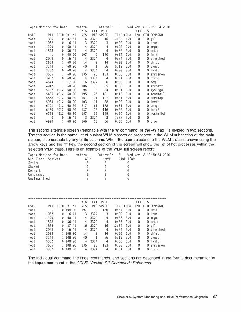
Topas Monitor for host: mothra Interval: 2 Wed Nov 8 12:27:34 2000DATA TEXT PAGE PGFAULTS

USER PID PPID PRI NI RES RES SPACE TIME CPU% I/O OTH COMMANDroot 1806 0 37 41 16 3374 16 13:25 1.0 0 0 gilroot 1032 0 16 41 3 3374 3 0:00 0.0 0 0 lrudroot 1290 0 60 41 4 3374 4 0:02 0.0 0 0 xmgcroot 1548 0 36 41 4 3374 4 0:26 0.0 0 0 netmroot 1 0 60 20 197 9 180 0:24 0.0 0 0 initroot 2064 0 16 41 4 3374 4 0:04 0.0 0 0 wlmschedroot 2698 1 60 20 14 2 14 0:00 0.0 0 0 shlaproot 3144 1 60 20 40 1 36 5:19 0.0 0 0 syncdroot 3362 0 60 20 4 3374 4 0:00 0.0 0 0 lvmbbroot 3666 1 60 20 135 23 123 0:00 0.0 0 0 errdemonroot 3982 0 60 20 4 3374 4 0:01 0.0 0 0 rtcmdroot 4644 1 17 20 6 3374 6 0:00 0.0 0 0 dogroot 4912 1 60 20 106 13 85 0:00 0.0 0 0 srcmstrroot 5202 4912 60 20 94 8 84 0:01 0.0 0 0 syslogdroot 5426 4912 60 20 195 76 181 0:12 0.0 0 0 sendmailroot 5678 4912 60 20 161 11 147 0:01 0.0 0 0 portmaproot 5934 4912 60 20 103 11 88 0:00 0.0 0 0 inetdroot 6192 4912 60 20 217 61 188 0:21 0.0 0 0 snmpdroot 6450 4912 60 20 137 10 116 0:00 0.0 0 0 dpid2root 6708 4912 60 20 157 29 139 0:06 0.0 0 0 hostmibdroot 0 0 16 41 3 3374 3 7:08 0.0 0 0root 6990 1 60 20 106 10 86 0:06 0.0 0 0 cron

The second alternate screen (reachable with the W command, or the -W flag), is divided in two sections.The top section is the same list of busiest WLM classes as presented in the WLM subsection of the mainscreen, also sortable by any of its columns. When the user selects one the WLM classes shown using thearrow keys and the ″f″ key, the second section of the screen will show the list of hot processes within theselected WLM class. Here is an example of the WLM full screen report:Topas Monitor for host: mothra Interval: 2 Wed Nov 8 12:30:54 2000WLM-Class (Active) CPU% Mem% Disk-I/O%System 0 0 0Shared 0 0 0Default 0 0 0Unmanaged 0 0 0Unclassified 0 0 0

==============================================================================DATA TEXT PAGE PGFAULTS

USER PID PPID PRI NI RES RES SPACE TIME CPU% I/O OTH COMMANDroot 1 0 108 20 197 9 180 0:24 0.0 0 0 initroot 1032 0 16 41 3 3374 3 0:00 0.0 0 0 lrudroot 1290 0 60 41 4 3374 4 0:02 0.0 0 0 xmgcroot 1548 0 36 41 4 3374 4 0:26 0.0 0 0 netmroot 1806 0 37 41 16 3374 16 13:25 0.0 0 0 gilroot 2064 0 16 41 4 3374 4 0:04 0.0 0 0 wlmschedroot 2698 1 108 20 14 2 14 0:00 0.0 0 0 shlaproot 3144 1 108 20 40 1 36 5:19 0.0 0 0 syncdroot 3362 0 108 20 4 3374 4 0:00 0.0 0 0 lvmbbroot 3666 1 108 20 135 23 123 0:00 0.0 0 0 errdemonroot 3982 0 108 20 4 3374 4 0:01 0.0 0 0 rtcmd

The individual command line flags, commands, and sections are described in the formal documentation ofthe topas command in the AIX 5L Version 5.2 Commands Reference.


Using the Performance Diagnostic ToolThe Performance Diagnostic Tool (PDT) is a tool available in operating system version 4. PDT collectsconfiguration and performance information and attempts to identify potential problems, both current andfuture.

PDT is an optionally installable component of the Base Operating System. Its name is bos.perf.diag_tool.After PDT has been installed, it must be activated with the /usr/sbin/perf/diag_tool/pdt_config command.This causes appropriate entries to be made in the crontab file, which causes PDT to run periodically,recording data and looking for new trends.

In assessing the configuration and the historical record of performance measurements, PDT attempts toidentify:

v Resource imbalances: asymmetrical aspects of configuration or device utilization

v Usage trends: changes in usage levels that will lead to saturation

v New consumers of resources: expensive processes that have not been observed previously

v Inappropriate system parameter values: settings that may cause problems

v Errors: hardware or software problems that may lead to performance problems

PDT is described in detail in Chapter 13. Using Performance Diagnostic Tool (PDT).

Using the Performance ToolboxThe Performance Toolbox (PTX) is a licensed product that allows graphical display of a variety ofperformance-related metrics. Among the advantages of PTX over ASCII reporting programs is that it ismuch easier to check current performance with a glance at the graphics monitor than by looking at ascreen full of numbers. PTX also facilitates the combination of information from multipleperformance-related commands and allows recording and playback.

PTX contains tools for local and remote system-activity monitoring and tuning. The product consists of twomain components: the PTX Manager and the PTX Agent. The PTX Agent is available as a separatelicensed product called the Performance Aide for AIX. The following figure shows a simplified LANconfiguration in which the PTX Manager is monitoring the activity of several systems.


The main purpose of the PTX Manager is to collect and display data from the various systems in theconfiguration. The primary program for this purpose is xmperf. The primary program used by the Agent tocollect and transmit data to the Manager is xmservd.

PTX is described in detail in the Performance Toolbox Version 2 and 3 for AIX: Guide and Reference andCustomizing Performance Toolbox and Performance Toolbox Extensions for AIX.

Recording with the Performance AgentIf you need to record information or a playback facility, several tools are included with the manager code(xmperf, 3dmon, azizo, ptxrlog). Other tools (xmservd, ptxtab, ptxsplit) are packaged with the agentcode.

Best suited for continuous monitoring are the following tools:

v The ptxrlog command can produce recordings in ASCII format, which allows you to print the output orpost-process it, or it can produce a recording file in binary to be viewed with the azizo or xmperfcommands.

v The xmservd daemon can act as a recording facility and is controlled through the xmservd.cfconfiguration file. This daemon can simultaneously provide near real-time network-based datamonitoring and local recording on a given node.

v The xmtrend daemon, much like xmservd, acts as a recording facility. The main difference is in thestorage requirements for each daemon. Typical xmservd recordings can consume several megabytesof disk storage every hour. The xmtrend agent was created to focus on providing manageable 24 x 7long-term recordings of large metric sets.

v The jazizo tool is a Java version that replaces azizo. Jazizo is a tool for analyzing the long-termperformance characteristics of a system. It analyzes recordings created by the xmtrend daemon, andprovides displays of the recorded data that can be customized.

v The wlmperf tools provide graphical views of Workload Manager (WLM) resource activities by class.This tool can generate reports from trend recordings made by the PTX daemons covering minutes,hours, days, weeks, or monthly periods.

Figure 16. LAN Configuration Using Performance Toolbox. This illustration shows five nodes of a local area networkthat are connected using the star topology. Each node on the network has the performance toolbox (PTX) agentrunning on it. One of the nodes is the PTX Manager and can monitor the other nodes via the resident agent.


Determining the Kind of Performance Problem ReportedWhen a performance problem is reported, determining the kind of performance problem often helps theperformance analyst to narrow the list of possible culprits.

A Particular Program Runs SlowlyAlthough this situation might seem trivial, there are still questions to be asked:

v Has the program always run slowly?

If the program has just started running slowly, a recent change might be the cause.

v Has the source code been changed or a new version installed?

If so, check with the programmer or vendor.

v Has something in the environment changed?

If a file used by the program (including its own executable program) has been moved, it may now beexperiencing Local Area Network (LAN) delays that did not exist previously. Or, files may be contendingfor a single disk accessor that were on different disks previously.

If the system administrator has changed system-tuning parameters, the program may be subject toconstraints that it did not experience previously. For example, if the schedtune -r command has beenused to change the way priority is calculated, programs that used to run rather quickly in thebackground may now be slowed down, while foreground programs have speeded up.

v Is the program written in the perl, awk, csh, or some other interpretive language?

While they allow programs to be written quickly, interpretive languages have the problem that they arenot optimized by a compiler. Also, it is easy in a language like perl or awk to request an extremelycompute- or I/O-intensive operation with a few characters. It is often worthwhile to perform a desk checkor informal peer review of such programs with the emphasis on the number of iterations implied by eachoperation.

v Does the program always run at the same speed, or is it sometimes faster?

The file system uses some of system memory to hold pages of files for future reference. If a disk-limitedprogram is run twice in quick succession, it will normally run faster the second time than the first.Similar phenomena might be observed with programs that use NFS. This can also occur with largeprograms, such as compilers. The program’s algorithm might not be disk-limited, but the time needed toload a large executable program might make the first execution of the program much longer thansubsequent ones.

v If the program has always run slowly, or has slowed down without any obvious change in itsenvironment, look at its dependency on resources.

Identifying the Performance-Limiting Resource describes techniques for finding the bottleneck.

Everything Runs Slowly at a Particular Time of DayMost people have experienced the rush-hour slowdown that occurs because a large number of people inthe organization habitually use the system at one or more particular times each day. This phenomenon isnot always simply due to a concentration of load. Sometimes it is an indication of an imbalance that is (atpresent) only a problem when the load is high. Other sources of recurring situations in the system shouldbe considered.

v If you run the iostat and netstat commands for a period that spans the time of the slowdown (or havepreviously captured data from your monitoring mechanism), are some disks much more heavily usedthan others? Is the CPU idle percentage consistently near zero? Is the number of packets sent orreceived unusually high?

– If the disks are unbalanced, see Monitoring and Tuning Disk I/O Use.

– If the CPU is saturated, use the ps or topas commands to identify the programs being run duringthis period. The script given in Using the vmstat, iostat, netstat, and sar Commands simplifies thesearch for the heaviest CPU users.


– If the slowdown is counter-intuitive, such as paralysis during lunch time, look for a pathologicalprogram such as a graphic xlock or game program. Some versions of the xlock program are knownto use huge amounts of CPU time to display graphic patterns on an idle display. It is also possiblethat someone is running a program that is a known CPU burner and is trying to run it at the leastintrusive time.

v Unless your /var/adm/cron/cron.allow file is null, you may want to check the contents of the/var/adm/cron/crontab directory for expensive operations.

If you find that the problem stems from conflict between foreground activity and long-running,CPU-intensive programs that are, or should be, run in the background, consider using the commandschedtune -r -d to give the foreground higher priority. See Tuning the Thread-Priority-Value Calculation.

Everything Runs Slowly at Unpredictable TimesThe best tool for this situation is an overload detector, such as the filtd program (a component of PTX).The filtd daemon can be set up to execute shell scripts or collect specific information when a particularcondition is detected. You can construct a similar, but more specialized, mechanism using shell scriptscontaining the vmstat, iostat, netstat, sar, and ps commands.

If the problem is local to a single system in a distributed environment, there is probably a pathologicalprogram at work, or perhaps two that intersect randomly.

Everything That an Individual User Runs is SlowSometimes a system seems to ″single out″ an individual.

v Quantify the problem. Ask the user which commands he uses frequently, and run them with the timecommand, as in the following example:# time cp .profile testjunkreal 0m0.08suser 0m0.00ssys 0m0.01s

Then run them under a satisfactory user ID. Is there a difference in the reported real time?

v A program should not show much CPU time (user+sys) difference from run to run, but may show a realtime difference because of more or slower I/O. Are the user’s files on an NFS-mounted directory? On adisk that has high activity for other reasons?

v Check the user’s .profile file for unusual $PATH specifications. For example, if you always search acouple of NFS-mounted directories (fruitlessly) before searching /usr/bin, everything will take longer.

A Number of LAN-Connected Systems Slow Down SimultaneouslyThere are some common problems that arise in the transition from independent systems to distributedsystems. The problems usually result from the need to get a new configuration running as soon aspossible, or from a lack of awareness of the cost of certain functions. In addition to tuning the LANconfiguration in terms of maximum transmission units (MTU) and mbufs (see Monitoring and TuningCommunications I/O Use), look for LAN-specific pathologies or nonoptimal situations that may haveevolved through a sequence of individually reasonable decisions.

v Use network statistics to ensure that there are no physical network problems. Ensure that commandssuch as netstat -v, entstat, tokstat, atmstat, or fddistat do not show excessive errors or collision onthe adapter.

v Some types of software or firmware bugs can sporadically saturate the LAN with broadcast or otherpackets.

When a broadcast storm occurs, even systems that are not actively using the network can be slowed bythe incessant interrupts and by the CPU resource consumed in receiving and processing the packets.These problems are better detected and localized with LAN analysis devices than with the normalperformance tools.


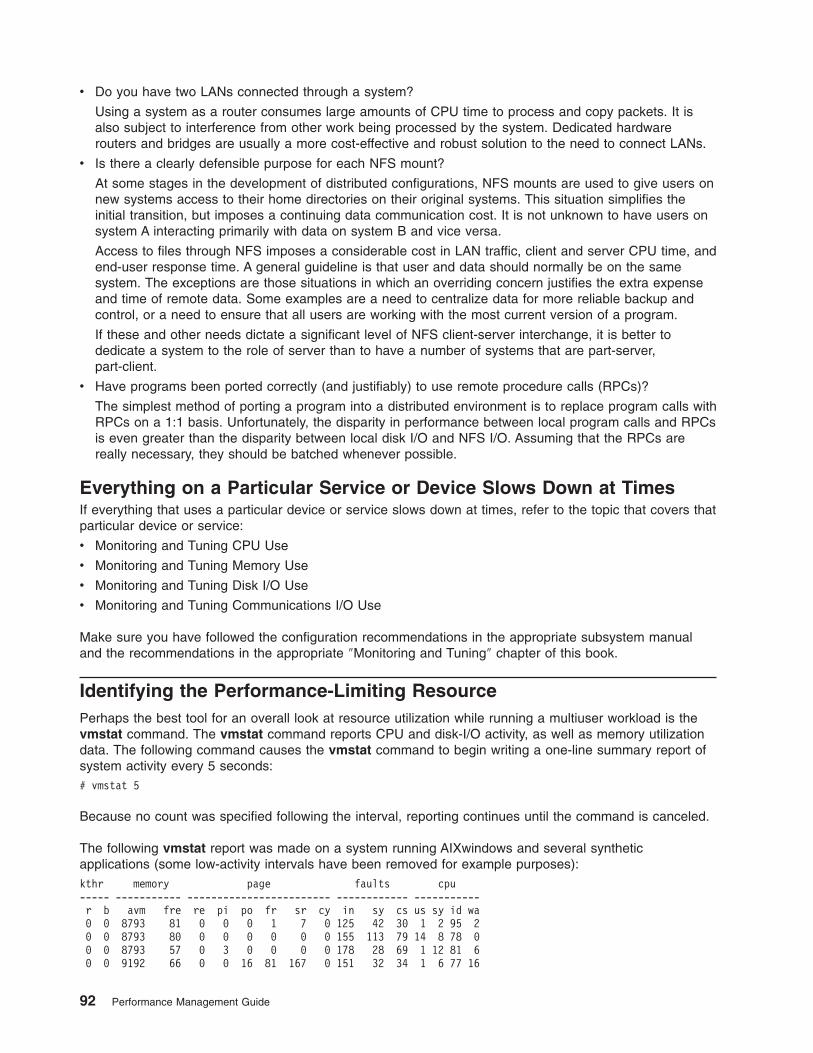
v Do you have two LANs connected through a system?

Using a system as a router consumes large amounts of CPU time to process and copy packets. It isalso subject to interference from other work being processed by the system. Dedicated hardwarerouters and bridges are usually a more cost-effective and robust solution to the need to connect LANs.

v Is there a clearly defensible purpose for each NFS mount?

At some stages in the development of distributed configurations, NFS mounts are used to give users onnew systems access to their home directories on their original systems. This situation simplifies theinitial transition, but imposes a continuing data communication cost. It is not unknown to have users onsystem A interacting primarily with data on system B and vice versa.

Access to files through NFS imposes a considerable cost in LAN traffic, client and server CPU time, andend-user response time. A general guideline is that user and data should normally be on the samesystem. The exceptions are those situations in which an overriding concern justifies the extra expenseand time of remote data. Some examples are a need to centralize data for more reliable backup andcontrol, or a need to ensure that all users are working with the most current version of a program.

If these and other needs dictate a significant level of NFS client-server interchange, it is better todedicate a system to the role of server than to have a number of systems that are part-server,part-client.

v Have programs been ported correctly (and justifiably) to use remote procedure calls (RPCs)?

The simplest method of porting a program into a distributed environment is to replace program calls withRPCs on a 1:1 basis. Unfortunately, the disparity in performance between local program calls and RPCsis even greater than the disparity between local disk I/O and NFS I/O. Assuming that the RPCs arereally necessary, they should be batched whenever possible.

Everything on a Particular Service or Device Slows Down at TimesIf everything that uses a particular device or service slows down at times, refer to the topic that covers thatparticular device or service:

v Monitoring and Tuning CPU Use

v Monitoring and Tuning Memory Use

v Monitoring and Tuning Disk I/O Use

v Monitoring and Tuning Communications I/O Use

Make sure you have followed the configuration recommendations in the appropriate subsystem manualand the recommendations in the appropriate ″Monitoring and Tuning″ chapter of this book.

Identifying the Performance-Limiting ResourcePerhaps the best tool for an overall look at resource utilization while running a multiuser workload is thevmstat command. The vmstat command reports CPU and disk-I/O activity, as well as memory utilizationdata. The following command causes the vmstat command to begin writing a one-line summary report ofsystem activity every 5 seconds:# vmstat 5

Because no count was specified following the interval, reporting continues until the command is canceled.

The following vmstat report was made on a system running AIXwindows and several syntheticapplications (some low-activity intervals have been removed for example purposes):kthr memory page faults cpu----- ----------- ------------------------ ------------ -----------r b avm fre re pi po fr sr cy in sy cs us sy id wa0 0 8793 81 0 0 0 1 7 0 125 42 30 1 2 95 20 0 8793 80 0 0 0 0 0 0 155 113 79 14 8 78 00 0 8793 57 0 3 0 0 0 0 178 28 69 1 12 81 60 0 9192 66 0 0 16 81 167 0 151 32 34 1 6 77 16


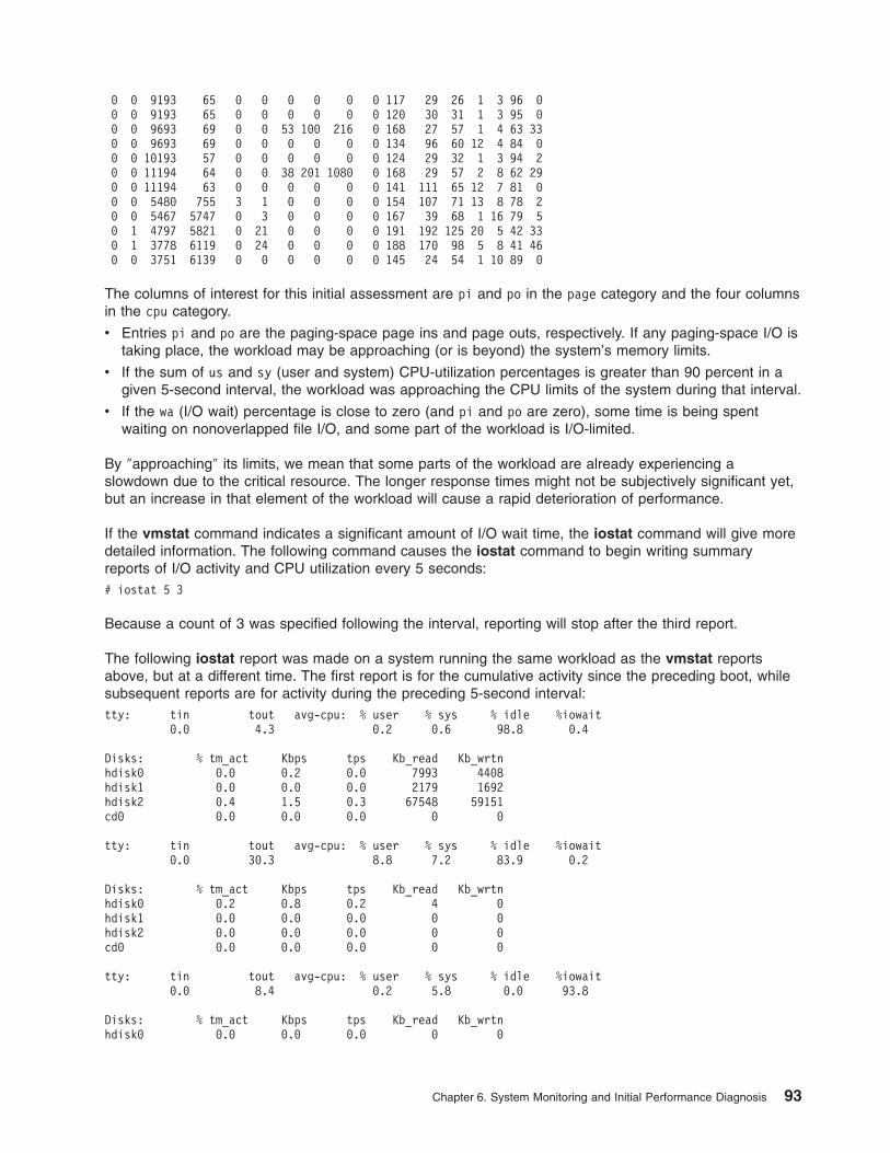
0 0 9193 65 0 0 0 0 0 0 117 29 26 1 3 96 00 0 9193 65 0 0 0 0 0 0 120 30 31 1 3 95 00 0 9693 69 0 0 53 100 216 0 168 27 57 1 4 63 330 0 9693 69 0 0 0 0 0 0 134 96 60 12 4 84 00 0 10193 57 0 0 0 0 0 0 124 29 32 1 3 94 20 0 11194 64 0 0 38 201 1080 0 168 29 57 2 8 62 290 0 11194 63 0 0 0 0 0 0 141 111 65 12 7 81 00 0 5480 755 3 1 0 0 0 0 154 107 71 13 8 78 20 0 5467 5747 0 3 0 0 0 0 167 39 68 1 16 79 50 1 4797 5821 0 21 0 0 0 0 191 192 125 20 5 42 330 1 3778 6119 0 24 0 0 0 0 188 170 98 5 8 41 460 0 3751 6139 0 0 0 0 0 0 145 24 54 1 10 89 0

The columns of interest for this initial assessment are pi and po in the page category and the four columnsin the cpu category.

v Entries pi and po are the paging-space page ins and page outs, respectively. If any paging-space I/O istaking place, the workload may be approaching (or is beyond) the system’s memory limits.

v If the sum of us and sy (user and system) CPU-utilization percentages is greater than 90 percent in agiven 5-second interval, the workload was approaching the CPU limits of the system during that interval.

v If the wa (I/O wait) percentage is close to zero (and pi and po are zero), some time is being spentwaiting on nonoverlapped file I/O, and some part of the workload is I/O-limited.

By ″approaching″ its limits, we mean that some parts of the workload are already experiencing aslowdown due to the critical resource. The longer response times might not be subjectively significant yet,but an increase in that element of the workload will cause a rapid deterioration of performance.

If the vmstat command indicates a significant amount of I/O wait time, the iostat command will give moredetailed information. The following command causes the iostat command to begin writing summaryreports of I/O activity and CPU utilization every 5 seconds:# iostat 5 3

Because a count of 3 was specified following the interval, reporting will stop after the third report.

The following iostat report was made on a system running the same workload as the vmstat reportsabove, but at a different time. The first report is for the cumulative activity since the preceding boot, whilesubsequent reports are for activity during the preceding 5-second interval:tty: tin tout avg-cpu: % user % sys % idle %iowait

0.0 4.3 0.2 0.6 98.8 0.4

Disks: % tm_act Kbps tps Kb_read Kb_wrtnhdisk0 0.0 0.2 0.0 7993 4408hdisk1 0.0 0.0 0.0 2179 1692hdisk2 0.4 1.5 0.3 67548 59151cd0 0.0 0.0 0.0 0 0

tty: tin tout avg-cpu: % user % sys % idle %iowait0.0 30.3 8.8 7.2 83.9 0.2

Disks: % tm_act Kbps tps Kb_read Kb_wrtnhdisk0 0.2 0.8 0.2 4 0hdisk1 0.0 0.0 0.0 0 0hdisk2 0.0 0.0 0.0 0 0cd0 0.0 0.0 0.0 0 0

tty: tin tout avg-cpu: % user % sys % idle %iowait0.0 8.4 0.2 5.8 0.0 93.8

Disks: % tm_act Kbps tps Kb_read Kb_wrtnhdisk0 0.0 0.0 0.0 0 0


hdisk1 0.0 0.0 0.0 0 0hdisk2 98.4 575.6 61.9 396 2488cd0 0.0 0.0 0.0 0 0

The first report, which displays cumulative activity since the last boot, shows that the I/O on this system isunbalanced. Most of the I/O (86.9 percent of kilobytes read and 90.7 percent of kilobytes written) is tohdisk2, which contains both the operating system and the paging space. The cumulative CPU utilizationsince boot statistic is usually meaningless, unless the system is used consistently 24 hours a day.

The second report shows a small amount of disk activity reading from hdisk0, which contains a separatefile system for the system’s primary user. The CPU activity arises from two application programs and theiostat command itself. Although the output of the iostat command is redirected to a file, the output is notvoluminous, and the system is not sufficiently memory-constrained to force any output during this interval.

In the third report, we have artificially created a near-thrashing condition by running a program thatallocates, and stores into, a large amount of memory (about 26 MB in this example). In the example,hdisk2 is active 98.4 percent of the time, which results in 93.8 percent I/O wait.

If the vmstat command indicates that there is a significant amount of CPU idle time when the systemseems subjectively to be running slowly, you might be experiencing delays due to kernel lock contention.This possibility can be investigated with the lockstat command (only available in AIX Version 4).

Determining the Limiting Factor for a Single ProgramIf you are the sole user of a system, you can get a general idea of whether a program is I/O or CPUdependent by using the time command as follows:# time cp foo.in foo.out

real 0m0.13suser 0m0.01ssys 0m0.02s

Note: Examples of the time command here and elsewhere in this guide use the version that is built intothe Korn shell (ksh). The official time command (/usr/bin/time) reports with a lower precision.

In this example, the fact that the real, elapsed time for the execution of the cp program (.13 seconds) issignificantly greater than the sum (.03 seconds) of the user and system CPU times indicates that theprogram is I/O bound. This occurs primarily because the foo.in file has not been read recently.

On an SMP the output takes on a new meaning. See time and timex Cautions.

Running the same command a few seconds later against the same file gives the following output:real 0m0.06suser 0m0.01ssys 0m0.03s

Most or all of the pages of the foo.in file are still in memory because there has been no interveningprocess to cause them to be reclaimed and because the file is small compared with the amount of RAMon the system. A small foo.out file would also be buffered in memory, and a program using it as inputwould show little disk dependency.

If you are trying to determine the disk dependency of a program, you must be sure that its input is in anauthentic state. That is, if the program will normally be run against a file that has not been accessedrecently, you must make sure that the file used in measuring the program is not in memory. If, on the otherhand, a program is usually run as part of a standard sequence in which it gets its input from the output ofthe preceding program, you should prime memory to ensure that the measurement is authentic. Forexample, the following command would have the effect of priming memory with the pages of the foo.infile:


# cp foo.in /dev/null

The situation is more complex if the file is large compared to RAM. If the output of one program is theinput of the next and the entire file will not fit in RAM, the second program will read pages at the head ofthe file, which displaces pages at the end. Although this situation is very hard to simulate authentically, it isnearly equivalent to one in which no disk caching takes place.

The case of a file that is (perhaps just slightly) larger than RAM is a special case of the RAM versus diskanalysis discussed in the next section.

Determining Whether the Problem is Related to Disk or MemoryJust as a large fraction of real memory is available for buffering files, the system’s page space is availableas temporary storage for program working data that has been forced out of RAM. Suppose that you havea program that reads little or no data and yet shows the symptoms of being I/O dependent. Worse, theratio of real time to user + system time does not improve with successive runs. The program is probablymemory-limited, and its I/O is to, and possibly from the paging space. A way to check on this possibility isshown in the following vmstatit (or in AIX 5.1, see the vmstat -I option) shell script:vmstat -s >temp.file # cumulative counts before the commandtime $1 # command under testvmstat -s >>temp.file # cumulative counts after executiongrep "pagi.*ins" temp.file >>results # extract only the datagrep "pagi.*outs" temp.file >>results # of interest

The vmstatit script summarizes the voluminous vmstat -s report, which gives cumulative counts for anumber of system activities since the system was started.

If the shell script is run as follows:# vmstatit "cp file1 file2" 2>results

the result is as follows:real 0m0.03suser 0m0.01ssys 0m0.02s

2323 paging space page ins2323 paging space page ins4850 paging space page outs4850 paging space page outs

The before-and-after paging statistics are identical, which confirms our belief that the cp command is notpaging-bound. An extended variant of the vmstatit shell script can be used to show the true situation, asfollows:vmstat -s >temp.filetime $1vmstat -s >>temp.fileecho "Ordinary Input:" >>resultsgrep "^[ 0-9]*page ins" temp.file >>resultsecho "Ordinary Output:" >>resultsgrep "^[ 0-9]*page outs" temp.file >>resultsecho "True Paging Output:" >>resultsgrep "pagi.*outs" temp.file >>resultsecho "True Paging Input:" >>resultsgrep "pagi.*ins" temp.file >>results

Because file I/O in the operating system is processed through the VMM, the vmstat -s command reportsordinary program I/O as page ins and page outs. When the previous version of the vmstatit shell scriptwas run against the cp command of a large file that had not been read recently, the result was as follows:


real 0m2.09suser 0m0.03ssys 0m0.74sOrdinary Input:

46416 page ins47132 page ins

Ordinary Output:146483 page outs147012 page outs

True Paging Output:4854 paging space page outs4854 paging space page outs

True Paging Input:2527 paging space page ins2527 paging space page ins

The time command output confirms the existence of an I/O dependency. The increase in page ins showsthe I/O necessary to satisfy the cp command. The increase in page outs indicates that the file is largeenough to force the writing of dirty pages (not necessarily its own) from memory. The fact that there is nochange in the cumulative paging-space-I/O counts confirms that the cp command does not build datastructures large enough to overload the memory of the test machine.

The order in which this version of the vmstatit script reports I/O is intentional. Typical programs read fileinput and then write file output. Paging activity, on the other hand, typically begins with the writing out of aworking-segment page that does not fit. The page is read back in only if the program tries to access it.The fact that the test system has experienced almost twice as many paging space page outs as pagingspace page ins since it was booted indicates that at least some of the programs that have been run onthis system have stored data in memory that was not accessed again before the end of the program.Memory-Limited Programs provides more information. See also Monitoring and Tuning Memory Use.

To show the effects of memory limitation on these statistics, the following example observes a givencommand in an environment of adequate memory (32 MB) and then artificially shrinks the system usingthe rmss command (see Assessing Memory Requirements Through the rmss Command). The commandsequence# cc -c ed.c# vmstatit "cc -c ed.c" 2>results

first primes memory with the 7944-line source file and the executable file of the C compiler, then measuresthe I/O activity of the second execution:real 0m7.76suser 0m7.44ssys 0m0.15sOrdinary Input:





Clearly, this is not I/O limited. There is not even any I/O necessary to read the source code. If we thenissue the following command:# rmss -c 8


to change the effective size of the machine to 8 MB, and perform the same sequence of commands, weget the following output:real 0m9.87suser 0m7.70ssys 0m0.18sOrdinary Input:





The following symptoms of I/O dependency are present:

v Elapsed time longer than total CPU time

v Significant amounts of ordinary I/O on the nth execution of the command

The fact that the elapsed time is longer than in the memory-unconstrained situation, and the existence ofsignificant amounts of paging-space I/O, make it clear that the compiler is being hampered by insufficientmemory.

Note: This example illustrates the effects of memory constraint. No effort was made to minimize the useof memory by other processes, so the absolute size at which the compiler was forced to page inthis environment does not constitute a meaningful measurement.

To avoid working with an artificially shrunken machine until the next restart, run# rmss -r

to release back to the operating system the memory that the rmss command had sequestered, thusrestoring the system to its normal capacity.

Managing WorkloadWhen you have exhausted the program performance-improvement and system-tuning possibilities, andperformance is still unsatisfactory at times, you have three choices:

v Let the situation remain as is.

v Upgrade the performance-limiting resource.

v Adopt workload-management techniques.

If you adopt the first approach, some of your less stoic users will experience increasing frustration anddecreasing productivity. If you choose to upgrade, you will most likely have to justify the expenditure. Thatperson will undoubtedly want to know if you have exhausted all possibilities with the current system, whichmeans you need to investigate the possibilities of workload management.

Workload management simply means assessing the components of the workload to determine whetherthey are all needed as soon as possible. Usually, there is work that can wait for a while; for example, areport that is needed first thing in the morning. That report is equally useful when run at 3 a.m. as at 4p.m. on the preceding day. The difference is that at 3 a.m. it uses CPU cycles and other resources thatwould otherwise be idle. Use the at or crontab command to request a program to run at a specific time orat regular intervals.


Similarly, some programs that do have to be run during the day can be run at reduced priority. They willtake longer to complete, but they will be less in competition with really time-critical processes.

A related technique is moving work from one machine to another; for example, running a compilation onthe machine where the source code resides. This kind of workload balancing requires more planning andmonitoring, because reducing the load on the network and increasing the CPU load on a server mightresult in a net loss.

Starting with AIX 4.3.3, AIX Workload Manager (WLM) is provided as an integrated part of the operatingsystem kernel. WLM is designed to give the system administrator greater control over how the schedulerand virtual memory manager (VMM) allocate CPU and physical memory resources to processes. In AIX5.1 and subsequent releases, disk usage can also be controlled by WLM. This can be used to preventdifferent classes of jobs from interfering with each other and to explicitly apply resources based on therequirements of different groups of users. For further information, see Server Consolidation on RS/6000.


Chapter 7. Monitoring and Tuning CPU Use

This chapter deals with techniques for detecting runaway or CPU-intensive programs and minimizing theiradverse effect on performance.

Readers who are not familiar with CPU scheduling may want to look at Performance Overview of the CPUScheduler before continuing.

The following sections cover the different aspects of CPU tuning:

v Monitoring CPU Use

v Using the time Command to Measure CPU Use

v Identifying CPU-Intensive Programs

v Using the tprof Program to Analyze Programs for CPU Use

v Using the pprof Command to Measure CPU usage of Kernel Threads

v Detecting Instruction Emulation with the emstat Tool

v Detecting Alignment Exceptions with the alstat Tool

v Restructuring Executable Programs with the fdpr Program

v Controlling Contention for the CPU

v CPU-Efficient User ID Administration (The mkpasswd Command)

Monitoring CPU UseThe processing unit is one of the fastest components of the system. It is comparatively rare for a singleprogram to keep the CPU 100 percent busy (that is, 0 percent idle and 0 percent wait) for more than a fewseconds at a time. Even in heavily loaded multiuser systems, there are occasional 10 milliseconds (ms)periods that end with all threads in a wait state. If a monitor shows the CPU 100 percent busy for anextended period, there is a good chance that some program is in an infinite loop. Even if the program is″merely″ expensive, rather than broken, it needs to be identified and dealt with.

The vmstat Command (CPU)The first tool to use is the vmstat command, which quickly provides compact information about varioussystem resources and their related performance problems. The vmstat command reports statistics aboutkernel threads in the run and wait queue, memory, paging, disks, interrupts, system calls, contextswitches, and CPU activity. The reported CPU activity is a percentage breakdown of user mode, systemmode, idle time, and waits for disk I/O.

Note: If the vmstat command is used without any options or only with the interval and optionally, thecount parameter, such as vmstat 2 10; then the first line of numbers is an average since systemreboot.

As a CPU monitor, the vmstat command is superior to the iostat command in that its one-line-per-reportoutput is easier to scan as it scrolls and there is less overhead involved if there are a lot of disks attachedto the system. The following example can help you identify situations in which a program has run away oris too CPU-intensive to run in a multiuser environment.# vmstat 2kthr memory page faults cpu----- ----------- ------------------------ ------------ -----------r b avm fre re pi po fr sr cy in sy cs us sy id wa1 0 22478 1677 0 0 0 0 0 0 188 1380 157 57 32 0 101 0 22506 1609 0 0 0 0 0 0 214 1476 186 48 37 0 160 0 22498 1582 0 0 0 0 0 0 248 1470 226 55 36 0 9

2 0 22534 1465 0 0 0 0 0 0 238 903 239 77 23 0 0


2 0 22534 1445 0 0 0 0 0 0 209 1142 205 72 28 0 02 0 22534 1426 0 0 0 0 0 0 189 1220 212 74 26 0 03 0 22534 1410 0 0 0 0 0 0 255 1704 268 70 30 0 02 1 22557 1365 0 0 0 0 0 0 383 977 216 72 28 0 0

2 0 22541 1356 0 0 0 0 0 0 237 1418 209 63 33 0 41 0 22524 1350 0 0 0 0 0 0 241 1348 179 52 32 0 161 0 22546 1293 0 0 0 0 0 0 217 1473 180 51 35 0 14

This output shows the effect of introducing a program in a tight loop to a busy multiuser system. The firstthree reports (the summary has been removed) show the system balanced at 50-55 percent user, 30-35percent system, and 10-15 percent I/O wait. When the looping program begins, all available CPU cyclesare consumed. Because the looping program does no I/O, it can absorb all of the cycles previouslyunused because of I/O wait. Worse, it represents a process that is always ready to take over the CPUwhen a useful process relinquishes it. Because the looping program has a priority equal to that of all otherforeground processes, it will not necessarily have to give up the CPU when another process becomesdispatchable. The program runs for about 10 seconds (five reports), and then the activity reported by thevmstat command returns to a more normal pattern.

The CPU statistics can be somewhat distorted on systems with very high device-interrupt load. Thissituation is due to the fact that the tool samples on timer interrupts. The timer is the lowest priority deviceand therefore it can easily be preempted by other interrupts. To eliminate this distortion, operating systemversions later than AIX 4.3.3 use a different method to sample the timer.

Note: For SMP systems the us, sy, id and wa columns are only averages over the processors (the sarcommand can report per-processor statistics). An I/O wait is distinguished from idle time only by thestate of a pending I/O. If there is any pending disk I/O, and the processor is not busy, then it is anI/O wait time. AIX 4.3.3 and later contains an enhancement to the method used to compute thepercentage of CPU time spent waiting on disk I/O (wio time). See Wait I/O Time Reporting for moredetails.

Optimum use would have the CPU working 100 percent of the time. This holds true in the case of asingle-user system with no need to share the CPU. Generally, if us + sy time is below 90 percent, asingle-user system is not considered CPU constrained. However, if us + sy time on a multiuser systemexceeds 80 percent, the processes may spend time waiting in the run queue. Response time andthroughput might suffer.

To check if the CPU is the bottleneck, consider the four cpu columns and the two kthr (kernel threads)columns in the vmstat report. It may also be worthwhile looking at the faults column:

v cpu

Percentage breakdown of CPU time usage during the interval. The cpu columns are as follows:

– us

The us column shows the percent of CPU time spent in user mode. A UNIX process can execute ineither user mode or system (kernel) mode. When in user mode, a process executes within itsapplication code and does not require kernel resources to perform computations, manage memory,or set variables.

– sy

The sy column details the percentage of time the CPU was executing a process in system mode.This includes CPU resource consumed by kernel processes (kprocs) and others that need access tokernel resources. If a process needs kernel resources, it must execute a system call and is therebyswitched to system mode to make that resource available. For example, reading or writing of a filerequires kernel resources to open the file, seek a specific location, and read or write data, unlessmemory mapped files are used.

– id


The id column shows the percentage of time which the CPU is idle, or waiting, without pending localdisk I/O. If there are no threads available for execution (the run queue is empty), the systemdispatches a thread called wait, which is also known as the idle kproc. On an SMP system, onewait thread per processor can be dispatched. The report generated by the ps command (with the -kor -g 0 option) identifies this as kproc or wait. If the ps report shows a high aggregate time for thisthread, it means there were significant periods of time when no other thread was ready to run orwaiting to be executed on the CPU. The system was therefore mostly idle and waiting for new tasks.

If there are no I/Os pending, all time charged to wait is classified as idle time. In operating systemversion 4.3.2 and earlier, an access to remote disks (NFS-mounted disks) is treated as idle time(with a small amount of sy time to execute the NFS requests) because there is no pending I/Orequest to a local disk. With AIX 4.3.3 and later NFS goes through the buffer cache, and waits inthose routines are accounted for in the wa statistics.

– wa

The wa column details the percentage of time the CPU was idle with pending local disk I/O (in AIX4.3.3 and later this is also true for NFS-mounted disks). If there is at least one outstanding I/O to adisk when wait is running, the time is classified as waiting for I/O. Unless asynchronous I/O is beingused by the process, an I/O request to disk causes the calling process to block (or sleep) until therequest has been completed. Once an I/O request for a process completes, it is placed on the runqueue. If the I/Os were completing faster, more CPU time could be used.

A wa value over 25 percent could indicate that the disk subsystem might not be balanced properly, orit might be the result of a disk-intensive workload.

For information on the change made to wa, see Wait I/O Time Reporting.

v kthr

Number of kernel threads in various queues averaged per second over the sampling interval. The kthrcolumns are as follows:

– r

Average number of kernel threads that are runnable, which includes threads that are running andthreads that are waiting for the CPU. If this number is greater than the number of CPUs, there is atleast one thread waiting for a CPU and the more threads there are waiting for CPUs, the greater thelikelihood of a performance impact.

– b

Average number of kernel threads in the VMM wait queue per second. This includes threads that arewaiting on filesystem I/O or threads that have been suspended due to memory load control.

If processes are suspended due to memory load control, the blocked column (b) in the vmstat reportindicates the increase in the number of threads rather than the run queue.

– p

For vmstat -I The number of threads waiting on I/Os to raw devices per second.Threads waiting onI/Os to filesystems would not be included here.

v faults

Information about process control, such as trap and interrupt rate. The faults columns are as follows:

– in

Number of device interrupts per second observed in the interval. Additional information can be foundin Assessing Disk Performance with the vmstat Command.

– sy

The number of system calls per second observed in the interval. Resources are available to userprocesses through well-defined system calls. These calls instruct the kernel to perform operations forthe calling process and exchange data between the kernel and the process. Because workloads andapplications vary widely, and different calls perform different functions, it is impossible to define howmany system calls per-second are too many. But typically, when the sy column raises over 10000calls per second on a uniprocessor, further investigations is called for (on an SMP system the

Chapter 7. Monitoring and Tuning CPU Use 101

number is 10000 calls per second per processor). One reason could be ″polling″ subroutines like theselect() subroutine. For this column, it is advisable to have a baseline measurement that gives acount for a normal sy value.

– cs

Number of context switches per second observed in the interval. The physical CPU resource issubdivided into logical time slices of 10 milliseconds each. Assuming a thread is scheduled forexecution, it will run until its time slice expires, until it is preempted, or until it voluntarily gives upcontrol of the CPU. When another thread is given control of the CPU, the context or workingenvironment of the previous thread must be saved and the context of the current thread must beloaded. The operating system has a very efficient context switching procedure, so each switch isinexpensive in terms of resources. Any significant increase in context switches, such as when cs is alot higher than the disk I/O and network packet rate, should be cause for further investigation.

The iostat CommandThe iostat command is the fastest way to get a first impression, whether or not the system has a diskI/O-bound performance problem (see Assessing Disk Performance with the iostat Command). The toolalso reports CPU statistics.

The following example shows a part of an iostat command output. The first stanza shows the summarystatistic since system startup.# iostat -t 2 6tty: tin tout avg-cpu: % user % sys % idle % iowait

0.0 0.8 8.4 2.6 88.5 0.50.0 80.2 4.5 3.0 92.1 0.50.0 40.5 7.0 4.0 89.0 0.00.0 40.5 9.0 2.5 88.5 0.00.0 40.5 7.5 1.0 91.5 0.00.0 40.5 10.0 3.5 80.5 6.0

The CPU statistics columns (% user, % sys, % idle, and % iowait) provide a breakdown of CPU usage.This information is also reported in the vmstat command output in the columns labeled us, sy, id, and wa.For a detailed explanation for the values, see The vmstat Command. Also note the change made to%iowait described in Wait I/O Time Reporting.

The sar CommandThe sar command gathers statistical data about the system. Though it can be used to gather some usefuldata regarding system performance, the sar command can increase the system load that can exacerbatea pre-existing performance problem if the sampling frequency is high. But compared to the accountingpackage, the sar command is less intrusive. The system maintains a series of system activity counterswhich record various activities and provide the data that the sar command reports. The sar commanddoes not cause these counters to be updated or used; this is done automatically regardless of whether ornot the sar command runs. It merely extracts the data in the counters and saves it, based on the samplingrate and number of samples specified to the sar command.

With its numerous options, the sar command provides queuing, paging, TTY, and many other statistics.One important feature of the sar command is that it reports either systemwide (global among allprocessors) CPU statistics (which are calculated as averages for values expressed as percentages, andas sums otherwise), or it reports statistics for each individual processor. Therefore, this command isparticularly useful on SMP systems.

There are three situations to use the sar command:

Real-time sampling and displayTo collect and display system statistic reports immediately, use the following command:


# sar -u 2 5

AIX texmex 3 4 000691854C00 01/27/00

17:58:15 %usr %sys %wio %idle17:58:17 43 9 1 4617:58:19 35 17 3 4517:58:21 36 22 20 2317:58:23 21 17 0 6317:58:25 85 12 3 0

Average 44 15 5 35

This example is from a single user workstation and shows the CPU utilization.

Display previously captured dataThe -o and -f options (write and read to/from user given data files) allow you to visualize the behavior ofyour machine in two independent steps. This consumes less resources during the problem-reproductionperiod. You can use a separate machine to analyze the data by transferring the file because the collectedbinary file keeps all data the sar command needs.# sar -o /tmp/sar.out 2 5 > /dev/null

The above command runs the sar command in the background, collects system activity data at 2-secondintervals for 5 intervals, and stores the (unformatted) sar data in the /tmp/sar.out file. The redirection ofstandard output is used to avoid a screen output.

The following command extracts CPU information from the file and outputs a formatted report to standardoutput:# sar -f/tmp/sar.out

AIX texmex 3 4 000691854C00 01/27/00

18:10:18 %usr %sys %wio %idle18:10:20 9 2 0 8818:10:22 13 10 0 7618:10:24 37 4 0 5918:10:26 8 2 0 9018:10:28 20 3 0 77

Average 18 4 0 78

The captured binary data file keeps all information needed for the reports. Every possible sar report couldtherefore be investigated. This also allows to display the processor-specific information of an SMP systemon a single processor system.

System activity accounting via cron daemonThe sar command calls a process named sadc to access system data. Two shell scripts (/usr/lib/sa/sa1and /usr/lib/sa/sa2) are structured to be run by the cron daemon and provide daily statistics and reports.Sample stanzas are included (but commented out) in the /var/spool/cron/crontabs/adm crontab file tospecify when the cron daemon should run the shell scripts.

The following lines show a modified crontab for the adm user. Only the comment characters for the datacollections were removed:#=================================================================# SYSTEM ACTIVITY REPORTS# 8am-5pm activity reports every 20 mins during weekdays.# activity reports every an hour on Saturday and Sunday.# 6pm-7am activity reports every an hour during weekdays.# Daily summary prepared at 18:05.#=================================================================0 8-17 * * 1-5 /usr/lib/sa/sa1 1200 3 &


0 * * * 0,6 /usr/lib/sa/sa1 &0 18-7 * * 1-5 /usr/lib/sa/sa1 &5 18 * * 1-5 /usr/lib/sa/sa2 -s 8:00 -e 18:01 -i 3600 -ubcwyaqvm &#=================================================================

Collection of data in this manner is useful to characterize system usage over a period of time and todetermine peak usage hours.

Useful CPU Options: The most useful CPU-related options for the sar command are:

v sar -P

The -P option reports per-processor statistics for the specified processors. By specifying the ALLkeyword, statistics for each individual processor and an average for all processors is reported. Of theflags which specify the statistics to be reported, only the -a, -c, -m, -u, and -w flags are meaningful withthe -P flag.

The following example shows the per-processor statistic while a CPU-bound program was running onprocessor number 0:# sar -P ALL 2 3

AIX rugby 3 4 00058033A100 01/27/00


1 0 4 0 962 0 1 0 993 0 0 0 100- 2 24 0 74

17:30:54 0 12 88 0 01 0 3 0 972 0 1 0 993 0 0 0 100- 3 23 0 74

17:30:56 0 11 89 0 01 0 3 0 972 0 0 0 1003 0 0 0 100- 3 23 0 74

Average 0 10 90 0 01 0 4 0 962 0 1 0 993 0 0 0 100- 3 24 0 74

The last line of every stanza, which starts with a dash (-) in the cpu column, is the average for allprocessors. An average (-) line displays only if the -P ALL option is used. It is removed if processorsare specified. The last stanza, labeled with the word Average instead of a time stamp, keeps theaverages for the processor-specific rows over all stanzas.

The following example shows the vmstat output during this time:# vmstat 2 5kthr memory page faults cpu----- ----------- ------------------------ ------------ ------------r b avm fre re pi po fr sr cy in sy cs us sy id wa0 0 5636 16054 0 0 0 0 0 0 116 266 5 0 1 99 01 1 5733 15931 0 0 0 0 0 0 476 50781 35 2 27 70 01 1 5733 15930 0 0 0 0 0 0 476 49437 27 2 24 74 01 1 5733 15930 0 0 0 0 0 0 473 48923 31 3 23 74 01 1 5733 15930 0 0 0 0 0 0 466 49383 27 3 23 74 0

The first numbered line is the summary since startup of the system. The second line reflects the start ofthe sar command, and with the third row, the reports are comparable. The vmstat command can only


display the average CPU utilization over all processors. This is comparable with the dashed (-) rowsfrom the CPU utilization output from the sar command.

v sar -u

This displays the CPU utilization. It is the default if no other flag is specified. It shows the sameinformation as the CPU statistics of the vmstat or iostat commands.

During the following example, a copy command was started:# sar -u -P ALL 1 5

AIX rugby 3 4 00058033A100 10/07/99


1 0 0 0 1002 0 0 0 1003 0 0 0 100- 0 0 0 100

13:33:44 0 2 66 0 321 0 1 0 992 0 0 0 1003 0 1 0 99- 0 17 0 82

13:33:45 0 1 52 44 31 0 1 0 992 0 4 0 963 0 0 0 100- 0 14 11 74

13:33:46 0 0 8 91 11 0 0 0 1002 0 0 0 1003 0 1 0 99- 0 2 23 75

13:33:47 0 0 7 93 01 0 0 0 1002 0 1 0 993 0 0 0 100- 0 2 23 75

Average 0 1 27 46 271 0 0 0 1002 0 1 0 993 0 0 0 100- 0 7 11 81

The cp command is working on processor number 0, and the three other processors are idle. Thisreflects the change with operating system version 4.3.3 (see Wait I/O Time Reporting).

v sar -c

The -c option shows the system call rate.# sar -c 1 319:28:25 scall/s sread/s swrit/s fork/s exec/s rchar/s wchar/s19:28:26 134 36 1 0.00 0.00 2691306 151719:28:27 46 34 1 0.00 0.00 2716922 153119:28:28 46 34 1 0.00 0.00 2716922 1531

Average 75 35 1 0.00 0.00 2708329 1527

While the vmstat command shows system call rates as well, the sar command can also show if thesesystem calls are read(), write(), fork(), exec(), and others. Pay particular attention to the fork/scolumn. If this is high, then further investigation might be needed using the accounting utilities, the tracecommand, or the tprof command.

v sar -q

The -q option shows the run-queue size and the swap-queue size.


# sar -q 5 3

19:31:42 runq-sz %runocc swpq-sz %swpocc19:31:47 1.0 100 1.0 10019:31:52 2.0 100 1.0 10019:31:57 1.0 100 1.0 100

Average 1.3 95 1.0 95

runq-szThe average number of threads that are runnable per second and the percentage of time thatthe run queue was occupied (the % field is subject to error).

swapq-szThe average number of threads in the VMM wait queue and the % of time that the swap queuewas occupied. (The % field is subject to error.)

The -q option can indicate whether you have too many jobs running (runq-sz) or have a potentialpaging bottleneck. In a highly transactional system, for example Enterprise Resource Planning (ERP),the run queue can be in the hundreds, because each transaction uses small amounts of CPU time. Ifpaging is the problem, run the vmstat command. High I/O wait indicates that there is significantcompeting disk activity or excessive paging due to insufficient memory.

The xmperf ProgramUsing the xmperf program displays CPU use as a moving skyline chart. The xmperf program is describedin detail in the Performance Toolbox Version 2 and 3 for AIX: Guide and Reference.

Using the time Command to Measure CPU UseUse the time command to understand the performance characteristics of a single program and itssynchronous children. It reports the real time, that is the elapsed time from beginning to end of theprogram. It also reports the amount of CPU time used by the program. The CPU time is divided into userand sys. The user value is the time used by the program itself and any library subroutines it calls. The sysvalue is the time used by system calls invoked by the program (directly or indirectly).

The sum of user + sys is the total direct CPU cost of executing the program. This does not include theCPU costs of parts of the kernel that can be said to run on behalf of the program, but which do notactually run on its thread. For example, the cost of stealing page frames to replace the page frames takenfrom the free list when the program started is not reported as part of the program’s CPU consumption.

On a uniprocessor, the difference between the real time and the total CPU time, that is:real - (user + sys)

is the sum of all of the factors that can delay the program, plus the program’s own unattributed costs. Onan SMP, an approximation would be as follows:real * number_of_processors - (user + sys)

In approximately the order of diminishing size, the factors can be:

v I/O required to bring in the program’s text and data

v I/O required to acquire real memory for the program’s use

v CPU time consumed by other programs

v CPU time consumed by the operating system

In the following example, the program used in the preceding section has been compiled with -O3 to makeit run more quickly. There is very little difference between the real (wall-clock) time required to run the


program and the sum of its user and system CPU times. The program is getting all the time it wants,probably at the expense of other programs in the system.# time looperreal 0m3.58suser 0m3.16ssys 0m0.04s

In the next example, we run the program at a less favorable priority by adding 10 to its nice value. It takesalmost twice as long to run, but other programs are also getting a chance to do their work:# time nice -n 10 looperreal 0m6.54suser 0m3.17ssys 0m0.03s

Note that we placed the nice command within the time command, rather than the reverse. If we hadentered# nice -n 10 time looper

we would have gotten a different time command (/usr/bin/time) with a lower-precision report, rather thanthe version of the time command we have been using, which is built into the ksh shell. If the timecommand comes first, you get the built-in version, unless you specify the fully qualified name of/usr/bin/time. If the time command is invoked from another command, you get /usr/bin/time.

time and timex CautionsTake several considerations into account when you use either the time or the timex command:

v The use of the /usr/bin/time and /usr/bin/timex commands is not recommended. When possible, usethe time subcommand of the Korn or C shell.

v The timex -s command uses the sar command to acquire additional statistics. Because the sarcommand is intrusive, the timex -s command is also. Especially for brief runs, the data reported by thetimex -s command may not precisely reflect the behavior of a program in an unmonitored system.

v Because of the length of the system clock tick (10 milliseconds) and the rules used by the scheduler inattributing CPU time use to threads, the results of the time command are not completely deterministic.Because the time is sampled, there is a certain amount of unavoidable variation between successiveruns. This variation is in terms of clock ticks. The shorter the run time of the program, the larger thevariation as a percentage of the reported result (see Accessing the Processor Timer).

v Use of the time or timex command (whether from /usr/bin or through the built-in shell time function) tomeasure the user or system time of a sequence of commands connected by pipes, entered on thecommand line, is not recommended. One potential problem is that syntax oversights can cause the timecommand to measure only one of the commands, without any indication of a user error. The syntax istechnically correct; it just does not produce the answer that the user intended.

v Although the time command syntax did not change, its output takes on a new meaning in an SMPenvironment:

On an SMP the real, or elapsed time may be smaller than the user time of a process. The user time isnow the sum of all the times spent by the threads or the process on all processors.

If a process has four threads, running it on a uniprocessor (UP) system shows that the real time isgreater than the user time:# time 4threadedprogreal 0m11.70suser 0m11.09ssys 0m0.08s

Running it on a 4-way SMP system could show that the real time is only about 1/4 of the user time. Thefollowing output shows that the multithreaded process distributed its workload on several processorsand improved its real execution time. The throughput of the system was therefore increased.


# time 4threadedprogreal 0m3.40suser 0m9.81ssys 0m0.09s

Identifying CPU-Intensive ProgramsTo locate the processes dominating CPU usage, there are two standard tools, the ps command and theacctcom command. Another tool to use is the topas monitor, which is described in Using the topasMonitor.

Using the ps CommandThe ps command is a flexible tool for identifying the programs that are running on the system and theresources they are using. It displays statistics and status information about processes on the system, suchas process or thread ID, I/O activity, CPU and memory utilization. In this chapter, we discuss only theoptions and output fields that are relevant for CPU.

Three of the possible ps output columns report CPU use, each in a different way.

ColumnValue Is:

C Recently used CPU time for the process (in units of clock ticks).

TIME Total CPU time used by the process since it started (in units of minutes and seconds).

%CPU Total CPU time used by the process since it started, divided by the elapsed time since the processstarted. This is a measure of the CPU dependence of the program.

CPU IntensiveThe following shell script:# ps -ef | egrep -v "STIME|$LOGNAME" | sort +3 -r | head -n 15

is a tool for focusing on the highest recently used CPU-intensive user processes in the system (the headerline has been reinserted for clarity):

UID PID PPID C STIME TTY TIME CMDmary 45742 54702 120 15:19:05 pts/29 0:02 ./looperroot 52122 1 11 15:32:33 pts/31 58:39 xhoggerroot 4250 1 3 15:32:33 pts/31 26:03 xmconsole allconroot 38812 4250 1 15:32:34 pts/31 8:58 xmconstats 0 3 30root 27036 6864 1 15:18:35 - 0:00 rlogindroot 47418 25926 0 17:04:26 - 0:00 coelogin <d29dbms:0>bick 37652 43538 0 16:58:40 pts/4 0:00 /bin/kshbick 43538 1 0 16:58:38 - 0:07 aixtermluc 60062 27036 0 15:18:35 pts/18 0:00 -ksh

Recent CPU use is the fourth column (C). The looping program’s process easily heads the list. Observethat the C value may understate the looping process’ CPU usage, because the scheduler stops counting at120.

CPU Time RatioThe ps command, run periodically, displays the CPU time under the TIME column and the ratio of CPUtime to real time under the %CPU column. Look for the processes that dominate usage. The au and voptions give similar information on user processes. The options aux and vg display both user and systemprocesses.

The following example is taken from a four-way SMP system:# ps auUSER PID %CPU %MEM SZ RSS TTY STAT STIME TIME COMMANDroot 19048 24.6 0.0 28 44 pts/1 A 13:53:00 2:16 /tmp/cpubound


root 19388 0.0 0.0 372 460 pts/1 A Feb 20 0:02 -kshroot 15348 0.0 0.0 372 460 pts/4 A Feb 20 0:01 -kshroot 20418 0.0 0.0 368 452 pts/3 A Feb 20 0:01 -kshroot 16178 0.0 0.0 292 364 0 A Feb 19 0:00 /usr/sbin/gettyroot 16780 0.0 0.0 364 392 pts/2 A Feb 19 0:00 -kshroot 18516 0.0 0.0 360 412 pts/0 A Feb 20 0:00 -kshroot 15746 0.0 0.0 212 268 pts/1 A 13:55:18 0:00 ps au

The %CPU is the percentage of CPU time that has been allocated to that process since the process wasstarted. It is calculated as follows:(process CPU time / process duration) * 100

Imagine two processes: The first starts and runs five seconds, but does not finish; then the second startsand runs five seconds but does not finish. The ps command would now show 50 percent %CPU for the firstprocess (five seconds CPU for 10 seconds of elapsed time) and 100 percent for the second (five secondsCPU for five seconds of elapsed time).

On an SMP, this value is divided by the number of available CPUs on the system. Looking back at theprevious example, this is the reason why the %CPU value for the cpubound process will never exceed 25,because the example is run on a four-way processor system. The cpubound process uses 100 percent ofone processor, but the %CPU value is divided by the number of available CPUs.

The THREAD OptionThe ps command can display threads and the CPUs that threads or processes are bound to by using theps -mo THREAD command. The following is an example:# ps -mo THREADUSER PID PPID TID ST CP PRI SC WCHAN F TT BND COMMANDroot 20918 20660 - A 0 60 1 - 240001 pts/1 - -ksh- - - 20005 S 0 60 1 - 400 - - -

The TID column shows the thread ID, the BND column shows processes and threads bound to a processor.

It is normal to see a process named kproc (PID of 516 in operating system version 4) using CPU time.When there are no threads that can be run during a time slice, the scheduler assigns the CPU time forthat time slice to this kernel process (kproc), which is known as the idle or wait kproc. SMP systems willhave an idle kproc for each processor. With operating system versions later than AIX 4.3.3 the nameshown in the output is wait.

For complete details about the ps command, see the AIX 5L Version 5.2 Commands Reference.

Using the acctcom CommandThe acctcom command displays historical data on CPU usage if the accounting system is activated.Starting the accounting system puts a measurable overhead on the system. Therefore, activate accountingonly if absolutely needed. To activate the accounting system, do the following:

1. Create an empty accounting file:# touch acctfile

2. Turn on accounting:# /usr/sbin/acct/accton acctfile

3. Allow accounting to run for a while and then turn off accounting:# /usr/sbin/acct/accton

4. Display what accounting captured, as follows:# /usr/sbin/acct/acctcom acctfileCOMMAND START END REAL CPU MEANNAME USER TTYNAME TIME TIME (SECS) (SECS) SIZE(K)#accton root pts/2 19:57:18 19:57:18 0.02 0.02 184.00#ps root pts/2 19:57:19 19:57:19 0.19 0.17 35.00


#ls root pts/2 19:57:20 19:57:20 0.09 0.03 109.00#ps root pts/2 19:57:22 19:57:22 0.19 0.17 34.00#accton root pts/2 20:04:17 20:04:17 0.00 0.00 0.00#who root pts/2 20:04:19 20:04:19 0.02 0.02 0.00

If you reuse the same file, you can see when the newer processes were started by looking for the acctonprocess (this was the process used to turn off accounting the first time).

Using the tprof Program to Analyze Programs for CPU UseThe typical program execution is a variable mixture of application code, library subroutines, and kernelservices. Frequently, a program that has not yet been tuned is found to expend most of its CPU cycles ina few statements or subroutines. Often these hot spots are a surprise to the programmer. They often canbe considered performance problems. Use the tprof command to pinpoint any hot spots (for additionalinformation see The tprof Command). The tprof command can profile any program produced by one of thecompilers: C, C++, and FORTRAN.

To determine whether the tprof program is installed and available, run the following command:# lslpp -lI bos.perf.tools

The raw data for the tprof program is obtained through the trace facility (see Analyzing Performance withthe Trace Facility). When a program is profiled, the trace facility is activated and instructed to collect datafrom the trace hook (hook ID 234) that records the contents of the Instruction Address Register when asystem-clock interrupt occurs (100 times a second per processor). Several other trace hooks are alsoactivated to allow the tprof program to track process and dispatch activity. The trace records are notwritten to a disk file; they are written to a pipe that is read by a program that builds a table of the uniqueprogram addresses that have been encountered and the number of times each one occurred. When theworkload being profiled is complete, the table of addresses and their occurrence counts is written to disk.The data-reduction component of the tprof program then correlates the instruction addresses that wereencountered with the ranges of addresses occupied by the various programs and reports the distribution ofaddress occurrences (ticks) across the programs involved in the workload.

The distribution of ticks is roughly proportional to the CPU time spent in each program (10 milliseconds pertick). After the high-use programs have been identified, the programmer can take action to restructure theirhot spots or minimize their use.

A tprof Example for releases prior to AIX 5.2The following C program initializes each byte of a large array of integers to 0x01, increments each integerby a random constant, and prints out a randomly selected integer. The program is representative ofprograms that process large arrays./* Array Incrementer -- Version 1 */#include <stdlib.h>#define Asize 1024#define RowDim InnerIndex#define ColDim OuterIndexmain(){

int Increment;int OuterIndex;int InnerIndex;int big [Asize][Asize];/* initialize every byte of the array to 0x01 */for(OuterIndex=0; OuterIndex<Asize; OuterIndex++){

for (InnerIndex=0; InnerIndex<Asize; InnerIndex++)big[RowDim][ColDim] = 0x01010101;

}Increment = rand();/* increment every element in the array */


for(OuterIndex=0; OuterIndex<Asize; OuterIndex++){

for (InnerIndex=0; InnerIndex<Asize; InnerIndex++){

big[RowDim][ColDim] += Increment;if (big[RowDim][ColDim] < 0)printf("Negative number. %d\n",big[RowDim][ColDim]);

}}printf("Version 1 Check Num: %d\n",

big[rand()%Asize][rand()%Asize]);return(0);

}

The program was compiled with the following command:# xlc -g version1.c -o version1

The -g parameter causes the C compiler to generate the object module with symbolic debugginginformation for use by the tprof program. Although the tprof program can profile optimized modules, the-O parameter has been omitted to make the line numbers that the tprof program uses more precise.When the C compiler is optimizing, it often does enough rearrangement of code to make the output of thetprof program harder to interpret. On the test system, this program runs in about 5.97 seconds of elapsedtime, of which more than 5.9 seconds is user CPU time. The program clearly meets its objective of beingCPU-limited.

We can profile the program with the following command (include the -m option on operating ystemversions later than AIX 4.3.3):# tprof -p version1 -x version1

A file called __version1.all (shown below) is created. It reports how many CPU ticks each of the programsinvolved in the execution consumed.

Process PID TID Total Kernel User Shared Other======= === === ===== ====== ==== ====== =====version1 30480 30481 793 30 763 0 0

ksh 32582 32583 8 8 0 0 0/etc/init 1 459 6 0 6 0 0/etc/syncd 3854 4631 5 5 0 0 0

tprof 5038 5019 4 2 2 0 0rlogind 11344 15115 2 2 0 0 0PID.771 770 771 1 1 0 0 0

tprof 11940 11941 1 1 0 0 0tprof 11950 11951 1 1 0 0 0tprof 13986 15115 1 1 0 0 0

ksh 16048 7181 1 1 0 0 0======= === === ===== ====== ==== ====== =====

Total 823 52 771 0 0Process FREQ Total Kernel User Shared Other======= === ===== ====== ==== ====== =====version1 1 793 30 763 0 0

ksh 2 9 9 0 0 0/etc/init 1 6 0 6 0 0/etc/syncd 1 5 5 0 0 0

tprof 4 7 5 2 0 0rlogind 1 2 2 0 0 0PID.771 1 1 1 0 0 0======= === ===== ====== ==== ====== =====

Total 11 823 52 771 0 0Total Ticks For version1( USER) = 763

Subroutine Ticks % Source Address Bytes============= ====== ====== ======= ======= =====

.main 763 92.7 version1.c 632 560


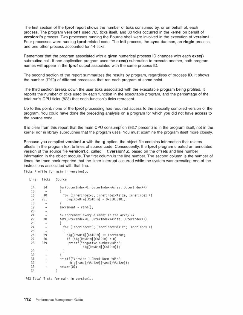
The first section of the tprof report shows the number of ticks consumed by, or on behalf of, eachprocess. The program version1 used 763 ticks itself, and 30 ticks occurred in the kernel on behalf ofversion1’s process. Two processes running the Bourne shell were involved in the execution of version1.Four processes were running tprof-related code. The init process, the sync daemon, an rlogin process,and one other process accounted for 14 ticks.

Remember that the program associated with a given numerical process ID changes with each exec()subroutine call. If one application program uses the exec() subroutine to execute another, both programnames will appear in the tprof output associated with the same process ID.

The second section of the report summarizes the results by program, regardless of process ID. It showsthe number (FREQ) of different processes that ran each program at some point.

The third section breaks down the user ticks associated with the executable program being profiled. Itreports the number of ticks used by each function in the executable program, and the percentage of thetotal run’s CPU ticks (823) that each function’s ticks represent.

Up to this point, none of the tprof processing has required access to the specially compiled version of theprogram. You could have done the preceding analysis on a program for which you did not have access tothe source code.

It is clear from this report that the main CPU consumption (92.7 percent) is in the program itself, not in thekernel nor in library subroutines that the program uses. You must examine the program itself more closely.

Because you compiled version1.c with the -g option, the object file contains information that relatesoffsets in the program text to lines of source code. Consequently, the tprof program created an annotatedversion of the source file version1.c, called __t.version1.c, based on the offsets and line numberinformation in the object module. The first column is the line number. The second column is the number oftimes the trace hook reported that the timer interrupt occurred while the system was executing one of theinstructions associated with that line.Ticks Profile for main in version1.c

Line Ticks Source

14 34 for(OuterIndex=0; OuterIndex<Asize; OuterIndex++)15 - {16 40 for (InnerIndex=0; InnerIndex<Asize; InnerIndex++)17 261 big[RowDim][ColDim] = 0x01010101;18 - }19 - Increment = rand();20 -21 - /* increment every element in the array */22 70 for(OuterIndex=0; OuterIndex<Asize; OuterIndex++)23 - {24 - for (InnerIndex=0; InnerIndex<Asize; InnerIndex++)25 - {26 69 big[RowDim][ColDim] += Increment;27 50 if (big[RowDim][ColDim] < 0)28 239 printf("Negative number.%d\n",

big[RowDim][ColDim]);29 - }30 - }31 - printf("Version 1 Check Num: %d\n",32 - big[rand()%Asize][rand()%Asize]);33 - return(0);34 - }

763 Total Ticks for main in version1.c


This file shows that the largest numbers of ticks are associated with accessing elements of the array big,so you should be able to enhance performance significantly by concentrating on the inner for loops. Thefirst (initialization) for loop is a case of inefficient programming, because it initializes the array one elementat a time. If you were setting the array to 0, use the bzero() subroutine. Because you are setting eachbyte to a specific character, use the memset() subroutine to replace the first for loop. (The efficientbzero() and memset() functions, like the str*() functions, are written in assembler language and usehardware instructions that have no direct equivalent in the C language.)

You must access the array one element at a time to increment the values, but ensure that the pattern ofmemory reference is to consecutive addresses, to maximize cache use. In this case, you have the rowdimension changing faster than the column dimension. Because C arrays are arranged in row-major order,you are skipping over a complete row with each successive memory reference. Because the rows are1024 integers long (4096 bytes), you are changing pages on every reference. The size of the array greatlyexceeds both the data cache and data Translation Lookaside Buffer (TLB) capacities, so you have writtena program for maximum cache and TLB thrashing. To fix this problem, transpose the two #definestatements to reverse the values of RowDim and ColDim.

The unoptimized form of the resulting program (version2.c) consumes about 2.7 CPU seconds, comparedwith 7.9 CPU seconds for program version1.

The following file, __t.version2.c, is the result of a tprof run against the unoptimized form:Ticks Profile for main in version2.c

Line Ticks Source

15 - memset(big,0x01,sizeof(big));16 - Increment = rand();17 -18 - /* increment in memory order */19 60 for(OuterIndex=0; OuterIndex<Asize; OuterIndex++)20 - {21 - for (InnerIndex=0; InnerIndex<Asize; InnerIndex++)22 - {23 67 big[RowDim][ColDim] += Increment;24 60 if (big[RowDim][ColDim] < 0)25 43 printf("Negative number. %d\n",big[RowDim][ColDim]);26 - }27 - }28 - printf("Version 2 Check Num: %d\n",29 - big[rand()%Asize][rand()%Asize]);30 - return(0);31 - }

230 Total Ticks for main in version2.c

By knowing its CPU use pattern, you have improved the CPU speed of this program by a factor of almostthree, for the unoptimized case. When you compile version1.c and version2.c with optimization andcompare their performance, the ″before and after″ improvement due to the changes is a factor of 7.

In many cases, most of a program’s CPU use will occur in the library subroutines it uses rather than in theprogram itself. If you take version2.c and remove the conditional test on line 24 and the printf() entry online 28, to create a version3.c that reads as follows:#include <string.h>#include <stdlib.h>#define Asize 256#define RowDim OuterIndex#define ColDim InnerIndex

main(){

int Increment;


int OuterIndex;int InnerIndex;int big [Asize][Asize];

/* Initialize every byte to 0x01 */memset(big,0x01,sizeof(big));Increment = rand();/* increment in memory order */for(OuterIndex=0; OuterIndex<Asize; OuterIndex++){

for (InnerIndex=0; InnerIndex<Asize; InnerIndex++){

big[RowDim][ColDim] += Increment;printf("RowDim=%d, ColDim=%d, Number=%d\n",

RowDim, ColDim, big[RowDim][ColDim]);}

}return(0);

}

the execution time becomes dominated by the printf() statement. The command:# tprof -v -s -k -p version3 -x version3 >/dev/null

produces a __version3.all that includes profiling data for the kernel and the shared subroutine librarylibc.a (the only shared library this program uses):

Process PID TID Total Kernel User Shared Other======= === === ===== ====== ==== ====== =====version3 28372 28373 818 30 19 769 0

ksh 27348 27349 5 5 0 0 0tprof 15986 19785 3 1 2 0 0tprof 7784 8785 1 1 0 0 0tprof 12904 13657 1 1 0 0 0

ksh 13940 13755 1 1 0 0 0======= === === ===== ====== ==== ====== =====

Total 829 39 21 769 0

Process FREQ Total Kernel User Shared Other======= === ===== ====== ==== ====== =====version3 1 818 30 19 769 0

ksh 2 6 6 0 0 0tprof 3 5 3 2 0 0

======= === ===== ====== ==== ====== =====Total 6 829 39 21 769 0

Total Ticks For version3( USER) = 19


.main 11 1.3 version3.c 632 320.printf 8 1.0 glink.s 1112 36

Total Ticks For version3( KERNEL) = 30


.sc_flih 7 0.8 low.s 13832 1244.i_enable 5 0.6 low.s 21760 256.vmcopyin 3 0.4 vmmove.c 414280 668

.xix_setattr 2 0.2 xix_sattr.c 819368 672.isreadonly 2 0.2 disubs.c 689016 60

.lockl 2 0.2 lockl.s 29300 208.v_pagein 1 0.1 v_getsubs1.c 372288 1044.curtime 1 0.1 clock.s 27656 76.trchook 1 0.1 noname 48168 856

.vmvcs 1 0.1 vmvcs.s 29744 2304


.spec_rdwr 1 0.1 spec_vnops.c 629596 240.rdwr 1 0.1 rdwr.c 658460 492.imark 1 0.1 isubs.c 672024 184.nodev 1 0.1 devsw_pin.c 135864 32

.ld_findfp 1 0.1 ld_libld.c 736084 240

Total Ticks For version3( SH-LIBs) = 769

Shared Object Ticks % Source Address Bytes============= ====== ====== ======= ======= =====libc.a/shr.o 769 92.0 /usr/lib 794624 724772

Profile: /usr/lib/libc.a shr.o

Total Ticks For version3(/usr/lib/libc.a) = 769


._doprnt 476 56.9 doprnt.c 36616 7052.fwrite 205 24.5 fwrite.c 50748 744.strchr 41 4.9 strchr.s 31896 196.printf 18 2.2 printf.c 313796 144._moveeq 16 1.9 memcmp.s 36192 184.strlen 10 1.2 strerror.c 46800 124.isatty 1 0.1 isatty.c 62932 112._xwrite 1 0.1 flsbuf.c 4240 280.__ioctl 1 0.1 ioctl.c 57576 240

This report confirms that most of the ticks are being used by the shared libraries (libc.a in this case). Theprofile of libc.a shows that most of those ticks are being consumed by the _doprnt() subroutine.

The _doprnt() subroutine is the processing module for the printf(), sprintf(), and other subroutines. Witha simple change, you have increased the run time from 2.7 seconds to 8.6 seconds, and the formattedprinting now consumes about 60 percent of the CPU time. This illustrates why formatting should be usedjudiciously. The performance of the _doprnt() subroutine is also affected by the locale. See Appendix E.National Language Support: Locale versus Speed. These tests were run in the C locale, which is the mostefficient.

A tprof Example for releases starting with AIX 5.2The tprof command has been completely rewritten for AIX 5.2 such that now it is much faster than beforeand provides more functionality. The syntax is different than the previous tprof, and you can view thecomplete documentation of tprof in AIX 5L Version 5.2 Commands Reference.

The following is an example of how to collect a CPU tick profile of the version1 program using the newtprof command, executed on a 4–way SMP system. Since this machine is a very fast running system, thecommand finished in less than a second. To make this program run longer, the array size was changed to4096 instead of 1024, which is the value of the Asize variable in version1.c:# tprof -z -u -p version1 -x version1

A file called version1.prof (shown below) is created in the current directory which reports how many CPUticks for each of the programs running on the system while version1 was running.

Process Freq Total Kernel User Shared Other======= ==== ===== ====== ==== ====== =====

wait 4 5810 5810 0 0 0./version1 1 1672 35 1637 0 0

/usr/bin/tprof 2 15 13 0 2 0/etc/syncd 1 2 2 0 0 0/usr/bin/sh 2 2 2 0 0 0

swapper 1 1 1 0 0 0/usr/bin/trcstop 1 1 1 0 0 0

rmcd 1 1 1 0 0 0


======= === ===== ====== ==== ====== =====Total 13 7504 5865 1637 2 0

Process PID TID Total Kernel User Shared Other======= === === ===== ====== ==== ====== =====

wait 16392 16393 1874 1874 0 0 0wait 12294 12295 1873 1873 0 0 0wait 20490 20491 1860 1860 0 0 0

./version1 245974 606263 1672 35 1637 0 0wait 8196 8197 203 203 0 0 0

/usr/bin/tprof 291002 643291 13 13 0 0 0/usr/bin/tprof 274580 610467 2 0 0 2 0

/etc/syncd 73824 110691 2 2 0 0 0/usr/bin/sh 245974 606263 1 1 0 0 0/usr/bin/sh 245976 606265 1 1 0 0 0

/usr/bin/trcstop 245976 606263 1 1 0 0 0swapper 0 3 1 1 0 0 0

rmcd 155876 348337 1 1 0 0 0======= === === ===== ====== ==== ====== =====

Total 7504 5865 1637 2 0

Total Samples = 7504 Total Elapsed Time = 18.76s

Profile: ./version1Total Ticks For All Processes (./version1) = 1637


.main 1637 21.82 version1.c 350 536

Profile: ./version1Total Ticks For ./version1[245974] (./version1) = 1637


.main 1637 21.82 version1.c 350 536

The first section of the report summarizes the results by program, regardless of the process ID. It showsthe number of different processes (Freq) that ran each program at some point.

The second section of the tprof report shows the number of ticks consumed by, or on behalf of, eachprocess. The program version1 used 1637 ticks itself and 35 ticks occurred in the kernel on behalf oftheversion1 process.

The third section breaks down the user ticks associated with the executable program being profiled. Itreports the number of ticks used by each function in the executable program, and the percentage of thetotal run’s CPU ticks (7504) that each function’s ticks represent. Since this system’s CPUs were mostlyidle, most of the 7504 ticks are idle ticks. To see what percentage of the busy time this program took,subtract the wait thread’s CPU ticks (these are the idle CPU ticks) from the total and then subtract thatfrom the total number of ticks. So, 7504–5810 gives us 1694. This is the total number of ticks for actualwork done on the system. If we divide the version1 program’s user ticks (1637) by 1694, we find that itspercentage of system busy ticks is 1637/1694*100, which is 96.6%.

Offline Processing with the tprof Command prior to AIX 5.2The -i Trace_File flag allows for offline processing by the tprof command of trace data files created by thesystem trace command. The -n flag allows you to specify a Gennames_File to be used when processingan offline file. These flags are useful when it is necessary to postprocess a trace file from a remotemachine or perform the trace data collection at one time and postprocess it at another time. In this case -n


with a Gennames_File must be used from the machine that the trace came from. The flags are also usefulwhen system loading is high and trace hooks are being missed by the tprof command. The offline optionrelieves this problem.

Trace hooks relevant to the tprof command must be collected by the trace command and are specified bythe trace -j flag. The gennames command is then executed to collect additional information for the tprofcommand. After the trace and gennames Gennames_File commands have executed, the trcrpt -rcommand must be executed on the trace logfile and redirected to another file. At this point an adjustedtrace logfile and a Gennames_File is input to the tprof command.

For example:

# trace -af -T 1000000 -L 10000000 -o trace.out -j 000,001,002,003,005,006,234,106,10C,134,139,00A,465# workload# trcoff# gennames > gennames.out# trcstop# trcrpt -r trace.out > trace.rpt

Next run the tprof command with at least the -i and -n flags, as follows:# tprof -i trace.rpt -n gennames.out -s -k -e

On systems with many CPUs, it is better to run the trace and trcrpt commands with the -C all flag (seeFormatting a Report from trace -C Output).

Offline Processing with the tprof Command starting with AIX 5.2The new tprof command can do offline processing of trace files, but it requires that filenames be specifiedwith a rootstring name. This can be whatever you want to call it. Also, there are certain suffixes requiredfor the input files that tprof will use. For example, the trace binary file should end in .trc. The trace binaryfile does not have to be post-processed with trcrpt -r any more. Also, instead of using gennames output,you need to collect gensyms output and put this in a file called rootstring.syms.

Let us call our rootstring trace1. Then to collect a trace, we can trace using all of the hooks or at least thefollowing hooks:# trace -af -T 1000000 -L 10000000 -o trace1.trc -j 000,001,002,003,005,006,234,106,10C,134,139,00A,465# workload# trcoff# gensyms > trace1.syms# trcstop# trcrpt -r trace1 -k -u -s -z

This creates a trace1.prof file which gives you a CPU profile of the system while trace was running.

Using the pprof Command to Measure CPU usage of Kernel ThreadsThe pprof command reports CPU usage on all kernel threads running within an interval using the traceutility. The raw process information is saved to pprof.flow and five reports are generated. If no flags arespecified, all reports are generated.

To determine whether the pprof program (available with AIX 4.3.3 and later) is installed and available, runthe following command:# lslpp -lI fileset_name

where fileset_name is perfagent.tools in AIX 4.3.3 or bos.perf.tools in AIX 5 or later.

The types of reports are as follows:


pprof.cpuLists all kernel level threads sorted by actual CPU time. Contains: Process Name, Process ID,Parent Process ID, Process State at Beginning and End, Thread ID, Parent Thread ID, ActualCPU Time, Start Time, Stop Time, Stop - Start.

pprof.famcpuLists the information for all families (processes with a common ancestor). The Process Name andProcess ID for the family is not necessarily the ancestor. Contains: Start Time, Process Name,Process ID, Number of Threads, Total CPU Time.

pprof.famindLists all processes grouped by families (processes with a common ancestor). Child process namesare indented with respect to the parent. Contains: Start Time, Stop Time, Actual CPU Time,Process ID, Parent Process ID, Thread ID, Parent Thread ID, Process State at Beginning andEnd, Level, Process Name.

pprof.namecpuLists information about each type of kernel thread (all executable with the same name). Contains:Process Name, Number of Threads, CPU Time, % of Total CPU Time.

pprof.startLists all kernel threads sorted by start time that were dispatched during the the pprof commandinterval. Contains: Process Name, Process ID, Parent Process ID, Process State Beginning andEnd, Thread ID, Parent Thread ID, Actual CPU Time, Start Time, Stop Time, Stop - Start.

Following is a sample pprof.namecpu file that was generated by running the tthreads32 program, whichforks off four threads, which in turn each fork off a process of their own. These processes then executeseveral ksh and sleep programs:

Pprof PROCESS NAME Report

Sorted by CPU Time

From: Thu Oct 19 17:53:07 2000To: Thu Oct 19 17:53:22 2000

Pname #ofThreads CPU_Time %======== ========== ======== ========

tthreads32 13 0.116 37.935sh 8 0.092 30.087

Idle 2 0.055 17.987ksh 12 0.026 8.503

trace 3 0.007 2.289java 3 0.006 1.962kproc 5 0.004 1.308

xmservd 1 0.000 0.000trcstop 1 0.000 0.000swapper 1 0.000 0.000

gil 1 0.000 0.000ls 4 0.000 0.000

sleep 9 0.000 0.000ps 4 0.000 0.000

syslogd 1 0.000 0.000nfsd 2 0.000 0.000

========== ======== ========70 0.306 100.000

The corresponding pprof.cpu is as follows:

Pprof CPU Report

Sorted by Actual CPU Time

From: Thu Oct 19 17:53:07 2000


To: Thu Oct 19 17:53:22 2000

E = Exec’d F = ForkedX = Exited A = Alive (when traced started or stopped)C = Thread Created

Pname PID PPID BE TID PTID ACC_time STT_time STP_time STP-STT===== ===== ===== === ===== ===== ======== ======== ======== ========Idle 774 0 AA 775 0 0.052 0.000 0.154 0.154

tthreads32 5490 11982 EX 18161 22435 0.040 0.027 0.154 0.126sh 11396 5490 EE 21917 5093 0.035 0.082 0.154 0.072sh 14106 5490 EE 16999 18867 0.028 0.111 0.154 0.043sh 13792 5490 EE 20777 18179 0.028 0.086 0.154 0.068ksh 5490 11982 FE 18161 22435 0.016 0.010 0.027 0.017

tthreads32 5490 11982 CX 5093 18161 0.011 0.056 0.154 0.098tthreads32 5490 11982 CX 18179 18161 0.010 0.054 0.154 0.099tthreads32 14506 5490 FE 17239 10133 0.010 0.128 0.143 0.015

ksh 11982 13258 AA 22435 0 0.010 0.005 0.154 0.149tthreads32 13792 5490 FE 20777 18179 0.010 0.059 0.086 0.027tthreads32 5490 11982 CX 18867 18161 0.010 0.057 0.154 0.097tthreads32 11396 5490 FE 21917 5093 0.009 0.069 0.082 0.013tthreads32 5490 11982 CX 10133 18161 0.008 0.123 0.154 0.030tthreads32 14106 5490 FE 16999 18867 0.008 0.088 0.111 0.023

trace 5488 11982 AX 18159 0 0.006 0.001 0.005 0.003kproc 1548 0 AA 2065 0 0.004 0.071 0.154 0.082Idle 516 0 AA 517 0 0.003 0.059 0.154 0.095java 11612 11106 AA 14965 0 0.003 0.010 0.154 0.144java 11612 11106 AA 14707 0 0.003 0.010 0.154 0.144trace 12544 5488 AA 20507 0 0.001 0.000 0.001 0.001

sh 14506 5490 EE 17239 10133 0.001 0.143 0.154 0.011trace 12544 5488 CA 19297 20507 0.000 0.001 0.154 0.153ksh 4930 2678 AA 5963 0 0.000 0.154 0.154 0.000

kproc 6478 0 AA 3133 0 0.000 0.154 0.154 0.000ps 14108 5490 EX 17001 18867 0.000 0.154 0.154 0.000

tthreads32 13794 5490 FE 20779 18179 0.000 0.154 0.154 0.000sh 13794 5490 EE 20779 18179 0.000 0.154 0.154 0.000ps 13794 5490 EX 20779 18179 0.000 0.154 0.154 0.000sh 14108 5490 EE 17001 18867 0.000 0.154 0.154 0.000

tthreads32 14108 5490 FE 17001 18867 0.000 0.154 0.154 0.000ls 13792 5490 EX 20777 18179 0.000 0.154 0.154 0.000

:::

Detecting Instruction Emulation with the emstat ToolThe POWER-based architecture deleted (that is, no longer supports) 35 POWER instructions (5 for thePowerPC 601 RISC Microprocessor ″bridge″). To maintain compatibility with older binaries (which maycontain these deleted instructions) the AIX Version 4 kernel includes emulation routines that providesupport for the deleted instructions. Attempting to execute a deleted instruction results in an illegalinstruction exception. The kernel decodes the illegal instruction, and if it is a deleted instruction, the kernelruns an emulation routine that functionally emulates the instruction.

However, depending upon the execution frequency of deleted instructions and the deleted instructionemulation path lengths, emulation can result in varying degrees of performance degradation due to kernelcontext switch and instruction emulation overhead. Even a very small percentage of emulation might resultin a big performance difference. The following table shows estimated instruction path lengths for several ofthe deleted instructions:


Instruction Emulated in Estimated Path Length (instructions)

abs assembler 117

doz assembler 120

mul assembler 127

rlmi C 425

sle C 447

clf C 542

div C 1079

Most emulation problems are usually seen on PowerPC 604 RISC Microprocessor systems. A typicalexample is a PowerPC 601 RISC Microprocessor system that gets upgraded to a PowerPC 604 RISCMicroprocessor system. If performance slows down instead of speeding up, it is most likely due toemulation.

The solution to emulation is to recompile the application in common mode. The default architectureplatform for compilations on AIX Version 4 is common architecture. However, the default architecture onAIX Version 3 was for POWER family, POWER2, and PowerPC 601 RISC Microprocessor. If thesebinaries ran on a PowerPC 604 RISC Microprocessor, some instructions could get emulated.

If binaries need to be compiled on AIX Version 3, then the Full Common Mode APAR must be installed onthat AIX Version 3 system, and the application must be compiled with the following options:-qarch=com -qdebug=useabs -bI:/lib/FCM/lowsys.exp

Instructions that are not common on all platforms must be removed from code written in assembler,because recompilation is only effective for high-level source code. Routines coded in assembler must bechanged so that they do not use missing instructions, because recompilation has no effect in this case.

The first step is to determine if instruction emulation is occurring by using the emstat tool.

To determine whether the emstat program is installed and available, run the following command:# lslpp -lI bos.adt.samples

This tool resides in the /usr/samples/kernel directory.

With operating system versions later than AIX 4.3.3, this command ships with the bos.perf.tools filesetand has a slightly modified output. To determine whether the emstat program is installed and available,run the following command:# lslpp -lI bos.perf.tools

The emstat command works similarly to the vmstat command in that you specify an interval time inseconds, and optionally, the number of intervals. The value in the first column is the cumulative countsince system boot, while the value in the second column is the number of instructions emulated during thatinterval. Emulations on the order of many thousands per second can have an impact on performance.

The following is an example of output from issuing the emstat 1 command in AIX 4.3.3:# /usr/samples/kernel/emstat 1

emstat total count emstat interval count21951937 2195193721967488 1555121974877 7389


21994354 1947722007329 1297522018171 1084222018171 0

The following is an example of output from issuing the emstat 1 command in AIX 5.1 or later:# emstat 1

Emulation EmulationSinceBoot Delta

0 00 00 0

Once emulation has been detected, the next step is to determine which application is emulatinginstructions. This is much harder to determine. One way is to run only one application at a time andmonitor it with the emstat program. Sometimes certain emulations cause a trace hook to be encountered.This can be viewed in the ASCII trace report file with the words PROGRAM CHECK. The process/threadassociated with this trace event is emulating instructions either due to its own code emulating instructions,or it is executing library or code in other modules that are emulating instructions.

Detecting Alignment Exceptions with the alstat ToolAIX compilers perform natural alignment of data types. For example, data of type short, which is 2 byteslong, is padded automatically to 4 bytes by the compiler. Common programming practices such astypecasting and usage of alignment pragmas can cause application data to be aligned incorrectly.POWER-based optimization assumes correct alignment of data. Thus, fetching misaligned data mayrequire multiple memory accesses where a single access should have sufficed. Misalignment of data cancause the hardware to generate an alignment exception, which would force the kernel to simulate theneeded memory accesses. As with the case of instrution emulation, this can degrade applicationperformance.

Starting with AIX 5.1, the alstat tool packaged with bos.perf.tools can be used to detect if alignmentexceptions are occurring. To show alignment exceptions on a per-CPU basis, use the -v option.

Because alstat and emstat are the same binary, either of these tools can be used to sho instructionemulation and alignment exceptions. To show instruction emulation, use the -e option on alstat. To showalignment exceptions, use the -a option on emstat.

The output for alstat looks similar to the following:# alstat -e 1

Alignment Alignment Emulation EmulationSinceBoot Delta SinceBoot Delta

0 0 0 00 0 0 00 0 0 0

Restructuring Executable Programs with the fdpr ProgramThe fdpr (feedback-directed program restructuring) program optimizes executable modules for fasterexecution and more efficient use of real memory. To determine whether the fdpr program is installed andavailable on your system, run the following command:# lslpp -lI perfagent.tools

The fdpr command is a performance-tuning utility that can improve both performance and real memoryutilization of user-level application programs. The source code is not necessary as input to the fdprprogram. However, stripped executable programs are not supported. If source code is available, programsbuilt with the -qfdpr compiler flag contain information to assist the fdpr program in producing reordered


programs with guaranteed functionality. If the -qfdpr flag is used, it should be used for all object modulesin a program. Static linking will not enhance performance if the -qfdpr flag is used.

The fdpr tool reorders the instructions in an executable program to improve instruction cache, TranslationLookaside Buffer (TLB), and real memory utilization by doing the following:

v Packing together highly executed code sequences (as determined through profiling)

v Recoding conditional branches to improve hardware branch prediction

v Moving infrequently executed code out of line

For example, given an ″if-then-else″ statement, the fdpr program might conclude that the program usesthe else branch more often than the if branch. It will then reverse the condition and the two branches asshown in the following figure.

Large applications (larger than 5 MB) that are CPU-bound can improve execution time up to 23 percent,but typically the performance is improved between 5 and 20 percent. The reduction of real memoryrequirements for text pages for this type of program can reach 70 percent. The average is between 20 and50 percent. The numbers depend on the application’s behavior and the optimization options issued whenusing the fdpr program.

The fdpr processing takes place in three stages:

1. The executable module to be optimized is instrumented to allow detailed performance-data collection.

2. The instrumented executable module is run in a workload provided by the user, and performance datafrom that run is recorded.

3. The performance data is used to drive a performance-optimization process that results in arestructured executable module that should perform the workload that exercised the instrumentedexecutable program more efficiently. It is critically important that the workload used to drive the fdprprogram closely match the actual use of the program. The performance of the restructured executableprogram with workloads that differ substantially from that used to drive the fdpr program isunpredictable, but can be worse than that of the original executable program.

As an example, the command# fdpr -p ProgramName -R3 -x test.sh

would use the testcase test.sh to run an instrumented form of program ProgramName. The output of thatrun would be used to perform the most aggressive optimization (-R3) of the program to form a newmodule called, by default, ProgramName.fdpr. The degree to which the optimized executable programperformed better in production than its unoptimized predecessor would depend largely on the degree towhich the testcase test.sh successfully imitated the production workload.

Note: The fdpr program incorporates advanced optimization algorithms that sometimes result in optimizedexecutable programs that do not function in the same way as the original executable module. It is

Figure 17. Example of Conditional Branch Recoding. The illustration shows how conditional branch recoding changescertain code. For example, the code If (condition) would become If (! condition); the code then stays then; instructionsbecomes other instructions; else stays else; other instructions become instruction; and endif stays endif.


absolutely essential that any optimized executable program be thoroughly tested before being usedin any production situation; that is, before its output is trusted.

In summary, users of the fdpr program should adhere to the following:

v Take pains to use a workload to drive the fdpr program that is representative of the intended use.

v Thoroughly test the functioning of the resulting restructured executable program.

v Use the restructured executable program only on the workload for which it has been tuned.

Controlling Contention for the CPUAIX Version 4 introduced the use of threads to control processor time consumption, but most of the systemmanagement tools still refer to the process in which a thread is running, rather than the thread itself.

Controlling the Priority of User ProcessesUser-process priorities can be manipulated using the nice or renice command or the setpri() subroutine,and displayed with the ps command. An overview of priority is provided in Process and Thread Priority.

Priority calculation is employed to accomplish the following:

v Share the CPU among threads

v Prevent starvation of any thread

v Penalize compute-bound threads

v Increase continuous discrimination between threads over time

The degree to which the user priorities can be manipulated is release-dependent. The algorithm forcalculating priority value in AIX 4.3.1 and prior releases is more limiting than the current algorithm. Thealgorithm was changed in AIX 4.3.2 so that user priorities can be manipulated more than in previousreleases. There is improved distinction between foreground and background processes. Using a givennice value will have a greater effect on CPU utilization. See “Priority Calculation” on page 126.

Running a Command with the nice CommandAny user can run a command at a less-favorable-than-normal priority by using the nice command. Onlythe root user can use the nice command to run commands at a more-favorable-than-normal priority. In thiscase, the nice command values range between -20 and 19.

With the nice command, the user specifies a value to be added to or subtracted from the standard nicevalue. The modified nice value is used for the process that runs the specified command. The priority ofthe process is still non-fixed; that is, the priority value is still recalculated periodically based on the CPUusage, nice value, and minimum user-process-priority value.

The standard nice value of a foreground process is 20 (24 for a ksh background process). The followingcommand would cause the vmstat command to be run in the foreground with a nice value of 25 (insteadof the standard 20), resulting in a less favorable priority.# nice -n 5 vmstat 10 3 > vmstat.out

If you use the root login, the vmstat command can be run at a more favorable priority with the following:# nice -n -5 vmstat 10 3 > vmstat.out

If you were not using root login and issued the preceeding example nice command, the vmstat commandwould still be run but at the standard nice value of 20, and the nice command would not issue any errormessage.

Setting a Fixed Priority with the setpri SubroutineAn application that runs under the root user ID can use the setpri() subroutine to set its own priority orthat of another process. For example:


retcode = setpri(0,59);

would give the current process a fixed priority of 59. If the setpri() subroutine fails, it returns -1.

The following program accepts a priority value and a list of process IDs and sets the priority of all of theprocesses to the specified value./*

fixprocpri.cUsage: fixprocpri priority PID . . .

*/

#include <sys/sched.h>#include <stdio.h>#include <sys/errno.h>

main(int argc,char **argv){

pid_t ProcessID;int Priority,ReturnP;

if( argc < 3 ) {printf(" usage - setpri priority pid(s) \n");exit(1);

}

argv++;Priority=atoi(*argv++);if ( Priority < 50 ) {

printf(" Priority must be >= 50 \n");exit(1);

}

while (*argv) {ProcessID=atoi(*argv++);ReturnP = setpri(ProcessID, Priority);if ( ReturnP > 0 )

printf("pid=%d new pri=%d old pri=%d\n",(int)ProcessID,Priority,ReturnP);

else {perror(" setpri failed ");

exit(1);}

}}

Displaying Process Priority with the ps CommandThe -l (lowercase L) flag of the ps command displays the nice values and current priority values of thespecified processes. For example, you can display the priorities of all of the processes owned by a givenuser with the following:# ps -lu hoetzel

F S UID PID PPID C PRI NI ADDR SZ WCHAN TTY TIME CMD241801 S 200 7032 7286 0 60 20 1b4c 108 pts/2 0:00 ksh200801 S 200 7568 7032 0 70 25 2310 88 5910a58 pts/2 0:00 vmstat241801 S 200 8544 6494 0 60 20 154b 108 pts/0 0:00 ksh

The output shows the result of the nice -n 5 command described previously. Process 7568 has an inferiorpriority of 70. (The ps command was run by a separate session in superuser mode, hence the presence oftwo TTYs.)

If one of the processes had used the setpri(10758, 59) subroutine to give itself a fixed priority, a sampleps -l output would be as follows:


F S UID PID PPID C PRI NI ADDR SZ WCHAN TTY TIME CMD200903 S 0 10758 10500 0 59 -- 3438 40 4f91f98 pts/0 0:00 fixpri

Modifying the Priority with the renice CommandThe renice command alters the nice value, and thus the priority, of one or more processes that arealready running. The processes are identified either by process ID, process group ID, or the name of theuser who owns the processes.

For AIX Version 4, the syntax of the renice command has been changed to complement the alternativesyntax of the nice command, which uses the -n flag to identify the nice-value increment.

The renice command cannot be used on fixed-priority processes. A non-root user can specify a value tobe added to, but not subtracted from the nice value of one or more running processes. The modification isdone to the nice values of the processes. The priority of these processes is still non-fixed. Only the rootuser can use the renice command to alter the priority value within the range of -20 to 20, or subtract fromthe nice value of one or more running processes.

To continue the example, use the renice command to alter the nice value of the vmstat process that youstarted with nice.# renice -n -5 7568# ps -lu hoetzel


Now the process is running at a more favorable priority that is equal to the other foreground processes. Toundo the effects of this, you could issue the following:# renice -n 5 7569# ps -lu hoetzel


In these examples, the renice command was run by the root user. When run by an ordinary user ID, thereare two major limitations to the use of the renice command:

v Only processes owned by that user ID can be specified.

v The nice value of the process cannot be decreased, not even to return the process to the defaultpriority after making its priority less favorable with the renice command.

Clarification of the nice and renice Command SyntaxThe nice and renice commands have different ways of specifying the amount that is to be added to thestandard nice value of 20.

For AIX Version 4, the syntax of the renice command has been changed to complement the alternativesyntax of the nice command, which uses the -n flag to identify the nice-value increment.

Command Command Resulting niceValue

Best Priority Value inAIX 4.3.1

Best Priority Value inAIX 4.3.2 andSubsequent Releases

nice -n 5 renice -n 5 25 65 70

nice -n +5 renice -n +5 25 65 70

nice -n -5 renice -n -5 15 55 55


Tuning the Thread-Priority-Value CalculationThis section discusses tuning using the following:

v Priority Calculation

v The schedutune command

The schedtune command and several enhancements to the CPU scheduler permit changes to theparameters used to calculate the priority value for each thread. See Process and Thread Priority forbackground information on priority.

To determine whether the schedtune program is installed and available, run the following command:# lslpp -lI bos.adt.samples

Priority CalculationThe formula for calculating the priority value is:priority value = base priority + nice penalty + (CPU penalty based on recent CPU usage)

The recent CPU usage value of a given thread is incremented by 1 each time that thread is in control ofthe CPU when the timer interrupt occurs (every 10 milliseconds). The recent CPU usage value isdisplayed as the C column in the ps command output. The maximum value of recent CPU usage is 120.

The default algorithm calculates the CPU penalty by dividing recent CPU usage by 2. TheCPU-penalty-to-recent-CPU-usage ratio is therefore 0.5. This ratio is controlled by a value called R (thedefault is 16). The formula is as follows:CPU_penalty = C * R/32

Once a second, the default algorithm divides the recent CPU usage value of every thread by 2. Therecent-CPU-usage-decay factor is therefore 0.5. This factor is controlled by a value called D (the default is16). The formula is as follows:C = C * D/32

For some users, the algorithm in AIX 4.3.1 does not allow enough distinction between foreground andbackground processes. The algorithm for calculating priority value was changed in AIX 4.3.2 to increasethe impact on priorities when the nice value is changed. As the units of CPU time increase, the prioritydecreases with the nice effect. Using schedtune -r -d can give additional control over the prioritycalculation by setting new values for R and D. See “Tuning with the schedtune Command” on page 127 forfurther information.

The algorithm guarantees that threads whose nice values are the default of 20 will behave exactly as theydid in AIX 4.3.1 and prior releases. When the nice value is not equal to the default, the priority will beaffected more due to the use of two formulas.

Begin with the following equation:p_nice = base priority + nice value

Now use the following formula:If p_nice > 60,

then x_nice = (p_nice * 2) - 60,else x_nice = p_nice.

If the nice value is greater than 20, then it has double the impact on the priority value than if it was lessthan or equal to 20. The new priority calculation (ignoring integer truncation) is as follows:priority value = x_nice + [(x_nice + 4)/64 * C*(R/32)]

Note: If the nice value is the default, the formulas for AIX 4.3.1 and AIX 4.3.2 yield the same results.


Tuning with the schedtune CommandTuning is accomplished through two options of the schedtune command: -r and -d. Each option specifiesa parameter that is an integer from 0 through 32. The parameters are applied by multiplying by theparameter’s value and then dividing by 32. The default r and d values are 16, which yields the samebehavior as the original algorithm [(D=R=16)/32=0.5]. The new range of values permits a far widerspectrum of behaviors. For example:# /usr/samples/kernel/schedtune -r 0

[(R=0)/32=0, (D=16)/32=0.5] would mean that the CPU penalty was always 0, making priority a function ofthe nice value only. No background process would get any CPU time unless there were no dispatchableforeground processes at all. The priority values of the threads would effectively be constant, although theywould not technically be fixed-priority threads.# /usr/samples/kernel/schedtune -r 5

[(R=5)/32=0.15625, (D=16)/32=0.5] would mean that a foreground process would never have to competewith a background process started with the command nice -n 10. The limit of 120 CPU time slicesaccumulated would mean that the maximum CPU penalty for the foreground process would be 18.# /usr/samples/kernel/schedtune -r 6 -d 16

[(R=6)/32=0.1875, (D=16)/32=0.5] would mean that, if the background process were started with thecommand nice -n 10, it would be at least one second before the background process began to receiveany CPU time. Foreground processes, however, would still be distinguishable on the basis of CPU usage.Long-running foreground processes that should probably be in the background would ultimatelyaccumulate enough CPU usage to keep them from interfering with the true foreground.# /usr/samples/kernel/schedtune -r 32 -d 32

[(R=32)/32=1, (D=32)/32=1] would mean that long-running threads would reach a C value of 120 andremain there, contending on the basis of their nice values. New threads would have priority, regardless oftheir nice value, until they had accumulated enough time slices to bring them within the priority valuerange of the existing threads.

Here are some guidelines for R and D:

v Smaller values of R narrow the priority range and make the nice value have more of an impact on thepriority.

v Larger values of R widen the priority range and make the nice value have less of an impact on thepriority.

v Smaller values of D decay CPU usage at a faster rate and can cause CPU-intensive threads to bescheduled sooner.

v Larger values of D decay CPU usage at a slower rate and penalize CPU-intensive threads more (thusfavoring interactive-type threads).

If you conclude that one or both parameters need to be modified to accommodate your workload, you canenter the schedtune command while logged on as root user. The changed values will remain until thenext schedtune command modifies them or until the next system boot. Values can be reset to theirdefaults with the command schedtune -D, but remember that all schedtune parameters are reset by thatcommand, including VMM memory load control parameters. To make a change to the parameters that willpersist across boots, add an appropriate line at the end of the /etc/inittab file.

Example of a Priority CalculationThe example shows R=4 and D=31 and assumes no other runnable threads:current_effective_priority

| base process priority| | nice value| | | count (time slices consumed)| | | | (schedtune -r)


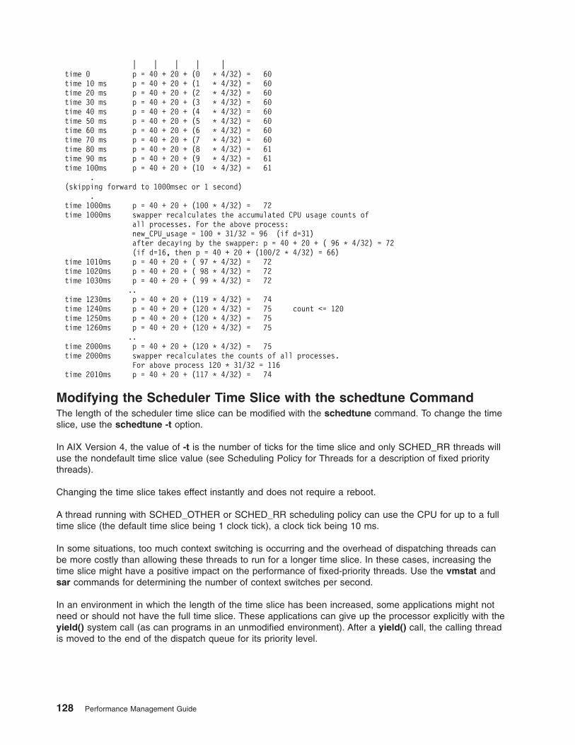
| | | | |time 0 p = 40 + 20 + (0 * 4/32) = 60time 10 ms p = 40 + 20 + (1 * 4/32) = 60time 20 ms p = 40 + 20 + (2 * 4/32) = 60time 30 ms p = 40 + 20 + (3 * 4/32) = 60time 40 ms p = 40 + 20 + (4 * 4/32) = 60time 50 ms p = 40 + 20 + (5 * 4/32) = 60time 60 ms p = 40 + 20 + (6 * 4/32) = 60time 70 ms p = 40 + 20 + (7 * 4/32) = 60time 80 ms p = 40 + 20 + (8 * 4/32) = 61time 90 ms p = 40 + 20 + (9 * 4/32) = 61time 100ms p = 40 + 20 + (10 * 4/32) = 61

.(skipping forward to 1000msec or 1 second)

.time 1000ms p = 40 + 20 + (100 * 4/32) = 72time 1000ms swapper recalculates the accumulated CPU usage counts of

all processes. For the above process:new_CPU_usage = 100 * 31/32 = 96 (if d=31)after decaying by the swapper: p = 40 + 20 + ( 96 * 4/32) = 72(if d=16, then p = 40 + 20 + (100/2 * 4/32) = 66)

time 1010ms p = 40 + 20 + ( 97 * 4/32) = 72time 1020ms p = 40 + 20 + ( 98 * 4/32) = 72time 1030ms p = 40 + 20 + ( 99 * 4/32) = 72

..time 1230ms p = 40 + 20 + (119 * 4/32) = 74time 1240ms p = 40 + 20 + (120 * 4/32) = 75 count <= 120time 1250ms p = 40 + 20 + (120 * 4/32) = 75time 1260ms p = 40 + 20 + (120 * 4/32) = 75

..time 2000ms p = 40 + 20 + (120 * 4/32) = 75time 2000ms swapper recalculates the counts of all processes.

For above process 120 * 31/32 = 116time 2010ms p = 40 + 20 + (117 * 4/32) = 74

Modifying the Scheduler Time Slice with the schedtune CommandThe length of the scheduler time slice can be modified with the schedtune command. To change the timeslice, use the schedtune -t option.

In AIX Version 4, the value of -t is the number of ticks for the time slice and only SCHED_RR threads willuse the nondefault time slice value (see Scheduling Policy for Threads for a description of fixed prioritythreads).

Changing the time slice takes effect instantly and does not require a reboot.

A thread running with SCHED_OTHER or SCHED_RR scheduling policy can use the CPU for up to a fulltime slice (the default time slice being 1 clock tick), a clock tick being 10 ms.

In some situations, too much context switching is occurring and the overhead of dispatching threads canbe more costly than allowing these threads to run for a longer time slice. In these cases, increasing thetime slice might have a positive impact on the performance of fixed-priority threads. Use the vmstat andsar commands for determining the number of context switches per second.

In an environment in which the length of the time slice has been increased, some applications might notneed or should not have the full time slice. These applications can give up the processor explicitly with theyield() system call (as can programs in an unmodified environment). After a yield() call, the calling threadis moved to the end of the dispatch queue for its priority level.


CPU-Efficient User ID Administration (The mkpasswd Command)To improve login response time and conserve CPU time in systems with many users, the operating systemcan use a hashed version of the /etc/passwd file to look up user IDs. When this facility is used, the/etc/passwd file still exists, but is not used in normal processing. The hashed versions of the file are builtby the mkpasswd command. If the hashed versions are not current, login processing reverts to a slow,CPU-intensive sequential search through /etc/passwd.

Prior to AIX 4.3, the command to run is mkpasswd /etc/passwd. This command creates a/etc/passwd.pag and /etc/passwd.dir file, and lookups of /etc/passwd will do a hashed lookup intopasswd.pag (as long as this file is newer than /etc/passwd and /etc/security/passwd. Otherwise,lookups will fall back to the default behavior).

Starting with AIX 4.3, the command to run is mkpasswd -f. This command creates indexed versions of/etc/passwd, /etc/security/passwd, and /etc/security/lastlog. The files created are /etc/passwd.nm.idx,/etc/passwd.id.idx, /etc/security/passwd.idx, and /etc/security/lastlog.idx. Note that this will greatlyenhance performance of applications that also need the encrypted password (such as login and any otherprogram that needs to do password authentication).

Applications can also be changed to use alternative routines such as _getpwent() instead of getpwent(),_getpwnam_shadow(name,0) instead of getpwnam(name), or _getpwuid_shadow(uid,0) instead ofgetpwuid(uid) to do name/ID resolution in cases where the encrypted password is not needed. Thisprevents a lookup of /etc/security/passwd.

Do not edit the password files by hand because the time stamps of the database files (.pag or .idx) willnot be in sync and the default lookup method (linear) will be used. If the passwd, mkuser, chuser,rmuser commands (or the SMIT command equivalents, with fast paths of the same name) are used toadminister user IDs, the hashed files are kept up to date automatically. If the /etc/passwd file is changedwith an editor or with the pwdadm command, the hashed or index files must be rebuilt.

Note: The mkpasswd command does not affect NIS, DCE, or LDAP user databases.



Chapter 8. Monitoring and Tuning Memory Use

The memory of a system is almost constantly filled to capacity. Even if currently running programs do notconsume all available memory, the operating system retains in memory the text pages of programs thatran earlier and the files that they used. There is no cost associated with this retention, because thememory would have been unused anyway. In many cases, the programs or files will be used again, whichreduces disk I/O.

This chapter describes how memory use can be measured and modified. It contains the following majorsections:

v Determining How Much Memory Is Being Used

v Finding Memory-Leaking Programs

v Assessing Memory Requirements Through the rmss Command

v Tuning VMM Memory Load Control with the schedtune Command

v Tuning VMM Page Replacement with the vmtune Command

v Tuning Paging-Space Thresholds

v Choosing a Page Space Allocation Method

v Using Shared Memory

v Using AIX Memory Affinity Support

Readers who are not familiar with the operating system’s virtual-memory management may want to look atPerformance Overview of the Virtual Memory Manager (VMM) before continuing.

Determining How Much Memory Is Being UsedSeveral performance tools provide reports of memory usage. The reports of most interest are from thevmstat, ps, and svmon commands.

The vmstat Command (Memory)The vmstat command summarizes the total active virtual memory used by all of the processes in thesystem, as well as the number of real-memory page frames on the free list. Active virtual memory isdefined as the number of virtual-memory working segment pages that have actually been touched (for adefinition see Late Page Space Allocation). This number can be larger than the number of real pageframes in the machine, because some of the active virtual-memory pages may have been written out topaging space.

When determining if a system might be short on memory or if some memory tuning needs to be done, runthe vmstat command over a set interval and examine the pi and po columns on the resulting report.These columns indicate the number of paging space page-ins per second and the number of paging spacepage-outs per second. If the values are constantly non-zero, there might be a memory bottleneck. Havingoccasional non-zero values is not be a concern because paging is the main principle of virtual memory.# vmstat 2 10kthr memory page faults cpu----- ----------- ------------------------ ------------ -----------r b avm fre re pi po fr sr cy in sy cs us sy id wa1 3 113726 124 0 14 6 151 600 0 521 5533 816 23 13 7 570 3 113643 346 0 2 14 208 690 0 585 2201 866 16 9 2 730 3 113659 135 0 2 2 108 323 0 516 1563 797 25 7 2 660 2 113661 122 0 3 2 120 375 0 527 1622 871 13 7 2 790 3 113662 128 0 10 3 134 432 0 644 1434 948 22 7 4 671 5 113858 238 0 35 1 146 422 0 599 5103 903 40 16 0 440 3 113969 127 0 5 10 153 529 0 565 2006 823 19 8 3 70


0 3 113983 125 0 33 5 153 424 0 559 2165 921 25 8 4 630 3 113682 121 0 20 9 154 470 0 608 1569 1007 15 8 0 770 4 113701 124 0 3 29 228 635 0 674 1730 1086 18 9 0 73

Notice the high I/O wait in the output and also the number of threads on the blocked queue. Most likely,the I/O wait is due to the paging in/out from paging space.

To see if the system has performance problems with its VMM, examine the columns under memory andpage:

v memory

Provides information about the real and virtual memory.

– avm

The avm (Active Virtual Memory) column represents the number of active virtual memory pagespresent at the time the vmstat sample was collected. Starting in AIX 4.3.2, a deferred-page-spacepolicy is in effect by default. Under this policy, the value for avm can be higher than the number ofpaging space pages used. The avm statistics do not include file pages.

Note: Starting with AIX 4.3.2, there is a slight change in reporting this value. See Looking at PagingSpace and Virtual Memory for an explanation.

Prior to AIX 4.3.2, the number in the avm field divided by 256 will yield the approximate number ofmegabytes (MB) allocated to paging space systemwide. This is also true for AIX 4.3.2 and later ifyou change the default page space policy. Prior to AIX 4.3.2 the same information is reflected in thePercent Used column of the lsps -s command output or with the svmon -G command under the pgspace inuse field.

– fre

The fre column shows the average number of free memory pages. A page is a 4 KB area of realmemory. The system maintains a buffer of memory pages, called the free list, that will be readilyaccessible when the VMM needs space. The minimum number of pages that the VMM keeps on thefree list is determined by the minfree parameter of the vmtune command (for details, see TuningVMM Page Replacement with the vmtune Command).

When an application terminates, all of its working pages are immediately returned to the free list. Itspersistent pages (files), however, remain in RAM and are not added back to the free list until theyare stolen by the VMM for other programs. Persistent pages are also freed if the corresponding file isdeleted.

For this reason, the fre value may not indicate all the real memory that can be readily available foruse by processes. If a page frame is needed, then persistent pages related to terminatedapplications are among the first to be handed over to another program.

If the fre value is substantially above the maxfree value, it is unlikely that the system is thrashing.Thrashing means that the system is continuously paging in and out. However, if the system isexperiencing thrashing, you can be assured that the fre value will be small.

v page

Information about page faults and paging activity. These are averaged over the interval and given inunits per second.

– re

Note: In AIX Version 4, reclaiming is no longer supported because the value it delivered byproviding limited information about the performance of the system was outweighed by thenegative affect on system performance due to the algorithm that kept track of reclaims.

– pi

The pi column details the number (rate) of pages paged in from paging space. Paging space is thepart of virtual memory that resides on disk. It is used as an overflow when memory is overcommitted. Paging space consists of logical volumes dedicated to the storage of working set pages


that have been stolen from real memory. When a stolen page is referenced by the process, a pagefault occurs, and the page must be read into memory from paging space.

Due to the variety of configurations of hardware, software and applications, there is no absolutenumber to look out for. But five page-ins per second per paging space should be the upper limit. Thisguideline should not be rigidly adhered to, but used as a reference. This field is important as a keyindicator of paging-space activity. If a page-in occurs, there must have been a previous page-out forthat page. It is also likely in a memory-constrained environment that each page-in will force adifferent page to be stolen and, therefore, paged out. But systems could also work fine when theyhave close to 10 pi per second for 1 minute and then work without any page-ins.

– po

The po column shows the number (rate) of pages paged out to paging space. Whenever a page ofworking storage is stolen, it is written to paging space, if it does not yet reside in paging space or if itwas modified. If not referenced again, it will remain on the paging device until the process terminatesor disclaims the space. Subsequent references to addresses contained within the faulted-out pagesresults in page faults, and the pages are paged in individually by the system. When a processterminates normally, any paging space allocated to that process is freed. If the system is reading in asignificant number of persistent pages (files), you might see an increase in po without correspondingincreases in pi. This does not necessarily indicate thrashing, but may warrant investigation intodata-access patterns of the applications.

– fr

Number of pages that were freed per second by the page-replacement algorithm during the interval.As the VMM page-replacement routine scans the Page Frame Table (PFT), it uses criteria to selectwhich pages are to be stolen to replenish the free list of available memory frames. The criteriainclude both kinds of pages, working (computational) and file (persistent) pages. Just because apage has been freed, it does not mean that any I/O has taken place. For example, if a persistentstorage (file) page has not been modified, it will not be written back to the disk. If I/O is notnecessary, minimal system resources are required to free a page.

– sr

Number of pages that were examined per second by the page-replacement algorithm during theinterval. The VMM page-replacement code scans the PFT and steals pages until the number offrames on the free list is at least the maxfree value. The page-replacement code might have to scanmany entries in the PFT before it can steal enough to satisfy the free list requirements. With stable,unfragmented memory, the scan rate and free rate might be nearly equal. On systems with multipleprocesses using many different pages, the pages are more volatile and disjoint. In this scenario, thescan rate might greatly exceed the free rate.

Memory is over committed when the ratio of fr to sr (fr:sr) is high.

An fr:sr ratio of 1:4 means that for every page freed, four pages had to be examined. It is difficult todetermine a memory constraint based on this ratio alone, and what constitutes a high ratio isworkload/application dependent.

– cy

Number of cycles per second of the clock algorithm. The VMM uses a technique known as the clockalgorithm to select pages to be replaced. This technique takes advantage of a referenced bit foreach page as an indication of what pages have been recently used (referenced). When thepage-stealer routine is called, it cycles through the PFT, examining each page’s referenced bit.

The cy column shows how many times per second the page-replacement code has scanned thePFT. Because the free list can be replenished without a complete scan of the PFT and because all ofthe vmstat fields are reported as integers, this field is usually zero. If not, it indicates a completescan of the PFT, and the stealer has to scan the PFT again, because fre is still under the maxfreevalue.

One way to determine the appropriate amount of RAM for a system is to look at the largest value for avmas reported by the vmstat command. Multiply that by 4 K to get the number of bytes and then comparethat to the number of bytes of RAM on the system. Ideally, avm should be smaller than total RAM. If not,

Chapter 8. Monitoring and Tuning Memory Use 133

some amount of virtual memory paging will occur. How much paging occurs will depend on the differencebetween the two values. Remember, the idea of virtual memory is that it gives us the capability ofaddressing more memory than we have (some of the memory is in RAM and the rest is in paging space).But if there is far more virtual memory than real memory, this could cause excessive paging which thenresults in delays. If avm is lower than RAM, then paging-space paging could be caused by RAM being filledup with file pages. In that case, tuning the minperm/maxperm values, could reduce the amount ofpaging-space paging (see Tuning VMM Page Replacement with the vmtune Command).

The vmstat -I CommandIn operating system versions later than AIX 4.3.3, the vmstat -I (uppercase i) command displays additionalinformation, such as file pages in per-second, file pages out per-second (that is, any VMM page-ins andpage-outs that are not paging space page-ins or paging space page-outs). The re and cy columns are notreported with this flag.

The vmstat -s CommandThe summary (-s) option sends a summary report to standard output starting from system initializationexpressed in absolute counts rather than on an interval basis. The recommended way of using thesestatistics is to run this command before a workload, save the output, and then run it again after theworkload and save its output. The next step is to determine the difference between the two sets of output.An awk script called vmstatit that does this automatically is provided in Determining Whether the Problemis Related to Disk or Memory.# vmstat -s

3231543 total address trans. faults63623 page ins383540 page outs

149 paging space page ins832 paging space page outs

0 total reclaims807729 zero filled pages faults

4450 executable filled pages faults429258 pages examined by clock

8 revolutions of the clock hand175846 pages freed by the clock18975 backtracks

0 lock misses40 free frame waits0 extend XPT waits

16984 pending I/O waits186443 start I/Os186443 iodones

141695229 cpu context switches317690215 device interrupts

0 software interrupts0 traps

55102397 syscalls

The page-in and page-out numbers in the summary represent virtual memory activity to page in or outpages from page space and file space. The paging space ins and outs are representative of only pagespace. If you are experiencing considerable I/O wait time, but are not memory-constrained, the problemmight be due to poor distribution of I/O across drives. To determine if the problem is due to paging spaceor files, take multiple samples of the vmstat -s command and see if the page ins and outs to pagingspace are the majority of the total paging. If the system is paging too much, using the vmtune commandmight help (see Tuning VMM Page Replacement with the vmtune Command). Creating separate pagingspaces on separate volumes might provide some benefit, but increasing the memory would definitely help.

The ps CommandThe ps command can also be used to monitor memory usage of individual processes. The ps v PIDcommand provides the most comprehensive report on memory-related statistics for an individual process,such as:


v Page faults

v Size of working segment that has been touched

v Size of working segment and code segment in memory

v Size of text segment

v Size of resident set

v Percentage of real memory used by this process

An example:# ps v

PID TTY STAT TIME PGIN SIZE RSS LIM TSIZ TRS %CPU %MEM COMMAND36626 pts/3 A 0:00 0 316 408 32768 51 60 0.0 0.0 ps v

The most important columns on the resulting ps report are described as follows:

PGIN Number of page-ins caused by page faults. Since all I/O is classified as page faults, this isbasically a measure of I/O volume.

SIZE Virtual size (in paging space) in kilobytes of the data section of the process (displayed as SZ byother flags). This number is equal to the number of working segment pages of the process thathave been touched times 4. If some working segment pages are currently paged out, this numberis larger than the amount of real memory being used. SIZE includes pages in the private segmentand the shared-library data segment of the process.

RSS Real-memory (resident set) size in kilobytes of the process. This number is equal to the sum ofthe number of working segment and code segment pages in memory times 4. Remember thatcode segment pages are shared among all of the currently running instances of the program. If 26ksh processes are running, only one copy of any given page of the ksh executable programwould be in memory, but the ps command would report that code segment size as part of the RSSof each instance of the ksh program.

TSIZ Size of text (shared-program) image. This is the size of the text section of the executable file.Pages of the text section of the executable program are only brought into memory when they aretouched, that is, branched to or loaded from. This number represents only an upper bound on theamount of text that could be loaded. The TSIZ value does not reflect actual memory usage. ThisTSIZ value can also be seen by executing the dump -ov command against an executableprogram (for example, dump -ov /usr/bin/ls).

TRS Size of the resident set (real memory) of text. This is the number of code segment pages times 4.This number exaggerates memory use for programs of which multiple instances are running. TheTRS value can be higher than the TSIZ value because other pages may be included in the codesegment such as the XCOFF header and the loader section.

%MEMCalculated as the sum of the number of working segment and code segment pages in memorytimes 4 (that is, the RSS value), divided by the size of the real memory of the machine in KB,times 100, rounded to the nearest full percentage point. This value attempts to convey thepercentage of real memory being used by the process. Unfortunately, like RSS, it tends theexaggerate the cost of a process that is sharing program text with other processes. Further, therounding to the nearest percentage point causes all of the processes in the system that have RSSvalues under 0.005 times real memory size to have a %MEM of 0.0.

Note: The ps command does not indicate memory consumed by shared memory segments ormemory-mapped segments. Because many applications use shared memory or memory-mappedsegments, the svmon command is a better tool to view the memory usage of these segments.


The svmon CommandThe svmon command provides a more in-depth analysis of memory usage. It is more informative, but alsomore intrusive, than the vmstat and ps commands. The svmon command captures a snapshot of thecurrent state of memory. However, it is not a true snapshot because it runs at the user level with interruptsenabled.

To determine whether svmon is installed and available, run the following command:# lslpp -lI fileset_name

where fileset_name is perfagent.tools in AIX 4.3 or bos.perf.tools in AIX 5 or later.

The svmon command can only be executed by the root user.

If an interval is used (-i option), statistics will be displayed until the command is killed or until the numberof intervals, which can be specified right after the interval, is reached.

You can use four different reports to analyze the displayed information:

Global (-G)Displays statistics describing the real memory and paging space in use for the whole system.

Process (-P)Displays memory usage statistics for active processes.

Segment (-S)Displays memory usage for a specified number of segments or the top ten highest memory-usageprocesses in descending order.

Detailed Segment (-D)Displays detailed information on specified segments.

Additional reports are available in AIX 4.3.3 and later, as follows:

User (-U)Displays memory usage statistics for the specified login names. If no list of login names issupplied, memory usage statistics display all defined login names.

Command (-C)Displays memory usage statistics for the processes specified by command name.

Workload Management Class (-W)Displays memory usage statistics for the specified workload management classes. If no classesare supplied, memory usage statistics display all defined classes.

To support 64-bit applications, the output format of the svmon command was modified in AIX 4.3.3 andlater.

Additional reports are available in operating system versions later than 4.3.3, as follows:

Frame (-F)Displays information about frames. When no frame number is specified, the percentage of usedmemory is reported. When a frame number is specified, information about that frame is reported.

Tier (-T)Displays information about tiers, such as the tier number, the superclass name when the -a flag isused, and the total number of pages in real memory from segments belonging to the tier.

How Much Memory is in UseTo print out global statistics, use the -G flag. In this example, we will repeat it five times at two-secondintervals.


# svmon -G -i 2 5m e m o r y i n u s e p i n p g s p a c e

size inuse free pin work pers clnt work pers clnt size inuse16384 16250 134 2006 10675 2939 2636 2006 0 0 40960 1267416384 16254 130 2006 10679 2939 2636 2006 0 0 40960 1267616384 16254 130 2006 10679 2939 2636 2006 0 0 40960 1267616384 16254 130 2006 10679 2939 2636 2006 0 0 40960 1267616384 16254 130 2006 10679 2939 2636 2006 0 0 40960 12676

The columns on the resulting svmon report are described as follows:

memoryStatistics describing the use of real memory, shown in 4 K pages.

size Total size of memory in 4 K pages.

inuse Number of pages in RAM that are in use by a process plus the number of persistentpages that belonged to a terminated process and are still resident in RAM. This value isthe total size of memory minus the number of pages on the free list.

free Number of pages on the free list.

pin Number of pages pinned in RAM (a pinned page is a page that is always resident in RAMand cannot be paged out).

in use Detailed statistics on the subset of real memory in use, shown in 4 K frames.

work Number of working pages in RAM.

pers Number of persistent pages in RAM.

clnt Number of client pages in RAM (client page is a remote file page).

pin Detailed statistics on the subset of real memory containing pinned pages, shown in 4 K frames.

work Number of working pages pinned in RAM.

pers Number of persistent pages pinned in RAM.

clnt Number of client pages pinned in RAM.

pg spaceStatistics describing the use of paging space, shown in 4 K pages. This data is reported only if the-r flag is not used. The value reported starting with AIX 4.3.2 is the actual number of paging-spacepages used (which indicates that these pages were paged out to the paging space). This differsfrom the vmstat command in that vmstat’s avm column which shows the virtual memory accessedbut not necessarily paged out.

size Total size of paging space in 4 K pages.

inuse Total number of allocated pages.

In our example, there are 16384 pages of total size of memory. Multiply this number by 4096 to see thetotal real memory size (64 MB). While 16250 pages are in use, there are 134 pages on the free list and2006 pages are pinned in RAM. Of the total pages in use, there are 10675 working pages in RAM, 2939persistent pages in RAM, and 2636 client pages in RAM. The sum of these three parts is equal to theinuse column of the memory part. The pin part divides the pinned memory size into working, persistent andclient categories. The sum of them is equal to the pin column of the memory part. There are 40960 pages(160 MB) of total paging space, and 12676 pages are in use. The inuse column of memory is usuallygreater than the inuse column of pg space because memory for file pages is not freed when a programcompletes, while paging-space allocation is.

In AIX 4.3.3 and later, systems the output of the same command looks similar to the following:


# svmon -G -i 2 5


work pers clntpin 5918 0 0in use 47554 13838 2695









The additional output field is the virtual field, which shows the number of pages allocated in the systemvirtual space.

Who is Using Memory?The following command displays the memory usage statistics for the top ten processes. If you do notspecify a number, it will display all the processes currently running in this system.# svmon -Pau 10

Pid Command Inuse Pin Pgspace15012 maker4X.exe 4783 1174 47812750 X 4353 1178 5544

15706 dtwm 3257 1174 400317172 dtsession 2986 1174 382721150 dtterm 2941 1174 369717764 aixterm 2862 1174 36442910 dtterm 2813 1174 3705

19334 dtterm 2813 1174 370413664 dtterm 2804 1174 370617520 aixterm 2801 1174 3619


Pid: 15012Command: maker4X.exe

Segid Type Description Inuse Pin Pgspace Address Range1572 pers /dev/hd3:62 0 0 0 0..-1142 pers /dev/hd3:51 0 0 0 0..-11bde pers /dev/hd3:50 0 0 0 0..-12c1 pers /dev/hd3:49 1 0 0 0..79ab pers /dev/hd2:53289 1 0 0 0..0404 work kernel extension 27 27 0 0..245801d9b work lib data 39 0 23 0..607909 work shared library text 864 0 7 0..655355a3 work sreg[4] 9 0 12 0..327681096 work sreg[3] 32 0 32 0..327831b9d work private 1057 1 1219 0..1306 : 65307..655351af8 clnt 961 0 0 0..1716

0 work kernel 1792 1146 3488 0..32767 : 32768..65535...

The output is divided into summary and detail sections. The summary section lists the top ten highestmemory-usage processes in descending order.

Pid 15012 is the process ID that has the highest memory usage. The Command indicates the commandname, in this case maker4X.exe. The Inuse column (total number of pages in real memory from segmentsthat are used by the process) shows 4783 pages (each page is 4 KB). The Pin column (total number ofpages pinned from segments that are used by the process) shows 1174 pages. The Pgspace column (totalnumber of paging-space pages that are used by the process) shows 4781 pages.

The detailed section displays information about each segment for each process that is shown in thesummary section. This includes the segment ID, the type of the segment, description (a textual descriptionof the segment, including the volume name and i-node of the file for persistent segments), number ofpages in RAM, number of pinned pages in RAM, number of pages in paging space, and address range.

The Address Range specifies one range for a persistent or client segment and two ranges for a workingsegment. The range for a persistent or a client segment takes the form ’0..x,’ where x is the maximumnumber of virtual pages that have been used. The range field for a working segment can be ’0..x :y..65535’, where 0..x contains global data and grows upward, and y..65535 contains stack area and growsdownward. For the address range, in a working segment, space is allocated starting from both ends andworking towards the middle. If the working segment is non-private (kernel or shared library), space isallocated differently. In this example, the segment ID 1b9d is a private working segment; its address rangeis 0..1306 : 65307..65535. The segment ID 909 is a shared library text working segment; its addressrange is 0..65535.

A segment can be used by multiple processes. Each page in real memory from such a segment isaccounted for in the Inuse field for each process using that segment. Thus, the total for Inuse may exceedthe total number of pages in real memory. The same is true for the Pgspace and Pin fields. The sum ofInuse, Pin, and Pgspace of all segments of a process is equal to the numbers in the summary section.

You can use one of the following commands to display the file name associated with the i-node:

v ncheck -i i-node_number volume_name

v find file_system_associated_with_lv_name -xdev -inum inode_number -print

To get a similar output in AIX 4.3.3 and later, use the following command:# svmon -Put 10

------------------------------------------------------------------------------Pid Command Inuse Pin Pgsp Virtual 64-bit Mthrd2164 X 15535 1461 34577 37869 N N


Vsid Esid Type Description Inuse Pin Pgsp Virtual Addr Range1966 2 work process private 9984 4 31892 32234 0..32272 :

65309..655354411 d work shared library text 3165 0 1264 1315 0..65535

0 0 work kernel seg 2044 1455 1370 4170 0..32767 :65475..65535

396e 1 pers code,/dev/hd2:18950 200 0 - - 0..7062ca3 - work 32 0 0 32 0..3278343d5 - work 31 0 6 32 0..327832661 - work 29 0 0 29 0..32783681f - work 29 0 25 29 0..32783356d f work shared library data 18 0 18 24 0..31034e8 3 work shmat/mmap 2 2 2 4 0..327675c97 - pers /dev/hd4:2 1 0 - - 0..05575 - pers /dev/hd2:19315 0 0 - - 0..04972 - pers /dev/hd2:19316 0 0 - - 0..54170 - pers /dev/hd3:28 0 0 - - 0..0755d - pers /dev/hd9var:94 0 0 - - 0..06158 - pers /dev/hd9var:90 0 0 - - 0..0

------------------------------------------------------------------------------Pid Command Inuse Pin Pgsp Virtual 64-bit Mthrd

25336 austin.ibm. 12466 1456 2797 11638 N N

Vsid Esid Type Description Inuse Pin Pgsp Virtual Addr Range14c3 2 work process private 5644 1 161 5993 0..6550 :

65293..655354411 d work shared library text 3165 0 1264 1315 0..65535

0 0 work kernel seg 2044 1455 1370 4170 0..32767 :65475..65535

13c5 1 clnt code 735 0 - - 0..4424d21 - pers /dev/andy:563 603 0 - - 0..6189e6 f work shared library data 190 0 2 128 0..3303942 - pers /dev/cache:16 43 0 - - 0..422ca3 - work 32 0 0 32 0..3278349f0 - clnt 10 0 - - 0..4711b07 - pers /dev/andy:8568 0 0 - - 0..0623 - pers /dev/hd2:22539 0 0 - - 0..12de9 - clnt 0 0 - - 0..01541 5 mmap mapped to sid 761b 0 0 - -5d15 - pers /dev/andy:487 0 0 - - 0..34513 - pers /dev/andy:486 0 0 - - 0..45cc4 4 mmap mapped to sid 803 0 0 - -242a - pers /dev/andy:485 0 0 - - 0..0

...

The Vsid column is the virtual segment ID, and the Esid column is the effective segment ID. The effectivesegment ID reflects the segment register that is used to access the corresponding pages.

Detailed Information on a Specific Segment IDThe -D option displays detailed memory-usage statistics for segments.# svmon -D 404Segid: 404Type: workingDescription: kernel extensionAddress Range: 0..24580Size of page space allocation: 0 pages ( 0.0 Mb)Inuse: 28 frames ( 0.1 Mb)

Page Frame Pin Ref Mod12294 3320 pin ref mod24580 1052 pin ref mod12293 52774 pin ref mod24579 20109 pin ref mod12292 19494 pin ref mod12291 52108 pin ref mod24578 50685 pin ref mod


12290 51024 pin ref mod24577 1598 pin ref mod12289 35007 pin ref mod24576 204 pin ref mod12288 206 pin ref mod4112 53007 pin mod4111 53006 pin mod4110 53005 pin mod4109 53004 pin mod4108 53003 pin mod4107 53002 pin mod4106 53001 pin mod4105 53000 pin mod4104 52999 pin mod4103 52998 pin mod4102 52997 pin mod4101 52996 pin mod4100 52995 pin mod4099 52994 pin mod4098 52993 pin mod4097 52992 pin ref mod

The detail columns are explained as follows:

Page Specifies the index of the page within the segment.

Frame Specifies the index of the real memory frame that the page resides in.

Pin Specifies a flag indicating whether the page is pinned.

Ref Specifies a flag indicating whether the page’s reference bit is on.

Mod Specifies a flag indicating whether the page is modified.

The size of page space allocation is 0 because all the pages are pinned in real memory.

An example output from AIX 4.3.3 and later, is very similar to the following:# svmon -D 629 -b

Segid: 629Type: workingAddress Range: 0..77Size of page space allocation: 7 pages ( 0.0 Mb)Virtual: 11 frames ( 0.0 Mb)Inuse: 7 frames ( 0.0 Mb)

Page Frame Pin Ref Mod0 32304 N Y Y3 32167 N Y Y7 32321 N Y Y8 32320 N Y Y5 32941 N Y Y1 48357 N N Y77 47897 N N Y

The -b flag shows the status of the reference and modified bits of all the displayed frames. After it isshown, the reference bit of the frame is reset. When used with the -i flag, it detects which frames areaccessed between each interval.

Note: Use this flag with caution because of its performance impacts.


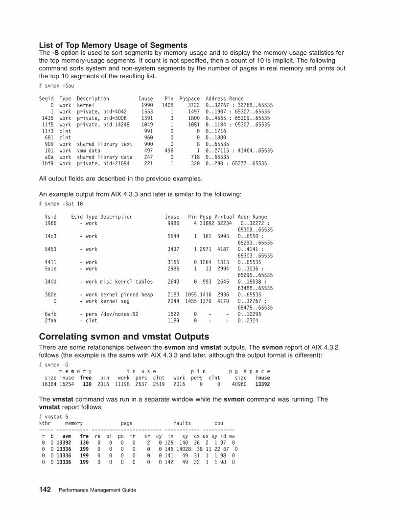
List of Top Memory Usage of SegmentsThe -S option is used to sort segments by memory usage and to display the memory-usage statistics forthe top memory-usage segments. If count is not specified, then a count of 10 is implicit. The followingcommand sorts system and non-system segments by the number of pages in real memory and prints outthe top 10 segments of the resulting list.# svmon -Sau

Segid Type Description Inuse Pin Pgspace Address Range0 work kernel 1990 1408 3722 0..32767 : 32768..655351 work private, pid=4042 1553 1 1497 0..1907 : 65307..65535

1435 work private, pid=3006 1391 3 1800 0..4565 : 65309..6553511f5 work private, pid=14248 1049 1 1081 0..1104 : 65307..6553511f3 clnt 991 0 0 0..1716681 clnt 960 0 0 0..1880909 work shared library text 900 0 8 0..65535101 work vmm data 497 496 1 0..27115 : 43464..65535a0a work shared library data 247 0 718 0..655351bf9 work private, pid=21094 221 1 320 0..290 : 65277..65535

All output fields are described in the previous examples.

An example output from AIX 4.3.3 and later is similar to the following:# svmon -Sut 10

Vsid Esid Type Description Inuse Pin Pgsp Virtual Addr Range1966 - work 9985 4 31892 32234 0..32272 :

65309..6553514c3 - work 5644 1 161 5993 0..6550 :

65293..655355453 - work 3437 1 2971 4187 0..4141 :

65303..655354411 - work 3165 0 1264 1315 0..655355a1e - work 2986 1 13 2994 0..3036 :

65295..65535340d - work misc kernel tables 2643 0 993 2645 0..15038 :

63488..65535380e - work kernel pinned heap 2183 1055 1416 2936 0..65535

0 - work kernel seg 2044 1455 1370 4170 0..32767 :65475..65535

6afb - pers /dev/notes:92 1522 0 - - 0..102952faa - clnt 1189 0 - - 0..2324

Correlating svmon and vmstat OutputsThere are some relationships between the svmon and vmstat outputs. The svmon report of AIX 4.3.2follows (the example is the same with AIX 4.3.3 and later, although the output format is different):# svmon -G

m e m o r y i n u s e p i n p g s p a c esize inuse free pin work pers clnt work pers clnt size inuse

16384 16254 130 2016 11198 2537 2519 2016 0 0 40960 13392

The vmstat command was run in a separate window while the svmon command was running. Thevmstat report follows:# vmstat 5kthr memory page faults cpu----- ----------- ------------------------ ------------ -----------r b avm fre re pi po fr sr cy in sy cs us sy id wa0 0 13392 130 0 0 0 0 2 0 125 140 36 2 1 97 00 0 13336 199 0 0 0 0 0 0 145 14028 38 11 22 67 00 0 13336 199 0 0 0 0 0 0 141 49 31 1 1 98 00 0 13336 199 0 0 0 0 0 0 142 49 32 1 1 98 0


0 0 13336 199 0 0 0 0 0 0 145 49 32 1 1 99 00 0 13336 199 0 0 0 0 0 0 163 49 33 1 1 92 60 0 13336 199 0 0 0 0 0 0 142 49 32 0 1 98 0

The global svmon report shows related numbers. The vmstatfre column relates to the svmon memoryfree column. The number that vmstat reports as Active Virtual Memory (avm) is reported by the svmoncommand as pg space inuse (13392).

The vmstat avm column provides the same figures as the pg space inuse column of the svmon commandexcept starting with AIX 4.3.2 where Deferred Page Space Allocation is used. In that case, the svmoncommand shows the number of pages actually paged out to paging space whereas the vmstat commandshows the number of virtual pages accessed but not necessarily paged out (see Looking at Paging Spaceand Virtual Memory).

Correlating svmon and ps OutputsThere are some relationships between the svmon and ps outputs. The svmon report of AIX 4.3.2 follows(the example is the same with AIX 4.3.3 and later, although the output format is different):# svmon -P 7226

Pid Command Inuse Pin Pgspace7226 telnetd 936 1 69

Pid: 7226Command: telnetd

Segid Type Description Inuse Pin Pgspace Address Range828 pers /dev/hd2:15333 0 0 0 0..01d3e work lib data 0 0 28 0..559909 work shared library text 930 0 8 0..655351cbb work sreg[3] 0 0 1 0..01694 work private 6 1 32 0..24 : 65310..6553512f6 pers code,/dev/hd2:69914 0 0 0 0..11

Compare with the ps report, which follows:# ps v 7226

PID TTY STAT TIME PGIN SIZE RSS LIM TSIZ TRS %CPU %MEM COMMAND7226 - A 0:00 51 240 24 32768 33 0 0.0 0.0 telnetd

SIZE refers to the virtual size in KB of the data section of the process (in paging space). This number isequal to the number of working segment pages of the process that have been touched (that is, the numberof paging-space pages that have been allocated) times 4. It must be multiplied by 4 because pages are in4 K units and SIZE is in 1 K units. If some working segment pages are currently paged out, this number islarger than the amount of real memory being used. The SIZE value (240) correlates with the Pgspacenumber from the svmon command for private (32) plus lib data (28) in 1 K units.

RSS refers to the real memory (resident set) size in KB of the process. This number is equal to the sum ofthe number of working segment and code segment pages in memory times 4. Remember that codesegment pages are shared among all of the currently running instances of the program. If 26 kshprocesses are running, only one copy of any given page of the ksh executable program would be inmemory, but the ps command would report that code segment size as part of the RSS of each instance ofthe ksh program. The RSS value (24) correlates with the Inuse numbers from the svmon command forprivate (6) working-storage segments, for code (0) segments, and for lib data (0) of the process in 1-Kunits.

TRS refers to the size of the resident set (real memory) of text. This is the number of code segment pagestimes four. As was noted earlier, this number exaggerates memory use for programs of which multipleinstances are running. This does not include the shared text of the process. The TRS value (0) correlates


with the number of the svmon pages in the code segment (0) of the Inuse column in 1 K units. The TRSvalue can be higher than the TSIZ value because other pages, such as the XCOFF header and the loadersection, may be included in the code segment.

The following calculations can be made for the values mentioned:SIZE = 4 * Pgspace of (work lib data + work private)RSS = 4 * Inuse of (work lib data + work private + pers code)TRS = 4 * Inuse of (pers code)

Calculating the Minimum Memory Requirement of a ProgramTo calculate the minimum memory requirement of a program, the formula would be:Total memory pages (4 KB units) = T + ( N * ( PD + LD ) ) + F

where:

T = Number of pages for text (shared by all users)

N = Number of copies of this program running simultaneously

PD = Number of working segment pages in process private segment

LD = Number of shared library data pages used by the process

F = Number of file pages (shared by all users)

Multiply the result by 4 to obtain the number of kilobytes required. You may want to add in the kernel,kernel extension, and shared library text segment values to this as well even though they are shared by allprocesses on the system. For example, some applications like CATIA and databases use very largeshared library modules. Note that because we have only used statistics from a single snapshot of theprocess, there is no guarantee that the value we get from the formula will be the correct value for theminimum working set size of a process. To get working set size, one would need to run a tool such as thermss command or take many snapshots during the life of the process and determine the average valuesfrom these snapshots (see Assessing Memory Requirements Through the rmss Command).

If we estimate the minimum memory requirement for the program pacman, shown in FindingMemory-Leaking Programs, the formula would be:

T = 2 (Inuse of code,/dev/lv01:12302 of pers)

PD = 1632 (Inuse of private of work)

LD = 12 (Inuse of lib data of work)

F = 1 (Inuse of /dev/hd2:53289 of pers)

That is: 2 + (N * (1632+ 12)) + 1, equal to 1644 * N + 3 in 4 KB units.

Finding Memory-Leaking ProgramsA memory leak is a program error that consists of repeatedly allocating memory, using it, and thenneglecting to free it. A memory leak in a long-running program, such as an interactive application, is aserious problem, because it can result in memory fragmentation and the accumulation of large numbers ofmostly garbage-filled pages in real memory and page space. Systems have been known to run out ofpage space because of a memory leak in a single program.

A memory leak can be detected with the svmon command, by looking for processes whose workingsegment continually grows. A leak in a kernel segment can be caused by an mbuf leak or by a devicedriver, kernel extension, or even the kernel. To determine if a segment is growing, use the svmoncommand with the -i option to look at a process or a group of processes and see if any segment continuesto grow.


Identifying the offending subroutine or line of code is more difficult, especially in AIXwindows applications,which generate large numbers of malloc() and free() calls. C++ provides a HeapView Debugger foranalyzing/tuning memory usage and leaks. Some third-party programs exist for analyzing memory leaks,but they require access to the program source code.

Some uses of the realloc() subroutine, while not actually programming errors, can have the same effectas a memory leak. If a program frequently uses the realloc() subroutine to increase the size of a dataarea, the working segment of the process can become increasingly fragmented if the storage released bythe realloc() subroutine cannot be reused for anything else.

Use the disclaim() system call and free() call to release memory that is no longer required. Thedisclaim() system call must be called before the free() call. It wastes CPU time to free memory after thelast malloc() call, if the program will finish soon. When the program terminates, its working segment isdestroyed and the real memory page frames that contained working segment data are added to the freelist. The following example is a memory-leaking program; its Inuse, Pgspace, and Address Range of theprivate working segment are continually growing.

An output example from AIX 5.2 follows:# svmon -P 13548 -i 1 3

Pid Command Inuse Pin Pgsp Virtual 64-bit Mthrd LPage13548 pacman 8535 2178 847 8533 N N N


48412 2 work process private - 2357 2 0 23576c01b d work shared library text - 1790 0 0 17904c413 f work shared library data - 11 0 0 113040c 1 pers code,/dev/mattlv:4097 - 2 0 - -ginger :svmon -P 13548 -i 1 3



48412 2 work process private - 2411 2 0 24116c01b d work shared library text - 1790 0 0 17904c413 f work shared library data - 11 0 0 113040c 1 pers code,/dev/mattlv:4097 - 2 0 - -



48412 2 work process private - 2421 2 0 24216c01b d work shared library text - 1790 0 0 17904c413 f work shared library data - 11 0 0 113040c 1 pers code,/dev/mattlv:4097 - 2 0 - -

Assessing Memory Requirements Through the rmss CommandThe rmss (Reduced-Memory System Simulator) command provides you with a means to simulate differentsizes of real memories that are smaller than your actual machine, without having to extract and replacememory boards. Moreover, the rmss command provides a facility to run an application over a range ofmemory sizes, displaying, for each memory size, performance statistics such as the response time of theapplication and the amount of paging. The rmss command is designed to help you answer the question:“How many megabytes of real memory does a system need to run the operating system and a given


application with an acceptable level of performance?”. In the multiuser context, it is designed to help youanswer the question: “How many users can run this application simultaneously in a machine with Xmegabytes of real memory?”

The main use for the rmss command is as a capacity planning tool, to determine how much memory aworkload needs. It can also be used as a problem determination tool, particularly for those cases wherehaving more memory degrades performance.

To determine whether the rmss command is installed and available, run the following command:# lslpp -lI fileset_name

where fileset_name is perfagent.tools in AIX 4.3 or bos.perf.tools in AIX 5 or later.

It is important to keep in mind that the memory size simulated by the rmss command is the total size ofthe machine’s real memory, including the memory used by the operating system and any other programsthat may be running. It is not the amount of memory used specifically by the application itself. Because ofthe performance degradation it can cause, the rmss command can be used only by a root user or amember of the system group.

Two Styles of Using rmssThe rmss command can be invoked in two ways:

1. To change the memory size and exit.

2. As a driver program, which executes a specified application multiple times over a range of memorysizes and displays important statistics that describe the application’s performance at each memorysize.

The first invocation technique is useful when you want to get the look and feel of how your applicationperforms at a given system memory size, when your application is too complex to be expressed as asingle command, or when you want to run multiple instances of the application. The second invocationtechnique is appropriate when you have an application that can be invoked as an executable program orshell script file.

Note: Before using the rmss command, run the command /usr/samples/kernel/schedtune -h 0 to turnoff VMM memory-load control (see Tuning VMM Memory Load Control with the schedtuneCommand). Otherwise, VMM memory-load control may interfere with your measurements at smallmemory sizes. When your experiments are complete, reset the memory load control parameters tothe values that are typically in effect on your system (if you typically use the default parameters,use /usr/samples/kernel/schedtune -D).

Using rmss to Change the Memory Size and ExitTo change the memory size and exit, use the -c flag. For example, to change the memory size to 128 MB,use the following:# rmss -c 128

The memory size is an integer or decimal fraction number of megabytes (for example, 128.25).Additionally, the size must be between 8 MB and the amount of physical real memory in your machine.Depending on the hardware and software configuration, the rmss command may not be able to changethe memory size to small sizes, because of the size of inherent system structures such as the kernel.When the rmss command is unable to change to a given memory size, it displays an error message.

The rmss command reduces the effective memory size of a system by stealing free page frames from thelist of free frames that is maintained by the VMM. The stolen frames are kept in a pool of unusable framesand are returned to the free frame list when the effective memory size is to be increased. Also, the rmsscommand dynamically adjusts certain system variables and data structures that must be kept proportionalto the effective size of memory.


It may take a short while (up to 15 to 20 seconds) to change the memory size. In general, the more youwant to reduce the memory size, the longer the rmss command takes to complete. When successful, thermss command responds with the following message:Simulated memory size changed to 128.00 Mb.

To display the current memory size, use the -p flag, as follows:# rmss -p

The rmss output is as follows:Simulated memory size is 128.00 Mb.

Finally, if you want to reset the memory size to the actual memory size of the machine, use the -r flag, asfollows:# rmss -r

No matter what the current simulated memory size, using the -r flag sets the memory size to be thephysical real memory size of the machine. A side effect of the rmss -r command is that the relatedvmtune parameters are also reset to their corresponding defaults.

Because this example was run on a 256 MB machine, the rmss command responded as follows:Simulated memory size changed to 256.00 Mb.

Note: The rmss command reports usable real memory. On machines that contain bad memory ormemory that is in use, the rmss command reports the amount of real memory as the amount ofphysical real memory minus the memory that is bad or in use by the system. For example, thermss -r command might report:Simulated memory size changed to 79.9062 Mb.

This could be a result of some pages being marked bad or a result of a device that is reservingsome pages for its own use (and thus not available to the user).

Using the -c, -p, and -r Flags: The -c, -p and -r flags of the rmss command have an advantage overthe other options in that they allow you to experiment with complex applications that cannot be expressedas a single executable program or shell script file. On the other hand, the -c, -p, and -r options have adisadvantage in that they force you to do your own performance measurements. Fortunately, you can usethe command vmstat -s to measure the paging-space activity that occurred while your application ran.

By running the command vmstat -s, running your application, then running the command vmstat -s again,and subtracting the number of paging-space page-ins before from the number of paging-space page-insafter, you can determine the number of paging-space page-ins that occurred while your program ran.Furthermore, by timing your program, and dividing the number of paging-space page-ins by the program’selapsed run time, you can obtain the average paging-space page-in rate.

It is also important to run the application multiple times at each memory size, for two reasons:

v When changing memory size, the rmss command often clears out a lot of memory. Thus, the first timeyou run your application after changing memory sizes it is possible that a substantial part of the runtime may be due to your application reading files into real memory. But, since the files may remain inmemory after your application terminates, subsequent executions of your application may result insubstantially shorter elapsed times.

v To get a feel for the average performance of the application at that memory size. It is impossible toduplicate the system state each time your application runs. Because of this, the performance of yourapplication can vary significantly from run to run.

To summarize, consider the following set of steps as a desirable way to invoke the rmss command:


while there are interesting memory sizes to investigate:{change to an interesting memory size using rmss -c;run the application once as a warm-up;for a couple of iterations:

{use vmstat -s to get the "before" value of paging-space page ins;run the application, while timing it;use vmstat -s to get the "after" value of paging-space page ins;subtract the "before" value from the "after" value to get the

number of page ins that occurred while the application ran;divide the number of paging-space page ins by the response time

to get the paging-space page-in rate;}

}run rmss -r to restore the system to normal memory size (or reboot)

The calculation of the (after - before) paging I/O numbers can be automated by using the vmstatit scriptdescribed in Determining Whether the Problem is Related to Disk or Memory.

Using rmss to Run a Command over a Range of Memory SizesThe -s, -f, -d, -n, and -o flags are used in combination to invoke the rmss command as a driver program.As a driver program, the rmss command executes a specified application over a range of memory sizesand displays statistics describing the application’s performance at each memory size. The syntax for thisinvocation style of the rmss command is as follows:rmss [ -s smemsize ] [ -f fmemsize ] [ -d memdelta ]

[ -n numiterations ] [ -o outputfile ] command

Each of the following flags is discussed in detail below. The -s, -f, and -d flags are used to specify therange of memory sizes.

-n This flag is used to specify the number of times to run and measure the command at eachmemory size.

-o This flag is used to specify the file into which to write the rmss report, while command is theapplication that you wish to run and measure at each memory size.

-s This flag specifies the starting size.

-f This flag specifies the final size.

-d This flag specifies the difference between sizes.

All values are in integer or decimal fractions of megabytes. For example, if you wanted to run andmeasure a command at sizes 256, 224, 192, 160 and 128 MB, you would use the following combination:-s 256 -f 128 -d 32

Likewise, if you wanted to run and measure a command at 128, 160, 192, 224, and 256 MB, you woulduse the following combination:-s 128 -f 256 -d 32

If the -s flag is omitted, the rmss command starts at the actual memory size of the machine. If the -f flagis omitted, the rmss command finishes at 8 MB. If the -d flag is omitted, there is a default of 8 MBbetween memory sizes.

What values should you choose for the -s, -f, and -d flags? A simple choice would be to cover the memorysizes of systems that are being considered to run the application you are measuring. However, incrementsof less than 8 MB can be useful, because you can get an estimate of how much space you will have whenyou settle on a given size. For instance, if a given application thrashes at 120 MB but runs withoutpage-ins at 128 MB, it would be useful to know where within the 120 to 128 MB range the applicationstarts thrashing. If it starts at 127 MB, you may want to consider configuring the system with more than


128 MB of memory, or you may want to try to modify the application so that there is more space. On theother hand, if the thrashing starts at 121 MB, you know that you have enough space with a 128 MBmachine.

The -n flag is used to specify how many times to run and measure the command at each memory size.After running and measuring the command the specified number of times, the rmss command displaysstatistics describing the average performance of the application at that memory size. To run the command3 times at each memory size, you would use the following:-n 3

If the -n flag is omitted, the rmss command determines during initialization how many times yourapplication must be run to accumulate a total run time of 10 seconds. The rmss command does this toensure that the performance statistics for short-running programs will not be significantly skewed byoutside influences, such as daemons.

Note: If you are measuring a very brief program, the number of iterations required to accumulate 10seconds of CPU time can be very large. Because each execution of the program takes a minimumof about 2 elapsed seconds of rmss overhead, specify the -n parameter explicitly for shortprograms.

What are good values to use for the -n flag? If you know that your application takes much more than 10seconds to run, you can specify -n 1 so that the command is run twce, but measured only once at eachmemory size. The advantage of using the -n flag is that the rmss command will finish sooner because itwill not have to spend time during initialization to determine how many times to run your program. This canbe particularly valuable when the command being measured is long-running and interactive.

It is important to note that the rmss command always runs the command once at each memory size as awarm-up before running and measuring the command. The warm-up is needed to avoid the I/O that occurswhen the application is not already in memory. Although such I/O does affect performance, it is notnecessarily due to a lack of real memory. The warm-up run is not included in the number of iterationsspecified by the -n flag.

The -o flag is used to specify a file into which to write the rmss report. If the -o flag is omitted, the reportis written into the file rmss.out.

Finally, command is used to specify the application to be measured. It can be an executable program orshell script, with or without command-line arguments. There are some limitations on the form of thecommand however. First, it cannot contain the redirection of input or output (for example, foo > output orfoo < input). This is because the rmss command treats everything to the right of the command name asan argument to the command. To redirect, place the command in a shell script file.

Usually, if you want to store the rmss output in a specific file, use the -o option. If you want to redirect thestandard output of the rmss command (for example, to concatenate it to the end of an existing file) thenuse the Korn shell to enclose the rmss invocation in parentheses, as follows:# (rmss -s 24 -f 8 foo) >> output

Interpreting rmss ResultsThe Report Generated for the foo Program example was produced by running the rmss command on anactual application program, although the name of the program has been changed to foo for anonymity.The specific command that would have been used to generate the report is as follows:# rmss -s 16 -f 8 -d 1 -n 1 -o rmss.out foo


Report Generated for the foo ProgramHostname: widgeon.austin.ibm.comReal memory size: 16.00 MbTime of day: Thu Jan 6 19:04:04 2000Command: foo

Simulated memory size initialized to 16.00 Mb.

Number of iterations per memory size = 1 warm-up + 1 measured = 2.

Memory size Avg. Pageins Avg. Response Time Avg. Pagein Rate(megabytes) (sec.) (pageins / sec.)-----------------------------------------------------------------16.00 115.0 123.9 0.915.00 112.0 125.1 0.914.00 179.0 126.2 1.413.00 81.0 125.7 0.612.00 403.0 132.0 3.111.00 855.0 141.5 6.010.00 1161.0 146.8 7.99.00 1529.0 161.3 9.58.00 2931.0 202.5 14.5

The report consists of four columns. The leftmost column gives the memory size, while the Avg. Pageinscolumn gives the average number of page-ins that occurred when the application was run at that memorysize. It is important to note that the Avg. Pageins column refers to all page-in operations, including code,data, and file reads, from all programs, that completed while the application ran. The Avg. Response Timecolumn gives the average amount of time it took the application to complete, while the Avg. Pagein Ratecolumn gives the average rate of page-ins.

Concentrate on the Avg. Pagein Rate column. From 16 MB to 13 MB, the page-in rate is relatively small(< 1.5 page-ins per second). However, from 13 MB to 8 MB, the page-in rate grows gradually at first, andthen rapidly as 8 MB is reached. The Avg. Response Time column has a similar shape: relatively flat atfirst, then increasing gradually, and finally increasing rapidly as the memory size is decreased to 8 MB.

Here, the page-in rate actually decreases when the memory size changes from 14 MB (1.4 page-ins persecond) to 13 MB (0.6 page-ins per second). This is not cause for alarm. In an actual system, it isimpossible to expect the results to be perfectly smooth. The important point is that the page-in rate isrelatively low at both 14 MB and 13 MB.

Finally, you can make a couple of deductions from the report. First, if the performance of the application isdeemed unacceptable at 8 MB (as it probably would be), then adding memory would enhanceperformance significantly. Note that the response time rises from approximately 124 seconds at 16 MB to202 seconds at 8 MB, an increase of 63 percent. On the other hand, if the performance is deemedunacceptable at 16 MB, adding memory will not enhance performance much, because page-ins do notslow the program appreciably at 16 MB.

Report for a 16 MB Remote CopyThe following example illustrates a report that was generated (on a client machine) by running the rmsscommand on a command that copied a 16 MB file from a remote (server) machine through NFS.Hostname: xray.austin.ibm.comReal memory size: 48.00 MbTime of day: Mon Jan 10 18:16:42 2000Command: cp /mnt/a16Mfile /dev/null

Simulated memory size initialized to 48.00 Mb.

Number of iterations per memory size = 1 warm-up + 4 measured = 5.

Memory size Avg. Pageins Avg. Response Time Avg. Pagein Rate(megabytes) (sec.) (pageins / sec.)


-----------------------------------------------------------------48.00 0.0 2.7 0.040.00 0.0 2.7 0.032.00 0.0 2.7 0.024.00 1520.8 26.9 56.616.00 4104.2 67.5 60.88.00 4106.8 66.9 61.4

Note that the response time and page-in rate in this report start relatively low, rapidly increase at amemory size of 24 MB, and then reach a plateau at 16 and 8 MB. This report shows the importance ofchoosing a wide range of memory sizes when you use the rmss command. If this user had only looked atmemory sizes from 24 MB to 8 MB, he or she might have missed an opportunity to configure the systemwith enough memory to accommodate the application without page-ins.

Hints for Using the -s, -f, -d, -n, and -o FlagsOne helpful feature of the rmss command, when used in this way, is that it can be terminated (by theinterrupt key, Ctrl-C by default) without destroying the report that has been written to the output file. Inaddition to writing the report to the output file, this causes the rmss command to reset the memory size tothe physical memory size of the machine.

You can run the rmss command in the background, even after you have logged out, by using the nohupcommand. To do this, precede the rmss command by the nohup command, and follow the entirecommand with an & (ampersand), as follows:# nohup rmss -s 48 -f 8 -o foo.out foo &

Guidelines to Consider When Running the rmss CommandNo matter which rmss invocation style you are using, it is important to re-create the end-user environmentas closely as possible. For instance, are you using the same model CPU, the same model disks, the samenetwork? Will the users have application files mounted from a remote node via NFS or some otherdistributed file system? This last point is particularly important, because pages from remote files aretreated differently by the VMM than pages from local files.

Likewise, it is best to eliminate any system activity that is not related to the desired system configuration orthe application you are measuring. For instance, you do not want to have people working on the samemachine as the rmss command unless they are running part of the workload you are measuring.

Note: You cannot run multiple invocations of the rmss command simultaneously.

When you have completed all runs of the rmss command, it is best to shut down and reboot the system.This will remove all changes that the rmss command has made to the system and will restore the VMMmemory load control parameters to their typical settings.

Tuning VMM Memory Load Control with the schedtune CommandThe VMM memory load control facility, described in VMM Memory Load Control Facility, protects anoverloaded system from thrashing.

For early versions of the operating system, if a large number of processes hit the system at the sametime, memory became overcommitted and thrashing occurred, causing performance to degrade rapidly. Amemory-load control mechanism was developed that could detect thrashing. Certain parameters affect thefunction of the load control mechanism.

With the schedtune command, the root user can affect the criteria used to determine thrashing, thecriteria used to determine which processes to suspend, the length of time to wait after thrashing endsbefore reactivating processes, the minimum number of processes exempt from suspension, or reset valuesto the defaults. To determine whether the schedtune command is installed and available, run the followingcommand:


# lslpp -lI bos.adt.samples

Memory Load Control TuningMemory load control is intended to smooth out infrequent peaks in load that might otherwise cause thesystem to thrash. It trades multiprogramming for throughput and is not intended to act continuously in aconfiguration that has too little RAM to handle its normal workload. The design was made for batch jobsand is not very discriminating. The AIX Workload Manager provides a better solution to protect criticaltasks.

The correct solution to a fundamental, persistent RAM shortage is to add RAM, not to experiment withmemory load control in an attempt to trade off response time for memory. The situations in which thememory-load-control facility may really need to be tuned are those in which there is more RAM, not lessthan the defaults were chosen for. An example would be configurations in which the defaults are tooconservative.

You should not change the memory load control parameter settings unless your workload is consistent andyou believe the default parameters are ill-suited to your workload.

The default parameter settings shipped with the system are always in force unless changed. The defaultvalues of these parameters have been chosen to ″fail safe″ across a wide range of workloads. Changedparameters last only until the next system boot. All memory load control tuning activities must be done bythe root user. The system administrator can use the schedtune command to change the parameters totune the algorithm to a particular workload or to disable it entirely. The source and object code of theschedtune command are in /usr/samples/kernel.

Note: The schedtune command is in the samples directory because it is very VMM-implementationdependent. The schedtune code that accompanies each release of the operating system is tailoredspecifically to the VMM in that release. Running the schedtune command from one release on adifferent release might result in an operating-system failure. It is also possible that the functions ofthe schedtune command may change from release to release. Do not propagate shell scripts or/etc/inittab entries that include the schedtune command to a new release without checking theschedtune documentation for the new release to make sure that the scripts will still have thedesired effect.

The schedtune -? command provides a terse description of the flags and options. A schedtune invocationwith no flags displays the current parameter settings, as follows:# /usr/samples/kernel/schedtune

THRASH SUSP FORK SCHED-h -p -m -w -e -f -d -r -t -sSYS PROC MULTI WAIT GRACE TICKS SCHED_D SCHED_R TIMESLICE MAXSPIN0 4 2 1 2 10 16 16 1 16384

CLOCK SCHED_FIFO2 IDLE MIGRATION FIXED_PRI-c -a -b -F

%usDELTA AFFINITY_LIM BARRIER/16 GLOBAL(1)100 7 4 0

The first five parameters specify the thresholds for the memory load control algorithm. These parametersset rates and thresholds for the algorithm. If the algorithm shows that RAM is overcommitted, the PROC(-p), MULTI (-m), WAIT (-w), and GRACE (-e) values are used. Otherwise, these values are ignored. Ifmemory load control is disabled, these latter values are not used.

After a tuning experiment, memory load control can be reset to its default characteristics by executing thecommand schedtune -D.


When you have determined the number of processes that ought to be able to run in your system duringperiods of peak activity, you can add a schedtune command at the end of the /etc/inittab file, whichensures that it will be run each time the system is booted, overriding the defaults that would otherwisetake effect with a reboot. For example, an appropriate /etc/inittab line for raising the minimum level ofmultiprogramming to 4 on an AIX Version 4 system would be as follows:schedtune:2:wait:/usr/samples/kernel/schedtune -m 4

Remember, do not propagated this line to a new release of the operating system without a check of theoperating system documentation.

While it is possible to vary other parameters that control the suspension rate of processes and the criteriaby which individual processes are selected for suspension, it is impossible to predict with any confidencethe effect of such changes on a particular configuration and workload. Great caution should be exercised ifmemory load control parameter adjustments other than those discussed here are considered.

The h ParameterThe h parameter controls the threshold defining memory overcommitment. Memory load control attemptsto suspend processes when this threshold is exceeded during any one-second period. The threshold is arelationship between two direct measures: the number of pages written to paging space in the last second(po) and the number of page steals occurring in the last second (fr). You can see both these values in thevmstat output. The number of page writes is usually much less than the number of page steals. Memoryis overcommitted when the following is true:po/fr > 1/h or po*h > fr

The command schedtune -h 0 effectively disables memory load control. If a system has at least 128 MBof memory, the default value is 0, otherwise the default value is 6. With at least 128 MB of RAM, thenormal VMM algorithms usually correct thrashing conditions on the average more efficiently than by usingmemory load control.

In some specialized situations, it might be appropriate to disable memory load control from the outset. Forexample, if you are using a terminal emulator with a time-out feature to simulate a multiuser workload,memory load control intervention may result in some responses being delayed long enough for theprocess to be killed by the time-out feature. Another example is, if you are using the rmss command toinvestigate the effects of reduced memory sizes, disable memory load control to avoid interference withyour measurement.

If disabling memory load control results in more, rather than fewer, thrashing situations (withcorrespondingly poorer responsiveness), then memory load control is playing an active and supportive rolein your system. Tuning the memory load control parameters then may result in improved performance oryou may need to add RAM.

A lower value of h raises the thrashing detection threshold; that is, the system is allowed to come closer tothrashing before processes are suspended. Regardless of the system configuration, when the above po/frfraction is low, thrashing is unlikely.

To alter the threshold to 4, enter the following:# /usr/samples/kernel/schedtune -h 4

In this way, you permit the system to come closer to thrashing before the algorithm starts suspendingprocesses.

The p ParameterThe p parameter determines whether a process is eligible for suspension and is used to set a threshold forthe ratio of two measures that are maintained for every process: the number of repages (r) and thenumber of page faults that the process has accumulated in the last second (f). A high ratio of repages to


page faults means the individual process is thrashing. A process is considered eligible for suspension (it isthrashing or contributing to overall thrashing) when the following is true:r/f > 1/p or r*p > f

The default value of p is 4, meaning that a process is considered to be thrashing (and a candidate forsuspension) when the fraction of repages to page faults over the last second is greater than 25 percent. Alow value of p results in a higher degree of individual process thrashing being allowed before a process iseligible for suspension.

To disable processes from being suspended by the memory load control, do the following:# /usr/samples/kernel/schedtune -p 0

Note that fixed-priority processes and kernel processes are exempt from being suspended.

The m ParameterThe m parameter determines a lower limit for the degree of multiprogramming, which is defined as thenumber of active processes. Active processes are those that can be run and are waiting for page I/O.Processes that are waiting for events and processes suspended are not considered active nor is the waitprocess considered active.

Setting the minimum multiprogramming level, m, effectively keeps m processes from being suspended.Suppose a system administrator knows that at least ten processes must always be resident and active inRAM for successful performance, and suspects that memory load control was too vigorously suspendingprocesses. If the command schedtune -m 10 was issued, the system would never suspend so manyprocesses that fewer than ten were competing for memory. The m parameter does not count:

v The kernel processes

v Processes that have been pinned in RAM with the plock() system call

v Fixed-priority processes with priority values less than 60

v Processes awaiting events

The system default of m=2 ensures that the kernel, all pinned processes, and two user processes willalways be in the set of processes competing for RAM.

While m=2 is appropriate for a desktop, single-user configuration, it is frequently too small for larger,multiuser, or server configurations with large amounts of RAM.

If the system you are installing is larger than 32 MB, but less than 128 MB, and is expected to supportmore than five active users at one time, consider raising the minimum level of multiprogramming of theVMM memory-load-control mechanism.

As an example, if your conservative estimate is that four of your most memory-intensive applicationsshould be able to run simultaneously, leaving at least 16 MB for the operating system and 25 percent ofreal memory for file pages, you could increase the minimum multiprogramming level from the default of 2to 4 with the following command:# /usr/samples/kernel/schedtune -m 4

On these systems, setting m to 4 or 6 may result in the best performance. Lower values of m, whileallowed, mean that at times as few as one user process may be active.

When the memory requirements of the thrashing application are known, the m value can be suitablychosen. Suppose thrashing is caused by numerous instances of one application of size M. Given thesystem memory size N, the m parameter should be set to a value close to N/M. Setting m too low wouldunnecessarily limit the number of processes that could be active at the same time.


The w ParameterThe w parameter controls the number of one-second intervals during which the po/fr fraction (explained inthe The h Parameter) must remain below 1/h before suspended processes are reactivated. The defaultvalue of one second is close to the minimum value allowed, which is zero. A value of one secondaggressively attempts to reactivate processes as soon as a one-second safe period has occurred. Largevalues of w run the risk of unnecessarily poor response times for suspended processes while theprocessor is idle for lack of active processes to run.

To alter the wait time to reactivate processes after two seconds, enter the following:# /usr/samples/kernel/schedtune -w 2

The e ParameterEach time a suspended process is reactivated, it is exempt from suspension for a period of e elapsedseconds. This ensures that the high cost (in disk I/O) of paging in the pages of a suspended processresults in a reasonable opportunity for progress. The default value of e is 2 seconds.

To alter this parameter, enter the following:# /usr/samples/kernel/schedtune -e 1

Suppose thrashing is caused occasionally by an application that uses lots of memory but runs for about Tseconds. The default system setting for e (2 seconds) would probably cause this application swapping inand out T/2 times on a busy system. In this case, resetting e to a longer time would help this application toprogress. System performance would improve when this offending application is pushed through quickly.

Tuning VMM Page Replacement with the vmtune CommandThe memory management algorithm, discussed in Real-Memory Management, tries to keep the size of thefree list and the percentage of real memory occupied by persistent segment pages within specifiedbounds. These bounds can be altered with the vmtune command, which can only be run by the root user.Changes made by this tool remain in effect until the next reboot of the system. To determine whether thevmtune command is installed and available, run the following command:# lslpp -lI bos.adt.samples

Note: The vmtune command is in the samples directory because it is very VMM-implementationdependent. The vmtune code that accompanies each release of the operating system is tailoredspecifically to the VMM in that release. Running the vmtune command from one release on adifferent release might result in an operating-system failure. It is also possible that the functions ofvmtune may change from release to release. Do not propagate shell scripts or /etc/inittab entriesthat include the vmtune command to a new release without checking the vmtune documentationfor the new release to make sure that the scripts will still have the desired effect.

Executing the vmtune command on AIX 4.3.3 with no options results in the following output:# /usr/samples/kernel/vmtunevmtune: current values:

-p -P -r -R -f -F -N -Wminperm maxperm minpgahead maxpgahead minfree maxfree pd_npages maxrandwrt

52190 208760 2 8 120 128 524288 0

-M -w -k -c -b -B -u -l -dmaxpin npswarn npskill numclust numfsbufs hd_pbuf_cnt lvm_bufcnt lrubucket defps

209581 4096 1024 1 93 96 9 131072 1

-s -n -S -hsync_release_ilock nokillroot v_pinshm strict_maxperm

0 0 0 0


number of valid memory pages = 261976 maxperm=79.7% of real memorymaximum pinable=80.0% of real memory minperm=19.9% of real memorynumber of file memory pages = 19772 numperm=7.5% of real memory

The output shows the current settings for all the parameters.

Executing the vmtune command on AIX 5.2 results in the following output:# /usr/samples/kernel/vmtunevmtune: current values:

-M -p -P -t -f -F -lmaxpin% minperm% maxperm% maxclient% minfree maxfree lrubucket

80.1 20.0 80.0 80.0 120 128 131072

-r -R -N -W -w -k -cminpgahead maxpgahead pd_npages maxrandwrt npswarn npskill numclust

2 8 65536 0 4096 1024 1

-b -B -u -d -s -Snumfsbufs hd_pbuf_cnt lvm_bufcnt defps sync_release_ilock v_pinshm

186 448 9 1 0 0

-L -g -h -n -jlgpg_regions lgpg_size strict_maxperm nokilluid j2_nPagesPerWriteBehindCluster

0 0 0 0 8

-J -z -Zj2_maxRandomWrite j2_nRandomCluster j2_nBufferPerPagerDevice

0 0 512

-q -Q -V -ij2_minPageReadAhead j2_maxPageReadAhead num_spec_dataseg spec_dataseg_int

2 8 0 512

-ymem_affinity_on

0

maxpin pages = 838861 minperm pages = 199609memory size pages = 1048576 maxperf pages = 798436remote pageouts scheduled 0 maxclient pages = 798436file pages 7690 numperm = 0.7% of real memorycompressed pages = 0 numcompress= 0.0% of real memoryclient pages = 0 numclient= 0.0% of real memory

Choosing minfree and maxfree SettingsThe purpose of the free list is to keep track of real-memory page frames released by terminatingprocesses and to supply page frames to requestors immediately, without forcing them to wait for pagesteals and the accompanying I/O to complete. The minfree limit specifies the free-list size below whichpage stealing to replenish the free list is to be started. The maxfree parameter is the size above whichstealing will end.

The objectives in tuning these limits are to ensure that:

v Any activity that has critical response-time objectives can always get the page frames it needs from thefree list.

v The system does not experience unnecessarily high levels of I/O because of premature stealing ofpages to expand the free list.

The default value of minfree and maxfree depend on the memory size of the machine. The default valueof maxfree is determined by this formula:maxfree = minimum (# of memory pages/128, 128)


By default the minfree value is the value of maxfree - 8. However, the difference between minfree andmaxfree should always be equal to or greater than maxpgahead. Or in other words, the value of maxfreeshould always be greater than or equal to minfree plus the size of maxpgahead. The minfree/maxfreevalues will be different if there is more than one memory pool. Memory pools were introduced in AIX 4.3.3for MP systems with large amounts of RAM. Each memory pool will have its own minfree/maxfree whichare determined by the previous formulas, but the minfree/maxfree values shown by the vmtunecommand will be the sum of the minfree/maxfree for all memory pools.

Remember, that minfree pages in some sense are wasted, because they are available, but not in use. Ifyou have a short list of the programs you want to run fast, you can investigate their memory requirementswith the svmon command (see Determining How Much Memory Is Being Used), and set minfree to thesize of the largest. This technique risks being too conservative because not all of the pages that a processuses are acquired in one burst. At the same time, you might be missing dynamic demands that come fromprograms not on your list that may lower the average size of the free list when your critical programs run.

A less precise but more comprehensive tool for investigating an appropriate size for minfree is the vmstatcommand. The following is a portion of a vmstat command output obtained while running an Ccompilation on an otherwise idle system.# vmstat 1kthr memory page faults cpu----- ----------- ------------------------ ------------ -----------r b avm fre re pi po fr sr cy in sy cs us sy id wa0 0 3085 118 0 0 0 0 0 0 115 2 19 0 0 99 00 0 3086 117 0 0 0 0 0 0 119 134 24 1 3 96 02 0 3141 55 2 0 6 24 98 0 175 223 60 3 9 54 340 1 3254 57 0 0 6 176 814 0 205 219 110 22 14 0 640 1 3342 59 0 0 42 104 249 0 163 314 57 43 16 0 421 0 3411 78 0 0 49 104 169 0 176 306 51 30 15 0 551 0 3528 160 1 0 10 216 487 0 143 387 54 50 22 0 271 0 3627 94 0 0 0 72 160 0 148 292 79 57 9 0 341 0 3444 327 0 0 0 64 102 0 132 150 41 82 8 0 111 0 3505 251 0 0 0 0 0 0 128 189 50 79 11 0 111 0 3550 206 0 0 0 0 0 0 124 150 22 94 6 0 01 0 3576 180 0 0 0 0 0 0 121 145 30 96 4 0 00 1 3654 100 0 0 0 0 0 0 124 145 28 91 8 0 11 0 3586 208 0 0 0 40 68 0 123 139 24 91 9 0 0

Because the compiler has not been run recently, the code of the compiler itself must be read in. All told,the compiler acquires about 2 MB in about 6 seconds. On this 32 MB system, maxfree is 64 and minfreeis 56. The compiler almost instantly drives the free list size below minfree, and several seconds of rapidpage-stealing activity take place. Some of the steals require that dirty working segment pages be written topaging space, which shows up in the po column. If the steals cause the writing of dirty permanent segmentpages, that I/O does not appear in the vmstat report (unless you have directed the vmstat command toreport on the I/O activity of the physical volumes to which the permanent pages are being written).

This example describes a fork() and exec() environment (not an environment where a process is longlived, such as in a database) and is not intended to suggest that you set minfree to 500 to accommodatelarge compiles. It suggests how to use the vmstat command to identify situations in which the free list hasto be replenished while a program is waiting for space. In this case, about 2 seconds were added to thecompiler execution time because there were not enough page frames immediately available. If youobserve the page frame consumption of your program, either during initialization or during normalprocessing, you will soon have an idea of the number page frames that need to be in the free list to keepthe program from waiting for memory.

If we concluded from the example above that minfree needed to be 128, and we had set maxpgahead to16 to improve sequential performance, we would use the following vmtune command:# /usr/samples/kernel/vmtune -f 128 -F 144


Tuning Memory PoolsIn operating system versions later than AIX 4.3.3, the vmtune -m number_of_memory_pools commandallows you to change the number of memory pools that are configured at system boot time. The -m flag istherefore not a dynamic change. The change is written to the kernel file if it is an MP kernel (the change isnot allowed on a UP kernel). A value of 0 restores the default number of memory pools.

By default, the vmtune -m command writes to the /usr/lib/boot/unix_mp file (/usr/lib/boot/unix_64 ifrunning on a 64–bit kernel), but this can be changed with the command vmtune -U path_to_unix_file.Before changing the kernel file, the vmtune command saves the original file as name_of_original_file.sav.

Tuning lrubucket to Reduce Memory Scanning OverheadTuning lrubucket can reduce scanning overhead on large memory systems. In AIX 4.3, a new parameterlrubucket was added. The page-replacement algorithm scans memory frames looking for a free frame.During this scan, reference bits of pages are reset, and if a free frame has not been found, a second scanis done. In the second scan, if the reference bit is still off, the frame will be used for a new page (pagereplacement).

On large memory systems, there may be too many frames to scan, so now memory is divided up intobuckets of frames. The page-replacement algorithm will scan the frames in the bucket and then start overon that bucket for the second scan before moving on to the next bucket. The default number of frames inthis bucket is 131072 or 512 MB of RAM. The number of frames is tunable with the command vmtune -l,and the value is in 4 K frames.

Choosing minperm and maxperm SettingsThe operating system takes advantage of the varying requirements for real memory by leaving in memorypages of files that have been read or written. If the file pages are requested again before their pageframes are reassigned, this technique saves an I/O operation. These file pages may be from local orremote (for example, NFS) file systems.

The ratio of page frames used for files versus those used for computational (working or program text)segments is loosely controlled by the minperm and maxperm values:

v If percentage of RAM occupied by file pages rises above maxperm, page-replacement steals only filepages.

v If percentage of RAM occupied by file pages falls below minperm, page-replacement steals both fileand computational pages.

v If percentage of RAM occupied by file pages is between minperm and maxperm, page-replacementsteals only file pages unless the number of file repages is higher than the number of computationalrepages.

In a particular workload, it might be worthwhile to emphasize the avoidance of file I/O. In anotherworkload, keeping computational segment pages in memory might be more important. To understand whatthe ratio is in the untuned state, we use the vmtune command with no arguments.# /usr/samples/kernel/vmtunevmtune: current values:

-p -P -r -R -f -F -N -Wminperm maxperm minpgahead maxpgahead minfree maxfree pd_npages maxrandwrt209508 838032 2 8 120 128 524288 0

-M -w -k -c -b -B -u -l -dmaxpin npswarn npskill numclust numfsbufs hd_pbuf_cnt lvm_bufcnt lrubucket defps838852 4096 1024 1 186 160 9 131072 1

-s -n -S -L -g -hsync_release_ilock nokilluid v_pinshm lgpa_regions lgpg_size strict_maxperm

0 0 0 0 0 0


-tmaxclient

838032

number of valid memory pages = 1048565 maxperm=79.9% of real memorymaximum pinable = 80.0% of real memory minperm=20.0% of real memorynumber of file memory pages = 6668 numperm=0.6% of real memorynumber of compressed memory pages = 0 compressed=0.0% of real memorynumber of client memory pages = 0 numclient=0.0% of real memory# of remote pgs sched-pageout = 0 maxcllient=79.9% of real memory

The default values are calculated by the following algorithm:minperm (in pages) = ((number of memory frames) - 1024) * .2maxperm (in pages) = ((number of memory frames) - 1024) * .8

The numperm value gives the number of file pages in memory, 19772. This is 7.5 percent of real memory.

If we know that our workload makes little use of recently read or written files, we may want to constrainthe amount of memory used for that purpose. The following command:# /usr/samples/kernel/vmtune -p 15 -P 50

sets minperm to 15 percent and maxperm to 50 percent of real memory. This would ensure that the VMMwould steal page frames only from file pages when the ratio of file pages to total memory pages exceeded50 percent. This should reduce the paging to page space with no detrimental effect on the persistentstorage. The maxperm value is not a strict limit, it is only considered when the VMM needs to performpage replacement. Because of this, it is usually safe to reduce the maxperm value on most systems.

On the other hand, if our application frequently references a small set of existing files (especially if thosefiles are in an NFS-mounted file system), we might want to allow more space for local caching of the filepages by using the following command:# /usr/samples/kernel/vmtune -p 30 -P 90

NFS servers that are used mostly for reads with large amounts of RAM can benefit from increasing thevalue of maxperm. This allows more pages to reside in RAM so that NFS clients can access them withoutforcing the NFS server to retrieve the pages from disk again.

Another example would be a program that reads 1.5 GB of sequential file data into the working storage ofa system with 2 GB of real memory. You may want to set maxperm to 50 percent or less, because you donot need to keep the file data in memory.

Placing a Hard Limit on Persistent File Cache with strict_maxpermStarting with AIX 4.3.3, a new vmtune option (-h) called strict_maxperm has been added. This option,when set to 1, places a hard limit on how much memory is used for a persistent file cache by making themaxperm value be the upper limit for this file cache. When the upper limit is reached, the least recentlyused (LRU) is performed on persistent pages.

Attention: The strict_maxperm option should only be enabled for those cases that require a hard limiton the persistent file cache. Improper use of strict_maxperm can cause unexpected system behaviorbecause it changes the VMM method of page replacement.

Placing a Hard Limit on Enhanced JFS File System Cache withmaxclientThe enhanced JFS file system uses client pages for its buffer cache, which are not affected by themaxperm and minperm threshold values. To establish hard limits on enhanced JFS file system cache,you can tune the maxclient parameter. This parameter represents the maximum number of client pages


that can be used for buffer cache. To change this value, you can use the vmtune command with the -toption. The value for maxclient will be shown as a percentage of real memory.

After the maxclient threshold is reached, LRU will begin to steal client pages that have not beenreferenced recently. If not enough client pages can be stolen, the LRU might replace other types of pages.By reducing the value for maxclient, you help prevent Enhanced JFS file-page accesses from causingLRU to replace working storage pages, minimizing paging from paging space. The maxclient parameteralso affects NFS clients and compressed pages. Also note that maxclient should generally be set to avalue that is less than or equal to maxperm, particularly in the case where strict_maxperm is enabled.

Tuning Paging-Space ThresholdsIf available paging space depletes to a low level, the operating system attempts to release resources byfirst warning processes to release paging space and finally by killing processes if there still is not enoughpaging space available for the current processes.

Choosing npswarn and npskill SettingsThe npswarn and npskill thresholds are used by the VMM to determine when to first warn processes andeventually when to kill processes.

These two parameters can be set through the vmtune command:

npswarn (-w)Specifies the number of free paging-space pages at which the operating system begins sendingthe SIGDANGER signal to processes. If the npswarn threshold is reached and a process ishandling this signal, the process can choose to ignore it or do some other action such as exit orrelease memory using the disclaim() subroutine. The default value in AIX Version 4 is determinedby the following formula:npswarn = maximum (512, 4*npskill)

The value of npswarn must be greater than zero and less than the total number of paging-spacepages on the system. It can be changed with the command vmtune -w.

npskill (-k)Specifies the number of free paging-space pages at which the operating system begins killingprocesses. If the npskill threshold is reached, a SIGKILL signal is sent to the youngest process.Processes that are handling SIGDANGER or processes that are using the early page-spaceallocation (paging space is allocated as soon as memory is requested) are exempt from beingkilled. The formula to determine the default value of npskill is as follows:npskill = maximum (64, number_of_paging_space_pages/128)

The npskill value must be greater than zero and less than the total number of paging spacepages on the system. It can be changed with the command vmtune -k.

nokillroot and nokilluid (-n)By setting the nokillroot option to 1 with the command vmtune -n 1, processes owned by root willbe exempt from being killed when the npskill threshold is reached. This option is only available inAIX 4.3.3 and 4.3.3.1.

By setting the nokilluid option to a nonzero value with the command vmtune -n, user IDs lowerthan this value will be exempt from being killed because of low page-space conditions. This optionis only available in operating system version 4.3.3.2 and later.

Tuning the fork() Retry Interval Parameter with schedtuneIf a process cannot be forked due to a lack of paging-space pages, the scheduler will retry the fork fivetimes. In between each retry, the scheduler will delay for a default of 10 clock ticks.


The -f parameter of the schedtune command specifies the number of clock ticks to wait before retrying afailed fork() call. For example, if a fork() subroutine call fails because there is not enough space availableto create a new process, the system retries the call after waiting the specified number of clock ticks. Thedefault value is 10, and because there is one clock tick every 10 ms, the system would retry the fork() callevery 100 ms.

If the paging space is low only due to brief, sporadic workload peaks, increasing the retry interval (such asin the following) might allow processes to delay long enough to be released:# /usr/samples/kernel/schedtune -f 15

In this way, when the system retries the fork() call, there is a higher chance of success because someprocesses might have finished their execution and, consequently, released pages from paging space.

Choosing a Page Space Allocation MethodThree page-space allocation policies are available:

v Late Page Space Allocation (LPSA)

v Early Page Space Allocation (EPSA)

v Deferred Page Space Allocation (DPSA)

Late Page Space AllocationPrior to AIX 4.3.2, the operating system by default used a late page-space allocation policy which meansthat a paging space page is only allocated when it is actually touched. Being touched means the page wasmodified somehow (for example, with the bzero() subroutine or if page was requested by the calloc()subroutine or the page was initialized to some value). With the late policy, paging space slots are allocatedif RAM pages are touched, but the pages are not assigned to a particular process until that process wantsto page out. Therefore, there is no guarantee that a process will always have sufficient paging spaceavailable if it needed to page out because some other process can start later and consume all of thepaging space.

Early Page Space AllocationIf you want to ensure that a process will not be killed due to low paging conditions, this process canpreallocate paging space by using the Early Page Space Allocation policy. This is done by setting anenvironment variable called PSALLOC to the value of early. This can be done from within the process orat the command line (PSALLOC=early command). When the process uses the malloc() subroutine toallocate memory, this memory will now have paging-space disk blocks reserved for this process, that is,they are reserved for this process so that there is a guarantee that if the process needed to page out,there will always be paging space slots available for it. If using early policy and if CPU savings is aconcern, you may want to set another environment variable called NODISCLAIM=true so that each free()subroutine call does not also result in a disclaim() system call.

Deferred Page Space AllocationA new page-space allocation policy (a modification of Late Page Space Allocation) was introduced in AIX4.3.2: Deferred Page Space Allocation. Prior to AIX 4.3.2, a page-space disk block was allocated when apage was touched. However, this paging space may never be used, especially on systems with large realmemory where paging is rare. With Deferred Page Space Allocation, the disk block allocation of pagingspace is delayed until it is necessary to page out the page, which results in no wasted paging spaceallocation. This does, however, result in additional overcommitment of paging space. On a system whereenough virtual memory is accessed that paging is necessary, the amount of paging space required may beas much as was required on previously.

After a page has been paged out to paging space, the disk block is reserved for that page if that page ispaged back into RAM. Therefore, the paging space percentage-used value may not necessarily reflect the


number of pages only in paging space because some of it may be back in RAM as well. If the page thatwas paged back in is working storage of a thread, and if the thread releases the memory associated withthat page or if the thread exits, then the disk block for that page is released.

Choosing between LPSA and DPSA with the vmtune CommandRunning the vmtune command with the -d option enables turning on or off the Deferred Page SpaceAllocation in order to preserve the Late Page Space Allocation policy. A value of 1 indicates that DPSAshould be on, and a value of 0 indicates that DPSA should be off. If you choose to turn DPSA off, makesure that the kernel level is at least AIX 4.3.2.6 or higher.

Looking at Paging Space and Virtual MemoryThe vmstat command (avm column), ps command (SIZE, SZ), and other utilities report the amount of virtualmemory actually accessed because with DPSA, the paging space may not get touched. The svmoncommand (up through AIX 4.3.2) shows the amount of paging space being used, so this value may bemuch smaller than the avm value of the vmstat command.

It is safer to use the lsps -s command rather than the lsps -a command to look at available paging spacebecause the command lsps -a only shows paging space that is actually being used. But the commandlsps -s will include paging space being used along with paging space that was reserved using the EPSApolicy.

Using Shared MemoryBy using the shmat() or mmap() subroutines, files can be explicitly mapped into memory. This avoidsbuffering and avoids system-call overhead. The memory areas are known as the shared memorysegments or regions. Beginning with AIX 4.2.1 and only affecting 32-bit applications, segment 14 wasreleased providing 11 shared memory segments (not including the shared library data or shared library textsegments) for processes (segments 3-12 and 14). Each of these segments are 256 MB in size.Applications can read/write the file by reading/writing in the segment. Applications can avoid overhead ofread/write system calls simply by manipulating pointers in these mapped segments.

Files or data can also be shared among multiple processes/threads. However, this requiressynchronization between these processes/threads and its handling is up to the application. Typical use isby database applications for use as a large database buffer cache.

Paging space is allocated for shared memory regions just as it would for the process private segment(paging space is used as soon as the pages are touched if deferred page space allocation policy is off).

Extended Shared Memory (EXTSHM)By default, each shared memory region (whatever its size), always consumes a 256 MB region of addressspace. AIX 4.2.1 and later implements Extended Shared Memory, which allows for more granular sharedmemory regions that can be in size of 1 byte up to 256 MB. However, the address space consumption willbe rounded up to the next page (4096 byte) boundary. Extended Shared Memory essentially removes thelimitation of only 11 shared memory regions, but note that when using EXTSHM, the mmap services areactually used and thus will have the same performance implications of mmap.

This feature is available to processes that have the variable EXTSHM set to ON (EXTSHM=ON) in theirprocess environment. There is no limit on the number of shared memory regions that a process canattach. File mapping is supported as before, but still consumes address space that is a multiple of 256 MB(segment size). Resizing a shared memory region is not supported in this mode. Kernel processes will stillhave the same behavior. Without this environment variable set, eleven 256 MB regions are available.

Extended Shared Memory has the following restrictions:

v I/O support is restricted in the same manner as for memory-mapped regions.


v Only uphysio() type of I/O is supported (no raw I/O).

v These shared memory regions cannot be used as I/O buffers where the unpinning of the buffer occursin an interrupt handler. For example, these regions cannot be used for async I/O buffers.

v The segments cannot be pinned using the plock() subroutine because memory-mapped segmentscannot be pinned with the plock() subroutine.

Using AIX Memory Affinity Support

InroductionIBM POWER-based SMP hardware systems contain several multichip modules (MCMs), each containingmultiple processors. System memory is attached to these MCMs. While any processor can access all ofthe memory in the system, a processor has faster access, and higher bandwidth, when addressingmemory that is attached to its own MCM rather than memory attached to the other MCMs in the system.

AIX has optional support to recognize the division of system memory among the MCMs. If the memoryaffinity support is enabled, AIX attempts to satisfy a page fault using memory attached to the MCMcontaining the processor that caused the page fault. This may provide a performance benefit to theapplication.

Enabling memory affinity.Using the memory affinity support on AIX is a two step process. The following vmtune command willenable the support:vmtune -y 0|1 (0 disabled, 1 enabled)

Note: A bosboot and a reboot are required in order for it to take effect.

This action will only tell AIX to organize its data structures along MCM boundaries. The default memoryallocation policy rotates among the MCMs. In order to obtain preferential local MCM memory allocation, anapplication must export the MEMORY_AFFINITY environment variable as follows:MEMORY_AFFINITY=MCM

This behavior is propogated across a fork. However, for this behavior to be retained across an exec, thevariable must be contained in the environment string passed to the exec function call.

Performance Effect Of Local MCM Memory AllocationThe effect local MCM memory allocation will have on a specific application is difficult to predict. Someapplications are unaffected, some might improve, and others might degrade.

Most applications must be bound to processors to get a performance benefit from memory affinity. This isneeded to prevent the AIX dispatcher from moving the application to processors in different MCMs whilethe application executes.

The most likely way to obtain a benefit from memory affinity is to limit the application to running only onthe processors contained in a single MCM. This can be done with the bindprocessor command and thebindprocessor() function. It can also be done with the resource set affinity commands and services.

When the application requires more processors than contained in a single MCM, the performance benefitthrough memory affinity depends on the memory allocation and access patterns of the various threads inthe application. Applications with threads that individually allocate and reference unique data areas maysee improved performance. Applications that share memory among all the threads are more likely to get adegradation from memory affinity.


Related InformationThe vmtune command and Tuning VMM Page Replacement with the vmtune Command.

The bindprocessor command or sub-routine.

WLM Class Attributes and Resource Set Attributes.


Chapter 9. File System, Logical Volume, and Disk I/OPerformance

This chapter focuses on file system tuning and the performance of locally attached disk drives.

If you are not familiar with the operating system concepts of volume groups, logical and physical volumes,and logical and physical partitions, read Performance Overview of Fixed-Disk Storage Management.

File-system configuration has a large effect on overall system performance and is time-consuming tochange after installation. Deciding on the number and types of hard disks, and the sizes and placementsof paging spaces and logical volumes on those hard disks, is therefore a critical preinstallation process.For an extensive discussion of the considerations for preinstallation disk configuration planning, see DiskPreinstallation Guidelines.

The following sections are presented in this chapter:

v Monitoring Disk I/O

v Monitoring and Tuning File Systems

v File System Types

v Differences Between JFS and Enhanced JFS

v Potential Performance Inhibitors for JFS and Enhanced JFS

v Performance Enhancements

v Summary of Tunable Parameters

v Changing File System Attributes that Affect Performance

v Changing Logical Volume Attributes That Affect Performance

v Physical Volume Considerations

v Volume Group Recommendations

v Reorganizing Logical Volumes

v Reorganizing File Systems

v Reorganizing JFS Log and Log Logical Volumes

v Tuning with vmtune

v Using Disk-I/O Pacing

v Tuning Logical Volume Striping

v Tuning Asynchronous Disk I/O

v Tuning Direct I/O

v Using Raw Disk I/O

v Using sync/fsync Calls

v Setting SCSI-Adapter and Disk-Device Queue Limits

v Expanding the Configuration

v Using RAID

v Using SSA

v Using Fast Write Cache

Monitoring Disk I/OWhen you are monitoring disk I/O, use the following to determine your course of action:

v Find the most active files, file systems, and logical volumes:


– Can ″hot″ file systems be better located on the physical drive or be spread across multiple physicaldrives? (lslv, iostat, filemon)

– Are ″hot″ files local or remote? (filemon)

– Does paging space dominate disk utilization? (vmstat, filemon)

– Is there enough memory to cache the file pages being used by running processes? (vmstat, svmon,vmtune)

– Does the application perform a lot of synchronous (non-cached) file I/O?

v Determine file fragmentation:

– Are ″hot″ files heavily fragmented? (fileplace)

v Find the physical volume with the highest utilization:

– Is the type of drive or I/O adapter causing a bottleneck? (iostat, filemon)

Building a Pre-Tuning BaselineBefore you make significant changes in your disk configuration or tuning parameters, it is a good idea tobuild a baseline of measurements that record the current configuration and performance.

Wait I/O Time ReportingAIX 4.3.3 and later contain enhancements to the method used to compute the percentage of CPU timespent waiting on disk I/O (wio time). The method used in AIX 4.3.2 and earlier versions of the operatingsystem can, under certain circumstances, give an inflated view of wio time on SMPs. The wio time isreported by the commands sar (%wio), vmstat (wa) and iostat (% iowait).

Another change is that the wa column details the percentage of time the CPU was idle with pending diskI/O to not only local, but also NFS-mounted disks.

Method Used in AIX 4.3.2 and EarlierAt each clock interrupt on each processor (100 times a second per processor), a determination is made asto which of the four categories (usr/sys/wio/idle) to place the last 10 ms of time. If the CPU was busy inusr mode at the time of the clock interrupt, then usr gets the clock tick added into its category. If the CPUwas busy in kernel mode at the time of the clock interrupt, then the sys category gets the tick. If the CPUwas not busy, a check is made to see if any I/O to disk is in progress. If any disk I/O is in progress, thewio category is incremented. If no disk I/O is in progress and the CPU is not busy, the idle category getsthe tick.

The inflated view of wio time results from all idle CPUs being categorized as wio regardless of the numberof threads waiting on I/O. For example, systems with just one thread doing I/O could report over 90percent wio time regardless of the number of CPUs it has.

Method Used in AIX 4.3.3 and LaterThe change in AIX 4.3.3 is to only mark an idle CPU as wio if an outstanding I/O was started on that CPU.This method can report much lower wio times when just a few threads are doing I/O and the system isotherwise idle. For example, a system with four CPUs and one thread doing I/O will report a maximum of25 percent wio time. A system with 12 CPUs and one thread doing I/O will report a maximum of 8.3percent wio time.

Also, starting with AIX 4.3.3, waiting on I/O to NFS mounted file systems is reported as wait I/O time.

Assessing Disk Performance with the iostat CommandBegin the assessment by running the iostat command with an interval parameter during your system’speak workload period or while running a critical application for which you need to minimize I/O delays. Thefollowing shell script runs the iostat command in the background while a copy of a large file runs in theforeground so that there is some I/O to measure:


# iostat 5 3 >io.out &# cp big1 /dev/null

This example leaves the following three reports in the io.out file:tty: tin tout avg-cpu: % user % sys % idle% iowait 0.0 1.3 0.2 0.6 98.9 0.3 Disks: % tm_act Kbps tps Kb_read Kb_wrtn hdisk0 0.0 0.3 0.0 2975348076 hdisk1 0.1 0.1 0.0 11971 26460 hdisk2 0.2 0.8 0.1 91200 108355 cd0 0.0 0.0 0.0 0 0 tty: tin toutavg-cpu: % user % sys % idle % iowait 0.8 0.8 0.6 9.7 50.2 39.5 Disks: % tm_act Kbps tps Kb_readKb_wrtn hdisk0 47.0 674.6 21.8 3376 24 hdisk1 1.2 2.4 0.6 0 12 hdisk2 4.0 7.9 1.8 8 32 cd0 0.0 0.0 0.0 00 tty: tin tout avg-cpu: % user % sys % idle % iowait 2.0 2.0 0.2 1.8 93.4 4.6 Disks: % tm_act Kbps tpsKb_read Kb_wrtn hdisk0 0.0 0.0 0.0 0 0 hdisk1 0.0 0.0 0.0 0 0 hdisk2 4.8 12.8 3.2 64 0 cd0 0.0 0.0 0.0 00

The first report is the summary since the last reboot and shows the overall balance (or, in this case,imbalance) in the I/O to each of the hard disks. hdisk1 was almost idle and hdisk2 received about 63percent of the total I/O (from Kb_read and Kb_wrtn).

Note: The system maintains a history of disk activity. If the history is disabled (smitty chgsys ->Continuously maintain DISK I/O history [false]), the following message displays when you runthe iostat command:Disk history since boot not available.

The interval disk I/O statistics are unaffected by this.

The second report shows the 5-second interval during which cp ran. Examine this information carefully.The elapsed time for this cp was about 2.6 seconds. Thus, 2.5 seconds of high I/O dependency are beingaveraged with 2.5 seconds of idle time to yield the 39.5 percent % iowait reported. A shorter intervalwould have given a more detailed characterization of the command itself, but this example demonstrateswhat you must consider when you are looking at reports that show average activity across intervals.

TTY ReportThe two columns of TTY information (tin and tout) in the iostat output show the number of charactersread and written by all TTY devices. This includes both real and pseudo TTY devices. Real TTY devicesare those connected to an asynchronous port. Some pseudo TTY devices are shells, telnet sessions, andaixterm windows.

Because the processing of input and output characters consumes CPU resources, look for a correlationbetween increased TTY activity and CPU utilization. If such a relationship exists, evaluate ways to improvethe performance of the TTY subsystem. Steps that could be taken include changing the applicationprogram, modifying TTY port parameters during file transfer, or perhaps upgrading to a faster or moreefficient asynchronous communications adapter.

In Shell Script fastport.sh for Fast File Transfers, you can find the fastport.sh script, which is intended tocondition a TTY port for fast file transfers in raw mode; for example, when a FAX machine is to beconnected. Using the script might improve CPU performance by a factor of 3 at 38400 baud.

CPU ReportThe CPU statistics columns (% user, % sys, % idle, and % iowait) provide a breakdown of CPU usage.This information is also reported in the vmstat command output in the columns labeled us, sy, id, and wa.For a detailed explanation for the values, see The vmstat Command. Also note the change made to %iowait described in Wait I/O Time Reporting.

On systems running one application, high I/O wait percentage might be related to the workload. Onsystems with many processes, some will be running while others wait for I/O. In this case, the % iowaitcan be small or zero because running processes ″hide″ some wait time. Although % iowait is low, abottleneck can still limit application performance.

Chapter 9. File System, Logical Volume, and Disk I/O Performance 167

If the iostat command indicates that a CPU-bound situation does not exist, and % iowait time is greaterthan 20 percent, you might have an I/O or disk-bound situation. This situation could be caused byexcessive paging due to a lack of real memory. It could also be due to unbalanced disk load, fragmenteddata or usage patterns. For an unbalanced disk load, the same iostat report provides the necessaryinformation. But for information about file systems or logical volumes, which are logical resources, youmust use tools such as the filemon or fileplace commands.

Drive ReportWhen you suspect a disk I/O performance problem, use the iostat command. To avoid the informationabout the TTY and CPU statistics, use the -d option. In addition, the disk statistics can be limited to theimportant disks by specifying the disk names.

Remember that the first set of data represents all activity since system startup.

Disks: Shows the names of the physical volumes. They are either hdisk or cd followed by a number. Ifphysical volume names are specified with the iostat command, only those names specified aredisplayed.

% tm_actIndicates the percentage of time that the physical disk was active (bandwidth utilization for thedrive) or, in other words, the total time disk requests are outstanding. A drive is active during datatransfer and command processing, such as seeking to a new location. The ″disk active time″percentage is directly proportional to resource contention and inversely proportional toperformance. As disk use increases, performance decreases and response time increases. Ingeneral, when the utilization exceeds 70 percent, processes are waiting longer than necessary forI/O to complete because most UNIX processes block (or sleep) while waiting for their I/O requeststo complete. Look for busy versus idle drives. Moving data from busy to idle drives can helpalleviate a disk bottleneck. Paging to and from disk will contribute to the I/O load.

Kbps Indicates the amount of data transferred (read or written) to the drive in KB per second. This is thesum of Kb_read plus Kb_wrtn, divided by the seconds in the reporting interval.

tps Indicates the number of transfers per second that were issued to the physical disk. A transfer is anI/O request through the device driver level to the physical disk. Multiple logical requests can becombined into a single I/O request to the disk. A transfer is of indeterminate size.

Kb_readReports the total data (in KB) read from the physical volume during the measured interval.

Kb_wrtnShows the amount of data (in KB) written to the physical volume during the measured interval.

Taken alone, there is no unacceptable value for any of the above fields because statistics are too closelyrelated to application characteristics, system configuration, and type of physical disk drives and adapters.Therefore, when you are evaluating data, look for patterns and relationships. The most commonrelationship is between disk utilization (%tm_act) and data transfer rate (tps).

To draw any valid conclusions from this data, you have to understand the application’s disk data accesspatterns such as sequential, random, or combination, as well as the type of physical disk drives andadapters on the system. For example, if an application reads/writes sequentially, you should expect a highdisk transfer rate (Kbps) when you have a high disk busy rate (%tm_act). Columns Kb_read and Kb_wrtncan confirm an understanding of an application’s read/write behavior. However, these columns provide noinformation on the data access patterns.

Generally you do not need to be concerned about a high disk busy rate (%tm_act) as long as the disktransfer rate (Kbps) is also high. However, if you get a high disk busy rate and a low disk transfer rate, youmay have a fragmented logical volume, file system, or individual file.


Discussions of disk, logical volume and file system performance sometimes lead to the conclusion that themore drives you have on your system, the better the disk I/O performance. This is not always truebecause there is a limit to the amount of data that can be handled by a disk adapter. The disk adapter canalso become a bottleneck. If all your disk drives are on one disk adapter, and your hot file systems are onseparate physical volumes, you might benefit from using multiple disk adapters. Performance improvementwill depend on the type of access.

To see if a particular adapter is saturated, use the iostat command and add up all the Kbps amounts forthe disks attached to a particular disk adapter. For maximum aggregate performance, the total of thetransfer rates (Kbps) must be below the disk adapter throughput rating. In most cases, use 70 percent ofthe throughput rate. In operating system versions later than 4.3.3 the -a or -A option will display thisinformation.

Assessing Disk Performance with the vmstat CommandTo prove that the system is I/O bound, it is better to use the iostat command. However, the vmstatcommand could point to that direction by looking at the wa column, as discussed in The vmstat Command.Other indicators for I/O bound are:

v The disk xfer part of the vmstat output

To display a statistic about the logical disks (a maximum of four disks is allowed), use the followingcommand:# vmstat hdisk0 hdisk1 1 8kthr memory page faults cpu disk xfer---- ---------- ----------------------- ------------ ----------- ------r b avm fre re pi po fr sr cy in sy cs us sy id wa 1 2 3 40 0 3456 27743 0 0 0 0 0 0 131 149 28 0 1 99 0 0 00 0 3456 27743 0 0 0 0 0 0 131 77 30 0 1 99 0 0 01 0 3498 27152 0 0 0 0 0 0 153 1088 35 1 10 87 2 0 110 1 3499 26543 0 0 0 0 0 0 199 1530 38 1 19 0 80 0 590 1 3499 25406 0 0 0 0 0 0 187 2472 38 2 26 0 72 0 530 0 3456 24329 0 0 0 0 0 0 178 1301 37 2 12 20 66 0 420 0 3456 24329 0 0 0 0 0 0 124 58 19 0 0 99 0 0 00 0 3456 24329 0 0 0 0 0 0 123 58 23 0 0 99 0 0 0

The disk xfer part provides the number of transfers per second to the specified physical volumes thatoccurred in the sample interval. One to four physical volume names can be specified. Transfer statisticsare given for each specified drive in the order specified. This count represents requests to the physicaldevice. It does not imply an amount of data that was read or written. Several logical requests can becombined into one physical request.

v The in column of the vmstat output

This column shows the number of hardware or device interrupts (per second) observed over themeasurement interval. Examples of interrupts are disk request completions and the 10 millisecond clockinterrupt. Since the latter occurs 100 times per second, the in field is always greater than 100. But thevmstat command also provides a more detailed output about the system interrupts.

v The vmstat -i output

The -i parameter displays the number of interrupts taken by each device since system startup. But, byadding the interval and, optionally, the count parameter, the statistic since startup is only displayed inthe first stanza; every trailing stanza is a statistic about the scanned interval.# vmstat -i 1 2priority level type count module(handler)

0 0 hardware 0 i_misc_pwr(a868c)0 1 hardware 0 i_scu(a8680)0 2 hardware 0 i_epow(954e0)0 2 hardware 0 /etc/drivers/ascsiddpin(189acd4)1 2 hardware 194 /etc/drivers/rsdd(1941354)3 10 hardware 10589024 /etc/drivers/mpsdd(1977a88)3 14 hardware 101947 /etc/drivers/ascsiddpin(189ab8c)5 62 hardware 61336129 clock(952c4)


10 63 hardware 13769 i_softoff(9527c)priority level type count module(handler)

0 0 hardware 0 i_misc_pwr(a868c)0 1 hardware 0 i_scu(a8680)0 2 hardware 0 i_epow(954e0)0 2 hardware 0 /etc/drivers/ascsiddpin(189acd4)1 2 hardware 0 /etc/drivers/rsdd(1941354)3 10 hardware 25 /etc/drivers/mpsdd(1977a88)3 14 hardware 0 /etc/drivers/ascsiddpin(189ab8c)5 62 hardware 105 clock(952c4)10 63 hardware 0 i_softoff(9527c)

Note: The output will differ from system to system, depending on hardware and software configurations(for example, the clock interrupts may not be displayed in the vmstat -i output although they willbe accounted for under the in column in the normal vmstat output). Check for high numbers inthe count column and investigate why this module has to execute so many interrupts.

Assessing Disk Performance with the sar CommandThe sar command is a standard UNIX command used to gather statistical data about the system. With itsnumerous options, the sar command provides queuing, paging, TTY, and many other statistics. With AIX4.3.3, the sar -d option generates real-time disk I/O statistics.# sar -d 3 3

AIX konark 3 4 0002506F4C00 08/26/99

12:09:50 device %busy avque r+w/s blks/s avwait avserv

12:09:53 hdisk0 1 0.0 0 5 0.0 0.0hdisk1 0 0.0 0 1 0.0 0.0

cd0 0 0.0 0 0 0.0 0.0

12:09:56 hdisk0 0 0.0 0 0 0.0 0.0hdisk1 0 0.0 0 1 0.0 0.0

cd0 0 0.0 0 0 0.0 0.0

12:09:59 hdisk0 1 0.0 1 4 0.0 0.0hdisk1 0 0.0 0 1 0.0 0.0

cd0 0 0.0 0 0 0.0 0.0

Average hdisk0 0 0.0 0 3 0.0 0.0hdisk1 0 0.0 0 1 0.0 0.0

cd0 0 0.0 0 0 0.0 0.0

The fields listed by the sar -d command are as follows:

%busyPortion of time device was busy servicing a transfer request. This is the same as the %tm_actcolumn in the iostat command report.

avque Average number of requests outstanding from the adapter to the device during that time. Theremay be additonal I/O operations in the queue of the device driver. This number is a good indicatorif an I/O bottleneck exists.

r+w/s Number of read/write transfers from or to device. This is the same as tps in the iostat commandreport.

blks/s Number of bytes transferred in 512-byte units

avwaitAverage number of transactions waiting for service (queue length). Average time (in milliseconds)that transfer requests waited idly on queue for the device. This number is currently not reportedand shows 0.0 by default.


avservNumber of milliseconds per average seek. Average time (in milliseconds) to service each transferrequest (includes seek, rotational latency, and data transfer times) for the device. This number iscurrently not reported and shows 0.0 by default.

Assessing Logical Volume Fragmentation with the lslv CommandThe lslv command shows, among other information, the logical volume fragmentation. To check logicalvolume fragmentation, use the command lslv -l lvname, as follows:# lslv -l hd2hd2:/usrPV COPIES IN BAND DISTRIBUTIONhdisk0 114:000:000 22% 000:042:026:000:046

The output of COPIES shows the logical volume hd2 has only one copy. The IN BAND shows how well theintrapolicy, an attribute of logical volumes, is followed. The higher the percentage, the better the allocationefficiency. Each logical volume has its own intrapolicy. If the operating system cannot meet thisrequirement, it chooses the best way to meet the requirements. In our example, there are a total of 114logical partitions (LP); 42 LPs are located on middle, 26 LPs on center, and 46 LPs on inner-edge. Sincethe logical volume intrapolicy is center, the in-band is 22 percent (26 / (42+26+46). The DISTRIBUTIONshows how the physical partitions are placed in each part of the intrapolicy; that is:edge : middle : center : inner-middle : inner-edge

See Position on Physical Volume for additional information about physical partitions placement.

Assessing Physical Placement of Data with the lslv CommandIf the workload shows a significant degree of I/O dependency, you can investigate the physical placementof the files on the disk to determine if reorganization at some level would yield an improvement. To see theplacement of the partitions of logical volume hd11 within physical volume hdisk0, use the following:# lslv -p hdisk0 hd11hdisk0:hd11:/home/opUSED USED USED USED USED USED USED USED USED USED 1-10USED USED USED USED USED USED USED 11-17

USED USED USED USED USED USED USED USED USED USED 18-27USED USED USED USED USED USED USED 28-34

USED USED USED USED USED USED USED USED USED USED 35-44USED USED USED USED USED USED 45-50

USED USED USED USED USED USED USED USED USED USED 51-600052 0053 0054 0055 0056 0057 0058 61-67

0059 0060 0061 0062 0063 0064 0065 0066 0067 0068 68-770069 0070 0071 0072 0073 0074 0075 78-84

Look for the rest of hd11 on hdisk1 with the following:# lslv -p hdisk1 hd11hdisk1:hd11:/home/op0035 0036 0037 0038 0039 0040 0041 0042 0043 0044 1-100045 0046 0047 0048 0049 0050 0051 11-17

USED USED USED USED USED USED USED USED USED USED 18-27USED USED USED USED USED USED USED 28-34

USED USED USED USED USED USED USED USED USED USED 35-44USED USED USED USED USED USED 45-50

0001 0002 0003 0004 0005 0006 0007 0008 0009 0010 51-600011 0012 0013 0014 0015 0016 0017 61-67


0018 0019 0020 0021 0022 0023 0024 0025 0026 0027 68-770028 0029 0030 0031 0032 0033 0034 78-84

From top to bottom, five blocks represent edge, middle, center, inner-middle, and inner-edge, respectively.

v A USED indicates that the physical partition at this location is used by a logical volume other than the onespecified. A number indicates the logical partition number of the logical volume specified with the lslv -pcommand.

v A FREE indicates that this physical partition is not used by any logical volume. Logical volumefragmentation occurs if logical partitions are not contiguous across the disk.

v A STALE physical partition is a physical partition that contains data you cannot use. You can also see theSTALE physical partitions with the lspv -m command. Physical partitions marked as STALE must beupdated to contain the same information as valid physical partitions. This process, calledresynchronization with the syncvg command, can be done at vary-on time, or can be started anytimethe system is running. Until the STALE partitions have been rewritten with valid data, they are not used tosatisfy read requests, nor are they written to on write requests.

In the previous example, logical volume hd11 is fragmented within physical volume hdisk1, with its firstlogical partitions in the inner-middle and inner regions of hdisk1, while logical partitions 35-51 are in theouter region. A workload that accessed hd11 randomly would experience unnecessary I/O wait time aslonger seeks might be needed on logical volume hd11. These reports also indicate that there are no freephysical partitions in either hdisk0 or hdisk1.

Assessing File Placement with the fileplace CommandTo see how the file copied earlier, big1, is stored on the disk, we can use the fileplace command. Thefileplace command displays the placement of a file’s blocks within a logical volume or within one or morephysical volumes.

To determine whether the fileplace command is installed and available, run the following command:# lslpp -lI perfagent.tools

Use the following command:# fileplace -pv big1

File: big1 Size: 3554273 bytes Vol: /dev/hd10Blk Size: 4096 Frag Size: 4096 Nfrags: 868 Compress: noInode: 19 Mode: -rwxr-xr-x Owner: hoetzel Group: system

Physical Addresses (mirror copy 1) Logical Fragment---------------------------------- ----------------0001584-0001591 hdisk0 8 frags 32768 Bytes, 0.9% 0001040-00010470001624-0001671 hdisk0 48 frags 196608 Bytes, 5.5% 0001080-00011270001728-0002539 hdisk0 812 frags 3325952 Bytes, 93.5% 0001184-0001995

868 frags over space of 956 frags: space efficiency = 90.8%3 fragments out of 868 possible: sequentiality = 99.8%

This example shows that there is very little fragmentation within the file, and those are small gaps. We cantherefore infer that the disk arrangement of big1 is not significantly affecting its sequential read-time.Further, given that a (recently created) 3.5 MB file encounters this little fragmentation, it appears that thefile system in general has not become particularly fragmented.

Occasionally, portions of a file may not be mapped to any blocks in the volume. These areas are implicitlyfilled with zeroes by the file system. These areas show as unallocated logical blocks. A file that has theseholes will show the file size to be a larger number of bytes than it actually occupies (that is, the ls -lcommand will show a large size, whereas the du command will show a smaller size or the number ofblocks the file really occupies on disk).


The fileplace command reads the file’s list of blocks from the logical volume. If the file is new, theinformation may not be on disk yet. Use the sync command to flush the information. Also, the fileplacecommand will not display NFS remote files (unless the command runs on the server).

Note: If a file has been created by seeking to various locations and writing widely dispersed records, onlythe pages that contain records will take up space on disk and appear on a fileplace report. The filesystem does not fill in the intervening pages automatically when the file is created. However, if sucha file is read sequentially (by the cp or tar commands, for example) the space between records isread as binary zeroes. Thus, the output of such a cp command can be much larger than the inputfile, although the data is the same.

Space Efficiency and SequentialityHigher space efficiency means files are less fragmented and probably provide better sequential fileaccess. A higher sequentiality indicates that the files are more contiguously allocated, and this willprobably be better for sequential file access.

Space efficiency =Total number of fragments used for file storage /(Largest fragment physical address -Smallest fragment physical address + 1)

Sequentiality =(Total number of fragments -Number of grouped fragments +1) /Total number of fragments

If you find that your sequentiality or space efficiency values become low, you can use the reorgvgcommand to improve logical volume utilization and efficiency (see Reorganizing Logical Volumes). Toimprove file system utilization and efficiency, see Reorganizing File Systems.

In this example, the Largest fragment physical address - Smallest fragment physical address + 1 is:0002539 - 0001584 + 1 = 956 fragments; total used fragments is: 8 + 48 + 812 = 868; the space efficiencyis 868 / 956 (90.8 percent); the sequentiality is (868 - 3 + 1) / 868 = 99.8 percent.

Because the total number of fragments used for file storage does not include the indirect blocks location,but the physical address does, the space efficiency can never be 100 percent for files larger than 32 KB,even if the file is located on contiguous fragments.

Assessing Paging Space I/O with the vmstat CommandI/O to and from paging spaces is random, mostly one page at a time. The vmstat reports indicate theamount of paging-space I/O taking place. Both of the following examples show the paging activity thatoccurs during a C compilation in a machine that has been artificially shrunk using the rmss command. Thepi and po (paging-space page-ins and paging-space page-outs) columns show the amount ofpaging-space I/O (in terms of 4096-byte pages) during each 5-second interval. The first report (summarysince system reboot) has been removed. Notice that the paging activity occurs in bursts.# vmstat 5 8kthr memory page faults cpu----- ----------- ------------------------ ------------ -----------r b avm fre re pi po fr sr cy in sy cs us sy id wa0 1 72379 434 0 0 0 0 2 0 376 192 478 9 3 87 10 1 72379 391 0 8 0 0 0 0 631 2967 775 10 1 83 60 1 72379 391 0 0 0 0 0 0 625 2672 790 5 3 92 00 1 72379 175 0 7 0 0 0 0 721 3215 868 8 4 72 162 1 71384 877 0 12 13 44 150 0 662 3049 853 7 12 40 410 2 71929 127 0 35 30 182 666 0 709 2838 977 15 13 0 710 1 71938 122 0 0 8 32 122 0 608 3332 787 10 4 75 110 1 71938 122 0 0 0 3 12 0 611 2834 733 5 3 75 17


The following ″before and after″ vmstat -s reports show the accumulation of paging activity. Rememberthat it is the paging space page ins and paging space page outs that represent true paging-space I/O. The(unqualified) page ins and page outs report total I/O, that is both paging-space I/O and the ordinary fileI/O, performed by the paging mechanism. The reports have been edited to remove lines that are irrelevantto this discussion.

# vmstat -s # before # vmstat -s # after

6602 page ins3948 page outs544 paging space page ins1923 paging space page outs0 total reclaims

7022 page ins4146 page outs689 paging space page ins2032 paging space page outs0 total reclaims

The fact that more paging-space page-ins than page-outs occurred during the compilation suggests thatwe had shrunk the system to the point that thrashing begins. Some pages were being repaged becausetheir frames were stolen before their use was complete.

Assessing Overall Disk I/O with the vmstat CommandThe technique just discussed can also be used to assess the disk I/O load generated by a program. If thesystem is otherwise idle, the following sequence:# vmstat -s >statout# testpgm# sync# vmstat -s >> statout# egrep "ins|outs" statout

yields a before and after picture of the cumulative disk activity counts, such as:5698 page ins5012 page outs


6671 page ins5268 page outs


During the period when this command (a large C compile) was running, the system read a total of 981pages (8 from paging space) and wrote a total of 449 pages (193 to paging space).

Detailed I/O Analysis with the filemon CommandThe filemon command uses the trace facility to obtain a detailed picture of I/O activity during a timeinterval on the various layers of file system utilization, including the logical file system, virtual memorysegments, LVM, and physical disk layers. Data can be collected on all the layers, or layers can bespecified with the -O layer option. The default is to collect data on the VM, LVM, and physical layers. Bothsummary and detailed reports are generated. Since it uses the trace facility, the filemon command can berun only by the root user or by a member of the system group.

To determine whether the filemon command is installed and available, run the following command:# lslpp -lI perfagent.tools

Tracing is started by the filemon command, optionally suspended with the trcoff subcommand andresumed with the trcon subcomand, and terminated with the trcstop subcommand (you may want toissue the command nice -n -20 trcstop to stop the filemon command since the filemon command iscurrently running at priority 40). As soon as tracing is terminated, the filemon command writes its report tostdout.


Note: Only data for those files opened after the filemon command was started will be collected, unlessyou specify the -u flag.

The filemon command can read the I/O trace data from a specified file, instead of from the real-time traceprocess. In this case, the filemon report summarizes the I/O activity for the system and periodrepresented by the trace file. This offline processing method is useful when it is necessary to postprocessa trace file from a remote machine or perform the trace data collection at one time and postprocess it atanother time.

The trcrpt -r command must be executed on the trace logfile and redirected to another file, as follows:# gennames > gennames.out# trcrpt -r trace.out > trace.rpt

At this point an adjusted trace logfile is fed into the filemon command to report on I/O activity captured bya previously recorded trace session as follows:# filemon -i trace.rpt -n gennames.out | pg

In this example, the filemon command reads file system trace events from the input file trace.rpt.Because the trace data is already captured on a file, the filemon command does not put itself in thebackground to allow application programs to be run. After the entire file is read, an I/O activity report forthe virtual memory, logical volume, and physical volume levels is displayed on standard output (which, inthis example, is piped to the pg command).

If the trace command was run with the -C all flag, then run the trcrpt command also with the -C all flag(see Formatting a Report from trace -C Output).

The following sequence of commands gives an example of the filemon command usage:# filemon -o fm.out -O all; cp /smit.log /dev/null ; trcstop

The report produced by this sequence, in an otherwise-idle system, is as follows:Thu Aug 19 11:30:49 1999System: AIX texmex Node: 4 Machine: 000691854C00

0.369 secs in measured intervalCpu utilization: 9.0%

Most Active Files------------------------------------------------------------------------

#MBs #opns #rds #wrs file volume:inode------------------------------------------------------------------------

0.1 1 14 0 smit.log /dev/hd4:8580.0 1 0 13 null0.0 2 4 0 ksh.cat /dev/hd2:168720.0 1 2 0 cmdtrace.cat /dev/hd2:16739

Most Active Segments------------------------------------------------------------------------

#MBs #rpgs #wpgs segid segtype volume:inode------------------------------------------------------------------------

0.1 13 0 5e93 ???0.0 2 0 22ed ???0.0 1 0 5c77 persistent

Most Active Logical Volumes------------------------------------------------------------------------

util #rblk #wblk KB/s volume description------------------------------------------------------------------------

0.06 112 0 151.9 /dev/hd4 /0.04 16 0 21.7 /dev/hd2 /usr


Most Active Physical Volumes------------------------------------------------------------------------

util #rblk #wblk KB/s volume description------------------------------------------------------------------------

0.10 128 0 173.6 /dev/hdisk0 N/A

------------------------------------------------------------------------Detailed File Stats------------------------------------------------------------------------

FILE: /smit.log volume: /dev/hd4 (/) inode: 858opens: 1total bytes xfrd: 57344reads: 14 (0 errs)

read sizes (bytes): avg 4096.0 min 4096 max 4096 sdev 0.0read times (msec): avg 1.709 min 0.002 max 19.996 sdev 5.092

FILE: /dev/nullopens: 1total bytes xfrd: 50600writes: 13 (0 errs)

write sizes (bytes): avg 3892.3 min 1448 max 4096 sdev 705.6write times (msec): avg 0.007 min 0.003 max 0.022 sdev 0.006

FILE: /usr/lib/nls/msg/en_US/ksh.cat volume: /dev/hd2 (/usr) inode: 16872opens: 2total bytes xfrd: 16384reads: 4 (0 errs)


lseeks: 10

FILE: /usr/lib/nls/msg/en_US/cmdtrace.cat volume: /dev/hd2 (/usr) inode: 16739opens: 1total bytes xfrd: 8192reads: 2 (0 errs)


lseeks: 8

------------------------------------------------------------------------Detailed VM Segment Stats (4096 byte pages)------------------------------------------------------------------------

SEGMENT: 5e93 segtype: ???segment flags:reads: 13 (0 errs)

read times (msec): avg 1.979 min 0.957 max 5.970 sdev 1.310read sequences: 1read seq. lengths: avg 13.0 min 13 max 13 sdev 0.0

SEGMENT: 22ed segtype: ???segment flags: inodereads: 2 (0 errs)


SEGMENT: 5c77 segtype: persistentsegment flags: pers deferreads: 1 (0 errs)



------------------------------------------------------------------------Detailed Logical Volume Stats (512 byte blocks)------------------------------------------------------------------------

VOLUME: /dev/hd4 description: /reads: 5 (0 errs)

read sizes (blks): avg 22.4 min 8 max 40 sdev 12.8read times (msec): avg 4.847 min 0.938 max 13.792 sdev 4.819read sequences: 3read seq. lengths: avg 37.3 min 8 max 64 sdev 22.9

seeks: 3 (60.0%)seek dist (blks): init 6344,

avg 40.0 min 8 max 72 sdev 32.0time to next req(msec): avg 70.473 min 0.224 max 331.020 sdev 130.364throughput: 151.9 KB/secutilization: 0.06

VOLUME: /dev/hd2 description: /usrreads: 2 (0 errs)



avg 16.0 min 16 max 16 sdev 0.0time to next req(msec): avg 162.160 min 8.497 max 315.823 sdev 153.663throughput: 21.7 KB/secutilization: 0.04

------------------------------------------------------------------------Detailed Physical Volume Stats (512 byte blocks)------------------------------------------------------------------------

VOLUME: /dev/hdisk0 description: N/Areads: 7 (0 errs)



avg 171086.0 min 8 max 684248 sdev 296274.2seek dist (%tot blks):init 48.03665,

avg 1.94110 min 0.00009 max 7.76331 sdev 3.36145time to next req(msec): avg 50.340 min 0.226 max 315.865 sdev 108.483throughput: 173.6 KB/secutilization: 0.10

Using the filemon command in systems with real workloads would result in much larger reports and mightrequire more trace buffer space. Space and CPU time consumption for the filemon command candegrade system performance to some extent. Use a nonproduction system to experiment with the filemoncommand before starting it in a production environment. Also, use offline processing and on systems withmany CPUs use the -C all flag with the trace command.

Note: Although the filemon command reports average, minimum, maximum, and standard deviation in itsdetailed-statistics sections, the results should not be used to develop confidence intervals or otherformal statistical inferences. In general, the distribution of data points is neither random norsymmetrical.

Global Reports of the filemon CommandThe global reports list the most active files, segments, logical volumes, and physical volumes during themeasured interval. They are shown at the beginning of the filemon report. By default, the logical file and


virtual memory reports are limited to the 20 most active files and segments, respectively, as measured bythe total amount of data transferred. If the -v flag has been specified, activity for all files and segments isreported. All information in the reports is listed from top to bottom as most active to least active.

Most Active Files:

#MBs Total number of MBs transferred over measured interval for this file. The rows are sorted by thisfield in decreasing order.

#opns Number of opens for files during measurement period.

#rds Number of read calls to file.

#wrs Number of write calls to file.

file File name (full path name is in detailed report).

volume:inodeThe logical volume that the file resides in and the i-node number of the file in the associated filesystem. This field can be used to associate a file with its corresponding persistent segment shownin the detailed VM segment reports. This field may be blank for temporary files created anddeleted during execution.

The most active files are smit.log on logical volume hd4 and file null. The application utilizes the terminfodatabase for screen management; so the ksh.cat and cmdtrace.cat are also busy. Anytime the shellneeds to post a message to the screen, it uses the catalogs for the source of the data.

To identify unknown files, you can translate the logical volume name, /dev/hd1, to the mount point of thefile system, /home, and use the find or the ncheck command:# find / -inum 858 -print/smit.log

or# ncheck -i 858 //:858 /smit.log

Most Active Segments:

#MBs Total number of MBs transferred over measured interval for this segment. The rows are sorted bythis field in decreasing order.

#rpgs Number of 4-KB pages read into segment from disk.

#wpgsNumber of 4-KB pages written from segment to disk (page out).

#segidVMM ID of memory segment.

segtypeType of segment: working segment, persistent segment (local file), client segment (remote file),page table segment, system segment, or special persistent segments containing file system data(log, root directory, .inode, .inodemap, .inodex, .inodexmap, .indirect, .diskmap).

volume:inodeFor persistent segments, name of logical volume that contains the associated file and the file’si-node number. This field can be used to associate a persistent segment with its correspondingfile, shown in the Detailed File Stats reports. This field is blank for nonpersistent segments.


If the command is still active, the virtual memory analysis tool svmon can be used to display moreinformation about a segment, given its segment ID (segid), as follows: svmon -D segid. See The svmonCommand for a detailed discussion.

In our example, the segtype ??? means that the system cannot identify the segment type, and you mustuse the svmon command to get more information.

Most Active Logical Volumes:

util Utilization of logical volume.

#rblk Number of 512-byte blocks read from logical volume.

#wblk Number of 512-byte blocks written to logical volume.

KB/s Average transfer data rate in KB per second.

volumeLogical volume name.

descriptionEither the file system mount point or the logical volume type (paging, jfslog, boot, or sysdump). Forexample, the logical volume /dev/hd2 is /usr; /dev/hd6 is paging, and /dev/hd8 is jfslog. Theremay also be the word compressed. This means all data is compressed automatically usingLempel-Zev (LZ) compression before being written to disk, and all data is uncompressedautomatically when read from disk (see Compression for details).

The utilization is presented in percentage, 0.06 indicates 6 percent busy during measured interval.

Most Active Physical Volumes:

util Utilization of physical volume.

Note: Logical volume I/O requests start before and end after physical volume I/O requests. Totallogical volume utilization will appear therefore to be higher than total physical volumeutilization.

#rblk Number of 512-byte blocks read from physical volume.

#wblk Number of 512-byte blocks written to physical volume.

KB/s Average transfer data rate in KB per second.

volumePhysical volume name.

descriptionSimple description of the physical volume type, for example, SCSI Multimedia CD-ROM Drive or16 Bit SCSI Disk Drive.

The utilization is presented in percentage, 0.10 indicates 10 percent busy during measured interval.

Detailed Reports of the filemon CommandThe detailed reports give additional information for the global reports. There is one entry for each reportedfile, segment, or volume in the detailed reports. The fields in each entry are described below for the fourdetailed reports. Some of the fields report a single value; others report statistics that characterize adistribution of many values. For example, response-time statistics are kept for all read or write requeststhat were monitored. The average, minimum, and maximum response times are reported, as well as thestandard deviation of the response times. The standard deviation is used to show how much the individualresponse times deviated from the average. Approximately two-thirds of the sampled response times are


between average minus standard deviation (avg - sdev) and average plus standard deviation (avg + sdev).If the distribution of response times is scattered over a large range, the standard deviation will be largecompared to the average response time.

Detailed File Stats: Detailed file statistics are provided for each file listed in the Most Active Filesreport. These stanzas can be used to determine what access has been made to the file. In addition to thenumber of total bytes transferred, opens, reads, writes, and lseeks, the user can also determine theread/write size and times.

FILE Name of the file. The full path name is given, if possible.

volumeName of the logical volume/file system containing the file.

inode I-node number for the file within its file system.

opens Number of times the file was opened while monitored.

total bytes xfrdTotal number of bytes read/written from/to the file.

reads Number of read calls against the file.

read sizes (bytes)Read transfer-size statistics (avg/min/max/sdev), in bytes.

read times (msec)Read response-time statistics (avg/min/max/sdev), in milliseconds.

writes Number of write calls against the file.

write sizes (bytes)Write transfer-size statistics.

write times (msec)Write response-time statistics.

lseeksNumber of lseek() subroutine calls.

The read sizes and write sizes will give you an idea of how efficiently your application is reading andwriting information. Use a multiple of 4 KB pages for best results.

Detailed VM Segment Stats: Each element listed in the Most Active Segments report has acorresponding stanza that shows detailed information about real I/O to and from memory.

SEGMENTInternal operating system’s segment ID.

segtypeType of segment contents.

segment flagsVarious segment attributes.

volumeFor persistent segments, the name of the logical volume containing the corresponding file.

inode For persistent segments, the i-node number for the corresponding file.

reads Number of 4096-byte pages read into the segment (that is, paged in).



read sequencesNumber of read sequences. A sequence is a string of pages that are read (paged in)consecutively. The number of read sequences is an indicator of the amount of sequential access.

read seq. lengthsStatistics describing the lengths of the read sequences, in pages.

writes Number of pages written from the segment to disk (that is, paged out).

write times (msec)Write response-time statistics.

write sequencesNumber of write sequences. A sequence is a string of pages that are written (paged out)consecutively.

write seq. lengthsStatistics describing the lengths of the write sequences, in pages.

By examining the reads and read-sequence counts, you can determine if the access is sequential orrandom. For example, if the read-sequence count approaches the reads count, the file access is morerandom. On the other hand, if the read-sequence count is significantly smaller than the read count and theread-sequence length is a high value, the file access is more sequential. The same logic applies for thewrites and write sequence.

Detailed Logical/Physical Volume Stats: Each element listed in the Most Active Logical Volumes /Most Active Physical Volumes reports will have a corresponding stanza that shows detailed informationabout the logical/physical volume. In addition to the number of reads and writes, the user can alsodetermine read and write times and sizes, as well as the initial and average seek distances for the logical /physical volume.

VOLUMEName of the volume.

descriptionDescription of the volume. (Describes contents, if dealing with a logical volume; describes type, ifdealing with a physical volume.)

reads Number of read requests made against the volume.

read sizes (blks)Read transfer-size statistics (avg/min/max/sdev), in units of 512-byte blocks.


read sequencesNumber of read sequences. A sequence is a string of 512-byte blocks that are read consecutively.It indicates the amount of sequential access.

read seq. lengthsStatistics describing the lengths of the read sequences, in blocks.

writes Number of write requests made against the volume.

write sizes (blks)Write transfer-size statistics.

write times (msec)Write-response time statistics.

write sequencesNumber of write sequences. A sequence is a string of 512-byte blocks that are writtenconsecutively.


write seq. lengthsStatistics describing the lengths of the write sequences, in blocks.

seeks Number of seeks that preceded a read or write request; also expressed as a percentage of thetotal reads and writes that required seeks.

seek dist (blks)Seek-distance statistics in units of 512-byte blocks. In addition to the usual statistics(avg/min/max/sdev), the distance of the initial seek operation (assuming block 0 was the startingposition) is reported separately. This seek distance is sometimes very large; it is reportedseparately to avoid skewing the other statistics.

seek dist (cyls)(Physical volume only) Seek-distance statistics in units of disk cylinders.

time to next reqStatistics (avg/min/max/sdev) describing the length of time, in milliseconds, between consecutiveread or write requests to the volume. This column indicates the rate at which the volume is beingaccessed.

throughputTotal volume throughput in KB per second.

utilizationFraction of time the volume was busy. The entries in this report are sorted by this field indecreasing order.

A long seek time can increase I/O response time and result in decreased application performance. Byexamining the reads and read sequence counts, you can determine if the access is sequential or random.The same logic applies to the writes and write sequence.

Guidelines for Using the filemon CommandFollowing are some guidelines for using the filemon command:

v The /etc/inittab file is always very active. Daemons specified in /etc/inittab are checked regularly todetermine whether they are required to be respawned.

v The /etc/passwd file is also always very active. Because files and directories access permissions arechecked.

v A long seek time increases I/O response time and decreases performance.

v If the majority of the reads and writes require seeks, you might have fragmented files and overly activefile systems on the same physical disk. However, for online transaction processing (OLTP) or databasesystems this behavior might be normal.

v If the number of reads and writes approaches the number of sequences, physical disk access is morerandom than sequential. Sequences are strings of pages that are read (paged in) or written (paged out)consecutively. The seq. lengths is the length, in pages, of the sequences. A random file access canalso involve many seeks. In this case, you cannot distinguish from the filemon output if the file accessis random or if the file is fragmented. Use the fileplace command to investigate further.

v Remote files are listed in the volume:inode column with the remote system name.

Because the filemon command can potentially consume some CPU power, use this tool with discretion,and analyze the system performance while taking into consideration the overhead involved in running thetool. Tests have shown that in a CPU-saturated environment:

v With little I/O, the filemon command slowed a large compile by about one percent.

v With a high disk-output rate, the filemon command slowed the writing program by about five percent.

Summary for Monitoring Disk I/OIn general, a high % iowait indicates that the system has an application problem, a memory shortage, oran inefficient I/O subsystem configuration. For example, the application problem might be due to


requesting a lot of I/O, but not doing much with the data. Understanding the I/O bottleneck and improvingthe efficiency of the I/O subsystem is the key in solving this bottleneck. Disk sensitivity can come in anumber of forms, with different resolutions. Some typical solutions might include:

v Limiting number of active logical volumes and file systems placed on a particular physical disk. The ideais to balance file I/O evenly across all physical disk drives.

v Spreading a logical volume across multiple physical disks. This is particularly useful when a number ofdifferent files are being accessed.

v Creating multiple Journaled File Systems (JFS) logs for a volume group and assigning them to specificfile systems (preferably on fast write cache devices). This is beneficial for applications that create,delete, or modify a large number of files, particularly temporary files.

v If the iostat output indicates that your workload I/O activity is not evenly distributed among the systemdisk drives, and the utilization of one or more disk drives is often 70-80 percent or more, considerreorganizing file systems, such as backing up and restoring file systems to reduce fragmentation.Fragmentation causes the drive to seek excessively and can be a large portion of overall response time.

v If large, I/O-intensive background jobs are interfering with interactive response time, you may want toactivate I/O pacing.

v If it appears that a small number of files are being read over and over again, consider whetheradditional real memory would allow those files to be buffered more effectively.

v If the workload’s access pattern is predominantly random, you might consider adding disks anddistributing the randomly accessed files across more drives.

v If the workload’s access pattern is predominantly sequential and involves multiple disk drives, you mightconsider adding one or more disk adapters. It may also be appropriate to consider building a stripedlogical volume to accommodate large, performance-critical sequential files.

v Using fast write cache devices.

v Using asynchronous I/O.

Each technique is discussed later in this chapter.

Guidelines for Tuning File SystemsThis section discusses file system tuning:

v File System Types

v Differences Between JFS and Enhanced JFS

v Potential Performance Inhibitors for JFS and Enhanced JFS

v Performance Enhancements

v Summary of Tunable Parameters

To review basic information about file systems, see AIX 5L Version 5.1 System Management Concepts:Operating Systems and Devices.

File System TypesThis section discusses the multiple file systems supported on AIX 5.1.

v Journaled File System

v Enhanced Journaled File System

v General Parallel File System

v Network File System

v RAM File System

Journaled File SystemJournaled File System (JFS) is the default file system for AIX 4.3.3 and earlier, as well as for AIX 5.1running under a 32-bit kernel.


A journaling file system allows for quick file system recovery after a crash has occurred by logging themetadata of files. By enabling file-system logging, the system records every change in the metadata of thefile into a reserved area of the file system. The actual write operations are performed after the logging ofchanges to the metadata has been completed.

Enhanced Journal File SystemEnhanced JFS (also known as JFS2) is another native AIX journaling file system that was introduced inAIX 5.1. Enhanced JFS is the default file system for 64-bit kernel environments. Due to address spacelimitations of the 32–bit kernel, Enhanced JFS is not recommended for use in 32-bit kernel environments.

General Parallel File System (GPFS)The General Parallel File System (GPFS) is a high-performance, shared-disk file system that can providefast data access to all nodes in a server cluster. Parallel and serial applications access files using standardUNIX file system interfaces, such as those in AIX.

GPFS provides high performance by striping I/O across multiple disks, high availability through logging,replication, and both server and disk failover.

For more information, see the IBM Redbook entitled GPFS on AIX Clusters: High Performance FileSystem Administration Simplified at http://www.redbooks.ibm.com/redbooks/SG246035.html.

Network File SystemThe Network File System (NFS) is a distributed file system that allows users to access files and directorieslocated on remote computers and treat those files and directories as if they were local. For example, userscan use operating system commands to create, remove, read, write, and set file attributes for remote filesand directories.

Performance tuning and other issues regarding NFS are found in the chapter Monitoring and Tuning NFSUse.

RAM File SystemA RAM disk is a simulated disk drive that resides in memory. RAM disks are designed to have significantlyhigher I/O performance over physical drives, and are typically used to overcome I/O bottlenecks withnonpersistent files. Do not use RAM disks for persistent data, as all data is lost if the system crashes orreboots.

To set up a RAM disk, use the mkramdisk command. The following example illustrates how to set up aRAM disk that is approximately 20 MB in size and how to create a file system on that RAM disk:mkramdisk 40000ls -l /dev | grep rammkfs -V jfs /dev/ramdiskxmkdir /ramdiskxmount -V jfs -o nointegrity /dev/ramdiskx /ramdiskx

where x is the logical RAM disk number. To remove a RAM disk, use the rmramdisk command. RAMdisks are also removed when the machine is rebooted.

Beginning with AIX 5.2, the previous maximum size limit of 2GB has been removed and the maximum sizeof a RAM disk is now just limited by the amount of available system memory.

Differences Between JFS and Enhanced JFSThis section discusses some of the main differences between JFS and Enhanced JFS.

Kernel Address SpaceAIX 5.1 offers two different types of kernels, a 32-bit kernel and a 64-bit kernel. The 32-bit and 64-bitkernels have common libraries, commands and utilities, and header files. However, the 64-bit kernel offersa degree of scaling for 64-bit hardware that the 32-bit kernel cannot.


http://www.redbooks.ibm.com/redbooks/SG246035.html



JFS is optimized for 32-bit kernel, and will run on 32-bit and 64-bit hardware. Enhanced JFS is optimizedto run on the 64-bit kernel, allowing it to take advantage of 64-bit functionality.

For a description of kernel address space issues and differences, see POWER-based-Architecture-UniqueTimer Access.

JournalingBefore writing actual data, a journaling file system logs the metadata, thus incurring an overhead penaltythat slows write throughput. One way of improving performance under JFS is to disable metadata loggingby using the nointegrity mount option. Note that the enhanced performance is achieved at the expense ofmetadata integrity. Therefore, use this option with extreme caution because a system crash can make afile system mounted with this option unrecoverable.

In contrast to JFS, Enhanced JFS does not allow you to disable metadata logging. However, theimplementation of journaling on Enhanced JFS makes it more suitable to handle metadata-intensiveapplications. Thus, the performance penalty is not as high under Enhanced JFS as it is under JFS.

Directory OrganizationAn index node, or i-node, is a data structure that stores all file and directory properties. When a programlooks up a file, it searches for the appropriate i-node by looking up a file name in a directory. Becausethese operations are performed very often, the mechanism used for searching is of particular importance.

JFS employs a linear organization for its directories, thus making searches linear as well. In contrast,Enhanced JFS employs a binary tree representation for directories, thus greatly accelerating access tofiles.

ScalingThe main advantage of using Enhanced JFS over JFS is scaling. Enhanced JFS provides the capability tostore much larger files than the existing JFS. The maximum size of a file under JFS is 64 gigabytes.Under Enhanced JFS, AIX currently supports files up to 16 terabytes in size, although the file systemarchitecture is set up to eventually handle file sizes of up to 4 petabytes.

Another scaling issue relates to accessing a large number of files. The following illustration shows howEnhanced JFS can improve performance for this type of access.


For this example, we are creating, deleting, and searching directories with unique, 10-byte file names. Theresults show that creating and deleting files is much faster under Enhanced JFS than under JFS.Performance for searches was approximately the same for both file system types.

A second example shows how results for create, delete, and search operations are generally much fasteron Enhanced JFS than on JFS when using non-unique file names. In this second example, file nameswere chosen to have the same first 64-bytes, appended by 10-byte unique names. The followingillustration shows the result for this test.

Figure 18.


On a related note, beginning with AIX 5.2, caching of long (greater than 32 characters) file names issupported in both the JFS and Enhanced JFS name caches. This improves the performance of directoryoperations, such as ls and find on directories with numerous long file name entries.

Miscellaneous Differences Between JFS and Enhanced JFSCloning with a system backup (mksysb) from a 64-bit enabled JFS2 system to a 32-bit system will not besuccesful.

Unlike the JFS file system, the JFS2 file system will not allow the link() API to be used on its binary typedirectory. This limitation may cause some applications that operate correctly on a JFS file system to fail ona JFS2 file system.

Summary of Differences Between JFS and Enhanced JFSThe following table summarizes the differences between JFS and Enhanced JFS.

Table 2. Functional Differences between JFS and Enhanced JFS

Function JFS Enhanced JFS

Optimization 32-bit kernel 64-bit kernel

Maximum file system size 1 terabyte 4 petabytes1

Maximum file size 64 gigabytes 4 petabytes1

Number of I-nodes Fixed at file system creation Dynamic, limited by disk space

Large file support As mount option Default

Online defragmentation Yes Yes

namefs Yes Yes

DMAPI Yes No

Figure 19.


Table 2. Functional Differences between JFS and Enhanced JFS (continued)

Function JFS Enhanced JFS

Compression Yes No

Quotas Yes No

Deferred update Yes No

Direct I/O support Yes Yes

Note: 1. This is an architectural limit. AIX currently only supports up to 16 terabytes.

Potential Performance Inhibitors for JFS and Enhanced JFSThis section discusses situations that can potentially inhibit JFS and Enhanced JFS performance.

Effects of File System Logging on File System ThroughputBecause write operations are performed after logging of metadata has been completed, write throughputcan be affected. For a description of how to avoid performance penalties associated with logging, seeMonitoring and Tuning Disk I/O.

Compression and fragmentationThe Journaled File System supports fragmented and compressed file systems as a means of saving diskspace. On average, data compression saves disk space by about a factor of two. However, thefragmentation and compression might incur performance loss associated with increased allocation activity.For a description of how compression and fragmentation might affect performance, see Monitoring andTuning Disk I/O.

To enhance performance, both JFS and Enhanced JFS allow for online defragmentation. The file systemcan be mounted and is accessible while the defragmentation process is underway.

Performance EnhancementsThis section discusses policies and mechanisms that you can use to enhance file system performanceunder AIX.

Release-behind Mechanism for JFS and Enhanced JFSRelease-behind is a mechanism under which pages are freed as soon as they are either committed topermanent storage (by writes) or delivered to an application (by reads). This solution addresses a scalingproblem when performing sequential I/O on very large files whose pages may not need to be re-accessedin the near future.

When writing a large file without using release-behind, writes will go very fast whenever there are availablepages on the free list. When the number of pages drops to minfree, VMM uses its Least Recently Used(LRU) algorithm to find candidate pages for eviction. As part of this process, VMM needs to acquire a lockthat is also being used for writing. This lock contention can cause a sharp performance degradation.

You enable this mechanism by specifying either the rbr flag (release-behind, sequential-read), the rbw flag(release-behind, sequential-write), or the rbrw flag (release-behind, sequential-read and -write) whenissuing the mount command.

A side-effect of using the release-behind mechanism is that you will notice an increase in CPU utilizationfor the same read or write throughput rate without release-behind. This is due to the work of freeingpages, which would normally be handled at a later time by the LRU daemon. Also note that all file pageaccesses result in disk I/O since file data is not cached by VMM.


Delayed Write OperationsJFS allows you to defer updates of data into permanent storage. Delayed write operations save extra diskoperations for files that are often rewritten. You can enable this feature by opening the file with thedeferred update flag, O_DEFER. This feature caches the data, allowing faster read and write operationsfrom other processes.

When writing to files that have been opened with this flag, data is not committed to permanent storageuntil a process issues the fsync command, forcing all updated data to be committed to disk. Also, if aprocess issues a synchronous write operation on a file, that is, the process has opened the file with theO_SYNC flag, the operation is not deferred even if the file was created with the O_DEFER flag.

Note: This feature is not available for Enhanced JFS.

Direct I/O supportBoth JFS and Enhanced JFS offer support for Direct I/O access to files. This access method bypasses thefile cache and transfers data directly from disk into the user space buffer, as opposed to using the normalcache policy of placing pages in kernel memory. For a description on how to tune Direct I/O, seeMonitoring and Tuning Disk I/O.

Summary of Tunable ParametersThe following table summarizes tunable parameters for JFS and Enhanced JFS file systems.

Table 3. JFS and Enhanced JFS Tunable Parameters

Function JFS Tuning Parameter Enhanced JFS Tuning Parameter

Sets the maximum amount ofmemory for caching files

vmtune -P maxperm vmtune -t maxclient (less than orequal to maxperm)

Sets the minimum amount of memoryfor caching files

vmtune -p minperm No equivalent

Sets a hard limit on memory forcaching files

vmtune -h strict_maxperm vmtune -t maxclient (always a hardlimit)

Sets the maximum pages used forsequential read ahead

vmtune -R maxpgahead vmtune -Q j2_maxPageReadAhead

Sets the mimimum pages used forsequential read ahead

vmtune -r minpgahead vmtune -q j2_minPageReadAhead

Sets the maximum number ofpending I/Os to a file

chdev -l sys0 -a maxpout maxpout chdev -l sys0 -a maxpout maxpout

Sets the minimum number of pedingI/Os to a file at which programsblocked by maxpout may proceed

chdev -l sys0 -a minpout minpout chdev -l sys0 -a minpout minpout

Sets the amount of modified datacache for a file with random writes

vmtune -W maxrandwrt vmtune -J j2_maxRandomWritevmtune -z j2_nRandomCluster

Controls the gathering of I/Os forsequential write behind

vmtune -C numclust vmtune -jj2_nPagesPerWriteBehindCluster

Sets the number of file systembufstructs

vmtune -b numfsbufs vmtune -Z j2_nBufferPerPagerDevice

Note: The amount of memory for caching files for Enhanced JFS, tuning parameter maxclient, is asubset of the amount of memory for file caching for JFS. The value of maxclient cannot exceed thevalue of maxperm.


Related Informationv The mount command.

v POWER-based-Architecture-Unique Timer Access

v Monitoring and Tuning Disk I/O

v Kernel Extensions and Device Support Programming Concepts

v Monitoring and Tuning NFS Use

Changing File System Attributes that Affect PerformanceThe longer a file system is used, the more fragmented it becomes. With the dynamic allocation ofresources, file blocks become more and more scattered, logically contiguous files become fragmented, andlogically contiguous logical volumes (LV) become fragmented.

When files are accessed from disk, the following take effect:

v Sequential access is no longer sequential

v Random access is slower

v Access time is dominated by longer seek time

However, once the file is in memory, these effects diminish. File system performance is also affected byphysical considerations, such as:

v Types of disks and number of adapters

v Amount of memory for file buffering

v Amount of local versus remote file access

v Pattern and amount of file access by application

AIX Version 4 enables the ability to have JFS file systems larger than 2 GB in size. In addition file systemfragmentation allows for better space utilization by subdividing 4 K blocks. The number of bytes per i-node(NBPI) is used to control how many i-nodes are created for a file system. Compression can be used forfile systems with a fragment size less than 4 KB. Fragment size and compression affect performance andare discussed in the following.

JFS File-System Fragment SizeThe fragments feature in AIX Version 4 allows the space in a file system to be allocated in less than 4 KBchunks. When a file system is created, the system administrator can specify the size of the fragments inthe file system. The allowable sizes are 512, 1024, 2048, and 4096 bytes (the default). Files smaller thana fragment are stored in a single fragment, conserving disk space, which is the primary objective.

Files smaller than 4096 bytes are stored in the minimum necessary number of contiguous fragments. Fileswhose size is between 4096 bytes and 32 KB (inclusive) are stored in one or more (4 KB) full blocks andin as many fragments as are required to hold the remainder. For example, a 5632-byte file would beallocated one 4 KB block, pointed to by the first pointer in the i-node. If the fragment size is 512, theneight fragments would be used for the first 4 KB block. The last 1.5 KB would use three fragments, pointedto by the second pointer in the i-node. For files greater than 32 KB, allocation is done in 4 KB blocks, andthe i-node pointers point to these 4 KB blocks.

Whatever the fragment size, a full block is considered to be 4096 bytes. In a file system with a fragmentsize less than 4096 bytes, however, a need for a full block can be satisfied by any contiguous sequence offragments totalling 4096 bytes. It need not begin on a multiple-of-4096-byte boundary.

The file system tries to allocate space for files in contiguous fragments by spreading the files themselvesacross the logical volume to minimize interfile allocation interference and fragmentation.


The primary performance hazard for file systems with small fragment sizes is space fragmentation. Theexistence of small files scattered across the logical volume can make it impossible to allocate contiguousor closely spaced blocks for a large file. Performance can suffer when accessing large files. Carried to anextreme, space fragmentation can make it impossible to allocate space for a file, even though there aremany individual free fragments.

Another adverse effect on disk I/O activity is the number of I/O operations. For a file with a size of 4 KBstored in a single fragment of 4 KB, only one disk I/O operation would be required to either read or writethe file. If the choice of the fragment size was 512 bytes, eight fragments would be allocated to this file,and for a read or write to complete, several additional disk I/O operations (disk seeks, data transfers, andallocation activity) would be required. Therefore, for file systems which use a fragment size of 4 KB, thenumber of disk I/O operations might be far less than for file systems which employ a smaller fragmentsize.

Part of a decision to create a small-fragment file system should be a policy for defragmenting the space inthat file system with the defragfs command. This policy must also take into account the performance costof running the defragfs command (see Defragmenting a File System).

JFS CompressionIf a file system is compressed, all data is compressed automatically using Lempel-Zev (LZ) compressionbefore being written to disk, and all data is uncompressed automatically when read from disk. The LZalgorithm replaces subsequent occurrences of a given string with a pointer to the first occurrence. On anaverage, a 50 percent savings in disk space is realized.

In AIX Version 4, file system data is compressed at the level of an individual logical blocks. To compressdata in large units (all the logical blocks of a file together, for example) would result in the loss of moreavailable disk space. By individually compressing a file’s logical blocks, random seeks and updates arecarried out much more rapidly.

When a file is written into a file system for which compression is specified, the compression algorithmcompresses the data 4096 bytes (a page) at a time, and the compressed data is then written in theminimum necessary number of contiguous fragments. Obviously, if the fragment size of the file system is 4KB, there is no disk-space payback for the effort of compressing the data. Therefore, compressionrequires fragmentation to be used, with a fragment size smaller than 4096.

Although compression should result in conserving space overall, there are valid reasons for leaving someunused space in the file system:

v Because the degree to which each 4096-byte block of data will compress is not known in advance, thefile system initially reserves a full block of space. The unneeded fragments are released aftercompression, but the conservative initial allocation policy may lead to premature ″out of space″indications.

v Some free space is necessary to allow the defragfs command to operate.

In addition to increased disk I/O activity and free-space fragmentation problems, file systems using datacompression have the following performance considerations:

v Degradation in file system usability arising as a direct result of the data compression/decompressionactivity. If the time to compress and decompress data is quite lengthy, it might not always be possible touse a compressed file system, particularly in a busy commercial environment where data needs to beavailable immediately.

v All logical blocks in a compressed file system, when modified for the first time, will be allocated 4096bytes of disk space, and this space will subsequently be reallocated when the logical block is written todisk. Performance costs are associated with reallocation, which does not occur in noncompressed filesystems.


v To perform data compression, approximately 50 CPU cycles per byte are required, and about 10 CPUcycles per byte for decompression. Data compression therefore places a load on the processor byincreasing the number of processor cycles.

v The JFS compression kproc (jfsc) runs at a fixed priority of 30 so that whilecompression/decompression is occurring, the CPU that this kproc is running on may not be available toother processes unless they run at a better priority.

Changing Logical Volume Attributes That Affect PerformanceVarious factors have performance implications and can be controlled when creating a logical volume.These options appear as prompts for values on the smitty mklv screen.

Position on Physical VolumeThe Intra-Physical Volume Allocation Policy specifies what strategy should be used for choosing physicalpartitions on a physical volume. The five general strategies are edge, inner-edge, middle, inner-middle,and center.

Physical partitions are numbered consecutively, starting with number one, from the outer-most edge to theinner-most edge.

The edge and inner-edge strategies specify allocation of partitions to the edges of the physical volume.These partitions have the slowest average seek times, which generally result in longer response times forany application that uses them. Edge on disks produced since the mid-1990s can hold more sectors pertrack so that the edge is faster for sequential I/O.

The middle and inner-middle strategies specify to avoid the edges of the physical volume and out of thecenter when allocating partitions. These strategies allocate reasonably good locations for partitions withreasonably good average seek times. Most of the partitions on a physical volume are available forallocation using this strategy.

The center strategy specifies allocation of partitions to the center section of each physical volume. Thesepartitions have the fastest average seek times, which generally result in the best response time for anyapplication that uses them. Fewer partitions on a physical volume satisfy the center strategy than anyother general strategy.

Figure 20. Intra-Physical Volume Allocation Policy. This figure illustrates storage position on a physical volume or disk.The disk is formatted into hundreds of tracks beginning at the outer edge of the disk and moving toward the center ofthe disk. Because of the way a disk is read (the tracks spinning under a movable read/write head), data that is writtentoward the center of the disk will have faster seek times than data that is written on the outer edge. In part, this is dueto the mechanical action of the read/write head and the sectors of each track having to pass under the head. Data ismore dense as it moves toward the center, resulting in less physical movement of the head. This results in fasteroverall throughput.


The paging space logical volume is a good candidate for allocation at the center of a physical volume ifthere is lot of paging activity. At the other extreme, the dump and boot logical volumes are usedinfrequently and, therefore, should be allocated at the beginning or end of the physical volume.

The general rule, then, is that the more I/Os, either absolutely or in the course of running an importantapplication, the closer to the center of the physical volumes the physical partitions of the logical volumeshould be allocated.

Range of Physical VolumesThe Inter-Physical Volume Allocation Policy specifies which strategy should be used for choosing physicaldevices to allocate the physical partitions of a logical volume. The choices are the minimum and maximumoptions.

The minimum option indicates the number of physical volumes used to allocate the required physicalpartitions. This is generally the policy to use to provide the greatest reliability and availability, withouthaving copies, to a logical volume. Two choices are available when using the minimum option, with copiesand without, as follows:

v Without Copies: The minimum option indicates one physical volume should contain all the physicalpartitions of this logical volume. If the allocation program must use two or more physical volumes, ituses the minimum number possible, remaining consistent with the other parameters.

v With Copies: The minimum option indicates that as many physical volumes as there are copies shouldbe used. If the allocation program must use two or more physical volumes, the minimum number ofphysical volumes possible are used to hold all the physical partitions. At all times, the constraintsimposed by other parameters such as the strict option are observed.

These definitions are applicable when extending or copying an existing logical volume. The existingallocation is counted to determine the number of physical volumes to use in the minimum with copiescase, for example.

The maximum option indicates the number of physical volumes used to allocate the required physicalpartitions. The maximum option intends, considering other constraints, to spread the physical partitions ofthis logical volume over as many physical volumes as possible. This is a performance-oriented option andshould be used with copies to improve availability. If an uncopied logical volume is spread across multiplephysical volumes, the loss of any physical volume containing a physical partition from that logical volumeis enough to cause the logical volume to be incomplete.

Figure 21. Inter-Physical Volume Allocation Policy. This illustration shows 2 physical volumes. One contains partition 1and a copy of partition 2. The other contains partition 2 with a copy of partition 1. The formula for allocation isMaximum Inter-Disk Policy (Range=maximum) with a Single Logical Volume Copy per Disk (Strict=y).


Maximum Number of Physical Volumes to Use for AllocationSets the maximum number of physical volumes for new allocation. The value should be between one andthe total number of physical volumes in the volume group. This option relates to Range of PhysicalVolumes.

Mirror Write ConsistencyThe LVM always ensures data consistency among mirrored copies of a logical volume during normal I/Oprocessing. For every write to a logical volume, the LVM generates a write request for every mirror copy. Aproblem arises if the system crashes in the middle of processing a mirrored write (before all copies arewritten). If mirror write consistency recovery is requested for a logical volume, the LVM keeps additionalinformation to allow recovery of these inconsistent mirrors. Mirror write consistency recovery should beperformed for most mirrored logical volumes. Logical volumes, such as the page space that do not use theexisting data when the volume group is re-varied on, do not need this protection.

The Mirror Write Consistency (MWC) record consists of one sector. It identifies which logical partitions maybe inconsistent if the system is not shut down correctly. When the volume group is varied back on-line, thisinformation is used to make the logical partitions consistent again.

Note: With Mirror Write Consistency LVs, because the MWC control sector is on the edge of the disk,performance may be improved if the mirrored logical volume is also on the edge.

Beginning in AIX 5, a mirror write consistency option called Passive Mirror Write Consistency (MWC) isavailable. The default mechanism for ensuring mirror write consistency is Active MWC. Active MWCprovides fast recovery at reboot time after a crash has occurred. However, this benefit comes at theexpense of write performance degradation, particularly in the case of random writes. Disabling ActiveMWC eliminates this write-performance penalty, but upon reboot after a crash you must use the syncvg -fcommand to manually synchronize the entire volume group before users can access the volume group. Toachieve this, automatic vary-on of volume groups must be disabled.

Enabling Passive MWC not only eliminates the write-performance penalty associated with Active MWC, butlogical volumes will be automatically resynchronized as the partitions are being accessed. This means thatthe administrator does not have to synchronize logical volumes manually or disable automatic vary-on. Thedisadvantage of Passive MWC is that slower read operations may occur until all the partitions have beenresynchronized.

You can select either mirror write consistency option within SMIT when creating or changing a logicalvolume. The selection option takes effect only when the logical volume is mirrored (copies > 1).

Allocate Each Logical Partition Copy on a Separate PVSpecifies whether to follow the strict allocation policy. Strict allocation policy allocates each copy of alogical partition on a separate physical volume. This option relates to Range of Physical Volumes.

Relocate the Logical Volume During Reorganization?Specifies whether to allow the relocation of the logical volume during reorganization. For striped logicalvolumes, the relocate parameter must be set to no (the default for striped logical volumes). Depending onyour installation you may want to relocate your logical volume.

Scheduling Policy for Reading/Writing Logical Partition CopiesDifferent scheduling policies can be set for the logical volume. Different types of scheduling policies areused for logical volumes with multiple copies, as follows:

v The parallel policy balances reads between the disks. On each read, the system checks whether theprimary is busy. If it is not busy, the read is initiated on the primary. If the primary is busy, the system


checks the secondary. If it is not busy, the read is initiated on the secondary. If the secondary is busy,the read is initiated on the copy with the least number of outstanding I/Os. Writes are initiatedconcurrently.

v The parallel/sequential policy always initiates reads on the primary copy. Writes are initiatedconcurrently.

v The parallel/round robin policy is similar to the parallel policy except that instead of always checking theprimary copy first, it alternates between the copies. This results in equal utilization for reads even whenthere is never more than one I/O outstanding at a time. Writes are initiated concurrently.

v The sequential policy results in all reads being issued to the primary copy. Writes happen serially, first tothe primary disk; only when that is completed is the second write initiated to the secondary disk.

For data that has only one physical copy, the logical volume device driver translates a logical read or writerequest address into a physical address and calls the appropriate physical device driver to service therequest. This single-copy policy handles Bad Block Relocation for write requests and returns all readerrors to the calling process.

Mirroring-scheduling policies, such as parallel and parallel/round-robin, can allow performance onread-intensive mirrored configurations to be equivalent to non-mirrored ones. Typically, performance onwrite-intensive mirrored configurations is less than non-mirrored, unless more disks are used.

Enable Write VerifySpecifies whether to verify all writes to the logical volume with a follow-up read. Setting this to Yes has animpact on performance.

Striping SizeWhen defining a striped logical volume, at least two physical drives are required. Stripe size can be anypower of 2 from 4 KB to 128 KB. The size of the logical volume in partitions must be an integral multiple ofthe number of disk drives used. See Tuning Logical Volume Striping for a detailed discussion.

Physical Volume ConsiderationsThe major performance issue for disk drives is application-related; that is, whether large numbers of smallaccesses will be made (random), or smaller numbers of large accesses (sequential). For random access,performance will generally be better using larger numbers of smaller capacity drives. The oppositesituation exists for sequential access (use faster drives or use striping with larger number of drives).

Volume Group RecommendationsIf possible, for easier system management and better performance, the default volume group, rootvg,should consist of only the physical volume on which the operating system is initially installed. Maintainingonly operating systems in the rootvg is a good decision because operating system updates, reinstallations,and crash recovery can be accomplished without endangering user data. Updates and reinstallations canbe done more quickly because only the operating system is included in the changes.

One or more other volume groups should be defined for the other physical volumes that hold the userdata. Having user data in alternate volume groups allows easier exporting of that data to other systems.

Place a highly active file system on one disk and the log for that file system on another if the activity wouldgenerate a lot of log transactions (see Reorganizing JFS Log and Log Logical Volumes). Cached devices(such as solid-state disks, SSA with Fast Write Cache, or disk arrays with write-cache) can provide formuch better performance for log logical volumes (JFS log or database logs).


Performance Impacts of Mirroring rootvgAlthough mirroring is common for customer data, particularly in database environments, it is used lessfrequently for system volumes.

In mirroring, when a write occurs, it must occur to all logical volume copies. Typically, this write will takelonger than if the logical volume was not mirrored. Mirroring can also cause additional CPU overhead,because two disk I/Os take more instructions to complete than one. It is important to understand the layoutof the rootvg logical volumes so one can guess where problems might exist when mirroring the rootvglogical volumes.

Looking at logical volumes typically found in rootvg, we expect most of the files in /, including the heavilyused /usr/bin where many executable programs reside, to be read-mostly data. The paging space shouldhave writes only if the amount of physical memory in the system is insufficient to hold the current level ofactivity. It is common for systems to page from time to time, but sustained heavy paging usually leads topoor response time. The addition of physical memory generally resolves this issue.

The /tmp and /var file systems do see file-write activity for many types of applications. Applications, suchas the compiler, often create and write temporary files in the /tmp directory. The /var directory receivesfiles destined for mail and printer queues. The jfslog is essentially write-only during normal operation. Ofthe remaining file systems, perhaps only the /home directory is active during normal operation. Frequently,user home directories are placed in other file systems, which simplifies rootvg management.

The rootvg can be mirrored by mirroring each logical volume in rootvg with the mklvcopy command; or inAIX 4.2.1 and later, rootvg can be mirrored using the mirrorvg command.

By default, the mirrorvg command uses the parallel scheduling policy and leaves write-verify off for alllogical volumes. It does not enable mirror-write consistency for page space. It does enable mirror-writeconsistency for all other logical volumes. Place logical volumes that are written to frequently close to theouter edge of the disk to minimize seek distance between the logical volume and the mirror-writeconsistency cache.

The caveat to mirroring rootvg not significantly affecting performance is that, if paging space is mirrored,the slowdown is directly related to paging rate. So systems that are configured to support very high pagingrates, with paging spaces on rootvg, might not want to implement rootvg mirroring.

In summary, mirrored rootvg might be worth considering if your workload does not have high sustainedpaging rates.

Reorganizing Logical VolumesIf you find that a volume was sufficiently fragmented to require reorganization, you can use the reorgvgcommand (or smitty reorgvg) to reorganize a logical volume and make it adhere to the stated policies.This command will reorganize the placement of physical partitions within the volume group according tothe logical volume characteristics. If logical volume names are specified with the command, highest priorityis given to the first logical volume in the list. To use this command, the volume group must be varied onand have free partitions. The relocatable flag of each logical volume must be set to yes for thereorganization to take place, otherwise the logical volume is ignored.

By knowing the usage pattern of logical volumes, you can make better decisions governing the policies toset for each volume. Guidelines are:

v Allocate hot LVs to different PVs.

v Spread hot LV across multiple PVs.

v Place hottest LVs in center of PVs, except for LVs that have Mirror Write Consistency Check turned on.

v Place coldest LVs on Edges of PVs (except when accessed sequentially).


v Make LV contiguous.

v Define LV to maximum size that you will need.

v Place frequently used logical volumes close together.

v Place sequential files on the edge.

Recommendations for Best PerformanceWhenever logical volumes are configured for better performance, the availability might be impacted.Decide whether performance or availability is more critical to your environment.

Use these guidelines when configuring for highest performance with the SMIT command:

v If the system does mostly reads, then mirroring with scheduling policy set to parallel can provide forbetter performance since the read I/Os will be directed to the copies that are least busy. If doing writes,then mirroring will cause a performance penalty because there will be multiple copies to write as well asthe Mirror Write Consistency record to update. You may also want to set the allocation policy to Strict tohave each copy on a separate physical volume.

v Set the write verify policy to No and, if the number of copies is greater than one, set the Mirror WriteConsistency to Off.

v In general, the most frequently accessed logical volumes should be in the center in order to minimizeseek distances; however, there are some exceptions:

– Disks hold more data per track on the edges of the disk. Logical volumes being accessed insequential manner could be placed on the edge for better performance.

– Another exception is for logical volumes that have Mirror Write Consistency Check (MWCC) turnedon. Because the MWCC sector is on the edge of the disk, performance may be improved if themirrored logical volume is also on the edge.

v Logical volumes that will be accessed frequently or concurrently should be placed close together on thedisk. Locality of reference is more important than placing them in the center.

v Put moderately used logical volumes in the middle, and put seldom-used logical volumes on the edge.

v By setting the Inter-Physical Volume Allocation Policy to maximum, you also ensure that the reads andwrites are shared among PVs.

Recommendations for Highest AvailabilityTo configure the system for highest availability (with the SMIT command), follow these guidelines:

v Use three LP copies (mirroring twice)

v Set write verify to Yes

v Set the inter policy to Minimum (mirroring copies = # of PVs)

v Set the scheduling policy to Sequential

v Set the allocation policy to Strict (no mirroring on the same PV)

v Include at least three physical volumes in a volume group

v Mirror the copies on physical volumes attached to separate buses, adapters, and power supplies

Having at least three physical volumes allows a quorum to be maintained in the event one physical volumebecomes unavailable. Using separate busses, adapters, and power allows the use of copies not attachedto the failing device.

Reorganizing File SystemsYou can reduce file system fragmentation as follows:

v Copying the files to a backup media

v Recreating the file system using the mkfs fsname command or deleting the contents of the file system

v Reloading the files into the new file system


This procedure loads the file sequentially and reduces fragmentation.

Reorganizing a File SystemFor example, a system has a separate logical volume and file system hd11 (mount point: /home/op).Because we decide that file system hd11 needs to be reorganized, we perform the following steps:

1. Back up the file system by file name. If you back up the file system by i-node instead of by name, therestore command puts the files back in their original places, which would not solve the problem. Runthe following commands:# cd /home/op# find . -print | backup -ivf/tmp/op.backup

This command creates a backup file (in a different file system), containing all of the files in the filesystem that is to be reorganized. If disk space on the system is limited, you can use tape to back upthe file system.

2. Run the following commands:# cd /# unmount /home/op

If any processes are using /home/op or any of its subdirectories, you must terminate those processesbefore the unmount command can complete successfully.

3. Re-create the file system on the /home/op logical volume, as follows:# mkfs /dev/hd11

You are prompted for confirmation before the old file system is destroyed. The name of the file systemdoes not change.

4. To restore the original situation (except that /home/op is empty), run the following:# mount /dev/hd11 /home/op# cd /home/op

5. Restore the data, as follows:# restore -xvf/tmp/op.backup >/dev/null

Standard output is redirected to /dev/null to avoid displaying the name of each of the files that wererestored, which is time-consuming.

6. Review the large file inspected earlier (see Assessing File Placement with the fileplace Command), asfollows:# fileplace -piv big1

We see that it is now (nearly) contiguous:File: big1 Size: 3554273 bytes Vol: /dev/hd11Blk Size: 4096 Frag Size: 4096 Nfrags: 868 Compress: noInode: 8290 Mode: -rwxr-xr-x Owner: hoetzel Group: system

INDIRECT BLOCK: 60307

Physical Addresses (mirror copy 1) Logical Fragment

---------------------------------- ----------------

0060299-0060306 hdisk1 8 frags 32768 Bytes, 0.9% 0008555-00085620060308-0061167 hdisk1 860 frags 3522560 Bytes, 99.1% 0008564-0009423

868 frags over space of 869 frags: space efficiency = 99.9%2 fragments out of 868 possible: sequentiality = 99.9%


The -i option that we added to the fileplace command indicates that the one-block gap between the firsteight blocks of the file and the remainder contains the indirect block, which is required to supplement thei-node information when the length of the file exceeds eight blocks.

Some file systems or logical volumes should not be reorganized because the data is either transitory (forexample, /tmp) or not in a file system format (log). The root file system is normally not very volatile andseldom needs reorganizing. It can only be done in install/maintenance mode. The same is true for /usrbecause many of these files are required for normal system operation.

Defragmenting a File SystemIf a file system has been created with a fragment size smaller than 4 KB, it becomes necessary after aperiod of time to query the amount of scattered unusable fragments. If many small fragments arescattered, it is difficult to find available contiguous space.

To recover these small, scattered spaces, use either the smitty dejfs or smitty dejfs2 command or thedefragfs command. Some free space must be available for the defragmentation procedure to be used.The file system must be mounted for read-write.

Reorganizing File System Log and Log Logical VolumesThe Journaled File System (JFS) and the Enhanced Journaled File System (JFS2) use a databasejournaling technique to maintain a consistent file system structure. This involves duplicating transactionsthat are made to file system metadata to the circular file system log. File system metadata includes thesuperblock, i-nodes, indirect data pointers, and directories.

When pages in memory are actually written to disk by a sync() or fsync() call, commit records are writtento the log to indicate that the data is now on disk. Log transactions occur in the following situations:

v When a file is created or deleted.

v When a write() call occurs for a file opened with O_SYNC and the write causes a new disk blockallocation.

v When the fsync() or sync() subroutines are called.

v When a write causes an indirect or double-indirect block to be allocated.

File system logs enable rapid and clean recovery of file systems if a system goes down. If an applicationis doing synchronous I/O or is creating and removing many files in a short amount of time, there might bea lot of I/O going to the log logical volume. If both the log logical volume and the file system logical volumeare on the same physical disk, this could cause an I/O bottleneck. The recommendation would be tomigrate the log device to another physical disk (this is especially useful for NFS servers).

Fast-write cached devices can provide for much better performance for log logical volumes (file system logor database logs).

AIX 4.3.2 provides a mount option called nointegrity for JFS file systems which bypasses the use of aJFS log for the file system mounted with this option. This can provide better performance as long as theadministrator knows that the fsck command might have to be run on the file system if the system goesdown without a clean shutdown.

Use the filemon command to record information about I/Os to the file system log. If you notice that a filesystem and its log device are both heavily utilized, it might be better to put each one on a separatephysical disk (assuming that there is more than one disk in that volume group).

You can have multiple log devices in a volume group. However, a log for a file system must be in thesame volume group as that of the file system. A log logical volume or file system logical volume can bemoved to another disk using the migratepv command, even while the system is running and in use.


Creating Log Logical VolumesPlacing the log logical volume on a physical volume different from your most active file system logicalvolume will increase parallel resource usage. You can use a separate log for each file system.

When you create your logical volumes, the performance of drives differs. Try to create a logical volume fora hot file system on a fast drive (possibly one with fast write cache), as follows:

1. Create new file system log logical volume, as follows:# mklv -t jfslog -y LVname VGname 1 PVname

or# mklv -t jfs2log -y LVname VGname 1 PVname

or# smitty mklv

2. Format the log as follows:# /usr/sbin/logform -V vfstype /dev/LVname

3. Modify /etc/filesystems and the logical volume control block (LVCB) as follows:# chfs -a log=/dev/LVname /filesystemname

4. Unmount and then mount file system.

Another way to create the log on a separate volume is to:

v Initially define the volume group with a single physical volume.

v Define a logical volume within the new volume group (this causes the allocation of the volume groupJFS log to be on the first physical volume).

v Add the remaining physical volumes to the volume group.

v Define the high-utilization file systems (logical volumes) on the newly added physical volumes.

Tuning with vmtuneThe vmtune command can be used to modify the VMM parameters that control the behavior of thememory-management subsystem. Some options are available to alter the defaults for LVM and filesystems; the options dealing with disk I/O are discussed in the following sections.

To determine whether the vmtune command is installed and available, run the following command:# lslpp -lI bos.adt.samples

The executable program for the vmtune command is found in the /usr/samples/kernel directory. Thevmtune command can only be executed by the root user. Changes made by this tool remain in place untilthe next reboot of the system. If a permanent change is needed, place an appropriate entry in the/etc/inittab file. For example:vmtune:2:wait:/usr/samples/kernel/vmtune -P 50

Note: The vmtune command is in the samples directory because it is VMM-implementation dependent.The vmtune code that accompanies each release of the operating system is tailored specifically tothe VMM in that release. Running the vmtune command from one release on a system with adifferent VMM release might result in an operating system failure. It is also possible that thefunctions of the vmtune command may change from release to release. Be sure to review theappropriate tuning information before using the vmtune command to change system parameters.

Sequential Read-AheadThe VMM sequential read-ahead feature, described in Sequential-Access Read Ahead can enhance theperformance of programs that access large files sequentially.


The following illustrates a typical read-ahead situation.

In this example, minpgahead is 2 and maxpgahead is 8 (the defaults). The program is processing the filesequentially. Only the data references that have significance to the read-ahead mechanism are shown,designated by A through F. The sequence of steps is:

A The first access to the file causes the first page (page 0) of the file to be read. At this point, theVMM makes no assumptions about random or sequential access.

B When the program accesses the first byte of the next page (page 1), with no intervening accessesto other pages of the file, the VMM concludes that the program is accessing sequentially. Itschedules minpgahead (2) additional pages (pages 2 and 3) to be read. Thus access B causes atotal of 3 pages to be read.

C When the program accesses the first byte of the first page that has been read ahead (page 2), theVMM doubles the page-ahead value to 4 and schedules pages 4 through 7 to be read.

D When the program accesses the first byte of the first page that has been read ahead (page 4), theVMM doubles the page-ahead value to 8 and schedules pages 8 through 15 to be read.

E When the program accesses the first byte of the first page that has been read ahead (page 8), theVMM determines that the page-ahead value is equal to maxpgahead and schedules pages 16through 23 to be read.

F The VMM continues reading maxpgahead pages when the program accesses the first byte of theprevious group of read-ahead pages until the file ends.

If the program were to deviate from the sequential-access pattern and access a page of the file out oforder, sequential read-ahead would be terminated. It would be resumed with minpgahead pages if theVMM detected that the program resumed sequential access.

The minpgahead and maxpgahead values can be changed by using options -r and -R in the vmtunecommand. If you are contemplating changing these values, keep in mind:

v The values should be from the set: 0, 1, 2, 4, 8, 16, and so on. The use of other values may haveadverse performance or functional effects.

– Values should be powers of 2 because of the doubling algorithm of the VMM.

– Values of maxpgahead greater than 16 (reads ahead of more than 64 KB) exceed the capabilities ofsome disk device drivers. In such a case, the read size stays at 64 KB.

– Higher values of maxpgahead can be used in systems where the sequential performance of stripedlogical volumes is of paramount importance.

v A minpgahead value of 0 effectively defeats the mechanism. This can adversely affect performance.However, it can be useful in some cases where I/O is random, but the size of the I/Os cause the VMM’sread-ahead algorithm to take effect. Another case where turning off page-ahead is useful is the case ofNFS reads on files that are locked. On these types of files, read-ahead pages are typically flushed byNFS so that reading ahead is not helpful. NFS and the VMM have been changed, starting with AIX4.3.3, to automatically turn off VMM read-ahead if it is operating on a locked file.

Figure 22. Sequential Read-Ahead Example. This illustration shows a row of blocks similating a segmented track of filepage numbers. These block segments are numbered 0, 1 through 3, 4 through 7, 8 through 15 and 16 through 23.The steps of a sequential read-ahead are found in the text immediately following the illustration.


v The maxpgahead values of 8 or 16 yield the maximum possible sequential I/O performance fornon-striped file systems.

v The buildup of the read-ahead value from minpgahead to maxpgahead is quick enough that for mostfile sizes there is no advantage to increasing minpgahead.

v The Sequential Read-Ahead can be tuned separately for JFS and Enhanced JFS. JFS PageRead-Ahead can be tuned with minpgahead and maxpgahead whereas j2_minPageReadAhead andj2_maxPageReadAhead are used for Enhanced JFS.

VMM Write-BehindWrite-behind involves asynchronously writing modified pages in memory to disk after reaching a thresholdrather than waiting for the syncd daemon to flush the pages to disk. This is done to limit the number ofdirty pages in memory, reduce system overhead, and minimize disk fragmentation. There are two types ofwrite-behind: sequential and random.

Sequential Write-BehindBy default, a file is partitioned into 16 K partitions or 4 pages. Each of these partitions is called a cluster. Ifall 4 pages of this cluster are dirty, then as soon as a page in the next partition is modified, the 4 dirtypages of this cluster are scheduled to go to disk. Without this feature, pages would remain in memory untilthe syncd daemon runs, which could cause I/O bottlenecks and fragmentation of the file.

The number of clusters that the VMM uses as a threshold is tunable. The default is one cluster. You candelay write-behind by increasing the numclust parameter using the vmtune -c command.

For enhanced JFS, the vmtune -j command is used to specify the number of pages to be scheduled atone time, rather than the number of clusters. The default number of pages for vmtune -j is 8.

Random Write-BehindThere may be applications that perform a lot of random I/O, that is, the I/O pattern does not meet therequirements of the write-behind algorithm and thus all the pages stay resident in memory until the syncddaemon runs. If the application has modified many pages in memory, this could cause a very largenumber of pages to be written to disk when the syncd daemon issues a sync() call.

The write-behind feature provides a mechanism such that when the number of dirty pages in memory for agiven file exceeds a defined threshold, these pages are then scheduled to be written to disk.

The administrator can tune the threshold by using the -W option of the vmtune command. The parameterto tune is maxrandwrt; the default value is 0 indicating that random write-behind is disabled. Increasingthis value to 128 indicates that once 128 memory-resident pages of a file are dirty, any subsequent dirtypages are scheduled to be written to the disk. The first set of pages will be flushed after a sync() call.

For enhanced JFS vmtune options j2_nRandomCluster (-z flag) and j2_maxRandomWrite (-J flag) areused to tune random write-behind. Both options have a default of 0. The j2_maxRandomWrite option hasthe same function for enhanced JFS as maxrandwrt does for JFS. That is, it specifies a limit for thenumber of dirty pages per file that can remain in memory. The j2_nRandomCluster option specifies thenumber of clusters apart two consecutive writes must be in order to be considered random.

Tuning File SyncsJFS file I/Os that are not sequential will accumulate in memory until certain conditions are met:

v The free list shrinks to minfree, and page replacement has to occur.

v The syncd daemon flushes pages at regularly scheduled intervals.

v The sync command is issued.

v Random-write-behind flushes the dirty pages after random-write-behind threshold is reached.


If too many pages accumulate before one of these conditions occur, then when pages do get flushed bythe syncd daemon, the i-node lock is obtained and held until all dirty pages have been written to disk.During this time, threads trying to access that file will get blocked because the i-node lock is not available.Remember that the syncd daemon currently flushes all dirty pages of a file, but one file at a time. Onsystems with large amount of memory and large numbers of pages getting modified, high peaks of I/Oscan occur when the syncd daemon flushes the pages.

A tunable option called sync_release_ilock has been added in AIX 4.3.2. The vmtune command with the-s option (value of 1 means release the i-node lock while flushing the modified pages, 0 means oldbehavior) allows the i-node lock to be released while dirty pages of that file are being flushed. This canresult in better response time when accessing this file during a sync() call.

This blocking effect can also be minimized by increasing the frequency of syncs in the syncd daemon.Change /sbin/rc.boot where it invokes the syncd daemon. Then reboot the system for it to take effect.For the current system, kill the syncd daemon and restart it with the new seconds value.

A third way to tune this behavior is by turning on random write-behind using the vmtune command (seeVMM Write-Behind).

Miscellaneous I/O Tuning ParametersThe following vmtune parameters can be useful in tuning disk I/O:

numfsbufsIf there are many simultaneous or large I/Os to a filesystem or if there are large sequential I/Os to a filesystem, it is possible that the I/Os might bottleneck at the file system level while waiting for bufstructs. Thenumber of bufstructs per file system (known as numfsbufs) can be increased using the vmtune -bcommand. The value takes effect only when a file system is mounted; so if you change the value, youmust first unmount and mount the file system again. The default value for numfsbufs is currently 93bufstructs per file system.

j2_nBufferPerPagerDeviceIn Enhanced JFS, the number of bufstructs is specified with the j2_nBufferPerPagerDevice parameter.The default number of bufstructs for an Enhanced JFS filesystem is currently 512. The number ofbufstructs per Enhanced JFS filesystem (j2_nBufferPerPagerDevice) can be increased using the vmtune-Z command. The value takes effect only when a file system is mounted.

lvm_bufcntIf an application is issuing very large raw I/Os rather than writing through the file system, the same type ofbottleneck as for file systems could occur at the LVM layer. Very large I/Os combined with very fast I/Odevices would be required to cause the bottleneck to be at the LVM layer. But if it does happen, aparameter called lvm_bufcnt can be increased by the vmtune -u command to provide for a larger numberof ″uphysio″ buffers. The value takes effect immediately. The current default value is 9 ″uphysio″ buffers.Because the LVM currently splits I/Os into 128 K each, and because the default value of lvm_bufcnt is 9,the 9*128 K can be written at one time. If you are doing I/Os that are larger than 9*128 K, then increasinglvm_bufcnt may be advantageous.

hd_pbuf_cntThe hd_pbuf_cnt parameter (-B) controls the number of pbufs available to the LVM device driver. Pbufsare pinned memory buffers used to hold I/O requests that are pending at the LVM layer.

In AIX Version 4, coalescing of sequential I/Os is done so that a single pbuf is used for each sequentialI/O request regardless of the number of pages in that I/O. It is difficult to encounter this type of bottleneck.With random I/O, the I/Os tend to get flushed sporadically with the exception of the case when the syncddaemon runs.


The best way to determine if a pbuf bottleneck is occurring is to examine a LVM variable calledhd_pendkblked. The following script can provide the value of this variable:#!/bin/ksh# requires root authority to run# determines number of times LVM had to wait on pbufs since system bootaddr=ècho "knlist hd_pendqblked" | /usr/sbin/crash 2>/dev/null |tail -1| cut -f2 -d:`value=ècho "od $addr 1 D" | /usr/sbin/crash 2>/dev/null | tail -1| cut -f2 -d:ècho "Number of waits on LVM pbufs are: $value"exit 0

Starting with AIX 4.3.3, the command vmtune -a also displays the hd_pendqblked value (see fsbufwaitcntand psbufwaitcnt).

Note: Do not set the hd_pbuf_cnt value too high, because the value cannot be lowered without a systemreboot.

pd_npagesSpecifies the number of pages that should be deleted in one chunk from RAM when a file is deleted.Changing this value may only be beneficial to real-time applications that delete files. By reducing the valueof pd_npages, a real-time application can get better response time because few number of pages will bedeleted before a process/thread is dispatched. The default value is the largest possible file size divided bythe page size (currently 4096); if the largest possible file size is 2 GB, then pd_npages is 524288 bydefault. It can be changed with option -N.

v_pinshmWhen you set the v_pinshm parameter to 1 (-S 1), it causes pages in shared memory segments to bepinned by VMM, if the application, which does the shmget(), specifies SHM_PIN as part of the flags. Thedefault value is 0. This option is only available with operating system 4.3.3 and later.

Applications can choose to have a tunable which specifies whether the application should use theSHM_PIN flag (for example, the lock_sga parameter in Oracle 8.1.5 and later). Avoid pinning too muchmemory, because in that case no page replacement can occur. Pinning is useful because it savesoverhead in async I/O from these shared memory segments (the async I/O kernel extension are notrequired to pin the buffers).

fsbufwaitcnt and psbufwaitcntTwo counters were added in AIX 5.1 which are incremented whenever a bufstruct was not available andthe VMM puts a thread on the VMM wait list. Use the crash command or new options (fsbufwaitcnt andpsbufwaitcnt), for the vmtune -a command to examine the values of these counters. The following is anexample of the output:# vmtune -ahd_pendqblked = 305psbufwaitcnt = 0fsbufwaitcnt = 337

xpagerbufwaitcntOne new counter was added in AIX 5.1, that is incremented whenever a bufstruct on an Enhanced JFSfilesystem is not available. Use the vmtune -a command to examine the value of this counter(xpagerbufwaitcnt). The following is an example of the output:# vmtune -a

xpagerbufwaitcnt = 815

Using Disk-I/O PacingDisk-I/O pacing is intended to prevent programs that generate very large amounts of output fromsaturating the system’s I/O facilities and causing the response times of less-demanding programs todeteriorate. Disk-I/O pacing enforces per-segment (which effectively means per-file) high- and low-watermarks on the sum of all pending I/Os. When a process tries to write to a file that already has high-water


mark pending writes, the process is put to sleep until enough I/Os have completed to make the number ofpending writes less than or equal to the low-water mark. The logic of I/O-request handling does notchange. The output from high-volume processes is slowed down somewhat.

The high- and low-water marks are set with the SMIT command by selecting System Environments ->Change / Show Characteristics of Operating System(smitty chgsys) and then entering the number ofpages for the high- and low-water marks. The default value for the high- and low-water marks is 0, whichdisables pacing. Changes to the maxpout and minpout values take effect immediately and remain inplace until they are explicitly changed.

ExampleThe effect of pacing on performance can be demonstrated with an experiment that consists of starting a vieditor session on a new file while another process is copying a 64 MB file with the cp command. The fileis copied from hdisk1 to hdisk0 and the vi executable program is located on hdisk0. For the vi session tostart, it must page itself in as well as perform a few other I/Os, which it does randomly one page at a time.This takes about 50 physical I/Os, which can be completed in 0.71 seconds on a slow machine whenthere is no contention for the disk. With the high-water mark set to the default of 0, the logical writes fromthe cp command run ahead of the physical writes, and a large queue builds up.

Each I/O started by the vi session must wait its turn in the queue before the next I/O can be issued, andthus the vi command is not able to complete its needed I/O until after the cp command finishes. Thefollowing table shows the elapsed seconds for cp execution and vi initialization with different pacingparameters.

High-Water Mark Low-Water Mark cp (sec) vi (sec)

0 0 50 vi not done

0 0 50 vi finished after cp

9 6 77 2.7

17 8 64 3.4

17 12 58 3.6

33 16 55 4.9

33 24 52 9.0

It is important to notice that the cp duration is always longer when pacing is set. Pacing sacrifices somethroughput on I/O-intensive programs to improve the response time of other programs. The challenge for asystem administrator is to choose settings that result in a throughput/response-time trade-off that isconsistent with the organization’s priorities.

The high- and low-water marks were chosen by trial and error, based on our knowledge of the I/O path.Choosing them is not straightforward because of the combination of write-behind and asynchronous writes.High-water marks of (4 * n) + 1, where n is a positive integer, work particularly well, because of thefollowing interaction:

v The write-behind feature sends the previous four pages to disk when a logical write occurs to the firstbyte of the fifth page.

v If the pacing high-water mark were a multiple of 4 (for example, 8), a process would hit the high-watermark when it requested a write that extended into the 9th page. It would then be put to sleep, beforethe write-behind algorithm had an opportunity to detect that the fourth dirty page is complete and thefour pages were ready to be written.

v The process would then sleep with four full pages of output until its outstanding writes fell below thepacing low-water mark.


v If, on the other hand, the high-water mark had been set to 9, write-behind would get to schedule thefour pages for output before the process was suspended.

One limitation of pacing is that it does not offer as much control when a process writes buffers larger than4 KB. When a write is sent to the VMM and the high-water mark has not been met, the VMM performsstart I/Os on all pages in the buffer, even if that results in exceeding the high-water mark. Pacing workswell on the cp command because the cp command writes 4 KB at a time; but if the cp command wrotelarger buffers, the times shown in the previous table for starting the vi session would increase.

Disk-I/O pacing is a tuning parameter that can improve interactive response time in some situations whereforeground or background programs that write large volumes of data are interfering with foregroundrequests. If not used properly, however, it can reduce throughput excessively. The settings in the previoustable are a good place to start, but some experimenting will be needed to find the best settings for yourworkload. For the newer systems, view these numbers as the minimum starting point.

Programs whose presence in a workload may make imposition of disk-I/O pacing necessary include:

v Programs that generate large amounts of output algorithmically, and thus are not constrained by thetime required to read input. Some such programs may need pacing on comparatively fast processorsand not need it on comparatively slow processors.

v Programs that write large, possibly somewhat modified, files that have been read in their entirety shortlybefore writing begins (by a previous command, for example).

v Filters, such as the tar command, that read a file and write it out again with little processing. The needfor pacing can be exacerbated if the input is being read from a faster disk drive than the output is beingwritten to.

Tuning Logical Volume StripingStriping is a technique for spreading the data in a logical volume across several disk drives in such a waythat the I/O capacity of the disk drives can be used in parallel to access data on the logical volume. Theprimary objective of striping is very high-performance reading and writing of large sequential files, but thereare also benefits for random access. The following illustration gives a simple example.


In an ordinary logical volume, the data addresses correspond to the sequence of blocks in the underlyingphysical partitions. In a striped logical volume, the data addresses follow the sequence of stripe units. Acomplete stripe consists of one stripe unit on each of the physical devices that contains part of the stripedlogical volume. The LVM determines which physical blocks on which physical drives correspond to a blockbeing read or written. If more than one drive is involved, the necessary I/O operations are scheduled for alldrives simultaneously.

As an example, a hypothetical lvs0 has a stripe-unit size of 64 KB, consists of six 2 MB partitions, andcontains a journaled file system (JFS). If an application is reading a large sequential file and read-aheadhas reached a steady state, each read will result in two or three I/Os being scheduled to each of the diskdrives to read a total of eight pages (assuming that the file is on consecutive blocks in the logical volume).The read operations are performed in the order determined by the disk device driver. The requested datais assembled from the various pieces of input and returned to the application.

Although each disk device will have a different initial latency, depending on where its accessor was at thebeginning of the operation, after the process reaches a steady state, all three disks should be reading atclose to their maximum speed.

Designing a Striped Logical VolumeWhen a striped logical volume is defined, you specify:

drives At least two physical drives are required. The drives used should have little other activity when theperformance-critical sequential I/O is taking place.Some combinations of disk adapter and disk drive will require dividing the workload of a stripedlogical volume between two or more adapters.

stripe unit sizeAlthough this can be any power of 2 from 4 KB through 128 KB, take sequential read-ahead into

Figure 23. Striped Logical Volume /dev/lvs0. This illustration shows three physical volumes or drives. Each physicaldrive is partitioned into two logical volumes. The first partition, or logical volume, of drive 1 contains stripe unit 1 and 4.Partition 1 of drive 2 contains stripe unit 2 and 5 and partition 1 of drive 3 contains stripe unit 3 and 6. The secondpartition of drive one contains stripe unit n and n+3. The second partition of drive 2 contains stripe unit n+1 and n+4.Partition 2 of drive 3 contains stripe unit n+2 and n+5.


account, because that will be the mechanism that issues most of the reads. The objective is tohave each read-ahead operation result in at least one I/O, ideally an equal number, to each diskdrive (see previous figure).

size The number of physical partitions allocated to the logical volume must be an integral multiple ofthe number of disk drives used.

attributesBeginning with AIX 4.3.3, striped logical volumes can be mirrored; that is, copies can now be setto more than 1.

Tuning for Striped Logical Volume I/OSequential and random disk I/Os benefit from disk striping. The following techniques have yielded thehighest levels of sequential I/O throughput:

v Spread the logical volume across as many physical volumes as possible.

v Use as many adapters as possible for the physical volumes.

v Create a separate volume group for striped logical volumes.

v Set a stripe-unit size of 64 KB.

v Set minpgahead to 2 (vmtune -r). See Sequential Read-Ahead.

v Set maxpgahead to 16 times the number of disk drives (vmtune -R). This causes page-ahead to bedone in units of the stripe-unit size (64 KB) times the number of disk drives, resulting in the reading ofone stripe unit from each disk drive for each read-ahead operation.

v Request I/Os for 64 KB times the number of disk drives. This is equal to the maxpgahead value.

v Modify maxfree (vmtune -F) to accommodate the change in maxpgahead (maxfree = minfree +maxpgahead). See Choosing minfree and maxfree Settings.

v Use 64-byte aligned I/O buffers. If the logical volume will occupy physical drives that are connected totwo or more disk adapters, the I/O buffers used should be allocated on 64-byte boundaries. This avoidshaving the LVM serialize the I/Os to the different disks. The following code would yield a 64-byte-alignedbuffer pointer:char *buffer;buffer = malloc(MAXBLKSIZE+64);buffer = ((int)buffer + 64) & ~0x3f;

If the striped logical volumes are on raw logical volumes and writes larger than 1.125 MB are being doneto these striped raw logical volumes, increasing the lvm_bufcnt parameter with the command vmtune -umight increase throughput of the write activity. See Miscellaneous I/O Tuning Parameters.

The example above is for a JFS striped logical volume. The same techniques apply to enhanced JFS,except the vmtune parameters used will be the enhanced JFS equivalents.

Also, it is not a good idea to mix striped and non-striped logical volumes in the same physical volume. Allphysical volumes should be the same size within a set of striped logical volumes.

Mirrored Striped Logical Volume Performance ImplicationsAIX 4.3.3 allows striping and mirroring together on the same logical volume. This feature provides aconvenient mechanism for high-performance redundant storage. Measurements indicate that read and filesystem write performance of striping and mirroring is approximately equal to the unmirrored case,assuming you have twice as many disks.

File system writes benefit from caching in the file system, which allows considerable overlap of writes todisk with the program initiating the writes. The raw write performance suffers. Because it is synchronous,both writes must complete before control is returned to the initiating program. Performing larger writesincreases raw write throughput. Also, Mirror Write Consistency (MWC) affects the performance of thiscase.


In summary, striping and mirroring allow redundant storage for very high-performance access.

Tuning Asynchronous Disk I/OIf an application does a synchronous I/O operation, it must wait for the I/O to complete. In contrast,asynchronous I/O operations run in the background and do not block user applications. This improvesperformance, because I/O operations and applications processing can run simultaneously. Manyapplications, such as databases and file servers, take advantage of the ability to overlap processing andI/O.

Applications can use the aio_read(), aio_write(), or lio_listio() subroutines (or their 64-bit counterparts) toperform asynchronous disk I/O. Control returns to the application from the subroutine as soon as therequest has been queued. The application can then continue processing while the disk operation is beingperformed.

To manage asynchronous I/O, each asynchronous I/O request has a corresponding control block in theapplication’s address space. This control block contains the control and status information for the request.It can be used again when the I/O operation is completed.

After issuing an asynchronous I/O request, the user application can determine when and how the I/Ooperation is completed. This information is provided in any of three ways:

v The application can poll the status of the I/O operation.

v The system can asynchronously notify the application when the I/O operation is done.

v The application can block until the I/O operation is complete.

In AIX Version 4, async I/O on JFS file systems is handled by kprocs. Async I/O on raw logical volumepartitions is handled directly by the kernel. Starting with AIX 4.3.2 (and with a PTF for 4.3.1), VirtualShared Disk (VSD) devices do not use kprocs.

Each I/O is handled by a single kproc, and typically the kproc cannot process any more requests from thequeue until that I/O has completed. The default minimum number of servers configured when async I/O isenabled is 1. This is the minservers attribute. There is also a maximum number of async I/O servers thatcan get created which is controlled by the maxservers attribute; this has a default value of 10. Thenumber of servers limits the number of asynchronous disk I/O operations that can be in progress in thesystem simultaneously. The number of servers can be set with the SMIT command (smitty->Devices->Asynchronous I/O->Change/Show Characteristics of Asynchronous I/O->{MINIMUM | MAXIMUM}number of servers or smitty aio) or with the chdev command.

In systems that seldom run applications that use asynchronous I/O, the defaults are usually adequate.

If the number of async I/O requests is high, then the recommendation is to increase maxservers toapproximately the number of simultaneous I/Os there might be. In most cases, it is better to leave theminservers parameter at the default value because the AIO kernel extension will generate additionalservers if needed.

Note: AIO actions performed against a raw Logical Volume do not use kproc server processes. Thesetting of maxservers and minservers have no effect in this case.

By looking at the CPU utilization of the AIO servers, if the utilization is evenly divided among all of them,that means that they’re all being used; you may want to try increasing them in this case. To see the AIOservers by name, run the pstat -a command. Run the ps -k command to see the AIO servers as the namekproc.


For environments in which the performance of asynchronous disk I/O is critical and the volume of requestsis high, but you do not have an approximate number of simultaneous I/Os, it is recommended thatmaxservers be set to at least 10*(number of disks accessed asynchronously).

This could be achieved for a system with three asynchronously accessed disks as follows:# chdev -l aio0 -a maxservers=’30’

In addition, you can set the maximum number of asynchronous I/O REQUESTS outstanding, and theserver PRIORITY. If you have a system with a high volume of asynchronous I/O applications, it might beappropriate to increase the REQUESTS number and lower the PRIORITY number.

Tuning Direct I/OWhen you are processing normal I/O to files, the I/O goes from the application buffer to the VMM and fromthere back to the application buffer. The contents of the buffer are cached in RAM through the VMM’s useof real memory as a file buffer cache. If the file cache hit rate is high, then this type of cached I/O is veryeffective in improving overall I/O performance. But applications that have poor cache hit rates orapplications that do very large I/Os may not get much benefit from the use of normal cached I/O. Inoperating system version 4.3, direct I/O was introduced as an alternative I/O method for files.

Direct I/O is only supported for program working storage (local persistent files). The main benefit of directI/O is to reduce CPU utilization for file reads and writes by eliminating the copy from the VMM file cache tothe user buffer. If the cache hit rate is low, then most read requests have to go to the disk. Writes arefaster with normal cached I/O in most cases. But if a file is opened with O_SYNC or O_DSYNC (seeUsing sync/fsync Calls), then the writes have to go to disk. In these cases, direct I/O can benefitapplications because the data copy is eliminated.

Another benefit is that direct I/O allows applications to avoid diluting the effectiveness of caching of otherfiles. When a file is read or written, that file competes for space in memory which could cause other filedata to get pushed out of memory. If an application developer knows that certain files have poorcache-utilization characteristics, then only those files could be opened with O_DIRECT.

For direct I/O to work efficiently, the I/O request should be appropriate for the type of file system beingused. The finfo() and ffinfo() subroutines can be used to query the offset, length, and address alignmentrequirements for fixed block size file systems, fragmented file systems, and bigfile file systems (direct I/Ois not supported on compressed file systems). The information queried are contained in the structurediocapbuf as described in /usr/include/sys/finfo.h.

To avoid consistency issues, if there are multiple calls to open a file and one or more of the calls did notspecify O_DIRECT and another open specified O_DIRECT, the file stays in the normal cached I/O mode.Similarly, if the file is mapped into memory through the shmat() or mmap() system calls, it stays in normalcached mode. If the last conflicting, non-direct access is eliminated, then the file system will move the fileinto direct I/O mode (either by using the close(), munmap(), or shmdt() subroutines). Changing fromnormal mode to direct I/O mode can be expensive because all modified pages in memory will have to beflushed to disk at that point.

Performance of Direct I/O ReadsEven though the use of direct I/O can reduce CPU usage, it typically results in longer elapsed times,especially for small I/O requests, because the requests would not be cached in memory.

Direct I/O reads cause synchronous reads from the disk, whereas with normal cached policy, the readsmay be satisfied from the cache. This can result in poor performance if the data was likely to be inmemory under the normal caching policy. Direct I/O also bypasses the VMM read-ahead algorithmbecause the I/Os do not go through the VMM. The read-ahead algorithm is very useful for sequential


access to files because the VMM can initiate disk requests and have the pages already be resident inmemory before the application has requested the pages. Applications can compensate for the loss of thisread-ahead by using one of the following methods:

v Issuing larger read requests (minimum of 128 K)

v Issuing asynchronous direct I/O read-ahead by the use of multiple threads

v Using the asynchronous I/O facilities such as aio_read() or lio_listio()

Performance of Direct I/O WritesDirect I/O writes bypass the VMM and go directly to the disk, so that there can be a significantperformance penalty; in normal cached I/O, the writes can go to memory and then be flushed to disk laterby a sync or write-behind operation. Because direct I/O writes do not get copied into memory, when a syncoperation is performed, it will not have to flush these pages to disk, thus reducing the amount of work thesyncd daemon has to perform.

Performance ExampleIn the following example, performance is measured on an RS/6000 E30, 233 MHz, with AIX 4.3.1 and JFSfile systems (your performance will vary depending on system configuration). KBPS is the throughput inkilobytes per second, and %CPU is CPU usage in percent.

# of 2.2 GB SSA Disks# of PCI SSA Adapters

11

21

41

61

81

Sequential read throughput, using JFS I/O

KBPS 7108 14170 18725 18519 17892

%CPU 23.9 56.1 92.1 97.0 98.3

Sequential read throughput, using JFS direct I/O

KBPS 7098 14150 22035 27588 30062

%CPU 4.4 9.1 22.0 39.2 54.4

Sequential read throughput, using raw I/O

KBPS 7258 14499 28504 30946 32165

%CPU 1.6 3.2 10.0 20.9 24.5

SummaryDirect I/O requires substantially fewer CPU cycles than regular I/O. I/O-intensive applications that do notget much benefit from the caching provided by regular I/O can enhance performance by using direct I/O.The benefits of direct I/O will grow in the future as increases in CPU speeds continue to outpace increasesin memory speeds.

What types of programs are good candidates for direct I/O? Programs that are typically CPU-limited andperform lots of disk I/O. “Technical” codes that have large sequential I/Os are good candidates.Applications that do numerous small I/Os will typically see less performance benefit, because direct I/Ocannot do read ahead or write behind. Applications that have benefited from striping are also goodcandidates.

Using Raw Disk I/OSome applications, such as databases, do not require a file system because they perform functions suchas logging, keeping track of data, and caching. Performance of these applications is usually better whenusing raw I/O rather than using file I/O because it avoids the additonal work of memory copies, logging,and inode locks.


When using raw I/O, applications should use the /dev/rlv* character special files. The /dev/lv* blockspecial files should not be used, as they break large I/Os into multiple 4K I/Os. The /dev/rhdisk* and/dev/hdisk* raw disk interfaces should not be used because they degrade performance and can alsocause data consistency problems.

Using sync/fsync CallsIf a file is opened with O_SYNC or O_DSYNC, then each write will cause the data for that write to beflushed to disk before the write returns. If the write causes a new disk allocation (the file is being extendedinstead of overwriting an existing page), then that write will also cause a corresponding JFS log write.

Forced synchronization of the contents of real memory and disk takes place in several ways:

v An application program makes an fsync() call for a specified file. This causes all of the pages thatcontain modified data for that file to be written to disk. The writing is complete when the fsync() callreturns to the program.

v An application program makes a sync() call. This causes all of the file pages in memory that containmodified data to be scheduled for writing to disk. The writing is not necessarily complete when thesync() call returns to the program.

v A user can enter the sync command, which in turn issues a sync() call. Again, some of the writes maynot be complete when the user is prompted for input (or the next command in a shell script isprocessed).

v The /usr/sbin/syncd daemon issues a sync() call at regular intervals, usually every 60 seconds. Thisensures that the system does not accumulate large amounts of data that exists only in volatile RAM.

A sync operation has several effects, aside from its small CPU consumption:

v It causes writes to be clumped, rather than spread out.

v It causes at least 28 KB of system data to be written, even if there has been no I/O activity since theprevious sync operation.

v It accelerates the writing of data to disk, defeating the write-behind algorithm. This effect is significantmainly in programs that issue an fsync() call after every write.

v When sync() or fsync() calls occur, log records are written to the JFS log device to indicate that themodified data has been committed to disk.

Setting SCSI-Adapter and Disk-Device Queue LimitsThe operating system has the ability to enforce limits on the number of I/O requests that can beoutstanding from the SCSI adapter to a given SCSI bus or disk drive. These limits are intended to exploitthe hardware’s ability to handle multiple requests while ensuring that the seek-optimization algorithms inthe device drivers are able to operate effectively.

For non-IBM devices, it is sometimes appropriate to modify the default queue-limit values that have beenchosen to handle the worst possible case. The following sections describe situations in which the defaultsshould be changed and the recommended new values.

Non-IBM Disk DriveFor IBM disk drives, the default number of requests that can be outstanding at any given time is 3 (8 forSSA). This value is based on complex performance considerations, and no direct interface is provided forchanging it. The default hardware queue depth for non-IBM disk drives is 1. If a specific non-IBM diskdrive does have the ability to buffer multiple requests, the system’s description of that device should bechanged accordingly.

As an example, the default characteristics of a non-IBM disk drive are displayed with the lsattr command,as follows:


# lsattr -D -c disk -s scsi -t osdiskpvid none Physical volume identifier Falseclr_q no Device CLEARS its Queue on errorq_err yes Use QERR bitq_type none Queuing TYPEqueue_depth 1 Queue DEPTHreassign_to 120 REASSIGN time out valuerw_timeout 30 READ/WRITE time out valuestart_timeout 60 START unit time out value

You can use SMIT (the fast path is smitty chgdsk) or the chdev command to change these parameters.For example, if your system contained a non-IBM SCSI disk drive hdisk5, the following command enablesqueuing for that device and sets its queue depth to 3:# chdev -l hdisk5 -a q_type=simple -a queue_depth=3

Non-IBM Disk ArrayA disk array appears to the operating system as a single, rather large, disk drive. A non-IBM disk array,like a non-IBM disk drive, is of class disk, subclass SCSI, type osdisk (which stands for ″Other SCSI DiskDrive″). Because a disk array actually contains a number of physical disk drives, each of which can handlemultiple requests, the queue depth for the disk array device has to be set to a value high enough to allowefficient use of all of the physical devices. For example, if hdisk7 were an eight-disk non-IBM disk array,an appropriate change would be as follows:# chdev -l hdisk7 -a q_type=simple -a queue_depth=24

If the disk array is attached through a SCSI-2 Fast/Wide SCSI adapter bus, it may also be necessary tochange the outstanding-request limit for that bus.

Expanding the ConfigurationUnfortunately, every performance-tuning effort ultimately does reach a point of diminishing returns. Thequestion then becomes, ″What hardware do I need, how much of it, and how do I make the best use ofit?″ That question is especially tricky with disk-limited workloads because of the large number of variables.Changes that might improve the performance of a disk-limited workload include:

v Adding disk drives and spreading the existing data across them. This divides the I/O load among moreaccessors.

v Acquiring faster disk drives to supplement or replace existing ones for high-usage data.

v Adding one or more disk adapters to attach the current and new disk drives.

v Adding RAM to the system and increasing the VMM’s minperm and maxperm parameters to improvethe in-memory caching of high-usage data.

For guidance more closely focused on your configuration and workload, you can use ameasurement-driven simulator, such as BEST/1.

Using RAIDRedundant Array of Independent Disks (RAID) is a term used to describe the technique of improving dataavailability through the use of arrays of disks and various data-striping methodologies. Disk arrays aregroups of disk drives that work together to achieve higher data-transfer and I/O rates than those providedby single large drives. An array is a set of multiple disk drives plus a specialized controller (an arraycontroller) that keeps track of how data is distributed across the drives. Data for a particular file is writtenin segments to the different drives in the array rather than being written to a single drive.

Arrays can also provide data redundancy so that no data is lost if a single drive (physical disk) in the arrayshould fail. Depending on the RAID level, data is either mirrored or striped.


Subarrays are contained within an array subsystem. Depending on how you configure it, an arraysubsystem can contain one or more sub-arrays, also referred to as Logical Units (LUN). Each LUN has itsown characteristics (RAID level, logical block size and logical unit size, for example). From the operatingsystem, each subarray is seen as a single hdisk with its own unique name.

RAID algorithms can be implemented as part of the operating system’s file system software, or as part ofa disk device driver (common for RAID 0 and RAID 1). These algorithms can be performed by a locallyembedded processor on a hardware RAID adapter. Hardware RAID adapters generally provide betterperformance than software RAID because embedded processors offload the main system processor byperforming the complex algorithms, sometimes employing specialized circuitry for data transfer andmanipulation.

LVMAIX LVM supports the following RAID options:

RAID 0 Striping

RAID 1 Mirroring

RAID 10 or 0+1 Mirroring and striping

RAID Levels and Their Performance ImplicationsEach of the RAID levels supported by disk arrays uses a different method of writing data and henceprovides different benefits.

RAID 0 - For PerformanceRAID 0 is also known as data striping. It is well-suited for program libraries requiring rapid loading of largetables, or more generally, applications requiring fast access to read-only data, or fast writing. RAID 0 isonly designed to increase performance; there is no redundancy, so any disk failures require reloading frombackups. Select RAID Level 0 for applications that would benefit from the increased performancecapabilities of this RAID Level. Never use this level for critical applications that require high availability.

RAID 1 - For Availability/Good Read Response TimeRAID 1 is also known as disk mirroring. It is most suited to applications that require high data availability,good read response times, and where cost is a secondary issue. The response time for writes can besomewhat slower than for a single disk, depending on the write policy; the writes can either be executed inparallel for speed or serially for safety. Select RAID Level 1 for applications with a high percentage of readoperations and where the cost is not the major concern.

RAID 2 - Rarely UsedRAID 2 is rarely used. It implements the same process as RAID 3, but can utilize multiple disk drives forparity, while RAID 3 can use only one.

RAID 3 - For CAD/CAM, Sequential Access to Large FilesRAID 3 and RAID 2 are parallel process array mechanisms, where all drives in the array operate inunison. Similar to data striping, information to be written to disk is split into chunks (a fixed amount ofdata), and each chunk is written out to the same physical position on separate disks (in parallel). Moreadvanced versions of RAID 2 and 3 synchronize the disk spindles so that the reads and writes can trulyoccur simultaneously (minimizing rotational latency buildups between disks). This architecture requiresparity information to be written for each stripe of data; the difference between RAID 2 and RAID 3 is thatRAID 2 can utilize multiple disk drives for parity, while RAID 3 can use only one. The LVM does notsupport Raid 3; therefore, a RAID 3 array must be used as a raw device from the host system.

Performance is very good for large amounts of data but poor for small requests because every drive isalways involved, and there can be no overlapped or independent operation. It is well-suited for large data


objects such as CAD/CAM or image files, or applications requiring sequential access to large data files.Select RAID 3 for applications that process large blocks of data. RAID 3 provides redundancy without thehigh overhead incurred by mirroring in RAID 1.

RAID 4 - Less Used (Parity Volume Bottleneck)RAID 4 addresses some of the disadvantages of RAID 3 by using larger chunks of data and striping thedata across all of the drives except the one reserved for parity. Write requests require aread/modify/update cycle that creates a bottleneck at the single parity drive. Therefore, RAID 4 is not usedas often as RAID 5, which implements the same process, but without the parity volume bottleneck.

RAID 5 - High Availability and Fewer Writes Than ReadsRAID 5, as has been mentioned, is very similar to RAID 4. The difference is that the parity information isdistributed across the same disks used for the data, thereby eliminating the bottleneck. Parity data is neverstored on the same drive as the chunks that it protects. This means that concurrent read and writeoperations can now be performed, and there are performance increases due to the availability of an extradisk (the disk previously used for parity). There are other enhancements possible to further increase datatransfer rates, such as caching simultaneous reads from the disks and transferring that information whilereading the next blocks. This can generate data transfer rates at up to the adapter speed.

RAID 5 is best used in environments requiring high availability and fewer writes than reads. Select RAIDlevel 5 for applications that manipulate small amounts of data, such as transaction processing applications.

RAID 6 - Seldom UsedRAID 6 is similar to RAID 5, but with additional parity information written that permits data recovery if twodisk drives fail. Extra parity disk drives are required, and write performance is slower than a similarimplementation of RAID 5.

RAID 7 - A Definition of 3rd PartiesThe RAID 7 architecture gives data and parity the same privileges. The level 7 implementation allows eachindividual drive to access data as fast as possible. This is achieved by three features:

v Independent control and data paths for each I/O device/interface.

v Each device/interface is connected to a high-speed data bus that has a central cache capable ofsupporting multiple host I/O paths.

v A real time, process-oriented operating system is embedded into the disk drive array architecture. Theembedded operating system ″frees″ the drives by allowing each drive head to move independently ofthe other disk drives. Also, the RAID 7 embedded operating system is enabled to handle aheterogeneous mix of disk drive types and sizes.

RAID 10 - RAID-0+1RAID-0+1, also known in the industry as RAID 10, implements block interleave data striping and mirroring.RAID 10 is not formally recognized by the RAID Advisory Board (RAB), but, it is an industry standard term.In RAID 10, data is striped across multiple disk drives, and then those drives are mirrored to another set ofdrives.

The performance of RAID 10 is approximately the same as RAID 0 for sequential I/Os. RAID 10 providesan enhanced feature for disk mirroring that stripes data and copies the data across all the drives of thearray. The first stripe is the data stripe; the second stripe is the mirror (copy) of the first data stripe, but itis shifted over one drive. Because the data is mirrored, the capacity of the logical drive is 50 percent of thephysical capacity of the hard disk drives in the array.

Summary of RAID LevelsThe advantages and disadvantages of the different RAID levels are summarized in the following table:

RAID Level Availability Capacity Performance Cost

0 none 100 percent high low


RAID Level Availability Capacity Performance Cost

1 mirroring 50 percent medium/high high

2/3 parity varies between 50 -100%

medium medium

4/5/6/7 parity varies between 50 -100%

medium medium

10 mirroring 50 percent high high

RAID Performance SummaryThe most common RAID implementations are: 0, 1, 3 and 5. Levels 2, 4 and 6 have problems withperformance and are functionally not better than the other ones. In most cases, RAID 5 is used instead ofRAID 3 because of the bottleneck when using only one disk for parity.

RAID 0 and RAID 1 can be implemented with software support only. RAID 3, 5 and 7 require bothhardware and software support (special RAID adapters or RAID array controllers).

For further information, see Configuring and Implementing the IBM Fibre Channel RAID Storage Server.

Using SSASerial Storage Architecture (SSA) is a high performance, serial interconnect technology used to connectdisk devices and host adapters. SSA subsystems are built up of loops of adapters and disks. SSA is aserial link designed especially for low-cost, high-performance connection to disk drives. It is a two-signalconnection (transmit and receive) providing full duplex communication. It uses a self-clocking code, whichmeans that the data clock is recovered from the data signal itself rather than being transmitted as aseparate signal.

Guidelines for Improving SSA PerformanceExamine these guidelines in terms of your situation:

v Limit the number of disks per adapter so that the adapter is not flooded. With high throughputs usinglarge block sizes, five to six disks can flood the adapter.

v Mirror across different adapters.

v The performance will be affected by the location of the logical volume on the disk. A contiguous,unfragmented partition in a logical volume will enhance performance.

v You can turn off mirror write consistency cache for logical volume mirroring, but doing so removes theguarantee of consistency of data in case of a crash. In this case, you would have to recopy all logicalvolumes to make sure they are consistent. However, the removal does provide a 20 percent plusenhancement in performance.

v For mirrored environments, make sure you are using the parallel scheduling policy.

v If any of the logical volume exists on more than one disk, stagger the partitions over the disks. This isautomatically accomplished when the logical volume is created with the inter policy set to Maximum.

v Balance the I/Os across the loop; do not place all the workload on one half of the loop.

v In a multi-initiator environment, place the disks adjacent to the adapter that is using them.

For further information, see Monitoring and Managing IBM SSA Disk Subsystems and A Practical Guide toSerial Storage Architecture for AIX.

Additional information about IBM storage solutions can be found in IBM Storage Solutions for e-businessand Introduction to Storage Area Network.


Using Fast Write CacheFast write cache (FWC) is an optional nonvolatile cache that provides redundancy with the standardadapter cache. The FWC tracks writes that have not been committed to disk.

FWC can significantly improve the response time for write operations. However, care must be taken not toflood the cache with write requests faster than the rate at which the cache can destage its data. It can alsoadversely affect the maximum I/O rate because additional processing is required in the adapter card todetermine if the data that is being transferred is in the cache.

Fast write cache typically provides significant advantages in specialized workloads, for example, copying adatabase onto a new set of disks. If the fast write cache is spread over multiple adapters, this can multiplythe benefit.

The FWC can also reduce JFS log bottlenecks because of three properties of the JFS log, as follows:

1. The JFS log is write-intensive. The FWC does not cache unmodified data.

2. The writes are small and frequent. Because the cache capacity is not enormous, it works best forhigh-rate small I/Os that are gathered together in the adapter into larger physical I/Os. Larger I/Os tendto have better performance because less disk rotations are normally needed to write the data.

3. Logs are not typically very large relative to the cache size, so the log does not tend to ″wash″ thecache frequently. Therefore, the log loses the benefit of rewriting over existing cached data. Althoughother array controllers with write caches have proven effective with logs, this article only discusses logperformance with the FWC.

When single disk bandwidth becomes the limiting performance factor, one solution is to stripe severalRAID 5 devices into a logical volume in conjunction with the FWC option of the SSA adapter. When theadapter is configured for RAID 5, writes equal to or larger than the stripe size bypass the cache. That iswhy 128 KB writes to a 2+p array with FWC are slower than 127 KB writes, and are equal to 128 KBwrites to 2+p without the FWC. This is intended to keep bulk sequential I/O from ″washing″ the cache. Thestripe size is 64 KB times the number of data disks in the RAID 5.



Chapter 10. Monitoring and Tuning Communications I/O Use

This chapter discusses several different communications protocols and ways to monitor and tune them. Itcontains the following major sections:

v UDP and TCP/IP Performance Overview

v Analyzing Network Performance

v Tuning TCP and UDP Performance

v Tuning mbuf Pool Performance

v Tuning Asynchronous Connections for High-Speed Transfers

v Tuning Name Resolution

v Improving telnetd/rlogind Performance

v Tuning the SP Network

UDP and TCP/IP Performance OverviewTo understand the performance characteristics of UDP (user datagram protocol) and TCP/IP, you must firstunderstand some of the underlying architecture. The following figure illustrates the structure that will bediscussed in this chapter.


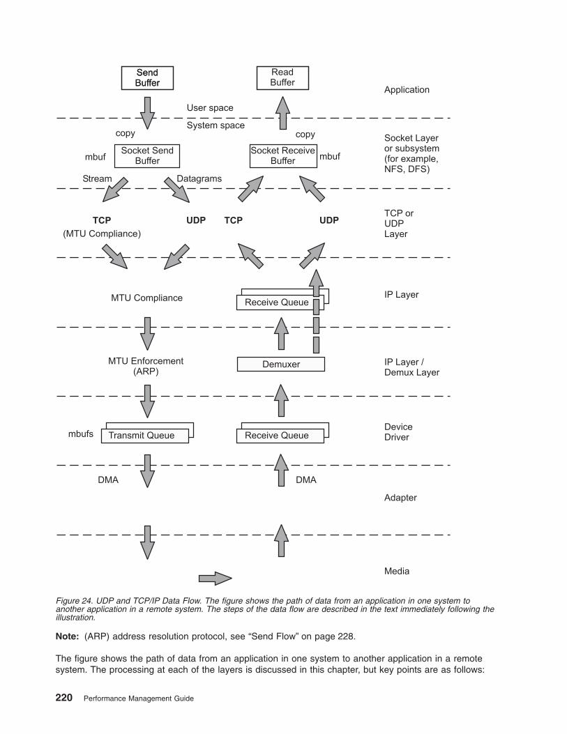
Note: (ARP) address resolution protocol, see “Send Flow” on page 228.

The figure shows the path of data from an application in one system to another application in a remotesystem. The processing at each of the layers is discussed in this chapter, but key points are as follows:

Figure 24. UDP and TCP/IP Data Flow. The figure shows the path of data from an application in one system toanother application in a remote system. The steps of the data flow are described in the text immediately following theillustration.


v The application’s write request causes the data to be copied from the application’s working segment tothe socket send buffer.

v The socket layer or subsystem calls UDP or TCP.

v The operating system has variable size clusters, so an optimum size is used when:

– UDP copies and computes the checksum of the data into a socket buffer.

– TCP copies the data to socket buffer.

v If the size of the data is larger than the maximum transfer unit (MTU) of the LAN, then:

– TCP breaks the output into segments that comply with the MTU limit.

– UDP leaves the breaking up of the output to the IP layer.

v If necessary, IP fragments the output into pieces that comply with the MTU, so that no outgoing packetexceeds the MTU limit.

v The packets are put on the device output queue and transmitted by the LAN adapter to the receivingsystem. If the output queue for the device overflows, the packet is discarded.

v Arriving packets are placed on the device driver’s receive queue, and pass through the Interface layerto IP.

v If IP in the receiving system determines that IP in the sending system had fragmented a block of data, itcoalesces the fragments into their original form and passes the data to TCP or UDP.

– TCP reassembles the original segments and places the input in the socket receive buffer.

– UDP passes the input on to the socket receive buffer. If the input socket (udp_recvspace) limit isreached, the packet is discarded.

v When the application makes a read request, the appropriate data is copied from the socket receivebuffer in kernel memory into the buffer in the application’s buffer.

Communication Subsystem Memory (mbuf) ManagementTo avoid fragmentation of kernel memory and the overhead of numerous calls to the xmalloc() subroutine,the various layers of the communication subsystem share common buffer pools. The mbuf managementfacility controls different buffer sizes. The pools consist of pinned pieces of kernel virtual memory; thismeans that they always reside in physical memory and are never paged out. The result is that the realmemory available for paging in application programs and data has been decreased by the amount that thembuf pools have been increased.

In addition to avoiding duplication, sharing the mbuf and cluster pools allows the various layers to passpointers to one another, reducing mbuf management calls and copying of data.

For additional details, see Tuning mbuf Pool Performance.

Socket LayerSockets provide the application program interface (API) to the communication subsystem. Several types ofsockets provide various levels of service by using different communication protocols. Sockets of typeSOCK_DGRAM use the UDP protocol. Sockets of type SOCK_STREAM use the TCP protocol.

The processes of opening, reading, and writing to sockets are similar to those for manipulating files.

The sizes of the buffers in system virtual memory (that is, the total number of bytes from the mbuf pools)that are used by the input and output sides of each socket are limited by system-wide default values(which can be overridden for a given socket by a call to the setsockopt() subroutine):

udp_sendspace and udp_recvspaceBuffer sizes for datagram sockets in bytes. The defaults are 9216 and 42080, respectively.

Chapter 10. Monitoring and Tuning Communications I/O Use 221

tcp_sendspace and tcp_recvspaceBuffer sizes for stream sockets in bytes. The defaults for both values are 16384. With AIX 4.3.3and later, these two parameters can also be set using ISNO (see Interface-Specific NetworkOptions (ISNO)).

Use the following to display these values:# no -a

A root user can set these values as follows:# no -o udp_sendspace=NewValue

The NewValue parameter must be less than or equal to the sb_max parameter, which controls themaximum amount of space that can be used by a socket’s send or receive buffer. The default value of thesb_max parameter depends on the operating system version and amount of real memory. The sb_maxvalue is displayed with the command no -a and set with the no command, as follows:# no -o sb_max=NewLimit

Note: Socket send or receive buffer sizes are limited to no more than sb_max bytes, because sb_max isa ceiling on buffer space consumption. The two quantities are not measured in the same way,however. The socket buffer size limits the amount of data that can be held in the socket buffers.The sb_max value limits the number of bytes of mbufs that can be in the socket buffer at any giventime. In an Ethernet environment, for example, each 2048-byte mbuf cluster might hold just 1500bytes of data. In that case, sb_max would have to be 1.37 times larger than the specified socketbuffer size to allow the buffer to reach its specified capacity. The guideline is to set sb_max to atleast twice the size of the largest socket buffer.

Send FlowAs an application writes to a socket, the socket layer calls the transport layer (either TCP or UDP), whichcopies the data from user space into the socket send buffer in kernel space. Depending on the amount ofdata being copied into the socket send buffer, the code puts the data into either mbufs or clusters.

Receive FlowOn the receive side, an application opens a socket and attempts to read data from it. If there is no data inthe socket receive buffer, the socket layer causes the application thread to go to the sleep state (blocking)until data arrives. When data arrives, it is put on the receive socket buffer queue and the applicationthread is made dispatchable. The data is then copied into the application’s buffer in user space, the mbufchain is freed, and control is returned to the application.

Socket CreationIn AIX 4.3.1 and later, the sockthresh value determines how much of the system’s network memory canbe used before socket creation is disallowed. The value of sockthresh is given as a percentage ofthewall. It has a default of 85 percent and can be set to any value from 1 to 100. However, sockthreshcannot be set to a value lower than the amount of memory currently in use.

The sockthresh option is intended to prevent situations where many connections are opened until all thenetwork memory on the machine is used. This leaves no memory for other operations, and the machinehangs and must be rebooted to recover. Use sockthresh to set the point at which new sockets should notbe allowed. Calls to the socket() and socketpair() subroutines will fail with an error of ENOBUFS, andincoming connection requests will be silently discarded. This allows the remaining network memory to beused by existing connections and prevents the machine from hanging.

The netstat -m statistic sockets not created because sockthresh was reached is incremented each timea socket creation fails because the amount of network memory already in use is over the sockthresh limit.

Use the following to display the sockthresh value:# no -o sockthresh


A root user can set the value as follows:# no -o sockthresh=NewValue

The default value can be set as follows:# no -d sockthresh

Ephemeral PortsWhen an application requests that the system assign the port (application is not requesting a specific portnumber), this is called an ephemeral port. Prior to AIX 4.3.1, the ephemeral port range was from 1024 to5000. Starting with AIX 4.3.1, the default starting ephemeral port number is 32768, and the default largestephemeral port number is 65535.

Using the no command, these values can be tuned with the tcp_ephemeral_low andtcp_ephemeral_high parameters. The maximum range would be to set tcp_ephemeral_low to 1024 andtcp_ephemeral_high to 65535. UDP ports have the same tunable parameters available throughudp_ephemeral_low and udp_ephemeral_high (defaults are identical).

Relative Level of Function in UDP and TCPThe following two sections contain descriptions of the function of UDP and TCP. To facilitate comparison ofUDP and TCP, both descriptions are divided into subsections on connection, error detection, errorrecovery, flow control, data size, and MTU handling.

UDP LayerUDP provides a low-cost protocol for applications that have the facilities to deal with communicationfailures. UDP is most suitable for request-response applications. Because such an application has tohandle a failure to respond anyway, it is little additional effort to handle communication error as one of thecauses of failure to respond. For this reason, and because of its low overhead, subsystems such as NFS,ONC RPC, DCE RPC, and DFS use UDP.

Features of the UDP layer are as follows:

ConnectionNone. UDP is essentially a stateless protocol. Each request received from the caller is handledindependently of those that precede or follow it. (If the connect() subroutine is called for adatagram socket, the information about the destination is considered a hint to cache the resolvedaddress for future use. It does not actually bind the socket to that address or affect UDP on thereceiving system.)

Error detectionChecksum creation and verification. The sending UDP builds the checksum and the receiving UDPchecks it. If the check fails, the packet is dropped.

Error recoveryNone. UDP does not acknowledge receipt of packets, nor does it detect their loss in transmissionor through buffer-pool overflow. Consequently, UDP never retransmits a packet. Recovery must beperformed by the application.

Flow controlNone. When UDP is asked to send, it sends the packet to IP. When a packet arrives from IP, it isplaced in the socket-receive buffer. If either the device driver/adapter buffer queue or thesocket-receive buffer is full when the packet arrives, the packet is dropped without an errorindication. The application or subsystem that sent the packet must detect the failure by timeout orsequence and retry the transmission. Various statistics show counts of discarded packets (see thenetstat -s and netstat -D commands in The netstat Command).

Data sizeMust fit in one buffer. This means that the buffer pools on both sides of UDP must have buffersizes that are adequate for the applications’ requirements. The maximum size of a UDP packet is


64 KB. Of course, an application that builds large blocks can break them into multiple datagramsitself (for example, DCE), but it is simpler to use TCP.

MTU handlingNone. Dealing with data larger than the maximum transfer unit (MTU) size for the interface is leftto IP. If IP has to fragment the data to make it fit the MTU, loss of one of the fragments becomesan error that the application or subsystem must deal with timeout and retransmit logic.

Send Flow: If udp_sendspace is large enough to hold the datagram, the application’s data is copiedinto mbufs in kernel memory. If the datagram is larger than udp_sendspace, an error is returned to theapplication.

The operating system chooses optimum size buffers from a power of 2 size buffer. For example, a write of8704 bytes is copied into two clusters, a 8192-byte and a 512-byte cluster. UDP adds the UDP header (inthe same mbuf, if possible), checksums the data, and calls the IP ip_output() routine.

Receive Flow: UDP verifies the checksum and queues the data onto the proper socket. If theudp_recvspace limit is exceeded, the packet is discarded. A count of these discards is reported by thenetstat -s command under udp: as socket buffer overflows. If the application is waiting for a receive orread on the socket, it is put on the run queue. This causes the receive to copy the datagram into theuser’s address space and release the mbufs, and the receive is complete. Usually, the receiver respondsto the sender to acknowledge the receipt and also return a response message.

In AIX 4.1.1 and later, UDP checksums the data ″on the fly″ when it copies it into the kernel mbuf. Whenreceiving, this same optimization can be done, but the application must enable it with theSO_CKSUMRECV option on a setsockopt() call. Applications that receive large UDP buffers shouldprogram to use this option for better performance.

TCP LayerTCP provides a reliable transmission protocol. TCP is most suitable for applications that, at least forperiods of time, are mostly output or mostly input. With TCP ensuring that packets reach their destination,the application is freed from error detection and recovery responsibilities. Applications that use TCPtransport include ftp, rcp, and telnet. DCE can use TCP if it is configured to use a connection-orientedprotocol.

Features of the TCP layer are as follows:

ConnectionExplicit. The instance of TCP that receives the connection request from an application (call it theinitiator, sender,or transmitter) establishes a session with its counterpart on the other system,which you will call the listener, or receiver. All exchanges of data and control packets are withinthe context of that session.

Error detectionChecksum creation and verification. The sending TCP builds the checksum and the receiving TCPchecks it. If checksum verification fails, the receiver does not acknowledge receipt of the packet.Some PCI adapters now have TCP checksum offload. For example, the Gigabit Ethernet adapterfor transmits and receives, and the ATM 155 adapter for transmits. The default is set to on. Thetransmit can be disabled with the ifconfig command and the checksum_offload parameter, whilethe receive requires a chdev command to set cx_checksum=no.

Error recoveryFull. TCP detects checksum failures and loss of a packet or fragment through timeout. In errorsituations TCP retransmits the data until it is received correctly (or notifies the application of anunrecoverable error).

Flow controlEnforced. TCP uses a discipline called a sliding window to ensure delivery to the receivingapplication. The sliding window concept is illustrated in the following figure. (The records shown in


the figure are for clarity only. TCP processes data as a stream of bytes and does not keep track ofrecord boundaries, which are application-defined.)

In this figure, the sending application is sleeping because it has attempted to write data that wouldcause TCP to exceed the send socket buffer space (that is, tcp_sendspace). The sending TCPstill has the last part of rec5, all of rec6 and rec7, and the beginning of rec8. The receiving TCPhas not yet received the last part of rec7 or any of rec8. The receiving application got rec4 and thebeginning of rec5 when it last read the socket, and it is now processing that data. When thereceiving application next reads the socket, it will receive (assuming a large enough read), the restof rec5, rec6, and as much of rec7 and rec8 as has arrived by that time.

After the next read, the following occur:

v The receiving TCP will be able to acknowledge that data

v The sending TCP will be able to discard the data

v The pending write will complete

The sending application will wake up. To avoid excessive LAN traffic when the application isreading in tiny amounts, TCP delays acknowledgment until the receiving application has read atotal amount of data that is at least half the receive window size or twice the maximum segmentsize.

If there is no data to send back, the receiver will delay up to 200 ms and then send the ACK. Thedelay time can be tuned by a new no parameter called fasttimeo. The default value is 200 ms,and the range of values can be between 50 ms and 200 ms. Reducing this value may enhanceperformance of request/response type of applications.

Note: When using TCP to exchange request/response messages, the application must use thesetsockopt() subroutine to turn on the TCP_NODELAY option. This causes TCP to send

Figure 25. TCP Sliding Window. This illustration depicts the TCP Sliding Window. A full description is in the textimmediately following the figure.


the message immediately (within the constraints of the sliding window), even though it isless than MTU-size. Otherwise, TCP would wait for up to 200 milliseconds for more data tosend before transmitting the message. Starting with AIX 4.3.3 the tcp_nodelay parametercan be set with the ifconfig or chdev command to set TCP_NODELAY on TCP sockets(see Interface-Specific Network Options (ISNO)).

In the course of establishing a session, the initiator and the listener converse to determine thereceive space for each end point. The size defines the size of the receive window. As data iswritten to the socket, it is moved into the sender’s buffer. When the receiver indicates that it hasspace available, the sender transmits enough data to fill that space (assuming that it contains thatmuch data). When the receiving application reads from the socket, the receiving socket returns asmuch data as it has in its receive socket buffer. TCP then informs the sender that the data hasbeen successfully delivered by sending a packet to advance the receiver window. Only then doesthe sending TCP discard the data from its own buffer, effectively moving the window to the right bythe amount of data delivered. If the window is full because the receiving application has fallenbehind, the sending thread will be blocked (or receive a specific errno) when it tries to write to thesocket.

The value of tcp_recvspace and tcp_sendspace are independent. The tcp_sendspace controlsthe buffering in the kernel of the sender. The tcp_recvspace controls the receiver space andtranslates into TCP’s receive window.

If the rfc1323 parameter is 1, the maximum TCP window size is 4 GB (instead of 64 KB).

Data sizeIndefinite. TCP does not process records or blocks; it processes a stream of bytes. If asend buffer is larger than the receiver can handle, it is segmented into MTU-size packets.Because it handles shortages of buffer space under the covers, TCP does not guaranteethat the number and size of data receives will be the same as the number and size ofsends. It is the responsibility of the two sides of the application to identify record or blockboundaries, if any, within the stream of data.

MTU handlingHandled by segmentation in TCP. When the connection is established, the initiator and thelistener negotiate a maximum segment size (MSS) to be used. The MSS is typicallysmaller than the MTU (see Tuning TCP Maximum Segment Size). If the output packet sizeexceeds the MSS, TCP does the segmentation, thus making fragmentation in IPunnecessary. The receiving TCP typically puts the segments on the socket receive queueas they arrive. If the receiving TCP detects the loss of a segment, it withholdsacknowledgment and holds back the succeeding segments until the missing segment hasbeen received successfully.

The additional operations performed by TCP to ensure a reliable connection result in about 5 to 10 percenthigher processor cost than in UDP.

Send Flow: When the TCP layer receives a write request from the socket layer, it allocates a new mbuffor its header information and copies the data in the socket-send buffer either into the TCP-header mbuf, ifthere is room, or into a newly allocated mbuf chain. If the data being copied is in clusters, the data is notactually copied into new clusters. Instead, a pointer field in the new mbuf header (this header is part of thembuf structure and is unrelated to the TCP header) is set to point to the clusters containing the data,thereby avoiding the overhead of one or more 4 KB copies. TCP then checksums the data (unless it isoffloaded by certain PCI adapters), updates its various state variables, which are used for flow control andother services, and finally calls the IP layer with the header mbuf now linked to the new mbuf chain.

Receive Flow: When the TCP input routine receives input data from IP, the following occur:

v It checksums the TCP header and data for corruption detection (unless it is offloaded by certain PCIadapters)


v Determines which connection this data is for

v Removes its header information

v Links the mbuf chain onto the socket-receive buffer associated with this connection

v Uses a socket service to wake up the application (if it is sleeping as described earlier)

IP LayerThe Internet Protocol provides a basic datagram service to the higher layers. If it is given a packet largerthan the MTU of the interface, it fragments the packet and sends the fragments to the receiving system,which reassembles them into the original packet. If one of the fragments is lost in transmission, theincomplete packet is ultimately discarded by the receiver. MTU path discovery can be enabled asdescribed in Tuning TCP Maximum Segment Size.

The length of time IP waits for a missing fragment is controlled by the ipfragttl parameter, which is setand displayed with the no command.

Following are some default values and value ranges for different network types:

Network Type Default (bytes) Range (bytes)

X.25 576 60-2058

SLIP 1006 60-4096

Standard Ethernet 1500 60 - 1500

IEEE 802.3 Ethernet 1492 60 - 1492

Gigabit Ethernet 9000 (Jumbo Frames) N/A

Token-Ring 4 Mbps 1492 60 - 4096

Token-Ring 16 Mbps 1492 60 - 17800

FDDI 4352 1 - 4352

SLA (socc) 61428 1 - 61428

ATM 9180 1 - 65527

HIPPI 65536 60 - 65536

SP Switch 65520 1 - 65520

Note: In general, you can increase the transmit and receive queues. This requires some memory, butavoids some problems. See Adapter Transmit and Receive Queue Tuning.

Send FlowWhen the IP output routine receives a packet from UDP or TCP, it identifies the interface to which thembuf chain should be sent, updates and checksums the IP part of the header, and passes the packet tothe interface (IF) layer.

IP determines the proper device driver and adapter to use, based on the network number. The driverinterface table defines the maximum MTU for this network. If the datagram is less than the MTU size, IPadds the IP header in the existing mbuf, checksums the IP header, and calls the driver to send the frame.If the driver send queue is full, an EAGAIN error is returned to IP, which returns it to UDP, which returns itto the sending application. The sender should delay and try again.

If the datagram is larger than the MTU size (which only occurs in UDP), IP fragments the datagram intoMTU-size fragments, appends a IP header (in an mbuf) to each, and calls the driver once for eachfragment frame. If the driver’s send queue is full, an EAGAIN error is returned to IP. IP discards all


remaining unsent fragments associated with this datagram and returns EAGAIN to UDP. UDP returnsEAGAIN the sending application. Since IP and UDP do not queue messages, it is up to the application todelay and try the send again.

Receive FlowIn AIX Version 4, in general, interfaces do not perform queuing and directly call the IP input queue routineto process the packet; the loopback interface will still perform queuing. In the case of queuing, the demuxlayer places incoming packets on this queue. If the queue is full, packets are dropped and never reach theapplication. If packets are dropped at the IP layer, a statistic called ipintrq overflows in the output of thenetstat -s command is incremented. If this statistic increases in value, then use the no command to tunethe ipqmaxlen tunable.

In AIX Version 4, the demux layer (formerly called the IF layer) calls IP on the interrupt thread. IP checksthe IP header checksum to make sure the header was not corrupted and determines if the packet is forthis system. If so, and the frame is not a fragment, IP passes the mbuf chain to the TCP or UDP inputroutine.

If the received frame is a fragment of a larger datagram (which only occurs in UDP), IP retains the frame.When the other fragments arrive, they are merged into a logical datagram and given to UDP when thedatagram is complete. IP holds the fragments of an incomplete datagram until the ipfragttl time (asspecified by the no command) expires. The default ipfragttl time is 30 seconds (an ipfragttl value of 60).If any fragments are lost due to problems such as network errors, lack of mbufs, or transmit queueoverruns, IP never receives them. When ipfragttl expires, IP discards the fragments it did receive. This isreported as a result from the netstat -s command. Under ip:, see fragments dropped after timeout.

Demux LayerThe interface layer (IF) is used on output and is the same level as the demux layer (used for input) in AIXVersion 4. It places transmit requests on to a transmit queue, where the requests are then serviced by thenetwork interface device driver. The size of the transmit queue is tunable, as described in AdapterTransmit and Receive Queue Tuning.

Send FlowWhen the demux layer receives a packet from IP, it attaches the link-layer header information to thebeginning of the packet, checks the format of the mbufs to make sure they conform to the device driver’sinput specifications, and then calls the device driver write routine.

The address resolution protocol (ARP) is also handled in this layer. ARP translates a 32-bit InternetProtocol (IP) address into a 48-bit hardware address.

Receive FlowIn AIX Version 4, when the demux layer receives a packet from the device driver, it calls IP on the interruptthread to perform IP input processing.

If the dog threads are enabled (see Enabling Thread Usage on LAN Adapters (dog threads)), the incomingpacket will be queued to the thread and the thread will handle calling IP, TCP, and the socket code.

LAN Adapters and Device DriversThe operating system environment supports many different kinds of LAN adapters. You can choose from awide variety of network interfaces. As the following table shows, as the speed of these networks varies, sodoes the performance.

Name Speed

Ethernet (en) 10 Mbit/sec - Gigabits/sec

IEEE 802.3 (et) 10 Mbit/sec - Gigabits/sec

Token-Ring (tr) 4 or 16 Mbit/sec


Name Speed

X.25 protocol (xt) 64 Kb/sec

Serial Line Internet Protocol, SLIP (sl) 64 Kb/sec

loopback (lo) N/A

FDDI (fi) 100 Mbit/sec

SOCC (so) 220 Mbit/sec

ATM (at) 100s Mbit/sec (many Gb/sec)

Refer to the PCI Adapter Placement Reference and RS/6000 Systems Handbook for slot placementguidelines and limitations that may exist on the number of adapters that can be supported for connectivityand the number that can be supported for maximum performance.

Several PCI machines have secondary PCI buses bridged onto a primary PCI bus. Some medium- tohigh-speed adapters perform slower on these secondary bus slots and some adapters are notrecommended to be used in these slots. Machines with some secondary PCI slots include E30, F40, andSP 332 MHz SMP-wide nodes.

The adapters differ, not only in the communications protocol and transmission medium they support, butalso in their interface to the I/O bus and the processor. Similarly, the device drivers vary in the techniqueused to convey the data between memory and the adapter. The following description of send and receiveflow applies to most adapters and device drivers, but details vary.

Send FlowAt the device-driver layer, the mbuf chain containing the packet is enqueued on the transmit queue. Themaximum total number of output buffers that can be queued is controlled by the system parameterxmt_que_size. In some cases, the data is copied into driver-owned DMA buffers. The adapter is thensignaled to start DMA operations.

At this point, control returns up the path to the TCP or UDP output routine, which continues sending aslong as it has data to send. When all data has been sent, control returns to the application, which thenruns asynchronously while the adapter transmits data. Device driver dependent, when the adapter hascompleted transmission, it sends an interrupt to the system. When the interrupt is handled, thedevice-interrupt routines are called to adjust the transmit queues and free the mbufs that held thetransmitted data.

Receive FlowWhen frames are received by an adapter, they are transferred from the adapter into a driver-managedreceive queue. The receive queue can consist of mbufs or the device driver can manage a separate poolof buffers for the device. In either case, the data is in an mbuf chain when it is passed from the devicedriver to the demux layer.

Some drivers receive frames through Direct Memory Access (DMA) into a pinned area of memory andthen allocate mbufs and copy the data into them. Drivers/adapters that receive large-MTU frames mayhave the frames accessed directly into cluster mbufs. The driver transfers the frame to the correct networkprotocol (IP in this example) by calling a demultiplexing function that identifies the packet type and putsthe mbuf containing the buffer on the input queue for that network protocol. If no mbufs are available or ifthe higher-level input queue is full, the incoming frames are discarded.


Analyzing Network PerformanceWhen performance problems arise, your system might be totally innocent, while the real culprit is buildingsaway. An easy way to tell if the network is affecting overall performance is to compare those operationsthat involve the network with those that do not. If you are running a program that does a considerableamount of remote reads and writes and it is running slowly, but everything else seems to be running asusual, then it is probably a network problem. Some of the potential network bottlenecks can be caused bythe following:

v Client-network interface

v Network bandwidth

v Network topology

v Server network interface

v Server CPU load

v Server memory usage

v Server bandwidth

v Inefficient configuration

Several tools can measure network statistics and give a variety of information, but only part of thisinformation is related to performance tuning.

To enhance performance, you can use the no (network options) command and the nfso command fortuning NFS options. You can also use the chdev and ifconfig commands to change system and networkparameters.

The ping CommandThe ping command is useful for the following:

v Determining the status of the network and various foreign hosts.

v Tracking and isolating hardware and software problems.

v Testing, measuring, and managing networks.

Some ping command options relevant to performance tuning are as follows:

-c Specifies the number of packets. This option is useful when you get an IP trace log. You cancapture a minimum of ping packets.

-s Specifies the length of packets. You can use this option to check fragmentation and reassembly.

-f Sends the packets at 10 ms intervals or immediately after each response. Only the root user canuse this option.

If you need to load your network or systems, the -f option is convenient. For example, if you suspect thatyour problem is caused by a heavy load, load your environment intentionally to confirm your suspicion.Open several aixterm windows and run the ping -f command in each window. Your Ethernet utilizationquickly gets to around 100 percent. The following is an example:# date ; ping -c 1000 -f wave ; dateFri Jul 23 11:52:39 CDT 1999PING wave.austin.ibm.com: (9.53.153.120): 56 data bytes.----wave.austin.ibm.com PING Statistics----1000 packets transmitted, 1000 packets received, 0% packet lossround-trip min/avg/max = 1/1/23 msFri Jul 23 11:52:42 CDT 1999

Note: This command can be very hard on a network and should be used with caution. Flood-pinging canonly be performed by the root user.


In this example, 1000 packets were sent for 3 seconds. Be aware that this command uses IP and InternetControl Message Protocol (ICMP) protocol and therefore, no transport protocol (UDP/TCP) and applicationactivities are involved. The measured data, such as round-trip time, does not reflect the total performancecharacteristics.

When you try to send a flood of packets to your destination, consider several points:

v Sending packets puts a load on your system.

v Use the netstat -i command to monitor the status of your network interface during the experiment. Youmay find that the system is dropping packets during a send by looking at the Oerrs output.

v You should also monitor other resources, such as mbufs and send/receive queue. It can be difficult toplace a heavy load onto the destination system. Your system might be overloaded before the othersystem is.

v Consider the relativity of the results. If you want to monitor or test just one destination system, do thesame experiment on some other systems for comparison, because your network or router might have aproblem.

The ftp CommandYou can use the ftp command to send a very large file by using /dev/zero as input and /dev/null asoutput. This allows you to transfer a large file without involving disks (which might be a bottleneck) andwithout having to cache the entire file in memory.

Use the following ftp subcommands (change count to increase or decrease the number of blocks read bythe dd command):> bin> put "|dd if=/dev/zero bs=32k count=10000" /dev/null

Remember, if you change the TCP send or receive space parameters, then for the ftp command, youmust refresh the inetd daemon with the refresh -s inetd command.

Make sure that tcp_senspace and tcp_recvspace are at least 65535 for the Gigabit Ethernet ″jumboframes″ and for the ATM with MTU 9180 or larger to get good performance due to larger MTU size.

An example to set the parameters is as follows:# no -o tcp_sendspace=65535# no -o tcp_recvspace=65535# refresh -s inetd0513-095 The request for subsystem refresh was completed successfully.

The ftp subcommands are as follows:ftp> bin200 Type set to I.ftp> put "|dd if=/dev/zero bs=32k count=10000" /dev/null200 PORT command successful.150 Opening data connection for /dev/null.10000+0 records in10000+0 records out226 Transfer complete.327680000 bytes sent in 8.932 seconds (3.583e+04 Kbytes/s)local: |dd if=/dev/zero bs=32k count=10000 remote: /dev/nullftp> quit221 Goodbye.


The netstat CommandThe netstat command is used to show network status. Traditionally, it is used more for problemdetermination than for performance measurement. However, the netstat command can be used todetermine the amount of traffic on the network to ascertain whether performance problems are due tonetwork congestion.

The netstat command displays information regarding traffic on the configured network interfaces, such asthe following:

v The address of any protocol control blocks associated with the sockets and the state of all sockets

v The number of packets received, transmitted, and dropped in the communications subsystem

v Cumulative statistics per interface

v Routes and their status

Using the netstat CommandThe netstat command displays the contents of various network-related data structures for activeconnections. In this chapter, only the options and output fields that are relevant for network performancedeterminations are discussed. For all other options and columns, see the AIX 5L Version 5.2 CommandsReference.

netstat -i: Shows the state of all configured interfaces.

The following example shows the statistics for a workstation with an integrated Ethernet and a Token-Ringadapter:# netstat -iName Mtu Network Address Ipkts Ierrs Opkts Oerrs Colllo0 16896 <Link> 144834 0 144946 0 0lo0 16896 127 localhost 144834 0 144946 0 0tr0 1492 <Link>10.0.5a.4f.3f.61 658339 0 247355 0 0tr0 1492 9.3.1 ah6000d 658339 0 247355 0 0en0 1500 <Link>8.0.5a.d.a2.d5 0 0 112 0 0en0 1500 1.2.3 1.2.3.4 0 0 112 0 0

The count values are summarized since system startup.

Name Interface name.

Mtu Maximum transmission unit. The maximum size of packets in bytes that are transmitted using theinterface.

Ipkts Total number of packets received.

Ierrs Total number of input errors. For example, malformed packets, checksum errors, or insufficientbuffer space in the device driver.

Opkts Total number of packets transmitted.

Oerrs Total number of output errors. For example, a fault in the local host connection or adapter outputqueue overrun.

Coll Number of packet collisions detected.

Note: The netstat -i command does not support the collision count for Ethernet interfaces (see Theentstat Command for Ethernet statistics).

Following are some tuning guidelines:

v If the number of errors during input packets is greater than 1 percent of the total number of inputpackets (from the command netstat -i); that is,Ierrs > 0.01 x Ipkts


Then run the netstat -m command to check for a lack of memory.

v If the number of errors during output packets is greater than 1 percent of the total number of outputpackets (from the command netstat -i); that is,Oerrs > 0.01 x Opkts

Then increase the send queue size (xmt_que_size) for that interface. The size of the xmt_que_sizecould be checked with the following command:# lsattr -El adapter

v If the collision rate is greater than 10 percent, that is,Coll / Opkts > 0.1

Then there is a high network utilization, and a reorganization or partitioning may be necessary. Use thenetstat -v or entstat command to determine the collision rate.

netstat -i -Z: This function of the netstat command clears all the statistic counters for the netstat -icommand to zero.

netstat -I interface interval: Displays the statistics for the specified interface. It offers information similarto the netstat -i command for the specified interface and reports it for a given time interval. For example:# netstat -I en0 1

input (en0) output input (Total) outputpackets errs packets errs colls packets errs packets errs colls

0 0 27 0 0 799655 0 390669 0 00 0 0 0 0 2 0 0 0 00 0 0 0 0 1 0 0 0 00 0 0 0 0 78 0 254 0 00 0 0 0 0 200 0 62 0 00 0 1 0 0 0 0 2 0 0

The previous example shows the netstat -I command output for the ent0 interface. Two reports aregenerated side by side, one for the specified interface and one for all available interfaces (Total). Thefields are similar to the ones in the netstat -i example, input packets = Ipkts, input errs = Ierrs and soon.

netstat -m: Displays the statistics recorded by the mbuf memory-management routines. The most usefulstatistics in the output of the netstat -m command are the counters that show the requests for mbufsdenied and non-zero values in the failed column. If the requests for mbufs denied is not displayed, thenthis must be an SMP system running operating system version 4.3.2 or later; for performance reasons,global statistics are turned off by default. To enable the global statistics, set the no parameterextended_netstats to 1. This can be done by changing the /etc/rc.net file and rebooting the system.

The following example shows the first part of the netstat -m output with extended_netstats set to 1:# netstat -m29 mbufs in use:16 mbuf cluster pages in use71 Kbytes allocated to mbufs0 requests for mbufs denied0 calls to protocol drain routines

Kernel malloc statistics:

******* CPU 0 *******By size inuse calls failed delayed free hiwat freed32 419 544702 0 0 221 800 064 173 22424 0 0 19 400 0128 121 37130 0 0 135 200 4256 1201 118326233 0 0 239 480 138512 330 671524 0 0 14 50 541024 74 929806 0 0 82 125 2


2048 384 1820884 0 0 8 125 56054096 516 1158445 0 0 46 150 218192 9 5634 0 0 1 12 2716384 1 2953 0 0 24 30 4132768 1 1 0 0 0 1023 0

By type inuse calls failed delayed memuse memmax mapb

Streams mblk statistic failures:0 high priority mblk failures0 medium priority mblk failures0 low priority mblk failures

If global statistics are not on and you want to determine the total number of requests for mbufs denied,add up the values under the failed columns for each CPU. If the netstat -m command indicates thatrequests for mbufs or clusters have failed or been denied, then you may want to increase the value ofthewall by using the no -o thewall=NewValue command. See Overview of the mbuf Management Facilityfor additional details about the use of thewall and maxmbuf.

Beginning with AIX 4.3.3, a delayed column was added. If the requester of an mbuf specified the M_WAITflag, then if an mbuf was not available, the thread is put to sleep until an mbuf is freed and can be usedby this thread. The failed counter is not incremented in this case; instead, the delayed column will beincremented. Prior to AIX 4.3.3, the failed counter was also not incremented, but there was no delayedcolumn.

Also, if the currently allocated amount of network memory is within 85 percent of thewall, you may want toincrease thewall. If the value of thewall is increased, use the vmstat command to monitor total memoryuse to determine if the increase has had a negative impact on overall memory performance.

If buffers are not available when a request is received, the request is most likely lost (to see if the adapteractually dropped a package, see Adapter Statistics). Keep in mind that if the requester of the mbufspecified that it could wait for the mbuf if not available immediately, this puts the requestor to sleep butdoes not count as a request being denied.

If the number of failed requests continues to increase, the system might have an mbuf leak. To help trackdown the problem, the no command parameter net_malloc_police can be set to 1, and the trace hookwith ID 254 can be used with the trace command.

After an mbuf/cluster is allocated and pinned, it can be freed by the application. Instead of unpinning thisbuffer and giving it back to the system, it is left on a free-list based on the size of this buffer. The next timethat a buffer is requested, it can be taken off this free-list to avoid the overhead of pinning. After thenumber of buffers on the free list reaches the highwater mark, buffers smaller than 4096 will be coalescedtogether into page-sized units so that they can be unpinned and given back to the system. When thebuffers are given back to the system, the freed column is incremented. If the freed value consistentlyincreases, the highwater mark is too low. In AIX 4.3.2 and later, the highwater mark is scaled according tothe amount of RAM on the system.

netstat -v: The netstat -v command displays the statistics for each Common Data Link Interface(CDLI)-based device driver that is in operation. Interface-specific reports can be requested using thetokstat, entstat, fddistat, or atmstat commands.

Every interface has its own specific information and some general information. The following exampleshows the Token-Ring and Ethernet part of the netstat -v command; other interface parts are similar. Witha different adapter, the statistics will differ somewhat. The most important output fields are highlighted.# netstat -v-------------------------------------------------------------ETHERNET STATISTICS (ent0) :Device Type: IBM 10/100 Mbps Ethernet PCI Adapter (23100020)


Hardware Address: 00:60:94:e9:29:18Elapsed Time: 9 days 19 hours 5 minutes 51 seconds

Transmit Statistics: Receive Statistics:-------------------- -------------------Packets: 0 Packets: 0Bytes: 0 Bytes: 0Interrupts: 0 Interrupts: 0Transmit Errors: 0 Receive Errors: 0Packets Dropped: 0 Packets Dropped: 0

Bad Packets: 0Max Packets on S/W Transmit Queue: 0S/W Transmit Queue Overflow: 0Current S/W+H/W Transmit Queue Length: 0

Broadcast Packets: 0 Broadcast Packets: 0Multicast Packets: 0 Multicast Packets: 0No Carrier Sense: 0 CRC Errors: 0DMA Underrun: 0 DMA Overrun: 0Lost CTS Errors: 0 Alignment Errors: 0Max Collision Errors: 0 No Resource Errors: 0Late Collision Errors: 0 Receive Collision Errors: 0Deferred: 0 Packet Too Short Errors: 0SQE Test: 0 Packet Too Long Errors: 0Timeout Errors: 0 Packets Discarded by Adapter: 0Single Collision Count: 0 Receiver Start Count: 0Multiple Collision Count: 0Current HW Transmit Queue Length: 0

General Statistics:-------------------No mbuf Errors: 0Adapter Reset Count: 0Driver Flags: Up Broadcast Running

Simplex 64BitSupport PrivateSegment

IBM 10/100 Mbps Ethernet PCI Adapter Specific Statistics:------------------------------------------------Chip Version: 25RJ45 Port Link Status : downMedia Speed Selected: 10 Mbps Half DuplexMedia Speed Running: UnknownReceive Pool Buffer Size: 384Free Receive Pool Buffers: 128No Receive Pool Buffer Errors: 0Inter Packet Gap: 96Adapter Restarts due to IOCTL commands: 0Packets with Transmit collisions:1 collisions: 0 6 collisions: 0 11 collisions: 02 collisions: 0 7 collisions: 0 12 collisions: 03 collisions: 0 8 collisions: 0 13 collisions: 04 collisions: 0 9 collisions: 0 14 collisions: 05 collisions: 0 10 collisions: 0 15 collisions: 0Excessive deferral errors: 0x0-------------------------------------------------------------TOKEN-RING STATISTICS (tok0) :Device Type: IBM PCI Tokenring Adapter (14103e00)Hardware Address: 00:20:35:7a:12:8aElapsed Time: 29 days 18 hours 3 minutes 47 seconds




Broadcast Packets: 18878 Broadcast Packets: 54615793Multicast Packets: 0 Multicast Packets: 569Timeout Errors: 0 Receive Congestion Errors: 0Current SW Transmit Queue Length: 0Current HW Transmit Queue Length: 0

General Statistics:-------------------No mbuf Errors: 0 Lobe Wire Faults: 0Abort Errors: 12 AC Errors: 0Burst Errors: 1 Frame Copy Errors: 0Frequency Errors: 0 Hard Errors: 0Internal Errors: 0 Line Errors: 0Lost Frame Errors: 0 Only Station: 1Token Errors: 0 Remove Received: 0Ring Recovered: 17 Signal Loss Errors: 0Soft Errors: 35 Transmit Beacon Errors: 0Driver Flags: Up Broadcast Running

AlternateAddress 64BitSupport ReceiveFunctionalAddr16 Mbps

IBM PCI Tokenring Adapter (14103e00) Specific Statistics:---------------------------------------------------------Media Speed Running: 16 Mbps Half DuplexMedia Speed Selected: 16 Mbps Full DuplexReceive Overruns : 0Transmit Underruns : 0ARI/FCI errors : 0Microcode level on the adapter :001PX11B2Num pkts in priority sw tx queue : 0Num pkts in priority hw tx queue : 0Open Firmware Level : 001PXRS02

The highlighted fields are described as follows:

v Transmit and Receive Errors

Number of output/input errors encountered on this device. This field counts unsuccessful transmissionsdue to hardware/network errors.

These unsuccessful transmissions could also slow down the performance of the system.

v Max Packets on S/W Transmit Queue

Maximum number of outgoing packets ever queued to the software transmit queue.

An indication of an inadequate queue size is if the maximal transmits queued equals the current queuesize (xmt_que_size). This indicates that the queue was full at some point.

To check the current size of the queue, use the lsattr -El adapter command (where adapter is, forexample, tok0 or ent0). Because the queue is associated with the device driver and adapter for theinterface, use the adapter name, not the interface name. Use the SMIT or the chdev command tochange the queue size.

v S/W Transmit Queue Overflow

Number of outgoing packets that have overflowed the software transmit queue. A value other than zerorequires the same actions as would be needed if the Max Packets on S/W Transmit Queue reaches thexmt_que_size. The transmit queue size must be increased.

v Broadcast Packets

Number of broadcast packets received without any error.

If the value for broadcast packets is high, compare it with the total received packets. The receivedbroadcast packets should be less than 20 percent of the total received packets. If it is high, this could


be an indication of a high network load; use multicasting. The use of IP multicasting enables a messageto be transmitted to a group of hosts, instead of having to address and send the message to eachgroup member individually.

v DMA Overrun

The DMA Overrun statistic is incremented when the adapter is using DMA to put a packet into systemmemory and the transfer is not completed. There are system buffers available for the packet to beplaced into, but the DMA operation failed to complete. This occurs when the MCA bus is too busy forthe adapter to be able to use DMA for the packets. The location of the adapter on the bus is crucial in aheavily loaded system. Typically an adapter in a lower slot number on the bus, by having the higher buspriority, is using so much of the bus that adapters in higher slot numbers are not being served. This isparticularly true if the adapters in a lower slot number are ATM or SSA adapters.

v Max Collision Errors

Number of unsuccessful transmissions due to too many collisions. The number of collisions encounteredexceeded the number of retries on the adapter.

v Late Collision Errors

Number of unsuccessful transmissions due to the late collision error.

v Timeout Errors

Number of unsuccessful transmissions due to adapter reported timeout errors.

v Single Collision Count

Number of outgoing packets with single (only one) collision encountered during transmission.

v Multiple Collision Count

Number of outgoing packets with multiple (2 - 15) collisions encountered during transmission.

v Receive Collision Errors

Number of incoming packets with collision errors during reception.

v No mbuf Errors

Number of times that mbufs were not available to the device driver. This usually occurs during receiveoperations when the driver must obtain memory buffers to process inbound packets. If the mbuf pool forthe requested size is empty, the packet will be discarded. Use the netstat -m command to confirm this,and increase the parameter thewall.

The No mbuf Errors value is interface-specific and not identical to the requests for mbufs denied fromthe netstat -m output. Compare the values of the example for the commands netstat -m and netstat -v(Ethernet and Token-Ring part).

To determine network performance problems, check for any Error counts in the netstat -v output.

Additional guidelines:

v To check for an overloaded Ethernet network, calculate (from the netstat -v command):(Max Collision Errors + Timeouts Errors) / Transmit Packets

If the result is greater than 5 percent, reorganize the network to balance the load.

v Another indication for a high network load is (from the command netstat -v):

If the total number of collisions from the netstat -v output (for Ethernet) is greater than 10 percent ofthe total transmitted packets, as follows:Number of collisions / Number of Transmit Packets > 0.1

netstat -p protocol: Shows statistics about the value specified for the protocol variable (udp, tcp, ip,icmp), which is either a well-known name for a protocol or an alias for it. Some protocol names and aliasesare listed in the /etc/protocols file. A null response indicates that there are no numbers to report. If thereis no statistics routine for it, the program report of the value specified for the protocol variable is unknown.

The following example shows the output for the ip protocol:


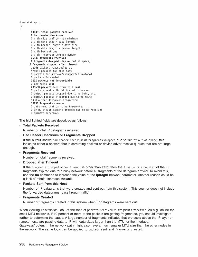
# netstat -p ipip::

491351 total packets received0 bad header checksums0 with size smaller than minimum0 with data size < data length0 with header length < data size0 with data length < header length0 with bad options0 with incorrect version number25930 fragments received0 fragments dropped (dup or out of space)0 fragments dropped after timeout12965 packets reassembled ok475054 packets for this host0 packets for unknown/unsupported protocol0 packets forwarded3332 packets not forwardable0 redirects sent405650 packets sent from this host0 packets sent with fabricated ip header0 output packets dropped due to no bufs, etc.0 output packets discarded due to no route5498 output datagrams fragmented10996 fragments created0 datagrams that can’t be fragmented0 IP Multicast packets dropped due to no receiver0 ipintrq overflows

The highlighted fields are described as follows:

v Total Packets Received

Number of total IP datagrams received.

v Bad Header Checksum or Fragments Dropped

If the output shows bad header checksum or fragments dropped due to dup or out of space, thisindicates either a network that is corrupting packets or device driver receive queues that are not largeenough.

v Fragments Received

Number of total fragments received.

v Dropped after Timeout

If the fragments dropped after timeout is other than zero, then the time to life counter of the ipfragments expired due to a busy network before all fragments of the datagram arrived. To avoid this,use the no command to increase the value of the ipfragttl network parameter. Another reason could bea lack of mbufs; increase thewall.

v Packets Sent from this Host

Number of IP datagrams that were created and sent out from this system. This counter does not includethe forwarded datagrams (passthrough traffic).

v Fragments Created

Number of fragments created in this system when IP datagrams were sent out.

When viewing IP statistics, look at the ratio of packets received to fragments received. As a guideline forsmall MTU networks, if 10 percent or more of the packets are getting fragmented, you should investigatefurther to determine the cause. A large number of fragments indicates that protocols above the IP layer onremote hosts are passing data to IP with data sizes larger than the MTU for the interface.Gateways/routers in the network path might also have a much smaller MTU size than the other nodes inthe network. The same logic can be applied to packets sent and fragments created.


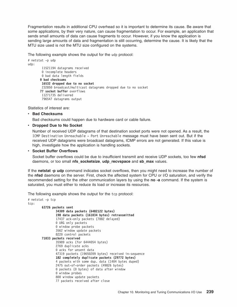
Fragmentation results in additional CPU overhead so it is important to determine its cause. Be aware thatsome applications, by their very nature, can cause fragmentation to occur. For example, an application thatsends small amounts of data can cause fragments to occur. However, if you know the application issending large amounts of data and fragmentation is still occurring, determine the cause. It is likely that theMTU size used is not the MTU size configured on the systems.

The following example shows the output for the udp protocol:# netstat -p udpudp:

11521194 datagrams received0 incomplete headers0 bad data length fields0 bad checksums16532 dropped due to no socket232850 broadcast/multicast datagrams dropped due to no socket77 socket buffer overflows11271735 delivered796547 datagrams output

Statistics of interest are:

v Bad Checksums

Bad checksums could happen due to hardware card or cable failure.

v Dropped Due to No Socket

Number of received UDP datagrams of that destination socket ports were not opened. As a result, theICMP Destination Unreachable - Port Unreachable message must have been sent out. But if thereceived UDP datagrams were broadcast datagrams, ICMP errors are not generated. If this value ishigh, investigate how the application is handling sockets.

v Socket Buffer Overflows

Socket buffer overflows could be due to insufficient transmit and receive UDP sockets, too few nfsddaemons, or too small nfs_socketsize, udp_recvspace and sb_max values.

If the netstat -p udp command indicates socket overflows, then you might need to increase the number ofthe nfsd daemons on the server. First, check the affected system for CPU or I/O saturation, and verify therecommended setting for the other communication layers by using the no -a command. If the system issaturated, you must either to reduce its load or increase its resources.

The following example shows the output for the tcp protocol:# netstat -p tcptcp:

63726 packets sent34309 data packets (6482122 bytes)198 data packets (161034 bytes) retransmitted17437 ack-only packets (7882 delayed)0 URG only packets0 window probe packets3562 window update packets8220 control packets

71033 packets received35989 acks (for 6444054 bytes)2769 duplicate acks0 acks for unsent data47319 packets (19650209 bytes) received in-sequence182 completely duplicate packets (29772 bytes)4 packets with some dup. data (1404 bytes duped)2475 out-of-order packets (49826 bytes)0 packets (0 bytes) of data after window0 window probes800 window update packets77 packets received after close


0 packets with bad hardware assisted checksum0 discarded for bad checksums0 discarded for bad header offset fields

0 connection request3125 connection requests1626 connection accepts4731 connections established (including accepts)5543 connections closed (including 31 drops)62 embryonic connections dropped38552 segments updated rtt (of 38862 attempts)0 resends due to path MTU discovery3 path MTU discovery terminations due to retransmits553 retransmit timeouts

28 connections dropped by rexmit timeout0 persist timeouts464 keepalive timeouts

26 keepalive probes sent1 connection dropped by keepalive

0 connections in timewait reused0 delayed ACKs for SYN0 delayed ACKs for FIN0 send_and_disconnects

Statistics of interest are:

v Packets Sent

v Data Packets

v Data Packets Retransmitted

v Packets Received

v Completely Duplicate Packets

v Retransmit Timeouts

For the TCP statistics, compare the number of packets sent to the number of data packets retransmitted. Ifthe number of packets retransmitted is over 10-15 percent of the total packets sent, TCP is experiencingtimeouts indicating that network traffic may be too high for acknowledgments (ACKs) to return before atimeout. A bottleneck on the receiving node or general network problems can also cause TCPretransmissions, which will increase network traffic, further adding to any network performance problems.

Also, compare the number of packets received with the number of completely duplicate packets. If TCP ona sending node times out before an ACK is received from the receiving node, it will retransmit the packet.Duplicate packets occur when the receiving node eventually receives all the retransmitted packets. If thenumber of duplicate packets exceeds 10-15 percent, the problem may again be too much network traffic ora bottleneck at the receiving node. Duplicate packets increase network traffic.

The value for retransmit timeouts occurs when TCP sends a packet but does not receive an ACK in time.It then resends the packet. This value is incremented for any subsequent retransmittals. These continuousretransmittals drive CPU utilization higher, and if the receiving node does not receive the packet, iteventually will be dropped.

netstat -s: The netstat -s command shows statistics for each protocol (while the netstat -p commandshows the statistics for the specified protocol).

netstat -s -s: The undocumented -s -s option shows only those lines of the netstat -s output that are notzero, making it easier to look for error counts.

netstat -s -Z: This is an undocumented function of the netstat command. It clears all the statisticcounters for the netstat -s command to zero.


netstat -r: Another option relevant to performance is the display of the discovered Path MaximumTransmission Unit (PMTU).

For two hosts communicating across a path of multiple networks, a transmitted packet will becomefragmented if its size is greater than the smallest MTU of any network in the path. Because packetfragmentation can result in reduced network performance, it is desirable to avoid fragmentation bytransmitting packets with a size no larger than the smallest MTU in the network path. This size is calledthe path MTU.

Use the netstat -r command to display this value. In the following is example the netstat -r -f inetcommand is used to display only the routing tables:# netstat -r -f inetRouting tablesDestination Gateway Flags Refs Use PMTU If Exp Groups

Route Tree for Protocol Family 2:default itsorusi UGc 1 348 - tr0 -9.3.1 sv2019e Uc 25 12504 - tr0 -itsonv sv2019e UHW 0 235 - tr0 -itsorusi sv2019e UHW 1 883 1492 tr0 -ah6000d sv2019e UHW 1 184 1492 tr0 -ah6000e sv2019e UHW 0 209 - tr0 -sv2019e sv2019e UHW 4 11718 1492 tr0 -coyote.ncs.mainz itsorusi UGHW 1 45 1492 tr0 -kresna.id.ibm.co itsorusi UGHW 0 14 1492 tr0 -9.184.104.111 kresna.id.ibm.com UGc 0 5 - tr0 -127 localhost U 3 96 - lo0 -

netstat -D: The -D option allows you to see packets coming into and going out of each layer in thecommunications subsystem along, with packets dropped at each layer.# netstat -D

Source Ipkts Opkts Idrops Odrops-------------------------------------------------------------------------------tok_dev0 19333058 402225 3 0ent_dev0 0 0 0 0

---------------------------------------------------------------Devices Total 19333058 402225 3 0-------------------------------------------------------------------------------tok_dd0 19333055 402225 0 0ent_dd0 0 0 0 0

---------------------------------------------------------------Drivers Total 19333055 402225 0 0-------------------------------------------------------------------------------tok_dmx0 796966 N/A 18536091 N/Aent_dmx0 0 N/A 0 N/A

---------------------------------------------------------------Demuxer Total 796966 N/A 18536091 N/A-------------------------------------------------------------------------------IP 694138 677411 7651 6523TCP 143713 144247 0 0UDP 469962 266726 0 812

---------------------------------------------------------------Protocols Total 1307813 1088384 7651 7335-------------------------------------------------------------------------------lo_if0 22088 22887 799 0tr_if0 796966 402227 0 289

---------------------------------------------------------------Net IF Total 819054 425114 799 289-------------------------------------------------------------------------------

---------------------------------------------------------------NFS/RPC Total N/A 1461 0 0-------------------------------------------------------------------------------(Note: N/A -> Not Applicable)


The Devices layer shows number of packets coming into the adapter, going out of the adapter, andnumber of packets dropped on input and output. There are various causes of adapter errors, and thenetstat -v command can be examined for more details.

The Drivers layer shows packet counts handled by the device driver for each adapter. Output of thenetstat -v command is useful here to determine which errors are counted.

The Demuxer values show packet counts at the demux layer, and Idrops here usually indicate that filteringhas caused packets to be rejected (for example, Netware or DecNet packets being rejected because theseare not handled by the system under examination).

Details for the Protocols layer can be seen in the output of the netstat -s command.

Note: In the statistics output, a N/A displayed in a field value indicates the count is not applicable. For theNFS/RPC statistics, the number of incoming packets that pass through RPC are the same packetswhich pass through NFS, so these numbers are not summed in the NFS/RPC Total field, hence theN/A. NFS has no outgoing packet or outgoing packet drop counters specific to NFS and RPC.Therefore, individual counts have a field value of N/A, and the cumulative count is stored in theNFS/RPC Total field.

The netpmon CommandThe netpmon command uses the trace facility to obtain a detailed picture of network activity during a timeinterval. Because it uses the trace facility, the netpmon command can be run only by a root user or by amember of the system group.

Also, the netpmon command cannot run together with any of the other trace-based performancecommands such as tprof and filemon. In its usual mode, the netpmon command runs in the backgroundwhile one or more application programs or system commands are being executed and monitored.

The netpmon command focuses on the following system activities:

v CPU usage

– By processes and interrupt handlers

– How much is network-related

– What causes idle time

v Network device driver I/O

– Monitors I/O operations through all Ethernet, Token-Ring, and Fiber-Distributed Data Interface (FDDI)network device drivers.

– In the case of transmission I/O, the command monitors utilizations, queue lengths, and destinationhosts. For receive ID, the command also monitors time in the demux layer.

v Internet socket calls

– Monitors send(), recv(), sendto(), recvfrom(), sendmsg(), read(), and write() subroutines onInternet sockets.

– Reports statistics on a per-process basis for the Internet Control Message Protocol (ICMP),Transmission Control Protocol (TCP), and the User Datagram Protocol (UDP).

v NFS I/O

– On client: RPC requests, NFS read/write requests.

– On server: Per-client, per-file, read/write requests.

The following will be computed:

v Response times and sizes associated with transmit and receive operations at the device driver level.

v Response times and sizes associated with all types of Internet socket read and write system calls.


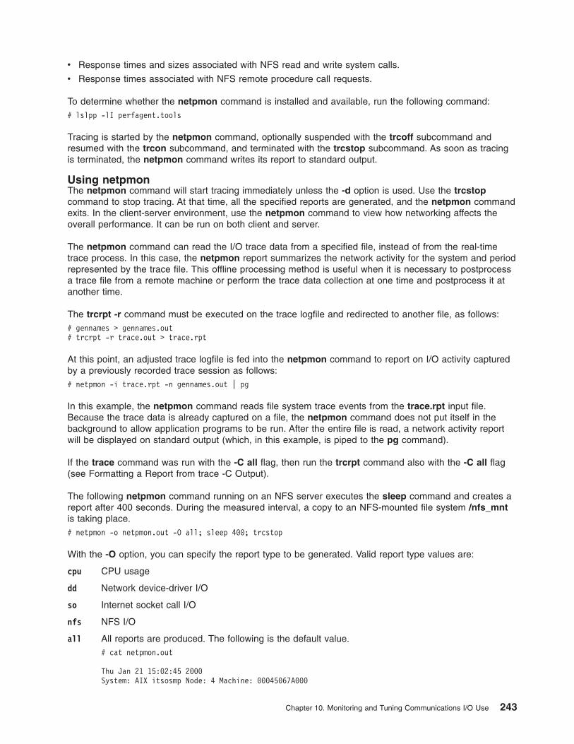
v Response times and sizes associated with NFS read and write system calls.

v Response times associated with NFS remote procedure call requests.

To determine whether the netpmon command is installed and available, run the following command:# lslpp -lI perfagent.tools

Tracing is started by the netpmon command, optionally suspended with the trcoff subcommand andresumed with the trcon subcommand, and terminated with the trcstop subcommand. As soon as tracingis terminated, the netpmon command writes its report to standard output.

Using netpmonThe netpmon command will start tracing immediately unless the -d option is used. Use the trcstopcommand to stop tracing. At that time, all the specified reports are generated, and the netpmon commandexits. In the client-server environment, use the netpmon command to view how networking affects theoverall performance. It can be run on both client and server.

The netpmon command can read the I/O trace data from a specified file, instead of from the real-timetrace process. In this case, the netpmon report summarizes the network activity for the system and periodrepresented by the trace file. This offline processing method is useful when it is necessary to postprocessa trace file from a remote machine or perform the trace data collection at one time and postprocess it atanother time.

The trcrpt -r command must be executed on the trace logfile and redirected to another file, as follows:# gennames > gennames.out# trcrpt -r trace.out > trace.rpt

At this point, an adjusted trace logfile is fed into the netpmon command to report on I/O activity capturedby a previously recorded trace session as follows:# netpmon -i trace.rpt -n gennames.out | pg

In this example, the netpmon command reads file system trace events from the trace.rpt input file.Because the trace data is already captured on a file, the netpmon command does not put itself in thebackground to allow application programs to be run. After the entire file is read, a network activity reportwill be displayed on standard output (which, in this example, is piped to the pg command).

If the trace command was run with the -C all flag, then run the trcrpt command also with the -C all flag(see Formatting a Report from trace -C Output).

The following netpmon command running on an NFS server executes the sleep command and creates areport after 400 seconds. During the measured interval, a copy to an NFS-mounted file system /nfs_mntis taking place.# netpmon -o netpmon.out -O all; sleep 400; trcstop

With the -O option, you can specify the report type to be generated. Valid report type values are:

cpu CPU usage

dd Network device-driver I/O

so Internet socket call I/O

nfs NFS I/O

all All reports are produced. The following is the default value.# cat netpmon.out

Thu Jan 21 15:02:45 2000System: AIX itsosmp Node: 4 Machine: 00045067A000


401.053 secs in measured interval========================================================================Process CPU Usage Statistics:-----------------------------

NetworkProcess (top 20) PID CPU Time CPU % CPU %----------------------------------------------------------nfsd 12370 42.2210 2.632 2.632nfsd 12628 42.0056 2.618 2.618nfsd 13144 41.9540 2.615 2.615nfsd 12886 41.8680 2.610 2.610nfsd 12112 41.4114 2.581 2.581nfsd 11078 40.9443 2.552 2.552nfsd 11854 40.6198 2.532 2.532nfsd 13402 40.3445 2.515 2.515lrud 1548 16.6294 1.037 0.000netpmon 15218 5.2780 0.329 0.000gil 2064 2.0766 0.129 0.129trace 18284 1.8820 0.117 0.000syncd 3602 0.3757 0.023 0.000swapper 0 0.2718 0.017 0.000init 1 0.2201 0.014 0.000afsd 8758 0.0244 0.002 0.000bootpd 7128 0.0220 0.001 0.000ksh 4322 0.0213 0.001 0.000pcimapsvr.ip 16844 0.0204 0.001 0.000netm 1806 0.0186 0.001 0.001----------------------------------------------------------Total (all processes) 358.3152 22.336 20.787Idle time 1221.0235 76.114

========================================================================First Level Interrupt Handler CPU Usage Statistics:---------------------------------------------------

NetworkFLIH CPU Time CPU % CPU %----------------------------------------------------------PPC decrementer 9.9419 0.620 0.000external device 4.5849 0.286 0.099UNKNOWN 0.1716 0.011 0.000data page fault 0.1080 0.007 0.000floating point 0.0012 0.000 0.000instruction page fault 0.0007 0.000 0.000----------------------------------------------------------Total (all FLIHs) 14.8083 0.923 0.099

========================================================================Second Level Interrupt Handler CPU Usage Statistics:----------------------------------------------------

NetworkSLIH CPU Time CPU % CPU %----------------------------------------------------------tokdd 12.4312 0.775 0.775ascsiddpin 0.5178 0.032 0.000----------------------------------------------------------Total (all SLIHs) 12.9490 0.807 0.775

========================================================================Network Device-Driver Statistics (by Device):---------------------------------------------

----------- Xmit ----------- -------- Recv ---------Device Pkts/s Bytes/s Util QLen Pkts/s Bytes/s Demux------------------------------------------------------------------------------token ring 0 31.61 4800 1.7% 0.046 200.93 273994 0.0080

========================================================================


Network Device-Driver Transmit Statistics (by Destination Host):----------------------------------------------------------------Host Pkts/s Bytes/s----------------------------------------ah6000c 31.57 47969.3.1.255 0.03 4itsorusi 0.00 0

========================================================================

TCP Socket Call Statistics (by Process):----------------------------------------

------ Read ----- ----- Write -----Process (top 20) PID Calls/s Bytes/s Calls/s Bytes/s------------------------------------------------------------------------telnetd 18144 0.03 123 0.06 0------------------------------------------------------------------------Total (all processes) 0.03 123 0.06 0

========================================================================

NFS Server Statistics (by Client):----------------------------------

------ Read ----- ----- Write ----- OtherClient Calls/s Bytes/s Calls/s Bytes/s Calls/s------------------------------------------------------------------------ah6000c 0.00 0 31.54 258208 0.01------------------------------------------------------------------------Total (all clients) 0.00 0 31.54 258208 0.01

========================================================================Detailed Second Level Interrupt Handler CPU Usage Statistics:-------------------------------------------------------------SLIH: tokddcount: 93039

cpu time (msec): avg 0.134 min 0.026 max 0.541 sdev 0.051SLIH: ascsiddpincount: 8136

cpu time (msec): avg 0.064 min 0.012 max 0.147 sdev 0.018COMBINED (All SLIHs)count: 101175

cpu time (msec): avg 0.128 min 0.012 max 0.541 sdev 0.053

========================================================================Detailed Network Device-Driver Statistics:------------------------------------------DEVICE: token ring 0recv packets: 80584

recv sizes (bytes): avg 1363.6 min 50 max 1520 sdev 356.3recv times (msec): avg 0.081 min 0.010 max 0.166 sdev 0.020demux times (msec): avg 0.040 min 0.008 max 0.375 sdev 0.040

xmit packets: 12678xmit sizes (bytes): avg 151.8 min 52 max 184 sdev 3.3xmit times (msec): avg 1.447 min 0.509 max 4.514 sdev 0.374

========================================================================Detailed Network Device-Driver Transmit Statistics (by Host):-------------------------------------------------------------HOST: ah6000cxmit packets: 12662

xmit sizes (bytes): avg 151.9 min 52 max 184 sdev 2.9xmit times (msec): avg 1.448 min 0.509 max 4.514 sdev 0.373

HOST: 9.3.1.255xmit packets: 14



HOST: itsorusixmit packets: 1


========================================================================Detailed TCP Socket Call Statistics (by Process):-------------------------------------------------PROCESS: telnetd PID: 18144reads: 12


writes: 23write sizes (bytes): avg 3.5 min 1 max 26 sdev 7.0write times (msec): avg 0.143 min 0.067 max 0.269 sdev 0.064

PROTOCOL: TCP (All Processes)reads: 12


writes: 23write sizes (bytes): avg 3.5 min 1 max 26 sdev 7.0write times (msec): avg 0.143 min 0.067 max 0.269 sdev 0.064

========================================================================Detailed NFS Server Statistics (by Client):-------------------------------------------CLIENT: ah6000cwrites: 12648


other calls: 5other times (msec): avg 1.928 min 0.371 max 8.065 sdev 3.068

COMBINED (All Clients)writes: 12648


other calls: 5other times (msec): avg 1.928 min 0.371 max 8.065 sdev 3.068

The output of the netpmon command is composed of two different types of reports: global and detailed.The global reports list statistics as follows:

v Most active processes

v First-level interrupt handlers

v Second-level interrupt handlers

v Network device drivers

v Network device-driver transmits

v TCP socket calls

v NFS server or client statistics

The global reports are shown at the beginning of the netpmon output and are the occurrences during themeasured interval. The detailed reports provide additional information for the global reports. By default, thereports are limited to the 20 most active statistics measured. All information in the reports is listed from topto bottom as most active to least active.

Global Reports of netpmonThe reports generated by the netpmon command begin with a header, which identifies the date, themachine ID, and the length of the monitoring period in seconds. The header is followed by a set of globaland detailed reports for all specified report types.


Process CPU Usage Statistics: Each row describes the CPU usage associated with a process. Unlessthe verbose (-v) option is specified, only the 20 most active processes are included in the list. At thebottom of the report, CPU usage for all processes is totaled, and CPU idle time is reported. The idle timepercentage number is calculated from the idle time divided by the measured interval. The differencebetween the CPU time totals and measured interval is due to Interrupt handlers.

The Network CPU % is the percentage of total time that this process spent executing network-related code.

If the -t flag is used, a thread CPU usage statistic is also present. Each process row described above isimmediately followed by rows describing the CPU usage of each thread owned by that process. The fieldsin these rows are identical to those for the process, except for the name field. Threads are not named.

In the example report, the Idle time percentage number (76.114 percent) shown in the global CPU usagereport is calculated from the Idle time (1221.0235) divided by the measured interval times 4 (401.053times 4), because there are four CPUs in this server. If you want to look at each CPU’s activity, you canuse sar, ps, or any other SMP-specific command. Similar calculation applies to the total CPU % that isoccupied by all processes. The Idle time is due to network I/O. The difference between the CPU Timetotals (1221.0235 + 358.315) and the measured interval is due to interrupt handlers and the multipleCPUs. It appears that in the example report, the majority of the CPU usage was network-related: (20.787 /22.336) = 93.07 percent. About 77.664 percent of CPU usage is either CPU idle or CPU wait time.

Note: If the result of total network CPU % divided by total CPU % is greater than 0.5 from Process CPU UsageStatistics for NFS server, then the majority of CPU usage is network-related.

This method is also a good way to view CPU usage by process without tying the output to a specificprogram.

First Level Interrupt Handler CPU Usage Statistics: Each row describes the CPU usage associatedwith a first-level interrupt handler (FLIH). At the bottom of the report, CPU usage for all FLIHs is totaled.

CPU TimeTotal amount of CPU time used by this FLIH

CPU %CPU usage for this interrupt handler as a percentage of total time

Network CPU %Percentage of total time that this interrupt handler executed on behalf of network-related events

Second Level Interrupt Handler CPU Usage Statistics: Each row describes the CPU usage associatedwith a second-level interrupt handler (SLIH). At the bottom of the report, CPU usage for all SLIHs istotaled.

Network Device-Driver Statistics (by Device): Each row describes the statistics associated with anetwork device.

DeviceName of special file associated with device

Xmit Pkts/sPackets per second transmitted through this device

Xmit Bytes/sBytes per second transmitted through this device

Xmit UtilBusy time for this device, as a percent of total time


Xmit QlenNumber of requests waiting to be transmitted through this device, averaged over time, includingany transaction currently being transmitted

Recv Pkts/sPackets per second received through this device

Recv Bytes/sBytes per second received through this device

Recv DemuxTime spent in demux layer as a fraction of total time

In this example, the Xmit QLen is only 0.046. This number is very small compared to its default size (30).Its Recv Bytes/s is 273994, much smaller than the Token-Ring transmit speed (16 Mb/s). Therefore, in thiscase, the network is not saturated, at least from this system’s view.

Network Device-Driver Transmit Statistics (by Destination Host): Each row describes the amount oftransmit traffic associated with a particular destination host, at the device-driver level.

Host Destination host name. An asterisk (*) is used for transmissions for which no host name can bedetermined.

Pkts/s Packets per second transmitted to this host.

Bytes/sBytes per second transmitted to this host.

TCP Socket Call Statistics for Each Internet Protocol (by Process): These statistics are shown foreach used Internet protocol. Each row describes the amount of read() and write() subroutine activity onsockets of this protocol type associated with a particular process. At the bottom of the report, all socketcalls for this protocol are totaled.

NFS Server Statistics (by Client): Each row describes the amount of NFS activity handled by thisserver on behalf of a particular client. At the bottom of the report, calls for all clients are totaled.

On a client machine, the NFS server statistics are replaced by the NFS client statistics (NFS ClientStatistics for each Server (by File), NFS Client RPC Statistics (by Server), NFS ClientStatistics (by Process)).

Detailed Reports of netpmonDetailed reports are generated for all requested (-O) report types. For these report types, a detailed reportis produced in addition to the global reports. The detailed reports contain an entry for each entry in theglobal reports with statistics for each type of transaction associated with the entry.

Transaction statistics consist of a count of the number of transactions for that type, followed by responsetime and size distribution data (where applicable). The distribution data consists of average, minimum, andmaximum values, as well as standard deviations. Roughly two-thirds of the values are between averageminus standard deviation and average plus standard deviation. Sizes are reported in bytes. Responsetimes are reported in milliseconds.

Detailed Second-Level Interrupt Handler CPU-Usage Statistics: The output fields are described asfollows:

SLIH Name of second-level interrupt handler

count Number of interrupts of this type

cpu time (msec)CPU usage statistics for handling interrupts of this type


Detailed Network Device-Driver Statistics (by Device): The output fields are described as follows:

DEVICEPath name of special file associated with device

recv packetsNumber of packets received through this device

recv sizes (bytes)Size statistics for received packets

recv times (msec)Response time statistics for processing received packets

demux times (msec)Time statistics for processing received packets in the demux layer

xmit packetsNumber of packets transmitted through this device

xmit sizes (bytes)Size statistics for transmitted packets

xmit times (msec)Response time statistics for processing transmitted packets

There are other detailed reports, such as Detailed Network Device-Driver Transmit Statistics (byHost) and Detailed TCP Socket Call Statistics for Each Internet Protocol (by Process). For anNFS client, there are the Detailed NFS Client Statistics for Each Server (by File), Detailed NFSClient RPC Statistics (by Server), and Detailed NFS Client Statistics (by Process) reports. For anNFS server, there is the Detailed NFS Server Statistics (by Client) report. They have similar outputfields as explained above.

In the example, the results from the Detailed Network Device-Driver Statistics lead to the following:

v recv bytes = 80584 packets * 1364 bytes/packet = 109,916,576 bytes

v xmit bytes = 12678 packets * 152 bytes/packet = 1,927,056 bytes

v total bytes exchanged = 109,916,576 + 1,927,056 = 111,843,632 bytes

v total bits exchanged = 111,843,632 * 8 bits/byte = 894,749,056 bits

v transmit speed = 894,749,056 / 401.053 = 2.23 Mb/s (assuming that the copy took the entire monitoringperiod)

As in the global device driver report, you can conclude that this case is not network-saturated. Theaverage receive size is 1363.6 bytes, near to the default MTU (maximum transmission unit) value, which is1492 when the device is a Token-Ring card. If this value is larger than the MTU (from lsattr -E -l interface,replacing interface with the interface name, such as en0 or tr0, you could change the MTU or adaptertransmit-queue length value to get better performance with the following command:# ifconfig tr0 mtu 8500

or# chdev -l ’tok0’ -a xmt_que_size=’150’

If the network is congested already, changing the MTU or queue value will not help.

Notes:

1. If transmit and receive packet sizes are small on the device driver statistics report, then increasing thecurrent MTU size will probably result in better network performance.

2. If system wait time due to network calls is high from the network wait time statistics for the NFS clientreport, the poor performance is due to the network.


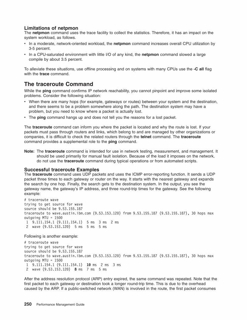
Limitations of netpmonThe netpmon command uses the trace facility to collect the statistics. Therefore, it has an impact on thesystem workload, as follows.

v In a moderate, network-oriented workload, the netpmon command increases overall CPU utilization by3-5 percent.

v In a CPU-saturated environment with little I/O of any kind, the netpmon command slowed a largecompile by about 3.5 percent.

To alleviate these situations, use offline processing and on systems with many CPUs use the -C all flagwith the trace command.

The traceroute CommandWhile the ping command confirms IP network reachability, you cannot pinpoint and improve some isolatedproblems. Consider the following situation:

v When there are many hops (for example, gateways or routes) between your system and the destination,and there seems to be a problem somewhere along the path. The destination system may have aproblem, but you need to know where a packet is actually lost.

v The ping command hangs up and does not tell you the reasons for a lost packet.

The traceroute command can inform you where the packet is located and why the route is lost. If yourpackets must pass through routers and links, which belong to and are managed by other organizations orcompanies, it is difficult to check the related routers through the telnet command. The traceroutecommand provides a supplemental role to the ping command.

Note: The traceroute command is intended for use in network testing, measurement, and management. Itshould be used primarily for manual fault isolation. Because of the load it imposes on the network,do not use the traceroute command during typical operations or from automated scripts.

Successful traceroute ExamplesThe traceroute command uses UDP packets and uses the ICMP error-reporting function. It sends a UDPpacket three times to each gateway or router on the way. It starts with the nearest gateway and expandsthe search by one hop. Finally, the search gets to the destination system. In the output, you see thegateway name, the gateway’s IP address, and three round-trip times for the gateway. See the followingexample:

# traceroute wavetrying to get source for wavesource should be 9.53.155.187traceroute to wave.austin.ibm.com (9.53.153.120) from 9.53.155.187 (9.53.155.187), 30 hops maxoutgoing MTU = 15001 9.111.154.1 (9.111.154.1) 5 ms 3 ms 2 ms2 wave (9.53.153.120) 5 ms 5 ms 5 ms

Following is another example:

# traceroute wavetrying to get source for wavesource should be 9.53.155.187traceroute to wave.austin.ibm.com (9.53.153.120) from 9.53.155.187 (9.53.155.187), 30 hops maxoutgoing MTU = 15001 9.111.154.1 (9.111.154.1) 10 ms 2 ms 3 ms2 wave (9.53.153.120) 8 ms 7 ms 5 ms

After the address resolution protocol (ARP) entry expired, the same command was repeated. Note that thefirst packet to each gateway or destination took a longer round-trip time. This is due to the overheadcaused by the ARP. If a public-switched network (WAN) is involved in the route, the first packet consumes


a lot of memory due to a connection establishment and may cause a timeout. The default timeout for eachpacket is 3 seconds. You can change it with the -w option.

The first 10 ms is due to the ARP between the source system (9.53.155.187) and the gateway9.111.154.1. The second 8 ms is due to the ARP between the gateway and the final destination (wave). Inthis case, you are using DNS, and every time before the traceroute command sends a packet, the DNSserver is searched.

Failed traceroute ExamplesFor a long path to your destination or complex network routes, you may see a lot of problems with thetraceroute command. Because many things are implementation-dependent, searching for the problemmay only waste your time. If all routers or systems involved are under your control, you may be able toinvestigate the problem completely.

Gateway (Router) Problem: In the following example, packets were sent from the system 9.53.155.187.There are two router systems on the way to the bridge. The routing capability was intentionally removedfrom the second router system by setting the option ipforwarding of the no command to 0. See thefollowing example:

# traceroute lamartrying to get source for lamarsource should be 9.53.155.187traceroute to lamar.austin.ibm.com (9.3.200.141) from 9.53.155.187 (9.53.155.187), 30 hops maxoutgoing MTU = 15001 9.111.154.1 (9.111.154.1) 12 ms 3 ms 2 ms2 9.111.154.1 (9.111.154.1) 3 ms !H * 6 ms !H

If an ICMP error message, excluding Time Exceeded and Port Unreachable, is received, it is displayed asfollows:

!H Host Unreachable

!N Network Unreachable

!P Protocol Unreachable

!S Source route failed

!F Fragmentation needed

Destination System Problem: When the destination system does not respond within a 3-secondtime-out interval, all queries are timed out, and the results are displayed with an asterisk (*).

# traceroute chuystrying to get source for chuyssource should be 9.53.155.187traceroute to chuys.austin.ibm.com (9.53.155.188) from 9.53.155.187 (9.53.155.187), 30 hops maxoutgoing MTU = 15001 * * *2 * * *3 * * *^C#

If you think that the problem is due to a communication link, use a longer timeout period with the -w flag.Although rare, all the ports queried might have been used. You can change the ports and try again.

Number of ″hops″ to Destination: Another output example might be as follows:# traceroute mysystem.university.edu (129.2.130.22)traceroute to mysystem.university.edu (129.2.130.22), 30 hops max1 helios.ee.lbl.gov (129.3.112.1) 0 ms 0 ms 0 ms2 lilac-dmc.university.edu (129.2.216.1) 39 ms 19 ms 39 ms3 lilac-dmc.university.edu (129.2.215.1) 19 ms 39 ms 19 ms


4 ccngw-ner-cc.university.edu (129.2.135.23) 39 ms 40 ms 19 ms5 ccn-nerif35.university.edu (129.2.167.35) 39 ms 39 ms 39 ms6 csgw/university.edu (129.2.132.254) 39 ms 59 ms 39 ms7 * * *8 * * *9 * * *10 * * *11 * * *12 * * *13 rip.university.EDU (129.2.130.22) 59 ms! 39 ms! 39 ms!

In this example, exactly half of the 12 gateway hops (13 is the final destination) are ″missing.″ However,these hops were actually not gateways. The destination host used the time to live (ttl) from the arrivingdatagram as the ttl in its ICMP reply; thus, the reply timed out on the return path. Because ICMPs are notsent for ICMPs, no notice was received. The ! (exclamation mark) after each round-trip time indicatessome type of software incompatibility problem. (The cause was diagnosed after the traceroute commandissued a probe of twice the path length. The destination host was really only seven hops away.)

The iptrace daemon, and the ipreport and ipfilter CommandsYou can use many tools for observing network activity. Some run under the operating system, others runon dedicated hardware. One tool that can be used to obtain a detailed, packet-by-packet description of theLAN activity generated by a workload is the combination of the iptrace daemon and the ipreportcommand. To use the iptrace daemon with operating system version 4, you need the bos.net.tcp.serverfileset. The iptrace daemon is included in this fileset, as well as some other useful commands such as thetrpt and tcdump commands. The iptrace daemon can only be started by a root user.

By default, the iptrace daemon traces all packets. The option -a allows exclusion of address resolutionprotocol (ARP) packets. Other options can narrow the scope of tracing to a particular source host (-s),destination host (-d), or protocol (-p). Because the iptrace daemon can consume significant amounts ofprocessor time, be as specific as possible when you describe the packets you want traced.

Because iptrace is a daemon, start the iptrace daemon with the startsrc command rather than directlyfrom the command line. This method makes it easier to control and shut down cleanly. A typical examplewould be as follows:# startsrc -s iptrace -a "-i tr0 /home/user/iptrace/log1"

This command starts the iptrace daemon with instructions to trace all activity on the Token-Ring interface,tr0, and place the trace data in /home/user/iptrace/log1. To stop the daemon, use the following:# stopsrc -s iptrace

If you did not start the iptrace daemon with the startsrc command, you must use the ps command to findits process ID with and terminate it with the kill command.

The ipreport command is a formatter for the log file. Its output is written to standard output. Options allowrecognition and formatting of RPC packets (-r), identifying each packet with a number (-n), and prefixingeach line with a 3-character string that identifies the protocol (-s). A typical ipreport command to formatthe log1 file just created (which is owned by the root user) would be as follows:# ipreport -ns log1 >log1_formatted

This would result in a sequence of packet reports similar to the following examples. The first packet is thefirst half of a ping packet. The fields of most interest are as follows:

v The source (SRC) and destination (DST) host address, both in dotted decimal and in ASCII

v The IP packet length (ip_len)

v The indication of the higher-level protocol in use (ip_p)


Packet Number 131TOK: =====( packet transmitted on interface tr0 )=====Fri Jan 14 08:42:07 2000TOK: 802.5 packetTOK: 802.5 MAC header:TOK: access control field = 0, frame control field = 40TOK: [ src = 90:00:5a:a8:88:81, dst = 10:00:5a:4f:35:82]TOK: routing control field = 0830, 3 routing segmentsTOK: routing segments [ ef31 ce61 ba30 ]TOK: 802.2 LLC header:TOK: dsap aa, ssap aa, ctrl 3, proto 0:0:0, type 800 (IP)IP: < SRC = 129.35.145.140 > (alborz.austin.ibm.com)IP: < DST = 129.35.145.135 > (xactive.austin.ibm.com)IP: ip_v=4, ip_hl=20, ip_tos=0, ip_len=84, ip_id=38892, ip_off=0IP: ip_ttl=255, ip_sum=fe61, ip_p = 1 (ICMP)ICMP: icmp_type=8 (ECHO_REQUEST) icmp_id=5923 icmp_seq=0ICMP: 00000000 2d088abf 00054599 08090a0b 0c0d0e0f |-.....E.........|ICMP: 00000010 10111213 14151617 18191a1b 1c1d1e1f |................|ICMP: 00000020 20212223 24252627 28292a2b 2c2d2e2f | !"#$%&’()*+,-./|ICMP: 00000030 30313233 34353637 |01234567 |

The next example is a frame from an ftp operation. Note that the IP packet is the size of the MTU for thisLAN (1492 bytes).Packet Number 501TOK: =====( packet received on interface tr0 )=====Fri Dec 10 08:42:51 1999TOK: 802.5 packetTOK: 802.5 MAC header:TOK: access control field = 18, frame control field = 40TOK: [ src = 90:00:5a:4f:35:82, dst = 10:00:5a:a8:88:81]TOK: routing control field = 08b0, 3 routing segmentsTOK: routing segments [ ef31 ce61 ba30 ]TOK: 802.2 LLC header:TOK: dsap aa, ssap aa, ctrl 3, proto 0:0:0, type 800 (IP)IP: < SRC = 129.35.145.135 > (xactive.austin.ibm.com)IP: < DST = 129.35.145.140 > (alborz.austin.ibm.com)IP: ip_v=4, ip_hl=20, ip_tos=0, ip_len=1492, ip_id=34233, ip_off=0IP: ip_ttl=60, ip_sum=5ac, ip_p = 6 (TCP)TCP: <source port=20(ftp-data), destination port=1032 >TCP: th_seq=445e4e02, th_ack=ed8aae02TCP: th_off=5, flags<ACK |>TCP: th_win=15972, th_sum=0, th_urp=0TCP: 00000000 01df0007 2cd6c07c 00004635 000002c2 |....,..|..F5....|TCP: 00000010 00481002 010b0001 000021b4 00000d60 |.H........!....`|

--------- Lots of uninteresting data omitted -----------TCP: 00000590 63e40000 3860000f 4800177d 80410014 |c...8`..H..}.A..|TCP: 000005a0 82220008 30610038 30910020 |."..0a.80.. |

The ipfilter command extracts different operation headers from an ipreport output file and displays themin a table. Some customized NFS information regarding requests and replies is also provided.

To determine whether the ipfilter command is installed and available, run the following command:# lslpp -lI perfagent.tools

An example command is as follows:# ipfilter log1_formatted

The operation headers currently recognized are: udp, nfs, tcp, ipx, icmp. The ipfilter command has threedifferent types of reports, as follows:

v A single file (ipfilter.all) that displays a list of all the selected operations. The table displays packetnumber, Time, Source & Destination, Length, Sequence #, Ack #, Source Port, Destination Port,Network Interface, and Operation Type.

v Individual files for each selected header (ipfilter.udp, ipfilter.nfs, ipfilter.tcp, ipfilter.ipx, ipfilter.icmp).The information contained is the same as ipfilter.all.


v A file nfs.rpt that reports on NFS requests and replies. The table contains: Transaction ID #, Type ofRequest, Status of Request, Call Packet Number, Time of Call, Size of Call, Reply Packet Number,Time of Reply, Size of Reply, and Elapsed millisecond between call and reply.

Adapter StatisticsThe commands in this section provide output comparable to the netstat -v command. They allow you toreset adapter statistics (-r) and to get more detailed output (-d) than the netstat -v command outputprovides.

The entstat CommandThe entstat command displays the statistics gathered by the specified Ethernet device driver. The usercan optionally specify that the device-specific statistics be displayed in addition to the device-genericstatistics. Using the -d option will list any extended statistics for this adapter and should be used to ensureall statistics are displayed. If no flags are specified, only the device-generic statistics are displayed.

The entstat command is also invoked when the netstat command is run with the -v flag. The netstatcommand does not issue any entstat command flags.# entstat ent0-------------------------------------------------------------ETHERNET STATISTICS (ent0) :Device Type: IBM 10/100 Mbps Ethernet PCI Adapter (23100020)Hardware Address: 00:60:94:e9:29:18Elapsed Time: 0 days 0 hours 0 minutes 0 seconds



Broadcast Packets: 0 Broadcast Packets: 0Multicast Packets: 0 Multicast Packets: 0No Carrier Sense: 0 CRC Errors: 0DMA Underrun: 0 DMA Overrun: 0Lost CTS Errors: 0 Alignment Errors: 0Max Collision Errors: 0 No Resource Errors: 0Late Collision Errors: 0 Receive Collision Errors: 0Deferred: 0 Packet Too Short Errors: 0SQE Test: 0 Packet Too Long Errors: 0Timeout Errors: 0 Packets Discarded by Adapter: 0Single Collision Count: 0 Receiver Start Count: 0Multiple Collision Count: 0Current HW Transmit Queue Length: 0

General Statistics:-------------------No mbuf Errors: 0Adapter Reset Count: 0Driver Flags: Up Broadcast Running

Simplex 64BitSupport

In the above report, you may want to concentrate on:

Transmit ErrorsNumber of output errors encountered on this device. This is a counter for unsuccessfultransmissions due to hardware/network errors.


Receive ErrorsNumber of input errors encountered on this device. This is a counter for unsuccessful receptiondue to hardware/network errors.

Packets DroppedNumber of packets accepted by the device driver for transmission which were not (for any reason)given to the device.

Max Packets on S/W Transmit QueueMaximum number of outgoing packets ever queued to the software transmit queue.

S/W Transmit Queue OverflowNumber of outgoing packets that have overflowed the transmit queue.

No Resource ErrorsNumber of incoming packets dropped by the hardware due to lack of resources. This error usuallyoccurs because the receive buffers on the adapter were exhausted. Some adapters may have thesize of the receive buffers as a configurable parameter. Check the device configuration attributes(or SMIT helps) for possible tuning information.

Single Collision Count/Multiple Collision CountNumber of collisions on an Ethernet network. These collisions are accounted for here rather thanin the collision column of the output of the netstat -i command.

Notice in this example, the Ethernet adapter is behaving well because there are no Receive Errors. Theseerrors are sometimes caused when a saturated network only transmits partial packets. The partial packetsare eventually retransmitted successfully but are recorded as receive errors.

If you receive S/W Transmit Queue Overflow errors, the value of Max Packets on S/W Transmit Queue willcorrespond to the transmit queue limit for this adapter (xmt_que_size).

Note: These values can represent the hardware queue if the adapter does not support a software transmitqueue. If there are transmit-queue overflows, then increased the hardware or software queue limitsfor the driver.

If there are not enough receive resources, this would be indicated by Packets Dropped: and depending onthe adapter type, would be indicated by Out of Rcv Buffers or No Resource Errors: or some similarcounter.

The elapsed time displays the real-time period that has elapsed since the last time the statistics werereset. To reset the statistics, use the entstat -r adapter_name command.

Similar output can be displayed for Token-Ring, FDDI, and ATM interfaces using the tokstat, fddistat, andatmstat commands.

The tokstat CommandThe tokstat command displays the statistics gathered by the specified Token-Ring device driver. The usercan optionally specify that the device-specific statistics be displayed in addition to the device driverstatistics. If no flags are specified, only the device driver statistics are displayed.

This command is also invoked when the netstat command is run with the -v flag. The netstat commanddoes not issue any tokstat command flags.

The output produced by the tokstat tok0 command and the problem determination are similar to thatdescribed in The entstat Command.


The fddistat CommandThe fddistat command displays the statistics gathered by the specified FDDI device driver. The user canoptionally specify that the device-specific statistics be displayed in addition to the device driver statistics. Ifno flags are specified, only the device driver statistics are displayed.

This command is also invoked when the netstat command is run with the -v flag. The netstat commanddoes not issue any fddistat command flags.

The output produced by the fddistat fddi0 command and the problem determination are similar to thatdescribed in The entstat Command.

The atmstat CommandThe atmstat command displays the statistics gathered by the specified ATM device driver. The user canoptionally specify that the device-specific statistics be displayed in addition to the device driver statistics. Ifno flags are specified, only the device driver statistics are displayed.

The output produced by the atmstat atm0 command and the problem determination are similar to thatdescribed in The entstat Command.

The no CommandUse the no command to display current network values and to change options.

-a Prints all options and current values (example: no -a)

-d Sets options back to default (example: no -d thewall)

-o option=NewValue (example: no -o thewall=16384)

For a listing of all attributes for the no command, see Network Option Tunable Parameters.

Some network attributes are run-time attributes that can be changed at any time. Others are load-timeattributes that must be set before the netinet kernel extension is loaded.

Note: When the no command is used to change parameters, the change is in effect only until the nextsystem boot. At that point, all parameters are initially reset to their defaults. To make the changepermanent, put the appropriate no command in the /etc/rc.net file.

If your system uses Berkeley-style network configuration, set the attributes near the top of the/etc/rc.bsdnet file. If you use an SP system, edit the tuning.cust file as documented in the RS/6000 SP:Installation and Relocation manual.

Note: The no command performs no-range checking. If it is used incorrectly, the no command can causeyour system to become inoperable.

The following tuning sections discuss some of the no command attributes and how to adjust them.

Tuning TCP and UDP PerformanceThe optimal settings of the tunable communications parameters vary with the type of LAN, as well as withthe communications-I/O characteristics of the predominant system and application programs. The followingsections describe the global principles of communications tuning, followed by specific recommendations forthe different types of LAN.

Overall RecommendationsYou can choose to tune primarily either for maximum throughput or for minimum memory use. Somerecommendations apply to one or the other; some apply to both. Recommended application block sizes fordifferent adapter devices are as follows:


Device Name Application Block Size

Ethernet Multiples of 4096

Token-Ring (4 Mb) Multiples of 4096

Token-Ring (16 Mb) Multiples of 4096

FDDI (tcp) Multiples of 4096

SOCC (tcp) 28672 bytes

HIPPI 65536 bytes

ATM Multiples of 4096

Maximizing ThroughputUse the following recommendations to tune for maximum throughput:

Request-Response Protocols: Follow these guidelines:

v For maximum number of transactions per second, use the smallest feasible messages.

v For maximum bytes per second, use messages that are at least 1000 bytes and equal to or just lessthan a multiple of 4096 bytes.

v If the requests and responses are fixed-size and fit into one datagram, use UDP.

– If possible, make the write sizes equal to the following:

(a multiple of the MTU size minus 28 bytes to allow for standard IP and UDP headers).

– In general, it is more efficient for the application to write large messages and have them fragmentedand reassembled by IP, than to have the application write multiple times.

– Whenever possible, use the connect() subroutine to associate an address with the UDP socket. Thismay not be possible on a server that is communicating with a number of clients through a singlesocket.

v If the requests or responses are variable-size, use TCP with the TCP_NODELAY option. Measurementsindicate that the overhead of TCP compared with UDP is negligible, especially if optimum write sizesare used.

– To avoid data copies in the kernel, make write sizes greater than 512 bytes.

– Make writes equal to or slightly less than, a multiple of MTU size. This will avoid the sending of asegment (packet) with just a few bytes in it.

Streaming: Follow these guidelines:

v TCP provides higher throughput than UDP and ensures reliable delivery.

v Writes should be in multiples of 16384 bytes. If possible, writes should be the size of the MSS (seeTuning TCP Maximum Segment Size).

Minimizing MemoryUse the following recommendations to tune for minimizing memory usage:

v If your traffic is predominantly local, use the largest MTU size that is supported by your LAN type. Thisminimizes the fragmentation of packets exchanged by local systems. The offsetting cost isfragmentation in gateways that connect your LAN to other LANs with smaller MTUs (see Tuning TCPMaximum Segment Size).

v Whenever possible, application programs should read and write in quantities of either:

– Less than or equal to 512 bytes

OR

– Slightly less than or equal to 4096 bytes (or multiples thereof)


If the applications were using TCP, both time and memory would be wasted. TCP tries to form outbounddata into MTU-sized packets. If the MTU of the LAN were larger than 14976 bytes, TCP would put thesending thread to sleep when the tcp_sendspace limit was reached.To force the data to be written, atimeout ACK from the receiver would be required.

Adapter Transmit and Receive Queue TuningMost communication drivers provide a set of tunable parameters to control transmit and receive resources.These parameters typically control the transmit queue and receive queue limits, but may also control thenumber and size of buffers or other resources. These parameters limit the number of buffers or packetsthat may be queued for transmit or limit the number of receive buffers that are available for receivingpackets. These parameters can be tuned to ensure enough queueing at the adapter level to handle thepeak loads generated by the system or the network.

Following are some general guidelines:

v Tune transmit queues when the CPU is faster than the network (more common on multi-processorsystems where many CPUs are transmitting to a single adapter).

v Tune transmit queues when socket buffer sizes are large.

v Tune receive queues when there is very bursty traffic.

v Tune transmit and receive queues when there is high rate of small-sized packets.

Transmit QueuesFor transmit, the device drivers may provide a transmit queue limit. There may be both hardware queueand software queue limits, depending on the driver and adapter. Some drivers have only a hardwarequeue; some have both hardware and software queues. Some drivers internally control the hardwarequeue and only allow the software queue limits to be modified. Generally, the device driver will queue atransmit packet directly to the adapter hardware queue. If the system CPU is fast relative to the speed ofthe network, or on an SMP system, the system may produce transmit packets faster than they can betransmitted on the network. This will cause the hardware queue to fill. After the hardware queue is full,some drivers provide a software queue and they will then queue to the software queue. If the softwaretransmit queue limit is reached, then the transmit packets are discarded. This can affect performancebecause the upper-level protocols must then time out and retransmit the packet.

Prior to AIX 4.2.1, the upper limits on the transmit queues were in the range of 150 to 250, depending onthe specific adapter. The system default values were low, typically 30. With AIX 4.2.1 and later, thetransmit queue limits were increased on most of the device drivers to 2048 buffers. The default valueswere also increased to 512 for most of these drivers. The default values were increased because thefaster CPUs and SMP systems can overrun the smaller queue limits.

Following are examples of MCA adapter transmit queue sizes:

MCA Adapter Type Default Range

Ethernet 512 20 - 2048

10/100 Ethernet 64 16,32,64,128,256

Token-Ring 99 or 512 32 - 2048

FDDI 512 3 - 2048

ATM / 155 ATM 512 0 - 2048

Following are examples of PCI adapter transmit queue sizes:

PCI Adapter Type Default Range

Ethernet 64 16 - 256

10/100 Ethernet 256, 512, or 2048 16 -16384


Token-Ring 96, 512, or 2048 32 - 16384

FDDI 30 or 2048 3 - 16384

155 ATM 100 or 2048 0 - 16384

For adapters that provide hardware queue limits, changing these values will cause more real memory tobe consumed on receives because of the associated control blocks and buffers associated with them.Therefore, raise these limits only if needed or for larger systems where the increase in memory use isnegligible. For the software transmit queue limits, increasing these limits does not increase memory usage.It only allows packets to be queued that were already allocated by the higher layer protocols.

Receive QueuesSome adapters allow you to configure the number of resources used for receiving packets from thenetwork. This might include the number of receive buffers (and even their size) or may be a receive queueparameter (which indirectly controls the number of receive buffers).

The receive resources may need to be increased to handle peak bursts on the network. The networkinterface device driver places incoming packets on a receive queue. If the receive queue is full, packetsare dropped and lost, resulting in the sender needing to retransmit. The receive queue is tunable using theSMIT or chdev commands (see How to Change the Parameters). The maximum queue size is specified toeach type of communication adapter (see Tuning MCA and PCI Adapters).

For the Micro Channel adapters and the PCI adapters, receive queue parameters typically control thenumber of receive buffers that are provided to the adapter for receiving input packets.

Device-Specific BuffersAIX 4.1.4 and later support device-specific mbufs. This allows a driver to allocate its own private set ofbuffers and have them pre-setup for Direct Memory Access (DMA). This can provide additionalperformance because the overhead to set up the DMA mapping is done one time. Also, the adapter canallocate buffer sizes that are best suited to its MTU size. For example, ATM, High Performance ParallelInterface (HIPPI), and the SP switch support a 64 K MTU (packet) size. The maximum system mbuf sizeis 16 KB. By allowing the adapter to have 64 KB buffers, large 64 K writes from applications can be copieddirectly into the 64 KB buffers owned by the adapter, instead of copying them into multiple 16 K buffers(which has more overhead to allocate and free the extra buffers).

The adapters that support Device Specific mbufs are:

v MCA ATM

v MCA HIPPI

v Various SP high speed switch adapters

Device-specific buffers add an extra layer of complexity for the system administrator. The systemadministrator must use device-specific commands to view the statistics relating to the adapter’s buffersand then change the adapter’s parameters as necessary. If the statistics indicate that packets werediscarded because not enough buffer resources were available, then those buffer sizes need to beincreased.

Due to differences between drivers and the utilities used to alter these parameters, the utilities andparameters are not fully described here. The MCA ATM parameters are listed in Micro Channel Adapter(MCA). Use the atmstat -d atm0 command to view the ATM statistics (substitute your ATM interfacenumber as needed).

When to Increase the Receive/Transmit Queue ParametersFollowing are some guidelines to help you determine when to increase the receive/transmit queueparameters:


1. When the CPU is much faster than the network and multiple applications may be using the samenetwork. This would be common on a larger multi-processor system (SMP).

2. When running with large values for tcp_sendspace or tcp_recvspace as set in the no options orrunning applications that might use system calls to increase the TCP send and receive socket bufferspace. These large values can cause the CPU to send down large numbers of packets to the adapter,which will need to be queued. Procedures are similar for udp_sendspace and udp_recvspace forUDP applications.

3. When there is very bursty traffic.

4. A high-traffic load of small packets can consume more resources than a high traffic load of largebuffers. Because large buffers take more time to send on the network. The packet rate will therefore beslower for larger packets.

Commands to Query and Change the Queue ParametersSeveral status utilities can be used to show the transmit queue high-water limits and number of queueoverflows. You can use the command netstat -v, or go directly to the adapter statistics utilities (entstat forEthernet, tokstat for Token-Ring, fddistat for FDDI, atmstat for ATM, and so on).

For an entstat example output, see The entstat Command. Another method is to use the netstat -i utility.If it shows non-zero counts in the Oerrs column for an interface, then this is typically the result of outputqueue overflows.

How to See the SettingsYou can use the lsattr -E -l adapter-name command or you can use the SMIT command (smittycommodev) to show the adapter configuration.

Different adapters have different names for these variables. For example, they may be namedsw_txq_size, tx_que_size, or xmt_que_size for the transmit queue parameter. The receive queue sizeand receive buffer pool parameters may be named rec_que_size, rx_que_size, or rv_buf4k_min forexample.

Following is the output of a lsattr -E -l atm0 command on an IBM PCI 155 Mbs ATM adapter. This outputshows the sw_txq_size is set to 250 and the rv_buf4K_min receive buffers set to x30.# lsattr -E -l atm0dma_mem 0x400000 N/A Falseregmem 0x1ff88000 Bus Memory address of Adapter Registers Falsevirtmem 0x1ff90000 Bus Memory address of Adapter Virtual Memory Falsebusintr 3 Bus Interrupt Level Falseintr_priority 3 Interrupt Priority Falseuse_alt_addr no Enable ALTERNATE ATM MAC address Truealt_addr 0x0 ALTERNATE ATM MAC address (12 hex digits) Truesw_txq_size 250 Software Transmit Queue size Truemax_vc 1024 Maximum Number of VCs Needed Truemin_vc 32 Minimum Guaranteed VCs Supported Truerv_buf4k_min 0x30 Minimum 4K-byte pre-mapped receive buffers Trueinterface_type 0 Sonet or SDH interface Trueadapter_clock 1 Provide SONET Clock Trueuni_vers auto_detect N/A True

Following is an example of a Micro Channel 10/100 Ethernet settings using the lsattr -E -l ent0 command.This output shows the tx_que_size and rx_que_size both set to 256.# lsattr -E -l ent0bus_intr_lvl 11 Bus interrupt level Falseintr_priority 3 Interrupt priority Falsedma_bus_mem 0x7a0000 Address of bus memory used for DMA Falsebus_io_addr 0x2000 Bus I/O address Falsedma_lvl 7 DMA arbitration level Falsetx_que_size 256 TRANSMIT queue size Truerx_que_size 256 RECEIVE queue size Trueuse_alt_addr no Enable ALTERNATE ETHERNET address True


alt_addr 0x ALTERNATE ETHERNET address Truemedia_speed 100_Full_Duplex Media Speed Trueip_gap 96 Inter-Packet Gap True

How to Change the ParametersThe following are some of the parameters that are user-configurable:

v Transmit Queue Size (tx_que_size)

The device driver supports a user-configurable transmit queue. This is the queue the adapter uses (notan extension of the adapter’s queue). It is configurable among the values of 16, 32, 64, 128 and 256,with a default of 256.

Because of the configurable size of the adapter’s hardware queue, the driver does not support asoftware queue.

v Receive Queue Size (rx_que_size)

The device driver supports a user-configurable receive queue. This is the queue the adapter uses (notan extension of the adapter’s queue). It is configurable among the values of 16, 32, 64, 128 and 256,with a default of 256.

v Receive Buffer Pool Size (rxbuf_pool_size)

The device driver supports a user-configurable receive buffer pool size. The buffer is the number ofpreallocated mbufs for receiving packets. The minimum size of the buffer is the receive queue size andthe maximum is 2 KB (the default value of 384).

v Media Speed (media_speed)

The device driver supports speeds of 10 (10 Mbps, half-duplex), 20 (10 Mbps, full-duplex), 100 (100Mbps, half-duplex), 200 (100 Mbps, full-duplex), and auto-negotiate on twisted pair. On the AUI port, thedevice driver supports speeds of 10 (10 Mbps, half-duplex) and 20 (10 Mbps, full-duplex). The bayonetNiell-Concelman (BNC) port will only support 10 (10 Mbps, half-duplex). This attribute isuser-configurable, with a default of auto-negotiate on twisted pair.

v Enable Alternate Address (use_alt_addr)

The device driver supports a configuration option to toggle use of an alternate network address. Thevalues are yes and no, with a default of no. When this value is set to yes, the alt_addr parameterdefines the address.

v Alternate Network Address (alt_addr)

For the network address, the device driver accepts the adapter’s hardware address or a configuredalternate network address. When the use_alt_addr configuration option is set to yes, this alternateaddress is used. Any valid individual address can be used, but a multicast address cannot be definedas a network address.

v Inter-Packet Gap (ip_gap)

The inter-packet gap (IPG) bit rate setting controls the aggressiveness of the adapter on the network. Asmaller number will increase the aggressiveness of the adapter, while a larger number will decrease theaggressiveness (and increase the fairness) of the adapter. If the adapter statistics show a large numberof collisions and deferrals, increase this number. Valid values range from 96 to 252, in increments of 4.The default value of 96 results in IPG of 9.6 microseconds for 10 Mb and 0.96 microseconds for 100Mb media speeds. Each unit of bit rate introduces an IPG of 100 ns at 10 Mb and 10 ns at 100 Mbmedia speed.

To change any of the parameter values, do the following:

1. Detach the interface by running the following command:# ifconfig en0 detach

where en0 represents the adapter name.

2. Use SMIT to display the adapter settings. Select Devices -> Communications -> adapter type ->Change/Show...


3. Move the cursor to the field you want to change, and press F4 to see the minimum and maximumranges for the field (or the specific set of sizes that are supported).

4. Select the appropriate size, and press Enter to update the ODM database.

5. Reattach the adapter by running the following command:# ifconfig en0 hosthame up

An alternative method to change these parameter values is to run the following command:# chdev -l [ifname] -a [attribute-name]=newvalue

For example, to change the above tx_que_size on en0 to 128, use the following sequence of commands.Note that this driver only supports four different sizes, so it is better to use the SMIT command to seethese values.# ifconfig en0 detach# chdev -l ent0 -a tx_que_size=128# ifconfig en0 hostname up

Tuning MCA and PCI AdaptersThe following information is provided to document the various adapter-tuning parameters. Theseparameters and values are for AIX 4.3.1 and are provided to aid you in understanding the various tuningparameters, or when a system is not available to view the parameters.

These parameter names, defaults, and range values were obtained from the ODM database. Thecomment field was obtained from the lsattr -E -l interface-name command.

The Notes field provides additional comments.

Micro Channel Adapter (MCA):

Feature Code: 2980Ethernet High-Performance LAN Adapter (8ef5)

Parameter Default Range Comment Notes------------- -------- -------- --------------------------- -----------------xmt_que_size 512 20-2048 TRANSMIT queue size SW TX queuerec_que_size 30 20-150 RECEIVE queue size See Note 1rec_pool_size 37 16-64 RECEIVE buffer pool size On Adapter

Feature Code: 2992Ethernet High-Performance LAN Adapter (8f95)

Parameter Default Range Comment Notes------------- --------- -------- ------------------- ----------xmt_que_size 512 20-2048 TRANSMIT queue size SW queue

Feature Code: 2994IBM 10/100 Mbps Ethernet TX MCA Adapter (8f62)

Parameter Default Range Comment Notes------------- -------- ---------------- --------------------- -----------tx_que_size 64 16,32,64,128,256 TRANSMIT queue size HW queuerx_que_size 32 16,32,64,128,256 RECEIVE queue size HW queue

Feature Code: 2970Token-Ring High-Performance Adapter (8fc8)

Parameter Default Range Comment Notes


------------- -------- -------- --------------------- ------------xmt_que_size 99 32-2048 TRANSMIT queue size SW queuerec_que_size 30 20-150 RECEIVE queue size See Note 1

Feature Code: 2972Token-Ring High-Performance Adapter (8fa2)

Parameter Default Range Comment Notes------------- -------- -------- ---------------------------- ----------xmt_que_size 512 32-2048 TRANSMIT queue size SW queuerx_que_size 32 32-160 HARDWARE RECEIVE queue size HW queue

Feature Code: 2727FDDI Primary Card, Single Ring Fiber

Parameter Default Range Comment Notes------------- -------- -------- ------------------------------ --------------------tx_que_size 512 3-2048 Transmit Queue Size (in mbufs)rcv_que_size 30 20-150 Receive Queue See Note 1

Feature Code: 2984100 Mbps ATM Fiber Adapter (8f7f)

Parameter Default Range Comment Notes--------------- ----- --------- -------------------------- -----sw_queue 512 0-2048 Software transmit queue len. SW Queuedma_bus_width 0x1000000 0x800000-0x40000000,0x100000Amount of memory to map for DMA See Note 3max_sml_bufs 50 40-400 Maximum Small ATM mbufs Max 256 byte buffersmax_med_bufs 100 40-1000 Maximum Medium ATM mbufs Max 4KB buffersmax_lrg_bufs 300 75-1000 Maximum Large ATM mbufs Max 8KB buffers See Note 2max_hug_bufs 50 0-400 Maximum Huge ATM mbufs Max 16KB buffersmax_spec_bufs 4 0-400 Maximum ATM MTB mbufs Max of max_spec_buf sizespec_buf_size 64 32-1024 Max Transmit Block (MTB) size (kbytes)sml_highwater 20 10-200 Minimum Small ATM mbufs Min 256 byte buffersmed_highwater 30 20-300 Minimum Medium ATM mbufs Min 4KB bufferslrg_highwater 70 65-400 Minimum Large ATM mbufs Min 8KB buffershug_highwater 10 4-300 Minimum Huge ATM mbufs Min 16KB buffersspec_highwater 20 0-300 Minimum ATM MTB mbufs Min 64KB buffersbest_peak_rate 1500 1-155000 Virtual Circuit Peak Segamentation Rate

Feature Code: 2989155 Mbps ATM Fiber Adapter (8f67)

Parameter Default Range Comment Notes------------- -------- -------- ---------- -------(same as ATM 100 adapter above)

Notes:

1. A software receive queue is provided only for compatibility with operating system version 3.2.xapplications that use the network device driver interface to read packets directly from the driver. Thisqueue limits how many input packets are queued for these applications to receive. This parameter isdefined only if bos.compat is installed.

This queue is not used by the typical TCP/IP stack.


2. MCA ATM: The receive side also uses the large (8 K) buffers. The receive logic only uses the 8 Kbuffers, so if this size runs low, it affects receive performance.

The other buffers sizes are only for transmit buffers.

3. MCA ATM: If you need to increase the total number of buffers, you may need to change thedma_bus_width (= 0x1000000) parameter. DMA bus memory width controls the total amount ofmemory used for ATM buffers. Increase this parameter if you get an error while you are increasing themaximum buffers or high-water limits.

PCI Adapters:Feature Code 2985IBM PCI Ethernet Adapter (22100020)

Parameter Default Range Comment Notes------------- -------- ----------------- ------------------- ---------tx_que_size 64 16,32,64,128,256 TRANSMIT queue size HW Queuesrx_que_size 32 16,32,64,128,256 RECEIVE queue size HW Queues

Featue Code 2968IBM 10/100 Mbps Ethernet PCI Adapter (23100020)

Parameter Default Range Comment Notes---------------- ------- ---------------- --------------------- --------------------tx_que_size 256 16,32,64,128,256 TRANSMIT queue size HW Queue Note 1rx_que_size 256 16,32,64,128,256 RECEIVE queue size HW Queue Note 2rxbuf_pool_size 384 16-2048 # buffers in receive Dedicat. receive

buffer pool buffers Note 3

Feature Code: 2969Gigabit Ethernet-SX PCI Adapter (14100401)

Parameter Default Range Comment Notes------------- ------- -------- ----------------------------------- ---------tx_que_size 512 512-2048 Software Transmit Queueu size SW Queuerx_que_size 512 512 Receive queue size HW Queuereceive_proc 6 0-128 Minimum Receive Buffer descriptiors

Feature Code: 29863Com 3C905-TX-IBM Fast EtherLink XL NIC

Parameter Default Range Comment Notes-------------- -------- ------ ---------------------------- ----------tx_wait_q_size 32 4-128 Driver TX Waiting Queue Size HW Queuesrx_wait_q_size 32 4-128 Driver RX Waiting Queue Size HW Queues

Feature Code: 2742SysKonnect PCI FDDI Adapter (48110040)

Parameter Default Range Comment Notes------------- -------- -------- ------------------- ---------------tx_queue_size 30 3-250 Transmit Queue Size SW QueueRX_buffer_cnt 42 1-128 Receive frame count Rcv buffer pool

Feature Code: 2979IBM PCI Tokenring Adapter (14101800)

Parameter Default Range Comment Notes------------- -------- ------- --------------------------- --------xmt_que_size 96 32-2048 TRANSMIT queue size SW Queuerx_que_size 32 32-160 HARDWARE RECEIVE queue size HW queue


Feature Code: 2979IBM PCI Tokenring Adapter (14103e00)

Parameter Default Range Comment Notes------------- -------- -------- -------------------- --------xmt_que_size 512 32-2048 TRANSMIT queue size SW Queuerx_que_size 64 32-512 RECEIVE queue size HW Queue

Feature Code: 2988IBM PCI 155 Mbps ATM Adapter (14107c00)

Parameter Default Range Comment Notes------------- --------- ------------ -------------------------------- --------sw_txq_size 100 0-4096 Software Transmit Queue size SW Queuerv_buf4k_min 48 (0x30) 0-512 (x200) Minimum 4K-byte pre-mapped receive buffers

Notes on the IBM 10/100 Mbps Ethernet PCI Adapter:

1. Prior to AIX 4.3.2, default tx_queue_size was 64.

2. Prior to AIX 4.3.2, default rx_que_size was 32.

3. In AIX 4.3.2 and later, the driver added a new parameter to control the number of buffers dedicated toreceiving packets.

Enabling Thread Usage on LAN Adapters (dog threads)Drivers, by default, call IP directly, which calls up the protocol stack to the socket level while running onthe interrupt level. This minimizes instruction path length, but increases the interrupt hold time. On an SMPsystem, a single CPU can become the bottleneck for receiving packets from a fast adapter. By enablingthe dog threads, the driver queues the incoming packet to the thread and the thread handles calling IP,TCP, and the socket code. The thread can run on other CPUs which may be idle. Enabling the dogthreads can increase capacity of the system in some cases.

Note: This feature is not supported on uniprocessors, because it would only add path length and slowdown performance.

This is a feature for the input side (receive) of LAN adapters. It can be configured at the interface levelwith the ifconfig command (ifconfig interface thread or ifconfig interface hostname up thread).

To disable the feature, use the ifconfig interface -thread command.

Guidelines when considering using dog threads are as follows:

v More CPUs than adapters need to be installed. Typically, at least two times more CPUs than adaptersare recommended.

v Systems with faster CPUs benefit less. Machines with slower CPU speed may be helped the most.

v This feature is most likely to enhance performance when there is high input packet rate. It will enhanceperformance more on MTU 1500 compared to MTU 9000 (jumbo frames) on Gigabit as the packet ratewill be higher on small MTU networks.

The dog threads run best when they find more work on their queue and do not have to go back to sleep(waiting for input). This saves the overhead of the driver waking up the thread and the systemdispatching the thread.

v The dog threads can also reduce the amount of time a specific CPU spends with interrupts masked.This can release a CPU to resume typical user-level work sooner.

v The dog threads can also reduce performance by about 10 percent if the packet rate is not fast enoughto allow the thread to keep running. The 10 percent is an average amount of increased CPU overheadneeded to schedule and dispatch the threads.


Tuning TCP Maximum Segment SizeThe TCP protocol includes a mechanism for both ends of a connection to negotiate the maximum segmentsize (MSS) to be used over the connection. Each end uses the OPTIONS field in the TCP header toadvertise a proposed MSS. The MSS that is chosen is the smaller of the values provided by the two ends.

The purpose of this negotiation is to avoid the delays and throughput reductions caused by fragmentationof the packets when they pass through routers or gateways and reassembly at the destination host.

The value of MSS advertised by the TCP software during connection setup depends on whether the otherend is a local system on the same physical network (that is, the systems have the same network number)or whether it is on a different (remote) network.

Local NetworkIf the other end of the connection is local, the MSS advertised by TCP is based on the MTU (maximumtransfer unit) of the local network interface, as follows:

TCP MSS = MTU - TCP header size - IP header size.

Because this is the largest possible MSS that can be accommodated without IP fragmentation, this valueis inherently optimal, so no MSS-tuning is required for local networks.

Remote NetworkWhen the other end of the connection is on a remote network, this operating system’s TCP defaults toadvertising an MSS of 512 bytes. This conservative value is based on a requirement that all IP routerssupport an MTU of at least 576 bytes.

The optimal MSS for remote networks is based on the smallest MTU of the intervening networks in theroute between source and destination. In general, this is a dynamic quantity and could only be ascertainedby some form of path MTU discovery. The TCP protocol, by default, does not provide a mechanism fordoing path MTU discovery, which is why a conservative MSS value is the default. However, it is possibleto enable the TCP PMTU discovery by using the following command:# no -o tcp_pmtu_discover=1

MTU path discovery was added to AIX 4.2.1, but the default is off. With AIX 4.3.3 and later, the default ison.

A typical side effect of this setting is to see the routing table increasing (one more entry per each activeTCP connection). The no option route_expire should be set to a non-zero value, in order to have anyunused cached route entry removed from the table, after route_expire time of inactivity.

While the conservative default is appropriate in the general Internet, it can be unnecessarily restrictive forprivate Intranets within an administrative domain. In such an environment, MTU sizes of the componentphysical networks are known, and the minimum MTU and optimal MSS can be determined by theadministrator. The operating system provides several ways in which TCP can be persuaded to use thisoptimal MSS. Both source and destination hosts must support these features. In a heterogeneous,multi-vendor environment, the availability of the feature on both systems can determine the choice ofsolution.

Static Routes: The default MSS of 512 can be overridden by specifying a static route to a specificremote network. Use the -mtu option of the route command to specify the MTU to that network. In thiscase, you would specify the actual minimum MTU of the route, rather than calculating an MSS value.

In a small, stable environment, this method allows precise control of MSS on a network-by-network basis.The disadvantages of this approach are as follows:

v It does not work with dynamic routing.


v It becomes impractical when the number of remote networks increases.

v Static routes must be set at both ends to ensure that both ends negotiate with a larger-than-defaultMSS.

When to Use the tcp_mssdflt Option of the no Command: This parameter is used to set themaximum packet size for communication with remote networks. However, only one value can be set evenif there are several adapters with different MTU sizes. The default value of 512 that TCP uses for remotenetworks can be changed via the no command. This change is a systemwide change.

To override the MSS default specify a value that is the minimum MTU value less 40 to allow for the typicallength of the TCP and IP headers.

The size is the same as the MTU for communication across a local network with one exception: thetcp_mssdflt size is only for the size of the data in a packet. Reduce the tcp_mssdflt for the size of anyheaders so that you send full packets instead of a full packet and a fragment. Calculate this as follows:MTU of interface - TCP header size - IP header size - rfc1323 header size

which is:MTU - 20 - 20 - 12, or MTU - 52

Limiting data to (MTU - 52) bytes ensures that, where possible, only full packets will be sent.

In an environment with a larger-than-default MTU, this method has the advantage in that the MSS doesnot need to be set on a per-network basis. The disadvantages are as follows:

v Increasing the default can lead to IP router fragmentation if the destination is on a network that is trulyremote and the MTUs of the intervening networks are not known.

v The tcp_mssdflt parameter must be set to the same value on the destination host.

Subnetting and the subnetsarelocal Option of the no Command: Several physical networks can bemade to share the same network number by subnetting. The no option subnetsarelocal specifies, on asystemwide basis, whether subnets are to be considered local or remote networks. With the command no-o subnetsarelocal=1 (the default), Host A on subnet 1 considers Host B on subnet 2 to be on the samephysical network.

The consequence is that when Host A and Host B establish a connection, they negotiate the MSSassuming they are on the same network. Each host advertises an MSS based on the MTU of its networkinterface, usually leading to an optimal MSS being chosen.

The advantages to this approach are as follows:

v It does not require any static bindings; MSS is automatically negotiated.

v It does not disable or override the TCP MSS negotiation, so that small differences in the MTU betweenadjacent subnets can be handled appropriately.

The disadvantages to this approach are as follows:

v Potential IP router fragmentation when two high-MTU networks are linked through a lower-MTUnetwork. The following figure illustrates this problem.


v In this scenario, Hosts A and B would establish a connection based on a common MTU of 4352. Apacket going from A to B would be fragmented by Router 1 and defragmented by Router 2. The reversewould occur going from B to A.

v Source and destination must both consider subnets to be local.

UDP Socket Buffer TuningUDP is a datagram protocol. Being a datagram, the entire message (datagram) must be copied into thekernel on a send operation as one atomic operation. The maximum amount of data that UDP can send atone time is limited by the size of the memory buffer assigned to a specific UDP socket, and the maximumpacket size that the IP layer can handle in each packet.

udp_sendspaceSet this parameter to 65536, because any value greater than 65536 is ineffective. Because UDP transmitsa packet as soon as it gets any data, and because IP has an upper limit of 65536 bytes per packet,anything beyond 65536 runs the small risk of being discarded by IP. The IP protocol will fragment thedatagram into smaller packets if needed, based on the MTU size of the interface the packet will be senton. For example, sending an 8 K datagram, IP would fragment this into 1500 byte packets if sent overEthernet. Because UDP does not implement any flow control, all packets given to UPD are passed to IP(where they may be fragmented) and then placed directly on the device drivers transmit queue.

udp_recvspaceOn the receive side, the incoming datagram (or fragment if the datagram is larger than the MTU size) willfirst be received into a buffer by the device driver. This will typically go into a buffer that is large enough tohold the largest possible packet from this device.

The setting of udp_recvspace is harder to compute because it varies by network adapter type, UDPsizes, and number of datagrams queued to the socket. Set the udp_recvspace larger rather than smaller,because packets will be discarded if it is too small.

For example, Ethernet might use 2 K receive buffers. Even if the incoming packet is maximum MTU sizeof 1500 bytes, it will only use 73 percent of the buffer. IP will queue the incoming fragments until a fullUDP datagram is received. It will then be passed to UDP. UDP will put the incoming datagram on thereceivers socket. However, if the total buffer space in use on this socket exceeds udp_recvspace, thenthe entire datagram will be discarded. This is indicated in the output of the netstat -s command asdropped due to full socket buffers errors.

Because the communication subsystem accounts for buffers used, and not the contents of the buffers, youmust account for this when setting udp_recvspace. In the above example, the 8 K datagram would befragmented into 6 packets which would use 6 receive buffers. These will be 2048 byte buffers for Ethernet.So, the total amount of socket buffer consumed by this one 8 K datagram is as follows:6*2048=12,288 bytes

Thus, you can see that the udp_recvspace must be adjusted higher depending on how efficient theincoming buffering is. This will vary by datagram size and by device driver. Sending a 64 byte datagramwould consume a 2 K buffer for each 64 byte datagram.

Figure 26. Inter-Subnet Fragmentation. This illustration show a data path from Host A, through an FDDI with anMTU=4352, through Router 1, to the Ethernet with an MTU=1500. From there it goes to Router 2 and another FDDIwith an MTU=4352 and out to Host B. An explanation of how fragmentation occurs in this example is described in thetext immediately following the illustration.


Then, you must account for the number of datagrams that may be queued onto this one socket. Forexample, NFS server receives UDP packets at one well-known socket from all clients. If the queue depthof this socket could be 30 packets, then you would use 30 * 12,288 = 368,640 for the udp_recvspace ifNFS is using 8 K datagrams. NFS Version 3 allows up to 32K datagrams.

A suggested starting value for udp_recvspace is 10 times the value of udp_sendspace, because UDPmay not be able to pass a packet to the application before another one arrives. Also, several nodes cansend to one node at the same time. To provide some staging space, this size is set to allow 10 packets tobe staged before subsequent packets are discarded. For large parallel applications using UDP, the valuemay have to be increased.

Note: The value of sb_max, which specifies the maximum socket buffer size for any socket buffer, shouldbe at least twice the size of the largest of the UDP and TCP send and receive buffers.

TCP Socket Buffer TuningThe following table shows some suggested minimum sizes for socket buffers based on the type of adapterand the MTU size. Note that setting these values too high can hurt performance. In addition, there is theNagle Black hole problem that can cause very low throughput for large MTU adapters, such as ATM if theTCP send and receive space parameters are not chosen correctly.

Device Speed MTU tcp_sendspace tcp_recvspace sb_max rfc1323

Ethernet 10 Mbit 1500 16384 16384 32768 0

Ethernet 100 Mbit 1500 65536 65536 65536 0

Ethernet Gigabit 1500 131072 65536 131072 0

Ethernet Gigabit 9000 131072 65535 (Note 1) 262144 0

Ethernet Gigabit 9000 262144 131072 (Note 1) 524288 1

ATM 155 Mbit 1500 16384 16384 131072 0

ATM 155 Mbit 9180 65535 65535 (Note 2) 131072 0

ATM 155 Mbit 65527 655360 655360 (Note 3) 1310720 1

FDDI 100 Mbit 4352 45056 45056 90012 0

Notes:

1. In the case of Gigabit Ethernet with a 9000 byte MTU, the performance was the same for both givensets of buffer sizes.

2. Certain combinations of TCP send and receive space will result in very low throughput (1 Mbit or less).This problem is described in detail in How a Large ATM MTU Causes Deadlocks in TCP DataTransfers, IEEE/ACM Transactions on Networking, Vol. 3, No.4 August 1995 and TCP Buffering andPerformance over an ATM Network, Internetworking: Research and Experience, Vol. 6 1-13, 1995.To avoid this problem, set the tcp_sendspace to a minimum of 3 times the MTU size or equal orlarger than the receivers tcp_recvspace. For example, on ATM with MTU 9180, a tcp_sendspace of16384 and a tcp_recvspace of 32768 or 65536 resulted in very poor performance. However, settingboth to 65536 resulted in excellent performance. Also, setting both equal to 16384 resulted inacceptable performance (the equal or larger rule).

3. TCP has only a 16-bit value to use for its window size. This translates to a maximum window size of65536 bytes. For adapters that have large MTU sizes (32 K or 64 K for example), TCP streamingperformance may be very poor. For example, on a device with a 64 K MTU size, and with atcp_recvspace set to 64 K, TCP can only send one packet and then its window will close. It must waitfor an ACK back from the receiver before it can send again. This problem can be solved in two ways:


v One option is to enable rfc1323. This option enhances TCP and allows it to overcome the 16 bitlimit so that it can use a window size larger than 64 Kb. You can then set the tcp_recvspace to alarge value such as 10 times the MTU size which will allow TCP to stream data and give goodperformance.

v The second option is to reduce the MTU size of the adapter. For example, use the commandifconfig at0 mtu 16384 to set the ATM MTU size to 16 K. This will cause TCP to compute a smallerMSS. With a 16 K MTU size, it could still send 4 packets for a 64 K window size.

Following are some general guidelines:

v Set the TCP send/recv space to at least 10 times the MTU size.

v MTU sizes above 16 K should use rfc1323=1 to allow larger TCP recvspace values.

v For high-speed adapters, larger TCP send/receive space values help performance.

v The window size is the receiver’s window size; therefore, rfc1323 affects only the receiver.

v For the Gigabit Ethernet adapter increase the tcp_sendspace. If the application gets blocked and is putto sleep due to a small tcp_sendspace, there is too much latency on wake up and sending the packetsagain to keep the adapter busy.

The ftp and rcp commands are examples of TCP applications that benefit from tuning the tcp_sendspaceand tcp_recvspace variables.

tcp_sendspaceTCP send buffer size can limit how much data the application can send before the application is put tosleep. The TCP socket send buffer is used to buffer the application data in the kernel using mbufs/clustersbefore it is sent beyond the socket and TCP layer. The default size of this buffer is specified by theparameter tcp_sendspace, but you can use the setsockopt() subroutine to override it.

If the amount of data that the application wants to send is smaller than the send buffer size and alsosmaller than the maximum segment size and if TCP_NODELAY is not set, then TCP will delay up to 200ms, until enough data exists to fill the send buffer or the amount of data is greater than or equal to themaximum segment size, before transmitting the packets.

If TCP_NODELAY is set, then the data is sent immediately (useful for request/response type ofapplications). If the send buffer size is less than or equal to the maximum segment size (ATM and SPswitches can have 64 K MTUs), then the application’s data will be sent immediately and the applicationmust wait for an ACK before sending another packet (this prevents TCP streaming and could reducethroughput).

Note: To maintain a steady stream of packets, increase the socket send buffer size so that it is greaterthan the MTU (3-10 times the MTU size could be used as a starting point).

If an application does nonblocking I/O (specified O_NDELAY or O_NONBLOCK on the socket), then if thesend buffer fills up, the application will return with an EWOULDBLOCK/EAGAIN error rather than being putto sleep. Applications must be coded to handle this error (suggested solution is to sleep for a short whileand try to send again).

When you are changing send/recv space values, in some cases you must stop/restart the inetd processas follows:# stopsrc -s inetd; startsrc -s inetd

tcp_recvspaceTCP receive-buffer size limits how much data the receiving system can buffer before the application readsthe data. The TCP receive buffer is used to accommodate incoming data. When the data is read by theTCP layer, TCP can send back an acknowledgment (ACK) for that packet immediately or it can delaybefore sending the ACK. Also, TCP tries to piggyback the ACK if a data packet was being sent backanyway. If multiple packets are coming in and can be stored in the receive buffer, TCP can acknowledge


all of these packets with one ACK. Along with the ACK, TCP returns a window advertisement to thesending system telling it how much room remains in the receive buffer. If not enough room remains, thesender will be blocked until the application has read the data. Smaller values will cause the sender toblock more. The size of the TCP receive buffer can be set using the setsockopt() subroutine or by thetcp_recvspace parameter.

rfc1323The TCP window size by default is limited to 65536 bytes (64 K) but can be set higher if rfc1323 is set to1. If you are setting tcp_recvspace to greater than 65536, set rfc1323=1 on each side of the connection.Without having rfc1323 set on both sides, the effective value for tcp_recvspace will be 65536.

If you are sending data through adapters that have large MTU sizes (32 K or 64 K for example), TCPstreaming performance may not be optimal because the packet or packets will be sent and the sender willhave to wait for an acknowledgment. By enabling the rfc1323 option using the command no -o rfc1323=1,TCP’s window size can be set as high as 4 GB. However, on adapters that have 64 K or larger MTUs,TCP streaming performance can be degraded if the receive buffer can only hold 64 K. If the receivingmachine does not support rfc1323, then reducing the MTU size is one way to enhance streamingperformance.

After setting the rfc1323 option to 1, you can increase the tcp_recvspace parameter to something muchlarger, such as 10 times the size of the MTU.

sb_maxThis parameter controls how much buffer space is consumed by buffers that are queued to a sender’ssocket or to a receiver’s socket. The system accounts for socket buffers used based on the size of thebuffer, not on the contents of the buffer.

If a device driver puts 100 bytes of data into a 2048-byte buffer, then the system considers 2048 bytes ofsocket buffer space to be used. It is common for device drivers to receive buffers into a buffer that is largeenough to receive the adapters maximum size packet. This often results in wasted buffer space but itwould require more CPU cycles to copy the data to smaller buffers.

Because there are so many different network device drivers, increase the sb_max value much higherrather than making it the same as the largest TCP or UDP socket buffer size parameters. After the totalnumber of mbufs/clusters on the socket reaches the sb_max limit, no additional buffers can be queued tothe socket until the application has read the data.

Note: When you are setting buffer size parameters to larger than 64 K, you must also increase the valueof sb_max, which specifies the maximum socket buffer size for any socket buffer.

One guideline would be to set it to twice as large as the largest TCP or UDP receive space.

Interface-Specific Network Options (ISNO)In AIX 4.3.3, a feature called Interface-Specific Network Options (ISNO) was introduced that allows IPnetwork interfaces to be custom-tuned for the best performance. Values set for an individual interface takeprecedence over the systemwide values set with the no command. The feature is enabled (the default) ordisabled for the whole system with the no command use_isno option. This single-point ISNO disableoption is included as a diagnostic tool to eliminate potential tuning errors if the system administrator needsto isolate performance problems.

Programmers and performance analysts should note that the ISNO values will not show up in the socket(meaning they cannot be read by the getsockopt() system call) until after the TCP connection is made.The interface this socket will actually be using is not known until the connection is complete, so the socketreflects the system defaults from the no command. After the connection is accepted, ISNO values are putinto the socket.


The following five parameters have been added for each supported network interface:

v rfc1323

v tcp_nodelay

v tcp_sendspace

v tcp_recvspace

v tcp_mssdflt

When set for a specific interface, these values override the corresponding no option values set for thesystem. These parameters are available for all of the mainstream TCP/IP interfaces (Token-Ring, FDDI,10/100 Ethernet, and Gigabit Ethernet), except the css# IP interface on the SP switch. As a simpleworkaround, SP switch users can set the tuning options appropriate for the switch using the systemwideno command, then use the ISNOs to set the values needed for the other system interfaces. ATM issupported and works correctly with AIX 4.3.3 (a software update is needed) and later.

These options are set for the TCP/IP interface (such as en0 or tr0), and not the network adapter (ent0 ortok0).

The five new ISNO parameters cannot be displayed or changed using SMIT. Following are commands thatcan be used first to verify system and interface support and then to set and verify the new values.

v Make sure the use_isno option is enabled by using the following command:# no -a | grep isnouse_isno = 1

v Make sure the interface supports the five new ISNOs by using the lsattr -El command:# lsattr -E -l en0 -Hattribute value description user_settable:rfc1323 N/A Truetcp_nodelay N/A Truetcp_sendspace N/A Truetcp_recvspace N/A Truetcp_mssdflt N/A True

v Set the interface-specific values, using either the ifconfig or chdev command. The ifconfig commandsets values temporarily (best used for testing). The chdev command alters the ODM, so custom valuesreturn after system reboots.

For example, to set the tcp_recvspace and tcp_sendspace to 64K and enable tcp_nodelay, use oneof the following methods:# ifconfig en0 tcp_recvspace 65536 tcp_sendspace 65536 tcp_nodelay 1

or# chdev -l en0 -a tcp_recvspace=65536 -a tcp_sendspace=65536 -a tcp_nodelay=1

v Verify the settings using the ifconfig or lsattr command:# ifconfig en0en0: flags=e080863<UP,BROADCAST,NOTRAILERS,RUNNING,SIMPLEX,MULTICAST,GROUPRT,64BIT>

inet 9.19.161.100 netmask 0xffffff00 broadcast 9.19.161.255tcp_sendspace 65536 tcp_recvspace 65536 tcp_nodelay 1

or# lsattr -El en0rfc1323 N/A Truetcp_nodelay 1 N/A Truetcp_sendspace 65536 N/A Truetcp_recvspace 65536 N/A Truetcp_mssdflt N/A True


IP Protocol Performance Tuning RecommendationsAt the IP layer, the only tunable parameter is ipqmaxlen, which controls the length of the IP input queuediscussed in IP Layer. In AIX Version 4, in general, interfaces do not do queuing. Packets can arrive veryquickly and overrun the IP input queue. You can use the netstat -s or netstat -p ip command to view anoverflow counter (ipintrq overflows).

If the number returned is greater than 0, overflows have occurred. Use the no command to set themaximum length of this queue. For example:# no -o ipqmaxlen=100

This example allows 100 packets to be queued up. The exact value to use is determined by the maximumburst rate received. If this cannot be determined, using the number of overflows can help determine whatthe increase should be. No additional memory is used by increasing the queue length. However, anincrease may result in more time spent in the off-level interrupt handler, because IP will have morepackets to process on its input queue. This could adversely affect processes needing CPU time. Thetradeoff is reduced packet-dropping versus CPU availability for other processing. It is best to increaseipqmaxlen by moderate increments if the tradeoff is a concern in your environment.

Ethernet Performance Tuning RecommendationsEthernet is one of the contributors to the ″least common denominator″ algorithm of MTU choice. If aconfiguration includes Ethernets and other LANs, and there is extensive traffic among them, the MTUs ofall of the LANs may need to be set to 1500 bytes to avoid fragmentation when data enters an Ethernet.Following are some guidelines:

v Do not change the default (and maximum) MTU of 1500 bytes.

v Set the application block size in multiples of 4096 bytes.

v Keep socket space settings at the default values.

v If the workload includes extensive use of services that use UDP, such as NFS or RPC, increasesb_max to allow for the fact that each 1500-byte MTU uses a 4096-byte buffer.

Token-Ring (4 MB) Performance Tuning RecommendationsThe default MTU of 1492 bytes is appropriate for Token-Rings that interconnect to Ethernets or toheterogeneous networks in which the minimum MTU is not known. Following are some guidelines:

v Unless the LAN has extensive traffic to outside networks, raise the MTU to the maximum of 3900 bytes.

v Application block size should be in multiples of 4096 bytes.

v Socket space settings can be left at the default values.

v If the workload includes extensive use of services that use UDP, such as NFS or RPC, increasesb_max to allow for the fact that each 1492-byte MTU uses a 4096-byte buffer.

Token-Ring (16 MB) Performance Tuning RecommendationsThe default MTU of 1492 bytes is appropriate for Token-Rings that interconnect to Ethernets or toheterogeneous networks in which the minimum MTU is not known. Following are some guidelines:

v Unless the LAN has extensive traffic to outside networks, raise the MTU to 8500 bytes. This allows NFS8 KB packets to fit in one MTU. Further increasing the MTU to the maximum of 17000 bytes seldomresults in corresponding throughput improvement.

v Application block size should be in multiples of 4096 bytes.

v Socket space settings can be left at the default values.

v If the workload includes extensive use of services that use UDP, such as NFS or RPC, and the MTUmust be left at the default because of interconnections, increase sb_max to allow for the fact that each1492-byte MTU uses a 4096-byte buffer.


FDDI Performance Tuning RecommendationsDespite the comparatively low MTU, this high-speed medium benefits from substantial increases in socketbuffer size. Following are some guidelines:

v Unless the LAN has extensive traffic to outside networks, the default MTU of 4352 bytes should beretained.

v Where possible, an application using TCP should write multiples of 4096 bytes at a time (preferably 8KB or 16 KB) for maximum throughput.

v Use no -o *_*space=NewSize to set the TCP and UDP socket send and receive space defaults toNewSize bytes. NewSize should be at least 57344 bytes (56 KB).

v Use no -o sb_max=(2*NewSize) to increase the maximum number of socket buffer space.

v For RS/6000 Model *90 or faster, use no -o rfc1323=1 to allow socket buffer sizes to be set to morethan 65536. Then use the previous procedure with NewSize of at least 128 KB.

ATM Performance Tuning RecommendationsFollowing are some guidelines:

v Unless the LAN has extensive traffic to outside networks, retain the default MTU of 9180 bytes. Wherepossible, an application using TCP should write multiples of 4096 bytes at a time (preferably 8 KB or 16KB) for maximum throughput.

v Use no -o *_*space=NewSize to set the TCP and UDP socket send and receive space defaults toNewSize bytes. NewSize should be at least 57344 bytes (56 KB).

v Use no -o sb_max=(2*NewSize) to increase the maximum number of socket buffer space.

v For RS/6000 Model *90 or faster, use no -o rfc1323=1 to allow socket buffer sizes to be set to morethan 65536. Then use the previous procedure with NewSize of at least 128 KB.

SOCC Performance Tuning RecommendationsFollowing are some guidelines:

v The default MTU 61428 bytes should not be changed.

v Where possible, an application using TCP should write 28672 bytes (28 KB) at a time for maximumthroughput.

v Set TCP and UDP socket send and receive space defaults to 57344 bytes.

HIPPI Performance Tuning RecommendationsFollowing are some guidelines:

v The default MTU of 65536 bytes should not be changed.

v Where possible, an application using TCP should write 65536 bytes at a time for maximum throughput.

v Set sb_max to a value greater than 2 * 655360.

v TCP and UDP socket send and receive space defaults should be set to 655360 bytes. Use no -orfc1323=1 to allow socket buffer sizes to be set to more than 65536.

Tuning mbuf Pool PerformanceThe network subsystem uses a memory management facility that revolves around a data structure calledan mbuf. Mbufs are mostly used to store data for incoming and outbound network traffic. Having mbufpools of the right size can have a very positive effect on network performance. If the mbuf pools areconfigured incorrectly, both network and system performance can suffer. In AIX Version 4, the mbufparameters are automatically tuned based on the system configuration, particularly the number ofcommunications adapters, and network requirements.


Overview of the mbuf Management FacilityThe mbuf management facility controls different buffer sizes that can range from 32 bytes up to 16384bytes. The pools are created from system memory by making an allocation request to the Virtual MemoryManager (VMM). The pools consist of pinned pieces of kernel virtual memory in which they always residein physical memory and are never paged out. The result is that the real memory available for paging inapplication programs and data has been decreased by the amount that the mbuf pools have beenincreased.

The network memory pool is split evenly among each processor. Each sub-pool is then split up intobuckets of 32-16384 bytes. Each bucket can borrow memory from other buckets on the same processorbut a processor cannot borrow memory from another processor’s network memory pool. When a networkservice needs to transport data, it can call a kernel service such as m_get() to obtain a memory buffer. Ifthe buffer is already available and pinned, it can get it immediately. If the upper limit has not been reachedand the buffer is not pinned, then a buffer is allocated and pinned. Once pinned, the memory stays pinnedbut can be freed back to the network pool. If the number of free buffers reaches a high-water mark, then acertain number is unpinned and given back to the system for general use. This unpinning is done by thenetm() kernel process. The caller of the m_get() subroutine can specify whether to wait for a networkmemory buffer. If M_DONTWAIT is specified and no pinned buffers are available at that time, a failedcounter is incremented. If M_WAIT is specified, the process is put to sleep until the buffer can be allocatedand pinned.

Tuning Network MemoryUse the command netstat -m to detect shortages of network memory (mbufs/clusters).

An upper limit is placed on how much of RAM can be used for network memory. You can tune thisparameter by setting maxmbuf or thewall. The unit of thewall is in 1 KB, so that 16384 indicates 16 MBof RAM.

The default value for thewall in operating system version

v 4.2.1 is 1/8 of RAM or 16384 (16 MB), whichever is smaller



v 4.3.2 and later is 1/2 of RAM or 1048576 (1 GB), whichever is smaller

The maximum value of thewall is 64 MB prior to operating system version 4.3.0, 128 MB in operatingsystem version AIX 4.3.0 and version AIX 4.3.1, and 1 GB in AIX 4.3.2 and higher (systems that are notCommon Hardware Reference Platform (CHRP) are limited to 256 MB).

The value of maxmbuf is also used to limit how much real memory can be used by the communicationssubsystem. You can view this by running the command lsattr -E -l sys0. If maxmbuf is greater than 0(can be changed using the chdev or smitty commands), the maxmbuf value is used regardless of thevalue of thewall. Previously, the upper limit on mbufs was the higher value of maxmbuf or thewall.

maxmbuf is set to 0. The value of 0 indicates that the system default (thewall) should be used.

The limit on network memory (thewall or maxmbuf) is also used to limit how much memory can be usedfor streams. The tunable parameter called strthresh (default value of 85 percent of thewall/maxmbuf)specifies that once the total amount of allocated memory has reached 85 percent, no more memory canbe given to STREAMS.

Similarly, another threshold called sockthresh (also defaults to 85 percent) specifies that once the totalamount of allocated memory has reached 85 percent of thewall/maxmbuf, no new socket connectionscan occur (the socket() and socketpair() system calls return with ENOBUFS). Use the no command to tunethese thresholds.


Tuning Asynchronous Connections for High-Speed TransfersAsync ports permit the connection to a computer of optional devices such as terminals, printers, faxmachines, and modems. Async ports are provided by adapter devices such as the 8-, 16-, or 64-port IBMadapters or the 128-port Digiboard adapter, which reside on the Micro Channel and provide multipleasynchronous connections, typically RS232 or RS422. Many adapters, such as the three IBM asyncadapters mentioned above, were originally designed for servicing terminals and printers, and so areoptimized for output (sends). Input processing (receives) is not as well optimized, perhaps because theassumption was once made that users could not type very fast. This is not a great concern when datatransmission is slow and irregular, as with keyboard input. It becomes a problem with raw-modeapplications, where massive chunks of input are transmitted by other computers and by devices such asfax machines. In raw-mode processing, data is treated as a continuous stream; input bytes are notassembled into lines, and erase and kill processing are disabled.

Async Port Tuning TechniquesWhile some adapters have inherent limitations, the guidelines and techniques described here can providebetter performance from these adapters for raw-mode transfers.

A shell script containing appropriate stty commands to implement most of the following tuning techniquesis given at the end of the section.

v For input processing, using the echo option is expensive, as it increases the time per character.Character echo is useful for canonical user input but is probably not necessary for most raw-modeapplications. Example:# stty -echo < /dev/ttyn

v Increase the value of the vmin variable for each TTY from the default of 4. The vmin variable value isthe minimum number of bytes that should be received when the read is successful. The value chosenfor the vmin variable should be the lesser of the application data-block size or 255 (the maximumallowed). If the application block size is variable or unknown, vmin should be set to 255. Setting thevmin variable to 255 will result in fewer read executions and will reduce CPU utilization by 15 to 20percent for file-transfer programs.

v Except on the 128-port adapter, set vtime > 0 to prevent an indefinite block on read. If the vtimevariable is set to zero on the 128-port adapter, POSIX line-discipline processing will be offloaded to theadapter hardware, significantly reducing CPU processing.

v For raw-mode sends where output translations are not needed, turn off the opost option in the POSIXline discipline. This will help the CPU performance by reducing the output path length. For file-transferapplications, which move large amounts of data on TTY lines, this can reduce CPU utilization by 3times. Example:# stty -opost < /dev/ttyn

v Because the 64-port adapter is prone to unpredictable data overruns at higher baud rates whenXON/XOFF is used for pacing, avoid the risk of losing data by using RTS/CTS hardware pacing instead.

v Because the 64-port-adapter concentrator boxes have a limited bandwidth and saturate at higher baudrates, adding more ports to a saturated concentrator will decrease the performance of all portsconnected. Instead, add another concentrator and continue until it is saturated or you have run out ofCPU.

Also, concentrator saturation is a concern because, if the concentrator box approaches overload, noadditional throughput is accepted. The effective baud rate is lowered, and there is a noticeable slowdownin work.

Shell Script fastport.sh for Fast File TransfersThe fastport.sh script is intended to condition a TTY port for fast file transfers in raw mode; for example,when a fax machine is to be connected. Using the script may improve CPU performance by a factor of 3at 38,400 baud. The fastport.sh script is not intended for the canonical processing that is used when


interacting with a user at an async terminal, because canonical processing cannot be easily buffered. Thebandwidth of the canonical read is too small for the fast-port settings to make a perceptible difference.

Any TTY port can be configured as a fast port. The improved performance is the result of reducing thenumber of interrupts to the CPU during the read cycle on a given TTY line. To configure a TTY port as afast port, do the following:

1. Create a TTY for the port using the command smitty -> Devices -> TTY -> Add a TTY), with EnableLOGIN=disable and BAUD rate=38,400.

2. Create the Korn shell script named fastport.sh, as follows:#****************************************************************## Configures a fastport for "raw" async I/O.##****************************************************************set -xsync;synci=$1if [ $i -le 100 ]then# for the native async ports and the 8-, 16-, and 64-port adapters# set vmin=255 and vtime=0.5 secs with the following sttystty -g </dev/tty$i |awk ’ BEGIN { FS=":";OFS=":" }{ $5="ff";$6=5;print $0 } ’ >foo

# for a 128-port adapter, remove the preceding stty, then# uncomment and use the# following stty instead to# set vmin=255 and vtime=0 to offload line discipline processing# stty -g </dev/tty$i |awk ’ BEGIN { FS=":";OFS=":" }# { $5="ff";$6=0;print $0 } ’ >foostty `cat foo ` </dev/tty$isleep 2# set raw mode with minimal input and output processingstty -opost -icanon -isig -icrnl -echo -onlcr</dev/tty$i

rm foosync;syncelse

echo "Usage is fastport.sh < TTY number >"fi

3. Run the script for TTY number with the following command:# fastport.sh ttynumber

Tuning Name ResolutionTCP/IP attempts to obtain an Internet Protocol (IP) address from a host name in a process known asname resolution. The process of translating an Internet Protocol address into a host name is known asreverse name resolution. A resolver routine is used to resolve names. It queries DNS, NIS and finally thelocal /etc/hosts file to find the required information.

You can accelerate the process of name resolution by overwriting the default search order, if you knowhow you want names to be resolved. This is done through the use of the /etc/netsvc.conf file or theNSORDER environment variable.

v If both the /etc/netsvc.conf file and the NSORDER are used, NSORDER overrides the/etc/netsvc.conf file. To specify host ordering with /etc/netsvc.conf, create the file and include thefollowing line:hosts=value,value,value

where value may be (lowercase only) bind, local, nis, bind4, bind6, local4, local6, nis4, or nis6 (for/etc/hosts). The order is specified on one line with values separated by commas. White spaces arepermitted between the commas and the equal sign.


The values specified and their ordering is dependent on the network configuration. For example, if thelocal network is organized as a flat network, then only the /etc/hosts file is needed. The/etc/netsvc.conf file would contain the following line:hosts=local

The NSORDER environment variable would be set as:NSORDER=local

v If the local network is a domain network using a name server for name resolution and an /etc/hosts filefor backup, specify both services. The /etc/netsvc.conf file would contain the following line:hosts=bind,local

The NSORDER environment variable would be set as:NSORDER=bind,local

The algorithm will attempt the first source in the list. The algorithm will then determine to try anotherspecified service based on:

v Current service is not running; therefore, it is unavailable.

v Current service could not find the name and is not authoritative.

Improving telnetd/rlogind PerformanceIn AIX 4.2, the rlogind daemon was changed to move portions of its code into the pseudo tty driver(ptydd) in the kernel. This change eliminated context switches needed to transfer a single character froman application to a terminal. This feature is enabled by default and cannot be configured.

In AIX 4.3, this change was extended to the telnetd daemon. Data coming in goes directly from the socketlayer to the pty device driver’s slave side. This change eliminated the need for a context switch of thetelnetd daemon to write incoming data to the PTS (pseudo-terminal slave).

This option is turned on by default in AIX 4.3.2 and later releases. Before AIX 4.3.2, you must add a -aflag to the telnetd daemon in /etc/inetd.conf and refresh the inetd daemon.

Expected performance improvements for the rlogind and telnetd daemons with this feature is about 50percent.

Tuning the SP NetworkThis section provides information about network tunable parameters that need special attention in an SPenvironment. For a more detailed discussion on SP tuning, see RS/6000 SP System Performance Tuning.

SP Switch Statistics

Note: The commands in this section are SP-specific.

The estat CommandThe unsupported and undocumented estat command can be helpful in determining SP Switch problems.The entstat command is located in the /usr/lpp/ssp/css directory and produces output similar to theentstat command. The output contains sections for transmit, receive, and general statistics.

The output that is helpful in determining SP Switch problems is Transmit Errors, Receive Errors, PacketsDropped, and No mbuf Errors. The second line in the output indicates how long the adapter has beenonline.


The vdidlxxxx CommandsThese unsupported and undocumented commands display the SP Switch pool usage since the SP Switchwas last started. There are several commands called vdidlxxxx (where vdidl3 is for an MCA-based node,vdidl3mx for a 332 MHz node, and vdidl3pci for the S70 and S7A). These commands are found in the/usr/lpp/ssp/css directory on each node. For the SP Switch, only the send pool is used becausemicrocode in the adapter manages the receive pool.

Following is an example for the vdidl3 command:# /usr/lpp/ssp/css/vdidl3 -isend pool: size=524288 anchor@=0x50002c00 start@=0x50dc0000 tags@=0x50001d00bkt allocd free success fail split comb freed12 0 0 0 0 1 0 013 0 0 0 0 0 0 014 0 0 0 0 0 0 015 0 0 0 0 0 0 016 0 8 0 0 0 0 0rsvd pool: size=262144 anchor@=0x50002000 start@=0x50e40000 tags@=0x50b84680bkt allocd free success fail split comb freed12 0 0 0 0 0 0 013 0 0 0 0 0 0 014 0 0 0 0 0 0 015 0 0 0 0 0 0 016 0 4 0 0 0 0 0recv pool: size=524288 anchor@=0x50002e00 start@=0x50e80000 tags@=0x50001e00bkt allocd free success fail split comb freed12 0 0 0 0 0 0 013 0 0 0 0 0 0 014 0 0 0 0 0 0 015 0 0 0 0 0 0 016 0 0 0 0 0 0 0

Interpret the output carefullt because some of the statistics have several meanings. For the SP Switch,only the send pool is used because the receive pool is managed by microcode in the adapter. Eachcolumn is described as follows:

bkt Lists the pool allocation in powers of 2 for the line it is on. The line starting with 12 means 2 to the12th or 4 KB allocations, and the line starting with 16 means 2 to the 16th or 64 KB allocations.

allocd Lists the current allocations at the time the command was run, for each of the size allocations inthe first column. This ″snapshot″ value fluctuates between successive executions of the command.

free Lists the number of buffers of each allocation that are allocated and unused at the time thecommand was run. In the above example, eight 64 K allocations are free for use. Thisinstantaneous value canfluctuates between successive executions of the command.

successThis counter increments every time an allocation of the given size succeeded. This counter iscumulative, so it shows the number of successes since the adapter was last initialized.

fail This counter is incremented every time an allocation is not available for the size requested.However, it is possible that the allocation is made by splitting up a larger allocation, or combiningsmaller ones into the size needed. A fail does not necessarily mean a packet was dropped. It isalso possible that an allocation was split from a larger allocation without incurring a failed count.This counter is cumulative, so it shows the number of fails since the adapter was last initialized.

split This counter indicates how many times the allocation size was extracted from the pool by carvingthe size needed from a larger allocation in the pool. This counter is cumulative, so it shows thenumber of splits since the adapter was last initialized.

comb This field is currently not used.

freed This field is currently not used.


SP System-Specific Tuning RecommendationsThe following are specific details for setting the network tunables for the SP system.

arptab_bsizNumber of ARP cache entries in each bucket (default = 7). See the following table forrecommendations.

arptab_nbNumber of ARP cache buckets (default = 25). See the following table for recommendations.

CSS MTU sizeThe recommended MTU of a switch is 65520. However, under some circumstances (for example,when you want to avoid the Nagle algorithm causing very slow traffic), it may be necessary toreduce this value. You can reduce the MTU of a switch to 32678 with only a 2 to 10 percent lossin throughput. However, CPU utilization will be slightly higher due to the per-packet overhead. Toreduce the MTU of the switch, run the following:ifconfig css0 mtu new_size

This command takes effect immediately and must be run as root user. Always use the same MTUacross all nodes in an SP.

rfc1323See rfc1323.

sb_maxSee TCP Socket Buffer Tuning.

tcp_mssdfltSee When to Use the tcp_mssdflt Option of the no Command.

tcp_sendspace and tcp_recvspaceSee TCP Socket Buffer Tuning. These parameters should never be higher than the major networkadapter transmit queue limit. To calculate this limit, use:(major adapter queue size) * (major network adapter MTU)

thewallSee Tuning Network Memory.

udp_sendspace and udp_recvspaceSee UDP Socket Buffer Tuning.

By default, the maximum number of ARP entries allowed is 175 (25 * 7). This default value of 175 mightnot be large enough in SP environments with many nodes. An inadequate number of slots in the ARPcache will slow the performance of nodes in the system. Use the following table to estimate optimal valuesfor the arptab_nb and arptab_bsiz variables.

Number of Nodes arptab_nb Number of Interfaces arptab_bsiz

1 - 64 25 1 - 3 7

65 - 128 64 4 8

129 - 256 128 5 10

257 - 512 256 more... 2 times number of interfaces

In general, arptab_nb increases monotonically with the number of nodes and arptab_bsiz with thenumber of IP interfaces in an SP system.

These parameters must be placed in the first section of the /etc/rc.net file in front of the configurationmethods.


Managing Tunable SP ParametersThe SP usually requires that tunable settings be changed from the default values in order to achieveoptimal performance of the entire system. Placement of these tunable values is crucial. If they are not setin the correct places, subsequent rebooting of the nodes or other changes can cause them to change orbe lost.

For all dynamically tunable values (those that take effect immediately), the setting for each node should beset in the tuning.cust file. This file is found in the /tftpboot directory on each node. There is also a copyof the file in this same directory on the Control Work Station (CWS). Tunable parameters changed usingthe no, nfso or vmtune command can be included in this file. Even though the sample files do not includenfso and vmtune commands, the commands can be added.

A small number of tuning recommendations that are not dynamically tunable values need to be changed inthe rc.net file. These tunable parameters are for ARP cache-tuning and setting the number of adaptertypes per interface. The following are the only tunable parameters that should be added to rc.net:

v arptab_nb

v arptab_bsize

v arpqsize

v ifsize

Using the sample tuning.cust settings selected as part of the installation is a sufficient starting point forthe SP nodes in the environment type selected.

If the system has nodes that require different tuning settings, it is recommended that a copy of eachsetting be saved on the CWS. When nodes with specific tuning settings are installed, that version oftuning.cust must be moved into /tftpboot on the CWS.

Another option is to create one tuning.cust file that determines the node number, and based on that nodenumber, sets the appropriate tuning values.

Initial Settings of SP Tunable ParametersWhen a node is installed, migrated or customized, and that node’s boot/install server does not have a/tftpboot/tuning.cust file, a default file with performance tuning variable settings in/usr/lpp/ssp/install/tuning.default is copied to /tftpboot/tuning.cust on that node. You can choose fromone of the four sample tuning files, or you can create and customize your own. The existing files arelocated in the /usr/lpp/ssp/install/config directory and are as follows:

tuning.commercialContains initial performance tuning parameters for a typical commercial environment.

tuning.developmentContains initial performance tuning parameters for a typical interactive or developmentenvironment. These are the default tuning parameters.

tuning.scientificContains initial performance tuning parameters for a typical engineering/scientific environment.

tuning.serverContains initial performance tuning parameters for a typical server environment.

The other option is to create and select your own alternate tuning file. While this may not be the initialchoice, it certainly must be the choice at some point in time. On the CWS, create a tuning.cust file, oryou can begin with one of the sample files. Edit the tuning.cust file and proceed to the installation ofnodes. This tuning.cust file is then propagated to each node’s /tftpboot/tuning.cust file from theboot/install server when the node is installed, migrated, or customized. The tuning file is maintained acrossreboots.


Tuning the SP Network for Specific WorkloadsThe following table provides a combined overview of tunable parameters for different environments. Thesettings given are only initial settings and are not guaranteed to be optimized for your environment.Examine your specific implementation and adjust your tuning settings accordingly.

Parameter CommercialEnvironment

Server Environment ScientificEnvironment

DevelopmentEnvironment

thewall 16384 65536 16384 16384

sb_max 1310720 1310720 1310720 1310720

subnetsarelocal 1 1 1 1

ipforwarding 1 1 1 1

tcp_sendspace 262144 65536 655360 65536

tcp_recvspace 262144 65536 655360 65536

udp_sendspace 65536 65536 65536 32768

udp_recvspace 655360 655360 655360 65536

rfc1323 1 1 1 1

tcp_mssdflt 1448 1448 Varies depending onother network types

1448

tcp_mtu_discover (AIX4.2.1 and later)

1 1 1 1

udp_mtu_discover (AIX4.2.1 and later)

1 1 1 1


Chapter 11. Monitoring and Tuning NFS Use

This chapter discusses Network File System (NFS) monitoring and tuning. It contains the following majorsections:

v NFS Overview

v Analyzing NFS Performance

v Tuning for NFS Performance

NFS OverviewNFS allows programs on one system to access files on another system transparently by mounting theremote directory. Usually, when the server is booted, directories are made available by the exportfscommand, and the daemons to handle remote access (nfsd daemons) are started. Similarly, the mountsof the remote directories and the initiation of the appropriate numbers of NFS block I/O daemons (bioddaemon) to handle remote access are performed during client system boot.

Prior to AIX 4.2.1, nfsd and biod daemons were processes that required tuning the number of nfsd andbiod daemons. Now, there is a single nfsd and biod daemon, each of which is multithreaded (multiplekernel threads within the process). Also, the number of threads is self-tuning in that it creates or deletesthreads as needed.

The following figure illustrates the structure of the dialog between NFS clients and a server. When a threadin a client system attempts to read or write a file in an NFS-mounted directory, the request is redirectedfrom the usual I/O mechanism to one of the client’s biod daemon. The biod daemon sends the request tothe appropriate server, where it is assigned to one of the server’s NFS daemons (nfsd daemon). Whilethat request is being processed, neither the biod nor the nfsd daemon involved do any other work.

NFS uses Remote Procedure Calls (RPC) to communicate. RPCs are built on top of the External DataRepresentation (XDR) protocol which transforms data to a generic format before transmitting and allowingmachines with different architectures to exchange information. The RPC library is a library of proceduresthat allows a local (client) process to direct a remote (server) process to execute a procedure call as if the

Figure 27. NFS Client-Server Interaction. This illustration shows two clients and one server on a network that is laidout in a typical star topology. Client A is running thread m in which data is directed to one of its biod daemons. ClientB is running thread n and directing data to its biod daemons. The respective daemons send the data across thenetwork to server Z where it is assigned to one of the server’s NFS (nfsd) daemons.


local (client) process had executed the procedure call in its own address space. Because the client andserver are two separate processes, they no longer have to exist on the same physical system.

The portmap daemon, portmapper, is a network service daemon that provides clients with a standardway of looking up a port number associated with a specific program. When services on a server arerequested, they register with portmap daemon as an available server. The portmap daemon thenmaintains a table of program-to-port pairs.

When the client initiates a request to the server, it first contacts the portmap daemon to see where theservice resides. The portmap daemon listens on a well-known port so the client does not have to look forit. The portmap daemon responds to the client with the port of the service that the client is requesting.The client, upon receipt of the port number, is able to make all of its future requests directly to theapplication.

The mountd daemon is a server daemon that answers a client request to mount a server’s exported filesystem or directory. The mountd daemon determines which file system is available by reading the/etc/xtab file. The mount process takes place as follows:

1. Client mount makes call to server’s portmap daemon to find the port number assigned to the mountddaemon.

2. The portmap daemon passes the port number to the client.

3. The client mount command then contacts the server mountd daemon directly and passes the name ofthe desired directory.

4. The server mountd daemon checks /etc/xtab (built by the exportfs -a command, which reads/etc/exports) to verify availability and permissions on the requested directory.

5. If all is verified, the server mountd daemon gets a file handle (pointer to file system directory) for theexported directory and passes it back to the client’s kernel.

The client only contacts the portmap daemon on its very first mount request after a system restart. Oncethe client knows the port number of the mountd daemon, the client goes directly to that port number forany subsequent mount request.

The biod daemon is the block input/output daemon and is required in order to perform read-ahead andwrite-behind requests, as well as directory reads. The biod daemon threads improve NFS performance byfilling or emptying the buffer cache on behalf of the NFS clients. When a user on a client system wants toread or write to a file on a server, the biod threads send the requests to the server. The following NFSoperations are sent directly to the server from the operating system’s NFS client kernel extension and donot require the use of the biod daemon:

v getattr()

Figure 28. The Mount and NFS Process. This illustration is a three column table with Client Activity, Client, and Serveras the three column headings. The first client activity is mount. An rpc call goes from the client to the server’sportmapper mountd. The second client activity is open/close read/write. There is two-way interaction between theclient’s biod daemon and the server’s nfsd daemon.


v setattr()

v lookup()

v readlink()

v create()

v remove()

v rename()

v link()

v symlink()

v mkdir()

v rmdir()

v readdir()

v readdirplus()

v fsstat()

The nfsd daemon is the active agent providing NFS services from the NFS server. The receipt of any oneNFS protocol request from a client requires the dedicated attention of an nfsd daemon thread until thatrequest is satisfied and the results of the request processing are sent back to the client.

NFS Network TransportPrior to AIX 4.2.1, UDP was the exclusive transport protocol for NFS packets. TCP was added as analternative protocol in AIX 4.2.1 and is now the default. UDP works efficiently over clean or efficientnetworks and responsive servers. For wide area networks or for busy networks or networks with slowerservers, TCP may provide better performance because its inherent flow control can minimize retransmitson the network.

NFS Version 3While the operating system supports both NFS Version 2 and Version 3 on the same machine, NFSVersion 3, which was introduced in AIX 4.2.1, can enhance performance in many ways:

Write ThroughputApplications running on client systems may periodically write data to a file, changing the file’s contents.The amount of time an application waits for its data to be written to stable storage on the server is ameasurement of the write throughput of a distributed file system. Write throughput is therefore animportant aspect of performance. All distributed file systems, including NFS, must ensure that data issafely written to the destination file while at the same time minimizing the impact of server latency on writethroughput.

The NFS Version 3 protocol offers a better alternative to increasing write throughput by eliminating thesynchronous write requirement of NFS Version 2 while retaining the benefits of close-to-open semantics.The NFS Version 3 client significantly reduces the latency of write operations to the server by writing thedata to the server’s cache file data (main memory), but not necessarily to disk. Subsequently, the NFSclient issues a commit operation request to the server that ensures that the server has written all the datato stable storage. This feature, referred to as safe asynchronous writes, can vastly reduce the number ofdisk I/O requests on the server, thus significantly improving write throughput.

The writes are considered ″safe″ because status information on the data is maintained, indicating whetherit has been stored successfully. Therefore, if the server crashes before a commit operation, the client willknow by looking at the status indication whether to resubmit a write request when the server comes backup.

Chapter 11. Monitoring and Tuning NFS Use 285

Read ThroughputNFS sequential read throughput as measured at the client is enhanced via the VMM read-ahead andcaching mechanisms. Read-ahead allows file data to be transferred to the client from the NFS server inanticipation of that data being requested by an NFS client application. By the time the request for data isissued by the application, it is possible that the data resides already in the client’s memory, and thus therequest can be satisfied immediately. VMM caching allows re-reads of file data to occur instantaneously,assuming that the data was not paged out of client memory which would necessitate retrieving the dataagain from the NFS server.

In addition, CacheFS, see Cache File System (CacheFS), may be used to further enhance readthroughput in environments with memory-limited clients, very large files, and/or slow network segments byadding the potential to satisfy read requests from file data residing in a local disk cache on the client.

Reduced Requests for File AttributesBecause read data can sometimes reside in the cache for extended periods of time in anticipation ofdemand, clients must check to ensure their cached data remains valid if a change is made to the file byanother application. Therefore, the NFS client periodically acquires the file’s attributes, which includes thetime the file was last modified. Using the modification time, a client can determine whether its cached datais still valid.

Keeping attribute requests to a minimum makes the client more efficient and minimizes server load, thusincreasing scalability and performance. Therefore, NFS Version 3 was designed to return attributes for alloperations. This increases the likelihood that the attributes in the cache are up to date and thus reducesthe number of separate attribute requests.

Efficient Use of High Bandwidth Network TechnologyNFS Version 2 has an 8 KB maximum buffer-size limitation, which restricts the amount of NFS data thatcan be transferred over the network at one time. In NFS Version 3, this limitation has been relaxed. Thedefault read/write size is 32KB for this operating system’s NFS and the maximum is 64KB, enabling NFSto construct and transfer larger chunks of data. This feature allows NFS to more efficiently use highbandwidth network technologies such as FDDI, 100baseT and 1000baseT Ethernet, and the SP Switch,and contributes substantially to NFS performance gains in sequential read/write performance.

Reduced Directory ″Lookup″ RequestsA full directory listing (such as that produced by the ls -l command) requires that name and attributeinformation be acquired from the server for all entries in the directory listing. NFS Version 2 clients querythe server separately for the file and directory names list and attribute information for all directory entries ina lookup request. With NFS Version 3, names list and attribute information is returned at one time,relieving both client and server from performing multiple tasks. However, in some environments, the NFSVersion 3 READDIRPLUS operation might cause slower performance.

Changes in AIX 5.2Beginning with AIX 5.2, the nfs_v3_server_readdirplus nfso option may be used in such environments todisable the use of READDIRPLUS. However, this is not generally recommended because this does notcomply with the NFS Version 3 standard.

Also in AIX 5.2, support was added for caching of longer filenames (greater than 31 characters) in theNFS client directory name lookup cache (dnlc). Implementation of this feature will benefit NFS client workloads using very long filenames, which previously would cause excessive NFS LOOKUP operations due todnlc misses. For example:# ls -l


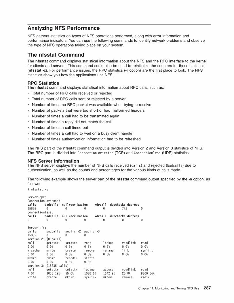
Analyzing NFS PerformanceNFS gathers statistics on types of NFS operations performed, along with error information andperformance indicators. You can use the following commands to identify network problems and observethe type of NFS operations taking place on your system.

The nfsstat CommandThe nfsstat command displays statistical information about the NFS and the RPC interface to the kernelfor clients and servers. This command could also be used to reinitialize the counters for these statistics(nfsstat -z). For performance issues, the RPC statistics (-r option) are the first place to look. The NFSstatistics show you how the applications use NFS.

RPC StatisticsThe nfsstat command displays statistical information about RPC calls, such as:

v Total number of RPC calls received or rejected

v Total number of RPC calls sent or rejected by a server

v Number of times no RPC packet was available when trying to receive

v Number of packets that were too short or had malformed headers

v Number of times a call had to be transmitted again

v Number of times a reply did not match the call

v Number of times a call timed out

v Number of times a call had to wait on a busy client handle

v Number of times authentication information had to be refreshed

The NFS part of the nfsstat command output is divided into Version 2 and Version 3 statistics of NFS.The RPC part is divided into Connection oriented (TCP) and Connectionless (UDP) statistics.

NFS Server InformationThe NFS server displays the number of NFS calls received (calls) and rejected (badcalls) due toauthentication, as well as the counts and percentages for the various kinds of calls made.

The following example shows the server part of the nfsstat command output specified by the -s option, asfollows:# nfsstat -s

Server rpc:Connection oriented:calls badcalls nullrecv badlen xdrcall dupchecks dupreqs15835 0 0 0 0 772 0Connectionless:calls badcalls nullrecv badlen xdrcall dupchecks dupreqs0 0 0 0 0 0 0

Server nfs:calls badcalls public_v2 public_v315835 0 0 0Version 2: (0 calls)null getattr setattr root lookup readlink read0 0% 0 0% 0 0% 0 0% 0 0% 0 0% 0 0%wrcache write create remove rename link symlink0 0% 0 0% 0 0% 0 0% 0 0% 0 0% 0 0%mkdir rmdir readdir statfs0 0% 0 0% 0 0% 0 0%Version 3: (15835 calls)null getattr setattr lookup access readlink read7 0% 3033 19% 55 0% 1008 6% 1542 9% 20 0% 9000 56%write create mkdir symlink mknod remove rmdir


175 1% 185 1% 0 0% 0 0% 0 0% 120 0% 0 0%rename link readdir readdir+ fsstat fsinfo pathconf87 0% 0 0% 1 0% 150 0% 348 2% 7 0% 0 0%commit97 0%

RPC output for server (-s) is as follows:

calls Total number of RPC calls received from clients

badcallsTotal number of calls rejected by the RPC layer

nullrecvNumber of times an RPC call was not available when it was thought to be received

badlenPackets truncated or damaged (number of RPC calls with a length shorter than a minimum-sizedRPC call)

xdrcallNumber of RPC calls whose header could not be External Data Representation (XDR) decoded

dupchecksNumber of RPC calls looked up in the duplicate request cache

dupreqsNumber of duplicate RPC calls found

The output also displays a count of the various kinds of calls and their respective percentages.

Duplicate checks are performed for operations that cannot be performed twice with the same result. Theclassic example is the rm command. The first rm command will succeed, but if the reply is lost, the clientwill retransmit it. We want duplicate requests like these to succeed, so the duplicate cache is consulted,and if it is a duplicate request, the same (successful) result is returned on the duplicate request as wasgenerated on the initial request.

By looking at the percentage of calls for different types of operations (such as getattr(), read(), write(), orreaddir()), you can decide what type of tuning to use. For example, if the percentage of getattr() calls isvery high, then tuning attribute caches may be advantageous. If the percentage of write() calls is veryhigh, then disk and LVM tuning is important. If the percentage of read() calls is very high, then using moreRAM for caching files could improve performance.

NFS Client InformationThe NFS client displays the number of calls sent and rejected, as well as the number of times a clienthandle was received (clgets) and a count of the various kinds of calls and their respective percentages.

The following example shows the nfsstat output specified for clients using the -c option, as follows:# nfsstat -c

Client rpc:Connection orientedcalls badcalls badxids timeouts newcreds badverfs timers0 0 0 0 0 0 0nomem cantconn interrupts0 0 0Connectionlesscalls badcalls retrans badxids timeouts newcreds badverfs6553 0 0 0 0 0 0timers nomem cantsend0 0 0

Client nfs:


calls badcalls clgets cltoomany6541 0 0 0Version 2: (6541 calls)null getattr setattr root lookup readlink read0 0% 590 9% 414 6% 0 0% 2308 35% 0 0% 0 0%wrcache write create remove rename link symlink0 0% 2482 37% 276 4% 277 4% 147 2% 0 0% 0 0%mkdir rmdir readdir statfs6 0% 6 0% 30 0% 5 0%Version 3: (0 calls)null getattr setattr lookup access readlink read0 0% 0 0% 0 0% 0 0% 0 0% 0 0% 0 0%write create mkdir symlink mknod remove rmdir0 0% 0 0% 0 0% 0 0% 0 0% 0 0% 0 0%rename link readdir readdir+ fsstat fsinfo pathconf0 0% 0 0% 0 0% 0 0% 0 0% 0 0% 0 0%commit0 0%

RPC output for the client (-c) is as follows:

calls Total number of RPC calls made to NFS.

badcallsTotal number of calls rejected by the RPC layer.

retransNumber of times a call had to be retransmitted due to a timeout while waiting for a reply from theserver. This is applicable only to RPC over connection-less transports.

badxidNumber of times a reply from a server was received that did not correspond to any outstandingcall. This means the server is taking too long to reply.

timeoutsNumber of times a call timed-out while waiting for a reply from the server.

newcredsNumber of times authentication information had to be refreshed.

badverfsNumber of times a call failed due to a bad verifier in the response.

timers Number of times the calculated timeout value was greater than or equal to the minimum specifiedtimeout value for a call.

nomemNumber of times a call failed due to a failure to allocate memory.

cantconnNumber of times a call failed due to a failure to make a connection to the server.

interruptsNumber of times a call was interrupted by a signal before completing.

cantsendNumber of times a send failed due to a failure to make a connection to the client.

The output also displays a count of the various kinds of calls and their respective percentages.

For performance monitoring, the nfsstat -c command provides information on whether the network isdropping UDP packets. A network may drop a packet if it cannot handle it. Dropped packets can be theresult of the response time of the network hardware or software or an overloaded CPU on the server.Dropped packets are not actually lost, because a replacement request is issued for them.


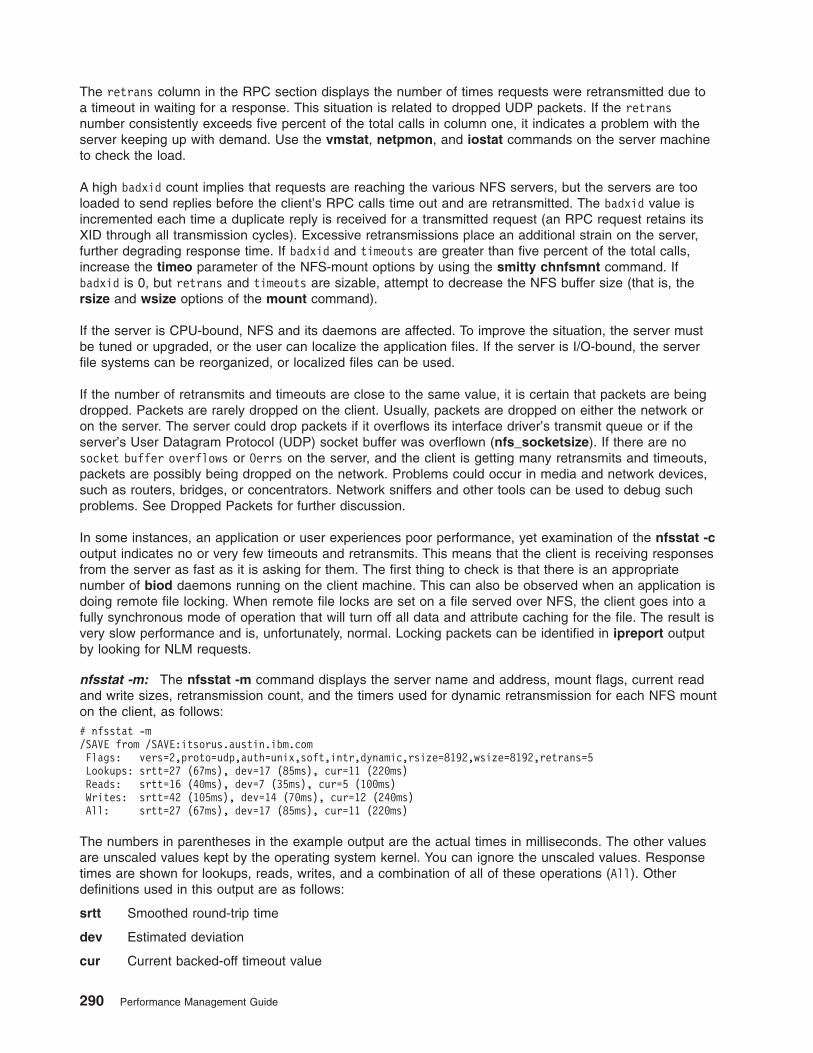
The retrans column in the RPC section displays the number of times requests were retransmitted due toa timeout in waiting for a response. This situation is related to dropped UDP packets. If the retransnumber consistently exceeds five percent of the total calls in column one, it indicates a problem with theserver keeping up with demand. Use the vmstat, netpmon, and iostat commands on the server machineto check the load.

A high badxid count implies that requests are reaching the various NFS servers, but the servers are tooloaded to send replies before the client’s RPC calls time out and are retransmitted. The badxid value isincremented each time a duplicate reply is received for a transmitted request (an RPC request retains itsXID through all transmission cycles). Excessive retransmissions place an additional strain on the server,further degrading response time. If badxid and timeouts are greater than five percent of the total calls,increase the timeo parameter of the NFS-mount options by using the smitty chnfsmnt command. Ifbadxid is 0, but retrans and timeouts are sizable, attempt to decrease the NFS buffer size (that is, thersize and wsize options of the mount command).

If the server is CPU-bound, NFS and its daemons are affected. To improve the situation, the server mustbe tuned or upgraded, or the user can localize the application files. If the server is I/O-bound, the serverfile systems can be reorganized, or localized files can be used.

If the number of retransmits and timeouts are close to the same value, it is certain that packets are beingdropped. Packets are rarely dropped on the client. Usually, packets are dropped on either the network oron the server. The server could drop packets if it overflows its interface driver’s transmit queue or if theserver’s User Datagram Protocol (UDP) socket buffer was overflown (nfs_socketsize). If there are nosocket buffer overflows or Oerrs on the server, and the client is getting many retransmits and timeouts,packets are possibly being dropped on the network. Problems could occur in media and network devices,such as routers, bridges, or concentrators. Network sniffers and other tools can be used to debug suchproblems. See Dropped Packets for further discussion.

In some instances, an application or user experiences poor performance, yet examination of the nfsstat -coutput indicates no or very few timeouts and retransmits. This means that the client is receiving responsesfrom the server as fast as it is asking for them. The first thing to check is that there is an appropriatenumber of biod daemons running on the client machine. This can also be observed when an application isdoing remote file locking. When remote file locks are set on a file served over NFS, the client goes into afully synchronous mode of operation that will turn off all data and attribute caching for the file. The result isvery slow performance and is, unfortunately, normal. Locking packets can be identified in ipreport outputby looking for NLM requests.

nfsstat -m: The nfsstat -m command displays the server name and address, mount flags, current readand write sizes, retransmission count, and the timers used for dynamic retransmission for each NFS mounton the client, as follows:# nfsstat -m/SAVE from /SAVE:itsorus.austin.ibm.comFlags: vers=2,proto=udp,auth=unix,soft,intr,dynamic,rsize=8192,wsize=8192,retrans=5Lookups: srtt=27 (67ms), dev=17 (85ms), cur=11 (220ms)Reads: srtt=16 (40ms), dev=7 (35ms), cur=5 (100ms)Writes: srtt=42 (105ms), dev=14 (70ms), cur=12 (240ms)All: srtt=27 (67ms), dev=17 (85ms), cur=11 (220ms)

The numbers in parentheses in the example output are the actual times in milliseconds. The other valuesare unscaled values kept by the operating system kernel. You can ignore the unscaled values. Responsetimes are shown for lookups, reads, writes, and a combination of all of these operations (All). Otherdefinitions used in this output are as follows:

srtt Smoothed round-trip time

dev Estimated deviation

cur Current backed-off timeout value


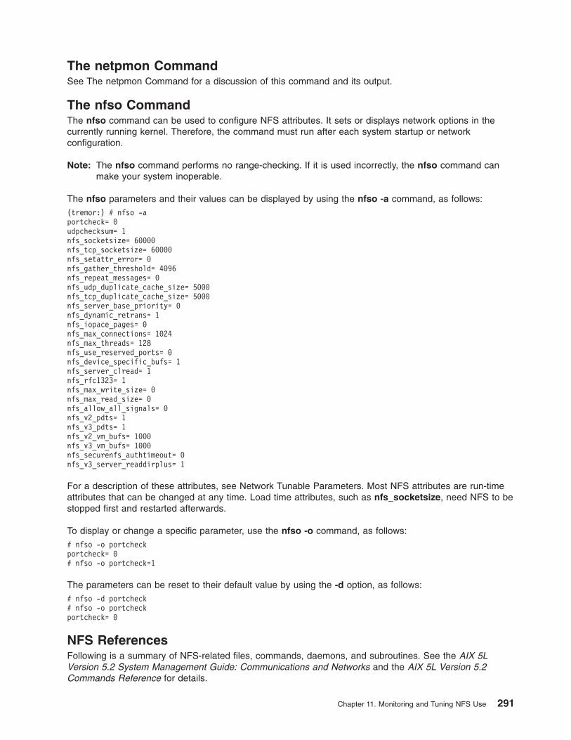
The netpmon CommandSee The netpmon Command for a discussion of this command and its output.

The nfso CommandThe nfso command can be used to configure NFS attributes. It sets or displays network options in thecurrently running kernel. Therefore, the command must run after each system startup or networkconfiguration.

Note: The nfso command performs no range-checking. If it is used incorrectly, the nfso command canmake your system inoperable.

The nfso parameters and their values can be displayed by using the nfso -a command, as follows:(tremor:) # nfso -aportcheck= 0udpchecksum= 1nfs_socketsize= 60000nfs_tcp_socketsize= 60000nfs_setattr_error= 0nfs_gather_threshold= 4096nfs_repeat_messages= 0nfs_udp_duplicate_cache_size= 5000nfs_tcp_duplicate_cache_size= 5000nfs_server_base_priority= 0nfs_dynamic_retrans= 1nfs_iopace_pages= 0nfs_max_connections= 1024nfs_max_threads= 128nfs_use_reserved_ports= 0nfs_device_specific_bufs= 1nfs_server_clread= 1nfs_rfc1323= 1nfs_max_write_size= 0nfs_max_read_size= 0nfs_allow_all_signals= 0nfs_v2_pdts= 1nfs_v3_pdts= 1nfs_v2_vm_bufs= 1000nfs_v3_vm_bufs= 1000nfs_securenfs_authtimeout= 0nfs_v3_server_readdirplus= 1

For a description of these attributes, see Network Tunable Parameters. Most NFS attributes are run-timeattributes that can be changed at any time. Load time attributes, such as nfs_socketsize, need NFS to bestopped first and restarted afterwards.

To display or change a specific parameter, use the nfso -o command, as follows:# nfso -o portcheckportcheck= 0# nfso -o portcheck=1

The parameters can be reset to their default value by using the -d option, as follows:# nfso -d portcheck# nfso -o portcheckportcheck= 0

NFS ReferencesFollowing is a summary of NFS-related files, commands, daemons, and subroutines. See the AIX 5LVersion 5.2 System Management Guide: Communications and Networks and the AIX 5L Version 5.2Commands Reference for details.


List of Network File System (NFS) FilesFollowing is a list of NFS files containing configuration information:

bootparamsLists clients that diskless clients can use for booting

exportsLists the directories that can be exported to NFS clients

networksContains information about networks on the Internet network

pcnfsd.confProvides configuration options for the rpc.pcnfsd daemon

rpc Contains database information for Remote Procedure Call (RPC) programs

xtab Lists directories that are currently exported

/etc/filesystemsLists all the file systems that are attempted to be mounted at system restart

List of NFS CommandsFollowing is a list of NFS commands:

chnfs Starts a specified number of biod and nfsd daemons

mknfs Configures the system to run NFS and starts NFS daemons

nfso Configures NFS network options

automountMounts an NFS file system automatically

chnfsexpChanges the attributes of an NFS-exported directory

chnfsmntChanges the attributes of an NFS-mounted directory

exportfsExports and unexports directories to NFS clients

lsnfsexpDisplays the characteristics of directories that are exported with NFS

lsnfsmntDisplays the characteristics of mounted NFS systems

mknfsexpExports a directory using NFS

mknfsmntMounts a directory using NFS

rmnfs Stops the NFS daemons

rmnfsexpRemoves NFS-exported directories from a server’s list of exports

rmnfsmntRemoves NFS-mounted file systems from a client’s list of mounts

List of NFS DaemonsFollowing is a list of NFS locking daemons:

lockd Processes lock requests through the RPC package


statd Provides crash-and-recovery functions for the locking services on NFS

Following is a list of network service daemons and utilities:

biod Sends the client’s read and write requests to the server

mountdAnswers requests from clients for file system mounts

nfsd Starts the daemons that handle a client’s request for file system operations

pcnfsdHandles service requests from PC-NFS clients

nfsstatDisplays information about a machine’s ability to receive calls

on Executes commands on remote machines

portmapMaps RPC program numbers to Internet port numbers

rexd Accepts request to run programs from remote machines

rpcgenGenerates C code to implement an RPC protocol

rpcinfoReports the status of RPC servers

rstatd Returns performance statistics obtained from the kernel

rup Shows the status of a remote host on the local network

rusersReports a list of users logged on to the remote machines

rusersdResponds to queries from the rusers command

rwall Sends messages to all users on the network

rwalld Handles requests from the rwall command

showmountDisplays a list of all clients that have mounted remote file systems

spray Sends a specified number of packets to a host

spraydReceives packets sent by the spray command

Following is a list of secure networking daemons and utilities:

chkey Changes the user’s encryption key

keyenvoyProvides an intermediary between user processes and the key server

keyloginDecrypts and stores the user’s secret key

keyservStores public and private keys

mkkeyservStarts the keyserv daemon and uncomments the appropriate entries in the /etc/rc.nfs file


newkeyCreates a new key in the public key file

rmkeyservStops the keyserv daemon and comments the entry for the keyserv daemon in the /etc/rc.nfs file

ypupdatedUpdates information in Network Information Service (NIS) maps

Following is a diskless client support configuration file:

bootparamdProvides information necessary for booting to diskless clients

Following is a list of NFS subroutines:

cbc_crypt(), des_setparity(), or ecb_crypt()Implements Data Encryption Standard (DES) routines.

Tuning for NFS PerformanceIn an NFS network, the server is the primary target for tuning, but a few things can be tuned on the clientas well.

How Many biod and nfsd Daemons Are Needed?Because biod and nfsd daemons handle one request at a time, and because NFS response time is oftenthe largest component of overall response time, it is undesirable to have threads blocked for lack of a biodor nfsd daemon.

Note: There is a single nfsd daemon and a single biod daemon, each of which is multithreaded (multiplekernel threads within the process). Also, the number of threads is self-tuning in that it createsadditional threads as needed. You can, however, tune the maximum number of nfsd threads byusing the nfs_max_threads parameter of the nfso command. You can also tune the maximumnumber of biod threads per mount via the biod mount option.

The general considerations for configuring NFS daemons are as follows:

v Increasing the number of daemons cannot compensate for inadequate client or server processor poweror memory, or inadequate server disk bandwidth. Before changing the number of daemons, you shouldcheck server and client resource-utilization levels with the iostat and vmstat commands.

v If the CPU or disk subsystem is already at near-saturation level, an increase in the number of daemonswill not yield better performance.

v NFS daemons are comparatively inexpensive. The biod or nfsd daemon costs a few pages in memory(some of them pinned). Of course, the unpinned pages are only in real memory if the nfsd or bioddaemon has been active recently. Further, idle nfsd or biod daemons do not consume CPU time.

v All NFS requests go through an nfsd daemon; only reads and writes go through a biod daemon.

Choosing Initial Numbers of nfsd and biod daemonsDetermining the best numbers of nfsd and biod daemons is an iterative process. Guidelines can give youno more than a reasonable starting point.

The defaults are a good starting point for small systems, but should probably be increased for clientsystems with more than two users or servers with more than two clients. A few guidelines are as follows:

v In each client, estimate the maximum number of files that will be written simultaneously. Configure atleast two biod daemons per file. If the files are large (more than 32 KB), you may want to start with fourbiod daemons per file to support read-ahead or write-behind activity. It is common for up to five bioddaemons to be busy writing to a single large file.


v In each server, start by configuring as many nfsd daemons as the sum of the numbers of bioddaemons that you have configured on the clients to handle files from that server. Add 20 percent toallow for non-read/write NFS requests.

v If you have fast client workstations connected to a slower server, you may have to constrain the rate atwhich the clients generate NFS requests.The best solution is to reduce the number of biod daemons onthe clients, with due attention to the relative importance of each client’s workload and response time.

Tuning the Numbers of nfsd and biod daemonsAfter you have arrived at an initial number of biod and nfsd daemons, or have changed one or the other,do the following:

v First, recheck the affected systems for CPU or I/O saturation with the vmstat and iostat commands. Ifthe server is now saturated, you must reduce its load or increase its power, or both.

v Use the command netstat -s to determine if any system is experiencing UDP socket bufferoverflows. If so, use the command no -a to verify that the recommendations in Tuning Other Layers toImprove NFS Performance have been implemented. If so, and the system is not saturated, increase thenumber of biod or nfsd daemons.

v Examine the nullrecv column in the nfsstat -s output. If the number starts to grow, it may mean thereare too many nfsd daemons. However, this is less likely on this operating system’s NFS servers than itis on other platforms. The reason for that is that all nfsd daemons are not awakened at the same timewhen an NFS request comes into the server. Instead, the first nfsd daemon wakes up, and if there ismore work to do, this daemon wakes up the second nfsd daemon, and so on.

To change the number of nfsd daemons, you can use the chnfs command, or set the nfsonfs_max_threads parameter as mentioned earlier.

To change the number of nfsd daemons on a server to 10, both immediately and at each subsequentsystem boot, use the following:# chnfs -n 10

To change the number of nfsd daemons on a system to 9, with the change delayed until the next systemboot, run the following command:# chnfs -I -n 9

To change the number of biod daemons per mount, use the biod mount option.

Increasing the number of biod daemons on the client worsens server performance because it allows theclient to send more request at once, further loading the network and the server. In extreme cases of aclient overrunning the server, it may be necessary to reduce the client to one biod daemon, as follows:# stopsrc -s biod

This leaves the client with the kernel process biod still running.

Performance Implications of Hard or Soft NFS MountsOne of the choices you make when configuring NFS-mounted directories is whether the mounts will behard (-o hard) or soft (-o soft). When, after a successful mount, an access to a soft-mounted directoryencounters an error (typically, a timeout), the error is immediately reported to the program that requestedthe remote access. When an access to a hard-mounted directory encounters an error, NFS retries theoperation.

A persistent error accessing a hard-mounted directory can escalate into a perceived performance problembecause the default number of retries (1000) and the default timeout value (0.7 second), combined with analgorithm that increases the timeout value for successive retries, mean that NFS continues to try tocomplete the operation.


It is technically possible to reduce the number of retries, or increase the timeout value, or both, usingoptions of the mount command. Unfortunately, changing these values sufficiently to remove the perceivedperformance problem might lead to unnecessary reported hard errors. Instead, use the intr option tomount the hard-mounted directories, which allows the user to interrupt from the keyboard a process that isin a retry loop.

Although soft-mounting the directories causes the error to be detected sooner, it runs a serious risk of datacorruption. In general, read/write directories should be hard-mounted.

Other mount Options That Affect PerformanceThe mount command provides some NFS-tuning options that are often ignored or used incorrectlybecause of a lack of understanding of their use.

Before you start adjusting mount options, make certain that you know what you are trying to achieve withrespect to packet delivery and packet turnaround on the server or network. You would use most of theNFS-specific mount options if your goal is to decrease the load on the NFS server, or to work aroundnetwork problems.

The NFS performance-specific mount options are all specified as a list entry on the -o option for themount command. Separate the options for the -o option on the command line only by a comma, not by acomma and a space.

The rsize and wsize OptionsThe most useful options are those for changing the read and write size values. These options define themaximum sizes of each RPC for read and write. Often, the rsize and wsize options of the mountcommand are decreased to decrease the read/write packet that is sent to the server. There can be tworeasons why you might want to do this:

1. The server may not be capable of handling the data volume and speeds inherent in transferring theread/write packets (8 KB for NFS Version 2 and 32 KB for NFS Version 3). This might be the case if aNFS client is using a PC as an NFS server. The PC will likely have limited memory available forbuffering large packets.

2. If a read/write size is decreased, there may be a subsequent reduction in the number of IP fragmentsgenerated by the call. If you are dealing with a faulty network, the chances of a call/reply paircompleting with a two-packet exchange are greater than if there must be seven packets successfullyexchanged. Likewise, if you are sending NFS packets across multiple networks with differentperformance characteristics, the packet fragments may not all arrive before the timeout value for IPfragments.

Reducing the rsize and wsize may improve the NFS performance in a congested network by sendingshorter package trains for each NFS request. But a side effect is that more packets are needed to senddata across the network, increasing total network traffic, as well as CPU utilization on both the server andclient.

If your NFS file system is mounted across a high-speed network, such as the SP Switch, then larger readand write packet sizes would enhance NFS file system performance. With NFS Version 3, rsize and wsizecan be set as high as 65536. The default is 32768. With NFS Version 2, the largest that rsize and wsizecan be is 8192, which is also the default.

Improving sequential I/O throughputOn AIX 5.1 and later, you can improve the performance of sequential I/O operations on very large files inNFS exported file systems by using a mechanism called release-behind.

For more information on release-behind, see Monitoring and Tuning File Systems.


Improving client throughput for large-file I/OOn special cases over NFS Version 3 where you are trying to perform sequential write operations on filesthat are larger than client memory, you can improve performance by using commit-behind. Under normalcircumstances, writing large files causes heavy page replacement activity on the client. This forces commitoperations to be performed one page at a time. Commit-behind enables a more aggressive logic forcommiting client pages and returning those pages to the free list.

You can enable commit-behind when mounting the file system by specifying the combehind flag with themount command. You also need to set an appropriate value for the numclust variable. This variablespecifies the number of 16-Kilobyte clusters processed by the sequential write-behind algorithm of theVirtual Memory Manager (VMM). When the I/O pattern is sequential, use a large value for numclust inorder to keep more pages in RAM before scheduling them for I/O. Increase the value for numclust ifstriped logical volumes or disk arrays are being used. On AIX 5.1, this parameter can be specified as amount option. On previous versions of AIX, use the vmtune command to specify a value for numclust.

Disabling Unused NFS ACL SupportIf your workload does not use the NFS access control list (ACL) support on a mounted file system, youcan reduce the workload on both client and server to some extent by specifying the noacl option. This canbe done as follows:options=noacl

Set this option as part of the client’s /etc/filesystems stanza for that file system.

Tuning to Avoid RetransmitsRelated to the hard-versus-soft mount question is the question of the appropriate timeout duration for agiven network configuration. If the server is heavily loaded, is separated from the client by one or morebridges or gateways, or is connected to the client by a WAN, the default timeout criterion may beunrealistic. If so, both server and client are burdened with unnecessary retransmits. For example, if thefollowing command:# nfsstat -c

reports a significant number (greater 5 percent of the total) of both timeouts and badxids, you couldincrease the timeo parameter with the following SMIT fast path:# smitty chnfsmnt

Identify the directory you want to change, and enter a new value on the line NFS TIMEOUT. In tenths ofa second.

The default time is 0.7 second (timeo=7), but this value is manipulated in the NFS kernel extensiondepending on the type of call. For read calls, for instance, the value is doubled to 1.4 seconds.

To achieve control over the timeo value for operating system version 4 clients, you must set thenfs_dynamic_retrans option of the nfso command to 0. There are two directions in which you canchange the timeo value, and in any given case, there is only one right way to change it. The correct way,making the timeouts longer or shorter, depends on why the packets are not arriving in the allotted time.

If the packet is only late and does finally arrive, then you may want to make the timeo variable longer togive the reply a chance to return before the request is retransmitted.

However, if the packet has been dropped and will never arrive at the client, then any time spent waiting forthe reply is wasted time, and you want to make the timeo shorter.

One way to estimate which option to take is to look at a client’s nfsstat -cr output and see if the client isreporting lots of badxid counts. A badxid value means that an RPC client received an RPC call reply that


was for a different call than the one it was expecting. Generally, this means that the client received aduplicate reply for a previously retransmitted call. Packets are thus arriving late and the timeo should belengthened.

Also, if you have a network analyzer available, you can apply it to determine which of the two situations isoccurring. Lacking that, you can try setting the timeo option higher and lower and see what gives betteroverall performance. In some cases, there is no consistent behavior. Your best option then is to track downthe actual cause of the packet delays/drops and fix the real problem; that is, server or network/networkdevice.

For LAN-to-LAN traffic through a bridge, try 50 (tenths of seconds). For WAN connections, try 200. Checkthe NFS statistics again after waiting at least one day. If the statistics still indicate excessive retransmits,increase timeo by 50 percent and try again. You will also want to examine the server workload and theloads on the intervening bridges and gateways to see if any element is being saturated by other traffic.

Dropped PacketsGiven that dropped packets are detected on an NFS client, the real challenge is to find out where they arebeing lost. Packets can be dropped at the client, the server, and somewhere on the network.

Packets Dropped by the ClientPackets are rarely dropped by a client. Because each client RPC call is self-pacing, that is, each call mustget a reply before going on, there is little opportunity for overrunning system resources. The most stressfuloperation is probably reading, where there is a potential for 1 MB+/sec of data flowing into the machine.While the data volume can be high, the actual number of simultaneous RPC calls is fairly small and eachbiod daemon has its own space allocated for the reply. Thus, it is very unusual for a client to droppackets.

Packets are more commonly dropped either by the network or by the server.

Packets Dropped by the ServerTwo situations exist where servers will drop packets under heavy loads:

1. Adapter Driver

When an NFS server is responding to a very large number of requests, the server will sometimesoverrun the interface driver output queue. You can observe this by looking at the statistics that arereported by the netstat -i command. Examine the columns marked Oerrs and look for any counts.Each Oerrs is a dropped packet. This is easily tuned by increasing the problem device driver’s transmitqueue size. The idea behind configurable queues is that you do not want to make the transmit queuetoo long, because of latencies incurred in processing the queue. But because NFS maintains the sameport and XID for the call, a second call can be satisfied by the response to the first call’s reply.Additionally, queue-handling latencies are far less than UDP retransmit latencies incurred by NFS if thepacket is dropped.

2. Socket Buffers

The second common place where a server will drop packets is the UDP socket buffer. Droppedpackets here are counted by the UDP layer and the statistics can be seen by using the netstat -p udpcommand. Examine the statistics marked UDP: for the socket buffer overflows statistic.

NFS packets will usually be dropped at the socket buffer only when a server has a lot of NFS writetraffic. The NFS server uses a UDP socket attached to NFS port 2049 and all incoming data isbuffered on that UDP port. The default size of this buffer is 60,000 bytes. You can divide that numberby the size of the default NFS write packet (8192) to find that it will take only eight simultaneous writepackets to overflow that buffer. This overflow could occur with just two NFS clients (with the defaultconfigurations).

In this situation there is either high volume or high burst traffic on the socket.


v If there is high volume, a mixture of writes plus other possibly non-write NFS traffic, there may notbe enough nfsd daemons to take the data off the socket fast enough to keep up with the volume.Recall that it takes a dedicated nfsd daemon to service each NFS call of any type.

v In the high burst case, there may be enough nfsd daemons, but the speed at which packets arriveon the socket is such that they cannot wake up fast enough to keep it from overflowing.

Each of the two situations is handled differently.

v In the case of high volume, it may be sufficient to just increase the number of nfsd daemonsrunning on the system. Because there is no significant penalty for running with more nfsd daemonson a machine, try this solution first. Also, see How Many biod and nfsd Daemons Are Needed?.

v In the case of high burst traffic, the only solution is to enlarge the socket, in the hope that somereasonable size will be sufficiently large enough to give the nfsd daemons time to catch up with theburst. Memory dedicated to this socket will not be available for any other use, so it must be notedthat a tuning objective of total elimination of socket buffer overflows by making the socket largermay result in this memory being underutilized for the vast majority of the time. A cautiousadministrator will watch the socket buffer overflow statistic, correlate it with performance problems,and determine how large to make the socket buffer. See Increasing NFS Socket Buffer Size fordetails on how to manipulate the NFS socket buffer.

You might see cases where the server has been tuned and no dropped packets are arriving for either thesocket buffer or the driver Oerrs, but clients are still experiencing timeouts and retransmits. Again, this is atwo-case scenario. If the server is heavily loaded, it may be that the server is just overloaded and thebacklog of work for nfsd daemons on the server is resulting in response times beyond the default timeoutset on the client. See NFS Tuning Checklist for hints on how to determine if this is the problem. The otherpossibility, and the most likely problem if the server is known to be otherwise idle, is that packets are beingdropped on the network.

Dropped Packets On the NetworkIf there are no socket buffer overflows or Oerrs on the server, the client is getting lots of timeouts andretransmits and the server is known to be idle, then packets are most likely being dropped on the network.What is meant by when network is mentioned? It means a large variety of things including media andnetwork devices such as routers, bridges, concentrators, and the whole range of things that can implementa transport for packets between the client and server.

Anytime a server is not overloaded and is not dropping packets, but NFS performance is bad, assume thatpackets are being dropped on the network. Much effort can be expended proving this and finding exactlyhow the network is dropping the packets. The easiest way of determining the problem depends mostly onthe physical proximity involved and resources available.

Sometimes the server and client are in close enough proximity to be direct-connected, bypassing thelarger network segments that may be causing problems. Obviously, if this is done and the problem isresolved, then the machines themselves can be eliminated as the problem. More often, however, it is notpossible to wire up a direct connection, and the problem must be tracked down in place.

Tuning the NFS File-Attribute CacheNFS maintains a cache on each client system of the attributes of recently accessed directories and files.Five parameters that can be set in the /etc/filesystems file control how long a given entry is kept in thecache. They are as follows:

actimeoAbsolute time for which file and directory entries are kept in the file-attribute cache after anupdate. If specified, this value overrides the following *min and *max values, effectively settingthem all to the actimeo value.

acregminMinimum time after an update that file entries will be retained. The default is 3 seconds.


acregmaxMaximum time after an update that file entries will be retained. The default is 60 seconds.

acdirminMinimum time after an update that directory entries will be retained. The default is 30 seconds.

acdirmaxMaximum time after an update that directory entries will be retained. The default is 60 seconds.

Each time the file or directory is updated, its removal is postponed for at least acregmin or acdirminseconds. If this is the second or subsequent update, the entry is kept at least as long as the intervalbetween the last two updates, but not more than acregmax or acdirmax seconds.

Tuning for Maximum Caching of NFS DataNFS does not have a data-caching function, but the Virtual Memory Manager (VMM) caches pages of NFSdata just as it caches pages of disk data. If a system is essentially a dedicated NFS server, it may beappropriate to permit the VMM to use as much memory as necessary for data caching. For a serverexporting JFS file systems, this is accomplished by setting the maxperm parameter, which controls themaximum percentage of memory occupied by JFS file pages, to 100 percent.

For example:# vmtune -P 100

On a server exporting Enhanced JFS file systems, this is accomplished by setting the maxclientparameter. The maxclient parameter controls the maximum percentage of memory occupied byclient-segment pages which is where Enhanced JFS file data is cached.

For example:# vmtune -t 100

The same technique could be used on NFS clients, but would only be appropriate if the clients wererunning workloads that had very little need for working-segment pages.

Cache File System (CacheFS)The Cache File System can be used to enhance performance of remote file systems or slow devices suchas CD-ROM. When a file system is cached, the data read from the remote file system or CD-ROM isstored in a cache on the local system, thereby avoiding the use of the network and NFS server when thesame data is accessed for the second time. CacheFS is designed as a layered file system; this meansthat CacheFS provides the ability to cache one file system (the NFS file system, also called the back-filesystem) on another (your local file system, also called the front-file system), as shown in the followingfigure:


Note that in AIX 4.3, only NFS Version 2 and NFS Version 3 are supported as back-file systems, and JFSis the only supported front-file system.

CacheFS works as follows:

1. After creating a CacheFS file system on a client system, the system administrator specifies which filesystems are to be mounted in the cache.

2. When a user on the client attempts to access files that are part of the back file system, those files areplaced in the cache. The cache does not get filled until a user requests access to a file or files.Therefore, the initial request to access a file will be at typical NFS speeds, but subsequent accesses tothe same file will be at local JFS speeds.

3. To ensure that the cached directories and files are kept up to date, CacheFS periodically checks theconsistency of files stored in the cache. It does so by comparing the current modification time to theprevious modification time.

4. If the modification times are different, all data and attributes for the directory or file are purged from thecache, and new data and attributes are retrieved from the back file system.

An example where CacheFS would be suitable is in a CAD environment where master-copies of drawingcomponents can be held on the server and cached-copies on the client workstation when in use.

CacheFS does not allow reads and writes on files that are 2 GB or larger in size.

CacheFS BenefitsBecause NFS data is cached on the local disk once it is read from the server, read requests to the NFSfile system can be satisfied much faster than if the data had to be retrieved over the net again. Dependingon the memory size and usage of the client, a small amount of data might be held and retrieved frommemory, so that the benefits of cached data on the disk applies to a large amount of data that cannot bekept in memory. An additional benefit is that data on the disk cache will be held at system shutdown,whereas data cached in memory will have to be retrieved from the server again after the reboot.

Figure 29. Cache File System (CacheFS). This illustration show a client machine and a server that are connect by anetwork. The storage media on the server contains the back file system. The storage media on the client contains thecached file system or the front file system.


Other potential NFS bottlenecks are a slow or busy network and a weak performing server with too manyNFS clients to serve. Therefore, access from the client system to the server is likely to be slow. CacheFSwill not prevent you from having to do the first read over the network and to access the server, but youcan avoid reads over the network for further requests for the same data.

If more read requests can be satisfied from the client’s local disk, the amount of NFS accesses to theserver will decrease. This means that more clients can be served by the server; thus, the client per serverratio will increase.

Fewer read requests over the network will decrease your network load and, therefore, allow you to getsome relief on very busy networks or space for other data transfers.

Not every application will benefit from CacheFS. Because CacheFS will only speed up read performance,mainly applications that have huge read requests for the same data over and over again will benefit fromCacheFS. Large CAD applications will certainly benefit from CacheFS, because of the often very largemodels that they have to load for their calculations.

Performance tests showed that sequential reads from the CacheFS file system are 2.4 times to 3.4 timesfaster than reads from the NFS server’s memory or disk.

What CacheFS Does Not DoCacheFS will not increase the write performance to NFS file systems. However, you have two writeoptions to choose as parameters to the -o option of the mount command, when mounting a CacheFS.They will influence the subsequent read performance to the data. The write options are as follows:

write-aroundThe write-around mode (the default) handles writes the same way that NFS does; that is, writesare made to the back file system, and the affected file is purged from the cache. This means thatwrite-around voids the cache and new data must be obtained back from the server after the write.

non-sharedYou can use the non-shared mode when you are certain that no one else will be writing to thecached file system. In this mode, all writes are made to both the front and the back file system,and the file remains in the cache. This means that future read accesses can be done to the cache,rather than going to the server.

Small reads might be kept in memory anyway (depending on your memory usage); so there is no benefitin also caching the data on the disk. Caching of random reads to different data blocks does not help,unless you will access the same data over and over again.

The initial read request still has to go to the server because only by the time a user attempts to accessfiles that are part of the back file system will those files be placed in the cache. For the initial read request,you will see typical NFS speed. Only for subsequent accesses to the same data, you will see local JFSaccess performance.

The consistency of the cached data is only checked at intervals. Therefore, it is dangerous to cache datathat is frequently changed. CacheFS should only be used for read-only or read-mostly data.

Write Performance over a cached NFS file system differs from NFS Version 2 to NFS Version 3.Performance tests have shown that:

v Sequential writes to a new file over NFS Version 2 to a CacheFS mount point can be 25 percent slowerthan writes directly to the NFS Version 2 mount point.

v Sequential writes to a new file over NFS Version 3 to a CacheFS mount point can be 6 times slowerthan writes directly to the NFS Version 3 mount point.


Configuring CacheFSCacheFS is not implemented by default or prompted at the time of the creation of an NFS file system.

Make sure to install fileset level 4.3.1.1 for enhanced CacheFS write performance over NFS in AIX 4.3.1.

The system administrator must specify explicitly which file systems are to be mounted in the cache asfollows:

1. Create the local cache file system by using the cfsadmin command:# cfsadmin -c -o parameters cache-directory

where parameters specify the resource parameters and cache-directory is the name of the directorywhere the cache should be created.

2. Mount the back file system onto the cache:# mount -V cachefs -o backfstype=nfs,cachedir=/cache-directory remhost:/rem-directory local-mount-point

where rem-directory is the name of the remote host and file system where the data resides, andlocal-mount-point is the mount point on the client where the remote file system should be mounted.

3. Alternately, you could administer CacheFS using the SMIT command (use the smitty cachefs fastpath).

Several parameters can be set at creation time, as follows:

maxblocksSets the maximum number of blocks that CacheFS is allowed to claim within the front file system.Default = 90 percent.

minblocksSets the minimum number of blocks that CacheFS is allowed to claim within the front file system.Default = 0 percent.

threshblocksSets the number of blocks that must be available in the JFS file system on the client side beforeCacheFS can claim more than the blocks specified by minblocks. Default = 85 percent.

maxfilesMaximum number of files that CacheFS can use, expressed as a percentage of the total numberof i-nodes in the front file system. Default = 90 percent.

minfilesMinimum number of files that CacheFS is always allowed to use, expressed as a percentage ofthe total number of i-nodes in the front file system. Default = 0 percent.

maxfilesizeLargest file size, expressed in megabytes, that CacheFS is allowed to cache. Default = 3.

RPC Tuning for NFSThe rpc.lockd daemon is multi-threaded and, by default, can create up to 33 threads. In situations wherethere is heavy remote procedure call (RPC) file locking activity, the rpc.lockd daemon might become abottleneck once it reaches the maximum number of threads. When that maximum is reached, anysubsequent requests will have to wait, which may result in other timeouts. If there are more than oneclient, the NFS server should have more lockd threads than the client side. The number of lockd threadscan be adjusted to a limit of 511 with the following:# chsys -s rpc.lockd -a <# of threads># stopsrc -s rpc.lockd; startsrc -s rpc.lockd


Tuning Other Layers to Improve NFS PerformanceNFS uses UDP or TCP to perform its network I/O. Ensure that you have applied the tuning techniquesdescribed in Tuning TCP and UDP Performance and Tuning mbuf Pool Performance. In particular, youshould:

v Ensure that the LAN adapter transmit and receive queues are set to the maximum (see AdapterTransmit and Receive Queue Tuning).

v Increase the maximum socket buffer size (sb_max) to at least 131072 bytes. If the MTU size is not4096 bytes or larger, set sb_max to at least 262144. Also set the UDP socket buffer sizes(udp_sendspace and udp_recvspace) to 131072 bytes. If you are using TCP, set tcp_sendspace andtcp_recvspace to this value.

v If possible, increase the MTU size on the LAN. On a 16 Mb Token-Ring, for example, an increase inMTU size from the default 1492 bytes to 8500 bytes allows a complete 8 KB NFS read or write requestto be transmitted without fragmentation. It also makes much more efficient use of mbuf space, reducingthe probability of overruns.

v A tunable parameter called nfs_tcp_socketsize provides default window sizes for TCP ports used inNFS connections. There is only one connect per client/server pair no matter how many mounts thereare. Do not set the nfs_tcp_socketsize value to less than 60,000. Large or busy servers should havelarger values until TCP NFS traffic shows no packets dropped from the output of the netstat -s -p tcpcommand.

v The maximum number of TCP connections allowed into the server can be controlled by the new optionnfs_max_connections. The default of 0 indicates that there is no limit. The client will close TCPconnections that have been idle for approximately 5 minutes, and the connection is reestablished whenuse warrants it. The server will close connections that have been idle for approximately 6 minutes.

v The operating system provides an option to turn off the UDP checksum for NFS only. You can use thenfso command option, called udpchecksum. The default is 1 (checksum enabled). Slight performancegains can be realized by turning it off, at the expense of increased chance of data corruption.

Increasing NFS Socket Buffer SizeIn the course of tuning UDP, you may find that the netstat -s command indicates a significant number ofUDP socket buffer overflows. As with ordinary UDP tuning, increase the sb_max value. You also needto increase the value of nfs_socketsize, which specifies the size of the NFS socket buffer. Following is anexample:# no -o sb_max=131072# nfso -o nfs_socketsize=130972

The previous example sequence sets sb_max to a value at least 100 bytes larger than the desired valueof nfs_socketsize and sets nfs_socketsize to 130972.

Note: In AIX Version 4, the socketsize is set dynamically. Configurations using the no and nfso commandmust be repeated every time the machine is booted. Add them in the /etc/rc.net or /etc/rc.nfs fileimmediately before the nfsd daemons are started and after the biod daemons are started. Theposition is crucial.

NFS Server Disk ConfigurationNFS servers that experience high levels of write activity can benefit from configuring the journal logicalvolume on a separate physical volume from the data volumes. See Disk Preinstallation Guidelines forfurther details.

It is often necessary to achieve high parallelism on data access. Concurrent access to a single file systemon a server by multiple clients or multiple client processes can result in throughput being bottlenecked onthe disk I/O for a particular device. You can use the iostat command to evaluate disk loading.


For large NFS servers, the general strategy should be to divide evenly the disk I/O demand across asmany disk and disk adapter devices as possible. This results in greater parallelism and the ability to rungreater numbers of nfsd daemons. On a system where disk I/O has been well-distributed, it is possible toreach a point where CPU load becomes the limiting factor on the server’s performance.

Misuses of NFS That Affect PerformanceMany of the misuses of NFS occur because people do not realize that the files that they are accessing areat the other end of an expensive communication path. A few examples of this are as follows:

v An application running on one system doing random updates of an NFS-mounted inventory file,supporting a real-time retail cash register application.

v A development environment in which a source code directory on each system was NFS-mounted on allof the other systems in the environment, with developers logging onto arbitrary systems to do editingand compiles. This practically guaranteed that all of the compiles would be obtaining their source codefrom, and writing their output to, remote systems.

v Running the ld command on one system to transform .o files in an NFS-mounted directory into an a.outfile in the same directory.

v Applications that issue writes that are not page-aligned (for example 10 KB). Writes less than 4 KB insize will always result in a pagein and in the case of NFS, this pagein goes over the network.

It can be argued that these are valid uses of the transparency provided by NFS. Perhaps this is so, butthese uses do cost processor time and LAN bandwidth and degrade response time. When a systemconfiguration involves NFS access as part of the standard pattern of operation, the configuration designersshould be prepared to defend the consequent costs with offsetting technical or business advantages, suchas:

v Placing all of the data or source code on a server, rather than on individual workstations, improvessource-code control and simplifies centralized backups.

v A number of different systems access the same data, making a dedicated server more efficient than oneor more systems combining client and server roles.

Another type of application that should not be run across NFS file systems is an application that doeshundreds of lockf() or flock() calls per second. On an NFS file system, all the lockf() or flock() calls (andother file locking calls) must go through the rpc.lockd daemon. This can severely degrade systemperformance because the lock daemon may not be able to handle thousands of lock requests per second.

Regardless of the client and server performance capacity, all operations involving NFS file locking willprobably seem unreasonably slow. There are several technical reasons for this, but they are all driven bythe fact that if a file is being locked, special considerations must be taken to ensure that the file issynchronously handled on both the read and write sides. This means there can be no caching of any filedata at the client, including file attributes. All file operations go to a fully synchronous mode with nocaching. Suspect that an application is doing network file locking if it is operating over NFS and showsunusually poor performance compared to other applications on the same client/server pair.

NFS Tuning ChecklistFollowing is a checklist that you can follow when tuning NFS:

1. Check to see if you are overrunning the server.

The general method is to see if slowing down the client will increase the performance. The followingmethods can be tried independently:

v Try running with just one biod daemon on the mount.

Try running with just one biod daemon on the affected client. If performance increases, thensomething is being overrun either in the network or on the server. Run the stopsrc -s biodcommand to stop all the SRC biod daemons. It will leave one kernel process biod with which youcan still run. See if it runs faster with just the one biod process. If it has no effect, restart the biod


daemons with the startsrc -s biod command. If it runs faster, attempt to determine where thepackets are being dropped when all daemons are running. Networks, network devices, slow server,overloaded server, or a poorly tuned server could all cause this problem.

v Try reducing the read/write sizes to see if things speed up.

v If you are using UDP, try using a TCP mount instead.

2. Check for Oerrs.

This is probably the most common under-configuration error that affects NFS servers.

If there are any Oerrs, increase the transmit queues for the network device. This can be done withthe machine running, but the interface must be detached before it is changed (rmdev -l). You cannotshut down the interface on a diskless machine, and you may not be at liberty to shut down theinterface if other work is going on. In this case, you can use the chdev command to put the changesin ODM so they will be activated on the next boot. Start by doubling the current value for the queuelength, and repeat the process (adding an additional 30 each time) until no Oerrs are reported. OnSP2 systems where NFS is configured to run across the high-speed switch, Oerrs may occur on theswitch when there has been a switch fault and the switch was temporarily unavailable. An error iscounted towards Oerr for each attempt to send on the switch that fails. These errors cannot beeliminated.

3. Look for any Errors.

Any counts that are very large indicate problems.

4. Check for NFS UDP/TCP buffer overruns.

When using UDP, buffer overruns on the NFS server are another frequent under-configuration forNFS servers. TCP sockets can be similarly overrun on very busy machines. Tuning for both is similar,so this section discusses only UDP.

Run the netstat -s command and examine the UDP statistics for the socket buffer overflowsstatistic. If it is anything other than 0, you are probably overrunning the NFS UDP buffer. Be aware,however, that this is the UDP socket buffer drop count for the entire machine, and it may or may notbe NFS packets that are being dropped. You can confirm that the counts are due to NFS bycorrelating between packet drop counts on the client using the nfsstat -cr command to socket bufferoverruns on the server while executing an NFS write test.

Socket buffer overflows can happen on heavily stressed servers or on servers that are slow inrelation to the client. Up to 10 socket buffer overflows are probably not a problem. Hundreds ofoverflows are. If this number continually goes up while you watch it, and NFS is having performanceproblems, NFS needs tuning.

Two factors can tune NFS socket buffer overruns. First try increasing the number of nfsd daemonsthat are being run on the server. If that does not solve the problem, you must adjust two kernelvariables, sb_max(socket buffer max) and nfs_socketsize (the size of the NFS server socket buffer).Use the no command to increase sb_max. Use the nfso command to increase the nfs_socketsizevariable.

The sb_max parameter must be set larger than nfs_socketsize. It is hard to suggest new values.The best values are the smallest ones that also make the netstat report 0 or just produce a fewsocket buffer overruns.

Remember, in AIX Version 4, the socket size is set dynamically. Configurations using the no and nfsocommand must be repeated every time the machine is booted. Add them in the /etc/rc.nfs file, rightbefore the nfsd daemons are started and after the biod daemons are started. The position is crucial.

5. Check for mbuf problems.

See if there are any requests for mbufs denied or delayed. If so, increase the number of mbufsavailable to the network. For more information about tuning to eliminate mbuf problems, see Tuningmbuf Pool Performance.

6. Check for very small interpacket delays.


There have been rare cases where this has caused problems with machines. If there is a router orother hardware between the server and client, you can check its documentation to see if theinterpacket delays can be configured. If so, try increasing the delay.

7. Check for media mismatches.

When packets are traversing two media with widely different speeds, the router might drop packetswhen taking them off the high speed net and trying to get them out on the slower net. This has beenseen particularly when a router was trying to take packets from a server on FDDI and send them to aclient on Ethernet. It could not send out the packets fast enough on Ethernet to keep up with theFDDI. The only solution is to try to slow down the volume of client requests, use smaller read/writesizes, and limit the number of biod daemons that can be used on a single file system.

8. Check for MTU mismatches.

Run the netstat -i command and check the MTU on the client and server. If they are different, trymaking them the same and see if the problem is eliminated. Also be aware that slow or wide areanetworks between the machines, routers, or bridges. may further fragment the packets to traversethese network segments. Attempt to determine the smallest MTU between source and destination,and change the rsize/wsize on the NFS mount to some number lower than that lowest-common-denominator MTU.

9. Check for routing problems.

Use the traceroute command to look for unexpected routing hops or delays.

10. Check for errlog entries.

Run the errpt command and look for reports of network device or network media problems. Also lookfor any disk errors that might be affecting NFS server performance on exported file systems.



Chapter 12. Monitoring and Tuning Java

This chapter provides insights and general guidelines for isolating bottlenecks and tuning performance inJava applications.

What is Java?Java is an object-oriented programming language developed by Sun Microsystems, Inc.. It is modeledafter C++, and was designed to be small, simple, and portable across platforms and operating systems atthe source and at the binary level. Java programs (applets and applications) can therefore run on anymachine that has installed the Java Virtual Machine (JVM).

Why Java?Java is a key component of Network Computing Framework (NCF), IBM’s software road map fore-business. Java has significant advantages over other languages and other environments that make itsuitable for just about any programming task.

The advantages of Java are as follows:

v Java is platform-independent.

One of the most significant advantages of Java is its ability to move easily from one computer system toanother. Crucial to any World Wide Web software is the ability to run the same program on manydifferent systems, Java succeeds at this by being platform-independent at both the source and binarylevels.

v Java is object-oriented.

Another advantage of Java is the ability to take advantage of the object-oriented methodology. Thisallows you to create modular programs and reusable code.

v Java is easy to learn.

Java was designed to be easy to use and is therefore easier to write, compile, debug, and learn.

v Java is the solution to e-business.

Because of Java’s robustness, ease of use, cross-platform capabilities and security features, it hasbecome a language of choice for providing worldwide Internet solutions.

Java Performance GuidelinesThe following are basic Java performance issues:

v Use StringBuffer instead of string concatenations, when doing excessive string manipulations to avoidunnecessarily creating objects that eventually must undergo garbage collection.

v Avoid excessive writing to the Java console to reduce the cost of string manipulations, text formatting,and output.

v Avoid the costs of object creation and manipulation by using primitive types for variables whennecessary.

v Cache frequently used objects to reduce the amount of garbage collection needed, and avoid the needto repeatedly create the objects.

v Group native operations to reduce the number of Java Native Interface (JNI) calls when possible.

v Use synchronized methods only when necessary, to limit the multitasking in the JVM and operatingsystem.

v Avoid invoking the garbage collector unless necessary. If you must invoke it, do so only during idle timeor some noncritical phase.

v Use int instead of long whenever possible, because 32-bit operations are executed faster than 64-bit.


v Declare methods as final whenever possible. Final methods are handled better by the JVM.

v Use the key word static final when creating constants in order to reduce the number of times thevariables need to be initialized.

v Avoid unnecessary ″casts″ and ″instanceof″ references because casting in Java is not done at compiletime but at run time.

v Avoid the use of vectors whenever possible when an array will suffice.

v Add and delete items from the end of the vector for better performance.

v Compile Java files with the -O option.

v Avoid allocating objects within loops.

v Use buffer I/O and tune the buffer size.

v Use connection pools and cached-prepared statements for database access.

v Use connection pools to the database and reuse connections rather than repeatedly opening andclosing connections.

v Maximize thread lifetimes and minimize thread creation and destruction cycles.

v Minimize contention for shared resources.

v Minimize creation of short lived objects.

v Avoid remote method calls.

v Use callbacks to avoid blocking remote method calls.

v Avoid creating an object that would only be used for accessing a method.

v Whenever possible, keep synchronized methods out of loops.

v Store string and char data as Unicode in the database.

v Reorder CLASSPATH so that the most used libraries occur first.

Monitoring JavaThere are several tools to monitor and identify performance inhibitors in your Java application.

vmstatThis command provides information about various system resources. It reports statistics on kernelthreads in the run queue as well as in the wait queue, memory usage, paging space, disk I/O,interrupts, system calls, context switches, and CPU activity.

iostat This command reports detailed disk I/O information.

topas This command reports CPU, network, disk I/O, Workload Manager and process activity.

tprof This command can be used to profile the application to pinpoint any hot routines/methods whichoften can be considered performance problems.

ps -mo THREADThis command shows to which CPU a process or thread is bound.

Java profilers [-Xrunhprof, Xrunjpa64 (64–bit kernel), -Xrunjpa 32–bit kernel)]Used to determine which routines or methods are the most heavily used.

java -verbose:gcThis option can be used to check the impact of garbage collection on your application. It reportstotal time spent doing garbage collection, average time per garbage collection, average memorycollected per garbage collection, and average objects collected per garbage collection.

Tuning JavaThe following are recommended AIX settings for your JAVA environment.


AIXTHREAD_SCOPE=SStarting with AIX 4.3.1, the default value for this variable is P. This signifies process-widecontention scope (M:N). For Java applications, you should set this value to S, which signifiessystem-wide contention scope (1:1).

AIXTHREAD_MUTEX_DEBUG=OFFMaintains a list of active mutexes for use by the debugger.

AIXTHERAD_COND_DEBUG=OFFMaintains a list of condition variables for use by the debugger.

AIXTHREAD_RWLOCK_DEBUG=OFFThe pthreads library maintains a list of active mutual exclusion locks, condition variables, andread-write locks for use by the debugger. When a lock is initialized, it is added to the list if it is notthere already. This list is implemented as a linked list, so searching it to determine if a lock ispresent or not has a performance implication when the list gets large. The problem is compoundedby the fact that the list is protected by a lock, which is held for the duration of the searchoperation. Other calls to the pthread_mutex_init() subroutine have to wait while the search isdone. For optimal performance, you should set the value of this thread-debug options to OFF. Theirdefault is ON

SPINLOOPTIME=500The spinloop time is the number of times that a process can spin on a busy lock before blocking.This value is set to 40 by default. If the tprof output indicates high CPU usage for the check_lockroutine, and if locks are usually available within a short amount of time, you should increase thespin time by setting the value to 500 or higher.

Also, the following settings are recommended for your Java environment:

ulimit -d unlimited

ulimit -m unlimited

ulimit -n unlimited

ulimit -s unlimited

Certain environment parameters and settings can be used to tune Java performance within theoperating system. In addition, many of the techniques for tuning system components, such asCPU, memory, network, I/O, and so on, can serve to increase Java performance. To determinewhich may be beneficial to your situation, refer to the specific sections in this book.

To obtain the best possible Java performance and scalability, you should use the latest availableversions for operating system and Java, as well as for your Just-In-Time (JIT) compiler .

Performance Implications for Garbage CollectionThe most common performance problem associated with Java relates to the Garbage Collectionmechanism. If the size of the Java heap is too large, the heap will have to reside outside of main memory.This would cause increased paging activity, which would affect Java performance. Also, a large heap cantake several seconds to fill up. This means that, although Garbage Collection would occur less frequently,pause times associated to Garbage Collection will increase. To tune the Java Virtual Machine (JVM) heap,use the java command with option -ms or -mx. Use the Garbage Collection statistics to help determineoptimal settings.

Chapter 12. Monitoring and Tuning Java 311


Chapter 13. Analyzing Performance with the Trace Facility

The operating system’s trace facility is a powerful system-observation tool. The trace facility captures asequential flow of time-stamped system events, providing a fine level of detail on system activity. Eventsare shown in time sequence and in the context of other events. Trace is a valuable tool for observingsystem and application execution. Unlike other tools that only provide CPU utilization or I/O wait time,trace expands that information to aid in understanding what events are happening, who is responsible,when the events are taking place, how they are affecting the system and why.

The operating system is instrumented to provide general visibility to system execution. Users can extendvisibility into their applications by inserting additional events and providing formatting rules.

Care was taken in the design and implementation of this facility to make the collection of trace dataefficient, so that system performance and flow would be minimally altered by activating trace. Because ofthis, the trace facility is extremely useful as a performance-analysis tool and as a problem-determinationtool.

The following sections provide more information on the trace facility:

v Understanding the Trace Facility

v Example of Trace Facility Use

v Starting and Controlling Trace from the Command Line

v Starting and Controlling Trace from a Program

v Using the trcrpt Command to Format a Report

v Adding New Trace Events

Understanding the Trace FacilityThe trace facility is more flexible than traditional system-monitor services that access and present statisticsmaintained by the system. It does not presuppose what statistics will be needed, instead, trace supplies astream of events and allows the user to decide what information to extract. With traditional monitorservices, data reduction (conversion of system events to statistics) is largely coupled to the systeminstrumentation. For example, many systems maintain the minimum, maximum, and average elapsed timeobserved for executions of task A and permit this information to be extracted.

The trace facility does not strongly couple data reduction to instrumentation, but provides a stream of traceevent records (usually abbreviated to events). It is not necessary to decide in advance what statistics willbe needed; data reduction is to a large degree separated from the instrumentation. The user may chooseto determine the minimum, maximum, and average time for task A from the flow of events. But it is alsopossible to:

v Extract the average time for task A when called by process B

v Extract the average time for task A when conditions XYZ are met

v Calculate the standard deviation of run time for task A

v Decide that some other task, recognized by a stream of events, is more meaningful to summarize.

This flexibility is invaluable for diagnosing performance or functional problems.

In addition to providing detailed information about system activity, the trace facility allows applicationprograms to be instrumented and their trace events collected in addition to system events. The trace filethen contains a complete record of the application and system activity, in the correct sequence and withprecise time stamps.


ImplementationA trace hook is a specific event that is to be monitored. A unique number is assigned to that event called ahook ID. The trace command monitors these hooks.

The trace command generates statistics on user processes and kernel subsystems. The binaryinformation is written to two alternate buffers in memory. The trace process then transfers the informationto the trace log file on disk. This file grows very rapidly. The trace program runs as a process which maybe monitored by the ps command. The trace command acts as a daemon, similar to accounting.

The following figure illustrates the implementation of the trace facility.

Monitoring facilities use system resources. Ideally, the overhead should be low enough as to notsignificantly affect system execution. When the trace program is active, the CPU overhead is less than 2percent. When the trace data fills the buffers and must be written to the log, additional CPU is required forfile I/O. Usually this is less than 5 percent. Because the trace program claims and pins buffer space, if theenvironment is memory-constrained, this might be significant. Be aware that the trace log and report filescan become very large.

Limiting the Amount of Trace Data CollectedThe trace facility generates large volumes of data. This data cannot be captured for extended periods oftime without overflowing the storage device. There are two ways to use the trace facility efficiently:

v The trace facility can be turned on and off in multiple ways to capture system activity. It is practical tocapture in this way seconds to minutes of system activity for post processing. This is enough time tocharacterize major application transactions or interesting sections of a long task.

v The trace facility can be configured to direct the event stream to standard output. This allows a real-timeprocess to connect to the event stream and provide data reduction as the events are recorded, therebycreating long-term monitoring capability. A logical extension for specialized instrumentation is to directthe data stream to an auxiliary device that can either store massive amounts of data or provide dynamicdata reduction. This technique is used by the performance tools tprof, pprof, netpmon, and filemon.

Starting and Controlling TraceThe trace facility provides three distinct modes of use:

Figure 30. Implementation of the Trace Facility. This illustration shows the trace process. In this process, the userprocess (kernel subsystems) sends trace hook calls to trace buffers labled A and B. From the buffers, they passthrough the trace driver and on to the trace log file of the user kernel.


Subcommand ModeTrace is started with a shell command (trace) and carries on a dialog with the user throughsubcommands. The workload being traced must be provided by other processes, because theoriginal shell process is in use.

Command ModeTrace is started with a shell command (trace -a) that includes a flag which specifies that the tracefacility is to run asynchronously. The original shell process is free to run ordinary commands,interspersed with trace-control commands.

Application-Controlled ModeTrace is started with the trcstart() subroutine and controlled by subroutine calls such as trcon()and trcoff() from an application program.

Formatting Trace DataA general-purpose trace-report facility is provided by the trcrpt command. The report facility provides littledata reduction, but converts the raw binary event stream to a readable ASCII listing. Data can be visuallyextracted by a reader, or tools can be developed to further reduce the data.

The report facility displays text and data for each event according to rules provided in the trace format file.The default trace format file is /etc/trcfmt, which contains a stanza for each event ID. The stanza for theevent provides the report facility with formatting rules for that event. This technique allows users to addtheir own events to programs and insert corresponding event stanzas in the format file to specify how thenew events should be formatted.

Viewing Trace DataWhen trace data is formatted, all data for a given event is usually placed on a single line. Additional linesmay contain explanatory information. Depending on the fields included, the formatted lines can easilyexceed 80 characters. It is best to view the reports on an output device that supports 132 columns.

Example of Trace Facility UseThe following takes you through an example of a typical trace.

Note: This example is more meaningful if the input file is not already cached in system memory. Chooseas the source file any file that is about 50 KB in size and has not been used recently.

Obtaining a Sample Trace FileTrace data accumulates rapidly. Bracket the data collection as closely around the area of interest aspossible. One technique for doing this is to issue several commands on the same command line. Forexample:# trace -a -k "20e,20f" -o trc_raw ; cp ../bin/track /tmp/junk ; trcstop

captures the execution of the cp command. We have used two features of the trace command. The -k″20e,20f″ option suppresses the collection of events from the lockl() and unlockl() functions. These callsare numerous on uniprocessor systems, but not on SMP systems, and add volume to the report withoutgiving us additional information. The -o trc_raw option causes the raw trace output file to be written in ourlocal directory.

Formatting the Sample TraceWe use the following form of the trcrpt command for our report:# trcrpt -O "exec=on,pid=on" trc_raw > cp.rpt

This reports both the fully qualified name of the file that is run and the process ID that is assigned to it.

Chapter 13. Analyzing Performance with the Trace Facility 315

The report file shows us that there are numerous VMM page assign and delete events in the trace, like thefollowing sequence:1B1 ksh 8526 0.003109888 0.162816

VMM page delete: V.S=0000.150E ppage=1F7Fworking_storage delete_in_progress process_private computational

1B0 ksh 8526 0.003141376 0.031488VMM page assign: V.S=0000.2F33 ppage=1F7F

working_storage delete_in_progress process_private computational

We are not interested in this level of VMM activity detail at the moment, so we reformat the trace asfollows:# trcrpt -k "1b0,1b1" -O "exec=on,pid=on" trc_raw > cp.rpt2

The -k ″1b0,1b1″ option suppresses the unwanted VMM events in the formatted output. It saves us fromhaving to retrace the workload to suppress unwanted events. We could have used the -k function of thetrcrpt command instead of that of the trace command to suppress the lockl() and unlockl() events, if wehad believed that we might need to look at the lock activity at some point. If we had been interested inonly a small set of events, we could have specified -d ″hookid1,hookid2″ to produce a report with onlythose events. Because the hook ID is the leftmost column of the report, you can quickly compile a list ofhooks to include or exclude. A comprehensive list of trace hook IDs is defined in the/usr/include/sys/trchkid.h file.

Reading a Trace ReportThe header of the trace report tells you when and where the trace was taken, as well as the commandthat was used to produce it:Thu Oct 28 13:34:05 1999System: AIX texmex Node: 4Machine: 000691854C00Internet Protocol Address: 09359BBB 9.53.155.187Buffering: Kernel Heap

trace -a -k 20e,20f -o trc_raw

The body of the report, if displayed in a small enough font, looks similar to the following:ID PROCESS NAME PID ELAPSED_SEC DELTA_MSEC APPL SYSCALL KERNEL INTERRUPT101 ksh 8526 0.005833472 0.107008 kfork LR = D0040AF8101 ksh 7214 0.012820224 0.031744 execve LR = 10015390134 cp 7214 0.014451456 0.030464 exec: cmd=cp ../bin/track /tmp/junk pid=7214 tid=24713

In cp.rpt2 you can see the following information:

v The fork(), exec(), and page fault activities of the cp process.

v The opening of the input file for reading and the creation of the /tmp/junk file

v The successive read()/write() system calls to accomplish the copy.

v The process cp becoming blocked while waiting for I/O completion, and the wait process beingdispatched.

v How logical-volume requests are translated to physical-volume requests.

v The files are mapped rather than buffered in traditional kernel buffers, and the read accesses causepage faults that must be resolved by the Virtual Memory Manager.

v The Virtual Memory Manager senses sequential access and begins to prefetch the file pages.

v The size of the prefetch becomes larger as sequential access continues.

v When possible, the disk device driver coalesces multiple file requests into one I/O request to the drive.

The trace output looks a little overwhelming at first. This is a good example to use as a learning aid. If youcan discern the activities described, you are well on your way to being able to use the trace facility todiagnose system-performance problems.


Filtering of the Trace ReportThe full detail of the trace data may not be required. You can choose specific events of interest to beshown. For example, it is sometimes useful to find the number of times a certain event occurred. Toanswer the question ″How many opens occurred in the copy example?″ first find the event ID for theopen() system call. This can be done as follows:# trcrpt -j | grep -i open

You should be able to see that event ID 15b is the OPEN SYSTEM CALL event. Now, process the datafrom the copy example as follows:# trcrpt -d 15b -O "exec=on" trc_raw

The report is written to standard output, and you can determine the number of open() subroutines thatoccurred. If you want to see only the open() subroutines that were performed by the cp process, run thereport command again using the following:# trcrpt -d 15b -p cp -O "exec=on" trc_raw

Starting and Controlling Trace from the Command LineThe trace facility is configured and data collection optionally started by the trace command, the detailedsyntax of which is described in the AIX 5L Version 5.2 Commands Reference.

After trace is configured by the trace command, there are controls to turn data collection on and off and tostop the trace facility (the trcstop subcommand deconfigures trace and unpins buffers). You can invokethe controls through: subcommands, commands, and subroutines. The subroutine interfaces are describedin Starting and Controlling Trace from a Program.

Controlling Trace in Subcommand ModeIf the trace routine is configured without the -a option, it runs in subcommand mode. Instead of the normalshell prompt, a prompt of ″->″ displays. In this mode, the following subcommands are recognized:

trcon Starts or resumes collection of event data

trcoff Suspends collection of event data

q or quitStops collection of event data and terminates the trace routine

!commandRuns the specified shell command

? Displays the available commands

For example:# trace -f -m "Trace of events during mycmd"-> !mycmd-> q#

Controlling Trace by CommandsIf the trace routine is configured to run asynchronously (trace -a), trace can be controlled by the followingcommands:

trcon Starts or resumes collection of event data

trcoff Suspends collection of event data

trcstopStops collection of event data and terminates the trace routine


For example:# trace -a -n -L 2000000 -T 1000000 -d -o trace.out# trcon# cp /a20kfile /b# trcstop

By specifying the -d (defer tracing until the trcon subcommand is entered) option, you can limit how muchtracing is done on the trace command itself. If the -d option is not specified, then tracing beginsimmediately and can log events for the trace command initializing its own memory buffers. Typically, wewant to trace everything but the trace command itself.

By default, the kernel buffer size (-T option) can be at most one half of the log buffer size (-L option). Ifyou use the -f flag, the buffer sizes can be the same.

The -n option is useful if there are kernel extension system calls that need to be traced.

Starting and Controlling Trace from a ProgramThe trace facility can be started from a program, through a subroutine call. The subroutine is trcstart() andis in the librts.a library. The syntax of the trcstart() subroutine is as follows:int trcstart(char *args)

where args is the options list that you would have entered for the trace command. By default, the systemtrace (channel 0) is started. If you want to start a generic trace, include a -g option in the args string. Onsuccessful completion, the trcstart() subroutine returns the channel ID. For generic tracing, this channel IDcan be used to record to the private generic channel.

When compiling a program using this subroutine, the link to the librts.a library must be specificallyrequested (use -l rts as a compile option).

Controlling Trace with Trace Subroutine CallsThe controls for the trace routine are available as subroutines from the librts.a library. The subroutinesreturn zero on successful completion. The subroutines are:

int trcon()Begins or resumes collection of trace data.

int trcoff()Suspends collection of trace data.

int trcstop()Stops collection of trace data and terminates the trace routine.

Using the trcrpt Command to Format a ReportThe trace report facility reads the trace log file, formats the trace entries, and writes a report. The trcrptcommand displays text and data for each event according to rules provided in the trace format file(/etc/trcfmt). Stanzas in the format file provide formatting rules for events or hooks. Users adding hooks toprograms can insert corresponding event stanzas in the format file to print their trace data (see AddingNew Trace Events).

The trcrpt facility does not produce any summary reports, but you can use the awk command to createsimple summaries through further processing of the trcrpt output.

The detailed syntax of the trcrpt command is described in the AIX 5L Version 5.2 Commands Reference.


Formatting a Report on the Same SystemThe trcrpt command formats reports of trace event data contained in the trace log file. You can specify theevents to be included (or omitted) in the report, as well as determine the presentation of the output withthis command.

You can use the System Management Interface Tool (SMIT) to run the trcrpt command by typing theSMIT fast path:# smitty trcrpt

To create a trace report to the newfile file, type:# trcrpt -o newfile

Formatting a Report on a Different SystemIt is often desirable to run the trcrpt command on another system than the system where the trace iscollected. There may be various reasons for this, such as:

v The system being traced might not be available for you to run the trcrpt command, and the trace mightbe collected by the system administrator or someone at the remote site.

v The system being traced is too busy for you to run the trcrpt command.

v The system being traced does not have enough file system space left to accommodate a very largetrcrpt file.

You can run the trace command on a system and run the trcrpt command on that trace file on a differentsystem. In order for this to work correctly, the output of the trcnm command is needed from the systemwhere the trace was run. Run the trcnm command and redirect the output into a file, as follows:# trcnm > trace.nm

If you want to use the trace file for other performance tools such as tprof, pprof, netpmon, and filemon,run the gennames Gennames_File command.

That file is then used with the -n flag of the trcrpt command, as follows:# trcrpt -n trace.nm -o newfile

If -n is not specified, then the trcrpt command generates a symbol table from the system on which thetrcrpt command is run.

Additionally, a copy of the /etc/trcfmt file from the system being traced might be beneficial bacause thatsystem may have different or more trace format stanzas than the system where the trcrpt command isbeing run. The trcrpt command can use the -t flag to specify the trace format file (by default it uses the/etc/trcfmt file from the system where the trcrpt command is being run). For example:# trcrpt -n trace.nm -t trcfmt_file -o newfile

Formatting a Report from trace -C OutputIf trace was run with the -C flag, one or more trace output files are generated. For example, if the trace filename was specified as trace.out and -C all was specified on a 4-way SMP, then a trace.out, trace.out-1,trace.out-2, trace.out-3, and trace.out-4 file was generated. When you run the trcrpt command, specifytrcrpt -C all and trace.out as the file name, and all the files will be read, as follows:# trcrpt -C all -r trace.out > trace.tr

This trace.tr file can then be used as input for other commands (it will include the trace data from eachCPU). The reason for the -C flag on trace is so that the trace can keep up with each CPU’s activities onthose systems which have many CPUs (more than 12, for example). Another reason is that the buffer sizefor the trace buffers is per CPU when you use the -C all flag.


Adding New Trace EventsThe operating system is shipped instrumented with key events. The user need only activate trace tocapture the flow of events from the operating system. Application developers may want to instrument theirapplication code during development for tuning purposes. This provides them with insight into how theirapplications are interacting with the system.

To add a trace event, you must design the trace records generated by your program in accordance withtrace interface conventions. You then add trace-hook macros to the program at the appropriate locations.Traces can then be taken through any of the standard ways of invoking and controlling trace (commands,subcommands, or subroutine calls). To use the trcrpt program to format your traces, add stanzasdescribing each new trace record and its formatting requirements to the trace format file.

Possible Forms of a Trace Event RecordA trace event can take several forms. An event consists of a hook word, optional data words, and anoptional time stamp, as shown in the following figure. A four-bit type is defined for each form that the eventrecord can take. The type field is imposed by the recording routine so that the report facility can alwaysskip from event to event when processing the data, even if the formatting rules in the trace format file areincorrect or missing for that event.

An event record should be as short as possible. Many system events use only the hook word and timestamp. The data words should seldom be used because using them is less efficient and is intrusive. A longformat allows the user to record a variable length of data. In this long form, the 16-bit data field of thehook word is converted to a length field that describes the length of the event record.

Trace ChannelsThe trace facility can accommodate up to eight simultaneous channels of trace-hook activity, which arenumbered 0-7. Channel 0 is always used for system events, but application events can also use it. Theother seven channels, called generic channels, can be used for tracing application-program activity.

When trace is started, channel 0 is used by default. A trace -n channel_number command starts trace to ageneric channel. Use of the generic channels has some limitations:

Figure 31. Format of a Trace Event Record. This illustration is a table containing 7 rows. Cells in the first row arelabeled 12–bit hook ID, 4–bit Type and 16–bit Data Field. The next 6 rows are simply labeled Data Word 1 throughData Word 5, and the last row is labeled 32–bit Time Stamp. A row heading for row 1 is Hook Word (required). Thenext 5 rows are labeled D1 (optional), D2 (optional), D3 (optional), D4 (optional), and (optional). The last row islabeled T (optional).


v The interface to the generic channels costs more CPU time than the interface to channel 0 because ofthe need to distinguish between channels and because generic channels record variable-length records.

v Events recorded on channel 0 and on the generic channels can be correlated only by time stamp, notby sequence, so there may be situations in which it is not possible to determine which event occurredfirst.

Macros for Recording Trace EventsMacros to record each possible type of event record are defined in the /usr/include/sys/trcmacros.h file.The event IDs are defined in the /usr/include/sys/trchkid.h file. Include these two files in any programthat is recording trace events.

The macros to record events on channel 0 with a time stamp are a follows:TRCHKL0T(hw)TRCHKL1T(hw,D1)TRCHKL2T(hw,D1,D2)TRCHKL3T(hw,D1,D2,D3)TRCHKL4T(hw,D1,D2,D3,D4)TRCHKL5T(hw,D1,D2,D3,D4,D5)

Similarly, to record events on channel 0 without a time stamp, use:TRCHKL0(hw)TRCHKL1(hw,D1)TRCHKL2(hw,D1,D2)TRCHKL3(hw,D1,D2,D3)TRCHKL4(hw,D1,D2,D3,D4)TRCHKL5(hw,D1,D2,D3,D4,D5)

The type field of the trace event record is set to the value that corresponds to the macro used, regardlessof the value of those 4 bits in the hw parameter.

Only two macros record events to one of the generic channels (1-7). These are as follows:TRCGEN(ch,hw,D1,len,buf)TRCGENT(ch,hw,D1,len,buf)

These macros record in the event stream specified by the channel parameter (ch) a hook word (hw), a dataword (D1) and len bytes from the user’s data segment beginning at the location specified by buf.

Use of Event IDsThe event ID in a trace record identifies that record as belonging to a particular class of records. Theevent ID is the basis on which the trace mechanism records or ignores trace hooks, as well as the basison which the trcrpt command includes or excludes trace records in the formatted report.

Event IDs are 12 bits (three hexadecimal digits) for a possible 4096 IDs. Event IDs that are reserved andshipped with code are permanently assigned to avoid duplication. To allow users to define events in theirenvironments or during development, the range of event IDs from hex 010 through hex 0FF has beenreserved for temporary use. Users can freely use IDs in this range in their own environment (that is, anyset of systems within which the users are prepared to ensure that the same event ID is not usedambiguously).

Note: It is important that users who make use of this event range do not let the code leave theirenvironment. If you ship code instrumented with temporary hook IDs to an environment in whichyou do not control the use of IDs, you risk collision with other programs that already use the sameIDs in that environment.


Event IDs should be conserved because there are so few of them, but they can be extended by using the16-bit Data Field. This yields a possible 65536 distinguishable events for every formal hook ID. The onlyreason to have a unique ID is that an ID is the level at which collection and report filtering are available inthe trace facility.

A user-added event can be formatted by the trcrpt command if there is a stanza for the event in thespecified trace format file. The trace format file is an editable ASCII file (see Syntax for Stanzas in theTrace Format File).

Examples of Coding and Formatting EventsThe following example shows the use of trace events to time the execution of a program loop:#include <sys/trcctl.h>#include <sys/trcmacros.h>#include <sys/trchkid.h>char *ctl_file = "/dev/systrctl";int ctlfd;int i;main(){

printf("configuring trace collection \n");if (trcstart("-ad")){

perror("trcstart");exit(1);

}

printf("opening the trace device \n");if((ctlfd = open(ctl_file,0))<0){

perror(ctl_file);exit(1);

}

printf("turning trace on \n");if(ioctl(ctlfd,TRCON,0)){

perror("TRCON");exit(1);

}

for(i=1;i<11;i++){TRCHKL1T(HKWD_USER1,i);

/* The code being measured goes here. The interval *//* between occurrences of HKWD_USER1 in the trace *//* file is the total time for one iteration. */

}

printf("turning trace off\n");if(ioctl(ctlfd,TRCSTOP,0)){

perror("TRCOFF");exit(1);

}

printf("stopping the trace daemon \n");if (trcstop(0)){

perror("trcstop");exit(1);

}

exit(0);}

When you compile the sample program, you must link to the librts.a library as follows:# xlc -O3 sample.c -o sample -l rts


HKWD_USER1 is event ID 010 hexadecimal (you can verify this by examining the/usr/include/sys/trchkid.h file). The report facility does not format the HKWD_USER1 event, unless rulesare provided in the trace format file. The following example of a stanza for HKWD_USER1 could be used:# User event HKWD_USER1 Formatting Rules Stanza# An example that will format the event usage of the sample program010 1.0 L=APPL "USER EVENT - HKWD_USER1" O2.0 \n \

"The # of loop iterations =" U4 \n \"The elapsed time of the last loop = " \endtimer(0x010,0x010) starttimer(0x010,0x010)

When you enter the example stanza, do not modify the master format file /etc/trcfmt, but instead make acopy and keep it in your own directory (assume you name it mytrcfmt). When you run the sampleprogram, the raw event data is captured in the default log file because no other log file was specified tothe trcstart() subroutine. You can filter the output report to get only your events. To do this, run the trcrptcommand as follows:# trcrpt -d 010 -t mytrcfmt -O "exec=on" > sample.rpt

You can browse the sample.rpt file to see the result.

Syntax for Stanzas in the Trace Format FileThe trace format file provides rules for presentation and display of the expected data for each event ID.This allows new events to be formatted without changing the report facility. Rules for new events aresimply added to the format file. The syntax of the rules provides flexibility in the presentation of the data.

A trace format stanza can be as long as required to describe the rules for any particular event. The stanzacan be continued to the next line by terminating the present line with a ’\’ character. The fields aredescribed in the AIX 5L Version 5.2 Files Reference.

Comments in the /etc/trcfmt file describe other format and macro possibilities and describe how a usercan define additional macros.



Chapter 14. Using Performance Diagnostic Tool (PDT)

PDT attempts to identify performance problems automatically by collecting and integrating a wide range ofperformance, configuration, and availability data. The data is regularly evaluated to identify and anticipatecommon performance problems.

PDT assesses the current state of a system and tracks changes in workload and performance. It attemptsto identify incipient problems and suggest solutions before the problems become critical.

For the most part, PDT functions with no required user input. PDT data collection and reporting are easilyenabled, and then no further administrator activity is required. Periodically, data is collected and recordedfor historical analysis, and a report is produced and mailed to the adm user. Normally, only the mostsignificant apparent problems are recorded on the report. If there are no significant problems, that fact isreported. PDT can be customized to direct its report to a different user or to report apparent problems of alower severity level.

This chapter contains the following main sections:

v Structure of PDT

v Scope of PDT Analysis

v Analyzing the PDT Report

v Installing and Enabling PDT

v Customizing PDT

v Responding to PDT Report Messages

Structure of PDTAs shown in the following illustration, the PDT application consists of three components:

v The collection component comprises a set of programs that periodically collect and record data.

v The retention component periodically reviews the collected data and discards data that is obsolete.

v The reporting component periodically produces a diagnostic report from the current set of historicaldata.


PDT considers various aspects of a system’s configuration, availability, and delivered performance inmaking its assessment. In particular, areas of configuration imbalance are sought out (such asI/O-configuration balance, paging-configuration balance) as well as other configuration problems (forexample, disks not allocated to volume groups). A wide variety of trending assessments is made, includingfile sizes, file-system sizes, paging-area usage, network delays, and workload-related delays.

Scope of PDT AnalysisPDT collects configuration, availability, workload, and performance data on a daily basis. This data ismaintained in a historical record. Approximately one month’s data is kept in this way. Also on a daily basis,PDT generates a diagnostic report, which is mailed to the adm user.

In addition to mailing the report, PDT stores a copy in the /var/perf/tmp/PDT_REPORT file. Before thenew report is written, the previous report is renamed /var/perf/tmp/PDT_REPORT.last.

While many common system performance problems are of a specific nature (a system might have too littlememory), PDT also attempts to apply some general concepts of well-performing systems to its search forproblems. Some of these concepts, together with examples of their application to the operating system,are as follows:

v Balanced Use of Resources

In general, if there are several resources of the same type, then a balanced use of those resourcesproduces better performance.

– Comparable numbers of physical volumes (disks) on each disk adapter

– Paging space distributed across multiple physical volumes

– Roughly equal measured load on different physical volumes

Figure 32. PDT Component Structure. This illustration is similar to an organizational chart with the three PDTapplication components at the top. They are; collection control, retention control and reporting control. A data path isdrawn from collection control to collectors and then on to PDT History. A data path is drawn from retention controldirectly to PDT History. Data travels from Reporting control to the reporter and a periodic report is sent by file or mail.Data in PDT History can be discarded when it is obsolete or passed on to the reporter where periodic reports are sentby file or mail. All data is originated by the cron.


v Operation within Bounds

Resources have limits to their use. Trends attempting to exceed those limits should be detected andreported.

– A disk drive cannot be used more than 100 percent of the time.

– File and file-system sizes cannot exceed the allocated space.

v Identified Workload Trends

Trends can indicate a change in the nature of the workload, as well as increases in the amount ofresource used:

– Number of users logged on

– Total number of processes

– CPU-idle percentage

v Error-Free Operation

Hardware or software errors often produce performance problems:

– Check the hardware and software error logs.

– Report bad VMM pages.

v Changes Investigated

New workloads or processes that start to consume resources may be the first sign of a problem.

v Appropriate Setting of System Parameters

There are many parameters in a system, and they must be set correctly.

– Is maxuproc set too low?

– Are the memory-load-control-parameter settings too high or too low?

PDT normally uses less than 30 seconds of CPU time. Daily data collection takes several elapsedminutes.

Analyzing the PDT ReportA PDT report consists of several sections and differs depending on the severity level chosen (see PDTSeverity Levels).

HeaderThe header section indicates the release number of PDT, the date the report was printed, the host fromwhich the data was collected, and the range of dates of the data that fed the analysis. The content of thissection is consistent for all severity levels.

An example of a report header follows:Performance Diagnostic Facility 1.0

Report printed: Thu Feb 10 17:54:50 2000

Host name: itsosmp.itsc.austin.ibm.comRange of analysis includes measurementsfrom: Hour 12 on Tuesday, February 8th, 2000to: Hour 17 on Wednesday, February 9th, 2000

Notice: To disable/modify/enable collection or reportingexecute the pdt_config script as root

Chapter 14. Using Performance Diagnostic Tool (PDT) 327

AlertsThe Alerts section focuses on identified violations of applied concepts and thresholds. The followingsubsystems may have problems when they appear in the Alerts section: file systems, I/O configuration,paging configuration, I/O balance, paging space, virtual memory, real memory, processes, and network.

For severity 1 levels, alerts focus on file systems, physical volumes, paging, and memory. If severity 2 or 3is selected, information on configuration and processes is added.

An example of an Alerts section follows:------------------------ Alerts ---------------------

I/O CONFIGURATION- Note: volume hdisk1 has 872 MB available for allocation

while volume hdisk0 has 148 MB available- Physical volume hdisk2 is unavailable; (in no volume group)

PAGING CONFIGURATION- Physical Volume hdisk2 (type: SCSI) has no paging space defined- Paging space paging00 on volume group rootvg is fragmented- Paging space paging01 on volume group uservg is fragmented

I/O BALANCE- Phys. volume hdisk2 is not busy

volume hdisk2, mean util. = 0.00 %

PROCESSES- First appearance of 20642 (cpubound) on top-3 cpu list

(cpu % = 24.10)- First appearance of 20106 (eatmem) on top-3 memory list

(memory % = 8.00)

FILE SYSTEMS- File system hd2 (/usr) is nearly full at 100 %

NETWORK- Host ah6000e appears to be unreachable.

(ping loss % = 100) and has been for the past 4 days

The I/O configuration indicates that the data is not well-distributed through the disks and that hdisk2 isnot used at all. Add this disk to a volume group and define a paging space on it. The existing paging areasare fragmented and should be reorganized; for example, with the reorgvg command. The I/O balancesection shows that hdisk2 is not busy, because hdisk2 has not been assigned to a volume group.

In most systems, /usr file system use is nearly 100 percent. Usually this is not a problem, but systemadministrators should check if there is any application writing data to this file system.

Upward and Downward TrendsPDT employs a statistical technique to determine whether there is a trend in a series of measurements. Ifa trend is detected, the slope of the trend is evaluated for its practical significance. An estimated date atwhich a file system or the page space will be full is provided, based on an assumption of continued lineargrowth. For upward trends, the following items are evaluated: files, file systems, hardware and softwareerrors, paging space, processes, and network. For downward trends, the following can be reported: files,file systems, and processes.

An example of an Upward Trends and Downward Trends section follows:---------------------- Upward Trends ----------------

FILES- File (or directory) /usr/adm/wtmp SIZE is increasing

now, 20 KB and increasing an avg. of 2163 bytes/day


- File (or directory) /var/adm/ras/ SIZE is increasingnow, 677 KB and increasing an avg. of 11909 bytes/day

FILE SYSTEMS- File system hd9var (/var) is growing

now, 17.00 % full, and growing an avg. of 0.38 %/day- File system lv00 (/usr/vice/cache) is growing

now, 51.00 % full, and growing an avg. of 4.64 %/dayAt this rate, lv00 will be full in about 9 days

PAGE SPACE- Page space hd6 USE is growing

now, 81.60 MB and growing an avg. of 2.69 MB/dayAt this rate, hd6 will be full in about 29 days

ERRORS- Software ERRORS; time to next error is 0.958 days

---------------------- Downward Trends --------------PROCESSES- Process 13906 (maker4X.e) CPU use is declining

now 1.20 % and declining an avg. of 0.68 % per day- Process 13906 (maker4X.e) MEMORY use is declining

now 13.00 and declining an avg. of 0.98 % per dayFILES- File (or directory) /tmp/ SIZE is decliningFILE SYSTEMS- File system hd3 (/tmp) is shrinking

The /usr/adm/wtmp is liable to grow unbounded. If it gets too large, login times can increase. In somecases, the solution is to delete the file. In most cases, it is important to identify the user causing thegrowth and work with that user to correct the problem.

The error log file is located in the directory /var/adm/ras. The ERRORS section shows that the number ofsoftware errors is increasing, which is most likely the reason why the directory size increased. Check theerror log, verify which application is in error, and correct the problem.

The increase in the use of paging space might be due to a process with a memory leak. That processshould be identified and the application fixed. However, the paging space might not be well-dimensionedand may need to be enlarged.

System HealthThe System Health section provides an assessment of the average number of processes in each processstate on the system. Additionally, workload indicators are noted for any upward trends.

An example of a System Health section follows:----------------------- System Health ---------------

SYSTEM HEALTH- Current process state breakdown:

75.00 [ 100.0 %] : active0.40 [ 0.5 %] : swapped75.00 = TOTAL[based on 1 measurement consisting of 10 2-second samples]

SummaryThe severity level of the current report is listed, as well as an indication as to whether more details areavailable at higher severity levels.

An example of a Summary section follows:-------------------- Summary -------------------------

This is a severity level 3 reportNo further details available at severity levels > 3


Any message (excluding header and summary information) occurring in the PDT report should beinvestigated. The indicated problem should be corrected or an explanation for the condition obtained.Possible responses to specific messages are covered in Responding to PDT Report Messages.

Installing and Enabling PDTPDT is installed through the installp command as the bos.perf.diag_tool option of the operating systemversion 4 BOS licensed program.

PDT must be enabled in order to begin collecting data and writing reports. Enable PDT by executing the/usr/sbin/perf/diag_tool/pdt_config script. Only the root user is permitted to run this script. Whenexecuted, the following message is displayed:# /usr/sbin/perf/diag_tool/pdt_config________________PDT customization menu__________________

1) show current PDT report recipient and severity level2) modify/enable PDT reporting3) disable PDT reporting4) modify/enable PDT collection5) disable PDT collection6) de-install PDT7) exit pdt_configPlease enter a number:

When you respond with 4, default PDT collection and reporting is enabled. The crontab entry for user admis updated to add the PDT entries (see Modifying the Collection, Retention, and Reporting Times for moredetail). The entries execute a shell script called Driver_ in the /usr/sbin/perf/diag_tool directory. Thisscript is passed three different parameters, each representing a collection profile, at three differentcollection times.

To terminate the pdt_config program, respond with 7.

To disable collection, respond with 5.

Customizing PDTCertain aspects of PDT can be customized. For example, any user can be designated as the regularrecipient of PDT reports, and the retention period for data in PDT’s historical record can be modified. Allcustomization is performed either by modifying one of the PDT files in the directory/var/perf/cfg/diag_tool/ or by executing the /usr/sbin/perf/diag_tool/pdt_config script.

It is recommended that no changes be made until after PDT has produced several reports, and a certainfamiliarity with PDT has been acquired.

Changing the PDT Report Recipient and Severity LevelBy default, PDT reports are generated with severity level 1 with only the most serious problems identified.There are other severity levels (2 and 3) at which more detailed information is frequently available. Further,whenever a PDT report is produced, it is mailed to the adm user. You can choose to have the reportmailed elsewhere or not mailed at all.

Both of these parameters are controlled with the /usr/sbin/perf/diag_tool/pdt_config script. The followingdialog changes the user and the severity level:# /usr/sbin/perf/diag_tool/pdt_config

________________PDT customization menu__________________

1) show current PDT report recipient and severity level


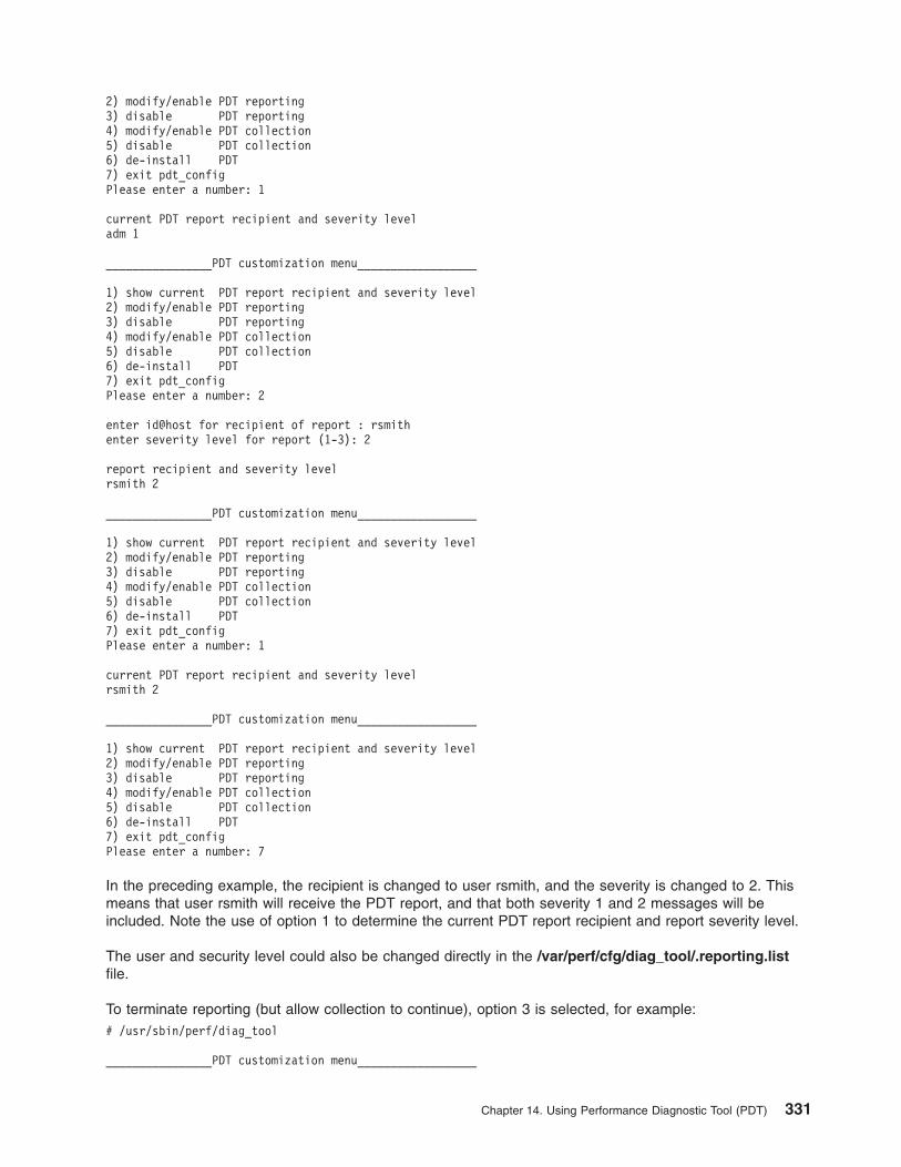
2) modify/enable PDT reporting3) disable PDT reporting4) modify/enable PDT collection5) disable PDT collection6) de-install PDT7) exit pdt_configPlease enter a number: 1

current PDT report recipient and severity leveladm 1


1) show current PDT report recipient and severity level2) modify/enable PDT reporting3) disable PDT reporting4) modify/enable PDT collection5) disable PDT collection6) de-install PDT7) exit pdt_configPlease enter a number: 2

enter id@host for recipient of report : rsmithenter severity level for report (1-3): 2

report recipient and severity levelrsmith 2



current PDT report recipient and severity levelrsmith 2



In the preceding example, the recipient is changed to user rsmith, and the severity is changed to 2. Thismeans that user rsmith will receive the PDT report, and that both severity 1 and 2 messages will beincluded. Note the use of option 1 to determine the current PDT report recipient and report severity level.

The user and security level could also be changed directly in the /var/perf/cfg/diag_tool/.reporting.listfile.

To terminate reporting (but allow collection to continue), option 3 is selected, for example:# /usr/sbin/perf/diag_tool




disable PDT reporting done



reporting has been disabled (file .reporting.list not found).

PDT Severity LevelsThe following lists indicate the possible problems associated with each severity level. Remember thatselecting severity n results in the reporting of all problems of severity less than or equal to n.

Severity 1 Problemsv Journaled File System (JFS) becomes unavailable

v JFS nearly full

v Physical volume not allocated to a volume group

v All paging spaces defined on one physical volume

v System appears to have too little memory for current workload

v Page space nearly full

v Possible problems in the settings of load control parameters

v VMM-detected bad memory frames

v Any host in .nodes becomes unreachable

Severity 2 Problemsv Imbalance in the I/O configuration (for example, disks per adapter)

v Imbalance in allocation of paging space on physical volumes with paging space

v Fragmentation of a paging space in a volume group

v Significant imbalance in measured I/O load to physical volumes

v New process is identified as a heavy memory or CPU consumer

v A file in .files exhibits systematic growth (or decline) in size

v A file system or page space exhibits systematic growth (or decline) in space utilization

v A host in .nodes exhibits degradation in ping delays or packet loss percentage

v A getty process consumes too much CPU time

v A process with high CPU or memory consumption exhibits systematic growth (or decline) in resourceuse

v maxuproc indicated as being possibly too low for a particular user ID

v A WORKLOAD TRACKING indicator shows an upward trend


Severity 3 MessagesSeverity 3 messages provide additional detail about problems identified at severity levels 1 and 2. Thisincludes the data-collection characteristics, such as number of samples, for severity 1 and 2 messages.

Obtaining a PDT Report on DemandAs an alternative to using the periodic report, any user can request a current report from the existing databy executing /usr/sbin/perf/diag_tool/pdt_report SeverityNum. The report is produced with the givenseverity (if none is provided, SeverityNum defaults to 1) and written to standard output. Generating areport in this way does not cause any change to the /var/perf/tmp/PDT_REPORT or to/var/perf/tmp/PDT_REPORT.last files.

Modifying the List of Files Monitored by PDTPDT analyzes files and directories for systematic growth in size. It examines only those files anddirectories listed in the file /var/perf/cfg/diag_tool/.files. The format of the .files file is one file or directoryname per line. The default content is as follows:/usr/adm/wtmp/var/spool/qdaemon//var/adm/ras//tmp/

You can use an editor to modify this file to track files and directories that are important to your system.

Modifying the List of Hosts That PDT MonitorsPDT tracks the average ping delay to hosts whose names are listed in the /var/perf/cfg/diag_tool/.nodesfile. This file is not shipped with PDT (which means that no host analysis is performed by default), but maybe created by the administrator. The format of the .nodes file is one host name per line in the file. Forexample, to monitor nodes chuys and hulahut, the file .nodes would be as follows:chuyshulahut

Changing the Historical-Record Retention PeriodPeriodically, a retention shell script is run that discards entries in the PDT historical record that are olderthan the designated retention period. The retention of all data is governed by the same retention policy.This policy is described in the /var/perf/cfg/diag_tool/.retention.list file. The default .retention.listcontent is as follows:* * * 35

which causes all data to be retained no more than 35 days. The number 35 can be replaced by anyunsigned integer.

PDT uses the historical record to assess trends and identify system changes. Extending the retentionperiod increases the scope of this analysis, but at the cost of additional disk storage and PDT processingtime.

The PDT historical record is maintained in /var/perf/tmp/.SM. The retention script creates a copy of thisfile in /var/perf/tmp/.SM.last prior to performing the retention operation. In addition, historical data that isdiscarded is appended to /var/perf/tmp/.SM.discards.

The existence of /var/perf/tmp/.SM.last provides limited backup, but the administrator should ensure thatthe /var/perf/tmp/.SM file is regularly backed up. If the file is lost, PDT continues to function, but withoutthe historical information. Over time, the historical record will grow again as new data is collected.


Modifying the Collection, Retention, and Reporting TimesCollection, reporting and retention are driven by three entries in the user adm cron table. Collection occurson every weekday at 9 a.m (Driver_ daily). Reporting occurs every weekday at 10 a.m (Driver_ daily2).The retention analysis is performed once a week, on Saturday evening at 9 p.m (Driver_ offweekly). Thefollowing files are used:

/var/perf/cfg/diag_tool/.collection.controlHandles collection information

/var/perf/cfg/diag_tool/.retention.controlHandles retention information

/var/perf/cfg/diag_tool/.reporting.controlHandles reporting information

The cron entries (created by executing the /usr/sbin/perf/diag_tool/pdt_config script and selecting option2) are shown below:0 9 * * 1-5 /usr/sbin/perf/diag_tool/Driver_ daily0 10 * * 1-5 /usr/sbin/perf/diag_tool/Driver_ daily20 21 * * 6 /usr/sbin/perf/diag_tool/Driver_ offweekly

The default times can be changed by altering the crontab for user adm.

Modifying the ThresholdsThe file /var/perf/cfg/diag_tool/.thresholds contains the thresholds used in analysis and reporting. Thesethresholds, listed below, have an effect on PDT report organization and content.

v DISK_STORAGE_BALANCE

The SCSI controllers having the largest and the smallest disk storage are identified. This is a static size,not the amount allocated or free. If the difference (in MB) between these two controllers exceedsDISK_STORAGE_BALANCE, a message is reported:SCSI Controller %s has %.0lf MB more storage than %s

The default value for DISK_STORAGE_BALANCE is 800. Any integer value between 0 and 10000 isvalid.

v PAGING_SPACE_BALANCE

The paging spaces having the largest and the smallest areas are identified. If the difference (in MB)between these two exceeds PAGING_SPACE_BALANCE, a message is reported. The default value is4. Any integer value between 0 and 100 is accepted. This threshold is presently not used in analysisand reporting.

v NUMBER_OF_BALANCE

The SCSI controllers having the largest and the least number of disks attached are identified. If thedifference between these two counts exceeds NUMBER_OF_BALANCE, a message is reported:SCSI Controller %s has %.0lf more disks than %s

The default value is 1. It can be set to any integer value in the range of 0 to 10000.

The same type of test is performed on the number of paging areas on each physical volume:Physical Volume %s has %.0lf paging areas, while Physical Volume %s has only %.0lf

v MIN_UTIL

Applies to process utilization. Changes in the top three CPU consumers are only reported if the newprocess had a utilization in excess of MIN_UTIL.First appearance of %s (%s) on top-3 cpu list

The same threshold applies to changes in the top-three memory consumers list:


First appearance of %s (%s) on top-3 memory list

The default value is 3. Any integer value from 0 to 100 is valid.

v FS_UTIL_LIMIT

Applies to journaled file system utilization. If the file system has a percentage use aboveFS_UTIL_LIMIT, a message is reported:File system %s (%s) is nearly full at %.0lf %%

The same threshold is applied to paging spaces:Paging space %s is nearly full at %.0lf %%

The default value is 90 percent. Any integer value between 0 and 100 is accepted.

Special attention should be given to /, /var, and /tmp file systems. The operating system uses theseareas for normal operation. If there remains no space in one of these, the behavior of the system isunpredictable. Error messages are provided when the execution of commands fails, but to detect thesefile system problems earlier, decrease FS_UTIL_LIMIT to 70 or 80 percent.

v MEMORY_FACTOR

The objective is to determine if the total amount of memory is adequately backed up by paging space. Ifreal memory is close to the amount of used paging space, then the system is likely paging and wouldbenefit from the addition of memory.

The formula is based on experience and actually compares MEMORY_FACTOR * memory with theaverage used paging space.

The current default is 0.9. By decreasing this number, a warning is produced more frequently:System has %.0lf MB memory; may be inadequate.

Increasing this number eliminates the message altogether. It can be set anywhere between 0.001 and100.

v TREND_THRESHOLD

Used in all trending assessments. It is applied after a linear regression is performed on all availablehistorical data. This technique basically draws the best line among the points. The slope of the fitted linemust exceed the last_value * TREND_THRESHOLD.File system %s (%s) is growing,now, %.2lf %% full, and growing an avg. of %.2lf %%/day

The objective is to try to ensure that a trend, however strong its statistical significance, has somepractical significance.

For example, if we determine that a file system is growing at X MB a day, and the last_value for the filesystem size is 100 MB, we require that X exceeds 100 MB * TREND_THRESHOLD to be reported as atrend of practical significance. The default value is 0.01; so a growth rate of 1 MB per day would berequired for reporting. The threshold can be set anywhere between 0.00001 and 100000.

This threshold assessment applies to trends associated with:

– CPU use by a top-three process

– Memory use by a top-three process

– Size of files indicated in the .files file

– Journaled file systems

– Paging spaces

– Hardware and software errors

– Workload indicators

– Processes per user


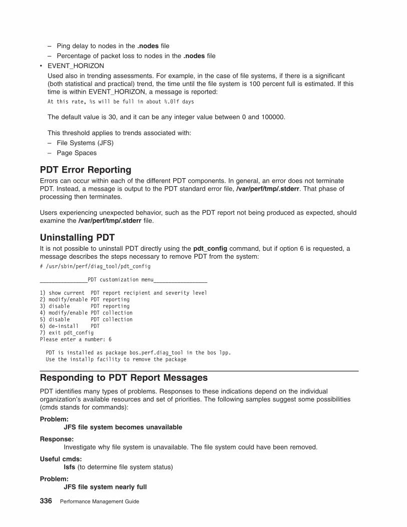
– Ping delay to nodes in the .nodes file

– Percentage of packet loss to nodes in the .nodes file

v EVENT_HORIZON

Used also in trending assessments. For example, in the case of file systems, if there is a significant(both statistical and practical) trend, the time until the file system is 100 percent full is estimated. If thistime is within EVENT_HORIZON, a message is reported:At this rate, %s will be full in about %.0lf days

The default value is 30, and it can be any integer value between 0 and 100000.

This threshold applies to trends associated with:

– File Systems (JFS)

– Page Spaces

PDT Error ReportingErrors can occur within each of the different PDT components. In general, an error does not terminatePDT. Instead, a message is output to the PDT standard error file, /var/perf/tmp/.stderr. That phase ofprocessing then terminates.

Users experiencing unexpected behavior, such as the PDT report not being produced as expected, shouldexamine the /var/perf/tmp/.stderr file.

Uninstalling PDTIt is not possible to uninstall PDT directly using the pdt_config command, but if option 6 is requested, amessage describes the steps necessary to remove PDT from the system:# /usr/sbin/perf/diag_tool/pdt_config



PDT is installed as package bos.perf.diag_tool in the bos lpp.Use the installp facility to remove the package

Responding to PDT Report MessagesPDT identifies many types of problems. Responses to these indications depend on the individualorganization’s available resources and set of priorities. The following samples suggest some possibilities(cmds stands for commands):

Problem:JFS file system becomes unavailable

Response:Investigate why file system is unavailable. The file system could have been removed.

Useful cmds:lsfs (to determine file system status)

Problem:JFS file system nearly full


Response:This problem could be caused by large or core files within the file system. Look for large files inthe file system, possibly caused by a runaway process. Attempt to identify the process or user thatgenerated those files. The system administrator should also verify if PDT report indicates along-term growth trend for this file system. Has this file system exhibited long-term growth trend(examine the rest of the PDT report or past PDT reports)?

Useful cmds:du, ls

Problem:Physical volume not allocated to a volume group

Response:If a physical volume is not allocated to a volume group, the operating system has no access tothis disk, and its space is being wasted. Use the lspv command to ensure that the disk is notallocated to any volume group, and if not, use the extendvg command to add the disk to a volumegroup.

Useful cmds:lspv (to confirm that the volume is not allocated)smitty (to manipulate volume groups)

Problem:All paging spaces defined on one physical volume

Response:The system has more than one physical volume, yet all paging space is defined on a singlevolume. If the system experiences paging, this configuration will result in reduced performance. Abetter I/O throughput could be achieved if the paging space is split equally among all physicalvolumes. Only one paging space should be defined per physical volume because the system willonly have access to one at a time. Use SMIT to create, modify, activate, or deactivate the pagingareas.

Useful cmds:smitty (to modify paging spaces)

Problem:Apparently too little memory for current workload

Response:If the system is paging heavily, more memory may be required on the system for goodperformance. The vmstat or svmon commands provide further details about the paging activity.See The vmstat Command, and The svmon Command, for more information on those commands.

Useful cmds:lsps -a, vmstat, svmon

Problem:Page space nearly full

Response:The system’s paging space may not be well dimensioned and may need to be enlarged, unlessthe problem is due to a process with a memory leak, in which case that process should beidentified and the application fixed. For systems up to 256 MB of memory, the paging spaceshould be twice the size of real memory. For memories larger than 256 MB, use the followingformula:total paging space = 512 MB + (memory size - 256 MB) * 1.25

Useful cmds:ps aucg (to examine process activity)smitty (to modify page space characteristics)


Problem:Possible problems in the settings of load control parameters

Response:The memory-load-control parameters are evaluated in relation to current paging activity. Forexample, if thrashing is occurring and load control is not enabled, it may be appropriate to enableload control. This situation might also be due to inappropriate load-control parameter settings. Usethe schedtune command to view or alter the configuration. Refer to Tuning VMM Memory LoadControl with the schedtune Command, for further details.

Useful cmdsschedtune

Problem:VMM-detected bad memory frames

Response:It might be necessary to have the memory analyzed. Compare the amount of installed memorywith the memory actually accessible. If the latter is less than the former, then bad memory hasbeen identified.You can use /usr/sbin/perf/diag_tool/getvmparms to examine the value of numframes todetermine the actual number of valid 4 KB memory frames.

Useful cmds:lscfg | grep mem (to obtain installed memory size in MB)

Problem:Any host in .nodes becomes unreachable

Response:Determine if problem is with current host (has a change in the /etc/hosts file been made?), withthe remote host (is it down?), or with the network (is the nameserver down?).The problem may be due to name resolution. Either Domain Name Service (DNS) configurationfiles or /etc/hosts should be checked depending on the type of name resolution being used at theenvironment.Use the ping command to check if the machine has access to other nodes in the same network.The remote node might be down. If it cannot access any other node, cables and connectionsshould be verified, as well as the routing table of the current machine. Verify cables andconnections by executing the netstat -r command.

Useful cmds:ping, netstat

Problem:Imbalance in the I/O configuration (number of disks per adapter)

Response:The number of disks per adapter should be equal whenever possible, to prevent one adapter frombeing overloaded. A guideline is to have no more than four devices per adapter, especially if theaccess to the disks is mostly sequential. Consider moving disks around so that an individualadapter is not overloaded.

Useful cmds:lscfg (to examine the current configuration)iostat (to determine if the actual load on the adapters is out of balance)

Problem:Imbalance in allocation of paging space on physical volumes with paging space

Response:A substantial imbalance in the sizes of paging spaces can cause performance problems. The


paging space should be equally distributed throughout the disks. Consider making paging spacesthe same size, except for a few extra megabytes on the primary paging space (hd6).

Useful cmds:smitty pgsp

Problem:Fragmentation of a paging space in a volume group

Response:Paging performance is better if paging areas are contiguous on a physical volume. However, whenpaging areas are enlarged, it is possible to create fragments that are scattered across the disksurface. Use the reorgvg command to reorganize the paging spaces.

Useful cmds:lspv -p hdiskn for each physical volume in the volume group. Look for more than one PP Rangewith the same LVNAME and a TYPE of paging.

Problem:Significant imbalance in measured I/O load to physical volumes

Response:The data is most likely not well-distributed throughout the disks. Use the iostat command to obtaininformation about the I/O activity of each disk (refer to Assessing Disk Performance with the iostatCommand). A disk should not be utilized more than 40 percent over a period of time.If one physical volume seems to be getting little I/O activity, consider moving data from busierphysical volumes onto less busy volumes. In general, the more evenly the I/O is distributed, thebetter the performance.Distribute data throughout the disks in a manner that balances I/O. Use the filemon command toobtain information about the most accessed files and file systems. This can be a good startingpoint in reorganizing the data. Refer to Detailed I/O Analysis with the filemon Command, for moreinformation on the filemon command.

Useful cmds:iostat -d 2 20 (to view the current distribution of I/O across physical volumes)

Problem:New process is a heavy consumer of memory or CPU

Response:Top CPU and memory consumers are regularly identified by PDT. If any of these processes havenot been detected before, they are highlighted in a problem report. Examine these processes forunusual behavior. Note that PDT simply looks at the process ID. If a known heavy user terminates,then is resumed (with a different process ID), it will be identified here as a new heavy user.

Useful cmds:ps aucg (to view all processes and their activity)

Problem:Any file in .files exhibits systematic growth (or decline) in size

Response:Look at the current size. Consider the projected growth rate. What user or application isgenerating the data? For example, the /var/adm/wtmp file is liable to grow unbounded. If it getstoo large, login times can increase. In some cases, the solution is to delete the file. In most cases,it is important to identify the user causing the growth and work with that user to correct theproblem.

Useful cmds:ls -al (to view file/directory sizes)

Problem:Any file system or paging space exhibits systematic growth (or decline) in space used


Response:Consider the projected growth rate and expected time until exceeding the available space. Analyzethe problem by identifying which user or process is generating the data. It may be necessary toenlarge the file system (or page space). On the other hand, the growth may be an undesirableeffect (for example, a process having a memory leak).

Useful cmds:smitty (to manipulate file systems/page spaces)ps aucg, svmon (to view process virtual memory activity)filemon (to view file system activity)

Problem:Degradation in ping response time or packet loss percentage for any host in .nodes

Response:There is probably a performance problem in the host or in the network. Is the host in questionexperiencing performance problems? Is the network having performance problems?

Useful cmds:ping, rlogin, rsh (to time known workloads on remote host)

Problem:A getty process that consumes too much CPU time

Response:Getty processes that use more than just a few percent of the CPU may be in error. It is possible incertain situations for these processes to consume system CPU, even though no users are actuallylogged in. In general, the solution is to terminate the process.

Useful cmds:ps aucg (to see how much CPU is being used)

Problem:A process that is a top consumer of CPU or memory resources exhibits systematic growthor decline in consumption

Response:Known large consumers of CPU and memory resources are tracked over time to see if theirdemands grow. As major consumers, a steady growth in their demand is of interest from severalperspectives. If the growth is normal, this represents useful capacity planning information. If thegrowth is unexpected, then evaluate the workload for a change (or a chronic problem, such as amemory leak). Use the vmstat and svmon commands while the process is running to gather moreinformation on its behavior.

Useful cmds:ps aucg, vmstat, svmon

Problem:maxuproc indicated as being possibly too low for a particular userid

Response:It is likely that this user is reaching the maxuproc threshold.maxuproc is a systemwide parameter that limits the number of processes that nonroot users areallowed to have simultaneously active. If the limit is too low, the user’s work can be delayed orterminated. On the other hand, the user might be accidentally creating more processes thanneeded or appropriate. Further investigation is warranted in either case. Consult the user in orderto clearly understand what is happening.

Useful cmds:lsattr -E -l sys0 | grep maxuproc to determine the current value of maxuproc (although it is also


reported directly in the PDT message).chdev -l sys0 -a maxuproc=100 to change maxuproc to 100 (for example). Root user authorityis required.

Problem:A WORKLOAD TRACKING indicator shows an upward trend

Response:The response depends on which workload indicator shows the trend:

loadavgRefers to 15-minute load average. In general, it indicates that the level of contention in thesystem is growing. Examine the rest of the PDT report for indicators of system bottlenecks(for example, substantial page space use might indicate a memory shortage; I/Oimbalances might indicate that the I/O subsystem requires attention).

nusersShows that the number of logged-on users on the system is growing. This is importantfrom a capacity planning perspective. Is the growth expected? Can it be explained?

nprocessesIndicates that the total number of processes on the system is growing. Are there usersreaching the maxuproc limitation? Perhaps there are ″runaway″ applications forking toomany processes.

STAT_ANumber of active processes. A trend here indicates processes are spending more timewaiting for the CPU.

STAT_WNumber of swapped processes. A trend here indicates that processes are contendingexcessively for memory.

STAT_ZNumber of zombie processes. Zombies should not stay around for a long period of time. Ifthe number of zombies on a system is growing, this may be cause for concern.

STAT_INumber of idle processes.

STAT_TNumber of processes stopped after receiving a signal. A trend here might indicate aprogramming error.

STAT_xNumber of processes reported by the ps command as being in state x, where x is a statenot listed in the other STAT_* states. The interpretation of a trend depends on themeaning of the character x. Refer to Using the ps Command, for more information on theps command.

cp Time required to copy a 40 KB file. An upward trend in the time to do a file copy suggestsdegradation in the I/O subsystem.

idle_pct_cpu0Idle percentage for processor 0. An upward trend in the idle percentage might indicateincreased contention in non-CPU resources such as paging or I/O. Such an increasesuggests the CPU resource is not being well-utilized.

idle_pct_avgAverage idle percentage for all processors. An upward trend in the idle percentage mightindicate increased contention in non-CPU resources such as paging or I/O. Such anincrease suggests the CPU resource is not being well-utilized.



Chapter 15. Reporting Performance Problems

If you believe that you have found a possible performance problem in the operating system, you can usetools and procedures for reporting the problem and supplying problem-analysis data. These tools areintended to ensure that you get a prompt and accurate response, with a minimum of effort and time onyour part.

The main sections in this topic are:

v Measuring the Baseline

v What is a Performance Problem

v Performance Problem Description

v Reporting a Performance Problem

Measuring the BaselinePerformance problems are often reported immediately following some change to system hardware orsoftware. Unless there is a pre-change baseline measurement with which to compare post-changeperformance, quantification of the problem is impossible.

Changes to any of the following can affect performance:

v Hardware configuration - Adding, removing, or changing configurations such as how the disks areconnected

v Operating system - Installing or updating a fileset, installing PTFs, and changing parameters

v Applications - Installing new versions and fixes

v Applications - Configuring or changing data placement

v Application tuning

v Tuning options in the operating system, RDBMS or an application

v Any changes

The best option is to measure the environment before and after each change. The alternative is runningthe measurements at regular intervals (for example, once a month) and save the output. When a problemis found, the previous capture can be used for comparison. It is worth collecting a series of outputs inorder to support the diagnosis of a possible performance problem.

To maximize performance diagnosis, collect data for various periods of the working day, week, or monthwhen performance is likely to be an issue. For example, you might have workload peaks as follows:

v In the middle of the mornings for online users

v During a late-night batch run

v During the end-of-month processing

v During major data loads

Use measurements to collect data for each of these peaks in workload, because a performance problemmight only cause problems during one of these periods and not during other times.

Note: Any measurement has an impact on the performance of the system being measured.The AIX Performance PMR (perfpmr) data collection tools are the preferred method for gathering baselinedata. Access these tools via the web at ftp://ftp.software.ibm.com/aix/tools/perftools/perfpmr. Follow theinstructions in the README file in the directory that matches the AIX version you will be measuring toobtain, install, and collect data on your system.


ftp://ftp.software.ibm.com/aix/tools/perftools/perfpmr

What is a Performance ProblemSupport personnel need to determine when a reported problem is a functional problem or a performanceproblem. When an application, a hardware system, or a network is not behaving correctly, this is referredto as a functional problem. For example, an application or a system with a memory leak has a functionalproblem.

Sometimes functional problems lead to performance problems; for example, when the functions are beingachieved, but the speed of the functions are slow. In these cases, rather than tune the system, it is moreimportant to determine the root cause of the problem and fix it. Another example would be whencommunication is slowed because of networks or name servers that are down.

Performance Problem DescriptionSupport personnel often receive problem reports stating that someone has a performance problem on thesystem and providing some data analysis. This information is insufficient to accurately determine thenature of a performance problem. The data might indicate 100 percent CPU utilization and a high runqueue, but that may have nothing to do with the cause of the performance problem.

For example, a system might have users logged in from remote terminals over a network that goes overseveral routers. The users report that the system is slow. Data might indicate that the CPU is very heavilyutilized. But the real problem could be that the characters get displayed after long delays on their terminalsdue to packets getting lost on the network (which could be caused by failing routers or overloadednetworks). This situation might have nothing to do with the CPU utilization on the machine. If on the otherhand, the complaint was that a batch job on the system was taking a long time to run, then CPU utilizationor I/O bandwidth might be related.

Always obtain as much detail as possible before you attempt to collect or analyze data, by asking thefollowing questions regarding the performance problem:

v Can the problem be demonstrated by running a specific command or reconstructing a sequence ofevents? (for example: ls /slow/fs or ping xxxxx). If not, describe the least complex example of theproblem.

v Is the slow performance intermittent? Does it get slow, but then disappear for a while? Does it occur atcertain times of the day or in relation to some specific activity?

v Is everything slow or only some things?

v What aspect is slow? For example, time to echo a character, or elapsed time to complete a transaction,or time to paint the screen?

v When did the problem start occurring? Was the situation the same ever since the system was firstinstalled or went into production? Did anything change on the system before the problem occurred(such as adding more users or migrating additional data to the system)?

v If client/server, can the problem be demonstrated when run just locally on the server (network versusserver issue)?

v If network related, how are the network segments configured (including bandwidth such as 10 Mb/sec or9600 baud)? Are there any routers between the client and server?

v What vendor applications are running on the system, and are those applications involved in theperformance issue?

v What is the impact of the performance problem on the users?

Reporting a Performance ProblemYou should report operating system performance problems to IBM support. Use your normal softwareproblem-reporting channel. If you are not familiar with the correct problem-reporting channel for yourorganization, check with your IBM representative.


The AIX Performance PMR (perfpmr) data collection tools are the best way to collect performance datawhen an AIX performance problem is suspected. Access these tools via the web atftp://ftp.software.ibm.com/aix/tools/perftools/perfpmr Follow the instructions in the README file in thedirectory that matches the AIX version you will be measuring to obtain, install, and collect data on yoursystem. Instructions are also provided on how to send the data to IBM support for analysis once a PMRhas been opened.

When someone reports a performance problem, it is not enough just to gather data and then analyze it.Without knowing the nature of the performance problem, you might waste a lot of time analyzing datawhich may have nothing to do with the problem being reported.

Before you involve support personnel to report a problem, prepare in advance the information that you willbe asked to supply to facilitate the problem to be investigated. Your local support personnel will attempt toquickly solve your performance problem directly with you.

Three further ways you can help to get the problem resolved faster are:

1. Provide a clear written statement of a simple specific instance of problem, but be sure to separate thesymptoms and facts from the theories, ideas and your own conclusions. PMRs that report ″the systemis slow″ require extensive investigation to determine what you mean by slow, how it is measured, andwhat is acceptable performance.

2. Provide information about everything that has changed on the system in the weeks before the problem.Missing something that changed can block a possible investigation path and will only delay finding aresolution. If all the facts are available, the performance team can quickly eliminate the unrelated ones.

3. Use the correct machine to supply information. In very large sites it is easy to accidentally collect thedata on the wrong machine. This makes it very hard to investigate the problem.

When you report the problem, supply the following basic information:

v A problem description that can be used to search the problem-history database to see if a similarproblem has already been reported.

v What aspect of your analysis led you to conclude that the problem is due to a defect in the operatingsystem?

v What is the hardware and software configuration in which the problem is occurring?

– Is the problem confined to a single system, or does it affect multiple systems?

– What are the models, memory sizes, as well as number and size of disks on the affected systems?

– What kinds of LAN and other communications media are connected to the systems?

– Does the overall configuration include those for other operating systems?

v What are the characteristics of the program or workload that is experiencing the problem?

– Does an analysis with the time, iostat, and vmstat commands indicate that it is CPU-limited orI/O-limited?

– Are the workloads being run on the affected systems: workstation, server, multiuser, or acombination?

v What are the performance objectives that are not being met?

– Is the primary objective in terms of console or terminal response time, throughput, or real-timeresponsiveness?

– Were the objectives derived from measurements on another system? If so, what was itsconfiguration?

If this is the first report of the problem, you will receive a PMR number for use in identifying any additionaldata you supply and for future reference.

Include all of the following items when the supporting information and the perfpmr data for the PMR is firstgathered:

Chapter 15. Reporting Performance Problems 345

ftp://ftp.software.ibm.com/aix/tools/perftools/perfpmr

v A means of reproducing the problem

– If possible, a program or shell script that demonstrates the problem should be included.

– At a minimum, a detailed description of the conditions under which the problem occurs is needed.

v The application experiencing the problem:

– If the application is, or depends on, any software product, the exact version and release of thatproduct should be identified.

– If the source code of a user-written application cannot be released, the exact set of compilerparameters used to create the executable program should be documented.


Chapter 16. Application Tuning

Before spending a lot of effort to improve the performance of a program, use the techniques in this chapterto help determine how much its performance can be improved and to find the areas of the program whereoptimization and tuning will have the most benefit. For an extensive discussion of these techniques, seeOptimization and Tuning Guide for XL Fortran, XL C and XL C++. Also see Designing and ImplementingEfficient Programs for additional hints and tips.

In general, the optimization process involves several steps:

v Some tuning involves changing the source code, for example, by reordering statements andexpressions. This technique is known as hand tuning.

v For FORTRAN and C programs, optimizing preprocessors are available to tune and otherwise transformsource code before it is compiled. The output of these preprocessors is FORTRAN or C source codethat has been optimized.

v The FORTRAN or C++ compiler translates the source code into an intermediate language.

v A code generator translates the intermediate code into machine language. The code generator canoptimize the final executable code to speed it up, depending on the selected compiler options. You canincrease the amount of optimization performed in this step by hand-tuning or preprocessing first.

The speed increase is affected by two factors:

v The amount of optimization applied to individual parts of the program

v The frequency of use for those parts of the program at run time

Speeding up a single routine might speed up the program significantly if that routine performs the majorityof the work, on the other hand, it might not improve overall performance much if the routine is rarely calledand does not take long anyway. Keep this point in mind when evaluating the performance techniques anddata, so that you focus on the techniques that are most valuable in your work.

This chapter contains the following major sections:

v Profiling

v Compiler Optimization Techniques

v Optimizing Preprocessors for FORTRAN and C

v Code-Optimization Techniques

ProfilingYou can use profiling tools to identify which portions of the program are executed most frequently or wheremost of the time is spent. Profilers are typically used after a basic tool, such as the vmstat or iostatcommands, shows that a CPU bottleneck is causing the slow performance.

Before you begin locating hot spots in your program, you need a fully functional program and realistic datavalues to feed it to.

Timing CommandsUse the timing commands discussed in Using the time Command to Measure CPU Use for testing anddebugging programs whose performance you are recoding and trying to improve. The output from the timecommand is in minutes and seconds, as follows:real 0m26.72suser 0m26.53ssys 0m0.03s

The output from the timex command is in seconds:


real 26.70user 26.55sys 0.02

Comparing the user+sys CPU time to the real time will give you an idea if your application is CPU-boundor I/O-bound.

Note: Be careful when you do this on an SMP system (see time and timex Cautions).

The timex command is also available through the SMIT command on the Analysis Tools menu, foundunder Performance and Resource Scheduling. The -p and -s options of the timex command allow datafrom accounting (-p) and the sar command (-s) to be accessed and reported. The -o option reports onblocks read or written.

The prof CommandThe prof command displays a profile of CPU usage for each external symbol (routine) of a specifiedprogram. In detail, it displays the following:

v The percentage of execution time spent between the address of that symbol and the address of thenext

v The number of times that function was called

v The average number of milliseconds per call

The prof command interprets the profile data collected by the monitor() subroutine for the object file(a.out by default), reads the symbol table in the object file, and correlates it with the profile file (mon.outby default) generated by the monitor() subroutine. A usage report is sent to the terminal, or can beredirected to a file.

To use the prof command, use the -p option to compile a source program in C, FORTRAN, PASCAL, orCOBOL. This inserts a special profiling startup function into the object file that calls the monitor()subroutine to track function calls. When the program is executed, the monitor() subroutine creates amon.out file to track execution time. Therefore, only programs that explicitly exit or return from the mainprogram cause the mon.out file to be produced. Also, the -p flag causes the compiler to insert a call tothe mcount() subroutine into the object code generated for each recompiled function of your program.While the program runs, each time a parent calls a child function, the child calls the mcount() subroutineto increment a distinct counter for that parent-child pair. This counts the number of calls to a function.

Note: You cannot use the prof command for profiling optimized code.

By default, the displayed report is sorted by decreasing percentage of CPU time. This is the same aswhen specifying the -t option.

The -c option sorts by decreasing number of calls and the -n option sorts alphabetically by symbol name.

If the -s option is used, a summary file mon.sum is produced. This is useful when more than one profilefile is specified with the -m option (the -m option specifies files containing monitor data).

The -z option includes all symbols, even if there are zero calls and time associated.

Other options are available and explained in the prof command in the AIX 5L Version 5.2 CommandsReference.

The following example shows the first part of the prof command output for a modified version of theWhetstone benchmark (Double Precision) program.


# cc -o cwhet -p -lm cwhet.c# cwhet > cwhet.out# profName %Time Seconds Cumsecs #Calls msec/call.main 32.6 17.63 17.63 1 17630..__mcount 28.2 15.25 32.88.mod8 16.3 8.82 41.70 8990000 0.0010.mod9 9.9 5.38 47.08 6160000 0.0009.cos 2.9 1.57 48.65 1920000 0.0008.exp 2.4 1.32 49.97 930000 0.0014.log 2.4 1.31 51.28 930000 0.0014.mod3 1.9 1.01 52.29 140000 0.0072.sin 1.2 0.63 52.92 640000 0.0010.sqrt 1.1 0.59 53.51.atan 1.1 0.57 54.08 640000 0.0009.pout 0.0 0.00 54.08 10 0.0.exit 0.0 0.00 54.08 1 0..free 0.0 0.00 54.08 2 0..free_y 0.0 0.00 54.08 2 0.

In this example, we see many calls to the mod8() and mod9() routines. As a starting point, examine thesource code to see why they are used so much. Another starting point could be to investigate why aroutine requires so much time.

Note: If the program you want to monitor uses a fork() system call, be aware that the parent and the childcreate the same file (mon.out). To avoid this problem, change the current directory of the childprocess.

The gprof CommandThe gprof command produces an execution profile of C, PASCAL, FORTRAN, or COBOL programs. Thestatistics of called subroutines are included in the profile of the calling program. The gprof command isuseful in identifying how a program consumes CPU resources. It is roughly a superset of the profcommand, giving additional information and providing more visibility to active sections of code.

The gprof ImplementationThe source code must be compiled with the -pg option. This action links in versions of library routinescompiled for profiling and reads the symbol table in the named object file (a.out by default), correlating itwith the call graph profile file (gmon.out by default). This means that the compiler inserts a call to themcount() function into the object code generated for each recompiled function of your program. Themcount() function counts each time a parent calls a child function. Also, the monitor() function is enabledto estimate the time spent in each routine.

The gprof command generates two useful reports:

v The call-graph profile, which shows the routines, in descending order by CPU time, plus theirdescendants. The profile allows you to understand which parent routines called a particular routine mostfrequently and which child routines were called by a particular routine most frequently.

v The flat profile of CPU usage, which shows the usage by routine and number of calls, similar to theprof output.

Each report section begins with an explanatory part describing the output columns. You can suppressthese pages by using the -b option.

Use -s for summaries and -z to display routines with zero usage.

Where the program is executed, statistics are collected in the gmon.out file. These statistics include thefollowing:

v The names of the executable program and shared library objects that were loaded

v The virtual memory addresses assigned to each program segment

Chapter 16. Application Tuning 349

v The mcount() data for each parent-child

v The number of milliseconds accumulated for each program segment

Later, when the gprof command is issued, it reads the a.out and gmon.out files to generate the tworeports. The call-graph profile is generated first, followed by the flat profile. It is best to redirect the gprofoutput to a file, because browsing the flat profile first may answer most of your usage questions.

The following example shows the profiling for the cwhet benchmark program. This example is also used inThe prof Command:# cc -o cwhet -pg -lm cwhet.c# cwhet > cwhet.out# gprof cwhet > cwhet.gprof

Call-Graph Profile: The call-graph profile is the first part of the cwhet.gprof file and looks similar to thefollowing:granularity: each sample hit covers 4 byte(s) Time: 62.85 seconds

called/total parentsindex %time self descendents called+self name index

called/total children

19.44 21.18 1/1 .__start [2][1] 64.6 19.44 21.18 1 .main [1]

8.89 0.00 8990000/8990000 .mod8 [4]5.64 0.00 6160000/6160000 .mod9 [5]1.58 0.00 930000/930000 .exp [6]1.53 0.00 1920000/1920000 .cos [7]1.37 0.00 930000/930000 .log [8]1.02 0.00 140000/140000 .mod3 [10]0.63 0.00 640000/640000 .atan [12]0.52 0.00 640000/640000 .sin [14]0.00 0.00 10/10 .pout [27]

-----------------------------------------------<spontaneous>

[2] 64.6 0.00 40.62 .__start [2]19.44 21.18 1/1 .main [1]0.00 0.00 1/1 .exit [37]

-----------------------------------------------

Usually the call graph report begins with a description of each column of the report, but it has beendeleted in this example. The column headings vary according to type of function (current, parent ofcurrent, or child of current function). The current function is indicated by an index in brackets at thebeginning of the line. Functions are listed in decreasing order of CPU time used.

To read this report, look at the first index [1] in the left-hand column. The .main function is the currentfunction. It was started by .__start (the parent function is on top of the current function), and it, in turn,calls .mod8 and .mod9 (the child functions are beneath the current function). All the accumulated time of.main is propagated to .__start. The self and descendents columns of the children of the current functionadd up to the descendents entry for the current function. The current function can have more than oneparent. Execution time is allocated to the parent functions based on the number of times they are called.

Flat Profile: The flat profile sample is the second part of the cwhet.gprof file and looks similar to thefollowing:granularity: each sample hit covers 4 byte(s) Total time: 62.85 seconds

% cumulative self self totaltime seconds seconds calls ms/call ms/call name30.9 19.44 19.44 1 19440.00 40620.00 .main [1]30.5 38.61 19.17 .__mcount [3]14.1 47.50 8.89 8990000 0.00 0.00 .mod8 [4]


9.0 53.14 5.64 6160000 0.00 0.00 .mod9 [5]2.5 54.72 1.58 930000 0.00 0.00 .exp [6]2.4 56.25 1.53 1920000 0.00 0.00 .cos [7]2.2 57.62 1.37 930000 0.00 0.00 .log [8]2.0 58.88 1.26 .qincrement [9]1.6 59.90 1.02 140000 0.01 0.01 .mod3 [10]1.2 60.68 0.78 .__stack_pointer [11]1.0 61.31 0.63 640000 0.00 0.00 .atan [12]0.9 61.89 0.58 .qincrement1 [13]0.8 62.41 0.52 640000 0.00 0.00 .sin [14]0.7 62.85 0.44 .sqrt [15]0.0 62.85 0.00 180 0.00 0.00 .fwrite [16]0.0 62.85 0.00 180 0.00 0.00 .memchr [17]0.0 62.85 0.00 90 0.00 0.00 .__flsbuf [18]0.0 62.85 0.00 90 0.00 0.00 ._flsbuf [19]

The flat profile is much less complex than the call-graph profile and very similar to the output of the profcommand. The primary columns of interest are the self seconds and the calls columns. These reflect theCPU seconds spent in each function and the number of times each function was called. The next columnsto look at are self ms/call (CPU time used by the body of the function itself) and total ms/call (time inthe body of the function plus any descendent functions called).

Normally, the top functions on the list are candidates for optimization, but you should also consider howmany calls are made to the function. Sometimes it can be easier to make slight improvements to afrequently called function than to make extensive changes to a piece of code that is called once.

A cross reference index is the last item produced and looks similar to the following:Index by function name

[18] .__flsbuf [37] .exit [5] .mod9[34] .__ioctl [6] .exp [43] .moncontrol[20] .__mcount [39] .expand_catname [44] .monitor[3] .__mcount [32] .free [22] .myecvt[23] .__nl_langinfo_std [33] .free_y [28] .nl_langinfo[11] .__stack_pointer [16] .fwrite [27] .pout[24] ._doprnt [40] .getenv [29] .printf[35] ._findbuf [41] .ioctl [9] .qincrement[19] ._flsbuf [42] .isatty [13] .qincrement1[36] ._wrtchk [8] .log [45] .saved_category_nam[25] ._xflsbuf [1] .main [46] .setlocale[26] ._xwrite [17] .memchr [14] .sin[12] .atan [21] .mf2x2 [31] .splay[38] .catopen [10] .mod3 [15] .sqrt

[7] .cos [4] .mod8 [30] .write

Note: If the program you want to monitor uses a fork() system call, be aware that the parent and the childcreate the same file (gmon.out). To avoid this problem, change the current directory of the childprocess.

The tprof CommandStandard UNIX performance tools often do not capture enough information to fully describe the enhancedperformance and function of the operating system. The tprof command is a versatile profiler that providesa detailed profile of CPU usage by every process ID and name. It further profiles at the application level,routine level, and even to the source statement level and provides both a global view and a detailed view.In addition, the tprof command can profile kernel extensions, stripped executable programs, and strippedlibraries. It will do subroutine level profiling for most executable program on which the stripnm commandwill produce a symbol table.


Because activity is recorded at 100 samples per second, estimates for short-running programs might notbe sufficiently accurate. Averaging multiple runs help generate a more accurate picture. The tprofcommand profiles only CPU activity; it does not profile other system resources, such as memory or disks.

The tprof command uses the system trace facility. Only one user at a time can execute the trace facility.Therefore, only one tprof command can be executing at one time.

Note that the tprof command cannot determine the address of a routine when interrupts are disabled.Therefore, it charges any ticks that occur while interrupts are disabled to the unlock_enable() routines.

The tprof command is described in detail in Using the tprof Program to Analyze Programs for CPU Use.The remainder of this section discusses its importance for application tuning.

For an example of the tprof command output, see A tprof Example.

Compiler Optimization TechniquesThe three main areas of source-code tuning are as follows:

v Programming techniques that take advantage of the optimizing compilers and the system srchitecture.

v BLAS, a library of Basic Linear Algebra Subroutines. If you have a numerically intensive program, thesesubroutines can provide considerable performance enhancement. An extension of BLAS is ESSL, theEngineering Scientific Subroutine Library. In addition to a subset of the BLAS library, ESSL includesother high-performance mathematical routines for chemistry, engineering, and physics. A Parallel ESSL(PESSL) exists for SMP machines.

v Compiler options and the use of preprocessors like KAP and VAST, available from third-party vendors.

In addition to these source-code tuning techniques, the fdpr program restructures object code. The fdprprogram is described in Restructuring Executable Programs with the fdpr Program.

Compiling with Optimization (-O, -O2, -O3, -O4, -O5, qstrict, -qhot,-qipa)To produce a program that achieves good performance, the first step is to take advantage of the basicoptimization features built into the compiler. Doing so can increase the speedup that comes from tuningyour program and can remove the need to perform some kinds of tuning.

RecommendationsFollow these guidelines for optimization:

v Use -O2 or -O3 -qstrict for any production-level FORTRAN, C, or C++ program you compile. For HighPerformance FORTRAN (HPF) programs, do not use the -qstrict option.

v Use the -qhot option for programs where the hotspots are loops or array language. Always use the-qhot option for HPF programs.

v Use the -qipa option near the end of the development cycle if compilation time is not a majorconsideration.

The -qipa option activates or customizes a class of optimizations known as interprocedural analysis. The-qipa option has several suboptions that are detailed in the compiler manual. It can be used in two ways:

v The first method is to compile with the -qipa option during both the compile and link steps. Duringcompilation, the compiler stores interprocedural analysis information in the .o file. During linking, the-qipa option causes a complete recompilation of the entire application.

v The second method is to compile the program for profiling with the -p/-pg option (with or without -qipa),and run it on a typical set of data. The resulting data can then be fed into subsequent compilations with-qipa so that the compiler concentrates optimization in the seconds of the program that are mostfrequently used.


Using -O4 is equivalent to using -O3 -qipa with automatic generation of architecture and tuning optionideal for that platform. Using the -O5 flag is similar to -O4 except that -qipa= level = 2.

You gain the following benefits when you use compiler optimization:

Branch optimizationRearranges the program code to minimize branching logic and to combine physically separateblocks of code.

Code motionIf variables used in a computation within a loop are not altered within the loop, the calculation canbe performed outside of the loop and the results used within the loop.

Common subexpression eliminationIn common expressions, the same value is recalculated in a subsequent expression. The duplicateexpression can be eliminated by using the previous value.

Constant propagationConstants used in an expression are combined, and new ones are generated. Some implicitconversions between integers and floating-point types are done.

Dead code eliminationEliminates code that cannot be reached or where the results are not subsequently used.

Dead store eliminationEliminates stores when the value stored is never referenced again. For example, if two stores tothe same location have no intervening load, the first store is unnecessary and is removed.

Global register allocationAllocates variables and expressions to available hardware registers using a ″graph coloring″algorithm.

InliningReplaces function calls with actual program code

Instruction schedulingReorders instructions to minimize execution time

Interprocedural analysisUncovers relationships across function calls, and eliminates loads, stores, and computations thatcannot be eliminated with more straightforward optimizations.

Invariant IF code floating (Unswitching)Removes invariant branching code from loops to make more opportunity for other optimizations.

Profile driven feedbackResults from sample program execution are used to improve optimization near conditionalbranches and in frequently executed code sections.

ReassociationRearranges the sequence of calculations in an array subscript expression, producing morecandidates for common expression elimination.

Store motionMoves store instructions out of loops.

Strength ReductionReplaces less efficient instructions with more efficient ones. For example, in array subscripting, anadd instruction replaces a multiply instruction.

Value numberingInvolves constant propagation, expression elimination, and folding of several instructions into asingle instruction.


When to Compile without OptimizationDo not use the -O option for programs that you intend to debug with a symbolic debugger, regardless ofwhether you use the -g option. However, because optimization is so important to HPF programs, use -O3-qhot for them even during debugging.

The optimizer rearranges assembler-language instructions, making it difficult to map individual instructionsto a line of source code. If you compile with the -g option, this rearrangement may give the appearancethat the source-level statements are executed in the wrong order when you use a symbolic debugger.

If your program produces incorrect results when it is compiled with any of the -O options, check yourprogram for unintentionally aliased variables in procedure references.

Compiling for Specific Hardware Platforms (-qarch, -qtune)Systems can use several type of processors. By using the -qarch and -qtune options, you can optimizeprograms for the special instructions and particular strengths of these processors.

RecommendationsFollow these guidelines for compiling for specific hardware platforms:

v If your program will be run only on a single system, or on a group of systems with the same processortype, use the -qarch option to specify the processor type.

v If your program will be run on systems with different processor types, and you can identify oneprocessor type as the most important, use the appropriate -qarch and -qtune settings. XL FORTRANand XL HPF users can use the xxlf and xxlhpf commands to select these settings interactively.

v If your program is intended to run on the full range of processor implementations, and is not intendedprimarily for one processor type, do not use either -qarch or -qtune.

Compiling for Floating-Point Performance (-qfloat)You can change some default floating-point options to enhance performance of floating-point intensiveprograms. Some of these options can affect conformance to floating-point standards. Using these optionscan change the results of computations, but in many cases the result is an increase in accuracy.

RecommendationsFollow these guidelines:

v For single-precision programs on POWER family and POWER2 platforms, you can enhanceperformance while preserving accuracy by using these floating-point options:-qfloat=fltint:rsqrt:hssngl

If your single-precision program is not memory-intensive (for example, if it does not access more datathan the available cache space), you can obtain equal or better performance, and greater precision, byusing:-qfloat=fltint:rsqrt -qautodbl=dblpad4

For programs that do not contain single-precision variables, use -qfloat=rsqrt:fltint only. Note that -O3without -qstrict automatically sets -qfloat=rsqrt:fltint.

v Single-precision programs are generally more efficient than double-precision programs, so promotingdefault REAL values to REAL(8) can reduce performance. Use the following -qfloat suboptions:

Specifying Cache Sizes (-qcache)If your program is intended to run exclusively on a single machine or configuration, you can help thecompiler tune your program to the memory layout of that machine by using the FORTRAN -qcache option.You must also specify the -qhot option for -qcache to have any effect. The -qhot option uses the -qcacheinformation to determine appropriate memory-management optimizations.


There are three types of cache: data, instruction, and combined. Models generally fall into two categories:those with both data and instruction caches, and those with a single, combined data/instruction cache. TheTYPE suboption lets you identify which type of cache the -qcache option refers to.

The -qcache option can also be used to identify the size and set associativity of a model’s level-2 cacheand the Translation Lookaside Buffer (TLB), which is a table used to locate recently referenced pages ofmemory. In most cases, you do not need to specify the -qcache entry for a TLB unless your program usesmore than 512 KB of data space.

There may be cases where a lower setting for the SIZE attribute gives enhanced performance, dependingon the system load at the time of a run.

Expanding Procedure Calls Inline (-Q)Inlining involves copying referenced procedures into the code from which they are referenced. Thiseliminates the calling overhead for inlined routines and enables the optimizer to perform otheroptimizations in the inlined routines.

For FORTRAN and C programs, you can specify the -Q option (along with -O2 or -O3) to have proceduresinlined into their reference points.

Inlining enhances performance in some programs, while it degrades performance in others. A program withinlining might slow down because of larger code size, resulting in more cache misses and page faults, orbecause there are not enough registers to hold all the local variables in some combined routines.

If you use the -Q option, always check the performance of the version of your program compiled with -O3and -Q to that compiled only with -O3. Performance of programs compiled with -Q might improvedramatically, deteriorate dramatically, or change little or not at all.

The compiler decides whether to inline procedures based on their size. You might be able to enhance yourapplication’s performance by using other criteria for inlining. For procedures that are unlikely to bereferenced in a typical execution (for example, error-handling and debugging procedures), disable inliningselectively by using the -Q-names option. For procedures that are referenced within hot spots, specify the-Q+names option to ensure that those procedures are always inlined.

When to Use Dynamic Linking and Static LinkingThe operating system provides facilities for creating and using dynamically linked shared libraries. Withdynamic linking, external symbols referenced in user code and defined in a shared library are resolved bythe loader at load time. When you compile a program that uses shared libraries, they are dynamicallylinked to your program by default.

The idea behind shared libraries is to have only one copy of commonly used routines and to maintain thiscommon copy in a unique shared-library segment. These common routines can significantly reduce thesize of executable programs, thereby saving disk space.

You can reduce the size of your programs by using dynamic linking, but there is usually a tradeoff inperformance. The shared library code is not present in the executable image on disk, but is kept in aseparate library file. Shared code is loaded into memory once in the shared library segment and shared byall processes that reference it. Dynamically linked libraries therefore reduce the amount of virtual storageused by your program, provided that several concurrently running applications (or copies of the sameapplication) use the procedures provided in the shared library. They also reduce the amount of disk spacerequired for your program provided that several different applications stored on a given system share alibrary. Other advantages of shared libraries are as follows:

v Load time might be reduced because the shared library code might already be in memory.


v Run-time performance can be enhanced because the operating system is less likely to page out sharedlibrary code that is being used by several applications, or copies of an application, rather than code thatis only being used by a single application. As a result, fewer page faults occur.

v The routines are not statically bound to the application but are dynamically bound when the applicationis loaded. This permits applications to automatically inherit changes to the shared libraries, withoutrecompiling or rebinding.

Disadvantages of dynamic linking include the following:

v From a performance viewpoint, there is ″glue code″ that is required in the executable program toaccess the shared segment. There is a performance cost in references to shared library routines ofabout eight machine cycles per reference. Programs that use shared libraries are usually slower thanthose that use statically-linked libraries.

v A more subtle effect is a reduction in ″locality of reference.″ You may be interested in only a few of theroutines in a library, and these routines may be scattered widely in the virtual address space of thelibrary. Thus, the total number of pages you need to touch to access all of your routines is significantlyhigher than if these routines were all bound directly into your executable program. One impact of thissituation is that, if you are the only user of these routines, you experience more page faults to get themall into real memory. In addition, because more pages are touched, there is a greater likelihood ofcausing an instruction translation lookaside buffer (TLB) miss.

v When a program references a limited number of procedures in a library, each page of the library thatcontains a referenced procedure must be individually paged into real memory. If the procedures aresmall enough that using static linking might have linked several procedures that are in different librarypages into a single page, then dynamic linking may increase paging thus decreasing performance.

v Dynamically linked programs are dependent on having a compatible library. If a library is changed (forexample, a new compiler release may change a library), applications might have to be reworked to bemade compatible with the new version of the library. If a library is removed from the system, programsusing that library will no longer work.

In statically-linked programs, all code is contained in a single executable module. Library references aremore efficient because the library procedures are statically linked into the program. Static linking increasesthe file size of your program, and it may increase the code size in memory if other applications, or othercopies of your application, are running on the system.

The cc command defaults to the shared-library option. To override the default, when you compile yourprograms to create statically-linked object files, use the -bnso option as follows:cc xxx.c -o xxx.noshr -O -bnso -bI:/lib/syscalls.exp

This option forces the linker to place the library procedures your program references into the program’sobject file. The /lib/syscalIs.exp file contains the names of system routines that must be imported to yourprogram from the system. This file must be specified for static linking. The routines that it names areimported automatically by libc.a for dynamic linking, so you do not need to specify this file during dynamiclinking. For further details on these options, see Appendix B. Efficient Use of the ld Command and the Idcommand.

Determining If Nonshared Libraries Help PerformanceOne method of determining whether your application is sensitive to the shared-library approach is torecompile your executable program using the nonshare option. If the performance is significantly better,you may want to consider trading off the other advantages of shared libraries for the performance gain. Besure to measure performance in an authentic environment, however. A program that had been boundnonshared might run faster as a single instance in a lightly loaded machine. That same program, whenused by a number of users simultaneously, might increase real memory usage enough to slow down thewhole workload.


Specifying the Link Order to Reduce Paging for Large ProgramsDuring the linkage phase of program compilation, the linker relocates program units in an attempt toimprove locality of reference. For example, if a procedure references another procedure, the linker maymake the procedures adjacent in the load module, so that both procedures fit into the same page of virtualmemory. This can reduce paging overhead. When the first procedure is referenced for the first time andthe page containing it is brought into real memory, the second procedure is ready for use withoutadditional paging overhead.

In very large programs where paging occurs excessively for pages of your program’s code, you maydecide to impose a particular link order on the linker. You can do this by arranging control sections in theorder you want them linked, and by using the -bnoobjreorder option to prevent the linker from reordering.A control section or CSECT is the smallest replaceable unit of code or data in an XCOFF object module.For further details, see the AIX 5L Version 5.2 Files Reference.

However, there are a number of risks involved in specifying a link order. Any link reordering should alwaysbe followed by thorough performance testing to demonstrate that your link order gives superior results foryour program over the link order that the linker chooses. Take the following points into account before youdecide to establish your own link order:

v You must determine the link order for all CSECTs in your program. The CSECTs must be presented tothe linker in the order in which you want to link them. In a large program, such an ordering effort isconsiderable and prone to errors.

v A performance benefit observed during development of a program can become a performance loss lateron, because the changing code size can cause CSECTs that were previously located together in a pageto be split into separate pages.

v Reordering can change the frequency of instruction cache-line collisions. On implementations with aninstruction cache or combined data and instruction cache that is two-way set-associative, any line ofprogram code can only be stored in one of two lines of the cache. If three or more short, interdependentprocedures have the same cache-congruence class, instruction-cache thrashing can reduceperformance. Reordering can cause cache-line collisions where none occurred before. It can alsoeliminate cache-line collisions that occur when -bnoobjreorder is not specified.

If you attempt to tune the link order of your programs, always test performance on a system where totalreal storage and memory utilization by other programs are similar to the anticipated working environment.A link order that works on a quiet system with few tasks running can cause page thrashing on a busiersystem.

Calling the BLAS and ESSL LibrariesThe Basic Linear Algebra Subroutines (BLAS) provide a high level of performance for linear algebraicequations in matrix-matrix, matrix-vector, and vector-vector operations. The Engineering and ScientificSubroutine Library (ESSL), contains a more comprehensive set of subroutines, all of which are tuned forthe POWER family, POWER2, and PowerPC architecture. The BLAS and ESSL subroutines can save youconsiderable effort in tuning many arithmetic operations, and still provide performance that is often betterthan that obtained by hand-tuning or by automatic optimization of hand-coded arithmetic operations. Youcan call functions from both libraries from FORTRAN, C, and C++ programs.

The BLAS library is a collection of Basic Linear Algebra Subroutines that have been highly tuned for theunderlying architecture. The BLAS subset is provided with the operating system (/lib/libblas.a).

Users should use this library for their matrix and vector operations, because they are tuned to a degreethat users are unlikely to achieve on their own.

The BLAS routines are designed to be called from FORTRAN programs, but can be used with Cprograms. Care must be taken due to the language difference when referencing matrixes. For example,FORTRAN stores arrays in column major order, while C uses row major order.


To include the BLAS library, which exists in /lib/libblas.a, use the -lblas option on the compiler statement(xlf -O prog.f -lblas). If calling BLAS from a C program, also include the -lxlf option for the FORTRANlibrary (cc -O prog.c -lblas -lxlf).

ESSL is a more advanced library that includes a variety of mathematical functions used in the areas ofengineering, chemistry and physics.

Advantages to using the BLAS or ESSL subroutines are as follows:

v BLAS and ESSL subroutine calls are easier to code than the operations they replace.

v BLAS and ESSL subroutines are portable across different platforms. The subroutine names and callingsequences are standardized.

v BLAS code is likely to perform well on all platforms. The internal coding of the routines is usuallyplatform-specific so that the code is closely tied to the architecture’s performance characteristics.

In an example program, the following nine lines of FORTRAN code:do l=1,controldo j=1,control

xmult=0.d0do k=1,control

xmult=xmult+a(i,k)*a(k,j)end dob(i,j)=xmult

end doend do

were replaced by the following line of FORTRAN that calls a BLAS routine:call dgemm (`n’,’n’,control,control,control,1,d0,a, control,a,1control,1.d0,b,control)

The following performance enhancement was observed:

Array Dimension MULT Elapsed BLAS Elapsed Ratio

101 x 101 .1200 .0500 2.40

201 x 201 .8900 .3700 2.41

301 x 301 16.4400 1.2300 13.37

401 x 401 65.3500 2.8700 22.77

501 x 501 170.4700 5.4100 31.51

This example demonstrates how a program using matrix multiplication operations could better use a level3 BLAS routine for enhanced performance. Note that the improvement increases as the array sizeincreases.

Profile Directed Feedback (PDF)PDF is a compiler option to do further procedural level optimization such as directing register allocations,instruction scheduling, and basic block rearrangement. To use PDF, do the following:

1. Compile the source files in a program with -qpdf1 (the function main() must be compiled also). The-lpdf option is required during the link step. All the other compilation options used must also be usedduring step 3.

2. Run the program all the way through a typical data set. The program records profiling informationwhen it exits into a file called .__BLOCKS in the directory specified by the PDFDIR environmentvariable or in the current working directory if that variable is not set. You can run the program multipletimes with different data sets, and the profiling information is accumulated to provide an accurate countof how often branches are taken and blocks of code are executed. It is important to use data that isrepresentative of the data used during a typical run of your finished program.


3. Recompile the program using the same compiler options as in step 1, but change -qpdf1 to -qpdf2.Remember that -L and -l are linker options, and you can change them at this point; in particular, omitthe -lpdf option. In this second compilation, the accumulated profiling information is used to fine-tunethe optimizations. The resulting program contains no profiling overhead and runs at full speed.

Two commands are available for managing the PDFDIR directory:

resetpdf pathnameClears all profiling information (but does not remove the data files) from the pathname directory. Ifpathname is not specified, from the PDFDIR directory; or if PDFDIR is not set, from the currentdirectory. When you make changes to the application and recompile some files, the profilinginformation for these files is automatically reset. Run the resetpdf command to reset the profilinginformation for the entire application, after making significant changes that may affect executioncounts for parts of the program that were not recompiled.

cleanpdf pathnameRemoves all profiling information from the pathname or PDFDIR or current directory. Removing theprofile information reduces the run-time overhead if you change the program and then go throughthe PDF process again. Run this program after compiling with -qpdf2.

The fdpr CommandThe fdpr command can rearrange the code within a compiled executable program to improve branchingperformance, move rarely used code away from program hot spots, and do other global optimizations. Itworks best for large programs with many conditional tests, or highly structured programs with multiple,sparsely placed procedures. The fdpr command is described in Restructuring Executable Programs withthe fdpr Program.

Optimizing Preprocessors for FORTRAN and CThe KAP and VAST preprocessors for the FORTRAN compiler can restructure FORTRAN source code tobetter use the POWER family, POWER2, and PowerPC processing unit resources and memory hierarchy.A version of the KAP preprocessor is also available for restructuring the code of C programs. Thepreprocessors perform memory management optimizations, algebraic transformations, inlining,interprocedural analysis, and other optimizations that improve the performance of FORTRAN or Capplications.

Performance tests indicate improvements in the range of 8 to 18 percent, on average, when a suite ofprograms is compiled with the preprocessors, compared to compiling with the same optimization optionsfor the unpreprocessed version.

The KAP and VAST preprocessors attempt to transform source-level algorithms into algorithms that cantake full advantage of the optimizing capabilities of the compiler. The preprocessors also generate listingsthat identify the transformations performed and areas of your code that prevent transformations from beingcarried out. The preprocessors analyze source code, and perform transformations that can improve aprogram’s performance.

Any transformation done by the preprocessors can also be accomplished through hand-tuning. Theadvantages of using a preprocessor rather than hand-tuning are as follows:

v In many cases, the preprocessors yield programs that perform as efficiently as, or more efficiently than,their hand-tuned equivalents, without a significant investment of programmer time. If you use thepreprocessors, you may not require as thorough an understanding of the architecture or of tuningtechniques discussed elsewhere in this book.

v For certain programs, you can get code that is highly optimized, simply by selecting appropriatecommand-line preprocessor options and by adding a small number of directives to the source code ofyour program. In cases where the preprocessors do not yield a noticeable improvement, work with thepreprocessor listings to see what areas of the source code prevent optimization.


v Some of the transformations done by the preprocessors involve considerable expansion of source code.While these expansions can improve your program’s efficiency, implementing them through hand-tuningwould increase the likelihood of algorithmic and typographical errors, reduce the readability of thesource code, and make program maintenance more difficult.

v The preprocessors can generate code that is tuned for a particular architectural configuration, even onethat is not available on POWER family, POWER2, and PowerPC systems. You can maintain a singleversion of source code, and produce transformed versions that are tuned for different POWER,POWER2, and PowerPC models or for machines with other cache and processor characteristics.

v The preprocessors can often improve on hand-tuned code. Although it is possible to tune your programsby hand to as great a level of efficiency as the preprocessors do, some of the more complicatedtransformations can lead to coding errors when attempted by hand.

Code-Optimization TechniquesThe degradation from inefficient use of memory is much greater than that from inefficient use of thecaches, because the difference in speed between memory and disk is much higher than between cacheand memory. Code-optimization techniques include the following:

v To minimize the code working set of a program, pack frequently executed code together, whileseparating infrequently used code. In other words, do not put long blocks of error handling code in lineand load frequently called modules next to their callers.

v To minimize the data working set, concentrate frequently used data together and avoid unnecessaryreferences to pages. This can be accomplished by using the malloc() subroutine instead of the calloc()subroutine, initializing data structures immediately before they are used and being sure to free anddisclaim allocated space when no longer needed.

v To minimize pinned storage, package pinned code in separate load modules. Make sure it is necessaryto use pinned code. Certain system structures (such as mbuf pools) are pinned in memory; do notarbitrarily increase them.

v Real-time techniques can be used, such as the plock() subroutine to pin code in memory, and prioritiespinned with the setpri() subroutine.

Mapped FilesThe use of mapped files is another code-optimization technique. Applications can use the shmat() ormmap() system calls to access files by address, instead of using multiple read and write system calls.Because there is always overhead associated with system calls, the fewer calls used, the better. Theshmat() or mmap() calls can enhance performance up to 50 times compared with traditional read() orwrite() system calls. To use the shmat() subroutine, a file is opened and a file descriptor (fd) returned, justas if read or write system calls are being used. A shmat() call then returns the address of the mapped file.Setting elements equal to subsequent addresses in a file, instead of using multiple read system calls, doesread from a file to a matrix.

The mmap() call allows mapping of memory to cross segment boundaries. A user can have more than 10areas mapped into memory. The mmap() functions provide page-level protection for areas of memory.Individual pages can have their own read or write, or they can have no-access permissions set. Themmap() call allows the mapping of only one page of a file.

The shmat() call also allows mapping of more than one segment, when a file being mapped is greaterthan a segment.

The following example program reads from a file using read statements:fd = open("myfile", O_RDONLY);for (i=0;i<cols;i++) {

for (j=0;j<rows;j++) {


read(fd,&n,sizeof(char));*p++ = n;

}}

Using the shmat() subroutine, the same result is accomplished without read statements:fd = open("myfile", O_RDONLY);nptr = (signed char *) shmat(fd,0,SHM_MAP | SHM_RDONLY);for (i=0;i<cols;i++) {

for (j=0;j<rows;j++) {*p++ = *nptr++;

}}

The only drawback to using explicitly mapped files is on the writes. The system write-behind feature, thatperiodically writes modified pages to a file in an orderly fashion using sequential blocks, does not applywhen an application uses the shmat() or mmap() subroutine. Modified pages can collect in memory andwill only be written randomly when the Virtual Memory Manager (VMM) needs the space. This situationoften results in many small writes to the disk, causing inefficiencies in CPU and disk usage.



Chapter 17. Using POWER4-based Systems

This chapter discusses performance issues related to POWER4-based servers and contains the followingmajor sections:

v POWER4 Performance Enhancements

v Scalability Enhancements for POWER4-based Systems

v 64-bit Kernel

v Enhanced JFS

v Related Information

POWER4 Performance EnhancementsThe POWER4 microprocessor provides many performance improvements over previous microprocessorarchitectures:

v It is optimized for symmetric multiprocessing (SMP), thus providing better instruction parallelism.

v It employs better scheduling for instructions and data prefetching and a more effective branch-predictionmechanism.

v It provides higher memory bandwidth than the POWER3 microprocessor, and is designed to operate atmuch higher frequencies.

Also, It is

Microprocessor ComparisonThe following table compares key aspects of different microprocessors used on the IBM server line.

Table 4. Processor Comparisons

POWER3 RS64 POWER4

Frequency 450 MHz 750 MHz > 1 GHz

Fixed Point Units 3 2 2

Floating Point Units 2 1 2

Load/Store Units 2 1 2

Branch/Other Units 1 1 2

Dispatch Width 4 4 5

Branch Prediction Dynamic Static Dynamic

I-cache size 32 KB 128 KB 64 KB

D-cache size 128 KB 128 KB 32 KB

L2-cache size 1, 4, 8 MB 2, 4, 8, 16 MB 1.44

L3-cache size N/A N/A Scales with number ofprocessors

Data Prefetch Yes No Yes


Scalability Enhancements for POWER4-based SystemsBeginning with AIX 5.1 running on POWER4-based systems, the operating system provides severalscalability advantages over previous systems, both in terms of workload and performance. Workloadscalability refers to the ability to handle an increasing application-workload. Performance scalability refersto maintaining an acceptable level of performance as software resources increase to meet the demands oflarger workloads.

The following are some of the most important scalability changes introduced in AIX 5.1.

Pinned Shared Memory for DatabaseAIX 4.3.3 and AIX 5.1 enable memory pages to be maintained in real memory all the time. Thismechanism is called pinning memory. Pinning a memory region prohibits the pager from stealing pagesfrom the pages that back the pinned memory region.

For more information on pinned memory, see Resource Management Overview.

Larger Memory SupportThe maximum real-memory size supported by the 64-bit kernel is 256 GB. This size is based upon theboot-time real memory requirements of hardware systems and possible I/O configurations that the 64-bitkernel supports. No minimum paging-space size requirement exists for the 64-bit kernel. This is becausedeferred paging-space allocation support was introduced into the kernel base in AIX 4.3.3.

Large Page SupportBeginning with AIX 5.1, the POWER4 processor in the IBM eServer pSeries systems supports two virtualpage sizes. It supports the traditional POWER architecture 4 KB page size, as well as the 16 MB pagesize, which is referred to as large page. AIX supports large page usage by both 32- and 64-bit applicationsand both the 32- and 64-bit versions of the AIX kernel support large pages.

Large page usage is primarily intended to provide performance improvements to high performancecomputing (HPC) applications. Memory-access intensive applications that use large amounts of virtualmemory may obtain performance improvements by using large pages. The large page performanceimprovements are attributable to reduced translation lookaside buffer (TLB) misses due to the TLB beingable to map a larger virtual memory range. Large pages also improve memory prefetching by eliminatingthe need to restart prefetch operations on 4 KB boundaries.

AIX must be configured to use large pages. Large pages are pinned(locked into physcal memory). Theyare not pageable and they cannot be used interchangeably with memory for standard programs. Thedefault is to not have any memory allocated to the large page physical memory pool, so the amount ofphysical memory to be used to back large pages must be specified. The vmtune command is used toconfigure the size of the large page physical memory pool. The following command allocates 4 GB to thelarge page physical memory pool:# vmtune -g 16777216 -L 256

The -g flag specifies the large page size in bytes. The allowable values are 16777216 (16 MB) or268435456 (256 MB). The -L flag is the number of the -g sized blocks that are allocated to the large pagephysical memory pool. While the 268435456 (256 MB) size is supported by the vmtune command, onPOWER4 architecture machines, the storage is managed in 16 MB size pages.

Before the new size large page memory pool can take effect, run the bosboot command and then reboot.

To use large pages for shared memory, the SHM_PIN parameter for the shmget() subroutine must beenabled for every system boot. It might be beneficial to include the following vmtune command in the/etc/inittab file to automatically enable the SHM_PIN parameter during system boot:


# vmtune -S 1

Note: Large page is a special-purpose performance-improvement feature and is not recommended forgeneral use. Large page usage only provides performance value to a select set of applications thatare primarily long-running memory-access intensive and that use large amounts of virtual memory.Not all applications benefit by using large pages and the performance of some applications can beseverely degraded by the use of large pages, especially applications that do a large number offork() operations (such as shell scripts).

For more detailed information, see AIX Support for Large Page.

64-bit KernelBeginning with AIX 5.1, the operating system provides a 64-bit kernel that addresses bottlenecks whichcould have limited throughput on 32-way systems. POWER4 systems are optimized for the 64-bit kernel,which is intended to increase scalability of RS/6000 IBM eServer pSeries systems. It is optimized forrunning 64-bit applications on POWER4 systems. The code base for the 64-bit kernel is almost identical tothat for the 32-bit kernel. However, 64-bit code is built using a more advanced compiler.

The 64-bit kernel also improves scalability by allowing you to use larger sizes of physical memory. The32-bit kernel is limited to 96 GB of physical memory.

64-bit Applications on 32-bit KernelThe performance of 64-bit applications running on the 64-bit kernel on POWER4-based systems should begreater than, or equal to, the same application running on the same hardware with the 32-bit kernel. The64-bit kernel allows 64-bit applications to be supported without requiring system call parameters to beremapped or reshaped. The 64-bit kernel applications use a more advanced compiler that is optimizedspecifically for the POWER4 system.

32-bit Applications on 64-bit KernelIn most instances, 32-bit applications can run on the 64-bit kernel without performance degradation.However, 32-bit applications on the 64-bit kernel will typically have slightly lower performance than on the32-bit call because of parameter reshaping. This performance degradation is typically not greater than 5%.For example, calling the fork() comand might result in significantly more overhead.

64-bit Applications on 64-bit Kernel, Non-POWER4 SystemsThe performance of 64-bit applications under the 64-bit kernel on non-POWER4 systems may be lowerthan that of the same applications on the same hardware under the 32-bit kernel. The non-POWER4systems are intended as a bridge to POWER4 systems and lack some of the support that is needed foroptimal 64-bit kernel performance.

64-bit Kernel Extensions on Non-POWER4 SystemsThe performance of 64-bit kernel extensions on POWER4 systems should be the same or better than their32-bit counterparts on the same hardware. However, performance of 64-bit kernel extensions onnon-POWER4 machines may be lower than that of 32-bit kernel extensions on the same hardwarebecause of the lack of optimization for 64-bit kernel performance on non-POWER4 systems.

Enhanced Journaled File System (JFS2)Enhanced JFS (also known as JFS2) provides better scalability than JFS. Additionally JFS2 is the defaultfile system for the 64-bit kernel. You can choose to use either JFS, which is the recommended file systemfor 32-bit environments, or Enhanced JFS, which is recommended for 64-bit kernel. For more informationon Enhanced JFS, see Monitoring and Tuning File Systems.

Chapter 17. Using POWER4-based Systems 365

http://www-1.ibm.com/servers/aix/whitepapers/large_page.html

Related InformationMonitoring and Tuning File Systems

Resource Management Overview

IBM Redbook The POWER4 Processor Introduction and Tuning Guide



Chapter 18. Monitoring and Tuning Partitions

This chapter provides insights and guidelines for considering, monitoring, and tuning AIX performance inpartitions running on POWER4-based systems. For more information about partitions and theirimplementation, see AIX 5L Version 5.2 AIX Installation in a Partitioned Environment or HardwareManagement Console Installation and Operations Guide.

This chapter contains the following topics:

v “Performance Considerations with Logical Partitioning”

v “Workload Management” on page 368

v “LPAR Performance Impacts” on page 369

v “CPUs in a partition” on page 369

v “Application Considerations” on page 370

Performance Considerations with Logical PartitioningPOWER4-based systems are configured in a variety of ways, including the following:

v larger systems with POWER4 CPUs packaged as Multi Chip Modules (MCM)

v smaller systems with POWER4 CPUs packaged as Single Chip Modules (SCM)

Application workloads might vary in their performance characteristics on these systems.

Partitioning offers flexible hardware use when the application software does not scale well across largenumbers of processors, or when flexibility of the partitions is needed. In these cases, running multipleinstances of an application on separate smaller partitions can provide better throughput than running asingle large instance of the application. For example, if an application is designed as a single process withlittle to no threading, it will often run fine on a 2-way or 4-way system but might run into limitations runningon larger SMP systems. Rather than redesigning the application to take advantage of the larger number ofCPUs, the application can run in a parallel set of smaller CPU partitions.

The performance implications of logical partitioning can be considered when doing detailed, small variationanalysis. The hypervisor and firmware handle the mapping of memory, CPUs and adapters for thepartition. Applications are generally unaware of where the partition’s memory is located, which CPUs havebeen assigned, or which adapters are in use. There are often a number of performance monitoring andtuning considerations for applications with respect to locality of memory to CPUs, sharing L2 and L3caches, and the overhead of the hypervisor managing the partitioned environment on the system.

Supported Operating SystemsPartitions on POWER4-based systems can run the following operating systems:

v Linux with a 64-bit kernel

v AIX 5L with a 32-bit kernel

v AIX 5L with a 64-bit kernel. The AIX 5L 64-bit kernel is optimized for running 64-bit applications andimproves scalability by allowing applications to use larger sizes of physical memory assigned to thatpartition.

AIX 4.3 and earlier versions of the operating system are not enabled for partitions and are not supported.

Each of the partitions on a system can run a different level of an operating system. Partitions are designedto isolate software running in one partition from software running in the other partitions. This includesprotection against natural software breaks and deliberate software attempts to break the LPAR barrier.Data access between partitions is prevented, other than normal network connectivity access. A softwarepartition crash in one partition will not cause a disruption to other partitions, including failures for bothapplication software and operating system software. Partitions cannot make extensive use of an underlying


hardware shared resource to the point where other partitions using that resource become starved, forexample partitions sharing the same PCI bridge chips are not able to lock the bus indefinitely.

System componentsSeveral system components must work together to implement and support the LPAR environment. Therelationship between processors, firmware, and operating system requires that specific functions need tobe supported by each of these components. Therefore, an LPAR implementation is not based solely onsoftware, hardware, or firmware, but on the relationship between the three components. The POWER4microprocessor supports an enhanced form of system call, known as Hypervisor mode, that allows aprivileged program access to certain hardware facilities. The support also includes protection for thosefacilities in the processor. This mode allows the processor to access information about systems locatedoutside the boundaries of the partition where the processor is located. The hypervisor does use a smallpercentage of the system CPU and memory resources, so comparing a workload running with thehypervisor to one running without the hypervisor will typically show some minor impacts.

A POWER4-based system can be booted in a variety of partition configurations, including the following:

v dedicated hardware system with no LPAR support running so the hypervisor is not running, called a FullSystem Partition

v partitions running on the system with the hypervisor running

Affinity Logical PartitioningSome POWER4-based systems have the ability to create affinity logical partitions. This featureautomatically determines which system CPU and memory resources are to be used for each partition,based on their relative physical location to each other. The HMC divides the system into symmetricalLPARs with 4-processor or 8-processor partitions, depending on the selection of the administrator in thesetup process. The processors and memory are aligned on MCM boundaries. This is designed to allow thesystem to be used as a set of identical cluster nodes and provides performance optimization for scientificand technical workloads. If the system is booted in this mode, the ability to tune resources by adding anddeleting CPUs and memory is not available. There is a performance gain in workloads running in anaffinity logical partition over a normal logical partition.

Workload Management

Workload Management in a PartitionThe same workload management facilities in AIX exist within each AIX partition. There are no differencesseen by the AIX Workload Manager running inside a partition. The AIX Workload Manager does notmanage workloads across partitions. Application owners may be experienced with specifying CPUs ormemory to a workload and want to extend this concept to partitions. CPUs are assigned to each partitionoutside the scope of the workload manager, so the ability to specify a set of CPUs from a specific MCM toa particular workload is not available. The workload manager and the bindprocessor command can stillbind the previously assigned CPUs to particular workloads.

Using Partitioning or Workload ManagementWhen making the choice between using partitions or using workload management for a particular set ofworkloads, applications, or solutions, there are several situations to consider. Generally, partitioning isconsidered the more appropriate mode of management in the following situations:

v When there are different application dependencies which require different versions or fix levels of theoperating system.

v When there are different security requirements which require different owners/administrators, strongseparation of sensitive data, or distributed applications with network firewalls between them.

v When there are different recovery procedures, for example HA clustering and application failover ordiffering disaster recovery procedures.


v When strong isolation of failures is needed such that application or operating system failures do notaffect each other.

v When strong separation of performance is needed such that the performance characteristics of the workloads must not interfere with each other.

Strong separation of performance is important when monitoring or tuning application workloads on asystem which supports partitioning. It can be challenging to establish effective AIX workload managementcontrols when working in conjunction with other critical workloads at the same time. Monitoring and tuningmultiple applications is more practical in separate partitions where granular resources can be assigned tothe partition.

LPAR Performance ImpactsThe hypervisor functions running a system in LPAR mode typically adds less than 5% overhead to normalmemory and I/O operations. The impact of running in an LPAR is not significantly different from running ona similar processor in SMP mode. Running multiple partitions simultaneously generally has littleperformance impact on the other partitions, but there are circumstances that can have differentcharacteristics. There is some extra overhead associated with the Hypervisor for the virtual memorymanagement. This should be minor for most workloads, but the impact increases with extensive amountsof page mapping activity. Partitioning may actually help performance in some cases for applications that donot scale well on large SMP systems by enforcing strong separation between workloads running in theseparate partitions.

Simulating Smaller SystemsWhen used on POWER4-based MCM systems, rmss allocates memory from the overall system withoutrespect to the location of that memory to the MCM. Detailed specific performance characteristics maychange depending on what memory is available and what memory is assigned to a partition. For example,if you were to use rmss to simulate an 8-way partition using local memory, the actual assigned memory isnot likely to be the physical memory closest to the MCM. In fact, the 8 processors are not likely going tobe the 8 processors on an MCM, but will instead be assigned from the available list.

When deconfiguring CPUs on an MCM based system, there are subtleties of the hypervisor implicitly usingpathways between MCMs and memory. While the performance impacts are small, there can be someslight differences that may affect detailed performance analysis.

AIX Memory AffinityAIX memory affinity is not available in LPAR mode.

CPUs in a partition

Assigned CPUsTo see what specific CPUs have been assigned to an LPAR, select the Managed System (CEC) object onthe HMC and view its properties. There is a tab that shows the current allocation state of all processorsthat are assigned to running partitions. AIX uses the firmware-provided numbers, so you can tell fromwithin a partition what processors are used, by looking at the CPU numbers and AIX loc codes.

A two-way partition checking on the status of the CPUs assigned to the partition looks similar to thefollowing:> lsdev -C | grep procproc17 Available 00-17 Processorproc23 Available 00-23 Processor

Chapter 18. Monitoring and Tuning Partitions 369

Disabling CPUsWhen disabling CPUs on a POWER4–based system with an MCM, there is still routing of control flow andmemory accessibility through the existing CPUs on the overall system. This could have some impacts onthe overall specific performance of a workload.

Application ConsiderationsGenerally, an application is not aware that it is running in an LPAR. There are some slight differenceswhich the system administrator is aware of, but these are masked from the application. Apart from theseconsiderations, AIX runs inside a partition the same way it runs on a standalone server. No differences areobserved either from the application or the administrator’s point of view. LPAR is transparent to AIXapplications and in general AIX performance tools. Third party applications only need to be certified for alevel of AIX.

The uname Command Run in LPARIn applications running on AIX 5L, the following is an example of the uname command and the stringreturned:> uname -L-1 NULL

The ″-1″ shows that the system is not running with any logical partitions, but in SMP mode.

For applications running on AIX 5L in a partition, this command will provide the partition number and thepartition name as managed by the HMC as follows:> uname -L

3 Web Server

Knowing that the application is running in an LPAR might be helpful when looking at and assessing slightperformance differences.

Virtual ConsoleThere is no physical console on each of the partitions. While the physical serial ports can be assigned tothe partitions, they can only be in one partition at a time. To provide an output for console messages, andfor diagnostic purposes, the firmware implements a virtual tty that is seen by AIX as a standard tty device.Its output is streamed to the HMC. The AIX diagnostics subsystem uses the virtual tty as the systemconsole. From a performance perspective, if much data is being written to the system console, which isbeing monitored on the HMC’s console, the connection to the HMC is limited by the serial cableconnection.

Time-of-Day ClockEach partition has its own Time-Of-Day clock values so that partitions can work with different time zones.The only way partitions can communicate with each other is through standard network connectivity. Whenlooking at traces or time-stamped information from each of the partitions on a system, they will each bedifferent according to how the partition was configured.

System serial numberThe uname -m command provides a variety of system information as the partition is defined. The serialnumber is the system serial number, which is the same across the partitions. The same system serialnumber will be seen in each of the partitions.

Memory considerationsPartitions are defined with a ″must have″, a ″desired″, and a minimum amount of memory. Whenassessing changing performance conditions across system reboots, it is important to know that memory


and CPU allocations might change based on the availability of the underlying resources. Also, keep inmind that the amount of memory allocated to the partition from the HMC is the total amount allocated.Within the partition itself, some of that physical memory is used in hypervisor page table translationsupport.

Memory is allocated by the system across the system. Applications in partitions cannot determine wherememory has been physically allocated.

PTX considerationsSince each LPAR can logically be viewed as a separate machine with a distinct IP address, PTX monitorswill treat each LPAR as a distinct machine. Each LPAR must have the PTX Agent xmservd installed toprovide LPAR statistics. The PTX Manager, xmperf, can view the LPAR as a whole or provide finergranularity views into individual processors within the LPAR. The xmperf skeleton consoles are alreadyset up to provide these views, but the LPAR naming process may need to be explained so that the usercan select the proper LPAR and processors within the LPAR.

The PTX 3dmon component is updated to show a summary of partitions recognized as running on asingle system. Like the xmperf operations, 3dmon views each LPAR as it would an individual SMPmachine. Select LPARs by their assigned host name.

Chapter 18. Monitoring and Tuning Partitions 371


Appendix A. Monitoring and Tuning Commands andSubroutines

Performance tools for the system environment fall into two general categories: those that tell you what isoccurring and those that let you do something about it. A few tools do both. This appendix lists theseperformance-related commands and subroutines. For details of the syntax and functions of the commands,see the AIX 5L Version 5.2 Commands Reference.

The performance-related commands are packaged as part of the perfagent.tools, bos.acct,bos.sysmgt.trace, bos.adt.samples, bos.perf.tools, and bos.perf.tune filesets that are shipped with theBase Operating System.

You can determine whether all the performance tools have been installed by running one of the followingcommands:

For AIX 5.2:# lslpp -lI perfagent.tools bos.sysmgt.trace bos.acct bos.perf.tools bos.perf.tune

For AIX 5.1:# lslpp -lI perfagent.tools bos.sysmgt.trace bos.acct bos.perf.tools bos.adt.samples

For AIX 4.3 and earlier:# lslpp -lI perfagent.tools bos.sysmgt.trace bos.acct bos.adt.samples

This appendix contains the following major sections:

v Performance Reporting and Analysis Commands

v Performance Tuning Commands

v Performance-Related Subroutines

Performance Reporting and Analysis CommandsPerformance reporting and analysis commands give you information on the performance of one or moreaspects of the system, or on one or more of the parameters that affect performance. The commands areas follows:

CommandFunction

alstat Reports alignment exceptions counts

atmstatShows Asynchronous Transfer Mode (ATM) adapter statistics

curt Reports CPU utilization for each kernel thread (beginning with AIX 5.2)

emstatReports emulation instruction counts

entstatShows ethernet device driver and device statistics

fddistatShows FDDI device driver and device statistics

filemonUses the trace facility to report on the I/O activity of physical volumes, logical volumes, individualfiles, and the Virtual Memory Manager


fileplaceDisplays the physical or logical placement of the blocks that constitute a file within the physical orlogical volume on which they reside

gprof Reports the flow of control among the subroutines of a program and the amount of CPU timeconsumed by each subroutine

ifconfigConfigures or displays network interface parameters for a network using TCP/IP

ioo Sets I/O related tuning parameters (along with vmo, replaces vmtune beginning with AIX 5.2)

iostat Displays utilization data for:

v Terminals

v CPU

v Disks

v Adapters (beginning with AIX 5.1)

ipfilterExtracts different operation headers from an ipreport output file and displays them in a table

ipreportGenerates a packet trace report from the specified packet trace file

iptraceProvides interface-level packet tracing for Internet protocols

lockstatDisplays information about kernel lock contention (only available in AIX Version 4)

locktraceTurns on lock tracing (beginning with AIX 5.1)

lsattr Displays attributes of the system that affect performance, such as:

v Processor speed (beginning with AIX 5.1)

v Size of the caches

v Size of real memory

v Maximum number of pages in the block I/O buffer cache

v Maximum number of kilobytes of memory allowed for mbufs

v High- and low-water marks for disk-I/O pacing

lsdev Displays devices in the system and their characteristics

lslv Displays information about a logical volume

lsps Displays the characteristics of paging spaces

lspv Displays information about a physical volume within a volume group

lsvg Displays information about volume groups

mtracePrints a multicast path from a source to a receiver

netpmonUses the trace facility to report on network activity, including:

v CPU consumption

v Data rates

v Response time


netstatDisplays a wide variety of configuration information and statistics on communications activity, suchas:

v Current status of the mbuf pool

v Routing tables

v Cumulative statistics on network activity

nfso Displays (or changes) the values of NFS options

nfsstatDisplays statistics on Network File System (NFS) and Remote Procedure Call (RPC) server andclient activity

no Displays (or changes) the values of network options, such as:

v Default send and receive socket buffer sizes

v Maximum total amount of memory used in mbuf and cluster pools

pdt_configStarts, stops, or changes the parameters of the Performance Diagnostic Tool

pdt_reportGenerates a PDT report based on the current historical data

pprof Reports CPU usage of all kernel threads over a period of time

prof Displays object file profile data

ps Displays statistics and status information about the processes in the system, such as:

v Process ID

v I/O activity

v CPU utilization

sar Displays statistics on operating-system activity, such as:

v Directory accesses

v Read and write system calls

v Forks and execs

v Paging activity

schedtuneDisplays (or changes) the values of VMM memory-load-control parameters, the CPU-time-sliceduration, and the paging-space-low retry interval

schedoSets tuning parameters for CPU scheduler (replaces schedtune starting with AIX 5.2)

smitty Displays (or changes) system-management parameters

splat Lock contention analysis tool (beginning with AIX 5.2)

svmonReports on the status of memory at system, process, and segment levels

tcpdumpPrints out packet headers

time, timexPrints the elapsed and CPU time used by the execution of a command

topas Reports selected local system statistics

tokstatShows Token-Ring device driver and device statistics

Appendix A. Monitoring and Tuning Commands and Subroutines 375

tprof Uses the trace facility to report the CPU consumption of kernel services, library subroutines,application-program modules, and individual lines of source code in the application program

trace, trcrptWrites a file that records the exact sequence of activities within the system

traceroutePrints the route that IP packets take to a network host

vmo Sets VMM related tuning parameters (along with ioo, replaces vmtune beginning with AIX 5.2)

vmstatDisplays VMM data, such as:

v Number of processes that are dispatchable or waiting

v Page-frame free-list size

v Page-fault activity

v CPU utilization

vmtuneDisplays (or changes) the page-replacement algorithm parameters for the Virtual Memory Manager(VMM)

Performance Tuning CommandsThe following tools allow you to change one or more performance-related aspects of the system.

CommandFunction

bindprocessorBinds or unbinds the kernel threads of a process to a processor

chdev Changes the characteristics of a device

chlv Changes only the characteristics of a logical volume

chps Changes attributes of a paging space

fdpr A performance tuning utility for improving execution time and real memory utilization of user-levelapplication programs

ifconfigConfigures or displays network interface parameters for a network using TCP/IP

ioo Sets I/O related tuning parameters (along with vmo, replaces vmtune starting with AIX 5.2)

migratepvMoves allocated physical partitions from one physical volume to one or more other physicalvolumes

mkps Adds an additional paging space to the system

nfso Configures Network File System (NFS) network variables

nice Runs a command at a lower or higher priority

no Configures network attributes

renice Alters the nice value of running processes

reorgvgReorganizes the physical partition allocation for a volume group

rmss Simulates a system with various sizes of memory for performance testing of applications


schedoSets tuning parameters for CPU scheduler (replaces schedtune starting with AIX 5.2)

schedtuneSets parameters for CPU scheduler and Virtual Memory Manager processing. Beginning in AIX5.2, this command is a compatibility script that calls schedo

smitty Changes (or displays) system-management parameters

tuncheckValidates a stanza file with tuning parameter values (beginning with AIX 5.2)

tundefaultResets all tuning parameters to their default values (beginning with AIX 5.2)

tunrestoreRestores all tuning parameter values from a stanza file (beginning with AIX 5.2)

tunsaveSaves all tuning parameter values in a stanza file (beginning with AIX 5.2)

vmo Sets VMM related tuning parameters (along with ioo, replaces vmtune starting with AIX 5.2)

vmtuneChanges operational parameters of the Virtual Memory Manager and other AIX components.Beginning in AIX 5.2, this command is a compatibility script that calls vmo and ioo

Performance-Related SubroutinesThe following subroutines can be used in monitoring and tuning performance:

bindprocessor()Binds kernel threads to a processor

getpri()Determines the scheduling priority of a running process

getpriority()Determines the nice value of a running process

getrusage()Retrieves information about the use of system resources

nice() Increments the nice value of the current process

psdanger()Retrieves information about paging space use

setpri()Changes the priority of a running process to a fixed priority

setpriority()Sets the nice value of a running process

Appendix A. Monitoring and Tuning Commands and Subroutines 377


Appendix B. Efficient Use of the ld Command

The binder (invoked as the final stage of a compile or directly by the ld command) has functions that arenot found in the typical UNIX linker. This situation can result in longer linking times if the additional powerof the operating system binder is not exploited. This appendix describes some techniques for moreefficient use of the binder.

Rebindable Executable ProgramsThe formal documentation of the binder refers to the ability of the binder to take an executable program (aload module) as input. Exploitation of this function can significantly improve the overall performance of thesystem with software-development workloads, as well as the response time of individual ld commands.

In most typical UNIX systems, the ld command always takes as input a set of files containing object code,either from individual .o files or from archived libraries of .o files. The ld command then resolves theexternal references among these files and writes an executable program with the default name of a.out.The a.out file can only be executed. If a bug is found in one of the modules that was included in the a.outfile, the defective source code is changed and recompiled, and then the entire ld process must berepeated, starting from the full set of .o files.

In this operating system, however, the binder can accept both .o and a.out files as input, because thebinder includes resolved External Symbol Dictionary (ESD) and Relocation Dictionary (RLD) information inthe executable file. This means that the user has the ability to rebind an existing executable program toreplace a single modified .o file, rather than build a new executable program from the beginning. Becausethe binding process consumes storage and processor cycles partly in proportion to the number of differentfiles being accessed and the number of different references to symbols that have to be resolved, rebindingan executable program with a new version of one module is much quicker than binding it from scratch.

Prebound Subroutine LibrariesEqually important in some environments is the ability to bind an entire subroutine library in advance of itsuse. The system subroutine libraries such as libc.a are, in effect, shipped in binder-output format, ratherthan as an archive file of .o files. This saves the user considerable processing time when binding anapplication with the required system libraries, because only the references from the application to thelibrary subroutines have to be resolved. References among the system library routines themselves havealready been resolved during the system-build process.

Many third-party subroutine libraries, however, are routinely shipped in archive form as raw .o files. Whenusers bind applications with such libraries, the binder must resolve symbols for the entire library each timethe application is bound. This results in long bind times in environments where applications are beingbound with large libraries on small machines.

The performance difference between bound and unbound libraries can be significant, especially inminimum configurations.

ExamplesFollowing is an example that illustrates efficient use of the ld command:

1. To prebind a library, use the following command on the archive file:# ld -r libfoo.a -o libfooa.o

2. The compile and bind of the FORTRAN program something.f is as follows:# xlf something.f libfooa.o


Notice that the prebound library is treated as another ordinary input file, not with the usual libraryidentification syntax (-lfoo).

3. To recompile the module and rebind the executable program after fixing a bug, use the following:# xlf something.f a.out

4. However, if the bug fix had resulted in a call to a different subroutine in the library, the bind would fail.The following Korn shell script tests for a failure return code and recovers:# !/usr/bin/ksh# Shell script for source file replacement bind#xlf something.f a.outrc=$?if [ "$rc" != 0 ]thenecho "New function added ... using libfooa.o"xlf something.o libfooa.ofi


Appendix C. Accessing the Processor Timer

Attempts to measure very small time intervals are often frustrated by the intermittent background activitythat is part of the operating system and by the processing time consumed by the system time routines.One approach to solving this problem is to access the processor timer directly to determine the beginningand ending times of measurement intervals, run the measurements repeatedly, and then filter the results toremove periods when an interrupt intervened.

The POWER and POWER2 architectures implement the processor timer as a pair of special-purposeregisters. The POWER-based architecture defines a 64-bit register called the TimeBase. Onlyassembler-language programs can access these registers.

Note: The time measured by the processor timer is the absolute wall-clock time. If an interrupt occursbetween accesses to the timer, the calculated duration will include the processing of the interruptand possibly other processes being dispatched before control is returned to the code being timed.The time from the processor timer is the raw time and should never be used in situations in which itwill not be subjected to a reasonableness test.

A pair of library subroutines make access to the TimeBase registers architecture-independent. Thesubroutines are as follows:

read_real_time()This subroutine obtains the current time from the appropriate source and stores it as two 32-bitvalues.

time_base_to_time()This subroutine ensures that the time values are in seconds and nanoseconds, performing anynecessary conversion from the TimeBase format.

The time-acquisition and time-conversion functions are separated in order to minimize the overhead oftime acquisition.

The following example shows how these subroutines could be used to measure the elapsed time for aspecific piece of code:#include <stdio.h>#include <sys/time.h>

int main(void) {timebasestruct_t start, finish;int val = 3;int w1, w2;double time;

/* get the time before the operation begins */read_real_time(&start, TIMEBASE_SZ);

/* begin code to be timed */printf("This is a sample line %d \n", val);/* end code to be timed */

/* get the time after the operation is completeread_real_time(&finish, TIMEBASE_SZ);

/* call the conversion routines unconditionally, to ensure *//* that both values are in seconds and nanoseconds regardless *//* of the hardware platform. */time_base_to_time(&start, TIMEBASE_SZ);time_base_to_time(&finish, TIMEBASE_SZ);

/* subtract the starting time from the ending time */


w1 = finish.tb_high - start.tb_high; /* probably zero */w2 = finish.tb_low - start.tb_low;

/* if there was a carry from low-order to high-order during *//* the measurement, we may have to undo it. */if (w2 < 0) {

w1--;w2 += 1000000000;

}

/* convert the net elapsed time to floating point microseconds */time = ((double) w2)/1000.0;if (w1 > 0)

time += ((double) w1)*1000000.0;

printf("Time was %9.3f microseconds \n", time);exit(0);

}

To minimize the overhead of calling and returning from the timer routines, the analyst can experiment withbinding the benchmark nonshared (see When to Use Dynamic Linking and Static Linking).

If this were a real performance benchmark, we would perform the code to be measured repeatedly. If wetimed a number of consecutive repetitions collectively, we could calculate an average time for theoperation, but it might include interrupt handling or other extraneous activity. If we timed a number ofrepetitions individually, we could inspect the individual times for reasonableness, but the overhead of thetiming routines would be included in each measurement. It may be desirable to use both techniques andcompare the results. In any case, the analyst will want to consider the purpose of the measurements inchoosing the method.

POWER-based-Architecture-Unique Timer Access

Note: The following discussion applies only to the POWER and POWER2 architectures (and the 601processor chip). The code examples will function correctly in a POWER-based system, but some ofthe instructions will be simulated. Because the purpose of accessing the processor timer is toobtain high-precision times with low overhead, simulation makes the results much less useful.

The POWER and POWER2 processor architectures include two special-purpose registers (an upperregister and a lower register) that contain a high-resolution timer. The upper register contains time inseconds, and the lower register contains a count of fractional seconds in nanoseconds. The actualprecision of the time in the lower register depends on its update frequency, which is model-specific.

Assembler Routines to Access the POWER Timer RegistersThe following assembler-language module (timer.s) provides routines (rtc_upper and rtc_lower) toaccess the upper and lower registers of the timer:

.globl .rtc_upper.rtc_upper: mfspr 3,4 # copy RTCU to return register

br

.globl .rtc_lower.rtc_lower: mfspr 3,5 # copy RTCL to return register

br

C Subroutine to Supply the Time in SecondsThe following module (second.c) contains a C routine that calls the timer.s routines to access the upperand lower register contents. It returns a double-precision real value of time in seconds.


double second(){

int ts, tl, tu;

ts = rtc_upper(); /* seconds */tl = rtc_lower(); /* nanoseconds */tu = rtc_upper(); /* Check for a carry from */if (ts != tu) /* the lower reg to the upper. */

tl = rtc_lower(); /* Recover from the race condition. */return ( tu + (double)tl/1000000000 );

}

The subroutine second() can be called from either a C routine or a FORTRAN routine.

Note: Depending on the length of time since the last system reset, the second.c module might yield avarying amount of precision. The longer the time since reset, the larger the number of bits ofprecision consumed by the whole-seconds part of the number. The technique shown in the first partof this appendix avoids this problem by performing the subtraction required to obtain an elapsedtime before converting to floating point.

Accessing Timer Registers in PowerPC SystemsThe PowerPC architecture includes a 64-bit TimeBase register, which is logically divided into 32-bit upperand lower fields (TBU and TBL). The TimeBase register is incremented at a frequency that is hardware-and software-implementation dependent and may vary from time to time. Transforming the values fromTimeBase into seconds is a more complex task than in the POWER architecture. To obtain time values inPowerPC systems, use the read_real_time() and time_base_to_time() interfaces.

Example of the second SubroutineAn example (main.c) of a C program using the second() subroutine is as follows:#include <stdio.h>double second();main(){

double t1,t2;

t1 = second();my_favorite_function();t2 = second();

printf("my_favorite_function time: %7.9f\n",t2 - t1);exit();

}

An example (main.f) of a FORTRAN program using the second() subroutine is as follows:double precision t1double precision t2

t1 = second()my_favorite_subroutine()t2 = second()write(6,11) (t2 - t1)

11 format(f20.12)end

To compile and use either main.c or main.f, use the following:xlc -O3 -c second.c timer.sxlf -O3 -o mainF main.f second.o timer.oxlc -O3 -o mainC main.c second.o timer.o

Appendix C. Accessing the Processor Timer 383


Appendix D. Determining CPU Speed

When using AIX 5.1 and subsequent releases, the following code returns the processor speed in hertz(Hz):lsattr -E -l proc0 | grep "Processor Speed"

When using earlier releases than AIX 5.1, use the uname command. Running the uname -m commandproduces output of the following form:xxyyyyyymmss

where:

xx 00

yyyyyyUnique CPU ID

mm Model ID (the numbers to use to determine CPU speed)

ss 00 (Submodel)

By cross-referencing the mm values from the uname -m output with the table below, you can determine theprocessor speed.Model ID Machine Type Processor Speed Architecture02 7015-930 25 Power10 7013-530 25 Power10 7016-730 25 Power11 7013-540 30 Power14 7013-540 30 Power18 7013-53H 33 Power1C 7013-550 41.6 Power20 7015-930 25 Power2E 7015-950 41 Power30 7013-520 20 Power31 7012-320 20 Power34 7013-52H 25 Power35 7012-32H 25 Power37 7012-340 33 Power38 7012-350 41 Power41 7011-220 33 RSC43 7008-M20 33 Power43 7008-M2A 33 Power46 7011-250 66 PowerPC47 7011-230 45 RSC48 7009-C10 80 PowerPC4C See Note 1.57 7012-390 67 Power257 7030-3BT 67 Power257 9076-SP2 Thin 67 Power258 7012-380 59 Power258 7030-3AT 59 Power259 7012-39H 67 Power259 9076-SP2 Thin w/L2 67 Power25C 7013-560 50 Power63 7015-970 50 Power63 7015-97B 50 Power64 7015-980 62.5 Power64 7015-98B 62.5 Power66 7013-580 62.5 Power67 7013-570 50 Power67 7015-R10 50 Power70 7013-590 66 Power270 9076-SP2 Wide 66 Power2


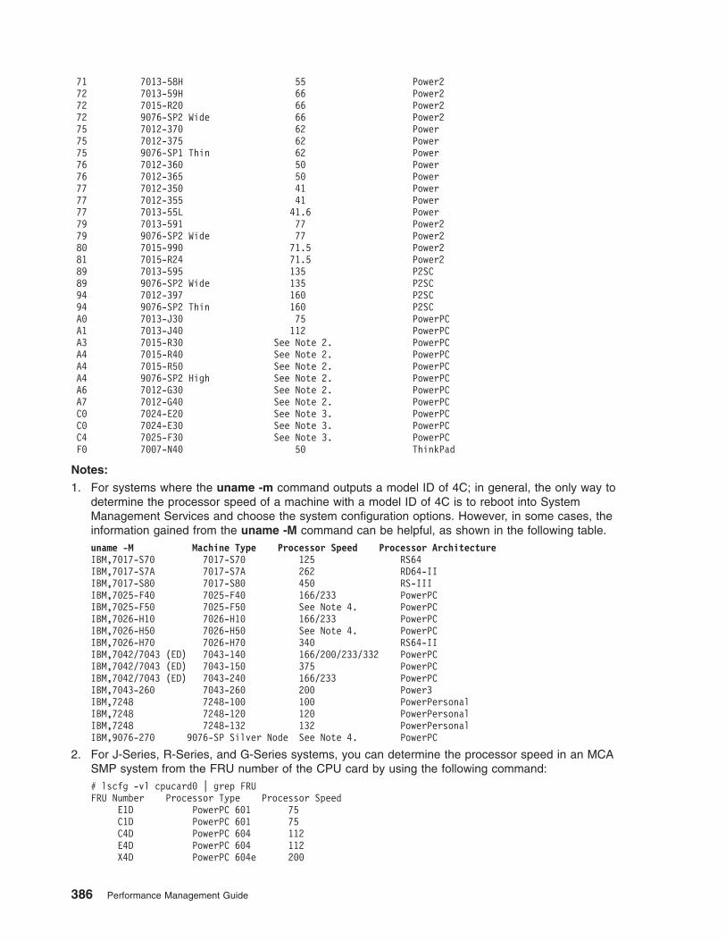
71 7013-58H 55 Power272 7013-59H 66 Power272 7015-R20 66 Power272 9076-SP2 Wide 66 Power275 7012-370 62 Power75 7012-375 62 Power75 9076-SP1 Thin 62 Power76 7012-360 50 Power76 7012-365 50 Power77 7012-350 41 Power77 7012-355 41 Power77 7013-55L 41.6 Power79 7013-591 77 Power279 9076-SP2 Wide 77 Power280 7015-990 71.5 Power281 7015-R24 71.5 Power289 7013-595 135 P2SC89 9076-SP2 Wide 135 P2SC94 7012-397 160 P2SC94 9076-SP2 Thin 160 P2SCA0 7013-J30 75 PowerPCA1 7013-J40 112 PowerPCA3 7015-R30 See Note 2. PowerPCA4 7015-R40 See Note 2. PowerPCA4 7015-R50 See Note 2. PowerPCA4 9076-SP2 High See Note 2. PowerPCA6 7012-G30 See Note 2. PowerPCA7 7012-G40 See Note 2. PowerPCC0 7024-E20 See Note 3. PowerPCC0 7024-E30 See Note 3. PowerPCC4 7025-F30 See Note 3. PowerPCF0 7007-N40 50 ThinkPad

Notes:

1. For systems where the uname -m command outputs a model ID of 4C; in general, the only way todetermine the processor speed of a machine with a model ID of 4C is to reboot into SystemManagement Services and choose the system configuration options. However, in some cases, theinformation gained from the uname -M command can be helpful, as shown in the following table.uname -M Machine Type Processor Speed Processor ArchitectureIBM,7017-S70 7017-S70 125 RS64IBM,7017-S7A 7017-S7A 262 RD64-IIIBM,7017-S80 7017-S80 450 RS-IIIIBM,7025-F40 7025-F40 166/233 PowerPCIBM,7025-F50 7025-F50 See Note 4. PowerPCIBM,7026-H10 7026-H10 166/233 PowerPCIBM,7026-H50 7026-H50 See Note 4. PowerPCIBM,7026-H70 7026-H70 340 RS64-IIIBM,7042/7043 (ED) 7043-140 166/200/233/332 PowerPCIBM,7042/7043 (ED) 7043-150 375 PowerPCIBM,7042/7043 (ED) 7043-240 166/233 PowerPCIBM,7043-260 7043-260 200 Power3IBM,7248 7248-100 100 PowerPersonalIBM,7248 7248-120 120 PowerPersonalIBM,7248 7248-132 132 PowerPersonalIBM,9076-270 9076-SP Silver Node See Note 4. PowerPC

2. For J-Series, R-Series, and G-Series systems, you can determine the processor speed in an MCASMP system from the FRU number of the CPU card by using the following command:# lscfg -vl cpucard0 | grep FRUFRU Number Processor Type Processor Speed

E1D PowerPC 601 75C1D PowerPC 601 75C4D PowerPC 604 112E4D PowerPC 604 112X4D PowerPC 604e 200


3. For the E-series and F-30 systems use the following command to determine CPU speed:# lscfg -vp | pg

Look for the following stanza:procF0 CPU Card

Part Number.................093H5280EC Level....................00E76527Serial Number...............17700008FRU Number..................093H2431Displayable Message.........CPU CardDevice Specific.(PL)........Device Specific.(ZA)........PS=166,PB=066,PCI=033,NP=001,CL=02,PBH

Z=64467000,PM=2.5,L2=1024Device Specific.(RM)........10031997 140951 VIC97276ROS Level and ID............03071997 135048

In the section Device Specific.(ZA), the section PS= is the processor speed expressed in MHz.

4. For F-50 and H-50 systems and SP Silver Node, the following commands can be used to determinethe processor speed of an F-50 system:# lscfg -vp | more

Look for the following stanza:Orca M5 CPU:Part Number.................08L1010EC Level....................E78405Serial Number...............L209034579FRU Number..................93H8945Manufacture ID..............IBM980Version.....................RS6KDisplayable Message.........OrcaM5 CPU DD1.3Product Specific.(ZC).......PS=0013c9eb00,PB=0009e4f580,SB=0004f27

ac0,NP=02,PF=461,PV=05,KV=01,CL=1

In the line containing Product Specific.(ZC), the entry PS= is the processor speed in hexadecimalnotation. To convert this to an actual speed, use the following conversions:0009E4F580 = 166 MHz0013C9EB00 = 332 MHz

The value PF= indicates the processor configuration.251 = 1 way 166 MHz261 = 2 way 166 MHz451 = 1 way 332 MHz461 = 2 way 332 MHz

Appendix D. Determining CPU Speed 387


Appendix E. National Language Support: Locale versus Speed

National Language Support (NLS) facilitates the use of the operating system in various languageenvironments. Because informed use of NLS is increasingly important in obtaining optimum performancefrom the system, this appendix contains a brief review of NLS.

NLS allows the operating system to be tailored to the individual user’s language and cultural expectations.A locale is a specific combination of language and geographic or cultural requirements that is identified bya compound name, such as en_US (English as used in the United States). For each supported locale,there is a set of message catalogs, collation value tables, and other information that defines therequirements of that locale. When the operating system is installed, the system administrator can choosewhat locale information should be installed. Thereafter, the individual users can control the locale of eachshell by changing the LANG and LC_ALL variables.

The one locale that does not conform to the structure just described is the C (or POSIX) locale. The Clocale is the system default locale unless the user explicitly chooses another. It is also the locale in whicheach newly forked process starts. Running in the C locale is the nearest equivalent in the operatingsystem to running in the original, unilingual form of UNIX. There are no C message catalogs. Instead,programs that attempt to get a message from the catalog are given back the default message that iscompiled into the program. Some commands, such as the sort command, revert to their original,character-set-specific algorithms.

The performance of NLS generally falls into three bands. The C locale is generally the fastest for theexecution of commands, followed by the single-byte (Latin alphabet) locales such as en_US, with themultibyte locales resulting in the slowest command execution.

Programming ConsiderationsHistorically, the C language has displayed a certain amount of provinciality in its interchangeable use ofthe words byte and character. Thus, an array declared char foo[10] is an array of 10 bytes. But not all ofthe languages in the world are written with characters that can be expressed in a single byte. Japaneseand Chinese, for example, require two or more bytes to identify a particular graphic to be displayed.Therefore, we distinguish between a byte, which is 8 bits of data, and a character, which is the amount ofinformation needed to represent a single graphic.

Two characteristics of each locale are the maximum number of bytes required to express a character inthat locale and the maximum number of output display positions a single character can occupy. Thesevalues can be obtained with the MB_CUR_MAX and MAX_DISP_WIDTH macros. If both values are 1, thelocale is one in which the equivalence of byte and character still holds. If either value is greater than 1,programs that do character-by-character processing, or that keep track of the number of display positionsused, must use internationalization functions to do so.

Because the multibyte encodings consist of variable numbers of bytes per character, they cannot beprocessed as arrays of characters. To allow efficient coding in situations where each character has toreceive extensive processing, a fixed-byte-width data type, wchar_t, has been defined. A wchar_t is wideenough to contain a translated form of any supported character encoding. Programmers can thereforedeclare arrays of wchar_t and process them with (roughly) the same logic they would have used on anarray of char, using the wide-character analogs of the traditional libc.a functions.

Unfortunately, the translation from the multibyte form in which text is entered, stored on disk, or written tothe display, to the wchar_t form, is computationally quite expensive. It should only be performed insituations in which the processing efficiency of the wchar_t form will more than compensate for the cost oftranslation to and from the wchar_t form.


Some Simplifying RulesIt is possible to write a slow, multilingual application program if the programmer is unaware of someconstraints on the design of multibyte character sets that allow many programs to run efficiently in amultibyte locale with little use of internationalization functions. For example:

v In all code sets supported by IBM, the character codes 0x00 through 0x3F are unique and encode theASCII standard characters. Being unique means that these bit combinations never appear as one of thebytes of a multibyte character. Because the null character is part of this set, the strlen(), strcpy(), andstrcat() functions work on multibyte as well as single-byte strings. The programmer must remember thatthe value returned by strlen() is the number of bytes in the string, not the number of characters.

v Similarly, the standard string function strchr(foostr, ’/’) works correctly in all locales, because the /(slash) is part of the unique code-point range. In fact, most of the standard delimiters are in the 0x00 to0x3F range, so most parsing can be accomplished without recourse to internationalization functions ortranslation to wchar_t form.

v Comparisons between strings fall into two classes: equal and unequal. Use the standard strcmp()function to perform comparisons. When you writeif (strcmp(foostr,"a rose") == 0)

you are not looking for ″a rose″ by any other name; you are looking for that set of bits only. If foostrcontains ″a rosE″ no match is found.

v Unequal comparisons occur when you are attempting to arrange strings in the locale-defined collationsequence. In that case, you would useif (strcoll(foostr,barstr) > 0)

and pay the performance cost of obtaining the collation information about each character.

v When a program is executed, it always starts in the C locale. If it will use one or moreinternationalization functions, including accessing message catalogs, it must execute:setlocale(LC_ALL, "");

to switch to the locale of its parent process before calling any internationalization function.

Setting the LocaleThe following command sequence:LANG=Cexport LANG

sets the default locale to C (that is, C is used unless a given variable, such as LC_COLLATE, is explicitlyset to something else).

The following sequence:LC_ALL=Cexport LC_ALL

forcibly sets all the locale variables to C, regardless of previous settings.

For a report on the current settings of the locale variables, type locale.


Appendix F. Summary of Tunable Parameters

Each of the following sections describes one of the operating system’s parameters that can affectperformance. This appendix contains the following major sections:

v Environment Variables

v Kernel Tunable Parameters

v Network Tunable Parameters

The parameters are described in alphabetical order within each section.

Environment VariablesThis section discusses the following topics:

v Thread Support Tunable Parameters

v Miscellaneous Tunable Parameters

Thread Support Tunable ParametersFollowing is a list of thread support parameters that can be tuned:

1. AIXTHREAD_COND_DEBUG (AIX 4.3.3 and subsequent versions)

Purpose: Maintains a list of condition variables for use by the debugger.

Values: Default: ONRange: ON, OFF

Display: echo $AIXTHREAD_COND_DEBUG (this is turned on internally, so the initial default value will notbe seen with the echo command)

Change: AIXTHREAD_COND_DEBUG={ON|OFF}export AIXTHREAD_COND_DEBUGChange takes effect immediately in this shell. Change is effective until logging out of this shell.Permanent change is made by adding AIXTHREAD_COND_DEBUG={ON|OFF} command to the/etc/environment file.

Diagnosis: Leaving it on makes debugging threaded applications easier, but may impose some overhead.

Tuning: If the program contains a large number of active condition variables and frequently creates anddestroys condition variables, this may create higher overhead for maintaining the list of conditionvariables. Setting the variable to OFF will disable the list.

Refer to “Thread Debug Options” on page 54.

2. AIXTHREAD_ENRUSG

Purpose: Enable or disable pthread resource collection.

Values: Default: OFFRange: ON, OFF

Display: echo $AIXTHREAD_ENRUSG (this is turned on internally, so the initial default value will not beseen with the echo command)

Change: AIXTHREAD_ENRUSG={ON|OFF}export AIXTHREAD_ENRUSGChange takes effect immediately in this shell. Change is effective until logging out of this shell.Permanent change is made by adding AIXTHREAD_ENRUSG={ON|OFF} command to the/etc/environment file.

Diagnosis: Turning it on allows for resource collection of all pthreads in a process, but will impose someoverhead.


Tuning:

Refer to “Thread Environment Variables” on page 51.

3. AIXTHREAD_GUARDPAGES (AIX 4.3 and later)

Purpose: Controls the number of guard pages to add to the end of the pthread stack.

Values: Default: 0Range: A positive integer

Display: echo $AIXTHREAD_GUARDPAGES(This is turned on internally, so the initial default value will not be seen with the echo command)

Change: AIXTHREAD_GUARDPAGES=nexport AIXTHREAD_GUARDPAGESChange takes effect immediately in this shell. Change is effective until logging out of this shell.Permanent change is made by adding AIXTHREAD_GUARDPAGES=n command to the/etc/environment file.

Diagnosis: N/A

Tuning: N/A

Refer to “Thread Environment Variables” on page 51.

4. AIXTHREAD_MINKTHREADS (AIX 4.3 and later)

Purpose Controls the the minimum number of kernel threads that should be used.

Values: Default: 8Range: A positive integer value

Display: echo $AIXTHREAD_MINKTHREADS (this is turned on internally, so the initial default value will notbe seen with the echo command)

Change: AIXTHREAD_MINKTHREADS=nexport AIXTHREAD_MINKTHREADSChange takes effect immediately in this shell. Change is effective until logging out of this shell.Permanent change is made by adding AIXTHREAD_MINKTHREADS =n command to the/etc/environment file.

Diagnosis: N/A

Tuning: The library scheduler will not reclaim kernel threads below this figure. A kernel thread may bereclaimed at virtually any point. Generally, a kernel thread is targeted as a result of a pthreadterminating.

Refer to: Variables for Process-Wide Contention Scope

5. AIXTHREAD_MNRATIO (AIX 4.3 and later)

Purpose: Controls the scaling factor of the library. This ratio is used when creating and terminating pthreads.

Values: Default: 8:1Range: Two positive values (p:k), where k is the number of kernel threads that should be employedto handle p runnable pthreads

Display: echo $AIXTHREAD_MNRATIO (this is turned on internally, so the initial default value will not beseen with the echo command)

Change: AIXTHREAD_MNRATIO=p:kexport AIXTHREAD_MNRATIOChange takes effect immediately in this shell. Change is effective until logging out of this shell.Permanent change is made by adding AIXTHREAD_MNRATIO=p:k command to the/etc/environment file.

Diagnosis: N/A


Tuning: May be useful for applications with a very large number of threads. However, always test a ratio of1:1 because it may provide for better performance.


6. AIXTHREAD_MUTEX_DEBUG (AIX 4.3.3 and later)

Purpose: Maintains a list of active mutexes for use by the debugger.

Values: Default: OFFRange: ON, OFF

Display: echo $AIXTHREAD_MUTEX_DEBUG (this is turned on internally, so the initial default value willnot be seen with the echo command)

Change: AIXTHREAD_MUTEX_DEBUG={ON|OFF}export AIXTHREAD_MUTEX_DEBUGChange takes effect immediately in this shell. Change is effective until logging out of this shell.Permanent change is made by adding AIXTHREAD_MUTEX_DEBUG={ON|OFF} command to the/etc/environment file.

Diagnosis: Setting the variable to ON makes debugging threaded applications easier, but may impose someoverhead.

Tuning: If the program contains a large number of active mutexes and frequently creates and destroysmutexes, this may create higher overhead for maintaining the list of mutexes. Leaving the variableoff disables the list.

Refer to: Thread Debug Options

7. AIXTHREAD_RWLOCK_DEBUG (AIX 4.3.3 and later)

Purpose: Maintains a list of read-write locks for use by the debugger.

Values: Default: ONRange: ON, OFF

Display: echo $AIXTHREAD_RWLOCK_DEBUG (this is turned on internally, so the initial default value willnot be seen with the echo command)

Change: AIXTHREAD_RWLOCK_DEBUG={ON|OFF}export AIXTHREAD_RWLOCK_DEBUGChange takes effect immediately in this shell. Change is effective until logging out of this shell.Permanent change is made by adding AIXTHREAD_RWLOCK_DEBUG={ON|OFF} command tothe /etc/environment file.

Diagnosis: Leaving it on makes debugging threaded applications easier, but may impose some overhead.

Tuning: If the program contains a large number of active read-write locks and frequently creates anddestroys read-write locks, this may create higher overhead for maintaining the list of read-writelocks. Setting the variable to OFF will disable the list.

Refer to: Thread Debug Options

8. AIXTHREAD_SCOPE (AIX 4.3.1 and later)

Purpose: Controls contention scope. P signifies process-based contention scope (M:N). S signifiessystem-based contention scope (1:1).

Values: Default: PPossible Values: P or S

Display: echo $AIXTHREAD_SCOPE (this is turned on internally, so the initial default value will not be seenwith the echo command)

Appendix F. Summary of Tunable Parameters 393

Change: AIXTHREAD_SCOPE={P|S}export AIXTHREAD_SCOPEChange takes effect immediately in this shell. Change is effective until logging out of this shell.Permanent change is made by adding AIXTHREAD_SCOPE={P|S} command to the/etc/environment file.

Diagnosis: If fewer threads are being dispatched than expected, then system scope should be tried.

Tuning: Tests on AIX 4.3.2 have shown that certain applications can perform much better with systembased contention scope (S). The use of this environment variable impacts only those threadscreated with the default attribute. The default attribute is employed when the attr parameter topthread_create is NULL.

Refer to: Thread Environment Variables

9. AIXTHREAD_SLPRATIO (AIX 4.3 and later)

Purpose: Controls the number of kernel threads that should be held in reserve for sleeping threads.

Values: Default: 1:12Range: Two positive values (k:p), where k is the number of kernel threads that should be held inreserve for p sleeping pthreads

Display: echo $AIXTHREAD_SLPRATIO (this is turned on internally, so the initial default value will not beseen with the echo command)

Change: AIXTHREAD_SLPRATIO=k:pexport AIXTHREAD_SLPRATIOChange takes effect immediately in this shell. Change is effective until logging out of this shell.Permanent change is made by adding AIXTHREAD_SLPRATIO=k:p command to the/etc/environment file.

Diagnosis: N/A

Tuning: In general, fewer kernel threads are required to support sleeping pthreads, because they aregenerally woken one at a time. This conserves kernel resources.


10. AIXTHREAD_STK=n (AIX 4.3.3 ML 09 and later)

Purpose: The decimal number of bytes that should be allocated for each pthread. This value may beoverridden by pthread_attr_setstacksize.

Values: Default: 98,304 bytes for 32bit applications, 196,608 bytes for 64bit applications.Range: Decimal integer values from 0 to 268,435,455 which will be rounded up to the nearest page(currently 4,096).

Display: echo $AIXTHREAD_STK (this is turned on internally, so the initial default value will not be seenwith the echo command)

Change: AIXTHREAD_STK=size export AIXTHREAD_STK Change takes effect immediately in this shell.Change is effective until logging out of this shell. Permanent change is made by addingAIXTHREAD_STK=size to the /etc/environment file.

Diagnosis: If analysis of a failing program indicates stack overflow, the default stack size can be increased.

Tuning: If trying to reach the 32,000 thread limit on a 32 bit application, it may be necessary to decreasethe default stack size.

11. MALLOCBUCKETS (Version 4.3.3.25 and later)

Purpose: Enables buckets-based extension in the default memory allocator which may enhance performanceof applications that issue large numbers of small allocation requests.


Values: MALLOCTYPE=buckets

MALLOCBUCKETS=[[ number_of_buckets:n | bucket_sizing_factor:n | blocks_per_bucket:n |bucket_statistics:[stdout|stderr|pathname]],...]

The following table displays default values of MALLOCBUCKETS.MALLOCBUCKETS Default ValuesMALLOCBUCKETS Options Default Valuenumber_of_buckets1 16bucket_sizing_factor (32-bit)2 32bucket_sizing_factor (64-bit)3 64blocks_per_bucket 10244

Notes:

1. The minimum value allowed is 1. The maximum value allowed is 128.

2. For 32-bit implementations, the value specified for bucket_sizing_factor must be a multiple of 8.

3. For 64-bit implementations, the value specified for bucket_sizing_factor must be a multiple of 16.

4. The bucket_statistics option is disabled by default.

Display: echo $MALLOCBUCKETS; echo $MALLOCTYPE

Change: Use the shell specific method of exporting the environment variables.

Diagnosis: If malloc performance is slow and many small malloc requests are issued, this feature mayenhance performance.


Tuning: To enable malloc buckets, the MALLOCTYPE environment variable has to be set to the value″buckets″.

The MALLOCBUCKETS environment variable may be used to change the default configuration ofthe malloc buckets, although the default values should be sufficient for most applications.

The number_of_buckets:n option can be used to specify the number of buckets available perheap, where n is the number of buckets. The value specified for n will apply to all available heaps.

The bucket_sizing_factor:n option can be used to specify the bucket sizing factor, where n is thebucket sizing factor in bytes.

The blocks_per_bucket:n option can be used to specify the number of blocks initially contained ineach bucket, where n is the number of blocks. This value is applied to all of the buckets. The valueof n is also used to determine how many blocks to add when a bucket is automatically enlargedbecause all of its blocks have been allocated.

The bucket_statistics option will cause the malloc subsystem to output a statistical summary formalloc buckets upon typical termination of each process that calls the malloc subsystem whilemalloc buckets is enabled. This summary will show buckets configuration information and thenumber of allocation requests processed for each bucket. If multiple heaps have been enabled byway of malloc multiheap, the number of allocation requests shown for each bucket will be the sumof all allocation requests processed for that bucket for all heaps.

The buckets statistical summary will be written to one of the following output destinations, asspecified with the bucket_statistics option.stdout Standard outputstderr Standard errorpathname A user-specified pathname

If a user-specified pathname is provided, statistical output will be appended to the existing contentsof the file (if any). Avoid using standard output as the output destination for a process whose outputis piped as input into another process.

Refer to: Malloc Buckets

12. MALLOCMULTIHEAP (AIX 4.3.1 and later)

Purpose: Controls the number of heaps within the process private segment.

Values: Default: 16 for 4.3.1 and 4.3.2, 32 for 4.3.3 and laterRange: A positive number between 1 and 32)

Display: echo $MALLOCMULTIHEAP (this is turned on internally, so the initial default value will not beseen with the echo command)

Change: MALLOCMULTIHEAP=[[heaps:n | considersize],...]export MALLOCMULTIHEAPChange takes effect immediately in this shell. Change is effective until logging out of this shell.Permanent change is made by adding MALLOCMULTIHEAP=[[heaps:n | considersize],...]command to the /etc/environment file.

Diagnosis: Look for lock contention on the malloc lock (located in segment F) or fewer than expected runnablethreads.


Tuning: Smaller number of heaps can help reduce size of the process. Certain multithreaded userprocesses which use the malloc subsystem heavily may obtain better performance by exporting theenvironment variable MALLOCMULTIHEAP=1 before starting the application.

The potential performance enhancement is particularly likely for multithreaded C++ programs,because these may make use of the malloc subsystem whenever a constructor or destructor iscalled.

Any available performance enhancement will be most evident when the multithreaded user processis running on an SMP system, and particularly when system scope threads are used (M:N ratio of1:1). However, in some cases, enhancement may also be evident under other conditions, and onuniprocessors.

If the considersize option is specified, an alternate heap selection algorithm is used that tries toselect an available heap that has enough free space to handle the request. This may minimize theworking set size of the process by reducing the number of sbrk() calls. However, there is a bitmore processing time required for this algorithm.


13. SPINLOOPTIME

Purpose: Controls the number of times to retry a busy lock before yielding to another processor (only forlibpthreads).

Values: Default: 1 on uniprocessors, 40 on multiprocessorsRange: A positive integer

Display: echo $SPINLOOPTIME (this is turned on internally, so the initial default value will not be seen withthe echo command)

Change: SPINLOOPTIME=nexport SPINLOOPTIMEChange takes effect immediately in this shell. Change is effective until logging out of this shell.Permanent change is made by adding SPINLOOPTIME=n command to the /etc/environment file.

Diagnosis: If threads are going to sleep often (lot of idle time), then the SPINLOOPTIME may not be highenough.

Tuning: Increasing the value from default of 40 on multiprocessor systems might be of benefit if there ispthread mutex contention.


14. YIELDLOOPTIME

Purpose: Controls the number of times to yield the processor before blocking on a busy lock (only forlibpthreads). The processor is yielded to another kernel thread, assuming there is another runnablekernel thread with sufficient priority.

Values: Default: 0Range: A positive value

Display: echo $YIELDLOOPTIME (this is turned on internally, so the initial default value will not be seenwith the echo command)

Change: YIELDLOOPTIME=nexport YIELDLOOPTIMEChange takes effect immediately in this shell. Change is effective until logging out of this shell.Permanent change is made by adding YIELDLOOPTIME=n command to the /etc/environment file.

Diagnosis: If threads are going to sleep often (lot of idle time), then the YIELDLOOPTIME may not be highenough.


Tuning: Increasing the value from default value of 0 may benefit if you do not want the threads to go tosleep when waiting for locks.


Miscellaneous Tunable ParametersFollowing is a list of miscellaneous parameters that can be tuned:

1. EXTSHM (AIX 4.2.1 and later)

Purpose: Turns on the extended shared memory facility.

Values: Default: Not setPossible Value: ON

Display: echo $EXTSHM

Change: EXTSHM=ONexport EXTSHMChange takes effect immediately in this shell. Change is effective until logging out of this shell.Permanent change is made by adding EXTSHM=ON command to the /etc/environment file.

Diagnosis: N/A

Tuning: Setting value to ON will allow a process to allocate shared memory segments as small as 1 byte(though this will be rounded up to the nearest page); this effectively removes the limitation of 11user shared memory segments. Maximum size of all segments together can still only be 2.75 GBworth of memory for 32-bit processes. 64-bit processes do not need to set this variable since avery large number of segments is available. Some restrictions apply for processes that set thisvariable, and these restrictions are the same as with processes that use mmap buffers.

Refer to: Extended Shared Memory (EXTSHM)

2. LDR_CNTRL

Purpose: Allows tuning of the kernel loader.

Values: Default: Not setPossible Values: PREREAD_SHLIB, LOADPUBLIC, IGNOREUNLOAD, USERREGS, MAXDATA,DSA

Display: echo $LDR_CNTRL

Change: LDR_CNTRL={PREREAD_SHLIB | LOADPUBLIC| ...}export LDR_CNTRLChange takes effect immediately in this shell. Change is effective until logging out of this shell.Permanent change is made by adding LDR_CNTRL={PREREAD_SHLIB | LOADPUBLIC| ...}command to the /etc/environment file.

Diagnosis: N/A


Tuning: The LDR_CNTRL environment variable can be used to control one or more aspects of the systemloader behavior. You can specify multiple options with the LDR_CNTRL variable. When doing this,separate the options using an @ character (that is,LDR_CNTRL=PREREAD_SHLIB@LOADPUBLIC).Specifying the PREREAD_SHLIB option will cause entire libraries to be read as soon as they areaccessed. With VMM readahead tuned, a library can be read in from disk and be cached inmemory by the time the program starts to access its pages. While this method can use morememory, it can enhance performance of programs that use many shared library pages providingthe access pattern is non-sequential. (for example, Catia).Specifying the LOADPUBLIC option directs the system loader to load all modules requested by anapplication into the global shared library segment. If a module cannot be loaded publicly into theglobal shared library segment then it is loaded privately for the application.Specifying the IGNOREUNLOAD option will cause modules that are marked to be unloaded andused again (if the module has not been unloaded already). As a side effect of this option, you canend up with two different data instances for the module.Specifying the USERREGS option will tell the system to save all general-purpose user registersacross system calls made by an application. This can be helpful in applications doing garbagecollection.The MAXDATA option for the LDR_CNTRL variable allows you to set or override maxdata valuespecified in an executable. If you want to use Large Program Support with a data heap size of0x30000000, then specify LDR_CNTRL=MAXDATA=0x30000000. To turn off Large ProgramSupport, specify LDR_CNTRL=MAXDATA=0.Specifying the DSA (Dynamic Segment Allocation) option will tell the system loader to runapplications using Very Large Program Support. The DSA option is only valid for 32-bit applicationswith a non-zero maxdata value.

3. NODISCLAIM

Purpose: Controls how calls to free() are being handled. When PSALLOC is set to early, all free() callsresult in a disclaim() system call. When NODISCLAIM is set to True, this does not occur.

Values: Default: Not setPossible Value: True

Display: echo $NODISCLAIM

Change: NODISCLAIM=trueexport NODISCLAIMChange takes effect immediately in this shell. Change is effective until logging out of this shell.Permanent change is made by adding NODISCLAIM=true command to the /etc/environment file.

Diagnosis: If number of disclaim() system calls is very high, you may want to set this variable.

Tuning: Setting this variable will eliminate calls to disclaim() from free() if PSALLOC is set to early.

Refer to: Early Page Space Allocation

4. NSORDER

Purpose: Overwrites the set name resolution search order.

Values: Default: bind, nis, localPossible Values: bind, local, nis, bind4, bind6, local4, local6, nis4, or nis6

Display: echo $NSORDER (this is turned on internally, so the initial default value will not be seen with theecho command)

Change: NSORDER=value, value, ...export NSORDERChange takes effect immediately in this shell. Change is effective until logging out of this shell.Permanent change is made by adding NSORDER=value command to the /etc/environment file.

Diagnosis: N/A

Tuning: NSORDER overrides the /etc/netsvc.conf file.

Refer to: Tuning Name Resolution


5. PSALLOC

Purpose: Sets the PSALLOC environment variable to determine the paging-space allocation policy.

Values: Default: Not setPossible Value: early

Display: echo $PSALLOC

Change: PSALLOC=earlyexport PSALLOCChange takes effect immediately in this shell. Change is effective until logging out of this shell.Permanent change is made by adding PSALLOC=early command to the /etc/environment file.

Diagnosis: N/A

Tuning: To ensure that a process is not killed due to low paging conditions, this process can preallocatepaging space by using the Early Page Space Allocation policy. However, this may result in wastedpaging space. You may also want to set the NODISCLAIM environment variable.

Refer to: Allocation and Reclamation of Paging Space Slots and Early Page Space Allocation

6. RT_GRQ (AIX 4.3.3.1 and later)

Purpose: Causes thread to be put on a global run queue rather than on a per-CPU run queue.

Values: Default: Not set; Range: ON, OFF

Display: echo $RT_GRQ

Change: RT_GRQ={OFF/ONexport RT_GRQChange takes effect immediately. Change is effective until next boot. Permanent change is madeby adding RT_GRQ={ON|OFF} command to the /etc/environment file.

Diagnosis: N/A

Tuning: May be tuned on multiprocessor systems. Set to ON, will cause the thread to be put on a globalrun queue. In that case, the global run queue is searched to see which thread has the best priority.This might allow to get the thread dispatched sooner and can improve performance for threads thatare running SCHED_OTHER, and are interrupt driven.

Refer to: Scheduler Run Queue

7. RT_MPC (AIX 4.3.3 and later)

Purpose: When running the kernel in real-time mode (see bosdebug command), an MPC can be sent to adifferent CPU to interrupt it if a better priority thread is runnable so that this thread can bedispatched immediately.

Values: Default: Not set; Range: ON

Display: echo $RT_MPC

Change: RT_MPC=ONexport RT_MPCChange takes effect immediately. Change is effective until next boot. Permanent change is madeby adding RT_MPC=ON command to the /etc/environment file.

Diagnosis: N/A


Kernel Tunable ParametersFollowing are kernel parameters, grouped into the following sections:

v Scheduler and Memory Load Control Tunable Parameters

v Virtual Memory Manager Tunable Parameters

v Synchronous I/O Tunable Parameters

v Asynchronous I/O Tunable Parameters

v Disk and Disk Adapter Tunable Parameters

v Interprocess Communication Tunable Parameters

Scheduler and Memory Load Control Tunable ParametersMost of the scheduler and memory load control tunable parameters are fully described in the schedo manpage. The following are a few other related parameters:

1. maxuproc

Purpose: Specifies the maximum number of processes per user ID.

Values: Default: 40; Range: 1 to 131072

Display: lsattr -E -l sys0 -a maxuproc

Change: chdev -l sys0 -a maxuproc=NewValueChange takes effect immediately and is preserved over boot. If value is reduced, then it goes intoeffect only after a system boot.

Diagnosis: Users cannot fork any additional processes.

Tuning: This is a safeguard to prevent users from creating too many processes.

Refer to: Responding to PDT Report Messages

2. ncargs

Purpose: Specifies the maximum allowable size of the ARG/ENV list (in 4KB blocks) when running exec()subroutines.


Display: lsattr -E -l sys0 -a ncargs

Change: chdev -l sys0 -a ncargs=NewValueChange takes effect immediately and is preserved over boot.

Diagnosis: Users cannot execute any additional processes because the argument list passed to the exec()system call is too long.

Tuning: This is a mechanism to prevent the exec() subroutines from failing if the argument list is too long.Please note that tuning to a higher ncargs value puts additional constraints on system memoryresources.

Virtual Memory Manager Tunable ParametersThe complete listing of the virtual memory manager tunable parameters is located in the vmo man page.

Synchronous I/O Tunable ParametersMost of the synchronous I/O tunable parameters are fully described in the ioo man page. The followingare a few other related parameters:


1. maxbuf

Purpose: Number of (4 KB) pages in the block-I/O buffer cache.


Display: lsattr -E -l sys0 -a maxbuf

Change: chdev -l sys0 -a maxbuf=NewValueChange is effective immediately and is permanent. If the -T flag is used, the change is immediateand lasts until the next boot. If the -P flag is used, the change is deferred until the next boot and ispermanent.

Diagnosis: If the sar —b command shows breads or bwrites with %rcache and %wcache being low, you mightwant to tune this parameter.

Tuning: This parameter normally has little performance effect on systems, where ordinary I/O does not usethe block-I/O buffer cache.

Refer to: Tuning Asynchronous Disk I/O

2. maxpout

Purpose: Specifies the maximum number of pending I/Os to a file.

Values: Default: 0 (no checking); Range: 0 to n (n should be a multiple of 4, plus 1)

Display: lsattr -E -l sys0 -a maxpout

Change: chdev -l sys0 -a maxpout=NewValueChange is effective immediately and is permanent. If the -T flag is used, the change is immediateand lasts until the next boot. If the -P flag is used, the change is deferred until the next boot and ispermanent.

Diagnosis: If the foreground response time sometimes deteriorates when programs with large amounts ofsequential disk output are running, sequential output may need to be paced.

Tuning: Set maxpout to 33 and minpout to 16. If sequential performance deteriorates unacceptably,increase one or both. If foreground performance is still unacceptable, decrease both.

3. minpout

Purpose: Specifies the point at which programs that have reached maxpout can resume writing to the file.

Values: Default: 0 (no checking); Range: 0 to n (n should be a multiple of 4, plus 1)

Display: lsattr -E -l sys0 -a minpout

Change: chdev -l sys0 -a minpout=NewValueChange is effective immediately and is permanent. If the -T flag is used, the change is immediateand lasts until the next boot. If the -P flag is used, the change is deferred until the next boot and ispermanent.

Diagnosis: If the foreground response time sometimes deteriorates when programs with large amounts ofsequential disk output are running, sequential output may need to be paced.

Tuning: Set maxpout to 33 and minpout to 16. If sequential performance deteriorates unacceptably,increase one or both. If foreground performance is still unacceptable, decrease both.

4. mount -o nointegrity

Purpose: A new mount option (nointegrity) may enhance local file system performance for certainwrite-intensive applications. This optimization basically eliminates writes to the JFS log. Note thatthe enhanced performance is achieved at the expense of metadata integrity. Therefore, use thisoption with extreme caution because a system crash can make a file system mounted with thisoption unrecoverable. Nevertheless, certain classes of applications do not require file data toremain consistent after a system crash, and these may benefit from using the nointegrity option.Two examples in which a nointegrity file system may be beneficial is for compiler temporary files,and for doing a nonmigration or mksysb installation.


5. Paging Space Size

Purpose: The amount of disk space required to hold pages of working storage.

Values: Default: configuration-dependent; Range: 32 MB to n MB for hd6, 16 MB to n MB for non-hd6

Display: lsps -amkps or chps or smitty pgsp

Change: Change is effective immediately and is permanent. Paging space is not necessarily put into useimmediately, however.

Diagnosis: Run: lsps -a. If processes have been killed for lack of paging space, monitor the situation with thepsdanger() subroutine.

Tuning: If it appears that there is not enough paging space to handle the normal workload, add a newpaging space on another physical volume or make the existing paging spaces larger.

6. syncd Interval

Purpose: The time between sync() calls by syncd.

Values: Default: 60; Range: 1 to any positive integer

Display: grep syncd /sbin/rc.bootvi /sbin/rc.boot or

Change: Change is effective at next boot and is permanent. An alternate method is to use the kill commandto terminate the syncd daemon and restart it from the command line with the command/usr/sbin/syncd interval.

Diagnosis: I/O to a file is blocked when syncd is running.

Tuning: At its default level, this parameter has little performance cost. No change is recommended.Significant reductions in the syncd interval in the interests of data integrity (as for HACMP) couldhave adverse performance consequences.

Asynchronous I/O Tunable Parameters1. maxreqs

Purpose: Specifies the maximum number of asynchronous I/O requests that can be outstanding at any onetime.

Values: Default: 4096; Range: 1 to AIO_MAX (/usr/include/sys/limits.h)

Display: lsattr -E -l aio0 -a maxreqs

Change: chdev -l aio0 -a maxreqs=NewValueChange is effective immediately and is permanent. If the -T flag is used, the change is immediateand lasts until the next boot. If the -P flag is used, the change is deferred until the next boot and ispermanent.

Diagnosis: N/A

Tuning: This includes requests that are in progress, as well as those that are waiting to be started. Themaximum number of asynchronous I/O requests cannot be less than the value of AIO_MAX, asdefined in the /usr/include/sys/limits.h file, but can be greater. It would be appropriate for asystem with a high volume of asynchronous I/O to have a maximum number of asynchronous I/Orequests larger than AIO_MAX.


2. maxservers

Purpose: Specifies the maximum number of AIO kprocs that will be created.

Values: Default: 10


Display: lsattr -E -l aio0 -a maxservers

Change: chdev -l aio0 -a maxservers=NewValueChange is effective immediately and is permanent. If the -T flag is used, the change is immediateand lasts until the next boot. If the -P flag is used, the change is deferred until the next boot and ispermanent.

Diagnosis: N/A

Tuning: This value limits the number of concurrent asynchronous I/O requests. The value should be aboutthe same as the expected number of concurrent AIO requests. This tunable parameter only affectsAIO on JFS file systems (or Virtual Shared Disks (VSD) before AIX 4.3.2).


3. minservers

Purpose: Specifies the number of AIO kprocs that will be created when the AIO kernel extension is loaded.

Values: Default: 1

Display: lsattr -E -l aio0 -a maxservers

Change: chdev -l aio0 -a minservers=NewValueChange is effective immediately and is permanent. If the -T flag is used, the change is immediateand lasts until the next boot. If the -P flag is used, the change is deferred until the next boot and ispermanent.

Diagnosis: N/A

Tuning: Making this a large number is not recommended, because each process takes up some memory.Leaving this number small is acceptable in most cases because AIO will create additional kprocsup to maxservers as needed. This tunable is only effective for AIO on JFS file systems (or VSDsbefore AIX 4.3.2).


Disk and Disk Adapter Tunable Parameters1. Disk Adapter Outstanding-Requests Limit

Purpose: Maximum number of requests that can be outstanding on a SCSI bus. (Applies only to the SCSI-2Fast/Wide Adapter.)


Display: lsattr -E -l scsin -a num_cmd_elems

Change: chdev -l scsin -a num_cmd_elems=NewValueChange is effective immediately and is permanent. If the -T flag is used, the change is immediateand lasts until the next boot. If the -P flag is used, the change is deferred until the next boot and ispermanent.

Diagnosis: Applications performing large writes to striped raw logical volumes are not obtaining the desiredthroughput rate.

Tuning: Value should equal the number of physical drives (including those in disk arrays) on the SCSI bus,times the queue depth of the individual drives.

2. Disk Drive Queue Depth

Purpose: Maximum number of requests the disk device can hold in its queue.

Values: Default: IBM disks=3; Non-IBM disks=0; Range: specified by manufacturer

Display: lsattr -E -l hdiskn


Change: chdev -l hdiskn -a q_type=simple -a queue_depth=NewValueChange is effective immediately and is permanent. If the -T flag is used, the change is immediateand lasts until the next boot. If the -P flag is used, the change is deferred until the next boot and ispermanent.

Diagnosis: N/A

Tuning: If the non-IBM disk drive is capable of request-queuing, make this change to ensure that theoperating system takes advantage of the capability.

Refer to: Setting SCSI-Adapter and Disk-Device Queue Limits

Interprocess Communication Tunable Parameters1. msgmax

Purpose: Specifies maximum message size.

Values: Dynamic with maximum value of 4 MB

Display: N/A

Change: N/A

Diagnosis: N/A

Tuning: Does not require tuning because it is dynamically adjusted as needed by the kernel.

2. msgmnb

Purpose: Specifies maximum number of bytes on queue.

Values: Dynamic with maximum value of 4 MB

Display: N/A

Change: N/A

Diagnosis: N/A


3. msgmni

Purpose: Specifies maximum number of message queue IDs.

Values: Dynamic with maximum value of 131072

Display: N/A

Change: N/A

Diagnosis: N/A


4. msgmnm

Purpose: Specifies maximum number of messages per queue.


Display: N/A

Change: N/A

Diagnosis: N/A



5. semaem

Purpose: Specifies maximum value for adjustment on exit.


Display: N/A

Change: N/A

Diagnosis: N/A


6. semmni

Purpose: Specifies maximum number of semaphore IDs.


Display: N/A

Change: N/A

Diagnosis: N/A


7. semmsl

Purpose: Specifies maximum number of semaphores per ID.


Display: N/A

Change: N/A

Diagnosis: N/A


8. semopm

Purpose: Specifies maximum number of operations per semop() call.


Display: N/A

Change: N/A

Diagnosis: N/A


9. semume

Purpose: Specifies maximum number of undo entries per process.


Display: N/A

Change: N/A

Diagnosis: N/A


10. semvmx

Purpose: Specifies maximum value of a semaphore.



Display: N/A

Change: N/A

Diagnosis: N/A


11. shmmax

Purpose: Specifies maximum shared memory segment size.

Values: Dynamic with maximum value of 256 MB for 32-bit processes and 0x80000000u for 64-bit

Display: N/A

Change: N/A

Diagnosis: N/A


12. shmmin

Purpose: Specifies minimum shared-memory-segment size.

Values: Dynamic with minimum value of 1

Display: N/A

Change: N/A

Diagnosis: N/A


13. shmmni

Purpose: Specifies maximum number of shared memory IDs.


Display: N/A

Change: N/A

Diagnosis: N/A


Network Tunable ParametersFollowing are network parameters, grouped into the following sections:

v Network Option Tunable Parameters

v NFS Option Tunable Parameters

v Streams Tunable Attributes

Network Option Tunable ParametersMost of the network option tunable parameters are fully described in the no man page. The following are afew other related parameters:

1. maxmbuf

Purpose: Maximum Kbytes of real memory allowed for MBUFS.

Values: Default: 0, Range: x to y


Display: lsattr -E -l sys0 -a maxmbuf

Change: chdev -l sys0 -a maxmbuf=NewValueChange is effective immediately and is permanent. If the -T flag is used, the change isimmediate and lasts until the next boot. If the -P flag is used, the change is deferred until thenext boot and is permanent.

Diagnosis: N/A

Tuning: If maxmbuf is greater than 0, the maxmbuf value is used regardless of the value of thewall.The upper limit on mbufs is the higher value of maxmbuf or thewall.

Refer to: Tuning Network Memory

2. MTU

Purpose: Limits the size of packets that are transmitted on the network.

Values: Default: configuration-dependent

Display: lsattr -E -l interface_name

Change: chdev -l interface_name -a mtu=NewValueWith the chdev command, the interface cannot be changed while it is in use. Change iseffective across reboots.An alternate method is as follows:ifconfig interface_name mtu NewValueThis changes the MTU size on a running system, but will not preserve the value across asystem reboot.

Diagnosis: Packet fragmentation statistics.

Tuning: Increase MTU size for the network interfaces. For the Gigabit Ethernet adapter use thedevice attribute jumbo_frames=yes to enable jumbo frames (just setting MTU to 9000 on theinterface is not enough).

Refer to: UDP and TCP/IP Performance Overview and Tuning TCP and UDP Performance

3. rfc1323

Purpose: Enables TCP enhancements as specified by RFC 1323 (TCP Extensions for HighPerformance). Value of 1 indicates that tcp_sendspace and tcp_recvspace can exceed 64KB.

Values: Default: 0; Range 0 to 1

Display: lsattr -El interface or ifconfig interface

Change: ifconfig interface rfc1323 NewValueORchdev -l interface -a rfc1323=NewValueThe ifconfig command sets values temporarily, making it useful for testing. The chdevcommand alters the ODM, so custom values return after system reboots.

Diagnosis: N/A

Tuning: The default value of 0 disables the RFC enhancements on a systemwide scale. A value of 1specifies that all TCP connections will attempt to negotiate the RFC enhancements. TheSOCKETS application can override the default behavior on individual TCP connections, usingthe setsockopt() subroutine. This is a run-time attribute. Make changes before attempting toset tcp_sendspace and tcp_recvspace to more than 64 KB.

Refer to: TCP Socket Buffer Tuning

4. tcp_mssdflt

Purpose: Default maximum segment size used in communicating with remote networks.

Values: Default: 512 bytes



Change: ifconfig interface tcp_mssdflt NewValueORchdev -l interface -a tcp_mssdflt=NewValueThe ifconfig command sets values temporarily, making it useful for testing. The chdevcommand alters the ODM, so custom values return after system reboots.

Diagnosis: N/A

Tuning: For AIX 4.2.1 or later, tcp_mssdflt is only used if path MTU discovery is not enabled or pathMTU discovery fails to discover a path MTU. Limiting data to (MTU - 52) bytes ensures that,where possible, only full packets will be sent. This is a run-time attribute.

Refer to: Tuning TCP Maximum Segment Size

5. tcp_nodelay

Purpose: Specifies that sockets using TCP over this interface follow the Nagle algorithm when sendingdata. By default, TCP follows the Nagle algorithm.

Values: Default: 0; Range: 0 or 1


Change: ifconfig interface tcp_nodelay NewValueORchdev -l interface -a tcp_nodelay=NewValueThe ifconfig command sets values temporarily, making it useful for testing. The chdevcommand alters the ODM, so custom values return after system reboots.

Diagnosis: N/A

Tuning: This is an Interface-Specific Network Option (ISNO) option.

Refer to: Relative Level of Function in UDP and TCP and Interface-Specific Network Options (ISNO)

6. tcp_recvspace

Purpose: Specifies the system default socket buffer size for receiving data. This affects the windowsize used by TCP.



Change: ifconfig interface tcp_recvspace NewValueORchdev -l interface -a tcp_recvspace=NewValueThe ifconfig command sets values temporarily, making it useful for testing. The chdevcommand alters the ODM, so custom values return after system reboots.

Diagnosis: N/A

Tuning: Setting the socket buffer size to 16 KB (16,384) improves performance over standardEthernet and Token-Ring networks. The default is a value of 16384.Lower bandwidth networks, such as Serial Line Internet Protocol (SLIP), or higher bandwidthnetworks, such as Serial Optical Link, should have different optimum buffer sizes. Theoptimum buffer size is the product of the media bandwidth and the average round-trip time ofa packet.

The tcp_recvspace attribute must specify a socket buffer size less than or equal to thesetting of the sb_max attribute. This is a dynamic attribute, but for daemons started by theinetd daemon, run the following commands: stopsrc -s inetd ; startsrc -s inetd



7. tcp_sendspace

Purpose: Specifies the system default socket buffer size for sending data.



Change: ifconfig interface tcp_sendspace NewValueORchdev -l interface -a tcp_sendspace=NewValueThe ifconfig command sets values temporarily, making it useful for testing. The chdevcommand alters the ODM, so custom values return after system reboots.

Diagnosis: N/A

Tuning: This affects the window size used by TCP. Setting the socket buffer size to 16 KB (16,384)improves performance over standard Ethernet and Token-Ring networks. The default is avalue of 16,384Lower bandwidth networks, such as Serial Line Internet Protocol (SLIP), or higher bandwidthnetworks, such as Serial Optical Link, should have different optimum buffer sizes. Theoptimum buffer size is the product of the media bandwidth and the average round-trip time ofa packet:optimum_window=bandwidth * average_round_trip_timeThe tcp_sendspace attribute must specify a socket buffer size less than or equal to thesetting of the sb_max attribute. The tcp_sendspace parameter is a dynamic attribute, but fordaemons started by the inetd daemon, run the following commands: stopsrc -s inetd ;startsrc -s inetd


8. xmt_que_size

Purpose: Specifies the maximum number of send buffers that can be queued up for the interface.

Values: Default: configuration-dependent

Display: lsattr -E -l interface_name

Change: ifconfig interface_name detachchdev -l interface_name -aque_size_name=NewValueifconfig interface_name hostname upCannot be changed while the interface is in use. Change is effective across reboots.

Diagnosis: netstat -i (Oerr > 0)

Tuning: Increase size.

Refer to: The netstat Command

NFS Option Tunable ParametersMost of the NFS option tunable parameters are fully described in the nfso man page. The following are afew other related parameters:

1. biod Count

Purpose: Number of biod processes available to handle NFS requests on a client.

Values: Default: 6; Range: 1 to any positive integer

Display: ps -efa | grep biod

Change: chnfs -b NewValueChange normally takes effect immediately and is permanent. The -N flag causes animmediate, temporary change. The -I flag causes a change that takes effect at the next boot.

Diagnosis: netstat -s to look for UDP socket buffer overflows.

Tuning: Increase number until socket buffer overflows cease.


Refer to: How Many biod and nfsd Daemons Are Needed?

2. combehind

Purpose: Enables commit-behind behavior on the NFS client when writing very large files over NFSVersion 3 mounts.


Display: nfsstat -m

Change: mount -o combehind

Diagnosis: Poor throughput when writing very large files (primarily files larger than the amount of systemmemory in the NFS client) over NFS Version 3 mounts.

Tuning: Use this mount option on the NFS client if the primary use of NFS is to write very large filesto the NFS server. Note that an undesirable feature of this option is that VMM caching ofNFS file data is effectively disabled on the client. Therefore, use of this option is discouragedin environments where good NFS read performance is necessary.

3. nfsd Count

Purpose: Specifies the maximum number of NFS server threads that are created to service incomingNFS requests.


Display: ps -efa | grep nfsd

Change: chnfs -n NewValueChange takes effect immediately and is permanent. The -N flag causes an immediate,temporary change. The -I flag causes a change that takes effect at the next boot.

Diagnosis: See nfs_max_threads

Tuning: See nfs_max_threads

Refer to: How Many biod and nfsd Daemons Are Needed?

4. numclust

Purpose: Used in conjunction with the combehind option to improve write throughput performancewhen writing large files over NFS Version 3 mounts.


Display: ps -efa | grep nfsd

Change: chnfs -n NewValueChange takes effect immediately and is permanent. The -N flag causes an immediate,temporary change. The -I flag causes a change that takes effect at the next boot.

Diagnosis: Poor throughput when writing very large files (primarily files larger than the amount of systemmemory in the NFS client) over NFS Version 3 mounts.

Tuning: Use this mount option on the NFS client if the primary use of NFS is to write very large filesto the NFS server. The value basically represents the minimum number of pages for whichVMM will attempt to generate a commit operation from the NFS client. Too low a value canresult in poor throughput due to an excessive number of commits (each of which results insynchronous writes on the server). Too high a value can also result in poor throughput due tothe NFS client memory filling up with modified pages which can cause the LRU daemon to beinvoked to start reclaiming pages. When the lrud runs, V3 writes essentially becomesynchronous because each write ends up being accompanied by a commit. This situation canbe avoided by using the numclust and combehind options.


Streams Tunable AttributesThe complete listing of the streams tunable attributes is located in the no man page.


Appendix G. Test Case Scenarios

Performance tuning is highly system- and application-dependent, however, there are some general tuningmethods that will work on almost any AIX system.

This appendix contains actual test cases from AIX users. If you have a similar scenario in your ownenvironment, use the information in these test cases to help you. Each case describes the type of systemand the problem that was encountered. It goes on to explain how to test for the particular performanceproblem and how to resolve the problem if it is detected.

This appendix contains the following test cases:

v Improving NFS Client Large File Writing Performance

v Improving Tivoli Storage Manager (TSM) Backup Performance

v Streamlining Security Subroutines with Password Indexing

Improve NFS Client Large File Writing PerformanceWriting large, sequential files over an NFS-mounted file system can cause a severe decrease in the filetransfer rate to the NFS server. In this scenario, you identify whether this situation exists and use the stepsto remedy the problem.

Assume the system is running an application that sequentially writes very large files (larger than theamount of physical memory on the machine) to an NFS-mounted file system. The file system is mountedusing NFS V3. The NFS server and client communicate over a 100 MB per second Ethernet network.When sequentially writing a small file, the throughput averages around 10 MB per second. However, whenwriting a very large file, the throughput average drops to well under 1 MB per second.

The application’s large file write is filling all of the client’s memory, causing the rate of transfer to the NFSserver to decrease. This happens because the client AIX system must invoke the LRUD kproc to releasesome pages in memory to accommodate the next set of pages being written by the application.

Use either of the following methods to detect if you are experiencing this problem:

v While a file is being written to the NFS server, run the nfsstat command periodically (every 10seconds) by typing the following:nfsstat

Check the nfsstat command output. If the number of V3 commit calls is increasing nearly linearly withthe number of V3 write calls, it is likely that this is the problem.

v Use the topas command (located in the bos.perf.tools fileset) to monitor the amount of data persecond that is being sent to the NFS server by typing the following:topas -i 1

If either of the methods listed indicate that the problem exists, the solution is to use the new mountcommand option called combehind when mounting the NFS server file system on the client system. Dothe following:

1. When the file system is not active, unmount it by typing the following:unmount /mnt

(assumes /mnt is local mount point)

2. Remount the remote file system by using the mount command option called comebehind, as follows:mount -o combehind server_hostname:/remote_mount_point /mnt


Improve Tivoli Storage Manager (TSM) Backup PerformanceIn this scenario, you will identify and correct a system performance problem that could be increasing yourbackup time when using Tivoli Storage Manager (TSM).

The scenario environment consists of two systems: one TSM client machine used as a database server,and a TSM backup server. The client machine is connected to the TSM backup server with point-to-pointEthernet running at 1 GB per second. The backint application, which is a multi-threaded TSM backupprogram for SAP database environments, runs on the client using the TSM backup APIs.

After upgrading both the TSM server and client machines from AIX 4.3.3, Maintenance Level 04 toMaintenance Level 09, and upgrading from TSM Version 3 to TSM Version 4, the time to backup thedatabase on the client using the backint application increased from 7 hours to 15 hours.

To determine the cause of the performance degradation and improve TSM backup performance, do thefollowing:

1. Test the network throughput performance by using the ftp and dd commands from the TSM clientmachine. Perform a memory-to-memory transfer to eliminate disk operations in either the client orserver by running the following:# ftp <hostname_of_TSM_server>

ftp> binftp> put "| dd if=/dev/zero bs=32k count=10000" /dev/null

In this scenario, the ftp and dd command output revealed a network throughput of about 81 MB persecond, which indicates that the network itself is not an issue. (If the network had been at fault, thenetstat tool would have been the next logical step.)

2. Test the client backup program capabilities by using the backint application as follows:

a. Examine any parameters used by the application to understand how it works and interacts withAIX. In this scenario, the backint application was seen to be using sequential read() calls of 128keach to get the data from disk on the client machine.

b. While the backint application is running, use the ps -eflm command to determine if the applicationis single or multi-threaded. The ps command output gives one line of output per thread in aprocess. The backint application was seen to be multi-threaded and the number of threads wastunable. Each thread reads from a different file being backed up, and all the data is sent to theTSM server to be written to tape.

3. Tune AIX to match what the application is doing as follows:

a. Use the vmtune command (/usr/samples/kernel/vmtune is part of bos.adt.samples fileset) tochange the amount of data actually read from disk by AIX in a single I/O when the callingapplication is doing sequential read() calls.

In this scenario, the vmtune parameter is maxpgahead -R because the files were stored in ajournaled file system (JFS) and not an enhanced journaled file system (JFS2). The default for thisparameter is 8, which means read, at most, eight 4 KB blocks (32 KB total) of data into memorywith a single I/O operation. Because the backint application asks to get 128 KB on each read()call, use the following command to tell AIX to read as much as 128 KB in a single I/O whensequential read() operations are being done:vmtune -R 32

b. Use the iostat 1 and vmstat 1 commands to monitor the client machine. While a backup is inprogress, enter the following:iostat 1vmstat 1

In this example, the list of available pages in AIX (the freelist = fre column in the vmstat commandoutput) was approaching zero at times. AIX will not function smoothly if the freelist gets too small.


c. Use the vmtune -f minfree -F maxfree command to increase the minimum and maximum size ofthe freelist that AIX will try to maintain. The formulas to determine the minfree and maxfree valuesare:minfree = 120 multiplied by the number of processors (12 in our case) or [120*12]

andmaxfree = 120 + maxpgahead (32) multiplied by the number of processors or [(120 + 32)*12].

Tune AIX by running the following command:vmtune -f 1440 -F 1824

d. Use the iostat 1 and vmstat 1 commands again to monitor another backup session. In thisscenario, the freelist was okay at all times and throughput improved dramatically so that backupnow takes just 8 hours.

4. Perform additional application tuning (if possible) by using the iostat 1 and vmstat 1 commands tomonitor another backup session.

Note: In step 3d, above, the iostat data showed that additional processor cycles and disk bandwidth werestill available, so the backint application parameters were modifed to add an additional concurrentthread during backup.

Overall backup time has now decreased to under 7 hours.

Streamline Security Subroutines with Password IndexingIn this scenario, you will verify that you have a high number of security subroutine processes and thenreduce the amount of processor time used for security subroutines by indexing the password file.

The scenario environment consists of one 2-way system used as a mail server. Mail is received remotelythrough POP3 (Post Office Protocol Version 3) and by local mail client with direct login on the server. Mailis sent by using the sendmail daemon. Because of the nature of a mail server, a high number of securitysubroutines are called for user authentication. After moving from a uniprocessor machine to the 2-waysystem, the uptime command returned 200 processes, compared to less than 1 on the uniprocessormachine.

To determine the cause of the performance degradation and reduce the amount of processor time used forsecurity subroutines, do the following:

1. Determine which processes consume a high percentage of processor time and whether the majority ofprocessor time is spent in kernel or user mode by running the following command (located in thebos.perf.tools fileset):topas -i 1

The topas command output in our scenario indicated that the majority of processor time, about 90%,was spent in user mode and the processes consuming the most processor time were sendmail andpop3d. (Had the majority of processor usage been kernel time, a kernel trace would be theappropriate tool to continue.)

2. Determine whether the user-mode processor time is spent in application code (user) or in sharedlibraries (shared) by running the following command to gather data for 60 seconds:tprof -ske -x "sleep 60"

The tprof command lists the names of the subroutines called out of shared libraries and is sorted bythe number of processor ticks spent for each subroutine. The tprof data, in this case, showed most ofthe processor time in user mode was spent in the libc.a system library for the security subroutines(and thoses subroutines called by them). (Had the tprof command shown that user-mode processortime was spent mostly in application code (user), then application debugging and profiling would havebeen necessary.)

Appendix G. Test Case Scenarios 415

3. To avoid having the /etc/passwd file scanned with each security subroutine, create an index for it byrunning the following command:mkpasswd -f

By using an indexed password file, the load average for this scenario was reduced from a value of 200 to0.6.


Appendix H. Notices

This information was developed for products and services offered in the U.S.A.

IBM may not offer the products, services, or features discussed in this document in other countries.Consult your local IBM representative for information on the products and services currently available inyour area. Any reference to an IBM product, program, or service is not intended to state or imply that onlythat IBM product, program, or service may be used. Any functionally equivalent product, program, orservice that does not infringe any IBM intellectual property right may be used instead. However, it is theuser’s responsibility to evaluate and verify the operation of any non-IBM product, program, or service.

IBM may have patents or pending patent applications covering subject matter described in this document.The furnishing of this document does not give you any license to these patents. You can send licenseinquiries, in writing, to:

IBM Director of LicensingIBM CorporationNorth Castle DriveArmonk, NY 10504-1785U.S.A.

The following paragraph does not apply to the United Kingdom or any other country where suchprovisions are inconsistent with local law: INTERNATIONAL BUSINESS MACHINES CORPORATIONPROVIDES THIS PUBLICATION "AS IS" WITHOUT WARRANTY OF ANY KIND, EITHER EXPRESS ORIMPLIED, INCLUDING, BUT NOT LIMITED TO, THE IMPLIED WARRANTIES OF NON-INFRINGEMENT,MERCHANTABILITY OR FITNESS FOR A PARTICULAR PURPOSE. Some states do not allow disclaimerof express or implied warranties in certain transactions, therefore, this statement may not apply to you.

This information could include technical inaccuracies or typographical errors. Changes are periodicallymade to the information herein; these changes will be incorporated in new editions of the publication. IBMmay make improvements and/or changes in the product(s) and/or the program(s) described in thispublication at any time without notice.

Licensees of this program who wish to have information about it for the purpose of enabling: (i) theexchange of information between independently created programs and other programs (including this one)and (ii) the mutual use of the information which has been exchanged, should contact:

IBM CorporationDept. LRAS/Bldg. 00311400 Burnet RoadAustin, TX 78758-3498U.S.A.

Such information may be available, subject to appropriate terms and conditions, including in some cases,payment of a fee.

The licensed program described in this document and all licensed material available for it are provided byIBM under terms of the IBM Customer Agreement, IBM International Program License Agreement or anyequivalent agreement between us.

For license inquiries regarding double-byte (DBCS) information, contact the IBM Intellectual PropertyDepartment in your country or send inquiries, in writing, to:


IBM World Trade Asia CorporationLicensing2-31 Roppongi 3-chome, Minato-kuTokyo 106, Japan

IBM may use or distribute any of the information you supply in any way it believes appropriate withoutincurring any obligation to you.

Information concerning non-IBM products was obtained from the suppliers of those products, theirpublished announcements or other publicly available sources. IBM has not tested those products andcannot confirm the accuracy of performance, compatibility or any other claims related to non-IBM products.Questions on the capabilities of non-IBM products should be addressed to the suppliers of those products.

Any references in this information to non-IBM Web sites are provided for convenience only and do not inany manner serve as an endorsement of those Web sites. The materials at those Web sites are not part ofthe materials for this IBM product and use of those Web sites is at your own risk.

This information contains examples of data and reports used in daily business operations. To illustratethem as completely as possible, the examples include the names of individuals, companies, brands, andproducts. All of these names are fictitious and any similarity to the names and addresses used by anactual business enterprise is entirely coincidental.

COPYRIGHT LICENSE:

This information contains sample application programs in source language, which illustrates programmingtechniques on various operating platforms. You may copy, modify, and distribute these sample programs inany form without payment to IBM, for the purposes of developing, using, marketing or distributingapplication programs conforming to the application programming interface for the operating platform forwhich the sample programs are written. These examples have not been thoroughly tested under allconditions. IBM, therefore, cannot guarantee or imply reliability, serviceability, or function of theseprograms. You may copy, modify, and distribute these sample programs in any form without payment toIBM for the purposes of developing, using, marketing, or distributing application programs conforming toIBM’s application programming interfaces.

Each copy or any portion of these sample programs or any derivative work, must include a copyrightnotice as follows:(c) (your company name) (year). Portions of this code are derived from IBM Corp. Sample Programs. (c)Copyright IBM Corp. _enter the year or years_. All rights reserved.

Any performance data contained herein was determined in a controlled environment. Therefore, the resultsobtained in other operating environments may vary significantly. Some measurements may have beenmade on development-level systems and there is no guarantee that these measurements will be the sameon generally available systems. Furthermore, some measurement may have been estimated throughextrapolation. Actual results may vary. Users of this document should verify the applicable data for theirspecific environment.

TrademarksThe following terms are trademarks of International Business Machines Corporation in the United States,other countries, or both:

AIX

C Set++

DB2

HACMP/6000

IBM


Micro Channel

OS/2

PowerPC

PowerPC Architecture

POWER2 Architecture

POWER-based

RS/6000

SAA

SP

SP2

UNIX is a registered trademark of The Open Group in the United States and other countries.

Microsoft, Windows, Windows NT, and the Windows logo are trademarks of Microsoft Corporation in theUnited States, other countries, or both.

Java and all Java-based trademarks and logos are registered trademarks of Sun Microsystems, Inc. in theUnited States, other countries, or both.

Other company, product, or service names may be the trademarks or service marks of others.

Appendix H. Notices 419


Index

Numerics3dmon 89

Aabout this book viiaccessing POWER timer registers 382accessing POWER-based timer registers 383accessing the processor timer 381adapter statistics 254adapter transmit and receive queue tuning 258administration

CPU-efficientuser ID 129

affinityprocessor 45

agentperformance recording 89

AIXTHREAD_COND_DEBUG 391AIXTHREAD_ENRUSG 391AIXTHREAD_GUARDPAGES 392AIXTHREAD_MINKTHREADS 392AIXTHREAD_MNRATIO 392AIXTHREAD_MUTEX_DEBUG 393AIXTHREAD_RWLOCK_DEBUG 393AIXTHREAD_SCOPE 393AIXTHREAD_SLPRATIO 394AIXTHREAD_STK=n 394allocation and reclamation of paging space slots 31alstat tool 121Amdahl’s law 48analyzing network performance 230analyzing performance with the trace facility 313analyzing programs for CPU use 110analyzing the PDT report 327application

parallelizing 40application tuning 347assessing memory requirements 145asynchronous connections

tuning 276asynchronous I/O tunable parameters 403ATM performance tuning 274attributes

file 190logical volume

changing 192tunable

streams 412azizo 89

Bbenchmarking

performance 15benchmarks

industry-standard 6

bindingprocessor 45

biod Count 410biod daemon 13

CC and C++ coding style 75cache

effective use 71fast write 217limiting enhanced JFS 159limiting persistent file 159

cache and TLBs 73cache coherency 44caches 8calls

sync/fsync 212classes of workload 10code-optimization techniques 360coherency

cache 44combehind 411commands

bindprocessor 56considerations 57

cautionstime and timex 107

CPUacctcom 109iostat 102ps 108sar 102time 106vmstat 99

diskfilemon 174filespace 172lslv 171sar 170vmstat 169, 173, 174

disk I/Oiostat 166

examples 379fdpr 359filemon

global reports 177ftp 231gprof 349id 379iostat 83ipfilter 252ipreport 252lockstat 57memory

interpreting rmss results 149ps 134rmss 145


commands (continued)memory (continued)

rmss guidelines 151schedtune 151svmon 136vmstat 131vmtune 155

mkpasswd 129monitoring and tuning 373netpmon 242netstat 83, 232nfsstat 287no 256performance analysis 373performance reporting 373performance tuning 376ping 230pprof 117prof 348sar 83schedtune 160schedtune -s 61tprof 351traceroute 250vmstat 83vmtune 162

compiler execution time 76compiler optimization techniques 352compiling for floating-point performance (-qfloat) 354compiling for specific hardware platforms 75, 354compiling with optimization 352components

workloadidentifying 63

compression 188computer

how fast 5configuration

expanding 213considerations

programming 389contention

memory and bus 45CPU

determining speed 385monitoring and tuning 99monitoring use 99

CPU options 104CPU time ratio 108CPU-intensive programs

identifying 108CPU-limited programs 70critical resources

identifying 12minimizing requirements 13

cross invalidate 44currently dispatched threads 9customizing PDT 330

Ddaemons

cron 103data serialization 41deferred allocation algorithm 32demux layer 228designing and implementing efficient programs 70determining CPU speed 385device related slowdown 92direct I/O

performanceexample 211reads 210writes 211

tuning 210directory organization 185disk adapter outstanding-requests limit 404disk and disk adapter tunable parameters 404disk drive queue depth 404disk I/O

assessing disk performance 166assessing overall 174asynchronous

tuning 209detailed analysis 174miscellaneous tuning parameters 203monitoring 165monitoring and tuning 165pre-tuning baseline 166raw 211summary 182wait time reporting 166

disk I/O pacing 36disk mirroring 81

striped 81disk striping

designing 207tuning logical volume 206

dispatchable threads 9dynamics

program execution 6system 10

Eearly allocation algorithm 32efficient use of the id command 379environment variables 391estat 278ethernet performance tuning 273example

tprof 110examples

second subroutine 383executable programs 9execution dynamics

program 6execution time

compiler 76expanding procedure calls inline (-Q) 355


EXTSHM 398

Ffacility

trace 315FDDI performance tuning 274file syncs

tuning 202file system

reorganizing 197file systems

monitoring and tuning 183types 183

filemon reports 177files

attributeschanging for performance 190

compression 191fragment size 190mapped 360

finding memory-leaking programs 144fixed disks 7fixed-disk storage management

disk-I/O pacing 36memory mapped files 36performance overview 33sequential-access read ahead 35write behind 36

fork () retry interval parametertuning 160

fragmentation 188disk

assessing 171free list 26ftp 231

GGPFS 184granularity

lock 42guidelines

performancecommunications preinstallation 82CPU preinstallation 78disk preinstallation 79installation 78memory preinstallation 78operating system preinstallation 78

Hhand tuning 347hardware hierarchy 7hierarchy

hardware 7caches 8fixed disks 7pipeline and registers 8real memory 8

hierarchy (continued)hardware (continued)

translation lookaside buffer 8software 8

current instructions 9currently dispatched threads 9dispatchable threads 9executable programs 9interrupt handlers 9waiting threads 9

HIPPI performance tuning recommendations 274how fast is that computer 5How-to

improve TSM backup performance 414

II/O

communicationsmonitoring and tuning 219

identifying critical resources 12CPU 12disk space 12memory 12network access 12

identifying perfornance-limiting resources 92identifying workload components 63identifying workloads 12improving telnetd/rlogind performance 278individual user slowdown 91initial settings of SP tunable paramaters 281installing and enabling PDT 330instruction emulation

dectecting 119, 121interface-specific network options 271interprocess communication tunable parameters 405interrupt handlers 9introducing the performance-tuning process 11introduction to multiprocessing 39IP layer 227IP performance tuning 273iso 9000 vii

Jjava

monitoring and tuning 309what is 309why 309

java performance guidelines 309jazizo 89JFS 183JFS and Enhanced JFS

differences 184JFS and enhanced JFS tunable parameters 189JFS2 184journaled file system

reorganizing 199journaling 185

Index 423

Kkernel

tunable parameters 401kernel threads

CPU usagemeasuring 117

kernel tunable parameters 401

LLAN slowdown 91late allocation algorithm 32LDR_CNTRL 398levels of optimization 74libraries

BLAS 357ESSL 357prebound subroutine 379

link orderspecifying 357

linkingdynamic 355static 355

localenational language support 389setting 390

lockscomplex 42granularity 42overhead 43simple 42types of 41waiting for 44

log logical volumecreating 200reorganizing 199

logical volumeallocation 194attributes

changing for performance 192designing 207mirror write consistency 194mirrored 208relocation 194reorganizing 196scheduling policy 194striping size 195tuning 206

I/O 208write verify 195

MMALLOCBUCKETS 394MALLOCMULTIHEAP 396management

real-memory 25managing tunable SP parameters 281managing workload 97mapped files 360

maxbuf 401maxclient 159maxmbuf 407maxperm 159maxreqs 403maxservers 403maxuproc 401measuring CPU usage of kernel threads 117measuring CPU use 106memory

AIX Memory Affinity Support 163assessing requirements 145computational versus file 27determining use 131extended shared 162monitoring and tuning 131requirements

calculating minimum 144using shared 162who is using 138

memory and bus contention 45memory load control algorithm 30memory load control facility

VMM 30memory load control tuning 152

the e parameter 155the h parameter 153the m parameter 154the p parameter 153the w parameter 155

memory mapped files 36memory use determination 131memory-limited programs 76methods

chosing page space allocation 161minfree and maxfree settings 156minimizing critical-resource requirements 13minperm 159minperm and maxperm settings 158minservers 404mirroring

disk 81striped 81

mode switching 24monitoring

performance 83monitoring and tuning commands and subroutines 373monitoring and tuning communications I/O use 219monitoring and tuning CPU use 99monitoring and tuning disk I/O use 165monitoring and tuning file systems 183monitoring and tuning java 309monitoring and tuning memory use 131monitoring and tuning NFS use 283monitoring disk I/O 165monitoring Java 310mountd 283msgmax 405msgmnb 405msgmni 405msgmnm 405


MTU 408multiprocessing

introduction to 39types of 39

shared disks 40shared memory 40shared memory cluster 40shared nothing (pure cluster) 39

multiuser 10

Nname resolution tuning 277national language support (NLS)

locale versus speed 389ncargs 401netstat 232network

tunable parameters 407network file system (NFS)

analyzing performance 287disk configuration 304monitoring and tuning 283overview 283references 291tuning checklist 305tuning for performance 294version 3 285

network tunable parameters 407maxmbuf 407MTU 408option 407rfc1323 408

NFS 184see network file system (NFS) 283, 287

NFS option tunable parameters 410nfsd 283nfsd Count 411nice 50, 123NLS

see national language support (NLS) 389NODISCLAIM 399non-shared 302npswarn and npskill settings 160NSORDER 399numclust 411

Oobjectives

performance 6setting 12

offline processing 116optimizing processors for FORTRAN and C 359options

thread 109useful CPU 104

outputscorrelating svmon and ps 143correlating svmon and vmstat 142

overheadlocking 43reducing memory scanning 158

Ppacing

disk I/O 204example 205

page replacement 27page space allocation

deferred 161early 161late 161

page space allocation methods 161paging space and virtual memory 162paging space slots

allocation and reclamation 31paging spaces

placement and sizes 80paging-space

assessing I/O 173tuning 160

parameterstunable 401

asynchronous I/O 403disk and disk adapter 404interprocess communication 405kernel 401miscellaneous 398network 407scheduler 401summary 391synchronous I/O 401thread support 391virtual memory manager 401

PDTsee performance diagnostic tool (PDT) 88, 325, 343

performancedevice specific slowdown 92disk

assessing 169, 170CPU report 167drive report 168tty report 167

disk mirroring 81disk or memory determination 95implementing 63initial diagnosis 83installation guidelines 78issues

SMP 45LAN slowdown 91limiting resource identification 92network

analyzing 230objectives 6planning for 63problem determination 90program

limiting factor determination 94

Index 425

performance (continued)recording 89slowdown 90

specific program 90unpredictable 91

subroutines 377time of day 90tuning

TCP and UDP 256user specific slowdown 91

performance analysis commands 373performance benchmarking 15performance concepts 5, 363performance diagnostic tool (PDT)

customizing 330error reporting 336severity levels 332thresholds 334

enabling 330installing 330measuring the baseline 343report analyzing 327report message 336scope of analysis 326structure 325uninstalling 336using 325using the 88

performance enhancementsJFS and enhanced JFS 188

performance inhibitors 188performance monitoring

continuouscase for 83

performance problemdescription 344reporting 344

performance problemsreporting 343

performance reporting commands 373performance requirements

documenting 64performance toolbox (PTX)

using the 88performance tuning

related information 16performance tuning commands 376performance-related installation guidelines 78performance-related subroutines 377performance-tuning

introducing 11physical volume

considerations 195maximum number 194position 192range 193

ping 230pinned storage

misuse of 78pipeline and registers 8

placementassessing file 172assessing physical data 171

planning and implementing for performance 63platforms

compiling for specific 75portmap 283POWER-based-architecture-unique timer access 382prebound subroutine libraries 379preprocessors and compilers

effective use of 74previously captured data

display 103priority

process and thread 20problems

performancereporting 343

process 49priority 20

processes and threads 19processing

offline 116processor affinity and binding 45processor scheduler

performance overview 19processor time slice

scheduler 24processor timer

accessing 381profile directed feedback (PDF) 358profiling 347program execution dynamics 6programming considerations 389programs

CPU-intensiveidentifying 108

efficientcache 71cache and TLBs 73CPU-limited 70designing and implementing 70levels of optimization 74preprocessors and compilers 74registers and pipeline 72

executablerestructuring 121

fdpr 121finding memory-leaking 144memory-limited 76rebindable executable 379tprof 110xmpert 106

ps command 134PSALLOC 400PTX

see performance toolbox (PTX) 88ptxrlog 89ptxsplit 89ptxtab 89


Qqueue limits

disk device 212scsi adapter 212

RRAID

see redundant array of independent disks(RAID) 213

RAM 8RAM disk 184real memory 8real-memory management 25rebindable executable programs 379recording

performance 89redundant array of independent disks (RAID) 213

levels 214summary 215

registers and pipeline 8, 72related publications viirenice 50repaging 28reporting performance problems 343reports

filemon 177requirements

performancedocumenting 64

workloadresource 64

resource allocationreflecting priorities 14

resource management overview 19resources

applying additional 14critical

identifying 12responding to PDT report messages 336response time 6

SMP 46, 48restructuring executable programs 121rfc1323 408RT_GRQ 400RT_MPC 400rules

simplifying 390run queue

scheduler 23

Sscalability

multiprocessor throughput 47scaling 185scenarios 413scheduler

processor 19processor time slice 24

scheduler (continued)run queue 23

scheduler tunable parameters 401scheduling

SMP thread 49algorithm variables 50default 50

thread 22scope of PDT analysis 326second subroutine example 383segments

persistent versus working 26semaem 406semmni 406semmsl 406semopm 406semume 406semvmx 406sequential read-ahead 200sequential-access read ahead 35serial storage architecture (SSA) 216serialization

data 41server 10setpri() 50setpriority() 50setting objectives 12setting the locale 390shmmax 407shmmin 407shmmni 407simplifying rules 390slow program 90SMP

see symmetrical multiprocessor (SMP) 39SMP performance issues 45

response time 46throughput 46workload concurrency 45

SMP thread scheduling 49SMP tools 55

the bindprocessor command 56SMP workloads 46

multiprocessability 46response time 48throughput scalability 47

snooping 44SOCC performance tuning 274socket layer 221socketpair() 222sodthresh 222software hierarchy 8SP Network tuning 278SP network tuning for specific workloads 282SP switch statistics 278SP system—specific tuning recommendations 280space efficiency and sequentiality 173specifying cache sizes (-qcache) 354speed

national language support 389

Index 427

SSAsee serial storage architecture (SSA) 216

streams tunable attributes 412strict_maxperm 159structuring

pageable code 77pageable data 77

subroutinelibraries

prebound 379subroutines

monitoring and tuning 373performance 377string.h 75

svmon command 136symmetrical multiprocessor (SMP)

concepts and architecture 39sync/fsync calls 212synchronous I/O tunable parameters 401system activity accounting 103system dynamics 10system monitoring 83

TTCP layer 224TCP socket buffer tuning 269tcp_mssdflt 408tcp_nodelay 409tcp_recvspace 409tcp_sendspace 270, 410TCP/IP

performance overview 219test case scenarios 413test cases 413text highlighting viithread 19, 49

priority 20scheduling policy 22support 19

thread option 109thread support tunable parameters 391thread tuning 51threads

environment variables 51debug options 54process-wide contention scope 54tuning summary 55

kernelmeasuring CPU usage 117

SMPscheduling 49

tuning 51threads and processes 19thresholds

VMM 29throughput 6

SMP 46throughput scalability

SMP 47time of day slowdown 91

time ratio 108timer

C subroutine 382processor

accessing 381timer access

POWER-based-architecture-unique 382timer registers

POWERassembler routines 382

POWER-basedaccessing 383

timing commands 347TLB see translation lookaside buffer 8token-ring (16 MB) performance tuning 273token-ring (4 MB) performance tuning 273tools

alstat 121emstat 119SMP 55

topas monitorusing the 85

trace channels 320trace data

formatting 315limiting 314viewing 315

trace eventsadding new 320

trace facilityanalyzing performance with 313controlling 314event IDs 321example 315implementing 314report formatting 318starting 314starting and controlling 317, 318understanding 313

trace fileexample 315sample

formatting 315obtaining 315

trace reportfiltering 317reading 316

translation lookaside buffer 8trcrpt 318tunable attributes

streams 412tunable parameters

asynchronous I/O 403disk and disk adapter 404interprocess communication 405kernel 401miscellaneous 398network 407

tcp_mssdflt 408tcp_nodelay 409tcp_recvspace 409


tunable parameters (continued)network (continued)

tcp_sendspace 410xmt_que_size 410

nfs option 410biod Count 410combehind 411nfsd Count 411numclust 411

scheduler 401summary 391synchronous I/O 401thread support 391virtual memory manager 401

tuningadapter queue 258application 347async port 276asynchronoous connections 276ATM 274ethernet 273FDDI 274hand 347HIPPI 274IP 273mbuf pool 274name resolution 277network memory 275SOCC 274SP network 278TCP and UDP 256TCP maximum segment size 266TCP socket buffer 269thread 51token-ring (16 MB) 273token-ring (4 MB) 273UDP socket buffer 268

tuning Java 310tuning logical volume striping 206tuning mbuf pool performance 274tuning memory pools 158tuning paging-space thresholds 160tuning TCP and UDP performance 256tuning TCP maximum segment size 266tuning VMM memory load control 151tuning VMM page replacement 155tuning with vmtune 200

UUDP

see user datagram protocol (UDP) 219UDP layer 223UDP socket buffer tuning 268understanding the trace facility 313unpredictable performance 91user datagram protocol (UDP)

performance overview 219user ID

administration for CPU efficiency 129using disk I/O pacing 204

using performance diagnostic tool (PDT) 325

Vvariables

environment 391vertual memory manager

tunable parameters 401virtual memory and paging space 162virtual memory manager (VMM)

memory load control facility 30performance overview 25thresholds 29

virtual memory manager tunable parameters 401VMM

see virtual memory manager (VMM) 25vmstat command 131volume group

considerations 195mirroring 196

Wwaiting threads 9what is java 309who should use this book viiwhy java 309wlmperf 89workload

benchmark 6classes 10managing 97understanding 5

workload concurrencySMP 45

workload multiprocessabilitySMP 46

workload resource requirementsestimating 64

measuring 66new program 68transforming from program level 69

workloadsidentifying 12SMP 46

workstation 10write behind 36

VMM 202write-around 302

Xxmperf 89, 106xmservd 89xmt_que_size 410xmtrend 89

YYIELDLOOPTIME 397

Index 429


Vos remarques sur ce document / Technical publication remark form

Titre / Title : Bull AIX 5L Performance Management Guide

Nº Reférence / Reference Nº : 86 A2 32EF 02 Daté / Dated : September 2002

ERREURS DETECTEES / ERRORS IN PUBLICATION

AMELIORATIONS SUGGEREES / SUGGESTIONS FOR IMPROVEMENT TO PUBLICATION

Vos remarques et suggestions seront examinées attentivement.Si vous désirez une réponse écrite, veuillez indiquer ci-après votre adresse postale complète.

Your comments will be promptly investigated by qualified technical personnel and action will be taken as required.If you require a written reply, please furnish your complete mailing address below.

NOM / NAME : Date :

SOCIETE / COMPANY :

ADRESSE / ADDRESS :

Remettez cet imprimé à un responsable BULL ou envoyez-le directement à :

Please give this technical publication remark form to your BULL representative or mail to:


Technical Publications Ordering FormBon de Commande de Documents Techniques

To order additional publications, please fill up a copy of this form and send it via mail to:Pour commander des documents techniques, remplissez une copie de ce formulaire et envoyez-la à :

BULL CEDOCATTN / Mr. L. CHERUBIN357 AVENUE PATTONB.P.2084549008 ANGERS CEDEX 01FRANCE

Phone / Téléphone : +33 (0) 2 41 73 63 96FAX / Télécopie +33 (0) 2 41 73 60 19E–Mail / Courrier Electronique : [email protected]

Or visit our web sites at: / Ou visitez nos sites web à:http://www.logistics.bull.net/cedochttp://www–frec.bull.com http://www.bull.com

CEDOC Reference #No Référence CEDOC

QtyQté


QtyQté


QtyQté

_ _ _ _ _ _ _ _ _ [ _ _ ] _ _ _ _ _ _ _ _ _ [ _ _ ] _ _ _ _ _ _ _ _ _ [ _ _ ]

_ _ _ _ _ _ _ _ _ [ _ _ ] _ _ _ _ _ _ _ _ _ [ _ _ ] _ _ _ _ _ _ _ _ _ [ _ _ ]

_ _ _ _ _ _ _ _ _ [ _ _ ] _ _ _ _ _ _ _ _ _ [ _ _ ] _ _ _ _ _ _ _ _ _ [ _ _ ]

_ _ _ _ _ _ _ _ _ [ _ _ ] _ _ _ _ _ _ _ _ _ [ _ _ ] _ _ _ _ _ _ _ _ _ [ _ _ ]

_ _ _ _ _ _ _ _ _ [ _ _ ] _ _ _ _ _ _ _ _ _ [ _ _ ] _ _ _ _ _ _ _ _ _ [ _ _ ]

_ _ _ _ _ _ _ _ _ [ _ _ ] _ _ _ _ _ _ _ _ _ [ _ _ ] _ _ _ _ _ _ _ _ _ [ _ _ ]

_ _ _ _ _ _ _ _ _ [ _ _ ] _ _ _ _ _ _ _ _ _ [ _ _ ] _ _ _ _ _ _ _ _ _ [ _ _ ]

[ _ _ ] : no revision number means latest revision / pas de numéro de révision signifie révision la plus récente

NOM / NAME : Date :

SOCIETE / COMPANY :

ADRESSE / ADDRESS :

PHONE / TELEPHONE : FAX :

E–MAIL :

For Bull Subsidiaries / Pour les Filiales Bull :

Identification:

For Bull Affiliated Customers / Pour les Clients Affiliés Bull :

Customer Code / Code Client :

For Bull Internal Customers / Pour les Clients Internes Bull :

Budgetary Section / Section Budgétaire :

For Others / Pour les Autres :

Please ask your Bull representative. / Merci de demander à votre contact Bull.



PLA

CE

BA

R C

OD

E IN

LO

WE

RLE

FT

CO

RN

ER

Utiliser les marques de découpe pour obtenir les étiquettes.Use the cut marks to get the labels.

AIX

86 A2 32EF 02

AIX 5LPerformanceManagement

Guide

AIX

86 A2 32EF 02


Guide

AIX

86 A2 32EF 02


Guide