Performance Evaluation of SWAT Model for

Groundwater variability analysis in Venna river basin of central India

Presented by

DEPARTMENT OF CIVIL ENGINEERING

VISVESVARAYA NATIONAL INSTITUTE OF TECHNOLOGY, NAGPUR, INDIA

Kaushlendra Verma and Yashwant B. Katpatal M.Tech. Student Professor, Dept. of Civil Engg

CONTENT

INTRODUCTION

OBJECTIVE

METHODOLOGY

RESULT AND DISCUSSION

REFERENCES

2

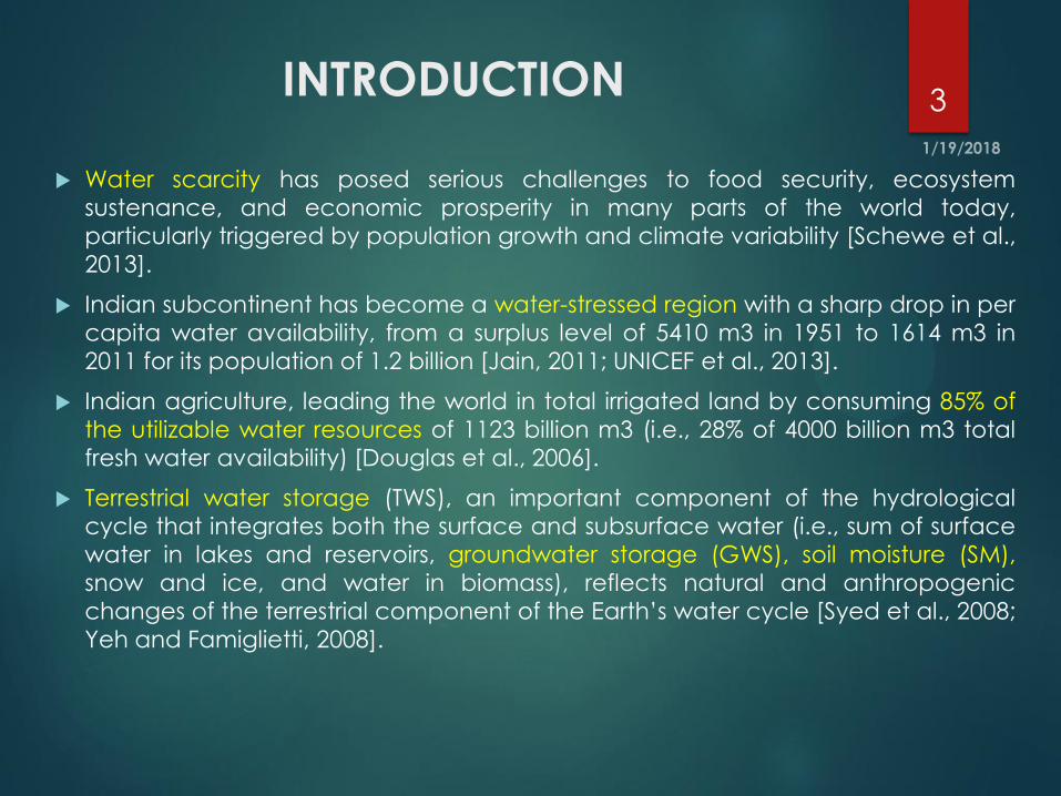
INTRODUCTION

Water scarcity has posed serious challenges to food security, ecosystem

sustenance, and economic prosperity in many parts of the world today,

particularly triggered by population growth and climate variability [Schewe et al.,

2013].

Indian subcontinent has become a water-stressed region with a sharp drop in per

capita water availability, from a surplus level of 5410 m3 in 1951 to 1614 m3 in

2011 for its population of 1.2 billion [Jain, 2011; UNICEF et al., 2013].

Indian agriculture, leading the world in total irrigated land by consuming 85% of

the utilizable water resources of 1123 billion m3 (i.e., 28% of 4000 billion m3 total

fresh water availability) [Douglas et al., 2006].

Terrestrial water storage (TWS), an important component of the hydrological

cycle that integrates both the surface and subsurface water (i.e., sum of surface

water in lakes and reservoirs, groundwater storage (GWS), soil moisture (SM),

snow and ice, and water in biomass), reflects natural and anthropogenic

changes of the terrestrial component of the Earth’s water cycle [Syed et al., 2008;

Yeh and Famiglietti, 2008].

3

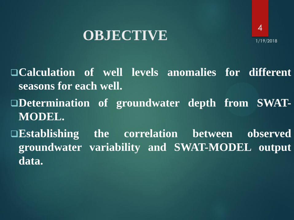
OBJECTIVE

Calculation of well levels anomalies for different

seasons for each well.

Determination of groundwater depth from SWAT-

MODEL.

Establishing the correlation between observed

groundwater variability and SWAT-MODEL output

data.

4

STUDY AREA

5

State – Maharashtra

Latitude – 20˚ 23’0.59” N

Longitude –79 ˚06’12.23”E

Area – 5675 km2

6

METHODOLOGY

7

Seasonal Groundwater level anomaly

8

0.00

5.00

10.00

15.00

20.00

25.00

30.00

1996 1997 1998 1999 2000 2001 2002 2003 2004 2005 2006 2007 2008 2009 2010 2011 2012 2013 2014 2015

Gro

un

dw

ate

r A

no

ma

ly (

m)

Post-Monsoon RABI Premonsoon Monsoon Post-Monsoon Kharif

Development of SWAT–model for

groundwater depth estimation

9

10

11

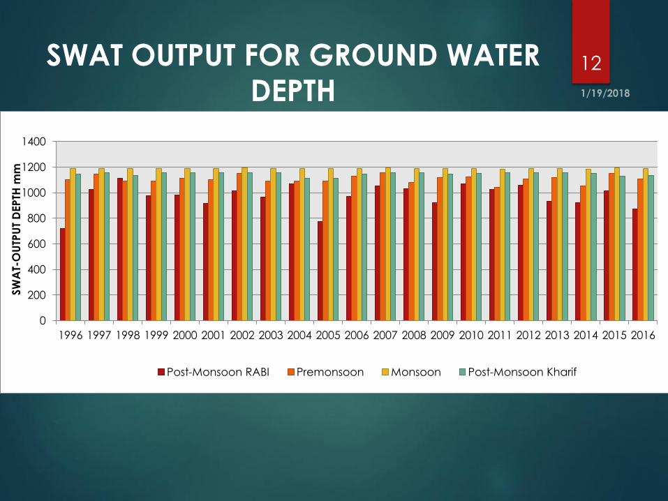
SWAT OUTPUT FOR GROUND WATER

DEPTH

12

0

200

400

600

800

1000

1200

1400

1996 1997 1998 1999 2000 2001 2002 2003 2004 2005 2006 2007 2008 2009 2010 2011 2012 2013 2014 2015 2016

SW

AT-

OU

TPU

T D

EP

TH m

m

Post-Monsoon RABI Premonsoon Monsoon Post-Monsoon Kharif

RESULTS

13

YEAR Premonsoon

Monsoon Post-Monsoon RABI Post-Monsoon KHARIF

SWAT WELL SWAT WELL SWAT WELL SWAT WELL

1996 1102.41 657.87 1188.12 773.48 719.68 708.96 1146.94 745.11

1997 1142.66 707.26 1190.66 721.40 1023.37 702.91 1154.22 731.92

1998 1089.19 697.72 1187.61 747.51 1110.03 751.70 1134.39 787.96

1999 1090.82 699.78 1186.94 790.72 975.76 750.11 1154.54 803.31

2000 1114.02 689.94 1188.63 831.89 983.38 744.67 1154.04 738.83

2001 1103.35 677.20 1187.33 808.98 916.22 718.06 1154.07 754.01

2002 1147.47 653.78 1191.83 772.56 1015.98 720.41 1153.73 740.20

2003 1091.93 687.20 1188.23 807.82 962.66 700.30 1153.83 757.19

2004 1091.50 656.94 1186.85 810.00 1069.21 715.29 1109.95 780.00

2005 1089.94 640.57 1187.80 795.76 776.33 684.08 1114.24 770.94

2006 1127.96 672.49 1190.28 803.60 969.53 722.62 1143.38 776.29

2007 1155.16 665.43 1192.40 808.28 1054.94 720.86 1152.76 764.44

2008 1077.06 670.96 1186.20 781.68 1029.16 748.38 1153.46 742.42

2009 1115.09 728.39 1188.13 752.14 920.82 706.11 1146.38 755.22

2010 1123.40 658.63 1189.59 815.83 1069.27 699.68 1151.29 793.60

2011 1038.89 708.98 1182.48 806.33 1022.70 754.82 1153.81 766.79

2012 1108.58 688.82 1187.96 810.00 1057.59 724.47 1154.43 780.00

2013 1119.78 673.49 1188.78 843.88 934.35 733.49 1154.89 771.83

2014 1050.12 703.55 1183.61 793.12 921.46 724.73 1149.95 758.99

2015 1148.81 659.93 1191.65 813.19 1011.05 717.23 1126.22 777.16

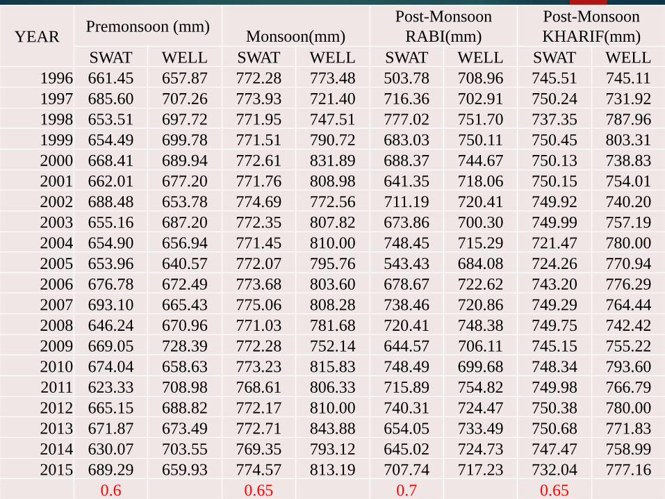
14

YEAR Premonsoon (mm)

Monsoon(mm)

Post-Monsoon

RABI(mm)

Post-Monsoon

KHARIF(mm)

SWAT WELL SWAT WELL SWAT WELL SWAT WELL

1996 661.45 657.87 772.28 773.48 503.78 708.96 745.51 745.11

1997 685.60 707.26 773.93 721.40 716.36 702.91 750.24 731.92

1998 653.51 697.72 771.95 747.51 777.02 751.70 737.35 787.96

1999 654.49 699.78 771.51 790.72 683.03 750.11 750.45 803.31

2000 668.41 689.94 772.61 831.89 688.37 744.67 750.13 738.83

2001 662.01 677.20 771.76 808.98 641.35 718.06 750.15 754.01

2002 688.48 653.78 774.69 772.56 711.19 720.41 749.92 740.20

2003 655.16 687.20 772.35 807.82 673.86 700.30 749.99 757.19

2004 654.90 656.94 771.45 810.00 748.45 715.29 721.47 780.00

2005 653.96 640.57 772.07 795.76 543.43 684.08 724.26 770.94

2006 676.78 672.49 773.68 803.60 678.67 722.62 743.20 776.29

2007 693.10 665.43 775.06 808.28 738.46 720.86 749.29 764.44

2008 646.24 670.96 771.03 781.68 720.41 748.38 749.75 742.42

2009 669.05 728.39 772.28 752.14 644.57 706.11 745.15 755.22

2010 674.04 658.63 773.23 815.83 748.49 699.68 748.34 793.60

2011 623.33 708.98 768.61 806.33 715.89 754.82 749.98 766.79

2012 665.15 688.82 772.17 810.00 740.31 724.47 750.38 780.00

2013 671.87 673.49 772.71 843.88 654.05 733.49 750.68 771.83

2014 630.07 703.55 769.35 793.12 645.02 724.73 747.47 758.99

2015 689.29 659.93 774.57 813.19 707.74 717.23 732.04 777.16 0.6 0.65 0.7 0.65

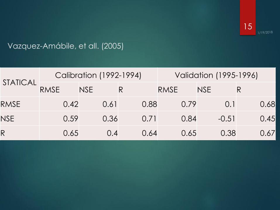
Vazquez-Amábile, et all. (2005)

STATICAL Calibration (1992-1994) Validation (1995-1996)

RMSE NSE R RMSE NSE R

RMSE 0.42 0.61 0.88 0.79 0.1 0.68

NSE 0.59 0.36 0.71 0.84 -0.51 0.45

R 0.65 0.4 0.64 0.65 0.38 0.67

15

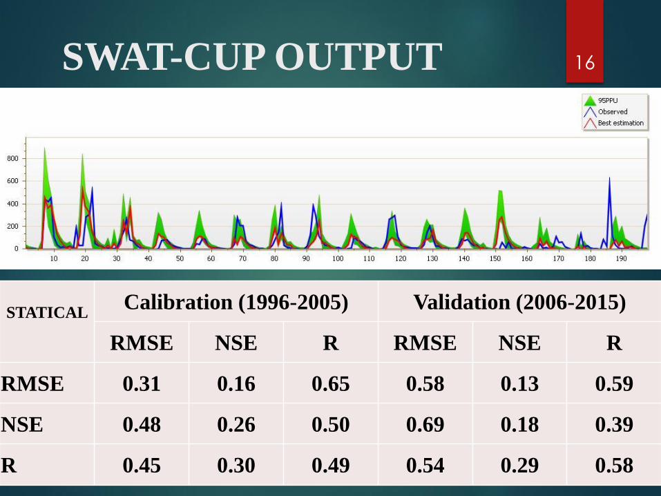
SWAT-CUP OUTPUT 16

STATICAL

Calibration (1996-2005) Validation (2006-2015)

RMSE NSE R RMSE NSE R

RMSE 0.31 0.16 0.65 0.58 0.13 0.59

NSE 0.48 0.26 0.50 0.69 0.18 0.39

R 0.45 0.30 0.49 0.54 0.29 0.58

REFERENCES

Ahmadi, S.H., and Sedghamiz, A., (2007). "Geo statistical analysis of spatial and temporal

variations of groundwater level." Environ. Monit. Assess., 129, 277–294. Antonellini, M. P., Mollema, B., Giambastiani, K. B, Caruso. L, Minchio. A, Pellegrini, L., Sabia, M.,

Ulazzi, E., and Gabbianelli, G. (2008). "Salt water intrusion in the coastal aquifer of the southern Po Plain." Italy, Hydrogeol. J., 16.1541–1556.

Caers, J. (2005). "Petroleum geostatistics. Richardson, Houston: Society of Petroleum Engineers."

CGWB., (2012)."Groundwater year book-India." Central Ground Water Board Ministry of Water Resources Government of India Faridabad. 1-63.

Gilbert, R.O. 1987. "Statistical Methods for Environmental Pollution Monitoring." Wiley, NY. Kendall, M.A. (1975). "Rank Correlation Methods." Charles Griffin, London, UK. Kousari, M.R., Ekhtesasi, M.R., Tazeh, M., Saremi, M.A., Asadi Z., M.A., (2011). "An investigation of

the Iranian climatic changes by considering the precipitation, temperature, and relative humidity parameters." Theor Appl Climatol. 103:321–335.

Malekian, A., and Kazemzadeh, M. (2016) "Spatio-Temporal Analysis of Regional Trends and Shift Changes of Autocorrelated Temperature Series in Urmia Lake Basin." Water Resour. Manage.,Springer 30 (2), 785-803.

Mini, P. K., Singh, D.K., and Sarangi, A.,(2014). "Spatio-Temporal Variability Analysis of Groundwater Level in Coastal Aquifers Using Geostatistics." International Journal of Environmental Research and Development. 4 (4), 329-336.

Sharma, K.D. (2009). "Groundwater management for food security." Current sci., 96 (11), 44- 447.

Tabari, H., Nikbakht, J. and Shiftehsome’e, B. (2012). "Investigation of groundwater level fluctuations in the north of Iran." Environ. Earth Sci., 66(1), 231-243.

Sen, P.K., (1968) "Estimates of the regression coefficient based on Kendall’s tau." J Am Stat Assoc 39, 1379–1389.

Taany, R. A., Tahboub, A. B., and Saffarini, G, A., (2009). "Geostatistical analysis of spatiotemporal variability of groundwater level fluctuations in Amman–Zarqa basin, Jordan: a case study." Environ.Geol., 57, 525–535.

17

18