Performance evaluation and optimisation of stand-alone

University of Wollongong University of Wollongong

Research Online Research Online

University of Wollongong Thesis Collection 2017+ University of Wollongong Thesis Collections

2018

Performance evaluation and optimisation of stand-alone ground source Performance evaluation and optimisation of stand-alone ground source

heat pumps and hybrid ground source heat pumps with integrated solar heat pumps and hybrid ground source heat pumps with integrated solar

photovoltaic thermal collectors photovoltaic thermal collectors

Lei Xia University of Wollongong Follow this and additional works at: https://ro.uow.edu.au/theses1

University of Wollongong University of Wollongong

Copyright Warning Copyright Warning

You may print or download ONE copy of this document for the purpose of your own research or study. The University

does not authorise you to copy, communicate or otherwise make available electronically to any other person any

copyright material contained on this site.

You are reminded of the following: This work is copyright. Apart from any use permitted under the Copyright Act

1968, no part of this work may be reproduced by any process, nor may any other exclusive right be exercised,

without the permission of the author. Copyright owners are entitled to take legal action against persons who infringe

their copyright. A reproduction of material that is protected by copyright may be a copyright infringement. A court

may impose penalties and award damages in relation to offences and infringements relating to copyright material.

Higher penalties may apply, and higher damages may be awarded, for offences and infringements involving the

conversion of material into digital or electronic form.

Unless otherwise indicated, the views expressed in this thesis are those of the author and do not necessarily Unless otherwise indicated, the views expressed in this thesis are those of the author and do not necessarily

represent the views of the University of Wollongong. represent the views of the University of Wollongong.

Recommended Citation Recommended Citation Xia, Lei, Performance evaluation and optimisation of stand-alone ground source heat pumps and hybrid ground source heat pumps with integrated solar photovoltaic thermal collectors, Doctor of Philosophy thesis, Sustainable Buildings Research Centre, University of Wollongong, 2018. https://ro.uow.edu.au/theses1/439

Research Online is the open access institutional repository for the University of Wollongong. For further information contact the UOW Library: [email protected]

https://ro.uow.edu.au/

https://ro.uow.edu.au/theses1

https://ro.uow.edu.au/theses1

https://ro.uow.edu.au/thesesuow

https://ro.uow.edu.au/theses1?utm_source=ro.uow.edu.au%2Ftheses1%2F439&utm_medium=PDF&utm_campaign=PDFCoverPages

Performance evaluation and optimisation of stand-alone

ground source heat pumps and hybrid ground source heat

pumps with integrated solar photovoltaic thermal

collectors

Lei Xia

B.Eng, M.Eng.

This thesis is presented as part of the requirements for the conferral of the degree:

Doctor of Philosophy

Faculty of Engineering and Information Sciences

Sustainable Buildings Research Centre

November 2018

i

Certification

I, Lei Xia, declare that this thesis submitted in fulfilment of the requirements for the

conferral of the degree Doctor of Philosophy, from the University of Wollongong, is

wholly my own work unless otherwise referenced or acknowledged. This document

has not been submitted for qualifications at any other academic institution.

Lei Xia

13 November 2018

ii

Abstract

Ground source heat pump (GSHP) systems and solar photovoltaic thermal (PVT)

collectors are among the energy efficient and environmentally friendly technologies.

This thesis aims to evaluate and optimise stand-alone GSHP systems and develop an

efficient GSHP-PVT system to provide space heating and cooling as well as domestic

hot water (DHW) for heating dominated buildings through performance evaluation,

optimal design and control optimisation.

To gain a better understanding on the dynamic characteristics and energy performance

of stand-alone GSHP systems, a number of experimental tests were carried out based

on an existing GSHP with active thermal slab system implemented in the Sustainable

Buildings Research Centre (SBRC) at the University of Wollongong. The effects of

two configurations (i.e. parallel and series) of the ground heat exchangers (GHEs),

different ground loop and slab loop differential pressure set-points and different slab

preheating starting time on the energy performance of this system were investigated.

The experimental results showed that the GSHP system with the parallel GHEs

outperformed that with the series GHEs. Starting the slab preheating earlier with a

larger differential pressure set-point in the slab loop resulted in a higher slab surface

temperature and indoor air temperature. Using a larger differential pressure set-point

in the slab loop achieved a higher COP of the heat pump and a higher COP of the

whole system, in comparison with that using a smaller differential pressure set-point

in the slab loop. The optimal operation scenario of the system was also determined

through the experimental tests.

A model-based control optimisation strategy for GSHP systems equipped with

variable speed pumps in the source side was then developed to minimise the system

energy consumption. The control strategy was formulated using simplified

iii

performance models and a hybrid optimisation technique which integrated a

performance map-based near-optimal strategy and the exhaustive search method. The

performance of the proposed strategy was evaluated through a case study and the

results showed that this model-based control strategy was more energy efficient than

a rule-based control strategy with two-stage control and a performance map-based

near-optimal control strategy. 7.98 % and 8.99 % energy savings can be achieved when

using this new control strategy under the whole heating and cooling periods

respectively, in comparison to the rule-based control strategy.

Appropriate integration of PVT collectors with GSHP systems could result in an

efficient system that can provide cooling and heating as well as domestic hot water

(DHW), offset the need of grid electricity and alleviate ground thermal imbalance. In

order to better understand the performance characteristics of hybrid GSHP-PVT

systems and facilitate the optimal design and control optimisation of such systems, a

GSHP-PVT system for residential buildings was developed. The life-time

performance of this system under different operation scenarios with different sizes of

PVT collectors was simulated and analysed. The simulation results demonstrated that

the PVT size had a significant influence on the overall performance of the hybrid

GSHP-PVT system and the selection of system operation scenario. An economic

analysis was then carried out to determine the optimum size of the PVT collectors for

the case study building.

Based on the results from the performance evaluation, a model-based design

optimisation strategy for GSHP-PVT systems was developed. To facilitate the design

optimisation, a dimension reduction strategy using Morris global sensitivity analysis

was first used to determine the key design parameters. A model-based design

optimisation strategy was then formulated to identify the optimal values of the key

iv

design parameters, in which an artificial neural network (ANN) model was used for

performance prediction and a genetic algorithm (GA) was implemented as the

optimisation technique. The simulation system developed in the performance

evaluation was used to generate necessary performance data for dimension reduction

analysis, and for the ANN model training and validation. The results showed that the

trained ANN model was able to provide acceptable estimations of the annual

operational cost of the GSHP-PVT system with R2 of 0.998. The 20-year life cycle

cost (LCC) of the GSHP-PVT system sized using the proposed design strategy was

20.1% and 10.2% lower than those of the two baseline design cases, respectively.

To further maximise the operation efficiency and minimise the operational cost of

GSHP-PVT systems, a model-based optimal control strategy for GSHP-PVT systems

was developed. This strategy was formulated using simplified adaptive models and a

GA. The simplified models were used to predict the system energy performance, and

the model parameters were continuously updated using the recursive least squares

(RLS) estimation technique with exponential forgetting. The results from simulation

tests showed that the simplified adaptive models combined with the RLS technique

were able to provide a reliable prediction of the system performance. The proposed

model-based control strategy was able to reduce the system electricity consumption by

7.8%, 7.1% and 7.5%, and increase the electricity generation by 4.4%, 6.2% and 5.1%

during the whole cooling, heating and transition periods respectively, in comparison

with a conventional control strategy.

The findings obtained from this thesis could be adapted and used to develop optimal

design and control strategies for stand-alone and hybrid GSHP systems to reduce their

initial investment and operational cost as well as improve their overall energy

performance.

v

Acknowledgement

This thesis could not be completed without the help and support of those who are

gratefully acknowledged here.

First, I would like to express my deepest gratitude and thanks to my supervisors, Dr

Zhenjun Ma and Dr Georgios Kokogiannakis. I would like to thank Zhenjun for his

patient guidance and experienced supervision throughout my research. My gratitude

also goes to Georgios, for his constructive advice and comments to improve my

research.

I would like to devote my appreciation to Mr Craig McLauchlan and Mr John Barron,

who gave me huge technical support and valuable advice on the setup of the

experimental test system.

I would like to sincerely thank all the staff and students in the Sustainable Buildings

Research Centre (SBRC) for their company and constant support throughout my PhD

study.

I further express my special appreciation to my beloved parents, for their

unconditioned love and support. I would also like to thank my girlfriend Joyce, for her

invaluable company and encouragement.

Finally, I would like to thank everyone who directly or indirectly offered his/her help

and support during my PhD study.

vi

Publications arising from this thesis

Journal papers published

• L. Xia, Z. Ma, G. Kokogiannakis, S. Wang, X. Gong, A model-based optimal

control strategy for ground source heat pump systems with integrated solar

photovoltaic thermal collectors, Applied Energy 228 (2018), 1399-1412.

• L. Xia, Z. Ma, G. Kokogiannakis, Z. Wang, S. Wang, A model-based design

optimization strategy for ground source heat pump systems with integrated

photovoltaic thermal collectors, Applied Energy 214 (2018) 178-190.

• L. Xia, Z. Ma, C. McLauchlan, S. Wang, Experimental investigation and

control optimization of a ground source heat pump system, Applied thermal

Engineering, 127 (2017) 70-80.

• Z. Ma, L. Xia, Model-based optimization of ground source heat pump systems,

Energy Procedia, 111 (2017) 12-20.

• X. Gong, L. Xia, Z. Ma, G, Chen, L. Wei, Investigation on the optimal cooling

tower input capacity of a cooling tower assisted ground source heat pump

system, Energy and Buildings 174 (2018) 239-253.

Conference paper

• L. Xia, Z. Ma, G. Kokogiannakis, Performance Simulation of a Ground Source

Heat Pump System Integrated with Solar Photovoltaic Thermal Collectors for

Residential Applications, in: The 15th International Conference of IBPSA,

2017.

vii

Table of Contents

Certification................................................................................................................... i

Abstract ........................................................................................................................ ii

Acknowledgement........................................................................................................ v

Publications arising from this thesis ........................................................................... vi

Table of Contents ....................................................................................................... vii

List of Figures ............................................................................................................ xii

List of Tables............................................................................................................. xvi

NOMENCLATURE ................................................................................................ xviii

GLOSSARY ............................................................................................................ xxiv

Chapter 1 Introduction ................................................................................................. 1

1.1 Background and motivation ............................................................................... 1

1.2 Research aim and objectives .............................................................................. 5

1.3 Research methodology ....................................................................................... 6

1.4 Thesis outline ..................................................................................................... 8

Chapter 2 Literature review ....................................................................................... 10

2.1 History and research development of GSHP systems ...................................... 10

2.1.1 History of GSHP systems ......................................................................... 10

2.1.2 Research development on stand-alone GSHP systems ............................. 12

2.1.3 Research development on hybrid GSHP systems ..................................... 15

2.2 General optimisation problem of GSHP systems ............................................ 26

2.2.1 Optimisation objective functions .............................................................. 27

2.2.2 Optimisation decision variables ................................................................ 31

2.2.3 Optimisation methods ............................................................................... 33

2.2.4 Optimisation techniques ............................................................................ 37

2.2.5 General design and control optimisation procedures of GSHP systems ... 37

2.3 Sensitivity analysis ........................................................................................... 39

viii

2.4 Review of design optimisation for GSHP systems .......................................... 44

2.4.1 Single-objective optimisation .................................................................... 45

2.4.2 Multi-objective optimisation ..................................................................... 48

2.5 Review of control optimisation for GSHP systems ......................................... 55

2.5.1 Component level control ........................................................................... 55

2.5.2 System level control .................................................................................. 56

2.6 Summary .......................................................................................................... 63

Chapter 3 Experimental investigation of a ground source heat pump system with active

thermal slabs ............................................................................................................... 66

3.1 Description of the experimental system ........................................................... 66

3.2 Design of experimental tests ............................................................................ 69

3.2.1 Description of the experimental tests ........................................................ 69

3.2.2 Description of the data acquisition system ................................................ 72

3.2.3 Experimental data analysis ........................................................................ 74

3.2.4 Uncertainty analysis .................................................................................. 75

3.3 Experimental test results and analysis .............................................................. 76

3.3.1 Test results of the GSHP system ............................................................... 76

3.3.2 Test results for GSHP with active thermal slab system. ........................... 78

3.4 Summary .......................................................................................................... 83

Chapter 4 Control optimisation of a stand-alone ground source heat pump system .. 85

4.1 Formulation of the model-based optimisation strategy .................................... 86

4.1.1 Outline of the optimisation strategy .......................................................... 86

4.1.2 Hybrid optimisation technique and optimisation constraints .................... 88

4.1.3 Description of the optimisation process .................................................... 89

4.1.4 Description of the component models ....................................................... 90

4.2 Results and discussion ...................................................................................... 93

4.2.1 Validation of the performance models ...................................................... 94

ix

4.2.2 Generation of the performance map-based near-optimal control strategy 96

4.2.3 Results of performance testing and evaluation ......................................... 98

4.3 Summary ........................................................................................................ 105

Chapter 5 Development and performance simulation of a ground source heat pump

system with integrated solar photovoltaic thermal collectors .................................. 107

5.1 Introduction .................................................................................................... 107

5.2 System development and operation scenarios................................................ 109

5.3 System modelling ........................................................................................... 113

5.4 Case study ...................................................................................................... 114

5.4.1 Building model and load characteristics ................................................. 114

5.4.2 Component sizing ................................................................................... 115

5.5 Results and discussion ................................................................................... 118

5.5.1 Annual energy consumption ................................................................... 118

5.5.2 Variation of the ground temperature ....................................................... 121

5.5.3 20-year life time performance evaluation ............................................... 121

5.5.4 Selection of the optimum PVT size ........................................................ 124

5.6 Summary ........................................................................................................ 126

Chapter 6 Model-based design optimisation of ground source heat pump systems with

integrated photovoltaic thermal collectors ............................................................... 128

6.1 Introduction .................................................................................................... 129

6.2 System simulation .......................................................................................... 130

6.3 Dimension reduction using Morris global sensitivity analysis ...................... 134

6.3.1 Morris sensitivity analysis method ......................................................... 135

6.3.2 Objective function ................................................................................... 136

6.3.3 Constraints .............................................................................................. 138

6.4 Development of the model-based design optimisation strategy .................... 139

6.4.1 Outline of the optimisation strategy ........................................................ 139

x

6.4.2 Development of the ANN performance model ....................................... 140

6.5 Performance test and evaluation .................................................................... 141

6.5.1 Setup of the test ....................................................................................... 141

6.5.2 Dimension reduction results .................................................................... 144

6.5.3 Performance evaluation of the design optimisation strategy .................. 146

6.6. Sensitivity study ............................................................................................ 152

6.7 Summary ........................................................................................................ 154

Chapter 7 Model-based optimal control of ground source heat pump systems with

integrated solar photovoltaic thermal collectors ...................................................... 155

7.1 Introduction .................................................................................................... 155

7.2 Formulation of the optimal control strategy ................................................... 157

7.2.1 Outline of the optimal control strategy ................................................... 157

7.2.2 Description of the cost function, GA fitness function and operating

constraints ......................................................................................................... 161

7.2.3 Description of adaptive performance models and model parameter tuning

techniques ......................................................................................................... 162

7.3 Performance test and results ........................................................................... 167

7.3.1 Set up of the tests .................................................................................... 167

7.3.2 Validation of the performance models .................................................... 171

7.3.3 Test and evaluation of the optimal control strategy ................................ 178

7.4 Summary ........................................................................................................ 183

Chapter 8 Conclusions and Recommendations ........................................................ 185

8.1 Summary of the key findings ......................................................................... 185

8.1.1 Experimental investigation of the GSHP system with active thermal slabs

.......................................................................................................................... 185

8.1.2 Control optimisation of stand-alone GSHP systems ............................... 187

8.1.3 Development and performance simulation of the GSHP-PVT system ... 187

xi

8.1.4 Design optimisation of GSHP-PVT systems .......................................... 188

8.1.5 Control optimisation of GSHP-PVT systems ......................................... 189

8.2 Recommendations for future work ................................................................ 190

References ................................................................................................................ 191

Appendix A - SBRC active thermal slab design ...................................................... 219

Appendix B - SBRC hydronic loop system ............................................................. 221

Appendix C - Control flow chart of three operation scenarios for the proposed GSHP-

PVT system .............................................................................................................. 222

xii

List of Figures

Fig. 1.1 Research methodology utilised in this thesis. ................................................. 7

Fig. 2.1 Research development on GSHP systems. ................................................... 12

Fig. 2.2 Schematic of the cooling tower assisted GSHP systems (Park et al., 2013). 16

Fig. 2.3 Schematic of the solar assisted GSHP system proposed by Chiasson and

Yavuzturk (2003). ...................................................................................................... 19

Fig. 2.4 Schematic of the solar assisted GSHP system for greenhouse heating (Ozgener

and Hepbasli, 2005b). ................................................................................................. 20

Fig. 2.5 Schematic of the solar assisted GSHP system installed in a single-family house

(Trillat-Berdal et al., 2006). ....................................................................................... 21

Fig. 2.6 Schematic of the solar assisted GSHP system with LHEST (Han et al., 2008).

.................................................................................................................................... 22

Fig. 2.7 Schematic of the HGSHP system with PCMs in a greenhouse (Benli and

Durmuş, 2009). ........................................................................................................... 23

Fig. 2.8 Schematic of the GSHP-PVT system in a dwelling (Bakker et al., 2005). ... 24

Fig. 2.9 Schematic of the GSHP-PVT system in load sharing applications (Entchev et

al., 2014). .................................................................................................................... 25

Fig. 2.10 Parameters influencing the performance of GSHPs. .................................. 32

Fig. 2.11 General model-based design optimisation procedure of GSHP systems. ... 38

Fig. 2.12 General control optimisation procedure of GSHP systems. ....................... 39

Fig. 3.1 Schematic of the experimental system. ......................................................... 67

Fig. 3.2 Hydronic loop and manifold box of the GSHP system. ................................ 68

Fig. 3.3 Configuration of the active thermal slab system. .......................................... 69

Fig. 3.4 A view of the active thermal slab system. .................................................... 69

Fig. 3.5 User interface of the building management system. ..................................... 72

Fig. 3.6 iButtons and indoor temperature measuring tree. ......................................... 73

Fig. 3.7 Heat extraction and power consumption of the heat pump and water pumps -

Parallel operation. ....................................................................................................... 77


Series operation. ......................................................................................................... 77

Fig. 3.9 Outdoor air temperature during the tests. ..................................................... 79

Fig. 3.10 Slab surface and indoor air temperature variation during different operation

scenarios. .................................................................................................................... 81

xiii

Fig. 4.1 Outline of the proposed model-based optimisation strategy. ....................... 87

Fig. 4.2 Illustration of the search range defined using the performance map-based near-

optimal strategy. ......................................................................................................... 89

Fig. 4.3 Validation of the component models using measured data. ......................... 96

Fig. 4.4 Comparison between the temperature set-points identified using the model-

based strategy with the exhaustive search method and the performance map-based

strategy. ...................................................................................................................... 98

Fig. 4.5 Search process of the proposed control strategy. ........................................ 101

Fig. 4.6 Building load and the operation mode of the heat pumps under the selected

heating and cooling day. .......................................................................................... 102

Fig. 4.7 Temperature set-points identified by three different control strategies under

the selected heating and cooling day. ....................................................................... 104

Fig. 4.8 Comparison of the power consumption of the proposed model-based strategy

and the performance map-based near-optimal strategy with the rule-based control

strategy. .................................................................................................................... 105

Fig. 5.1 Schematic diagram of the proposed GSHP-PVT system............................ 110

Fig. 5.2 Schematic of three operation scenarios. ..................................................... 111

Fig. 5.3 Illustration of the simulation system developed in TRNSYS for scenario 2.

.................................................................................................................................. 113

Fig. 5.4 The house model developed in DesignBuilder. .......................................... 114

Fig. 5.5 Heating and cooling load profile of the house. ........................................... 115

Fig. 5.6 Annual energy consumption of different components with different sizes of

the PVT collectors. ................................................................................................... 119

Fig. 5.7 Annual energy consumption of the system under three scenarios with different

sizes of PVT collectors............................................................................................. 121

Fig. 5.8 Variation of the ground temperature in the first year operation. ................ 121

Fig. 5.9 Variation of the ground temperature in 20 years operation. ....................... 122

Fig. 5.10 Variation of the annual system energy consumption under three scenarios

with the PVT area of 48 m2 in 20 years operation. .................................................. 123

Fig. 5.11 20-year life time energy consumption of the system with different PVT sizes

under three scenarios. ............................................................................................... 123

Fig. 5.12 Annual electricity generation of the system with different PVT sizes. .... 124

Fig. 5.13 20-year net present value of the system with different PVT sizes............ 126

xiv

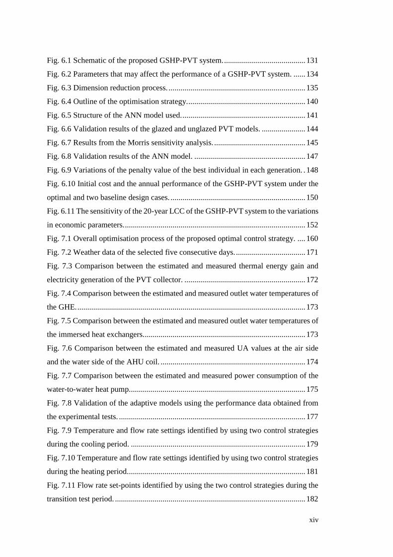
Fig. 6.1 Schematic of the proposed GSHP-PVT system. ......................................... 131

Fig. 6.2 Parameters that may affect the performance of a GSHP-PVT system. ...... 134

Fig. 6.3 Dimension reduction process. ..................................................................... 135

Fig. 6.4 Outline of the optimisation strategy. ........................................................... 140

Fig. 6.5 Structure of the ANN model used. .............................................................. 141

Fig. 6.6 Validation results of the glazed and unglazed PVT models. ...................... 144

Fig. 6.7 Results from the Morris sensitivity analysis. .............................................. 145

Fig. 6.8 Validation results of the ANN model. ........................................................ 147

Fig. 6.9 Variations of the penalty value of the best individual in each generation. . 148

Fig. 6.10 Initial cost and the annual performance of the GSHP-PVT system under the

optimal and two baseline design cases. .................................................................... 150

Fig. 6.11 The sensitivity of the 20-year LCC of the GSHP-PVT system to the variations

in economic parameters. ........................................................................................... 152

Fig. 7.1 Overall optimisation process of the proposed optimal control strategy. .... 160

Fig. 7.2 Weather data of the selected five consecutive days. ................................... 171

Fig. 7.3 Comparison between the estimated and measured thermal energy gain and

electricity generation of the PVT collector. ............................................................. 172

Fig. 7.4 Comparison between the estimated and measured outlet water temperatures of

the GHE. ................................................................................................................... 173

Fig. 7.5 Comparison between the estimated and measured outlet water temperatures of

the immersed heat exchangers. ................................................................................. 173

Fig. 7.6 Comparison between the estimated and measured UA values at the air side

and the water side of the AHU coil. ......................................................................... 174

Fig. 7.7 Comparison between the estimated and measured power consumption of the

water-to-water heat pump. ........................................................................................ 175

Fig. 7.8 Validation of the adaptive models using the performance data obtained from

the experimental tests. .............................................................................................. 177

Fig. 7.9 Temperature and flow rate settings identified by using two control strategies

during the cooling period. ........................................................................................ 179


during the heating period. ......................................................................................... 181

Fig. 7.11 Flow rate set-points identified by using the two control strategies during the

transition test period. ................................................................................................ 182

xv

xvi

List of Tables

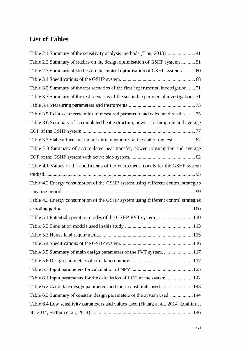
Table 2.1 Summary of the sensitivity analysis methods (Tian, 2013). ...................... 41

Table 2.2 Summary of studies on the design optimisation of GSHP systems. .......... 51

Table 2.3 Summary of studies on the control optimisation of GSHP systems. ......... 60

Table 3.1 Specifications of the GSHP system. ........................................................... 68

Table 3.2 Summary of the test scenarios of the first experimental investigation. ..... 71

Table 3.3 Summary of the test scenarios of the second experimental investigation. . 71

Table 3.4 Measuring parameters and instruments. ..................................................... 73

Table 3.5 Relative uncertainties of measured parameter and calculated results. ....... 75

Table 3.6 Summary of accumulated heat extraction, power consumption and average

COP of the GSHP system........................................................................................... 77

Table 3.7 Slab surface and indoor air temperatures at the end of the test. ................. 82

Table 3.8 Summary of accumulated heat transfer, power consumption and average

COP of the GSHP system with active slab system. ................................................... 82

Table 4.1 Values of the coefficients of the component models for the GSHP system

studied. ....................................................................................................................... 95

Table 4.2 Energy consumption of the GSHP system using different control strategies

- heating period. .......................................................................................................... 99


- cooling period. ....................................................................................................... 100

Table 5.1 Potential operation modes of the GSHP-PVT system. ............................. 110

Table 5.2 Simulation models used in this study. ...................................................... 113

Table 5.3 House load requirements. ......................................................................... 115

Table 5.4 Specifications of the GSHP system. ......................................................... 116

Table 5.5 Summary of main design parameters of the PVT system. ....................... 117

Table 5.6 Design parameters of circulation pumps. ................................................. 117

Table 5.7 Input parameters for calculation of NPV. ................................................ 125

Table 6.1 Input parameters for the calculation of LCC of the system. .................... 142

Table 6.2 Candidate design parameters and their constraints used. ......................... 143

Table 6.3 Summary of constant design parameters of the system used. .................. 144

Table 6.4 Low sensitivity parameters and values used (Huang et al., 2014, Ibrahim et

al., 2014, Fudholi et al., 2014). ................................................................................ 146

xvii

Table 6.5 Comparison between the optimal values identified and those of two baseline

cases. ........................................................................................................................ 149

Table 6.6 The optimisation results with the variations of different economic parameters.

.................................................................................................................................. 153

Table 7.1 Statistical indices of model validation results. ......................................... 177

Table 7.2 Electricity consumption and generation of the GSHP-PVT system when

using different control strategies. ............................................................................. 182

xviii

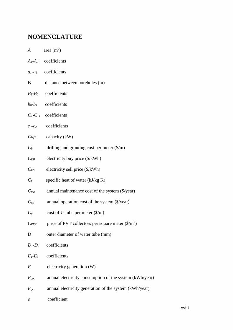
NOMENCLATURE

A area (m2)

A1-A3 coefficients

a1-a3 coefficients

B distance between boreholes (m)

B1-B5 coefficients

b0-b4 coefficients

C1-C11 coefficients

c0-c2 coefficients

Cap capacity (kW)

Cb drilling and grouting cost per meter ($/m)

CEB electricity buy price ($/kWh)

CES electricity sell price ($/kWh)

Cf specific heat of water (kJ/kg K)

Cma annual maintenance cost of the system ($/year)

Cop annual operation cost of the system ($/year)

Cp cost of U-tube per meter ($/m)

CPVT price of PVT collectors per square meter ($/m2)

D outer diameter of water tube (mm)

D1-D3 coefficients

E1-E3 coefficients

E electricity generation (W)

Econ annual electricity consumption of the system (kWh/year)

Egen annual electricity generation of the system (kWh/year)

e coefficient

xix

F1-F3 coefficients

FR heat removal efficiency factor

f coefficient

Gt incident solar radiation on the PVT collector (W/m2)

H pump head (m)

Hb borehole depth (m)

h enthalpy (kJ/kg)

hc overall convection heat loss coefficient (W/m2K)

hf fluid convective heat transfer coefficient (W/(m2 K))

hn natural convection heat loss coefficient (W/m2K)

hr radiation heat loss coefficient (W/m2K)

hs saturated air enthalpy at the temperature Ts (kJ/kg)

hw convection heat loss coefficient due to the wind (W/m2K)

J cost function (kW)

j number of design parameters

K number of elementary effects

k thermal conductivity (W/(m K))

L length (m)

MCma annual maintenance cost per square meter ($/m2)

Mpvt total circulating fluid mass flow rate through PVT collector (kg/s)

M flow rate (kg/s)

mpvt circulating fluid mass flow rate per PVT tube (kg/s)

N number

Ng number of glass covers

Ns number of simulations

xx

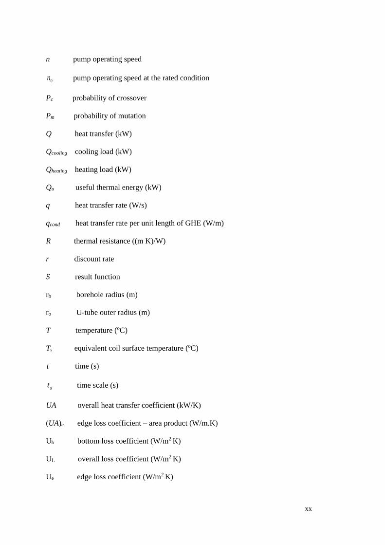
n pump operating speed

0n pump operating speed at the rated condition

Pc probability of crossover

Pm probability of mutation

Q heat transfer (kW)

Qcooling cooling load (kW)

Qheating heating load (kW)

Qu useful thermal energy (kW)

q heat transfer rate (W/s)

qcond heat transfer rate per unit length of GHE (W/m)

R thermal resistance ((m K)/W)

r discount rate

S result function

rb borehole radius (m)

ro U-tube outer radius (m)

T temperature (oC)

Ts equivalent coil surface temperature (oC)

t time (s)

st time scale (s)

UA overall heat transfer coefficient (kW/K)

(UA)e edge loss coefficient – area product (W/m.K)

Ub bottom loss coefficient (W/m2 K)

UL overall loss coefficient (W/m2 K)

Ue edge loss coefficient (W/m2 K)

xxi

Ut top loss coefficient (W/m2 K)

V loss function

VTK volume of water tank (L)

v wind velocity (m/s)

W power consumption (kW)

w uncertainty (%)

x regression variable

cx half shank spacing (m)

y observed variable

α absorptance

, , , , coefficients

εg emittance of glass

εp emittance of PV plate

forgetting factor

temperature coefficient

efficiency

mean value of the elementary effects

Stefan’s Boltzmann constant (W/m2 K4)

standard deviation of the elementary effects

τ transmittance

( )PV transmittance-absorptance of the PV cell

increment

Superscripts

n near

xxii

o optimal

Subscripts

0 initial

a air

abs absorber

amb ambient

ins insulation

b borehole

c condition

cf air floor conditioned floor

con constant

des design

est estimation

GR ground recharge

g ground heat exchanger

ga energy gain

gr grout material

HP heat pump

hx heat exchanger

i inner

in inlet

l load side

m motor

mp mean plate

o outer

xxiii

out outlet

p pipe

pu pump

pv photovoltaic

ref reference

s source side

set set-point

so soil

TK tank

t trial

th thermal

tot total

v VFD

var variable

WH water heater

w water

xxiv

GLOSSARY

CAPFT ratio of the full capacity under a given condition to the reference capacity

COP coefficient of performance

CVRMSE coefficient of variation of the root mean square error

DC residual cost ($)

EE elementary effect ($)

EIRFT ratio of the energy efficiency at the full capacity under a given condition

to the reference efficiency

EIRFPLR ratio of the power at a part load to the power at the full load under the

same condition

GHE ground heat exchanger

GSHP ground source heat pump

IC initial cost ($)

LCC life cycle cost ($)

MC maintenance cost ($)

NPV net present value ($)

OC operating cost ($)

PLR part load ratio

PVT photovoltaic thermal collector

RC replacement cost ($)

SG specific gravity

WWHP water-to-water heat pump

1

Chapter 1 Introduction

1.1 Background and motivation

Primary energy shortage, increasing energy demand and global warming due to

greenhouse gas emissions have become major worldwide challenges. Buildings are

among the major energy users which consume around 40% of global energy usage and

are responsible for a similar share of greenhouse gas emissions (Pérez-Lombard et al.,

2008, Berardi, 2017). A significant proportion of energy consumption in buildings is

due to the use of heating, ventilation, and air conditioning (HVAC) systems (Chung,

2011). Due to the expected increase in population and the growing demand for better

indoor thermal comfort, the energy consumption of building HVAC systems is

projected to be even higher in the future (Wan et al., 2012, Ürge-Vorsatz et al., 2015).

Sustainable development is therefore becoming increasingly important, and reducing

greenhouse gas emissions and energy consumption of buildings propels researchers to

explore substitutes of traditional HVAC systems.

A ground source heat pump (GSHP) system, which can transform earth energy into

useful energy to heat and cool buildings, has been receiving wide attention because of

its advantages of high efficiency, environmentally friendliness and easiness to be

integrated with other energy systems (Urchueguía et al., 2008, Sarbu and Sebarchievici,

2014, Chen et al., 2015). It was reported that proper use of GSHP systems could reduce

the energy consumption in buildings by 30–70% for heating and by 20–50% for

cooling, in comparison to the use of conventional air-conditioning systems and air

source heat pumps (Benli and Durmuş, 2009). GSHP systems have been widely used

in both residential and commercial applications and the installation of GSHP systems

has grown continuously on a global basis from 10% to 30% annually in recent years

2

(Sarbu and Sebarchievici, 2014). A wide variety of GSHP systems which use different

types of heat sources or sinks, such as ground, ground water, or surface water have

been investigated (Yang et al., 2010). These systems can be grouped into two

categories, i.e. open loop and closed loop, according to the type and installation of

ground heat exchangers (GHEs). Closed loop systems which consist of two typical

types of GHEs, i.e. vertical and horizontal GHEs, have attracted more interest than the

open loop systems due to their high efficiency and reliability (Sarbu and Sebarchievici,

2014, Curtis et al., 2005).

One of the major challenges relating to the application of GSHP systems is the ground

thermal imbalance, which can result in the performance deterioration of GSHP systems

(Yu et al., 2008, Man et al., 2010b, Wang et al., 2016). In order to solve this problem,

hybrid ground source heat pump (HGSHP) systems have been developed. HGSHP

systems utilise auxiliary heat sinks or auxiliary heat sources to supply a fraction of the

cooling or heating demand of a building (Phetteplace and Sullivan, 1998, Chiasson

and Yavuzturk, 2003, Man et al., 2011). The use of HGSHP systems can effectively

alleviate ground thermal imbalance, and in the meantime, can reduce the initial costs

and ground area requirement in comparison to conventional stand-alone GSHP

systems (ASHRAE, 1995, Qi et al., 2014).

In the past few decades, significant efforts have been made on the modelling

(Piechowski, 1999, Yavuzturk and Spitler, 1999, Florides and Kalogirou, 2007, Yang

et al., 2010, Li and Lai, 2015) and performance evaluation (Michopoulos et al., 2013,

Congedo et al., 2012, Liu et al., 2015, Safa et al., 2015, Wang et al., 2012, Jeon et al.,

2010) of GSHP systems. These efforts provided the fundamental theories and

references for the design and control optimisation of GSHP systems. Optimal design

of GSHP systems is crucial to minimise the high initial cost of such systems while still

3

ensuring their high efficiency. Research on proper size of GSHP systems started in the

middle of 1980s. The International Ground Source Heat Pump Association provided a

method for the design of vertical GHEs (Bose, 1984). The ASHRAE manuals

(ASHRAE, 1995, Kavanaugh and Rafferty, 2014) also provided a practical design

method to size the GHEs of GSHP systems. A number of early studies developed and

improved various types of mathematical models of GSHP systems and used them to

formulate design strategies (Rottmayer et al., 1997, Yavuzturk and Spitler, 1999,

Kavanaugh and Rafferty, 1997, Kavanaugh, 1998, Thornton et al., 1997,

Ramamoorthy et al., 2001b). In recent years, a number of design optimisation

strategies have been developed for GSHP systems (Huang et al., 2014, Neugebauer

and Sołowiej, 2012, Esen and Turgut, 2015, Verma and Murugesan, 2014, Sanaye and

Niroomand, 2009, Sanaye and Niroomand, 2010, Park et al., 2011, Zhao et al., 2009,

Sayyadi and Nejatolahi, 2011).

Inefficient or improper control strategies used for GSHP systems could lead to the

lower operating efficiency and the gradual degradation of their long-term performance.

Control optimisation of GSHP systems is therefore important to improve their

operating efficiency while providing satisfactory indoor thermal comfort. Compared

to the efforts that have been made on the optimal design of GSHP systems, the amount

of work on the optimal control of GSHP systems is insufficient and only a limited

number of studies have been carried out on the development of optimal control

strategies for GSHP systems (Sundbrandt, 2011, Verhelst, 2012, Sivasakthivel et al.,

2014b, Montagud et al., 2014, Cervera-Vázquez et al., 2015a).

In heating dominated buildings, where the space heating and domestic hot water

(DHW) account for a large amount of total energy consumption, utilising solar energy

as the auxiliary heat source in a GSHP system could be a promising solution to

4

significantly reduce building energy demand. A photovoltaic thermal collector (PVT)

which combines a photovoltaic (PV) and a solar thermal collector, is able to convert a

fraction of the incoming solar radiation into electricity and convert the excess heat

generated from the PV cell into useful thermal energy (Anderson et al., 2009). The

appropriate integration of PVT collectors with GSHP systems could result in an

efficient system that can provide cooling and heating as well as domestic hot water

(DHW), and offset the need of grid electricity. The excess heat generated from the

PVT collector can be used to recharge the ground to alleviate the ground thermal

imbalance so that the long-term performance of the GSHP system can be guaranteed.

Over the last several years, there is an increasing attention to develop hybrid GSHP

systems with integrated PVT collectors (GSHP-PVT). Most of the existing studies

focused on the model development and performance simulation of GSHP-PVT

systems (Bakker et al., 2005, Canelli et al., 2015), and performance evaluation and

comparison of GSHP-PVT systems with different heating and cooling systems

(Entchev et al., 2014, Brischoux and Bernier, 2016, Bertram et al., 2012, Putrayudha

et al., 2015). These existing studies demonstrated that the GSHP-PVT system can

result in a better energy performance in comparison to conventional heating and

cooling systems and/or stand-alone GSHP systems. However, the results from these

studies were highly dependent on the size of the major components and the control

strategies used. The influence of the PVT size on the performance of the GSHP-PVT

system and the effect of the PVT size on the operation of hybrid GSHP-PVT systems

have not been discussed in detail yet. Therefore, there is a need to further examine the

effect of the PVT size on the system performance.

The high initial investment of both GSHP systems and PVT collectors makes the short-

term economics of hybrid GSHP-PVT systems unattractive. The optimisation of the

5

key design parameters of such systems therefore becomes more important to reduce

the upfront cost and ensure robust performance of such systems. However, the

influence of the major components on the performance of hybrid GSHP-PVT systems

and the approach to proper sizing of such systems have not been thoroughly

investigated and discussed. Therefore, there is a need to develop optimal design

strategies to optimise the key design parameters of GSHP-PVT systems. The coupling

of GSHP systems with PVT collectors makes the hybrid GSHP-PVT system highly

dynamic. Quantifying the system performance is not a trivial task. Intelligent or

optimal control of such systems is therefore essential. Compared to the efforts that

have been made on the optimal control of stand-alone GSHP and other earlier

developed HGSHP systems, the amount of work on the optimal control of GSHP-PVT

systems is still far from sufficient (Entchev et al., 2016, Putrayudha et al., 2015). It is

therefore also important to develop practical and reliable optimal control strategies for

such systems.

1.2 Research aim and objectives

The overall aim of the project is to evaluate and optimise stand-alone GSHP systems

and develop an efficient HGSHP system with integrated water-based PVT collectors

to provide space heating and cooling as well as DHW for heating dominated buildings

through performance evaluation, optimal design and control optimisation. The overall

project aim will be achieved through the following objectives:

I. Examination of the performance characteristics of a stand-alone GSHP system

implemented in a net-zero office building and development of an optimal

control strategy for stand-alone GSHP systems.

II. Development and modelling a hybrid GSHP-PVT system and evaluation of its

6

performance under different operation scenarios with different PVT sizes to

examine the effect of the PVT size on the system performance.

III. Development of a model-based design optimisation strategy for the hybrid

GSHP-PVT system to identify the optimal values of the key design parameters

determined through a dimension reduction method.

IV. Development of a model-based control strategy for the hybrid GSHP-PVT

system to identify energy efficient control settings to maximise the operating

efficiency.

1.3 Research methodology

The research methodology utilised in this study is schematically illustrated in Fig. 1.1.

Objective I was realised through an experimental investigation and control

optimisation of a GSHP with an active thermal slab system equipped with variable

speed water pumps at both source side and load side of the system. The experimental

tests were carried out to examine the effects of the GHE configurations, ground loop

and slab loop differential pressure (DP) set-points and slab preheating starting time on

the performance of the system. A model-based control strategy was then developed to

determine the optimal operating speed of the variable speed pumps in the ground loop.

Objective II was achieved through a simulation investigation. A GSHP-PVT system

for residential applications was developed. A 20-year life-time performance

simulation was performed under different operation scenarios with different sizes of

the PVT collectors, to investigate the effect of the PVT size on the performance of the

system. The performance characteristics of the GSHP-PVT system obtained from

dynamic simulations were then used to facilitate the design and control optimisation

of GSHP-PVT systems through objectives III and IV. In order to realise objectives III

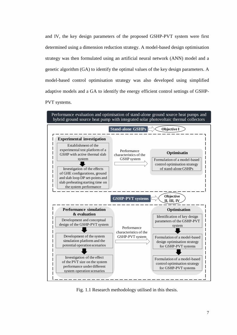
7

and IV, the key design parameters of the proposed GSHP-PVT system were first

determined using a dimension reduction strategy. A model-based design optimisation

strategy was then formulated using an artificial neural network (ANN) model and a

genetic algorithm (GA) to identify the optimal values of the key design parameters. A

model-based control optimisation strategy was also developed using simplified

adaptive models and a GA to identify the energy efficient control settings of GSHP-

PVT systems.

Fig. 1.1 Research methodology utilised in this thesis.

Establishment of the

experimental test platform of a

GSHP with active thermal slab

system

Performance evaluation and optimisation of stand-alone ground source heat pumps and hybrid ground source heat pump with integrated solar photovoltaic thermal collectors

Investigation of the effects

of GHE configurations, ground

and slab loop DP set-points and

slab preheating starting time on

the system performance

Development and conceptual

design of the GSHP-PVT system

Performance simulation & evaluation

Development of the system

simulation platform and the

potential operation scenarios

Investigation of the effect

of the PVT size on the system

performance under different

system operation scenarios

Performance characteristics of the

GSHP system

Performance

characteristics of the

GSHP-PVT system

Formulation of a model-based

control optimisation strategy

of stand-alone GSHPs


design optimisation strategy

for GSHP-PVT systems

Identification of key design

parameters of the GSHP-PVT

system


control optimisation strategy

for GSHP-PVT systems

Objective

II, III, IV

Objective IStand-alone GSHPs

GSHP-PVT systems

Optimisation

Optimisatin

Experimental investigation

8

1.4 Thesis outline

This chapter provided the background and motivation of this research. It also outlined

the research aim and objectives, and the primary research methodology utilised in this

thesis. The subsequent chapters are structured as follows.

Chapter 2 provides a literature review of stand-alone and hybrid GSHP systems, with

a major focus on the design and control optimisation of GSHP systems.

Chapter 3 describes the experimental platform of a GSHP system implemented in a

net-zero office building and the design of experimental tests. The effects of two GHE

configurations, different ground loop and slab loop differential pressure set-points and

different slab preheating starting time on the energy performance of the GSHP system

are experimentally investigated.

Chapter 4 presents the development of a model-based control optimisation strategy for

stand-alone GSHP systems. The control strategy was formulated using simplified

performance models and a hybrid optimisation technique, which integrated a

performance map-based near-optimal strategy and the exhaustive search method, to

determine the optimal operating speed of the variable speed pumps in the ground loop

system.

Chapter 5 presents the development and performance simulation of a GSHP system

integrated with water-based solar photovoltaic thermal (PVT) collectors for residential

buildings. A dynamic simulation system was developed and used to facilitate the

performance evaluation. A 20-year life-time performance simulation was performed

under three operation scenarios with different sizes of the PVT collectors. An

economic analysis was then carried out to determine the optimum size of the PVT

collectors for the case study building.

9

Chapter 6 presents the development of a model-based design optimisation strategy to

determine the optimal values of the key design parameters of GSHP-PVT systems, in

which an artificial neural network (ANN) model was used for performance prediction

and a genetic algorithm (GA) was used as the optimisation technique. To facilitate the

design optimisation, a dimension reduction strategy using Morris global sensitivity

analysis was used to determine the key design parameters of GSHP-PVT systems. The

performance test and evaluation of the proposed strategy was also presented.

Chapter 7 presents the development of a model-based control optimisation strategy for

GSHP-PVT systems to identify energy efficient control settings. The strategy was

formulated using simplified adaptive models and a GA. The performance test and

evaluation of the adaptive models and the optimal control strategy were presented as

well.

Chapter 8 summarises the key findings obtained from the thesis and some

recommendations for future work.

10

Chapter 2 Literature review

This thesis mainly focuses on the performance evaluation and optimisation of stand-

alone ground source heat pump (GSHP) systems and hybrid ground source heat pump

systems with integrated solar photovoltaic thermal collectors (GSHP-PVT). This

chapter therefore provides a literature review on the research development, optimal

design and control optimisation of stand-alone and hybrid GSHP systems in order to

identify some research gaps to facilitate the development of optimisation strategies for

such systems.

This chapter is organised as follows: Section 2.1 introduces the history and current

research development of GSHP systems. Section 2.2 presents the general optimisation

problem and optimisation procedures for design and control optimisations of GSHP

systems. Section 2.3 overviews the sensitivity analysis methods used to determine the

decision variables to facilitate the optimisation of GSHP systems. Sections 2.4 and 2.5

are the literature review on the design optimisation and control optimisation of GSHP

systems, respectively. The major findings obtained from the literature review are

summarised in Section 2.6.

2.1 History and research development of GSHP systems

2.1.1 History of GSHP systems

The concept of ground source heat pump was first introduced in a Swiss patent in 1912

(Ball et al., 1983) and the research related to the GSHP technology has been gradually

carried out in North America and Europe since 1930s. After the World War Two, a

number of companies in North America started to develop and make GSHP products,

following with some European companies, which led to the first prosperity in the

development of GSHP systems (Ingersoll and Plass, 1948).

11

In 1970s, the outbreak of worldwide energy crisis impelled the development of new

energy sources instead of fossil fuels. GSHPs started receiving increasing attention

because of their advantages of high efficiency and environmentally friendly (IGSHPA,

2007). In 1976, International Ground Source Heat Pump Association (IGSHPA) was

established, aiming at improving and promoting the GSHP technology, and in the

meantime, to regulate the market of GSHP products. Efforts spearheaded by IGSHPA

led to the construction of a research and test facility at the Oklahoma State University

(OSU) campus. In 1978, the US Department of Energy (DOE) granted OSU a contract

for the DOE Solar Assisted project and GSHP research began in earnest (Bose et al.,

1985).

Nowadays, GSHP systems have become an air-conditioning alternative for both

residential and commercial buildings. The global installations of GSHP systems have

grown continuously with a range from 10% to 30% annually in recent years (Bose et

al., 2002). Many studies have also been carried out on different aspects of GSHPs in

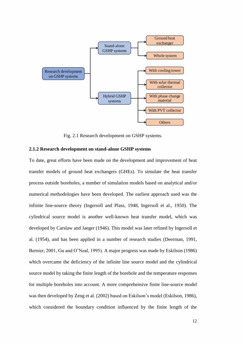
order to facilitate better application of this technology. These studies can be broadly

divided into the research on stand-alone GSHP systems and the research on hybrid

GSHP (HGSHP) systems, as illustrated in Fig. 2.1.

12

Fig. 2.1 Research development on GSHP systems.

2.1.2 Research development on stand-alone GSHP systems

To date, great efforts have been made on the development and improvement of heat

transfer models of ground heat exchangers (GHEs). To simulate the heat transfer

process outside boreholes, a number of simulation models based on analytical and/or

numerical methodologies have been developed. The earliest approach used was the

infinite line-source theory (Ingersoll and Plass, 1948, Ingersoll et al., 1950). The

cylindrical source model is another well-known heat transfer model, which was

developed by Carslaw and Jaeger (1946). This model was later refined by Ingersoll et

al. (1954), and has been applied in a number of research studies (Deerman, 1991,

Bernier, 2001, Gu and O’Neal, 1995). A major progress was made by Eskilson (1986)

which overcame the deficiency of the infinite line source model and the cylindrical

source model by taking the finite length of the borehole and the temperature responses

for multiple boreholes into account. A more comprehensive finite line-source model

was then developed by Zeng et al. (2002) based on Eskilson’s model (Eskilson, 1986),

which considered the boundary condition influenced by the finite length of the

Research development

on GSHP systems

Stand-alone

GSHP systems

Hybrid GSHP

systems

With cooling tower

With solar thermal collector

With phase changematerial

With PVT collector

Others

Ground heat

exchanger

Whole system

13

borehole and the ground surface. Apart from the above classical simulation models for

the heat transfer outside the borehole, a number of typical numerical models have also

been developed. These include but not limited to the transient finite-element model

developed by Muraya et al. (1996), the finite difference model developed by

Rottmayer et al. (1997), the three-dimensional unstructured finite volume model

developed by Li and Zheng (2009), and a number of analytical models such as the

solid cylindrical heat source model developed by Man (2010a) and the finite cylinder-

source model developed by Bandos et al. (2014).

To determine the thermal resistance inside the borehole and the circulating fluid

temperature entering and leaving GHE, a one-dimensional model (Bose et al., 1985),

a two-dimensional model (Hellström, 1991) and a quasi-three-dimensional model

(Zeng et al., 2003) have been developed.

A large number of studies have also been carried out on the performance evaluation of

stand-alone GSHP systems. For instance, İnallı and Esen (2004) evaluated the energy

performance of a GSHP system with horizontal GHEs implemented in Elazığ, Turkey

through experimental tests. The overall coefficient of performance (COP) of the

system with horizontal GHEs buried at the depth of 1 m and 2 m were found to be 2.66

and 2.8, respectively. The cooling performance of a GSHP system was also evaluated

by İnallı and Esen (2005). The seasonal energy efficiency ratio (SEER) of the system

was found to be 10.5.

Ozgener and Hepbasli (2007) carried out a detailed exergetic and energetic modelling

of a solar assisted GSHP system and a stand-alone GSHP system. The results showed

that the heat pump COP of the two GSHP systems investigated was around 3.12 and

3.64 and the COP of their whole systems varied between 2.72 and 3.43, respectively.

Hwang et al. (2009) evaluated the cooling performance of a GSHP system installed in

14

a school building in Korea by comparing its performance with an air source heat pump

(ASHP) system with the same cooling capacity. The test results showed that the heat

pump and the system COPs of the GSHP system were 8.3 and 5.9 respectively, under

the partial load condition of 65%. The heat pump and the system COPs of the ASHP

system were only 3.9 and 3.4, respectively.

Wu et al. (2010) evaluated the performance of a GSHP system with horizontal slinky

heat exchangers through experiments and simulations. The experimental test results

showed that the average COP of the GSHP system during a two-month operation was

2.5. The results from the simulation showed that increasing the coil central interval

distance could improve the specific heat extraction of the slinky heat exchanger and

increasing the coil diameter could boost the heat extraction per meter length of the soil.

Ozyurt and Ekinci (2011) experimentally evaluated the performance of a vertical

GSHP system under the winter climatic condition of Erzurum, Turkey. The tests were

carried out under laboratory conditions for space heating. The results showed that the

COPs of the heat pump and the whole system were in the ranges of 2.43-3.55 and 2.07-

3.04, respectively.

Kim et al. (2012) evaluated the cooling and heating performance of a vertical GSHP

system installed in the Pusan National University, Korea, through experimental tests.

The results showed that the heat pump COP varied from 6.0 to 10.9 and the overall

system COP varied from 4.3 to 7.4 under the cooling operation, while COPs of the

heat pump and the overall system were around 4.3-8.3 and 3.0-6.2 under the heating

operation.

Li et al. (2013) examined the long-term performance and environmental effects of a

large scale GSHP system installed in Akabira, Japan. It was found that the average

COPs of the heat pump and the system were around 3.0 and 2.7, respectively. The

https://scholar.google.com/citations?user=-1Iz7rIAAAAJ&hl=zh-CN&oi=sra

15

average heat extraction rate of the borehole was around 27.7 W/m. The numerical

simulation results suggested that the heat exchange rate of the GHEs could be

maintained during the long-term operation.

Safa et al. (2015) experimentally evaluated the performance of a GSHP system with

horizontal GHEs. The test results showed that the system COP was between 4.9 and

5.6 during the cooling test period, while the COPs during early and later heating test

periods were between 3.05 and 3.44, and between 2.78 to 2.98, respectively.

The research carried out on stand-alone GSHP systems has revealed the performance

characteristics of such systems especially the heat transfer characteristics of different

GHEs. The simulation models developed in these studies have been used to develop

hybrid GSHP systems and design and control optimisation of GSHP systems.

2.1.3 Research development on hybrid GSHP systems

The major purpose of using hybrid GSHP (HGSHP) systems is to reduce the high

initial cost of GSHP systems and, in the meantime, to improve the system performance

through maintaining the ground thermal balance. In a HGSHP system, auxiliary heat

rejecters or absorbers were utilised to supply a fraction of building cooling or heating

demand. The most commonly used auxiliary heat rejecters and heat absorbers in

HGSHP systems are cooling towers and solar thermal collectors, respectively. In

recent decades, some newly developed energy technologies such as phase change

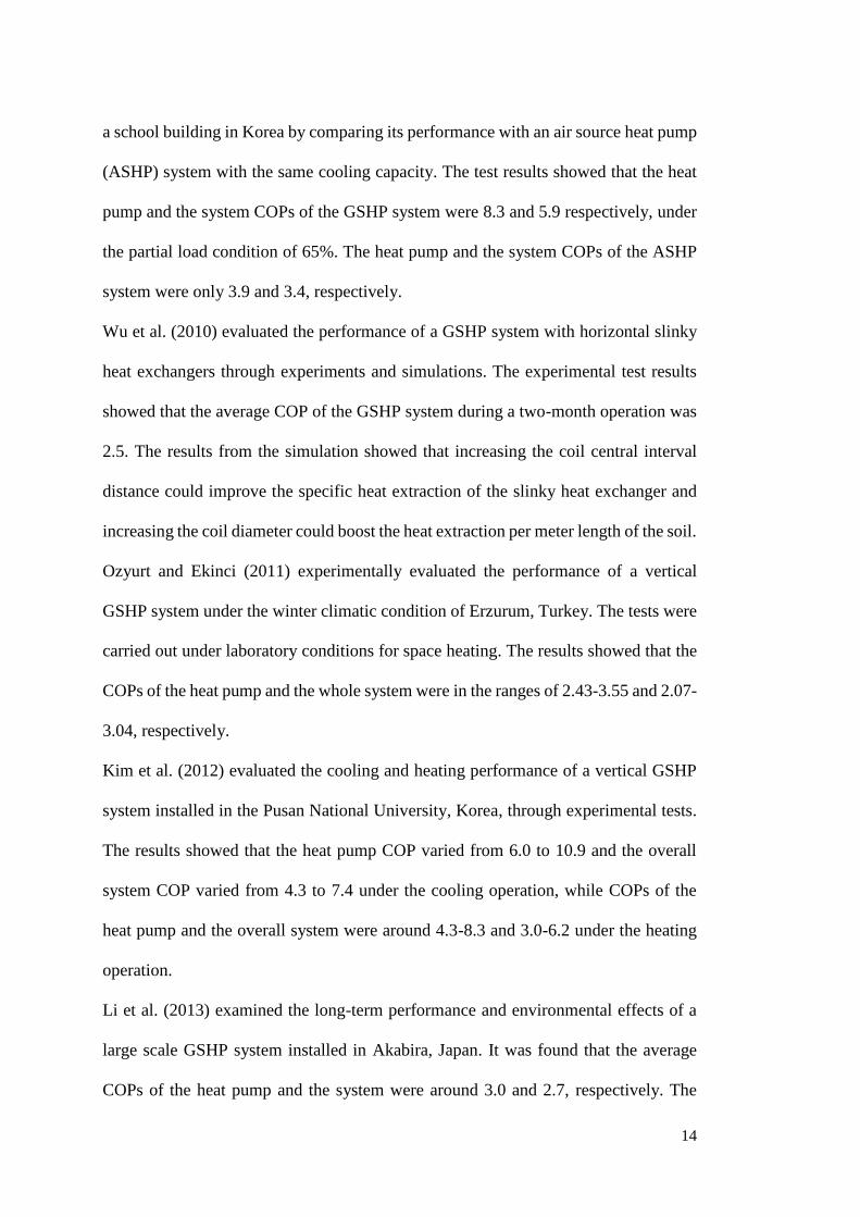
materials (PCMs) and photovoltaic thermal collectors (PVT) have also been used to

be coupled with GSHP systems.

2.1.3.1 Cooling tower assisted GSHP systems

In a cooling tower assisted GSHP system, cooling tower can be connected with GSHP

systems with either serial configuration or parallel configuration, as illustrated in Fig.

2.2 (Park et al., 2013).

16

a) serial configuration b) parallel configuration

Fig. 2.2 Schematic of the cooling tower assisted GSHP systems (Park et al., 2013).

The ASHRAE manual (ASHRAE, 1995) first discussed the advantages of using

cooling tower assisted GSHP systems for cooling dominated buildings considering the

initial costs and the available ground area for the installation of GHEs.

Kavanaugh and Rafferty (1997) discussed the possibility of a HGSHP with a fluid

cooler as an auxiliary cooling system. Kavanaugh (1998) then proposed an improved

design method to size fluid coolers and cooling towers in HGSHP systems.

Man et al.(2008, 2010b) analysed the heat transfer process of a cooling tower assisted

GSHP system and developed a practical hourly simulation model for such systems

based on the analysis results. The optimal HGSHP system for the case study building

was then determined based on the hourly simulation using the simulation model

developed.

The energy performance of a cooling tower assisted GSHP system with both parallel

and serial configurations was experimentally evaluated by Park et al. (2013), under

various leaving fluid temperatures of the GHE and fluid flow rates in the auxiliary

loop, respectively. The results showed that the COPs of this HGSHP with parallel and

17

serial configurations were 18% and 6% respectively, higher than that of a stand-alone

GSHP system.

Lee et al. (2014) investigated the transient characteristics of a cooling tower assisted

GSHP system through experimental tests. The results showed that the performance

enhancement of this system was highly dependent on the leaving water temperature

set-point of the GHE. The COP of this HGSHP system at the optimal set-point

temperature of 30 oC was 7.2% higher than that of a stand-alone GSHP system.

Zhou et al. (2016) developed a simulation system for a cooling tower assisted GSHP

with both parallel and serial configurations in TRNSYS. The 30 years’ operation of

the system under different operation schemes was simulated. The results showed that

activating the cooling tower during the transition seasons when the temperature

difference between the air wet-bulb temperature and the ground temperature was 8-12

oC can provide the highest benefits of using this HGSHP system.

A number of studies (Yavuzturk and Spitler, 2000, Zhang et al., 2015, Sagia and

Rakopoulos, 2012, Man et al., 2010b) evaluated and compared the performance of

several traditional control strategies used for cooling tower assisted GSHP systems,

which could be broadly categorised into three groups: 1) to activate the cooling tower

based on the temperature set-point of the heat pump entering/exiting fluid; 2) to

activate the cooling tower based on the temperature difference between the heat pump

entering/exiting fluid temperature and the ambient air dry-bulb/wet-bulb temperature;

and 3) to activate the cooling tower during a fixed time period. The results from these

studies suggested that control strategies with longer operation hours of cooling towers

provided more benefits than those with less operation hours, and the control strategy

based on the difference between the heat pump exiting fluid temperature and the air

wet-bulb temperature outperformed the others.

18

Yang et al. (2014) investigated three intermittent operation strategies for a HGSHP

system with double-cooling towers to solve the problem of the underground heat

accumulation. The three operation strategies activated the cooling towers and the GHE

at different time periods in a week. The optimal intermittent operating condition was

then identified through an economic analysis.

2.1.3.2 Solar assisted GSHP systems

Solar thermal collector is the most commonly used auxiliary heat absorber in HGSHP

systems for heating-dominated applications. Solar thermal collectors can be coupled

with GSHP systems in different approaches. For instance, in a solar assisted GSHP

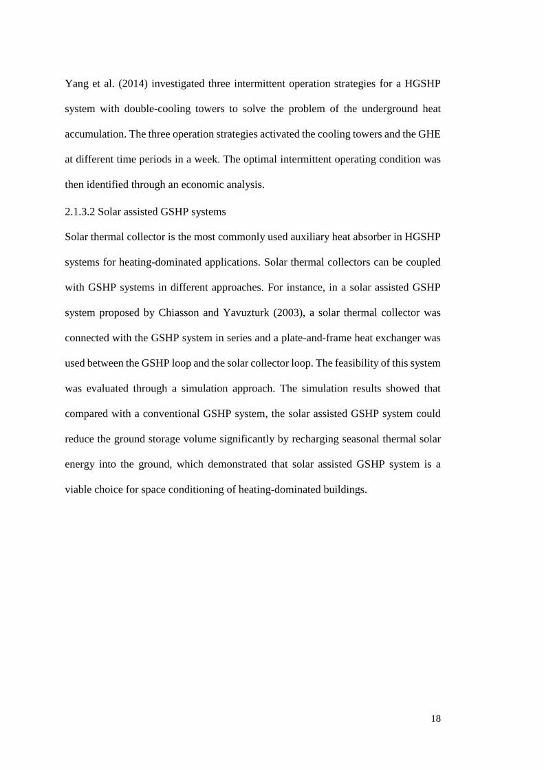
system proposed by Chiasson and Yavuzturk (2003), a solar thermal collector was

connected with the GSHP system in series and a plate-and-frame heat exchanger was

used between the GSHP loop and the solar collector loop. The feasibility of this system

was evaluated through a simulation approach. The simulation results showed that

compared with a conventional GSHP system, the solar assisted GSHP system could

reduce the ground storage volume significantly by recharging seasonal thermal solar

energy into the ground, which demonstrated that solar assisted GSHP system is a

viable choice for space conditioning of heating-dominated buildings.

19

Fig. 2.3 Schematic of the solar assisted GSHP system proposed by Chiasson and

Yavuzturk (2003).

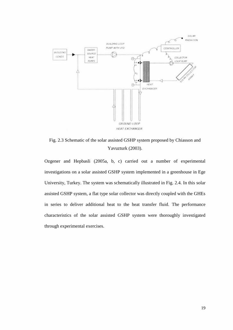
Ozgener and Hepbasli (2005a, b, c) carried out a number of experimental

investigations on a solar assisted GSHP system implemented in a greenhouse in Ege

University, Turkey. The system was schematically illustrated in Fig. 2.4. In this solar

assisted GSHP system, a flat type solar collector was directly coupled with the GHEs

in series to deliver additional heat to the heat transfer fluid. The performance

characteristics of the solar assisted GSHP system were thoroughly investigated

through experimental exercises.

20

Fig. 2.4 Schematic of the solar assisted GSHP system for greenhouse heating

(Ozgener and Hepbasli, 2005b).

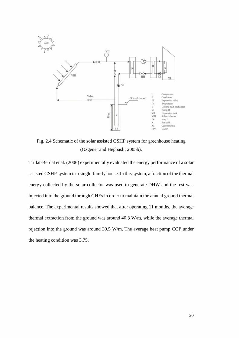
Trillat-Berdal et al. (2006) experimentally evaluated the energy performance of a solar

assisted GSHP system in a single-family house. In this system, a fraction of the thermal

energy collected by the solar collector was used to generate DHW and the rest was

injected into the ground through GHEs in order to maintain the annual ground thermal

balance. The experimental results showed that after operating 11 months, the average

thermal extraction from the ground was around 40.3 W/m, while the average thermal

rejection into the ground was around 39.5 W/m. The average heat pump COP under

the heating condition was 3.75.

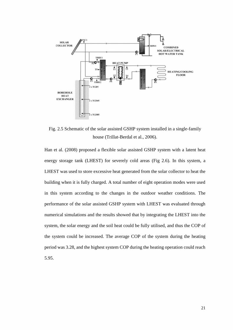
https://www.sciencedirect.com/topics/earth-and-planetary-sciences/greenhouses

21

Fig. 2.5 Schematic of the solar assisted GSHP system installed in a single-family

house (Trillat-Berdal et al., 2006).

Han et al. (2008) proposed a flexible solar assisted GSHP system with a latent heat

energy storage tank (LHEST) for severely cold areas (Fig 2.6). In this system, a

LHEST was used to store excessive heat generated from the solar collector to heat the

building when it is fully charged. A total number of eight operation modes were used

in this system according to the changes in the outdoor weather conditions. The

performance of the solar assisted GSHP system with LHEST was evaluated through

numerical simulations and the results showed that by integrating the LHEST into the

system, the solar energy and the soil heat could be fully utilised, and thus the COP of

the system could be increased. The average COP of the system during the heating

period was 3.28, and the highest system COP during the heating operation could reach

5.95.

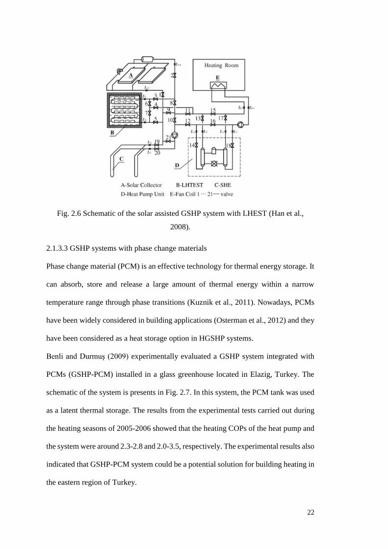
22

Fig. 2.6 Schematic of the solar assisted GSHP system with LHEST (Han et al.,

2008).

2.1.3.3 GSHP systems with phase change materials

Phase change material (PCM) is an effective technology for thermal energy storage. It

can absorb, store and release a large amount of thermal energy within a narrow

temperature range through phase transitions (Kuznik et al., 2011). Nowadays, PCMs

have been widely considered in building applications (Osterman et al., 2012) and they

have been considered as a heat storage option in HGSHP systems.

Benli and Durmuş (2009) experimentally evaluated a GSHP system integrated with

PCMs (GSHP-PCM) installed in a glass greenhouse located in Elazig, Turkey. The

schematic of the system is presents in Fig. 2.7. In this system, the PCM tank was used

as a latent thermal storage. The results from the experimental tests carried out during

the heating seasons of 2005-2006 showed that the heating COPs of the heat pump and

the system were around 2.3-2.8 and 2.0-3.5, respectively. The experimental results also

indicated that GSHP-PCM system could be a potential solution for building heating in

the eastern region of Turkey.

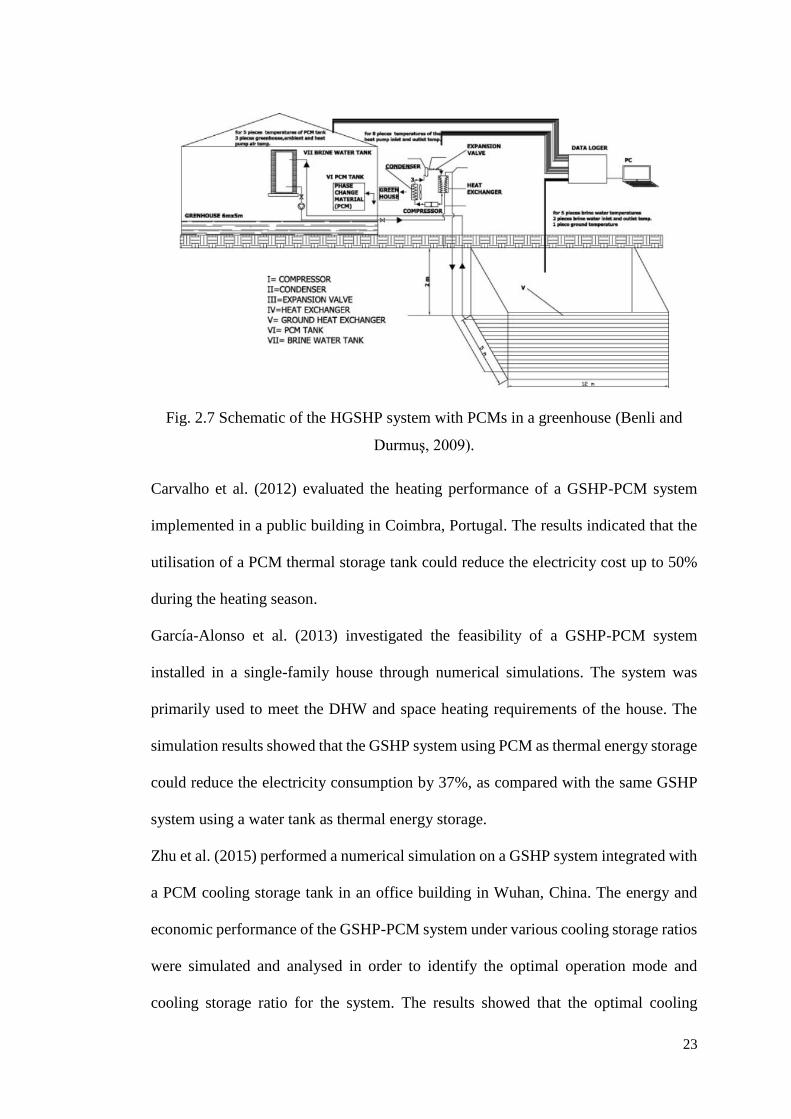
23

Fig. 2.7 Schematic of the HGSHP system with PCMs in a greenhouse (Benli and

Durmuş, 2009).

Carvalho et al. (2012) evaluated the heating performance of a GSHP-PCM system

implemented in a public building in Coimbra, Portugal. The results indicated that the

utilisation of a PCM thermal storage tank could reduce the electricity cost up to 50%

during the heating season.

García-Alonso et al. (2013) investigated the feasibility of a GSHP-PCM system

installed in a single-family house through numerical simulations. The system was

primarily used to meet the DHW and space heating requirements of the house. The

simulation results showed that the GSHP system using PCM as thermal energy storage

could reduce the electricity consumption by 37%, as compared with the same GSHP

system using a water tank as thermal energy storage.

Zhu et al. (2015) performed a numerical simulation on a GSHP system integrated with

a PCM cooling storage tank in an office building in Wuhan, China. The energy and

economic performance of the GSHP-PCM system under various cooling storage ratios

were simulated and analysed in order to identify the optimal operation mode and

cooling storage ratio for the system. The results showed that the optimal cooling

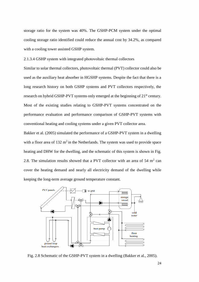
24

storage ratio for the system was 40%. The GSHP-PCM system under the optimal

cooling storage ratio identified could reduce the annual cost by 34.2%, as compared

with a cooling tower assisted GSHP system.

2.1.3.4 GSHP system with integrated photovoltaic thermal collectors

Similar to solar thermal collectors, photovoltaic thermal (PVT) collector could also be

used as the auxiliary heat absorber in HGSHP systems. Despite the fact that there is a

long research history on both GSHP systems and PVT collectors respectively, the

research on hybrid GSHP-PVT systems only emerged at the beginning of 21st century.

Most of the existing studies relating to GSHP-PVT systems concentrated on the

performance evaluation and performance comparison of GSHP-PVT systems with

conventional heating and cooling systems under a given PVT collector area.

Bakker et al. (2005) simulated the performance of a GSHP-PVT system in a dwelling

with a floor area of 132 m2 in the Netherlands. The system was used to provide space

heating and DHW for the dwelling, and the schematic of this system is shown in Fig.

2.8. The simulation results showed that a PVT collector with an area of 54 m2 can

cover the heating demand and nearly all electricity demand of the dwelling while

keeping the long-term average ground temperature constant.

Fig. 2.8 Schematic of the GSHP-PVT system in a dwelling (Bakker et al., 2005).

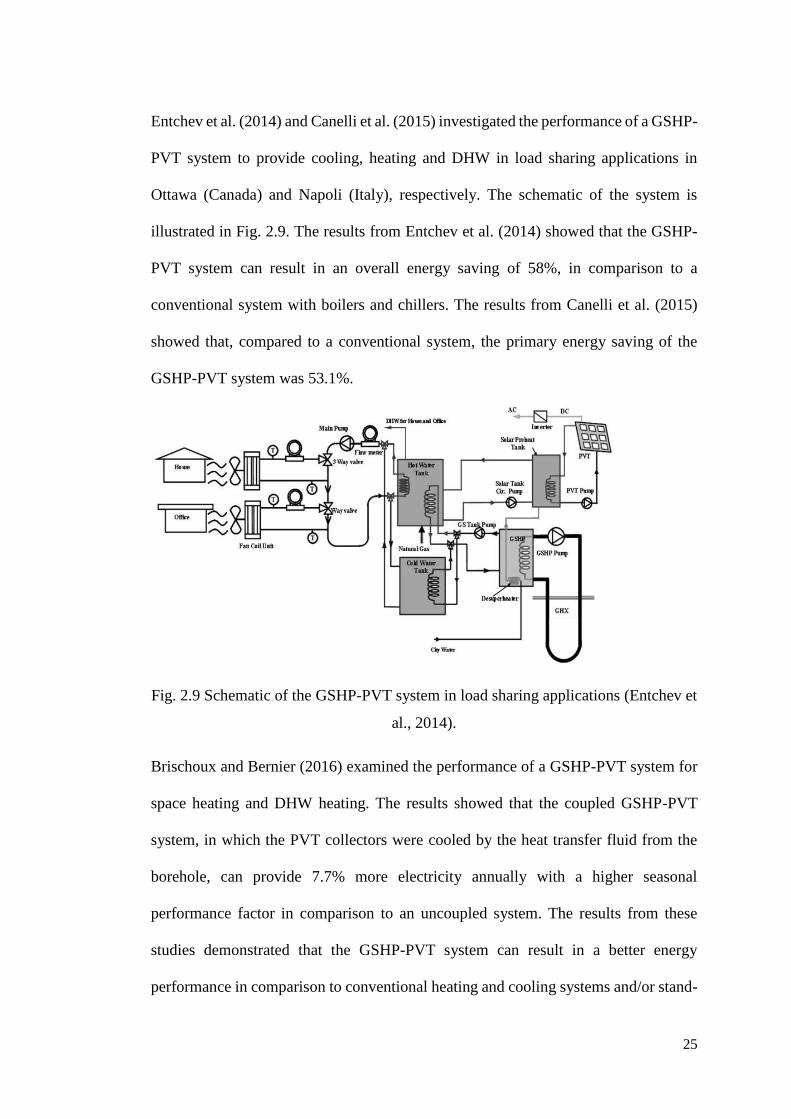
25

Entchev et al. (2014) and Canelli et al. (2015) investigated the performance of a GSHP-

PVT system to provide cooling, heating and DHW in load sharing applications in

Ottawa (Canada) and Napoli (Italy), respectively. The schematic of the system is

illustrated in Fig. 2.9. The results from Entchev et al. (2014) showed that the GSHP-

PVT system can result in an overall energy saving of 58%, in comparison to a

conventional system with boilers and chillers. The results from Canelli et al. (2015)

showed that, compared to a conventional system, the primary energy saving of the

GSHP-PVT system was 53.1%.

Fig. 2.9 Schematic of the GSHP-PVT system in load sharing applications (Entchev et

al., 2014).

Brischoux and Bernier (2016) examined the performance of a GSHP-PVT system for

space heating and DHW heating. The results showed that the coupled GSHP-PVT

system, in which the PVT collectors were cooled by the heat transfer fluid from the

borehole, can provide 7.7% more electricity annually with a higher seasonal

performance factor in comparison to an uncoupled system. The results from these

studies demonstrated that the GSHP-PVT system can result in a better energy

performance in comparison to conventional heating and cooling systems and/or stand-

26

alone GSHP systems. However, the results from these studies were highly dependent

on the size of the PVT collector used. Bertram et al. (2012) investigated the key design

parameters, such as location, wind velocity, size of PVT collectors and total GHE

length, on the energy performance of a hybrid GSHP system with unglazed PVT

collectors. Entchev et al. (2016) proposed an artificial neural network (ANN)-based

method to control a GSHP-PVT system in a single house located in Ottawa (Canada).

The results showed that the ANN-based strategy can reduce the primary energy

consumption and carbon dioxide equivalent emissions by up to 36%, and reduce the

operating cost by up to 81% when compared to a conventional on-off control.

Putrayudha et al. (2015) developed a fuzzy logic controller to minimise the energy

consumption of a GSHP-PVT system in a single residential house in Incheon, South

Korea. The results showed that this fuzzy logic controller was able to reduce the annual

energy consumption by 18.3% in comparison to a conventional on-off control.

Most of the existing studies on GSHP systems were focused on the modelling and

performance evaluation of different GSHP systems. The results demonstrated the

feasibility of GSHP systems under various climate conditions and provided the

fundamental theories and references for the design and control optimisation of GSHP

systems.

2.2 General optimisation problem of GSHP systems

Optimisation is the discipline to find one or more feasible solutions that can result in

the extreme value of one or more objectives subjected to certain constraints (Pardalos

and Resende, 2001). The key issues related to the development and formulation of an

optimisation strategy of GSHP systems include a) Definition of the objective function;

b) Determination of the key variables to be optimised and the corresponding

27

constraints; c) Determination of the methods to be used to formulate the optimisation

problem; and d) Selection of an appropriate optimisation technique if model-based

methods are used. For different types of GSHP systems, the design and control

problems could be significantly different.

2.2.1 Optimisation objective functions

For a given optimisation problem, the definition of an appropriate optimisation

objective function is important because it directly affects the optimisation results.

According to the number of objective functions used to formulate the optimisation

problem, the optimisation of GSHP systems can be divided into single-objective

optimisation and multi-objective optimisation.

2.2.1.1 Single-objective optimisation

The general single-objective optimisation problem can be described as (Aravelli, 2014)

finding 1 2, ,...T

nX x x x= which minimises or maximises the objective function f(X)

Subject to (l) (u)

i i ix x x i=1,2,…m

( ) 0,jg X j=1,2,…n (2.1)

( ) 0,kh X = k=1,2,…p

where xi is the optimisation decision variable, gj(X) and hk(X) are the optimisation

constraints, and (l)

ix and (u)

ix denote the lower and upper bounds on xi.

The objective functions used in the optimisation studies of GSHP systems can be

categorised into two major groups, i.e., economic and thermodynamic.

Thermodynamic objective function

The thermodynamic objective based on the first or second law of thermodynamics is

usually used for the energy performance of heat pump systems. One of the major

thermodynamic objectives used in the optimisation of GSHP systems is the system

28

irreversibility, which can be presented in terms of exergy destruction or entropy

generation. This objective aims at identifying the place where inefficiencies occur, so

that the performance of the system can be improved. This objective can be denoted by

the following simplified equation (Cornelissen, 1997):

total kI I= (2.2)

where, Itotal is the total exergy destruction or irreversibility, and Ik is the exergy

destruction of each component in a GSHP system.

Another well-known thermodynamic objective is the coefficient of performance

(COP), which normally denotes the efficiency of heat pumps and refrigeration systems.

COP is a ratio of the useful heating or cooling energy provided (Q) by the system to

the energy consumption (W) of the system, as expressed in Eq. (2.3).

QCOP

W= (2.3)

There are also other thermodynamic objectives that have been used in the design and

control of GSHP systems such as the system performance factor (Montagud et al.,

2014), relative performance loss (RPL) (Gultekin et al., 2014), and energy

extraction/dissipation rates (Rezaei-Bazkiaei et al., 2013).

Economic objective function

The optimisation based on economic objectives aims at minimising the power

consumption or the overall cost of the system, which brings financial benefits for the

investors and users.

In recent decades, the total cost or life cycle cost, which comprises the all costs arising

from installation, operation, maintenance and disposition over a fixed period of time

is often used as the objective function in the design optimisation of GSHP systems

instead of simple initial cost (Asiedu and Gu, 1998). There are a number of metrics

29

which can represent the total cost of a GSHP system. In literature (Sayyaadi et al.,

2009), the annual total revenue requirement (TRR, total product cost) was introduced

as the optimisation objective, which can be denoted by Eq. (2.4):

P elec kC Z Z= + (2.4)

where, PC represents the annual total revenue requirement, elecZ is the levelized cost

rate of the expenditures for the electricity supplied to the whole system, and kZ

represents the cost rate associated with the capital investment, operating and

maintenance expenses.

In another optimisation study (Sanaye and Niroomand, 2009), an objective function,

named the total annual cost (TAC), was used and defined as:

El invTAC C C= + (2.5)

where, CEI is the annual cost of the power consumption, and Cinv is the initial

investment cost for the annual system operation.

The economic objectives used in the control of GSHP systems are relatively simple,

since the system has already been installed and therefore no initial cost needs to be

considered. The total energy consumption and the operational cost of the system are

mostly adopted.

2.2.1.2 Multi-objective optimisation

The general multi-objective optimisation problem can be described as (Aravelli, 2014):

Minimises the objective function f1(X), f2(X),…, fk(X)

Subject to ( ) 0,jg X j=1,2,…n (2.6)

( ) 0,kh X = k=1,2,…p

where 1 2, ,...T

nX x x x= is an n-component design vector.

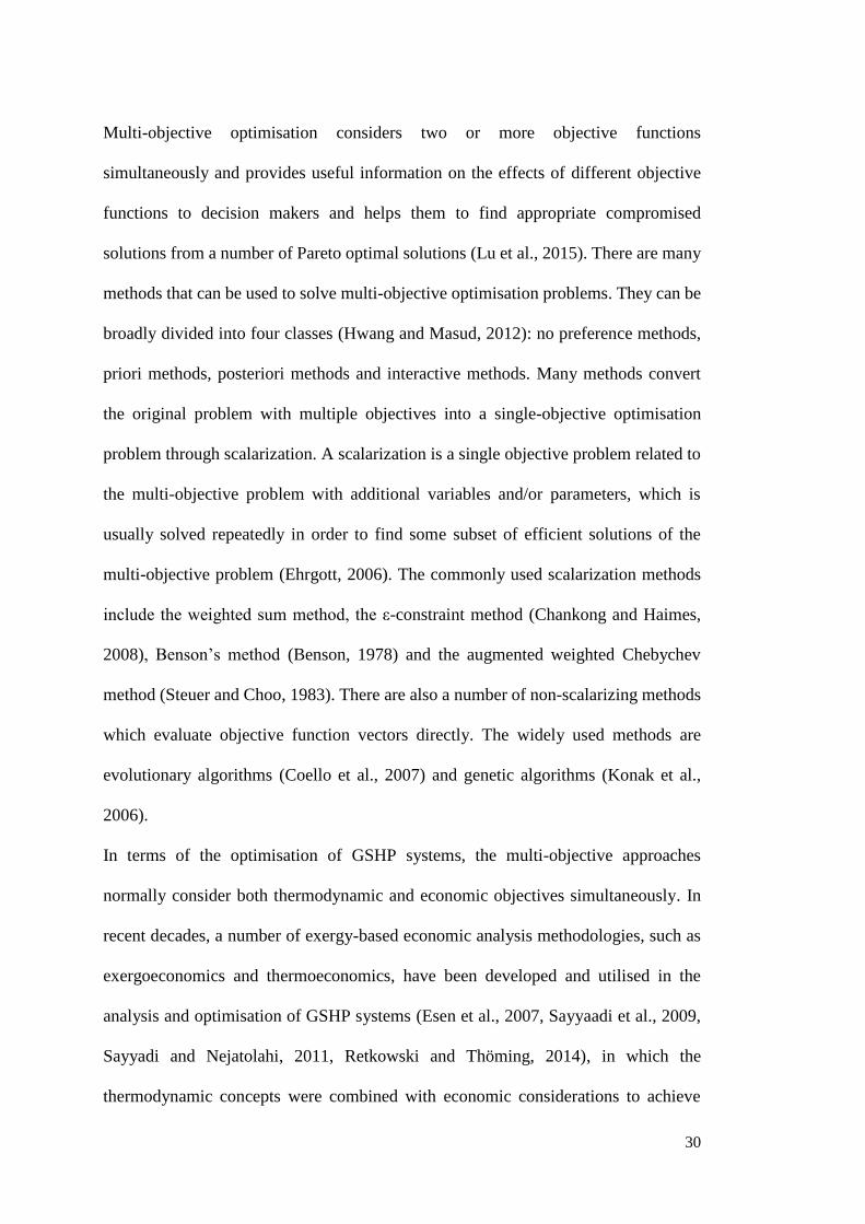
30

Multi-objective optimisation considers two or more objective functions

simultaneously and provides useful information on the effects of different objective

functions to decision makers and helps them to find appropriate compromised

solutions from a number of Pareto optimal solutions (Lu et al., 2015). There are many

methods that can be used to solve multi-objective optimisation problems. They can be

broadly divided into four classes (Hwang and Masud, 2012): no preference methods,

priori methods, posteriori methods and interactive methods. Many methods convert

the original problem with multiple objectives into a single-objective optimisation

problem through scalarization. A scalarization is a single objective problem related to

the multi-objective problem with additional variables and/or parameters, which is

usually solved repeatedly in order to find some subset of efficient solutions of the

multi-objective problem (Ehrgott, 2006). The commonly used scalarization methods

include the weighted sum method, the ε-constraint method (Chankong and Haimes,

2008), Benson’s method (Benson, 1978) and the augmented weighted Chebychev

method (Steuer and Choo, 1983). There are also a number of non-scalarizing methods

which evaluate objective function vectors directly. The widely used methods are

evolutionary algorithms (Coello et al., 2007) and genetic algorithms (Konak et al.,

2006).

In terms of the optimisation of GSHP systems, the multi-objective approaches

normally consider both thermodynamic and economic objectives simultaneously. In

recent decades, a number of exergy-based economic analysis methodologies, such as

exergoeconomics and thermoeconomics, have been developed and utilised in the

analysis and optimisation of GSHP systems (Esen et al., 2007, Sayyaadi et al., 2009,

Sayyadi and Nejatolahi, 2011, Retkowski and Thöming, 2014), in which the

thermodynamic concepts were combined with economic considerations to achieve

31

both thermodynamic and economic objectives.

2.2.2 Optimisation decision variables

For a given optimisation problem, the main procedure is to determine the decision

variables and their optimal values that lead to the minimisation or maximisation of the

objective function. The parameters influencing the thermodynamic and economic

performance of GSHP systems are summarised in Fig. 2.10. They can be classified

into five major groups: soil properties, climate and distribution system parameters,

ground heat exchanger parameters, heat pump parameters and supplementary

heat/cold source parameters. Some of them are controllable and can be optimised,

while some of them are fixed parameters which can only be measured but cannot be

controlled. The controllable and fixed parameters vary in different optimisation cases.

In some cases, especially in the design optimisations, there are normally a large

number of controllable parameters, and it is therefore crucial to determine the key

parameters that have significant influence on the optimisation objective function. The

key parameters will be further optimised through the optimisation process, while those

with a less impact on the objective function will not be optimised.

32

Fig. 2.10 Parameters influencing the performance of GSHPs.

Parameters influencing the performance of (H)GSHPs

Soil properties

*Soil conductivity, density,

diffusivity, temperature

and moisture

*Grout material properties

*Ground water movement

Climate and

distribution system

*Ambient air temperature,

humidity, wind speed

*Indoor temperature

set-point

*Distribution pipe network

size

*Water pump size

Ground heat

exchanger (GHE)

*GHE inlet/outlet fluid

temperature and flow rate

*U-tube type, diameter and

conductivity

*Borehole diameter, depth,

resistance and distance

*Half shank space

Heat pump unit

*Condenser inlet/outlet fluid


*Condenser pressure

*Evaporator inlet/outlet fluid


*Evaporator pressure

*Compressor efficiency

*Mass flow rate of refrigerant

*Type & number of heat pump

Supplementary

heat/cold source

*Type and Capacity

*Connection and

distribution method

*Inlet/outlet fluid


*Type of working fluid

33

2.2.3 Optimisation methods

For a particular optimisation problem, the optimisation framework can be formulated

based on the objective function, the key variables and constraints identified. The

selection of appropriate optimisation methods plays a critical role in developing a

robust and effective optimisation strategy. For a specific optimisation problem, there

always exist several available optimisation methods. These methods often have

different characteristics and structures, and each of them has advantages over others

in one or a few aspects (Wang and Ma, 2008).

2.2.3.1 Optimal design methods for GSHP systems

The currently most used design methods for GSHP systems are still rules-of-thumb

design methods, which are primarily acquired from practical engineering experience

based on several simplifications and assumptions. Such approaches are relatively easy

to be implemented and can help installers with minimal training and knowledge to

solve some design problems of GSHP systems. However, rules-of-thumb design

methods sometimes result in oversized or undersized systems, and they are less

effective in the design of complex multi-functional GSHP systems, due to their

limitations in analysing the system performance to the changes of design parameters

and the interactions among different design parameters.

Nowadays, GSHP systems are designed to satisfy different requirements for buildings

and the integration of other energy systems with GSHP systems made the optimisation

problems becoming even more complex. These all brought challenges for the optimal

design of GSHP systems. Therefore, more systematic model-based design methods

have been developed, which require a number of performance models to capture the

dynamic heat transfer process and to predict the performance of the system with

different design parameters. Based on the type of the models used, the model-based

34

design methods can be categorised into two: the analytical model-based methods, and

the numerical model-based methods.

The analytical model-based methods use mass, energy, entropy and exergy balance

equations representing the heat transfer process to analyse the system performance and

find the optimal solution of the design problem. The design methods usually optimise

the design parameters by minimising the entropy generation during the heat transfer

process (Marzbanrad et al., 2007, Kord and Jazayeri, 2012, Li and Lai, 2013, Huang

et al., 2014). The numerical model-based design methods usually determine the design

parameters by means of numerical computations and with the help of simulation

programs (Kjellsson et al., 2010, Khalajzadeh et al., 2011, Gultekin et al., 2014).

The use of analytical models can lead to the exact solutions of the design problems,

which are suitable for the investigation of the system performance with varying design

parameters. However, sometimes the system performance is hard to be completely

represented in the form of the mathematical expressions, or sometimes the

mathematical expressions are too complicated, especially in hybrid GSHP systems.

The numerical models are therefore developed to solve the design problems where

analytical solutions are not available or mathematical process is difficult. Numerical

methods are capable of handling large systems, different degrees of nonlinearities, and

are more flexible than analytical methods.

2.2.3.2 Optimal control methods for GSHP systems

Model-based control methods

The model-based control methods are currently the most effective and preferable

approach (Atam and Helsen, 2016). They are capable of finding the optimal control

settings and are able to solve different control optimisation problems by using various

degrees of models and approaches. The tools required to realise the control strategy

35

are the system and/or component models and optimisation techniques. The models are

used as emulators to predict the system energy or cost performance and the system

response to the changes of control settings. The function of the optimisation techniques

is to find the most cost effective or energy efficient control settings to minimise the

system energy consumption or operating cost. According to the types of models used

to formulate the control strategy, the model-based control methods can be divided into

physical/semi-physical model-based control and black-box model-based control.

In the physical/semi-physical model-based control methods, physical models or semi-

physical models are utilised in the control strategy to predict the system performance.

Physical models formulated by a set of mathematical equations that describe the

fundamental laws and physical process of energy, mass, heat transfer and balance, etc.

The parameters used in the mathematical equations usually have physical meanings.

The physical models are in general have a high prediction accuracy and a high control

reliability within their operating conditions. A semi-physical model simplifies the

physical process based on a physical model to certain extent, so that the model

structure becomes less complicated and the computational cost can be manageable.

However, semi-physical models generally need a large dataset to train the model

parameters in order to achieve desirable predictions.

In the black-box model-based control methods, black-box models are used to predict

the system energy or cost performance. These models do not require any detailed

knowledge on the physical process or the working principle of the system of concern.

They are able to relate input variables with output variables using pre-programmed

logics. The parameters in these models have no physical significance. However, these

models require extensive training data to ensure the reliable performance prediction

and they are only accurate and reliable within the range of the training data covered.

36

Performance map-based control methods

The performance map-based control methods use the performance map generated from

the detailed simulations or extensive performance tests of the targeted system over a

significant range of settings or operation conditions. The performance map is then

utilised to find the optimal control settings of the system.

The performance map-based control methods could be practical and effective in the

control of relatively small and simple GSHP systems. However, it is impractical to

apply them to control large and complicated systems since generating performance

maps requires extensive work, and they can be only used for the control of specific

system under the working conditions the performance maps cover.

Model-free control methods

Model-free control methods do not require a specific model of the system to be

controlled but still require a relation between control inputs and controlled outputs,

which made them more complicated than rule-based control methods but simpler than

model-based methods.

The only model-free control method that has been utilised in the control of GSHP

systems is the extremum seeking control (ESC) (Hu et al., 2014, 2016). ESC aims to

design an extremum seeking controller that uses measurements to dynamically search

for the optimum inputs (Nesic, 2009). In this method, the optimal control is realised

online by minimising an objective function through the analysis of the relationship

between control inputs Uopt and controlled outputs f(t,u ) (Hu et al., 2014, 2016):

arg min (t, u)optu f= (2.7)

ESC is a relatively new control method in the control optimisation of GSHP systems,

but it has proven to be an effective approach to achieving near optimal solution (Hu et

al., 2016). Since there are only few studies that used model-free methods in the control

37

of GSHP systems, it is difficult to comment on the effectiveness of these methods

compared to other types of control methods.

2.2.4 Optimisation techniques

The optimisation problems related to the optimal design and control of GSHP systems

often have the characteristics of nonlinear, dynamic and highly restricted by a number

of constraints. An optimisation technique is therefore essential to identify the optimal

solution of the complex optimisation problem. For a given optimisation problem, there

always exist several optimisation techniques, with different structures and

characteristics. Each is superior to others in one or more aspects. To date, different

types of optimisation techniques have been used in the design and control optimisation

of GSHP systems. Among them, the most commonly used techniques include Nelder–

Mead method (Sanaye and Niroomand, 2010, Shi et al., 2014, Sanaye and Niroomand,

2009), response surface method (Khalajzadeh et al., 2011, Park et al., 2010), dynamic

programming (De Ridder et al., 2011, Atam et al., 2016), evolutionary algorithms and

genetic algorithms (Sayyaadi et al., 2009, Sanaye and Niroomand, 2009, Neugebauer

and Sołowiej, 2012, Sayyadi and Nejatolahi, 2011, Rezaei-Bazkiaei et al., 2013,

Huang et al., 2015, Pu et al., 2017).

2.2.5 General design and control optimisation procedures of GSHP systems

Although rule-based design methods are commonly used in sizing GSHP systems, they

can hardly be regarded as “optimal” methods, since such methods have limitations in

analysing the system performance to the changes of design parameters and the

interactions among different design parameters. The rule-based design methods are

normally used to size the major components of GSHP systems, such as the GHEs and

the heat pump, rather than the whole system. The results obtained using rule-based

38

design methods are normally not the global optimal solutions to the design problem.

Most of the current design optimisation strategies developed for GSHP systems used

various performance models to capture the dynamic performance of the system to the

changes of different design parameters. The general model-based design optimisation

procedure of GSHP systems is summarised and shown in Fig. 2.11. The design

optimisation problem can be either single-objective or multi-objective. Since the

determination of the key design parameters is crucial for the design optimisation of

GSHP systems, sensitivity analysis was generally performed in a number of design

optimisation strategies to identify the key design parameters.

Fig. 2.11 General model-based design optimisation procedure of GSHP systems.

Based on the review of existing studies on the control optimisation of GSHP systems,

Optimisation

execution

Optimisationpreparation

Single-objective Multi-objective

scalarization methods

non-scalarizing methods

Determination of the key design

parameters (Sensitivity analysis)

Development of system

performance models

Selection of optimisation

method and technique

Determination of optimisationobjective function(s)

Performance prediction models

Objective function

Key design parameters

Single-objective optimiser

Generation of simulation scenarios

Optimisationconstraints

Scalarizing multiple objectives into single objective

Performance prediction models

Objective functions


Multi-objective optimiser


Optimisationconstraints

Pareto-optimal solutions

Decision making process

Optimal values of the key design parameters

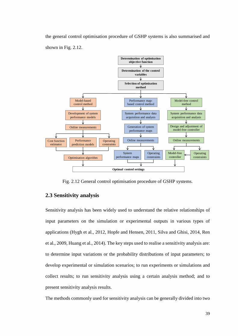
39

the general control optimisation procedure of GSHP systems is also summarised and

shown in Fig. 2.12.

Fig. 2.12 General control optimisation procedure of GSHP systems.

2.3 Sensitivity analysis

Sensitivity analysis has been widely used to understand the relative relationships of

input parameters on the simulation or experimental outputs in various types of

applications (Hygh et al., 2012, Hopfe and Hensen, 2011, Silva and Ghisi, 2014, Ren

et al., 2009, Huang et al., 2014). The key steps used to realise a sensitivity analysis are:

to determine input variations or the probability distributions of input parameters; to

develop experimental or simulation scenarios; to run experiments or simulations and

collect results; to run sensitivity analysis using a certain analysis method; and to

present sensitivity analysis results.

The methods commonly used for sensitivity analysis can be generally divided into two

Model-based control method

Performance map-based control method

Model-free control method

Determination of the control

variables

Determination of optimisationobjective function

Selection of optimisation

method

Development of system

performance models

Generation of system

performance mapsOnline measurements

Performance

prediction modelsCost function

estimatorOperatingconstraints

Optimisation algorithm

Online measurements

Optimal control settings

System performance data

acquisition and analysis

System

performance maps

Design and adjustment of model-free controller

Online measurements

Model-free

controller

System performance data

acquisition and analysis

Operating

constraints

Operating

constraints

40

major groups: local methods and global methods. Local sensitivity analysis focuses on

the effects of inputs on a certain point or a base case, while global sensitivity analysis

focuses more on the effects of inputs over the whole input space (Mara and Tarantola,

2008). Local sensitivity analysis is relatively simple with low computational demand,

but less reliable compared to global sensitivity analysis. There are a number of

branches in the global sensitivity analysis: regression methods, screening-based

methods, variance-based methods and meta-modelling methods. The characteristics of

these methods are summarised in Table 2.1 (Tian, 2013).

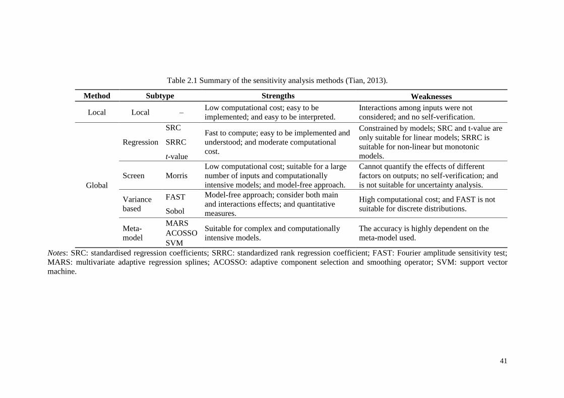
41

Table 2.1 Summary of the sensitivity analysis methods (Tian, 2013).

Method Subtype Strengths Weaknesses

Local Local – Low computational cost; easy to be

implemented; and easy to be interpreted.

Interactions among inputs were not

considered; and no self-verification.

Global

Regression

SRC Fast to compute; easy to be implemented and

understood; and moderate computational

cost.

Constrained by models; SRC and t-value are

only suitable for linear models; SRRC is

suitable for non-linear but monotonic

models.

SRRC

t-value

Screen Morris

Low computational cost; suitable for a large

number of inputs and computationally

intensive models; and model-free approach.

Cannot quantify the effects of different

factors on outputs; no self-verification; and

is not suitable for uncertainty analysis.

Variance

based

FAST Model-free approach; consider both main

and interactions effects; and quantitative

measures.

High computational cost; and FAST is not

suitable for discrete distributions. Sobol

Meta-

model

MARS Suitable for complex and computationally

intensive models.

The accuracy is highly dependent on the

meta-model used. ACOSSO

SVM

Notes: SRC: standardised regression coefficients; SRRC: standardized rank regression coefficient; FAST: Fourier amplitude sensitivity test;

MARS: multivariate adaptive regression splines; ACOSSO: adaptive component selection and smoothing operator; SVM: support vector

machine.

42

As there are a large number of variables that affect the performance of GSHP systems,

sensitivity analysis was used to determine the key variables in a number of studies for

performance analysis and optimal design of GSHP systems. For instance, Corberan et

al. (2011) examined the sensitivity of a GSHP system to different control temperature

set-points using a quasi-steady state mathematical model. The results showed that the

most influential factor to the system power consumption was the building space

temperature set-point. The building return water temperature set-point was less

influential than the space air temperature, and the building water return bandwidth had

almost a negligible effect on the compressor power consumption. Casasso and Sethi

(2014) undertook a sensitivity analysis to investigate the most influential parameters

on the performance of GSHP systems through simulations. The ground heat exchanger

(GHE) design parameters and the physical parameters of the soil were studied. The

results demonstrated that the length of the GHE was the most important parameter in

the design of GSHP systems, followed by the heat carrier fluid, pipe spacing and grout

material. Hong et al. (2016) conducted a sensitivity analysis of the impact factors of

GSHP systems in terms of energy performance and environmental impact. The results

showed that from the perspective of energy performance, the borehole length was

found to be the most influential impact factor, while the U-tube spacing was found to

be the least influential impact factor. Robert and Gosselin (2014) developed a method

to size the GSHP systems by minimising the total cost of the project and performed a

sensitivity analysis to determine the most influential design variables on the total cost.

The results showed that the number of boreholes and the borehole depth were the two

most influential parameters on the total cost, followed by the distance between

boreholes. Huang et al. (2014, 2015) utilised a global sensitivity analysis to determine

the most influential design parameters of vertical GHEs to facilitate the optimal design

43

of vertical GHEs. The results demonstrated that the circulating fluid mass flow rate,

borehole number, borehole depth, pipe outer radius and borehole radius were the

sensitive design parameters, which were used as the decision variables and optimised

in the optimisation process. Pu et al. (2017) also developed a design strategy to

optimise the design parameters of GHEs. In this strategy, a sensitivity analysis was

used to investigate the relative impacts of the design parameters on two performance

indicators, i.e. the entropy generation number and the integrated evaluation factor

(integrative performance factor that considers the effect of both overall heat transfer

coefficient and pressure drop). The results from the sensitivity analysis showed that

the GHE inlet fluid temperature was the most influential design parameter on the

entropy generation number and had no impact on the integrated evaluation factor. The

GHE inlet fluid flow velocity had a limited impact on the entropy generation number

but with a great impact on the integrated evaluation factor. The U-tube diameter and

pipe spacing had moderate impacts on both performance indicators. In recent years, a

group of studies (Sivasakthivel et al., 2014a, Sivasakthivel et al., 2014b, Esen and

Turgut, 2015, Verma and Murugesan, 2014) utilised the Taguchi method to formulate

design optimisation strategies for GSHP systems. The Taguchi method is originally an

experimental design method that uses orthogonal arrays to help to form a matrix for

the design of experiments and provide guidance on how to obtain maximum

information from a minimum number of experiments. In these strategies, the Taguchi

method was used for the design of experiments and signal-to-noise (SN) ratio and the

analysis of variance (ANOVA) method were used to analyse the experimental results

and identify the optimum design scenarios. The results from these studies

demonstrated that optimal design strategies formulated by using the Taguchi method

were able to identify both the optimal values of design parameters and the relative

44

sensitivities of the design parameters to the optimisation objective function.

The above studies demonstrated that proper use of sensitivity analysis in the

performance investigation and optimisation of GSHP systems could accurately

identify the most influential variables on the objective function and consequently

improve the optimisation efficiency.

2.4 Review of design optimisation for GSHP systems

Research on the design optimisation of GSHP systems started from mid 1990s. Most

of the earlier studies were focused on the development and improvement of

mathematical models of GSHPs to facilitate the system design. For instance,

Rottmayer et al. (1997) developed a U-tube heat exchanger model based on the finite-

difference method which can be used in the design and annual performance simulation

of GSHP systems. Yavuzturk and Spitler (1999) proposed a short time-step non-

dimensional temperature response factor model for vertical GHEs based on a transient

two-dimensional finite volume numerical model. It was implemented as part of a

component model in TRNSYS to facilitate the performance simulation of vertical

GHEs. Kavanaugh et al. (1997, 1998) developed a numerical model of HGSHP

systems and used this model to formulate a design strategy for such systems. Thornton

et al. (1997) proposed a detailed component-based simulation model for GSHP

systems. The model was calibrated by the monitored data collected from a family

housing unit and was implemented in TRNSYS. These earlier publications provided

fundamental theories and some useful tools for the future development of more

systematic optimisation methodologies for GSHP systems.

In the last two decades, a number of systematic model-based optimisation strategies

for the design of GSHP systems have been developed. Recent literatures on the design

45

optimisation of GSHP systems can be generally divided into single-objective

optimisation and multi-objective optimisation.

2.4.1 Single-objective optimisation

2.4.1.1 Thermodynamic objectives

Thermodynamic objective functions were normally used in the optimal design of

GSHP systems, which include the system irreversibility, exergy loss and

entropy/enthalpy generation, and the system COP/EER. Marzbanrad et al. (2007) and

Li and Lai (2013) used the entropy generation rate as the optimisation objective

function to optimise vertical GHEs in GSHP systems. The heat transfer and hydraulics

models of vertical GHEs were developed and a number of simulation exercises were

carried out. The major design parameters were identified through the analysis and

comparison of simulation outcomes. Kord and Jazayeri (2012) conducted an exergy

analysis of a GSHP system with vertical GHEs. The optimal total length of the GHE

and fluid mass flow rate inside the GHE were identified through the minimisation of

the system exergy destruction. Gultekin et al. (2014) investigated the effect of the

distance between vertical boreholes on heat transfer rate per unit borehole length

through a number of simulations. Four different configurations consisting of 2, 3, 5

and 9 boreholes respectively were considered and the 3 and 6 months average heat

transfer rates per unit borehole length of the most critical borehole in these

configurations were compared with each other to determine the optimal borehole

distance. Lanini et al. (2014) evaluated the energetic potential of borehole thermal

energy storage through experimental tests and numerical simulations. The

experimental and simulation results were used to facilitate the design optimisation of

vertical borehole fields with an objective of inter-seasonal heat storage. Most of the

above studies solved the design problem through comparing the system performance

46

with different sets of design parameters without using a specific optimisation

technique. Some useful tools and methods for the design of vertical GHEs were

provided in these studies. However, the results from these studies may not be optimal

because not all possible solutions were considered. Huang et al. (2014) developed an

optimal design strategy for vertical GHEs by using an entropy generation minimisation

method and a genetic algorithm (GA). The key design parameters of vertical GHEs

were first determined using a global sensitivity analysis method and then optimised by

a GA optimisation technique. Neugebauer and Sołowiej (2012) proposed a design

method to determine the minimum install depth and outer diameter of horizontal GHEs

(HGHEs). The unitary heat flux from the ground to HGHE pipe was used as the

objective function and a GA was used as the optimisation technique to facilitate the

optimisation. Esen and Turgut (2015) carried out a design optimisation of GSHP

systems with vertical GHEs. Taguchi method was applied to design the experiments

and analysis of variance (ANOVA) and signal/noise (S/N) ratio were used for

evaluation of the experiment results and identify the optimum design scenarios to

maximise the system COP. Verma and Murugesan (2014) utilised the same

optimisation method and objective function as those used in Esen and Turgut (2015)

to optimise the key design parameters of a solar assisted ground source heat pump

system.

2.4.1.2 Economic objectives

Economic objective functions are also frequently used in the design of GSHP systems,

which include total initial cost, total annual cost and life cycle cost. Ramamoorthy et

al. (2001a) used a system simulation approach to investigate various design

alternatives on the performance of a HGSHP system with a cooling pond as a

supplemental heat rejecter, in order to optimally size the GHEs and the cooling pond.

47

The system life-time cost was used as the objective function to evaluate the

performance of each design alternative. Sanaye and Niroomand (2009) carried out a

thermal-economic design optimisation of a GSHP system with vertical GHEs. The

total annual cost of the GSHP system was used as the objective function. Two

optimisation techniques, i.e. Nelder–Mead method and GA, were adopted to search for

the optimal values of the design parameters. A thermal-economic design optimisation

of a GSHP system with horizontal GHEs was then carried out using the same objective

function and optimisation technique (Sanaye and Niroomand, 2010). Robert and

Gosselin (2014) proposed a new design methodology to determine the optimal number

of boreholes, borehole depth and spacing, and the optimal size of the heat pumps in

GSHP systems, based on total cost minimisation. Park et al. (2011) proposed a method

to determine the optimal total length of GHEs and the optimal control strategy of the

supplemental equipment in HGSHP systems using the response surface method (RSM).

The optimisation results based on the minimisation of total initial costs, total present

value costs and annual energy use were presented, respectively. Each objective

function was considered independently in the optimisation. Zhao et al. (2009)

proposed a design method to optimally size a HGSHP system integrated with solar

collectors. The method was formulated using mathematical models and the constrained

variable metric method. The system annual heating cost was used as the objective

function.

2.4.1.3 Other objectives

Besides the traditional economic and thermodynamic objective functions, other

objective functions were also used in the development of the optimisation strategies.

For instance, Rezaei-Bazkiaei et al. (2013) adopted the reciprocal of the difference

between the ground energy extraction rate and the circulating pump energy

48

consumption rate as the objective function to determine the optimal working fluid

temperature, thickness, position and thermal properties of the intermediate layer of

HGHEs. Bayer et al. (2014) used the annual ground temperature change as the

objective function in an optimisation strategy to size the total vertical GHE fields.

Katsura et al. (2017) used the total heating and cooling loads from GSHPs in response

to an arbitrarily set total GHE length as the optimisation objective and utilised a GA

as the optimisation technique to formulate an optimal design method for a heat

recovery GSHP system (HR-GSHP).

2.4.2 Multi-objective optimisation

Khalajzadeh et al. (2011) carried out a multi-objective optimisation to optimise the

key design parameters of vertical GHEs in a GSHP system using the response surface

(RSM) method to maximise both the heat transfer efficiency and the heat exchanger

efficiency of vertical GHEs. Huang et al. (2015) developed a multi-objective design

optimisation strategy for vertical GHEs to minimise the system upfront cost and

entropy generation number simultaneously. The key design parameters were first

determined via a global sensitivity analysis method, and then optimised using a multi-

objective genetic algorithm (MOGA). A decision-making strategy was then used to

determine the final solution of the multi-objective optimisation problem. Pu et al.

(2017) also proposed a multi-objective design optimisation strategy for vertical GHEs.

This strategy was formulated using Kriging response surface model and a MOGA to

minimise the entropy generation rate and maximise the integrated evaluation factor

simultaneously. The integrated evaluation factor considered the effect of overall heat

transfer coefficient factor and pressure drop factor. Sivasakthivel et al. (2014a)

performed a multi-objective optimisation to optimise the key design parameters of

GSHP systems used for space heating applications. Three objective functions, i.e.

49

GHE length, COP and thermal resistance of GHE, were considered in the optimisation

with the weighting factors of 0.35, 0.35 and 0.3, respectively. Sayyaadi et al. (2009)

developed a multi-objective design optimisation strategy of a GSHP system with

vertical GHEs to minimise both the total exergy destruction and the total cost of the

system. The sensitivities of the optimised system to the interest rate, operating hours

and the cost of electricity were also studied. Sayyaadi and Nejatolahi (2011) further

developed another multi-objective design optimisation strategy for a cooling tower-

assisted GSHP system to minimise the total irreversibility and the total product cost.

12 decision variables were optimised through the optimisation process using a multi-

objective evolutionary algorithm (MOEA). This strategy was evaluated in three design

cases. The sensitivity of the cooling cost for the base case and three optimised systems

to the variation of the interest rate, the annual cooling operating hours, the electricity

price, and the water price were analysed. Retkowski and Thöming (2014) also

developed a design optimisation strategy for GSHP systems with vertical GHEs. The

strategy used a mixed-integer nonlinear programming (MINLP) to formulate the

system mathematical model and used Generalized-Reduced-Gradient-2 algorithm

(GRG2) and an Evolutionary algorithm (EA) as the optimisation techniques to identify

optimal values of the design parameters. Three different objective functions, i.e. total

annual cost of the system, system COP and the ratio of total annual cost to the system

COP, were considered. Zeng et al. (2015, 2016) developed a novel multi-objective

optimisation method to determine the optimal capacity and operation of a hybrid

GSHP system integrated with combined cooling, heating and power system (CCHP-

GSHP). The multi-objective which included the environment objective (i.e. carbon

dioxide emission reduction rate), the economy objective (i.e. annual total cost saving

rate) and the energy objective (i.e. primary energy saving rate), was chosen to evaluate

50

the performance of the CCHP-GSHP system.

From the above review, it can be seen that systematic model-based design methods

have gradually been developed for GSHP systems and the design optimisation focus

has gradually been developed from single-objective to more comprehensive multi-

objective optimisation. The main findings of these design optimisation studies

reviewed are summarised in Table 2.2.

51

Table 2.2 Summary of studies on the design optimisation of GSHP systems.

Optimisation type Optimisation

objectives Optimisation variables

Optimisation

technique Source

Single-

objective

Thermo-

dynamic

Entropy generation rate Borehole depth and mass flow rate inside the GHE. N/A (Marzbanrad et

al., 2007)

Entropy generation rate Borehole depth, U-tube diameter and mass flow rate

inside the GHE. N/A (Li and Lai, 2013)

Exergy destruction Total length of the GHE and fluid mass flow rate

inside the GHE. N/A

(Kord and

Jazayeri, 2012)

Heat transfer rate per

unit borehole length

Distance between boreholes, and borehole field

configuration. N/A

(Gultekin et al.,

2014)

Underground inter-

seasonal heat storage

Overall arrangement of borehole field (relations

between number diameter and depth of boreholes) N/A

(Lanini et al.,

2014)

Entropy generation rate Borehole number, depth and radius, U-tube outer

radius and fluid mass flow rate inside GHEs. GA

(Huang et al.,

2014)

Unitary heat flux from

the ground to pipe Outside diameter and install depth of the HGHE. GA

(Neugebauer and

Sołowiej, 2012)

System COP Borehole depth, inlet/outlet water temperature of

evaporator/condenser.

Taguchi

method

(Esen and Turgut,

2015)

System COP

Thermal conductivity, inner radius of U-tube and

solar collector pipe, borehole depth, specific heat

capacity and flow rate of working fluid, and

reflectivity of glass cover.

Taguchi

method

(Verma and

Murugesan, 2014)

Economic Life cycle cost GHE and cooling pond size. N/A (Ramamoorthy et

al., 2001a)

52

Total annual cost of the

system

U-tube diameter, inlet/outlet water temperature of the

GHE, refrigerant saturation temperature in the

evaporator/condenser of the heat pump cycle.

Nelder-Mead

method and

GA

(Sanaye and

Niroomand,

2009)

Total annual cost of the

system

GHE configuration, U-tube pipe diameter,

inlet/outlet water temperature of the GHE, refrigerant

saturation temperature in the evaporator/condenser of

the heat pump cycle.

Nelder–Mead

method and

GA

(Sanaye and

Niroomand,

2010)

Total cost of the system Borehole number, depth and spacing, and size of

heat pump.

“fmincon”

from Matlab

(Robert and

Gosselin, 2014)

Total initial cost or life

cycle cost or annual

energy use

Total length of the GHE, and control strategy of the

supplemental equipment. RSM (Park et al., 2011)

System annual heating

cost

Solar collector area, borehole depth and total length

of the GHE.

Constrained

variable

metric

method

(Zhao et al.,

2009)

Others

Reciprocal of the

difference between the

ground energy

extraction rate and the

pump energy

consumption rate

Working fluid temperature, intermediate layer

thickness and position, and thermal properties of the

HGHE.

GA (Rezaei-Bazkiaei

et al., 2013)

Annual ground

temperature change Overall arrangement of the borehole field.

Linear

optimisation

technique

(Bayer et al.,

2014)

Total heating and

cooling load from

GSHPs in response to

Heat extraction from the ground and the heat

rejection to the ground. GA

(Katsura et al.,

2017)

53

an arbitrarily set total

GHE length

Multi-objective

Total heat transfer

efficiency/heat

exchanger efficiency

Reynolds number, inlet water temperature of the

GHE, U-tube diameter and borehole depth. RSM

(Khalajzadeh et

al., 2011)

Entropy generation

rate/system upfront cost

Borehole number, depth and radius, U-tube outer

radius and fluid mass flow rate inside the GHE. MOGA

(Huang et al.,

2015)

Entropy generation

rate/integrated

evaluation factor

GHE inlet water temperature and flow rate, and U-

tube diameter and spacing. MOGA (Pu et al., 2017)

Length, COP and

thermal resistance of

GHE

Radius of U-tube and borehole, U-tube and grout

thermal conductivity, inlet water temperature and

flow rate of the GHE, and distance between U-tubes.

Taguchi

method

(Sivasakthivel et

al., 2014a)

Total exergy

destruction /total cost of

the system

Temperature difference between the inlet and outlet

working fluid in the condenser, evaporator and

GHEs, temperature difference between the brine

outlet temperature and soil temperature, the

magnitude of super heating in the evaporator, the

magnitude of sub cooling in the condenser and the

U-tube diameter of the GHE.

EA (Sayyaadi et al.,

2009)

Total exergy

destruction /total cost of

the system

Condenser/evaporator saturation temperature,

inlet/outlet water temperature of the GHE and the

cooling tower, ratio of the tube length to the shell

diameter of condenser/evaporator, the magnitude of

super heating in the evaporator, the magnitude of sub

cooling in the condenser, and fluid mass flow rate

inside the GHE.

MOEA (Sayyadi and

Nejatolahi, 2011)

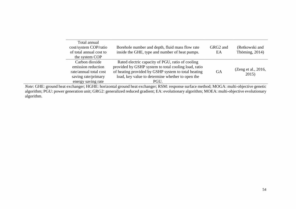
54

Total annual

cost/system COP/ratio

of total annual cost to

the system COP

Borehole number and depth, fluid mass flow rate

inside the GHE, type and number of heat pumps.

GRG2 and

EA

(Retkowski and

Thöming, 2014)

Carbon dioxide

emission reduction

rate/annual total cost

saving rate/primary

energy saving rate

Rated electric capacity of PGU, ratio of cooling

provided by GSHP system to total cooling load, ratio

of heating provided by GSHP system to total heating

load, key value to determine whether to open the

PGU.

GA (Zeng et al., 2016,

2015)

Note: GHE: ground heat exchanger; HGHE: horizontal ground heat exchanger; RSM: response surface method; MOGA: multi-objective genetic

algorithm; PGU: power generation unit; GRG2: generalized reduced gradient; EA: evolutionary algorithm; MOEA: multi-objective evolutionary

algorithm.

55

2.5 Review of control optimisation for GSHP systems

Compared with the efforts on the design optimisation of GSHP systems, less work has

been done on the control optimisation of GSHP systems. Previous work on the control

optimisation of GSHP systems can be generally divided into component level control

and system level control. The component level control focuses on maximising the

performance of individual components without considering the interactions with other

components, while the system-level control aims at improving the overall performance

of the whole system by considering the interactions among different components.

2.5.1 Component level control

Some control strategies were developed for the control of a certain system component

of GSHP systems. For instance, Svensson (1996) developed a model-based optimal

control strategy for water-to-water heat pumps to improve the energy performance and

reduce the operational cost. The adaptive steady-state process model of the heat pump

was developed and a sequential quadratic programming (SQP) algorithm was used to

solve the optimisation problem. Ridder et al. (2011) developed an optimal control

algorithm of borehole thermal storage systems (BTES) to minimise the terminal cost

associated with the use of BTES using a dynamic programming technique. The

optimisation results provided the optimal heat flux for a given field temperature, time

and demand. Hecht-Méndez et al. (2013) proposed a control strategy to identify the

optimal GHE operation patterns in a multiple GHE field by considering the impact of

the groundwater flow. This strategy was formulated using numerical simulation

models and a linear programming method.

56

2.5.2 System level control

2.5.2.1 Control of stand-alone GSHP systems

Sundbrandt (2011) developed a model predictive control (MPC) strategy for a GSHP

system to provide heating, cooling and domestic hot water (DHW) for a house. The

MPC controller was evaluated and compared to a conventional controller. The results

showed that the MPC controller could generally reduce the system power consumption

by 1-3% compared to the conventional controller. Zhang et al. (2013) developed a

nonlinear optimal control strategy for GSHP systems using radial basis function neural

network (RBFNN) predictive control algorithm and an adaptive particle swarm

optimisation (APSO) algorithm. In this strategy, RBFNN was used to estimate and

forecast the performance of the GSHP system, and APSO was used to identify the

optimal control settings. The simulation results showed that the proposed control

strategy could effectively reduce the total energy consumption of the system as

compared to a conventional control without optimisation. Sivasakthivel et al. (2014b)

utilised the Taguchi method and utility concept to optimise the operating parameters

of a GSHP system in order to improve the overall COP of the system. The operating

parameters were first optimised for heating and cooling operation, respectively. The

optimisation was then extended to optimise the operating parameters for combined

heating and cooling operation using the utility concept. Gao et al. (2016) proposed an

optimal control strategy for a small capacity GSHP system to minimise the total energy

consumption of the system. A self-defined optimisation algorithm was developed to

identify the optimal set-point of the chilled water return temperature and the width of

the water temperature control band. The effectiveness of the proposed strategy was

evaluated based on simulations. The results showed that the proposed strategy could

reduce the energy consumption by 9.59% in a typical spring day and by 2.97% in a

57

typical summer day, compared to a basic control strategy. Performance map-based

control strategies were proposed by Montagud et al. (2014) and Cervera-Vázquez et

al. (2015a, b, 2017) for GSHP systems to minimise the energy consumption of GSHP

systems. The system performance factor, defined as the ratio of the thermal load to the

electric energy consumption during a time interval, was used as the objective function

in these studies. The performance map generated from detailed simulations or

extensive performance tests of the targeted system over a significant range of settings

or operation conditions was utilised to find the optimal control settings of the targeted

system.

2.5.2.2 Control of HGSHP systems

The optimal control of HGSHP systems is rather defficult. The use of supplimentary

heat and/or cold source makes the optimisation problem of the whole system highly

nonlinear and more operational constraints should be taken into account. To date, only

a few studies were carried out on the optimal control of HGSHP systems. Verhelst

(2012) proposed an MPC stratgy to optimise the operation of a HGSHP system that

comprised of a GSHP system, a passive cooler, a gas boiler and and a chiller. The

control objective is to maximise thermal comfort, minimise energy cost and a long-

term sustainable use of the ground. The automatic control and dynamic optimisation

toolkit (ACADO) (Houska et al., 2011) was used as the solver in the MPC strategy.

Atam et al. (2014) proposed a convex approch for a non-convex optimal control

problem of the same HGSHP system through convexification. The optimisation

problem was solved using IBM CPLEX optimiser (IBM, 2018). The optimisation

results showed that the convex approximation of the optimal control problem gave

optimal results in terms of the responses and cost criteria. Atam et al. (2016) then

utilised three control approches, namely prediction-based dynamic programming (DP)

58

control approaches, nonlinear model predictive control (NMPC) approach, and linear

optimal control (LOC) approach, to minimising the total power consumption of this

HGSHP system under a range of operational constrainsts. The effectiveness of the

three proposed control approches were analysed and compared. The results showed

that NMPC was the most optimal control strategy when all the factors were considered

simutaneously. Hu et al. (2014, 2016) adopted a model-free control strategy based on

extremum seeking control (ESC) scheme to optimise the operation of a cooling tower-

assisted GSHP system. This model-free control strategy did not require a specific

model of the system. The combined power consumption of the GHE loop water pump,

cooling tower fan and pump, and heat pump compressor was minimised through the

optimal control of the cooling tower fan speed and water pump speed. The

performance evaluation results showed that this ESC strategy could effectively

achieve near optimal efficiency. Putrayudha et al. (2015) developed an optimal control

strategy to minimise the total energy consumption of a GSHP-PVT system in a single

residential house using a fuzzy logic (FL) controller. Two FL control systems were

used to control the operation of the GSHP system and the PVT system, respectively.

The results from a case study showed that using the fuzzy logic controller could reduce

the system total energy consumption by 18.3%, compared to a conventional on-off

controller. Ikeda et al. (2017) developed a control optimisation strategy for the

operation a HGSHP system with three heat pump units, an air-source heat pump

(ASHP) and an auxiliary boiler. This strategy used numerical simulation models and

a new optimisation algorithm called epsilon-constrained differential evolution with

random jumping to determine the optimal load rates of the heat pumps and the ASHP

in each time step. The optimisation results showed that the proposed strategy could

reduce the operating costs by 6.81% and 12.56% for a single day and 7 days,

59

respectively, compared to an empirical control strategy. Weeratunge et al. (2018)

developed an MPC controller for the intermittent operation of a solar assisted GSHP

system. The MPC controller was formulated using simplified mathematical models

developed based on the experimental results and a mixed integer linear programming

to identify the optimal control settings that minimise the system operational cost. The

effectiveness of the MPC controller was evaluated through a case study. The results

showed that using the proposed MPC controller on the solar assisted GSHP system

with an integrated thermal storage tank could reduce the operational cost by 7.8%,

compared to a conventional set-point controller.

All these reviewed control strategies have been tested and validated under various

working conditions. Energy or cost savings can be achieved when using these control

strategies, compared to the conventional control strategies. The major findings of these

control optimisation studies reviewed are summarised in Table 2.3.

https://www.sciencedirect.com/science/article/pii/S0360544218304882#!

60

Table 2.3 Summary of studies on the control optimisation of GSHP systems.

System type Optimisation

objectives Optimisation variables

Optimisation

method

Optimisation

technique Source

Component

Heat pump System power

consumption

Condenser water outlet temperature, and the water

flow rates through the evaporator and condenser.

Model-based

method

SQP (Svensson, 1996)

GHE

System operational

cost Heat extraction from the ground. DP

(De Ridder et al.,

2011)

Overall ground

temperature change GHE operation patterns.

Linear

programming

(Hecht-Mendez

et al., 2013)

Stand-alone GSHP

System power

consumption

Average temperature in the water tank, inlet brine

temperature of the GHE, and supply water

temperature of the user side.

MIQP (Sundbrandt,

2011)

Globe energy

consumption of the

system

Supply water temperatures and flow rates of the

GHE side and user side. APSO

(Yating et al.,

2013)

System COP Condenser inlet and outlet temperatures,

evaporator inlet and outlet temperatures.

Taguchi

method

(Sivasakthivel et

al., 2014b)

System power

consumption

Set-point of the chilled water return temperature

and the width of the water temperature control

band.

Self-defined

optimisation

algorithm

(Gao et al.,

2016)

System

performance factor

Internal and external circulation pump

frequencies, building space temperature set-point

and bandwidth. Performance

map-based

method

N/A (Montagud et al.,

2014)

System

performance factor


frequencies, building supply air temperature set-

point.

N/A

(Cervera-

Vázquez et al.,

2015a)

61

System

performance factor


frequencies. N/A

(Cervera-

Vázquez et al.,

2015b)

System

performance factor


frequencies, building supply air temperature set-

point.

N/A

(Cervera-

Vázquez et al.,

2017)

HGSHP

with a

boiler, a

passive

cooler and

a chiller

System total energy

consumption

Water supply temperature for heating/cooling, and

circulating fluid mean temperature inside GHEs.

Model-based

method

CPLEX

optimiser of

IBM (IBM,

2018)

(Atam et al.,

2014)

Total energy

consumption



DP/NMPC/

LOC

(Atam et al.,

2016)

Indoor thermal

comfort, energy

consumption, and

long-term

sustainability for

borehole use



ACADO

(Houska et al.,

2011)

(Verhelst, 2012)

with

cooling

tower

System power

consumption

Cooling tower fan speed and condensing water

flow rate. Model-free

method

ESC (Hu et al., 2014)

System power

consumption

Relative air flow rate into the cooling tower and

the water pump flow rate. ESC (Hu et al., 2016)

with PVT

collector

System total energy

consumption

The fractional state of operation of the GSHP and

the PVT circulation pump operational state.

Model-based

method

Fuzzy logic

controller

(Putrayudha et

al., 2015)

with

ASHP and

auxiliary

boiler

System operational

cost The load rates of the GSHP and the ASHP. eDE-RJ

(Ikeda et al.,

2017)

62

with solar

thermal

collector

System operational

cost

On/off of the heat pump, circulation pumps and

the auxiliary heater. MILP

(Weeratunge et

al., 2018)

Note: SQP: sequential quadratic programming; MIQP: mixed integer quadratic Programming; APSO: adaptive particle swarm optimisation; DP:

dynamic programming; NMPC: nonlinear model predictive control; LOC: linear optimal control; ACADO: automatic control and dynamic

optimisation; ESC: extremum seeking control; ASHP: air source heat pump; PVT: photovoltaic thermal collector; eDE-RJ: epsilon-constrained

differential evolution algorithm with random jumping; MILP: mixed integer linear programming.

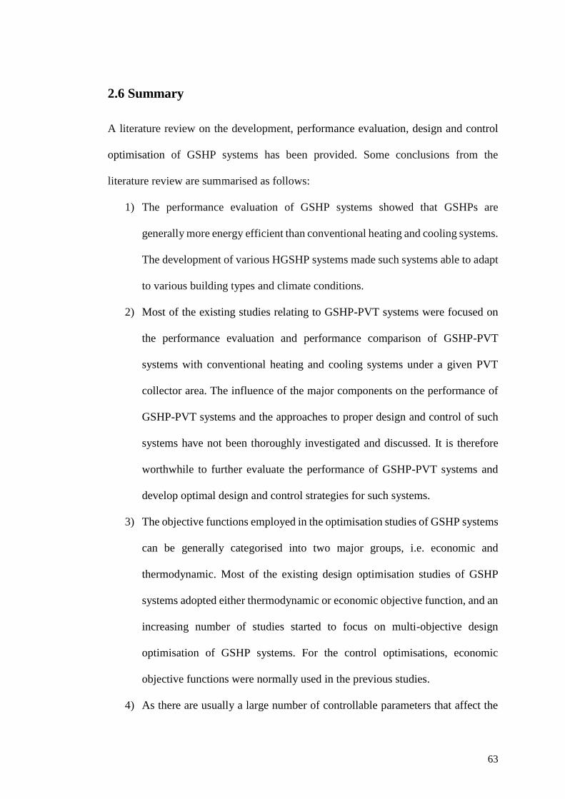
63

2.6 Summary

A literature review on the development, performance evaluation, design and control

optimisation of GSHP systems has been provided. Some conclusions from the

literature review are summarised as follows:

1) The performance evaluation of GSHP systems showed that GSHPs are

generally more energy efficient than conventional heating and cooling systems.

The development of various HGSHP systems made such systems able to adapt

to various building types and climate conditions.

2) Most of the existing studies relating to GSHP-PVT systems were focused on

the performance evaluation and performance comparison of GSHP-PVT

systems with conventional heating and cooling systems under a given PVT

collector area. The influence of the major components on the performance of

GSHP-PVT systems and the approaches to proper design and control of such

systems have not been thoroughly investigated and discussed. It is therefore

worthwhile to further evaluate the performance of GSHP-PVT systems and

develop optimal design and control strategies for such systems.

3) The objective functions employed in the optimisation studies of GSHP systems

can be generally categorised into two major groups, i.e. economic and

thermodynamic. Most of the existing design optimisation studies of GSHP

systems adopted either thermodynamic or economic objective function, and an

increasing number of studies started to focus on multi-objective design

optimisation of GSHP systems. For the control optimisations, economic

objective functions were normally used in the previous studies.

4) As there are usually a large number of controllable parameters that affect the

64

performance of GSHP systems, the selection of decision variables is important

in the optimisation of GSHP systems. The proper use of sensitivity analysis

could accurately identify the most influential variables on the objective

function and consequently facilitate the optimisation of GSHP systems.

5) Rules-of-thumb design approaches have been widely used in the design

applications of GSHP systems, which can quickly size the system with

controlled computational cost. However, using such design approaches could

result in under-sizing or over-sizing issues especially in the design of complex

GSHP systems. Model-based design methods are more reliable and can handle

various design optimisation problems with good results. However, the models

used to formulate the model-based design strategies need to be trained and

validated first to ensure reliable performance prediction.

6) Compared to the efforts that have been made on the optimal design, the

research relating to the development of optimal control strategies for GSHP

systems is still insufficient. The existing control strategies for GSHP systems

were mainly developed using model-based approaches. However, their

effectiveness relies on the accuracy of the control models used, and they are

generally computational extensive. The development of black-box models such

as artificial neural networks (ANNs) is a promising direction in the model-

based control of GSHP systems since they are simple enough without any

detailed knowledge on the physical working process, and the computational

cost is usually manageable. The performance map-based control approaches

are effective in the control of relatively small and simple GSHP systems, but it

is impractical to apply them in the control of large and complicated systems

since generating a performance map of such systems requires extensive work.

65

The studies using model-free approaches like extremum seeking control (ESC)

are rather few at the current stage, and it is difficult to conclude on the control

effectiveness of such methods.

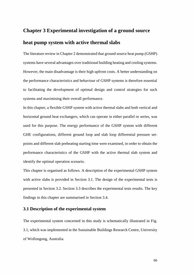
66

Chapter 3 Experimental investigation of a ground source

heat pump system with active thermal slabs

The literature review in Chapter 2 demonstrated that ground source heat pump (GSHP)

systems have several advantages over traditional building heating and cooling systems.

However, the main disadvantage is their high upfront costs. A better understanding on

the performance characteristics and behaviour of GSHP systems is therefore essential

to facilitating the development of optimal design and control strategies for such

systems and maximising their overall performance.

In this chapter, a flexible GSHP system with active thermal slabs and both vertical and

horizontal ground heat exchangers, which can operate in either parallel or series, was

used for this purpose. The energy performance of the GSHP system with different

GHE configurations, different ground loop and slab loop differential pressure set-

points and different slab preheating starting time were examined, in order to obtain the

performance characteristics of the GSHP with the active thermal slab system and

identify the optimal operation scenario.

This chapter is organised as follows. A description of the experimental GSHP system

with active slabs is provided in Section 3.1. The design of the experimental tests is

presented in Section 3.2. Section 3.3 describes the experimental tests results. The key

findings in this chapter are summarised in Section 3.4.

3.1 Description of the experimental system

The experimental system concerned in this study is schematically illustrated in Fig.

3.1, which was implemented in the Sustainable Buildings Research Centre, University

of Wollongong, Australia.

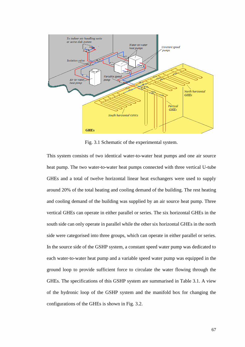
67

Fig. 3.1 Schematic of the experimental system.

This system consists of two identical water-to-water heat pumps and one air source

heat pump. The two water-to-water heat pumps connected with three vertical U-tube

GHEs and a total of twelve horizontal linear heat exchangers were used to supply

around 20% of the total heating and cooling demand of the building. The rest heating

and cooling demand of the building was supplied by an air source heat pump. Three

vertical GHEs can operate in either parallel or series. The six horizontal GHEs in the

south side can only operate in parallel while the other six horizontal GHEs in the north

side were categorised into three groups, which can operate in either parallel or series.

In the source side of the GSHP system, a constant speed water pump was dedicated to

each water-to-water heat pump and a variable speed water pump was equipped in the

ground loop to provide sufficient force to circulate the water flowing through the

GHEs. The specifications of this GSHP system are summarised in Table 3.1. A view

of the hydronic loop of the GSHP system and the manifold box for changing the

configurations of the GHEs is shown in Fig. 3.2.

68

Table 3.1 Specifications of the GSHP system.

Components Parameters Value

Two water-to-water

heat pumps

Total rated cooling capacity (kW) 32.8

Total rated heating capacity (kW) 40.8

Vertical heat

exchangers

Number of boreholes (-) 3

Diameter of borehole (mm) 150

Depth per borehole (m) 91

Borehole spacing (m) 8

Horizontal heat

exchangers

Loop pitch (m) 1.5

Number of pipes (-) 12

Length of per pipe (m) 125

Trench length (m) 17

a) Hydronic loop b) Manifold box

Fig. 3.2 Hydronic loop and manifold box of the GSHP system.

The indoor terminal system includes a number of indoor air handling units (AHUs)

and an active thermal slab system. The AHUs were installed around the building to

provide heating/cooling during the working hours. The active thermal slab system was

implemented at the first floor of the building and was mainly used to preheat the office

area at the first floor during the night in the heating season. The main configuration of

the active thermal slab system in shown in Fig. 3.3. The detailed design diagram of the

active thermal slab system, and the whole hydronic loop system are presented in

Appendix A and Appendix B, respectively. The active thermal slab system was divided

into three manifolds, for the east office, west office area and the central area,

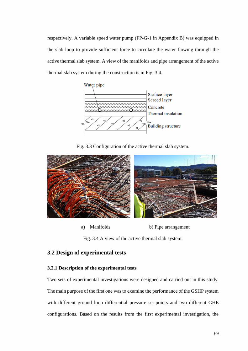
69

respectively. A variable speed water pump (FP-G-1 in Appendix B) was equipped in

the slab loop to provide sufficient force to circulate the water flowing through the

active thermal slab system. A view of the manifolds and pipe arrangement of the active

thermal slab system during the construction is in Fig. 3.4.

Fig. 3.3 Configuration of the active thermal slab system.

a) Manifolds b) Pipe arrangement

Fig. 3.4 A view of the active thermal slab system.

3.2 Design of experimental tests

3.2.1 Description of the experimental tests

Two sets of experimental investigations were designed and carried out in this study.

The main purpose of the first one was to examine the performance of the GSHP system

with different ground loop differential pressure set-points and two different GHE

configurations. Based on the results from the first experimental investigation, the

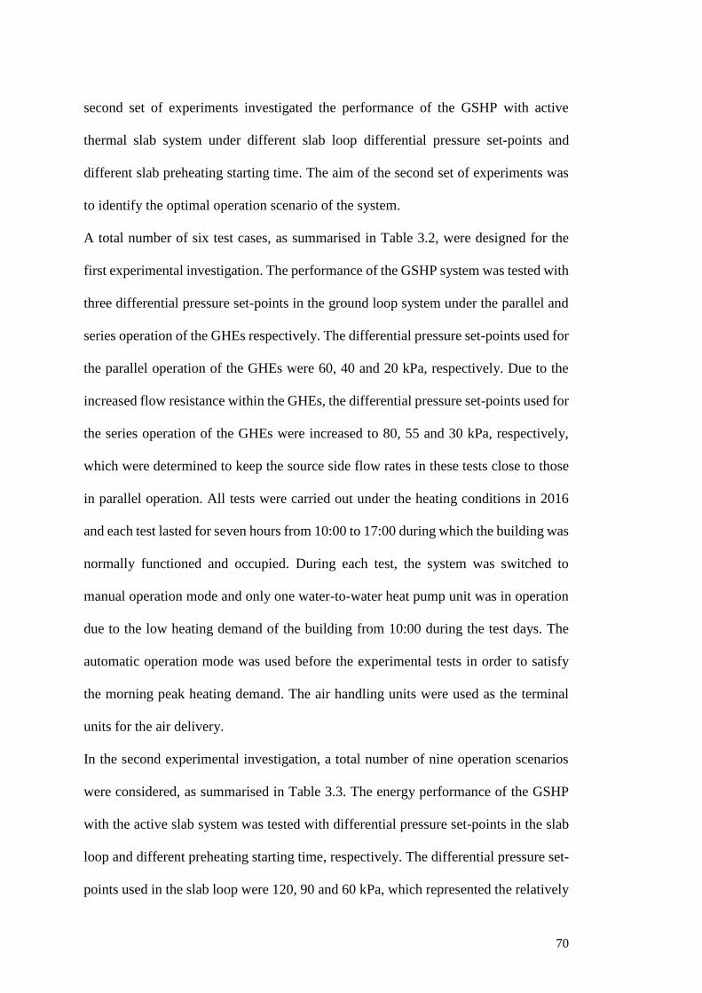
70

second set of experiments investigated the performance of the GSHP with active

thermal slab system under different slab loop differential pressure set-points and

different slab preheating starting time. The aim of the second set of experiments was

to identify the optimal operation scenario of the system.

A total number of six test cases, as summarised in Table 3.2, were designed for the

first experimental investigation. The performance of the GSHP system was tested with

three differential pressure set-points in the ground loop system under the parallel and

series operation of the GHEs respectively. The differential pressure set-points used for

the parallel operation of the GHEs were 60, 40 and 20 kPa, respectively. Due to the

increased flow resistance within the GHEs, the differential pressure set-points used for

the series operation of the GHEs were increased to 80, 55 and 30 kPa, respectively,

which were determined to keep the source side flow rates in these tests close to those

in parallel operation. All tests were carried out under the heating conditions in 2016

and each test lasted for seven hours from 10:00 to 17:00 during which the building was

normally functioned and occupied. During each test, the system was switched to

manual operation mode and only one water-to-water heat pump unit was in operation

due to the low heating demand of the building from 10:00 during the test days. The

automatic operation mode was used before the experimental tests in order to satisfy

the morning peak heating demand. The air handling units were used as the terminal

units for the air delivery.

In the second experimental investigation, a total number of nine operation scenarios

were considered, as summarised in Table 3.3. The energy performance of the GSHP

with the active slab system was tested with differential pressure set-points in the slab

loop and different preheating starting time, respectively. The differential pressure set-

points used in the slab loop were 120, 90 and 60 kPa, which represented the relatively

71

high, medium and relatively low water flow rate circulating through the slab,

respectively. Three starting time for the active thermal slab preheating was also

selected. The system was switched on from 21:00, 0:00 and 3:00, respectively. The

slab preheating was switched off at 7:00 in all tests. The AHUs were then switched on

to provide heating during the working hours. The tests of the GSHP with the active

slab system were carried out under the heating conditions in July and August 2017.

During the tests, the whole active thermal slab system and two water-to-water heat

pump units were used. The ground loop differential pressure set-point and the GHE

configuration were determined based on the results from the first experimental

investigation.

Table 3.2 Summary of the test scenarios of the first experimental investigation.

Test

cases

Differential pressure

set-point (kPa)

Vertical heat

exchangers

Horizontal heat

Exchangers Source side flow

rate South North

A 60 Parallel Parallel Parallel Relatively high

B 80 Series Parallel Series

C 40 Parallel Parallel Parallel Medium

D 55 Series Parallel Series

E 20 Parallel Parallel Parallel Relatively low

F 30 Series Parallel Series

Table 3.3 Summary of the test scenarios of the second experimental investigation.

Operation

scenarios

Differential pressure

set-point (kPa)

Circulation flow

rate through slab Operating time

1

120 Relatively high

21:00-7:00 (next day)

2 0:00-7:00

3 3:00-7:00

4

90 Medium

21:00-7:00 (next day)

5 0:00-7:00

6 3:00-7:00

7 60 Relatively low

21:00-7:00 (next day)

8 0:00-7:00

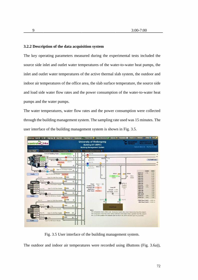
72

9 3:00-7:00

3.2.2 Description of the data acquisition system

The key operating parameters measured during the experimental tests included the

source side inlet and outlet water temperatures of the water-to-water heat pumps, the

inlet and outlet water temperatures of the active thermal slab system, the outdoor and

indoor air temperatures of the office area, the slab surface temperature, the source side

and load side water flow rates and the power consumption of the water-to-water heat

pumps and the water pumps.

The water temperatures, water flow rates and the power consumption were collected

through the building management system. The sampling rate used was 15 minutes. The

user interface of the building management system is shown in Fig. 3.5.

Fig. 3.5 User interface of the building management system.

The outdoor and indoor air temperatures were recorded using iButtons (Fig. 3.6a)),

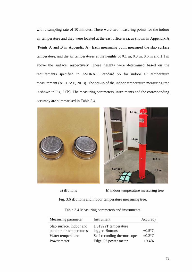
73

with a sampling rate of 10 minutes. There were two measuring points for the indoor

air temperature and they were located at the east office area, as shown in Appendix A

(Points A and B in Appendix A). Each measuring point measured the slab surface

temperature, and the air temperatures at the heights of 0.1 m, 0.3 m, 0.6 m and 1.1 m

above the surface, respectively. These heights were determined based on the

requirements specified in ASHRAE Standard 55 for indoor air temperature

measurement (ASHRAE, 2013). The set-up of the indoor temperature measuring tree

is shown in Fig. 3.6b). The measuring parameters, instruments and the corresponding

accuracy are summarised in Table 3.4.

a) iButtons b) indoor temperature measuring tree

Fig. 3.6 iButtons and indoor temperature measuring tree.

Table 3.4 Measuring parameters and instruments.

Measuring parameter Instrument Accuracy

Slab surface, indoor and

outdoor air temperatures

DS1922T temperature

logger iButtons ±0.5°C

Water temperature Self-recording thermoscope ±0.2°C

Power meter Edge G3 power meter ±0.4%

74

Water flow rate

Trimec MG040 digital

flow meter ±0.5%

3.2.3 Experimental data analysis

As mentioned in Section 3.2.1, all the experimental tests were carried out under the

heating condition, and the load side referred to the condenser side of the water-to-water

heat pump and the source side referred to the evaporator side.

The energy performance of the GSHP system was evaluated in terms of Coefficient of

Performance (COP). The average COP of the water-to-water heat pumps (COPHP) and

the whole GSHP system (COPsys) during the operation were calculated using Eq. (3.1)

and Eq. (3.2), respectively, in which the load side heat transfer rate (lQ ) was calculated

using Eq. (3.3).

1

,

1 1

( )HP

n

l i

iHP Nn

HP j i

i j

Q t

COP

W t

=

= =

=

(3.1)

, ,s

1

, , , ,s,

1 1 1 1

( )pu l puHP

n

l i

isys N NNn

HP j pu l k pu m i

i j k m

Q t

COP

W W W t

=

= = = =

=

+ +

(3.2)

, ,( )l f l l in l outQ c M T T= − (3.3)

where Q is the heat transfer rate, W is the power consumption, N is the number, it is

the measuring time interval, cp is the specific heat capacity of water, M is the water

mass flow rate, T is the temperature, and the subscripts HP, pu, l, s, in and out represent

heat pump, water pump, load side, source side, inlet and outlet, respectively.

The thermal performance of the active thermal slab system was evaluated by analysing

the indoor air temperature distributions. The air temperature at a certain height was the

75

average of the temperature measurements at the two measuring points.

3.2.4 Uncertainty analysis

In order to validate the experimental results, an uncertainty analysis was carried out.

The uncertainties of single measured parameters ( Xiw ) and calculated parameters

( w ) can be obtained using Eq. (3.4) and Eq. (3.5), respectively (Moffat, 1988, Koca

et al., 2014).

Xi i

i

Sw w

X

=

(3.4)

1

22

1

( )N

i

i i

Sw w

X

=

=

(3.5)

where S is the result function containing a number of independent measured variables,

and wi is the uncertainty of the ith independent variable Xi.

The relative uncertainties of all measured parameters and calculated parameters are

presented in Table 3.5.

Table 3.5 Relative uncertainties of measured parameter and calculated results.

Parameter

Relative

uncertainty

Measured parameters Slab surface temperature (°C) 0.82%

Air temperature (°C) 0.96%

Load side inlet water temperature of heat pump (°C) 0.43%

Load side outlet water temperature of heat pump (°C) 0.31%

Source side inlet water temperature of heat pump (°C) 0.55%

Source side outlet water temperature of heat pump (°C) 0.72%

Load side water flow rate (L/min) 0.50%

Source side water flow rate (L/min) 0.50%

Power of water-to-water heat pump (W) 0.40%

Power of load side constant speed pump (W) 0.40%

Power of source side constant speed pump (W) 0.40%

Power of slab loop variable speed pump (W) 0.40%

Power of ground loop variable speed pump (W) 0.40%

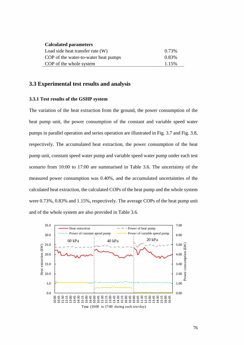
76

Calculated parameters Load side heat transfer rate (W) 0.73%

COP of the water-to-water heat pumps 0.83%

COP of the whole system 1.15%

3.3 Experimental test results and analysis

3.3.1 Test results of the GSHP system

The variation of the heat extraction from the ground, the power consumption of the

heat pump unit, the power consumption of the constant and variable speed water

pumps in parallel operation and series operation are illustrated in Fig. 3.7 and Fig. 3.8,

respectively. The accumulated heat extraction, the power consumption of the heat

pump unit, constant speed water pump and variable speed water pump under each test

scenario from 10:00 to 17:00 are summarised in Table 3.6. The uncertainty of the

measured power consumption was 0.40%, and the accumulated uncertainties of the

calculated heat extraction, the calculated COPs of the heat pump and the whole system

were 0.73%, 0.83% and 1.15%, respectively. The average COPs of the heat pump unit

and of the whole system are also provided in Table 3.6.

0.00

1.00

2.00

3.00

4.00

5.00

6.00

7.00

0.0

5.0

10.0

15.0

20.0

25.0

30.0

35.0

10

:00

10

:45

11

:30

12

:15

13

:00

13

:45

14

:30

15

:15

16

:00

16

:45

10

:00

10

:45

11

:30

12

:15

13

:00

13

:45

14

:30

15

:15

16

:00

16

:45

10

:00

10

:45

11

:30

12

:15

13

:00

13

:45

14

:30

15

:15

16

:00

16

:45

Po

wer

co

nsu

mp

tio

n (

kW

)

Heat

ext

racti

on

(kW

)

Time (10:00 to 17:00 during each test day)

Heat extraction Power of heat pump

Power of constant speed pump Power of variable speed pump

60 kPa 40 kPa 20 kPa

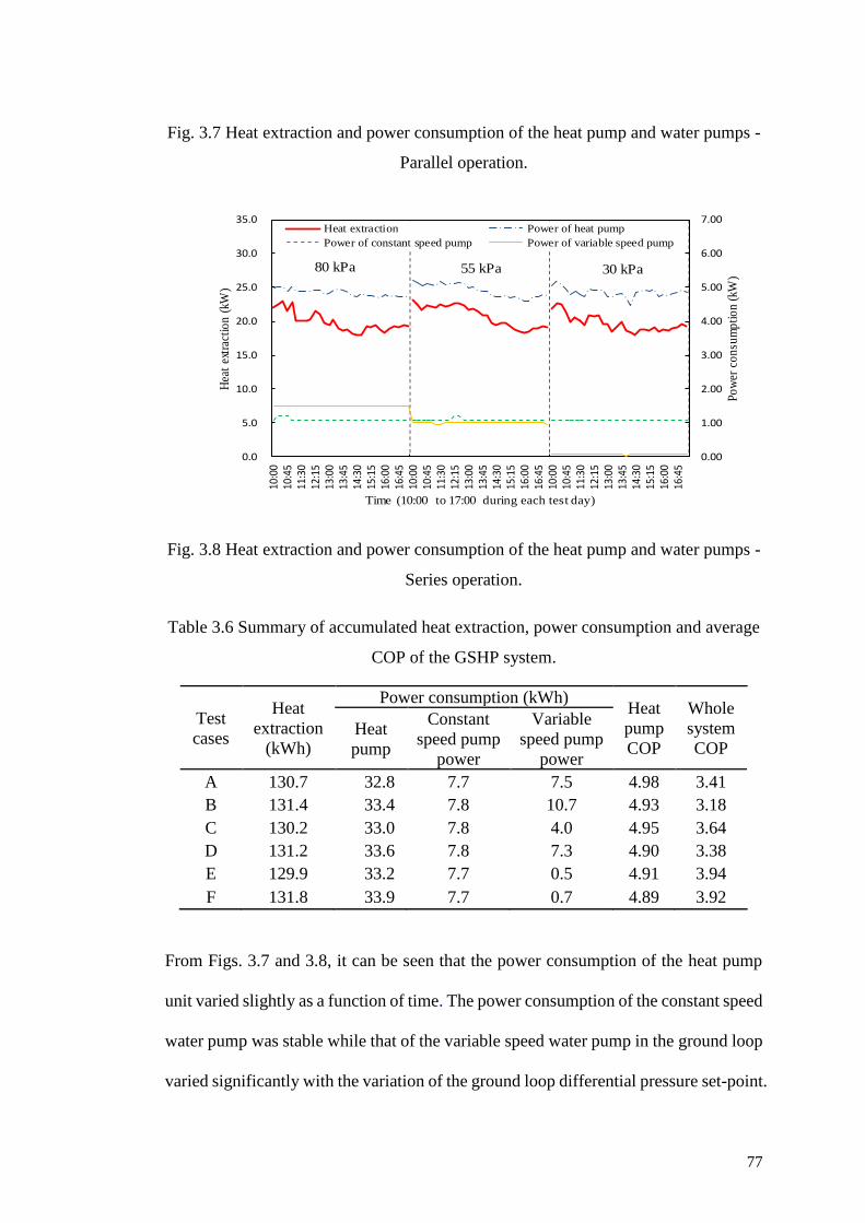
77


Parallel operation.


Series operation.

Table 3.6 Summary of accumulated heat extraction, power consumption and average

COP of the GSHP system.

Test

cases

Heat

extraction

(kWh)

Power consumption (kWh) Heat

pump

COP

Whole

system

COP

Heat

pump

Constant

speed pump

power

Variable

speed pump

power

A 130.7 32.8 7.7 7.5 4.98 3.41

B 131.4 33.4 7.8 10.7 4.93 3.18

C 130.2 33.0 7.8 4.0 4.95 3.64

D 131.2 33.6 7.8 7.3 4.90 3.38

E 129.9 33.2 7.7 0.5 4.91 3.94

F 131.8 33.9 7.7 0.7 4.89 3.92

From Figs. 3.7 and 3.8, it can be seen that the power consumption of the heat pump

unit varied slightly as a function of time. The power consumption of the constant speed

water pump was stable while that of the variable speed water pump in the ground loop

varied significantly with the variation of the ground loop differential pressure set-point.

0.00

1.00

2.00

3.00

4.00

5.00

6.00

7.00

0.0

5.0

10.0

15.0

20.0

25.0

30.0

35.0

10:0

010

:45

11:3

012

:15

13:0

013

:45

14:3

015

:15

16:0

016

:45

10:0

010

:45

11:3

012

:15

13:0

013

:45

14:3

015

:15

16:0

016

:45

10:0

010

:45

11:3

012

:15

13:0

013

:45

14:3

015

:15

16:0

016

:45

Po

wer

co

nsu

mp

tio

n (

kW)

Hea

t ex

trac

tio

n (

kW)

Time (10:00 to 17:00 during each test day)

Heat extraction Power of heat pump

Power of constant speed pump Power of variable speed pump

80 kPa 55 kPa 30 kPa

78

The larger the ground loop differential pressure set-point used, the more power the

variable speed pump consumed.

From Table 3.6, it can be seen that the daily heating demands of the building during

the test days were very close to each other, as the accumulated heat extraction and the

power consumption of the heat pump were very similar among these tests. The

difference in the average COP of the heat pump unit between the parallel and series

operations of GHEs was relatively small. The average COP of the whole system with

the relatively high and medium source side flow rates under the parallel operation of

GHEs was obviously higher than that under the series operation of GHEs. The whole

system COPs under the parallel operation of GHEs were 7.23%, 7.69% and 0.51%

higher than those under the series operation for the relatively high, medium and

relatively low source flow rate conditions, respectively. It can be seen that the GSHP

system showed a better performance when the parallel operation of GHEs compared

to that of series operation.

A larger differential pressure set-point in the ground loop (i.e. larger source side flow

rate) was generally beneficial to the operation of the heat pump unit for both parallel

and series operations of GHEs. However, the increase in the power consumption of

the variable water pump in the ground loop offset the benefit achieved by the heat

pump unit in the experimental system investigated, resulting in a lower overall COP

of the GSHP system.

3.3.2 Test results for GSHP with active thermal slab system.

Based on the results from the first experimental investigation, the GHEs operated in

parallel configuration and the ground loop differential pressure set-point was set at 20

kPa during the experimental tests of the GSHP with active thermal slab system. Fig.

3.9 presents the outdoor air temperature during all the test periods. It can be seen that

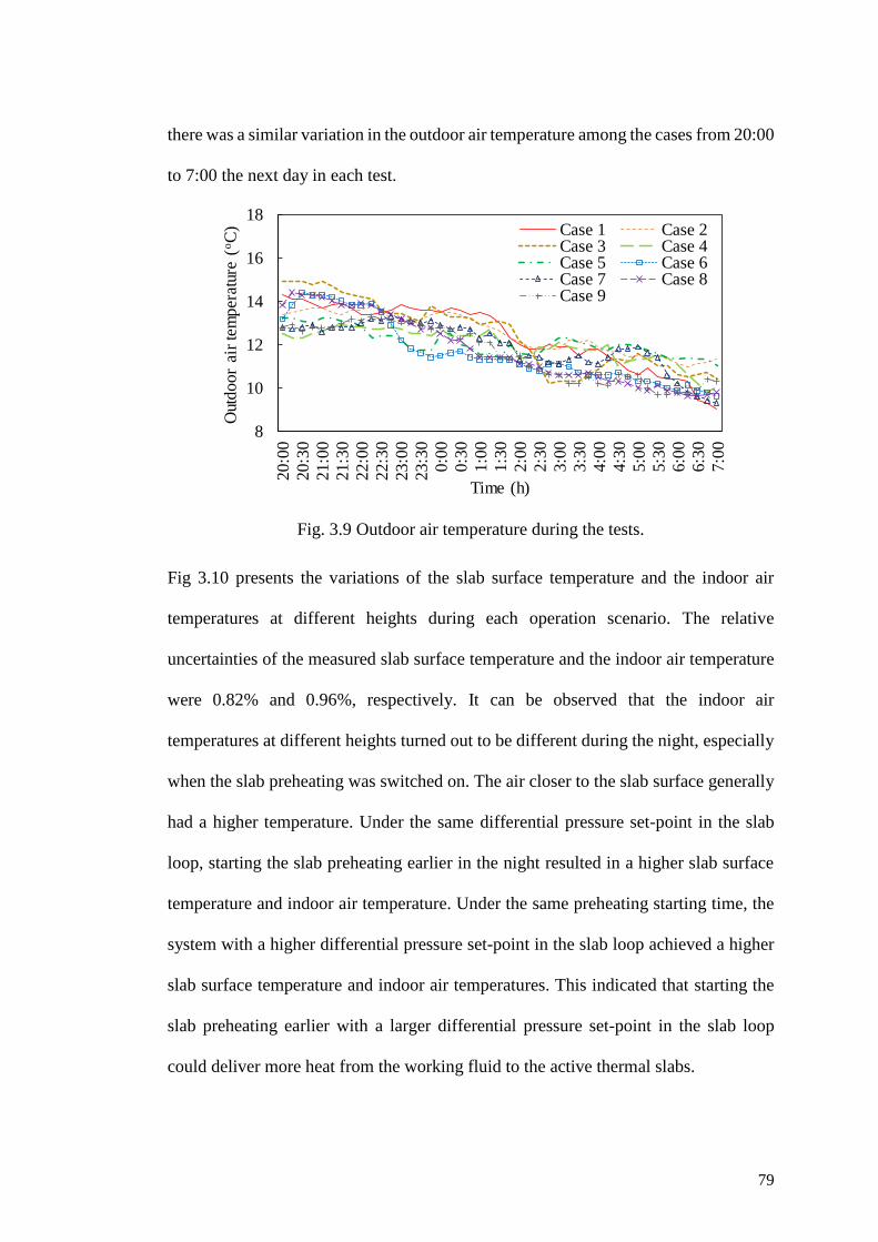
79

there was a similar variation in the outdoor air temperature among the cases from 20:00

to 7:00 the next day in each test.

Fig. 3.9 Outdoor air temperature during the tests.

Fig 3.10 presents the variations of the slab surface temperature and the indoor air

temperatures at different heights during each operation scenario. The relative

uncertainties of the measured slab surface temperature and the indoor air temperature

were 0.82% and 0.96%, respectively. It can be observed that the indoor air

temperatures at different heights turned out to be different during the night, especially

when the slab preheating was switched on. The air closer to the slab surface generally

had a higher temperature. Under the same differential pressure set-point in the slab

loop, starting the slab preheating earlier in the night resulted in a higher slab surface

temperature and indoor air temperature. Under the same preheating starting time, the

system with a higher differential pressure set-point in the slab loop achieved a higher

slab surface temperature and indoor air temperatures. This indicated that starting the

slab preheating earlier with a larger differential pressure set-point in the slab loop

could deliver more heat from the working fluid to the active thermal slabs.

8

10

12

14

16

18

20

:00

20

:30

21

:00

21

:30

22

:00

22

:30

23

:00

23

:30

0:0

0

0:3

0

1:0

0

1:3

0

2:0

0

2:3

0

3:0

0

3:3

0

4:0

0

4:3

0

5:0

0

5:3

0

6:0

0

6:3

0

7:0

0

Out

do

or

air

tem

per

atur

e (o

C)

Time (h)

Case 1 Case 2Case 3 Case 4Case 5 Case 6Case 7 Case 8Case 9

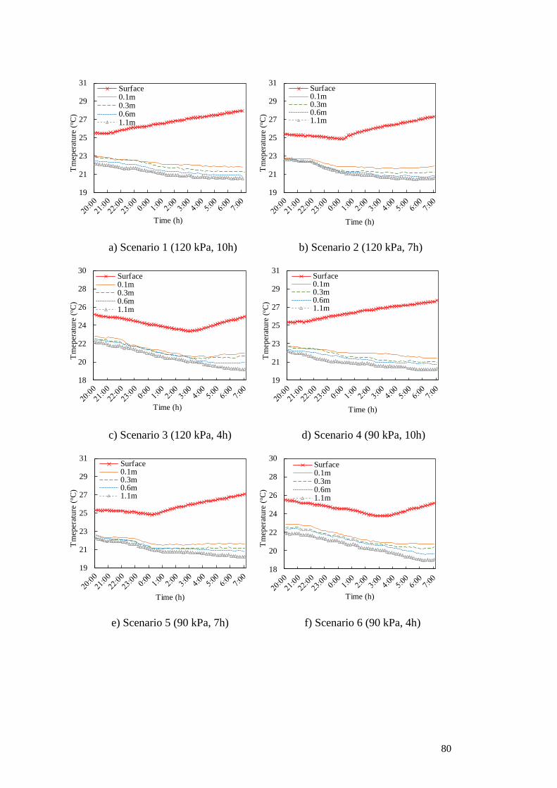
80

a) Scenario 1 (120 kPa, 10h) b) Scenario 2 (120 kPa, 7h)

c) Scenario 3 (120 kPa, 4h) d) Scenario 4 (90 kPa, 10h)

e) Scenario 5 (90 kPa, 7h) f) Scenario 6 (90 kPa, 4h)

19

21

23

25

27

29

31

Tm

eper

atu

re (

oC

)

Time (h)

Surface0.1m0.3m0.6m1.1m

19

21

23

25

27

29

31

Tm

eper

atu

re (

oC

)

Time (h)


18

20

22

24

26

28

30

Tm

eper

atu

re (

oC

)

Time (h)


19

21

23

25

27

29

31T

mep

erat

ure

(oC

)

Time (h)


19

21

23

25

27

29

31

Tm

eper

atu

re (

oC

)

Time (h)


18

20

22

24

26

28

30

Tm

eper

atu

re (

oC

)

Time (h)


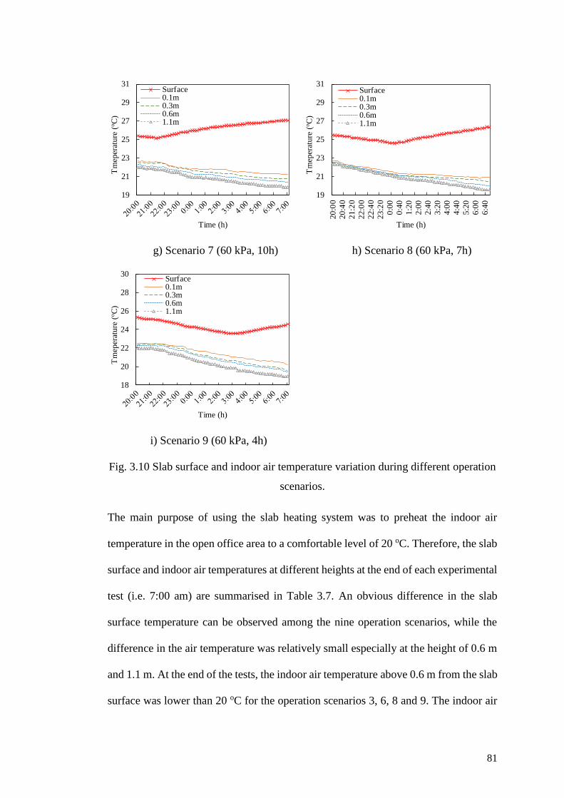
81

g) Scenario 7 (60 kPa, 10h) h) Scenario 8 (60 kPa, 7h)

i) Scenario 9 (60 kPa, 4h)

Fig. 3.10 Slab surface and indoor air temperature variation during different operation

scenarios.

The main purpose of using the slab heating system was to preheat the indoor air

temperature in the open office area to a comfortable level of 20 oC. Therefore, the slab

surface and indoor air temperatures at different heights at the end of each experimental

test (i.e. 7:00 am) are summarised in Table 3.7. An obvious difference in the slab

surface temperature can be observed among the nine operation scenarios, while the

difference in the air temperature was relatively small especially at the height of 0.6 m

and 1.1 m. At the end of the tests, the indoor air temperature above 0.6 m from the slab

surface was lower than 20 oC for the operation scenarios 3, 6, 8 and 9. The indoor air

19

21

23

25

27

29

31

Tm

eper

atu

re (

oC

)

Time (h)


19

21

23

25

27

29

31

20

:00

20

:40

21

:20

22

:00

22

:40

23

:20

0:0

0

0:4

0

1:2

0

2:0

0

2:4

0

3:2

0

4:0

0

4:4

0

5:2

0

6:0

0

6:4

0

Tm

eper

atu

re (

oC

)

Time (h)


18

20

22

24

26

28

30

Tm

eper

atu

re (

oC

)

Time (h)


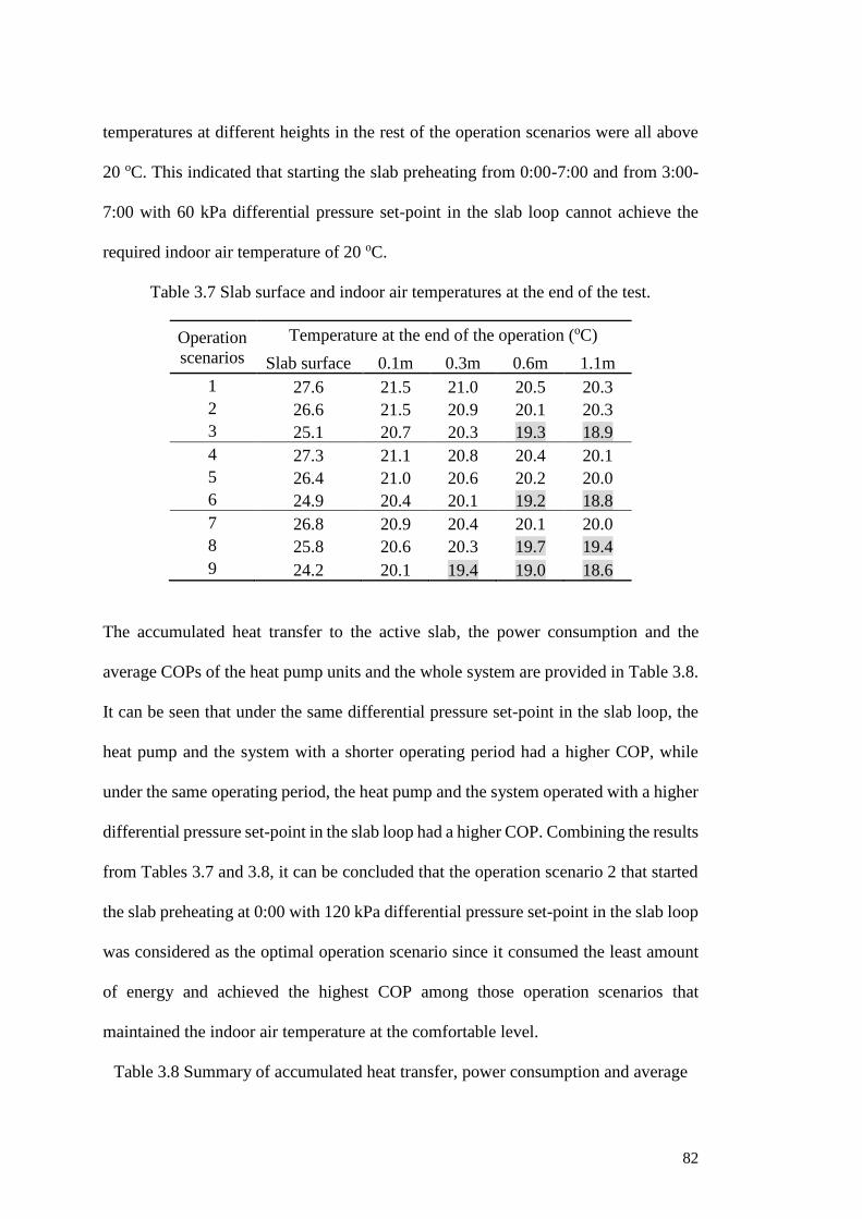
82

temperatures at different heights in the rest of the operation scenarios were all above

20 oC. This indicated that starting the slab preheating from 0:00-7:00 and from 3:00-

7:00 with 60 kPa differential pressure set-point in the slab loop cannot achieve the

required indoor air temperature of 20 oC.

Table 3.7 Slab surface and indoor air temperatures at the end of the test.

Operation

scenarios

Temperature at the end of the operation (oC)

Slab surface 0.1m 0.3m 0.6m 1.1m

1 27.6 21.5 21.0 20.5 20.3

2 26.6 21.5 20.9 20.1 20.3

3 25.1 20.7 20.3 19.3 18.9

4 27.3 21.1 20.8 20.4 20.1

5 26.4 21.0 20.6 20.2 20.0

6 24.9 20.4 20.1 19.2 18.8

7 26.8 20.9 20.4 20.1 20.0

8 25.8 20.6 20.3 19.7 19.4

9 24.2 20.1 19.4 19.0 18.6

The accumulated heat transfer to the active slab, the power consumption and the

average COPs of the heat pump units and the whole system are provided in Table 3.8.

It can be seen that under the same differential pressure set-point in the slab loop, the

heat pump and the system with a shorter operating period had a higher COP, while

under the same operating period, the heat pump and the system operated with a higher

differential pressure set-point in the slab loop had a higher COP. Combining the results

from Tables 3.7 and 3.8, it can be concluded that the operation scenario 2 that started

the slab preheating at 0:00 with 120 kPa differential pressure set-point in the slab loop

was considered as the optimal operation scenario since it consumed the least amount

of energy and achieved the highest COP among those operation scenarios that

maintained the indoor air temperature at the comfortable level.

Table 3.8 Summary of accumulated heat transfer, power consumption and average

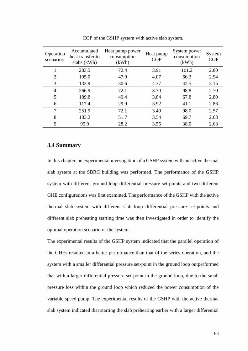
83

COP of the GSHP system with active slab system.

Operation

scenarios

Accumulated

heat transfer to

slabs (kWh)

Heat pump power

consumption

(kWh)

Heat pump

COP

System power

consumption

(kWh)

System

COP

1 283.5 72.4 3.91 101.2 2.80

2 195.0 47.9 4.07 66.3 2.94

3 133.9 30.6 4.37 42.5 3.15

4 266.9 72.1 3.70 98.8 2.70

5 189.8 49.4 3.84 67.8 2.80

6 117.4 29.9 3.92 41.1 2.86

7 251.9 72.1 3.49 98.0 2.57

8 183.2 51.7 3.54 69.7 2.63

9 99.9 28.2 3.55 38.0 2.63

3.4 Summary

In this chapter, an experimental investigation of a GSHP system with an active thermal

slab system at the SBRC building was performed. The performance of the GSHP

system with different ground loop differential pressure set-points and two different

GHE configurations was first examined. The performance of the GSHP with the active

thermal slab system with different slab loop differential pressure set-points and

different slab preheating starting time was then investigated in order to identify the

optimal operation scenario of the system.

The experimental results of the GSHP system indicated that the parallel operation of

the GHEs resulted in a better performance than that of the series operation, and the

system with a smaller differential pressure set-point in the ground loop outperformed

that with a larger differential pressure set-point in the ground loop, due to the small

pressure loss within the ground loop which reduced the power consumption of the

variable speed pump. The experimental results of the GSHP with the active thermal

slab system indicated that starting the slab preheating earlier with a larger differential

84

pressure set-point in the slab loop at night resulted in a higher slab surface temperature

and indoor air temperature. Using a larger differential pressure set-point in the slab

loop achieved higher COPs of the heat pump and the whole system, in comparison

with that using a smaller differential pressure set-point in the slab loop. The scenario

where the slab preheating started at 0:00 with 120 kPa differential pressure set-point

in the slab loop was considered as the optimal operation scenario. It is worthwhile to

note that, the results obtained from the experiment investigations are subjected to the

specific GSHP system with active slabs. However, the results obtained can be used to

guide the development of optimal control strategies for the studied system.

85

Chapter 4 Control optimisation of a stand-alone ground

source heat pump system

The energy performance of a GSHP system is significantly influenced by the control

strategy used. Optimal control of GSHP systems is therefore crucial to maximising

their operational performance while maintaining the indoor thermal comfort at

acceptable levels (Sayyaadi et al., 2009, Cervera-Vázquez et al., 2015b). In the past

few decades, an increasing number of studies focused on the development of effective

control strategies for various GSHP systems (Yavuzturk and Spitler, 2000, Park et al.,

2011, Zhai et al., 2012, Yang et al., 2014, Montagud et al., 2014, Esen et al., 2008a,

Yating et al., 2013, Gang et al., 2014). The results from these studies demonstrated

that proper control of GSHP systems is essential to substantially reducing the

operational costs of GSHP systems. However, the research in this area is insufficient

compared to that on design optimisation and optimal sizing of GSHP systems. This

chapter presents an optimal control strategy for stand-alone GSHP systems equipped

with variable speed pumps in the ground loop system. The performance of this strategy

was validated based on the GSHP system installed at the Sustainable Buildings

Research Centre (SBRC) building introduced in Chapter 3. The control strategy was

formulated using simplified performance models and a hybrid optimisation technique

which integrated a performance map-based near-optimal strategy and the exhaustive

search method to determine the optimal operating speed of the variable speed pumps

in the ground loop system. By using this hybrid optimisation technique, the

computational cost of the optimisation problem can be generally manageable and the

optimisation strategy can therefore be adapted to practically control and optimise the

operation of the variable speed pumps in the ground loop of GSHP systems.

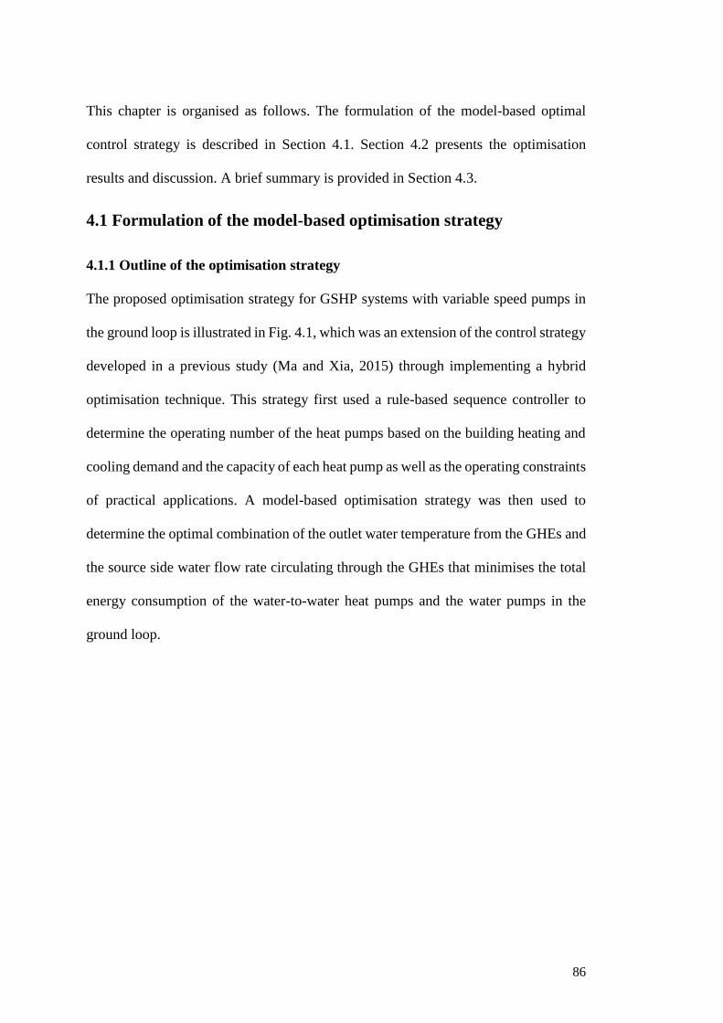
86

This chapter is organised as follows. The formulation of the model-based optimal

control strategy is described in Section 4.1. Section 4.2 presents the optimisation

results and discussion. A brief summary is provided in Section 4.3.

4.1 Formulation of the model-based optimisation strategy

4.1.1 Outline of the optimisation strategy

The proposed optimisation strategy for GSHP systems with variable speed pumps in

the ground loop is illustrated in Fig. 4.1, which was an extension of the control strategy

developed in a previous study (Ma and Xia, 2015) through implementing a hybrid

optimisation technique. This strategy first used a rule-based sequence controller to

determine the operating number of the heat pumps based on the building heating and

cooling demand and the capacity of each heat pump as well as the operating constraints

of practical applications. A model-based optimisation strategy was then used to

determine the optimal combination of the outlet water temperature from the GHEs and

the source side water flow rate circulating through the GHEs that minimises the total

energy consumption of the water-to-water heat pumps and the water pumps in the

ground loop.

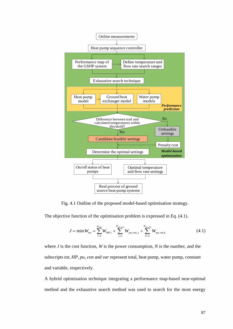
87

Fig. 4.1 Outline of the proposed model-based optimisation strategy.

The objective function of the optimisation problem is expressed in Eq. (4.1).

, ,var

, , , ,var,

1 1 1

minpu con puHP

N NN

tot HP i pu con j pu k

i j k

J W W W W= = =

= = + + (4.1)

where J is the cost function, W is the power consumption, N is the number, and the

subscripts tot, HP, pu, con and var represent total, heat pump, water pump, constant

and variable, respectively.

A hybrid optimisation technique integrating a performance map-based near-optimal

method and the exhaustive search method was used to search for the most energy

Heat pump sequence controller

Model-based

optimization

On/off status of heat pumps

Optimal temperature and flow rate settings

Real process of ground source heat pump systems

Online measurements

Define temperature and flow rate search ranges

Performance map of the GSHP system

Exhaustive search technique

Heat pump model

Water pump models

Ground heat exchanger model

Yes

Candidate feasible settings

No

Unfeasible settings

Determine the optimal settings

Difference between trail and calculated temperatures within

threshold?

Performance prediction

Penalty cost

88

efficient settings, which will be introduced in Section 4.1.2 and a description of the

optimisation process will be presented in Section 4.1.3.

The outputs from the optimisation strategy are the on/off status of the heat pumps and

the optimal setting of the outlet water temperature from the GHEs as well as the source

side flow rate, which can be used as a set-point to control the operation of the variable

speed pumps in the ground loop system.

4.1.2 Hybrid optimisation technique and optimisation constraints

A hybrid optimisation technique, which is an integration of a performance map-based

near-optimal method and the exhaustive search method developed in an early study

(Ma et al., 2008), was used to seek the optimal solution of the optimisation problem.

In this technique, a performance map of the GSHP system of concern should be first

generated through experimental investigation or detailed computer simulation under

various working conditions.

Based on the performance map generated, a linear model, as expressed in Eq. (4.2),

can be regressed to determine a near-optimal control setting under a given condition.

This linear model was a function of the borehole wall temperature (Tb) and the ratio of

the load that was provided by the water-to-water heat pumps (Q) to the total design

capacity of the two water-to-water heat pumps (Qdes). This near-optimal control setting

was then used as a search centre to define a relatively narrow search range as shown

in Eq. (4.3). Fig. 4.2 illustrates the search range defined using the near-optimal control

setting determined using Eq. (4.2). As the near-optimal control setting was actually a

near-optimal solution of the optimisation problem for the current working condition,

the optimal combination of the GHE outlet water temperature set-point and the source

side flow rate can then be identified within the narrow search range defined using the

exhaustive search method with a small increment.

89

,

g,out 1 2 3( )n o

b

des

QT A A T A

Q= + + (4.2)

, ,

g,out ,out ,out

n o n o

g gT T T T T− + (4.3)

where T is the temperature, Q is the load, A1-A3 are the coefficients, the superscripts n

and o represent near and optimal, and the subscripts g, out and des refer to ground heat

exchanger, outlet and design, respectively.

Fig. 4.2 Illustration of the search range defined using the performance map-based

near-optimal strategy.

As a low water flow rate will lead to a laminar flow in the GHEs and a poor heat

transfer to the ground (Cervera-Vázquez et al., 2015b), the lower limit of the source

side water flow rate was estimated when the variable speed pump operated at 10 Hz

using pump affinity laws. The upper limit of the water flow rate in the ground loop

was determined when the variable speed pump operated at 50 Hz.

4.1.3 Description of the optimisation process

For a given trial combination of the GHE outlet water temperature and the source side

flow rate, the water-to-water heat pump model was first used to determine the power

consumption of the heat pumps and the outlet water temperature from the source side

heat exchangers of the heat pumps. This temperature was then used as the inlet water

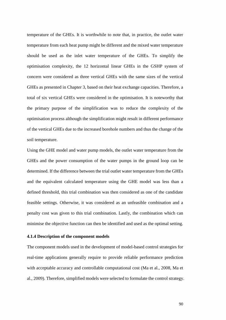
90

temperature of the GHEs. It is worthwhile to note that, in practice, the outlet water

temperature from each heat pump might be different and the mixed water temperature

should be used as the inlet water temperature of the GHEs. To simplify the

optimisation complexity, the 12 horizontal linear GHEs in the GSHP system of

concern were considered as three vertical GHEs with the same sizes of the vertical

GHEs as presented in Chapter 3, based on their heat exchange capacities. Therefore, a

total of six vertical GHEs were considered in the optimisation. It is noteworthy that

the primary purpose of the simplification was to reduce the complexity of the

optimisation process although the simplification might result in different performance

of the vertical GHEs due to the increased borehole numbers and thus the change of the

soil temperature.

Using the GHE model and water pump models, the outlet water temperature from the

GHEs and the power consumption of the water pumps in the ground loop can be

determined. If the difference between the trial outlet water temperature from the GHEs

and the equivalent calculated temperature using the GHE model was less than a

defined threshold, this trial combination was then considered as one of the candidate

feasible settings. Otherwise, it was considered as an unfeasible combination and a

penalty cost was given to this trial combination. Lastly, the combination which can

minimise the objective function can then be identified and used as the optimal setting.

4.1.4 Description of the component models

The component models used in the development of model-based control strategies for

real-time applications generally require to provide reliable performance prediction

with acceptable accuracy and controllable computational cost (Ma et al., 2008, Ma et

al., 2009). Therefore, simplified models were selected to formulate the control strategy.

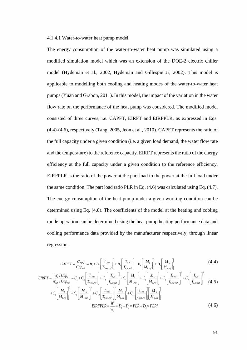
91

4.1.4.1 Water-to-water heat pump model

The energy consumption of the water-to-water heat pump was simulated using a

modified simulation model which was an extension of the DOE-2 electric chiller

model (Hydeman et al., 2002, Hydeman and Gillespie Jr, 2002). This model is

applicable to modelling both cooling and heating modes of the water-to-water heat

pumps (Yuan and Grabon, 2011). In this model, the impact of the variation in the water

flow rate on the performance of the heat pump was considered. The modified model

consisted of three curves, i.e. CAPFT, EIRFT and EIRFPLR, as expressed in Eqs.

(4.4)-(4.6), respectively (Tang, 2005, Jeon et al., 2010). CAPFT represents the ratio of

the full capacity under a given condition (i.e. a given load demand, the water flow rate

and the temperature) to the reference capacity. EIRFT represents the ratio of the energy

efficiency at the full capacity under a given condition to the reference efficiency.

EIRFPLR is the ratio of the power at the part load to the power at the full load under

the same condition. The part load ratio PLR in Eq. (4.6) was calculated using Eq. (4.7).

The energy consumption of the heat pump under a given working condition can be

determined using Eq. (4.8). The coefficients of the model at the heating and cooling

mode operation can be determined using the heat pump heating performance data and

cooling performance data provided by the manufacturer respectively, through linear

regression.

, ,

1 2 3 4 5

, , , , , ,

l out s inc l s

ref l out ref s in ref l ref s ref

T TCap M MCAPFT B B B B B

Cap T T M M

= = + + + +

(4.4)

2 2

, , , ,

1 2 3 4 5 6 7

, , , , , , , , , ,

2

8 9

, ,

/

/

l out s in l out s inc c l s

ref ref l out ref s in ref l ref s ref l out ref s in ref

l s

l ref s r

T T T TW Cap M MEIRFT C C C C C C C

W Cap T T M M T T

M MC C

M M

= = + + + + + +

+ +

2

, ,

10 11

, , , , , ,

l out s inl s

ef l out ref l ref s in ref s ref

T TM MC C

T M T M

+ +

(4.5)

2

1 2 3

c

WEIRFPLR D D PLR D PLR

W= = + + (4.6)

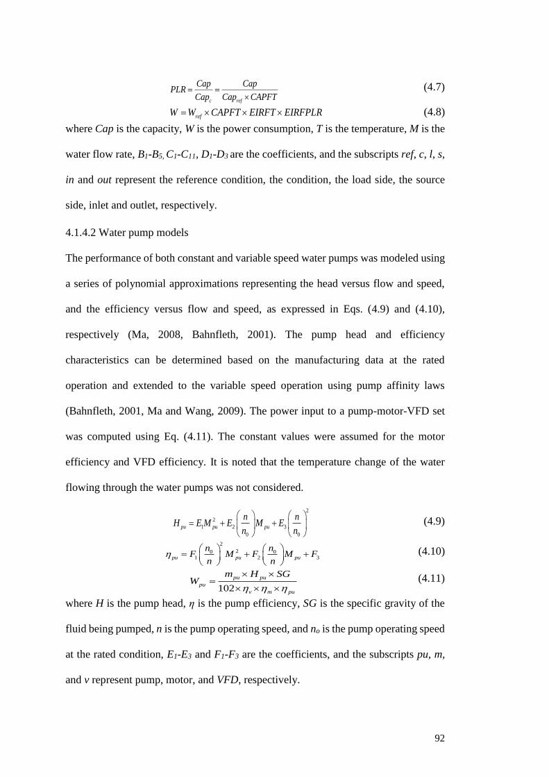
92

c ref

Cap CapPLR

Cap Cap CAPFT= =

(4.7)

refW W CAPFT EIRFT EIRFPLR= (4.8)

where Cap is the capacity, W is the power consumption, T is the temperature, M is the

water flow rate, B1-B5, C1-C11, D1-D3 are the coefficients, and the subscripts ref, c, l, s,

in and out represent the reference condition, the condition, the load side, the source

side, inlet and outlet, respectively.

4.1.4.2 Water pump models

The performance of both constant and variable speed water pumps was modeled using

a series of polynomial approximations representing the head versus flow and speed,

and the efficiency versus flow and speed, as expressed in Eqs. (4.9) and (4.10),

respectively (Ma, 2008, Bahnfleth, 2001). The pump head and efficiency

characteristics can be determined based on the manufacturing data at the rated

operation and extended to the variable speed operation using pump affinity laws

(Bahnfleth, 2001, Ma and Wang, 2009). The power input to a pump-motor-VFD set

was computed using Eq. (4.11). The constant values were assumed for the motor

efficiency and VFD efficiency. It is noted that the temperature change of the water

flowing through the water pumps was not considered.

2

2

1 2 3

0 0

pu pu pu

n nH E M E M E

n n

= + +

(4.9)

2

20 01 2 3pu pu pu

n nF M F M F

n n

= + +

(4.10)

102

pu pu

pu

v m pu

m H SGW

=

(4.11)

where H is the pump head, η is the pump efficiency, SG is the specific gravity of the

fluid being pumped, n is the pump operating speed, and no is the pump operating speed

at the rated condition, E1-E3 and F1-F3 are the coefficients, and the subscripts pu, m,

and v represent pump, motor, and VFD, respectively.

93

4.1.4.3 Ground heat exchanger model

The borehole wall temperature (Tb) at the end of the nth time step since the start of the

operation, was determined by Eq. (4.12) (Yavuzturk and Spitler, 1999). The g function

in Eq. (4.12) was calculated using Eq. (4.13), in which the time-dependent borehole

wall temperature for a single step pulse of a given ground thermal conductivity was

simulated using the numerical model of vertical GHEs available in TRNSYS. The

thermal resistance per borehole length (Rb) was determined by Eq. (4.14), which

included the thermal resistances of the pipe wall and the inside fluid and the thermal

resistance of the grout material (Lamarche et al., 2010). Based on the thermal

resistance per borehole length, the outlet water temperature from GHEs can be easily

determined based on the relationship described in Eq. (4.15).

1 1,0

1

( ),

2

ni i n i b

b s

i so b s b

Q Q t t rT T g

N k L t L− −

=

− −= +

(4.12)

( ),02 /,

/

so b b b si b

s b b

k T R Q NL Tt rg

t L Q NL

− − =

(4.13)

4, ,

4 4

, ,

ln( / )1 1[ln ln ln( )]

4 2 4 4

gr so p o p ib b bb

gr p o c gr so b c p p i f

k k r rr r rR

k r x k k r x k r h

−= + + + +

+ − (4.14)

g, g,( ) / 2

/

in out b

b

b

T T TR

Q NL

+ −= (4.15)

where T is the temperature, r is the radius, k is the thermal conductivity, t is the time,

ts is the time scale, L is the depth, Q is the total heat transfer, N is the number of

boreholes, R is the thermal resistance, xc is the half shank spacing and defined as the

centre-to-centre distance between the two legs of the U-tube, hf is the convective heat

transfer coefficient, and the subscripts b, g, gr, i, o, p, so and 0 represent the borehole,

ground heat exchanger, grout material, inner, outer, pipe, soil and initial, respectively.

4.2 Results and discussion

The performance of the proposed control strategy was validated through computer

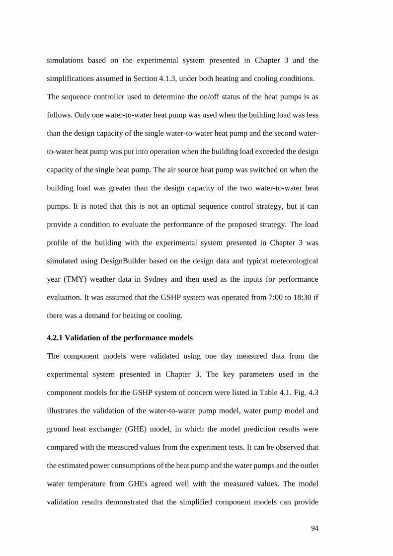
94

simulations based on the experimental system presented in Chapter 3 and the

simplifications assumed in Section 4.1.3, under both heating and cooling conditions.

The sequence controller used to determine the on/off status of the heat pumps is as

follows. Only one water-to-water heat pump was used when the building load was less

than the design capacity of the single water-to-water heat pump and the second water-

to-water heat pump was put into operation when the building load exceeded the design

capacity of the single heat pump. The air source heat pump was switched on when the

building load was greater than the design capacity of the two water-to-water heat

pumps. It is noted that this is not an optimal sequence control strategy, but it can

provide a condition to evaluate the performance of the proposed strategy. The load

profile of the building with the experimental system presented in Chapter 3 was

simulated using DesignBuilder based on the design data and typical meteorological

year (TMY) weather data in Sydney and then used as the inputs for performance

evaluation. It was assumed that the GSHP system was operated from 7:00 to 18:30 if

there was a demand for heating or cooling.

4.2.1 Validation of the performance models

The component models were validated using one day measured data from the

experimental system presented in Chapter 3. The key parameters used in the

component models for the GSHP system of concern were listed in Table 4.1. Fig. 4.3

illustrates the validation of the water-to-water pump model, water pump model and

ground heat exchanger (GHE) model, in which the model prediction results were

compared with the measured values from the experiment tests. It can be observed that

the estimated power consumptions of the heat pump and the water pumps and the outlet

water temperature from GHEs agreed well with the measured values. The model

validation results demonstrated that the simplified component models can provide

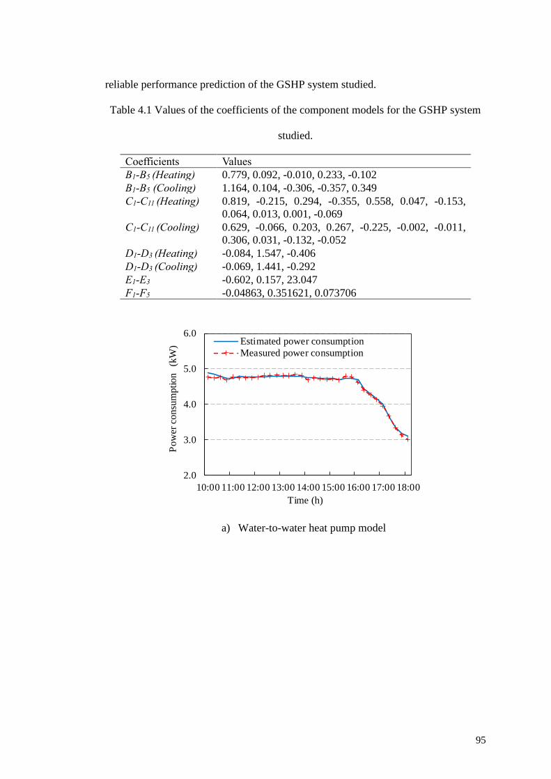
95

reliable performance prediction of the GSHP system studied.

Table 4.1 Values of the coefficients of the component models for the GSHP system

studied.

Coefficients Values

B1-B5 (Heating) 0.779, 0.092, -0.010, 0.233, -0.102

B1-B5 (Cooling) 1.164, 0.104, -0.306, -0.357, 0.349

C1-C11 (Heating) 0.819, -0.215, 0.294, -0.355, 0.558, 0.047, -0.153,

0.064, 0.013, 0.001, -0.069

C1-C11 (Cooling) 0.629, -0.066, 0.203, 0.267, -0.225, -0.002, -0.011,

0.306, 0.031, -0.132, -0.052

D1-D3 (Heating) -0.084, 1.547, -0.406

D1-D3 (Cooling) -0.069, 1.441, -0.292

E1-E3 -0.602, 0.157, 23.047

F1-F5 -0.04863, 0.351621, 0.073706

a) Water-to-water heat pump model

2.0

3.0

4.0

5.0

6.0

10:00 11:00 12:00 13:00 14:00 15:00 16:00 17:00 18:00

Pow

er c

onsu

mpti

on

(kW

)

Time (h)

Estimated power consumption

Measured power consumption

96

b) Water pump model

c) GHE model

Fig. 4.3 Validation of the component models using measured data.

4.2.2 Generation of the performance map-based near-optimal control strategy

To generate the performance map-based control strategy, a similar model-based

control strategy as that of the proposed control strategy was developed. In this strategy,

the same component models as those presented in Section 4.1.4 were used as the

performance predictors but used the exhaustive search method as the optimisation

0.5

0.7

0.9

1.1

1.3

1.5

10:00 11:00 12:00 13:00 14:00 15:00 16:00 17:00 18:00

Pow

er c

onsu

mpti

on

(kW

)

Time (h)

Estimated-constant speed pumpMeasured-constant speed pumpEstimated-variable speed pumpMeasured-variable speed pump

19

20

21

22

23

24

25

10:00 11:00 12:00 13:00 14:00 15:00 16:00 17:00 18:00

Tem

per

atu

re

(oC

)

Time (h)

Estimated GHE outlet water temperatureMeasured GHE outlet water temperature

97

technique and a wider search range for the GHE outlet water temperature set-point (i.e.

20-40 oC under the cooling conditions and 6-19 oC under the heating conditions). The

optimal GHE outlet water temperature and the corresponding ground temperature

under each working condition were then identified based on small search increments

of 0.1 oC and 0.05 kg/s for the outlet water temperature of the GHEs and the source

side water flow rate, respectively. A performance map for the optimal GHE outlet

water temperature can then be generated using Eq. (4.2) based on the simulated data

in conjunction with the load provided by the water-to-water heat pumps and the total

design capacity of the two water-to-water heat pumps. Through regression, the

identified values for the coefficients of A1-A3 in Eq. (4.2) under the heating condition

were -1.0469, 1.0843 and -1.5389, and under the cooling conditions were 0.2324,

0.9763 and 2.4211, respectively.

Fig. 4.4 illustrates a comparison between the set-point of the GHE outlet water

temperature predicted by the performance map-based near-optimal control strategy (i.e.

predicted using Eq. (4.2)) and the optimal values identified using the exhaustive search

method under the heating and cooling conditions. A good agreement between the two

sets of data can be observed, demonstrating that the performance map-based strategy

can provide near-optimal control settings.

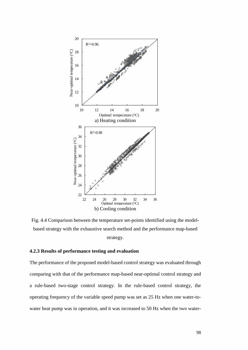
98

a) Heating condition

b) Cooling condition

Fig. 4.4 Comparison between the temperature set-points identified using the model-

based strategy with the exhaustive search method and the performance map-based

strategy.

4.2.3 Results of performance testing and evaluation

The performance of the proposed model-based control strategy was evaluated through

comparing with that of the performance map-based near-optimal control strategy and

a rule-based two-stage control strategy. In the rule-based control strategy, the

operating frequency of the variable speed pump was set as 25 Hz when one water-to-

water heat pump was in operation, and it was increased to 50 Hz when the two water-

10

12

14

16

18

20

10 12 14 16 18 20

Near-

optim

al

tem

pera

ture

(oC

)

Optimal temperature (oC)

R2=0.96

22

24

26

28

30

32

34

36

22 24 26 28 30 32 34 36

Near-

optim

al

tem

pera

ture

(oC

)

Optimal temperature (oC)

R2=0.98

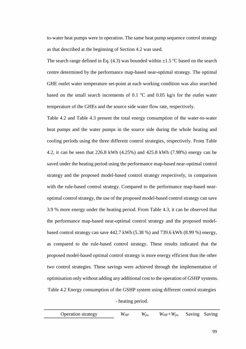
99

to-water heat pumps were in operation. The same heat pump sequence control strategy

as that described at the beginning of Section 4.2 was used.

The search range defined in Eq. (4.3) was bounded within ±1.5 oC based on the search

centre determined by the performance map-based near-optimal strategy. The optimal

GHE outlet water temperature set-point at each working condition was also searched

based on the small search increments of 0.1 oC and 0.05 kg/s for the outlet water

temperature of the GHEs and the source side water flow rate, respectively.

Table 4.2 and Table 4.3 present the total energy consumption of the water-to-water

heat pumps and the water pumps in the source side during the whole heating and

cooling periods using the three different control strategies, respectively. From Table

4.2, it can be seen that 226.8 kWh (4.25%) and 425.8 kWh (7.98%) energy can be

saved under the heating period using the performance map-based near-optimal control

strategy and the proposed model-based control strategy respectively, in comparison

with the rule-based control strategy. Compared to the performance map-based near-

optimal control strategy, the use of the proposed model-based control strategy can save

3.9 % more energy under the heating period. From Table 4.3, it can be observed that

the performance map-based near-optimal control strategy and the proposed model-

based control strategy can save 442.7 kWh (5.38 %) and 739.6 kWh (8.99 %) energy,

as compared to the rule-based control strategy. These results indicated that the

proposed model-based optimal control strategy is more energy efficient than the other

two control strategies. These savings were achieved through the implementation of

optimisation only without adding any additional cost to the operation of GSHP systems.


- heating period.

Operation strategy WHP Wpu WHP+Wpu Saving Saving

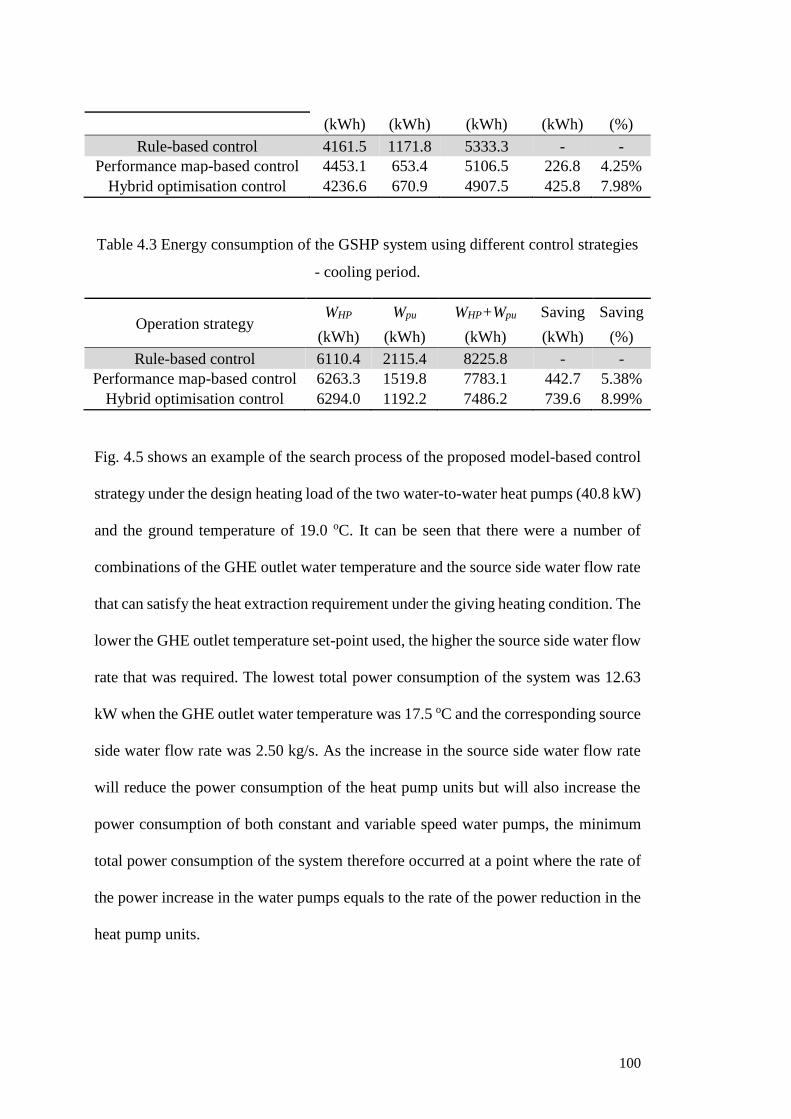
100

(kWh) (kWh) (kWh) (kWh) (%)

Rule-based control 4161.5 1171.8 5333.3 - -

Performance map-based control 4453.1 653.4 5106.5 226.8 4.25%

Hybrid optimisation control 4236.6 670.9 4907.5 425.8 7.98%


- cooling period.

Operation strategy WHP Wpu WHP+Wpu Saving Saving

(kWh) (kWh) (kWh) (kWh) (%)

Rule-based control 6110.4 2115.4 8225.8 - -

Performance map-based control 6263.3 1519.8 7783.1 442.7 5.38%

Hybrid optimisation control 6294.0 1192.2 7486.2 739.6 8.99%

Fig. 4.5 shows an example of the search process of the proposed model-based control

strategy under the design heating load of the two water-to-water heat pumps (40.8 kW)

and the ground temperature of 19.0 oC. It can be seen that there were a number of

combinations of the GHE outlet water temperature and the source side water flow rate

that can satisfy the heat extraction requirement under the giving heating condition. The

lower the GHE outlet temperature set-point used, the higher the source side water flow

rate that was required. The lowest total power consumption of the system was 12.63

kW when the GHE outlet water temperature was 17.5 oC and the corresponding source

side water flow rate was 2.50 kg/s. As the increase in the source side water flow rate

will reduce the power consumption of the heat pump units but will also increase the

power consumption of both constant and variable speed water pumps, the minimum

total power consumption of the system therefore occurred at a point where the rate of

the power increase in the water pumps equals to the rate of the power reduction in the

heat pump units.

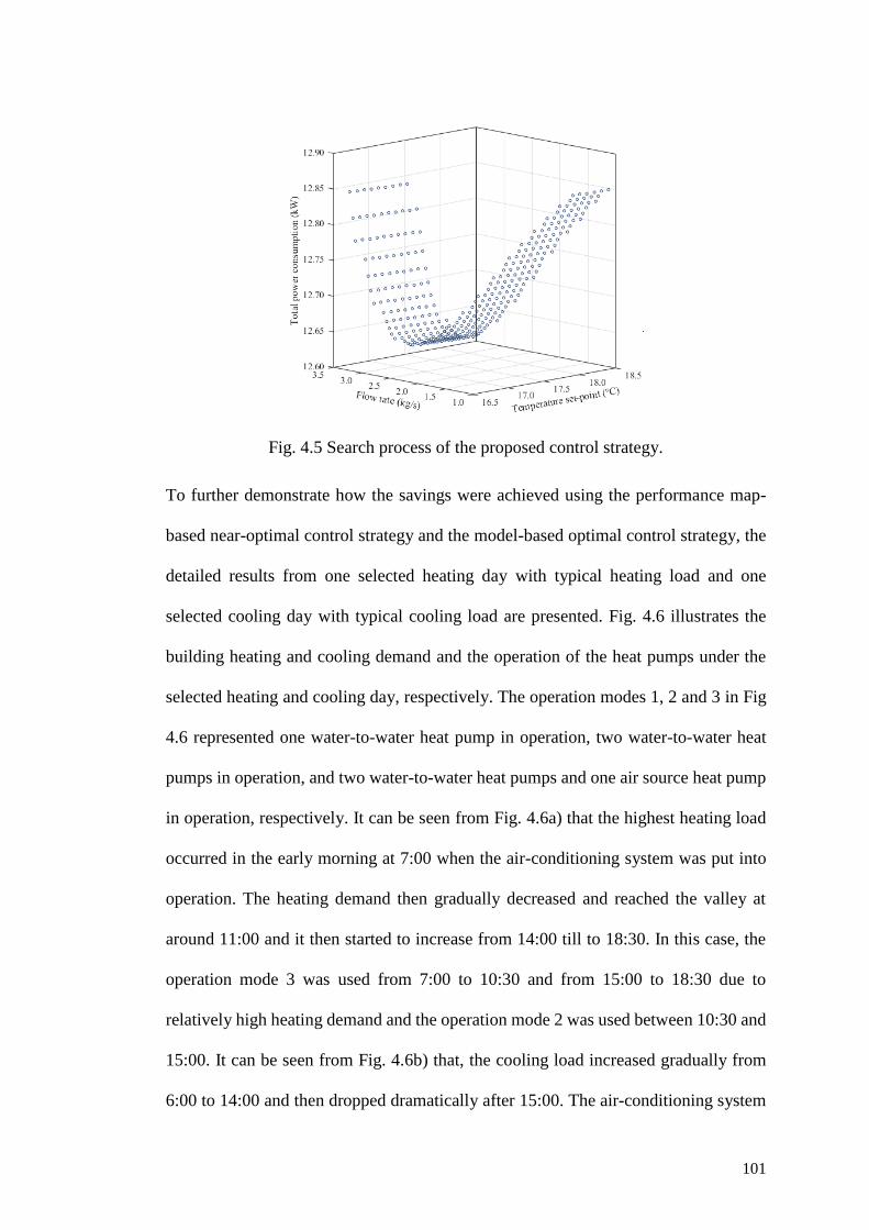
101

Fig. 4.5 Search process of the proposed control strategy.

To further demonstrate how the savings were achieved using the performance map-

based near-optimal control strategy and the model-based optimal control strategy, the

detailed results from one selected heating day with typical heating load and one

selected cooling day with typical cooling load are presented. Fig. 4.6 illustrates the

building heating and cooling demand and the operation of the heat pumps under the

selected heating and cooling day, respectively. The operation modes 1, 2 and 3 in Fig

4.6 represented one water-to-water heat pump in operation, two water-to-water heat

pumps in operation, and two water-to-water heat pumps and one air source heat pump

in operation, respectively. It can be seen from Fig. 4.6a) that the highest heating load

occurred in the early morning at 7:00 when the air-conditioning system was put into

operation. The heating demand then gradually decreased and reached the valley at

around 11:00 and it then started to increase from 14:00 till to 18:30. In this case, the

operation mode 3 was used from 7:00 to 10:30 and from 15:00 to 18:30 due to

relatively high heating demand and the operation mode 2 was used between 10:30 and

15:00. It can be seen from Fig. 4.6b) that, the cooling load increased gradually from

6:00 to 14:00 and then dropped dramatically after 15:00. The air-conditioning system

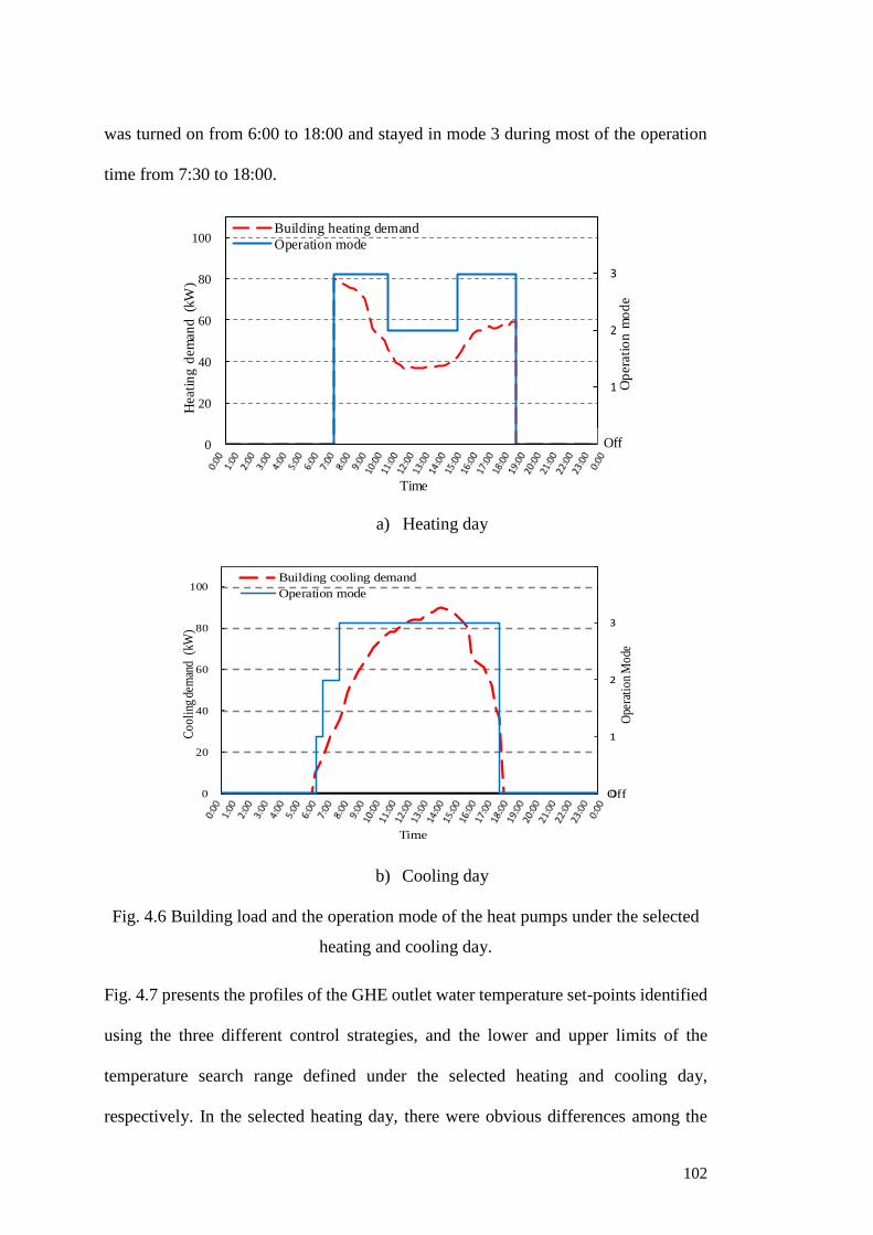
102

was turned on from 6:00 to 18:00 and stayed in mode 3 during most of the operation

time from 7:30 to 18:00.

a) Heating day

b) Cooling day

Fig. 4.6 Building load and the operation mode of the heat pumps under the selected

heating and cooling day.

Fig. 4.7 presents the profiles of the GHE outlet water temperature set-points identified

using the three different control strategies, and the lower and upper limits of the

temperature search range defined under the selected heating and cooling day,

respectively. In the selected heating day, there were obvious differences among the

0

1

2

3

4

0

20

40

60

80

100

0:00 2:24 4:48 7:12 9:36 12:00 14:24 16:48 19:12 21:36 0:00

Op

era

tio

n m

od

e

Heati

ng

dem

an

d (k

W)

Time

Building heating demand

Operation mode

Off

0

1

2

3

4

0

20

40

60

80

100

0:001:122:243:364:486:007:128:249:3610:4812:0013:1214:2415:3616:4818:0019:1220:2421:3622:480:00

Ope

rati

on

Mo

de

Co

oli

ng d

eman

d (

kW)

Time

Building cooling demand

Operation mode

Off

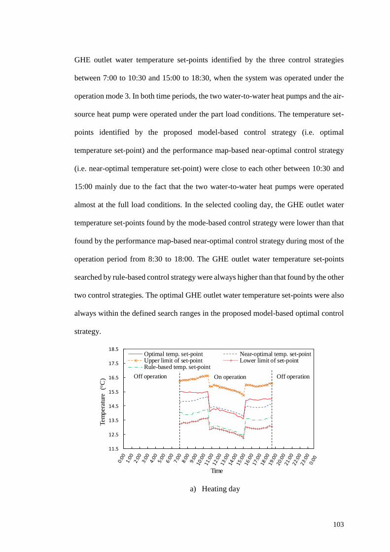
103

GHE outlet water temperature set-points identified by the three control strategies

between 7:00 to 10:30 and 15:00 to 18:30, when the system was operated under the

operation mode 3. In both time periods, the two water-to-water heat pumps and the air-

source heat pump were operated under the part load conditions. The temperature set-

points identified by the proposed model-based control strategy (i.e. optimal

temperature set-point) and the performance map-based near-optimal control strategy

(i.e. near-optimal temperature set-point) were close to each other between 10:30 and

15:00 mainly due to the fact that the two water-to-water heat pumps were operated

almost at the full load conditions. In the selected cooling day, the GHE outlet water

temperature set-points found by the mode-based control strategy were lower than that

found by the performance map-based near-optimal control strategy during most of the

operation period from 8:30 to 18:00. The GHE outlet water temperature set-points

searched by rule-based control strategy were always higher than that found by the other

two control strategies. The optimal GHE outlet water temperature set-points were also

always within the defined search ranges in the proposed model-based optimal control

strategy.

a) Heating day

11.5

12.5

13.5

14.5

15.5

16.5

17.5

18.5

Tem

per

atur

e (o

C)

Time

Optimal temp. set-point Near-optimal temp. set-pointUpper limit of set-point Lower limit of set-pointRule-based temp. set-point

Off operation Off operationOn operation

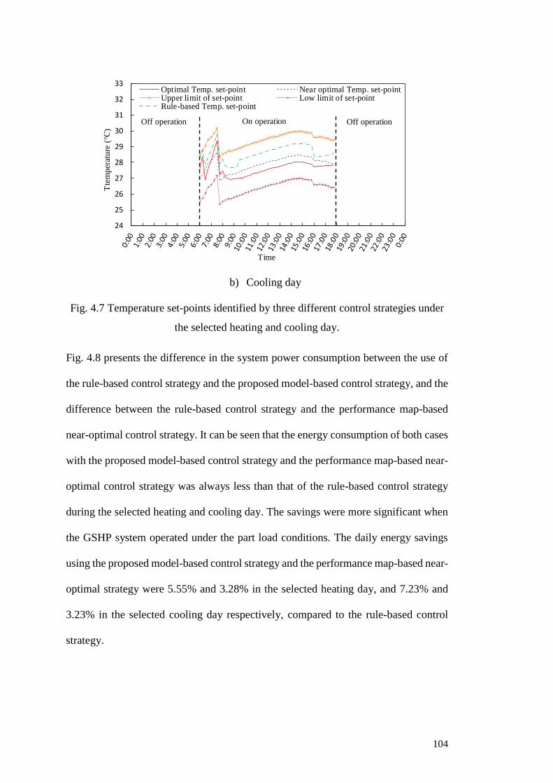
104

b) Cooling day

Fig. 4.7 Temperature set-points identified by three different control strategies under

the selected heating and cooling day.

Fig. 4.8 presents the difference in the system power consumption between the use of

the rule-based control strategy and the proposed model-based control strategy, and the

difference between the rule-based control strategy and the performance map-based

near-optimal control strategy. It can be seen that the energy consumption of both cases

with the proposed model-based control strategy and the performance map-based near-

optimal control strategy was always less than that of the rule-based control strategy

during the selected heating and cooling day. The savings were more significant when

the GSHP system operated under the part load conditions. The daily energy savings

using the proposed model-based control strategy and the performance map-based near-

optimal strategy were 5.55% and 3.28% in the selected heating day, and 7.23% and

3.23% in the selected cooling day respectively, compared to the rule-based control

strategy.

24

25

26

27

28

29

30

31

32

33

Tte

mper

ature

(℃

)

Time

Optimal Temp. set-point Near optimal Temp. set-pointUpper limit of set-point Low limit of set-pointRule-based Temp. set-point

Off operation Off operationOn operation

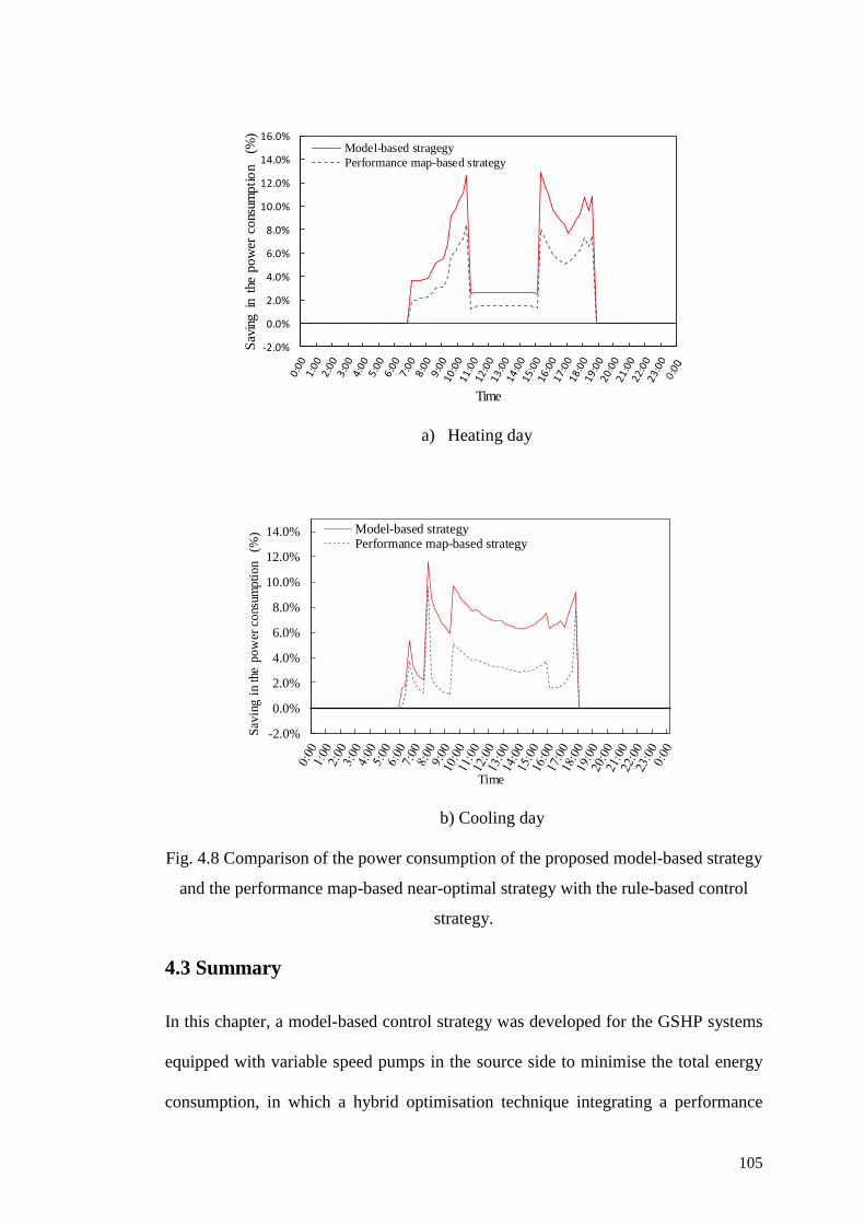
105

a) Heating day

b) Cooling day

Fig. 4.8 Comparison of the power consumption of the proposed model-based strategy

and the performance map-based near-optimal strategy with the rule-based control

strategy.

4.3 Summary

In this chapter, a model-based control strategy was developed for the GSHP systems

equipped with variable speed pumps in the source side to minimise the total energy

consumption, in which a hybrid optimisation technique integrating a performance

-2.0%

0.0%

2.0%

4.0%

6.0%

8.0%

10.0%

12.0%

14.0%

16.0%

Sav

ing

in t

he p

ow

er c

ons

umptio

n (

%)

Time

Model-based stragegy

Performance map-based strategy

-2.0%

0.0%

2.0%

4.0%

6.0%

8.0%

10.0%

12.0%

14.0%

Sav

ing

in t

he p

ow

er c

ons

umpti

on

(%

)

Time

Model-based strategyPerformance map-based strategy

106

map-based near-optimal strategy and the exhaustive search method was used to

identify the most energy efficient control settings.

The optimisation results demonstrated that the proposed model-based control strategy

was more energy efficient than the rule-based control strategy with two-stage control

and the performance map-based near-optimal control strategy. 425.8 kWh (7.98 %)

and 739.6 kWh (8.99 %) energy savings can be approximately achieved when using

the proposed model-based control strategy under the whole heating and cooling

periods respectively, as compared to the rule-based control strategy. 226.8 kWh

(4.25 %) and 442.7 kWh (5.38 %) energy can also be saved under the whole heating

and cooling periods when the performance map-based near-optimal control strategy

was used, in comparison with the rule-based control strategy. The methodology used

to develop this proposed control strategy could be potentially adapted to develop the

control strategies for other types of GSHP systems. However, as each system is unique,

the models used can be different dependent on the user preferences and the models

should also be trained using the manufacturing data of the system components used.

107

Chapter 5 Development and performance simulation of a

ground source heat pump system with integrated solar

photovoltaic thermal collectors

This chapter presents the development, simulation and performance evaluation of a

ground source heat pump (GSHP) system integrated with water-based solar

photovoltaic thermal (PVT) collectors for residential buildings. The GSHP-PVT

system was developed to provide space cooling and heating as well as domestic hot

water (DHW), and offset the need of grid electricity by generating electricity from the

PV cells. A dynamic simulation system was developed using TRNSYS and used to

facilitate the performance evaluation of the proposed system. Three potential operation

scenarios for the GSHP-PVT system were designed. A 20-year life-time performance

simulation was performed under the three proposed operation scenarios with different

sizes of the PVT collectors to investigate the effect of the PVT size on the performance

of the system. An economic analysis was then carried out to determine the optimum

size of the PVT collectors for the case study building.

This chapter is organised as follows. Section 5.1 presents a brief introduction of the

research background. The development of the system and the corresponding operation

scenarios is described in Section 5.2. A brief introduction of the simulation system and

the case study are provided in Section 5.3 and Section 5.4, respectively. Section 5.5

presents the optimisation results and discussion. The keys findings are presented in

Section 5.6.

5.1 Introduction

One of the major challenges relating to the application of GSHP systems is the ground

108

thermal imbalance, which can result in performance deterioration of GSHP systems

(Yu et al., 2008, Man et al., 2010b, Wang et al., 2016). In order to address this issue,

hybrid ground source heat pump (HGSHP) systems, which utilise auxiliary heat sink

or source to supply a fraction of building cooling or heating demand, have been

developed (Phetteplace and Sullivan, 1998, Chiasson and Yavuzturk, 2003, Man et al.,

2011). The use of HGSHP systems can effectively alleviate the ground thermal

imbalance, and in the meantime, can reduce the initial costs and ground area

requirement in comparison to conventional stand-alone GSHP systems (ASHRAE,

1995, Qi et al., 2014). In heating dominated residential buildings, where the space

heating and domestic hot water (DHW) account for a large amount of energy

consumption, an efficient energy system that integrates a ground source heat pump

(GSHP) system with water-based photovoltaic thermal (PVT) collectors could be a

promising solution to the building energy demand. An appropriate integrated GSHP-

PVT system can provide cooling and heating as well as domestic hot water (DHW),

offset the need of grid electricity and alleviate ground thermal imbalance.

The existing studies of GSHP-PVT systems were mainly focusing on the performance

evaluation and performance comparison among different heating and cooling systems

under a given PVT collector area (Bakker et al., 2005, Entchev et al., 2014, Canelli et

al., 2015, Putrayudha et al., 2015, Brischoux and Bernier, 2016). The results from these

studies demonstrated that the GSHP-PVT system can result in a better energy

performance in comparison to conventional heating and cooling systems and stand-

alone GSHP systems. The performance of a GSHP-PVT system is highly dependent

on the size of the PVT collectors used. However, there is currently no relevant research

that has studied the influence of the PVT size on the performance of the GSHP-PVT

system in detail and has discussed the effect of the PVT size on the operation of hybrid

109

GSHP-PVT systems.

In order to fill the research gap mentioned above and gain a better understanding on

the dynamic characteristics and energy performance of GSHP-PVT systems, this

Chapter aims at performing a performance evaluation of the GSHP-PVT system

developed. In this Chapter, a GSHP system integrated with water-based PVT

collectors was developed to provide cooling, heating and DHW for residential

buildings. Three different operation scenarios of the system were designed and the

simulation systems for each scenario were developed. The effect of the PVT size on

the performance of the three operation scenarios was investigated in a case study

building under the weather condition of Melbourne, Australia. An economic analysis

was also carried out to determine the optimum PVT size for the case study building.

5.2 System development and operation scenarios

The proposed GSHP-PVT system is schematically illustrated in Fig. 5.1. The system

is mainly designed to provide heating and cooling, as well as DHW for heating

dominated buildings. The hybrid system consisted of a PVT collector, a water tank

with immersed heat exchangers, a water-to-water heat pump unit, three water

circulation pumps, a vertical ground heat exchanger (GHE) loop, an indoor air-

handling unit (AHU) and an electric water heater. This system can operate under

different modes, as described in Table 5.1, to provide functional requirements to the

house through on-off control of the isolation valves.

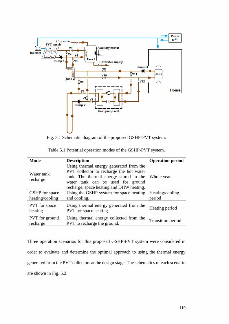
110

Fig. 5.1 Schematic diagram of the proposed GSHP-PVT system.

Table 5.1 Potential operation modes of the GSHP-PVT system.

Mode Description Operation period

Water tank

recharge

Using thermal energy generated from the

PVT collector to recharge the hot water

tank. The thermal energy stored in the

water tank can be used for ground

recharge, space heating and DHW heating.

Whole year

GSHP for space

heating/cooling

Using the GSHP system for space heating

and cooling.

Heating/cooling

period

PVT for space

heating

Using thermal energy generated from the

PVT for space heating. Heating period

PVT for ground

recharge

Using thermal energy collected from the

PVT to recharge the ground. Transition period

Three operation scenarios for this proposed GSHP-PVT system were considered in

order to evaluate and determine the optimal approach to using the thermal energy

generated from the PVT collectors at the design stage. The schematics of each scenario

are shown in Fig. 5.2.

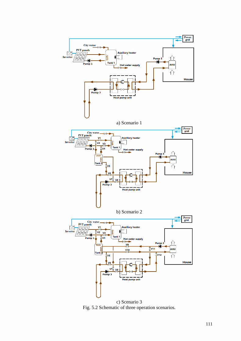
111

a) Scenario 1

b) Scenario 2

c) Scenario 3

Fig. 5.2 Schematic of three operation scenarios.

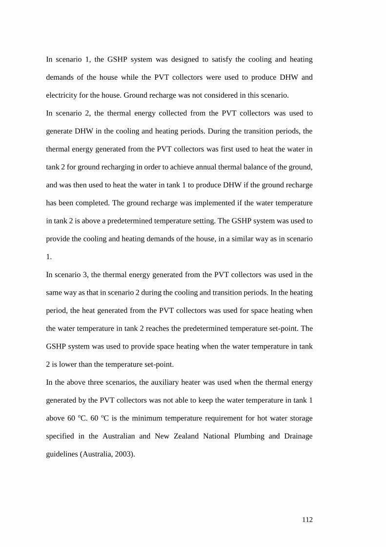
112

In scenario 1, the GSHP system was designed to satisfy the cooling and heating

demands of the house while the PVT collectors were used to produce DHW and

electricity for the house. Ground recharge was not considered in this scenario.

In scenario 2, the thermal energy collected from the PVT collectors was used to

generate DHW in the cooling and heating periods. During the transition periods, the

thermal energy generated from the PVT collectors was first used to heat the water in

tank 2 for ground recharging in order to achieve annual thermal balance of the ground,

and was then used to heat the water in tank 1 to produce DHW if the ground recharge

has been completed. The ground recharge was implemented if the water temperature

in tank 2 is above a predetermined temperature setting. The GSHP system was used to

provide the cooling and heating demands of the house, in a similar way as in scenario

1.

In scenario 3, the thermal energy generated from the PVT collectors was used in the

same way as that in scenario 2 during the cooling and transition periods. In the heating

period, the heat generated from the PVT collectors was used for space heating when

the water temperature in tank 2 reaches the predetermined temperature set-point. The

GSHP system was used to provide space heating when the water temperature in tank

2 is lower than the temperature set-point.

In the above three scenarios, the auxiliary heater was used when the thermal energy

generated by the PVT collectors was not able to keep the water temperature in tank 1

above 60 oC. 60 oC is the minimum temperature requirement for hot water storage

specified in the Australian and New Zealand National Plumbing and Drainage

guidelines (Australia, 2003).

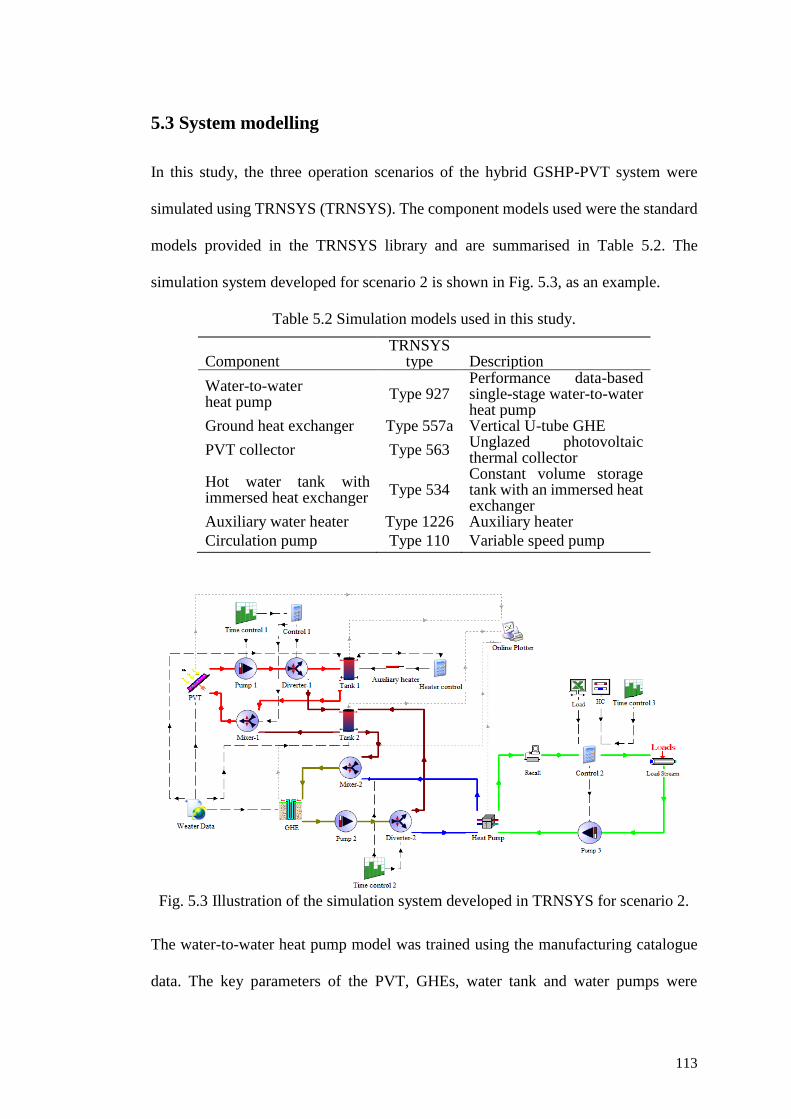
113

5.3 System modelling

In this study, the three operation scenarios of the hybrid GSHP-PVT system were

simulated using TRNSYS (TRNSYS). The component models used were the standard

models provided in the TRNSYS library and are summarised in Table 5.2. The

simulation system developed for scenario 2 is shown in Fig. 5.3, as an example.

Table 5.2 Simulation models used in this study.

Component TRNSYS

type Description

Water-to-water heat pump

Type 927 Performance data-based single-stage water-to-water heat pump

Ground heat exchanger Type 557a Vertical U-tube GHE

PVT collector Type 563 Unglazed photovoltaic thermal collector

Hot water tank with immersed heat exchanger

Type 534 Constant volume storage tank with an immersed heat exchanger

Auxiliary water heater Type 1226 Auxiliary heater

Circulation pump Type 110 Variable speed pump

Fig. 5.3 Illustration of the simulation system developed in TRNSYS for scenario 2.

The water-to-water heat pump model was trained using the manufacturing catalogue

data. The key parameters of the PVT, GHEs, water tank and water pumps were

114

determined using the product specifications, which will be introduced in the following

section.

5.4 Case study

5.4.1 Building model and load characteristics

A two-storey Australian house (Craig James, 2016) with a floor area of 248 m2 and

the conditioned area of 200 m2 was used for the performance analysis. The house

model was developed in DesignBuilder, and is shown in Fig. 5.4.

Fig. 5.4 The house model developed in DesignBuilder.

The heating and cooling thermostat settings used in the load calculation were specified

according to Nationwide House Energy Rating Scheme (NatHERS, 2012). For the

living spaces, the heating thermostat setting was set to 20 oC. For sleeping spaces, a

heating thermostat setting of 18 oC from 7:00 to 9:00 and 16:00 to 24:00, and 15 oC

from 9:00 to 16:00 and 24:00 to 7:00 was used. The cooling thermostat was set as 24.0

oC.

The annual heating and cooling demands of the house were simulated using

DesignBuilder based on the weather data from International Weather for Energy

Calculations (IWEC) of Melbourne and are presented in Fig. 5.5. Table 5.3

summarises the design load and the annual load requirement of the house, which were

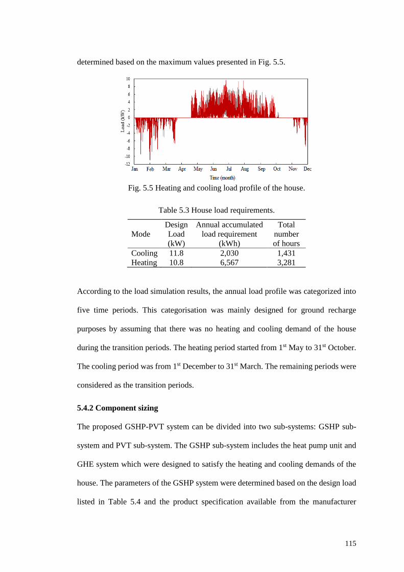
115

determined based on the maximum values presented in Fig. 5.5.

Fig. 5.5 Heating and cooling load profile of the house.

Table 5.3 House load requirements.

Mode

Design

Load

Annual accumulated

load requirement

Total

number

of hours (kW) (kWh)

Cooling 11.8 2,030 1,431

Heating 10.8 6,567 3,281

According to the load simulation results, the annual load profile was categorized into

five time periods. This categorisation was mainly designed for ground recharge

purposes by assuming that there was no heating and cooling demand of the house

during the transition periods. The heating period started from 1st May to 31st October.

The cooling period was from 1st December to 31st March. The remaining periods were

considered as the transition periods.

5.4.2 Component sizing

The proposed GSHP-PVT system can be divided into two sub-systems: GSHP sub-

system and PVT sub-system. The GSHP sub-system includes the heat pump unit and

GHE system which were designed to satisfy the heating and cooling demands of the

house. The parameters of the GSHP system were determined based on the design load

listed in Table 5.4 and the product specification available from the manufacturer

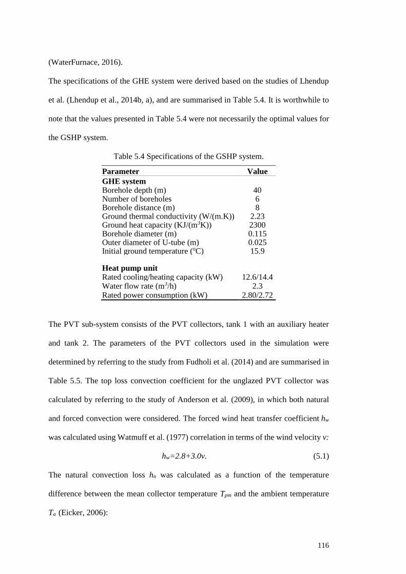
116

(WaterFurnace, 2016).

The specifications of the GHE system were derived based on the studies of Lhendup

et al. (Lhendup et al., 2014b, a), and are summarised in Table 5.4. It is worthwhile to

note that the values presented in Table 5.4 were not necessarily the optimal values for

the GSHP system.

Table 5.4 Specifications of the GSHP system.

Parameter Value

GHE system Borehole depth (m) 40 Number of boreholes 6 Borehole distance (m) 8 Ground thermal conductivity (W/(m.K)) 2.23 Ground heat capacity (KJ/(m3K)) 2300 Borehole diameter (m) 0.115 Outer diameter of U-tube (m) 0.025 Initial ground temperature (oC) 15.9 Heat pump unit Rated cooling/heating capacity (kW) 12.6/14.4 Water flow rate (m3/h) 2.3 Rated power consumption (kW) 2.80/2.72

The PVT sub-system consists of the PVT collectors, tank 1 with an auxiliary heater

and tank 2. The parameters of the PVT collectors used in the simulation were

determined by referring to the study from Fudholi et al. (2014) and are summarised in

Table 5.5. The top loss convection coefficient for the unglazed PVT collector was

calculated by referring to the study of Anderson et al. (2009), in which both natural

and forced convection were considered. The forced wind heat transfer coefficient hw

was calculated using Watmuff et al. (1977) correlation in terms of the wind velocity v:

hw=2.8+3.0v. (5.1)

The natural convection loss hn was calculated as a function of the temperature

difference between the mean collector temperature Tpm and the ambient temperature

Ta (Eicker, 2006):

117

hn=1.78(Tpm-Ta)1/3. (5.2)

Ten different sizes of the PVT collectors with 24, 30, 36, 42, 48, 54, 60, 66, 72 and 78

m2 were considered to examine the impact of the PVT size on the performance of the

proposed system. Trial simulations of scenarios 2 were performed and it was found

that 24 m2 was the minimum area of the PVT collectors that can achieve annual ground

thermal balance through recharging the ground in the transition periods, while 78 m2

was determined as the maximum area of the PVT collectors covering the north rooftop

area of the house. The parameters of all circulation pumps used in the system are

summarised in Table 5.6.

Table 5.5 Summary of main design parameters of the PVT system.

Parameter Value

PVT collector

Absorptivity 0.9 Emissivity 0.8 Electrical efficiency at standard conditions 12% Absorber plate thickness (m) 0.002 Absorber thermal conductivity (W/m·K) 51 Back material thickness (m) 0.05 Back material thermal conductivity (W/m·K) 0.045 Insulation conductivity (W/m·K) 0.045 Number of water tubes 100-340 Outer diameter of water tube (m) 0.02 Other relevant parameters

Volume of tank 1 (Vieira et al., 2014) (L) 250 Volume of tank 2 (L) 250 Power of auxiliary heater (kW) 5.0

Table 5.6 Design parameters of circulation pumps.

Name Function Parameters

Pump 1 Circulation of water between PVT and water tanks

Flow rate: 0.2-0.68 kg/s; Power: 45-70 W. Efficiency: 40%-55%

Pump 2 Source side circulation and ground recharge

Rated flow rate: 0.65 kg/s; Rated power: 94 W. Efficiency: 58%

Pump 3 Load side circulation Rated flow rate: 0.65 kg/s; Rated power: 70 W. Efficiency: 55%

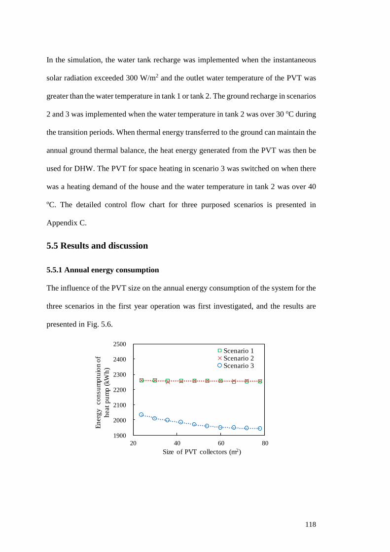
118

In the simulation, the water tank recharge was implemented when the instantaneous

solar radiation exceeded 300 W/m2 and the outlet water temperature of the PVT was

greater than the water temperature in tank 1 or tank 2. The ground recharge in scenarios

2 and 3 was implemented when the water temperature in tank 2 was over 30 oC during

the transition periods. When thermal energy transferred to the ground can maintain the

annual ground thermal balance, the heat energy generated from the PVT was then be

used for DHW. The PVT for space heating in scenario 3 was switched on when there

was a heating demand of the house and the water temperature in tank 2 was over 40

oC. The detailed control flow chart for three purposed scenarios is presented in

Appendix C.

5.5 Results and discussion

5.5.1 Annual energy consumption

The influence of the PVT size on the annual energy consumption of the system for the

three scenarios in the first year operation was first investigated, and the results are

presented in Fig. 5.6.

1900

2000

2100

2200

2300

2400

2500

20 40 60 80

En

erg

y

co

nsu

mp

tuio

n o

f

heat

pu

mp

(kW

h)

Size of PVT collectors (m2)

Scenario 1Scenario 2Scenario 3

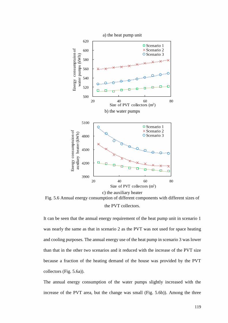
119

a) the heat pump unit

b) the water pumps

c) the auxiliary heater

Fig. 5.6 Annual energy consumption of different components with different sizes of

the PVT collectors.

It can be seen that the annual energy requirement of the heat pump unit in scenario 1

was nearly the same as that in scenario 2 as the PVT was not used for space heating

and cooling purposes. The annual energy use of the heat pump in scenario 3 was lower

than that in the other two scenarios and it reduced with the increase of the PVT size

because a fraction of the heating demand of the house was provided by the PVT

collectors (Fig. 5.6a)).

The annual energy consumption of the water pumps slightly increased with the

increase of the PVT area, but the change was small (Fig. 5.6b)). Among the three

500

520

540

560

580

600

620

20 40 60 80

En

erg

y

co

nsu

mp

tuio

n o

f

wate

r p

um

ps (

kW

h)



3900

4200

4500

4800

5100

20 40 60 80

En

erg

y c

on

su

mp

tuio

n o

f

au

xiliary

h

eate

r (k

Wh

)



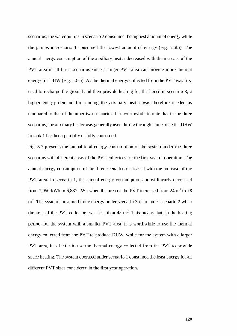
120

scenarios, the water pumps in scenario 2 consumed the highest amount of energy while

the pumps in scenario 1 consumed the lowest amount of energy (Fig. 5.6b)). The

annual energy consumption of the auxiliary heater decreased with the increase of the

PVT area in all three scenarios since a larger PVT area can provide more thermal

energy for DHW (Fig. 5.6c)). As the thermal energy collected from the PVT was first

used to recharge the ground and then provide heating for the house in scenario 3, a

higher energy demand for running the auxiliary heater was therefore needed as

compared to that of the other two scenarios. It is worthwhile to note that in the three

scenarios, the auxiliary heater was generally used during the night-time once the DHW

in tank 1 has been partially or fully consumed.

Fig. 5.7 presents the annual total energy consumption of the system under the three

scenarios with different areas of the PVT collectors for the first year of operation. The

annual energy consumption of the three scenarios decreased with the increase of the

PVT area. In scenario 1, the annual energy consumption almost linearly decreased

from 7,050 kWh to 6,837 kWh when the area of the PVT increased from 24 m2 to 78

m2. The system consumed more energy under scenario 3 than under scenario 2 when

the area of the PVT collectors was less than 48 m2. This means that, in the heating

period, for the system with a smaller PVT area, it is worthwhile to use the thermal

energy collected from the PVT to produce DHW, while for the system with a larger

PVT area, it is better to use the thermal energy collected from the PVT to provide

space heating. The system operated under scenario 1 consumed the least energy for all

different PVT sizes considered in the first year operation.

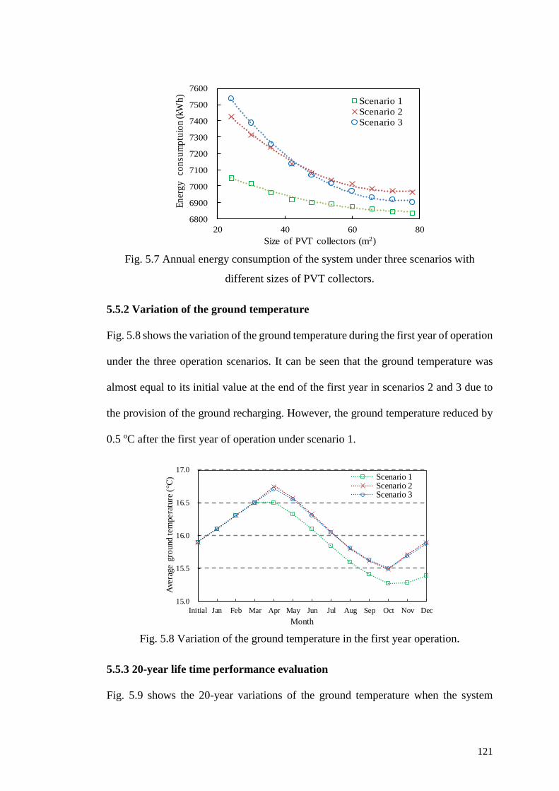
121

Fig. 5.7 Annual energy consumption of the system under three scenarios with

different sizes of PVT collectors.

5.5.2 Variation of the ground temperature

Fig. 5.8 shows the variation of the ground temperature during the first year of operation

under the three operation scenarios. It can be seen that the ground temperature was

almost equal to its initial value at the end of the first year in scenarios 2 and 3 due to

the provision of the ground recharging. However, the ground temperature reduced by

0.5 oC after the first year of operation under scenario 1.

Fig. 5.8 Variation of the ground temperature in the first year operation.

5.5.3 20-year life time performance evaluation

Fig. 5.9 shows the 20-year variations of the ground temperature when the system

6800

6900

7000

7100

7200

7300

7400

7500

7600

20 40 60 80

En

erg

y

con

sum

ptu

ion

(kW

h)


Scenario 1

Scenario 2

Scenario 3

15.0

15.5

16.0

16.5

17.0

Initial Jan Feb Mar Apr May Jun Jul Aug Sep Oct Nov Dec

Ave

rage g

round t

em

pera

ture

(℃

)

Month


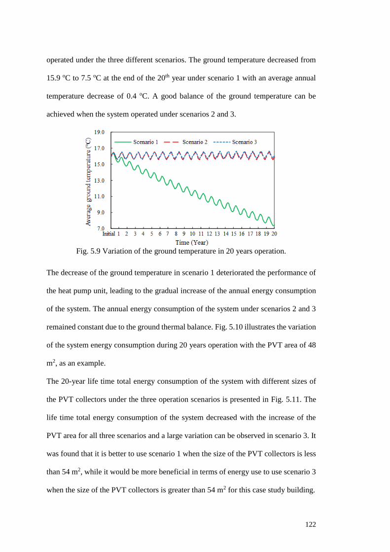
122

operated under the three different scenarios. The ground temperature decreased from

15.9 oC to 7.5 oC at the end of the 20th year under scenario 1 with an average annual

temperature decrease of 0.4 oC. A good balance of the ground temperature can be

achieved when the system operated under scenarios 2 and 3.

Fig. 5.9 Variation of the ground temperature in 20 years operation.

The decrease of the ground temperature in scenario 1 deteriorated the performance of

the heat pump unit, leading to the gradual increase of the annual energy consumption

of the system. The annual energy consumption of the system under scenarios 2 and 3

remained constant due to the ground thermal balance. Fig. 5.10 illustrates the variation

of the system energy consumption during 20 years operation with the PVT area of 48

m2, as an example.

The 20-year life time total energy consumption of the system with different sizes of

the PVT collectors under the three operation scenarios is presented in Fig. 5.11. The

life time total energy consumption of the system decreased with the increase of the

PVT area for all three scenarios and a large variation can be observed in scenario 3. It

was found that it is better to use scenario 1 when the size of the PVT collectors is less

than 54 m2, while it would be more beneficial in terms of energy use to use scenario 3

when the size of the PVT collectors is greater than 54 m2 for this case study building.

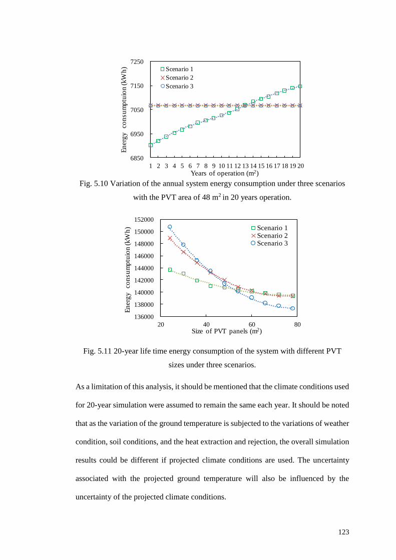
123

Fig. 5.10 Variation of the annual system energy consumption under three scenarios

with the PVT area of 48 m2 in 20 years operation.

Fig. 5.11 20-year life time energy consumption of the system with different PVT

sizes under three scenarios.

As a limitation of this analysis, it should be mentioned that the climate conditions used

for 20-year simulation were assumed to remain the same each year. It should be noted

that as the variation of the ground temperature is subjected to the variations of weather

condition, soil conditions, and the heat extraction and rejection, the overall simulation

results could be different if projected climate conditions are used. The uncertainty

associated with the projected ground temperature will also be influenced by the

uncertainty of the projected climate conditions.

6850

6950

7050

7150

7250

1 2 3 4 5 6 7 8 9 10 11 12 13 14 15 16 17 18 19 20

En

erg

y

co

nsu

mp

tuio

n (kW

h)

Years of operation (m2)

Scenario 1

Scenario 2

Scenario 3

136000

138000

140000

142000

144000

146000

148000

150000

152000

20 40 60 80

En

erg

y

co

nsu

mp

tuio

n (kW

h)

Size of PVT panels (m2)


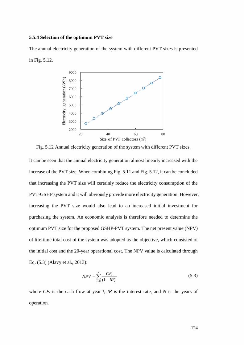
124

5.5.4 Selection of the optimum PVT size

The annual electricity generation of the system with different PVT sizes is presented

in Fig. 5.12.

Fig. 5.12 Annual electricity generation of the system with different PVT sizes.

It can be seen that the annual electricity generation almost linearly increased with the

increase of the PVT size. When combining Fig. 5.11 and Fig. 5.12, it can be concluded

that increasing the PVT size will certainly reduce the electricity consumption of the

PVT-GSHP system and it will obviously provide more electricity generation. However,

increasing the PVT size would also lead to an increased initial investment for

purchasing the system. An economic analysis is therefore needed to determine the

optimum PVT size for the proposed GSHP-PVT system. The net present value (NPV)

of life-time total cost of the system was adopted as the objective, which consisted of

the initial cost and the 20-year operational cost. The NPV value is calculated through

Eq. (5.3) (Alavy et al., 2013):

0 (1 )

Nt

tt

CFNPV

IR=

=+

(5.3)

where CFt is the cash flow at year t, IR is the interest rate, and N is the years of

operation.

2000

3000

4000

5000

6000

7000

8000

9000

20 40 60 80

Ele

ctr

icit

y g

en

era

tio

n (kW

h)


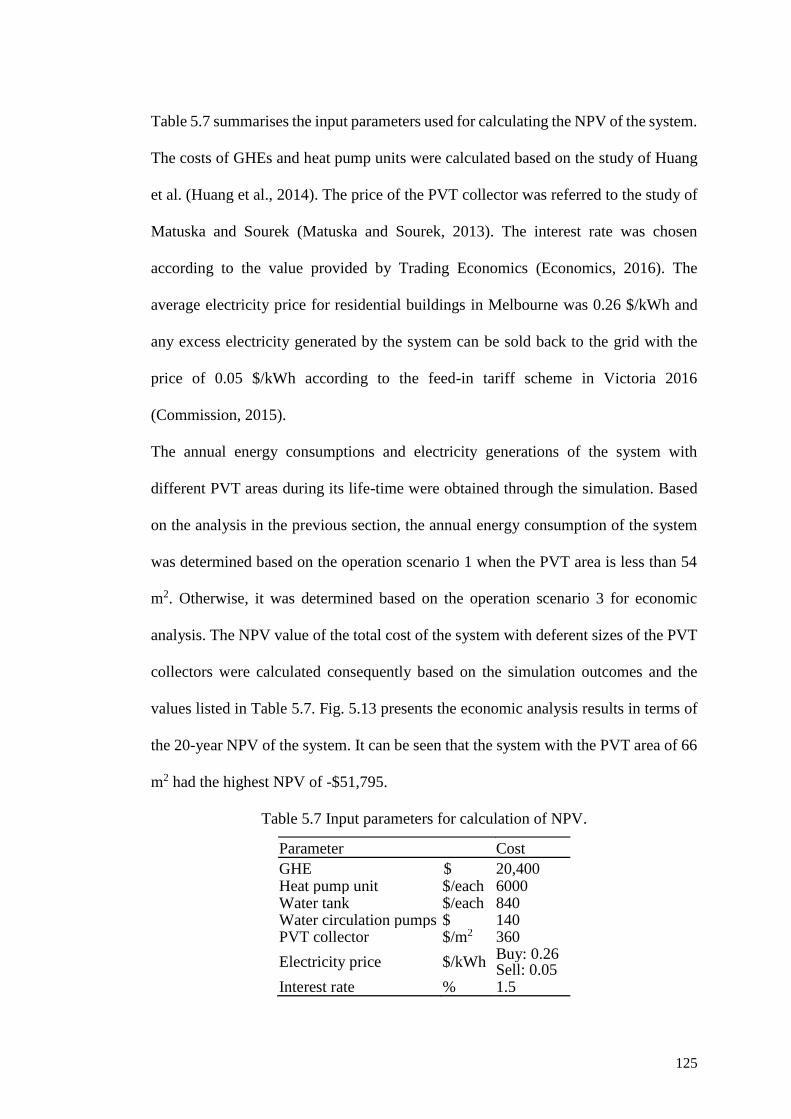
125

Table 5.7 summarises the input parameters used for calculating the NPV of the system.

The costs of GHEs and heat pump units were calculated based on the study of Huang

et al. (Huang et al., 2014). The price of the PVT collector was referred to the study of

Matuska and Sourek (Matuska and Sourek, 2013). The interest rate was chosen

according to the value provided by Trading Economics (Economics, 2016). The

average electricity price for residential buildings in Melbourne was 0.26 $/kWh and

any excess electricity generated by the system can be sold back to the grid with the

price of 0.05 $/kWh according to the feed-in tariff scheme in Victoria 2016

(Commission, 2015).

The annual energy consumptions and electricity generations of the system with

different PVT areas during its life-time were obtained through the simulation. Based

on the analysis in the previous section, the annual energy consumption of the system

was determined based on the operation scenario 1 when the PVT area is less than 54

m2. Otherwise, it was determined based on the operation scenario 3 for economic

analysis. The NPV value of the total cost of the system with deferent sizes of the PVT

collectors were calculated consequently based on the simulation outcomes and the

values listed in Table 5.7. Fig. 5.13 presents the economic analysis results in terms of

the 20-year NPV of the system. It can be seen that the system with the PVT area of 66

m2 had the highest NPV of -$51,795.

Table 5.7 Input parameters for calculation of NPV.

Parameter Cost

GHE $ 20,400 Heat pump unit $/each 6000 Water tank $/each 840 Water circulation pumps $ 140 PVT collector $/m2 360

Electricity price $/kWh Buy: 0.26 Sell: 0.05

Interest rate % 1.5

126

Fig. 5.13 20-year net present value of the system with different PVT sizes.

The analysis of the simulation results showed that the PVT size had a siginificant

influence on both the thermal and electricity outputs of the GSHP-PVT system and

consequently affected the performance of the whole system. In general, the system

with a larger PVT area consumed less energy and produces more electricity. However,

an additional upfront cost will offset the benefit obtained. Therefore, the PVT should

be appropriately sized and the system should be properly contolled to maximise the

economic value of hybrid GSHP-PVT systems.

5.6 Summary

This study presented the simulation and performance evaluation of a ground source

heat pump (GSHP) system integrated with water-based solar photovoltaic thermal

(PVT) collectors under three different operation scenarios. The simulation exercises

were carried out based on a case study building under the weather condition of

Melbourne, Australia. The results showed that the PVT size had a significant influence

on the overall performance and operation scenario used of the hybrid GSHP-PVT

system. For the case building studied, it is more effective to use the heat generated by

the PVT collectors to produce domestic hot water (DHW) if the area of the PVT

collectors is less than 54 m2. Otherwise, it is better to use the heat generated by the

-$58,000

-$56,000

-$54,000

-$52,000

-$50,000

-$48,000

24 30 36 42 48 54 60 66 72 78

20-y

ear

NP

V


127

PVT collectors to recharge the ground during the transition periods and to provide

space heating in the heating period. The result from the 20-year life-time economic

analysis of the system showed that the optimum PVT size for the case building was 66

m2, since the system with the PVT size of 66 m2 had the highest net present value

(NPV) of -$51,795. It is worthwhile to note that, the optimum operation scenario and

the optimum PVT size obtained were subjected to the climate conditions, but the

simulation system developed in this study can be used to facilitate the performance

evaluation of such systems under different climate conditions. This study

demonstrated how building simulation tools offer the capability of analysing and

selecting control strategies for complex low energy systems at the design stage. The

thorough investigation of the dynamic characteristics and energy performance of the

GSHP-PVT system is important for the development of design and control

optimisation strategies for GSHP-PVT systems.

128

Chapter 6 Model-based design optimisation of ground source

heat pump systems with integrated photovoltaic thermal

collectors

The results from Chapter 5 showed that the hybrid GSHP-PVT system can result in a

better energy performance in comparison to conventional heating and cooling systems

and/or stand-alone GSHP systems. However, the high initial investment of both

GSHPs and PVT collectors makes the short-term economics of such systems

unattractive. The optimisation of the key design parameters of GSHP-PVT systems

therefore becomes more important. This chapter presents a model-based design

optimisation strategy for GSHP-PVT systems. A dimension reduction strategy using

Morris global sensitivity analysis was first used to determine the key design parameters

of the GSHP-PVT system. A model-based design optimisation strategy was then

formulated to identify the optimal values of the key design parameters to minimise the

life-cycle cost (LCC) of the GSHP-PVT system, in which an artificial neural network

(ANN) model was used for performance prediction and a genetic algorithm (GA) was

implemented as the optimisation technique. A simulation system of a GSHP-PVT

system developed in TRNSYS was used to generate necessary performance data for

dimension reduction analysis, and for the ANN model training and validation.


research background on the design optimisation of hybrid GSHP-PVT systems. The

virtual simulation system is described in Section 6.2. The descriptions of the dimension

reduction method and the model-based design optimisation strategy are provided in

Section 6.3 and Section 6.4, respectively. Section 6.5 provides the results from the

performance test and evaluation of the proposed strategy. Section 6.6 presents a

129

sensitivity study to understand the sensitivity of the optimisation results to different

prices. A brief summary is provided in Section 6.7.

6.1 Introduction

The high initial investment of both GSHP and PVT collectors makes the short-term

economics of such systems unattractive and the optimisation of the key design

parameters of the GSHP-PVT system therefore becomes more important to reduce the

upfront cost while realising the satisfactory performance of the system. To date, only

a limited number of studies examined the effect of key design parameters on the energy

performance of hybrid GSHP-PVT systems (Bertram et al., 2012).

Artificial neural network (ANN) has been widely used to analyse complex engineering

problems (Kalogirou, 2000, Wong et al., 2010). The main advantage of ANN models

is that they can simulate multivariable problems with complex relationships among the

variables and can approximate the implicit non-linear relationship between input and

output variables by means of ‘learning’ with the training data (Esen et al., 2008b,

Wong et al., 2010). Genetic algorithm (GA) is known as an efficient optimisation

algorithm that can provide good solutions with random initialisations (Wang et al.,

2010, Ma and Wang, 2011a). The use of ANN and GA to formulate optimisation

problems for buildings and building energy systems has been reported in a number of

studies. For instance, Kalogirou (2004) developed a design optimisation method that

combined ANN and GA to size the major design parameters of solar systems. The

results showed that the optimal solutions obtained by using the proposed method

increased the life cycle savings of 4.9% and 3.1% when subsidized and non-subsidized

fuel prices were used respectively, as compared to the solutions obtained by using

traditional trial-and-error method. Magnier and Haghighat (2010) developed a multi-

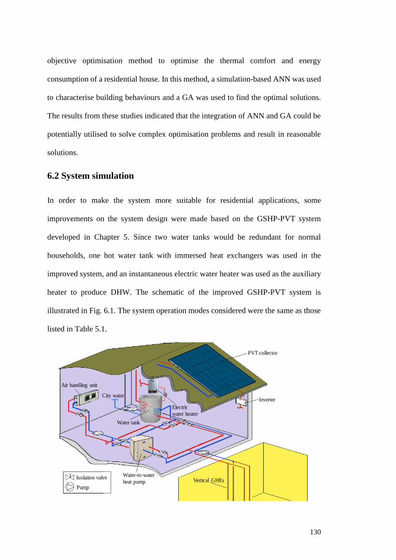
130

objective optimisation method to optimise the thermal comfort and energy

consumption of a residential house. In this method, a simulation-based ANN was used

to characterise building behaviours and a GA was used to find the optimal solutions.

The results from these studies indicated that the integration of ANN and GA could be

potentially utilised to solve complex optimisation problems and result in reasonable

solutions.

6.2 System simulation

In order to make the system more suitable for residential applications, some

improvements on the system design were made based on the GSHP-PVT system

developed in Chapter 5. Since two water tanks would be redundant for normal

households, one hot water tank with immersed heat exchangers was used in the

improved system, and an instantaneous electric water heater was used as the auxiliary

heater to produce DHW. The schematic of the improved GSHP-PVT system is

illustrated in Fig. 6.1. The system operation modes considered were the same as those

listed in Table 5.1.

PVT collector

Air handling unit

City water

Water tank

Electric

water heater

Inverter

Vertical GHEsWater-to-water

heat pumpIsolation valve

Pump

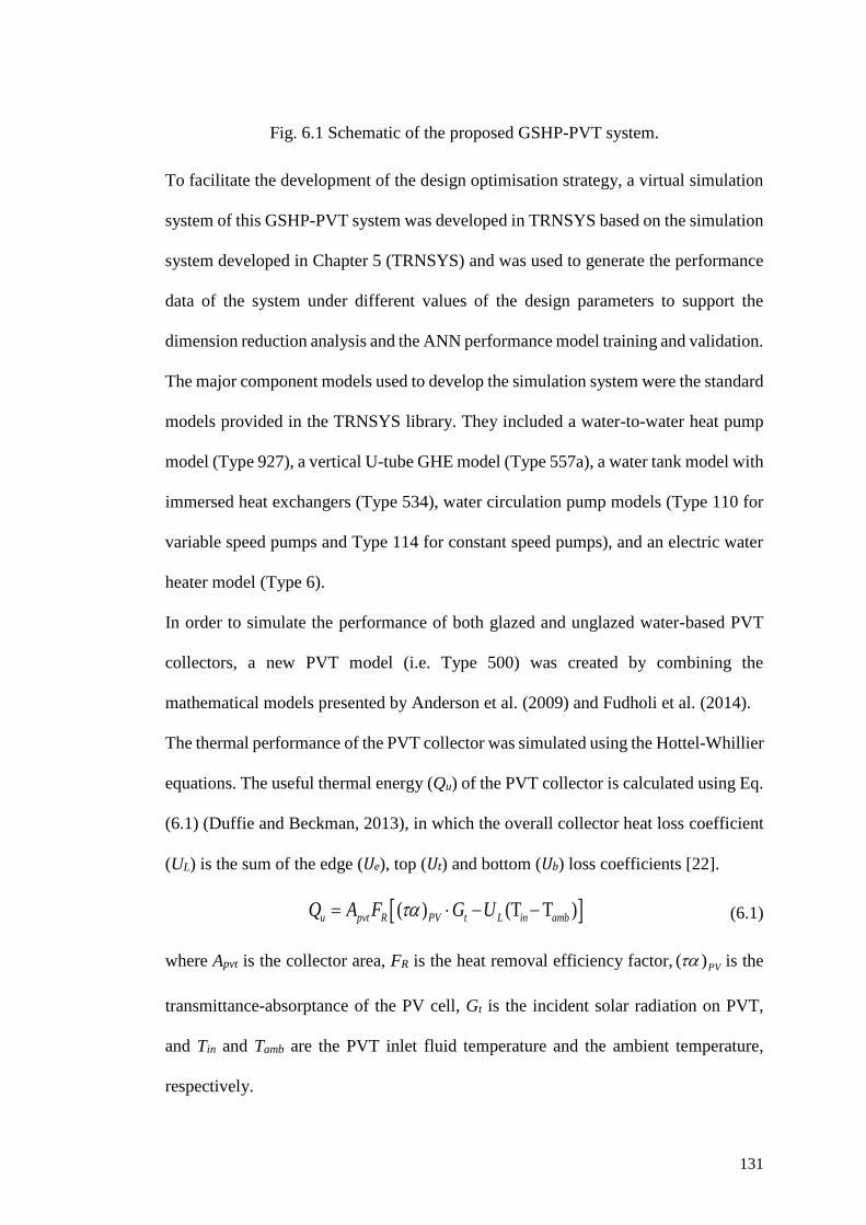
131

Fig. 6.1 Schematic of the proposed GSHP-PVT system.

To facilitate the development of the design optimisation strategy, a virtual simulation

system of this GSHP-PVT system was developed in TRNSYS based on the simulation

system developed in Chapter 5 (TRNSYS) and was used to generate the performance

data of the system under different values of the design parameters to support the

dimension reduction analysis and the ANN performance model training and validation.

The major component models used to develop the simulation system were the standard

models provided in the TRNSYS library. They included a water-to-water heat pump

model (Type 927), a vertical U-tube GHE model (Type 557a), a water tank model with

immersed heat exchangers (Type 534), water circulation pump models (Type 110 for

variable speed pumps and Type 114 for constant speed pumps), and an electric water

heater model (Type 6).

In order to simulate the performance of both glazed and unglazed water-based PVT

collectors, a new PVT model (i.e. Type 500) was created by combining the

mathematical models presented by Anderson et al. (2009) and Fudholi et al. (2014).

The thermal performance of the PVT collector was simulated using the Hottel-Whillier

equations. The useful thermal energy (Qu) of the PVT collector is calculated using Eq.

(6.1) (Duffie and Beckman, 2013), in which the overall collector heat loss coefficient

(UL) is the sum of the edge (Ue), top (Ut) and bottom (Ub) loss coefficients [22].

( ) (T T )u pvt R PV t L in ambQ A F G U= − − (6.1)

where Apvt is the collector area, FR is the heat removal efficiency factor, ( )PV is the

transmittance-absorptance of the PV cell, Gt is the incident solar radiation on PVT,

and Tin and Tamb are the PVT inlet fluid temperature and the ambient temperature,

respectively.

132

The edge and bottom loss coefficients can be determined using Eqs. (6.2) and (6.3),

respectively (Duffie and Beckman, 2013). For glazed and unglazed PVT collectors,

the top loss coefficient (Ut) is calculated using Eqs. (6.4) (Fudholi et al., 2014) and

(6.5) (Anderson et al., 2009), respectively.

( )ee

pvt

UAU

A= (6.2)

insb

ins

kU

L= (6.3)

( )( )

1

2 2

1

1

2 1 0.133( 0.00591 )

mp amb mp ambg

t eg pw

mp ambp w

gmp g

T T T TNU

N fhT TC Nh N

T N f

−

−

+ + = + + − + − + + −

+

(6.4)

t r cU h h= + (6.5)

where (UA)e is the edge loss coefficient – area product, and kins and Lins are the thermal

conductivity and the thickness of the back insulation respectively, Ng is the number of

the glass covers, hw is the convection heat loss coefficient due to the wind, is the

Stefan-Boltzmann constant, p is the plate emittance,

g is the glass emittance, Tmp is

the mean plate temperature, C, f, e are the coefficients which can be obtained following

the method provided by Fudholi et al. (2014), and hr and hc are the radiation heat loss

and overall convection heat loss coefficients respectively which can be found using

the methodology provided in Anderson et al. (2009).

The thermal efficiency (th ) and electrical efficiency (

pv ) of PVT collectors can be

calculated using Eqs. (6.6) and (6.7), respectively.

uth

pvt t

Q

A G = (6.6)

133

(1 ( ))pv r cell refT T = − − (6.7)

where r is the reference efficiency of the PV module, is the temperature

coefficient, Tcell is the cell temperature, and Tref is the reference temperature.

In the simulation, the GSHP-PVT system operated the same way as the operation

scenario 3 proposed in Chapter 5, since the performance evaluation carried out on the

improved system showed that scenario 3 was still the most energy efficient one among

the three operation scenarios proposed in Chapter 5. The PVT water pump was

switched on when the incident solar radiation was over 300 W/m2 and the PVT mean

plate temperature was 5 oC higher than the average water temperature in the water tank.

The ground recharge was implemented when the water temperature in the tank during

the transition periods was over 30 oC. The amount of the thermal energy to be

recharged into the ground was estimated based on the annual heat extraction and heat

rejection from the GSHP system simulated using the same GSHP-PVT system but

without using the ground recharge. Once the thermal energy transferred to the ground

can maintain the annual ground thermal balance, the heat energy generated from the

PVT collectors during the transition periods was used for DHW only. During the

cooling periods, the heat energy generated from the PVT was only used for DHW.

During the heating periods, the heat generated by the PVT collectors was used for

DHW heating and for space heating when the building has a heating demand and the

water temperature in the water tank was over 40 oC. The electric water heater was only

used to heat the water from the water tank when there was a DHW demand and the

water temperature in the tank was lower than the required temperature. The ground

source heat pump was used when there was a cooling demand or when there was a

heating demand and the water temperature in the water tank was below 40 oC. The

supply and return chilled water temperatures of the GSHP system were assumed to be

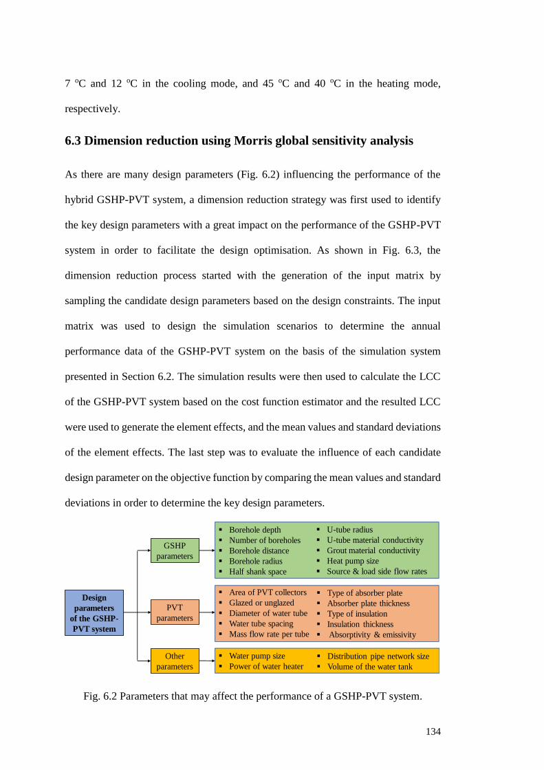
134

7 oC and 12 oC in the cooling mode, and 45 oC and 40 oC in the heating mode,

respectively.

6.3 Dimension reduction using Morris global sensitivity analysis

As there are many design parameters (Fig. 6.2) influencing the performance of the

hybrid GSHP-PVT system, a dimension reduction strategy was first used to identify

the key design parameters with a great impact on the performance of the GSHP-PVT

system in order to facilitate the design optimisation. As shown in Fig. 6.3, the

dimension reduction process started with the generation of the input matrix by

sampling the candidate design parameters based on the design constraints. The input

matrix was used to design the simulation scenarios to determine the annual

performance data of the GSHP-PVT system on the basis of the simulation system

presented in Section 6.2. The simulation results were then used to calculate the LCC

of the GSHP-PVT system based on the cost function estimator and the resulted LCC

were used to generate the element effects, and the mean values and standard deviations

of the element effects. The last step was to evaluate the influence of each candidate

design parameter on the objective function by comparing the mean values and standard

deviations in order to determine the key design parameters.

Fig. 6.2 Parameters that may affect the performance of a GSHP-PVT system.

Design

parameters

of the GSHP-

PVT system

GSHP

parameters

PVT

parameters

Other

parameters

▪ Borehole depth

▪ Number of boreholes

▪ Borehole distance

▪ Borehole radius

▪ Half shank space

▪ Area of PVT collectors

▪ Glazed or unglazed

▪ Diameter of water tube

▪ Water tube spacing

▪ Mass flow rate per tube

▪ U-tube radius

▪ U-tube material conductivity

▪ Grout material conductivity

▪ Heat pump size

▪ Source & load side flow rates

▪ Type of absorber plate

▪ Absorber plate thickness

▪ Type of insulation

▪ Insulation thickness

▪ Absorptivity & emissivity

▪ Water pump size

▪ Power of water heater

▪ Distribution pipe network size

▪ Volume of the water tank

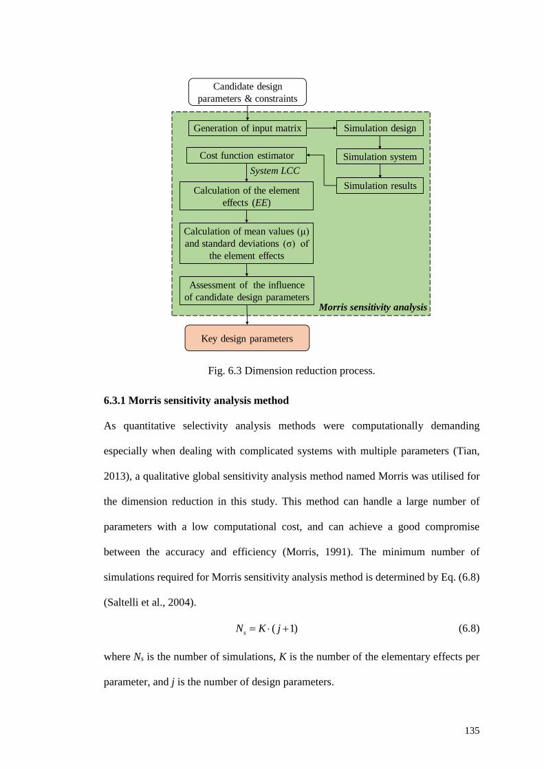
135

Fig. 6.3 Dimension reduction process.

6.3.1 Morris sensitivity analysis method

As quantitative selectivity analysis methods were computationally demanding

especially when dealing with complicated systems with multiple parameters (Tian,

2013), a qualitative global sensitivity analysis method named Morris was utilised for

the dimension reduction in this study. This method can handle a large number of

parameters with a low computational cost, and can achieve a good compromise

between the accuracy and efficiency (Morris, 1991). The minimum number of

simulations required for Morris sensitivity analysis method is determined by Eq. (6.8)

(Saltelli et al., 2004).

( 1)sN K j= + (6.8)

where Ns is the number of simulations, K is the number of the elementary effects per

parameter, and j is the number of design parameters.

Cost function estimator

Assessment of the influence

of candidate design parametersMorris sensitivity analysis

Simulation design

Candidate design

parameters & constraints


Simulation system

Generation of input matrix

Simulation resultsCalculation of the element

effects (EE)

Calculation of mean values (μ)

and standard deviations (σ) of

the element effects

System LCC

136

From Morris analysis, two sensitivity indicators, i.e. mean value (μ) and standard

deviation (σ) of the absolute values of the elementary effects as defined in Eqs. (6.9)

and (6.10) respectively, can be obtained (Saltelli et al., 2004). The mean value is used

to estimate the main influence of the input parameter on the output while the standard

deviation is used to evaluate the interactions among the parameters or the non-linear

effects. In the Morris method, the factors are generally represented by a plane (μ, σ) in

order to compare their relative influence (Sohier et al., 2015).

1

/k

i

i

EE K=

= (6.9)

2

1

/k

i

i

EE K =

= − (6.10)

where EE is the elementary effect.

The elementary effect EE is derived from a model y=y(x1 ,…, xj) with j input

parameters, i.e. x1,…, xj. The EE for the ith input parameter at the kth sampling point is

calculated by Eq. (6.11) (Heiselberg et al., 2009).

(k) (k) (k) (k) (k) (k) (k) (k)

1 2 1 1 1(k)(x , x ..., x , x , x ,..., x ) (x ,..., x )i i i j j

i

y yEE

− ++ −=

(6.11)

The successful use of Morris sensitivity analysis method is dependent on the proper

sampling of each input parameter within its defined range. The Latin hypercube

sampling method was used for this purpose, which can generate a certain number of

discretised values within the constraints defined for each parameter to improve the

efficiency of the Morris method (Sohier et al., 2015).

6.3.2 Objective function

The objective function used in the dimension reduction was the 20-year life cycle cost

(LCC) of the GSHP-PVT system in net present value. The LCC generally includes the

137

initial cost (IC), operation cost (OC), maintenance cost (MC), replacement cost (RC)

and residual cost (DC), as expressed in Eq. (6.12) (Woodward, 1997, Zhu et al., 2012).

The initial cost was determined by Eq. (6.13), in which the upfront costs of GHEs,

PVT collectors and water tank were determined using Eqs. (6.14)-(6.16), respectively.

The 20-year operational cost was determined using Eq. (6.17) (Zhu et al., 2012), in

which the annual operational cost was determined using Eq. (6.18). The 20-year

maintenance cost was determined using Eq. (6.19) (Zhu et al., 2012), in which the

annual maintenance cost was determined using Eq. (6.20). In this study, the

replacement cost was not considered and the residual cost was also not considered due

to the lack of the information on calculating the salvage values of the GSHP system

and the PVT collectors.

LCC IC OC MC RC DC= + + + + (6.12)

GHE HP PVT TK Pu WHIC IC IC IC IC IC IC= + + + + + (6.13)

GHE p p b bIC C L C L= + (6.14)

PVT PVT PVTIC C A= (6.15)

1 2Tk TKIC AV A= + (6.16)

1 (1 )( )

n

op

rOC C

r

−− += (6.17)

1

1

( ) ,

( ) ,

Ni i i i

con gen EB con gen

i

op Ni i i i

con gen ES con gen

i

E E C if E E

C

E E C if E E

=

=

−

= −

(6.18)

1 (1 )( )

n

ma

rMC C

r

−− += (6.19)

ma ma cfC MC A= (6.20)

138

where pC is the cost of the U-tube per meter,

pL is the total U-tube length within all

boreholes, bC is the drilling cost and grouting cost per meter, bL is the total borehole

length, PVTC is the cost of the PVT collectors per square meter, PVTA is the area of the

PVT collector, VTK is the volume of the water tank, A1 and A2 are the coefficients which

were determined based on the tank prices of various volumes, r is the discount rate,

opC is the annual operational cost, i

conE and i

genE are the electricity consumption and

generation of the system at the ith simulation time step, respectively, EBC and ESC are

the electricity buy and sell prices per kWh, respectively, N is the total number of

simulation time steps, maC is the annual maintenance cost of the system, maMC is the

annual maintenance cost per square meter, Acf is the air conditioned floor area of the

building, and the subscripts GHE, HP, PVT, TK, Pu and WH represent the ground heat

exchanger, heat pump unit, photovoltaic thermal collector, water tank, water

circulation pump and water heater, respectively.

6.3.3 Constraints

The following constraints were applied in the dimension reduction. The minimum area

of the PVT collectors was determined based on the thermal energy required to recharge

the ground in order to achieve an annual thermal balance. The amount of the thermal

energy to be recharged into the ground was estimated based on the simulation results

as described in Section 6.2. The maximum value was determined based on the north

rooftop area of the building. The variation ranges of the other design parameters of the

PVT collector were determined based on the data used in previous studies (Farghally

et al., 2013, Chow et al., 2008, Ibrahim et al., 2014, Tiwari et al., 2009, Sukesh et al.,

2015, Fudholi et al., 2014, Anderson et al., 2009, Chow et al., 2009, Bhattarai et al.,

2012), and the details are presented in Section 6.5.

139

The capacity of the GSHP system was determined to satisfy the heating and cooling

demand of the building at the design conditions. The estimated total length of the

vertical GHEs was associated with the design load and the design heat flux through

GHEs. The acceptable range of the heat flux was dependent on the thermal

conductivity of the soil on the site (Banks, 2012). The variation ranges of the

geometrical parameters such as the number of boreholes, borehole depth, and the

distance between boreholes were determined based on the recommended values from

practical engineering projects (Handbook, 2015, Banks, 2012, Huang et al., 2014).

The volume of the water tank was determined based on the estimated daily average

hot water consumption of the building according to the Australian and New Zealand

Standard for Heated Water Services (Australia, 2003).

6.4 Development of the model-based design optimisation strategy

6.4.1 Outline of the optimisation strategy

The primary aim of the design optimisation was to determine the optimal values of the

key design parameters to minimise the 20-year life cycle cost (LCC) of the GSHP-

PVT system in terms of the net present value. The outline of the optimisation strategy

is illustrated in Fig. 6.4, which was developed using a model-based approach and the

key parameters identified through the dimension reduction. In this strategy, an ANN

model was used to predict the system performance under different working conditions

and a GA was used as the optimisation technique to identify the optimal solution of

the optimisation problem to minimise the cost function. The same cost function and

constraints as those used in the dimension reduction strategy were used as the

optimisation objective and optimisation constraints, respectively.

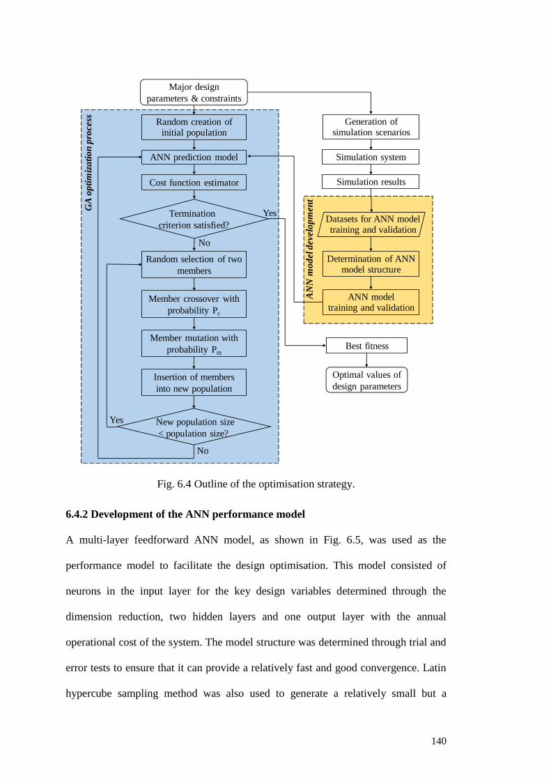
140

Fig. 6.4 Outline of the optimisation strategy.

6.4.2 Development of the ANN performance model

A multi-layer feedforward ANN model, as shown in Fig. 6.5, was used as the

performance model to facilitate the design optimisation. This model consisted of

neurons in the input layer for the key design variables determined through the

dimension reduction, two hidden layers and one output layer with the annual

operational cost of the system. The model structure was determined through trial and

error tests to ensure that it can provide a relatively fast and good convergence. Latin

hypercube sampling method was also used to generate a relatively small but a

AN

N m

od

el d

evelo

pm

en

t

ANN prediction model

GA

op

tim

iza

tio

n p

rocess

Optimal values of

design parameters

Simulation system

Cost function estimator


Major design

parameters & constraints

Simulation results

Datasets for ANN model training and validation

Termination

criterion satisfied?

Random selection of two

members

Member crossover with

probability Pc

Member mutation with

probability Pm

Insertion of members

into new population

Random creation of initial population

Determination of ANN model structure

ANN model training and validation

New population size

< population size?

No

Yes

Best fitness

No

Yes

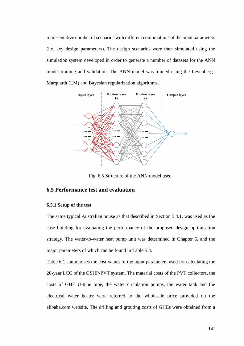
141

representative number of scenarios with different combinations of the input parameters

(i.e. key design parameters). The design scenarios were then simulated using the

simulation system developed in order to generate a number of datasets for the ANN

model training and validation. The ANN model was trained using the Levenberg–

Marquardt (LM) and Bayesian regularization algorithms.

Fig. 6.5 Structure of the ANN model used.

6.5 Performance test and evaluation

6.5.1 Setup of the test

The same typical Australian house as that described in Section 5.4.1, was used as the

case building for evaluating the performance of the proposed design optimisation

strategy. The water-to-water heat pump unit was determined in Chapter 5, and the

major parameters of which can be found in Table 5.4.

Table 6.1 summarises the cost values of the input parameters used for calculating the

20-year LCC of the GSHP-PVT system. The material costs of the PVT collectors, the

costs of GHE U-tube pipe, the water circulation pumps, the water tank and the

electrical water heater were referred to the wholesale price provided on the

alibaba.com website. The drilling and grouting costs of GHEs were obtained from a

Input layer Hidden layer

1#Output layerHidden layer

2#

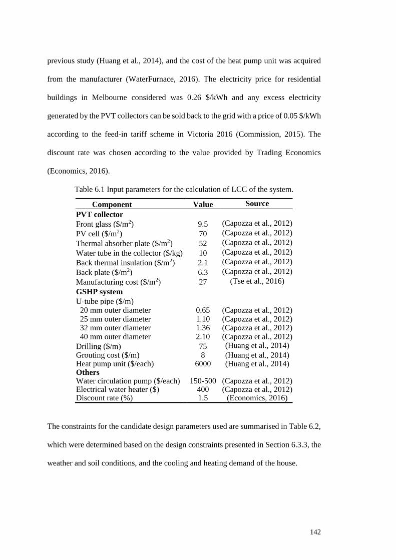
142

previous study (Huang et al., 2014), and the cost of the heat pump unit was acquired

from the manufacturer (WaterFurnace, 2016). The electricity price for residential

buildings in Melbourne considered was 0.26 $/kWh and any excess electricity

generated by the PVT collectors can be sold back to the grid with a price of 0.05 $/kWh

according to the feed-in tariff scheme in Victoria 2016 (Commission, 2015). The

discount rate was chosen according to the value provided by Trading Economics

(Economics, 2016).

Table 6.1 Input parameters for the calculation of LCC of the system.

Component Value Source

PVT collector

Front glass ($/m2) 9.5 (Capozza et al., 2012)

PV cell ($/m2) 70 (Capozza et al., 2012)

Thermal absorber plate ($/m2) 52 (Capozza et al., 2012)

Water tube in the collector ($/kg) 10 (Capozza et al., 2012)

Back thermal insulation ($/m2) 2.1 (Capozza et al., 2012)

Back plate ($/m2) 6.3 (Capozza et al., 2012)

Manufacturing cost ($/m2) 27 (Tse et al., 2016)

GSHP system

U-tube pipe ($/m)

20 mm outer diameter 0.65 (Capozza et al., 2012) 25 mm outer diameter 1.10 (Capozza et al., 2012) 32 mm outer diameter 1.36 (Capozza et al., 2012) 40 mm outer diameter 2.10 (Capozza et al., 2012)

Drilling ($/m) 75 (Huang et al., 2014)

Grouting cost ($/m) 8 (Huang et al., 2014) Heat pump unit ($/each) 6000 (Huang et al., 2014) Others Water circulation pump ($/each) 150-500 (Capozza et al., 2012) Electrical water heater ($) 400 (Capozza et al., 2012) Discount rate (%) 1.5 (Economics, 2016)

The constraints for the candidate design parameters used are summarised in Table 6.2,

which were determined based on the design constraints presented in Section 6.3.3, the

weather and soil conditions, and the cooling and heating demand of the house.

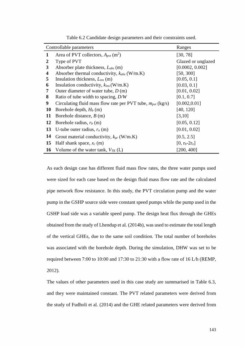
143

Table 6.2 Candidate design parameters and their constraints used.

Controllable parameters Ranges

1 Area of PVT collectors, Apvt (m2) [30, 78]

2 Type of PVT Glazed or unglazed

3 Absorber plate thickness, Labs (m) [0.0002, 0.002]

4 Absorber thermal conductivity, kabs (W/m.K) [50, 300]

5 Insulation thickness, Lins (m) [0.05, 0.1]

6 Insulation conductivity, kins (W/m.K) [0.03, 0.1]

7 Outer diameter of water tube, D (m) [0.01, 0.02]

8 Ratio of tube width to spacing, D/W [0.1, 0.7]

9 Circulating fluid mass flow rate per PVT tube, mpvt (kg/s) [0.002,0.01]

10 Borehole depth, Hb (m) [40, 120]

11 Borehole distance, B (m) [3,10]

12 Borehole radius, rb (m) [0.05, 0.12]

13 U-tube outer radius, ro (m) [0.01, 0.02]

14 Grout material conductivity, kgr (W/m.K) [0.5, 2.5]

15 Half shank space, xc (m) [0, rb-2ro]

16 Volume of the water tank, VTK (L) [200, 400]

As each design case has different fluid mass flow rates, the three water pumps used

were sized for each case based on the design fluid mass flow rate and the calculated

pipe network flow resistance. In this study, the PVT circulation pump and the water

pump in the GSHP source side were constant speed pumps while the pump used in the

GSHP load side was a variable speed pump. The design heat flux through the GHEs

obtained from the study of Lhendup et al. (2014b), was used to estimate the total length

of the vertical GHEs, due to the same soil condition. The total number of boreholes

was associated with the borehole depth. During the simulation, DHW was set to be

required between 7:00 to 10:00 and 17:30 to 21:30 with a flow rate of 16 L/h (REMP,

2012).

The values of other parameters used in this case study are summarised in Table 6.3,

and they were maintained constant. The PVT related parameters were derived from

the study of Fudholi et al. (2014) and the GHE related parameters were derived from

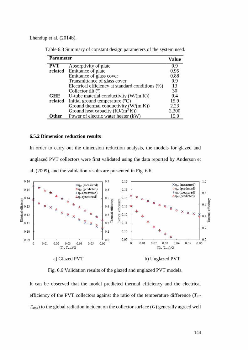
144

Lhendup et al. (2014b).

Table 6.3 Summary of constant design parameters of the system used.

Parameter Value

PVT related

Absorptivity of plate 0.9 Emittance of plate 0.95 Emittance of glass cover 0.88 Transmittance of glass cover 0.9 Electrical efficiency at standard conditions (%) 13 Collector tilt (o) 30

GHE related

U-tube material conductivity (W/(m.K)) 0.4 Initial ground temperature (oC) 15.9 Ground thermal conductivity (W/(m.K)) 2.23 Ground heat capacity (KJ/(m3 K)) 2,300

Other Power of electric water heater (kW) 15.0

6.5.2 Dimension reduction results

In order to carry out the dimension reduction analysis, the models for glazed and

unglazed PVT collectors were first validated using the data reported by Anderson et

al. (2009), and the validation results are presented in Fig. 6.6.

a) Glazed PVT b) Unglazed PVT

Fig. 6.6 Validation results of the glazed and unglazed PVT models.

It can be observed that the model predicted thermal efficiency and the electrical

efficiency of the PVT collectors against the ratio of the temperature difference (Tin-

Tamb) to the global radiation incident on the collector surface (G) generally agreed well

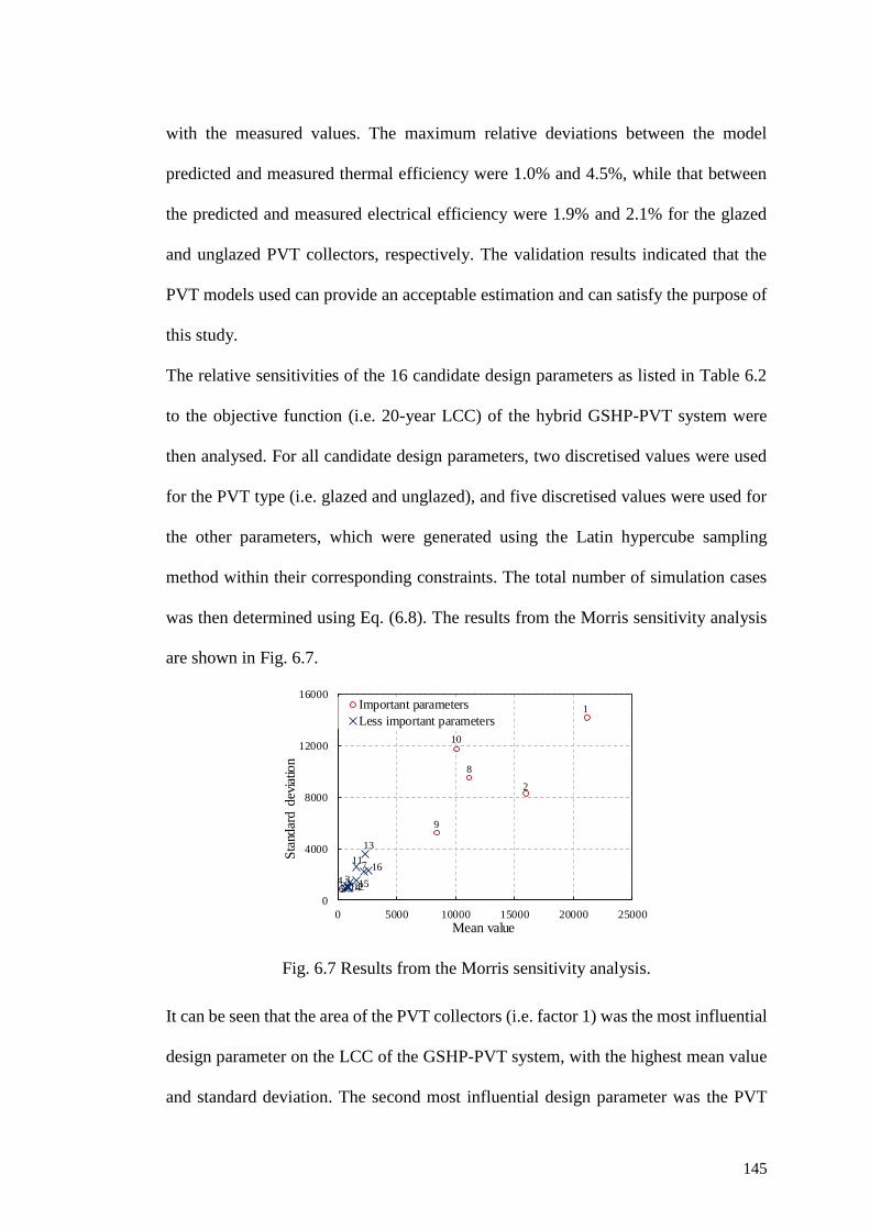
145

with the measured values. The maximum relative deviations between the model

predicted and measured thermal efficiency were 1.0% and 4.5%, while that between

the predicted and measured electrical efficiency were 1.9% and 2.1% for the glazed

and unglazed PVT collectors, respectively. The validation results indicated that the

PVT models used can provide an acceptable estimation and can satisfy the purpose of

this study.

The relative sensitivities of the 16 candidate design parameters as listed in Table 6.2

to the objective function (i.e. 20-year LCC) of the hybrid GSHP-PVT system were

then analysed. For all candidate design parameters, two discretised values were used

for the PVT type (i.e. glazed and unglazed), and five discretised values were used for

the other parameters, which were generated using the Latin hypercube sampling

method within their corresponding constraints. The total number of simulation cases

was then determined using Eq. (6.8). The results from the Morris sensitivity analysis

are shown in Fig. 6.7.

Fig. 6.7 Results from the Morris sensitivity analysis.

It can be seen that the area of the PVT collectors (i.e. factor 1) was the most influential

design parameter on the LCC of the GSHP-PVT system, with the highest mean value

and standard deviation. The second most influential design parameter was the PVT

1

2

8

9

10

3456

711

12

13

1415

16

0

4000

8000

12000

16000

0 5000 10000 15000 20000 25000

Sta

ndar

d d

evia

tion

Mean value

Important parameters

Less important parameters

146

type (i.e. factor 2), followed by the ratio of the tube width to the spacing (i.e. factor 8),

the borehole depth (i.e. factor 10) and the circulation fluid mass flow rate per PVT

tube (i.e. factor 9). The remaining parameters can be considered as the parameters with

a less impact on the LCC of the GSHP-PVT system and the constant values determined

based on the existing studies and design practices (see Table 6.4) were therefore used

in the following design optimisation.

Table 6.4 Low sensitivity parameters and values used (Huang et al., 2014, Ibrahim et

al., 2014, Fudholi et al., 2014).

Parameters Values

Absorber plate thickness (m) 0.002

Absorber thermal conductivity (W/(m.K)) 51

Insulation thickness (m) 0.05

Insulation conductivity W/(m.K) 0.045

Outer diameter of water tube (m) 0.012

Borehole distance (m) 8

Borehole radius (m) 0.06

U-tube outer radius (m) 0.0125

Grout material conductivity (W/(m.K)) 2.42

Half shank space (m) 0.025

Volume of the water tank (L) 250

6.5.3 Performance evaluation of the design optimisation strategy

6.5.3.1 ANN model validation

The total number of the datasets used for the ANN model training was 30 times of the

number of the key design variables, which was considered to be sufficient to accurately

sample the search space of the design variables (Conraud-Bianchi, 2008). Another 30

datasets were used to validate the effectiveness of the ANN model. Each dataset

corresponded to a simulation scenario with different combinations of the key design

parameters identified through the dimension reduction analysis. Therefore, a total

number of 180 scenarios were designed and simulated using the simulation system

developed in Section 6.2.

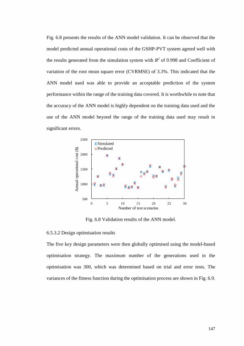
147

Fig. 6.8 presents the results of the ANN model validation. It can be observed that the

model predicted annual operational costs of the GSHP-PVT system agreed well with

the results generated from the simulation system with R2 of 0.998 and Coefficient of

variation of the root mean square error (CVRMSE) of 3.3%. This indicated that the

ANN model used was able to provide an acceptable prediction of the system

performance within the range of the training data covered. It is worthwhile to note that

the accuracy of the ANN model is highly dependent on the training data used and the

use of the ANN model beyond the range of the training data used may result in

significant errors.

Fig. 6.8 Validation results of the ANN model.

6.5.3.2 Design optimisation results

The five key design parameters were then globally optimised using the model-based

optimisation strategy. The maximum number of the generations used in the

optimisation was 300, which was determined based on trial and error tests. The

variances of the fitness function during the optimisation process are shown in Fig. 6.9.

500

1000

1500

2000

2500

0 5 10 15 20 25 30

Annual

opera

tional

cost

($)

Number of test scenarios

Simulated

Predicted

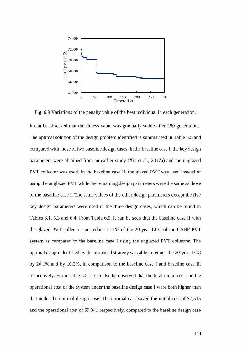
148

Fig. 6.9 Variations of the penalty value of the best individual in each generation.

It can be observed that the fitness value was gradually stable after 250 generations.

The optimal solution of the design problem identified is summarised in Table 6.5 and

compared with those of two baseline design cases. In the baseline case I, the key design

parameters were obtained from an earlier study (Xia et al., 2017a) and the unglazed

PVT collector was used. In the baseline case II, the glazed PVT was used instead of

using the unglazed PVT while the remaining design parameters were the same as those

of the baseline case I. The same values of the other design parameters except the five

key design parameters were used in the three design cases, which can be found in

Tables 6.1, 6.3 and 6.4. From Table 6.5, it can be seen that the baseline case II with

the glazed PVT collector can reduce 11.1% of the 20-year LCC of the GSHP-PVT

system as compared to the baseline case I using the unglazed PVT collector. The

optimal design identified by the proposed strategy was able to reduce the 20-year LCC

by 20.1% and by 10.2%, in comparison to the baseline case I and baseline case II,

respectively. From Table 6.5, it can also be observed that the total initial cost and the

operational cost of the system under the baseline design case I were both higher than

that under the optimal design case. The optimal case saved the initial cost of $7,515

and the operational cost of $9,341 respectively, compared to the baseline design case

64000

66000

68000

70000

72000

74000

0 50 100 150 200 250 300

Pen

alty

val

ue (

$)

Generation

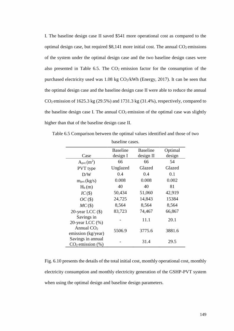
149

I. The baseline design case II saved $541 more operational cost as compared to the

optimal design case, but required $8,141 more initial cost. The annual CO2 emissions

of the system under the optimal design case and the two baseline design cases were

also presented in Table 6.5. The CO2 emission factor for the consumption of the

purchased electricity used was 1.08 kg CO2/kWh (Energy, 2017). It can be seen that

the optimal design case and the baseline design case II were able to reduce the annual

CO2 emission of 1625.3 kg (29.5%) and 1731.3 kg (31.4%), respectively, compared to

the baseline design case I. The annual CO2 emission of the optimal case was slightly

higher than that of the baseline design case II.

Table 6.5 Comparison between the optimal values identified and those of two

baseline cases.

Case Baseline

design I

Baseline

design II

Optimal

design

Apvt (m2) 66 66 54

PVT type Unglazed Glazed Glazed

D/W 0.4 0.4 0.1

mpvt (kg/s) 0.008 0.008 0.002

Hb (m) 40 40 81

IC ($) 50,434 51,060 42,919

OC ($) 24,725 14,843 15384

MC ($) 8,564 8,564 8,564

20-year LCC ($) 83,723 74,467 66,867

Savings in

20-year LCC (%) - 11.1 20.1

Annual CO2

emission (kg/year) 5506.9 3775.6 3881.6

Savings in annual

CO2 emission (%) - 31.4 29.5

Fig. 6.10 presents the details of the total initial cost, monthly operational cost, monthly

electricity consumption and monthly electricity generation of the GSHP-PVT system

when using the optimal design and baseline design parameters.

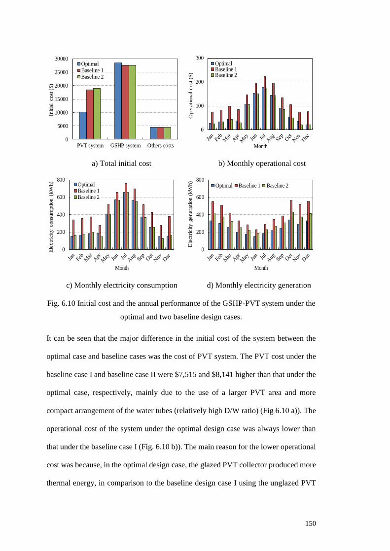
150

a) Total initial cost b) Monthly operational cost

c) Monthly electricity consumption d) Monthly electricity generation

Fig. 6.10 Initial cost and the annual performance of the GSHP-PVT system under the

optimal and two baseline design cases.

It can be seen that the major difference in the initial cost of the system between the

optimal case and baseline cases was the cost of PVT system. The PVT cost under the

baseline case I and baseline case II were $7,515 and $8,141 higher than that under the

optimal case, respectively, mainly due to the use of a larger PVT area and more

compact arrangement of the water tubes (relatively high D/W ratio) (Fig 6.10 a)). The

operational cost of the system under the optimal design case was always lower than

that under the baseline case I (Fig. 6.10 b)). The main reason for the lower operational

cost was because, in the optimal design case, the glazed PVT collector produced more

thermal energy, in comparison to the baseline design case I using the unglazed PVT

0

5000

10000

15000

20000

25000

30000

PVT system GSHP system Others costs

Initia

l cost

($)

OptimalBaseline 1Baseline 2

0

100

200

300

Opera

tional

cost

($)

Month


0

200

400

600

800

Ele

ctr

icity c

onsu

mption (

kW

h)

Month


0

200

400

600

800

Ele

ctr

icity g

enera

tion (

kW

h)

Month

Optimal Baseline 1 Baseline 2

151

collector and even with a larger PVT area. This results in a lower electrical demand

for producing DHW (Fig. 6.10 c)). Although the baseline design case I generated more

electricity monthly (Fig. 6.10 d)) in comparison to the optimal design case, the gap

between the electricity buy and sell prices made this benefit less obvious. The

operational cost of the system under the baseline case II was lower than that under the

optimal design case in particular during the transition periods (i.e. April and

November). The difference in the monthly electricity consumption of the system

between the optimal case and the baseline case II was relatively small (Fig. 6.10 c)),

but the monthly electricity generation of the system under the baseline case II was

always higher than that under the optimal design case (Fig. 6.10 d)), due to the use of

a larger PVT area. It is worthwhile to note that, in this analysis, the priority of the

thermal energy collected from the PVT system was used for ground recharging during

the transition periods. Therefore, the power consumption during the transition periods

was mainly resulted by the use of electric heater for DHW supply.

The results of the performance test and evaluation demonstrated the effectiveness of

the proposed optimal design strategy for hybrid GSHP-PVT systems. The ANN model

was able to provide an acceptable estimation of the system performance and the GA

was able to find the near optimal solutions of the optimisation problem. However, the

proposed strategy is computationally intensive in comparison to traditional rule-of-

thumb design methods, due to the requirement of the extensive data for ANN model

training and validation. This would be a major obstacle of applying this strategy to

real-world design. However, this design optimisation strategy and the associated

results can be used to facilitate the development of practical and efficient design

strategies that can be readily used in practice.

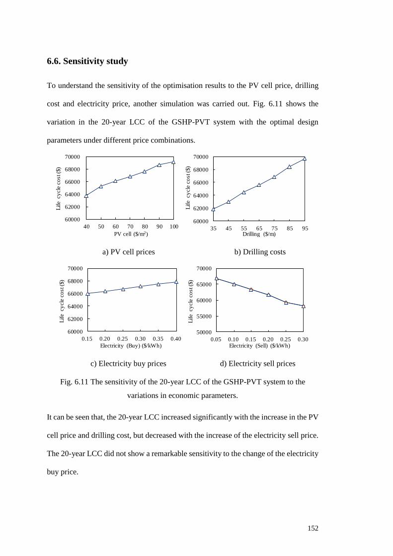
152

6.6. Sensitivity study

To understand the sensitivity of the optimisation results to the PV cell price, drilling

cost and electricity price, another simulation was carried out. Fig. 6.11 shows the

variation in the 20-year LCC of the GSHP-PVT system with the optimal design

parameters under different price combinations.

a) PV cell prices b) Drilling costs

c) Electricity buy prices d) Electricity sell prices

Fig. 6.11 The sensitivity of the 20-year LCC of the GSHP-PVT system to the

variations in economic parameters.

It can be seen that, the 20-year LCC increased significantly with the increase in the PV

cell price and drilling cost, but decreased with the increase of the electricity sell price.

The 20-year LCC did not show a remarkable sensitivity to the change of the electricity

buy price.

60000

62000

64000

66000

68000

70000

40 50 60 70 80 90 100

Lif

e cy

cle

co

st ($

)

PV cell ($/m2)

60000

62000

64000

66000

68000

70000

35 45 55 65 75 85 95

Lif

e cy

cle

co

st ($

)

Drilling ($/m)

60000

62000

64000

66000

68000

70000

0.15 0.20 0.25 0.30 0.35 0.40

Lif

e cy

cle

co

st ($

)

Electricity (Buy) ($/kWh)

50000

55000

60000

65000

70000

0.05 0.10 0.15 0.20 0.25 0.30

Lif

e cy

cle

co

st ($

)

Electricity (Sell) ($/kWh)

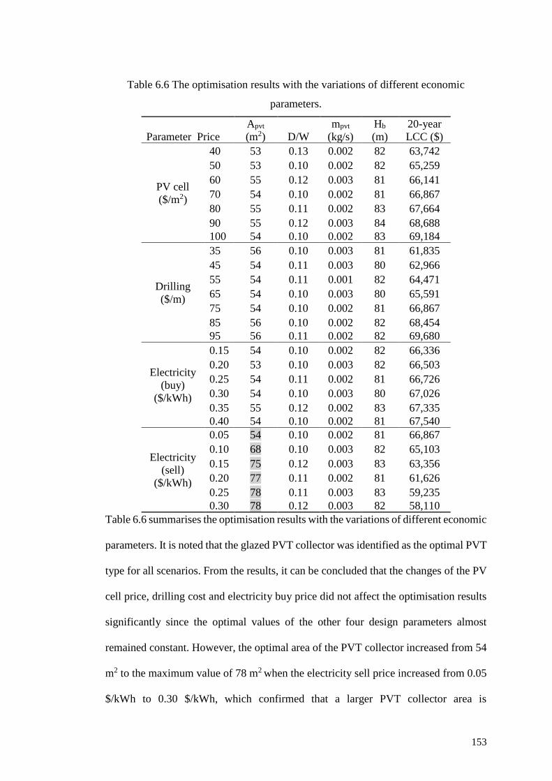
153

Table 6.6 The optimisation results with the variations of different economic

parameters.

Parameter Price

Apvt

(m2) D/W

mpvt

(kg/s)

Hb

(m)

20-year

LCC ($)

PV cell

($/m2)

40 53 0.13 0.002 82 63,742

50 53 0.10 0.002 82 65,259

60 55 0.12 0.003 81 66,141

70 54 0.10 0.002 81 66,867

80 55 0.11 0.002 83 67,664

90 55 0.12 0.003 84 68,688

100 54 0.10 0.002 83 69,184

Drilling

($/m)

35 56 0.10 0.003 81 61,835

45 54 0.11 0.003 80 62,966

55 54 0.11 0.001 82 64,471

65 54 0.10 0.003 80 65,591

75 54 0.10 0.002 81 66,867

85 56 0.10 0.002 82 68,454

95 56 0.11 0.002 82 69,680

Electricity

(buy)

($/kWh)

0.15 54 0.10 0.002 82 66,336

0.20 53 0.10 0.003 82 66,503

0.25 54 0.11 0.002 81 66,726

0.30 54 0.10 0.003 80 67,026

0.35 55 0.12 0.002 83 67,335

0.40 54 0.10 0.002 81 67,540

Electricity

(sell)

($/kWh)

0.05 54 0.10 0.002 81 66,867

0.10 68 0.10 0.003 82 65,103

0.15 75 0.12 0.003 83 63,356

0.20 77 0.11 0.002 81 61,626

0.25 78 0.11 0.003 83 59,235

0.30 78 0.12 0.003 82 58,110

Table 6.6 summarises the optimisation results with the variations of different economic

parameters. It is noted that the glazed PVT collector was identified as the optimal PVT

type for all scenarios. From the results, it can be concluded that the changes of the PV

cell price, drilling cost and electricity buy price did not affect the optimisation results

significantly since the optimal values of the other four design parameters almost

remained constant. However, the optimal area of the PVT collector increased from 54

m2 to the maximum value of 78 m2 when the electricity sell price increased from 0.05

$/kWh to 0.30 $/kWh, which confirmed that a larger PVT collector area is

154

economically beneficial to the system if the electricity generated by the system can be

sold back to the electric grid with a higher price.

6.7 Summary

This chapter presented a new design optimisation strategy for a hybrid ground source

heat pump system integrated with photovoltaic thermal collectors (GSHP-PVT). In

this strategy, an artificial neural network (ANN) model was used for performance

prediction and a genetic algorithm (GA) was used as the optimisation technique. The

20-year life cycle cost (LCC) of the GSHP-PVT system was used as the optimisation

objective.

This proposed design methodology was evaluated through a case study. The ANN

model was trained and validated using the datasets created through a number of

numerical simulations, based on the key design parameters identified by a dimension

reduction strategy using Morris global sensitivity analysis method. The results showed

that the ANN model was able to provide acceptable estimations of the annual

operational cost of the GSHP-PVT system with R2 of 0.998 and CVRMSE of 3.3%.

The optimisation results showed that the 20-year LCC of the GSHP-PVT system under

the optimal design case was 20.1% and 10.2% lower than those of the two baseline

design cases I and II, respectively. The sensitivity of the optimisation results to the

variations in the PV cell price, drilling cost and electricity buy and sell prices was also

analysed. It was shown that the PV cell price, drilling cost and electricity buy price

had limited impacts on the overall optimisation results. However, the electricity sell

price greatly affected the optimal PVT collector area. The results from this study could

be served as a basis to develop advanced design strategies for hybrid GSHP-PVT

systems suitable for real applications.

155

Chapter 7 Model-based optimal control of ground source

heat pump systems with integrated solar photovoltaic

thermal collectors

Control optimisation is another important approach to maximising the system

operating efficiency in order to further offset the high upfront cost of hybrid GSHP-

PVT systems. This chapter presents a model-based optimal control strategy for GSHP-

PVT systems. The control strategy was formulated using simplified adaptive models

and a genetic algorithm (GA) to identify energy efficient control settings under the

giving working conditions. The simplified models were used to predict the system

energy performance, and the model parameters were continuously updated using the

recursive least squares (RLS) estimation technique with exponential forgetting. The

performances of the adaptive models and the optimal control strategy were evaluated

based on a virtual simulation system representing a GSHP-PVT system for residential

applications. The performance of the major adaptive models was also validated using

the experimental data.


research background on the control optimisation of hybrid GSHP-PVT systems. The

model-based control optimisation strategy is then introduced in Section 7.2. Section

7.3 presents the performance test and evaluation of the proposed strategy. A brief

summary is provided in Section 7.4.

7.1 Introduction

During the last decade, an increasing number of studies have been carried out on the

development of optimal control strategies for stand-alone GSHP and hybrid GSHP

156

(HGSHP) systems (Sundbrandt, 2011, Sivasakthivel et al., 2014b, Xia et al., 2017b,

Hu et al., 2016, Ikeda et al., 2017). However, the optimal control of GSHP-PVT

systems has not been extensively studied.

The model-based approach has been widely used in the HVAC field to achieve energy

efficient control with acceptable robustness (Wang and Ma, 2008, Ma and Wang,

2011a, Ge et al., 2011, Candanedo et al., 2013, Afram and Janabi-Sharifi, 2015, Afram

et al., 2017). The model-based control approach generally employs different types of

models to estimate system energy performance and dynamics to the changes of control

settings. The models used can vary from black box models to detailed physical models

dependent on the control accuracy and computational efficiency required (Nassif et al.,

2008). For online control of hybrid GSHP-PVT systems, it is important to develop

relatively simple, yet reliable, models to capture the dynamic behavior of the system

within the entire working range.

The development of online identification techniques allows the models to be

reasonably simple, and self-tuning techniques can be used to reduce the uncertainty of

the models since new measured data can be continuously utilised to identify and update

model parameters (Wang and Jin, 2000). Simplified adaptive models which combine

online identification and self-tuning techniques have been developed and employed to

formulate optimal control strategies for HVAC systems (Wang and Jin, 2000,

Soyguder and Alli, 2009, Yan et al., 2008, Zhao et al., 2012). The results from these

studies demonstrated that the model-based optimal control strategies using self-tuning

adaptive models and online parameter estimation techniques can provide a better and

more robust control performance, in comparison to traditional control strategies.

This chapter aims to developing an optimal control strategy for hybrid GSHP-PVT

systems. The control strategy was formulated using simplified adaptive models and a

157

GA to identify energy efficient control settings. The simplified adaptive models were

selected and used as the performance predictors and the model parameters were

continuously updated by using the RLS estimation with exponential forgetting. To the

best of our knowledge, this is the first time that a model-based control strategy using

adaptive models was developed to systematically optimise the operation of hybrid

GSHP-PVT systems. The performance of this strategy was tested and evaluated based

on a virtual simulation environment representing a GSHP-PVT system for residential

applications. The results obtained from this study could be potentially used to drive

the development of advanced strategies for real-time control and optimisation of

hybrid GSHP-PVT systems.

7.2 Formulation of the optimal control strategy

7.2.1 Outline of the optimal control strategy

The overall optimisation process of the optimal control strategy is illustrated in Fig.

7.1, in which the system operation mode as presented in Table 5.1 was first determined

based on the given working conditions. The model-based performance optimiser was

then used to identify the energy efficient control settings. It mainly consisted of model-

based performance predictors, model parameter estimators, operating constraints, cost

function estimators and a GA optimiser. The parameters of the adaptive performance

models were continuously identified and updated using the latest measurements and

the RLS estimation technique with exponential forgetting (Aström and Wittenmark,

2013). The adaptive performance models used included a simplified water-to-water

heat pump model, a GHE model, a water-based PVT model, a fictitious global AHU

coil model, an immersed heat exchanger model and water pump models. Since GA is

known as an efficient optimisation algorithm that can provide good solutions with

158

random initialization and has been successfully applied in a number of building HVAC

related optimisation studies (Wang and Jin, 2000, Wang et al., 2010, Kalogirou, 2004,

Fong et al., 2010, Ma and Wang, 2011a, b), a GA optimiser was used to seek the

optimal solution of the optimisation problem. The control settings optimised were the

heat pump load side supply water temperature (Tl,in,set), the heat pump source side

supply water temperature (Ts,in,set), water mass flow rate of the PVT collector (Mpvt)

and water mass flow rate for the ground recharge (MGR). The operating constraints

provided the upper and lower search limits of the control settings to be optimised. A

supervisor was used to provide the final control settings for the real process based on

the compromise of the control stability and energy savings according to the rules

defined. For each given operation condition, a set of optimal control settings will be

identified by the GA optimiser and the predicted cost will be compared to the cost

related to the last control settings. If the difference between the two sets of costs is

larger than 1.0%, the control settings identified by the GA optimiser will be used to

update the last settings. Otherwise, the control settings will remain unchanged.

The detailed prediction process for a GA trail and the interconnections among the

performance models under different operation modes are also illustrated in Fig. 7.1.

The water tank recharge mode is used throughout the year. When the operation

condition meets the requirement for the water tank recharge, the PVT water pump will

be switched on and the power consumption of the PVT water pump (Wpu.pvt) and the

electricity generation of the PVT collector (E) will be predicted by the performance

model under the trail setting of the circulating water mass flow rate (Mpvt). Otherwise,

only the electricity generation is predicted. The GSHP for the space cooling mode is

only activated during the cooling period and the power consumptions of the heat pump

(WHP), the load side circulation water pump (Wpu.l) and the source side circulation

159

water pump (Wpu.s) are predicted based on the trail settings of the heat pump load side

supply water temperature set-point (Tl,in,set) and the source side supply water

temperature set-point (Ts,in,set). The ground recharge mode is only activated during the

transition period, during which it was assumed that there is no heating or cooling

requirement of the house. The thermal energy to be recharged into the ground (QGR)

and the power consumption of the source side circulation water pump (Wpu.s) are

predicted based on the inlet water temperature of the GHEs and the trail settings of the

ground recharge circulating water mass flow rate (MGR). During the heating period, the

strategy will first determine to use the PVT or GSHP for space heating based on the

current online measurements. If the PVT is used for space heating, no control setting

needs to be optimised and the only output from the performance model is the power

consumption of the load side circulation water pump (Wpu.l). If the GSHP is used for

space heating, the prediction process is the same as that of the GSHP for space cooling

mode, but different operating constraints will be applied.

160

Fig. 7.1 Overall optimisation process of the proposed optimal control strategy.

Search

ranges

Optimal settings

Supervisor

Control settings

Real process of the GSHP-PVT system

AHU model

Ml,Tl,out

Cost function estimators

Tl,in,t

Qcooling

GHE model

Ts,in,t, Ms,t

Heat pump

model

Ts,out, Ms,t

WHP,est, Ts,in,est,

Ms,t

Update

Ms,t

No

Yes

Ms

Source side

pump model

WHP

Wpu,s

Load side

pump model

Wpu,l

Immersed heat

exchanger model

Mpvt,t

PVT model

Yes

Mpvt,,t,Tpvt,in

PVT pump

model

Wpu,pvt

No

Mpvt,t, Tpvt,out

E

E

Tpm, TTK

MGR,t, Tg,in

GHE model

Ground recharge?

Yes

Wpu,s

Source side

pump model

MGR,t

Qgr

Immersed heat

exchanger modelAHU model

Tl,in,t

Qheating, Tl,in,pvt,TTK

GHE model

Ts,in,t, Ms,t

Heat pump

model

Ts,out, Ms,t

WHP,est, Ts,in,est,

Ms,t

Update

Ms,t

No

YesMs

Source side

pump model

WHP

Wpu,s

Load side

pump model

Wpu,l

AHU model

No

Load side

pump model

Ml,pvt

Wpu,l

Tb, TTK

Performance

optimizer

Whole year Cooling period Transition period Heating period

Water tank recharge?PVT for

space heating?

Yes

GSHP for space heating

Model parameter estimators (Corresponding model tuning & parameter update)

Operation mode

selection

Online measurements

Operation data

GSHP for space cooling

Tl,in,pvt,Gt, Tamb

GA optimiser (Trial settings generation & optimal settings identification) Operating

constraints

Gt, Tamb

MGR,t, Tg,out

Tb

Model-based

predictors

Cost

PVT model

Ml

Ml,Tl,out

Ml

TTKTTK

GR

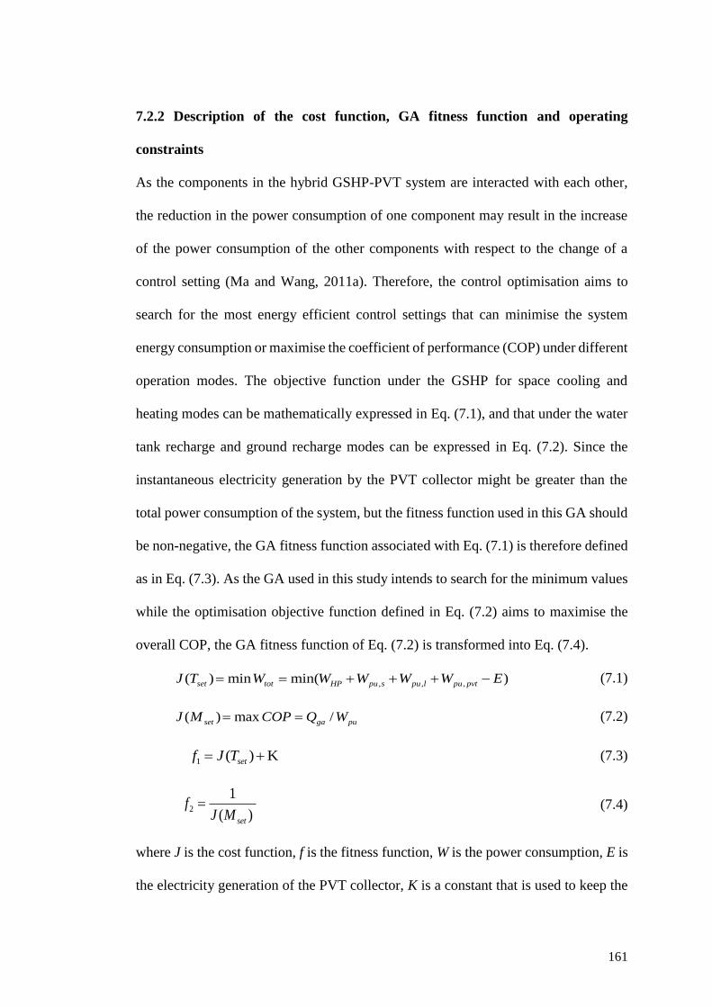
161

7.2.2 Description of the cost function, GA fitness function and operating

constraints

As the components in the hybrid GSHP-PVT system are interacted with each other,

the reduction in the power consumption of one component may result in the increase

of the power consumption of the other components with respect to the change of a

control setting (Ma and Wang, 2011a). Therefore, the control optimisation aims to

search for the most energy efficient control settings that can minimise the system

energy consumption or maximise the coefficient of performance (COP) under different

operation modes. The objective function under the GSHP for space cooling and

heating modes can be mathematically expressed in Eq. (7.1), and that under the water

tank recharge and ground recharge modes can be expressed in Eq. (7.2). Since the

instantaneous electricity generation by the PVT collector might be greater than the

total power consumption of the system, but the fitness function used in this GA should

be non-negative, the GA fitness function associated with Eq. (7.1) is therefore defined

as in Eq. (7.3). As the GA used in this study intends to search for the minimum values

while the optimisation objective function defined in Eq. (7.2) aims to maximise the

overall COP, the GA fitness function of Eq. (7.2) is transformed into Eq. (7.4).

, , ,( ) min min( )set tot HP pu s pu l pu pvtJ T W W W W W E= = + + + − (7.1)

( ) max /set ga puJ M COP Q W= = (7.2)

1 ( ) Ksetf J T= + (7.3)

2

1

( )set

fJ M

= (7.4)

where J is the cost function, f is the fitness function, W is the power consumption, E is

the electricity generation of the PVT collector, K is a constant that is used to keep the

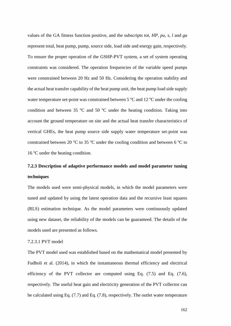
162

values of the GA fitness function positive, and the subscripts tot, HP, pu, s, l and ga

represent total, heat pump, pump, source side, load side and energy gain, respectively.

To ensure the proper operation of the GSHP-PVT system, a set of system operating

constraints was considered. The operation frequencies of the variable speed pumps

were constrained between 20 Hz and 50 Hz. Considering the operation stability and

the actual heat transfer capability of the heat pump unit, the heat pump load side supply

water temperature set-point was constrained between 5 oC and 12 oC under the cooling

condition and between 35 oC and 50 oC under the heating condition. Taking into

account the ground temperature on site and the actual heat transfer characteristics of

vertical GHEs, the heat pump source side supply water temperature set-point was

constrained between 20 oC to 35 oC under the cooling condition and between 6 oC to

16 oC under the heating condition.

7.2.3 Description of adaptive performance models and model parameter tuning

techniques

The models used were semi-physical models, in which the model parameters were

tuned and updated by using the latest operation data and the recursive least squares

(RLS) estimation technique. As the model parameters were continuously updated

using new dataset, the reliability of the models can be guaranteed. The details of the

models used are presented as follows.

7.2.3.1 PVT model

The PVT model used was established based on the mathematical model presented by

Fudholi et al. (2014), in which the instantaneous thermal efficiency and electrical

efficiency of the PVT collector are computed using Eq. (7.5) and Eq. (7.6),

respectively. The useful heat gain and electricity generation of the PVT collector can

be calculated using Eq. (7.7) and Eq. (7.8), respectively. The outlet water temperature

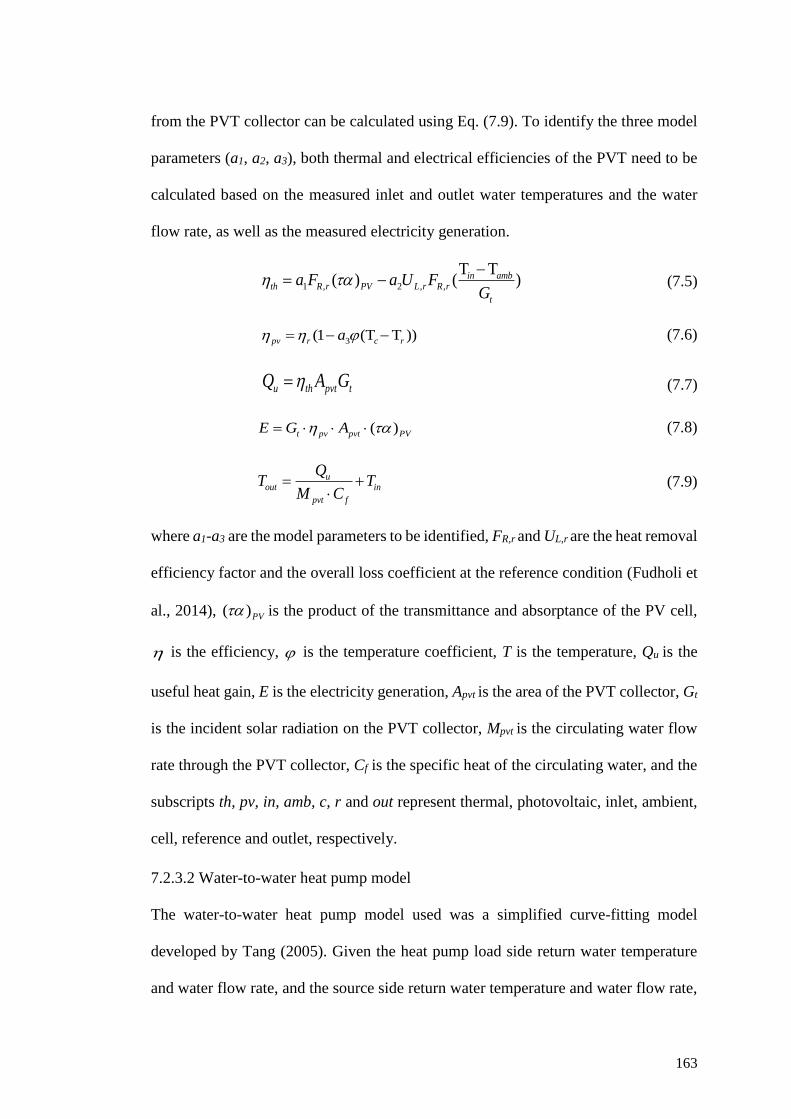
163

from the PVT collector can be calculated using Eq. (7.9). To identify the three model

parameters (a1, a2, a3), both thermal and electrical efficiencies of the PVT need to be

calculated based on the measured inlet and outlet water temperatures and the water

flow rate, as well as the measured electricity generation.

1 , 2 , ,

T T( ) ( )in amb

th R r PV L r R r

t

a F a U FG

−

= − (7.5)

3(1 (T T ))pv r c ra = − − (7.6)

u th pvt tQ A G= (7.7)

( )t pv pvt PVE G A = (7.8)

uout in

pvt f

QT T

M C= +

(7.9)

where a1-a3 are the model parameters to be identified, FR,r and UL,r are the heat removal

efficiency factor and the overall loss coefficient at the reference condition (Fudholi et

al., 2014), ( )PV is the product of the transmittance and absorptance of the PV cell,

is the efficiency, is the temperature coefficient, T is the temperature, Qu is the

useful heat gain, E is the electricity generation, Apvt is the area of the PVT collector, Gt

is the incident solar radiation on the PVT collector, Mpvt is the circulating water flow

rate through the PVT collector, Cf is the specific heat of the circulating water, and the

subscripts th, pv, in, amb, c, r and out represent thermal, photovoltaic, inlet, ambient,

cell, reference and outlet, respectively.

7.2.3.2 Water-to-water heat pump model

The water-to-water heat pump model used was a simplified curve-fitting model

developed by Tang (2005). Given the heat pump load side return water temperature

and water flow rate, and the source side return water temperature and water flow rate,

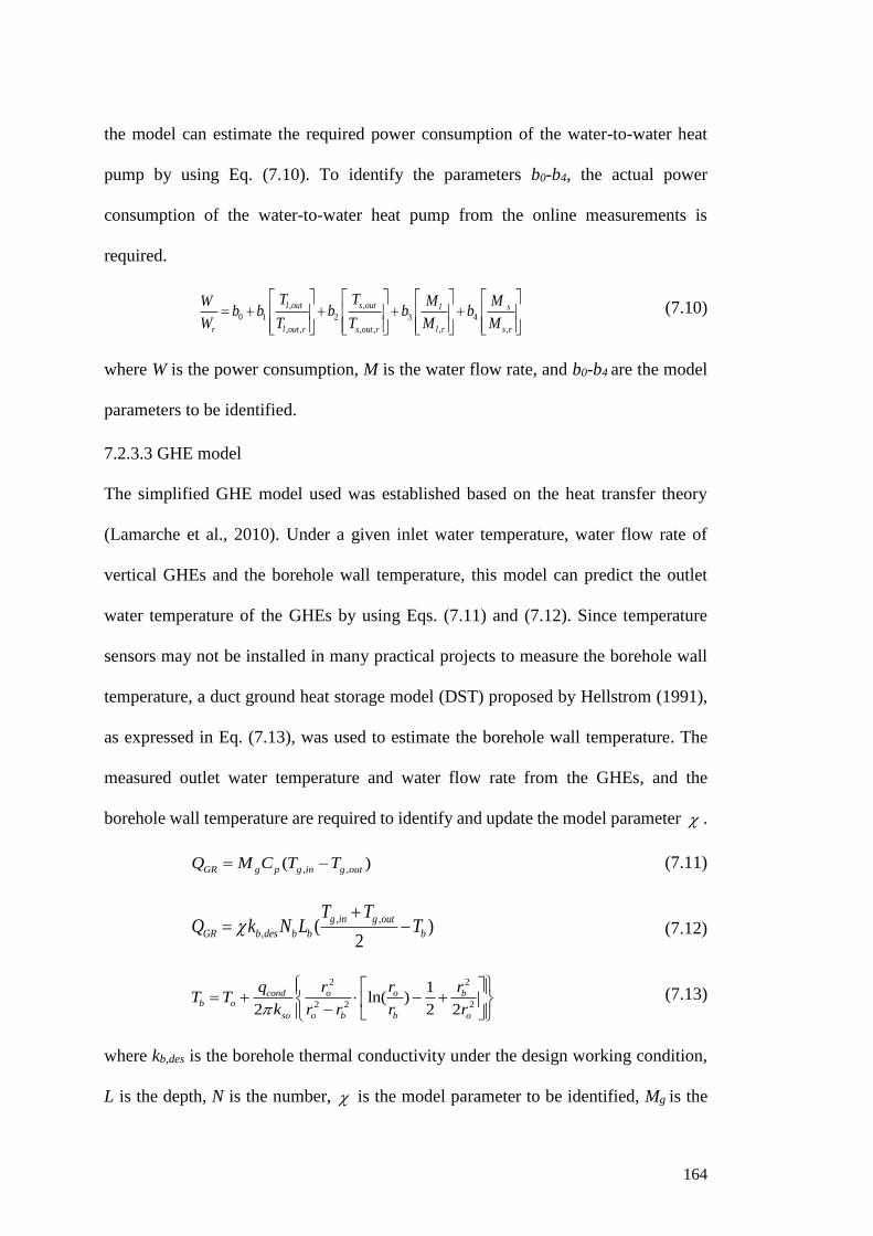
164

the model can estimate the required power consumption of the water-to-water heat

pump by using Eq. (7.10). To identify the parameters b0-b4, the actual power

consumption of the water-to-water heat pump from the online measurements is

required.

, ,

0 1 2 3 4

, , , , , ,

l out s out l s

r l out r s out r l r s r

T T M MWb b b b b

W T T M M

= + + + +

(7.10)

where W is the power consumption, M is the water flow rate, and b0-b4 are the model

parameters to be identified.

7.2.3.3 GHE model

The simplified GHE model used was established based on the heat transfer theory

(Lamarche et al., 2010). Under a given inlet water temperature, water flow rate of

vertical GHEs and the borehole wall temperature, this model can predict the outlet

water temperature of the GHEs by using Eqs. (7.11) and (7.12). Since temperature

sensors may not be installed in many practical projects to measure the borehole wall

temperature, a duct ground heat storage model (DST) proposed by Hellstrom (1991),

as expressed in Eq. (7.13), was used to estimate the borehole wall temperature. The

measured outlet water temperature and water flow rate from the GHEs, and the

borehole wall temperature are required to identify and update the model parameter .

, ,( )GR g p g in g outQ M C T T= − (7.11)

, ,

, ( )2

g in g out

GR b des b b b

T TQ k N L T

+= − (7.12)

2 2

2 2 2

1ln( )

2 2 2

cond o o bb o

so o b b o

q r r rT T

k r r r r

= + − +

−

(7.13)

where kb,des is the borehole thermal conductivity under the design working condition,

L is the depth, N is the number, is the model parameter to be identified, Mg is the

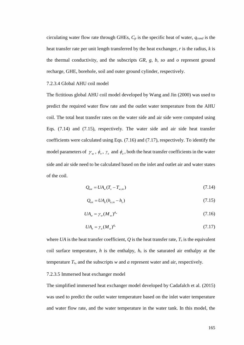
165

circulating water flow rate through GHEs, Cp is the specific heat of water, qcond is the

heat transfer rate per unit length transferred by the heat exchanger, r is the radius, k is

the thermal conductivity, and the subscripts GR, g, b, so and o represent ground

recharge, GHE, borehole, soil and outer ground cylinder, respectively.

7.2.3.4 Global AHU coil model

The fictitious global AHU coil model developed by Wang and Jin (2000) was used to

predict the required water flow rate and the outlet water temperature from the AHU

coil. The total heat transfer rates on the water side and air side were computed using

Eqs. (7.14) and (7.15), respectively. The water side and air side heat transfer

coefficients were calculated using Eqs. (7.16) and (7.17), respectively. To identify the

model parameters of w , w , a and a , both the heat transfer coefficients in the water

side and air side need to be calculated based on the inlet and outlet air and water states

of the coil.

,( )tot w s w inQ UA T T= − (7.14)

,( )tot a a in sQ UA h h= − (7.15)

( ) w

w w wUA M= (7.16)

( ) a

a a aUA M= (7.17)

where UA is the heat transfer coefficient, Q is the heat transfer rate, Ts is the equivalent

coil surface temperature, h is the enthalpy, hs is the saturated air enthalpy at the

temperature Ts, and the subscripts w and a represent water and air, respectively.

7.2.3.5 Immersed heat exchanger model

The simplified immersed heat exchanger model developed by Cadafalch et al. (2015)

was used to predict the outlet water temperature based on the inlet water temperature

and water flow rate, and the water temperature in the water tank. In this model, the

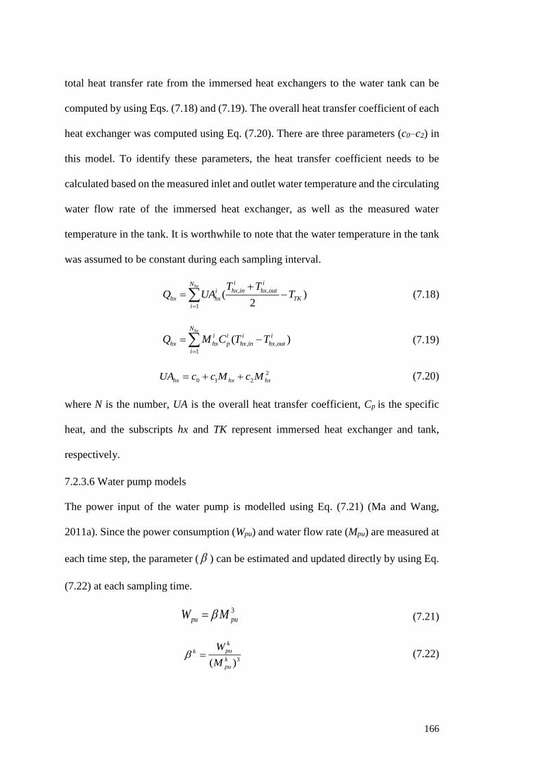
166

total heat transfer rate from the immersed heat exchangers to the water tank can be

computed by using Eqs. (7.18) and (7.19). The overall heat transfer coefficient of each

heat exchanger was computed using Eq. (7.20). There are three parameters (c0–c2) in

this model. To identify these parameters, the heat transfer coefficient needs to be

calculated based on the measured inlet and outlet water temperature and the circulating

water flow rate of the immersed heat exchanger, as well as the measured water

temperature in the tank. It is worthwhile to note that the water temperature in the tank

was assumed to be constant during each sampling interval.

, ,

1

( )2

hxi iN

hx in hx outi

hx hx TK

i

T TQ UA T

=

+= − (7.18)

, ,

1

( )hxN

i i i i

hx hx p hx in hx out

i

Q M C T T=

= − (7.19)

2

0 1 2hx hx hxUA c c M c M= + + (7.20)

where N is the number, UA is the overall heat transfer coefficient, Cp is the specific

heat, and the subscripts hx and TK represent immersed heat exchanger and tank,

respectively.

7.2.3.6 Water pump models

The power input of the water pump is modelled using Eq. (7.21) (Ma and Wang,

2011a). Since the power consumption (Wpu) and water flow rate (Mpu) are measured at

each time step, the parameter ( ) can be estimated and updated directly by using Eq.

(7.22) at each sampling time.

3

pu puW M= (7.21)

3( )

k

puk

k

pu

W

M = (7.22)

167

7.2.3.7 Recursive least squares estimation with exponential forgetting

The adaptive models used were linear in the parameters directly or linear in the

parameters after the logarithmic transformation. To ensure reliable estimation of these

models under various working conditions, the recursive least squares (RLS) estimation

technique with exponential forgetting (Aström and Wittenmark, 2013), as shown in

Eq. (7.23), was used to update the model parameters. In the RLS estimation, the

unknown parameters of a linear model were determined by minimising the sum of the

squares of the difference between the actual observations and the computed values.

Exponential forgetting is an approach to discarding more remote data exponentially,

which is realised by considering a forgetting factor (i.e. in Eq. (7.23)) that gives

more weight to the most recent data (Ma and Wang, 2011a).

2

1

1( , ) ( ( ) ( ) )

2

tt i T

i

V t y i x i −

=

= − (7.23)

where V is the loss function, y is the observed variable, is the parameter to be

determined, x is the regression variable and is the forgetting factor, and i is a time

step. ( 0 1 ).

7.3 Performance test and results

7.3.1 Set up of the tests

In order to test the performance of the proposed control strategy, a virtual simulation

system representing the hybrid GSHP-PVT system under study was developed using

TRNSYS. The details about the virtual simulation system and the component models

used can be found in Chapter 6. It is worthwhile to note that in this performance test,

the virtual simulation system was used to mimic the real system to generate the “real-

time” operation data. In practical applications, these adaptive performance models will

168

be continuously tuned in the same way at each control time interval but using the latest

performance data from the measurements obtained from the real systems.

During the test, the water tank recharge mode was switched on when the PVT mean

plate temperature was 8 oC higher than the water temperature in the water tank, and

was switched off when the temperature difference between the PVT plate and the water

tank was less than 2 oC (Entchev et al., 2014) to ensure a relatively high heat transfer

efficiency of the PVT collector. The ground recharge was implemented between 10:00

and 17:00 during the transition period when the water temperature in the tank was over

30 oC. The amount of the thermal energy to be recharged into the ground was estimated

based on the predetermined annual heat extraction and heat rejection from the GSHP

system through simulations. Once the thermal energy transferred to the ground can

maintain the annual ground thermal balance, the ground recharge was then completed,

and the heat energy generated from the PVT collector was used for DHW only. The

space heating/cooling mode was used when there was a heating or cooling demand

from 17:00 to 10:00 of the next day on the weekdays and all day on the weekends

when the house was occupied. Under the space heating mode, the PVT for space

heating was implemented when the water temperature in the water tank was over 40

oC. Otherwise, the GSHP for space heating model was applied. Under the space

cooling mode, only the GSHP was used. For stable control and operation, a minimal

time interval was introduced to avoid frequent ON/OFF of the major system

components. The DHW consumption of the building was set between 7:00 to 10:00

and 17:30 to 21:30 with a flow rate of 16 L/h throughout the year (REMP, 2012). The

electric water heater was used to heat the water from the water tank when there was a

DHW demand and the water temperature from the tank was lower than the required

temperature for hot water.

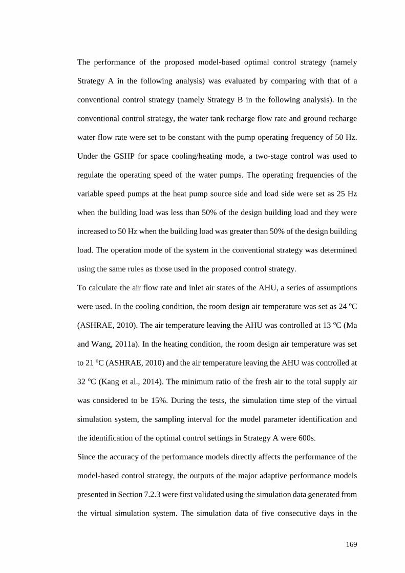
169

The performance of the proposed model-based optimal control strategy (namely

Strategy A in the following analysis) was evaluated by comparing with that of a

conventional control strategy (namely Strategy B in the following analysis). In the

conventional control strategy, the water tank recharge flow rate and ground recharge

water flow rate were set to be constant with the pump operating frequency of 50 Hz.

Under the GSHP for space cooling/heating mode, a two-stage control was used to

regulate the operating speed of the water pumps. The operating frequencies of the

variable speed pumps at the heat pump source side and load side were set as 25 Hz

when the building load was less than 50% of the design building load and they were

increased to 50 Hz when the building load was greater than 50% of the design building

load. The operation mode of the system in the conventional strategy was determined

using the same rules as those used in the proposed control strategy.

To calculate the air flow rate and inlet air states of the AHU, a series of assumptions

were used. In the cooling condition, the room design air temperature was set as 24 oC

(ASHRAE, 2010). The air temperature leaving the AHU was controlled at 13 oC (Ma

and Wang, 2011a). In the heating condition, the room design air temperature was set

to 21 oC (ASHRAE, 2010) and the air temperature leaving the AHU was controlled at

32 oC (Kang et al., 2014). The minimum ratio of the fresh air to the total supply air

was considered to be 15%. During the tests, the simulation time step of the virtual

simulation system, the sampling interval for the model parameter identification and

the identification of the optimal control settings in Strategy A were 600s.

Since the accuracy of the performance models directly affects the performance of the

model-based control strategy, the outputs of the major adaptive performance models

presented in Section 7.2.3 were first validated using the simulation data generated from

the virtual simulation system. The simulation data of five consecutive days in the

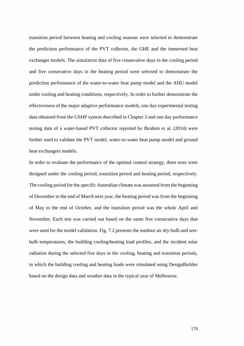
170

transition period between heating and cooling seasons were selected to demonstrate

the prediction performance of the PVT collector, the GHE and the immersed heat

exchanger models. The simulation data of five consecutive days in the cooling period

and five consecutive days in the heating period were selected to demonstrate the

prediction performance of the water-to-water heat pump model and the AHU model

under cooling and heating conditions, respectively. In order to further demonstrate the

effectiveness of the major adaptive performance models, one day experimental testing

data obtained from the GSHP system described in Chapter 3 and one day performance

testing data of a water-based PVT collector reported by Ibrahim et al. (2014) were

further used to validate the PVT model, water-to-water heat pump model and ground

heat exchangers models.

In order to evaluate the performance of the optimal control strategy, three tests were

designed under the cooling period, transition period and heating period, respectively.

The cooling period for the specific Australian climate was assumed from the beginning

of December to the end of March next year, the heating period was from the beginning

of May to the end of October, and the transition period was the whole April and

November. Each test was carried out based on the same five consecutive days that

were used for the model validation. Fig. 7.2 presents the outdoor air dry-bulb and wet-

bulb temperatures, the building cooling/heating load profiles, and the incident solar

radiation during the selected five days in the cooling, heating and transition periods,

in which the building cooling and heating loads were simulated using DesignBuilder

based on the design data and weather data in the typical year of Melbourne.

171

a) cooling period

b) heating period

c) Transition period

Fig. 7.2 Weather data of the selected five consecutive days.

7.3.2 Validation of the performance models

Fig. 7.3 presents the estimated and measured thermal energy gain and electricity

generation of the PVT collector. It is worthwhile to note here that the estimated values

10

15

20

25

30

35

40

45

0

2

4

6

8

10

12

0:0

0

4:0

0

8:0

0

12:0

0

16:0

0

20:0

0

0:0

0

4:0

0

8:0

0

12:0

0

16:0

0

20:0

0

0:0

0

4:0

0

8:0

0

12:0

0

16:0

0

20:0

0

0:0

0

4:0

0

8:0

0

12:0

0

16:0

0

20:0

0

0:0

0

4:0

0

8:0

0

12:0

0

16:0

0

20:0

0

0:0

0

Tem

pera

ture

(oC

)

Coolin

g

load (

kW

)

Time (h)

Cooling load GtDry bulb temperature Wet bulb temeprature

0

500

1000

Gt

(w/m

2)

0

5

10

15

20

0

2

4

6

8

10

0:0

04

:00

8:0

01

2:0

01

6:0

02

0:0

00

:00

4:0

08

:00

12:0

01

6:0

02

0:0

00

:00

4:0

08

:00

12:0

01

6:0

02

0:0

00

:00

4:0

08

:00

12:0

01

6:0

02

0:0

00

:00

4:0

08

:00

12:0

01

6:0

02

0:0

00

:00

Tem

pera

ture

(oC

)

Heating l

oad (

kW

)

Time (h)

Heating load GtDry bulb temperature Wet bulb temeprature

0

500

1000

Gt

(w/m

2)

5

10

15

20

25

30

35

0

200

400

600

800

1000

0:0

04:0

08:0

012

:00

16:0

020:0

00:0

04:0

08:0

012

:00

16:0

020:0

00:0

04:0

08:0

012

:00

16:0

020:0

00:0

04:0

08:0

012

:00

16:0

020

:00

0:0

04:0

08:0

012

:00

16:0

020

:00

0:0

0

Tem

pera

ture

(oC

)

Gt

(W/m

2)

Time (h)

Gt Dry bulb temperature Wet bulb temperature

172

were calculated by the simplified PVT model, while the ‘measured’ values were

calculated using the performance data generated by the virtual simulation system. It

can be seen that both the estimated and ‘measured’ thermal energy gains and electricity

generations varied with the variation of the incident solar radiation during the day and

they both were close to each other. It can also be observed that the thermal energy gain

was much higher than the electricity generation, especially when the incident solar

radiation was high, indicating that the water-based PVT collectors had a comparatively

higher thermal efficiency than the electric efficiency.

Fig. 7.3 Comparison between the estimated and measured thermal energy gain and

electricity generation of the PVT collector.

Fig. 7.4 and Fig. 7.5 present the validation results of the GHE model and the immersed

heat exchanger model respectively, based on the performance data generated by the

virtual simulation system. It can be observed that the estimated outlet water

temperatures of the GHE and immersed heat exchangers agreed well with the

‘measured’ values, indicating that both models can provide acceptable performance

prediction.

0

4000

8000

12000

16000

20000

0:0

0

4:0

0

8:0

0

12

:00

16

:00

20

:00

0:0

0

4:0

0

8:0

0

12

:00

16

:00

20

:00

0:0

0

4:0

0

8:0

0

12

:00

16

:00

20

:00

0:0

0

4:0

0

8:0

0

12

:00

16

:00

20

:00

0:0

0

4:0

0

8:0

0

12

:00

16

:00

20

:00

0:0

0

Energ

y g

enera

tion

(W)

Time (h)

Estimated thermal energy gainMeasured thermal energy gainEstimated electicity generationMeasured electicity generation

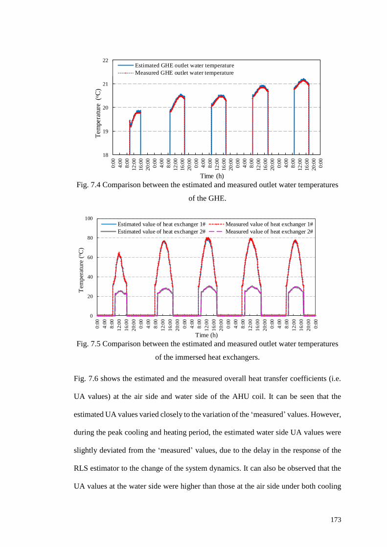
173

Fig. 7.4 Comparison between the estimated and measured outlet water temperatures

of the GHE.

Fig. 7.5 Comparison between the estimated and measured outlet water temperatures

of the immersed heat exchangers.

Fig. 7.6 shows the estimated and the measured overall heat transfer coefficients (i.e.

UA values) at the air side and water side of the AHU coil. It can be seen that the

estimated UA values varied closely to the variation of the ‘measured’ values. However,

during the peak cooling and heating period, the estimated water side UA values were

slightly deviated from the ‘measured’ values, due to the delay in the response of the

RLS estimator to the change of the system dynamics. It can also be observed that the

UA values at the water side were higher than those at the air side under both cooling

18

19

20

21

22

0:0

0

4:0

0

8:0

0

12

:00

16:0

0

20:0

0

0:0

0

4:0

0

8:0

0

12:0

0

16:0

0

20:0

0

0:0

0

4:0

0

8:0

0

12:0

0

16:0

0

20

:00

0:0

0

4:0

0

8:0

0

12:0

0

16

:00

20

:00

0:0

0

4:0

0

8:0

0

12

:00

16

:00

20:0

0

0:0

0

Tem

pera

ture

(o

C)

Time (h)

Estimated GHE outlet water temperature

Measured GHE outlet water temperature

0

20

40

60

80

100

0:0

0

4:0

0

8:0

0

12:0

0

16:0

0

20:0

0

0:0

0

4:0

0

8:0

0

12:0

0

16:0

0

20:0

0

0:0

0

4:0

0

8:0

0

12:0

0

16:0

0

20:0

0

0:0

0

4:0

0

8:0

0

12:0

0

16:0

0

20:0

0

0:0

0

4:0

0

8:0

0

12:0

0

16:0

0

20:0

0

0:0

0

Tem

per

atu

re (

oC

)

Time (h)

Estimated value of heat exchanger 1# Measured value of heat exchanger 1#

Estimated value of heat exchanger 2# Measured value of heat exchanger 2#

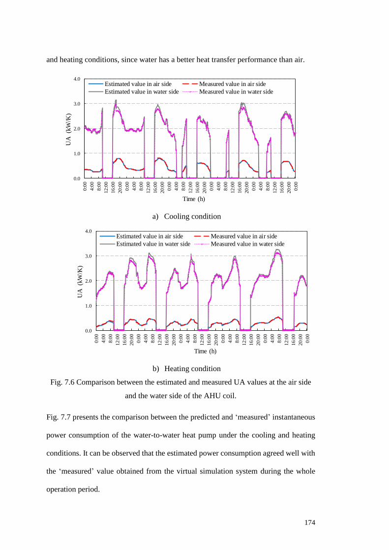
174

and heating conditions, since water has a better heat transfer performance than air.

a) Cooling condition

b) Heating condition

Fig. 7.6 Comparison between the estimated and measured UA values at the air side

and the water side of the AHU coil.

Fig. 7.7 presents the comparison between the predicted and ‘measured’ instantaneous

power consumption of the water-to-water heat pump under the cooling and heating

conditions. It can be observed that the estimated power consumption agreed well with

the ‘measured’ value obtained from the virtual simulation system during the whole

operation period.

0.0

1.0

2.0

3.0

4.00

:00

4:0

0

8:0

0

12

:00

16

:00

20

:00

0:0

0

4:0

0

8:0

0

12

:00

16

:00

20

:00

0:0

0

4:0

0

8:0

0

12

:00

16

:00

20

:00

0:0

0

4:0

0

8:0

0

12

:00

16

:00

20

:00

0:0

0

4:0

0

8:0

0

12

:00

16

:00

20

:00

0:0

0

UA

(kW

/K)

Time (h)

Estimated value in air side Measured value in air side

Estimated value in water side Measured value in water side

0.0

1.0

2.0

3.0

4.0

0:0

0

4:0

0

8:0

0

12

:00

16

:00

20

:00

0:0

0

4:0

0

8:0

0

12

:00

16

:00

20

:00

0:0

0

4:0

0

8:0

0

12

:00

16

:00

20

:00

0:0

0

4:0

0

8:0

0

12

:00

16

:00

20

:00

0:0

0

4:0

0

8:0

0

12

:00

16

:00

20

:00

0:0

0

UA

(kW

/K)

Time (h)

Estimated value in air side Measured value in air side

Estimated value in water side Measured value in water side

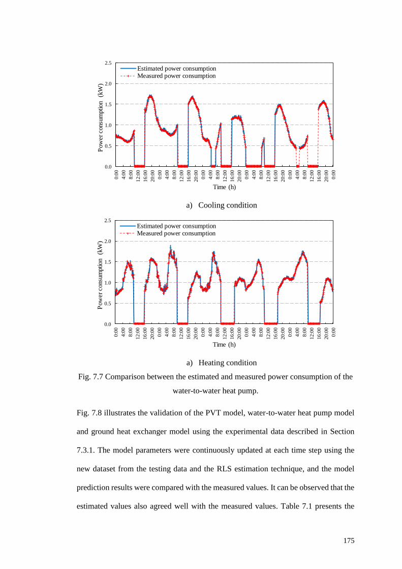
175

a) Cooling condition

a) Heating condition

Fig. 7.7 Comparison between the estimated and measured power consumption of the

water-to-water heat pump.

Fig. 7.8 illustrates the validation of the PVT model, water-to-water heat pump model

and ground heat exchanger model using the experimental data described in Section

7.3.1. The model parameters were continuously updated at each time step using the

new dataset from the testing data and the RLS estimation technique, and the model

prediction results were compared with the measured values. It can be observed that the

estimated values also agreed well with the measured values. Table 7.1 presents the

0.0

0.5

1.0

1.5

2.0

2.5

0:0

0

4:0

0

8:0

0

12:0

0

16

:00

20

:00

0:0

0

4:0

0

8:0

0

12:0

0

16:0

0

20

:00

0:0

0

4:0

0

8:0

0

12:0

0

16:0

0

20:0

0

0:0

0

4:0

0

8:0

0

12:0

0

16:0

0

20:0

0

0:0

0

4:0

0

8:0

0

12:0

0

16:0

0

20:0

0

0:0

0

Pow

er

consu

mption

(kW

)

Time (h)

Estimated power consumptionMeasured power consumption

0.0

0.5

1.0

1.5

2.0

2.5

0:0

0

4:0

0

8:0

0

12:0

0

16:0

0

20

:00

0:0

0

4:0

0

8:0

0

12:0

0

16:0

0

20:0

0

0:0

0

4:0

0

8:0

0

12:0

0

16:0

0

20:0

0

0:0

0

4:0

0

8:0

0

12

:00

16:0

0

20:0

0

0:0

0

4:0

0

8:0

0

12

:00

16

:00

20

:00

0:0

0

Pow

er

consu

mption

(kW

)

Time (h)

Estimated power consumptionMeasured power consumption

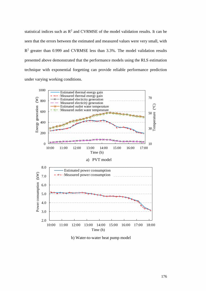
176

statistical indices such as R2 and CVRMSE of the model validation results. It can be

seen that the errors between the estimated and measured values were very small, with

R2 greater than 0.999 and CVRMSE less than 3.3%. The model validation results

presented above demonstrated that the performance models using the RLS estimation

technique with exponential forgetting can provide reliable performance prediction

under varying working conditions.

a) PVT model

b) Water-to-water heat pump model

10

30

50

70

0

200

400

600

800

1000

10:00 11:00 12:00 13:00 14:00 15:00 16:00 17:00

Tem

per

atu

re

(oC

)

En

ergy

gen

erat

ion

(W

)

Time (h)

Estimated thermal energy gainMeasured thermal energy gainEstimated electicity generationMeasured electicity generationEstimated outlet water temperatureMeasured outlet water temperature

2.0

3.0

4.0

5.0

6.0

7.0

8.0

10:00 11:00 12:00 13:00 14:00 15:00 16:00 17:00 18:00

Pow

er c

onsu

mpti

on

(kW

)

Time (h)

Estimated power consumption

Measured power consumption

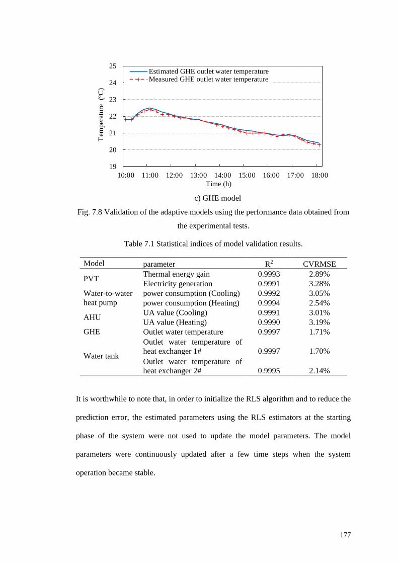
177

c) GHE model

Fig. 7.8 Validation of the adaptive models using the performance data obtained from

the experimental tests.

Table 7.1 Statistical indices of model validation results.

Model parameter R2 CVRMSE

PVT Thermal energy gain 0.9993 2.89%

Electricity generation 0.9991 3.28%

Water-to-water

heat pump

power consumption (Cooling) 0.9992 3.05%

power consumption (Heating) 0.9994 2.54%

AHU UA value (Cooling) 0.9991 3.01%

UA value (Heating) 0.9990 3.19%

GHE Outlet water temperature 0.9997 1.71%

Water tank

Outlet water temperature of

heat exchanger 1# 0.9997 1.70%

Outlet water temperature of

heat exchanger 2# 0.9995 2.14%

It is worthwhile to note that, in order to initialize the RLS algorithm and to reduce the

prediction error, the estimated parameters using the RLS estimators at the starting

phase of the system were not used to update the model parameters. The model

parameters were continuously updated after a few time steps when the system

operation became stable.

19

20

21

22

23

24

25

10:00 11:00 12:00 13:00 14:00 15:00 16:00 17:00 18:00

Tem

per

atu

re

(oC

)

Time (h)

Estimated GHE outlet water temperatureMeasured GHE outlet water temperature

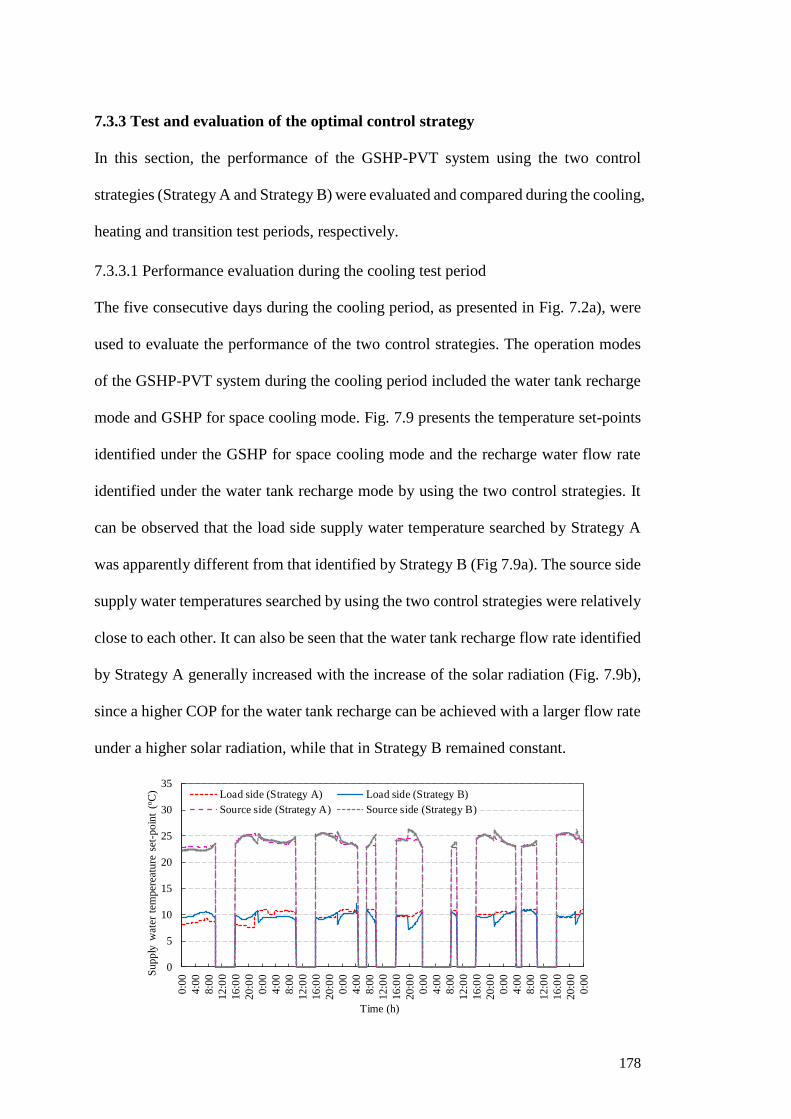
178

7.3.3 Test and evaluation of the optimal control strategy

In this section, the performance of the GSHP-PVT system using the two control

strategies (Strategy A and Strategy B) were evaluated and compared during the cooling,

heating and transition test periods, respectively.

7.3.3.1 Performance evaluation during the cooling test period

The five consecutive days during the cooling period, as presented in Fig. 7.2a), were

used to evaluate the performance of the two control strategies. The operation modes

of the GSHP-PVT system during the cooling period included the water tank recharge

mode and GSHP for space cooling mode. Fig. 7.9 presents the temperature set-points

identified under the GSHP for space cooling mode and the recharge water flow rate

identified under the water tank recharge mode by using the two control strategies. It

can be observed that the load side supply water temperature searched by Strategy A

was apparently different from that identified by Strategy B (Fig 7.9a). The source side

supply water temperatures searched by using the two control strategies were relatively

close to each other. It can also be seen that the water tank recharge flow rate identified

by Strategy A generally increased with the increase of the solar radiation (Fig. 7.9b),

since a higher COP for the water tank recharge can be achieved with a larger flow rate

under a higher solar radiation, while that in Strategy B remained constant.

0

5

10

15

20

25

30

35

0:0

0

4:0

0

8:0

0

12:0

0

16:0

0

20

:00

0:0

0

4:0

0

8:0

0

12:0

0

16

:00

20

:00

0:0

0

4:0

0

8:0

0

12

:00

16:0

0

20:0

0

0:0

0

4:0

0

8:0

0

12:0

0

16:0

0

20

:00

0:0

0

4:0

0

8:0

0

12

:00

16

:00

20:0

0

0:0

0Su

pp

ly w

ater

tem

per

eatu

re s

et-p

oin

t (o

C)

Time (h)

Load side (Strategy A) Load side (Strategy B)

Source side (Strategy A) Source side (Strategy B)

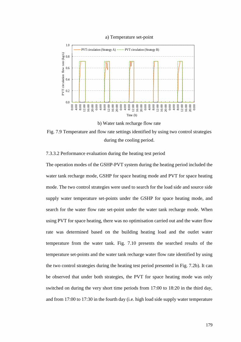
179

a) Temperature set-point

b) Water tank recharge flow rate


during the cooling period.

7.3.3.2 Performance evaluation during the heating test period

The operation modes of the GSHP-PVT system during the heating period included the

water tank recharge mode, GSHP for space heating mode and PVT for space heating

mode. The two control strategies were used to search for the load side and source side

supply water temperature set-points under the GSHP for space heating mode, and

search for the water flow rate set-point under the water tank recharge mode. When

using PVT for space heating, there was no optimisation carried out and the water flow

rate was determined based on the building heating load and the outlet water

temperature from the water tank. Fig. 7.10 presents the searched results of the

temperature set-points and the water tank recharge water flow rate identified by using

the two control strategies during the heating test period presented in Fig. 7.2b). It can

be observed that under both strategies, the PVT for space heating mode was only

switched on during the very short time periods from 17:00 to 18:20 in the third day,

and from 17:00 to 17:30 in the fourth day (i.e. high load side supply water temperature

0.0

0.2

0.4

0.6

0.8

1.0

0:0

0

4:0

0

8:0

0

12

:00

16

:00

20

:00

0:0

0

4:0

0

8:0

0

12

:00

16

:00

20

:00

0:0

0

4:0

0

8:0

0

12

:00

16

:00

20

:00

0:0

0

4:0

0

8:0

0

12

:00

16

:00

20

:00

0:0

0

4:0

0

8:0

0

12

:00

16

:00

20

:00

0:0

0

PV

T c

ircula

tion fl

ow

rate

(kg/s

)

Time (h)

PVT circulation (Strategy A) PVT circulation (Strategy B)

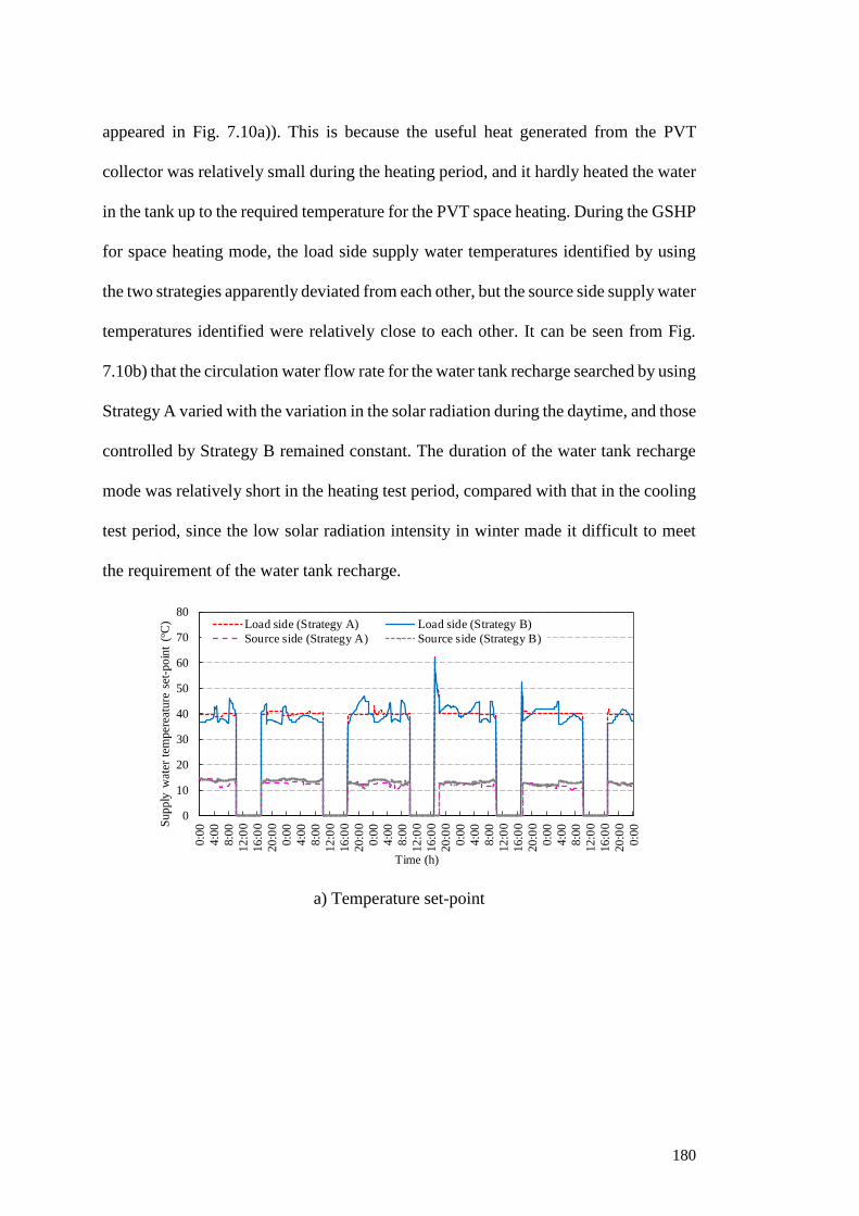
180

appeared in Fig. 7.10a)). This is because the useful heat generated from the PVT

collector was relatively small during the heating period, and it hardly heated the water

in the tank up to the required temperature for the PVT space heating. During the GSHP

for space heating mode, the load side supply water temperatures identified by using

the two strategies apparently deviated from each other, but the source side supply water

temperatures identified were relatively close to each other. It can be seen from Fig.

7.10b) that the circulation water flow rate for the water tank recharge searched by using

Strategy A varied with the variation in the solar radiation during the daytime, and those

controlled by Strategy B remained constant. The duration of the water tank recharge

mode was relatively short in the heating test period, compared with that in the cooling

test period, since the low solar radiation intensity in winter made it difficult to meet

the requirement of the water tank recharge.

a) Temperature set-point

0

10

20

30

40

50

60

70

80

0:0

0

4:0

0

8:0

0

12

:00

16

:00

20

:00

0:0

0

4:0

0

8:0

0

12

:00

16

:00

20:0

0

0:0

0

4:0

0

8:0

0

12:0

0

16:0

0

20:0

0

0:0

0

4:0

0

8:0

0

12:0

0

16:0

0

20:0

0

0:0

0

4:0

0

8:0

0

12:0

0

16:0

0

20

:00

0:0

0Supp

ly w

ater

tem

per

eatu

re s

et-p

oin

t (o

C)

Time (h)

Load side (Strategy A) Load side (Strategy B)

Source side (Strategy A) Source side (Strategy B)

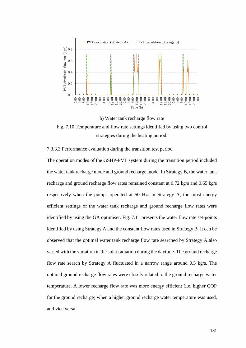
181

b) Water tank recharge flow rate

Fig. 7.10 Temperature and flow rate settings identified by using two control

strategies during the heating period.

7.3.3.3 Performance evaluation during the transition test period

The operation modes of the GSHP-PVT system during the transition period included

the water tank recharge mode and ground recharge mode. In Strategy B, the water tank

recharge and ground recharge flow rates remained constant at 0.72 kg/s and 0.65 kg/s

respectively when the pumps operated at 50 Hz. In Strategy A, the most energy

efficient settings of the water tank recharge and ground recharge flow rates were

identified by using the GA optimiser. Fig. 7.11 presents the water flow rate set-points

identified by using Strategy A and the constant flow rates used in Strategy B. It can be

observed that the optimal water tank recharge flow rate searched by Strategy A also

varied with the variation in the solar radiation during the daytime. The ground recharge

flow rate search by Strategy A fluctuated in a narrow range around 0.3 kg/s. The

optimal ground recharge flow rates were closely related to the ground recharge water

temperature. A lower recharge flow rate was more energy efficient (i.e. higher COP

for the ground recharge) when a higher ground recharge water temperature was used,

and vice versa.

0.0

0.2

0.4

0.6

0.8

1.0

0:0

0

4:0

0

8:0

0

12

:00

16

:00

20

:00

0:0

0

4:0

0

8:0

0

12

:00

16

:00

20

:00

0:0

0

4:0

0

8:0

0

12

:00

16

:00

20

:00

0:0

0

4:0

0

8:0

0

12

:00

16

:00

20

:00

0:0

0

4:0

0

8:0

0

12

:00

16

:00

20

:00

0:0

0

PV

T c

ircu

lati

on

fl

ow

rat

e (k

g/s)

Time (h)


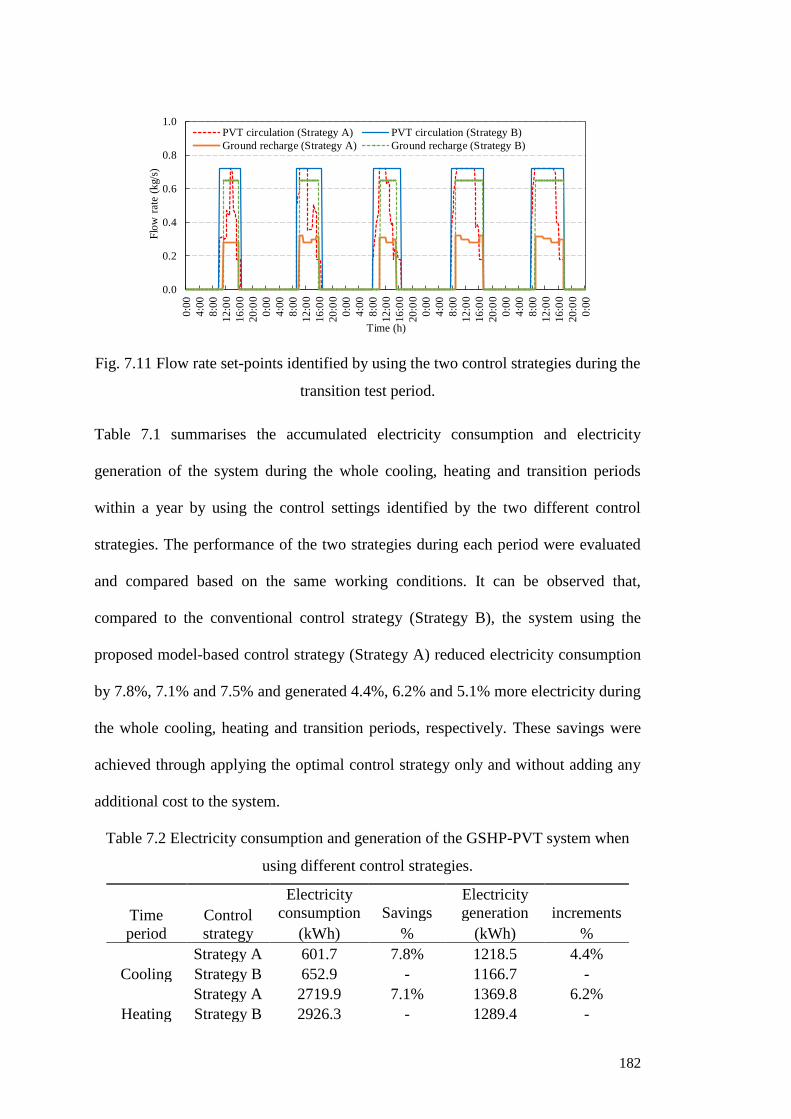
182

Fig. 7.11 Flow rate set-points identified by using the two control strategies during the

transition test period.

Table 7.1 summarises the accumulated electricity consumption and electricity

generation of the system during the whole cooling, heating and transition periods

within a year by using the control settings identified by the two different control

strategies. The performance of the two strategies during each period were evaluated

and compared based on the same working conditions. It can be observed that,

compared to the conventional control strategy (Strategy B), the system using the

proposed model-based control strategy (Strategy A) reduced electricity consumption

by 7.8%, 7.1% and 7.5% and generated 4.4%, 6.2% and 5.1% more electricity during

the whole cooling, heating and transition periods, respectively. These savings were

achieved through applying the optimal control strategy only and without adding any

additional cost to the system.

Table 7.2 Electricity consumption and generation of the GSHP-PVT system when

using different control strategies.

Time

period

Control

strategy

Electricity

consumption Savings

Electricity

generation increments

(kWh) % (kWh) %

Cooling

Strategy A 601.7 7.8% 1218.5 4.4%

Strategy B 652.9 - 1166.7 -

Heating

Strategy A 2719.9 7.1% 1369.8 6.2%

Strategy B 2926.3 - 1289.4 -

0.0

0.2

0.4

0.6

0.8

1.0

0:0

0

4:0

0

8:0

0

12:0

0

16

:00

20:0

0

0:0

0

4:0

0

8:0

0

12:0

0

16

:00

20:0

0

0:0

0

4:0

0

8:0

0

12:0

0

16

:00

20

:00

0:0

0

4:0

0

8:0

0

12:0

0

16:0

0

20

:00

0:0

0

4:0

0

8:0

0

12:0

0

16:0

0

20

:00

0:0

0

Flo

w r

ate

(kg/

s)

Time (h)


Ground recharge (Strategy A) Ground recharge (Strategy B)

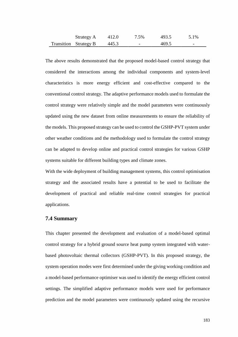
183

Transition

Strategy A 412.0 7.5% 493.5 5.1%

Strategy B 445.3 - 469.5 -

The above results demonstrated that the proposed model-based control strategy that

considered the interactions among the individual components and system-level

characteristics is more energy efficient and cost-effective compared to the

conventional control strategy. The adaptive performance models used to formulate the

control strategy were relatively simple and the model parameters were continuously

updated using the new dataset from online measurements to ensure the reliability of

the models. This proposed strategy can be used to control the GSHP-PVT system under

other weather conditions and the methodology used to formulate the control strategy

can be adapted to develop online and practical control strategies for various GSHP

systems suitable for different building types and climate zones.

With the wide deployment of building management systems, this control optimisation

strategy and the associated results have a potential to be used to facilitate the

development of practical and reliable real-time control strategies for practical

applications.

7.4 Summary

This chapter presented the development and evaluation of a model-based optimal

control strategy for a hybrid ground source heat pump system integrated with water-

based photovoltaic thermal collectors (GSHP-PVT). In this proposed strategy, the

system operation modes were first determined under the giving working condition and

a model-based performance optimiser was used to identify the energy efficient control

settings. The simplified adaptive performance models were used for performance

prediction and the model parameters were continuously updated using the recursive

184

least squares (RLS) estimation technique with exponential forgetting to ensure reliable

performance prediction. A genetic algorithm (GA) was used to search for the optimal

solution for the optimisation problem. The performance of the adaptive models and

the proposed control strategy were tested and evaluated based on a virtual simulation

system that represented a hybrid GSHP-PVT system in a residential application in

Melbourne, Australia. The major adaptive models were also validations using the

experimental testing data.

The model validation results showed that the simplified adaptive models combined

with the least squares (RLS) estimation technique were able to provide a reliable

prediction of the system performance under various working conditions. The test and

evaluation of the optimal control strategy showed that this strategy was able to reduce

the system electricity consumption by 7.8%, 7.1% and 7.5%, and increase the

electricity generation by 4.4%, 6.2% and 5.1% during the whole cooling, heating and

transition periods respectively, in comparison to a conventional control strategy. This

method can be potentially adapted to develop online and practical control strategies

for stand-alone GSHP and hybrid GSHP-PVT systems.

185

Chapter 8 Conclusions and Recommendations

This thesis presented the performance evaluation and optimisation of stand-alone

ground source heat pump (GSHP) systems and hybrid GSHP with integrated

photovoltaic thermal collectors (GSHP-PVT). A range of experimental tests were first

carried out based on a GSHP with an active thermal slab system to evaluate its energy

performance and operating behaviours. A model-based control optimisation strategy

was then developed for stand-alone GSHP systems equipped with variable speed

pumps in the source side to minimise the total energy consumption. To address ground

thermal imbalance issue and maximise the overall performance, a GSHP-PVT system

was then developed. The life-time performance of this system under different

operation scenarios with different sizes of PVT collectors was simulated and analysed

to investigate the impact of the PVT size on the performance of the system. A model-

based design optimisation strategy was then developed to determine the optimal values

of the key design parameters of the GSHP-PVT systems. A model-based control

optimisation strategy was also developed to identify energy efficient control settings

to minimise the operating cost. The optimal design and control strategies developed in

this thesis are more effective than traditional design and control strategies, and they

can be potentially adapted to develop advanced and practical design and control

strategies for stand-alone GSHP and hybrid GSHP-PVT systems suitable for real

applications. Major findings obtained from this thesis are summarised as follows.

8.1 Summary of the key findings

8.1.1 Experimental investigation of the GSHP system with active thermal slabs

Experimental tests were carried out based on a GSHP with active thermal slabs

implemented in the Sustainable Buildings Research Centre (SBRC) at the University

186

of Wollongong. The effects of two GHE configurations (i.e. parallel and series),

different ground loop and slab loop differential pressure set-points and different slab

preheating starting time on the energy performance of the GSHP with active thermal

slabs were investigated to understand its performance characteristics and identify the

optimal operation scenario. The main findings from the experimental investigation are

as below:

• The GSHP system with parallel GHEs showed a better performance than that

with series GHEs. The average coefficient of performances (COP) of the

system under the parallel operation of the GHEs were 7.23%, 7.69% and 0.51%

higher than those under the series operation for the high, medium and low

source flow rate conditions, respectively.

• A larger differential pressure set-point in the ground loop (i.e. larger source

side flow rate) was generally beneficial to the operation of the heat pump unit

for both parallel and series operation of GHEs. However, the increase in the

power consumption of the variable water pump in the ground loop offset the

benefit achieved by the heat pump unit, resulting in a lower overall COP of the

GSHP system.

• Starting the slab preheating earlier with a larger differential pressure set-point

in the slab loop at night resulted in a higher slab surface temperature and indoor

air temperature. Using a larger differential pressure set-point in the slab loop

achieved higher COPs of the heat pump and the whole system, in comparison

with that using a smaller differential pressure set-point in the slab loop. The

optimal operation scenario for the active thermal slab system identified from

the experimental tests was to start the slab preheating at 0:00 with 120 kPa

differential pressure set-point in the slab loop.

187

8.1.2 Control optimisation of stand-alone GSHP systems

A model-based control optimisation strategy of GSHP systems equipped with variable

speed pumps in the source side was developed to minimise the total energy

consumption. The control strategy was formulated using simplified performance

models and a hybrid optimisation technique which integrated a performance map-

based near-optimal strategy and the exhaustive search method. It is the first time that

the hybrid optimisation technique was used to formulate the control strategy for stand-

alone GSHP systems. The main findings are as follows.

• This hybrid optimisation technique can significantly narrow the search range,

so that the computational cost of the optimisation problem can be generally

manageable and the optimisation strategy can be adapted to practically control

and optimise the GSHP systems.

• This model-based control strategy offered more energy savings than a rule-

based control strategy with two-stage control and a performance map-based

near-optimal control strategy. 7.98 % and 8.99 % energy savings can be

achieved when using this strategy under the whole heating and cooling periods

respectively, in comparison to the rule-based control strategy.

8.1.3 Development and performance simulation of the GSHP-PVT system

A GSHP system integrated with water-based PVT collectors to provide space cooling

and heating as well as domestic hot water (DHW) for residential buildings was

developed. A dynamic simulation system for this system was also developed and used

to facilitate the performance evaluation. The 20-year life-time performance of this

system was simulated under three operation scenarios with different sizes of the PVT

collectors. An economic analysis was also carried out to determine the optimum size

of the PVT collectors for the case study building. This study revealed how the PVT

188

size could influence the performance of GSHP-PVT systems and demonstrated how

building simulation tools offer the capability of analysing and selecting control

strategies for complex low energy systems at the design stage. The major conclusions

obtained from the performance simulation are presented below.

• PVT size had a significant influence on the overall performance of the hybrid

GSHP-PVT system. For the case study building, it is more effective to use the

heat generated by the PVT collectors to produce domestic hot water if the area

of the PVT collectors was less than 54 m2. Otherwise, it is better to use the heat

generated by the PVT collectors to recharge the ground during the transition

periods and to provide space heating during the heating period.

• The optimum PVT size for the case building was 66 m2, which can result in

the highest net present value.

8.1.4 Design optimisation of GSHP-PVT systems

To develop the optimal design strategy, a dimension reduction strategy using Morris

global sensitivity analysis was first used to determine the key design parameters of the

GSHP-PVT system. A model-based design optimisation strategy was then formulated

to identify the optimal values of the key design parameters, in which an artificial neural

network (ANN) model was used for performance prediction and a genetic algorithm

(GA) was implemented as the optimisation technique. A simulation system of a GSHP-

PVT system developed using TRNSYS was used to generate necessary performance

data for dimension reduction analysis, and for the ANN model training and validation.

It is the first time that a model-based design optimisation strategy was developed for

GSHP-PVT systems. This strategy developed in this study can be potentially adapted

to formulate the design optimisation strategies for GSHP systems and other building

energy systems. The major findings obtained from the performance evaluation of this

189

design strategy are summarised below.

• The trained ANN model was able to provide acceptable estimations of the

annual operational cost of the GSHP-PVT system with R2 of 0.998 and

CVRMSE of 3.3%.

• The 20-year LCC of the GSHP-PVT system sized using the proposed design

strategy was 20.1% and 10.2% lower than those of the two baseline design

cases, respectively.

• The results from the sensitivity analysis showed that the PV cell price, drilling

cost and electricity buy price had limited impacts on the overall optimisation

results. However, the electricity sell price greatly affected the optimal PVT

collector area.

8.1.5 Control optimisation of GSHP-PVT systems

A model-based control optimisation strategy for GSHP-PVT systems was developed

to maximise overall operation efficiency. The control strategy was formulated using

simplified adaptive models and a genetic algorithm to identify energy efficient control

settings under the giving working conditions. The simplified models were used to

predict the system energy performance, and the model parameters were continuously

updated using the recursive least squares (RLS) estimation technique with exponential

forgetting. A model-based control optimisation strategy was first time developed for

GSHP-PVT systems. The methodology used to develop the strategy can be potentially

adapted to develop online and practical control strategies for stand-alone GSHP and

hybrid GSHP-PVT systems. The main findings from the simulation test and evaluation

of this control strategy are summarised as below.

• The simplified adaptive models combined with the RLS technique were able

to provide a reliable prediction of the system performance under various

190

working conditions.

• The optimal control strategy was able to reduce the system electricity

consumption by 7.8%, 7.1% and 7.5%, and increase the electricity generation

by 4.4%, 6.2% and 5.1% during the whole cooling, heating and transition

periods respectively, in comparison with a conventional control strategy.

8.2 Recommendations for future work

Firstly, the control optimisation strategy for stand-alone GSHP systems developed in

this study was mainly focused on the source side of the GSHP system. It would be

worthwhile to further develop optimal control strategies for the whole GSHP system

in which the interactions between the source side and load side characteristics are

considered.

Secondly, the proposed design optimisation strategy for hybrid GSHP-PVT systems

was computationally intensive, due to the requirement of the extensive data for ANN

model training and validation. This would be a major obstacle of applying this strategy

to real-world design. It would be worthwhile to further improve the efficiency of this

design strategy to make it more applicable for practical applications.

Lastly, the two control optimisation strategies developed in this study were evaluated

through computer simulations. With the wide deployment of building management

systems, the proposed control strategies can be potentially adapted to develop practical

real-time control strategies. It would be beneficial to further improve the two proposed

control strategies and evaluate their effectiveness in practical applications.

191

References

Afram, A. & Janabi-Sharifi, F. 2015. Gray-box modeling and validation of

residential HVAC system for control system design. Applied Energy, vol. 137,

pp. 134-150.

Afram, A., Janabi-Sharifi, F., Fung, A. S. & Raahemifar, K. 2017. Artificial

neural network (ANN) based model predictive control (MPC) and optimization

of HVAC systems: A state of the art review and case study of a residential

HVAC system. Energy and Buildings, vol. 141, pp. 96-113.

Alavy, M., Nguyen, H. V., Leong, W. H. & Dworkin, S. B. 2013. A

methodology and computerized approach for optimizing hybrid ground source

heat pump system design. Renewable Energy, vol. 57, pp. 404-412.

Anderson, T. N., Duke, M., Morrison, G. & Carson, J. K. 2009. Performance

of a building integrated photovoltaic/thermal (BIPVT) solar collector. Solar

energy, vol. 83, no. 4, pp. 445-455.

Aravelli, A. 2014. Multi-objective design optimization of engineering systems:

Uncertainty approach and practical applications. PhD thesis, University of

Miami.

Ashrae 1995. Commercial/institutional ground-source heat pump engineering

manual, Inc., Atlanta, ASHRAE.

Ashrae 2010. Standard 55-2010: Thermal Environmental Conditions for

Human Occupancy. Atlanta: ASHRAE.

Ashrae 2013. Standard 55-2013. Thermal environmental conditions for human

occupancy. Atlanta: ASHRAE.

Asiedu, Y. & Gu, P. 1998. Product life cycle cost analysis: state of the art

review. International Journal of Production Research, vol. 36, no. 4, pp. 883-

908.

192

Aström, K. J. & Wittenmark, B. 2013. Adaptive control, Courier Corporation.

Atam, E. & Helsen, L. 2016. Ground-coupled heat pumps: Part 1–Literature

review and research challenges in modeling and optimal control. Renewable

and Sustainable Energy Reviews, vol. 54, pp. 1653-1667.

Atam, E., Patteeuw, D., Antonov, S. P. & Helsen, L. 2016. Optimal control

approaches for analysis of energy use minimization of hybrid ground-coupled

heat pump systems. IEEE Transactions on Control Systems Technology, vol.

24, no. 2, pp. 525-540.

Atam, E., Picard, D. & Helsen, L. A convex approach to energy use

minimization of buildings equipped with hybrid ground-coupled heat pump

systems. Proc. 9th Int. Conf. Syst. Simulation Build.(SSB), 2014.

Australia, S. 2003. AS/NZS 3500.4. National Plumbing and Drainage: Part 4-

Heated Water Services.

Bahnfleth, W. P. 2001. Comparative analysis of variable and constant primary-

flow chilled-water-plant performance. Heating, Piping, Air Conditioning

Engineering, vol. 73, no. 4, pp. 41-50.

Bakker, M., Zondag, H., Elswijk, M., Strootman, K. & Jong, M. 2005.

Performance and costs of a roof-sized PV/thermal array combined with a

ground coupled heat pump. Solar energy, vol. 78, no. 2, pp. 331-339.

Ball, D., Fischer, R. & Hodgett, D. 1983. Design methods for ground-source

heat pumps. Battelle Columbus Laboratories, Columbus, OH.

Bandos, T. V., Campos-Celador, , López-González, L. M. & Sala-Lizarraga, J.

M. 2014. Finite cylinder-source model for energy pile heat exchangers: Effects

of thermal storage and vertical temperature variations. Energy, vol. 78, pp. 639-

648.

Banks, D. 2012. An introduction to thermogeology: ground source heating and

193

cooling, John Wiley & Sons.

Bayer, P., De Paly, M. & Beck, M. 2014. Strategic optimization of borehole

heat exchanger field for seasonal geothermal heating and cooling. Applied

Energy, vol. 136, pp. 445-453.

Benli, H. & Durmuş, A. 2009. Evaluation of ground-source heat pump

combined latent heat storage system performance in greenhouse heating.

Energy and Buildings, vol. 41, no. 2, pp. 220-228.

Benson, H. P. 1978. Existence of efficient solutions for vector maximization

problems. Journal of Optimization Theory and Applications, vol. 26, no. 4, pp.

569-580.

Berardi, U. 2017. A cross-country comparison of the building energy

consumptions and their trends. Resources, Conservation and Recycling, vol.

123, pp. 230-241.

Bernier, M. A. 2001. Ground-coupled heat pump system

simulation/Discussion. ASHRAE transactions, vol. 107, pp. 605.

Bertram, E., Glembin, J. & Rockendorf, G. 2012. Unglazed PVT collectors as

additional heat source in heat pump systems with borehole heat exchanger.

Energy Procedia, vol. 30, pp. 414-423.

Bhattarai, S., Oh, J.-H., Euh, S.-H., Kafle, G. K. & Kim, D. H. 2012.

Simulation and model validation of sheet and tube type photovoltaic thermal

solar system and conventional solar collecting system in transient states. Solar

Energy Materials and Solar Cells, vol. 103, pp. 184-193.

Bose, J. E. 1984. Closed-loop ground-coupled heat pump design manual,

Engineering Technology Extension Oklahoma State University.

Bose, J. E., Parker, J. D. & Mcquiston, F. C. 1985. Design/data manual for

194

closed-loop ground-coupled he at pump systems, American Society of Heating,

Refrigerating, and Air-Conditioning Engineers.

Bose, J. E., Smith, M. & Spitler, J. Advances in ground source heat pump

systems-an international overview. 7th IEA Heat Pump Conference. 1: 313,

2002.

Brischoux, P. & Bernier, M. 2016. Coupling PV/T collectors with a ground-

source heat pump system in a double U-tube borehole. ASHRAE winter

conference. Orlando, Florida.

Cadafalch, J., Carbonell, D., Consul, R. & Ruiz, R. 2015. Modelling of storage

tanks with immersed heat exchangers. Solar energy, vol. 112, pp. 154-162.

Candanedo, J., Dehkordi, V. & Stylianou, M. 2013. Model-based predictive

control of an ice storage device in a building cooling system. Applied Energy,

vol. 111, pp. 1032-1045.

Canelli, M., Entchev, E., Sasso, M., Yang, L. & Ghorab, M. 2015. Dynamic

simulations of hybrid energy systems in load sharing application. Applied

Thermal Engineering, vol. 78, pp. 315-325.

Capozza, A., De Carli, M. & Zarrella, A. 2012. Design of borehole heat

exchangers for ground-source heat pumps: A literature review, methodology

comparison and analysis on the penalty temperature. Energy and Buildings, vol.

55, pp. 369-379.

Carslaw, H. S. & Jaeger, J. C. 1946. Conduction of heat in solids, Oxford, UK,

Clarendon Press.

Carvalho, A., Quintino, A., Fong, J. & De Almeida, A. 2012. Thermal storage

coupled to a ground source heat pump in a public services building. Journal of

Sustainable Energy, vol. 3, no. 4, pp. 1-4.

Casasso, A. & Sethi, R. 2014. Efficiency of closed loop geothermal heat pumps:

195

A sensitivity analysis. Renewable Energy, vol. 62, pp. 737-746.

Cervera-Vázquez, J., Cazorla-Marin, A., Montagud, C. & Corberan, J. M. 2017.

Optimal control and operation of a GSHP system for heating and cooling in an

office building. IGSHPA Technical/Research Conference and Expo. Denver,

USA.

Cervera-Vázquez, J., Montagud, C. & Corberán, J. 2015a. In situ optimization

methodology for ground source heat pump systems: Upgrade to ensure user

comfort. Energy and Buildings, vol. 109, pp. 195-208.

Cervera-Vázquez, J., Montagud, C. & Corberán, J. 2015b. In situ optimization

methodology for the water circulation pumps frequency of ground source heat

pump systems: Analysis for multistage heat pump units. Energy and Buildings,

vol. 88, pp. 238-247.

Chankong, V. & Haimes, Y. Y. 2008. Multiobjective decision making: theory

and methodology, Courier Dover Publications.

Chen, J., Xia, L., Li, B. & Mmereki, D. 2015. Simulation and experimental

analysis of optimal buried depth of the vertical U-tube ground heat exchanger

for a ground-coupled heat pump system. Renewable Energy, vol. 73, pp. 46-

54.

Chiasson, A. D. & Yavuzturk, C. 2003. Assessment of the viability of hybrid

geothermal heat pump systems with solar thermal collectors. ASHRAE

transactions, vol. 109, no. 2, pp. 487-500.

Chow, T. T., He, W., Chan, A., Fong, K., Lin, Z. & Ji, J. 2008. Computer

modeling and experimental validation of a building-integrated photovoltaic

and water heating system. Applied Thermal Engineering, vol. 28, no. 11, pp.

1356-1364.

Chow, T. T., Pei, G., Fong, K., Lin, Z., Chan, A. & Ji, J. 2009. Energy and

196

exergy analysis of photovoltaic–thermal collector with and without glass cover.

Applied Energy, vol. 86, no. 3, pp. 310-316.

Chung, W. 2011. Review of building energy-use performance benchmarking

methodologies. Applied Energy, vol. 88, no. 5, pp. 1470-1479.

Coello, C. a. C., Lamont, G. B. & Van Veldhuizen, D. A. 2007. Evolutionary

algorithms for solving multi-objective problems, Springer.

Commission, E. S. 2015. Minimum Electricity Feed-in Tariff to Apply from 1

January 2016 to 31 December 2016: Final Decision, August.

Congedo, P., Colangelo, G. & Starace, G. 2012. CFD simulations of horizontal

ground heat exchangers: a comparison among different configurations. Applied


Conraud-Bianchi, J. 2008. A methodology for the optimization of building

energy, thermal, and visual performance. Masters Abstracts International, vol.

47, no. 04.

Corberan, J., Finn, D., Montagud, C., Murphy, F. & Edwards, K. 2011. A

quasi-steady state mathematical model of an integrated ground source heat

pump for building space control. Energy and Buildings, vol. 43, no. 1, pp. 82-

92.

Cornelissen, R. L. 1997. Thermodynamics and sustainable development; the

use of exergy analysis and the reduction of irreversibility, Universiteit Twente.

Craig James, S. S. 2016. US overtakes Australia to build biggest homes [Onli

ne]. Commsec. Available: https://www.commsec.com.au/content/dam/EN/Re

searchNews/Eco_Insights31.10_US_overtakes_Australia_to_build_biggest_h

omes..pdf.

Curtis, R., Lund, J., Sanner, B., Rybach, L. & Hellström, G. Ground source

heat pumps–geothermal energy for anyone, anywhere: current worldwide

https://www.commsec.com.au/content/dam/EN/ResearchNews/Eco_Insights31.10_US_overtakes_Australia_to_build_biggest_homes..pdf



197

activity. Proceedings World Geothermal Congress, 2005. pp. 1-9.

De Ridder, F., Diehl, M., Mulder, G., Desmedt, J. & Van Bael, J. 2011. An

optimal control algorithm for borehole thermal energy storage systems. Energy

and Buildings, vol. 43, no. 10, pp. 2918-2925.

Deerman, J. 1991. Simulation of vertical U-tube ground-coupled heat pump

systems using the cylindrical heat source solution. ASHRAE transactions, vol.

97, no. 1, pp. 287-295.

Duffie, J. A. & Beckman, W. A. 2013. Solar engineering of thermal processes,

Wiley New York.

Trading Economics. 2016. Australia Interest Rate [Online]. Available:

http://www.tradingeconomics.com/australia/interest-rate.

Ehrgott, M. 2006. A discussion of scalarization techniques for multiple

objective integer programming. Annals of Operations Research, vol. 147, no.

1, pp. 343-360.

Eicker, U. 2006. Solar technologies for buildings, John Wiley & Sons.

Department of the Environment and Energy. 2017. National Greenhouse Acc

ounts Factors [Online]. Available: https://www.environment.gov.au/system/fi

les/resources/5a169bfb-f417-4b00-9b70-6ba328ea8671/files/national-greenh

ouse-accounts-factors-july-2017.pdf.

Entchev, E., Yang, L., Ghorab, M. & Lee, E. 2014. Performance analysis of a

hybrid renewable microgeneration system in load sharing applications. Applied

Thermal Engineering, vol. 71, no. 2, pp. 697-704.

Entchev, E., Yang, L., Ghorab, M., Rosato, A. & Sibilio, S. 2016. Energy,

economic and environmental performance simulation of a hybrid renewable

microgeneration system with neural network predictive control. Alexandria

Engineering Journal.

http://www.tradingeconomics.com/australia/interest-rate

https://www.environment.gov.au/system/files/resources/5a169bfb-f417-4b00-9b70-6ba328ea8671/files/national-greenhouse-accounts-factors-july-2017.pdf



198

Esen, H., Inalli, M., Esen, M. & Pihtili, K. 2007. Energy and exergy analysis

of a ground-coupled heat pump system with two horizontal ground heat

exchangers. Building and Environment, vol. 42, no. 10, pp. 3606-3615.

Esen, H., Inalli, M., Sengur, A. & Esen, M. 2008a. Forecasting of a ground-

coupled heat pump performance using neural networks with statistical data

weighting pre-processing. International Journal of Thermal Sciences, vol. 47,

no. 4, pp. 431-441.

Esen, H., Inalli, M., Sengur, A. & Esen, M. 2008b. Performance prediction of

a ground-coupled heat pump system using artificial neural networks. Expert

Systems with Applications, vol. 35, no. 4, pp. 1940-1948.

Esen, H. & Turgut, E. 2015. Optimization of operating parameters of a ground

coupled heat pump system by Taguchi method. Energy and Buildings, vol. 107,

pp. 329-334.

Eskilson, P. 1986. Thermal analysis of heat extraction boreholes. Univ. Lund,

vol. 22.

Farghally, H., Ahmed, N., El-Madany, H., Atia, D. & Fahmy, F. 2013. Design

and sensitivity analysis of photovoltaic/thermal solar collector. International

Journal, vol. 4, no. 5.

Florides, G. & Kalogirou, S. 2007. Ground heat exchangers—A review of

systems, models and applications. Renewable Energy, vol. 32, no. 15, pp.

2461-2478.

Fong, K., Yuen, S., Chow, C. K. & Leung, S. W. 2010. Energy management

and design of centralized air-conditioning systems through the non-revisiting

strategy for heuristic optimization methods. Applied Energy, vol. 87, no. 11,

pp. 3494-3506.

199

Fudholi, A., Sopian, K., Yazdi, M. H., Ruslan, M. H., Ibrahim, A. & Kazem,

H. A. 2014. Performance analysis of photovoltaic thermal (PVT) water

collectors. Energy Conversion and Management, vol. 78, pp. 641-651.

Gang, W., Wang, J. & Wang, S. 2014. Performance analysis of hybrid ground

source heat pump systems based on ANN predictive control. Applied Energy,

vol. 136, pp. 1138-1144.

Gao, J., Huang, G. & Xu, X. 2016. An optimization strategy for the control of

small capacity heat pump integrated air-conditioning system. Energy

Conversion and Management, vol. 119, pp. 1-13.

García-Alonso, J., Aguilar, F. & Montero, E. 2013. Energy simulation and

feasibility of a Ground-Source Heat Pump coupled with a Phase Change

Material energy storage system for heat supply. Renewable Energy & Power

Quality Journal, vol. 11.

Ge, G., Xiao, F. & Xu, X. 2011. Model-based optimal control of a dedicated

outdoor air-chilled ceiling system using liquid desiccant and membrane-based

total heat recovery. Applied Energy, vol. 88, no. 11, pp. 4180-4190.

Gu, Y. & O’neal, D. L. 1995. An analytical solution to transient heat

conduction in a composite region with a cylindrical heat source. Journal of

solar energy engineering, vol. 117, no. 3, pp. 242-248.

Gultekin, A., Aydın, M. & Sisman, A. Determination of Optimal Distance

Between Boreholes. Proc. Thirty-Ninth Workshop on Geothermal Reservoir

Engineering Stanford University, 2014 Stanford, USA.

Han, Z., Zheng, M., Kong, F., Wang, F., Li, Z. & Bai, T. 2008. Numerical

simulation of solar assisted ground-source heat pump heating system with

latent heat energy storage in severely cold area. Applied Thermal Engineering,

vol. 28, no. 11-12, pp. 1427-1436.

200

Handbook, ASHRAE. 2015. HVAC applications. ASHRAE Handbook,

Fundamentals, no. 2003.

Hecht-Mendez, J., De Paly, M., Beck, M. & Bayer, P. 2013. Optimization of

energy extraction for vertical closed-loop geothermal systems considering

groundwater flow. Energy Conversion and Management, vol. 66, pp. 1-10.

Heiselberg, P., Brohus, H., Hesselholt, A., Rasmussen, H., Seinre, E. &

Thomas, S. 2009. Application of sensitivity analysis in design of sustainable

buildings. Renewable Energy, vol. 34, no. 9, pp. 2030-2036.

Hellström, G. 1991. Ground heat storage: thermal analyses of duct storage

systems, Sweden, Department of Mathematical Physics, Lund University.

Hong, T., Kim, J., Chae, M., Park, J., Jeong, J. & Lee, M. 2016. Sensitivity

analysis on the impact factors of the GSHP system considering energy

generation and environmental impact using LCA. Sustainability, vol. 8, no. 4,

pp. 376.

Hopfe, C. J. & Hensen, J. L. 2011. Uncertainty analysis in building

performance simulation for design support. Energy and Buildings, vol. 43, no.

10, pp. 2798-2805.

Houska, B., Ferreau, H. J. & Diehl, M. 2011. ACADO toolkit—An open‐

source framework for automatic control and dynamic optimization. Optimal

Control Applications and Methods, vol. 32, no. 3, pp. 298-312.

Hu, B., Li, Y., Mu, B., Wang, S., Seem, J. E. & Cao, F. 2014. Extremum

seeking control of hybrid ground source heat pump system. 15th International

Refrigeration and Air Conditioning Conference. Indiana, USA.

Hu, B., Li, Y., Mu, B., Wang, S., Seem, J. E. & Cao, F. 2016. Extremum

seeking control for efficient operation of hybrid ground source heat pump

system. Renewable Energy, vol. 86, pp. 332-346.

201

Huang, S., Ma, Z. & Cooper, P. 2014. Optimal design of vertical ground heat

exchangers by using entropy generation minimization method and genetic

algorithms. Energy Conversion and Management, vol. 87, pp. 128-137.

Huang, S., Ma, Z. & Wang, F. 2015. A multi-objective design optimization

strategy for vertical ground heat exchangers. Energy and Buildings, vol. 87, pp.

233-242.

Hwang, C.-L. & Masud, A. S. M. 2012. Multiple objective decision making—

methods and applications: a state-of-the-art survey, Springer Science &

Business Media.

Hwang, Y., Lee, J.-K., Jeong, Y.-M., Koo, K.-M., Lee, D.-H., Kim, I.-K., Jin,

S.-W. & Kim, S. H. 2009. Cooling performance of a vertical ground-coupled

heat pump system installed in a school building. Renewable Energy, vol. 34,

no. 3, pp. 578-582.

Hydeman, M. & Gillespie Jr, K. L. 2002. Tools and techniques to calibrate

electric chiller component models/Discussion. ASHRAE transactions, vol. 108,

pp. 733.

Hydeman, M., Webb, N., Sreedharan, P. & Blanc, S. 2002. Development and

testing of a reformulated regression-based electric chiller model/Discussion.

ASHRAE transactions, vol. 108, pp. 1118.

Hygh, J. S., Decarolis, J. F., Hill, D. B. & Ranjithan, S. R. 2012. Multivariate

regression as an energy assessment tool in early building design. Building and

Environment, vol. 57, pp. 165-175.

Ibm. 2018. CPLEX Optimizer [Online]. Available: http://www01.ibm.com/so

ftware/commerce/optimization/cplex-optimizer/ [Accessed 30, April 2018].

Ibrahim, A., Fudholi, A., Sopian, K., Othman, M. Y. & Ruslan, M. H. 2014.

Efficiencies and improvement potential of building integrated photovoltaic

http://www01.ibm.com/software/commerce/optimization/cplex-optimizer/

http://www01.ibm.com/software/commerce/optimization/cplex-optimizer/

202

thermal (BIPVT) system. Energy Conversion and Management, vol. 77, pp.

527-534.

Igshpa 2007. Closed ‐ loop/geothermal heat pump systems: Design and

installation standards. Stillwater: International Ground Source Heat Pump

Association–Oklahoma State University.

Ikeda, S., Choi, W. & Ooka, R. 2017. Optimization method for multiple heat

source operation including ground source heat pump considering dynamic

variation in ground temperature. Applied Energy, vol. 193, pp. 466-478.

İnallı, M. & Esen, H. 2005. Seasonal cooling performance of a ground-coupled

heat pump system in a hot and arid climate. Renewable Energy, vol. 30, no. 9,

pp. 1411-1424.

İNallı, M. & Esen, H. 2004. Experimental thermal performance evaluation of

a horizontal ground-source heat pump system. Applied Thermal Engineering,

vol. 24, no. 14, pp. 2219-2232.

Ingersoll, L., Adler, F., Plass, H. & Ingersoll, A. 1950. Theory of earth heat

exchangers for the heat pump. ASHVE Trans, vol. 56, pp. 167-188.

Ingersoll, L. & Plass, H. 1948. Theory of the ground pipe source for the heat

pump. ASHVE Trans, vol. 54, no. 3, pp. 339-348.

Ingersoll, L. R., Zabel, O. J. & Ingersoll, A. C. 1954. Heat conduction with

engineering, geological, and other applications, Madison, University of

Wisconsins Press.

Jeon, J., Lee, S., Hong, D. & Kim, Y. 2010. Performance evaluation and

modeling of a hybrid cooling system combining a screw water chiller with a

ground source heat pump in a building. Energy, vol. 35, no. 5, pp. 2006-2012.

Kalogirou, S. A. 2000. Applications of artificial neural-networks for energy

203

systems. Applied Energy, vol. 67, no. 1, pp. 17-35.

Kalogirou, S. A. 2004. Optimization of solar systems using artificial neural-

networks and genetic algorithms. Applied Energy, vol. 77, no. 4, pp. 383-405.

Kang, S.-H., Kim, H.-J. & Cho, Y.-H. 2014. A study on the control method of

single duct VAV terminal unit through the determination of proper minimum

air flow. Energy and Buildings, vol. 69, pp. 464-472.

Katsura, T., Naganoa, K., Miyashitaa, Y., Nguyena, H. D. & Nakamurab, Y.

2017. Development of Optimum Design Method for the Heat Recovery

Ground Source Heat Pump System. 12th IEA Heat Pump Conference 2017.

Rotterdam, Netherlands.

Kavanaugh, S. P. 1998. A design method for hybrid ground-source heat pumps.


Kavanaugh, S. P. & Rafferty, K. D. 1997. Ground-source heat pumps: design

of geothermal systems for commercial and institutional buildings, Atlanta, GA,

American Society of Heating, Refrigerating and Air-Conditioning Engineers.

Kavanaugh, S. P. & Rafferty, K. D. 2014. Geothermal heating and cooling:

design of ground-source heat pump systems, Atlanta, GA, American Society

of Heating, Refrigerating and Air-Conditioning Engineers.

Khalajzadeh, V., Heidarinejad, G. & Srebric, J. 2011. Parameters optimization

of a vertical ground heat exchanger based on response surface methodology.

Energy and Buildings, vol. 43, no. 6, pp. 1288-1294.

Kim, E., Lee, J., Jeong, Y., Hwang, Y., Lee, S. & Park, N. 2012. Performance

evaluation under the actual operating condition of a vertical ground source heat

pump system in a school building. Energy and Buildings, vol. 50, pp. 1-6.

Kjellsson, E., Hellstrom, G. & Perers, B. 2010. Optimization of systems with

the combination of ground-source heat pump and solar collectors in dwellings.

204

Energy, vol. 35, no. 6, pp. 2667-2673.

Koca, A., Gemici, Z., Topacoglu, Y., Cetin, G., Acet, R. C. & Kanbur, B. B.

2014. Experimental investigation of heat transfer coefficients between

hydronic radiant heated wall and room. Energy and Buildings, vol. 82, pp. 211-

221.

Konak, A., Coit, D. W. & Smith, A. E. 2006. Multi-objective optimization

using genetic algorithms: A tutorial. Reliability Engineering & System Safety,

vol. 91, no. 9, pp. 992-1007.

Kord, A. S. & Jazayeri, S. A. 2012. Optimization and Analysis of a Vertical

Ground-Coupled Heat Pump. International Journal of Renewable Energy

Research (IJRER), vol. 2, no. 1, pp. 33-37.

Kuznik, F., David, D., Johannes, K. & Roux, J.-J. 2011. A review on phase

change materials integrated in building walls. Renewable and Sustainable

Energy Reviews, vol. 15, no. 1, pp. 379-391.

Lamarche, L., Kajl, S. & Beauchamp, B. 2010. A review of methods to

evaluate borehole thermal resistances in geothermal heat-pump systems.

Geothermics, vol. 39, no. 2, pp. 187-200.

Lanini, S., Delaleux, F., Py, X., Olives, R. & Nguyen, D. 2014. Improvement

of borehole thermal energy storage design based on experimental and

modelling results. Energy and Buildings, vol. 77, pp. 393-400.

Lee, J. S., Park, H. & Kim, Y. 2014. Transient performance characteristics of

a hybrid ground-source heat pump in the cooling mode. Applied Energy, vol.

123, pp. 121-128.

Lhendup, T., Aye, L. & Fuller, R. J. 2014a. In-situ measurement of borehole

thermal properties in Melbourne. Applied Thermal Engineering, vol. 73, no. 1,

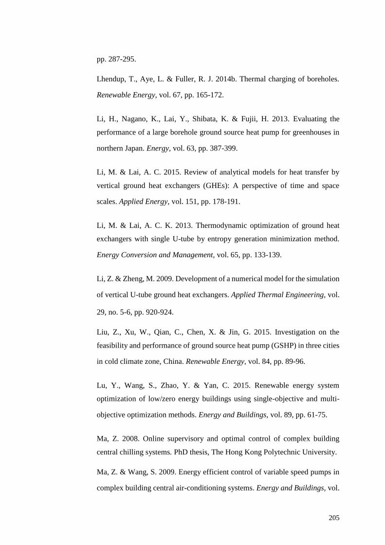
205

pp. 287-295.

Lhendup, T., Aye, L. & Fuller, R. J. 2014b. Thermal charging of boreholes.

Renewable Energy, vol. 67, pp. 165-172.

Li, H., Nagano, K., Lai, Y., Shibata, K. & Fujii, H. 2013. Evaluating the

performance of a large borehole ground source heat pump for greenhouses in

northern Japan. Energy, vol. 63, pp. 387-399.

Li, M. & Lai, A. C. 2015. Review of analytical models for heat transfer by

vertical ground heat exchangers (GHEs): A perspective of time and space

scales. Applied Energy, vol. 151, pp. 178-191.

Li, M. & Lai, A. C. K. 2013. Thermodynamic optimization of ground heat

exchangers with single U-tube by entropy generation minimization method.

Energy Conversion and Management, vol. 65, pp. 133-139.

Li, Z. & Zheng, M. 2009. Development of a numerical model for the simulation

of vertical U-tube ground heat exchangers. Applied Thermal Engineering, vol.

29, no. 5-6, pp. 920-924.

Liu, Z., Xu, W., Qian, C., Chen, X. & Jin, G. 2015. Investigation on the

feasibility and performance of ground source heat pump (GSHP) in three cities

in cold climate zone, China. Renewable Energy, vol. 84, pp. 89-96.

Lu, Y., Wang, S., Zhao, Y. & Yan, C. 2015. Renewable energy system

optimization of low/zero energy buildings using single-objective and multi-

objective optimization methods. Energy and Buildings, vol. 89, pp. 61-75.

Ma, Z. 2008. Online supervisory and optimal control of complex building

central chilling systems. PhD thesis, The Hong Kong Polytechnic University.

Ma, Z. & Wang, S. 2009. Energy efficient control of variable speed pumps in

complex building central air-conditioning systems. Energy and Buildings, vol.

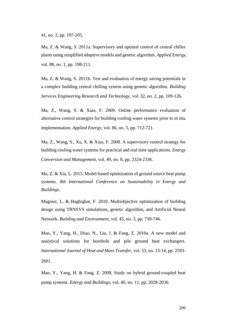
206

41, no. 2, pp. 197-205.

Ma, Z. & Wang, S. 2011a. Supervisory and optimal control of central chiller

plants using simplified adaptive models and genetic algorithm. Applied Energy,

vol. 88, no. 1, pp. 198-211.

Ma, Z. & Wang, S. 2011b. Test and evaluation of energy saving potentials in

a complex building central chilling system using genetic algorithm. Building

Services Engineering Research and Technology, vol. 32, no. 2, pp. 109-126.

Ma, Z., Wang, S. & Xiao, F. 2009. Online performance evaluation of

alternative control strategies for building cooling water systems prior to in situ

implementation. Applied Energy, vol. 86, no. 5, pp. 712-721.

Ma, Z., Wang, S., Xu, X. & Xiao, F. 2008. A supervisory control strategy for

building cooling water systems for practical and real time applications. Energy

Conversion and Management, vol. 49, no. 8, pp. 2324-2336.

Ma, Z. & Xia, L. 2015. Model-based optimization of ground source heat pump

systems. 8th International Conference on Sustainability in Energy and

Buildings.

Magnier, L. & Haghighat, F. 2010. Multiobjective optimization of building

design using TRNSYS simulations, genetic algorithm, and Artificial Neural

Network. Building and Environment, vol. 45, no. 3, pp. 739-746.

Man, Y., Yang, H., Diao, N., Liu, J. & Fang, Z. 2010a. A new model and

analytical solutions for borehole and pile ground heat exchangers.

International Journal of Heat and Mass Transfer, vol. 53, no. 13-14, pp. 2593-

2601.

Man, Y., Yang, H. & Fang, Z. 2008. Study on hybrid ground-coupled heat

pump systems. Energy and Buildings, vol. 40, no. 11, pp. 2028-2036.

207

Man, Y., Yang, H., Spitler, J. D. & Fang, Z. 2011. Feasibility study on novel

hybrid ground coupled heat pump system with nocturnal cooling radiator for

cooling load dominated buildings. Applied Energy, vol. 88, no. 11, pp. 4160-

4171.

Man, Y., Yang, H. & Wang, J. 2010b. Study on hybrid ground-coupled heat

pump system for air-conditioning in hot-weather areas like Hong Kong.

Applied Energy, vol. 87, no. 9, pp. 2826-2833.

Mara, T. A. & Tarantola, S. Application of global sensitivity analysis of model

output to building thermal simulations. Building Simulation, 2008. Springer,

pp. 290-302.

Marzbanrad, J., Sharifzadegan, A. & Kahrobaeian, A. 2007. Thermodynamic

optimization of GSHPS heat exchangers. International Journal of

Thermodynamics, vol. 10, no. 3, pp. 107-111.

Matuska, T. & Sourek, B. 2013. Solar heat pump system with hybrid PVT

collectors for a family house. Central Europe towards Sustainable Building.

Prague, Czech Republic.

Michopoulos, A., Zachariadis, T. & Kyriakis, N. 2013. Operation

characteristics and experience of a ground source heat pump system with a

vertical ground heat exchanger. Energy, vol. 51, pp. 349-357.

Moffat, R. J. 1988. Describing the uncertainties in experimental results.

Experimental thermal and fluid science, vol. 1, no. 1, pp. 3-17.

Montagud, C., Corberán, J. M. & Montero, 2014. In situ optimization

methodology for the water circulation pumps frequency of ground source heat

pump systems. Energy and Buildings, vol. 68, pp. 42-53.

Morris, M. D. 1991. Factorial sampling plans for preliminary computational

experiments. Technometrics, vol. 33, no. 2, pp. 161-174.

208

Muraya, N. K., Oneal, D. L. & Heffington, W. M. 1996. Thermal interference

of adjacent legs in a vertical U-tube heat exchanger for a ground-coupled heat

pump. American Society of Heating, Refrigerating and Air-Conditioning

Engineers, Inc., Atlanta, GA (United States).

Nassif, N., Moujaes, S. & Zaheeruddin, M. 2008. Self-tuning dynamic models

of HVAC system components. Energy and Buildings, vol. 40, no. 9, pp. 1709-

1720.

Nathers 2012. Software Accreditation Protocol.

Nesic, D. Extremum seeking control: Convergence analysis. Control

Conference (ECC), 2009 European, 2009. IEEE, pp. 1702-1715.

Neugebauer, M. & Sołowiej, P. 2012. Optimization with the use of genetic

algorithms of the location depth of horizontal ground heat exchangers.

Inżynieria Rolnicza, vol. 16, pp. 89-97.

Osterman, E., Tyagi, V., Butala, V., Rahim, N. A. & Stritih, U. 2012. Review

of PCM based cooling technologies for buildings. Energy and Buildings, vol.

49, pp. 37-49.

Ozgener, O. & Hepbasli, A. 2005a. Experimental investigation of the

performance of a solar ‐ assisted ground ‐ source heat pump system for

greenhouse heating. International Journal of Energy Research, vol. 29, no. 3,

pp. 217-231.

Ozgener, O. & Hepbasli, A. 2005b. Experimental performance analysis of a

solar assisted ground-source heat pump greenhouse heating system. Energy

and Buildings, vol. 37, no. 1, pp. 101-110.

Ozgener, O. & Hepbasli, A. 2005c. Performance analysis of a solar-assisted

ground-source heat pump system for greenhouse heating: an experimental

study. Building and Environment, vol. 40, no. 8, pp. 1040-1050.

209

Ozgener, O. & Hepbasli, A. 2007. Modeling and performance evaluation of

ground source (geothermal) heat pump systems. Energy and Buildings, vol. 39,

no. 1, pp. 66-75.

Ozyurt, O. & Ekinci, D. A. 2011. Experimental study of vertical ground-source

heat pump performance evaluation for cold climate in Turkey. Applied Energy,

vol. 88, no. 4, pp. 1257-1265.

Pérez-Lombard, L., Ortiz, J. & Pout, C. 2008. A review on buildings energy

consumption information. Energy and Buildings, vol. 40, no. 3, pp. 394-398.

Pardalos, P. M. & Resende, M. G. 2001. Handbook of applied optimization,

Oxford University Press.

Park, H., Kim, W., Jeon, J. & Kim, Y. Optimization of a hybrid ground source

heat pump using the response surface method. Proceedings of the SAREK

2010 Summer Annual Conference, 2010. pp. 611-616.

Park, H., Kim, W., Jeon, J. & Kim, Y. Optimization of a hybrid ground source

heat pump using the response surface method. World renewable energy

congress, 2011 Linkoping, Sweden.

Park, H., Lee, J. S., Kim, W. & Kim, Y. 2013. The cooling seasonal

performance factor of a hybrid ground-source heat pump with parallel and

serial configurations. Applied Energy, vol. 102, pp. 877-884.

Phetteplace, G. & Sullivan, W. 1998. Performance of a hybrid ground-coupled

pump system. ASHRAE transactions, vol. 104, pp. 763.

Piechowski, M. 1999. Heat and mass transfer model of a ground heat

exchanger: theoretical development. International Journal of Energy Research,

vol. 23, no. 7, pp. 571-588.

Pu, L., Qi, D., Xu, L. & Li, Y. 2017. Optimization on the performance of

ground heat exchangers for GSHP using Kriging model based on MOGA.

210

Applied Thermal Engineering, vol. 118, pp. 480-489.

Putrayudha, S. A., Kang, E. C., Evgueniy, E., Libing, Y. & Lee, E. J. 2015. A

study of photovoltaic/thermal (PVT)-ground source heat pump hybrid system

by using fuzzy logic control. Applied Thermal Engineering, vol. 89, pp. 578-

586.

Qi, Z. S., Gao, Q., Liu, Y., Yan, Y. Y. & Spitler, J. D. 2014. Status and

development of hybrid energy systems from hybrid ground source heat pump

in China and other countries. Renewable and Sustainable Energy Reviews, vol.

29, pp. 37-51.

Ramamoorthy, M., Jin, H., Chaisson, A. & Spitler, J. D. 2001a. Optimal sizing

of hybrid ground-source heat pump systems that use a cooling pond as a

supplemental heat rejecter-A system simulation approach. TRANSACTIONS-

AMERICAN SOCIETY OF HEATING REFRIGERATING AND AIR

CONDITIONING ENGINEERS, vol. 107, no. 1, pp. 26-38.

Ramamoorthy, M., Jin, H., Chiasson, A. D. & Spitler, J. D. 2001b. Optimal

sizing of hybrid ground-source heat pump systems that use a cooling pond as

a supplemental heat rejecter--a system simulation approach/Discussion.


Remp 2012. Water Heating Data Collection and Analysis. Commonwealth

Department of the Environment and Energy.

Ren, H., Gao, W. & Ruan, Y. 2009. Economic optimization and sensitivity

analysis of photovoltaic system in residential buildings. Renewable Energy,

vol. 34, no. 3, pp. 883-889.

Retkowski, W. & Thöming, J. 2014. Thermoeconomic optimization of vertical

ground-source heat pump systems through nonlinear integer programming.

Applied Energy, vol. 114, pp. 492-503.

211

Rezaei-Bazkiaei, A., Dehghan-Niri, E., Kolahdouz, E. M., Weber, A. S. &

Dargush, G. F. 2013. A passive design strategy for a horizontal ground source

heat pump pipe operation optimization with a non-homogeneous soil profile.

Energy and Buildings, vol. 61, pp. 39-50.

Robert, F. & Gosselin, L. 2014. New methodology to design ground coupled

heat pump systems based on total cost minimization. Applied Thermal

Engineering, vol. 62, no. 2, pp. 481-491.

Rottmayer, S. P., Beckman, W. A. & Mitchell, J. W. 1997. Simulation of a

single vertical U-tube ground heat exchanger in an infinite medium. Atlanta,

GA: American Society of Heating, Refrigerating and Air-Conditioning

Engineers, Inc.

Safa, A. A., Fung, A. S. & Kumar, R. 2015. Heating and cooling performance

characterisation of ground source heat pump system by testing and TRNSYS

simulation. Renewable Energy, vol. 83, pp. 565-575.

Sagia, Z. & Rakopoulos, C. 2012. New control strategy for a hybrid ground

source heat pump system coupled to a closed circuit cooling tower. Journal of

Applied Mechanical Engineering, vol. 1, no. 2, pp. 1-8.

Saltelli, A., Tarantola, S., Campolongo, F. & Ratto, M. 2004. Sensitivity

analysis in practice: a guide to assessing scientific models, John Wiley & Sons.

Sanaye, S. & Niroomand, B. 2009. Thermal-economic modeling and

optimization of vertical ground-coupled heat pump. Energy Conversion and

Management, vol. 50, no. 4, pp. 1136-1147.

Sanaye, S. & Niroomand, B. 2010. Horizontal ground coupled heat pump:

Thermal-economic modeling and optimization. Energy Conversion and

Management, vol. 51, no. 12, pp. 2600-2612.

Sarbu, I. & Sebarchievici, C. 2014. General review of ground-source heat

212

pump systems for heating and cooling of buildings. Energy and Buildings, vol.

70, pp. 441-454.

Sayyaadi, H., Amlashi, E. H. & Amidpour, M. 2009. Multi-objective

optimization of a vertical ground source heat pump using evolutionary

algorithm. Energy Conversion and Management, vol. 50, no. 8, pp. 2035-2046.

Sayyadi, H. & Nejatolahi, M. 2011. Thermodynamic and thermoeconomic

optimization of a cooling tower-assisted ground source heat pump.

Geothermics, vol. 40, no. 3, pp. 221-232.

Shi, Z., Song, S. & Hu, S. Optimized Design of Ground-Source Heat Pump

System Heat Exchanger. Proceedings of the 8th International Symposium on

Heating, Ventilation and Air Conditioning, 2014. Springer, pp. 723-730.

Silva, A. S. & Ghisi, E. 2014. Uncertainty analysis of user behaviour and

physical parameters in residential building performance simulation. Energy

and Buildings, vol. 76, pp. 381-391.

Sivasakthivel, T., Murugesan, K. & Sahoo, P. K. 2014a. Optimization of

ground heat exchanger parameters of ground source heat pump system for

space heating applications. Energy, vol. 78, pp. 573-586.

Sivasakthivel, T., Murugesan, K. & Thomas, H. R. 2014b. Optimization of

operating parameters of ground source heat pump system for space heating and

cooling by Taguchi method and utility concept. Applied Energy, vol. 116, pp.

76-85.

Sohier, H., Piet-Lahanier, H. & Farges, J.-L. 2015. Analysis and optimization

of an air-launch-to-orbit separation. Acta Astronautica, vol. 108, pp. 18-29.

Soyguder, S. & Alli, H. 2009. Predicting of fan speed for energy saving in

HVAC system based on adaptive network based fuzzy inference system.

213

Expert Systems with Applications, vol. 36, no. 4, pp. 8631-8638.

Steuer, R. E. & Choo, E.-U. 1983. An interactive weighted Tchebycheff

procedure for multiple objective programming. Mathematical programming,

vol. 26, no. 3, pp. 326-344.

Sukesh, N., Lakshmisagar, P. & Kumar, G. 2015. Heat Transfer Analysis of

Fin Performance for PVT Absorber. Journal of Mechanical Engineering and

Automation, vol. 5, no. 3B, pp. 1-4.

Sundbrandt, M. 2011. Control of a Ground Source Heat Pump using Hybrid

Model Predictive Control. MSc Thesis, Linkopings University.

Svensson, M. C. 1996. Model-based optimizing control of a water-to-water

heat pump unit. Modeling, Identification and Control, vol. 17, no. 4, pp. 279-

295.

Tang, C. C. 2005. Modeling packaged heat pumps in a quasi-steady state

energy simulation program. Oklahoma State University.

Thornton, J., Mcdowell, T., Shonder, J., Hughes, P., Pahud, D. & Hellström,

G. 1997. Residential vertical geothermal heat pump system models: calibration

to data. Ashrae Transaction 1997, vol. 103, no. 2, pp. 660-674.

Tian, W. 2013. A review of sensitivity analysis methods in building energy

analysis. Renewable and Sustainable Energy Reviews, vol. 20, pp. 411-419.

Tiwari, A., Dubey, S., Sandhu, G., Sodha, M. & Anwar, S. 2009. Exergy

analysis of integrated photovoltaic thermal solar water heater under constant

flow rate and constant collection temperature modes. Applied Energy, vol. 86,

no. 12, pp. 2592-2597.

Trillat-Berdal, V., Souyri, B. & Fraisse, G. 2006. Experimental study of a

ground-coupled heat pump combined with thermal solar collectors. Energy and

214

Buildings, vol. 38, no. 12, pp. 1477-1484.

Trnsys. The Transient Energy System Simulation Tool [Online]. Available:

http://www.trnsys.com.

Tse, K.-K., Chow, T.-T. & Su, Y. 2016. Performance evaluation and economic

analysis of a full scale water-based photovoltaic/thermal (PV/T) system in an

office building. Energy and Buildings, vol. 122, pp. 42-52.

Urchueguía, J., Zacarés, M., Corberán, J., Montero, A., Martos, J. & Witte, H.

2008. Comparison between the energy performance of a ground coupled water

to water heat pump system and an air to water heat pump system for heating

and cooling in typical conditions of the European Mediterranean coast. Energy

Conversion and Management, vol. 49, no. 10, pp. 2917-2923.

Urge-Vorsatz, D., Cabeza, L. F., Serrano, S., Barreneche, C. & Petrichenko, K.

2015. Heating and cooling energy trends and drivers in buildings. Renewable

and Sustainable Energy Reviews, vol. 41, pp. 85-98.

Verhelst, C. 2012. Model Predictive Control of Ground Coupled Heat Pump

Systems in Office Buildings. PhD thesis, Katholieke Universiteit Leuven.

Verma, V. & Murugesan, K. 2014. Optimization of solar assisted ground

source heat pump system for space heating application by Taguchi method and

utility concept. Energy and Buildings, vol. 82, pp. 296-309.

Wan, K. K., Li, D. H., Pan, W. & Lam, J. C. 2012. Impact of climate change

on building energy use in different climate zones and mitigation and adaptation

implications. Applied Energy, vol. 97, pp. 274-282.

Wang, E., Fung, A. S., Qi, C. & Leong, W. H. 2012. Performance prediction

of a hybrid solar ground-source heat pump system. Energy and Buildings, vol.

47, pp. 600-611.

http://www.trnsys.com/

215

Wang, J. J., Jing, Y. Y. & Zhang, C. F. 2010. Optimization of capacity and

operation for CCHP system by genetic algorithm. Applied Energy, vol. 87, no.

4, pp. 1325-1335.

Wang, S. & Jin, X. 2000. Model-based optimal control of VAV air-

conditioning system using genetic algorithm. Building and Environment, vol.

35, no. 6, pp. 471-487.

Wang, S. & Ma, Z. 2008. Supervisory and optimal control of building HVAC

systems: a review. HVAC&R Research, vol. 14, no. 1, pp. 3-32.

Wang, Z., Wang, F., Ma, Z., Wang, X. & Wu, X. 2016. Research of heat and

moisture transfer influence on the characteristics of the ground heat pump

exchangers in unsaturated soil. Energy and Buildings, vol. 130, pp. 140-149.

Waterfurnace. 2016. Versatec Ultra NSKW Specification Catalog [Online]. A

vailable: http://www.geoexchange.com.au/download/WaterFurnace%20NSK

W%2050HZ%20Aurora%20SC2566WN_Specification%20Catalogue.pdf.

Watmuff, J., Charters, W. & Proctor, D. 1977. Solar and wind induced external

coefficients for solar collectors. Comples, 2. Rev. Inter. Heliotech., Marseille.

Weeratunge, H., Narsilio, G., De Hoog, J., Dunstall, S. & Halgamuge, S. 2018.

Model predictive control for a solar assisted ground source heat pump system.

Energy, vol. 152, pp. 974-984.

Wong, S. L., Wan, K. K. & Lam, T. N. 2010. Artificial neural networks for

energy analysis of office buildings with daylighting. Applied Energy, vol. 87,

no. 2, pp. 551-557.

Woodward, D. G. 1997. Life cycle costing—theory, information acquisition

and application. International journal of project management, vol. 15, no. 6,

pp. 335-344.

http://www.geoexchange.com.au/download/WaterFurnace%20NSKW%2050HZ%20Aurora%20SC2566WN_Specification%20Catalogue.pdf

http://www.geoexchange.com.au/download/WaterFurnace%20NSKW%2050HZ%20Aurora%20SC2566WN_Specification%20Catalogue.pdf

216

Wu, Y., Gan, G., Verhoef, A., Vidale, P. L. & Gonzalez, R. G. 2010.

Experimental measurement and numerical simulation of horizontal-coupled

slinky ground source heat exchangers. Applied Thermal Engineering, vol. 30,

no. 16, pp. 2574-2583.

Xia, L., Ma, Z. & Kokogiannakis, G. 2017a. Performance Simulation of a

Ground Source Heat Pump System Integrated with Solar Photovoltaic Thermal

Collectors for Residential Applications. Building Simulation San Francisco.

Xia, L., Ma, Z., Mclauchlan, C. & Wang, S. 2017b. Experimental investigation

and control optimization of a ground source heat pump system. Applied


Yan, Y., Zhou, J., Lin, Y., Yang, W., Wang, P. & Zhang, G. 2008. Adaptive

optimal control model for building cooling and heating sources. Energy and

Buildings, vol. 40, no. 8, pp. 1394-1401.

Yang, H., Cui, P. & Fang, Z. 2010. Vertical-borehole ground-coupled heat

pumps: A review of models and systems. Applied Energy, vol. 87, no. 1, pp.

16-27.

Yang, J., Xu, L., Hu, P., Zhu, N. & Chen, X. 2014. Study on intermittent

operation strategies of a hybrid ground-source heat pump system with double-

cooling towers for hotel buildings. Energy and Buildings, vol. 76, pp. 506-512.

Yating, Z., Guiyang, W. & Guang, H. GCHP system optimal predictive control

based on RBFNN and APSO algorithm. 32nd Chinese Control Conference

(CCC), 2013. IEEE.

Yavuzturk, C. & Spitler, J. D. 1999. A short time step response factor model

for vertical ground loop heat exchangers. ASHRAE transactions, vol. 105, no.

2, pp. 475-485.

Yavuzturk, C. & Spitler, J. D. 2000. Comparative study of operating and

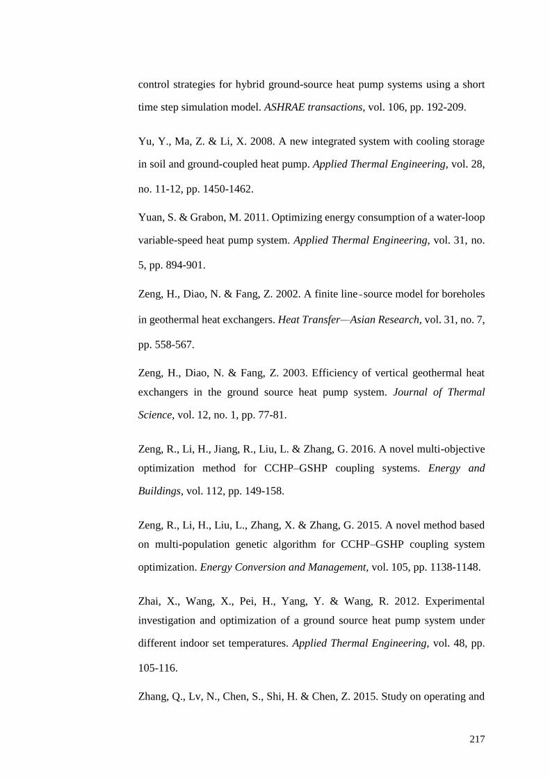
217

control strategies for hybrid ground-source heat pump systems using a short

time step simulation model. ASHRAE transactions, vol. 106, pp. 192-209.

Yu, Y., Ma, Z. & Li, X. 2008. A new integrated system with cooling storage

in soil and ground-coupled heat pump. Applied Thermal Engineering, vol. 28,

no. 11-12, pp. 1450-1462.

Yuan, S. & Grabon, M. 2011. Optimizing energy consumption of a water-loop

variable-speed heat pump system. Applied Thermal Engineering, vol. 31, no.

5, pp. 894-901.

Zeng, H., Diao, N. & Fang, Z. 2002. A finite line‐source model for boreholes

in geothermal heat exchangers. Heat Transfer—Asian Research, vol. 31, no. 7,

pp. 558-567.

Zeng, H., Diao, N. & Fang, Z. 2003. Efficiency of vertical geothermal heat

exchangers in the ground source heat pump system. Journal of Thermal

Science, vol. 12, no. 1, pp. 77-81.

Zeng, R., Li, H., Jiang, R., Liu, L. & Zhang, G. 2016. A novel multi-objective

optimization method for CCHP–GSHP coupling systems. Energy and

Buildings, vol. 112, pp. 149-158.

Zeng, R., Li, H., Liu, L., Zhang, X. & Zhang, G. 2015. A novel method based

on multi-population genetic algorithm for CCHP–GSHP coupling system

optimization. Energy Conversion and Management, vol. 105, pp. 1138-1148.

Zhai, X., Wang, X., Pei, H., Yang, Y. & Wang, R. 2012. Experimental

investigation and optimization of a ground source heat pump system under

different indoor set temperatures. Applied Thermal Engineering, vol. 48, pp.

105-116.

Zhang, Q., Lv, N., Chen, S., Shi, H. & Chen, Z. 2015. Study on operating and

218

control strategies for hybrid ground source heat pump system. Procedia

Engineering, vol. 121, pp. 1894-1901.

Zhao, J., Chen, Y., Lu, S. & Cui, J. 2009. Optimization of serial combined

system of ground-coupled heat pump and solar collector. Transactions of

Tianjin University, vol. 15, pp. 37-42.

Zhao, Y., Xie, W. & Tu, X. 2012. Performance-based parameter tuning method

of model-driven PID control systems. ISA transactions, vol. 51, no. 3, pp. 393-

399.

Zhou, S., Cui, W., Li, Z. & Liu, X. 2016. Feasibility study on two schemes for

alleviating the underground heat accumulation of the ground source heat pump.

Sustainable Cities and Society, vol. 24, pp. 1-9.

Zhu, N., Hu, P., Lei, Y., Jiang, Z. & Lei, F. 2015. Numerical study on ground

source heat pump integrated with phase change material cooling storage

system in office building. Applied Thermal Engineering, vol. 87, pp. 615-623.

Zhu, Y., Tao, Y. & Rayegan, R. 2012. A comparison of deterministic and

probabilistic life cycle cost analyses of ground source heat pump (GSHP)

applications in hot and humid climate. Energy and Buildings, vol. 55, pp. 312-

321.

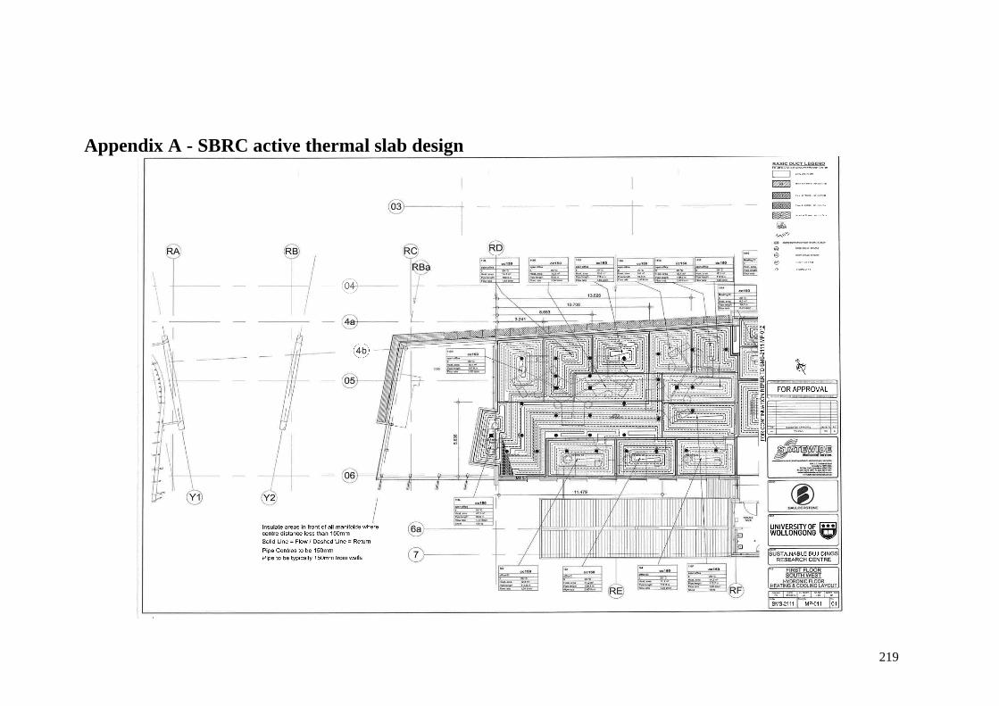
219

Appendix A - SBRC active thermal slab design

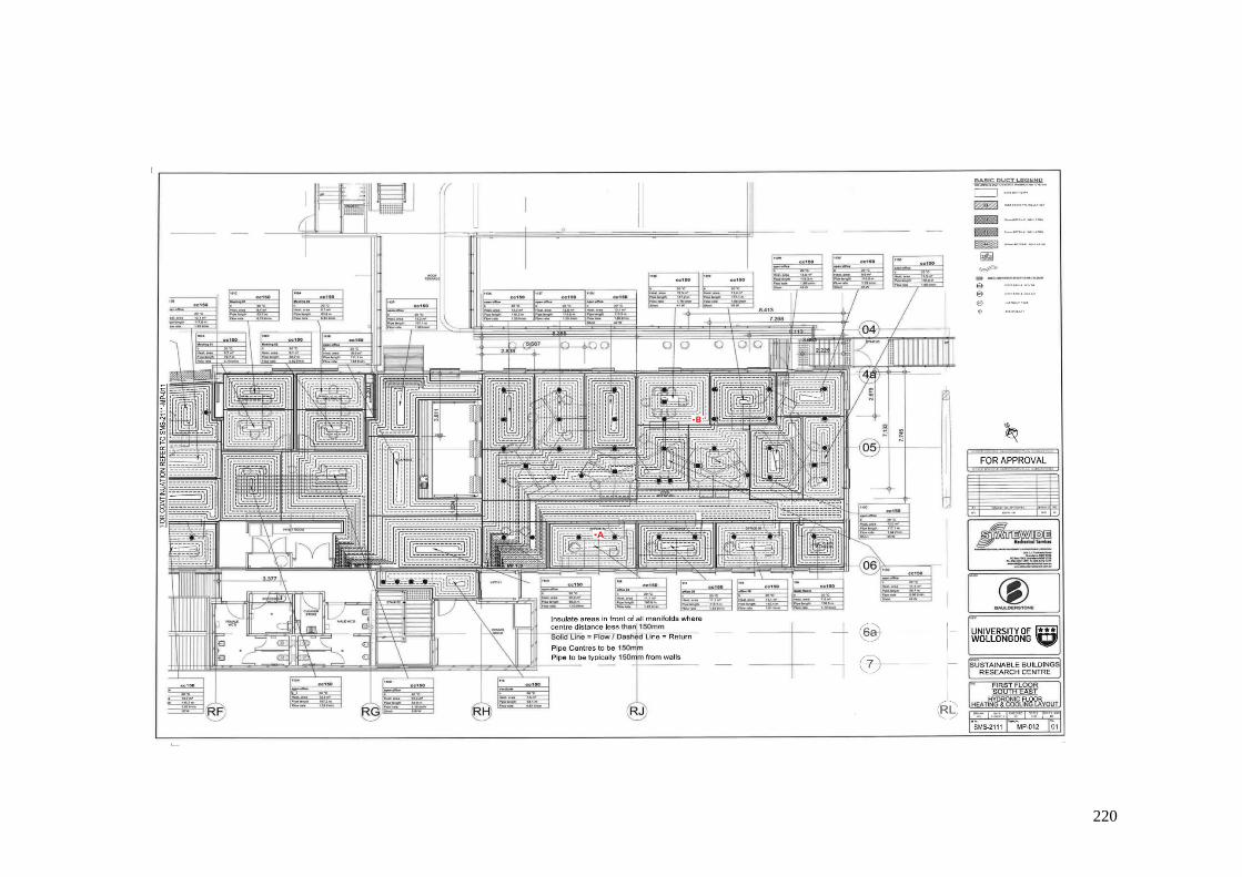
220

221

Appendix B - SBRC hydronic loop system

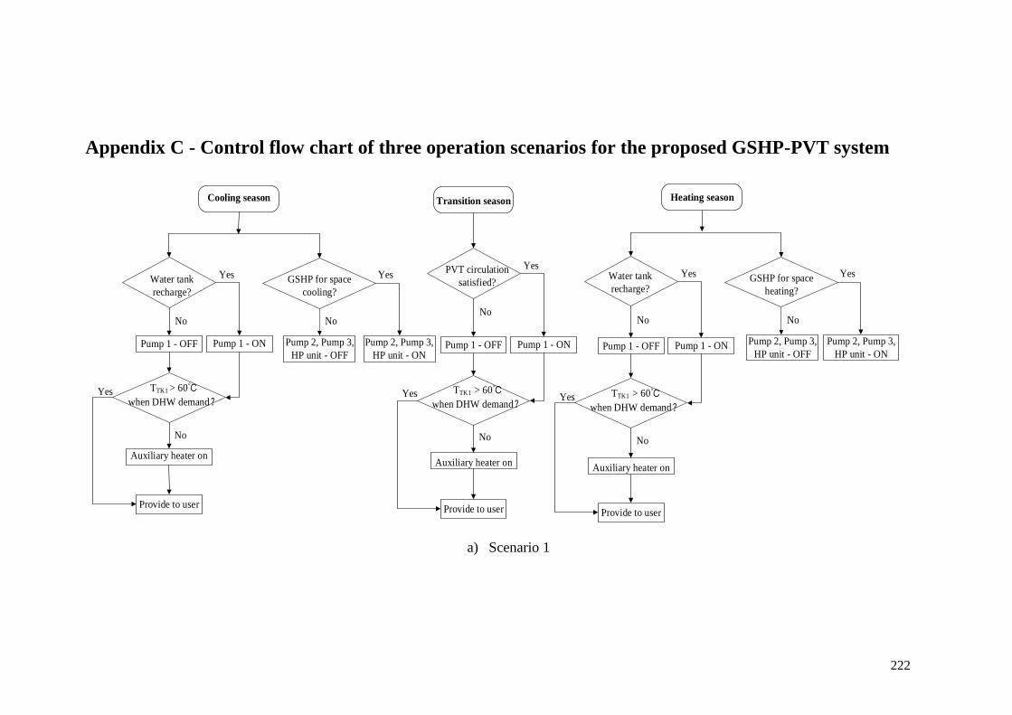
222

Appendix C - Control flow chart of three operation scenarios for the proposed GSHP-PVT system

a) Scenario 1

Cooling season

Water tank

recharge?

Pump 1 - ON Pump 2, Pump 3,

HP unit - ON

GSHP for space

cooling?

Yes

TTK1 > 60

when DHW demand？

Pump 1 - OFF

No

Auxiliary heater on

No

Provide to user

Yes

Pump 2, Pump 3,

HP unit - OFF

Yes

No

Transition season

Pump 1 - ON

Yes

TTK1 > 60

when DHW demand？

Pump 1 - OFF

No

No

Provide to user

Yes

Heating season


HP unit - ON

Yes

TTK1 > 60

when DHW demand？

Pump 1 - OFF

No

No

Provide to user

Yes

Pump 2, Pump 3,

HP unit - OFF

Yes

No

Auxiliary heater onAuxiliary heater on

PVT circulation

satisfied? GSHP for space

heating?

Water tank

recharge?

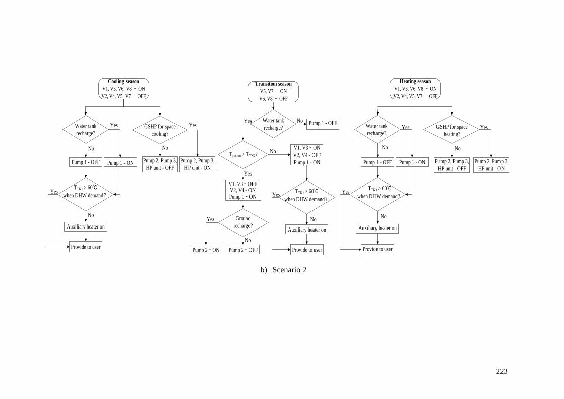
223

b) Scenario 2

Cooling season

V1, V3, V6, V8 – ON

V2, V4, V5, V7 – OFF


HP unit - ON

GSHP for space

cooling?

Yes

TTK1 > 60

when DHW demand？

Pump 1 - OFF

No

Auxiliary heater on

No

Provide to user

Yes

Pump 2, Pump 3,

HP unit - OFF

Yes

No

Transition season

V5, V7 – ON

V6, V8 – OFF

V1, V3–ON

V2, V4 - OFF

Pump 1 - ON

Tpvt, out > TTK2?No

Auxiliary heater on

No

Provide to user

Yes

Yes

No

V1, V3–OFFV2, V4 - ONPump 1–ON

Ground

recharge?

Pump 2–ON

No

Yes

Pump 2–OFF

Heating season

V1, V3, V6, V8 – ON

V2, V4, V5, V7 – OFF


HP unit - ON

Yes

Pump 1 - OFF

No

Auxiliary heater on

No

Provide to user

Yes

Pump 2, Pump 3,

HP unit - OFF

Yes

No

Water tank

recharge?

TTK1 > 60

when DHW demand？

TTK1 > 60

when DHW demand？

Water tank

recharge?Pump 1 - OFFYes

GSHP for space

heating?

Water tank

recharge?

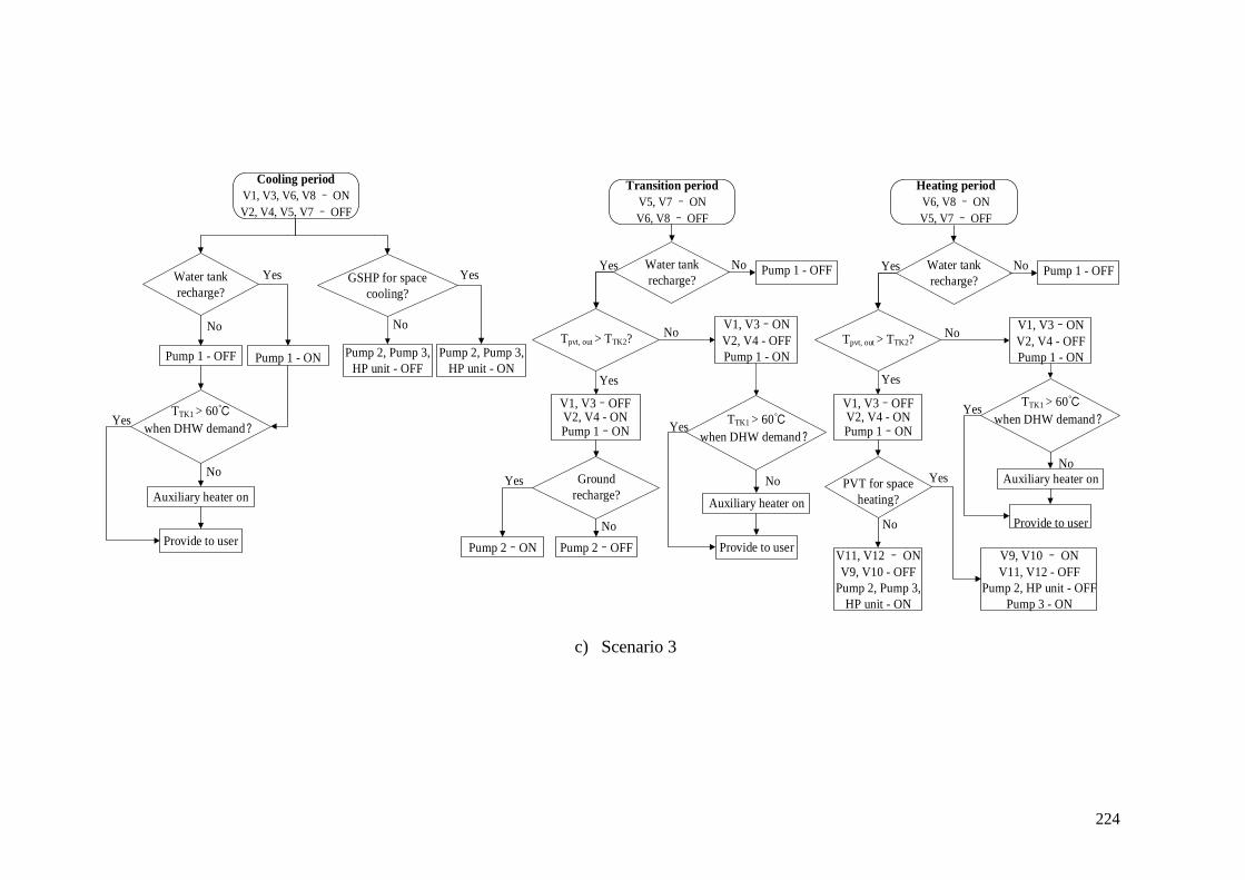
224

c) Scenario 3

Heating period

V6, V8 – ON

V5, V7 – OFF

V9, V10 – ON

V11, V12 - OFF

Pump 2, HP unit - OFF

Pump 3 - ON

PVT for space

heating?

V11, V12 – ON

V9, V10 - OFF

Pump 2, Pump 3,

HP unit - ON

Yes

No

Cooling period

V1, V3, V6, V8 – ON

V2, V4, V5, V7 – OFF


HP unit - ON

GSHP for space

cooling?

Yes

TTK1 > 60

when DHW demand？

Pump 1 - OFF

No

Auxiliary heater on

No

Provide to user

Yes

Pump 2, Pump 3,

HP unit - OFF

Yes

No

Transition period

V5, V7 – ON

V6, V8 – OFF

V1, V3–ON

V2, V4 - OFF

Pump 1 - ON

Tpvt, out > TTK2?No

Auxiliary heater on

No

Provide to user

Yes

Yes

No


Ground

recharge?

Pump 2–ON

No

Yes

Pump 2–OFF

Water tank

recharge?

TTK1 > 60

when DHW demand？

Water tank


V1, V3–ON

V2, V4 - OFF

Pump 1 - ON

Tpvt, out > TTK2?No

NoWater tank


Yes


Auxiliary heater on

No

Provide to user

YesTTK1 > 60

when DHW demand？

Documents

Performance evaluation and optimisation of stand-alone