Performance Calibration of Photogrammetic … issue/NCEITCS-2017/NCEITCS-143.pdfPerformance Calibration of Photogrammetic Optical Systems ... experiment results are presented that

International Journal of Engineering Trends and Technology (IJETT) – Special Issue – April 2017

ISSN: 2231-5381 http://www.ijettjournal.org Page 240

Performance Calibration of Photogrammetic Optical

Systems T. Saikanth1, R.S. Chandrasekhar2, B.Venu gopal Rreddy

2 ,V. Punna Rao1, C. Gireesh1, Pamidighantam V. Ramana1

1Vasavi College of Engineering, Ibrahimbagh, Hyderabad 500 031.

2Research CentreImarat, Vignyakancha, Hyderabad 500 058.

Abstract: The performance of a digital optical imaging system

with a CCD sensor depends on the precision of the optical elements

in the design and assembly. The lens fabrication and assembly

introduces offset and misalignment between mechanical and optical

axis. A precise analysis and experimental estimation of optical

system parameter errors can be used to improve the image quality

through software algorithms. In this manuscript, we report our work

about a method to measure optical system parameters like principal

point, focal length, and distortion etc of optical imager using

Simulation Tools, Open CV and an Autocollimator Theodolite. These

parameters are very crucial for the synthetic error analysis of digital

optical imaging system. The calibration experiments result in

estimation of optical performance parameters, which are used to

develop image enhancement algorithms. The parameters are

extracted from a set of image templates using different methods. In

part I, we present the calibration analysis and in part II, the

experiment results are presented that show excellent agreement with

the calibration model.

Keywords: Photogrammetic , Principal point, Focal length,

Distortion, OpenCV, Autocollimator Theodolite, MATLAB.

I. INTRODUCTION

Imager calibration is used to determine intrinsic and

extrinsic parameters for imaging systems, but it is also used to

determine the complete lens distortion model. The intrinsic

parameters include focal length, principal point, skew

coefficient, distortions. The extrinsic parameters can include

the rotation matrix and translation vector between the imager

coordinate system and the world coordinate system. Imager

calibration has been studied extensively in computer vision

and photogrammetry, and even recently new techniques have

been proposed. In the first part, we presented the theoretical

analyasis of optical parameters using pin hole imager model.

In the present part, we describe the experimental results.

1.1. Types of parameters: Two types of parameters need to be

recovered are

Intrinsic imager parameters

Extrinsic imager parameters

Intrinsic imager parameters: These are the parameters that

characterize the optical, geometric, and digital characteristics

of the imager

Effective focal length f.

The transformation between image planes

coordinates and pixel coordinates.

The geometric distortion introduced by the optics.

Extrinsic imager parameters: These are the parameters that

identify uniquely the transformation between the unknown

imager reference frame and the known world reference frame.

1) Finding the translation vector between the relative

positions of the origins of the two reference frames.

2) Finding the rotation matrix that brings the corresponding

axes of the two frames into alignment.

Recently, many calibration methods were compared and

described. Most of them were based on Tsai, Heikkila &

Silven or Zhang methods [1] [2]. All three methods are based

on the pinhole camera model and include radial distortion

models.

Zhang’s method uses a checkerboard pattern, which is

placed in front of the camera. At least three different images in

various angles and positions must be acquired for the

computation of camera calibration model. After the

acquisition of the images the algorithms for detection of

corners are used and corners of the checkerboard pattern are

extracted. These points are used in calculations for camera

calibration. This method is also used in OpenCV and Camera

calibration.

Imager Calibration: The imager calibration is implemented

by 3D reference object based calibration. Before the

calibration it is necessary to adjust the 3D scanning system. It

must be set to cover the whole scanning area. This means

determining the position of the imager, zoom and focus on the

scanning surface. It is necessary to use appropriate calibration

objects, patterns or shapes. These patterns are then used in the

calculations of intrinsic and extrinsic parameters of the system

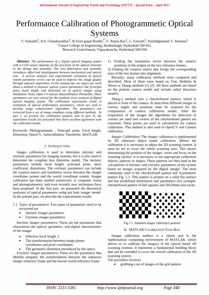
based on images acquired by the digital imager. The most

commonly used is the checkerboard pattern and Asymmetric

pattern Fig. 1.1. This pattern is printed on a solid flat surface

and has predefined dimensions and parameters (for example.

checkerboard pattern of 6x6 squares and 20x20mm size each).

Fig.1.1. Standard imager calibration patterns

II. MATLAB CALIBRATION TOOL BOX

Imager calibration toolbox is a robust tool in the

mathematical computing environment of MATLAB, which

allows us to calibrate the imagers of the optical based 3D

scanning systems. It represents a fundamental building block

that can be extended to cover the overall calibration of the 3D

scanning system.

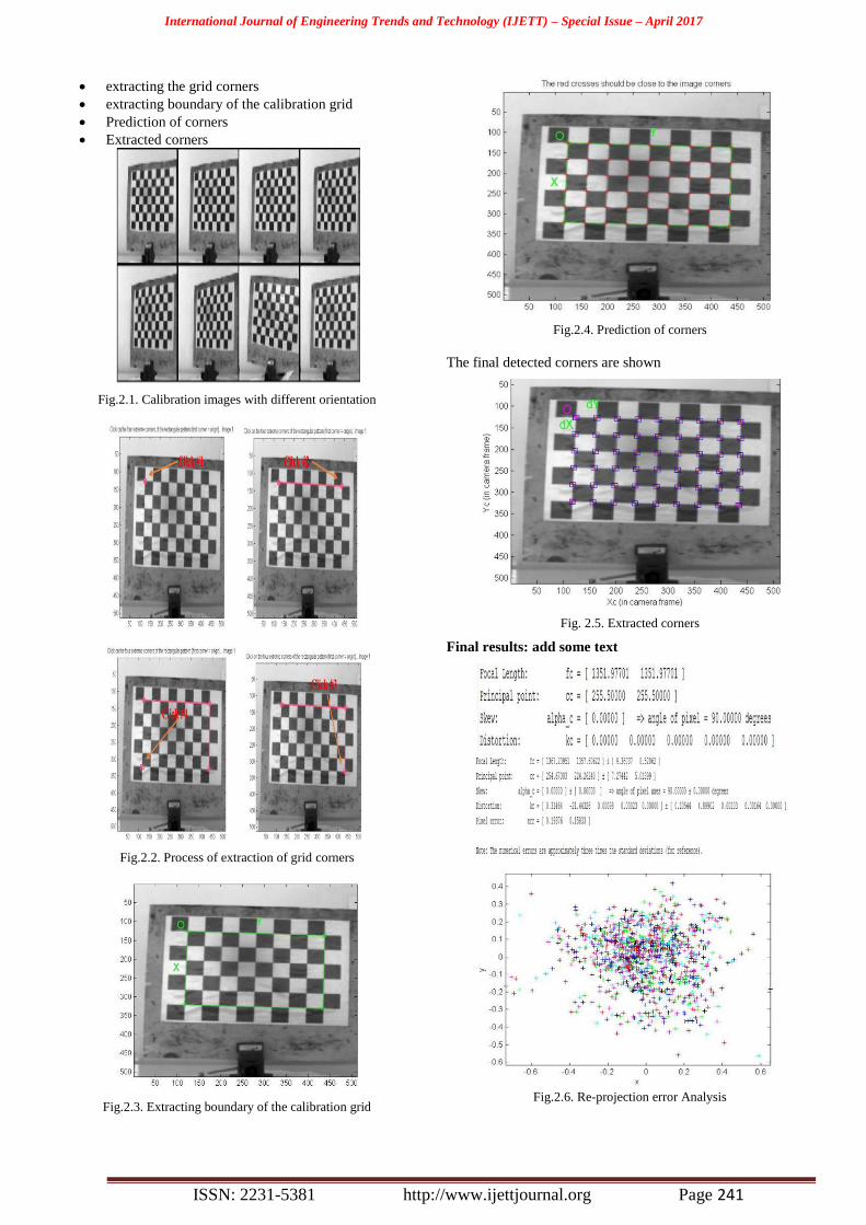
The procedure involves

grabbing a set of images of the grid pattern



extracting the grid corners

extracting boundary of the calibration grid

Prediction of corners

Extracted corners

Fig.2.1. Calibration images with different orientation

Fig.2.2. Process of extraction of grid corners

Fig.2.3. Extracting boundary of the calibration grid

Fig.2.4. Prediction of corners

The final detected corners are shown

Fig. 2.5. Extracted corners

Final results: add some text

Fig.2.6. Re-projection error Analysis



Disadvantages

The main disadvantage of camera calibration toolbox

is the need of carrying out certain steps manually

(especially in comparison with fully automated

calibration method via OpenCV), Thereby extending

the time of calibration.

The most time consuming is the determination of

borders of calibration pattern. Because in every

calibration image (there are normally more than 20

images) it is necessary to define four border points as

we done in section of “Extract the grid corners”.

It is necessary to manually enter some configuration

parameters and also confirm and execute individual

calibration steps.

The another main disadvantage is matlab tool box

wouldn’t work for the asymmetric pattern which is

most accurate pattern to compute the calibration

process, as it would be done by centroiding of circles,

whereas chessboard pattern will be done by corners

extraction of squares.

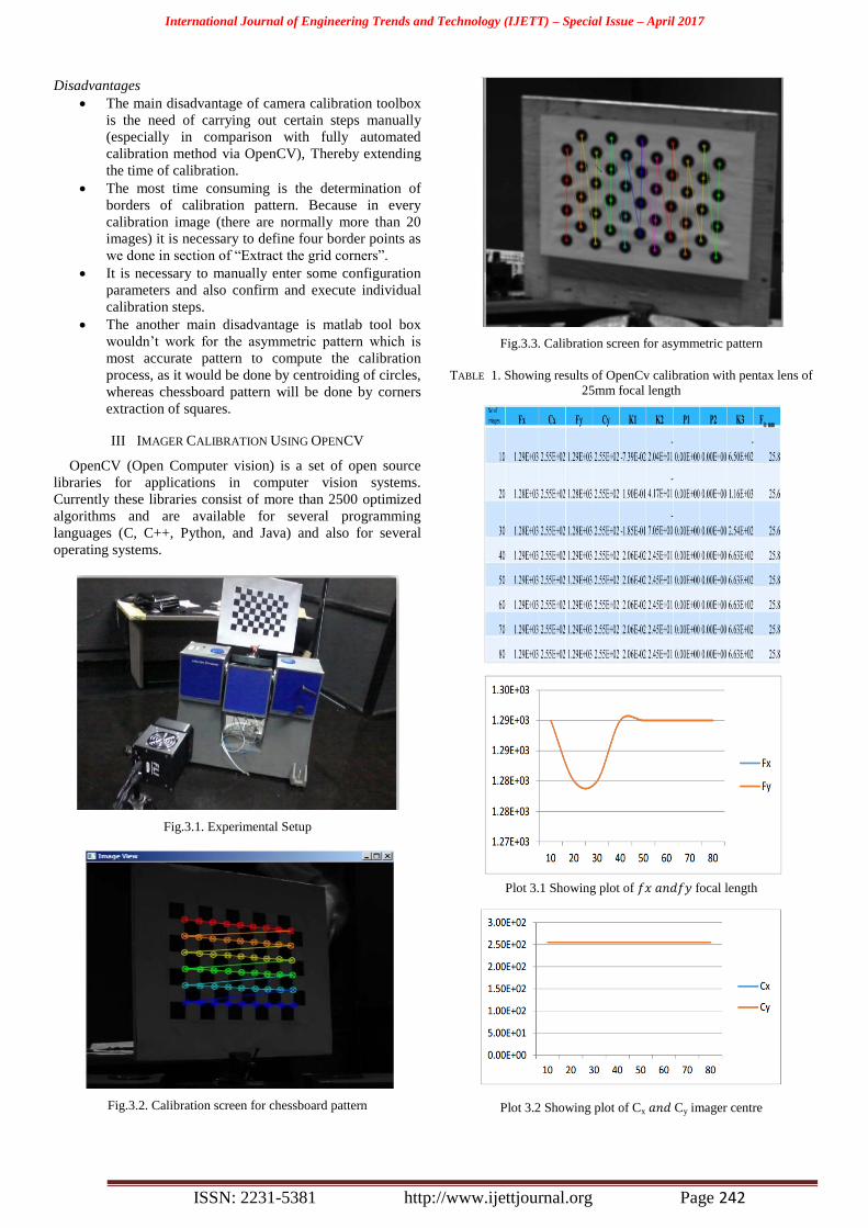
III IMAGER CALIBRATION USING OPENCV

OpenCV (Open Computer vision) is a set of open source

libraries for applications in computer vision systems.

Currently these libraries consist of more than 2500 optimized

algorithms and are available for several programming

languages (C, C++, Python, and Java) and also for several

operating systems.

Fig.3.1. Experimental Setup

Fig.3.2. Calibration screen for chessboard pattern

Fig.3.3. Calibration screen for asymmetric pattern

TABLE 1. Showing results of OpenCv calibration with pentax lens of

25mm focal length

Plot 3.1 Showing plot of 𝑓𝑥 𝑎𝑛𝑑𝑓𝑦 focal length

Plot 3.2 Showing plot of Cx 𝑎𝑛𝑑 Cy imager centre



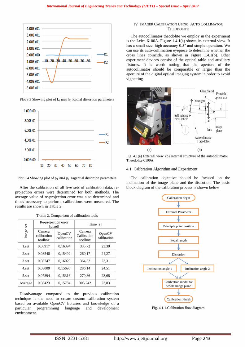
Plot 3.3 Showing plot of k1 𝑎𝑛𝑑 k2 Radial distortion parameters

Plot 3.4 Showing plot of p1 𝑎𝑛𝑑 p2 Tagential distortion parameters

After the calibration of all five sets of calibration data, re-

projection errors were determined for both methods. The

average value of re-projection error was also determined and

times necessary to perform calibrations were measured. The

results are shown in Table 2.

TABLE 2. Comparison of calibration tools

Imag

e se

t

Re-projection error

[pixel] Time [s]

Camera

calibration

toolbox

OpenCV

calibration

Camera

Calibration

toolbox

OpenCV

calibration

1.set 0,08917 0,16394 335,72 23,39

2.set 0,08548 0,15492 260,17 24,27

3.set 0,08747 0,16029 364,32 23,31

4.set 0,08009 0,15690 286,14 24,51

5.set 0,07894 0,15316 279,86 23,68

Average 0,08423 0,15784 305,242 23,83

Disadvantage compared to the previous calibration

technique is the need to create custom calibration system

based on available OpenCV libraries and knowledge of a

particular programming language and development

environment.

IV IMAGER CALIBRATION USING AUTO COLLIMATOR

THEODOLITE

The autocollimator theodolite we employ in the experiment

is the Leica 6100A. Figure 1.4.1(a) shows its external view. It

has a small size, high accuracy 0.5″ and simple operation. We

can use its auto-collimation eyepiece to determine whether the

cross lines coincide, as shown in Figure 1.4.1(b). Other

experiment devices consist of the optical table and auxiliary

fixtures. It is worth noting that the aperture of the

autocollimator should be comparable or larger than the

aperture of the digital optical imaging system in order to avoid

vignetting.

(a) (b)

Fig. 4.1(a) External view (b) Internal structure of the autocollimator

Theodolite 6100A

4.1. Calibration Algorithm and Experiment:

The calibration objective should be focused on the

inclination of the image plane and the distortion. The basic

block diagram of the calibration process is shown below

Fig. 4.1.1.Calibration flow diagram

Calibration begin

External Parameter

Principle point position

Focal length

Distortion

Inclination angle 1 Inclination angle 2

Calibration model for

whole image plane

Calibration Finish



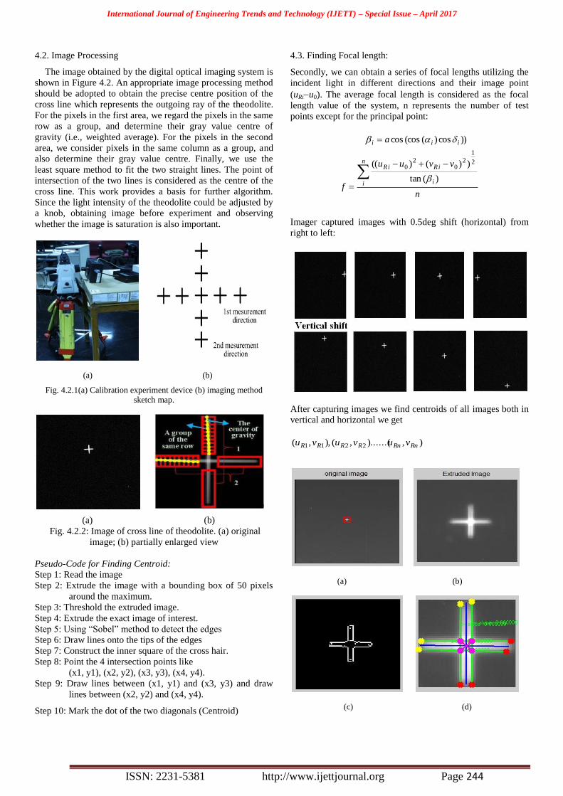
4.2. Image Processing

The image obtained by the digital optical imaging system is

shown in Figure 4.2. An appropriate image processing method

should be adopted to obtain the precise centre position of the

cross line which represents the outgoing ray of the theodolite.

For the pixels in the first area, we regard the pixels in the same

row as a group, and determine their gray value centre of

gravity (i.e., weighted average). For the pixels in the second

area, we consider pixels in the same column as a group, and

also determine their gray value centre. Finally, we use the

least square method to fit the two straight lines. The point of

intersection of the two lines is considered as the centre of the

cross line. This work provides a basis for further algorithm.

Since the light intensity of the theodolite could be adjusted by

a knob, obtaining image before experiment and observing

whether the image is saturation is also important.

(a) (b)

Fig. 4.2.1(a) Calibration experiment device (b) imaging method

sketch map.

(a) (b)

Fig. 4.2.2: Image of cross line of theodolite. (a) original

image; (b) partially enlarged view

Pseudo-Code for Finding Centroid:

Step 1: Read the image

Step 2: Extrude the image with a bounding box of 50 pixels

around the maximum.

Step 3: Threshold the extruded image.

Step 4: Extrude the exact image of interest.

Step 5: Using “Sobel” method to detect the edges

Step 6: Draw lines onto the tips of the edges

Step 7: Construct the inner square of the cross hair.

Step 8: Point the 4 intersection points like

(x1, y1), (x2, y2), (x3, y3), (x4, y4).

Step 9: Draw lines between (x1, y1) and (x3, y3) and draw

lines between (x2, y2) and (x4, y4).

Step 10: Mark the dot of the two diagonals (Centroid)

4.3. Finding Focal length:

Secondly, we can obtain a series of focal lengths utilizing the

incident light in different directions and their image point

(uRiu0). The average focal length is considered as the focal

length value of the system, n represents the number of test

points except for the principal point:

n

vvuu

f

a

n

i i

iRiR

iii

)(tan

))()((

))cos)((coscos

2

1

20

20

Imager captured images with 0.5deg shift (horizontal) from

right to left:

After capturing images we find centroids of all images both in

vertical and horizontal we get

),)......(,(),,( 2211 RnRnRRRR vuvuvu

(a) (b)

(c) (d)



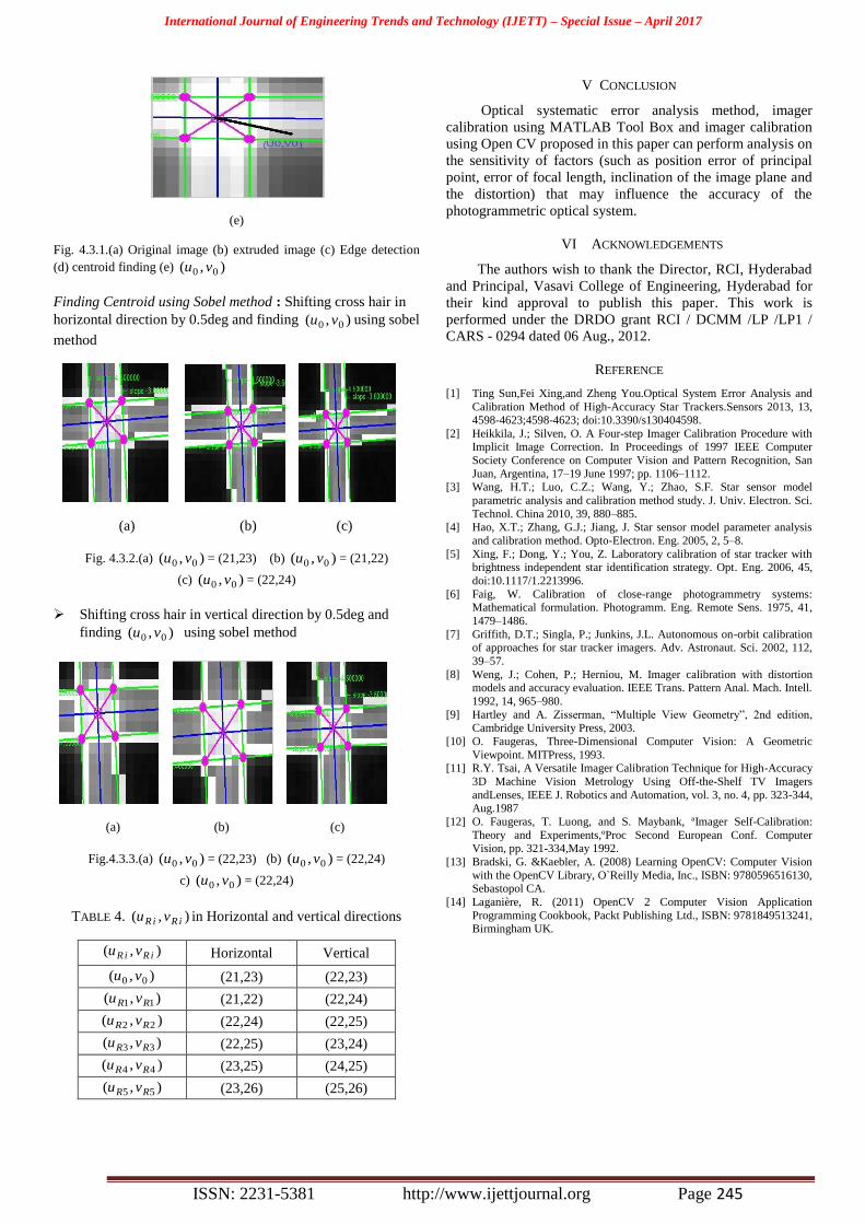
(e)

Fig. 4.3.1.(a) Original image (b) extruded image (c) Edge detection

(d) centroid finding (e) ),( 00 vu

Finding Centroid using Sobel method : Shifting cross hair in

horizontal direction by 0.5deg and finding ),( 00 vu using sobel

method

(a) (b) (c)

Fig. 4.3.2.(a) ),( 00 vu = (21,23) (b) ),( 00 vu = (21,22)

(c) ),( 00 vu = (22,24)

Shifting cross hair in vertical direction by 0.5deg and

finding ),( 00 vu using sobel method

(a) (b) (c)

Fig.4.3.3.(a) ),( 00 vu = (22,23) (b) ),( 00 vu = (22,24)

c) ),( 00 vu = (22,24)

TABLE 4. ),( iRiR vu in Horizontal and vertical directions

),( iRiR vu Horizontal Vertical

),( 00 vu (21,23) (22,23)

),( 11 RR vu (21,22) (22,24)

),( 22 RR vu (22,24) (22,25)

),( 33 RR vu (22,25) (23,24)

),( 44 RR vu (23,25) (24,25)

),( 55 RR vu (23,26) (25,26)

V CONCLUSION

Optical systematic error analysis method, imager

calibration using MATLAB Tool Box and imager calibration

using Open CV proposed in this paper can perform analysis on

the sensitivity of factors (such as position error of principal

point, error of focal length, inclination of the image plane and

the distortion) that may influence the accuracy of the

photogrammetric optical system.

VI ACKNOWLEDGEMENTS

The authors wish to thank the Director, RCI, Hyderabad

and Principal, Vasavi College of Engineering, Hyderabad for

their kind approval to publish this paper. This work is

performed under the DRDO grant RCI / DCMM /LP /LP1 /

CARS - 0294 dated 06 Aug., 2012.

REFERENCE

[1] Ting Sun,Fei Xing,and Zheng You.Optical System Error Analysis and

Calibration Method of High-Accuracy Star Trackers.Sensors 2013, 13, 4598-4623;4598-4623; doi:10.3390/s130404598.

[2] Heikkila, J.; Silven, O. A Four-step Imager Calibration Procedure with Implicit Image Correction. In Proceedings of 1997 IEEE Computer

Society Conference on Computer Vision and Pattern Recognition, San

Juan, Argentina, 17–19 June 1997; pp. 1106–1112. [3] Wang, H.T.; Luo, C.Z.; Wang, Y.; Zhao, S.F. Star sensor model

parametric analysis and calibration method study. J. Univ. Electron. Sci.

Technol. China 2010, 39, 880–885. [4] Hao, X.T.; Zhang, G.J.; Jiang, J. Star sensor model parameter analysis

and calibration method. Opto-Electron. Eng. 2005, 2, 5–8.

[5] Xing, F.; Dong, Y.; You, Z. Laboratory calibration of star tracker with brightness independent star identification strategy. Opt. Eng. 2006, 45,

doi:10.1117/1.2213996.

[6] Faig, W. Calibration of close-range photogrammetry systems: Mathematical formulation. Photogramm. Eng. Remote Sens. 1975, 41,

1479–1486.

[7] Griffith, D.T.; Singla, P.; Junkins, J.L. Autonomous on-orbit calibration of approaches for star tracker imagers. Adv. Astronaut. Sci. 2002, 112,

39–57.

[8] Weng, J.; Cohen, P.; Herniou, M. Imager calibration with distortion models and accuracy evaluation. IEEE Trans. Pattern Anal. Mach. Intell.

1992, 14, 965–980.

[9] Hartley and A. Zisserman, “Multiple View Geometry”, 2nd edition, Cambridge University Press, 2003.

[10] O. Faugeras, Three-Dimensional Computer Vision: A Geometric

Viewpoint. MITPress, 1993. [11] R.Y. Tsai, A Versatile Imager Calibration Technique for High-Accuracy

3D Machine Vision Metrology Using Off-the-Shelf TV Imagers

andLenses, IEEE J. Robotics and Automation, vol. 3, no. 4, pp. 323-344, Aug.1987

[12] O. Faugeras, T. Luong, and S. Maybank, ªImager Self-Calibration:

Theory and Experiments,ºProc Second European Conf. Computer Vision, pp. 321-334,May 1992.

[13] Bradski, G. &Kaebler, A. (2008) Learning OpenCV: Computer Vision

with the OpenCV Library, O`Reilly Media, Inc., ISBN: 9780596516130, Sebastopol CA.

[14] Laganière, R. (2011) OpenCV 2 Computer Vision Application

Programming Cookbook, Packt Publishing Ltd., ISBN: 9781849513241, Birmingham UK.

Documents

Performance Calibration of Photogrammetic … issue/NCEITCS-2017/NCEITCS-143.pdfPerformance Calibration of Photogrammetic Optical Systems ... experiment results are presented that