Embed Size (px)
Citation preview

FFl—rapport 2010/02383
Performance analysis of the proposed new restoring camera
for hyperspectral imaging
Gudrun Høye (FFI) and Andrei Fridman (NEO)
Norwegian Defence Research Establishment (FFI)
26 November 2010

2 FFI-rapport 2010/02383
FFI-rapport 2010/02383
1142
Keywords
Hyperspektral avbildning
Hyperspektralt kamera
Keystone korreksjon
Resampling
Bildebehandling
Optisk design
Avbildende spektrometri
Approved by
Svein Erik Hamran Project Manager
Stian Løvold Director of Research
Johnny Bardal Director

FFI-rapport 2010/02383 3
English summary This report investigates the performance of the proposed new restoring camera for hyperspectral imaging. The suggested camera will eliminate keystone in the postprocessing of the data with no resolution loss and will be able to collect several times more light than current hyperspectral cameras with hardware corrected keystone. A virtual camera is created in Matlab for the analyses, and data from a real hyperspectral image is used as input. The performance of the restoring camera is compared to the conventional hyperspectral cameras, that either correct keystone in hardware or apply resampling to the collected data. The analyses show that the restoring camera outperforms by far the conventional cameras under all light conditions. Conventional cameras have misregistration errors as large as 15-20%, and these errors remain even if the amount of light increases. The restoring camera, on the other hand, has negligible misregistration errors and is limited only by photon noise. This camera therefore performs better and better as the amount of light increases. In very bright light, the standard deviation of the error for the restoring camera (compared to an ideal camera) is only 0.6% and the maximum error less than 2%. The optical design for the restoring camera is included in the report. The optics is as sharp as the best conventional designs and collects four times more light. The camera must be calibrated very precisely and a method for doing so is described in the report. We have also looked briefly into the potential of resampling cameras. Resampling cameras are generally believed to be significantly worse than cameras with hardware corrected keystone. However, our analyses show that resampling cameras can compete quite well with such cameras. In particular, a resampling camera that uses a high-resolution sensor combined with binning of pixels is shown to make an excellent camera for low light applications. The performance will, however, still be noticeably worse than what can be achieved with the suggested restoring camera. We propose a joint FFI-NEO project with the goal of building the new restoring camera. The project would benefit from NEO’s expertise in design of hyperspectral cameras and FFI’s expertise in processing of hyperspectral data. Key issues to be addressed would be verification of the performance of the mixing chambers, and development and implementation of the calibration method for the camera. The outcome of the project would be a rather impressive instrument which will by far outperform the current generation of hyperspectral cameras.

4 FFI-rapport 2010/02383
Sammendrag I denne rapporten undersøker vi ytelsen til det foreslåtte nye mikselkameraet for hyperspektral avbildning. Kameraet vil eliminere keystone i etterprosesseringen av dataene uten tap av oppløsning og vil ha en optikk som er flere ganger så lyssterk som dagens hyperspektrale kameraer hvor keystone korrigeres i hardware. Vi har laget et virtuelt kamera i Matlab der data fra et ekte hyperspektralt bilde brukes som input for analysene. Mikselkameraets ytelse er sammenliknet med de konvensjonelle hyperspektrale kameraene som enten korrigerer keystone i hardware eller resampler dataene. Våre analyser viser at mikselkameraet har en vesentlig bedre ytelse enn de konvensjonelle kameraene under alle lysforhold. For konvensjonelle kameraer kan feilregistreringen være så stor som 15-20%, og denne feilen forsvinner ikke selv om lysmengden øker. Mikselkameraet på den annen side, har neglisjerbar feilregistrering og ytelsen er kun begrenset av fotonstøyen. Dette kameraet presterer derfor bare bedre og bedre når lysmengden øker. I svært sterkt lys blir standardavviket til feilen (sammenliknet med et ideelt kamera) så lavt som 0.6% og maksimumfeilen mindre enn 2%. Rapporten inkluderer et forslag til optisk design for mikselkameraet. Denne optikken er like skarp som i de beste konvensjonelle designene og fire ganger så lyssterk. Kameraet må kalibreres svært nøyaktig og en metode for å gjøre dette er beskrevet i rapporten. Vi har også undersøkt hvilke muligheter som ligger i å benytte resamplingskameraer. Det ser ut til å være en utbredt oppfatning at disse kameraene har vesentlig dårligere ytelse enn de kameraene som korrigerer keystone i hardware. Våre analyser viser imidlertid at resamplingskameraer konkurrerer godt med sistnevnte type kameraer. Spesielt viser analysene at et resamplingskamera som benytter en sensor med høy oppløsning og slår sammen piksler, vil være et utmerket kamera for applikasjoner med lite lys. Ytelsen vil imidlertid fremdeles være vesentlig dårligere enn hva det foreslåtte mikselkameraet vil kunne prestere. Vi foreslår å opprette et felles FFI-NEO prosjekt med det formål å lage det nye mikselkameraet. Prosjektet vil dra nytte av NEOs ekspertise innenfor design av hyperspektrale kameraer og FFIs ekspertise innenfor prosessering av hyperspektrale data. Viktige momenter å se på i den videre prosessen er verifisering av blandekamrenes ytelse, og utvikling og implementering av kalibreringsmetoden for kameraet. Resultatet av prosjektet vil være et hyperspektralt kamera som har vesentlig forbedret ytelse sammenlignet med dagens kameraer.

FFI-rapport 2010/02383 5
Contents
Preface 7
1 Introduction 9
2 Approach 10
3 How are the simulations performed? 113.1 The mixing chambers 13
3.2 Photon noise 15
3.3 Readout noise 16
4 Results 184.1 Resampling camera vs HW corrected camera – misregistration error 20
4.2 Resampling camera vs HW corrected camera – photon and readout noise
included 22
4.3 Resampling camera with binning 24
4.4 Resampling camera with binning vs HW corrected camera with binning 26
4.5 Resampling camera with binning vs HW corrected camera with binning
– low light 28
4.6 Restoring camera vs HW corrected camera and resampling camera
– misregistration error 30
4.7 Restoring camera vs HW corrected camera and resampling camera
– photon and readout noise included 32
4.8 HW corrected camera – three different keystone values 34
4.9 Restoring camera vs HW corrected camera – bright light 36
4.10 Restoring camera with transitions 38
4.11 Summary 42
5 Optical design 43
6 Camera calibration 506.1 Errors due to misalignment between mixels and sensor pixels 50
6.2 Calibration 52
7 What is next? 55
8 Conclusion 56

6 FFI-rapport 2010/02383
Appendix A Different input signals 57
Appendix B Resampling with high-resolution cubic splines vs bilinear resampling 62
Appendix C Third order polynomial transitions 66
Appendix D Virtual camera software 68D.1 HW corrected camera (example) 72
D.2 Resampling camera (example) 73
D.3 Restoring camera (example) 74
References 76

FFI-rapport 2010/02383 7
Preface As a result of cooperation between Forsvarets forskningsinstitutt (FFI) and Norsk Elektro Optikk AS (NEO) a new concept for hyperspectral imaging has emerged. Preliminary analyses showed that the concept has the potential to improve the quality of hyperspectral data substantially. Based on this, it was decided to continue the joint work and to analyse the performance of the new camera more thoroughly. The results from these analyses, including a suggestion for the optical design for the camera, are presented in this report.

8 FFI-rapport 2010/02383
FFI-rapport 2010/02383 9
1 Introduction Hyperspectral cameras are increasingly used for various military, scientific, and commercial purposes. Users constantly demand better optical resolution and higher light sensitivity. However, the current generation of instruments already has extremely tight tolerances for optical aberrations compared to other imaging systems. For this reason, the development of hyperspectral cameras has more or less converged to a couple of standard layouts, each of them with some inherent limitations such as minimum possible F-number, maximum possible spatial resolution, etc. In a previous report [1] we suggested a new concept for hyperspectral imaging that has the potential to improve the quality of hyperspectral data substantially. Unlike conventional resampling, the proposed method does not introduce any loss of resolution, and any keystone in the system is eliminated in the postprocessing of the data. The strict keystone requirements that severely limits the design of current hyperspectral cameras with hardware corrected keystone, therefore do not apply to a camera based on the new concept. This opens up the possibility of designing a camera that collects several times more light than the conventional cameras with hardware corrected keystone. In this report we investigate the performance of a camera based on the proposed concept. This is done through simulations and comparison with the performance of conventional cameras (Chapters 3 and 4). We also suggest an optical design for the new camera, that is as sharp as the best conventional designs and collects four times more light (Chapter 5). We also outline a method for calibrating the camera to the necessary accuracy (Chapter 6). Suggestions for further work and key issues to be addressed are given in Chapter 7. Finally, the conclusions from our analyses are presented in Chapter 8.

10 FFI-rapport 2010/02383
2 Approach Before building a camera based on the proposed concept [1], we would like to have an idea how much such a camera could outperform conventional instruments. We will therefore compare the new camera’s performance to that of currently used cameras, which either correct keystone in hardware or apply resampling to the recorded data. The quality of hyperspectral data depends not only on the specifications of the camera used, but also on the content of the scene being captured by the camera. The new camera should therefore be tested on data that resembles as closely as possible the data that it will be collecting in real life. Since the proposed camera has never been built, we will use simulations to test its performance. We will create a virtual camera in Matlab (see Appendix D for a description of the program), which can be used to simulate both the new camera and the conventional ones. We will use the hyperspectral data of a real scene (captured by a real hyperspectral camera) as the scene to be captured and run this data through the virtual camera. The virtual camera will distort the data somewhat in accordance with the modelled optical distortions, sensor characteristics, and photon noise. Then, by comparing the data at the output of the virtual camera with the data at the input, we will be able to evaluate the quality of the camera. For example, we can check what is more important: lower photon noise or lower keystone. Because in the end we are not interested in low keystone or low photon noise. What we are really interested in is how close the captured data is to the real scene, or perhaps even more importantly, whether the quality of the data will allow us to detect and identify the objects of interest in real world scenes.

FFI-rapport 2010/02383 11
3 How are the simulations performed? A hyperspectral data set containing 1600 spatial pixels (originally captured by HySpex VNIR1600 hyperspectral camera) forms the scene to be captured by the virtual camera. The virtual camera is set to have significantly lower resolution (320 pixels) than the resolution of the scene. By doing this we simulate the fact that any real scene contains smaller details than the resolution of the camera being tested. Figure 3.1 shows the number of photons in the signal from the scene (cyan) for one spectral band. The corresponding scene pixel values are shown in red. The signal contains several large peaks as well as broader areas with only small variations in the signal strength. The performance of our virtual cameras can therefore be evaluated with respect to both these cases. Further, the number of pixels is large enough that some conclusions can be drawn based on statistics.
Figure 3.1 The scene.
In this report we will investigate the performance of three different types of cameras:
1) Camera with hardware corrected keystone (HW corrected camera) 2) Camera that uses resampling (resampling camera) 3) Camera based on the new consept with restoring (restoring camera)
We will now describe how the simulations are performed for each of these three cameras.
The HW corrected camera is simulated by shifting the scene pixels to the left relative to the sensor pixels by an amount equal to the maximum residual keystone. This is in a way
1) HW corrected camera:
the worst case scenario, since a real camera will never have so large keystone in every spatial pixel in every spectral band. However, this assumption ensures that we will be able to examine the effect of having maximum residual keystone also in the most difficult areas of the image, where adjacent pixels are significantly different from each other.

12 FFI-rapport 2010/02383
Hyperspectral cameras for the visible range currently produced by Norsk Elektro Optikk AS (Norway) have F-number 2.5 and are designed to have a keystone not larger than 0.1 pixel. These cameras are among the best in the world and will be used as our reference for a HW corrected camera throughout the simulations.
For our virtual resampling camera we assume a keystone of 32 pixels, i.e., the content of the 320 scene pixels is spread over 352 pixels when recorded onto the sensor. The keystone is assumed to be linear across the image, changing from zero on the left side of the image to 32 pixels on the right side. The recorded pixels are then resampled onto the scene pixel grid to give the final data. The resampling method used is high-resolution cubic splines
2) Resampling camera:
[3], which gives noticeably better results than the commonly used bilinear resampling (see Appendix A for a comparison of the two methods).
For our virtual restoring camera we also assume a keystone of 32 pixels. The data are restored using the method described in
3) Restoring camera:
[1]. For the method to work, light mixing chambers must be inserted into the slit. The light propagation through the chambers is modelled with geometric raytracing. See Section 3.1 for a description of the mixing chambers. Photon and readout noise are included in the calculations and will be described in more detail in Sections 3.2 and 3.3. The readout noise depends on the choice of sensor. One of the best upcoming sensors, which we will use as a reference, has the following preliminary specifications: full-well is 30 000 electrons and the readout noise in the global shutter mode is 2 2 electrons (rms). For a HW corrected camera we expect to bin two pixels in the spectral direction, which gives a full-well of 60 000 electrons. For a resampling or restoring camera we expect to bin three pixels in the spectral direction, which gives a full-well of 90 000 electrons. We see that the input signal (Figure 3.1) is well below saturation for all three cameras. For the calculations, we will assume that the quantum efficiency is 100% , i.e., when 1 photon is hitting the sensor 1 electron-hole pair is being generated. When evaluating the performance of the cameras, we calculate the error in the final data relative to the input. The relative error, dE , is given by
( )final init
init
E EdE
E−
= (3.1)
where initE is the scene pixel value and finalE is the calculated value of the same pixel after the
signal has been processed by the camera. We can then find the standard deviation of dE over the 320 pixels and we can also determine the maximum relative error. Both are important parameters when evaluating the performance of the cameras, as we will see when discussing the results in Chapter 4.

FFI-rapport 2010/02383 13
3.1 The mixing chambers
The mixing chambers are required in order to use the method described in [1] to restore the data. The purpose of the mixing chambers is to mix the light that goes through each chamber as evenly as possible. The chambers are inserted into the slit and the light content of each chamber corresponds to the light content of a scene pixel. The projection of a scene pixel onto the slit will hereafter be referred to as a ’mixel’. The light content of a mixel will then be equal to the light content of the corresponding chamber. Since there are fewer mixels than sensor pixels and the light distribution inside each mixel is known, it will be possible to restore the exact energy of each mixel based on the recorded sensor pixel values. Figure 3.2 shows an example of how the mixing chambers may look (only a few chambers are shown).
Figure 3.2 The mixing chambers. This picture is for illustration purposes only. The dimensions of the real mixing chambers will depend on the sensor pixel size and the optics, and are given in Chapter 5.
Geometric raytracing is used to model how the mixing chambers work. Many rays (a few hundred) are launched from five areas of the front face in each mixing chamber. The intensity of the rays corresponds to the illumination of the corresponding area of the front face. It is assumed that the walls of the chambers are infinitely thin1
and 100% reflective.
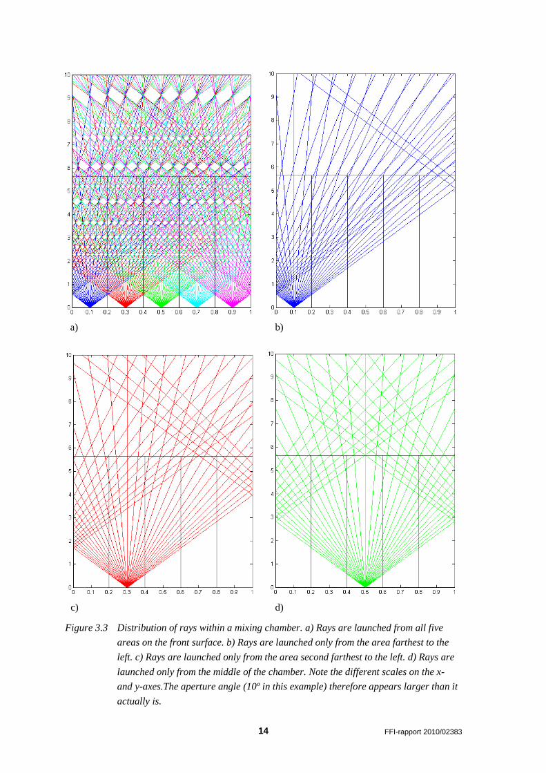
Figure 3.3 shows how the rays are distributed inside one chamber (fewer rays are shown than what is used in the calculations). The horizontal black line shows the back face of the chamber. We see from Figure 3.3a) that at certain distances from the front face of the chamber the rays are not evenly distributed at all (appearing as ‘holes’ in the figure). Choosing the right length for the chamber is therefore crucial to obtain the best possible performance. The length (L) of the mixing chambers can be written as: L k F w= ⋅ ⋅ (3.2)
1 In reality, the chamber walls will be very much thinner than the resolution limit of the optics, and they are therefore not expected to affect the restoring process.
14 FFI-rapport 2010/02383
a) b)
c) d)
Figure 3.3 Distribution of rays within a mixing chamber. a) Rays are launched from all five areas on the front surface. b) Rays are launched only from the area farthest to the left. c) Rays are launched only from the area second farthest to the left. d) Rays are launched only from the middle of the chamber. Note the different scales on the x- and y-axes.The aperture angle (10º in this example) therefore appears larger than it actually is.

FFI-rapport 2010/02383 15
where w is the width of the chamber, F is the F-number of the foreoptics, and k is a constant that is chosen in such a way that the back face of each chamber has as even illumination as possible. We have used the value k=2 in our simulations, which gives a very even light distribution while at the same time keeping the number of reflections as low as possible (half of the rays are reflected once, while the rest of the rays pass through the chamber without being reflected). The length of the chamber shown in Figure 3.3 corresponds to this value of k. Figure 3.3b)-d) show the distribution of light when the rays are launched from a single area at the front face of the chamber, simulating that light is coming only to one part of the chamber. We see that even in these extreme cases the rays are mixed well. Figure 3.4 shows the performance of the mixing chambers for a part of the input signal (pixels #244-#253) from Figure 3.1. We see that even a very uneven light distribution (cyan) at the front face of the chamber corresponding to mixel #249, results in an almost completely even light distribution (red) at the back face of the chamber.
Figure 3.4 Performance of the mixing chambers.
3.2 Photon noise
The photon noise follows a poisson distribution with mean E and standard deviation E , where E is the number of photons in the signal [7]. The resulting relative error dE in the signal E due to photon noise has zero mean value and standard deviation
1phdE E
σ = (3.3)
Figure 3.5a) shows the relative error in the input signal in Figure 3.1 due to photon noise. Figure 3.5b) shows the same when the signal is amplified four times. The relative error due to photon noise decreases when the signal increases; when the signal is amplified by a factor 2 the error decreases with a factor 2 . This can be seen directly from Equation (3.3) or its graphic representation in Figure 3.6 which shows the relative error (1 ph
dEσ ) as a function of number of
photons in the signal.

16 FFI-rapport 2010/02383
a)
b)
Figure 3.5 Examples of relative error due to photon noise for a) the input signal in Figure 3.1 and b) four times that signal.
Figure 3.6 Relative error (1 phdEσ ) due to photon noise as a function of the number of photons in
the signal.
3.3 Readout noise
The readout noise follows a gaussian distribution with zero mean value and standard deviation roσ [7]. The resulting relative error dE in the signal E due to readout noise has zero mean
value and standard deviation
ro rodE E
σσ = (3.4)

FFI-rapport 2010/02383 17
The sensor we assume for our virtual cameras has readout noise per pixel with standard deviation 2 2roσ = electrons. For a HW corrected camera we expect to bin two pixels in the spectral
direction, which gives a standard deviation of 2 2 2 4HWroσ = ⋅ = electrons in the final binned
data. For a resampling or restoring camera we expect to bin three pixels in the spectral direction, which gives a standard deviation of 2 2 3 5R
roσ = ⋅ ≈ electrons in the final binned data.
Figure 3.7 shows the relative error in the input signal in Figure 3.1 due to readout noise with standard deviation roσ =5 electrons. We see that the readout noise is very small compared to the
signal.
Figure 3.7 Example of relative error due to readout noise for the input signal in Figure 3.1.
Figure 3.8 shows the relative error (1 dEσ ) due to photon noise (blue curve) and readout noise
(green curve) as a function of the number of photons in the signal. We see that the photon noise dominates when there are more than 25 photons in the signal. Only for very low light, when there are less than 25 photons in the signal, will the readout noise dominate. In our simulations the number of photons in the signal is always much larger than 25, and the readout error will therefore be negligible compared to the photon noise.
Figure 3.8 Relative error (1 dEσ ) due to photon noise (blue curve) and readout noise (green
curve) as a function of the number of photons in the signal.
18 FFI-rapport 2010/02383
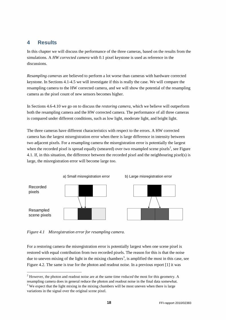
4 Results In this chapter we will discuss the performance of the three cameras, based on the results from the simulations. A HW corrected camera with 0.1 pixel keystone is used as reference in the discussions. Resampling cameras are believed to perform a lot worse than cameras with hardware corrected keystone. In Sections 4.1-4.5 we will investigate if this is really the case. We will compare the resampling camera to the HW corrected camera, and we will show the potential of the resampling camera as the pixel count of new sensors becomes higher. In Sections 4.6-4.10 we go on to discuss the restoring camera, which we believe will outperform both the resampling camera and the HW corrected camera. The performance of all three cameras is compared under different conditions, such as low light, moderate light, and bright light. The three cameras have different characteristics with respect to the errors. A HW corrected camera has the largest misregistration error when there is large difference in intensity between two adjacent pixels. For a resampling camera the misregistration error is potentially the largest when the recorded pixel is spread equally (smeared) over two resampled scene pixels2 Figure 4.1
, see . If, in this situation, the difference between the recorded pixel and the neighbouring pixel(s) is
large, the misregistration error will become large too.
Recordedpixels
Resampledscene pixels
a) Small misregistration error b) Large misregistration error
Figure 4.1 Misregistration error for resampling camera.
For a restoring camera the misregistration error is potentially largest when one scene pixel is restored with equal contribution from two recorded pixels. The reason for this is that the noise due to uneven mixing of the light in the mixing chambers3
Figure 4.2, is amplified the most in this case, see
. The same is true for the photon and readout noise. In a previous report [1] it was
2 However, the photon and readout noise are at the same time reduced the most for this geometry. A resampling camera does in general reduce the photon and readout noise in the final data somewhat. 3 We expect that the light mixing in the mixing chambers will be most uneven when there is large variations in the signal over the original scene pixel.

FFI-rapport 2010/02383 19
shown that in general the restoring camera increases the noise in the system somewhat (typically by a factor ~1.4).
Recordedpixels
Restoredscene pixels
a) Almost no amplification of noise b) Amplification of noise
> σ
σ σσ
~ σ
σσ σ σ
Figure 4.2 Amplification of noise in a restoring camera. Light pink colour indicates noise with standard deviation σ in the recorded pixels. For the geometry to the left (a) there is almost no increase in noise level during the restoring process. For the geometry to the right (b) there is a noticeable increase in noise level during the restoring of the data.
The results in this chapter are presented as graphs that show the relative error in hyperspectral data after the signal has been processed by the virtual cameras. Photon and readout noise are included in many of the graphs and since this noise is random, the relative error will vary slightly (for the same case) from one simulation to the next. This should be kept in mind when discussing the graphs. The simulations are based on the input signal shown in Figure 3.1. This is believed to represent a typical input signal for the cameras. Naturally, the performance of the cameras may vary for different input signals. However, we believe that the main conclusions drawn in this chapter will be valid also for other input signals. In Appendix A we have investigated briefly the performance of the same cameras for two other input signals. The results show that the performance of the three cameras relative to each other (which is the main focus of our report) is similar for different input signals.

20 FFI-rapport 2010/02383
4.1 Resampling camera vs HW corrected camera – misregistration error
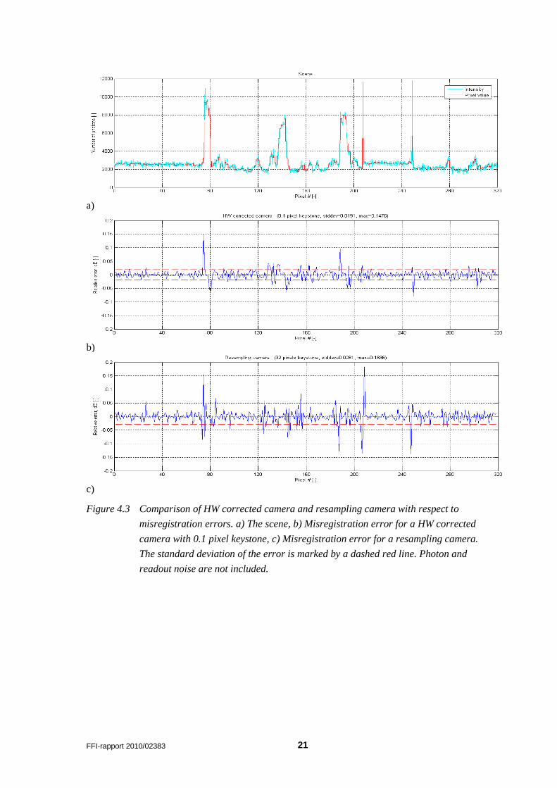
In order to examine the performance of the proposed resoring camera [1] later in this chapter, let us first take a look at the performance of the conventional systems: those where the keystone is corrected in hardware, and those where a relatively large keystone is handled by resampling. We will first look at the error caused by misregistration alone, i.e., when photon and readout noise are not taken into account. Figure 4.3a) shows the input signal (cyan), and how this signal would be recorded by an ideal camera which would simply average the signal inside each pixel (red).
Figure 4.3b) shows the misregistration error for a HW corrected camera with 0.1 pixel keystone. The graph shows random looking errors (standard deviation 1.9%) with distinct peaks up to 15% in the areas with large differences between adjacent pixels. Figure 4.3c) shows the misregistration error in a resampling camera with 32 pixels keystone. The misregistration error for this camera is somewhat larger (standard deviation 2.8%) than for the HW corrected camera. The peaks are higher too - up to about 18%. As already mentioned, the largest possible misregistration error in a resampling camera occurs when a recorded pixel that is very different from its neighbour(s) is distributed equally between two resampled scene pixels. This means that in order to examine the performance of a resampling camera properly, we have to make sure that difficult areas of the image (the areas with high contrast) end up in a part of the sensor where the most smearing will occur during resampling. Luckily, the examined image (Figure 4.3a) has a very sharp brightness change between pixels #75 and #76. And these pixels are situated in on of the areas of the sensor, which is going to be smeared the most during resampling. As expected, there is a quite large error peak in the resampled image here (pixel #75), see Figure 4.3c). So, it looks like we managed to put the resampling camera in the situation where large misregistration errors will occur. On the other hand, the border between pixels #80 and #81 (Figure 4.3a) is recorded in an area of the sensor which is smeared very little during resampling, and as we can see the error here is very small (Figure 4.3c) 4
.
We conclude that with respect to misregistration errors alone, the resampling camera performs somewhat worse than the HW corrected camera. However, the difference in performance is not as large as is generally believed.
4 Note also the two very large error peaks in pixels #208 and #209 in the resampled image (Figure 4.3c), which are not visible in the image from the HW corrected camera (Figure 4.3b). The reason is that a very small area in the middle of pixel #208 in the input signal (Figure 4.3a) has very high brightness compared to the surroundings. For the HW corrected camera, where the pixel is shifted by 10% of its length (0.1 pixel keystone), the brightness of pixels #207, #208, and #209 does not change much since the bright area is still within the same pixel: #207 is still dark, #208 is still bright, #209 is still dark. However, for the resampling camera the bright area is distributed over two pixels in the final image, creating a quite large misregistration error.
FFI-rapport 2010/02383 21
a)
b)
c)
Figure 4.3 Comparison of HW corrected camera and resampling camera with respect to misregistration errors. a) The scene, b) Misregistration error for a HW corrected camera with 0.1 pixel keystone, c) Misregistration error for a resampling camera. The standard deviation of the error is marked by a dashed red line. Photon and readout noise are not included.

22 FFI-rapport 2010/02383
4.2 Resampling camera vs HW corrected camera – photon and readout noise included
Let us now look at what happens when photon and readout noise are included. Figure 4.4a) shows the results for the HW corrected camera. The standard deviation of the relative error has increased from 1.9% to 2.8%, but the peaks are similar to before. It looks like the photon and readout noise are not able to completely mask the misregistration errors at this signal level. Figure 4.4b) shows the results for the resampling camera. The standard deviation for the relative error has increased from 2.8% to 3.3%, but also here the peaks are similar to before. The HW corrected camera still looks somewhat better than the resampling camera, but the difference is less now that photon and readout noise are included. Of course, since keystone correction is not required from the optical system of the resampling camera, it will be able to collect much more light and may benefit from having significantly lower photon noise relative to the signal than the HW corrected camera. Figure 4.4c) shows the relative error for a resampling camera that collects four times more light. The standard deviation for the relative error has decreased from 3.3% to 2.9% and is now very similar to the standard deviation for the HW corrected camera (2.8%). However, the peaks are still as large as before. We conclude that a resampling camera can compete quite well with a HW corrected camera, since it can collect four times more light, thereby decreasing the influence of photon noise. Another interesting thing about the performance of the resampling camera which is worth mentioning here, is the fact that the error is large only in a few small areas where there are two adjacent pixels with large difference in brightness. It is possible that by processing these places in a way suggested in a previous report [2] the performance of the resampling camera can be significantly improved in terms of the peak error.

FFI-rapport 2010/02383 23
a)
b)
c)
Figure 4.4 Comparison of HW corrected camera and resampling camera when photon and readout noise are included. The figures show the relative error for a) a HW corrected camera with 0.1 pixel keystone, b) a resampling camera, c) a resampling camera collecting four times more light. The standard deviation of the error is marked by a dashed red line.

24 FFI-rapport 2010/02383
4.3 Resampling camera with binning
Probably, a good way to use resampling is to accept some resolution loss, i.e., to bin two or more pixels in the spatial direction. Figure 4.5 shows how the error caused by misregistration alone (photon and readout noise are not taken into account) is decreasing when pixels are being binned. Figure 4.5a) shows the misregistration error in the resampling system at full resolution, i.e., when there is no pixel binning. If we sacrifice half of the resolution and bin two pixels in the spatial direction (Figure 4.5b), then the result looks a lot nicer. The misregistration error is now actually smaller than for the HW corrected camera (Figure 4.3b) with standard deviation 1.2% versus 1.9% and peaks up to 9% versus 15%. And things will get even better if we bin three pixels instead of two (Figure 4.5c). The misregistration error is now very small (standard deviation 1.1% and peaks up to 6%) compared to the HW corrected camera (Figure 4.3b).

FFI-rapport 2010/02383 25
a)
b)
c)
Figure 4.5 Resampling camera with binning. The figures show the misregistration error for a resampling camera with a) original resolution, b) bin factor 2, c) bin factor 3. The standard deviation of the error is marked by a dashed red line. Photon and readout noise are not included.

26 FFI-rapport 2010/02383
4.4 Resampling camera with binning vs HW corrected camera with binning
Let us include photon and readout noise in the calculations and compare the resampling camera with bin factor 2 (i.e., when two pixels are binned in the spatial direction) with the HW corrected camera. Figure 4.6a) shows the HW corrected camera at full resolution and Figure 4.6c) shows the resampling camera with bin factor 2 and four times more light. We see that when photon and readout noise are taken into account, the resampling camera with bin factor 2 performs very much better than the HW corrected system with standard deviation 1.5% versus 2.8% and peaks up to 9% versus 16%. Perhaps it is a bit unfair to compare a high resolution HW corrected camera and a low resolution resampling camera, and to claim that the latter is superior due to lower misregistration error. For comparison, we will bin pixels in the spatial direction for the HW corrected camera, too. Figure 4.6b) shows the performance of the HW corrected camera with bin factor 2. As expected, the errors decrease also for the HW corrected camera when pixels are being binned (standard deviation 2.0% versus 2.8% and peaks up to 8% versus 16%). However, the resampling camera with bin factor 2 still performs better. Even though the resampling system with bin factor 2 is comparable to the HW corrected system with bin factor 2 in terms of maximum relative error (9% versus 8%), the performance of the resampling system is noticeably better if the criterion is the standard deviation of the error (1.5% versus 2.0%). It is not very surprising since the resampling system in this example collects four times more light than the HW corrected camera. The contribution from the photon noise is therefore much less for the resampling camera.

FFI-rapport 2010/02383 27
a)
b)
c)
Figure 4.6 Comparison of HW corrected camera with binning and resampling camera with binning. The figures show the relative error for a) a HW corrected camera with original resolution, b) a HW corrected camera with bin factor 2, c) a resampling camera with bin factor 2 and four times more light. The standard deviation of the error is marked by a dashed red line. Photon and readout noise are included.

28 FFI-rapport 2010/02383
4.5 Resampling camera with binning vs HW corrected camera with binning – low light
The advantage of the resampling camera with bin factor 2 over the HW corrected camera with the same bin factor will further increase in low light situations. Figure 4.7a) shows a poorly lit scene (the signal is ten times weaker than the one which was used for all the previous graphs). Here the advantage of the resampling camera with bin factor 2 and four times more light (Figure 4.7c) over the HW corrected camera with the same bin factor (Figure 4.7b) is very clear: both the peak error (9% versus 18%) and the standard deviation of the error (2.5% versus 5.3%) are significantly lower for the resampling system. This shows that removing the traditional stringent requirements for accurate keystone correction in hardware, and instead resampling the data from a high resolution sensor, makes it possible to create an excellent camera for low light applications.

FFI-rapport 2010/02383 29
a)
b)
c)
Figure 4.7 Comparison of HW corrected camera with binning and resampling camera with binning in low light. a) The scene (low light), b) Relative error in low light for a HW corrected camera with bin factor 2, c) Relative error in low light for a resampling camera with bin factor 2 and four times more light. The standard deviation of the error is marked by a dashed red line. Photon and readout noise are included.

30 FFI-rapport 2010/02383
4.6 Restoring camera vs HW corrected camera and resampling camera – misregistration error
So, we can have either a camera with relatively slow optics and keystone corrected in hardware (not perfectly though), or we can decide to give up any degree of keystone correction and get a camera with very much faster optics but larger misregistration errors which occur after resampling the data to the correct grid. It would have been great to combine the advantages of these two solutions. And there is a way to do that. A method of keystone correction by resizing all spectral bands to the same grid is described and explained in [1]. Probably, an even better expression for it would be ‘keystone elimination’. The method eliminates keystone to a much higher degree than HW corrected cameras. At the same time the original spatial resolution is preserved (to be exact, sensor pixel count should be 5-10% higher than the required resolution). The proposed new restoring camera is based on this method. Since it will not be necessary to correct keystone in hardware, this camera can also collect at least four times more light (see Chapter 5 for suggestion for the optical design), just like the resampling camera. We will now compare the error caused by misregistration alone (i.e., photon and readout noise are not taken into account) for all three cameras. This was already done in Section 4.1 for the HW corrected camera and the resampling camera, but we will include the same graphs here for comparison when discussing the restoring camera. Figure 4.8a) shows the input signal (cyan), and how this signal would be recorded by an ideal camera which would simply average the signal inside each pixel (red). Figure 4.8b) shows the misregistration error for the HW corrected camera with 0.1 pixel residual keystone, and Figure 4.8c) shows the misregistration error for the resampling system. Now there is something new. Figure 4.8d) shows the misregistration error for a restoring camera. Compared to the results for the HW corrected camera and the resampling camera, this result looks incredibly good. The misregistration error is practically zero (standard deviation 0.07% and peaks up to 0.6%). The very small error that is present is due to the fact that the mixing chambers do not mix the light perfectly (the light mixing is calculated by use of the ray propagation model in Chapter 3.1). The preliminary evaluation in [1] showed that the restoring process amplifies noise somewhat, so in the next section we will investigate what happens when photon and readout noise are present in the system.

FFI-rapport 2010/02383 31
a)
b)
c)
d)
Figure 4.8 Comparison of HW corrected camera, resampling camera and restoring camera with respect to misregistration errors. a) The scene, b) Misregistration errors for a HW corrected camera, c) Misregistration errors for a resampling camera, d) Misregistration errors for a restoring camera. The standard deviation of the error is marked by a dashed red line. Photon and readout noise are not included.

32 FFI-rapport 2010/02383
4.7 Restoring camera vs HW corrected camera and resampling camera – photon and readout noise included
We will now discuss the performance of the three cameras when photon and readout noise are included. Figure 4.9a) and b) show the results for the HW corrected camera and the resampling camera respectively. Both cameras perform worse when photon and readout noise are included, with large error peaks that are caused by misregistration clearly visible above the photon noise (see Section 4.2 for detailed discussion). Figure 4.9c) shows the results for the restoring camera. We see that the restoring camera has similar performance to the HW corrected camera (standard deviation 2.7% versus 2.8% and peaks up to 13% versus 16%). We expected the errors to be larger for the restoring camera due to noise amplification. However, the almost complete absence of misregistration errors seems to outweigh the effect of noise amplification. But... Isn't the restoring camera capable of collecting four times more light than the camera with HW corrected keystone5
Figure 4.9? Yes, it is. And when the restoring system is getting so much more light,
the difference in performance to the competing systems becomes quite dramatic. d) shows the relative error for the restoring camera which now collects four times more light. The difference in performance when compared to the HW corrected camera is very visible: standard deviation 1.4% versus 2.8% and peaks up to 5% versus 16%! Unlike the graph for the HW corrected system (Figure 4.9a), the graph of the relative error for the restoring system (Figure 4.9d) does not contain any noticeable peaks. The misregistration error in the latter system is virtually zero, as has already been shown in the Figure 4.8d), and the performance of the restoring camera is therefore limited only by photon noise. More light – better performance, and no peaks in the areas with large differences between adjacent pixels. The resampling camera can, of course, also collect four times more light, and as we saw in Section 4.2 (Figure 4.4c) it then performs almost as well as the HW corrected camera. However, both these cameras look almost equally bad compared to the restoring camera. Resampling is often seen as unacceptable from users point of view because the data quality is believed to be too poor (!) compared to HW corrected systems with 0.1 pixel keystone. Using the same logic, we can now state that, based on the simulations, it is unacceptable to use a HW corrected camera because the data quality is too poor compared to a restoring camera!
5 This is assuming that there are no losses in the mixing chambers. F-number F1.25 in the optics (Chapter 5) was achieved by using spherical surfaces only. We believe that small losses in the mixing chambers can be compensated for by decreasing the F-number slightly (for example with help of aspheric surfaces).

FFI-rapport 2010/02383 33
a)
b)
c)
d)
Figure 4.9 Comparison between HW corrected camera, resampling camera, and restoring camera. The figures show the relative error for a) a HW corrected camera, b) a resampling camera, c) a restoring camera, d) a restoring camera collecting four times more light. The standard deviation of the error is marked by a dashed red line. Photon and readout noise are included.

34 FFI-rapport 2010/02383
4.8 HW corrected camera – three different keystone values
Can it be that the criterion ‘0.1 pixel keystone’ for the HW corrected camera is too relaxed? Figure 4.10 shows the relative error in cameras with different keystone values. Photon noise and readout noise are taken into account. The HW corrected camera with 0.1 pixel keystone is shown in Figure 4.10a) as a reference (standard deviation 2.8% and peaks up to 16%). After looking at the relative error in the HW corrected system with residual keystone 0.15 pixel (Figure 4.10b), we can conclude that the criterion ‘0.1 pixel keystone’ definitely makes sense, at least for the following reason: if the keystone is larger, then it is better to collect more light without correcting the keystone in hardware and to resample the captured data. Really, the relative error in the resampling camera, which does not need to be corrected for keystone and therefore is able to collect four times more light (Figure 4.4c), actually looks somewhat better than the HW corrected camera with 0.15 pixel keystone (standard deviation 2.9% versus 3.5% and peaks up to 18% versus 20%). And of course, the HW corrected camera with only 0.05 pixel residual keystone (Figure 4.10c) looks a lot better than the reference camera (Figure 4.10a) – no surprise here. There are no noticeable peaks, and the errors look quite random. The standard deviation of the error is down to 2.0% and the maximum error is less than 8%. The misregistration errors caused by keystone in the HW corrected camera seem to be quite small and are almost masked by the photon noise. In fact, this HW corrected camera looks slightly better than the restoring camera (Figure 4.9c) if both of them receive the same amount of light. However, the restoring camera with proper optics (i.e., collecting four times more light), still demonstrates much better performance since the misregistration errors are nearly zero and the photon noise is much lower (Figure 4.9d). If the HW corrected camera with 0.05 pixel residual keystone is being used to capture a much brighter scene (five times more light), then the misregistration errors caused by keystone again become visible in the areas with large differences between adjacent pixels (Figure 4.10d). We can clearly see the misregistration error peaks around pixels #75, #80, #189, and #250. This shows that misregistration errors affect the performance of HW corrected cameras even when the keystone is as low as 0.05 pixel. Also, it is worth remembering that designing and assembling a high-resolution camera with 0.1 pixel keystone is already quite difficult. Making a camera with 0.05 pixel keystone and reasonably high pixel count is going to be extremely challenging.

FFI-rapport 2010/02383 35
a)
b)
c)
d)
Figure 4.10 Comparison of HW corrected cameras with different keystone values. The figures show the relative error for HW corrected cameras with a) 0.1 pixel keystone, b) 0.15 pixel keystone, c) 0.05 pixel keystone, d) 0.05 pixel keystone and five times brighter scene. The standard deviation of the error is marked by a dashed red line. Photon and readout noise are included.

36 FFI-rapport 2010/02383
4.9 Restoring camera vs HW corrected camera – bright light
Let us imagine that there is enough light for the HW corrected camera. Let us say there is so much light that we have to shorten the integration time for the restoring camera, because if we do not do it then the four times faster optics of the restoring camera will simply saturate the sensor. How does the restoring camera fair compared to the HW corrected camera when they both receive the same amount of light under optimum light conditions? Figure 4.11a) shows the scene which is now five times brighter than before. When the HW corrected camera (Figure 4.11b) is receving five times more light than in the previous examples, the standard deviation of the relative error decreases from 2.8% to 2.1%. However, the peak error remains more or less the same (around 15%). The restoring camera (Figure 4.11c) shows much better performance under the same light conditions. The standard deviation of the error is 1.3%. The maximum error is less than 4% and not linked to any signal features. The errors are dominated by photon noise and appear completely random. In principle, it may be possible to avoid saturation in the restoring camera by either using multiple exposures (provided that the sensor is fast enough) or by increasing the dispersion in the camera and binning eight pixels in the spectral direction, giving a full-well of 240 000 electrons6
. The camera can then again collect four times more light.
Figure 4.11d) shows the relative error of such a camera. The errors are now remarkably low (standard deviation 0.6% and maximum error less than 2%) and still appear completely random. Even in so bright light the performance of the restoring camera is limited only by photon noise. Both the misregistration errors (Figure 4.8d) and the readout noise (specifications in Section 3.3) are very much lower. Sure, it is tempting to have an instrument which is limited not by various engineering inperfections, but by the nature of light itself!
6 Binning eight pixels will of course increase the readout noise somewhat (standard deviation of the error will increase to 8 electrons), but the readout noise will still be small even in relatively low light conditions. Multi-exposure is, however, the preferable method if the sensor is fast enough.

FFI-rapport 2010/02383 37
a)
b)
c)
d)
Figure 4.11 Comparison of HW corrected camera and restoring camera in bright light. a) The scene (bright light), b) Relative error for a HW corrected camera, c) Relative error for a restoring camera, d) Relative error for a restoring camera collecting four times more light. The standard deviation of the error is marked by a dashed red line. Photon and readout noise are included.

38 FFI-rapport 2010/02383
4.10 Restoring camera with transitions
Up to now, we have assumed that the transitions between the mixels in the restoring camera are instant. However, when the mixels are projected onto the sensor, the transitions between the mixels are no longer instant. This is due to ‘smearing’ of the signal in the optics between the slit and the sensor. If the shape of the transition is known, the signal can be accurately restored as before. If the shape of the transition is not known, or is known only approximately, errors will be introduced in the restored signal. In order to investigate the magnitude of these errors, we simulate a system with transitions between the mixels and try to restore the data while making different assumptions about the transitions. For the simulations in this section we assumed that the mixing of the light in the mixing chambers is perfect (as opposed to the simulations in the previous sections) and that there is no noise in the system. Any errors in the restored signal will then be due only to the discrepancy between the actual transitions and the assumed transitions in the system. We have used third order polynomials to describe the transitions, see Appendix C for details. In reality the transitions will not look exactly like this, but this will be sufficient to give us a good indication of the errors involved. Figure 4.12a) shows the transition between mixel #106 and mixel #107 as it appears when these mixels are projected onto the sensor. The signal increases smoothly from mixel #106 (value of about 2000) to mixel #107 (value of about 2060). In this example, the transition extends 30% into each mixel, and we will refer to this as a 30% transition (this transition width would correspond to quite sharp optics). The width of the transition will in general be wavelength and field dependant. Figure 4.12b)-d) show the relative error in the restored data for different transition widths when we assume that the transitions are instant. For the narrow 10% transition (Figure 4.12b) the error is very small with peaks up to 0.8% and a standard deviation of only 0.06%. For the somewhat wider 30% transition the standard deviation is still small (0.5%) but the peaks are now noticeable (up to 8%). For the 50% transition the standard deviation for the relative error has increased to 1.2% and the largest peak (15%) is comparable to the largest peak for the HW corrected system (Figure 4.8b). Note that the errors appear because during the restoring process we assume that the transitions are instant while in reality they are not. If we had assumed 10%, 30%, and 50% transitions respectively during the restoring process, the errors would have been zero (for the ideal case with no noise or other error sources). Naturally, the error is largest when the assumed transition deviates the most from the true transition (instant transition versus 50% transition).

FFI-rapport 2010/02383 39
a)
b)
c)
d)
Figure 4.12 Restoring camera with transitions. The data are restored assuming instant transition. a) Example of transition, b) Restoring camera with 10% transition, c) Restoring camera with 30% transition, d) Restoring camera with 50% transition. Photon and readout noise are not included.

40 FFI-rapport 2010/02383
In the above example, we assumed instant transitions when trying to restore the data. Imagine now that we instead want to use any information we have about the transitions in the system, but that we only know the transition for a wavelength somewhere at the middle of the spectrum. We apply this value also for all the other wavelengths, but let us say that in this particular system the shorter wavelengths will have a somewhat narrower transition than what we are assuming and the longer wavelengths will have a somewhat wider transition. How will this affect the errors in the restored data? This situation was simulated by using 20%, 30%, 40%, and 50% transitions respectively and then the data was restored assuming 35% transitions. Figure 4.13 shows the resulting error in each case. We see that we also here get the largest errors when the deviations between the assumed transitions (35%) and the true transitions (20% or 50%) are the largest, see Figure 4.13a) and d). The standard deviations are small (0.5% and 0.7%) but the peaks are quite large (up to 6%). When the deviations are smaller (30% and 40% transitions) the standard deviation decreases to about 0.2% and the largest peaks are only about 2%, see Figure 4.13b) and c). The shape of the point spread function (in the optics between the slit and the sensor) determines the shape of the transitions between the mixels as they are recorded onto the sensor. A common problem in current hyperspectral design is to achieve equal point spread function at any given point in the image for all wavelengths. Huge effort is put into this during design and manufacturing, but the result is never perfect. There is usually noticeable variation in the point spread function for different wave lengths for the same spatial position, resulting in keystonelike misregistration errors in the final image. Moreover, this requirement holds back the design, so that it is not possible to achieve for instance lower F-number, sharper image, wider field of view, etc. However, for our restoring system it does not matter if the point spread function varies with the wavelength (as long as we know its shape). When we restore the data, we restore the initial ‘sharp’ data (where the transitions are instant), i.e., we restore the signal as it was before being ‘smeared out’ by the optics between the slit and the sensor. However, this way of restoring the ‘sharp’ data may affect the noise in the system, and this is something that should be investigated further. The results in this section show that the presence of transitions does not prevent us from restoring the data, but that it is important to know the shape of the transition reasonably well. We expect that in a real system the point spread function will be accurately measured for several wavelengths at several field points, providing us with the necessary information about the transitions. Alternatively, we can assume a certain transition which will not be too much off, and restore the data according to this assumption. This will eliminate the hazzle of determining the shape of the actual transitions, and the resulting error may still be acceptable.

FFI-rapport 2010/02383 41
a)
b)
c)
d)
Figure 4.13 Restoring camera with a) 20% transition, b) 30% transition, c) 40% transition, d) 50% transition. The data are restored assuming 35% transition. Photon and readout noise are not included.

42 FFI-rapport 2010/02383
4.11 Summary
We have compared the performance of the new restoring camera with the conventional HW corrected and resampling cameras. Resampling cameras are generally believed to be significantly worse than HW corrected cameras, but our analyses show that this is not necessarily true. The resampling camera has larger misregistration errors than a HW corrected camera with 0.1 pixel keystone, but it is also able to collect about four times more light. Accepting some resolution loss by binning spatial pixels two by two, reduces the misregistration errors significantly both for the resampling and HW corrected camera. In low light, when photon noise dominates, the resampling camera with binning outperforms the HW corrected camera with binning since it can collect four times more light. A resampling camera that uses a high-resolution sensor and binning therefore makes an excellent camera for low light applications and competes well with a HW corrected camera also under normal light conditions. The restoring camera outperforms both the HW corrected camera and the resampling camera under all light conditions, most of the time by a large margin. The restoring camera has negligible misregistration errors and is limited only by photon noise. The HW corrected camera with 0.1 pixel keystone, on the other hand, has noticeable misregistration errors (up to about 15%) and collects four times less light. Its performance is therefore noticeably worse. In very low light, the misregistration errors of the HW corrected camera are masked by photon noise, i.e., the HW corrected camera is also photon noise limited. However, the restoring camera still performs better due to its ability to collect more light. In very bright light, the restoring camera truly shows its strength. The HW corrected camera is not able to take full advantage of the brighter light conditions, since its misregistration errors remain the same even if the amount of light is increased. The restoring camera, on the other hand, is limited only by photon noise and will perform better and better as the scene gets brighter. For a very bright scene the restoring camera shows truly amazing performance; the standard deviation of the error is down to 0.6% and the maximum error is less than 2%! Note that since the restoring camera is photon noise limited (negligible misregistration errors even in bright light), these results will be the same also for differently shaped input signals – it is only the amount of light in the scene that matters.

FFI-rapport 2010/02383 43
5 Optical design Optical design of conventional hyperspectral cameras where keystone is corrected in hardware, can be quite challenging. Cameras that use refractive optics often have all the optics of the objective lens on the same side of the aperture stop. This makes the aberration correction more difficult, and in the end limits the F-number to approximately F2.5 as well as the image quality. Also, use of refractive optics (especially when all components are located on the same side of the aperture stop) makes it difficult to correct keystone to the same degree as it is done in the Offner and Dyson systems. On the other hand, a higher number of optical surfaces allows for precise correction of the shape of the point spread function, making it very similar across the wavelength range. This type of correction is almost as important as the keystone correction. The Offner design is more or less free of keystone errors. However, the F-number is relatively high (F2.8, or even worse for a high resolution system). In order to keep the keystone correction as perfect as the Offner design permits, the foreoptics for such a camera is often reflective. In order to get a decent field of view – 10 degrees or more – the foreoptics consists of 3 mirrors, and at least 2 of them are off-axis aspheres. Since the foreoptics has the same F-number as the Offner camera attached to it, these mirrors have to be aligned with accuracy 5 μm-20 μm. The alignment procedure can be quite complex since none of these mirrors are able to form an aberration free image without the other two mirrors or some sort of null-corrector. Also, in an Offner camera it is very difficult to equalize the point spread function across different spectral channels to the same degree as it can be done in the Hyspex VNIR1600 design. The Dyson design can also be made nearly free of keystone error... in theory - if it is perfectly aligned. The F-number can be as low as F1.2 in some designs. However, those cameras seem to have rather low spatial resolution – a few hundred pixels. How low the F-number of a high resolution Dyson camera can be, is unclear. One of the newer designs [4] has F1.8, and the included spot diagrams suggest that it is able to resolve ~1000 spatial pixels. We were unable to find any Dyson based design with higher spatial resolution. The reason for this is perhaps the fact that it is quite difficult to make a high resolution camera based on the Dyson design due to very stringent centration requirements. If we demand the keystone to be less than 1 μm (a lousy requirement for a high resolution system with ~7 μm pixels, by the way), the centration of the optics has to be better than ~0.3-0.4 μm – which is more or less impossible to achieve at the moment. Another potential difficulty is the extremely short distance required between the last optical surface and the sensor. Ideally, this distance should be zero. The last, but not the least, potential problem is the design and especially the manufacturing and alignment of the reflective foreoptics. Just like in the case of the Offner designs, the foreoptics for a Dyson camera has the same F-number as the Dyson camera itself. The alignment of the off-axis aspheric mirrors in the foreoptics at such low F-number is extremely challenging.

44 FFI-rapport 2010/02383
For the proposed restoring camera, however, keystone correction is not required. This makes it
possible to design sharper optics with lower F-number. Let us examine how good the optics of
our restoring camera can be.
Figure 5.1 shows an example of the part of the optics that projects the slit with mixing chambers
onto the sensor. This is a lens relay with magnification -0.33x. It is telecentric both in the object
space and the image space. The dispersive element is a diffraction grating which is placed at the
aperture stop. Placing the aperture stop in the middle of the system allows for very good
aberration correction. The F-number in the image plane is as low as F1.25. The image quality is
also good even though the system consists of spherical surfaces only. Figure 5.2 shows Huygens
point spread function (PSF) for various wavelengths and field points, and we see that most of the
energy ends up inside the pixel. This is quantified by Figure 5.3 (enslitted energy versus distance
from the center of the pixel) which shows that more than 80% of the energy ends up inside the
right pixels for all wavelengths and field points. Clearly, the shape of those curves varies a lot
across spectral channels, which indicates varying point spread function. However, this variation
will be taken into account during the restoring process (see Chapter 4.10). This means that for the
restoring camera the point spread functions for different spectral channels can be allowed to be
different, and the designer can optimize the optical system for maximum sharpness and the lowest
F-number.
Figure 5.1 Relay system for the restoring camera. Different colours correspond to different field
points. The direction of the dispersion is perpendicular to the drawing plane.The
dispersion is therefore not visible in this figure.
This relay system has relatively tight centration requirements of 5-20 μm. Even though this
suggests a need for active centration, such requirements are very well within reach for several
optical companies. The part of the optics after the diffraction grating has to be tilted by a few
degrees. Fortunately, the tolerances for that tilt are much more relaxed than for the rest of the
system.
Slit Diffraction grating
Sensor

FFI-rapport 2010/02383 45
0.0000
0.1000
0.2000
0.3000
0.4000
0.5000
0.6000
0.7000
0.8000
0.9000
1.0000
Huygens PSF
21.10.20100.4200 µm at 0.0000, 0.0000 mm.Image size is 19.52 µm square.Strehl ratio: 0.090
Center coordinates: 1.45358194E+000, -1.43229152E-015
0.0000
0.1000
0.2000
0.3000
0.4000
0.5000
0.6000
0.7000
0.8000
0.9000
1.0000
Huygens PSF
21.10.20100.4200 µm at 0.0000, 8.5000 mm.Image size is 19.52 µm square.Strehl ratio: 0.095
Center coordinates: 1.37947387E+000, 8.49802104E+000
0.0000
0.1000
0.2000
0.3000
0.4000
0.5000
0.6000
0.7000
0.8000
0.9000
1.0000
Huygens PSF
21.10.20100.7100 µm at 0.0000, 0.0000 mm.Image size is 19.52 µm square.Strehl ratio: 0.257
Center coordinates: 1.10699049E-001, -1.53786106E-015
0.0000
0.1000
0.2000
0.3000
0.4000
0.5000
0.6000
0.7000
0.8000
0.9000
1.0000
Huygens PSF
21.10.20100.7100 µm at 0.0000, 8.5000 mm.Image size is 19.52 µm square.Strehl ratio: 0.136
Center coordinates: 5.55091855E-002, 8.44761126E+000
0.0000
0.1000
0.2000
0.3000
0.4000
0.5000
0.6000
0.7000
0.8000
0.9000
1.0000
Huygens PSF
21.10.20101.0000 µm at 0.0000, 0.0000 mm.Image size is 19.52 µm square.Strehl ratio: 0.253
Center coordinates: -1.35521948E+000, -2.09873453E-015
0.0000
0.1000
0.2000
0.3000
0.4000
0.5000
0.6000
0.7000
0.8000
0.9000
1.0000
Huygens PSF
21.10.20101.0000 µm at 0.0000, 8.5000 mm.Image size is 19.52 µm square.Strehl ratio: 0.344
Center coordinates: -1.39672863E+000, 8.44309823E+000
Figure 5.2 Relay system. Huygens point spread function (PSF) for various wavelengths and
field points. The black box in the middle of each graph marks the borders of the
rectangular pixel where the light is supposed to be focused. The rectangular pixel is
formed by three 6.5μm x 6.5μm square pixels binned in the spectral direction.
Center (of field of view)
Edge (of field of view)
420 nm
710 nm
1000 nm

46 FFI-rapport 2010/02383
0.0
0
0.1
0.65
0.2
1.3
0.3
1.95
0.4
2.6
0.5
3.25
0.6
3.9
0.7
4.55
0.8
5.2
0.9
5.85
1.0
6.5
Y Distance From Centroid in µm
Diff. Limit0.0000, 0.0000 mm0.0000, 4.0000 mm
0.0000, 6.0000 mm0.0000, 8.5000 mm
relay_f1_25_5_Y-only.zmxConfiguration 1 of 1
Fraction of Enclosed Energy
FFT Diffraction Y-Enclosed Energy
18.11.2010Wavelength: 0.420000 µmSurface: Image
0.0
0
0.1
0.65
0.2
1.3
0.3
1.95
0.4
2.6
0.5
3.25
0.6
3.9
0.7
4.55
0.8
5.2
0.9
5.85
1.0
6.5
Y Distance From Centroid in µm
Diff. Limit0.0000, 0.0000 mm0.0000, 4.0000 mm
0.0000, 6.0000 mm0.0000, 8.5000 mm
relay_f1_25_5_Y-only.zmxConfiguration 1 of 1
Fraction of Enclosed Energy
FFT Diffraction Y-Enclosed Energy
18.11.2010Wavelength: 0.860000 µmSurface: Image
0.0
0
0.1
0.65
0.2
1.3
0.3
1.95
0.4
2.6
0.5
3.25
0.6
3.9
0.7
4.55
0.8
5.2
0.9
5.85
1.0
6.5
Y Distance From Centroid in µm
Diff. Limit0.0000, 0.0000 mm0.0000, 4.0000 mm
0.0000, 6.0000 mm0.0000, 8.5000 mm
relay_f1_25_5_Y-only.zmxConfiguration 1 of 1
Fraction of Enclosed Energy
FFT Diffraction Y-Enclosed Energy
18.11.2010Wavelength: 0.480000 µmSurface: Image
0.0
0
0.1
0.65
0.2
1.3
0.3
1.95
0.4
2.6
0.5
3.25
0.6
3.9
0.7
4.55
0.8
5.2
0.9
5.85
1.0
6.5
Y Distance From Centroid in µm
Diff. Limit0.0000, 0.0000 mm0.0000, 4.0000 mm
0.0000, 6.0000 mm0.0000, 8.5000 mm
relay_f1_25_5_Y-only.zmxConfiguration 1 of 1
Fraction of Enclosed Energy
FFT Diffraction Y-Enclosed Energy
18.11.2010Wavelength: 1.000000 µmSurface: Image
0.0
0
0.1
0.65
0.2
1.3
0.3
1.95
0.4
2.6
0.5
3.25
0.6
3.9
0.7
4.55
0.8
5.2
0.9
5.85
1.0
6.5
Y Distance From Centroid in µm
Diff. Limit0.0000, 0.0000 mm0.0000, 4.0000 mm
0.0000, 6.0000 mm0.0000, 8.5000 mm
relay_f1_25_5_Y-only.zmxConfiguration 1 of 1
Fraction of Enclosed Energy
FFT Diffraction Y-Enclosed Energy
18.11.2010Wavelength: 0.710000 µmSurface: Image
relay_f1_25_5_Y-only.zmxConfiguration 1 of 1
3D Layout
18.11.2010
X
Y
Z
Figure 5.3 Relay system. Enslitted energy in the spatial direction for five different wavelengths
and field points (different colours correspond to different field points). The black
curves show the enslitted energy for a diffraction limited system. As we increase the
x-value, more and more energy is enclosed. When we are at the middle of the x-axis
(3.25 μm, correponding to the distance from the center to the edge of the pixel) we
see how large fraction of the energy ends up in the pixel of interest. The rest of the
energy is spilled into the adjacent pixels.
420 nm
480 nm
710 nm
860 nm
1000 nm

FFI-rapport 2010/02383 47
A great property of this relay is that, unlike Offner and Dyson relays, it has magnification which is significantly higher than -1. The relay was designed to have -0.33x magnification. This means two things. First, the mixels will be much larger than the sensor pixels. The sensor pixels are 6.5 μm and the mixels will be 3.3 times7
larger, i.e., the mixels will be 21.5 μm in size. Second, the F-number for the foreoptics will be much higher than the F1.25 from the system's specifications. The foreoptics for this relay should have F-number F3.8 (=F1.25/0.33), which makes the optimum length of the mixing chambers equal to 163.4 μm (=2·F3.8·21.5 μm). This is great news: larger mixing chambers are probably easier to manufacture, and the F3.8 foreoptics is definitely much easier to design, manufacture and align than an F1.25 one. Of course, the relay magnification does not have to be exactly -0.33x. If we would like to have even larger mixing chambers and foreoptics with even higher F-number, the magnification can be increased further. However, the optical system will then become larger, too.
Figure 5.4 shows the foreoptics with F3.8 and 25 degrees field of view. The foreoptics consists of 3 mirrors, 2 of them are off-axis 6th order aspheres. The centration tolerances for the mirrors are ~50 μm. Figure 5.5 shows Huygens point spread function at the entrance of the mixing chambers. This figure and Figure 5.6 (ensquared energy) show that the spot size is quite small compared to the mixel size. This is great. The same figures show that the point spread function is wavelength dependant, which is caused only by diffraction in this case. This is not particularly great since the inequality of the point spread functions for different wavelengths may cause keystone-like misregistration errors. Since the restoring process restores scene pixel values as they appear after having been projected onto the mixels, any misregistration errors that are introduced before the slit, will not be corrected for. Fortunately, the Airy disks are quite small compared to the mixel size, and the probability of occurence of this type of misregistration error, as well as its value, are quite low. Perhaps it is possible to design a refractive component to be placed right in front of the mixing chambers, which would blur shorter wavelengths somewhat in order to equalize the point spread functions. However, we will have to make sure that such a component will not disrupt the work of the mixing chambers. Whether such a component can be made is unclear at the moment. Nevertheless, even without this refractive compensator, the difference between point spread functions across the spectral bands in the foreoptics seems to be smaller than what happens in more traditional designs. The optics shown in this chapter can be customised or improved. The field of view for the foreoptics can be changed and increased to at least 40 degrees. If the magnification of the relay is changed from -0.33x to -0.16x, for example, then the required F-number for the foreoptics will increase to F7.5. This will allow for even wider field of view and even more relaxed centration tolerances for the mirrors. If we decide that it is acceptable to use aspheric surfaces in the relay, then the F-number can be further decreased or we can further improve image sharpness or perhaps decrease the number of optical elements. However, even in its present state the optics is as sharp as the best conventional designs, in addition to collecting four times more light. It is also relatively straightforward to manufacture and assemble. 7 There will typically be about 10% more sensor pixels than mixels. The mixel size relative the pixel size will therefore be 1.1/0.33=3.3, i.e., the mixels will be 3.3 times larger than the sensor pixels.

48 FFI-rapport 2010/02383
Figure 5.4 Foreoptics for the restoring camera
0.0000
0.1000
0.2000
0.3000
0.4000
0.5000
0.6000
0.7000
0.8000
0.9000
1.0000
Huygens PSF
18.11.20100.4200 µm at 0.00, 0.00 (deg).Image size is 21.50 µm square.Strehl ratio: 0.137
Center coordinates: -2.00461392E+001, 4.34073696E-012
0.0000
0.1000
0.2000
0.3000
0.4000
0.5000
0.6000
0.7000
0.8000
0.9000
1.0000
Huygens PSF
18.11.20100.4200 µm at 0.00, 12.50 (deg).Image size is 21.50 µm square.Strehl ratio: 0.148
Center coordinates: -1.95069567E+001, 2.50087712E+001
0.0000
0.1000
0.2000
0.3000
0.4000
0.5000
0.6000
0.7000
0.8000
0.9000
1.0000
Huygens PSF
18.11.20101.0000 µm at 0.00, 0.00 (deg).Image size is 21.50 µm square.Strehl ratio: 0.711
Center coordinates: -2.00461392E+001, 4.34073696E-012
0.0000
0.1000
0.2000
0.3000
0.4000
0.5000
0.6000
0.7000
0.8000
0.9000
1.0000
Huygens PSF
18.11.20101.0000 µm at 0.00, 12.50 (deg).Image size is 21.50 µm square.Strehl ratio: 0.458
Center coordinates: -1.95069567E+001, 2.50087712E+001
Figure 5.5 Foreoptics. Huygens point spread function (PSF) for the shortest and longest
wavelength at different field points at the entrance of the mixing chamber. The size
of each graph corresponds to one mixel.
Center (of field of view)
Edge (of field of view)
1000 nm
420 nm

FFI-rapport 2010/02383 49
0.0
0
0.1
1.075
0.2
2.15
0.3
3.225
0.4
4.3
0.5
5.375
0.6
6.45
0.7
7.525
0.8
8.6
0.9
9.675
1.0
10.75
Half Width From Centroid in µm
Diff. Limit0.00, 0.00 (deg)0.00, 8.00 (deg)
0.00, 12.50 (deg)
Fraction of Enclosed Energy
FFT Diffraction Ensquared Energy
0.0
0
0.1
1.075
0.2
2.15
0.3
3.225
0.4
4.3
0.5
5.375
0.6
6.45
0.7
7.525
0.8
8.6
0.9
9.675
1.0
10.75
Half Width From Centroid in µm
Diff. Limit0.00, 0.00 (deg)0.00, 8.00 (deg)
0.00, 12.50 (deg)
Fraction of Enclosed Energy
FFT Diffraction Ensquared Energy
Figure 5.6 Foreoptics. Ensquared energy at different field points (different colours) for the
shortest and longest wavelength. The black curves show the ensquared energy for a
diffraction limited system. As we increase the x-value, more and more energy is
enclosed. When we are at the end of the x-axis (10.75 μm, correponding to the
distance from the center to the edge of the mixel), we see how large fraction of the
energy ends up in the mixel of interest. The rest of the energy is spilled into the
adjacent mixels.
1000 nm
420 nm

50 FFI-rapport 2010/02383
6 Camera calibration Until now, we have assumed that the relative position of the mixels and the sensor pixels is known with absolute accuracy. Of course, this is not going to be the case with a real camera – we will never know anything exactly. We have already seen that a wrong assumption about the shape of the transitions between the mixels when the mixels are imaged onto the sensor (Chapter 4.10), translates into misregistration errors during the restoring process. It would be reasonable to expect that the same will happen if we misjudge the relative position of the mixels and the pixels. Let us therefore check how precisely we need to know this relative position.
6.1 Errors due to misalignment between mixels and sensor pixels
We will investigate how large errors we get in the restored data if there is a misalignment between the mixing chambers and the sensor, i.e., if we misjudge their relative position. Figure 6.1a) shows the relative error due to misregistration for a HW corrected camera with 0.1 pixel keystone as a reference. Noise and other error sources have not been included. How large misalignment between mixels and sensor pixels can be allowed in our restoring system before the errors become comparable to the errors in the HW corrected system? Since we want to consider the misalignment error alone, we assume that the signal is perfectly mixed in the mixing chambers and that there are no other error sources present. The transitions between the mixels are modeled as being instant. Figure 6.1b) shows the resulting error in the restored data when the misalignment is 0.06 pixel. The error is comparable to that of the HW corrected system. The standard deviation of the errors is 2% (versus 1.9%) with peaks up to about 18% (versus 15%). In a HW corrected system a keystone of 0.1 pixel is equivalent to 0.1 pixel ”misalignment” of the incoming signal (relative the sensor). It would therefore be natural to think that a 0.1 pixel misalignment in our restoring system should give the same error as a HW corrected system with 0.1 pixel keystone. However, the restoring process amplifies the noise somewhat [1] and this is the reason why the errors are comparable to the HW corrected system already at 0.06 pixel misalignment. Since we aim at a camera that performs substantially better than a HW corrected camera, we should try to decrease the misalignment further. Figure 6.1c) shows the resulting error in the restored data when the misalignment is 0.01 pixel. The error is now quite small with standard deviation 0.3% and peaks up to 3%. This may be acceptable for our restoring camera. We would, however, like to decrease the error even further, if possible. Figure 6.1d) shows the error when the misalignment is only 0.001 pixel. The error is now very small with standard deviation 0.03% and peaks up to 0.3%, and can be considered negligible.
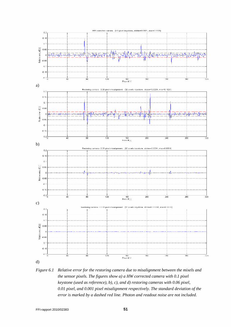
FFI-rapport 2010/02383 51
a)
b)
c)
d)
Figure 6.1 Relative error for the restoring camera due to misalignment between the mixels and the sensor pixels. The figures show a) a HW corrected camera with 0.1 pixel keystone (used as reference), b), c), and d) restoring cameras with 0.06 pixel, 0.01 pixel, and 0.001 pixel misalignment respectively. The standard deviation of the error is marked by a dashed red line. Photon and readout noise are not included.

52 FFI-rapport 2010/02383
We conclude that the misalignment betweeen the mixing chambers and the sensor should be less than 0.01 pixel, preferably as small as 0.001 pixel, in order not to contribute noticeably to the errors. In the following section we will see how we can achieve this.
6.2 Calibration
The restoring camera shows extremely good performance, but this is only true as long as we know the precise relative position of the mixels and the pixels. It is also necessary to know the point spread function of the relay optics (to determine the transitions between the mixels). The point spread function is to some extent known from the optical design, but the ’relative position of the mixels and the pixels’ requirement looks very demanding. The pixel size of the sensor in question is 6.5 μm, and we would like to know its position at least down to 65 nm, or preferably 6.5 nm. A detailed description of the calibration method for a restoring camera is outside the scope of this report. However, we would like to show that it is at least possible to measure the relative alignment between mixels and pixels with such precision. From a mechanical engineer's point of view this level of precision would sound... well... ’insane’ is the word, but in fact there are low cost devices which are able to move things with 0.5 nm (!) resolution. We are talking about piezo actuators. For example, the company Physik Instrumente (PI) GmbH & Co. KG [5] sells piezo actuators which have 45 μm travel range with 0.45 nm resolution. The same company sells a linear translation stage P-620.1 CD/CL with 50 μm travel range, 0.2 nm resolution, 0.02% linearity, and ±1 nm repeatability [6]. If we decide to adjust the position of the slit rather than the sensor, then the desired accuracy is 22 nm (which corresponds to 0.1% of a mixel) or at least 220 nm (which correspondes to 1% of a mixel), and the translation stage P-620.1 CD/CL seems to be far more precise than needed. We now know that we can move the slit very precisely. But how will we know the relative position of the mixels and the pixels? Let us place a single mixel at one end of the slit, see Figure 6.2.
Figure 6.2 The mixel array with one single mixel at the left end of the slit.
The light from the single mixel will illuminate an area on the sensor somewhat larger than one pixel, see Figure 6.3. The blue curve shows the intensity distribution that is determined by the size of the mixel and the point spread function of the optics. If we knew the shape of the intensity distribution, we would be able to derive the relative position of that mixel and the pixels since we can measure the signal from the illuminated pixels.

FFI-rapport 2010/02383 53
Figure 6.3 Intensity distribution (blue curve) of light coming from a single mixel onto the sensor pixels. The shape of the curve is determined by the size of the mixel and the point spread function of the optics.
Mounting the slit on a high resolution translation stage makes it possible to measure the intensity distribution. We need to read out the signal from the lit pixels, move the mixel (together with the whole slit, of course) by a few nanometers, take another readout, move the mixel again, take another readout, etc. It will then be possible to determine the intensity distribution in the sensor plane based on these measurements. Alternatively, the data can be stored as a look-up table for finding the position of the single mixel relative to the sensor. If we also place a single mixel at the other end of the slit, then we will be able to measure both the length of the slit and its position relative to the sensor. It may even be possible to do this during normal image acquisition, by using either a dedicated light source or even the light coming from the scene. This means that more or less every frame captured by the camera will have calibration data that can be used when restoring the image, i.e., requirements for alignment stability during flight will be far more relaxed (μm range instead of nm range). Actually, extra mixels combined with a translation stage may also be a very useful tool for measuring the size and shape of the transitions between mixels, not only at the edges of the field of view but everywhere. Knowing the size and shape of the transitions is important when restoring the data (Section 4.10). If we introduce a second array of mixels which is parallel to the main array of mixels (Figure 6.4), then the intensity distribution (i.e., the transitions) can be determined at several field points for all wavelengths.

54 FFI-rapport 2010/02383
Figure 6.4 The mixel array with a single mixel at the end and a second mixel array below.
During this type of calibration, the main mixel array (the upper one) is covered by a shutter and the second mixel array (the lower one) is used for measuring the illumination curves for many wavelengths and field points simultaneously. This calibration may be performed in a lab, or perhaps the calibration equipment may even be built into the camera. When the calibration is complete, the lower mixel array is covered by a shutter. The upper mixel array can then be used for image capture, while the single mixels on each side of the mixel array is used for real time measurements of the slit position and length.

FFI-rapport 2010/02383 55
7 What is next? In order to complete the development of the restoring camera described in this report, the following steps should be taken: 1) Implement code in the virtual camera software, that models the differences in point spread function width at different wavelengths. The current version of the virtual camera software does not take into account misregistration errors due to this. If the differences in point spread function width are large, the total misregistration errors may increase significantly. Modeling this effect in software will allow for a more realistic evaluation of the camera’s performance. Also, it will be easier to balance different aspects of camera performance during the design phase if all those aspects are taken into account in the virtual camera software. Their influence on the final data can then be checked in advance. 2) The optimum length of the mixing chambers and their light mixing properties should be verified by use of wave optics. In this report the light propagation inside the mixing chambers was modeled using geometric ray tracing. 3) The optimum dimensions of the mixing chambers (as well as required tolerances and expected light loss) should be verified with manufacturers. The focal length of the foreoptics and the magnification of the relay system should be adjusted accordingly. 4) It should be investigated which of the following methods is the best way to handle smile-effect in the camera: a) correction of the smile-effect in hardware or b) precise characterization of the smile-effect and resampling in the spectral direction. 5) The slit with the mixing chambers should be purchased and tested. It may be possible to test a single chamber by focusing light with correct numerical aperture to the input of the mixing chamber, and inspecting the light distribution at its output with a microscope. The slit with the mixing chambers can also be inserted into any hyperspectral camera which uses a flat transmissive slit. It means that, in principle, the concept can be tested with an existing camera. 6) A mount for the slit should be designed and manufactured. It should be possible to use off-the-shelf nanopositioning stages for this purpose. Such stages do not cost much and are far more accurate than we need. 7) The calibration procedure briefly described in Section 6.2 should be thoroughly developed and implemented in software. Finally, the proposed restoring camera with very low F-number should be built!

56 FFI-rapport 2010/02383
8 Conclusion Our analyses have shown that the proposed new restoring camera outperforms the conventional cameras under all light conditions. Conventional cameras have misregistration errors as large as 15-20%, and these errors remain even if the amount of light increases. The restoring camera, on the other hand, has negligible misregistration errors and is limited only by photon noise. This camera therefore performs better and better as the amount of light increases. In very bright light, the standard deviation of the error for the restoring camera is down to 0.6% and the maximum error is less than 2%! We propose a joint FFI-NEO project with the goal of building the new restoring camera. The project would benefit from NEO’s expertise in design of hyperspectral cameras and FFI’s expertise in processing of hyperspectral data. Key issues to be adressed would be verification of the performance of the mixing chambers and development and implementation of the calibration method for the camera. The outcome of the project would be a rather impressive instrument which will by far outperform the current generation of hyperspectral cameras.

FFI-rapport 2010/02383 57
Appendix A Different input signals In this report, we have compared the performance of three different virtual cameras. This was done by comparing the errors each camera introduce to a given input signal. The input signal that has been used in the simulations is shown in Figure A.1a). It contains several large peaks (up to 10 000 photons per pixel) as well as broader areas with only small variations in the signal (2000-3000 photons per pixel), providing the possibility to study the virtual cameras’ performance with respect to two key features of a real scene. The number of pixels (320) is large enough that some conclusions can be drawn based on statistics. Of course, using a different input signal might result in different errors both with respect to standard deviation and peak value. However, the key question is whether the performance of these three cameras relative to each other will be significantly changed by this? We therefore have compared results also for two other input signals. These two signals have somewhat different characteristics than the first input signal. Figure A.1b), c), and d) show the performance of the HW corrected, resampling, and restoring cameras respectively for the input signal (scene 1) that we have used in our simulations previously in this report. Photon noise and readout noise were included in the calculations and the signal was amplified four times for the resampling and restoring cameras to simulate their ability to collect considerably more light than the HW corrected camera. The results have already been presented and discussed in Chapter 4. The main conclusions are that the HW corrected and resampling cameras have quite similar performance, but that the error peaks are somewhat larger for the resampling camera. The restoring camera performs considerably better than the other two cameras, both with respect to standard deviation and peak value for the error. The second input signal (scene 2) is shown in Figure A.2a). The signal varies mainly between 1500 and 3500 photons per pixel and does not contain any large peaks. Figure A.2b), c), and d) show the performance for the three cameras for this input signal. Again the HW corrected and resampling cameras show quite similar performance, while the restoring camera performs considerably better than the other two cameras. However, this time none of the cameras have large error peaks. This is as expected since the input signal itself does not have any areas with very large difference between adjacent pixels8
. This is an example of a signal that would not be a very good choice for our simulations since it does not provide the possibility to investigate the cameras’ performance around peaks in the incoming signal.
8 The one quite large peak in the input signal around pixel #161 is placed in an area of the sensor where it is not sensitive to resampling, and it has a position inside the pixel which is not sensitive to the 0.1 pixel keystone of the HW corrected camera.

58 FFI-rapport 2010/02383
The third input signal (scene 3) is shown in Figure A.3a). It varies mainly between 2000 and 4000 photons per pixel, but has some smaller peaks and a large area with high pixel values (10 000-14 000 photons per pixel) at the right end. Figure A.3b), c), and d) show the performance of the three cameras for this input signal. Again the HW corrected and resampling cameras show quite similar performance, with somewhat larger error peaks for the resampling camera, while the restoring camera performs considerably better than the other two cameras. Note, however, that the errors for the HW corrected and resampling cameras are noticeably larger for this input signal than for the previous two signals (the scale on the y-axis is different in this figure compared to Figure A.1a and Figure A.2a). The error for the restoring camera is, on the other hand, approximately the same as before. The performance of the restoring camera relative the other two cameras is therefore actually better for this input signal than for the signal we used in our simulations. The restoring camera’s performance seems to be less sensitive to the “shape” of the input signal than the other two cameras. This makes sense since the restoring camera is limited only by photon noise. We conclude that our findings in this report regarding the three cameras’ performance relative to each other do not change significantly if different input signals are used. We therefore expect the main conclusions in this report to be valid also for other input signals than the one which was used in our simulations.
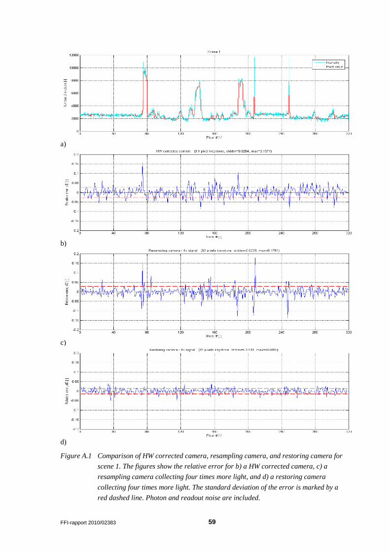
FFI-rapport 2010/02383 59
a)
b)
c)
d)
Figure A.1 Comparison of HW corrected camera, resampling camera, and restoring camera for scene 1. The figures show the relative error for b) a HW corrected camera, c) a resampling camera collecting four times more light, and d) a restoring camera collecting four times more light. The standard deviation of the error is marked by a red dashed line. Photon and readout noise are included.

60 FFI-rapport 2010/02383
a)
b)
c)
d)
Figure A.2 Comparison of HW corrected camera, resampling camera, and restoring camera for scene 2. The figures show the relative error for b) a HW corrected camera, c) a resampling camera collecting four times more light, and d) a restoring camera collecting four times more light. The standard deviation of the error is marked by a red dashed line. Photon and readout noise are included.

FFI-rapport 2010/02383 61
a)
b)
c)
d)
Figure A.3 Comparison of HW corrected camera, resampling camera, and restoring camera for scene 3. The figures show the relative error for b) a HW corrected camera, c) a resampling camera collecting four times more light, and d) a restoring camera collecting four times more light. The standard deviation of the error is marked by a red dashed line. Photon and readout noise are included.

62 FFI-rapport 2010/02383
Appendix B Resampling with high-resolution cubic splines vs bilinear resampling
Bilinear resampling is a fast and straighforward way to resample an image, or a line of an image, from one grid to another. The method applies a linear interpolating function and uses the two nearest pixels to calculate the value of the new grid point. However, this method smoothens the data quite much, especially in areas of the image where the grid points are shifted by about half a pixel relative each other. This may introduce quite large errors in the data. In this report we have used a more advanced resampling method, where the interpolating function
( )f x is made up of high-resolution cubic splines that are applied over the four nearest pixels [3]:
3 2
3 2
( ) ( 2) ( 3) 1, (0,1)( ) 5 8 4 , (1, 2)
f x a x a xf x ax ax ax a
= + − + +
= − + − (B.1)
Here a =-3/4. The first function is applied over the interval x =0 to x =1. The second function is applied over the interval x =1 to x =2. The interpolating function is symmetric about x =0. Parker et al [3] have investigated and compared several different resampling methods for general imaging, including bilinear resampling and resampling with high-resolution cubic splines. Their conclusion is that high-resolution cubic splines give the best overall performance. We have compared the use of bilinear resampling to resampling with high-resolution cubic splines for the three input signals discussed in Appendix A. This was done to verify that resampling with high-resolution cubic splines is in fact better to use than bilinear resampling for typical hyperspectral data. Figure B.1a) shows the input signal (scene 1) that we have used in our simulations throughout this report. Figure B.1b) shows the resulting misregistration error when bilinear resampling is used. Figure B.1c) shows the same for resampling with high-resolution cubic splines. Photon and readout noise are not included since we want to study the misregistration error (resulting from the choice of resampling method) alone. It is clear from the figures that resampling with high-resolution cubic splines gives the smallest error with a standard deviation of 2.8% versus 3.1% for bilinear resampling and peaks up to 18% versus 28%. Figure B.2 shows the results for the second input signal (scene 2). Again, resampling with high-resolution cubic splines gives the smallest error with a standard deviation of 2.5% versus 2.9% for bilinear resampling and peaks up to 9% versus 13%. Figure B.3 shows the results for the third input signal. Also here, resampling with high-resolution cubic splines gives the smallest error with a standard deviation of 3.8% versus 4.6% for bilinear resampling and peaks up to 31% versus 48%.

FFI-rapport 2010/02383 63
We conclude that resampling with high-resolution cubic splines gives better results than bilinear resampling for hyperspectral data.
a)
b)
c)
Figure B.1 Comparison of the performance obtained by the two different resampling methods for scene 1. The figures show the relative error for a resampling camera that uses b) bilinear resampling and c) high-resolution cubic splines. The standard deviation of the error is marked by a red dashed line. Photon and readout noise are not included.

64 FFI-rapport 2010/02383
a)
b)
c)
Figure B.2 Comparison of the performance obtained by the two different resampling methods for scene 2. The figures show the relative error for a resampling camera that uses b) bilinear resampling and c) high-resolution cubic splines. The standard deviation of the error is marked by a red dashed line. Photon and readout noise are not included.

FFI-rapport 2010/02383 65
a)
b)
c)
Figure B.3 Comparison of the performance obtained by the two different resampling methods for scene 3. The figures show the relative error for a resampling camera that uses b) bilinear resampling and c) high-resolution cubic splines. The standard deviation of the error is marked by a red dashed line. Photon and readout noise are not included.

66 FFI-rapport 2010/02383
Appendix C Third order polynomial transitions
Figure C.1 Example of a third order polynomial transition (red).
Figure C.1 shows an example of a third order polynomial transition (red) between two mixels. The transition starts at 1x x= and ends at 2x x= . The ‘sharp’ value of mixel #1 (i.e., the signal level of the part of the mixel that is not affected by the transition) is equal to 1y . The ‘sharp’ value of mixel #2 is equal to 2y .
The equation for the third order polynomial transition is
30 0 0( ) ( )y a x x c x x y= − + − + (C.1)
Here a and c are two constants that can be determined from the boundary conditions 1 1( )y x y= (or equivalently 2 2( )y x y= ) and 1'( ) 0y x = (or equivalently 2'( ) 0y x = ), which gives
22 1
2 1
2 1
43( )
3( )2( )
cax x
y ycx x
= −−
−=
−
(C.2)

FFI-rapport 2010/02383 67
This transition has odd symmetry about its center 0 0( , )x y , where 0x and 0y are given by
1 2
0
1 20
2
2
x xx
y yy
+=
+=
(C.3)
In order to calculate the transition between the two mixels we must know the size and position of the transition zone, i.e., 1x and 2x , and the ‘sharp’ mixel values 1y and 2y .

68 FFI-rapport 2010/02383
Appendix D Virtual camera software The software for the virtual camera was written in Matlab v7.9.0 (R2009b). The program has a user friendly interface and can easily be expanded by adding new modules. Below, we will describe how to use the virtual camera. Examples of how to use the program to simulate a HW corrected, resampling, and restoring camera are given in the following sections. The program is started by writing ’VirtualCamera’ in the Matlab command line. Figure D.1 shows the window that appears. Select the relevant parameters for the type of simulation you want to run and click the OK-button to start the calculations. Output from the program: mean value, standard deviation, and maximum value for the relative error in the calculated scene pixel values, is shown in the box in the lower right corner. In addition, one or more figures (depending on your choice) may be generated. Clicking the Close-button closes the program.
Figure D.1 Virtual camera interface.

FFI-rapport 2010/02383 69
Now, let us take a closer look at all the input parameters in the ‘VirtualCamera’ window: 1. Input signal (scene):
At the moment there is only one possible choice here: • Real image
Choosing ’Real image’, results in a real hyperspectral image being used as the input for the calculations. A pop-up menu appears (see Figure D.2), where the name of the input file must be given together with information about the image, which line of the image you want your virtual camera to look at, and your choice of downsampling factor for the image. In the ‘VirtualCamera’ window you may also choose to amplify the signal by some factor.
Figure D.2 Pop-up menu that apperas when using a real hyperspectral image as input to the virtual camera.
2. Slit:
Choose between the following:
• No mixing • Ideal mixing • Geometric ray tracing

70 FFI-rapport 2010/02383
Choosing ’No mixing’, results in the light passing through the slit without being mixed. Choosing ’Ideal mixing’, results in the light being perfectly mixed in the mixing chambers when passing through the slit. Choosing ’Geometric ray tracing’ results in the light being mixed in the mixing chambers when passing through the slit. Geometric ray tracing is used to model how the light mixes in the chambers. A pop-up menu appears where parameters for the mixing chambers can be chosen, see Figure D.3 for details.
Figure D.3 Pop-up menu for geometric ray tracing. Parameters for how to model the mixing chambers are set here. These parameters include the number of input bins per chamber, the number of rays per input bin, the number of output bins per chamber, the opening angle for the incoming light, the length of the mixing chambers, and the distance to the ’line of interest’. When the last parameter is set equal to 1, the output of the slit is set equal to the output at the back face of the mixing chambers.
3. Transition:
Choose between the following:
• No transition • 3rd order polynomial
Choosing ’No transition’ results in instant transitions being used between the mixels. Choosing ’3rd order polynomial’ results in 3rd order polynomial transitions being used between the mixels. The width of the transition must be given.

FFI-rapport 2010/02383 71
4. Misalignment & keystone:
Set misalignment and keystone value. 5. Record pixels:
At the moment there is only one possible choice here:
• Numeric When choosing ’Numeric’, the input signal is recorded numerically onto the sensor pixels. 6. Noise:
Select if photon noise and readout noise should be included in the calculations. For the readout noise the number of electrons (standard deviation) must be given. 7. Calculate input signal (scene) based on recorded values:
Choose between the following
• Hardware corrected keystone • Resampling • Restoring
When ’Hardware corrected keystone’ is chosen, the values of the scene pixels are calculated according to a HW corrected camera. When ’Resampling’ is chosen, the values of the scene pixels are calculated according to a resampling camera. It is possible to choose between three different resampling methods; ’high-resolution cubic splines’, ’cubic B-splines’, and ’bilinear’. When ’Restoring’ is chosen, the values of the scene pixels are calculated according to a restoring camera. It is possible to choose either restoring with ’Constant Intensity’ (assumes that the transitions between the mixels are instant) or restoring with ’Transition – 3rd order polynom’ (assumes that there are 3rd order polynomial transitions between the mixels). If the latter is chosen, a pop-up menu appears where the width of the transition can be typed in. You may also choose to bin the output scene pixels by a some factor. Plot options:
Choose to plot one or more of the following:
• Input signal & scene pixel value • Mixel signal after slit (signal at the output of the mixing chambers) • Relative error in calculated scene pixel value

72 FFI-rapport 2010/02383
D.1 HW corrected camera (example)
Figure D.4 Example of typical input to the program when simulating a HW corrected camera.
Figure D.4 shows an example of typical input to the program when simulating a HW corrected camera:
1. A real image is used as the input signal. There is no amplification of the signal (amplification factor is set to 1).
2. There is no mixing of the light in the slit. 3. There are no transitions (not applicable to a HW corrected camera). 4. The misalignment is set to 0.1 pixel in order to simulate 0.1 pixel keystone everywhere9
9 Alternatively, one could set the keystone to 0.1 pixel, but this would give a gradually increasing keystone going from zero at the left end of the image to 0.1 pixel at the right end of the image. The keystone would then be much smaller than 0.1 pixel over a large part of the image, and the situation with respect to keystone would be very different at the left and right side of the image.
. The keystone is set to zero.

FFI-rapport 2010/02383 73
5. The signal is recorded numerically onto the sensor pixels. 6. Photon noise is included. The read-out noise is set to have a standard deviation of
4 electrons. 7. The values of the scene pixels are calculated as if the signal has been run through a HW
corrected camera. The bin factor is set to 1, i.e., there is no binning of the resulting scene pixels.
It has been chosen to plot the input signal and scene pixel values (see Figure 3.1 for example) and the relative error in the calculated scene pixel values (see Figure 4.4a for example). Output from the program (mean value, standard deviation, and max value for the relative error in the calculated scene pixel values) is shown in the box in the lower right corner.
D.2 Resampling camera (example)
Figure D.5 Example of typical input values to the program when simulating a resampling camera.
74 FFI-rapport 2010/02383
Figure D.5 shows an example of typical input to the program when simulating a resampling camera:
1. A real image is used as the input signal. The signal is amplified by a factor 4. 2. There is no mixing of the light in the slit. 3. There are no transitions (not applicable to a resampling camera). 4. The misalignment is set to zero. The keystone is set to 32 pixels. 5. The signal is recorded numerically onto the sensor pixels. 6. Photon noise is included. The read-out noise is set to have a standard deviation of
5 electrons. 7. The values of the scene pixels are calculated as if the signal has been processed by a
resampling camera. It is chosen to use high-resolution cubic splines for the resampling. The bin factor is set to 2.
It has been chosen to plot the relative error in the calculated scene pixel values (see Figure 4.6c for example). Output from the program (mean value, standard deviation, and max value for the relative error in the calculated scene pixel values) is shown in the box in the lower right corner.
D.3 Restoring camera (example)
Figure D.6 shows an example of typical input to the program when simulating a restoring camera:
1. A real image is used as the input signal. The signal is amplified by a factor 4. 2. Geometric ray tracing is used to model the mixing of the light in the mixing chambers in
the slit. 3. The transitions are instant10
4. The misalignment is set to zero. The keystone is set to 32 pixels. .
5. The signal is recorded numerically onto the sensor pixels. 6. Photon noise is included. The read-out noise is set to have a standard deviation of
5 electrons. 7. The values of the scene pixels are calculated as if the signal has been processed by a
restoring camera, assuming that the transitions between mixels are instant. The bin factor is set to 1, i.e., there is no binning of the resulting scene pixels.
It has been chosen to plot the mixel signal after the slit (see Figure 3.4 for example) and the relative error in the calculated scene pixel values (see Figure 4.9d for example). Output from the program (mean value, standard deviation, and max value for the relative error in the calculated scene pixel values) is shown in the box in the lower right corner.
10 If 3rd order polynomial transitions are to be used, ’ideal mixing’ must be chosen for the slit.

FFI-rapport 2010/02383 75
Figure D.6 Example of typical input to the program when simulating a restoring camera.

76 FFI-rapport 2010/02383
References [1] G Høye and A Fridman (2009): “A method for restoring data in a hyperspectral imaging
system with large keystone without loss of spatial resolution”, FFI-rapport 2009/01351, FORTROLIG
[2] A Fridman and G Høye (2009): “Use of large keystone effect for high quality hyperspectral imaging”, Norsk Elektro Optikk AS, January 2009.
[3] J A Parker, R V Kenyon and D E Troxel (1983): “Comparison of Interpolating Methods for Image Resampling”, IEE trans. on medical imaging, Vol MI-2, No 1, March 1983.
[4] P Mouroulis, B van Gorp, R O Green, D Cohen, D Wilson, D Randall, J Rodriguez, O Polanco, K Balasubramanian, R Vargas, R Hein, H Sobel, M Eastwood and H Dierssen (2010): “Design of an Airborne Portable Remote Imaging Spectrometer (PRISM) for the Coastal Ocean”. Jet Propulsion Laboratory, California Institute of Technology and Departement of Marine Sciences, University of Connecticut Avery Point.
[5] www.physikinstrumente.com [6] http://www.physikinstrumente.com/en/products/prspecs.php?sortnr=202300 [7] Bahaa E A Salech, M C Teich (1991): “Fundamentals of Photonics”, John Wiley & Sons
Inc., 1991.