Embed Size (px)
Citation preview
Politecnico di Milano
SCHOOL OF INDUSTRIAL AND INFORMATION ENGINEERING
Master of Science in Telecommunication Engineering
Master Thesis
Performance Analysis of Intensity Modulated PAM-4
with Pre-compensation Filter and Direct Detection
in Short Reach Optical Communication
Candidate:
Alessandro Viganó, 833473
Supervisor:
Prof. Maurizio Magarini
Academic year 2015-2016

Contents
List of Figures VI
List of Tables VII
Sommario XIII
1 Introduction 1
2 Optical Channel 4
2.1 Introduction . . . . . . . . . . . . . . . . . . . . . . . . . . . . . . . . . 4
2.2 Receiver . . . . . . . . . . . . . . . . . . . . . . . . . . . . . . . . . . . 5
2.2.1 Non Coherent Receiver . . . . . . . . . . . . . . . . . . . . . . . 5
2.2.2 Coherent Receiver . . . . . . . . . . . . . . . . . . . . . . . . . 6
2.2.3 Self-Coherent . . . . . . . . . . . . . . . . . . . . . . . . . . . . 7
2.3 Fiber Propagation . . . . . . . . . . . . . . . . . . . . . . . . . . . . . . 8
2.3.1 Attenuation . . . . . . . . . . . . . . . . . . . . . . . . . . . . . 8
2.3.2 Chromatic Dispersion . . . . . . . . . . . . . . . . . . . . . . . . 9
3 Basics of Digital Transmission 12
3.1 Design Of The Transmitter . . . . . . . . . . . . . . . . . . . . . . . . . 12
3.2 AWGN Channel Modeling . . . . . . . . . . . . . . . . . . . . . . . . . 13
3.3 Design Of The Receiver . . . . . . . . . . . . . . . . . . . . . . . . . . 13
3.3.1 Matched Filter . . . . . . . . . . . . . . . . . . . . . . . . . . . 14
3.3.2 Frequency Selective Channel . . . . . . . . . . . . . . . . . . . . 16
4 Non-Coherent versus Self-Coherent 17
4.1 Non Coherent . . . . . . . . . . . . . . . . . . . . . . . . . . . . . . . . 17
4.1.1 PAM . . . . . . . . . . . . . . . . . . . . . . . . . . . . . . . . . 18
II
4.1.2 Non Coherent Detection and Chromatic Dispersion . . . . . . . 20
4.2 Self-Coherent . . . . . . . . . . . . . . . . . . . . . . . . . . . . . . . . 23
4.3 Other Self Coherent Methods . . . . . . . . . . . . . . . . . . . . . . . 26
4.3.1 Beating Methods . . . . . . . . . . . . . . . . . . . . . . . . . . 27
4.3.2 Coherent-like Methods . . . . . . . . . . . . . . . . . . . . . . . 30
4.3.3 Overview Of Self Coherent Methods . . . . . . . . . . . . . . . . 32
5 Simulation Results 34
5.1 Introduction . . . . . . . . . . . . . . . . . . . . . . . . . . . . . . . . . 34
5.2 Simulation Setup . . . . . . . . . . . . . . . . . . . . . . . . . . . . . . 35
5.3 Measures of Performance . . . . . . . . . . . . . . . . . . . . . . . . . . 39
5.3.1 Signal-to-Distortion Ratio . . . . . . . . . . . . . . . . . . . . . 39
5.3.2 Bit Error Rate . . . . . . . . . . . . . . . . . . . . . . . . . . . 40
5.3.3 Error Vector Magnitude (EVM) . . . . . . . . . . . . . . . . . . 40
5.3.4 Scatter Plot . . . . . . . . . . . . . . . . . . . . . . . . . . . . . 42
5.4 Numerical Results . . . . . . . . . . . . . . . . . . . . . . . . . . . . . . 42
5.4.1 Simulated Bit Error Rate . . . . . . . . . . . . . . . . . . . . . 42
5.4.2 BER Estimation From EVM . . . . . . . . . . . . . . . . . . . . 44
5.4.3 Total Impulse Response With Mismatch . . . . . . . . . . . . . 49
5.4.4 Scatter Plots After Detection . . . . . . . . . . . . . . . . . . . 51
5.4.5 Power of the Interference After the Photo-Diode . . . . . . . . . 54
5.4.6 Eye Diagrams . . . . . . . . . . . . . . . . . . . . . . . . . . . . 58
6 Conclusions 60
Bibliography 62
III
List of Figures
2.1 Generic scheme of an optical transmission system . . . . . . . . . . . . 4
2.2 A dual polarization Coherent receiver . . . . . . . . . . . . . . . . . . . 6
2.3 Values of the attenuation versus the wavelength . . . . . . . . . . . . . 10
2.4 Total chromatic dispersion for di�erent wavelengths and waveguide and
material dispersion components . . . . . . . . . . . . . . . . . . . . . . 11
3.1 Scheme of a digital transmission system . . . . . . . . . . . . . . . . . . 12
4.1 PAM-4 IM/DD constellation . . . . . . . . . . . . . . . . . . . . . . . . 18
4.2 PDF of the received signal in presence of only Gaussian noise . . . . . . 19
4.3 IM-DD spectrum in the C-band after 40 km . . . . . . . . . . . . . . . 21
4.4 IM-DD spectrum in the C-band after 60 km . . . . . . . . . . . . . . . 22
4.5 IM-DD spectrum in the C-band after 80 km . . . . . . . . . . . . . . . 22
4.6 Up-conversion scheme . . . . . . . . . . . . . . . . . . . . . . . . . . . . 23
4.7 Passband signal spectrum . . . . . . . . . . . . . . . . . . . . . . . . . 24
4.8 Receiver scheme . . . . . . . . . . . . . . . . . . . . . . . . . . . . . . . 24
4.9 Baseband signal spectrum after the photo-detector . . . . . . . . . . . 25
4.10 Optically �ltered SSB . . . . . . . . . . . . . . . . . . . . . . . . . . . . 27
4.11 Receiver . . . . . . . . . . . . . . . . . . . . . . . . . . . . . . . . . . . 28
4.12 Virtual SSB scheme . . . . . . . . . . . . . . . . . . . . . . . . . . . . . 28
4.13 Iterative algorithm for Virtual SSB . . . . . . . . . . . . . . . . . . . . 29
4.14 BPS transmitter scheme . . . . . . . . . . . . . . . . . . . . . . . . . . 29
4.15 SCI transmitter scheme . . . . . . . . . . . . . . . . . . . . . . . . . . . 30
4.16 SCI receiver scheme . . . . . . . . . . . . . . . . . . . . . . . . . . . . . 31
4.17 DP-SCI transmitter scheme . . . . . . . . . . . . . . . . . . . . . . . . 31
4.18 DP-SCI receiver scheme . . . . . . . . . . . . . . . . . . . . . . . . . . 31
IV
4.19 SV Transmitter . . . . . . . . . . . . . . . . . . . . . . . . . . . . . . . 32
4.20 SV receiver . . . . . . . . . . . . . . . . . . . . . . . . . . . . . . . . . 32
5.1 Reference scheme for the simulation . . . . . . . . . . . . . . . . . . . . 35
5.2 Impulse response of the rectangular transmission �lter . . . . . . . . . . 36
5.3 Impulse response of the Nyquist equi-ripple transmission �lter with roll-
o� = 0.3 . . . . . . . . . . . . . . . . . . . . . . . . . . . . . . . . . . 36
5.4 BER vs mismatch: rectangular �lter . . . . . . . . . . . . . . . . . . . 43
5.5 BER vs mismatch: Nyquist equi-ripple �lter . . . . . . . . . . . . . . . 43
5.6 BER vs mismatch for di�erent SDR: rectangular �lter . . . . . . . . . . 44
5.7 BER vs mismatch for di�erent SDR: Nyquist equi-ripple �lter . . . . . 44
5.8 BER vs SDR for di�erent mismatch: rectangular �lter . . . . . . . . . 45
5.9 BER vs SDR for di�erent mismatch: Nyquist equi-ripple �lter . . . . . 45
5.10 Real and estimated SDR for rectangular �ltering . . . . . . . . . . . . . 46
5.11 Real and estimated SDR for Nyquist equi-ripple �ltering . . . . . . . . 46
5.12 Real and estimated BER for rectangular �ltering . . . . . . . . . . . . 47
5.13 Real and estimated BER for Nyquist equi-ripple �ltering . . . . . . . . 47
5.14 BER vs mismatch for di�erent roll-o� Nyquist equi-ripple �lter and for
rectangular �lter . . . . . . . . . . . . . . . . . . . . . . . . . . . . . . 48
5.15 Spectra of signal with rectangular �lter and with Nyquist equi-ripple
�lter . . . . . . . . . . . . . . . . . . . . . . . . . . . . . . . . . . . . . 49
5.16 Impulse response of the cascade among rectangular �lter, pre-compensation
and CD with mismatch = 2% . . . . . . . . . . . . . . . . . . . . . . . 49
5.17 Impulse response of the cascade among rectangular �lter, pre-compensation
and CD with mismatch = 4% . . . . . . . . . . . . . . . . . . . . . . . 50
5.18 Impulse response of the cascade among Nyquist equi-ripple �lter, pre-
compensation and CD with mismatch = 2% . . . . . . . . . . . . . . . 50
5.19 Impulse response of the cascade among Nyquist equi-ripple �lter, pre-
compensation and CD with mismatch = 4% . . . . . . . . . . . . . . . 51
5.20 Scatter plot of the rectangular �ltered signal after detection (mismatch
= 0.5%) . . . . . . . . . . . . . . . . . . . . . . . . . . . . . . . . . . . 51
5.21 Scatter plot of the rectangular �ltered signal after detection (mismatch
= 1%) . . . . . . . . . . . . . . . . . . . . . . . . . . . . . . . . . . . . 52
V
5.22 Scatter plot of the rectangular �ltered signal after detection (mismatch
= 1.5%) . . . . . . . . . . . . . . . . . . . . . . . . . . . . . . . . . . . 52
5.23 Scatter plot of the rectangular �ltered signal after detection (mismatch
= 2%) . . . . . . . . . . . . . . . . . . . . . . . . . . . . . . . . . . . . 52
5.24 Scatter plot of the equi-ripple �ltered signal after detection (mismatch
= 0.5%) . . . . . . . . . . . . . . . . . . . . . . . . . . . . . . . . . . . 53
5.25 Scatter plot of the equi-ripple �ltered signal after detection (mismatch
= 1%) . . . . . . . . . . . . . . . . . . . . . . . . . . . . . . . . . . . . 53
5.26 Scatter plot of the equi-ripple �ltered signal after detection (mismatch
= 1.5%) . . . . . . . . . . . . . . . . . . . . . . . . . . . . . . . . . . . 53
5.27 Scatter plot of the equi-ripple �ltered signal after detection (mismatch
= 2%) . . . . . . . . . . . . . . . . . . . . . . . . . . . . . . . . . . . . 54
5.28 Eye diagram of detected signal with rectangular �lter in transmission
and mismatch of 2% . . . . . . . . . . . . . . . . . . . . . . . . . . . . 58
5.29 Eye diagram of detected signal with rectangular �lter in transmission
and mismatch of 4% . . . . . . . . . . . . . . . . . . . . . . . . . . . . 58
5.30 Eye diagram of detected signal with equi-ripple �lter in transmission
and mismatch of 2% . . . . . . . . . . . . . . . . . . . . . . . . . . . . 59
5.31 Eye diagram of detected signal with equi-ripple �lter in transmission
and mismatch of 4% . . . . . . . . . . . . . . . . . . . . . . . . . . . . 59
VI

List of Tables
2.1 Optical �ber bands . . . . . . . . . . . . . . . . . . . . . . . . . . . . . 9
4.1 Recap of other self-coherent methods . . . . . . . . . . . . . . . . . . . 32
VII

List of Acronyms
ASE Ampli�ed Spontaneuos Emission.
AWGN Additive White Gaussian Noise.
BER Bit Error Rate.
BPS Blockwise Phase Switching.
CD Chromatic Dispersion.
CSPR Carrier-to-Signal Power Ratio.
DAC Digital to Analog Converter.
DD Direct Detection.
DP-SCI Dual Polarization SCI.
DSB Double Side Band.
EVM Error Vector Magnitude.
IDFT Inverse Discrete Fourier Transform.
IFFT Inverse Fast Fourier Transform.
IFT Inverse Fourier Transform.
IM Intensity Modulation.
ISI Inter Symbol Interference.
LTI Linear Time Invariant.
VIII

NRZ Non Return to Zero.
OFDM Orthogonal Frequnecy Division Multiplexing.
OOK On-O� Keying.
PAM Pulse Amplitude Modulation.
PBS Polarization Beam Splitter.
PDF Probability Density Function.
RC Raised Cosine.
SCI Signal Carrier Interleaved.
SDR Signal-to-Distortion Ratio.
SMF Single Mode Fiber.
SNR Signal-to-Noise Ratio.
SOP State Of Polarization.
SRRC Square Root Raised Cosine.
SSB Single Side Band.
SSBI Signal-to-Signal Beating Interference.
IX

Sommario
La trasmissione su �bra ottica a rate 100Gbit/s con ricezione coerente è una tec-
nologia commerciale ormai consolidata, che permette la trasmissione su collegamenti
in �bra �no a distanze di migliaia di chilometri. Nei collegamenti a medio raggio, �no
agli 80 km, il costo di questa tecnologia è troppo alto, poichè prevede l'utilizzo di un
laser in ricezione, oltre alla presenza di un ibrido ottico e di quattro fotodiodi per pola-
rizzazione. Il vantaggio dei sistemi coerenti è la possibilità di equalizzare al ricevitore
tutte le distorsioni lineari subite dal segnale durante la trasmissione, in particolare la
dispersione cromatica.
Recentemente, sono state sono state proposte diverse soluzioni a bassa complessità per
ridurre i costi. In particolare, possiamo distinguere tra due principali tipi di soluzioni:
i sistemi self-coherent e quelli non coerenti.
I sistemi self-coherent prevedono la trasmissione della portante insieme con il segnale
di informazione. Il segnale ottico trasmesso deve essere a banda laterale singola. In
questo modo, dopo il fotodiodo al ricevitore, il battimento tra il segnale e la portante
non risente della dispersione cromatica.
La maggior parte dei sistemi self-coherent utilizza l'OFDM come schema di modu-
lazione, anche se esistono esempi di sistemi self-coherent con modulazione a singola
portante. Nel lavoro di tesi questo tipo di sistemi è introdotto senza speci�care un
particolare schema di modulazione.
I sistemi non coerenti sono ancora più semplici e prevedono la trasmissione di diversi
valori di intensità della luce laser (modulazione di intensità). Dato che il ricevitore è
costituito solo da un fotodiodo, il segnale elettrico generato è proporzionale al qua-
drato dell'ampiezza del campo ottico. La cascata tra trasmettitore, canale e ricevitore
non è perciò lineare e non è più possibile equalizzare la dispersione cromatica.
Il contributo di questo lavoro di tesi è la valutazione delle prestazioni di un sistema
con modulazione di intensità e ricezione coerente, che per tenere conto della dispersione
X
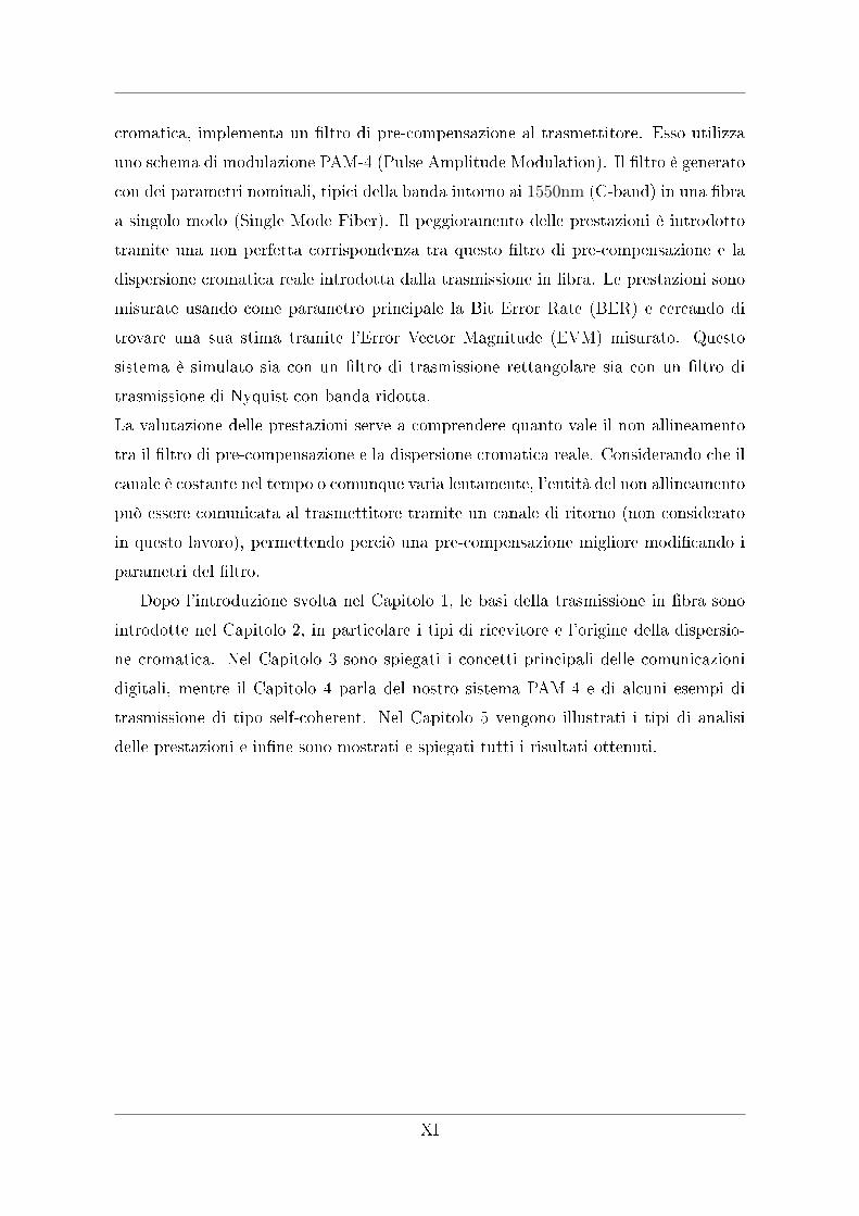
cromatica, implementa un �ltro di pre-compensazione al trasmettitore. Esso utilizza
uno schema di modulazione PAM-4 (Pulse Amplitude Modulation). Il �ltro è generato
con dei parametri nominali, tipici della banda intorno ai 1550nm (C-band) in una �bra
a singolo modo (Single Mode Fiber). Il peggioramento delle prestazioni è introdotto
tramite una non perfetta corrispondenza tra questo �ltro di pre-compensazione e la
dispersione cromatica reale introdotta dalla trasmissione in �bra. Le prestazioni sono
misurate usando come parametro principale la Bit Error Rate (BER) e cercando di
trovare una sua stima tramite l'Error Vector Magnitude (EVM) misurato. Questo
sistema è simulato sia con un �ltro di trasmissione rettangolare sia con un �ltro di
trasmissione di Nyquist con banda ridotta.
La valutazione delle prestazioni serve a comprendere quanto vale il non allineamento
tra il �ltro di pre-compensazione e la dispersione cromatica reale. Considerando che il
canale è costante nel tempo o comunque varia lentamente, l'entità del non allineamento
può essere comunicata al trasmettitore tramite un canale di ritorno (non considerato
in questo lavoro), permettendo perciò una pre-compensazione migliore modi�cando i
parametri del �ltro.
Dopo l'introduzione svolta nel Capitolo 1, le basi della trasmissione in �bra sono
introdotte nel Capitolo 2, in particolare i tipi di ricevitore e l'origine della dispersio-
ne cromatica. Nel Capitolo 3 sono spiegati i concetti principali delle comunicazioni
digitali, mentre il Capitolo 4 parla del nostro sistema PAM-4 e di alcuni esempi di
trasmissione di tipo self-coherent. Nel Capitolo 5 vengono illustrati i tipi di analisi
delle prestazioni e in�ne sono mostrati e spiegati tutti i risultati ottenuti.
XI
Abstract
The �ber optic transmission with rate 100Gbit/s with coherent reception is a
commercially available and consolidate technology, since it allows transmission on
�ber links up to distance of thousands of kilometers. In a medium reach link, up to 80
km, the cost of such a technology is too high, since it implies the use of a laser at the
receiver, in addition to an optical hybrid and four photo-diodes per polarization. The
advantage of coherent systems is the possibility to equalize all the linear distortions
undergone by the signal during transmission at the receiver, in particular for the
Chromatic Dispersion (CD).
Recently, many low complexity techniques have been proposed to reduce the costs.
In particular, we can distinguish between two main types of solutions: self-coherent
systems and non coherent one.
The self-coherent systems implement the transmission of the carrier along with the
information signal. The transmitted optical signal must be Single Side Band (SSB).
In this way, after going through the photo-detector at the receiver, the beating between
signal and carrier is not a�ected by Chromatic Dispersion.
The biggest part of self-coherent systems uses OFDM as modulation scheme, but there
are also examples of single carrier self-coherent systems. This work introduces self-
coherent systems without specifying a particular modulation scheme.
Non coherent systems are even easier and exploit the transmission of di�erent values
of the laser light intensity (Intensity Modulation). Since the receiver consists only
of a photo-diode, the generated electrical signal is proportional to the square of the
amplitude of the optical �eld. The cascade between transmitter, channel and receiver
is therefore non-linear and it is not possible to equalize CD anymore.
The contribute of this work is the evaluation of the performance of a system with
Intensity Modulation (IM) and Direct Detection (DD) techniques, that implements a
pre-compensation �lter to face with Chromatic Dispersion. It uses a PAM-4 (Pulse
XII

Amplitude Modulation) modulation scheme. This �lter is built with nominal param-
eters, typical of the band around 1550nm (C-band) in a Single Mode Fiber (SMF).
The degradation of the performance is introduced with the misalignment between this
pre-compensation �lter and the real CD introduced by the �ber transmission. Perfor-
mance is measured using the Bit Error Rate (BER) as main parameter and trying to
�nd an estimate of it by means of the measured Error Vector Magnitude (EVM). This
system is simulated with both a rectangular transmission �lter and a Nyquist �lter
with reduced bandwidth. The evaluation of the performance needs to understand how
much the misalignment between pre-compensation �lter and actual CD is. Consid-
ering that the channel is time invariant, or anyway it varies slowly, the entity of the
misalignment can be communicated at the transmitter by means of a feedback channel
(not considered in this work), therefore allowing a better pre-compensation with the
modi�cation of the parameters of the �lter.
After introduction in Chapter 1, in Chapter 2 the �ber transmissions are intro-
duced, in particular the types of receiver and the origin of Chromatic Dispersion. In
Chapter 3 the main concepts of digital communications are explained, while Chapter
4 deals with our PAM-4 system and many self-coherent examples. In Chapter 5 the
types of performance analysis are illustrated and �nally all the obtained results are
shown.
XIII
Chapter 1
Introduction
Fiber communications are the basis of the modern Internet. The entire transport
network is composed by optical �ber links, with distances that can reach thousands
of kilometers. This network allows the transferring of an enormous amount of data
and the demand for bandwidth is constantly increasing, due to the success of mobile
communications, HD video streaming and cloud services.
Nowadays, the technology used for the transport network is the coherent transmis-
sion at 100Gbit/s per channel. It uses a Polarization Division Multiplexing (PDM)
with Quadrature Phase Shift Keying (QPSK) modulation with a coherent receiver [1].
The coherent receiver is used to recover the entire �eld information and it allows,
di�erently from the Direct Detection technique, to equalize every linear impairments.
This is because every Digital Signal Processing algorithm can be applied after the
coherent receiver, having access to the complete baseband signal [2]. The coherent
receiver is equipped with a laser, called Local Oscillator, that should have the same
wavelength of the laser used at the transmitter as optical carrier. The local oscillator
beam and the information beam are the inputs af a device called Optical Hybrid that
makes them interfere in order to recover the real and imaginary part of the optical
�eld. The 100G coherent technology is mature and widely adopted for the long haul
links, where high costs and energy consumption of the coherent technology are justi�ed
by the length of the �ber link.
At the opposite, when the distance decreases under 80 km, the high cost of a coher-
ent receiver can be excessive [3]. This is the case for the short and medium reach links,
present in the metro and access networks and also in short intra or inter data-center
connections (also called client optics) [4]. The increasing bandwidth demand makes
1
these links the bottleneck of the network [5]. Therefore the switch from conventional
media to �ber optics technology is necessary to satisfy this demand. Medium and
short reach communication must respect some factors:
• High spectral e�ciency;
• Low power consumption;
• Low costs and small components size;
• Low complexity.
Many studies have been done in the recent years and many examples can be found
in literature that try to reach the 100Gbit/s data rate while satisfying the previous
requirements.
In particular, the proposed solutions can be distinguished in single-carrier Intensity
Modulation (IM) with Direct Detection (DD) and self-coherent system, often imple-
menting Orthogonal Frequnecy Division Multiplexing (OFDM).
The �rst type of solutions uses the non coherent detection, introducing high order
modulation [4] to increase the total bit rate using the same bandwidth. Although a
simple approach is the multiplexing of a number of wavelengths, everyone of them
carrying a fraction of the total capacity [6], a better solution is to create a single
wavelength 100G channel to reduce components costs [7]. One of the main cost factor
is the bandwidth of the used devices, so the reduction of bandwidth occupation is
another important aspect [8], [9].
Intensity Modulation is sensitive to Chromatic Dispersion (CD), that is limiting the
length of an uncompensated �ber link. So to make these systems working on longer
link, the problem of CD must be addressed.
The self-coherent solution is another way to face the problem of cost reduction.
They still use a non coherent receiver, but they look at the beating of the signal with
the carrier, that is added at the transmitter [10].
The most studied modulation scheme for these systems is the multi-carrier OFDM [11],
that allows a simpler equalization in the frequency domain and that is more �exible
in power and bit allocation. Furthermore, it is easier to take care of CD with a self-
coherent system, just using an optical Single Side Band (SSB) signal that does not
undergo power fading in frequency domain [12].
2
In this work we �rstly give a general view of the self-coherent transmission, pre-
senting many examples of them.
Then we focus our attention on a simpler non coherent system. In particular, the
PAM-4 single carrier IM systems with DD are used, with di�erent �ltering of the
spectrum: the rectangular �lter and a Nyquist FIR �lter with equi-ripple characteris-
tic.
The problem of the Chromatic Dispersion is faced with the introduction of a pre-
compensation �lter at the transmitter. This allows to maintain a very simple receiver.
The di�erence between CD parameter used in this �lter and the actual CD intro-
duced by the channel creates a degradation of the performance that is studied in this
work, trying to �nd a relation between Bit Error Rate (BER) and mismatch of pre-
compensation �lter.
This information can be sent back to the transmitter in order to perform a better
pre-equalization (this will not be treated in this thesis).
Publication
The study and the results carried out in this work were summarized in the con-
ference paper: A.Viganó, M.Magarini and A.Spalvieri, "Performance Analysis in a
PAM-4 Fiber Transmission IM-DD with Pre-compensation Filter", in Proc. European
Conference on Computer Science, pp. 1-6, Rome, Italy, 21-23 October 2016.
3
Chapter 2
Optical Channel
In this chapter the �ber transmission channel is explained by focusing on how the
light �eld propagates in an optical �ber. Chromatic Dispersion (CD) and its e�ect on
the received signal are described. The theory is derived by [13].
2.1 Introduction
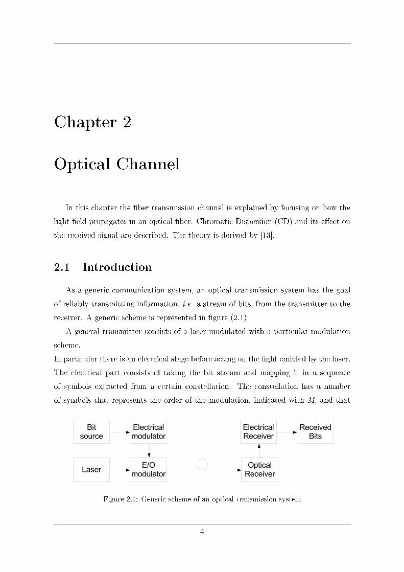
As a generic communication system, an optical transmission system has the goal
of reliably transmitting information, i.e. a stream of bits, from the transmitter to the
receiver. A generic scheme is represented in �gure (2.1).
A general transmitter consists of a laser modulated with a particular modulation
scheme.
In particular there is an electrical stage before acting on the light emitted by the laser.
The electrical part consists of taking the bit stream and mapping it in a sequence
of symbols extracted from a certain constellation. The constellation has a number
of symbols that represents the order of the modulation, indicated with M, and that
Figure 2.1: Generic scheme of an optical transmission system
4
depends on the number k of consecutive bits mapped on a single symbol, as indicated
in (2.1)
k = log2(M). (2.1)
This sequence of symbols is then converted in an analog waveform with a Digital to
Analog Converter (DAC). The waveform modulates the laser output, by means of an
electro-optical modulator. The laser output is a light beam with a certain frequency
f0 and wavelength λ0, that are linked by
c = f0λ0. (2.2)
There's no existing laser with a perfect monochromatic spectrum, but lasers are
the best coherent light sources anyway, so the emitted light is considered to have a
single frequency.
2.2 Receiver
There are two types of receiver for the optical transmission systems and they are
made possible by the photo-diode, i.e. the device capable of transforming the light in
an electrical current.
The two types are:
• Non Coherent receiver
• Coherent receiver
In this work, a compromise between these two conventional receivers is also studied,
i.e. a solution that stays in between complexity and cost e�ectiveness: the self-coherent
system.
2.2.1 Non Coherent Receiver
A non coherent receiver is composed only by the photo-detector (or photo-diode).
The photo-diode transforms the optical signal in an electrical current, that is propor-
tional to the intensity of the optical �eld impinging on the surface of the photo-diode.
This techniques is also called Direct Detection (DD)
i(t)α |e(t)|2 . (2.3)
5
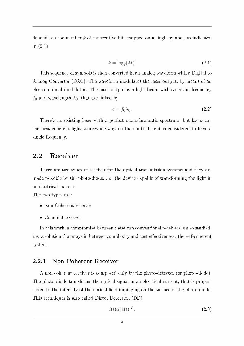
Figure 2.2: A dual polarization Coherent receiver
In order to reduce the noise produced by the optical ampli�ers, called Ampli�ed Spon-
taneous Emission (ASE noise), an optical �lter is often put before the photo-detector.
From equation (2.3) we can understand how the receiver cannot recover phase infor-
mation of the optical �eld. With a non coherent receiver, only Intensity Modulation
(IM) is possible, e.g. the Non Return to Zero - On O� Keying (NRZ OOK) [14].
This implies a reduction in spectral e�ciency due to the impossibility to use complex
modulation schemes. At a �xed rate, we cannot take advantage of both modulus and
phase of the received symbols using DD, so the spectral e�ciency is halved.
2.2.2 Coherent Receiver
A coherent receiver can recover the real and the imaginary part of the complex
baseband modulation signal instead. This is done by adding a laser at the receiver, as
shown in �gure (2.2), that might be at the same wavelength of the transmission laser
and in phase with it.
The real part of the signal is recovered on one arm of the Optical Hybrid. This is done
when the laser and the received signal are in phase. To cancel the additional terms,
another photo-diode must be added. Its input is obtained adding to the carrier a 180◦
phase switch. Looking at the baseband equivalent we have that
y1(t) = |e(t) + c|2 = |e(t)|2 + c2 + 2c<{e(t)} (2.4)
y2(t) = |e(t)− c|2 = |e(t)|2 + c2 − 2c<{e(t)}. (2.5)
6
The output of the two photo-diodes is then subtracted in order to isolate only the real
parts
y1(t)− y2(t) = 4c<{e(t)}. (2.6)
On the other arm of the Optical Hybrid, the local laser, or the received signal as
well, are delayed by π/2 before interfering with each other, so the imaginary part is
recovered as
y3(t) = |e(t)− jc|2 = |e(t)|2 + c2 + 2c={e(t)} (2.7)
y4(t) = |e(t) + jc|2 = |e(t)|2 + c2 − 2c={e(t)}. (2.8)
As before, the two signals are subtracted after the detection
y3(t)− y4(t) = 4c={e(t)}. (2.9)
These operations are done by an integrated optic device called Optical 90◦ Hybrid.
More complexity is added if we also want to consider the possible State Of Polarization
(SOP); in this case a Polarization Beam Splitter (PBS) is added before two Optical Hy-
brids, that operate as described above. The PBS projects the signal on two orthogonal
polarizations, while the laser SOP is controlled via a Polarization Controller.
2.2.3 Self-Coherent
The self-coherent uses a classical non coherent receiver, but the carrier is added at
the transmitter [15]. The transmitted signal is y(t) = e(t) + c, so we are in the same
case described by the �rst line of eq (2.5) at the receiver, as
y(t) = |e(t) + c|2 = |e(t)|2 + c2 + 2c<{e(t)} (2.10)
The term c2 is a constant, the term |e(t)|2 is called Signal to Signal Beating Interfer-
ence (SSBI) and the remaining term is the signal we are interested in, called signal to
carrier beating.
SSBI is an interfering term, since it cannot be removed optically; so it must be taken
into account. The transmitted power is divided between signal and carrier: in par-
ticular, higher power in the carrier results in ampli�cation of the signal to the carrier
beating. Anyway, to avoid nonlinearities, a limited power must be concentrated in a
single wavelength.
7
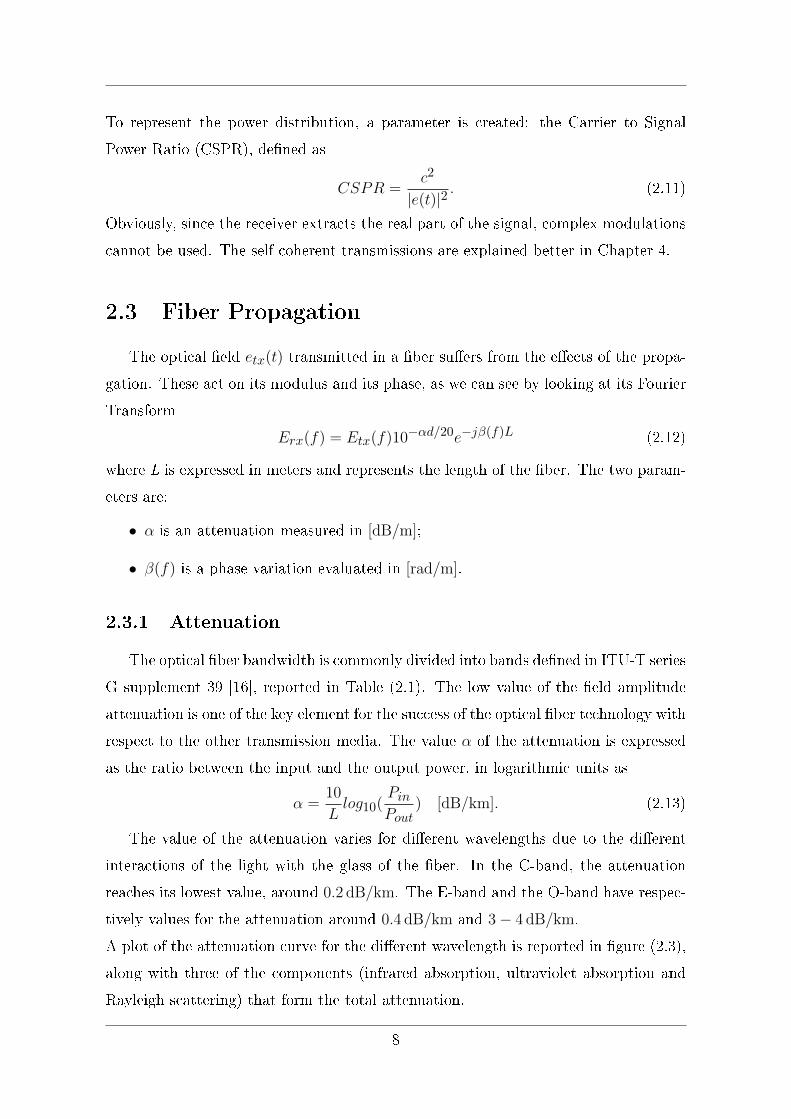
To represent the power distribution, a parameter is created: the Carrier to Signal
Power Ratio (CSPR), de�ned as
CSPR =c2
|e(t)|2. (2.11)
Obviously, since the receiver extracts the real part of the signal, complex modulations
cannot be used. The self-coherent transmissions are explained better in Chapter 4.
2.3 Fiber Propagation
The optical �eld etx(t) transmitted in a �ber su�ers from the e�ects of the propa-
gation. These act on its modulus and its phase, as we can see by looking at its Fourier
Transform
Erx(f) = Etx(f)10−αd/20e−jβ(f)L (2.12)
where L is expressed in meters and represents the length of the �ber. The two param-
eters are:
• α is an attenuation measured in [dB/m];
• β(f) is a phase variation evaluated in [rad/m].
2.3.1 Attenuation
The optical �ber bandwidth is commonly divided into bands de�ned in ITU-T series
G supplement 39 [16], reported in Table (2.1). The low value of the �eld amplitude
attenuation is one of the key element for the success of the optical �ber technology with
respect to the other transmission media. The value α of the attenuation is expressed
as the ratio between the input and the output power, in logarithmic units as
α =10
Llog10(
PinPout
) [dB/km]. (2.13)
The value of the attenuation varies for di�erent wavelengths due to the di�erent
interactions of the light with the glass of the �ber. In the C-band, the attenuation
reaches its lowest value, around 0.2 dB/km. The E-band and the O-band have respec-
tively values for the attenuation around 0.4 dB/km and 3− 4 dB/km.
A plot of the attenuation curve for the di�erent wavelength is reported in �gure (2.3),
along with three of the components (infrared absorption, ultraviolet absorption and
Rayleigh scattering) that form the total attenuation.
8

Band Name Range (nm) Range(THz)
O-band Original 1260-1360 237.9-220.4
E-band Extended 1360-1460 220.4-205.3
S-band Short wavelength 1460-1530 205.3-195.9
C-band Conventional 1530-1565 195.9-191.6
L-band Long wavelength 1565-1625 191.6-184.5
U-band Ultra-long wavelength 1625-1675 184.5-179.0
Table 2.1: Optical �ber bands
2.3.2 Chromatic Dispersion
The phase variation β(f) term indicated in (2.12) can be expanded in Taylor series
as
β(f) = β0 +dβ
df
∣∣∣∣f=0
f +1
2
d2β
df2
∣∣∣∣f=0
f2, (2.14)
where
• β0 is a frequency independent phase shift;
• β1 = dβdf
∣∣∣∣f=0
is a linear phase shift term representing a delay in time, linked to
the group velocity vg of signal (the speed of the information) as vg = 2π/β1;
• β2 = 12d2β
df2
∣∣∣∣f=0
is the change of the group velocity depending on the frequency.
So β2 is the parameter responsible of the CD: each frequency component travels
at di�erent velocity.
The total value of CD is originated by three components of dispersion that depend on
how the �ber is built:
• Waveguide Dispersion: the intrinsic dispersion induced by the propagation;
• Composite Material Dispersion: originated by the change of the refractive index
of core and cladding at di�erent wavelength;
• Composite Pro�le Dispersion: due to the refractive index pro�le of the �ber.
9
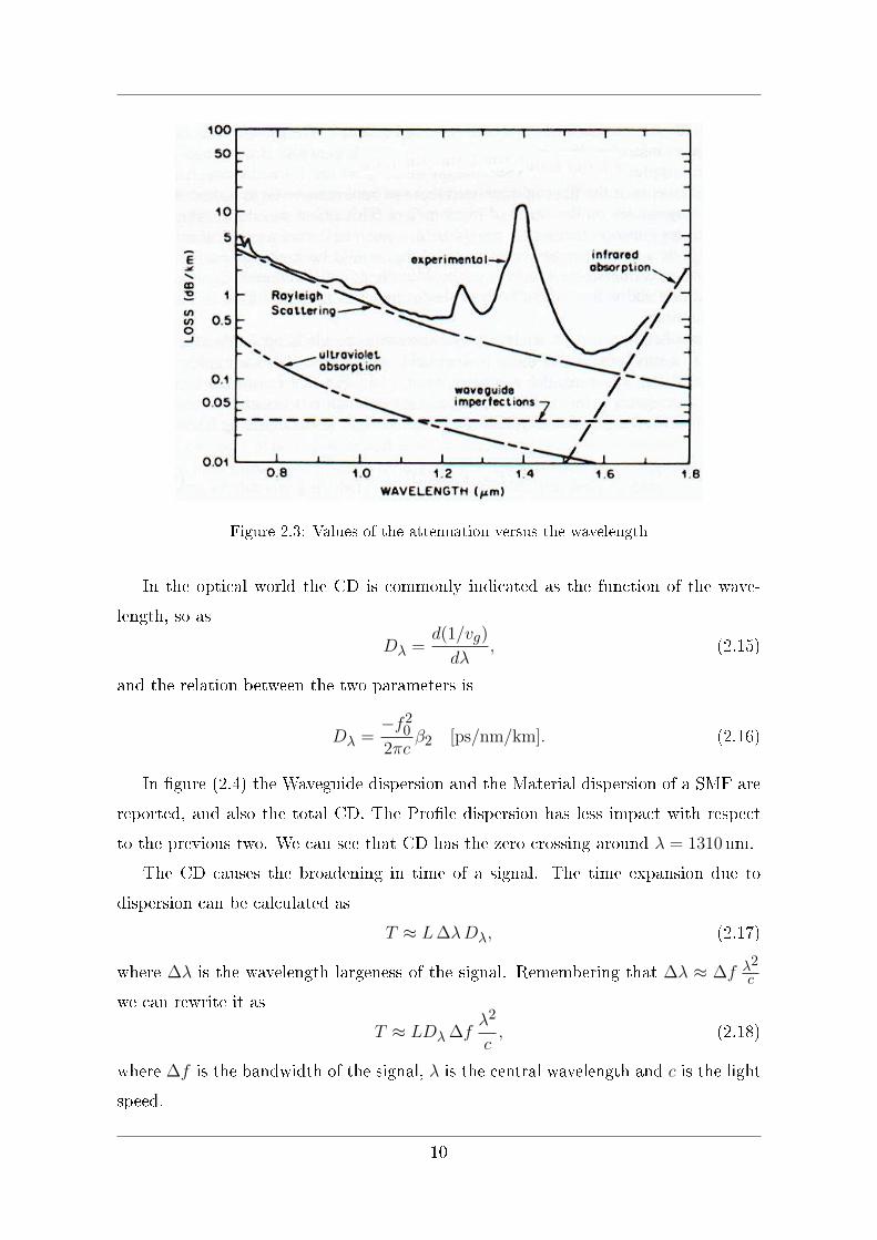
Figure 2.3: Values of the attenuation versus the wavelength
In the optical world the CD is commonly indicated as the function of the wave-
length, so as
Dλ =d(1/vg)
dλ, (2.15)
and the relation between the two parameters is
Dλ =−f202πc
β2 [ps/nm/km]. (2.16)
In �gure (2.4) the Waveguide dispersion and the Material dispersion of a SMF are
reported, and also the total CD. The Pro�le dispersion has less impact with respect
to the previous two. We can see that CD has the zero crossing around λ = 1310 nm.
The CD causes the broadening in time of a signal. The time expansion due to
dispersion can be calculated as
T ≈ L∆λDλ, (2.17)
where ∆λ is the wavelength largeness of the signal. Remembering that ∆λ ≈ ∆f λ2c
we can rewrite it as
T ≈ LDλ ∆fλ2
c, (2.18)
where ∆f is the bandwidth of the signal, λ is the central wavelength and c is the light
speed.
10
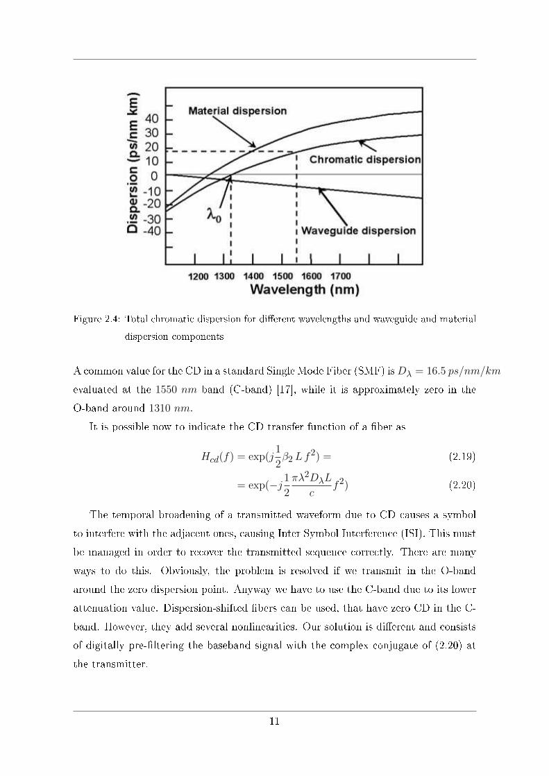
Figure 2.4: Total chromatic dispersion for di�erent wavelengths and waveguide and material
dispersion components
A common value for the CD in a standard Single Mode Fiber (SMF) isDλ = 16.5 ps/nm/km
evaluated at the 1550 nm band (C-band) [17], while it is approximately zero in the
O-band around 1310 nm.
It is possible now to indicate the CD transfer function of a �ber as
Hcd(f) = exp(j1
2β2 Lf
2) = (2.19)
= exp(−j 1
2
πλ2DλL
cf2) (2.20)
The temporal broadening of a transmitted waveform due to CD causes a symbol
to interfere with the adjacent ones, causing Inter Symbol Interference (ISI). This must
be managed in order to recover the transmitted sequence correctly. There are many
ways to do this. Obviously, the problem is resolved if we transmit in the O-band
around the zero dispersion point. Anyway we have to use the C-band due to its lower
attenuation value. Dispersion-shifted �bers can be used, that have zero CD in the C-
band. However, they add several nonlinearities. Our solution is di�erent and consists
of digitally pre-�ltering the baseband signal with the complex conjugate of (2.20) at
the transmitter.
11

Chapter 3
Basics of Digital Transmission
The theory explained in this chapter is used as reference for all the work. The
main source from which the arguments are derived is [15].
It is explained a general digital transmission system, especially how transmitter, chan-
nel and receiver are modeled.
3.1 Design Of The Transmitter
The purpose of a transmission system is to transfer informations from the trans-
mitter to the receiver as more reliable as possible.
Using Fig. (3.1) as a reference, in a digital communication scheme we have to
transmit a stream of bits bi from a point to another. To do this, k bits are grouped to
be mapped in one symbol extracted from a constellation of M complex symbols. This
two parameters are linked as follow
k = log2(M). (3.1)
The constellation used from the modulator to maps bit in symbols is represented as a
Figure 3.1: Scheme of a digital transmission system
12
symbol set
A = {a1, a2, a3, ...aM}. (3.2)
These symbols have to be transmitted on the channel. Before this, they are �ltered
with the transmission �lter to create the waveform. If we indicate with htx(t) the
transmission �lter, the transmitted waveform is
s(t) =+∞∑
n=−∞a(n)htx(t− nTs), (3.3)
where Ts is the symbol duration. Its inverse, Rs = 1/Ts is the symbol rate and it is
measured in symbol/s or Baud (Bd). We can assume that the transmission �lter has
a limited time duration equal to Ts, e.g. it is di�erent from zero only in the interval
−Ts < t < Ts.
3.2 AWGN Channel Modeling
The symbols now travel along the channel, that can be represented as a Linear Time
Invariant (LTI) �lter with impulse response hch(t). This �lter takes into account all
the linear e�ects induced by the transmission media. In case of ideal channel, it is
represented as a Dirac delta.
hch(t) = δ(t) =
1 t = 0,
0 t 6= 0.(3.4)
Actually, an ideal channel cannot exist. At least, channel introduces a delay that
can be represented as a delta translated by τ , where τ indicates the time delay. A
non ideal channel introduces distortion on the signal and makes symbols interfere with
each others. This situation is represented by a channel �lter length greater than the
symbol duration. After the channel it is added the Additive White Gaussian Noise
(AWGN), that is indicated with w(t).
3.3 Design Of The Receiver
After having gone through the channel, the signal is �ltered by the receiver �lter
and then sampled every Ts seconds in order to recover the original symbols sequence.
13
If the receiver �lter is indicated with hrx(t), the received signal by r(t) and the signal
at the output of the received �lter by y(t) we can write
y(t) = r(t) ∗ hrx(t), (3.5)
r(t) = [(s(t) ∗ hch(t)) + w(t)] . (3.6)
After sampling, we obtain that
y(n) = a(n) ∗ p(n) + w′(n), (3.7)
where w′(n) is the �ltered and sampled noise and
p(n) = htx(t) ∗ hch(t) ∗ hrx(t)|t=nTs . (3.8)
In eq (3.8) p(n) indicates the discrete equivalent �lter obtained by the cascade of
transmission �lter, channel impulse response and receiver �lter.
From the sequence y(n), the decision device recovers the estimated sequence a(n) di-
viding the signal space in decision regions. Then the demodulator does the de-mapping
operation, obtaining the estimated stream of bits bi.
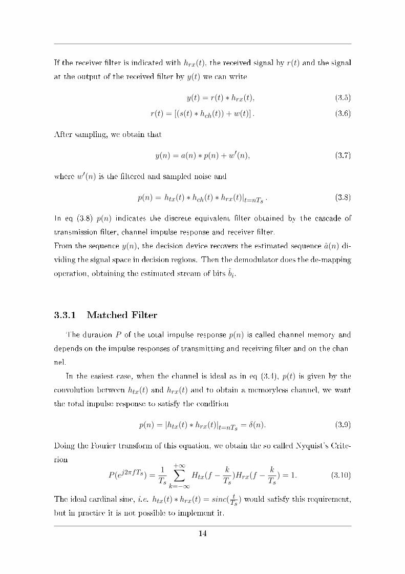
3.3.1 Matched Filter
The duration P of the total impulse response p(n) is called channel memory and
depends on the impulse responses of transmitting and receiving �lter and on the chan-
nel.
In the easiest case, when the channel is ideal as in eq (3.4), p(t) is given by the
convolution between htx(t) and hrx(t) and to obtain a memoryless channel, we want
the total impulse response to satisfy the condition
p(n) = |htx(t) ∗ hrx(t)|t=nTs = δ(n). (3.9)
Doing the Fourier transform of this equation, we obtain the so called Nyquist's Crite-
rion
P (ej2πfTs) =1
Ts
+∞∑k=−∞
Htx(f − k
Ts)Hrx(f − k
Ts) = 1. (3.10)
The ideal cardinal sine, i.e. htx(t) ∗ hrx(t) = sinc( tTs
) would satisfy this requirement,
but in practice it is not possible to implement it.
14

Anyway, there are many types of waveform, which have bandwidth greater than the
minimum bandwidth (or Nyquist bandwidth) of the sinc Bmin = 1/2Ts, that can
satisfy the Nyquist Criterion. For example, a common choice is the so called Raised
Cosine (RC) function that are de�ned as
RC(f) =
T |f | ≤ 1−α
2Ts,
T cos2(πTs2α (|f | − 1−α2Ts
)) 1−α2Ts
< |f | ≤ 1+α2Ts
,
0 |f | > 1+α2Ts
.
(3.11)
The parameter α is the Roll-O� factor and indicates the fraction of excess bandwidth
of the waveform with respect to the Nyquist bandwidth. The total bandwidth is so
B = Bmin(1 + α) = 12Ts
(1 + α).
To obtain p(t) as a Raised Cosine function, the transmitting and receiving �lter must
be the so called Square Root Raised Cosine (SRRC) function. This two types of
function are linked by
RC(f) = SRRC(f) ∗ SRRC(f) (3.12)
SRRC(F ) =√|RC(f)|. (3.13)
In general, the design of the receiving �lter is based on the maximization of the Sig-
nal to Noise Ratio (SNR). Assuming that we are transmitting only an isolate impulse,
so we are in absence of ISI, we can de�ne g(t) as the convolution between transmitting
�lter and channel impulse response
g(t) = htx(t) ∗ hch(t). (3.14)
So, before the receiving �lter, we have
r(t) = a(0)g(t) + w(t). (3.15)
The total impulse response, evaluated in its maximum value, is
p(t0) =
∫ +∞
−∞G(f)Hrx(f)ej2πft0df, (3.16)
that is the inverse Fourier Transform of the cascade between the two transferring
function.
The SNR after the receiver is de�ned as
SNR =|p(t0)|2
σ2w=|∫ +∞−∞ G(f)Hrx(f)ej2πft0df |2
N02
∫ +∞−∞ |Hrx(f)|2df
, (3.17)
15
where N0/2 is the noise power spectral density and σ2w is the noise power spectral
density after the receiving �lter, while the nominator is the power of the signal.
It has been proven that the maximum of this ratio can be obtained when the absolute
value at the nominator is splittable (Schwarz's inequality); it happens when
Hrx(f) = G∗(f)e−j2πft0 . (3.18)
This is the so called Matched Filter, that both minimizes ISI and maximizes the SNR.
Substituting it in the SNR formula (equation (3.17)), the maximum achievable SNR
is found to be
SNR =2EgN0
, (3.19)
being Eg the energy of g(t).
The receiver impulse response is then obtained from the inverse Fourier Transform of
eq (3.18)
hrx(t) = g(t0 − t). (3.20)
The Matched Filter is therefore the time inverted and delayed version of g(t).
3.3.2 Frequency Selective Channel
In the case in which the channel is not ideal, i.e. it is not a Dirac delta, two cases
can be distinguished looking at the Fourier Transform of the channel impulse response
Hch(f) = F{hch(t)}.
• Hch(f) ≈ 1 for |f | ≤ 1/2Ts:
In this case we can approximate hch(n) ≈ hch(0)δ(n);
• Hch(f) with rapid variation in the frequency interval |f | ≤ 1/2Ts:
In this case we cannot approximate the channel impulse response with only one
sample. The length of the total impulse response p(t) will be greater than one.
In the case that the channel cannot be approximated with one sample, it is said that
the channel has memory. Because of that, Inter Symbol Interference (ISI) arises: a
received symbol is degraded by the overlapping of the previous and following symbols.
y(n) = a(n) ∗ p(n) =P−1∑i=0
a(n− i)p(i), (3.21)
where P is the length of the total impulse response.
16
Chapter 4
Non-Coherent versus Self-Coherent
In this chapter the non coherent transmissions system are introduced. In particular,
we focus on a PAM-4 as intensity modulation scheme that can be used with a non
coherent receiver. We also explain the probability of error of this scheme in case of
Gaussian interference.
Then the problem of the CD in a non coherent system is discussed.
In the following section, the concept of self-coherent system is presented as possibility
to overcome this problem. Many examples of self-coherent are then summarized.
4.1 Non Coherent
The non coherent detection uses only a photo-detector at the receiver to generate
an electrical current proportional to the intensity of the light impinging on the surface
of the photo-detector, as said in chapter 2. This receiver structure is also de�ned as
Direct Detection.
With this type of receiver, the information must be referred at the unique quantity
that the receiver can distinguish: the intensity of the light.
The used modulation technique is therefore the Intensity Modulation: the electrical
waveform acts on the intensity of the laser beam, making it varying according to the
levels of the modulation.
There are two ways for changing the output laser power [18]. The �rst is the direct
modulation, in which the light is modulated directly in the laser cavity, that can be
a Fabry-Perot or a Distributed Feedback cavity. The other is the external modulator,
a separated device that acts on the emitted light by the laser, that has a constant
17
power. The commercially used external modulator is the Mach-Zehnder Interferomet-
ric modulator.
In this thesis, we study a PAM-4 modulation scheme, with only positive amplitude
levels, that can be distinguished by the receiver.
4.1.1 PAM
The system studied in this work uses a Pulse Amplitude Modulation (PAM). With
respect to the canonical OOK, the PAM utilizes more amplitude signal level in order
to increase spectral e�ciency. The same bit rate can be reached, using the PAM, with
a reduced Baud rate with respect to OOK.
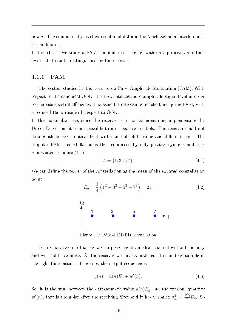
In this particular case, since the receiver is a non coherent one, implementing the
Direct Detection, it is not possible to use negative symbols. The receiver could not
distinguish between optical �eld with same absolute value and di�erent sign. The
unipolar PAM-4 constellation is then composed by only positive symbols and it is
represented in �gure (4.1)
A = {1; 3; 5; 7}. (4.1)
We can de�ne the power of the constellation as the mean of the squared constellation
point
Ea =1
4
(12 + 32 + 52 + 72
)= 21. (4.2)
Figure 4.1: PAM-4 IM/DD constellation
Let us now assume that we are in presence of an ideal channel without memory
and with additive noise. At the receiver we have a matched �lter and we sample in
the right time instant. Therefore, the output sequence is
y(n) = a(n)Eg + w′(n). (4.3)
So, it is the sum between the deterministic value a(n)Eg and the random quantity
w′(n), that is the noise after the receiving �lter and it has variance σ2w =N02 Eg. So
18
-2 0 2 4 6 8 100
0.2
0.4
0.6
0.8
1
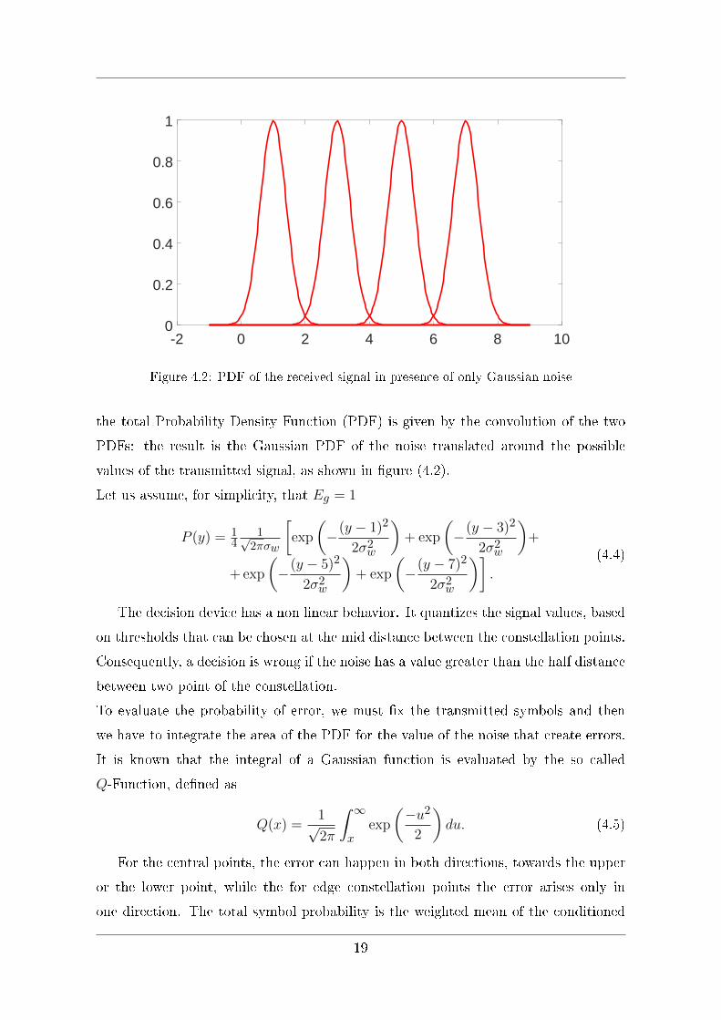
Figure 4.2: PDF of the received signal in presence of only Gaussian noise
the total Probability Density Function (PDF) is given by the convolution of the two
PDFs: the result is the Gaussian PDF of the noise translated around the possible
values of the transmitted signal, as shown in �gure (4.2).
Let us assume, for simplicity, that Eg = 1
P (y) = 14
1√2πσw
[exp
(−(y − 1)2
2σ2w
)+ exp
(−(y − 3)2
2σ2w
)+
+ exp
(−(y − 5)2
2σ2w
)+ exp
(−(y − 7)2
2σ2w
)].
(4.4)
The decision device has a non linear behavior. It quantizes the signal values, based
on thresholds that can be chosen at the mid distance between the constellation points.
Consequently, a decision is wrong if the noise has a value greater than the half distance
between two point of the constellation.
To evaluate the probability of error, we must �x the transmitted symbols and then
we have to integrate the area of the PDF for the value of the noise that create errors.
It is known that the integral of a Gaussian function is evaluated by the so called
Q-Function, de�ned as
Q(x) =1√2π
∫ ∞x
exp
(−u2
2
)du. (4.5)
For the central points, the error can happen in both directions, towards the upper
or the lower point, while the for edge constellation points the error arises only in
one direction. The total symbol probability is the weighted mean of the conditioned
19
probability of error of every point
Ps(e) =1
2Q
(√2EgN0
)+
1
22Q
(√2EgN0
), (4.6)
where the �rst term stays for the two edge points and the second term stays for the
central points.
For a general M-PAM constellation, there is a formula for evaluating the symbol error
probability
Ps(e) =2(M − 1)
MQ
(√2EgN0
). (4.7)
From the symbol error probability we can also evaluate the bit error probability.
Actually, in most cases it can be only approximated, because it depends on the mapping
between symbols and bits. It can be better calculated in case of Gray mapping, when
adjacent symbols di�er for one bit and so, assuming that errors happen only between
adjacent symbols, one symbol error corresponds to one bit error. Having log2(M) bits
per symbol, the bit error probability is
Pb(e) = 1log2(M)
Ps(e) =
= 1log2(M)
[12Q
(√2EgN0
)+ 1
22Q
(√2EgN0
)].
(4.8)
The formula in equation (4.6) is derived for the case of only Gaussian interference,
i.e. the AWGN noise. When we are in presence of other types of interference, equation
(4.6) can be used as an approximation of the symbols error probability. How good is
this approximation depends on the statistical property of the interference.
4.1.2 Non Coherent Detection and Chromatic Dispersion
In a non coherent system the CD cannot be equalized after the photo-diode since
the channel becomes quadratic [19].
Since we are using IM, the optical transmitted signal is composed by the information
signal and the carrier, that is added with a bias of the modulators described in section
4.1.
The baseband equivalent of the transmitted signal can be indicated as
tx(t) = s(t) + C, (4.9)
20
where s(t) is the real signal, so it has a complex symmetry in the frequency domain,
and C indicates the carrier. The total transmitted signal tx(t) travels in the �ber and
is convoluted with the CD impulse response hcd(t).
The photo-detector does the square modulus of signal tx(t) and the produced current
is
i(t) = |tx(t) ∗ hcd(t)|2 = |(s(t) + C) ∗ hcd(t)|2 =
= |C|2 + |s(t)|2 + 2C Re{s(t) ∗ hcd(t)},(4.10)
where
Re{s(t) ∗ hcd(t)} =
= s(t) ∗ hcd(t) + (s(t) ∗ hcd(t))∗
mS(f) exp(−j 12β2f
2L) + S∗(−f) exp(j 12β2f2L) =
= 2S(f) cos(12β2f
2L).
(4.11)
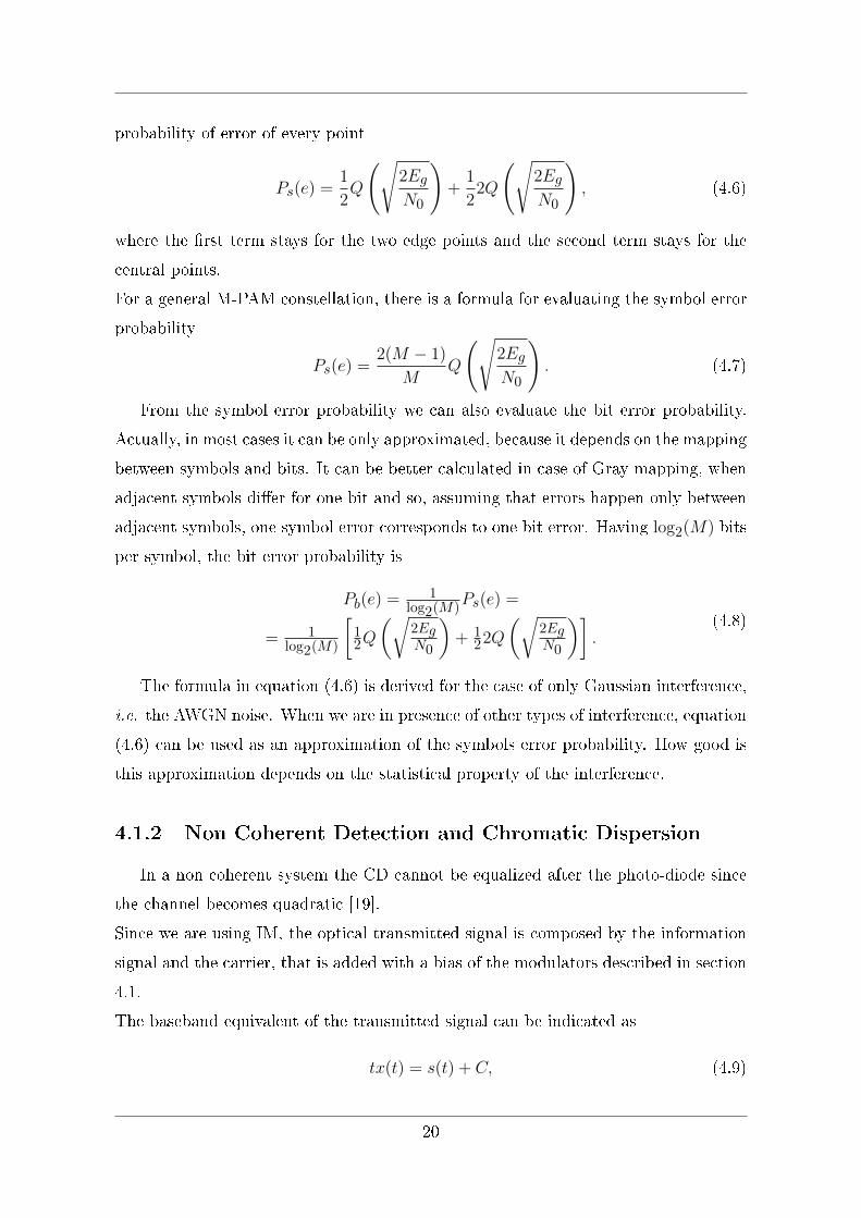
We can see that the signal is degraded by the cosine term, that creates notches in the
frequency domain in particular points of the spectrum. These notches correspond to
the argument of the cosine equal to π/2 + kπ.
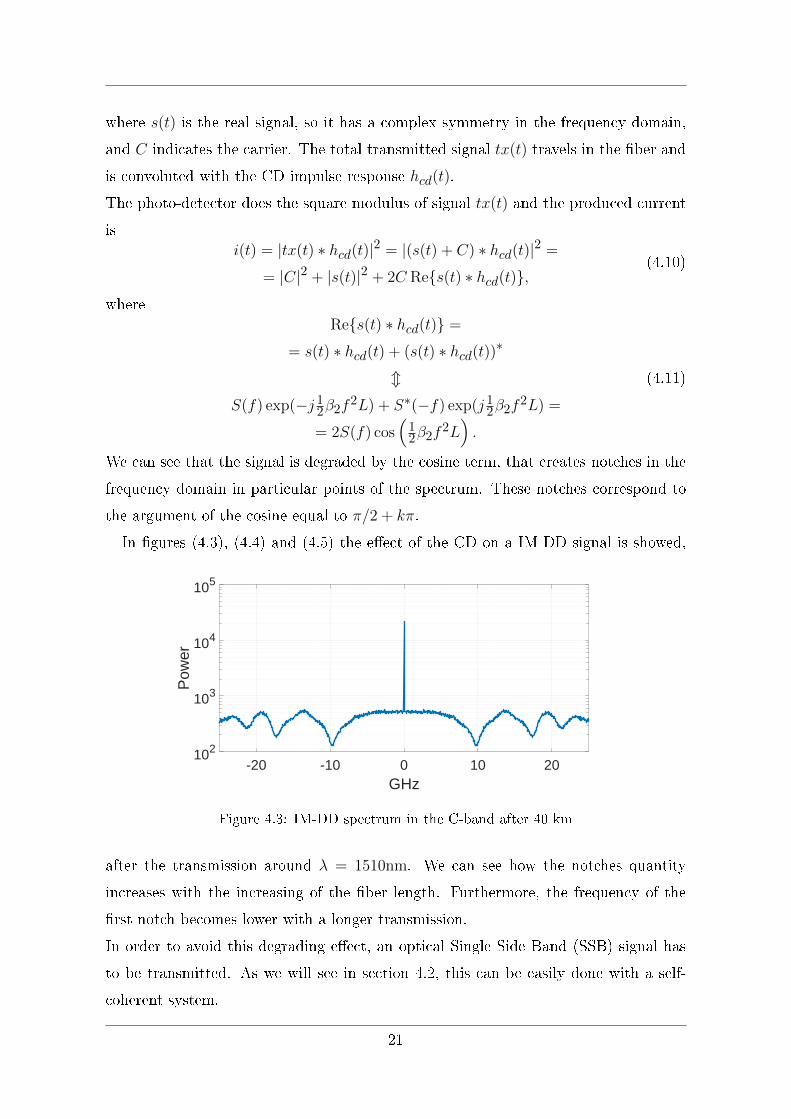
In �gures (4.3), (4.4) and (4.5) the e�ect of the CD on a IM-DD signal is showed,
-20 -10 0 10 20GHz
102
103
104
105
Pow
er
Figure 4.3: IM-DD spectrum in the C-band after 40 km
after the transmission around λ = 1510nm. We can see how the notches quantity
increases with the increasing of the �ber length. Furthermore, the frequency of the
�rst notch becomes lower with a longer transmission.
In order to avoid this degrading e�ect, an optical Single Side Band (SSB) signal has
to be transmitted. As we will see in section 4.2, this can be easily done with a self-
coherent system.
21
-20 -10 0 10 20GHz
102
103
104
105
Pow
er
Figure 4.4: IM-DD spectrum in the C-band after 60 km
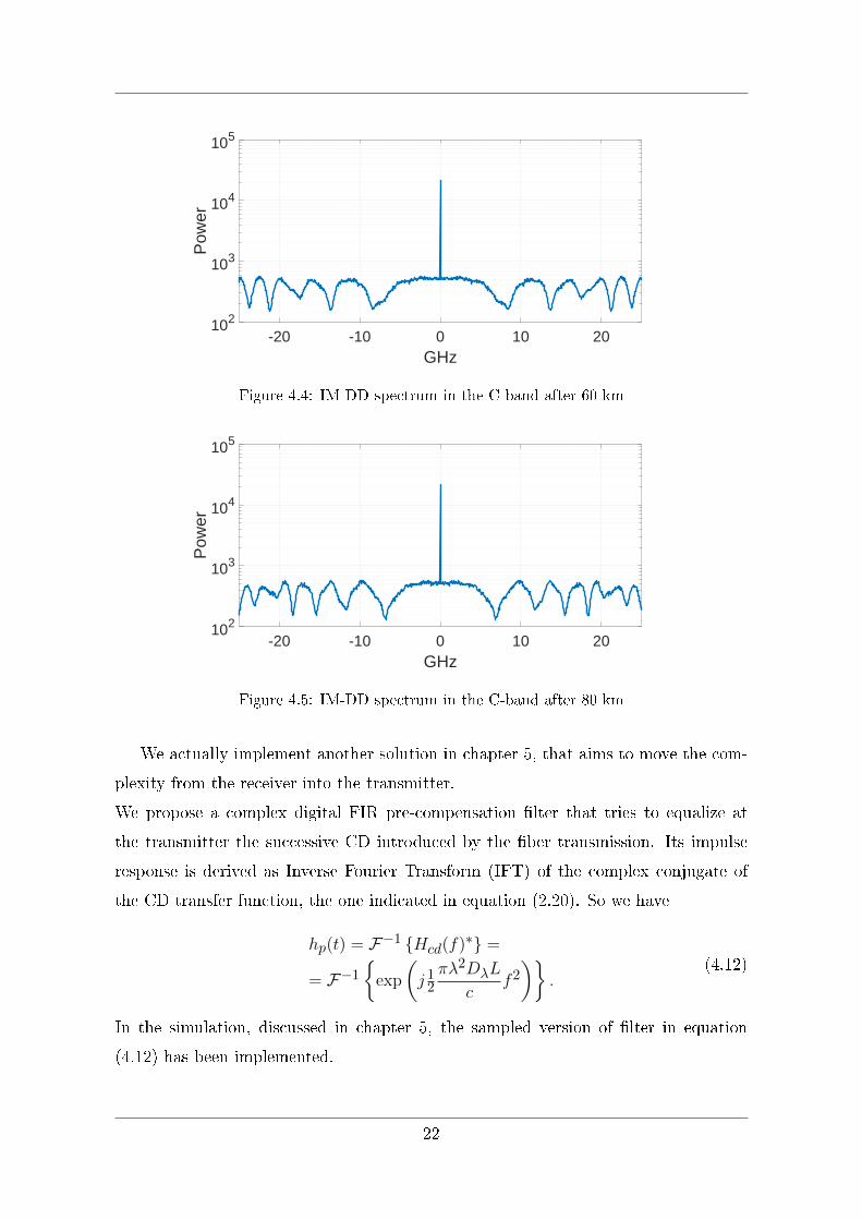
-20 -10 0 10 20GHz
102
103
104
105
Pow
er
Figure 4.5: IM-DD spectrum in the C-band after 80 km
We actually implement another solution in chapter 5, that aims to move the com-
plexity from the receiver into the transmitter.
We propose a complex digital FIR pre-compensation �lter that tries to equalize at
the transmitter the successive CD introduced by the �ber transmission. Its impulse
response is derived as Inverse Fourier Transform (IFT) of the complex conjugate of
the CD transfer function, the one indicated in equation (2.20). So we have
hp(t) = F−1 {Hcd(f)∗} =
= F−1{
exp
(j 12πλ2DλL
cf2)}
.(4.12)
In the simulation, discussed in chapter 5, the sampled version of �lter in equation
(4.12) has been implemented.
22
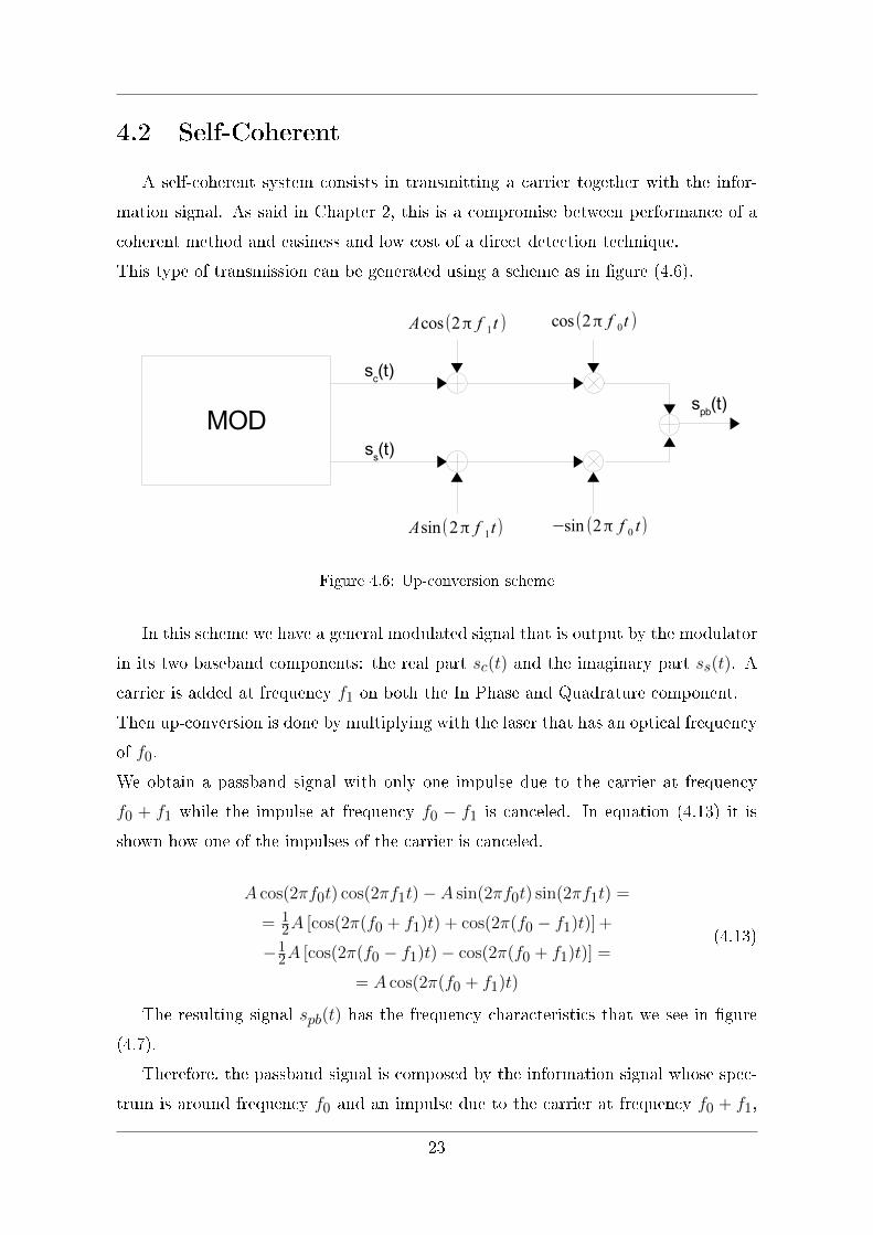
4.2 Self-Coherent
A self-coherent system consists in transmitting a carrier together with the infor-
mation signal. As said in Chapter 2, this is a compromise between performance of a
coherent method and easiness and low cost of a direct detection technique.
This type of transmission can be generated using a scheme as in �gure (4.6).
Figure 4.6: Up-conversion scheme
In this scheme we have a general modulated signal that is output by the modulator
in its two baseband components: the real part sc(t) and the imaginary part ss(t). A
carrier is added at frequency f1 on both the In Phase and Quadrature component.
Then up-conversion is done by multiplying with the laser that has an optical frequency
of f0.
We obtain a passband signal with only one impulse due to the carrier at frequency
f0 + f1 while the impulse at frequency f0 − f1 is canceled. In equation (4.13) it is
shown how one of the impulses of the carrier is canceled.
A cos(2πf0t) cos(2πf1t)− A sin(2πf0t) sin(2πf1t) =
= 12A [cos(2π(f0 + f1)t) + cos(2π(f0 − f1)t)] +
−12A [cos(2π(f0 − f1)t)− cos(2π(f0 + f1)t)] =
= A cos(2π(f0 + f1)t)
(4.13)
The resulting signal spb(t) has the frequency characteristics that we see in �gure
(4.7).
Therefore, the passband signal is composed by the information signal whose spec-
trum is around frequency f0 and an impulse due to the carrier at frequency f0 + f1,
23
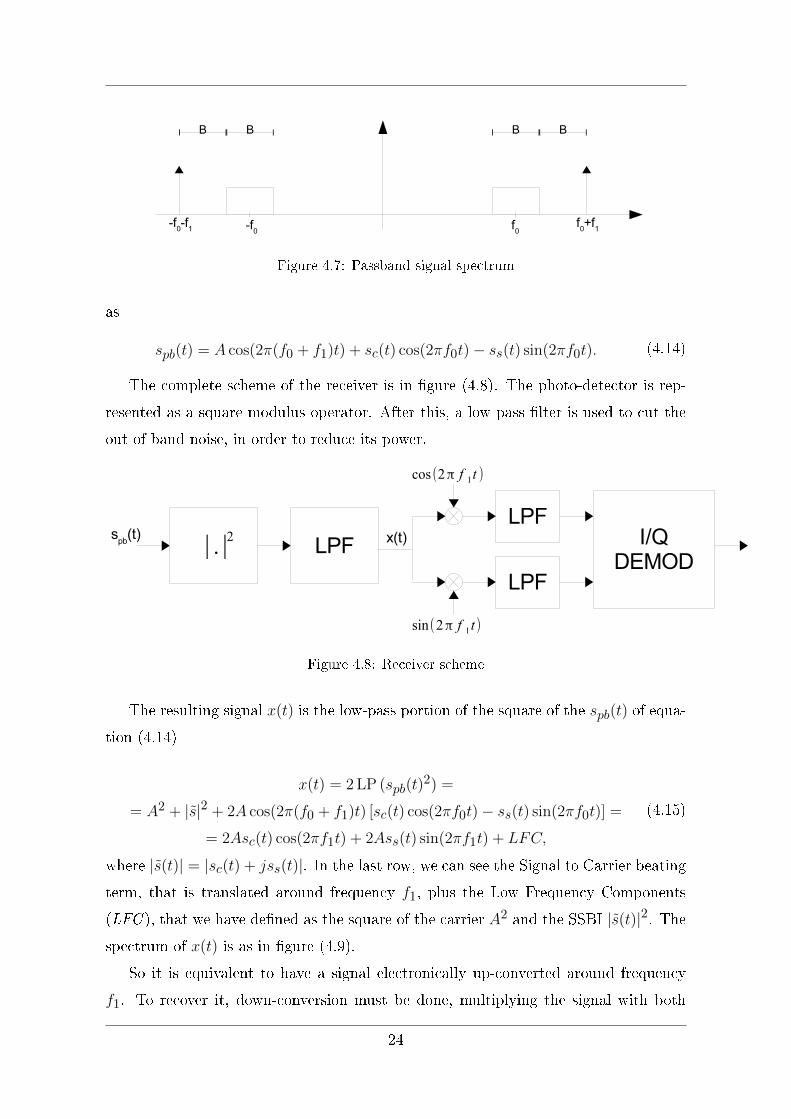
Figure 4.7: Passband signal spectrum
as
spb(t) = A cos(2π(f0 + f1)t) + sc(t) cos(2πf0t)− ss(t) sin(2πf0t). (4.14)
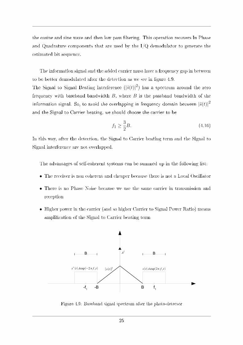
The complete scheme of the receiver is in �gure (4.8). The photo-detector is rep-
resented as a square modulus operator. After this, a low pass �lter is used to cut the
out of band noise, in order to reduce its power.
Figure 4.8: Receiver scheme
The resulting signal x(t) is the low-pass portion of the square of the spb(t) of equa-
tion (4.14)
x(t) = 2 LP (spb(t)2) =
= A2 + |s|2 + 2A cos(2π(f0 + f1)t) [sc(t) cos(2πf0t)− ss(t) sin(2πf0t)] =
= 2Asc(t) cos(2πf1t) + 2Ass(t) sin(2πf1t) + LFC,
(4.15)
where |s(t)| = |sc(t) + jss(t)|. In the last row, we can see the Signal to Carrier beatingterm, that is translated around frequency f1, plus the Low Frequency Components
(LFC ), that we have de�ned as the square of the carrier A2 and the SSBI |s(t)|2. Thespectrum of x(t) is as in �gure (4.9).
So it is equivalent to have a signal electronically up-converted around frequency
f1. To recover it, down-conversion must be done, multiplying the signal with both
24
the cosine and sine wave and then low pass �ltering. This operation recovers In Phase
and Quadrature components that are used by the I/Q demodulator to generate the
estimated bit sequence.
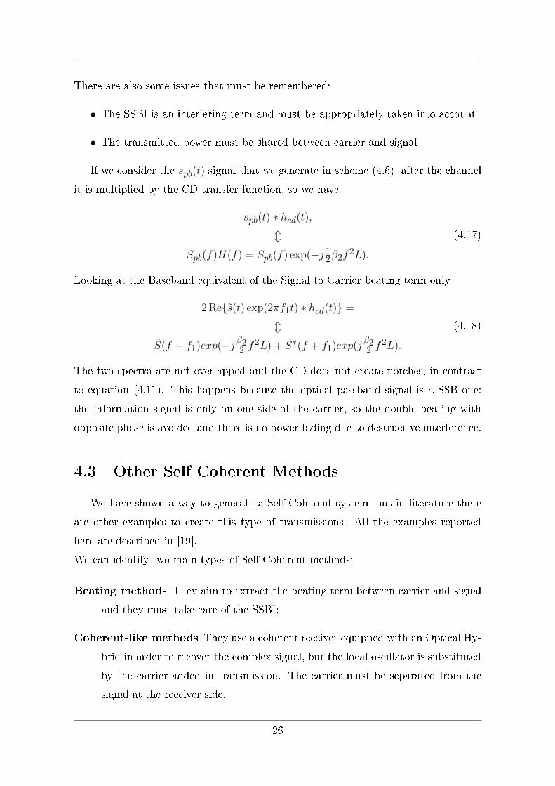
The information signal and the added carrier must have a frequency gap in between
to be better demodulated after the detection as we see in �gure 4.9.
The Signal to Signal Beating Interference (|s(t)|2) has a spectrum around the zero
frequency with baseband bandwidth B, where B is the passband bandwidth of the
information signal. So, to avoid the overlapping in frequency domain between |s(t)|2
and the Signal to Carrier beating, we should choose the carrier to be
f1 ≥3
2B. (4.16)
In this way, after the detection, the Signal to Carrier beating term and the Signal to
Signal interference are not overlapped.
The advantages of self-coherent systems can be summed up in the following list:
• The receiver is non coherent and cheaper because there is not a Local Oscillator
• There is no Phase Noise because we use the same carrier in transmission and
reception
• Higher power in the carrier (and so higher Carrier to Signal Power Ratio) means
ampli�cation of the Signal to Carrier beating term
Figure 4.9: Baseband signal spectrum after the photo-detector
25
There are also some issues that must be remembered:
• The SSBI is an interfering term and must be appropriately taken into account
• The transmitted power must be shared between carrier and signal
If we consider the spb(t) signal that we generate in scheme (4.6), after the channel
it is multiplied by the CD transfer function, so we have
spb(t) ∗ hcd(t),m
Spb(f)H(f) = Spb(f) exp(−j 12β2f2L).
(4.17)
Looking at the Baseband equivalent of the Signal to Carrier beating term only
2 Re{s(t) exp(2πf1t) ∗ hcd(t)} =
mS(f − f1)exp(−j β22 f
2L) + S∗(f + f1)exp(jβ22 f
2L).
(4.18)
The two spectra are not overlapped and the CD does not create notches, in contrast
to equation (4.11). This happens because the optical passband signal is a SSB one:
the information signal is only on one side of the carrier, so the double beating with
opposite phase is avoided and there is no power fading due to destructive interference.
4.3 Other Self Coherent Methods
We have shown a way to generate a Self Coherent system, but in literature there
are other examples to create this type of transmissions. All the examples reported
here are described in [19].
We can identify two main types of Self Coherent methods:
Beating methods They aim to extract the beating term between carrier and signal
and they must take care of the SSBI;
Coherent-like methods They use a coherent receiver equipped with an Optical Hy-
brid in order to recover the complex signal, but the local oscillator is substituted
by the carrier added in transmission. The carrier must be separated from the
signal at the receiver side.
26

Beating methods:
• O�set SSB
• Virtual SSB
• Block-wise Phase Switching (BPS)
Coherent-like methods:
• Signal Carrier Interleaved (SCI)
• Dual Polarization SCI (DP-SCI)
• Signal Carrier Pol-Mux with Stokes Vector (SV) receiver
4.3.1 Beating Methods
If we want to extract the beating term between carrier and signal, we have to create
an optical Single Side Band signal, similar to what we did in scheme (4.6). This avoids
the creation of notches in the spectrum as in equation (4.11).
O�set SSB
The �rst way to generate an SSB signal suppresses one sideband using an optical
�lter, after having directly modulated the laser with the signal [20]. The signal is
previously complex upconverted at fRF as in �gure (4.10). The carrier is added at
the laser frequency, thanks to the bias of the intensity modulation.
Figure 4.10: Optically �ltered SSB
The receiver in �gure (4.11) must do IQ demodulation on the detected signal that
corresponds to a baseband signal up-converted to frequency frf . This receiver scheme
27
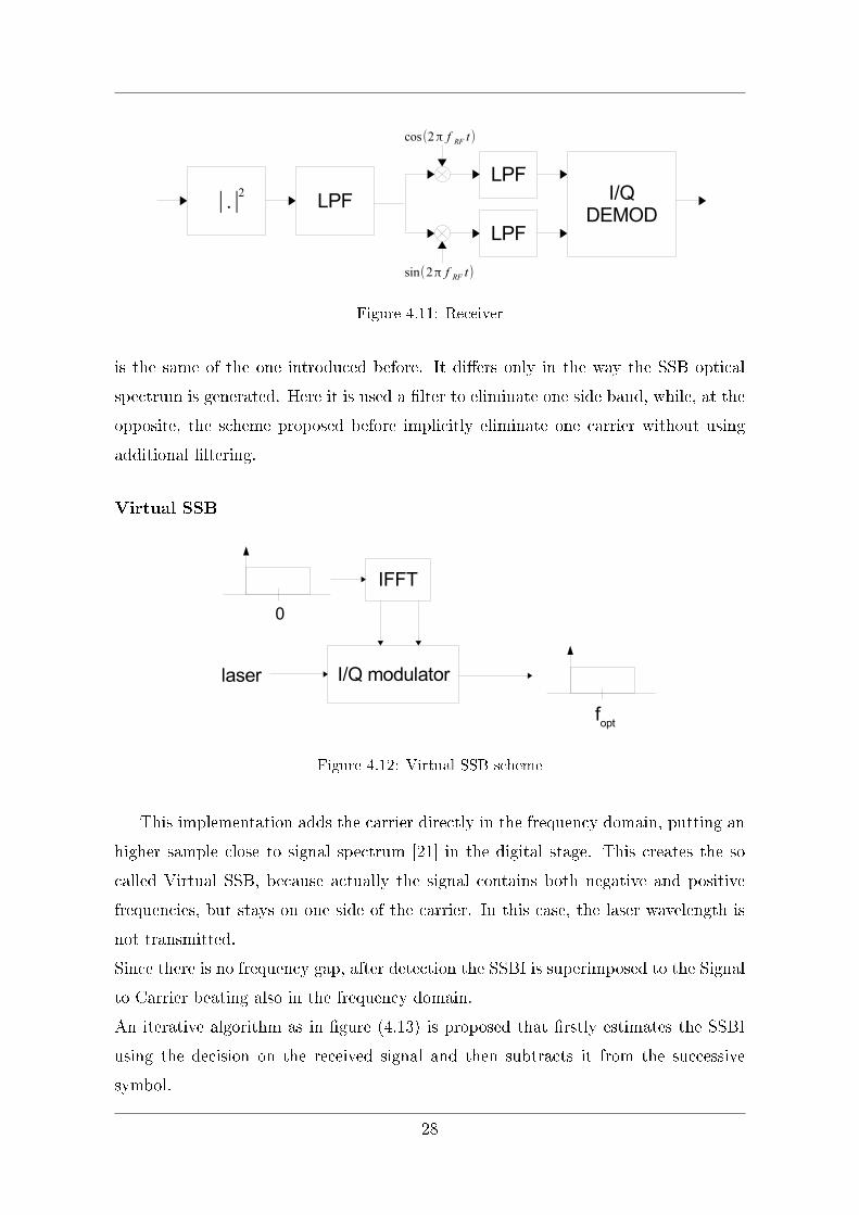
Figure 4.11: Receiver
is the same of the one introduced before. It di�ers only in the way the SSB optical
spectrum is generated. Here it is used a �lter to eliminate one side band, while, at the
opposite, the scheme proposed before implicitly eliminate one carrier without using
additional �ltering.
Virtual SSB
Figure 4.12: Virtual SSB scheme
This implementation adds the carrier directly in the frequency domain, putting an
higher sample close to signal spectrum [21] in the digital stage. This creates the so
called Virtual SSB, because actually the signal contains both negative and positive
frequencies, but stays on one side of the carrier. In this case, the laser wavelength is
not transmitted.
Since there is no frequency gap, after detection the SSBI is superimposed to the Signal
to Carrier beating also in the frequency domain.
An iterative algorithm as in �gure (4.13) is proposed that �rstly estimates the SSBI
using the decision on the received signal and then subtracts it from the successive
symbol.
28
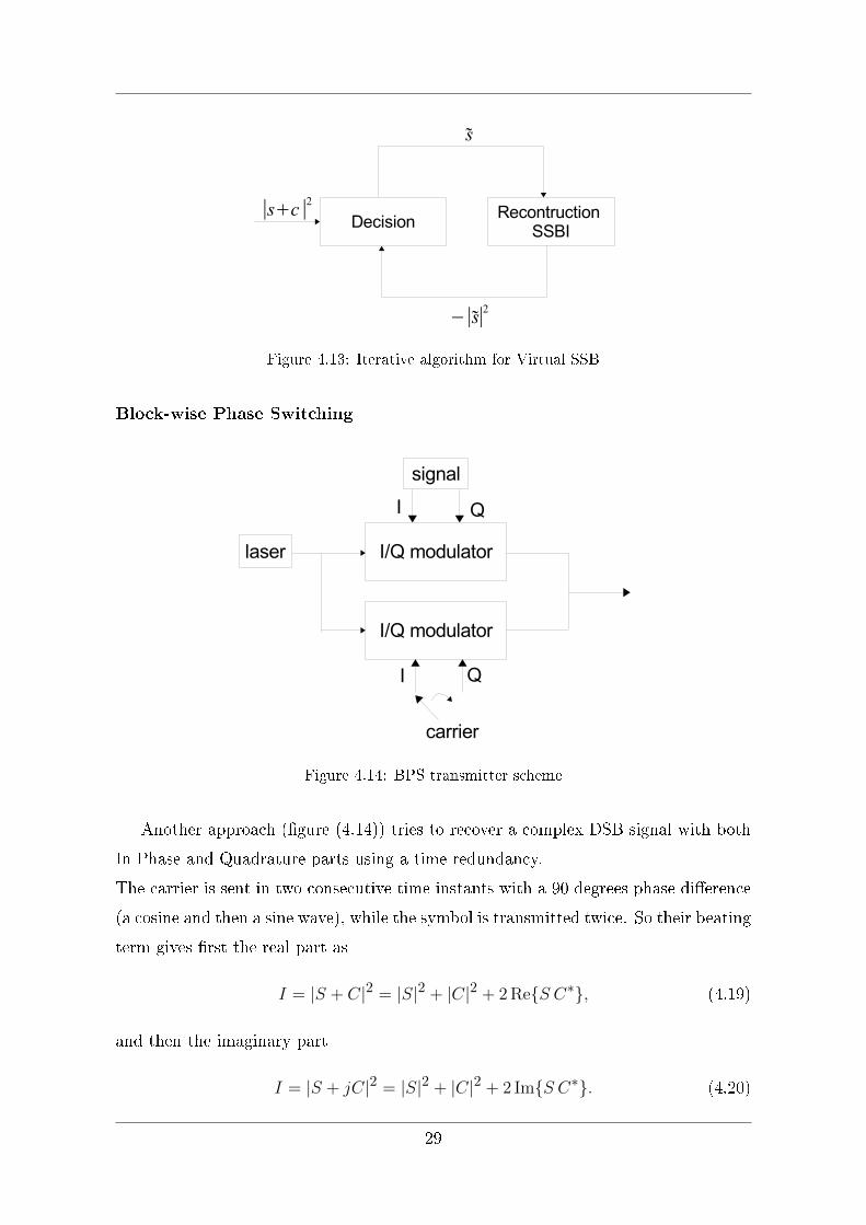
Figure 4.13: Iterative algorithm for Virtual SSB
Block-wise Phase Switching
Figure 4.14: BPS transmitter scheme
Another approach (�gure (4.14)) tries to recover a complex DSB signal with both
In Phase and Quadrature parts using a time redundancy.
The carrier is sent in two consecutive time instants with a 90 degrees phase di�erence
(a cosine and then a sine wave), while the symbol is transmitted twice. So their beating
term gives �rst the real part as
I = |S + C|2 = |S|2 + |C|2 + 2 Re{S C∗}, (4.19)
and then the imaginary part
I = |S + jC|2 = |S|2 + |C|2 + 2 Im{S C∗}. (4.20)
29
This scheme is called Block-wise Phase Switching (BPS) [22] since we can divide
transmission in blocks.
It is not speci�ed how to handle the SSBI, but similarly as before a frequency separation
can be applied.
4.3.2 Coherent-like Methods
This type of approaches recovers simultaneously both real and imaginary part using
a coherent receiver, that naturally eliminates the SSBI.
These solutions have higher costs with respect to the previous ones, since optical hybrid
is used and also polarization is exploited to increase spectral e�ciency. The various
methods di�er in the way they separate carrier and signal.
The simplest scheme acts this separation in the frequency domain. It adds the
carrier introducing a bias to the laser [19]. At the receiver the total beam is split: on
a branch the carrier is �ltered and used as input of the optical hybrid, that combines
it with the signal, isolated on the other branch, to give in output the In Phase and
Quadrature parts. This means that a frequency gap must be added and that it must
be used a narrow band �lter at the receiver.
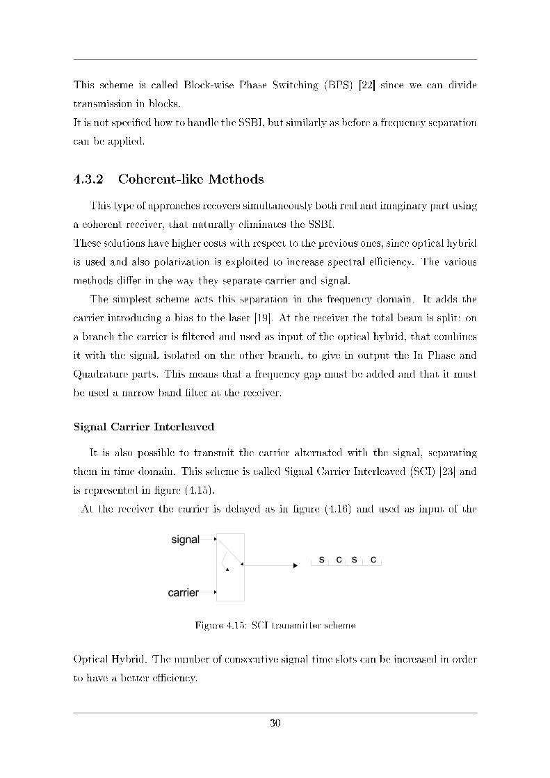
Signal Carrier Interleaved
It is also possible to transmit the carrier alternated with the signal, separating
them in time domain. This scheme is called Signal Carrier Interleaved (SCI) [23] and
is represented in �gure (4.15).
At the receiver the carrier is delayed as in �gure (4.16) and used as input of the
Figure 4.15: SCI transmitter scheme
Optical Hybrid. The number of consecutive signal time slots can be increased in order
to have a better e�ciency.
30
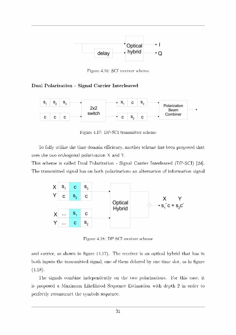
Figure 4.16: SCI receiver scheme
Dual Polarization - Signal Carrier Interleaved
Figure 4.17: DP-SCI transmitter scheme
To fully utilize the time domain e�ciency, another scheme has been proposed that
uses the two orthogonal polarization X and Y.
This scheme is called Dual Polarization - Signal Carrier Interleaved (DP-SCI) [24].
The transmitted signal has on both polarizations an alternation of information signal
Figure 4.18: DP-SCI receiver scheme
and carrier, as shown in �gure (4.17). The receiver is an optical hybrid that has in
both inputs the transmitted signal, one of them delayed by one time slot, as in �gure
(4.18).
The signals combine independently on the two polarizations. For this case, it
is proposed a Maximum Likelihood Sequence Estimation with depth 2 in order to
perfectly reconstruct the symbols sequence.
31
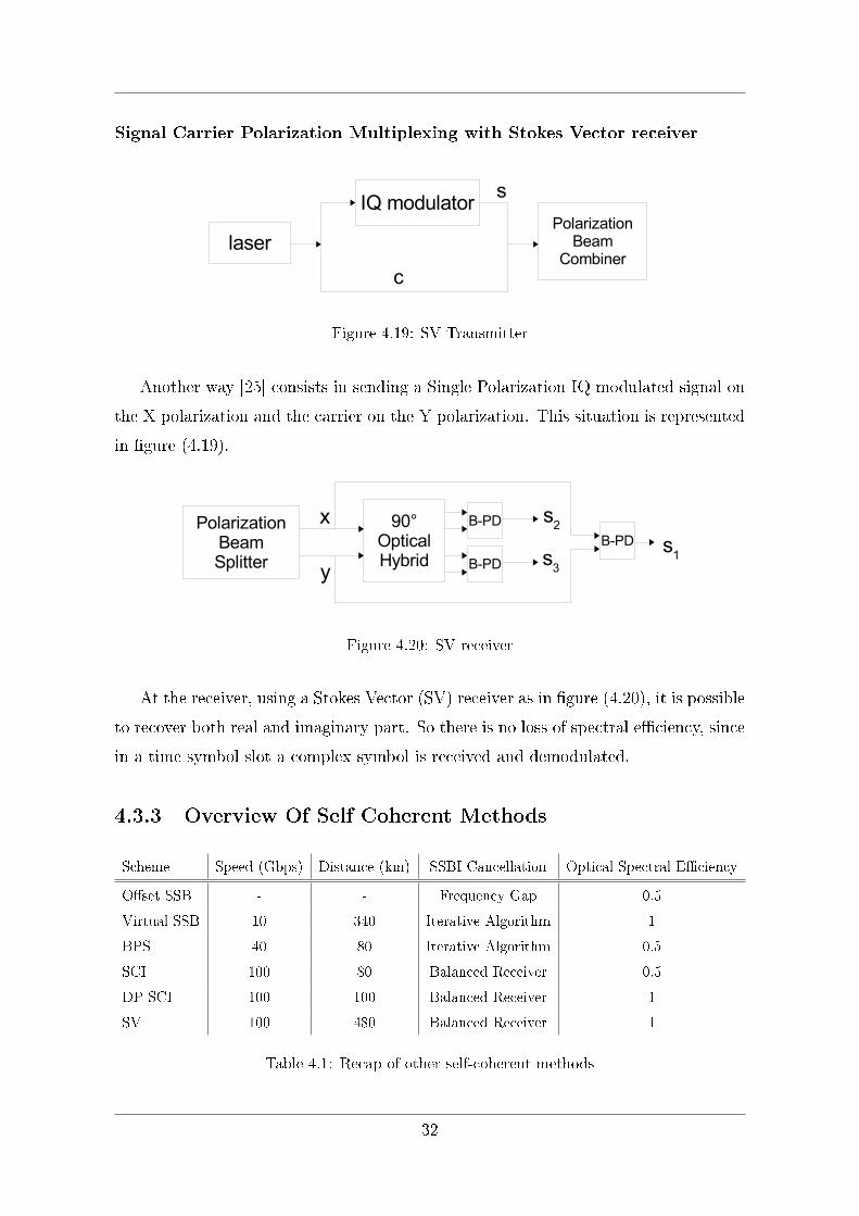
Signal Carrier Polarization Multiplexing with Stokes Vector receiver
Figure 4.19: SV Transmitter
Another way [25] consists in sending a Single Polarization IQ modulated signal on
the X polarization and the carrier on the Y polarization. This situation is represented
in �gure (4.19).
Figure 4.20: SV receiver
At the receiver, using a Stokes Vector (SV) receiver as in �gure (4.20), it is possible
to recover both real and imaginary part. So there is no loss of spectral e�ciency, since
in a time symbol slot a complex symbol is received and demodulated.
4.3.3 Overview Of Self Coherent Methods
Scheme Speed (Gbps) Distance (km) SSBI Cancellation Optical Spectral E�ciency
O�set SSB - - Frequency Gap 0.5
Virtual SSB 10 340 Iterative Algorithm 1
BPS 40 80 Iterative Algorithm 0.5
SCI 100 80 Balanced Receiver 0.5
DP-SCI 100 100 Balanced Receiver 1
SV 100 480 Balanced Receiver 1
Table 4.1: Recap of other self-coherent methods
32

In the table (4.1) all the previous schemes are summed up with information on max-
imum throughput, reached distance, types of SSBI cancellation method and spectral
e�ciencies.
33
Chapter 5
Simulation Results
The aim of this chapter is to describe how the Montecarlo simulations have been
implemented and to introduce the parameters that are used to evaluate the perfor-
mance.
Furthermore, the obtained results are showed and commented for two types of �lter-
ing in transmission: a rectangular �lter, that has a constant value in the symbol time
duration and it is zero elsewhere, and a �lter similar to the RC function introduced
in chapter 3, but with a equi-ripple characteristic, so with more attenuated frequency
side lobes.
5.1 Introduction
The thesis activity has been carried on with the help of a simulator that was built
with the MATLAB R© software.
Di�erent types of Montecarlo simulations have been carried out to evaluate both nu-
merically and graphically the e�ects of the Chromatic Dispersion on our system in
terms of performance.
The simulations have been developed to visualize the performance changing due
to variations of the mismatch percentage between the pre-compensation �lter and
the actual �ber CD transfer function. The main parameter that we have taken into
account is the Bit Error Rate (BER). We also introduced the Signal to Distortion Ratio
(SDR) and the Error Vector Magnitude (EVM) as performance indicators. The study
is focused on two types of transmission �lter, both respecting the Nyquist criterion.
One is a rectangular �lter, typically used in the NRZ transmissions, and the other is
34
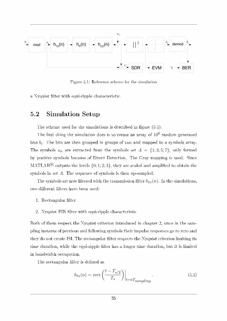
Figure 5.1: Reference scheme for the simulation
a Nyquist �lter with equi-ripple characteristic.
5.2 Simulation Setup
The scheme used for the simulations is described in �gure (5.1).
The �rst thing the simulation does is to create an array of 106 random generated
bits bi. The bits are then grouped in groups of two and mapped to a symbols array.
The symbols an are extracted from the symbols set A = {1; 3; 5; 7}, only formed
by positive symbols because of Direct Detection. The Gray mapping is used. Since
MATLAB R© outputs the levels {0; 1; 2; 3}, they are scaled and ampli�ed to obtain the
symbols in set A. The sequence of symbols is then up-sampled.
The symbols are now �ltered with the transmission �lter htx(n). In the simulations,
two di�erent �lters have been used:
1. Rectangular �lter
2. Nyquist FIR �lter with equi-ripple characteristic
Both of them respect the Nyquist criterion introduced in chapter 2, since in the sam-
pling instants of previous and following symbols their impulse responses go to zero and
they do not create ISI. The rectangular �lter respects the Nyquist criterion limiting its
time duration, while the equi-ripple �lter has a longer time duration, but it is limited
in bandwidth occupation.
The rectangular �lter is de�ned as
htx(n) = rect
(t− Ts/2Ts
)∣∣∣∣t=nTsampling
. (5.1)
35
-10 -8 -6 -4 -2 0 2 4 6 8 10Ts/2
0
0.5
1
1.5
Am
plitu
de
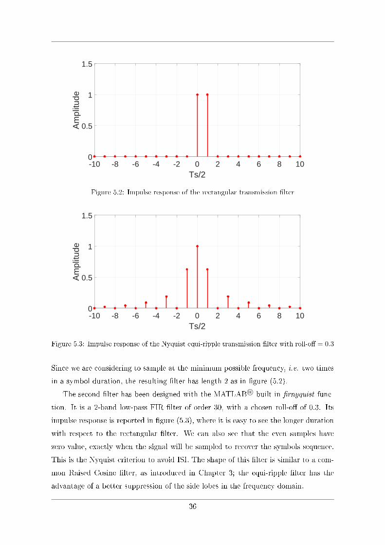
Figure 5.2: Impulse response of the rectangular transmission �lter
-10 -8 -6 -4 -2 0 2 4 6 8 10Ts/2
0
0.5
1
1.5
Am
plitu
de
Figure 5.3: Impulse response of the Nyquist equi-ripple transmission �lter with roll-o� = 0.3
Since we are considering to sample at the minimum possible frequency, i.e. two times
in a symbol duration, the resulting �lter has length 2 as in �gure (5.2).
The second �lter has been designed with the MATLAB R© built in �rnyquist func-
tion. It is a 2-band low-pass FIR �lter of order 30, with a chosen roll-o� of 0.3. Its
impulse response is reported in �gure (5.3), where it is easy to see the longer duration
with respect to the rectangular �lter. We can also see that the even samples have
zero value, exactly when the signal will be sampled to recover the symbols sequence.
This is the Nyquist criterion to avoid ISI. The shape of this �lter is similar to a com-
mon Raised Cosine �lter, as introduced in Chapter 3; the equi-ripple �lter has the
advantage of a better suppression of the side lobes in the frequency domain.
36
After the transmission �lter, always referring as scheme in �gure (5.1), the pre-
compensation �lter is introduced: its impulse response is derived as Inverse Discrete
Fourier Transform (IDFT) of the complex conjugate of the CD transfer function, as
said in chapter 4 in equation (4.12). The discrete-time impulse response hp(n) is
obtained by approximating the computation of inverse Fourier transform with Inverse
Discrete Fourier Transform (IDFT), where a sampling in frequency domain is chosen
to avoid aliasing in time-domain, so
hp(n) = IDFT−1 {Hcd(fk)∗} =
= IDFT−1{
exp
(j 12πλ2DλL
cf2k
)}.
(5.2)
The IDFT is evaluated with Inverse Fast Fourier Transform (IFFT) algorithm, with a
chosen number of frequency samples equal to NFFT = 1024.
The parameters that have been used in the simulations are:
• λ = 1.54294 nm
• D = 16.5 ps/nm/km
• L = 80 km
• fmax = 50GHz
The �rst two parameters are typical of a C-band utilization of a Single Mode Fiber,
while a length of 80 km is used as a reference value for the medium reach applications.
The fmax is chosen equal to 50GHz because we are considering a 50Gbaud PAM-4
signal and we are sampling at the Nyquist frequency.
Since we want to represent a system with total bit rate of 100Gbps and we are using
a PAM-4 modulation, the symbol rate is found to be Rs = Rb/ log2(M) = 50Gbaud.
Up-sampling by 2 the symbols sequence, we obtain a sampling frequency of fs =
100GHz.
After up-sampling, the CD is applied, making the convolution with the IDFT of the
sampled version of equation (2.20).
The parameters used for this �lter have been chosen with varying values, in order
to account for misalignment in the pre-compensation. In particular, what is varying
37

is the percentage of the product Dλ ∗ L, so the actual CD transfer function is
Hcd(f) = exp
(−j 1
2
πλ2DλL(1 +m)
cf2), (5.3)
where 0 < m < 1 is the percentage of mismatch.
After the CD, before the photo-detector, the array of symbols is �rstly cut to take
care of the delay introduced of the two convolutions and then it is down-sampled by
2.
The channel introduces the discrete time zero-mean complex Gaussian noise wn with
variance σ2w. Then the photo-detector is represented as a square modulus operator,
since it is proportional only to intensity of the optical �eld, as seen in equation (2.3).
Independent decisions are taken by comparison with equally spaced thresholds
centered at the medium distance between constellation points. If we assume not to
have noise, the output an must be the square of the transmitted symbols sequence an.
So a square root operator, not represented in the scheme, is used to bring back the
points at they levels in set A. After decision, the following de-mapping extract from
the estimated symbols sequence the estimated bits stream bi. These last operations
are in inverse order with respect to the sequence of operations that we have done at
the beginning.
The signal before the photo-detector is the result between the two successive con-
volution with pre-compensation and CD �lter. It can be represented as
rn = an ⊗ hm(n) + wn, (5.4)
where ⊗ denotes the discrete convolution and
hm(n) = hp(n)⊗ hcd(n), (5.5)
is the impulse response of the cascade of the two �lters. In ideal case of perfect
pre-compensation, hm(n) is the Kronecker delta
δn =
1, n = 0,
0, n 6= 0.(5.6)
In all the other cases, when the pre-compensation �lter does not equalize perfectly the
CD, hm(n) is longer than one and ISI arises. The received symbols are overlapped
with the tails of the impulse responses of the previous symbols and this generates
38
performance degradations.
The results that are showed in the following are valid both for positive and negative
mismatch m, since the CD has a symmetry in its frequency response and also in the
time domain impulse response.
5.3 Measures of Performance
The simulations analyze this type of performance indicators:
• Signal-to-Distortion Ratio (SDR)
• Bit Error Rate (BER)
• Error Vector Magnitude (EVM)
• Scatter Plot
5.3.1 Signal-to-Distortion Ratio
The SDR measures the quality of the signal at the input of the photo-detector. It
is de�ned as the ratio between the power of the desired signal and the power of the
total distortion, that in our case is the sum between the power of the noise and the
power of the ISI. So we have
SDR =Pa
PISI + SNR−1Pa. (5.7)
The power of the desired signal is calculated as average between the square of the
possible values of the constellation an, so
Pa =1
|A|
|A|−1∑i=0
a2i = 21, (5.8)
where |A| is the cardinality of the set A.The SNR is the Signal-to-Noise Ratio and it is de�ned as the ratio between Pa and
the variance of the Gaussian noise
SNR =Paσ2w
. (5.9)
39
In absence of ISI, when we have perfect pre-compensation, the SNR and the SDR
coincide, since we have SDR =Pa
SNR−1Pa= SNR.
The power of the ISI term is calculated as
PISI = Pa∑k
|1− hm(k)|2 . (5.10)
Obviously, this implies to know the shape the impulse response hm(n), so to know the
mismatch and the residual Chromatic Dispersion. Consequently, the SDR de�ned in
equation (5.7) is not possible to be known at the receiver, especially for the case of
Direct Detection that we are implementing. Anyway, in the simulation environment
where the parameters are decided by us, it is easy to calculate the SDR. In �gure
(5.1) it is shown that the SDR is evaluated before the photo-detector and it uses the
computing of the power of the error sequence en.
5.3.2 Bit Error Rate
In the simulation, the BER performance has been evaluated by comparing the
transmitted bit sequence with the estimated one, produced at the output of the de-
modulator. The number of errors obtained by this comparing has been divided by the
total number of transmitted bits.
An estimation of BER can be considered good if the total number of errors is greater
or equal to 100. Therefore, having generated 106 random bits, BER can be considered
well estimated for values not lower then 10−4.
The evaluation of the BER has been carried out by varying the SNR or the mis-
match percentage, or both.
5.3.3 Error Vector Magnitude (EVM)
EVM is a measure of the quality of a communication system. It describes the
absolute distance between the received complex symbols and the ideal point of the
constellation. It is used in the wireless communications and if it is a�ected by Gaussian
noise, a relation with the BER has already been found. In [26] and [27] the estimation
of the BER using the EVM is extended to optical communications.
EVM measurements can be data-aided or non-data-aided. The data-aided EVM
can be calculated using a training sequence that is known both at the transmitter
40
and at the receiver. So correct data are used to evaluate EVM. In the latter case the
symbols sequence is not known and the decisions are used to be the reference points
for estimating EVM.
In case of non-data-aided EVM, if the BER is too high, the measurements bring to an
underestimation of the real value of the EVM. This happens because, when distortion
is high, the received symbol can be very far from the transmitted one. It can bring to
an error in the decision, since the decision device chooses for the nearest constellation
point, and so to a smaller EVM contribute.
Consequently, non-data-aided EVM is a good performance metric only for big enough
SDR.
The data-aided EVM is de�ned as
EVM =
√1/K
∑Kk=1 |rk − ak|2
Pa, (5.11)
where rk is the received symbol and ak is the correspondent transmitted one. K is the
number of symbols used to averaging and Pa is the average symbols power, evaluated
in equation (5.8). As it is shown in �gure (5.1), the EVM is calculated before the
threshold detector, at the output of the photo-detector. From the EVM we estimate
a SDR, denoted as Estimated SDR (SDRest). They are linked by
EVM =
√1
SDRest. (5.12)
This SDRest is di�erent from the SDR evaluated in equation (5.7), because the last
one was referred to the signal before the photo-detector and it was calculated having
access at the �eld information. The SDRest is instead based only on the intensity
information of the signal after the non-coherent receiver.
Similarly to equation (5.11), the non-data-aided EVM is de�ned as
EVM =
√1/K
∑Kk=1 |rk − ak|2
Pa, (5.13)
where now ak denotes the sequence of decisions made on the received symbols.
When the SDR is high, we have that ak = ak and so the non-data-aided EVM corre-
sponds to the data-aided EVM.
41
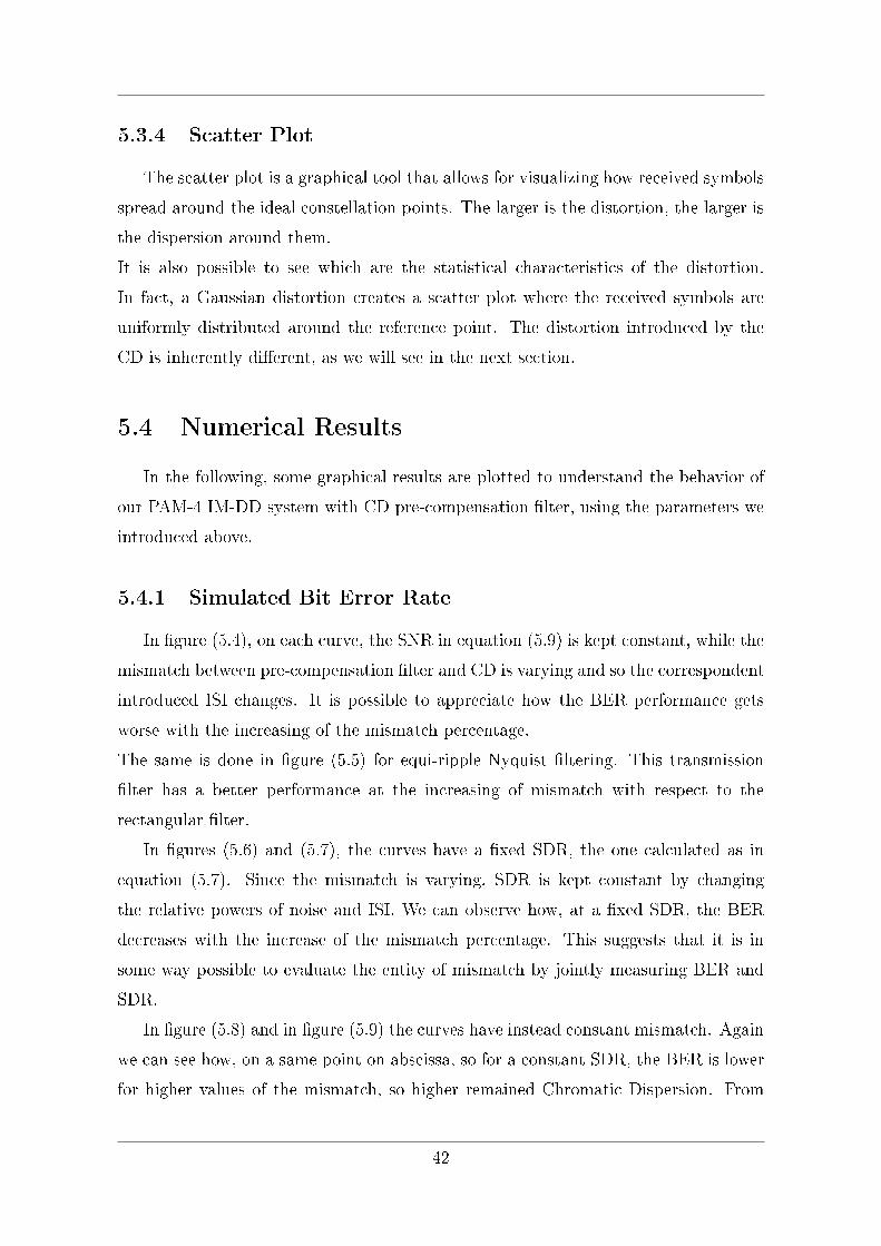
5.3.4 Scatter Plot
The scatter plot is a graphical tool that allows for visualizing how received symbols
spread around the ideal constellation points. The larger is the distortion, the larger is
the dispersion around them.
It is also possible to see which are the statistical characteristics of the distortion.
In fact, a Gaussian distortion creates a scatter plot where the received symbols are
uniformly distributed around the reference point. The distortion introduced by the
CD is inherently di�erent, as we will see in the next section.
5.4 Numerical Results
In the following, some graphical results are plotted to understand the behavior of
our PAM-4 IM-DD system with CD pre-compensation �lter, using the parameters we
introduced above.
5.4.1 Simulated Bit Error Rate
In �gure (5.4), on each curve, the SNR in equation (5.9) is kept constant, while the
mismatch between pre-compensation �lter and CD is varying and so the correspondent
introduced ISI changes. It is possible to appreciate how the BER performance gets
worse with the increasing of the mismatch percentage.
The same is done in �gure (5.5) for equi-ripple Nyquist �ltering. This transmission
�lter has a better performance at the increasing of mismatch with respect to the
rectangular �lter.
In �gures (5.6) and (5.7), the curves have a �xed SDR, the one calculated as in
equation (5.7). Since the mismatch is varying, SDR is kept constant by changing
the relative powers of noise and ISI. We can observe how, at a �xed SDR, the BER
decreases with the increase of the mismatch percentage. This suggests that it is in
some way possible to evaluate the entity of mismatch by jointly measuring BER and
SDR.
In �gure (5.8) and in �gure (5.9) the curves have instead constant mismatch. Again
we can see how, on a same point on abscissa, so for a constant SDR, the BER is lower
for higher values of the mismatch, so higher remained Chromatic Dispersion. From
42

-6 -5 -4 -3 -2 -1 0% Mismatch
10-510-5
10-4
10-3
10-2
10-1
100
BE
R
SNR = 5 dBSNR = 10 dBSNR = 15 dBSNR = 20 dBSNR = 25 dB
Figure 5.4: BER vs mismatch: rectangular �lter
-6 -5 -4 -3 -2 -1 0% Mismatch
10-5
10-4
10-3
10-2
10-1
100
BE
R
SNR = 5 dB - NyquistSNR = 10 dB - NyquistSNR = 15 dB - NyquistSNR = 20 dB - NyquistSNR = 25 dB - Nyquist
Figure 5.5: BER vs mismatch: Nyquist equi-ripple �lter
these �gures and the previous ones we can observe that, when the power of the total
distortion is dominated by ISI that actually is not Gaussian, there are less errors than
what expected from the Gaussian approximation.
43
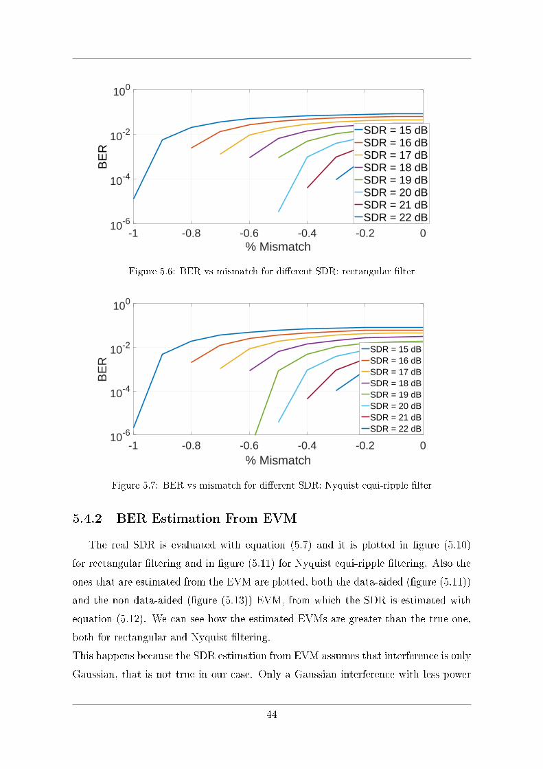
-1 -0.8 -0.6 -0.4 -0.2 0% Mismatch
10-6
10-4
10-2
100
BE
R
SDR = 15 dBSDR = 16 dBSDR = 17 dBSDR = 18 dBSDR = 19 dBSDR = 20 dBSDR = 21 dBSDR = 22 dB
Figure 5.6: BER vs mismatch for di�erent SDR: rectangular �lter
-1 -0.8 -0.6 -0.4 -0.2 0% Mismatch
10-6
10-4
10-2
100
BE
R
SDR = 15 dBSDR = 16 dBSDR = 17 dBSDR = 18 dBSDR = 19 dBSDR = 20 dBSDR = 21 dBSDR = 22 dB
Figure 5.7: BER vs mismatch for di�erent SDR: Nyquist equi-ripple �lter
5.4.2 BER Estimation From EVM
The real SDR is evaluated with equation (5.7) and it is plotted in �gure (5.10)
for rectangular �ltering and in �gure (5.11) for Nyquist equi-ripple �ltering. Also the
ones that are estimated from the EVM are plotted, both the data-aided (�gure (5.11))
and the non data-aided (�gure (5.13)) EVM, from which the SDR is estimated with
equation (5.12). We can see how the estimated EVMs are greater than the true one,
both for rectangular and Nyquist �ltering.
This happens because the SDR estimation from EVM assumes that interference is only
Gaussian, that is not true in our case. Only a Gaussian interference with less power
44
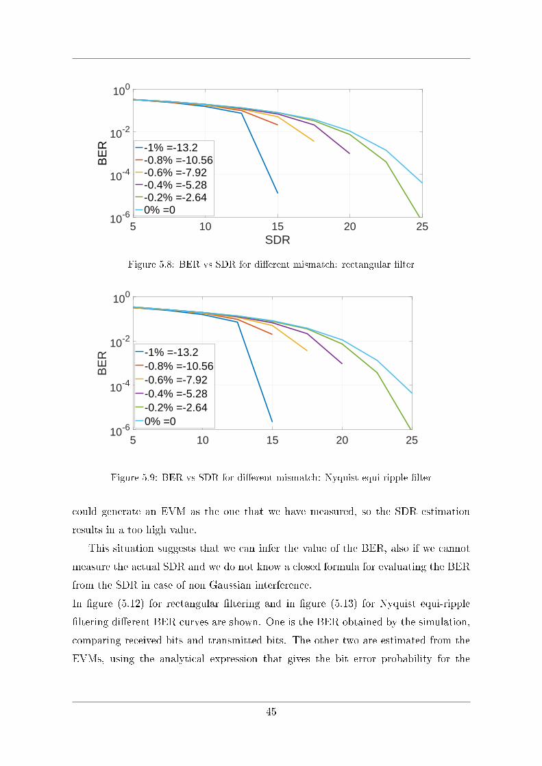
5 10 15 20 25SDR
10-6
10-4
10-2
100
BE
R -1% =-13.2-0.8% =-10.56-0.6% =-7.92-0.4% =-5.28-0.2% =-2.640% =0
Figure 5.8: BER vs SDR for di�erent mismatch: rectangular �lter
5 10 15 20 2510-6
10-4
10-2
100
BE
R -1% =-13.2-0.8% =-10.56-0.6% =-7.92-0.4% =-5.28-0.2% =-2.640% =0
Figure 5.9: BER vs SDR for di�erent mismatch: Nyquist equi-ripple �lter
could generate an EVM as the one that we have measured, so the SDR estimation
results in a too high value.
This situation suggests that we can infer the value of the BER, also if we cannot
measure the actual SDR and we do not know a closed formula for evaluating the BER
from the SDR in case of non Gaussian interference.
In �gure (5.12) for rectangular �ltering and in �gure (5.13) for Nyquist equi-ripple
�ltering di�erent BER curves are shown. One is the BER obtained by the simulation,
comparing received bits and transmitted bits. The other two are estimated from the
EVMs, using the analytical expression that gives the bit error probability for the
45
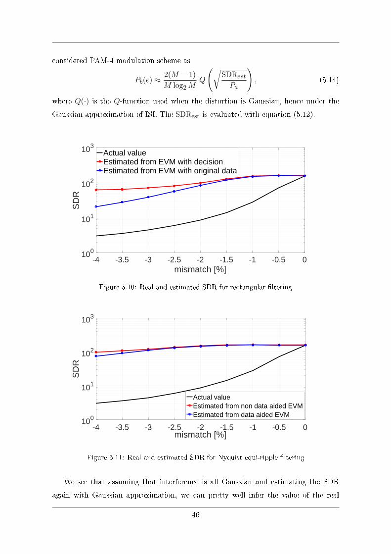
considered PAM-4 modulation scheme as
Pb(e) ≈2(M − 1)
M log2MQ
(√SDRestPa
), (5.14)
where Q(·) is the Q-function used when the distortion is Gaussian, hence under the
Gaussian approximation of ISI. The SDRest is evaluated with equation (5.12).
-4 -3.5 -3 -2.5 -2 -1.5 -1 -0.5 0mismatch [%]
100
101
102
103
SD
R
Actual valueEstimated from EVM with decisionEstimated from EVM with original data
Figure 5.10: Real and estimated SDR for rectangular �ltering
-4 -3.5 -3 -2.5 -2 -1.5 -1 -0.5 0mismatch [%]
100
101
102
103
SD
R
Actual valueEstimated from non data aided EVMEstimated from data aided EVM
Figure 5.11: Real and estimated SDR for Nyquist equi-ripple �ltering
We see that assuming that interference is all Gaussian and estimating the SDR
again with Gaussian approximation, we can pretty well infer the value of the real
46
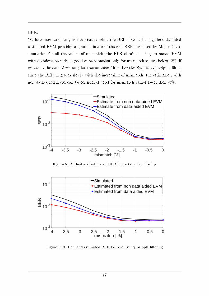
BER.
We have now to distinguish two cases: while the BER obtained using the data-aided
estimated EVM provides a good estimate of the real BER measured by Monte Carlo
simulation for all the values of mismatch, the BER obtained using estimated EVM
with decisions provides a good approximation only for mismatch values below -2%, if
we are in the case of rectangular transmission �lter. For the Nyquist equi-ripple �lter,
since the BER degrades slowly with the increasing of mismatch, the estimation with
non data-aided EVM can be considered good for mismatch values lower then -3%.
-4 -3.5 -3 -2.5 -2 -1.5 -1 -0.5 0mismatch [%]
10-3
10-2
10-1
BE
R
SimulatedEstimate from non data-aided EVMEstimate from data-aided EVM
Figure 5.12: Real and estimated BER for rectangular �ltering
-4 -3.5 -3 -2.5 -2 -1.5 -1 -0.5 0mismatch [%]
10-3
10-2
10-1
BE
R
SimulatedEstimated from non data aided EVMEstimated from data aided EVM
Figure 5.13: Real and estimated BER for Nyquist equi-ripple �ltering
47

-7 -6 -5 -4 -3 -2 -1 0delta D*L [%]
10-3
10-2
10-1
100
BE
R
Nyquist filter (roll off = 0.2)Nyquist filter (roll off = 0.3)Nyquist filter (roll off = 0.4)Rectangular filter
Figure 5.14: BER vs mismatch for di�erent roll-o� Nyquist equi-ripple �lter and for rectan-
gular �lter
In �gure (5.14) the BER vs mismatch is evaluated for di�erent type of �ltering
and roll-o� factor of the equi-ripple Nyquist �lter, with a constant SNR. It is possible
to see that the modi�cation of the roll-o� factor does not create great change of the
simulated performance. As we can see by the previous �gures, the equi-ripple �ltering
seems to have better performance against the residual Chromatic Dispersion left by
the misalignment among pre-compensation and actual CD of the channel.
The �ltering of the signal spectrum, and so the reducing of its bandwidth, improves
the performance of the system because a larger spectrum is more a�ected by the e�ect
of CD, since the di�erence in propagation time for each frequency components becomes
bigger.
In �gure (5.15) the spectra of rectangular �ltered signal and the Nyquist �ltered version
with roll-o� factor equal to 0.3 are compared. We can see in red the main lobe of
the cardinal sine, obtained by the Fourier Transform of the rectangular �lter, and in
blue the equi-ripple Nyquist �ltered spectrum that shows a reduction of bandwidth
occupation.
48
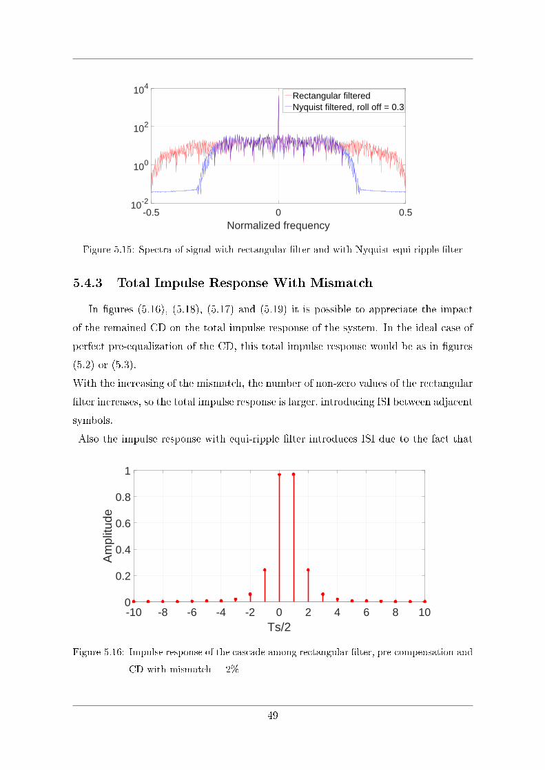
-0.5 0 0.5Normalized frequency
10-2
100
102
104Rectangular filteredNyquist filtered, roll off = 0.3
Figure 5.15: Spectra of signal with rectangular �lter and with Nyquist equi-ripple �lter
5.4.3 Total Impulse Response With Mismatch
In �gures (5.16), (5.18), (5.17) and (5.19) it is possible to appreciate the impact
of the remained CD on the total impulse response of the system. In the ideal case of
perfect pre-equalization of the CD, this total impulse response would be as in �gures
(5.2) or (5.3).
With the increasing of the mismatch, the number of non-zero values of the rectangular
�lter increases, so the total impulse response is larger, introducing ISI between adjacent
symbols.
Also the impulse response with equi-ripple �lter introduces ISI due to the fact that
-10 -8 -6 -4 -2 0 2 4 6 8 10Ts/2
0
0.2
0.4
0.6
0.8
1
Am
plitu
de
Figure 5.16: Impulse response of the cascade among rectangular �lter, pre-compensation and
CD with mismatch = 2%
49
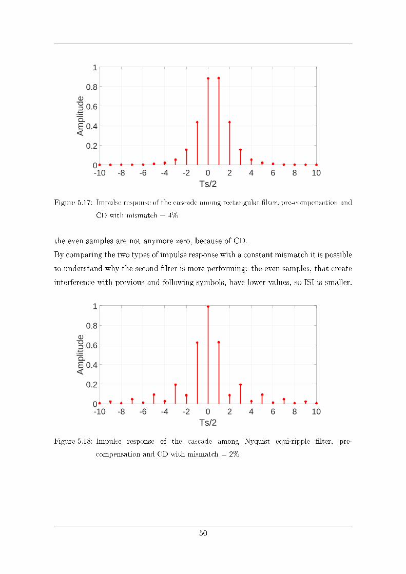
-10 -8 -6 -4 -2 0 2 4 6 8 10Ts/2
0
0.2
0.4
0.6
0.8
1
Am
plitu
de
Figure 5.17: Impulse response of the cascade among rectangular �lter, pre-compensation and
CD with mismatch = 4%
the even samples are not anymore zero, because of CD.
By comparing the two types of impulse response with a constant mismatch it is possible
to understand why the second �lter is more performing: the even samples, that create
interference with previous and following symbols, have lower values, so ISI is smaller.
-10 -8 -6 -4 -2 0 2 4 6 8 10Ts/2
0
0.2
0.4
0.6
0.8
1
Am
plitu
de
Figure 5.18: Impulse response of the cascade among Nyquist equi-ripple �lter, pre-
compensation and CD with mismatch = 2%
50
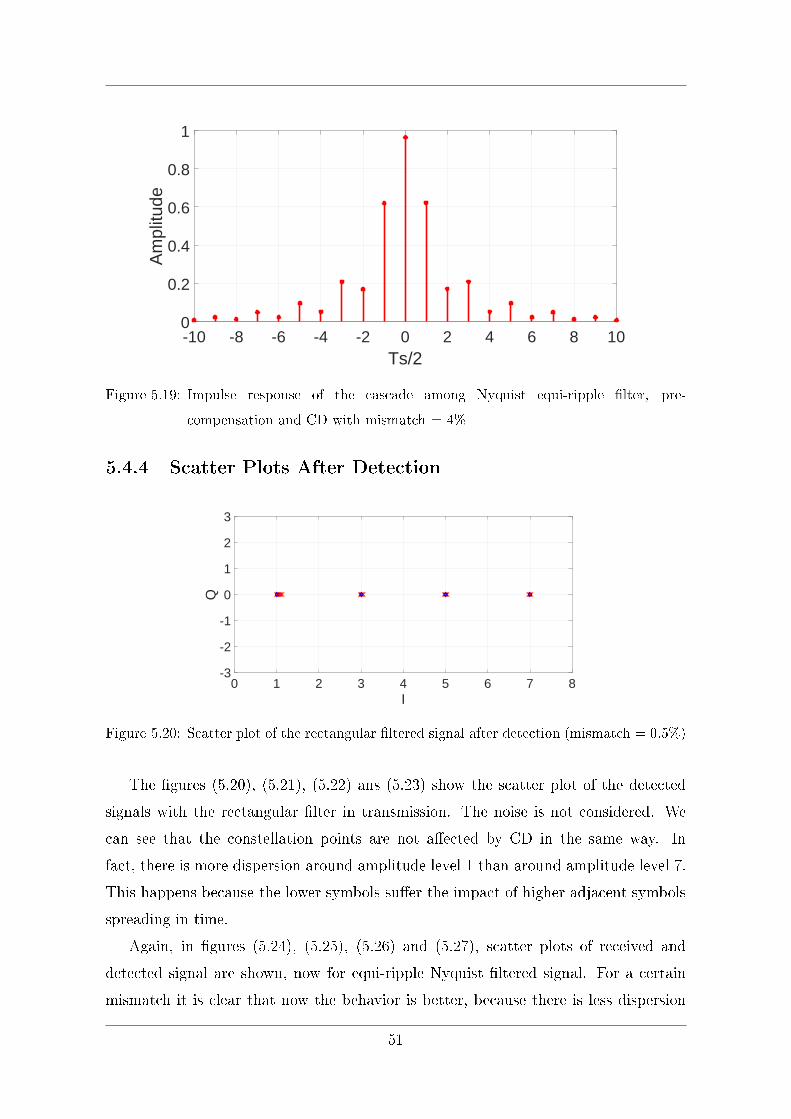
-10 -8 -6 -4 -2 0 2 4 6 8 10Ts/2
0
0.2
0.4
0.6
0.8
1
Am
plitu
de
Figure 5.19: Impulse response of the cascade among Nyquist equi-ripple �lter, pre-
compensation and CD with mismatch = 4%
5.4.4 Scatter Plots After Detection
0 1 2 3 4 5 6 7 8I
-3
-2
-1
0
1
2
3
Q
Figure 5.20: Scatter plot of the rectangular �ltered signal after detection (mismatch = 0.5%)
The �gures (5.20), (5.21), (5.22) ans (5.23) show the scatter plot of the detected
signals with the rectangular �lter in transmission. The noise is not considered. We
can see that the constellation points are not a�ected by CD in the same way. In
fact, there is more dispersion around amplitude level 1 than around amplitude level 7.
This happens because the lower symbols su�er the impact of higher adjacent symbols
spreading in time.
Again, in �gures (5.24), (5.25), (5.26) and (5.27), scatter plots of received and
detected signal are shown, now for equi-ripple Nyquist �ltered signal. For a certain
mismatch it is clear that now the behavior is better, because there is less dispersion
51

0 1 2 3 4 5 6 7 8I
-3
-2
-1
0
1
2
3
Q
Figure 5.21: Scatter plot of the rectangular �ltered signal after detection (mismatch = 1%)
0 1 2 3 4 5 6 7 8I
-3
-2
-1
0
1
2
3
Q
Figure 5.22: Scatter plot of the rectangular �ltered signal after detection (mismatch = 1.5%)
0 1 2 3 4 5 6 7 8I
-3
-2
-1
0
1
2
3
Q
Figure 5.23: Scatter plot of the rectangular �ltered signal after detection (mismatch = 2%)
around the constellation points and this creates less errors. In the �gures the signal
are noiseless, so all distortion is caused by CD that is remained after the cascade of
pre-compensation �lter and the �ber channel.
52
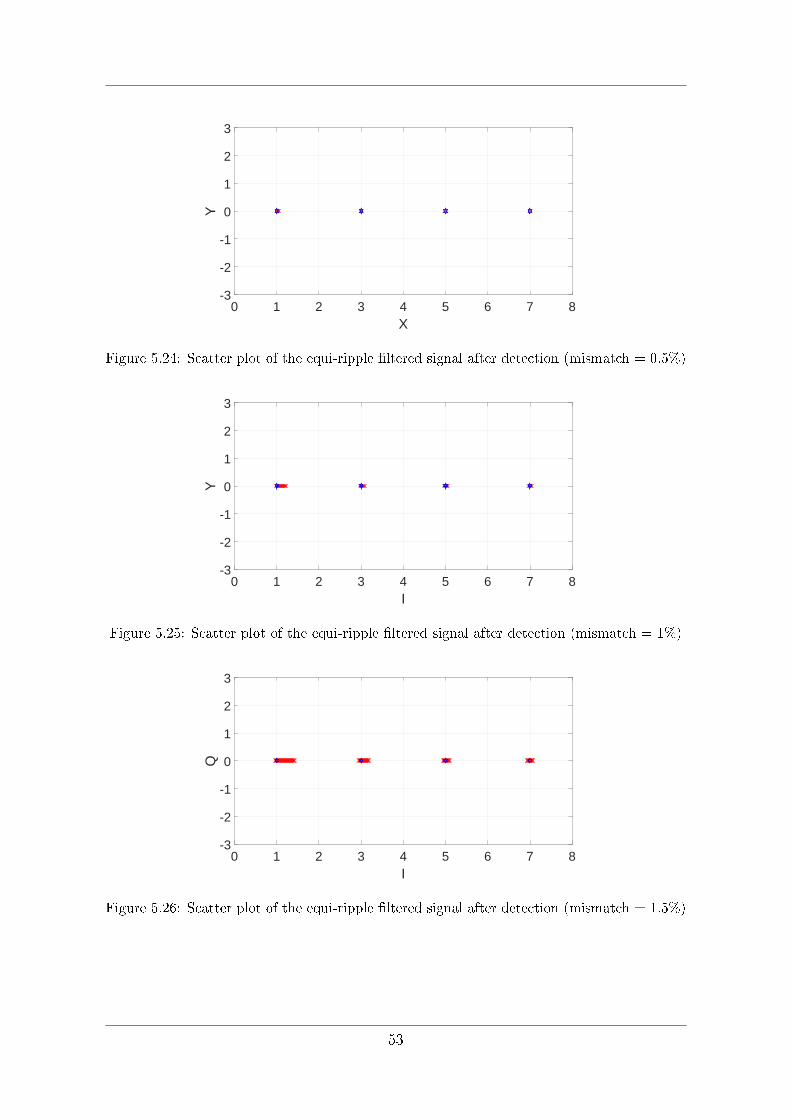
0 1 2 3 4 5 6 7 8X
-3
-2
-1
0
1
2
3
Y
Figure 5.24: Scatter plot of the equi-ripple �ltered signal after detection (mismatch = 0.5%)
0 1 2 3 4 5 6 7 8I
-3
-2
-1
0
1
2
3
Y
Figure 5.25: Scatter plot of the equi-ripple �ltered signal after detection (mismatch = 1%)
0 1 2 3 4 5 6 7 8I
-3
-2
-1
0
1
2
3
Q
Figure 5.26: Scatter plot of the equi-ripple �ltered signal after detection (mismatch = 1.5%)
53
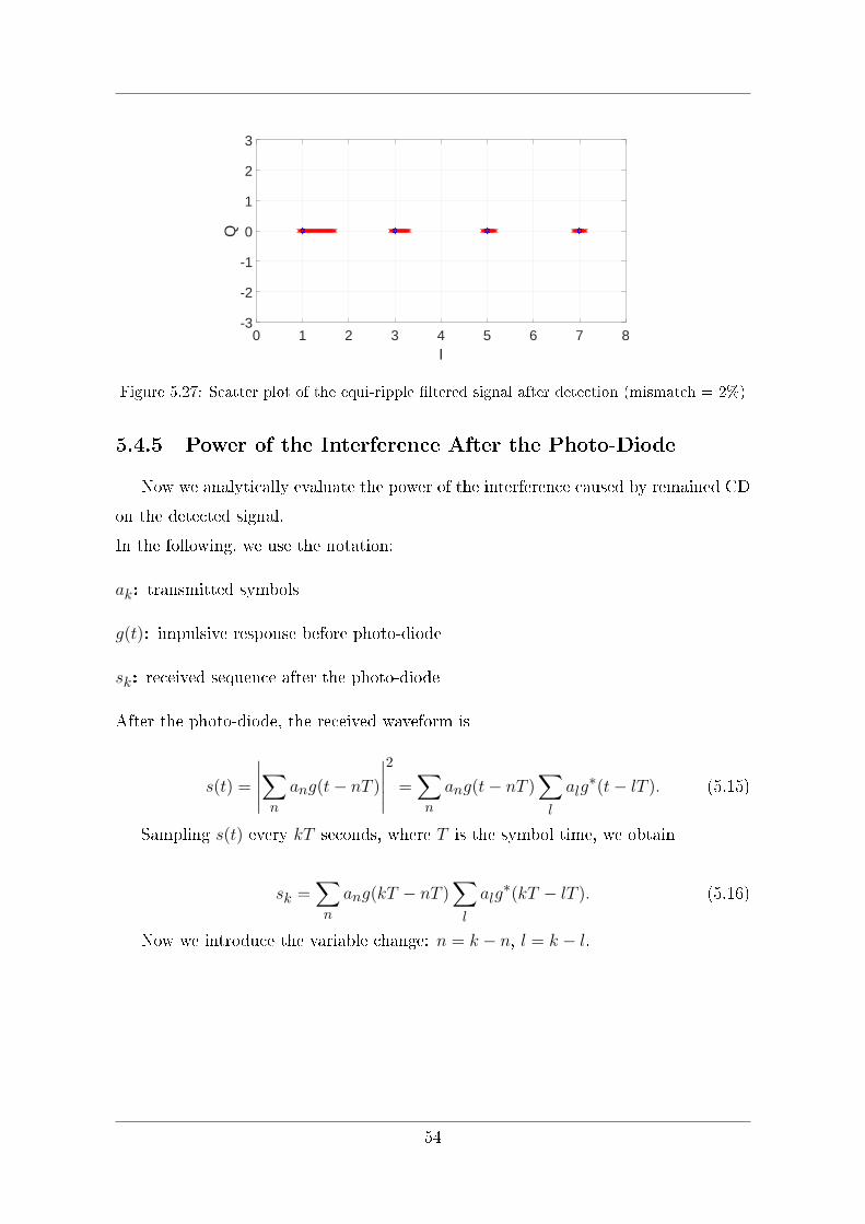
0 1 2 3 4 5 6 7 8I
-3
-2
-1
0
1
2
3
Q
Figure 5.27: Scatter plot of the equi-ripple �ltered signal after detection (mismatch = 2%)
5.4.5 Power of the Interference After the Photo-Diode
Now we analytically evaluate the power of the interference caused by remained CD
on the detected signal.
In the following, we use the notation:
ak: transmitted symbols
g(t): impulsive response before photo-diode
sk: received sequence after the photo-diode
After the photo-diode, the received waveform is
s(t) =
∣∣∣∣∣∑n
ang(t− nT )
∣∣∣∣∣2
=∑n
ang(t− nT )∑l
alg∗(t− lT ). (5.15)
Sampling s(t) every kT seconds, where T is the symbol time, we obtain
sk =∑n
ang(kT − nT )∑l
alg∗(kT − lT ). (5.16)
Now we introduce the variable change: n = k − n, l = k − l.
54
We can rewrite the received sequence as
sk =∑n ak−ng(nT )
∑l ak−lg
∗(lT ) =
=∑n
∑l ak−nak−lg(nT )g∗(lT ) =
=∑n a
2k−n|g(nT )|2+
+∑n
∑l 6=n ak−nak−lg(nT )g∗(lT ) =
= a2kg(0) +∑n 6=0 a
2k−n|g(nT )|2 +
∑n
∑l 6=n ak−nak−lg(nT )g∗(lT )
(5.17)
We describe the terms in the last row. The �rst term is the correct sample, the
second one is the common ISI, introduced by the impulse response that is longer than
one, and the third term is another ISI term, given by the beating between previous
and successive symbols, caused by the square operation of the photo-diode.
Now we do the expectations of the square of last two terms to calculate the power of the
total interference. The square operation is done by multiplying the total interference
term with its complex conjugate.
PISI = E
A︷ ︸︸ ︷∑n 6=0
a2k−n|g(nT )|2 +
B︷ ︸︸ ︷∑n
∑l 6=n
ak−nak−lg(nT )g∗(lT )
∗∗
C︷ ︸︸ ︷∑
q 6=0
a2k−q|g(qT )|2 +
D︷ ︸︸ ︷∑q
∑p6=q
ak−qak−pg∗(qT )g(pT )
=
(5.18)
In the following, the simpli�cation E [ak−n] = E [ak] for every value of n, since the
constellation is constant.
The term A ∗ C is
E[∑
n 6=0
∑q 6=0 a
2k−n|g(nT )|2a2k−q|g(qT )|2
]=
= E[a4k]∑n 6=0 |g(nT )|4+ n = q
+E[a2k]2∑n 6=0
∑q 6=0,q 6=n |g(nT )|2|g(qT )|2 n 6= q.
(5.19)
55
The term B ∗ C is
E[∑
n
∑l 6=n
∑q 6=0 ak−nak−la
2k−qg(nT )g∗(lT )|g(qT )|2
]=
= E[a3k]E[ak]∑n 6=0
∑l 6=n |g(nT )2|g(nT )g∗(lT )+ q = n
+E[a3k]E[ak]∑n
∑l 6=n6=0 g(nT )|g(lT )|2g∗(lT )+ q = l
+E[a2k]E[ak]2∑n
∑l 6=n
∑q 6=0,q 6=l,q 6=n g(nT )g∗(lT )|g(qT )|2 q 6= l 6= n.
(5.20)
The product A ∗D is the complex conjugate of B ∗ C.The term B ∗D is
E[∑
n
∑l 6=n
∑q
∑p6=q ak−nak−lak−qak−pg(nT )g∗(lT )g∗(qT )g(pT )
]=
= E[a2k]2∑n
∑l 6=n |g(nT )|2|g(lT )|2+
n = q, l = p
+E[a2k]E[ak]2∑n
∑l 6=n
∑p 6=l,p6=n |g(nT )|2g∗(lT )g(pT )+
n = q, l 6= p
+E[a2k]E[ak]2∑n
∑q 6=n
∑l 6=n,l 6=q |g(lT )|2g(nT )g∗(qT )+
n 6= q, l = p
+E[a2k]E[ak]2∑n
∑l 6=n
∑q 6=l,q 6=n g(nT )2g∗(lT )g∗(qT )+
n = p, q 6= l
+E[a2k]E[ak]2∑n
∑l 6=n
∑p 6=n,p6=l g
∗(lT )2g(nT )g(pT )
q = l, n 6= p
+E[a2k]2∑n
∑l 6=n g(nT )2g∗(lT )2+
n = p, l = q
+E[ak]4∑n
∑l 6=n
∑q 6=n,q 6=l
∑p6=n,p 6=l,p6=q g(nT )g∗(lT )g∗(qT )g(pT )
n 6= l 6= q 6= p.
(5.21)
56
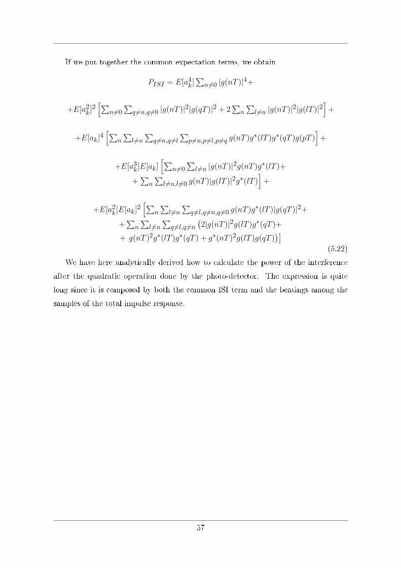
If we put together the common expectation terms, we obtain
PISI = E[a4k]∑n 6=0 |g(nT )|4+
+E[a2k]2[∑
n 6=0
∑q 6=n,q 6=0 |g(nT )|2|g(qT )|2 + 2
∑n
∑l 6=n |g(nT )|2|g(lT )|2
]+
+E[ak]4[∑
n
∑l 6=n
∑q 6=n,q 6=l
∑p6=n,p 6=l,p6=q g(nT )g∗(lT )g∗(qT )g(pT )
]+
+E[a3k]E[ak][∑
n 6=0
∑l 6=n |g(nT )|2g(nT )g∗(lT )+
+∑n
∑l 6=n,l 6=0 g(nT )|g(lT )|2g∗(lT )
]+
+E[a2k]E[ak]2[∑
n
∑l 6=n
∑q 6=l,q 6=n,q 6=0 g(nT )g∗(lT )|g(qT )|2+
+∑n
∑l 6=n
∑q 6=l,q 6=n
(2|g(nT )|2g(lT )g∗(qT )+
+ g(nT )2g∗(lT )g∗(qT ) + g∗(nT )2g(lT )g(qT ))]
(5.22)
We have here analytically derived how to calculate the power of the interference
after the quadratic operation done by the photo-detector. The expression is quite
long since it is composed by both the common ISI term and the beatings among the
samples of the total impulse response.
57
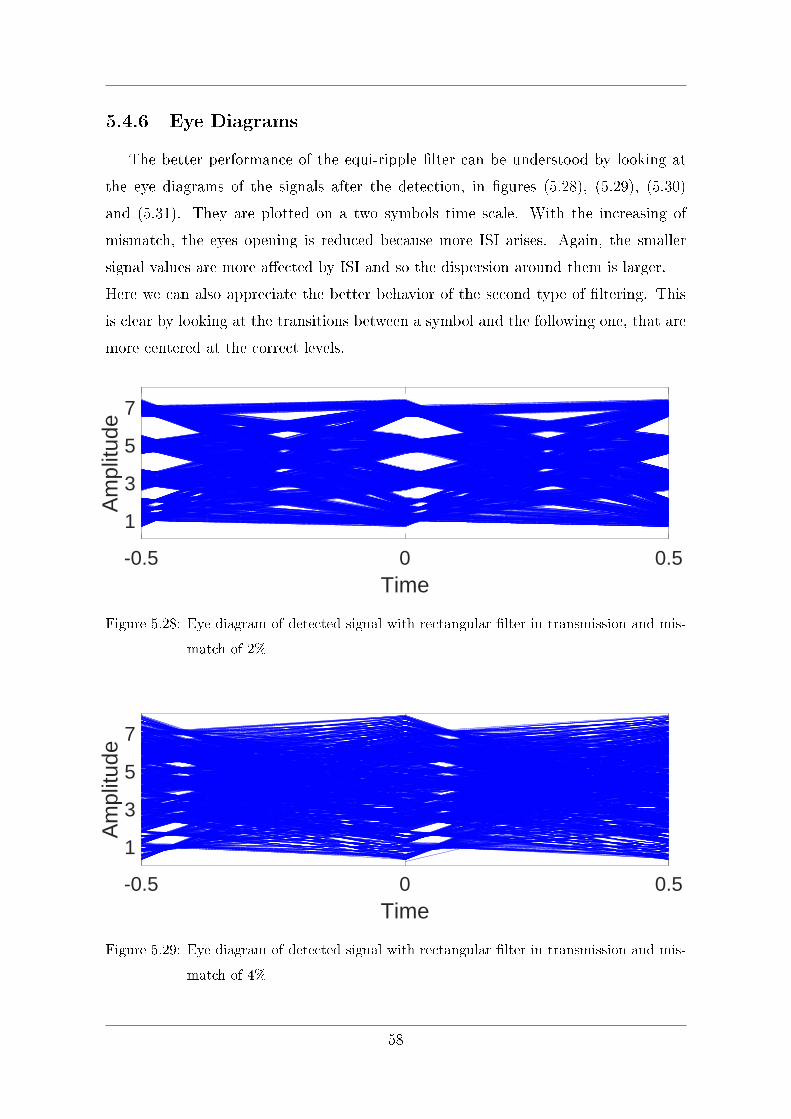
5.4.6 Eye Diagrams
The better performance of the equi-ripple �lter can be understood by looking at
the eye diagrams of the signals after the detection, in �gures (5.28), (5.29), (5.30)
and (5.31). They are plotted on a two symbols time scale. With the increasing of
mismatch, the eyes opening is reduced because more ISI arises. Again, the smaller
signal values are more a�ected by ISI and so the dispersion around them is larger.
Here we can also appreciate the better behavior of the second type of �ltering. This
is clear by looking at the transitions between a symbol and the following one, that are
more centered at the correct levels.
-0.5 0 0.5Time
1
3
5
7
Am
plitu
de
Figure 5.28: Eye diagram of detected signal with rectangular �lter in transmission and mis-
match of 2%
-0.5 0 0.5Time
1
3
5
7
Am
plitu
de
Figure 5.29: Eye diagram of detected signal with rectangular �lter in transmission and mis-
match of 4%
58
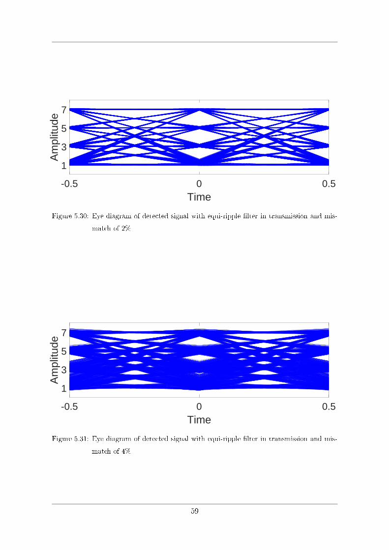
-0.5 0 0.5Time
1
3
5
7
Am
plitu
de
Figure 5.30: Eye diagram of detected signal with equi-ripple �lter in transmission and mis-
match of 2%
-0.5 0 0.5Time
1
3
5
7
Am
plitu
de
Figure 5.31: Eye diagram of detected signal with equi-ripple �lter in transmission and mis-
match of 4%
59
Chapter 6
Conclusions
The problem at the basis of this work is the technology for the medium and short
reach optical �ber link. This technology must respect requirements about costs and
easiness, that are fundamental for the feasibility of its realization. The solution must
exploit a single photo-detector. This is in contrast to coherent detection, that is used
in long haul links and allows for a complete equalization of impairments at the receiver.
The target rate is �xed to 100 Gbps, in order to assure the same performance of
the 100 G coherent channel. Since we are forced to use Direct Detection, the choice is
among Intensity Modulation transmission and self-coherent system.
After having explained what a self-coherent system is and having introduced many
examples of it, we studied the performance of an IM-DD system that has the advantage
of an easy implementation.
The major impairment that a�icts the �ber transmission is the Chromatic Disper-
sion, so we have considered its as unique source of distortion, in addition to Gaussian
noise.
To face the problem of CD, that cannot be equalized at the receiver since after the
photo-detector the channel is quadratic, we introduced a digital �lter placed at the
transmitter that tries to pre-compensate for the estimated CD. The �lter coe�cients
are obtained using the Inverse Discrete Fourier Transform of the conjugate of the CD
transfer function with nominal parameters typical of a SMF used in the C-band.
Our study focused on the performance of a Intensity Modulation-Direct Detection
PAM-4 scheme, that uses only positive levels since only intensity can be received.
We have introduced two types of transmission �lter, to understand the di�erent
performance and how they change against remained CD. The �rst �lter is a rectangular
60
�lter while the second is a equi-ripple Nyquist �lter built in MATLAB R©. This second
�lter reduces the bandwidth occupation of the transmitted signal.
The performance has been evaluated in terms of Bit Error Rate. Then we tried to
estimate the probability of error with the measured Error Vector Magnitude, obtaining
some good results. The BER has been calculated for di�erent values of the mismatch
between the pre-compensation �lter and the real value of the CD, that can vary due
to changes of temperature or of the length of the �ber.
The results show that the equi-ripple Nyquist �lter gives better BER values with
respect to the rectangular one, since the lower bandwidth occupation guarantees better
resistance against CD, that results in a lower Inter Symbol Interference.
The comparing of the results is also done by looking at the e�ect of the remained
CD on the total impulse responses of the system with both transmission �lters and
observing the eye diagrams of the received signals.
By looking at the obtained graphical results, if it was possible to know the exact
value of both Signal-to-Distortion Ratio and Bit Error Rate, we would be able to
estimate the value of the mismatch of the pre-compensation �lter, in order to feedback
this information to the transmitter allowing for a better equalization.
The use of pre-compensation for the CD can be a solution for limiting complexity
of the receiver; the results we have obtained suggest that PAM-4 with IM-DD can be
a good choice for a short reach �ber link.
61
Bibliography
[1] T. J. Xia and G. A. Wellbrock, �Commercial 100-gbit/s coherent transmission
systems,� Optical Fiber Telecommunications, p. 45, 2013.
[2] M. Kuschnerov, F. N. Hauske, K. Piyawanno, B. Spinnler, M. S. Al�ad, A. Napoli,
and B. Lankl, �Dsp for coherent single-carrier receivers,� Journal of lightwave
technology, vol. 27, no. 16, pp. 3614�3622, 2009.
[3] K. Szczerba, J. Karout, P. Westbergh, E. Agrell, M. Karlsson, P. Andrekson, and
A. Larsson, �Experimental comparison of modulation formats in im/dd links,�
2011.
[4] C. Cole, I. Lyubomirsky, A. Ghiasi, and V. Telang, �Higher-order modulation for
client optics,� IEEE Communications Magazine, vol. 51, no. 3, pp. 50�57, 2013.
[5] X. Xu, E. Zhou, G. N. Liu, T. Zuo, Q. Zhong, L. Zhang, Y. Bao, X. Zhang,
J. Li, and Z. Li, �Advanced modulation formats for 400-gbps short-reach optical
inter-connection,� Optics express, vol. 23, no. 1, pp. 492�500, 2015.
[6] T. Takahara, T. Tanaka, M. Nishihara, L. Li, Z. Tao, and J. C. Rasmussen, �100-
gb/s (2× 50-gb/s) transmission over 80-km using 10-gb/s class dml,� in 2012 17th
Opto-Electronics and Communications Conference, 2012.
[7] P. Little, �Who's afraid of the big, bad dsp?,� in Ethernet Alliance 100GbE per
Lambda for Data Center Workshop, 2014.
[8] D. Sadot, G. Dorman, A. Gorshtein, E. Sonkin, and O. Vidal, �Single channel
112gbit/sec pam4 at 56gbaud with digital signal processing for data centers ap-
plications,� Optics express, vol. 23, no. 2, pp. 991�997, 2015.
62
[9] N. Kikuchi and R. Hirai, �Intensity-modulated/direct-detection (im/dd) nyquist
pulse-amplitude modulation (pam) signaling for 100-gbit/s/λ optical short-reach
transmission,� in 2014 The European Conference on Optical Communication
(ECOC), 2014.
[10] S. Adhikari, S. Jansen, M. Al�ad, B. Inan, V. Slei�er, A. Lobato, P. Leoni, and
W. Rosenkranz, �Self-coherent optical ofdm: An interesting alternative to direct
or coherent detection,� in 2011 13th International Conference on Transparent
Optical Networks, pp. 1�4, IEEE, 2011.
[11] B. J. Schmidt, Z. Zan, L. B. Du, and A. J. Lowery, �120 gbit/s over 500-km
using single-band polarization-multiplexed self-coherent optical ofdm,� Journal
of lightwave technology, vol. 28, no. 4, pp. 328�335, 2010.
[12] J. von Hoyningen-Huene and C. Ruprecht, �Ofdm for optical access,� in Optical
Fiber Communication Conference, pp. Th1H�1, Optical Society of America, 2015.
[13] M. Martinelli and P. Martelli, Fundamental of Optical Communications. Wiley
International, 2012.
[14] J. Kahn, �Modulation and detection techniques for optical communication sys-
tems,� in Coherent Optical Technologies and Applications, p. CThC1, Optical
Society of America, 2006.
[15] D. Pilori, �Discrete-multitone modulation for short distance 100 gbit/s optical
links,� master's thesis, Politecnico di Milano, 2015.
[16] ITU-T, �Optical system design and engineering considerations.� Supplement 39,
September 2012. Geneva: International Telecommunication Union.
[17] T. Tanaka, M. Nishihara, T. Takahara, L. Li, Z. Tao, and J. C. Rasmussen, �Ex-
perimental investigation of 100-gbps transmission over 80-km single mode �ber
using discrete multi-tone modulation,� in SPIE OPTO, pp. 86460J�86460J, In-
ternational Society for Optics and Photonics, 2012.
[18] C. Cox, E. Ackerman, R. Helkey, and G. E. Betts, �Techniques and performance
of intensity-modulation direct-detection analog optical links,� IEEE Transactions
on Microwave theory and techniques, vol. 45, no. 8, pp. 1375�1383, 1997.
63
[19] D. Che, Q. Hu, and W. Shieh, �Linearization of direct detection optical channels
using self-coherent subsystems,� Journal of Lightwave Technology, vol. 34, no. 2,
pp. 516�524, 2016.
[20] A. Lowery and J. Armstrong, �Orthogonal-frequency-division multiplexing for
dispersion compensation of long-haul optical systems,� Optics Express, vol. 14,
no. 6, pp. 2079�2084, 2006.
[21] W.-R. Peng, B. Zhang, K.-M. Feng, X. Wu, A. E. Willner, and S. Chi, �Spectrally
e�cient direct-detected ofdm transmission incorporating a tunable frequency gap
and an iterative detection techniques,� Journal of Lightwave Technology, vol. 27,
no. 24, pp. 5723�5735, 2009.
[22] X. Chen, A. Li, D. Che, Q. Hu, Y. Wang, J. He, and W. Shieh, �Block-wise
phase switching for double-sideband direct detected optical ofdm signals,� Optics
express, vol. 21, no. 11, pp. 13436�13441, 2013.
[23] X. Chen, D. Che, A. Li, J. He, and W. Shieh, �Signal-carrier interleaved optical
ofdm for direct detection optical communication,� Optics express, vol. 21, no. 26,
pp. 32501�32507, 2013.
[24] D. Che, H. Khodakarami, and W. Shieh, �Dual-polarization signal carrier inter-
leaved direct detection through discrete-time gaussian channel with conjugate
inter-symbol interference,� in Opto-Electronics and Communications Conference
(OECC), 2015, pp. 1�3, IEEE, 2015.
[25] W. Shieh, D. Che, Q. Hu, and A. Li, �Linearization of optical channels with stokes
vector direct detection,� in Optical Fiber Communication Conference, pp. Th1E�
5, Optical Society of America, 2015.
[26] R. Schmogrow, B. Nebendahl, M. Winter, A. Josten, D. Hillerkuss, S. Koenig,
J. Meyer, M. Dreschmann, M. Huebner, C. Koos, et al., �Error vector magnitude
as a performance measure for advanced modulation formats,� IEEE Photonics
Technology Letters, vol. 24, no. 1, pp. 61�63, 2012.
[27] Z. Dong, F. N. Khan, Q. Sui, K. Zhong, C. Lu, and A. P. T. Lau, �Optical
performance monitoring: A review of current and future technologies,� Journal
of Lightwave Technology, vol. 34, no. 2, pp. 525�543, 2016.
64


![CHAPTER-4 Line Codes RZ: Return to Zero [ pulse for half ... · NRZ . Return to Zero[ pulse for full duration of T. b ] Unipolar (NRZ) Unipolar NRZ . NRZ-inverted (differential](https://img.pdfslide.us/doc/110x75/5cc1fa9b88c9933e3a8d2cb0/chapter-4-line-codes-rz-return-to-zero-pulse-for-half-nrz-return-to.jpg)