PERFORANCE SIMULATION OF SINGLE …qspace.qu.edu.qa/bitstream/handle/10576/7945/060316-11-fulltext.pdf · DOMESTIC REFRIGERATOR USING ... (evaporator, condenser, compressor, ... PERFORANCE

Engineering Journal of the University of Qatar, Vol. 16, 2003, pp.109-124

PERFORMANCE SIMULATION OF SINGLE-EVAPORATOR DOMESTIC REFRIGERATOR USING ALTERNATIVE

REFRIGERANTS

Talib Kshash Murtadha and Salam Hadi Hussain Mechanical Engineering Department

University of Technology, Baghdad

Republic of Iraq

ABSTRACT

The search for well-functioning and energy-optimized refrigeration systems has made modeling and simulation of such systems an important tool for the industry in terms of product development. The present study explores how REFSIM ( a general computer model for simulation of steady-state performance systems) can be used to handle the physics of a domestic refrigerator. Organization of the model is discussed and approach to modeling of main components with more detailed description in a domestic refrigerator (evaporator, condenser, compressor, capillary tube with and without heat exchange, and suction line) is explained. The modeling effort emphasis was on the local phenomena to be described by fundamental thermodynamic, heat transfer and fluid mechanics relationships. Good agreement is found with experiments for a wide range of operating conditions to a domestic refrigerator.

I. INTRODUCTION

Several authors (Cleland 1990,Domanski and Didion 1984, James and James 1986) recognized that the ability to simulate the steady response of refrigeration systems will give engineers in the refrigeration industry the same advantages that simulation has brought to the fields of electronics, fluid power, etc. The main advantages of such simulations include better understanding of system and component behavior, and the ability to test ideas without doing experiments. In this way, it is possible to improve control and system performance, lower energy consumption, and shorten the time it takes to get a product on the market.

In spite of this, dynamic modeling and simulation is not yet a commonly used tool within the refrigeration community. The main reason is the complexity and difficulty of the modeling task. Refrigeration systems tend to very diverse, making it difficult to build general simulation models. Furthermore, the basic physical processes of refrigeration systems (evaporation, condensation, throttling, … ) are very complex, and difficult to describe on both detail and system levels.

Yasuda et al. (1981), James and James (1987), MacArthur and Gland (1989) have done some work in the area of dynamic modeling of thermo-fluid systems, but none of this work has, to our knowledge, led to a general methodology for the modeling and simulation of these systems.

The emphasis on energy conservation over the past decade has resulted in the development of many domestic refrigerator performance simulation. Most of these models are composites of a sequence of regression analysis simulations of the major components individual performance. These models are adequate for simulating a typical domestic refrigerator performance or even for design change performance estimation of a specific domestic refrigerator if all of the component test data are available as input.

A totally different approach to modeling performance, one of beginning with “first principles”, has also been taken, but in far fewer cases. These models, one of which is discussed in this paper, incorporate the fundamental correlations and laws of thermodynamics, fluid mechanics and heat transfer into a network of logic that will allow for prediction of the state properties of either the refrigerant or the air at any pre-selected point of their respective circuits. These models are best used when applied to research problems in trying to understand the impact of the

109

Murthada and Hussain

local phenomena on the overall system. Their accuracy is, of course, limited to the accuracy of the correlation used and is not necessarily any better than the accuracy of the regression analysis models, however, the first principles models, if designed correctly, require far less and easier to obtain input data.

II. DESCRIPTION OF THE MODEL

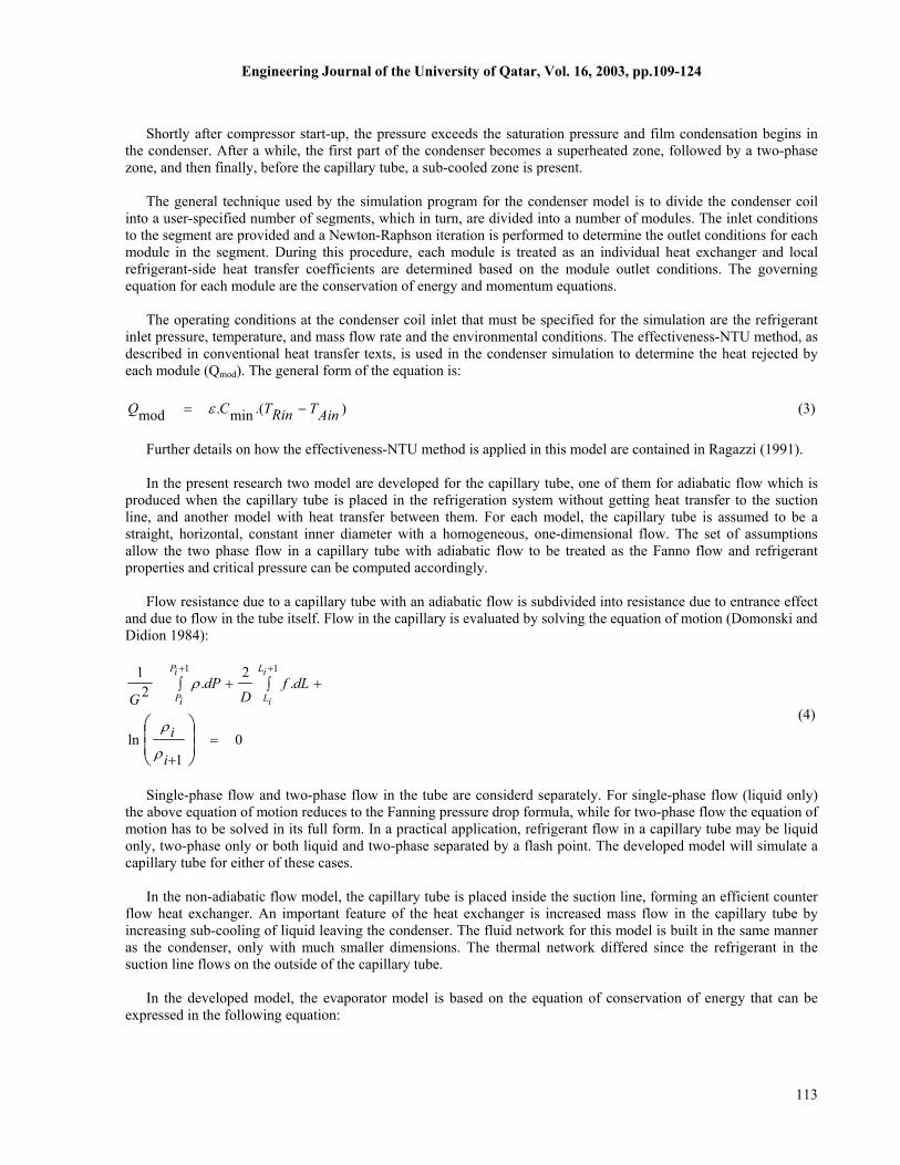
The advancement of this model depends on the fact that all refrigerant thermodynamic states in the system are not subject to any restrictions and are found exclusively as a result of the iteration process in the solution logic of the main program. This flexibility increases the accuracy of the simulation results.

During domestic refrigerator operation, there is a one to one relationship between working medium parameters and operation conditions, i.e., for given ambient conditions there is just one refrigerant state at any location within the system, which constitutes steady state operation. This unique set of refrigerant state and flow conditions has to be sought by a domestic refrigerator simulation program in an iteration process.

In order to set up an iteration procedure for a domestic refrigerator model, balances taking place have to be recognized. The fact that the domestic refrigerators thermodynamic cycle is a closed loop makes it convenient to utilize a pressure-enthalpy diagram so that the two properties, enthalpy and pressure, may be explicitly highlighted at the entrance and exit of each component.

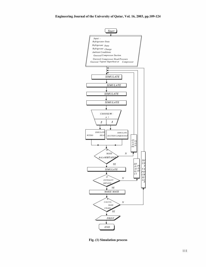
The explanation of the logic used to iterate these three balances is given below. For sake of clarity, only the four main components, i.e. a compressor, a condenser, a capillary tube and an evaporator are discussed. Required input to the program is restricted to environmental conditions and domestic refrigerator design data as fixed parameters; it also includes initiating guesses of refrigerant states, which will automatically converge to the true state conditions through the iterative process.

The simulation process (Fig.1) starts with a guessed refrigerant pressure and vapour superheat at the compressor can inlet, and the compressor discharge pressure. From these data and the compressor performance simulation, the refrigerant mass flow rate is determined. Next, the condenser and the capillary tube are simulated and mass flow balance is sought by comparing refrigerant mass flow rate through the compressor and capillary tube. If compared mass flows are not equal simulation of the compressor, the condenser and the capillary tube is resumed with unchanged refrigerant state at the compressor can inlet and modified guess of compressor discharge pressure. For instance, in the case of mass flow rate through a capillary tube being smaller than mass flow rate through a compressor, compressor discharge pressure is increased. Increasing this pressure reduces refrigerant mass flow rate through the compressor. Then the condenser is simulated with this smaller mass flow rate and at higher saturation temperature. Consequently, refrigerant reaching the expansion device inlet is at higher pressure and has more sub-cooling. Both factors promote increase of mass flow rate through the capillary tube. Thus, an increase in discharge pressure has a clear and opposite impact on mass flow rates through the compressor and the capillary tube and the appropriate discharge pressure will be found for which mass flow balance exists. Once a mass flow balance is reached, simulation of the evaporator is performed in a backward scheme with the known refrigerant state at evaporator exit and refrigerant mass flow rate. Since the thermodynamic process in a capillary tube is assumed to be adiabatic, refrigerant enthalpy at the evaporator inlet should be equal to the enthalpy at the condenser outlet. If these enthalpies are not equal (enthalpy balance is not reached) a new calculation loop starts from the beginning with a modified guess on the refrigerant pressure at the compressor can inlet. From condenser operation point of view, change in compressor suction pressure induces change in refrigerant mass flow rate and modification of condenser saturation temperature caused by the system mass flow balance search. These two changes have opposing effects on refrigerant enthalpy at the condenser exit, leaving it relatively unaltered. On the other hand, the same change of compressor suction pressure has a strong effect on refrigerant enthalpy at the evaporator inlet by change in evaporator saturation temperature and refrigerant mass flow rate, both working in the same enthalpy change direction, thus an appropriate suction pressure at the compressor inlet can always be found which enthalpy balance exists.

110


CCHHOOOOSSEE WWYY ::

II== ??

IIFF

MMAASSSS

BBAALLAANNOOBBTTAAIINNEE

SSIIMM UULLAATTEE

SSUUCCTTIIOONN LLIINNEEA

EEXXCCHHAANNG

AADDJJUU SSTTSSUUCCTT

PPRREESSSSUU

YYEE

SSIIMMUULLAATTEE

IIFF

EENNTTHHAALLPPYY A A COOBBTTAAIINNEE

?

AADDJJUU SSTTHHEEA

PPRREESSSSUU

MMAAKKEE MMAASSSS

AA

DDJJUUSS TT

VVAAPPOOUURRSSUUPPEE

EENNDD

22 11

SSIIMMUULLAATTEECA AWWIITTHHOO HHEEAATT

C A G

NN

NN

YYEE

NN

YYEE

SSttaarrtt

SSIIMMUULLAATTEE

SSIIMMUULLAATTEE

SSIIMMUULLAATTEE

SSIIMMUULLAATTEE

IInnppuutt:: --RReeffrriiggeerraattoorr DDaattaa

RReeffrriiggeerraanntt DDaattaaRReeffrriiggeerraanntt CChhaarrggeeAAmmbbiieenntt CCoonnddiittiioonnss

GGuueesssseedd CCoommpprreessssoorr SSuuccttiioonn

GGuueesssseedd CCoommpprreessssoorr HHeeaadd PPrreessssuurree GGuueesssseedd VVaappoouurr SSuuppeerrhheeaatt aatt CCoommpprreessssoorr

IISS

CCAALLCCUULLA MM AASSSS

Q A OCCHHAARRGG?

PPRRIINNTT

Fig. (1) Simulation process

111


In the third iterative loop, the refrigerant mass balance in the system is used to adjust refrigerant superheat (or quality) at the entrance to the compressor can. Specifically, refrigerant mass inventory is made. It is based on refrigerant states in the system, which were found to satisfy enthalpy and pressure balances with assumed vapour superheat (or quality) at the compressor can inlet. The amount of refrigerant obtained from mass inventory calculations is compared to the refrigerant charge. If the amount of refrigerant calculated is smaller than refrigerant input into the domestic refrigerator, the superheat (or quality) guess is decreased and all calculations are automatically resumed from the beginning. As explained above, the final solution is obtained by searching for pressure balance, energy balance and by satisfying the mass conservation law. This is realized in three iteration loops in which refrigerant discharge pressure, refrigerant pressure and superheat (or quality) are being iterated. All three loops are being iterated using the secant method. In the course of the computing process the main program gathers information about the domestic refrigerator particular component’s performance, updated at each iteration loop and applies them to anticipate changes in state property value which is being iterated. This allows for the iteration process to converge faster with each iteration loop.

III. DESCRIPTION OF SUBMODELS AND MASS INVENTORY

The following domestic refrigerator components have individual algorithms subroutined into main program logic: hermetic compressor, condenser, evaporator, capillary tube, connecting tubings. Models of these components have been explained in (Hussain, 2000). An abbreviated description of the fist four major components and the refrigerant mass inventory is all that is discussed here.

The hermetic compressor was designed so that the suction inlet pipe was directed towards the inlet port of the intake muffler. Gas drawn into the cylinder was a mixture of heated gas from the housing, and that came directly from the suction line. It was desirable that the intake be as direct as possible, since additional superheat added within the compressor has a negative effect on both capacity and efficiency (Dossat, 1991).

The volume flow rate was calculated using a volumetric efficiency ζv:

60.. rpm

strokecomp

oN

Vvs

mζ

ρ= (1)

The volumetric efficiency is compressor, and refrigerant (R12 & R134a) specific, and depends moderately on the pressure ratio (Pc/Pe) (Cullimore et al. 1996). However, in the present work this dependency was neglected.

The work (W) delivered by the compressor to the fluid was calculated using an isentropic efficiency (ζis) that depends on the actual compressor and refrigerant (Domonski and Didion 1984), such that

−−−

−

×−

=

1

1

11

1

.1

.60

.1

γγγ

γ

γ

ζ

ePcP

pnePcp

ePstrokeVrpmN

isW

(2)

The approximated values of the volumetric and isentropic efficiency were found from experiments performed by Rasmussen (1997), where both efficiencies were determined as functions of compressor speed (1800-5000 rpm) at different condensing/evaporating temperatures. The isentropic efficiency decreased slightly as speed increased, and was also found to decrease with decreasing condensation temperature. The volumetric efficiency was found to decrease with both increased speed as well as increased pressure ratio.

112


Shortly after compressor start-up, the pressure exceeds the saturation pressure and film condensation begins in the condenser. After a while, the first part of the condenser becomes a superheated zone, followed by a two-phase zone, and then finally, before the capillary tube, a sub-cooled zone is present.

The general technique used by the simulation program for the condenser model is to divide the condenser coil

into a user-specified number of segments, which in turn, are divided into a number of modules. The inlet conditions to the segment are provided and a Newton-Raphson iteration is performed to determine the outlet conditions for each module in the segment. During this procedure, each module is treated as an individual heat exchanger and local refrigerant-side heat transfer coefficients are determined based on the module outlet conditions. The governing equation for each module are the conservation of energy and momentum equations.

The operating conditions at the condenser coil inlet that must be specified for the simulation are the refrigerant inlet pressure, temperature, and mass flow rate and the environmental conditions. The effectiveness-NTU method, as described in conventional heat transfer texts, is used in the condenser simulation to determine the heat rejected by each module (Qmod). The general form of the equation is:

).(min.mod AinTRinTCQ −= ε (3)

Further details on how the effectiveness-NTU method is applied in this model are contained in Ragazzi (1991).

In the present research two model are developed for the capillary tube, one of them for adiabatic flow which is produced when the capillary tube is placed in the refrigeration system without getting heat transfer to the suction line, and another model with heat transfer between them. For each model, the capillary tube is assumed to be a straight, horizontal, constant inner diameter with a homogeneous, one-dimensional flow. The set of assumptions allow the two phase flow in a capillary tube with adiabatic flow to be treated as the Fanno flow and refrigerant properties and critical pressure can be computed accordingly.

Flow resistance due to a capillary tube with an adiabatic flow is subdivided into resistance due to entrance effect and due to flow in the tube itself. Flow in the capillary is evaluated by solving the equation of motion (Domonski and Didion 1984):

01

ln

.2

.21 11

=+

+∫+∫

++

i

i

dLfD

dPG

iL

iL

iP

iP

ρ

ρ

ρ

(4)

Single-phase flow and two-phase flow in the tube are considerd separately. For single-phase flow (liquid only) the above equation of motion reduces to the Fanning pressure drop formula, while for two-phase flow the equation of motion has to be solved in its full form. In a practical application, refrigerant flow in a capillary tube may be liquid only, two-phase only or both liquid and two-phase separated by a flash point. The developed model will simulate a capillary tube for either of these cases.

In the non-adiabatic flow model, the capillary tube is placed inside the suction line, forming an efficient counter flow heat exchanger. An important feature of the heat exchanger is increased mass flow in the capillary tube by increasing sub-cooling of liquid leaving the condenser. The fluid network for this model is built in the same manner as the condenser, only with much smaller dimensions. The thermal network differed since the refrigerant in the suction line flows on the outside of the capillary tube.

In the developed model, the evaporator model is based on the equation of conservation of energy that can be expressed in the following equation:

113


canQdislineQ

LqlineQcondQEsuclineQQevap

++

+=++ (5)

WEcanQ −= (6) Mass inventory of refrigerant is used for iteration of refrigerant superheat or quality at the compressor can inlet. Accuracy of mass inventory results depends on accuracy of evaluation of mean refrigerant density in particular domestic refrigerator components and accuracy of internal volume determinations. In order to minimize the error of computations, mass inventory results are used on a relative basis, i.e. calculated charge is compared not to the actual refrigerant charge only, but to the mass of refrigerant calculated for operating conditions at which superheat at the compressor can inlet is known as a design parameter.

In a domestic refrigerator compressor and connecting tubes refrigerant flow is single-phase or two-phase with vapour/liquid velocity slip ratio close to 1. Mean density is known for these components from performed calculations during iterative process closing enthalpy and pressure balances. In the case of both coils, the refrigerant is in part by single-phase, While, in most of the coil some type of two phase annular flow prevails. For this flow regime, mean density is evaluated in terms of densities of saturated liquid and vapour, and the void fraction as correlated by (Tandon et al., 1985) based on (Lisa et el.,1995) results:

[ ]476.0/285/115.0)(

1125

2)(

176.00361.0

)(

088.038.01

112550

2)(

63.09293.0

)(

315.0928.11

ttXttXttXF

where

feRfor

ttXF

feR

ttXF

feR

feRfor

ttXF

feR

ttXF

feR

+=

≥

−

+

−

−=

<<

−

+

−

−=

α

α

(8

(7

f

iDxrefGfeR

and

µ

×−×=

)1(

Mean refrigerant density is calculated for each tube individually. This is possible since the program employtube-by-tube simulation model for a condenser.

11

)

)

s

4


IV. PRESSURE DROP CORRELATIONS

Single-phase pressure drops are calculated using churchill’s equation (Churchill 1977)for the Darcy friction factor as follows:

( )16Re/37530

1627.0

9.0

Re

7ln457.2

12/1

2/3)(

112

Re

88

=

+−=

++=

B

DA

where

BAf

λ

(9)

This function agrees very well with experiments at both high and low Reynolds number, but overestimated the friction factor somewhat in the transition region. In the case of two-phase flow, refrigerant pressure drop inside a tube is calculated by (Jung and Radermacher, 1989, 1993) with evaporation and (Lockhart-Martinelli, 1949) with condensation.

V. CONVENTIONAL HEAT-TRANSFER CORRELATIONS

Convective heat transfer between fluid and thermal sub models here is characterized by the heat-transfer coefficient αHT (Cullimore et al. 1996): (10)

TAconvQ HXIHT ∆=α

Where AHXI and ∆T are the inside heat-transfer area and temperature difference between refrigerant and tube wall temperature, respectively.

In the case of single-phase flow, �HT is calculated from the Nusselt number according to

k

DNu HTα

= (11)

Where:

<= 1960Re66.3Nu

He

In Nucleregime(Dittuis used

(12) >= 6420RePrRe0 nNu

<<−= 6420Re1960Pr)12567.0(Re116.0

8.0023.nNu

re the coefficient n= 0.3 corresponds to cooling and n= 0.4 corresponding to heating.

the present research, two fundamental boiling heat-transfer regimes are considered: nucleate and film. ate boiling is characterized by the bubbles that form at the wall and then drift into the bulk liquid stream. This exists for qualities 0.0 to 0.7 only. Film boiling, however, is characterized by vapour-dominated heat-transfer

s-Boelter Correlation). For qualities between 0.7 and 1.0, an interpolation between the two regime corrlations .

115


In the case of two-phase flow in a condensation process, heat transfer is calculated using a Rohsenow correlation (Rohsenow and Hartnett 1973) for refrigerant (R12) and a Dobson correlation (Dobson, 1994) for refrigerant R134a.

VI. HEAT TRANSFER-SECONDARY SIDE OF TUBE

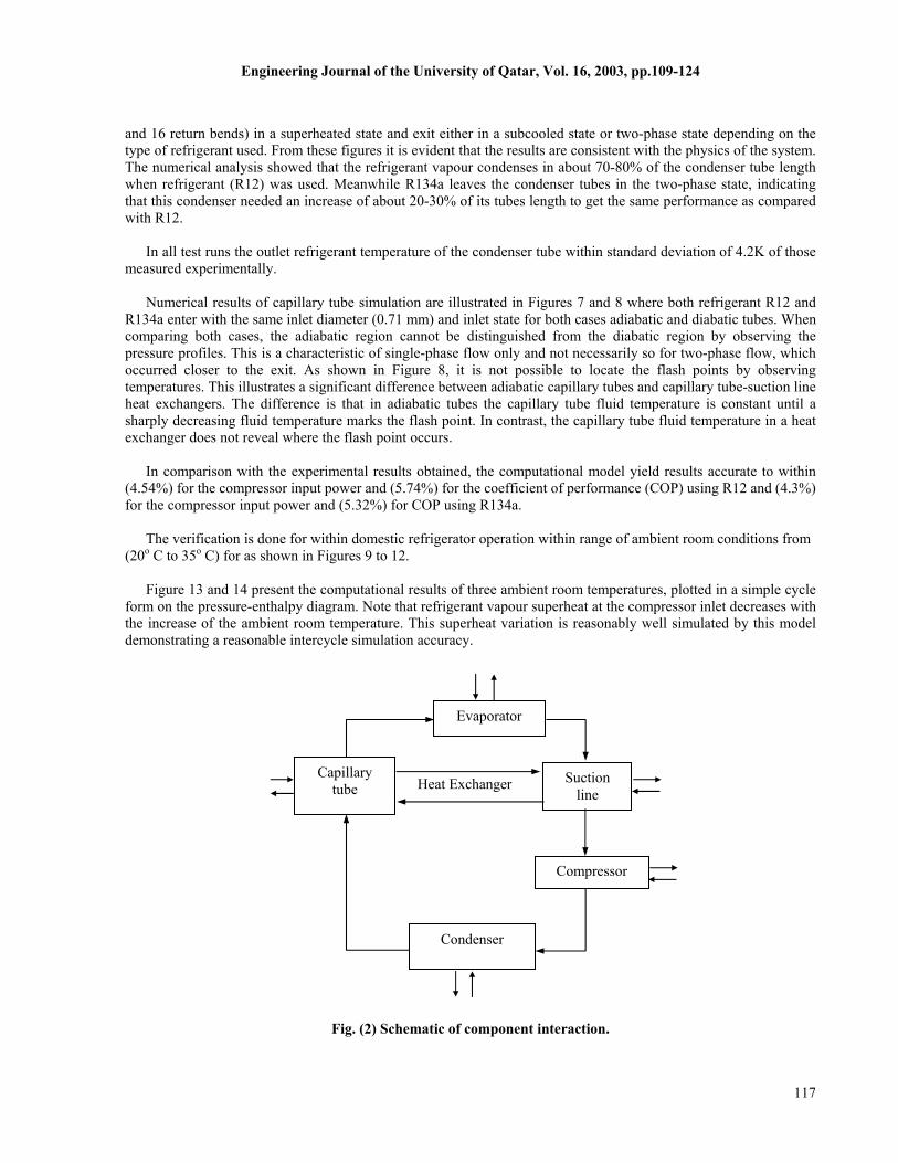
The dominant heat-transfer mechanism from the condenser, compressor, and the evaporator (see Figure 2) to the surrounding air is due to a combination of natural convection and radiation:

)()(

)(44

aHXOHXO

HXO

TwTArHaTwTAradQ

aTwTAcHconvQ

whereradQconvQQ

−=−=

−=

+=

εσ&

&

&&&

(14

(13

(15

Assuming a cabinet-wall temperature of refrigerator approximately equal to the ambient temperature. Followinthe work of (Jakobsen, 1995) on a domestic refrigerator of the type considered here, the total air heat-transfecoefficient [in W/m2.K] for the condenser can be fitted as

461.099.5 TrHcHH cond ∆+=+= (16

Similarly, for the compressor

451.066.6 TH comp ∆+= (17 and for the evaporator

393.009.5 TH evap ∆+= 18 However, as temperature variations are relatively small, all heat-transfer coefficients, that include botconvection and radiation are modeled as constants. Actual values are listed as “air-side heat-transfer coefficientsalong with other model parameters in the section results and validation.

The heat-transfer between the capillary tube and the suction line is calculated by this research following thprescription described in the section on conventional heat transfer. Here, we have assumed that the most importancontribution to this heat transfer is a consequence of the capillary tube being co-axially aligned within the sectioline.

VII. RESULTS AND VALIDATION

In this section key results from simulation of refrigeration cycle are presented and compared to measuremenfrom a 9 ft3 (0.2548 m3) top-mount refrigerator-freezer, with a static condenser using R12 and R134a refrigerantAll refrigeration components remained the same throughout the test, except that the length of the capillary tubcompressor size and the amount of charge were changed for each refrigerant.

One of the features of the simulation model is that the results contain much more information than measuremenprovide. Example of this include the detailed information about pressure and temperature distribution along capillartube and condenser tubes. The main advantages of such simulation include better understanding of system ancomponent behavior when they are used different alternative refrigerants for comparison purpose.

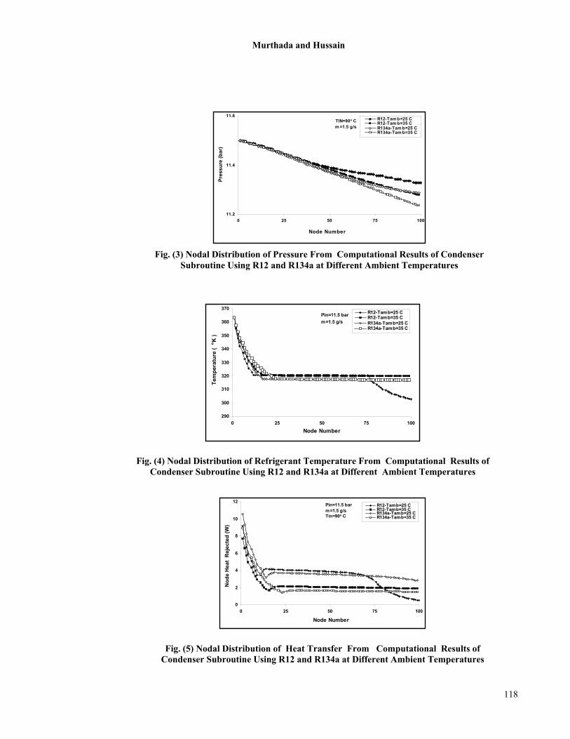
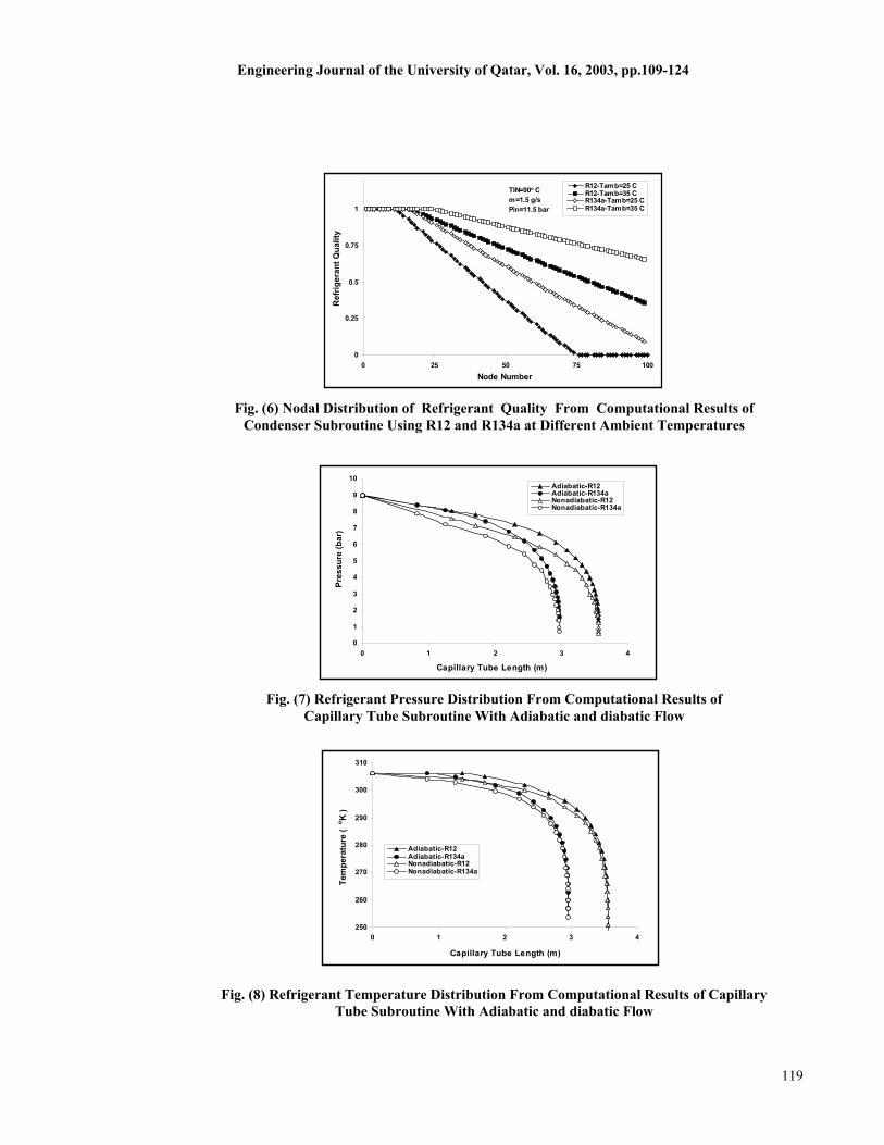
Numerical results of condenser (type of wire and tube) simulation are illustrated in Figures 3,4,5 and 6 wherrefrigerant (R12 or R134a) enters the condenser (total tubes length 7.65 m subdivided into 100 nodes of equal lengt

11

)

)

)

g r

)

)

)

h ”

e t n

ts s. e,

ts y d

e h

6


and 16 return bends) in a superheated state and exit either in a subcooled state or two-phase state depending on the type of refrigerant used. From these figures it is evident that the results are consistent with the physics of the system. The numerical analysis showed that the refrigerant vapour condenses in about 70-80% of the condenser tube length when refrigerant (R12) was used. Meanwhile R134a leaves the condenser tubes in the two-phase state, indicating that this condenser needed an increase of about 20-30% of its tubes length to get the same performance as compared with R12.

In all test runs the outlet refrigerant temperature of the condenser tube within standard deviation of 4.2K of those measured experimentally.

Numerical results of capillary tube simulation are illustrated in Figures 7 and 8 where both refrigerant R12 and R134a enter with the same inlet diameter (0.71 mm) and inlet state for both cases adiabatic and diabatic tubes. When comparing both cases, the adiabatic region cannot be distinguished from the diabatic region by observing the pressure profiles. This is a characteristic of single-phase flow only and not necessarily so for two-phase flow, which occurred closer to the exit. As shown in Figure 8, it is not possible to locate the flash points by observing temperatures. This illustrates a significant difference between adiabatic capillary tubes and capillary tube-suction line heat exchangers. The difference is that in adiabatic tubes the capillary tube fluid temperature is constant until a sharply decreasing fluid temperature marks the flash point. In contrast, the capillary tube fluid temperature in a heat exchanger does not reveal where the flash point occurs.

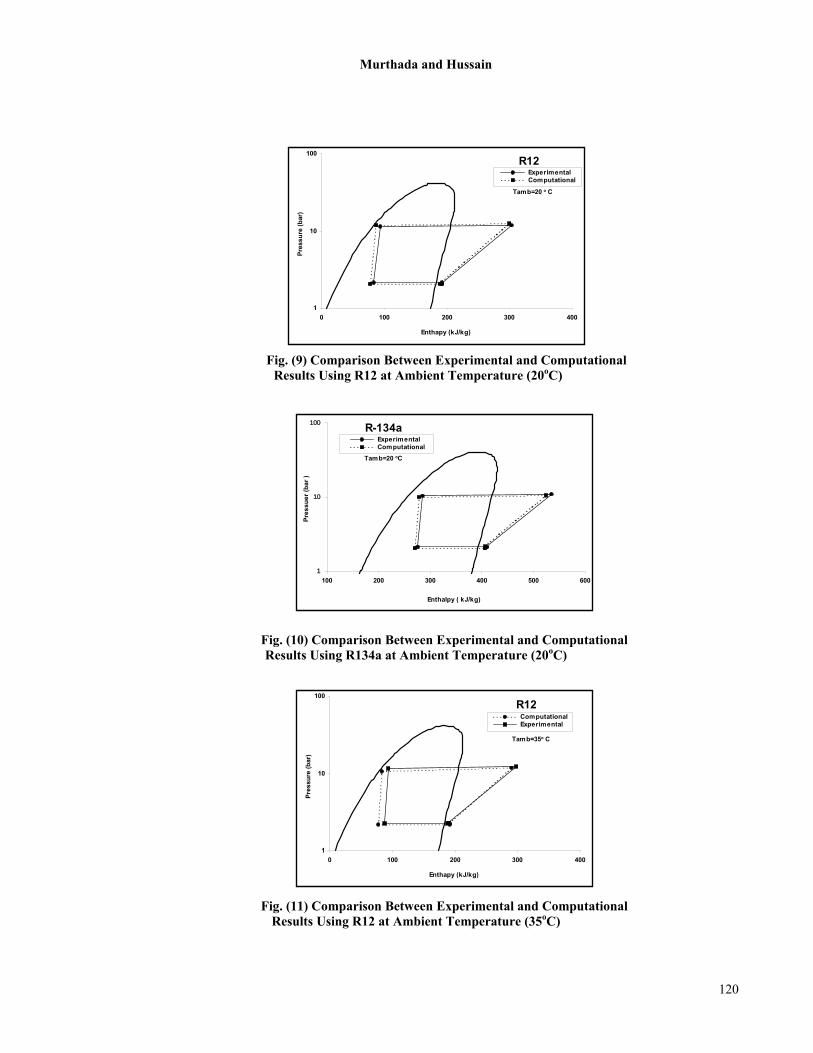
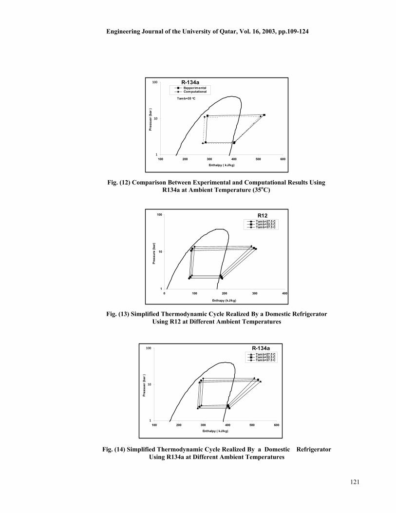
In comparison with the experimental results obtained, the computational model yield results accurate to within (4.54%) for the compressor input power and (5.74%) for the coefficient of performance (COP) using R12 and (4.3%) for the compressor input power and (5.32%) for COP using R134a.

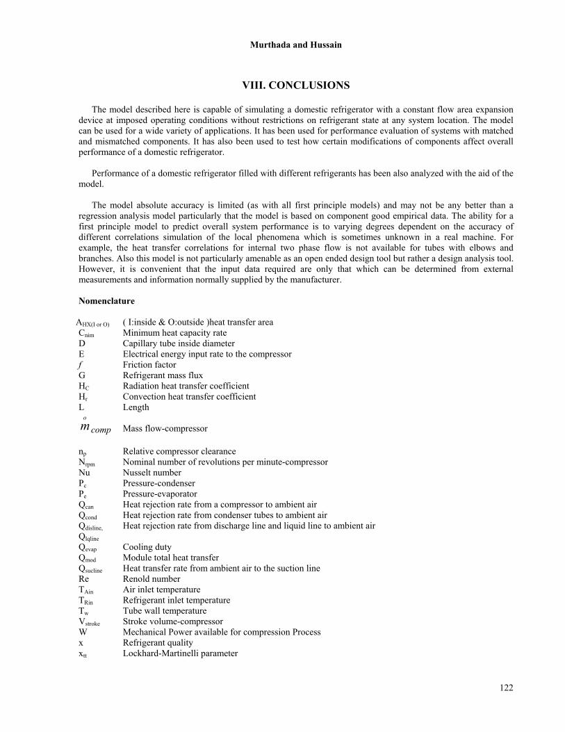
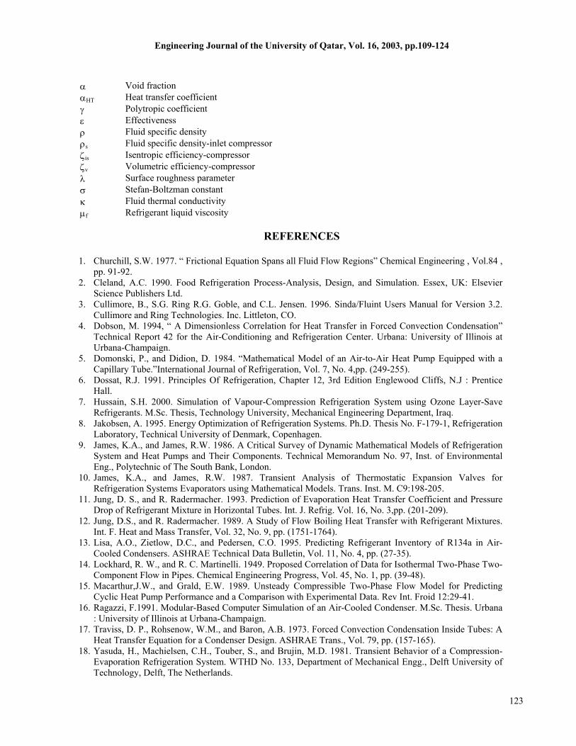
The verification is done for within domestic refrigerator operation within range of ambient room conditions from (20o C to 35o C) for as shown in Figures 9 to 12. Figure 13 and 14 present the computational results of three ambient room temperatures, plotted in a simple cycle form on the pressure-enthalpy diagram. Note that refrigerant vapour superheat at the compressor inlet decreases with the increase of the ambient room temperature. This superheat variation is reasonably well simulated by this model demonstrating a reasonable intercycle simulation accuracy.

Compressor

Heat Exchanger

Condenser

Suction line

Evaporator

Capillary tube

Fig. (2) Schematic of component interaction.

117


TIN=90o C

11.2

11.4

11.6

0 25 50 75 100

Node Number

Pres

sure

(bar

)

R12-Tam b=25 CR12-Tam b=35 CR134a-Tam b=25 CR134a-Tam b=35 C

m =1.5 g/s

Fig. (3) Nodal Distribution of Pressure From Computational Results of Condenser Subroutine Using R12 and R134a at Different Ambient Temperatures

290

300

310

320

330

340

350

360

370

0 25 50 75 100Node Number

Tem

pera

ture

( o K

)

R12-Tamb=25 CR12-Tamb=35 CR134a-Tamb=25 CR134a-Tamb=35 C

Pin=11.5 barm=1.5 g/s

Fig. (4) Nodal Distribution of Refrigerant Temperature From Computational Results of

Condenser Subroutine Using R12 and R134a at Different Ambient Temperatures

0

2

4

6

8

10

12

0 25 50 75 100

Node Number

Nod

e H

eat

Rej

ecte

d (W

)


Pin=11.5 barm=1.5 g/sTin=90o C

Fig. (5) Nodal Distribution of Heat Transfer From Computational Results of

Condenser Subroutine Using R12 and R134a at Different Ambient Temperatures

118


Fig. (6) Nodal Distribution of Refrigerant Quality From Computational Results of Condenser Subroutine Using R12 and R134a at Different Ambient Temperatures

TIN=90o C

0

0.25

0.5

0.75

1

0 25 50 75 100Node Number

Ref

riger

ant Q

ualit

y


m=1.5 g/sPin=11.5 bar

0

1

2

3

4

5

6

7

8

9

10

0 1 2 3 4

Capillary Tube Length (m)

Pres

sure

(bar

)

Adiabatic-R12Adiabatic-R134aNonadiabatic-R12Nonadiabatic-R134a

250

260

270

280

290

300

310

0 1 2 3 4

Capillary Tube Length (m)

Tem

pera

ture

( o K

)

Adiabatic-R12Adiabatic-R134aNonadiabatic-R12Nonadiabatic-R134a

Fig. (7) Refrigerant Pressure Distribution From Computational Results of Capillary Tube Subroutine With Adiabatic and diabatic Flow

Fig. (8) Refrigerant Temperature Distribution From Computational Results of Capillary Tube Subroutine With Adiabatic and diabatic Flow

119


R12

1

10

100

0 100 200 300 400

Enthapy (kJ/kg)

Pres

sure

(bar

)

Experimental Computational

Tamb=20 o C

R12

1

10

100

0 100 200 300 400

Enthapy (kJ/kg)

Pres

sure

(bar

)

Computational Experimental

Tamb=35o C

R-134a

1

10

100

100 200 300 400 500 600

Enthalpy ( kJ/kg)

Pres

suer

(bar

)

Experimental Computational

Tamb=20 oC

Fig. (10) Comparison Between Experimental and Computational Results Using R134a at Ambient Temperature (20oC)

Fig. (9) Comparison Between Experimental and Computational Results Using R12 at Ambient Temperature (20oC)

Fig. (11) Comparison Between Experimental and Computational

Results Using R12 at Ambient Temperature (35oC)

120


R-134a

1

10

100

100 200 300 400 500 600

Enthalpy ( kJ/kg)

Pres

suer

(bar

)

Expperimental Computational

Tamb=35 oC

R12

1

10

100

0 100 200 300 400

Enthapy (kJ/kg)

Pres

sure

(bar

)

Tamb=27.5 CTamb=32.5 CTamb=37.5 C

R-134a

1

10

100

100 200 300 400 500 600

Enthalpy ( kJ/kg)

Pres

suer

(bar

)

Tamb=27.5 CTamb=32.5 CTamb=37.5 C

Fig. (13) Simplified Thermodynamic Cycle Realized By a Domestic Refrigerator Using R12 at Different Ambient Temperatures

Fig. (12) Comparison Between Experimental and Computational Results Using R134a at Ambient Temperature (35oC)

Fig. (14) Simplified Thermodynamic Cycle Realized By a Domestic Refrigerator

Using R134a at Different Ambient Temperatures

121


VIII. CONCLUSIONS

The model described here is capable of simulating a domestic refrigerator with a constant flow area expansion device at imposed operating conditions without restrictions on refrigerant state at any system location. The model can be used for a wide variety of applications. It has been used for performance evaluation of systems with matched and mismatched components. It has also been used to test how certain modifications of components affect overall performance of a domestic refrigerator.

Performance of a domestic refrigerator filled with different refrigerants has been also analyzed with the aid of the model.

The model absolute accuracy is limited (as with all first principle models) and may not be any better than a regression analysis model particularly that the model is based on component good empirical data. The ability for a first principle model to predict overall system performance is to varying degrees dependent on the accuracy of different correlations simulation of the local phenomena which is sometimes unknown in a real machine. For example, the heat transfer correlations for internal two phase flow is not available for tubes with elbows and branches. Also this model is not particularly amenable as an open ended design tool but rather a design analysis tool. However, it is convenient that the input data required are only that which can be determined from external measurements and information normally supplied by the manufacturer.

Nomenclature

AHX(I or O) ( I:inside & O:outside )heat transfer area Cnim Minimum heat capacity rate D Capillary tube inside diameter E Electrical energy input rate to the compressor f Friction factor G Refrigerant mass flux HC Radiation heat transfer coefficient Hr Convection heat transfer coefficient L Length

compom

Mass flow-compressor

np Relative compressor clearance Nrpm Nominal number of revolutions per minute-compressor Nu Nusselt number Pc Pressure-condenser Pe Pressure-evaporator Qcan Heat rejection rate from a compressor to ambient air Qcond Heat rejection rate from condenser tubes to ambient air Qdisline, Qlqline

Heat rejection rate from discharge line and liquid line to ambient air

Qevap Cooling duty Qmod Module total heat transfer Qsucline Heat transfer rate from ambient air to the suction line Re Renold number TAin Air inlet temperature TRin Refrigerant inlet temperature Tw Tube wall temperature Vstroke Stroke volume-compressor W Mechanical Power available for compression Process x Refrigerant quality xtt Lockhard-Martinelli parameter

122


α Void fraction αHT Heat transfer coefficient γ Polytropic coefficient ε Effectiveness ρ Fluid specific density ρs Fluid specific density-inlet compressor ζis Isentropic efficiency-compressor ζv Volumetric efficiency-compressor λ Surface roughness parameter σ Stefan-Boltzman constant κ Fluid thermal conductivity µf Refrigerant liquid viscosity

REFERENCES

1. Churchill, S.W. 1977. “ Frictional Equation Spans all Fluid Flow Regions” Chemical Engineering , Vol.84 ,

pp. 91-92. 2. Cleland, A.C. 1990. Food Refrigeration Process-Analysis, Design, and Simulation. Essex, UK: Elsevier

Science Publishers Ltd. 3. Cullimore, B., S.G. Ring R.G. Goble, and C.L. Jensen. 1996. Sinda/Fluint Users Manual for Version 3.2.

Cullimore and Ring Technologies. Inc. Littleton, CO. 4. Dobson, M. 1994, “ A Dimensionless Correlation for Heat Transfer in Forced Convection Condensation”

Technical Report 42 for the Air-Conditioning and Refrigeration Center. Urbana: University of Illinois at Urbana-Champaign.

5. Domonski, P., and Didion, D. 1984. “Mathematical Model of an Air-to-Air Heat Pump Equipped with a Capillary Tube.”International Journal of Refrigeration, Vol. 7, No. 4,pp. (249-255).

6. Dossat, R.J. 1991. Principles Of Refrigeration, Chapter 12, 3rd Edition Englewood Cliffs, N.J : Prentice Hall.

7. Hussain, S.H. 2000. Simulation of Vapour-Compression Refrigeration System using Ozone Layer-Save Refrigerants. M.Sc. Thesis, Technology University, Mechanical Engineering Department, Iraq.

8. Jakobsen, A. 1995. Energy Optimization of Refrigeration Systems. Ph.D. Thesis No. F-179-1, Refrigeration Laboratory, Technical University of Denmark, Copenhagen.

9. James, K.A., and James, R.W. 1986. A Critical Survey of Dynamic Mathematical Models of Refrigeration System and Heat Pumps and Their Components. Technical Memorandum No. 97, Inst. of Environmental Eng., Polytechnic of The South Bank, London.

10. James, K.A., and James, R.W. 1987. Transient Analysis of Thermostatic Expansion Valves for Refrigeration Systems Evaporators using Mathematical Models. Trans. Inst. M. C9:198-205.

11. Jung, D. S., and R. Radermacher. 1993. Prediction of Evaporation Heat Transfer Coefficient and Pressure Drop of Refrigerant Mixture in Horizontal Tubes. Int. J. Refrig. Vol. 16, No. 3,pp. (201-209).

12. Jung, D.S., and R. Radermacher. 1989. A Study of Flow Boiling Heat Transfer with Refrigerant Mixtures. Int. F. Heat and Mass Transfer, Vol. 32, No. 9, pp. (1751-1764).

13. Lisa, A.O., Zietlow, D.C., and Pedersen, C.O. 1995. Predicting Refrigerant Inventory of R134a in Air-Cooled Condensers. ASHRAE Technical Data Bulletin, Vol. 11, No. 4, pp. (27-35).

14. Lockhard, R. W., and R. C. Martinelli. 1949. Proposed Correlation of Data for Isothermal Two-Phase Two-Component Flow in Pipes. Chemical Engineering Progress, Vol. 45, No. 1, pp. (39-48).

15. Macarthur,J.W., and Grald, E.W. 1989. Unsteady Compressible Two-Phase Flow Model for Predicting Cyclic Heat Pump Performance and a Comparison with Experimental Data. Rev Int. Froid 12:29-41.

16. Ragazzi, F.1991. Modular-Based Computer Simulation of an Air-Cooled Condenser. M.Sc. Thesis. Urbana : University of Illinois at Urbana-Champaign.

17. Traviss, D. P., Rohsenow, W.M., and Baron, A.B. 1973. Forced Convection Condensation Inside Tubes: A Heat Transfer Equation for a Condenser Design. ASHRAE Trans., Vol. 79, pp. (157-165).

18. Yasuda, H., Machielsen, C.H., Touber, S., and Brujin, M.D. 1981. Transient Behavior of a Compression-Evaporation Refrigeration System. WTHD No. 133, Department of Mechanical Engg., Delft University of Technology, Delft, The Netherlands.

123


124

19. Rasmussen, B.D. 1997. Variable Speed Hermetic Reciprocating Compressor for Domestic Refrigerators. Ph.D. Thesis No. ET-Ph-D. 97-03, Department of Energy Engineering, Technical University of Denmark, Copenhagen.

20. Tandon, T.N., Varma, H.K., and Gupta, C.P. 1985. A Void Fraction Model for Annular Two-Phase Flow. International Journal of Heat and Mass Transfer, Vol. 28, No.1, pp. (191-198).

Documents

PERFORANCE SIMULATION OF SINGLE …qspace.qu.edu.qa/bitstream/handle/10576/7945/060316-11-fulltext.pdf · DOMESTIC REFRIGERATOR USING ... (evaporator, condenser, compressor, ... PERFORANCE